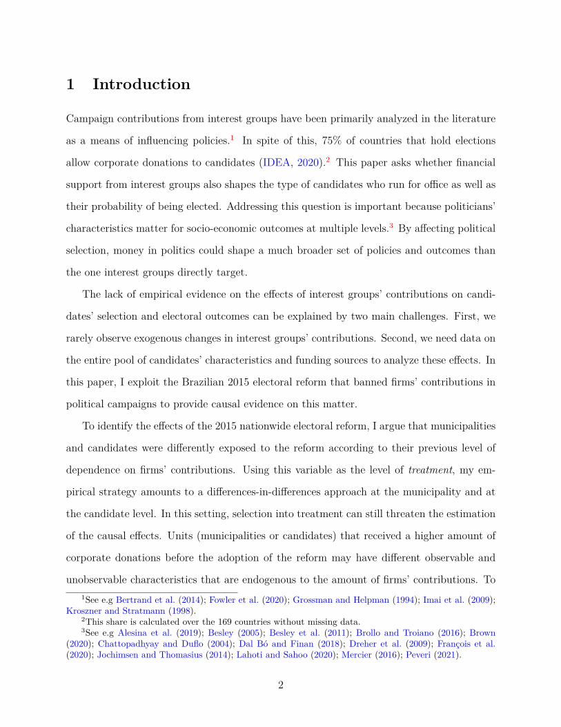
Interest Groups' Contributions and Political Selection:

Interest Groups’ Contributions and Political Selection:

Evidence from Brazil

Julieta Peveri∗

October 2021

JOB MARKET PAPER

Click here for the most recent version

Abstract

While the role of interest groups’ contributions in shaping policies has been well-studied, little is known about their effects on political selection and electoral outcomes.This paper studies a Brazilian reform that banned firms’ contributions to provide ev-idence in this regard. I use a weighted differences-in-differences strategy exploitingvariation in municipalities’ and candidates’ dependence on firms’ funding before thereform. I find that the ban had little effect on political competition. However, it dete-riorated the electoral advantage of low-educated incumbents and of incumbents fromtraditional political parties. The negative effects for incumbents are concentrated inoil-dependent municipalities, where rent-seeking is more likely, and in localities withlower economic growth and higher mortality rates. These results are consistent withthe reform crowding out incumbents who heavily relied on the financial advantage tobe re-elected rather than on a good performance while in power.

Keywords: interest groups contributions, quality incumbency advantage, financialincumbency advantage, political selection.JEL Codes: D72, D73, H70.

∗Aix-Marseille University (Aix-Marseille School of Economics), CNRS. Mail: [email protected] thank my advisors Nicolas Berman and Marc Sangnier. Benjamin Blumenthal, Gianmarco Daniele, MichaelDorsch, Vincenzo Galasso, Tommaso Giommoni, Alberto Grillo, Jeremy Lucchetti, Marion Mercier, MassimoMorelli, Paolo Pinotti, Lorenzo Rotunno, Avner Seror, Guido Tabellini, and seminar participants at AMSE,the 20th Journees Louis-Andre Gerard-Varet , the 2nd Conference of Corruption and Tax Evasion, the14th RGS Doctoral Conference in Economics, the 15th BiGSEM Doctoral Workshop on Economics andManagement, the CLEAN unit meeting for valuable comments and feedback. This work was supported byFrench National Research Agency Grants ANR-17-EURE-0020.

1

1 Introduction

Campaign contributions from interest groups have been primarily analyzed in the literature

as a means of influencing policies.1 In spite of this, 75% of countries that hold elections

allow corporate donations to candidates (IDEA, 2020).2 This paper asks whether financial

support from interest groups also shapes the type of candidates who run for office as well as

their probability of being elected. Addressing this question is important because politicians’

characteristics matter for socio-economic outcomes at multiple levels.3 By affecting political

selection, money in politics could shape a much broader set of policies and outcomes than

the one interest groups directly target.

The lack of empirical evidence on the effects of interest groups’ contributions on candi-

dates’ selection and electoral outcomes can be explained by two main challenges. First, we

rarely observe exogenous changes in interest groups’ contributions. Second, we need data on

the entire pool of candidates’ characteristics and funding sources to analyze these effects. In

this paper, I exploit the Brazilian 2015 electoral reform that banned firms’ contributions in

political campaigns to provide causal evidence on this matter.

To identify the effects of the 2015 nationwide electoral reform, I argue that municipalities

and candidates were differently exposed to the reform according to their previous level of

dependence on firms’ contributions. Using this variable as the level of treatment, my em-

pirical strategy amounts to a differences-in-differences approach at the municipality and at

the candidate level. In this setting, selection into treatment can still threaten the estimation

of the causal effects. Units (municipalities or candidates) that received a higher amount of

corporate donations before the adoption of the reform may have different observable and

unobservable characteristics that are endogenous to the amount of firms’ contributions. To1See e.g Bertrand et al. (2014); Fowler et al. (2020); Grossman and Helpman (1994); Imai et al. (2009);

Kroszner and Stratmann (1998).2This share is calculated over the 169 countries without missing data.3See e.g Alesina et al. (2019); Besley (2005); Besley et al. (2011); Brollo and Troiano (2016); Brown

(2020); Chattopadhyay and Duflo (2004); Dal Bo and Finan (2018); Dreher et al. (2009); Francois et al.(2020); Jochimsen and Thomasius (2014); Lahoti and Sahoo (2020); Mercier (2016); Peveri (2021).

2

overcome this issue, I use weighted regressions where weights are calibrated to ensure compa-

rable groups of units across different levels of treatment on selected covariates. The weighting

accounts for time-variant selection on observables, while the differences-in-differences strat-

egy deals with time-invariant selection on unobservables.

I find that interest groups’ contributions were not fully compensated by alternative

sources after the ban. Consequently, campaign spending decreased more in those munic-

ipalities where candidates used to rely more on corporate funds. However, the reform has

minor composition effects at the aggregate level. The pool of candidates was stable in terms

of size, total wealth, and entry of new candidates. Political competition outcomes, such

as the margin of victory or the Herfindahl-Hirschman index, were also unaffected. At the

candidate level of analysis, female candidates who relied on firms’ funds were less likely to

re-contest than men. This effect varies from −7% to −20% depending on the incumbency

status and the level of firms’ dependence.

The reform resulted in a significant drop in the probability of winning for incumbents

with specific characteristics, suggesting that corporate contributions were relevant for the

selection of elected politicians. In particular, low-educated incumbents and incumbents from

big parties who were previously relying on firms’ contributions lost around 5% of their share

of votes. In contrast, graduate incumbents and incumbents from small parties kept their

previous level of electoral support. The effects are non-monotonic as they are concentrated

in incumbents with intermediate levels of firms’ dependence rather than in high-dependent

ones. The latter were better able to substitute their contributions with alternative fundings,

curbing the electoral effects of lower funds.

Among incumbents with a moderate level of firms’ dependence, the heterogeneity among

educational levels and party size is not driven by differences in re-contesting decisions or in

abilities to compensate for firms’ funds. On the contrary, heterogenous spillover effects are at

play. More precisely, the number of challengers after the reform increased in municipalities

run by low-educated incumbents or incumbents from a big political party who were previously

3

funded by firms. Yet, the effects on electoral outcomes persist even when controlling for

candidates’ entry and variation in contributions. This highlights differences in marginal

returns of contributions across individual characteristics as a complementary mechanism.

I present a theoretical framework that helps to interpret the empirical findings. I build on

the interaction between the financial and the quality incumbency advantage. Low-performant

incumbents rely more on campaign spending to manipulate voters’ perception of their qual-

ity. This can explain why, for a given drop in contributions and a given entry of challengers,

high-educated incumbents were less penalized by voters than non-graduate officeholders.

The mechanism would be the same for the heterogeneity with respect to party size if, condi-

tional on being funded by firms, candidates from big parties were more prone to rent-seeking

behaviors. I further assume that the entry of challengers inversely depends on the incum-

bent’s probability of winning. Therefore, for a given drop in incumbent’s contributions,

challengers are more prone to run for office if there is a low-quality incumbent rather than

a high-performant politician holding power. This is consistent with the aforementioned het-

erogenous spillover effects. Finally, I model total contributions as a sum of different types of

donors’ contributions, who give different weights to each candidate’s characteristic. Hence,

the reform may penalize candidates who have difficulties in fund-raising despite their level

of performance, explaining the lower likelihood of female candidates in re-contesting.

I provide additional evidence in favor of the interaction between the financial and the qual-

ity incumbency advantage by using alternative proxies for quality: (i) a dummy to identify

incumbents associated with a high local economic growth; (ii) a dummy to assess high levels

of mortality rates in the municipality and (iii) a dummy to identify oil-dependent municipal-

ities. Regarding the latest, Caselli and Michaels (2013) provide evidence that oil revenues

in Brazilian municipalities do not translate into improvements in welfare-relevant outcomes,

but they are instead associated with a high level of corruption. I find that the adverse effects

for incumbents’ electoral advantage are concentrated in oil-dependent municipalities and in

municipalities where incumbents were associated with low economic performance and high

4

mortality rates. This result reinforces the claim that banning interest groups’ contributions

mostly affected the electoral prospects of low-quality incumbents. Moreover, results are ro-

bust when controlling for candidates’ declared wealth, which can be correlated with other

individual characteristics such as educational level, gender and party orientation.

This paper contributes to the literature on interest groups’ effects in politics. There is

no consensus on how interest groups affect electoral outcomes. One view is that interest

groups contribute to candidates to buy political influence. Accordingly, contributions can

be assimilated to an investment that will only pay off if the recipient wins the election. As a

result, interest groups will tend to contribute more to the electoral favorite (Grossman and

Helpman, 2001). An alternative argument is that interest groups can increase the probability

of winning of the candidates they support by boosting their resources for campaign spending,

leading to a self-fulfilling prophecy.4 These upshots are especially relevant for incumbents.

Since incumbents usually enjoy good electoral prospects, their higher attraction of corporate

contributions can be a plausible source of their electoral advantage or a simple correlation

(Fouirnaies and Hall, 2014). To the best of my knowledge, there is only one recent work

providing empirical evidence in this regard. Fouirnaies (2021) analyzes candidates who ran

for the Party Labour in the UK parliamentary elections and finds that candidates who were

sponsored by trade unions electorally out-performed other ones. He focuses on revealing the

mechanisms through which interest groups can affect electoral outcomes. He finds that those

effects are mainly driven by the role of interest groups in preliminary stages by increasing

candidates’ probability of being nominated in constituencies where their party has high

electoral support. Using a very different setting, where first stage nominations do not play

a role, I provide further evidence that interest groups’ contributions affect the likelihood of

a candidate being elected.

This paper generally speaks to the large literature which studies the sources of the in-

cumbency advantage. In particular, a quality advantage relative to challengers has been4For the literature of the effects on campaign spending on electoral outcomes see Bombardini and Trebbi

(2011); Levitt (1994), among others.

5

pointed out by Ashworth and Bueno de Mesquita (2008) and Eggers (2017). On the other

side, Fouirnaies and Hall (2014) use legislative races for the US to provide evidence of the

existence of a financial incumbency advantage, primarily triggered by access-oriented inter-

est groups’ contributions. However, there is a lack of empirical evidence for this financial

advantage as a source of electoral success that this paper aims to fill in. My results suggest

that there is a causal effect for low-educated incumbents and incumbents from big parties.

Closely connected is the scarce literature on the effects of interest groups’ contributions on

politicians’ selection. Coate and Morris (1995) assume that only “bad” politicians are willing

to deviate from citizens’ ideal policies to favor special groups in exchange for money. If that

is the case, interest groups’ campaign contributions are likely to go towards politicians of

lower quality. Further, if different donors sponsor different types of politicians, as suggested

by Barber (2016) and Hall (2014), the pool of contributors can be an important determinant

of the pool of candidates. I provide evidence that corporate donations have little effect on the

selection of the pool of candidates but significantly affect the selection of elected politicians.

Finally, this paper relates to the literature on campaign funding reforms. In particular,

Avis et al. (2021 forthcoming) analyze the other big component of the 2015 Brazilian reform,

the introduction of campaign spending limits. They find that stricter limits lead to a larger

pool of candidates that is on average less wealthy and they also reduce the probability

that mayors are re-elected. This paper adds to the understanding of the overall effects of

the aforementioned electoral reform. Moreover, studying the ban of corporate donations is

particularly relevant as it can be followed by the vast majority of electoral democracies. I

show that in Brazil the reform led to a better selection of elected politicians. Further research

is encouraged for the external validity of this result.

The remainder of the paper is organized as follows. Section 2 describes the institutional

context of Brazilian municipal elections, the background of the reform, the data and the em-

pirical strategy. The results are presented in Section 3, following by a theoretical framework

to interpret the results in Section 4 and robustness in Section 5. Lastly, Section 6 contains

6

concluding remarks.

2 Empirical framework

2.1 Institutional context

This paper focuses on candidates who run for mayor positions in Brazilian municipalities.

Elections occur once every four years. Mayors are elected by absolute majority vote through

a two-round system and face a term limit after their second consecutive term. Voting in

Brazil is mandatory for all literate citizens over 18 and under 70, and optional for illiterate

citizens, the ones aged 16 and 17, and those older than 70.

Mayors are important political figures in Brazil. They are the executive authority at the

local level, responsible for providing public services, urban planning, raising local taxes, and

administering the municipality’s budget.

I exploit the 2015 electoral reform introduced of campaign funding regulation. This law

bans contributions from firms and imposes campaign spending limits.5 This reform was a

response to the revelations of Operation Car Wash (Operacao Lava Jato) which disclosed

a large-scale corruption scandal in Brazil, mostly related to money laundering, and led to

the incarceration of several influential businessmen and politicians. Much of the bribery

was connected to the Brazilian construction firm Odebrecht which paid billions of dollars,

mainly in the form of legal campaign contributions, to several Latin politicians in exchange

of over-inflated public contracts.

2.2 Data

Data on contributions and candidates’ characteristics is rich in Brazil. All candidates and

parties have to open a bank account to be used for campaign purposes exclusively. For5New aspects such as the creation of a public fund to finance part of electoral campaigns based on

performance clauses and the changes on individual contributions limits were voted but were from 2020 only,which I do not add to the analysis.

7

each donation made, the information about the donor and the amount of the contributions

is publicly available. Besides, the Tribunal Superior Eleitoral provides information about

candidates’ characteristics such as name, gender, age, occupation, level of education and

political party. I use candidates’ characteristics and campaigns contributions data from

2004, 2008, 2012 and 2016 elections.

Table 1 shows some descriptive statistics about candidates running for mayor in the

sample of elections. Brazil’s politics is characterized by multi-party competition (34 parties

were present in the last local elections). The percentage of men was around 87% in 2012 and

2016, with a mean age of 49 years old. About half of the candidates under consideration do

not have a university degree. Another fact of particular relevance is that the occupational

category with the highest level of representation among challengers is businessmen, which

could reinforce the influence firms have in politics.

Before the reform, firms were responsible for around 15% of the campaign ressources.

After it, candidates relied relatively more on their own resources and contributions from

citizens. We can observe a reduction of the mean and the median campaign donations after

the 2015 electoral reform took place. However, the standard deviations of all these variables

suggest a high heterogeneity across parties and candidates. Information regarding economic

sectors of corporate donors is only available from 2012 and are listed in Appendix A3 ranked

according to 2012 donations size. The category which is ranked first is Building construc-

tion. Other related construction sectors, such as Construction of highways and railways and

Construction of water supply networks, sewage collection, and related constructions appear

3rd and 19th respectively in the ranking. Real estates and related financial corporations also

have an important weight in candidates’ funding. To complement the analysis, I report in

Table A4 the most repeated words in firms’ names in the three elections before the reform.

The main words used in corporations’ names among donors are “trade”, “office” and “con-

struction”. Together with the Car Wash’s revelations aforementioned, it raises alarm bells

on a potential trade between firms’ contributions and over-rated construction public leases.

8

Table 1: Descriptive statistics.

2004 2008 2012 2016

Mean number of candidates per municipality 2.8 2.6 2.5 2.8Number of political parties (total) 27 27 29 34Percentage of males 90% 89% 87% 87%Mean age 47.8 48.7 48.7 49.3

Level of educationLower than high-school 25.50% 22.32% 17.51% 16.03%High-school 24.59% 25.38% 26.63% 25.81%University incomplete 7.53% 7.93% 6.97% 6.21%University complete 42.38% 44.37% 48.89% 51.96%

OccupationMayor 15.61% 21.91% 17.19% 17.26%Businessman 5.52% 8.49% 11.43% 12.86%Agricultor 11.82% 10.31% 9.28% 8.33%Public officer 9.25% 8.34% 10.66% 10.46%Merchant 10.23% 8.26% 6.13% 5.26%Professor 5.30% 5.05% 5.29% 5.14%Lawyer 5.33% 4.73% 5.12% 5.70%

Campaign funding

Mean total campaign contributions 54,830 R$(161,943)

94,998 R$(550,385)

154,079 R$(759,115)

92,708 R$(31,5189)

Average % funding by firms 16.77%(28%)

15.14%(24%)

13.85%(22%)

Average % funding by party’s resources 11.71%(29%)

18.46%(30%)

21.23%(31%)

13.41%(24%)

Average % funding by citizens 31.68%(34%)

35%(31%)

32.41%(29%)

44.95%(33%)

Average % own funding 36.89%(39%)

31.12%(33%)

32.34%(32%)

41.54%(33%)

Average % other funding 0.29%(0.15%)

0.02%(0.54%)

0.0004%(0.02%)

0.008%(0.18%)

Campaign funding and electoral outcomes% of races won by the candidate who received more contributions 63% 67% 60% 64%% of races won by the candidate who received more firms’ contributions 57% 55% 52%% of races won by the incumbent (1) 57% 68% 57% 48 %

Data is taken from Tribunal Superior Eleitoral (TSE). (1) races are restricted to elections in which the incumbent contests forre-election. Standard deviations are in parenthesis. There is a total of 5,556 municipalities in 2004; 5,541 in 2008, 5,541 in 2012and 5,568 in 2016.

The bottom part of Table 1 displays some numbers that illustrate the importance of

money in politics. In more than 60% of races the candidate who received the most contri-

butions was the one who won, and in more than half of the elections, the individual who

attracted more corporate contributions.

Interestingly, the percentage of races won by the incumbent, conditional on the incumbent

re-contesting, was about 57% to 68% in the elections before the reform and dropped down

9

to 48% afterward. This drop in the electoral advantage may not only be a consequence of

the ban of interest groups, but it could also arise from the economic recession or from the

introduction of spending limits.

In order to test whether different donors support different candidates, I regress the contri-

butions of each group of donors with respect to candidates’ characteristics before the reform

took place. Figure 1 and Appendix A1 display the coefficient estimates. While gender is

not significant in attracting party or firms contributions, citizens favor more female incum-

bents, but women contribute less to their own campaign than men. Candidates from the

extreme parties received significantly fewer contributions from citizens, but also from firms

and parties, and the effect is of similar magnitude.

The financial advantage of incumbents is important for the purposes of this paper. Figure

1 shows that everything else equal, they received higher amounts from all types of donors,

supporting the existence of a financial incumbency advantage documented by Fouirnaies

and Hall (2014). When restricting the sample to incumbents (see Appendix A), individual

covariates are not explicative of firms’ contributions, and only the initial level of local GDP is

significant. However, there are important differences between citizens’ and candidates’ own

contributions, which could have implications for the reform analysis if candidates substitute

interest groups’ funds with these alternative sources. Indeed, if different candidates have

different fund-raising costs, banning contributions from a kind of donor may have effects on

the selection of candidates.

The most direct mechanism through which contributions can affect electoral outcomes is

through campaign spending.6 Table A5 from Appendix A shows the spending categories for

candidates’ running for mayor for each election, revealing that candidates mostly spend on

advertising, especially through printed materials, employees, and lease of vehicles and real6However, recent research suggests that interest groups’ contributions can also affect candidates’ nomi-

nation in a first stage (Fouirnaies, 2021) and candidates’ manifesto (Cage et al., 2021).

10

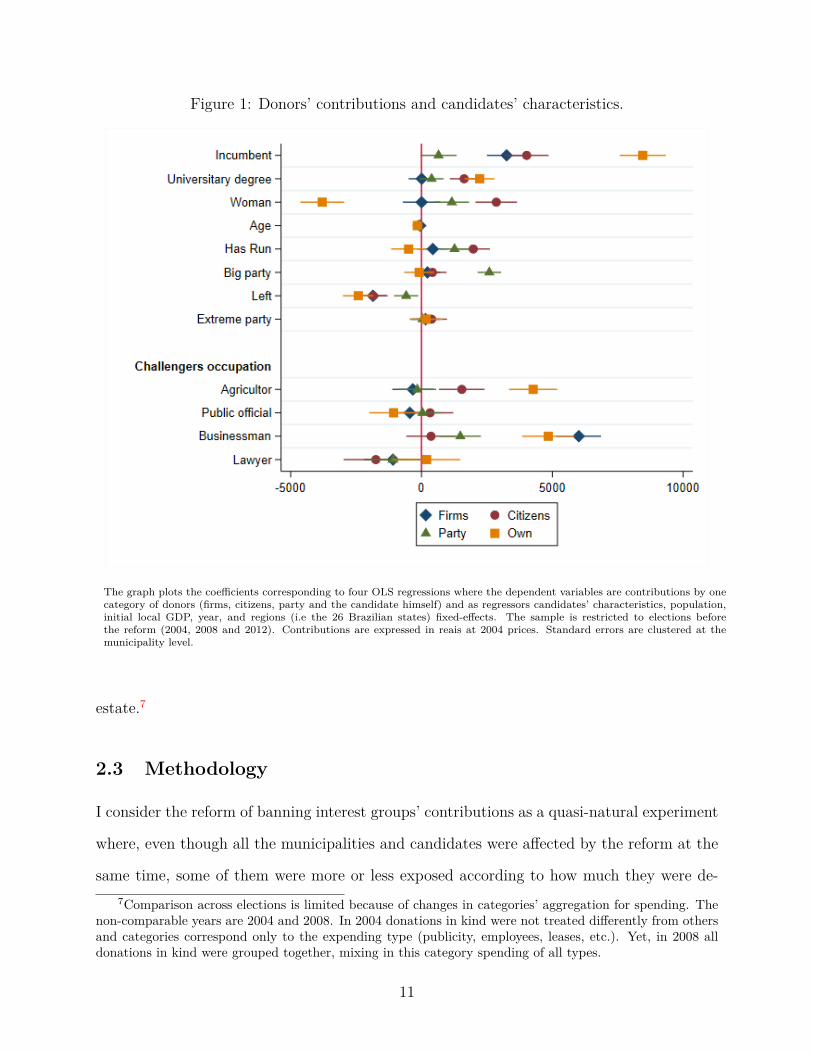
Figure 1: Donors’ contributions and candidates’ characteristics.

The graph plots the coefficients corresponding to four OLS regressions where the dependent variables are contributions by onecategory of donors (firms, citizens, party and the candidate himself) and as regressors candidates’ characteristics, population,initial local GDP, year, and regions (i.e the 26 Brazilian states) fixed-effects. The sample is restricted to elections beforethe reform (2004, 2008 and 2012). Contributions are expressed in reais at 2004 prices. Standard errors are clustered at themunicipality level.

estate.7

2.3 Methodology

I consider the reform of banning interest groups’ contributions as a quasi-natural experiment

where, even though all the municipalities and candidates were affected by the reform at the

same time, some of them were more or less exposed according to how much they were de-7Comparison across elections is limited because of changes in categories’ aggregation for spending. The

non-comparable years are 2004 and 2008. In 2004 donations in kind were not treated differently from othersand categories correspond only to the expending type (publicity, employees, leases, etc.). Yet, in 2008 alldonations in kind were grouped together, mixing in this category spending of all types.

11

pendent on interest groups’ funds. I implement a differences-in-differences strategy following

equation (1).

yu,t = α + ϕ Firms’ dependenceu,t + γ Firms’ dependenceu,t ∗ 2016+

δr ∗ δt + ϵu,t

(1)

where yu,t is the outcome for unit u, firms’ dependenceu is the treatment variable, δr are

regions’ fixed-effects and δt are year fixed-effects. The coefficient paired with the interaction

between firms’ dependence and the year after the reform (γ) captures the effect of the ban

of interest groups.

There are two important issues to adress. First, the definition of the treatment and the

unit of analysis and second, selection into treatment.

Treatment definition and units of observation

I will use two levels of analysis: a treatment defined at the municipality level and a

second at the candidate level. The first has the advantage of assessing the reform’s effects

on aggregate outcomes, such as the composition of the pool of candidates, the margin of

victory, and the entry of new candidates. However, as the treatment aggregates information

on all the candidates from a given municipality, it does not identify selection effects at the

individual level. The reverse applies to the candidate-level treatment.

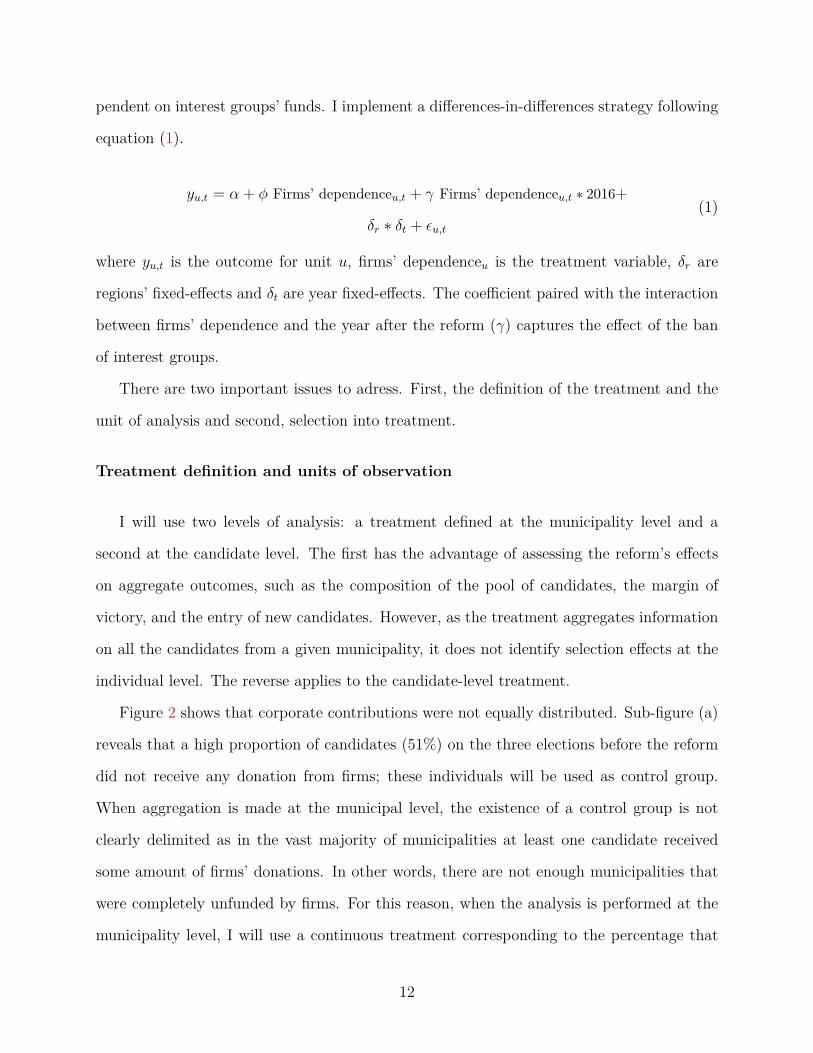
Figure 2 shows that corporate contributions were not equally distributed. Sub-figure (a)

reveals that a high proportion of candidates (51%) on the three elections before the reform

did not receive any donation from firms; these individuals will be used as control group.

When aggregation is made at the municipal level, the existence of a control group is not

clearly delimited as in the vast majority of municipalities at least one candidate received

some amount of firms’ donations. In other words, there are not enough municipalities that

were completely unfunded by firms. For this reason, when the analysis is performed at the

municipality level, I will use a continuous treatment corresponding to the percentage that

12

firms’ contributions represented on the total amount of contributions, averaged on the three

elections before the reform.8 At the individual level, I divide the treated group, i.e candidates

whose campaigns were partly sponsored by firms, into two categories: mid-dependent and

high-dependent individuals according to whether they were below or above the median of the

distribution of firms’ contributions. Section 5 provides alternative definitions for the reform

exposure for each unit of analysis.

Figure 2: Density of firms’ contributions before 2016 (in log.).

(a) By candidate (b) By municipality

Sub-figure (a) shows the density of the log. of firms’ contributions funded by firms, expressed in constant prices, inthe Brazilian elections for candidates running for mayors in 2004, 2008 and 2008. Sub-figure (b) shows the densityof the log. of firms’ contributions, expressed in constant prices, averaged per candidate at the municipalitiy levelfunded by firms in the same election. The log is replaced by 0 if firms’ contributions equals 0.

A recent work by Callaway et al. (2021) studies the interpretation of the parameters and

the underlying assumptions in cases where the treatment is continuous in the differences-in-

differences framework. Several cautions have to be taken with respect to the binary treatment

case and a parallel with the dose-response setting helps to the understanding. Callaway

et al. (2021) show that under parallel trends assumption on untreated potential outcomes,

the average treatment effect of a dose d, among those who received dose d (ATT(d|d)) is

nonparametrically identified, contrary to the average treatment effect ATE(d) which may8This approach is similar to the one used in the seminal work by Card (1992) where, to evaluate a

national reform of a minimum wage, he relies on the regional variation of the share of workers earning lessthan the minimum wage.

13

not be identified in case of selection bias.9 For the latter be identified, one needs to make

a stronger parallel trend assumption which states that there can be some selection into a

particular dose but, on average across exposure levels, there is no selection into a specific

level. The authors also state that in the absence of selection bias both (ATT(d|d)) and

ATE(d) are the same.

Selection into treatment

In the reform under consideration, the fact that localities and candidates attracted more

or less money from interest groups may be related to observable and unobservable charac-

teristics that may not only invalidate the parallel trends assumption but also threaten the

causal interpretation of the treatment effect. To deal with this issue, I use weighted regres-

sions to have comparable units across different levels of treatment. The weights are obtained

using an entropy balancing approach developed by Hainmueller (2012) and extended by

Tubbicke (2020) for continuous treatments. It is a data processing approach that calibrates

weights in order to exactly adjust inequalities in representation with respect to the first, sec-

ond, and possibly higher moments of the covariate distributions (Hainmueller, 2012). This

method has been proved to be successful in eradicating correlations between covariates and

the continuous treatment variable even when selection into treatment is strong (Tubbicke,

2020).10

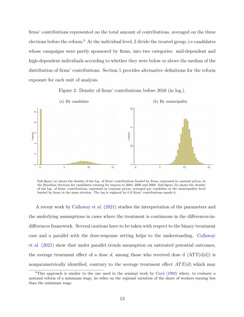
Figure 3 shows the balance of covariates before and after the weighting process for the

analysis at the municipal level. It shows that the higher the percentage that corporate

contributions represented before the reform (measured by the y-axis), the higher the total

level of contributions, the number of candidates of different categories, of population,the

spending limit introduced in 2016 and the lower the local per capita GDP. After the weighting

procedure instead, all the correlations between the treatment and the selected covariates9Dose denotes the degree of exposure to the treatment.

10Tubbicke (2020) shows that this weighting scheme is double-robust and has several advantages withrespect to the generalized propensity score method in achieving covariate balance.

14

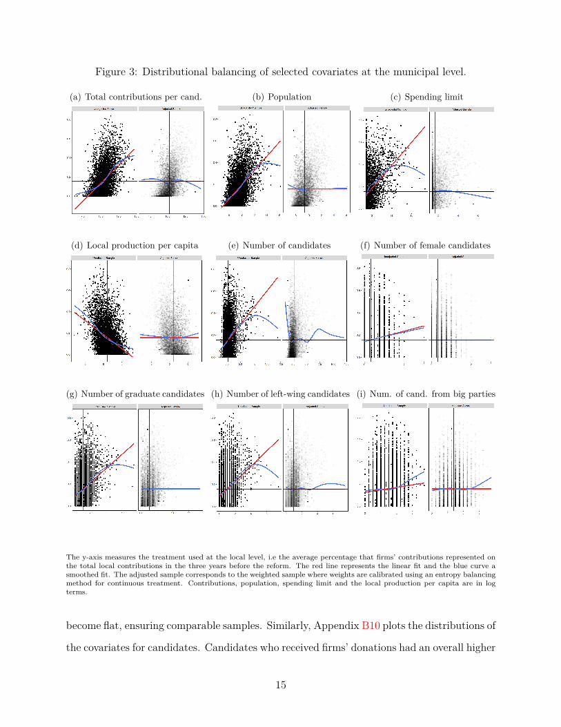
Figure 3: Distributional balancing of selected covariates at the municipal level.

(a) Total contributions per cand. (b) Population (c) Spending limit

(d) Local production per capita (e) Number of candidates (f) Number of female candidates

(g) Number of graduate candidates (h) Number of left-wing candidates (i) Num. of cand. from big parties

The y-axis measures the treatment used at the local level, i.e the average percentage that firms’ contributions represented onthe total local contributions in the three years before the reform. The red line represents the linear fit and the blue curve asmoothed fit. The adjusted sample corresponds to the weighted sample where weights are calibrated using an entropy balancingmethod for continuous treatment. Contributions, population, spending limit and the local production per capita are in logterms.

become flat, ensuring comparable samples. Similarly, Appendix B10 plots the distributions of

the covariates for candidates. Candidates who received firms’ donations had an overall higher

15

level of total contributions, they were more likely to run in more populated municipalities,

and in municipalities with more candidates. There are small differences between the level of

firms’ dependence across gender, party size and party wing. However, the higher the degree

of firms’ dependence, the higher the proportion of graduate candidates and of incumbents

(sub-figures B10 (f) and (i) respectively). The entropy balancing method is highly performant

in achieving covariate balancing, as is shown by the distribution of covariates in the adjusted

sample.11

By including the amount of total contributions as a covariate, the main difference between

the control and treated group is the composition of the pool of donors. Further, I also

account balance the spending limit introduced in 2016. Therefore, the aim is to compare

municipalities (or candidates) with similar characteristics, received a similar amount of total

contributions and that were exposed to similar levels of spending limit, but with the key

difference that in the second group firms were part of the pool of donors.

Using those weights and the treatments previously defined I estimate equation (1).

3 Results

In this section, I analyze the effects of the reform on the pool of candidates, on political

competition and on the incumbency advantage. Section 3.1 uses municipalities as units of

analysis, while section 3.2 focuses on candidates.

3.1 Effects of banning firms’ contributions on aggregate outcomes

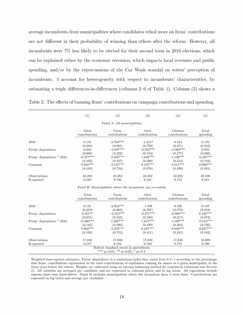
Table 2 shows that in municipalities more dependent on firms’ contributions the reform had

a significant negative effect on candidates’ average level of contributions, implying that can-

didates were not able to fully compensate the loss of firms’ money. It is however possible to11Another advantage of this method, as highlighted by Tubbicke (2020) is that it avoids extreme weights.

At the local level of analysis, the weight range is from 0 to 34, and at the individual one, it goes from 0 to19.

16

observe in columns (2), (3) and (4) that corporate contributions were highly compensated

by party funding, self funding and citizens’ donations, making the contributions’ structure

of municipalities who used to receive donations from firms very similar to the less depen-

dent ones. As expected, the average drop in contributions is translated into less campaign

spending (see column (5) of Table 2). The effects are stronger when restricting the sample to

those municipalities where the incumbent does not face a term limit, as displayed in Panel

B. This is consistent with incumbents being the most affected by the reform as they were the

candidates who enjoyed higher funding from firms. Figure 4 provides evidence for parallel

trends before the reform using the adjusted sample described in the previous section. As a

matter of fact, parallel trends are violated when using an unweighted estimation as shown

in Figure B7 of Appendix B.

In Table 3 I test whether the reform shaped the characteristics of the pool of candidates

given that different candidates may have different abilities to substitute contributions, as

well as different incentives to run for office. I find that preventing interest groups’ contribu-

tions encouraged the entry of left-wing candidates and discouraged the ones from traditional

parties when the incumbent did not face a term limit (Panel B). An interpretation is that

as left-wing candidates (candidates from big parties) were relatively less (more) funded by

firms (see Figure 1), this reform may have rebalanced this relative disadvantage (advantage).

However, those effects are small in magnitude. A 1% increase in the percentage of contri-

butions funded by firms before the reform corresponds to an increase of 0.03 in the entry of

left-wing candidates and a decrease of the same magnitude in candidates from the five biggest

parties in the aftermaths of the ban. Parallel trends regarding candidates’ characteristics

are plotted in Figure B8 of Appendix B and they hold for all outcomes.

The last set of results encompasses the incumbency advantage. Following the same

methodology, I compare the probability of incumbents to be re-elected conditional on re-

contesting across the local level of firms’ dependence.12 Column (1) of Table 4 shows that on12Weights are re-estimating for each sample restriction.

17

average incumbents from municipalities where candidates relied more on firms’ contributions

are not different in their probability of winning than others after the reform. However, all

incumbents were 7% less likely to be elected for their second term in 2016 elections, which

can be explained either by the economic recession, which impacts local revenues and public

spending, and/or by the repercussions of the Car Wash scandal on voters’ perception of

incumbents. I account for heterogeneity with respect to incumbents’ characteristics, by

estimating a triple differences-in-differences (columns 2–6 of Table 4). Column (3) shows a

Table 2: The effects of banning firms’ contributions on campaign contributions and spending.

(1) (2) (3) (4) (5)

Panel A: All municipalities

Totalcontributions

Partycontributions

Owncontributions

Citizenscontributions

Totalspending

2016 0.155 4.768*** -1.341* 0.194 0.170(0.216) (0.901) (0.759) (0.271) (0.216)

Firms’ dependence 0.032 -2.937*** -2.352*** -1.003*** 0.055(0.060) (0.222) (0.154) (0.177) (0.060)

Firms’ dependence * 2016 -0.377*** 2.450*** 1.648*** 1.130*** -0.387***(0.103) (0.437) (0.200) (0.214) (0.103)

Constant 9.922*** 3.545*** 8.478*** 8.911*** 9.900***(0.163) (0.724) (0.376) (0.240) (0.161)

Observations 22,282 22,282 22,282 22,282 22,108R-squared 0.182 0.192 0.101 0.172 0.181

Panel B: Municipalities where the incumbent can re-contest

Totalcontributions

Partycontributions

Owncontributions

Citizenscontributions

Totalspending

2016 0.121 4.954*** -1.108 0.126 0.137(0.219) (0.963) (0.787) (0.278) (0.219)

Firms’ dependence 0.161** -2.552*** -2.271*** -0.908*** 0.192***(0.071) (0.252) (0.186) (0.217) (0.072)

Firms’ dependence * 2016 -0.490*** 1.887*** 1.617*** 1.109*** -0.512***(0.125) (0.500) (0.239) (0.262) (0.126)

Constant 9.962*** 3.353*** 8.447*** 8.949*** 9.937***(0.162) (0.755) (0.411) (0.241) (0.162)

Observations 17,040 17,040 17,040 17,040 16,889R-squared 0.187 0.194 0.103 0.172 0.186

Robust standard errors in parentheses*** p<0.01, ** p<0.05, * p<0.1

Weighted least-squares estimates. Firms’ dependence is a continuous index that varies from 0 to 1 according to the percentagethat firms’ contributions represented in the total contributions of candidates running for mayor in a given municipality in thethree years before the reform. Weights are calibrated using an entropy balancing method for continuous tretament (see Section2). All variables are averaged per candidate and are expressed in constant prices and in log terms. All regressions includeregions times year fixed-effects. Panel B excludes municipalities where the incumbent faces a term limit. Contributions areexpressed in log terms and average per candidate.

18

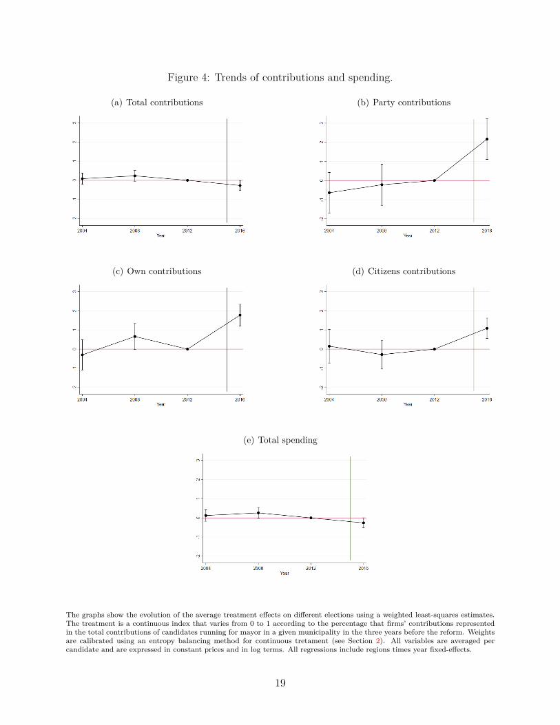
Figure 4: Trends of contributions and spending.

(a) Total contributions (b) Party contributions

(c) Own contributions (d) Citizens contributions

(e) Total spending

The graphs show the evolution of the average treatment effects on different elections using a weighted least-squares estimates.The treatment is a continuous index that varies from 0 to 1 according to the percentage that firms’ contributions representedin the total contributions of candidates running for mayor in a given municipality in the three years before the reform. Weightsare calibrated using an entropy balancing method for continuous tretament (see Section 2). All variables are averaged percandidate and are expressed in constant prices and in log terms. All regressions include regions times year fixed-effects.

19

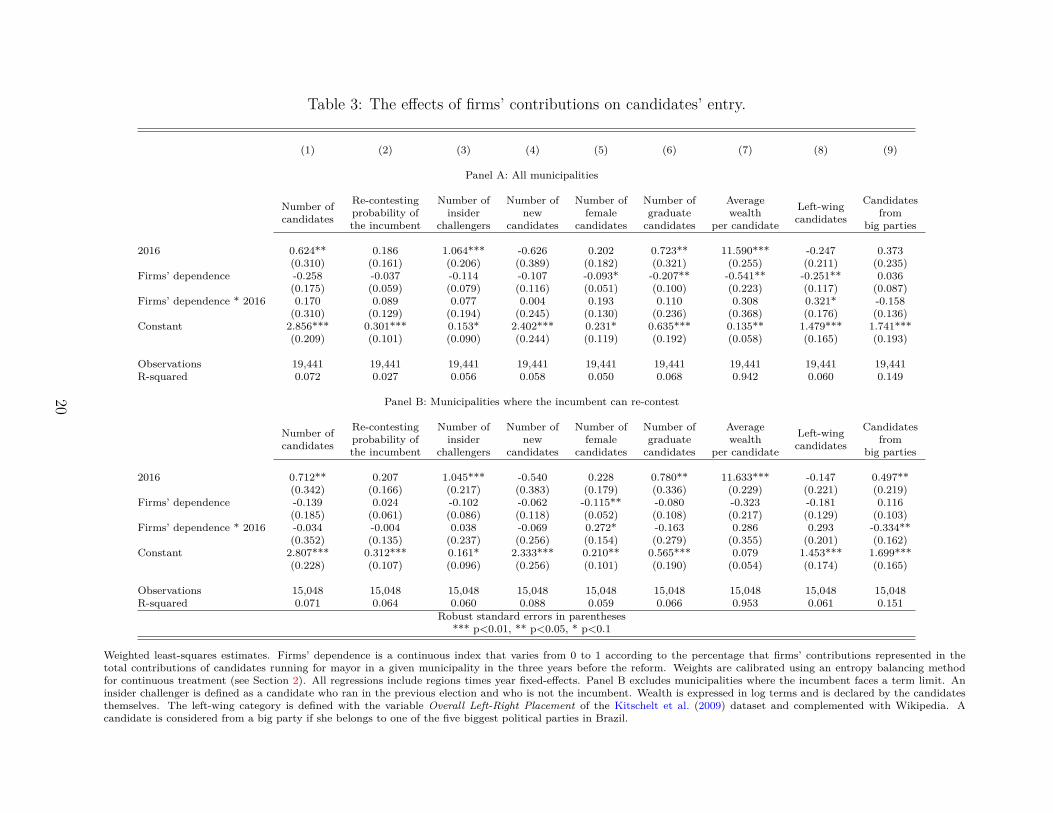
Table 3: The effects of firms’ contributions on candidates’ entry.

(1) (2) (3) (4) (5) (6) (7) (8) (9)

Panel A: All municipalities

Number ofcandidates

Re-contestingprobability ofthe incumbent

Number ofinsider

challengers

Number ofnew

candidates

Number offemale

candidates

Number ofgraduate

candidates

Averagewealth

per candidate

Left-wingcandidates

Candidatesfrom

big parties

2016 0.624** 0.186 1.064*** -0.626 0.202 0.723** 11.590*** -0.247 0.373(0.310) (0.161) (0.206) (0.389) (0.182) (0.321) (0.255) (0.211) (0.235)

Firms’ dependence -0.258 -0.037 -0.114 -0.107 -0.093* -0.207** -0.541** -0.251** 0.036(0.175) (0.059) (0.079) (0.116) (0.051) (0.100) (0.223) (0.117) (0.087)

Firms’ dependence * 2016 0.170 0.089 0.077 0.004 0.193 0.110 0.308 0.321* -0.158(0.310) (0.129) (0.194) (0.245) (0.130) (0.236) (0.368) (0.176) (0.136)

Constant 2.856*** 0.301*** 0.153* 2.402*** 0.231* 0.635*** 0.135** 1.479*** 1.741***(0.209) (0.101) (0.090) (0.244) (0.119) (0.192) (0.058) (0.165) (0.193)

Observations 19,441 19,441 19,441 19,441 19,441 19,441 19,441 19,441 19,441R-squared 0.072 0.027 0.056 0.058 0.050 0.068 0.942 0.060 0.149

Panel B: Municipalities where the incumbent can re-contest

Number ofcandidates

Re-contestingprobability ofthe incumbent

Number ofinsider

challengers

Number ofnew

candidates

Number offemale

candidates

Number ofgraduate

candidates

Averagewealth

per candidate

Left-wingcandidates

Candidatesfrom

big parties

2016 0.712** 0.207 1.045*** -0.540 0.228 0.780** 11.633*** -0.147 0.497**(0.342) (0.166) (0.217) (0.383) (0.179) (0.336) (0.229) (0.221) (0.219)

Firms’ dependence -0.139 0.024 -0.102 -0.062 -0.115** -0.080 -0.323 -0.181 0.116(0.185) (0.061) (0.086) (0.118) (0.052) (0.108) (0.217) (0.129) (0.103)

Firms’ dependence * 2016 -0.034 -0.004 0.038 -0.069 0.272* -0.163 0.286 0.293 -0.334**(0.352) (0.135) (0.237) (0.256) (0.154) (0.279) (0.355) (0.201) (0.162)

Constant 2.807*** 0.312*** 0.161* 2.333*** 0.210** 0.565*** 0.079 1.453*** 1.699***(0.228) (0.107) (0.096) (0.256) (0.101) (0.190) (0.054) (0.174) (0.165)

Observations 15,048 15,048 15,048 15,048 15,048 15,048 15,048 15,048 15,048R-squared 0.071 0.064 0.060 0.088 0.059 0.066 0.953 0.061 0.151

Robust standard errors in parentheses*** p<0.01, ** p<0.05, * p<0.1

Weighted least-squares estimates. Firms’ dependence is a continuous index that varies from 0 to 1 according to the percentage that firms’ contributions represented in thetotal contributions of candidates running for mayor in a given municipality in the three years before the reform. Weights are calibrated using an entropy balancing methodfor continuous treatment (see Section 2). All regressions include regions times year fixed-effects. Panel B excludes municipalities where the incumbent faces a term limit. Aninsider challenger is defined as a candidate who ran in the previous election and who is not the incumbent. Wealth is expressed in log terms and is declared by the candidatesthemselves. The left-wing category is defined with the variable Overall Left-Right Placement of the Kitschelt et al. (2009) dataset and complemented with Wikipedia. Acandidate is considered from a big party if she belongs to one of the five biggest political parties in Brazil.

20

significant disparity regarding the level of education. The reform barely affected the electoral

prospects of graduate incumbents while it heavily reduced the re-election probability for low

educated ones. On the contrary, there are no differential effects across gender, party wing,

party size or total wealth. More generally, this result is confirmed when focusing on the

characteristics of the winner candidates regardless of whether the winner is the incumbent

(see Table A6).

However, it is important to mention that in municipalities where candidates relied more

on firms’ contributions, graduate incumbents’ were more likely to re-contest after the ban,

as well as wealthier incumbents (see Appendix A7).

Using the aggregated percentage of firms’ contributions in the municipality as a treatment

can mislead the identification of the mechanisms as it does not differentiate between munici-

palities where the firms’ dependence is driven by the incumbents’ funding or by challengers’

dependence. I move to the candidate’s level of analysis to tackle this issue.

3.2 Effects of banning firms’ contributions on individual outcomes

In this section I compare individuals who were exposed by the reform using as control group

candidates who didn’t receive any firms’ contributions the previous election. As detailed in

section 2, I divide the treatment group into two categories: mid-firms’ dependent candidates

and high-dependent ones, defined according to whether they received below or above the

median of firms’ contributions. I restrict the sample to incumbents who don’t face a term

limit and runners-up, as around 70% of firms’ funding before the reform was concentrated

among the top two candidates.13

Figure 6 shows the general effects of the reform for incumbents and runners-up. In-

cumbents who relied on firms’ funding before the reform were equally likely to re-contest

compared to incumbents non-dependent on firms’ contributions with similar characteristics.13The median is calculated using the full sample of incumbents who don’t face a term limit and runners-up,

conditional on firms’ contributions being greater than 0. Results are robust when estimating the treatmentincluding all challengers and when defining the median separately for incumbents and runners-up.

21

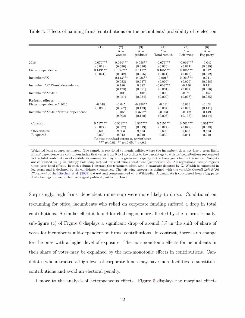
Table 4: Effects of banning firms’ contributions on the incumbents’ probability of re-election

(1) (2) (3) (4) (5) (6)X =

womanX =

graduateX =

Total wealthX =

Left-wingX =

Big party

2016 -0.070*** -0.064*** -0.058** -0.076*** -0.066*** -0.042(0.019) (0.020) (0.026) (0.020) (0.021) (0.029)

Firms’ dependence 0.149*** 0.132*** 0.113** 0.165*** 0.185*** 0.072(0.041) (0.042) (0.056) (0.041) (0.046) (0.072)

Incumbent*X -0.113*** -0.035** 0.001* 0.064*** 0.011(0.032) (0.017) (0.000) (0.020) (0.018)

Incumbent*X*Firms’ dependence 0.180 0.082 -0.003*** -0.156 0.111(0.173) (0.081) (0.001) (0.097) (0.086)

Incumbent*X*2016 -0.008 -0.006 0.000 -0.021 -0.040(0.057) (0.034) (0.000) (0.038) (0.035)

Reform effectsFirms’ dependence * 2016 -0.048 -0.045 -0.298** -0.011 0.026 -0.134

(0.083) (0.087) (0.133) (0.087) (0.093) (0.141)Incumbent*X*2016*Firms’ dependence -0.066 0.370** -0.003 -0.302 0.149

(0.302) (0.170) (0.003) (0.196) (0.174)

Constant 0.517*** 0.523*** 0.535*** 0.515*** 0.501*** 0.507***(0.077) (0.077) (0.079) (0.077) (0.078) (0.078)

Observations 9,603 9,603 9,603 9,603 9,603 9,603R-squared 0.039 0.042 0.040 0.039 0.041 0.040

Robust standard errors in parentheses*** p<0.01, ** p<0.05, * p<0.1

Weighted least-squares estimates. The sample is restricted to municipalities where the incumbent does not face a term limit.Firms’ dependence is a continuous index that varies from 0 to 1 according to the percentage that firms’ contributions representedin the total contributions of candidates running for mayor in a given municipality in the three years before the reform. Weightsare calibrated using an entropy balancing method for continuous treatment (see Section 2). All regressions include regionstimes year fixed-effects. In each column I interact the treatment effect with a covariate denoted by X. Wealth is expressed inlog terms and is declared by the candidates themselves. The left-wing category is defined with the variable Overall Left-RightPlacement of the Kitschelt et al. (2009) dataset and complemented with Wikipedia. A candidate is considered from a big partyif she belongs to one of the five biggest political parties in Brazil.

Surprisingly, high firms’ dependent runners-up were more likely to do so. Conditional on

re-running for office, incumbents who relied on corporate funding suffered a drop in total

contributions. A similar effect is found for challengers more affected by the reform. Finally,

sub-figure (c) of Figure 6 displays a significant drop of around 3% in the shift of share of

votes for incumbents mid-dependent on firms’ contributions. In contrast, there is no change

for the ones with a higher level of exposure. The non-monotonic effects for incumbents in

their share of votes may be explained by the non-monotonic effects in contributions. Can-

didates who attracted a high level of corporate funds may have more facilities to substitute

contributions and avoid an electoral penalty.

I move to the analysis of heterogeneous effects. Figure 5 displays the marginal effects

22

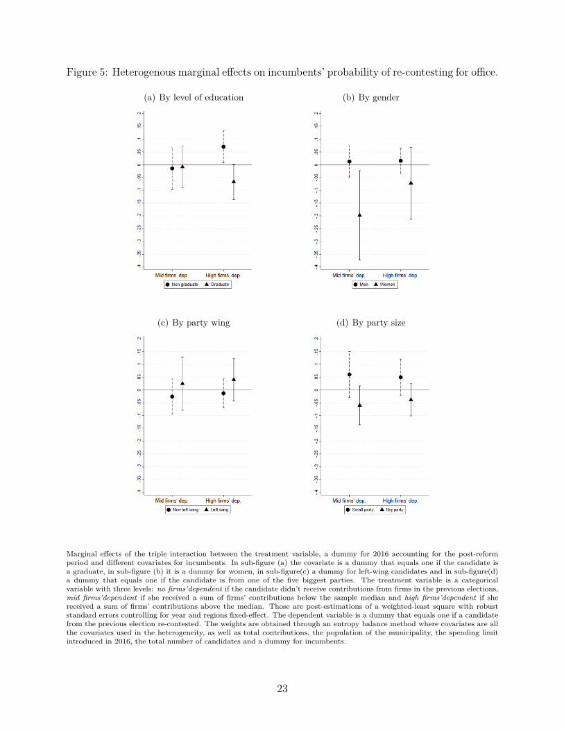
Figure 5: Heterogenous marginal effects on incumbents’ probability of re-contesting for office.

(a) By level of education (b) By gender

(c) By party wing (d) By party size

Marginal effects of the triple interaction between the treatment variable, a dummy for 2016 accounting for the post-reformperiod and different covariates for incumbents. In sub-figure (a) the covariate is a dummy that equals one if the candidate isa graduate, in sub-figure (b) it is a dummy for women, in sub-figure(c) a dummy for left-wing candidates and in sub-figure(d)a dummy that equals one if the candidate is from one of the five biggest parties. The treatment variable is a categoricalvariable with three levels: no firms’dependent if the candidate didn’t receive contributions from firms in the previous elections,mid firms’dependent if she received a sum of firms’ contributions below the sample median and high firms’dependent if shereceived a sum of firms’ contributions above the median. Those are post-estimations of a weighted-least square with robuststandard errors controlling for year and regions fixed-effect. The dependent variable is a dummy that equals one if a candidatefrom the previous election re-contested. The weights are obtained through an entropy balance method where covariates are allthe covariates used in the heterogeneity, as well as total contributions, the population of the municipality, the spending limitintroduced in 2016, the total number of candidates and a dummy for incumbents.

23

Figure 6: Marginal effects of the reform on incumbents and runners-up.

(a) Probability of re-contesting(b) Variation in total contribu-tions (in log.)

(c) Share of votes in next elec-tions

Marginal effects of the interaction between the treatment variable and a dummy for 2016 accounting for the post-reform. Thetreatment variable is a categorical variable with three levels: no firms’dependent if the candidate didn’t receive contributionsfrom firms in the previous elections, mid firms’dependent if she received a sum of firms’ contributions below the sample medianand high firms’dependent if she received a sum of firms’ contributions above the median. Those are post-estimations of aweighted-least square with robust standard errors controlling for year and regions fixed-effects. In sub-figure (a) the dependentvariable is a dummy that equals one if a candidate from previous election re-contested, in sub-figure (b) is the variation inthe log. of total contributions conditional on re-contesting and in (c) is the share of votes in next elections. The weights areobtained through an entropy balance method where covariates are graduate, gender, party-wing, party size, total contributions,the population of the municipality, the spending limit introduced in 2016, the total number of candidates and a dummy forincumbents.

in re-contesting decisions when performing the heterogeneity across several covariates for

incumbents and Appendix B2 for runners-up. The coefficients are displayed in Appendix A9.

Sub-figure (a) shows that there are no differences among mid-firms’ dependent incumbents

between graduates and non-graduates. However, among high-dependent candidates, non-

graduate incumbents were 7% more likely to re-contest and a symmetric effect is found for

graduate officeholders. Sub-figure (b) plots differences in gender. Female incumbents are

less likely to run for re-election after the reform and the difference is significant for mid-

dependent candidates. The same discouragement is found for runners-up (Figure B2 and

Table A9). While there is no heterogeneity among party-wing (sub-figure (c)), sub-figure

(d) shows that among exposed incumbents, candidates from big parties were less likely to

re-contest compared to candidates from small ones.

24

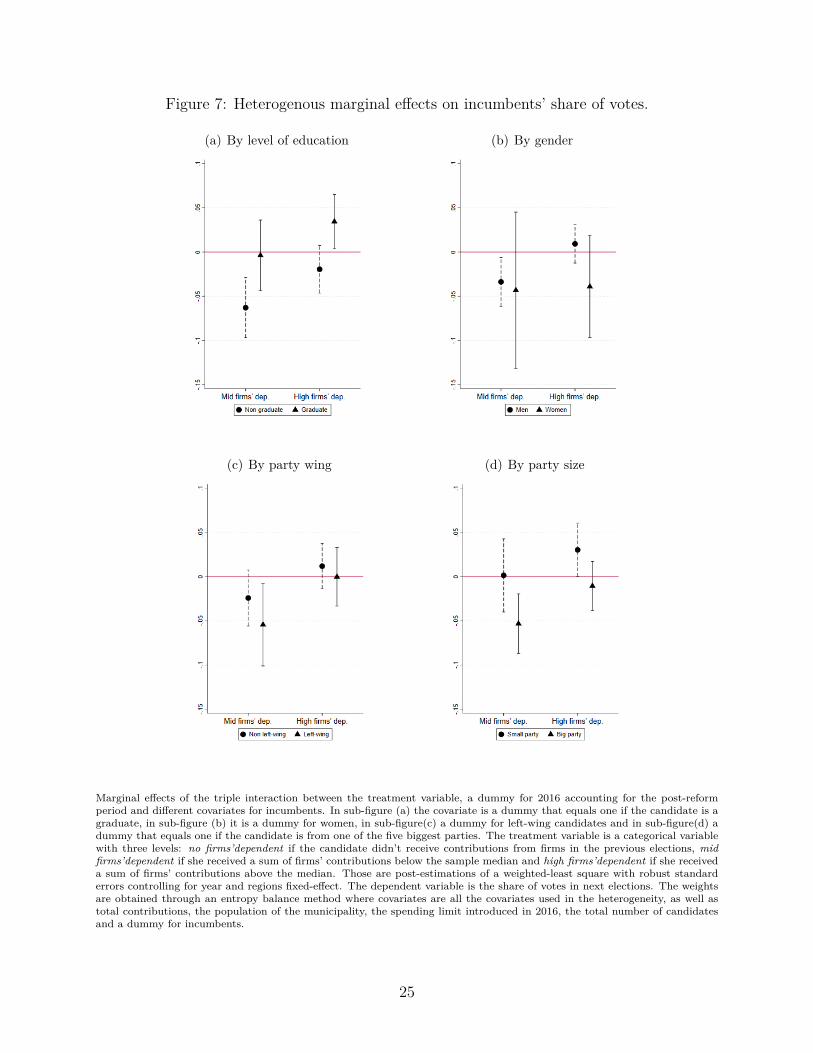
Figure 7: Heterogenous marginal effects on incumbents’ share of votes.

(a) By level of education (b) By gender

(c) By party wing (d) By party size

Marginal effects of the triple interaction between the treatment variable, a dummy for 2016 accounting for the post-reformperiod and different covariates for incumbents. In sub-figure (a) the covariate is a dummy that equals one if the candidate is agraduate, in sub-figure (b) it is a dummy for women, in sub-figure(c) a dummy for left-wing candidates and in sub-figure(d) adummy that equals one if the candidate is from one of the five biggest parties. The treatment variable is a categorical variablewith three levels: no firms’dependent if the candidate didn’t receive contributions from firms in the previous elections, midfirms’dependent if she received a sum of firms’ contributions below the sample median and high firms’dependent if she receiveda sum of firms’ contributions above the median. Those are post-estimations of a weighted-least square with robust standarderrors controlling for year and regions fixed-effect. The dependent variable is the share of votes in next elections. The weightsare obtained through an entropy balance method where covariates are all the covariates used in the heterogeneity, as well astotal contributions, the population of the municipality, the spending limit introduced in 2016, the total number of candidatesand a dummy for incumbents.

25

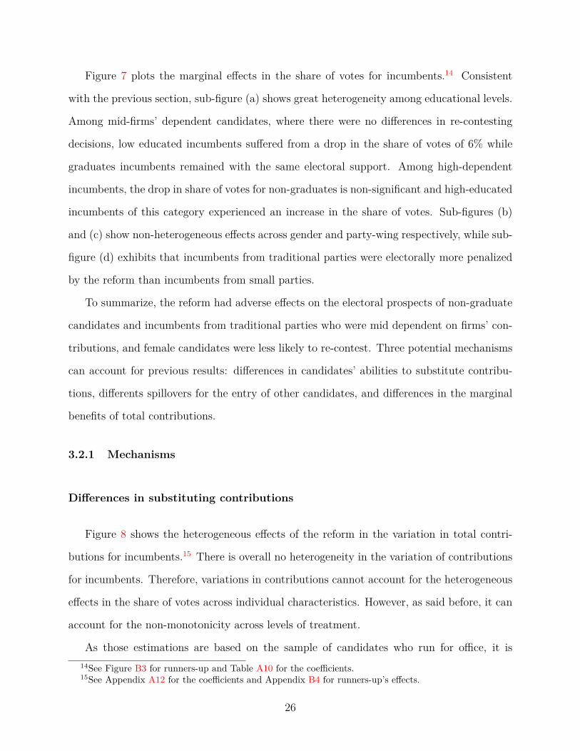
Figure 7 plots the marginal effects in the share of votes for incumbents.14 Consistent

with the previous section, sub-figure (a) shows great heterogeneity among educational levels.

Among mid-firms’ dependent candidates, where there were no differences in re-contesting

decisions, low educated incumbents suffered from a drop in the share of votes of 6% while

graduates incumbents remained with the same electoral support. Among high-dependent

incumbents, the drop in share of votes for non-graduates is non-significant and high-educated

incumbents of this category experienced an increase in the share of votes. Sub-figures (b)

and (c) show non-heterogeneous effects across gender and party-wing respectively, while sub-

figure (d) exhibits that incumbents from traditional parties were electorally more penalized

by the reform than incumbents from small parties.

To summarize, the reform had adverse effects on the electoral prospects of non-graduate

candidates and incumbents from traditional parties who were mid dependent on firms’ con-

tributions, and female candidates were less likely to re-contest. Three potential mechanisms

can account for previous results: differences in candidates’ abilities to substitute contribu-

tions, differents spillovers for the entry of other candidates, and differences in the marginal

benefits of total contributions.

3.2.1 Mechanisms

Differences in substituting contributions

Figure 8 shows the heterogeneous effects of the reform in the variation in total contri-

butions for incumbents.15 There is overall no heterogeneity in the variation of contributions

for incumbents. Therefore, variations in contributions cannot account for the heterogeneous

effects in the share of votes across individual characteristics. However, as said before, it can

account for the non-monotonicity across levels of treatment.

As those estimations are based on the sample of candidates who run for office, it is14See Figure B3 for runners-up and Table A10 for the coefficients.15See Appendix A12 for the coefficients and Appendix B4 for runners-up’s effects.

26

Figure 8: Heterogenous marginal effects on the variation of incumbents’ contributions.

(a) By level of education (b) By gender

(c) By party wing (d) By party size

Marginal effects of the triple interaction between the treatment variable, a dummy for 2016 accounting for the post-reformperiod and different covariates for incumbents. In sub-figure (a) the covariate is a dummy that equals one if the candidate is agraduate, in sub-figure (b) it is a dummy for women, in sub-figure(c) a dummy for left-wing candidates and in sub-figure(d) adummy that equals one if the candidate is from one of the five biggest parties. The treatment variable is a categorical variablewith three levels: no firms’dependent if the candidate didn’t receive contributions from firms in the previous elections, midfirms’dependent if she received a sum of firms’ contributions below the sample median and high firms’dependent if she receiveda sum of firms’ contributions above the median. Those are post-estimations of a weighted-least square with robust standarderrors controlling for year and regions fixed-effect. The dependent variable is the variation in the log of contributions. Theweights are obtained through an entropy balance method where covariates are all the covariates used in the heterogeneity,as well as total contributions, the population of the municipality, the spending limit introduced in 2016, the total number ofcandidates and a dummy for incumbents.

27

difficult to test if expected changes in contributions drive effects on re-contesting decisions.

Yet, there is evidence that female mayors in Brazil attracted fewer campaign contributions

when running for re-election (Brollo and Troiano, 2016). Thus, the higher cost in fund-

raising for female politicians could be behind the discouragement of female candidates when

interest groups are no longer allowed to contribute.

Entry of challengers

Another potential mechanism is that heterogenous spillover effects on challengers’ re-

contesting decisions exist. Figure 9 and Appendix A12 provide evidence supporting this

channel. There is an increase in the number of challengers challengers in municipalities

where the incumbent was a graduate or a candidate from a big party. When controlling for

the increase of challengers and for the variation in contributions, the effects on the share

of votes persist even though there are mitigated. Therefore, spillover effects can partially

account for the electoral loss of low-educated and incumbents from big parties. Further,

the fact that some incumbents had a higher drop in the share of votes for a given drop in

contributions and a given change in candidates’ entry can be driven by differences in the

marginal benefits of contributions. Yet, the interpretation of the heterogeneity in these two

channels is not straightforward. Differences in the quality of incumbents can be at play.

Quality incumbency advantage

The interaction of a quality and a financial incumbency advantage can explain both the

differences in marginal benefits of incumbents’ contributions and the heterogeneity in the

entry of challengers. First, low-quality incumbents may need more resources than high-

quality incumbents to attract voters as they have to compensate for their bad performance

while in office. If that is the case, the former will experience a higher drop in their share of

votes for a given drop in contributions. Second, challengers’ decisions of running for office

are likely to be inversely correlated with the incumbent’s expected probability of winning.

28

Figure 9: Heterogenous marginal effects on the entry of challengers.

(a) By level of education (b) By gender

(c) By party wing (d) By party size

Marginal effects of the triple interaction between the treatment variable, a dummy for 2016 accounting for the post-reformperiod and different covariates for incumbents. In sub-figure (a) the covariate is a dummy that equals one if the candidate is agraduate, in sub-figure (b) it is a dummy for women, in sub-figure(c) a dummy for left-wing candidates and in sub-figure(d) adummy that equals one if the candidate is from one of the five biggest parties. The treatment variable is a categorical variablewith three levels: no firms’dependent if the candidate didn’t receive contributions from firms in the previous elections, midfirms’dependent if she received a sum of firms’ contributions below the sample median and high firms’dependent if she receiveda sum of firms’ contributions above the median. Those are post-estimations of a weighted-least square with robust standarderrors controlling for year and regions fixed-effect. The dependent variable is the variation of challengers. The weights areobtained through an entropy balance method where covariates are all the covariates used in the heterogeneity, as well as totalcontributions, the population of the municipality, the spending limit introduced in 2016, the total number of candidates and adummy for incumbents.

29

Thus, for a given shock in incumbents’ contributions, they will be more encouraged to run

for office if the incumbent is a low-quality type.

For the previous arguments to hold, the educational level and the size of the party have

to be a sign of the incumbent’s quality. The level of education has been used in the literature

as a proxy of politicians’ quality (see Ferraz and Finan (2009) and Galasso and Nannicini

(2011), among others). On the other hand, candidates from big parties are likely to have

more political connections and to provide higher levels of rents to interest groups.

Figure 10: Marginal effects of the reform for different proxies for quality.

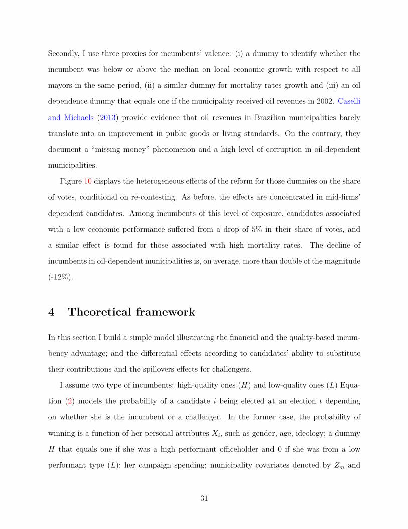
(a) Economic growth (b) Mortality growth (c) Oil dependence

Marginal effects of the triple interaction between the treatment variable, a dummy for 2016 accounting for the post-reformperiod and different covariates for incumbents. In sub-figure (a) the covariate is a dummy that equals one if the incumbentwas above the median of local economic growth, in sub-figure (b) it is a dummy that equals one if the incumbent was abovethe median of local mortality growth and in sub-figure(c) a dummy that equals one if the municipality received oil royaltiesin 2002. The treatment variable is a categorical variable with three levels: no firms’dependent if the candidate didn’t receivecontributions from firms in the previous elections, mid firms’dependent if she received a sum of firms’ contributions belowthe sample median and high firms’dependent if she received a sum of firms’ contributions above the median. Those are post-estimations of a weighted-least square with robust standard errors controlling for year and regions fixed-effect. The dependentvariable is the share of votes in next elections. The weights are obtained through an entropy balance method where covariatesare all the covariates used in the heterogeneity, as well as total contributions, the population of the municipality, the spendinglimit introduced in 2016, the total number of candidates and a dummy for incumbents.

I provide further evidence suggesting that a quality component drives previous results.

First, I control by declared wealth, as the educational level may be correlated with the socio-

economic status that may explain the findings. Results hold and the drop in the probability

of being elected for low educated incumbents becomes stronger (see Figures B5 and B6).

30

Secondly, I use three proxies for incumbents’ valence: (i) a dummy to identify whether the

incumbent was below or above the median on local economic growth with respect to all

mayors in the same period, (ii) a similar dummy for mortality rates growth and (iii) an oil

dependence dummy that equals one if the municipality received oil revenues in 2002. Caselli

and Michaels (2013) provide evidence that oil revenues in Brazilian municipalities barely

translate into an improvement in public goods or living standards. On the contrary, they

document a “missing money” phenomenon and a high level of corruption in oil-dependent

municipalities.

Figure 10 displays the heterogeneous effects of the reform for those dummies on the share

of votes, conditional on re-contesting. As before, the effects are concentrated in mid-firms’

dependent candidates. Among incumbents of this level of exposure, candidates associated

with a low economic performance suffered from a drop of 5% in their share of votes, and

a similar effect is found for those associated with high mortality rates. The decline of

incumbents in oil-dependent municipalities is, on average, more than double of the magnitude

(-12%).

4 Theoretical framework

In this section I build a simple model illustrating the financial and the quality-based incum-

bency advantage; and the differential effects according to candidates’ ability to substitute

their contributions and the spillovers effects for challengers.

I assume two type of incumbents: high-quality ones (H) and low-quality ones (L) Equa-

tion (2) models the probability of a candidate i being elected at an election t depending

on whether she is the incumbent or a challenger. In the former case, the probability of

winning is a function of her personal attributes Xi, such as gender, age, ideology; a dummy

H that equals one if she was a high performant officeholder and 0 if she was from a low

performant type (L); her campaign spending; municipality covariates denoted by Zm and

31

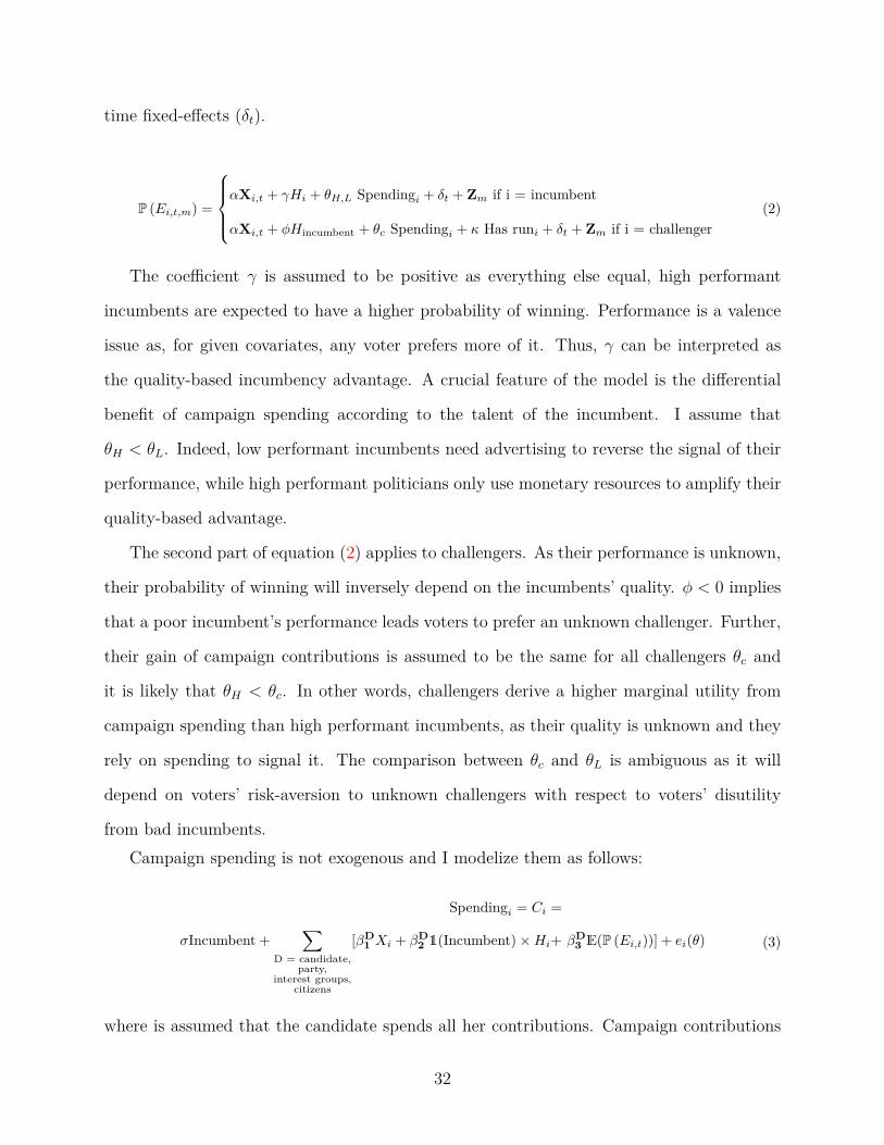
time fixed-effects (δt).

P (Ei,t,m) =

αXi,t + γHi + θH,L Spendingi + δt + Zm if i = incumbent

αXi,t + ϕHincumbent + θc Spendingi + κ Has runi + δt + Zm if i = challenger(2)

The coefficient γ is assumed to be positive as everything else equal, high performant

incumbents are expected to have a higher probability of winning. Performance is a valence

issue as, for given covariates, any voter prefers more of it. Thus, γ can be interpreted as

the quality-based incumbency advantage. A crucial feature of the model is the differential

benefit of campaign spending according to the talent of the incumbent. I assume that

θH < θL. Indeed, low performant incumbents need advertising to reverse the signal of their

performance, while high performant politicians only use monetary resources to amplify their

quality-based advantage.

The second part of equation (2) applies to challengers. As their performance is unknown,

their probability of winning will inversely depend on the incumbents’ quality. ϕ < 0 implies

that a poor incumbent’s performance leads voters to prefer an unknown challenger. Further,

their gain of campaign contributions is assumed to be the same for all challengers θc and

it is likely that θH < θc. In other words, challengers derive a higher marginal utility from

campaign spending than high performant incumbents, as their quality is unknown and they

rely on spending to signal it. The comparison between θc and θL is ambiguous as it will

depend on voters’ risk-aversion to unknown challengers with respect to voters’ disutility

from bad incumbents.Campaign spending is not exogenous and I modelize them as follows:

Spendingi = Ci =

σIncumbent +∑

D = candidate,party,

interest groups,citizens

[βD1 Xi + βD

2 1(Incumbent) × Hi+ βD3 E(P (Ei,t))] + ei(θ) (3)

where is assumed that the candidate spends all her contributions. Campaign contributions

32

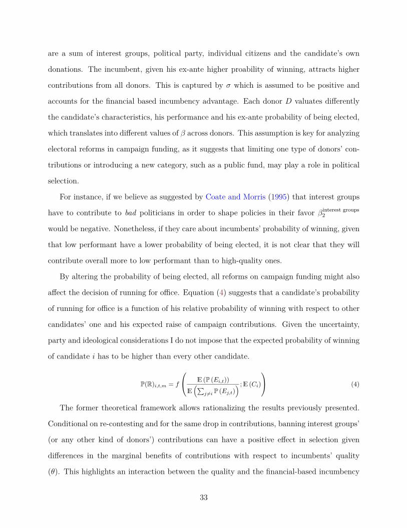
are a sum of interest groups, political party, individual citizens and the candidate’s own

donations. The incumbent, given his ex-ante higher proability of winning, attracts higher

contributions from all donors. This is captured by σ which is assumed to be positive and

accounts for the financial based incumbency advantage. Each donor D valuates differently

the candidate’s characteristics, his performance and his ex-ante probability of being elected,

which translates into different values of β across donors. This assumption is key for analyzing

electoral reforms in campaign funding, as it suggests that limiting one type of donors’ con-

tributions or introducing a new category, such as a public fund, may play a role in political

selection.

For instance, if we believe as suggested by Coate and Morris (1995) that interest groups

have to contribute to bad politicians in order to shape policies in their favor βinterest groups2

would be negative. Nonetheless, if they care about incumbents’ probability of winning, given

that low performant have a lower probability of being elected, it is not clear that they will

contribute overall more to low performant than to high-quality ones.

By altering the probability of being elected, all reforms on campaign funding might also

affect the decision of running for office. Equation (4) suggests that a candidate’s probability

of running for office is a function of his relative probability of winning with respect to other

candidates’ one and his expected raise of campaign contributions. Given the uncertainty,

party and ideological considerations I do not impose that the expected probability of winning

of candidate i has to be higher than every other candidate.

P(R)i,t,m = f

E (P (Ei,t))E

(∑j =i P (Ej,t)

) ;E (Ci)

(4)

The former theoretical framework allows rationalizing the results previously presented.

Conditional on re-contesting and for the same drop in contributions, banning interest groups’

(or any other kind of donors’) contributions can have a positive effect in selection given

differences in the marginal benefits of contributions with respect to incumbents’ quality

(θ). This highlights an interaction between the quality and the financial-based incumbency

33

advantage. Nonetheless, taking into account that different candidates have different abilities

to raise contributions from different donors, there is room for negative selection effects for

the ones with a higher cost of fundraising. Finally, as challengers were not favored by interest

groups’ contributions, the reform may have encouraged them to run if they anticipate that

incumbents would suffer from a drop in their probability of winning after the reform.

5 Robustness checks

5.1 Aggregate outcomes

Section 3.1 focused on weighted regressions to account for differences in observables between

municipalities according to their degree of firms’ dependence before the reform and potential

selection into this treatment. As previously mentioned, an unrestricted and unweighted

sample analysis does not validate the assumption of parallel trends (see Figure B7).

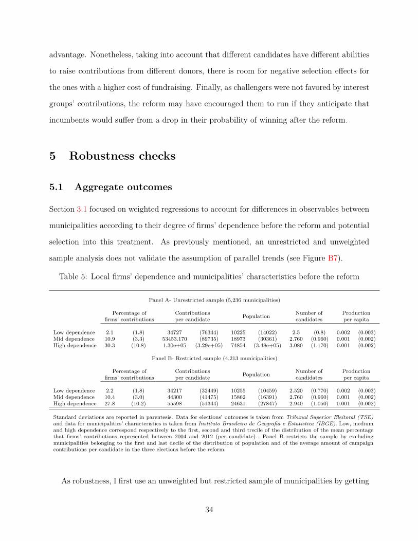
Table 5: Local firms’ dependence and municipalities’ characteristics before the reform

Panel A- Unrestricted sample (5,236 municipalities)

Percentage offirms’ contributions

Contributionsper candidate Population Number of

candidatesProductionper capita

Low dependence 2.1 (1.8) 34727 (76344) 10225 (14022) 2.5 (0.8) 0.002 (0.003)Mid dependence 10.9 (3.3) 53453.170 (89735) 18973 (30361) 2.760 (0.960) 0.001 (0.002)High dependence 30.3 (10.8) 1.30e+05 (3.29e+05) 74854 (3.48e+05) 3.080 (1.170) 0.001 (0.002)

Panel B- Restricted sample (4,213 municipalities)

Percentage offirms’ contributions

Contributionsper candidate Population Number of

candidatesProductionper capita

Low dependence 2.2 (1.8) 34217 (32449) 10255 (10459) 2.520 (0.770) 0.002 (0.003)Mid dependence 10.4 (3.0) 44300 (41475) 15862 (16391) 2.760 (0.960) 0.001 (0.002)High dependence 27.8 (10.2) 55598 (51344) 24631 (27847) 2.940 (1.050) 0.001 (0.002)

Standard deviations are reported in parentesis. Data for elections’ outcomes is taken from Tribunal Superior Eleitoral (TSE)and data for municipalities’ characteristics is taken from Instituto Brasileiro de Geografia e Estatistica (IBGE). Low, mediumand high dependence correspond respectively to the first, second and third trecile of the distribution of the mean percentagethat firms’ contributions represented between 2004 and 2012 (per candidate). Panel B restricts the sample by excludingmunicipalities belonging to the first and last decile of the distribution of population and of the average amount of campaigncontributions per candidate in the three elections before the reform.

As robustness, I first use an unweighted but restricted sample of municipalities by getting

34

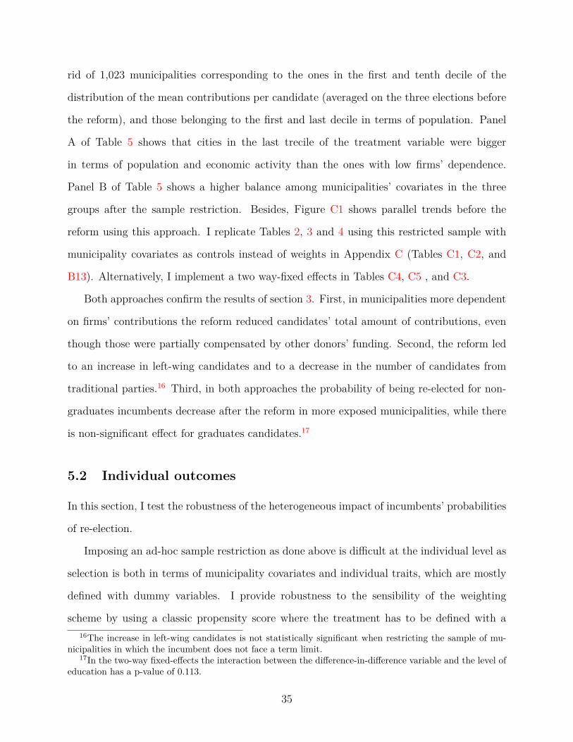
rid of 1,023 municipalities corresponding to the ones in the first and tenth decile of the

distribution of the mean contributions per candidate (averaged on the three elections before

the reform), and those belonging to the first and last decile in terms of population. Panel

A of Table 5 shows that cities in the last trecile of the treatment variable were bigger

in terms of population and economic activity than the ones with low firms’ dependence.

Panel B of Table 5 shows a higher balance among municipalities’ covariates in the three

groups after the sample restriction. Besides, Figure C1 shows parallel trends before the

reform using this approach. I replicate Tables 2, 3 and 4 using this restricted sample with

municipality covariates as controls instead of weights in Appendix C (Tables C1, C2, and

B13). Alternatively, I implement a two way-fixed effects in Tables C4, C5 , and C3.

Both approaches confirm the results of section 3. First, in municipalities more dependent

on firms’ contributions the reform reduced candidates’ total amount of contributions, even

though those were partially compensated by other donors’ funding. Second, the reform led

to an increase in left-wing candidates and to a decrease in the number of candidates from

traditional parties.16 Third, in both approaches the probability of being re-elected for non-

graduates incumbents decrease after the reform in more exposed municipalities, while there

is non-significant effect for graduates candidates.17

5.2 Individual outcomes

In this section, I test the robustness of the heterogeneous impact of incumbents’ probabilities

of re-election.

Imposing an ad-hoc sample restriction as done above is difficult at the individual level as

selection is both in terms of municipality covariates and individual traits, which are mostly

defined with dummy variables. I provide robustness to the sensibility of the weighting

scheme by using a classic propensity score where the treatment has to be defined with a16The increase in left-wing candidates is not statistically significant when restricting the sample of mu-

nicipalities in which the incumbent does not face a term limit.17In the two-way fixed-effects the interaction between the difference-in-difference variable and the level of

education has a p-value of 0.113.

35

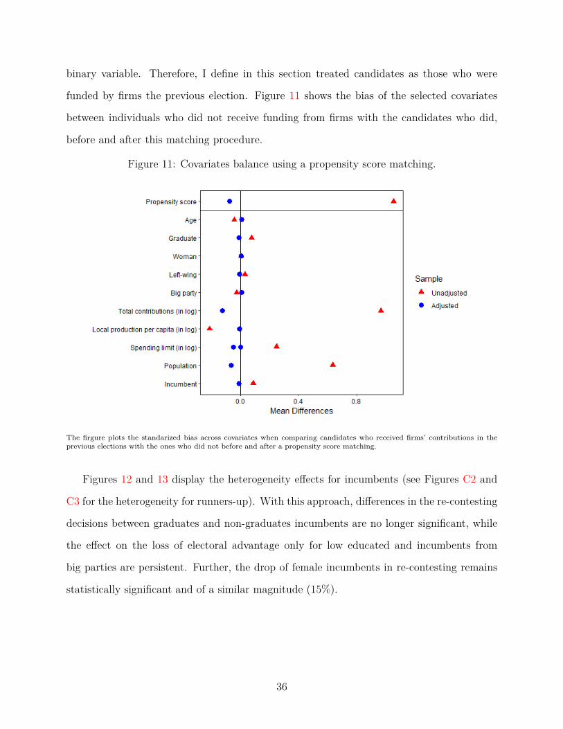
binary variable. Therefore, I define in this section treated candidates as those who were

funded by firms the previous election. Figure 11 shows the bias of the selected covariates

between individuals who did not receive funding from firms with the candidates who did,

before and after this matching procedure.

Figure 11: Covariates balance using a propensity score matching.

The firgure plots the standarized bias across covariates when comparing candidates who received firms’ contributions in theprevious elections with the ones who did not before and after a propensity score matching.

Figures 12 and 13 display the heterogeneity effects for incumbents (see Figures C2 and

C3 for the heterogeneity for runners-up). With this approach, differences in the re-contesting

decisions between graduates and non-graduates incumbents are no longer significant, while

the effect on the loss of electoral advantage only for low educated and incumbents from

big parties are persistent. Further, the drop of female incumbents in re-contesting remains

statistically significant and of a similar magnitude (15%).

36

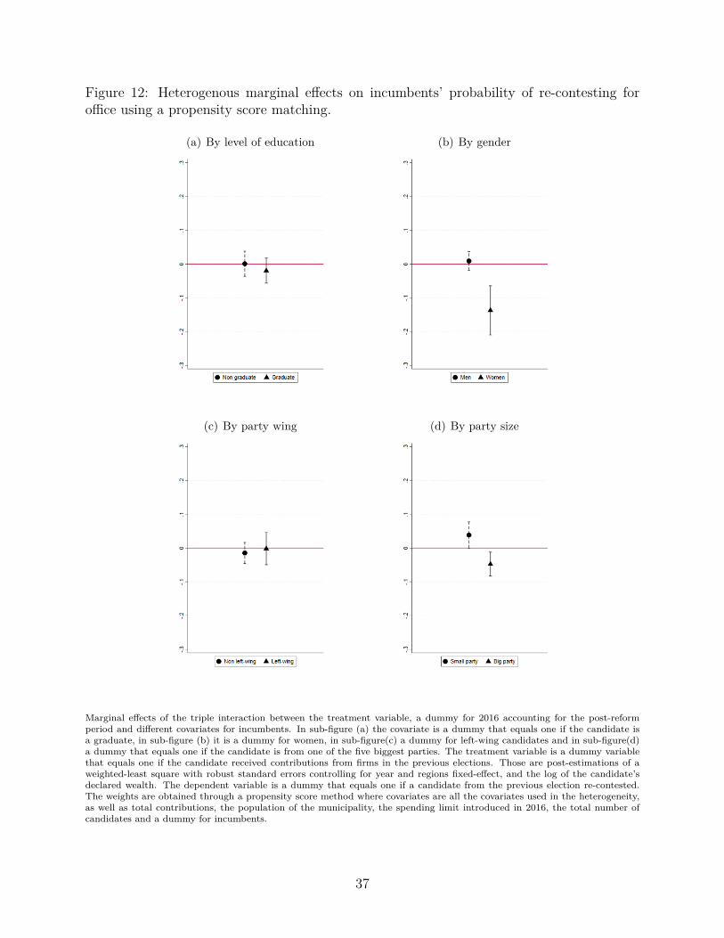
Figure 12: Heterogenous marginal effects on incumbents’ probability of re-contesting foroffice using a propensity score matching.

(a) By level of education (b) By gender

(c) By party wing (d) By party size

Marginal effects of the triple interaction between the treatment variable, a dummy for 2016 accounting for the post-reformperiod and different covariates for incumbents. In sub-figure (a) the covariate is a dummy that equals one if the candidate isa graduate, in sub-figure (b) it is a dummy for women, in sub-figure(c) a dummy for left-wing candidates and in sub-figure(d)a dummy that equals one if the candidate is from one of the five biggest parties. The treatment variable is a dummy variablethat equals one if the candidate received contributions from firms in the previous elections. Those are post-estimations of aweighted-least square with robust standard errors controlling for year and regions fixed-effect, and the log of the candidate’sdeclared wealth. The dependent variable is a dummy that equals one if a candidate from the previous election re-contested.The weights are obtained through a propensity score method where covariates are all the covariates used in the heterogeneity,as well as total contributions, the population of the municipality, the spending limit introduced in 2016, the total number ofcandidates and a dummy for incumbents.

37

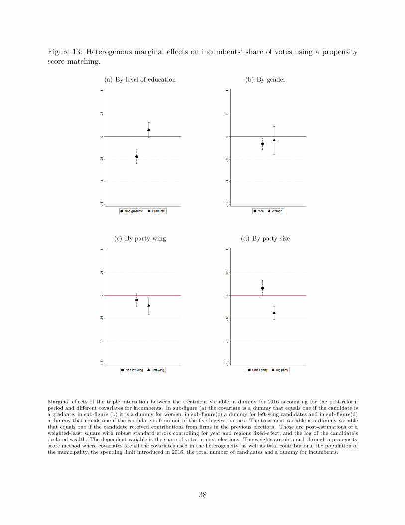
Figure 13: Heterogenous marginal effects on incumbents’ share of votes using a propensityscore matching.

(a) By level of education (b) By gender

(c) By party wing (d) By party size

Marginal effects of the triple interaction between the treatment variable, a dummy for 2016 accounting for the post-reformperiod and different covariates for incumbents. In sub-figure (a) the covariate is a dummy that equals one if the candidate isa graduate, in sub-figure (b) it is a dummy for women, in sub-figure(c) a dummy for left-wing candidates and in sub-figure(d)a dummy that equals one if the candidate is from one of the five biggest parties. The treatment variable is a dummy variablethat equals one if the candidate received contributions from firms in the previous elections. Those are post-estimations of aweighted-least square with robust standard errors controlling for year and regions fixed-effect, and the log of the candidate’sdeclared wealth. The dependent variable is the share of votes in next elections. The weights are obtained through a propensityscore method where covariates are all the covariates used in the heterogeneity, as well as total contributions, the population ofthe municipality, the spending limit introduced in 2016, the total number of candidates and a dummy for incumbents.

38

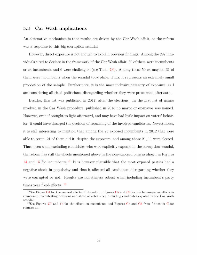
5.3 Car Wash implications

An alternative mechanism is that results are driven by the Car Wash affair, as the reform

was a response to this big corruption scandal.

However, direct exposure is not enough to explain previous findings. Among the 297 indi-

viduals cited to declare in the framework of the Car Wash affair, 50 of them were incumbents

or ex-incumbents and 6 were challengers (see Table C6). Among those 50 ex-mayors, 31 of

them were incumbents when the scandal took place. Thus, it represents an extremely small

proportion of the sample. Furthermore, it is the most inclusive category of exposure, as I

am considering all cited politicians, disregarding whether they were prosecuted afterward.

Besides, this list was published in 2017, after the elections. In the first list of names

involved in the Car Wash procedure, published in 2015 no mayor or ex-mayor was named.

However, even if brought to light afterward, and may have had little impact on voters’ behav-

ior, it could have changed the decision of rerunning of the involved candidates. Nevertheless,

it is still interesting to mention that among the 23 exposed incumbents in 2012 that were

able to rerun, 21 of them did it, despite the exposure, and among those 21, 11 were elected.

Thus, even when excluding candidates who were explicitly exposed in the corruption scandal,

the reform has still the effects mentioned above in the non-exposed ones as shown in Figures

14 and 15 for incumbents.18 It is however plausible that the most exposed parties had a

negative shock in popularity and thus it affected all candidates disregarding whether they

were corrupted or not. Results are nonetheless robust when including incumbent’s party

times year fixed-effects. 19

18See Figure C4 for the general effects of the reform; Figures C5 and C6 for the heterogenous effects inrunners-up re-contesting decisions and share of votes when excluding candidates exposed in the Car Washscandal.

19See Figures C7 and 17 for the effects on incumbents and Figures C7 and C8 from Appendix C forrunners-up.

39

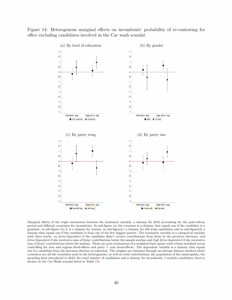
Figure 14: Heterogenous marginal effects on incumbents’ probability of re-contesting foroffice excluding candidates involved in the Car wash scandal.

(a) By level of education (b) By gender

(c) By party wing (d) By party size

Marginal effects of the triple interaction between the treatment variable, a dummy for 2016 accounting for the post-reformperiod and different covariates for incumbents. In sub-figure (a) the covariate is a dummy that equals one if the candidate is agraduate, in sub-figure (b) it is a dummy for women, in sub-figure(c) a dummy for left-wing candidates and in sub-figure(d) adummy that equals one if the candidate is from one of the five biggest parties. The treatment variable is a categorical variablewith three levels: no firms’dependent if the candidate didn’t receive contributions from firms in the previous elections, midfirms’dependent if she received a sum of firms’ contributions below the sample median and high firms’dependent if she received asum of firms’ contributions above the median. Those are post-estimations of a weighted-least square with robust standard errorscontrolling for year and regions fixed-effects and party × year fixed-effects. The dependent variable is a dummy that equalsone if a candidate from the previous election re-contested. The weights are obtained through an entropy balance method wherecovariates are all the covariates used in the heterogeneity, as well as total contributions, the population of the municipality, thespending limit introduced in 2016, the total number of candidates and a dummy for incumbents. I exclude candidates cited todeclare in the Car Wash scandal listed in Table C6.

40

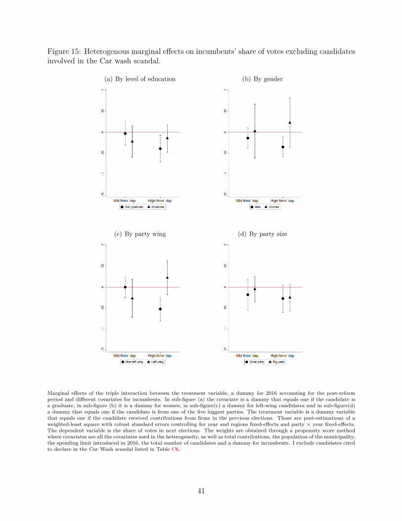
Figure 15: Heterogenous marginal effects on incumbents’ share of votes excluding candidatesinvolved in the Car wash scandal.

(a) By level of education (b) By gender

(c) By party wing (d) By party size

Marginal effects of the triple interaction between the treatment variable, a dummy for 2016 accounting for the post-reformperiod and different covariates for incumbents. In sub-figure (a) the covariate is a dummy that equals one if the candidate isa graduate, in sub-figure (b) it is a dummy for women, in sub-figure(c) a dummy for left-wing candidates and in sub-figure(d)a dummy that equals one if the candidate is from one of the five biggest parties. The treatment variable is a dummy variablethat equals one if the candidate received contributions from firms in the previous elections. Those are post-estimations of aweighted-least square with robust standard errors controlling for year and regions fixed-effects and party × year fixed-effects.The dependent variable is the share of votes in next elections. The weights are obtained through a propensity score methodwhere covariates are all the covariates used in the heterogeneity, as well as total contributions, the population of the municipality,the spending limit introduced in 2016, the total number of candidates and a dummy for incumbents. I exclude candidates citedto declare in the Car Wash scandal listed in Table C6.

41

Figure 16: Heterogenous marginal effects on incumbents’ probability of re-contesting foroffice when controlling for party fixed-effects.

(a) By level of education (b) By gender

(c) By party wing (d) By party size

Marginal effects of the triple interaction between the treatment variable, a dummy for 2016 accounting for the post-reformperiod and different covariates for incumbents. In sub-figure (a) the covariate is a dummy that equals one if the candidate is agraduate, in sub-figure (b) it is a dummy for women, in sub-figure(c) a dummy for left-wing candidates and in sub-figure(d) adummy that equals one if the candidate is from one of the five biggest parties. The treatment variable is a categorical variablewith three levels: no firms’dependent if the candidate didn’t receive contributions from firms in the previous elections, midfirms’dependent if she received a sum of firms’ contributions below the sample median and high firms’dependent if she received asum of firms’ contributions above the median. Those are post-estimations of a weighted-least square with robust standard errorscontrolling for year and regions fixed-effects and party × year fixed-effects. The dependent variable is a dummy that equalsone if a candidate from the previous election re-contested. The weights are obtained through an entropy balance method wherecovariates are all the covariates used in the heterogeneity, as well as total contributions, the population of the municipality, thespending limit introduced in 2016, the total number of candidates and a dummy for incumbents.

42

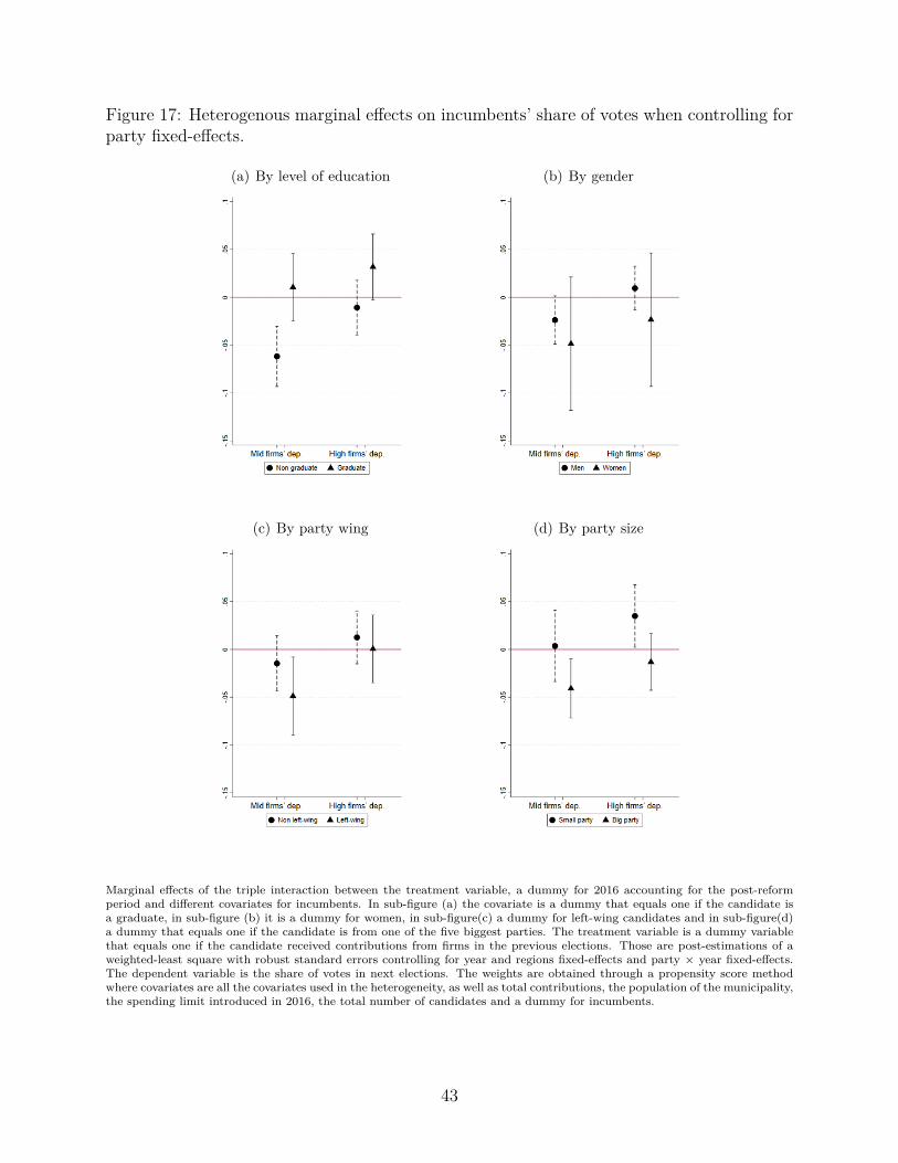
Figure 17: Heterogenous marginal effects on incumbents’ share of votes when controlling forparty fixed-effects.

(a) By level of education (b) By gender

(c) By party wing (d) By party size

Marginal effects of the triple interaction between the treatment variable, a dummy for 2016 accounting for the post-reformperiod and different covariates for incumbents. In sub-figure (a) the covariate is a dummy that equals one if the candidate isa graduate, in sub-figure (b) it is a dummy for women, in sub-figure(c) a dummy for left-wing candidates and in sub-figure(d)a dummy that equals one if the candidate is from one of the five biggest parties. The treatment variable is a dummy variablethat equals one if the candidate received contributions from firms in the previous elections. Those are post-estimations of aweighted-least square with robust standard errors controlling for year and regions fixed-effects and party × year fixed-effects.The dependent variable is the share of votes in next elections. The weights are obtained through a propensity score methodwhere covariates are all the covariates used in the heterogeneity, as well as total contributions, the population of the municipality,the spending limit introduced in 2016, the total number of candidates and a dummy for incumbents.

43

6 Conclusions

Interest groups’ contributions have been mainly analyzed as a tool to deviate the policy

agenda in their favor. A recent real-life illustration is the Brazilian Car Wash scandal that

revealed how construction companies exchanged contributions for over-rated public con-

tracts. This paper shows that interest groups’ contributions also shape candidates’ selection,

amplifying the influence of money in politics.

I provided evidence that candidates’ probability of running for office is dependent on the

structure of campaign contributions. I find that preventing firms’ contributions discouraged

female candidates, who already represent a small percentage of the sample, from running for

office. This result is consistent with women having greater difficulty in raising contributions

(Brollo and Troiano, 2016).

There are important heterogenous effects on the incumbency advantage across incum-

bents’ levels of education and rent-seeking behaviors. Among incumbents relying on firms’

funding before the reform, incumbents who didn’t have a university degree, those who were

associated with a lower economic performance, or those who belonged to municipalities where

rent-seeking is more plausible, were less likely to be re-elected. I interpret the results as the

reform having deteriorated the electoral advantage of incumbents who mainly relied on a

financial-based advantage to be re-elected rather than on a good performance while in office.

Considering that the vast majority of democracies still allow firms to contribute to polit-

ical campaigns, this paper opens doors for further research and discussions on the benefits

and side effects of banning corporate donations on candidates’ selection.

44

ReferencesAlesina, Alberto, Traviss Cassidy, and Ugo Troiano. “Old and young politicians.” Economica

86, 344: (2019) 689–727.

Ashworth, Scott, and Ethan Bueno de Mesquita. “Electoral selection, strategic challengerentry, and the incumbency advantage.” The Journal of Politics 70, 4: (2008) 1006–1025.

Avis, Eric, Claudio Ferraz, Frederico Finan, and Carlos Varjao. “Money and politics: The ef-fects of campaign spending limits on political entry and competition.” American EconomicJournal: Applied Economics forthcoming.

Barber, Michael J. “Ideological donors, contribution limits, and the polarization of Americanlegislatures.” The Journal of Politics 78, 1: (2016) 296–310.

Bertrand, Marianne, Matilde Bombardini, and Francesco Trebbi. “Is it whom you know orwhat you know? An empirical assessment of the lobbying process.” American EconomicReview 104, 12: (2014) 3885–3920.

Besley, Timothy. “Political selection.” Journal of Economic Perspectives 19, 3: (2005)43–60.

Besley, Timothy, Jose G Montalvo, and Marta Reynal-Querol. “Do educated leaders matter?”The Economic Journal 121, 554: (2011) F205–227.

Bombardini, Matilde, and Francesco Trebbi. “Votes or money? Theory and evidence fromthe US Congress.” Journal of Public Economics 95, 7-8: (2011) 587–611.

Brollo, Fernanda, and Ugo Troiano. “What happens when a woman wins an election?Evidence from close races in Brazil.” Journal of Development Economics 122: (2016)28–45.

Brown, Craig O. “Economic leadership and growth.” Journal of Monetary Economics 116:(2020) 298–333.

Cage, Julia, Caroline Le Pennec, and Elisa Mougin. “Money and Ideology: Evidence fromCandidate Manifestos.” Available at SSRN 3894330 .

Callaway, Brantly, Andrew Goodman-Bacon, and Pedro HC Sant’Anna. “Difference-in-Differences with a Continuous Treatment.” arXiv preprint arXiv:2107.02637 .

Card, David. “Using regional variation in wages to measure the effects of the federal minimumwage.” Ilr Review 46, 1: (1992) 22–37.

Caselli, Francesco, and Guy Michaels. “Do oil windfalls improve living standards? Evidencefrom Brazil.” American Economic Journal: Applied Economics 5, 1: (2013) 208–38.

Chattopadhyay, Raghabendra, and Esther Duflo. “Women as policy makers: Evidence froma randomized policy experiment in India.” Econometrica 72, 5: (2004) 1409–1443.

45

Coate, Stephen, and Stephen Morris. “On the form of transfers to special interests.” Journalof political Economy 103, 6: (1995) 1210–1235.

Dal Bo, Ernesto, and Frederico Finan. “Progress and perspectives in the study of politicalselection.” Annual Review of Economics 10: (2018) 541–575.

Dreher, Axel, Michael J Lamla, Sarah M Lein, and Frank Somogyi. “The impact of politicalleaders’ profession and education on reforms.” Journal of Comparative Economics 37, 1:(2009) 169–193.

Eggers, Andrew C. “Quality-based explanations of incumbency effects.” The Journal ofPolitics 79, 4: (2017) 1315–1328.

Ferraz, Claudio, and Frederico Finan. “Motivating politicians: The impacts of monetaryincentives on quality and performance.” Technical report, National Bureau of EconomicResearch, 2009.

Fouirnaies, Alexander. “How Do Interest Groups Influence Elections? Evidence from BritishTrade Unions 1900-2019.” Available at SSRN: http://dx.doi.org/10.2139/ssrn.3771526 .

Fouirnaies, Alexander, and Andrew B Hall. “The financial incumbency advantage: Causesand consequences.” The Journal of Politics 76, 3: (2014) 711–724.

Fowler, Anthony, Haritz Garro, and Jorg L Spenkuch. “Quid pro quo? corporate returns tocampaign contributions.” The Journal of Politics 82, 3: (2020) 844–858.

Francois, Abel, Sophie Panel, and Laurent Weill. “Educated dictators attract more foreigndirect investment.” Journal of Comparative Economics 48, 1: (2020) 37–55.

Galasso, Vincenzo, and Tommaso Nannicini. “Competing on good politicians.” AmericanPolitical Science Review 105, 1: (2011) 79–99.

Grossman, Gene M, and Elhanan Helpman. “Protection for sale.” The American EconomicReview 84, 4: (1994) 833–850.

. Special interest politics. MIT press, 2001.

Hainmueller, Jens. “Entropy balancing for causal effects: A multivariate reweighting methodto produce balanced samples in observational studies.” Political Analysis 20, 1: (2012)25–46.

Hall, Andrew B. “How the Public Funding of Elections Increases Candidate Polarization.”Unpublished manuscript, Stanford University, Palo Alto .

IDEA. “Political Finance Database.”, 2020. Downloaded on 02/10/2021, https://www.idea.int/data-tools/data/political-finance-database.

Imai, Susumu, Hajime Katayama, and Kala Krishna. “Is protection really for sale? A surveyand directions for future research.” International Review of Economics & Finance 18, 2:(2009) 181–191.

46

Jochimsen, Beate, and Sebastian Thomasius. “The perfect finance minister: Whom toappoint as finance minister to balance the budget.” European Journal of Political Economy34: (2014) 390–408.

Kitschelt, Herbert, Kent Freeze, Kiril Kolev, and Yi-Ting Wang. “Measuring democraticaccountability: An initial report on an emerging data set.” Revista de ciencia polıtica 29,3: (2009) 741–773.

Kroszner, Randall S, and Thomas Stratmann. “Interest-group competition and the organiza-tion of congress: theory and evidence from financial services’ political action committees.”American Economic Review 1163–1187.

Lahoti, Rahul, and Soham Sahoo. “Are educated leaders good for education? Evidence fromIndia.” Journal of Economic Behavior & Organization 176: (2020) 42–62.

Levitt, Steven D. “Using repeat challengers to estimate the effect of campaign spending onelection outcomes in the US House.” Journal of Political Economy 102, 4: (1994) 777–798.

Mercier, Marion. “The return of the prodigy son: Do return migrants make better leaders?”Journal of Development Economics 122: (2016) 76–91.

Peveri, Julieta. “The Wise, the Politician and the Strongman: National Leaders’ Type andQuality of Governance.” Working paper AMSE 2021-20 .

Tubbicke, Stefan. “Entropy balancing for continuous treatments.” arXiv preprintarXiv:2001.06281 .

47

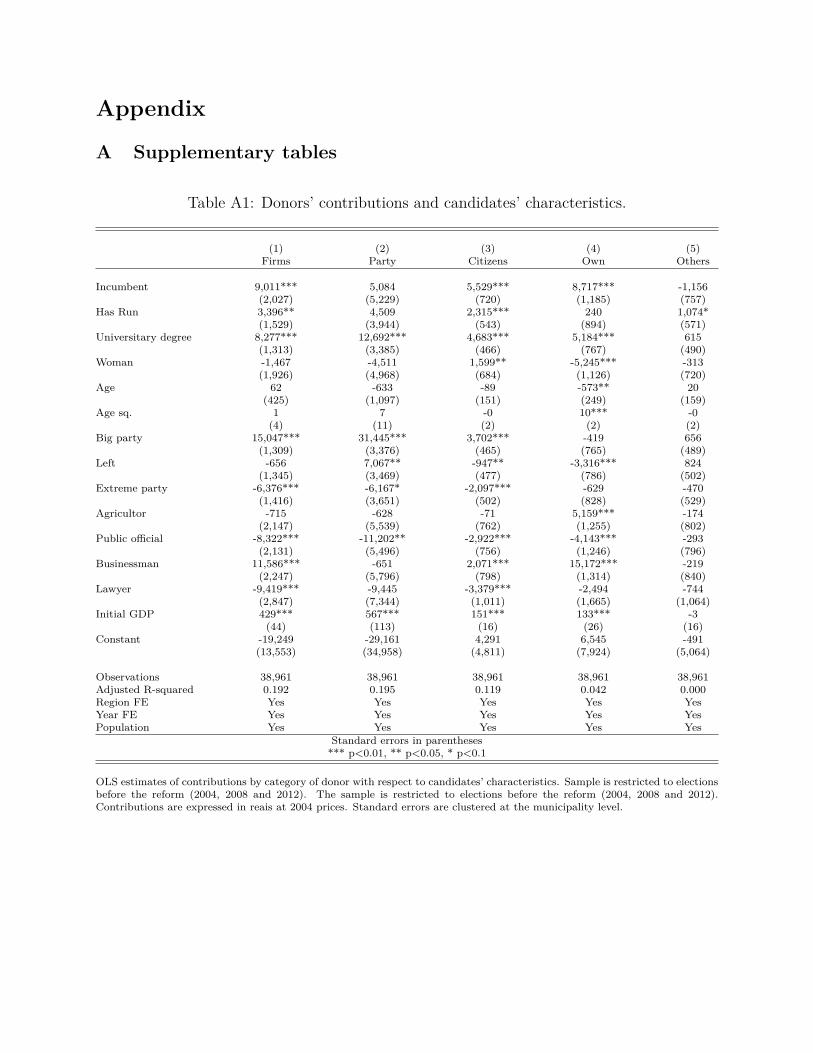
Appendix

A Supplementary tables

Table A1: Donors’ contributions and candidates’ characteristics.

(1) (2) (3) (4) (5)Firms Party Citizens Own Others

Incumbent 9,011*** 5,084 5,529*** 8,717*** -1,156(2,027) (5,229) (720) (1,185) (757)

Has Run 3,396** 4,509 2,315*** 240 1,074*(1,529) (3,944) (543) (894) (571)

Universitary degree 8,277*** 12,692*** 4,683*** 5,184*** 615(1,313) (3,385) (466) (767) (490)

Woman -1,467 -4,511 1,599** -5,245*** -313(1,926) (4,968) (684) (1,126) (720)

Age 62 -633 -89 -573** 20(425) (1,097) (151) (249) (159)

Age sq. 1 7 -0 10*** -0(4) (11) (2) (2) (2)

Big party 15,047*** 31,445*** 3,702*** -419 656(1,309) (3,376) (465) (765) (489)

Left -656 7,067** -947** -3,316*** 824(1,345) (3,469) (477) (786) (502)

Extreme party -6,376*** -6,167* -2,097*** -629 -470(1,416) (3,651) (502) (828) (529)

Agricultor -715 -628 -71 5,159*** -174(2,147) (5,539) (762) (1,255) (802)

Public official -8,322*** -11,202** -2,922*** -4,143*** -293(2,131) (5,496) (756) (1,246) (796)

Businessman 11,586*** -651 2,071*** 15,172*** -219(2,247) (5,796) (798) (1,314) (840)

Lawyer -9,419*** -9,445 -3,379*** -2,494 -744(2,847) (7,344) (1,011) (1,665) (1,064)

Initial GDP 429*** 567*** 151*** 133*** -3(44) (113) (16) (26) (16)

Constant -19,249 -29,161 4,291 6,545 -491(13,553) (34,958) (4,811) (7,924) (5,064)

Observations 38,961 38,961 38,961 38,961 38,961Adjusted R-squared 0.192 0.195 0.119 0.042 0.000Region FE Yes Yes Yes Yes YesYear FE Yes Yes Yes Yes YesPopulation Yes Yes Yes Yes Yes

Standard errors in parentheses*** p<0.01, ** p<0.05, * p<0.1

OLS estimates of contributions by category of donor with respect to candidates’ characteristics. Sample is restricted to electionsbefore the reform (2004, 2008 and 2012). The sample is restricted to elections before the reform (2004, 2008 and 2012).Contributions are expressed in reais at 2004 prices. Standard errors are clustered at the municipality level.

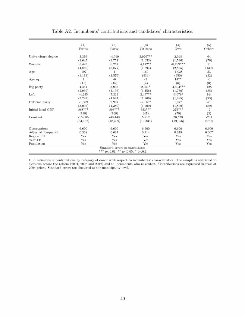
Table A2: Incumbents’ contributions and candidates’ characteristics.

(1) (2) (3) (4) (5)Firms Party Citizens Own Others

Universitary degree 3,316 -4,919 3,920*** 2,048 64(2,645) (3,751) (1,033) (1,546) (76)

Woman 5,423 6,257 4,172** -8,799*** 11(4,850) (6,877) (1,894) (2,835) (139)

Age -197 1 169 -1,038 33(1,111) (1,576) (434) (650) (32)

Age sq. 1 -0 -3 14** -0(11) (15) (4) (6) (0)

Big party 4,451 3,993 2,061* -4,594*** 128(2,959) (4,195) (1,156) (1,730) (85)

Left -4,235 7,324 2,497** -3,678* 144(3,242) (4,597) (1,266) (1,895) (93)

Extreme party -1,589 2,907 -2,163* 1,377 -79(3,095) (4,389) (1,209) (1,809) (89)

Initial local GDP 868*** 893*** 353*** 275*** -2(119) (169) (47) (70) (3)

Constant -15,085 -40,440 5,912 26,578 -731(34,137) (48,409) (13,335) (19,956) (979)

Observations 6,600 6,600 6,600 6,600 6,600Adjusted R-squared 0.368 0.661 0.214 0.079 0.007Region FE Yes Yes Yes Yes YesYear FE Yes Yes Yes Yes YesPopulation Yes Yes Yes Yes Yes

Standard errors in parentheses*** p<0.01, ** p<0.05, * p<0.1

OLS estimates of contributions by category of donor with respect to incumbents’ characteristics. The sample is restricted toelections before the reform (2004, 2008 and 2012) and to incumbents who re-contest. Contributions are expressed in reais at2004 prices. Standard errors are clustered at the municipality level.

49

Table A3: Economic sector of firms donors by total contributions in 2012.

Economic sector Total

Building construction 35812071Retail trade of motor vehicle fuels 32022123Construction of highways and railways 19568909Real estate developments 13833591Multiple banks, with commercial portfolio 13804518Retail trade in goods in general, with predominance of food products - supermarkets 11892347Retail trade in new cars, vans and utilities 10706749Other civil engineering works not previously specified 10571015Road cargo transportation, except dangerous products and changes, intercity, interstate and international 8858876Retail trade in building materials in general 7151433Brewing and draft beers 6831261Industrial assembly works 5517250Engineering services 5274438Wholesale of beer, draft beer and soda 4758757Retail trade in goods in general, with predominance of food products - minimarkets, grocery stores and warehouses 4525236Earthworks 4478408Retail trade in pasta 4426066Cleaning in buildings and homes 4419585Construction of water supply networks, sewage collection and related constructions, except irrigation works 4135351Wholesale of food products in general 4109862Purchase and sale of own properties 4050303Manufacture of cellulose and other pulp for papermaking 3995435Rental of own properties 3993337Holdings of non-financial institutions 3711051Furniture retail trade 3450984Manufacture of raw sugar 3442461Surveillance and private security activities 3304477Wholesale of medicines and drugs for human use 3208645Consulting activities in business management, except specific technical consulting 3178806

Economic sector of firms’ donors and total donations in reais in 2012, ranked by total donations.

Table A4: Most repeated words in firms donors’ names.

Original word Translated word Repeated timescomercio trade 2951posto office 1599construtora/ construcoes / construcao construction 2010servicos services 1232silva silva 1169auto auto 1080industria industry 1040ind ind 982engenharia engineering 942comercial business 866grafica printer 828empreendimentos enterprise 766editora editor 715oliveira oliveira 638santos santos 628sa plc 520transportes transport 514souza souza 480brasil brazil 471

List of most repeated words in Portuguese and in English in the list of firms’ names. Each firm is counted once. Data isaggregated for 2004, 2008 and 2008 elections for mayors.

50

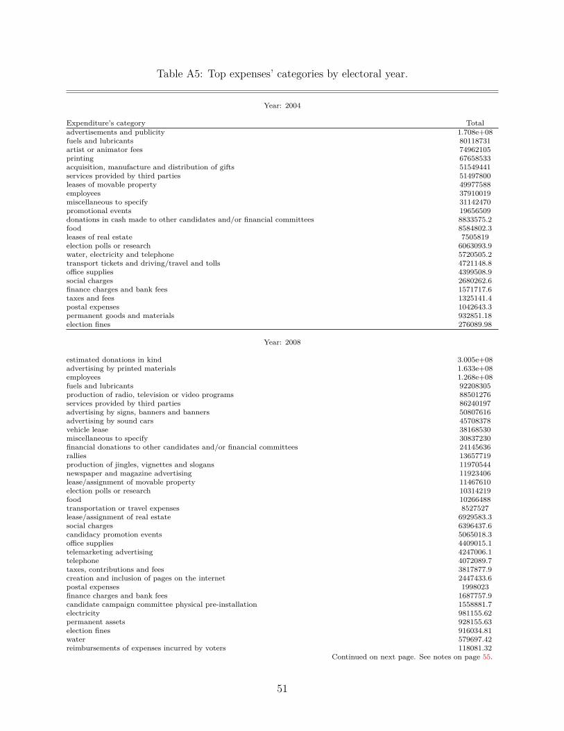
Table A5: Top expenses’ categories by electoral year.

Year: 2004

Expenditure’s category Totaladvertisements and publicity 1.708e+08fuels and lubricants 80118731artist or animator fees 74962105printing 67658533acquisition, manufacture and distribution of gifts 51549441services provided by third parties 51497800leases of movable property 49977588employees 37910019miscellaneous to specify 31142470promotional events 19656509donations in cash made to other candidates and/or financial committees 8833575.2food 8584802.3leases of real estate 7505819election polls or research 6063093.9water, electricity and telephone 5720505.2transport tickets and driving/travel and tolls 4721148.8office supplies 4399508.9social charges 2680262.6finance charges and bank fees 1571717.6taxes and fees 1325141.4postal expenses 1042643.3permanent goods and materials 932851.18election fines 276089.98

Year: 2008

estimated donations in kind 3.005e+08advertising by printed materials 1.633e+08employees 1.268e+08fuels and lubricants 92208305production of radio, television or video programs 88501276services provided by third parties 86240197advertising by signs, banners and banners 50807616advertising by sound cars 45708378vehicle lease 38168530miscellaneous to specify 30837230financial donations to other candidates and/or financial committees 24145636rallies 13657719production of jingles, vignettes and slogans 11970544newspaper and magazine advertising 11923406lease/assignment of movable property 11467610election polls or research 10314219food 10266488transportation or travel expenses 8527527lease/assignment of real estate 6929583.3social charges 6396437.6candidacy promotion events 5065018.3office supplies 4409015.1telemarketing advertising 4247006.1telephone 4072089.7taxes, contributions and fees 3817877.9creation and inclusion of pages on the internet 2447433.6postal expenses 1998023finance charges and bank fees 1687757.9candidate campaign committee physical pre-installation 1558881.7electricity 981155.62permanent assets 928155.63election fines 916034.81water 579697.42reimbursements of expenses incurred by voters 118081.32

Continued on next page. See notes on page 55.

51

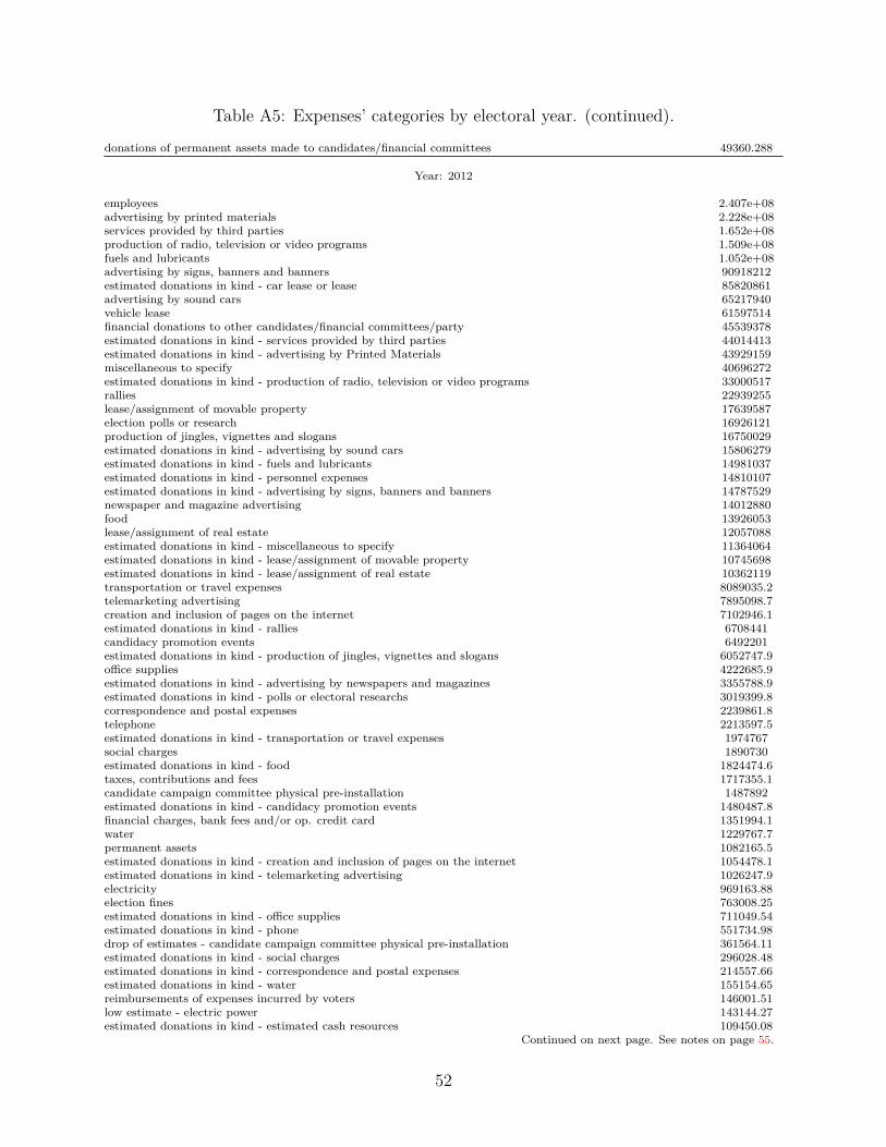
Table A5: Expenses’ categories by electoral year. (continued).

donations of permanent assets made to candidates/financial committees 49360.288

Year: 2012

employees 2.407e+08advertising by printed materials 2.228e+08services provided by third parties 1.652e+08production of radio, television or video programs 1.509e+08fuels and lubricants 1.052e+08advertising by signs, banners and banners 90918212estimated donations in kind - car lease or lease 85820861advertising by sound cars 65217940vehicle lease 61597514financial donations to other candidates/financial committees/party 45539378estimated donations in kind - services provided by third parties 44014413estimated donations in kind - advertising by Printed Materials 43929159miscellaneous to specify 40696272estimated donations in kind - production of radio, television or video programs 33000517rallies 22939255lease/assignment of movable property 17639587election polls or research 16926121production of jingles, vignettes and slogans 16750029estimated donations in kind - advertising by sound cars 15806279estimated donations in kind - fuels and lubricants 14981037estimated donations in kind - personnel expenses 14810107estimated donations in kind - advertising by signs, banners and banners 14787529newspaper and magazine advertising 14012880food 13926053lease/assignment of real estate 12057088estimated donations in kind - miscellaneous to specify 11364064estimated donations in kind - lease/assignment of movable property 10745698estimated donations in kind - lease/assignment of real estate 10362119transportation or travel expenses 8089035.2telemarketing advertising 7895098.7creation and inclusion of pages on the internet 7102946.1estimated donations in kind - rallies 6708441candidacy promotion events 6492201estimated donations in kind - production of jingles, vignettes and slogans 6052747.9office supplies 4222685.9estimated donations in kind - advertising by newspapers and magazines 3355788.9estimated donations in kind - polls or electoral researchs 3019399.8correspondence and postal expenses 2239861.8telephone 2213597.5estimated donations in kind - transportation or travel expenses 1974767social charges 1890730estimated donations in kind - food 1824474.6taxes, contributions and fees 1717355.1candidate campaign committee physical pre-installation 1487892estimated donations in kind - candidacy promotion events 1480487.8financial charges, bank fees and/or op. credit card 1351994.1water 1229767.7permanent assets 1082165.5estimated donations in kind - creation and inclusion of pages on the internet 1054478.1estimated donations in kind - telemarketing advertising 1026247.9electricity 969163.88election fines 763008.25estimated donations in kind - office supplies 711049.54estimated donations in kind - phone 551734.98drop of estimates - candidate campaign committee physical pre-installation 361564.11estimated donations in kind - social charges 296028.48estimated donations in kind - correspondence and postal expenses 214557.66estimated donations in kind - water 155154.65reimbursements of expenses incurred by voters 146001.51low estimate - electric power 143144.27estimated donations in kind - estimated cash resources 109450.08

Continued on next page. See notes on page 55.

52

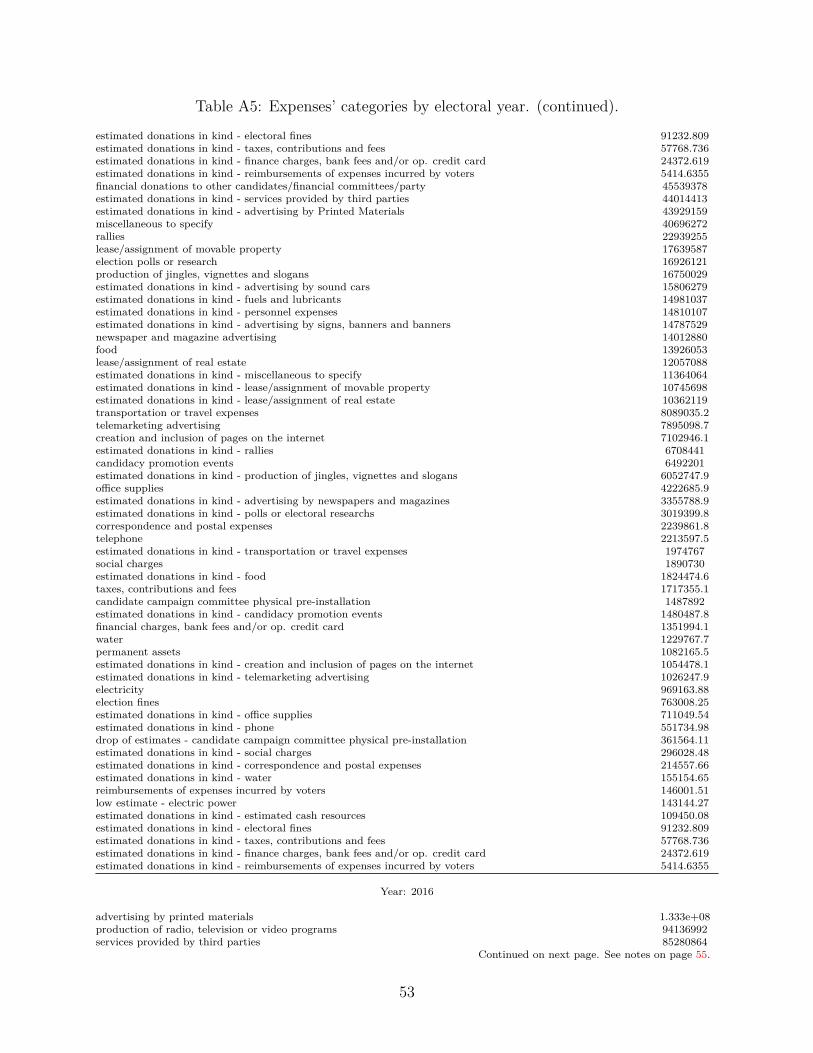
Table A5: Expenses’ categories by electoral year. (continued).

estimated donations in kind - electoral fines 91232.809estimated donations in kind - taxes, contributions and fees 57768.736estimated donations in kind - finance charges, bank fees and/or op. credit card 24372.619estimated donations in kind - reimbursements of expenses incurred by voters 5414.6355financial donations to other candidates/financial committees/party 45539378estimated donations in kind - services provided by third parties 44014413estimated donations in kind - advertising by Printed Materials 43929159miscellaneous to specify 40696272rallies 22939255lease/assignment of movable property 17639587election polls or research 16926121production of jingles, vignettes and slogans 16750029estimated donations in kind - advertising by sound cars 15806279estimated donations in kind - fuels and lubricants 14981037estimated donations in kind - personnel expenses 14810107estimated donations in kind - advertising by signs, banners and banners 14787529newspaper and magazine advertising 14012880food 13926053lease/assignment of real estate 12057088estimated donations in kind - miscellaneous to specify 11364064estimated donations in kind - lease/assignment of movable property 10745698estimated donations in kind - lease/assignment of real estate 10362119transportation or travel expenses 8089035.2telemarketing advertising 7895098.7creation and inclusion of pages on the internet 7102946.1estimated donations in kind - rallies 6708441candidacy promotion events 6492201estimated donations in kind - production of jingles, vignettes and slogans 6052747.9office supplies 4222685.9estimated donations in kind - advertising by newspapers and magazines 3355788.9estimated donations in kind - polls or electoral researchs 3019399.8correspondence and postal expenses 2239861.8telephone 2213597.5estimated donations in kind - transportation or travel expenses 1974767social charges 1890730estimated donations in kind - food 1824474.6taxes, contributions and fees 1717355.1candidate campaign committee physical pre-installation 1487892estimated donations in kind - candidacy promotion events 1480487.8financial charges, bank fees and/or op. credit card 1351994.1water 1229767.7permanent assets 1082165.5estimated donations in kind - creation and inclusion of pages on the internet 1054478.1estimated donations in kind - telemarketing advertising 1026247.9electricity 969163.88election fines 763008.25estimated donations in kind - office supplies 711049.54estimated donations in kind - phone 551734.98drop of estimates - candidate campaign committee physical pre-installation 361564.11estimated donations in kind - social charges 296028.48estimated donations in kind - correspondence and postal expenses 214557.66estimated donations in kind - water 155154.65reimbursements of expenses incurred by voters 146001.51low estimate - electric power 143144.27estimated donations in kind - estimated cash resources 109450.08estimated donations in kind - electoral fines 91232.809estimated donations in kind - taxes, contributions and fees 57768.736estimated donations in kind - finance charges, bank fees and/or op. credit card 24372.619estimated donations in kind - reimbursements of expenses incurred by voters 5414.6355

Year: 2016

advertising by printed materials 1.333e+08production of radio, television or video programs 94136992services provided by third parties 85280864

Continued on next page. See notes on page 55.

53

Table A5: Expenses’ categories by electoral year. (continued).

employees 68459472fuels and lubricants 56180833advertising by stickers 47491821militancy and street mobilization activities 44540245write-off of estimated - car lease or lease 35826677advertising by sound cars 33916897rallies 33296054miscellaneous to specify 25785843car lease or lease 25542119estimated donations in kind - militancy and street mobilization activities 13495782estimated donations in kind - services provided by third parties 13275028production of jingles, vignettes and slogans 12695607financial donations to other candidates/parties 12688105own services provided by third parties 10193697election polls or tests 8394420.6lease/assignment of real estate 8342681.5newspaper and magazine advertising 7835315.5estimated donations in kind - Advertising by Printed Materials 7290680.5lease/assignment of movable property (except vehicles) 6939475.9food 6473441.7estimated donations in kind - personnel expenses 6323569.5estimated donations in kind - Advertising by Sound Cars 5799354.4estimated donations in kind - own services provided by third parties 5365859.6estimated donations in kind - lease/assignment of real estate 5159863.2candidacy promotion events 4584391.9transportation or travel expenses 4342410creation and inclusion of pages on the internet 3861636.6estimated donations in kind - production of radio, television or video programs 3262763estimated donations in kind - miscellaneous to specify 2970096.2estimated donations in kind - advertising by stickers 2653356.5office supplies 2133421.2estimated donations in kind - lease/assignment of movable property (except vehicles) 1728759.2estimated donations in kind - production of jingles, vignettes and slogans 1538933.4estimated donations in kind - rallies 1456129.3correspondence and postal expenses 1228070.1estimated donations in kind - fuels and lubricants 1225913.3physical pre-installation of campaign committee 1136876.7financial charges, bank fees and/or op. credit card 999973.26Water 808606.52taxes, contributions and fees 568429.04electricity 480523.79social charges 402361.95hosting expenses 377902.93estimated donations in kind - transportation or travel expenses 360831.28estimated donations in kind - polls or electoral tests 327780.7acquisition/donation of movable or immovable property 305627.19estimated donations in kind - advertising by newspapers and magazines 263424.38election fines 188095.74telephone 183510.27estimated donations in kind - candidacy promotion events 176389.96estimated donations in kind - creation and inclusion of pages on the internet 169893.11estimated donations in kind - physical pre-installation of campaign committee 121751.75estimated donations in kind - food 106526.49low estimate - phone 79897.05reimbursements of expenses incurred by voters 63798.951estimated donations in kind - office supplies 57314.195low estimate - electric power 22305.389estimated donations in kind - correspondence and postal expenses 21204.155low estimate - hosting expenses 19925.724estimated donations in kind - water 11009.551estimated donations in kind - social charges 8371.6339estimated donations in kind - finance charges, bank fees and/or op. credit card 1739.3516estimated donations in kind - reimbursements of expenses incurred by voters 1565.4597estimated donations in kind - taxes, contributions and fees 1366.2669

Continued on next page. See notes on page 55.

54

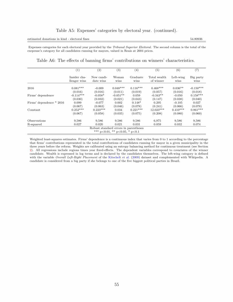
Table A5: Expenses’ categories by electoral year. (continued).

estimated donations in kind - electoral fines 54.80936

Expenses categories for each electoral year provided by the Tribunal Superior Eleitoral. The second column is the total of theexepense’s category for all candidates running for mayors, valued in Reais at 2004 prices.

Table A6: The effects of banning firms’ contributions on winners’ characteristics.

(1) (2) (3) (4) (5) (6) (7)

Insider cha-llenger wins

New candi-date wins

Womanwins

Graduatewins

Total wealthof winner

Left-wingwins

Big partywins

2016 0.081*** -0.009 0.048*** 0.116*** 0.468*** 0.036** -0.150***(0.016) (0.016) (0.011) (0.019) (0.057) (0.016) (0.018)

Firms’ dependence -0.114*** -0.058* -0.051** 0.059 -0.343** -0.050 0.158***(0.030) (0.032) (0.021) (0.043) (0.147) (0.038) (0.040)

Firms’ dependence * 2016 0.099 -0.077 0.002 0.148* 0.295 -0.105 0.027(0.067) (0.063) (0.046) (0.078) (0.241) (0.066) (0.078)

Constant 0.252*** 0.223*** 0.034 0.221*** 12.023*** 0.410*** 0.861***(0.067) (0.058) (0.035) (0.075) (0.208) (0.080) (0.060)

Observations 9,586 9,586 9,586 9,586 6,975 9,586 9,586R-squared 0.027 0.020 0.021 0.031 0.059 0.032 0.074

Robust standard errors in parentheses*** p<0.01, ** p<0.05, * p<0.1

Weighted least-squares estimates. Firms’ dependence is a continuous index that varies from 0 to 1 according to the percentagethat firms’ contributions represented in the total contributions of candidates running for mayor in a given municipality in thethree years before the reform. Weights are calibrated using an entropy balancing method for continuous treatment (see Section2). All regressions include regions times year fixed-effects. The dependent variables correspond to covariates of the winnercandidate. Wealth is expressed in log terms and is declared by the candidates themselves. The left-wing category is definedwith the variable Overall Left-Right Placement of the Kitschelt et al. (2009) dataset and complemented with Wikipedia. Acandidate is considered from a big party if she belongs to one of the five biggest political parties in Brazil.

55

Table A7: Effects of banning firms’ contributions on the incumbents’ probability of re-contesting

(1) (2) (3) (4) (5) (6)X =

womanX =

graduateX =

Total wealthX =

Left-wingX =

Big party

2016 0.181*** 0.165*** 0.094*** 0.161*** 0.120*** 0.172***(0.014) (0.014) (0.016) (0.014) (0.015) (0.015)

Firms’ dependence 0.022 0.043 0.011 0.034 0.030 -0.054(0.031) (0.031) (0.035) (0.032) (0.033) (0.035)

Incumbent*X 0.465*** 0.578*** 0.004*** 0.482*** 0.685***(0.010) (0.008) (0.001) (0.008) (0.007)

Incumbent*X*Firms’ dependence -0.115** -0.031 -0.005 0.011 0.023(0.050) (0.036) (0.004) (0.038) (0.036)

Incumbent*X*2016 -0.010 0.022 -0.002** 0.032** -0.066***(0.016) (0.016) (0.001) (0.015) (0.016)

Reform effectsFirms’ dependence * 2016 0.002 -0.011 -0.102 -0.018 0.035 -0.002

(0.063) (0.065) (0.077) (0.066) (0.068) (0.077)Incumbent*X*2016*Firms’ dependence 0.107 0.139* 0.014** -0.039 0.030

(0.079) (0.078) (0.006) (0.071) (0.078)

Constant 0.406*** 0.398*** 0.382*** 0.413*** 0.262*** 0.203***(0.056) (0.055) (0.052) (0.056) (0.044) (0.042)

Observations 17,307 17,307 17,307 17,307 17,307 17,307R-squared 0.053 0.089 0.312 0.074 0.168 0.451

Weighted least-squares estimates. The sample is restricted to municipalities where the incumbent does not face a term limit.Firms’ dependence is a continuous index that varies from 0 to 1 according to the percentage that firms’ contributions representedin the total contributions of candidates running for mayor in a given municipality in the three years before the reform. Thedependent variable is a dully that equals one if the incumbent runs for re-election. Weights are calibrated using an entropybalancing method for continuous treatment (see Section 2). All regressions include regions times year fixed-effects. In eachcolumn I interact the treatment effect with a covariate denoted by X. Wealth is expressed in log terms and is declared by thecandidates themselves. The left-wing category is defined with the variable Overall Left-Right Placement of the Kitschelt et al.(2009) dataset and complemented with Wikipedia. A candidate is considered from a big party if she belongs to one of the fivebiggest political parties in Brazil.

56

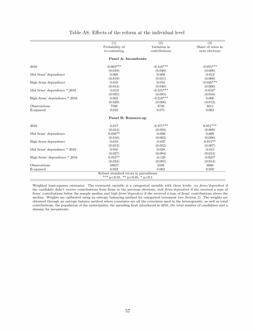
Table A8: Effects of the reform at the individual level

(1) (2) (3)Probability ofre-contesting

Variation incontributions

Share of votes innext elections

Panel A: Incumbents

2016 -0.093*** -0.416*** -0.055***(0.019) (0.048) (0.008)

Mid firms’ dependence 0.008 0.008 -0.012(0.018) (0.051) (0.008)

High firms dependence 0.010 0.054 -0.020***(0.014) (0.040) (0.006)

Mid firms’ dependence * 2016 -0.012 -0.315*** -0.034*(0.035) (0.085) (0.016)

High firms’ dependence * 2016 0.003 -0.218*** 0.006(0.029) (0.066) (0.012)

Observations 7598 4736 4814R-squared 0.022 0.071 0.063

Panel B: Runners-up

2016 0.017 -0.371*** 0.051***(0.014) (0.058) (0.008)

Mid firms’ dependence 0.036** -0.008 0.009(0.016) (0.063) (0.008)

High firms dependence 0.018 -0.037 0.015**(0.013) (0.052) (0.007)

Mid firms’ dependence * 2016 0.010 0.028 -0.015(0.027) (0.094) (0.014)

High firms’ dependence * 2016 0.052** -0.120 -0.024*(0.024) (0.085) (0.014)

Observations 10827 3598 3660R-squared 0.023 0.062 0.050

Robust standard errors in parentheses*** p<0.01, ** p<0.05, * p<0.1

Weighted least-squares estimates. The treatment variable is a categorical variable with three levels: no firms’dependent ifthe candidate didn’t receive contributions from firms in the previous elections, mid firms’dependent if she received a sum offirms’ contributions below the sample median and high firms’dependent if she received a sum of firms’ contributions above themedian. Weights are calibrated using an entropy balancing method for categorical tretament (see Section 2). The weights areobtained through an entropy balance method where covariates are all the covariates used in the heterogeneity, as well as totalcontributions, the population of the municipality, the spending limit introduced in 2016, the total number of candidates and adummy for incumbents.

57

Table A9: Heterogenous effects on re-contesting decisions.

(1) (2) (3) (4)X =

graduateX =

womanX =

left-wingX =

big party

Panel A: Incumbents

Mid firms’ dependence * 2016 -0.015 0.013 -0.026 0.061(0.049) (0.037) (0.042) (0.054)

High firms’ dependence * 2016 0.070* 0.016 -0.013 0.050(0.038) (0.030) (0.034) (0.043)

Mid firms’ dependence * 2016 * X 0.006 -0.210* 0.051 -0.121*(0.070) (0.112) (0.076) (0.071)

High firms’ dependence * 2016 * X -0.137** -0.087 0.053 -0.088(0.057) (0.090) (0.061) (0.058)

Observations 7598 7598 7598 7598R-squared 0.026 0.023 0.027 0.023

Panel B: Runners-up

Mid firms’ dependence * 2016 -0.020 0.022 -0.021 -0.016(0.037) (0.030) (0.033) (0.043)

High firms’ dependence * 2016 0.015 0.067** 0.105*** -0.009(0.032) (0.026) (0.030) (0.037)

Mid firms’ dependence * 2016 * X 0.068 -0.074 0.098* 0.043(0.055) (0.078) (0.059) (0.056)

High firms’ dependence * 2016 * X 0.082* -0.143** -0.171*** 0.104**(0.049) (0.072) (0.052) (0.049)

Observations 10827 10827 10827 10827R-squared 0.026 0.025 0.027 0.024

Robust standard errors in parentheses*** p<0.01, ** p<0.05, * p<0.1

Weighted least-squares estimates. The treatment variable is a categorical variable with three levels: no firms’dependent if thecandidate didn’t receive contributions from firms in the previous elections, mid firms’dependent if she received a sum of firms’contributions below the sample median and high firms’dependent if she received a sum of firms’ contributions above the median.Weights are calibrated using an entropy balancing method for categorical tretament (see Section 2). Each column correspondsto a triple differences-in-differences with respect to the variable denoted as the column name. The dependent variable is adummy that equals one if a candidate from the previous election re-contested. The weights are obtained through an entropybalance method where covariates are all the covariates used in the heterogeneity, as well as total contributions, the populationof the municipality, the spending limit introduced in 2016, the total number of candidates and a dummy for incumbents.

58

Table A10: Heterogenous effects on share of votes.

(1) (2) (3) (4)X =

graduateX =

womanX =

left-wingX =

big party

Panel A: Incumbents

Mid firms’ dependence * 2016 -0.063** -0.034* -0.024 0.001(0.021) (0.017) (0.019) (0.025)

High firms’ dependence * 2016 -0.019 0.009 0.012 0.030+

(0.016) (0.013) (0.016) (0.018)Mid firms’ dependence * 2016 * X 0.059* -0.009 -0.030 -0.055*

(0.032) (0.056) (0.034) (0.032)High firms’ dependence * 2016 * X 0.054** -0.048 -0.012 -0.041+

(0.025) (0.038) (0.025) (0.025)Observations 4814 4814 4814 4814R-squared 0.065 0.064 0.065 0.065

Panel B: Runners-up

Mid firms’ dependence * 2016 -0.017 -0.018 -0.013 -0.022(0.020) (0.016) (0.017) (0.024)

High firms’ dependence * 2016 -0.037** -0.031** -0.052*** -0.014(0.017) (0.014) (0.015) (0.019)

Mid firms’ dependence * 2016 * X -0.001 -0.007 -0.005 0.010(0.031) (0.044) (0.034) (0.031)

High firms’ dependence * 2016 * X 0.030 0.055 0.084** -0.019(0.026) (0.037) (0.028) (0.026)

Observations 3674 3674 3674 3674R-squared 0.056 0.052 0.057 0.051

Robust standard errors in parentheses*** p<0.01, ** p<0.05, * p<0.1

Weighted least-squares estimates. The treatment variable is a categorical variable with three levels: no firms’dependent if thecandidate didn’t receive contributions from firms in the previous elections, mid firms’dependent if she received a sum of firms’contributions below the sample median and high firms’dependent if she received a sum of firms’ contributions above the median.Weights are calibrated using an entropy balancing method for categorical tretament (see Section 2). Each column corresponds toa triple differences-in-differences with respect to the variable denoted as the column name. The dependent variable is the shareof votes in next elections. The weights are obtained through an entropy balance method where covariates are all the covariatesused in the heterogeneity, as well as total contributions, the population of the municipality, the spending limit introduced in2016, the total number of candidates and a dummy for incumbents.

59

Table A11: Heterogenous effects on contributions.

(1) (2) (3) (4)X =

graduateX =

womanX =

left-wingX =

big party

Panel A: Incumbents

Mid firms’ dependence * 2016 -0.363*** -0.320*** -0.231** -0.341**(0.103) (0.089) (0.093) (0.143)

High firms’ dependence * 2016 -0.171* -0.226** -0.303*** -0.193*(0.092) (0.069) (0.081) (0.104)

Mid firms’ dependence * 2016 * X 0.124 0.067 -0.280 0.058(0.169) (0.267) (0.200) (0.174)

High firms’ dependence * 2016 * X -0.090 0.059 0.269* -0.057(0.132) (0.220) (0.139) (0.137)

Observations 4736 4736 4736 4736R-squared 0.073 0.071 0.075 0.072

Panel B: Runners-up

Mid firms’ dependence * 2016 -0.067 -0.207** -0.143 -0.093(0.135) (0.105) (0.120) (0.148)

High firms’ dependence * 2016 0.074 0.008 0.111 -0.049(0.104) (0.083) (0.097) (0.122)

Mid firms’ dependence * 2016 * X -0.342* -0.142 -0.264 -0.217(0.201) (0.353) (0.217) (0.200)

High firms’ dependence * 2016 * X -0.279* -0.577** -0.479** -0.004(0.162) (0.279) (0.174) (0.162)

Observations 3616 3616 3616 3616R-squared 0.069 0.069 0.070 0.067

Robust standard errors in parentheses*** p<0.01, ** p<0.05, * p<0.1

Weighted least-squares estimates. The treatment variable is a categorical variable with three levels: no firms’dependent if thecandidate didn’t receive contributions from firms in the previous elections, mid firms’dependent if she received a sum of firms’contributions below the sample median and high firms’dependent if she received a sum of firms’ contributions above the median.Weights are calibrated using an entropy balancing method for categorical tretament (see Section 2). Each column correspondsto a triple differences-in-differences with respect to the variable denoted as the column name. The dependent variable is thevariation in the log of contributions between two consecutive elections. The weights are obtained through an entropy balancemethod where covariates are all the covariates used in the heterogeneity, as well as total contributions, the population of themunicipality, the spending limit introduced in 2016, the total number of candidates and a dummy for incumbents.

60

Table A12: Heterogenous effects on challengers’ entry with respect to incumbents’ firms’dependence.

(1) (2) (3) (4)X =

graduateX =

womanX =

left-wingX =

big party

Mid firms’ dependence * 2016 0.635*** 0.425*** 0.260* 0.302(0.163) (0.127) (0.144) (0.190)

High firms’ dependence * 2016 0.262** 0.138 0.154 -0.009(0.125) (0.099) (0.118) (0.141)

Mid firms’ dependence * 2016 * X -0.521** -0.347 0.407 0.104(0.245) (0.532) (0.275) (0.251)

High firms’ dependence * 2016 * X -0.278 0.172 -0.034 0.347*(0.188) (0.289) (0.194) (0.190)

Observations 4824 4824 4824 4824R-squared 0.083 0.080 0.080 0.082

Robust standard errors in parentheses*** p<0.01, ** p<0.05, * p<0.1

Weighted least-squares estimates. The treatment variable is a categorical variable with three levels: no firms’dependent if thecandidate didn’t receive contributions from firms in the previous elections, mid firms’dependent if she received a sum of firms’contributions below the sample median and high firms’dependent if she received a sum of firms’ contributions above the median.Weights are calibrated using an entropy balancing method for categorical tretament (see Section 2). Each column correspondsto a triple differences-in-differences with respect to the variable denoted as the column name. The dependent variable is thevariation of challengers. The weights are obtained through an entropy balance method where covariates are all the covariatesused in the heterogeneity, as well as total contributions, the population of the municipality, the spending limit introduced in2016, the total number of candidates and a dummy for incumbents.

61

B Supplementary figures

Figure B1: Degree of local firms’ dependence.

Low, medium and high firms’ dependence correspond respectively to the first, second and third trecile of the distribution of themean percentage that firms’ contributions represented between 2004 and 20winner02 (per candidate).

62

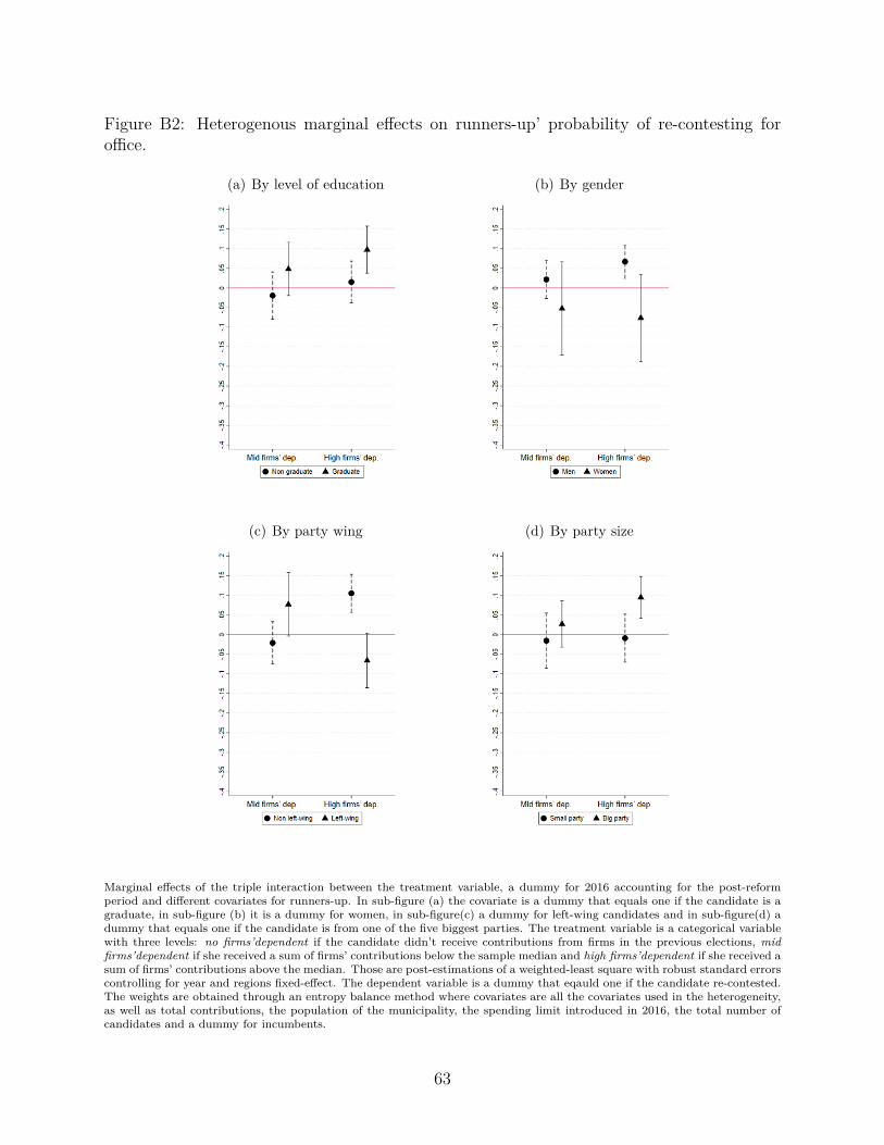
Figure B2: Heterogenous marginal effects on runners-up’ probability of re-contesting foroffice.

(a) By level of education (b) By gender

(c) By party wing (d) By party size

Marginal effects of the triple interaction between the treatment variable, a dummy for 2016 accounting for the post-reformperiod and different covariates for runners-up. In sub-figure (a) the covariate is a dummy that equals one if the candidate is agraduate, in sub-figure (b) it is a dummy for women, in sub-figure(c) a dummy for left-wing candidates and in sub-figure(d) adummy that equals one if the candidate is from one of the five biggest parties. The treatment variable is a categorical variablewith three levels: no firms’dependent if the candidate didn’t receive contributions from firms in the previous elections, midfirms’dependent if she received a sum of firms’ contributions below the sample median and high firms’dependent if she received asum of firms’ contributions above the median. Those are post-estimations of a weighted-least square with robust standard errorscontrolling for year and regions fixed-effect. The dependent variable is a dummy that eqauld one if the candidate re-contested.The weights are obtained through an entropy balance method where covariates are all the covariates used in the heterogeneity,as well as total contributions, the population of the municipality, the spending limit introduced in 2016, the total number ofcandidates and a dummy for incumbents.

63

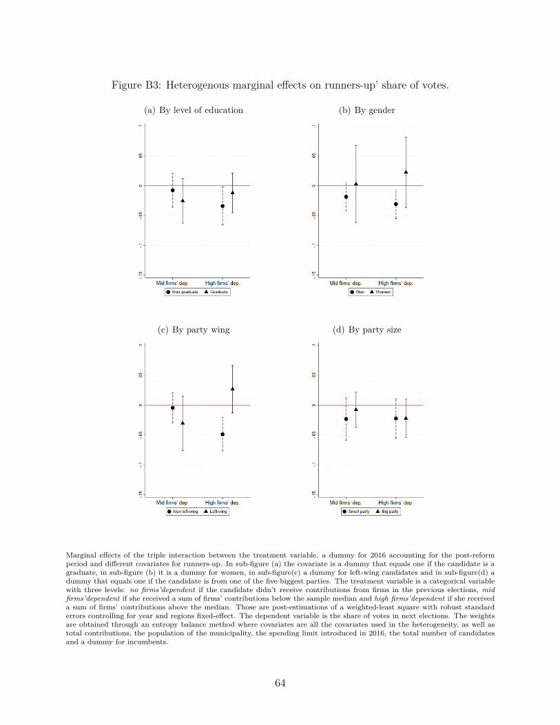
Figure B3: Heterogenous marginal effects on runners-up’ share of votes.

(a) By level of education (b) By gender

(c) By party wing (d) By party size

Marginal effects of the triple interaction between the treatment variable, a dummy for 2016 accounting for the post-reformperiod and different covariates for runners-up. In sub-figure (a) the covariate is a dummy that equals one if the candidate is agraduate, in sub-figure (b) it is a dummy for women, in sub-figure(c) a dummy for left-wing candidates and in sub-figure(d) adummy that equals one if the candidate is from one of the five biggest parties. The treatment variable is a categorical variablewith three levels: no firms’dependent if the candidate didn’t receive contributions from firms in the previous elections, midfirms’dependent if she received a sum of firms’ contributions below the sample median and high firms’dependent if she receiveda sum of firms’ contributions above the median. Those are post-estimations of a weighted-least square with robust standarderrors controlling for year and regions fixed-effect. The dependent variable is the share of votes in next elections. The weightsare obtained through an entropy balance method where covariates are all the covariates used in the heterogeneity, as well astotal contributions, the population of the municipality, the spending limit introduced in 2016, the total number of candidatesand a dummy for incumbents.

64

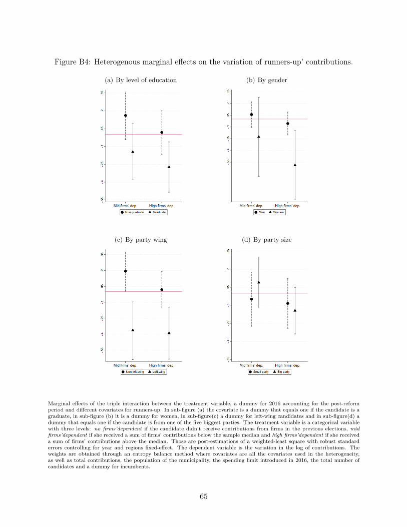
Figure B4: Heterogenous marginal effects on the variation of runners-up’ contributions.

(a) By level of education (b) By gender

(c) By party wing (d) By party size

Marginal effects of the triple interaction between the treatment variable, a dummy for 2016 accounting for the post-reformperiod and different covariates for runners-up. In sub-figure (a) the covariate is a dummy that equals one if the candidate is agraduate, in sub-figure (b) it is a dummy for women, in sub-figure(c) a dummy for left-wing candidates and in sub-figure(d) adummy that equals one if the candidate is from one of the five biggest parties. The treatment variable is a categorical variablewith three levels: no firms’dependent if the candidate didn’t receive contributions from firms in the previous elections, midfirms’dependent if she received a sum of firms’ contributions below the sample median and high firms’dependent if she receiveda sum of firms’ contributions above the median. Those are post-estimations of a weighted-least square with robust standarderrors controlling for year and regions fixed-effect. The dependent variable is the variation in the log of contributions. Theweights are obtained through an entropy balance method where covariates are all the covariates used in the heterogeneity,as well as total contributions, the population of the municipality, the spending limit introduced in 2016, the total number ofcandidates and a dummy for incumbents.

65

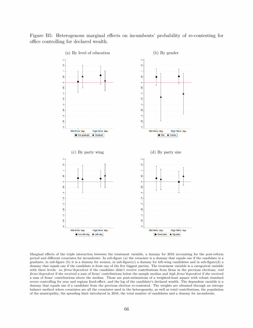
Figure B5: Heterogenous marginal effects on incumbents’ probability of re-contesting foroffice controlling for declared wealth.

(a) By level of education (b) By gender

(c) By party wing (d) By party size

Marginal effects of the triple interaction between the treatment variable, a dummy for 2016 accounting for the post-reformperiod and different covariates for incumbents. In sub-figure (a) the covariate is a dummy that equals one if the candidate is agraduate, in sub-figure (b) it is a dummy for women, in sub-figure(c) a dummy for left-wing candidates and in sub-figure(d) adummy that equals one if the candidate is from one of the five biggest parties. The treatment variable is a categorical variablewith three levels: no firms’dependent if the candidate didn’t receive contributions from firms in the previous elections, midfirms’dependent if she received a sum of firms’ contributions below the sample median and high firms’dependent if she receiveda sum of firms’ contributions above the median. Those are post-estimations of a weighted-least square with robust standarderrors controlling for year and regions fixed-effect, and the log of the candidate’s declared wealth. The dependent variable is adummy that equals one if a candidate from the previous election re-contested. The weights are obtained through an entropybalance method where covariates are all the covariates used in the heterogeneity, as well as total contributions, the populationof the municipality, the spending limit introduced in 2016, the total number of candidates and a dummy for incumbents.

66

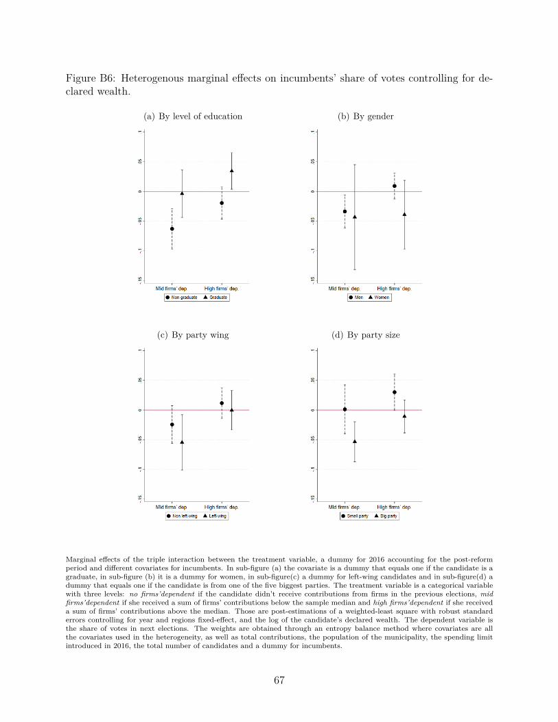
Figure B6: Heterogenous marginal effects on incumbents’ share of votes controlling for de-clared wealth.

(a) By level of education (b) By gender

(c) By party wing (d) By party size

Marginal effects of the triple interaction between the treatment variable, a dummy for 2016 accounting for the post-reformperiod and different covariates for incumbents. In sub-figure (a) the covariate is a dummy that equals one if the candidate is agraduate, in sub-figure (b) it is a dummy for women, in sub-figure(c) a dummy for left-wing candidates and in sub-figure(d) adummy that equals one if the candidate is from one of the five biggest parties. The treatment variable is a categorical variablewith three levels: no firms’dependent if the candidate didn’t receive contributions from firms in the previous elections, midfirms’dependent if she received a sum of firms’ contributions below the sample median and high firms’dependent if she receiveda sum of firms’ contributions above the median. Those are post-estimations of a weighted-least square with robust standarderrors controlling for year and regions fixed-effect, and the log of the candidate’s declared wealth. The dependent variable isthe share of votes in next elections. The weights are obtained through an entropy balance method where covariates are allthe covariates used in the heterogeneity, as well as total contributions, the population of the municipality, the spending limitintroduced in 2016, the total number of candidates and a dummy for incumbents.

67

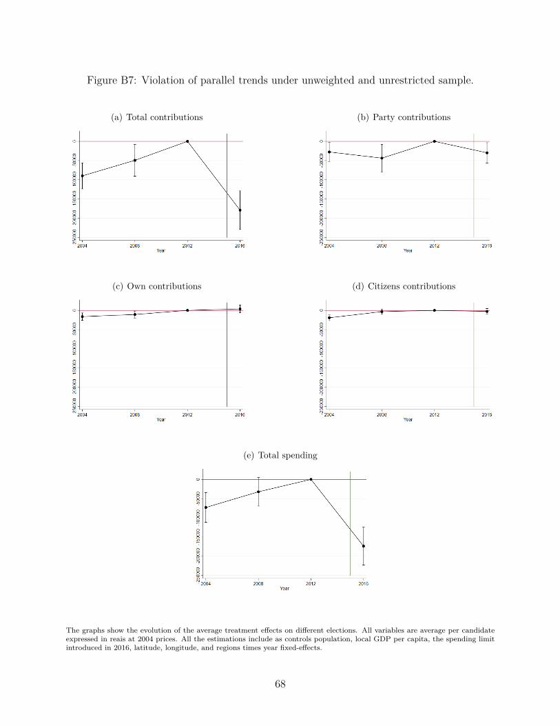
Figure B7: Violation of parallel trends under unweighted and unrestricted sample.

(a) Total contributions (b) Party contributions

(c) Own contributions (d) Citizens contributions

(e) Total spending

The graphs show the evolution of the average treatment effects on different elections. All variables are average per candidateexpressed in reais at 2004 prices. All the estimations include as controls population, local GDP per capita, the spending limitintroduced in 2016, latitude, longitude, and regions times year fixed-effects.

68

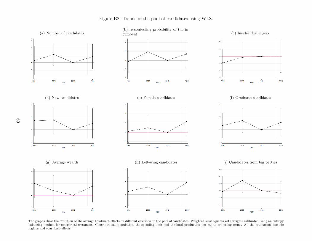
Figure B8: Trends of the pool of candidates using WLS.

(a) Number of candidates(b) re-contesting probability of the in-cumbent (c) Insider challengers

(d) New candidates (e) Female candidates (f) Graduate candidates

(g) Average wealth (h) Left-wing candidates (i) Candidates from big parties

The graphs show the evolution of the average treatment effects on different elections on the pool of candidates. Weighted least squares with weights calibrated using an entropybalancing method for categorical tretament. Contributions, population, the spending limit and the local production per capita are in log terms. All the estimations includeregions and year fixed-effects.

69

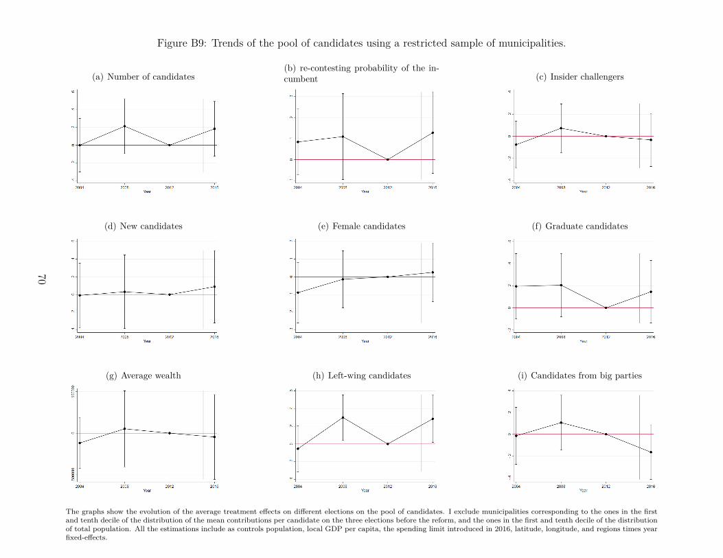
Figure B9: Trends of the pool of candidates using a restricted sample of municipalities.

(a) Number of candidates(b) re-contesting probability of the in-cumbent (c) Insider challengers

(d) New candidates (e) Female candidates (f) Graduate candidates

(g) Average wealth (h) Left-wing candidates (i) Candidates from big parties

The graphs show the evolution of the average treatment effects on different elections on the pool of candidates. I exclude municipalities corresponding to the ones in the firstand tenth decile of the distribution of the mean contributions per candidate on the three elections before the reform, and the ones in the first and tenth decile of the distributionof total population. All the estimations include as controls population, local GDP per capita, the spending limit introduced in 2016, latitude, longitude, and regions times yearfixed-effects.

70

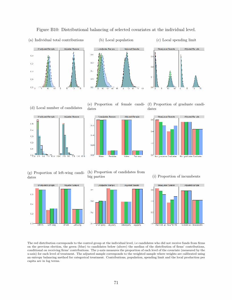
Figure B10: Distributional balancing of selected covariates at the individual level.

(a) Individual total contributions (b) Local population (c) Local spending limit

(d) Local number of candidates(e) Proportion of female candi-dates

(f) Proportion of graduate candi-dates

(g) Proportion of left-wing candi-dates

(h) Proportion of candidates frombig parties (i) Proportion of incumbents

The red distribution corresponds to the control group at the individual level, i.e candidates who did not receive funds from firmson the previous election, the green (blue) to candidates below (above) the median of the distribution of firms’ contributions,conditional on receiving firms’ contributions. The y-axis measures the proportion of each level of the covariate (measured by thex-axis) for each level of treatment. The adjusted sample corresponds to the weighted sample where weights are calibrated usingan entropy balancing method for categorical treatment. Contributions, population, spending limit and the local production percapita are in log terms.

71

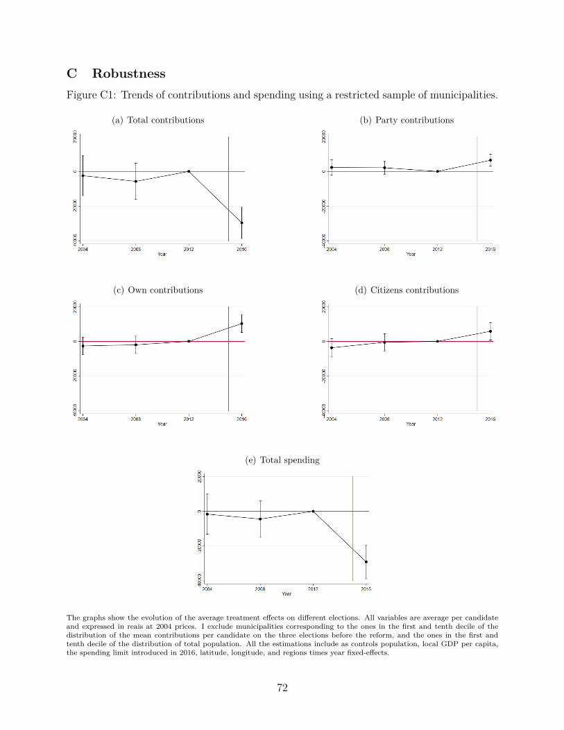
C RobustnessFigure C1: Trends of contributions and spending using a restricted sample of municipalities.

(a) Total contributions (b) Party contributions

(c) Own contributions (d) Citizens contributions

(e) Total spending

The graphs show the evolution of the average treatment effects on different elections. All variables are average per candidateand expressed in reais at 2004 prices. I exclude municipalities corresponding to the ones in the first and tenth decile of thedistribution of the mean contributions per candidate on the three elections before the reform, and the ones in the first andtenth decile of the distribution of total population. All the estimations include as controls population, local GDP per capita,the spending limit introduced in 2016, latitude, longitude, and regions times year fixed-effects.

72

Table C1: The effects of banning firms’ contributions on campaign contributions and spending using a restricted sample ofmunicipalities.

(1) (2) (3) (4) (5)

Panel A: All municipalities

Total contributions Party contributions Own contributions Citizens contributions Total spending

2016 -7,703 9,990*** -10,628*** -11,705*** -6,026(6,739) (2,178) (2,247) (2,768) (5,498)

Firms’ dependence 38,275*** -6,450*** -15,376*** -2,791* 32,764***(3,771) (1,064) (1,358) (1,445) (3,172)

Firms’ dependence * 2016 -32,406*** 5,923*** 13,118*** 8,621*** -28,685***(5,317) (1,201) (2,161) (2,168) (4,218)

Constant -12,394 -1,810 -4,779 10,006 -2,824(16,764) (4,626) (7,337) (6,519) (13,292)

Observations 15,163 15,163 15,163 15,163 15,023R-squared 0.172 0.163 0.041 0.178 0.071

Panel B: Municipalities where the incumbent can re-contest

Total contributions Party contributions Own contributions Citizens contributions Total spending

2016 -15,451** 8,781*** -12,321*** -12,573*** -12,905**(7,406) (1,748) (1,834) (3,026) (5,377)

Firms’ dependence 35,893*** -6,267*** -15,854*** -3,740** 31,545***(4,017) (1,142) (1,550) (1,561) (3,446)

Firms’ dependence * 2016 -29,305*** 5,861*** 13,574*** 9,843*** -27,357***(6,017) (1,377) (2,261) (2,480) (3,973)

Constant -18,727 -4,291 -4,223 10,748 -9,275(17,822) (5,058) (8,246) (7,109) (14,257)

Observations 11,684 11,684 11,684 11,684 11,566R-squared 0.374 0.149 0.118 0.176 0.305

Robust standard errors in parentheses*** p<0.01, ** p<0.05, * p<0.1

OLS estimates. Standard errors are clustered at the municipality level. Firms’ dependence is a continuous index that varies from 0 to 1 according to the percentage that firms’contributions represented in the total contributions of candidates running for mayor in a given municipality in the three years before the reform. I exclude municipalities in thefirst and last deciles in the distribution of mean contributions per candidate, as well as municipalities in the first and last decile in the distribution of population. All regressionsinclude regions times year fixed-effects, local production per capita, population times year fixed effects, the spending limit introduced in 2016, latitude and longitude. Panel Bexcludes municipalities where incumbents face a term limit.

73

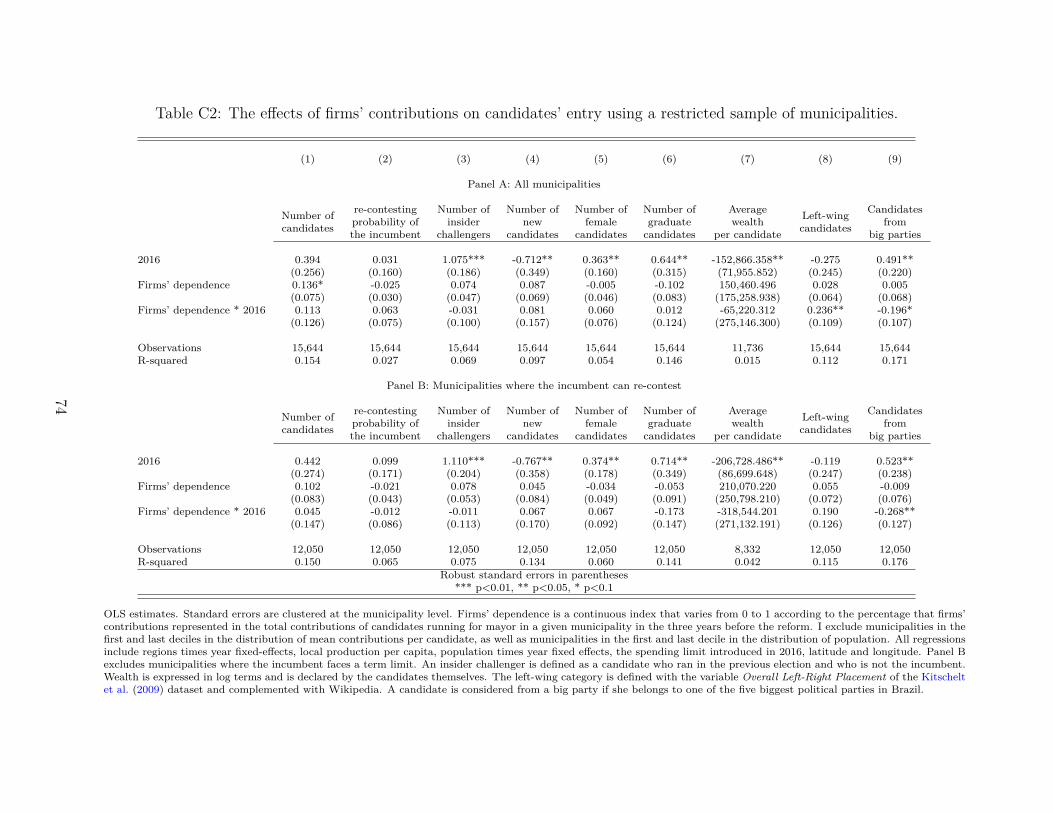
Table C2: The effects of firms’ contributions on candidates’ entry using a restricted sample of municipalities.

(1) (2) (3) (4) (5) (6) (7) (8) (9)

Panel A: All municipalities

Number ofcandidates

re-contestingprobability ofthe incumbent

Number ofinsider

challengers

Number ofnew

candidates

Number offemale

candidates

Number ofgraduate

candidates

Averagewealth

per candidate

Left-wingcandidates

Candidatesfrom

big parties

2016 0.394 0.031 1.075*** -0.712** 0.363** 0.644** -152,866.358** -0.275 0.491**(0.256) (0.160) (0.186) (0.349) (0.160) (0.315) (71,955.852) (0.245) (0.220)

Firms’ dependence 0.136* -0.025 0.074 0.087 -0.005 -0.102 150,460.496 0.028 0.005(0.075) (0.030) (0.047) (0.069) (0.046) (0.083) (175,258.938) (0.064) (0.068)

Firms’ dependence * 2016 0.113 0.063 -0.031 0.081 0.060 0.012 -65,220.312 0.236** -0.196*(0.126) (0.075) (0.100) (0.157) (0.076) (0.124) (275,146.300) (0.109) (0.107)

Observations 15,644 15,644 15,644 15,644 15,644 15,644 11,736 15,644 15,644R-squared 0.154 0.027 0.069 0.097 0.054 0.146 0.015 0.112 0.171

Panel B: Municipalities where the incumbent can re-contest

Number ofcandidates

re-contestingprobability ofthe incumbent

Number ofinsider

challengers

Number ofnew

candidates

Number offemale

candidates

Number ofgraduate

candidates

Averagewealth

per candidate

Left-wingcandidates

Candidatesfrom

big parties

2016 0.442 0.099 1.110*** -0.767** 0.374** 0.714** -206,728.486** -0.119 0.523**(0.274) (0.171) (0.204) (0.358) (0.178) (0.349) (86,699.648) (0.247) (0.238)

Firms’ dependence 0.102 -0.021 0.078 0.045 -0.034 -0.053 210,070.220 0.055 -0.009(0.083) (0.043) (0.053) (0.084) (0.049) (0.091) (250,798.210) (0.072) (0.076)

Firms’ dependence * 2016 0.045 -0.012 -0.011 0.067 0.067 -0.173 -318,544.201 0.190 -0.268**(0.147) (0.086) (0.113) (0.170) (0.092) (0.147) (271,132.191) (0.126) (0.127)

Observations 12,050 12,050 12,050 12,050 12,050 12,050 8,332 12,050 12,050R-squared 0.150 0.065 0.075 0.134 0.060 0.141 0.042 0.115 0.176

Robust standard errors in parentheses*** p<0.01, ** p<0.05, * p<0.1

OLS estimates. Standard errors are clustered at the municipality level. Firms’ dependence is a continuous index that varies from 0 to 1 according to the percentage that firms’contributions represented in the total contributions of candidates running for mayor in a given municipality in the three years before the reform. I exclude municipalities in thefirst and last deciles in the distribution of mean contributions per candidate, as well as municipalities in the first and last decile in the distribution of population. All regressionsinclude regions times year fixed-effects, local production per capita, population times year fixed effects, the spending limit introduced in 2016, latitude and longitude. Panel Bexcludes municipalities where the incumbent faces a term limit. An insider challenger is defined as a candidate who ran in the previous election and who is not the incumbent.Wealth is expressed in log terms and is declared by the candidates themselves. The left-wing category is defined with the variable Overall Left-Right Placement of the Kitscheltet al. (2009) dataset and complemented with Wikipedia. A candidate is considered from a big party if she belongs to one of the five biggest political parties in Brazil.

74

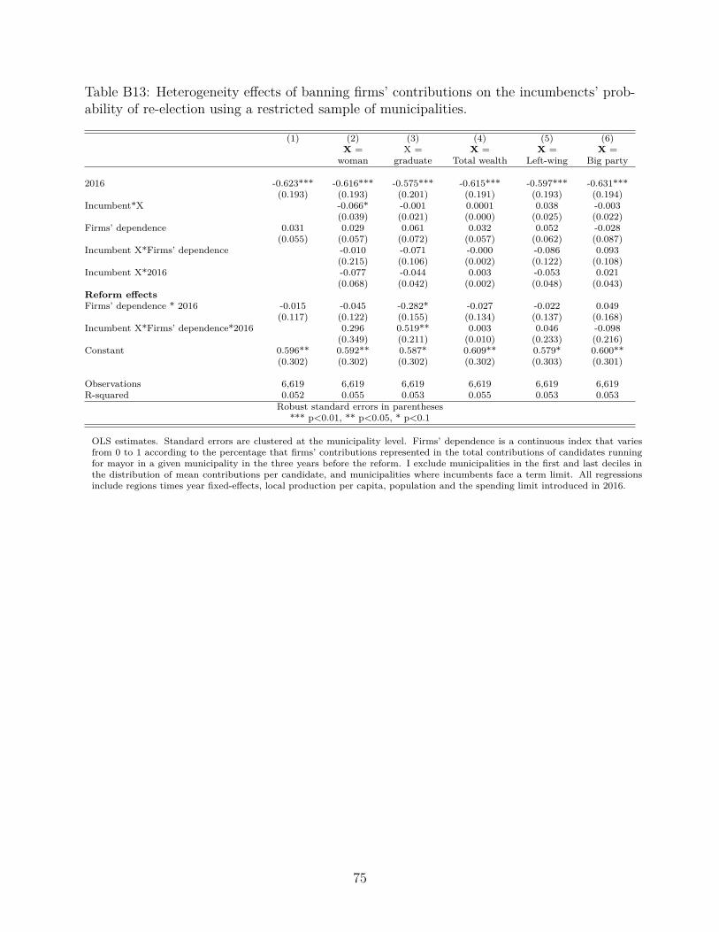
Table B13: Heterogeneity effects of banning firms’ contributions on the incumbencts’ prob-ability of re-election using a restricted sample of municipalities.

(1) (2) (3) (4) (5) (6)X =

womanX =

graduateX =

Total wealthX =

Left-wingX =

Big party

2016 -0.623*** -0.616*** -0.575*** -0.615*** -0.597*** -0.631***(0.193) (0.193) (0.201) (0.191) (0.193) (0.194)

Incumbent*X -0.066* -0.001 0.0001 0.038 -0.003(0.039) (0.021) (0.000) (0.025) (0.022)

Firms’ dependence 0.031 0.029 0.061 0.032 0.052 -0.028(0.055) (0.057) (0.072) (0.057) (0.062) (0.087)

Incumbent X*Firms’ dependence -0.010 -0.071 -0.000 -0.086 0.093(0.215) (0.106) (0.002) (0.122) (0.108)

Incumbent X*2016 -0.077 -0.044 0.003 -0.053 0.021(0.068) (0.042) (0.002) (0.048) (0.043)

Reform effectsFirms’ dependence * 2016 -0.015 -0.045 -0.282* -0.027 -0.022 0.049

(0.117) (0.122) (0.155) (0.134) (0.137) (0.168)Incumbent X*Firms’ dependence*2016 0.296 0.519** 0.003 0.046 -0.098

(0.349) (0.211) (0.010) (0.233) (0.216)Constant 0.596** 0.592** 0.587* 0.609** 0.579* 0.600**

(0.302) (0.302) (0.302) (0.302) (0.303) (0.301)

Observations 6,619 6,619 6,619 6,619 6,619 6,619R-squared 0.052 0.055 0.053 0.055 0.053 0.053

Robust standard errors in parentheses*** p<0.01, ** p<0.05, * p<0.1

OLS estimates. Standard errors are clustered at the municipality level. Firms’ dependence is a continuous index that variesfrom 0 to 1 according to the percentage that firms’ contributions represented in the total contributions of candidates runningfor mayor in a given municipality in the three years before the reform. I exclude municipalities in the first and last deciles inthe distribution of mean contributions per candidate, and municipalities where incumbents face a term limit. All regressionsinclude regions times year fixed-effects, local production per capita, population and the spending limit introduced in 2016.

75

Table C4: The effects of banning firms’ contributions on campaign contributions - TWFE.

(1) (2) (3) (4) (5)

Panel A: All municipalities

Total contributions Party contributions Own contributions Citizens contributions Total spending

2016 0.105 13.670*** -1.856 -0.581 0.101(0.524) (3.197) (1.706) (1.487) (0.527)

Firms’ dependence * 2016 -0.478*** 1.373*** 1.913*** 0.540** -0.489***(0.085) (0.504) (0.289) (0.271) (0.085)

Constant 9.989*** 3.039*** 7.903*** 7.481*** 9.986***(0.012) (0.059) (0.040) (0.047) (0.012)

Observations 15,450 15,450 15,450 15,450 15,310R-squared 0.589 0.486 0.396 0.431 0.590

Panel B: Municipalities where the incumbent can re-contest

Total contributions Party contributions Own contributions Citizens contributions Total spending

2016 0.912*** 9.619*** -1.564 -0.100 0.670**(0.310) (1.451) (1.127) (0.805) (0.323)

Firms’ dependence * 2016 -0.563*** 2.403*** 1.963*** 0.015 -0.587***(0.088) (0.495) (0.301) (0.295) (0.089)

Constant 10.028*** 3.365*** 7.888*** 7.390*** 10.024***(0.010) (0.051) (0.034) (0.040) (0.011)

Observations 16,722 16,722 16,722 16,722 16,558R-squared 0.770 0.567 0.481 0.535 0.773

Robust standard errors in parentheses*** p<0.01, ** p<0.05, * p<0.1

OLS estimates with year and municipalities fixed-effects. Standard errors are clustered at the municipality level. Firms’ dependence is a continuous index that varies from 0 to1 according to the percentage that firms’ contributions represented in the total contributions of candidates running for mayor in a given municipality in the three years beforethe reform. All regressions include regions times year fixed-effects and the spending limit introduced in 2016. Panel B excludes municipalities where incumbents face a termlimit.

76

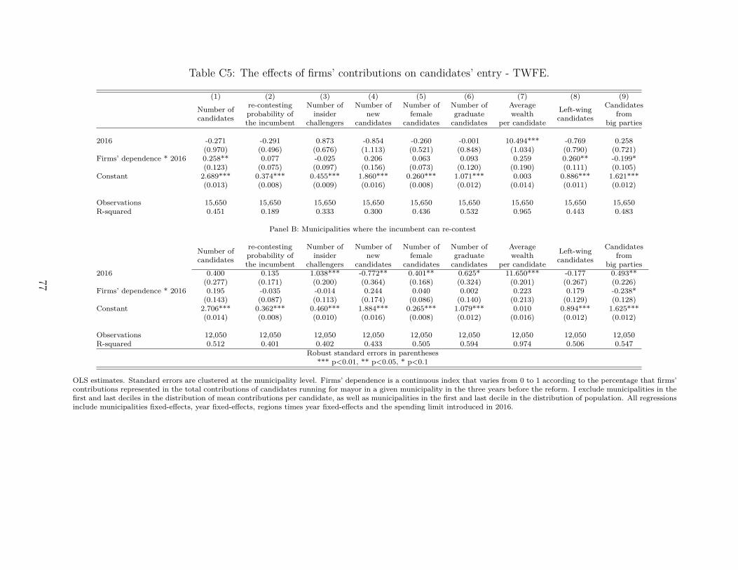
Table C5: The effects of firms’ contributions on candidates’ entry - TWFE.

(1) (2) (3) (4) (5) (6) (7) (8) (9)

Number ofcandidates

re-contestingprobability ofthe incumbent

Number ofinsider

challengers

Number ofnew

candidates

Number offemale

candidates

Number ofgraduate

candidates

Averagewealth

per candidate

Left-wingcandidates

Candidatesfrom

big parties

2016 -0.271 -0.291 0.873 -0.854 -0.260 -0.001 10.494*** -0.769 0.258(0.970) (0.496) (0.676) (1.113) (0.521) (0.848) (1.034) (0.790) (0.721)

Firms’ dependence * 2016 0.258** 0.077 -0.025 0.206 0.063 0.093 0.259 0.260** -0.199*(0.123) (0.075) (0.097) (0.156) (0.073) (0.120) (0.190) (0.111) (0.105)

Constant 2.689*** 0.374*** 0.455*** 1.860*** 0.260*** 1.071*** 0.003 0.886*** 1.621***(0.013) (0.008) (0.009) (0.016) (0.008) (0.012) (0.014) (0.011) (0.012)

Observations 15,650 15,650 15,650 15,650 15,650 15,650 15,650 15,650 15,650R-squared 0.451 0.189 0.333 0.300 0.436 0.532 0.965 0.443 0.483

Panel B: Municipalities where the incumbent can re-contest

Number ofcandidates

re-contestingprobability ofthe incumbent

Number ofinsider

challengers

Number ofnew

candidates

Number offemale

candidates

Number ofgraduate

candidates

Averagewealth

per candidate

Left-wingcandidates

Candidatesfrom

big parties2016 0.400 0.135 1.038*** -0.772** 0.401** 0.625* 11.650*** -0.177 0.493**

(0.277) (0.171) (0.200) (0.364) (0.168) (0.324) (0.201) (0.267) (0.226)Firms’ dependence * 2016 0.195 -0.035 -0.014 0.244 0.040 0.002 0.223 0.179 -0.238*

(0.143) (0.087) (0.113) (0.174) (0.086) (0.140) (0.213) (0.129) (0.128)Constant 2.706*** 0.362*** 0.460*** 1.884*** 0.265*** 1.079*** 0.010 0.894*** 1.625***

(0.014) (0.008) (0.010) (0.016) (0.008) (0.012) (0.016) (0.012) (0.012)

Observations 12,050 12,050 12,050 12,050 12,050 12,050 12,050 12,050 12,050R-squared 0.512 0.401 0.402 0.433 0.505 0.594 0.974 0.506 0.547

Robust standard errors in parentheses*** p<0.01, ** p<0.05, * p<0.1

OLS estimates. Standard errors are clustered at the municipality level. Firms’ dependence is a continuous index that varies from 0 to 1 according to the percentage that firms’contributions represented in the total contributions of candidates running for mayor in a given municipality in the three years before the reform. I exclude municipalities in thefirst and last deciles in the distribution of mean contributions per candidate, as well as municipalities in the first and last decile in the distribution of population. All regressionsinclude municipalities fixed-effects, year fixed-effects, regions times year fixed-effects and the spending limit introduced in 2016.

77

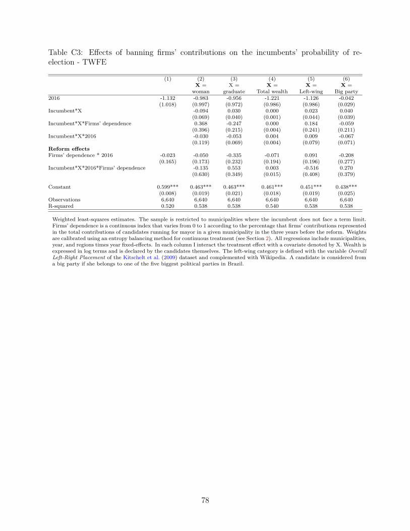
Table C3: Effects of banning firms’ contributions on the incumbents’ probability of re-election - TWFE

(1) (2) (3) (4) (5) (6)X =

womanX =

graduateX =

Total wealthX =

Left-wingX =

Big party2016 -1.132 -0.983 -0.956 -1.221 -1.126 -0.042

(1.018) (0.997) (0.972) (0.986) (0.986) (0.029)Incumbent*X -0.094 0.030 0.000 0.023 0.040

(0.069) (0.040) (0.001) (0.044) (0.039)Incumbent*X*Firms’ dependence 0.368 -0.247 0.000 0.184 -0.059

(0.396) (0.215) (0.004) (0.241) (0.211)Incumbent*X*2016 -0.030 -0.053 0.004 0.009 -0.067

(0.119) (0.069) (0.004) (0.079) (0.071)Reform effectsFirms’ dependence * 2016 -0.023 -0.050 -0.335 -0.071 0.091 -0.208

(0.165) (0.173) (0.232) (0.194) (0.196) (0.277)Incumbent*X*2016*Firms’ dependence -0.135 0.553 0.003 -0.516 0.270

(0.630) (0.349) (0.015) (0.408) (0.379)

Constant 0.599*** 0.463*** 0.463*** 0.461*** 0.451*** 0.438***(0.008) (0.019) (0.021) (0.018) (0.019) (0.025)

Observations 6,640 6,640 6,640 6,640 6,640 6,640R-squared 0.520 0.538 0.538 0.540 0.538 0.538

Weighted least-squares estimates. The sample is restricted to municipalities where the incumbent does not face a term limit.Firms’ dependence is a continuous index that varies from 0 to 1 according to the percentage that firms’ contributions representedin the total contributions of candidates running for mayor in a given municipality in the three years before the reform. Weightsare calibrated using an entropy balancing method for continuous treatment (see Section 2). All regressions include municipalities,year, and regions times year fixed-effects. In each column I interact the treatment effect with a covariate denoted by X. Wealth isexpressed in log terms and is declared by the candidates themselves. The left-wing category is defined with the variable OverallLeft-Right Placement of the Kitschelt et al. (2009) dataset and complemented with Wikipedia. A candidate is considered froma big party if she belongs to one of the five biggest political parties in Brazil.

78

Figure C2: Heterogenous marginal effects on runners-up’ probability of re-contesting foroffice using propensity score.

(a) By level of education (b) By gender

(c) By party wing (d) By party size

Marginal effects of the triple interaction between the treatment variable, a dummy for 2016 accounting for the post-reformperiod and different covariates for runners-up. In sub-figure (a) the covariate is a dummy that equals one if the candidate is agraduate, in sub-figure (b) it is a dummy for women, in sub-figure(c) a dummy for left-wing candidates and in sub-figure(d) adummy that equals one if the candidate is from one of the five biggest parties. The treatment variable is a categorical variablewith three levels: no firms’dependent if the candidate didn’t receive contributions from firms in the previous elections, midfirms’dependent if she received a sum of firms’ contributions below the sample median and high firms’dependent if she received asum of firms’ contributions above the median. Those are post-estimations of a weighted-least square with robust standard errorscontrolling for year and regions fixed-effects and party × year fixed-effects. The dependent variable is a dummy that equalsone if a candidate from the previous election re-contested. The weights are obtained through an entropy balance method wherecovariates are all the covariates used in the heterogeneity, as well as total contributions, the population of the municipality, thespending limit introduced in 2016, the total number of candidates and a dummy for incumbents.

79

Figure C4: Marginal effects of the reform on incumbents and runners-up excluding candidatesinvolved in the Car wash scandal.

(a) Probability of re-contesting(b) Variation in total contribu-tions (in log.)

(c) Share of votes in next elec-tions

Marginal effects of the interaction between the treatment variable and a dummy for 2016 accounting for the post-reform. Thetreatment variable is a categorical variable with three levels: no firms’dependent if the candidate didn’t receive contributionsfrom firms in the previous elections, mid firms’dependent if she received a sum of firms’ contributions below the sample medianand high firms’dependent if she received a sum of firms’ contributions above the median. Those are post-estimations of aweighted-least square with robust standard errors controlling for year and regions fixed-effects. In sub-figure (a) the dependentvariable is a dummy that equals one if a candidate from previous election re-contested, in sub-figure (b) is the variation inthe log. of total contributions conditional on re-contesting and in (c) is the share of votes in next elections. The weights areobtained through an entropy balance method where covariates are graduate, gender, party-wing, party size, total contributions,the population of the municipality, the spending limit introduced in 2016, the total number of candidates and a dummy forincumbents. I exclude candidates cited to declare in the Car Wash scandal listed in Table C6.

80

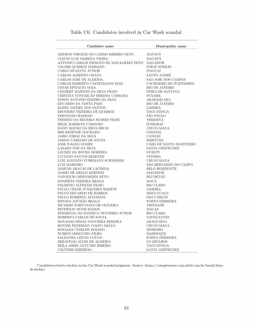
Table C6: Candidates involved in Car Wash scandal

Candidate name Municipality name

ARTHUR VIRGILIO DO CARMO RIBEIRO NETO MANAUSCLECIO LUIS VILHENA VIEIRA MACAPAANTONIO CARLOS PEIXOTO DE MAGALHAES NETO SALVADORVALMIR QUEIROZ MARIANO PARAUAPEBASCARLO BUSATTO JUNIOR ITAGUAICARLOS ALBERTO GRANA SANTO ANDRECARLOS JOSE DE ALMEIDA SAO JOSE DOS CAMPOSCARLOS ROBERTO CASTEGLIONE DIAS CACHOEIRO DE ITAPEMIRIMCESAR EPITACIO MAIA RIO DE JANEIROCOLBERT MARTINS DA SILVA FILHO FEIRA DE SANTANACRISTINA CONCEICAO BREDDA CARRARA SUMAREEDSON ANTONIO EDINHO DA SILVA ARARAQUARAEDUARDO DA COSTA PAES RIO DE JANEIROELISEU DANIEL DOS SANTOS LIMEIRAERONIDES TEIXEIRA DE QUEIROZ TAGUATINGAFERNANDO HADDAD SAO PAULOFIRMINO DA SILVEIRA SOARES FILHO TERESINAHELIL BARRETO CARDOZO ITABORAIILSON MAURO DA SILVA BRUM URUGUAIANAIRIS REZENDE MACHADO GOIANIAJAIRO JORGE DA SILVA CANOASJAISON CARDOSO DE SOUZA IMBITUBAJOSE IVALDO GOMES CABO DE SANTO AGOSTINHOLAZARO NOE DA SILVA SANTA GERTRUDESLAUREZ DA ROCHA MOREIRA GURUPILUCIANO SANTOS REZENDE VITORIALUIZ AUGUSTO FUHRMANN SCHNEIDER URUGUAIANALUIZ MARINHO SAO BERNARDO DO CAMPOMARCIO ARAUJO DE LACERDA BELO HORIZONTEMARIO DE MELLO KERTESZ SALVADORNAPOLEAO BERNARDES NETO BLUMENAUDONISETE PEREIRA BRAGA MAUAPALMINIO ALTIMARI FILHO RIO CLAROPAULO CEZAR JUNQUEIRA HADICH LIMEIRAPAULO EDUARDO DE BARROS MOGI GUACUPAULO ROBERTO ALTOMANI SAO CARLOSRENATA ANCHAO BRAGA PORTO FERREIRARICARDO FORTUNATO DE OLIVEIRA TRINDADERIVERTON MUSSI RAMOS MACAEDERMEVAL DA FONSECA NEVOEIRO JUNIOR RIO CLAROROBERTO CARLOS DE SOUZA NAVEGANTESRONALDO DIMAS NOGUEIRA PEREIRA ARAGUAINARONNIE PETERSON COLPO MELLO URUGUAIANAROSALBA CIARLINI ROSADO MOSSORORUBENS MERGUIZO FILHO MAIRINQUESALDANHA LEIVAS COUGO PORTO FERREIRASEBASTIAO ALVES DE ALMEIDA GUARULHOSZEILA AIRES ANTUNES RIBEIRO TAGUATINGAVALTIMIR RIBEIRAO SANTA GERTRUDES

Candidates cited to declare in the Car Wash scandal judgment. Source: https://complemento.veja.abril.com.br/brasil/lista-de-fachin/

81

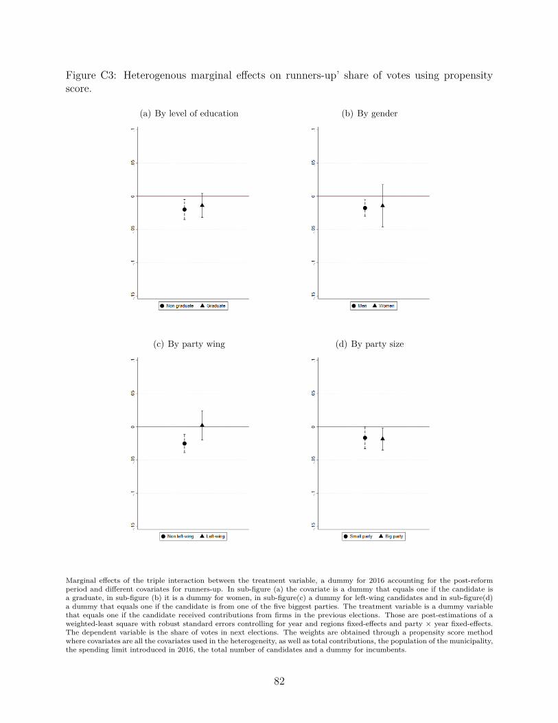
Figure C3: Heterogenous marginal effects on runners-up’ share of votes using propensityscore.

(a) By level of education (b) By gender

(c) By party wing (d) By party size

Marginal effects of the triple interaction between the treatment variable, a dummy for 2016 accounting for the post-reformperiod and different covariates for runners-up. In sub-figure (a) the covariate is a dummy that equals one if the candidate isa graduate, in sub-figure (b) it is a dummy for women, in sub-figure(c) a dummy for left-wing candidates and in sub-figure(d)a dummy that equals one if the candidate is from one of the five biggest parties. The treatment variable is a dummy variablethat equals one if the candidate received contributions from firms in the previous elections. Those are post-estimations of aweighted-least square with robust standard errors controlling for year and regions fixed-effects and party × year fixed-effects.The dependent variable is the share of votes in next elections. The weights are obtained through a propensity score methodwhere covariates are all the covariates used in the heterogeneity, as well as total contributions, the population of the municipality,the spending limit introduced in 2016, the total number of candidates and a dummy for incumbents.

82

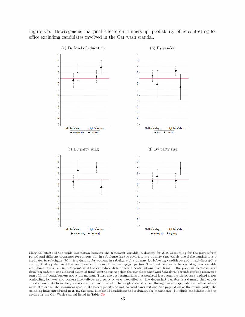
Figure C5: Heterogenous marginal effects on runners-up’ probability of re-contesting foroffice excluding candidates involved in the Car wash scandal.

(a) By level of education (b) By gender

(c) By party wing (d) By party size

Marginal effects of the triple interaction between the treatment variable, a dummy for 2016 accounting for the post-reformperiod and different covariates for runners-up. In sub-figure (a) the covariate is a dummy that equals one if the candidate is agraduate, in sub-figure (b) it is a dummy for women, in sub-figure(c) a dummy for left-wing candidates and in sub-figure(d) adummy that equals one if the candidate is from one of the five biggest parties. The treatment variable is a categorical variablewith three levels: no firms’dependent if the candidate didn’t receive contributions from firms in the previous elections, midfirms’dependent if she received a sum of firms’ contributions below the sample median and high firms’dependent if she received asum of firms’ contributions above the median. Those are post-estimations of a weighted-least square with robust standard errorscontrolling for year and regions fixed-effects and party × year fixed-effects. The dependent variable is a dummy that equalsone if a candidate from the previous election re-contested. The weights are obtained through an entropy balance method wherecovariates are all the covariates used in the heterogeneity, as well as total contributions, the population of the municipality, thespending limit introduced in 2016, the total number of candidates and a dummy for incumbents. I exclude candidates cited todeclare in the Car Wash scandal listed in Table C6.

83

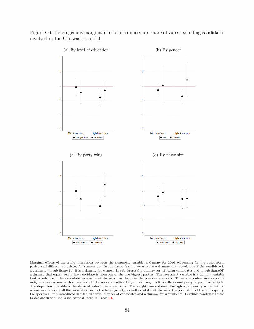
Figure C6: Heterogenous marginal effects on runners-up’ share of votes excluding candidatesinvolved in the Car wash scandal.

(a) By level of education (b) By gender

(c) By party wing (d) By party size

Marginal effects of the triple interaction between the treatment variable, a dummy for 2016 accounting for the post-reformperiod and different covariates for runners-up. In sub-figure (a) the covariate is a dummy that equals one if the candidate isa graduate, in sub-figure (b) it is a dummy for women, in sub-figure(c) a dummy for left-wing candidates and in sub-figure(d)a dummy that equals one if the candidate is from one of the five biggest parties. The treatment variable is a dummy variablethat equals one if the candidate received contributions from firms in the previous elections. Those are post-estimations of aweighted-least square with robust standard errors controlling for year and regions fixed-effects and party × year fixed-effects.The dependent variable is the share of votes in next elections. The weights are obtained through a propensity score methodwhere covariates are all the covariates used in the heterogeneity, as well as total contributions, the population of the municipality,the spending limit introduced in 2016, the total number of candidates and a dummy for incumbents. I exclude candidates citedto declare in the Car Wash scandal listed in Table C6.

84

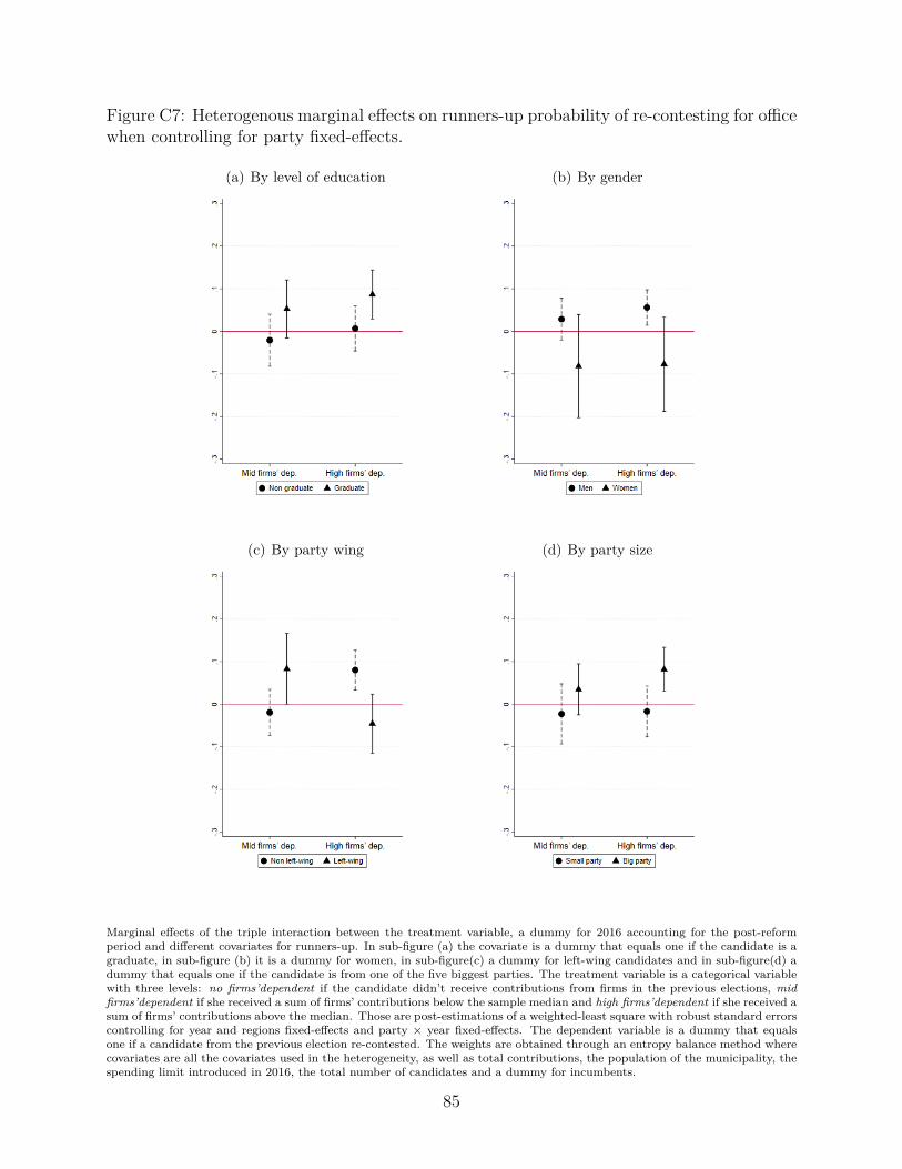
Figure C7: Heterogenous marginal effects on runners-up probability of re-contesting for officewhen controlling for party fixed-effects.

(a) By level of education (b) By gender

(c) By party wing (d) By party size

Marginal effects of the triple interaction between the treatment variable, a dummy for 2016 accounting for the post-reformperiod and different covariates for runners-up. In sub-figure (a) the covariate is a dummy that equals one if the candidate is agraduate, in sub-figure (b) it is a dummy for women, in sub-figure(c) a dummy for left-wing candidates and in sub-figure(d) adummy that equals one if the candidate is from one of the five biggest parties. The treatment variable is a categorical variablewith three levels: no firms’dependent if the candidate didn’t receive contributions from firms in the previous elections, midfirms’dependent if she received a sum of firms’ contributions below the sample median and high firms’dependent if she received asum of firms’ contributions above the median. Those are post-estimations of a weighted-least square with robust standard errorscontrolling for year and regions fixed-effects and party × year fixed-effects. The dependent variable is a dummy that equalsone if a candidate from the previous election re-contested. The weights are obtained through an entropy balance method wherecovariates are all the covariates used in the heterogeneity, as well as total contributions, the population of the municipality, thespending limit introduced in 2016, the total number of candidates and a dummy for incumbents.

85

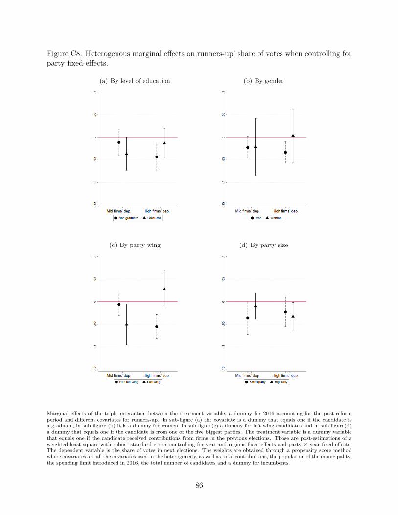
Figure C8: Heterogenous marginal effects on runners-up’ share of votes when controlling forparty fixed-effects.

(a) By level of education (b) By gender

(c) By party wing (d) By party size

Marginal effects of the triple interaction between the treatment variable, a dummy for 2016 accounting for the post-reformperiod and different covariates for runners-up. In sub-figure (a) the covariate is a dummy that equals one if the candidate isa graduate, in sub-figure (b) it is a dummy for women, in sub-figure(c) a dummy for left-wing candidates and in sub-figure(d)a dummy that equals one if the candidate is from one of the five biggest parties. The treatment variable is a dummy variablethat equals one if the candidate received contributions from firms in the previous elections. Those are post-estimations of aweighted-least square with robust standard errors controlling for year and regions fixed-effects and party × year fixed-effects.The dependent variable is the share of votes in next elections. The weights are obtained through a propensity score methodwhere covariates are all the covariates used in the heterogeneity, as well as total contributions, the population of the municipality,the spending limit introduced in 2016, the total number of candidates and a dummy for incumbents.

86