Intercomparison of subglacial sediment-deformation models: application to the Late Weichselian western Barents margin

Intercomparison of subglacial sediment deformationmodels: application to the late Weichselian western

Barents margin.

DANIEL HOWELL 1, MARTIN J. SIEGERT 2 AND JULIAN A. DOWDESWELL 2

1 Centre for Glaciology, Institute of Geography and Earth Sciences, University of Wales, Aberystwyth, SY233DB, UK.

2 Bristol Glaciology Centre, School of Geographical Sciences, University of Bristol, Bristol, BS8 1SS, UK.

1

ABSTRACT. Numerical experiments where a simple ice-sheet model was

coupled with sediment deformation models were performed to

investigate the transport of glacigenic material to the western

Barents Shelf during the Late Weichselian. The ice sheet model,

and its environmental inputs, has been matched previously with a

series of geological datasets relating to the maximum extent of

the ice sheet (Howell and others, in press). Additional geological

data on the volumes of sediment delivered to the Bear Island Fan

(Barents continental margin) are available to compare results. The

experiments indicate the sensitivity of sediment transport and

deposition to the variations in (a) the ice stream model and (b) a

variety of model parameters. Two ice-stream models were used (1) a

'height above buoyancy' model, in which basal velocity is

controlled by basal driving stress and a buoyancy-induced

reduction in the normal load beneath a marine based ice sheet and

(2) a modified version of the method presented by Alley (1990) in

which basal velocity is related to pore-water pressure, sediment

thickness, and driving basal stress. The results of the two

different models were then compared. An extensive set of

sensitivity tests was carried out to determine sediment transport

response to changes in the model’s parameters. Results indicate

that, using physically realistic parameters for deforming

subglacial sediment, both models reproduce the volume of Late

Weichselian sediment measured on the Bear Island Fan. Results from

both models are sensitive to (1) cohesion of the sediment, and (2)

the thickness of deforming sediment beneath the ice-sheet. The two

models exhibited different degrees of sensitivity to the sediment

parameters, with the 'height above buoyancy' model proving to be

less sensitive to variations in the thickness of the deforming

sediment layer than the model proposed by Alley (1990). The

2

differences between the two models examined here highlights the

need for a comprehensive comparison of all the methodologies for

calculating basal ice motion and sediment transport currently in

use.

3

INTRODUCTION

Numerical ice-sheet models calculate ice flow by coupling

algorithms for internal ice deformation, and basal ice motion. The

laws governing ice deformation within an ice sheet are well known

and are based on Glen's flow law for ice (Glen 1955), and

different model formulations of internal ice deformation have been

found to produce ice-sheets which are in good agreement with one

another (Huybrechts and Payne, 1996). However there are a variety

of different algorithms available to calculate basal ice-sheet

motion (Table 1). Sensitivity tests have been carried out on the

response of basal motion to variation in model parameters.

However, an intercomparison of ice-stream/sediment-deformation

model techniques has yet to be undertaken.

Pattyn (1996) performed a flow line experiment comparing basal-

motion models based on Height Above Buoyancy and sub-glacial water

flux in reconstructing the modern ice-flux of the Shirase glacier

in Antarctica. However the flow-line nature of his experiment

makes it difficult to generalise the results to a model of a

complete ice-sheet. There was also no long-term geological

evidence available to compare the results from the models. In

general, the highly multivariate nature of time-dependent ice-

sheet models makes it difficult to select a simple comparison

methodology to understand how sediment deformation algorithms

affect ice-sheet results. However, several authors have recently

investigated the transport of sediment beneath ice sheets using

numerical modelling (Jenson and others, 1995,1996; Dowdeswell and

Siegert, in press). Consequently it is becoming increasingly

4

important to investigate possible discrepancies between the

available models for ice-sheet basal motion.

This paper aims to highlight the effect of using two different

methods for calculating ice-sheet basal motion. The models are

applied to determine the sediment delivery to the margin of the

Late Weichselian ice sheet in the Barents Sea. There are several

features related to this former ice sheet which lend it to the

experiment proposed here. Firstly a new ice-sheet reconstruction

of the Late Weichselian Eurasian ice sheet has recently been

conducted using the ice-sheet model, and associated environmental

inputs, employed here (Howell and others, in press). Secondly the

presence of large glacigenic sedimentary fans on the margins of

the Barents Sea provides a geological control on the model

results. Late Weichselian sediment volumes have been measured on

the Bear Island Fan (4,000 km3; Laberg and Vorren, 1996a) and the

smaller Storfjorden Fan (700 km3; Laberg and Vorren, 1996b), along

the western Barents Sea continental margin (Figure 1). Thirdly the

presence of the glacigenic sedimentary fans precisely locates the

active ice streams which transported the sediment. Interfan

margins are characterised by low sediment thicknesses, indicating

that the ice-sheet terminating in these regions was relatively

inactive. Finally there is currently a thick layer of soft,

unconsolidated sediments throughout the Barents Sea. Thus,

sediment transport during the relatively brief Late Weichselian

glaciation did not strip the sediment layer from any part of the

Barents Sea. Consequently in modelling sediment deformation during

this period it can be assumed that there the actual thickness of

easily deformable sediments exceeded the thickness of the shear

zone within the subglacial sediments for the entire Late

Weichselian glaciation. Therefore processes of sediment 'creation

5

and depletion' need not be considered, and the number of unknowns

in the model is thereby reduced.

In summary, we have undertaken an intercomparison of two ice-

stream/sediment models by applying the models to the well

documented glaciation of the Barents Sea with specific reference

to a well known glacigenic fan system. The results are valuable in

themselves in the context of reconstructing the glacial and

sedimentological history of the Barents Sea. The comparison of

these two models also acts as an indicator that a more widespread

comparison of all the basal deformation models currently in use is

needed.

THE NUMERICAL MODEL

The Late Weichselian Eurasian ice sheet was modelled using a

topographic grid as a boundary condition, consisting of 310 (E) by

240 (N) 20 km 20 km grid cells covering the UK, Scandinavia,

northern Russia and the Barents and Kara Seas (Fig. 1).. A time

dependent, vertically integrated, finite-difference numerical ice-

sheet model was used to determine ice-sheet flow, and an elastic-

sheet lithosphere model used to calculate the isostatic depression

caused by ice loading. In discrete experiments, the ice-sheet

model was coupled to two subglacial sediment deformation models.

Ice motion within the ice-sheet was modelled by solving the

continuity equation for ice flow (Mahaffy, 1976):

ht

F u,h b (1)

6

where F(u, h) is the net flux of ice out of a cell (via internal

deformation and basal motion of the ice sheet), and depends on

ice-sheet thickness (h) and velocity (u). The mass budget term, b,

incorporates a number of processes including surface accumulation

and ablation, iceberg calving and ice shelf basal melting.

Equation 1 is solved using an implicit finite-difference technique

(Huybrechts and Payne, 1996).

Internal ice-sheet deformation is modelled using a depth-

averaged ice velocity equation:

u x 2A

n 2( bx2 by

2)n 12 bx h (2a)

where

bx ighsin x (2b)

and bx is the basal shear stress in the x direction, dependent on

ice thickness (h), acceleration due to gravity (g = 9.81 ms-1),

density of ice (i = 910 kg m-3) and ice-sheet surface slope (x)

(Paterson, 1994). A is a flow law parameter, here taken to be a

constant 10-16 Pa-3 a-1 after (Huybrechts and Payne, 1996), and the

flow law exponent n used is be 3. Similar equations apply for

motion in the y direction.

Modelling of isostatic bedrock adjustment is after Oerlemans and

van der Veen (1984) and Le Meur and Huybrechts (1996). The Earth

is modelled as a two layer system, with an elastic lithosphere

controlling the final isostatic depression, and an underlying

relaxed asthenosphere controlling the time taken to reach the

7

equilibrium position. The lithosphere is modelled as an elastic

sheet where an equilibrium depression caused by a discrete load at

a point x = 0, is given by

w(x')12D

qx 2(x') (3a)

where,

x x

(3b)

and

(3c)

In equations 6a, 6b, and 6c, x is the distance from the applied

load, m is the density of the mantle (3,300 kg m-3), qx is the

magnitude of the applied load, D is the flexural rigidity of the

lithosphere, and is a Kelvin function of zero order. Fjeldskaar

(1994) determined that the flexural rigidity in Scandinavia was

between 1 1024 and 1 1026 N m. Our study uses a flexural

rigidity value of 1 1025 N m. Equation 6a is linear and,

therefore, the total deflection of the lithosphere can be

approximated as the sum of the deflections caused by discrete

loads in each cell. The lithosphere is allowed to approach the

equilibrium deflection computed in Equation 6a by a exponential

decay (Le Meur and Huybrechts, 1996):

8

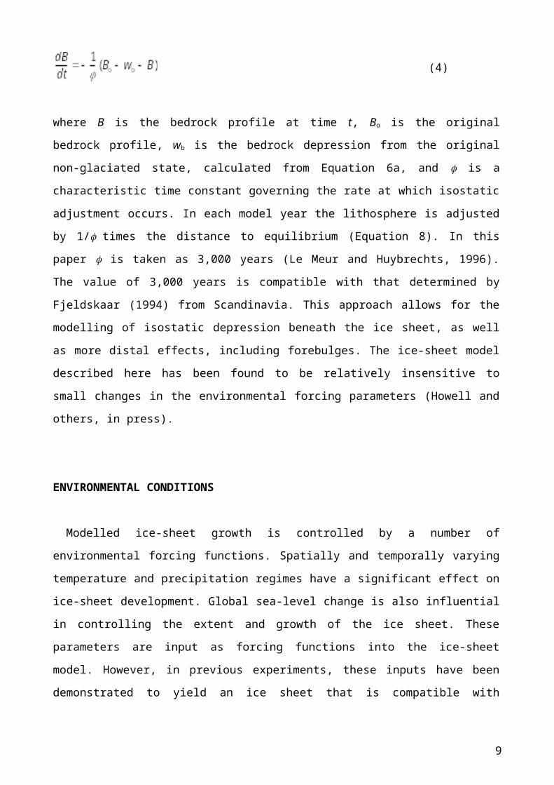
(4)

where B is the bedrock profile at time t, Bo is the original

bedrock profile, wb is the bedrock depression from the original

non-glaciated state, calculated from Equation 6a, and is a

characteristic time constant governing the rate at which isostatic

adjustment occurs. In each model year the lithosphere is adjusted

by 1/ times the distance to equilibrium (Equation 8). In this

paper is taken as 3,000 years (Le Meur and Huybrechts, 1996).

The value of 3,000 years is compatible with that determined by

Fjeldskaar (1994) from Scandinavia. This approach allows for the

modelling of isostatic depression beneath the ice sheet, as well

as more distal effects, including forebulges. The ice-sheet model

described here has been found to be relatively insensitive to

small changes in the environmental forcing parameters (Howell and

others, in press).

ENVIRONMENTAL CONDITIONS

Modelled ice-sheet growth is controlled by a number of

environmental forcing functions. Spatially and temporally varying

temperature and precipitation regimes have a significant effect on

ice-sheet development. Global sea-level change is also influential

in controlling the extent and growth of the ice sheet. These

parameters are input as forcing functions into the ice-sheet

model. However, in previous experiments, these inputs have been

demonstrated to yield an ice sheet that is compatible with

9

geological data relating to the extent of the last ice sheet

(Howell and others, in press).

Sea-level depression

The time-dependent change in sea level, adapted from Fairbanks

(1989) and Shackleton (1987), is used to describe the variation in

sea level during the last glacial cycle. The sea-level function

has been corrected by the Stuiver and Reimer (1993) calibration so

that it is in calendar years (Siegert and Dowdeswell, 1995a). Our

model therefore runs in calendar years. The sea-level curve is

used to adjust bedrock heights through time, and to parameterise

the transition between modern and glacial-maximum temperatures.

Full-glacial conditions are assumed to coincide with maximum

global sea-level depression, while modern sea level is correlated

with modern climatic conditions.

Palaeoenvironmental conditions

The accumulation regime employed in this paper is identical to

the one presented in Howell and others (in press). There is a lack

of data concerning the climatic regime of the Eurasian Arctic

during the Late Weichselian. However, in previous experiments we

employed an inverse modelling procedure to produce an estimate of

the accumulation regime throughout the Late Weichselian. Modern

temperature and precipitation regimes have been established using

the data presented by Vose and others (1992). An initial estimate

of the last glacial maximum temperature regime was obtained by

10

adjusting modern values using the latitude-dependent variations

proposed by Manabe and Broccoli (1985). The transition between

modern and glacial maximum conditions was parameterised using the

sea-level curve of Fairbanks (1987) and Shackleton (1989).The ice-

sheet model was run using the initial estimate for climatic

conditions, and the resulting ice-sheet limits were compared with

those determined from geological observations. Changes were then

made to the last glacial maximum temperature and precipitation

regime end members to improve the correlation between the modelled

and geologically-determined ice-sheet limits. This process was

iterated until a satisfactory match was obtained, as described in

Howell and others (in press).

METHODOLOGY

We use a time-dependent ice-sheet model, linked to a sediment

deformation model, to investigate the effect of different ice-

stream models on glacigenic deposits for the Late Weichselian

Barents Sea. The positioning of glacigenic sedimentary fans at the

mouths of bathymetric troughs in the Eurasian High Arctic suggests

that topographically controlled ice streams were the dominant

factor in draining ice from the Barents Sea. Thus, any ice-stream

model used in the context of the Barents Sea must locate ice-

stream activity within major cross-shelf troughs. The existence of

substantial glacigenic deposits also indicates that sub-glacial

deformation was the dominant mechanism by which basal motion of

the ice-streams occurred, and consequently basal sliding of the

ice sheet is assumed to be negligible. Furthermore, measurements

11

of the rates of sediment deposition on the sedimentary fans

located on the western margin of the Barents Sea are available for

the Late Weichselian (Laberg and Vorren, 1996a,b; Faleide and

others, 1996), providing data truthing our model results.

Consequently the glaciation of the Late Weichselian Barents Sea is

an ideal case study for conducting comparative tests on different

ice-stream/sediment models.

The variety of the types of model available to simulate basal

motion of an ice sheet is indicated in Table 1. The methods

described may be broadly classified into ‘height above buoyancy’,

‘sub-glacial pore water pressure’, ‘basal temperature’, and

‘sediment properties’ models. In addition all of the models use

the shear stress at the base of the ice sheet as a controlling

factor on basal motion. As indicated in Table 1 some of these

models are only suitable for flowline modelling (e.g. Alley 1990),

and require modification to work in a map-plane reconstruction of

an entire ice sheet. Furthermore, map-plane versions of models

driven entirely by sediment properties (e.g. Jenson et al. 1995,

1996, Pfeffer et al. 1997) require ice-stream locations to be

explicitly defined both spatially and temporally. The simple

vertically-integrated ice-sheet model employed here is isothermal

in nature, that is, it cannot calculate basal temperature

dynamically. As a consequence it is unsuitable for examining basal

motion models which rely on basal temperature calculations (e.g.

Marshall and Clarke, 1997, Payne 1995). However the ice-sheet

model employed here is suitable for examining the two most widely

used classes of models, where basal motion is dependant on height

above buoyancy or pore water pressure. In order to concentrate on

the differences between the two classes of models, rather than

specifics of each individual model, we have selected simple

12

examples of each class of model for the experiments conducted

here. We stress that this work should be seen as the beginning of

a process of intercomparison of models, rather than an isolated

exercise.

Two different experiments were designed, using independent

methods for calculating basal motion beneath an ice-stream (1)

using a 'height above buoyancy' method (Budd and others, 1984), and

(2) a modified version of Alley's (1989, 1990) pore-water pressure

driven ice-stream model. In each case the basal motion was coupled

with a depth-averaged sediment deformation model. The ice-sheet

model was run from the onset of glaciation until the initiation of

glacial retreat, providing a calculation of the total sediment

volume delivered to the edge of the continental shelf during the

Late Weichselian. Sediment volumes deposited on trough mouth fans

on the western margin of the Barents Sea during the Late

Weichselian have been measured, indicating that approximately

4,000 km3 (Laberg and Vorren, 1996a) of sediments were delivered to

the Bear Island Fan, and 700 km3 were deposited on the Storfjorden

fan (Laberg and Vorren, 1996b). These estimates of sediment

accumulation were compared with the sediment volume predicted

within each model.

A full set of sensitivity tests were performed for each model in

order to examine the effects on sediment volume by varying key

parameters within the ice-stream and sediment models.

Height Above Buoyancy model

The first method for modelling basal motion of the ice sheet

uses a 'height above buoyancy' model to calculate effective

13

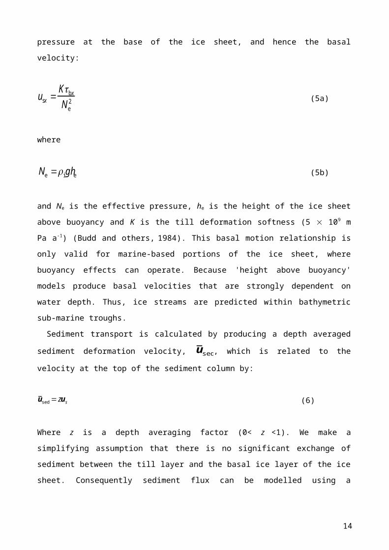
pressure at the base of the ice sheet, and hence the basal

velocity:

usx Kbx

Ne2 (5a)

where

Ne ighe (5b)

and Ne is the effective pressure, he is the height of the ice sheet

above buoyancy and K is the till deformation softness (5 109 m

Pa a-1) (Budd and others, 1984). This basal motion relationship is

only valid for marine-based portions of the ice sheet, where

buoyancy effects can operate. Because 'height above buoyancy'

models produce basal velocities that are strongly dependent on

water depth. Thus, ice streams are predicted within bathymetric

sub-marine troughs.

Sediment transport is calculated by producing a depth averaged

sediment deformation velocity, u sed, which is related to thevelocity at the top of the sediment column by:

u sedzus (6)

Where z is a depth averaging factor (0< z <1). We make a

simplifying assumption that there is no significant exchange of

sediment between the till layer and the basal ice layer of the ice

sheet. Consequently sediment flux can be modelled using a

14

continuity equation, similar in form to the continuity equation

for the ice sheet (Equation 1).

It is assumed that the velocity at the top of the deforming

sediment layer is equal to the velocity at the base of the ice

(i.e. all basal motion occurs through sediment deformation rather

than ice-sheet sliding). At some depth, hb, within the sediment

column sediment deformation rates will equal zero. The thickness

of the layer of water saturated sediments beneath Ice Stream B has

been found to be around 6 m (Blankenship and others, 1986;

Blankenship and others, 1987). However modelling has suggested

that, away from the margin of an ice sheet, the deforming

thickness may be less than 6 m (Murray, 1990). Boulton and

Hindmarsh (1987) suggested that most of the deformation within the

sediment column occurs near the top of the sediment column. In

order to account for this concentration of velocity at the top of

the sediment column we use a deforming sediment thickness, hb, of 5

m in the initial experiment combined with a depth-averaging

factor, z, of 0.2. The combination of these values are in line

with Hooke and others (1995) who used hb=4 and z=1/3, and

Dowdeswell and Siegert (in press) who used hb=2 and z=0.5. The

response of the sediment model to variations in hb and z are then

subjected to extensive sensitivity testing.

As already noted the presence of pre-Late Weichselian soft

sediments beneath sub-glacial till throughout the entire Barents

Sea indicates a greater availability of deformable sediment than

was actually mobilised during the Late Weichselian. We therefore

assume that the depth of deforming sediment, hb, remained constant

throughout the model run.

15

Pore water pressure model

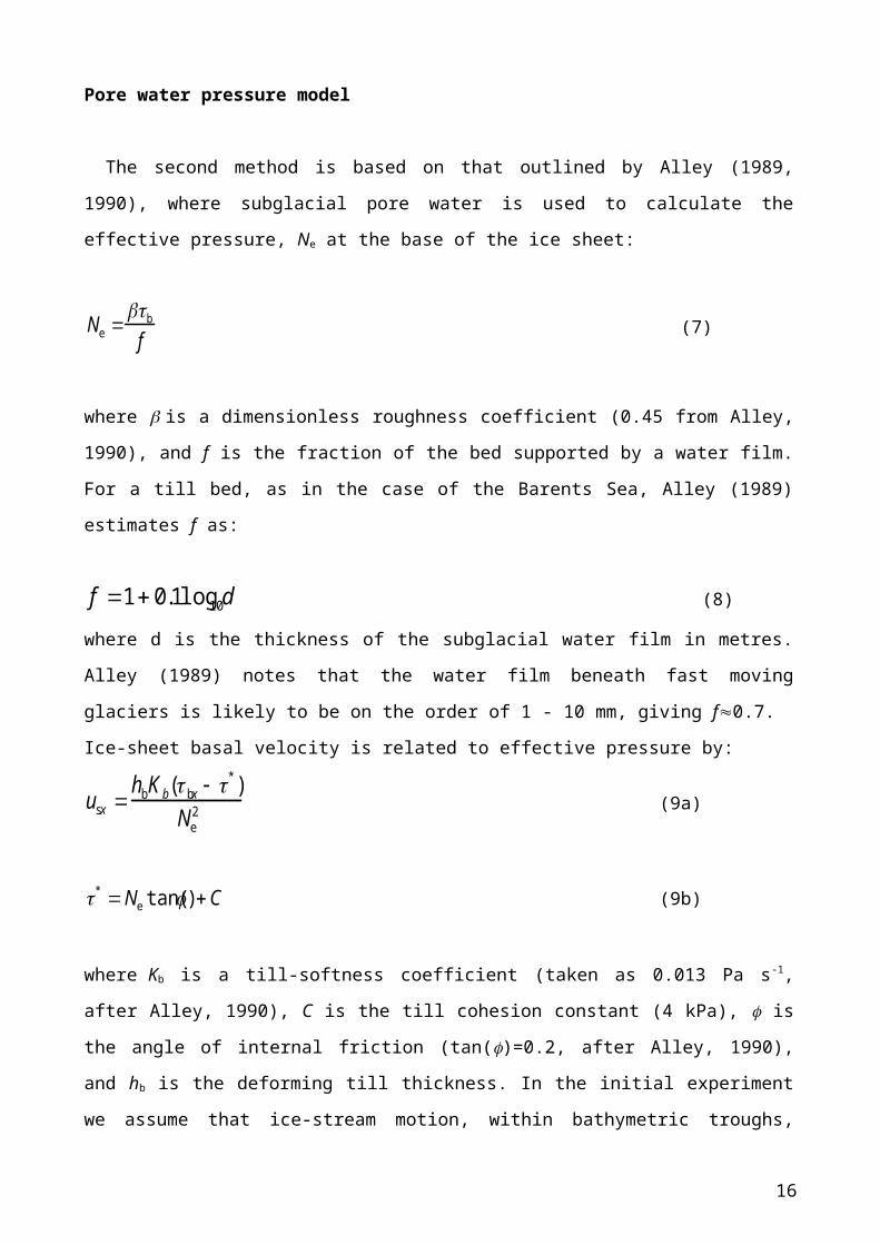
The second method is based on that outlined by Alley (1989,

1990), where subglacial pore water is used to calculate the

effective pressure, Ne at the base of the ice sheet:

Ne b

f (7)

where is a dimensionless roughness coefficient (0.45 from Alley,

1990), and f is the fraction of the bed supported by a water film.

For a till bed, as in the case of the Barents Sea, Alley (1989)

estimates f as:

f 10.1log10d (8)

where d is the thickness of the subglacial water film in metres.

Alley (1989) notes that the water film beneath fast moving

glaciers is likely to be on the order of 1 - 10 mm, giving f0.7.

Ice-sheet basal velocity is related to effective pressure by:

usx hbK b( bx *)

Ne2 (9a)

* Netan() C (9b)

where Kb is a till-softness coefficient (taken as 0.013 Pa s-1,

after Alley, 1990), C is the till cohesion constant (4 kPa), is

the angle of internal friction (tan()=0.2, after Alley, 1990),

and hb is the deforming till thickness. In the initial experiment

we assume that ice-stream motion, within bathymetric troughs,

16

occurs with f=0.7. We also assume that no significant ice-sheet

basal motion occurs outside the trough areas. This assumption is

justified by noting that the glacially transported material at the

margins of the Barents Sea is concentrated in trough mouth fans.

The effects of using different values for f and are examined in

sensitivity tests.

Sediment deformation is calculated using the same assumptions as

for the 'height above buoyancy' model. To keep the comparison

between models as close as possible, the initial experiment uses a

deformable sediment layer, hb, 5 m thick, with a depth averaged

velocity, z, equal to 0.2 of the ice-sheet basal velocity. The

effects on sediment delivery to the continental margin of

variations in these parameters are tested in sensitivity tests.

RESULTS

Height Above Buoyancy model

The ice-sheet thickness and surface elevation produced for the

Late Weichselian maximum in the Eurasian Arctic using the 'height

above buoyancy' model described above are shown in Figure 2a-b.

The entire Barents and Kara seas are fully glaciated, with ice

thicknesses of around 2,000 m in the Barents Sea and 1,400 m in

the Kara Sea. Ice divides occurred on areas of high elevation over

Svalbard (1,400 m), Novaya Zemlya (1,500 m) and Scandinavia. Ice

flowed westwards from Novaya Zemlya into the Barents Sea and,

subsequently, towards the continental margin. Ice flow out of the

ice sheet was concentrated in the Bear Island Trough, resulting in

17

a significant lowering of the surface elevation of the ice sheet

in this region (Figure 2a).

The sediment volume transported across a transect along the

continental margin for the Late Weichselian is shown in Figure 3.

The location of the transect is indicated in Figure 1. The mouth

of the Bear Island Trough is the main region of sediment

development, with 4,200 km3 of sediments delivered to the

continental margin during the Late Weichselian. We do not model

sediment dispersal beyond the ice-sheet margin, rather it is

assumed that the sediments delivered to the continental margin are

then distributed over the Bear Island Trough Mouth Fan by a

combination of gravity and current driven processes. The

Storfjorden fan is calculated to have received just over 900 km3 of

sediments during the Late Weichselian.

The sediment delivery under the 'height above buoyancy' model is

controlled by a number of parameters, most notably the depth-

averaging function for till velocities, the thickness of the

actively-deforming sediment layer and the till deformation

softness, K. These sensitivity of the sediment volume to variation

in these factors is shown in Figure 4. The model is pseudo-

linearly sensitive to the thickness of the deforming sediment and

the depth-averaging factor. This result is unsurprising, since

basal motion of the ice-sheet is not dependent on either factor

(Equation 8a), and consequently there is no feedback involved. The

sediment volume is somewhat sensitive to the sediment deformation

softness parameter K, but small changes (20%) to K do not result

in the predicted sediment volumes on the Bear Island lying outside

realistic limits.

18

Pore-Water Pressure Model

The ice-sheet thickness and surface elevations predicted for the

Late Weichselian maximum in the Eurasian Arctic using the modified

Alley (1990) pore water pressure model are shown in Figure 2c-d.

The entire Barents and Kara seas are fully glaciated, with ice

thicknesses of up to 2,000 m in the Barents Sea and 1,400 m in the

Kara Sea. Note that the ice-sheet produced using this basal motion

regime is broadly similar to that produced by the 'height above

buoyancy' model described above, with a similar depression of the

surface caused by high ice fluxes from an ice-stream in the Bear

Island Trough. The ice sheet also exhibits spreading centres on

Svalbard, Novaya Zemlya and Scandinavia, just as the 'height above

buoyancy' based reconstruction does, although there are small

differences in the precise configuration of the two ice sheets as

a result of the different basal motion regime employed. Thus

changes to the ice-stream model do not yield significantly

different results.

Modelled sediment delivery to the western continental margin of

the Barents Sea is summarised in Figure 3. Approximately 3,800 km3

of sediment are delivered to the Bear Island Fan, ~10% less than

the 4,200 km3 predicted under the 'height above buoyancy' model.

The 'pore water pressure' model (Alley, 1990) predicts around

1,000 km3 of sediment at the margin of the Storfjorden trough,

slightly higher than for the 'height above buoyancy' model. This

is somewhat higher than the 700 km3 given by Laberg and Vorren

(1996b), but is still in reasonably good agreement. Differences

between the two models are most marked in the region between the

Storfjorden and Bear Island Fans, where ice velocities are lowest

19

in both cases. The models are in reasonably close agreement in

regions of high ice velocities.

The volume of sediment predicted to be delivered to the

continental margin by the pore water pressure model is sensitive

to the roughness coefficient, (Figure 5a), the till cohesion, C

(Figure 5b), the fraction of the bed supported by a water film, f

(Figure 5c), and the thickness of actively deforming sediment

layer (Figure 5d). As with the 'height above buoyancy' method

there is no feedback from the depth averaging factor back into the

ice-sheet model, and consequently sediment delivered depends

linearly on the depth averaging factor used (Figure 5). However

the basal-ice velocity in the ‘pore water pressure’ model is

dependent on the thickness of the deforming layer, and

consequently there is a non-linear relationship between these two

variables (Figure 5). It can be seen that the model is relatively

insensitive to changes ( 50%) in the depth of the deforming

layer. Deforming thicknesses, hb, of between 4.5 m and 6 m

(combined with a depth averaging parameter, z, of 0.2) yield

sediment volumes broadly in line with the geological evidence. The

sediment volume is somewhat sensitive to the till cohesion (C),

where a change of +50% results in 30% less sediment reaching the

continental margin. A change of -50% in C produces 40% more

sediment at the margin. Increases in the till cohesion beyond

these ranges results in relatively little further change in

sediment yield, however neglecting till cohesion entirely produces

unrealistically high sediment volumes with some 6,800 km3 of

sediment being delivered to the Bear Island Fan. The model is also

sensitive to the fraction of the bed supported by a water film (f),

where a change of +10% in f results in +20% in sediment yield, and

a change of -10% in f reduces sediment yield by around 15%. The

20

sediment yield also depends inversely on the roughness coefficient

(Figure 5a). Small decreases (<10%) in have relatively little

effect on the sediment volumes, however decreasing by more than

10% results in unrealistically easy deformation of the basal

sediments, and consequent large increases in sediments transported

to the continental margin (a sediment volume of 7,200 km3 on the

Bear Island Fan for = 0.2). Increasing has much less of an

effect on sediment yields.

SUMMARY AND CONCLUSIONS

The Late Weichselian Barents Sea ice sheet was underlain by soft

deforming sediments, which were transported to the continental

margins where they accumulated as large fans. A number of

geophysical datasets are available from which measurements of the

sediment volume over the Bear Island Trough (4,000 km3) and

Storfjorden Trough (700 km3) fans can be made. These measurements

provide ideal geological data to test and compare models of ice-

stream/sediment delivery.

We have used two different models for basal ice-sheet

motion/sediment transport to reconstruct the sediment delivery to

western continental margin of the Barents Sea during the Late

Weichselian; (1) a 'height above buoyancy' model and (2) a model

based on the approach of Alley (1990). These experiments allow the

intercomparison of the respective models. Both models are able to

accurately reproduce the observed volume of Late Weichselian

sediment on the Bear Island Fan. The results of both models

exhibit a degree of sensitivity to geo-technical properties of the

deforming sediment, for which relatively little real world control

21

data exists. Both models depend on the till deformation softness,

while the Alley (1990) model also incorporates the internal angle

of friction. The velocity profile within the deforming sediments

is also crucial to both models, and is the subject of some

uncertainty. However neither model is highly sensitive to small

changes in the major model parameters and, for both models,

changes to key parameters within a realistic range of values do

not result in predictions incompatible with available geological

data.

The two models presented here are dependent on different

parameters, with the 'height above buoyancy' model being dependent

on the till softness, till depth, sediment velocity depth

averaging factor, basal shear stress of the driving ice sheet, and

topographic depth. The Alley (1990) model also depends on basal

shear stress, till thickness, sediment velocity depth averaging

factor and a till softness coefficient. However the angle of

internal friction within the till, the sediment roughness, and the

fraction of the ice-sheet bed supported by a water film also

influence ice-sheet motion and sediment transport in the Alley

(1990) model, whereas they are not accounted for in the 'height

above buoyancy' model used here. Although both models incorporate

a till softness coefficient, this is formulated in different ways

for the two models. The Alley (1990) model defines till softness

as a coefficient with units of Pa s-1, while the 'height above

buoyancy' model defines till softness as a coefficient with units

of m Pa a-1. This discrepancy arise from differences in the

formulation of sediment velocity in the two models (Equations 5

and 9). Furthermore the way in which sediment volumes vary

according to changes in key parameters differs between the models.

In particular the models exhibit different responses to changes in

22

the thickness of the layer of actively deforming sediments, hb. The

'height above buoyancy' model is linearly dependent on hb (Figure

4a), while the Alley (1990) model is non-linearly dependent on hb,

and is more highly sensitive to increases in the thickness (Figure

5d). For example, if the depth averaging parameter, z, is held

constant at 0.2, a change from hb=2 m to hb=4 m in the 'height

above buoyancy' model results in an increase in sediment volumes

on the Bear Island Fan of 810 km3, compared with 1,518 km3 for the

Alley (1990) model. However a change from hb=6 m to hb=8 m in the

'height above buoyancy' produces 818 km3 more sediment, compared

with an increase of 3,782 km3 for the Alley (1990) model. Compared

to the 'height above buoyancy', the Alley (1990) model is more

sensitive to changes in the thickness of the deforming sediment

layer, and is more sensitive at greater deforming layer

thicknesses.

A number of other conclusions relating to the model

intercomparison are (1) the geographical pattern of sedimentation

is similar, though not identical, in the two models. Both models

produce large volumes of sediment on the Bear Island and

Storfjorden troughs, and relatively smaller amounts in the

interfan region. For the Bear Island Fan the 'height above

buoyancy' model produces 12% more sediment (4,200 km3) than the

Alley (1990) model. The Alley model (1990) produces 10% more

sediment than the 'height above buoyancy' on the Storfjorden Fan

(1,000 km3). Thus, the two models are in broad agreement on their

predictions for sediment volume delivered to the major fan systems

on the western margin of the Barents Sea. (2) A higher degree of

disagreement is found in regions where sedimentation rate is

lowest (i.e. small fans and inter-fan regions). For the region

between the major Bear Island and Storfjorden fans, the Alley

23

(1990) model produces 28% more sediment than the 'height above

buoyancy' model, much greater than 10% and 12% differences for the

major fan systems. (3) The location and ice velocities of major

ice streams predicted by both models is broadly similar, with fast

flowing ice in the Bear Island Trough and the Storfjorden Trough,

with slower moving ice in between. The 'height above buoyancy'

model predicts ice velocities up to 1,000 ma-1 in the Bear Island

Trough, and 500 ma-1 in the Storfjorden Trough, with localised

velocities of up to 200 ma-1 northwest of Bear Island. Much slower

moving ice (<50 m a-1) characterised the rest of the continental

margin. The Alley (1990) model predicted ice flowing at around

1,000 ma-1 in the Bear Island Trough, and 600 ma-1 in the

Storfjorden Trough. Velocities elsewhere on the western margin

were of the order of tens of m a-1, except for localised fluxes

north-west of Bear Island and off north-west Svalbard.

In a small study of this kind it has obviously not been possible

to compare all of the available models for ice-sheet basal motion.

The experiments performed here highlight the need for a large

scale review of the similarities and differences in reconstructed

ice-sheets produced by the different methodologies. This

comparison should include more classes of models than in this

preliminary study, and should include more examples from each

class, and may best be done as an analogue to the modelled

internal ice-sheet dynamics testing exercises carried out as part

of the EISMINT program (Huybrechts and Payne, 1996).

ACKNOWLEDGEMENTS

24

DH acknowledges receipt of a University of Wales, Aberystwyth PhD

studentship.

25

REFERENCES

Alley, R.B., 1990, Multiple steady states in ice-water-till systems.

Annals of Glaciology, 14:. 1-5.

Blanksenship, D.D., Bentley, C.R., Rooney, S.T., and Alley, R.B., 1986,

Seismic measurements reveal a saturated porous layer beneath an active

Antarctic ice stream: Nature, v. 332, p. 54-57.

Blanksenship, D.D., Bentley, C.R., Rooney, S.T., and Alley, R.B. ,

1987, Till beneath Ice Stream B. 1. Properties derived from seismic

travel times: Journal of Geophysical Research, v. 92, p. 8903-8912.

Boulton, G.S., and Hindmarsh, R.C.A. 1987. Sediment deformation beneath

glaciers: rheology and geological consequences. Journal of Geophysical

Research, 92: 9059-9082.

Budd, W.F., Jenssen, D., and Smith, I.N. 1984. A three-dimensional

time-dependant model of the West Antarctic Ice Sheet. Annals of

Glaciology, 5: 29-36.

Dowdeswell, J.A., and Siegert, M.J., In Press. Ice-sheet numerical

modelling and marine geophysical measurements of glacier-derived

sedimentation on the Eurasian Arctic continental margins. Geological

Society of America Bulletin.

Fairbanks, R.G. 1989. A 17,000-year glacio-eustatic sea level

record: Influence of glacial melting rates on the Younger Dryas

event and deep ocean circulation. Nature , 342: 637-643.Faleide, J. I., Solheim, A., Fiedler, A., Hjelstuen, B. O., Andersen,

E. S., and Vanneste, K., 1996, Late Cenozoic evolution of the western

Barents Sea-Svalbard continental margin: Global and Planetary Change, v. 12,

p. 53-74.

Fjeldskaar, W. 1994., Viscosity and thickness of the asthenosphere

detected from the Fennoscandian uplift. Earth and Planetary Science

Letters, 126: 399-410.

26

Glen, J.W., The creep of polycrystaline ice. Proceedings of the Royal

Society of London, Series A. 228: 519-538.Hooke, R. LeB., and Elverhøi, A., 1996, Sediment flux from a fjord

during glacial periods, Isfjorden, Spitsbergen. Global and Planetary Change,

v. 12, p. 237-249.

Howell, D., Siegert, M. J., and Dowdeswell, J. A. In Press. Numerical

modelling of the Eurasian High Arctic Ice Sheet: an inverse experiment

using geological boundary conditions. XXXXX (Iíve emailed Neil to ask

what the reference for this should be now)

Huybrechts, Ph., and Payne, A., 1996. The EISMINT benchmarks for

testing ice-sheet models. Annals of Glaciology, 23: 1-12.

Jenson, J. W., Clark, P. U., MacAyeal, D. R., Ho, C., and Vela,

J.C. 1995. Numerical modeling of advective transport of saturated

deforming sediment beneath the Lake Michigan Lobe, Laurentide Ice

Sheet. Geomorphology, 14: 157-166.

Jenson, J. W., MacAyeal, D. R., Clark, P. U., Ho, C. L., and Vela,

J.C. 1996. Numerical modeling of subglacial sediment deformation:

Implications for the behaviour of the Lake Michigan Lobe,

Laurentide Ice Sheet. Journal of Geophysical Research, 101: 8717-8728.

Laberg, J.S., and Vorren, T.O. 1996a. The glacier-fed fan at the

mouth of Storfjorden Trough: a comparative study. In, Laberg,

J.S., Late Pleistocene evolution of the submarine fans off the

western Barents Sea margin. Unpublished Thesis. University of Troms¯,

Norway

Laberg J.S., and Vorren, T.O. 1996b. The Late Pleistocene

evolution of the Bear Island Trough Mouth Fan. In, Laberg, J.S.,

Late Pleistocene evolution of the submarine fans off the western

Barents Sea margin. Unpublished Thesis. University of Troms¯, Norway.

Le Meur, E., and Huybrechts, Ph. 1996. A comparison of different

ways of dealing with isostasy: examples from modelling the

27

Antarctic ice sheet during the last glacial cycle. Annals of

Glaciology, 23: 309-317.MacAyeal, D.R., 1992, Irregular oscillations of the West Antarctic ice

sheet: Nature, v. 359, p. 29-32.

Mahaffy, M.W. 1976. A three-dimensional numerical model of ice

sheets: tests on the Barnes Ice Cap, Northwest Territories. Journal

of Geophysical Research, 81:1059-1066.

Manabe, S., and Broccoli, A.J. 1985. The influence of continental

ice sheets on the climate of an ice age. Journal of Geophysics Research,

90: 2167-2190.

Marshall, S.J., and Clarke, G.K.C., 1997. A continuum mixture

model of ice stream thermomechanics in the Laurentide Ice Sheet

1. Theory. Journal of Geophysical Research. 102: 20,599-20,613.Murray, T., 1990, Deformable Glacier Beds: Measurement and Modelling:

Unpublished PhD Thesis, University College of Wales, Aberystwyth. 321pp.

Oerlemans, J., and van der Veen, C.J. 1984. Ice Sheets and

Climate. Reidel Publishing Company, 216 pp.

Patterson, W.S.B., 1994. The Physics of Glaciers (third edition).

Pergammon Press.

Pattyn, F., 1996. Numerical modelling of a fast-flowing outlet

glacier: experiments with different basal conditions. Annals of

Glaciology, 23: 237-246.

Shackleton, N.J. 1987. Oxygen isotopes, ice volume and sea level.

Quaternary Science Reviews. 6: 183-190.

Siegert, M.J., and Dowdeswell, J.A. 1995a. Numerical modeling of

the Late Weichselian Svalbard-Barents Sea Ice Sheet. Quaternary

Research, 43: 1-13.

Stuiver, M., and Reimer, P.J. 1993. Extended 14C data base and

revised CALIB 3.0 14C age calibration program. Radiocarbon. 35: 215-

230.

28

Vose, R.S., Schmoyer, R.L., Steurer, P.M., Peterson., T.C., Heim,

R., Karl, T.R., Eischeid, J.K. 1992. The global historical

climatology network: long-term monthly temperature,

precipitation, sea level pressure, and station pressure data. U.S.

Department of Energy publication ORNL/CDIAC-53.

29

Table 1. A selection of methods used to calculate basal ice-sheet

motion. Each model is briefly described, and the values for

important parameters in each model given. All the models presented

calculate ice-stream motion by using driving stress raised to some

power, p, in addition to the parameters described. The exponent,

p, used in each model is given in the table. The models are also

grouped by category: ‘HAB’ is a ‘height above buoyancy’ model,

‘Pore water’ indicates that basal flux is driven by pore water

pressure, ‘Basal Temp’ denotes ice streams dependant on basal

temperature in a given grid cell, ‘Sediment driven’ indicates that

basal motion is controlled by sediment properties, and ‘Sub grid

cell’ indicates that ice streams are allowed to occupy less than

an entire grid cell. The table also distinguishes between ‘flow

line’ models, and ‘map plane’ models.

Figure 1. Modern bathymetry of the Barents Sea (contour interval

50 m). Transect AAí, used in experiments on sediment transfer to

the western margin of the Barents Sea (figure X) is shown. The

current elevation of the transect AAí is given in the inset. Dark

shading is land above present sea level, light shading is the area

up to 200m below present sea level.

Figure 2. The Eurasian High Arctic ice sheet modelled at the last

glacial maximum. (a) Ice-sheet surface elevation (contoured in 250

m intervals) using a ëheight above buoyancyí model. (b) Ice-sheet

thickness (contoured in 250 m intervals) using a ëheight above

30

buoyancyí model. (c) Ice-sheet surface elevation (contoured in 250

m intervals) using the pore water pressure model of Alley (1990).

(d) Ice-sheet thickness (contoured in 250 m intervals) using the

pore water pressure model of Alley (1990). In each case the modern

coastline and continental shelf break (500m water depth contour)

is shown for reference.

Figure 3. The predicted sediment flux delivered across transect

AAí (Fig. 1) during the Late Weichselian (in km3 per km) using a

ëheight above buoyancyí model and the pore water pressure of Alley

(1990). The modern bathymetry is also shown (in metres below sea

level) for reference.

Figure 4. Experiments on the sensitivity of the volume of

sediments (in km3) calculated on the Bear Island Fan to changes in

model parameters for the ëheight above buoyancyí model. (a)

Changes in sediment volume (km3) due to changes in the thickness of

the deforming layer of sediments (in m). (b) Changes in sediment

volume (in km3) due to changes in the depth averaging factor used.

(c) Changes in sediment volume (in km3) due to changes in the till

deformation softness (in m Pa a-1). In each case the vertical line

indicates the standard value used in the experiments here.

31

Figure 5. Experiments on the sensitivity of the volume of

sediments (in km3) predicted on the Bear Island Fan to changes in

model parameters for the Alley (1990) sediment model. (a) Changes

in sediment volume (km3) due to changes in the roughness

coefficient. (b) Changes in sediment volume (in km3) due to changes

in the till cohesion constant. (c) Changes in sediment volume (in

km3) due to changes in the fraction of the bed supported by a water

film. (d) Changes in sediment volume (km3) due to changes in the

thickness of the deforming layer of sediments (in m). In each case

the vertical line indicates the standard value used in the

experiments here.

32