Interannual variation of Gulf Stream heat transport in a high-resolution model forced by reanalysis data

N. M. J. Hall Æ B. Barnier Æ T. Penduff Æ J. M. Molines

Interannual variation of Gulf Stream heat transportin a high-resolution model forced by reanalysis data

Received: 14 November 2003 / Accepted: 6 April 2004 / Published online: 14 August 2004 Springer-Verlag 2004

Abstract The variability present in a 1/6th degreeAtlantic ocean simulation forced by analysed wind stressand heat flux over a 20-year period is investigated bymeans of heat transport diagnostics. A section is definedwhich follows the Gulf Stream and its seaward extension,and transport of heat across this section is analysed toreveal the physical mechanisms responsible for ‘inter-gyre’ heat exchanges on a variety of time scales. Heattransport across another section that crosses the GulfStream is also diagnosed to reveal the temporal behav-iour of the ‘gyre’ circulation. The Ekman response towind stress variations accounts for the annual cycle andmuch of the interannual variability in both measures. Forthe intergyre heat transports, cancellation by transient-mean flow terms leads to a very weak annual cycle.Transient eddies account for approximately half the totalintergyre transport of 0.7 Petawatts. They also accountfor a significant fraction of the interannual variability,but separate experiments with repeated-annual-cycleforcing indicate that the transient eddy component of theheat transport variability is internally generated. Linksbetween the intergyre transport, the wind-driven gyrecirculation, the surface heat budget and the atmospheric‘North Atlantic Oscillation’ are discussed.

1 Introduction

The importance of the Atlantic Ocean for the globalclimate stems largely from its horizontal transfer of heat.Time variability in Atlantic Ocean heat transport mir-rors time variability in other climatic indicators in theatmosphere and ocean. In the North Atlantic it is theGulf Stream and associated gyre and eddy circulationsthat are responsible for the greater part of the heat

transport. Variability in Gulf Stream transports, bothalong and across the stream might therefore serve as auseful indicator of climate variability and of the way theatmosphere and ocean influence one another. Forexample, a mechanism involving interannual compen-sation between atmospheric and oceanic heat transportsfirst postulated by Bjerknes (1964) has recently beentaken up by Marshall et al. (2001) to describe a coupledsystem whose behaviour is determined by the responsetime of Gulf Stream heat transports to changes inatmospheric forcing. In fact the Gulf Stream responds toboth wind stress and heat flux anomalies on a range oftime scales from seasonal to interdecadal and a varietyof processes are involved. These include Ekman currentsand Rossby wave dynamics, nonlinear control of gyrecirculations and transient eddy heat transports and largescale overturning circulations. It is therefore importantto determine which processes contribute to heat trans-ports on which time scales, and which processes aresusceptible to atmospheric influence.

The large-scale atmospheric disturbances that giverise to anomalous ocean heat transports and sea surfacetemperature anomalies (SSTAs) have often been char-acterised by a single index, the North Atlantic Oscilla-tion (NAO, see e.g. Hurrell 1996). In recent years therehas been great interest in the coupling of the NAO withoceanic mechanisms that create and propagate temper-ature anomalies, and which maintain oceanic heattransports. Indeed, many of the recent modelling studiesof North Atlantic variability have been couched in termsof the response to the NAO (Visbeck et al. 1998; Ha-kkinen 1999; Eden and Jung 2001; Pavia and Chassignet2002; Gulev et al. 2003). The atmospheric NAO haspower on all time scales but exhibits a slightly reddenedspectrum, suggesting some long-term oceanic memory ofthe phenomenon. SSTAs generated by the NAO maytherefore feed back on the atmospheric circulation.These SSTAs arise either from local forcing (seasonal tointerannual time scales) or from anomalous advec-tion (interannual to decadal time scales) and their

N. M. J. Hall (&) Æ B. Barnier Æ T. Penduff Æ J. M. MolinesLEGI, BP53, 38041 Grenoble Cedex 9, FranceE-mail: [email protected]

Climate Dynamics (2004) 23: 341–351DOI 10.1007/s00382-004-0449-2

propagation along the north Atlantic current can deter-mine the nature and time scale of atmosphere oceaninteraction (Hansen and Bezdek 1996; Sutton and Allen1997; Saravanan and McWilliams 1997; Krahmann et al.2001). Anomalies in large-scale current systems generatedby the NAO manifest themselves as an anomaly gyre(Marshall et al. 2001)which straddles theGulf Streamandcan be interpreted as a change in the trajectory of thestreamwith an associated change in heat transport. Usinga long time series of observed cross-stream temperaturecontrast, Czaja andMarshall (2001) present evidence thatNAO-induced Gulf Stream heat transport anomalies doindeed feed back on the atmosphere on decadal timescales. The fact that atmospheric variability, and morespecifically the NAO can also affect the trajectory of theGulf Stream on interannual time scales has been con-firmed observationally byTaylor andStephens (1998) andFrankignoul et al.(2001). These studies give a responsetime of less than two years. Observations are, of course,unable to provide accurate information on interannualvariations in heat transport, and for this we must turn tomodelling studies.

Given the central role of horizontal ocean heattransports in recent discussions of Atlantic climate var-iability, it is timely to perform a detailed diagnosis in arealistic modelling framework, paying particular atten-tion to the Gulf Stream. The model integrations con-sidered should have the following properties:

1. Ekman heat fluxes should be adequately represented.The Ekman transport and the associated barotropicreturn flow can account for a large part of the annualcycle and interannual variability of the heat transport(Jayne and Marotzke 2001).

2. Gyre scale circulations, jet structures and magnitudesshould be well simulated. The Gulf Stream shouldhave a reasonable mass transport, velocity crosssection and trajectory.

3. Mesoscale eddies should be adequately resolved, asthey account for a significant fraction of intergyretransport, which is not necessarily well captured bydiffusive parametrizations.

4. The model must be forced at the surface by somerepresentation of atmospheric heat and momentumfluxes with realistic spatio-temporal characteristics,consistent with those of the NAO.

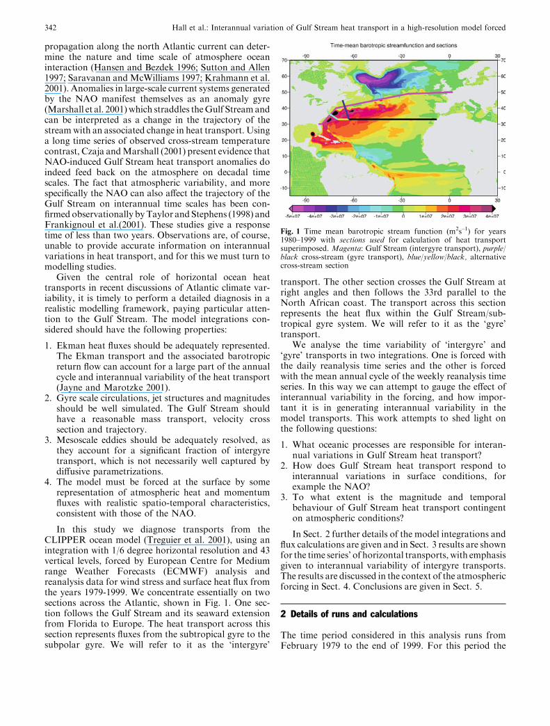
In this study we diagnose transports from theCLIPPER ocean model (Treguier et al. 2001), using anintegration with 1/6 degree horizontal resolution and 43vertical levels, forced by European Centre for Mediumrange Weather Forecasts (ECMWF) analysis andreanalysis data for wind stress and surface heat flux fromthe years 1979-1999. We concentrate essentially on twosections across the Atlantic, shown in Fig. 1. One sec-tion follows the Gulf Stream and its seaward extensionfrom Florida to Europe. The heat transport across thissection represents fluxes from the subtropical gyre to thesubpolar gyre. We will refer to it as the ‘intergyre’

transport. The other section crosses the Gulf Stream atright angles and then follows the 33rd parallel to theNorth African coast. The transport across this sectionrepresents the heat flux within the Gulf Stream/sub-tropical gyre system. We will refer to it as the ‘gyre’transport.

We analyse the time variability of ‘intergyre’ and‘gyre’ transports in two integrations. One is forced withthe daily reanalysis time series and the other is forcedwith the mean annual cycle of the weekly reanalysis timeseries. In this way we can attempt to gauge the effect ofinterannual variability in the forcing, and how impor-tant it is in generating interannual variability in themodel transports. This work attempts to shed light onthe following questions:

1. What oceanic processes are responsible for interan-nual variations in Gulf Stream heat transport?

2. How does Gulf Stream heat transport respond tointerannual variations in surface conditions, forexample the NAO?

3. To what extent is the magnitude and temporalbehaviour of Gulf Stream heat transport contingenton atmospheric conditions?

In Sect. 2 further details of the model integrations andflux calculations are given and in Sect. 3 results are shownfor the time series’ of horizontal transports, with emphasisgiven to interannual variability of intergyre transports.The results are discussed in the context of the atmosphericforcing in Sect. 4. Conclusions are given in Sect. 5.

2 Details of runs and calculations

The time period considered in this analysis runs fromFebruary 1979 to the end of 1999. For this period the

Fig. 1 Time mean barotropic stream function (m2s–1) for years1980–1999 with sections used for calculation of heat transportsuperimposed. Magenta: Gulf Stream (intergyre transport), purple/black cross-stream (gyre transport), blue/yellow/black, alternativecross-stream section

342 Hall et al.: Interannual variation of Gulf Stream heat transport in a high-resolution model forced

output for currents and temperature have been stored asconsecutive 5-day means, a strategy that effectively elim-inates aliasing from inertial motions, but still retains theessential information for transient fluxes (see Crosnieret al. 2001). Prior to the analysis period, the model wassubjected to an 8-year spinup, using the weekly meanclimatology from the atmospheric reanalysis, so that onlythe details of the annual cycle were retained in the surfaceforcing, and not the interannual variability. In one inte-gration this mean-annual-cycle forcing was simply con-tinued for another 20 years.We call this the ‘annual cycle’run. In the other integration the actual daily reanalyses(1979–93) and analyses (1994–99) were used to provide anexperiment with forced interannual variability. We callthis the ‘interannual’ run. In both cases, constant hydro-graphic data were used to provide mass fluxes and tem-perature profiles at the open boundaries of the model (theDrake passage, the Aghulas passage, the straits ofGibraltar and the Arctic Ocean) using the methoddescribed by Treguier et al. (2001).

The motivation for diagnosing two runs with withdifferent forcing is to examine the effect on the inter-annual variability. The annual cycle run has no inter-annual variability in the forcing. Any interannualvariability seen in the model heat transport in this run istherefore generated by internal dynamics. In the diag-nosis that follows we will attempt to identify differentdynamical mechanisms for internally and externallygenerated model variability by comparing the two runs.Another feature of the annual cycle run is that theforcing contains no short (sub-weekly) time scale‘weather noise’. This is a normal consequence of taking amean annual cycle over a sufficient number of years.Weather noise forcing is a deviation from the annualcycle and as such, can be interpreted as another form ofinterannual variability. If short time scales exist in the20-year mean annual cycle they are unlikely to have anyphysical significance. In our case we guarrantee theirremoval by using weekly mean values for surface heatflux and wind stress. It is feasible that this could influ-ence the directly forced component of transient oceanicheat transport, but it will be seen that this is unlikely toaffect its interannual variability. This is because thecurrents respond rapidly but the temperatures takelonger to adjust. Integration of the flux up to the weeklytime scale is therefore linear, and still accounted for withsmoothed annual cycle forcing.

While the reanalysis wind stress is applied directly tothe model, the surface heat flux is subjected to a cor-rection and is specified as follows:

Qtot ¼ QsrðzÞ þ Qlr þ Qlþs þ@Q@Tðx; y; season)ðTc � T Þ;

ð1Þ

where the terms on the right are respectively: shortwaveradiation (penetrative); longwave radiation and latentplus sensible heat flux (all provided by reanalysis data)and finally a correction term in which T is the model’ssurface temperature and Tc an observed (Reynolds and

Smith 1994) weekly climatology. Details of this forcingstrategy, including the determination of @Q

@T , are given byBarnier (1998). The presence of the correction term isessential to guarantee that the model has a reasonablyrealistic climatology, and it also serves to allow the modelsome degree of liberty in its horizontal heat transport,which would otherwise be determined entirely by externalflux data (barring seasonal storage terms). If this termwere to be left out, there would be an implicit assumptionthat the ocean model is perfect, and that it is in perfectsynchronisationwith the observed atmosphere, so the twosystems are interacting exactly as in the observations. Infact the model and flux estimates contain errors, andcannot be expected to give a perfect match to the observedtime development of the fluxes. To be physically consis-tentwemust therefore accept that its horizontal fluxes andits interaction with the atmosphere would be different.The correction term thus represents an approach to amore physically consistent, if less realistic, coupled sys-tem, and can be viewed as part of the representation of theocean’s interaction with the free atmosphere in the ab-sence of full coupling. It does, however, add a term to thesurface interaction that is not present in the observations,and which is sometimes quite large. Salinity is treated in asimilar way to temperature with a pseudo-salt flux derivedfrom analysed evaporation minus precipitation and cli-matological river runoffs. Likewise, a correction term isapplied with the same coefficient as for heat flux. Forfurther details see Treguier et al. (2001).

Figure 1 shows a long-term mean (1980–1999) of thebarotropic (depth integrated) stream-function from theinterannual run. Note that the tight gradients that rep-resent the Gulf Stream separate from the coast somewhatnorth of Cape Hateras, a ubiquitous error for z-coordi-nate primitive equation models. There is a permanentstanding recirculation feature at the point of separation,which is more compact and further north than theobserved recirculation gyre. The mass transport andcross-stream velocity profile of the stream are, however,quite realistic owing to the model’s relatively high reso-lution. Superimposed on Fig. 1 are the sections definedfor the calculation of transports. The ‘Gulf Stream’ sec-tion has been chosen to loosely follow a contour ofbarotropic stream-function and is completed to connectwith the European coast. ‘Intergyre’ transport is calcu-lated across this section. The ‘cross stream’ section cutsacross the Gulf Stream at right angles and then followsthe 33�N latitude circle. The ‘gyre’ transport is calculatedacross this section. A second option is also definedthat cuts across the Gulf Stream before it separates fromthe coast.

The heat transports across these sections are given by

½vT � ¼ cpqZ0

�H

ZE

W

T ð�kÞ � v� ds dz:: ð2Þ

The section starts at the western boundary and ds is adistance element along the section. Heat transport due

Hall et al.: Interannual variation of Gulf Stream heat transport in a high-resolution model forced 343

to velocity vector v and temperature T is positive to theleft ( kis the vertical unit vector), i.e. from the southerninto the northern part of the basin. Model variables aredefined on an Arakawa C grid and the calculation wascarried out across segments that run along a staircasebetween stream function/vorticity points. Appropriatenorthward or eastward velocities are defined at the midpoints of these segments. Temperatures were interpo-lated horizontally onto the velocity points from the twogrid boxes either side of the segment. There is a gooddeal of cancellation in this calculation and double pre-cision was necessary to ensure that the expected masstransport was obtained, and that the heat transport wasstable to small redefinitions of the boundary.

All sections that join the two coasts have a constantnet mass transport to the south of 109 kg s–1 or 1 Sv.This is the mass transport that enters at the northernboundary and leaves at the eastern boundary in additionto the Antarctic circumpolar transport. Its existenceleads to conceptual problems in calculating the heattransport, which depends on the scale chosen for tem-perature. If the temperature is measured in Kelvins, theheat transport is everywhere southwards owing to themass transport. This heat transport is real, but irrelevantsince heat lost to the south is immediately replaced fromthe north and so there is no impact on surface fluxes andno importance for climate variability. Formally, the heattransport input at the north should be subtracted. Byobservational convention, we just use Celsius instead ofKelvin, implicitly assuming that the water at thenorthern boundary has a uniform temperature of zeroCelsius. The associated constant error is insignificantcompared to typical cross-latitude heat transports.

In the next section we present time series of heattransports calculated in this way. In cases where theannual cycle has been removed, the following procedurewas applied. A mean value for each day of the year wascalculated. This was done by taking the stored 5-daymean values from the model and assigning to them theirmid-point date. An average for each date was then takenover all realisations in the 20-year run for each date. Fordates with no realisations a value was assigned by linearinterpolation. The resulting mean annual cycle was thensmoothed with a 21-day running mean and finally sub-tracted from the 20-year time series, again assigningappropriate mid-point dates to the 5-day mean valuesthat make up the time series

3 Heat transports

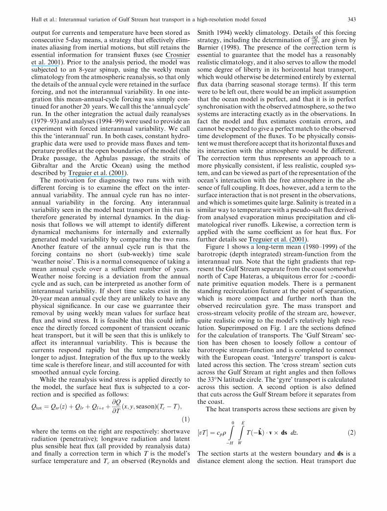
The northward transport of heat in the Atlantic is astrong function of latitude, and this is borne out by themodel integration. The annual mean transport peaks at15�N, and shows a steep decline between 30 and 50�N.Figure 2 shows the annual mean transport for a numberof individual years from the integration, illustrating thedegree of interannual variability. The amount of vari-ability, and the strength of the annual cycle (not shown)

are similarly functions of latitude. The greater thetransport, the more variable it is and this variablility andseasonality also declines rapidly north of 30�N. Themodel heat transport is within the range of observedestimates shown in Ganachaud and Wunch (2003, seetheir Fig. 3). Although it is low in the tropics andSouthern Hemisphere compared with their own estimatethe agreement in the Gulf stream region is good.

These basic facts about cross-latitude transport pro-vide the backdrop for interpreting time series’ of inter-gyre heat transport across the Gulf Stream section, andgyre heat transport across the cross-stream section.These time series are displayed in Fig. 3. It can be seenimmediately that the intergyre and gyre transports, asdefined here, have a very different character to theirtime-variability. The gyre transports have a strong an-nual cycle while the intergyre transports have almostnone. The peak to peak magnitudes of their respective(smoothed) annual cycles are 0.484 PW (gyre) (one PW= 1015 Watts) and 0.193 PW (intergyre) (the respectivestandard deviations are 0.147 PW and 0.041 PW). Partof this difference is due to the difference in mean latitudeof the two sections: the annual cycle is stronger at 33�N,where the cross-stream section connects with the easternboundary, than it is at 50�N where the Gulf Streamsection connects. In fact the annual cycle for the inter-gyre transport has a magnitude equivalent to transportacross 45�N, while the annual cycle for the gyre trans-port is actually stronger than the transport at 33�N.

Fig. 2 Annual mean cross-latitude heat transport as a function oflatitude for each year from 1982 to 1993. The discontinuity at 36�Ncoincides with the open boundary in the Gulf of Cadiz

344 Hall et al.: Interannual variation of Gulf Stream heat transport in a high-resolution model forced

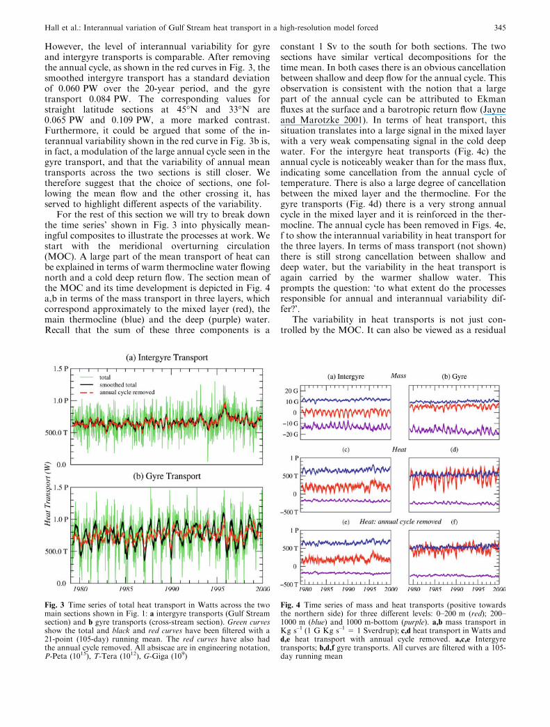
However, the level of interannual variability for gyreand intergyre transports is comparable. After removingthe annual cycle, as shown in the red curves in Fig. 3, thesmoothed intergyre transport has a standard deviationof 0.060 PW over the 20-year period, and the gyretransport 0.084 PW. The corresponding values forstraight latitude sections at 45�N and 33�N are0.065 PW and 0.109 PW, a more marked contrast.Furthermore, it could be argued that some of the in-terannual variability shown in the red curve in Fig. 3b is,in fact, a modulation of the large annual cycle seen in thegyre transport, and that the variability of annual meantransports across the two sections is still closer. Wetherefore suggest that the choice of sections, one fol-lowing the mean flow and the other crossing it, hasserved to highlight different aspects of the variability.

For the rest of this section we will try to break downthe time series’ shown in Fig. 3 into physically mean-ingful composites to illustrate the processes at work. Westart with the meridional overturning circulation(MOC). A large part of the mean transport of heat canbe explained in terms of warm thermocline water flowingnorth and a cold deep return flow. The section mean ofthe MOC and its time development is depicted in Fig. 4a,b in terms of the mass transport in three layers, whichcorrespond approximately to the mixed layer (red), themain thermocline (blue) and the deep (purple) water.Recall that the sum of these three components is a

constant 1 Sv to the south for both sections. The twosections have similar vertical decompositions for thetime mean. In both cases there is an obvious cancellationbetween shallow and deep flow for the annual cycle. Thisobservation is consistent with the notion that a largepart of the annual cycle can be attributed to Ekmanfluxes at the surface and a barotropic return flow (Jayneand Marotzke 2001). In terms of heat transport, thissituation translates into a large signal in the mixed layerwith a very weak compensating signal in the cold deepwater. For the intergyre heat transports (Fig. 4c) theannual cycle is noticeably weaker than for the mass flux,indicating some cancellation from the annual cycle oftemperature. There is also a large degree of cancellationbetween the mixed layer and the thermocline. For thegyre transports (Fig. 4d) there is a very strong annualcycle in the mixed layer and it is reinforced in the ther-mocline. The annual cycle has been removed in Figs. 4e,f to show the interannual variability in heat transport forthe three layers. In terms of mass transport (not shown)there is still strong cancellation between shallow anddeep water, but the variability in the heat transport isagain carried by the warmer shallow water. Thisprompts the question: ‘to what extent do the processesresponsible for annual and interannual variability dif-fer?’.

The variability in heat transports is not just con-trolled by the MOC. It can also be viewed as a residual

Fig. 3 Time series of total heat transport in Watts across the twomain sections shown in Fig. 1: a intergyre transports (Gulf Streamsection) and b gyre transports (cross-stream section). Green curvesshow the total and black and red curves have been filtered with a21-point (105-day) running mean. The red curves have also hadthe annual cycle removed. All absiscae are in engineering notation,P-Peta (1015), T-Tera (1012), G-Giga (109)

Fig. 4 Time series of mass and heat transports (positive towardsthe northern side) for three different levels: 0–200 m (red); 200–1000 m (blue) and 1000 m-bottom (purple). a,b mass transport inKg s–1 (1 G Kg s–1 = 1 Sverdrup); c,d heat transport in Watts andd,e heat transport with annual cycle removed. a,c,e Intergyretransports; b,d,f gyre transports. All curves are filtered with a 105-day running mean

Hall et al.: Interannual variation of Gulf Stream heat transport in a high-resolution model forced 345

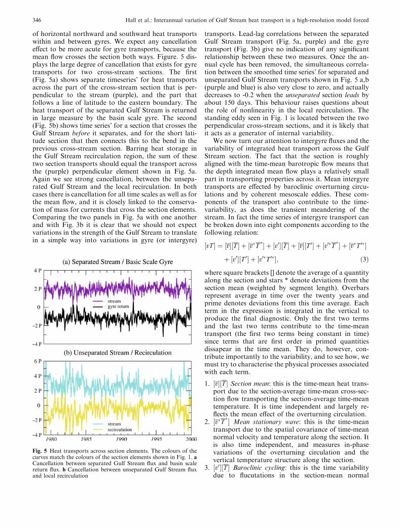
of horizontal northward and southward heat transportswithin and between gyres. We expect any cancellationeffect to be more acute for gyre transports, because themean flow crosses the section both ways. Figure. 5 dis-plays the large degree of cancellation that exists for gyretransports for two cross-stream sections. The first(Fig. 5a) shows separate timeseries’ for heat transportsacross the part of the cross-stream section that is per-pendicular to the stream (purple), and the part thatfollows a line of latitude to the eastern boundary. Theheat transport of the separated Gulf Stream is returnedin large measure by the basin scale gyre. The second(Fig. 5b) shows time series’ for a section that crosses theGulf Stream before it separates, and for the short lati-tude section that then connects this to the bend in theprevious cross-stream section. Barring heat storage inthe Gulf Stream recirculation region, the sum of thesetwo section transports should equal the transport acrossthe (purple) perpendicular element shown in Fig. 5a.Again we see strong cancellation, between the unsepa-rated Gulf Stream and the local recirculation. In bothcases there is cancellation for all time scales as well as forthe mean flow, and it is closely linked to the conserva-tion of mass for currents that cross the section elements.Comparing the two panels in Fig. 5a with one anotherand with Fig. 3b it is clear that we should not expectvariations in the strength of the Gulf Stream to translatein a simple way into variations in gyre (or intergyre)

transports. Lead-lag correlations between the separatedGulf Stream transport (Fig. 5a, purple) and the gyretransport (Fig. 3b) give no indication of any significantrelationship between these two measures. Once the an-nual cycle has been removed, the simultaneous correla-tion between the smoothed time series’ for separated andunseparated Gulf Stream transports shown in Fig. 5 a,b(purple and blue) is also very close to zero, and actuallydecreases to -0.2 when the unseparated section leads byabout 150 days. This behaviour raises questions aboutthe role of nonlinearity in the local recirculation. Thestanding eddy seen in Fig. 1 is located between the twoperpendicular cross-stream sections, and it is likely thatit acts as a generator of internal variability.

We now turn our attention to intergyre fluxes and thevariability of integrated heat transport across the GulfStream section. The fact that the section is roughlyaligned with the time-mean barotropic flow means thatthe depth integrated mean flow plays a relatively smallpart in transporting properties across it. Mean intergyretransports are effected by baroclinic overturning circu-lations and by coherent mesoscale eddies. These com-ponents of the transport also contribute to the time-variability, as does the transient meandering of thestream. In fact the time series of intergyre transport canbe broken down into eight components according to thefollowing relation:

½vT � ¼ ½v�½T � þ ½v�T �� þ ½v0�½T � þ ½v�½T 0� þ ½v0�T �� þ ½v�T 0��

þ ½v0�½T 0� þ ½v0�T 0��; ð3Þ

where square brackets [] denote the average of a quantityalong the section and stars * denote deviations from thesection mean (weighted by segment length). Overbarsrepresent average in time over the twenty years andprime denotes deviations from this time average. Eachterm in the expression is integrated in the vertical toproduce the final diagnostic. Only the first two termsand the last two terms contribute to the time-meantransport (the first two terms being constant in time)since terms that are first order in primed quantitiesdissapear in the time mean. They do, however, con-tribute importantly to the variability, and to see how, wemust try to characterise the physical processes associatedwith each term.

1. ½v�½T � Section mean: this is the time-mean heat trans-port due to the section-average time-mean cross-sec-tion flow transporting the section-average time-meantemperature. It is time independent and largely re-flects the mean effect of the overturning circulation.

2. ½v�T �� Mean stationary wave: this is the time-meantransport due to the spatial covariance of time-meannormal velocity and temperature along the section. Itis also time independent, and measures in-phasevariations of the overturning circulation and thevertical temperature structure along the section.

3. ½v0�½T � Baroclinic cycling: this is the time variabilitydue to flucutations in the section-mean normal

Fig. 5 Heat transports across section elements. The colours of thecurves match the colours of the section elements shown in Fig. 1. aCancellation between separated Gulf Stream flux and basin scalereturn flux. b Cancellation between unseparated Gulf Stream fluxand local recirculation

346 Hall et al.: Interannual variation of Gulf Stream heat transport in a high-resolution model forced

velocity and their vertical covariance with section-mean time-mean temperature. Non-zero values implya vertical covariance because the mass transportacross the section is time independent.

4. ½v�½T 0� Temperature cycling: this is the time variabilitydue to fluctuations in section-mean temperature.

5. ½v0�T �� Stream meander: this is the time variability dueto along-section spatial covariance between normalvelocity fluctuations and mean temperature. It can beinterpreted as a measure of variability in the orien-tation of the Gulf Stream jet on all scales.

6. ½v�T 0�� Isotherm meander: this is the time variabilitydue to the along-section spatial covariance betweentemperature fluctuations and mean normal velocity.It can be interpreted as a measure of variability in theorientation of the Gulf Stream front on all scales.

7. ½v0�½T 0� Transient MOC: this is the transport andvariability due to the time covariance of fluctuationsin section-mean normal velocity and temperature. Ithas a non-zero time mean, and as with the barocliniccycling term, it requires vertical covariance betweenvelocity and temperature because the mass transportis constant.

8. ½v0�T 0�� Transient eddies: this is the transport andvariability due to time-space covarying anomalies. Itis generated by coherent structures in time and space.We identify this term with the action of mesoscaleeddies.

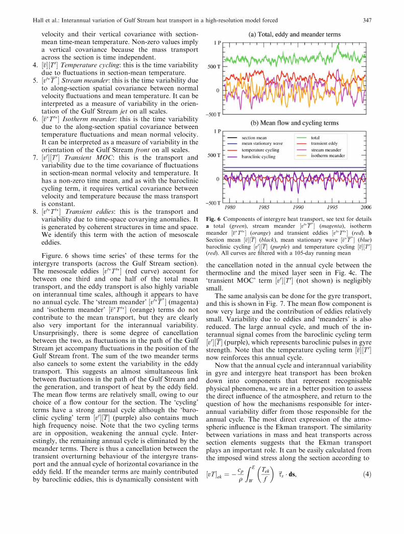
Figure. 6 shows time series’ of these terms for theintergyre transports (across the Gulf Stream section).The mesoscale eddies ½v0�T 0�� (red curve) account forbetween one third and one half of the total meantransport, and the eddy transport is also highly variableon interannual time scales, although it appears to haveno annual cycle. The ‘stream meander’ ½v0�T �� (magenta)and ‘isotherm meander’ ½v�T 0�� (orange) terms do notcontribute to the mean transport, but they are clearlyalso very important for the interannual variability.Unsurprisingly, there is some degree of cancellationbetween the two, as fluctuations in the path of the GulfStream jet accompany fluctuations in the position of theGulf Stream front. The sum of the two meander termsalso cancels to some extent the variability in the eddytransport. This suggests an almost simultaneous linkbetween fluctuations in the path of the Gulf Stream andthe generation, and transport of heat by the eddy field.The mean flow terms are relatively small, owing to ourchoice of a flow contour for the section. The ‘cycling’terms have a strong annual cycle although the ‘baro-clinic cycling’ term ½v0�½T � (purple) also contains muchhigh frequency noise. Note that the two cycling termsare in opposition, weakening the annual cycle. Inter-estingly, the remaining annual cycle is eliminated by themeander terms. There is thus a cancellation between thetransient overturning behaviour of the intergyre trans-port and the annual cycle of horizontal covariance in theeddy field. If the meander terms are mainly contributedby baroclinic eddies, this is dynamically consistent with

the cancellation noted in the annual cycle between thethermocline and the mixed layer seen in Fig. 4c. The‘transient MOC’ term ½v0�½T 0� (not shown) is negligiblysmall.

The same analysis can be done for the gyre transport,and this is shown in Fig. 7. The mean flow component isnow very large and the contribution of eddies relativelysmall. Variability due to eddies and ‘meanders’ is alsoreduced. The large annual cycle, and much of the in-terannual signal comes from the baroclinic cycling term½v0�½T � (purple), which represents baroclinic pulses in gyrestrength. Note that the temperature cycling term ½v�½T 0�now reinforces this annual cycle.

Now that the annual cycle and interannual variabilityin gyre and intergyre heat transport has been brokendown into components that represent recognisablephysical phenomena, we are in a better position to assessthe direct influence of the atmosphere, and return to thequestion of how the mechanisms responsible for inter-annual variability differ from those responsible for theannual cycle. The most direct expression of the atmo-spheric influence is the Ekman transport. The similaritybetween variations in mass and heat transports acrosssection elements suggests that the Ekman transportplays an important role. It can be easily calculated fromthe imposed wind stress along the section according to

½vT �ek ¼ �cp

q

Z E

W

Tek

f

� �~ss � ds, ð4Þ

Fig. 6 Components of intergyre heat transport, see text for detailsa total (green), stream meander ½v0�T �� (magenta), isothermmeander ½v�T 0�� (orange) and transient eddies ½v0�T 0�� (red). b

Section mean ½v�½T � (black), mean stationary wave ½v�T �� (blue)baroclinic cycling ½v0�½T � (purple) and temperature cycling ½v�½T 0�(red). All curves are filtered with a 105-day running mean

Hall et al.: Interannual variation of Gulf Stream heat transport in a high-resolution model forced 347

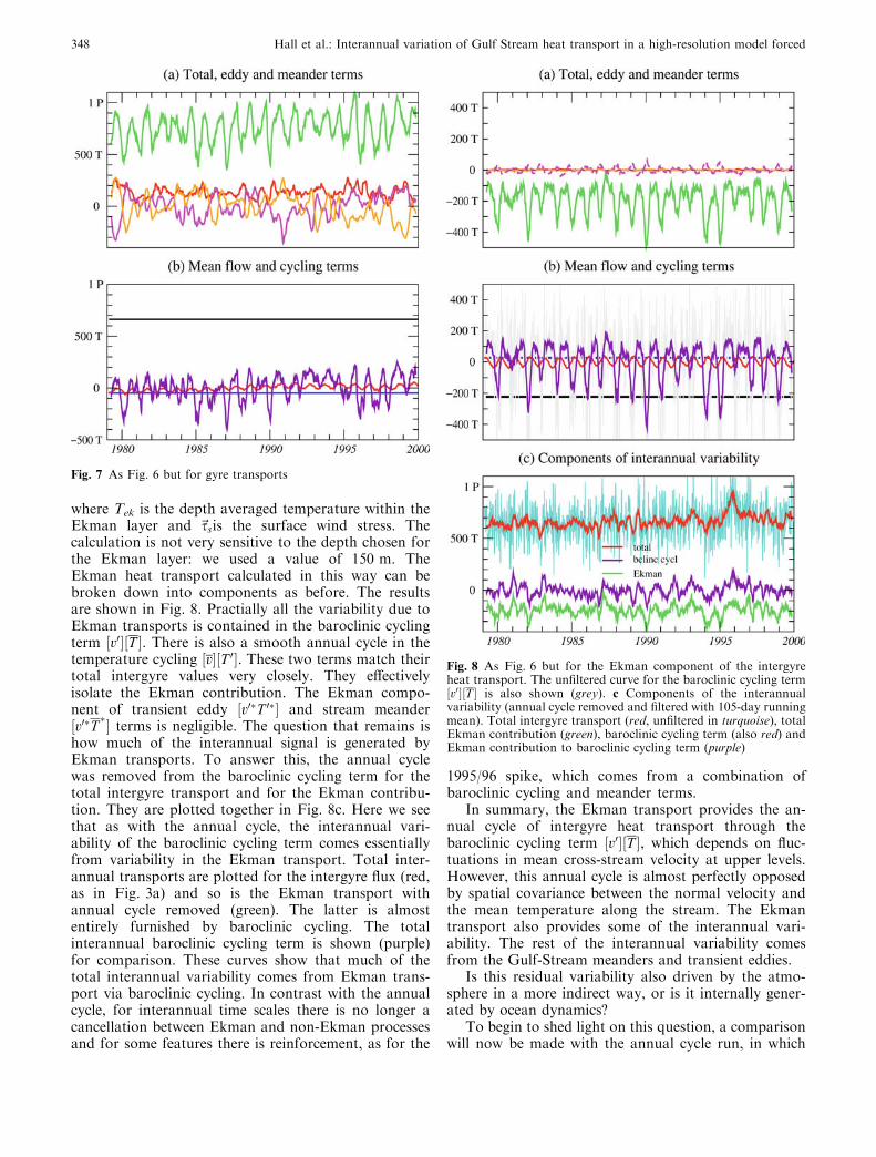
where Tek is the depth averaged temperature within theEkman layer and ~ssis the surface wind stress. Thecalculation is not very sensitive to the depth chosen forthe Ekman layer: we used a value of 150 m. TheEkman heat transport calculated in this way can bebroken down into components as before. The resultsare shown in Fig. 8. Practially all the variability due toEkman transports is contained in the baroclinic cyclingterm ½v0�½T �. There is also a smooth annual cycle in thetemperature cycling ½v�½T 0�. These two terms match theirtotal intergyre values very closely. They effectivelyisolate the Ekman contribution. The Ekman compo-nent of transient eddy ½v0�T 0�� and stream meander½v0�T �� terms is negligible. The question that remains ishow much of the interannual signal is generated byEkman transports. To answer this, the annual cyclewas removed from the baroclinic cycling term for thetotal intergyre transport and for the Ekman contribu-tion. They are plotted together in Fig. 8c. Here we seethat as with the annual cycle, the interannual vari-ability of the baroclinic cycling term comes essentiallyfrom variability in the Ekman transport. Total inter-annual transports are plotted for the intergyre flux (red,as in Fig. 3a) and so is the Ekman transport withannual cycle removed (green). The latter is almostentirely furnished by baroclinic cycling. The totalinterannual baroclinic cycling term is shown (purple)for comparison. These curves show that much of thetotal interannual variability comes from Ekman trans-port via baroclinic cycling. In contrast with the annualcycle, for interannual time scales there is no longer acancellation between Ekman and non-Ekman processesand for some features there is reinforcement, as for the

1995/96 spike, which comes from a combination ofbaroclinic cycling and meander terms.

In summary, the Ekman transport provides the an-nual cycle of intergyre heat transport through thebaroclinic cycling term ½v0�½T �, which depends on fluc-tuations in mean cross-stream velocity at upper levels.However, this annual cycle is almost perfectly opposedby spatial covariance between the normal velocity andthe mean temperature along the stream. The Ekmantransport also provides some of the interannual vari-ability. The rest of the interannual variability comesfrom the Gulf-Stream meanders and transient eddies.

Is this residual variability also driven by the atmo-sphere in a more indirect way, or is it internally gener-ated by ocean dynamics?

To begin to shed light on this question, a comparisonwill now be made with the annual cycle run, in which

Fig. 7 As Fig. 6 but for gyre transports

Fig. 8 As Fig. 6 but for the Ekman component of the intergyreheat transport. The unfiltered curve for the baroclinic cycling term½v0�½T � is also shown (grey). c Components of the interannualvariability (annual cycle removed and filtered with 105-day runningmean). Total intergyre transport (red, unfiltered in turquoise), totalEkman contribution (green), baroclinic cycling term (also red) andEkman contribution to baroclinic cycling term (purple)

348 Hall et al.: Interannual variation of Gulf Stream heat transport in a high-resolution model forced

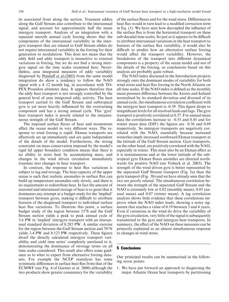
there is no interannual variability in the atmosphericforcing. Figure 9 shows the resulting intergyre heattransport and its decomposition (the years marked onthe axis are merely nominal). Comparing Fig. 9 withFig. 6 it can be seen that there is less interannual vari-ability in the intergyre heat transport in the annual cyclerun. The interannual standard deviation is 0.035 PW forthe (smoothed) annual cycle run compared to 0.063 PWfor the interannual run. However, the variability in thetransient eddy and meander terms is just as strong in theannual cycle run. The difference lies chiefly in the Ek-man-generated interannual variability which shows upin the baroclinic cycling term ½v0�½T �, and is of courselargely absent from the annual cycle run (where there isno interannual signal from the wind stress). It seems,therefore, from a superficial examination that it is notnecessary to appeal to atmospheric influences to explainthe magnitude of the non-Ekman interannual variabil-ity. It can all be internally generated. Whether this is truefor the individual features of the time series, or lowerfrequency components of the NAO signal, remains to beseen.

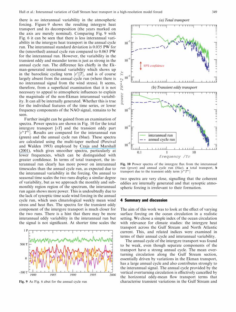
Further insight can be gained from an examination ofspectra. Power spectra are shown in Fig. 10 for the totalintergyre transport [vT] and the transient eddy part½v0�T 0��. Results are compared for the interannual run(green) and the annual cycle run (blue). These spectraare calculated using the multi-taper method (Percivaland Walden 1993) employed by Czaja and Marshall(2001), which gives smoother spectra, particularly atlower frequencies, which can be distinguished withgreater confidence. In terms of total transport, the in-terannual run clearly has more power on interannualtimescales than the annual cycle run, as expected due tothe interannual variability in the forcing. On annual toseasonal time scales the two runs display a similar degreeof variability, but as we approach the monthly and sub-monthly region region of the spectrum, the interannualrun again shows more power. This is undoubtedly due tothe lack of synoptic time scale wind forcing in the annualcycle run, which uses clmatological weekly mean windstress and heat flux. The spectra for the transient eddycomponent of the intergyre transport is much closer forthe two runs. There is a hint that there may be moreinterannual eddy variability in the interannual run butthe signal is not significant. At shorter time scales the

two spectra are very close, signalling that the coherenteddies are internally generated and that synoptic atmo-spheric forcing is irrelevant to their formation.

4 Summary and discussion

The aim of this work was to look at the effect of varyingsurface forcing on the ocean circulation in a realisticsetting. We chose a simple index of the ocean circulationwith relevance for climate studies: the intergyre heattransport across the Gulf Stream and North Atlanticcurrent. This, and related indices were examined interms of their annual cycle and interannual variability.

The annual cycle of the intergyre transport was foundto be weak, even though separate components of thetransport have a strong annual cycle. The mean over-turning circulation along the Gulf Stream section,essentially driven by variations in the Ekman transport,has a large annual cycle and also contributes strongly tothe interannual signal. The annual cycle provided by thevertical overturning circulation is effectively cancelled bythe horizontal eddy-mean flow transport terms thatcharacterise transient variations in the Gulf Stream andFig. 9 As Fig. 6 abut for the annual cycle run

Fig. 10 Power spectra of the intergyre flux from the interannualrun (green) and annual cycle run (blue). a total transport, btransport due to the transient eddy term ½v0�T 0��

Hall et al.: Interannual variation of Gulf Stream heat transport in a high-resolution model forced 349

its associated front along the section. Transient eddiesalong the Gulf Stream also contribute to the interannualsignal, and account for approximately half the meanintergyre transport. Analysis of an integration with arepeated smooth annual cycle forcing shows that thecomponents of the interannual variability in the inter-gyre transport that are related to Gulf Stream eddies donot require interannual variability in the forcing for theirgeneration or modulation. This does not mean that theeddy field and eddy transport is insensitive to externalvariations in forcing, but we do not find a strong inter-gyre signal on the time scales examined here. Never-theless, area integrated measures of eddy variabilitydiagnosed by Penduff et al.(2003) from the same modelintegration do show a tendency to follow the NAOsignal with a 4–12 month lag, in accordance with TO-PEX/Poseidon altimeter data. It appears therefore thatthe eddy heat transport is not strongly controlled by thegeneral level of area integrated eddy activity. The heattransport carried by the Gulf Stream and subtropicalgyre is yet more heavily influenced by the overturningcomponent and has a strong annual cycle. This ‘gyre’heat transport index is poorly related to the instanta-neous strength of the Gulf Stream.

The imposed surface fluxes of heat and momentumaffect the ocean model in very different ways. The re-sponse to wind forcing is rapid. Ekman transports areeffectively set up immediately and are quite independentof the details of the model. Furthermore, the strongconstraint on mass conservation imposed by the model’srigid lid upper boundary condition means that there isno ability to store heat by accumulating mass, andchanges in the wind driven circulation immediatelytranslate into changes in heat transport.

In contrast, the response to heat flux variations issubject to lag and storage. The heat capacity of the upperocean is such that realistic anomalies in surface flux canbuild up temperature anomalies only slowly, and there isno requirement to redistribute heat. In fact the amount ofseasonal and interannual storage of heat is so great that itdominates any attempt at a budget study for the ‘implied’transport between gyres, making it difficult to attributefeatures of the diagnosed transport to individual surfaceheat flux variations. To illustrate this point, a surfacebudget study of the region between 15�S and the GulfStream section yields a peak to peak annual cycle of5.6 PW in ‘implied’ intergyre transport with an interan-nual standard deviation of 0.285 PW. A similar exercisefor the region between the Gulf Stream section and 70�Nyields 3.4 PW and 0.123 PW respectively. These figuresdwarf the directly calculated intergyre transport vari-ability and yield time series’ completely unrelated to it,demonstrating the dominance of strorage terms on alltime scales considered. This result also offers some guid-ance as to what to expect from alternative forcing data-sets. For example the NCEP reanalysis has somesystematic differences in surface heat flux from that of theECMWF (see Fig. 4 of Garnier et al. 2000) although thetwo products show greater consistency for the variability

of the surface fluxes and for the wind stress. Differences inheat flux would in turn lead to a modified correction termin Eq. (1). We have seen how decoupled the influence ofthe surface flux is from the horizontal transport on thesesub-decadal time scales. So just as it appears to be difficultto attribute interannual variations in the heat transport tofeatures of the surface flux variability, it would also bedifficult to predict how an alternative surface forcingwould affect the transport variability. However, thebreakdown of the transport into different dynamicalcomponents is a property of the ocean model and not ofthe details of the forcing, so conclusions based on thisanalysis are probably quite robust.

The NAO index discussed in the Introduction projectsstrongly onto the dominant modes of variability for bothwind stress and heat flux forcing in the North Atlantic onall time scales. If the NAO index is defined as the monthlymean pressure difference between the Azores and Icelandnormalised by its standard deviation and divested of itsannual cycle, the simultaneous correlation coefficientwiththe intergyre heat transport is -0.39. This figure drops toinsignificant levels for all resolved leads and lags. The gyretransport is positively correlated at 0.37. For annualmeandata the correlations increase to –0.55 and 0.45 and forwinter mean data (DJF) the figures are –0.36 and 0.69respectively. So intergyre transports are negatively cor-related with the NAO, essentially because increasedwesterlies imply increased southward Ekman transport atthe latitude of the Gulf Stream section. Gyre transports,on the other hand, are positively correlatedwith theNAO,especially in winter. This must also be an Ekman effect asit is instantaneous and at the lower latitude of the sub-tropical gyre Ekman fluxes anomlies are directed north-wards for positive NAO (see Visbeck et al. 2003). Thestrength of the wind driven gyre is better represented bythe separated Gulf Stream transport (Fig. 5a) than thegyre transport (Fig. 3b) and we have already seen that thetwo are poorly related. The simultaneous correlation be-tween the strength of the separated Gulf Stream and theNAO is extremely low at 0.02 (monthly mean), 0.05 (an-nual mean) and 0.07 (winter mean). A lag correlationanalysis shows little evidence that these correlations im-prove when the NAO index leads, showing a noisy sig-nature that reaches a value of 0.19 between 3 and 4 years.Even if variations in the wind do drive the variability ofthe gyre circulation, very little of the signal is subsequentlytransmitted to the gyre and intergyre heat transports. Insummary, the effect of the NAO on these measures can beprimarily explained as an almost simultaneous responseto changes in wind stress.

5 Conclusions

Our prinicipal results can be summarised in the follow-ing seven points:

1. We have put forward an approach to diagnosing themajor Atlantic Ocean heat transports by partitioning

350 Hall et al.: Interannual variation of Gulf Stream heat transport in a high-resolution model forced

between ‘intergyre’ and ‘gyre’ components, whichserves to isolate some aspects of the annual and in-terannual variability.

2. The ocean model transports 3 0.7 PW northwardsacross the Gulf Stream - North Atlantic current.About half of this transport is effected by the tran-sient eddies.

3. Because of a cancellation between the Ekman-over-turning component and horizontal transient-meanflow (‘meander’) terms, the annual cycle in the in-tergyre heat transport is weak, much weaker than theannual cycle in gyre transport.

4. The Ekman component also accounts for a largefraction of the interannual variability in intergyreheat transport.

5. Terms associated with transient eddies also accountfor a significant fraction of the interannual variabil-ity, but appear to be independent of the surfaceforcing.

6. Perhaps surprisingly, the link between the wind-dri-ven gyre circulation and the gyre and intergyretransport is poor, and the response of the former tointerannual changes in wind stress is masked byinternal variability.

7. It is difficult to attribute any aspect of transportvariability to variations in surface heat flux on thetime scales considered here because of the amount ofstorage in the system.

These conclusions serve to quantify some of our ini-tial expectations from simple theories. There are furtherquestions to be explored in terms of the response tosurface forcing. It is hoped that longer integrations ofthis sort will become available so that these processescan be examined on longer time scales. With more re-alisations, more definitive quantifications can also bemade for shorter time scales.

Acknowledgements We are very grateful to Arnaud Czaja for helpwith calculation of spectra and for useful comments. We thank thereviewer for comments that helped us to clarify some of the dis-cussion. This work was funded by a fellowship from the EuropeanUnion and the Centre National de la Recherche Scientifique.Support for computations was provided by the Institut du Devel-oppement et des Recources en Information Scientifique (IDRIS).The CLIPPER project was supported by the Institut Nationale desSciences de l’Univers (INSU), the Institut Francais de Recherchepour l’Exploitation de la Mer (IFREMER), the Service Hydrog-raphique et Oceanographique de la Marine (SHOM) and theCentre Nationale d’Etudes Spatiales (CNES).

References

Barnier B (1998) Forcing the ocean. In: Chassignet E, Verron J(eds.) Ocean modelling and parametrization’, Kluwer, Dardr-echt, NL, pp 45–80

Bjerknes J (1964) Atlantic air-sea interaction. Adv Geophys 10:1–82

Crosnier L, B Barnier, Treguier A-M (2001) Aliasing of inertialoscillations in the 1/6�Atlantic circulation Clipper model: im-pact on the mean meridional heat transport. Ocean Modelling3: 21–32

Czaja A, Marshall JC (2001) Observations of atmosphere-oceancoupling in the North Atlantic. QJR Meteorol Soc 127: 1893–1916

Eden C, Jung T (2001) North Atlantic interdecadal variability:oceanic response to the North Atlantic Oscillation (1865-1997).J Clim 14: 676–691

Frankignoul C, de Coetlogon G, Joyce TM, Dong S (2001) GulfStream variability and ocean-atmosphere interaction. J PhysOceanogr 31: 3516–3529

Ganachaud A, Wunch C (2003) Large-scale ocean heat andfreshwater transports during the world ocean circulationexperiment. J Clim 16: 696–705

Garnier E, Barnier B, Siefridt L, Beranger K (2000) Investigatingthe 15 year air-sea flux climatology from the ECMWF reanal-ysis project as a surface boundary condition for ocean models.Int J Climatol 20: 1653–1673

Gulev S, Barnier B, Knochel H, Molines J.M, Cottet M(2003)Water mass transformation in the North Atlantic and its impacton the meridional circulation: insights from an ocean modelforced by NCEP-NCAR reanalysis surface fluxes. J clim 16:3085–3110

Hakkinen S (1999) Variability of the simulated meridional heattransport in the North Atlantic for periods 1951-1993. J Geo-phys Res 104: 10,991–11,007

Hansen DV, Bezdek HF (1996) On the nature of decadal anomaliesin the North Atlantic sea surface termperature. J Geophys Res101: 8749–8758

Hurrell JW (1996) Influence of variations in the extratropicalwintertime teleconnections on Northern Hemisphere tempera-ture. Geophys Res Lett 23: 665–668

Jayne SR, Marotzke J (2001) The dynamics of ocean heat transportvariability. Rev Geophys 39: 386–411

Krahmann G, Visbeck M, Reverdin G (2001) Formation andpropagation of temperature anomalies along the North AtlanticCurrent. J Phys Oceanogr 31: 1287–1303

Marshall JC, Johnson H, Goodman J (2001) A study of theinteraction of the North Atlantic Oscillation with ocean circu-lation. J Clim 14: 1399–1421

Penduff T, Barnier B, Dewar WK, O’Brien JJ (2003) Dynamicalresponse of the ocean eddy field to the North Atlantic Oscil-lation: a model-data comparison. J Phys Oceanogr (Accepted)

Pavia AM, Chassignet EP (2002) North Atlantic modelling of lowfrequency variability in mode water formation. J Phys Ocea-nogr 32: 2666–2680

Percival DB, Walden TA (1993) Spectral analysis for physicalapplications. Multitaper and conventional univariate tech-niques. Cambridge University Press, Cambridge, UK

Reynolds RW, Smith TM (1994) Improved global sea surfacetemperature analyses using optimum interpolation. J. Clim 7:929-948

Saravanan R, McWilliams J (1997) Stochasticity and spatial re-sponse in interdecadal climate fluctuations. J Clim 10: 2299–2320

Sutton R, Allen M (1997) Decadal predictability of North Atlanticsea surface temperature and climate. Nature 388: 363–367

Taylor AH, Stephens JA (1998) The North Atlantic Oscillation andthe latitude of the Gulf Stream. Tellus 50A: 134–142

Treguier A-M, Barnier B, de Miranda A, Molines J-M, Grima N,Imbard M, Madec G, C Messager Michel S (2001) Aneddy permitting model of the Atlantic circulation: evaluat-ing open boundary conditions. J Geophys Res 106: 22 ,115–22,129

Visbeck M, Cullen H, Krahmann G, Naik N (1998) An oceanmodel’s response to North Atlantic Oscillation like wind forc-ing. Geophys Res Lett 25: 4521–4524

Visbeck M, Chassignet EP, Curry RG, Delworth TL, Dickson RR,Krahmann G (2003) The ocean’s response to North AtlanticOscillation variability. In: The North Atlantic Oscillation: cli-mate significance and environmental impacts, Hurrel JW,Kushnir Y, Ottersen G, Visbeck M,eds. Geophysical Mono-graph Series 134: pp 279

Hall et al.: Interannual variation of Gulf Stream heat transport in a high-resolution model forced 351