Interannual variability of estimated monthly nitrogen deposition to coastal waters due to variations of atmospheric variables model input

Atmospheric Research 96 (2010) 88–102

Contents lists available at ScienceDirect

Atmospheric Research

j ourna l homepage: www.e lsev ie r.com/ locate /atmos

Interannual variability of estimated monthly nitrogen deposition to coastalwaters due to variations of atmospheric variables model input

Andrea L. Pineda Rojas a,b,c,⁎, Laura E. Venegas a,d

a National Scientific and Technological Research Council (CONICET), Argentinab Centro de Investigaciones del Mar y la Atmósfera (CIMA/CONICET-UBA), Argentinac Department of Atmospheric and Oceanic Sciences, Faculty of Sciences, Univ. of Buenos Aires, Ciudad Universitaria, Pabellón II, Piso 2, 1428 – Buenos Aires, Argentinad Department of Chemical Engineering, National Technological University, Av. Mitre 750, 1870 – Avellaneda, Buenos Aires, Argentina

a r t i c l e i n f o

⁎ Corresponding author. Department of AtmosSciences, Faculty of Sciences, Univ. of Buenos Aires,Pabellón II, Piso 2, 1428 – Buenos Aires, Argentina.

E-mail addresses: [email protected] (A.L. [email protected] (L.E. Venegas).

0169-8095/$ – see front matter © 2009 Elsevier B.V.doi:10.1016/j.atmosres.2009.11.016

a b s t r a c t

Article history:Received 26 June 2009Received in revised form 25 November 2009Accepted 26 November 2009

In this work, the influence of the interannual variation of meteorological input data on thenitrogen (N) deposition estimated applying atmospheric dispersion models is discussed. As acase study, the deposition of atmospheric oxidized N coming from the NOx generated in theMetropolitan Area of Buenos Aires to waters of de la Plata River is evaluated for three years,considering high spatial (1 km2) and temporal (1 h) resolutions. The interannual variation ofmonthly N dry deposition is in the range 10–160%, being mostly controlled by thephotochemical activity of the atmosphere and the frequency of winds towards the river. Thevariation of monthly wet deposition values between years is in general greater than a factor of2. It is mainly affected by the frequency of rainy hours and the precipitation rate during offshorewind conditions, and reaches a factor of 124 as a result of the variation of these variables in afactor of 4 and 3, respectively. These results show that estimated monthly N deposition tocoastal waters may vary significantly between years. The evaluation of the atmospheric N thatcan be transferred to coastal waters can therefore be improved considering several years ofatmospheric input data.

© 2009 Elsevier B.V. All rights reserved.

Keywords:Oxidized nitrogen compoundsBuenos Airesde la Plata RiverAtmospheric depositionInterannual variability

1. Introduction

The continuous increase of the population at coastal urbanzones leads to greater emissions of air pollutants, which notonly affects the human health and welfare but also producesdiverse impacts on the environment. In urban areas, themajor atmospheric N emission source is given by fossil fuelcombustion that releases nitrogen oxides (NOx). In an urbanatmosphere, the NOx are oxidized to form other nitrogenspecies such as nitrogen dioxide (NO2), gaseous nitric acid(HNO3) and ammonium nitrate (NH4NO3) aerosol. These

pheric and OceanicCiudad Universitaria

neda Rojas),

All rights reserved.

,

compounds can be transferred to the aquatic surface throughdry and wet deposition processes (Poor et al., 2001; Pryoret al., 2001; Gao, 2002; Whitall et al., 2003; Schlünzen andMeyer, 2007; Bencs et al., 2009). In the absence ofprecipitation, dry deposition occurs when species are trans-ported downward mainly by atmospheric turbulence andthen absorbed or adsorbed by the surface. Wet deposition isproduced when the precipitation scavenges substances beingpresent in the air column, transferring them to the surface.These processes depend on the physical and chemicalcharacteristics of the substance (e.g., the diffusivity of thespecies in air, its solubility and reactivity in water) andmeteorological conditions (e.g., atmospheric stability, windspeed, wind direction, and precipitation rate), which not onlyaffect the chemical transformation rates between the differ-ent N species and hence their ambient concentrations, butalso their deposition velocities. The complex relationshipsbetween dry and wet deposition processes and atmospheric

89A.L. Pineda Rojas, L.E. Venegas / Atmospheric Research 96 (2010) 88–102

and emission conditions make the deposition of nitrogen tocoastal waters to vary considerably with time.

In previous papers (Pineda Rojas and Venegas, 2008, 2009),we estimated oxidized nitrogen (NO2, gaseous HNO3 and NO3

−

aerosol) deposition fluxes to coastal waters of de la Plata River(Buenos Aires, Argentina). The atmospheric dispersion modelDAUMOD-RD (version 3) (Pineda Rojas and Venegas, 2009)was applied to area source emissions and CALPUFFmodel (Scireet al., 2000) to main point sources of NOx in the MetropolitanArea of Buenos Aires (MABA). Maximum total oxidized N drydeposition fluxes (7–13 kg-N km−2 month−1) to the de laPlata River were within the range of values obtained in othercoastal sites of the world, and N wet deposition fluxes (1–4 kg-N km−2 month−1) were consistently lower than valuesreported by other authors given the very low frequency ofrain events with offshore wind and that only source emissionsin the MABA were considered. The objective of this study is todiscuss the variations ofmonthly N deposition values estimatedconsidering three different years of meteorological input data.Interannual variability of monthly meteorological variables inthe area for the period 1999–2001 is presented. The seasonaland interannual variations of estimated monthly dry and wetdeposition of oxidized N species generated from NOx emissionsin the MABA to de la Plata River are discussed focusing on theinfluence of atmospheric variables on chemistry, transport,dispersion and subsequent deposition.

2. Estimation of N deposition to coastal waters of de laPlata River

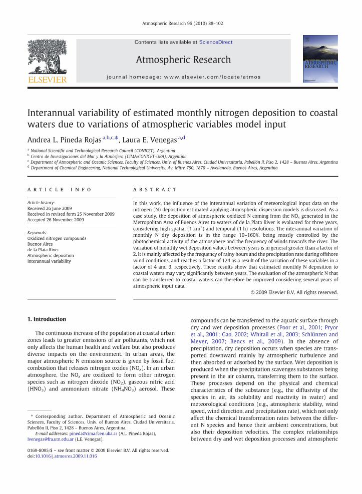
The Metropolitan Area of Buenos Aires (MABA) isconsidered one of the ten greatest urban conglomerates inthe world and the third mega-city in Latin America, followingMexico City (Mexico) and Sao Paulo (Brazil). It is composed ofthe city of Buenos Aires (200 km2 — 2.8 million inhabitants)and the Greater Buenos Aires (3600 km2 — 8.7 millioninhabitants) (Fig. 1). In the urban area, there are numerous

Fig. 1. Area of study: waters of de la Plata River in front of the MetropolitanArea of Buenos Aires (MABA) formed by the city of Buenos Aires (CBA) andthe Greater Buenos Aires (GBA); domestic airport ( ); international airport( ); power plants (▲); oil company (△).

NOx emission sources coming from road traffic, residential,commercial and low industrial activities, and aircrafts at themain airports. Moreover, the main point sources located nearthe coast are the stacks of four Power Plants and a large oilcompany. Due to the geographical location of the MABA,pollutants released to the atmosphere are transportedtowards de la Plata River during great part of the year. De laPlata River is a shallow river-type estuary of 327 km long andwith a width varying between 2 and 227 km. In front of theMABA, the river is 42 kmwidth and shows a large zonewheredepths are less than 5 m. The river constitutes the mainsource of drinking water for the city of Buenos Aires andsurrounding areas.

To estimate the deposition of atmospheric nitrogen (N),coming from the N emitted in the MABA, to surface waters ofde la Plata River, the DAUMOD-RD (version 3) model wasapplied to area source NOx emissions and the CALPUFF modelto the emissions coming from themain point sources near thecoast. Both models were applied over a surface of the river of2339 km2 (Fig. 1), considering spatial and temporal resolu-tions of 1 km2 and 1 h, respectively. Three years (1999–2001)of hourly surface meteorological information measured in acoastal site within the domestic airport and sounding datafrom the site located in the international airport (Fig. 1), wereused. The NOx emission data belong to a high resolutionemission inventory developed for the Metropolitan Area ofBuenos Aires (Pineda Rojas et al., 2007) and the emissionsfrom the stacks of the four Power Plants and the large oilcompany. The emission inventory includes area sourceemissions: residential, commercial, small industries, roadtraffic and aircrafts landing/take-off at both the domestic andthe international airports. The emission factors used inpreparing the emission inventory were derived considering:a) monitoring studies undertaken in Buenos Aires (Rideoutet al., 2005); b) The EMEP/CORINAIR Atmospheric InventoryGuidebook (European Environment Agency, 2001); c) The USEnvironmental Protection Agency's manual on the Compila-tion of Air Pollution Emission Factors (US EPA, 1995). Thesefactors were applied to fuel consumption, gas supply data andvehicle kilometres travelled within each grid square. Data ontraffic flow and bus service frequencies was also available.Aircraft emissions were computed knowing the scheduledhourly flights, the type of aircraft, the information availableon LTO (landing/take-off) cycles and NOx emission factors(Romano et al, 1999, EMEP/CORINAIR, 2001). Table 1 includes

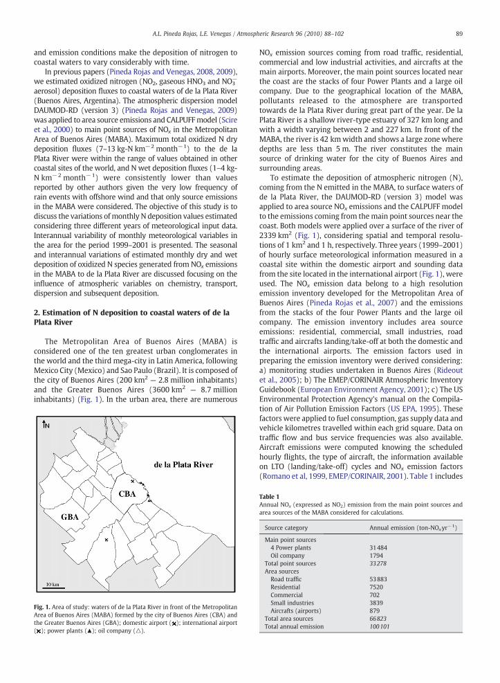
Table 1Annual NOx (expressed as NO2) emission from the main point sources andarea sources of the MABA considered for calculations.

Source category Annual emission (ton-NOxyr−1)

Main point sources4 Power plants 31484Oil company 1794

Total point sources 33278Area sources

Road traffic 53883Residential 7520Commercial 702Small industries 3839Aircrafts (airports) 879

Total area sources 66823Total annual emission 100101

90 A.L. Pineda Rojas, L.E. Venegas / Atmospheric Research 96 (2010) 88–102

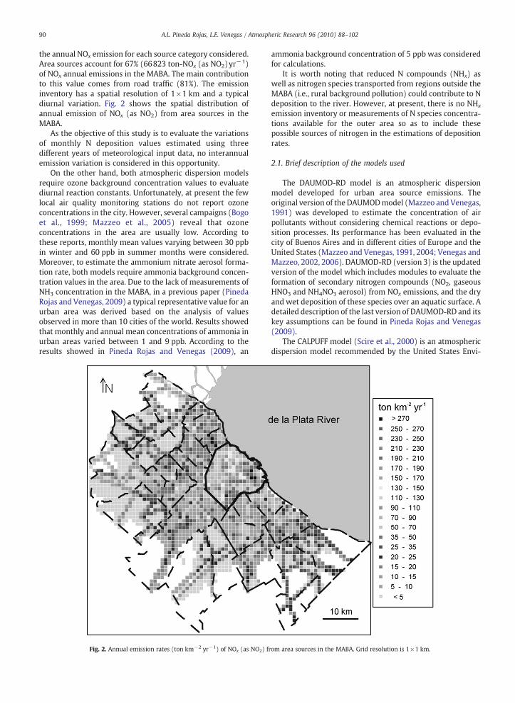
the annual NOx emission for each source category considered.Area sources account for 67% (66823 ton-NOx (as NO2)yr−1)of NOx annual emissions in the MABA. The main contributionto this value comes from road traffic (81%). The emissioninventory has a spatial resolution of 1×1 km and a typicaldiurnal variation. Fig. 2 shows the spatial distribution ofannual emission of NOx (as NO2) from area sources in theMABA.

As the objective of this study is to evaluate the variationsof monthly N deposition values estimated using threedifferent years of meteorological input data, no interannualemission variation is considered in this opportunity.

On the other hand, both atmospheric dispersion modelsrequire ozone background concentration values to evaluatediurnal reaction constants. Unfortunately, at present the fewlocal air quality monitoring stations do not report ozoneconcentrations in the city. However, several campaigns (Bogoet al., 1999; Mazzeo et al., 2005) reveal that ozoneconcentrations in the area are usually low. According tothese reports, monthly mean values varying between 30 ppbin winter and 60 ppb in summer months were considered.Moreover, to estimate the ammonium nitrate aerosol forma-tion rate, both models require ammonia background concen-tration values in the area. Due to the lack of measurements ofNH3 concentration in the MABA, in a previous paper (PinedaRojas and Venegas, 2009) a typical representative value for anurban area was derived based on the analysis of valuesobserved in more than 10 cities of the world. Results showedthat monthly and annual mean concentrations of ammonia inurban areas varied between 1 and 9 ppb. According to theresults showed in Pineda Rojas and Venegas (2009), an

Fig. 2. Annual emission rates (ton km−2 yr−1) of NOx (as NO2) f

ammonia background concentration of 5 ppb was consideredfor calculations.

It is worth noting that reduced N compounds (NHx) aswell as nitrogen species transported from regions outside theMABA (i.e., rural background pollution) could contribute to Ndeposition to the river. However, at present, there is no NHx

emission inventory or measurements of N species concentra-tions available for the outer area so as to include thesepossible sources of nitrogen in the estimations of depositionrates.

2.1. Brief description of the models used

The DAUMOD-RD model is an atmospheric dispersionmodel developed for urban area source emissions. Theoriginal version of the DAUMODmodel (Mazzeo and Venegas,1991) was developed to estimate the concentration of airpollutants without considering chemical reactions or depo-sition processes. Its performance has been evaluated in thecity of Buenos Aires and in different cities of Europe and theUnited States (Mazzeo and Venegas, 1991, 2004; Venegas andMazzeo, 2002, 2006). DAUMOD-RD (version 3) is the updatedversion of the model which includes modules to evaluate theformation of secondary nitrogen compounds (NO2, gaseousHNO3 and NH4NO3 aerosol) from NOx emissions, and the dryand wet deposition of these species over an aquatic surface. Adetailed description of the last version of DAUMOD-RD and itskey assumptions can be found in Pineda Rojas and Venegas(2009).

The CALPUFF model (Scire et al., 2000) is an atmosphericdispersion model recommended by the United States Envi-

rom area sources in the MABA. Grid resolution is 1×1 km.

91A.L. Pineda Rojas, L.E. Venegas / Atmospheric Research 96 (2010) 88–102

ronmental Protection Agency (US EPA). CALPUFF can beapplied to estimate concentration and deposition of atmo-spheric pollutants emitted from point sources. Taking intoaccount that the point sources considered in this studyare located near the coast (Fig. 1) and that only the plumebehaviour over the water surface is modelled, the CALPUFFmodel was applied in slug mode (to avoid errors associatedto circular puffs near the emission source) and screeningmode (i.e., spatial homogeneity of atmospheric variables isassumed).

The DAUMOD-RD (version 3) model was developed inorder to evaluate deposition of nitrogen compounds to awater surface, when NOx emissions come from a greatnumber of area sources in a coastal city. Both CALPUFF andDAUMOD-RD models include the same parameterisations ofchemical transformations and deposition processes. However,DAUMOD-RD model requires much less computation timethan CALPUFF when it is applied to a great number of areasources. Area source emissions of NOx in the MABA are givenusing a grid net with a resolution of 1×1 km that includes2203 area sources. The application of CALPUFF to all thesesources would require a considerable amount of computationtime, so DAUMOD-RD (version 3) was applied to area sourceemissions.

The chemical transformation scheme included in bothmodels assumes that nitrogen oxides (NOx=NO+NO2) areall transformed to nitrogen dioxide (NO2), which is thenoxidized to gaseous nitric acid (HNO3) and organic nitrates(RNO3). HNO3 can then react with gaseous ammonia (NH3)present in the atmosphere to produce ammonium nitrate(NH4NO3) aerosol (Atkinson, 2000; Jenkin and Clemitshaw,2000; Seinfeld and Pandis, 2006). RNO3 is not subject tosubsequent reactions or deposition. The chemical transfor-mations through which NO2 is lost and gaseous HNO3 isformed are considered as pseudo-first-order reactions. Thereaction constants for these transformations are evaluated asfunctions of ozone (O3) background concentration (precursorof the hydroxyl radical), the atmospheric stability index,varying between 2 (moderate unstable) and 6 (moderatestable) according to the Pasquill–Gifford–Turner classifica-tion (Gifford, 1976), and the vertically averaged NOx

concentration (Scire et al., 1984, 2000). In addition, at eachhour the models evaluate the fraction of NH4NO3 aerosolbeing in equilibrium with gaseous HNO3 and NH3, as afunction of the equilibrium constant for this reaction, theconcentration of available gaseous HNO3 and the backgroundconcentration of gaseous NH3. The equilibrium constant is anonlinear function of temperature and relative humidity andit is estimated through a double linear interpolation algo-rithm on these variables, following the relationships obtainedby Stelson and Seinfeld (1982). It is assumed that theavailable HNO3 concentration results from the NOx oxidation.

The wet removal of gaseous species occurs whensubstances are dissolved within falling drops and cantherefore be important in the case of soluble gases such asHNO3. On the other hand, the precipitation scavenging ofaerosols is one of the most effective mechanisms to removepollutants from the atmosphere and occurs when drops“collide” or “impact” with particles. This mechanism is veryeffective to remove aerosols such as nitrate. A simpleapproach that has shown to give realistic estimates of the

long-term wet removal of gases and aerosols, is the scav-enging coefficients method (Maul, 1980; Scire et al., 2000).Through this methodology, the wet deposition flux can beestimated as (Seinfeld and Pandis, 2006):

Fw = ΛhCm ð1Þ

where h is the vertical extension of the pollutant plumebelow the cloud, Cm is the vertically averaged speciesconcentration within the pollutant plume before the wetremoval process and Λ is the scavenging coefficient given byΛ=λ(p0 /p1), where p0 is the precipitation rate, p1 is aconstant (=1 mm h−1) and λ is a washout coefficient (s−1)dependent on the pollutant (Scire et al., 2000). The values ofλ considered in both models are: 6.0×10−5 s−1 for gaseousHNO3, 1.0×10−4 s−1 for NO3

− aerosol and zero for NO2 due toits low solubility in water (Lee and Schwartz, 1981). After thewet removal, the species concentration (C′) that remains inthe air is evaluated as:

C′ = C expð−ΛΔtÞ ð2Þ

where C is the pollutant concentration before the rainscavenging and Δt is the time step of the model.

The dry deposition flux is estimated as the product of thespecies concentration (C′) and the species deposition velocity(vd) at a reference height near the surface (as deposition isestimated over a water surface, the reference height isconsidered 1 m)

Fd = vdC′ ð3Þ

Among the most widely used methodologies to estimatethe deposition velocity is the resistance method (Seinfeld andPandis, 2006). Under steady-state conditions, the depositionvelocity (cm s−1) of a gaseous substance over an aquaticsurface can be expressed as:

vdg = ½ra + rdg + rw�−1 ð4Þ

where ra is the aerodynamic resistance representing theeffect of turbulent transport through the atmospheric surfacelayer, rdg is the quasi-laminar layer resistance for gaseousspecies including the effect of molecular diffusion in this sub-layer, and rw is the water surface resistance which representsthe tendency of the surface to “capture” the species once theycome into contact. In the case of aerosols, deposition is alsofavoured by particle settling due to the action of gravity. Thedeposition velocity for aerosol particles (vdp) can be estimat-ed by:

vdp = ½ra + rdp + rardpvs�−1 + vs ð5Þ

where rdp is the quasi-laminar layer resistance for aerosolsand vs is the gravitational settling velocity, being bothparameters dependent on the aerosol particle size. In themodels, the resistances are parameterised as a function of thespecies diffusivity in air, its solubility and reactivity in water,the atmospheric stability and the friction velocity, followingthe methodology described in Seinfeld and Pandis (2006). Toinclude rdp and vs dependencies on particle size, a log-normaldistribution with typical geometric mean diameter (0.48 μm)

92 A.L. Pineda Rojas, L.E. Venegas / Atmospheric Research 96 (2010) 88–102

and standard deviation (2.0 μm) for nitrate aerosol is con-sidered (Scire et al., 2000).

3. Results and discussion

3.1. Meteorological variables in the area during 1999–2001

3.1.1. Wind speed and directionWind is one of the variables with greatest influence on the

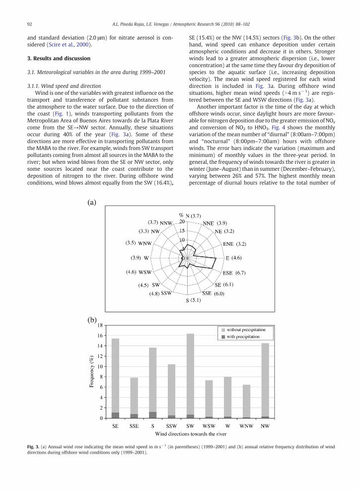
transport and transference of pollutant substances fromthe atmosphere to the water surface. Due to the direction ofthe coast (Fig. 1), winds transporting pollutants from theMetropolitan Area of Buenos Aires towards de la Plata Rivercome from the SE→NW sector. Annually, these situationsoccur during 40% of the year (Fig. 3a). Some of thesedirections are more effective in transporting pollutants fromthe MABA to the river. For example, winds from SW transportpollutants coming from almost all sources in the MABA to theriver; but when wind blows from the SE or NW sector, onlysome sources located near the coast contribute to thedeposition of nitrogen to the river. During offshore windconditions, wind blows almost equally from the SW (16.4%),

Fig. 3. (a) Annual wind rose indicating the mean wind speed in m s−1 (in parentdirections during offshore wind conditions only (1999–2001).

SE (15.4%) or the NW (14.5%) sectors (Fig. 3b). On the otherhand, wind speed can enhance deposition under certainatmospheric conditions and decrease it in others. Strongerwinds lead to a greater atmospheric dispersion (i.e., lowerconcentration) at the same time they favour dry deposition ofspecies to the aquatic surface (i.e., increasing depositionvelocity). The mean wind speed registered for each winddirection is included in Fig. 3a. During offshore windsituations, higher mean wind speeds (N4 m s−1) are regis-tered between the SE and WSW directions (Fig. 3a).

Another important factor is the time of the day at whichoffshore winds occur, since daylight hours are more favour-able for nitrogendeposition due to the greater emission of NOx

and conversion of NO2 to HNO3. Fig. 4 shows the monthlyvariation of the mean number of “diurnal” (8:00am–7:00pm)and “nocturnal” (8:00pm–7:00am) hours with offshorewinds. The error bars indicate the variation (maximum andminimum) of monthly values in the three-year period. Ingeneral, the frequency of winds towards the river is greater inwinter (June–August) than in summer (December–February),varying between 26% and 57%. The highest monthly meanpercentage of diurnal hours relative to the total number of

heses) (1999–2001) and (b) annual relative frequency distribution of wind

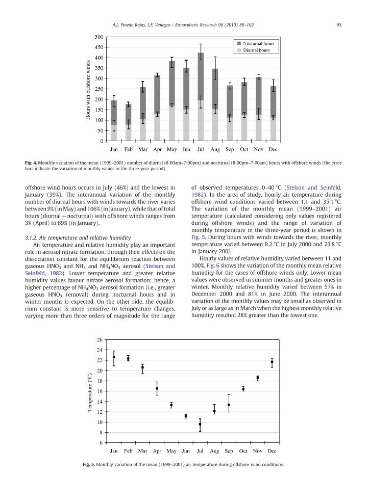
Fig. 4. Monthly variation of the mean (1999–2001) number of diurnal (8:00am–7:00pm) and nocturnal (8:00pm–7:00am) hours with offshore winds (the errorbars indicate the variation of monthly values in the three-year period).

93A.L. Pineda Rojas, L.E. Venegas / Atmospheric Research 96 (2010) 88–102

offshore wind hours occurs in July (46%) and the lowest inJanuary (39%). The interannual variation of the monthlynumber of diurnal hours with winds towards the river variesbetween 9% (inMay) and 106% (in January),while that of totalhours (diurnal+nocturnal) with offshore winds ranges from3% (April) to 69% (in January).

3.1.2. Air temperature and relative humidityAir temperature and relative humidity play an important

role in aerosol nitrate formation, through their effects on thedissociation constant for the equilibrium reaction betweengaseous HNO3 and NH3 and NH4NO3 aerosol (Stelson andSeinfeld, 1982). Lower temperature and greater relativehumidity values favour nitrate aerosol formation; hence, ahigher percentage of NH4NO3 aerosol formation (i.e., greatergaseous HNO3 removal) during nocturnal hours and inwinter months is expected. On the other side, the equilib-rium constant is more sensitive to temperature changes,varying more than three orders of magnitude for the range

Fig. 5. Monthly variation of the mean (1999–2001) ai

of observed temperatures 0–40 °C (Stelson and Seinfeld,1982). In the area of study, hourly air temperature duringoffshore wind conditions varied between 1.1 and 35.1 °C.The variation of the monthly mean (1999–2001) airtemperature (calculated considering only values registeredduring offshore winds) and the range of variation ofmonthly temperature in the three-year period is shown inFig. 5. During hours with winds towards the river, monthlytemperature varied between 8.2 °C in July 2000 and 23.8 °Cin January 2001.

Hourly values of relative humidity varied between 11 and100%. Fig. 6 shows the variation of the monthly mean relativehumidity for the cases of offshore winds only. Lower meanvalues were observed in summer months and greater ones inwinter. Monthly relative humidity varied between 57% inDecember 2000 and 81% in June 2000. The interannualvariation of the monthly values may be small as observed inJuly or as large as in Marchwhen the highest monthly relativehumidity resulted 28% greater than the lowest one.

r temperature during offshore wind conditions.

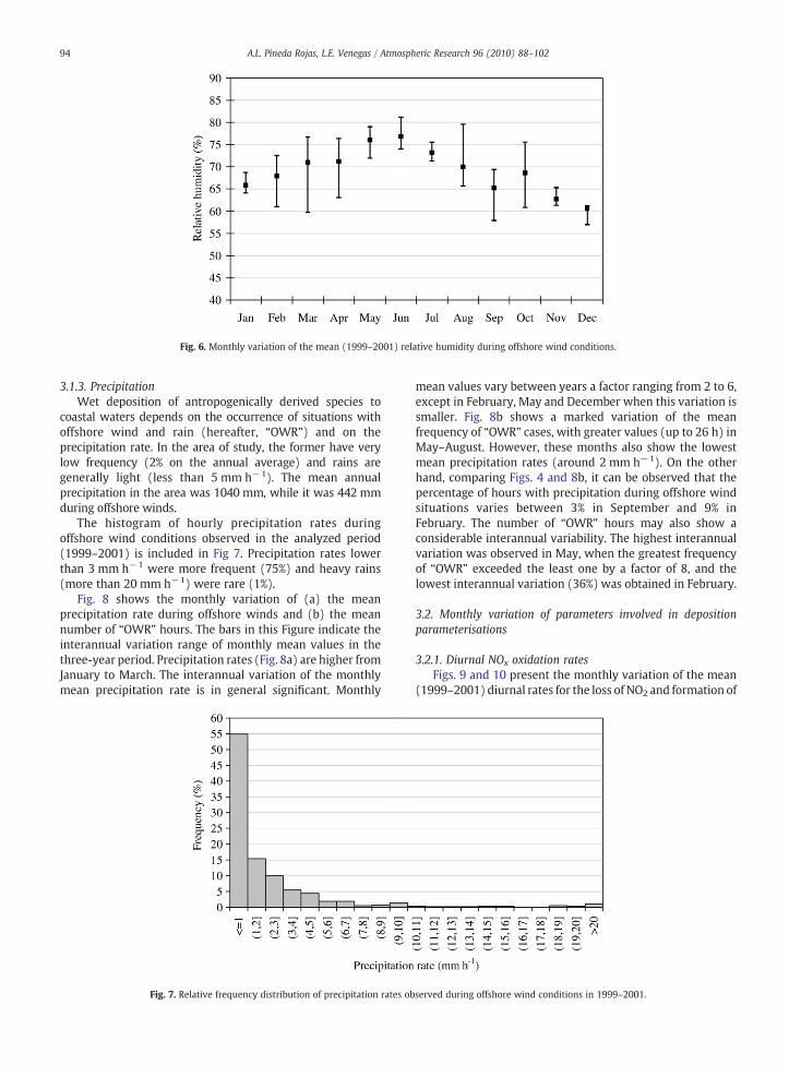
Fig. 6. Monthly variation of the mean (1999–2001) relative humidity during offshore wind conditions.

94 A.L. Pineda Rojas, L.E. Venegas / Atmospheric Research 96 (2010) 88–102

3.1.3. PrecipitationWet deposition of antropogenically derived species to

coastal waters depends on the occurrence of situations withoffshore wind and rain (hereafter, “OWR”) and on theprecipitation rate. In the area of study, the former have verylow frequency (2% on the annual average) and rains aregenerally light (less than 5 mm h−1). The mean annualprecipitation in the area was 1040 mm, while it was 442 mmduring offshore winds.

The histogram of hourly precipitation rates duringoffshore wind conditions observed in the analyzed period(1999–2001) is included in Fig 7. Precipitation rates lowerthan 3 mm h−1 were more frequent (75%) and heavy rains(more than 20 mm h−1) were rare (1%).

Fig. 8 shows the monthly variation of (a) the meanprecipitation rate during offshore winds and (b) the meannumber of “OWR” hours. The bars in this Figure indicate theinterannual variation range of monthly mean values in thethree-year period. Precipitation rates (Fig. 8a) are higher fromJanuary to March. The interannual variation of the monthlymean precipitation rate is in general significant. Monthly

Fig. 7. Relative frequency distribution of precipitation rates ob

mean values vary between years a factor ranging from 2 to 6,except in February, May and December when this variation issmaller. Fig. 8b shows a marked variation of the meanfrequency of “OWR” cases, with greater values (up to 26 h) inMay–August. However, these months also show the lowestmean precipitation rates (around 2 mm h−1). On the otherhand, comparing Figs. 4 and 8b, it can be observed that thepercentage of hours with precipitation during offshore windsituations varies between 3% in September and 9% inFebruary. The number of “OWR” hours may also show aconsiderable interannual variability. The highest interannualvariation was observed in May, when the greatest frequencyof “OWR” exceeded the least one by a factor of 8, and thelowest interannual variation (36%) was obtained in February.

3.2. Monthly variation of parameters involved in depositionparameterisations

3.2.1. Diurnal NOx oxidation ratesFigs. 9 and 10 present the monthly variation of the mean

(1999–2001) diurnal rates for the loss of NO2 and formation of

served during offshore wind conditions in 1999–2001.

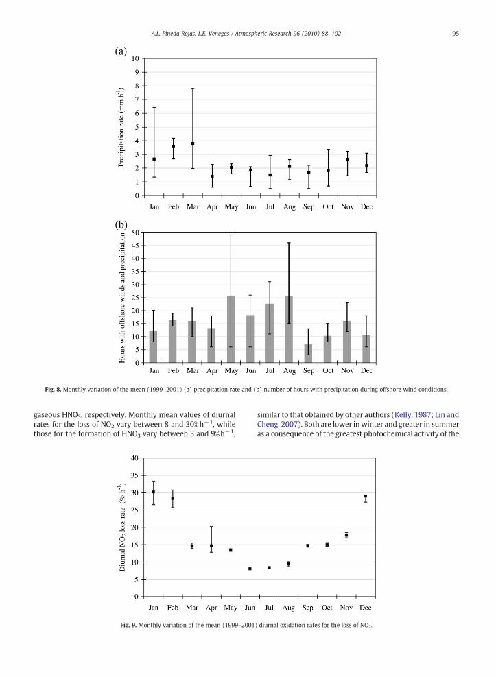
Fig. 8. Monthly variation of the mean (1999–2001) (a) precipitation rate and (b) number of hours with precipitation during offshore wind conditions.

95A.L. Pineda Rojas, L.E. Venegas / Atmospheric Research 96 (2010) 88–102

gaseous HNO3, respectively. Monthly mean values of diurnalrates for the loss of NO2 vary between 8 and 30%h−1, whilethose for the formation of HNO3 vary between 3 and 9%h−1,

Fig. 9. Monthly variation of the mean (1999–2001

similar to that obtained by other authors (Kelly, 1987; Lin andCheng, 2007). Both are lower inwinter and greater in summeras a consequence of the greatest photochemical activity of the

) diurnal oxidation rates for the loss of NO2.

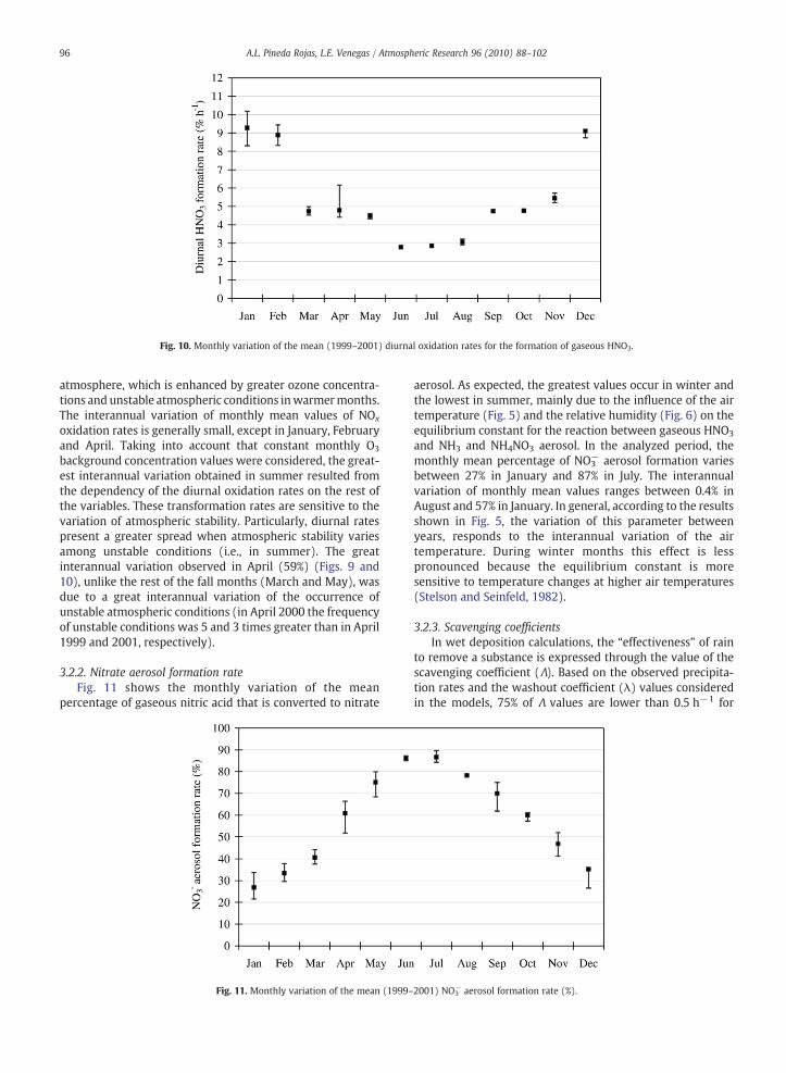
Fig. 10. Monthly variation of the mean (1999–2001) diurnal oxidation rates for the formation of gaseous HNO3.

96 A.L. Pineda Rojas, L.E. Venegas / Atmospheric Research 96 (2010) 88–102

atmosphere, which is enhanced by greater ozone concentra-tions and unstable atmospheric conditions inwarmermonths.The interannual variation of monthly mean values of NOx

oxidation rates is generally small, except in January, Februaryand April. Taking into account that constant monthly O3

background concentration values were considered, the great-est interannual variation obtained in summer resulted fromthe dependency of the diurnal oxidation rates on the rest ofthe variables. These transformation rates are sensitive to thevariation of atmospheric stability. Particularly, diurnal ratespresent a greater spread when atmospheric stability variesamong unstable conditions (i.e., in summer). The greatinterannual variation observed in April (59%) (Figs. 9 and10), unlike the rest of the fall months (March and May), wasdue to a great interannual variation of the occurrence ofunstable atmospheric conditions (in April 2000 the frequencyof unstable conditions was 5 and 3 times greater than in April1999 and 2001, respectively).

3.2.2. Nitrate aerosol formation rateFig. 11 shows the monthly variation of the mean

percentage of gaseous nitric acid that is converted to nitrate

Fig. 11. Monthly variation of the mean (1999–

aerosol. As expected, the greatest values occur in winter andthe lowest in summer, mainly due to the influence of the airtemperature (Fig. 5) and the relative humidity (Fig. 6) on theequilibrium constant for the reaction between gaseous HNO3

and NH3 and NH4NO3 aerosol. In the analyzed period, themonthly mean percentage of NO3

− aerosol formation variesbetween 27% in January and 87% in July. The interannualvariation of monthly mean values ranges between 0.4% inAugust and 57% in January. In general, according to the resultsshown in Fig. 5, the variation of this parameter betweenyears, responds to the interannual variation of the airtemperature. During winter months this effect is lesspronounced because the equilibrium constant is moresensitive to temperature changes at higher air temperatures(Stelson and Seinfeld, 1982).

3.2.3. Scavenging coefficientsIn wet deposition calculations, the “effectiveness” of rain

to remove a substance is expressed through the value of thescavenging coefficient (Λ). Based on the observed precipita-tion rates and the washout coefficient (λ) values consideredin the models, 75% of Λ values are lower than 0.5 h−1 for

2001) NO3− aerosol formation rate (%).

97A.L. Pineda Rojas, L.E. Venegas / Atmospheric Research 96 (2010) 88–102

gaseous HNO3 and lower than 0.9 h−1 for NO3− aerosol.

According to the parameterisation of the scavenging coeffi-cient, monthly variation of the mean Λ values follows thevariation of the mean precipitation rate during “OWR” hours(Fig. 8a). The monthly mean values of Λ varied between 0.3and 0.8 h−1 for HNO3 and between 0.5–1.4 h−1 for NO3

−. Ingeneral, the mean scavenging coefficients were greater fromJanuary to March, when greater precipitation rates occurred(Fig. 8a).

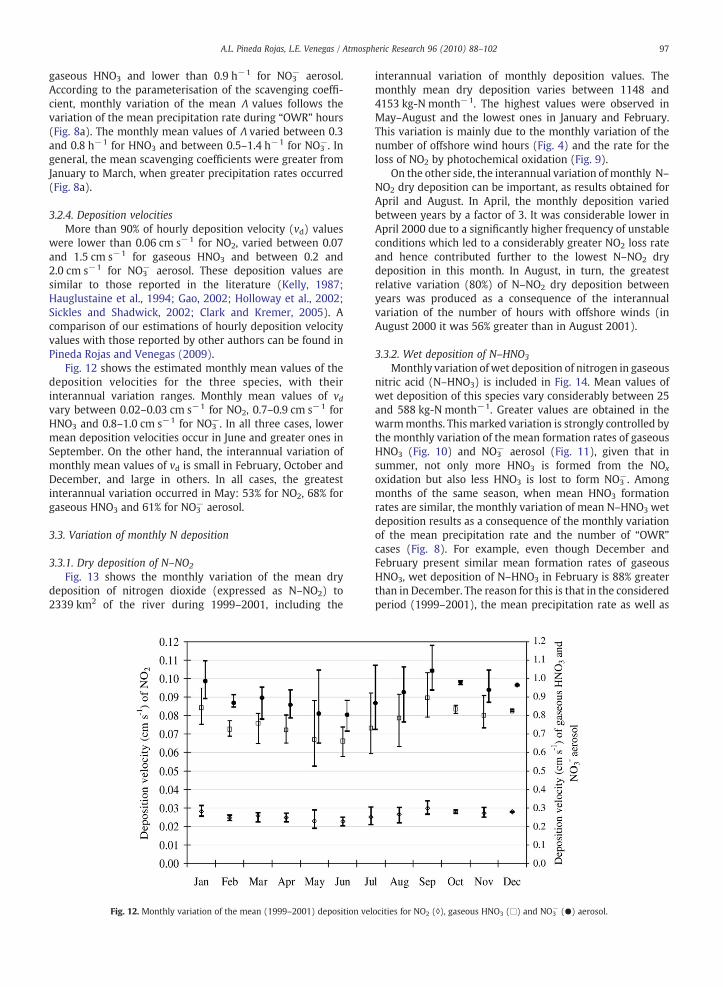
3.2.4. Deposition velocitiesMore than 90% of hourly deposition velocity (vd) values

were lower than 0.06 cm s−1 for NO2, varied between 0.07and 1.5 cm s−1 for gaseous HNO3 and between 0.2 and2.0 cm s−1 for NO3

− aerosol. These deposition values aresimilar to those reported in the literature (Kelly, 1987;Hauglustaine et al., 1994; Gao, 2002; Holloway et al., 2002;Sickles and Shadwick, 2002; Clark and Kremer, 2005). Acomparison of our estimations of hourly deposition velocityvalues with those reported by other authors can be found inPineda Rojas and Venegas (2009).

Fig. 12 shows the estimated monthly mean values of thedeposition velocities for the three species, with theirinterannual variation ranges. Monthly mean values of vdvary between 0.02–0.03 cm s−1 for NO2, 0.7–0.9 cm s−1 forHNO3 and 0.8–1.0 cm s−1 for NO3

−. In all three cases, lowermean deposition velocities occur in June and greater ones inSeptember. On the other hand, the interannual variation ofmonthly mean values of vd is small in February, October andDecember, and large in others. In all cases, the greatestinterannual variation occurred in May: 53% for NO2, 68% forgaseous HNO3 and 61% for NO3

− aerosol.

3.3. Variation of monthly N deposition

3.3.1. Dry deposition of N–NO2

Fig. 13 shows the monthly variation of the mean drydeposition of nitrogen dioxide (expressed as N–NO2) to2339 km2 of the river during 1999–2001, including the

Fig. 12. Monthly variation of the mean (1999–2001) deposition vel

interannual variation of monthly deposition values. Themonthly mean dry deposition varies between 1148 and4153 kg-N month−1. The highest values were observed inMay–August and the lowest ones in January and February.This variation is mainly due to the monthly variation of thenumber of offshore wind hours (Fig. 4) and the rate for theloss of NO2 by photochemical oxidation (Fig. 9).

On the other side, the interannual variation of monthly N–NO2 dry deposition can be important, as results obtained forApril and August. In April, the monthly deposition variedbetween years by a factor of 3. It was considerable lower inApril 2000 due to a significantly higher frequency of unstableconditions which led to a considerably greater NO2 loss rateand hence contributed further to the lowest N–NO2 drydeposition in this month. In August, in turn, the greatestrelative variation (80%) of N–NO2 dry deposition betweenyears was produced as a consequence of the interannualvariation of the number of hours with offshore winds (inAugust 2000 it was 56% greater than in August 2001).

3.3.2. Wet deposition of N–HNO3

Monthly variation of wet deposition of nitrogen in gaseousnitric acid (N–HNO3) is included in Fig. 14. Mean values ofwet deposition of this species vary considerably between 25and 588 kg-N month−1. Greater values are obtained in thewarmmonths. This marked variation is strongly controlled bythe monthly variation of the mean formation rates of gaseousHNO3 (Fig. 10) and NO3

− aerosol (Fig. 11), given that insummer, not only more HNO3 is formed from the NOx

oxidation but also less HNO3 is lost to form NO3−. Among

months of the same season, when mean HNO3 formationrates are similar, the monthly variation of mean N–HNO3 wetdeposition results as a consequence of the monthly variationof the mean precipitation rate and the number of “OWR”cases (Fig. 8). For example, even though December andFebruary present similar mean formation rates of gaseousHNO3, wet deposition of N–HNO3 in February is 88% greaterthan in December. The reason for this is that in the consideredperiod (1999–2001), the mean precipitation rate as well as

ocities for NO2 (◊), gaseous HNO3 (□) and NO3− (●) aerosol.

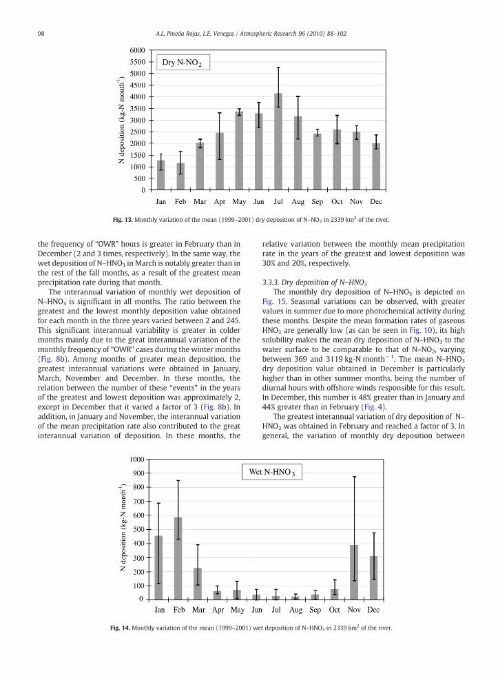
Fig. 13. Monthly variation of the mean (1999–2001) dry deposition of N–NO2 in 2339 km2 of the river.

98 A.L. Pineda Rojas, L.E. Venegas / Atmospheric Research 96 (2010) 88–102

the frequency of “OWR” hours is greater in February than inDecember (2 and 3 times, respectively). In the same way, thewet deposition of N–HNO3 in March is notably greater than inthe rest of the fall months, as a result of the greatest meanprecipitation rate during that month.

The interannual variation of monthly wet deposition ofN–HNO3 is significant in all months. The ratio between thegreatest and the lowest monthly deposition value obtainedfor each month in the three years varied between 2 and 245.This significant interannual variability is greater in coldermonths mainly due to the great interannual variation of themonthly frequency of “OWR” cases during the winter months(Fig. 8b). Among months of greater mean deposition, thegreatest interannual variations were obtained in January,March, November and December. In these months, therelation between the number of these “events” in the yearsof the greatest and lowest deposition was approximately 2,except in December that it varied a factor of 3 (Fig. 8b). Inaddition, in January and November, the interannual variationof the mean precipitation rate also contributed to the greatinterannual variation of deposition. In these months, the

Fig. 14. Monthly variation of the mean (1999–2001) we

relative variation between the monthly mean precipitationrate in the years of the greatest and lowest deposition was30% and 20%, respectively.

3.3.3. Dry deposition of N–HNO3

The monthly dry deposition of N–HNO3 is depicted onFig. 15. Seasonal variations can be observed, with greatervalues in summer due to more photochemical activity duringthese months. Despite the mean formation rates of gaseousHNO3 are generally low (as can be seen in Fig. 10), its highsolubility makes the mean dry deposition of N–HNO3 to thewater surface to be comparable to that of N–NO2, varyingbetween 369 and 3119 kg-N month−1. The mean N–HNO3

dry deposition value obtained in December is particularlyhigher than in other summer months, being the number ofdiurnal hours with offshore winds responsible for this result.In December, this number is 48% greater than in January and44% greater than in February (Fig. 4).

The greatest interannual variation of dry deposition of N–HNO3 was obtained in February and reached a factor of 3. Ingeneral, the variation of monthly dry deposition between

t deposition of N–HNO3 in 2339 km2 of the river.

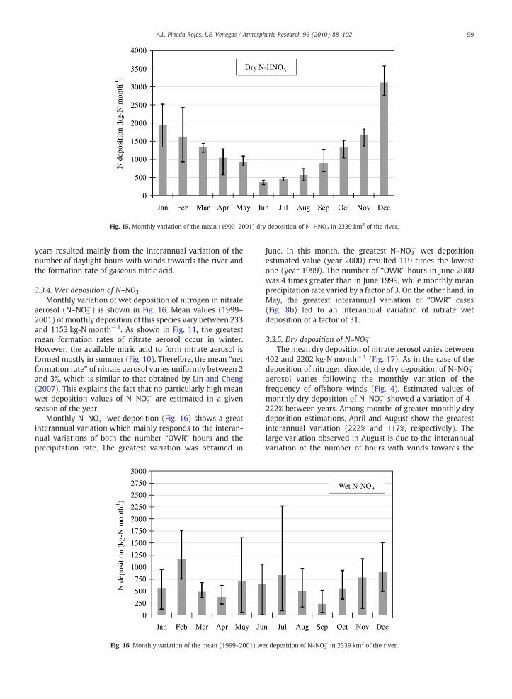
Fig. 15. Monthly variation of the mean (1999–2001) dry deposition of N–HNO3 in 2339 km2 of the river.

99A.L. Pineda Rojas, L.E. Venegas / Atmospheric Research 96 (2010) 88–102

years resulted mainly from the interannual variation of thenumber of daylight hours with winds towards the river andthe formation rate of gaseous nitric acid.

3.3.4. Wet deposition of N–NO3−

Monthly variation of wet deposition of nitrogen in nitrateaerosol (N–NO3

−) is shown in Fig. 16. Mean values (1999–2001) of monthly deposition of this species vary between 233and 1153 kg-N month−1. As shown in Fig. 11, the greatestmean formation rates of nitrate aerosol occur in winter.However, the available nitric acid to form nitrate aerosol isformed mostly in summer (Fig. 10). Therefore, the mean “netformation rate” of nitrate aerosol varies uniformly between 2and 3%, which is similar to that obtained by Lin and Cheng(2007). This explains the fact that no particularly high meanwet deposition values of N–NO3

− are estimated in a givenseason of the year.

Monthly N–NO3− wet deposition (Fig. 16) shows a great

interannual variation which mainly responds to the interan-nual variations of both the number “OWR” hours and theprecipitation rate. The greatest variation was obtained in

Fig. 16. Monthly variation of the mean (1999–2001) we

June. In this month, the greatest N–NO3− wet deposition

estimated value (year 2000) resulted 119 times the lowestone (year 1999). The number of “OWR” hours in June 2000was 4 times greater than in June 1999, while monthly meanprecipitation rate varied by a factor of 3. On the other hand, inMay, the greatest interannual variation of “OWR” cases(Fig. 8b) led to an interannual variation of nitrate wetdeposition of a factor of 31.

3.3.5. Dry deposition of N–NO3−

The mean dry deposition of nitrate aerosol varies between402 and 2202 kg-N month−1 (Fig. 17). As in the case of thedeposition of nitrogen dioxide, the dry deposition of N–NO3

−

aerosol varies following the monthly variation of thefrequency of offshore winds (Fig. 4). Estimated values ofmonthly dry deposition of N–NO3

− showed a variation of 4–222% between years. Among months of greater monthly drydeposition estimations, April and August show the greatestinterannual variation (222% and 117%, respectively). Thelarge variation observed in August is due to the interannualvariation of the number of hours with winds towards the

t deposition of N–NO3− in 2339 km2 of the river.

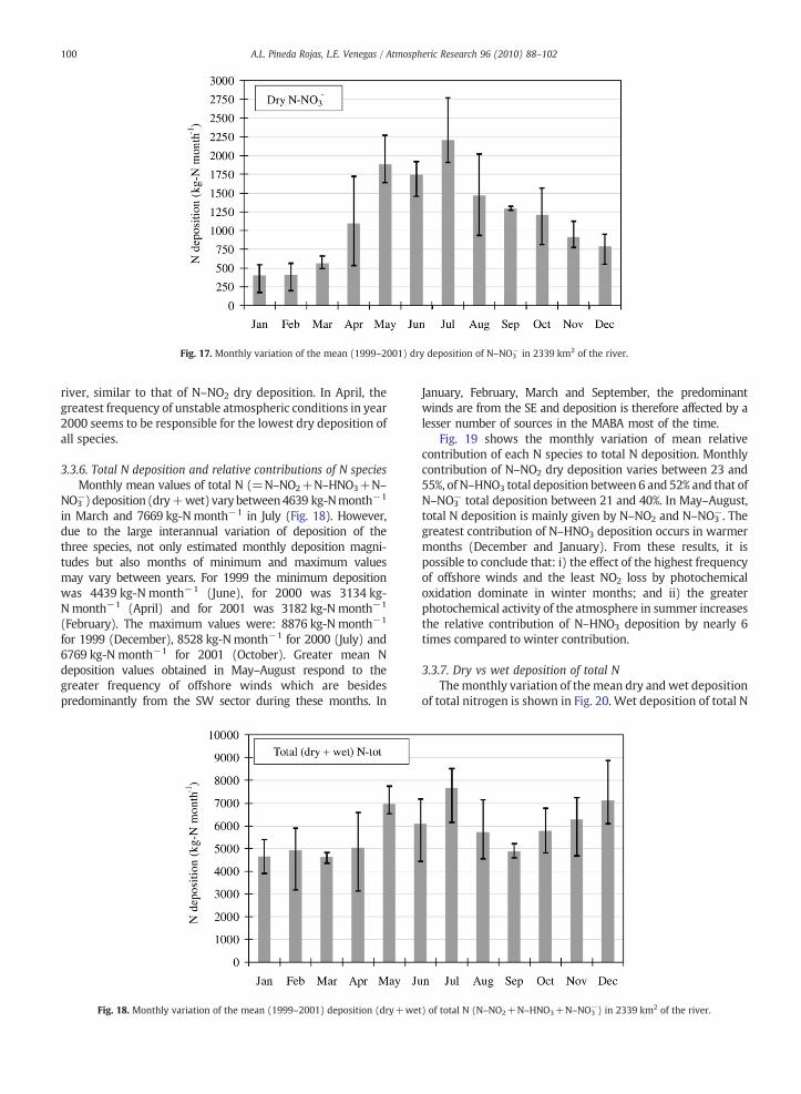
Fig. 17. Monthly variation of the mean (1999–2001) dry deposition of N–NO3− in 2339 km2 of the river.

100 A.L. Pineda Rojas, L.E. Venegas / Atmospheric Research 96 (2010) 88–102

river, similar to that of N–NO2 dry deposition. In April, thegreatest frequency of unstable atmospheric conditions in year2000 seems to be responsible for the lowest dry deposition ofall species.

3.3.6. Total N deposition and relative contributions of N speciesMonthly mean values of total N (=N–NO2+N–HNO3+N–

NO3−)deposition (dry+wet) varybetween4639 kg-Nmonth−1

in March and 7669 kg-Nmonth−1 in July (Fig. 18). However,due to the large interannual variation of deposition of thethree species, not only estimated monthly deposition magni-tudes but also months of minimum and maximum valuesmay vary between years. For 1999 the minimum depositionwas 4439 kg-N month−1 (June), for 2000 was 3134 kg-Nmonth−1 (April) and for 2001 was 3182 kg-Nmonth−1

(February). The maximum values were: 8876 kg-Nmonth−1

for 1999 (December), 8528 kg-Nmonth−1 for 2000 (July) and6769 kg-N month−1 for 2001 (October). Greater mean Ndeposition values obtained in May–August respond to thegreater frequency of offshore winds which are besidespredominantly from the SW sector during these months. In

Fig. 18. Monthly variation of the mean (1999–2001) deposition (dry+we

January, February, March and September, the predominantwinds are from the SE and deposition is therefore affected by alesser number of sources in the MABA most of the time.

Fig. 19 shows the monthly variation of mean relativecontribution of each N species to total N deposition. Monthlycontribution of N–NO2 dry deposition varies between 23 and55%, of N–HNO3 total deposition between 6 and 52% and that ofN–NO3

− total deposition between 21 and 40%. In May–August,total N deposition is mainly given by N–NO2 and N–NO3

−. Thegreatest contribution of N–HNO3 deposition occurs in warmermonths (December and January). From these results, it ispossible to conclude that: i) the effect of the highest frequencyof offshore winds and the least NO2 loss by photochemicaloxidation dominate in winter months; and ii) the greaterphotochemical activity of the atmosphere in summer increasesthe relative contribution of N–HNO3 deposition by nearly 6times compared to winter contribution.

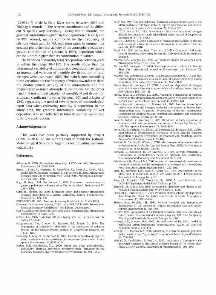
3.3.7. Dry vs wet deposition of total NThemonthly variation of themean dry andwet deposition

of total nitrogen is shown in Fig. 20. Wet deposition of total N

t) of total N (N–NO2+N–HNO3+N–NO3−) in 2339 km2 of the river.

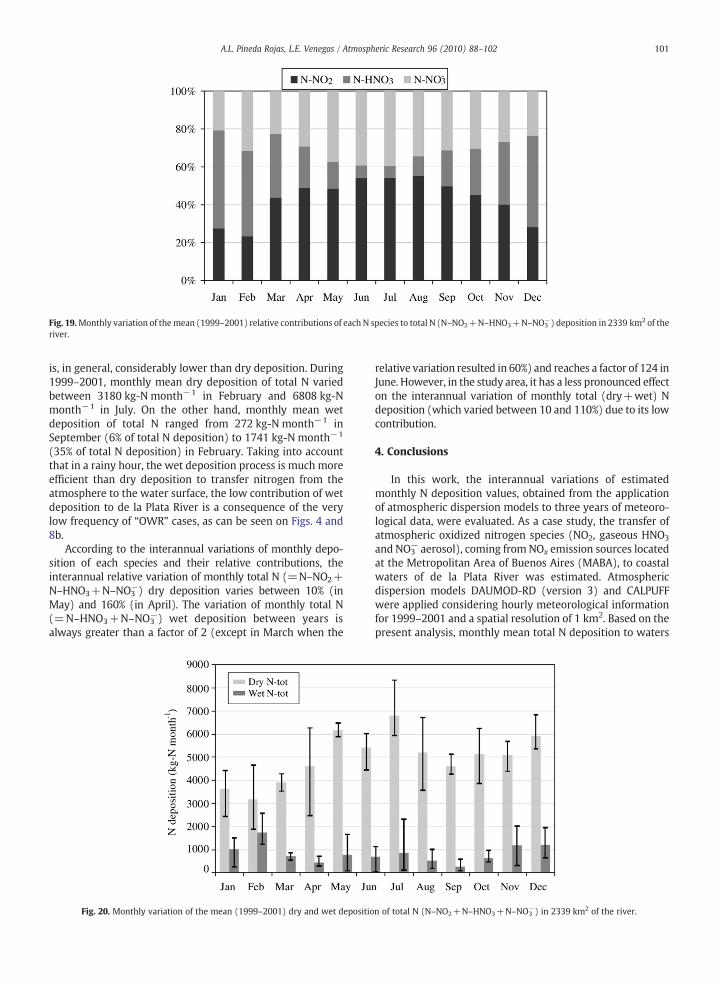
Fig. 19.Monthly variation of themean (1999–2001) relative contributions of each N species to total N (N–NO2+N–HNO3+N–NO3−) deposition in 2339 km2 of the

river.

101A.L. Pineda Rojas, L.E. Venegas / Atmospheric Research 96 (2010) 88–102

is, in general, considerably lower than dry deposition. During1999–2001, monthly mean dry deposition of total N variedbetween 3180 kg-N month−1 in February and 6808 kg-Nmonth−1 in July. On the other hand, monthly mean wetdeposition of total N ranged from 272 kg-N month−1 inSeptember (6% of total N deposition) to 1741 kg-N month−1

(35% of total N deposition) in February. Taking into accountthat in a rainy hour, the wet deposition process is much moreefficient than dry deposition to transfer nitrogen from theatmosphere to the water surface, the low contribution of wetdeposition to de la Plata River is a consequence of the verylow frequency of “OWR” cases, as can be seen on Figs. 4 and8b.

According to the interannual variations of monthly depo-sition of each species and their relative contributions, theinterannual relative variation of monthly total N (=N–NO2+N–HNO3+N–NO3

−) dry deposition varies between 10% (inMay) and 160% (in April). The variation of monthly total N(=N–HNO3+N–NO3

−) wet deposition between years isalways greater than a factor of 2 (except in March when the

Fig. 20. Monthly variation of the mean (1999–2001) dry and wet depositio

relative variation resulted in 60%) and reaches a factor of 124 inJune. However, in the study area, it has a less pronounced effecton the interannual variation of monthly total (dry+wet) Ndeposition (which varied between 10 and 110%) due to its lowcontribution.

4. Conclusions

In this work, the interannual variations of estimatedmonthly N deposition values, obtained from the applicationof atmospheric dispersion models to three years of meteoro-logical data, were evaluated. As a case study, the transfer ofatmospheric oxidized nitrogen species (NO2, gaseous HNO3

and NO3− aerosol), coming from NOx emission sources located

at the Metropolitan Area of Buenos Aires (MABA), to coastalwaters of de la Plata River was estimated. Atmosphericdispersion models DAUMOD-RD (version 3) and CALPUFFwere applied considering hourly meteorological informationfor 1999–2001 and a spatial resolution of 1 km2. Based on thepresent analysis, monthly mean total N deposition to waters

n of total N (N–NO2+N–HNO3+N–NO3−) in 2339 km2 of the river.

102 A.L. Pineda Rojas, L.E. Venegas / Atmospheric Research 96 (2010) 88–102

(2339 km2) of de la Plata River varies between 4639 and7669 kg-N month−1. The relative contributions of the differ-ent N species vary seasonally. During winter months, thegreatest contribution is given by the deposition of N–NO2 andN–NO3

− aerosol, mainly controlled by the frequency ofoffshore winds and the NOx oxidation rates. In summer, thegreatest photochemical activity of the atmosphere leads to agreater contribution of gaseous N–HNO3 deposition whichcan be 6 times higher than its contribution in winter.

The variation of monthly total N deposition between yearsis within the range 10–110%. The results show that theinterannual variability of atmospheric conditions may lead toan interannual variation of monthly dry deposition of totalnitrogen which can reach 160%. The main factors controllingthese variations are the frequency of winds towards the river,the photochemical activity of the atmosphere and thefrequency of unstable atmospheric conditions. On the otherhand, the interannual variation of monthly N wet depositionis always significant (it varies between 60% and a factor of124), suggesting the need of several years of meteorologicalinput data when estimating monthly N deposition. In thestudy area, the greatest interannual variability of wetdeposition was not reflected in total deposition values dueto its low contribution.

Acknowledgements

This work has been partially supported by ProjectCONICET-PIP 6169. The authors wish to thank the NationalMeteorological Service of Argentina for providing meteoro-logical data.

References

Atkinson, R., 2000. Atmospheric chemistry of VOCs and NOx. AtmosphericEnvironment 34, 2063–2101.

Bencs, L., Krata, A., Horemans, B., Buczyńska, A.J., Dirtu, A.C., Godoi, A.F.L.,Godoi, R.H.M., Potgieter-Vermaak, S., Van Grieken, R., 2009. Atmosphericnitrogen fluxes at the Belgian coast: 2004–2006. Atmospheric Environ-ment 43, 3786–3798.

Bogo, H., Negri, R.M., San Roman, E., 1999. Continuous measurement ofgaseous pollutants in Buenos Aires City. Atmospheric Environment 33,2587–2598.

Clark, H., Kremer, J.N., 2005. Estimating direct and episodic atmosphericnitrogen deposition to a coastal waterbody. Marine EnvironmentalResearch 59, 349–366.

EMEP/CORINAIR, 2001. Emission Inventory Guidebook. Air Traffic B851.European Environment Agency, 2001. Joint EMEP/CORINAIR Atmospheric

Emission Inventory Guidebook, Third Edition. Copenhagen.Gao, Y., 2002. Atmospheric nitrogen deposition to Barnegat Bay. Atmospheric

Environment 36, 5783–5794.Gifford, F.A., 1976. Turbulent diffusion typing schemes: a review. Nuclear

Safety 17, 25–43.Hauglustaine, D.A., Granier, C., Brasseur, G.P., Megie, G., 1994. The

importance of atmospheric chemistry in the calculation of radiativeforcing on the climate system. Journal of Geophysical Research 99,1173–1186.

Holloway, T., Levy, H., Carmichael, G., 2002. Transfer of reactive nitrogen inAsia: development and evaluation of a source–receptor model. Atmo-spheric Environment 36, 4251–4264.

Jenkin, M.E., Clemitshaw, K.C., 2000. Ozone and other photochemicalpollutants: chemical processes governing their formation in theplanetary boundary layer. Atmospheric Environment 34, 2499–2527.

Kelly, N.A., 1987. The photochemical formation and fate of nitric acid in theMetropolitan Detroit Area: ambient, captive-air irradiation and model-ing results. Atmospheric Environment 21, 2163–2177.

Lee, Y., Schwartz, S.E., 1981. Evaluation of the rate of uptake of nitrogendioxide by atmospheric and surface liquid water. Journal of GeophysicalResearch 86, 11971–11983.

Lin, L.-C., Cheng, M.-T., 2007. Evaluation of formation rates of NO2 to gaseousand particulate nitrate in the urban atmosphere. Atmospheric Environ-ment 41, 1903–1910.

Maul, P.R., 1980. Atmospheric Transport of Sulfur Compound Pollutants.Central Electricity Generating Bureau MID/SSD/80/0026/R, Nottingham,England.

Mazzeo, N.A., Venegas, L.E., 1991. Air pollution model for an urban area.Atmospheric Research 26, 165–179.

Mazzeo, N.A., Venegas, L.E., 2004. Some aspects of air pollution in BuenosAires City. International Journal of Environment and Pollution 22,365–379.

Mazzeo, N.A., Venegas, L.E., Choren, H., 2005. Analysis of NO, NO2, O3 and NOx

concentrations measured at a green area of Buenos Aires City duringwintertime. Atmospheric Environment 39, 3055–3068.

Pineda Rojas, A.L., Venegas, L.E., 2008. Dry and wet deposition of nitrogenemitted in Buenos Aires city to waters of de la Plata River. Water, Air, andSoil Pollution 193, 175–188.

Pineda Rojas, A.L., Venegas, L.E., 2009. Atmospheric deposition of nitrogenemitted in the Metropolitan Area of Buenos Aires to coastal waters of dela Plata River. Atmospheric Environment 43, 1339–1348.

Pineda Rojas, A.L., Venegas, L.E., Mazzeo, N.A., 2007. Emission inventory ofcarbon monoxide and nitrogen oxides for area sources at Buenos AiresMetropolitan Area (Argentina). Proceedings of the 6th InternationalConference on Urban Air Quality, EmissionMeasurements andModellingSessions, Limassol, Cyprus, pp. 35–38.

Poor, N., Pribble, R., Greening, H., 2001. Direct wet and dry deposition ofammonia, nitric acid, ammonium and nitrate to Tampa Bay Estuary, FL,USA. Atmospheric Environment 35, 3947–3955.

Pryor, S.C., Barthelmie, R.J., Schoof, J.T., Sorensen, L.L., Erickson III, D.J., 2001.Implications of heterogeneous chemistry of nitric acid for nitrogendeposition to marine ecosystems: observations and modelling. Water,Air, and Soil Pollution: Focus 1, 99–107.

Rideout, G., Gourley, D., Walker, J., 2005. Measurement of in-service vehicleemissions in Sao Paulo, Santiago and Buenos Aires. ARPEL EnvironmentalReport # 25. ESAA, Ottawa, Canada.

Romano, D., Gaudioso, D., De Lauretis, R., 1999. Aircraft emissions: acomparison of methodologies based on different data availability.Environmental Monitoring and Assessment 56, 51–74.

Schlünzen, K.H., Meyer, E.M.I., 2007. Impacts of meteorological situations andchemical reactions on daily dry deposition of nitrogen into the southernNorth Sea. Atmospheric Environment 41, 289–302.

Scire, J.S., Lurmann, F.W., Bass, A., Hanna, S.R., 1984. Development of theMESOPUFF II dispersion model. EPA-600/3-84-057. EnvironmentalResearch & Technology Inc, p. 91.

Scire, J.S., Strimaitis, D.G., Yamartino, R.J., 2000. A User's Guide for theCALPUFF Dispersion Model. Earth Tech Inc, p. 521.

Seinfeld, J.H., Pandis, S.N., 2006. Atmospheric Chemistry and Physics of AirPollution, Second Edition. John Wiley & Sons, p. 1326.

Sickles II, J.E., Shadwick, D.S., 2002. Precision of atmospheric dry depositiondata from the Clean Air Status and Trends Network. AtmosphericEnvironment 36, 5671–5686.

Stelson, A.W., Seinfeld, J.H., 1982. Relative humidity and temperaturedependence of the ammonium nitrate dissociation constant. Atmo-spheric Environment 16, 983–992.

US EPA, 1995. Compilation of Air Pollution Emission Factors, AP-42, 5th ed.United States Environmental Protection Agency, Office of Air QualityPlanning and Standards, Research Triangle Park, NC.

Venegas, L.E., Mazzeo, N.A., 2002. An evaluation of DAUMOD model inestimating urban background concentrations. Water, Air and SoilPollution: Focus 2, 433–443.

Venegas, L.E., Mazzeo, N.A., 2006. Modelling of urban background pollutionin Buenos Aires city (Argentina). Environmental Modelling and Software21, 577–586.

Whitall, D., Hendrickson, B., Paerl, H., 2003. Importance of atmosphericallydeposited nitrogen to the annual nitrogen budget of the Neuse Riverestuary, North Carolina. Environment International 29, 393–399.