Interactive Visualization of Functional Brain Connectivity Master’s Thesis André van Dixhoorn

Welcome message from author
This document is posted to help you gain knowledge. Please leave a comment to let me know what you think about it! Share it to your friends and learn new things together.
Transcript

Interactive Visualization of
Functional Brain Connectivity
Master’s Thesis
André van Dixhoorn


Interactive Visualization of
Functional Brain Connectivity
THESIS
submitted in partial fulfillment of the
requirements for the degree of
MASTER OF SCIENCE
in
COMPUTER SCIENCE
by
André van Dixhoorn
born in Terneuzen, the Netherlands
Section Computer Graphics and Visualization
Deptartment of Intelligent Systems
Faculty EEMCS, Delft University of Technology
Delft, the Netherlands
http://graphics.tudelft.nl
Division of Image Processing
Department of Radiology
Leiden University Medical Center
Leiden, the Netherlands
www.lumc.nl

© 2011 André van Dixhoorn.
Cover picture: A combination of techniques for the visualization of functional brain con-
nectivity in spatial context, from both tools presented in this thesis.
Interactive Visualization of
Functional Brain Connectivity
Author: André van Dixhoorn
Student id: 1183044
Email: [email protected]
Abstract
Functional brain connectivity from fMRI studies has become an important tool
in studying functional interactions in the human brain as a complex network. The
correlation between the fMRI activity traces of distinct brain regions indicates to
what extent they are functionally connected. fMRI connectivity data typically con-
sists of a matrix of correlations, also denoted as functional correlations, either at the
voxel level or averaged over anatomically defined brain regions using an anatomical
template such as the Automated Anatomical Labeling (AAL).
In this thesis, we present methods for the interactive visualization of functional
brain connectivity, both for region-based connectivity matrices and for correlation
data at voxel resolution. The techniques were implemented in two different visual
analysis applications, containing different representations that are coupled, sup-
porting linked interaction. A GPU-accelerated raycasting technique was used to
enable the real-time visualization of the voxel-wise functional brain networks. We
have evaluated our tools via case studies with domain scientists at two different uni-
versity medical centers.
Thesis Committee:
Chair: Prof. Dr. Ir. F.W. Jansen, Faculty EEMCS, TU Delft
University supervisor: Dr. C.P. Botha, Faculty EEMCS, TU Delft
Company supervisor: Dr. J.R. Milles, Department of Radiology, LUMC

Preface
The research discussed in this Master’s thesis is the final step in obtaining the Master of
Science degree in Computer Science at Delft University of Technology, The Netherlands.
It describes the results of work that was performed in the Section Computer Graphics
and Visualization (Department of Intelligent Systems) at Delft University during the last
year-and-a-bit.
This work would not have come to fruition without the people involved in this group. I
would to thank the following people in particular:
First of all, my daily supervisor, dr. Charl P. Botha. His dedication and commitment,
and not to mention his overwhelming enthusiasm, have surely brought the best out of
me (and many other of his ‘ducklings’ before). His optimistic view helped me to recon-
sider my often skeptical attitude towards my own contributions.
I would also like to express my gratitude to Julien Milles of the LUMC, for providing
the required background knowledge on the topic, organizing evaluation sessions and
his fruitful comments and new ideas and to Matthan Caan for organizing an evaluation
session at the AMC.
Thanks also to Bastijn Vissers for always being ready for a good discussion during a
coffee break, which at numerous times helped me to step back from a problem and re-
view it again from a higher level. His involvement in my project was greatly appreciated.
Likewise, I would like to thank Noeska, Thomas Gerwin, François, Nick, Christian and all
Peters in the group for the enjoyable time during the lunch break and numerous ‘kitchen
talks’. The informal work culture in the group provided a pleasant and supportive work-
ing atmosphere.
Finally, I would like to thank my friends and family, who have always supported
me and believed unconditionally in my work. I am especially grateful to my girlfriend,
Monique, who helped me to clear my mind, put things into perspective and encouraged
me to finally finish my thesis work.
André van Dixhoorn
Delft, the Netherlands
December 23, 2011
iii


Contents
Preface iii
Contents v
List of Figures vii
1 Introduction 1
1.1 Context . . . . . . . . . . . . . . . . . . . . . . . . . . . . . . . . . . . . . . . . 1
1.2 Motivation . . . . . . . . . . . . . . . . . . . . . . . . . . . . . . . . . . . . . . 2
1.3 Research Questions . . . . . . . . . . . . . . . . . . . . . . . . . . . . . . . . . 4
1.4 Contributions . . . . . . . . . . . . . . . . . . . . . . . . . . . . . . . . . . . . 4
1.5 Structure of this thesis . . . . . . . . . . . . . . . . . . . . . . . . . . . . . . . 5
2 Background and related work 7
2.1 Developments in neuro imaging . . . . . . . . . . . . . . . . . . . . . . . . . 7
2.2 Related work . . . . . . . . . . . . . . . . . . . . . . . . . . . . . . . . . . . . . 10
2.3 The basics of raycasting . . . . . . . . . . . . . . . . . . . . . . . . . . . . . . . 17
3 Visual analysis of integrated resting state functional brain connectivity and
anatomy 19
3.1 Introduction . . . . . . . . . . . . . . . . . . . . . . . . . . . . . . . . . . . . . 20
3.2 Related work . . . . . . . . . . . . . . . . . . . . . . . . . . . . . . . . . . . . . 21
3.3 Method . . . . . . . . . . . . . . . . . . . . . . . . . . . . . . . . . . . . . . . . 23
3.4 Implementation . . . . . . . . . . . . . . . . . . . . . . . . . . . . . . . . . . . 27
3.5 Evaluation . . . . . . . . . . . . . . . . . . . . . . . . . . . . . . . . . . . . . . 28
3.6 Conclusions and Future Work . . . . . . . . . . . . . . . . . . . . . . . . . . . 32
4 Interactive visualization of voxel-wise fMRI brain connectivity 33
4.1 Data preprocessing . . . . . . . . . . . . . . . . . . . . . . . . . . . . . . . . . 33
4.2 Visualization Pipeline . . . . . . . . . . . . . . . . . . . . . . . . . . . . . . . . 36
4.3 Direct Matrix Visualization . . . . . . . . . . . . . . . . . . . . . . . . . . . . . 39
v

CONTENTS
4.4 Anatomical Visualization . . . . . . . . . . . . . . . . . . . . . . . . . . . . . . 43
4.5 Pseudo anatomical visualization . . . . . . . . . . . . . . . . . . . . . . . . . 55
4.6 Linking the visualizations . . . . . . . . . . . . . . . . . . . . . . . . . . . . . 61
4.7 Comparative visualization . . . . . . . . . . . . . . . . . . . . . . . . . . . . . 64
4.8 Evaluation . . . . . . . . . . . . . . . . . . . . . . . . . . . . . . . . . . . . . . 66
5 Implementation of voxel-wise connectivity visualization: selected topics 73
5.1 Used libraries and tools . . . . . . . . . . . . . . . . . . . . . . . . . . . . . . . 73
5.2 General implementation notes . . . . . . . . . . . . . . . . . . . . . . . . . . 74
5.3 Direct Matrix Visualization . . . . . . . . . . . . . . . . . . . . . . . . . . . . . 79
5.4 Anatomical Visualization . . . . . . . . . . . . . . . . . . . . . . . . . . . . . . 81
5.5 Technical challenges . . . . . . . . . . . . . . . . . . . . . . . . . . . . . . . . 83
6 Conclusions and Future Work 87
6.1 Summary . . . . . . . . . . . . . . . . . . . . . . . . . . . . . . . . . . . . . . . 87
6.2 Discussion . . . . . . . . . . . . . . . . . . . . . . . . . . . . . . . . . . . . . . 88
6.3 Future work . . . . . . . . . . . . . . . . . . . . . . . . . . . . . . . . . . . . . . 89
Bibliography 91
A BrainCove: A tool for voxel-wise fMRI brain connectivity visualization 107
A.1 Introduction . . . . . . . . . . . . . . . . . . . . . . . . . . . . . . . . . . . . . 107
A.2 Related work . . . . . . . . . . . . . . . . . . . . . . . . . . . . . . . . . . . . . 108
A.3 Method . . . . . . . . . . . . . . . . . . . . . . . . . . . . . . . . . . . . . . . . 110
A.4 Implementation . . . . . . . . . . . . . . . . . . . . . . . . . . . . . . . . . . . 117
A.5 Evaluation . . . . . . . . . . . . . . . . . . . . . . . . . . . . . . . . . . . . . . 117
A.6 Conclusions . . . . . . . . . . . . . . . . . . . . . . . . . . . . . . . . . . . . . 121
vi
List of Figures
1.1 Analysis pipeline for functional brain connectivity . . . . . . . . . . . . . . . . . 2
2.1 Network data shown as a matrix bitmap . . . . . . . . . . . . . . . . . . . . . . . 11
2.2 The effect of reordering rows and columns of a pixmap . . . . . . . . . . . . . . 11
2.3 Visualization of large correlation matrices with a tile-based technique . . . . . 12
2.4 A node-link visualization of the whole-brain, voxel-wise functional connectome 13
2.5 Brain activation from fMRI shown as patch of colour on a MRI scan . . . . . . . 13
2.6 Visual representations of resting-state networks from a group ICA study . . . . 14
2.7 Visual representation of fMRI activity data in 3-D . . . . . . . . . . . . . . . . . 14
2.8 A screenshot of the ConnectomeViewer application . . . . . . . . . . . . . . . . 15
2.9 The interactive visualization tool for functional connectivity analysis by Ek-
lund et al. . . . . . . . . . . . . . . . . . . . . . . . . . . . . . . . . . . . . . . . . . 17
2.10 Overview of the basic raycasting algorithm . . . . . . . . . . . . . . . . . . . . . 18
2.11 Linear interpolation using 8 samples . . . . . . . . . . . . . . . . . . . . . . . . . 18
3.1 Screenshot of the application for region-based visual analysis . . . . . . . . . . 22
3.2 The matrix bitmap with several links highlighted . . . . . . . . . . . . . . . . . . 25
3.3 Hierarchical Edge Bundles view with multiple links selected . . . . . . . . . . . 27
3.4 Identifying outliers using the scatter plot . . . . . . . . . . . . . . . . . . . . . . . 29
3.5 The Scatterplot View showing and hiding the symmetric intra-hemispheric
connections . . . . . . . . . . . . . . . . . . . . . . . . . . . . . . . . . . . . . . . . 30
4.1 Screenshot of each of the three implemented visualizations . . . . . . . . . . . 37
4.2 The visualization pipeline . . . . . . . . . . . . . . . . . . . . . . . . . . . . . . . 38
4.3 The basic idea of raycasting the correlation matrix . . . . . . . . . . . . . . . . . 40
4.4 Raycasting functional connectivity in an anatomical representation of the brain 45
4.5 Looking up the correlation value between a seed voxel and a voxel in the volume 45
4.6 Blocky artifacts due to undersampling of the index volume . . . . . . . . . . . . 46
4.7 The complete pipeline for the two-pass raycasting of the correlation volume . 47
4.8 Smooth rendering of the correlation volume using the two-pass approach . . . 48
4.9 World to volume transformations . . . . . . . . . . . . . . . . . . . . . . . . . . . 51
vii

LIST OF FIGURES
4.10 A coronal section of the brain . . . . . . . . . . . . . . . . . . . . . . . . . . . . . 52
4.11 Splitting the brain . . . . . . . . . . . . . . . . . . . . . . . . . . . . . . . . . . . . 54
4.12 Mercator projection of the world . . . . . . . . . . . . . . . . . . . . . . . . . . . 56
4.13 2D mapping of the cerebral cortex using circle packing . . . . . . . . . . . . . . 57
4.14 A cross-section diagram showing the geometrical concept of the Lambert’s
projection . . . . . . . . . . . . . . . . . . . . . . . . . . . . . . . . . . . . . . . . . 58
4.15 A cross-section diagram showing the geometrical concept of the Braun’s pro-
jection . . . . . . . . . . . . . . . . . . . . . . . . . . . . . . . . . . . . . . . . . . . 59
4.16 Deriving the ray path for Braun’s projection . . . . . . . . . . . . . . . . . . . . . 59
4.17 The Lambert’s Cylindrical flatmap representation of the brain . . . . . . . . . . 60
4.18 The coordinated linking between the pixmap and anatomical representation . 63
4.19 A screenshot of the application when two datasets are opened . . . . . . . . . . 65
5.1 An overview of the main components of the application . . . . . . . . . . . . . 74
5.2 The general rendering pipeline . . . . . . . . . . . . . . . . . . . . . . . . . . . . 75
5.3 A class diagram of the custom vtkMappers . . . . . . . . . . . . . . . . . . . . . . 76
5.4 The interaction between classes during the initialization of the CLRayCaster
object . . . . . . . . . . . . . . . . . . . . . . . . . . . . . . . . . . . . . . . . . . . 77
5.5 The interaction between classes during the a user interaction . . . . . . . . . . 78
5.6 The customized VTK volume rendering pipeline for the direct matrix visual-
ization . . . . . . . . . . . . . . . . . . . . . . . . . . . . . . . . . . . . . . . . . . . 79
5.7 Sharing OpenCL memory objects from a single OpenCL context with multiple
OpenGL contexts . . . . . . . . . . . . . . . . . . . . . . . . . . . . . . . . . . . . . 84
5.8 Difference in 3-D volume support between OpenCL implementations . . . . . 85
A.1 An overview of the application window with two datasets . . . . . . . . . . . . . 111
A.2 Reordering the rows and columns using the AAL template . . . . . . . . . . . . 111
A.3 The basic idea of raycasting the correlation matrix . . . . . . . . . . . . . . . . . 112
A.4 Brushing the matrix representation highlights the selected voxels in the anatom-
ical view . . . . . . . . . . . . . . . . . . . . . . . . . . . . . . . . . . . . . . . . . . 113
A.5 Interactively selecting seed voxels on the cortical surface . . . . . . . . . . . . . 114
A.6 The complete pipeline for the two-pass raycasting of the correlation volume . 115
A.7 Splitting the brain . . . . . . . . . . . . . . . . . . . . . . . . . . . . . . . . . . . . 116
A.8 The Lambert’s Cylindrical flatmap representation of the brain . . . . . . . . . . 117
viii
CHAPTER 1
Introduction
In this chapter, we introduce the concept of functional brain connectivity and motivate
the use of visualization techniques in this context. We then present our main research
questions and specify the main contributions represented by this work.
1.1 Context
With functional MRI (fMRI) connectivity, the functional connections between different
parts of the brain can be measured non-invasively, in vivo and in 3-D, down to the voxel
level. Functional connections can be studied during the performance of a task, such that
the brain networks involved in completing that task can be identified. Research in this
area has found numerous networks that are activated during the performance of various
tasks, such as the motor, primary sensory language and attention networks [Raichle 07].
Another field of research that recently attracted attention in the field is the study of
the functional connections during resting state, in order to shed light on the intrinsic
connectivity networks of the brain. In resting state functional brain connectivity, the
subject is asked to lie at rest (commonly with their eyes closed) and not to think about
anything special.
Functional brain connectivity has already proven itself to be a valuable tool for re-
search in areas related to cognitive psychology, neuroscience and behavioral studies.
Traditional approaches in fMRI connectivity research used a seed-based approach, where
only the brain regions connected to a selected seed region are derived, or independent
component analysis (ICA) to describe the functional connectivity networks.
Just recently, researchers have begun to focus on whole-brain networks, applying
concepts from graph theory that enable more complete studies of brain networks than
the aforementioned traditional methods. The first studies focused on inter-regional con-
nectivity, where the properties of the brain network were explored by measuring the con-
nectivity between all anatomical brain regions, such as the 90 cortical and sub-cortical
regions of the AAL template [Biswal 95].
Later, research has also started to focus on functional brain connectivity at the voxel
level [van den Heuvel 08a]. The resulting connectivity networks are several orders of
1
1. INTRODUCTION
magnitude larger than the region-based connectivity networks. In a typical 4mm isotropic
resolution, the raw BOLD-fMRI image contains about 20,000 voxels, and the resulting
network thus consists of 20,000 nodes and 400,000,000 links (including symmetrical links).
1.2 Motivation
The existing methods for analysis of functional connectivity, whether they are focusing
on finding independent networks or based on graph-theoretic concepts are computa-
tionally intensive and completely offline. In the current workflow, researchers follow a
typical process of data acquisition, data preprocessing and the actual analysis. Most of
the tasks in acquisition and preprocessing are automated using standard tools that are
widely used in the field, such as SPM1, FSL2, DPARSF3, a combination of SPM and REST4
or commercial packages such as Brain Voyager QX5. The actual data analysis can also
be performed using these tools, or is performed using in-house developed algorithms in
environments such as Matlab.
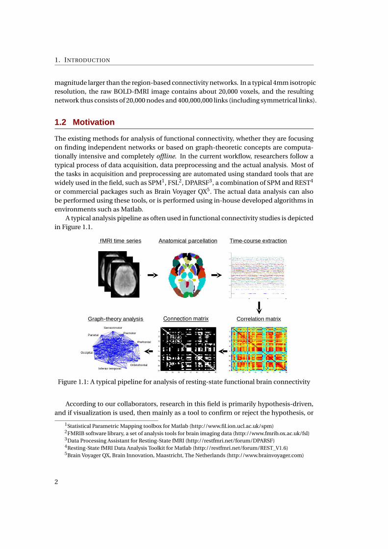
A typical analysis pipeline as often used in functional connectivity studies is depicted
in Figure 1.1.
Figure 1.1: A typical pipeline for analysis of resting-state functional brain connectivity
According to our collaborators, research in this field is primarily hypothesis-driven,
and if visualization is used, then mainly as a tool to confirm or reject the hypothesis, or
1Statistical Parametric Mapping toolbox for Matlab (http://www.fil.ion.ucl.ac.uk/spm)2FMRIB software library, a set of analysis tools for brain imaging data (http://www.fmrib.ox.ac.uk/fsl)3Data Processing Assistant for Resting-State fMRI (http://restfmri.net/forum/DPARSF)4Resting-State fMRI Data Analysis Toolkit for Matlab (http://restfmri.net/forum/REST_V1.6)5Brain Voyager QX, Brain Innovation, Maastricht, The Netherlands (http://www.brainvoyager.com)
2

1.2. Motivation
presenting the results in a paper at the very end of the research pipeline. Using visual-
ization for hypothesis confirmation is usually referred to as confirmatory visual analy-
sis [Garcia 04].
In resting-state fMRI and fMRI studies in general, the visual representations used
are often two-dimensional image slices (usually sagittal, coronal or transverse planes)
of anatomical (MRI) data with activated (or functionally connected) brain regions high-
lighted on top [Rehm 98]. For the visualization of resting-state connectivity networks,
techniques similar to those for fMRI are can be employed, by considering the compo-
nents in the resting-state network as activated brain regions, rendering them as overlay
on higher resolution anatomical scans, color coded by their significance.
For visualization of whole brain fMRI connectivity data, other methods have to be
employed. Whereas the networks from seed-based analysis or ICA consist of a limited
number of (separated) brain regions, full brain fMRI connectivity by definition studies
the network consisting of all individual brain regions. Thus, simply rendering the corre-
sponding regions as overlay on a structural scan is not an option (this would highlight
the entire image).
To reduce the computational burden during the analysis, researchers typically averaged
the connectivity over anatomically defined brain regions using an anatomical template
such as the Automated Anatomical Labeling (AAL). The reduced network size enabled
the visualization of the networks using the node-link diagrams. However, even when us-
ing a network where anatomical template such as the Automated Anatomical Labeling
(AAL), containing just 90 nodes, filtering on the link strength is required to remove a large
portion of the links that would otherwise cause visual clutter in the view.
With increasing computational power, studies on functional brain connectivity at
voxel-level become more popular [Ferrarini 11, Tomasi 10, van den Heuvel 08a]. The
higher resolution is considered to provide a more accurate description of the underly-
ing topological network [Ferrarini 11], making it an important factor in studies on the
topological organization of the functional connectivity brain networks.
Although the application of both region-based and voxel-wise functional brain con-
nectivity has become widespread in research and clinical settings, the visualization and
visual analysis of this type of data has yet seen little attention: methods for the interac-
tive visualization of functional brain networks are still scarce.
In this thesis, we present two tools that facilitate the interactive visualization of func-
tional brain connectivity. We first present an application for the visual analysis of region-
based resting-state fMRI brain connectivity data that links information visualization dis-
plays with three dimensional visualizations that represent the data in its spatial context.
The visual analysis tool contains numerous methods for interactive filtering of the data
and the identification of outliers. We show the effectiveness of this tool by reproducing
important findings from the literature and by means of a case study evaluation with two
domain experts.
We then present a toolkit for the visualization of the large brain networks from voxel-
wise studies with highly interactive matrix representations and 3-D spatial representa-
3
1. INTRODUCTION
tions, implemented in a raycasting framework that enables interactive exploration of the
data. One of the unique aspects of this technique is the side-by-side coupled visualiza-
tion of two of these voxel-based brain networks, enabling their direct visual comparison.
To our knowledge, this is the first report of a technique integrating real-time correlation
matrix and spatial context visualization that enables this type of visual comparison for
voxel-based functional connectivity networks. Furthermore, we employ a flat-map rep-
resentation for showing the connectivity data in spatial context with minimal occlusion,
as well as real-time correlation volume splitting to enable visualization of and interaction
also with interior volumes of the brain between the two lobes.
1.3 Research Questions
The main research question can be formulated as follows:
How can we visualize whole-brain functional MRI connectivity data in a way
that facilitates explorative visual analysis of the data and visual comparison
between datasets?
To answer this question, the following research topics will be studied:
• What techniques can be used to represent the complete connectivity matrix both
directly and in its spatial context?
• What methods should be used to facilitate real-time interaction with the visual
representations, such as filtering and zoom-and-pan interaction?
• How can the visual representations be used to enable visual comparison between
datasets?
• How can we visually represent the strength of the connection between distinct
brain regions?
The main technical challenge is the implementation of techniques for the coordi-
nated linking between multiple views and methods that are able to deal with large cor-
relation matrices (up to 1 gigabyte in size), while maintaining interactive frame-rates
on desktop PCs. Furthermore, the massive amount of connections demands a carefully
designed visual representation to show the connections with minimal amount of visual
clutter.
1.4 Contributions
The contributions of this thesis are:
• We present a visual analysis approach for studying connectivity in region-based
functional MRI data that couples information and scientific visualization views.
4
1.5. Structure of this thesis
• We introduce a representation method based on a circular node-link layout in
combination with hierarchical edge bundling that shows the connectivity between
regions in the context of anatomical hierarchy
• We present a technique with which large voxel-based fMRI connectivity matrices
of around twenty-thousand by twenty-thousand correlations can be interactively
visualized on a desktop PC, both directly and in their anatomical context.
• We introduce a method that allows for the interactive visual comparison of multi-
ple of these large connectivity matrices in a side-by-side or difference visualization,
which, to the best of our knowledge, has not been shown before.
• We evaluate our approaches by reproducing important findings from literature,
and by performing a case study with groups of domain scientists from different
university medical centers
• We introduce a raycasting framework for the interactive visualization of large cor-
relation matrices
1.5 Structure of this thesis
In the next chapter, the reader is presented with a more elaborate description of the med-
ical and scientifical context in which this research is conducted and discuss the clinical
relevance of the modality of functional brain connectivity. In the same chapter, we will
furthermore discuss some concepts that are important in the development of our meth-
ods and give an overview of existing work from the literature that is related to our subject.
In Chapter 3, we presented our tool for the visual analysis of region based resting-
state functional brain connectivity. The main work in this thesis is the implementation
of interactive visualization techniques for voxel-wise functional brain connectivity. The
methods and evaluation of our methods (by means of a performance evaluation and a
case study with domain experts from two university medical centers) of this work are
presented in Chapter 4. This chapter is a superset of a paper on this subject, recently
submitted. A pre-print of this paper can be found in Appendix A.
Relevant implementation details and important technical challenges and issues are
discussed in Chapter 5.
Finally, a general discussion about the voxel-wise visualization tool with conclusions
and recommendations for future work is given in Chapter 6. Appendix A contains the
paper that summarizes the work from Chapter 4. This paper is submitted to EuroVis
2012.
5


CHAPTER 2
Background and related work
In this chapter, we will discuss background concepts that will facilitate in a better under-
standing of the topic of this thesis. We will start with a more elaborate discussion about
the development of fMRI connectivity to highlight the relevance of functional connec-
tivity in scientific and clinical setting. Furthermore, this chapter discusses work from the
literature that is relevant in the topic of visualizing network data and functional brain
networks in particular. We conclude with a description of some important concepts used
in the implementation of our method.
2.1 Developments in neuro imaging
The advent of non-invasive imaging techniques has given a massive boost to scientific
research of the human brain. Until recently, the only way scientists could see in the brain
for research on diseases and brain function, was by brain autopsy after the patient had
died. Autopsy studies revealed the structural features of the brain, such as shape, size
and cellular and chemical circuitry of the brain structure [Orrison 00]. However, because
this examination could only be done at one point in time, many questions about the
development of diseases in and maturing of the brain remained unanswered. To answer
these questions and to enable diagnosis and treatment planning, studies of the brain in
vivo were required.
The first technique (in the 1900s) that enabled researchers and clinicians to see im-
ages of the brain in living humans was pneumoencephalography (PEG), an X-ray tech-
nique that consisted of replacing spinal fluid with air to show the brain more clearly on an
X-ray image. However, this method was a considered dangerous and extremely painful
for the patient, causing severe headaches and a long recovery period [Marcus E. 09]. For-
tunately, the introduction of new imaging techniques developed in the 1970s and 1980s
rendered this method obsolete [Filler 09].
One of these new imaging techniques, also using X-rays, was computerized (axial) to-
mography (CAT or CT). The CT scanner (for which its inventors Hounsfield and Cormack
were awarded the Nobel Prize in Physiology or Medicine in 1979) received enormous at-
tention and has, since its invention in 1971, seen a constant stream of improvements.
7

2. BACKGROUND AND RELATED WORK
Today, CT is still one of the most important methods of radiological diagnosis [Fuchs 01].
CT is typically used for diagnosis of many types of cancer, assessment of pulmonary em-
bolisms and abdominal aortic aneurysms and invaluable in diagnosing and treatment
of skeletal structures because of the clear images it is able to produce of bone structure,
blood vessels and muscle tissue [Aisen 86].
The other ground-breaking imaging technique, developed more or less concurrently
with CT, is magnetic resonance imaging (MRI). Unlike CT, this method does not expose
the patient to the (potentially harmful) radiation of X-ray imaging, but uses a strong mag-
netic field to align hydrogen atoms in the body from which it generates the image. MRI
has a superior image resolution and differentiation of soft tissue, which makes it espe-
cially useful in neuroimaging [Aisen 86].
There are some important limitations involved with both imaging techniques. First
of all, the radiation exposure involved by CT imaging has been estimated to increase
the probability of lifetime cancer mortality, especially for children [Semelka 07, Bren-
ner 01, De Mauri 11, Smith-Bindman 09]. MRI does not use the radiation, but has the
disadvantage that the scan takes longer to complete which increases the risk for claus-
trophobic reactions [Murphy 97].
Another important limitation of traditional CT and MRI is that they can only be used
to generate images of static anatomical structure. This means that this technique is un-
able to capture dynamic processes in the body such as brain activity and blood flow. For
research and diagnosis of brain function, this dynamic information is vital, meaning that
other techniques are required to capture it.
One of the earliest techniques that was able to produces images of functional pro-
cesses in the body is positron emission tomography (PET). PET measures the distribu-
tion of a radioactive tracer (commonly a radioactive glucose) that has been injected into
the body. Active regions of the brain consume relatively much oxygen and glucose and
the higher concentration of radioactive glucose in these regions will be detected by the
sensors in the PET scanner. This way, PET indirectly measures regions with higher brain
activity [Marcus E. 09].
Another modality to study brain activity is functional MRI (fMRI). Functional MRI
is also based on the assumption that active regions in the brain consume more oxygen,
which causes an increase in oxygen delivery. At the same time, the extraction of oxy-
gen from the blood is increased in the activated area and this inbalance in saturation of
the oxygen molecules can be measured in the signal intensity of a T2-weighed MRI im-
age. This effect is commonly referred to as the ’blood oxygen level dependent contrast’
(BOLD) signal [Ogawa 90, Marcus E. 09].
Apart from PET and fMRI, there are other methods that can detect brain activity, such
as electroencephalography (EEG) and magnetoencephalography (MEG). Discussing all
modalities is beyond the scope of this thesis. For a discussion of these techniques, we
refer the reader to the relevant literature ( [Niedermeyer 99, Baillet 01, Cohen 72]).
The new techniques to measure brain activity enabled researchers to correlate lo-
calized brain activity with cognitive functions and have revolutionized the field of neu-
roscience. The number of studies related to fMRI has been growing exponentially over
the last decade [Russell A. ,Maldjian 03] and the influence of fMRI became widespread in
8
2.1. Developments in neuro imaging
the area of mind sciences such as cognitive neuroscience, cognitive psychology and neu-
ropsychology. Moreover, fMRI has even initiated the new research fields of social neuro-
science, developmental neuroscience and neuroeconomics [Ashby 11, Russell A. , Mar-
cus E. 09].
The ability to correlate brain activity with cognitive functions such as language, rea-
soning, memory and spatial recognition has provided unique insight into the underlying
functional properties of the brain and also where in the brain the processing takes place.
Most studies related to fMRI can be grouped under the label of ‘brain mapping’, with
the main focus on relating cognitive function to brain anatomy. However, the traditional
fMRI technology is only slowly translating into the clinical domain [Matthews 06].
Relatively new in neuroimaging is the notion of brain connectivity. Developments
in the last decade that increased the acquisition speed of MRI scanners has enabled new
technologies that revolutionized the use of MRI in a clinical setting [Holdsworth 08]. First
of all, the invention of diffusion tensor imaging (DTI) enabled researchers and clinicians
for the first time to access the white matter connectivity of a living human brain [Bi-
han 95,Le Bihan 91], commonly referred to as structural connectivity. Second, functional
connectivity MRI (fcMRI) uses the already popular fMRI technique to reveal informa-
tion about the degree to which activated areas in the brain are functionally coupled to-
gether [van den Heuvel 10, Rogers 07]. Functional brain connectivity is the mechanism
we will focus on in this thesis.
Functional connectivity is defined as the temporal dependency of neuronal activa-
tion patterns of anatomically separated brain regions [Biswal 95, van den Heuvel 10]. Al-
though functional connectivity from fMRI can be used to study the functional networks
involved in achieving specific tasks, a recent trend is to focus on task-independent activ-
ity patterns.
In these studies, the neuronal activity of a resting brain is assessed by scanning a
subject who is asked to lie quietly during the scan [Fox 10, Biswal 95, van den Heuvel 10].
The brain is also very active in resting-state and shows spontaneous fluctuations in the
BOLD signal that cannot be attributed to noise. This type of functional connectivity is
commonly referred to as resting-state functional connectivity (rs-fcMRI).
The exploration of functional connectivity by resting-state fMRI has revealed impor-
tant new insight in the overall organization of functional communication in the brain
and tremendously increases the application of fMRI in the clinical domain [Fox 10,van den
Heuvel 10, Wishart 02, Greicius 08].
One of the most important discoveries is the existence of consistent resting-state
brain networks that have been found across subjects and sessions [Damoiseaux 06]. At
least five different resting-state networks have been found so far
[Damoiseaux 06, De Luca 06, Beckmann 05]. One of the networks that has received con-
siderable attention across a variety of fields is the ‘default mode network’ (DMN) [Damoi-
seaux 06,Raichle 07,Morcom 07,Greicius 03,Fransson 06,Greicius 09]. Since its discovery,
there is an ongoing debate on the function of the DMN. It has been suggested that the
default mode defines the baseline of the brain. Other studies ‘question the default mode
as a fundamental metric of brain functioning’ [Morcom 07]. The resting-state activity
in the DMN has also been thought to be involved in self-referential mental activity [Gus-
9

2. BACKGROUND AND RELATED WORK
nard 01] and daydreaming (also referred to as ‘mindwandering’) [Mason 07] and memory
retrieval [Buckner 05, Addis 09].
Because of the involvement of the DMN in self-reflection and memory, resting-state
functional connectivity has now firmly established itself as clinical tool for research into
disorders that affect self-referential thinking (such as schizophrenia, depression, bipolar
disorder and autism) and memory (such as Alzheimer’s disease) [Andrews-Hanna 10,
Broyd 09, Buckner 05]. Research in this area has found that these diseases can greatly
change the functional brain connectivity [Moussa ]. This enables the use of rs-fcMRI as a
diagnostic tool for such neurological diseases [Sakoglu 10, Bettus 09, Bettus 10, Koch 10,
Greicius 04, Douw 10].
The methods for analysis of resting-state fMRI data can be grouped into two types:
model-dependent (or model-driven) and model-free (data-driven) approaches. In model-
dependent analysis, a voxel (or region) is chosen for which the correlation with all other
voxels (or regions) is computed. The predefined voxel is usually called the ‘seed’ and
this method is therefore often referred to as the seed-method. In model-free analysis,
no predefined ‘seed’ voxel is used, but analysis is performed on the timeseries to find
regions in the brain that are strongly (functionally) connected independent networks.
Popular methods include independent component analysis (ICA) [Damoiseaux 06, Cal-
houn 01, van de Ven 04, McKeown 98] and clustering [Salvador 05a, van den Heuvel 08b,
Mezer 09]. An important characteristic of model-free approaches is the selection of a
seed regions requires a priori knowledge about the brain regions, because resulting net-
work depends highly on the selected seed region [Li 09]. The relationship of and dif-
ferences between model-free and model-based approaches is discussed by a number of
authors [Li 09, Joel 11, Van Dijk 10].
A recent interesting development in the field of rs-fcMRI networks is the inclusion
of network and graph theory to examine the more global organization of the functional
brain network [He 10,Bullmore 09,Van Dijk 10,van den Heuvel 10]. In the graph-theoretic
view, the brain is represented as a complex network compromising nodes and links,
with nodes corresponding to brain regions such as anatomical areas from a brain at-
las and links corresponding to the functional connectivity between the regions [van den
Heuvel 10]. The full network can than represented in a connectivity matrix, that holds the
functional connectivity metric for each pair of regions. Within resting-state fMRI studies,
the metric used to indicate connectivity between distinct brain regions is the correlation
between the rs-fMRI time-series of the corresponding regions [van den Heuvel 10]. The
regions are then said to be functionally connected (i.e. a link is present), if their correla-
tion is above a certain pre-defined threshold. The resulting networks are shown to corre-
spond well to structural connectivity as measured with diffusion tensor imaging [van den
Heuvel 09].
The graph-theoretic approach has revealed some important network characteristics
of the functional network in the resting brain, that are altered under various pathologies,
such as Alzheimer’s disease [Supekar 08] and schizophrenia [Liu 08, Yu 11]. This enables
the use of functional connectivity MRI as a diagnostic tool for such neurological diseases
[Sakoglu 10, Bettus 09, Bettus 10, Koch 10, Greicius 04, Douw 10].
10
2.2. Related work
2.2 Related work
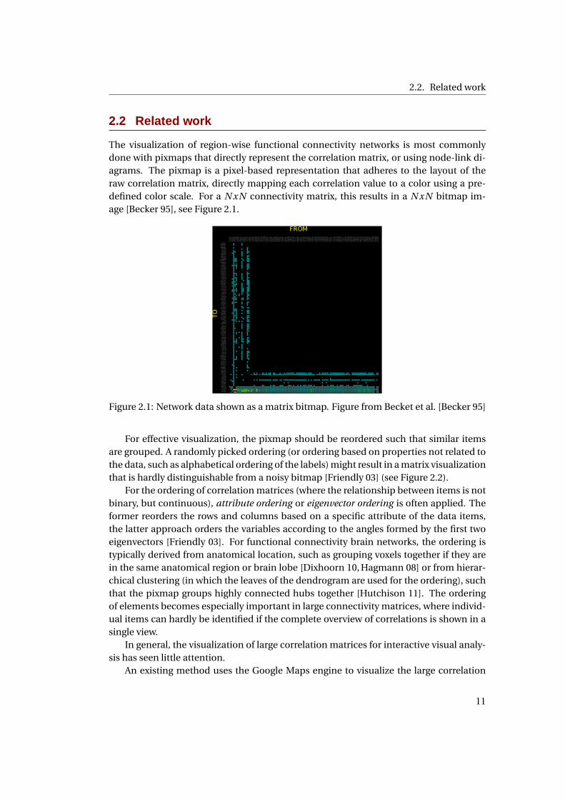
The visualization of region-wise functional connectivity networks is most commonly
done with pixmaps that directly represent the correlation matrix, or using node-link di-
agrams. The pixmap is a pixel-based representation that adheres to the layout of the
raw correlation matrix, directly mapping each correlation value to a color using a pre-
defined color scale. For a N xN connectivity matrix, this results in a N xN bitmap im-
age [Becker 95], see Figure 2.1.
FROM
TO
SNFCCA2147T
SNJ SCA0241T
OKLDCA0344T
SKTNCA0107T
SCRMCA0404T
SHOKCA0296T
PTLDOR6203T
GRDNCA0294T
RENONV0344T
LSANCA0301T
ANHMCA0211T
LSANCA0292T
STTLWA0604T
SNBRCA0101T
SNDGCA0787T
SPKNWA0102T
PHNXAZMA03T
SLKCUTMA02T
ALBQNMMA02T
CLSPCOMA02T
DNVRCOZJ 05T
MDLDTXMU02T
SNANTXCA02T
AUSTTXGR07T
FTWOTXED24T
OKCYOKCE04T
WCHTKSBR24T
OMAHNENW14T
DLLSTXTL44T
DLLSTXTL34T
TULSOKTB04T
HSTNTX0154T
HSTNTX0144T
KSCYMO0904T
MPLSMNDT40T
MPLSMNDT18T
DESMIADT08T
LTRKARFR15T
BTRGLAMA04T
STLSMO0934T
PEORILPJ 51T
SPFDILSD51T
OKBRILOA53T
NWORLAMA04T
WKSHWI0231T
J CSNMSPS14T
OKBRILOA52T
MMPHTNMA43T
CHCGILCL57T
CHCGILCL59T
MOBLALAZ01T
SBNDIN0502T
IPLSIN0102T
GDRPMIBL50T
BRHMALMT01T
NSVLTNMT43T
LSVLKYCS02T
MTGMALMT01T
LNNGMIMN50T
DYTNOH1504T
DTRTMIBH50T
CNCNOHWS14T
TOLDOH2103T
ATLNGATL04T
KNVLTNMA71T
ATLNGANW05T
CLMBOH1103T
ATLNGATL01T
MACNGAGA02T
CLEVOH0203T
AKRNOH2505T
CHTNWVLE25T
CHRLNCCA03T
PITBPADG43T
PITBPADG09T
TAMPFLCO02T
J CVLFLCL03T
CLMASCTL03T
BFLONYFR05T
ORLDFLMA03T
WPBHFLAN04T
GNBONCEU03T
HRBGPAHA42T
OJ USFLTL03T
SYRCNYSU13T
ARTNVACK04T
RCMDVAIT03T
BLTMMDCH01T
RCMTNCXA03T
WASHDCSW06T
NRFLVABS03T
ALBYNYSS05T
WAYNPALA42T
SPFDMABR02T
NWHNCT0205T
NYCQNYRP08T
MNCHNHCO03T
FRMNMAWA04T
PHLAPASL42T
CMBRMA0119T
CMDNNJ CE03T
NWRKNJ 0208T
WHPLNY0504T
FRHDNJ 0202T
RCPKNJ 0203T
WHPLNY0203T
NYCMNYBW24T
NYCMNYBW55T
NYCMNYBW51T
NYCMNY5450T
SNFCCA2147T
SNJSCA0241T
OKLDCA0344T
SKTNCA0107T
SCRMCA0404T
SHOKCA0296T
PTLDOR6203T
GRDNCA0294T
RENONV0344T
LSANCA0301T
ANHMCA0211T
LSANCA0292T
STTLWA0604T
SNBRCA0101T
SNDGCA0787T
SPKNWA0102T
PHNXAZMA03T
SLKCUTMA02T
ALBQNMMA02T
CLSPCOMA02T
DNVRCOZJ05T
MDLDTXMU02T
SNANTXCA02T
AUSTTXGR07T
FTWOTXED24T
OKCYOKCE04T
WCHTKSBR24T
OMAHNENW14T
DLLSTXTL44T
DLLSTXTL34T
TULSOKTB04T
HSTNTX0154T
HSTNTX0144T
KSCYMO0904T
MPLSMNDT40T
MPLSMNDT18T
DESMIADT08T
LTRKARFR15T
BTRGLAMA04T
STLSMO0934T
PEORILPJ51T
SPFDILSD51T
OKBRILOA53T
NWORLAMA04T
WKSHWI0231T
JCSNMSPS14T
OKBRILOA52T
MMPHTNMA43T
CHCGILCL57T
CHCGILCL59T
MOBLALAZ01T
SBNDIN0502T
IPLSIN0102T
GDRPMIBL50T
BRHMALMT01T
NSVLTNMT43T
LSVLKYCS02T
MTGMALMT01T
LNNGMIMN50T
DYTNOH1504T
DTRTMIBH50T
CNCNOHWS14T
TOLDOH2103T
ATLNGATL04T
KNVLTNMA71T
ATLNGANW05T
CLMBOH1103T
ATLNGATL01T
MACNGAGA02T
CLEVOH0203T
AKRNOH2505T
CHTNWVLE25T
CHRLNCCA03T
PITBPADG43T
PITBPADG09T
TAMPFLCO02T
JCVLFLCL03T
CLMASCTL03T
BFLONYFR05T
ORLDFLMA03T
WPBHFLAN04T
GNBONCEU03T
HRBGPAHA42T
OJUSFLTL03T
SYRCNYSU13T
ARTNVACK04T
RCMDVAIT03T
BLTMMDCH01T
RCMTNCXA03T
WASHDCSW06T
NRFLVABS03T
ALBYNYSS05T
WAYNPALA42T
SPFDMABR02T
NWHNCT0205T
NYCQNYRP08T
MNCHNHCO03T
FRMNMAWA04T
PHLAPASL42T
CMBRMA0119T
CMDNNJCE03T
NWRKNJ0208T
WHPLNY0504T
FRHDNJ0202T
RCPKNJ0203T
WHPLNY0203T
NYCMNYBW24T
NYCMNYBW55T
NYCMNYBW51T
NYCMNY5450T
Figure 2.1: Network data shown as a matrix bitmap. Figure from Becket et al. [Becker 95]
For effective visualization, the pixmap should be reordered such that similar items
are grouped. A randomly picked ordering (or ordering based on properties not related to
the data, such as alphabetical ordering of the labels) might result in a matrix visualization
that is hardly distinguishable from a noisy bitmap [Friendly 03] (see Figure 2.2).
For the ordering of correlation matrices (where the relationship between items is not
binary, but continuous), attribute ordering or eigenvector ordering is often applied. The
former reorders the rows and columns based on a specific attribute of the data items,
the latter approach orders the variables according to the angles formed by the first two
eigenvectors [Friendly 03]. For functional connectivity brain networks, the ordering is
typically derived from anatomical location, such as grouping voxels together if they are
in the same anatomical region or brain lobe [Dixhoorn 10, Hagmann 08] or from hierar-
chical clustering (in which the leaves of the dendrogram are used for the ordering), such
that the pixmap groups highly connected hubs together [Hutchison 11]. The ordering
of elements becomes especially important in large connectivity matrices, where individ-
ual items can hardly be identified if the complete overview of correlations is shown in a
single view.
In general, the visualization of large correlation matrices for interactive visual analy-
sis has seen little attention.
An existing method uses the Google Maps engine to visualize the large correlation
11

2. BACKGROUND AND RELATED WORK
Auto data: Alpha order
Displa
Gratio
Hroom
Length
MPGPrice
Rep77
Rep78
Rseat
Trunk
TurnWeight
Weight
TurnTrunk Rseat Rep78 Rep77 Price
MPG Length Hroom
Gratio Displa
Auto data: PC2/1 order
Gratio
MPGRep78
Rep77
Price
Hroom
Trunk
Rseat
Length
Weight
Displa
Turn
Turn Displa Weight
Length Rseat Trunk Hroom Price
Rep77 Rep78 MPG Gratio
Figure 2.2: The effect of reordering rows and columns. Left the matrix in which the rows
and columns are orderend on alphabet, right the same data matrix with ordering based
on the angles of the first two eigenvectors. Figure from [Friendly 03].
Figure 2.3: Visualization of large correlation matrices with a tile-based technique, using
the Google Maps tile engine. Figure from Andrey Shabalin (http://shabal.in) [Shabalin ].
matrix in an interactive fashion (see Figure 2.3) [Shabalin ]. This method relies on a large
set of pre-rendered tiles in various resolutions (seven different resolutions in this case),
where each tile is a small part of the entire pixmap. This method facilitates interactive
visualization, enabling the user to navigate the pixmap representation using zoom and
pan.
A major advantage of this method is that it is able to visualize a correlation matrix of
12

2.2. Related work
arbitrary size, only limited by the amount of storage available to store the tile database.
However, the tile-based technique has also some disadvantages. Zooming, for instance
is restricted to the seven pre-defined resolutions. Furthermore, generating the tiles from
the raw correlation data is a time-consuming task. This means that interactively adjust-
ing the color map, or changing the contents of the visualization by interactive filtering is
not supported.
To see the functional network in its spatial context, the correlation matrix is typically
represented as a node-link diagram, inter-connecting the N nodes with a straight line,
whose thickness or color is based on the connectivity strength.
For voxel-wise connectivity, the node-link representation is not feasible. The high
number of nodes and massive amount of links would easily result in a completely clut-
tered image if the network is rendered in using the inherent spatial positions of the nodes.
In Zuo et al. [Zuo 11], the node-link representation is used to render a network of 22,000
nodes, but here the nodes are grouped in twenty functional communities, such that the
links are drawn between 20 regions instead of between each voxel pair in their spatial
position (see Figure 2.4). Furthermore, the visualization procedures were carried out on
a graphics workstation, rather than on a standard desktop computer.
Figure 2.4: A node-link visualization of the whole-brain functional connectome (B), with
the nodes grouped into 20 functional communities, as shown in (A). Image courtesy of
Zuo et al. [Zuo 11]
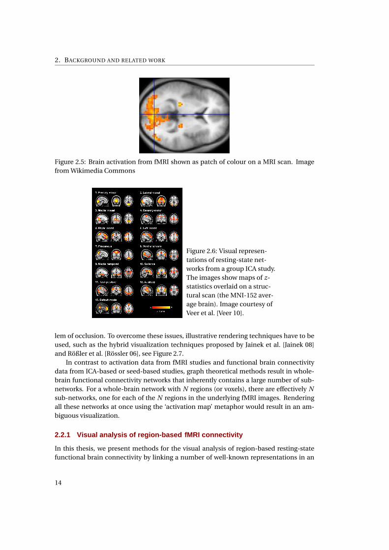
Another commonly used method for the visualization of functional connectivity net-
works is the connectivity map. This representation is similar to the activity maps rep-
resentation often used to visualize brain activation data in fMRI studies. Activity maps
show a ‘map’ of the brain with for each voxel a statistical value (z or t statistic) repre-
senting the ‘activity’ at that voxel. Activity maps are usually visualized by mapping the
statistical values to colors and drawing them on a slice of a MRI brain scan, see Figure
2.5.
Connectivity maps are typically used to visually represent resting-state networks from
group ICA studies, as shown in Figure 2.6.
The activity map metaphor can also be extended to 3-D, such that the complete ac-
tivation map can be rendered in its spatial context. However, three-dimensional repre-
sentations that include anatomical context from a structural scan introduce the prob-
13
2. BACKGROUND AND RELATED WORK
Figure 2.5: Brain activation from fMRI shown as patch of colour on a MRI scan. Image
from Wikimedia Commons
Figure 2.6: Visual represen-
tations of resting-state net-
works from a group ICA study.
The images show maps of z-
statistics overlaid on a struc-
tural scan (the MNI-152 aver-
age brain). Image courtesy of
Veer et al. [Veer 10].
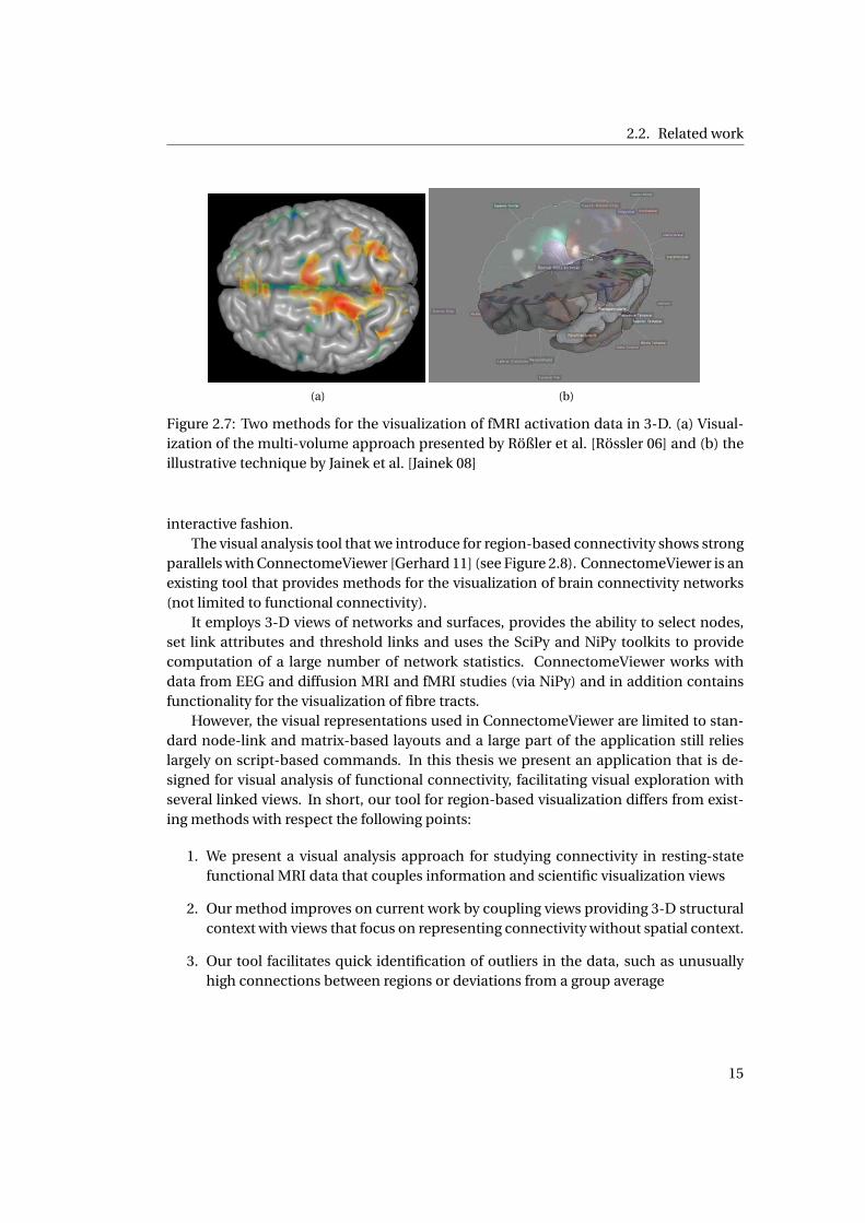
lem of occlusion. To overcome these issues, illustrative rendering techniques have to be
used, such as the hybrid visualization techniques proposed by Jainek et al. [Jainek 08]
and Rößler et al. [Rössler 06], see Figure 2.7.
In contrast to activation data from fMRI studies and functional brain connectivity
data from ICA-based or seed-based studies, graph theoretical methods result in whole-
brain functional connectivity networks that inherently contains a large number of sub-
networks. For a whole-brain network with N regions (or voxels), there are effectively N
sub-networks, one for each of the N regions in the underlying fMRI images. Rendering
all these networks at once using the ‘activation map’ metaphor would result in an am-
biguous visualization.
2.2.1 Visual analysis of region-based fMRI connectivity
In this thesis, we present methods for the visual analysis of region-based resting-state
functional brain connectivity by linking a number of well-known representations in an
14
2.2. Related work
(a) (b)
Figure 2.7: Two methods for the visualization of fMRI activation data in 3-D. (a) Visual-
ization of the multi-volume approach presented by Rößler et al. [Rössler 06] and (b) the
illustrative technique by Jainek et al. [Jainek 08]
interactive fashion.
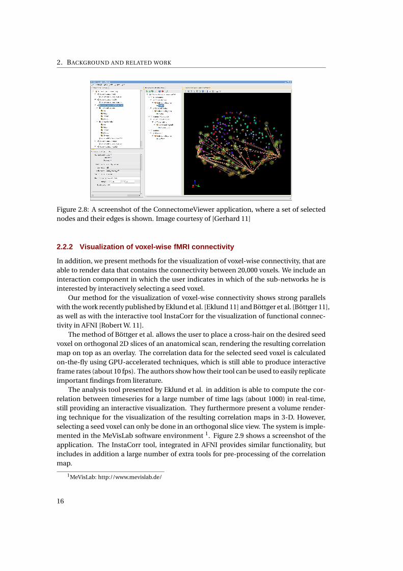
The visual analysis tool that we introduce for region-based connectivity shows strong
parallels with ConnectomeViewer [Gerhard 11] (see Figure 2.8). ConnectomeViewer is an
existing tool that provides methods for the visualization of brain connectivity networks
(not limited to functional connectivity).
It employs 3-D views of networks and surfaces, provides the ability to select nodes,
set link attributes and threshold links and uses the SciPy and NiPy toolkits to provide
computation of a large number of network statistics. ConnectomeViewer works with
data from EEG and diffusion MRI and fMRI studies (via NiPy) and in addition contains
functionality for the visualization of fibre tracts.
However, the visual representations used in ConnectomeViewer are limited to stan-
dard node-link and matrix-based layouts and a large part of the application still relies
largely on script-based commands. In this thesis we present an application that is de-
signed for visual analysis of functional connectivity, facilitating visual exploration with
several linked views. In short, our tool for region-based visualization differs from exist-
ing methods with respect the following points:
1. We present a visual analysis approach for studying connectivity in resting-state
functional MRI data that couples information and scientific visualization views
2. Our method improves on current work by coupling views providing 3-D structural
context with views that focus on representing connectivity without spatial context.
3. Our tool facilitates quick identification of outliers in the data, such as unusually
high connections between regions or deviations from a group average
15
2. BACKGROUND AND RELATED WORK
Figure 2.8: A screenshot of the ConnectomeViewer application, where a set of selected
nodes and their edges is shown. Image courtesy of [Gerhard 11]
2.2.2 Visualization of voxel-wise fMRI connectivity
In addition, we present methods for the visualization of voxel-wise connectivity, that are
able to render data that contains the connectivity between 20,000 voxels. We include an
interaction component in which the user indicates in which of the sub-networks he is
interested by interactively selecting a seed voxel.
Our method for the visualization of voxel-wise connectivity shows strong parallels
with the work recently published by Eklund et al. [Eklund 11] and Böttger et al. [Böttger 11],
as well as with the interactive tool InstaCorr for the visualization of functional connec-
tivity in AFNI [Robert W. 11].
The method of Böttger et al. allows the user to place a cross-hair on the desired seed
voxel on orthogonal 2D slices of an anatomical scan, rendering the resulting correlation
map on top as an overlay. The correlation data for the selected seed voxel is calculated
on-the-fly using GPU-accelerated techniques, which is still able to produce interactive
frame rates (about 10 fps). The authors show how their tool can be used to easily replicate
important findings from literature.
The analysis tool presented by Eklund et al. in addition is able to compute the cor-
relation between timeseries for a large number of time lags (about 1000) in real-time,
still providing an interactive visualization. They furthermore present a volume render-
ing technique for the visualization of the resulting correlation maps in 3-D. However,
selecting a seed voxel can only be done in an orthogonal slice view. The system is imple-
mented in the MeVisLab software environment 1. Figure 2.9 shows a screenshot of the
application. The InstaCorr tool, integrated in AFNI provides similar functionality, but
includes in addition a large number of extra tools for pre-processing of the correlation
map.
1MeVisLab: http://www.mevislab.de/
16

2.3. The basics of raycasting
Figure 2.9: A screenshot of the interactive visualization tool for functional connectivity
analysis by Eklund et al. [Eklund 11]. Image from Eklund et al. [Eklund 11].
The three tools discussed above are similar to the work presented in this thesis, but
focus mostly on the task of computing the actual correlation data. In this thesis, we will
approach the topic from a visualization point-of-view. In short, our method differs with
respect the following points:
1. The correlation matrix is computed in a pre-processing step such that we can pro-
vide a pixmap visualization that allows for detection of groups of voxels that are
correlated.
2. We provide a picking tool that allows the user to interactively and dynamically se-
lect a seed voxel on the cortical surface, directly in the 3-D representation.
3. We present a flat-map representation that visualizes the complete cortical connec-
tivity map in pseudo-anatomical context.
4. Our tool allows for interactive side-by-side comparison and difference visualiza-
tion of multiple datasets.
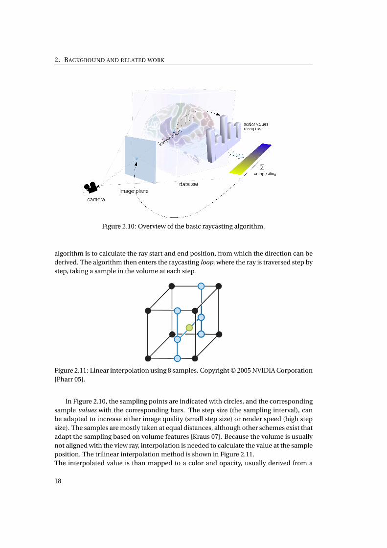
2.3 The basics of raycasting
Volume raycasting is a direct volume rendering (DVR) technique that maps a three di-
mensional scene to a two dimensional screen, by shooting rays from the observer via a
pixel in the projection plane (or viewport) into the scene, taking samples along the ray
that are composited to form the final pixel color. This process is best explained with a
picture, see Figure 2.10.
The figure shows the overview of the raycasting technique. Rays are ‘shot’ from the
camera (eye) through a pixel in the image plane into the volume. The first step of the
17
2. BACKGROUND AND RELATED WORK
Figure 2.10: Overview of the basic raycasting algorithm.
algorithm is to calculate the ray start and end position, from which the direction can be
derived. The algorithm then enters the raycasting loop, where the ray is traversed step by
step, taking a sample in the volume at each step.
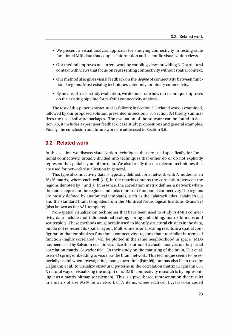
Figure 2.11: Linear interpolation using 8 samples. Copyright © 2005 NVIDIA Corporation
[Pharr 05].
In Figure 2.10, the sampling points are indicated with circles, and the corresponding
sample values with the corresponding bars. The step size (the sampling interval), can
be adapted to increase either image quality (small step size) or render speed (high step
size). The samples are mostly taken at equal distances, although other schemes exist that
adapt the sampling based on volume features [Kraus 07]. Because the volume is usually
not aligned with the view ray, interpolation is needed to calculate the value at the sample
position. The trilinear interpolation method is shown in Figure 2.11.
The interpolated value is than mapped to a color and opacity, usually derived from a
18

2.3. The basics of raycasting
transfer function. Finally, the samples are shaded based on their orientation and the
position of the light source. The orientation of the sample is defined by its normal and
typically estimated from the central differences between neighbouring voxels.
The resulting colors and opacity values are then composited to form the final color value
for the pixel, using front-to-back (FTB) or back-to-front (BTF) compositing.
19


CHAPTER 3
Visual analysis of integrated restingstate functional brain connectivity
and anatomy
Published as: A.F. van Dixhoorn, B.H. Vissers, L. Ferrarini, J. Milles, and C. P.
Botha, Visual analysis of integrated resting state functional brain connectiv-
ity and anatomy, in “Eurographics Workshop on Visual Computing for Biol-
ogy and Medicine”, 2010
Abstract
Resting state functional magnetic resonance imaging (rs-fMRI) is an important modality
in the study of the func- tional architecture of the human brain. The correlation between
the resting state fMRI activity traces of different brain regions indicates to what extent
they are functionally connected. rs-fMRI data typically consists of a matrix of correla-
tions, also denoted as functional correlations, between regions in the brain. Visualiza-
tion is required for a good understanding of the data. Several well-known representations
have been used to visualize this type of data, including multi-dimensional scaling, spring
embedding, scatter plots and network visualization. None of these methods provide the
ability to show the functional correlation in relation to the anatomical distance and po-
sition of the regions, while preserving the ability to quickly identify outliers in the data.
In this paper, a visual analysis application is presented that overcomes this limitation
by combining the strengths of the two-dimensional representations with three dimen-
sional network and iso-surfacing visualizations. We show how the application facilitates
rs-fMRI connectivity research by means of a case study evaluation.
Note
A considerable part of the work documented in this paper was performed by Bastijn Vis-
sers, the second author. His contributions are listed below.
21

3. VISUAL ANALYSIS OF INTEGRATED RESTING STATE FUNCTIONAL BRAIN CONNECTIVITY
AND ANATOMY
• Implementation of the matrix bitmap view
• Implementation of the info view
• General contributions to the text and graphics in the paper
• Performance measurements
• General contributions in the case study evaluation and in the evaluation using gen-
eral examples
3.1 Introduction
Recent developments in medical imaging techniques have accelerated research in brain
mapping and brain functional connectivity. A number of studies have investigated the
relationship between brain activity and functional connectivity. Methods used include
resting state functional magnetic resonance imaging (rs-fMRI) connectivity of healthy
persons in resting state [Salvador 05a] as well as diffusion spectrum or tensor imaging
(DSI/DTI) to identify structural connections in the human brain.
Resting state fMRI is based on the observation that low-frequency (0.01H z −0.1H z)
signal fluctuations in grey matter regions are perceivable in a resting brain. These signals
seem to relate to spontaneous neuronal activity. Correlations between resting state sig-
nals from different parts of the brain indicate the functional connectivity between those
regions [Biswal 95]. Research by Hagmann et al. revealed a strong relationship between
structural and functional connectivity [Hagmann 08]. More recently, Salvador et al. [Sal-
vador 05a] studied the organization of the human brain in a resting state by investigating
pairwise functional connections between ninety anatomical regions of interest (ROIs).
Salvador and his group revealed that the amount of connectivity between regions can be
predicted by the anatomical distance between the respective regions, generally satisfy-
ing an inverse square law. Pairs of anatomical regions that significantly deviate from this
relation were identified as being regions that are anatomically symmetric (interhemi-
spheric) or local (intra-hemispheric, neighboring). Comparing the functional brain ar-
chitecture of healthy persons with that of a patient affected by brain injury revealed a
significant difference in the interhemispheric connectivity [Salvador 05a]. The output
of this type of study usually are the individual matrices containing the correlation be-
tween each pair of anatomical regions for each subject. In our case this set of matrices is
supplemented with an average connectivity matrix representing the connectivity char-
acteristics of the whole subject group.
The existing analysis pipeline is primarily hypothesis-driven, and consists of com-
pute -intensive offline analysis of the correlation data. Up to now, our collaborators have
not been making use of visual analysis capabilities, only seldom using non-interactive
visual representations of the correlation matrix.
In this paper we present a system which uses coupled views in order to facilitate sci-
entists’ understanding of functional connectivity data. The contributions of this work
can be summarized as follows:
22
3.2. Related work
• We present a visual analysis approach for studying connectivity in resting-state
functional MRI data that couples information and scientific visualization views.
• Our method improves on current work by coupling views providing 3-D structural
context with views that focus on representing connectivity without spatial context.
• Our method also gives visual feedback on the degree of connectivity between func-
tional regions. Most existing techniques cater only for binary connectivity.
• By means of a case study evaluation, we demonstrate how our technique improves
on the existing pipeline for rs-fMRI connectivity analysis.
The rest of this paper is structured as follows; in Section 3.2 related work is examined,
followed by our proposed solution presented in section 3.3. Section 3.4 briefly summa-
rizes the used software packages. The evaluation of the software can be found in Sec-
tion 3.5, it includes expert user feedback, case study propositions and general examples.
Finally, the conclusion and future work are addressed in Section 3.6.
3.2 Related work
In this section we discuss visualization techniques that are used specifically for func-
tional connectivity, broadly divided into techniques that either do or do not explicitly
represent the spatial layout of the data. We also briefly discuss relevant techniques that
are used for network visualization in general.
This type of connectivity data is typically defined, for a network with N nodes, as an
N xN matrix, where each cell (i , j ) in the matrix contains the correlation between the
regions denoted by i and j . In essence, the correlation matrix defines a network where
the nodes represent the regions and links represent functional connectivity.The regions
are mostly defined by anatomical templates, such as the Talairach atlas [Talairach 88]
and the standard brain templates from the Montreal Neurological Institute [Evans 92]
(also known as the AAL template).
Non-spatial visualization techniques that have been used to study rs-fMRI connec-
tivity data include multi-dimensional scaling, spring embedding, matrix bitmaps and
scatterplots. These methods are generally used to identify structural clusters in the data,
but do not represent its spatial layout. Multi-dimensional scaling results in a spatial con-
figuration that emphasizes functional connectivity: regions that are similar in terms of
function (highly correlated), will be plotted in the same neighborhood in space. MDS
has been used by Salvador et al. to visualize the output of a cluster analysis on the partial
correlation matrix [Salvador 05a]. In their study on the maturing of the brain, Fair et al.
use 2-D spring embedding to visualize the brain network. This technique seems to be es-
pecially useful when investigating change over time [Fair 09], but has also been used by
Hagmann et al. to visualize structural patterns in the correlation matrix [Hagmann 08].
A natural way of visualizing the output of rs-fMRI connectivity research is by represent-
ing it as a matrix bitmap (or pixmap). This is a pixel-based representation that results
in a matrix of size N xN for a network of N items, where each cell (i , j ) is color coded
23

3. VISUAL ANALYSIS OF INTEGRATED RESTING STATE FUNCTIONAL BRAIN CONNECTIVITY
AND ANATOMY
Figure 3.1: The application’s main window with the three main components. (A) - The
Anatomical Views component. Contains the Anatomical Region View (left) and Anatom-
ical Network View (right). (B) - The Abstract Views component. From left to right the
Scatterplot View, Matrix Bitmap and Hierarchical Edge Bundling View. (C) - The Filtering
and Selection View with the Selection Info View (top) and Filter View (bottom).
according to the connection strength between region i and j [Fair 08, Becker 95]. Order-
ing the matrix enhances the ability to detect patterns of relations. A typical ordering that
has been used in rs-fMRI connectivity research is based on anatomical hierarchy [Hag-
mann 08].
The relation between anatomical distance, as extracted from an anatomical tem-
plate, and functional distance can be visualized using a scatterplot [Salvador 05a]. For
the dataset used in this paper, this is illustrated in figure 3.5.
When representation of the spatial layout of the data is required, the most common
visualization is a spatially embedded node-link diagram. In this network visualization
method, the regions and connections between them are rendered as a network in three
dimensions, where each node, representing a ROI, is rendered at the center of mass of
the corresponding region. Connections between the ROIs are visualized as lines be-
tween the nodes, and the link strength can be encoded by line thickness or color. A two-
dimensional pseudo-anatomical variation has been used by Fair et al. [Fair 09], Dosen-
bach et al. [Dosenbach 07] and Hagmann et al. [Hagmann 08]. Visualizations in three di-
mensions in a correct anatomical context have been used by Worsley et al. [Worsley 05],
and to a lesser degree by Bezgin et al. and Cao and Worshley [Bezgin 09, Cao 99].
As can be seen in [Worsley 05] combining the contours of the regions with the links
in one view quickly starts cluttering the view. Ghoniem et al. argue that when graphs
are bigger than twenty vertices, the matrix-based visualization outperforms node-link
representations on most tasks [Ghoniem 05]. Another way to deal with the cluttering
problem is to use the node-link visualization in an interactive fashion, where the user
24

3.3. Method
is able to threshold the edges based on their strength. There are tools available for the
analysis and visualization of fMRI correlation data, such as the BrainMiner visualiza-
tion tool [Mueller 00], CoCoMac Paxinos 3-D Viewer [Bezgin 09], and the commercial
software BrainVoyager QX [Goebel 06], focusing mostly on the basic 3-D representation
of connections. Network visualizations are also used in the research domains of com-
munication networks, social networks and biological networks [Becker 95, Pavlopou-
los 08, Henry 07].
We present a visual analysis application that incorporates several of the aforemen-
tioned techniques, combining them in various linked views of the same data. The idea
of querying in a query friendly view and providing insight in a (3-D) visualization view is
proven to be useful in [Kuß 08]. Using this approach, disadvantages of one view can be
compensated for by using the other views. Our solution improves on the state of the art
in the following ways: In contrast to the systems in [Mueller 00,Bezgin 09,Goebel 06], our
tool interactively couples views for quick outlier and pattern detection with 3-D spatial
representations as well as techniques for interactive selection and filtering. In addition,
we introduce the application of hierarchical edge bundling [Holten 06] to visualize hier-
archy and adjacency relations in the brain.
3.3 Method
The methods that are currently used for studying resting-state functional connectivity
MRI data work well in studying basic questions concerning the data, but they do not cope
well when both the anatomical information and functional connectivity data are part
of the research question. In this section, we present our visual analysis approach that
couples the anatomical information and the connectivity data (consisting of data from 53
subjects) by combining existing techniques from information visualization and scientific
visualization to improve on the existing pipeline for rs-fMRI connectivity analysis. In the
rest of this section we describe our method, starting by giving a general overview of the
system and then following with the details of the system’s components.
3.3.1 Application Overview
We implemented our method as a software tool that loads the anatomical data (from
an AAL template) and functional connectivity data from a file and displays this data in
several different linked views. A selection in any of the views is reflected in the other
views, where possible. The views are sub-windows in the application’s main window (see
figure 3.1) and can be categorized into three main components: the anatomical (figure
3.1A), the abstract (figure 3.1B) and the filtering and selection views (figure 3.1C).
3.3.2 Anatomical Views (figure 3.1A)
The Anatomical Regions and Anatomical Network views use a 3-D window to render their
information in anatomical context. The views are linked: Mouse interaction in one view
25

3. VISUAL ANALYSIS OF INTEGRATED RESTING STATE FUNCTIONAL BRAIN CONNECTIVITY
AND ANATOMY
has its effect on both views. The anatomical data is loaded from an AAL brain template
with 90 anatomical regions.
Anatomical Regions
Using the AAL brain template, iso surfaces are extracted for each of the 90 anatomical re-
gions. A default color map is used to distinguish different regions. The default color map
also visualizes brain lobes by encoding the lobe regions in a similar color. The Anatomi-
cal Regions View offers two main modes of interaction: region mode and link mode.
The region mode is activated when a single region is selected (as opposed to a selection
of links, in which always two or more regions are selected). In this mode, the Anatomi-
cal Region View will render this region in its own color, and all other regions according
to a colormap that is based on either correlation or deviation from 1D2 . Additionally, the
opacity of the region surfaces is based on this number, emphasizing highly correlated or
highly unexpected linked regions. This mode gives the analyst the ability to quickly see
the connection properties for a single region.
The link mode is activated when multiple regions are selected (one link or more selected).
So, if a selection is made in any of the other views, this mode is automatically enabled. In
this case the Anatomical Regions View highlights all anatomical regions that are part of
the selection in their default color. Furthermore, this mode has two options. Either the
non-selected regions can be completely removed from the view, or they can be rendered
in dark gray in order to provide context.
The main role of this view is to visualize regions that are selected (either in the view
itself or in other views, see section 3.3.4) in their anatomical context (spatial location and
size).
Anatomical Network
In the Anatomical Network view each selected region is represented as a node with its
diameter being based upon the total correlation strength of all the links this region par-
ticipates in. The links are represented as tubes with their diameter being based upon the
(absolute) correlation strength of the link it represents.
3.3.3 Abstract Views (figure 3.1B)
This component consists of three 2-D views that focus on the connectivity information
outside of its anatomical context.
Scatterplot
Having the Euclidean anatomical distance on the x-axis and the correlation strength on
the y-axis, the scatterplot shows the relation between distance and correlation. A curve
is plotted in the scatterplot showing the rule of thumb ( 1D2 ). The general spread of the
points is expected to be around this curve. Points far away from the curve, may be con-
26

3.3. Method
sidered outliers. The main purpose of this view is spotting and selecting outliers in the
data.
Matrix Bitmap
The matrix bitmap is a direct visualization of the correlation matrix, although the rows
and columns are re-ordered. The left half of the columns (and top half of the rows) reflect
regions of the left hemisphere, the right (and bottom) half reflects the right hemisphere.
This way, the horizontal and vertical center lines are mirroring left and right symmetrical
regions. The minor (secondary) diagonal defines the line of full symmetry. See figure 3.2
for a visual explanation.
Each pixel in the bitmap represents a link and the color encodes some statistic for
that link. Three statistics are available for each link, resulting in three different matrix
bitmaps.
The first matrix bitmap directly visualizes the correlation matrix of the subject, giving
each pixel a color value directly based upon the correlation of that link. The second one
subtracts the average correlation matrix from the correlation matrix of the current sub-
ject, giving each pixel a color based upon the correlation of the link minus the average
correlation for that link using a perceptually linear colormap. The third matrix bitmap
subtracts the matrix containing the rule of thumb values from the correlation matrix of
the current subject, effectively showing for each link the difference with the expected
value for that link, thus emphasizing links that deviate significantly from the expected
value.
The selected links in the bitmap are currently displayed by placing a black dot in
the top and left edge of the bitmap, its place corresponding to the column and row the
selected link is in. This way, when all selected links are in one area of the brain the user
will quickly notice this as all the black dots are close together.
Hierarchical Edge Bundles This view visualizes hierarchy of the brain, based on the
Brodmann regions, in a circular layout. The root of the hierarchy is the whole brain,
represented by a node in the center of the circle. The next level in the hierarchy is the
distinction between the left and right brain half (with nodes left and right from the root
node). The next level are the seven lobes in the human brain for each brain half and
finally, the lowest level in the hierarchy are the 45 regions for each brain half.
Each link is represented as an (elastic) edge between two region nodes. The edge
is attracted by the nodes from higher hierarchy levels by the bundling strength which
can be varied by the user. Increasing the bundling strength results in all edges going
through their anatomical parents in the hierarchy, bundling similar links together as long
as they take the same route through the brain hierarchy. Decreasing this value results in
smooth edges which pass loosely by their anatomical parents. The main purpose of the
hierarchical edge bundles view is to show the course of a link from one region through
the hierarchy of the brain to the other region. See also figure 3.3.
27

3. VISUAL ANALYSIS OF INTEGRATED RESTING STATE FUNCTIONAL BRAIN CONNECTIVITY
AND ANATOMY
Figure 3.2: The matrix bitmap with several links highlighted. The highlighted link in the
left top is the symmetrical equivalent of the highlighted link in the right bottom. The
same holds for the pair of highlighted links in the right top of the bitmap. Additionally,
the link in the left top is the half-symmetrical equivalent of the link in the right top (on
the same row). The same applies to the two links in the right top and right bottom of the
matrix (in the same column).
3.3.4 Filtering and Selection (figure 3.1C)
The last component consists of two views. The info view shows textual, statistical infor-
mation of the current selection, the filter view enables the user to occlude data from the
other views.
Info view
The info view (top view in the component) shows information on the current selection.
It shows general and statistical information such as the name and ID of a single link,
or number of selected links otherwise, distance, correlation, mean, and median for the
selected link(s) as well as the total set.
The main purpose of this view is to enable the user to quickly gain insight in the
current selection values, and how those relate to the total dataset.
28

3.4. Implementation
Figure 3.3: Hierarchical Edge Bundles view with multiple links selected. Edges loosely
follow the brain’s hierarchy. For printing purposes, the image has been post-processed
not to show all links, and to let the selected links stand out more.
Filter view
The filter view enables the user to filter on a min, max or range of correlation or distance.
Another option is to filter on a confidence interval around the curve 1D2 . In case of the
range and confidence interval filters outliers as well as inliers can be filtered. Filtered
links and regions will no longer appear in the views.
The main purpose of this view is to occlude values which are not interesting for the
data analyst, this way also preventing occlusion of the important values.
3.4 Implementation
The cross-platform application is implemented in C++, using Qt4, Qt Designer, Qwt, VTK
and finally Matlab for loading the connectivity matrices.
All time consuming tasks are performed once, on startup of the tool. This includes
generating iso-surfaces of all regions in the brain template image and building the iso-
29

3. VISUAL ANALYSIS OF INTEGRATED RESTING STATE FUNCTIONAL BRAIN CONNECTIVITY
AND ANATOMY
surfaces (nodes and links) for the network representation. Once loaded the complete
application is real-time, without any optimization as is.
Creating the fully connected network involves generating 90 spheres and 4005 tubes,
which requires under ten seconds on a system having an Intel 2 Core Duo T7300 (2Ghz),
NVIDIA GeForce 8600M GT, and running on Windows 7 64-bit Professional. To prevent
blocking the user interface, this task is performed in a separate thread and the user is
updated on the progress. The total amount of memory used ranges from 170 to about
250 Megabytes.
3.5 Evaluation
We evaluated the proposed system following the guidelines and terminology set forth
for case study research [Yin 09]. The main study question was defined as: How can the
proposed visualization tool assist neuroscientists in their research on resting state fMRI
connectivity? We defined the case in this question as being the use of our software by the
third and fourth authors of this paper, respectively LF and JM, both published neurosci-
entists and experts in rs-fMRI connectivity.
For the purpose of this evaluation, two meetings were held with the users. We first
conducted an informal interview during which users could give general feedback on the
system prototype. Two weeks later we conducted a focused review, during which we used
the tool to analyse a real-world multi-subject dataset together with the domain scientists,
collecting and structuring their feedback according to the case study propositions that
we had formulated before the session. Together the propositions and the accompanying
structured feedback function to answer the main study question.
In the following subsections, we first illustrate the general use of the visualization
tool with four examples, after which we discuss user feedback structured according to
the case study propositions.
3.5.1 General examples
The dataset used in the following examples consists of the 90×90 correlation matrices of
53 subjects, as well as the average correlation matrix over all subjects.
Symmetric interhemispheric connections show an unusually high correlation Several
long distance connections are correlated unusually strongly and deviate significantly
from the expected relation ( 1D2
). Using the presented tool, just one action is required to
see which connections these outliers represent. The user makes a selection in the scat-
ter plot using the mouse (see figure 3.4 (a)) and the Network View immediately updates
the network representation, now only showing those regions that correspond to the se-
lected points in the scatter plot (see figure 3.4 (b)). At the same time, the Regions View
is updated and renders a three dimensional, anatomically correct representation of the
selected regions (see figure 3.4(c)).
Another way to easily spot these outliers is to look at the correlation bitmap matrix.
These connections are visible as pixels at the second diagonal (from the right top to the
center of the triangular matrix, see section 3.3.3) and indeed pop out by their bright color.
30
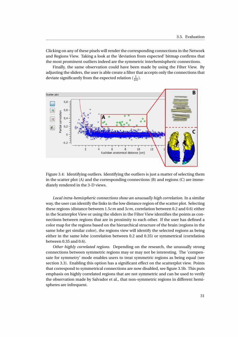
3.5. Evaluation
Clicking on any of these pixels will render the corresponding connections in the Network
and Regions View. Taking a look at the ’deviation from expected’ bitmap confirms that
the most prominent outliers indeed are the symmetric interhemispheric connections.
Finally, the same observation could have been made by using the Filter View. By
adjusting the sliders, the user is able create a filter that accepts only the connections that
deviate significantly from the expected relation ( 1D2
).
Figure 3.4: Identifying outliers. Identifying the outliers is just a matter of selecting them
in the scatter plot (A) and the corresponding connections (B) and regions (C) are imme-
diately rendered in the 3-D views.
Local intra-hemispheric connections show an unusually high correlation. In a similar
way, the user can identify the links in the low distance region of the scatter plot. Selecting
these regions (distance between 1.5cm and 3cm, correlation between 0.2 and 0.6) either
in the Scatterplot View or using the sliders in the Filter View identifies the points as con-
nections between regions that are in proximity to each other. If the user has defined a
color map for the regions based on the hierarchical structure of the brain (regions in the
same lobe get similar color), the regions view will identify the selected regions as being
either in the same lobe (correlation between 0.2 and 0.35) or symmetrical (correlation
between 0.35 and 0.6).
Other highly correlated regions. Depending on the research, the unusually strong
connections between symmetric regions may or may not be interesting. The ’compen-
sate for symmetry’ mode enables users to treat symmetric regions as being equal (see
section 3.3). Enabling this option has a significant effect on the scatterplot view. Points
that correspond to symmetrical connections are now disabled, see figure 3.5b. This puts
emphasis on highly correlated regions that are not symmetric and can be used to verify
the observation made by Salvador et al., that non-symmetric regions in different hemi-
spheres are infrequent.
31

3. VISUAL ANALYSIS OF INTEGRATED RESTING STATE FUNCTIONAL BRAIN CONNECTIVITY
AND ANATOMY
Differences in the population. One additional feature that our method offers is the
ability to see whether the relations also hold for individual subjects. For instance, us-
ing the subject-slider in the top of the application’s main window, we were able to ob-
serve that the selected connections in figure 3.5b are not consistently highly correlated
throughout the set of individual subjects.
(a) Scatter plot with symmetry compensation
disabled
(b) Scatter plot with symmetry compensation
enabled
Figure 3.5: The Scatterplot View with the symmetric intra-hemispheric connections vis-
ible (3.5a) and hidden (3.5b). The latter view immediately reveals an unusually strong
connection at D = 4.8 for this subject. Selecting this region shows the connection in
anatomical context (representing the connection between Frontal_Inf_Oper_R and Tem-
poral_Pole_Mid_R).
3.5.2 Case study propositions and user feedback
The scatterplot allows the rapid localization of interesting correlations (outliers). This
proposition was confirmed, although the possibility of using absolute correlation would
make it more useful. This will be implemented in future versions of the software.
The matrix bitmap allows the rapid detection of interesting correlations (high, deviat-
ing from expectation or from average, etc.) and visual patterns of correlations. Patterns
could point in the direction of whole groups being correlated. This proposition was con-
firmed, with the users adding that high correlation in fact pops out. It was noted that the
ordering of the elements is very important.
The hierarchical edge bundles are better than the dendrogram for showing connectivity
through grouping, as they are able to represent connections between parcels in different
hemispheres through the hierarchy in-between. Dendrogram can be double-sided, but
packing is inefficient. Both users claimed that due to this technique being new in the
context of this application, they would need to use it more extensively before being able
to comment. They agreed speculatively that it could be useful and commented that the
specific hierarchy chosen becomes important and further that the color map should be
adapted so that high correlations should be more visible, especially so due to the visual
complexity of this representation.
The 3-D spatial embedding of functional correlation allows the study of these connec-
32

3.5. Evaluation
tions in their anatomical context & Being able to query in the anatomical view (click on
region, see all connected regions) aids in the understanding of brain architecture. This
was considered useful especially in the comparison of cases to controls, where research
is able to focus on specific regions of the brain, based on prior knowledge of the pathol-
ogy under study. For example in Alzheimer’s Disease patients, it is expected that the
hippocampus plays a role, so researchers can use spatial querying to rapidly see how
other regions are connected. Also, an initial selection in 2-D views, based on obvious
high correlations, can be further specified in the spatial view in order to determine the
total connectivity of a region and hence localize communication hubs.
Visual filtering and zooming alleviates clutter problems in the 3-D spatial view and
scatterplot & Linked interaction leads to the conceptually different views strengthening
each other. Users agreed with both these propositions, even claiming that the linked in-
teraction was an essential element of the tool.
The tool is useful during the pre-processing of data, in order to detect interesting as-
pects (outliers) for further analysis using the traditional pipeline. Although the users
thought that the tool might be useful during the exploration phase, they commented
that current research focuses on local and global efficiency of the neural architecture, in
which none of the connections can be discarded. In this case, the tool is less useful in
its role as data filtering method. However, in the future data will be acquired on a much
larger number of connections, in which case the tool could be more useful in determin-
ing which parts to focus on.
The tool is useful for checking the quality of the data, i.e. whether it satisfies expecta-
tions & The tool could be useful for rapidly finding subjects that deviate from the whole
collection. One of the users explained that in a previous study there had been some er-
rors during data acquisition resulting in zero correlation between a specific region and
all others, and that it had taken a while before this error was finally discovered. Such an
error would have shown up as an obvious black line in the correlation pixmap and hence
the error would have been detected at an early stage. Also being able to scroll through
all the subjects in the study, visually inspecting a subset of the connections, could be
helpful in rapidly locating outlier datasets and other errors in the data acquisition. Users
claimed that with this tool they would more readily do visual checks of their data in the
future in order to help ensure its quality.
Detecting ‘outlier’ links with a specific region without actually selecting all the links
is easy using the link view. In the link view, comparing the diameter of the node to the
diameter of the tube indicates the relation between this link compared to all other links
this region participates in. When the diameter of the node (ROI) is small compared to the
diameter of the tube (link) the link is an outlier in the set of links the region participates
in.
Generally, both users were very enthusiastic about possibilities the tool offered for
future research. An important point for future improvement was the addition of visual
encodings of group statistics over connections, so that for example mean and standard
deviation could be visualized for the whole group.
Based on this case study and its analysis, we conclude that the proposed visual anal-
ysis tool can facilitate research on rs-fMRI connectivity by offering new ways of looking
33
3. VISUAL ANALYSIS OF INTEGRATED RESTING STATE FUNCTIONAL BRAIN CONNECTIVITY
AND ANATOMY
at study data that enable the rapid localisation and anatomical contextualization of in-
teresting characteristics, whether they be the result of acquisition errors or genuinely
interesting phenomena. However, to fully answer the main case study question, all the
propositions need to be taken into account. As we are planning to release the tool as
open source, we expect to analyze a wider range of user feedback in the future.
3.6 Conclusions and Future Work
In this paper we have presented a tool that strongly couples a number of well-known
visualization techniques in order to enable the visual analysis of data acquired in rs-fMRI
connectivity research. An analyst is able, using the tool, to quickly identify correlated
brain regions, visualize the relation to their corresponding distances in the anatomical
space and spot connections that deviate from the general relation.
Currently, the proposed tool uses a rough approximation for the anatomical distance,
but even with this approximation it is possible to replicate many observations made in
a study typical for rs-fMRI connectivity research, by Salvador et al. [Salvador 05a]. A dis-
tance measure based on the center of mass of the regions, or even a shortest surface-to-
surface distance, may improve the reliability.
Several improvements and additions will be reviewed, such as visualizing change
over time to visualize differences between different subjects. Another addition that will
be evaluated is combining rs-fMRI connectivity data with data that is acquired from re-
search on the structural connectivity of the brain (DSI/DTI studies). This could give
insight in the relation between functional connectivity measured by brain activity and
structural connectivity.
In addition, we will collect case study data of the users to perform more formal case
studies and quantitatively compare this to results found with other visualization meth-
ods. When it appears that multiple users perform the same task multiple times, the case
studies will be extended with task performance measurements on those specific tasks.
Finally, new visual representations for connectivity exploration, (especially to improve
on the visualization of continuous connectivity) will be studied.
34

CHAPTER 4
Interactive visualization of voxel-wisefMRI brain connectivity
This chapter is an extended version of the submitted paper:
A.F. van Dixhoorn, J. Milles, B. van Lew and C.P. Botha, BrainCove: A tool
for voxel-wise fMRI brain connectivity visualization, in “Eurographics/ IEEE-
VGTC Symposium on Visualization”, 2012
A pre-print of this paper is included in Appendix A.
In the last half-decade, whole-brain, voxel-based analysis of functional brain connectiv-
ity has become an important topic in the field of neuroscience. In the previous chap-
ter, we presented a tool for visual analysis whole-brain functional networks. However,
the used techniques are not suitable for interactive visualization of functional brain net-
works at the voxel level. In general, methods for the visualization of whole-brain func-
tional connectivity networks at voxel resolution are little explored. In this chapter, we
present techniques that utilize the recent advances in GPU technology for visualization
and visual analysis of this type of data.
First, we will discuss the data preprocessing that is required to have the input data in
the appropriate form for the visualization. Next, the visualization pipeline and proposed
methods for voxel based fMRI connectivity are discussed.
4.1 Data preprocessing
Before the fMRI connectivity data can be loaded into our system, it has to be prepro-
cessed and converted to our native format. Our collaborators provided us with data in
two different formats:
• A 4D NIfTI-1 [Cox 04] (180 timepoints) file with raw BOLD signal for a single sub-
ject, registered to a T1-weighted scan of the same subject (also supplied). The NIfTI
file contains data from a resting-state experiment.
35

4. INTERACTIVE VISUALIZATION OF voxel-wise FMRI BRAIN CONNECTIVITY
• A whole brain connectivity matrix containing the correlations between all voxels,
from a resting state fMRI connectivity experiment. The file contains the correla-
tions in scan order, packed into a large float array. A second file is supplied with
the 3D coordinate in MNI-152 space for each voxel in the data (also in scan-order).
The latter format is currently used as the native format in our system. Before the raw
BOLD-fMRI data can be used in the visualization tool, it has to be preprocessed and
aligned to standard space, after which a connectivity matrix can be extracted.
4.1.1 Motion correction
The first step in the preprocessing pipeline is motion correction on the 4D fMRI dataset,
to compensate for the head motion during the scan. For activation signals in fMRI stud-
ies, within-subject head motion is still the major source of data quality degradation
[Speck 06], so correction of this artifact is vital to prevent invalid conclusions based on
the variation of image intensity between the individual scans at each timepoint. For
functional brain connectivity, the influence of head motion on the coupling of functional
brain networks has also been reported to be a significant factor [Van Dijk 12]. Leading
fMRI analysis packages such as AFNI, BrainVoyager, SPM and FSL include tools to cor-
rect the head motion in intra-subject datasets. We used the MCFLIRT1 tool to remove
the effect of head movement in our datasets.
4.1.2 Brain extraction
The BOLD-fMRI volumes usually still contain some non-brain substances that need to
be removed to simplify analysis further down the pipeline and increase the robustness of
inter-subject registration. Most brain extraction algorithms (BEAs) are region- or edge-
based (or a combination of both) and separate the brain from non-brain tissue based on
the intensity difference between the brain and the cerebrospinal fluid (using deformable
models, edge detection or intensity thresholding) [Iglesias 11,Boesen 04]. In our datasets,
non-brain tissue was removed with the Brain Extraction Tool (BET) [Smith 02] in both the
4D fMRI dataset and the high-resolution T1 weighted MRI scan.
4.1.3 Intensity normalization
Intensity normalization is required to remove global effects from the BOLD signal that
are not interesting for the study at hand, such as intensity variation due to scanner drift
or change in blood pressure. It is also important to remove global intensity variation in
inter-subject studies. A straight-forward approach is to normalize the 4D dataset such
that the average intensity of the individual volumes is constant over the entire dataset.
However, this method is discouraged because it can result in the loss of signal because it
assumes that the global effect is the same in the entire brain, which is not necessarily the
case [Macey 04]. A simple method to force all timeseries onto a common scale, without
1Motion correction FLIRT, the linear image registration tool in FMRIB tuned for the motion correction
problem [Jenkinson 02]
36

4.1. Data preprocessing
affecting the statistical results, is to approximate the normalization by scaling the inten-
sities in each individual volume in the fMRI data with a single factor. This is commonly
referred to as grand mean scaling and is performed automatically in the FMRI Expert
Analysis tool (FEAT), which is used to preprocess our data.
4.1.4 Registration to standard space
To allow for comparison between subjects and to study functional connectivity in re-
lation to anatomically relevant regions, the fMRI data must be registered to standard
space. Registration of fMRI to standard space is complicated by the need for a two-way
conversion: between-modality and between-subject. To reduce the complexity and in-
crease accuracy, the registration process is usually carried out in two steps. The first
step is a between-modality registration to register the fMRI data to a higher resolution
T1 weighted anatomical scan of the same subject. The second step involves a between-
subject registration of the anatomical scan to a standard template, such as the MNI-152
average brain template.
Between-modality registration is complicated by the contrast and intensity differences
between the two modalities, which makes it challenging to find a correspondence be-
tween the images [Gholipour 07]. The registration is usually performed using an itera-
tive optimization process either via minimization of a cost function (minimizing sum-
of-square intensity differences) or maximization of mutual information (MI) in the joint
histogram of the images or correlation ratio (CR) [Gholipour 07]. Between-modality reg-
istration is often performed with a 6 degrees-of-freedom rigid-body transformation (to
account for translation and rotation) and a global scale coefficient (to account for dif-
ference in image resolution) between an single volume in the 4D fMRI dataset and the
anatomical volume [Jenkinson 02].
In inter-subject, intra-modality registration, the contrast and intensity range of both im-
ages (after intensity normalization) is more or less the same, but the brain shape can
vary significantly. This requires a transform with more degrees-of-freedom (DOF), such
as the 12-DOF affine transformation used in FSL FLIRT, or even more complex, non-
linear transformations to account for deformations within the brain [Kostelec 03, Jenk-
inson 02, Gholipour 07]. For a review on registration of functional brain registration, the
reader is referred to [Gholipour 07].
The fMRI data from our collaborators was registered to the MNI-152 standard space (see
Chapter 2) in the two-step approach by a 6-DOF rigid body registration of a single volume
from the 4D fMRI dataset (the one used as a reference volume for the motion correction)
to a higher resolution anatomical scan of the same subject, and a 12-DOF linear registra-
tion of the anatomical scan to MNI-152 space. The resulting two transformation matri-
ces where then combined to allow a single-step registration of the entire fMRI dataset to
MNI-152 space.
37
4. INTERACTIVE VISUALIZATION OF voxel-wise FMRI BRAIN CONNECTIVITY
4.1.5 Obtaining the functional connectivity matrix
Once the data has been pre-processed and normalized to standard space, the connectiv-
ity matrix has to be generated from the voxel timeseries. The size of the matrix depends
on the number of voxels (and timeseries) in the fMRI dataset. For a typical isotropic
resolution of 4mm, the number of voxels ranges from twenty to thirty thousand. After
preprocessing, registering and masking of our data, 21954 voxels were remaining.
As a measure for functional connectivity between voxels, we have used Pearson’s corre-
lation of the corresponding voxel’s time series, commonly used to assess connectivity in
functional brain networks [Fair 07, Salvador 05b, Eguíluz 05, Achard 06, Ferrarini 11].
The correlation matrix was built by evaluating the Pearson’s correlation coefficient
ri , j for each pair of timeseries (i , j ), after they have been normalized to zero-mean [Fer-
rarini 11]. This process results in a square, symmetric matrix of over 480 million correla-
tions, where each row and column corresponds to a voxel with coordinates in anatomical
(MNI-152) space. The ordering of row and column elements is arbitrary and depends on
the order in which the timeseries where extracted from the fMRI data. In our case, the
timeseries where extracted in scan-order, and thus the ordering of the elements in the
correlation matrix is in scan order. The correlation matrix is stored in a raw binary file
with the correlations packed in 32-bit floating point.
In order to evaluate the correlations in the connectivity matrix in relation to anatomi-
cal position, a mapping between the row and column indices in the matrix and the 3D
coordinate is also exported.
All meta information required to visualize the correlation matrix is collected in a cus-
tom header file. The header contains a reference to the raw file that contains the correla-
tion matrix, the size of the matrix (number of voxels), the voxel spacing and the mapping
between the row and column indices and the 3D coordinate of each voxel. The header
template can be seen in listing 4.1.
Listing 4.1: The format used for the header file of our input data.
<?xml version ="1.0" encoding="UTF -8"?><vbfcmri version="1.0">
<dataFile src="./ subj_001.bin" size="21954"></dataFile ><dataSpacing x="4.0" y="4.0" z="4.0"></dataSpacing ><dataCoords >
<![CDATA[<!-- A list of coordinates , each coordinate --><!-- starting on a new line. Coordinates --><!-- are in the format X,Y,Z in MNI -152 space -->]]>
</dataCoords ></vbfcmri >
38
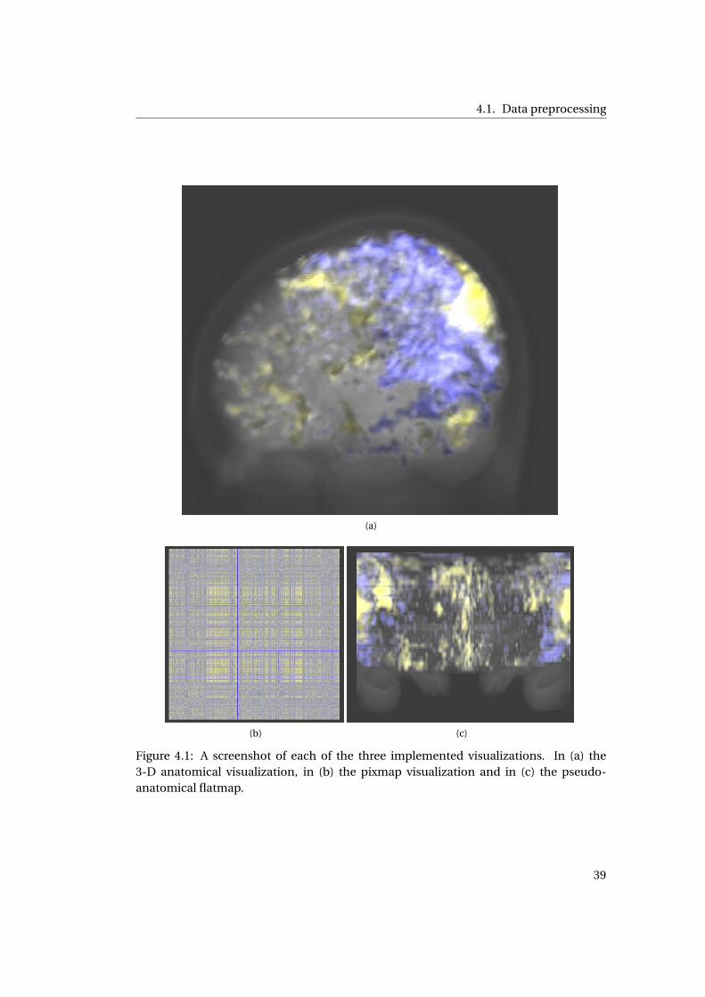
4.1. Data preprocessing
(a)
(b) (c)
Figure 4.1: A screenshot of each of the three implemented visualizations. In (a) the
3-D anatomical visualization, in (b) the pixmap visualization and in (c) the pseudo-
anatomical flatmap.
39

4. INTERACTIVE VISUALIZATION OF voxel-wise FMRI BRAIN CONNECTIVITY
4.2 Visualization Pipeline
Once the data is preprocessed and converted to the required input format, it can en-
ter the visualization pipeline. The pipeline is depicted schematically in Figure 4.2. In
Figure 4.2: The visualization pipeline. Figure from [dos Santos 04].
the visualization pipeline, the data is transformed to a pictorial form. Visual representa-
tions take maximum advantage of the human visual system. The main reasons for visual
representation of data are to allow humans to get better insight in the data and draw con-
clusions from it or to communicate the data or results from data analysis to an audience
that does not have a sufficient understanding of the data structure. A good motivation
for visual representation is expressed by Tamara Munzner:
“Visualization allows people to offload cognition to the perceptual system,
using carefully designed images as a form of external memory. The
human visual system is a very high-bandwidth channel to the brain,
with a significant amount of processing occurring in parallel and at
the pre-conscious level.”
Tamara Munzner in Fundamentals of Computer Graphics [Munzner 09]
The high dimensional nature of connectivity data makes the visualization of it a chal-
lenging task. In essence, the visualization of functional connectivity projects N points
in N dimensional space to a two-dimensional space (the screen), where N equals the
number of timeseries (voxels) in the data. Mapping such high-dimensional data to two
or three dimensions is far from straight-forward.
The problem of mapping high-dimensionality to screen-space is even more complicated
by the fact that brain connectivity data is inherently related to anatomy and anatom-
ical position. The relation between functional connectivity of two brain regions and
their anatomical locations is crucial for research in the neuroscience domain and should
therefore be somehow reflected in the visualization.
We identified the following requirements that visualizations of functional brain con-
nectivity should satisfy. In short, the visualizations should:
• Facilitate exploratory analysis by visualization and interaction
• Represent whether two voxels (brain regions) are connected
• Represent the strength of their connection
40
4.3. Direct Matrix Visualization
• Represent the relation between voxels and their anatomical location
• Provide general anatomical context
• Allow to focus on subsets in the data
• Render at interactive speed (at least 12 fps) during interaction
• Enable comparison between datasets
• Facilitate control over the representation
Based on these requirements, we propose three methods for the visualization of func-
tional brain connectivity data: a direct matrix visualization, an anatomical 3-D visual-
ization and a 2-D pseudo-anatomical flat map representation, shown in Figure 4.1 at
page 37. Each visualization technique will be described in a separate section below. The
methods are driven by a raycasting technique, which was already briefly discussed in
Chapter 2.
4.3 Direct Matrix Visualization
A widely used technique for the visualization of connectivity matrices is the direct ma-
trix visualization (DMV) 2. This method is already frequently being used in the visual-
ization of functional connectivity data to visualize results of an analysis (for instance
[Achard 06, Yu 11, Liu 08]). However, existing methods, including the method discussed
in Chapter 3, are capable of showing networks of relative small size only (at most a thou-
sand of rows and columns). Connectivity matrices of this size can be represented easily
in a single bitmap, which can be drawn directly on the screen.
The visualization of large connectivity matrices, consisting of thousands of rows and
columns, the rendering is more challenging. First of all, the screen resolution of today’s
monitors is not high enough to represent each cell in the matrix with its own pixel. That
means that zoom-and-pan techniques are required to enable the user to see the entire
connectivity matrix in its full detail. In this section, we present a technique that is, dif-
ferent from most existing techniques, is capable of visualizing connectivity matrices of
tens of thousands of rows and columns. We start with a basic description of the pixmap
representation, and then discuss our method in more detail.
4.3.1 The basics
Direct matrix visualization is a pixel-oriented technique, that results in a matrix of N x N
where each cell (i , j ) is color coded according to the connectivity between the each item.
The representation is effectively a bitmap with a colored pixel for each correlation. For
large correlation matrices, this requires a considerable amount of space, both in terms
of screen space and memory. Since our connectivity matrices are an order of magnitude
2In this thesis also referred to as pixmap, or matrix bitmap
41

4. INTERACTIVE VISUALIZATION OF voxel-wise FMRI BRAIN CONNECTIVITY
larger than what can be displayed on current monitors, only a portion of the matrix can
be displayed at its highest resolution at a single time.
4.3.2 Raycasting the correlation matrix
Instead of rendering the complete correlation matrix to an image, we propose a tech-
nique in which only the visible part of the correlation is rendered to the screen. For
this, we employed a raycasting technique that is able to render large correlation ma-
trices while maintaining interactive speed. This technique is memory-efficient, because
apart from the raw correlation data, it only requires an image of the size of the current
viewport to be in memory. Ray casting involves a projection of view coordinates (pixel
coordinates) to object coordinates using a series of transformations. In the matrix visu-
alization method, this transformation pipeline is ‘abused’ to find for each pixel on the
screen, the corresponding index in the correlation matrix.
Although there is no three dimensional object to render, the correlation matrix that we
want to visualize can be conceptually thought of as a texture-mapped plane. As such, we
can define a (virtual) plane in world space that is used as a ‘proxy object’ for the correla-
tion matrix. The technique is best illustrated with a schematic overview, see Figure 4.3.
When a ray is cast, it travels through the image plane at some pixel position p. The im-
Figure 4.3: The basic idea of raycasting the correlation matrix, with the corresponding
transformations. Transformation A transforms a pixel coordinate to object-space, in this
case a position on the proxy plane. Transformation B then interpolates this position to a
cell index in the raw correlation matrix. Finally, C maps the correlation value to a color
using a continuous color scale, which is assigned to the pixel in the projection plane.
age plane can either be the entire screen or a part of it (such as an image that is shown
42
4.3. Direct Matrix Visualization
in the the user interface). When the ray travels further through the image plane, it hits
the proxy object at some position q in world space. This coordinate is then transformed
to an index in the raw correlation matrix, and a correlation value can be retrieved. As
with regular volume rendering, a color map (in volume rendering usually referred to as
a transfer function) is used to map the data value to a color. In volume raycasting, the
algorithm would then continue by advancing the ray, but since there is only one value in
the z direction for the ‘virtual plane’ the algorithm stops and the color is assigned to the
corresponding screen pixel.
4.3.3 Mapping correlation to color
In the matrix visualizations, correlations are represented by color. The use of color to
represent numbers allows people to offload cognition to the human visual system which
is highly effective in detecting structure in images [Munzner 09]. The color mapping
should allow to easily apply the reverse mapping back to the raw data. Thus, the de-
sign of a color scale is an important factor in making effective visualizations and has a
powerful effect on how structure in the data is perceived [Rogowitz 96]. It is important
that the used color map does not bias the inferences people draw from the visualization.
Therefore, a color map should define a directly proportional relation between color and
the data attribute (unless one specifically wants to focus on some attributes in the data).
The design of ‘good’ colormaps has been well studied in the field of cognitive perception
and resulted in a number of rules for the design of colormaps that are perceptually lin-
ear [Rogowitz 96, Ware 88, Rheingans 90, Levkowitz 92, Moreland 09]. Correlation values
vary on a continuous scale between -1 and 1, which means that a continuous diverging
color scale is required. In our visualization, we have used perceptually linear colormaps
with different colors, that are continuous-diverging [Moreland 09], to discriminate be-
tween negative and positive correlation.
To be able to focus on high connectivity, it is also possible to employ non-linear col-
ormaps that draw attention to regions with high correlation.
4.3.4 Reordering the matrix
The effectiveness of the matrix visualization is highly affected by the ordering of items
along the rows and columns of the matrix. A randomly picked ordering (or ordering
based on properties not related to the data, such as alphabetical ordering of the labels)
might result in a matrix visualization that is hardly distinguishable from a noisy bitmap.
For functional brain connectivity, it was also previously noted that the ordering of the
matrix is important to be an effective representation [Dixhoorn 10].
In general, Friendly and Kwan [Friendly 03] state that unordered factors or variables
should be ordered according to what the user wants to see or show. They call their idea
effect-ordered data displays. Mueller et al. examined the use of graph ordering algo-
rithms for effective matrix-based visualization of connectivity data [Mueller 07]. Order-
ings can be selected a priori or derived from the data. In the first case, the ordering is
43
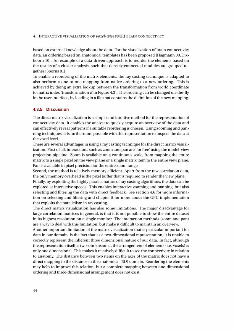
4. INTERACTIVE VISUALIZATION OF voxel-wise FMRI BRAIN CONNECTIVITY
based on external knowledge about the data. For the visualization of brain connectivity
data, an ordering based on anatomical templates has been proposed [Hagmann 08, Dix-
hoorn 10]. An example of a data-driven approach is to reorder the elements based on
the results of a cluster analysis, such that densely connected modules are grouped to-
gether [Sporns 01].
To enable a reordering of the matrix elements, the ray casting technique is adapted to
also perform a one-to-one mapping from native ordering to a new ordering. This is
achieved by doing an extra lookup between the transformation from world coordinate
to matrix index (transformation B in Figure 4.3). The ordering can be changed on-the-fly
in the user interface, by loading in a file that contains the definition of the new mapping.
4.3.5 Discussion
The direct matrix visualization is a simple and intuitive method for the representation of
connectivity data. It enables the analyst to quickly acquire an overview of the data and
can effectively reveal patterns if a suitable reordering is chosen. Using zooming and pan-
ning techniques, it is furthermore possible with this representation to inspect the data at
the voxel level.
There are several advantages in using a ray casting technique for the direct matrix visual-
ization. First of all, interactions such as zoom and pan are ‘for free’ using the model-view
projection pipeline. Zoom is available on a continuous scale, from mapping the entire
matrix to a single pixel on the view plane or a single matrix item to the entire view plane.
Pan is available in pixel precision for the entire zoom range.
Second, the method is relatively memory efficient. Apart from the raw correlation data,
the only memory overhead is the pixel buffer that is required to render the view plane.
Finally, by exploiting the highly parallel nature of ray casting algorithms, the data can be
explored at interactive speeds. This enables interactive zooming and panning, but also
selecting and filtering the data with direct feedback. See section 4.6 for more informa-
tion on selecting and filtering and chapter 5 for more about the GPU implementation
that exploits the parallelism in ray casting.
The direct matrix visualization has also some limitations. The major disadvantage for
large correlation matrices in general, is that it is not possible to show the entire dataset
in its highest resolution on a single monitor. The interaction methods (zoom and pan)
are a way to deal with this limitation, but make it difficult to maintain an overview.
Another important limitation of the matrix visualization that is particular important for
data in our domain, is the fact that as a two-dimensional representation, it is unable to
correctly represent the inherent three dimensional nature of our data. In fact, although
the representation itself is two-dimensional, the arrangement of elements (i.e. voxels) is
only one dimensional. This makes it relatively difficult to see the connectivity in relation
to anatomy. The distance between two items on the axes of the matrix does not have a
direct mapping to the distance in the anatomical (3D) domain. Reordering the elements
may help to improve this relation, but a complete mapping between one-dimensional
ordering and three-dimensional arrangement does not exist.
44
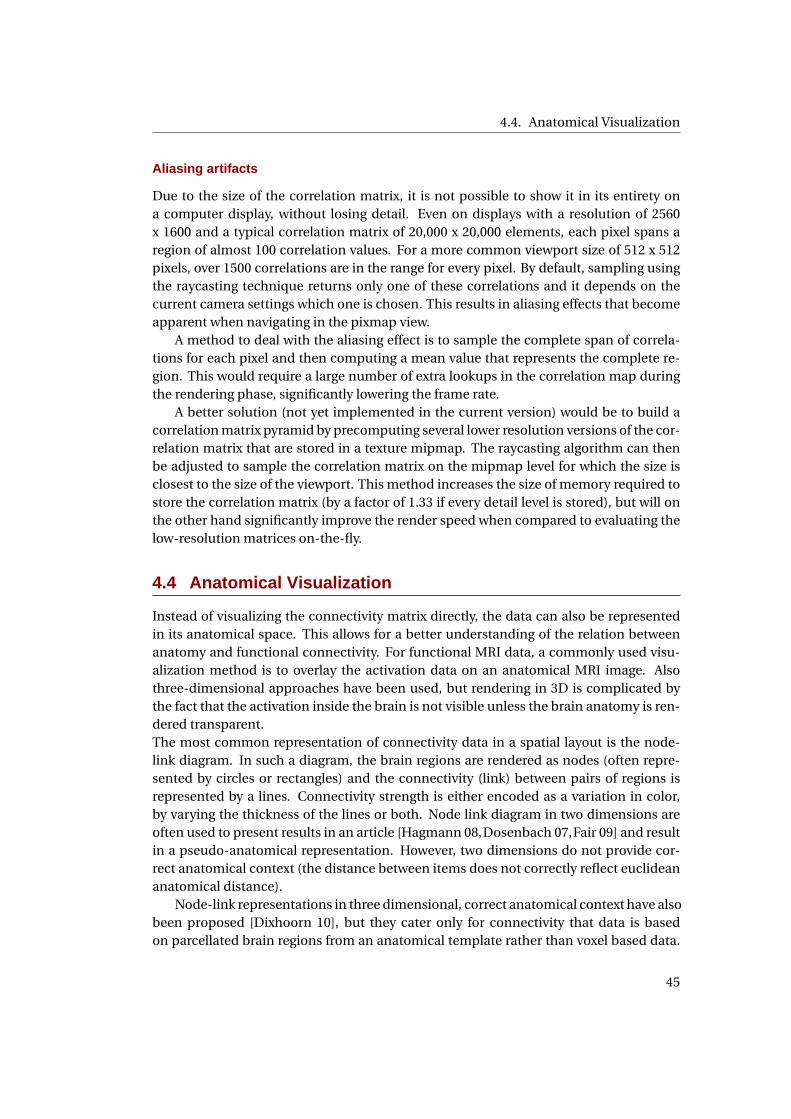
4.4. Anatomical Visualization
Aliasing artifacts
Due to the size of the correlation matrix, it is not possible to show it in its entirety on
a computer display, without losing detail. Even on displays with a resolution of 2560
x 1600 and a typical correlation matrix of 20,000 x 20,000 elements, each pixel spans a
region of almost 100 correlation values. For a more common viewport size of 512 x 512
pixels, over 1500 correlations are in the range for every pixel. By default, sampling using
the raycasting technique returns only one of these correlations and it depends on the
current camera settings which one is chosen. This results in aliasing effects that become
apparent when navigating in the pixmap view.
A method to deal with the aliasing effect is to sample the complete span of correla-
tions for each pixel and then computing a mean value that represents the complete re-
gion. This would require a large number of extra lookups in the correlation map during
the rendering phase, significantly lowering the frame rate.
A better solution (not yet implemented in the current version) would be to build a
correlation matrix pyramid by precomputing several lower resolution versions of the cor-
relation matrix that are stored in a texture mipmap. The raycasting algorithm can then
be adjusted to sample the correlation matrix on the mipmap level for which the size is
closest to the size of the viewport. This method increases the size of memory required to
store the correlation matrix (by a factor of 1.33 if every detail level is stored), but will on
the other hand significantly improve the render speed when compared to evaluating the
low-resolution matrices on-the-fly.
4.4 Anatomical Visualization
Instead of visualizing the connectivity matrix directly, the data can also be represented
in its anatomical space. This allows for a better understanding of the relation between
anatomy and functional connectivity. For functional MRI data, a commonly used visu-
alization method is to overlay the activation data on an anatomical MRI image. Also
three-dimensional approaches have been used, but rendering in 3D is complicated by
the fact that the activation inside the brain is not visible unless the brain anatomy is ren-
dered transparent.
The most common representation of connectivity data in a spatial layout is the node-
link diagram. In such a diagram, the brain regions are rendered as nodes (often repre-
sented by circles or rectangles) and the connectivity (link) between pairs of regions is
represented by a lines. Connectivity strength is either encoded as a variation in color,
by varying the thickness of the lines or both. Node link diagram in two dimensions are
often used to present results in an article [Hagmann 08,Dosenbach 07,Fair 09] and result
in a pseudo-anatomical representation. However, two dimensions do not provide cor-
rect anatomical context (the distance between items does not correctly reflect euclidean
anatomical distance).
Node-link representations in three dimensional, correct anatomical context have also
been proposed [Dixhoorn 10], but they cater only for connectivity that data is based
on parcellated brain regions from an anatomical template rather than voxel based data.
45

4. INTERACTIVE VISUALIZATION OF voxel-wise FMRI BRAIN CONNECTIVITY
Even for a relatively low amount of brain regions, the view easily becomes cluttered with
the links that are rendered on top of each other [Dixhoorn 10]. The problem of clutter
caused by overlapping links makes node-link diagrams unsuitable for the representation
of our data.
A different method would be to adapt the three dimensional visualization method
often used to visualize activity data from fMRI studies. In those visualizations, the acti-
vated brain regions are rendered in an otherwise semi-transparent brain volume. How-
ever, whereas in activation studies only the network of brain regions are shown that are
active during a specific task, whole brain functional connectivity contains the connec-
tivity information about a large number of networks. In fact, voxel based functional con-
nectivity data describes as many networks as there are voxels. As each voxel is part of
many different networks, displaying all networks simultaneously in a single visualiza-
tion is not possible. Instead, we propose a method that is based on user interaction to
show connectivity data of selected brain regions (seeds). The method of representation
is inspired by the work of Jainek et al. [Jainek 08], who used illustrative techniques for the
visualization of activity data. Our method is different in that we use non-photorealistic
rendering techniques to render connectivity data for a by the user interactively selected
seed voxel.
4.4.1 The basics
The anatomical visualization enables the interactive exploration of connectivity data in
an anatomical context. The anatomical context is provided by two features: a semi-
transparent contour visualization of a human head that shows overall anatomical con-
text and a semi-transparent brain volume that shows anatomical context from an atlas,
enhanced with contour lines to outline the atlas regions. To explore the activity data,
the analyst can hover over the brain volume with the mouse. When the mouse is moved
over the brain volume, the connectivity data is shown for the brain region currently un-
der the mouse cursor, by highlighting all voxels that are functionally connected to the
current seed voxel. The strength of connectivity is represented by varying the color of the
corresponding voxel, with the same color map as used in the direct matrix visualization.
To enhance the visualization, the opacity of each voxel is also varied based on the con-
nectivity strength such that voxels with high correlation are emphasized. The method is
implemented in the ray casting framework that was briefly discussed in Section 4.3.
4.4.2 Raycasting the correlation volume
The general idea of the raycasting technique that was designed for the visualization of
functional connectivity data in anatomical space is schematically illustrated in Figure
4.4. The figure shows how direct volume rendering is used to render the connectivity
data after a user has selected a particular voxel (in this figure indicated with a red cir-
cle). The raycaster then renders the volume by shooting rays through it and looking up
the correlation between the seed voxel and each voxel it visits when stepping through
46

4.4. Anatomical Visualization
Figure 4.4: Raycasting functional connectivity in an anatomical representation of the
brain.
the volume. Given the two voxel positions, the raycaster needs to know the mapping be-
tween the 3D coordinates and the corresponding position in the correlation matrix. See
Figure 4.5 for a schematic representation of this mapping.
5
6
20
x y z idx
5 6 19 35
5 6 20 36
... ... ... ...
21 29 25 21954
18
14
5
x y z idx
5 6 19 35
5 6 20 36
... ... ... ...
21 29 25 21954
0.7689
Figure 4.5: Looking up the correlation value between a seed voxel and a voxel in the
volume.
This mapping is created from the voxel coordinates that are defined in the input file
(see Listing 4.1). From these coordinates, a three dimensional lookup table (LUT) is con-
structed in which the list index of every voxel in the coordinate list is stored. Whereas
the list of coordinates in the input file in fact defines a mapping from a one dimensional
coordinate (the list index) to a three dimensional coordinate (a coordinate in anatomi-
cal 3D space), the 3D LUT constructed in this step actually defines the inverse mapping:
for a given 3D voxel coordinate, it returns the native matrix index corresponding to that
47

4. INTERACTIVE VISUALIZATION OF voxel-wise FMRI BRAIN CONNECTIVITY
voxel. The 3D LUT can also be interpreted as a volume, so in the remainder of this text,
we will refer to it as the index volume.
Rendering in two passes
While stepping through the volume, the raycaster can now use the index volume to lookup
the correlation between the current position in the volume and the seed position. If the
correlation is nonzero (and below a certain threshold, see Section 4.6), the correlation
value is mapped to a color and opacity value and added in the compositing process.
The method presented so far does both the correlation lookup and the rendering of
the color-mapped correlation value in a single step. However, for low resolution index
volumes, this results in a bad image quality. The 4mm voxel resolution of our input data
also is not high enough, resulting in in a visualization with blocky artifacts as can be seen
in Figure 4.6.
Figure 4.6: Blocky artifacts due to undersampling of the index volume.
A common method in volume rendering to reduce aliasing artifacts is to oversample
the volume during the ray integration by taking extra samples between the voxels and
48
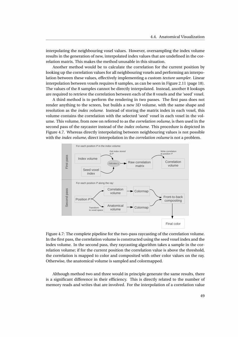
4.4. Anatomical Visualization
interpolating the neighbouring voxel values. However, oversampling the index volume
results in the generation of new, interpolated index values that are undefined in the cor-
relation matrix. This makes the method unusable in this situation.
Another method would be to calculate the correlation for the current position by
looking up the correlation values for all neighbouring voxels and performing an interpo-
lation between these values, effectively implementing a custom texture sampler. Linear
interpolation between voxels requires 8 samples, as can be seen in Figure 2.11 (page 18).
The values of the 8 samples cannot be directly interpolated. Instead, another 8 lookups
are required to retrieve the correlation between each of the 8 voxels and the ‘seed’ voxel.
A third method is to perform the rendering in two passes. The first pass does not
render anything to the screen, but builds a new 3D volume, with the same shape and
resolution as the index volume. Instead of storing the matrix index in each voxel, this
volume contains the correlation with the selected ‘seed’ voxel in each voxel in the vol-
ume. This volume, from now on referred to as the correlation volume, is then used in the
second pass of the raycaster instead of the index volume. This procedure is depicted in
Figure 4.7. Whereas directly interpolating between neighbouring values is not possible
with the index volume, direct interpolation in the correlation volume is not a problem.
����������� ������� �����
� ����
��������������
������������
����������������� ���
����� ��������
����������� ����� ������������
������� ��
�������� ��
����� ��������������������������������
����� �������������� ��������� ��
����������
� ��!�������������� ��
����� ��������
"� ����� ����
��� �����
�����#��#$ �%�����������
����� �
����� �
Figure 4.7: The complete pipeline for the two-pass raycasting of the correlation volume.
In the first pass, the correlation volume is constructed using the seed voxel index and the
index volume. In the second pass, they raycasting algorithm takes a sample in the cor-
relation volume; if for the current position the correlation value is above the threshold,
the correlation is mapped to color and composited with other color values on the ray.
Otherwise, the anatomical volume is sampled and colormapped.
Although method two and three would in principle generate the same results, there
is a significant difference in their efficiency. This is directly related to the number of
memory reads and writes that are involved. For the interpolation of a correlation value
49
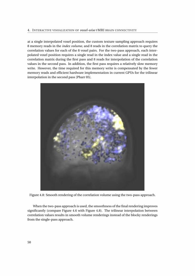
4. INTERACTIVE VISUALIZATION OF voxel-wise FMRI BRAIN CONNECTIVITY
at a single interpolated voxel position, the custom texture sampling approach requires
8 memory reads in the index volume, and 8 reads in the correlation matrix to query the
correlation values for each of the 8 voxel pairs. For the two-pass approach, each inter-
polated voxel position requires a single read in the index value and a single read in the
correlation matrix during the first pass and 8 reads for interpolation of the correlation
values in the second pass. In addition, the first pass requires a relatively slow memory
write. However, the time required for this memory write is compensated by the fewer
memory reads and efficient hardware implementation in current GPUs for the trilinear
interpolation in the second pass [Pharr 05].
Figure 4.8: Smooth rendering of the correlation volume using the two-pass approach.
When the two-pass approach is used, the smoothness of the final rendering improves
significantly (compare Figure 4.6 with Figure 4.8). The trilinear interpolation between
correlation values results in smooth volume renderings instead of the blocky renderings
from the single-pass approach.
50
4.4. Anatomical Visualization
Rendering anatomical context
If the correlation is zero (or below a certain threshold), then no color would be assigned
to that particular voxel and the raycaster would take a next step on the ray. However, for
better anatomical context, the non-correlated voxels are used to render anatomical con-
text. While presenting results from activation or connectivity-based studies, the data is
usually overlayed on a 2D anatomical brain image. This reveals the inherent anatomical
context that is present in the data, but does not show the three-dimensional relations
between the data and the anatomy. In three dimensional representations, rendering
the anatomical context is a more challenging task. Rendering the brain as an opaque
surface would occlude connectivity data for voxels inside the brain. Several methods
have been proposed for fused rendering of functional activity (or connectivity) data and
anatomical MRI data, including projecting all activations in the brain to the brains’ sur-
face [Stokking 01, Viergever 01], using clipping planes and rendering the brain anatomy
semi-transparent.
The first method (commonly referred to as ‘normal fusion’) integrates the functional
activity data along the inward normal to the cortical surface and color maps the inte-
grated activity data on the surface. However, this method has the disadvantage of pro-
viding a misleading anatomical [Rehm 98].
The use of clipping planes allows for the visualization of the activity or connectiv-
ity data in its correct anatomical position, even if the brain anatomy is rendered in an
opaque surface representation. Despite that advantage, it is not possible to view the
functional data in the brain as a whole in a single representation.
Semi-transparent rendering of the brain anatomy, the method used in our visualiza-
tion, is probably the most natural way of representation, reflecting what we intuitively
expect to see. Although the method is not optimal because it suffers from the perceptual
issues inherent to 3D visualization, such as occlusion and difficult depth perception, this
may be outweighed by the benefits of helping the user to form a mental model of the
dataset [Munzner 09].
Our method of context visualization consists of two complementary context modal-
ities: a semi-transparent high-resolution structural scan of a head that provides overall
orientational context and anatomy based atlas regions that shows individual brain re-
gions from the Automated Anatomical Labeling (AAL) atlas [Tzourio-Mazoyer 02].
The AAL atlas contains 45 cortical and subcortical regions for both hemispheres. The
individual atlas regions need to be represented differently in the visualization. For a dis-
crete set, the best visual channel to distinguish the region is the hue channel. Although
it would be possible to assign a different color to each atlas region, this would not re-
sult in an effective representation, because the number of hues that people can reliably
distinguish is only around a dozen [Munzner 09]. An alternative approach is to assign
different colors only to individual brain lobes [Dixhoorn 10]. Following this approach,
we generated a color palette with 7 different colors (one for each brain lobe) using the
ColorBrewer tool 3 and render brain regions in the same brain lobe with the same color.
Individual regions are then made visible by emphasizing their contours using a moderate
3Color Brewer website: www.colorbrewer2.org
51
4. INTERACTIVE VISUALIZATION OF voxel-wise FMRI BRAIN CONNECTIVITY
black line, using the following function:
s(P,V ) = (1−|∇(P ) ·V |)n (4.1)
Here, P is the value at the current position, ∇(P ) is the gradient at the current position,
V is the viewing direction and n controls the sharpness of the contour [Csébfalvi 01]. For
our purposes, a value of 7 for n gives a good enhancement of the contour line.
The high resolution and atlas data are sent to the raycaster as 3D volumes. In the
remainder of this text, they will be referred to as the highres volume and atlas volume.
Note: During the first evaluation session (see Section 4.8.2), it became ap-
parent that the AAL atlas volume is not often used in the field of functional
brain connectivity. Domain scientists appeared not to be familiar with the
AAL template and found the representation with the AAL colors somewhat
confusing. Therefore, the AAL template volume was removed from the visu-
alization at a later stage.
Volume transformations
For each position along the ray, the raycasting algorithm determines what should be ren-
dered. If the position is outside of the brain, the raycaster looks up the color for the voxel
in the highres volume. If the position is inside the brain volume, the color that is assigned
to the voxel depends on the correlation of the voxel with the seed position. If the correla-
tion is high enough, the resulting voxel color is taken to be the colormapped correlation
value. If there is no correlation (or the correlation does not exceed a certain threshold),
the voxel is colored according to the anatomical atlas region the position belongs to.
To be able to render the final image in only one pass, the three volumes have to be
aligned somehow. This is realized by forcing each volume to be in the same standard
space. The high resolution volume and the atlas volume that are used in the visualiza-
tion are already in MNI-152 space, and the index volume that is built from the voxel
coordinates is also in MNI-space, as a result of the preprocessing (see Section 4.1). This
means that when the raycasting algorithm takes steps along the ray trough the volume in
world space, it should be able to convert the world space coordinate to voxel coordinate
for each volume.
In addition, the mapping should also compensate for resolution differences between
the individual volumes. In our data, the correlation matrix is calculated from the raw
bold fMRI 4D volume that was resampled to an isotropic 4mm resolution and the index
volume (which is built from the matrix 3D coordinates) is thus also in a 4mm resolu-
tion. The AAL template volume and MRI head volume on the other hand, are available
in a 2mm and 0.5mm isotropic resolution respectively. To compensate for the resolution
differences, each volume that is sent to the raycaster is joined with its volume transfor-
mation matrix, which directly converts the world coordinate to the corresponding voxel
coordinate. The world coordinate system is set to equal the coordinate space of the vol-
ume with the highest resolution, in this case the MRI head volume, such that the trans-
formation matrix for this volume is the identity matrix. See Figure 4.9 for a sample trans-
52

4.4. Anatomical Visualization
formation between a world space coordinate and the native voxel coordinate for each
volume.
Figure 4.9: The transformation of a world space coordinate to a voxel coordinate for each
volume.
4.4.3 Picking a seed voxel
Since the anatomical visualization shows the correlation of voxels with a seed voxel, the
user must be presented with a method to select this seed voxel. Selecting a position in
3D space using a flat display and the mouse is a difficult task. The standard mouse in-
teraction does not support selections in 3 dimensions and the lack of visual feedback
on the depth perception makes the interaction in 3D environments a vivid field of study
[Vanacken 09].
Typical methods include the use of slice planes to indicate the target position and the
raycasting technique, that selects a position on the object directly under the mouse cur-
sor. The first method is previously used to select the target position for a seed voxel for
functional connectivity visualization. This method allows the user to select a seed posi-
tion on a 2D slice of the raw fMRI data [Eklund 11]. This enables a precise placement of
the seed voxel in the brain volume. However, using a 2D presentation to select a position
in a 3D space is not ideal, since it may be difficult to mentally reconstruct the 3D location
from browsing through a set of 2D slices [Tory 03].
53
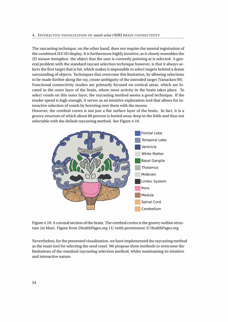
4. INTERACTIVE VISUALIZATION OF voxel-wise FMRI BRAIN CONNECTIVITY
The raycasting technique, on the other hand, does not require the mental registration of
the combined 2D/3D display. It is furthermore highly intuitive, as it closely resembles the
2D mouse metaphor: the object that the user is currently pointing at is selected. A gen-
eral problem with the standard raycast selection technique however, is that it always se-
lects the first target that is hit, which makes it impossible to select targets behind a dense
surrounding of objects. Techniques that overcome this limitation, by allowing selections
to be made further along the ray, create ambiguity of the intended target [Vanacken 09].
Functional connectivity studies are primarily focused on cortical areas, which are lo-
cated in the outer layer of the brain, where most activity in the brain takes place. To
select voxels on this outer layer, the raycasting method seems a good technique. If the
render speed is high enough, it serves as an intuitive exploration tool that allows for in-
teractive selection of voxels by hovering over them with the mouse.
However, the cerebral cortex is not just a flat surface layer of the brain. In fact, it is a
groovy structure of which about 60 percent is buried away deep in the folds and thus not
selectable with the default raycasting method. See Figure 4.10.
Frontal Lobe
Temporal Lobe
Ventricle
White Matter
Basal Ganglia
Thalamus
Midbrain
Limbic System
Pons
Medula
Spinal Cord
Cerebellum
Figure 4.10: A coronal section of the brain. The cerebral cortex is the groovy outline struc-
ture (in blue). Figure from [HealthPages.org 11] (with permission) © HealthPages.org
Nevertheless, for the presented visualization, we have implemented the raycasting method
as the main tool for selecting the seed voxel. We propose three methods to overcome the
limitations of the standard raycasting selection method, whilst maintaining its intuitive
and interactive nature.
54

4.4. Anatomical Visualization
Increasing the size of the seed region
Probably the simplest method that allows the selection of voxels deeper beneath the sur-
face of the brain is to increase the size of the seed region. Currently, only spherical re-
gions are supported, but the implementation of support for different shapes is straight-
forward. Once a seed region multiple voxels is selected, for each voxel in the brain, the
correlation with a group of voxels rather than a single voxel has to be computed. For each
voxel v in the set of all voxels V , this results in a number of correlation values C (v, w) (one
for each voxel w in the seed region W ), that have to be reduced to a single number C to
be able to represent the correlation of the seed region with v . Different statistics can be
used as the final correlation C , such as taking the mean value, the median, maximum or
minimum. For now, the maximum statistic has been implemented:
C = maxi∈Vj∈W
(C (i , j )) (4.2)
Other aggregation operations can be implemented easily.
Selecting an atlas region
Instead of using only purely spatial information to increase the size of the seed region,
it is also possible to use the anatomical atlas to define a seed region. When a voxel is
selected using the raycasting method, the voxel position is used to pull the corresponding
atlas region from the atlas volume. Then, all voxels from the found atlas region are used
as the seed region and the process continues as discussed above.
Depth-splitting the brain
As discussed above, the most important limitation of the standard raycasting method for
selecting a target in a 3D environment is that it does not allow the selection of targets that
are occluded by regions closer to the viewer. Although technically, it would be possible to
select those targets by increasing the seed region, this is often not desired as this makes
the resulting correlation map more and more ambiguous.
In essence, selecting a target in 3D that is occluded by other regions, introduces an ac-
cess problem [Vanacken 09]. Intuitively, we might solve this problem (in a real world
situation) by partly splitting the volume and using the resulting ‘crack’ to select the de-
sired seed position, after which the volume can be closed again. A method following
this metaphor has been employed to allow subcortical selections to be made. Using the
mouse, a virtual split plane can be placed allowing the brain volume to be pushed ajar.
Similar techniques have previously been applied as a focus+context method, to show a
focus object (selection) or reveal hidden structure in the data. For an overview of tech-
niques, the reader is referred to McGuffin et al. [McGuffin 03], Bruckner et al. [Bruck-
ner 06] and the review on general occlusion management techniques by Elmqvist and
Tsigas [Elmqvist 08].
Splitting the brain at the current mouse position is made possible with a simple mouse
gesture: holding the shift button while moving the mouse pointer in the direction of the
55
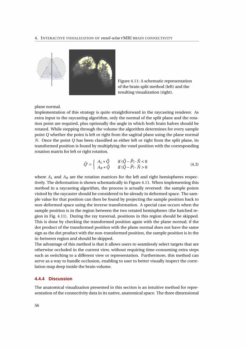
4. INTERACTIVE VISUALIZATION OF voxel-wise FMRI BRAIN CONNECTIVITY
Figure 4.11: A schematic representation
of the brain split method (left) and the
resulting visualization (right).
plane normal.
Implementation of this strategy is quite straightforward in the raycasting renderer. As
extra input to the raycasting algorithm, only the normal of the split plane and the rota-
tion point are required, plus optionally the angle in which both brain halves should be
rotated. While stepping through the volume the algorithm determines for every sample
point Q whether the point is left or right from the sagittal plane using the plane normal
N . Once the point Q has been classified as either left or right from the split plane, its
transformed position is found by multiplying the voxel position with the corresponding
rotation matrix for left or right rotation.
~Q ′ =
{
AL ∗ ~Q if (~Q −~P ) · ~N < 0
AR ∗ ~Q if (~Q −~P ) · ~N > 0(4.3)
where AL and AR are the rotation matrices for the left and right hemispheres respec-
tively. The deformation is shown schematically in Figure 4.11. When implementing this
method in a raycasting algorithm, the process is actually reversed: the sample points
visited by the raycaster should be considered to be already in deformed space. The sam-
ple value for that position can then be found by projecting the sample position back to
non-deformed space using the inverse transformation. A special case occurs when the
sample position is in the region between the two rotated hemispheres (the hatched re-
gion in Fig. 4.11). During the ray traversal, positions in this region should be skipped.
This is done by checking the transformed position again with the plane normal; if the
dot product of the transformed position with the plane normal does not have the same
sign as the dot product with the non-transformed position, the sample position is in the
in-between region and should be skipped.
The advantage of this method is that it allows users to seamlessly select targets that are
otherwise occluded in the current view, without requiring time-consuming extra steps
such as switching to a different view or representation. Furthermore, this method can
serve as a way to handle occlusion, enabling to user to better visually inspect the corre-
lation map deep inside the brain volume.
4.4.4 Discussion
The anatomical visualization presented in this section is an intuitive method for repre-
sentation of the connectivity data in its native, anatomical space. The three dimensional
56

4.5. Pseudo anatomical visualization
visualization is able to correctly show the relation between functional connectivity and
the corresponding anatomical locations of distinct voxels in the brain.
Whereas node-link diagrams, often used for the visualization of functional connectivity,
use the metaphor of physical connection between functionally connected regions, the
visualization method presented in this section used the metaphor of simultaneous acti-
vation (or deactivation), which closely resembles what is measured.
The anatomical visualization is enhanced by rendering a semi-transparent human head
volueme for overall context, and coloring the regions of an anatomical atlas template to
amplify the relation between functional connectivity and anatomical regions.
An issue inherent to 3D visualization and navigation is the difficulty of selecting a 3D
position on a 2D screen with input devices that are designed for 2D interaction. We pre-
sented a method that is based on the metaphor of splitting the volume to deal with this
issue, which gives direct feedback and does not require the user to switch between differ-
ent views or representations. The effectiveness of such a tool must be evaluated in real
world situations (see Chapter 4.8).
A second issue related to three dimensional rendering, is the problem of occlusion. Al-
though the occlusion problem is partly solved by interaction, such as rotation and zoom-
ing, it prevents the user from being able to see the complete correlation field for the se-
lected voxel at a single glance. Since this is a problem inherent to three dimensional vi-
sualization, another representation is required to be able to solve this. In the next section
we will discuss a method that is meant as a starting point for a ‘flat map’ of the human
brain, in which correlations can be explored with minimal occlusion.
All methods presented in this section are implemented in a raycasting framework that
uses a combination of the Visualization Toolkit (VTK) for the rendering pipeline and 3D
environment setup, and the Open Compute Language (OpenCL) for the actual raycasting
implementation. Using OpenCL, the visualization can be rendered at interactive speeds
on current consumer graphics cards. More detailed implementation notes are discussed
in the next chapter.
4.5 Pseudo anatomical visualization
The two representations we have represented so far both have their own unique abilities
and limitations. The direct matrix visualization provides the ability to show the complete
dataset in a single, comprehensible representation that has good potential for detecting
patterns in the data, but does not correctly show the anatomical structure of the data.
The anatomical visualization discussed in the previous section on the other hand, cor-
rectly shows the connectivity data in its anatomical context, but is unable to provide a
clear view on the entire dataset in a single picture and requires interaction to be able to
see the entire dataset. One of the main problems with the anatomical representation is
that it suffers from occlusion.
In this section, we will present a method that is designed to reduce the occlusion to a
minimum, whilst maintaining as much of the anatomical spacing as possible. The basic
idea is to create a projection of the brain’s surface onto a two-dimensional map, similar
57

4. INTERACTIVE VISUALIZATION OF voxel-wise FMRI BRAIN CONNECTIVITY
to the projection of the Earth’s surface in typical world maps.
Studies in the field of cartography have resulted in numerous projection methods. A
commonly used projection for world maps, used by major street mapping services, such
as Bing Maps, Google Maps and Yahoo Maps [Elson 07], is the Mercator projection, in-
vented by the cartographer Garardus Mercator (1512 - 1594). The Mercator projection
is a cylindrical projection, that maps parallels and meridians to a rectangular grid. The
parallels (horizontal lines) are spaced farther apart farther away from the equation, re-
sulting in a scale distortion closer to the poles (see Figure 4.12). The map is usually cut
off at latitudes around 82-84◦, because the area of the regions near 90◦ becomes infi-
nite [Maling 91].
Figure 4.12: A Mercator projection of the world, between latitudes of +82◦and -82◦. Fig-
ure from Wikimedia Commons [Commons" 11]
In the field of human neuroimaging, the need for two-dimensional mappings has
also been recognized to visualize data that has been buried deep inside the grooves of
the cerebral cortex [Dale 99, Fischl 99]. For an overview of the available methods, the
reader is referred to Tosun et al. [Tosun 04], Dale et al [Dale 99] and Fischl et al. [Fis-
chl 99]. A method that has attracted significant attention is the circle packing technique
proposed for the use of flattening of the cerebellum and the cortical surface by Hurdal
et al. [Hurdal 99, Stephenson 00, Hurdal 01]. The process of flattening usually consists of
three steps: creating a tessellated mesh of the gray matter surface, introducing cuts that
will define the map boundary, and flattening the triangulated mesh by iteratively calcu-
58
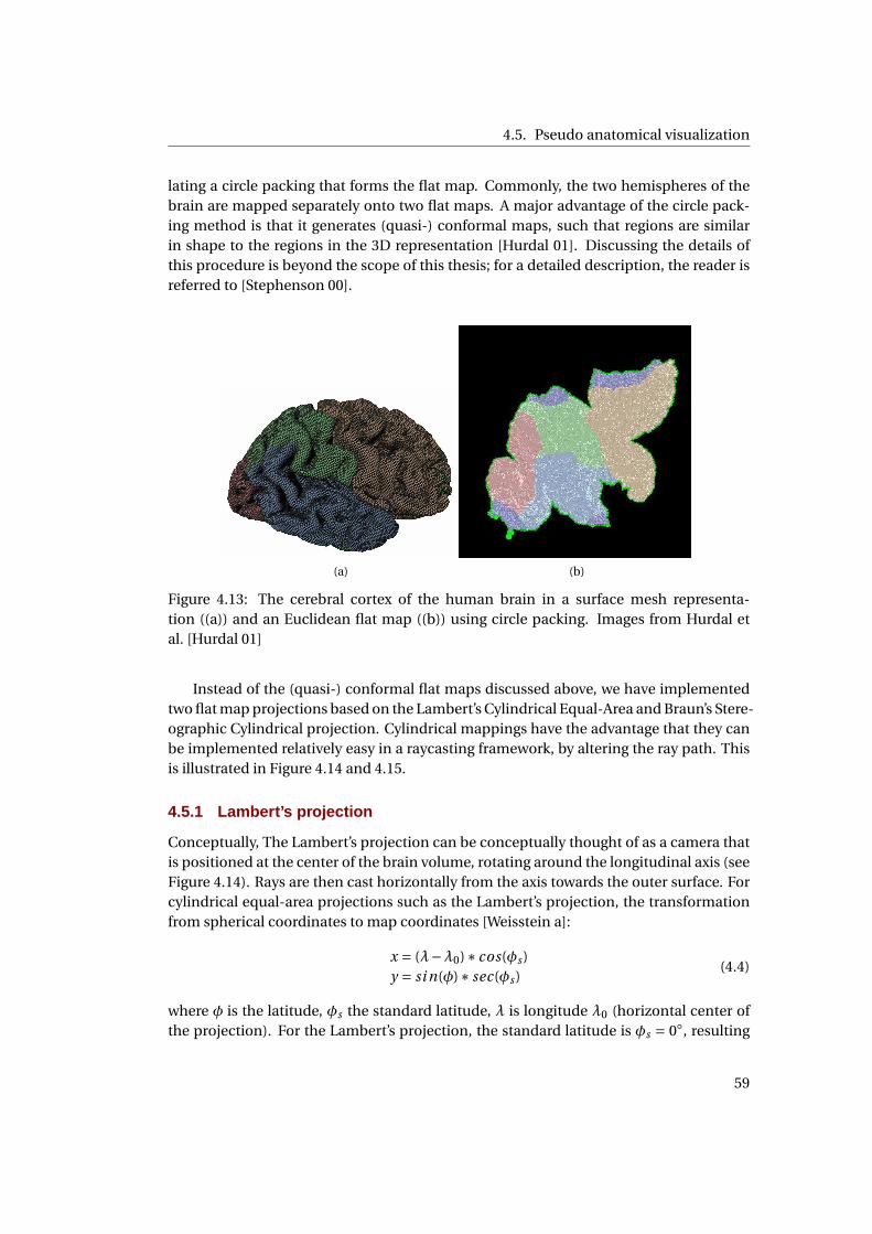
4.5. Pseudo anatomical visualization
lating a circle packing that forms the flat map. Commonly, the two hemispheres of the
brain are mapped separately onto two flat maps. A major advantage of the circle pack-
ing method is that it generates (quasi-) conformal maps, such that regions are similar
in shape to the regions in the 3D representation [Hurdal 01]. Discussing the details of
this procedure is beyond the scope of this thesis; for a detailed description, the reader is
referred to [Stephenson 00].
(a) (b)
Figure 4.13: The cerebral cortex of the human brain in a surface mesh representa-
tion ((a)) and an Euclidean flat map ((b)) using circle packing. Images from Hurdal et
al. [Hurdal 01]
Instead of the (quasi-) conformal flat maps discussed above, we have implemented
two flat map projections based on the Lambert’s Cylindrical Equal-Area and Braun’s Stere-
ographic Cylindrical projection. Cylindrical mappings have the advantage that they can
be implemented relatively easy in a raycasting framework, by altering the ray path. This
is illustrated in Figure 4.14 and 4.15.
4.5.1 Lambert’s projection
Conceptually, The Lambert’s projection can be conceptually thought of as a camera that
is positioned at the center of the brain volume, rotating around the longitudinal axis (see
Figure 4.14). Rays are then cast horizontally from the axis towards the outer surface. For
cylindrical equal-area projections such as the Lambert’s projection, the transformation
from spherical coordinates to map coordinates [Weisstein a]:
x = (λ−λ0)∗ cos(φs)
y = si n(φ)∗ sec(φs)(4.4)
where φ is the latitude, φs the standard latitude, λ is longitude λ0 (horizontal center of
the projection). For the Lambert’s projection, the standard latitude is φs = 0◦, resulting
59

4. INTERACTIVE VISUALIZATION OF voxel-wise FMRI BRAIN CONNECTIVITY
Figure 4.14: A cross-section diagram showing the geometrical concept of the Lambert’s
projection. The dotted vertical lines indicate the surface of a cylinder tangent to the
bounding sphere, which is shown in this cross-section as a circle. The arrows indicate
the ray path used in the raycasting algorithm. The values along the ray are composited
and projected on the inner surface of the cylinder, which is then unrolled to form the
resulting flat map.
in a simplified version of the transformation:
x = (λ−λ0)
y = si n(φ)(4.5)
The horizontal center of the projection determines which part of the brain is shown in
the center of the map. In MNI orientation, the anterior part of the brain is at 0◦, thus
the resulting map should project 0◦in the center and -180◦and +180◦at both horizontal
extremes. Thus, λ0 =−180◦.
For a raycasting algorithm, the inverse transformation is used to find the object co-
ordinate from a given map coordinate (x, y):
φ= si n−1(y)
λ= x +λ0(4.6)
The ray start position for the raycasting algorithm is fixed along the anterior-posterior
and medio-lateral axes, varying only on the superior-inferior axis. For simplicity, the
end position of the ray is taken to be on the surface of a sphere that just encloses the
brain volume and found by converting the spherical coordinates φ and λ to the Cartesian
coordinates:x = r ∗ cos(φ)∗ si n(λ)
y = r ∗ si n(φ)∗ si n(λ)
z = r ∗ cos(λ)
(4.7)
60
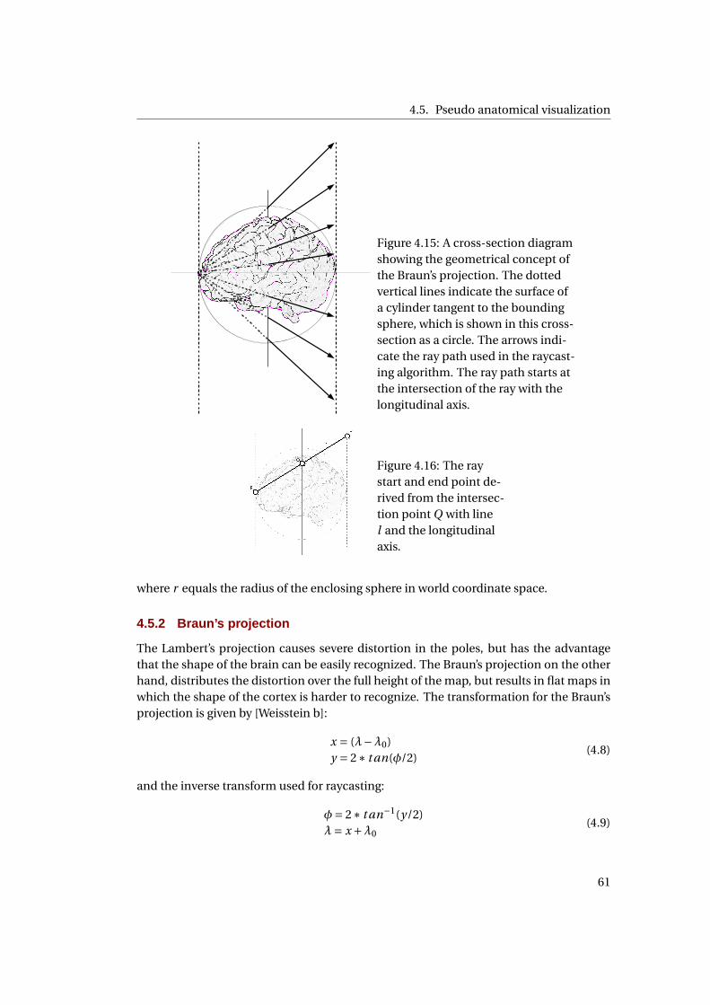
4.5. Pseudo anatomical visualization
Figure 4.15: A cross-section diagram
showing the geometrical concept of
the Braun’s projection. The dotted
vertical lines indicate the surface of
a cylinder tangent to the bounding
sphere, which is shown in this cross-
section as a circle. The arrows indi-
cate the ray path used in the raycast-
ing algorithm. The ray path starts at
the intersection of the ray with the
longitudinal axis.
Figure 4.16: The ray
start and end point de-
rived from the intersec-
tion point Q with line
l and the longitudinal
axis.
where r equals the radius of the enclosing sphere in world coordinate space.
4.5.2 Braun’s projection
The Lambert’s projection causes severe distortion in the poles, but has the advantage
that the shape of the brain can be easily recognized. The Braun’s projection on the other
hand, distributes the distortion over the full height of the map, but results in flat maps in
which the shape of the cortex is harder to recognize. The transformation for the Braun’s
projection is given by [Weisstein b]:
x = (λ−λ0)
y = 2∗ t an(φ/2)(4.8)
and the inverse transform used for raycasting:
φ= 2∗ t an−1(y/2)
λ= x +λ0(4.9)
61

4. INTERACTIVE VISUALIZATION OF voxel-wise FMRI BRAIN CONNECTIVITY
Braun’s projection is conceptually similar to the Lambert’s projection. The difference is
the position of the camera and thus, the start position of the rays for the raycasting algo-
rithm. The camera position is also varying along the superior-inferior axis, but the actual
position on the axis is derived from a line l from the ray end position R, intersecting the
superior-inferior axis and the equatorial point P of the minimum bounding sphere at the
opposite meridian, see Figure 4.16. In the raycasting algorithm, the ray integration then
starts from the intersection point Q of l with the vertical axis and ends at position R.
A visualization of the cortical flat map using Lambert’s projection can be seen in Fig-
ure 4.17.
Figure 4.17: The Lambert’s Cylindrical flatmap representation of the brain, viewing from
the anterior in the middle to posterior at the two sides. In this visualization, a voxel in the
visual cortex is selected (see also the corresponding slice views). The context rendering
of the background shows the shape of the cortex.
4.5.3 Skipping subcortical regions
With the camera at the center of the brain volume, the view would quickly get occluded
by nearby voxels. If the camera would be placed exactly in the center of a voxel, the
voxel’s color would be smudged over the entire width of the map. To work around this,
only voxels that are part of the cortical surface contribute in the correlation map. All
non-cortical voxels are simply skipped during the ray traversal using a cerebral cortex
mask.
4.5.4 Selecting seed voxels
Selecting seed voxels in the pseudo-anatomical representations works in a similar way to
making selections in the 3-D anatomical representation, using the raycasting selection
method. In order to select a voxel on the cortical surface in the flat map representation,
the ray is traversed in the opposite direction (starting from point R in Figure 4.16).
62

4.6. Linking the visualizations
4.5.5 Discussion
The pseudo-anatomical visualization presented in this section is a method for visualizing
the complete correlation map in a single view, where the inherent occlusion of a 3-D
representation is traded for distortion of the volume shape. There are four important
aspects to consider for the pseudo-anatomical representations.
First of all, the flat maps visualize the correlation map in a distorted space. Some
regions of the cortical surface are allocated much more space than others. This is es-
pecially true for the Lambert’s projection, where the regions near both poles are highly
compressed. This means that some regions in the correlation map are much more pro-
nounced than others. The same holds for Braun’s projection, although in this case the
distortion is more evenly distributed over the correlation map.
The distortion furthermore makes it harder to orient and navigate in this representa-
tion. Rendering context such as coloring and outlining regions based on the anatomical
atlas labels (AAL) may facilitate users to orient themselves in the visualization and relate
position in the flat map to the actual anatomical location.
Third, it is important to note that the flat maps implemented using both projections
do not actually flatten the cortical sulci. This means that the parts of the cortical sur-
face that are hidden deep inside the grooves are still occluded in the presented pseudo-
anatomical representations. Representations that are able to use completely map the
cortical structure, such as the circle packing methods discussed at the start of this sec-
tion.
Finally, because voxels outside cortical surface regions are not represented, these
pseudo-anatomical representations are only suitable to represent cortical functional con-
nectivity. Although this is sufficient to cover a large portion of the fMRI connectivity re-
lated research, this characteristic makes the presented pseudo-anatomical visualizations
inadequate in studies that involve subcortical regions, such as the medial temporal lobes
and Hippocampus, that are situated in-between the two hemispheres, important for un-
derstanding Alzheimer’s disease. This is also the case for the circle packing technique
and in general for every representation that only maps the cortical surface.
The representations presented in this section are implemented in the same raycast-
ing framework as the anatomical visualization. In fact, the same OpenCL kernel is used
for the actual rendering. The desired representation (anatomical 3-D or one of the two
flat map representations) is chosen by a single argument to the raycasting kernel.
4.6 Linking the visualizations
The different visualization techniques discussed in the previous section each have their
own unique advantages and disadvantages. The pixmap representation is able to visual-
ize the complete network in a single view such that patterns in the data can be quickly
found, while the anatomical and pseudo-anatomical views are able to show the correla-
tion map in its spatial context. A powerful method to deal with the shortcomings of the
individual representations is to link them together, such that the disadvantages of one
view can be compensated for by using the other views.
63
4. INTERACTIVE VISUALIZATION OF voxel-wise FMRI BRAIN CONNECTIVITY
The linked view mechanism is implemented according to the abstract model for co-
ordination proposed by Boukhelifa et al., which describes how abstract objects can be
shared between views to achieve coordinated exploratory tasks in the views [Boukhe-
lifa 03]. In our method, the abstract object is a selection object used to share selec-
tions between multiple views and a camera object to share view settings between views
for shared navigation. Selection objects are shared using a producer-consumer design
pattern, which provides maximum freedom for choosing which views should be linked.
Once a selection is updated in one of the views, the view enumerates all consumer views,
which are then updated using the producer’s selection object.
4.6.1 Selection types
The data type with which we are dealing supports to types of selections to be made: voxel
selections and link selections. How each type of selection behaves in the three available
visualizations will be discussed in the next sections.
Voxel selections
Voxel selections define which voxels are to be shown. Selections of this type can be
made in the anatomical representation only (selecting a seed voxel, as discussed in Sec-
tion 4.4.3), but are highlighted in all representations. In the anatomical visualization, the
voxel selection type is represented by highlighting the selected voxel (or group of voxels)
and all other voxels that have a functional connectivity higher than the current threshold.
In the pixmap visualization, the selection highlights the row and column corresponding
to the current voxel. In case of a group of voxels in the selection, all corresponding rows
and columns are highlighted.
The slice views currently only support voxel selections. When a voxel selection is
made in the anatomical view, the slice views automatically scroll to the corresponding
slice index and show the selected position with a red sphere. It would also be possible
to show the correlation map on the slices, but this is not yet implemented in the current
version of the tool.
Link selections
Instead of a single voxel, link selections define which pairs of voxels or links are to be
shown in the visualization. This type of selection can only be made in the pixmap repre-
sentation, where each pixel represents a connection between two voxels. The technique
to actually perform the selection is discussed in Section 4.6.2. Link selections are rep-
resented both in the pixmap visualization and the anatomical visualization in different
ways. In the pixmap visualization, selected links are shown by highlighting their cor-
responding pixel location (increasing the color intensity of the pixels). The anatomical
visualization shows the selected link in spatial context, by highlighting the correspond-
ing two voxels. If a group of links is selected (using the brushing technique discussed in
Section 4.6.2), all voxels that are part of the selection are highlighted in the anatomical
64
4.7. Comparative visualization
representation. This allows for quick identification of voxels that are participating in an
interesting correlation pattern in the pixmap view.
4.6.2 Linking the pixmap to the anatomical views
The major disadvantage of the pixmap representation is the lack of spatial information
inherent in this view. Although this can be partly compensated for by reordering the rows
and columns of the matrix bitmap, a one-to-one mapping of one-dimensional order and
three-dimensional location does not exist, leaving the integration of functional connec-
tivity and anatomy a difficult task. To improve the integration of functional connectivity
and spatial location, the pixmap representation was linked to a anatomical visualization
in 3-D. By hovering with the mouse over the pixmap, the 3-D visualization highlights
in real-time the voxels corresponding to the connection currently pointed at with the
mouse cursor. This allows the user to quickly identify the spatial position of interesting
links in the pixmap view, such as links with exceptionally high correlation.
Furthermore, we implemented a brushing technique that allows the user to select a
group of links using the mouse. The corresponding voxels are then highlighted in the
anatomical view (see Figure 4.18). This enables quick inspection of which voxels are
involved in densely connected regions in the matrix, which are shown as blocks of highly
saturated pixels. Whether these blocks are visible in the pixmap and thus the advantage
of the brushing technique, is highly dependent to the ordering of the elements along the
rows and columns of the matrix.
4.6.3 Linking the anatomical views to the pixmap view
The linkage between the pixmap and anatomical views is bi-directional. This means that
selections made in the anatomical view are also represented in the pixmap visualization.
The correlation map for a selected seed voxel shown in the anatomical view corresponds
to a single row or column in the pixmap view. If a group of voxels is used as the seed
region instead, then the row and column for each individual voxel is highlighted in the
pixmap.
Visualization of selections in the pixmap representation suffer from the aliasing issue
discussed in Section 4.3.5. To solve this and to make sure that the selection is always
visible in the pixmap representation, the raycasting algorithm explicitly checks for every
element in the selection in which pixel of the pixmap the element would be represented.
The pixel is then ‘forced’ to show the selection.
4.7 Comparative visualization
An important feature of our tool is the ability to visually compare multiple datasets. The
tool is set up using a multi document interface (MDI) such that multiple datasets can
be loaded for comparison. Once a datafile has been loaded, a child window is opened
in the MDI view, which can be moved, resized, maximized an minimized freely within
the MDI parent area. The child window contains all relevant interface elements for the
65
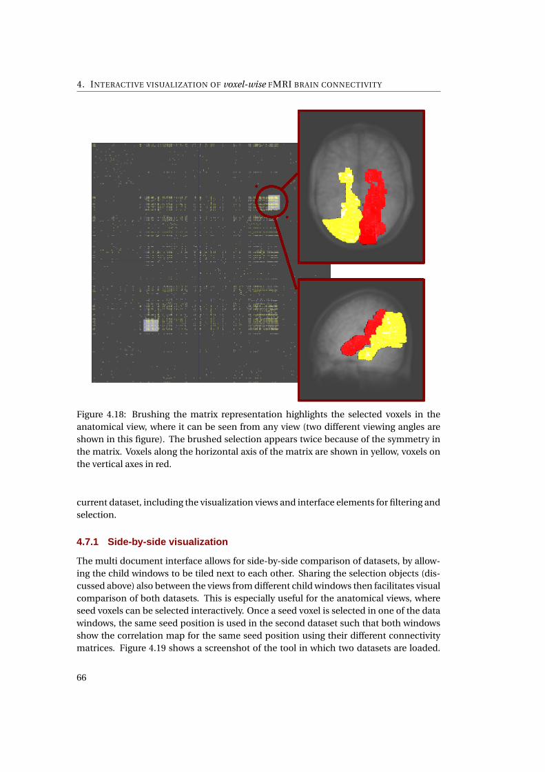
4. INTERACTIVE VISUALIZATION OF voxel-wise FMRI BRAIN CONNECTIVITY
Figure 4.18: Brushing the matrix representation highlights the selected voxels in the
anatomical view, where it can be seen from any view (two different viewing angles are
shown in this figure). The brushed selection appears twice because of the symmetry in
the matrix. Voxels along the horizontal axis of the matrix are shown in yellow, voxels on
the vertical axes in red.
current dataset, including the visualization views and interface elements for filtering and
selection.
4.7.1 Side-by-side visualization
The multi document interface allows for side-by-side comparison of datasets, by allow-
ing the child windows to be tiled next to each other. Sharing the selection objects (dis-
cussed above) also between the views from different child windows then facilitates visual
comparison of both datasets. This is especially useful for the anatomical views, where
seed voxels can be selected interactively. Once a seed voxel is selected in one of the data
windows, the same seed position is used in the second dataset such that both windows
show the correlation map for the same seed position using their different connectivity
matrices. Figure 4.19 shows a screenshot of the tool in which two datasets are loaded.
66
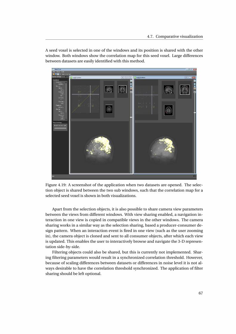
4.7. Comparative visualization
A seed voxel is selected in one of the windows and its position is shared with the other
window. Both windows show the correlation map for this seed voxel. Large differences
between datasets are easily identified with this method.
Figure 4.19: A screenshot of the application when two datasets are opened. The selec-
tion object is shared between the two sub windows, such that the correlation map for a
selected seed voxel is shown in both visualizations.
Apart from the selection objects, it is also possible to share camera view parameters
between the views from different windows. With view sharing enabled, a navigation in-
teraction in one view is copied in compatible views in the other windows. The camera
sharing works in a similar way as the selection sharing, based a producer-consumer de-
sign pattern. When an interaction event is fired in one view (such as the user zooming
in), the camera object is cloned and sent to all consumer objects, after which each view
is updated. This enables the user to interactively browse and navigate the 3-D represen-
tation side-by-side.
Filtering objects could also be shared, but this is currently not implemented. Shar-
ing filtering parameters would result in a synchronized correlation threshold. However,
because of scaling differences between datasets or differences in noise level it is not al-
ways desirable to have the correlation threshold synchronized. The application of filter
sharing should be left optional.
67
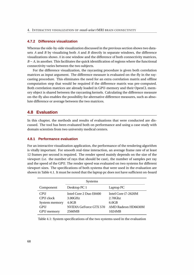
4. INTERACTIVE VISUALIZATION OF voxel-wise FMRI BRAIN CONNECTIVITY
4.7.2 Difference visualization
Whereas the side-by-side visualization discussed in the previous section shows two data-
sets A and B by visualizing both A and B directly in separate windows, the difference
visualizations shows A in one window and the difference of both connectivity matrices,
B − A, in another. This facilitates the quick identification of regions where the functional
connectivity varies between the two subjects.
For the difference visualization, the raycasting procedure is given both correlation
matrices as input argument. The difference measure is evaluated on-the-fly in the ray-
casting procedure. This eliminates the need for an extra correlation matrix and offline
computation step that would be required if the difference matrix was pre-computed.
Both correlation matrices are already loaded in GPU-memory and their OpenCL mem-
ory object is shared between the raycasting kernels. Calculating the difference measure
on-the-fly also enables the possibility for alternative difference measures, such as abso-
lute difference or average between the two matrices.
4.8 Evaluation
In this chapter, the methods and results of evaluations that were conducted are dis-
cussed. The tool has been evaluated both on performance and using a case study with
domain scientists from two university medical centers.
4.8.1 Performance evaluation
For an interactive visualization application, the performance of the rendering algorithm
is vitally important. For smooth real-time interaction, an average frame rate of at least
12 frames per second is required. The render speed mainly depends on the size of the
viewport (i.e. the number of rays that should be cast), the number of samples per ray
and the speed of the GPU. The render speed was evaluated on two systems for different
viewport sizes. The specifications of both systems that were used in the evaluation are
shown in Table 4.1. It must be noted that the laptop pc does not have sufficient on-board
Systems
Component Desktop PC 1 Laptop PC
CPU Intel Core 2 Duo E8400 Intel Core i7-2620M
CPU clock 3.00GHz 2.70Ghz
System memory 4.0GB 6.0GB
GPU NVIDIA GeForce GTX 570 AMD Radeon HD6630M
GPU memory 2560MB 1024MB
Table 4.1: System specifications of the two systems used in the evaluation
68

4.8. Evaluation
GPU memory to contain two datasets. This means that it was not possible to evaluate
the performance of the comparative visualization on this system.
For a cold start of the application, the time required to load the raw correlation data
file from the disk until the visualizations are shown on the screen ranges from 13 seconds
on the laptop PC to 18 seconds, on the desktop PC.
We also measured the framerate of the visualizations for different sizes of the render
window. We made sure that the objects (pixmap and 3-D volume) were zoomed in such
that they covered the entire viewport. The table below lists the performance measures
we took on the two different machines.
Frame rate
Desktop PC Laptop PC
Pixmap 512 x 512 76 fps 206 fps
Pixmap 1024 x 1024 72 fps 120 fps
Anatomical 512 x 512 21.66 fps 5.12 fps
Anatomical 1024 x 1024 7.85 fps 1.98 fps
Linked single-subject 21.03 fps 3.64 fps
Linked dual-subject 14.36 fps -
Linked triple-subject 10.36 fps -
Table 4.2: Performance measurements for the different visualizations on two systems.
In the linked configuration, the size of both view ports is roughly 430 x 430 pixels,
which is a typical size for both windows on a monitor with a resolution of 1280 x 1024.
The frame rate in the linked configuration mostly depends on the size of the anatomical
view; decreasing the size of the 3-D viewport will improve the frame rate in the linked
visualizations.
Discussion
An interesting observation that can be made from this evaluation is that the frame rate
of the pixmap visualization is much higer on the laptop pc than on the desktop pc. The
opposite is true for the anatomical visualization. This difference may be due to different
implementations of OpenCL, such as a performance difference in the OpenGL/OpenCL
interoptability implementation. The performance measurements of the NVIDIA card in-
dicate that for the pixmap visualization, the size of the view port is does not really influ-
ence the frame rate. The frame rate there is thus limited by other factors, such as resizing
the OpenGL texture during a zoom operation or the overhead involved in locking and
unlocking the OpenGL texture when accessing it from OpenCL. It may also be a device
driver related issue, as bugs in the OpenCL driver implementation are still common.
In the anatomical visualization, the size of the view port has a strong impact on the
frame rate on both systems. The frame rate on the desktop PC remains interactive in
the linked dual-subject visualization and even performs quite well in the triple-subject
69
4. INTERACTIVE VISUALIZATION OF voxel-wise FMRI BRAIN CONNECTIVITY
visualization. It must be noted that opening more datasets results in smaller view ports
for each visualization, which may contribute to a stabilizing frame rate.
The render speed for the anatomical visualization may be significantly improved by
optimizing the OpenCL raycasting implementation. In the current implementation, the
correlation volume is always re-computed, even if the seed voxel did not change. Fur-
thermore, the current implementation always runs the volume deformation code, even
if the angle is 0◦. Finally, the current raycasting implementation for the anatomical rep-
resentation does not check for intersections of the ray with the bounding volume. Thus,
even ray paths that do not enter the bounding volume at all are completely traversed.
Besides these algorithmic improvements, the OpenCL code can be further optimized
by overlapping memory accesses, usage of local memory for caching and storing the float
array for that represents the correlation matrix in texture memory instead of the non-
cached global memory.
4.8.2 Case study with domain scientists
The prototype application with the presented visualization techniques was evaluated
with domain scientists in order to investigate the possible role of the application in the
existing pipeline of fMRI connectivity research. The evaluation was set up as an ex-
ploratory case study following the guidelines set out by Yin [Yin 09]. The main study
question was formulated as: How can the functional connectivity visualization tool, called
BrainCove, assist domain scientists in studying patterns in functional brain connectiv-
ity, the relation with brain anatomy and in studying inter-subject or inter-group differ-
ences? and the case was defined as the use of our application by external domain ex-
perts who were targeted as prospective end users. An evaluation session was held with
two groups, one with a group of four neuroscientists from the Leiden University Medical
Center (LUMC) and a second at the Amsterdam Medical Center (AMC), in which the tool
was first presented to a group of 30 people from the neuroimaging and neuroscience do-
main in an informal and interactive presentation and then continued as case study with
a smaller group of researchers (8 in total) specialized in fMRI connectivity.
In the following sections, we will discuss the user feedback structured according to
the case study propositions.
Matrix Visualization
The matrix visualization gives an overview of the data and allows for the detection of
groups of voxels that are correlated. This proposition was confirmed by all participants.
One user specifically mentioned that the matrix visualization is very usable to quickly
select high peaks of highly correlated groups of voxels. Participants added that feedback
about the ordering is important and that rendering of labels would make this represen-
tation more comprehensible, although it was also noted that the lack of labels is com-
pensated by highlighting the corresponding voxels in the anatomical visualization.
The matrix visualization allows for a quick check on the quality of the data, such that
errors can be identified before using the data further in the analysis pipeline. The use of
70
4.8. Evaluation
the matrix visualization for quality checks was not directly apparent to the participants.
They agreed that this representation could be used to detect large artifacts in the data,
but noted that these artifacts would have already been detected earlier in the analysis
pipeline.
Being able to see the spatial context for correlations or groups of correlations using
the view linking aids in interpreting the FC matrix. The participants agreed that the view
linking helps in interpreting the FC matrix, even claiming that without the linked interac-
tion, they would not have a clue on how to interpret the matrix. One of the users further
stated that the matrix visualization would be most useful to find large scale differences
between subjects. The linking would then help to see where the differences are in spatial
context.
Anatomical Visualization
The visualization of FC in spatial context supports mental integration of FC and anatomy.
During the evaluation session at the LUMC, the participants mentioned that they find it
difficult to navigate in the current 3-D visualization, because of a lack of reference. To
our surprise, the AAL atlas visualization with the different colors for each region is hardly
used in the field. Scientists usually navigate and orient themselves within the data using
orthogonal slices of a structural brain or by manually typing in the MNI coordinates.
They strongly suggested that we should integrate a set of simple orthogonal slice views
linked to the 3-D anatomical view that would serve as an anatomical reference. With
such an anatomical reference, they would confirm this proposition.
We implemented this before conducting the second evaluation session at the AMC,
where the users confirmed this hypothesis, stating that this integration of functional con-
nectivity and anatomy is an essential element of this type of visualization.
The visualization of FC data in which the voxels emit “light” when they are function-
ally connected is an intuitive representation of the correlation maps. All users gener-
ally confirmed this proposition. It was remarked that this method corresponds to the
metaphor used in other tools used in the field: “what lights up is active”. Users from both
groups noted that the colormap used to represent the correlation could be improved,
such that the scaling is more diverse. They indicated that the current color map shows
the correlation map too brightly, which makes it hard to see differences. One of the users
further remarked that the color map was not warm enough. Participants in both groups
further suggested to add a colormap legend in the scene and to make the range of the
colormap adjustable.
Interactively selecting a seed voxel by hovering with the mouse over the voxel of inter-
est facilitates the detection of interesting networks and abnormalities. This proposition
was confirmed by all participants. They indicated that this interaction technique is the
biggest difference with other tools. One participant stated that the tool could make a sig-
nificant contribution to the procedure of selecting a seed voxel in seed-based analysis.
The current method includes a priori selection of a seed voxel and computation of the
correlations with all other voxels. According to the participant, loading the whole-brain
correlation matrix into our application would allow for better comprehension in select-
71
4. INTERACTIVE VISUALIZATION OF voxel-wise FMRI BRAIN CONNECTIVITY
ing the seed voxel because the effect of choosing a specific seed voxel is immediately
visualized.
The brain split approach is useful for selecting voxels inside the brain volume (for in-
stance, in the cingulate cortex). The participants did not readily confirm this proposition.
One participant from the first group remarked that he had trouble finding the cingulate
between the brain lobes due to the lack of anatomical reference. The participants gener-
ally agreed that orthogonal slice views would be preferred for selecting voxels inside the
brain volume. In the second session, the three orthogonal views with the MNI structural
brain was considered a better technique for selecting a seed voxel in the brain volume,
which confirmed the findings from the first session. Interestingly, one of the participants
in the AMC group considered the brain split approach an effective method for reducing
occlusion in the 3-D visualization, but not so much for probing. It was furthermore ar-
gued that to make this approach more effective, it should be possible to place the split
plane at arbitrary position to be able to probe in regions deeper past the cerebral cortex.
Context visualization using a high resolution MRI head volume and a coloured and
outlined anatomical atlas aids in relating FC to anatomical regions. The utility of the col-
ored anatomical atlas was not directly apparent to the participants in the first session.
One of the participants even noted that the coloring was more confusing then helpful.
Again, the suggestion was made to integrate a linked view with orthogonal slices of a
structural brain or a semi-transparent surface rendering of the brain (usually referred to
as a “glass brain”) for providing anatomical context. Following these suggestions, we re-
moved the anatomical atlas coloring from the volume rendering and integrated orthogo-
nal slice views in the tool. During the second evaluation session, participants confirmed
that the slices with a structural MNI brain are the preferred way for navigation purposes
and provide sufficient anatomical context.
Flat map
Visualizing FC in a 2D projection of the spatial locations facilitates in forming a mental
map of the complete connectivity network in a single view. Remarkably, researchers from
both groups were not familiar with the use of “flat maps” for two-dimensional repre-
sentation of functional connectivity in anatomical context. They generally found it dif-
ficult to orient themselves in the cylindrical flat map representation without structural
anatomical context and mentioned that a learning curve would be involved to get accus-
tomed to such a representation. One participant further commented that the presented
flat map is limited to functional connectivity studies of the cortex, which makes it un-
suitable for use in groups that focus on sub-cortical regions. In general, participants did,
however, see potential in the use of mappings that are able to represent the complete
connectivity network in a single view.
Visual Comparison
Coordinated visualizing multiple datasets side-by-side supports the finding of differences
between subjects. All participants confirmed this proposition, noting that the visual com-
72

4.8. Evaluation
parison would be a powerful tool mainly for visually comparing single subjects or pa-
tients to a group mean, since this is mostly a visual task. This would also enable the
use of resting state fMRI connectivity as a disease marker. One of the attending medical
doctors further remarked that the visual comparison could also be employed in interven-
tion measurement in a clinical setting. For example, patients with obsessive-compulsive
disorder are increasingly being treated with deep brain stimulation (DBS). Being able to
visualize the functional network of the brain pre-DBS and post-DBS side-by-side would
allow clinicians to see changes in the network, which is helpful in judging whether the
current treatment is effective or should be changed.
Visualizing the difference between two datasets supports the finding of differences be-
tween subjects or the impact of preprocessing on FC networks. The value of visualizing the
absolute correlation difference between different subjects was not directly confirmed.
It was remarked that absolute difference in correlation between subjects could be at-
tributed to noise or to differences in the strength of the measured signal. Participants
did see potential in using the difference visualization within one subject to compare the
influence of using different preprocessing pipelines. However, participants did see the
greatest potential in connecting the tool to a database with group averages such as for
healthy subjects and for different pathologies, such that single subjects can be visually
compared with the group average. Another suggestion was to create the average on-
demand from a group study.
General remarks
The participants in the first group were generally impressed by the visualizations and saw
the potential in the tool, but stated that due to the lack of anatomical reference (by means
of structural data) and the inability to select voxels that are at a distance from the cortical
surface, they would not readily use the tool for visual analysis. They suggested the use
of a high resolution brain surface rendering, such as the one generally used in the SPM
toolbox, or orthogonal slices of the MNI structural brain volume. Once the anatomical
reference could be dealt with, they saw potential in using the tool especially to compare
individual subjects to a group average, such as in comparing pathologies with healthy
subjects with patients with different pathologies or with the effects of drugs on func-
tional connectivity. They furthermore suggested to add a feature that makes it possible
to select different types of connectivity (such as hub voxels) on-the-fly, using a pipeline
that is running in the background and a method that enables the creation of high-quality
pictures for publications.
The domain scientists in the second evaluation session were generally quite enthu-
siastic about the possibilities the tool offers for the visualization of the connectivity data.
We attribute the difference in enthusiasm between the first and second evaluation to our
addition of anatomical reference using the structural MNI slice views before conduct-
ing the second evaluation. Especially the visual comparison of individuals and group
averages was considered an important contribution. An interesting clinical use case in
this context was proposed by one of the medical doctors present during the evaluation,
involved in treatment of neurological disorders using deep brain stimulation. He un-
73

4. INTERACTIVE VISUALIZATION OF voxel-wise FMRI BRAIN CONNECTIVITY
derlined the value of the visual comparison for intervention measurement in DBS. He
continued that one of the critical steps in this treatment is finding the location in the
brain where to start the DBS, by looking at patterns in the resting state fMRI connectivity
network. This step could benefit from being able to quickly compare the brain network
of the patient to a group average.
Both groups independently considered the ability to visually compare connectivity
networks to be the major contribution of the tool.
74
CHAPTER 5
Implementation of voxel-wiseconnectivity visualization: selected
topics
This chapter discusses several interesting implementation details of our methods. We
will start with an overview of the libraries and tools used for the implementation. In
Section 5.2, general implementation notes are discussed including the VTK pipeline that
is employed and the linkage between VTK and OpenCL. The subsequent sections dis-
cuss the implementation details of each individual visualization. We conclude with an
overview of relevant technical challenges we faced during the implementation.
5.1 Used libraries and tools
For the implementation of the BrainCove tool, the following toolkits and frameworks
have been used:
• Qt framework for the user interface
• The Visualization Toolkit (VTK) for the rendering pipeline
• The Open Compute Language (OpenCL) for the parallel implementation of the
raycasting algorithm
All these toolkits and frameworks are cross-platform and open source (except for device-
dependent OpenCL implementations). The project is configured using CMake, which
allows easy compilation on numerous platforms, although so far the software has been
tested on Windows only.
75
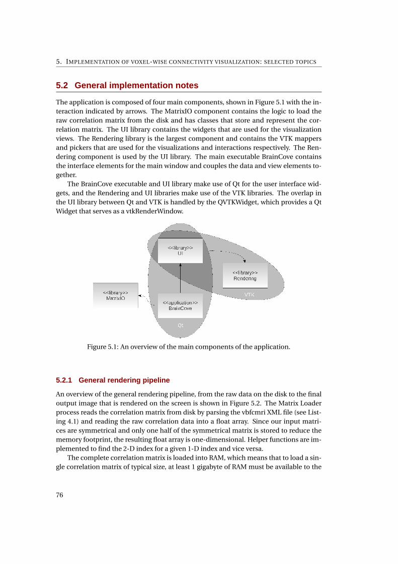
5. IMPLEMENTATION OF VOXEL-WISE CONNECTIVITY VISUALIZATION: SELECTED TOPICS
5.2 General implementation notes
The application is composed of four main components, shown in Figure 5.1 with the in-
teraction indicated by arrows. The MatrixIO component contains the logic to load the
raw correlation matrix from the disk and has classes that store and represent the cor-
relation matrix. The UI library contains the widgets that are used for the visualization
views. The Rendering library is the largest component and contains the VTK mappers
and pickers that are used for the visualizations and interactions respectively. The Ren-
dering component is used by the UI library. The main executable BrainCove contains
the interface elements for the main window and couples the data and view elements to-
gether.
The BrainCove executable and UI library make use of Qt for the user interface wid-
gets, and the Rendering and UI libraries make use of the VTK libraries. The overlap in
the UI library between Qt and VTK is handled by the QVTKWidget, which provides a Qt
Widget that serves as a vtkRenderWindow.
Figure 5.1: An overview of the main components of the application.
5.2.1 General rendering pipeline
An overview of the general rendering pipeline, from the raw data on the disk to the final
output image that is rendered on the screen is shown in Figure 5.2. The Matrix Loader
process reads the correlation matrix from disk by parsing the vbfcmri XML file (see List-
ing 4.1) and reading the raw correlation data into a float array. Since our input matri-
ces are symmetrical and only one half of the symmetrical matrix is stored to reduce the
memory footprint, the resulting float array is one-dimensional. Helper functions are im-
plemented to find the 2-D index for a given 1-D index and vice versa.
The complete correlation matrix is loaded into RAM, which means that to load a sin-
gle correlation matrix of typical size, at least 1 gigabyte of RAM must be available to the
76
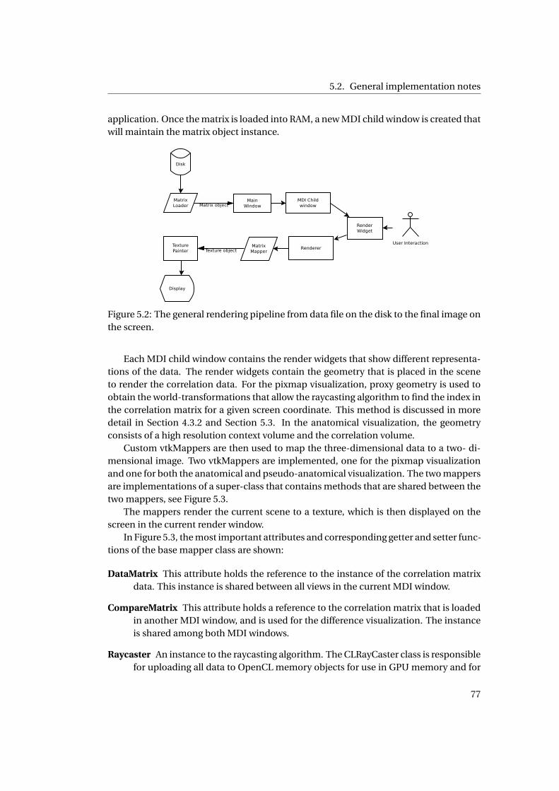
5.2. General implementation notes
application. Once the matrix is loaded into RAM, a new MDI child window is created that
will maintain the matrix object instance.
Figure 5.2: The general rendering pipeline from data file on the disk to the final image on
the screen.
Each MDI child window contains the render widgets that show different representa-
tions of the data. The render widgets contain the geometry that is placed in the scene
to render the correlation data. For the pixmap visualization, proxy geometry is used to
obtain the world-transformations that allow the raycasting algorithm to find the index in
the correlation matrix for a given screen coordinate. This method is discussed in more
detail in Section 4.3.2 and Section 5.3. In the anatomical visualization, the geometry
consists of a high resolution context volume and the correlation volume.
Custom vtkMappers are then used to map the three-dimensional data to a two- di-
mensional image. Two vtkMappers are implemented, one for the pixmap visualization
and one for both the anatomical and pseudo-anatomical visualization. The two mappers
are implementations of a super-class that contains methods that are shared between the
two mappers, see Figure 5.3.
The mappers render the current scene to a texture, which is then displayed on the
screen in the current render window.
In Figure 5.3, the most important attributes and corresponding getter and setter func-
tions of the base mapper class are shown:
DataMatrix This attribute holds the reference to the instance of the correlation matrix
data. This instance is shared between all views in the current MDI window.
CompareMatrix This attribute holds a reference to the correlation matrix that is loaded
in another MDI window, and is used for the difference visualization. The instance
is shared among both MDI windows.
Raycaster An instance to the raycasting algorithm. The CLRayCaster class is responsible
for uploading all data to OpenCL memory objects for use in GPU memory and for
77

5. IMPLEMENTATION OF VOXEL-WISE CONNECTIVITY VISUALIZATION: SELECTED TOPICS
Figure 5.3: A class diagram of the custom vtkMappers with the most important attributes
and functions.
executing the OpenCL kernel that will perform the actual raycasting. More details
are discussed in the next section.
Texture An instance to a wrapper class for a shared OpenCL/OpenGL texture object.
Internally, the texture is stored as an OpenGL texture instance. Using the Open-
CL/GL interoptability, the OpenCL raycasting kernel is able to write directly to this
texture. After execution of the raycasting algorithm, the texture is then rendered
on the screen using the Painter instance.
Painter This attribute is an instance to a CLTexturePainter class. This class takes a CLTex-
ture2DObject as input and renders the internal OpenGL texture to a quad using
standard OpenGL texture mapping methods.
Selection This holds a reference to DataSelection that is shared between linked views. It
is used in the Raycaster to decide which elements are to be drawn.
Filters A list of DataFilter instances that are used in the Raycaster to apply on-the-fly
filtering of the correlation data. Currently, only the absolute correlation threshold
is available as a DataFilter.
5.2.2 Linking VTK and OpenCL
The raycasting algorithm can be speed up considerably by using a parallel implementa-
tion that can be executed on the GPU. Although VTK already contains vtkVolume map-
pers that are able to perform the raycasting algorithm on the GPU using GL shaders,
these mappers cannot be easily adapted for the purpose of rendering our abstract cor-
relation data. Instead, we chose to implement a custom vtkMapper with the actual ray-
casting algorithm in OpenCL. OpenCL is a royalty-free framework for general-purpose
78

5.2. General implementation notes
:Mapper :CLRayCaster :CLProgram :CLMemoryObject :cl
Init(‘file.cl’)
SetSourcePath(‘file.cl’)
BuildProgram()
clBuildProgramFromFile(‘file.cl’)
cl::Program
SetMatrix(m)
SetMatrix(m)
GetCLObject(m)
clCreateBuffer
cl::Buffer
cl::Buffer
Figure 5.4: A sequence diagram showing the interaction between classes during the ini-
tialization of the CLRayCaster object.
parallel programming that, compared to the OpenGL shader language, offers increased
freedom in for programming.
An important aspect of OpenCL for our application is that it supports 2-D and 3-D
images and access to the texture sampling that is implemented on most graphics hard-
ware. However, other functionality that is required for graphics programming, such as
matrix multiplication and view transformations is not directly supported and has to be
implemented from scratch.
The central part for the linkage between VTK and OpenCL is the CLRayCaster class.
This class is an implementation of a CLProgram wrapper interface, that contains func-
tionality to build and execute OpenCL kernels. The CLRayCaster object is constructed
in one of the vtk correlation mappers. During initialization of the CLRayCaster object,
the source code for the kernel is loaded into a cl_pr og r am object and compiled for the
current rendering device 1. After initialization, the CLRayCaster gets the correlation ma-
1Although OpenCL supports both CPUs as GPUs as computing devices, our implementation has only
been tested on (and is forced to use) GPU devices
79

5. IMPLEMENTATION OF VOXEL-WISE CONNECTIVITY VISUALIZATION: SELECTED TOPICS
:User :RenderWindow :Mapper :CLRayCaster :CLProgram :cl
interact
Render()
ComputeMatrices()
CastRays()
UpdateCLStructs()
RunKernel(kernel)
enqueueNDRangeKernel(kernel)
Render LoopRender Loop
Figure 5.5: A sequence diagram showing the interaction between classes during the a
user interaction.
trix object from the mapper. In order to be used in the OpenCL kernel on the GPU, the
correlation matrix must be transferred to GPU memory. OpenCL supports raw data by
means of cl_buffer objects that can be sent as arguments to the OpenCL kernel. To save
memory, the GPU correlation data object is shared between each mapper by means of
an application-wide memory pool object. This pool object is implemented using a dic-
tionary that contains the pointer to the correlation matrix in system memory and the
corresponding pointer to GPU memory as key-value pair. When a GPU memory object
of the correlation matrix is requested, the memory pool object is first queried. If the
current correlation matrix pointer is not yet in the dictionary, the OpenCL GPU mem-
ory object is first constructed and the key-value pair is stored in the dictionary. Once an
update is requested, because of a change somewhere in the pipeline (usually because of
user interaction), the Render method of the mapper is called, with a reference to the cur-
rent vtkRenderer and vtkVolume objects from which the view-to-world transformation
matrices are computed. The resulting transformation matrix, the current selection and
active filters and the output texture are then passed as arguments to the actual raycasting
function in the Raycaster object. This function contains the logic to execute the OpenCL
kernel that performs the actual raycasting in parallel. This is also shown in the sequence
80

5.3. Direct Matrix Visualization
diagram in Figures 5.4 and 5.5.
5.3 Direct Matrix Visualization
The direct matrix visualization has been implemented in a custom volume mapper for
use with the Visualization Toolkit (VTK). The VTK pipeline is used for setting up the ren-
der window, placing the matrix ‘plane’ in the scene and interacting with the scene (such
as zooming and panning). For the matrix visualization, the VTK pipeline is shown in
Figure 5.6.
Figure 5.6: The customized VTK volume rendering pipeline for the direct matrix visual-
ization, showing all relevant modules.
In the standard VTK volume rendering pipeline, the input to a volume mapper is a
VTK image data object, optionally filtered with an image to image filtering module. Di-
rectly loading the correlation matrix into a VTK image data object is not feasible: be-
cause the input correlation matrix is symmetric, only half of it is stored in memory,
but this data structure is not supported by the default VTK image object. However, the
VTK pipeline requires a vtkImageData object in order to compute the world bounds.
81

5. IMPLEMENTATION OF VOXEL-WISE CONNECTIVITY VISUALIZATION: SELECTED TOPICS
In order to use the VTK rendering pipeline with a minimum amount of modifications,
a dummy vtkImageData object is used as input for the mapper with an extent of 0 ≤
x < 1; 0 ≤ y < 1; 0 ≤ z ≤ 0; and the x and y spacing equal to the dimensions of the
correlation matrix. Thus, for a correlation matrix of N xN , the vtkImageData is set to
have voxel spacing of < N − 1; N − 1; 0 >. As a result, the mapper’s world bounds are:
0 ≤ x < 20,000; 0 ≤ y < 20,000; 0 ≤ z ≤ 0; This makes the mapping from world coordi-
nates to matrix indices quite easy: it just involves a round-off to the nearest integer coor-
dinate i , j , where i is the i th row in the correlation matrix and j the column index for the
correlation value. However, this 2-D index is valid only for the raw correlation matrix and
does not take the reordering of rows and columns into account. To find the correct index
in the reordered matrix, an extra lookup is required using a simple 1-D ‘reorder’ lookup
table that maps indices in the raw correlation data to indices in the reordered matrix.
The correlation data is then sent to the raycasting algorithm in OpenCL as a one-
dimensional float array, encapsulated in a cl_buffer object, along with the view-to-world
transformation matrix (calculated from the bounds of the proxy plane). The algorithm
for raycasting the pixmap is implemented in an OpenCL kernel that is executed for every
pixel in the view port. The implementation contains the following steps for every pixel:
Pixels that are outside the bounds of the correlation matrix are set to a transparant color,
Listing 5.1 Step-by-step description of the pixmap raycasting algorithm
1. Convert pixel coordinate (x, y) to normalized view coordinate [-1. . . 1]
2. Transform the normalized view coordinate to a world coordinate using the view-
to-world transformation matrix, with z = 0
3. If the world coordinate is within the bounds of the proxy object, convert the world
coordinate to a matrix index. Because the bounds of the correlation matrix are
equal to the bounds of the proxy object, this means rounding off to the nearest
integer coordinate (i , j )
4. Looking up i and j in the lookup table to find the corresponding indices in the
reordered matrix, (i ′, j ′)
5. Converting the 2-D matrix index (i ′, j ′) to a 1-D array index k
6. Retrieving the correlation value at k in the correlation float array
7. Mapping the correlation to color using a lookup in the colormap, available to the
OpenCL program as an RGB texture
8. Storing the color value in the texture at pixel (x, y)
such that for those pixels the background of the render window is shown.
82
5.4. Anatomical Visualization
5.3.1 Implementation details of the matrix picker
The technique that facilitates making selections in the matrix visualization uses the ray-
cast selection method, as discussed in Chapter 4. For selecting the correlation matrix
element at the current mouse position, steps one to three of Listing 5.1 are used.
5.4 Anatomical Visualization
The anatomical visualization resembles the traditional raycasting method a lot more
than the matrix visualization discussed in the previous section. The main difference
with the traditional direct volume rendering is that instead of a single volume, multi-
ple volumes are used in the rendering. Furthermore, the anatomical visualization uses
a two-step raycaster as discussed in Chapter 4. Both steps of this raycasting method are
implemented in OpenCL kernels that are run on the GPU. The first step starts a 3-D range
OpenCL kernel that takes the index volume, an empty correlation volume, a seed voxel
index and the raw correlation matrix as its input. The correlation volume is then built by
evaluating for each position the correlation value between the voxel at that position and
the seed voxel, see Listing 5.2.
Listing 5.2 Step-by-step description of the first step in the rendering of the anatomical
visualizationFor each position P in the index volume:
1. Retrieve the index value i stored at P in the index volume.
2. Convert the 2-D index i , j (where j is the index of the seed voxel) to a 1-D triangular
matrix index k.
3. Retrieve the correlation c at index k from the correlation array
4. Filter the correlation value: if c is below the correlation threshold t , set c = 0. Oth-
erwise, leave c intact.
5. Store the correlation c at position P in the correlation volume.
Once the correlation volume is constructed, the second kernel is executed. The ar-
guments passed to this kernel are:
• the Correlation Volume
• the Atlas Volume
• the High resolution MRI Volume
• the world-to-voxel transformation matrices for each volume
• the view-to-world transformation matrix
83

5. IMPLEMENTATION OF VOXEL-WISE CONNECTIVITY VISUALIZATION: SELECTED TOPICS
• an enum that defines the desired visualization (anatomical or pseudo-anatomical)
• color maps (as color texture) for each volume
• the plane normal of the split plane
• the rotation point
• deformation matrices for the regions left and right of the split plane
The corresponding algorithm is shown in Listing 5.3.
Listing 5.3 Step-by-step description of the second step in the rendering of the anatomical
visualizationFor each pixel coordinate P of the render texture:
1. Calculate the start and end position for the ray at pixel position P
a) For the anatomical visualization, use the view-to-world transformation
b) For the pseudo-anatomical visualization, use the transformations as dis-
cussed in Section 4.5
2. Calculate the step size (length of ray divided by the sampling distance)
3. For each sample position Q:
a) Identify the position as being in the region left or right from the split plane
b) Transform the position using the corresponding deformation matrix
c) Test the transformed position, advance ray if outside the region identified in
step 3a
d) Transform Q to voxel space for each volume (position R, S, T for respectively
the high resolution, atlas and correlation volume)
e) If T is within the bounds of the correlation volume, retrieve the correlation
value c
f ) If c is above the threshold, map c to a color in one of the color textures and
apply FTB compositing
g) If T is not within the bounds of the correlation volume, or if c is below the
threshold, sample the high resolution volume at R and map the sample value
to a color using the color texture, then apply FTB compositing
4. Write the resulting color to the render texture at pixel position P
84

5.5. Technical challenges
5.4.1 Accessing and writing the volumes in OpenCL
In the VTK pipeline, each volume (the index volume, correlation volume and context vol-
umes) is stored in a vtkImageData object. To make the volume accessible in the OpenCL
kernel, the image objects (in fact, the pointer to the Scalar array of the vtkImageData
object, vtkImageData::GetScalarPointer()) are uploaded to OpenCL Image3D (texture)
objects. This makes it possible to use the hardware accelerated texture sampling and
caching in OpenCL, speeding up the algorithm significantly.
5.5 Technical challenges
Numerous technical challenges had to be addressed during the implementation of the
visualizations, most of them related to the implementation using OpenCL, which is a
relatively new framework.
5.5.1 Debugging OpenCL kernels
One of the greatest difficulties in developing OpenCL programs is the lack of good de-
bugging and profiling tools. Whereas debugging solutions are quite mature already for
CUDA (such as NVIDIA Parallel Nsight), the tools for OpenCL are still in its infancy and
do not yet support debugging of the kernel source (AMD gDebugger).
Limited debugging support is available in the AMD and Intel implementations of
OpenCL, when the kernel runs on the CPU instead of the GPU, using printf statements.
Furthermore, results of the kernel execution, such as the contents of the 3-D volumes,
can be checked with AMD gDebugger. Unfortunately, the latest version of the tool that
was used (6.0) still suffers from severe child diseases causing the debugger to crash in
many situations.
Fortunately, the OpenCL framework employs a ‘just-in-time’ compilation model. This
makes it possible to change the source code of the OpenCL kernel and, using a simple
button in the interface, to recompile the OpenCL program on-the-fly. The change is im-
mediately reflected in the visualization, facilitating kernel debugging by trial-and-error.
5.5.2 Interoptability of OpenCL and OpenGL
The final output of a direct volume rendering approach such as the raycasting technique
that is used in this work, is an image that is shown on the screen. As the implementation
of VTK on our system is using OpenGL for the actual rendering of objects on the screen, it
makes sense to have the final image as an OpenGL texture that can then be rendered us-
ing a texture-mapped quad using simple OpenGL calls. This is possible by employing the
OpenCL/OpenGL interoptability. This mechanism enables the use of OpenGL textures
in the OpenCL kernel, allowing the kernel to directly read from and write to the OpenGL
texture. The raycasting pipeline employs this functionality by sharing the OpenGL tex-
ture with the OpenCL program. The main advantage of this method is that it reduces the
number of (costly) transfers between host and GPU.
85

5. IMPLEMENTATION OF VOXEL-WISE CONNECTIVITY VISUALIZATION: SELECTED TOPICS
Sharing OpenCL memory objects between mappers
The interoptability between OpenCL and OpenGL is enabled by passing a reference to
the current OpenGL context to the function that creates the OpenCL context. This method
allows the OpenCL context to be shared with only one OpenGL context. However, VTK is
designed in a way that each render window has its own unique render context.
Technically, it would be possible to create multiple OpenCL contexts, one for each
render window. But this conflicts with another requirement: the OpenCL memory object
that contains the data of the correlation matrix has to be shared among the different
views. Sharing OpenCL memory objects is only possible in a single OpenCL context.
Thus, only one application-wide OpenCL context should exist, which should then be
shared among all render windows. To achieve this, the OpenCL context is bound to the
OpenGL context of one render window (the first one that is created). The display lists of
this OpenGL context are then shared with all OpenGL contexts that are created thereafter
(see Figure 5.7).
������������
�������������
�������������
������������ ����������
�������������
������������������
Figure 5.7: The method that enables sharing of OpenCL memory objects from a single
OpenCL context with multiple OpenGL contexts.
5.5.3 OpenCL implementation differences between vendors
Although the OpenCL specifications covers most necessary aspects, there are some key
differences between the vendor-specific implementations. Most of the differences are in
the support for OpenCL extensions, but an other important difference is due to incon-
sistent interpretation of the specification.
OpenCL extension support
A major difference between the current vendor implementations of AMD and NVIDIA
is the support for writing to 3-D images. Writes to 3-D images are supported by the
cl_khr_3d_image_writes extension, which is supported by the current AMD implementa-
tion, but currently not available in NVIDIA implementations of OpenCL. This extension
is relevant for the two-step raycasting approach discussed in Section 4.4.2 and 5.4.
To overcome this limitation for NVIDIA hardware, an extra intermediate correlation
volume has to be used. For to the first OpenCL kernel, in which the current correlation
map is written, the correlation volume is passed as a one dimensional float array. The
kernel writes to this ‘volume’ by converting the 3-D volume indices to a 1-D array in-
86
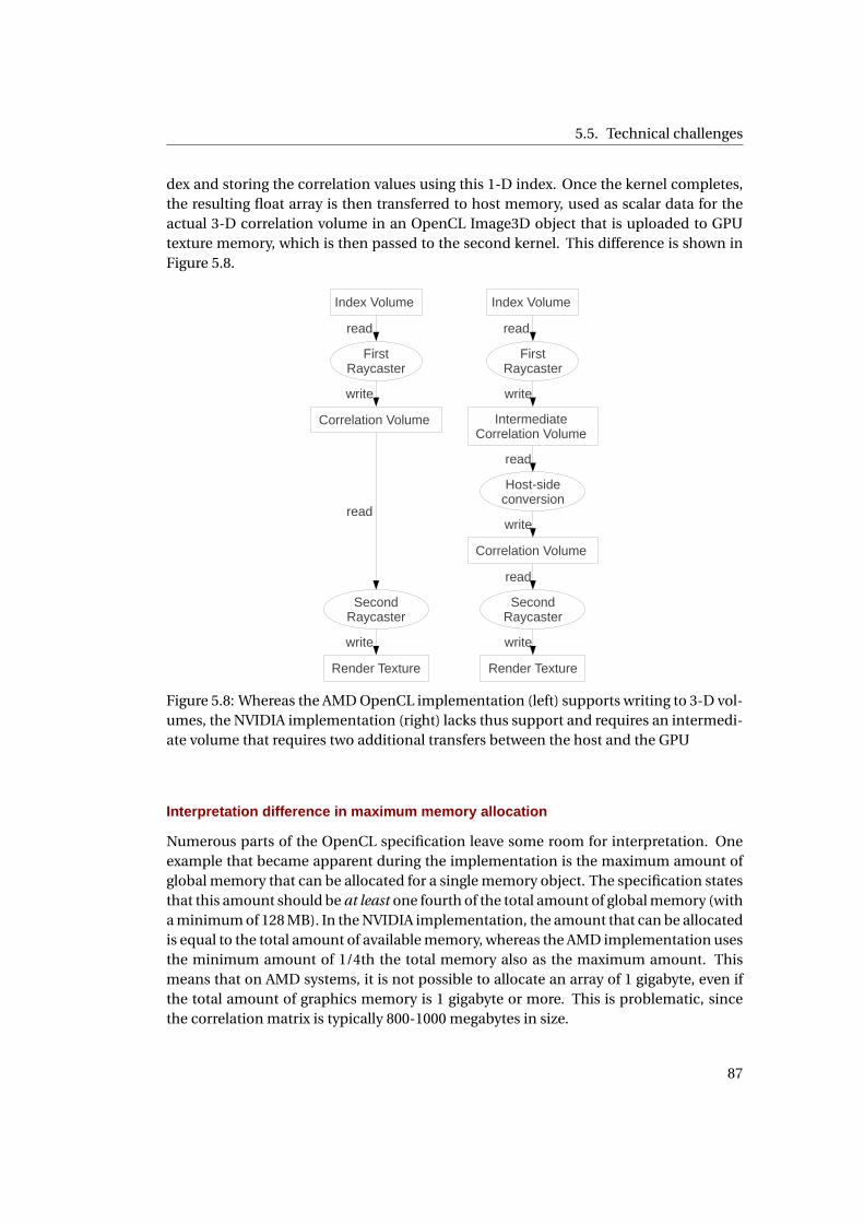
5.5. Technical challenges
dex and storing the correlation values using this 1-D index. Once the kernel completes,
the resulting float array is then transferred to host memory, used as scalar data for the
actual 3-D correlation volume in an OpenCL Image3D object that is uploaded to GPU
texture memory, which is then passed to the second kernel. This difference is shown in
Figure 5.8.
����������� �����������
� ������������
� ������������
������� �������� �������� ����������� ��������
������ ��������� ��
������� ��������
���������������
���������������
������������� �������������
�������������
�� �����������
���������������
�� �����������
�������������
�� ����������
������������
�� ����������
������������
�� ����������
Figure 5.8: Whereas the AMD OpenCL implementation (left) supports writing to 3-D vol-
umes, the NVIDIA implementation (right) lacks thus support and requires an intermedi-
ate volume that requires two additional transfers between the host and the GPU
Interpretation difference in maximum memory allocation
Numerous parts of the OpenCL specification leave some room for interpretation. One
example that became apparent during the implementation is the maximum amount of
global memory that can be allocated for a single memory object. The specification states
that this amount should be at least one fourth of the total amount of global memory (with
a minimum of 128 MB). In the NVIDIA implementation, the amount that can be allocated
is equal to the total amount of available memory, whereas the AMD implementation uses
the minimum amount of 1/4th the total memory also as the maximum amount. This
means that on AMD systems, it is not possible to allocate an array of 1 gigabyte, even if
the total amount of graphics memory is 1 gigabyte or more. This is problematic, since
the correlation matrix is typically 800-1000 megabytes in size.
87

5. IMPLEMENTATION OF VOXEL-WISE CONNECTIVITY VISUALIZATION: SELECTED TOPICS
One option would be to split the array with correlation values over multiple memory
objects, but this would increase the complexity of the kernel, which in that case should
be able to handle a variable amount of arguments. Instead, we employed a different
approach, in which the array of correlation values is allocated in a GL_ARRAY_BUFFER,
which does not have this limitation in maximum allocation size. Using the OpenCL/GL
interoptability, this OpenGL array buffer is then shared with the OpenCL context and can
be used in the OpenCL kernel as a regular cl memory object.
88
CHAPTER 6
Conclusions and Future Work
In this chapter, the methods and results are discussed and related to the main research
question. First, we will summarize the methods presented in this thesis and the results
from the evaluations. We will then discuss and reflect on the results and draw conclu-
sions. Finally, we will provide a number of recommendations for future work.
6.1 Summary
In this thesis, we presented two tools for the visualization of functional brain connec-
tivity. In Chapter 3 we discussed a tool for the visual analysis of region based functional
brain connectivity. This applications combines several well-known types of visualization
with coordinated linking that facilitates an analyst to quickly identify correlated brain re-
gions, visualize the relation to their corresponding distances in the anatomical space and
spot connections that deviate from a previously found general relation between anatom-
ical and functional distance. We showed that the methods presented in this tool facili-
tate region-based fMRI brain connectivity research, by means of a case study with two
domain experts.
The main work of this thesis was described in Chapter 4, where we presented techniques
for the visualization of functional brain connectivity at the voxel level. The tool we pre-
sented contains visualizations that facilitate the visual analysis of voxel-wise fMRI con-
nectivity, allowing the analyst to quickly identify interesting patterns in the functional
network of the brain and differences in connectivity patterns between subjects or groups
by visually comparing multiple datasets side-by-side. The side-by-side visual compari-
son is the major contribution of this work and is, to the best of our knowledge, not shown
before.
Three different visualizations were presented, including a pixmap representation and
direct volume rendering of the correlation map for a given seed voxel in both anatomical
context and in a flat-map layout that shows the correlation map in pseudo-anatomical
spacing. We evaluated our tool in case studies with groups of domain scientists at two
different university medical centers.
89
6. CONCLUSIONS AND FUTURE WORK
6.2 Discussion
The research goal for this thesis work was to develop methods for the real-time and in-
teractive visualization of region-based and voxel-wise functional brain networks. Two
separate tools were developed. The first tool is able to visualize connectivity matrices
from region-based studies, but does not cater for connectivity matrices in voxel resolu-
tion.
We therefore developed a second system that, by taking full advantage of GPU ac-
celerated raycasting, is able to visualize voxel-wise fMRI brain connectivity data. Three
different representations were proposed: a zoomable and pannable pixmap visualization
that facilitates an overview of the complete network in a single view, a 3-D visualization
that renders the correlation map for a selected voxel (or group of voxels) in anatomi-
cal context and a pseudo-anatomical flat map representation that shows the correlation
map in minimal occlusion.
We have shown that the current version of the tool is able to render these visualiza-
tions at interactive speed on a desktop PC. It furthermore allows for side-by-side visual-
ization of two or more of such datasets, even with an implementation that is not yet fully
optimized. For real-time visualizations, a recent mid- to high-range graphics card with
full OpenCL 1.1 support is required.
To show multiple datasets side-by-side, a card with at least two gigabytes of on-board
texture memory must be used. Cards with this amount of texture memory (or more) are
becoming more common every year, with prices lowering. This makes it possible for our
approach to be used in standard desktop machines in a research or clinical environment
at relatively low cost.
A case study evaluation was conducted that provided many useful suggestions to im-
prove on the applicability of our tool in the current research pipeline. We were surprised
to hear that the neuroscientists in the two university medical centers were not familiar
with coloring according to anatomical atlases for orientation in the brain. Instead, they
orient themselves completely on structural scans and coordinates in MNI space.
A strong suggestion from domain scientists during the first case study therefore was
to remove the coloring based on the AAL atlas, and add an extra view with orthogonal
slices of a structural MNI brain for anatomical reference in its place. This view further-
more makes it possible to accurately select a position for the seed voxel, something that
is hard to do in the anatomical representation.
We were also surprised to find that flat map representations are hardly used in the
community. Although cortical flap maps are commonly used in the ‘FreeSurfer’ com-
munity, the experts on fMRI connectivity in our evaluation groups were not familiar with
them or could not use them at all, because they are focusing on sub-cortical areas in their
research. They also had problems orienting themselves and navigating in our flattened
representations. The version of the pseudo-anatomical representation shown to them
used colors based on the AAL template, which was replaced in a later version with a gray
scale volume rendered representation of a structural volume. The effectiveness of this
new version has to be reevaluated.
Another interesting find from the case study evaluation was that the ability to visu-
90
6.3. Future work
alize multiple networks side-by-side was found to be the major contribution of our tool,
making it useful as is for visualizing differences between subjects or patients and a group
mean. Furthermore, the side-by-side visualization could be used to show changes of the
functional brain network over time, such as pre- and post deep brain stimulation (DBS),
to visually evaluate the effectiveness of the DBS treatment.
6.3 Future work
We identified numerous additions and improvements that could still be implemented in
both solutions.
For our region-based tool, interesting additions include the visualization of change
over time to visualize differences between different subjects. Another addition that should
be evaluated is combining rs-fMRI connectivity data with data that is acquired from re-
search on the structural connectivity of the brain (DSI/DTI studies). This could give
insight in the relation between functional connectivity measured by brain activity and
structural connectivity.
The case study evaluation of the voxel-based visualization tool also revealed numerous
interesting possibilities and improvements for future versions of the tool.
An interesting suggestion, that surfaced from both evaluation sessions, was to link
the application to a database of group mean networks, to be able to compare functional
brain networks of individuals to the average network of a group of interest. This could
also facilitate the use of functional MRI connectivity as a disease marker or for interven-
tion measurement.
A related addition would be the functionality to create mean networks on-the-fly,
from a set of already available functional networks, such that the dataset of an individual
subject can be compared with the average set of a custom designed group. The current
version supports the visualization of the absolute correlation difference of two datasets,
but the derivation of other difference measures should also be supported.
Currently, the input to our application is a correlation that is pre-computed using an
external tool. However, related work has shown that it is possible to compute the cor-
relations on-the-fly. The addition of this functionality, thus allowing the user to directly
load pre-processed 4-D NIFTI files, would make the tool considerably more attractive,
making it a better fit in the current pipeline.
Also in terms of visualization, several questions need to be answered. First of all,
the current anatomical visualization lacks the anatomical reference that our prospective
users need to accurately select a seed location. Although the slice view implementation
that is currently used compensates for this lack of reference, from a visualization point-
of-view it would be desired to integrate the anatomical reference and correlation map
in a single view. This is especially important for the brain split method that allows the
selection of a seed voxel inside the brain volume.
Furthermore, alternative flat-map representations need to be investigated. The cur-
rent pseudo-anatomical visualization severely distorts the cortical surface. A possibility
91
6. CONCLUSIONS AND FUTURE WORK
would be the use of the cortical flat maps as generated by FreeSurfer, or the circle packing
method briefly discussed in this thesis. However, the implementation of these mappings
in a raycasting framework is not straightforward. A possible method is the use of defor-
mation fields to construct the warped volume.
Finally, a technique should be found to solve the aliasing problem in the pixmap vi-
sualization. A possible solution is the use of mipmaps, but this requires the correlation
data to be stored in a texture instead of in the current simple approach, where the corre-
lation matrix is stored in a float array in global memory.
In this thesis we discussed a system for the visual analysis of region-based connectivity,
but the main work focused on the visualization of functional brain connectivity at the
voxel-level. Still, the tool we proposed for region-based connectivity contains function-
ality that is interesting also for functional brain networks at voxel resolution. Therefore,
a good strategy for future work would be to fuse both systems into a single visual analysis
application that is able to visualize both region-based and voxel-wise connectivity and
automatically switches to the most optimal visualization based on the resolution of the
dataset.
92

Bibliography
[Achard 06] Sophie Achard, Raymond Salvador, Brandon Whitcher, John
Suckling & Ed Bullmore. A Resilient, Low-Frequency, Small-World
Human Brain Functional Network with Highly Connected Associ-
ation Cortical Hubs. The Journal of Neuroscience, vol. 26, no. 1,
pages 63 –72, January 2006.
[Addis 09] Donna Rose Addis, Ling Pan, Mai-Anh Vu, Noa Laiser & Daniel L
Schacter. Constructive episodic simulation of the future and the
past: distinct subsystems of a core brain network mediate imagin-
ing and remembering. Neuropsychologia, vol. 47, no. 11, pages
2222–2238, September 2009. PMID: 19041331.
[Aisen 86] AM Aisen, W Martel, EM Braunstein, KI McMillin, WA Phillips &
TF Kling. MRI and CT evaluation of primary bone and soft-tissue
tumors. American Journal of Roentgenology, vol. 146, no. 4, pages
749 –756, April 1986.
[Andrews-Hanna 10] Jessica R Andrews-Hanna, Jay S Reidler, Jorge Sepulcre, Renee
Poulin & Randy L Buckner. Functional-anatomic fractionation of
the brain’s default network. Neuron, vol. 65, no. 4, pages 550–562,
February 2010. PMID: 20188659.
[Ashby 11] F. Gregory Ashby. Statistical analysis of FMRI data. MIT Press,
March 2011.
[Baillet 01] S. Baillet, J. C Mosher & R. M Leahy. Electromagnetic brain map-
ping. IEEE Signal Processing Magazine, vol. 18, no. 6, pages 14–30,
November 2001.
[Becker 95] R.A. Becker, S.G. Eick & A.R. Wilks. Visualizing network data. Vi-
sualization and Computer Graphics, IEEE Transactions on, vol. 1,
no. 1, page 16–28, 1995.
[Beckmann 05] Christian F Beckmann, Marilena DeLuca, Joseph T Devlin &
Stephen M Smith. Investigations into resting-state connectivity
93

BIBLIOGRAPHY
using independent component analysis. Philosophical Transac-
tions of the Royal Society of London. Series B, Biological Sciences,
vol. 360, no. 1457, pages 1001–1013, May 2005. PMID: 16087444.
[Bettus 09] Gaelle Bettus, Eric Guedj, Florian Joyeux, Sylviane Confort-
Gouny, Elisabeth Soulier, Virginie Laguitton, Patrick J Cozzone,
Patrick Chauvel, Jean-Philippe Ranjeva, Fabrice Bartolomei &
Maxime Guye. Decreased basal fMRI functional connectivity in
epileptogenic networks and contralateral compensatory mecha-
nisms. Human Brain Mapping, vol. 30, no. 5, pages 1580–1591,
May 2009. PMID: 18661506.
[Bettus 10] Gaelle Bettus, Fabrice Bartolomei, Sylviane Confort-Gouny, Eric
Guedj, Patrick Chauvel, Patrick J Cozzone, Jean-Philippe Ranjeva
& Maxime Guye. Role of resting state functional connectivity MRI
in presurgical investigation of mesial temporal lobe epilepsy. Jour-
nal of Neurology, Neurosurgery, and Psychiatry, vol. 81, no. 10,
pages 1147–1154, October 2010. PMID: 20547611.
[Bezgin 09] Gleb Bezgin, Andrew Reid, Dirk Schubert & Rolf Kötter. Matching
spatial with ontological brain regions using Java tools for visual-
ization, database access, and integrated data analysis. Neuroin-
formatics, vol. 7, no. 1, page 7–22, 2009.
[Bihan 95] Denis Le Bihan & D. Le Bihan. Diffusion and perfusion mag-
netic resonance imaging: Applications to functional mri. Raven
Pr, March 1995.
[Biswal 95] Bharat Biswal, F Zerrin Yetkin, Victor M Haughton & James S
Hyde. Functional connectivity in the motor cortex of resting
human brain using echo-planar MRI. Magnetic Resonance in
Medicine, vol. 34, no. 4, page 537–541, 1995.
[Boesen 04] Kristi Boesen, Kelly Rehm, Kirt Schaper, Sarah Stoltzner, Roger
Woods, Eileen Lüders & David Rottenberg. Quantitative compari-
son of four brain extraction algorithms. NeuroImage, vol. 22, no. 3,
pages 1255–1261, July 2004. PMID: 15219597.
[Böttger 11] Joachim Böttger, Daniel S. Margulies, Peter Horn, Ulrich W.
Thomale, Ilana Podlipsky, Irit Shapira-Lichter, Shereen J.
Chaudhry, Christine Szkudlarek, Karsten Mueller, Gabriele
Lohmann, Talma Hendler, Georg Bohner, Jochen B. Fiebach, Arno
Villringer, Peter Vajkoczy & Alexander Abbushi. A software tool for
interactive exploration of intrinsic functional connectivity opens
new perspectives for brain surgery. Acta Neurochirurgica, vol. 153,
no. 8, pages 1561–1572, April 2011.
94
Bibliography
[Boukhelifa 03] N. Boukhelifa, J. C Roberts & P. J Rodgers. A coordination model for
exploratory multiview visualization. In International Conference
on Coordinated and Multiple Views in Exploratory Visualization,
2003. Proceedings, pages 76– 85. IEEE, July 2003.
[Brenner 01] David J. Brenner, Carl D. Elliston, Eric J. Hall & Walter E. Berdon.
Estimated Risks of Radiation-Induced Fatal Cancer from Pediatric
CT. American Journal of Roentgenology, vol. 176, no. 2, pages 289
–296, February 2001.
[Broyd 09] Samantha J Broyd, Charmaine Demanuele, Stefan Debener,
Suzannah K Helps, Christopher J James & Edmund J S Sonuga-
Barke. Default-mode brain dysfunction in mental disorders: a sys-
tematic review. Neuroscience and Biobehavioral Reviews, vol. 33,
no. 3, pages 279–296, March 2009. PMID: 18824195.
[Bruckner 06] S. Bruckner & M. E Groller. Exploded Views for Volume Data. IEEE
Transactions on Visualization and Computer Graphics, vol. 12,
no. 5, pages 1077–1084, October 2006.
[Buckner 05] Randy L. Buckner, Abraham Z. Snyder, Benjamin J. Shannon, Gina
LaRossa, Rimmon Sachs, Anthony F. Fotenos, Yvette I. Sheline,
William E. Klunk, Chester A. Mathis, John C. Morris & Mark A.
Mintun. Molecular, Structural, and Functional Characterization
of Alzheimer’s Disease: Evidence for a Relationship between De-
fault Activity, Amyloid, and Memory. The Journal of Neuroscience,
vol. 25, no. 34, pages 7709 –7717, 2005.
[Bullmore 09] Ed Bullmore & Olaf Sporns. Complex brain networks: graph the-
oretical analysis of structural and functional systems. Nature Re-
views. Neuroscience, vol. 10, no. 3, pages 186–198, March 2009.
PMID: 19190637.
[Calhoun 01] V D Calhoun, T Adali, G D Pearlson & J J Pekar. A method for mak-
ing group inferences from functional MRI data using independent
component analysis. Human Brain Mapping, vol. 14, no. 3, pages
140–151, November 2001. PMID: 11559959.
[Cao 99] Jin Cao & Keith Worsley. The Geometry of Correlation Fields with
an Application to Functional Connectivity of the Brain. The Annals
of Applied Probability, vol. 9, no. 4, pages 1021–1057, 1999.
[Cohen 72] David Cohen. Magnetoencephalography: Detection of the Brain’s
Electrical Activity with a Superconducting Magnetometer. Science,
vol. 175, no. 4022, pages 664 –666, February 1972.
95

BIBLIOGRAPHY
[Commons" 11] "Wikimedia Commons". Mercator projection.
http://en.wikipedia.org/wiki/Mercator_projection, August
2011.
[Cox 04] Robert Cox, John Ashburner, Hester Breman, Kate Fissell, Chris-
tian Haselgrove, Colin Holmes, Jack Lancaster, David Rex,
Stephen Smith, Jeffrey Woodward & Stephen Strother. A (Sort of)
New Image Data Format Standard: NIfTI-1. NeuroImage, vol. 22,
page 1, 2004.
[Csébfalvi 01] Balázs Csébfalvi, Lukas Mroz, Helwig Hauser, Andreas König &
Eduard Gröller. Fast visualization of object contours by non-
photorealistic volume rendering. COMPUTER GRAPHICS FO-
RUM, vol. 20, pages 452—460, 2001.
[Dale 99] Anders M. Dale, Bruce Fischl & Martin I. Sereno. Cortical Surface-
Based Analysis: I. Segmentation and Surface Reconstruction. Neu-
roImage, vol. 9, no. 2, pages 179–194, February 1999.
[Damoiseaux 06] J. S. Damoiseaux, S. A. R. B. Rombouts, F. Barkhof, P. Scheltens,
C. J. Stam, S. M. Smith & C. F. Beckmann. Consistent resting-
state networks across healthy subjects. Proceedings of the National
Academy of Sciences of the United States of America, vol. 103,
no. 37, pages 13848–13853, September 2006. PMID: 16945915 PM-
CID: 1564249.
[De Luca 06] M De Luca, C F Beckmann, N De Stefano, P M Matthews & S M
Smith. fMRI resting state networks define distinct modes of long-
distance interactions in the human brain. NeuroImage, vol. 29,
no. 4, pages 1359–1367, February 2006. PMID: 16260155.
[De Mauri 11] A. De Mauri, M. Brambilla, D. Chiarinotti, R. Matheoud, A. Car-
riero & M. De Leo. Estimated Radiation Exposure from Medical
Imaging in Hemodialysis Patients. Journal of the American Soci-
ety of Nephrology, vol. 22, no. 3, page 571–578, 2011.
[Dixhoorn 10] Andre F. van Dixhoorn, Bastijn H. Vissers, Luca Ferrarini, Julien
Milles & Charl P. Botha. Visual Analysis of Integrated Resting State
Functional Brain Connectivity and Anatomy. In VCBM, pages 57–
64, 2010.
[dos Santos 04] Selan dos Santos & Ken Brodlie. Gaining understanding of multi-
variate and multidimensional data through visualization. Com-
puters & Graphics, vol. 28, no. 3, pages 311–325, June 2004.
[Dosenbach 07] Nico U. F. Dosenbach, Damien A. Fair, Francis M. Miezin,
Alexander L. Cohen, Kristin K. Wenger, Ronny A. T. Dosenbach,
96

Bibliography
Michael D. Fox, Abraham Z. Snyder, Justin L. Vincent, Marcus E.
Raichle, Bradley L. Schlaggar & Steven E. Petersen. Distinct brain
networks for adaptive and stable task control in humans. Proc Natl
Acad Sci U S A, vol. 104, no. 26, pages 11073–11078, 2007.
[Douw 10] Linda Douw, Marjolein de Groot, Edwin van Dellen, Jan J.
Heimans, Hanneke E. Ronner, Cornelis J. Stam & Jaap C. Reijn-
eveld. ‘Functional Connectivity’ Is a Sensitive Predictor of Epilepsy
Diagnosis after the First Seizure. PLoS ONE, vol. 5, no. 5, page
e10839, May 2010.
[Eguíluz 05] Victor M. Eguíluz, Dante R. Chialvo, Guillermo A. Cecchi, Marwan
Baliki & A. Vania Apkarian. Scale-Free Brain Functional Networks.
Physical Review Letters, vol. 94, no. 1, page 018102, January 2005.
[Eklund 11] A. Eklund, O. Friman, M. Andersson & H. Knutsson. A GPU Accel-
erated Interactive Interface for Exploratory Functional Connectiv-
ity Analysis of fMRI Data. In ICIP, Brussels, Belgium, September
2011.
[Elmqvist 08] N. Elmqvist & P. Tsigas. A Taxonomy of 3D Occlusion Management
for Visualization. IEEE Transactions on Visualization and Com-
puter Graphics, vol. 14, no. 5, pages 1095–1109, October 2008.
[Elson 07] Jeremy Elson, Jon Howell & John R. Douceur. MapCruncher: in-
tegrating the world’s geographic information. SIGOPS Oper. Syst.
Rev., vol. 41, no. 2, page 50–59, April 2007.
[Evans 92] A C Evans, D L Collins & B Milner. An MRI-based stereotactic atlas
from 250 young normal subjects. no. 18, page 408, 1992.
[Fair 07] D.A. Fair, B.L. Schlaggar, A.L. Cohen, F.M. Miezin, N.U.F. Dosen-
bach, K.K. Wenger, M.D. Fox, A.Z. Snyder, M.E. Raichle & S.E. Pe-
tersen. A method for using blocked and event-related fMRI data to
study "resting state" functional connectivity. NeuroImage, vol. 35,
no. 1, pages 396–405, 2007.
[Fair 08] Damien A Fair, Alexander L Cohen, Nico U F Dosenbach, Jessica A
Church, Francis M Miezin, Deanna M Barch, Marcus E Raichle,
Steven E Petersen & Bradley L Schlaggar. The maturing architec-
ture of the brain’s default network. Proceedings of the National
Academy of Sciences of the United States of America, vol. 105,
no. 10, page 4028–4032, 2008.
[Fair 09] Damien A Fair, Alexander L Cohen, Jonathan D Power, Nico U F
Dosenbach, Jessica A Church, Francis M Miezin, Bradley L Schlag-
gar & Steven E Petersen. Functional Brain Networks Develop from
97
BIBLIOGRAPHY
a “Local to Distributed” Organization. PLoS Comput Biol, vol. 5,
no. 5, pages e1000381+, 2009.
[Ferrarini 11] Luca Ferrarini, Ilya M. Veer, Baldur van Lew, Nicole Y.L. Oei,
Mark A. van Buchem, Johan H.C. Reiber, Serge A.R.B. Rombouts &
J. Milles. Non-parametric model selection for subject-specific topo-
logical organization of resting-state functional connectivity. Neu-
roImage, vol. 56, no. 3, pages 1453–1462, June 2011.
[Filler 09] Aaron Filler. The History, Development and Impact of Computed
Imaging in Neurological Diagnosis and Neurosurgery: CT, MRI,
and DTI. Nature Precedings, July 2009.
[Fischl 99] Bruce Fischl, Martin I. Sereno & Anders M. Dale. Cortical Surface-
Based Analysis: II: Inflation, Flattening, and a Surface-Based Coor-
dinate System. NeuroImage, vol. 9, no. 2, pages 195–207, February
1999.
[Fox 10] Michael D. Fox & Michael Greicius. Clinical applications of resting
state functional connectivity. Frontiers in Systems Neuroscience,
vol. 4, page 19, 2010.
[Fransson 06] Peter Fransson. How default is the default mode of brain func-
tion? Further evidence from intrinsic BOLD signal fluctuations.
Neuropsychologia, vol. 44, no. 14, pages 2836–2845, 2006. PMID:
16879844.
[Friendly 03] Michael Friendly & Ernest Kwan. Effect ordering for data displays.
Comput. Stat. Data Anal., vol. 43, no. 4, page 509–539, 2003.
[Fuchs 01] Victor R. Fuchs & Harold C. Sox. Physicians? Views Of The Relative
Importance Of Thirty Medical Innovations. Health Affairs, vol. 20,
no. 5, pages 30 –42, 2001.
[Garcia 04] R.E. Garcia, M.C.F. de Oliveira, J.C. Maldonado & M. Mendonça.
Visual analysis of data from empirical studies. In International
Workshop on Visual Languages and Computing, 2004.
[Gerhard 11] Stephan Gerhard, Alessandro Daducci, Alia Lemkaddem, Reto
Meuli & Jean-Philippe Thiran. The Connectome Viewer Toolkit:
An open source framework to manage, analyze, and visualize con-
nectomes. Frontiers in Neuroinformatics, vol. 5, page 3, 2011.
[Gholipour 07] A. Gholipour, N. Kehtarnavaz, R. Briggs, M. Devous & K. Gopinath.
Brain Functional Localization: A Survey of Image Registration
Techniques. IEEE Transactions on Medical Imaging, vol. 26, no. 4,
pages 427–451, April 2007.
98
Bibliography
[Ghoniem 05] Mohammad Ghoniem, Jean-Daniel Fekete & Philippe Castagliola.
On the readability of graphs using node-link and matrix-based
representations: a controlled experiment and statistical analysis.
Information Visualization, vol. 4, no. 2, 2005.
[Goebel 06] Rainer Goebel, Fabrizio Esposito & Elia Formisano. Analysis of
functional image analysis contest (FIAC) data with brainvoyager
QX: From single-subject to cortically aligned group general linear
model analysis and self-organizing group independent component
analysis. Human brain mapping, vol. 27, no. 5, page 392–401,
2006.
[Greicius 03] Michael D Greicius, Ben Krasnow, Allan L Reiss & Vinod Menon.
Functional connectivity in the resting brain: a network analy-
sis of the default mode hypothesis. Proceedings of the National
Academy of Sciences of the United States of America, vol. 100,
no. 1, pages 253–258, January 2003. PMID: 12506194.
[Greicius 04] Michael D. Greicius, Gaurav Srivastava, Allan L. Reiss & Vinod
Menon. Default-mode network activity distinguishes Alzheimer’s
disease from healthy aging: Evidence from functional MRI. Pro-
ceedings of the National Academy of Sciences of the United States
of America, vol. 101, no. 13, pages 4637 –4642, March 2004.
[Greicius 08] Michael Greicius. Resting-state functional connectivity in neu-
ropsychiatric disorders. Current Opinion in Neurology, vol. 21,
no. 4, pages 424–430, August 2008. PMID: 18607202.
[Greicius 09] Michael D Greicius, Kaustubh Supekar, Vinod Menon & Robert F
Dougherty. Resting-state functional connectivity reflects structural
connectivity in the default mode network. Cerebral Cortex (New
York, N.Y.: 1991), vol. 19, no. 1, pages 72–78, January 2009. PMID:
18403396.
[Gusnard 01] Debra A. Gusnard & Marcus E. Raichle. Searching for a baseline:
Functional imaging and the resting human brain. Nat Rev Neu-
rosci, vol. 2, no. 10, pages 685–694, October 2001.
[Hagmann 08] Patric Hagmann, Leila Cammoun, Xavier Gigandet, Reto Meuli,
Christopher J Honey, Van J Wedeen & Olaf Sporns. Mapping the
Structural Core of Human Cerebral Cortex. PLoS Biol, vol. 6, no. 7,
page e159, July 2008.
[He 10] Yong He & Alan Evans. Graph theoretical modeling of brain con-
nectivity. Current Opinion in Neurology, vol. 23, no. 4, pages 341–
350, August 2010. PMID: 20581686.
99

BIBLIOGRAPHY
[HealthPages.org 11] Inc. HealthPages.org. Brain Anatomy | White Matter, Cerebel-
lum, Cerebral Cortex, Medulla. http://healthpages.org/anatomy-
function/brain-anatomy/, February 2011.
[Henry 07] Nathalie Henry, Jean-Daniel Fekete & Michael J. McGuffin. Node-
Trix: A Hybrid Visualization of Social Networks. IEEE Transactions
on Visualization and Computer Graphics, vol. 13, no. 6, 2007.
[Holdsworth 08] Samantha J Holdsworth & Roland Bammer. Magnetic resonance
imaging techniques: fMRI, DWI, and PWI. Seminars in Neurology,
vol. 28, no. 4, pages 395–406, September 2008. PMID: 18843569.
[Holten 06] Danny Holten. Hierarchical Edge Bundles: Visualization of Adja-
cency Relations in Hierarchical Data. IEEE Transactions on Visu-
alization and Computer Graphics, vol. 12, no. 5, 2006.
[Hurdal 99] Monica K. Hurdal, Philip L. Bowers, Ken Stephenson, De Witt L.
Sumners, Kelly Rehm, Kirt Schaper & David A. Rottenberg. Quasi-
Conformally Flat Mapping the Human Cerebellum. In Chris
Taylor & Alain Colchester, editors, Medical Image Computing
and Computer-Assisted Intervention – MICCAI’99, volume 1679,
pages 279–286. Springer Berlin Heidelberg, Berlin, Heidelberg,
1999.
[Hurdal 01] M. K Hurdal, K. W Kurtz & D. C Banks. Case study: interacting with
cortical flat maps of the human brain. In Visualization, 2001. VIS
’01. Proceedings, pages 469–591. IEEE, October 2001.
[Hutchison 11] R.Matthew Hutchison, Thilo Womelsdorf, Joseph S. Gati, L.Stan
Leung, Ravi S. Menon & Stefan Everling. Resting-State Connectiv-
ity Identifies Distinct Functional Networks in Macaque Cingulate
Cortex. Cerebral Cortex, 2011.
[Iglesias 11] Juan Eugenio Iglesias, Cheng-Yi Liu, Paul M Thompson &
Zhuowen Tu. Robust brain extraction across datasets and com-
parison with publicly available methods. IEEE Transactions on
Medical Imaging, vol. 30, no. 9, pages 1617–1634, September 2011.
PMID: 21880566.
[Jainek 08] W. M Jainek, S. Born, D. Bartz, W. Straßer & J. Fischer. Illustrative
Hybrid Visualization and Exploration of Anatomical and Func-
tional Brain Data. Computer Graphics Forum, vol. 27, no. 3, pages
855–862, May 2008.
[Jenkinson 02] Mark Jenkinson, Peter Bannister, Michael Brady & Stephen Smith.
Improved Optimization for the Robust and Accurate Linear Reg-
istration and Motion Correction of Brain Images. NeuroImage,
vol. 17, no. 2, pages 825–841, October 2002.
100
Bibliography
[Joel 11] Suresh E Joel, Brian S Caffo, Peter C M van Zijl & James J Pekar.
On the relationship between seed-based and ICA-based measures
of functional connectivity. Magnetic Resonance in Medicine: Of-
ficial Journal of the Society of Magnetic Resonance in Medicine /
Society of Magnetic Resonance in Medicine, vol. 66, no. 3, pages
644–657, September 2011. PMID: 21394769.
[Koch 10] Walter Koch, Stephan Teipel, Sophia Mueller, Jens Benninghoff,
Maxmilian Wagner, Arun L W Bokde, Harald Hampel, Ute Coates,
Maximilian Reiser & Thomas Meindl. Diagnostic power of default
mode network resting state fMRI in the detection of Alzheimer’s dis-
ease. Neurobiology of Aging, June 2010. PMID: 20541837.
[Kostelec 03] P.J. Kostelec & S. Periaswamy. Image registration for MRI. Modern
signal processing, vol. 46, page 161–184, 2003.
[Kraus 07] M. Kraus, M. Strengert, T. Klein & T. Ertl. Adaptive sampling in
three dimensions for volume rendering on GPUs. In 2007 6th In-
ternational Asia-Pacific Symposium on Visualization, 2007. APVIS
’07, pages 113–120. IEEE, February 2007.
[Kuß 08] A. Kuß, S. Prohaska, B. Meyer, J. Rybak & H. Hege. Ontology-
Based Visualization of Hierarchical Neuroanatomical Structures.
In Charl Botha, Gordon Kindlmann, Wiro Niessen & Bernhard
Preim, editors, Proc Visual Computing for Biomedicine 2008,
pages 177–184, 2008.
[Le Bihan 91] D Le Bihan. Molecular diffusion nuclear magnetic resonance
imaging. Magnetic Resonance Quarterly, vol. 7, no. 1, pages 1–30,
January 1991. PMID: 2043461.
[Levkowitz 92] H. Levkowitz & G. T Herman. Color scales for image data. IEEE
Computer Graphics and Applications, vol. 12, no. 1, pages 72–80,
January 1992.
[Li 09] Kaiming Li, Lei Guo, Jingxin Nie, Gang Li & Tianming Liu. Review
of methods for functional brain connectivity detection using fMRI.
Computerized Medical Imaging and Graphics: The Official Jour-
nal of the Computerized Medical Imaging Society, vol. 33, no. 2,
pages 131–139, March 2009. PMID: 19111443.
[Liu 08] Yong Liu, Meng Liang, Yuan Zhou, Yong He, Yihui Hao, Ming
Song, Chunshui Yu, Haihong Liu, Zhening Liu & Tianzi Jiang. Dis-
rupted small-world networks in schizophrenia. Brain: A Journal
of Neurology, vol. 131, no. Pt 4, pages 945–961, April 2008. PMID:
18299296.
101

BIBLIOGRAPHY
[Macey 04] Paul M Macey, Katherine E Macey, Rajesh Kumar & Ronald M
Harper. A method for removal of global effects from fMRI time se-
ries. NeuroImage, vol. 22, no. 1, pages 360–366, May 2004.
[Maldjian 03] Joseph A. Maldjian, Paul J. Laurienti, Robert A. Kraft & Jonathan H.
Burdette. An automated method for neuroanatomic and cytoar-
chitectonic atlas-based interrogation of fMRI data sets. NeuroIm-
age, vol. 19, no. 3, pages 1233–1239, July 2003.
[Maling 91] DH Maling. Coordinate systems and map projections for GIS. Geo-
graphical Information Systems: Principles and Applications. John
Wiley & sons, page 135–146, 1991.
[Marcus E. 09] Raichle Marcus E. A brief history of human brain mapping. Trends
in Neurosciences, vol. 32, no. 2, pages 118–126, February 2009.
[Mason 07] Malia F. Mason, Michael I. Norton, John D. Van Horn, Daniel M.
Wegner, Scott T. Grafton & C. Neil Macrae. Wandering Minds: The
Default Network and Stimulus-Independent Thought. Science,
vol. 315, no. 5810, pages 393 –395, January 2007.
[Matthews 06] Paul M. Matthews, Garry D. Honey & Edward T. Bullmore. Appli-
cations of fMRI in translational medicine and clinical practice. Nat
Rev Neurosci, vol. 7, no. 9, pages 732–744, 2006.
[McGuffin 03] M. J McGuffin, L. Tancau & R. Balakrishnan. Using deformations
for browsing volumetric data. In IEEE Visualization, 2003. VIS
2003, pages 401–408. IEEE, October 2003.
[McKeown 98] M J McKeown, S Makeig, G G Brown, T P Jung, S S Kindermann, A J
Bell & T J Sejnowski. Analysis of fMRI data by blind separation into
independent spatial components. Human Brain Mapping, vol. 6,
no. 3, pages 160–188, 1998. PMID: 9673671.
[Mezer 09] Aviv Mezer, Yossi Yovel, Ofer Pasternak, Tali Gorfine & Yaniv As-
saf. Cluster analysis of resting-state fMRI time series. NeuroImage,
vol. 45, no. 4, pages 1117–1125, May 2009. PMID: 19146962.
[Morcom 07] Alexa M Morcom & Paul C Fletcher. Does the brain have a base-
line? Why we should be resisting a rest. NeuroImage, vol. 37, no. 4,
pages 1073–1082, October 2007. PMID: 17681817.
[Moreland 09] Kenneth Moreland. Diverging Color Maps for Scientific Visualiza-
tion. In Proceedings of the 5th International Symposium on Ad-
vances in Visual Computing: Part II, ISVC ’09, page 92–103, Berlin,
Heidelberg, 2009. Springer-Verlag.
102

Bibliography
[Moussa ] Malaak Nasser Moussa, Crystal D. Vechlekar, Jonathan H. Bur-
dette, Matt R. Steen, Christina E. Hugenschmidt & Paul J. Lauri-
enti. Changes in Cognitive State Alter Human Functional Brain
Networks. vol. 5. PMID: 21991252 PMCID: 3159402.
[Mueller 00] Klaus Mueller, Tom Welsh, Wei Zhu, Jeffrey Meade & Nora Volkow.
Brainminer: A visualization tool for ROI-based discovery of func-
tional relationships, 2000.
[Mueller 07] C. Mueller, B. Martin & A. Lumsdaine. A comparison of vertex or-
dering algorithms for large graph visualization. In 2007 6th In-
ternational Asia-Pacific Symposium on Visualization, 2007. APVIS
’07, pages 141–148. IEEE, February 2007.
[Munzner 09] Tamara Munzner. Visualization. In Peter Shirley & Steve
Marschner, editors, Fundamentals of Computer Graphics, page
675–707. AK Peters, third edition, 2009.
[Murphy 97] Kieran J. Murphy & James A. Brunberg. Adult claustrophobia, anx-
iety and sedation in MRI. Magnetic Resonance Imaging, vol. 15,
no. 1, pages 51–54, 1997.
[Niedermeyer 99] Ernst Niedermeyer & Fernando Lopes Da Silva. Electroen-
cephalography: Basic principles, clinical applications, and re-
lated fields. Williams & Wilkins, 4th edition, January 1999.
[Ogawa 90] S Ogawa, T M Lee, A R Kay & D W Tank. Brain magnetic resonance
imaging with contrast dependent on blood oxygenation. Proceed-
ings of the National Academy of Sciences, vol. 87, no. 24, pages
9868 –9872, December 1990.
[Orrison 00] William W. Orrison. Neuroimaging. W.B. Saunders Company, 1st
edition, January 2000.
[Pavlopoulos 08] Georgios A. Pavlopoulos, Anna-Lynn Wegener & Reinhard Schnei-
der. A survey of visualization tools for biological network analysis.
BioData Mining, vol. 1, 2008.
[Pharr 05] Matt Pharr & Randima Fernando. GPU gems 2: Programming
techniques for High-Performance graphics and General-Purpose
computation. Addison-Wesley Professional, March 2005.
[Raichle 07] Marcus E Raichle & Abraham Z Snyder. A default mode of brain
function: a brief history of an evolving idea. NeuroImage, vol. 37,
no. 4, pages 1083–1090; discussion 1097–1099, October 2007.
PMID: 17719799.
103
BIBLIOGRAPHY
[Rehm 98] K Rehm, K Lakshminaryan, S Frutiger, K A Schaper, D W Sumn-
ers, S C Strother, J R Anderson & D A Rottenberg. A symbolic en-
vironment for visualizing activated foci in functional neuroimag-
ing datasets. Medical Image Analysis, vol. 2, no. 3, pages 215–226,
September 1998. PMID: 9873900.
[Rheingans 90] Penny Rheingans & Brice Tebbs. A tool for dynamic explorations of
color mappings. SIGGRAPH Comput. Graph., vol. 24, no. 2, page
145–146, February 1990.
[Robert W. 11] Cox Robert W. AFNI: What a long strange trip it’s been. NeuroIm-
age, 2011.
[Rogers 07] Baxter P Rogers, Victoria L Morgan, Allen T Newton & John C
Gore. Assessing functional connectivity in the human brain by
fMRI. Magnetic Resonance Imaging, vol. 25, no. 10, pages 1347–
1357, December 2007. PMID: 17499467.
[Rogowitz 96] Bernice Rogowitz, Lloyd Treinish & Steve Bryson. How NOT to lie
with visualization. Comput. Phys., vol. 10, pages 268–273, June
1996.
[Rössler 06] F. Rössler, E. Tejada, T. Fangmeier, T. Ertl & M. Knauff. GPU-based
Multi-Volume Rendering for the Visualization of Functional Brain
Images. In IN PROCEEDINGS OF SIMVIS 2006, 2006.
[Russell A. ] Poldrack Russell A. The future of fMRI in cognitive neuroscience.
NeuroImage, no. 0.
[Sakoglu 10] Unal Sakoglu, Godfrey D Pearlson, Kent A Kiehl, Y Michelle Wang,
Andrew M Michael & Vince D Calhoun. A method for evaluating
dynamic functional network connectivity and task-modulation:
application to schizophrenia. Magma (New York, N.Y.), vol. 23,
no. 5-6, pages 351–366, December 2010. PMID: 20162320.
[Salvador 05a] Raymond Salvador, John Suckling, Martin R. Coleman, John D.
Pickard, David Menon & Ed Bullmore. Neurophysiological Archi-
tecture of Functional Magnetic Resonance Images of Human Brain.
Cerebral Cortex, vol. 15, pages 1332–1342, 2005.
[Salvador 05b] Raymond Salvador, John Suckling, Christian Schwarzbauer &
Ed Bullmore. Undirected graphs of frequency-dependent func-
tional connectivity in whole brain networks. Philosophical Trans-
actions of the Royal Society B: Biological Sciences, vol. 360,
no. 1457, pages 937 –946, May 2005.
104

Bibliography
[Semelka 07] Richard C Semelka, Diane M Armao, Jorge Elias Junior & Walter
Huda. Imaging strategies to reduce the risk of radiation in CT stud-
ies, including selective substitution with MRI. Journal of Magnetic
Resonance Imaging, vol. 25, no. 5, pages 900–909, May 2007.
[Shabalin ] Andrey Shabalin. eQTL Map Visualization using Google Maps En-
gine. http://shabal.in/visuals/Panoramic/eQTL_GL.html.
[Smith-Bindman 09] Rebecca Smith-Bindman, Jafi Lipson, Ralph Marcus, Kwang-Pyo
Kim, Mahadevappa Mahesh, Robert Gould, Amy Berrington de
Gonzalez & Diana L. Miglioretti. Radiation Dose Associated With
Common Computed Tomography Examinations and the Asso-
ciated Lifetime Attributable Risk of Cancer. Arch Intern Med,
vol. 169, no. 22, pages 2078–2086, December 2009.
[Smith 02] Stephen M Smith. Fast robust automated brain extraction. Human
Brain Mapping, vol. 17, no. 3, pages 143–155, November 2002.
PMID: 12391568.
[Speck 06] O. Speck, J. Hennig & M. Zaitsev. Prospective Real-Time Slice-
by-Slice Motion Correction for fMRI in Freely Moving Subjects.
Magnetic Resonance Materials in Physics, Biology and Medicine,
vol. 19, pages 55–61, May 2006.
[Sporns 01] Olaf Sporns & Giulio Tononi. Classes of network connectivity and
dynamics. Complexity, vol. 7, no. 1, pages 28–38, September 2001.
[Stephenson 00] Ken Stephenson, Philip L Bowers, De Witt, De Witt L. Sumners,
L. Sumners, David, David A Rottenberg, Address Dr, Monica K
Hurdal, Monica K Hurdal & Department Of Mathematics. Cor-
tical Surface Flattening: A Quasi-Conformal Approach Using Cir-
cle Packings. NEUROIMAGE, SUBMITTED. AVAILABLE AS FSU
MATHEMATICS DEPARTMENT REPORT, pages 01—14, 2000.
[Stokking 01] Rik Stokking, Karel J Zuiderveld & Max A Viergever. Integrated vol-
ume visualization of functional image data and anatomical sur-
faces using normal fusion. Human Brain Mapping, vol. 12, no. 4,
pages 203–218, April 2001.
[Supekar 08] Kaustubh Supekar, Vinod Menon, Daniel Rubin, Mark Musen &
Michael D. Greicius. Network Analysis of Intrinsic Functional
Brain Connectivity in Alzheimer’s Disease. PLoS Comput Biol,
vol. 4, no. 6, page e1000100, June 2008.
[Talairach 88] Jean Talairach & Pierre Tournoux. Co-planar stereotaxic atlas of
the human brain. 3-Dimensional proportional system: an ap-
proach to cerebral imaging. Thieme, New York, 1988.
105

BIBLIOGRAPHY
[Tomasi 10] Dardo Tomasi & Nora D. Volkow. Functional connectivity density
mapping. Proceedings of the National Academy of Sciences, May
2010.
[Tory 03] M. Tory. Mental registration of 2D and 3D visualizations (an em-
pirical study). In IEEE Visualization, 2003. VIS 2003, pages 371–
378. IEEE, October 2003.
[Tosun 04] Duygu Tosun, Maryam E. Rettmann, Xiao Han, Xiaodong Tao,
Chenyang Xu, Susan M. Resnick, Dzung L. Pham & Jerry L. Prince.
Cortical surface segmentation and mapping. NeuroImage, vol. 23,
Supplement 1, no. 0, pages S108–S118, 2004.
[Tzourio-Mazoyer 02] N. Tzourio-Mazoyer, B. Landeau, D. Papathanassiou, F. Crivello,
O. Etard, N. Delcroix, B. Mazoyer & M. Joliot. Automated Anatom-
ical Labeling of Activations in SPM Using a Macroscopic Anatomi-
cal Parcellation of the MNI MRI Single-Subject Brain. NeuroImage,
vol. 15, pages 273–289, 2002.
[van de Ven 04] Vincent G van de Ven, Elia Formisano, David Prvulovic, Chris-
tian H Roeder & David E J Linden. Functional connectivity as re-
vealed by spatial independent component analysis of fMRI mea-
surements during rest. Human Brain Mapping, vol. 22, no. 3, pages
165–178, July 2004. PMID: 15195284.
[van den Heuvel 08a] M P van den Heuvel, C J Stam, M Boersma & H E Hulshoff Pol.
Small-world and scale-free organization of voxel-based resting-
state functional connectivity in the human brain. NeuroImage,
vol. 43, no. 3, pages 528–539, November 2008. PMID: 18786642.
[van den Heuvel 08b] Martijn van den Heuvel, Rene Mandl & Hilleke Hulshoff Pol. Nor-
malized Cut Group Clustering of Resting-State fMRI Data. PLoS
ONE, vol. 3, no. 4, page e2001, April 2008.
[van den Heuvel 09] Martijn P van den Heuvel, René C. W Mandl, René S Kahn &
Hilleke E Hulshoff Pol. Functionally linked resting-state networks
reflect the underlying structural connectivity architecture of the
human brain. Human Brain Mapping, vol. 30, no. 10, pages 3127–
3141, October 2009.
[van den Heuvel 10] Martijn P van den Heuvel & Hilleke E Hulshoff Pol. Exploring the
brain network: a review on resting-state fMRI functional connec-
tivity. European Neuropsychopharmacology: The Journal of the
European College of Neuropsychopharmacology, vol. 20, no. 8,
pages 519–534, August 2010. PMID: 20471808.
106

Bibliography
[Van Dijk 10] Koene R A Van Dijk, Trey Hedden, Archana Venkataraman, Karley-
ton C Evans, Sara W Lazar & Randy L Buckner. Intrinsic functional
connectivity as a tool for human connectomics: theory, properties,
and optimization. Journal of Neurophysiology, vol. 103, no. 1,
pages 297–321, January 2010. PMID: 19889849.
[Van Dijk 12] Koene R.A. Van Dijk, Mert R. Sabuncu & Randy L. Buckner. The
influence of head motion on intrinsic functional connectivity MRI.
NeuroImage, vol. 59, no. 1, pages 431–438, January 2012.
[Vanacken 09] Lode Vanacken, Tovi Grossman & Karin Coninx. Multimodal
selection techniques for dense and occluded 3D virtual envi-
ronments. International Journal of Human-Computer Studies,
vol. 67, no. 3, pages 237–255, March 2009.
[Veer 10] Ilya M. Veer, Christian F. Beckmann, Marie-José van Tol, Luca Fer-
rarini, Julien Milles, Dick J. Veltman, André Aleman, Mark A. van
Buchem, Nic J. van der Wee & Serge A.R.B. Rombouts. Whole
brain resting-state analysis reveals decreased functional connectiv-
ity in major depression. Frontiers in Systems Neuroscience, vol. 4,
page 41, 2010.
[Viergever 01] M.A Viergever, J.B.A Maintz, W.J Niessen, H.J Noordmans, J.P.W
Pluim, R Stokking & K.L Vincken. Registration, segmentation, and
visualization of multimodal brain images. Computerized Medical
Imaging and Graphics, vol. 25, no. 2, pages 147–151, March 2001.
[Ware 88] C. Ware. Color sequences for univariate maps: theory, experiments
and principles. IEEE Computer Graphics and Applications, vol. 8,
no. 5, pages 41–49, September 1988.
[Weisstein a] Eric W. Weisstein. Cylindrical Equal-Area Projec-
tion. http://mathworld.wolfram.com/CylindricalEqual-
AreaProjection.html.
[Weisstein b] Eric W. Weisstein. Stereographic Projection.
http://mathworld.wolfram.com/StereographicProjection.html.
[Wishart 02] Heather A Wishart, Andrew J Saykin & Thomas W McAllister.
Functional magnetic resonance imaging: emerging clinical appli-
cations. Current Psychiatry Reports, vol. 4, no. 5, pages 338–345,
October 2002. PMID: 12230962.
[Worsley 05] Keith J. Worsley, Jen-I Chen, Jason Lerch & Alan C. Evans. Com-
paring functional connectivity via thresholding correlations and
singular value decomposition. Philosophical transactions of the
Royal Society of London. Series B, Biological sciences, vol. 360,
no. 1457, pages 913–20, 2005.
107

BIBLIOGRAPHY
[Yin 09] Robert K. Yin. Case study research: design and methods. Sage
Publications, 4 edition, 2009.
[Yu 11] Qingbao Yu, Jing Sui, Srinivas Rachakonda, Hao He, Godfrey
Pearlson & Vince D Calhoun. Altered small-world brain networks
in temporal lobe in patients with schizophrenia performing an au-
ditory oddball task. Frontiers in Systems Neuroscience, vol. 5,
page 7, 2011. PMID: 21369355.
[Zuo 11] Xi-Nian Zuo, Ross Ehmke, Maarten Mennes, Davide Imperati,
F. Xavier Castellanos, Olaf Sporns & Michael P. Milham. Network
Centrality in the Human Functional Connectome. Cerebral Cor-
tex, October 2011.
108
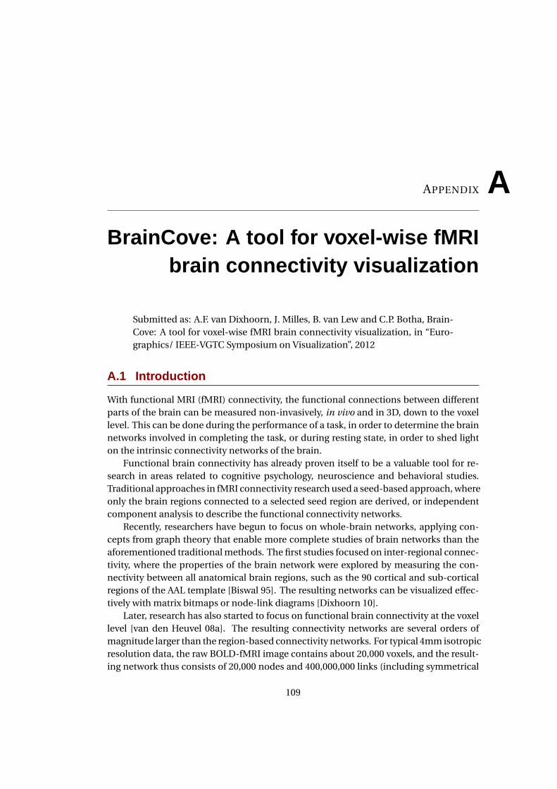
APPENDIX A
BrainCove: A tool for voxel-wise fMRIbrain connectivity visualization
Submitted as: A.F. van Dixhoorn, J. Milles, B. van Lew and C.P. Botha, Brain-
Cove: A tool for voxel-wise fMRI brain connectivity visualization, in “Euro-
graphics/ IEEE-VGTC Symposium on Visualization”, 2012
A.1 Introduction
With functional MRI (fMRI) connectivity, the functional connections between different
parts of the brain can be measured non-invasively, in vivo and in 3D, down to the voxel
level. This can be done during the performance of a task, in order to determine the brain
networks involved in completing the task, or during resting state, in order to shed light
on the intrinsic connectivity networks of the brain.
Functional brain connectivity has already proven itself to be a valuable tool for re-
search in areas related to cognitive psychology, neuroscience and behavioral studies.
Traditional approaches in fMRI connectivity research used a seed-based approach, where
only the brain regions connected to a selected seed region are derived, or independent
component analysis to describe the functional connectivity networks.
Recently, researchers have begun to focus on whole-brain networks, applying con-
cepts from graph theory that enable more complete studies of brain networks than the
aforementioned traditional methods. The first studies focused on inter-regional connec-
tivity, where the properties of the brain network were explored by measuring the con-
nectivity between all anatomical brain regions, such as the 90 cortical and sub-cortical
regions of the AAL template [Biswal 95]. The resulting networks can be visualized effec-
tively with matrix bitmaps or node-link diagrams [Dixhoorn 10].
Later, research has also started to focus on functional brain connectivity at the voxel
level [van den Heuvel 08a]. The resulting connectivity networks are several orders of
magnitude larger than the region-based connectivity networks. For typical 4mm isotropic
resolution data, the raw BOLD-fMRI image contains about 20,000 voxels, and the result-
ing network thus consists of 20,000 nodes and 400,000,000 links (including symmetrical
109
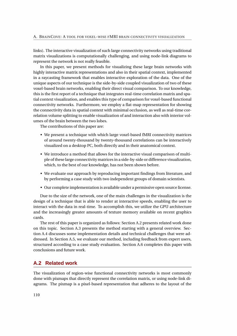
A. BRAINCOVE: A TOOL FOR VOXEL-WISE FMRI BRAIN CONNECTIVITY VISUALIZATION
links). The interactive visualization of such large connectivity networks using traditional
matrix visualizations is computationally challenging, and using node-link diagrams to
represent the network is not really feasible.
In this paper, we present methods for visualizing these large brain networks with
highly interactive matrix representations and also in their spatial context, implemented
in a raycasting framework that enables interactive exploration of the data. One of the
unique aspects of our technique is the side-by-side coupled visualization of two of these
voxel-based brain networks, enabling their direct visual comparison. To our knowledge,
this is the first report of a technique that integrates real-time correlation matrix and spa-
tial context visualization, and enables this type of comparison for voxel-based functional
connectivity networks. Furthermore, we employ a flat-map representation for showing
the connectivity data in spatial context with minimal occlusion, as well as real-time cor-
relation volume splitting to enable visualization of and interaction also with interior vol-
umes of the brain between the two lobes.
The contributions of this paper are:
• We present a technique with which large voxel-based fMRI connectivity matrices
of around twenty-thousand by twenty-thousand correlations can be interactively
visualized on a desktop PC, both directly and in their anatomical context.
• We introduce a method that allows for the interactive visual comparison of multi-
ple of these large connectivity matrices in a side-by-side or difference visualization,
which, to the best of our knowledge, has not been shown before.
• We evaluate our approach by reproducing important findings from literature, and
by performing a case study with two independent groups of domain scientists.
• Our complete implementation is available under a permissive open source license.
Due to the size of the network, one of the main challenges in the visualization is the
design of a technique that is able to render at interactive speeds, enabling the user to
interact with the data in real-time. To accomplish this, we utilize the GPU architecture
and the increasingly greater amounts of texture memory available on recent graphics
cards.
The rest of this paper is organized as follows: Section A.2 presents related work done
on this topic. Section A.3 presents the method starting with a general overview. Sec-
tion A.4 discusses some implementation details and technical challenges that were ad-
dressed. In Section A.5, we evaluate our method, including feedback from expert users,
structured according to a case study evaluation. Section A.6 completes this paper with
conclusions and future work.
A.2 Related work
The visualization of region-wise functional connectivity networks is most commonly
done with pixmaps that directly represent the correlation matrix, or using node-link di-
agrams. The pixmap is a pixel-based representation that adheres to the layout of the
110
A.2. Related work
raw correlation matrix, directly mapping each correlation value to a color using a pre-
defined color scale. For a N xN connectivity matrix, this results in a N xN bitmap im-
age [Becker 95]. For effective visualization, the pixmap should be reordered such that
similar items are grouped [Friendly 03]. For functional connectivity brain networks, the
ordering is typically derived from anatomical location, such as grouping voxels together
if they are in the same anatomical region or brain lobe [Dixhoorn 10, Hagmann 08] or
from hierarchical clustering (in which the leaves of the dendrogram are used for the or-
dering), such that the pixmap groups highly connected hubs together [Hutchison 11].
To see the functional network in its spatial context, the correlation matrix is typi-
cally represented as a node-link diagram, inter-connecting the N nodes with a straight
line, whose thickness or color is based on the connectivity strength. The visual analysis
of region-wise whole-brain functional connectivity networks has been studied before by
Van Dixhoorn et al. [Dixhoorn 10], where the problem of visual clutter that arises when
rendering node-link networks with twenty or more nodes [Ghoniem 05] was addressed
by allowing the user to interactively filter on the connection strength. The node-link rep-
resentation has also been used to visualize voxel-wise connectivity by Zuo et al. [Zuo 11],
but here the links are drawn between twenty functional communities instead of between
each voxel pair. Furthermore, the visualization procedures were carried out on a graph-
ics workstation, rather than on a standard desktop computer.
Instead of the node-link representation, we employ a method typically used to visual-
ize brain activation data from fMRI studies. An approach for this was described by Jainek
et al. [Jainek 08], where illustrative techniques are used to visualize functional data in
anatomical context. To represent the activation data, the metaphor is used of activated
regions emitting light. However, instead of a single activation map, our data consists of
a large number of networks, one for each voxel in the underlying fMRI images. Render-
ing all these networks at once in would result in an ambiguous visualization. Instead, our
method includes an interaction component in which the user indicates in which network
he is interested by interactively selecting a seed voxel.
Our method certainly shows parallels with the work recently published by Eklund et
al. [Eklund 11] and Böttger et al. [Böttger 11], as well as with the interactive tool InstaCorr
for thi visualization of functional connectivity in AFNI [Robert W. 11]. The method of
Böttger et al. allows the user to place a cross-hair on the desired seed voxel on orthogonal
2D slices of an anatomical scan, rendering the resulting correlation map on top as an
overlay. The tools presented by Eklund et al. and InstaCorr provide similar functionality,
but in addition they are able to visualize the correlation maps in their 3-D spatial layout.
Our work is similar to those methods, but differs with respect the following points: 1.)
The correlation matrix is computed in a pre-processing step such that we can provide a
pixmap visualization that allows for detection of groups of voxels that are correlated. 2.)
We provide a picking tool that allows the user to interactively and dynamically select a
seed voxel on the cortical surface, directly in the 3-D representation. 3.) Our tool allows
for interactive side-by-side comparison and difference visualization of multiple datasets.
111

A. BRAINCOVE: A TOOL FOR VOXEL-WISE FMRI BRAIN CONNECTIVITY VISUALIZATION
A.3 Method
We implemented our visualization techniques as a new visual analysis tool that we have
dubbed BrainCove. An overview of the application window can be seen in Fig. A.1. The
graphical user interface of our application uses the Multiple Document Interface (MDI)
to facilitate the loading of multiple datasets. The child windows are by default arranged
in a tile pattern, that allows for side-by-side comparison but the user is free to move,
maximize and minimize each window. Each child window consists of three main com-
ponents: the pixmap representation at the top left, the orthogonal slice views at the top
right and the anatomical visualization spanning the full width at the bottom. The views
can be resized freely.
The input to our application is an already pre-processed correlation matrix in raw
binary format, combined with a list of coordinates in the well-known standardized MNI
space that correspond to the elements in the correlation matrix. In the next section, we
will briefly discuss the pre-processing pipeline that is used to derive the required corre-
lation matrix. In the subsequent sections, we will describe the individual components of
our tool.
A.3.1 Data pre-processing
Prior to loading the data into our tool, the fMRI data sets have to be pre-processed and
converted to the right format. The steps to pre-process our data are described in the pa-
per by Ferrarini et al. [Ferrarini 11] and include motion-correction, removal of non-brain
tissue, grand mean intensity normalization, registration to MNI-152 standard space and
downsampling to 4mm isotropic resolution.
Once the fMRI datasets have been pre-processed, the next step is to compute the
correlation matrix. First, white matter (WM) and cerebrospinal fluid (CSF) time series
and the average whole-brain signal are extracted from the fMRI data sets. The data is
then masked with the Automated Anatomical Labeling (AAL, [Tzourio-Mazoyer 02]) atlas
and using regression analysis the influence of artifacts is reduced (see Ferrarini et al. for
details). The final correlation matrix is computed by evaluating the Pearson’s correlation
coefficient between each pair of neural activation timeseries. This raw correlation map
and a list of coordinates corresponding to the rows and columns of the matrix are the
input to our application.
A.3.2 Pixmap view
The pixmap representation is a direct visualization of the correlation matrix, where the
correlation values are mapped to colors using a continuous colorscale. The elements on
the rows and columns are reordered to make the visualization more effective. The re-
ordering is based on the AAL atlas and is computed by looking up the atlas region for
each voxel. The resulting list of atlas region numbers is then grouped by the atlas num-
bers to form the ordering of the rows and columns of the correlation matrix, thus group-
112
A.3. Method
Figure A.1: An overview of the application window with two datasets. Each dataset is
opened in its own child window. Each child window contains of three views: the pixmap
view on the top-left, the slice views on the top right and the anatomical view on the
bottom.
ing voxels together that are anatomically close to each other. This procedure is depicted
graphically in Fig. A.2.
���������� � � � � � ��� ����� �����
�������� ��
��
��
��
��
��
��� ������
������
���������������������
���������� � � � � � ��� ����� �����
��������� � � �� �� � �� ��� �� �
���������� � � � ����� � ��� � �����
��������� � � � � �� �� ��� �� ��
���� !����������
���������� � � ����� � � ��� � �����
��������� �� �� �� �� � � ��� � �
���� !����"���
Figure A.2: Reordering the rows and columns using the AAL template.
Directly mapping each correlation in the matrix to a colored pixel results in a bitmap
of 400 megapixels. If each color is to be represented with three 8-bit channels, the com-
plete bitmap would require 1.2 gigabytes of storage on top of the 800 megabytes that
is required to store the raw correlation matrix. In order to display such an image on the
113

A. BRAINCOVE: A TOOL FOR VOXEL-WISE FMRI BRAIN CONNECTIVITY VISUALIZATION
Figure A.3: The basic idea of raycasting the correlation matrix, with the corresponding
transformations. Transformation A transforms a pixel coordinate to object-space, in this
case a position on the proxy plane. Transformation B then interpolates this position to a
cell index in the raw correlation matrix. Finally, C maps the correlation value to a color
using a continuous color scale, which is assigned to the pixel in the projection plane.
screen, while maintaining an interactive frame rate, we propose a technique that is based
on GPU raycasting. The main advantage of this approach is that the maximum size of the
image to display only depends on the size of the viewport, thus requiring little memory.
Furthermore, the raycasting technique is highly parallel, meaning that the display of the
pixmap can be accelerated significantly by performing the rendering on the GPU.
The general idea of the raycasting algorithm that we employed for the accelerated
rendering of a large correlation matrix is shown schematically in Fig. A.3. In the scene,
a plane at z = 0 is used as a proxy object to convert from screen coordinates to indices
in the correlation matrix. Since there are only values at z = 0, the raycasting algorithm
is relatively simple, no loop is required to step through the scene. The actual raycasting
algorithm is implemented in the Open Compute Language (OpenCL) and runs on the
GPU. For fast access, the entire correlation matrix is uploaded to a GPU buffer which is
accessible in the OpenCL kernel as a float array. The OpenCL kernel is executed for each
pixel in the viewport. Using a view-to-world transformation matrix, the pixel coordinate
is converted into a coordinate in the proxy plane’s object space. From the object space,
a simple one-to-one mapping gives the corresponding indices in the correlation matrix.
The correlation value at that particular index is then mapped using a colormap to form
the final pixel color.
Interaction and Filtering
The raycasting framework that is used for rendering the pixmap has an important ad-
vantage: zoom and pan come basically for free, as this is built-in in the transformation
pipeline. Another advantage is that applying a filter is nothing more than an extra state-
ment in the raycasting algorithm, which means that filtering can be done on-the-fly;
there is no need to recreate the entire correlation matrix. The tool currently only supports
thresholding on absolute correlation as a filter, but other filters can be implemented eas-
ily.
A limitation of the pixmap representation is that it does not correctly show the spa-
tial component of the connectivity network. Although the ordering of the elements based
114

A.3. Method
on their anatomical location does reveal some spatial information, it remains difficult to
mentally integrate the connectivity values and the inherent spatial context. To improve
the integration of functional connectivity and spatial location, we linked the pixmap
representation to a anatomical visualization in 3-D. By hovering with the mouse over
the pixmap, the 3-D visualization highlights in real-time the voxels corresponding to the
connection currently pointed at with the mouse cursor. Furthermore, we implemented
a brushing technique that allows the user to select a group of links using the mouse. The
corresponding voxels are then highlighted in the anatomical view (see Fig. A.4).
Figure A.4: Brushing the matrix representation highlights the selected voxels in the
anatomical view, where it can be seen from any view (two different viewing angles are
shown in this figure). The brushed selection appears twice because of the symmetry in
the matrix. Voxels along the horizontal axis of the matrix are shown in yellow, voxels on
the vertical axes in red.
A.3.3 Anatomical view
In the anatomical view, the connectivity network is rendered in its spatial context. The
traditional method for visualization of the brain connectivity network is the node-link
representation. However, for connectivity networks on the voxel-level, the node-link
representation is not feasible. Instead, we employ the visualization method commonly
used to represent activation data from fMRI studies in its spatial context, where the ac-
tivated regions are highlighted and the deactivated regions are hidden. For connectivity
data, this corresponds to highlighting regions that are strongly connected to a certain
seed voxel and hiding the other regions. The visualization of the correlation map for a
selected seed voxel can be seen in Fig. A.5.
Our method allows the user to select a seed voxel and a correlation threshold, and
the resulting correlation map is shown in real-time in a 3-D visualization. The visualiza-
tion is implemented in a raycasting framework that runs on the GPU, enabling real-time
interaction.
The raycasting algorithm is similar to standard raycasting, with the exception that
the volume to render is not static but depends on the current seed voxel and correlation
115
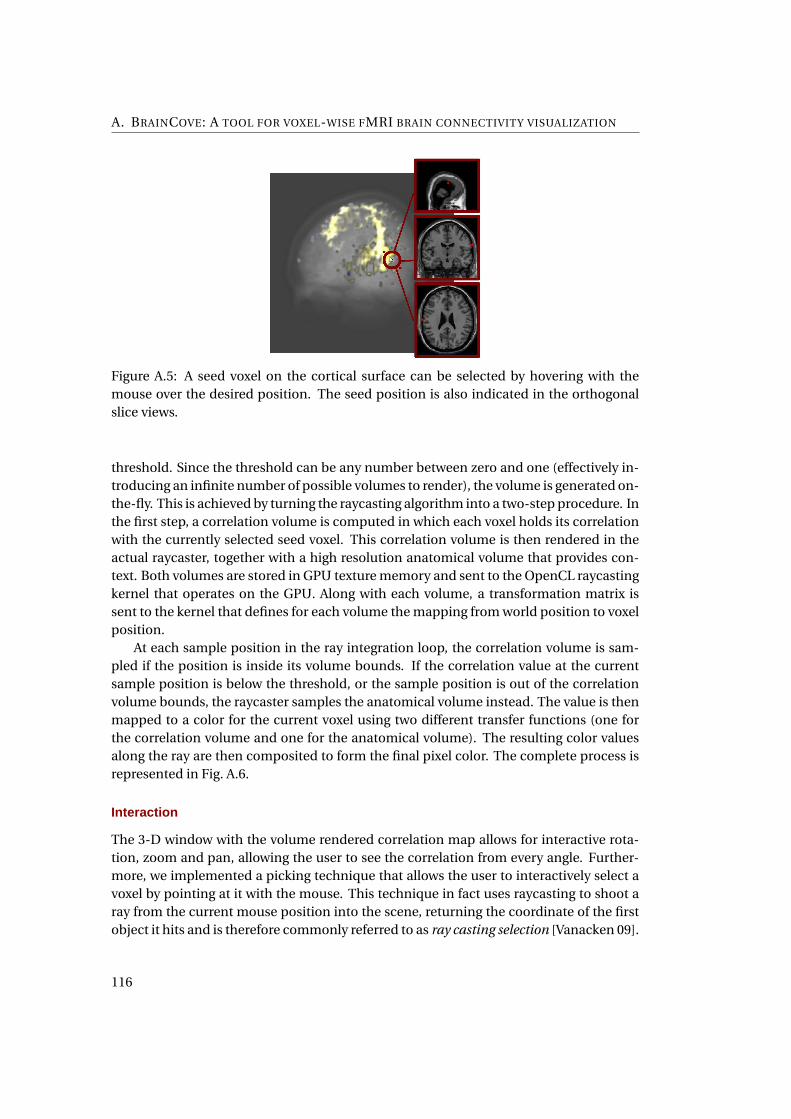
A. BRAINCOVE: A TOOL FOR VOXEL-WISE FMRI BRAIN CONNECTIVITY VISUALIZATION
Figure A.5: A seed voxel on the cortical surface can be selected by hovering with the
mouse over the desired position. The seed position is also indicated in the orthogonal
slice views.
threshold. Since the threshold can be any number between zero and one (effectively in-
troducing an infinite number of possible volumes to render), the volume is generated on-
the-fly. This is achieved by turning the raycasting algorithm into a two-step procedure. In
the first step, a correlation volume is computed in which each voxel holds its correlation
with the currently selected seed voxel. This correlation volume is then rendered in the
actual raycaster, together with a high resolution anatomical volume that provides con-
text. Both volumes are stored in GPU texture memory and sent to the OpenCL raycasting
kernel that operates on the GPU. Along with each volume, a transformation matrix is
sent to the kernel that defines for each volume the mapping from world position to voxel
position.
At each sample position in the ray integration loop, the correlation volume is sam-
pled if the position is inside its volume bounds. If the correlation value at the current
sample position is below the threshold, or the sample position is out of the correlation
volume bounds, the raycaster samples the anatomical volume instead. The value is then
mapped to a color for the current voxel using two different transfer functions (one for
the correlation volume and one for the anatomical volume). The resulting color values
along the ray are then composited to form the final pixel color. The complete process is
represented in Fig. A.6.
Interaction
The 3-D window with the volume rendered correlation map allows for interactive rota-
tion, zoom and pan, allowing the user to see the correlation from every angle. Further-
more, we implemented a picking technique that allows the user to interactively select a
voxel by pointing at it with the mouse. This technique in fact uses raycasting to shoot a
ray from the current mouse position into the scene, returning the coordinate of the first
object it hits and is therefore commonly referred to as ray casting selection [Vanacken 09].
116

A.3. Method
����������� ������� �����
� ����
��������������
������������
����������������� ���
����� ��������
����������� ����� ������������
������� ��
�������� ��
����� ��������������������������������
����� �������������� ��������� ��
����������
� ��!�������������� ��
����� ��������
"� ����� ����
��� �����
�����#��#$ �%�����������
����� �
����� �
Figure A.6: The complete pipeline for the two-pass raycasting of the correlation volume.
In the first pass, the correlation volume is constructed using the seed voxel index and the
index volume. In the second pass, they raycasting algorithm takes a sample in the cor-
relation volume; if for the current position the correlation value is above the threshold,
the correlation is mapped to color and composited with other color values on the ray.
Otherwise, the anatomical volume is sampled and colormapped.
The size of the seed can also be increased, such that a group of voxels is used as the
seed region. In addition, it is also possible to use the AAL region to which the selected
voxel belongs as a seed region. Using the ray casting selection, it is not possible to se-
lect voxels behind the outer cortical layer of the brain. To overcome this limitation, two
alternative selection methods have been implemented.
Brain cleaving To be able to select structures that are located in-between the two hemi-
spheres, such as the Thalamus or the Hippocampus, we employed a volume deformation
method with which the user is able to spread the two brain hemispheres apart, similar
to the Hinge Spreader proposed by McGuffin et al. [McGuffin 03]. Once the two brain
halves are spread apart, the user can use the mouse to select a voxel on the inner side of
each hemisphere, in the same way as selecting a voxel on the cortical surface. The de-
formation is implemented in the raycasting algorithm using ray deformation, and uses a
saggital plane, passing through a point P that is located between the two hemispheres.
While stepping through the volume the algorithm determines for every sample point Q
whether the point is to the left or to the right of the saggital plane, using its plane normal
N . Once the point Q has been classified as either left or right from the split plane, its
transformed position is found by multiplying the voxel position with the corresponding
rotation matrix for left or right rotation.
~Q ′ =
{
AL ∗ ~Q if (~Q −~P ) · ~N < 0
AR ∗ ~Q if (~Q −~P ) · ~N > 0(A.1)
where AL and AR are the rotation matrices for the left and right hemispheres respec-
tively. See Fig. A.7 for a schematic representation of this method. When implementing
this method in a raycasting algorithm, the process is actually reversed: the sample points
visited by the raycaster should be considered to be already in deformed space. The sam-
117

A. BRAINCOVE: A TOOL FOR VOXEL-WISE FMRI BRAIN CONNECTIVITY VISUALIZATION
ple value for that position can then be found by projecting the sample position back to
non-deformed space using the inverse transformation. A special case occurs when the
sample position is in the region between the two rotated hemispheres (the hatched re-
gion in Fig. A.7). During the ray traversal, positions in this region should be skipped.
This is done by checking the transformed position again with the plane normal; if the
dot product of the transformed position with the plane normal does not have the same
sign as the dot product with the non-transformed position, the sample position is in the
in-between region and should be skipped.
Figure A.7: A schematic representation of the brain split method (left) and the resulting
visualization (right). The hatched region in the left drawing indicates the region in which
the raycaster can skip the voxels.
Slice view The brain split approach discussed above allows for the selection of voxels
between the two hemispheres, but not for selections at arbitrary positions in the brain
volume. To allow for selection of seed voxels at arbitrary positions in the brain, a view
window is available that contains three slice views, one for each orthogonal plane (saggi-
tal, coronal and transverse). Using the mouse, a seed point can be selected on any of the
three slices. The three slice views are linked: as the cursor is moved in one of the views,
the other slices views are updated such that they show the same position. The slice views
are also linked with the anatomical and pixmap view, such that the seed voxel selected in
the anatomical view is also shown in the slice view (see Fig. A.5).
A.3.4 Flat mapping
The anatomical view described in the previous section shows the correlation map in its
correct spatial context, but suffers from the occlusion problem inherent to any 3-D vi-
sualization. This makes it difficult, if not impossible, to see the entire correlation map
in a single view. To solve this, a flat map of the cerebral cortex is required on which the
correlation map can be overlayed, allowing the user to see the complete correlation map
in a single view, without the need for interaction.
A class of projections that can be implemented relatively easy in a raycasting tech-
nique are the cylindrical mappings. From this class of cylindrical projections, we have
implemented two projections: the the Lambert’s Cylindrical Equal-Area and Braun’s Stere-
ographic Cylindrical projection to map the cerebral cortex to a flat representation. The
118

A.4. Implementation
Lambert’s projection causes severe distortion in the poles, but the advantage that the
shape of the brain can be easily recognized. The Braun’s projection on the other hand,
distributes the distortion over the full height of the map, but results in brain maps that
are harder to recognize.
Figure A.8: The Lambert’s Cylindrical flatmap representation of the brain, viewing from
the anterior in the middle to posterior at the two sides. In this visualization, a voxel in
the visual cortex is selected (see also the corresponding slice views).
A.4 Implementation
The visualization techniques described in the previous sections are implemented in a
prototype application in C++ using the Qt framework. The raycasting framework is im-
plemented using the Visualization Toolkit (VTK) by implementing a custom VTK volume
mapper for the pixmap and anatomical visualizations. The actual raycasting algorithm
is implemented in OpenCL kernels that are executed on the GPU. The OpenCL raycaster
renders to a texture that is shared with OpenGL using the OpenCL/GL interoptability.
This texture is then mapped to a quad in the VTK render window, a method commonly
used in the VTK volume raycast mappers. So far, we have only tested our tool on Win-
dows 7 - 64 bit, but since all toolkits and frameworks that are used are cross-platform, the
application should run Linux and Mac OS X as well. The OpenCL application has been
tested on both NVIDIA and AMD graphics cards with OpenCL 1.1 compatible drivers.
To enable real-time visualization, the raw correlation matrices are transferred to the
GPU using an OpenCL buffer object. The size of a matrix depends on the resolution of the
input fMRI volume. For a typical resolution of 4mm, the resulting correlation matrix is
about 800-900 megabytes in size. Thus, to visualize two datasets concurrently, a graphics
card with at least 2 gigabytes of onboard memory is required.
A.5 Evaluation
The prototype application with the presented visualization techniques was evaluated
with domain scientists in order to investigate the possible role of the application in the
119
A. BRAINCOVE: A TOOL FOR VOXEL-WISE FMRI BRAIN CONNECTIVITY VISUALIZATION
existing pipeline of fMRI connectivity research. The evaluation was set up as an ex-
ploratory case study following the guidelines set out by Yin [Yin 09]. The main study
question was formulated as: How can the functional connectivity visualization tool, called
BrainCove, assist domain scientists in studying patterns in functional brain connectiv-
ity, the relation with brain anatomy and in studying inter-subject or inter-group differ-
ences? and the case was defined as the use of our application by external domain ex-
perts who were targeted as prospective end users. An evaluation session was held with
two groups, one with a group of four neuroscientists from the Leiden University Medical
Center (LUMC) and a second at the Amsterdam Medical Center (AMC), in which the tool
was first presented to a group of 30 people from the neuroimaging and neuroscience do-
main in an informal and interactive presentation and then continued as case study with
a smaller group of researchers (8 in total) specialized in fMRI connectivity.
In the following sections, we will discuss the user feedback structured according to
the case study propositions.
A.5.1 Matrix Visualization
The matrix visualization gives an overview of the data and allows for the detection of
groups of voxels that are correlated. This proposition was confirmed by all participants.
One user specifically mentioned that the matrix visualization is very usable to quickly
select high peaks of highly correlated groups of voxels. Participants added that feedback
about the ordering is important and that rendering of labels would make this represen-
tation more comprehensible, although it was also noted that the lack of labels is com-
pensated by highlighting the corresponding voxels in the anatomical visualization.
The matrix visualization allows for a quick check on the quality of the data, such that
errors can be identified before using the data further in the analysis pipeline. The use of
the matrix visualization for quality checks was not directly apparent to the participants.
They agreed that this representation could be used to detect large artifacts in the data,
but noted that these artifacts would have already been detected earlier in the analysis
pipeline.
Being able to see the spatial context for correlations or groups of correlations using
the view linking aids in interpreting the FC matrix. The participants agreed that the view
linking helps in interpreting the FC matrix, even claiming that without the linked interac-
tion, they would not have a clue on how to interpret the matrix. One of the users further
stated that the matrix visualization would be most useful to find large scale differences
between subjects. The linking would then help to see where the differences are in spatial
context.
A.5.2 Anatomical Visualization
The visualization of FC in spatial context supports mental integration of FC and anatomy.
During the evaluation session at the LUMC, the participants mentioned that they find it
difficult to navigate in the current 3-D visualization, because of a lack of reference. To
our surprise, the AAL atlas visualization with the different colors for each region is hardly
120

A.5. Evaluation
used in the field. Scientists usually navigate and orient themselves within the data using
orthogonal slices of a structural brain or by manually typing in the MNI coordinates.
They strongly suggested that we should integrate a set of simple orthogonal slice views
linked to the 3-D anatomical view that would serve as an anatomical reference. With
such an anatomical reference, they would confirm this proposition.
We implemented this before conducting the second evaluation session at the AMC,
where the users confirmed this hypothesis, stating that this integration of functional con-
nectivity and anatomy is an essential element of this type of visualization.
The visualization of FC data in which the voxels emit “light” when they are function-
ally connected is an intuitive representation of the correlation maps. All users gener-
ally confirmed this proposition. It was remarked that this method corresponds to the
metaphor used in other tools used in the field: “what lights up is active”. Users from both
groups noted that the colormap used to represent the correlation could be improved,
such that the scaling is more diverse. They indicated that the current color map shows
the correlation map too brightly, which makes it hard to see differences. One of the users
further remarked that the color map was not warm enough. Participants in both groups
further suggested to add a colormap legend in the scene and to make the range of the
colormap adjustable.
Interactively selecting a seed voxel by hovering with the mouse over the voxel of inter-
est facilitates the detection of interesting networks and abnormalities. This proposition
was confirmed by all participants. They indicated that this interaction technique is the
biggest difference with other tools. One participant stated that the tool could make a sig-
nificant contribution to the procedure of selecting a seed voxel in seed-based analysis.
The current method includes a priori selection of a seed voxel and computation of the
correlations with all other voxels. According to the participant, loading the whole-brain
correlation matrix into our application would allow for better comprehension in select-
ing the seed voxel because the effect of choosing a specific seed voxel is immediately
visualized.
The brain split approach is useful for selecting voxels inside the brain volume (for in-
stance, in the cingulate cortex). The participants did not readily confirm this proposition.
One participant from the first group remarked that he had trouble finding the cingulate
between the brain lobes due to the lack of anatomical reference. The participants gener-
ally agreed that orthogonal slice views would be preferred for selecting voxels inside the
brain volume. In the second session, the three orthogonal views with the MNI structural
brain was considered a better technique for selecting a seed voxel in the brain volume,
which confirmed the findings from the first session. Interestingly, one of the participants
in the AMC group considered the brain split approach an effective method for reducing
occlusion in the 3-D visualization, but not so much for probing. It was furthermore ar-
gued that to make this approach more effective, it should be possible to place the split
plane at arbitrary position to be able to probe in regions deeper past the cerebral cortex.
Context visualization using a high resolution MRI head volume and a coloured and
outlined anatomical atlas aids in relating FC to anatomical regions. The utility of the col-
ored anatomical atlas was not directly apparent to the participants in the first session.
One of the participants even noted that the coloring was more confusing then helpful.
121

A. BRAINCOVE: A TOOL FOR VOXEL-WISE FMRI BRAIN CONNECTIVITY VISUALIZATION
Again, the suggestion was made to integrate a linked view with orthogonal slices of a
structural brain or a semi-transparent surface rendering of the brain (usually referred to
as a “glass brain”) for providing anatomical context. Following these suggestions, we re-
moved the anatomical atlas coloring from the volume rendering and integrated orthogo-
nal slice views in the tool. During the second evaluation session, participants confirmed
that the slices with a structural MNI brain are the preferred way for navigation purposes
and provide sufficient anatomical context.
A.5.3 Flat map
Visualizing FC in a 2D projection of the spatial locations facilitates in forming a mental
map of the complete connectivity network in a single view. Remarkably, researchers from
both groups were not familiar with the use of “flat maps” for two-dimensional repre-
sentation of functional connectivity in anatomical context. They generally found it dif-
ficult to orient themselves in the cylindrical flat map representation without structural
anatomical context and mentioned that a learning curve would be involved to get accus-
tomed to such a representation. One participant further commented that the presented
flat map is limited to functional connectivity studies of the cortex, which makes it un-
suitable for use in groups that focus on sub-cortical regions. In general, participants did,
however, see potential in the use of mappings that are able to represent the complete
connectivity network in a single view.
A.5.4 Visual Comparison
Coordinated visualizing multiple datasets side-by-side supports the finding of differences
between subjects. All participants confirmed this proposition, noting that the visual com-
parison would be a powerful tool mainly for visually comparing single subjects or pa-
tients to a group mean, since this is mostly a visual task. This would also enable the
use of resting state fMRI connectivity as a disease marker. One of the attending medical
doctors further remarked that the visual comparison could also be employed in interven-
tion measurement in a clinical setting. For example, patients with obsessive-compulsive
disorder are increasingly being treated with deep brain stimulation (DBS). Being able to
visualize the functional network of the brain pre-DBS and post-DBS side-by-side would
allow clinicians to see changes in the network, which is helpful in judging whether the
current treatment is effective or should be changed.
Visualizing the difference between two datasets supports the finding of differences be-
tween subjects or the impact of preprocessing on FC networks. The value of visualizing the
absolute correlation difference between different subjects was not directly confirmed.
It was remarked that absolute difference in correlation between subjects could be at-
tributed to noise or to differences in the strength of the measured signal. Participants
did see potential in using the difference visualization within one subject to compare the
influence of using different preprocessing pipelines. However, participants did see the
greatest potential in connecting the tool to a database with group averages such as for
healthy subjects and for different pathologies, such that single subjects can be visually
122
A.6. Conclusions
compared with the group average. Another suggestion was to create the average on-
demand from a group study.
A.5.5 General remarks
The participants in the first group were generally impressed by the visualizations and saw
the potential in the tool, but stated that due to the lack of anatomical reference (by means
of structural data) and the inability to select voxels that are at a distance from the cortical
surface, they would not readily use the tool for visual analysis. They suggested the use
of a high resolution brain surface rendering, such as the one generally used in the SPM
toolbox, or orthogonal slices of the MNI structural brain volume. Once the anatomical
reference could be dealt with, they saw potential in using the tool especially to compare
individual subjects to a group average, such as in comparing pathologies with healthy
subjects with patients with different pathologies or with the effects of drugs on func-
tional connectivity. They furthermore suggested to add a feature that makes it possible
to select different types of connectivity (such as hub voxels) on-the-fly, using a pipeline
that is running in the background and a method that enables the creation of high-quality
pictures for publications.
The domain scientists in the second evaluation session were generally quite enthu-
siastic about the possibilities the tool offers for the visualization of the connectivity data.
We attribute the difference in enthusiasm between the first and second evaluation to our
addition of anatomical reference using the structural MNI slice views before conduct-
ing the second evaluation. Especially the visual comparison of individuals and group
averages was considered an important contribution. An interesting clinical use case in
this context was proposed by one of the medical doctors present during the evaluation,
involved in treatment of neurological disorders using deep brain stimulation. He un-
derlined the value of the visual comparison for intervention measurement in DBS. He
continued that one of the critical steps in this treatment is finding the location in the
brain where to start the DBS, by looking at patterns in the resting state fMRI connectivity
network. This step could benefit from being able to quickly compare the brain network
of the patient to a group average.
Both groups independently considered the ability to visually compare connectivity
networks to be the major contribution of the tool.
A.6 Conclusions
In this paper, we presented a tool that couples a number of visualizations in order to
facilitate the visual analysis of voxel-wise fMRI connectivity. Using our tool, the analyst
is able to quickly identify interesting patterns in the functional network of the brain and
differences in connectivity patterns between subjects or groups by visually comparing
multiple datasets side-by-side. Currently, three different visualizations are implemented,
including a pixmap representation and direct volume rendering of the correlation map
for a given seed voxel in both anatomical context and a flat-map layout that shows the
123

A. BRAINCOVE: A TOOL FOR VOXEL-WISE FMRI BRAIN CONNECTIVITY VISUALIZATION
correlation map in pseudo-anatomical spacing. We evaluated our tool in case studies
with groups of domain scientists at two different academic medical centers.
Currently, the flat-map representation uses cylindrical projections that result in a
distorted projection. We plan to review other types of cortical maps that produce less
distorted projections. The brain split approach that allows a user to select seed voxels in-
between the two hemisphere will be extended such that the split plane can be placed at
arbitrary position. We plan to implement several of the suggestions that were made dur-
ing the case study evaluation, such as the ability to manually type in MNI coordinates
for the seed voxel, rendering of labels in the matrix and anatomical views and enhance-
ment of the colormap. On the longer term, functionality to calculate the connectivity
measures on-the-fly will be added, such that the tool can directly read pre-processed 4D
NIFTI files. Finally, we plan to extend the comparitive visualization by allowing the im-
port and on-the-fly generation of group mean datasets, that allows the analyst to visually
compare individual patients with an overall group.
124
Related Documents