1 Abstract—Evolutionary algorithms are global optimization methods that have been used in many real-world applications. In this paper we introduce a Markov model for evolutionary algo- rithms that is based on interactions among individuals in the population. This interactive Markov model has the potential to provide tractable models for optimization problems of realistic size. We propose two simple evolutionary algorithms with popu- lation-proportion-based selection and a modified mutation oper- ator. The selection operator whose probability is linearly propor- tional to the number of individuals at each point of the search space. The mutation operator randomly modifies an entire indi- vidual rather than a single decision variable. We exactly model these evolutionary algorithms with the new interactive Markov model. We present simulation results to confirm the interactive Markov model theory. The main contribution is the introduction of interactive Markov theory to model simple evolutionary algo- rithms. We note that many other evolutionary algorithms, both new and old, might be able to be modeled by this method. Index Terms—Evolutionary algorithm; Markov model; popu- lation-proportion-based selection; transition probability; interac- tive Markov model I. INTRODUCTION VOLUTIONARY is algorithms (EAs) have received much attention over the past few decades due to their ability as global optimization methods for real-world applications [1, 2]. Some popular EAs include the genetic algorithm (GA) [3], evolutionary programming (EP) [4], differential evolution (DE) [5, 6], evolution strategy (ES) [7], particle swarm optimization (PSO) [8, 9], and biogeography-based optimization (BBO) [10, Manuscript received December 3, 2013. This material was supported in part by the U.S. National Science Foundation under Grant No. 0826124, the Na- tional Natural Science Foundation of China under Grant No. 61305078, 61074032 and the Shaoxing City Public Technology Applied Research Project under Grant No. 2013B70004. Haiping Ma was with the Department of Electrical Engineering, Shaoxing University, Shaoxing, Zhejiang, 312000, China. He is now with the Shanghai Key Laboratory of Power Station Automation Technology, School of Mechatronic Engineering and Automation, Shanghai University, Shanghai, 200072, China (e-mail: [email protected]). Dan Simon is with the Department of Electrical and Computer Engineering, Cleveland State University, Cleveland, Ohio, 44115, USA (e-mail: [email protected]). Minrui Fei is with the Shanghai Key Laboratory of Power Station Automation Technology, School of Mechatronic Engineering and Automation, Shanghai University, Shanghai, 200072, China (e-mail: [email protected]). Hongwei Mo is with the Department of Automation, Harbin Engineering University, Harbin, Heilongjiang, China (e-mail: [email protected]). 11]. Inspired by natural processes, EAs are search methods that are fundamentally different than traditional, analytic optimiza- tion techniques; EAs are based on the collective learning pro- cess of a population of candidate solutions to an optimization problem. In this paper we often use the shorthand term indi- vidual to refer to a candidate solution. The population in an EA is usually randomly initialized, and each iteration (also called a generation) evolves toward better and better solutions by selection processes (which can be either random or deterministic), mutation, and recombination (which is omitted in some EAs). The environment delivers quality information about individuals (fitness values for maximization problems, and cost values for minimization problems). Indi- viduals with high fitness are selected to reproduce more often than those with lower fitness. All individuals have a small mutation probability to allow the introduction of new infor- mation into the population. Each EA works on the principles of different natural phe- nomena. For example, the GA is based on survival of the fittest, DE is based on vector differences of candidate solutions, ES uses self-adaptive mutation rates, PSO is based on the flocking behavior of birds, BBO is based on the migration behavior of species, and ACO is based on the behavior of ants seeking a path between their colony and a food source. All of these EAs have certain features in common, and probabilistically share information between candidate solutions to improve the solu- tion fitness. This behavior makes them applicable to all kinds of optimization problems. EAs have been applied to many opti- mization problems and have proven effective for solving var- ious kinds of problems, including unimodal, multimodal, de- ceptive, constrained, dynamic, noisy, and multi-objective problems [12]. Evolutionary Algorithm Models Although EAs have shown good performance on various problems, it is still a challenge to understand the kinds of problems for which each EA is most effective, and why. The performance of EAs depends on the problem representation and the tuning parameters. For many problems, when a good rep- resentation is chosen and the tuning parameters are set to ap- propriate values, EAs can be very effective. When poor choices are made for the problem representation or the tuning parame- ters, an EA might perform no better than random search. If there is a mathematical model that can predict the improvement in fitness from one generation to the next, it could be used to find optimal values of the problem representation or the tuning parameters. For example, consider a problem with very expensive fitness function evaluations. For some problems we may even need to Interactive Markov Models of Evolutionary Algorithms Haiping Ma, Dan Simon, Minrui Fei, and Hongwei Mo E

Welcome message from author
This document is posted to help you gain knowledge. Please leave a comment to let me know what you think about it! Share it to your friends and learn new things together.
Transcript

1
Abstract—Evolutionary algorithms are global optimization
methods that have been used in many real-world applications. In
this paper we introduce a Markov model for evolutionary algo-
rithms that is based on interactions among individuals in the
population. This interactive Markov model has the potential to
provide tractable models for optimization problems of realistic
size. We propose two simple evolutionary algorithms with popu-
lation-proportion-based selection and a modified mutation oper-
ator. The selection operator whose probability is linearly propor-
tional to the number of individuals at each point of the search
space. The mutation operator randomly modifies an entire indi-
vidual rather than a single decision variable. We exactly model
these evolutionary algorithms with the new interactive Markov
model. We present simulation results to confirm the interactive
Markov model theory. The main contribution is the introduction
of interactive Markov theory to model simple evolutionary algo-
rithms. We note that many other evolutionary algorithms, both
new and old, might be able to be modeled by this method.
Index Terms—Evolutionary algorithm; Markov model; popu-
lation-proportion-based selection; transition probability; interac-
tive Markov model
I. INTRODUCTION
VOLUTIONARY is algorithms (EAs) have received much
attention over the past few decades due to their ability as
global optimization methods for real-world applications [1, 2].
Some popular EAs include the genetic algorithm (GA) [3],
evolutionary programming (EP) [4], differential evolution (DE)
[5, 6], evolution strategy (ES) [7], particle swarm optimization
(PSO) [8, 9], and biogeography-based optimization (BBO) [10,
Manuscript received December 3, 2013. This material was supported in part
by the U.S. National Science Foundation under Grant No. 0826124, the Na-tional Natural Science Foundation of China under Grant No. 61305078,
61074032 and the Shaoxing City Public Technology Applied Research Project
under Grant No. 2013B70004. Haiping Ma was with the Department of Electrical Engineering, Shaoxing
University, Shaoxing, Zhejiang, 312000, China. He is now with the Shanghai
Key Laboratory of Power Station Automation Technology, School of Mechatronic Engineering and Automation, Shanghai University, Shanghai,
200072, China (e-mail: [email protected]).
Dan Simon is with the Department of Electrical and Computer Engineering, Cleveland State University, Cleveland, Ohio, 44115, USA (e-mail:
Minrui Fei is with the Shanghai Key Laboratory of Power Station Automation Technology, School of Mechatronic Engineering and Automation,
Shanghai University, Shanghai, 200072, China (e-mail:
[email protected]). Hongwei Mo is with the Department of Automation, Harbin Engineering
University, Harbin, Heilongjiang, China (e-mail: [email protected]).
11]. Inspired by natural processes, EAs are search methods that
are fundamentally different than traditional, analytic optimiza-
tion techniques; EAs are based on the collective learning pro-
cess of a population of candidate solutions to an optimization
problem. In this paper we often use the shorthand term indi-
vidual to refer to a candidate solution.
The population in an EA is usually randomly initialized, and
each iteration (also called a generation) evolves toward better
and better solutions by selection processes (which can be either
random or deterministic), mutation, and recombination (which
is omitted in some EAs). The environment delivers quality
information about individuals (fitness values for maximization
problems, and cost values for minimization problems). Indi-
viduals with high fitness are selected to reproduce more often
than those with lower fitness. All individuals have a small
mutation probability to allow the introduction of new infor-
mation into the population.
Each EA works on the principles of different natural phe-
nomena. For example, the GA is based on survival of the fittest,
DE is based on vector differences of candidate solutions, ES
uses self-adaptive mutation rates, PSO is based on the flocking
behavior of birds, BBO is based on the migration behavior of
species, and ACO is based on the behavior of ants seeking a
path between their colony and a food source. All of these EAs
have certain features in common, and probabilistically share
information between candidate solutions to improve the solu-
tion fitness. This behavior makes them applicable to all kinds of
optimization problems. EAs have been applied to many opti-
mization problems and have proven effective for solving var-
ious kinds of problems, including unimodal, multimodal, de-
ceptive, constrained, dynamic, noisy, and multi-objective
problems [12].
Evolutionary Algorithm Models
Although EAs have shown good performance on various
problems, it is still a challenge to understand the kinds of
problems for which each EA is most effective, and why. The
performance of EAs depends on the problem representation and
the tuning parameters. For many problems, when a good rep-
resentation is chosen and the tuning parameters are set to ap-
propriate values, EAs can be very effective. When poor choices
are made for the problem representation or the tuning parame-
ters, an EA might perform no better than random search. If
there is a mathematical model that can predict the improvement
in fitness from one generation to the next, it could be used to
find optimal values of the problem representation or the tuning
parameters.
For example, consider a problem with very expensive fitness
function evaluations. For some problems we may even need to
Interactive Markov Models of
Evolutionary Algorithms
Haiping Ma, Dan Simon, Minrui Fei, and Hongwei Mo
E

2
perform long, tedious, expensive physical experiments to
evaluate fitness. If we can find a model that reduces fitness
function evaluations in an EA, we can use the model during the
early generations to adjust the EA tuning parameters, or to find
out which EAs will perform the best. A mathematical model of
the EA could be useful to develop effective algorithmic modi-
fications. More generally, an EA model could be useful to
produce insights to how the algorithm behaves, and under what
conditions it is likely to be effective.
There has been significant research in obtaining mathemat-
ical models of EAs. One of the earliest approaches was schema
theory, which analyzes the growth and decay over time of
various bit combinations in discrete EAs [3]. It has several
disadvantages, including the fact that it is only an approximate
model. Perhaps the most developed EA model is based on
Markov theory [13-15], which has been a valuable theoretical
tool that has been applied to several EAs including genetic
algorithms [16] and simulated annealing [17]. Infinite popula-
tion size Markov models are discussed in detail in [18], and
exact finite population size Markov models are discussed in
[19].
In Markov models of EAs, a Markov state represents an EA
population distribution. Each state describes how many indi-
viduals there are at each point of the search space. The Markov
model reveals the probability of arriving at any population
given any starting population, in the limit as the generation
count approaches infinity. But the size of Markov model in-
creases drastically with the population size and search space
cardinality. These computational requirements restrict the ap-
plication of the Markov model to very small problems, as we
discuss in more detail in Section II.
Overview of the Paper
The goals of this paper are twofold. First, we present a
Markov model of EAs that is based on interactions among
individuals. The standard EA Markov model applies to the
population as a whole; that is, it does not explicitly model in-
teractions among individuals. This is an extremely limiting
assumption when modeling EAs, and it leads directly to in-
tractable Markov model sizes, as we show in Section II. In
interactive Markov models, we define the states as the possible
values of each individual. This gives a separate Markov model
for each individual in the population, but the separate models
interact with each other. The transition probabilities for each
Markov model are functions of the states of other Markov
models, which is a natural and powerful extension of the
standard noninteractive Markov model. This method can lead
to a better understanding of EA behavior on problems with
realistic size.
The second goal of this paper is to propose two simple EAs
that use population-based selection probabilities, which we call
population-proportion-based selection. We use a modified
mutation operator in the EAs. The modified mutation operator
randomly modifies an entire individual rather than modifying a
single decision variable, as in standard EA mutation. We ex-
actly model these EAs with the interactive Markov model.
Finally, we confirm the interactive Markov model with simu-
lation on a set of test problems.
Section II introduces the preliminary foundations of interac-
tive Markov models, presents two new simple EAs, models
them using an interactive Markov model, and uses interactive
Markov model theory to analyze their convergence. Section III
discusses the similarities and differences between our two new
simple EAs and standard, well-established EAs. Section IV
explores the performance of the proposed EAs using both
Markov theory and simulations. Section V presents some con-
cluding remarks and recommends some directions for future
work.
Notation: The symbols and notations used in this paper are
summarized in Table 1.
Table 1 Symbols and Notation
A, B Interactive Markov model matrices
K Search space cardinality = number of states in
interactive Markov model
mi Fraction of population that is equal to xi
m Vector of population fractions: im m
n Vector of number of individuals that are allowed to
change, or movers
N1 Number of optimal individuals that are allowed to
change (Strategy B)
N Population size
pij Probability of transition from sj to si
pm Mutation probability
P Markov transition matrix: i jP p
rand(a, b) Uniformly distributed random number between a and b
is Markov model state i
S Number of elites (Strategy B)
t Generation number
T Number of states in standard Markov Model
xi Search space point
yk EA individual k
Y EA population
α Replacement pool probability
β Selection parameter
λ Modification probability
μ Selection probability
φ Selection pressure
σ Elitism vector, or stayers (Strategy B): k
II. INTERACTIVE MARKOV MODELS
This section presents the foundation for interactive Markov
models (Section A), presents two new EA selection strategies
(Section B), discusses their convergence properties (Section C),
and analyzes the interactive Markov model transition matrix of
the two new EAs (Section D).
A. Fundamentals of Interactive Markov Models
A standard, noninteractive Markov model is a random pro-
cess with a discrete set of possible states is ( 1, ,i K ), where
K is the number of possible states, also called the cardinality
of the state space. The probability that the system transitions
from state js to is is given by the probability i jp , which is
called a transition probability. The K K matrix i jP p is
called the transition matrix. In standard, noninteractive Markov
models of EAs, i jp is the probability that the EA population

3
transitions from the jth possible population distribution to the
ith possible population distribution in one generation. In the
standard Markov model, one highly restrictive assumption is
that the transition probabilities apply to the entire population
rather than to individuals. That is, individual behavior is not
explicitly modeled; it is only the population as a whole that is
modeled.
To illustrate this point, consider an EA search space with a
cardinality of 2K ; that is, there are K points in the search
space. We denote these points as {x1, x2, …, xK}. Suppose there
are a large number of EA individuals distributed over these K
points. Suppose im t m t is the K-element column vector
containing the fraction of the population that is equal to each
point at generation t; that is, im t is the fraction of the popu-
lation that is equal to xi at generation t. Then the equation
1m t Pm t describes how the fractions of the population
change from one generation to the next. However, this equation
assumes that the transition probabilities i jP p do not de-
pend on the value of m t ; that is, they do not depend on the
population distribution. Interactive Markov models, as dis-
cussed in this paper, deal with cases where the elements of P
are functions of m t , so transition probabilities are functions
of the Markov states. In this case P is written as a function of
m t ; that is, P P m t , and the Markov model becomes
interactive:
1m t P m t m t . (1)
A standard Markov model with constant P can model EAs if
the states are properly defined, and in fact this is exactly how
EA Markov models have been defined up to this point. Given K
points in search space and N individuals in the population, there
are 1K N
TN
possible states for the population as a
whole, and we can define a ,T T transition matrix which
contains the transition probabilities from every population
distribution to every other population distribution [14]. How-
ever, this idea is not useful in practice because there is not a
tractable way to handle the proliferation of states. For instance,
for a small problem with K=100 and N=20, we obtain T on the
order of 1022
. Markov models of that order are clearly not
tractable. For a slightly larger problem with K=200 and N=30,
we obtain T on the order of 1037
.
In contrast, interactive Markov models in the form of (1)
prove to be tractable for much larger search spaces and popu-
lations. For instance, if K=100, then the interactive Markov
model consists of only 100 states, regardless of the population
size. An interactive Markov model of this size is simple to
handle. The challenge that we address in this paper is how to
define the interactive Markov model for a given EA, and how to
obtain theoretical results based on the interactive model.
The interactive Markov model is a fundamentally different
modeling approach than the standard (noninteractive) Markov
model. The states of the standard Markov model consist of
population distributions, while the states of the interactive
Markov model consist of fractions of each individual in the
search space. This difference means that the standard Markov
model transition matrix is independent of the EA population,
while the interactive Markov model transition matrix is a
function of the population distribution. The standard Markov
model transition matrix is thus larger (T states) but with a
simple form, while the interactive Markov model transition
matrix is much smaller (K states) but with a more complicated
form. Both the standard and the interactive Markov models are
exact. However, due to their fundamentally different ap-
proaches to the definition of state, neither one is a subset of the
other, and neither one can be derived from the other.
For standard Markov models, many theorems are available
for stability and convergence. But for interactive Markov
models, such results do not come easily, given the immense
variety of the possible forms of P . The literature [20] dis-
cusses a particular class of P functions that are defined as
follows for a K-state system:
for all ,
where
[1,
0, for all ,
min 0 for all
]
[1, ]
[1, ]
i j i j i
i j
k j k j k
k
ij i j ij
m k j k j k
k
a b mp m i j
a b m
a b
K
K
K
a i j
a b m j
(2)
where the summations go from 1 to K, and im t m t is
abbreviated to im m . Given values for the matrices i jA a
and i jB b , we have a complete interactive Markov model.
The specification of the transition matrix P m is complete
from (2), and the evolution of m t from any initial value
0m is determined by (1). In a standard Markov model, the
probability i jp m of a transition from state j to state i would be
constant; that is, i j i jp m a . But in an interactive Markov
model, i jp m depends on m . The transition probability
i jp m is, in a sense, a measure of the attractive power of the
ith state. In (2), if 0i jb then a greater population in the ith
state makes it more attractive, and if 0i jb then crowding in
the ith state makes it less attractive.
Since the columns of i jP m p m must each sum to one,
a normalization of i jp m is needed. The division in (2) of each
column of the matrix i j i j ia b m by the corresponding column
sum k j k j kka b m provides the desired normalization.
B. Selection Strategies
In this subsection, we modify two previously-published
models of social processes to obtain two simple EAs that use
population-based selection. We will see that these EAs have
interactive Markov models of the form of (2).

4
1) Strategy A
The first new EA that we introduce, which we call Strategy
A, is based on a social process model in Example 1 in [20].
Strategy A involves the selection of random individuals from
the search space, and the replacement of individuals in the
population with the randomly-selected individuals. The basic
form of Strategy A does not include recombination or mutation,
although it could be modified to include these features. Strategy
A includes three tuning parameters: , , and . The population
of Strategy A evolves according to the following two rules.
(a) Denote [0,1] as the replacement pool probability. We
randomly choose round N individuals, where N is the pop-
ulation size. Denote [0,1]j as the modification probability,
which is similar to crossover probability in GAs. j is typically
chosen as a decreasing function of fitness; that is, good indi-
viduals should have a smaller probability of modification than
poor individuals.
(b) The jth individual chosen above, where
j [1, round(N)], has a probability of j of being replaced
with one of K individuals from the search space (recall that K is
the cardinality of the search space, and {xi : 1, ,i K } is the
search space). The probability of selecting the ith individual xi
is denoted as i and is composed of two parts: [0,1] is as-
signed to each individual equally; and the remaining probabil-
ity 1 is assigned among the xi individuals in the proportions
1, , Km m , where mi is the proportion of the xi individuals in
the population. That is, the selection probability of xi is
1i iK m . Note that 1
1K
ii
.
Note that if the selection probability is independent of mi,
that is, 1 , the selection probability of each individual xi is
1i K . According to the above two rules, an EA that oper-
ates according to Strategy A can be written as shown in Algo-
rithm 1. We see from the algorithm listing that Strategy A has
four tuning parameters: N (population size), α (replacement
pool probability), β (the constant component of the selection
probability), and λ (modification probability, which is a func-
tion of fitness).
ALGORITHM 1 – AN EVOLUTIONARY ALGORITHM BASED ON STRATEGY A.
Generate an initial population of individuals Y = {yk : 1, ,k N }
While not (termination criterion)
Randomly choose round N parent individuals
For each chosen parent individual yj ( 1, ,roundj N )
Use modification probability j to probabilistically decide whether to modify yj
If modifying yj then
Select xi ( 1, ,i K ) with probability [ 1 iK m ]
yj xi
End modification
Next individual: j j+1
Next generation
2) Strategy B
The second new EA that we introduce, which we call Strat-
egy B, is based on a social process model in Example 6 in [20].
Similar to Strategy A, Strategy B also involves the selection of
random individuals from the search space, and the replacement
of individuals in the population with the randomly-selected
individuals. However, Strategy B also includes elites. Strategy
B includes four tuning parameters: , , and , which are sim-
ilar to the same quantities in Strategy A; and 1 , which is an
elitism parameter. The population of Strategy B evolves ac-
cording to the following two rules.
(a) For each individual yk in the population, if yk is the best
individual in the search space, there is a probability 1 that it
will be classified as elite, where 1 [0,1] is a user-defined
tuning parameter.
(b) If yk is not classified as elite, use k to probabilistically
decide whether to modify yk. If yk is selected for modification, it
is replaced with xi with probability proportional to im ,
where mi is the fraction of the population that is comprised of xi
individuals. Recall that {xi : 1, ,i K } is the search space.
Similar to Strategy A, Strategy B does not include recom-
bination or mutation, although it could be modified to include
these features. According to the above two rules, an EA that
operates according to Strategy B can be written as shown in
Algorithm 2. We see from the algorithm listing that Strategy B
has the same four tuning parameters as Strategy A: N (popula-
tion size), α (replacement pool probability), β (selection con-
stant), and λ (modification probability, which is a function of
fitness). However, note that α and β are used differently in
Strategies A and B.

5
ALGORITHM 2 – AN EVOLUTIONARY ALGORITHM BASED ON STRATEGY B.
Generate an initial population of individuals Y = {yk : 1, ,k N }
While not (termination criterion)
For each individual yk
If yk is not the best individual in the search space then
Use modification probability k to decide whether to modify yk
If modifying yk then
Select xi ( 1, ,i K ) with probability im
yk xi
End modification
End if
Next individual: k k+1
Next generation
In Strategy B we set the selection probability of xi to
Pr ii k iy x m (3)
for i [1, K], where the population of individuals is
: 1, ,ky k N , N is the population size, and ( [0,1], ) are
user-defined tuning parameters. Equation (3) gives the proba-
bility that yk is replaced by xi, and this probability is a linear
function of mi, which is the proportion of xi individuals in the
population. Note that (3) holds for all k [1, N] (assuming that
the given yk is selected for replacement).
3) Selection Pressure in Strategy A and Strategy B
The selection probabilities in Strategy A and Strategy B are
both linear with respect to the fraction of xi individuals in the
population. Figure 1 depicts the selection probability.
mi
Pr(selection)
min(mi) max(mi) Figure 1 – Selection probability in Strategy A and Strategy B evolutionary
algorithms. The min and max operators are taken over i [1, K], where K is the cardinality of the search space.
In Figure 1, if the search space cardinality K is greater than
the population size N, as in practical EA implementations, then
min(mi) = 0. This is because there are not enough individuals in
the population to completely cover the search space, so there
are always some search space individuals xi that are not repre-
sented in the population.
In Strategies A and B, if selection is overly-biased toward
selecting populous individuals, the population may converge
quickly to a uniformity while not widely exploring the search
space. If selection is not biased strongly toward populous in-
dividuals, the population will be more widely scattered with a
smaller representation of good individuals. Note that the most
populous individuals will be the ones with highest fitness if we
define modification probability k as a decreasing function of
fitness. We will see this effect later in our simulation results in
Section IV.
A useful metric for quantifying the difference between var-
ious selection methods is selection pressure , which is de-
fined as follows [3, p. 34]:
max Pr(selection)
average Pr(selection) (4)
where Pr selection is the probability that an individual is se-
lected as a replacement.
The most populous individual has the maximum fraction
max im , which we denote as mmax. The average individual has
the average fraction maxmax min 2 2i im m m , assuming
that K > N, as discussed earlier in this section. Then the selec-
tion pressure of (4), when applied to Strategy B (Algorithm 2),
can be written as
max
max / 2
m
m
(5)
If we normalize the selection probabilities so that they sum to 1,
we get
1 1
1
Pr
1
K K
k i i
i i
K
i
i
y x m
K m K
(6)
In the above equation we used the fact that 1
1K
iim
because
the sum of all the fractions of the xi individuals in the popula-
tion must equal 1. If we desire a given selection pressure , we
can solve (5) and (6) for and to obtain the following:
max
max
max
2
2 2 1
2 1
2 2 1
m
Km
Km
(7)
Note that (7) also holds for Strategy A (Algorithm 1) if is
replaced with /K, and is replaced with (1).

6
C. Convergence
In this subsection, we present a theorem that summarizes the
convergence conditions of interactive Markov models.
Theorem 1: Consider an interactive Markov model in the form
of (1). If there exists a positive integer R such that 1
R
t
P m t
is positive definite for all 0m t such that 1
1K
i
i
m t
,
where 1,2, ,t R , then 1
R
t
P m t
converges as R → ∞ to a
steady state which has all nonzero entries.
Proof: See [21] for a proof and discussion.
Later in this section, we will use Theorem 1 to show that
there is a unique limiting distribution for the states of the in-
teractive Markov models in this paper. We will also show that
the probability of each state of the interactive Markov model is
nonzero at all generations after the first one. In particular,
Theorem 1 will show that Algorithms 1 and 2 have a unique
limiting distribution with nonzero probabilities for each point
in the search space. This implies that Algorithms 1 and 2 will
both eventually find the globally optimal solution to an opti-
mization problem.
D. Interactive Markov Model Transition Matrices
The previous subsections presented two simple but new se-
lection strategies, and showed that they both have a unique
population distribution as the generation count approaches
infinity. Now we analyze their interactive Markov models in
more detail and find the solutions to the steady-state population
distribution.
1) Interactive Markov Model for Strategy A
Selection:
We can use the development of Example 1 in [20] to obtain
the following interactive Markov model of Strategy A:
1 1 1 if
1 if
j j j
i j
j i
K m i jp
K m i j
(8)
for (i, j) [1, K]. The quantity pij gives the probability that a
given individual in the population transitions from xj to xi in one
generation. The first equality in (8), when i = j, denotes the
probability that an individual does not change from one gener-
ation to the next. This probability is composed of three parts:
(a) the first term, 1 , denotes the probability that the indi-
vidual is not selected for the replacement pool;
(b) the first part of the second term is the product of the prob-
ability that the individual is selected for the replacement pool
( ), and the probability that the individual is not selected for
modification (1 j );
(c) the second part of the second term is the product of the
probability that the individual is selected for the replacement
pool ( ), the probability that the individual is selected for
modification (j ), and the probability that the selected indi-
vidual is replaced with itself ( 1 jK m ).
For the second equality in (8), when i j , denotes the
probability that an individual is changed from one generation to
the next. This probability is very similar to the second part of
the second term of the first equality as discussed in paragraph
(c) above, the difference being that im is used instead of
jm ;
that is, the selected individual is changed from xj to xi.
Mutation:
Next we add mutation into the interactive Markov model of
Strategy A. Typically, EA mutation is implemented by proba-
bilistically complementing each bit in each individual. Then the
probability that individual xi mutates to become xk can be
written as
Pr 1ikik
q HH
ki i k m mp x x p p
(9)
where pm (0, 1) is the mutation rate, q is the number of bits in
each individual, and Hij is the Hamming distance between bit
strings xi and xj.
But with this type of mutation, the transition matrix elements
kj ki ij
i
p p p would not satisfy the form of (2) and (8). So we
use a modified mutation operator that randomly modifies an
entire individual rather than a single decision variable of an
individual. Mutation of the jth individual is implemented as
follows.
For each individual yj
If rand(0, 1) < pm
yj rand(L, U)
End if
Next individual
In the above mutation logic, rand(a, b) is a uniformly dis-
tributed random number between a and b, and L and U are the
lower and upper bounds of the search space. The above logic
mutates each individual with a probability of pm. If mutation
occurs for a given individual, the individual is replaced with a
random individual within the search domain. The descriptions
of Strategy A and Strategy B with mutation are the same as
Algorithm 1 and 2 except that we add the operation,
“probabilistically decide whether to mutate each individual in
the population” at the end of each generation. Note that muta-
tion acts on all individuals Y = {yk : 1, ,k N }. In particular,
for Strategy B, we use elitism only to prevent selection, but not
to prevent mutation.
Now, the transition probability of the modified mutation
operator is described as
(1 ) if
if
m m
ki
m
p p K k ip
p K k i
(10)
Then the transition probability of Strategy A with mutation, and
the corresponding A and B matrices described in (2), can be
written as follows:

7
2
2
1 1 1 1(1 ) 1 (1 ) 1 (1 ) 1 1 1 if
1 11 1 (1 ) 1 1 1 if
kj ki ij
i
m m m m mj j m j
m mm m mj j m k
p p p
K p K p K p K p pp m k j
K K K K K K
K p K pp p pp m k j
K K K K K K
(11)
and
2
2
1 1 1 1(1 ) 1 (1 ) 1 (1 ) 1 if
1 11 1 (1 ) 1 if
1 1
m m m m mj j
kj
m mm m mj j
kj j m
K p K p K p K p pk j
K K K K K Ka
K p K pp p pk j
K K K K K K
b p
(12)
The derivation of (11) is in the appendix. Now we are in a
position to state the main result of this subsection.
Theorem 2: The K1 equilibrium population fraction vector
m* of Algorithm 1, which is exactly modeled by the interac-
tive Markov model of (1) and (11), is equal to the dominant
eigenvector (normalized so its elements sum to one) of the
matrix 0 1
K
i j j k jkA a b a
, where aij is given by (12), and
jb is shorthand notation for i jb in (12) since all the rows of B
are the same.
Proof: This theorem derives from Theorem 1 in [20]. We
provide the proof in the appendix.
Next we consider the special case 1i K . In this case, the
transition probability (11) is written as
1 1(1 ) 1 (1 ) 1 if
1 1 if
jm m
j
kj
jm mj
K p K pk j
K K Kp
p pk j
K K K
(13)
which is independent of mi; that is, the interactive Markov
model reduces to a standard noninteractive Markov model. In
this case we can use Theorem 1 in [20] or standard
noninteractive Markov theory [13] to obtain the equilibrium
population fraction vector m*.
2) Interactive Markov Model for Strategy B
Before discussing the interactive Markov model of Strategy
B, we define some notation. Suppose that k denotes the
fraction of individuals that always remain equal to xk for each
k [1, K]. Then kk is the fraction of all individuals that
never change. We call these individuals stayers. 1, , Kn n n
denotes the fractions of all individuals that are allowed to
change, and we call these individuals movers. 1, , Km m m
denotes the fractions of all individuals in the population. The
fraction of xj individuals thus includes two parts: j , which
denotes the fraction of all xj individuals that are not allowed to
change; and 11
K
k jkn
, which denotes the fraction of all xj
individuals that may change in future generations. So the
fraction vector m is given by
1
1K
k
k
m n
(14)
The vector is related to EA elitism since it defines the
proportion of individuals in the population that are not allowed
to change in subsequent generations. One common approach
to elitism is to prevent only optimal individuals from changing
in future generations [12]. That is, 1 0 (assuming, without
loss of generality, that x1 is the optimal point in the search
space), and 0k for all k > 1. In this case (14) becomes
1 1 1
1
1 for 1, which corresponds to the optimal state
1 for 1, which correspond to nonoptimal statesi
i
n im
n i
(15)
Note that Strategy B elitism is a little different than standard
EA elitism. In Strategy B, we assume that we know if an in-
dividual is at the global optimum. This is not always the case
in practice, but it may be the case for certain problems. If S
individuals at the global optimum are retained as elites, then
1 S N (this quantity could change from one generation to
the next). If 1N individuals at the global optimum are allowed
to change, then 1 1n N N S . If an individual is not at the
global optimum, then we must always allow it to change that
is, we can implement elitism only for individuals that are at the
global optimum.
8
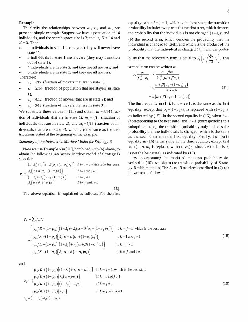
Example
To clarify the relationships between , n , and m , we
present a simple example. Suppose we have a population of 14
individuals, and the search space size is 3; that is, N = 14 and
K = 3. Then:
2 individuals in state 1 are stayers (they will never leave
state 1);
3 individuals in state 1 are movers (they may transition
out of state 1);
4 individuals are in state 2, and they are all movers; and
5 individuals are in state 3, and they are all movers.
Therefore:
1 3 12n (fraction of movers that are in state 1);
1 2 14 (fraction of population that are stayers in state
1);
2 4 12n (fraction of movers that are in state 2); and
3 5 12n (fraction of movers that are in state 3).
We substitute these values in (15) and obtain 1 5 14m (frac-
tion of individuals that are in state 1), 2 4 14m (fraction of
individuals that are in state 2), and 3 5 14m (fraction of in-
dividuals that are in state 3), which are the same as the dis-
tributions stated at the beginning of the example.
Summary of the Interactive Markov Model for Strategy B
Now we use Example 6 in [20], combined with (6) above, to
obtain the following interactive Markov model of Strategy B
selection:
1 1 1 1
1 1 1
1
1
11 1 if 1, which is the best state
1 if 1 and
1 1 if
1 if , and
1
1
1
j
i j
j j i
j i
n i j
n i jp
n i j
n i j i
(16)
The above equation is explained as follows. For the first
equality, when i = j = 1, which is the best state, the transition
probability includes two parts: (a) the first term, which denotes
the probability that the individuals is not changed 11 ; and
(b) the second term, which denotes the probability that the
individual is changed to itself, and which is the product of the
probability that the individual is changed (1 ), and the proba-
bility that the selected xi term is equal to 1
1
1
K
k
k
. This
second term can be written as
1 11 1
1 1 1
1
1 1 1 1
1 1(
1
1
)K K
kk kk
m
n
K
n
m
(17)
The third equality in (16), for 1i j , is the same as the first
equality, except that 1 11 jn is replaced with 11 jn
as indicated by (15). In the second equality in (16), when 1i
(corresponding to the best state) and 1j (corresponding to a
suboptimal state), the transition probability only includes the
probability that the individuals is changed, which is the same
as the second term in the first equality. Finally, the fourth
equality in (16) is the same as the third equality, except that
1 11 jn is replaced with 11 jn since 1i (that is, xi
is not the best state), as indicated by (15).
By incorporating the modified mutation probability de-
scribed in (10), we obtain the transition probability of Strate-
gy B with mutation. The A and B matrices described in (2) can
be written as follows:
11 1 1 1
1 1 1
1
1
1 1 1 if 1, which is the best state
1 1 if 1 and
1 1 1 if
1 1 if , an
1
1
d 1
kj ki ij
i
m m
m m j
m m j j k
m m j k
p p p
p K p n k j
p K p n k j
p K p n k j
p K p n k j k
(18)
and
1 1 1
1
1
1 1 if 1, which is the best state
1 if 1 and
1 1 if
1 if , and
1
1
1
1
1
m m
m m j
k j
m m j j
m m j
kj m j
p K p k j
p K p k ja
p K p k j
p K p k j k
b p
(19)

9
The derivation of (18) is in the appendix. Now we can
state the main result of this subsection.
Theorem 3: Assume that the search space has a single global
optimum. Then the K1 equilibrium fraction vector of movers
n* of Algorithm 2, which is exactly modeled by the interactive
Markov model of (1) and (18), is equal to the dominant ei-
genvector (normalized so its elements sum to one) of the ma-
trix 0 1
K
i j j k jkA a b a
, where aij is given by (19), and
jb
is shorthand notation for i jb in (19) since all the rows of B are
the same. Furthermore, the equilibrium fraction vector m* is
obtained by substituting n* in (15).
Proof: The proof of Theorem 3 is analogous to that of Theo-
rem 2, which is given in the appendix.
E. Computational Complexity
The computational cost of Algorithms 1 and 2, like most
other EAs, is dominated by the computational cost of the fit-
ness function. Algorithms 1 and 2 compute the fitness of each
individual in the population once per generation. Therefore,
the computational cost of Algorithms 1 and 2 are the same
order of magnitude as any other EA that uses a typical selec-
tion-evaluation-recombination strategy. Algorithms 1 and 2
also require a roulette-wheel process to select the replacement
individual (xi in Algorithms 1 and 2), which requires effort on
the order of K2, but that computational cost can be greatly
reduced by using linear ranking [12, Section 8.7.5].
The computational cost of the interactive Markov model
calculations requires the formation of the transition matrix
components, which is (12) for Algorithm 1 and (19) for Al-
gorithm 2. After the transition matrix is computed, the domi-
nant eigenvector of a certain matrix needs to be computed in
order to calculate the equilibrium population, as stated in
Theorems 2 and 3. There are many methods for calculating
eigenvectors, most of which have a computational cost on the
order of K3, where K is the order of the matrix, and which is
equal to the cardinality of the search space in this paper.
In summary, using the interactive Markov chain model to
calculate an equilibrium population requires three steps:
(a) Calculation of the transition matrix components, as shown
in (12) for Algorithm 1 and (19) for Algorithm 2; (b) For-
mation of a certain matrix, as shown in Theorem 2 for Algo-
rithm 1 and Theorem 3 for Algorithm 2; (c) Calculation of a
dominant eigenvector, as described in Theorem 2 for Algo-
rithm 1 and Theorem 3 for Algorithm 2. The eigenvector
calculation dominates the computational effort of these three
steps, and is the on the order of K3, where K is the cardinality
of the search space.
III. SIMILARITIES OF EAS
In this section we discuss some similarities between Strat-
egy A, Strategy B, and other popular EAs.
First we point out the equivalences of Strategy A and
Strategy B as presented in Algorithms 1 and 2 in Section II.
Note that we only consider the case of selection here. If the
replacement pool probability = 1 in Strategy A, then it
reduces to strategy B if elitism is not used (1 = 0). Although
the probability of selection of xi in the two strategies appears
different, they are essentially the same because they both use a
selection probability that is a linear function of the fractions of
the xi individuals in the population.
Next we discuss the equivalence of Strategy B, and a ge-
netic algorithm with global uniform recombination (GA/GUR)
and elitism with no mutation, which is described in [22, Fig-
ure 3]. Strategy B and GA/GUR are equivalent under the fol-
lowing circumstances:
In GA/GUR we replace an entire individual instead of
only one decision variable at a time;
In GA/GUR we use a selection probability that is pro-
portional to the fractions of individuals in the population;
and
In strategy B we use modification probability 1k .
This implementation of GA/GUR has been called the Holland
algorithm [23]. Algorithm 3 shows this implementation of
GA/GUR.
ALGORITHM 3 GENETIC ALGORITHM WITH GLOBAL UNIFORM RECOMBINATION (GA/GUR) WITH SELECTION PROBABILITY PROPORTIONAL TO THE FRACTIONS OF
INDIVIDUALS IN THE POPULATION. THIS IS EQUIVALENT TO STRATEGY B IN ALGORITHM 2 IF K = 1 FOR ALL K.
Generate an initial population of individuals Y= {yk : 1, ,k N }
While not (termination criterion)
For each individual yk
If yk is not the best individual in the search space then
Use population proportions to probabilistically select xi, [1, ]i K
yk xi
End if
Next individual: k k+1
Next generation
Next we discuss the equivalences of Strategy B, and bioge-
ography-based optimization (BBO) [11] with elitism and no
mutation. BBO is an evolutionary algorithm that is inspired by
the migration of species between islands, and is described by
Figure 2 in [22]. BBO involves the migration of decision var-
iables between individuals in an EA population. If we allow
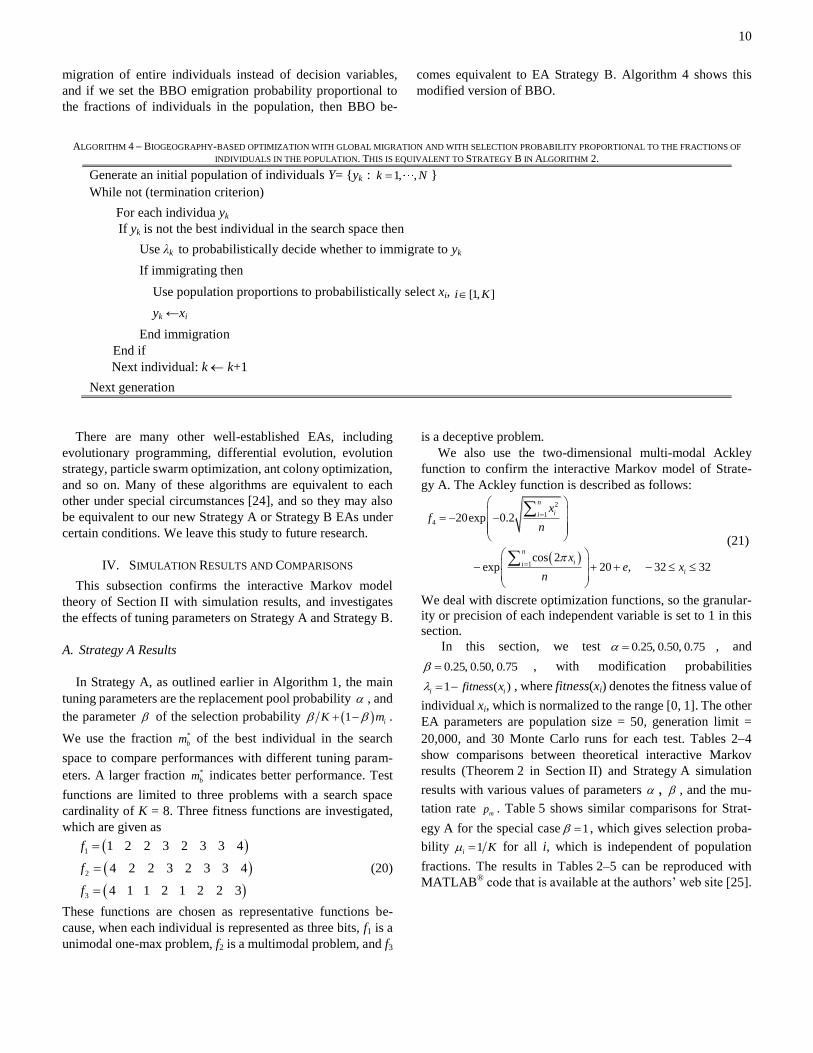
10
migration of entire individuals instead of decision variables,
and if we set the BBO emigration probability proportional to
the fractions of individuals in the population, then BBO be-
comes equivalent to EA Strategy B. Algorithm 4 shows this
modified version of BBO.
ALGORITHM 4 BIOGEOGRAPHY-BASED OPTIMIZATION WITH GLOBAL MIGRATION AND WITH SELECTION PROBABILITY PROPORTIONAL TO THE FRACTIONS OF
INDIVIDUALS IN THE POPULATION. THIS IS EQUIVALENT TO STRATEGY B IN ALGORITHM 2.
Generate an initial population of individuals Y= {yk : 1, ,k N }
While not (termination criterion)
For each individua yk
If yk is not the best individual in the search space then
Use λk to probabilistically decide whether to immigrate to yk
If immigrating then
Use population proportions to probabilistically select xi, [1, ]i K
yk ←xi
End immigration
End if
Next individual: k k+1
Next generation
There are many other well-established EAs, including
evolutionary programming, differential evolution, evolution
strategy, particle swarm optimization, ant colony optimization,
and so on. Many of these algorithms are equivalent to each
other under special circumstances [24], and so they may also
be equivalent to our new Strategy A or Strategy B EAs under
certain conditions. We leave this study to future research.
IV. SIMULATION RESULTS AND COMPARISONS
This subsection confirms the interactive Markov model
theory of Section II with simulation results, and investigates
the effects of tuning parameters on Strategy A and Strategy B.
A. Strategy A Results
In Strategy A, as outlined earlier in Algorithm 1, the main
tuning parameters are the replacement pool probability , and
the parameter of the selection probability 1 iK m .
We use the fraction *
bm of the best individual in the search
space to compare performances with different tuning param-
eters. A larger fraction *
bm indicates better performance. Test
functions are limited to three problems with a search space
cardinality of K = 8. Three fitness functions are investigated,
which are given as
1
2
3
1 2 2 3 2 3 3 4
4 2 2 3 2 3 3 4
4 1 1 2 1 2 2 3
f
f
f
(20)
These functions are chosen as representative functions be-
cause, when each individual is represented as three bits, f1 is a
unimodal one-max problem, f2 is a multimodal problem, and f3
is a deceptive problem.
We also use the two-dimensional multi-modal Ackley
function to confirm the interactive Markov model of Strate-
gy A. The Ackley function is described as follows:
2
14
1
20exp 0.2
cos 2exp 20 , 32 32
n
ii
n
iii
xf
n
xe x
n
(21)
We deal with discrete optimization functions, so the granular-
ity or precision of each independent variable is set to 1 in this
section.
In this section, we test 0.25, 0.50, 0.75 , and
0.25, 0.50, 0.75 , with modification probabilities
1 ( )i ifitness x , where fitness(xi) denotes the fitness value of
individual xi, which is normalized to the range [0, 1]. The other
EA parameters are population size = 50, generation limit =
20,000, and 30 Monte Carlo runs for each test. Tables 24
show comparisons between theoretical interactive Markov
results (Theorem 2 in Section II) and Strategy A simulation
results with various values of parameters , , and the mu-
tation rate m
p . Table 5 shows similar comparisons for Strat-
egy A for the special case 1 , which gives selection proba-
bility 1i K for all i, which is independent of population
fractions. The results in Tables 2–5 can be reproduced with
MATLAB® code that is available at the authors’ web site [25].

11
TABLE 2 STRATEGY A RESULTS FOR TEST PROBLEMS WITH 0.25 AND DIFFERENT MUTATION RATES. THE NUMBERS IN THE TABLE SHOW THE PROPORTION OF
OPTIMAL INDIVIDUALS IN THE POPULATION.
No mutation 0.001mp 0.01mp 0.1mp
Markov Simulation Markov Simulation Markov Simulation Markov Simulation
f1
0.25 0.8155 0.8154 0.8016 0.7956 0.6829 0.6844 0.2232 0.2265
0.50 0.8155 0.8183 0.8086 0.7983 0.7471 0.7354 0.3342 0.3226
0.75 0.8155 0.8126 0.8109 0.7996 0.7694 0.7642 0.4288 0.4209
f2
0.25 0.8412 0.8463 0.8298 0.8249 0.7356 0.7234 0.3736 0.3782
0.50 0.8412 0.8407 0.8356 0.8307 0.7858 0.7795 0.4748 0.4666
0.75 0.8412 0.8445 0.8374 0.8270 0.8038 0.8032 0.5474 0.5424
f3
0.25 0.8645 0.8616 0.8542 0.8450 0.7630 0.7671 0.2727 0.2719
0.50 0.8645 0.8644 0.8593 0.8583 0.8128 0.8036 0.4315 0.4247
0.75 0.8645 0.8643 0.8611 0.8567 0.8298 0.8250 0.5393 0.5267
f4
0.25 0.8109 0.8137 0.8015 0.7961 0.7253 0.7278 0.2076 0.2079
0.50 0.8109 0.8125 0.8031 0.8000 0.7327 0.7270 0.2135 0.2190
0.75 0.8109 0.8131 0.8057 0.8056 0.7586 0.7613 0.3869 0.3856
Ave. CPU time (s) 81.7 83.4 86.2 89.3
TABLE 3 STRATEGY A RESULTS FOR TEST PROBLEMS WITH 0.5 AND DIFFERENT MUTATION RATES. THE NUMBERS IN THE TABLE SHOW THE PROPORTION OF
OPTIMAL INDIVIDUALS IN THE POPULATION.
No mutation 0.001mp 0.01mp 0.1mp
Markov Simulation Markov Simulation Markov Simulation Markov Simulation
f1
0.25 0.5667 0.5696 0.5544 0.5482 0.4598 0.4621 0.2012 0.2043
0.50 0.5667 0.5655 0.5605 0.5489 0.5085 0.4928 0.2622 0.2561
0.75 0.5667 0.5618 0.5626 0.5410 0.5268 0.5181 0.3095 0.3009
f2
0.25 0.6658 0.6651 0.6570 0.6426 0.5872 0.5830 0.3528 0.3535
0.50 0.6658 0.6623 0.6614 0.6562 0.6234 0.6140 0.4198 0.4180
0.75 0.6658 0.6682 0.6628 0.6587 0.6368 0.6282 0.4650 0.4648
f3
0.25 0.6631 0.6611 0.6522 0.6463 0.5623 0.5598 0.2338 0.2334
0.50 0.6631 0.6660 0.6576 0.6430 0.6100 0.6097 0.3231 0.3230
0.75 0.6631 0.6657 0.6595 0.6481 0.6271 0.6231 0.3882 0.3815
f4
0.25 0.7404 0.7387 0.7184 0.7118 0.5341 0.5318 0.0413 0.0428
0.50 0.7404 0.7337 0.7294 0.7204 0.6313 0.6300 0.0956 0.0880
0.75 0.7404 0.7398 0.7331 0.7382 0.6671 0.6599 0.1698 0.1526
Ave. CPU time (s) 82.9 85.1 87.2 91.0

12
TABLE 4 STRATEGY A RESULTS FOR TEST PROBLEMS WITH 0.75 AND DIFFERENT MUTATION RATES. THE NUMBERS IN THE TABLE SHOW THE PROPORTION OF
OPTIMAL INDIVIDUALS IN THE POPULATION.
No mutation 0.001mp 0.01mp 0.1mp
Markov Simulation Markov Simulation Markov Simulation Markov Simulation
f1
0.25 0.3615 0.3695 0.3559 0.3452 0.3142 0.3129 0.1868 0.1883
0.50 0.3615 0.3618 0.3587 0.3497 0.3354 0.3317 0.2232 0.2220
0.75 0.3615 0.3610 0.3596 0.3593 0.3435 0.3425 0.2473 0.2518
f2
0.25 0.5276 0.5260 0.5224 0.5158 0.4828 0.4850 0.3374 0.3337
0.50 0.5276 0.5252 0.5224 0.5219 0.5034 0.5045 0.3834 0.3852
0.75 0.5276 0.5289 0.5260 0.5194 0.5110 0.5094 0.4116 0.4122
f3
0.25 0.4394 0.4396 0.4326 0.4321 0.3809 0.3814 0.2095 0.2099
0.50 0.4394 0.4398 0.4360 0.4375 0.4075 0.4076 0.2599 0.2609
0.75 0.4394 0.4389 0.4371 0.4370 0.4175 0.4100 0.2928 0.2959
f4
0.25 0.3521 0.3566 0.3274 0.3204 0.1805 0.1834 0.0356 0.0362
0.50 0.3521 0.3585 0.3395 0.3311 0.2463 0.2411 0.0547 0.0556
0.75 0.3521 0.3539 0.3436 0.3406 0.2764 0.2805 0.0730 0.0711
Ave. CPU time (s) 88.6 90.4 93.5 97.6
TABLE 5 STRATEGY A RESULTS FOR TEST PROBLEMS WITH 1 AND DIFFERENT MUTATION RATES. THE NUMBERS IN THE TABLE SHOW THE PROPORTION OF
OPTIMAL INDIVIDUALS IN THE POPULATION.
No mutation 0.001mp 0.01mp 0.1mp
Markov Simulation Markov Simulation Markov Simulation Markov Simulation
f1
0.25 0.2667 0.2654 0.2644 0.2675 0.2469 0.2475 0.1767 0.1797
0.50 0.2667 0.2665 0.2655 0.2667 0.2560 0.2572 0.2004 0.1988
0.75 0.2667 0.2665 0.2659 0.2691 0.2594 0.2604 0.2142 0.2161
f2
0.25 0.4444 0.4445 0.4416 0.4475 0.4198 0.4225 0.3258 0.3279
0.50 0.4444 0.4453 0.4430 0.4462 0.4312 0.4305 0.3586 0.3574
0.75 0.4444 0.4453 0.4436 0.4406 0.4354 0.4387 0.3772 0.3767
f3
0.25 0.3077 0.3066 0.3049 0.3037 0.2833 0.2823 0.1935 0.1938
0.50 0.3077 0.3067 0.3063 0.3062 0.2946 0.2896 0.2243 0.2232
0.75 0.3077 0.3076 0.3068 0.3081 0.2987 0.3011 0.2420 0.2436
f4
0.25 0.0842 0.0815 0.0818 0.0812 0.0662 0.0672 0.0307 0.0323
0.50 0.0842 0.0840 0.0829 0.0818 0.0737 0.0711 0.0398 0.0400
0.75 0.0842 0.0828 0.0833 0.0865 0.0768 0.0780 0.0461 0.0471
Ave. CPU time (s) 71.2 73.3 75.9 78.4
Several things are notable about Tables 25. First, we note
that the parent selection probability does not affect the
proportion of individuals in the population in the case of no
mutation. This is because divides out of the * * *m P m m
equilibrium equation in this case. The finding is consistent with
[20, p. 162]. However, we see that can slightly affect the
proportion of individuals in the case of nonzero mutation.
Second, for a given parent selection probability and a
given parameter , the proportion of optimal individuals de-
creases with the mutation rate mp . This indicates that low
mutation rates have better performance for the test problems
that we study. A high mutation rate of 0.1 results in too much
exploration, and the population remains too widely distributed
across the search space.
Third, for a given parent selection probability and a given
mutation rate mp , the proportion of optimal individuals de-
creases with increasing . This is because the modification
probability i tends to result in a population in which good
individuals dominate, and increasing causes individuals
with high populations to be more likely to replace other indi-
viduals.
Fourth, Tables 25 show that the interactive Markov model
results and the simulation results match well for all test prob-
lems, which confirms the interactive Markov model theory.
Fifth, the average CPU times in the last rows of Tables 25
show the simulation times of Strategy A for the four test
problems. Strategy A runs faster with smaller mutation rates.
The reason is that larger mutation rates require more mutation
operations, which slightly increases computation time. How-
ever, in more realistic and interesting real-world problems,
computational effort it dominated by fitness function evalua-
tion, which is independent of the mutation rate.

13
B. Strategy B Results
In this section we investigate the effect of selection pressure
, which influences the selection probability im of xi in
Strategy B, as shown in (7). In this section we test only the
unimodal one-max problem f1 (recall that Theorem 3 assumes
that the optimization problem is unimodal). Recall that EA
selection pressure is constrained to the domain 1, 2 [3, p.
34]. In this section, we test 1.25,1.50,1.75 in (7) to compute
parameters , of the population-proportion-based selection
probability, and we test elitism probabilities
1 0.25, 0.50, 0.75 . The other parameters of the EA are the
same as those described above in the previous subsection. Ta-
ble 6 shows comparisons between interactive Markov theory
results and Strategy B simulation results. The results in Table 6
can be reproduced with MATLAB® code that is available at the
authors’ web site [25].
TABLE 6 STRATEGY B RESULTS FOR TEST PROBLEM F1. THE NUMBERS IN THE TABLE SHOW THE PROPORTION OF OPTIMAL INDIVIDUALS IN THE POPULATION.
No mutation 0.001mp 0.01mp 0.1mp
Markov Simulation Markov Simulation Markov Simulation Markov Simulation
1.25 1 0.25 0.3139 0.3164 0.3131 0.3134 0.3060 0.3081 0.2529 0.2526
1 0.50 0.3372 0.3354 0.3363 0.3329 0.3287 0.3295 0.2711 0.2736
1 0.75 0.3582 0.3559 0.3573 0.3561 0.3493 0.3467 0.2880 0.2925
1.50 1 0.25 0.4022 0.4056 0.4009 0.4019 0.3897 0.3926 0.3068 0.3063
1 0.50 0.4514 0.4517 0.4500 0.4479 0.4384 0.4431 0.3494 0.3451
1 0.75 0.4901 0.4938 0.4887 0.4929 0.4770 0.4780 0.3848 0.3842
1.75 1 0.25 0.5955 0.5914 0.5933 0.5950 0.5740 0.5749 0.4271 0.4262
1 0.50 0.6511 0.6522 0.6492 0.6452 0.6320 0.6323 0.4944 0.4922
1 0.75 0.6893 0.6869 0.6875 0.6864 0.6719 0.6687 0.5423 0.5393
Ave. CPU time (s) 72.4 75.3 79.1 85.2
We note several things from Table 6. First, for a given value
of elitism probability 1 and mutation rate
mp , performance
improves as selection pressure increases. This is expected
because a larger value of exploits more information from
the population. For a more complicated problem with a larger
search space, we might arrive at different conclusions about
the effect of on performance.
Second, for a given value of selection pressure and mu-
tation rate mp , performance improves as elitism probability
1 increases. Again, this is expected for simple problems such
as the test problem studied in this section, but the conclusion
may not hold for more complicated problems.
Third, for a given value of elitism probability 1 and se-
lection pressure , performance improves as mutation rate
mp decreases. This again indicates that low mutation rates
give better performance for the test problems that we study. A
high mutation rate of 0.1 results in too much exploration, and
the population remains too widely distributed across the search
space.
Fourth, we see that the interactive Markov model theory and
the simulation results match well, which confirms the interac-
tive Markov model theory.
Fifth, we see that Strategy B runs faster with smaller muta-
tion rates (the same observation we made for Strategy A in
Tables 25). The reason is that larger mutation rates result in
more mutation operations, which slightly increases computa-
tion time.
V. CONCLUSION
This paper first presented a formal interactive Markov
model, which involves separate but interacting Markov mod-
els for each individual in an EA population. This is a new
model for studying EAs. Then we proposed two simple EAs
whose basic features are population-proportion-based selec-
tion and modified mutation, and analyzed them exactly with
interactive Markov models. The theoretical results were con-
firmed with simulation results, and showed how the interactive
Markov model can describe the convergence of the EAs. The
theoretical and simulation results in Tables 26 can be re-
produced with MATLAB® code that is available at the au-
thors’ web site [25].
The use of interactive Markov models to model evolution-
ary algorithms can lead to useful conclusions. Interactive
Markov models prove to be tractable for much larger search
spaces and populations than noninteractive Markov models.
The noninteractive (standard) Markov model has a state space
whose dimension grows factorially with search space cardi-
nality and population size, while the interactive Markov model
has a state space whose dimension grows linearly with the
cardinality of the search space, and is independent of popula-
tion size. Like the noninteractive Markov model, the interac-
tive Markov model provides exact models for the behavior of
the EA. Interactive Markov models can be studied as functions
of EA tuning parameters to predict their impact on EA per-
formance, and to provide real-time adaptation. Just as
noninteractive Markov models have led to the development of
dynamic system models, the same can happen with interactive

14
Markov models. Although the interactive Markov models in
this paper explicitly provide only steady-state probabilities,
they might also be used to understand transient EA behavior,
and to obtain the probability of optimum-hitting each genera-
tion, and to obtain expected hitting times. We see some re-
search in this direction for noninteractive Markov models [27],
[28]; such results are impractical for real-world problems due
to the large transition matrices of noninteractive Markov
models, but such a limitation will not be as great a concern for
interactive Markov models.
For future work beyond the suggestions listed above, we
see several important directions. First, the interactive Markov
model analysis of this paper was based on two simple EAs;
future work should explore how to apply the model to other
EAs. Second, we only used two examples from the earlier
literature to derive new EAs, but we could use other previ-
ously-published examples to construct additional EA para-
digms that use population-proportion-based selection. Third,
population-proportion-based selection is a new selection
strategy that does not require fitness calculations (possible
computational cost savings), and future work could develop an
entire family of modified EAs based on this selection strategy.
Fourth, we suggest for future work the combination of es-
timation of distribution algorithms (EDAs) with our new-
ly-proposed population-proportion-based selection operator.
Recall that EDAs use fitness values to approximate the dis-
tribution of an EA population’s fitness values. In contrast, our
population-proportion-based selection uses population sizes
rather than fitness values for selection. However, EDA ideas
could be incorporated in population-proportion-based selec-
tion by approximating the probability distribution of the pop-
ulation sizes, and then performing selection on the basis of
approximate distribution. This idea would merge the ad-
vantages of EDAs with the advantages of popula-
tion-proportion-based selection.
Finally, we note that methods will need to be developed to
handle problems with realistic sizes. The interactive Markov
model presented here enables tractability for problems of
reasonable size, which is a significant advantage over the
standard noninteractive Markov models published before now.
However, the interactive Markov model is still the same size
as the search space, which can be quite large. For realistic
problem sizes, say with a search space on the order of trillions,
the interactive Markov model will also be on the order of
trillions. Methods will need to be developed to reduce the
interactive Markov model to a tractable size.
APPENDIX
A. Here we derive the interactive Markov model of strategy A with mutation shown in (11). The selection transition matrix
sP of
Strategy A in (8) can be written as
1 1 1 2 1 1
1 2 2 2 2 2
1 2
1 1 1 1 1
1 1 1 1 1
1 1 1 1 1
K
K
S i j
K K K K K
K m K m K m
K m K m K mP p
K m K m K m
(A.1)
Transition matrix MP of the modified mutation in (10) can be written as
1
1
1
m m m m
m m m m
M ki
m m m m
p p K p K p K
p K p p K p KP p
p K p K p p K
(A.2)
where mp is the mutation rate. So the transition matrix of Strategy A with mutation can be computed by A kj M S ki ij
i
P p P P p p :
1 1 1 2 1 1
1 2 2 2 2 2
1 2
1
1
1
1 1 1 1 1
1 1 1 1 1
1 1 1
m m m m
m m m m
A kj
m m m m
K
K
K K
p p K p K p K
p K p p K p KP p
p K p K p p K
K m K m K m
K m K m K m
K m K m
1 1K K KK m
(A.3)
Element 111,1AP p in (A.3) is obtained as follows.

15
1 1 1 1 2 1
1 1 1 1 1
1 2 3
1 1
1,1 1 1 1 1 1 1
1 1 1 1 1 1
1
1 1(1 ) 1 1
A m m m m K
m m m m m
m K
m
P p p K K m p K K m p K K m
p p K K K p K K p p K m
p K m m m
K p K
K K
1 1 1 1 1
1 1 12
1(1 ) 1 1 1
1 1 1 1(1 ) 1 (1 ) 1 (1 ) 1 1 1
m m m
m m m m mm
p K p pm m
K K K K
K p K p K p K p pp m
K K K K K K
(A.4)
Element 121, 2AP p in (A.3) is obtained as follows.
2 1 2 2 2 2
2 2 1 2 2
2 2 2 2 2
2
1, 2 1 1 1 1 1 1
1 1 1 1 1
1 1
1 1 1
A m m m m K
m m m m m
m m m m K
m m m
P p p K K m p K K m p K K m
p p K K p p K m p K K
p K K p K m p K K p K m
p p K K p K
2 2 2
2 1 2 2
2 2 2 2
2 1 2 1
2 2
2
1 1 1
1 2( ) 1 1
1(1 ) 1 1 1
1 11 1 (1 )
m
m m m K
m mm
m m
mm m
K K p K K
p p K m p K m m
K p K pp
K K K K K K
K p pm m
K K
K p K pp p
K K K K
12
1 1 1m mm
pp m
K K
(A.5)
We follow the same process to obtain
2
2
1 1 1 1(1 ) 1 (1 ) 1 (1 ) 1 1 1 if
1 11 1 (1 ) 1 1 1 if
m m m m mj j m j
kj
m mm m mj j m k
K p K p K p K p pp m k j
K K K K K Kp
K p K pp p pp m k j
K K K K K K
(A.6)
which is equivalent to (11), as desired.
B. Here we derive the interactive Markov model of strategy B with mutation as shown in (18). The selection transition matrix sP of
Strategy B in (16) can be written as
1 1 1 1 1 2 1 1 1 1 1
1 1 2 2 2 1 2 1 2
1 1 2 1 1
1 1 1 1
1 1 1 1
1 1 1 1
K
K
S i j
K K K K K
n n n
n n nP p
n n n
(B.1)
Transition matrix MP of the modified mutation operator (10) can be written as
1
1
1
m m m m
m m m m
M ki
m m m m
p p K p K p K
p K p p K p KP p
p K p K p p K
(B.2)
So the transition matrix of Strategy B with mutation can be computed as B kj M S ki ij
i
P p P P p p :
1 1 1 1 1 2 1 1 1 1 1
1 1 2 2 2 1 2 1 2
1 1 2 1
1
1
1
1 1 1 1
1 1 1 1
1 1 1
m m m m
m m m m
B kj
m m m m
K
K
K K K
p P K p K p K
p K p p K p KP p
p K p K p p K
n n n
n n n
n n
11K Kn
(B.3)
Element 111,1BP p in (B.3) is obtained as follows.

16
1 1 1 1 1 1 1 2 1 1
1 1 1 1 1 1 1
1 1 2 3
1 1 1 1 1
1,1 1 1 1 1 1
1 1 1 1 1
1
1 1 1 1 1
B m m m m K
m m m m m
m K
m m m m m
P p p K n p K n p K n
p p K K p K p p K n
p K n n n
p p K K p K p p K
1 1
1 1 1 1
1 1 1 1 1
1 1
1 1 1
m
m m
n
p K K n
p K p n
(B.4)
Element 121, 2BP p in (B.3) is obtained as follows.
2 1 1 1 2 2 1 2 2 1
2 2 1 1 1 2 1 2 3
2 2
2 2 1 1 1 2 2
1, 2 1 1 1 1 1
1 1 1 1
1 1
1 1 1 1 1
B m m m m K
m m m m m K
m m
m m m m m m
P p p K n p K n p K n
p p K p p K n p K n n n
p K K p K
p p K p p K n p K K p K
2 1 1 1
2 1 1 1
1 1
1 1
m
m m
p K K n
p K p n
(B.5)
Element 222, 2BP p in (B.3) is obtained as follows.
2 1 1 1 2 2 1 2 2 1
2 1 2 2 2 2 1 2
2 1 1 3
2 1 2 2
2, 2 1 1 1 1 1
1 1 1 1 1 1
1
1 1 1
B m m m m K
m m m m m m m m
m K
m m m m m
P p K n p p K n p K n
p K p p K p p K K p K p p K n
p K n n n
p K p p K p p K K
2 2 1 2
2 1 1 2
2 2 1 2
1 1 1
1 1
1 1 1
m m m
m
m m
p K p p K n
p K K n
p K p n
(B.6)
Element 212,1BP p in (B.3) is obtained as follows.
1 1 1 1 1 1 1 2 1 1
1 1 1 1 1 1 1 2
1 1 1 3
1 1 1 1 1
2,1 1 1 1 1 1
1 1 1 1 1
1
1 1 1 1
B m m m m K
m m m m m m m
m K
m m m m m m m
P p K n p p K n p K n
p K K p K p K p p K p p K n
p K n n n
p K K p K p K p p K p p K
1 1 2
1 1 1 2
1 1 2
1
1 1
1 1
m
m m
n
p K K n
p K p n
(B.7)
We can follow the same process to obtain
1 1 1 1
1 1 1
1
1
11 1 1 if 1, which is the best state
1 1 if 1 and
1 1 1 if
1 1 if ,
1
a 1n
1
d
m m
m m j
kj
m m j j k
m m j k
p K p n k j
p K p n k jP
p K p n k j
p K p n k j k
(B.8)
Which is equivalent to (18), as desired.
C. Here we derive Theorem 2. Before proceeding with the
proof, we establish the preliminary foundation. Time indices
and function arguments will usually be suppressed to simplify
notation: , ,i i ij ijm m t m m t p p m . The notation
im m is defined by 1m m t m t . The symbol u
indicates the ,1K vector of ones 1, ,1u . The ith
equation of the interactive Markov model (1) will often be
written in the form
1i ij j i ij j ii i
j j i
ij j ji i ij j ji i
j i j i j i
m p m m p m p m
p m p m p m p m
(C.1)
where j means the sum over all j from 1 to K ; and
j i means the sum over all j from 1 to K except j i .
Next, we formally prove Theorem 2. It follows from the
definition of 0A and (2) that
0 0P m A mb and 0 0b u I A (C.2)

17
Namely, 0 j j kjkb b b a
because all the rows of B are
the same. Thus the Markov chain can be written as
0 0 0 0
0 0 0 0
1
1
m t A mb m A b m I m
A u I A m I m A u A m I m
(C.3)
To find the equilibrium *m , set *1m t m m in this equa-
tion and rearrange terms to get
* * *
0 0A m u A m m (C.4)
Thus, an equilibrium * 0m for the Markov chain exists if and
only if (C.3) has a solution *m such that * 0m with * 1kk
m .
Since 0A is indecomposable by the equations of the inter-
active Markov model of strategy A, it has a real positive
dominant eigenvalue and a corresponding positive eigenvec-
tor. We call the root and the eigenvector z (normalized so
that its elements sum to one). Then we obtain:
0 0 0 0, ,A z z u A z A z u A z z (C.5)
The first equation is true by the definitions of and z ; the
second equation follows from the first on pre-multiplying by
u ; and the third follows from the first two. However, com-
parison of (C.4) to the third equation of (C.5) shows that *m z is a solution to (C.4). Thus, we have an equilibrium *m z which is a positive dominant eigenvector of
0A with
eigenvalue
* * * * *
0 0 0 0 01 1 1u A z u A m u m u A m u I A m b m
(C.6)
Furthermore, *m z is a unique solution to (C.4) since a
nonnegative indecomposable matrix cannot have two
nonnegative and linearly independent eigenvectors. This
completes the proof of Theorem 2.
REFERENCES
[1] C. Ahn, Advances in Evolutionary Algorithms: Theory, Design and
Practice. New York: Springer Publishing, 2006.
[2] D. H. Wolpert, and W. G. Macready, “No free lunch theorems for optimization”, IEEE Transactions on Evolutionary Computation, vol. 1,
no. 1, pp. 67–82, 1997.
[3] C. Reeves, and J. Rowe, Genetic Algorithms: Principles and Perspec-tives, Norwell, Massachusetts: Kluwer Academic Publisher, 2003, pp.
173–200.
[4] X. Yao, Y. Liu, and G. Lin, “Evolutionary programming made faster”, IEEE Transactions on Evolutionary Computation, vol. 3, no. 2, pp.
82–102, 1999.
[5] S. Das and P. N. Suganthan, “Differential evolution – A survey of the
state-of-the-art”, IEEE Transactions on Evolutionary Computation. vol.
15, no. 1, pp. 4–31, Feb. 2011.
[6] R. Storn and K. V. Price, “Differential Evolution – a simple and effi-cient heuristic for global optimization over continuous spaces”, Journal
of Global Optimization, vol. 11, no. 4, pp. 341–359, Dec. 1997.
[7] H. G. Beyer, “Toward a theory of evolution strategies: the (μ, λ)-theory”, Evolutionary Computation, vol. 2, no. 4, pp. 381–407, Winter, 1994.
[8] D. Bratton and J. Kennedy, “Defining a standard for particle swarm
optimization”, in Proceedings of IEEE Swarm Intelligence Symposium, Honolulu, Hawaii, pp. 120–127, 2007.
[9] J. Kennedy, and R. Eberhart, “Particle swarm optimization”, in Pro-
ceedings of IEEE International Conference on Neural Networks, Perth, WA, pp. 1942–1948. 1995.
[10] H. Ma, “An analysis of the equilibrium of migration models for bio-
geography-based optimization”, Information Sciences, vol. 180, no. 18, pp. 3444–3464, 2010.
[11] D. Simon, “Biogeography-based Optimization”, IEEE Transactions on
Evolutionary Computation, vol. 12, no. 6, pp. 702–713, 2008. [12] D. Simon, Evolutionary Optimization Algorithms, John Wiley & Sons,
2013.
[13] A. Nix, and M. Vose, “Modeling genetic algorithms with Markov chains”, Annals of Mathematics and Artificial Intelligence, vol. 5, no. 1,
pp. 79–88, 1992.
[14] D. Simon, M. Ergezer, D. Du, and R. Rarick, “Markov models for biogeography-based optimization”, IEEE Transactions on Systems,
Man, and Cybernetics - Part B: Cybernetics, vol. 41, no. 1, pp. 299–306,
2011. [15] D. Simon, “A dynamic system model of biogeography-based optimi-
zation”, Applied Soft Computing, vol. 11, pp. 5652–5661, 2011.
[16] J. Suzuki, “A Markov chain analysis on simple genetic algorithms”, IEEE Transactions on Systems, Man, and Cybernetics, Part B: Cyber-
netics, vol. 25, no. 4, pp. 655–659, 1995.
[17] P. J. Van Laarhoven, E. H. Aarts, Simulated Annealing: Theory and Applications, New York: Springer Publishing, 1987.
[18] M. D. Vose, The Simple Genetic Algorithm: Foundations and Theory. The MIT Press, 1999.
[19] W. M Spears, Evolutionary Algorithms: The Role of Mutation and
Recombination, New York: Springer Publishing, 2000. [20] J. Conlisk, “Interactive Markov chains”, Journal of Mathematical Soci-
ology, vol.4, pp. 157-185, 1976.
[21] Y. Gerchak, “On interactive chains with finite population”, Journal of Mathematical Sociology, vol. 9, pp. 255-258, 1983.
[22] D. Simon, R. Rarick, M. Ergezer, and D. Du, “Analytical and numerical
comparisons of biogeography-based optimization and genetic algo-rithms”, Information Sciences, vol. 181, no. 7, pp. 1224–1248, 2011.
[23] J. Dieterich and B. Hartke, “Empirical review of standard benchmark
functions using evolutionary global optimization”, http://arxiv.org/abs/1207.4318.
[24] H. Ma, D. Simon, M. Fei, and Z. Chen, “On the Equivalences and
Differences of Evolutionary Algorithms”, Engineering Applications of Artificial Intelligence, vol. 26, no. 10, pp. 2397-2407, 2013.
[25] H. Ma, D. Simon, M. Fei, and H. Mo, “Interactive Markov Models of
Evolutionary Algorithms (web site)”, http://academic.csuohio.edu/simond/InteractiveMarkov, November
2013.
[26] J. He, and X. Yao, “Towards an analytic framework for analysing the computation time of evolutionary algorithms”, Artificial Intelligence,
vol. 145, pp. 59–97, 2003.
[27] K. De Jong, W. Spears, and D. Gordon, “Using Markov chains to ana-lyze GAFOs,” Foundations of Genetic Algorithms, vol. 3 (L. Whitley
and M. Vose, editors), Morgan Kaufmann, pp. 115-138, 1995. [28] J. He, F. He, and X. Yao, “A unified Markov chain approach to ana-
lysing randomized search heuristics,” arXiv:1312.2368 , 2013.
Haiping Ma received the M.Sc. degree in Control Engineering from Taiyuan University of Technology. He is a Ph.D. candidate with the Shanghai Key La-boratory of Power Station Automation Technology, School of Mechatronic Engineering and Automation, Shanghai University. His main research interests include evolutionary computation, in-
formation fusion, intelligent control and signal processing. He has published 15 papers on evolutionary algorithms.

18
Dan Simon received his B.S. from
Arizona State University, his M.S. from
the University of Washington, and his
Ph.D. from Syracuse University, all in
electrical engineering. Before joining
academia, he had 14 years of experience
in various engineering industries, in-
cluding aerospace, automotive, bio-
medical, process control, and software
engineering. He continues his relationship with industry by
teaching short curses and through regular consulting. He
joined Cleveland State University in 1999 and has been a Full
Professor in the Electrical and Computer Engineering De-
partment since 2008. His teaching and research interests in-
clude control theory, computer intelligence, and embedded
systems. He is an associate editor for the journals Aerospace
Science and Technology, Mathematical Problems in Engi-
neering, and International Journal of Swarm Intelligence. His
research has been funded by the NASA Glenn Research Cen-
ter, the Cleveland Clinic, the National Science Foundation,
and several industrial organizations. He has written over 100
refereed publications, and is the author of the textbooks Op-
timal State Estimation (John Wiley & Sons, 2006) and Evo-
lutionary Optimization Algorithms (John Wiley & Sons,
2013).
Hongwei Mo received his BS and PhD
degrees from Automation College of
Harbin Engineering University. He is
presently a professor of Automation
College of Harbin Engineering Univer-
sity. He was a visiting Scholar of UC
Davis (California, USA) from 2003-2004.
His main research interests include nat-
ural computing, artificial immune sys-
tems, data mining, intelligent systems, and artificial intelli-
gence. He has published 30 papers and two books on AIS. He
is a director at the Biomedicine Engineering Academy of
Heilongjiang Province, commissioner of the China Neural
Network Committee, and a senior member of the Computer
Academy of China. He is secretary-general chairman and
associate chairman of the organizing committee of the 16th
China Neural Network Conference and 1st Conference of
Special Topic on Artificial Immune Systems, a member of the
program committee of the 2nd International Conference on
Natural Computing, Fuzzy Systems, and Knowledge Discov-
ery (ICNC-FSKD2006), 1st International Conference on
Rough Sets and Knowledge Discovery, 6th International
Conference on Simulation Learning and Evolution, 13th IEEE
International Conference on Mechanics and Automa-
tion(ICMA2007), Biology Inspired Computing 2008, and
numerous other conferences. He served as a member of the
editorial board for the International Journal on Information
Technology Research.
Related Documents