Interactive Educational Models - for Structural Dynamics - CORE

Interactive Educational Modelsfor Structural Dynamics

by

Gilberto Mosqueda

B.S., Civil and Environmental EngineeringUniversity of California at Irvine, 1996

Submitted to the Department of Civil and Environmental Engineeringin Partial Fulfillment of the Requirements for the Degree ofMaster of Science in Civil and Environmental Engineering

at the

Massachusetts Institute of Technology

June 1998

© 1998 Massachusetts Institute of TechnologyAll rights reserved

Signature of Author ............................... .......... ... ...................Department of Civil and Environmental Engineering

May 8, 1998

Certified by .....................................Eduardo Kausel

Professor of Civil and Environmental EngineeringThesis Supervisor

Accepted by ....................Joseph M. Sussman

Chairman, Departmental Committee on Graduate Studies

JUN 021998lng~Rs

Interactive Educational Modelsfor Structural Dynamics

by

Gilberto Mosqueda

Submitted to the Department of Civil and Environmental Engineeringon May 8, 1998 in Partial Fulfillment of the

Requirements for the Degree ofMasters of Science in Civil and Environmental Engineering.

ABSTRACT

An interactive program developed for the MATLAB environment is presented to assiststudents in learning structural dynamics. The program is intended to supplement lecturesand textbooks by providing a tool for students to observe the effect of parameters ondynamic systems. The functions of the program include plotting the response of a singledegree of freedom system subjected to a variety of dynamics loads. The forcing functionscan be applied directly on the mass or as support motion. In addition other insightful plotscan easily be accessed through the program interface, such as the transfer function andFourier Transform of the excitation force. The graphical interface is designed to beintuitive and emphasizes simplicity in using the program, obtaining plots and moreimportantly, comparing results.

In analyzing the response of structures due to support excitation, the programmakes use of a unique relationship that exists between the support motion and responsetype. A formulation is derived for the support impulse response function that, whenconvolved with the excitation, results in function that relates the input type to the outputtype. Inputting displacement results in the displacement response while an inputacceleration record will produce the acceleration response.

Thesis Supervisor: Eduardo KauselTitle: Professor of Civil and Environmental Engineering

_L~~ __~ _~~ _~___X__ll__1__1_11 _I__LLXI-I X.~- ~ll~.

Acknowledgements

I would like to thank Professor Eduardo Kausel for giving me the opportunity to work on thisproject and guiding me from start to finish. His insights where key to the success of this report

This work would not have been possible without the contribution of NSF. This project was fundedby the Mid-America Earthquake Center for the purpose of innovation in undergraduate teachingmethods.

I would also like to thank Olga, whose visits gave me something to look forward too and for hersupport in achieving my educational goals. Though school separated us for some time, thecompensation will come when we're back together again.

To my brother Eddie who accompanied me during my first year in Boston. I'm also in debt to himfor his consulting on the pedagogy of technology and providing valuable input into this report.

El apoyo y el cariflo de mi familia durante mis afios de estudio, han echo todo esto possible. Poreso, le quiero dar las gracias a mis padres, Pedro y Alicia, y a mi hermana Patricia por simpreayudarme en todas las maneras possibles. A mis hermanitos, Pedro Jr. y Jose, que algun dia llegena cumplir mas que yo, se que si pueden.

Graduate school was not even on option until Professor Villaverde gave me the opportunity to getinvolved in research at UCI and develop an interest in academia.

I would not have been able to survive in Boston without certain individuals who gave me somememorable times here. For this I would like to thank Jose y Lorena for getting me out of MITevery now and then and especially for proofreading this report; My roommates Carlos and Hector,we got to do Puerto Rico again; Abel for his advice on computers when they where driving mecrazy; My classmates: Casey, Emma, Kathy, Mia, Patricia, David, Gerry, Larry, Mark, andSalvatore.

En memoria de mi Abuelita, Soledad Cruz.

_~YI~~_ ~ ____1 n1~___(_1__4___I _~~r____~_i_~l

TABLE OF CONTENTS

LIST OF FIGURES ........................................................................................................... 10

LIST OF TABLES ................................................................................................... 11

CH APTER 1 ................................................................................... ............................... 13

INTRODUCTION

CHAPTER 2 ......................................................................................................... 17

USING TECHNOLOGY TO ENHANCE EDUCATION

2.1 LEARNING ENVIRONMENT ....................................... ....... .. ................. 19

2.2 INTERFACE D ESIGN ............................................. ..................................................... 22

2.3 EDUCATIONAL SOFTW ARE ........................................... ................................................. 24

CH APTER 3 .................................................................................... .............................. 27

MATLAB IN EDUCATION

3.1 CREATING EDUCATIONAL MODELS ....................................... .................... 28

3.2 DISTRIBUTING MATLAB SOFTWARE........................................ 29

CHAPTER 4 ........................................................................................................ 31

SDOF SYSTEM

4.1 EQUATIONS OF M OTION ........................................... ..................................................... 31

4.2 FREE V IBRATION .. .............................................................................................. 33

4.3 FORCE ON M ASS .................................................. 34

4.3.1 Harmonic Loading......................................... .................... 34

4.3.2 Random Loading............................................................ 35

4.3.2.1 State-Space Solution............................................... ............. 35

_1 - -11111~114~ _~~Y- ~II~---L YY-I-~ ~- -I^XX-~LI~-I~-~ ^----111~-111 41dll 1 -r~ -I-- --- --- __.----... 1~. I~_l~l~p ~ ̂- --~----*-~~Llltl(l_ --l~.i

4.4 SUPPORT M OTION ............................................................................... ......................... 37

4.4.1 Harmonic Excitation ......................................................................... 38

4.4.2 Random Excitation.......................................................................................................... 38

4.4.2.1 C onvolution ........................................ ................. ......... 39

4.4.2.2 Input-Output relation for support motion ......................................... 41

4.5 PERIODIC LOADING- INITIAL CONDITIONS ........................................ 44

4.5.1 F orce O n M ass.............................................................................................. .................. 44

4 .5.2 S up p ort M o tion ........................................................................................................................ 4 6

4.6 FOURIER TRANSFORM ........................................ 46

CHAPTER 5 ................................................................................... ............................... 47

PROGRAM DESCRIPTION

5.1 INPUT OPTIONS ................... .................................................. 48

5.1.1 System Properties..................................................... 51

5.1.2 Initial Conditions ............................................................... 51

5.1.3 Display Parameters......................................................................................................... 52

5.2 FORCING FUNCTION ........................................ 53

5. 2.1 Free Vibration........................................ . ........................................ 54

5 .2 .2 S in uso id a l................................................................................................................................. 5 5

5.2.3 Point Data.................................................................... 56

5.2.4 File ..................................................... .................. 58

5.2.5 Transient/Periodic Loading .............................................................................. ................. 60

5.3 OUTPUT OPTIONS ............................................................ 61

5.3.1 Displacement Response.............................. ............. ................. 61

5.3.2 Plot Options Menu ...................................................................... 61

5.3.2.1 Forcing Function ............................................................. 62

5.3.2.2 Transfer Function and Phase Angle................................... .......................... 63

5.3.2.3 L oad Fourier Transform ........................................................................................ ................... 64

5.3.2.4 R esponse Fourier T ransform .............................................................................................................. 65

5.4 PROGRAM STRUCTURE ........................................ ................................. 66

8

CHAPTER 6 ................................................................................... ............................... 69

APPLYING THE SOFTWARE

6.1 PROGRAM GOALS .......................................................................... ............................... 70

6.2 EXAMPLES OF USE ....................... ...... ................ .. ............... .............................. 72

6.3 PROBLEM SET ................................................... 73

6.3.1 Free Vibration.............................................. ...................................... 74

6.3.2 Harmonic Excitation ................................................................................................................ 75

6. 3.3 Earthquake Engineering ........................ ................................................... 78

6.4 REMARKS ............................................................................................................................ 82

CHAPTER 7 .................................................................................... .............................. 83

CONCLUSION

BIBLIO GRAPH Y ............................................................................................................ 85

APENDIX............................................................................................................................87

~IU__IYr~____ll__^~l_11-~~e~ll-.1l~rr 1~-nl*1~1 ~- L-i-------i.j

LIST OF FIGURES

Figure 1. Cart model for single degree of freedom system ........................................ 32

Figure 2. Free body diagram for force on mass. ............................................. 32

Figure 3. Free body diagram for support motion ........................................ ..... 33

Figure 4. Screen snapshot of main window. ................................................. 49

Figure 5. System properties input options. ................................................. 51

Figure 6. Initial Conditions input options. .................................... ............ 52

Figure 7. Display Parameters input options ........................................... ....... 53

Figure 8. Sinusoidal Loading Options .................................................... 55

Figure 9. Force Time History produced from settings in Figure 8. ................................. 56

Figure 10. Point Data input options ..................................... ...... .................. 57

Figure 11. Excitation created from input in Figure 10 ..................................................... 57

Figure 12. File selection input options ..................................... .............. 59

Figure 13. Forcing function created with data. in input file ................................................ 59

Figure 14. Periodic loading with period of 2 seconds ....................................... .... 60

Figure 15. Excitation Plot corresponding to response in Figure 4 ................................... 62

Figure 16. Transfer Function and Phase Angle corresponding to Figure 4. .................... 63

Figure 17. FFT of both forcing functions shown if Figure 16 ...................................... 64

Figure 18. FFT of response plots displayed in Figure 4. ..................................... .... 65

Figure 19. Flow chart of SDOF PLOT program (Part 1) ...................................... ... 67

Figure 20. Flow Chart of SDOF PLOT program (Part 2) ...................................... ... 68

Figure 21. Display from Free Vibration problem. ............................................. 74

Figure 22. R esponse for case a ................................................................... ................... 76

Figure 23. Response for case b. .................................................................... ................. 76

Figure 24. R esponse for case c ................................................................... ................... 77

Figure 25. Transfer function for 1% and 5% damping. ..................................... ..... 78

Figure 26. First 20 seconds of the acceleration record for El Centro ............................... 79

Figure 27. FFT of El Centro acceleration record show in Figure 26 .............................. 80

Figure 28. Response to El Centro with 1% and 5% damping ..................................... 81

Figure 29. FFT for Response plots shown in Figure 28.................................. ..... 81

LIST OF TABLES

Table 1. Unit combinations for Free Vibration and Force on Mass...............................50

Table 2. Units' combinations for Support Motion ....................................... ..... 50

L_~-F_----^Y- ~L--L -tIQn*e~L~---L^* ~-~ i~~LII-- *_C-- i-~t~li*illlX

12

CHAPTER 1

INTRODUCTION

The purpose of this project is to develop a tutorial software package to assist in the

teaching of structural dynamics. In dynamics, the complex equations and variable motion

of bodies under dynamic loads make it difficult for many students to visualize the

problems they are challenged with. Although it is the conceptual understanding of theories

and equations that are essential for problem solving, a firm visual representation could

simplify the learning process for students that may experience difficulties. This program

aims to overcome some of the limits of traditional teaching tools by making use of modern

technology to incorporate interactive figures into the structural dynamics curriculum.

Since the phenomenon under study is time dependent, teaching and learning in

dynamics has great potential for improvement with the use of visual tools provided by

computer graphics. Computers offer the ability to create animations and interactive

figures, which are not possible with current teaching tools such as textbooks and

chalkboards. The advantage of using computer graphics is that they are able to represent

the dynamic phenomena adequately and allow the user to experiment with the effect of

parameters (Chabay and Sherwood, 1992).

Y

These new educational technologies are not intended to replace existing teaching

methods, but rather to increase the availability of options for instructors to present material

to students (Bracket, 1998). The use of computers as teaching tools is relatively new, thus

the effect they will have on improving the learning process is not precisely known. In

order to tap the potentials that exist for technology in education, there is a need for

educators to introduce innovative teaching tools into the field. Moreover, it seems logical

that the use of computers in education would have the greatest impact in a course such as

structural dynamics where pictures in books cannot display the subject matter under

consideration.

In an effort to improve the teaching of structural dynamics, an interactive tutorial

program was developed for students enrolled in a course at the undergraduate level. The

program allows the user to quickly obtain the graphical response of a single degree of

freedom (sdof) system subjected to a variety of dynamic loads. The input parameter for the

program could be varied, including mass, stiffness, damping ratio, and applied dynamic

loads.

The tutorial program is designed with student-oriented features in mind. The

program is user friendly making it simple to use and understand. It was designed to

simplify changing system parameters, create forcing functions, and graph the response to

these dynamic loads. Within minutes, the user of the program can begin to create plots and

observe the role each variable plays in controlling the behavior of a vibrating system.

Curious students could quickly obtain answers to "what if?" scenarios by modifying input

variables and pressing a button to plot the response. In addition to understanding behavior,

recognizing these same variables within equations will simplify the mathematical

expressions for the student and build on their problem solving skills.

The SDOF PLOT program was created as a function for the MATLAB (MATrix

LABoratory) computing environment. Starting the function from the MATLAB command

prompt will produce the user-friendly interface. Students could use this program on their

own time to review dynamics or to assist them in completing homework assignments.

Students' personal use of the program will provide an inexpensive option for tutorials that

can be accessed at any time without the limitations of tutors whom are, unfortunately,

scarcely available. The program can also be used as a tool to supplement lectures. The

display can be projected onscreen to provide students with visual aids that can lead to a

deeper understanding of the concepts being presented to them. It is precisely these

enhancements that technology can add to a teaching environment that will be discuss next.

I_~~)_ ~__l_ ___j~Yer__________I~~_~ 1___ IIIILI~LIIII.-LI~BFM9~--II -~~~_

16

CHAPTER 2

USING TECHNOLOGY TO ENHANCE

EDUCATION

Perhaps the largest difference between computers and existing educational media is

the two-way, dynamic capabilities of interactive programs (Chabay and Sherwood, 1992).

Interactive programs require active input from the user and are able to modify the display

according to the user's response. In fact, some programs require interaction from the user

in order for anything to happen at all. This works as an advantage for computer tutorials

since they move at the pace of the user.

Other existing educational media are primarily passive and of a one-way nature.

Such limited student interaction with learning material relegates students to the role of

passive observers whom are expected to absorb new information as it is passed on from

instructors and textbooks. A cautionary note about lectures is that they tend to move

rapidly and at a pace that may be comprehensible too only a small fraction of the students

present. Appropriate technologies can eliminate such constraints through software tutorials

that require interaction and move at the pace of the user. Means and Olsen (1995) assert

that advanced levels of comprehension and conceptual understanding take place not by the

-.l---x--l~- U Y~-r I~-(I~LI ~- ~-~Y~*-PI~t l^rmrrs^--- ------------. l-lr~---~

passive reception of facts but by the active processing of information. This is in

agreement with the constructivist theory on learning behavior. "Central to the vision of

constructivism is the notion of the organism as 'active' - not just responding to stimuli, as

in the behaviorist rubric, but engaging, grappling, and seeking to make sense of things."

(Perkins, 1992)

Because of its uniqueness from traditional teaching methods, technology in the

classroom offers the potential to better reach current educational goals, and may allow

educators to reach previously unobtainable goals (Brackett, 1998). The expansion of

teaching methods allows students to learn in a variety of environments, offering more

options from which to acquire their knowledge. It has been the author's experience as a

learner and teaching assistant in a course on structural dynamics that students sometime

need theories explained from different perspectives before they are able to fully understand

concepts. Sometimes an explanation in the lecture might suffice, at other times the book

will function best, or even an explanation from another student could be much better in

getting the point across to the learner.

Computers simply provide additional means for students to access information that

may lead to a clearer understanding of concepts presented through lectures or textbooks.

Computers might work well in some areas and might only work for some students.

Overall, technology could supplement the learning process, and possibly speed it up, by

providing alternate teaching and learning tools. As Alfred Bork (1987) states, the main

advantage of the computer as a teaching tool is it allows educators to make learning

interactive for all students. The needs of each student can be given more attention by

individualizing the learning experience.

While technology can help create powerful educational opportunities for students,

technology in and of itself is not enough to sufficiently enhance the process of teaching.

Salomon and Perkins (1996) assert that in order for computer technology to profoundly

affect learning in a drastic manner, the whole culture of the learning environment must be

considered.

2.1 Learning Environment

The potential that exists for computers in education can be better understood by

looking at the different components of an educational environment. David Perkins (1992)

describes the five facets of a learning environment as: information banks, symbol pads,

construction kits, phenomenaria, and task managers. Furthermore, he explains how each

facet could be improved amid new information processing technology.

1. Information banks consist primarily of textbooks and other references such as

dictionaries and encyclopedias. Lectures also fall into this category.

Technology expands the amount of information available, as well as shorten the

access path. An example of this is the World Wide Web (WWW) with the use

of hypertext links providing access to information all over the world.

2. Symbol Pads provide surfaces for the construction and manipulation of

symbols primarily for the purpose of supporting the learner's short-term

memories. In addition to notepads, technology has introduced word processor

and drawing applications featuring easy editing and rearranging of large

portions of symbols.

I _---~ ~--~------ ~-nxr^r^-l-- r-_

3. Construction Kits include laboratory apparata that allow students to assemble

objects and simulations; a classical example being Lego building blocks. This

area has been dramatically expanded by computers, allowing for abstract

entities such as commands in programming language, creatures in a simulated

ecology, or equations in a mathematics program.

4. Phenomenaria serve the specific purpose of presenting phenomena and making

them accessible to scrutiny and manipulation. Information technology provides

flexible resources for creating complex phenomenaria such as simulations.

5. Task Managers provide a means of setting tasks, guides, and sometimes help

in the execution of these tasks. In this aspect, information-processing

technologies bring the possibility of electronic task managers.

Perkins' facets seem to focus on K-12 or pre-college teaching, though they could

arguably apply to a learning environment in higher education, the focus of this paper.

Moreover, the high availability of computers in universities, unlike many preparatory

schools, allows for an even better implementation of computers into the learning

environment.

A typical classroom setting consist mainly of "information banks" (teacher and

text), "symbol pads" (notebooks, scratch paper, worksheets), and "task managers" (the

teacher, written instructions) (Perkins, 1992). Through laboratory exercises, some classes

do include "phenomenaria" (physics demonstrations, strength testing of materials) and

"construction kits" (building circuits, programming). Most of these laboratory settings are

only available for a limited time since they usually require the instructor or an assistant to

be present. In addition, expensive equipment is put in jeopardy by allowing novice users to

experiment freely. To avoid this risk, the lab supervisor performs the experiment while the

students simply observe without much interactive input into the exercises.

Using technology, present components of the learning environment could be

enhanced and those that are non-existent could be introduced to build a more effective

environment. For example, the recent introduction of the COMMAND (Course

Management and Delivery System) system at MIT provides improved information banks

and task managers by placing courses virtually on-line (Sanchez, 1998). The course

homepage contains lecture notes, homework assignments and a timetable displaying due

dates for upcoming assignments. When applicable, students could submit their homework

online as well. With most of the related course information on the web, not only can

students access documents faster, but they can also access them from any computer online.

The COMMAND environment could be further enhanced to include animations and

interactive figures by incorporating a web-based learning environment such as Momentous,

currently under development (Shepherdson, 1998).

Computers have potential to enhance each aspect of an educational environment,

however, most work is needed in construction kits and phenomenaria since they appear to

be the most deficient in current classrooms. It is particularly these two areas that this

project targets to improve. With respect to phenomenaria, computers displaying

simulations could be projected in the classroom as a visualization tool to enhance the

lecture. Virtual laboratories could also be created that will allow the user to build an

apparatus and simulate its behavior. An electronic learning package, including simulations

._.~.- -~-~-~- -- L-~-~~l^-- --^---Li-L-ri~~ ii- *rr ~'i p';ir~ 3------YLrr

and interactive programs would make phenomenaria and construction kits available to the

students at all times at which computers are available. In addition, software will allow

students to experiment freely with simulations at their own pace. The MATLAB/Simulink

package provides an excellent example of an interactive electronic environment for system

dynamics (Tomovic, 1996). Another example is the Working ModelTM package that

simulates the physical behavior of dynamic systems including kinematics and mechanical

vibrations (Interactive Revolution).

One of the truly great advantages of infusing technology into educational practices

is that computer simulations can encourage students to think about problems in different

ways. While simulations could probably be better demonstrated without a computer,

physical experiments are also very expensive to arrange and present (Kerr, 1996: p. 11).

2.2 Interface Design

Developing successful educational software, especially at the college level, requires

three main pools of knowledge for the designer. One area of expertise is, naturally, a solid

background on the subject for which the program is intended. Developing software also

requires programming skills, particularly in the area of building a user-interface. The

other, which increases program usability, is a level of knowledge as to what works in terms

of computer aided education. A highly sophisticated program with exceptional content

will do very little for users if these contents are not easily accessible. A user-friendly

interface with clear graphics is almost as important as the contents of the program.

According to Chabay and Sherwood (1992), when designing an interface "a major

challenge is to produce graphics and text displays that make intuitively obvious what next

moves are possible". An intuitive program is particularly important in getting students to

actually use the program. It is questionable as to how much time students will spend using

educational software if it requires time to learn how to use. One might think that on-screen

instructions are sufficient to insure ease of use, however, even experienced users do not

read online instructions.

In order to make the program as user-friendly as possibly, it is essential that the

display is made central to designing the application. The screen should not be cluttered

with information since this could distract the user's attention from significant objects.

Placing emphasis on dominant graphics by highlighting, enlarging, or bolding will attract

attention to items of importance. Also, only necessary graphics such as those that are

currently active should remain on the screen. Other irrelevant graphics need to be removed

or shown on separate slides. A clear and concise screen is important to keep the student

focused on what is important and to avoid confusing the user with more options than are

necessary.

To take full advantage of technology, an interface should allow for direct

manipulation of parameters and conditions from the user. Without this, the contents will

be presented in a fashion similar to that of a book with preset pictures. Controls to

manipulate input variables could be simplified by restricting user actions to only one input

device, the mouse or keyboard. If the keyboard is required, it is best to limit its use,

especially to type in long commands. Also, due to the random possibilities of keyboard

II ~ _- ____ _~_~__/IU__I__IPI___IU__CI___VLII_ -I.II~~I-XYII L_

input, it needs to be checked for validity with feedback provided to the user on mistakes or

program limitations.

It is important that the user be aware of what actions are possible at all times. The

user should feel a sense of control over the program to avoid frustration, otherwise the

program will become a hindrance rather than a tool. In order to insure its use among

students, the program needs to simplify learning and not provide more material to learn.

Metaxas (1996) states, "Keeping it simple pays off not only in terms of production cost and

robustness, but it also... increases usability". The above suggestions in design, could

improve the use and effectiveness of educational programs among students.

2.3 Educational Software

Within the last several years, engineering educators have been highly active in

developing educational software, though most work has been concentrated in electrical

engineering education. Only a few developers have published results from their experience

using technology in the classroom, and for this reason, not enough extensive studies have

been conducted to determine the success computer tutorials may have at the college level.

In Civil Engineering, very little has been done in terms of educational software. The few

existing programs dealing with dynamics are focused more on kinematics. Software on

mechanical vibrations with applications to structural dynamics is almost non-existent.

Following is a list of software programs developed and used for engineering education.

At Rose-Hulman Institue of Technology, the program "Working Model" is being

used to help students visualize problems and develop their dynamic intuition (Cornwell,

1996). Results of surveys given to students show that this simulations program was rated

as the best teaching tool in terms of visualization and intuition. Students also suggested

that the program was not as effective in teaching "problem solving skills" and

"learning/comprehension". Lectures and homework were found to be the best tool for this

purpose.

Another program "BEST" (Basic Engineering Software for Teaching Dynamics),

which also focuses on kinematics, was developed to improve teaching at the university of

Missouri-Rolla. Here it was found that students "gained some visualization ability but

they did not, ... gain a significantly greater understanding of the conceptual elegance of

dynamics or problem solving ability" from the program (Flori, 1994). The instructor found

the most effective use of the program was to run simulations on screen during lectures then

turn to the blackboards to write the governing equations. This procedure proved to be

successful in helping students to better understand the equations and concepts.

Observations from use of the MATLAB/Simulink package at Purdue University

reveal that visual software helps students spend more time on analyzing engineering

problems and optimizing the design instead of spending time number crunching and

learning the mathematics (Tomovic, 1996). Here, the software was applied to a system

dynamics course for mechanical engineers. Additionally, Tomovic mentions that the

success of applying MATLAB is partly due to the ease of learning how to use the software.

From the reviewed programs, the use of technology in the classroom, particularly in

dynamics, is assisting students in their visualization skills. It also appears as though some

programs did not work as well as intended. In order to have a more successful

I_~~_ I ____~_~LPPI___ ___~_____rlY*-XYrPI_____ I

implementation of software tutorials, project goals need to be clearly defined. In addition

instructors need to adopt new pedagogical techniques, which are supportive of technology

and help meet the set goals. Simply distributing software among students will not assure

its proper use. Homework assignments need to be modified to include technology in the

curriculum. Problem sets could ask more advanced questions that can be solved by

applying the software to assure students properly use the software.

CHAPTER 3

MATLAB IN EDUCATION

This SDOF PLOT application was developed using the MATLAB environment.

MATLAB has become the premium technical computing environment in engineering and

science both in industry and government (Math Works, 1995). The professional version of

the MATLAB software is quite expensive. However, The Student Edition of MATLAB,

makes it affordable for students with only insignificant limitations. These limitations are

mainly in the size of matrices that can be used (maximum of 8192 elements).

The extremely high level language of MATLAB performs vast numerical, as well

as symbolic, operations from the command line or from a script program file. The ability

to create objects such as matrices and to perform operations on the fly makes MATLAB a

good example of a construction kit. Its powerful graphics library also gives MATLAB the

capabilities to display phenomenaria. Indeed, it has had great success in academia as it has

been used "not simply to get the answers, but rather to understand how to get the answers"

(Math Works, 1995).

The MATLAB package comes complete with demonstrations and sample

programs, some of which contain great educational value. The DEMO library helps in two

aspects, by: 1) by explaining mathematical concepts with the use of graphics; and 2)

.._._-- - ---- --IX----------r~-~-.__~~

teaching how to use the actual MATLAB software for various purposes. Many of the

demonstration programs include a slide show explaining the different steps to solve the

stipulated problem, concurrently showing the MATLAB commands used to execute each

step of the analysis.

3.1 Creating Educational Models

MATLAB offers a variety of mathematical functions, as well as a graphics library,

making it ideal for creating interactive educational modules. The developer needs not

worry about creating plotting functions, scaling the axis, or writing complicated

mathematical algorithms such as convolution to get a program running. MATLAB

functions provide for the creation of interactive figures in the minimal required

programming time, allowing the developer to concentrate on the application's

effectiveness. Information on applying MATLAB functions used within the proposed

program is presented in Chapter 4.

The SDOF PLOT program was created as a function for the MATLAB computing

environment, requiring the user to have MATLAB installed in their computer to run the

application. Initially, the program was developed using MATLAB version 4.3 in the

UNIX environment. With the release of version 5.1 within the final stages of development,

the program was upgraded to remove functions that will be eliminated in future versions.

Basically, the program was modified to remove errors or warning given by both versions

used. In the final stages, the program was tested using version 5.1 on both UNIX and PC

environments as well as the UNIX version 4.3. Both versions used in UNIX consisted of

the professional edition of MATLAB. These same versions are available to all MIT

students through the ATHENA network. On the PC, the professional and the student

versions 5.1 were used for testing and the program appeared to functioned well on both

editions. A technical note on using PCs, the main window appears as transparent when

first called from the MATAB prompt on some computers. Minimizing the window to the

toolbar and, then again maximizing, appeared to get the window back to normal view.

Other PC test also resulted in different color schemes such as the screen producing a quick

flash in a color similar to the plotting color. Besides the color coordination, the

calculations and plots worked well and where clearly visible.

3.2 Distributing MATLAB Software

Custom MATLAB functions consists of an ASCII text file that the software

compiles at execution time. Keeping the program files in this format gives MATLAB

some platform independence. This program, for example, was developed using a UNIX

environment and was transferred directly to the PC without making any additional changes.

In a computer environment such as the one established at MIT, students will be able

to access the script file containing the MATLAB program from a course locker and run

MATLAB from the MIT-ATHENA network. The UNIX network is available through

computer clusters campus-wide providing convenient access for students on campus.

A disadvantage in using MATLAB to develop educational models is that the user is

required to have access to MATLAB in order to execute the program. In addition, the user

must also have access to the script files containing the program. This could provide access

_~~_II~ L_~__ C_ n__Y_~I___L~___1_I_1LLir*~~

problems for students wishing to study off-campus or using this type of program at schools

which are not as conveniently wired as MIT. Another option is for students to purchase

The Student Edition ofMA TLAB that is comparable in cost to course textbooks.

However, MATLAB functions are not only restricted to the MATLAB

environment. An additional compiler is available which transform MATLAB code into C

or C++ code, enabling the program to run independent of MATLAB.

CHAPTER 4

SDOF SYSTEM

This chapter explains the methods used to solve for the response of a sdof system as

illustrated in the SDOF PLOT program. A brief overview of the equations and functions

used within the program will be given. Different methods were used to solve for the

displacement response of the sdof model, depending on the forcing selected. The response

resulting from free vibration and harmonic excitation is solved from an analytical

expression while the rest of the problems required a numerical technique. The numerical

methods used for arbitrary forcing functions are the convolution integral and a solution in

the state-space form using a MATLAB function.

4.1 Equations of Motion

This program computes the response of a single degree of freedom system that can

be familiarly modeled as a rolling mass attached by a spring and viscous damper (Figure

1). Within the program, the vibrating system can be exited in three different ways: 1)

Initial Conditions; 2) Force on Mass; and 3) Ground Motion. Disturbances due to Initial

Conditions can be combined with the other two loading conditions, but, Force on Mass and

Ground Motion are mutually exclusive. Using the rolling cart model for a sdof, the

___ _1_1__ _Y__ _Il__~~_ _~ _1_I___P~-i-* ~~IC-^IPLYh.

equations of motion are obtained for the different forcing conditions. The model consists

of a mass, m, a spring with linear stiffness, k, and a viscous damper with a constant, c.

k

Figure 1. Cart model for single degree of freedom system.

In the case that a time variant force is applied on the mass, the equation of motion

in terms of displacement, v, can be obtained from the free body diagram in Figure 2.

vkv

my4 ........................ F (t)

Figure 2. Free body diagram for force on mass.

mi; + c + kv = F(t) (1)

For support motion, v,, the equation of motion in terms of absolute response is

given by equation (2). An equivalent equation can also be expressed in terms of the relative

response y, where y = v- v,.

kv - kvg m

Figure 3. Free body diagram for support motion.

mi+c + kv= cg, + kVg (2)

m + c> + ky = -mgi (3)

4.2 Free Vibration

In the event that the system is subjected to some initial disturbance, and left to

vibrate freely with no other interaction on the system, then the forcing function becomes

zero. Using equation (1), the resulting equilibrium equation is a second order homogenous

differential equation with a known analytical solution. For free vibration, given initial

velocity, 0, and displacement, vo , the program uses equation (5) to solve for the

displacement, v(t). In equation (5), the natural frequency c = k / m, the damped

frequency od = l 2, and the damping ratio is given by 5 = .

mi + ci + kv = 0 (4)

v(t) = e- c vo COS(adt) + sin(wdt)O)d

.--n.-x^lu^rrul-- *~---.p-rru*~L i - ---iqyr~inul~~~.' r~Lrylxr;-----nlr ~q

4.3 Force on Mass

In the case that the force is applied on the mass, then the following mathematical

solutions are implemented in the program to solve for the response.

4.3.1 Harmonic Loading

Free vibration apart, the simplest response to obtain from a dynamic system is that

due to harmonic loading. Applying a simple harmonic forcing function on the mass also

has a known analytical expression for the response. The solution for the displacement

given by equation (7) considers only the steady state response of the vibrating system due

to a harmonic force of magnitude P0.

mi + cy + kv = P sin(cot) (6)

Po (7)v(t) = H(r)- sin(ot - ) (7)k

In equation (7) the transfer function H(r) and the phase angle 0 are give by:

H(r) = (1- r2)2 +(2 )2 112 (8)

20-r (9)= tan1 2 ) (9)

Consequently, these same equations are used to calculate the graphs of the transfer

function and phase angle, which can be displayed by the program. For plotting purposes,

the value of the frequency ratio, r, is given a range from 0 to 3.

4.3.2 Random Loading

Since an exact analytical solution cannot be derived for all possible cases, solving

the response to any arbitrary loading requires the use of numerical techniques. One of the

simplest tools to use in MATLAB is the state-space solution, which works effectively for

any arbitrary load vector. In addition, this function can also account for the effects of

initial conditions.

4.3.2.1 State-Space Solution

MATLAB has a variety of functions available for solving differential equations in

the state-space form. For this reason it can be convenient to express a structural system

subjected to dynamic loading in terms of state-space equations. The transformation is

quite simple and can be done in terms of the mass, stiffness, and damping matrices, even

when dealing with multi-degree of freedom systems. These matrices are essential to

solving the equations of motion in any form. The transformation from the equilibrium

equation of motion to the state-space form will be shown for a sdof system. Once the

state-space equations are known, MATLAB provides a function to solve for the response

of the system given any arbitrary loading vector and initial conditions.

Equations in state-space form consist of a set of first order differential equations.

In the case of a single degree of freedom system, two first order equations are used to

represent the second order equation of motion. The state-space form for use in MATLAB

is as follows:

i = Ax + Bu (10)y = Cx + Du

The goal here is to represent the equations of motion in the form of equation (10).

Recalling the equation of motion for a single degree of freedom system and solving for the

acceleration, i;, equation (11) is obtained.

mi + cv + kv = F(t)

c . k 1 (11)v = -- v--v + -F(t)

m m m

Next provide the following substitutions:

, = v (12)

x 2 =V

u = F(t)

to obtain two equivalent first order equations.

'I = Ox, + x 2 + Ou (13)

k c 12 ---- X1 -- X 2 +-

m m m

Letting, the value of y = x, = v, the state space equations can be expressed in matrix form

as:

{} [1 o1X{}{2 (14)

{y)=[1 0 x + 0)ux2

In MATLAB, equations in state-space form with continuous time and arbitrary

input can be solved using the LSIM function. The command for executing this function

contains the following syntax:

[x,y] = LSIM(A,B,C,D,t,u,yO,vO)

The required input matrices A, B, C, and D used in equation (10) are given for a sdof

system in equation (14). The inputs t and u are both vectors that must be of the same

length. Vector t contains continuous time points and vector u contains the forcing

function corresponding to the time vector. The time points in vector t must be equally

spaced with all points having the same increment. The last two optional input variables

specify the systems initial conditions, namely displacement (yO) and velocity (vO).

Finally the output x and y give the displacement and velocity response in vector form.

These output vectors are also similar in size to t and correspond in time with the input

time vector. For an input time vector of size 1 x n, then x is a 2 x n matrix consisting of

both displacement and velocity, one in each row of the matrix. The vector y of size 1 x n

contains repetitive data for the displacement.

4.4 Support Motion

In addition to applying the force on the mass, this program also allows for analysis

of the response of structures due to Support Motion. The ground excitation functions that

can be created for this selection are identical to the options available for Force on Mass.

__

4.4.1 Harmonic Excitation

When the support excitation is harmonic, an analytical solution also exists for the

steady state response. Using the equation for relative motion, the equilibrium equation can

be expressed by equation (15). The response is then given by equation (16).

mi; + c + kv = vg o sin(ot) + Vg0 cos(ot) (15)

v(t) = H, (r)vgo sin(wt - qg) ( 16 )

In the above equation, the support transfer function, Hg (r), and the phase angle, g, for

the response due to harmonic support excitation are give by:

1+ (2r)2 11/2 (17)

(1- r2)2 + (2r )2

tan-, (2,r)3 (18)

-r2)+ (2r)2

4.4.2 Random Excitation

In the case of support motion a different solution technique is used to solve for the

response to arbitrary loading. The method used in this case is convolution, primarily

because of the convenient input-output relationship that results from applying this method.

First, the method of convolution will be summarized, then an extremely flexible solution to

support motion based on the convolution integral will be given.

4.4.2.1 Convolution

The convolution integral provides a general solution to arbitrary excitation, which

can be easily implemented in computer applications. To solve for the response of a sdof

system using convolution, it is necessary to first obtain Duhamel's Integral.

A unit impulse applied to a sdof system at time t = v is transferred to the system in

the form of momentum, i.e.

FAt = mi = 1

After the impulse, the system absorbs the momentum resulting in some displacement and

velocity of the system. Since no loading occurs thereafter, the system is left to vibrate

freely with the initial conditions induced by the impulse. These initial conditions due to a

unit impulse are:

v = O, 9 =1m

The total response for a unit impulse applied at time t = z could then be expressed as the

free vibration response given by equation (5) with the above initial conditions.

h(t - ) = e- 0 cos(Wdt) + .O sin(dt) (9)

The resulting expression for h(t - r) is the impulse response function due to a unit impulse

applied at time z .

XIIII__Y1I__~II_~_1C_----YII111 s^lii-Il --II..

Now suppose we have an arbitrary load F(t). Any load can be divided along the

time axis into segments of width dt and be considered as the sum of several impulses.

The system response to this arbitrary load is then the sum or superposition of the response

due to each individual impulse. Symbolically this can be written as:

n (20)v(t)= h(t - r,)F(r) (0)

1=0

As the time step dt becomes infinitesimally small, the summation described in equation

(39) can be written in integral form as Duhamel's Integral.

(21)v(t) = h(t - r)F(r)d (

0

This integral can be more conveniently expressed as the convolution of the two

integrated functions. The displacement response of a sdof system subjected to an arbitrary

load, F(t), can be expressed as:

v(t) = h(t) * F(t) (22)

MATLAB also provides a function for execution of the convolution integral. The

solution for the displacement using convolution can be carried out in MATLAB code as:

v = conv(h, F)*dt.

The input vectors, h and F are the two time functions to be convoluted, namely the impulse

response function and the forcing function. Multiplying the result by the time-step (dt)

used in both input vectors is required to obtain the correct magnitude of the response since

MATLAB assumes a time step of one.

4.4.2.2 Input-Output relation for support motion

This program makes use of a special relationship that exists between support

excitation and absolute response type. The formulation is based on a support impulse

response that functions regardless of the input record selected, whether it is acceleration,

velocity, or displacement. The response type or output displayed by the program is

consistent with the input selected.

In terms of the convolution integral, the solution for relative displacement given

ground acceleration, as expressed in equation (3), is given by equation (23). The effective

force, F(t), is substituted by the right hand side of equation (3).

y(t) = -mig * h (23)

The relative velocity and acceleration of the system can also be found by differentiating the

above equation to obtain:

y(t) = -mig, * h (24)

- m i (25)

m-- -mi9 *h

= -i;, - mi;v, * h

Equation (25) for relative acceleration can be rewritten in terms of the absolute acceleration

by substituting i = j + i, .

j(t)+ i9 = -mVi * (26)

.. ,~~- L--i*~p-x,+rr~-x ~-~l---s~- -rcu- ---)e-

= -m * ig (27)

The absolute acceleration can now be obtained given a ground acceleration record and the

second derivative of the impulse response function. The latter function can be obtained by

taking the second derivative with respect to time of the impulse response function given by

equation (19).

h(t) = (od COS(codt) - o sin(odt)) (28)

m c d

h(t)= e (2 0ood COS(odt) + C 2 (1 - 2 2 )sin(odt)) (29)mCod

From equation (27), the expression - mh can then be thought of as the impulse response

function for absolute acceleration given ground acceleration.

Turning now to equation (13) for absolute displacement response, its solution can

also be obtained in terms of convolution. The solution to this equation consists again of

the convolution between the impulse response function and effective loading:

v(t) = h *(c~, + kVg) (30)

If both the ground velocity and ground displacements are known, then equation (30) can be

solved directly. However, only one, velocity or displacement is usually know and

obtaining the other by numerical methods can lead to inaccurate results. Therefore, it is

advantageous to express the solution for v(t) in terms of only one ground motion variable.

Displacement is a convenient choice since it will provide a function that relates ground

displacement to absolute displacement.

v(t) = c(h * vg,) + k(h * Vg) (31)

= c(h*v ,)+ k(h*v,)

= (ch + kh) * v,

Substituting in the appropriate expression for the impulse response function and its

derivative, the expression for absolute displacement becomes:

ce-wt ke -cl (32)v(t) = O ce (od cos(odt) - ) sin(ot))+ - sin(o0t) *Vg

mo d mo d

= e-' (2 cod COS(Wdt) + C(1 - 2 2 )sin(Wdt))* Vg

The - m factor aside, the rest of convolution term to the left is simply h.

Alternatively, the - mh term can also be obtained directly from equation (31) since the

impulse response function must satisfy the equation for free vibration, mj + ch + kh = 0 .

It is particularly interesting to note that the solution to obtain the absolute

displacement from the ground displacement is similar to that of obtaining the absolute

acceleration form the ground acceleration. In fact, the two procedures are identical and

provide a convenient function that relates the input type to the output type. From both

cases, the term - mh can be generalized as the ground impulse response function that

relates input type to output type. This expression is particularly useful for computer

applications since one function can provide a relationship between ground displacement to

absolute displacement or ground acceleration to absolute acceleration.

~ -------------~il_...s~rrr~- .-- -~rr~---~ ll ~L--L~Lr_-~YY~- -~ YIYI"I~-l -Is~l-illP-~--(Ps~llI-L-LII~--~ ----~-i~CI~

v = -m * v (33)

v = -mh * ;

This technique does impose some limitations on the use of initial conditions. The

use of initial conditions should be limited only when finding the response in terms of

absolute displacement. The complete solution to displacement response given a ground

displacement record and initial conditions can be obtained by the superposition of

equations (5 & 32).

v(t) = e - vo cos(odt) + si ) + -m * v

4.5 Periodic Loading- Initial Conditions

When loading the structure with an arbitrary periodic load, and the steady state

periodic response is desired, then the true initial condition must be found such that the

responses at the beginning of each period are equivalent. In other words, the initial

conditions must match the final conditions at the end of a period. The procedure to obtain

the true initial conditions is quite similar, but different calculations are required, in

considering the two different loading conditions being considered.

4.5.1 Force On Mass

Within each period, the complete response is given by the sum of the free vibration

due to the true initial conditions plus the response due to the forcing. The response due to

forcing can be expressed as the convolution of the forcing function for the period and the

impulse response function. Taking advantage of the periodicity of the response, the

following two equations must be satisfied for a period of length tp.

-'0 CV + siov n (vo = v(tp)=e O v cos(COdtP) + sin(odtp) +

o(d

CO(Oo0 + OV0 ) sin(odtp)

To simplify the equations, the following substitutions will be made:

C = e - a)p cos(wdtp)

S = e- "P sin(odtp )

Equations (34 & 35) can now be written more conveniently as:

vo =C + (S vOd0 Y= + W )£O

02-Sv o + C - S oCd d

S (36)+ -v o + F(t) * h(t) Ip

od

(37)+ F(t) * h(t) |,p

These two equations can be solved simultaneously in matrix form for the unknown initial

displacement and velocity.

-- 1lcs -S

1-C-S c

Od d

CO2S 1-C+ S 0od d

(38)

F(t) * h(t) ltpF(t) * h(t) ,

o = '(t,) = e

F(t) * h(t) It(34)

+ F(t) * h(t) 1,(35)

0:

~81111_ .1_.._~_ _ .._ili.ll~.^^-~LTI .-̂ X__-.l

vO = -

-Op (O COS(Codtp

4.5.2 Support Motion

For support motion the same procedure is carried out as above. The main

difference in this case is in obtaining the response due to the support excitation. The

resulting solution for the initial conditions is given in the following equation.

CS -S (39)

v0 Od cd F(t) * h(t) |,

Vo Co2S 1-C+S F(t)*h(t) I,od d

4.6 Fourier Transform

In obtaining the Fourier Transform of the response or excitation, the data vector is

first resized using linearly interpolation to obtain a vector of n points where n is a power of

two. Having a vector of this size will enable the application of the Fast Fourier Transform

to the data allowing for a much faster analysis. Once the vector is resized, a MATLAB

function is executed to apply the Fast Fourier Transform. In MATLAB the FFT (v_fft)

of a vector v is obtained as follows:

v fft = fft(v)

The FFT function returns an array of complex numbers, twice the length of the input

vector. To obtain the absolute magnitude of the part that is of interest, the abs function

(absolute value) is used on only the first half of the vector. For a vector with n points, the

MATLAB command would be as follows:

V fft = abs( v fft(1:n/2))*dt

CHAPTER 5

PROGRAM DESCRIPTION

An interactive program was developed to aid students in the process of learning

structural dynamics (Figure 4). This program aims to visually reinforce the fundamental

concepts of dynamics by graphically demonstrating the response of structures under

dynamic loads. The program is simple to use and allows for the comparison in response

between different systems and excitation. The interface is developed to be user-friendly

and intuitive so as to minimize time spent learning how to use the program. Although

there are more powerful analysis tools, which also include animations, most of these

require days to learn, and hours just to set up a model. This application is designed to get

the student started quickly and manage the completion of a meaningful exercise in a

limited amount of time.

The program accepts user input through buttons, pull-down menus, and editable

text boxes. It also provides a graphical output window that displays the response of a single

degree of freedom system subjected to the selected loading conditions. In addition to the

response, other graphs are also available for display, such as the transfer function and the

Fourier Transform of the loading. The available output, as well as input options, featured

in the program will be discussed in greater detail in the sections that follow.

i~--r~-^i-l -- l~l -x-rm~--- *;-- ~ ~ --- ~-l- aimaddWWWWWWWWL II

The program display is organized by grouping common objects together in separate

panels. The top half of the main window is used to display the plot of the response. The

two main control buttons are located in the center of the display to emphasize their

importance. These buttons are used for adding or removing plots from the graphics area.

The remaining lower half of the window contains the interface input options. These

options are also grouped in distinctive panels and are titled for identification. The different

sections and their individual components can be viewed in Figure 4. Although much

emphasis has been placed on cluttered screens, at the same time it is important to keep all

of the available options visible to the student at all times. This insures awareness of

possible moves, giving the student a sense of control over the program. To simplify the

interface, the panel section for loading criteria adjusts to provide options corresponding

only to the current conditions.

5.1 Input Options

This program makes use of the MATLAB graphics and user-interface libraries to

form an intuitive display that provides user-friendly interaction. Numerical input data,

such as mass, is entered through editable text boxes. Pull-down menus provide for the

selection of different loading conditions and types available. Buttons maintain the overall

control of the program actions like plotting or exiting the program. Top-level menu items

are also included to provide for the option of various plots that may be of interest to the

student.

Figure 4. Screen snapshot of main window.

49

Unit options are not included within the program. Rather than numerical values,

the user should concentrate on relative magnitudes between the different examples under

comparison. If exact values are desired, then the graphs do contain a numerical scale and

the units are consistent with those selected for the input. Examples of the input unit

combinations that can be used are shown in Tables 1 and 2.

Table 1. Unit combinations for Free Vibration and Force on Mass.

Mass Stiffness Init. Vel. Init. Disp Force Output

Kg N/m m/s m N m

lb*s 2/in. lb./in in/sec in lb. in.

lb*s 2/ft lb./ft ft/sec ft Lb ft(slug).

Table 2. Units' combinations for Support Motion.

Mass Stiffness Init. Vel. Init. Disp Excitation Output

Kg N/m m/s m m m

Kg N/m m/s2 m/s2

lb*s 2/in. lb/in in/sec in in in.

lb*s 2/ft lb/ft ft/sec ft ft ft(slug).

5.1.1 System Properties

The SDOF PLOT application allows the user to define a system consisting of a

mass, spring, and dashpot as discussed in Chapter 3. The SYSTEM PROPERTIES input

provides a means of specifying the system to be studied. The Mass, % Damping, Stiffness,

and Freq. (Hz.) (frequency) are numerically entered into the program through the section of

the user interface shown in Figure 5.2. The Mass and Stiffness selected will automatically

update the frequency input option. However, if a certain frequency is desired, entering a

value for Freq. (Hz.) will automatically update the Stiffness of the system while keeping

the Mass value constant. The damping value entered is in terms of % Damping or the

damping ratio X 100.

Figure 5. System properties input options.

5.1.2 Initial Conditions

In addition to the different forcing functions available, the oscillator can also be

disturbed with initial conditions. The INITIAL CONDITIONS parameters allow for

specifying the initial displacement (Displ.) and Velocity. A Reset button is provided to set

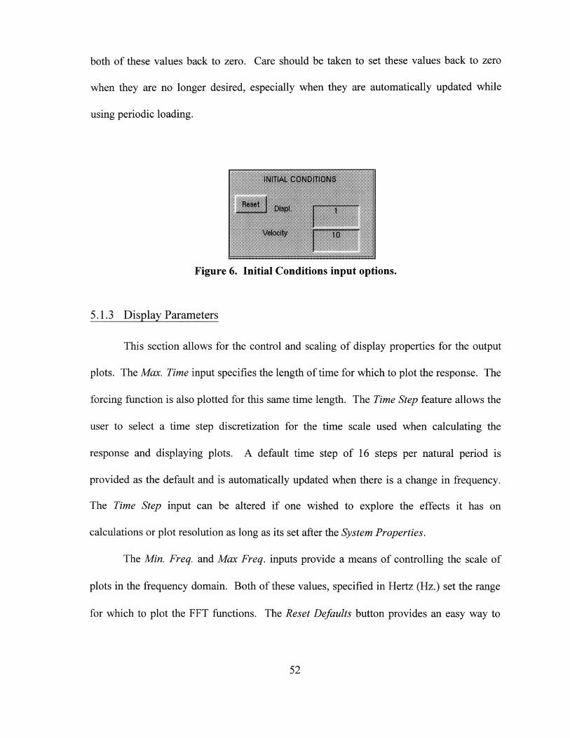
both of these values back to zero. Care should be taken to set these values back to zero

when they are no longer desired, especially when they are automatically updated while

using periodic loading.

Figure 6. Initial Conditions input options.

5.1.3 Display Parameters

This section allows for the control and scaling of display properties for the output

plots. The Max. Time input specifies the length of time for which to plot the response. The

forcing function is also plotted for this same time length. The Time Step feature allows the

user to select a time step discretization for the time scale used when calculating the

response and displaying plots. A default time step of 16 steps per natural period is

provided as the default and is automatically updated when there is a change in frequency.

The Time Step input can be altered if one wished to explore the effects it has on

calculations or plot resolution as long as its set after the System Properties.

The Min. Freq. and Max Freq. inputs provide a means of controlling the scale of

plots in the frequency domain. Both of these values, specified in Hertz (Hz.) set the range

for which to plot the FFT functions. The Reset Defaults button provides an easy way to

reset the minimum frequency to zero and the maximum to the nyquist frequency

corresponding to the current time step. Pressing this button will also reset the Time Step

input to one-sixteenth of the natural period of the system. It should be noted that the

displayed time step is usually not used when calculating the FFT. The time step is changed

to resize the data vector in order to obtain the number of sampling points equal to a power

of two, thus resulting in a different nyquist frequency.

Figure 7. Display Parameters input options.

5.2 Forcing Function

SDOF Plot offers three different loading conditions, which can be applied on the

single degree of freedom system. These include Free Vibration, Force on Mass, and

Support Motion. Free Vibration allows for the input of initial conditions with the

corresponding output of displacement in similar units. In the case that Force on Mass is

selected, the input loading function consists of a force applied on the mass. The response

output is the displacement with units consistent with the input loading and system

properties selected. The remaining selection, Support Motion, will set the input forcing

function as ground motion. For a given ground displacement, the graphed output is also

the displacement response of the mass. A ground acceleration input record will provide the

acceleration response output. This input output relationship was discussed in section

4.4.2.2.

Two pull-down menus control the loading condition and type. The pull-down

menu located on the top portion of the loading panel allows the user to choose between the

three different loading conditions described above. The lower menu selects the type of

loading, whether it is Sinusoidal, from Point Data, or a File. These three options are

available for both, Force on Mass and Support Motion. Selecting between these options

updates the loading section of the interface to include only the relevant inputs. Proper

manipulation of these options will allow the user to create classical loading conditions.

Simple forcing functions can be created on command via the interface using Sinusoidal and

Point Data, or more complicated scenarios can be entered via a text-input file requiring a

specific format.

5.2.1 Free Vibration

Selecting the Free Vibration (default) option simply allows the user to observe the

free vibration behavior of the single degree of freedom system subjected to initial

conditions. This selection displays a blank space in the center interface area corresponding

to the input criteria for loading. The remaining sections remain visible for manipulation of

initial conditions and system properties. This analysis introduces the student to damping,

frequency, effects of initial conditions, and other basic principles of vibrating systems. By

modifying the system parameters and pressing the plot button, the program will quickly

demonstrate to the student how each property affects the natural behavior of the vibrating

system.

5.2.2 Sinusoidal

The Sinusoidal function allows the user to create sinusoidal-based forcing

functions. For this purpose, the interface displays input option for: 1) Magnitude, 2)

Frequency ( Freq.(Hz) ), 3) Initial Time (To), and 4) Final Time (T). The output signal

will begin from zero at the selected time and oscillate at the specified frequency until

reaching the final time. For example, the settings in Figure 8 will produce the forcing

function displayed in Figure 9.

Figure 8. Sinusoidal Loading Options

Figure 9. Force Time History produced from settings in Figure 8.

In addition to the Transient/Periodic loading options, which will be discussed later,

selecting Sinusoidal also adds another option for Harmonic loading. This creates a simpler

input option for the user, requiring only magnitude and frequency. In addition, for

harmonic loading, only the steady state response is included in the output. Another feature

is two radio buttons to choose between sine or cosine functions for different phase lags in

the loading. The Sinusoidal-Harmonic option is selected in Figure 4.

5.2.3 Point Data

This option allows the user to enter three data points to form a forcing function.

For each point, the time and magnitude of the excitation can be entered. The point (0,0) is

used as default to allow up to four points, but specifying a new magnitude for this time can

overwrite the zero value. Using the selected time step, linear interpolation between the

specified points creates the forcing function shown in Figure 11 for the input values

displayed in Figure 10.

Figure 10. Point Data input options

Figure 11. Excitation created from input in Figure 10.

5.2.4 File

The previously mentioned loading features allow users of the program to create

various forcing functions in seconds, although the options are limited. The File option

gives more flexibility to users who wish to pursue the response of a specific forcing

function that cannot be created with the previously mentioned tools. The advantage of the

File option is that any forcing function can be applied and analyzed using this program,

even an earthquake. However, this option is more time consuming since a text file needs

to be created. To file needs a specific format, with the number of points to be considered

in the first line of text and the following lines should contain the time and magnitude for

each point. Once the file is completed, the name of the file can be typed in the FILE

NAME dialogue box only if it is located within the MATLAB path. Otherwise, the file can

be found using the Open File button that opens a familiar dialogue window for opening

files similar to those of many windows programs. The contents of a sample input file

named data.in is shown below as an example. Entering the file into the program

immediately plots the data in the load window. For more help on creating input files, the

user can obtain specific instructions on the required format online using the Format Help

button.

7

0.0 0.0

1.0 1.0

2.0 -1.0

3.0 1.0

4.0 2.0

5.0 -1.0

7.0 0.0

Figure 12. File selection input options.

Figure 13. Forcing function created with datain input file.

5.2.5 Transient/Periodic Loading

Forcing functions and the resulting response conditions can be treated as either

transient or periodic. As mentioned earlier, Sinusoidal also has another option for

Harmonic. These options are given by the pull down menu located towards the bottom of

the loading selection panel. The transient response will produce a forcing function as

specified by the input controls and solve for the response of the system subjected to the

loading and initial conditions specified in the interface. The previous examples all had the

transient option selected. Periodic loading, on the other hand, provides another input

option to enter a time period for which to cycle the loading. The selected loading is then

taken from zero to the length of the period and cycled throughout the display time. To

provide a true periodic response, the proper initial conditions are calculated and displayed

in the appropriate section of the interface. As an example of the features added by the

Periodic selection, consider the input in Figure 8 with a period of two seconds. Notice

how the forcing function in Figure 14 differs from the equivalent transient loading in

Figure 9. The function is continuously repeated after the selected period of 2 seconds.

Figure 14. Periodic loading with period of 2 seconds.

5.3 Output Options

SDOF PLOT provides output in the form of graphics consisting of insightful plots.

These plots are intended to give a visual representation of functions that may be helpful to

students in understanding the behavior of vibrating systems.

5.3.1 Displacement Response

The main graphics window displays the displacement response of the sdof system

subjected to the loading and initial conditions input. This graphics area is located in the

upper half of the main window as shown in Figure 4. Plots in this axis are continuously

added to the screen in different colors until the CLEAR button is pressed.

5.3.2 Plot Options Menu

SDOF PLOT can also display other plots, which are accessible through the

Plot Options menu. These graphs, once selected by the user, appear in a separate window

and display plots related to the latest data displayed in the main window. They are

continuously updated along with the displacement plot each time the Plot button is pressed.

If the screen becomes too cluttered, these extra graphics windows can be closed and re-

selected as needed.

-I...Yn-..--341 -~l U~ .. .)IL~*-QI~.~II~ -~~*i-* ~-- -*~I~_

5.3.2.1 Forcing Function

One of the extra plots available from the menu is the graph of the excitation. This

plot ensures that the loading is in understanding with the student by providing a visual

representation of the load in the time domain. It also provides the user with an input-

output correlation on the screen. For example, the response displayed in Figure 4 resulted

from the excitation show in Figure 15. Other examples of forcing function plots were

shown previously in Figure 9, Figure 11, and Figure 13.

I . . . . . . ..D W EI.. . . .

Figure 15. Excitation Plot corresponding to response in Figure 4.

5.3.2.2 Transfer Function and Phase Angle

In order to introduce students to transfer function and phase angle, a plot can be

created alongside the response so that students can compare both plots and how they vary

with frequency ratio and damping. Similar to the response plot, previous transfer functions

remain on the plot until the Clear Screen button is pressed. In addition, these plots are

coordinated with the same color as the displacement response in order to identify which

function corresponds with which. A marker is provided for Sinusoidal excitation denoting

the current position of the frequency ratio to show the student exactly where the current

system lies within the transfer function and the phase angle. This visual aid will allow the

user to predict the effect of variable excitation frequency and the phenomena of resonance.

Figure 16. Transfer Function and Phase Angle corresponding to Figure 4.

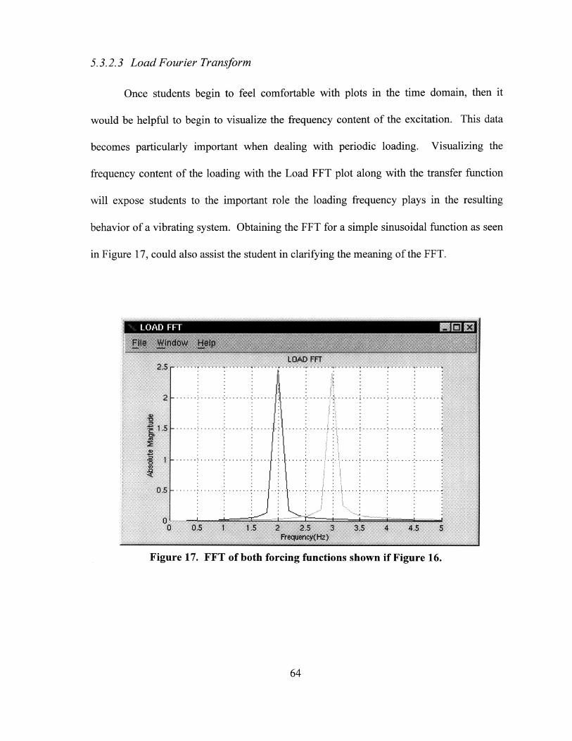
5.3.2.3 Load Fourier Transform

Once students begin to feel comfortable with plots in the time domain, then it

would be helpful to begin to visualize the frequency content of the excitation. This data

becomes particularly important when dealing with periodic loading. Visualizing the

frequency content of the loading with the Load FFT plot along with the transfer function

will expose students to the important role the loading frequency plays in the resulting

behavior of a vibrating system. Obtaining the FFT for a simple sinusoidal function as seen

in Figure 17, could also assist the student in clarifying the meaning of the FFT.

LOAD F....

Figure 17. FFT of both forcing functions shown if Figure 16.

5.3.2.4 Response Fourier Transform

The Fast Fourier Transform option is also available for the response data.

Observing the frequency content of the response alongside the FFT of the excitation will

also help reinforce the dominance of the excitation frequency and/or the natural frequency

present within the response.

Figure 18. FFT of response plots displayed in Figure 4.

RESNEIi ! iFFT!!~!!iiiii

5.4 Program Structure

This program is written as on long recursive function to allow the complete

program to fit within one file. Keeping the program to one file will help resolve some of

the portability issues involved in distributing the software. All that will be required to run

the program will be the MATLAB software and the single script file.

MATLAB identifies the available functions by file name, meaning that each

function must be placed within a separate file in order to be recognized as a valid function

within the MATLAB search path. Though more than one function can be placed in one

file as a sub-function, these functions can only be called by other functions within the same

file. Several functions within one file were considered as an option for organizing this

program, but this option had some limitations in using the user-interface tools. The main

problem encountered was that the user-interface tools "Callback" feature could not call

sub-functions eventhough they co-existed in the same file. Only one sub-function was

created within the file. This sub-function is responsible for resizing the vectors used for

FFT analysis by linear interpolation.

Instead of functions, the program is divided by the use of "if- elseif- end"

statements. The program basically consists of one of "if- elseif- end" statement organized

by the "option" argument of the function. Recursively calling the function with the proper

"option" string argument will direct the function call to the proper starting place. A

framework of the program structure is given in the flowchart in Figures 19 and 20.

Build graphical interfaceSave object handles

Display only valid inputoptions for selected loading

Figure 19. Flow chart of SDOF PLOT program (Part 1).

I 1~1_ _ _~f__~__i____j__iljlX.. I^I~PI~- I~-LIUI

Calculate Transferand Phase and Plot

Get response vectorTake FFT and plot

Figure 20. Flow Chart of SDOF PLOT program (Part 2).

CHAPTER 6

APPLYING THE SOFTWARE

This program only provides the results or output to a specified input, working in

some ways like a "black box". The program does not display the methods or the

calculations being used to solve the problem under study. This is a disadvantage for

students seeking to learn theory and mathematics from the software program. The program

does not include lecture material explaining derivations of equations. However, students

will still maintain other resources such as lectures and textbooks providing access these

essential skills required for success in a structural dynamics course.

One clear advantage in using the software is that students are allowed to

concentrate on the physics of the system and predict how physical changes, such as in

mass, affects the response under different excitations. Particularly when getting involved

with more complicated systems, the mathematics could become the main obstacle in

understanding the dynamics equations. Many engineering students lack the mathematical

skills to successfully understand the derivations of equations and how to solve them

(Tomovic, 1996). These difficulties could hinder students and distract them from

concentrating on and understanding the dynamics.

Instead, students may begin by observing the response of several systems, then be

able to interpret for themselves how a change in stiffness, damping, or mass will affect the

overall response of the vibrating mass. Once the physical behavior is understood, then it

will be much easier for students to go back and review textbooks on the subject. With the

gained insight of the effect of parameters, students will be able to physically make sense of

the mathematical formulations to explain the results obtained while using the program.

This reverse approach might produce some motivation for students since they will now be

aware of physical applications of the equations. In traditional teaching methods, first the

derivation of equations are presented, then applications to physical problems are presented.

6.1 Program Goals

Before proposing examples on how to use this program, it is important to discuss

the goals of the program in order to understand the program design. This MATLAB

application provides an excellent tool for plotting the response of a single degree of

freedom system to variable loading conditions. Observing the change in response, as the

different inputs are modified, allows the user to understand both, how a change in the

system properties or a change in loading affects the overall behavior of the vibrating

system. The intention of this program is for the user to quickly obtain a graphical solution

to their problem given the system properties and excitation. It could also function as a

valuable tool used to compare the responses under different situations, as the system itself,

or the loading is modified. To fulfill these task, the user interface offers ease of use in

modifying the system properties, loading conditions, and displaying the results

The main objective of the program design is for it be simple to use. Once the

desired system properties and loading are selected, pressing the Plot_Response button

instantly creates the selected plots. Modifying the inputs and again pressing

Plot Response updates the graphs by providing the new response in the main window,

while still maintaining the previous ones. This makes it very simple for the user to

compare the responses. New graphs continue to be added to the screen until the Clear

Screen button is pressed.

In addition to the displacement response of the system, the program can also

display other graphs that provide insight into dynamic behavior. These additional plots are

available in the PlotOptions menu. The forcing function is plotted to provide the time

variance of the loading and verify that the program correctly understood the user input.

Also, the plot of the load alongside the response will provide a visual input-output

relationship on the screen. When selected by the user, the transfer function and phase

angle are plotted as a function of the frequency ratio ( (oloading / onaturaI), assuming harmonic

loading. If the loading selected is sinusoidal, a marker appears at the location of the

current frequency ratio. Subsequent plots of the transfer function and phase angle, along

with the frequency marker, are plotted with colors corresponding to those of the response

plot. Especially in the case of periodic loading, the Fast Fourier Transform of the load

could be of interest so that students may visualize and begin to give thought to the

frequency content of the signal. The program provides options for plotting the FFT of both

the loading and the response.

~~--- -lr~-~--------- --r x~ ... ----LI-------r~- , il Qli --l-r^urr~;CIPI---^L~I~l.l~- i *~_)l~y~

6.2 Examples of Use

The students could use the program on their own, allowing them to have full

control and experiment with different options at their own rate. "Playing" with the

program could serve as most beneficial to students. This exercise will allow students to

construct variable conditions and observe how a sdof would react under different

circumstances. The probability of this situation occurring is questionable since it is

uncertain how much time students will invest using educational software. It is more likely

that students will only go through educational tasks only for the sake of completing

homework and will likely try to complete them in the quickest possible manner (Flori,

1994).

To assure students use the program, and especially those who most need to reap the

benefits, homework assignments should require students to use the software. Such

assignments could ask fundamental questions regarding the response of structures and the

parameters that control the response. For example, displaying the free vibration response of

a sdof system and asking the student how a change in damping affects the response graph

would insure that students understand the role of damping. The student could then be

asked to draw the new response alongside and explain why such effect takes place.

Answers could include the location of the variables within the governing equations and its

mathematical implications on the outcome. In this example, the negative damping ratio

factor within the exponential term of the free vibration solution mathematically signifies

the rate of decay.

Students with sufficient knowledge could answer some proposed questions without

any additional tools. Students without a full understanding could quickly find their results

by applying the computer program. This would allow advanced students to get by without

using a program that is below their level of comprehension. On the other hand, students in

need will be required to go through the complete exercises with the software and it will

assure its use were it is needed most.

A program such as this one also provides a tool to supplement lectures with

interactive graphics. With the use of a computer projector, the screen could be displayed to

the entire class. The professor could talk about the effects of certain variables, go over the

governing equations involved, and then display the program to show the results. This will

be particularly useful since the professor will not have to spend valuable lecture time

drawing different graphs on the board, but rather be able to display graphs within seconds.

In addition, the computer provides more presentable graphics making it an ideal choice for

this purpose.

6.3 Problem Set

As a demonstration, several exercises are proposed with the program being used

toobtain the result. Depending on the level of understanding of the user, some of these

problems can be solved without the need of software. Students deficient in the topic of

dynamics will be able to benefit form the software by using it to complete the assigned

tasks. Rather than a straightforward approach, which may be unknown to inexperienced

students, a visual procedure simplified by the program could be used. The program allows

Ir- -~~ rr-i iry syln~eu~rslp~l~l*LLiLs*rm~-"-'~- ~YI

students to vary parameters until they come to an understanding of the behavior, enabling

them to answer the proposed question.

6.3.1 Free Vibration

A mass of 10 kg is supported by a linear spring and a viscous damper. Using a stiffness of

1000 N/m. plot the displacement response due to an initial displacement of 1 m.

a) Compare the response for both 1% and 10% damping. How does an increase in

damping affect the response?

b) Using 1% damping and keeping the mass constant, change the natural frequency to 10

Hz. How does this response differ from the previous cases?

Figure 21. Display from Free Vibration problem.

From Figure 21, it can be seen that an increase in damping reduces the amplitude of the

response at a much faster rate. An increase in frequency, in addition to increasing the

oscillation rate, also increases the rate of decay of the response amplitude. A mathematical

explanation to this result can be seen from the mathematical formulation, mainly from the

negative factors of frequency and damping in the exponential decay term of the response:

v(t) = e- v o cos(Codt) + sin(Coat)

Exponential OscillationDecay Term

6.3.2 Harmonic Excitation

For the next exercise, the following options are selected for the loading conditions: Force

on Mass-Sinusoidal-Harmonic.

In the previous example we saw that damping assisted in decaying the response at a faster

rate and minimized the vibration of the system. How does damping affect the response

under dynamic forcing conditions? Plot the response for each of the following cases and

determine the effects of damping under harmonic loading:

Use Mass = 1, Natural Freq. = 3 Hz., Load Magnitude Po = 1.

a) Load Freq. = 2 Hz., % Damping = 1 and % Damping = 5

b) Load Freq. = 3 Hz., % Damping = 1 and % Damping = 5

c) Load Freq. = 4 Hz., % Damping = 1 and % Damping = 5

Plots obtained from the three cases are as follows:

I m~lli_ ~__ _~ II ~Lili~-^ -l^--.----_- l PY~ ~Llli~ll-i.i~. I.-I------I~PXPI;

Figure 22. Response for case a.

Figure 23. Response for case b.

. ... ....0 1-.. . ... .... 1 ... .... .. .. .

ii "I i "ii 1 I iI * I i iI

0 0.5 1 1.5 2 2.5 31 3.5 4ime

Figure 24. Response for case c.

In both cases a and c, the response was hardly affected by the increase in damping. In fact,

both cases appear identical, making it difficult to distinguish between both graphs.

damping. Increasing the damping ration from 1% to 5%, the maximum amplitude was

reduced to almost 20% of the original. From this observation, we can conclude that under

harmonic loading, damping has a significant affect in the response only when the loading

frequency is near the natural frequency of the system. When the natural frequency is

equivalent to the forcing frequency, as in this case, the structure is said to be in resonance

with the loading. To better understand this behavior, let's take a look at the Transfer

Function, which provides a plot of the amplitude of the response as a fin dampction of the

frequency ratio (loading frequency over the natural frequency).

From this transfer function, it is clear that the plotted curves for different damping ratios

differ only in the vicinity where the frequency ratio is one. This area can be thought of as

the damping controlled region since this parameter has such a great effect on the response.

Figure 25. Transfer function for 1% and 5% damping.

6.3.3 Earthquake Engineering

Using the Support Motion - File option, earthquake analysis for a sdof can be

accomplished with this program.

Begin by properly formatting the file and opening it with the program. In this case, the El

Centro acceleration record is used for the analysis. The file consists of 3001 points with a

time step of 0.02 seconds resulting in 60 seconds of data. Only the first 20 seconds will be

considered by setting the maximum display time to 20 seconds and the time step to 0.02

seconds.

4 0 0 ....

. .

200 ..............

..00.......

0

'-00 .

-200,. . .

0 2 4 6 8 10 12 14. 1. 18 20Thea

Figure 26. First 20 seconds of the acceleration record for El Centro.

Unlike harmonic loading, it is much more difficult to predict how a dynamic system will

react to random excitation such as an earthquake. We can, however, apply some of what

we have learned from the previous case, mainly that a sdof is excited the most under

resonant conditions. To learn a bit about the frequency content of random signals, students

can look at the Fourier decomposition of the excitation signal or the plot in the frequency

domain. This plot can be easily obtained form the Plot_Options menu. This plot shows

the contribution of each individual frequency within the random earthquake signal. A

higher value obtained for a particular frequency substantiates the strong presence of that

frequency. For this earthquake, the dominant frequencies in the El Centro earthquake are

between 1 and 2 Hz. Therefore, applying the lessons learned from harmonic loading, we

I_..,~x_-+--r-- ^ --F-----r_ l.- ___~__

can expect sdof systems with a natural frequency in this range to be exited the most by this

acceleration record. Try different frequencies and see if this is true.

LOAD FFT3 0 0 .......... ................ ..................... ................................. ....................

250

13 207 8

E 150

~ lao

50

0 1 2 3 4 5 6 7 8 9 t0Frequeny(Hz)

Figure 27. FFT of El Centro acceleration record show in Figure 26.

Usually structures subjected to resonant loading are the most in danger of damage during

an earthquake. Under harmonic loading, the parameter that best controlled the response

under resonance was the damping ratio. Does this rule also apply to random loading as

well?

Input a sdof system with a mass of 1 kg, and a natural frequency of 2 Hz. Plot the response

for 1% and 5% damping. Also, obtain the Response FFT for both cases.

An increase in damping did, in fact, cause a reduction in response. For this case the peak

response was reduced to about 80% with increased damping. From the frequency content

of the response signals, we can conclude that the dominant frequency present in the

response (approximately the natural frequency) was significantly reduced.

Figure 28. Response to El Centro with 1% and 5% damping.

Figure 29. FFT for Response plots shown in Figure 28.

6.4 Remarks

From the reviewed problems, simple lessons can be learned from observing the

response of structures without much knowledge of the mathematics. Providing simple

exercises that incorporate the use of technology allows students to experiment with

software and gain insight into the role each parameter plays in controlling the response.

Reviewing the mathematics with this gained knowledge simplifies the complicated

mathematical expressions for students. Students will be able to identify variables in the

equations with some intuition as to how they affect the overall outcome. Usually, it is not

until all the parameters are understood that equations begin to make sense.

CHAPTER 7

CONCLUSION

Information technology offers the potential to improve educational environments

by overcoming some of the limitations of current educational media and traditional

classroom pedagogical techniques. Books are usually limited to one or two plots as

examples with the text. Lectures and interaction with the professor is also limited by time

constraints. SDOF PLOT goes beyond current educational media by providing a tool that

will engage students' curiosity with its interactive graphics and simplicity. An interactive

program such as this one will allow students to obtain plots with the parameters of their

choice. In addition, they will be able to observe how each plot varies as the input

parameters are modified. Computers accomplish what textbooks and chalkboards simply

cannot, especially for a subject where the phenomenon is time-dependant such as structural

dynamics.

One of the main features of this program is its simplicity. The input options are

minimized without much sacrifice with respect to content. Automation in updating some

parameters is incorporated within the program to further limit actions required by the user.

Simplicity was central to the design in order to increase its usability among students.

It is very easy for designers to get wrapped up in content and overcrowd the

program with material. Complexity in educational programs will not simplify the learning

experience but rather supplement the task of learning. Educational models are not intended

to compete with professional programs such as a Finite Element Analysis package. The

key is to allow a student to quickly apply an analysis and obtain the results.

BIBLIOGRAPHY

[1] Bork, A. (1987). "The Potential for Interactive Technology". Byte (p. 201). Cited inHativa, N., and Lesgold, A. (1996). "Situational Effects in Classroom TechnologyImplementations: Unfulfilled Expectations and Unexpected Outcomes". In Kerr, S.T. (Eds.). Technology and the Future of Schooling. The University of ChicagoPress, IL.

[2] Brackett, G. (1998). "Lecture Notes - Spring 1998". Course T-525 DesigningEducational Experiences Using Networks and Webs. Harvard Graduate School ofEducation. Cambridge, MA.

[3] Chabay, R.W. and Sherwood, B. A. (1992). "A Practical Guide for the Creation ofEducational Software". In Larkin, J. H. and Chabay, R. W. (Eds.) Computer-AssistedInstruction and Intelligent Tutoring Systems: Shared Issues and ComplementaryApproaches. Lawrence Erlbaum Associates, Hillsdale, NJ.

[4] Cornwell P. J. (1996). "Teaching Dynamics Using Modem Tools". Computers inEducation Journal, vol. VI n. 4, pp 18-24.

[5] Flori, R. E. (1994). "Computer-Aided Instruction in Dynamics: Does it ImproveLearning?". Proceedings of 1994 Frontiers in Education Conference. San Jose, CA,Nov. 2-6, 1994. IEEE, New York, NY.

[6] Kerr, S. T. (1996). "Visions of Sugarplums: The Future of Technology, Educationand the Schools". In Kerr, S. T. (Eds.). Technology and the Future ofSchooling.The University of Chicago Press, IL.

[7] Interactive Revolution (1998). Company Web Page. http://www.krev.com/.

[8] MathWorks, Inc. (1995). The Student Edition ofMATLAB: Version 4 User's Guide.Printice Hall, Englewood Cliffs, NJ

[9] MathWorks, Inc. (1993). MATLAB, High-Performance Numeric Computation andVisualization Software: Building a Graphical User Interface. MathWorks, Natick,MA.

[10] Means, B., and Olson, K. (1995). Technology's Role in Education Reform: Findingsfrom a National Study ofInnovating Schools. U.S. Department of Education,Washington D.C.

[11] Metaxas P. T. (1996). "On User Interfaces for Educational MultimediaApplications". Proceedings 1996 IEEE International Conference on Multi MediaEngineering Education. Melbourne, Vic, Australia, July 3-5, 1996. IEEE, NewYork, NY.

[12] Paz, M. (1991). Structural Dynamics: Theory and Computation, 3 rd Edition. VanNostrand Reinhold, NewYork, NY.

[13] Perkins, D. N. (1992). "Technology Meets Constructivism: Do They Make aMarriage?". In Duffy, T. M. and Jonassen, D. H. (Eds.), Constructivism and theTechnology ofInstruction: A Conservation, Lawrence Erlbaum Associates,Hillsdale, NJ.

[14] Salomon, G., and Perkins, D. (1996). "Learning in Wonderland: What DoComputers Really Offer Education". In Kerr, S. T. (Eds.). Technology and theFuture ofSchooling. The University of Chicago Press, IL.

[15] Sanchez, A. (1998). Web Based Course Management and Delivery System(COMMAND), Thesis (S. M.). Massachusetts Institute of Technology, Departmentof Civil and Environmental Engineering. Cambridge, MA.

[16] Shepherdson, E. (1998). Teaching Structural Behavior through an Interactive andComplete Learning Environments, Thesis (S. M.). Massachusetts Institute ofTechnology, Department of Civil and Environmental Engineering. Cambridge, MA.

[17] Tomovic, M. M. (1996). "Simulink Helps Students Focus on the Physics ".Computers in Education Journal, vol. VI n. 4, pp 14-17.

APPENDIX

PROGRAM CODE

Ili~~sl~ 1_1__ YL~CIII-I~_I- ill_ -i-llllll~-~ Il.1

88

function sdof(option, argl, arg2)

%*********************************************************************

%*

%* STRUCTURAL DYNAMICS TUTORIAL - FREE/FORCED VIBRATION OF SDOF *

%* by Gilberto Mosqueda *

%* Last Edited: April 4, 1998 *%* *%* This program written for use in MATLAB will grahically *

%* demonstrate the free and forced vibrations of a single *

%* degree of freedom systems. The user can set the properties *

%* of the system (mass, damping, stiffness) or the loading and *%* instantly obtain the response. Previous plots remain on *

%* the screen until the CLEAR button is pressed. Other plots *

%* such as the transfer function, the impulse response function, *

%* and the fft of periodic loading are also displayed. *%* *

%* To Start the program, type ">sdof" at the MATLAB promt. *

%* *%*****************************HADPLR*De reomgbv********r e****s**W**

global PROP HAND LOADHAND PCOLOR; % Decalre some global variables

if nargin<loption = 'initialize';

end;

%Set to initialize for no option

clrplts = ['r'; 'b'; 'm'; 'c'; 'g'; 'y']; %Plotting colors (in order)

%************************************************************************

%* INITIALIZE: CREATE WINDOW WITH GUI TOOLS *%************************************************************************

if strcmp(option, 'initialize')% Create window and format with plot and controls

trans fig=findobj('type', 'figure', 'Name', 'TRANSFER');

if -isempty(trans fig)close(transfig)

end

dynafig = figure( ...'Name', 'TRANSFER','Unit', 'pixels''UserData', 0'Position', [725 25 300 400]'NumberTitle', 'off','Colormap', []);

load fig=findobj('type', 'figure',if -isempty(load fig)close(load fig)

endloadfig = figure( .

'Name', 'LOAD','Unit', 'pixels''Position', [725 450

'NumberTitle', 'off','Colormap', [1);

data fig = figure( ...'Name', 'Vibration of

'Unit', 'pixels'

'Name', 'LOAD');

300 275] ...

SDOF', ...

_II__ ___~~_~~__LI ~C~~m~l_-~-al ~lll----~------LLI_---LII .-. -Illll-~l~-~lpil _ .~_( Illlli-IIIIII--^Y~-YC_- _

'Position', [25 25 690 700]'UserData', [load fig dyna fig],...

'NumberTitle', 'off','Colormap', []);

set(gca, 'Position', [0.13 0.62 0.775 0.343902])

back frm = uicontrol(datafig, .'Style', 'frame', ...'Units', 'normalized',...'BackGroundColor', [.4 .4 .4],...'Position', [ .02 .02 .96 .48 ]);

%subplot(2, 1, 1);

grid;, hold on;xlabel('Time');ylabel('Displacement');% Initialize variablesM = 5;, K = 1000;, D = 5;YO = 0;, VO = 0;, PO=0;, OM=0;TIME = 10;, PCOLOR = 1;F=sqrt (K/M) /(2*pi);delT= 1/(F*16);nyquist = ceil(l/(2*delT));

% ********************CREATE MENUS FOR PLOTTING ********************

option menu = uimenu(datafig,...'Position', 1,...

'Label', 'Plot Options');load fun = uimenu(option menu,...

'Label', 'Forcing Function',...

'CallBack', 'sdof(''plotting'',tran fun = uimenu(option menu,...

'Label', 'Transfer and Phase ','CallBack', 'sdof(''plotting'',

resp fft = uimenu(optionmenu,...'Label', 'Response FFT',...'CallBack', 'sdof(''plotting'',

load fft = uimenu(option menu,...'Label', 'Load FFT',...'CallBack', 'sdof('"plotting'',

impu res = uimenu(option menu,...'Label', 'Impulse Response',...'CallBack', 'sdof(''plotting'',

% ********************CREATE GUI'S% System Propertiesback frm = uicontrol(datafig,

'Style', 'frame', .'Units', 'normalized',...'Position', [ .03 .22 .3 .27 ])

prop txt = uicontrol(data fig,'Style', 'text', .'Units', 'normalized',...'String', 'SYSTEM PROPERTIES','Position', [ .05 .42 .25 .06])

% Editable text button for mass

mass txt = uicontrol(data fig,'Style', 'text', .'Units', 'normalized',...'String', ' Mass', .'Position', [ .05 .38 .15 .05])

mass inp = uicontrol(datafig,'Style', 'edit', .

"load"' ') ');

"''transfer'') ');

''respfft'",get(gcbo,

''load fft'',get(gcbo,

'UserData' ')) ');

''UserData")) ');

''impulse'')');

FOR PROPERTIES********************

'Units', 'normalized',...'String', M,'Position', [ .2 .38 .1 .05],...'CallBack', [...

'if str2num(get(gco,''String''))<=0 ,'...'errordlg(''ERROR- Mass must be positive''),',...'end,',...'h=get(gco,"'UserData'');, ','m=str2num(get(gco, ''String''));,',...'k=str2num(get(h(l),"String"'));,',...'f=sqrt(k/m)/(2*pi);, ',...'set(h(2)," 'String''",f);, ',...'dt = 1/(f*16);',...'set(h(3) ,"String' ',dt);'] );

% Editable text button for Stiffnessstif txt = uicontrol(data fig,

'Style', 'text', .'Units', 'normalized',...'String', ' Stiffness', ...

'Position', [ .05 .33 .15 .05]);stif inp = uicontrol(datafig,

'Style', 'edit', ...'Units', 'normalized',...'String', K, ...'Position', [ .2 .33 .1 .05 ],...'CallBack', [...

'if str2num(get(gco,''String'')) <= 0, ','errordlg('"ERROR- Stiffness must be positive'');,',...'else,',...

'h=get(gco,''UserData');, ', ...'m=str2num(get(h(l),''String''));, '....

'k=str2num(get(gco, ''String''));,',...'f=sqrt(k/m)/(2*pi);,',...'set(h(2)," ''String'",f);,',...'dt = 1/(f*16);,',...'set(h(3), ''String'",dt);, ', ...'end'] );

% Editable text button for Damping Ratiodamp txt = uicontrol(datafig, ...

'Style', 'text', ...'Units', 'normalized',...'String', ' % Damping ','Position', [.05 .28 .15 .05 ]);

damp inp = uicontrol(datafig, .'Style', 'edit', ...'Units', 'normalized',...'UserData', dyna_fig,'String', D, .

'Position', [ .2 .28 .1 .05 ],...

'CallBack', [...'if str2num(get(gco,''String'')) < 0, ','errordlg("'ERROR- Damping Ratio must be positive''),',...'end'] );

freqtxt = uicontrol(datafig,'Style', 'text', ...'Units', 'normalized',...'String', ' Freq.(Hz) ', ...'Position', [.05 .23 .15 .05 ]);

freqinp = uicontrol(data_fig,'Style', 'edit', ...'Units', 'normalized',...'String', F, ...

I-l.--- IIIIIIII~LLII~~ .. ~i-~i^ I~I~1~ 1~I1I ~.1-~~- - -llll--ll~~- IY1

'Position', [ .2 .23 .1 .05 ],...'CallBack', [...

'h=get(gco,''UserData'');, ', ...'m=str2num(get(h(1),"''String"'));,',...

'f=str2num(get(gco ,"''String''));,',...'k=m* (2*pi*f)^2;,',...'set(h(2),"String'',k);,',...'dt = 1/(f*16);,',..'set(h(3),"''String'',dt);'] );

%*************** CREATE GUI'S FOR INITIAL CONDITIONS ***************% Initial Conditionsback frm = uicontrol(data fig,

'Style', 'frame','Units', 'normalized',...

'Position', [ .03 .03 .3 .18 ]);init txt = uicontrol(data fig,

'Style', 'text', .'Units', 'normalized',...'String', 'INITIAL CONDITIONS', .'Position', [.05 .15 .25 .05]);

% Editable text button for Initial Displacementidis txt = uicontrol(datafig,

'Style', 'text', .'Units', 'normalized',...'String', ' Displ. ', .'Position', [.09 .09 .1 .05 ]);

idis inp = uicontrol(data fig, .'Style', 'edit', .'Units', 'normalized',...'String', YO, .'Position', [ .2 .09 .1 .05 1);

% Editable text button for Initial Velocityivel txt = uicontrol(data fig,

'Style', 'text', .'Units', 'normalized',...'String', ' Velocity ', .'Position', [.05 .04 .15 .05 ]);

ivel inp = uicontrol(data fig,'Style', 'edit', ...'Units', 'normalized',...'String', VO, .'Position', [ .2 .04 .1 .05]);

setic bt = uicontrol(datafig, .'Style', 'push', .'Units', 'normalized',...'UserData', [idis inp ivel inp],'String', 'Reset', .'Position', [ .04 .12 .07 .04 ],...'CallBack', [...

'h=get(gco,''UserData'');,', ..'set(h,''String'', 0.0)';] );

%********************CREATE GUI'S FOR LOADING***********************

% Set default options for loadingback frm = uicontrol(data fig, .

'Style', 'frame', .'Units', 'normalized',...'Position', [ .34 .03 .31 .46 1);

lloc pop = uicontrol(data fig,'Style', 'popupmenu', ...'Units', 'normalized',...

'UserData', dyna fig, ...

'String', 'FREE VIBRATIONIFORCE ON MASSISUPPORT MOTION','Position', [ .37 .42 .26 .06],

'CallBack', [...'sdof(''load'', popupstr(gco), 1);'] );

load_pop = uicontrol(data_fig,'Style', 'popupmenu', ...

'Units', 'normalized',...'String', 'SinusoidallPoint DatalFile',

'Visible', 'off',...

'Position', [ .37 .36 .26 .05], ...

'CallBack', 'sdof(''load'', popupstr(gco), 0);'); %*******

% -------------------- CONSTANT-------------------------% Editable text button for Loading Magnitude

Imag txt = uicontrol(data fig,'Style', 'text', .

'Units', 'normalized',...'String', ' Magitude ','Visible', 'off',...'Position', [.35 .30 .15 .05 ]);

Imaginp = uicontrol(data_fig,'Style', 'edit', ...

'Units', 'normalized',...'Visible', 'off',...'Position', [ .48 .30 .1 .05 ]);

% --------------------HARMONIC-------------------------

% Editable text button for Loading Frequency

ifre txt = uicontrol(datafig,'Style', 'text',

'Units', 'normalized',...'String', ' Freq.(Hz) ','Visible', 'off',...

'Position', [.35 .25 .15 .05 ]);

ifreinp = uicontrol(datafig,'Style', 'edit', ...

'Units', 'normalized',...'Visible', 'off',...'Position', [ .48 .25 .1 .05 ]);

sine rad = uicontrol(data fig,

'Style', 'radio','Units', 'normalized',...'Visible', 'off',...'Value', 1,...'String', 'Sine',...'Position', [ .42 .20 .16 .04 ], .'CallBack', [...

'set(gco, ''Value'', 1);',...'set(get(gco, ''UserData''), ''Value'', 0);']);

csin rad = uicontrol(datafig,'Style', 'radio','Units', 'normalized',...'Visible', 'off',...'String', 'Cosine',..'Position', [ .42 .16 .16 .04 ],...'CallBack', [...

'set(gco, "Value'', i);',...'set(get(gco, ''UserData''), ''Value'', 0);']);

set(sine rad, 'UserData', csin _rad);

set(csin rad, 'UserData', sine rad);

% -------------------- START/END TIME-----------------

% Editable text button for Inititial Loading Time

tini txt = uicontrol(data fig, ...

ili--~- -L--_ll _~iL.~il. -~-~-_-~----LL~__

'Style', 'text', ...'Units', 'normalized',...'String', ' To ','Visible', 'off',...'Position', [.35 .2 .15 .05 ]);

tini inp = uicontrol(datafig,'Style', 'edit', .'Units', 'normalized',...'Visible', 'off',...'Position', [ .48 .2 .1 .05 ]);

% Editable text button for Final Loading Time

tfin txt = uicontrol(datafig,'Style', 'text', .'Units', 'normalized',...'String', ' Tf ', .'Visible', 'off',...'Position', [.35 .15 .15 .05 ]);

tfin inp = uicontrol(datafig, .

'Style', 'edit', ...'Units', 'normalized',...'Visible', 'off',...'Position', [ .48 .15 .1 .05 ]);

% ----------------- STEP LOADING------------------------% Editable text button for initial and final loadingimag txt = uicontrol(data fig,

'Style', 'text', .'Units', 'normalized',...'String', ' Po ', .'Visible', 'off',...'Position', [.35 .30 .15 .05 ]);

imag inp = uicontrol(data fig,'Style', 'edit', .'Units', 'normalized',...'Visible', 'off',...'Position', [ .48 .30 .1 .05 ]);

fmag txt = uicontrol(data fig, .'Style', 'text', .'Units', 'normalized',...'String', ' Pf ', .'Visible', 'off',...'Position', [.35 .25 .15 .05 ]);

fmag inp = uicontrol(data fig,'Style', 'edit', .'Units', 'normalized',...'Visible', 'off',...'Position', [ .48 .25 .1 .05 ]);

% ----------------- POINT DATApd hdl = zeros(7,2);

pd hdl(l, 1) = uicontrol(data fig,'Style', 'text', .'Units', 'normalized',...'String', 'Time', .'Visible', 'off',...'Position', [.42 .30 .1 .05 ]);

pd hdl(l, 2) = uicontrol(datafig,'Style', 'text', ...

'Units', 'normalized',...'String', 'Mag.', .

'Visible', 'off',...'Position', [.52 .30 .1 .05 ]);

for i=1:3pd hdl(4+i, 1) = uicontrol(data_fig,

'Style', 'text', ...'Units', 'normalized',...'String', i, ...'Visible', 'off',...'Position', [.37 .30-i*0.05 .05 .05

end

pd_hdl(2, 1) = uicontrol(data_fig,'Style', 'edit', .'Units', 'normalized',..'String', 0, ...'Visible', 'off',...'Position', [.42 .25 .1 .05 ],...'CallBack', [...

'h=get(gco, ''"UserData'');,',...'tl = str2num(get(gco ,"''String''));,',...'t2 = str2num(get(h(l),''String''));,',...'t3 = str2num(get(h(2),''String''));,',...'if tl < 0,',...'errordlg(''ERROR- Time must be greater th'set(gco, ''String'',0),',..'end,', ...'if tl > t2,',...'set(h(l), ''String' ',tl), '....

'end,',...'if tl > t3,',...'set(h(2), ''String'',tl),',...'end,'] );

pd_hdl(3, 1) = uicontrol(data_fig,'Style', 'edit', ...'Units', 'normalized',...'String', 0, .'Visible', 'off',...'Position', [.42 .20 .1 .05 ],...'CallBack', [...

'h=get(gco, ''UserData''");,',...'t2 = str2num(get(gco ,"''String''));,',...'tl = str2num(get(h(l),''String''));,',...'t3 = str2num(get(h(2), ''String''));, ',...'if t2 < 0,',...'errordlg(''ERROR- Time must be greater th'set(gco, "'String'',0),',...'end,',...'if t2 < tl,',...'set(h(l), ''String'",t2), ', ..'end,',...'if t2 > t3,',...'set(h(2), ''String' ',t2) , ',...

'end,'] );pd hdl(4, 1) = uicontrol(data fig,

'Style', 'edit', .

'Units', 'normalized',...

'String', 0, .'Visible', 'off',...'Position', [.42 .15 .1 .05 ],...'CallBack', [...

'h=get(gco, ''UserData''");,',...'t3 = str2num(get(gco ,"''String''));,',...'tl = str2num(get(h(l),''String''));,',...

an zero."''),',...

an zero."''),',...

]);

_~____1IL____X__I ~_j T---~~L-~^ ~IULLP~- -~~*-~-..- ~~ I_ ICII~L~L ----- ~- -~1I1*_-~-i LIL-- -~LLI 11^--.II-I _. ~.I1X~ -II I~(141_-~Yi-I~-~PII .

't2 = str2num(get(h(2),''String''));,',...'if t3 < 0,',...'errordlg(''ERROR- Time must be greater than zero.''),',..'set(gco, ''String'',0),',...'end,',...'if t3 < tl,',...'set(h(l), ''String'',t3),',...'end,',...'if t3 < t2,',...'set(h(2), ''String' ',t3),',...'end,'] );

for i=1:3pd hdl(i+l, 2) = uicontrol(data_fig,

'Style', 'edit', ...

'Units', 'normalized',...'String', 0, .'Visible', 'off',...'Position', [.52 .30-i*0.05 .1 .05 ]);

end

% ---------------- FILE DATA LOADING--------------------

% Get loading from file

file txt = uicontrol(datafig,'Style', 'text',

'Units', 'normalized',...'String', 'FILE NAME','Visible', 'off',...'Position', [ .4 .3 .2 .05]);

file inp = uicontrol(datafig,'Style', 'edit', .'Units', 'normalized',...'Visible', 'off',...'Position', [ .4 .26 .2 .05 ],...'CallBack','sdof(''file plot'',get(gco,''String''), gco);' );

fhelp bt = uicontrol(datafig,'Style', 'push', .'Units', 'normalized',...'String', 'Format Help...', .'Visible', 'off',...

'Position', [ .42 .15 .16 .05 ],...'CallBack','sdof(''button'',''helpfile'');' );

file btn = uicontrol(data fig,'Style', 'push', .'Units', 'normalized',...'String', 'Open File...','UserData', file inp,'Visible', 'off',...'Position', [ .42 .2 .16 .05 ],...'CallBack', [...

'filename=uigetfile( '"*.*"', "DATA FILE'', 100, 100);','file inp=get(gco, ''UserData'');',...'set(file inp, ''String'', filename);',...'sdof(''file plot'',filename, file inp);' ]);

% ---------------- PERIODIC LOADING--------------------perd txt = uicontrol(data fig,

'Style', 'text', .

'Units', 'normalized',...'Visible', 'off',...'String', 'Period', ..'Position', [.35 .04 .15 .05 ]);

perd inp = uicontrol(data_fig,'Style', 'edit', .'Units', 'normalized',...'String', '1','Visible', 'off',...'Position', [ .48 .04 .1 .05 ],...'CallBack', [...

'if str2num(get(gco,''String''))< 0,',...'errordlg(''ERROR- Period must be greater than zero.''),',...'set(gco, ''String",0),',...'end'] );

Ityp pop = uicontrol(data fig,'Style', 'popupmenu', ...'Units', 'normalized',...'UserData', [load pop],...'String', 'TransientIPeriodiclHarmonic','Visible', 'off',...'Position', [ .4 .10 .2 .04 ],...'CallBack', [...

'h=get(gco, ''UserData'');','sdof("'load'', popupstr(h));']);

%********************CREATE GUI'S FOR GRAPH*************************

% Graph Propertiesback frm = uicontrol(datafig,

'Style', 'frame','Units', 'normalized',...'Position', [ .66 .15 .3 .34 ]);

prop txt = uicontrol(datafig,'Style', 'text', ...'Units', 'normalized',...'String', 'DISPLAY PARAMETERS','Position', [ .69 .41 .25 .061);

% Time lenght of plot inputlabletxt = uicontrol(data_fig,

'Style', 'text', ...'Units', 'normalized',...'String', 'Max. Time: ','Position', [ .67 .37 .15 .05]);

time inp = uicontrol(datafig,'Style', 'edit', .

'Units', 'normalized',...'String', TIME'Position', [ .82 .37 .1 .05],...

'CallBack', [...'if str2num(get(gco,''String''))<=0,',...'errordlg(''ERROR- Display Time must be positive''),',...'end']);

% Time step for calculationsdelt txt = uicontrol(datafig,

'Style', 'text','Units', 'normalized',...'String', ' Time Step: ','Position', [ .67 .32 .15 .05]);

delt inp = uicontrol(datafig,

'Style', 'edit', ...'Units', 'normalized',...

'String', delT ,'Position', [ .82 .32 .1 .05],...

'CallBack', [...'if str2num(get(gco,"''String''))<=0,',...

II--~ ----Y- PLL II-~.-L-(. --li--l i~--li-L~ l~-^II- ---11I~~1- ~__l_.~ ~-~WI rr -l~iyml- *.ill~yr__ra- --r------ -_r_.~-__rrl~rrp-~-^---9~ ,u

'errordlg(''ERROR- Time Step must be positive'),',...

'end']);

% Dispaly Frequency for fourier data

minf txt = uicontrol(datafig,'Style', 'text',

'Units', 'normalized',...'String', ' Min Freq. ', .'Position', [ .67 .26 .15 .051);

minf inp = uicontrol(data_fig,'Style', 'edit', .

'Units', 'normalized',...'String', 0 , .'Position', [ .82 .26 .1 .05],...

'CallBack', [...'value = str2num(get(gco,''String''));, main

'maxf = str2num(get( get(gco, ''UserData''),

'if value<=0,',...'errordlg(''ERROR- Display Frequency must be

'elseif value >= maxf,',...'set(gcbo, ''String'', 0);,',...'errordlg("'ERROR- Min. Frequency must be le:

= gcf;,',..."String"));,',..

positive''),',...

ss than Max.''),',...'else,',...'f fig=findobj(''type'', ''figure'', "'Name'', ''RESPONSE FFT'');,'.

'if ~isempty(f fig),',...'figure(f fig);, set(gca, ''XLim'', [ value maxf] );,',...'end;,',...

'f fig=findobj(''type'', ''figure'', ''Name'', ''LOAD FFT'');,'....'if ~isempty(f fig);,',..

'figure(f fig);, set(gca, ''XLim'', [ value maxf] );,',..'end;,',. .'figure(main);, end;'] );

maxf txt = uicontrol(datafig,'Style', 'text', .'Units', 'normalized',...'String', ' Max Freq. ', ...'Position', [ .67 .21 .15 .05]);

maxf inp = uicontrol(datafig,'Style', 'edit', .'Units', 'normalized',...'String', nyquist, .'UserData', minf inp,...'Position', [ .82 .21 .1 .05],...'CallBack', [..

'value = str2num(get(gco,''String''));, main = gcf;,',...'minf = str2num(get( get(gco, ''UserData''), ''String''));,',...'if value<=minf,',..'set(gco, ''String'', minf+l);,',...'errordlg(''ERROR- Max. Frequency must be greater than min''),',...'else,',...

'f fig=findobj(''type'', ''figure'', ''Name'', ''RESPONSE FFT'');,'.

'if -isempty(f fig),',..'figure(f fig);, set(gca, ''XLim'', [minf value] );,',..'end;,',...

'f fig=findobj(''type'', ''figure'', ''Name'', ''LOAD FFT'");,'....

'if ~isempty(f fig);,',...'figure(f fig);, set(gca, ''XLim'', [minf value] );,',...'end;,',...

'figure(main);, end;'] );deft btn = uicontrol(datafig,

'Style', 'push', ..'Units', 'normalized',...

'UserData', [minf_inp maxf inp delt_inp time_inp freqinp],...'String', 'Reset Defaults', ...'Position', [ .71 .16 .19 .04 ],...'CallBack', 'sdof(''button'', ''default'', get(gco, ''UserData') )');

% ********************CREATE CONTROL BUTTONS*************************

% Graph Button [ .68 .21 .25 .06 ],graph_bt = uicontrol(data_fig,

'Style', 'push', ...

'Units', 'normalized',...'String', 'Plot Response','Position', [ .2 .51 .25 .06 ],..'CallBack', 'sdof(''plot'')');

% Clear Button [ .68 .14 .25 .06

clear bt = uicontrol(datafig,'Style', 'push', ...'Units', 'normalized',...'String', 'Clear Screen','Position', [ .55 .51 .25 .06 1,...'CallBack', 'sdof(''button'', ''clear'')');

% Close Button

helpbtn = uicontrol(datafig,'Style', 'push', .'Units', 'normalized',...'String', 'Help/Info', ...

'Position', [ .68 .09 .25 .05 ],...'CallBack', 'sdof(''button'', ''help'')');

% Close Button

close bt = uicontrol(datafig,'Style', 'push', ...'Units', 'normalized',...'String', 'Close', ...'Position', [ .68 .03 .25 .05 ],...'CallBack', 'sdof(''button'', ''close'')');

% Get Points with Mouse

% ******************** SAVE OBJECT HANDLES ***************************

%Set UserData for objectsset(mass_inp, 'UserData', [stifinp freqinp delt_inp time_inp]);

set(stif inp, 'UserData', [mass_inp freq_inp delt_inp time_inp]);

set(freq inp, 'UserData', [massinp stif_inp delt_inp time_inp]);

set(delt inp, 'UserData', [massinp stifinp freqinp time_inp]);

set(timeinp, 'UserData', [mass_inp stif_inp freq_inp delt_inp]);

set(pd hdl(2, 1), 'UserData', [pdhdl(3, 1) pdhdl(4, 1)]);

set(pd_hdl(3, 1), 'UserData', [pd_hdl(2, 1) pd_hdl(4, 1)]);set(pd hdl(4, 1), 'UserData', [pdhdl(2, 1) pd_hdl(3, 1)]);

set(resp fft, 'UserData', [minf inp maxf_inp]);set(load fft, 'UserData', [minf inp maxfinp]);

set(option_menu, 'UserData', [minf_inp maxf_inp]);set(minfinp, 'UserData', maxf_inp);

LOAD HAND = [Imagtxt Imag inpifre_txt lfre_inptini txt tini inp

tfin txt tfin inpimag txt imag inpfmag txt fmag inpfile txt file inpfilebtn Ityp_pop

perd txt perd inpsine rad csin rad

___I__ ~ IXYrYYl___il~______- -1_- 1111 11111 P ~-~Cl-- I----^X ^IP I~--UIII~L-- l(-_

Iloc pop load popfhelp bt 0.0 ];

LOADHAND = [ LOADHAND ; pdhdl ];

PROP HAND = [massinp stif inp damp inp idis_inp ivelinp load_pop, .timeinp deltinp];

%* CHANGE LOAD OPTION: DISPLAY PROPER INPUT OPTIONS

elseif strcmp(option, 'load') %change in load type, reset load displayloadtype=argl;resp type=popupstr(LOADHAND(8,2));current=get(LOAD HAND(8,2), 'Value');%For change in load condition, set to specified laodingif nargin<3 %

arg2=0;end;

if arg2==l & ~strcmp(load type, 'FREE VIBRATION')loadtype = popupstr(LOADHAND(11,2));

end

% Remove Harmonic option when changing from sinusoidalif -strcmp(load type, 'Sinusoidal') & strcmp(resp type, 'Harmonic')

current=l;end;if strcmp(load type, 'Sinusoidal')

set(LOAD HAND(8,2), 'String','TransientlPeriodiclHarmonic' );else

set(LOAD HAND(8,2), 'String','TransientlPeriodic' );end;set(LOAD HAND(8,2), 'Value', current);resptype=popupstr(LOADHAND(8,2));

% Select proper displays for the type of loading selectedset(LOAD HAND(1,:),set(LOAD HAND(2,:),set(LOAD HAND(3,:),set(LOAD HAND(4,:),set(LOAD HAND(5,:),set(LOAD HAND(6,:),set(LOAD HAND(7,:),set(LOAD HAND(8,1),set(LOAD HAND(8,2),set(LOAD HAND(9,:),set(LOAD HAND(10,:),set(LOAD HAND(11,2),set(LOAD HAND(12,1),set(LOAD HAND(13:19,

'Visible','off');'Visible','off');'Visible','off');'Visible','off');'Visible','off');'Visible','off');'Visible','off');'Visible','off');'Visible','on' );'Visible','off');'Visible','off');'Visible','on');'Visible','off');

:), 'Visible','off');

if strcmp(load type, 'FREE VIBRATION')set(LOAD HAND(8,2), 'Visible','off');set(LOAD HAND(11,2), 'Visible','off');

elseif strcmp(load type, 'Point Data')set(LOAD HAND(13:19,:), 'Visible','on');

elseif strcmp(load type, 'Step Load')set(LOAD HAND(1,:), 'Visible','on' );set(LOAD HAND(3,:), 'Visible','on' );set(LOAD HAND(4,:), 'Visible','on' );

elseif strcmp(load type, 'Sinusoidal')

100

set(LOAD HAND(1,:), 'Visible','on' );set(LOAD HAND(2,:), 'Visible','on' );set(LOAD HAND(3,:), 'Visible','on' );set(LOAD HAND(4,:), 'Visible','on' );

elseif strcmp(load type, 'Triangular')set(LOAD HAND(3,:), 'Visible','on' );set(LOAD HAND(4,:), 'Visible','on' );set(LOAD HAND(5,:), 'Visible','on' );set(LOAD HAND(6,:), 'Visible','on' );

elseif strcmp(load type, 'File')set(LOAD HAND(7,:), 'Visible','on' );set(LOAD HAND(8,1), 'Visible','on' );set(LOAD HAND(12,1),'Visible','on' );

end;

% Set period display if response is periodicif strcmp(resp_type, 'Periodic') & ~strcmp(load_type, 'Free Vibration')

set(LOAD_HAND(9,:), 'Visible','on' );elseif strcmp(resp type, 'Harmonic')

set(LOAD HAND(3,:), 'Visible','off');set(LOAD HAND(4,:), 'Visible','off');set(LOAD HAND(10,:), 'Visible','on');

end;

%************************************************************************

%* PLOT GRAPH: READ INPUT AND PLOT GRAPH *%************************************************************************

elseif strcmp(option, 'plot') %plot response with selected optionssetptr(gcf, 'watch');

M =str2num(get(PROP HAND(l),'String'));, sdof('check', M, 0);K =str2num(get(PROP HAND(2),'String'));, sdof('check', K, 0);D =str2num(get(PROP HAND(3),'String'));, sdof('check', D, -.001);YO =str2num(get(PROP HAND(4),'String'));VO =str2num(get(PROP HAND(5),'String'));TIME=str2num(get(PROP HAND(7),'String'));, sdof('check', TIME, 0);delT=str2num(get(PROP HAND(8),'String'));, sdof('check', delT, 0);applied 1 = popupstr(LOADHAND(11,1));load type = popupstr(PROP HAND(6));load perd = popupstr(LOADHAND(8,2));

if strcmp(applied _1, 'FREE VIBRATION')loadtype = 'Free Vibration';

end

% Calculate system propertiesD= 0.01*D;C =D*2*sqrt(K*M);W = sqrt(K/M);Wd=W*sqrt(l-D^2);T=(2*pi)/W;% Set matrices for using lsim functionAl=[ 0 1; -K/M -C/M];A2=[ 0 ; 1/M];A3=[l 0];A4=0;

if (delT <= 0)delT=T/16;

end;tl = (0:delT:TIME);

C IILIL1__ -LX_*YI1-- -III~-I~^--IC- I^~1C~-~lrYIII .. ~L-l*~-*ll*~)l~li-_i_ __ ~.- 1.IIII.II.X-CI^I_~-I.-I~ _s~ I i

s=size(tl,2);true s=s;if strcmp(load perd, 'Periodic')

P =str2num(get(LOAD HAND(9,2),'String'));, sdof('check', P, .001);

p=round(P/delT); % make sure p is greater than one

sdof('check', p, 1);

if s<=p, s=p+l;, tl = (0:delT:P+delT);, end;

end;%*************FORM LOAD VECTOR***************************

if strcmp(load type, 'Free Vibration')

LOAD = zeros(l,s);

elseif strcmp(load type, 'Sinusoidal')

PO =str2num(get(LOAD HAND(1,2),'String'));

OM =str2num(get(LOAD HAND(2,2),'String'));, sdof('check', OM, 0);

if -strcmp(load perd, 'Harmonic')

To =str2num(get(LOAD HAND(3,2),'String'));, sdof('check', To, 0);

Tf =str2num(get(LOAD HAND(4,2),'String'));, sdof('check', Tf, To);

elseTo = 0;, Tf = 0;

end

OM = OM*(2*pi);i=round(To/delT)+l;, f=round(Tf/delT);

if (f>s), f=s;, end;

LOAD = zeros(l,s);LOAD(i:f) = PO*sin(OM*tl(l:(f-i+l)));

elseif strcmp(load type, 'Point Data')

data = zeros(2,3);for i=1:3

for j=1:2

data(j,i) = str2num(get(LOAD HAND(13+i,j),'String'));end

end

LOAD = zeros(l,size(tl,2));time = data(l,:);load = data(2,:);npts = 3;

i=l; Po=0;, Pf=0;for j=l: (npts)

f=round(time(j)/delT)+1;ft =f;if (f>s), f=s;, end;Po=Pf;LOAD(i)= Po;Pf= load(j);for c=(i+l):f, LOAD(c)= LOAD(c-l)+(Pf-Po)/(ft-i);, end;

i=f;end

elseif strcmp(load type, 'File')

data = get(LOAD HAND(7,2),'UserData');LOAD = zeros(l,size(tl,2));time = data(l,:);load = data(2,:);npts = size(time,2);i=l; Po=0;, Pf=0;

for j=l:(npts)f=round(time(j)/delT)+1;ft = f;if (f>s), f=s;, end;Po=Pf;

102

LOAD(i)= Po;Pf= load(j);for c=(i+l):f, LOAD(c)

= LOAD(c-l)+(Pf-Po)/(ft-i);, end;

i=f;end

end

%For support motion, acc, multiply by mass to obtain rel dis.

if strcmp(appliedl 1, 'TEST')

LOAD=LOAD*(-M);

end;

%************FOR PERIODIC LOADING, CYCLE LOADING*******************

if (~-strcmp(load_type, 'Free Vibration') & strcmp(load_perd, 'Periodic'))

Load P = LOAD(l:p);cycles=floor(s/p);, a=l;, b=l;if cycles<2, b=p;, end;if cycles < 100

for c=2:cyclesa=a+p;, b=a+p-l;LOAD(a:b)=Load P;end

elseerrordlg('Please select a larger period');

error;end

for c=(b+l) :(s-l)LOAD(c)=Load P(c-b);

end%SET INITIAL CONDITIONS FOR PERIODIC LOADING

if strcmp(applied1 i, 'SUPPORT MOTION')

n=p+l;tl P=tl(l:n);,L P=LOAD(1:n);,L P(1)=0;Gl=zeros(l,n);, G2=zeros(l,n);C1=W*W/Wd*(1-2*D^2);C2=W*2*D;C3=-W*W*D*W/Wd*(3-4*D*D);C4=W*W*(1-4*D*D);for c=l:n

G1(c)=exp(-D*W*tl(c)) * (Cl*sin(Wd*tl(c))+C2*cos(Wd*tl(c)));G2(c)=exp(-D*W*tl(c))*(C3*sin(Wd*tl(c)) +C4*cos(Wd*tl(c) ));end;Disp=conv(L P, Gl)*delT;, Y=Disp(n);Velo=conv(L P, G2)*delT;, V=Velo(n);

sl=exp(-D*W*P)*sin(Wd*P);cl=exp(-D*W*P)*cos(Wd*P);matl=[ l-cl-D*(W/Wd)*sl -sl/Wd

W^2*sl/Wd l-cl+D*(W/Wd)*sl];initc=matl\[Y; V];YO=initc(l);, VO=initc(2);set(PROP HAND(4),'String', YO);set(PROP HAND(5),'String', VO);

elsetl P=tl(l:p+l);,L P=LOAD(1:p+l);,LP(1)=0;[D1,V1] = lsim(Al, A2, A3, A4, L P, tl P, [0, 0]);

sl=exp(-D*W*P)*sin(Wd*P);cl=exp(-D*W*P)*cos(Wd*P);matl=[ l-cl-D*(W/Wd)*sl -sl/Wd

W^2*sl/Wd l-cl+D*(W/Wd)*sl];initc=matl\[Vl(p+l,l); Vl(p+1,2)];

103

I __*___* LICIIY__ -~*Yl~---D^~---1 -1. 1- -1 1-1 -W - l~-L

YO=initc(1);, VO=initc(2);set(PROP HAND(4),'String', YO);set(PROP HAND(5),'String', VO);

endend

%**************SINUSOIDAL- PHASE AND TRANSFER******************

if strcmp(load type, 'Sinusoidal')r=OM/W;

if strcmp(applied 1,'SUPPORT MOTION')m=l/sqrt( (1-r^2)^2+(2*D*r)^2 )*sqrt(l+(2*D*r)^2);UO=1;ang=(2*D*r)^3/((l-r^2)+(2*D*r)^2);if ang<0, theta = atan ( ang ) + pi;else, theta = atan ( ang );end

elsem=l/sqrt( (1-r^2)^2+(2*D*r)^2 );UO=PO/K;if r==l, theta=pi/2;elseif r<l, theta= atan( (2*D*r)/( (1-r^2)else, theta= atan( (2*D*r)/( (1-r^2)end

end;else

m=O;, theta=0;

) );) ) +pi;

endset(LOAD HAND(2,2), 'UserData', [ m theta ]);

%********************SOLVE FOR RESOPONSE*********************

if strcmp(load type, 'Free Vibration')xpltl = (YO*cos(Wd*tl)+((VO+YO*D*W)/Wd)*sin(Wd*tl)).*exp(-D*W*tl);

%---------------SINUSOIDAL HARMONIC- -------------------elseif strcmp(load type, 'Sinusoidal') & strcmp(loadperd,

sine=get(LOAD HAND(10,1), 'Value');if sine==l

xpltl= m*UO * sin(OM*tl-theta);, LOAD=PO*sin(OM*tl);else

xpltl= m*UO * cos(OM*tl-theta);, LOAD=PO*cos(OM*tl);end;

% ----------- SUPPORT MOTION ----------------------------elseif strcmp(applied i1, 'SUPPORT MOTION')

GIRF=zeros(l,s);C1=W*W/Wd* (-2*D^2);C2=W*2*D;for c=l:s

GIRF(c)=exp(-D*W*tl(c))*(Cl*sin(Wd*tl(c))+C2*cos(Wd*tl(end;

tsize = size(tl, 2);gsize = size(GIRF, 2);if tsize >gsize

tl=tl(l:gsize);elseif gsize > tsizeGIRF = GIRF(1:tsize);

end

xplts=conv(LOAD,GIRF);,C2= (VO+D*W*YO) /Wd;

'Harmonic')

xplts=xplts(l:s) *delT;

104

c)));

for c=l:sxpltl(c)=xplts(c)+exp(-D*W*tl(c))*(C2*sin(Wd*tl(c))+YO*cos(Wd*tl(c)));

end;

tl=tl(l:true s);xpltl=xpltl(l:true_s);LOAD=LOAD(1:trues);

% --------- ALL OTHER LOADING--------------------------------else

LOAD(1)=O;tsize = size(tl, 2);isize = size(LOAD, 2);if tsize >isize

tl=tl(l:lsize);elseif isize > tsize

LOAD = LOAD(1:tsize);end[xpltl,ypltl] = isim(Al, A2, A3, A4, LOAD, tl, [YO, V0]);

tl=tl(l:true s);xpltl=xpltl(l:true s);LOAD=LOAD(1:true s);

end;set(PROP HAND(6), 'UserData', [LOAD; tl]);clr = clr plts(PCOLOR);

%********************PLOT GRAPH OR RESPONSE********************

if strcmp(appliedl,'SUPPORT MOTION')plot (tl, xpltl, clr);ylabel('Absolute Response');

elseif strcmp(applied l,'TEST')plot (tl, xpltl, clr);

ylabel('Relative Displacement');else

plot (tl, xpltl, clr);ylabel('Displacement');

endxlabel('Time');PCOLOR=PCOLOR+1;if (PCOLOR >= 7), PCOLOR = 1;, end;

trans fig=findobj ('type', 'figure', 'Name', 'TRANSFER');

if ~isempty(trans fig)sdof('plotting', 'transfer');

endload fig=findobj ('type', 'figure', 'Name', 'LOAD');

if -isempty(load fig) & -strcmp(load type,'Free Vibration')sdof('plotting', 'load');

end

Ifft fig=findobj('type', 'figure', 'Name', 'LOAD FFT');

if -isempty(lfft fig) & ~strcmp(load type,'Free Vibration')

sdof('plotting', 'load fft');end

rfft fig=findobj('type', 'figure', 'Name', 'RESPONSE FFT');

if -isempty(rfft fig)

sdof('plotting', 'respfft');end

setptr(gcf, 'arrow');

105

.-- --aUYLI-P^x-~XI UL "1IUI~-OLI I~ --l-r LIII~4- LY^ ~-- II~ -~~.

%* PLOT MENU OPTIONS *%************************************************************************

elseif strcmp(option, 'plotting')setptr(gcf, 'watch');main = gcf;if strcmp(argl, 'resp fft')

%************************Respose Fourier Transform************************

h=get(gca, 'Children');

rfft fig=findobj('type', 'figure', 'Name',if isempty(rfft fig)

rfft fig = figure( ...'Name', 'RESPONSE FFT',

'Position', [725 40 300 200]'UserData', arg2,...'NumberTitle', 'off','Colormap', []);

else

figure(rfftfig);end

s=size(h,l);i=l;while i<s & ~strcmp(get(h(i),

i=i+l;end

'RESPONSE FFT');

'type'), 'line')

if -strcmp(get(h(i), 'type'), 'line')%errordlg('No response to analyze');

elsedata=get( h(i), 'YData');tdata=get( h(i), 'XData');delT = tdata(2);if PCOLOR == 1, pcolor = 1;else, pcolor = PCOLOR-1;, endclr = clr plts(pcolor);

rsize=size(data,2);if strcmp( popupstr(LOAD HAND(8,2)), 'Periodic')period = str2num( get(LOAD HAND(9,2), 'String') );points = round(period/delT); sdof('check', points, 1);if rsize > points, rsize=points;, end;

data = data(l:rsize);end

%interpolate to get points to then=2;while n<rsize

n=n*2;

power of 2

end

response = linear iteration(data, rsize, n);delT = delT*rsize/n;resp fft=fft(response);

absolute=abs(resp fft(l:floor(n/2)))*delT;nyquist=1/(2*delT);fft freq=(0: (n/2-1))/(n/2)*nyquist;hold on;

106

plot(fft freq, absolute, clr);h=get(gcf, 'UserData');minf = str2num(get(h(l), 'String'));

maxf = str2num(get(h(2), 'string'));set(gca, 'XLim', [minf maxf]);

title('Response FFT');xlabel('Frequency(Hz)');ylabel('Absolute Magnitude');grid on;

end

elseif strcmp(argl, 'load')****************************LOADING********************************

main=gcf;load fig=findobj ('type', 'figure', 'Name', 'LOAD');

if isempty(load fig)

load fig = figure( ...

'Name', 'LOAD',...'Position', [725 600 300 150] ..

'NumberTitle', 'off','Colormap', []);

else

figure(loadfig);end

if PCOLOR == 1, pcolor = 1;

else, pcolor = PCOLOR-1;, end

clr = clr plts(pcolor);%Get load vector

data = get(PROP HAND(6), 'UserData');if -isempty(data)

LOAD = data(l,:);time = data(2,:);

hold on;plot(time, LOAD, clr);xlabel('Time');

ylabel('Excitation Magnitude')grid on;

endfigure(main);

elseif strcmp(argl, 'load fft')%****************LOADING FOURIER TRANSFORM********************

main=gcf;load fig=findobj('type', 'figure', 'Name', 'LOAD FFT');

if isempty(load_fig)load_fig = figure( ...

'Name', 'LOAD FFT',...

'Position', [725 600 300 120]'UserData', arg2,...'NumberTitle', 'off', ...'Colormap', []);

else

figure(load fig);end

if PCOLOR == 1, pcolor = 1;

else, pcolor = PCOLOR-1;, endclr = clr plts(pcolor);%Get load vector

data = get(PROP HAND(6), 'UserData');

if -~isempty(data)load = data(l,:);time = data(2,:);

107

...._- ~-XC?~Y"I~----rl~U~I^L LLP-YLLI1~ LII~O~I~-ll~q~XI-----~C-~----~-l~ ~--ri - .

delT = time(2);isize=size(load,2);if strcmp( popupstr(LOAD HAND(8,2)), 'Periodic')period = str2num( get(LOAD HAND(9,2), 'String') );points = round(period/delT); sdof('check', points, 1);

if isize > points, isize=points;, end;

load = load(l:lsize);time = time(l:lsize);

end

%interpolate to get points to the power of 2

n=2;while n<lsize

n=n*2;endLOAD = linear iteration(load, isize, n);

delT = delT*lsize/n;load fft=fft(LOAD);absolute=abs(load fft(l:floor(n/2)))*delT;nyquist=1/(2*delT);fft freq=(0: (n/2-l))/(n/2)*nyquist;

hold on;plot(fft freq, absolute, clr);h=get(gcf, 'UserData');minf = str2num(get(h(l), 'String'));

maxf = str2num(get(h(2), 'string'));set(gca, 'XLim', [minf maxf]);

title('LOAD FFT');xlabel('Frequency(Hz) ');

ylabel('Absolute Magnitude');grid on;

end

elseif strcmp(argl, 'impulse')%*****************IMPULSE RESPONSE FUNCTION*****************

elseif strcmp(argl, 'transfer')%*****************Transfer Function and Phase Angle*****************

%Determine if figure exist, else create onetrans fig=findobj('type', 'figure', 'Name', 'TRANSFER');if isempty(trans fig)

trans fig = figure( ...'Name', 'TRANSFER','Unit', 'pixels''UserData', 0, .'Position', [725 25 300 400] ..'NumberTitle', 'off','Colormap', []);

else

figure(trans fig);end

%Get Values from data.

applied l=popupstr(LOAD HAND(11,1));M =str2num(get(PROP HAND(l),'String'));K =str2num(get(PROP HAND(2),'String'));D =str2num(get(PROP HAND(3),'String'));OM =str2num(get(LOAD HAND(2,2),'String'));ratio = get(LOAD HAND(2,2), 'UserData');if isempty(ratio), ratio=[0 0];, end;D= 0.01*D;, OM=OM*2*pi;

108

W = sqrt(K/M);r = (0:.01:3);s=size(r,2);trans = zeros(l,s);phase = zeros (l,s);

if isempty(OM)r v = 0;

elser v= OM/W;

end

for i=l:s

if strcmp(appliedl,'SUPPORT MOTION') %Transmisibility

trans(i)=sqrt(l+(2*D*r(i))^2)/sqrt((-r(i)^2)^2+(2*D*r(i)) ^2);ang(i)=(2*D*r(i))^3/((l-r(i)A2)+(2*D*r(i))A 2 );if ang(i)<0

phase(i) = atan ( ang(i) ) + pi;else

phase(i) = atan ( ang(i) );end

else %Use transfer functiontrans(i) = 1/sqrt( (1-r(i)^2)^2+(2*D*r(i))^2 );

if r(i)<lphase(i) = atan ( (2*D*r(i))/(l-r(i)^2) );

elseif r(i)==lphase(i) = pi/2;

elsephase(i) = atan ( (2*D*r(i))/(l-r(i)^2) )+pi;

endend

end

phase=phase*180/pi;

flag=get(gcf, 'UserData');if PCOLOR == 1, pcolor = 1;

else, pcolor = PCOLOR-1;, end

clr = clr plts(pcolor);

subplot(2, 1, 1);

hold on;plot(r, trans, clr);%grid on;m=ratio(l);x=[r v r v];, y=[O m];plot(x,y, clr);if flag==0

grid on;xlabel('Frequency Ratio');if strcmp(applied 1,'SUPPORT MOTION'), ylabel('Transmisibility');

else, ylabel('Amplitude');, end;

title('Transfer Function');

end;

subplot(2, 1, 2);

hold on;

plot(r, phase, clr)%grid on;set(gca, 'YLim', [0 180]);

theta=ratio(2)*180/pi;

109

_I_~_~r~l_~ i~j__ll~

x=[r v r v];, y=[O theta];plot(x,y, clr);if flag==O

grid on;xlabel('Frequency Ratio');ylabel('Phase Angle(deg)');

end;

set(gcf, 'UserData', 1);

end

figure (main);setptr(gcf, 'arrow');

%**********************************************************************

%* BUTTON CALLBACKS *% * * * 99** * * * * * * 9 * * * *9 9 9 9 9 * * * * * * * * * * * * 9 9 **** * 9 * 9 9 * * 9 9 99*

elseif strcmp(option, 'button')

if strcmp(argl, 'close')fh=gcf;h=get(gcf, 'Userdata');trans=findobj ('type', 'figure', 'Name', 'TRANSFER');load =findobj('type', 'figure', 'Name', 'LOAD');rfft =findobj('type', 'figure', 'Name', 'RESPONSE FFT');

Ifft =findobj('type', 'figure', 'Name', 'LOAD FFT');if -isempty(trans), close(trans);, end;if -isempty(load) , close(load);, end;if -isempty(rfft) , close(rfft);, end;if ~isempty(lfft) , close(lfft);, end;close(fh);

elseif strcmp(argl, 'default')

%min max dt t freqfreq = str2num(get(arg2(5), 'String'));time = ceil(5/freq);dt = 1/(16*freq);minf = 0;maxf = ceil(l/(2*dt)); % nyquistset(arg2(1), 'String', minf);set(arg2(2), 'String', maxf);set(arg2(3), 'String', dt );set(arg2(4), 'String', time);

elseif strcmp(argl, 'help')

ttlStr='VIBRATION OF SDOF';hlpStr= ...

This interactive program plots the responseof a single degree of freedom system to thespecified forcing function. Enter the system'properties and loading conditions, then press'the PLOT button to obtain the response.

Previous plots remain on the screen, to allow'for comparison of the different results. Toclear the screen press the CLEAR button. ];

helpfun(ttlStr,hlpStr);

elseif strcmp(argl, 'helpfile')

110

ttlStr='Input File Format';

hlpStr= ...

To input a random forcing function, suchas an earthquake, prepare a file with the

following format. Note the "Point Data"

option that allows you to specify a function

consisting of up to three points.

File Format:

number of points' tl P1' t2 P2't3 P3

'tn Pnhelpfun(ttlStr,hlpStr);

elseif strcmp(argl, 'clear')

plot btn=findobj('String', 'Plot Respons

set(plot btn, 'Enable', 'off');

cla, PCOLOR=1;main=gcf; %, h=get(main, 'UserData');

trans=findobj('type', 'figure', 'Name',

load =findobj('type', 'figure', 'Name',

rfft =findobj('type', 'figure', 'Name',

Ifft =findobj('type', 'figure', 'Name',

if ~isempty(trans), figure(trans);subplot(2,1,1), cla, subplot(2,1,

if ~isempty(load) , figure(load);, cla,

if -isempty(rfft) , figure(rfft);, cla,

if ~isempty(lfft) , figure(lfft);, cla,set(trans, 'UserData', 0);figure (main)set(plot btn, 'Enable', 'on');

e');

'TRANSFER');'LOAD');'RESPONSE FFT');'LOAD FFT');

2), cla,end;end;end;

end;

endelseif strcmp(option, 'file plot')

filename = argl;filedat = fopen(filename, 'r');npts = fscanf(filedat, '%d', 1);time = zeros(l,npts);load = zeros(l,npts);for j=l:npts

time(j) = fscanf(filedat, '%g', 1);load(j) = fscanf(filedat, '%g', 1);

end

main=gcf;load fig=findobj('type', 'figure', 'Name', 'LOAD');if isempty(load fig)

load fig = figure( ...'Name', 'LOAD',...'Position', [725 450 300 275] ....'NumberTitle', 'off','Colormap', []);

elsefigure(load fig);

end

if PCOLOR == 1, pcolor = 1;

else, pcolor = PCOLOR-1;, end

clr = clr_plts(pcolor);%Get load vector

plot(time, load, clr);title('Loading')ylabel ('magnitude')grid;figure (main);data = [time; load];set(arg2, 'UserData', data);

elseif strcmp(option, 'check')if isempty(argl)

errordlg('A required input is missing');error('A required input is missing');

error;elseif argl<arg2

errordlg('Improper input specified, check data');

error('Improper input specified, check data');end

end

function vec2=linear iteration(vecl, nl, n2)

x=nl/n2;vec = zeros(l,n2);vec(l)=vecl(l);for i=2: (n2-1)

t= (i-l) *x+l;j=floor(t);e=t-j;vec(i)=(l-e)*vecl(j)+e*vecl(j+l);

endvec(n2)=vecl (nl);vec2=vec;

112