TH ` ESE en vue d’obtenir le grade de Docteur de l’Universit´ e de Lyon d´ elivr´ e par l’ ´ Ecole Normale Sup´ erieure de Lyon Discipline : Informatique Laboratoire de l’Informatique du Parall´ elisme ´ Ecole Doctorale en Informatique et Math´ ematiques de Lyon pr´ esent´ ee et soutenue publiquement le 5 Octobre 2015 par Monsieur Fabio ZANASI Interacting Hopf Algebras the theory of linear systems Directeurs de th` ese : M. Filippo BONCHI M. Daniel HIRSCHKOFF Apr` es l’avis de : M. Samson ABRAMSKY M. Pierre-Louis CURIEN M. Peter SELINGER Devant le jury compos´ ee de : M. Samson ABRAMSKY Rapporteur M. Filippo BONCHI Directeur M. Pierre-Louis CURIEN Rapporteur M. Daniel HIRSCHKOFF Directeur M. Samuel MIMRAM Examinateur M. Prakash PANANGADEN Examinateur

Welcome message from author
This document is posted to help you gain knowledge. Please leave a comment to let me know what you think about it! Share it to your friends and learn new things together.
Transcript
THESE
en vue d’obtenir le grade de
Docteur de l’Universite de Lyon
delivre par l’Ecole Normale Superieure de Lyon
Discipline : Informatique
Laboratoire de l’Informatique du Parallelisme
Ecole Doctorale en Informatique et Mathematiques de Lyon
presentee et soutenue publiquement le 5 Octobre 2015par Monsieur Fabio ZANASI
Interacting Hopf Algebras
the theory of linear systems
Directeurs de these : M. Filippo BONCHIM. Daniel HIRSCHKOFF
Apres l’avis de : M. Samson ABRAMSKYM. Pierre-Louis CURIENM. Peter SELINGER
Devant le jury composee de : M. Samson ABRAMSKY RapporteurM. Filippo BONCHI DirecteurM. Pierre-Louis CURIEN RapporteurM. Daniel HIRSCHKOFF DirecteurM. Samuel MIMRAM ExaminateurM. Prakash PANANGADEN Examinateur

Acknoweldgements
I am deeply grateful to Filippo Bonchi for the amazing amount of time, energy and passion thathe invested in me. I think it is very rare to find such a dedicated supervisor and I am very luckyto have met him. I also thank him for making me work on beautiful topics and teach me to seekelegant solutions and stay away from convoluted ones.
I thank Daniel Hirschkoff for his guidance through French lifestyle, regulations and their mys-teries. Life in and outside the university would have been much harder without his support.Daniel’s self-control and positive attitude really helped me carrying on during bad periods.
Even if it was not officially my supervisor, Pawel Sobocinski played a key role for this thesis.He first disclosed to me the beauties of “Australian” category theory and influenced me with hisradical views on concurrency and circuit theory. Also, he co-authored the articles that formed thisthesis and he has always been extremely available for questions and discussion. I sincerely thankhim for his time and his great teaching.
I wish to thank Samson Abramsky, Pierre-Louis Curien and Peter Selinger for writing a reportabout my thesis and for the huge amount of feedback they sent me, which helped immensely inimproving the manuscript. I also thank Samuel Mimram and Prakash Panangaden for acceptingof being part of the committee and bringing their insightful perspective on my work.
Thanks to my co-authors Facundo Carreiro, Alessandro Facchini, Stefan Milius, AlexandraSilva and Yde Venema: working with them was a pleasant and enriching experience. I want toalso thank Alexandra, as well as Tom Hirschowitz, Matteo Mio and Damien Pous, for the supportand the precious advices they have been giving me during my PhD.
Working in the Plume team was a very enjoyable experience. I wish to thank all the membersthat have been working at the lab during my stay, as well as the staff, for the nice atmospherethey have been creating and the interesting discussions.
I thank my parents for their constant support — both moral and substantial, with provisionsof balsamic vinegar and other goods that made me feel less homesick. My last and speechlessthank is for Laura: this thesis is dedicated to her.
Abstract
Scientists in diverse fields use diagrammatic formalisms to reason about various kindsof networks, or compound systems. Examples include electrical circuits, signal flow graphs,Penrose and Feynman diagrams, Bayesian networks, Petri nets, Kahn process networks, proofnets, UML specifications, amongst many others. Graphical languages provide a convenientabstraction of some underlying mathematical formalism, which gives meaning to diagrams.For instance, signal flow graphs, foundational structures in control theory, are traditionallytranslated into systems of linear equations. This is typical: diagrammatic languages are usedas an interface for more traditional mathematics, but rarely studied per se.
Recent trends in computer science analyse diagrams as first-class objects using formalmethods from programming language semantics. In many such approaches, diagrams are gen-erated as the arrows of a PROP — a special kind of monoidal category — by a two-dimensionalsyntax and equations. The domain of interpretation of diagrams is also formalised as a PROPand the (compositional) semantics is expressed as a functor preserving the PROP structure.
The first main contribution of this thesis is the characterisation of SVk, the PROP oflinear subspaces over a field k. This is an important domain of interpretation for diagramsappearing in diverse research areas, like the signal flow graphs mentioned above. We present bygenerators and equations the PROP IH of string diagrams whose free model is SVk. The nameIH stands for interacting Hopf algebras: indeed, the equations of IH arise by distributive lawsbetween Hopf algebras, which we obtain using Lack’s technique for composing PROPs. Thesignificance of the result is two-fold. On the one hand, it offers a canonical string diagrammaticsyntax for linear algebra: linear maps, kernels, subspaces and the standard linear algebraictransformations are all faithfully represented in the graphical language. On the other hand,the equations of IH describe familiar algebraic structures — Hopf algebras and Frobeniusalgebras — which are at the heart of graphical formalisms as seemingly diverse as quantumcircuits, signal flow graphs, simple electrical circuits and Petri nets. Our characterisationenlightens the provenance of these axioms and reveals their linear algebraic nature.
Our second main contribution is an application of IH to the semantics of signal processingcircuits. We develop a formal theory of signal flow graphs, featuring a string diagrammaticsyntax for circuits, a structural operational semantics and a denotational semantics. Weprove soundness and completeness of the equations of IH for denotational equivalence. Also,we study the full abstraction question: it turns out that the purely operational picture istoo concrete — two graphs that are denotationally equal may exhibit different operationalbehaviour. We classify the ways in which this can occur and show that any graph can berealised — rewritten, using the equations of IH, into an executable form where the operationalbehaviour and the denotation coincide. This realisability theorem — which is the culminationof our developments — suggests a reflection about the role of causality in the semantics ofsignal flow graphs and, more generally, of computing devices.
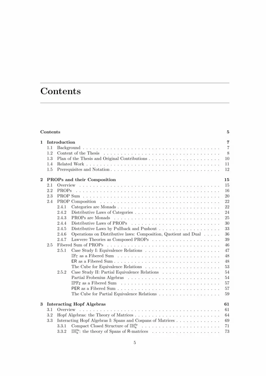
Contents
Contents 5
1 Introduction 71.1 Background . . . . . . . . . . . . . . . . . . . . . . . . . . . . . . . . . . . . . . . . 71.2 Content of the Thesis . . . . . . . . . . . . . . . . . . . . . . . . . . . . . . . . . . 81.3 Plan of the Thesis and Original Contributions . . . . . . . . . . . . . . . . . . . . . 101.4 Related Work . . . . . . . . . . . . . . . . . . . . . . . . . . . . . . . . . . . . . . . 111.5 Prerequisites and Notation . . . . . . . . . . . . . . . . . . . . . . . . . . . . . . . . 12
2 PROPs and their Composition 152.1 Overview . . . . . . . . . . . . . . . . . . . . . . . . . . . . . . . . . . . . . . . . . 152.2 PROPs . . . . . . . . . . . . . . . . . . . . . . . . . . . . . . . . . . . . . . . . . . 162.3 PROP Sum . . . . . . . . . . . . . . . . . . . . . . . . . . . . . . . . . . . . . . . . 202.4 PROP Composition . . . . . . . . . . . . . . . . . . . . . . . . . . . . . . . . . . . 22
2.4.1 Categories are Monads . . . . . . . . . . . . . . . . . . . . . . . . . . . . . . 222.4.2 Distributive Laws of Categories . . . . . . . . . . . . . . . . . . . . . . . . . 242.4.3 PROPs are Monads . . . . . . . . . . . . . . . . . . . . . . . . . . . . . . . 252.4.4 Distributive Laws of PROPs . . . . . . . . . . . . . . . . . . . . . . . . . . 302.4.5 Distributive Laws by Pullback and Pushout . . . . . . . . . . . . . . . . . . 332.4.6 Operations on Distributive laws: Composition, Quotient and Dual . . . . . 362.4.7 Lawvere Theories as Composed PROPs . . . . . . . . . . . . . . . . . . . . 39
2.5 Fibered Sum of PROPs . . . . . . . . . . . . . . . . . . . . . . . . . . . . . . . . . 462.5.1 Case Study I: Equivalence Relations . . . . . . . . . . . . . . . . . . . . . . 47
IFr as a Fibered Sum . . . . . . . . . . . . . . . . . . . . . . . . . . . . . . 48ER as a Fibered Sum . . . . . . . . . . . . . . . . . . . . . . . . . . . . . . . 48The Cube for Equivalence Relations . . . . . . . . . . . . . . . . . . . . . . 53
2.5.2 Case Study II: Partial Equivalence Relations . . . . . . . . . . . . . . . . . 54Partial Frobenius Algebras . . . . . . . . . . . . . . . . . . . . . . . . . . . 54IPFr as a Fibered Sum . . . . . . . . . . . . . . . . . . . . . . . . . . . . . 57PER as a Fibered Sum . . . . . . . . . . . . . . . . . . . . . . . . . . . . . . 57The Cube for Partial Equivalence Relations . . . . . . . . . . . . . . . . . . 59
3 Interacting Hopf Algebras 613.1 Overview . . . . . . . . . . . . . . . . . . . . . . . . . . . . . . . . . . . . . . . . . 613.2 Hopf Algebras: the Theory of Matrices . . . . . . . . . . . . . . . . . . . . . . . . . 643.3 Interacting Hopf Algebras I: Spans and Cospans of Matrices . . . . . . . . . . . . . 69
3.3.1 Compact Closed Structure of IHSp
R . . . . . . . . . . . . . . . . . . . . . . . 713.3.2 IHSp
R : the theory of Spans of R-matrices . . . . . . . . . . . . . . . . . . . . 73
5
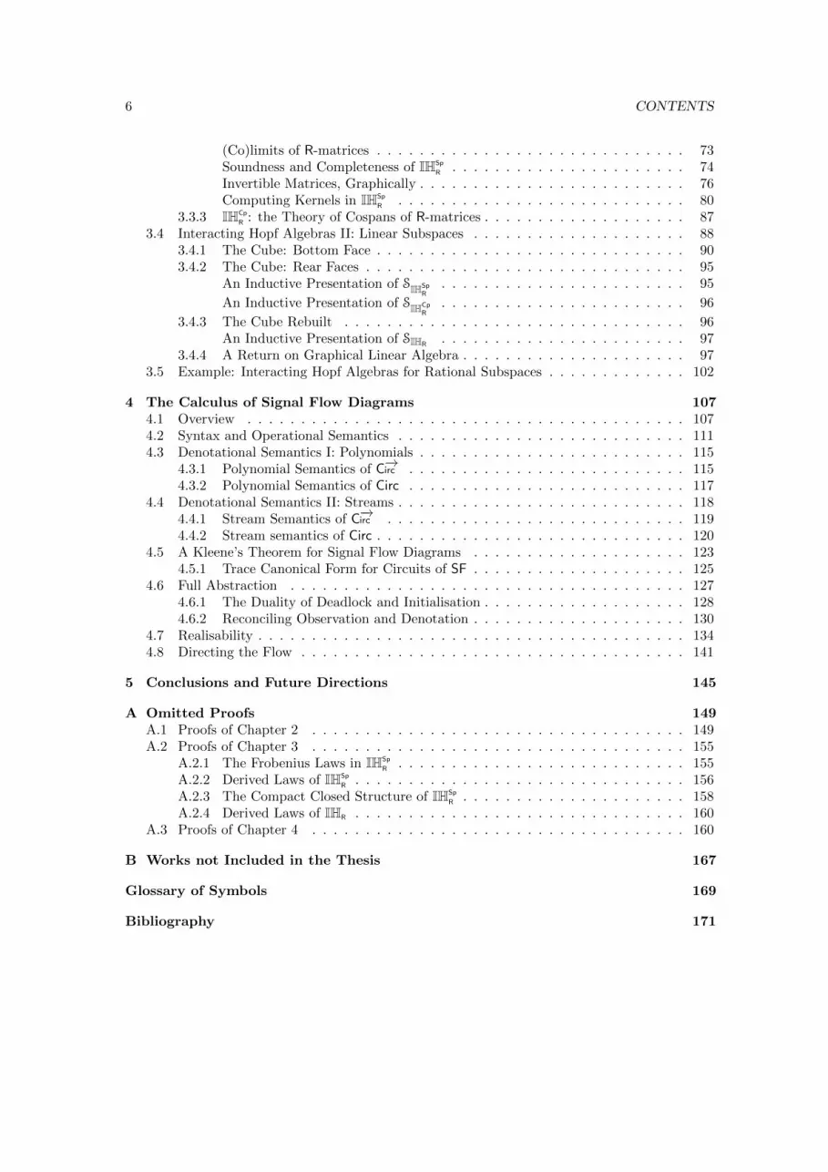
6 CONTENTS
(Co)limits of R-matrices . . . . . . . . . . . . . . . . . . . . . . . . . . . . . 73Soundness and Completeness of IHSp
R . . . . . . . . . . . . . . . . . . . . . . 74Invertible Matrices, Graphically . . . . . . . . . . . . . . . . . . . . . . . . . 76Computing Kernels in IHSp
R . . . . . . . . . . . . . . . . . . . . . . . . . . . 803.3.3 IHCp
R : the Theory of Cospans of R-matrices . . . . . . . . . . . . . . . . . . . 873.4 Interacting Hopf Algebras II: Linear Subspaces . . . . . . . . . . . . . . . . . . . . 88
3.4.1 The Cube: Bottom Face . . . . . . . . . . . . . . . . . . . . . . . . . . . . . 903.4.2 The Cube: Rear Faces . . . . . . . . . . . . . . . . . . . . . . . . . . . . . . 95
An Inductive Presentation of SIHSpR
. . . . . . . . . . . . . . . . . . . . . . . 95
An Inductive Presentation of SIHCpR
. . . . . . . . . . . . . . . . . . . . . . . 96
3.4.3 The Cube Rebuilt . . . . . . . . . . . . . . . . . . . . . . . . . . . . . . . . 96An Inductive Presentation of SIHR
. . . . . . . . . . . . . . . . . . . . . . . 973.4.4 A Return on Graphical Linear Algebra . . . . . . . . . . . . . . . . . . . . . 97
3.5 Example: Interacting Hopf Algebras for Rational Subspaces . . . . . . . . . . . . . 102
4 The Calculus of Signal Flow Diagrams 1074.1 Overview . . . . . . . . . . . . . . . . . . . . . . . . . . . . . . . . . . . . . . . . . 1074.2 Syntax and Operational Semantics . . . . . . . . . . . . . . . . . . . . . . . . . . . 1114.3 Denotational Semantics I: Polynomials . . . . . . . . . . . . . . . . . . . . . . . . . 115
4.3.1 Polynomial Semantics of C−→irc . . . . . . . . . . . . . . . . . . . . . . . . . . 1154.3.2 Polynomial Semantics of Circ . . . . . . . . . . . . . . . . . . . . . . . . . . 117
4.4 Denotational Semantics II: Streams . . . . . . . . . . . . . . . . . . . . . . . . . . . 1184.4.1 Stream Semantics of C−→irc . . . . . . . . . . . . . . . . . . . . . . . . . . . . 1194.4.2 Stream semantics of Circ . . . . . . . . . . . . . . . . . . . . . . . . . . . . . 120
4.5 A Kleene’s Theorem for Signal Flow Diagrams . . . . . . . . . . . . . . . . . . . . 1234.5.1 Trace Canonical Form for Circuits of SF . . . . . . . . . . . . . . . . . . . . 125
4.6 Full Abstraction . . . . . . . . . . . . . . . . . . . . . . . . . . . . . . . . . . . . . 1274.6.1 The Duality of Deadlock and Initialisation . . . . . . . . . . . . . . . . . . . 1284.6.2 Reconciling Observation and Denotation . . . . . . . . . . . . . . . . . . . . 130
4.7 Realisability . . . . . . . . . . . . . . . . . . . . . . . . . . . . . . . . . . . . . . . . 1344.8 Directing the Flow . . . . . . . . . . . . . . . . . . . . . . . . . . . . . . . . . . . . 141
5 Conclusions and Future Directions 145
A Omitted Proofs 149A.1 Proofs of Chapter 2 . . . . . . . . . . . . . . . . . . . . . . . . . . . . . . . . . . . 149A.2 Proofs of Chapter 3 . . . . . . . . . . . . . . . . . . . . . . . . . . . . . . . . . . . 155
A.2.1 The Frobenius Laws in IHSp
R . . . . . . . . . . . . . . . . . . . . . . . . . . . 155A.2.2 Derived Laws of IHSp
R . . . . . . . . . . . . . . . . . . . . . . . . . . . . . . . 156A.2.3 The Compact Closed Structure of IHSp
R . . . . . . . . . . . . . . . . . . . . . 158A.2.4 Derived Laws of IHR . . . . . . . . . . . . . . . . . . . . . . . . . . . . . . . 160
A.3 Proofs of Chapter 4 . . . . . . . . . . . . . . . . . . . . . . . . . . . . . . . . . . . 160
B Works not Included in the Thesis 167
Glossary of Symbols 169
Bibliography 171
Chapter 1
Introduction
1.1 Background
Scientists in diverse fields use diagrammatic formalisms to reason about various kinds of net-works, or compound systems. Examples include electrical circuits, signal flow graphs, Penroseand Feynman diagrams, proof nets, Bayesian networks, Petri nets, Kahn process networks, UMLspecifications, amongst many others.
These diagrams are formalised to various extent and the mathematics that lies behind theintended meaning of diagrams in several such families is, by now, well-understood. An illustrativeexample are signal flow graphs, foundational structures widely used in control theory and engineer-ing since the 1950’s, which are traditionally translated into systems of equations and then solvedusing standard techniques. This perspective is influenced by physics, where a system is typicallymodeled by a continuous state-space and the interactions that may occur in it are expressed ascontinuous state-space transformations, e.g. using differential equations.
Computer science has a rather different approach to modeling. Rather than on global be-haviour, the focus is on local, rule-based interactions — typically, occurring in a discrete state-space. The formal semantics of programming languages rests on cornerstones such as composition-ality, types and the use of methods from algebra and logic. In recent years, these principles havestarted to be fruitfully transferred from one-dimensional syntax to the analysis of diagrammaticlanguages. Monoidal categories have been widely recognised [10, 1, 7, 89] as the right mathemati-cal setting in which diagrammatic notations can be studied in a compositional, resource sensitivefashion. Arrows of a monoidal category enjoy a graphical rendition as string diagrams [63, 100]and the two ways — composition and monoidal product — of combining arrows are representedpictorially, respectively, by horizontal and vertical juxtaposition of diagrams.
The main actors of our developments are PROPs (Product and Permutation categories [79]),which are symmetric monoidal categories with objects the natural numbers. PROPs can serve bothas a syntax and as a semantics for graphical languages. Also, similarly to Lawvere theories [77, 60],they naturally support the expression of an algebraic structure describing equivalence of stringdiagrams.
We mention two illustrative examples of this approach. The first concerns concurrency theory :in this area coexist traditional graphical formalisms, like Petri nets [92], and the more recentprocess calculi, like CCS [83], CSP [57] and the π-calculus [98]. In the last two decades, someapproaches [33, 103, 32] attempted to merge the benefits of the two worlds by modeling Petrinets in a compositional way, as graphical process algebras formally described in the frameworkof PROPs. A proposal that naturally fits this picture is the Petri calculus [103]. The syntax isgiven by a PROP Petri whose arrows n → m are bounded Petri nets with n ports on the left
7
8 CHAPTER 1. INTRODUCTION
and m on the right, freely constructed starting from a small set of connectors. The meaning ofthese diagrams is given in terms of transition systems whose transitions have two labels, intuitivelycorresponding to left and right boundary of a Petri net: these systems also form a PROP 2LTS.The compositional semantics is given as a PROP functor taking a Petri net to its state graph.
Petri→ 2LTS
The equations between string diagrams which axiomatise this semantics are subject of ongoingwork [104]. Interestingly, the identified algebraic theory is not far removed from those appearingin compositional approaches to quantum information, like the ZX-calculus [41, 42]. This is oursecond motivating example of diagrammatic formalism, originated in the research programme ofcategorical quantum mechanics [1, 2], whose aim is to develop high-level methods — informed bythe formal semantics of programming languages — for quantum physics. The ZX-calculus is analgebra of interacting quantum observables, which can be presented as a PROP ZX whose stringdiagrams represent physical processes. The equations of ZX describe the interplay of familiarstructures such as Frobenius algebras and Hopf algebras, which will also appear in our develop-ments. The meaning of diagrams of ZX is given by linear maps between finite-dimensional Hilbertspaces, forming a PROP HS.
ZX→ HS
1.2 Content of the Thesis
The first main contribution of this thesis is a characterisation of the PROP SVk whose arrowsn → m are linear subspaces of kn × km, for a field k, and composition is relational. This is aparticularly important domain of interpretation for many diagrammatic languages: the meaningof well-behaved classes of systems — like the signal flow graphs and certain families of Petri netsand quantum processes — can be typically expressed in terms of linear subspaces. Our result is apresentation by generators and equations of the PROP IH of string diagrams whose free model isSVk. That means, there is an interpretation of the diagrams of IH as subspaces of SVk, which isalso a (symmetric monoidal) isomorphism
IH∼=−→ SVk.
The significance of the result is two-fold. On the one hand, we contend that IH is a canonicalsyntax for linear algebra. Traditional linear algebra abounds in different encodings of the sameentities: for instance, spaces are described as a collection of basis elements or as the solution setto a system of equations; matrices, and matrix-related concepts are used ubiquitously as stopgap,common notational conveniences. IH provides an uniform description for linear maps, spaces,kernels, etc. based on a small set of simple string diagrams as primitives. Standard methodslike Gaussian elimination can be faithfully mimicked in the graphical language, resulting in analternative, often insightful perspective on the subject matter.
On a different viewpoint, we believe that the equational theory of IH is of independent interest,as it describes fundamental algebraic structures — Hopf algebras and Frobenius algebras — whichare at the heart of graphical formalisms as seemingly diverse as categorical quantum mechanics,signal flow graphs, simple electrical circuits and Petri nets. Our characterisation enlightens theprovenance of these axioms and reveals their linear algebraic nature.
The name IH stands for interacting Hopf algebras. Indeed, we construct IH modularly, startingfrom the PROP HA — freely generated by the equations of Hopf algebras — and its oppositePROP HAop . Using Lack’s technique for composing PROPs [71], we define two distributive lawsthat describe different ways of letting HA and HAop interact. IH is the result of merging theequational theories generated by the two distributive laws. This modular account of IH is actuallycrucial in constructing the isomorphism IH ∼= SVk — both with an inductive definition and auniversal property — and will be useful in a number of other ways in our developments. Moreabstractly, our analysis gives new insights on the interplay of Frobenius and Hopf algebras: for
1.2. CONTENT OF THE THESIS 9
instance, while the authors of the ZX-calculus initially regarded the Frobenius structures as morefundamental, our modular construction reveals that the constituting blocks are Hopf algebras, andthe Frobenius equations arise by their composition. In fact, IH axiomatise the phase-free fragmentof ZX.
Our second main contribution is the use of IH to develop a formal theory of signal processing inwhich circuits are first-class citizens. We introduce the signal flow calculus and analyse it using thestandard methods of programming language theory. The calculus is based on a string diagrammaticsyntax, whose terms are meant to represent signal processing circuits. A key feature which makesour language different from similar proposals is that there is no primitive for recursion: feedbacksare a derived notion. Moreover, the wires in our circuits are non-directed and thus there are noassumptions about causal direction of signal flow, allowing us to forego traditional restrictionssuch as connecting “inputs” to “outputs”. This motivates our formulation of the denotationalsemantics in terms of linear relations rather than functions. Circuit diagrams form a PROP Circand the (compositional) semantics of a circuit c : n→ m is given by a functor
〈〈·〉〉 : Circ→ SVk((x))
where we regard the subspace 〈〈c〉〉 ⊆ k((x))n×k((x))m as a relation between k((x))n and k((x))m.Here k((x)) is the field of Laurent series, a generalised notion of stream typical in algebraicapproaches [11] to signal processing. We are able to characterise ordinary signal flow graphs —with information flowing from inputs on the left to outputs on the right — as a certain subclassof Circ, whose semantics are precisely the rational behaviours in SVk((x)).
Our design choices make the syntax of Circ abstract enough to enable the use of IH to reasonabout equivalence of circuits. We prove that the equations of IH are a sound and complete axioma-tisation for the denotational semantics. This result supports our claim that signal flow graphsare first-class citizens of our theory: contrary to traditional approaches, there is a completelygraphical way of reasoning about graph transformations and their properties, without the need oftranslating them first into systems of equations.
A fully fledged theory of signal flow graphs demands an operational understanding of circuitdiagrams in Circ as executable state-machines. For this purpose, we equip the signal flow calculuswith a structural operational semantics and study the full-abstraction question: how denotationaland operational equivalence compare. Interestingly, it turns out that, in our approach, it is thepurely operational picture to be too concrete – two circuits that are denotationally equal mayexhibit different operational behaviour. The problem lies in the generosity of our syntax, whichallows for the formation of circuits in which flow directionality cannot be coherently determined.This is not problematic for the denotational semantics, which simply describes a relation betweenports, but it is for the operational semantics, which is instead deputed to capture the executionof circuits. We classify the ways in which the operational semantics may be less abstract than thedenotational semantics, and prove full-abstraction for all the circuits that are free of deadlocks andof initialisation steps. Interestingly, our argument relies on a syntactic characterisation of theseproperties, which reveals a connection with a duality that can be elegantly described using themodular character of IH.
Because the semantics is not fully abstract for the whole signal flow calculus, one may wonderabout the status of all those circuit diagrams — featuring deadlocks or initialisation steps — whichdo not have a clear operational status. Our answer is that they do not contribute by any meansto the expressivity of the calculus: we prove that, for any behaviour 〈〈c〉〉 denoted by a circuit c,there exists a circuit d, for which the operational semantics is fully abstract, that properly realises〈〈c〉〉, that is, 〈〈d〉〉 = 〈〈c〉〉. In the spirit of the diagrammatic approach, we formulate this result asa procedure effectively transforming c into d, using the equations of IH as the rewriting steps.
This realisability theorem is the culmination of our work. It makes us able to crystallise what webelieve is the main conceptual contribution of the signal flow calculus: a fully fledged operationaltheory of signal flow graphs as mathematical objects is possible without relying on primitivesfor flow directionality. Discarding the concept of causality is harmless, because the realisability
10 CHAPTER 1. INTRODUCTION
theorem guarantees that any diagram can be transformed into a proper circuit, for which theoperational semantics describes the step-by-step execution of a state machine. Moreover, it isbeneficial, because it is only by forgetting flow that we disclose the beautiful algebraic landscapeIH underlying signal flow graphs.
We believe that this lesson can be fruitfully applied to the categorical modeling of other dynam-ical systems, like electrical circuits and Kahn process networks. Hopefully, the modular techniquesthat we used to shape IH will contribute to a uniform methodology to axiomatise various kindsof behaviour, thus shedding light on the algebraic structure of a wider spectrum of computingdevices, as well as connecting them with existing approaches in quantum and concurrency theory.
1.3 Plan of the Thesis and Original Contributions
We give an overview of the structure of the thesis and pointers to the main contributions. Thereader may find at the beginning of each chapter a more detailed introduction and a synopsis.
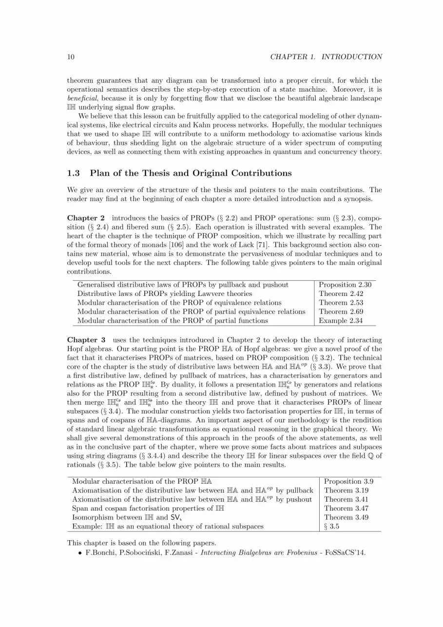
Chapter 2 introduces the basics of PROPs (§ 2.2) and PROP operations: sum (§ 2.3), compo-sition (§ 2.4) and fibered sum (§ 2.5). Each operation is illustrated with several examples. Theheart of the chapter is the technique of PROP composition, which we illustrate by recalling partof the formal theory of monads [106] and the work of Lack [71]. This background section also con-tains new material, whose aim is to demonstrate the pervasiveness of modular techniques and todevelop useful tools for the next chapters. The following table gives pointers to the main originalcontributions.
Generalised distributive laws of PROPs by pullback and pushout Proposition 2.30Distributive laws of PROPs yielding Lawvere theories Theorem 2.42Modular characterisation of the PROP of equivalence relations Theorem 2.53Modular characterisation of the PROP of partial equivalence relations Theorem 2.69Modular characterisation of the PROP of partial functions Example 2.34
Chapter 3 uses the techniques introduced in Chapter 2 to develop the theory of interactingHopf algebras. Our starting point is the PROP HA of Hopf algebras: we give a novel proof of thefact that it characterises PROPs of matrices, based on PROP composition (§ 3.2). The technicalcore of the chapter is the study of distributive laws between HA and HAop (§ 3.3). We prove thata first distributive law, defined by pullback of matrices, has a characterisation by generators andrelations as the PROP IHSp
R . By duality, it follows a presentation IHCp
R by generators and relationsalso for the PROP resulting from a second distributive law, defined by pushout of matrices. Wethen merge IHCp
R and IHSp
R into the theory IH and prove that it characterises PROPs of linearsubspaces (§ 3.4). The modular construction yields two factorisation properties for IH, in terms ofspans and of cospans of HA-diagrams. An important aspect of our methodology is the renditionof standard linear algebraic transformations as equational reasoning in the graphical theory. Weshall give several demonstrations of this approach in the proofs of the above statements, as wellas in the conclusive part of the chapter, where we prove some facts about matrices and subpacesusing string diagrams (§ 3.4.4) and describe the theory IH for linear subspaces over the field Q ofrationals (§ 3.5). The table below give pointers to the main results.
Modular characterisation of the PROP HA Proposition 3.9Axiomatisation of the distributive law between HA and HAop by pullback Theorem 3.19Axiomatisation of the distributive law between HA and HAop by pushout Theorem 3.41Span and cospan factorisation properties of IH Theorem 3.47Isomorphism between IH and SVk Theorem 3.49Example: IH as an equational theory of rational subspaces § 3.5
This chapter is based on the following papers.
• F.Bonchi, P.Sobocinski, F.Zanasi - Interacting Bialgebras are Frobenius - FoSSaCS’14.
1.4. RELATED WORK 11
• F.Bonchi, P.Sobocinski, F.Zanasi - Interacting Hopf Algebras - http://arxiv.org/abs/
1403.7048.
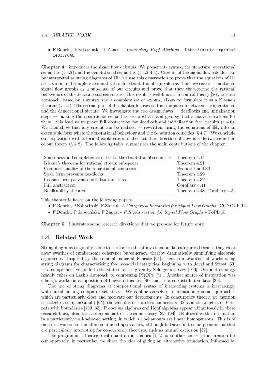
Chapter 4 introduces the signal flow calculus. We present its syntax, the structural operationalsemantics (§ 4.2) and the denotational semantics (§ 4.3-4.4). Circuits of the signal flow calculus canbe interpreted as string diagrams of IH: we use this observation to prove that the equations of IHare a sound and complete axiomatisation for denotational equivalence. Then we recover traditionalsignal flow graphs as a sub-class of our circuits and prove that they characterise the rationalbehaviours of the denotational semantics. This result is well-known in control theory [76], but ourapproach, based on a syntax and a complete set of axioms, allows to formulate it as a Kleene’stheorem (§ 4.5). The second part of the chapter focuses on the comparison between the operationaland the denotational picture. We investigate the two design flaws — deadlocks and initialisationsteps — making the operational semantics less abstract and give syntactic characterisations forthem: this lead us to prove full abstraction for deadlock and initialisation free circuits (§ 4.6).We then show that any circuit can be realised — rewritten, using the equations of IH, into anexecutable form where the operational behaviour and the denotation coincides (§ 4.7). We concludeour exposition with a formal explanation of the fact that direction of flow is a derivative notionof our theory (§ 4.8). The following table summarises the main contributions of the chapter.
Soundness and completeness of IH for the denotational semantics Theorem 4.14Kleene’s theorem for rational stream subspaces Theorem 4.21Compositionality of the operational semantics Proposition 4.36Span form prevents deadlocks Theorem 4.29Cospan form prevents initialisation steps Theorem 4.32Full abstraction Corollary 4.41Realisability theorem Theorem 4.48, Corollary 4.52
This chapter is based on the following papers.
• F.Bonchi, P.Sobocinski, F.Zanasi - A Categorical Semantics for Signal Flow Graphs - CONCUR’14.
• F.Bonchi, P.Sobocinski, F.Zanasi - Full Abstraction for Signal Flow Graphs - PoPL’15.
Chapter 5 illustrates some research directions that we propose for future work.
1.4 Related Work
String diagrams originally came to the fore in the study of monoidal categories because they clearaway swathes of cumbersome coherence bureaucracy, thereby dramatically simplifying algebraicarguments. Inspired by the seminal paper of Penrose [91], there is a tradition of works usingstring diagrams for characterising free monoidal categories, beginning with Joyal and Street [63]— a comprehensive guide to the state of art is given by Selinger’s survey [100]. Our methodologyheavily relies on Lack’s approach to composing PROPs [71]. Another source of inspiration wasCheng’s works on composition of Lawvere theories [40] and iterated distributive laws [39].
The use of string diagrams as compositional syntax of interacting systems is increasinglywidespread among computer scientists. We confine ourselves to mentioning some approacheswhich are particularly close and motivate our developments. In concurrency theory, we mentionthe algebra of Span(Graph) [65], the calculus of stateless connectors [32] and the algebra of Petrinets with boundaries [103, 33]. Frobenius algebras and Hopf algebras appear ubiquitously in theseresearch lines, often interacting as part of the same theory [32, 104]: IH describes this interactionin a particularly well-behaved setting, in which all behaviours are linear homogeneous. This is ofmuch relevance for the aforementioned approaches, although it leaves out some phenomena thatare particularly interesting for concurrency theorists, such as mutual exclusion [32].
The programme of categorical quantum mechanics [1, 2] is another source of inspiration forour approach: in particular, we share the idea of giving an alternative foundation, informed by
12 CHAPTER 1. INTRODUCTION
computer science, category theory and logic, to a subject which is traditionally studied withnon-compositional methods. Our theory IH is particularly relevant for one of the most studiedformalisms in categorical quantum mechanics, namely the ZX-calculus [41, 42]. The equations ofIH are at the core of the ZX-calculus, which essentially only adds the properly quantum featuressuch as phase operators.
In this thesis we give presentations by generations and relations of various PROPs whose arrowsare well-known mathematical objects, such as (partial) functions, equivalence relations, matricesand subspaces. This kind of characterisation has been studied for different purposes in diverseareas. We want to mention in particular the research thread on two-dimensional rewriting [35,73, 75, 86] where presentations for PROPs of matrices [75], functions [35] and relations [73] arederived in a uniform way by the study of normal forms. Our work relies on a rather differentmethodology, being based on distributive laws instead of rewriting systems. Actually, there arepoints of contact between the two approaches, which could be fruitfully combined: we commentmore extensively on this in the conclusions (Chapter 5).
Closely related to rewriting approaches is the formalism of interaction nets [72], a diagrammaticlanguage which generalises proof nets [52, 46] and is adapted to the encoding various computationalmodels such as Turing machines and cellular automata [74]. Apparently, IH cannot be reproducedusing interaction nets: the form of interaction that it expresses is of a more general kind, featuringdiagrams that communicate on multiple ports.
The earliest reference for signal flow graphs that we are aware of is Shannon’s 1942 technicalreport [101]. They appear to have been independently rediscovered by Mason in the 1950s [81]and subsequently gained foundational status in electrical engineering, signal processing and controltheory. Our vision of signal flow graphs is inspired by Willems’ behavioural approach [112, 111],which is the attempt to, in part, reexamine the central concepts of control theory without givingdefinitional status to derivable causal information such as direction of flow. Interestingly, signalflow graphs recently attracted coalgebraic modeling [96, 97, 12]. This line of research analyses thecoincidence of signal flow graphs, rational streams and a certain class of finite weighted automatausing coinduction and the theory of coalgebras. The main difference with these works is that wegive a formal syntax for circuits and a sound and complete axiomatisation for semantic equivalence.These features are also present in the work of Milius [82], but its syntax is one-dimensional anddiagrams are just used for notational convenience. Also, the circuit language is of a rather differentflavour; most notably, it features primitives for recursion, which are not necessary in our approach.
Another recent approach to signal flow graphs is Baez and Erbele’s manuscript [8], whichappeared on arXiv shortly after our works [24, 22] and the submission of [21]. In [8], the authorsindependently give an equational presentation for PROPs of linear subspaces, which is equivalentto our theory IH — this paper is inserted in Baez’s programme of network theory [7], whichaims at uniformly describing various kinds of networks used by engineers, ecologists and otherscientists using methods from (higher) category theory. A major difference with [8] is in the use ofdistributive laws of PROPs, which is pervasive in our work and enables a number of analyses thatare hampered by a monolithic approach, most notably the characterisation of the isomorphism
IH∼=−→ SVk as a universal arrow and the span/cospan factorisation for IH. The modular account
of IH also means a different choice of primitives: in our approach, feedback is a derivative notion,being constructible by combining the generators of the building blocks HA and HAop of IH;instead, in [8] the “cup” and “cap” forming a feedback loop appear among the generators. Anothersignificant difference with [8] is that we give a formal operational semantics, which allows us tostudy full abstraction and realisability, and make a statement about the role of causality in signalflow theory.
1.5 Prerequisites and Notation
We assume familiarity with the basics of category theory (see e.g. [80, 29]), the definition ofsymmetric strict monoidal category [80, 100] (which we often abbreviate as SMC) and of bicate-gory [29, 15]. We write Cop for the opposite of a category C and x/C for the coslice category of C
1.5. PREREQUISITES AND NOTATION 13
under x ∈ C. Composition of arrows f : x→ y, g : y → z is indicated with f ; g : x→ z. We writeC[x, y] for the set of arrows from x to y in a small category C. It will be sometimes convenient
to indicate an arrow f : x → y of C as xf−→ y or x
f∈C−−−→ y. When naming objects and arrows is
unnecessary we simply write∈C−−→ or −→ if C is clear from the context. For C symmetric monoidal,
we use ⊕ for the monoidal product, I for the unit object and σx,y : x⊕y → y⊕x for the symmetryassociated with x, y ∈ C. For a natural number n > 0, n is the set {1, . . . , n} and 0 = ∅. Wereserve bold letters x,y, z,v,u,w for vectors over a field k. We write 0 for the zero vector (thelength will typically be clear from the context) and [v1, . . . ,vn] for the space spanned by vectorsv1, . . . ,vn. Also, ( ) is the unique element of the space with dimension zero.

Chapter 2
PROPs and their Composition
2.1 Overview
This chapter introduces the basics of the theory of PROPs, focusing on operations to combinePROPs to form richer structures.
PROPs — an abbreviation of product and permutation category — are symmetric monoidalcategories with objects the natural numbers. They made their first appearance in [79] as a meansto describe one-sorted algebraic theories. There is a close analogy between PROPs and Lawveretheories [77, 60], with the former being strictly more general. Lawvere theories describe thealgebraic structure borne on an object of a cartesian category, whereas PROPs fulfill the samepurpose in arbitrary symmetric monoidal categories. We will further explore the relation betweenthe two notions in § 2.4.7.
PROPs share the ability to describe non-cartesian contexts with operads [78], another familyof categories adapted to the study of universal algebra. However, whereas operads are restrictedto operations with coarity 1, PROPs can describe operations with arbitrary arity and coarity.For instance, the level of generality of PROPs is required to express Frobenius algebras and Hopfalgebras, which are central in our developments.
Just as Lawvere theories and operads, PROPs allow natural constructions that arise in universalalgebra: in this chapter we focus on three of them. The first is the sum of theories, which simplytakes the disjoint union of the generators and of the equations. We also study the fibered sum,in which some structure in common between the summed theories may be identified. The mainfocus of our developments will be on a third kind of construction: the composition of theories bymeans of a distributive law. This operation, which for PROPs has been developed by Lack [71], ishelpful to describe the modular nature of many algebraic structures. To explain the core intuition,a simple motivating example is the one of a ring, presented by equations:
(a+ b) + c = a+ (b+ c)
a+ b = b+ a
a+ 0 = a
a+ (−a) = 0
(a · b) · c = a · (b · c)a · 1 = a
1 · a = a
a · (b+ c) = (a · b) + (a · c)(b+ c) · a = (b · a) + (c · a).
The idea is to read these equations according to the following pattern: the first column definesan abelian group, the second a monoid and the third the distributivity of the monoid over thegroup. One can make this formal by expressing the monoid and the abelian group as monads;then, orienting left-to-right the equations in the third column defines a distributive law of monadsin the sense of Beck [14]. This law yields a new monad, presented by all the above equations: thusrings arise by the composition of monoids with abelian groups.
15
16 CHAPTER 2. PROPS AND THEIR COMPOSITION
Note that, differently from sum and fibered sum, a distributive law yields new equationsexpressing the interaction of the theories involved. We will see in a number of examples thatPROP composition, combined with sum and fibered sum, is a powerful heuristics to ease theanalysis of complex algebraic structure, allowing to understand them modularly, similarly to thecase of rings.
This methodology will be applied to the PROPs of commutative monoids, of bialgebras andof special Frobenius algebras. All these examples are also included in [71]. We will also show,as original contributions, the modular understanding of the PROP of partial functions (Exam-ple 2.34), of equivalence relations (§ 2.5.1) and of partial equivalence relations (§ 2.5.2). Ouranalysis will produce a presentation by generators and equations for each of these PROPs. Forour purposes, it will be also of importance to develop some ramifications of the composing PROPtechnique: in particular, we show how Lack’s definition of composition can be extended to includedistributive laws by pullback and pushout (§ 2.4.5); we recast in the setting of PROPs some basicoperations on distributive laws such as composition, quotient and dual (§ 2.4.6); finally, we studya family of distributive laws yielding Lawvere theories as the result of composition (§ 2.4.7). Thesecontributions are also original, when not stated otherwise. They are included to demonstrate thepervasiveness of the modular approach, as well as to give a series of useful techniques for thedevelopments of the next chapter.
Synopsis The chapter is organised as follows.
• § 2.2 introduces PROPs and their graphical language of string diagrams. We describe thegeneration of a PROP by a signature and equations.
• § 2.3 introduces the operation of PROP sum.
• § 2.4 illustrates the operation of PROP composition. We first explain this form of compo-sition in the simpler case of plain categories: categories can be thought as monads (§ 2.4.1)and composed by distributive laws (§ 2.4.2). We then describe this approach for the caseof PROPs: § 2.4.3 shows how PROPs can be thought as monads and § 2.4.4 introducesdistributive laws of PROPs.
In the second part we investigate some ramifications of this technique. In § 2.4.5 we show howto define distributive laws by pullback and pushouts. § 2.4.6 explains some basic operationson distributive laws: composition, quotient and dual. Finally, in § 2.4.7 we investigate afamily of distributive law of PROPs yielding Lawvere theories as the result of composition.
• § 2.5 discusses the operation of fibered sum of PROPs. We give a detailed example of howfibered sum, along with PROP sum and composition, can be used to give a presentationby generators and equations to the PROP of equivalence relations (§ 2.5.1) and of partialequivalence relations (§ 2.5.2).
We remark that the material presented in § 2.5.1-2.5.2 is not needed in the sequel, thus itcan be safely skipped on a first reading. Nonetheless, those sections offer warm-up examplesof the “cube” construction that will be pivotal in Chapter 3.
2.2 PROPs
Our exposition is founded on categories called PROPs (product and permutation categories [79]).
Definition 2.1. A PROP is a symmetric strict monoidal category with objects the natural num-bers, where ⊕ on objects is addition. Morphisms between PROPs are strict symmetric monoidalfunctors that are identity on objects: PROPs and their morphisms form the category PROP.
We call a sub-PROP a sub-category of a PROP T which is also a PROP.
2.2. PROPS 17
(t1 ; t3)⊕ (t2 ; t4) = (t1 ⊕ t2) ; (t3 ⊕ t4)
(t1 ; t2) ; t3 = t1 ; (t2 ; t3) idn ; c = c = c ; idm(t1 ⊕ t2)⊕ t3 = t1 ⊕ (t2 ⊕ t3) id0 ⊕ t = t = t⊕ id0
σ1,1 ;σ1,1 = id2 (t⊕ idz) ;σm,z = σn,z ; (idz ⊕ t)
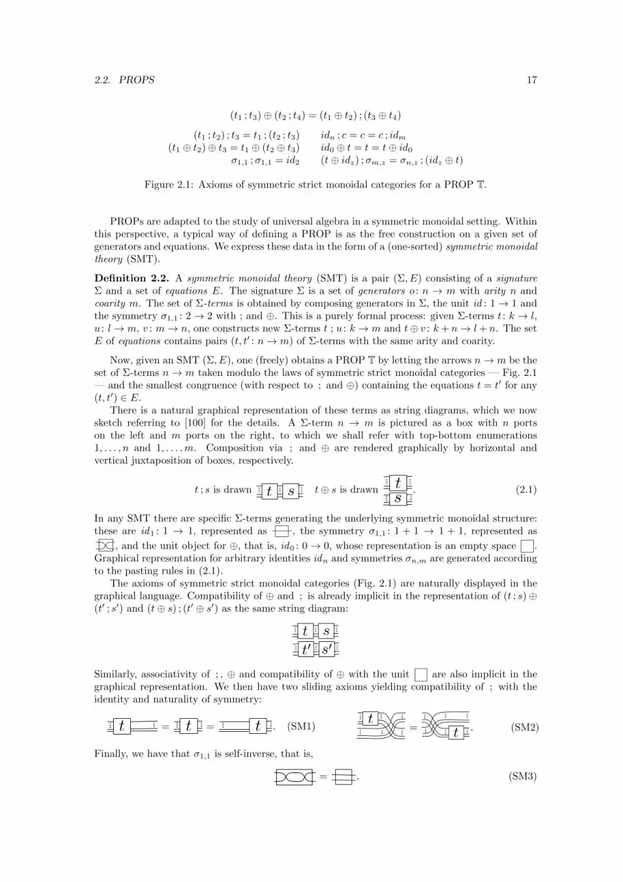
Figure 2.1: Axioms of symmetric strict monoidal categories for a PROP T.
PROPs are adapted to the study of universal algebra in a symmetric monoidal setting. Withinthis perspective, a typical way of defining a PROP is as the free construction on a given set ofgenerators and equations. We express these data in the form of a (one-sorted) symmetric monoidaltheory (SMT).
Definition 2.2. A symmetric monoidal theory (SMT) is a pair (Σ, E) consisting of a signatureΣ and a set of equations E. The signature Σ is a set of generators o : n → m with arity n andcoarity m. The set of Σ-terms is obtained by composing generators in Σ, the unit id : 1→ 1 andthe symmetry σ1,1 : 2→ 2 with ; and ⊕. This is a purely formal process: given Σ-terms t : k → l,u : l→ m, v : m→ n, one constructs new Σ-terms t ; u : k → m and t⊕ v : k+ n→ l+ n. The setE of equations contains pairs (t, t′ : n→ m) of Σ-terms with the same arity and coarity.
Now, given an SMT (Σ, E), one (freely) obtains a PROP T by letting the arrows n→ m be theset of Σ-terms n→ m taken modulo the laws of symmetric strict monoidal categories — Fig. 2.1— and the smallest congruence (with respect to ; and ⊕) containing the equations t = t′ for any(t, t′) ∈ E.
There is a natural graphical representation of these terms as string diagrams, which we nowsketch referring to [100] for the details. A Σ-term n → m is pictured as a box with n portson the left and m ports on the right, to which we shall refer with top-bottom enumerations1, . . . , n and 1, . . . ,m. Composition via ; and ⊕ are rendered graphically by horizontal andvertical juxtaposition of boxes, respectively.
t ; s is drawn st t⊕ s is drawn ts
. (2.1)
In any SMT there are specific Σ-terms generating the underlying symmetric monoidal structure:these are id1 : 1 → 1, represented as , the symmetry σ1,1 : 1 + 1 → 1 + 1, represented as
, and the unit object for ⊕, that is, id0 : 0→ 0, whose representation is an empty space .Graphical representation for arbitrary identities idn and symmetries σn,m are generated accordingto the pasting rules in (2.1).
The axioms of symmetric strict monoidal categories (Fig. 2.1) are naturally displayed in thegraphical language. Compatibility of ⊕ and ; is already implicit in the representation of (t ; s)⊕(t′ ; s′) and (t⊕ s) ; (t′ ⊕ s′) as the same string diagram:
stst 00
Similarly, associativity of ; , ⊕ and compatibility of ⊕ with the unit are also implicit in thegraphical representation. We then have two sliding axioms yielding compatibility of ; with theidentity and naturality of symmetry:
t = t = t . (SM1)t
= t . (SM2)
Finally, we have that σ1,1 is self-inverse, that is,
= . (SM3)
18 CHAPTER 2. PROPS AND THEIR COMPOSITION
As expected, graphical reasoning is sound and complete, in the sense that an equality betweenarrows of a PROP follows from the axioms in Fig. 2.1 if and only if it can be derived in thegraphical language by using (SM1)-(SM3) — cf. [63, 100].
Convention 2.3. In equational reasoning, we will often orient equations of SMTs: the notationc1 ⇒ c2 means the use of the equation c1 = c2 to rewrite a string diagram c1 into c2.
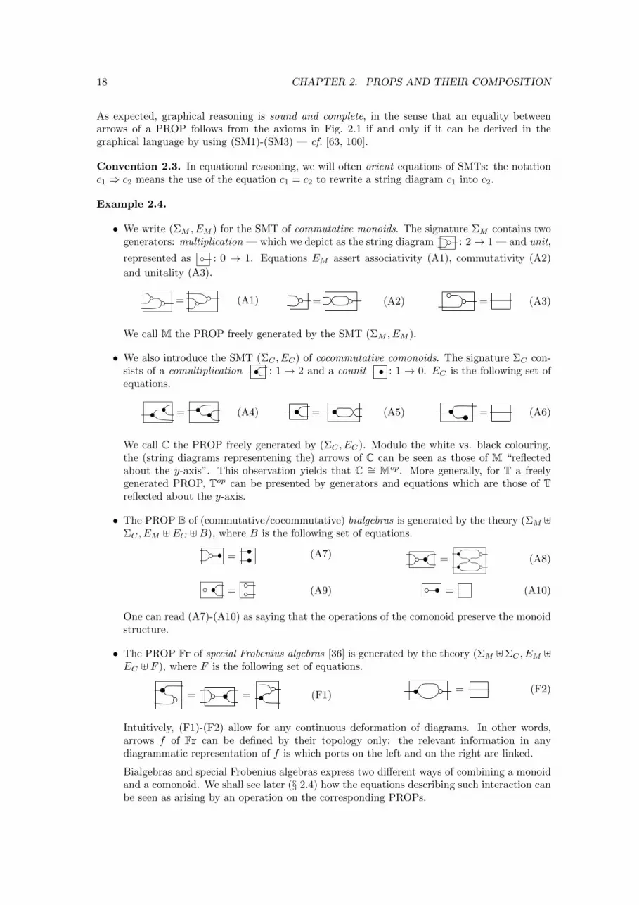
Example 2.4.
• We write (ΣM , EM ) for the SMT of commutative monoids. The signature ΣM contains twogenerators: multiplication — which we depict as the string diagram : 2→ 1 — and unit,
represented as : 0 → 1. Equations EM assert associativity (A1), commutativity (A2)
and unitality (A3).
= (A1) = (A2) = (A3)
We call M the PROP freely generated by the SMT (ΣM , EM ).
• We also introduce the SMT (ΣC , EC) of cocommutative comonoids. The signature ΣC con-sists of a comultiplication : 1 → 2 and a counit : 1 → 0. EC is the following set ofequations.
= (A4) = (A5) = (A6)
We call C the PROP freely generated by (ΣC , EC). Modulo the white vs. black colouring,the (string diagrams representening the) arrows of C can be seen as those of M “reflectedabout the y-axis”. This observation yields that C ∼= Mop. More generally, for T a freelygenerated PROP, Top can be presented by generators and equations which are those of Treflected about the y-axis.
• The PROP B of (commutative/cocommutative) bialgebras is generated by the theory (ΣM ]ΣC , EM ] EC ]B), where B is the following set of equations.
= (A7)
= (A9)
= (A8)
= (A10)
One can read (A7)-(A10) as saying that the operations of the comonoid preserve the monoidstructure.
• The PROP Fr of special Frobenius algebras [36] is generated by the theory (ΣM ]ΣC , EM ]EC ] F ), where F is the following set of equations.
= = (F1)= (F2)
Intuitively, (F1)-(F2) allow for any continuous deformation of diagrams. In other words,arrows f of Fr can be defined by their topology only: the relevant information in anydiagrammatic representation of f is which ports on the left and on the right are linked.
Bialgebras and special Frobenius algebras express two different ways of combining a monoidand a comonoid. We shall see later (§ 2.4) how the equations describing such interaction canbe seen as arising by an operation on the corresponding PROPs.
2.2. PROPS 19
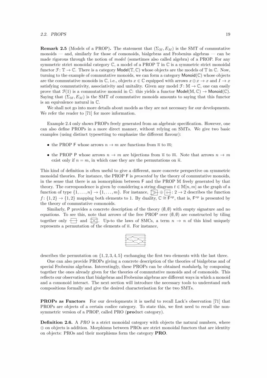
Remark 2.5 (Models of a PROP). The statement that (ΣM , EM ) is the SMT of commutativemonoids — and, similarly for those of comonoids, bialgebras and Frobenius algebras — can bemade rigorous through the notion of model (sometimes also called algebra) of a PROP. For anysymmetric strict monoidal category C, a model of a PROP T in C is a symmetric strict monoidalfunctor F : T→ C. There is a category Model(T,C) whose objects are the models of T in C. Now,turning to the example of commutative monoids, we can form a category Monoid(C) whose objectsare the commutative monoids in C, i.e., objects x ∈ C equipped with arrows x⊕x→ x and I → xsatisfying commutativity, associativity and unitality. Given any model F : M→ C, one can easilyprove that F(1) is a commutative monoid in C: this yields a functor Model(M,C) → Monoid(C).Saying that (ΣM , EM ) is the SMT of commutative monoids amounts to saying that this functoris an equivalence natural in C.
We shall not go into more details about models as they are not necessary for our developments.We refer the reader to [71] for more information.
Example 2.4 only shows PROPs freely generated from an algebraic specification. However, onecan also define PROPs in a more direct manner, without relying on SMTs. We give two basicexamples (using distinct typesetting to emphasize the different flavour):
• the PROP F whose arrows n→ m are functions from n to m;
• the PROP P whose arrows n → m are bijections from n to m. Note that arrows n → mexist only if n = m, in which case they are the permutations on n.
This kind of definition is often useful to give a different, more concrete perspective on symmetricmonoidal theories. For instance, the PROP F is presented by the theory of commutative monoids,in the sense that there is an isomorphism between F and the PROP M freely generated by thattheory. The correspondence is given by considering a string diagram t ∈M[n,m] as the graph of afunction of type {1, . . . , n} → {1, . . . ,m}. For instance, ⊕ : 2→ 2 describes the function
f : {1, 2} → {1, 2} mapping both elements to 1. By duality, C ∼= Fop , that is, Fop is presented bythe theory of commutative comonoids.
Similarly, P provides a concrete description of the theory (∅, ∅) with empty signature and noequations. To see this, note that arrows of the free PROP over (∅, ∅) are constructed by tiling
together only and . Up-to the laws of SMCs, a term n → n of this kind uniquelyrepresents a permutation of the elements of n. For instance,
describes the permutation on {1, 2, 3, 4, 5} exchanging the first two elements with the last three.
One can also provide PROPs giving a concrete description of the theories of bialgebras and ofspecial Frobenius algebras. Interestingly, these PROPs can be obtained modularly, by composingtogether the ones already given for the theories of commutative monoids and of comonoids. Thisreflects our observation that bialgebras and Frobenius algebras are different ways in which a monoidand a comonoid interact. The next section will introduce the necessary tools to understand suchcompositions formally and give the desired characterisation for the two SMTs.
PROPs as Functors For our developments it is useful to recall Lack’s observation [71] thatPROPs are objects of a certain coslice category. To state this, we first need to recall the non-symmetric version of a PROP, called PRO (product category).
Definition 2.6. A PRO is a strict monoidal category with objects the natural numbers, where⊕ on objects is addition. Morphisms between PROs are strict monoidal functors that are identityon objects: PROs and their morphisms form the category PRO.
20 CHAPTER 2. PROPS AND THEIR COMPOSITION
Roughly, a PROP T can be described as a PRO that contains a copy of P, which forms itssymmetry structure. This is made precise by observing that P is the initial object in the categoryPROP. The unique PROP morphism AT : P → T can be inductively defined starting from theassignment of the symmetry σ1,1 : 2→ 2 to the permutation p1,1 ∈ P[2, 2] which interchanges thetwo elements of 2 = {1, 2} — all the other permutations in P are obtained from p1,1 and theidentities via ; and ⊕. Now, by regarding AT : P → T as a PRO morphism, one can define afunctor from PROP to the coslice category P/PRO, which maps T to AT : P → T. By initialityof P, this functor is fully faithful and thus exhibits PROP as a full subcategory of P/PRO.
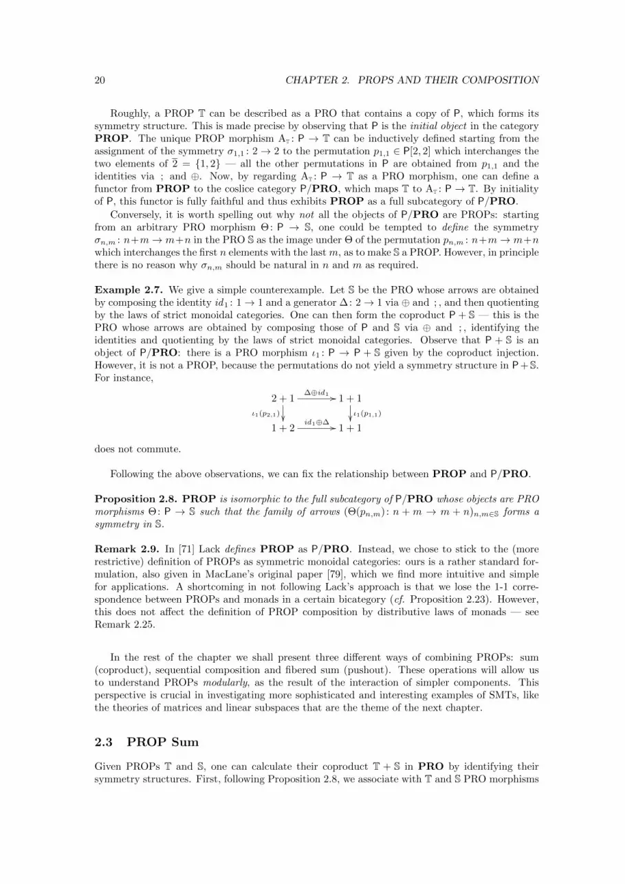
Conversely, it is worth spelling out why not all the objects of P/PRO are PROPs: startingfrom an arbitrary PRO morphism Θ: P → S, one could be tempted to define the symmetryσn,m : n+m→ m+n in the PRO S as the image under Θ of the permutation pn,m : n+m→ m+nwhich interchanges the first n elements with the last m, as to make S a PROP. However, in principlethere is no reason why σn,m should be natural in n and m as required.
Example 2.7. We give a simple counterexample. Let S be the PRO whose arrows are obtainedby composing the identity id1 : 1→ 1 and a generator ∆: 2→ 1 via ⊕ and ; , and then quotientingby the laws of strict monoidal categories. One can then form the coproduct P + S — this is thePRO whose arrows are obtained by composing those of P and S via ⊕ and ; , identifying theidentities and quotienting by the laws of strict monoidal categories. Observe that P + S is anobject of P/PRO: there is a PRO morphism ι1 : P → P + S given by the coproduct injection.However, it is not a PROP, because the permutations do not yield a symmetry structure in P+S.For instance,
2 + 1
ι1(p2,1)��
∆⊕id1 // 1 + 1
ι1(p1,1)��
1 + 2id1⊕∆ // 1 + 1
does not commute.
Following the above observations, we can fix the relationship between PROP and P/PRO.
Proposition 2.8. PROP is isomorphic to the full subcategory of P/PRO whose objects are PROmorphisms Θ: P → S such that the family of arrows (Θ(pn,m) : n + m → m + n)n,m∈S forms asymmetry in S.
Remark 2.9. In [71] Lack defines PROP as P/PRO. Instead, we chose to stick to the (morerestrictive) definition of PROPs as symmetric monoidal categories: ours is a rather standard for-mulation, also given in MacLane’s original paper [79], which we find more intuitive and simplefor applications. A shortcoming in not following Lack’s approach is that we lose the 1-1 corre-spondence between PROPs and monads in a certain bicategory (cf. Proposition 2.23). However,this does not affect the definition of PROP composition by distributive laws of monads — seeRemark 2.25.
In the rest of the chapter we shall present three different ways of combining PROPs: sum(coproduct), sequential composition and fibered sum (pushout). These operations will allow usto understand PROPs modularly, as the result of the interaction of simpler components. Thisperspective is crucial in investigating more sophisticated and interesting examples of SMTs, likethe theories of matrices and linear subspaces that are the theme of the next chapter.
2.3 PROP Sum
Given PROPs T and S, one can calculate their coproduct T + S in PRO by identifying theirsymmetry structures. First, following Proposition 2.8, we associate with T and S PRO morphisms
2.3. PROP SUM 21
AT : P→ T and AS : P→ S. Then, let T + S be given by the following pushout in PRO:
PAS //
AT��
S
��T // T + S
Proposition 2.10. T + S is the coproduct of T and S in PROP.
Proof We check that T + S is a PROP. Pushouts in PRO may be calculated as in Cat: thatmeans, arrows of T + S are given by (1) combining the arrows of T and S via ⊕ and ; , and (2)
identifying the permutations, i.e. the arrows∈T−−→ and
∈S−−→ in the image of the same arrow∈P−−→.
PRO morphisms T→ T + S←− S simply interpret arrows of T and S as arrows of T + S.We define the symmetry σn,m : n+m→ m+n in T+S to be the image under AT (equivalently,
under AS) of the permutation in P which interchanges the first n elements with the last m. Thisarrow is a symmetry (i.e., a natural isomorphism) in T by definition of AT, and also in S bydefinition of AS. Since arrows in T + S are just combinations of arrows of T and S, it follows thatσn,m is an isomorphism natural in n and m also in T+S. Therefore, T+S is a symmetric monoidalcategory and thus a PROP.
Since T, S and T+S are PROPs and PROP is a full subcategory of P/PRO (Proposition 2.8),it follows that arrows T→ T + S←− S in the above diagram are PROP morphisms: we let thembe the coproduct injections. With an analogous reasoning it is straitghtforward to check that theuniversal property of T + S as pushout in PRO yields the one as coproduct in PROP. �
When T and S are freely generated PROPs, the above description provides a simple recipe fora presentation of T + S.
Proposition 2.11. Suppose that T and S are PROPs freely generated by SMTs (Σ1, E1) and(Σ2, E2) respectively. Then T + S is freely generated by the sum of theories (Σ1 ] Σ2, E1 ] E2).
By Proposition 2.11, arrows n → m of T + S are Σ1 ] Σ2-terms quotiented by E1 ] E2. Wecan always represent these arrows as sequences
n∈T−−→ ∈S−−→ ∈T−−→ . . .
∈S−−→ ∈T−−→ m (2.2)
of Σ1- and Σ2-terms modulo E1 and E2. To see this, recall that Σ1 ]Σ2-terms are constructed bycomposing the generators of Σ1]Σ2, id : 1→ 1 and σ1,1 : 2→ 2 with ; and ⊕. Then, functorialityof ⊕ — cf. Fig.2.1 — allows to put any term f ⊕ g consisting of a Σ1-term f and a Σ2-term g intothe shape (f ⊕ id) ; (id ⊕ g) of a Σ1-term followed by a Σ2-term, and similarly for g⊕ f . It followsthat any Σ1 ] Σ2-terms is equal modulo the equations of Fig. 2.1 to a sequence as in (2.2).
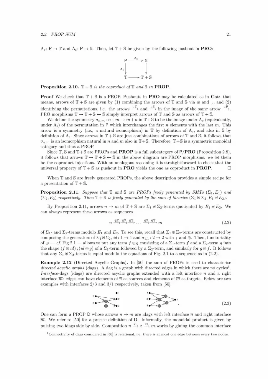
Example 2.12 (Directed Acyclic Graphs). In [50] the sum of PROPs is used to characterisedirected acyclic graphs (dags). A dag is a graph with directed edges in which there are no cycles1.Interface-dags (idags) are directed acyclic graphs extended with a left interface n and a rightinterface m: edges can have elements of n as sources and elements of m as targets. Below are twoexamples with interfaces 2/3 and 3/1 respectively, taken from [50].
1
2
1
3
2
1
1
3
2
. (2.3)
One can form a PROP D whose arrows n→ m are idags with left interface n and right interfacem. We refer to [50] for a precise definition of D. Informally, the monoidal product is given by
putting two idags side by side. Composition ng1−→ z
g2−→ m works by gluing the common interface
1Connectivity of dags considered in [50] is relational, i.e. there is at most one edge between every two nodes.
22 CHAPTER 2. PROPS AND THEIR COMPOSITION
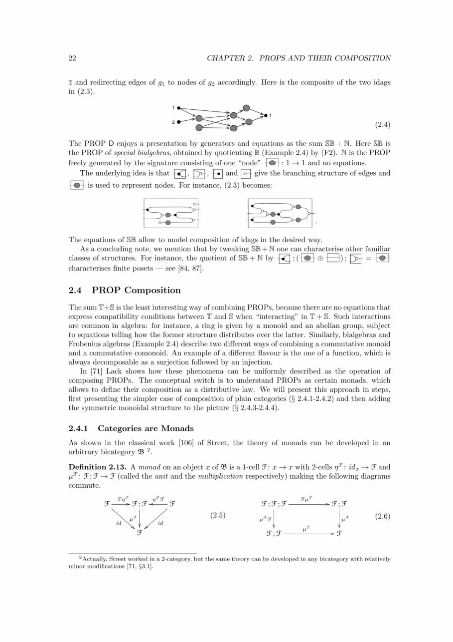
z and redirecting edges of g1 to nodes of g2 accordingly. Here is the composite of the two idagsin (2.3).
1
21
(2.4)
The PROP D enjoys a presentation by generators and equations as the sum SB + N. Here SB isthe PROP of special bialgebras, obtained by quotienting B (Example 2.4) by (F2). N is the PROP
freely generated by the signature consisting of one “node” : 1→ 1 and no equations.
The underlying idea is that , , and give the branching structure of edges and
is used to represent nodes. For instance, (2.3) becomes:
.
The equations of SB allow to model composition of idags in the desired way.As a concluding note, we mention that by tweaking SB+N one can characterise other familiar
classes of structures. For instance, the quotient of SB + N by ; ( ⊕ ) ; =
characterises finite posets — see [84, 87].
2.4 PROP Composition
The sum T+S is the least interesting way of combining PROPs, because there are no equations thatexpress compatibility conditions between T and S when “interacting” in T + S. Such interactionsare common in algebra: for instance, a ring is given by a monoid and an abelian group, subjectto equations telling how the former structure distributes over the latter. Similarly, bialgebras andFrobenius algebras (Example 2.4) describe two different ways of combining a commutative monoidand a commutative comonoid. An example of a different flavour is the one of a function, which isalways decomposable as a surjection followed by an injection.
In [71] Lack shows how these phenomena can be uniformly described as the operation ofcomposing PROPs. The conceptual switch is to understand PROPs as certain monads, whichallows to define their composition as a distributive law. We will present this approach in steps,first presenting the simpler case of composition of plain categories (§ 2.4.1-2.4.2) and then addingthe symmetric monoidal structure to the picture (§ 2.4.3-2.4.4).
2.4.1 Categories are Monads
As shown in the classical work [106] of Street, the theory of monads can be developed in anarbitrary bicategory B 2.
Definition 2.13. A monad on an object x of B is a 1-cell F : x→ x with 2-cells ηF : idx → F andµF : F ;F → F (called the unit and the multiplication respectively) making the following diagramscommute.
F
id!!
FηF // F ;F
µF
��
FηFFoo
id}}
F
(2.5)
F ;F ;F
µFF
��
FµF
// F ;F
µF
��F ;F
µF
// F
(2.6)
2Actually, Street worked in a 2-category, but the same theory can be developed in any bicategory with relativelyminor modifications [71, §3.1].
2.4. PROP COMPOSITION 23
A morphism between monads xF−→ x and x
G−→ x is a 2-cell θ : F → G making the followingdiagrams commute3.
idx
ηF
��
ηG
��F
θ // G
(2.7)
F ;F
µF
��
θθ // G ;G
µG
��F
θ // G
(2.8)
An epimorphic monad morphism is called a monad quotient.
For B = Cat, the above definition yields the standard notion of monad as an endofunctor witha pair of natural transformations. Something interesting happens for the case of the bicategoryB = Span(Set), defined below.
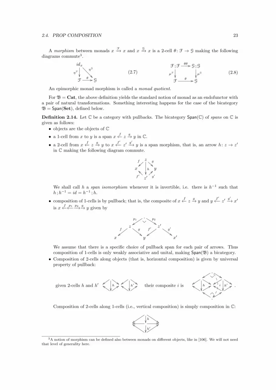
Definition 2.14. Let C be a category with pullbacks. The bicategory Span(C) of spans on C isgiven as follows:
• objects are the objects of C
• a 1-cell from x to y is a span xf←− z g−→ y in C.
• a 2-cell from xf←− z
g−→ y to xf ′←− z′
g′−→ y is a span morphism, that is, an arrow h : z → z′
in C making the following diagram commute.
zf
~~h
��
g
x y
z′f ′
__
g′
??
We shall call h a span isomorphism whenever it is invertible, i.e. there is h−1 such thath ;h−1 = id = h−1 ;h.
• composition of 1-cells is by pullback; that is, the composite of xf←− z g−→ y and y
f ′←− z′ g′
−→ x′
is xf←− p1←− p2−→ g−→ y given by
.p1
yyp2
%%z
f
{{g
""
z′f ′
{{g′
$$x y x′
We assume that there is a specific choice of pullback span for each pair of arrows. Thuscomposition of 1-cells is only weakly associative and unital, making Span(B) a bicategory.
• Composition of 2-cells along objects (that is, horizontal composition) is given by universalproperty of pullback:
given 2-cells h and h′zz
h
��
$$ zzh′
��
$$dd :: dd :: their composite i is
.yy %%
i
��
yyh
��
%% yyh′
��
%%ee 99 ee 99
.
ee 99.
Composition of 2-cells along 1-cells (i.e., vertical composition) is simply composition in C:
zzh�� $$ooh′
��
//dd ::
3A notion of morphism can be defined also between monads on different objects, like in [106]. We will not needthat level of generality here.
24 CHAPTER 2. PROPS AND THEIR COMPOSITION
The interest for the bicategory of spans stems from the following folklore observation.
Proposition 2.15. Small categories are precisely the monads in Span(Set).
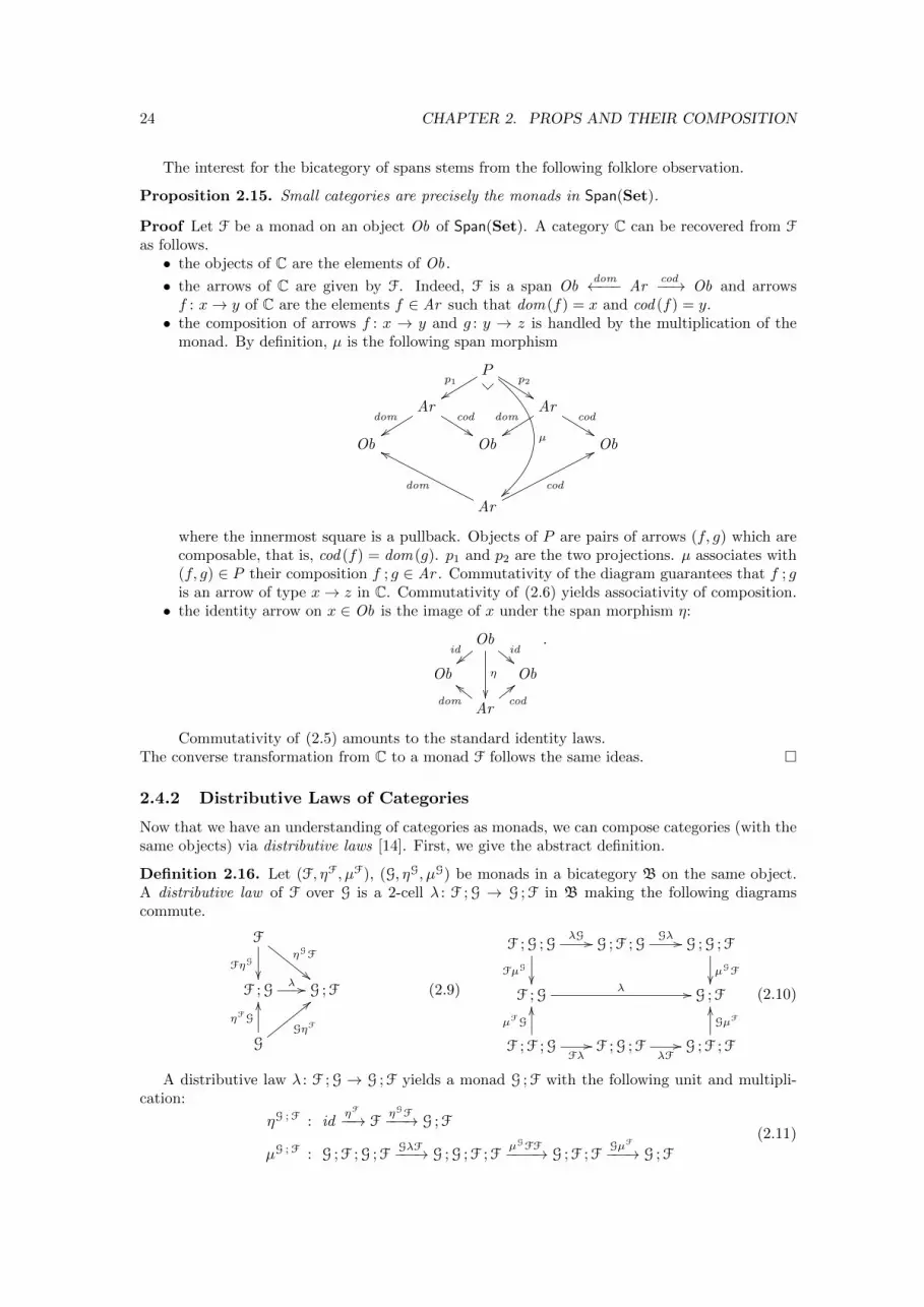
Proof Let F be a monad on an object Ob of Span(Set). A category C can be recovered from F
as follows.• the objects of C are the elements of Ob .
• the arrows of C are given by F. Indeed, F is a span Obdom←−−− Ar
cod−−→ Ob and arrowsf : x→ y of C are the elements f ∈ Ar such that dom (f) = x and cod (f) = y.
• the composition of arrows f : x → y and g : y → z is handled by the multiplication of themonad. By definition, µ is the following span morphism
Pp1
yy
µ
}}
p2
%%Ar
dom
yycod
%%
Ardom
yycod
%%Ob Ob Ob
Ar
dom
gg
cod
77
where the innermost square is a pullback. Objects of P are pairs of arrows (f, g) which arecomposable, that is, cod (f) = dom (g). p1 and p2 are the two projections. µ associates with(f, g) ∈ P their composition f ; g ∈ Ar . Commutativity of the diagram guarantees that f ; gis an arrow of type x→ z in C. Commutativity of (2.6) yields associativity of composition.
• the identity arrow on x ∈ Ob is the image of x under the span morphism η:
Obid||
η
��
id""
Ob Ob
Ardom
bbcod
<<
.
Commutativity of (2.5) amounts to the standard identity laws.The converse transformation from C to a monad F follows the same ideas. �
2.4.2 Distributive Laws of Categories
Now that we have an understanding of categories as monads, we can compose categories (with thesame objects) via distributive laws [14]. First, we give the abstract definition.
Definition 2.16. Let (F, ηF, µF), (G, ηG, µG) be monads in a bicategory B on the same object.A distributive law of F over G is a 2-cell λ : F ;G → G ;F in B making the following diagramscommute.
F
FηG
��
ηGF
""F ;G
λ // G ;F
G
ηFG
OO
GηF
<< (2.9)
F ;G ;G
FµG
��
λG // G ;F ;GGλ // G ;G ;F
µGF��
F ;Gλ // G ;F
F ;F ;G
µFG
OO
Fλ// F ;G ;F
λF// G ;F ;F
GµF
OO (2.10)
A distributive law λ : F ;G → G ;F yields a monad G ;F with the following unit and multipli-cation:
ηG ;F : idηF−−→ F
ηGF−−−→ G ;F
µG ;F : G ;F ;G ;FGλF−−−→ G ;G ;F ;F
µGFF−−−−→ G ;F ;FGµF
−−−→ G ;F
(2.11)
2.4. PROP COMPOSITION 25
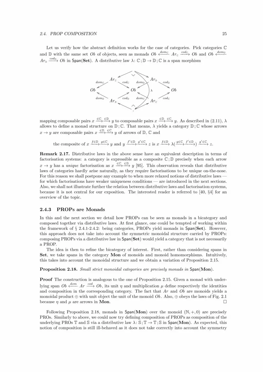
Let us verify how the abstract definition works for the case of categories. Pick categories Cand D with the same set Ob of objects, seen as monads Ob
domC←−−− ArCcodC−−−→ Ob and Ob
domD←−−−ArD
codD−−−→ Ob in Span(Set). A distributive law λ : C ;D→ D ;C is a span morphism
vv
λ
zz
((ArC
domC
wwcodC
''
ArDdomD
wwcodD
''Ob Ob Ob
ArDdomD
gg
codD
77
ArCdomC
gg
codC
77
.
hh 66
mapping composable pairs x∈C−−→ ∈D−−→ y to composable pairs x
∈D−−→ ∈C−−→ y. As described in (2.11), λallows to define a monad structure on D ;C. That means, λ yields a category D ;C whose arrows
x→ y are composable pairs x∈D−−→ ∈C−−→ y of arrows of D, C and
the composite of xf∈D−−−→ g∈C−−→ y and y
f ′∈D−−−→ g′∈C−−−→ z is xf∈D−−−→ λ(
g∈C−−→ f ′∈D−−−→)g′∈C−−−→ z.
Remark 2.17. Distributive laws in the above sense have an equivalent description in terms offactorisation systems: a category is expressible as a composite C ;D precisely when each arrow
x → y has a unique factorisation as x∈C−−→ ∈D−−→ y [95]. This observation reveals that distributive
laws of categories hardly arise naturally, as they require factorisations to be unique on-the-nose.For this reason we shall postpone any example to when more relaxed notions of distributive laws —for which factorisations have weaker uniqueness conditions — are introduced in the next sections.Also, we shall not illustrate further the relation between distributive laws and factorisation systems,because it is not central for our exposition. The interested reader is referred to [40, §4] for anoverview of the topic.
2.4.3 PROPs are Monads
In this and the next section we detail how PROPs can be seen as monads in a bicategory andcomposed together via distributive laws. At first glance, one could be tempted of working withinthe framework of § 2.4.1-2.4.2: being categories, PROPs yield monads in Span(Set). However,this approach does not take into account the symmetric monoidal structure carried by PROPs:composing PROPs via a distributive law in Span(Set) would yield a category that is not necessarilya PROP.
The idea is then to refine the bicategory of interest. First, rather than considering spans inSet, we take spans in the category Mon of monoids and monoid homomorphisms. Intuitively,this takes into account the monoidal structure and we obtain a variation of Proposition 2.15.
Proposition 2.18. Small strict monoidal categories are precisely monads in Span(Mon).
Proof The construction is analogous to the one of Proposition 2.15. Given a monad with under-
lying span Obdom←−−− Ar
cod−−→ Ob , its unit η and multiplication µ define respectively the identitiesand composition in the corresponding category. The fact that Ar and Ob are monoids yields amonoidal product ⊕ with unit object the unit of the monoid Ob . Also, ⊕ obeys the laws of Fig. 2.1because η and µ are arrows in Mon. �
Following Proposition 2.18, monads in Span(Mon) over the monoid (N,+, 0) are preciselyPROs. Similarly to above, we could now try defining composition of PROPs as composition of theunderlying PROs T and S via a distributive law λ : S ;T→ T ;S in Span(Mon). As expected, thisnotion of composition is still ill-behaved as it does not take correctly into account the symmetry
26 CHAPTER 2. PROPS AND THEIR COMPOSITION
structure. The problem is that T ;S contains two copies of P, one given by AT : P→ T→ T ;S andthe other by AS : P→ S→ T ;S, which do not necessarily agree.
The correct approach is to make explicit the symmetry structure of any PROP R in the formof a left and a right action τ R : P ;R → R and ρR : R ;P → R, yielded by AR : P → R. Then, weshall define the composite T⊗PS of PROPs T and S as a coequaliser in PRO
T ;P ;SρTS //
S1τS// T ;S // T⊗PS (2.12)
which, intuitively, is responsible for identifying the two copies of P in T ;S.This account of PROPs is actually reminiscent of the familiar notion of bimodule, which in
algebra designates abelian groups with both a left and a right action over a ring; the construc-tion (2.12) corresponds to the usual tensor product of bimodules.
This suggests the idea to express PROPs as monads in Span(Mon) with a bimodule structureand compose them using (2.12). To make this formal, we first define the bicategory of bimodulesin a given bicategory B. We will then focus on bimodules in Span(Mon) to capture PROPs.
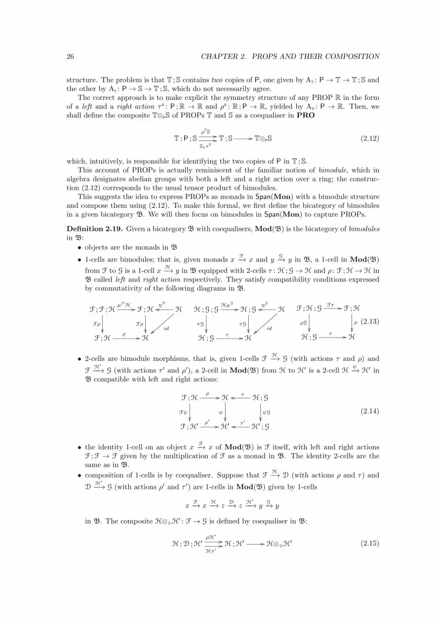
Definition 2.19. Given a bicategory B with coequalisers, Mod(B) is the bicategory of bimodulesin B:
• objects are the monads in B
• 1-cells are bimodules; that is, given monads xF−→ x and y
G−→ y in B, a 1-cell in Mod(B)
from F to G is a 1-cell xH−→ y in B equipped with 2-cells τ : H ;G→ H and ρ : F ;H→ H in
B called left and right action respectively. They satisfy compatibility conditions expressedby commutativity of the following diagrams in B.
F ;F ;H
Fρ
��
µFH // F ;H
Fρ
��
HηFoo
id}}F ;H
ρ // H
H ;G ;G
τG
��
HµG
// H ;G
τG
��
HηGoo
id}}H ;G
τ // H
F ;H ;GFτ //
ρG
��
F ;H
ρ
��H ;G
τ // H
(2.13)
• 2-cells are bimodule morphisms, that is, given 1-cells FH−→ G (with actions τ and ρ) and
FH′−−→ G (with actions τ ′ and ρ′), a 2-cell in Mod(B) from H to H′ is a 2-cell H
ψ−→ H′ inB compatible with left and right actions:
F ;Hρ //
Fψ
��
H
ψ
��
H ;Gτoo
ψG
��F ;H′
ρ′ // H′ H′ ;Gτ ′oo
(2.14)
• the identity 1-cell on an object xF−→ x of Mod(B) is F itself, with left and right actions
F ;F → F given by the multiplication of F as a monad in B. The identity 2-cells are thesame as in B.
• composition of 1-cells is by coequaliser. Suppose that FH−→ D (with actions ρ and τ) and
DH′−−→ G (with actions ρ′ and τ ′) are 1-cells in Mod(B) given by 1-cells
xF−→ x
H−→ zD−→ z
H′−−→ yG−→ y
in B. The composite H⊗DH′ : F → G is defined by coequaliser in B:
H ;D ;H′ρH′ //
Hτ ′// H ;H′ // H⊗DH
′ (2.15)
2.4. PROP COMPOSITION 27
• given that 2-cells in Mod(B) are also 2-cells in B, horizontal and vertical composition of2-cells in Mod(B) is defined as in B.
The same construction of Definition 2.19 is used in [40] to give an account of Lawvere theoriesas monads in a bicategory. Interestingly, it also appears in topological field theory to describeorbifold completion — see [37, Def. 4.1].
We now focus on our main application. Since Span(Mon) has coequalisers [55], one canform the bicategory Mod(Span(Mon)) of bimodules in Span(Mon). The next example detailshow Definition 2.19 instantiates for this case. We shall later verify that PROPs are monads inMod(Span(Mon)).
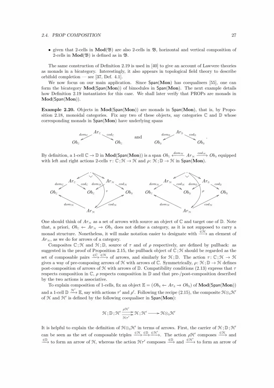
Example 2.20. Objects in Mod(Span(Mon)) are monads in Span(Mon), that is, by Propo-sition 2.18, monoidal categories. Fix any two of these objects, say categories C and D whosecorresponding monads in Span(Mon) have underlying spans
ArCdomC
wwcodC
''ObC ObC
andArDdomD
wwcodD
''ObD ObD
.
By definition, a 1-cell C −→ D in Mod(Span(Mon)) is a span ObCdomH←−−−− ArH
codH−−−→ ObD equippedwith left and right actions 2-cells τ : C ;H→ H and ρ : H ;D→ H in Span(Mon).
.ww
τ
}}
''ArC
domCyy
codC%%
ArHdomH
xxcodH
&&ObC ObC ObD
ArH
domH
gg
codH
77
.ww
ρ
}}
''ArH
domH
xxcodH
&&
ArDdomDyy
codD%%
ObC ObD ObD
ArH
domH
gg
codH
77
One should think of ArH as a set of arrows with source an object of C and target one of D. Notethat, a priori, ObC ←− ArH −→ ObD does not define a category, as it is not supposed to carry a
monad structure. Nonetheless, it will make notation easier to designate with∈H−−→ an element of
ArH, as we do for arrows of a category.
Composites C ;H and H ;D, source of τ and of ρ respectively, are defined by pullback: assuggested in the proof of Proposition 2.15, the pullback object of C ;H should be regarded as the
set of composable pairs∈C−−→ ∈H−−→ of arrows, and similarly for H ;D. The action τ : C ;H → H
gives a way of pre-composing arrows of H with arrows of C. Symmetrically, ρ : H ;D→ H definespost-composition of arrows of H with arrows of D. Compatibility conditions (2.13) express that τrespects composition in C, ρ respects composition in D and that pre-/post-composition describedby the two actions is associative.
To explain composition of 1-cells, fix an object E = (ObE ←− Ar E −→ ObE) of Mod(Span(Mon))
and a 1-cell D H′−−→ E, say with actions τ ′ and ρ′. Following the recipe (2.15), the composite H⊗DH′
of H and H′ is defined by the following coequaliser in Span(Mon):
H ;D ;H′ρH′ //
Hτ ′// H ;H′ // H⊗DH
′
It is helpful to explain the definition of H⊗DH′ in terms of arrows. First, the carrier of H ;D ;H′
can be seen as the set of composable triples∈H−−→ ∈D−−→ ∈H′−−−→. The action ρH′ composes
∈H−−→ and∈D−−→ to form an arrow of H, whereas the action Hτ ′ composes
∈D−−→ and∈H′−−−→ to form an arrow of
28 CHAPTER 2. PROPS AND THEIR COMPOSITION
H′. Either ways we obtain a composable pair∈H−−→ ∈H′−−−→. Equalizing these two actions amounts to
quotient the set of pairs∈H−−→ ∈H′−−−→ by the equivalence generated by the following relation:
h−→ h′−→ ≡Dg−→ g′−→ iff there exist
d∈D−−→ such thath−→ = ρ(
g−→ d−→) andg′−→ = τ ′(
d−→ h′−→). (2.16)
Therefore the 1-cell H⊗DH′ will be a span ObC ←−−→ ObE, whose carrier is the set of ≡D-equivalence
classes of composable pairs∈H−−→ ∈H′−−−→. We shall use the notation [
f−→ g−→]≡D for the equivalence class
with witnessf−→ g−→.
Remark 2.21 (Unit Laws). Let FH−→ G be a 1-cell in Mod(Span(Mon)). Since composition is
weakly unital, there are isomorphisms
H ∼= F⊗FH (2.17) H ∼= H⊗GG (2.18)
involving the identity 1-cells FF−→ F and G
G−→ G. For later use it is useful to make explicit howthese isomorphisms are defined. We focus on (2.17), the description of (2.18) being analogous.Using the arrow view of 1-cells H and F⊗DH , the two directions of the iso (2.17) are given by
f∈H−−−→ 7→ [id∈F−−−→ f∈H−−−→]≡F
[h∈F−−−→ g∈H−−−→]≡F
7→ ρ(h−→ g−→)
where ρ is the right action of the bimodule H. The right-to-left direction is well-defined: thedefinition of ≡F is given according to (2.16), with left and right actions of F being given by themultiplication µF of the monad F in Span(Mon). Then, compatibility of ρ with µF guaranteesthat composable pairs which are equal modulo ≡F are mapped into the same value by ρ. We nowcheck that the two mappings are invertible. First,
f∈H−−−→ 7→ [id∈F−−−→ f∈H−−−→]≡F
7→ ρ(id−→ f−→) =
f∈H−−−→
because ρ is compatible with the unit ηF of the monad F, which is given by insertion of the identity
arrowid−→ (see proof of Proposition 2.15). Conversely,
[h∈F−−−→ g∈H−−−→]≡F
7→ ρ(h−→ g−→) 7→ [
id∈F−−−→ ρ(h−→ g−→)∈H−−−−−−−−→]≡F
= [h∈F−−−→ g∈H−−−→]≡F
becauseh∈F−−−→ witnesses condition (2.16) for
h∈F−−−→ g∈H−−−→ andid∈F−−−→ ρ(
h−→ g−→)−−−−−−→, meaning that they arein the same ≡F- equivalence class.
We now prove that any PROP yields a monad in Mod(Span(Mon)). We fist present anabstract approach (the same given in [71]) and then also sketch a more direct argument. Letus write B(x, x) for the monoidal category of 1-cells x → x in B and Mnd(C) for the categoryof monoids in a monoidal category C. It is useful to recall the following standard result (seee.g. [71, 40]).
Proposition 2.22. Fix a bicategory B, x ∈ B and a monad xF−→ x. There is an equivalence
Mnd(Mod(B)(F,F)) ' F/Mnd(B(x, x)).
We instantiate Proposition 2.22 to the case in which B = Span(Mon), x = N and F = P.
Mnd(Mod(Span(Mon))(P,P)) ' P/Mnd(Span(Mon)(N,N)). (2.19)
We verify that PROPs live in the category on the right hand side. Objects in Mnd(Span(Mon)(N,N))are monoids in Span(Mon)(N,N), which are monad on N in Span(Mon) and thus, by Proposi-tion 2.18 are precisely PROs. Morphisms in Mnd(Span(Mon)(N,N)) are monoid homomorphismsin Span(Mon)(N,N), thus are identity-on-objects monoidal functors between PROs, that is, PROmorphisms. Therefore, objects of the coslice P/Mnd(Span(Mon)(N,N)) are PRO morphisms with
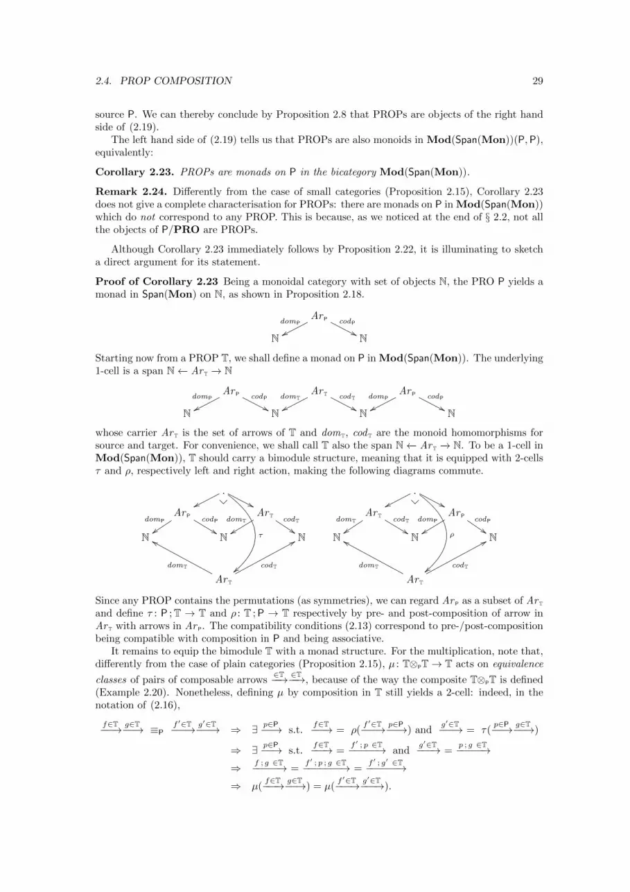
2.4. PROP COMPOSITION 29
source P. We can thereby conclude by Proposition 2.8 that PROPs are objects of the right handside of (2.19).
The left hand side of (2.19) tells us that PROPs are also monoids in Mod(Span(Mon))(P,P),equivalently:
Corollary 2.23. PROPs are monads on P in the bicategory Mod(Span(Mon)).
Remark 2.24. Differently from the case of small categories (Proposition 2.15), Corollary 2.23does not give a complete characterisation for PROPs: there are monads on P in Mod(Span(Mon))which do not correspond to any PROP. This is because, as we noticed at the end of § 2.2, not allthe objects of P/PRO are PROPs.
Although Corollary 2.23 immediately follows by Proposition 2.22, it is illuminating to sketcha direct argument for its statement.
Proof of Corollary 2.23 Being a monoidal category with set of objects N, the PRO P yields amonad in Span(Mon) on N, as shown in Proposition 2.18.
Ar PdomP
wwcodP
''N N
Starting now from a PROP T, we shall define a monad on P in Mod(Span(Mon)). The underlying1-cell is a span N←− Ar T −→ N
Ar PdomP
wwcodP
''
Ar TdomT
wwcodT
''
Ar PdomP
wwcodP
''N N N N
whose carrier Ar T is the set of arrows of T and domT, cod T are the monoid homomorphisms forsource and target. For convenience, we shall call T also the span N←− Ar T −→ N. To be a 1-cell inMod(Span(Mon)), T should carry a bimodule structure, meaning that it is equipped with 2-cellsτ and ρ, respectively left and right action, making the following diagrams commute.
.ww
τ
||
''Ar P
domP
zzcodP
%%
Ar TdomT
yycodT
$$N N N
Ar T
domT
ff
codT
88
.ww
ρ
||
''Ar T
domT
zzcodT
%%
Ar PdomP
yycodP
$$N N N
Ar T
domT
ff
codT
88
Since any PROP contains the permutations (as symmetries), we can regard Ar P as a subset of Ar T
and define τ : P ;T → T and ρ : T ;P → T respectively by pre- and post-composition of arrow inAr T with arrows in Ar P. The compatibility conditions (2.13) correspond to pre-/post-compositionbeing compatible with composition in P and being associative.
It remains to equip the bimodule T with a monad structure. For the multiplication, note that,differently from the case of plain categories (Proposition 2.15), µ : T⊗PT→ T acts on equivalence
classes of pairs of composable arrows∈T−−→ ∈T−−→, because of the way the composite T⊗PT is defined
(Example 2.20). Nonetheless, defining µ by composition in T still yields a 2-cell: indeed, in thenotation of (2.16),
f∈T−−−→ g∈T−−→ ≡Pf ′∈T−−−→ g′∈T−−−→ ⇒ ∃ p∈P−−→ s.t.
f∈T−−−→ = ρ(f ′∈T−−−→ p∈P−−→) and
g′∈T−−−→ = τ(p∈P−−→ g∈T−−→)
⇒ ∃ p∈P−−→ s.t.f∈T−−−→ =
f ′ ; p ∈T−−−−−→ andg′∈T−−−→ =
p ; g ∈T−−−−−→⇒ f ; g ∈T−−−−−→ =
f ′ ; p ; g ∈T−−−−−−−→ =f ′ ; g′ ∈T−−−−−−→
⇒ µ(f∈T−−−→ g∈T−−→) = µ(
f ′∈T−−−→ g′∈T−−−→).
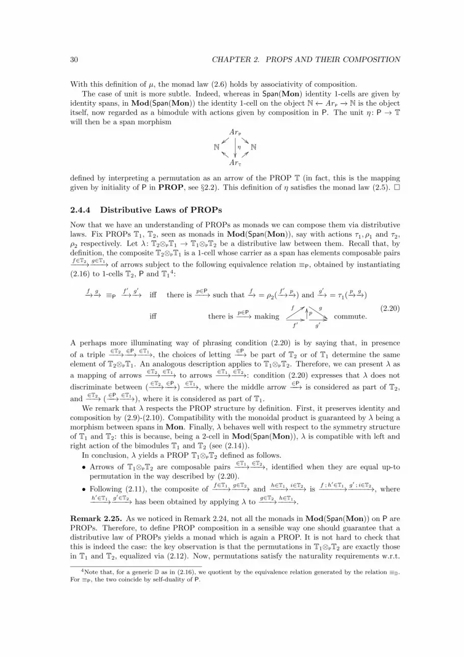
30 CHAPTER 2. PROPS AND THEIR COMPOSITION
With this definition of µ, the monad law (2.6) holds by associativity of composition.The case of unit is more subtle. Indeed, whereas in Span(Mon) identity 1-cells are given by
identity spans, in Mod(Span(Mon)) the identity 1-cell on the object N←− Ar P −→ N is the objectitself, now regarded as a bimodule with actions given by composition in P. The unit η : P → Twill then be a span morphism
Ar P
|| ""η
��N N
Ar T
bb <<
defined by interpreting a permutation as an arrow of the PROP T (in fact, this is the mappinggiven by initiality of P in PROP, see §2.2). This definition of η satisfies the monad law (2.5). �
2.4.4 Distributive Laws of PROPs
Now that we have an understanding of PROPs as monads we can compose them via distributivelaws. Fix PROPs T1, T2, seen as monads in Mod(Span(Mon)), say with actions τ1, ρ1 and τ2,ρ2 respectively. Let λ : T2⊗PT1 → T1⊗PT2 be a distributive law between them. Recall that, bydefinition, the composite T2⊗PT1 is a 1-cell whose carrier as a span has elements composable pairsf∈T2−−−→ g∈T1−−−→ of arrows subject to the following equivalence relation ≡P, obtained by instantiating(2.16) to 1-cells T2, P and T1
4:
f−→ g−→ ≡Pf ′−→ g′−→ iff there is
p∈P−−→ such thatf−→ = ρ2(
f ′−→ p−→) andg′−→ = τ1(
p−→ g−→)
iff there isp∈P−−→ making
g
%%f 99
f ′//pOO
g′// commute.
(2.20)
A perhaps more illuminating way of phrasing condition (2.20) is by saying that, in presence
of a triple∈T2−−→ ∈P−−→ ∈T1−−→, the choices of letting
∈P−−→ be part of T2 or of T1 determine the sameelement of T2⊗PT1. An analogous description applies to T1⊗PT2. Therefore, we can present λ as
a mapping of arrows∈T2−−→ ∈T1−−→ to arrows
∈T1−−→ ∈T2−−→: condition (2.20) expresses that λ does not
discriminate between (∈T2−−→ ∈P−−→)
∈T1−−→, where the middle arrow∈P−−→ is considered as part of T2,
and∈T2−−→ (
∈P−−→ ∈T1−−→), where it is considered as part of T1.We remark that λ respects the PROP structure by definition. First, it preserves identity and
composition by (2.9)-(2.10). Compatibility with the monoidal product is guaranteed by λ being amorphism between spans in Mon. Finally, λ behaves well with respect to the symmetry structureof T1 and T2: this is because, being a 2-cell in Mod(Span(Mon)), λ is compatible with left andright action of the bimodules T1 and T2 (see (2.14)).
In conclusion, λ yields a PROP T1⊗PT2 defined as follows.
• Arrows of T1⊗PT2 are composable pairs∈T1−−→ ∈T2−−→, identified when they are equal up-to
permutation in the way described by (2.20).
• Following (2.11), the composite off∈T1−−−→ g∈T2−−−→ and
h∈T1−−−→ i∈T2−−−→ isf ;h′∈T1−−−−−→ g′ ; i∈T2−−−−−→, where
h′∈T1−−−−→ g′∈T2−−−−→ has been obtained by applying λ tog∈T2−−−→ h∈T1−−−→.
Remark 2.25. As we noticed in Remark 2.24, not all the monads in Mod(Span(Mon)) on P arePROPs. Therefore, to define PROP composition in a sensible way one should guarantee that adistributive law of PROPs yields a monad which is again a PROP. It is not hard to check thatthis is indeed the case: the key observation is that the permutations in T1⊗PT2 are exactly thosein T1 and T2, equalized via (2.12). Now, permutations satisfy the naturality requirements w.r.t.
4Note that, for a generic D as in (2.16), we quotient by the equivalence relation generated by the relation ≡D.For ≡P, the two coincide by self-duality of P.
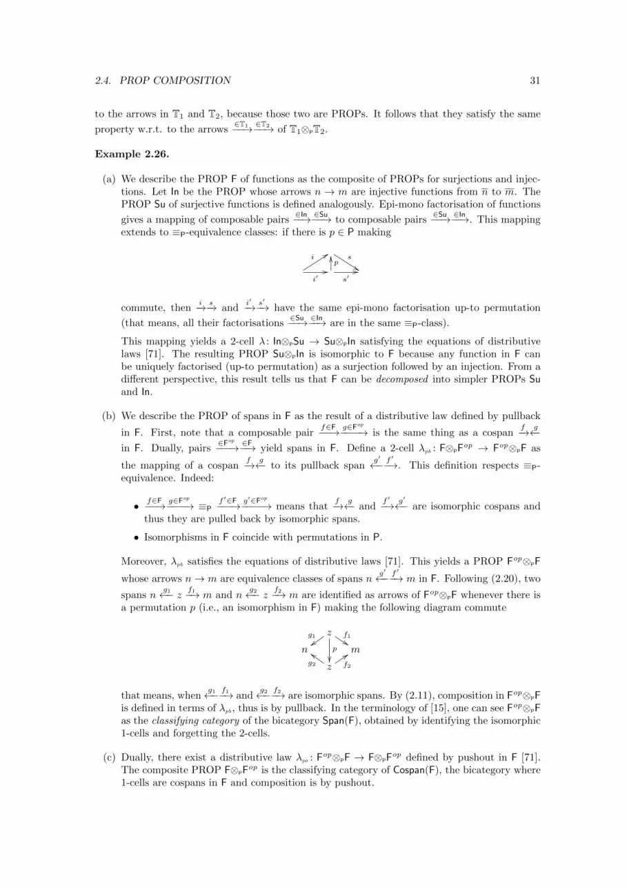
2.4. PROP COMPOSITION 31
to the arrows in T1 and T2, because those two are PROPs. It follows that they satisfy the same
property w.r.t. to the arrows∈T1−−→ ∈T2−−→ of T1⊗PT2.
Example 2.26.
(a) We describe the PROP F of functions as the composite of PROPs for surjections and injec-tions. Let In be the PROP whose arrows n → m are injective functions from n to m. ThePROP Su of surjective functions is defined analogously. Epi-mono factorisation of functions
gives a mapping of composable pairs∈In−−→ ∈Su−−→ to composable pairs
∈Su−−→ ∈In−−→. This mappingextends to ≡P-equivalence classes: if there is p ∈ P making
s
%%i99
i′//pOO
s′//
commute, theni−→ s−→ and
i′−→ s′−→ have the same epi-mono factorisation up-to permutation
(that means, all their factorisations∈Su−−→ ∈In−−→ are in the same ≡P-class).
This mapping yields a 2-cell λ : In⊗PSu → Su⊗PIn satisfying the equations of distributivelaws [71]. The resulting PROP Su⊗PIn is isomorphic to F because any function in F canbe uniquely factorised (up-to permutation) as a surjection followed by an injection. From adifferent perspective, this result tells us that F can be decomposed into simpler PROPs Suand In.
(b) We describe the PROP of spans in F as the result of a distributive law defined by pullback
in F. First, note that a composable pairf∈F−−→ g∈Fop
−−−−→ is the same thing as a cospanf−→ g←−
in F. Dually, pairs∈Fop
−−−→ ∈F−−→ yield spans in F. Define a 2-cell λpb : F⊗PFop → Fop⊗PF as
the mapping of a cospanf−→ g←− to its pullback span
g′←− f ′−→. This definition respects ≡P-equivalence. Indeed:
• f∈F−−→ g∈Fop
−−−−→ ≡Pf ′∈F−−−→ g′∈Fop
−−−−→ means thatf−→ g←− and
f ′−→ g′←− are isomorphic cospans andthus they are pulled back by isomorphic spans.
• Isomorphisms in F coincide with permutations in P.
Moreover, λpb satisfies the equations of distributive laws [71]. This yields a PROP Fop⊗PF
whose arrows n→ m are equivalence classes of spans ng′←− f ′−→ m in F. Following (2.20), two
spans ng1←− z f1−→ m and n
g2←− z f2−→ m are identified as arrows of Fop⊗PF whenever there isa permutation p (i.e., an isomorphism in F) making the following diagram commute
zg1
zzf1
%%p
��n m
zg2
ddf2
99
that means, wheng1←− f1−→ and
g2←− f2−→ are isomorphic spans. By (2.11), composition in Fop⊗PFis defined in terms of λpb, thus is by pullback. In the terminology of [15], one can see Fop⊗PFas the classifying category of the bicategory Span(F), obtained by identifying the isomorphic1-cells and forgetting the 2-cells.
(c) Dually, there exist a distributive law λpo : Fop⊗PF → F⊗PFop defined by pushout in F [71].
The composite PROP F⊗PFop is the classifying category of Cospan(F), the bicategory where
1-cells are cospans in F and composition is by pushout.
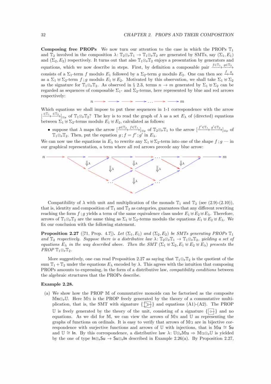
32 CHAPTER 2. PROPS AND THEIR COMPOSITION
Composing free PROPs We now turn our attention to the case in which the PROPs T1
and T2 involved in the composition λ : T2⊗PT1 → T1⊗PT2 are generated by SMTs, say (Σ1, E1)and (Σ2, E2) respectively. It turns out that also T1⊗PT2 enjoys a presentation by generators and
equations, which we now describe in steps. First, by definition a composable pairf∈T1−−−→ g∈T2−−−→
consists of a Σ1-term f modulo E1 followed by a Σ2-term g modulo E2. One can then seef−→ g−→
as a Σ1 ] Σ2-term f ; g modulo E1 ] E2. Motivated by this observation, we shall take Σ1 ] Σ2
as the signature for T1⊗PT2. As observed in § 2.3, terms n → m generated by Σ1 ] Σ2 can beregarded as sequences of composable Σ1- and Σ2-terms, here represented by blue and red arrowsrespectively:
n // // // // . . . // // m
Which equations we shall impose to put these sequences in 1-1 correspondence with the arrow
[∈T1−−→ ∈T2−−→]≡P
of T1⊗PT2? The key is to read the graph of λ as a set Eλ of (directed) equationsbetween Σ1 ] Σ2-terms modulo E1 ] E2, calculated as follows:
• suppose that λ maps the arrow [g∈T2−−−→ f∈T1−−−→]≡P
of T2⊗PT1 to the arrow [f ′∈T1−−−−→ g′∈T2−−−−→]≡P
ofT1⊗PT2. Then, put the equation g ; f = f ′ ; g′ in Eλ.
We can now use the equations in Eλ to rewrite any Σ1 ]Σ2-term into one of the shape f ; g — inour graphical representation, a term where all red arrows precede any blue arrow:
n // //
%%�
// //
&&�
// . . .
&&
//
&&�
// // m88
''
�
88
''
�
99
. . .
77
''
� . . .
77
77
Compatibility of λ with unit and multiplication of the monads T1 and T2 (see (2.9)-(2.10)),that is, identity and composition of T1 and T2 as categories, guarantees that any different rewritingreaching the form f ; g yields a term of the same equivalence class under E1 ]E2 ]Eλ. Therefore,arrows of T1⊗PT2 are the same thing as Σ1 ] Σ2-terms modulo the equations E1 ] E2 ] Eλ. Wefix our conclusion with the following statement.
Proposition 2.27 ([71, Prop. 4.7]). Let (Σ1, E1) and (Σ2, E2) be SMTs generating PROPs T1
and T2 respectively. Suppose there is a distributive law λ : T2⊗PT1 → T1⊗PT2, yielding a set ofequations Eλ in the way described above. Then the SMT (Σ1 ] Σ2, E1 ] E2 ] Eλ) presents thePROP T1⊗PT2.
More suggestively, one can read Proposition 2.27 as saying that T1⊗PT2 is the quotient of thesum T1 +T2 under the equations Eλ encoded by λ. This agrees with the intuition that composingPROPs amounts to expressing, in the form of a distributive law, compatibility conditions betweenthe algebraic structures that the PROPs describe.
Example 2.28.
(a) We show how the PROP M of commutative monoids can be factorised as the compositeMu⊗PU. Here Mu is the PROP freely generated by the theory of a commutative multi-plication, that is, the SMT with signature { } and equations (A1)-(A2). The PROP
U is freely generated by the theory of the unit, consisting of a signature { } and noequations. As we did for M, we can view the arrows of Mu and U as representing thegraphs of functions on ordinals. It is easy to verify that arrows of Mu are in bijective cor-respondence with surjective functions and arrows of U with injections, that is Mu ∼= Suand U ∼= In. By this correspondence, a distributive law λ : U⊗PMu ⇒ Mu⊗PU is yieldedby the one of type In⊗PSu → Su⊗PIn described in Example 2.26(a). By Proposition 2.27,
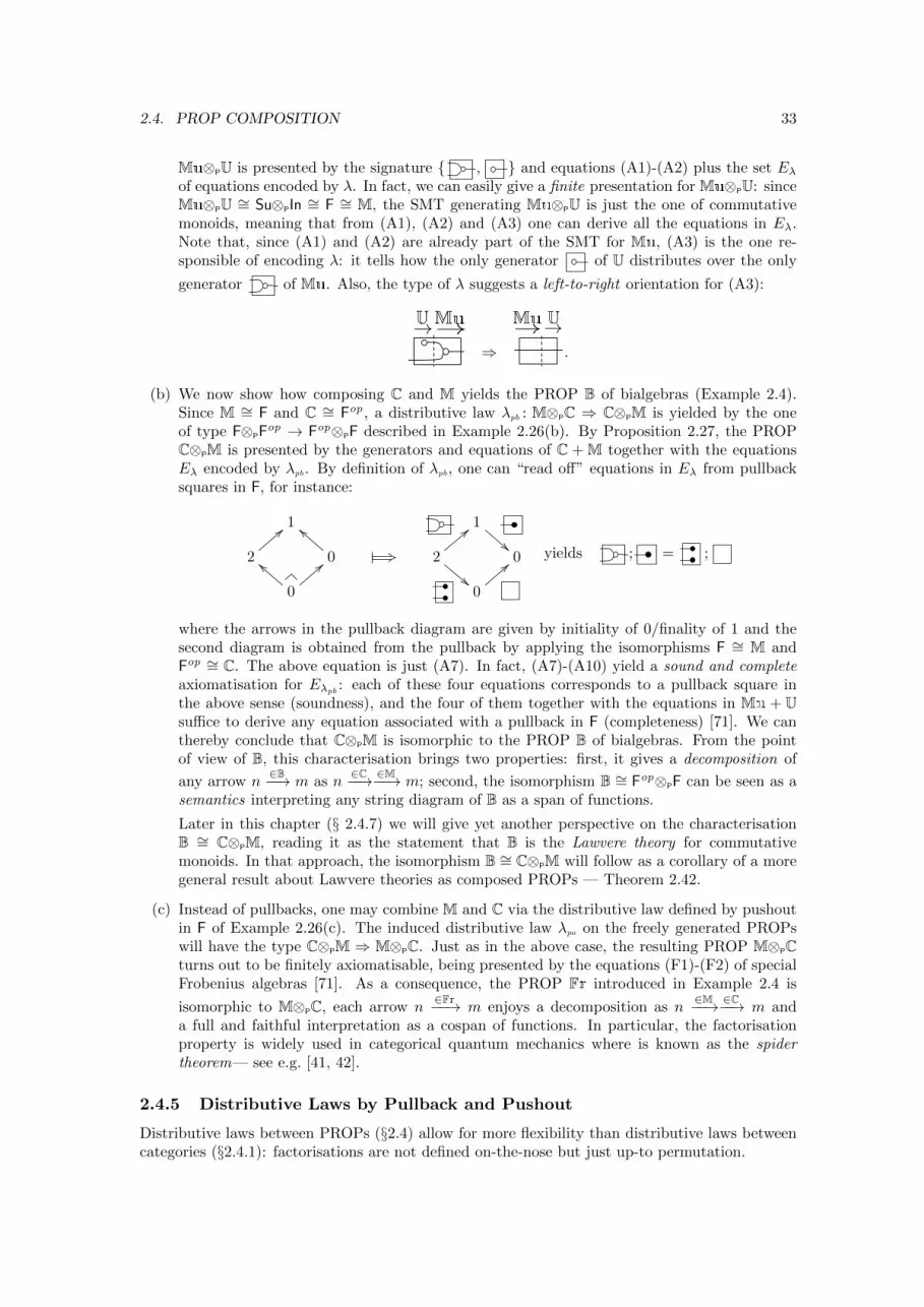
2.4. PROP COMPOSITION 33
Mu⊗PU is presented by the signature { , } and equations (A1)-(A2) plus the set Eλof equations encoded by λ. In fact, we can easily give a finite presentation for Mu⊗PU: sinceMu⊗PU ∼= Su⊗PIn ∼= F ∼= M, the SMT generating Mu⊗PU is just the one of commutativemonoids, meaning that from (A1), (A2) and (A3) one can derive all the equations in Eλ.Note that, since (A1) and (A2) are already part of the SMT for Mu, (A3) is the one re-sponsible of encoding λ: it tells how the only generator of U distributes over the only
generator of Mu. Also, the type of λ suggests a left-to-right orientation for (A3):
!!U M
⇒!! UM
.
(b) We now show how composing C and M yields the PROP B of bialgebras (Example 2.4).Since M ∼= F and C ∼= Fop , a distributive law λpb : M⊗PC ⇒ C⊗PM is yielded by the oneof type F⊗PF
op → Fop⊗PF described in Example 2.26(b). By Proposition 2.27, the PROPC⊗PM is presented by the generators and equations of C + M together with the equationsEλ encoded by λpb. By definition of λpb, one can “read off” equations in Eλ from pullbacksquares in F, for instance:
1 1
!!2
==
0
aa
�� +3 2
==
!!
0
0
aa ==
0
== yields ; = ;
where the arrows in the pullback diagram are given by initiality of 0/finality of 1 and thesecond diagram is obtained from the pullback by applying the isomorphisms F ∼= M andFop ∼= C. The above equation is just (A7). In fact, (A7)-(A10) yield a sound and completeaxiomatisation for Eλpb
: each of these four equations corresponds to a pullback square inthe above sense (soundness), and the four of them together with the equations in Mu + Usuffice to derive any equation associated with a pullback in F (completeness) [71]. We canthereby conclude that C⊗PM is isomorphic to the PROP B of bialgebras. From the pointof view of B, this characterisation brings two properties: first, it gives a decomposition of
any arrow n∈B−−→ m as n
∈C−−→ ∈M−−→ m; second, the isomorphism B ∼= Fop⊗PF can be seen as asemantics interpreting any string diagram of B as a span of functions.
Later in this chapter (§ 2.4.7) we will give yet another perspective on the characterisationB ∼= C⊗PM, reading it as the statement that B is the Lawvere theory for commutativemonoids. In that approach, the isomorphism B ∼= C⊗PM will follow as a corollary of a moregeneral result about Lawvere theories as composed PROPs — Theorem 2.42.
(c) Instead of pullbacks, one may combine M and C via the distributive law defined by pushoutin F of Example 2.26(c). The induced distributive law λpo on the freely generated PROPswill have the type C⊗PM ⇒ M⊗PC. Just as in the above case, the resulting PROP M⊗PCturns out to be finitely axiomatisable, being presented by the equations (F1)-(F2) of specialFrobenius algebras [71]. As a consequence, the PROP Fr introduced in Example 2.4 is
isomorphic to M⊗PC, each arrow n∈Fr−−→ m enjoys a decomposition as n
∈M−−→ ∈C−−→ m anda full and faithful interpretation as a cospan of functions. In particular, the factorisationproperty is widely used in categorical quantum mechanics where is known as the spidertheorem— see e.g. [41, 42].
2.4.5 Distributive Laws by Pullback and Pushout
Distributive laws between PROPs (§2.4) allow for more flexibility than distributive laws betweencategories (§2.4.1): factorisations are not defined on-the-nose but just up-to permutation.
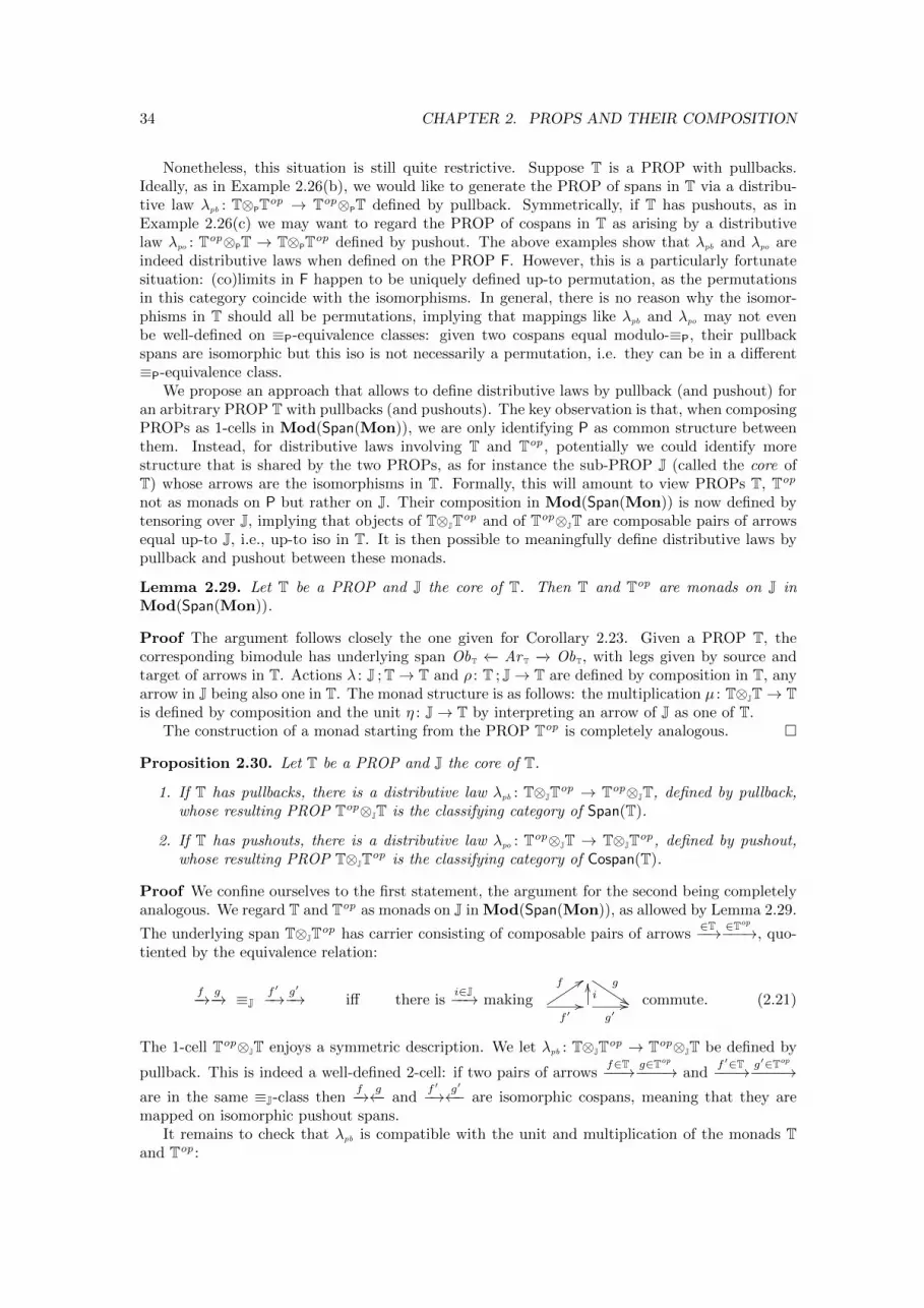
34 CHAPTER 2. PROPS AND THEIR COMPOSITION
Nonetheless, this situation is still quite restrictive. Suppose T is a PROP with pullbacks.Ideally, as in Example 2.26(b), we would like to generate the PROP of spans in T via a distribu-tive law λpb : T⊗PTop → Top⊗PT defined by pullback. Symmetrically, if T has pushouts, as inExample 2.26(c) we may want to regard the PROP of cospans in T as arising by a distributivelaw λpo : Top⊗PT → T⊗PTop defined by pushout. The above examples show that λpb and λpo areindeed distributive laws when defined on the PROP F. However, this is a particularly fortunatesituation: (co)limits in F happen to be uniquely defined up-to permutation, as the permutationsin this category coincide with the isomorphisms. In general, there is no reason why the isomor-phisms in T should all be permutations, implying that mappings like λpb and λpo may not evenbe well-defined on ≡P-equivalence classes: given two cospans equal modulo-≡P, their pullbackspans are isomorphic but this iso is not necessarily a permutation, i.e. they can be in a different≡P-equivalence class.
We propose an approach that allows to define distributive laws by pullback (and pushout) foran arbitrary PROP T with pullbacks (and pushouts). The key observation is that, when composingPROPs as 1-cells in Mod(Span(Mon)), we are only identifying P as common structure betweenthem. Instead, for distributive laws involving T and Top , potentially we could identify morestructure that is shared by the two PROPs, as for instance the sub-PROP J (called the core ofT) whose arrows are the isomorphisms in T. Formally, this will amount to view PROPs T, Top
not as monads on P but rather on J. Their composition in Mod(Span(Mon)) is now defined bytensoring over J, implying that objects of T⊗JTop and of Top⊗JT are composable pairs of arrowsequal up-to J, i.e., up-to iso in T. It is then possible to meaningfully define distributive laws bypullback and pushout between these monads.
Lemma 2.29. Let T be a PROP and J the core of T. Then T and Top are monads on J inMod(Span(Mon)).
Proof The argument follows closely the one given for Corollary 2.23. Given a PROP T, thecorresponding bimodule has underlying span ObT ←− Ar T −→ ObT, with legs given by source andtarget of arrows in T. Actions λ : J ;T→ T and ρ : T ; J→ T are defined by composition in T, anyarrow in J being also one in T. The monad structure is as follows: the multiplication µ : T⊗JT→ Tis defined by composition and the unit η : J→ T by interpreting an arrow of J as one of T.
The construction of a monad starting from the PROP Top is completely analogous. �
Proposition 2.30. Let T be a PROP and J the core of T.
1. If T has pullbacks, there is a distributive law λpb : T⊗JTop → Top⊗JT, defined by pullback,whose resulting PROP Top⊗JT is the classifying category of Span(T).
2. If T has pushouts, there is a distributive law λpo : Top⊗JT → T⊗JTop, defined by pushout,whose resulting PROP T⊗JTop is the classifying category of Cospan(T).
Proof We confine ourselves to the first statement, the argument for the second being completelyanalogous. We regard T and Top as monads on J in Mod(Span(Mon)), as allowed by Lemma 2.29.
The underlying span T⊗JTop has carrier consisting of composable pairs of arrows∈T−−→ ∈Top
−−−→, quo-tiented by the equivalence relation:
f−→ g−→ ≡Jf ′−→ g′−→ iff there is
i∈J−−→ makingg
%%f 99
f ′//i
OO
g′// commute. (2.21)
The 1-cell Top⊗JT enjoys a symmetric description. We let λpb : T⊗JTop → Top⊗JT be defined by
pullback. This is indeed a well-defined 2-cell: if two pairs of arrowsf∈T−−−→ g∈Top
−−−−→ andf ′∈T−−−→ g′∈Top
−−−−→are in the same ≡J-class then
f−→ g←− andf ′−→ g′←− are isomorphic cospans, meaning that they are
mapped on isomorphic pushout spans.It remains to check that λpb is compatible with the unit and multiplication of the monads T
and Top :
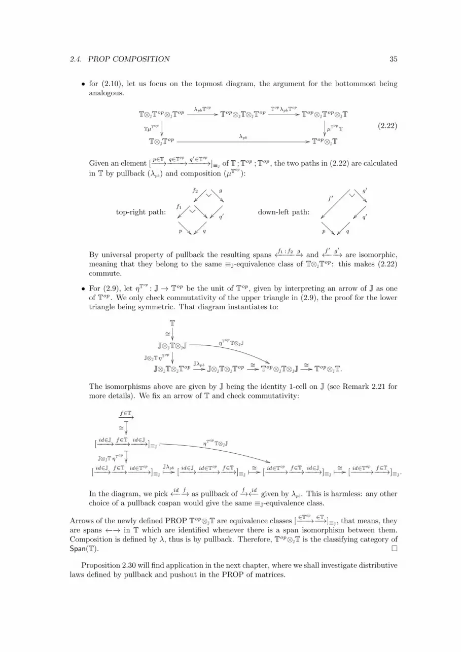
2.4. PROP COMPOSITION 35
• for (2.10), let us focus on the topmost diagram, the argument for the bottommost beinganalogous.
T⊗JTop⊗JTop
TµTop
��
λpbTop
// Top⊗JT⊗JTopTopλpbTop
// Top⊗JTop⊗JT
µTopT��
T⊗JTopλpb // Top⊗JT
(2.22)
Given an element [p∈T−−→ q∈Top
−−−−→ q′∈Top
−−−−→]≡J of T ;Top ;Top , the two paths in (2.22) are calculated
in T by pullback (λpb) and composition (µTop
):
top-right path:
f2
��g
��f1
�� �� q′��
p �� q��
down-left path:
f ′
��
g′
��
q′��
p �� q��
By universal property of pullback the resulting spansf1 ; f2←−−−− g−→ and
f ′←− g′−→ are isomorphic,meaning that they belong to the same ≡J-equivalence class of T⊗JTop : this makes (2.22)commute.
• For (2.9), let ηTop
: J → Top be the unit of Top , given by interpreting an arrow of J as oneof Top . We only check commutativity of the upper triangle in (2.9), the proof for the lowertriangle being symmetric. That diagram instantiates to:
T∼=��
J⊗JT⊗JJJ⊗JT ηT
op
��
ηTop
T⊗JJ
''J⊗JT⊗JTop
Jλpb // J⊗JT⊗JTop∼= // Top⊗JT⊗JJ
∼= // Top⊗JT.
The isomorphisms above are given by J being the identity 1-cell on J (see Remark 2.21 formore details). We fix an arrow of T and check commutativity:
f∈T−−−→_∼=��
[id∈J−−−→ f∈T−−−→ id∈J−−−→]≡J_J⊗JT ηT
op
��
� ηTop
T⊗JJ
**
[id∈J−−−→ f∈T−−−→ id∈Top
−−−−→]≡J�Jλpb // [
id∈J−−−→ id∈Top
−−−−→ f∈T−−−→]≡J� ∼= // [
id∈Top
−−−−→ f∈T−−−→ id∈J−−−→]≡J� ∼= // [
id∈Top
−−−−→ f∈T−−−→]≡J .
In the diagram, we pickid←− f−→ as pullback of
f−→ id←− given by λpb. This is harmless: any otherchoice of a pullback cospan would give the same ≡J-equivalence class.
Arrows of the newly defined PROP Top⊗JT are equivalence classes [∈Top
−−−→ ∈T−−→]≡J , that means, theyare spans ←−−→ in T which are identified whenever there is a span isomorphism between them.Composition is defined by λ, thus is by pullback. Therefore, Top⊗JT is the classifying category ofSpan(T). �
Proposition 2.30 will find application in the next chapter, where we shall investigate distributivelaws defined by pullback and pushout in the PROP of matrices.
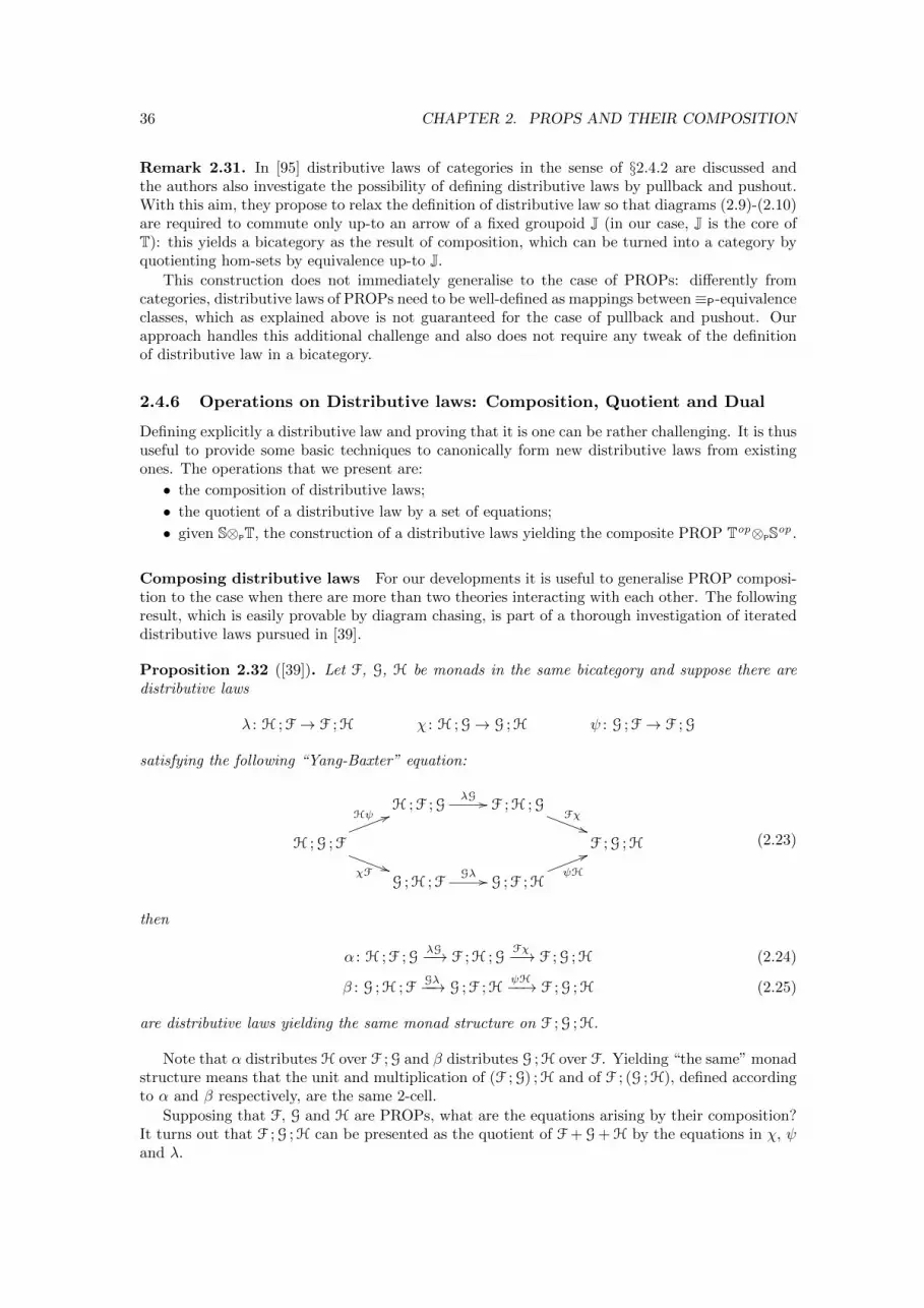
36 CHAPTER 2. PROPS AND THEIR COMPOSITION
Remark 2.31. In [95] distributive laws of categories in the sense of §2.4.2 are discussed andthe authors also investigate the possibility of defining distributive laws by pullback and pushout.With this aim, they propose to relax the definition of distributive law so that diagrams (2.9)-(2.10)are required to commute only up-to an arrow of a fixed groupoid J (in our case, J is the core ofT): this yields a bicategory as the result of composition, which can be turned into a category byquotienting hom-sets by equivalence up-to J.
This construction does not immediately generalise to the case of PROPs: differently fromcategories, distributive laws of PROPs need to be well-defined as mappings between≡P-equivalenceclasses, which as explained above is not guaranteed for the case of pullback and pushout. Ourapproach handles this additional challenge and also does not require any tweak of the definitionof distributive law in a bicategory.
2.4.6 Operations on Distributive laws: Composition, Quotient and Dual
Defining explicitly a distributive law and proving that it is one can be rather challenging. It is thususeful to provide some basic techniques to canonically form new distributive laws from existingones. The operations that we present are:
• the composition of distributive laws;
• the quotient of a distributive law by a set of equations;
• given S⊗PT, the construction of a distributive laws yielding the composite PROP Top⊗PSop .
Composing distributive laws For our developments it is useful to generalise PROP composi-tion to the case when there are more than two theories interacting with each other. The followingresult, which is easily provable by diagram chasing, is part of a thorough investigation of iterateddistributive laws pursued in [39].
Proposition 2.32 ([39]). Let F, G, H be monads in the same bicategory and suppose there aredistributive laws
λ : H ;F → F ;H χ : H ;G→ G ;H ψ : G ;F → F ;G
satisfying the following “Yang-Baxter” equation:
H ;F ;GλG // F ;H ;G
Fχ
))H ;G ;F
Hψ 55
χF ))
F ;G ;H
G ;H ;FGλ // G ;F ;H
ψH
55(2.23)
then
α : H ;F ;GλG−−→ F ;H ;G
Fχ−−→ F ;G ;H (2.24)
β : G ;H ;FGλ−−→ G ;F ;H
ψH−−→ F ;G ;H (2.25)
are distributive laws yielding the same monad structure on F ;G ;H.
Note that α distributes H over F ;G and β distributes G ;H over F. Yielding “the same” monadstructure means that the unit and multiplication of (F ;G) ;H and of F ; (G ;H), defined accordingto α and β respectively, are the same 2-cell.
Supposing that F, G and H are PROPs, what are the equations arising by their composition?It turns out that F ;G ;H can be presented as the quotient of F + G + H by the equations in χ, ψand λ.
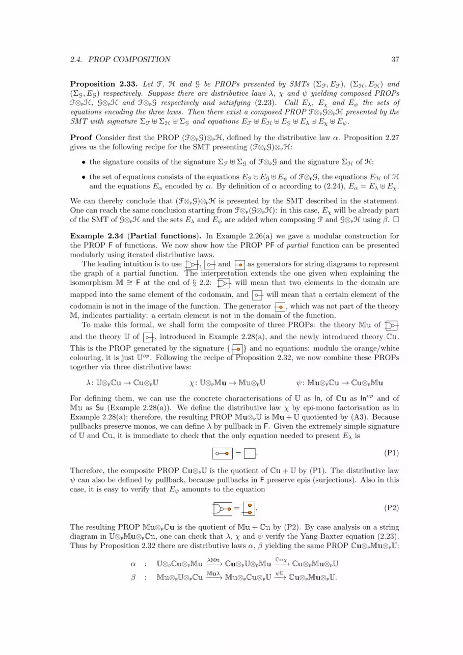
2.4. PROP COMPOSITION 37
Proposition 2.33. Let F, H and G be PROPs presented by SMTs (ΣF, EF), (ΣH, EH) and(ΣG, EG) respectively. Suppose there are distributive laws λ, χ and ψ yielding composed PROPsF⊗PH, G⊗PH and F⊗PG respectively and satisfying (2.23). Call Eλ, Eχ and Eψ the sets ofequations encoding the three laws. Then there exist a composed PROP F⊗PG⊗PH presented by theSMT with signature ΣF ] ΣH ] ΣG and equations EF ] EH ] EG ] Eλ ] Eχ ] Eψ.
Proof Consider first the PROP (F⊗PG)⊗PH, defined by the distributive law α. Proposition 2.27gives us the following recipe for the SMT presenting (F⊗PG)⊗PH:
• the signature consits of the signature ΣF ] ΣG of F⊗PG and the signature ΣH of H;
• the set of equations consists of the equations EF ]EG ]Eψ of F⊗PG, the equations EH of Hand the equations Eα encoded by α. By definition of α according to (2.24), Eα = Eλ ]Eχ.
We can thereby conclude that (F⊗PG)⊗PH is presented by the SMT described in the statement.One can reach the same conclusion starting from F⊗P(G⊗PH): in this case, Eχ will be already partof the SMT of G⊗PH and the sets Eλ and Eψ are added when composing F and G⊗PH using β. �
Example 2.34 (Partial functions). In Example 2.26(a) we gave a modular construction forthe PROP F of functions. We now show how the PROP PF of partial function can be presentedmodularly using iterated distributive laws.
The leading intuition is to use , and as generators for string diagrams to representthe graph of a partial function. The interpretation extends the one given when explaining theisomorphism M ∼= F at the end of § 2.2: will mean that two elements in the domain are
mapped into the same element of the codomain, and will mean that a certain element of the
codomain is not in the image of the function. The generator , which was not part of the theoryM, indicates partiality: a certain element is not in the domain of the function.
To make this formal, we shall form the composite of three PROPs: the theory Mu of
and the theory U of , introduced in Example 2.28(a), and the newly introduced theory Cu.
This is the PROP generated by the signature { } and no equations: modulo the orange/whitecolouring, it is just Uop . Following the recipe of Proposition 2.32, we now combine these PROPstogether via three distributive laws:
λ : U⊗PCu→ Cu⊗PU χ : U⊗PMu→Mu⊗PU ψ : Mu⊗PCu→ Cu⊗PMu
For defining them, we can use the concrete characterisations of U as In, of Cu as Inop and ofMu as Su (Example 2.28(a)). We define the distributive law χ by epi-mono factorisation as inExample 2.28(a); therefore, the resulting PROP Mu⊗PU is Mu + U quotiented by (A3). Becausepullbacks preserve monos, we can define λ by pullback in F. Given the extremely simple signatureof U and Cu, it is immediate to check that the only equation needed to present Eλ is
= . (P1)
Therefore, the composite PROP Cu⊗PU is the quotient of Cu + U by (P1). The distributive lawψ can also be defined by pullback, because pullbacks in F preserve epis (surjections). Also in thiscase, it is easy to verify that Eψ amounts to the equation
= . (P2)
The resulting PROP Mu⊗PCu is the quotient of Mu + Cu by (P2). By case analysis on a stringdiagram in U⊗PMu⊗PCu, one can check that λ, χ and ψ verify the Yang-Baxter equation (2.23).Thus by Proposition 2.32 there are distributive laws α, β yielding the same PROP Cu⊗PMu⊗PU:
α : U⊗PCu⊗PMuλMu−−−→ Cu⊗PU⊗PMu
Cuχ−−−→ Cu⊗PMu⊗PU
β : Mu⊗PU⊗PCuMuλ−−−→Mu⊗PCu⊗PU
ψU−−→ Cu⊗PMu⊗PU.
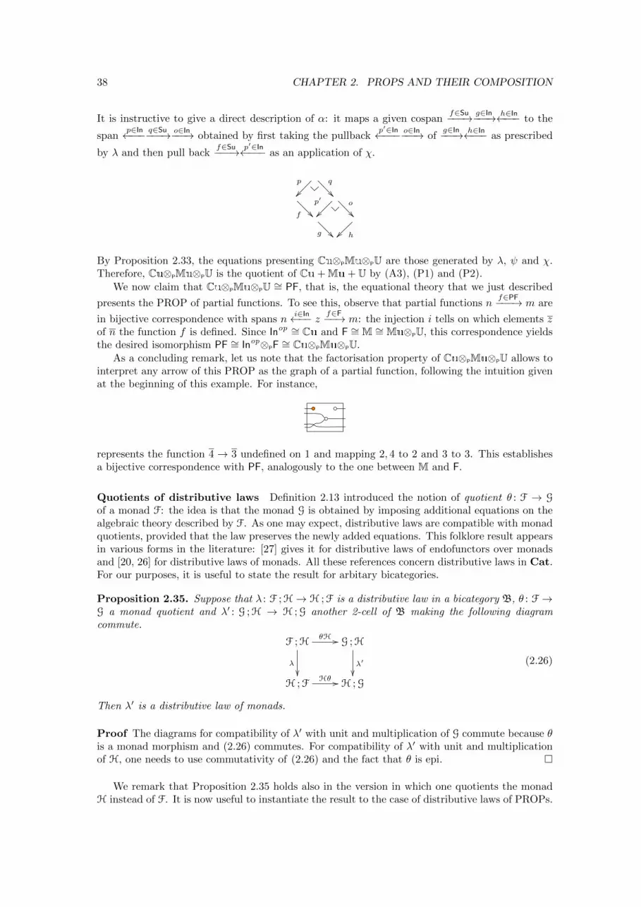
38 CHAPTER 2. PROPS AND THEIR COMPOSITION
It is instructive to give a direct description of α: it maps a given cospanf∈Su−−−→ g∈In−−−→ h∈In←−−− to the
spanp∈In←−−− q∈Su−−−→ o∈In−−−→ obtained by first taking the pullback
p′∈In←−−− o∈In−−−→ ofg∈In−−−→ h∈In←−−− as prescribed
by λ and then pull backf∈Su−−−→ p′∈In←−−− as an application of χ.
p
��q
��
f ��p′
��o
��
g �� h��
By Proposition 2.33, the equations presenting Cu⊗PMu⊗PU are those generated by λ, ψ and χ.Therefore, Cu⊗PMu⊗PU is the quotient of Cu + Mu + U by (A3), (P1) and (P2).
We now claim that Cu⊗PMu⊗PU ∼= PF, that is, the equational theory that we just described
presents the PROP of partial functions. To see this, observe that partial functions nf∈PF−−−→ m are
in bijective correspondence with spans ni∈In←−− z f∈F−−→ m: the injection i tells on which elements z
of n the function f is defined. Since Inop ∼= Cu and F ∼= M ∼= Mu⊗PU, this correspondence yieldsthe desired isomorphism PF ∼= Inop⊗PF ∼= Cu⊗PMu⊗PU.
As a concluding remark, let us note that the factorisation property of Cu⊗PMu⊗PU allows tointerpret any arrow of this PROP as the graph of a partial function, following the intuition givenat the beginning of this example. For instance,
represents the function 4 → 3 undefined on 1 and mapping 2, 4 to 2 and 3 to 3. This establishesa bijective correspondence with PF, analogously to the one between M and F.
Quotients of distributive laws Definition 2.13 introduced the notion of quotient θ : F → G
of a monad F: the idea is that the monad G is obtained by imposing additional equations on thealgebraic theory described by F. As one may expect, distributive laws are compatible with monadquotients, provided that the law preserves the newly added equations. This folklore result appearsin various forms in the literature: [27] gives it for distributive laws of endofunctors over monadsand [20, 26] for distributive laws of monads. All these references concern distributive laws in Cat.For our purposes, it is useful to state the result for arbitary bicategories.
Proposition 2.35. Suppose that λ : F ;H→ H ;F is a distributive law in a bicategory B, θ : F →G a monad quotient and λ′ : G ;H → H ;G another 2-cell of B making the following diagramcommute.
F ;HθH //
λ
��
G ;H
λ′
��H ;F
Hθ // H ;G
(2.26)
Then λ′ is a distributive law of monads.
Proof The diagrams for compatibility of λ′ with unit and multiplication of G commute because θis a monad morphism and (2.26) commutes. For compatibility of λ′ with unit and multiplicationof H, one needs to use commutativity of (2.26) and the fact that θ is epi. �
We remark that Proposition 2.35 holds also in the version in which one quotients the monadH instead of F. It is now useful to instantiate the result to the case of distributive laws of PROPs.
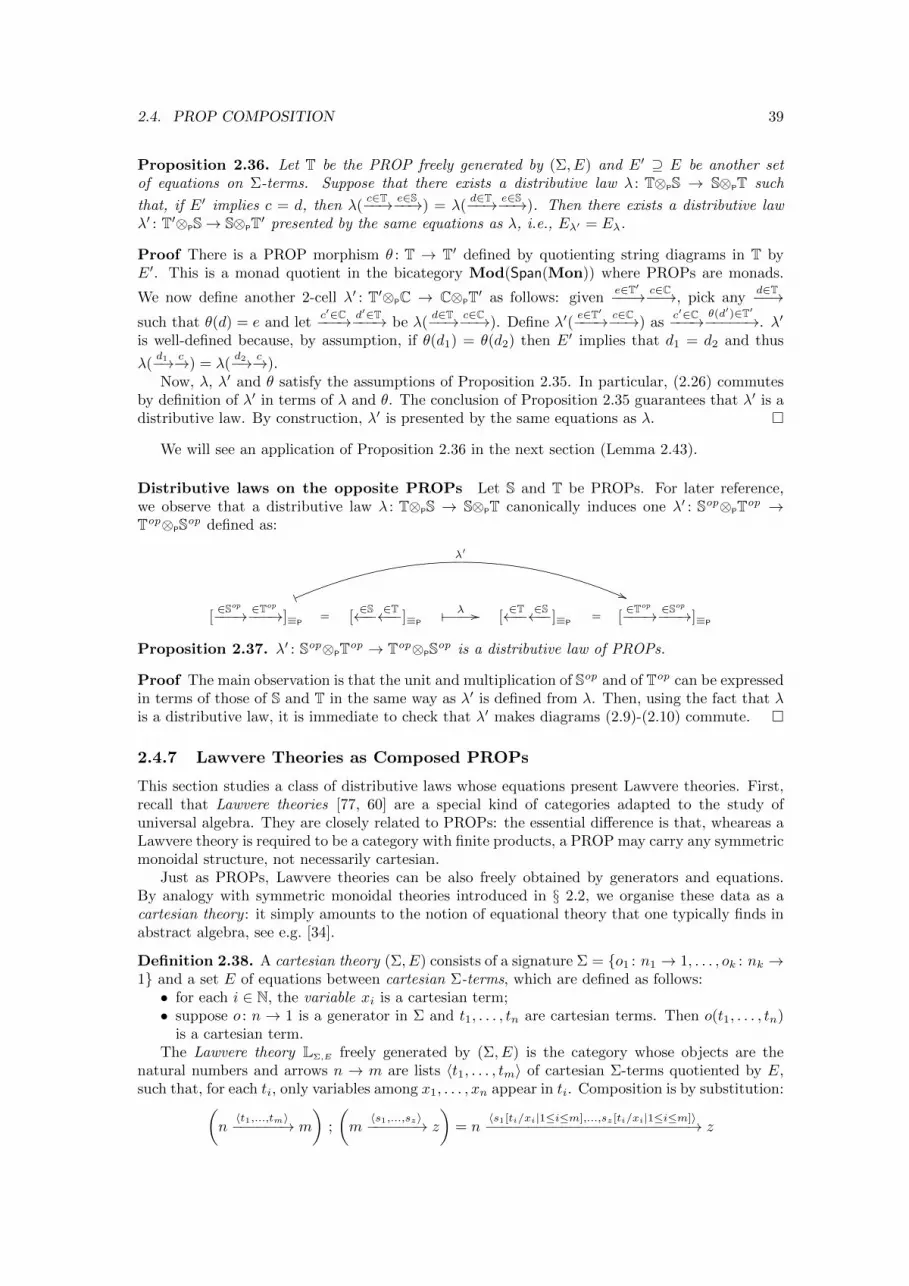
2.4. PROP COMPOSITION 39
Proposition 2.36. Let T be the PROP freely generated by (Σ, E) and E′ ⊇ E be another setof equations on Σ-terms. Suppose that there exists a distributive law λ : T⊗PS → S⊗PT such
that, if E′ implies c = d, then λ(c∈T−−→ e∈S−−→) = λ(
d∈T−−→ e∈S−−→). Then there exists a distributive lawλ′ : T′⊗PS→ S⊗PT′ presented by the same equations as λ, i.e., Eλ′ = Eλ.
Proof There is a PROP morphism θ : T → T′ defined by quotienting string diagrams in T byE′. This is a monad quotient in the bicategory Mod(Span(Mon)) where PROPs are monads.
We now define another 2-cell λ′ : T′⊗PC → C⊗PT′ as follows: givene∈T′−−−→ c∈C−−→, pick any
d∈T−−→such that θ(d) = e and let
c′∈C−−−→ d′∈T−−−→ be λ(d∈T−−→ c∈C−−→). Define λ′(
e∈T′−−−→ c∈C−−→) asc′∈C−−−→ θ(d′)∈T′−−−−−→. λ′
is well-defined because, by assumption, if θ(d1) = θ(d2) then E′ implies that d1 = d2 and thus
λ(d1−→ c−→) = λ(
d2−→ c−→).Now, λ, λ′ and θ satisfy the assumptions of Proposition 2.35. In particular, (2.26) commutes
by definition of λ′ in terms of λ and θ. The conclusion of Proposition 2.35 guarantees that λ′ is adistributive law. By construction, λ′ is presented by the same equations as λ. �
We will see an application of Proposition 2.36 in the next section (Lemma 2.43).
Distributive laws on the opposite PROPs Let S and T be PROPs. For later reference,we observe that a distributive law λ : T⊗PS → S⊗PT canonically induces one λ′ : Sop⊗PTop →Top⊗PSop defined as:
[∈Sop−−−→ ∈Top
−−−→]≡P
-
λ′
((
= [∈S←−− ∈T←−−]≡P
� λ // [∈T←−− ∈S←−−]≡P
= [∈Top
−−−→ ∈Sop−−−→]≡P
Proposition 2.37. λ′ : Sop⊗PTop → Top⊗PSop is a distributive law of PROPs.
Proof The main observation is that the unit and multiplication of Sop and of Top can be expressedin terms of those of S and T in the same way as λ′ is defined from λ. Then, using the fact that λis a distributive law, it is immediate to check that λ′ makes diagrams (2.9)-(2.10) commute. �
2.4.7 Lawvere Theories as Composed PROPs
This section studies a class of distributive laws whose equations present Lawvere theories. First,recall that Lawvere theories [77, 60] are a special kind of categories adapted to the study ofuniversal algebra. They are closely related to PROPs: the essential difference is that, wheareas aLawvere theory is required to be a category with finite products, a PROP may carry any symmetricmonoidal structure, not necessarily cartesian.
Just as PROPs, Lawvere theories can be also freely obtained by generators and equations.By analogy with symmetric monoidal theories introduced in § 2.2, we organise these data as acartesian theory : it simply amounts to the notion of equational theory that one typically finds inabstract algebra, see e.g. [34].
Definition 2.38. A cartesian theory (Σ, E) consists of a signature Σ = {o1 : n1 → 1, . . . , ok : nk →1} and a set E of equations between cartesian Σ-terms, which are defined as follows:• for each i ∈ N, the variable xi is a cartesian term;• suppose o : n → 1 is a generator in Σ and t1, . . . , tn are cartesian terms. Then o(t1, . . . , tn)
is a cartesian term.The Lawvere theory LΣ,E freely generated by (Σ, E) is the category whose objects are the
natural numbers and arrows n → m are lists 〈t1, . . . , tm〉 of cartesian Σ-terms quotiented by E,such that, for each ti, only variables among x1, . . . , xn appear in ti. Composition is by substitution:
(n〈t1,...,tm〉−−−−−−→ m
);
(m〈s1,...,sz〉−−−−−−→ z
)= n
〈s1[ti/xi|1≤i≤m],...,sz [ti/xi|1≤i≤m]〉−−−−−−−−−−−−−−−−−−−−−−−−→ z
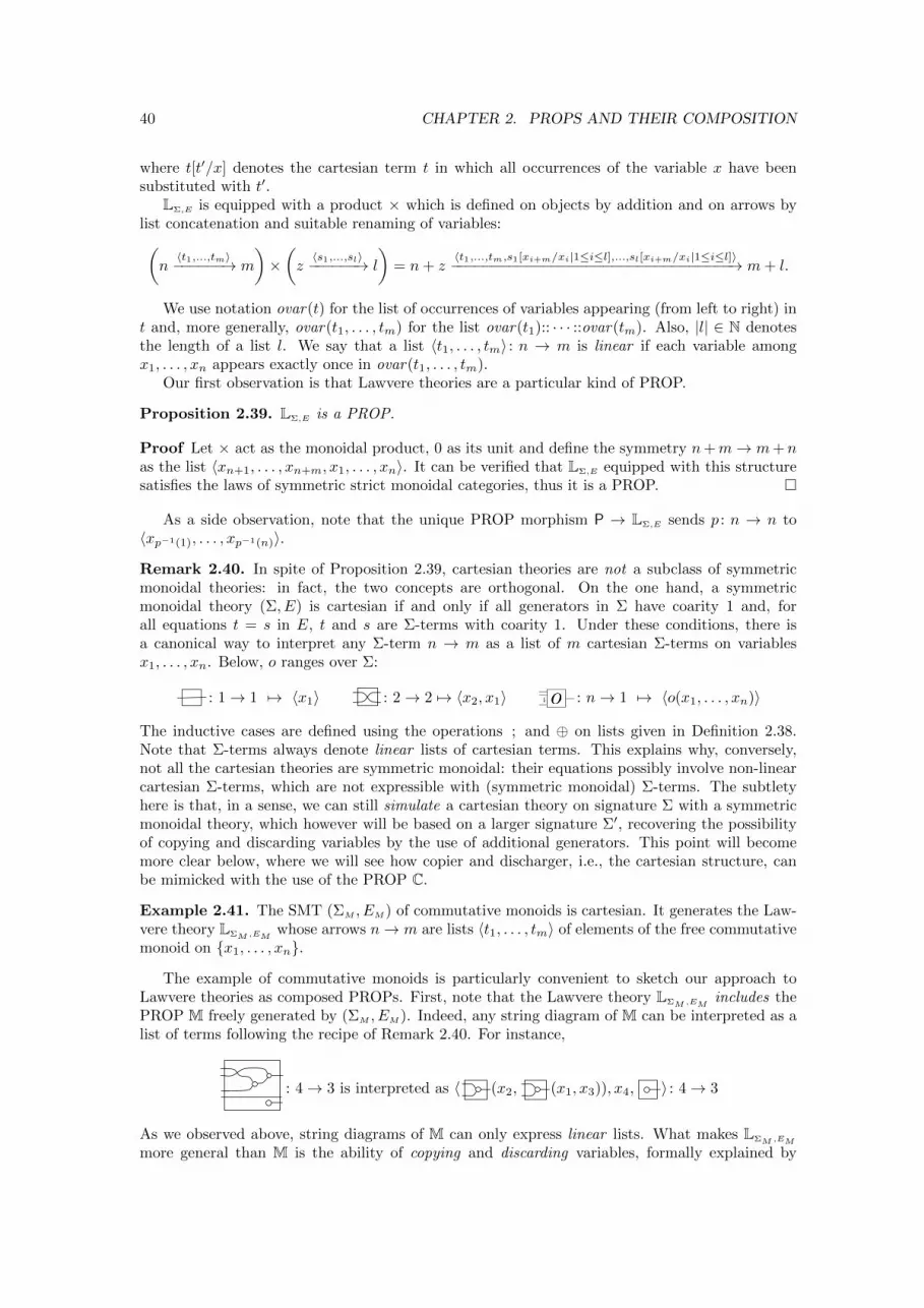
40 CHAPTER 2. PROPS AND THEIR COMPOSITION
where t[t′/x] denotes the cartesian term t in which all occurrences of the variable x have beensubstituted with t′.
LΣ,E is equipped with a product × which is defined on objects by addition and on arrows bylist concatenation and suitable renaming of variables:
(n〈t1,...,tm〉−−−−−−→ m
)×(z〈s1,...,sl〉−−−−−−→ l
)= n+ z
〈t1,...,tm,s1[xi+m/xi|1≤i≤l],...,sl[xi+m/xi|1≤i≤l]〉−−−−−−−−−−−−−−−−−−−−−−−−−−−−−−−−−→ m+ l.
We use notation ovar(t) for the list of occurrences of variables appearing (from left to right) int and, more generally, ovar(t1, . . . , tm) for the list ovar(t1):: · · · ::ovar(tm). Also, |l| ∈ N denotesthe length of a list l. We say that a list 〈t1, . . . , tm〉 : n → m is linear if each variable amongx1, . . . , xn appears exactly once in ovar(t1, . . . , tm).
Our first observation is that Lawvere theories are a particular kind of PROP.
Proposition 2.39. LΣ,E is a PROP.
Proof Let × act as the monoidal product, 0 as its unit and define the symmetry n+m→ m+ nas the list 〈xn+1, . . . , xn+m, x1, . . . , xn〉. It can be verified that LΣ,E equipped with this structuresatisfies the laws of symmetric strict monoidal categories, thus it is a PROP. �
As a side observation, note that the unique PROP morphism P → LΣ,E sends p : n → n to〈xp−1(1), . . . , xp−1(n)〉.
Remark 2.40. In spite of Proposition 2.39, cartesian theories are not a subclass of symmetricmonoidal theories: in fact, the two concepts are orthogonal. On the one hand, a symmetricmonoidal theory (Σ, E) is cartesian if and only if all generators in Σ have coarity 1 and, forall equations t = s in E, t and s are Σ-terms with coarity 1. Under these conditions, there isa canonical way to interpret any Σ-term n → m as a list of m cartesian Σ-terms on variablesx1, . . . , xn. Below, o ranges over Σ:
: 1→ 1 7→ 〈x1〉 : 2→ 2 7→ 〈x2, x1〉 o : n→ 1 7→ 〈o(x1, . . . , xn)〉
The inductive cases are defined using the operations ; and ⊕ on lists given in Definition 2.38.Note that Σ-terms always denote linear lists of cartesian terms. This explains why, conversely,not all the cartesian theories are symmetric monoidal: their equations possibly involve non-linearcartesian Σ-terms, which are not expressible with (symmetric monoidal) Σ-terms. The subtletyhere is that, in a sense, we can still simulate a cartesian theory on signature Σ with a symmetricmonoidal theory, which however will be based on a larger signature Σ′, recovering the possibilityof copying and discarding variables by the use of additional generators. This point will becomemore clear below, where we will see how copier and discharger, i.e., the cartesian structure, canbe mimicked with the use of the PROP C.
Example 2.41. The SMT (ΣM , EM) of commutative monoids is cartesian. It generates the Law-vere theory LΣM,EM
whose arrows n→ m are lists 〈t1, . . . , tm〉 of elements of the free commutativemonoid on {x1, . . . , xn}.
The example of commutative monoids is particularly convenient to sketch our approach toLawvere theories as composed PROPs. First, note that the Lawvere theory LΣM,EM
includes thePROP M freely generated by (ΣM , EM). Indeed, any string diagram of M can be interpreted as alist of terms following the recipe of Remark 2.40. For instance,
: 4→ 3 is interpreted as 〈 (x2, (x1, x3)), x4, 〉 : 4→ 3
As we observed above, string diagrams of M can only express linear lists. What makes LΣM,EM
more general than M is the ability of copying and discarding variables, formally explained by
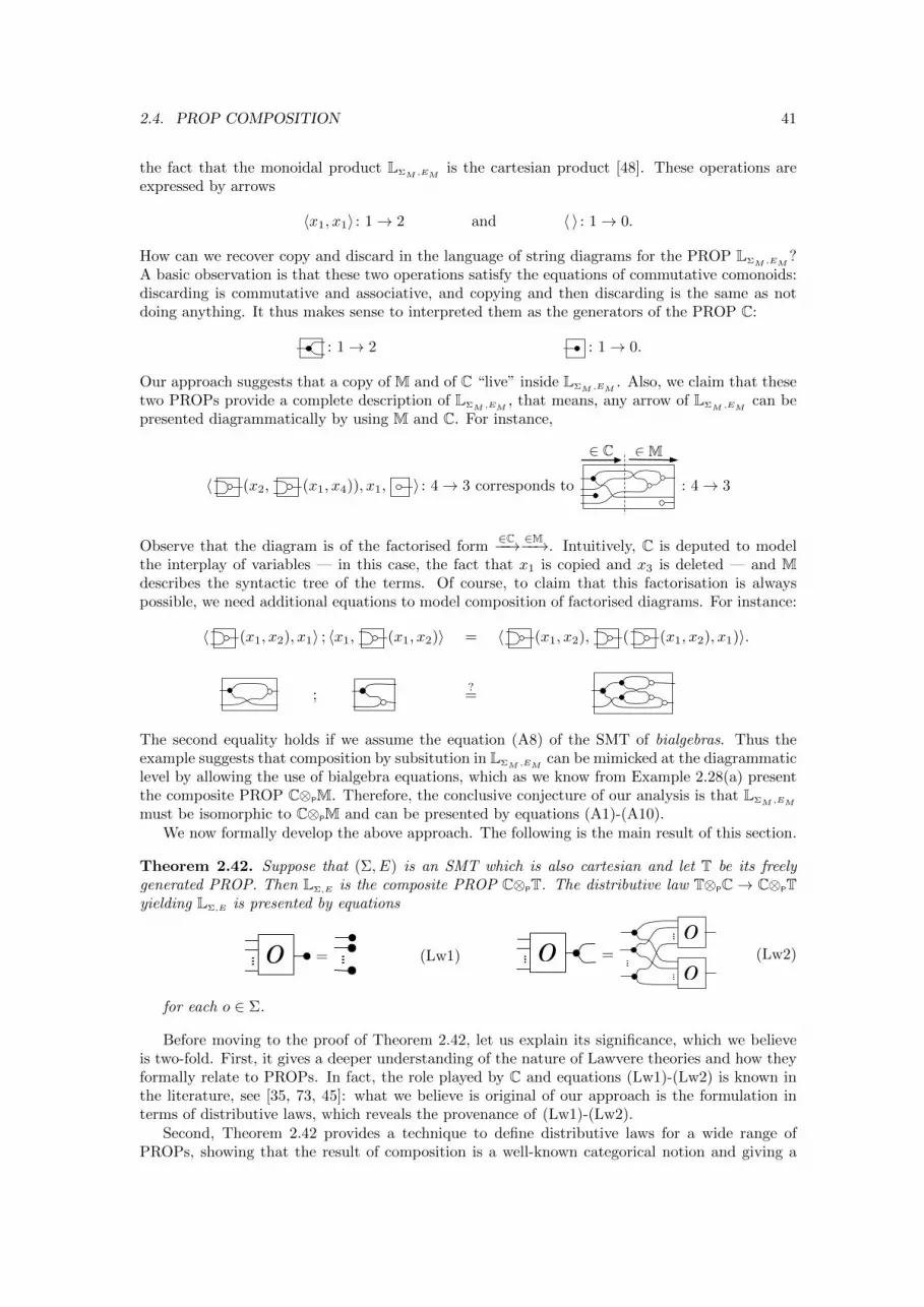
2.4. PROP COMPOSITION 41
the fact that the monoidal product LΣM,EMis the cartesian product [48]. These operations are
expressed by arrows
〈x1, x1〉 : 1→ 2 and 〈 〉 : 1→ 0.
How can we recover copy and discard in the language of string diagrams for the PROP LΣM,EM?
A basic observation is that these two operations satisfy the equations of commutative comonoids:discarding is commutative and associative, and copying and then discarding is the same as notdoing anything. It thus makes sense to interpreted them as the generators of the PROP C:
: 1→ 2 : 1→ 0.
Our approach suggests that a copy of M and of C “live” inside LΣM,EM. Also, we claim that these
two PROPs provide a complete description of LΣM,EM, that means, any arrow of LΣM,EM
can bepresented diagrammatically by using M and C. For instance,
〈 (x2, (x1, x4)), x1, 〉 : 4→ 3 corresponds to
2M2 C
: 4→ 3
Observe that the diagram is of the factorised form∈C−−→ ∈M−−→. Intuitively, C is deputed to model
the interplay of variables — in this case, the fact that x1 is copied and x3 is deleted — and Mdescribes the syntactic tree of the terms. Of course, to claim that this factorisation is alwayspossible, we need additional equations to model composition of factorised diagrams. For instance:
〈 (x1, x2), x1〉 ; 〈x1, (x1, x2)〉 = 〈 (x1, x2), ( (x1, x2), x1)〉.
;?=
The second equality holds if we assume the equation (A8) of the SMT of bialgebras. Thus theexample suggests that composition by subsitution in LΣM,EM
can be mimicked at the diagrammaticlevel by allowing the use of bialgebra equations, which as we know from Example 2.28(a) presentthe composite PROP C⊗PM. Therefore, the conclusive conjecture of our analysis is that LΣM,EM
must be isomorphic to C⊗PM and can be presented by equations (A1)-(A10).We now formally develop the above approach. The following is the main result of this section.
Theorem 2.42. Suppose that (Σ, E) is an SMT which is also cartesian and let T be its freelygenerated PROP. Then LΣ,E is the composite PROP C⊗PT. The distributive law T⊗PC → C⊗PTyielding LΣ,E is presented by equations
o = (Lw1) o =
o
o(Lw2)
for each o ∈ Σ.
Before moving to the proof of Theorem 2.42, let us explain its significance, which we believeis two-fold. First, it gives a deeper understanding of the nature of Lawvere theories and how theyformally relate to PROPs. In fact, the role played by C and equations (Lw1)-(Lw2) is known inthe literature, see [35, 73, 45]: what we believe is original of our approach is the formulation interms of distributive laws, which reveals the provenance of (Lw1)-(Lw2).
Second, Theorem 2.42 provides a technique to define distributive laws for a wide range ofPROPs, showing that the result of composition is a well-known categorical notion and giving a
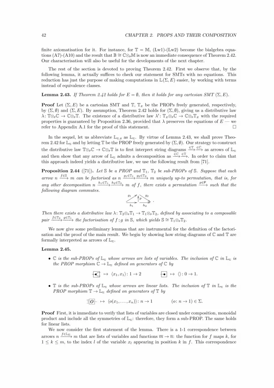
42 CHAPTER 2. PROPS AND THEIR COMPOSITION
finite axiomatisation for it. For instance, for T = M, (Lw1)-(Lw2) become the bialgebra equa-tions (A7)-(A10) and the result that B ∼= C⊗PM is now an immediate consequence of Theorem 2.42.Our characterisation will also be useful for the developments of the next chapter.
The rest of the section is devoted to proving Theorem 2.42. First we observe that, by thefollowing lemma, it actually suffices to check our statement for SMTs with no equations. Thisreduction has just the purpose of making computations in L(Σ, E) easier, by working with termsinstead of equivalence classes.
Lemma 2.43. If Theorem 2.42 holds for E = ∅, then it holds for any cartesian SMT (Σ, E).
Proof Let (Σ, E) be a cartesian SMT and T, TE be the PROPs freely generated, respectively,by (Σ, ∅) and (Σ, E). By assumption, Theorem 2.42 holds for (Σ, ∅), giving us a distributive lawλ : T⊗PC → C⊗PT. The existence of a distributive law λ′ : TE⊗PC → C⊗PTE with the requiredproperties is guaranteed by Proposition 2.36, provided that λ preserves the equations of E — werefer to Appendix A.1 for the proof of this statement. �
In the sequel, let us abbreviate LΣ,∅ as LΣ. By virtue of Lemma 2.43, we shall prove Theo-rem 2.42 for LΣ and by letting T be the PROP freely generated by (Σ, ∅). Our strategy to construct
the distributive law T⊗PC → C⊗PT is to first interpret string diagrams∈T−−→ ∈C−−→ as arrows of LΣ
and then show that any arrow of LΣ admits a decomposition as∈C−−→ ∈T−−→. In order to claim that
this approach indeed yields a distributive law, we use the following result from [71].
Proposition 2.44 ([71]). Let S be a PROP and T1, T2 be sub-PROPs of S. Suppose that each
arrow nf∈S−−→ m can be factorised as n
g1∈T1−−−−→ g2∈T2−−−−→ m uniquely up-to permutation, that is, for
any other decomposition nh1∈T1−−−−→ h2∈T2−−−−→ m of f , there exists a permutation
p∈P−−→ such that thefollowing diagram commutes.
g2
%%g199
h1
//pOO
h2
// .
Then there exists a distributive law λ : T2⊗PT1 → T1⊗PT2, defined by associating to a composable
pairf∈T2−−−→ g∈T1−−−→ the factorisation of f ; g in S, which yields S ∼= T1⊗PT2.
We now give some preliminary lemmas that are instrumental for the definition of the factori-sation and the proof of the main result. We begin by showing how string diagrams of C and T areformally interpreted as arrows of LΣ.
Lemma 2.45.
• C is the sub-PROPs of LΣ whose arrows are lists of variables. The inclusion of C in LΣ isthe PROP morphism C→ LΣ defined on generators of C by
7→ 〈x1, x1〉 : 1→ 2 7→ 〈〉 : 0→ 1.
• T is the sub-PROPs of LΣ whose arrows are linear lists. The inclusion of T in LΣ is thePROP morphism T→ LΣ defined on generators of T by
o 7→ 〈o(x1, . . . , xn)〉 : n→ 1 (o : n→ 1) ∈ Σ.
Proof First, it is immediate to verify that lists of variables are closed under composition, monoidalproduct and include all the symmetries of LΣ: therefore, they form a sub-PROP. The same holdsfor linear lists.
We now consider the first statement of the lemma. There is a 1-1 correspondence between
arrows nf∈LΣ−−−→ m that are lists of variables and functions m→ n: the function for f maps k, for
1 ≤ k ≤ m, to the index l of the variable xl appearing in position k in f . This correspondence

2.4. PROP COMPOSITION 43
yields an isomorphism between the sub-PROP of LΣ whose arrows are lists of variables and Fop .
Composing this isomorphism with the one C∼=−→ Fop yields the PROP morphism inductively
defined in the statement of the lemma.We now turn to the second statement. By construction, arrows of T are Σ-terms: the interpre-
tation of Remark 2.40 defines a faithful PROP morphism T → LΣ which coincides with the oneof the statement. The image of this PROP morphism are precisely the linear lists in LΣ. �
Lemma 2.45 allows us to use LΣ as an environment where letting C and T interact. Thefollowing statement guarantees the soundness of the interaction described by (Lw1)-(Lw2).
Lemma 2.46. Equations (Lw1) and (Lw2) are sound in LΣ under the interpretation of T and Cas sub-PROPs of LΣ.
Proof We first focus on (Lw1). Following the isomorphisms of Lemma 2.45, o ∈ T[n, 1] is
interpreted as the arrow 〈o(x1, . . . , xn)〉 ∈ LΣ[n, 1] and ∈ C[0, 1] as 〈〉 ∈ LΣ[1, 0]. The left-hand
side of (Lw1) is then the composite 〈o(x1, . . . , xn)〉 ; 〈〉 ∈ LΣ[n, 0], which is equal by definition to〈〉 ∈ LΣ[n, 0]. Therefore, the left- and right-hand side of (Lw1) are the same arrow of LΣ.
It remains to show soundness of (Lw2). Following Lemma 2.45, the left-hand side o ;
is interpreted in LΣ as the composite 〈o(x1, . . . , xn)〉 ; 〈x1, x1〉. The right-hand side is interpretedas 〈x1, . . . , xn, x1, . . . , xn〉 ; 〈o(x1, . . . , xn), o(xn+1, . . . , xn+n)〉. By definition, both composites areequal to 〈o(x1, . . . , xn), o(x1, . . . , xn)〉 in LΣ. Therefore, (Lw2) is also sound in LΣ. �
It is useful to observe that (Lw1)-(Lw2) allows us to copy and discard not only the generatorsbut arbitrary string diagrams of T.
Lemma 2.47. Suppose d is a string diagram of T. Then the following holds in T+C quotientedby (Lw1)-(Lw2).
d =
d
d(Law3) d = (Law4)
Proof The proof is by induction on d . For (Law3), the base cases of and follow
by (SM1) and (SM2). The base case of o , for o a generator in Σ, is given by (Lw2). Theinductive cases of composition by ; and ⊕ immediately follow by inductive hypothesis. The proofof (Law4) is analogous. �
We can now show the factorisation lemma.
Lemma 2.48. Any arrow nf∈LΣ−−−→ m has a factorisation n
c∈C−−→ d∈T−−→ m which is unique up-topermutation.
Proof Since the cartesian theory generating LΣ has no equations, nf−→ m is just a list of cartesian
Σ-terms 〈t1, . . . , tm〉. The factorisation consists in replacing all variables appearing in 〈t1, . . . , tm〉with fresh ones x1, . . . , xz, so that no repetition occurs: this gives us the second component of the
decomposition as a linear list zd∈T−−→ m. The first component c will be the list n
ovar(t1,...,tm)∈C−−−−−−−−−−−→ zof variables originally occurring in f , so that post-composition with d yields 〈t1, . . . , tm〉. Thereader can consult Appendix A.1 for further details. �
Example 2.49. Suppose T is the free PROP on signature Σ = {o : 2 → 1}. The arrow〈o(x1, o(x1, x3)), x2〉 : 3 → 2 in LΣ is factorised as 〈x1, x1, x3, x2〉 ; 〈o(x1, o(x2, x3)), x4〉. Observethat this decomposition is unique only-up to permutation: for instance, another factorisation is〈x1, x1, x2, x3〉 ; 〈o(x1, o(x2, x4)), x3〉 — in this case, the mediating permutation is 〈x1, x2, x4, x3〉.
We now have all the ingredients to conclude the proof of our main statement.
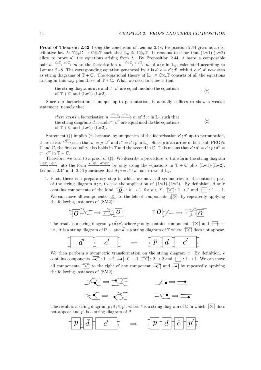
44 CHAPTER 2. PROPS AND THEIR COMPOSITION
Proof of Theorem 2.42 Using the conclusion of Lemma 2.48, Proposition 2.44 gives us a dis-tributive law λ : T⊗PC → C⊗PT such that LΣ
∼= C⊗PT. It remains to show that (Lw1)-(Lw2)allow to prove all the equations arising from λ. By Proposition 2.44, λ maps a composable
pair nd∈T−−→ c∈C−−→ m to the factorisation n
c′∈C−−−→ d′∈T−−−→ m of d ; c in LΣ, calculated according toLemma 2.48. The corresponding equation generated by λ is d ; c = c′ ; d′, with d, c, c′, d′ now seenas string diagrams of T + C. The equational theory of LΣ
∼= C⊗PT consists of all the equationsarising in this way plus those of T + C. What we need to show is that
the string diagrams d ; c and c′ ; d′ are equal modulo the equationsof T + C and (Lw1)-(Lw2).
(†)
Since our factorisation is unique up-to permutation, it actually suffices to show a weakerstatement, namely that
there exists a factorisation nc′′∈C−−−→ d′′∈T−−−→ m of d ; c in LΣ such that
the string diagrams d ; c and c′′ ; d′′ are equal modulo the equationsof T + C and (Lw1)-(Lw2).
(‡)
Statement (‡) implies (†) because, by uniqueness of the factorisation c′ ; d′ up-to permutation,
there existsp∈P−−→ such that d′ = p ; d′′ and c′′ = c′ ; p in LΣ. Since p is an arrow of both sub-PROPs
T and C, the first equality also holds in T and the second in C. This means that c′ ; d′ = c′ ; p ; d′′ =c′′ ; d′′ in T + C.
Therefore, we turn to a proof of (‡). We describe a procedure to transform the string diagramd∈T−−→ c∈C−−→ into the form
c′′∈C−−−→ d′′∈T−−−→ by only using the equations in T + C plus (Lw1)-(Lw2).Lemmas 2.45 and 2.46 guarantee that d ; c = c′′ ; d′′ as arrows of LΣ.
1. First, there is a preparatory step in which we move all symmetries to the outmost partof the string diagram d ; c, to ease the application of (Lw1)-(Lw2). By definition, d only
contains components of the kind o : k → 1, for o ∈ Σ, : 2 → 2 and : 1 → 1.
We can move all components to the left of components o by repeatedly applyingthe following instances of (SM2):
o =⇒ o o =⇒ oThe result is a string diagram p ; d ; c′, where p only contains components and —
i.e., it is a string diagram of P — and d is a string diagram of T where does not appear.
c0d0 =⇒ p c0d
We then perform a symmetric transformation on the string diagram c. By definition, c
contains components : 1→ 2, : 0→ 1, : 2→ 2 and : 1→ 1. We can move
all components to the right of any component and by repeatedly applying
the following instances of (SM2):
=⇒ =⇒
=⇒ =⇒
The result is a string diagram p ; d ; c ; p′, where c is a string diagram of C in which doesnot appear and p′ is a string diagram of P.
p c0d =⇒ p p0d c
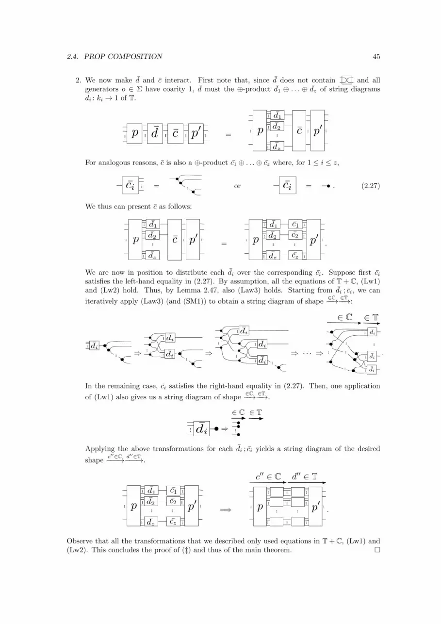
2.4. PROP COMPOSITION 45
2. We now make d and c interact. First note that, since d does not contain and allgenerators o ∈ Σ have coarity 1, d must the ⊕-product d1 ⊕ . . . ⊕ dz of string diagramsdi : ki → 1 of T.
p p0d c =
dz
d2
d1
p p0c
For analogous reasons, c is also a ⊕-product c1 ⊕ . . .⊕ cz where, for 1 ≤ i ≤ z,
ci = or ci = . (2.27)
We thus can present c as follows:
dz
d2
d1
p p0c =
dz
d2
d1 c1
c2
cz
p p0 .
We are now in position to distribute each di over the corresponding ci. Suppose first cisatisfies the left-hand equality in (2.27). By assumption, all the equations of T + C, (Lw1)and (Lw2) hold. Thus, by Lemma 2.47, also (Law3) holds. Starting from di ; ci, we can
iteratively apply (Law3) (and (SM1)) to obtain a string diagram of shape∈C−−→ ∈T−−→:
di
⇒ di
di
⇒di
di
di
⇒ · · · ⇒
di
di
di
2 C 2 T
.
In the remaining case, ci satisfies the right-hand equality in (2.27). Then, one application
of (Lw1) also gives us a string diagram of shape∈C−−→ ∈T−−→.
di ⇒
2 C 2 T
Applying the above transformations for each di ; ci yields a string diagram of the desired
shapec′′∈C−−−→ d′′∈T−−−→.
dz
d2
d1 c1
c2
cz
p p0 =⇒ p p0
c00 2 C d00 2 T
.
Observe that all the transformations that we described only used equations in T + C, (Lw1) and(Lw2). This concludes the proof of (‡) and thus of the main theorem. �
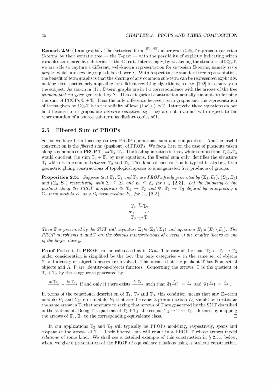
46 CHAPTER 2. PROPS AND THEIR COMPOSITION
Remark 2.50 (Term graphs). The factorised form∈C−−→ ∈T−−→ of arrows in C⊗PT represents cartesian
Σ-terms by their syntatic tree — the T-part — with the possibility of explictly indicating whichvariables are shared by sub-terms — the C-part. Interestingly, by weakening the structure of C⊗PT,we are able to capture a different, well-known representation for cartesian Σ-terms, namely termgraphs, which are acyclic graphs labeled over Σ. With respect to the standard tree representation,the benefit of term graphs is that the sharing of any common sub-term can be represented explicitly,making them particularly appealing for efficient rewriting algorithms, see e.g. [102] for a survey onthe subject. As shown in [45], Σ-term graphs are in 1-1 correspondence with the arrows of the freegs-monoidal category generated by Σ. This categorical construction actually amounts to formingthe sum of PROPs C + T. Thus the only difference between term graphs and the representationof terms given by C⊗PT is in the validity of laws (Lw1)-(Lw2). Intuitively, these equations do nothold because term graphs are resource-sensitive, e.g. they are not invariant with respect to therepresentation of a shared sub-term as distinct copies of it.
2.5 Fibered Sum of PROPs
So far we have been focusing on two PROP operations: sum and composition. Another usefulconstruction is the fibered sum (pushout) of PROPs. We focus here on the case of pushouts takenalong a common sub-PROP T1 ⇒ T2,T3. The leading intuition is that, while composition T2⊗PT3
would quotient the sum T2 + T3 by new equations, the fibered sum only identifies the structureT1 which is in common between T2 and T3. This kind of construction is typical in algebra, fromgeometric gluing constructions of topological spaces to amalgamated free products of groups.
Proposition 2.51. Suppose that T1, T2 and T3 are PROPs freely generated by (Σ1, E1), (Σ2, E2)and (Σ3, E3) respectively, with Σ1 ⊆ Σi and E1 ⊆ Ei for i ∈ {2, 3}. Let the following be thepushout along the PROP morphisms Φ: T1 → T2 and Ψ: T1 → T3 defined by interpreting aΣ1-term modulo E1 as a Σi-term modulo Ei, for i ∈ {2, 3}.
T1Φ //
Ψ ��
T2
��T3
Γ// T
Then T is presented by the SMT with signature Σ2 ] (Σ3 \Σ1) and equations E2 ] (E3 \E1). ThePROP morphisms Λ and Γ are the obvious interpretations of a term of the smaller theory as oneof the larger theory.
Proof Pushouts in PROP can be calculated as in Cat. The case of the span T2 ←− T1 −→ T3
under consideration is simplified by the fact that only categories with the same set of objectsN and identity-on-object functors are involved. This means that the pushout T has N as set ofobjects and Λ, Γ are identity-on-objects functors. Concerning the arrows, T is the quotient ofT2 + T3 by the congruence generated by
g∈T2−−−→ ∼ h∈T3−−−→ if and only if there existsf∈T1−−−→ such that Φ(
f−→) =g−→ and Ψ(
f−→) =h−→ .
In terms of the equational description of T1, T2 and T3, this condition means that any Σ2-termmodulo E2 and Σ3-term modulo E3 that are the same Σ1-term modulo E1 should be treated asthe same arrow in T; that amounts to saying that arrows of T are generated by the SMT describedin the statement. Being T a quotient of T2 + T3, the cospan T2 −→ T←− T3 is formed by mappingthe arrows of T2, T3 to the corresponding equivalence class. �
In our applications T2 and T3 will typically be PROPs modeling, respectively, spans andcospans of the arrows of T1. Their fibered sum will result in a PROP T whose arrows modelrelations of some kind. We shall see a detailed example of this construction in § 2.5.1 below,where we give a presentation of the PROP of equivalence relations using a pushout construction.
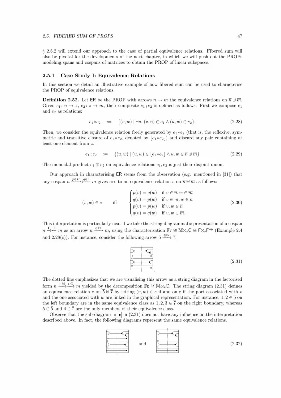
2.5. FIBERED SUM OF PROPS 47
§ 2.5.2 will extend our approach to the case of partial equivalence relations. Fibered sum willalso be pivotal for the developments of the next chapter, in which we will push out the PROPsmodeling spans and cospans of matrices to obtain the PROP of linear subspaces.
2.5.1 Case Study I: Equivalence Relations
In this section we detail an illustrative example of how fibered sum can be used to characterisethe PROP of equivalence relations.
Definition 2.52. Let ER be the PROP with arrows n → m the equivalence relations on n ]m.Given e1 : n → z, e2 : z → m, their composite e1 ; e2 is defined as follows. First we compose e1
and e2 as relations:
e1∗e2 := {(v, w) | ∃u. (v, u) ∈ e1 ∧ (u,w) ∈ e2}. (2.28)
Then, we consider the equivalence relation freely generated by e1∗e2 (that is, the reflexive, sym-metric and transitive closure of e1 ∗e2, denoted by be1∗e2c) and discard any pair containing atleast one element from z.
e1 ; e2 := {(u,w) | (u,w) ∈ be1∗e2c ∧ u,w ∈ n ]m} (2.29)
The monoidal product e1 ⊕ e2 on equivalence relations e1, e2 is just their disjoint union.
Our approach in characterising ER stems from the observation (e.g. mentioned in [31]) that
any cospan np∈F−−−→ q∈F←−− m gives rise to an equivalence relation e on n ]m as follows:
(v, w) ∈ e iff
p(v) = q(w) if v ∈ n,w ∈ mq(v) = p(w) if v ∈ m,w ∈ np(v) = p(w) if v, w ∈ nq(v) = q(w) if v, w ∈ m.
(2.30)
This interpretation is particularly neat if we take the string diagrammatic presentation of a cospan
nF−→ F←− m as an arrow n
∈Fr−−→ m, using the characterisation Fr ∼= M⊗PC ∼= F⊗PFop (Example 2.4
and 2.28(c)). For instance, consider the following arrow 5∈Fr−−→ 7:
.
(2.31)
The dotted line emphasizes that we are visualising this arrow as a string diagram in the factorised
form n∈M−−→ ∈C−−→ m yielded by the decomposition Fr ∼= M⊗PC. The string diagram (2.31) defines
an equivalence relation e on 5 ] 7 by letting (v, w) ∈ e if and only if the port associated with vand the one associated with w are linked in the graphical representation. For instance, 1, 2 ∈ 5 onthe left boundary are in the same equivalence class as 1, 2, 3 ∈ 7 on the right boundary, whereas5 ∈ 5 and 4 ∈ 7 are the only members of their equivalence class.
Observe that the sub-diagram in (2.31) does not have any influence on the interpretationdescribed above. In fact, the following diagrams represent the same equivalence relations.
and (2.32)
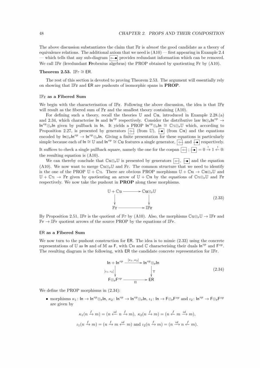
48 CHAPTER 2. PROPS AND THEIR COMPOSITION
The above discussion substantiates the claim that Fr is almost the good candidate as a theory ofequivalence relations. The additional axiom that we need is (A10) — first appearing in Example 2.4— which tells that any sub-diagram provides redundant information which can be removed.
We call IFr (irredundant Frobenius algebras) the PROP obtained by quotienting Fr by (A10).
Theorem 2.53. IFr ∼= ER.
The rest of this section is devoted to proving Theorem 2.53. The argument will essentially relyon showing that IFr and ER are pushouts of isomorphic spans in PROP.
IFr as a Fibered Sum
We begin with the characterisation of IFr. Following the above discussion, the idea is that IFrwill result as the fibered sum of Fr and the smallest theory containing (A10).
For defining such a theory, recall the theories U and Cu, introduced in Example 2.28.(a)and 2.34, which characterise In and Inop respectively. Consider the distributive law In⊗PIn
op →Inop⊗PIn given by pullback in In. It yields a PROP Inop⊗PIn ∼= Cu⊗PU which, according toProposition 2.27, is presented by generators (from U), (from Cu) and the equations
encoded by In⊗PInop → Inop⊗PIn. Giving a finite presentation for these equations is particularly
simple because each of In ∼= U and Inop ∼= Cu features a single generator, and respectively.
It suffices to check a single pullback square, namely the one for the cospan ; = 0!−→ 1
!←− 0:
the resulting equation is (A10).We can thereby conclude that Cu⊗PU is presented by generators , and the equation
(A10). We now want to merge Cu⊗PU and Fr. The common structure that we need to identifyis the one of the PROP U + Cu. There are obvious PROP morphisms U + Cu → Cu⊗PU andU + Cu → Fr given by quotienting an arrow of U + Cu by the equations of Cu⊗PU and Frrespectively. We now take the pushout in PROP along these morphisms.
U + Cu //
��
Cu⊗PU
��Fr // IFr
(2.33)
By Proposition 2.51, IFr is the quotient of Fr by (A10). Also, the morphisms Cu⊗PU→ IFr andFr→ IFr quotient arrows of the source PROP by the equations of IFr.
ER as a Fibered Sum
We now turn to the pushout construction for ER. The idea is to mimic (2.33) using the concreterepresentations of U as In and of M as F, with Cu and C characterising their duals Inop and Fop .The resulting diagram is the following, with ER the candidate concrete representation for IFr.
In + Inop[κ1, κ2] //
[ι1, ι2]
��
Inop⊗PIn
Υ
��F⊗PF
op
Π// ER
(2.34)
We define the PROP morphisms in (2.34):
• morphisms κ1 : In→ Inop⊗PIn, κ2 : Inop → Inop⊗PIn, ι1 : In→ F⊗PFop and ι2 : Inop → F⊗PF
op
are given by
κ1(nf−→ m) = (n
id←− n f−→ m), κ2(nf−→ m) = (n
f←− m id−→ m),
ι1(nf−→ m) = (n
f−→ mid←− m) and ι2(n
f−→ m) = (nid−→ n
f←− m).
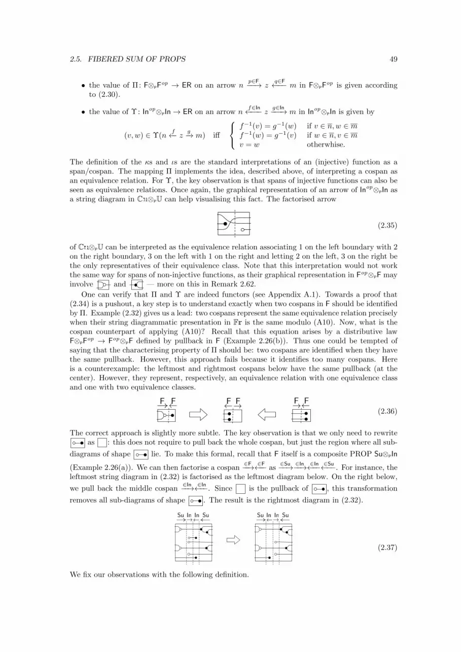
2.5. FIBERED SUM OF PROPS 49
• the value of Π: F⊗PFop → ER on an arrow n
p∈F−−→ zq∈F←−− m in F⊗PF
op is given accordingto (2.30).
• the value of Υ: Inop⊗PIn→ ER on an arrow nf∈In←−−− z g∈In−−−→ m in Inop⊗PIn is given by
(v, w) ∈ Υ(nf←− z g−→ m) iff
f−1(v) = g−1(w) if v ∈ n,w ∈ mf−1(w) = g−1(v) if w ∈ n, v ∈ mv = w otherwhise.
The definition of the κs and ιs are the standard interpretations of an (injective) function as aspan/cospan. The mapping Π implements the idea, described above, of interpreting a cospan asan equivalence relation. For Υ, the key observation is that spans of injective functions can also beseen as equivalence relations. Once again, the graphical representation of an arrow of Inop⊗PIn asa string diagram in Cu⊗PU can help visualising this fact. The factorised arrow
(2.35)
of Cu⊗PU can be interpreted as the equivalence relation associating 1 on the left boundary with 2on the right boundary, 3 on the left with 1 on the right and letting 2 on the left, 3 on the right bethe only representatives of their equivalence class. Note that this interpretation would not workthe same way for spans of non-injective functions, as their graphical representation in Fop⊗PF mayinvolve and — more on this in Remark 2.62.
One can verify that Π and Υ are indeed functors (see Appendix A.1). Towards a proof that(2.34) is a pushout, a key step is to understand exactly when two cospans in F should be identifiedby Π. Example (2.32) gives us a lead: two cospans represent the same equivalence relation preciselywhen their string diagrammatic presentation in Fr is the same modulo (A10). Now, what is thecospan counterpart of applying (A10)? Recall that this equation arises by a distributive lawF⊗PF
op → Fop⊗PF defined by pullback in F (Example 2.26(b)). Thus one could be tempted ofsaying that the characterising property of Π should be: two cospans are identified when they havethe same pullback. However, this approach fails because it identifies too many cospans. Hereis a counterexample: the leftmost and rightmost cospans below have the same pullback (at thecenter). However, they represent, respectively, an equivalence relation with one equivalence classand one with two equivalence classes.
! ! ! !FFFF !!FF(2.36)
The correct approach is slightly more subtle. The key observation is that we only need to rewriteas : this does not require to pull back the whole cospan, but just the region where all sub-
diagrams of shape lie. To make this formal, recall that F itself is a composite PROP Su⊗PIn
(Example 2.26(a)). We can then factorise a cospan∈F−−→ ∈F←−− as
∈Su−−→ ∈In−−→ ∈In←−− ∈Su←−−. For instance, theleftmost string diagram in (2.32) is factorised as the leftmost diagram below. On the right below,
we pull back the middle cospan∈In−−→ ∈In←−−. Since is the pullback of , this transformation
removes all sub-diagrams of shape . The result is the rightmost diagram in (2.32).
InInSu Su!! !! InInSu Su! ! !!
(2.37)
We fix our observations with the following definition.
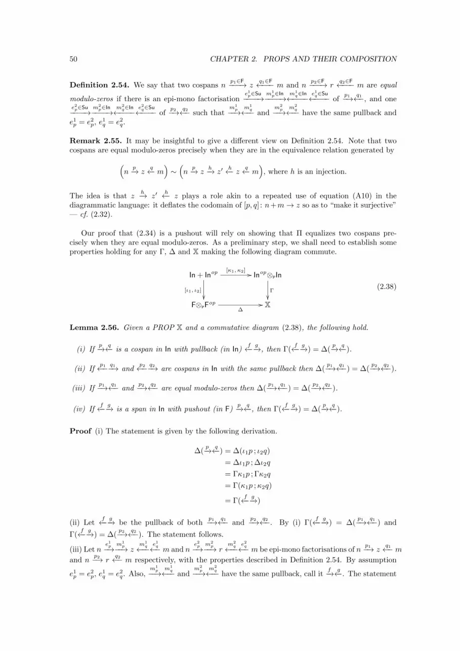
50 CHAPTER 2. PROPS AND THEIR COMPOSITION
Definition 2.54. We say that two cospans np1∈F−−−→ z
q1∈F←−−− m and np2∈F−−−→ r
q2∈F←−−− m are equal
modulo-zeros if there is an epi-mono factorisatione1p∈Su−−−−→
m1p∈In−−−−→
m1q∈In←−−−−
e1q∈Su←−−−− ofp1−→ q1←−, and one
e2p∈Su−−−−→m2p∈In−−−−→
m2q∈In←−−−−
e2q∈Su←−−−− ofp2−→ q2←− such that
m1p−−→
m1q←−− and
m2p−−→
m2q←−− have the same pullback and
e1p = e2
p, e1q = e2
q.
Remark 2.55. It may be insightful to give a different view on Definition 2.54. Note that twocospans are equal modulo-zeros precisely when they are in the equivalence relation generated by
(n
p−→ zq←− m
)∼(n
p−→ zh−→ z′
h←− z q←− m)
, where h is an injection.
The idea is that zh−→ z′
h←− z plays a role akin to a repeated use of equation (A10) in thediagrammatic language: it deflates the codomain of [p, q] : n+m→ z so as to “make it surjective”— cf. (2.32).
Our proof that (2.34) is a pushout will rely on showing that Π equalizes two cospans pre-cisely when they are equal modulo-zeros. As a preliminary step, we shall need to establish someproperties holding for any Γ, ∆ and X making the following diagram commute.
In + Inop[κ1, κ2] //
[ι1, ι2]
��
Inop⊗PIn
Γ
��F⊗PF
op
∆// X
(2.38)
Lemma 2.56. Given a PROP X and a commutative diagram (2.38), the following hold.
(i) Ifp−→ q←− is a cospan in In with pullback (in In)
f←− g−→, then Γ(f←− g−→) = ∆(
p−→ q←−).
(ii) Ifp1←− q1−→ and
p2←− q2−→ are cospans in In with the same pullback then ∆(p1−→ q1←−) = ∆(
p2−→ q2←−).
(iii) Ifp1−→ q1←− and
p2−→ q2←− are equal modulo-zeros then ∆(p1−→ q1←−) = ∆(
p2−→ q2←−).
(iv) Iff←− g−→ is a span in In with pushout (in F)
p−→ q←−, then Γ(f←− g−→) = ∆(
p−→ q←−).
Proof (i) The statement is given by the following derivation.
∆(p−→ q←−) = ∆(ι1p ; ι2q)
= ∆ι1p ; ∆ι2q
= Γκ1p ; Γκ2q
= Γ(κ1p ;κ2q)
= Γ(f←− g−→)
(ii) Letf←− g−→ be the pullback of both
p1−→ q1←− andp2−→ q2←−. By (i) Γ(
f←− g−→) = ∆(p1−→ q1←−) and
Γ(f←− g−→) = ∆(
p2−→ q2←−). The statement follows.
(iii) Let ne1p−→
m1p−−→ z
m1q←−−e1q←− m and n
e2p−→m2p−−→ r
m2q←−−e2q←− m be epi-mono factorisations of n
p1−→ zq1←− m
and np2−→ r
q2←− m respectively, with the properties described in Definition 2.54. By assumption
e1p = e2
p, e1q = e2
q. Also,m1p−−→
m1q←−− and
m2p−−→
m2q←−− have the same pullback, call it
f−→ g←−. The statement
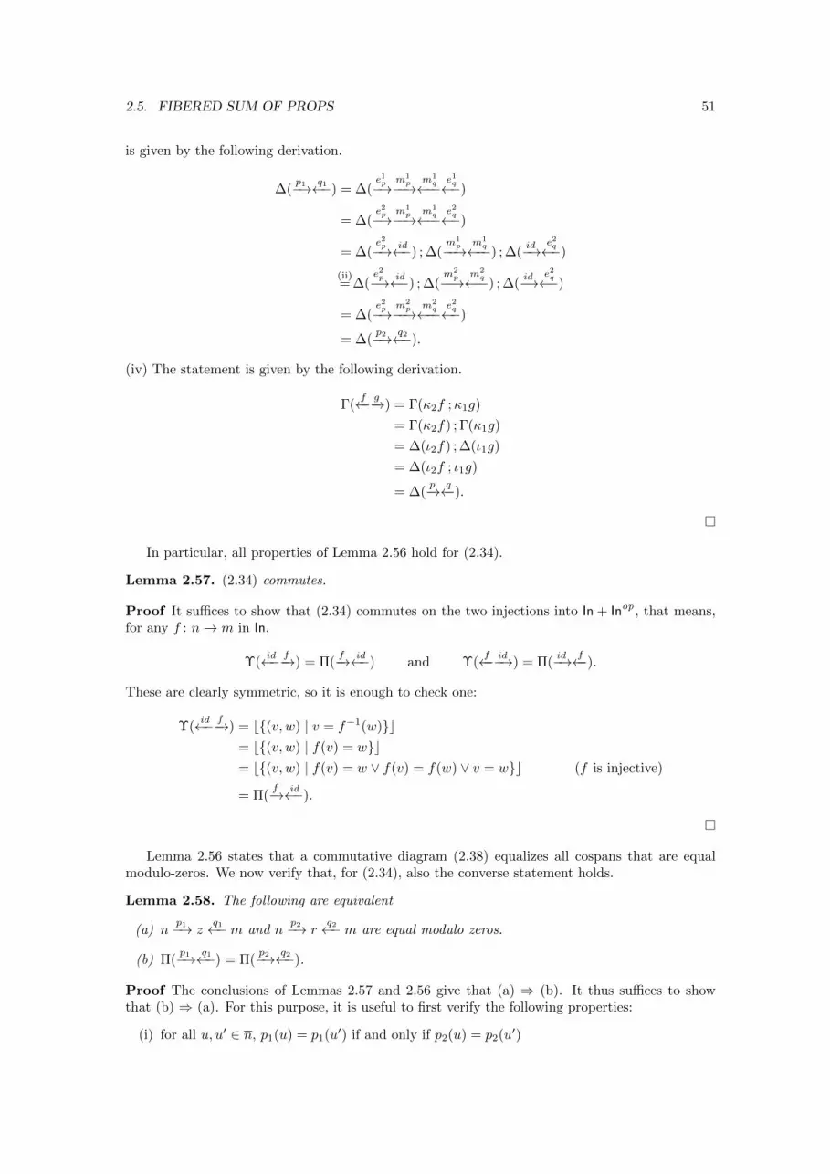
2.5. FIBERED SUM OF PROPS 51
is given by the following derivation.
∆(p1−→ q1←−) = ∆(
e1p−→m1p−−→
m1q←−−e1q←−)
= ∆(e2p−→
m1p−−→
m1q←−−e2q←−)
= ∆(e2p−→ id←−) ; ∆(
m1p−−→
m1q←−−) ; ∆(
id−→e2q←−)
(ii)= ∆(
e2p−→ id←−) ; ∆(m2p−−→
m2q←−−) ; ∆(
id−→e2q←−)
= ∆(e2p−→
m2p−−→
m2q←−−e2q←−)
= ∆(p2−→ q2←−).
(iv) The statement is given by the following derivation.
Γ(f←− g−→) = Γ(κ2f ;κ1g)
= Γ(κ2f) ; Γ(κ1g)
= ∆(ι2f) ; ∆(ι1g)
= ∆(ι2f ; ι1g)
= ∆(p−→ q←−).
�
In particular, all properties of Lemma 2.56 hold for (2.34).
Lemma 2.57. (2.34) commutes.
Proof It suffices to show that (2.34) commutes on the two injections into In + Inop , that means,for any f : n→ m in In,
Υ(id←− f−→) = Π(
f−→ id←−) and Υ(f←− id−→) = Π(
id−→ f←−).
These are clearly symmetric, so it is enough to check one:
Υ(id←− f−→) = b{(v, w) | v = f−1(w)}c
= b{(v, w) | f(v) = w}c= b{(v, w) | f(v) = w ∨ f(v) = f(w) ∨ v = w}c (f is injective)
= Π(f−→ id←−).
�
Lemma 2.56 states that a commutative diagram (2.38) equalizes all cospans that are equalmodulo-zeros. We now verify that, for (2.34), also the converse statement holds.
Lemma 2.58. The following are equivalent
(a) np1−→ z
q1←− m and np2−→ r
q2←− m are equal modulo zeros.
(b) Π(p1−→ q1←−) = Π(
p2−→ q2←−).
Proof The conclusions of Lemmas 2.57 and 2.56 give that (a) ⇒ (b). It thus suffices to showthat (b) ⇒ (a). For this purpose, it is useful to first verify the following properties:
(i) for all u, u′ ∈ n, p1(u) = p1(u′) if and only if p2(u) = p2(u′)
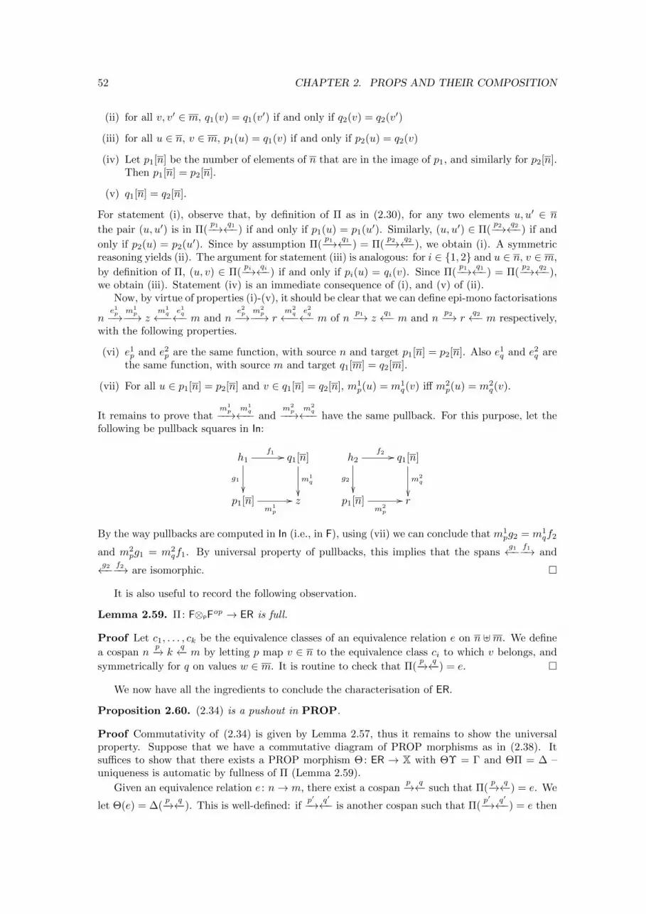
52 CHAPTER 2. PROPS AND THEIR COMPOSITION
(ii) for all v, v′ ∈ m, q1(v) = q1(v′) if and only if q2(v) = q2(v′)
(iii) for all u ∈ n, v ∈ m, p1(u) = q1(v) if and only if p2(u) = q2(v)
(iv) Let p1[n] be the number of elements of n that are in the image of p1, and similarly for p2[n].Then p1[n] = p2[n].
(v) q1[n] = q2[n].
For statement (i), observe that, by definition of Π as in (2.30), for any two elements u, u′ ∈ n
the pair (u, u′) is in Π(p1−→ q1←−) if and only if p1(u) = p1(u′). Similarly, (u, u′) ∈ Π(
p2−→ q2←−) if and
only if p2(u) = p2(u′). Since by assumption Π(p1−→ q1←−) = Π(
p2−→ q2←−), we obtain (i). A symmetricreasoning yields (ii). The argument for statement (iii) is analogous: for i ∈ {1, 2} and u ∈ n, v ∈ m,
by definition of Π, (u, v) ∈ Π(pi−→ qi←−) if and only if pi(u) = qi(v). Since Π(
p1−→ q1←−) = Π(p2−→ q2←−),
we obtain (iii). Statement (iv) is an immediate consequence of (i), and (v) of (ii).Now, by virtue of properties (i)-(v), it should be clear that we can define epi-mono factorisations
ne1p−→
m1p−−→ z
m1q←−−e1q←− m and n
e2p−→m2p−−→ r
m2q←−−e2q←− m of n
p1−→ zq1←− m and n
p2−→ rq2←− m respectively,
with the following properties.
(vi) e1p and e2
p are the same function, with source n and target p1[n] = p2[n]. Also e1q and e2
q arethe same function, with source m and target q1[m] = q2[m].
(vii) For all u ∈ p1[n] = p2[n] and v ∈ q1[n] = q2[n], m1p(u) = m1
q(v) iff m2p(u) = m2
q(v).
It remains to prove thatm1p−−→
m1q←−− and
m2p−−→
m2q←−− have the same pullback. For this purpose, let the
following be pullback squares in In:
h1
g1
��
f1 // q1[n]
m1q
��p1[n]
m1p
// z
h2
g2
��
f2 // q1[n]
m2q
��p1[n]
m2p
// r
By the way pullbacks are computed in In (i.e., in F), using (vii) we can conclude that m1pg2 = m1
qf2
and m2pg1 = m2
qf1. By universal property of pullbacks, this implies that the spansg1←− f1−→ and
g2←− f2−→ are isomorphic. �
It is also useful to record the following observation.
Lemma 2.59. Π: F⊗PFop → ER is full.
Proof Let c1, . . . , ck be the equivalence classes of an equivalence relation e on n ]m. We define
a cospan np−→ k
q←− m by letting p map v ∈ n to the equivalence class ci to which v belongs, and
symmetrically for q on values w ∈ m. It is routine to check that Π(p−→ q←−) = e. �
We now have all the ingredients to conclude the characterisation of ER.
Proposition 2.60. (2.34) is a pushout in PROP.
Proof Commutativity of (2.34) is given by Lemma 2.57, thus it remains to show the universalproperty. Suppose that we have a commutative diagram of PROP morphisms as in (2.38). Itsuffices to show that there exists a PROP morphism Θ: ER → X with ΘΥ = Γ and ΘΠ = ∆ –uniqueness is automatic by fullness of Π (Lemma 2.59).
Given an equivalence relation e : n→ m, there exist a cospanp−→ q←− such that Π(
p−→ q←−) = e. We
let Θ(e) = ∆(p−→ q←−). This is well-defined: if
p′−→ q′←− is another cospan such that Π(p′−→ q′←−) = e then
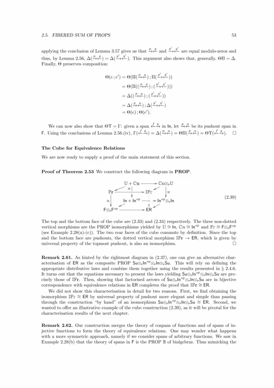
2.5. FIBERED SUM OF PROPS 53
applying the conclusion of Lemma 3.57 gives us thatp−→ q←− and
p′−→ q′←− are equal modulo-zeros and
thus, by Lemma 2.56, ∆(p−→ q←−) = ∆(
p′−→ q′←−). This argument also shows that, generally, ΘΠ = ∆.Finally, Θ preserves composition:
Θ(e ; e′) = Θ(Π(p−→ q←−) ; Π(
p′−→ q′←−))
= Θ(Π((p−→ q←−) ; (
p′−→ q′←−)))
= ∆((p−→ q←−) ; (
p′−→ q′←−))
= ∆(p−→ q←−) ; ∆(
p′−→ q′←−)
= Θ(e) ; Θ(e′).
We can now also show that ΘΥ = Γ: given a spanf←− g−→ in In, let
p−→ q←− be its pushout span in
F. Using the conclusions of Lemma 2.56.(iv), Γ(f←− g−→) = ∆(
p−→ q←−) = ΘΠ(p−→ q←−) = ΘΥ(
f←− g−→). �
The Cube for Equivalence Relations
We are now ready to supply a proof of the main statement of this section.
Proof of Theorem 2.53 We construct the following diagram in PROP.
U + Cu∼=
��
vv
// Cu⊗PUww
∼=��
Fr //
∼=��
IFr
��In + Inop
vv// Inop⊗PInxx
F⊗PFop // ER
(2.39)
The top and the bottom face of the cube are (2.33) and (2.34) respectively. The three non-dottedvertical morphisms are the PROP isomorphisms yielded by U ∼= In, Cu ∼= Inop and Fr ∼= F⊗PF
op
(see Example 2.28(a)-(c)). The two rear faces of the cube commute by definition. Since the topand the bottom face are pushouts, the dotted vertical morphism IFr → ER, which is given byuniversal property of the topmost pushout, is also an isomorphism. �
Remark 2.61. As hinted by the rightmost diagram in (2.37), one can give an alternative char-acterisation of ER as the composite PROP Su⊗PIn
op⊗PIn⊗PSu. This will rely on defining theappropriate distributive laws and combine them together using the results presented in § 2.4.6.It turns out that the equations necessary to present the laws yielding Su⊗PIn
op⊗PIn⊗PSu are pre-cisely those of IFr. Then, showing that factorised arrows of Su⊗PIn
op⊗PIn⊗PSu are in bijectivecorrespondence with equivalence relations in ER completes the proof that IFr ∼= ER.
We did not show this characterisation in detail for two reasons. First, we find obtaining theisomorphism IFr ∼= ER by universal property of pushout more elegant and simple than passingthrough the construction “by hand” of an isomorphism Su⊗PIn
op⊗PIn⊗PSu ∼= ER. Second, wewanted to offer an illustrative example of the cube construction (2.39), as it will be pivotal for thecharacterisation results of the next chapter.
Remark 2.62. Our construction merges the theory of cospans of functions and of spans of in-jective functions to form the theory of equivalence relations. One may wonder what happenswith a more symmetric approach, namely if we consider spans of arbitrary functions. We saw inExample 2.28(b) that the theory of spans in F is the PROP B of bialgebras. Thus mimicking the
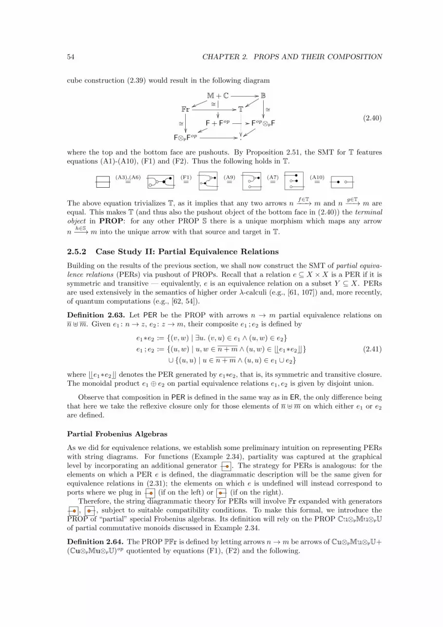
54 CHAPTER 2. PROPS AND THEIR COMPOSITION
cube construction (2.39) would result in the following diagram
M + C∼=
��
vv
// Byy ∼=
��Fr //
∼=��
T
��
F + Fop
vv// Fop⊗PF
yyF⊗PFop // .
(2.40)
where the top and the bottom face are pushouts. By Proposition 2.51, the SMT for T featuresequations (A1)-(A10), (F1) and (F2). Thus the following holds in T.
(A3),(A6)=
(F1)=
(A9)=
(A7)=
(A10)=
The above equation trivializes T, as it implies that any two arrows nf∈T−−−→ m and n
g∈T−−→ m areequal. This makes T (and thus also the pushout object of the bottom face in (2.40)) the terminalobject in PROP: for any other PROP S there is a unique morphism which maps any arrow
nh∈S−−→ m into the unique arrow with that source and target in T.
2.5.2 Case Study II: Partial Equivalence Relations
Building on the results of the previous section, we shall now construct the SMT of partial equiva-lence relations (PERs) via pushout of PROPs. Recall that a relation e ⊆ X ×X is a PER if it issymmetric and transitive — equivalently, e is an equivalence relation on a subset Y ⊆ X. PERsare used extensively in the semantics of higher order λ-calculi (e.g., [61, 107]) and, more recently,of quantum computations (e.g., [62, 54]).
Definition 2.63. Let PER be the PROP with arrows n → m partial equivalence relations onn ]m. Given e1 : n→ z, e2 : z → m, their composite e1 ; e2 is defined by
e1∗e2 := {(v, w) | ∃u. (v, u) ∈ e1 ∧ (u,w) ∈ e2}e1 ; e2 := {(u,w) | u,w ∈ n+m ∧ (u,w) ∈ bbe1∗e2cc}
∪ {(u, u) | u ∈ n+m ∧ (u, u) ∈ e1 ∪ e2}(2.41)
where bbe1∗e2cc denotes the PER generated by e1∗e2, that is, its symmetric and transitive closure.The monoidal product e1 ⊕ e2 on partial equivalence relations e1, e2 is given by disjoint union.
Observe that composition in PER is defined in the same way as in ER, the only difference beingthat here we take the reflexive closure only for those elements of n ]m on which either e1 or e2
are defined.
Partial Frobenius Algebras
As we did for equivalence relations, we establish some preliminary intuition on representing PERswith string diagrams. For functions (Example 2.34), partiality was captured at the graphicallevel by incorporating an additional generator . The strategy for PERs is analogous: for theelements on which a PER e is defined, the diagrammatic description will be the same given forequivalence relations in (2.31); the elements on which e is undefined will instead correspond toports where we plug in (if on the left) or (if on the right).
Therefore, the string diagrammatic theory for PERs will involve Fr expanded with generators, , subject to suitable compatibility conditions. To make this formal, we introduce the
PROP of “partial” special Frobenius algebras. Its definition will rely on the PROP Cu⊗PMu⊗PUof partial commutative monoids discussed in Example 2.34.
Definition 2.64. The PROP PFr is defined by letting arrows n→ m be arrows of Cu⊗PMu⊗PU+(Cu⊗PMu⊗PU)op quotiented by equations (F1), (F2) and the following.
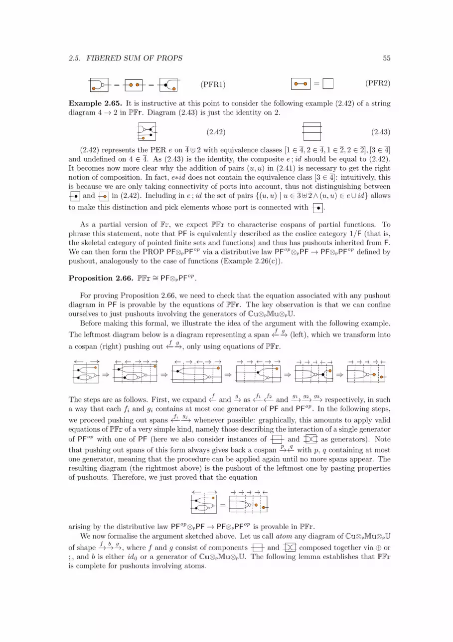
2.5. FIBERED SUM OF PROPS 55
= = (PFR1) = (PFR2)
Example 2.65. It is instructive at this point to consider the following example (2.42) of a stringdiagram 4→ 2 in PFr. Diagram (2.43) is just the identity on 2.
(2.42) (2.43)
(2.42) represents the PER e on 4] 2 with equivalence classes [1 ∈ 4, 2 ∈ 4, 1 ∈ 2, 2 ∈ 2], [3 ∈ 4]and undefined on 4 ∈ 4. As (2.43) is the identity, the composite e ; id should be equal to (2.42).It becomes now more clear why the addition of pairs (u, u) in (2.41) is necessary to get the rightnotion of composition. In fact, e∗id does not contain the equivalence class [3 ∈ 4]: intuitively, thisis because we are only taking connectivity of ports into account, thus not distinguishing between
and in (2.42). Including in e ; id the set of pairs {(u, u) | u ∈ 3] 2∧ (u, u) ∈ e∪ id} allows
to make this distinction and pick elements whose port is connected with .
As a partial version of Fr, we expect PFr to characterise cospans of partial functions. Tophrase this statement, note that PF is equivalently described as the coslice category 1/F (that is,the skeletal category of pointed finite sets and functions) and thus has pushouts inherited from F.We can then form the PROP PF⊗PPF
op via a distributive law PFop⊗PPF→ PF⊗PPFop defined by
pushout, analogously to the case of functions (Example 2.26(c)).
Proposition 2.66. PFr ∼= PF⊗PPFop.
For proving Proposition 2.66, we need to check that the equation associated with any pushoutdiagram in PF is provable by the equations of PFr. The key observation is that we can confineourselves to just pushouts involving the generators of Cu⊗PMu⊗PU.
Before making this formal, we illustrate the idea of the argument with the following example.
The leftmost diagram below is a diagram representing a spanf←− g−→ (left), which we transform into
a cospan (right) pushing outf←− g−→, only using equations of PFr.
!!
⇒!! !! !
⇒
! !! ! !⇒
!! !! !
⇒! !! !!
⇒! !! !!
The steps are as follows. First, we expandf←− and
g−→ asf1←− f2←− and
g1−→ g2−→ g3−→ respectively, in sucha way that each fi and gi contains at most one generator of PF and PFop . In the following steps,
we proceed pushing out spansfi←− gj−→ whenever possible: graphically, this amounts to apply valid
equations of PFr of a very simple kind, namely those describing the interaction of a single generator
of PFop with one of PF (here we also consider instances of and as generators). Note
that pushing out spans of this form always gives back a cospanp−→ q←− with p, q containing at most
one generator, meaning that the procedure can be applied again until no more spans appear. Theresulting diagram (the rightmost above) is the pushout of the leftmost one by pasting propertiesof pushouts. Therefore, we just proved that the equation
!!
=
! !! !!
arising by the distributive law PFop⊗PPF→ PF⊗PPFop is provable in PFr.
We now formalise the argument sketched above. Let us call atom any diagram of Cu⊗PMu⊗PUof shape
f−→ b−→ g−→, where f and g consist of components and composed together via ⊕ or; , and b is either id0 or a generator of Cu⊗PMu⊗PU. The following lemma establishes that PFris complete for pushouts involving atoms.
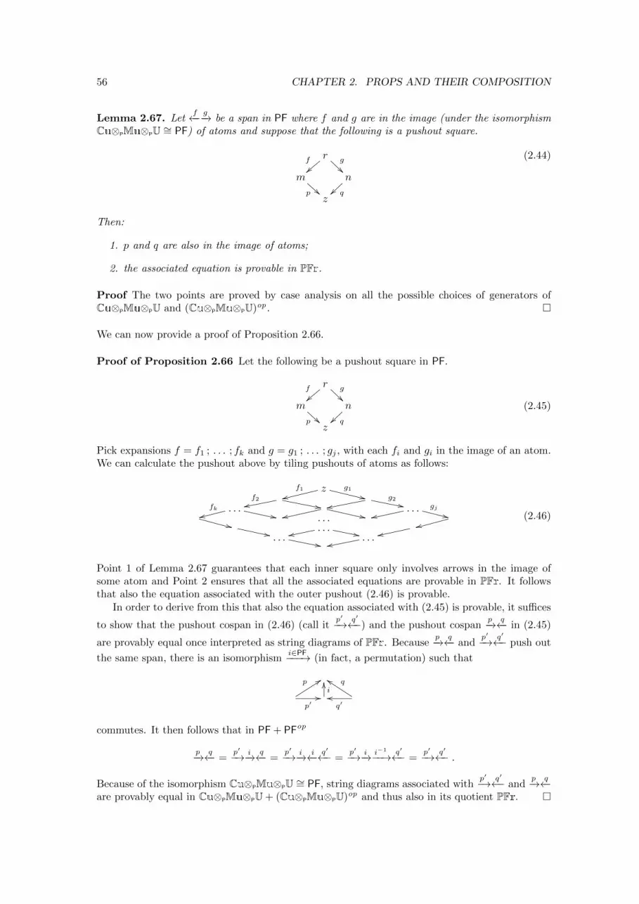
56 CHAPTER 2. PROPS AND THEIR COMPOSITION
Lemma 2.67. Letf←− g−→ be a span in PF where f and g are in the image (under the isomorphism
Cu⊗PMu⊗PU ∼= PF) of atoms and suppose that the following is a pushout square.
rf
}}g
m
p !!n
q~~z
(2.44)
Then:
1. p and q are also in the image of atoms;
2. the associated equation is provable in PFr.
Proof The two points are proved by case analysis on all the possible choices of generators ofCu⊗PMu⊗PU and (Cu⊗PMu⊗PU)op . �
We can now provide a proof of Proposition 2.66.
Proof of Proposition 2.66 Let the following be a pushout square in PF.
rf
}}g
m
p !!n
q~~z
(2.45)
Pick expansions f = f1 ; . . . ; fk and g = g1 ; . . . ; gj , with each fi and gi in the image of an atom.We can calculate the pushout above by tiling pushouts of atoms as follows:
zf1
ssg1
++f2rr ,, rr
g2,,. . .fk
ss ,, ,,rr. . .
rrgj++
++. . .
ss,, . . .rr ,, rr. . . ,, . . .rr
(2.46)
Point 1 of Lemma 2.67 guarantees that each inner square only involves arrows in the image ofsome atom and Point 2 ensures that all the associated equations are provable in PFr. It followsthat also the equation associated with the outer pushout (2.46) is provable.
In order to derive from this that also the equation associated with (2.45) is provable, it suffices
to show that the pushout cospan in (2.46) (call itp′−→ q′←−) and the pushout cospan
p−→ q←− in (2.45)
are provably equal once interpreted as string diagrams of PFr. Becausep−→ q←− and
p′−→ q′←− push out
the same span, there is an isomorphismi∈PF−−−→ (in fact, a permutation) such that
p 99
p′//i
OO qee
q′oo
commutes. It then follows that in PF + PFop
p−→ q←− =p′−→ i−→ q←− =
p′−→ i−→ i←− q′←− =p′−→ i−→ i−1
−−→ q′←− =p′−→ q′←− .
Because of the isomorphism Cu⊗PMu⊗PU ∼= PF, string diagrams associated withp′−→ q′←− and
p−→ q←−are provably equal in Cu⊗PMu⊗PU + (Cu⊗PMu⊗PU)op and thus also in its quotient PFr. �
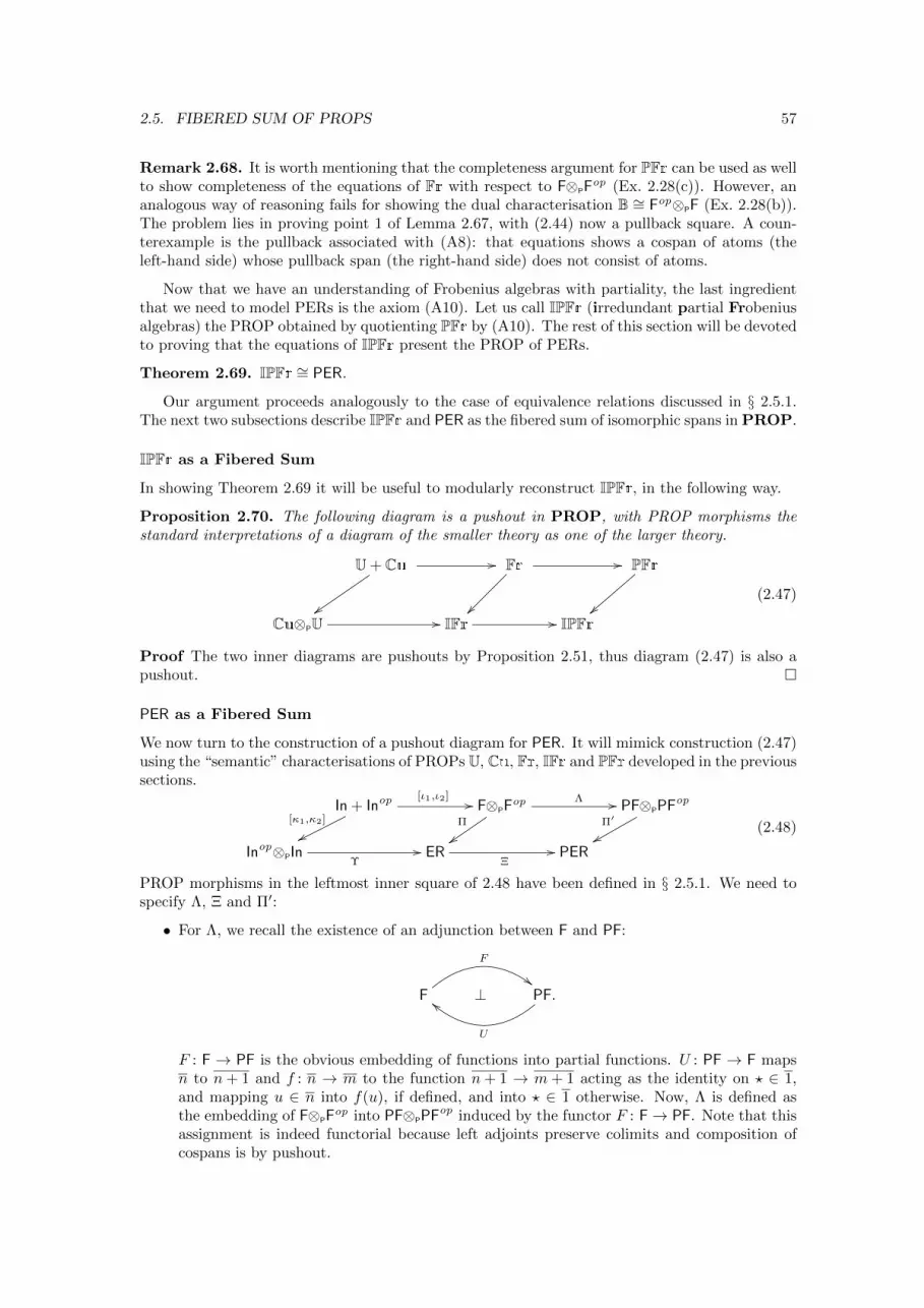
2.5. FIBERED SUM OF PROPS 57
Remark 2.68. It is worth mentioning that the completeness argument for PFr can be used as wellto show completeness of the equations of Fr with respect to F⊗PF
op (Ex. 2.28(c)). However, ananalogous way of reasoning fails for showing the dual characterisation B ∼= Fop⊗PF (Ex. 2.28(b)).The problem lies in proving point 1 of Lemma 2.67, with (2.44) now a pullback square. A coun-terexample is the pullback associated with (A8): that equations shows a cospan of atoms (theleft-hand side) whose pullback span (the right-hand side) does not consist of atoms.
Now that we have an understanding of Frobenius algebras with partiality, the last ingredientthat we need to model PERs is the axiom (A10). Let us call IPFr (irredundant partial Frobeniusalgebras) the PROP obtained by quotienting PFr by (A10). The rest of this section will be devotedto proving that the equations of IPFr present the PROP of PERs.
Theorem 2.69. IPFr ∼= PER.
Our argument proceeds analogously to the case of equivalence relations discussed in § 2.5.1.The next two subsections describe IPFr and PER as the fibered sum of isomorphic spans in PROP.
IPFr as a Fibered Sum
In showing Theorem 2.69 it will be useful to modularly reconstruct IPFr, in the following way.
Proposition 2.70. The following diagram is a pushout in PROP, with PROP morphisms thestandard interpretations of a diagram of the smaller theory as one of the larger theory.
U + Cu
zz
// Fr
��
// PFr
}}Cu⊗PU // IFr // IPFr
(2.47)
Proof The two inner diagrams are pushouts by Proposition 2.51, thus diagram (2.47) is also apushout. �
PER as a Fibered Sum
We now turn to the construction of a pushout diagram for PER. It will mimick construction (2.47)using the “semantic” characterisations of PROPs U, Cu, Fr, IFr and PFr developed in the previoussections.
In + Inop[κ1,κ2]
ww
[ι1,ι2] // F⊗PFop
Π
zz
Λ // PF⊗PPFop
Π′
xxInop⊗PIn
Υ// ER
Ξ// PER
(2.48)
PROP morphisms in the leftmost inner square of 2.48 have been defined in § 2.5.1. We need tospecify Λ, Ξ and Π′:
• For Λ, we recall the existence of an adjunction between F and PF:
F
F
##⊥ PF.
U
bb
F : F → PF is the obvious embedding of functions into partial functions. U : PF → F mapsn to n+ 1 and f : n → m to the function n+ 1 → m+ 1 acting as the identity on ? ∈ 1,and mapping u ∈ n into f(u), if defined, and into ? ∈ 1 otherwise. Now, Λ is defined asthe embedding of F⊗PF
op into PF⊗PPFop induced by the functor F : F→ PF. Note that this
assignment is indeed functorial because left adjoints preserve colimits and composition ofcospans is by pushout.
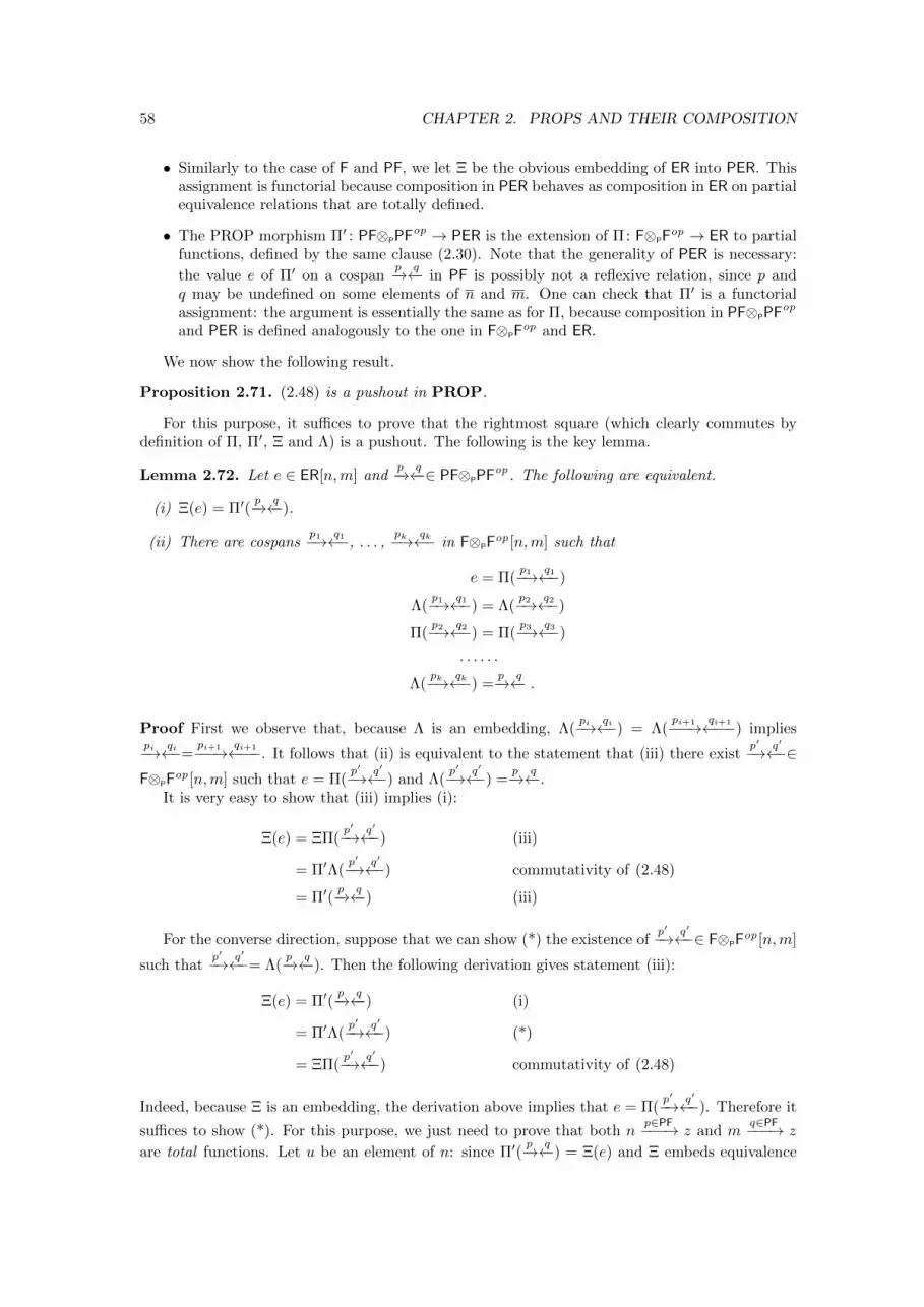
58 CHAPTER 2. PROPS AND THEIR COMPOSITION
• Similarly to the case of F and PF, we let Ξ be the obvious embedding of ER into PER. Thisassignment is functorial because composition in PER behaves as composition in ER on partialequivalence relations that are totally defined.
• The PROP morphism Π′ : PF⊗PPFop → PER is the extension of Π: F⊗PF
op → ER to partialfunctions, defined by the same clause (2.30). Note that the generality of PER is necessary:
the value e of Π′ on a cospanp−→ q←− in PF is possibly not a reflexive relation, since p and
q may be undefined on some elements of n and m. One can check that Π′ is a functorialassignment: the argument is essentially the same as for Π, because composition in PF⊗PPF
op
and PER is defined analogously to the one in F⊗PFop and ER.
We now show the following result.
Proposition 2.71. (2.48) is a pushout in PROP.
For this purpose, it suffices to prove that the rightmost square (which clearly commutes bydefinition of Π, Π′, Ξ and Λ) is a pushout. The following is the key lemma.
Lemma 2.72. Let e ∈ ER[n,m] andp−→ q←−∈ PF⊗PPF
op. The following are equivalent.
(i) Ξ(e) = Π′(p−→ q←−).
(ii) There are cospansp1−→ q1←−, . . . ,
pk−→ qk←− in F⊗PFop [n,m] such that
e = Π(p1−→ q1←−)
Λ(p1−→ q1←−) = Λ(
p2−→ q2←−)
Π(p2−→ q2←−) = Π(
p3−→ q3←−)
. . . . . .
Λ(pk−→ qk←−) =
p−→ q←− .
Proof First we observe that, because Λ is an embedding, Λ(pi−→ qi←−) = Λ(
pi+1−−−→ qi+1←−−−) impliespi−→ qi←−=
pi+1−−−→ qi+1←−−−. It follows that (ii) is equivalent to the statement that (iii) there existp′−→ q′←−∈
F⊗PFop [n,m] such that e = Π(
p′−→ q′←−) and Λ(p′−→ q′←−) =
p−→ q←−.It is very easy to show that (iii) implies (i):
Ξ(e) = ΞΠ(p′−→ q′←−) (iii)
= Π′Λ(p′−→ q′←−) commutativity of (2.48)
= Π′(p−→ q←−) (iii)
For the converse direction, suppose that we can show (*) the existence ofp′−→ q′←−∈ F⊗PF
op [n,m]
such thatp′−→ q′←−= Λ(
p−→ q←−). Then the following derivation gives statement (iii):
Ξ(e) = Π′(p−→ q←−) (i)
= Π′Λ(p′−→ q′←−) (*)
= ΞΠ(p′−→ q′←−) commutativity of (2.48)
Indeed, because Ξ is an embedding, the derivation above implies that e = Π(p′−→ q′←−). Therefore it
suffices to show (*). For this purpose, we just need to prove that both np∈PF−−−→ z and m
q∈PF−−−→ z
are total functions. Let u be an element of n: since Π′(p−→ q←−) = Ξ(e) and Ξ embeds equivalence
2.5. FIBERED SUM OF PROPS 59
relations into PERs, then Π′(p−→ q←−) is in fact an equivalence relation, meaning that u belongs to
some equivalence class of the partition induced by Π′(p−→ q←−). It follows by definition of Π′ that
p : n→ z is defined on u. With a similar argument, one can show that q : m→ z is defined on all
elements of m and thus both p and q are total functions. This implies thatp−→ q←− is in the image
of the embedding Λ. �
Proof of Proposition 2.71 The leftmost square in (2.48) has already been proven to be apushout (Lemma 2.60), thus it suffices to show that the rightmost square is also a pushout.With this aim, recall that pushouts in PROP can be calculated as in Cat. In particular, (2.48)involves categories all with the same objects and identity-on-objects functors. This means thatthe pushout object is the quotient of ER and F⊗PF
op along the equivalence relation generated by
{(e, p−→ q←−) | there isp′−→ q′←− such that Π(
p′−→ q′←−) = e and Λ(p′−→ q′←−) =
p−→ q←−}. (2.49)
Lemma 2.72 proves that Π′ and Ξ map ne∈ER−−−→ m and n
p−→ q←− m to the same arrow exactlywhen they are in the equivalence relation described above. This means that PER indeed quotientsby (2.49) and thus is the desired pushout object. �
The Cube for Partial Equivalence Relations
We are now able to conclude the characterisation of partial equivalence relations.
Proof of Theorem 2.69 We construct the following diagram in PROP.
U + Cuuu
//
∼=
��
Fr
vv
//
∼=
��
PFruu
∼=
��
Cu⊗PU //
∼=
��
IFr //
∼=
��
IPFr
��
In + Inop
uu
// F⊗PFop
vv
// PF⊗PPFop
uuInop⊗PIn // ER // PER
The top and bottom face are pushout diagrams (2.47) and (2.48) respectively. The vertical edgesare PROP isomorphisms. Also, all the rear faces commute by definition. Therefore, the arrowIPFr→ PER given by universal property of the topmost pushout is also a PROP isomorphism. �
Remark 2.73. Differently from the case of equivalence relations (Remark 2.61), it is not clearhow a modular story of partial equivalence relations could be reconstructed only using PROPcomposition. Intuitively, to present IPFr as a composed PROP, we would need in particularequations to push components to the extreme left of any diagram. This should also involve a
distributive law λ : U⊗PMu→Mu⊗PU. Consider now the value of λ on : because now
indicates partiality, it should not be defined as — following (A3) — but rather as —
following (PFR1). However, is not of the correct type U⊗PMu.

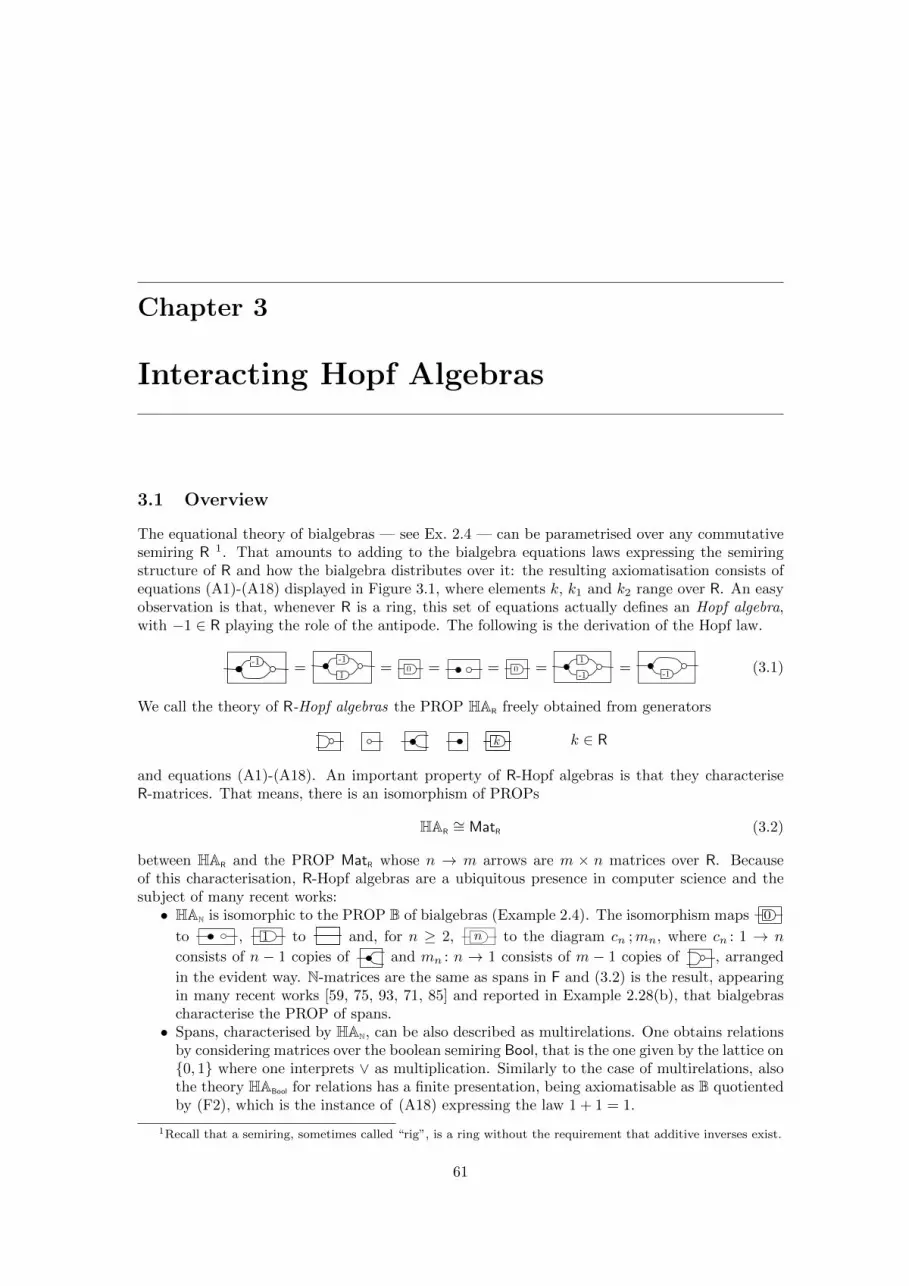
Chapter 3
Interacting Hopf Algebras
3.1 Overview
The equational theory of bialgebras — see Ex. 2.4 — can be parametrised over any commutativesemiring R 1. That amounts to adding to the bialgebra equations laws expressing the semiringstructure of R and how the bialgebra distributes over it: the resulting axiomatisation consists ofequations (A1)-(A18) displayed in Figure 3.1, where elements k, k1 and k2 range over R. An easyobservation is that, whenever R is a ring, this set of equations actually defines an Hopf algebra,with −1 ∈ R playing the role of the antipode. The following is the derivation of the Hopf law.
-1 =-1
1= 0 = = 0 =
-1
1=
-1(3.1)
We call the theory of R-Hopf algebras the PROP HAR freely obtained from generators
k k ∈ R
and equations (A1)-(A18). An important property of R-Hopf algebras is that they characteriseR-matrices. That means, there is an isomorphism of PROPs
HAR∼= MatR (3.2)
between HAR and the PROP MatR whose n → m arrows are m × n matrices over R. Becauseof this characterisation, R-Hopf algebras are a ubiquitous presence in computer science and thesubject of many recent works:• HAN is isomorphic to the PROP B of bialgebras (Example 2.4). The isomorphism maps 0
to , 1 to and, for n ≥ 2, n to the diagram cn ;mn, where cn : 1 → n
consists of n − 1 copies of and mn : n → 1 consists of m − 1 copies of , arranged
in the evident way. N-matrices are the same as spans in F and (3.2) is the result, appearingin many recent works [59, 75, 93, 71, 85] and reported in Example 2.28(b), that bialgebrascharacterise the PROP of spans.
• Spans, characterised by HAN, can be also described as multirelations. One obtains relationsby considering matrices over the boolean semiring Bool, that is the one given by the lattice on{0, 1} where one interprets ∨ as multiplication. Similarly to the case of multirelations, alsothe theory HABool for relations has a finite presentation, being axiomatisable as B quotientedby (F2), which is the instance of (A18) expressing the law 1 + 1 = 1.
1Recall that a semiring, sometimes called “rig”, is a ring without the requirement that additive inverses exist.
61
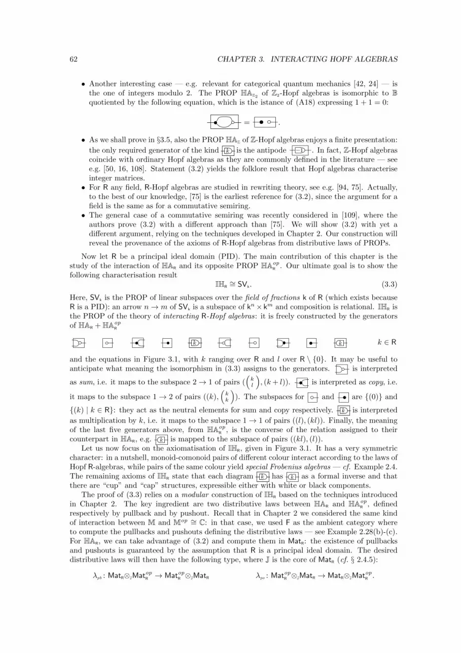
62 CHAPTER 3. INTERACTING HOPF ALGEBRAS
• Another interesting case — e.g. relevant for categorical quantum mechanics [42, 24] — isthe one of integers modulo 2. The PROP HAZ2
of Z2-Hopf algebras is isomorphic to Bquotiented by the following equation, which is the istance of (A18) expressing 1 + 1 = 0:
= .
• As we shall prove in §3.5, also the PROP HAZ of Z-Hopf algebras enjoys a finite presentation:
the only required generator of the kind k is the antipode 1� . In fact, Z-Hopf algebrascoincide with ordinary Hopf algebras as they are commonly defined in the literature — seee.g. [50, 16, 108]. Statement (3.2) yields the folklore result that Hopf algebras characteriseinteger matrices.
• For R any field, R-Hopf algebras are studied in rewriting theory, see e.g. [94, 75]. Actually,to the best of our knowledge, [75] is the earliest reference for (3.2), since the argument for afield is the same as for a commutative semiring.
• The general case of a commutative semiring was recently considered in [109], where theauthors prove (3.2) with a different approach than [75]. We will show (3.2) with yet adifferent argument, relying on the techniques developed in Chapter 2. Our construction willreveal the provenance of the axioms of R-Hopf algebras from distributive laws of PROPs.
Now let R be a principal ideal domain (PID). The main contribution of this chapter is thestudy of the interaction of HAR and its opposite PROP HAop
R . Our ultimate goal is to show thefollowing characterisation result
IHR∼= SVk. (3.3)
Here, SVk is the PROP of linear subspaces over the field of fractions k of R (which exists becauseR is a PID): an arrow n→ m of SVk is a subspace of kn× km and composition is relational. IHR isthe PROP of the theory of interacting R-Hopf algebras: it is freely constructed by the generatorsof HAR + HAop
R
k k k ∈ R
and the equations in Figure 3.1, with k ranging over R and l over R \ {0}. It may be useful toanticipate what meaning the isomorphism in (3.3) assigns to the generators. is interpreted
as sum, i.e. it maps to the subspace 2→ 1 of pairs ((kl
), (k+ l)). is interpreted as copy, i.e.
it maps to the subspace 1→ 2 of pairs ((k),(kk
)). The subspaces for and are {(0)} and
{(k) | k ∈ R}: they act as the neutral elements for sum and copy respectively. k is interpreted
as multiplication by k, i.e. it maps to the subspace 1→ 1 of pairs ((l), (kl)). Finally, the meaningof the last five generators above, from HAop
R , is the converse of the relation assigned to theircounterpart in HAR, e.g. k is mapped to the subspace of pairs ((kl), (l)).
Let us now focus on the axiomatisation of IHR, given in Figure 3.1. It has a very symmetriccharacter: in a nutshell, monoid-comonoid pairs of different colour interact according to the laws ofHopf R-algebras, while pairs of the same colour yield special Frobenius algebras — cf. Example 2.4.The remaining axioms of IHR state that each diagram k has k as a formal inverse and thatthere are “cup” and “cap” structures, expressible either with white or black components.
The proof of (3.3) relies on a modular construction of IHR based on the techniques introducedin Chapter 2. The key ingredient are two distributive laws between HAR and HAop
R , definedrespectively by pullback and by pushout. Recall that in Chapter 2 we considered the same kindof interaction between M and Mop ∼= C: in that case, we used F as the ambient category whereto compute the pullbacks and pushouts defining the distributive laws — see Example 2.28(b)-(c).For HAR, we can take advantage of (3.2) and compute them in MatR: the existence of pullbacksand pushouts is guaranteed by the assumption that R is a principal ideal domain. The desireddistributive laws will then have the following type, where J is the core of MatR (cf. § 2.4.5):
λpb : MatR⊗JMatopR → MatopR ⊗JMatR λpo : MatopR ⊗JMatR → MatR⊗JMatopR .
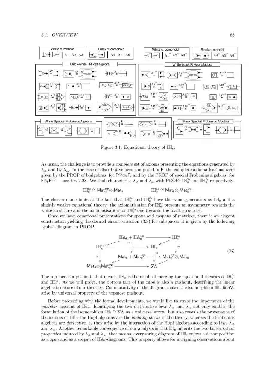
3.1. OVERVIEW 63
= = =
White Special Frobenius Algebra
= = =
Black Special Frobenius Algebra
=
= =
=-1-1
White c. comonoidWhite c. monoid Black c. comonoid Black c. monoid
==
= = +
0 =
= =
= =
=
1
=
=
Black-white R-Hopf algebra White-black R-Hopf algebra
k1k2k1 k2
k1
k2k1 k2
kkk
k
k k ==
=
= +
0 =
=
==
=
=
1 =
k1
k2k1 k2kk
k k
ll ll
A1 A2 A3 A1 A2 A3 A4 A5 A6A4 A5 A6
A7 A8
A9 A10
A11
A12
= k1k2k1 k2
A13 A14
A15 A16
A17
A18
kk k
k
kk
A7 A8
A9 A10
A11
A12
A13 A14
A15 A16
A17
A18
I3
I1 I2
I5 I6I7 I8I3 I4 I4
op
op
op
op
op
op
opop op
op
op
op
opopop op op op
Figure 3.1: Equational theory of IHR.
As usual, the challenge is to provide a complete set of axioms presenting the equations generated byλpb and by λpo. In the case of distributive laws computed in F, the complete axiomatisations weregiven by the PROP of bialgebras, for Fop⊗PF, and by the PROP of special Frobenius algebras, forF⊗PF
op — see Ex. 2.28. We shall characterise λpb and λpo with PROPs IHSp
R and IHCp
R respectively:
IHSp
R∼= MatopR ⊗JMatR IHCp
R∼= MatR⊗JMatopR .
The chosen name hints at the fact that IHSp
R and IHCp
R have the same generators as IHR and aslightly weaker equational theory: the axiomatisation for IHSp
R presents an asymmetry towards thewhite structure and the axiomatisation for IHCp
R one towards the black structure.Once we have equational presentations for spans and cospans of matrices, there is an elegant
construction yielding the desired characterisation (3.3) for subspaces: it is given by the following“cube” diagram in PROP.
HAR + HAopR
∼=
��
tt
// IHSp
R
vv ∼=��
IHCp
R//
∼=��
IHR
∼=
��MatR + MatopR
tt// MatopR ⊗JMatRvv
MatR⊗JMatopR// SVk
(�)
The top face is a pushout, that means, IHR is the result of merging the equational theories of IHSp
R
and IHCp
R . As we will prove, the bottom face of the cube is also a pushout, describing the linearalgebraic nature of our theories. Commutativity of the diagram makes the isomorphism IHR
∼= SVk
arise by universal property of the topmost pushout.
Before proceeding with the formal developments, we would like to stress the importance of themodular account of IHR. Identifying the two distributive laws λpb and λpo not only enables theformulation of the isomorphism IHR
∼= SVk as a universal arrow, but also reveals the provenance ofthe axioms of IHR: the Hopf algebras are the building blocks of the theory, whereas the Frobeniusalgebras are derivative, as they arise by the interaction of the Hopf algebras according to laws λpb
and λpo. Another remarkable consequence of our analysis is that IHR inherits the two factorisationproperties induced by λpb and λpo, that means, every string diagram of IHR enjoys a decompositionas a span and as a cospan of HAR-diagrams. This property allows for intriguing observations about
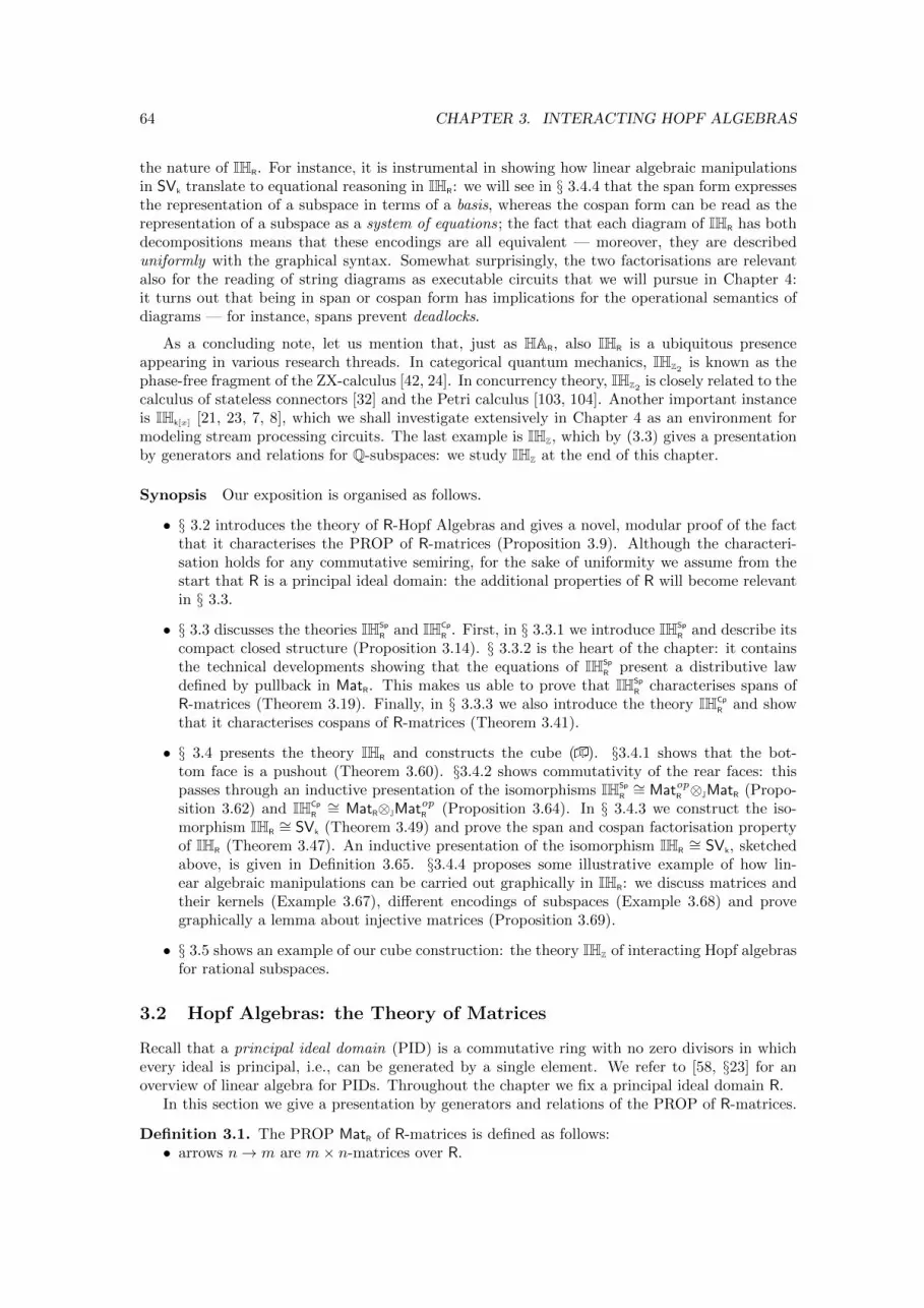
64 CHAPTER 3. INTERACTING HOPF ALGEBRAS
the nature of IHR. For instance, it is instrumental in showing how linear algebraic manipulationsin SVk translate to equational reasoning in IHR: we will see in § 3.4.4 that the span form expressesthe representation of a subspace in terms of a basis, whereas the cospan form can be read as therepresentation of a subspace as a system of equations; the fact that each diagram of IHR has bothdecompositions means that these encodings are all equivalent — moreover, they are describeduniformly with the graphical syntax. Somewhat surprisingly, the two factorisations are relevantalso for the reading of string diagrams as executable circuits that we will pursue in Chapter 4:it turns out that being in span or cospan form has implications for the operational semantics ofdiagrams — for instance, spans prevent deadlocks.
As a concluding note, let us mention that, just as HAR, also IHR is a ubiquitous presenceappearing in various research threads. In categorical quantum mechanics, IHZ2
is known as thephase-free fragment of the ZX-calculus [42, 24]. In concurrency theory, IHZ2
is closely related to thecalculus of stateless connectors [32] and the Petri calculus [103, 104]. Another important instanceis IHk[x] [21, 23, 7, 8], which we shall investigate extensively in Chapter 4 as an environment formodeling stream processing circuits. The last example is IHZ, which by (3.3) gives a presentationby generators and relations for Q-subspaces: we study IHZ at the end of this chapter.
Synopsis Our exposition is organised as follows.
• § 3.2 introduces the theory of R-Hopf Algebras and gives a novel, modular proof of the factthat it characterises the PROP of R-matrices (Proposition 3.9). Although the characteri-sation holds for any commutative semiring, for the sake of uniformity we assume from thestart that R is a principal ideal domain: the additional properties of R will become relevantin § 3.3.
• § 3.3 discusses the theories IHSp
R and IHCp
R . First, in § 3.3.1 we introduce IHSp
R and describe itscompact closed structure (Proposition 3.14). § 3.3.2 is the heart of the chapter: it containsthe technical developments showing that the equations of IHSp
R present a distributive lawdefined by pullback in MatR. This makes us able to prove that IHSp
R characterises spans ofR-matrices (Theorem 3.19). Finally, in § 3.3.3 we also introduce the theory IHCp
R and showthat it characterises cospans of R-matrices (Theorem 3.41).
• § 3.4 presents the theory IHR and constructs the cube (�). §3.4.1 shows that the bot-tom face is a pushout (Theorem 3.60). §3.4.2 shows commutativity of the rear faces: thispasses through an inductive presentation of the isomorphisms IHSp
R∼= MatopR ⊗JMatR (Propo-
sition 3.62) and IHCp
R∼= MatR⊗JMatopR (Proposition 3.64). In § 3.4.3 we construct the iso-
morphism IHR∼= SVk (Theorem 3.49) and prove the span and cospan factorisation property
of IHR (Theorem 3.47). An inductive presentation of the isomorphism IHR∼= SVk, sketched
above, is given in Definition 3.65. §3.4.4 proposes some illustrative example of how lin-ear algebraic manipulations can be carried out graphically in IHR: we discuss matrices andtheir kernels (Example 3.67), different encodings of subspaces (Example 3.68) and provegraphically a lemma about injective matrices (Proposition 3.69).
• § 3.5 shows an example of our cube construction: the theory IHZ of interacting Hopf algebrasfor rational subspaces.
3.2 Hopf Algebras: the Theory of Matrices
Recall that a principal ideal domain (PID) is a commutative ring with no zero divisors in whichevery ideal is principal, i.e., can be generated by a single element. We refer to [58, §23] for anoverview of linear algebra for PIDs. Throughout the chapter we fix a principal ideal domain R.
In this section we give a presentation by generators and relations of the PROP of R-matrices.
Definition 3.1. The PROP MatR of R-matrices is defined as follows:• arrows n→ m are m× n-matrices over R.
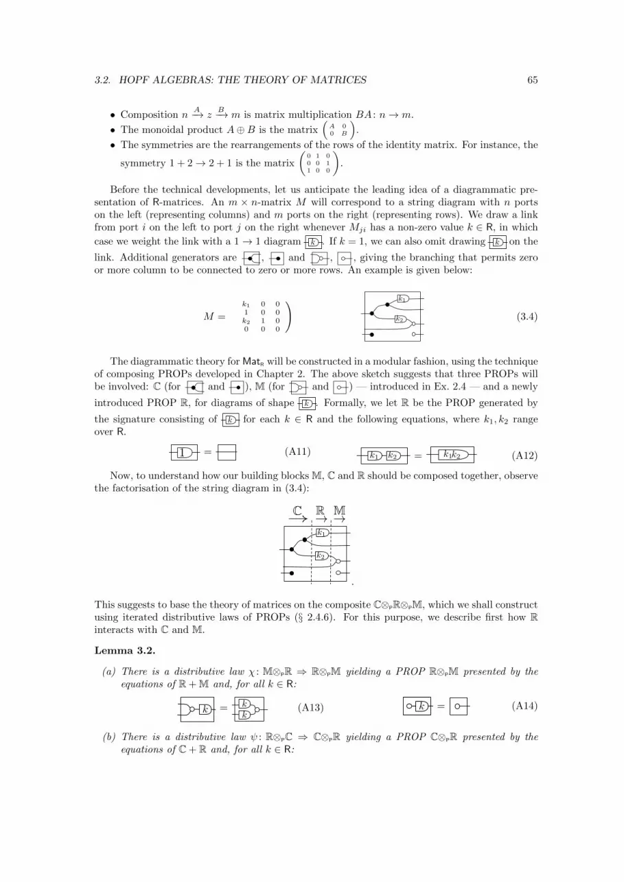
3.2. HOPF ALGEBRAS: THE THEORY OF MATRICES 65
• Composition nA−→ z
B−→ m is matrix multiplication BA : n→ m.
• The monoidal product A⊕B is the matrix(A 00 B
).
• The symmetries are the rearrangements of the rows of the identity matrix. For instance, the
symmetry 1 + 2→ 2 + 1 is the matrix
(0 1 00 0 11 0 0
).
Before the technical developments, let us anticipate the leading idea of a diagrammatic pre-sentation of R-matrices. An m × n-matrix M will correspond to a string diagram with n portson the left (representing columns) and m ports on the right (representing rows). We draw a linkfrom port i on the left to port j on the right whenever Mji has a non-zero value k ∈ R, in which
case we weight the link with a 1→ 1 diagram k . If k = 1, we can also omit drawing k on the
link. Additional generators are , and , , giving the branching that permits zeroor more column to be connected to zero or more rows. An example is given below:
M =
(k1 0 01 0 0k2 1 00 0 0
) k1
k2 (3.4)
The diagrammatic theory for MatR will be constructed in a modular fashion, using the techniqueof composing PROPs developed in Chapter 2. The above sketch suggests that three PROPs willbe involved: C (for and ), M (for and ) — introduced in Ex. 2.4 — and a newly
introduced PROP R, for diagrams of shape k . Formally, we let R be the PROP generated by
the signature consisting of k for each k ∈ R and the following equations, where k1, k2 rangeover R.
1 = (A11) k1 k2 = k1k2 (A12)
Now, to understand how our building blocks M, C and R should be composed together, observethe factorisation of the string diagram in (3.4):
k1
k2
! ! !MRC
.
This suggests to base the theory of matrices on the composite C⊗PR⊗PM, which we shall constructusing iterated distributive laws of PROPs (§ 2.4.6). For this purpose, we describe first how Rinteracts with C and M.
Lemma 3.2.
(a) There is a distributive law χ : M⊗PR ⇒ R⊗PM yielding a PROP R⊗PM presented by theequations of R + M and, for all k ∈ R:
k = kk
(A13) k = (A14)
(b) There is a distributive law ψ : R⊗PC ⇒ C⊗PR yielding a PROP C⊗PR presented by theequations of C + R and, for all k ∈ R:
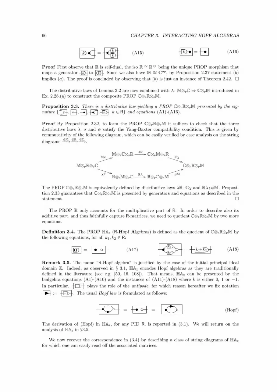
66 CHAPTER 3. INTERACTING HOPF ALGEBRAS
k =kk
(A15) k = (A16)
Proof First observe that R is self-dual, the iso R ∼= Rop being the unique PROP morphism thatmaps a generator k to k . Since we also have M ∼= Cop , by Proposition 2.37 statement (b)
implies (a). The proof is concluded by observing that (b) is just an instance of Theorem 2.42. �
The distributive laws of Lemma 3.2 are now combined with λ : M⊗PC⇒ C⊗PM introduced inEx. 2.28.(a) to construct the composite PROP C⊗PR⊗PM.
Proposition 3.3. There is a distributive law yielding a PROP C⊗PR⊗PM presented by the sig-nature { , , , , k | k ∈ R} and equations (A1)-(A16).
Proof By Proposition 2.32, to form the PROP C⊗PR⊗PM it suffices to check that the threedistributive laws λ, σ and ψ satisfy the Yang-Baxter compatibility condition. This is given bycommutativity of the following diagram, which can be easily verified by case analysis on the string
diagrams∈M−−→ ∈R−−→ ∈C−−→.
M⊗PC⊗PRλR // C⊗PM⊗PR Cχ
**M⊗PR⊗PC
Mψ 44
χC **
C⊗PR⊗PM
R⊗PM⊗PCRλ // R⊗PC⊗PM
ψM
44
The PROP C⊗PR⊗PM is equivalently defined by distributive laws λR ;Cχ and Rλ ;ψM. Proposi-tion 2.33 guarantees that C⊗PR⊗PM is presented by generators and equations as described in thestatement. �
The PROP R only accounts for the multiplicative part of R. In order to describe also itsadditive part, and thus faithfully capture R-matrices, we need to quotient C⊗PR⊗PM by two moreequations.
Definition 3.4. The PROP HAR (R-Hopf Algebras) is defined as the quotient of C⊗PR⊗PM bythe following equations, for all k1, k2 ∈ R:
0 = (A17)k1
k2
= k1 k2+ (A18)
Remark 3.5. The name “R-Hopf algebra” is justified by the case of the initial principal idealdomain Z. Indeed, as observed in § 3.1, HAZ encodes Hopf algebras as they are traditionallydefined in the literature (see e.g. [50, 16, 108]). That means, HAZ can be presented by thebialgebra equations (A1)-(A10) and the instances of (A11)-(A18) where k is either 0, 1 or −1.
In particular, 1� plays the role of the antipode, for which reason hereafter we fix notation
:= 1� . The usual Hopf law is formulated as follows:
= = (Hopf)
The derivation of (Hopf) in HAR, for any PID R, is reported in (3.1). We will return on theanalysis of HAZ in §3.5.
We now recover the correspondence in (3.4) by describing a class of string diagrams of HAR
for which one can easily read off the associated matrices.
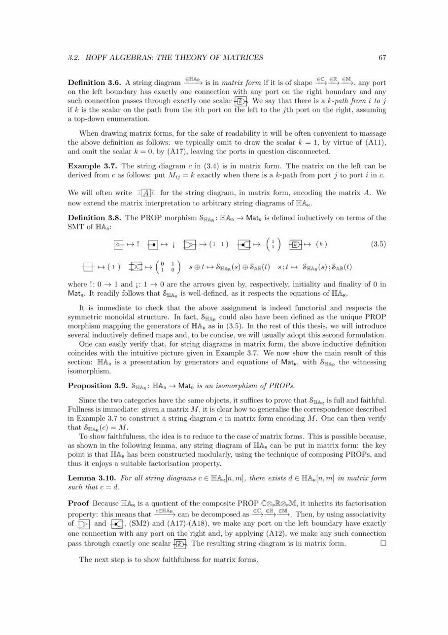
3.2. HOPF ALGEBRAS: THE THEORY OF MATRICES 67
Definition 3.6. A string diagram∈HAR−−−→ is in matrix form if it is of shape
∈C−−→ ∈R−−→ ∈M−−→, any porton the left boundary has exactly one connection with any port on the right boundary and anysuch connection passes through exactly one scalar k . We say that there is a k-path from i to jif k is the scalar on the path from the ith port on the left to the jth port on the right, assuminga top-down enumeration.
When drawing matrix forms, for the sake of readability it will be often convenient to massagethe above definition as follows: we typically omit to draw the scalar k = 1, by virtue of (A11),and omit the scalar k = 0, by (A17), leaving the ports in question disconnected.
Example 3.7. The string diagram c in (3.4) is in matrix form. The matrix on the left can bederived from c as follows: put Mij = k exactly when there is a k-path from port j to port i in c.
We will often write A for the string diagram, in matrix form, encoding the matrix A. We
now extend the matrix interpretation to arbitrary string diagrams of HAR.
Definition 3.8. The PROP morphism SHAR: HAR → MatR is defined inductively on terms of the
SMT of HAR:
7→ ! 7→ ¡ 7→ (1 1 ) 7→(
11
)k 7→ (k ) (3.5)
7→ ( 1 ) 7→(
0 11 0
)s⊕ t 7→ SHAR
(s)⊕ SAB(t) s ; t 7→ SHAR(s) ; SAB(t)
where ! : 0 → 1 and ¡ : 1 → 0 are the arrows given by, respectively, initiality and finality of 0 inMatR. It readily follows that SHAR
is well-defined, as it respects the equations of HAR.
It is immediate to check that the above assignment is indeed functorial and respects thesymmetric monoidal structure. In fact, SHAR
could also have been defined as the unique PROPmorphism mapping the generators of HAR as in (3.5). In the rest of this thesis, we will introduceseveral inductively defined maps and, to be concise, we will usually adopt this second formulation.
One can easily verify that, for string diagrams in matrix form, the above inductive definitioncoincides with the intuitive picture given in Example 3.7. We now show the main result of thissection: HAR is a presentation by generators and equations of MatR, with SHAR
the witnessingisomorphism.
Proposition 3.9. SHAR: HAR → MatR is an isomorphism of PROPs.
Since the two categories have the same objects, it suffices to prove that SHARis full and faithful.
Fullness is immediate: given a matrix M , it is clear how to generalise the correspondence describedin Example 3.7 to construct a string diagram c in matrix form encoding M . One can then verifythat SHAR
(c) = M .To show faithfulness, the idea is to reduce to the case of matrix forms. This is possible because,
as shown in the following lemma, any string diagram of HAR can be put in matrix form: the keypoint is that HAR has been constructed modularly, using the technique of composing PROPs, andthus it enjoys a suitable factorisation property.
Lemma 3.10. For all string diagrams c ∈ HAR[n,m], there exists d ∈ HAR[n,m] in matrix formsuch that c = d.
Proof Because HAR is a quotient of the composite PROP C⊗PR⊗PM, it inherits its factorisation
property: this means thatc∈HAR−−−−→ can be decomposed as
∈C−−→ ∈R−−→ ∈M−−→. Then, by using associativityof and , (SM2) and (A17)-(A18), we make any port on the left boundary have exactly
one connection with any port on the right and, by applying (A12), we make any such connection
pass through exactly one scalar k . The resulting string diagram is in matrix form. �
The next step is to show faithfulness for matrix forms.
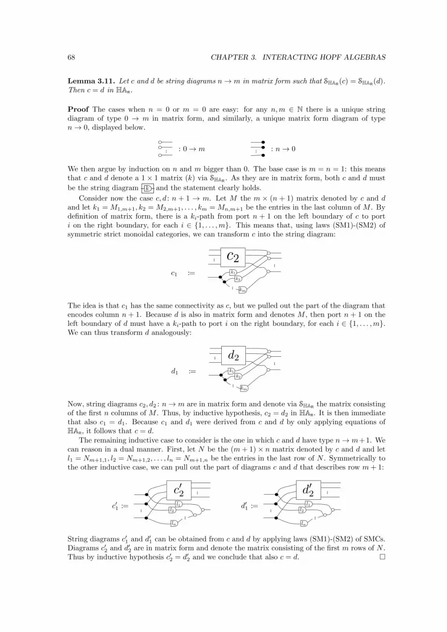
68 CHAPTER 3. INTERACTING HOPF ALGEBRAS
Lemma 3.11. Let c and d be string diagrams n→ m in matrix form such that SHAR(c) = SHAR
(d).Then c = d in HAR.
Proof The cases when n = 0 or m = 0 are easy: for any n,m ∈ N there is a unique stringdiagram of type 0 → m in matrix form, and similarly, a unique matrix form diagram of typen→ 0, displayed below.
: 0→ m : n→ 0
We then argue by induction on n and m bigger than 0. The base case is m = n = 1: this meansthat c and d denote a 1× 1 matrix (k) via SHAR
. As they are in matrix form, both c and d must
be the string diagram k and the statement clearly holds.
Consider now the case c, d : n + 1 → m. Let M the m × (n + 1) matrix denoted by c and dand let k1 = M1,m+1, k2 = M2,m+1, . . . , km = Mn,m+1 be the entries in the last column of M . Bydefinition of matrix form, there is a ki-path from port n + 1 on the left boundary of c to porti on the right boundary, for each i ∈ {1, . . . ,m}. This means that, using laws (SM1)-(SM2) ofsymmetric strict monoidal categories, we can transform c into the string diagram:
c1 :=
c2k1
k2k2
km
The idea is that c1 has the same connectivity as c, but we pulled out the part of the diagram thatencodes column n + 1. Because d is also in matrix form and denotes M , then port n + 1 on theleft boundary of d must have a ki-path to port i on the right boundary, for each i ∈ {1, . . . ,m}.We can thus transform d analogously:
d1 := k1
k2k2
km
d2
Now, string diagrams c2, d2 : n→ m are in matrix form and denote via SHARthe matrix consisting
of the first n columns of M . Thus, by inductive hypothesis, c2 = d2 in HAR. It is then immediatethat also c1 = d1. Because c1 and d1 were derived from c and d by only applying equations ofHAR, it follows that c = d.
The remaining inductive case to consider is the one in which c and d have type n→ m+1. Wecan reason in a dual manner. First, let N be the (m+ 1)× n matrix denoted by c and d and letl1 = Nm+1,1, l2 = Nm+1,2, . . . , ln = Nm+1,n be the entries in the last row of N . Symmetrically tothe other inductive case, we can pull out the part of diagrams c and d that describes row m+ 1:
c′1 := l1l2
ln
c02d′1 := l1
l2
ln
d02
String diagrams c′1 and d′1 can be obtained from c and d by applying laws (SM1)-(SM2) of SMCs.Diagrams c′2 and d′2 are in matrix form and denote the matrix consisting of the first m rows of N .Thus by inductive hypothesis c′2 = d′2 and we conclude that also c = d. �
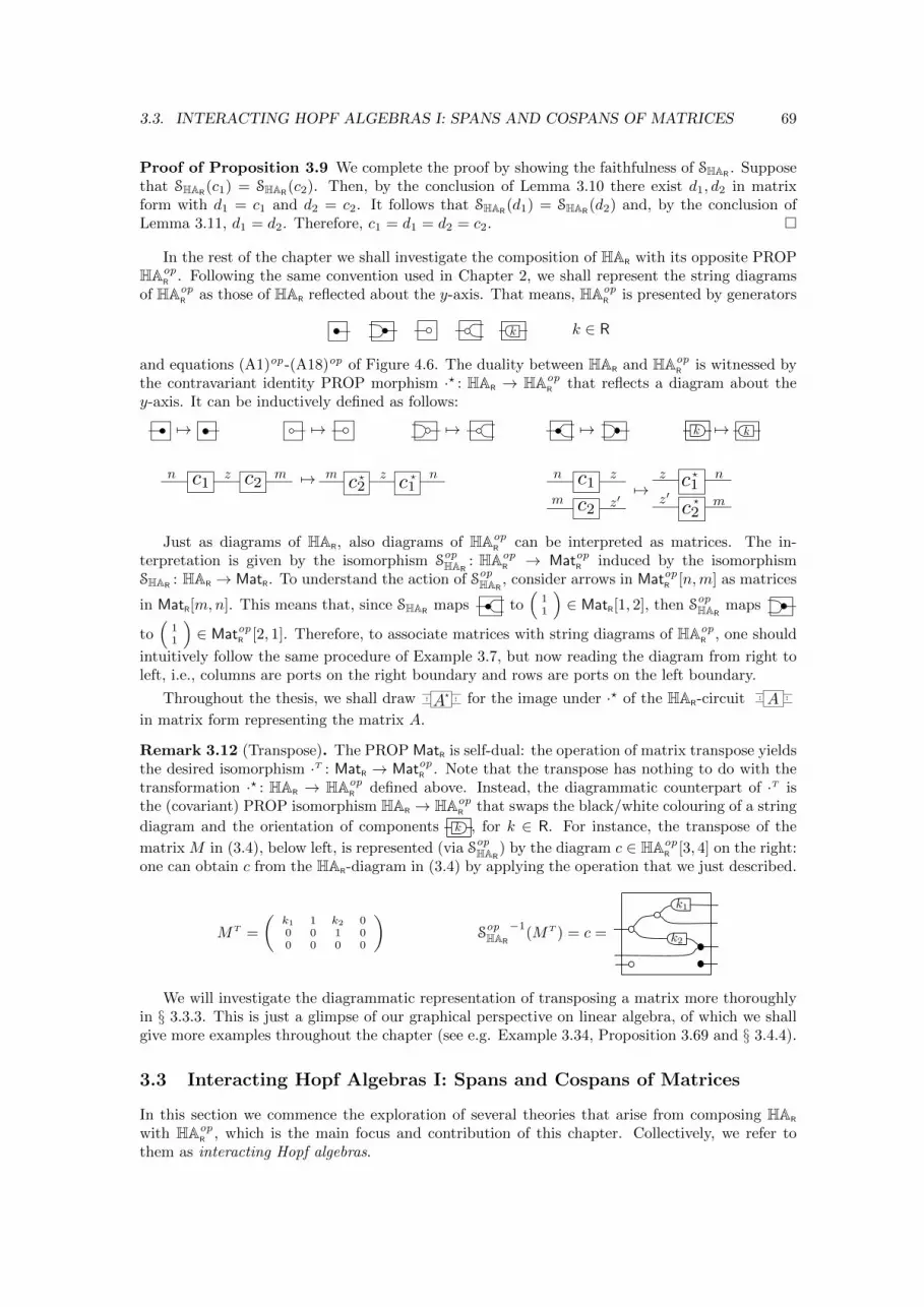
3.3. INTERACTING HOPF ALGEBRAS I: SPANS AND COSPANS OF MATRICES 69
Proof of Proposition 3.9 We complete the proof by showing the faithfulness of SHAR. Suppose
that SHAR(c1) = SHAR
(c2). Then, by the conclusion of Lemma 3.10 there exist d1, d2 in matrixform with d1 = c1 and d2 = c2. It follows that SHAR
(d1) = SHAR(d2) and, by the conclusion of
Lemma 3.11, d1 = d2. Therefore, c1 = d1 = d2 = c2. �
In the rest of the chapter we shall investigate the composition of HAR with its opposite PROPHAop
R . Following the same convention used in Chapter 2, we shall represent the string diagramsof HAop
R as those of HAR reflected about the y-axis. That means, HAopR is presented by generators
k k ∈ R
and equations (A1)op-(A18)op of Figure 4.6. The duality between HAR and HAopR is witnessed by
the contravariant identity PROP morphism ·? : HAR → HAopR that reflects a diagram about the
y-axis. It can be inductively defined as follows:
7→ 7→ 7→ 7→ k 7→ k
n mc1 c2z 7→ nm c1c2
z? ? n
m
c1
c2
z
z07→
n
m
c1
c2
z
z0
?
?
Just as diagrams of HAR, also diagrams of HAopR can be interpreted as matrices. The in-
terpretation is given by the isomorphism SopHAR
: HAopR → MatopR induced by the isomorphism
SHAR: HAR → MatR. To understand the action of SopHAR
, consider arrows in MatopR [n,m] as matrices
in MatR[m,n]. This means that, since SHARmaps to
(11
)∈ MatR[1, 2], then S
opHAR
maps
to(
11
)∈ MatopR [2, 1]. Therefore, to associate matrices with string diagrams of HAop
R , one should
intuitively follow the same procedure of Example 3.7, but now reading the diagram from right toleft, i.e., columns are ports on the right boundary and rows are ports on the left boundary.
Throughout the thesis, we shall draw A? for the image under ·? of the HAR-circuit A
in matrix form representing the matrix A.
Remark 3.12 (Transpose). The PROP MatR is self-dual: the operation of matrix transpose yieldsthe desired isomorphism ·T : MatR → MatopR . Note that the transpose has nothing to do with thetransformation ·? : HAR → HAop
R defined above. Instead, the diagrammatic counterpart of ·T isthe (covariant) PROP isomorphism HAR → HAop
R that swaps the black/white colouring of a string
diagram and the orientation of components k , for k ∈ R. For instance, the transpose of the
matrix M in (3.4), below left, is represented (via SopHAR
) by the diagram c ∈ HAopR [3, 4] on the right:
one can obtain c from the HAR-diagram in (3.4) by applying the operation that we just described.
MT =
(k1 1 k2 00 0 1 00 0 0 0
)SopHAR
−1(MT ) = c =
k1
k2
We will investigate the diagrammatic representation of transposing a matrix more thoroughlyin § 3.3.3. This is just a glimpse of our graphical perspective on linear algebra, of which we shallgive more examples throughout the chapter (see e.g. Example 3.34, Proposition 3.69 and § 3.4.4).
3.3 Interacting Hopf Algebras I: Spans and Cospans of Matrices
In this section we commence the exploration of several theories that arise from composing HAR
with HAopR , which is the main focus and contribution of this chapter. Collectively, we refer to
them as interacting Hopf algebras.
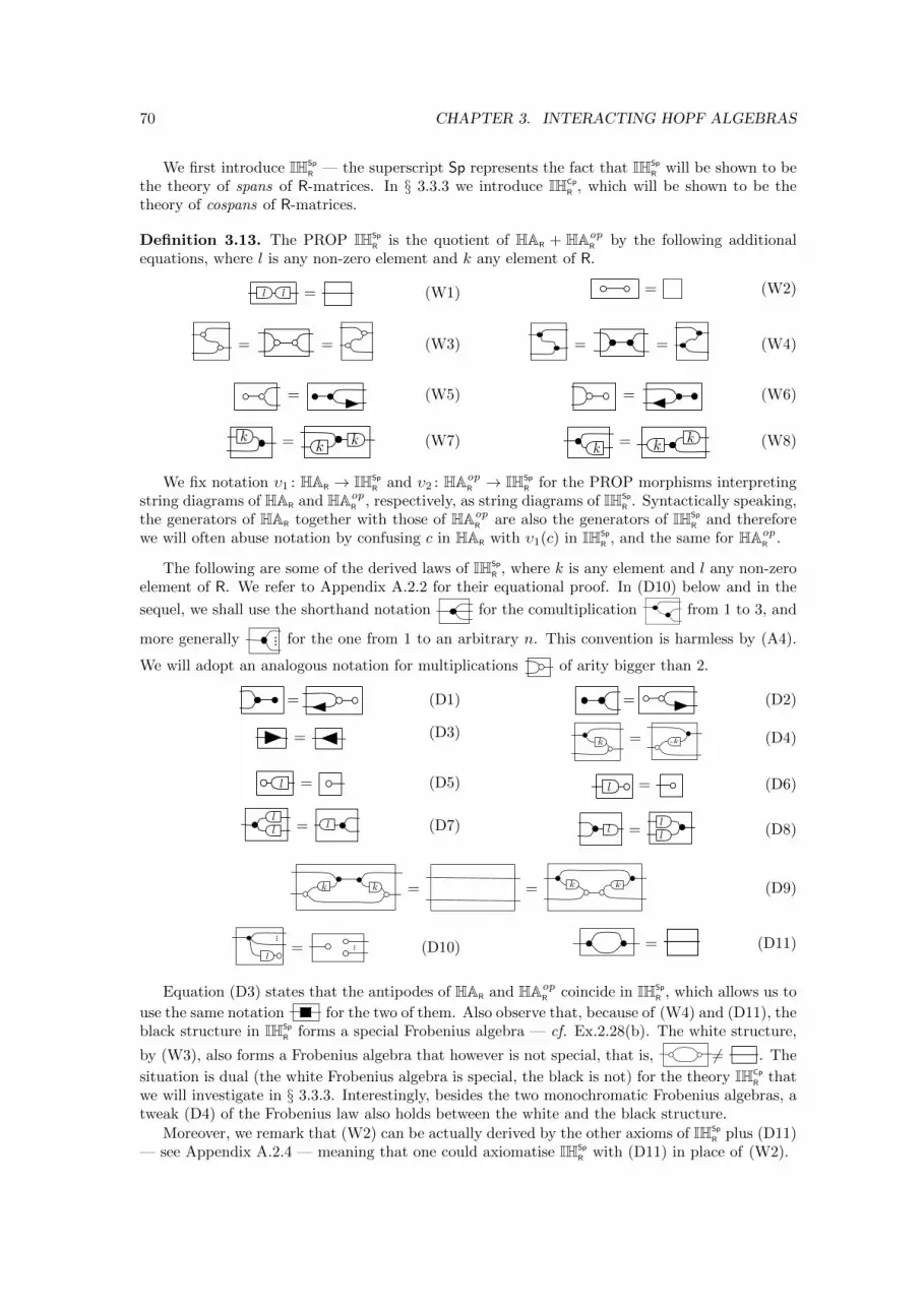
70 CHAPTER 3. INTERACTING HOPF ALGEBRAS
We first introduce IHSp
R — the superscript Sp represents the fact that IHSp
R will be shown to bethe theory of spans of R-matrices. In § 3.3.3 we introduce IHCp
R , which will be shown to be thetheory of cospans of R-matrices.
Definition 3.13. The PROP IHSp
R is the quotient of HAR + HAopR by the following additional
equations, where l is any non-zero element and k any element of R.
ll = (W1) = (W2)
= = (W3) = = (W4)
= (W5) = (W6)
k = kk (W7) k = kk (W8)
We fix notation υ1 : HAR → IHSp
R and υ2 : HAopR → IHSp
R for the PROP morphisms interpretingstring diagrams of HAR and HAop
R , respectively, as string diagrams of IHSp
R . Syntactically speaking,the generators of HAR together with those of HAop
R are also the generators of IHSp
R and thereforewe will often abuse notation by confusing c in HAR with υ1(c) in IHSp
R , and the same for HAopR .
The following are some of the derived laws of IHSp
R , where k is any element and l any non-zeroelement of R. We refer to Appendix A.2.2 for their equational proof. In (D10) below and in the
sequel, we shall use the shorthand notation for the comultiplication from 1 to 3, and
more generally for the one from 1 to an arbitrary n. This convention is harmless by (A4).
We will adopt an analogous notation for multiplications of arity bigger than 2.
= (D1) = (D2)
= (D3)k = -k (D4)
l = (D5) l = (D6)
ll = l (D7) l = l
l(D8)
k k = = k k (D9)
l= (D10) = (D11)
Equation (D3) states that the antipodes of HAR and HAopR coincide in IHSp
R , which allows us to
use the same notation for the two of them. Also observe that, because of (W4) and (D11), theblack structure in IHSp
R forms a special Frobenius algebra — cf. Ex.2.28(b). The white structure,
by (W3), also forms a Frobenius algebra that however is not special, that is, 6= . The
situation is dual (the white Frobenius algebra is special, the black is not) for the theory IHCp
R thatwe will investigate in § 3.3.3. Interestingly, besides the two monochromatic Frobenius algebras, atweak (D4) of the Frobenius law also holds between the white and the black structure.
Moreover, we remark that (W2) can be actually derived by the other axioms of IHSp
R plus (D11)— see Appendix A.2.4 — meaning that one could axiomatise IHSp
R with (D11) in place of (W2).
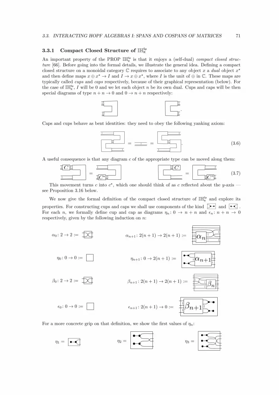
3.3. INTERACTING HOPF ALGEBRAS I: SPANS AND COSPANS OF MATRICES 71
3.3.1 Compact Closed Structure of IHSpR
An important property of the PROP IHSp
R is that it enjoys a (self-dual) compact closed struc-ture [66]. Before going into the formal details, we illustrate the general idea. Defining a compactclosed structure on a monoidal category C requires to associate to any object x a dual object x?
and then define maps x⊕ x? → I and I → x⊕ x?, where I is the unit of ⊕ in C. These maps aretypically called cups and caps respectively, because of their graphical representation (below). Forthe case of IHSp
R , I will be 0 and we let each object n be its own dual. Cups and caps will be thenspecial diagrams of type n+ n→ 0 and 0→ n+ n respectively:
.
Caps and cups behave as bent identities: they need to obey the following yanking axiom:
= = . (3.6)
A useful consequence is that any diagram c of the appropriate type can be moved along them:
C=
C?
C=
C ?(3.7)
This movement turns c into c?, which one should think of as c reflected about the y-axis —see Proposition 3.16 below.
We now give the formal definition of the compact closed structure of IHSp
R and explore its
properties. For constructing cups and caps we shall use components of the kind and .For each n, we formally define cup and cap as diagrams ηn : 0 → n + n and εn : n + n → 0respectively, given by the following induction on n:
α0 : 2→ 2 := αn+1 : 2(n+ 1)→ 2(n+ 1) := ↵n
η0 : 0→ 0 := ηn+1 : 0→ 2(n+ 1) := ↵n+1
β0 : 2→ 2 := βn+1 : 2(n+ 1)→ 2(n+ 1) := �n
ε0 : 0→ 0 := εn+1 : 2(n+ 1)→ 0 := �n+1
For a more concrete grip on that definition, we show the first values of ηn:
η1 = η2 = η3 =
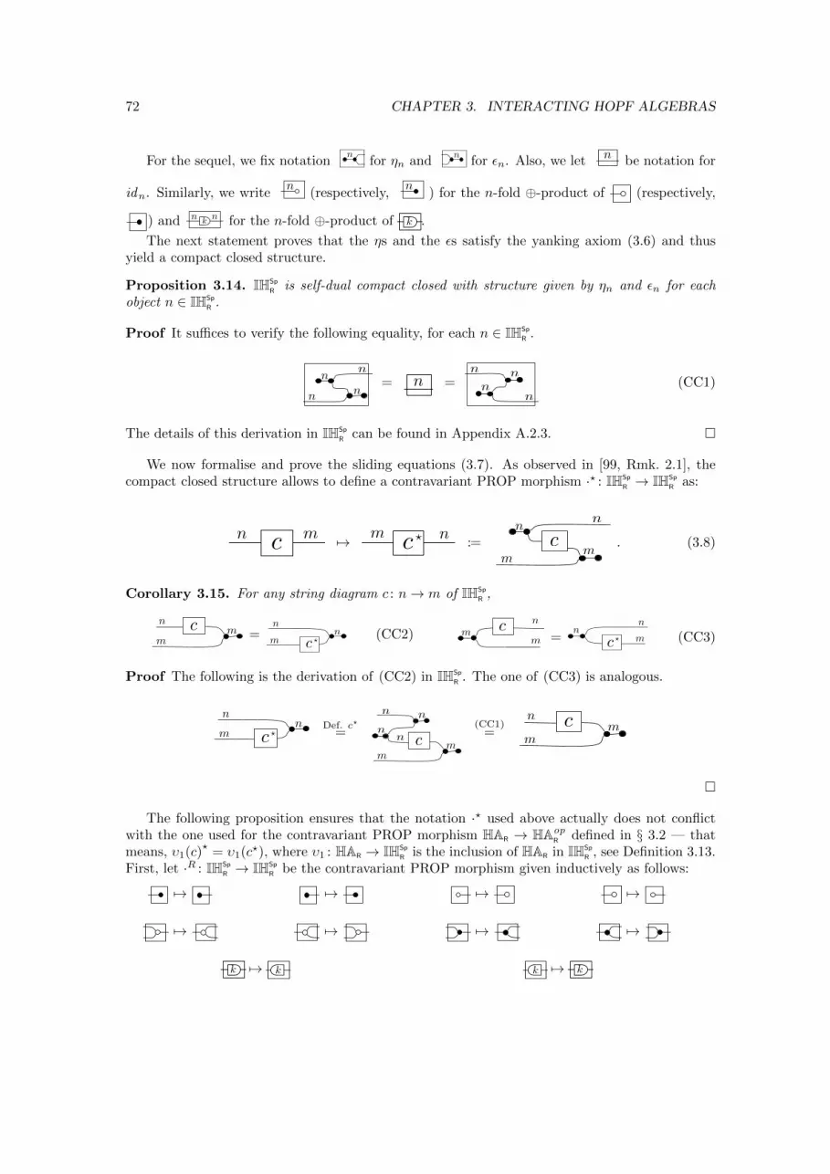
72 CHAPTER 3. INTERACTING HOPF ALGEBRAS
For the sequel, we fix notationn
for ηn andn
for εn. Also, we let n be notation for
idn. Similarly, we writen
(respectively,n
) for the n-fold ⊕-product of (respectively,
) and n nk for the n-fold ⊕-product of k .
The next statement proves that the ηs and the εs satisfy the yanking axiom (3.6) and thusyield a compact closed structure.
Proposition 3.14. IHSp
R is self-dual compact closed with structure given by ηn and εn for eachobject n ∈ IHSp
R .
Proof It suffices to verify the following equality, for each n ∈ IHSp
R .
nn
n
n= n =
n nn
n(CC1)
The details of this derivation in IHSp
R can be found in Appendix A.2.3. �
We now formalise and prove the sliding equations (3.7). As observed in [99, Rmk. 2.1], thecompact closed structure allows to define a contravariant PROP morphism ·? : IHSp
R → IHSp
R as:
cn m 7→ c nm ? := cn
n
mm
. (3.8)
Corollary 3.15. For any string diagram c : n→ m of IHSp
R ,
mm
n c= m c ?
nn
(CC2) mm
nc= mc ?
nn
(CC3)
Proof The following is the derivation of (CC2) in IHSp
R . The one of (CC3) is analogous.
m c ?n
nDef. c?
=
n n
nn
mm
c(CC1)
= mm
n c
�
The following proposition ensures that the notation ·? used above actually does not conflictwith the one used for the contravariant PROP morphism HAR → HAop
R defined in § 3.2 — thatmeans, υ1(c)
?= υ1(c?), where υ1 : HAR → IHSp
R is the inclusion of HAR in IHSp
R , see Definition 3.13.First, let ·R : IHSp
R → IHSp
R be the contravariant PROP morphism given inductively as follows:
7→ 7→ 7→ 7→
7→ 7→ 7→ 7→
k 7→ k k 7→ k
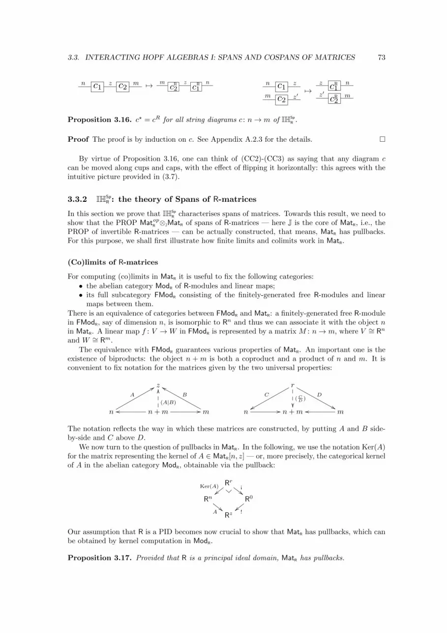
3.3. INTERACTING HOPF ALGEBRAS I: SPANS AND COSPANS OF MATRICES 73
n mc1 c2z 7→ nm
c1c2z RR n
m
c1
c2
z
z07→
n
m
c1
c2
z
z0R
R
Proposition 3.16. c? = cR for all string diagrams c : n→ m of IHSp
R .
Proof The proof is by induction on c. See Appendix A.2.3 for the details. �
By virtue of Proposition 3.16, one can think of (CC2)-(CC3) as saying that any diagram ccan be moved along cups and caps, with the effect of flipping it horizontally: this agrees with theintuitive picture provided in (3.7).
3.3.2 IHSpR : the theory of Spans of R-matrices
In this section we prove that IHSp
R characterises spans of matrices. Towards this result, we need toshow that the PROP MatopR ⊗JMatR of spans of R-matrices — here J is the core of MatR, i.e., thePROP of invertible R-matrices — can be actually constructed, that means, MatR has pullbacks.For this purpose, we shall first illustrate how finite limits and colimits work in MatR.
(Co)limits of R-matrices
For computing (co)limits in MatR it is useful to fix the following categories:
• the abelian category ModR of R-modules and linear maps;• its full subcategory FModR consisting of the finitely-generated free R-modules and linear
maps between them.
There is an equivalence of categories between FModR and MatR: a finitely-generated free R-modulein FModR, say of dimension n, is isomorphic to Rn and thus we can associate it with the object nin MatR. A linear map f : V →W in FModR is represented by a matrix M : n→ m, where V ∼= Rn
and W ∼= Rm.
The equivalence with FModR guarantees various properties of MatR. An important one is theexistence of biproducts: the object n + m is both a coproduct and a product of n and m. It isconvenient to fix notation for the matrices given by the two universal properties:
z
n
A
88
n+moo //(A|B)
OO
m
B
ff rD
&&
C
xx(CD )
��n // n+m moo
The notation reflects the way in which these matrices are constructed, by putting A and B side-by-side and C above D.
We now turn to the question of pullbacks in MatR. In the following, we use the notation Ker(A)for the matrix representing the kernel of A ∈ MatR[n, z] — or, more precisely, the categorical kernelof A in the abelian category ModR, obtainable via the pullback:
RrKer(A)||
¡""
Rn
A""
R0
!||
Rz
Our assumption that R is a PID becomes now crucial to show that MatR has pullbacks, which canbe obtained by kernel computation in ModR.
Proposition 3.17. Provided that R is a principal ideal domain, MatR has pullbacks.
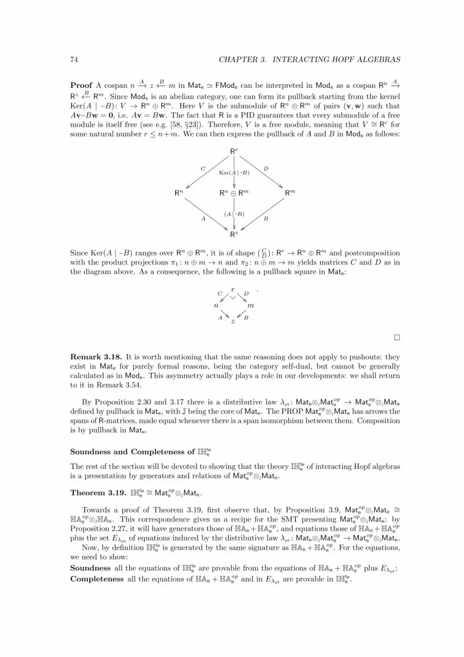
74 CHAPTER 3. INTERACTING HOPF ALGEBRAS
Proof A cospan nA−→ z
B←− m in MatR ' FModR can be interpreted in ModR as a cospan RnA−→
RzB←− Rm. Since ModR is an abelian category, one can form its pullback starting from the kernel
Ker(A | −B) : V → Rn ⊕ Rm. Here V is the submodule of Rn ⊕ Rm of pairs (v,w) such thatAv−Bw = 0, i.e. Av = Bw. The fact that R is a PID guarantees that every submodule of a freemodule is itself free (see e.g. [58, §23]). Therefore, V is a free module, meaning that V ∼= Rr forsome natural number r ≤ n+m. We can then express the pullback of A and B in ModR as follows:
Rr
C
{{
Ker(A | −B)
��
D
##Rn
A
##
Rn ⊕ Rm
(A | −B)
��
Rm
B
{{Rz
Since Ker(A | −B) ranges over Rn ⊕ Rm, it is of shape (CD ) : Rr → Rn ⊕ Rm and postcompositionwith the product projections π1 : n⊕m → n and π2 : n⊕m → m yields matrices C and D as inthe diagram above. As a consequence, the following is a pullback square in MatR:
rC~~
D!!
n
A m
B}}z
.
�
Remark 3.18. It is worth mentioning that the same reasoning does not apply to pushouts: theyexist in MatR for purely formal reasons, being the category self-dual, but cannot be generallycalculated as in ModR. This asymmetry actually plays a role in our developments: we shall returnto it in Remark 3.54.
By Proposition 2.30 and 3.17 there is a distributive law λpb : MatR⊗JMatopR → MatopR ⊗JMatRdefined by pullback in MatR, with J being the core of MatR. The PROP MatopR ⊗JMatR has arrows thespans of R-matrices, made equal whenever there is a span isomorphism between them. Compositionis by pullback in MatR.
Soundness and Completeness of IHSp
R
The rest of the section will be devoted to showing that the theory IHSp
R of interacting Hopf algebrasis a presentation by generators and relations of MatopR ⊗JMatR.
Theorem 3.19. IHSp
R∼= MatopR ⊗JMatR.
Towards a proof of Theorem 3.19, first observe that, by Proposition 3.9, MatopR ⊗JMatR ∼=HAop
R ⊗JHAR. This correspondence gives us a recipe for the SMT presenting MatopR ⊗JMatR: byProposition 2.27, it will have generators those of HAR +HAop
R , and equations those of HAR +HAopR
plus the set Eλpbof equations induced by the distributive law λpb : MatR⊗JMatopR → MatopR ⊗JMatR.
Now, by definition IHSp
R is generated by the same signature as HAR +HAopR . For the equations,
we need to show:
Soundness all the equations of IHSp
R are provable from the equations of HAR + HAopR plus Eλpb
;
Completeness all the equations of HAR + HAopR and in Eλpb
are provable in IHSp
R .
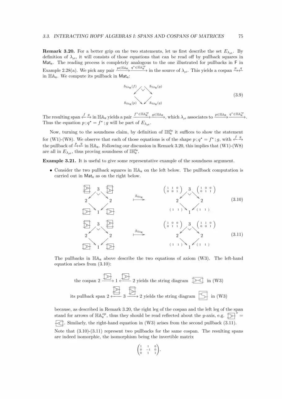
3.3. INTERACTING HOPF ALGEBRAS I: SPANS AND COSPANS OF MATRICES 75
Remark 3.20. For a better grip on the two statements, let us first describe the set Eλpb. By
definition of λpb, it will consists of those equations that can be read off by pullback squares inMatR. The reading process is completely analogous to the one illustrated for pullbacks in F in
Example 2.28(a). We pick any pairp∈HAR−−−−→ q?∈HAop
R−−−−−→ in the source of λpb. This yields a cospanp−→ q←−
in HAR. We compute its pullback in MatR:
SHAR (f)
��
SHAR (g)
��
SHAR (p) �� SHAR (q)��
(3.9)
The resulting spanf←− g−→ in HAR yields a pair
f?∈HAopR−−−−−−→ g∈HAR−−−−→, which λpb associates to
p∈HAR−−−−→ q?∈HAopR−−−−−→.
Thus the equation p ; q? = f? ; g will be part of Eλpb.
Now, turning to the soundness claim, by definition of IHSp
R it suffices to show the statement
for (W1)-(W8). We observe that each of those equations is of the shape p ; q? = f? ; g, withf←− g−→
the pullback ofp−→ q←− in HAR. Following our discussion in Remark 3.20, this implies that (W1)-(W8)
are all in Eλpb, thus proving soundness of IHSp
R .
Example 3.21. It is useful to give some representative example of the soundness argument.
• Consider the two pullback squares in HAR on the left below. The pullback computation iscarried out in MatR as on the right below.
3
~~ 2
2
~~1
� SHAR //
3(
1 1 00 0 1
)~~
(1 0 00 1 1
)
2
( 1 1 )
2
( 1 1 )~~1
(3.10)
3
~~ 2
2
~~1
� SHAR //
3(
1 0 00 1 1
)~~
(1 1 00 0 1
)
2
( 1 1 )
2
( 1 1 )~~1
(3.11)
The pullbacks in HAR above describe the two equations of axiom (W3). The left-handequation arises from (3.10):
the cospan 2 −−−→ 1←−−− 2 yields the string diagram in (W3)
its pullback span 2←−−− 3 −−−→ 2 yields the string diagram in (W3)
because, as described in Remark 3.20, the right leg of the cospan and the left leg of the span
stand for arrows of HAopR , thus they should be read reflected about the y-axis, e.g.
?=
. Similarly, the right-hand equation in (W3) arises from the second pullback (3.11).
Note that (3.10)-(3.11) represent two pullbacks for the same cospan. The resulting spansare indeed isomorphic, the isomorphism being the invertible matrix
(1 1 00 −1 00 1 1
).
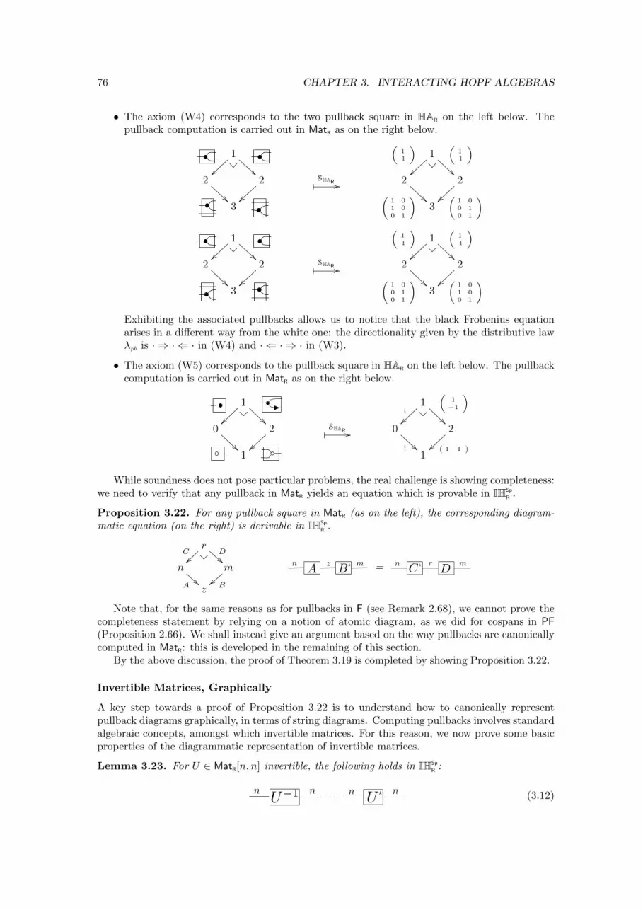
76 CHAPTER 3. INTERACTING HOPF ALGEBRAS
• The axiom (W4) corresponds to the two pullback square in HAR on the left below. Thepullback computation is carried out in MatR as on the right below.
1
~~ 2
2
~~3
� SHAR //
1(
11
)~~
(11
)
2
(1 01 00 1
)
2
(1 00 10 1
)~~3
1
~~ 2
2
~~3
� SHAR //
1(
11
)~~
(11
)
2
(1 00 10 1
)
2
(1 01 00 1
)~~3
Exhibiting the associated pullbacks allows us to notice that the black Frobenius equationarises in a different way from the white one: the directionality given by the distributive lawλpb is · ⇒ · ⇐ · in (W4) and · ⇐ · ⇒ · in (W3).
• The axiom (W5) corresponds to the pullback square in HAR on the left below. The pullbackcomputation is carried out in MatR as on the right below.
1
~~ 0
2
~~1
� SHAR //
1¡
~~
(1−1
)
0
!
2
( 1 1 )~~1
While soundness does not pose particular problems, the real challenge is showing completeness:we need to verify that any pullback in MatR yields an equation which is provable in IHSp
R .
Proposition 3.22. For any pullback square in MatR (as on the left), the corresponding diagram-matic equation (on the right) is derivable in IHSp
R .
rC~~
D!!
n
A m
B}}z
n mzA B? = n m
C D? r
Note that, for the same reasons as for pullbacks in F (see Remark 2.68), we cannot prove thecompleteness statement by relying on a notion of atomic diagram, as we did for cospans in PF(Proposition 2.66). We shall instead give an argument based on the way pullbacks are canonicallycomputed in MatR: this is developed in the remaining of this section.
By the above discussion, the proof of Theorem 3.19 is completed by showing Proposition 3.22.
Invertible Matrices, Graphically
A key step towards a proof of Proposition 3.22 is to understand how to canonically representpullback diagrams graphically, in terms of string diagrams. Computing pullbacks involves standardalgebraic concepts, amongst which invertible matrices. For this reason, we now prove some basicproperties of the diagrammatic representation of invertible matrices.
Lemma 3.23. For U ∈ MatR[n, n] invertible, the following holds in IHSp
R :
n nU�1 = n n
U ? (3.12)
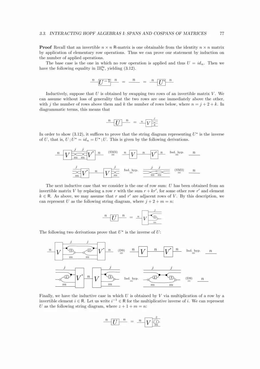
3.3. INTERACTING HOPF ALGEBRAS I: SPANS AND COSPANS OF MATRICES 77
Proof Recall that an invertible n× n R-matrix is one obtainable from the identity n× n matrixby application of elementary row operations. Thus we can prove our statement by induction onthe number of applied operations.
The base case is the one in which no row operation is applied and thus U = idn. Then wehave the following equality in IHSp
R , yielding (3.12).
n nU�1 = n = n n
U ?
Inductively, suppose that U is obtained by swapping two rows of an invertible matrix V . Wecan assume without loss of generality that the two rows are one immediately above the other,with j the number of rows above them and k the number of rows below, where n = j + 2 + k. Indiagrammatic terms, this means that
n nU = n V k
j
In order to show (3.12), it suffices to prove that the string diagram representing U? is the inverseof U , that is, U ;U? = idn = U? ;U . This is given by the following derivations.
n Vj j
nV?
m m
(SM3)=
n Vnn V
? Ind. hyp.= n
Vjj
nV?
m m
Ind. hyp.=
j j
m m
(SM3)= n
The next inductive case that we consider is the one of row sum: U has been obtained from aninvertible matrix V by replacing a row r with the sum r+ kr′, for some other row r′ and elementk ∈ R. As above, we may assume that r and r′ are adjacent rows of V . By this description, wecan represent U as the following string diagram, where j + 2 +m = n:
n nU =
j
knV
m
The following two derivations prove that U? is the inverse of U :
j
knV
m m
j
V? nk (D9)
=n V
nn V?
Ind. hyp.= n
j
kVmm
j
V? nk Ind. hyp.
=m
j
k
j
k
m
(D9)= n
Finally, we have the inductive case in which U is obtained by V via multiplication of a row by ainvertible element i ∈ R. Let us write i−1 ∈ R for the multiplicative inverse of i. We can representU as the following string diagram, where z + 1 +m = n:
n nU = n
V m
zi
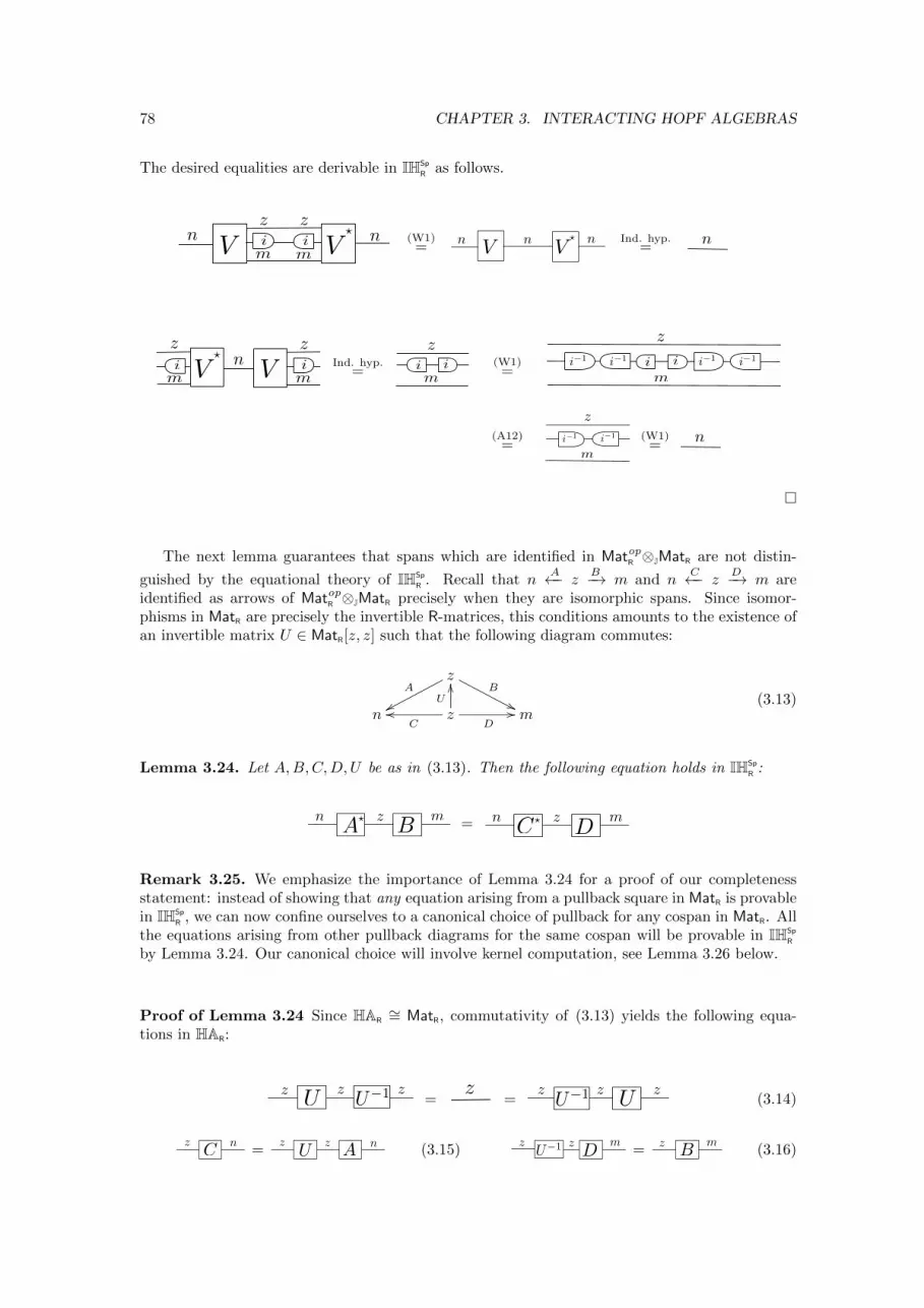
78 CHAPTER 3. INTERACTING HOPF ALGEBRAS
The desired equalities are derivable in IHSp
R as follows.
nV m
zi nVm
z?
i (W1)=
n Vnn V
? Ind. hyp.= n
n V m
ziV
?
m
zi Ind. hyp.
= ii
z
m(W1)=
ii
z
mi�1i�1 i�1 i�1
(A12)=
m
z
i�1 i�1 (W1)= n
�
The next lemma guarantees that spans which are identified in MatopR ⊗JMatR are not distin-
guished by the equational theory of IHSp
R . Recall that nA←− z
B−→ m and nC←− z
D−→ m areidentified as arrows of MatopR ⊗JMatR precisely when they are isomorphic spans. Since isomor-phisms in MatR are precisely the invertible R-matrices, this conditions amounts to the existence ofan invertible matrix U ∈ MatR[z, z] such that the following diagram commutes:
zB
''A
xxn z
Coo
U
OO
D// m
(3.13)
Lemma 3.24. Let A,B,C,D,U be as in (3.13). Then the following equation holds in IHSp
R :
n mzA B? = n m
C D? z
Remark 3.25. We emphasize the importance of Lemma 3.24 for a proof of our completenessstatement: instead of showing that any equation arising from a pullback square in MatR is provablein IHSp
R , we can now confine ourselves to a canonical choice of pullback for any cospan in MatR. Allthe equations arising from other pullback diagrams for the same cospan will be provable in IHSp
R
by Lemma 3.24. Our canonical choice will involve kernel computation, see Lemma 3.26 below.
Proof of Lemma 3.24 Since HAR∼= MatR, commutativity of (3.13) yields the following equa-
tions in HAR:
zz zU�1U =
z=
z zzU�1 U (3.14)
z nC = A nzz
U (3.15)m
Dzz
U�1 =m
Bz(3.16)
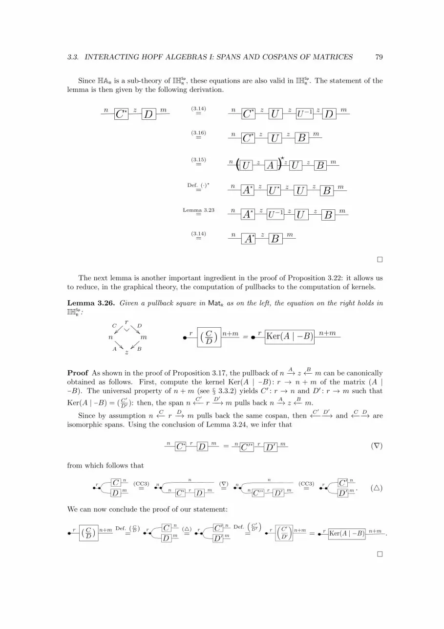
3.3. INTERACTING HOPF ALGEBRAS I: SPANS AND COSPANS OF MATRICES 79
Since HAR is a sub-theory of IHSp
R , these equations are also valid in IHSp
R . The statement of thelemma is then given by the following derivation.
n mC D? z (3.14)
= n mC D
? z z zU U�1
(3.16)= n
C? m
Bz zU
(3.15)= ( (?n
A mBz z zUU
Def. (·)?=
nA? ? m
Bzzz
UU
Lemma 3.23=
nA? m
Bz z zUU�1
(3.14)= n mz
A B?
�
The next lemma is another important ingredient in the proof of Proposition 3.22: it allows usto reduce, in the graphical theory, the computation of pullbacks to the computation of kernels.
Lemma 3.26. Given a pullback square in MatR as on the left, the equation on the right holds inIHSp
R :
rC~~
D!!
n
A m
B}}z
n+mr ( CD ) =
n+mKer(A | �B)r
Proof As shown in the proof of Proposition 3.17, the pullback of nA−→ z
B←− m can be canonicallyobtained as follows. First, compute the kernel Ker(A | −B) : r → n + m of the matrix (A |−B). The universal property of n + m (see § 3.3.2) yields C ′ : r → n and D′ : r → m such that
Ker(A | −B) = (C′
D′ ): then, the span nC′←− r D′−−→ m pulls back n
A−→ zB←− m.
Since by assumption nC←− r
D−→ m pulls back the same cospan, thenC′←− D′−−→ and
C←− D−→ areisomorphic spans. Using the conclusion of Lemma 3.24, we infer that
n mC D? r = n mrC ?
D0 0 (∇)
from which follows that
C
D
n
mr (CC3)
= n mC D? r
nn
(∇)= n mrC ? D0 0
nn
(CC3)=
C
D
n
mr
0
0 . (4)
We can now conclude the proof of our statement:
n+mr ( CD )
Def.(CD
)=
C
D
n
mr (4)
=C
D
n
mr
0
0
Def.(C′D′
)=
n+mr✓
C 0
D0
◆= n+mKer(A | �B)r .
�
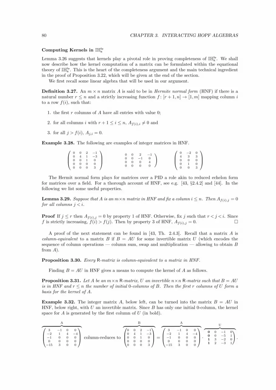
80 CHAPTER 3. INTERACTING HOPF ALGEBRAS
Computing Kernels in IHSp
R
Lemma 3.26 suggests that kernels play a pivotal role in proving completeness of IHSp
R . We shallnow describe how the kernel computation of a matrix can be formulated within the equationaltheory of IHSp
R . This is the heart of the completeness argument and the main technical ingredientin the proof of Proposition 3.22, which will be given at the end of the section.
We first recall some linear algebra that will be used in our argument.
Definition 3.27. An m × n matrix A is said to be in Hermite normal form (HNF) if there is anatural number r ≤ n and a strictly increasing function f : [r + 1, n] → [1,m] mapping column ito a row f(i), such that:
1. the first r columns of A have all entries with value 0;
2. for all columns i with r + 1 ≤ i ≤ n, Af(i),i 6= 0 and
3. for all j > f(i), Aj,i = 0.
Example 3.28. The following are examples of integer matrices in HNF.
0 0 2 −10 4 1 −30 0 1 00 0 0 00 0 0 3
(0 0 2 −10 0 −1 00 0 0 40 0 0 0
)
0 −2 04 3 30 0 00 1 00 0 3
The Hermit normal form plays for matrices over a PID a role akin to reduced echelon formfor matrices over a field. For a thorough account of HNF, see e.g. [43, §2.4.2] and [44]. In thefollowing we list some useful properties.
Lemma 3.29. Suppose that A is an m×n matrix in HNF and fix a column i ≤ n. Then Af(i),j = 0for all columns j < i.
Proof If j ≤ r then Af(i),j = 0 by property 1 of HNF. Otherwise, fix j such that r < j < i. Sincef is strictly increasing, f(i)> f(j). Then by property 3 of HNF, Af(i),j = 0. �
A proof of the next statement can be found in [43, Th. 2.4.3]. Recall that a matrix A iscolumn-equivalent to a matrix B if B = AU for some invertible matrix U (which encodes thesequence of column operations — column sum, swap and multiplication — allowing to obtain Bfrom A).
Proposition 3.30. Every R-matrix is column-equivalent to a matrix in HNF.
Finding B = AU in HNF gives a means to compute the kernel of A as follows.
Proposition 3.31. Let A be an m×n R-matrix, U an invertible n×n R-matrix such that B = AUis in HNF and r ≤ n the number of initial 0-columns of B. Then the first r columns of U form abasis for the kernel of A.
Example 3.32. The integer matrix A, below left, can be turned into the matrix B = AU inHNF, below right, with U an invertible matrix. Since B has only one initial 0-column, the kernelspace for A is generated by the first column of U (in bold).
A︷ ︸︸ ︷
3 −1 0 0−2 1 4 −4−1 0 0 00 0 0 0−15 3 0 0
column-reduces to
B︷ ︸︸ ︷
0 0 2 −10 4 1 −30 0 1 00 0 0 00 0 0 3
=
A︷ ︸︸ ︷
3 −1 0 0−2 1 4 −4−1 0 0 00 0 0 0−15 3 0 0
·
U︷ ︸︸ ︷(0 0 −1 00 0 −5 11 3 −2 01 2 −3 1
).
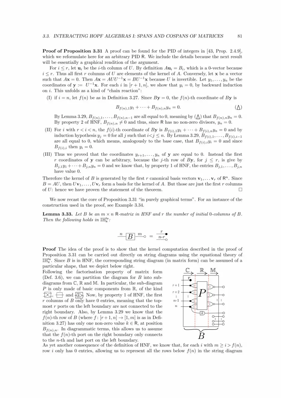
3.3. INTERACTING HOPF ALGEBRAS I: SPANS AND COSPANS OF MATRICES 81
Proof of Proposition 3.31 A proof can be found for the PID of integers in [43, Prop. 2.4.9],which we reformulate here for an arbitrary PID R. We include the details because the next resultwill be essentially a graphical rendition of the argument.
For i ≤ r, let ui be the i-th column of U . By definition Aui = Bi, which is a 0-vector becausei ≤ r. Thus all first r columns of U are elements of the kernel of A. Conversely, let x be a vectorsuch that Ax = 0. Then Ax = AUU−1x = BU−1x because U is invertible. Let y1, . . . , yn be thecoordinates of y := U−1x. For each i in [r + 1, n], we show that yi = 0, by backward inductionon i. This unfolds as a kind of “chain reaction”:
(I) if i = n, let f(n) be as in Definition 3.27. Since By = 0, the f(n)-th coordinate of By is
Bf(n),1y1 + · · ·+Bf(n),nyn = 0. (a
)
By Lemma 3.29, Bf(n),1, . . . , Bf(n),n−1 are all equal to 0, meaning by (a
) that Bf(n),nyn = 0.By property 2 of HNF, Bf(n),n 6= 0 and thus, since R has no non-zero divisors, yn = 0.
(II) For i with r < i < n, the f(i)-th coordinate of By is Bf(i),1y1 + · · · + Bf(i),nyn = 0 and byinduction hypothesis yj = 0 for all j such that i<j ≤ n. By Lemma 3.29, Bf(i),1, . . . , Bf(i),i−1
are all equal to 0, which means, analogously to the base case, that Bf(i),iyi = 0 and sinceBf(i),i then yi = 0.
(III) Thus we proved that the coordinates yr+1, . . . , yn of y are equal to 0. Instead the firstr coordinates of y can be arbitrary, because the j-th row of By, for j ≤ r, is give byBj,1y1 + · · ·+Bj,nyn = 0 and we know that, by property 1 of HNF, the entries Bj,1, . . . , Bj,nhave value 0.
Therefore the kernel of B is generated by the first r canonical basis vectors v1, . . .vr of Rn. SinceB = AU , then Uv1, . . . , Uvr form a basis for the kernel of A. But those are just the first r columnsof U : hence we have proven the statement of the theorem. �
We now recast the core of Proposition 3.31 “in purely graphical terms”. For an instance of theconstruction used in the proof, see Example 3.34.
Lemma 3.33. Let B be an m× n R-matrix in HNF and r the number of initial 0-columns of B.Then the following holds in IHSp
R :
n mB =
rn-r
Proof The idea of the proof is to show that the kernel computation described in the proof ofProposition 3.31 can be carried out directly on string diagrams using the equational theory ofIHSp
R . Since B is in HNF, the corresponding string diagram (in matrix form) can be assumed of aparticular shape, that we depict below right.Following the factorisation property of matrix form(Def. 3.6), we can partition the diagram for B into sub-diagrams from C, R and M. In particular, the sub-diagramP is only made of basic components from R, of the kind
, and k . Now, by property 1 of HNF, the firstr columns of B only have 0 entries, meaning that the top-most r ports on the left boundary are not connected to theright boundary. Also, by Lemma 3.29 we know that thef(n)-th row of B (where f : [r+ 1, n]→ [1,m] is as in Defi-nition 3.27) has only one non-zero value k ∈ R, at positionBf(n),n. In diagrammatic terms, this allows us to assumethat the f(n)-th port on the right boundary only connectsto the n-th and last port on the left boundary.
r
Pn
r + 2
r + 1
n-1
B
k
!!!MRC
As yet another consequence of the definition of HNF, we know that, for each i with m ≥ i > f(n),row i only has 0 entries, allowing us to represent all the rows below f(n) in the string diagram
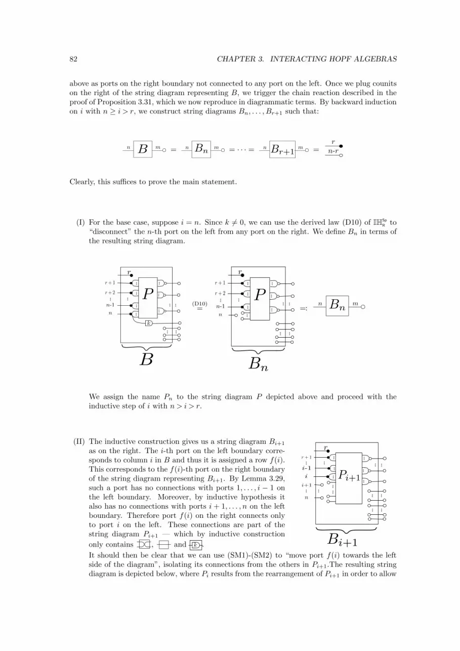
82 CHAPTER 3. INTERACTING HOPF ALGEBRAS
above as ports on the right boundary not connected to any port on the left. Once we plug counitson the right of the string diagram representing B, we trigger the chain reaction described in theproof of Proposition 3.31, which we now reproduce in diagrammatic terms. By backward inductionon i with n ≥ i > r, we construct string diagrams Bn, . . . , Br+1 such that:
n mB = n mBn = · · · = n mBr+1 =r
n-r
Clearly, this suffices to prove the main statement.
(I) For the base case, suppose i = n. Since k 6= 0, we can use the derived law (D10) of IHSp
R to“disconnect” the n-th port on the left from any port on the right. We define Bn in terms ofthe resulting string diagram.
r
Pn
r + 2
r + 1
n-1
B
k
(D10)=
r
Pn
r + 2
r + 1
Bn
n-1 =:n mBn
We assign the name Pn to the string diagram P depicted above and proceed with theinductive step of i with n > i > r.
(II) The inductive construction gives us a string diagram Bi+1
as on the right. The i-th port on the left boundary corre-sponds to column i in B and thus it is assigned a row f(i).This corresponds to the f(i)-th port on the right boundaryof the string diagram representing Bi+1. By Lemma 3.29,such a port has no connections with ports 1, . . . , i − 1 onthe left boundary. Moreover, by inductive hypothesis italso has no connections with ports i + 1, . . . , n on the leftboundary. Therefore port f(i) on the right connects onlyto port i on the left. These connections are part of thestring diagram Pi+1 — which by inductive construction
only contains , and k .
r
n
r + 1
Pi+1
Bi+1
i+1
i
i-1
It should then be clear that we can use (SM1)-(SM2) to “move port f(i) towards the leftside of the diagram”, isolating its connections from the others in Pi+1.The resulting stringdiagram is depicted below, where Pi results from the rearrangement of Pi+1 in order to allow
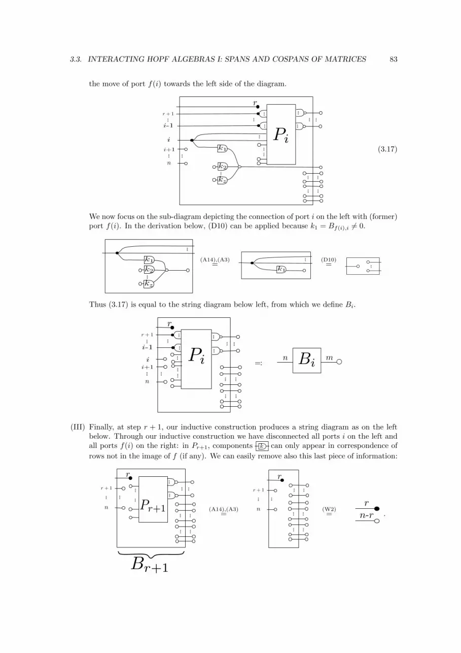
3.3. INTERACTING HOPF ALGEBRAS I: SPANS AND COSPANS OF MATRICES 83
the move of port f(i) towards the left side of the diagram.
r
n
r + 1
i+1
i
i-1
k1
k2
kz
Pi(3.17)
We now focus on the sub-diagram depicting the connection of port i on the left with (former)port f(i). In the derivation below, (D10) can be applied because k1 = Bf(i),i 6= 0.
k1
k2
kz
(A14),(A3)=
k1
(D10)=
Thus (3.17) is equal to the string diagram below left, from which we define Bi.
r
n
r + 1
i+1
i-1
i Pi =:n mBi
(III) Finally, at step r + 1, our inductive construction produces a string diagram as on the leftbelow. Through our inductive construction we have disconnected all ports i on the left andall ports f(i) on the right: in Pr+1, components k can only appear in correspondence of
rows not in the image of f (if any). We can easily remove also this last piece of information:
r
n
r + 1
Br+1
Pr+1 (A14),(A3)=
r
n
r + 1
(W2)=
rn-r .
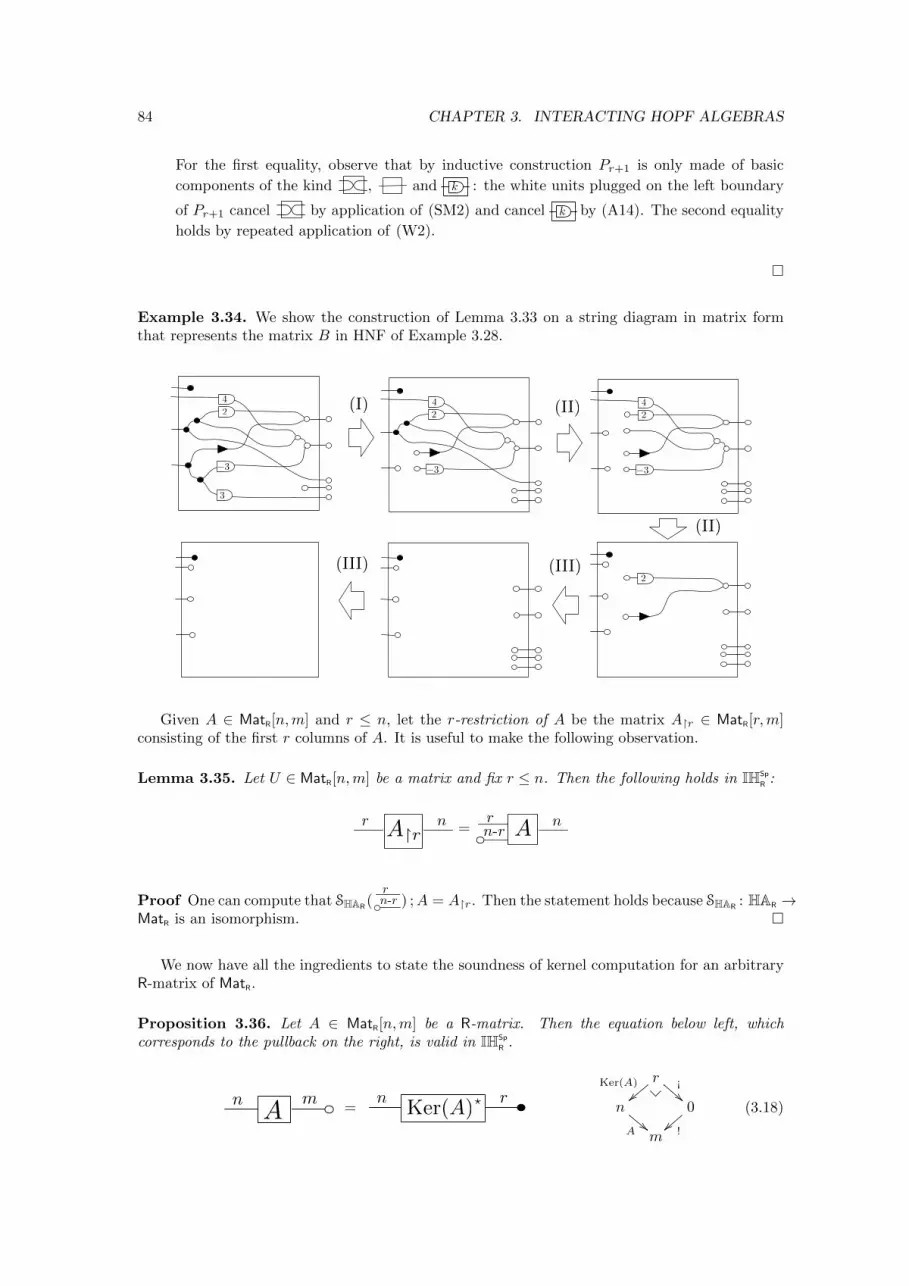
84 CHAPTER 3. INTERACTING HOPF ALGEBRAS
For the first equality, observe that by inductive construction Pr+1 is only made of basic
components of the kind , and k : the white units plugged on the left boundary
of Pr+1 cancel by application of (SM2) and cancel k by (A14). The second equality
holds by repeated application of (W2).
�
Example 3.34. We show the construction of Lemma 3.33 on a string diagram in matrix formthat represents the matrix B in HNF of Example 3.28.
4
3
2
�3
4
2
�3
4
2
�3
2
(I) (II)
(III)
(II)
(III)
Given A ∈ MatR[n,m] and r ≤ n, let the r-restriction of A be the matrix A�r ∈ MatR[r,m]consisting of the first r columns of A. It is useful to make the following observation.
Lemma 3.35. Let U ∈ MatR[n,m] be a matrix and fix r ≤ n. Then the following holds in IHSp
R :
nr A�r = nrn-r A
Proof One can compute that SHAR(
rn-r ) ;A = A�r. Then the statement holds because SHAR
: HAR →MatR is an isomorphism. �
We now have all the ingredients to state the soundness of kernel computation for an arbitraryR-matrix of MatR.
Proposition 3.36. Let A ∈ MatR[n,m] be a R-matrix. Then the equation below left, whichcorresponds to the pullback on the right, is valid in IHSp
R .
n mA =
?n rKer(A)
rKer(A)
||¡
!!n
A ""0
!}}m
(3.18)
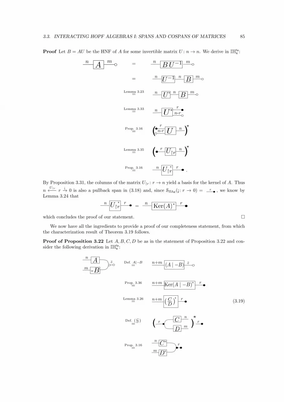
3.3. INTERACTING HOPF ALGEBRAS I: SPANS AND COSPANS OF MATRICES 85
Proof Let B = AU be the HNF of A for some invertible matrix U : n→ n. We derive in IHSp
R :
n mA = n
U�1 mB
= n nU�1 m
B
Lemma 3.23= n n m
BU?
Lemma 3.33=
r
n-rn U ?
Prop. 3.16= n-r
(?(r
U n
Lemma 3.35=
(?( r nU�r
Prop. 3.16=
n U�rr?
.
By Proposition 3.31, the columns of the matrix U�r : r → n yield a basis for the kernel of A. Thus
nU�r←−− r
¡−→ 0 is also a pullback span in (3.18) and, since SHAR(¡ : r → 0) = r , we know by
Lemma 3.24 that
n U�rr?
= ?n rKer(A)
which concludes the proof of our statement. �
We now have all the ingredients to provide a proof of our completeness statement, from whichthe characterization result of Theorem 3.19 follows.
Proof of Proposition 3.22 Let A,B,C,D be as in the statement of Proposition 3.22 and con-sider the following derivation in IHSp
R :
A z
-B
n
m
Def. A|−B= (A | �B) zn+m
Prop. 3.36=
n+m Ker(A | �B)? r
Lemma 3.26= n+m ? r( C
D ) (3.19)
Def.(CD
)=
n
m
C
D
(?( r r
Prop. 3.16=
n
mD
C?
?r
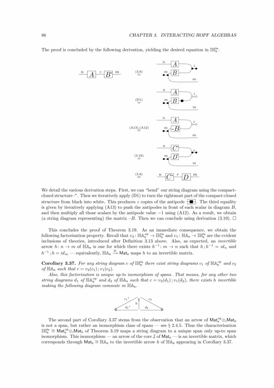
86 CHAPTER 3. INTERACTING HOPF ALGEBRAS
The proof is concluded by the following derivation, yielding the desired equation in IHSp
R .
n mzA B? (3.8)
=
n
m
A
Bm
z
(D1)=
n
m
A
Bm
z
(A13),(A12)=
n
m
A
m
z
-B
(3.19)=
n
m
m
D
C?
?
r
(3.8)=
n mC D? r
We detail the various derivation steps. First, we can “bend” our string diagram using the compact-closed structure ·?. Then we iteratively apply (D1) to turn the rightmost part of the compact-closed
structure from black into white. This produces z copies of the antipode . The third equalityis given by iteratively applying (A13) to push the antipodes in front of each scalar in diagram B,and then multiply all those scalars by the antipode value −1 using (A12). As a result, we obtain(a string diagram representing) the matrix −B. Then we can conclude using derivation (3.19). �
This concludes the proof of Theorem 3.19. As an immediate consequence, we obtain thefollowing factorisation property. Recall that υ2 : HAop
R → IHSp
R and υ1 : HAR → IHSp
R are the evidentinclusions of theories, introduced after Definition 3.13 above. Also, as expected, an invertiblearrow h : n → m of HAR is one for which there exists h−1 : m → n such that h ;h−1 = idn and
h−1 ;h = idm — equivalently, HAR
∼=−→ MatR maps h to an invertible matrix.
Corollary 3.37. For any string diagram c of IHSp
R there exist string diagrams c1 of HAopR and c2
of HAR such that c = υ2(c1) ; υ1(c2).Also, this factorisation is unique up-to isomorphism of spans. That means, for any other two
string diagrams d1 of HAopR and d2 of HAR such that c = υ2(d1) ; υ1(d2), there exists h invertible
making the following diagram commute in HAR.
c1?
xx
c2
&&d1?
ooh
OO
d2 //
The second part of Corollary 3.37 stems from the observation that an arrow of MatopR ⊗JMatRis not a span, but rather an isomorphism class of spans — see § 2.4.5. Thus the characterisationIHSp
R∼= MatopR ⊗JMatR of Theorem 3.19 maps a string diagram to a unique span only up-to span
isomorphism. This isomorphism — an arrow of the core J of MatR — is an invertible matrix, whichcorresponds through MatR ∼= HAR to the invertible arrow h of HAR appearing in Corollary 3.37.
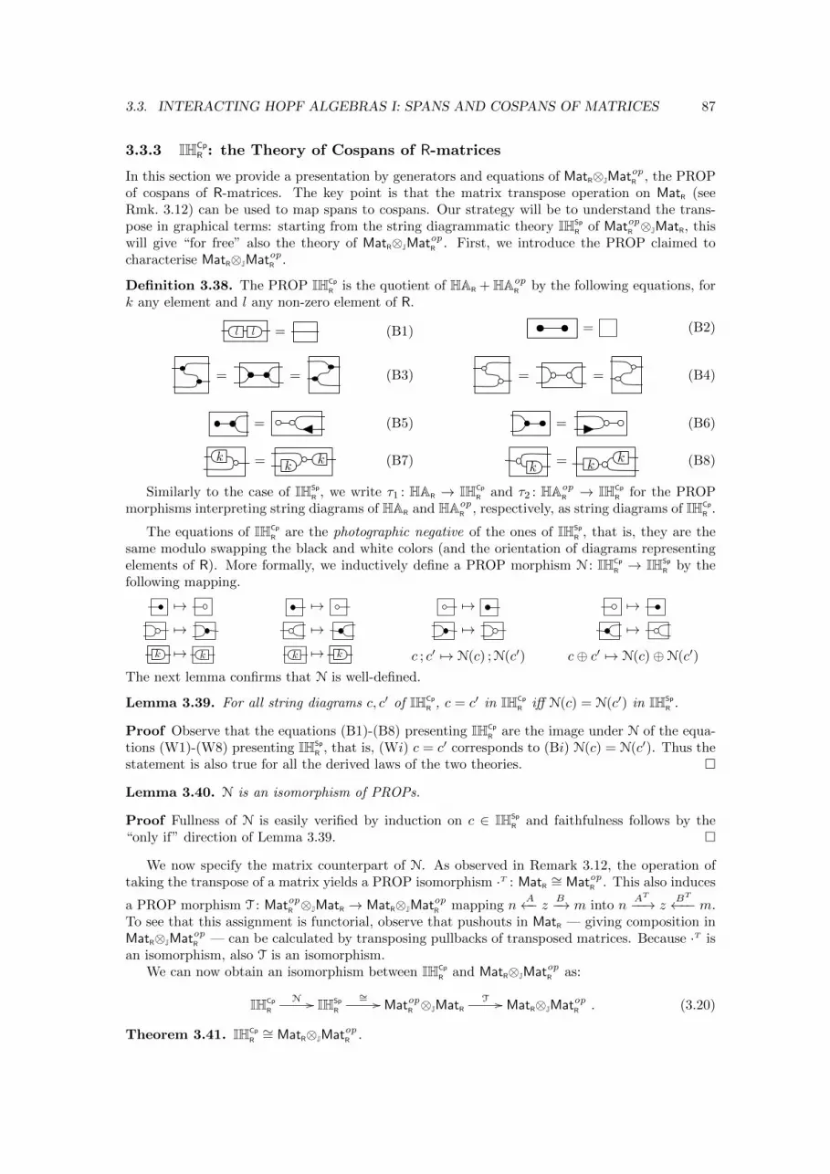
3.3. INTERACTING HOPF ALGEBRAS I: SPANS AND COSPANS OF MATRICES 87
3.3.3 IHCpR : the Theory of Cospans of R-matrices
In this section we provide a presentation by generators and equations of MatR⊗JMatopR , the PROPof cospans of R-matrices. The key point is that the matrix transpose operation on MatR (seeRmk. 3.12) can be used to map spans to cospans. Our strategy will be to understand the trans-pose in graphical terms: starting from the string diagrammatic theory IHSp
R of MatopR ⊗JMatR, thiswill give “for free” also the theory of MatR⊗JMatopR . First, we introduce the PROP claimed tocharacterise MatR⊗JMatopR .
Definition 3.38. The PROP IHCp
R is the quotient of HAR + HAopR by the following equations, for
k any element and l any non-zero element of R.
ll = (B1) = (B2)
= = (B3) = = (B4)
= (B5) = (B6)
k = kk (B7) k = k
k (B8)
Similarly to the case of IHSp
R , we write τ1 : HAR → IHCp
R and τ2 : HAopR → IHCp
R for the PROPmorphisms interpreting string diagrams of HAR and HAop
R , respectively, as string diagrams of IHCp
R .
The equations of IHCp
R are the photographic negative of the ones of IHSp
R , that is, they are thesame modulo swapping the black and white colors (and the orientation of diagrams representingelements of R). More formally, we inductively define a PROP morphism N : IHCp
R → IHSp
R by thefollowing mapping.
7→ 7→ 7→ 7→7→ 7→ 7→ 7→
k 7→ k k 7→ k c ; c′ 7→ N(c) ;N(c′) c⊕ c′ 7→ N(c)⊕N(c′)
The next lemma confirms that N is well-defined.
Lemma 3.39. For all string diagrams c, c′ of IHCp
R , c = c′ in IHCp
R iff N(c) = N(c′) in IHSp
R .
Proof Observe that the equations (B1)-(B8) presenting IHCp
R are the image under N of the equa-tions (W1)-(W8) presenting IHSp
R , that is, (Wi) c = c′ corresponds to (Bi) N(c) = N(c′). Thus thestatement is also true for all the derived laws of the two theories. �
Lemma 3.40. N is an isomorphism of PROPs.
Proof Fullness of N is easily verified by induction on c ∈ IHSp
R and faithfulness follows by the“only if” direction of Lemma 3.39. �
We now specify the matrix counterpart of N. As observed in Remark 3.12, the operation oftaking the transpose of a matrix yields a PROP isomorphism ·T : MatR ∼= MatopR . This also induces
a PROP morphism T : MatopR ⊗JMatR → MatR⊗JMatopR mapping nA←− z B−→ m into n
AT−−→ zBT←−− m.
To see that this assignment is functorial, observe that pushouts in MatR — giving composition inMatR⊗JMatopR — can be calculated by transposing pullbacks of transposed matrices. Because ·T isan isomorphism, also T is an isomorphism.
We can now obtain an isomorphism between IHCp
R and MatR⊗JMatopR as:
IHCp
R
N // IHSp
R
∼= // MatopR ⊗JMatRT // MatR⊗JMatopR . (3.20)
Theorem 3.41. IHCp
R∼= MatR⊗JMatopR .
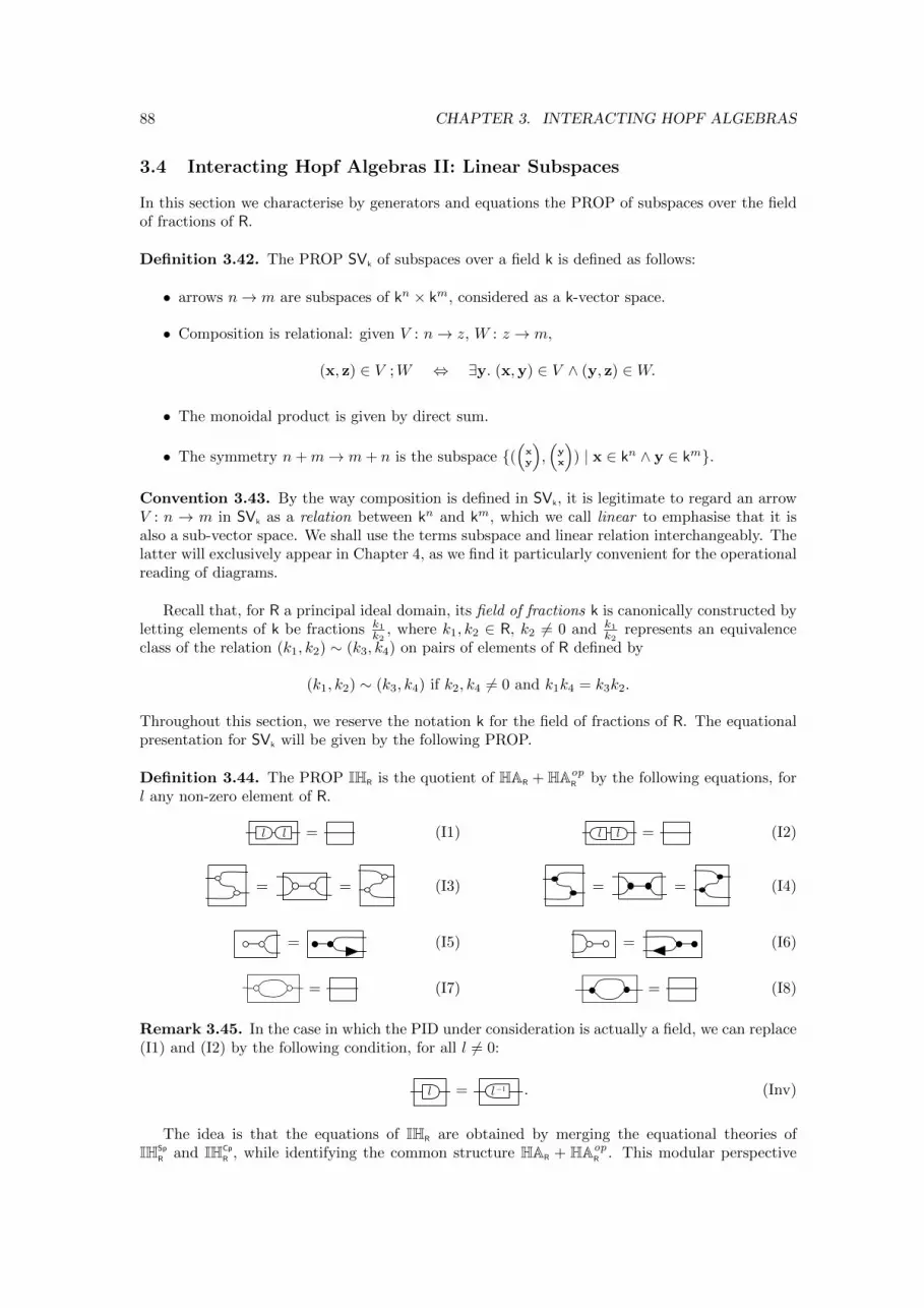
88 CHAPTER 3. INTERACTING HOPF ALGEBRAS
3.4 Interacting Hopf Algebras II: Linear Subspaces
In this section we characterise by generators and equations the PROP of subspaces over the fieldof fractions of R.
Definition 3.42. The PROP SVk of subspaces over a field k is defined as follows:
• arrows n→ m are subspaces of kn × km, considered as a k-vector space.
• Composition is relational: given V : n→ z, W : z → m,
(x, z) ∈ V ;W ⇔ ∃y. (x,y) ∈ V ∧ (y, z) ∈W.
• The monoidal product is given by direct sum.
• The symmetry n+m→ m+ n is the subspace {((
xy
),(yx
)) | x ∈ kn ∧ y ∈ km}.
Convention 3.43. By the way composition is defined in SVk, it is legitimate to regard an arrowV : n → m in SVk as a relation between kn and km, which we call linear to emphasise that it isalso a sub-vector space. We shall use the terms subspace and linear relation interchangeably. Thelatter will exclusively appear in Chapter 4, as we find it particularly convenient for the operationalreading of diagrams.
Recall that, for R a principal ideal domain, its field of fractions k is canonically constructed byletting elements of k be fractions k1
k2, where k1, k2 ∈ R, k2 6= 0 and k1
k2represents an equivalence
class of the relation (k1, k2) ∼ (k3, k4) on pairs of elements of R defined by
(k1, k2) ∼ (k3, k4) if k2, k4 6= 0 and k1k4 = k3k2.
Throughout this section, we reserve the notation k for the field of fractions of R. The equationalpresentation for SVk will be given by the following PROP.
Definition 3.44. The PROP IHR is the quotient of HAR + HAopR by the following equations, for
l any non-zero element of R.
ll = (I1) ll = (I2)
= = (I3) = = (I4)
= (I5) = (I6)
= (I7) = (I8)
Remark 3.45. In the case in which the PID under consideration is actually a field, we can replace(I1) and (I2) by the following condition, for all l 6= 0:
l = l�1 . (Inv)
The idea is that the equations of IHR are obtained by merging the equational theories ofIHSp
R and IHCp
R , while identifying the common structure HAR + HAopR . This modular perspective
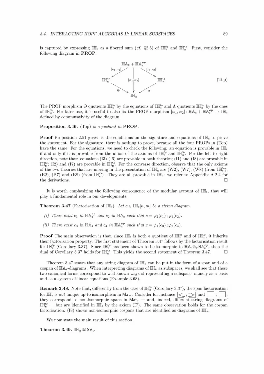
3.4. INTERACTING HOPF ALGEBRAS II: LINEAR SUBSPACES 89
is captured by expressing IHR as a fibered sum (cf. §2.5) of IHSp
R and IHCp
R . First, consider thefollowing diagram in PROP.
HAR + HAopR
[υ1,υ2]
xx[ϕ1,ϕ2]
��
[τ1,τ2]
&&IHSp
R
Θ &&
IHCp
R
ΛxxIHR
(Top)
The PROP morphism Θ quotients IHSp
R by the equations of IHCp
R and Λ quotients IHCp
R by the onesof IHSp
R . For later use, it is useful to also fix the PROP morphism [ϕ1, ϕ2] : HAR + HAopR → IHR
defined by commutativity of the diagram.
Proposition 3.46. (Top) is a pushout in PROP.
Proof Proposition 2.51 gives us the conditions on the signature and equations of IHR to provethe statement. For the signature, there is nothing to prove, because all the four PROPs in (Top)have the same. For the equations, we need to check the following: an equation is provable in IHR
if and only if it is provable from the union of the axioms of IHCp
R and IHSp
R . For the left to rightdirection, note that: equations (I3)-(I6) are provable in both theories; (I1) and (I8) are provable inIHSp
R ; (I2) and (I7) are provable in IHCp
R . For the converse direction, observe that the only axiomsof the two theories that are missing in the presentation of IHR are (W2), (W7), (W8) (from IHSp
R ),(B2), (B7) and (B8) (from IHCp
R ). They are all provable in IHR: we refer to Appendix A.2.4 forthe derivations. �
It is worth emphasizing the following consequence of the modular account of IHR, that willplay a fundamental role in our developments.
Theorem 3.47 (Factorisation of IHR). Let c ∈ IHR[n,m] be a string diagram.
(i) There exist c1 in HAopR and c2 in HAR such that c = ϕ2(c1) ;ϕ1(c2).
(ii) There exist c3 in HAR and c4 in HAopR such that c = ϕ1(c3) ;ϕ2(c4).
Proof The main observation is that, since IHR is both a quotient of IHSp
R and of IHCp
R , it inheritstheir factorisation property. The first statement of Theorem 3.47 follows by the factorisation resultfor IHSp
R (Corollary 3.37). Since IHCp
R has been shown to be isomorphic to HAR⊗PHAopR , then the
dual of Corollary 3.37 holds for IHCp
R . This yields the second statement of Theorem 3.47. �
Theorem 3.47 states that any string diagram of IHR can be put in the form of a span and of acospan of HAR-diagrams. When interpreting diagrams of IHR as subspaces, we shall see that thesetwo canonical forms correspond to well-known ways of representing a subspace, namely as a basisand as a system of linear equations (Example 3.68).
Remark 3.48. Note that, differently from the case of IHSp
R (Corollary 3.37), the span factorisation
for IHR is not unique up-to isomorphism in MatR. Consider for instance ; and ; :they correspond to non-isomorphic spans in MatR — and, indeed, different string diagrams ofIHSp
R — but are identified in IHR by the axiom (I7). The same observation holds for the cospanfactorisation: (I8) shows non-isomorphic cospans that are identified as diagrams of IHR.
We now state the main result of this section.
Theorem 3.49. IHR∼= SVk.
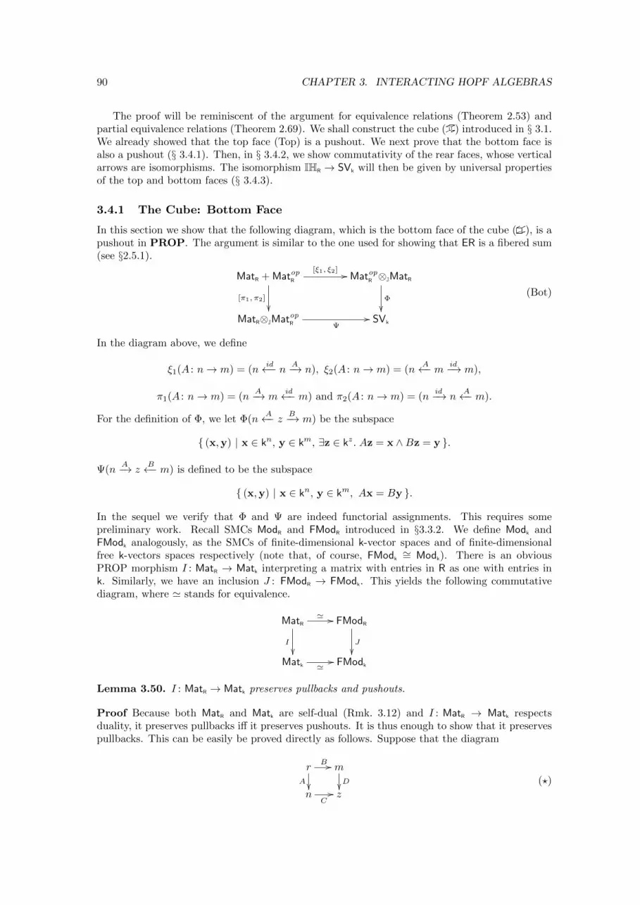
90 CHAPTER 3. INTERACTING HOPF ALGEBRAS
The proof will be reminiscent of the argument for equivalence relations (Theorem 2.53) andpartial equivalence relations (Theorem 2.69). We shall construct the cube (�) introduced in § 3.1.We already showed that the top face (Top) is a pushout. We next prove that the bottom face isalso a pushout (§ 3.4.1). Then, in § 3.4.2, we show commutativity of the rear faces, whose verticalarrows are isomorphisms. The isomorphism IHR → SVk will then be given by universal propertiesof the top and bottom faces (§ 3.4.3).
3.4.1 The Cube: Bottom Face
In this section we show that the following diagram, which is the bottom face of the cube (�), is apushout in PROP. The argument is similar to the one used for showing that ER is a fibered sum(see §2.5.1).
MatR + MatopR
[ξ1, ξ2] //
[π1, π2]
��
MatopR ⊗JMatR
Φ
��MatR⊗JMatopR Ψ
// SVk
(Bot)
In the diagram above, we define
ξ1(A : n→ m) = (nid←− n A−→ n), ξ2(A : n→ m) = (n
A←− m id−→ m),
π1(A : n→ m) = (nA−→ m
id←− m) and π2(A : n→ m) = (nid−→ n
A←− m).
For the definition of Φ, we let Φ(nA←− z B−→ m) be the subspace
{ (x,y) | x ∈ kn, y ∈ km, ∃z ∈ kz. Az = x ∧Bz = y }.
Ψ(nA−→ z
B←− m) is defined to be the subspace
{ (x,y) | x ∈ kn, y ∈ km, Ax = By }.
In the sequel we verify that Φ and Ψ are indeed functorial assignments. This requires somepreliminary work. Recall SMCs ModR and FModR introduced in §3.3.2. We define Modk andFModk analogously, as the SMCs of finite-dimensional k-vector spaces and of finite-dimensionalfree k-vectors spaces respectively (note that, of course, FModk
∼= Modk). There is an obviousPROP morphism I : MatR → Matk interpreting a matrix with entries in R as one with entries ink. Similarly, we have an inclusion J : FModR → FModk. This yields the following commutativediagram, where ' stands for equivalence.
MatR
I
��
' // FModR
J
��Matk '
// FModk
Lemma 3.50. I : MatR → Matk preserves pullbacks and pushouts.
Proof Because both MatR and Matk are self-dual (Rmk. 3.12) and I : MatR → Matk respectsduality, it preserves pullbacks iff it preserves pushouts. It is thus enough to show that it preservespullbacks. This can be easily be proved directly as follows. Suppose that the diagram
r
A��
B // mD��
nC// z
(?)
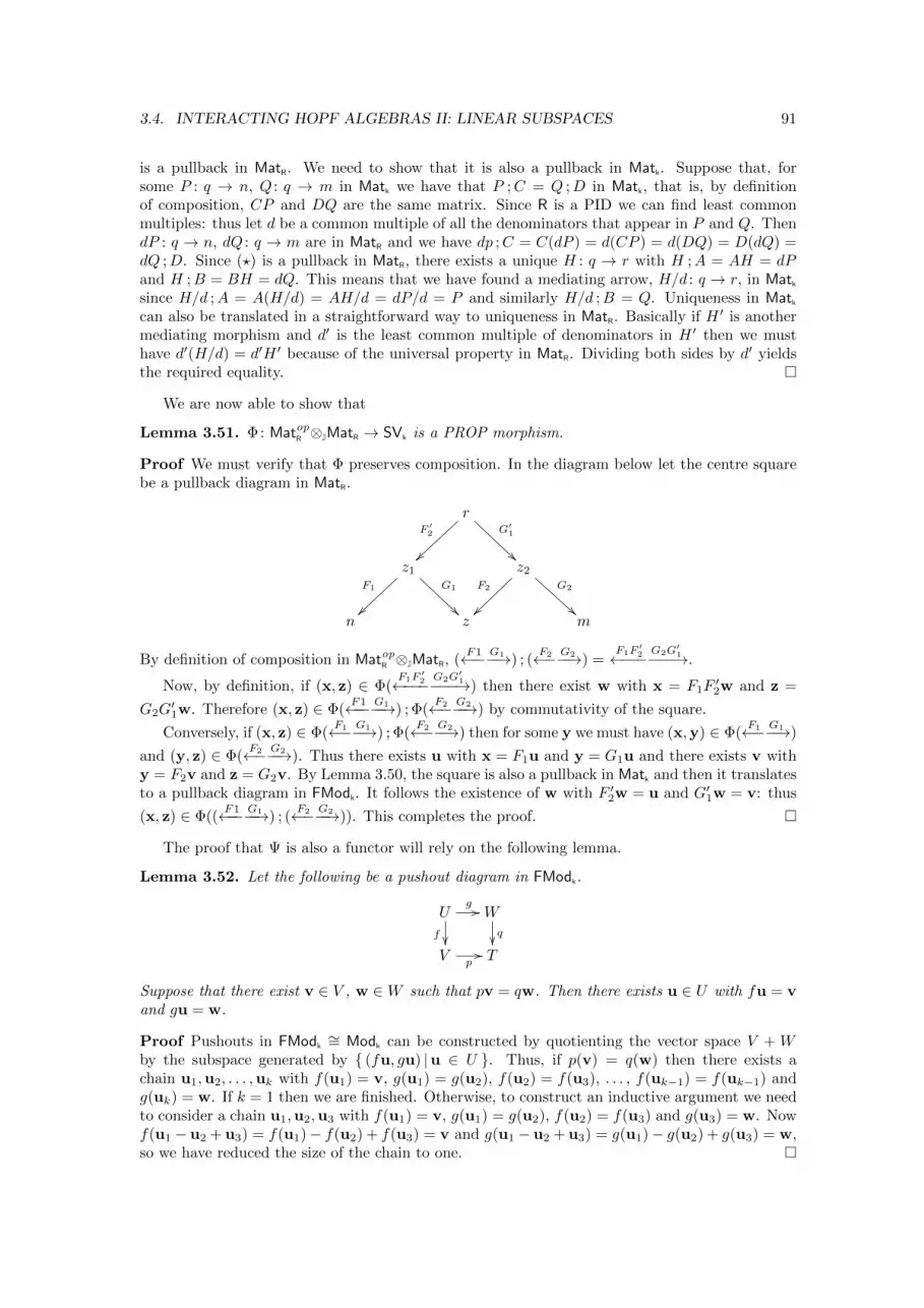
3.4. INTERACTING HOPF ALGEBRAS II: LINEAR SUBSPACES 91
is a pullback in MatR. We need to show that it is also a pullback in Matk. Suppose that, forsome P : q → n, Q : q → m in Matk we have that P ;C = Q ;D in Matk, that is, by definitionof composition, CP and DQ are the same matrix. Since R is a PID we can find least commonmultiples: thus let d be a common multiple of all the denominators that appear in P and Q. ThendP : q → n, dQ : q → m are in MatR and we have dp ;C = C(dP ) = d(CP ) = d(DQ) = D(dQ) =dQ ;D. Since (?) is a pullback in MatR, there exists a unique H : q → r with H ;A = AH = dPand H ;B = BH = dQ. This means that we have found a mediating arrow, H/d : q → r, in Matksince H/d ;A = A(H/d) = AH/d = dP/d = P and similarly H/d ;B = Q. Uniqueness in Matkcan also be translated in a straightforward way to uniqueness in MatR. Basically if H ′ is anothermediating morphism and d′ is the least common multiple of denominators in H ′ then we musthave d′(H/d) = d′H ′ because of the universal property in MatR. Dividing both sides by d′ yieldsthe required equality. �
We are now able to show that
Lemma 3.51. Φ: MatopR ⊗JMatR → SVk is a PROP morphism.
Proof We must verify that Φ preserves composition. In the diagram below let the centre squarebe a pullback diagram in MatR.
rF ′2
~~
G′1
z1
F1
~~
G1
z2
F2
~~
G2
!!n z m
By definition of composition in MatopR ⊗JMatR, (F1←−− G1−−→) ; (
F2←− G2−−→) =F1F
′2←−−− G2G
′1−−−→.
Now, by definition, if (x, z) ∈ Φ(F1F
′2←−−− G2G
′1−−−→) then there exist w with x = F1F
′2w and z =
G2G′1w. Therefore (x, z) ∈ Φ(
F1←−− G1−−→) ; Φ(F2←− G2−−→) by commutativity of the square.
Conversely, if (x, z) ∈ Φ(F1←− G1−−→) ; Φ(
F2←− G2−−→) then for some y we must have (x,y) ∈ Φ(F1←− G1−−→)
and (y, z) ∈ Φ(F2←− G2−−→). Thus there exists u with x = F1u and y = G1u and there exists v with
y = F2v and z = G2v. By Lemma 3.50, the square is also a pullback in Matk and then it translatesto a pullback diagram in FModk. It follows the existence of w with F ′2w = u and G′1w = v: thus
(x, z) ∈ Φ((F1←−− G1−−→) ; (
F2←− G2−−→)). This completes the proof. �
The proof that Ψ is also a functor will rely on the following lemma.
Lemma 3.52. Let the following be a pushout diagram in FModk.
U
f ��
g // Wq��
Vp// T
Suppose that there exist v ∈ V , w ∈W such that pv = qw. Then there exists u ∈ U with fu = vand gu = w.
Proof Pushouts in FModk∼= Modk can be constructed by quotienting the vector space V + W
by the subspace generated by { (fu, gu) |u ∈ U }. Thus, if p(v) = q(w) then there exists achain u1,u2, . . . ,uk with f(u1) = v, g(u1) = g(u2), f(u2) = f(u3), . . . , f(uk−1) = f(uk−1) andg(uk) = w. If k = 1 then we are finished. Otherwise, to construct an inductive argument we needto consider a chain u1,u2,u3 with f(u1) = v, g(u1) = g(u2), f(u2) = f(u3) and g(u3) = w. Nowf(u1 − u2 + u3) = f(u1)− f(u2) + f(u3) = v and g(u1 − u2 + u3) = g(u1)− g(u2) + g(u3) = w,so we have reduced the size of the chain to one. �
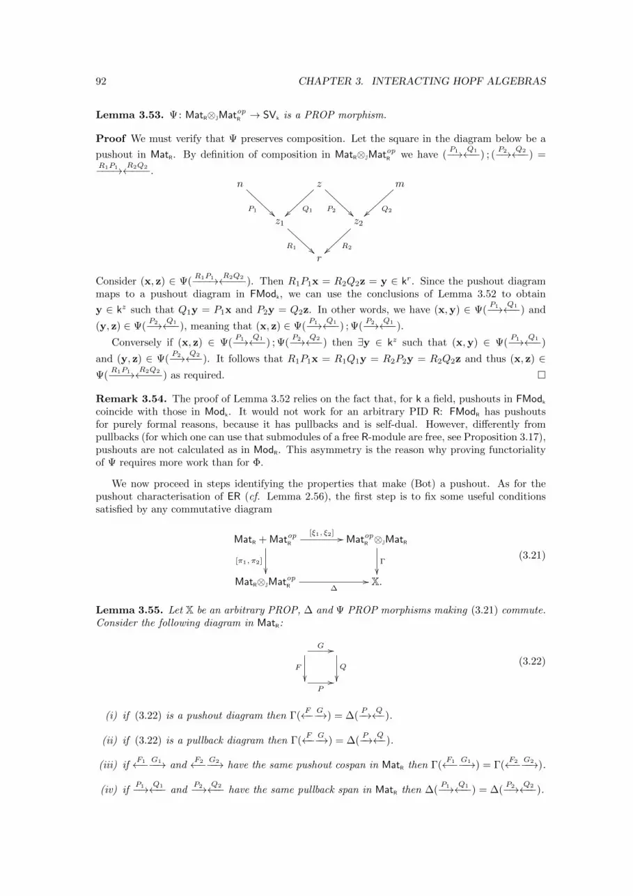
92 CHAPTER 3. INTERACTING HOPF ALGEBRAS
Lemma 3.53. Ψ: MatR⊗JMatopR → SVk is a PROP morphism.
Proof We must verify that Ψ preserves composition. Let the square in the diagram below be a
pushout in MatR. By definition of composition in MatR⊗JMatopR we have (P1−→ Q1←−−) ; (
P2−→ Q2←−−) =R1P1−−−→ R2Q2←−−−.
n
P1
z
Q1~~ P2
m
Q2}}z1
R1
z2
R2~~r
Consider (x, z) ∈ Ψ(R1P1−−−→ R2Q2←−−−). Then R1P1x = R2Q2z = y ∈ kr. Since the pushout diagram
maps to a pushout diagram in FModk, we can use the conclusions of Lemma 3.52 to obtain
y ∈ kz such that Q1y = P1x and P2y = Q2z. In other words, we have (x,y) ∈ Ψ(P1−→ Q1←−−) and
(y, z) ∈ Ψ(P2−→ Q1←−−), meaning that (x, z) ∈ Ψ(
P1−→ Q1←−−) ; Ψ(P2−→ Q1←−−).
Conversely if (x, z) ∈ Ψ(P1−→ Q1←−−) ; Ψ(
P2−→ Q2←−−) then ∃y ∈ kz such that (x,y) ∈ Ψ(P1−→ Q1←−−)
and (y, z) ∈ Ψ(P2−→ Q2←−−). It follows that R1P1x = R1Q1y = R2P2y = R2Q2z and thus (x, z) ∈
Ψ(R1P1−−−→ R2Q2←−−−) as required. �
Remark 3.54. The proof of Lemma 3.52 relies on the fact that, for k a field, pushouts in FModk
coincide with those in Modk. It would not work for an arbitrary PID R: FModR has pushoutsfor purely formal reasons, because it has pullbacks and is self-dual. However, differently frompullbacks (for which one can use that submodules of a free R-module are free, see Proposition 3.17),pushouts are not calculated as in ModR. This asymmetry is the reason why proving functorialityof Ψ requires more work than for Φ.
We now proceed in steps identifying the properties that make (Bot) a pushout. As for thepushout characterisation of ER (cf. Lemma 2.56), the first step is to fix some useful conditionssatisfied by any commutative diagram
MatR + MatopR
[ξ1, ξ2] //
[π1, π2]
��
MatopR ⊗JMatR
Γ
��MatR⊗JMatopR ∆
// X.
(3.21)
Lemma 3.55. Let X be an arbitrary PROP, ∆ and Ψ PROP morphisms making (3.21) commute.Consider the following diagram in MatR:
G //
F
��Q
��P//
(3.22)
(i) if (3.22) is a pushout diagram then Γ(F←− G−→) = ∆(
P−→ Q←−).
(ii) if (3.22) is a pullback diagram then Γ(F←− G−→) = ∆(
P−→ Q←−).
(iii) ifF1←− G1−−→ and
F2←− G2−−→ have the same pushout cospan in MatR then Γ(F1←− G1−−→) = Γ(
F2←− G2−−→).
(iv) ifP1−→ Q1←−− and
P2−→ Q2←−− have the same pullback span in MatR then ∆(P1−→ Q1←−−) = ∆(
P2−→ Q2←−−).
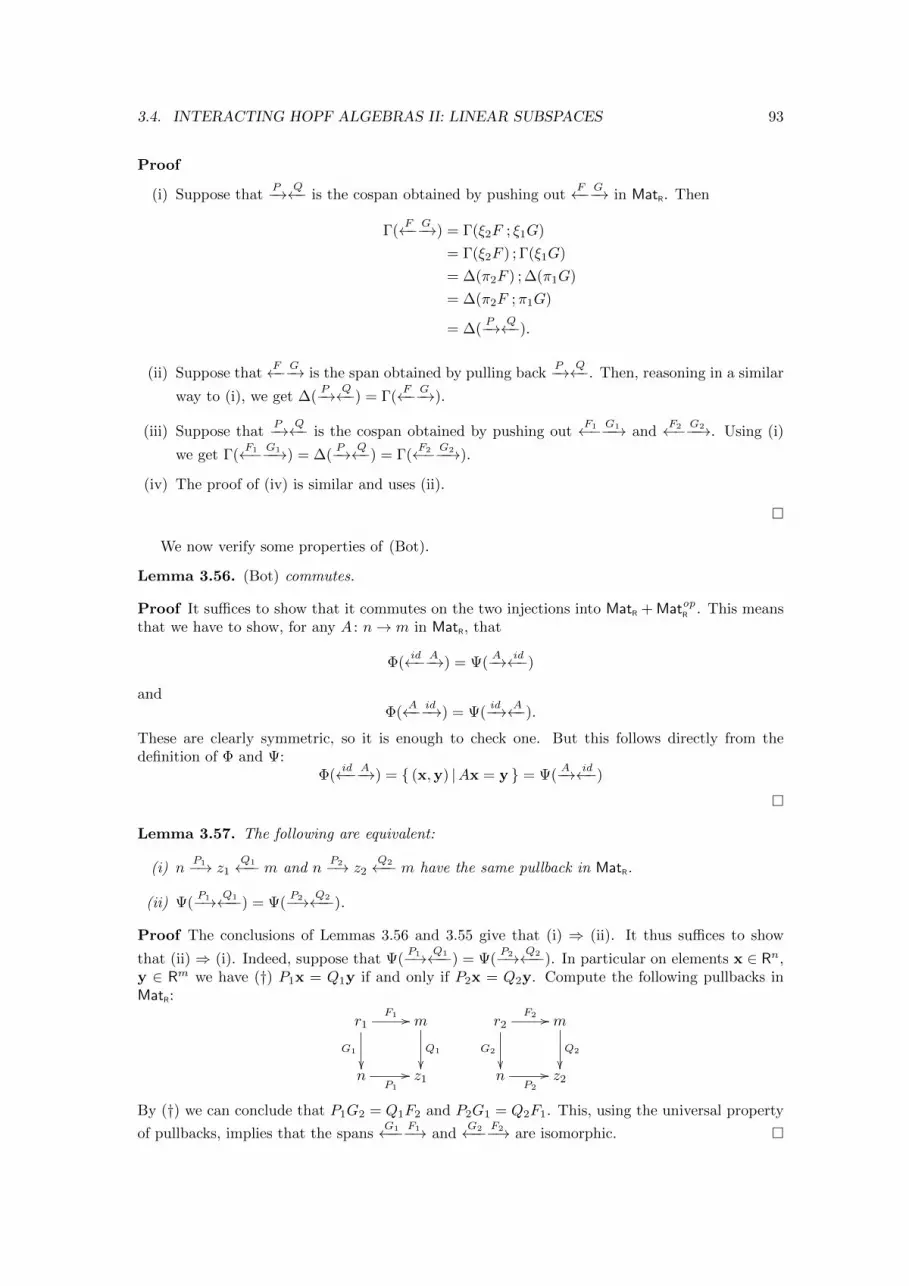
3.4. INTERACTING HOPF ALGEBRAS II: LINEAR SUBSPACES 93
Proof
(i) Suppose thatP−→ Q←− is the cospan obtained by pushing out
F←− G−→ in MatR. Then
Γ(F←− G−→) = Γ(ξ2F ; ξ1G)
= Γ(ξ2F ) ; Γ(ξ1G)
= ∆(π2F ) ; ∆(π1G)
= ∆(π2F ;π1G)
= ∆(P−→ Q←−).
(ii) Suppose thatF←− G−→ is the span obtained by pulling back
P−→ Q←−. Then, reasoning in a similar
way to (i), we get ∆(P−→ Q←−) = Γ(
F←− G−→).
(iii) Suppose thatP−→ Q←− is the cospan obtained by pushing out
F1←− G1−−→ andF2←− G2−−→. Using (i)
we get Γ(F1←− G1−−→) = ∆(
P−→ Q←−) = Γ(F2←− G2−−→).
(iv) The proof of (iv) is similar and uses (ii).
�
We now verify some properties of (Bot).
Lemma 3.56. (Bot) commutes.
Proof It suffices to show that it commutes on the two injections into MatR + MatopR . This meansthat we have to show, for any A : n→ m in MatR, that
Φ(id←− A−→) = Ψ(
A−→ id←−)
andΦ(
A←− id−→) = Ψ(id−→ A←−).
These are clearly symmetric, so it is enough to check one. But this follows directly from thedefinition of Φ and Ψ:
Φ(id←− A−→) = { (x,y) |Ax = y } = Ψ(
A−→ id←−)
�
Lemma 3.57. The following are equivalent:
(i) nP1−→ z1
Q1←−− m and nP2−→ z2
Q2←−− m have the same pullback in MatR.
(ii) Ψ(P1−→ Q1←−−) = Ψ(
P2−→ Q2←−−).
Proof The conclusions of Lemmas 3.56 and 3.55 give that (i) ⇒ (ii). It thus suffices to show
that (ii) ⇒ (i). Indeed, suppose that Ψ(P1−→ Q1←−−) = Ψ(
P2−→ Q2←−−). In particular on elements x ∈ Rn,y ∈ Rm we have (†) P1x = Q1y if and only if P2x = Q2y. Compute the following pullbacks inMatR:
r1
G1
��
F1 // m
Q1
��n
P1
// z1
r2
G2
��
F2 // m
Q2
��n
P2
// z2
By (†) we can conclude that P1G2 = Q1F2 and P2G1 = Q2F1. This, using the universal property
of pullbacks, implies that the spansG1←−− F1−→ and
G2←−− F2−→ are isomorphic. �
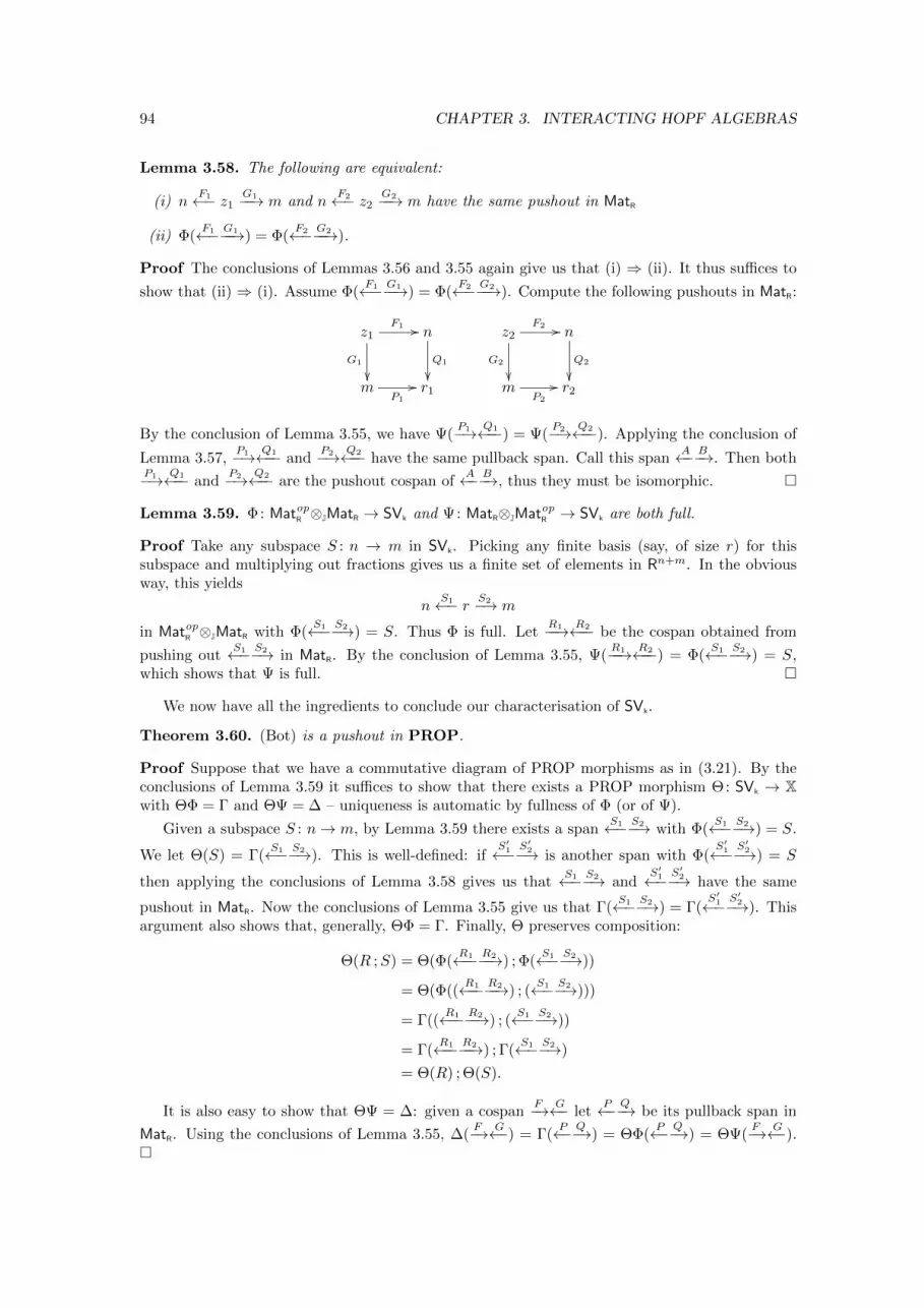
94 CHAPTER 3. INTERACTING HOPF ALGEBRAS
Lemma 3.58. The following are equivalent:
(i) nF1←− z1
G1−−→ m and nF2←− z2
G2−−→ m have the same pushout in MatR
(ii) Φ(F1←− G1−−→) = Φ(
F2←− G2−−→).
Proof The conclusions of Lemmas 3.56 and 3.55 again give us that (i) ⇒ (ii). It thus suffices to
show that (ii) ⇒ (i). Assume Φ(F1←− G1−−→) = Φ(
F2←− G2−−→). Compute the following pushouts in MatR:
z1
G1
��
F1 // n
Q1
��m
P1
// r1
z2
G2
��
F2 // n
Q2
��m
P2
// r2
By the conclusion of Lemma 3.55, we have Ψ(P1−→ Q1←−−) = Ψ(
P2−→ Q2←−−). Applying the conclusion of
Lemma 3.57,P1−→ Q1←−− and
P2−→ Q2←−− have the same pullback span. Call this spanA←− B−→. Then both
P1−→ Q1←−− andP2−→ Q2←−− are the pushout cospan of
A←− B−→, thus they must be isomorphic. �
Lemma 3.59. Φ: MatopR ⊗JMatR → SVk and Ψ: MatR⊗JMatopR → SVk are both full.
Proof Take any subspace S : n → m in SVk. Picking any finite basis (say, of size r) for thissubspace and multiplying out fractions gives us a finite set of elements in Rn+m. In the obviousway, this yields
nS1←− r S2−→ m
in MatopR ⊗JMatR with Φ(S1←− S2−→) = S. Thus Φ is full. Let
R1−−→ R2←−− be the cospan obtained from
pushing outS1←− S2−→ in MatR. By the conclusion of Lemma 3.55, Ψ(
R1−−→ R2←−−) = Φ(S1←− S2−→) = S,
which shows that Ψ is full. �
We now have all the ingredients to conclude our characterisation of SVk.
Theorem 3.60. (Bot) is a pushout in PROP.
Proof Suppose that we have a commutative diagram of PROP morphisms as in (3.21). By theconclusions of Lemma 3.59 it suffices to show that there exists a PROP morphism Θ: SVk → Xwith ΘΦ = Γ and ΘΨ = ∆ – uniqueness is automatic by fullness of Φ (or of Ψ).
Given a subspace S : n→ m, by Lemma 3.59 there exists a spanS1←− S2−→ with Φ(
S1←− S2−→) = S.
We let Θ(S) = Γ(S1←− S2−→). This is well-defined: if
S′1←− S′2−→ is another span with Φ(S′1←− S′2−→) = S
then applying the conclusions of Lemma 3.58 gives us thatS1←− S2−→ and
S′1←− S′2−→ have the same
pushout in MatR. Now the conclusions of Lemma 3.55 give us that Γ(S1←− S2−→) = Γ(
S′1←− S′2−→). Thisargument also shows that, generally, ΘΦ = Γ. Finally, Θ preserves composition:
Θ(R ;S) = Θ(Φ(R1←−− R2−−→) ; Φ(
S1←− S2−→))
= Θ(Φ((R1←−− R2−−→) ; (
S1←− S2−→)))
= Γ((R1←−− R2−−→) ; (
S1←− S2−→))
= Γ(R1←−− R2−−→) ; Γ(
S1←− S2−→)
= Θ(R) ; Θ(S).
It is also easy to show that ΘΨ = ∆: given a cospanF−→ G←− let
P←− Q−→ be its pullback span in
MatR. Using the conclusions of Lemma 3.55, ∆(F−→ G←−) = Γ(
P←− Q−→) = ΘΦ(P←− Q−→) = ΘΨ(
F−→ G←−).�
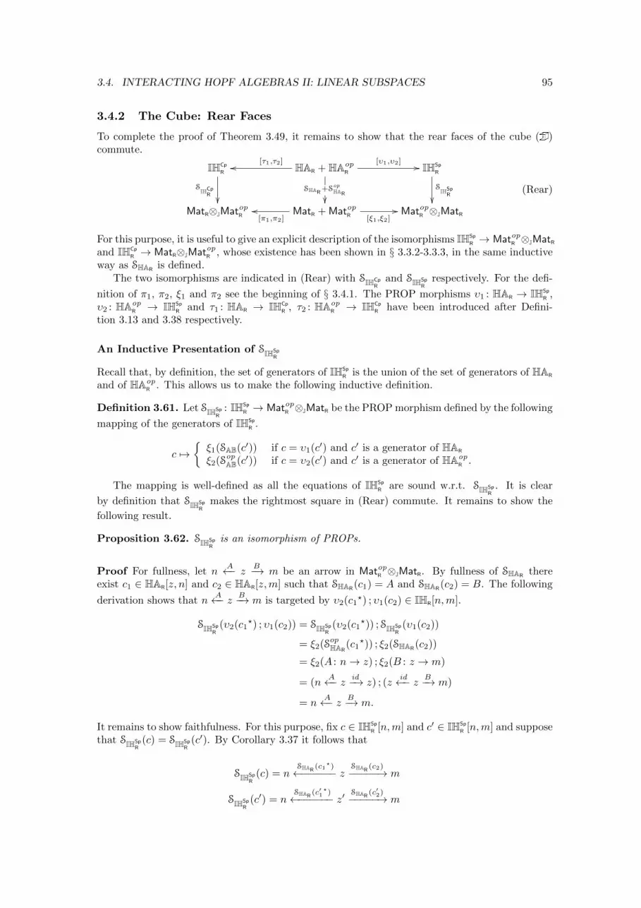
3.4. INTERACTING HOPF ALGEBRAS II: LINEAR SUBSPACES 95
3.4.2 The Cube: Rear Faces
To complete the proof of Theorem 3.49, it remains to show that the rear faces of the cube (�)commute.
IHCp
R
SIHCp
R
��
HAR + HAopR
[τ1,τ2]oo
SHAR+SopHAR��
[υ1,υ2] // IHSp
R
SIHSp
R
��MatR⊗JMatopR MatR + MatopR [ξ1,ξ2]
//[π1,π2]oo MatopR ⊗JMatR
(Rear)
For this purpose, it is useful to give an explicit description of the isomorphisms IHSp
R → MatopR ⊗JMatRand IHCp
R → MatR⊗JMatopR , whose existence has been shown in § 3.3.2-3.3.3, in the same inductiveway as SHAR
is defined.The two isomorphisms are indicated in (Rear) with SIHCp
Rand SIHSp
Rrespectively. For the defi-
nition of π1, π2, ξ1 and π2 see the beginning of § 3.4.1. The PROP morphisms υ1 : HAR → IHSp
R ,υ2 : HAop
R → IHSp
R and τ1 : HAR → IHCp
R , τ2 : HAopR → IHCp
R have been introduced after Defini-tion 3.13 and 3.38 respectively.
An Inductive Presentation of SIHSpR
Recall that, by definition, the set of generators of IHSp
R is the union of the set of generators of HAR
and of HAopR . This allows us to make the following inductive definition.
Definition 3.61. Let SIHSpR
: IHSp
R → MatopR ⊗JMatR be the PROP morphism defined by the following
mapping of the generators of IHSp
R .
c 7→{ξ1(SAB(c′)) if c = υ1(c′) and c′ is a generator of HAR
ξ2(SopAB(c′)) if c = υ2(c′) and c′ is a generator of HAopR .
The mapping is well-defined as all the equations of IHSp
R are sound w.r.t. SIHSpR
. It is clear
by definition that SIHSpR
makes the rightmost square in (Rear) commute. It remains to show the
following result.
Proposition 3.62. SIHSpR
is an isomorphism of PROPs.
Proof For fullness, let nA←− z
B−→ m be an arrow in MatopR ⊗JMatR. By fullness of SHARthere
exist c1 ∈ HAR[z, n] and c2 ∈ HAR[z,m] such that SHAR(c1) = A and SHAR
(c2) = B. The following
derivation shows that nA←− z B−→ m is targeted by υ2(c1
?) ; υ1(c2) ∈ IHR[n,m].
SIHSpR
(υ2(c1?) ; υ1(c2)) = SIHSp
R(υ2(c1
?)) ; SIHSpR
(υ1(c2))
= ξ2(SopHAR(c1
?)) ; ξ2(SHAR(c2))
= ξ2(A : n→ z) ; ξ2(B : z → m)
= (nA←− z id−→ z) ; (z
id←− z B−→ m)
= nA←− z B−→ m.
It remains to show faithfulness. For this purpose, fix c ∈ IHSp
R [n,m] and c′ ∈ IHSp
R [n,m] and supposethat SIHSp
R(c) = SIHSp
R(c′). By Corollary 3.37 it follows that
SIHSpR
(c) = nSHAR (c1
?)←−−−−−− z SHAR (c2)−−−−−→ m
SIHSpR
(c′) = nSHAR (c′1
?)←−−−−−− z′ SHAR (c′2)−−−−−→ m
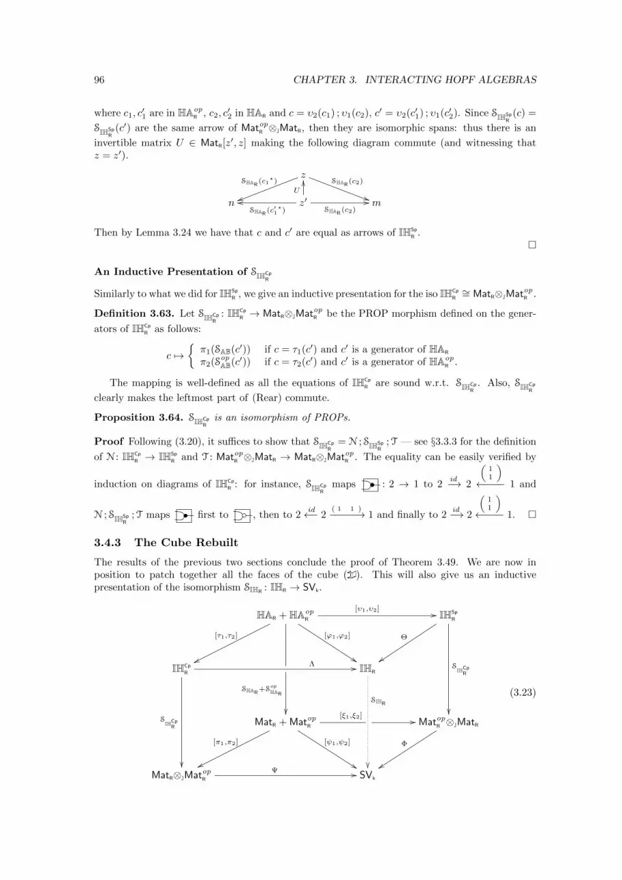
96 CHAPTER 3. INTERACTING HOPF ALGEBRAS
where c1, c′1 are in HAop
R , c2, c′2 in HAR and c = υ2(c1) ; υ1(c2), c′ = υ2(c′1) ; υ1(c′2). Since SIHSp
R(c) =
SIHSpR
(c′) are the same arrow of MatopR ⊗JMatR, then they are isomorphic spans: thus there is an
invertible matrix U ∈ MatR[z′, z] making the following diagram commute (and witnessing that
z = z′).
zSHAR (c2)
))
SHAR (c1?)
uun z′SHAR (c′1
?)
ooU
OO
SHAR (c2)// m
Then by Lemma 3.24 we have that c and c′ are equal as arrows of IHSp
R .�
An Inductive Presentation of SIHCpR
Similarly to what we did for IHSp
R , we give an inductive presentation for the iso IHCp
R∼= MatR⊗JMatopR .
Definition 3.63. Let SIHCpR
: IHCp
R → MatR⊗JMatopR be the PROP morphism defined on the gener-
ators of IHCp
R as follows:
c 7→{π1(SAB(c′)) if c = τ1(c′) and c′ is a generator of HAR
π2(SopAB(c′)) if c = τ2(c′) and c′ is a generator of HAopR .
The mapping is well-defined as all the equations of IHCp
R are sound w.r.t. SIHCpR
. Also, SIHCpR
clearly makes the leftmost part of (Rear) commute.
Proposition 3.64. SIHCpR
is an isomorphism of PROPs.
Proof Following (3.20), it suffices to show that SIHCpR
= N ; SIHSpR
;T — see §3.3.3 for the definition
of N : IHCp
R → IHSp
R and T : MatopR ⊗JMatR → MatR⊗JMatopR . The equality can be easily verified by
induction on diagrams of IHCp
R : for instance, SIHCpR
maps : 2 → 1 to 2id−→ 2
(11
)←−−−− 1 and
N ; SIHSpR
;T maps first to , then to 2id←− 2
( 1 1 )−−−−−→ 1 and finally to 2id−→ 2
(11
)←−−−− 1. �
3.4.3 The Cube Rebuilt
The results of the previous two sections conclude the proof of Theorem 3.49. We are now inposition to patch together all the faces of the cube (�). This will also give us an inductivepresentation of the isomorphism SIHR
: IHR → SVk.
HAR + HAopR
[ϕ1,ϕ2]
%%
SHAR+SopHAR
��
[τ1,τ2]
ww
[υ1,υ2] // IHSp
R
Θ
zzSIHCp
R
��
IHCp
R
Λ //
SIHCp
R
��
IHR
SIHR
��
MatR + MatopR
[ψ1,ψ2]
%%
[π1,π2]
ww
[ξ1,ξ2] // MatopR ⊗JMatR
Φ
yyMatR⊗JMatopR
Ψ // SVk
(3.23)
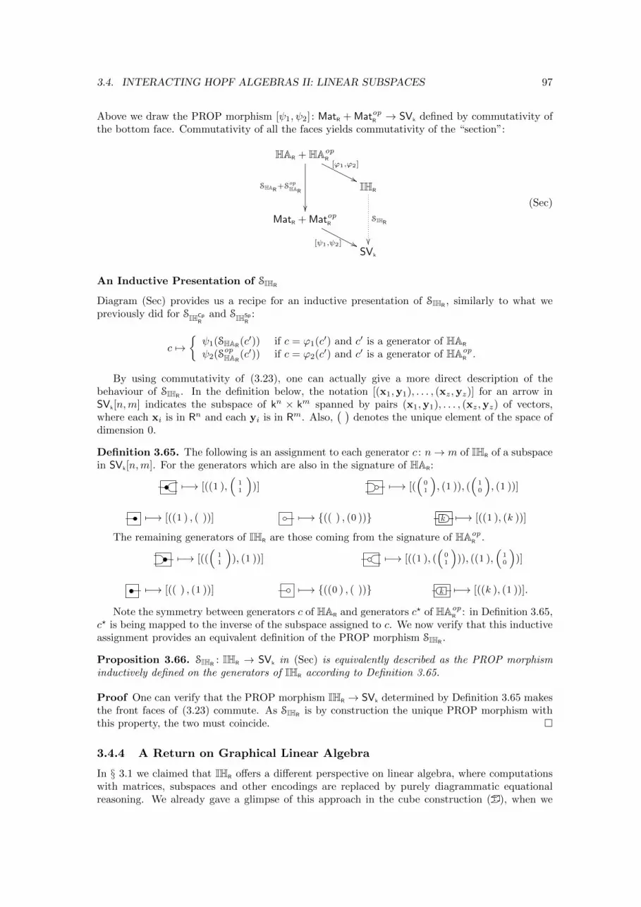
3.4. INTERACTING HOPF ALGEBRAS II: LINEAR SUBSPACES 97
Above we draw the PROP morphism [ψ1, ψ2] : MatR + MatopR → SVk defined by commutativity ofthe bottom face. Commutativity of all the faces yields commutativity of the “section”:
HAR + HAopR
[ϕ1,ϕ2]
''SHAR+S
opHAR
��
IHR
SIHR
��
MatR + MatopR
[ψ1,ψ2] ''SVk
(Sec)
An Inductive Presentation of SIHR
Diagram (Sec) provides us a recipe for an inductive presentation of SIHR, similarly to what we
previously did for SIHCpR
and SIHSpR
:
c 7→{ψ1(SHAR
(c′)) if c = ϕ1(c′) and c′ is a generator of HAR
ψ2(SopHAR(c′)) if c = ϕ2(c′) and c′ is a generator of HAop
R .
By using commutativity of (3.23), one can actually give a more direct description of thebehaviour of SIHR
. In the definition below, the notation [(x1,y1), . . . , (xz,yz)] for an arrow inSVk[n,m] indicates the subspace of kn × km spanned by pairs (x1,y1), . . . , (xz,yz) of vectors,where each xi is in Rn and each yi is in Rm. Also,
( )denotes the unique element of the space of
dimension 0.
Definition 3.65. The following is an assignment to each generator c : n→ m of IHR of a subspacein SVk[n,m]. For the generators which are also in the signature of HAR:
7−→ [((1 ),(
11
))] 7−→ [(
(01
), (1 )), (
(10
), (1 ))]
7−→ [((1 ) , ( ))] 7−→ {(( ) , (0 ))} k 7−→ [((1 ), (k ))]
The remaining generators of IHR are those coming from the signature of HAopR .
7−→ [(((
11
)), (1 ))] 7−→ [((1 ), (
(01
))), ((1 ),
(10
))]
7−→ [(( ) , (1 ))] 7−→ {((0 ) , ( ))} k 7−→ [((k ), (1 ))].
Note the symmetry between generators c of HAR and generators c? of HAopR : in Definition 3.65,
c? is being mapped to the inverse of the subspace assigned to c. We now verify that this inductiveassignment provides an equivalent definition of the PROP morphism SIHR
.
Proposition 3.66. SIHR: IHR → SVk in (Sec) is equivalently described as the PROP morphism
inductively defined on the generators of IHR according to Definition 3.65.
Proof One can verify that the PROP morphism IHR → SVk determined by Definition 3.65 makesthe front faces of (3.23) commute. As SIHR
is by construction the unique PROP morphism withthis property, the two must coincide. �
3.4.4 A Return on Graphical Linear Algebra
In § 3.1 we claimed that IHR offers a different perspective on linear algebra, where computationswith matrices, subspaces and other encodings are replaced by purely diagrammatic equationalreasoning. We already gave a glimpse of this approach in the cube construction (�), when we
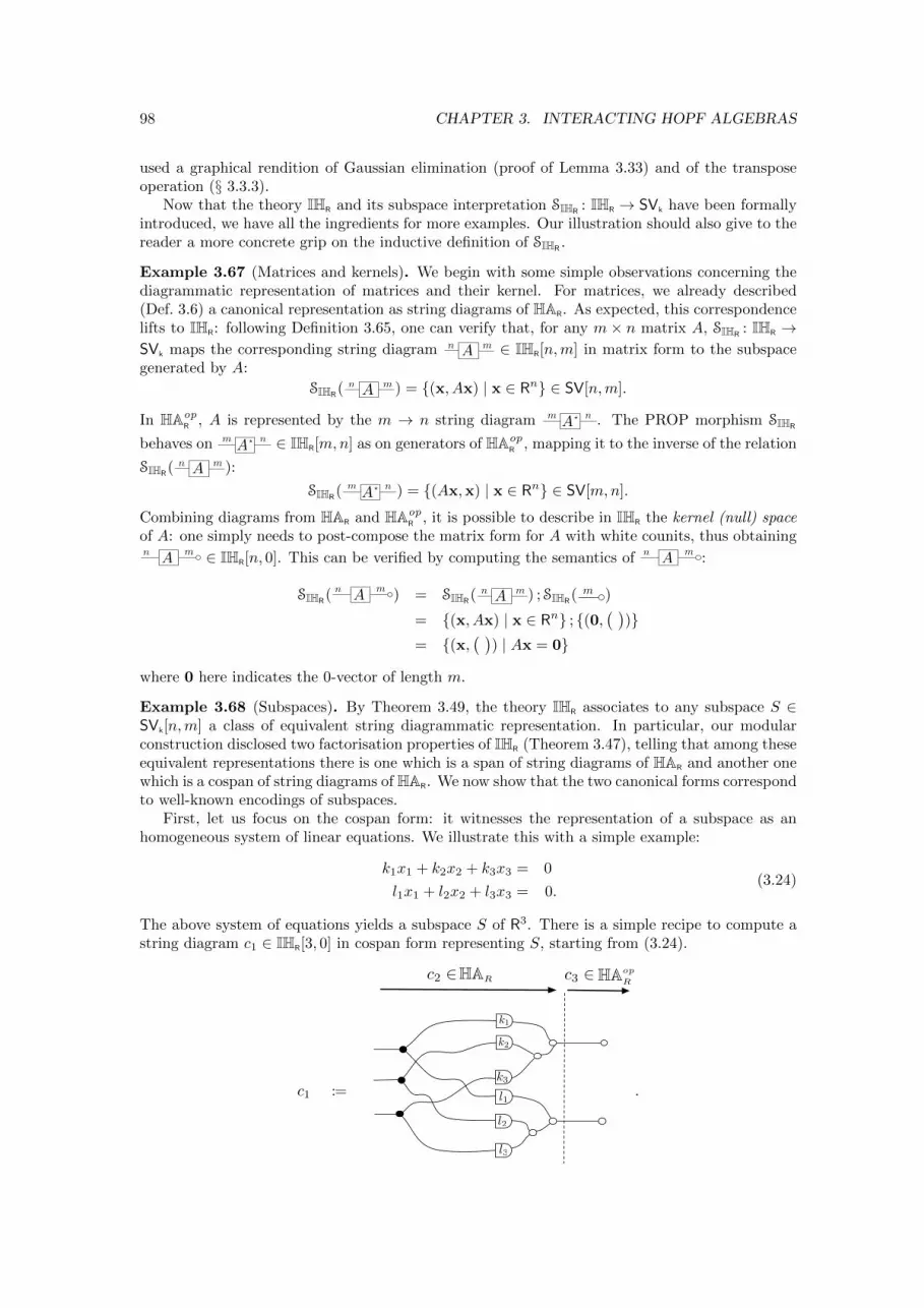
98 CHAPTER 3. INTERACTING HOPF ALGEBRAS
used a graphical rendition of Gaussian elimination (proof of Lemma 3.33) and of the transposeoperation (§ 3.3.3).
Now that the theory IHR and its subspace interpretation SIHR: IHR → SVk have been formally
introduced, we have all the ingredients for more examples. Our illustration should also give to thereader a more concrete grip on the inductive definition of SIHR
.
Example 3.67 (Matrices and kernels). We begin with some simple observations concerning thediagrammatic representation of matrices and their kernel. For matrices, we already described(Def. 3.6) a canonical representation as string diagrams of HAR. As expected, this correspondencelifts to IHR: following Definition 3.65, one can verify that, for any m × n matrix A, SIHR
: IHR →SVk maps the corresponding string diagram n mA ∈ IHR[n,m] in matrix form to the subspacegenerated by A:
SIHR( n mA ) = {(x, Ax) | x ∈ Rn} ∈ SV[n,m].
In HAopR , A is represented by the m → n string diagram m
An? . The PROP morphism SIHR
behaves on mA
n? ∈ IHR[m,n] as on generators of HAopR , mapping it to the inverse of the relation
SIHR( n mA ):
SIHR( m
An? ) = {(Ax,x) | x ∈ Rn} ∈ SV[m,n].
Combining diagrams from HAR and HAopR , it is possible to describe in IHR the kernel (null) space
of A: one simply needs to post-compose the matrix form for A with white counits, thus obtainingn m
A ∈ IHR[n, 0]. This can be verified by computing the semantics of n mA :
SIHR( n m
A ) = SIHR( n mA ) ; SIHR
( m )
= {(x, Ax) | x ∈ Rn} ; {(0,( )
)}= {(x,
( )) | Ax = 0}
where 0 here indicates the 0-vector of length m.
Example 3.68 (Subspaces). By Theorem 3.49, the theory IHR associates to any subspace S ∈SVk[n,m] a class of equivalent string diagrammatic representation. In particular, our modularconstruction disclosed two factorisation properties of IHR (Theorem 3.47), telling that among theseequivalent representations there is one which is a span of string diagrams of HAR and another onewhich is a cospan of string diagrams of HAR. We now show that the two canonical forms correspondto well-known encodings of subspaces.
First, let us focus on the cospan form: it witnesses the representation of a subspace as anhomogeneous system of linear equations. We illustrate this with a simple example:
k1x1 + k2x2 + k3x3 = 0
l1x1 + l2x2 + l3x3 = 0.(3.24)
The above system of equations yields a subspace S of R3. There is a simple recipe to compute astring diagram c1 ∈ IHR[3, 0] in cospan form representing S, starting from (3.24).
c1 := l1
k1
k2k2
l2
l3
k3
HAR HAop
Rc2 2 c3 2
.
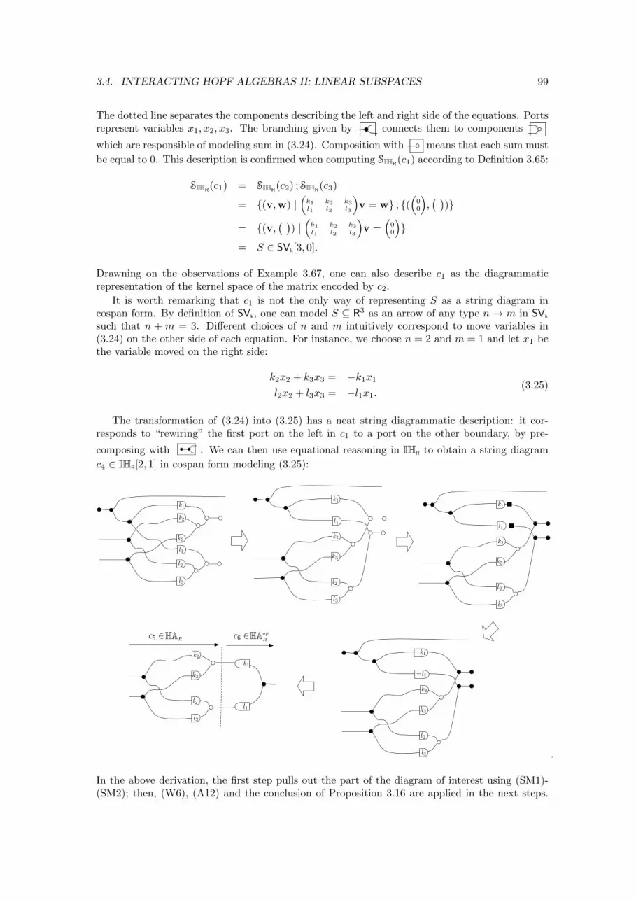
3.4. INTERACTING HOPF ALGEBRAS II: LINEAR SUBSPACES 99
The dotted line separates the components describing the left and right side of the equations. Portsrepresent variables x1, x2, x3. The branching given by connects them to components
which are responsible of modeling sum in (3.24). Composition with means that each sum must
be equal to 0. This description is confirmed when computing SIHR(c1) according to Definition 3.65:
SIHR(c1) = SIHR
(c2) ; SIHR(c3)
= {(v,w) |(k1 k2 k3l1 l2 l3
)v = w} ; {(
(00
),( )
)}
= {(v,( )
) |(k1 k2 k3l1 l2 l3
)v =
(00
)}
= S ∈ SVk[3, 0].
Drawning on the observations of Example 3.67, one can also describe c1 as the diagrammaticrepresentation of the kernel space of the matrix encoded by c2.
It is worth remarking that c1 is not the only way of representing S as a string diagram incospan form. By definition of SVk, one can model S ⊆ R3 as an arrow of any type n→ m in SVk
such that n + m = 3. Different choices of n and m intuitively correspond to move variables in(3.24) on the other side of each equation. For instance, we choose n = 2 and m = 1 and let x1 bethe variable moved on the right side:
k2x2 + k3x3 = −k1x1
l2x2 + l3x3 = −l1x1.(3.25)
The transformation of (3.24) into (3.25) has a neat string diagrammatic description: it cor-responds to “rewiring” the first port on the left in c1 to a port on the other boundary, by pre-
composing with . We can then use equational reasoning in IHR to obtain a string diagram
c4 ∈ IHR[2, 1] in cospan form modeling (3.25):
k2k2
l2
l3
k3
k1�
l1�
l1
k1
k2k2
l2
l3
k3
l1
k1
k2k2
l2
l3
k3
l1
k1
k2k2
l2
l3
k3
k2k2
l2
l3
k3
k1�
l1�
c5 2HAR HAop
Rc6 2
.
In the above derivation, the first step pulls out the part of the diagram of interest using (SM1)-(SM2); then, (W6), (A12) and the conclusion of Proposition 3.16 are applied in the next steps.
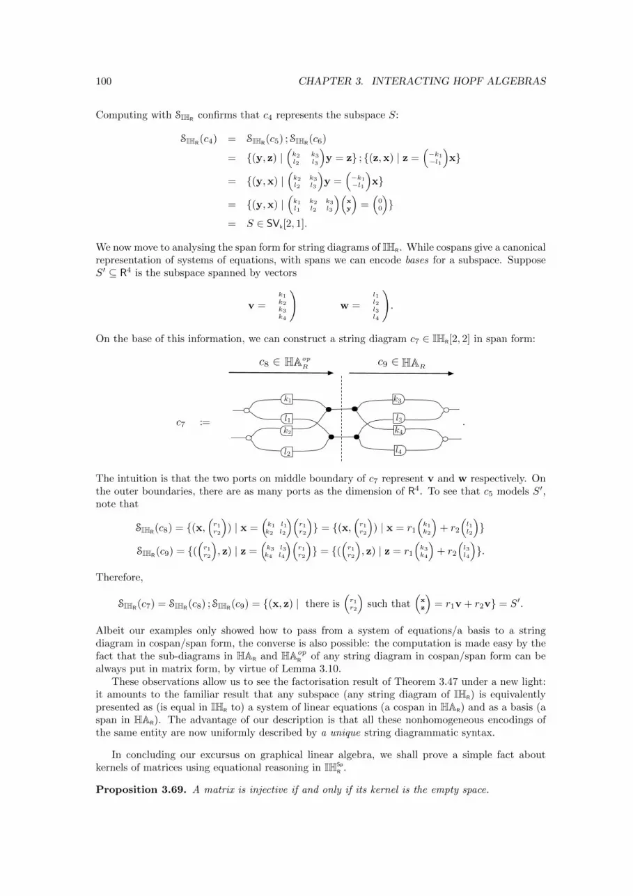
100 CHAPTER 3. INTERACTING HOPF ALGEBRAS
Computing with SIHRconfirms that c4 represents the subspace S:
SIHR(c4) = SIHR
(c5) ; SIHR(c6)
= {(y, z) |(k2 k3l2 l3
)y = z} ; {(z,x) | z =
(−k1−l1
)x}
= {(y,x) |(k2 k3l2 l3
)y =
(−k1−l1
)x}
= {(y,x) |(k1 k2 k3l1 l2 l3
)(xy
)=(00
)}
= S ∈ SVk[2, 1].
We now move to analysing the span form for string diagrams of IHR. While cospans give a canonicalrepresentation of systems of equations, with spans we can encode bases for a subspace. SupposeS′ ⊆ R4 is the subspace spanned by vectors
v =
(k1k2k3k4
)w =
(l1l2l3l4
).
On the base of this information, we can construct a string diagram c7 ∈ IHR[2, 2] in span form:
c7 :=
k3
k4
k1
k2k2
l1 l3
l4l2
HARHAop
Rc8 2 c9 2
.
The intuition is that the two ports on middle boundary of c7 represent v and w respectively. Onthe outer boundaries, there are as many ports as the dimension of R4. To see that c5 models S′,note that
SIHR(c8) = {(x,
(r1r2
)) | x =
(k1 l1k2 l2
)(r1r2
)} = {(x,
(r1r2
)) | x = r1
(k1k2
)+ r2
(l1l2
)}
SIHR(c9) = {(
(r1r2
), z) | z =
(k3 l3k4 l4
)(r1r2
)} = {(
(r1r2
), z) | z = r1
(k3k4
)+ r2
(l3l4
)}.
Therefore,
SIHR(c7) = SIHR
(c8) ; SIHR(c9) = {(x, z) | there is
(r1r2
)such that
(xz
)= r1v + r2v} = S′.
Albeit our examples only showed how to pass from a system of equations/a basis to a stringdiagram in cospan/span form, the converse is also possible: the computation is made easy by thefact that the sub-diagrams in HAR and HAop
R of any string diagram in cospan/span form can bealways put in matrix form, by virtue of Lemma 3.10.
These observations allow us to see the factorisation result of Theorem 3.47 under a new light:it amounts to the familiar result that any subspace (any string diagram of IHR) is equivalentlypresented as (is equal in IHR to) a system of linear equations (a cospan in HAR) and as a basis (aspan in HAR). The advantage of our description is that all these nonhomogeneous encodings ofthe same entity are now uniformly described by a unique string diagrammatic syntax.
In concluding our excursus on graphical linear algebra, we shall prove a simple fact aboutkernels of matrices using equational reasoning in IHSp
R .
Proposition 3.69. A matrix is injective if and only if its kernel is the empty space.
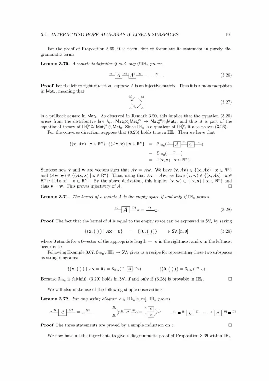
3.4. INTERACTING HOPF ALGEBRAS II: LINEAR SUBSPACES 101
For the proof of Proposition 3.69, it is useful first to formulate its statement in purely dia-grammatic terms.
Lemma 3.70. A matrix is injective if and only if IHR proves
n mA A
n? = n . (3.26)
Proof For the left to right direction, suppose A is an injective matrix. Thus it is a monomorphismin MatR, meaning that
id��
id��
A �� A��(3.27)
is a pullback square in MatR. As observed in Remark 3.20, this implies that the equation (3.26)arises from the distribuitve law λpb : MatR⊗JMatopR → MatopR ⊗JMatR, and thus it is part of theequational theory of IHSp
R∼= MatopR ⊗JMatR. Since IHR is a quotient of IHSp
R , it also proves (3.26).For the converse direction, suppose that (3.26) holds true in IHR. Then we have that
{(x, Ax) | x ∈ Rn} ; {(Ax,x) | x ∈ Rn} = SIHR( n m
A An? )
= SIHR( n )
= {(x,x) | x ∈ Rn}.
Suppose now v and w are vectors such that Av = Aw. We have (v, Av) ∈ {(x, Ax) | x ∈ Rn}and (Aw,w) ∈ {(Ax,x) | x ∈ Rn}. Thus, using that Av = Aw, we have (v,w) ∈ {(x, Ax) | x ∈Rn} ; {(Ax,x) | x ∈ Rn}. By the above derivation, this implies (v,w) ∈ {(x,x) | x ∈ Rn} andthus v = w. This proves injectivity of A. �
Lemma 3.71. The kernel of a matrix A is the empty space if and only if IHR proves
n mA = n . (3.28)
Proof The fact that the kernel of A is equal to the empty space can be expressed in SVk by saying
{(x,( ) )
| Ax = 0} = {(0,( ) )} ∈ SVk[n, 0] (3.29)
where 0 stands for a 0-vector of the appropriate length — m in the rightmost and n in the leftmostoccurrence.
Following Example 3.67, SIHR: IHR → SVk gives us a recipe for representing these two subspaces
as string diagrams:
{(x,( ) )
| Ax = 0} = SIHR( n m
A ) {(0,( ) )} = SIHR
( n )
Because SIHRis faithful, (3.29) holds in SVk if and only if (3.28) is provable in IHR. �
We will also make use of the following simple observations.
Lemma 3.72. For any string diagram c ∈ HAR[n,m], IHR proves
n mc = m mnn
nc =
mn
n
c
cmn n c = mn mc
Proof The three statements are proved by a simple induction on c. �
We now have all the ingredients to give a diagrammatic proof of Proposition 3.69 within IHR.
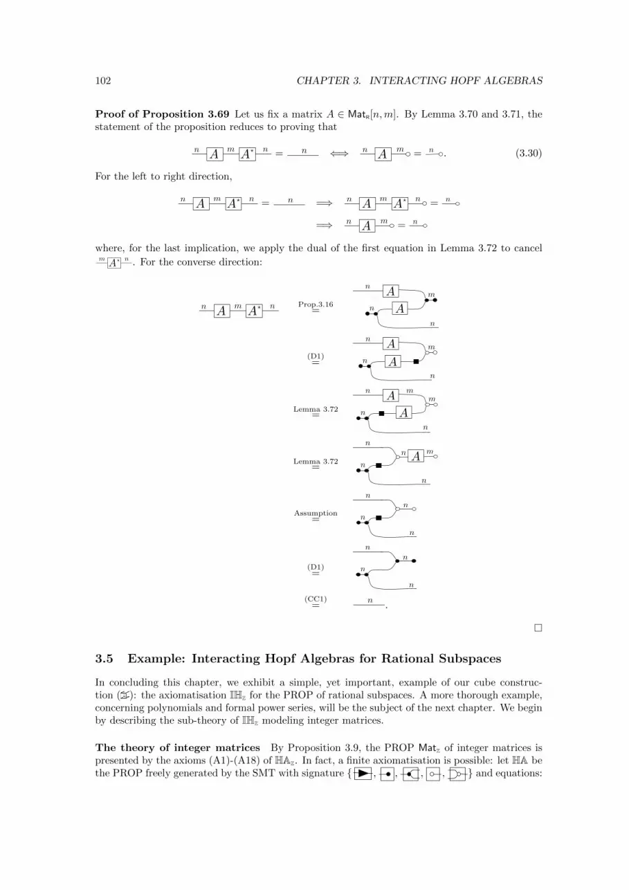
102 CHAPTER 3. INTERACTING HOPF ALGEBRAS
Proof of Proposition 3.69 Let us fix a matrix A ∈ MatR[n,m]. By Lemma 3.70 and 3.71, thestatement of the proposition reduces to proving that
n mA A
n? = n ⇐⇒ n mA = n . (3.30)
For the left to right direction,
n mA A
n? = n =⇒ n mA A
n? = n
=⇒ n mA = n
where, for the last implication, we apply the dual of the first equation in Lemma 3.72 to cancelm
An? . For the converse direction:
n mA A
n? Prop.3.16=
nA
A
m
n
n
(D1)=
nA
A
m
n
n
Lemma 3.72=
nA
Am
n
n
m
Lemma 3.72=
n
Am
n
n
n
Assumption=
n
n
n
n
(D1)=
n
n
n
n
(CC1)=
n.
�
3.5 Example: Interacting Hopf Algebras for Rational Subspaces
In concluding this chapter, we exhibit a simple, yet important, example of our cube construc-tion (�): the axiomatisation IHZ for the PROP of rational subspaces. A more thorough example,concerning polynomials and formal power series, will be the subject of the next chapter. We beginby describing the sub-theory of IHZ modeling integer matrices.
The theory of integer matrices By Proposition 3.9, the PROP MatZ of integer matrices ispresented by the axioms (A1)-(A18) of HAZ. In fact, a finite axiomatisation is possible: let HA bethe PROP freely generated by the SMT with signature { , , , , } and equations:
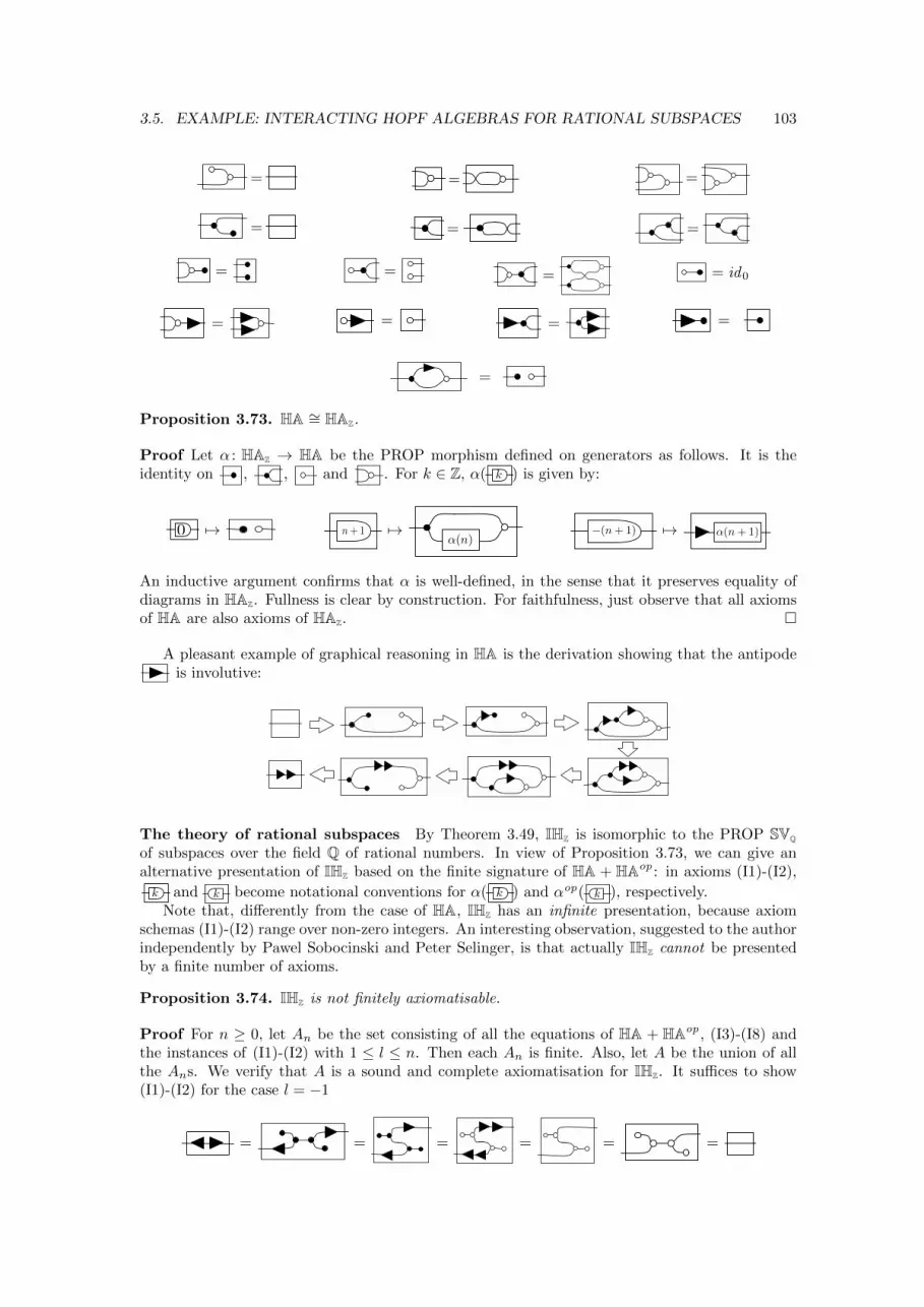
3.5. EXAMPLE: INTERACTING HOPF ALGEBRAS FOR RATIONAL SUBSPACES 103
= = =
= = =
= = = = id0
= = = =
=
Proposition 3.73. HA ∼= HAZ.
Proof Let α : HAZ → HA be the PROP morphism defined on generators as follows. It is theidentity on , , and . For k ∈ Z, α( k ) is given by:
0 7→ n + 1 7→↵(n)
�(n + 1) 7→ ↵(n + 1)
An inductive argument confirms that α is well-defined, in the sense that it preserves equality ofdiagrams in HAZ. Fullness is clear by construction. For faithfulness, just observe that all axiomsof HA are also axioms of HAZ. �
A pleasant example of graphical reasoning in HA is the derivation showing that the antipodeis involutive:
The theory of rational subspaces By Theorem 3.49, IHZ is isomorphic to the PROP SVQ
of subspaces over the field Q of rational numbers. In view of Proposition 3.73, we can give analternative presentation of IHZ based on the finite signature of HA + HAop : in axioms (I1)-(I2),
k and k become notational conventions for α( k ) and αop( k ), respectively.Note that, differently from the case of HA, IHZ has an infinite presentation, because axiom
schemas (I1)-(I2) range over non-zero integers. An interesting observation, suggested to the authorindependently by Pawel Sobocinski and Peter Selinger, is that actually IHZ cannot be presentedby a finite number of axioms.
Proposition 3.74. IHZ is not finitely axiomatisable.
Proof For n ≥ 0, let An be the set consisting of all the equations of HA + HAop , (I3)-(I8) andthe instances of (I1)-(I2) with 1 ≤ l ≤ n. Then each An is finite. Also, let A be the union of allthe Ans. We verify that A is a sound and complete axiomatisation for IHZ. It suffices to show(I1)-(I2) for the case l = −1
= = = = = =
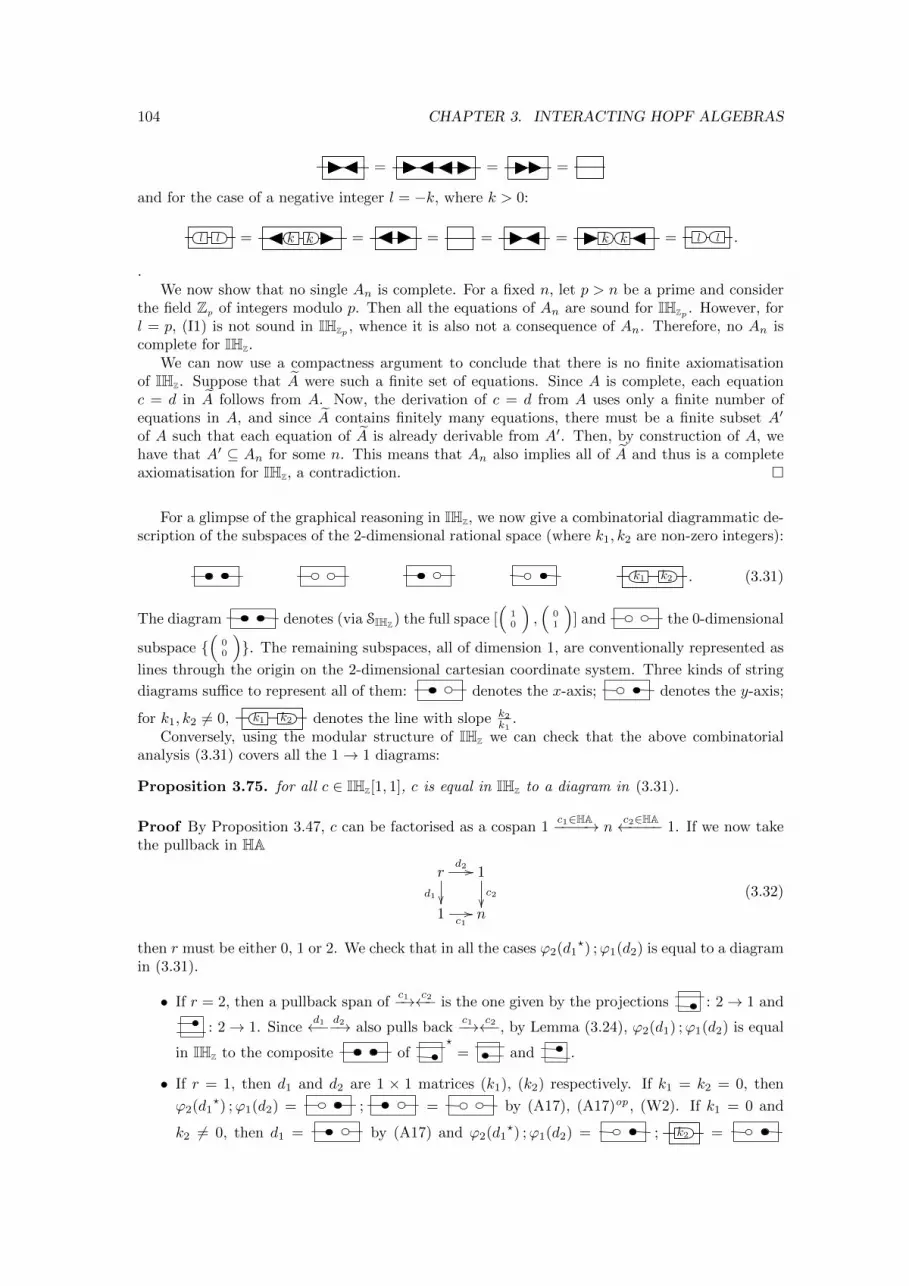
104 CHAPTER 3. INTERACTING HOPF ALGEBRAS
= = =
and for the case of a negative integer l = −k, where k > 0:
ll = kk = = = = kk = ll .
.We now show that no single An is complete. For a fixed n, let p > n be a prime and consider
the field Zp of integers modulo p. Then all the equations of An are sound for IHZp . However, forl = p, (I1) is not sound in IHZp , whence it is also not a consequence of An. Therefore, no An iscomplete for IHZ.
We can now use a compactness argument to conclude that there is no finite axiomatisationof IHZ. Suppose that A were such a finite set of equations. Since A is complete, each equationc = d in A follows from A. Now, the derivation of c = d from A uses only a finite number ofequations in A, and since A contains finitely many equations, there must be a finite subset A′
of A such that each equation of A is already derivable from A′. Then, by construction of A, wehave that A′ ⊆ An for some n. This means that An also implies all of A and thus is a completeaxiomatisation for IHZ, a contradiction. �
For a glimpse of the graphical reasoning in IHZ, we now give a combinatorial diagrammatic de-scription of the subspaces of the 2-dimensional rational space (where k1, k2 are non-zero integers):
k1 k2 . (3.31)
The diagram denotes (via SIHZ) the full space [(
10
),(
01
)] and the 0-dimensional
subspace {(
00
)}. The remaining subspaces, all of dimension 1, are conventionally represented as
lines through the origin on the 2-dimensional cartesian coordinate system. Three kinds of string
diagrams suffice to represent all of them: denotes the x-axis; denotes the y-axis;
for k1, k2 6= 0, k1 k2 denotes the line with slope k2
k1.
Conversely, using the modular structure of IHZ we can check that the above combinatorialanalysis (3.31) covers all the 1→ 1 diagrams:
Proposition 3.75. for all c ∈ IHZ[1, 1], c is equal in IHZ to a diagram in (3.31).
Proof By Proposition 3.47, c can be factorised as a cospan 1c1∈HA−−−−→ n
c2∈HA←−−−− 1. If we now takethe pullback in HA
r
d1 ��
d2 // 1c2��
1c1// n
(3.32)
then r must be either 0, 1 or 2. We check that in all the cases ϕ2(d1?) ;ϕ1(d2) is equal to a diagram
in (3.31).
• If r = 2, then a pullback span ofc1−→ c2←− is the one given by the projections : 2→ 1 and
: 2→ 1. Sinced1←− d2−→ also pulls back
c1−→ c2←−, by Lemma (3.24), ϕ2(d1) ;ϕ1(d2) is equal
in IHZ to the composite of?
= and .
• If r = 1, then d1 and d2 are 1 × 1 matrices (k1), (k2) respectively. If k1 = k2 = 0, then
ϕ2(d1?) ;ϕ1(d2) = ; = by (A17), (A17)op , (W2). If k1 = 0 and
k2 6= 0, then d1 = by (A17) and ϕ2(d1?) ;ϕ1(d2) = ; k2 =
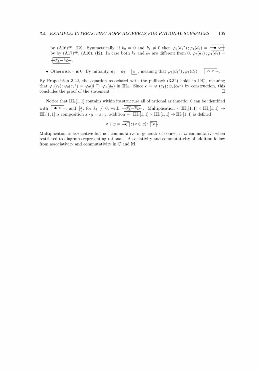
3.5. EXAMPLE: INTERACTING HOPF ALGEBRAS FOR RATIONAL SUBSPACES 105
by (A16)op , (I2). Symmetrically, if k2 = 0 and k1 6= 0 then ϕ2(d1?) ;ϕ1(d2) =
by by (A17)op , (A16), (I2). In case both k1 and k2 are different from 0, ϕ2(d1) ;ϕ1(d2) =
k1 k2 .
• Otherwise, r is 0. By initiality, d1 = d2 = , meaning that ϕ2(d1?) ;ϕ1(d2) = .
By Proposition 3.22, the equation associated with the pullback (3.32) holds in IHw
Z , meaningthat ϕ1(c1) ;ϕ2(c2
?) = ϕ2(d1?) ;ϕ1(d2) in IHZ. Since c = ϕ1(c1) ;ϕ2(c2
?) by construction, thisconcludes the proof of the statement. �
Notice that IHZ[1, 1] contains within its structure all of rational arithmetic: 0 can be identified
with , and k2
k1, for k1 6= 0, with k1 k2 . Multiplication · : IHZ[1, 1] × IHZ[1, 1] →
IHZ[1, 1] is composition x · y = x ; y, addition +: IHZ[1, 1]× IHZ[1, 1]→ IHZ[1, 1] is defined
x+ y = ; (x⊕ y) ; .
Multiplication is associative but not commutative in general: of course, it is commutative whenrestricted to diagrams representing rationals. Associativity and commutativity of addition followfrom associativity and commutativity in C and M.

Chapter 4
The Calculus of Signal Flow Diagrams
[T]he reason why physics has ceased to look for causes isthat in fact there are no such things. The law ofcausality, I believe, like much that passes muster amongphilosophers, is a relic of a bygone age, surviving, likethe monarchy, only because it is erroneously supposed todo no harm.
— Bertrand Russell, On the Notion of Cause (1913).
4.1 Overview
Feedback and related notions such as self-reference and recursion are at the core of several disci-plines, including computer science, engineering and control theory. In control, linear dynamicalsystems are amongst the most extensively studied and well-understood classes of systems with feed-back. They are signal transducers with two standard interpretations: discrete, where—roughlyspeaking—signals come one after the other in the form of a stream, and continuous, where signalsare typically well-behaved real-valued functions.
From the earliest days, diagrams played a central role in motivating the subject matter. Graph-ical representations were not merely intuitive, but also closely resembled physical manifestations(implementations) of linear dynamic systems, such as electrical circuits. While differing in levelsof formality and minor technical details, the various notions share the same set of fundamentalfeatures—and for this reason we will group them all under the umbrella of signal flow graphs.These features are: (i) the ability to copy, (ii) to add and (iii) to amplify signals, (iv) the ability todelay a signal (in the discrete, stream-based interpretation) or to differentiate/integrate a signal(in the continuous interpretation), (v) the possibility of feedback loops and (vi) the concept ofdirected signal flow. Notably, while features (i)-(v) are usually present in physical manifestations,(vi) seems to have been included to facilitate human understanding as well as to avoid “nonsensi-cal” diagrams where the intended signal flow seems to be incompatible or paradoxical. Of course,physical electrical wires do not insist on a particular orientation of electron flow; both are possibleand the actual flow direction depends on the context.
In this chapter we introduce a string diagrammatic theory of signal flow graphs, which wecall the signal flow calculus. The syntax is based on the following operations, sequential ( ; ) andparallel (⊕) composition. Terms generated by the syntax are referred to as circuits.
107
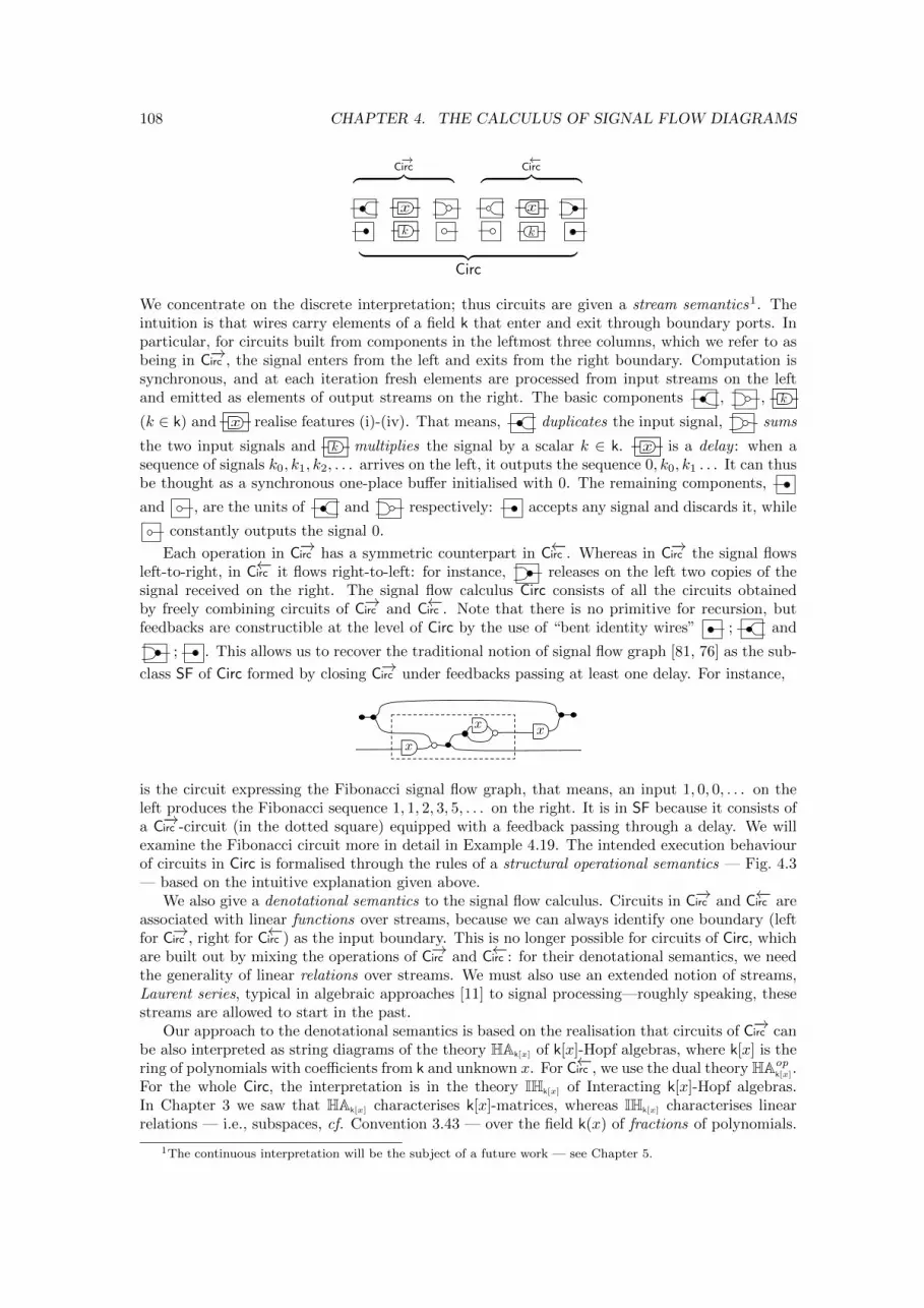
108 CHAPTER 4. THE CALCULUS OF SIGNAL FLOW DIAGRAMS
C−→irc︷ ︸︸ ︷ C
←−irc︷ ︸︸ ︷
x x
k k
︸ ︷︷ ︸Circ
We concentrate on the discrete interpretation; thus circuits are given a stream semantics1. Theintuition is that wires carry elements of a field k that enter and exit through boundary ports. Inparticular, for circuits built from components in the leftmost three columns, which we refer to asbeing in C−→irc , the signal enters from the left and exits from the right boundary. Computation issynchronous, and at each iteration fresh elements are processed from input streams on the leftand emitted as elements of output streams on the right. The basic components , , k
(k ∈ k) and x realise features (i)-(iv). That means, duplicates the input signal, sums
the two input signals and k multiplies the signal by a scalar k ∈ k. x is a delay : when asequence of signals k0, k1, k2, . . . arrives on the left, it outputs the sequence 0, k0, k1 . . . It can thusbe thought as a synchronous one-place buffer initialised with 0. The remaining components,
and , are the units of and respectively: accepts any signal and discards it, while
constantly outputs the signal 0.
Each operation in C−→irc has a symmetric counterpart in C←−irc . Whereas in C−→irc the signal flowsleft-to-right, in C←−irc it flows right-to-left: for instance, releases on the left two copies of thesignal received on the right. The signal flow calculus Circ consists of all the circuits obtainedby freely combining circuits of C−→irc and C←−irc . Note that there is no primitive for recursion, butfeedbacks are constructible at the level of Circ by the use of “bent identity wires” ; and
; . This allows us to recover the traditional notion of signal flow graph [81, 76] as the sub-
class SF of Circ formed by closing C−→irc under feedbacks passing at least one delay. For instance,
xxx
is the circuit expressing the Fibonacci signal flow graph, that means, an input 1, 0, 0, . . . on theleft produces the Fibonacci sequence 1, 1, 2, 3, 5, . . . on the right. It is in SF because it consists ofa C−→irc -circuit (in the dotted square) equipped with a feedback passing through a delay. We willexamine the Fibonacci circuit more in detail in Example 4.19. The intended execution behaviourof circuits in Circ is formalised through the rules of a structural operational semantics — Fig. 4.3— based on the intuitive explanation given above.
We also give a denotational semantics to the signal flow calculus. Circuits in C−→irc and C←−irc areassociated with linear functions over streams, because we can always identify one boundary (leftfor C−→irc , right for C←−irc ) as the input boundary. This is no longer possible for circuits of Circ, whichare built out by mixing the operations of C−→irc and C←−irc : for their denotational semantics, we needthe generality of linear relations over streams. We must also use an extended notion of streams,Laurent series, typical in algebraic approaches [11] to signal processing—roughly speaking, thesestreams are allowed to start in the past.
Our approach to the denotational semantics is based on the realisation that circuits of C−→irc canbe also interpreted as string diagrams of the theory HAk[x] of k[x]-Hopf algebras, where k[x] is thering of polynomials with coefficients from k and unknown x. For C←−irc , we use the dual theory HAop
k[x].For the whole Circ, the interpretation is in the theory IHk[x] of Interacting k[x]-Hopf algebras.In Chapter 3 we saw that HAk[x] characterises k[x]-matrices, whereas IHk[x] characterises linearrelations — i.e., subspaces, cf. Convention 3.43 — over the field k(x) of fractions of polynomials.
1The continuous interpretation will be the subject of a future work — see Chapter 5.
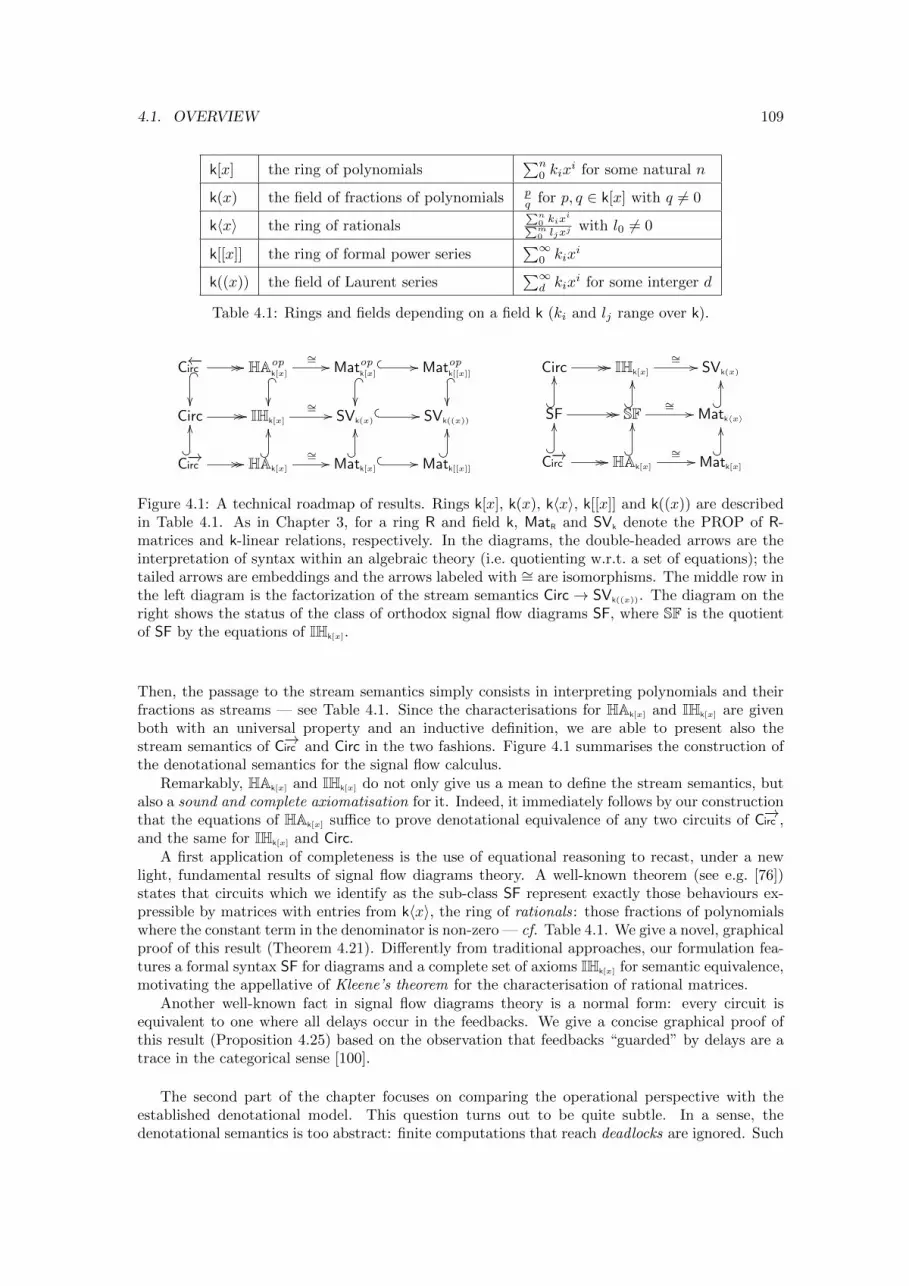
4.1. OVERVIEW 109
k[x] the ring of polynomials∑n
0 kixi for some natural n
k(x) the field of fractions of polynomials pq for p, q ∈ k[x] with q 6= 0
k〈x〉 the ring of rationals∑n
0 kixi∑m
0 ljxjwith l0 6= 0
k[[x]] the ring of formal power series∑∞
0 kixi
k((x)) the field of Laurent series∑∞d kix
i for some interger d
Table 4.1: Rings and fields depending on a field k (ki and lj range over k).
C←−irc� _��
// // HAopk[x]� _
��
∼= // Matopk[x]
� � //� _
��
Matopk[[x]]� _
��Circ // // IHk[x]
∼= // SVk(x)
� � // SVk((x))
C−→irc?�
OO
// // HAk[x]
?�
OO
∼= // Matk[x]
� � //?�
OO
Matk[[x]]
?�
OO
Circ // // IHk[x]
∼= // SVk(x)
SF?�
OO
// // SF?�
OO
∼= // Matk〈x〉?�
OO
C−→irc?�
OO
// // HAk[x]
?�
OO
∼= // Matk[x]
?�
OO
Figure 4.1: A technical roadmap of results. Rings k[x], k(x), k〈x〉, k[[x]] and k((x)) are describedin Table 4.1. As in Chapter 3, for a ring R and field k, MatR and SVk denote the PROP of R-matrices and k-linear relations, respectively. In the diagrams, the double-headed arrows are theinterpretation of syntax within an algebraic theory (i.e. quotienting w.r.t. a set of equations); thetailed arrows are embeddings and the arrows labeled with ∼= are isomorphisms. The middle row inthe left diagram is the factorization of the stream semantics Circ→ SVk((x)). The diagram on theright shows the status of the class of orthodox signal flow diagrams SF, where SF is the quotientof SF by the equations of IHk[x].
Then, the passage to the stream semantics simply consists in interpreting polynomials and theirfractions as streams — see Table 4.1. Since the characterisations for HAk[x] and IHk[x] are givenboth with an universal property and an inductive definition, we are able to present also thestream semantics of C−→irc and Circ in the two fashions. Figure 4.1 summarises the construction ofthe denotational semantics for the signal flow calculus.
Remarkably, HAk[x] and IHk[x] do not only give us a mean to define the stream semantics, butalso a sound and complete axiomatisation for it. Indeed, it immediately follows by our constructionthat the equations of HAk[x] suffice to prove denotational equivalence of any two circuits of C−→irc ,and the same for IHk[x] and Circ.
A first application of completeness is the use of equational reasoning to recast, under a newlight, fundamental results of signal flow diagrams theory. A well-known theorem (see e.g. [76])states that circuits which we identify as the sub-class SF represent exactly those behaviours ex-pressible by matrices with entries from k〈x〉, the ring of rationals: those fractions of polynomialswhere the constant term in the denominator is non-zero — cf. Table 4.1. We give a novel, graphicalproof of this result (Theorem 4.21). Differently from traditional approaches, our formulation fea-tures a formal syntax SF for diagrams and a complete set of axioms IHk[x] for semantic equivalence,motivating the appellative of Kleene’s theorem for the characterisation of rational matrices.
Another well-known fact in signal flow diagrams theory is a normal form: every circuit isequivalent to one where all delays occur in the feedbacks. We give a concise graphical proof ofthis result (Proposition 4.25) based on the observation that feedbacks “guarded” by delays are atrace in the categorical sense [100].
The second part of the chapter focuses on comparing the operational perspective with theestablished denotational model. This question turns out to be quite subtle. In a sense, thedenotational semantics is too abstract: finite computations that reach deadlocks are ignored. Such
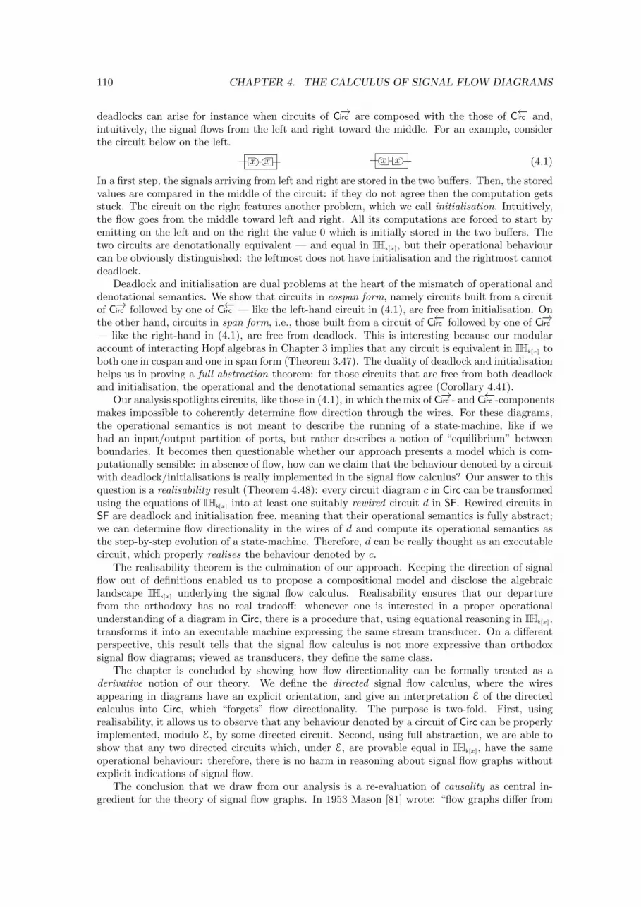
110 CHAPTER 4. THE CALCULUS OF SIGNAL FLOW DIAGRAMS
deadlocks can arise for instance when circuits of C−→irc are composed with the those of C←−irc and,intuitively, the signal flows from the left and right toward the middle. For an example, considerthe circuit below on the left.
x x xx
(4.1)
In a first step, the signals arriving from left and right are stored in the two buffers. Then, the storedvalues are compared in the middle of the circuit: if they do not agree then the computation getsstuck. The circuit on the right features another problem, which we call initialisation. Intuitively,the flow goes from the middle toward left and right. All its computations are forced to start byemitting on the left and on the right the value 0 which is initially stored in the two buffers. Thetwo circuits are denotationally equivalent — and equal in IHk[x], but their operational behaviourcan be obviously distinguished: the leftmost does not have initialisation and the rightmost cannotdeadlock.
Deadlock and initialisation are dual problems at the heart of the mismatch of operational anddenotational semantics. We show that circuits in cospan form, namely circuits built from a circuitof C−→irc followed by one of C←−irc — like the left-hand circuit in (4.1), are free from initialisation. Onthe other hand, circuits in span form, i.e., those built from a circuit of C←−irc followed by one of C−→irc— like the right-hand in (4.1), are free from deadlock. This is interesting because our modularaccount of interacting Hopf algebras in Chapter 3 implies that any circuit is equivalent in IHk[x] toboth one in cospan and one in span form (Theorem 3.47). The duality of deadlock and initialisationhelps us in proving a full abstraction theorem: for those circuits that are free from both deadlockand initialisation, the operational and the denotational semantics agree (Corollary 4.41).
Our analysis spotlights circuits, like those in (4.1), in which the mix of C−→irc - and C←−irc -componentsmakes impossible to coherently determine flow direction through the wires. For these diagrams,the operational semantics is not meant to describe the running of a state-machine, like if wehad an input/output partition of ports, but rather describes a notion of “equilibrium” betweenboundaries. It becomes then questionable whether our approach presents a model which is com-putationally sensible: in absence of flow, how can we claim that the behaviour denoted by a circuitwith deadlock/initialisations is really implemented in the signal flow calculus? Our answer to thisquestion is a realisability result (Theorem 4.48): every circuit diagram c in Circ can be transformedusing the equations of IHk[x] into at least one suitably rewired circuit d in SF. Rewired circuits inSF are deadlock and initialisation free, meaning that their operational semantics is fully abstract;we can determine flow directionality in the wires of d and compute its operational semantics asthe step-by-step evolution of a state-machine. Therefore, d can be really thought as an executablecircuit, which properly realises the behaviour denoted by c.
The realisability theorem is the culmination of our approach. Keeping the direction of signalflow out of definitions enabled us to propose a compositional model and disclose the algebraiclandscape IHk[x] underlying the signal flow calculus. Realisability ensures that our departurefrom the orthodoxy has no real tradeoff: whenever one is interested in a proper operationalunderstanding of a diagram in Circ, there is a procedure that, using equational reasoning in IHk[x],transforms it into an executable machine expressing the same stream transducer. On a differentperspective, this result tells that the signal flow calculus is not more expressive than orthodoxsignal flow diagrams; viewed as transducers, they define the same class.
The chapter is concluded by showing how flow directionality can be formally treated as aderivative notion of our theory. We define the directed signal flow calculus, where the wiresappearing in diagrams have an explicit orientation, and give an interpretation E of the directedcalculus into Circ, which “forgets” flow directionality. The purpose is two-fold. First, usingrealisability, it allows us to observe that any behaviour denoted by a circuit of Circ can be properlyimplemented, modulo E, by some directed circuit. Second, using full abstraction, we are able toshow that any two directed circuits which, under E, are provable equal in IHk[x], have the sameoperational behaviour: therefore, there is no harm in reasoning about signal flow graphs withoutexplicit indications of signal flow.
The conclusion that we draw from our analysis is a re-evaluation of causality as central in-gredient for the theory of signal flow graphs. In 1953 Mason [81] wrote: “flow graphs differ from
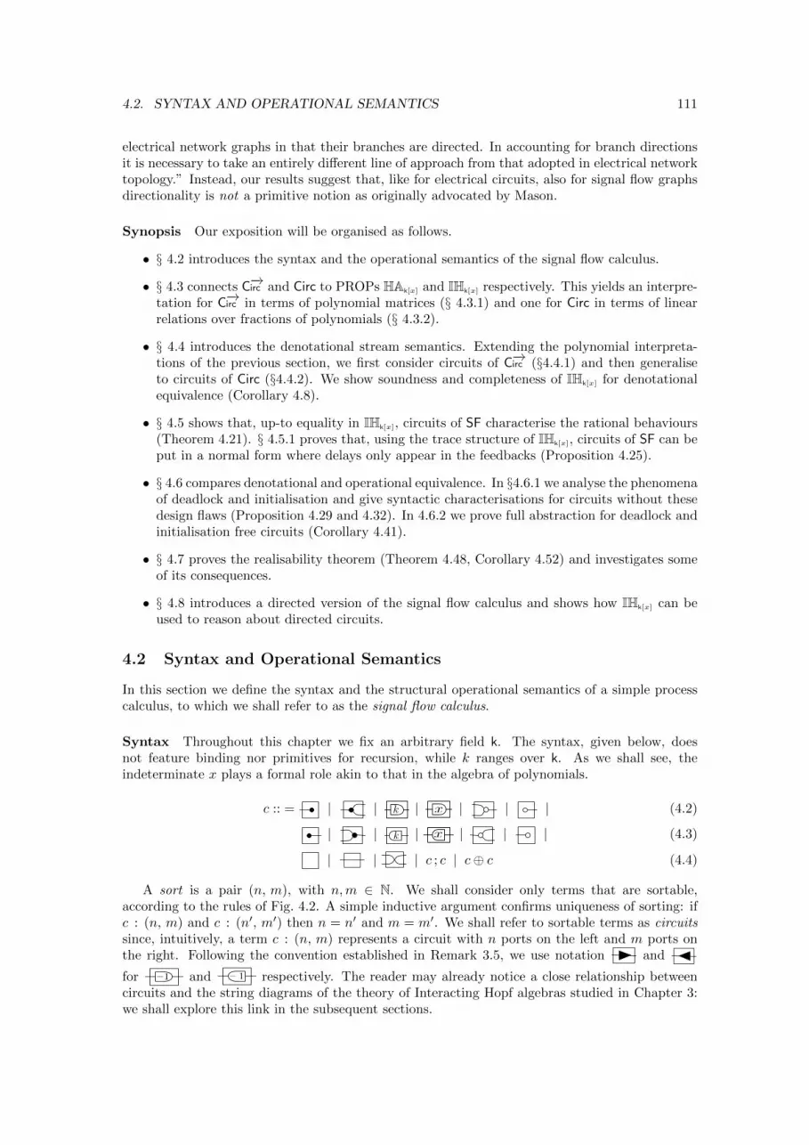
4.2. SYNTAX AND OPERATIONAL SEMANTICS 111
electrical network graphs in that their branches are directed. In accounting for branch directionsit is necessary to take an entirely different line of approach from that adopted in electrical networktopology.” Instead, our results suggest that, like for electrical circuits, also for signal flow graphsdirectionality is not a primitive notion as originally advocated by Mason.
Synopsis Our exposition will be organised as follows.
• § 4.2 introduces the syntax and the operational semantics of the signal flow calculus.
• § 4.3 connects C−→irc and Circ to PROPs HAk[x] and IHk[x] respectively. This yields an interpre-tation for C−→irc in terms of polynomial matrices (§ 4.3.1) and one for Circ in terms of linearrelations over fractions of polynomials (§ 4.3.2).
• § 4.4 introduces the denotational stream semantics. Extending the polynomial interpreta-tions of the previous section, we first consider circuits of C−→irc (§4.4.1) and then generaliseto circuits of Circ (§4.4.2). We show soundness and completeness of IHk[x] for denotationalequivalence (Corollary 4.8).
• § 4.5 shows that, up-to equality in IHk[x], circuits of SF characterise the rational behaviours(Theorem 4.21). § 4.5.1 proves that, using the trace structure of IHk[x], circuits of SF can beput in a normal form where delays only appear in the feedbacks (Proposition 4.25).
• § 4.6 compares denotational and operational equivalence. In §4.6.1 we analyse the phenomenaof deadlock and initialisation and give syntactic characterisations for circuits without thesedesign flaws (Proposition 4.29 and 4.32). In 4.6.2 we prove full abstraction for deadlock andinitialisation free circuits (Corollary 4.41).
• § 4.7 proves the realisability theorem (Theorem 4.48, Corollary 4.52) and investigates someof its consequences.
• § 4.8 introduces a directed version of the signal flow calculus and shows how IHk[x] can beused to reason about directed circuits.
4.2 Syntax and Operational Semantics
In this section we define the syntax and the structural operational semantics of a simple processcalculus, to which we shall refer to as the signal flow calculus.
Syntax Throughout this chapter we fix an arbitrary field k. The syntax, given below, doesnot feature binding nor primitives for recursion, while k ranges over k. As we shall see, theindeterminate x plays a formal role akin to that in the algebra of polynomials.
c :: = | | k | x | | | (4.2)
| | k | x | | | (4.3)
| | | c ; c | c⊕ c (4.4)
A sort is a pair (n, m), with n,m ∈ N. We shall consider only terms that are sortable,according to the rules of Fig. 4.2. A simple inductive argument confirms uniqueness of sorting: ifc : (n, m) and c : (n′, m′) then n = n′ and m = m′. We shall refer to sortable terms as circuitssince, intuitively, a term c : (n, m) represents a circuit with n ports on the left and m ports onthe right. Following the convention established in Remark 3.5, we use notation and
for 1� and 1� respectively. The reader may already notice a close relationship betweencircuits and the string diagrams of the theory of Interacting Hopf algebras studied in Chapter 3:we shall explore this link in the subsequent sections.
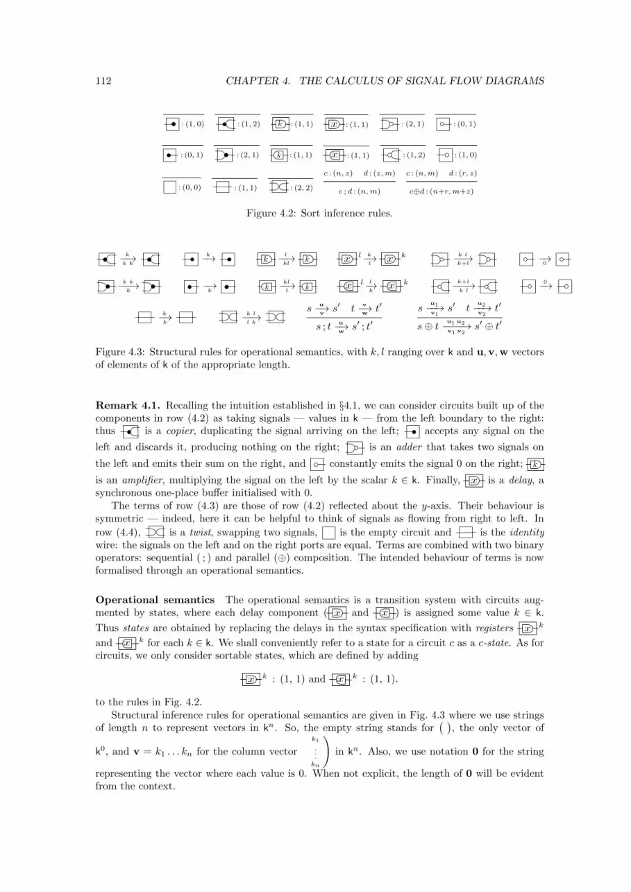
112 CHAPTER 4. THE CALCULUS OF SIGNAL FLOW DIAGRAMS
: (1, 0) : (1, 2) k : (1, 1) x : (1, 1) : (2, 1) : (0, 1)
: (0, 1) : (2, 1) k : (1, 1)
x
: (1, 1) : (1, 2) : (1, 0)
: (0, 0) : (1, 1) : (2, 2)
c : (n, z) d : (z,m)
c ; d : (n,m)
c : (n,m) d : (r, z)
c⊕d : (n+r,m+z)
Figure 4.2: Sort inference rules.
k−−→k k
k−→ kl−−→kl
k x l k−→l
x k k l−−→k+l
−→0
k k−−→k
−→k k
kl−−→l k
x l l−→k
x k k+l−−−→k l
0−→
k−→k
k l−−→l k
su−→vs′ t
v−→wt′
s ; tu−→ws′ ; t′
su1−−→v1
s′ tu2−−→v2
t′
s⊕ t u1 u2−−−−→v1 v2
s′ ⊕ t′
Figure 4.3: Structural rules for operational semantics, with k, l ranging over k and u,v,w vectorsof elements of k of the appropriate length.
Remark 4.1. Recalling the intuition established in §4.1, we can consider circuits built up of thecomponents in row (4.2) as taking signals — values in k — from the left boundary to the right:thus is a copier, duplicating the signal arriving on the left; accepts any signal on the
left and discards it, producing nothing on the right; is an adder that takes two signals on
the left and emits their sum on the right, and constantly emits the signal 0 on the right; k
is an amplifier, multiplying the signal on the left by the scalar k ∈ k. Finally, x is a delay, asynchronous one-place buffer initialised with 0.
The terms of row (4.3) are those of row (4.2) reflected about the y-axis. Their behaviour issymmetric — indeed, here it can be helpful to think of signals as flowing from right to left. In
row (4.4), is a twist, swapping two signals, is the empty circuit and is the identitywire: the signals on the left and on the right ports are equal. Terms are combined with two binaryoperators: sequential ( ; ) and parallel (⊕) composition. The intended behaviour of terms is nowformalised through an operational semantics.
Operational semantics The operational semantics is a transition system with circuits aug-mented by states, where each delay component ( x and x) is assigned some value k ∈ k.
Thus states are obtained by replacing the delays in the syntax specification with registers x k
and x k for each k ∈ k. We shall conveniently refer to a state for a circuit c as a c-state. As forcircuits, we only consider sortable states, which are defined by adding
x k : (1, 1) and x k : (1, 1).
to the rules in Fig. 4.2.Structural inference rules for operational semantics are given in Fig. 4.3 where we use strings
of length n to represent vectors in kn. So, the empty string stands for( )
, the only vector of
k0, and v = k1 . . . kn for the column vector
(k1
.
.
.kn
)in kn. Also, we use notation 0 for the string
representing the vector where each value is 0. When not explicit, the length of 0 will be evidentfrom the context.
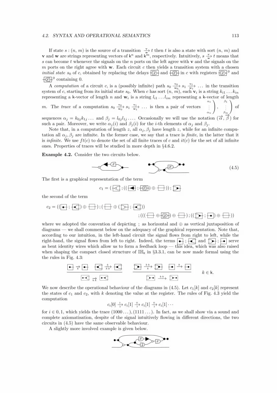
4.2. SYNTAX AND OPERATIONAL SEMANTICS 113
If state s : (n, m) is the source of a transitionv−→wt then t is also a state with sort (n, m) and
v and w are strings representing vectors of kn and km, respectively. Intuitively, sv−→wt means that
s can become t whenever the signals on the n ports on the left agree with v and the signals on them ports on the right agree with w. Each circuit c then yields a transition system with a choseninitial state s0 of c, obtained by replacing the delays x and x in c with registers x 0 and
x 0 containing 0.
A computation of a circuit c, is a (possibly infinite) path s0v0−−→w0
s1v1−−→w1
. . . in the transitionsystem of c, starting from its initial state s0. When c has sort (n, m), each vi is a string ki1 . . . kinrepresenting a k-vector of length n and wi is a string li1 . . . lim representing a k-vector of length
m. The trace of a computation s0v0−−→w0
s1v1−−→w1
. . . is then a pair of vectors
(α1
.
.
.αn
),
(β1
.
.
.βm
)of
sequences αj = k0jk1j . . . and βj = l0j l1j . . . . Occasionally we will use the notation (−→α ,−→β ) forsuch a pair. Moreover, we write αj(i) and βj(i) for the i-th elements of αj and βj .
Note that, in a computation of length z, all αj , βj have length z, while for an infinite compu-tation all αj , βj are infinite. In the former case, we say that a trace is finite, in the latter that itis infinite. We use ft(c) to denote the set of all finite traces of c and it(c) for the set of all infiniteones. Properties of traces will be studied in more depth in §4.6.2.
Example 4.2. Consider the two circuits below.
xx (4.5)
The first is a graphical representation of the term
c1 = ( ; (( ; x)⊕ )) ;
the second of the term
c2 = (( ; )⊕ ) ; ( ⊕ ( ; ))
; ((( ⊕ x )⊕ ) ; (( ; )⊕ ))
where we adopted the convention of depicting ; as horizontal and ⊕ as vertical juxtaposition ofdiagrams — we shall comment below on the adequacy of the graphical representation. Note that,according to our intuition, in the left-hand circuit the signal flows from right to left, while theright-hand, the signal flows from left to right. Indeed, the terms ; and ; serveas bent identity wires which allow us to form a feedback loop — this idea, which was also raisedwhen shaping the compact closed structure of IHR in §3.3.1, can be now made formal using thethe rules in Fig. 4.3:
−→k
k−−→k k
−→k k
k k−−→k
k−→
k k−−→k ∈ k.
We now describe the operational behaviour of the diagrams in (4.5). Let c1[k] and c2[k] representthe states of c1 and c2, with k denoting the value at the register. The rules of Fig. 4.3 yield thecomputation
ci[0]1−→1ci[1]
0−→1ci[1]
0−→1ci[1] · · ·
for i ∈ 0, 1, which yields the trace (1000 . . . ), (1111 . . . ). In fact, as we shall show via a sound andcomplete axiomatisation, despite of the signal intuitively flowing in different directions, the twocircuits in (4.5) have the same observable behaviour.
A slightly more involved example is given below.
x2
x
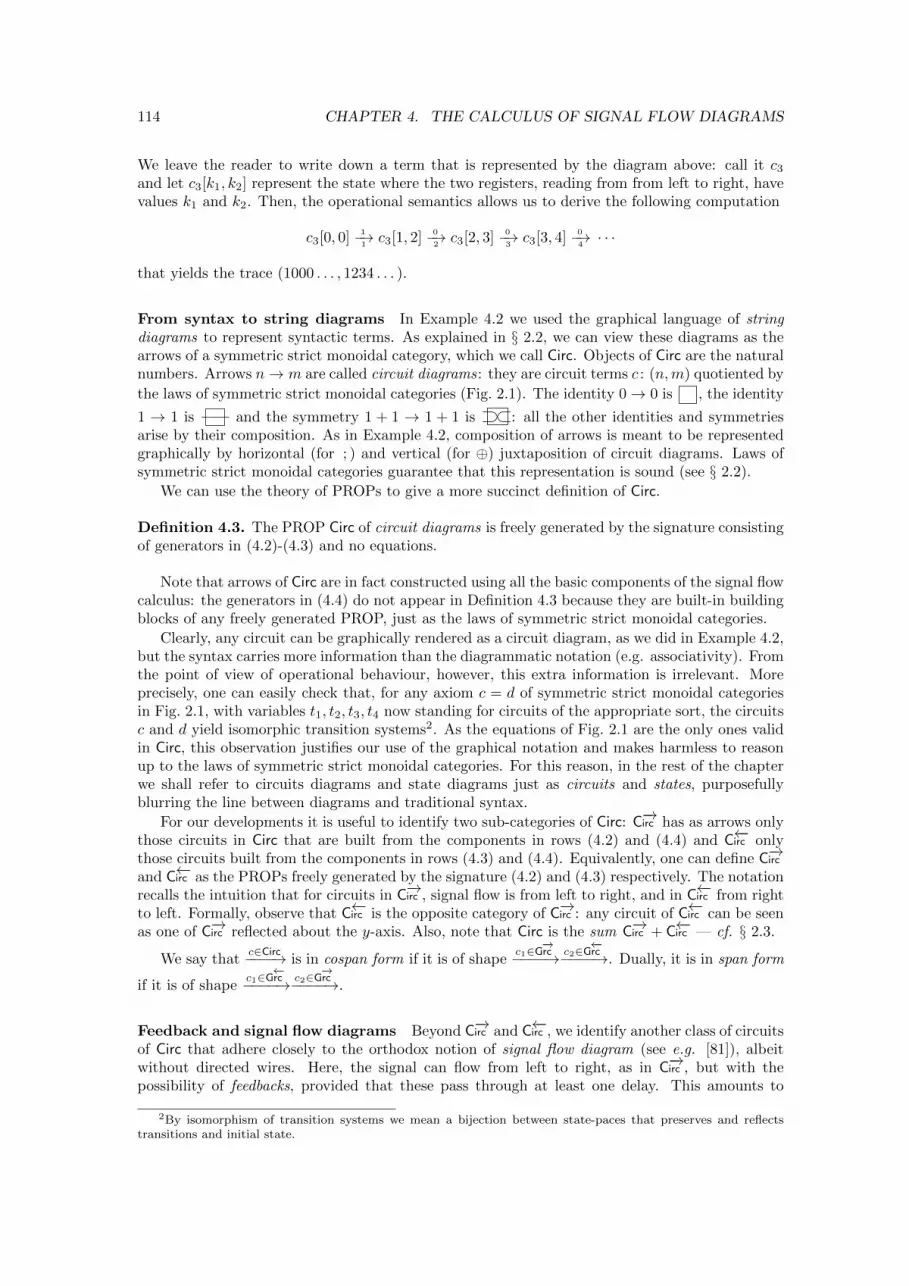
114 CHAPTER 4. THE CALCULUS OF SIGNAL FLOW DIAGRAMS
We leave the reader to write down a term that is represented by the diagram above: call it c3and let c3[k1, k2] represent the state where the two registers, reading from from left to right, havevalues k1 and k2. Then, the operational semantics allows us to derive the following computation
c3[0, 0]1−→1c3[1, 2]
0−→2c3[2, 3]
0−→3c3[3, 4]
0−→4· · ·
that yields the trace (1000 . . . , 1234 . . . ).
From syntax to string diagrams In Example 4.2 we used the graphical language of stringdiagrams to represent syntactic terms. As explained in § 2.2, we can view these diagrams as thearrows of a symmetric strict monoidal category, which we call Circ. Objects of Circ are the naturalnumbers. Arrows n→ m are called circuit diagrams: they are circuit terms c : (n,m) quotiented by
the laws of symmetric strict monoidal categories (Fig. 2.1). The identity 0→ 0 is , the identity
1 → 1 is and the symmetry 1 + 1 → 1 + 1 is : all the other identities and symmetriesarise by their composition. As in Example 4.2, composition of arrows is meant to be representedgraphically by horizontal (for ; ) and vertical (for ⊕) juxtaposition of circuit diagrams. Laws ofsymmetric strict monoidal categories guarantee that this representation is sound (see § 2.2).
We can use the theory of PROPs to give a more succinct definition of Circ.
Definition 4.3. The PROP Circ of circuit diagrams is freely generated by the signature consistingof generators in (4.2)-(4.3) and no equations.
Note that arrows of Circ are in fact constructed using all the basic components of the signal flowcalculus: the generators in (4.4) do not appear in Definition 4.3 because they are built-in buildingblocks of any freely generated PROP, just as the laws of symmetric strict monoidal categories.
Clearly, any circuit can be graphically rendered as a circuit diagram, as we did in Example 4.2,but the syntax carries more information than the diagrammatic notation (e.g. associativity). Fromthe point of view of operational behaviour, however, this extra information is irrelevant. Moreprecisely, one can easily check that, for any axiom c = d of symmetric strict monoidal categoriesin Fig. 2.1, with variables t1, t2, t3, t4 now standing for circuits of the appropriate sort, the circuitsc and d yield isomorphic transition systems2. As the equations of Fig. 2.1 are the only ones validin Circ, this observation justifies our use of the graphical notation and makes harmless to reasonup to the laws of symmetric strict monoidal categories. For this reason, in the rest of the chapterwe shall refer to circuits diagrams and state diagrams just as circuits and states, purposefullyblurring the line between diagrams and traditional syntax.
For our developments it is useful to identify two sub-categories of Circ: C−→irc has as arrows onlythose circuits in Circ that are built from the components in rows (4.2) and (4.4) and C←−irc onlythose circuits built from the components in rows (4.3) and (4.4). Equivalently, one can define C−→ircand C←−irc as the PROPs freely generated by the signature (4.2) and (4.3) respectively. The notationrecalls the intuition that for circuits in C−→irc , signal flow is from left to right, and in C←−irc from rightto left. Formally, observe that C←−irc is the opposite category of C−→irc : any circuit of C←−irc can be seenas one of C−→irc reflected about the y-axis. Also, note that Circ is the sum C−→irc + C←−irc — cf. § 2.3.
We say thatc∈Circ−−−−→ is in cospan form if it is of shape
c1∈C−→irc−−−−→ c2∈C
←−irc−−−−→. Dually, it is in span form
if it is of shapec1∈C
←−irc−−−−→ c2∈C
−→irc−−−−→.
Feedback and signal flow diagrams Beyond C−→irc and C←−irc , we identify another class of circuitsof Circ that adhere closely to the orthodox notion of signal flow diagram (see e.g. [81]), albeitwithout directed wires. Here, the signal can flow from left to right, as in C−→irc , but with thepossibility of feedbacks, provided that these pass through at least one delay. This amounts to
2By isomorphism of transition systems we mean a bijection between state-paces that preserves and reflectstransitions and initial state.
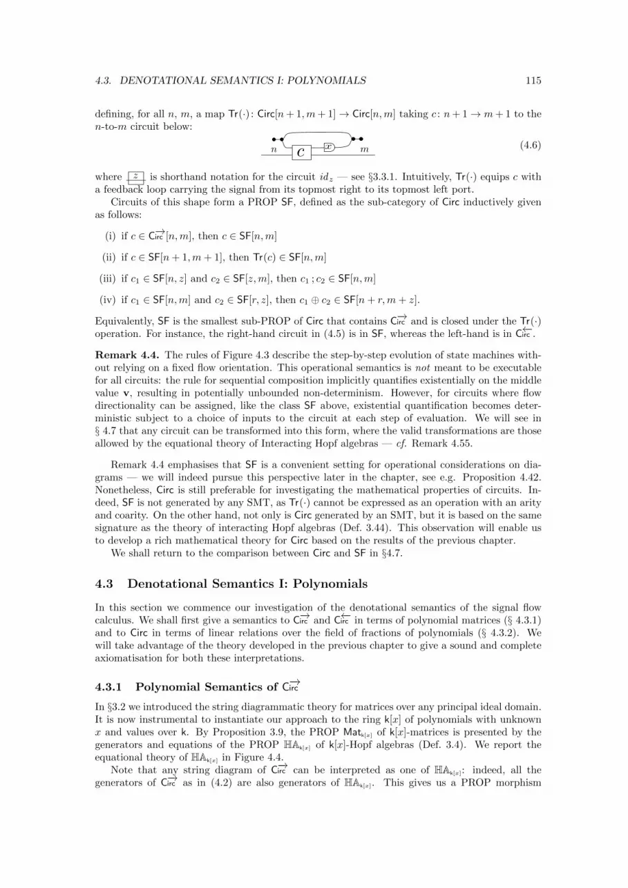
4.3. DENOTATIONAL SEMANTICS I: POLYNOMIALS 115
defining, for all n, m, a map Tr(·) : Circ[n+ 1,m+ 1]→ Circ[n,m] taking c : n+ 1→ m+ 1 to then-to-m circuit below:
n mxc (4.6)
where z is shorthand notation for the circuit idz — see §3.3.1. Intuitively, Tr(·) equips c witha feedback loop carrying the signal from its topmost right to its topmost left port.
Circuits of this shape form a PROP SF, defined as the sub-category of Circ inductively givenas follows:
(i) if c ∈ C−→irc [n,m], then c ∈ SF[n,m]
(ii) if c ∈ SF[n+ 1,m+ 1], then Tr(c) ∈ SF[n,m]
(iii) if c1 ∈ SF[n, z] and c2 ∈ SF[z,m], then c1 ; c2 ∈ SF[n,m]
(iv) if c1 ∈ SF[n,m] and c2 ∈ SF[r, z], then c1 ⊕ c2 ∈ SF[n+ r,m+ z].
Equivalently, SF is the smallest sub-PROP of Circ that contains C−→irc and is closed under the Tr(·)operation. For instance, the right-hand circuit in (4.5) is in SF, whereas the left-hand is in C←−irc .
Remark 4.4. The rules of Figure 4.3 describe the step-by-step evolution of state machines with-out relying on a fixed flow orientation. This operational semantics is not meant to be executablefor all circuits: the rule for sequential composition implicitly quantifies existentially on the middlevalue v, resulting in potentially unbounded non-determinism. However, for circuits where flowdirectionality can be assigned, like the class SF above, existential quantification becomes deter-ministic subject to a choice of inputs to the circuit at each step of evaluation. We will see in§ 4.7 that any circuit can be transformed into this form, where the valid transformations are thoseallowed by the equational theory of Interacting Hopf algebras — cf. Remark 4.55.
Remark 4.4 emphasises that SF is a convenient setting for operational considerations on dia-grams — we will indeed pursue this perspective later in the chapter, see e.g. Proposition 4.42.Nonetheless, Circ is still preferable for investigating the mathematical properties of circuits. In-deed, SF is not generated by any SMT, as Tr(·) cannot be expressed as an operation with an arityand coarity. On the other hand, not only is Circ generated by an SMT, but it is based on the samesignature as the theory of interacting Hopf algebras (Def. 3.44). This observation will enable usto develop a rich mathematical theory for Circ based on the results of the previous chapter.
We shall return to the comparison between Circ and SF in §4.7.
4.3 Denotational Semantics I: Polynomials
In this section we commence our investigation of the denotational semantics of the signal flowcalculus. We shall first give a semantics to C−→irc and C←−irc in terms of polynomial matrices (§ 4.3.1)and to Circ in terms of linear relations over the field of fractions of polynomials (§ 4.3.2). Wewill take advantage of the theory developed in the previous chapter to give a sound and completeaxiomatisation for both these interpretations.
4.3.1 Polynomial Semantics of C−→ircIn §3.2 we introduced the string diagrammatic theory for matrices over any principal ideal domain.It is now instrumental to instantiate our approach to the ring k[x] of polynomials with unknownx and values over k. By Proposition 3.9, the PROP Matk[x] of k[x]-matrices is presented by thegenerators and equations of the PROP HAk[x] of k[x]-Hopf algebras (Def. 3.4). We report theequational theory of HAk[x] in Figure 4.4.
Note that any string diagram of C−→irc can be interpreted as one of HAk[x]: indeed, all thegenerators of C−→irc as in (4.2) are also generators of HAk[x]. This gives us a PROP morphism
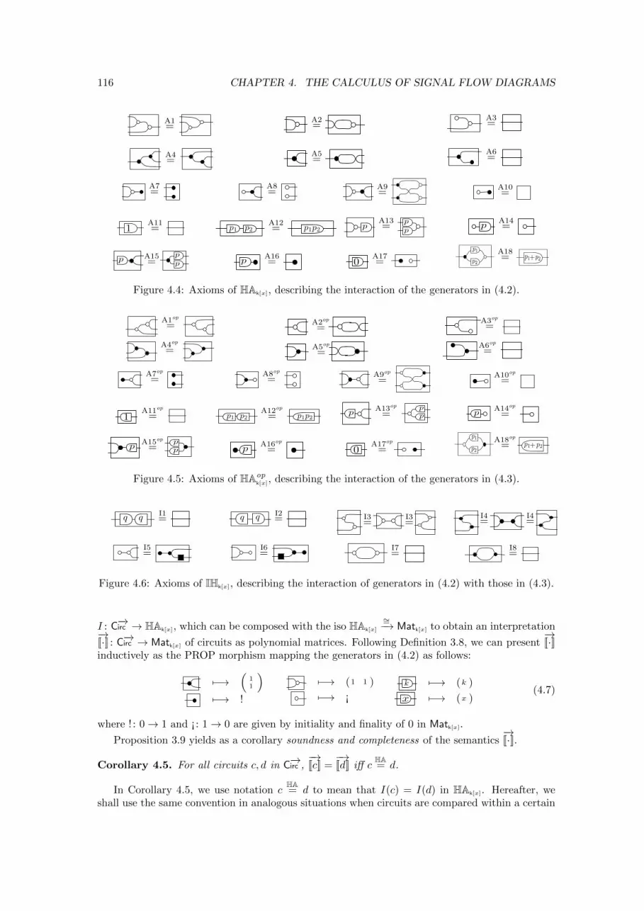
116 CHAPTER 4. THE CALCULUS OF SIGNAL FLOW DIAGRAMS
A1=
A2=
A3=
A4=
A5=
A6=
A7=
A8=
A9=
A10=
1A11= p1 p2
A12= p1p2 p
A13= p
p pA14=
p A15= p
pp
A16= 0
A17= p2
p1 A18= +p1 p2
Figure 4.4: Axioms of HAk[x], describing the interaction of the generators in (4.2).
A1op
= A2op
=A3op
=
A4op
= A5op
=A6op
=
A7op
=A8op
=A9op
=A10op
=
1A11op
= p1 p2A12op
= p1p2p A13op
= pp
pA14op
=
pA15op
=pp p
A16op
= 0A17op
= p2
p1 A18op
= +p1 p2
Figure 4.5: Axioms of HAopk[x], describing the interaction of the generators in (4.3).
qq I1= qq I2
= I3=
I3=
I4=
I4=
I5=
I6=
I7=
I8=
Figure 4.6: Axioms of IHk[x], describing the interaction of generators in (4.2) with those in (4.3).
I : C−→irc → HAk[x], which can be composed with the iso HAk[x]
∼=−→ Matk[x] to obtain an interpretation−→[[·]] : C−→irc → Matk[x] of circuits as polynomial matrices. Following Definition 3.8, we can present
−→[[·]]
inductively as the PROP morphism mapping the generators in (4.2) as follows:
7−→(
11
)
7−→ !
7−→ (1 1 )
7−→ ¡
k 7−→ (k )
x 7−→ (x )(4.7)
where ! : 0→ 1 and ¡ : 1→ 0 are given by initiality and finality of 0 in Matk[x].
Proposition 3.9 yields as a corollary soundness and completeness of the semantics−→[[·]].
Corollary 4.5. For all circuits c, d in C−→irc ,−→[[c]] =
−→[[d]] iff c
HA= d.
In Corollary 4.5, we use notation cHA= d to mean that I(c) = I(d) in HAk[x]. Hereafter, we
shall use the same convention in analogous situations when circuits are compared within a certain
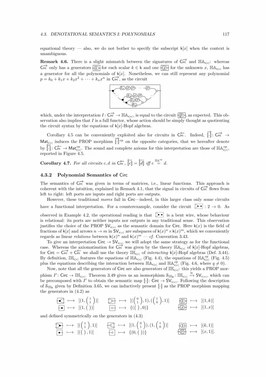
4.3. DENOTATIONAL SEMANTICS I: POLYNOMIALS 117
equational theory — also, we do not bother to specify the subscript k[x] when the context isunambiguous.
Remark 4.6. There is a slight mismatch between the signatures of C−→irc and HAk[x]: whereas
C−→irc only has a generators k for each scalar k ∈ k and one x for the unknown x, HAk[x] has
a generator for all the polynomials of k[x]. Nonetheless, we can still represent any polynomialp = k0 + k1x+ k2x
2 + · · ·+ knxn in C−→irc , as the circuit
. . . . . .
xxx
x . . .x
k0
k1
k2
kn x
which, under the interpretation I : C−→irc → HAk[x], is equal to the circuit p , as expected. This ob-servation also implies that I is a full functor, whose action should be simply thought as quotientingthe circuit syntax by the equations of k[x]-Hopf algebras.
Corollary 4.5 can be conveniently exploited also for circuits in C←−irc . Indeed,−→[[·]] : C−→irc →
Matk[x] induces the PROP morphism−→[[·]]op on the opposite categories, that we hereafter denote
by←−[[·]] : C←−irc → Matopk[x]. The sound and complete axioms for this interpretation are those of HAop
k[x],reported in Figure 4.5.
Corollary 4.7. For all circuits c, d in C←−irc ,←−[[c]] =
←−[[d]] iff c
HAop
= d.
4.3.2 Polynomial Semantics of Circ
The semantics of C−→irc was given in terms of matrices, i.e., linear functions. This approach iscoherent with the intuition, explained in Remark 4.1, that the signal in circuits of C−→irc flows fromleft to right: left ports are inputs and right ports are outputs.
However, these traditional mores fail in Circ—indeed, in this larger class only some circuits
have a functional interpretation. For a counterexample, consider the circuit : 2 → 0. As
observed in Example 4.2, the operational reading is that is a bent wire, whose behaviouris relational: its ports are neither inputs nor outputs in any traditional sense. This observationjustifies the choice of the PROP SVk(x) as the semantic domain for Circ. Here k(x) is the field offractions of k[x] and arrows n→ m in SVk(x) are subspaces of k(x)n×k(x)m, which we convenientlyregards as linear relations between k(x)n and k(x)m — cf. Convention 3.43.
To give an interpretation Circ → SVk(x) we will adopt the same strategy as for the functionalcase. Whereas the axiomatisation for C−→irc was given by the theory HAk[x] of k[x]-Hopf algebras,for Circ = C−→irc + C←−irc we shall use the theory IHk[x] of interacting k[x]-Hopf algebras (Def. 3.44).By definition, IHk[x] features the equations of HAk[x] (Fig. 4.4), the equations of HAop
k[x] (Fig. 4.5)plus the equations describing the interaction between HAk[x] and HAop
k[x] (Fig. 4.6, where q 6= 0).Now, note that all the generators of Circ are also generators of IHk[x]: this yields a PROP mor-
phism I ′ : Circ → IHk[x]. Theorem 3.49 gives us an isomorphism SIHR: IHk[x]
∼=−→ SVk(x), which canbe precomposed with I ′ to obtain the semantic map [[·]] : Circ→ SVk(x). Following the descriptionof SIHR
given by Definition 3.65, we can inductively present [[·]] as the PROP morphism mappingthe generators in (4.2) as
7−→ [(1,(
11
))]
7−→ [(1,( )
)]
7−→ [((
01
), 1), (
(10
), 1)]
7−→ {(( )
, 0)}k 7−→ [(1, k)]
x 7−→ [(1, x)]
and defined symmetrically on the generators in (4.3)
7−→ [((
11
), 1)]
7−→ [(( )
, 1)]
7−→ [(1,(
01
)), (1,
(10
))]
7−→ {(0,( )
)}k 7−→ [(k, 1)]
x 7−→ [(x, 1)].
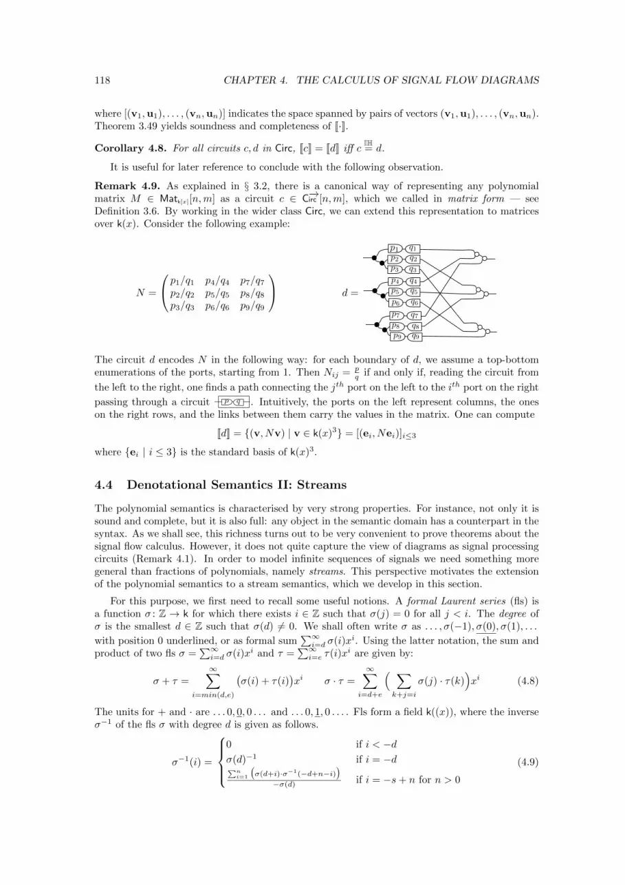
118 CHAPTER 4. THE CALCULUS OF SIGNAL FLOW DIAGRAMS
where [(v1,u1), . . . , (vn,un)] indicates the space spanned by pairs of vectors (v1,u1), . . . , (vn,un).Theorem 3.49 yields soundness and completeness of [[·]].
Corollary 4.8. For all circuits c, d in Circ, [[c]] = [[d]] iff cIH= d.
It is useful for later reference to conclude with the following observation.
Remark 4.9. As explained in § 3.2, there is a canonical way of representing any polynomialmatrix M ∈ Matk[x][n,m] as a circuit c ∈ C−→irc [n,m], which we called in matrix form — seeDefinition 3.6. By working in the wider class Circ, we can extend this representation to matricesover k(x). Consider the following example:
N =
p1/q1 p4/q4 p7/q7
p2/q2 p5/q5 p8/q8
p3/q3 p6/q6 p9/q9
d =
p1 q1
p2 q2
q3p3
p6 q6
p7 q7
p8 q8
p9 q9
p4 q4
p5 q5
The circuit d encodes N in the following way: for each boundary of d, we assume a top-bottomenumerations of the ports, starting from 1. Then Nij = p
q if and only if, reading the circuit from
the left to the right, one finds a path connecting the jth port on the left to the ith port on the right
passing through a circuit p q . Intuitively, the ports on the left represent columns, the oneson the right rows, and the links between them carry the values in the matrix. One can compute
[[d]] = {(v, Nv) | v ∈ k(x)3} = [(ei, Nei)]i≤3
where {ei | i ≤ 3} is the standard basis of k(x)3.
4.4 Denotational Semantics II: Streams
The polynomial semantics is characterised by very strong properties. For instance, not only it issound and complete, but it is also full: any object in the semantic domain has a counterpart in thesyntax. As we shall see, this richness turns out to be very convenient to prove theorems about thesignal flow calculus. However, it does not quite capture the view of diagrams as signal processingcircuits (Remark 4.1). In order to model infinite sequences of signals we need something moregeneral than fractions of polynomials, namely streams. This perspective motivates the extensionof the polynomial semantics to a stream semantics, which we develop in this section.
For this purpose, we first need to recall some useful notions. A formal Laurent series (fls) isa function σ : Z → k for which there exists i ∈ Z such that σ(j) = 0 for all j < i. The degree ofσ is the smallest d ∈ Z such that σ(d) 6= 0. We shall often write σ as . . . , σ(−1), σ(0), σ(1), . . .
with position 0 underlined, or as formal sum∑∞i=d σ(i)xi. Using the latter notation, the sum and
product of two fls σ =∑∞i=d σ(i)xi and τ =
∑∞i=e τ(i)xi are given by:
σ + τ =
∞∑
i=min(d,e)
(σ(i) + τ(i)
)xi σ · τ =
∞∑
i=d+e
( ∑
k+j=i
σ(j) · τ(k))xi (4.8)
The units for + and · are . . . 0, 0, 0 . . . and . . . 0, 1, 0 . . . . Fls form a field k((x)), where the inverseσ−1 of the fls σ with degree d is given as follows.
σ−1(i) =
0 if i < −dσ(d)−1 if i = −d∑n
i=1
(σ(d+i)·σ−1(−d+n−i)
)−σ(d) if i = −s+ n for n > 0
(4.9)
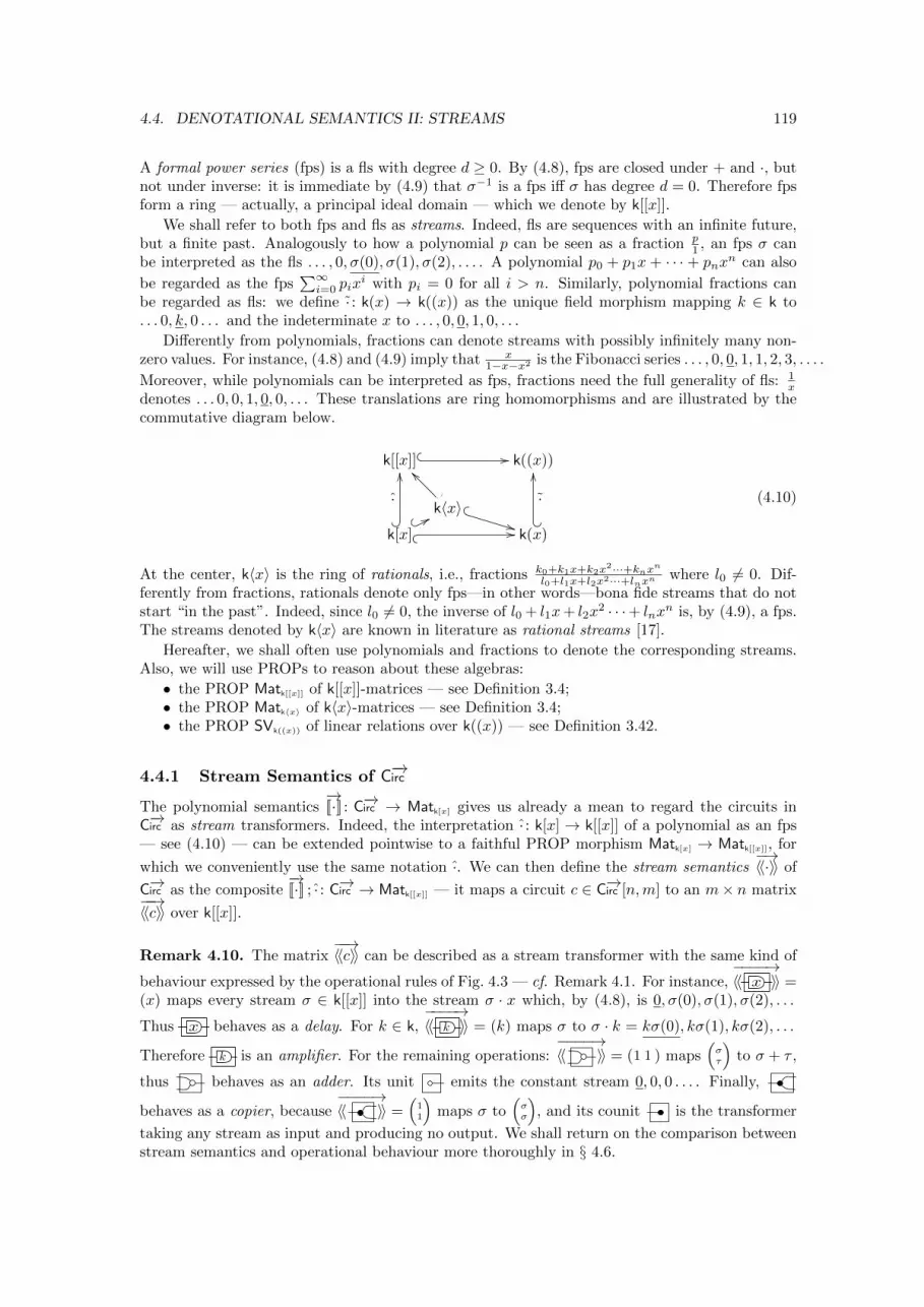
4.4. DENOTATIONAL SEMANTICS II: STREAMS 119
A formal power series (fps) is a fls with degree d ≥ 0. By (4.8), fps are closed under + and ·, butnot under inverse: it is immediate by (4.9) that σ−1 is a fps iff σ has degree d = 0. Therefore fpsform a ring — actually, a principal ideal domain — which we denote by k[[x]].
We shall refer to both fps and fls as streams. Indeed, fls are sequences with an infinite future,but a finite past. Analogously to how a polynomial p can be seen as a fraction p
1 , an fps σ canbe interpreted as the fls . . . , 0, σ(0), σ(1), σ(2), . . . . A polynomial p0 + p1x + · · · + pnx
n can also
be regarded as the fps∑∞i=0 pix
i with pi = 0 for all i > n. Similarly, polynomial fractions canbe regarded as fls: we define · : k(x) → k((x)) as the unique field morphism mapping k ∈ k to. . . 0, k, 0 . . . and the indeterminate x to . . . , 0, 0, 1, 0, . . .
Differently from polynomials, fractions can denote streams with possibly infinitely many non-zero values. For instance, (4.8) and (4.9) imply that x
1−x−x2 is the Fibonacci series . . . , 0, 0, 1, 1, 2, 3, . . . .
Moreover, while polynomials can be interpreted as fps, fractions need the full generality of fls: 1x
denotes . . . 0, 0, 1, 0, 0, . . . These translations are ring homomorphisms and are illustrated by thecommutative diagram below.
k[[x]] �� // k((x))
k〈x〉/ O
__
� w
**k[x]+ � 88�� //
?�
·
OO
k(x)� ?
·
OO
(4.10)
At the center, k〈x〉 is the ring of rationals, i.e., fractions k0+k1x+k2x2···+knxn
l0+l1x+l2x2···+lnxn where l0 6= 0. Dif-ferently from fractions, rationals denote only fps—in other words—bona fide streams that do notstart “in the past”. Indeed, since l0 6= 0, the inverse of l0 + l1x+ l2x
2 · · ·+ lnxn is, by (4.9), a fps.
The streams denoted by k〈x〉 are known in literature as rational streams [17].
Hereafter, we shall often use polynomials and fractions to denote the corresponding streams.Also, we will use PROPs to reason about these algebras:
• the PROP Matk[[x]] of k[[x]]-matrices — see Definition 3.4;• the PROP Matk〈x〉 of k〈x〉-matrices — see Definition 3.4;• the PROP SVk((x)) of linear relations over k((x)) — see Definition 3.42.
4.4.1 Stream Semantics of C−→ircThe polynomial semantics
−→[[·]] : C−→irc → Matk[x] gives us already a mean to regard the circuits in
C−→irc as stream transformers. Indeed, the interpretation · : k[x] → k[[x]] of a polynomial as an fps— see (4.10) — can be extended pointwise to a faithful PROP morphism Matk[x] → Matk[[x]], for
which we conveniently use the same notation ·. We can then define the stream semantics−→〈〈·〉〉 of
C−→irc as the composite−→[[·]] ; · : C−→irc → Matk[[x]] — it maps a circuit c ∈ C−→irc [n,m] to an m× n matrix−−→〈〈c〉〉 over k[[x]].
Remark 4.10. The matrix−−→〈〈c〉〉 can be described as a stream transformer with the same kind of
behaviour expressed by the operational rules of Fig. 4.3 — cf. Remark 4.1. For instance,−−−−→〈〈 x 〉〉 =
(x) maps every stream σ ∈ k[[x]] into the stream σ · x which, by (4.8), is 0, σ(0), σ(1), σ(2), . . .
Thus x behaves as a delay. For k ∈ k,−−−−→〈〈 k 〉〉 = (k) maps σ to σ · k = kσ(0), kσ(1), kσ(2), . . .
Therefore k is an amplifier. For the remaining operations:−−−−→〈〈 〉〉 = (1 1 ) maps
(στ
)to σ + τ ,
thus behaves as an adder. Its unit emits the constant stream 0, 0, 0 . . . . Finally,
behaves as a copier, because−−−−→〈〈 〉〉 =
(11
)maps σ to
(σσ
), and its counit is the transformer
taking any stream as input and producing no output. We shall return on the comparison betweenstream semantics and operational behaviour more thoroughly in § 4.6.
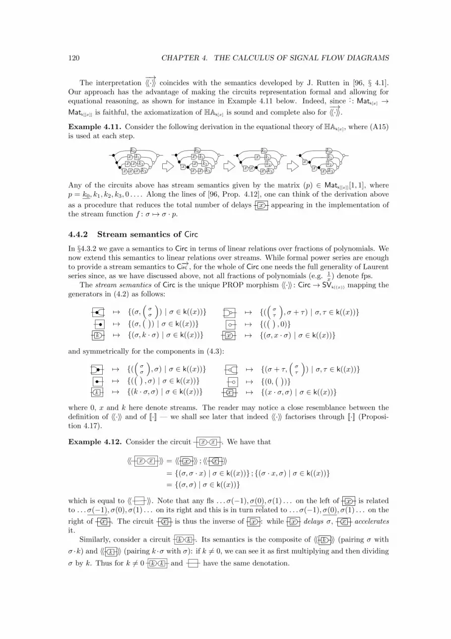
120 CHAPTER 4. THE CALCULUS OF SIGNAL FLOW DIAGRAMS
The interpretation−→〈〈·〉〉 coincides with the semantics developed by J. Rutten in [96, § 4.1].
Our approach has the advantage of making the circuits representation formal and allowing forequational reasoning, as shown for instance in Example 4.11 below. Indeed, since · : Matk[x] →Matk[[x]] is faithful, the axiomatization of HAk[x] is sound and complete also for
−→〈〈·〉〉.Example 4.11. Consider the following derivation in the equational theory of HAk[x], where (A15)is used at each step.
xx xxx k1
k2
k3
k0
x xx
x k1
k2
k3
k0
xx
xk1
k2
k3
k0
x x xx xx k1
k2
k3
k0
Any of the circuits above has stream semantics given by the matrix (p) ∈ Matk[[x]][1, 1], wherep = k0, k1, k2, k3, 0 . . . . Along the lines of [96, Prop. 4.12], one can think of the derivation above
as a procedure that reduces the total number of delays x appearing in the implementation ofthe stream function f : σ 7→ σ · p.
4.4.2 Stream semantics of Circ
In §4.3.2 we gave a semantics to Circ in terms of linear relations over fractions of polynomials. Wenow extend this semantics to linear relations over streams. While formal power series are enoughto provide a stream semantics to C−→irc , for the whole of Circ one needs the full generality of Laurentseries since, as we have discussed above, not all fractions of polynomials (e.g. 1
x ) denote fps.The stream semantics of Circ is the unique PROP morphism 〈〈·〉〉 : Circ→ SVk((x)) mapping the
generators in (4.2) as follows:
7→ {(σ,(σσ
)) | σ ∈ k((x))}
7→ {(σ,( )
) | σ ∈ k((x))}k 7→ {(σ, k · σ) | σ ∈ k((x))}
7→ {((στ
), σ + τ) | σ, τ ∈ k((x))}
7→ {(( )
, 0)}x 7→ {(σ, x · σ) | σ ∈ k((x))}
and symmetrically for the components in (4.3):
7→ {((σσ
), σ) | σ ∈ k((x))}
7→ {(( )
, σ) | σ ∈ k((x))}k 7→ {(k · σ, σ) | σ ∈ k((x))}
7→ {(σ + τ,(στ
)) | σ, τ ∈ k((x))}
7→ {(0,( )
)}
x 7→ {(x · σ, σ) | σ ∈ k((x))}
where 0, x and k here denote streams. The reader may notice a close resemblance between thedefinition of 〈〈·〉〉 and of [[·]] — we shall see later that indeed 〈〈·〉〉 factorises through [[·]] (Proposi-tion 4.17).
Example 4.12. Consider the circuit x x . We have that
〈〈 x x 〉〉 = 〈〈 x 〉〉 ; 〈〈 x〉〉= {(σ, σ · x) | σ ∈ k((x))} ; {(σ · x, σ) | σ ∈ k((x))}= {(σ, σ) | σ ∈ k((x))}
which is equal to 〈〈 〉〉. Note that any fls . . . σ(−1), σ(0), σ(1) . . . on the left of x is relatedto . . . σ(−1), σ(0), σ(1) . . . on its right and this is in turn related to . . . σ(−1), σ(0), σ(1) . . . on the
right of x. The circuit x is thus the inverse of x : while x delays σ, x acceleratesit.
Similarly, consider a circuit k k . Its semantics is the composite of 〈〈 k 〉〉 (pairing σ with
σ ·k) and 〈〈 k 〉〉 (pairing k ·σ with σ): if k 6= 0, we can see it as first multiplying and then dividing
σ by k. Thus for k 6= 0 k k and have the same denotation.
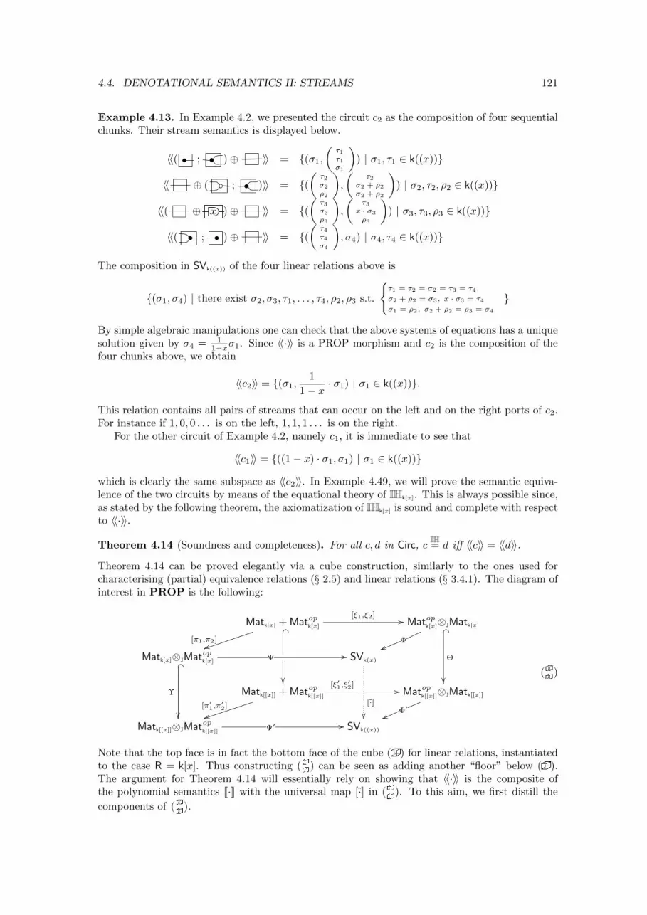
4.4. DENOTATIONAL SEMANTICS II: STREAMS 121
Example 4.13. In Example 4.2, we presented the circuit c2 as the composition of four sequentialchunks. Their stream semantics is displayed below.
〈〈( ; )⊕ 〉〉 = {(σ1,
(τ1τ1σ1
)) | σ1, τ1 ∈ k((x))}
〈〈 ⊕ ( ; )〉〉 = {((τ2σ2
ρ2
),
(τ2
σ2 + ρ2
σ2 + ρ2
)) | σ2, τ2, ρ2 ∈ k((x))}
〈〈( ⊕ x )⊕ 〉〉 = {((τ3σ3
ρ3
),
(τ3
x · σ3
ρ3
)) | σ3, τ3, ρ3 ∈ k((x))}
〈〈( ; )⊕ 〉〉 = {((τ4τ4σ4
), σ4) | σ4, τ4 ∈ k((x))}
The composition in SVk((x)) of the four linear relations above is
{(σ1, σ4) | there exist σ2, σ3, τ1, . . . , τ4, ρ2, ρ3 s.t.
{τ1 = τ2 = σ2 = τ3 = τ4,
σ2 + ρ2 = σ3, x · σ3 = τ4σ1 = ρ2, σ2 + ρ2 = ρ3 = σ4
}
By simple algebraic manipulations one can check that the above systems of equations has a uniquesolution given by σ4 = 1
1−xσ1. Since 〈〈·〉〉 is a PROP morphism and c2 is the composition of thefour chunks above, we obtain
〈〈c2〉〉 = {(σ1,1
1− x · σ1) | σ1 ∈ k((x))}.
This relation contains all pairs of streams that can occur on the left and on the right ports of c2.For instance if 1, 0, 0 . . . is on the left, 1, 1, 1 . . . is on the right.
For the other circuit of Example 4.2, namely c1, it is immediate to see that
〈〈c1〉〉 = {((1− x) · σ1, σ1) | σ1 ∈ k((x))}
which is clearly the same subspace as 〈〈c2〉〉. In Example 4.49, we will prove the semantic equiva-lence of the two circuits by means of the equational theory of IHk[x]. This is always possible since,as stated by the following theorem, the axiomatization of IHk[x] is sound and complete with respectto 〈〈·〉〉.
Theorem 4.14 (Soundness and completeness). For all c, d in Circ, cIH= d iff 〈〈c〉〉 = 〈〈d〉〉.
Theorem 4.14 can be proved elegantly via a cube construction, similarly to the ones used forcharacterising (partial) equivalence relations (§ 2.5) and linear relations (§ 3.4.1). The diagram ofinterest in PROP is the following:
Matk[x] + Matopk[x]� _
��
[π1,π2]tt
[ξ1,ξ2] // Matopk[x]⊗JMatk[x]
Φvv
� _
Θ
��
Matk[x]⊗JMatopk[x]Ψ //
� _
Υ
��
SVk(x)
[·]��
Matk[[x]] + Matopk[[x]]
[π′1,π′2]
tt
//[ξ′1,ξ′2]
Matopk[[x]]⊗JMatk[[x]]
Φ′
vvMatk[[x]]⊗JMatopk[[x]] Ψ′ // SVk((x))
(��
)
Note that the top face is in fact the bottom face of the cube (�) for linear relations, instantiatedto the case R = k[x]. Thus constructing (�
�) can be seen as adding another “floor” below (�).
The argument for Theorem 4.14 will essentially rely on showing that 〈〈·〉〉 is the composite ofthe polynomial semantics [[·]] with the universal map [·] in (�
�). To this aim, we first distill the
components of (��
).
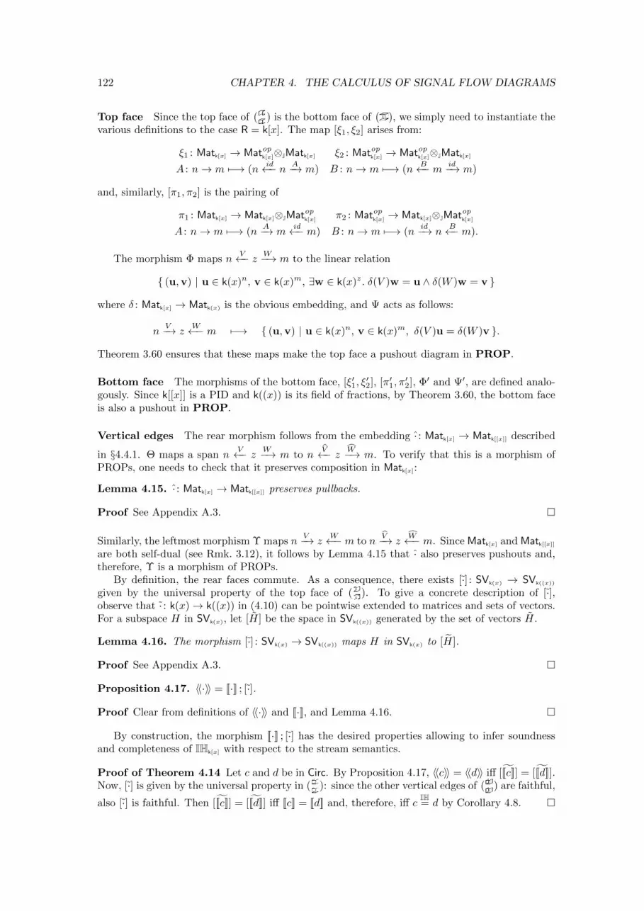
122 CHAPTER 4. THE CALCULUS OF SIGNAL FLOW DIAGRAMS
Top face Since the top face of (��
) is the bottom face of (�), we simply need to instantiate thevarious definitions to the case R = k[x]. The map [ξ1, ξ2] arises from:
ξ1 : Matk[x] → Matopk[x]⊗JMatk[x] ξ2 : Matopk[x] → Matopk[x]⊗JMatk[x]
A : n→ m 7−→ (nid←− n A−→ m) B : n→ m 7−→ (n
B←− m id−→ m)
and, similarly, [π1, π2] is the pairing of
π1 : Matk[x] → Matk[x]⊗JMatopk[x] π2 : Matopk[x] → Matk[x]⊗JMatopk[x]
A : n→ m 7−→ (nA−→ m
id←− m) B : n→ m 7−→ (nid−→ n
B←− m).
The morphism Φ maps nV←− z W−→ m to the linear relation
{ (u,v) | u ∈ k(x)n, v ∈ k(x)m, ∃w ∈ k(x)z. δ(V )w = u ∧ δ(W )w = v }
where δ : Matk[x] → Matk(x) is the obvious embedding, and Ψ acts as follows:
nV−→ z
W←− m 7−→ { (u,v) | u ∈ k(x)n, v ∈ k(x)m, δ(V )u = δ(W )v }.
Theorem 3.60 ensures that these maps make the top face a pushout diagram in PROP.
Bottom face The morphisms of the bottom face, [ξ′1, ξ′2], [π′1, π
′2], Φ′ and Ψ′, are defined analo-
gously. Since k[[x]] is a PID and k((x)) is its field of fractions, by Theorem 3.60, the bottom faceis also a pushout in PROP.
Vertical edges The rear morphism follows from the embedding · : Matk[x] → Matk[[x]] described
in §4.4.1. Θ maps a span nV←− z
W−→ m to nV←− z
W−→ m. To verify that this is a morphism ofPROPs, one needs to check that it preserves composition in Matk[x]:
Lemma 4.15. · : Matk[x] → Matk[[x]] preserves pullbacks.
Proof See Appendix A.3. �
Similarly, the leftmost morphism Υ maps nV−→ z
W←− m to nV−→ z
W←− m. Since Matk[x] and Matk[[x]]
are both self-dual (see Rmk. 3.12), it follows by Lemma 4.15 that · also preserves pushouts and,therefore, Υ is a morphism of PROPs.
By definition, the rear faces commute. As a consequence, there exists [·] : SVk(x) → SVk((x))
given by the universal property of the top face of (��
). To give a concrete description of [·],observe that · : k(x)→ k((x)) in (4.10) can be pointwise extended to matrices and sets of vectors.For a subspace H in SVk(x), let [H] be the space in SVk((x)) generated by the set of vectors H.
Lemma 4.16. The morphism [·] : SVk(x) → SVk((x)) maps H in SVk(x) to [H].
Proof See Appendix A.3. �
Proposition 4.17. 〈〈·〉〉 = [[·]] ; [·].
Proof Clear from definitions of 〈〈·〉〉 and [[·]], and Lemma 4.16. �
By construction, the morphism [[·]] ; [·] has the desired properties allowing to infer soundnessand completeness of IHk[x] with respect to the stream semantics.
Proof of Theorem 4.14 Let c and d be in Circ. By Proposition 4.17, 〈〈c〉〉 = 〈〈d〉〉 iff [[[c]]] = [[[d]]].Now, [·] is given by the universal property in (�
�): since the other vertical edges of (�
�) are faithful,
also [·] is faithful. Then [[[c]]] = [[[d]]] iff [[c]] = [[d]] and, therefore, iff cIH= d by Corollary 4.8. �
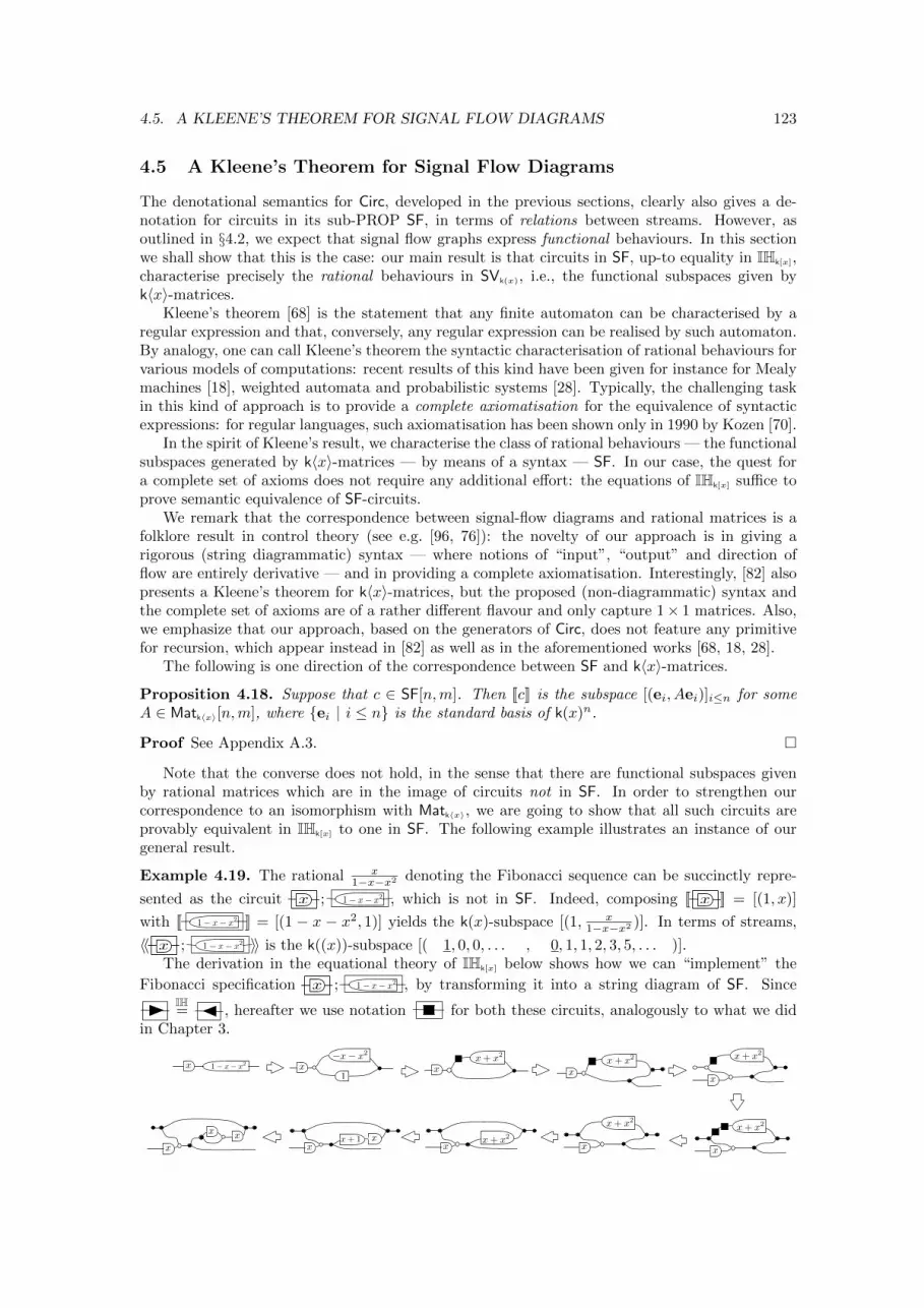
4.5. A KLEENE’S THEOREM FOR SIGNAL FLOW DIAGRAMS 123
4.5 A Kleene’s Theorem for Signal Flow Diagrams
The denotational semantics for Circ, developed in the previous sections, clearly also gives a de-notation for circuits in its sub-PROP SF, in terms of relations between streams. However, asoutlined in §4.2, we expect that signal flow graphs express functional behaviours. In this sectionwe shall show that this is the case: our main result is that circuits in SF, up-to equality in IHk[x],characterise precisely the rational behaviours in SVk(x), i.e., the functional subspaces given byk〈x〉-matrices.
Kleene’s theorem [68] is the statement that any finite automaton can be characterised by aregular expression and that, conversely, any regular expression can be realised by such automaton.By analogy, one can call Kleene’s theorem the syntactic characterisation of rational behaviours forvarious models of computations: recent results of this kind have been given for instance for Mealymachines [18], weighted automata and probabilistic systems [28]. Typically, the challenging taskin this kind of approach is to provide a complete axiomatisation for the equivalence of syntacticexpressions: for regular languages, such axiomatisation has been shown only in 1990 by Kozen [70].
In the spirit of Kleene’s result, we characterise the class of rational behaviours — the functionalsubspaces generated by k〈x〉-matrices — by means of a syntax — SF. In our case, the quest fora complete set of axioms does not require any additional effort: the equations of IHk[x] suffice toprove semantic equivalence of SF-circuits.
We remark that the correspondence between signal-flow diagrams and rational matrices is afolklore result in control theory (see e.g. [96, 76]): the novelty of our approach is in giving arigorous (string diagrammatic) syntax — where notions of “input”, “output” and direction offlow are entirely derivative — and in providing a complete axiomatisation. Interestingly, [82] alsopresents a Kleene’s theorem for k〈x〉-matrices, but the proposed (non-diagrammatic) syntax andthe complete set of axioms are of a rather different flavour and only capture 1× 1 matrices. Also,we emphasize that our approach, based on the generators of Circ, does not feature any primitivefor recursion, which appear instead in [82] as well as in the aforementioned works [68, 18, 28].
The following is one direction of the correspondence between SF and k〈x〉-matrices.
Proposition 4.18. Suppose that c ∈ SF[n,m]. Then [[c]] is the subspace [(ei, Aei)]i≤n for someA ∈ Matk〈x〉[n,m], where {ei | i ≤ n} is the standard basis of k(x)n.
Proof See Appendix A.3. �
Note that the converse does not hold, in the sense that there are functional subspaces givenby rational matrices which are in the image of circuits not in SF. In order to strengthen ourcorrespondence to an isomorphism with Matk〈x〉, we are going to show that all such circuits areprovably equivalent in IHk[x] to one in SF. The following example illustrates an instance of ourgeneral result.
Example 4.19. The rational x1−x−x2 denoting the Fibonacci sequence can be succinctly repre-
sented as the circuit x ; 1� x� x2 , which is not in SF. Indeed, composing [[ x ]] = [(1, x)]
with [[ 1� x� x2 ]] = [(1 − x − x2, 1)] yields the k(x)-subspace [(1, x1−x−x2 )]. In terms of streams,
〈〈 x ; 1� x� x2 〉〉 is the k((x))-subspace [( 1, 0, 0, . . . , 0, 1, 1, 2, 3, 5, . . . )].The derivation in the equational theory of IHk[x] below shows how we can “implement” the
Fibonacci specification x ; 1� x� x2 , by transforming it into a string diagram of SF. SinceIH= , hereafter we use notation for both these circuits, analogously to what we did
in Chapter 3.
x 1� x� x2 x
x
xx
xx
xxxx + 1
xx
1
�x� x2
xx + x2
x + x2 x + x2
x + x2x + x2
x + x2
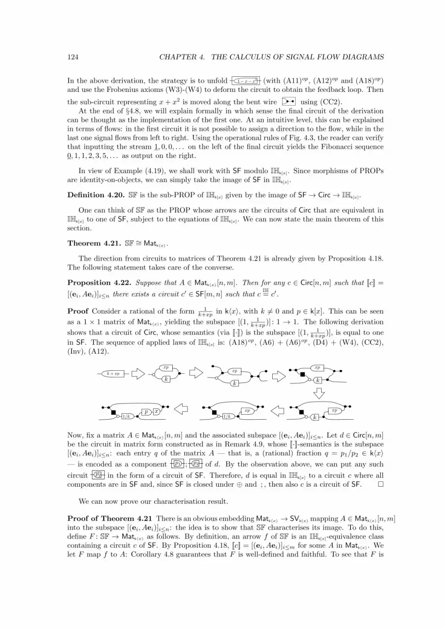
124 CHAPTER 4. THE CALCULUS OF SIGNAL FLOW DIAGRAMS
In the above derivation, the strategy is to unfold 1� x� x2 (with (A11)op, (A12)op and (A18)op)and use the Frobenius axioms (W3)-(W4) to deform the circuit to obtain the feedback loop. Then
the sub-circuit representing x+ x2 is moved along the bent wire using (CC2).At the end of §4.8, we will explain formally in which sense the final circuit of the derivation
can be thought as the implementation of the first one. At an intuitive level, this can be explainedin terms of flows: in the first circuit it is not possible to assign a direction to the flow, while in thelast one signal flows from left to right. Using the operational rules of Fig. 4.3, the reader can verifythat inputting the stream 1, 0, 0, . . . on the left of the final circuit yields the Fibonacci sequence0, 1, 1, 2, 3, 5, . . . as output on the right.
In view of Example (4.19), we shall work with SF modulo IHk[x]. Since morphisms of PROPsare identity-on-objects, we can simply take the image of SF in IHk[x].
Definition 4.20. SF is the sub-PROP of IHk[x] given by the image of SF→ Circ→ IHk[x].
One can think of SF as the PROP whose arrows are the circuits of Circ that are equivalent inIHk[x] to one of SF, subject to the equations of IHk[x]. We can now state the main theorem of thissection.
Theorem 4.21. SF ∼= Matk〈x〉.
The direction from circuits to matrices of Theorem 4.21 is already given by Proposition 4.18.The following statement takes care of the converse.
Proposition 4.22. Suppose that A ∈ Matk〈x〉[n,m]. Then for any c ∈ Circ[n,m] such that [[c]] =
[(ei, Aei)]i≤n there exists a circuit c′ ∈ SF[m,n] such that cIH= c′.
Proof Consider a rational of the form 1k+xp in k〈x〉, with k 6= 0 and p ∈ k[x]. This can be seen
as a 1 × 1 matrix of Matk〈x〉, yielding the subspace [(1, 1k+xp )] : 1 → 1. The following derivation
shows that a circuit of Circ, whose semantics (via [[·]]) is the subspace [(1, 1k+xp )], is equal to one
in SF. The sequence of applied laws of IHk[x] is: (A18)op , (A6) + (A6)op , (D4) + (W4), (CC2),(Inv), (A12).
k + xp
k
xp
k
xp
k
xp
k
xp
xp
1/k1/kxp
Now, fix a matrix A ∈ Matk〈x〉[n,m] and the associated subspace [(ei, Aei)]i≤n. Let d ∈ Circ[n,m]be the circuit in matrix form constructed as in Remark 4.9, whose [[·]]-semantics is the subspace[(ei, Aei)]i≤n: each entry q of the matrix A — that is, a (rational) fraction q = p1/p2 ∈ k〈x〉— is encoded as a component p1 ; p2 of d. By the observation above, we can put any such
circuit p2 in the form of a circuit of SF. Therefore, d is equal in IHk[x] to a circuit c where allcomponents are in SF and, since SF is closed under ⊕ and ; , then also c is a circuit of SF. �
We can now prove our characterisation result.
Proof of Theorem 4.21 There is an obvious embedding Matk〈x〉 → SVk(x) mappingA ∈ Matk〈x〉[n,m]into the subspace [(ei, Aei)]i≤n: the idea is to show that SF characterises its image. To do this,define F : SF → Matk〈x〉 as follows. By definition, an arrow f of SF is an IHk[x]-equivalence classcontaining a circuit c of SF. By Proposition 4.18, [[c]] = [(ei, Aei)]i≤m for some A in Matk〈x〉. Welet F map f to A: Corollary 4.8 guarantees that F is well-defined and faithful. To see that F is
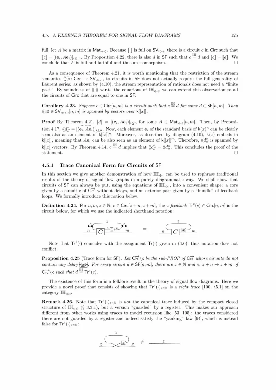
4.5. A KLEENE’S THEOREM FOR SIGNAL FLOW DIAGRAMS 125
full, let A be a matrix in Matk〈x〉. Because [[·]] is full on SVk(x), there is a circuit c in Circ such that
[[c]] = [(ei, Aei)]i≤m. By Proposition 4.22, there is also d in SF such that cIH= d and [[c]] = [[d]]. We
conclude that F is full and faithful and thus an isomorphism. �
As a consequence of Theorem 4.21, it is worth mentioning that the restriction of the streamsemantics 〈〈·〉〉 : Circ → SVk((x)) to circuits in SF does not actually require the full generality ofLaurent series: as shown by (4.10), the stream representation of rationals does not need a “finitepast.” By soundness of 〈〈·〉〉 w.r.t. the equations of IHk[x], we can extend this observation to allthe circuits of Circ that are equal to one in SF.
Corollary 4.23. Suppose c ∈ Circ[n,m] is a circuit such that cIH= d for some d ∈ SF[n,m]. Then
〈〈c〉〉 ∈ SVk((x))[n,m] is spanned by vectors over k[[x]].
Proof By Theorem 4.21, [[d]] = [(ei, Aei)]i≤n for some A ∈ Matk〈x〉[n,m]. Then, by Proposi-
tion 4.17, 〈〈d〉〉 = [ ˜(ei, Aei)]i≤n. Now, each element ei of the standard basis of k(x)n can be clearlyseen also as an element of k[[x]]n. Moreover, as described by diagram (4.10), k〈x〉 embeds ink[[x]], meaning that Aei can be also seen as an element of k[[x]]m. Therefore, 〈〈d〉〉 is spanned by
k[[x]]-vectors. By Theorem 4.14, cIH= d implies that 〈〈c〉〉 = 〈〈d〉〉. This concludes the proof of the
statement. �
4.5.1 Trace Canonical Form for Circuits of SF
In this section we give another demonstration of how IHk[x] can be used to rephrase traditionalresults of the theory of signal flow graphs in a purely diagrammatic way. We shall show thatcircuits of SF can always be put, using the equations of IHk[x], into a convenient shape: a coregiven by a circuit c of C−→irc without delays, and an exterior part given by a “bundle” of feedbackloops. We formally introduce this notion below.
Definition 4.24. For n,m, z ∈ N, c ∈ Circ[z + n, z +m], the z-feedback Trz(c) ∈ Circ[n,m] is thecircuit below, for which we use the indicated shorthand notation:
z
n C
zz
zzmx =:
n C
z
mx
Note that Tr1(·) coincides with the assignment Tr(·) given in (4.6), thus notation does notconflict.
Proposition 4.25 (Trace form for SF). Let C−→irc \x be the sub-PROP of C−→irc whose circuits do not
contain any delay x . For every circuit d ∈ SF[n,m], there are z ∈ N and c : z + n→ z +m of
C−→irc \x such that dIH= Trz(c).
The existence of this form is a folklore result in the theory of signal flow diagrams. Here weprovide a novel proof that consists of showing that Trz(·)z∈N is a right trace [100, §5.1] on thecategory IHk[x].
Remark 4.26. Note that Trz(·)z∈N is not the canonical trace induced by the compact closedstructure of IHk[x] (§ 3.3.1), but a version “guarded” by a register. This makes our approachdifferent from other works using traces to model recursion like [53, 105]: the traces consideredthere are not guarded by a register and indeed satisfy the “yanking” law [64], which is insteadfalse for Trz(·)z∈N:
x
z
z z 6= z .
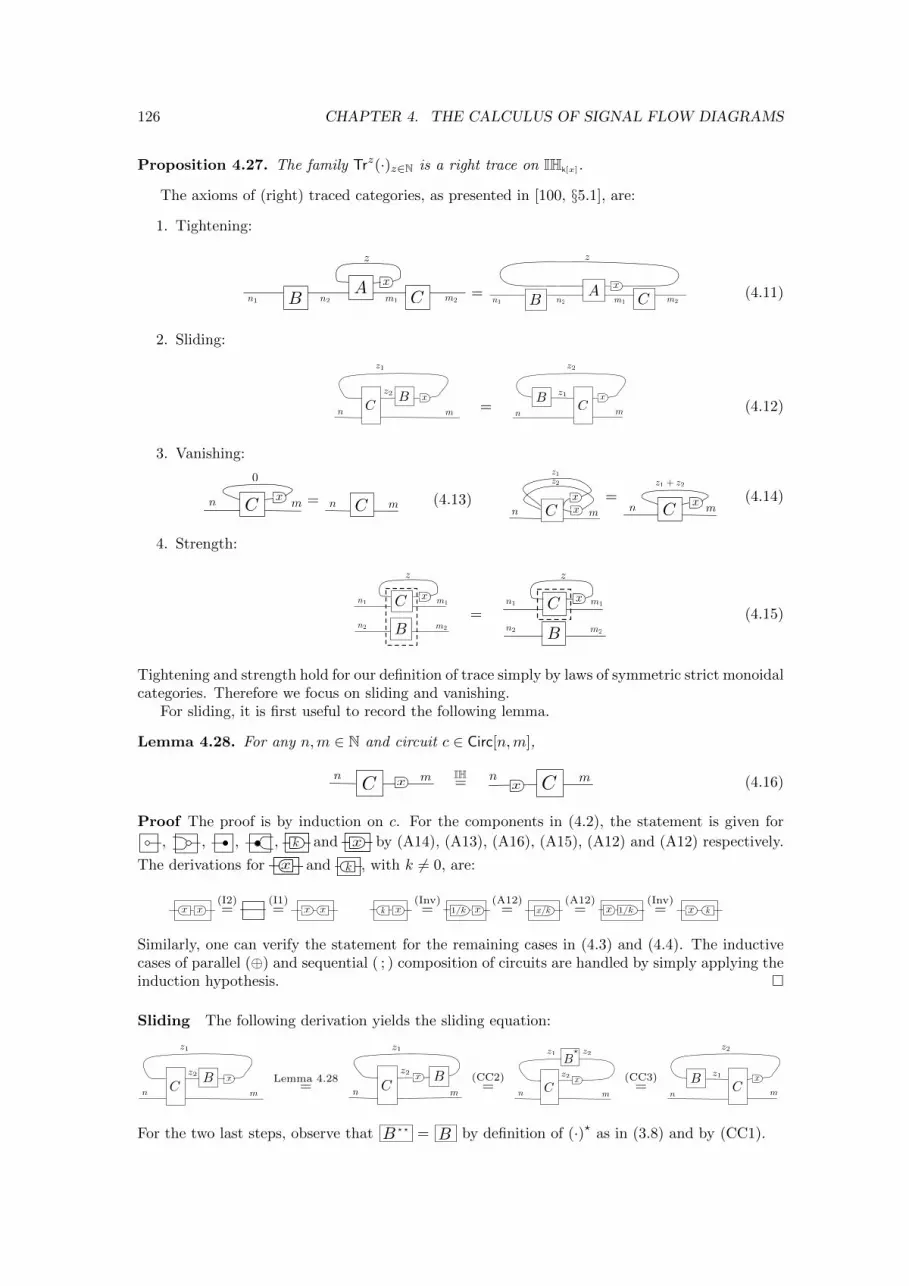
126 CHAPTER 4. THE CALCULUS OF SIGNAL FLOW DIAGRAMS
Proposition 4.27. The family Trz(·)z∈N is a right trace on IHk[x].
The axioms of (right) traced categories, as presented in [100, §5.1], are:
1. Tightening:
A x
B C
z
m1 m2n1 n2= A x
B C
z
m1 m2n1 n2(4.11)
2. Sliding:
x
n Cm
B
z1
z2
=x
nC m
B z1
z2
(4.12)
3. Vanishing:
Cxn m
0
= Cn m (4.13)C
xx
z1z2
n m
=C
xn m
z1 + z2
(4.14)
4. Strength:
xC
B
z
m1
m2
n1
n2
=xC
B
z
m1
m2
n1
n2
(4.15)
Tightening and strength hold for our definition of trace simply by laws of symmetric strict monoidalcategories. Therefore we focus on sliding and vanishing.
For sliding, it is first useful to record the following lemma.
Lemma 4.28. For any n,m ∈ N and circuit c ∈ Circ[n,m],
Cn mx
IH= n m
x C (4.16)
Proof The proof is by induction on c. For the components in (4.2), the statement is given for
, , , , k and x by (A14), (A13), (A16), (A15), (A12) and (A12) respectively.
The derivations for x and k , with k 6= 0, are:
xx (I2)=
(I1)= x x xk
(Inv)= x1/k
(A12)= x/k
(A12)= x 1/k
(Inv)= x k
Similarly, one can verify the statement for the remaining cases in (4.3) and (4.4). The inductivecases of parallel (⊕) and sequential ( ; ) composition of circuits are handled by simply applying theinduction hypothesis. �
Sliding The following derivation yields the sliding equation:
x
n Cm
B
z1
z2Lemma 4.28
= n Cm
B
z1
z2 x (CC2)=
n Cm
z1
z2 x
z2?B
(CC3)=
x
nC m
B z1
z2
For the two last steps, observe that B ? ? = B by definition of (·)? as in (3.8) and by (CC1).
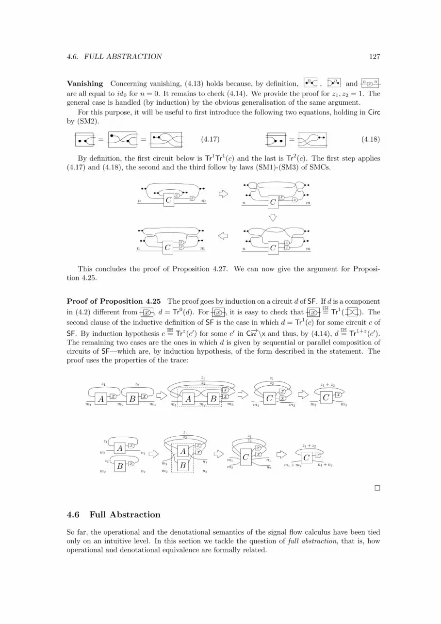
4.6. FULL ABSTRACTION 127
Vanishing Concerning vanishing, (4.13) holds because, by definition,n
,n
and n x n
are all equal to id0 for n = 0. It remains to check (4.14). We provide the proof for z1, z2 = 1. Thegeneral case is handled (by induction) by the obvious generalisation of the same argument.
For this purpose, it will be useful to first introduce the following two equations, holding in Circby (SM2).
= = (4.17) = (4.18)
By definition, the first circuit below is Tr1Tr1(c) and the last is Tr2(c). The first step applies(4.17) and (4.18), the second and the third follow by laws (SM1)-(SM3) of SMCs.
n mx
xC n mx
xC
n m
xxCn m
xxC
This concludes the proof of Proposition 4.27. We can now give the argument for Proposi-tion 4.25.
Proof of Proposition 4.25 The proof goes by induction on a circuit d of SF. If d is a component
in (4.2) different from x , d = Tr0(d). For x , it is easy to check that xIH= Tr1( ). The
second clause of the inductive definition of SF is the case in which d = Tr1(c) for some circuit c of
SF. By induction hypothesis cIH= Trz(c′) for some c′ in C−→irc \x and thus, by (4.14), d
IH= Tr1+z(c′).
The remaining two cases are the ones in which d is given by sequential or parallel composition ofcircuits of SF—which are, by induction hypothesis, of the form described in the statement. Theproof uses the properties of the trace:
BA x x
m1 m2 m3
z1 z2
BAxx
m1 m2 m3
z1
z2
Cxx
m1 m3
z1z2
C x
m1 m3
z1 + z2
A x
B x
Ax
B
xC
xx
C xm1
m2
n1
n2
z1
z2 m1
m2
n1
n2
z1z2
m1
m2
n1
n2
z1z2
z1 + z2
m1 + m2 n1 + n2
�
4.6 Full Abstraction
So far, the operational and the denotational semantics of the signal flow calculus have been tiedonly on an intuitive level. In this section we tackle the question of full abstraction, that is, howoperational and denotational equivalence are formally related.
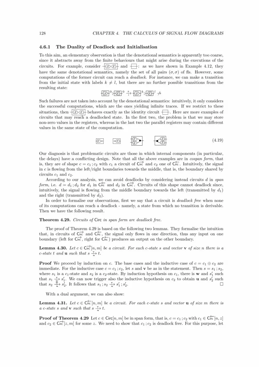
128 CHAPTER 4. THE CALCULUS OF SIGNAL FLOW DIAGRAMS
4.6.1 The Duality of Deadlock and Initialisation
To this aim, an elementary observation is that the denotational semantics is apparently too coarse,since it abstracts away from the finite behaviours that might arise during the executions of the
circuits. For example, consider x x and : as we have shown in Example 4.12, they
have the same denotational semantics, namely the set of all pairs (σ, σ) of fls. However, somecomputations of the former circuit can reach a deadlock. For instance, we can make a transitionfrom the initial state with labels k 6= l, but there are no further possible transitions from theresulting state:
x 0; x 0 k−→l
x k; x l 6→Such failures are not taken into account by the denotational semantics: intuitively, it only considersthe successful computations, which are the ones yielding infinite traces. If we restrict to these
situations, then x x behaves exactly as the identity circuit . Here are more examples ofcircuits that may reach a deadlocked state. In the first two, the problem is that we may storenon-zero values in the registers, whereas in the last two the parallel registers may contain differentvalues in the same state of the computation.
x xxx x
x (4.19)
Our diagnosis is that problematic circuits are those in which internal components (in particular,the delays) have a conflicting design. Note that all the above examples are in cospan form, thatis, they are of shape c = c1 ; c2 with c1 a circuit of C−→irc and c2 one of C←−irc . Intuitively, the signalin c is flowing from the left/right boundaries towards the middle, that is, the boundary shared bycircuits c1 and c2.
According to our analysis, we can avoid deadlocks by considering instead circuits d in spanform, i.e. d = d1 ; d2 for d1 in C←−irc and d2 in C−→irc . Circuits of this shape cannot deadlock since,intuitively, the signal is flowing from the middle boundary towards the left (transmitted by d1)and the right (transmitted by d2).
In order to formalise our observations, first we say that a circuit is deadlock free when noneof its computations can reach a deadlock - namely, a state from which no transition is derivable.Then we have the following result.
Theorem 4.29. Circuits of Circ in span form are deadlock free.
The proof of Theorem 4.29 is based on the following two lemmas. They formalise the intuitionthat, in circuits of C−→irc and C←−irc , the signal only flows in one direction, thus any input on oneboundary (left for C−→irc , right for C←−irc ) produces an output on the other boundary.
Lemma 4.30. Let c ∈ C−→irc [n,m] be a circuit. For each c-state s and vector v of size n there is ac-state t and u such that s
v−→ut.
Proof We proceed by induction on c. The base cases and the inductive case of c = c1 ⊕ c2 areimmediate. For the inductive case c = c1 ; c2, let s and v be as in the statement. Then s = s1 ; s2,where s1 is a c1-state and s2 is a c2-state. By induction hypothesis on c1, there is w and s′1 suchthat s1
v−→ws′1. We can now trigger also the inductive hypothesis on c2 to obtain u and s′2 such
that s2w−−→us′2. It follows that s1 ; s2
v−→us′1 ; s′2. �
With a dual argument, we can also show:
Lemma 4.31. Let c ∈ C←−irc [n,m] be a circuit. For each c-state s and vector u of size m there isa c-state s and v such that s
v−→ut.
Proof of Theorem 4.29 Let c ∈ Circ[n,m] be in span form, that is, c = c1 ; c2 with c1 ∈ C←−irc [n, z]and c2 ∈ C−→irc [z,m] for some z. We need to show that c1 ; c2 is deadlock free. For this purpose, let
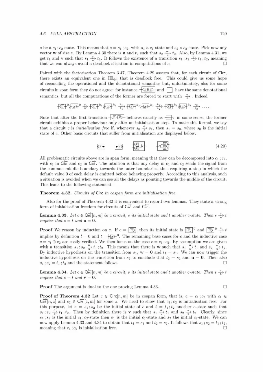
4.6. FULL ABSTRACTION 129
s be a c1 ; c2-state. This means that s = s1 ; s2, with s1 a c1-state and s2 a c2-state. Pick now anyvector w of size z. By Lemma 4.30 there is u and t2 such that s2
w−−→ut2. Also, by Lemma 4.31, we
get t1 and v such that s1v−→wt1. It follows the existence of a transition s1 ; s2
v−→ut1 ; t2, meaning
that we can always avoid a deadlock situation in computations of c. �
Paired with the factorisation Theorem 3.47, Theorem 4.29 asserts that, for each circuit of Circ,there exists an equivalent one in IHk[x] that is deadlock free. This could give us some hopeof reconciling the operational and the denotational semantics but, unfortunately, also for some
circuits in span form they do not agree: for instance, xx
and have the same denotational
semantics, but all the computations of the former are forced to start with0−→0
. Indeed
x 0; x 0 0−→0
x k1 ; x k1k1−−→k1
x k2 ; x k2k2−−→k2
x k3 ; x k3k3−−→k3
. . . .
Note that after the first transition xx
behaves exactly as : in some sense, the formercircuit exhibits a proper behaviour only after an initialisation step. To make this formal, we saythat a circuit c is initialisation free if, whenever s0
0−→0s1, then s1 = s0, where s0 is the initial
state of c. Other basic circuits that suffer from initialisation are displayed below.
x xxx
xx (4.20)
All problematic circuits above are in span form, meaning that they can be decomposed into c1 ; c2,with c1 in C←−irc and c2 in C−→irc . The intuition is that any delay in c1 and c2 sends the signal fromthe common middle boundary towards the outer boundaries, thus requiring a step in which thedefault value 0 of each delay is emitted before behaving properly. According to this analysis, sucha situation is avoided when we can see all the delays as pointing towards the middle of the circuit.This leads to the following statement.
Theorem 4.32. Circuits of Circ in cospan form are initialisation free.
Also for the proof of Theorem 4.32 it is convenient to record two lemmas. They state a strongform of initialisation freedom for circuits of C−→irc and C←−irc .
Lemma 4.33. Let c ∈ C−→irc [n,m] be a circuit, s its initial state and t another c-state. Then s0−→ut
implies that s = t and u = 0.
Proof We reason by induction on c. If c = x , then its initial state is x 0 and x 0 0−→lt
implies by definition l = 0 and t = x 0. The remaining base cases for c and the inductive casec = c1 ⊕ c2 are easily verified. We then focus on the case c = c1 ; c2. By assumption we are givenwith a transition s1 ; s2
0−→ut1 ; t2. This means that there is w such that s1
0−→wt1 and s2
w−−→ut2.
By inductive hypothesis on the transition from s1, w = 0 and t1 = s1. We can now trigger theinductive hypothesis on the transition from s2 to conclude that t2 = s2 and u = 0. Then alsos1 ; s2 = t1 ; t2 and the statement follows. �
Lemma 4.34. Let c ∈ C←−irc [n,m] be a circuit, s its initial state and t another c-state. Then sv−→0t
implies that s = t and v = 0.
Proof The argument is dual to the one proving Lemma 4.33. �
Proof of Theorem 4.32 Let c ∈ Circ[n,m] be in cospan form, that is, c = c1 ; c2 with c1 ∈C−→irc [n, z] and c2 ∈ C←−irc [z,m] for some z. We need to show that c1 ; c2 is initialisation free. Forthis purpose, let s = s1 ; s2 be the initial state of c and t = t1 ; t2 another c-state such thats1 ; s2
0−→0t1 ; t2. Then by definition there is v such that s1
0−→vt1 and s2
v−→0t2. Clearly, since
s1 ; s2 is the initial c1 ; c2-state then s1 is the initial c1-state and s2 the initial c2-state. We cannow apply Lemma 4.33 and 4.34 to obtain that t1 = s1 and t2 = s2. It follows that s1 ; s2 = t1 ; t2,meaning that c1 ; c2 is initialisation free. �
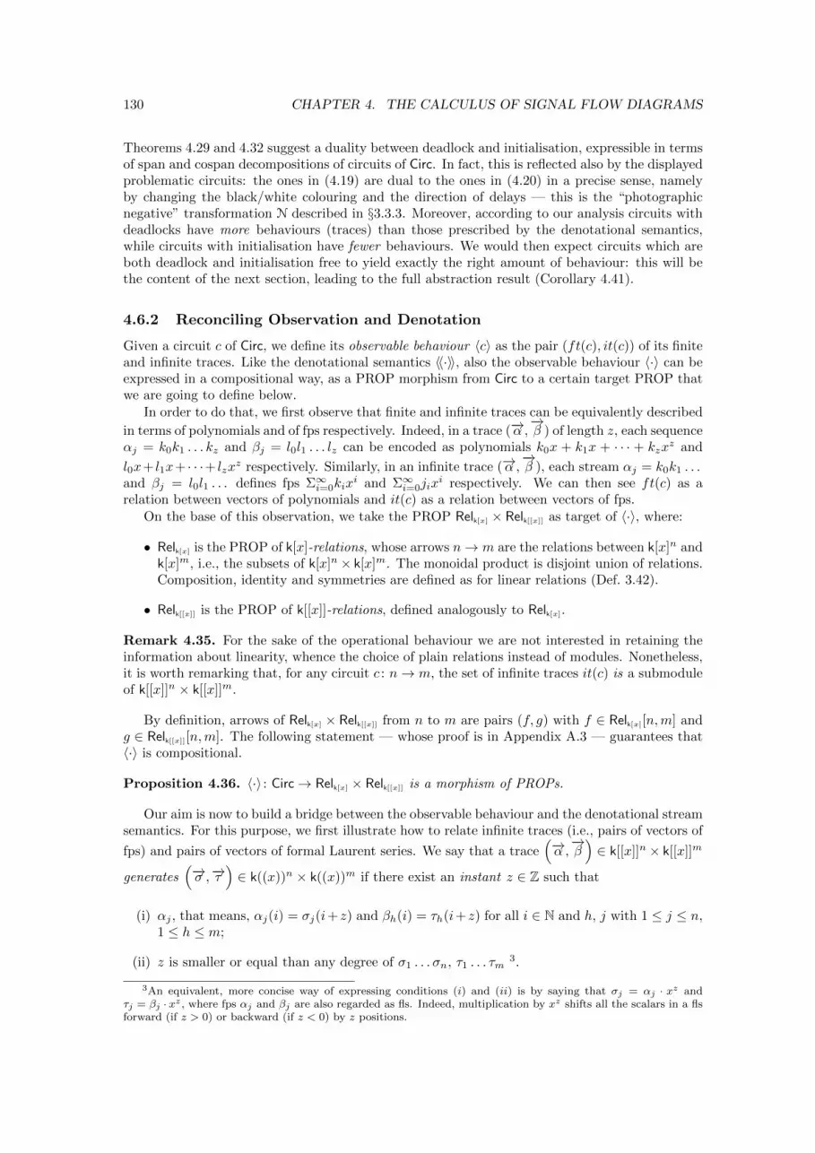
130 CHAPTER 4. THE CALCULUS OF SIGNAL FLOW DIAGRAMS
Theorems 4.29 and 4.32 suggest a duality between deadlock and initialisation, expressible in termsof span and cospan decompositions of circuits of Circ. In fact, this is reflected also by the displayedproblematic circuits: the ones in (4.19) are dual to the ones in (4.20) in a precise sense, namelyby changing the black/white colouring and the direction of delays — this is the “photographicnegative” transformation N described in §3.3.3. Moreover, according to our analysis circuits withdeadlocks have more behaviours (traces) than those prescribed by the denotational semantics,while circuits with initialisation have fewer behaviours. We would then expect circuits which areboth deadlock and initialisation free to yield exactly the right amount of behaviour: this will bethe content of the next section, leading to the full abstraction result (Corollary 4.41).
4.6.2 Reconciling Observation and Denotation
Given a circuit c of Circ, we define its observable behaviour 〈c〉 as the pair (ft(c), it(c)) of its finiteand infinite traces. Like the denotational semantics 〈〈·〉〉, also the observable behaviour 〈·〉 can beexpressed in a compositional way, as a PROP morphism from Circ to a certain target PROP thatwe are going to define below.
In order to do that, we first observe that finite and infinite traces can be equivalently described
in terms of polynomials and of fps respectively. Indeed, in a trace (−→α ,−→β ) of length z, each sequenceαj = k0k1 . . . kz and βj = l0l1 . . . lz can be encoded as polynomials k0x + k1x + · · · + kzx
z and
l0x+ l1x+ · · ·+ lzxz respectively. Similarly, in an infinite trace (−→α ,−→β ), each stream αj = k0k1 . . .
and βj = l0l1 . . . defines fps Σ∞i=0kixi and Σ∞i=0jix
i respectively. We can then see ft(c) as arelation between vectors of polynomials and it(c) as a relation between vectors of fps.
On the base of this observation, we take the PROP Relk[x] × Relk[[x]] as target of 〈·〉, where:
• Relk[x] is the PROP of k[x]-relations, whose arrows n→ m are the relations between k[x]n andk[x]m, i.e., the subsets of k[x]n× k[x]m. The monoidal product is disjoint union of relations.Composition, identity and symmetries are defined as for linear relations (Def. 3.42).
• Relk[[x]] is the PROP of k[[x]]-relations, defined analogously to Relk[x].
Remark 4.35. For the sake of the operational behaviour we are not interested in retaining theinformation about linearity, whence the choice of plain relations instead of modules. Nonetheless,it is worth remarking that, for any circuit c : n→ m, the set of infinite traces it(c) is a submoduleof k[[x]]n × k[[x]]m.
By definition, arrows of Relk[x] × Relk[[x]] from n to m are pairs (f, g) with f ∈ Relk[x][n,m] andg ∈ Relk[[x]][n,m]. The following statement — whose proof is in Appendix A.3 — guarantees that〈·〉 is compositional.
Proposition 4.36. 〈·〉 : Circ→ Relk[x] × Relk[[x]] is a morphism of PROPs.
Our aim is now to build a bridge between the observable behaviour and the denotational streamsemantics. For this purpose, we first illustrate how to relate infinite traces (i.e., pairs of vectors of
fps) and pairs of vectors of formal Laurent series. We say that a trace(−→α ,−→β
)∈ k[[x]]n × k[[x]]m
generates(−→σ ,−→τ
)∈ k((x))n × k((x))m if there exist an instant z ∈ Z such that
(i) αj , that means, αj(i) = σj(i+ z) and βh(i) = τh(i+ z) for all i ∈ N and h, j with 1 ≤ j ≤ n,1 ≤ h ≤ m;
(ii) z is smaller or equal than any degree of σ1 . . . σn, τ1 . . . τm3.
3An equivalent, more concise way of expressing conditions (i) and (ii) is by saying that σj = αj · xz andτj = βj · xz , where fps αj and βj are also regarded as fls. Indeed, multiplication by xz shifts all the scalars in a flsforward (if z > 0) or backward (if z < 0) by z positions.
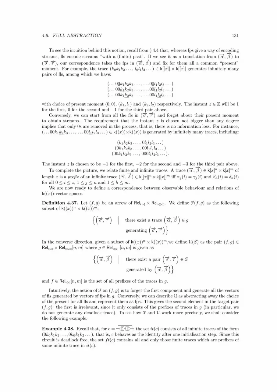
4.6. FULL ABSTRACTION 131
To see the intuition behind this notion, recall from § 4.4 that, whereas fps give a way of encoding
streams, fls encode streams “with a (finite) past”. If we see it as a translation from (−→α ,−→β ) to
(−→σ ,−→τ ), our correspondence takes the fps in (−→α ,−→β ) and fix for them all a common “present”moment. For example, the trace (k0k1k2 . . . , l0l1l2 . . . ) ∈ k[[x]] × k[[x]] generates infinitely manypairs of fls, among which we have:
(. . . 00k1k2k3 . . . , . . . 00l1l2l3 . . . )(. . . 00k1k2k3 . . . , . . . 00l1l2l3 . . . )(. . . 00k1k2k3 . . . , . . . 00l1l2l3 . . . )
with choice of present moment (0, 0), (k1, l1) and (k2, l2) respectively. The instant z ∈ Z will be 1for the first, 0 for the second and −1 for the third pair above.
Conversely, we can start from all the fls in (−→σ ,−→τ ) and forget about their present momentto obtain streams. The requirement that the instant z is chosen not bigger than any degreeimplies that only 0s are removed in the process, that is, there is no information loss. For instance,(. . . 00k1k2k3 . . . , . . . 00l1l2l3 . . . ) ∈ k((x))×k((x)) is generated by infinitely many traces, including:
(k1k2k3 . . . , 0l1l2l3 . . . )(0k1k2k3 . . . , 00l1l2l3 . . . )
(00k1k2k3 . . . , 000l1l2l3 . . . ).
The instant z is chosen to be −1 for the first, −2 for the second and −3 for the third pair above.
To complete the picture, we relate finite and infinite traces. A trace (−→α ,−→β ) ∈ k[x]n× k[x]m of
length z is a prefix of an infinite trace (−→γ ,−→δ ) ∈ k[[x]]n×k[[x]]m iff αj(i) = γj(i) and βh(i) = δh(i)for all 0 ≤ i ≤ z, 1 ≤ j ≤ n and 1 ≤ h ≤ m.
We are now ready to define a correspondence between observable behaviour and relations ofk((x))-vector spaces.
Definition 4.37. Let (f, g) be an arrow of Relk[x] × Relk[[x]]. We define F(f, g) as the followingsubset of k((x))n × k((x))m:
{(−→σ ,−→τ) ∣∣∣ there exist a trace
(−→α ,−→β)∈ g
generating(−→σ ,−→τ
)}
In the converse direction, given a subset of k((x))n × k((x))m,we define U(S) as the pair (f, g) ∈Relk[x] × Relk[[x]][n,m] where g ∈ Relk[[x]][n,m] is given as
{(−→α ,−→β) ∣∣∣ there exist a pair
(−→σ ,−→τ)∈ S
generated by(−→α ,−→β
)}
and f ∈ Relk[x][n,m] is the set of all prefixes of the traces in g.
Intuitively, the action of F on (f, g) is to forget the first component and generate all the vectorsof fls generated by vectors of fps in g. Conversely, we can describe U as abstracting away the choiceof the present for all fls and represent them as fps. This gives the second element in the target pair(f, g): the first is irrelevant, since it only consists of the prefixes of traces in g (in particular, wedo not generate any deadlock trace). To see how F and U work more precisely, we shall considerthe following example.
Example 4.38. Recall that, for c = xx
, the set it(c) consists of all infinite traces of the form(0k0k1k2 . . . , 0k0k1k2 . . . ), that is, c behaves as the identity after one initialisation step. Since thiscircuit is deadlock free, the set ft(c) contains all and only those finite traces which are prefixes ofsome infinite trace in it(c).
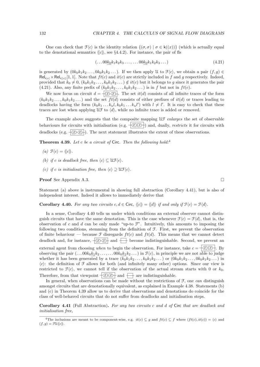
132 CHAPTER 4. THE CALCULUS OF SIGNAL FLOW DIAGRAMS
One can check that F〈c〉 is the identity relation {(σ, σ) | σ ∈ k((x))} (which is actually equalto the denotational semantics 〈〈c〉〉, see §4.4.2). For instance, the pair of fls
(. . . 00k0k1k2k3 . . . , . . . 00k0k1k2k3 . . . ) (4.21)
is generated by (0k0k1k2 . . . , 0k0k1k2 . . . ). If we then apply U to F〈c〉, we obtain a pair (f, g) ∈Relk[x]×Relk[[x]][1, 1]. Note that ft(c) and it(c) are strictly included in f and g respectively. Indeed,provided that k0 6= 0, (k0k1k2 . . . , k0k1k2 . . . ) /∈ it(c) but it belongs to g since it generates the pair(4.21). Also, any finite prefix of (k0k1k2 . . . , k0k1k2 . . . ) is in f but not in ft(c).
We now focus on circuit d = x x . The set it(d) consists of all infinite traces of the form
(k0k1k2 . . . , k0k1k2 . . . ) and the set ft(d) consists of either prefixes of it(d) or traces leading todeadlocks having the form (k0k1 . . . kul, k0k1 . . . kul
′) with l 6= l′. It is easy to check that thesetraces are lost when applying UF to 〈d〉, while no infinite trace is added or removed.
The example above suggests that the composite mapping UF enlarges the set of observable
behaviours for circuits with initialisation (e.g. xx
) and, dually, restricts it for circuits with
deadlocks (e.g. x x ). The next statement illustrates the extent of these observations.
Theorem 4.39. Let c be a circuit of Circ. Then the following hold:4
(a) F〈c〉 = 〈〈c〉〉.
(b) if c is deadlock free, then 〈c〉 ⊆ UF〈c〉.
(c) if c is initialisation free, then 〈c〉 ⊇ UF〈c〉.
Proof See Appendix A.3. �
Statement (a) above is instrumental in showing full abstraction (Corollary 4.41), but is also ofindependent interest. Indeed it allows to immediately derive that
Corollary 4.40. For any two circuits c, d ∈ Circ, 〈〈c〉〉 = 〈〈d〉〉 if and only if F〈c〉 = F〈d〉.
In a sense, Corollary 4.40 tells us under which conditions an external observer cannot distin-guish circuits that have the same denotation. This is the case whenever F〈c〉 = F〈d〉, that is, theobservation of c and d can be only made “up-to F”. Intuitively, this amounts to imposing thefollowing two conditions, stemming from the definition of F. First, we prevent the observationof finite behaviour — because F disregards ft(c) and ft(d). This means that we cannot detect
deadlock and, for instance, x x and become indistinguishable. Second, we prevent an
external agent from choosing when to begin the observation. For instance, take c = xx
. Byobserving the pair (. . . 00k0k1k2 . . . , . . . 00k0k1k2 . . . ) in F〈c〉, in principle we are not able to judgewhether it has been generated by a trace (k0k1k2 . . . , k0k1k2 . . . ) or (0k0k1k2 . . . , 0k0k1k2 . . . ) in〈c〉: the definition of F allows for both (and infinitely many other) options. Since our view isrestricted to F〈c〉, we cannot tell if the observation of the actual stream starts with 0 or k0.
Therefore, from that viewpoint xx
and are indistinguishable.In general, when observations can be made without the restrictions of F, one can distinguish
amongst circuits that are denotationally equivalent, as explained in Example 4.38. Statements (b)and (c) in Theorem 4.39 allow us to derive that observations and denotations do coincide for theclass of well-behaved circuits that do not suffer from deadlocks and initialisation steps.
Corollary 4.41 (Full Abstraction). For any two circuits c and d of Circ that are deadlock andinitialisation free,
4The inclusions are meant to be component-wise, e.g. it(c) ⊆ g and ft(c) ⊆ f where (ft(c), it(c)) = 〈c〉 and(f, g) = FU〈〈c〉〉.
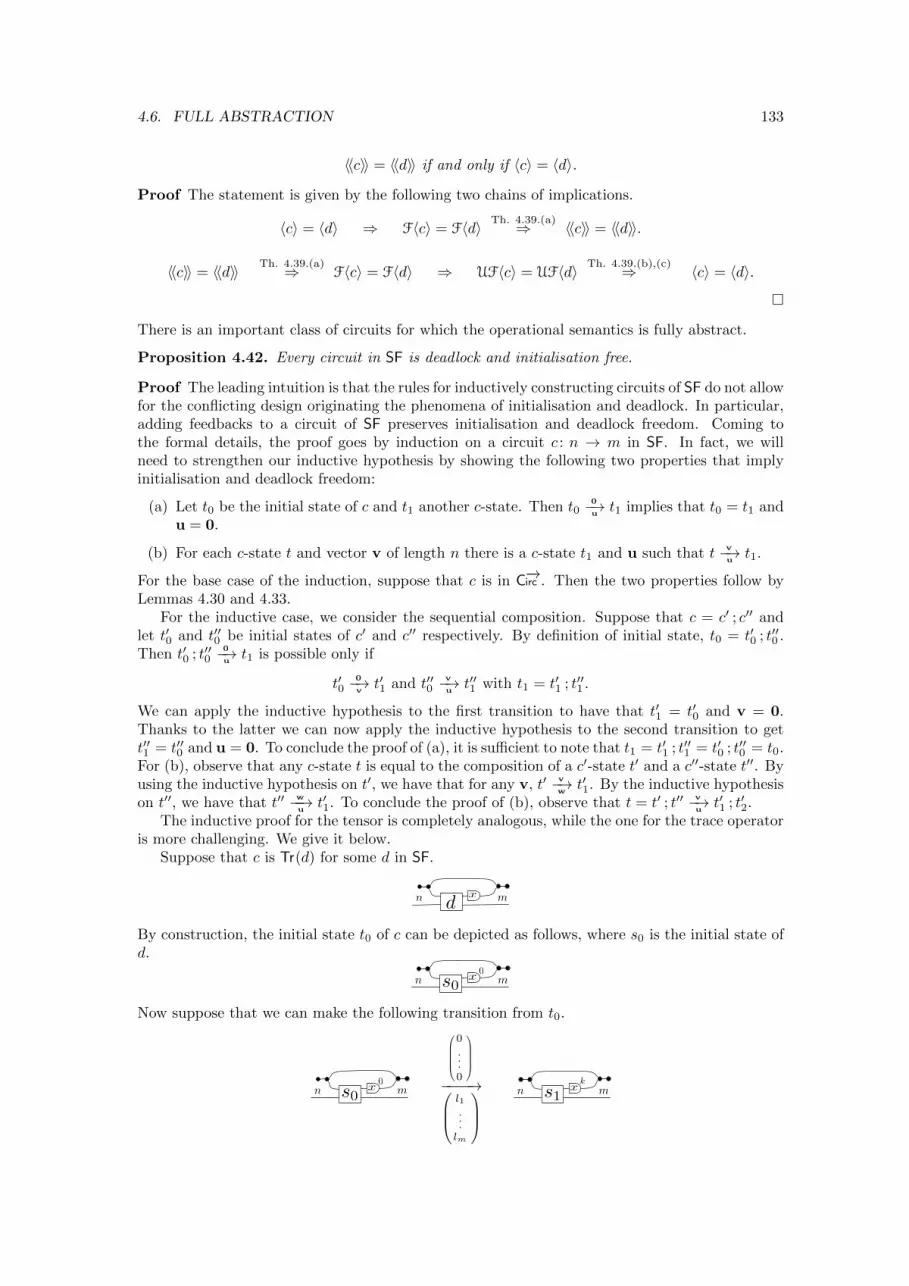
4.6. FULL ABSTRACTION 133
〈〈c〉〉 = 〈〈d〉〉 if and only if 〈c〉 = 〈d〉.
Proof The statement is given by the following two chains of implications.
〈c〉 = 〈d〉 ⇒ F〈c〉 = F〈d〉 Th. 4.39.(a)⇒ 〈〈c〉〉 = 〈〈d〉〉.
〈〈c〉〉 = 〈〈d〉〉 Th. 4.39.(a)⇒ F〈c〉 = F〈d〉 ⇒ UF〈c〉 = UF〈d〉 Th. 4.39.(b),(c)⇒ 〈c〉 = 〈d〉.�
There is an important class of circuits for which the operational semantics is fully abstract.
Proposition 4.42. Every circuit in SF is deadlock and initialisation free.
Proof The leading intuition is that the rules for inductively constructing circuits of SF do not allowfor the conflicting design originating the phenomena of initialisation and deadlock. In particular,adding feedbacks to a circuit of SF preserves initialisation and deadlock freedom. Coming tothe formal details, the proof goes by induction on a circuit c : n → m in SF. In fact, we willneed to strengthen our inductive hypothesis by showing the following two properties that implyinitialisation and deadlock freedom:
(a) Let t0 be the initial state of c and t1 another c-state. Then t00−→ut1 implies that t0 = t1 and
u = 0.
(b) For each c-state t and vector v of length n there is a c-state t1 and u such that tv−→ut1.
For the base case of the induction, suppose that c is in C−→irc . Then the two properties follow byLemmas 4.30 and 4.33.
For the inductive case, we consider the sequential composition. Suppose that c = c′ ; c′′ andlet t′0 and t′′0 be initial states of c′ and c′′ respectively. By definition of initial state, t0 = t′0 ; t′′0 .Then t′0 ; t′′0
0−→ut1 is possible only if
t′00−→vt′1 and t′′0
v−→ut′′1 with t1 = t′1 ; t′′1 .
We can apply the inductive hypothesis to the first transition to have that t′1 = t′0 and v = 0.Thanks to the latter we can now apply the inductive hypothesis to the second transition to gett′′1 = t′′0 and u = 0. To conclude the proof of (a), it is sufficient to note that t1 = t′1 ; t′′1 = t′0 ; t′′0 = t0.For (b), observe that any c-state t is equal to the composition of a c′-state t′ and a c′′-state t′′. Byusing the inductive hypothesis on t′, we have that for any v, t′ v−→
wt′1. By the inductive hypothesis
on t′′, we have that t′′ w−−→ut′1. To conclude the proof of (b), observe that t = t′ ; t′′ v−→
ut′1 ; t′2.
The inductive proof for the tensor is completely analogous, while the one for the trace operatoris more challenging. We give it below.
Suppose that c is Tr(d) for some d in SF.
mn xd
By construction, the initial state t0 of c can be depicted as follows, where s0 is the initial state ofd.
mn xs00
Now suppose that we can make the following transition from t0.
mn xs00
0
.
.
.0
−−−−→l1...lm
mn xs1
k
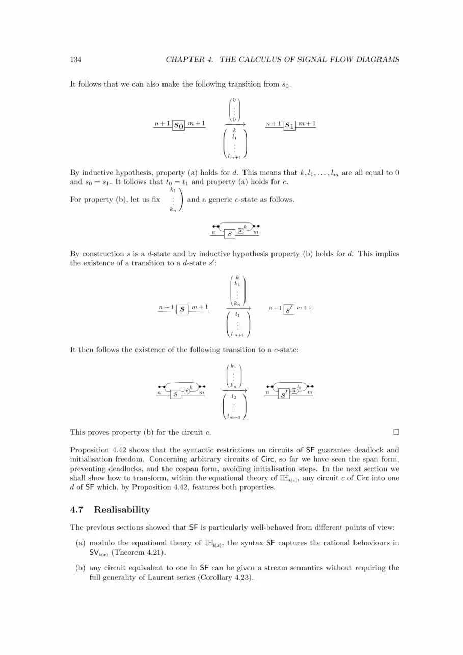
134 CHAPTER 4. THE CALCULUS OF SIGNAL FLOW DIAGRAMS
It follows that we can also make the following transition from s0.
n + 1 m + 1s0
0
.
.
.0
−−−−→
kl1...
lm+1
s1n + 1 m + 1
By inductive hypothesis, property (a) holds for d. This means that k, l1, . . . , lm are all equal to 0and s0 = s1. It follows that t0 = t1 and property (a) holds for c.
For property (b), let us fix
(k1
.
.
.kn
)and a generic c-state as follows.
mn xk
s
By construction s is a d-state and by inductive hypothesis property (b) holds for d. This impliesthe existence of a transition to a d-state s′:
n + 1 m + 1s
kk1
.
.
.kn
−−−−−→
l1...
lm+1
n + 1 m + 1s0
It then follows the existence of the following transition to a c-state:
mn xk
s
k1
.
.
.kn
−−−−−→
l2...
lm+1
l1
mn xs0
This proves property (b) for the circuit c. �
Proposition 4.42 shows that the syntactic restrictions on circuits of SF guarantee deadlock andinitialisation freedom. Concerning arbitrary circuits of Circ, so far we have seen the span form,preventing deadlocks, and the cospan form, avoiding initialisation steps. In the next section weshall show how to transform, within the equational theory of IHk[x], any circuit c of Circ into oned of SF which, by Proposition 4.42, features both properties.
4.7 Realisability
The previous sections showed that SF is particularly well-behaved from different points of view:
(a) modulo the equational theory of IHk[x], the syntax SF captures the rational behaviours inSVk(x) (Theorem 4.21).
(b) any circuit equivalent to one in SF can be given a stream semantics without requiring thefull generality of Laurent series (Corollary 4.23).
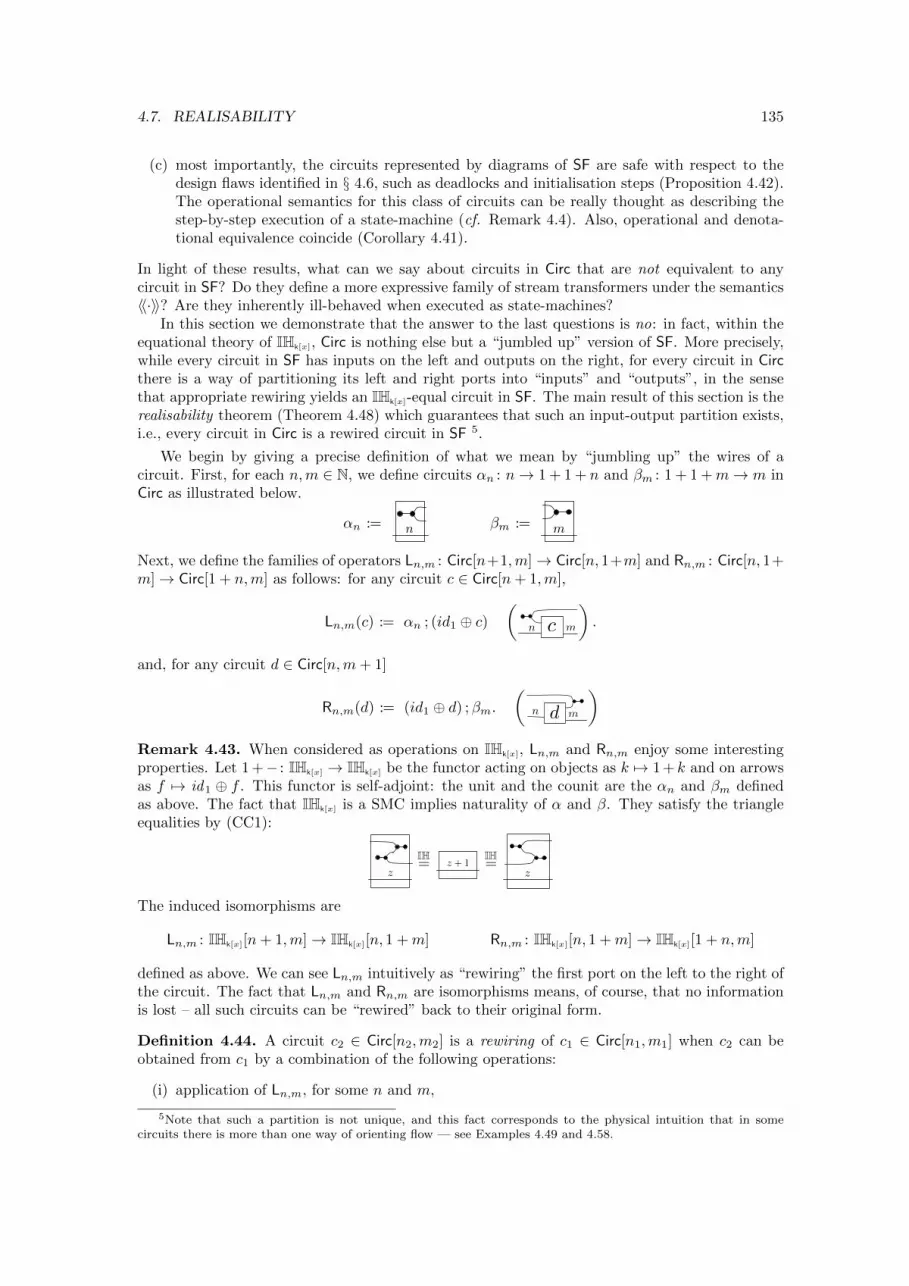
4.7. REALISABILITY 135
(c) most importantly, the circuits represented by diagrams of SF are safe with respect to thedesign flaws identified in § 4.6, such as deadlocks and initialisation steps (Proposition 4.42).The operational semantics for this class of circuits can be really thought as describing thestep-by-step execution of a state-machine (cf. Remark 4.4). Also, operational and denota-tional equivalence coincide (Corollary 4.41).
In light of these results, what can we say about circuits in Circ that are not equivalent to anycircuit in SF? Do they define a more expressive family of stream transformers under the semantics〈〈·〉〉? Are they inherently ill-behaved when executed as state-machines?
In this section we demonstrate that the answer to the last questions is no: in fact, within theequational theory of IHk[x], Circ is nothing else but a “jumbled up” version of SF. More precisely,while every circuit in SF has inputs on the left and outputs on the right, for every circuit in Circthere is a way of partitioning its left and right ports into “inputs” and “outputs”, in the sensethat appropriate rewiring yields an IHk[x]-equal circuit in SF. The main result of this section is therealisability theorem (Theorem 4.48) which guarantees that such an input-output partition exists,i.e., every circuit in Circ is a rewired circuit in SF 5.
We begin by giving a precise definition of what we mean by “jumbling up” the wires of acircuit. First, for each n,m ∈ N, we define circuits αn : n→ 1 + 1 + n and βm : 1 + 1 +m→ m inCirc as illustrated below.
αn := n βm := m
Next, we define the families of operators Ln,m : Circ[n+1,m]→ Circ[n, 1+m] and Rn,m : Circ[n, 1+m]→ Circ[1 + n,m] as follows: for any circuit c ∈ Circ[n+ 1,m],
Ln,m(c) := αn ; (id1 ⊕ c)(
n c m
).
and, for any circuit d ∈ Circ[n,m+ 1]
Rn,m(d) := (id1 ⊕ d) ;βm.
(n md
)
Remark 4.43. When considered as operations on IHk[x], Ln,m and Rn,m enjoy some interestingproperties. Let 1 +− : IHk[x] → IHk[x] be the functor acting on objects as k 7→ 1 + k and on arrowsas f 7→ id1 ⊕ f . This functor is self-adjoint: the unit and the counit are the αn and βm definedas above. The fact that IHk[x] is a SMC implies naturality of α and β. They satisfy the triangleequalities by (CC1):
z
IH= z + 1
IH=
z
The induced isomorphisms are
Ln,m : IHk[x][n+ 1,m]→ IHk[x][n, 1 +m] Rn,m : IHk[x][n, 1 +m]→ IHk[x][1 + n,m]
defined as above. We can see Ln,m intuitively as “rewiring” the first port on the left to the right ofthe circuit. The fact that Ln,m and Rn,m are isomorphisms means, of course, that no informationis lost – all such circuits can be “rewired” back to their original form.
Definition 4.44. A circuit c2 ∈ Circ[n2,m2] is a rewiring of c1 ∈ Circ[n1,m1] when c2 can beobtained from c1 by a combination of the following operations:
(i) application of Ln,m, for some n and m,
5Note that such a partition is not unique, and this fact corresponds to the physical intuition that in somecircuits there is more than one way of orienting flow — see Examples 4.49 and 4.58.
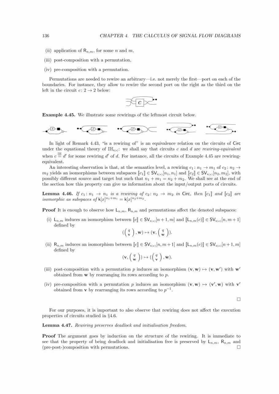
136 CHAPTER 4. THE CALCULUS OF SIGNAL FLOW DIAGRAMS
(ii) application of Rn,m, for some n and m,
(iii) post-composition with a permutation,
(iv) pre-composition with a permutation.
Permutations are needed to rewire an arbitrary—i.e. not merely the first—port on each of theboundaries. For instance, they allow to rewire the second port on the right as the third on theleft in the circuit c : 2→ 2 below:
c
Example 4.45. We illustrate some rewirings of the leftmost circuit below.
x x x xx
In light of Remark 4.43, “is a rewiring of” is an equivalence relation on the circuits of Circunder the equational theory of IHk[x]: we shall say that circuits c and d are rewiring-equivalent
when cIH= d′ for some rewiring d′ of d. For instance, all the circuits of Example 4.45 are rewiring-
equivalent.An interesting observation is that, at the semantics level, a rewiring c1 : n1 → m1 of c2 : n2 →
m2 yields an isomorphisms between subspaces [[c1]] ∈ SVk(x)[n1, n1] and [[c2]] ∈ SVk(x)[n2,m2], withpossibly different source and target but such that n1 +m1 = n2 +m2. We shall see at the end ofthe section how this property can give us information about the input/output ports of circuits.
Lemma 4.46. If c1 : n1 → n1 is a rewiring of c2 : n2 → m2 in Circ, then [[c1]] and [[c2]] areisomorphic as subspaces of k[x]n1+m1 = k[x]n2+m2 .
Proof It is enough to observe how Ln,m, Rn,m and permutations affect the denoted subspaces:
(i) Ln,m induces an isomorphism between [[c]] ∈ SVk(x)[n+ 1,m] and [[Ln,m(c)]] ∈ SVk(x)[n,m+ 1]defined by
((qv
),w) 7→ (v,
(qw
)).
(ii) Rn,m induces an isomorphism between [[c]] ∈ SVk(x)[n,m+ 1] and [[Ln,m(c)]] ∈ SVk(x)[n+ 1,m]defined by
(v,(qw
)) 7→ (
(qv
),w).
(iii) post-composition with a permutation p induces an isomorphism (v,w) 7→ (v,w′) with w′
obtained from w by rearranging its rows according to p.
(iv) pre-composition with a permutation p induces an isomorphism (v,w) 7→ (v′,w) with v′
obtained from v by rearranging its rows according to p−1.
�
For our purposes, it is important to also observe that rewiring does not affect the executionproperties of circuits studied in §4.6.
Lemma 4.47. Rewiring preserves deadlock and initialisation freedom.
Proof The argument goes by induction on the structure of the rewiring. It is immediate tosee that the property of being deadlock and initialisation free is preserved by Ln,m, Rn,m and(pre-post-)composition with permutations. �
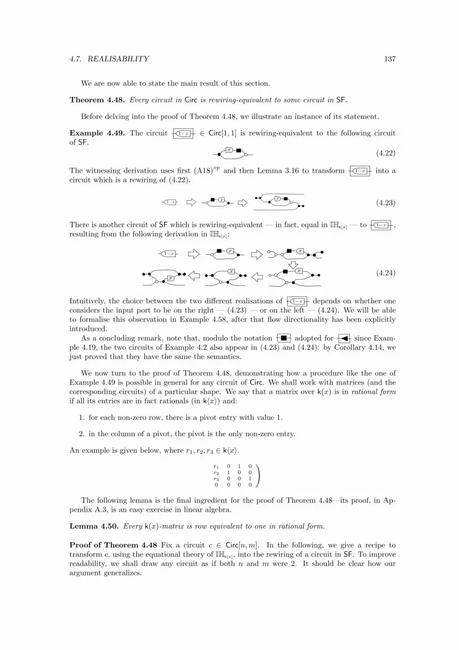
4.7. REALISABILITY 137
We are now able to state the main result of this section.
Theorem 4.48. Every circuit in Circ is rewiring-equivalent to some circuit in SF.
Before delving into the proof of Theorem 4.48, we illustrate an instance of its statement.
Example 4.49. The circuit 1�x ∈ Circ[1, 1] is rewiring-equivalent to the following circuitof SF.
x(4.22)
The witnessing derivation uses first (A18)op
and then Lemma 3.16 to transform 1�x into acircuit which is a rewiring of (4.22).
x1�xx
(4.23)
There is another circuit of SF which is rewiring-equivalent — in fact, equal in IHk[x] — to 1�x ,resulting from the following derivation in IHk[x]:
x
x x
xx1�x
(4.24)
Intuitively, the choice between the two different realisations of 1�x depends on whether oneconsiders the input port to be on the right — (4.23) — or on the left — (4.24). We will be ableto formalise this observation in Example 4.58, after that flow directionality has been explicitlyintroduced.
As a concluding remark, note that, modulo the notation adopted for since Exam-ple 4.19, the two circuits of Example 4.2 also appear in (4.23) and (4.24): by Corollary 4.14, wejust proved that they have the same the semantics.
We now turn to the proof of Theorem 4.48, demonstrating how a procedure like the one ofExample 4.49 is possible in general for any circuit of Circ. We shall work with matrices (and thecorresponding circuits) of a particular shape. We say that a matrix over k(x) is in rational formif all its entries are in fact rationals (in k〈x〉) and:
1. for each non-zero row, there is a pivot entry with value 1.
2. in the column of a pivot, the pivot is the only non-zero entry.
An example is given below, where r1, r2, r3 ∈ k〈x〉.(
r1 0 1 0r2 1 0 0r3 0 0 10 0 0 0
)
The following lemma is the final ingredient for the proof of Theorem 4.48—its proof, in Ap-pendix A.3, is an easy exercise in linear algebra.
Lemma 4.50. Every k(x)-matrix is row equivalent to one in rational form.
Proof of Theorem 4.48 Fix a circuit c ∈ Circ[n,m]. In the following, we give a recipe totransform c, using the equational theory of IHk[x], into the rewiring of a circuit in SF. To improvereadability, we shall draw any circuit as if both n and m were 2. It should be clear how ourargument generalizes.
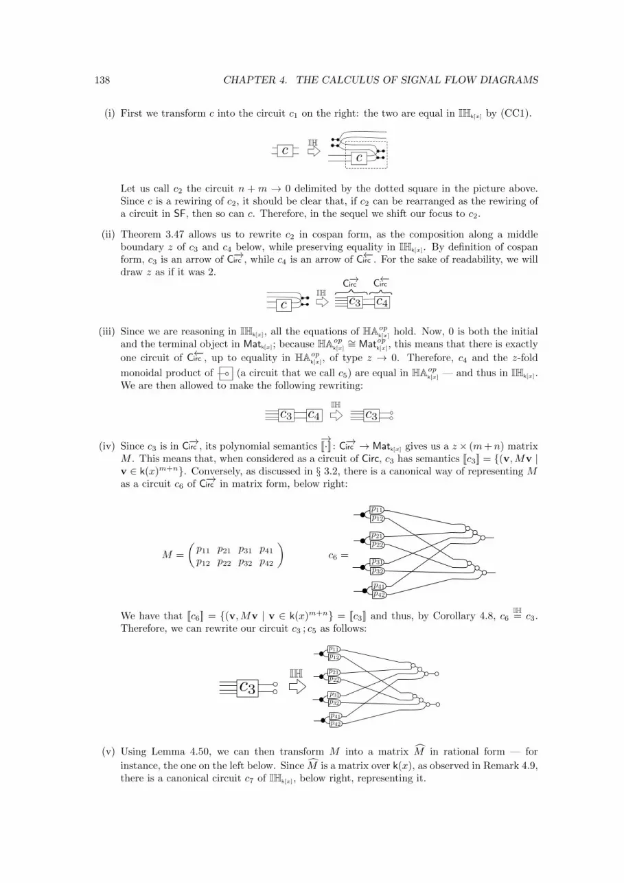
138 CHAPTER 4. THE CALCULUS OF SIGNAL FLOW DIAGRAMS
(i) First we transform c into the circuit c1 on the right: the two are equal in IHk[x] by (CC1).
cc
IH
Let us call c2 the circuit n + m → 0 delimited by the dotted square in the picture above.Since c is a rewiring of c2, it should be clear that, if c2 can be rearranged as the rewiring ofa circuit in SF, then so can c. Therefore, in the sequel we shift our focus to c2.
(ii) Theorem 3.47 allows us to rewrite c2 in cospan form, as the composition along a middleboundary z of c3 and c4 below, while preserving equality in IHk[x]. By definition of cospanform, c3 is an arrow of C−→irc , while c4 is an arrow of C←−irc . For the sake of readability, we willdraw z as if it was 2.
c3 c4cIH
C�!irc C �irc
(iii) Since we are reasoning in IHk[x], all the equations of HAopk[x] hold. Now, 0 is both the initial
and the terminal object in Matk[x]; because HAopk[x]∼= Matopk[x], this means that there is exactly
one circuit of C←−irc , up to equality in HAopk[x], of type z → 0. Therefore, c4 and the z-fold
monoidal product of (a circuit that we call c5) are equal in HAopk[x] — and thus in IHk[x].
We are then allowed to make the following rewriting:
c3 c4 c3IH
(iv) Since c3 is in C−→irc , its polynomial semantics−→[[·]] : C−→irc → Matk[x] gives us a z× (m+n) matrix
M . This means that, when considered as a circuit of Circ, c3 has semantics [[c3]] = {(v,Mv |v ∈ k(x)m+n}. Conversely, as discussed in § 3.2, there is a canonical way of representing Mas a circuit c6 of C−→irc in matrix form, below right:
M =
(p11 p21 p31 p41
p12 p22 p32 p42
)c6 =
p11p12
p21p22
p31
p32
p41p42
We have that [[c6]] = {(v,Mv | v ∈ k(x)m+n} = [[c3]] and thus, by Corollary 4.8, c6IH= c3.
Therefore, we can rewrite our circuit c3 ; c5 as follows:
c3
p11
p12
p21p22
p31
p32
p41p42
IH
(v) Using Lemma 4.50, we can then transform M into a matrix M in rational form — for
instance, the one on the left below. Since M is a matrix over k(x), as observed in Remark 4.9,there is a canonical circuit c7 of IHk[x], below right, representing it.
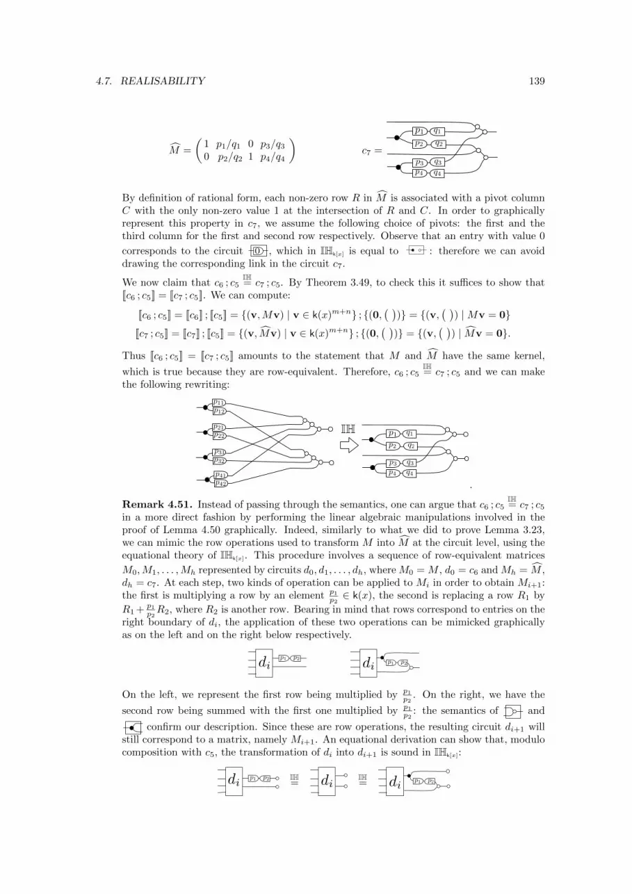
4.7. REALISABILITY 139
M =
(1 p1/q1 0 p3/q3
0 p2/q2 1 p4/q4
)c7 =
p1 q1
p2
q3
q2
p3
p4 q4
By definition of rational form, each non-zero row R in M is associated with a pivot columnC with the only non-zero value 1 at the intersection of R and C. In order to graphicallyrepresent this property in c7, we assume the following choice of pivots: the first and thethird column for the first and second row respectively. Observe that an entry with value 0
corresponds to the circuit 0 , which in IHk[x] is equal to : therefore we can avoiddrawing the corresponding link in the circuit c7.
We now claim that c6 ; c5IH= c7 ; c5. By Theorem 3.49, to check this it suffices to show that
[[c6 ; c5]] = [[c7 ; c5]]. We can compute:
[[c6 ; c5]] = [[c6]] ; [[c5]] = {(v,Mv) | v ∈ k(x)m+n} ; {(0,( )
)} = {(v,( )
) |Mv = 0}[[c7 ; c5]] = [[c7]] ; [[c5]] = {(v, Mv) | v ∈ k(x)m+n} ; {(0,
( ))} = {(v,
( )) | Mv = 0}.
Thus [[c6 ; c5]] = [[c7 ; c5]] amounts to the statement that M and M have the same kernel,
which is true because they are row-equivalent. Therefore, c6 ; c5IH= c7 ; c5 and we can make
the following rewriting:
p11
p1 q1
p2
q3
q2
p3
p12
p21p22
p31
p32
p41p42
p4 q4
IH
.
Remark 4.51. Instead of passing through the semantics, one can argue that c6 ; c5IH= c7 ; c5
in a more direct fashion by performing the linear algebraic manipulations involved in theproof of Lemma 4.50 graphically. Indeed, similarly to what we did to prove Lemma 3.23,we can mimic the row operations used to transform M into M at the circuit level, using theequational theory of IHk[x]. This procedure involves a sequence of row-equivalent matrices
M0,M1, . . . ,Mh represented by circuits d0, d1, . . . , dh, where M0 = M , d0 = c6 and Mh = M ,dh = c7. At each step, two kinds of operation can be applied to Mi in order to obtain Mi+1:the first is multiplying a row by an element p1
p2∈ k(x), the second is replacing a row R1 by
R1 + p1
p2R2, where R2 is another row. Bearing in mind that rows correspond to entries on the
right boundary of di, the application of these two operations can be mimicked graphicallyas on the left and on the right below respectively.
p1 p2di p1 p2di
On the left, we represent the first row being multiplied by p1
p2. On the right, we have the
second row being summed with the first one multiplied by p1
p2: the semantics of and
confirm our description. Since these are row operations, the resulting circuit di+1 willstill correspond to a matrix, namely Mi+1. An equational derivation can show that, modulocomposition with c5, the transformation of di into di+1 is sound in IHk[x]:
p1 p2diIH= di
IH= p1 p2di
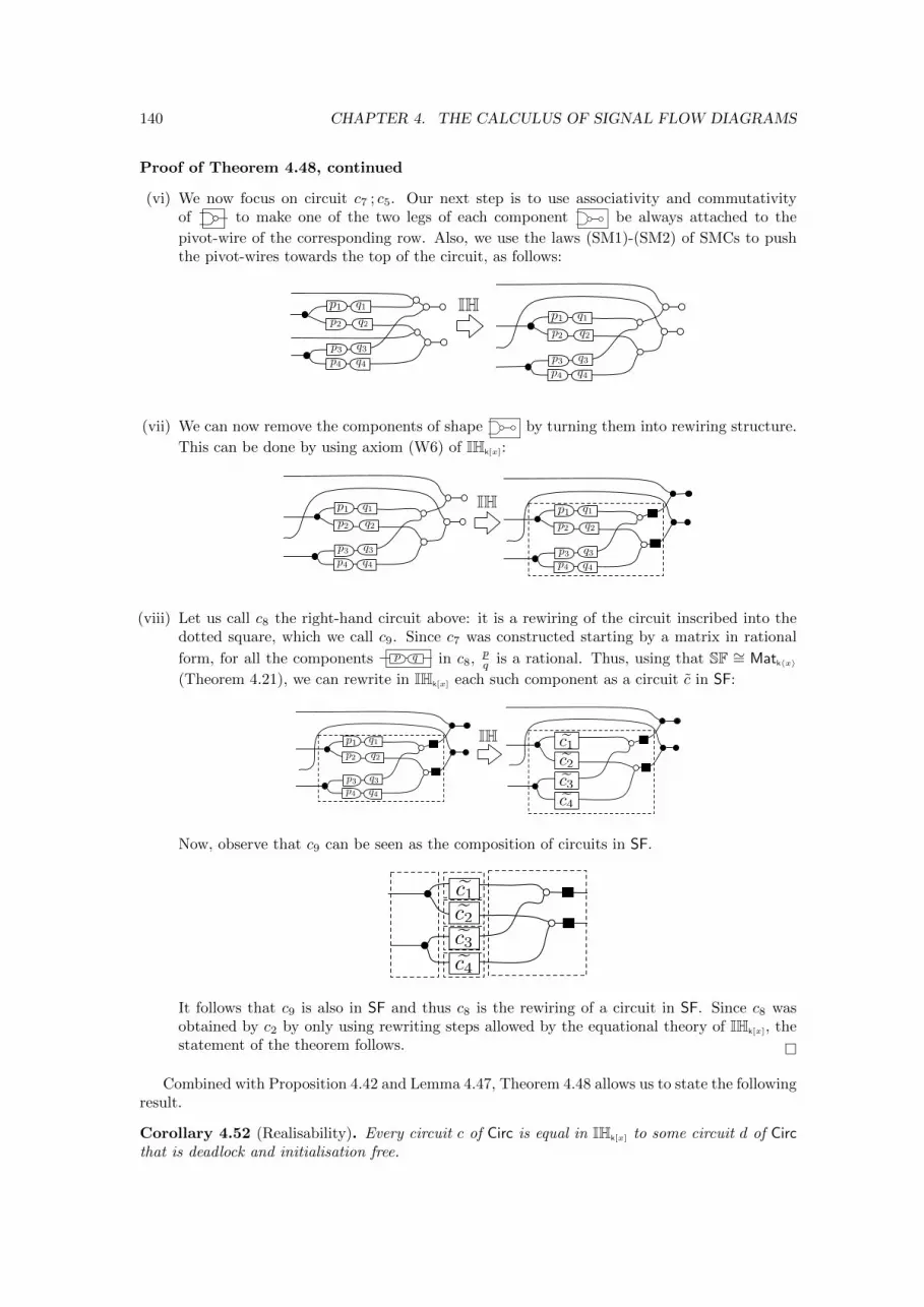
140 CHAPTER 4. THE CALCULUS OF SIGNAL FLOW DIAGRAMS
Proof of Theorem 4.48, continued
(vi) We now focus on circuit c7 ; c5. Our next step is to use associativity and commutativityof to make one of the two legs of each component be always attached to the
pivot-wire of the corresponding row. Also, we use the laws (SM1)-(SM2) of SMCs to pushthe pivot-wires towards the top of the circuit, as follows:
p1 q1
p2
q3
q2
p3
p4 q4
p1 q1
p2
q3
q2
p3
p4 q4
IH
(vii) We can now remove the components of shape by turning them into rewiring structure.
This can be done by using axiom (W6) of IHk[x]:
p1 q1
p2
q3
q2
p3
p4 q4
p1 q1
p2
q3
q2
p3
p4 q4
IH
(viii) Let us call c8 the right-hand circuit above: it is a rewiring of the circuit inscribed into thedotted square, which we call c9. Since c7 was constructed starting by a matrix in rational
form, for all the components p q in c8, pq is a rational. Thus, using that SF ∼= Matk〈x〉
(Theorem 4.21), we can rewrite in IHk[x] each such component as a circuit c in SF:
p1 q1
p2
q3
q2
p3
p4 q4
ec1
ec2
ec3
ec4
IH
Now, observe that c9 can be seen as the composition of circuits in SF.
ec1
ec2
ec3
ec4
It follows that c9 is also in SF and thus c8 is the rewiring of a circuit in SF. Since c8 wasobtained by c2 by only using rewriting steps allowed by the equational theory of IHk[x], thestatement of the theorem follows. �
Combined with Proposition 4.42 and Lemma 4.47, Theorem 4.48 allows us to state the followingresult.
Corollary 4.52 (Realisability). Every circuit c of Circ is equal in IHk[x] to some circuit d of Circthat is deadlock and initialisation free.
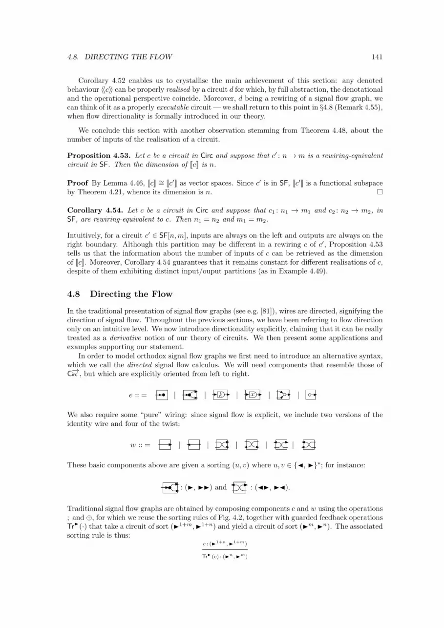
4.8. DIRECTING THE FLOW 141
Corollary 4.52 enables us to crystallise the main achievement of this section: any denotedbehaviour 〈〈c〉〉 can be properly realised by a circuit d for which, by full abstraction, the denotationaland the operational perspective coincide. Moreover, d being a rewiring of a signal flow graph, wecan think of it as a properly executable circuit — we shall return to this point in §4.8 (Remark 4.55),when flow directionality is formally introduced in our theory.
We conclude this section with another observation stemming from Theorem 4.48, about thenumber of inputs of the realisation of a circuit.
Proposition 4.53. Let c be a circuit in Circ and suppose that c′ : n→ m is a rewiring-equivalentcircuit in SF. Then the dimension of [[c]] is n.
Proof By Lemma 4.46, [[c]] ∼= [[c′]] as vector spaces. Since c′ is in SF, [[c′]] is a functional subspaceby Theorem 4.21, whence its dimension is n. �
Corollary 4.54. Let c be a circuit in Circ and suppose that c1 : n1 → m1 and c2 : n2 → m2, inSF, are rewiring-equivalent to c. Then n1 = n2 and m1 = m2.
Intuitively, for a circuit c′ ∈ SF[n,m], inputs are always on the left and outputs are always on theright boundary. Although this partition may be different in a rewiring c of c′, Proposition 4.53tells us that the information about the number of inputs of c can be retrieved as the dimensionof [[c]]. Moreover, Corollary 4.54 guarantees that it remains constant for different realisations of c,despite of them exhibiting distinct input/ouput partitions (as in Example 4.49).
4.8 Directing the Flow
In the traditional presentation of signal flow graphs (see e.g. [81]), wires are directed, signifying thedirection of signal flow. Throughout the previous sections, we have been referring to flow directiononly on an intuitive level. We now introduce directionality explicitly, claiming that it can be reallytreated as a derivative notion of our theory of circuits. We then present some applications andexamples supporting our statement.
In order to model orthodox signal flow graphs we first need to introduce an alternative syntax,which we call the directed signal flow calculus. We will need components that resemble those ofC−→irc , but which are explicitly oriented from left to right.
e :: = | | k | x | |
We also require some “pure” wiring: since signal flow is explicit, we include two versions of theidentity wire and four of the twist:
w :: = | | | | |
These basic components above are given a sorting (u, v) where u, v ∈ {�, �}∗; for instance:
: (�, ��) and : (��, ��).
Traditional signal flow graphs are obtained by composing components e and w using the operations; and ⊕, for which we reuse the sorting rules of Fig. 4.2, together with guarded feedback operationsTr�(·) that take a circuit of sort (�1+m,�1+n) and yield a circuit of sort (�m,�n). The associatedsorting rule is thus:
c : (�1+n,�1+m)
Tr�(c) : (�n,�m)
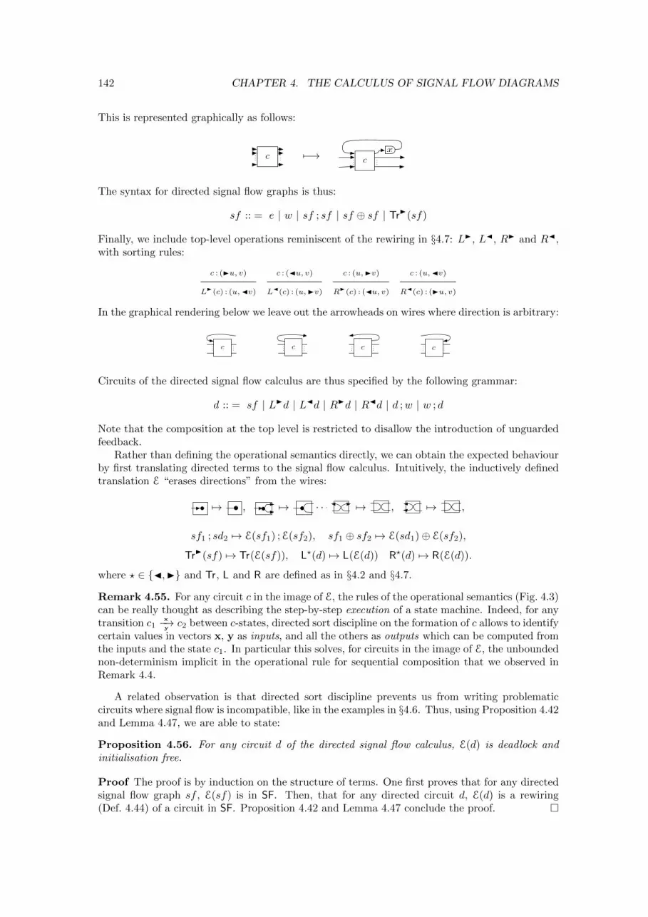
142 CHAPTER 4. THE CALCULUS OF SIGNAL FLOW DIAGRAMS
This is represented graphically as follows:
c...... 7−→ ...
...
x
c
The syntax for directed signal flow graphs is thus:
sf :: = e | w | sf ; sf | sf ⊕ sf | Tr�(sf)
Finally, we include top-level operations reminiscent of the rewiring in §4.7: L�, L�, R� and R�,with sorting rules:
c : (�u, v)
L�(c) : (u,�v)
c : (�u, v)
L�(c) : (u,�v)
c : (u,�v)
R�(c) : (�u, v)
c : (u,�v)
R�(c) : (�u, v)
In the graphical rendering below we leave out the arrowheads on wires where direction is arbitrary:
c...... c...
......
... c ...... c
Circuits of the directed signal flow calculus are thus specified by the following grammar:
d :: = sf | L�d | L�d | R�d | R�d | d ;w | w ; d
Note that the composition at the top level is restricted to disallow the introduction of unguardedfeedback.
Rather than defining the operational semantics directly, we can obtain the expected behaviourby first translating directed terms to the signal flow calculus. Intuitively, the inductively definedtranslation E “erases directions” from the wires:
7→ , 7→ · · · 7→ , 7→ ,
sf1 ; sd2 7→ E(sf1) ;E(sf2), sf1 ⊕ sf2 7→ E(sd1)⊕ E(sf2),
Tr�(sf) 7→ Tr(E(sf)), L?(d) 7→ L(E(d)) R?(d) 7→ R(E(d)).
where ? ∈ {�,�} and Tr, L and R are defined as in §4.2 and §4.7.
Remark 4.55. For any circuit c in the image of E, the rules of the operational semantics (Fig. 4.3)can be really thought as describing the step-by-step execution of a state machine. Indeed, for anytransition c1
x−→yc2 between c-states, directed sort discipline on the formation of c allows to identify
certain values in vectors x, y as inputs, and all the others as outputs which can be computed fromthe inputs and the state c1. In particular this solves, for circuits in the image of E, the unboundednon-determinism implicit in the operational rule for sequential composition that we observed inRemark 4.4.
A related observation is that directed sort discipline prevents us from writing problematiccircuits where signal flow is incompatible, like in the examples in §4.6. Thus, using Proposition 4.42and Lemma 4.47, we are able to state:
Proposition 4.56. For any circuit d of the directed signal flow calculus, E(d) is deadlock andinitialisation free.
Proof The proof is by induction on the structure of terms. One first proves that for any directedsignal flow graph sf , E(sf) is in SF. Then, that for any directed circuit d, E(d) is a rewiring(Def. 4.44) of a circuit in SF. Proposition 4.42 and Lemma 4.47 conclude the proof. �
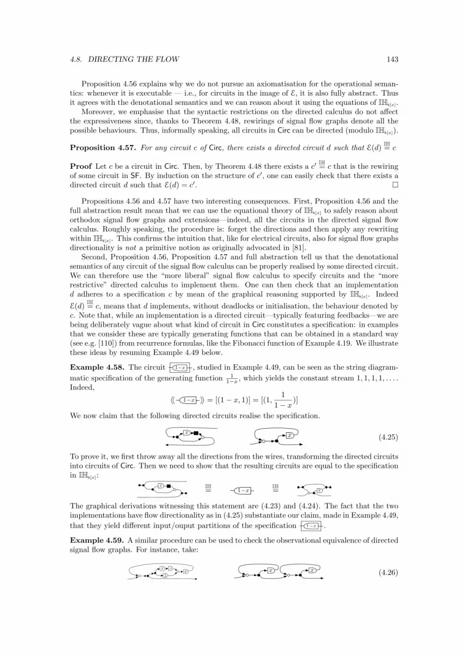
4.8. DIRECTING THE FLOW 143
Proposition 4.56 explains why we do not pursue an axiomatisation for the operational seman-tics: whenever it is executable — i.e., for circuits in the image of E, it is also fully abstract. Thusit agrees with the denotational semantics and we can reason about it using the equations of IHk[x].
Moreover, we emphasise that the syntactic restrictions on the directed calculus do not affectthe expressiveness since, thanks to Theorem 4.48, rewirings of signal flow graphs denote all thepossible behaviours. Thus, informally speaking, all circuits in Circ can be directed (modulo IHk[x]).
Proposition 4.57. For any circuit c of Circ, there exists a directed circuit d such that E(d)IH= c
Proof Let c be a circuit in Circ. Then, by Theorem 4.48 there exists a c′IH= c that is the rewiring
of some circuit in SF. By induction on the structure of c′, one can easily check that there exists adirected circuit d such that E(d) = c′. �
Propositions 4.56 and 4.57 have two interesting consequences. First, Proposition 4.56 and thefull abstraction result mean that we can use the equational theory of IHk[x] to safely reason aboutorthodox signal flow graphs and extensions—indeed, all the circuits in the directed signal flowcalculus. Roughly speaking, the procedure is: forget the directions and then apply any rewritingwithin IHk[x]. This confirms the intuition that, like for electrical circuits, also for signal flow graphsdirectionality is not a primitive notion as originally advocated in [81].
Second, Proposition 4.56, Proposition 4.57 and full abstraction tell us that the denotationalsemantics of any circuit of the signal flow calculus can be properly realised by some directed circuit.We can therefore use the “more liberal” signal flow calculus to specify circuits and the “morerestrictive” directed calculus to implement them. One can then check that an implementationd adheres to a specification c by mean of the graphical reasoning supported by IHk[x]. Indeed
E(d)IH= c, means that d implements, without deadlocks or initialisation, the behaviour denoted by
c. Note that, while an implementation is a directed circuit—typically featuring feedbacks—we arebeing deliberately vague about what kind of circuit in Circ constitutes a specification: in examplesthat we consider these are typically generating functions that can be obtained in a standard way(see e.g. [110]) from recurrence formulas, like the Fibonacci function of Example 4.19. We illustratethese ideas by resuming Example 4.49 below.
Example 4.58. The circuit 1�x , studied in Example 4.49, can be seen as the string diagram-
matic specification of the generating function 11−x , which yields the constant stream 1, 1, 1, 1, . . . .
Indeed,
〈〈 1�x 〉〉 = [(1− x, 1)] = [(1,1
1− x )]
We now claim that the following directed circuits realise the specification.
x x (4.25)
To prove it, we first throw away all the directions from the wires, transforming the directed circuitsinto circuits of Circ. Then we need to show that the resulting circuits are equal to the specificationin IHk[x]:
x IH= 1�x
IH= x
The graphical derivations witnessing this statement are (4.23) and (4.24). The fact that the twoimplementations have flow directionality as in (4.25) substantiate our claim, made in Example 4.49,
that they yield different input/ouput partitions of the specification 1�x .
Example 4.59. A similar procedure can be used to check the observational equivalence of directedsignal flow graphs. For instance, take:
x2
x -1 xx (4.26)
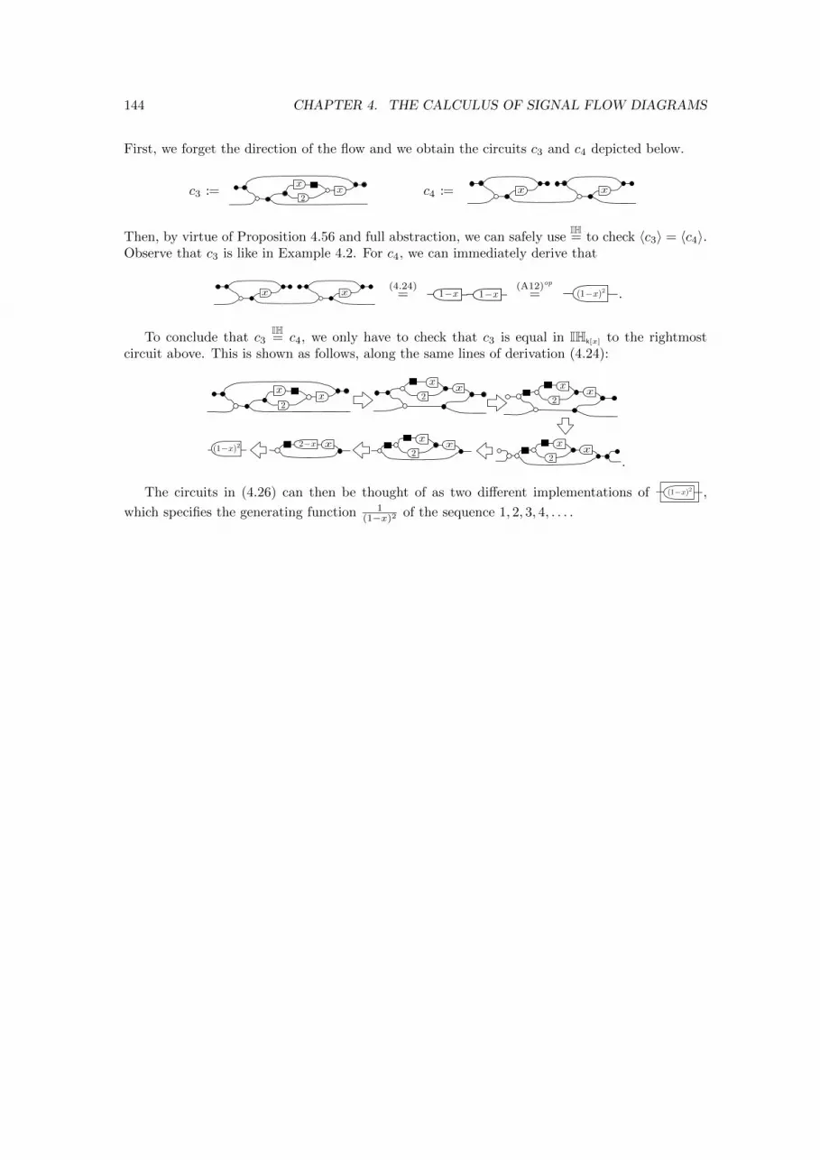
144 CHAPTER 4. THE CALCULUS OF SIGNAL FLOW DIAGRAMS
First, we forget the direction of the flow and we obtain the circuits c3 and c4 depicted below.
c3 := x2
xc4 := x x
Then, by virtue of Proposition 4.56 and full abstraction, we can safely useIH= to check 〈c3〉 = 〈c4〉.
Observe that c3 is like in Example 4.2. For c4, we can immediately derive that
x x(4.24)
= 1�x 1�x(A12)op
= (1�x)2 .
To conclude that c3IH= c4, we only have to check that c3 is equal in IHk[x] to the rightmost
circuit above. This is shown as follows, along the same lines of derivation (4.24):
x2
2
xxx
2
xx
2
xx2
xxx2�x
(1�x)2
.
The circuits in (4.26) can then be thought of as two different implementations of (1�x)2 ,
which specifies the generating function 1(1−x)2 of the sequence 1, 2, 3, 4, . . . .
Chapter 5
Conclusions and Future Directions
In this thesis we focused on a characterisation of linear dynamical systems. However, we wouldlike to stress the importance of the methodology grounding our investigation, as we believe it isfruitfully applicable to other classes of systems. The first principle underlying our approach ismodularity : similarly to IH, most of the interesting graphical languages are quite complex; wecontend that the right mix of PROP operations — sum, fibered sum and especially composition— enables formal analyses that are hampered by monolithic approaches. The second principle isthe conviction that a formal theory of circuit diagrams should not be endowed with a primitivenotion of causality. We believe that signal flow graphs provide a strong case of how discarding flowdirectionality is not only harmless, but beneficial for a compositional understanding of computingdevices.
In the rest of this section, we mention some of the most promising directions for future research.
Computing with distributive laws Distributive laws yield rewriting systems: when we readoff the equations from the graph of the law, these are oriented, thus it is natural to view them asrewriting rules. Unfortunately, a distributive law does not tell much about the algorithmic aspectsof the associated rewriting: for instance, it guarantees that a factorisation exists for each diagram,but it does not produce a terminating sequence of rewriting steps to reach it. An interestingquestion is thus what principles and general assumptions guarantee termination and other usefulproperties of the rewriting associated with the law. More generally, we are interested in exploringthe computational content of distributive laws: for instance, the development of new algorithmsfor linear algebraic manipulations in IH would greatly improve the appeal of our graphical syntax.
Exploring these aspects would also clarify the connection between our work and existing ap-proaches to string diagram rewriting, such as the research surrounding the Quantomatic softwarepackage [67] and the line of works on higher-dimensional rewriting systems [35, 73, 75, 86].
Categorical control theory Our approach to signal flow graphs only scratched the surfaceof the rich body of work devoted to these structures in control theory. A research thread thatwe find particularly worth investigating is Willems’ behavioural approach — see e.g. [111, 112].Our proximity to Willems’ vision of systems is efficaciously synthesised by the following passagein [111].
Adding a signal flow direction is often a figment of one’s imagination, and when some-thing is not real, it will turn out to be cumbersome sooner or later. [...] The in-put/output framework is totally inappropriate for dealing with all but the most specialsystem interconnections. [The input/output representation] often needlessly compli-cates matters, mathematically and conceptually. A good theory of systems takes the
145
146 CHAPTER 5. CONCLUSIONS AND FUTURE DIRECTIONS
behavior as the basic notion and the reference point for concepts and definitions, andswitches back and forth between a wide variety of convenient representations.
Within this perspective, Willems’ analysis treats behaviour as a relation rather than a function,which makes it close to our approach and opens the way for studying the system propertiesconsidered in [112, 111], such as controllability, stabilisability and autonomy. Understanding theirstring diagrammatic significance may yield syntactic characterisations, similar to those that weproposed for deadlock and initialisation freedom, and result in new methods for static analysis.
Another question stemming from traditional control theory is how to extend our approach toinclude an operational semantics for the continuous-time interpretation of signal flow graphs, wherethe registers stand for differentiation/integration of a signal. This perspective has been pursuedin [8], using the Laplace transform to reduce the continuous case to the discrete case. Anotherrelevant work is [13], which studies the denotational semantics of a class of network diagrams incontinuous time using hyperreals. However, these authors focus only on the denotational picture,whereas we would also like to understand how to give an operational account of the continuous-time interpretation. The approach described in [90], which gives a coinductive formalism forelementary calculus not far removed from our stream semantics, may be helpful in this respect.
Beyond signal flow graphs: other models of computation It is a natural research questionto extend our methodology to other classes of systems: we mention below some of the mostpromising directions.
First, we believe our approach may be fruitful for graphical formalisms that, like signal flowgraphs, are typically translated to more traditional mathematics and seldom reasoned about di-rectly. We think in particular of electrical circuits — which already attracted categorical model-ing [9] — and Kahn process networks [30] — whose formalisation in monoidal categories has beenstudied in [56, 13]. The key is to understand how to generalise our picture to the modeling ofother kinds of behaviour, such as non-linearity, asynchrony and non-determinism.
Another important class of formalisms that we would like to tackle are automata. A promisingstarting point is the observation that signal flow graphs can be thought as weighted automata on asingleton alphabet — see e.g. [97]. Can we characterise the string diagrammatic analogue of otherclasses of automata? There are at least two ways of extending the case of signal flow diagrams: thefirst is to enlarge the alphabet, which yields circuits processing infinite trees in place of streams;the second is to generalise the elements of streams from fields to semirings — this is motivated bythe case of non-deterministic automata, which are weighted automata for the boolean semiring.
Yet another interesting research direction concerns quantitative models of computation. In [51],Fritz gave a presentation by generators and relations for the PROP of stochastic matrices. Byanalogy with the case studied in this thesis, we may hope to use this result to achieve a presentationfor the PROP whose arrows are the probabilistic analogue of relations, and indeed there are notionsof this kind appearing in the literature [88]. The technical challenge here is that stochastic matriceshave an inherently non-local character, because values in a column must always sum to 1. Thisprevents the PROP of stochastic matrices from having the limits and colimits necessary to formour cube construction.
Our approach was inspired by graphical formalisms developed in quantum information andconcurrency theory: we argued that IH lies somehow at the intersection, as it captures the interplayof Frobenius and Hopf algebras that appear in both research threads. It is a natural question toask whether we can apply our methodology to model the features which are specific of each ofthese areas. For instance, we observed that IHZ2
only describes the phase-free fragment of the ZX-calculus: it would be interesting to extend our characterisation to include in the picture properlyquantum aspects such as the presence of phases. We believe that a modular characterisation forthe full ZX-calculus would be particularly valuable for the quantum community: completeness forZX and its variants have been intensively studied in recent years [5, 6, 47].
Another motivating example for our developments were the algebras for Petri nets [103, 33]and for connectors [32] developed in concurrency theory. In the former case, we believe that ourmodular understanding may bring important insights towards a complete axiomatisation for the
147
proposed calculi: preliminary investigations in this direction [104] are promising as the identifiedstructure is quite close to IHZ2
. In the latter case, the formalism for stateless connectors proposed
in [32] is extremely close to IHZ2, the only difference being that is undefined on input
(11
).
Nonetheless, this difference is crucial as it prevents us from modeling properly concurrent featuressuch as mutual exclusion. We leave as future work to explore a modular account of the calculusof stateless connectors, which may also give useful insights for an equational theory of calculi ofstateful connectors like Reo [4].

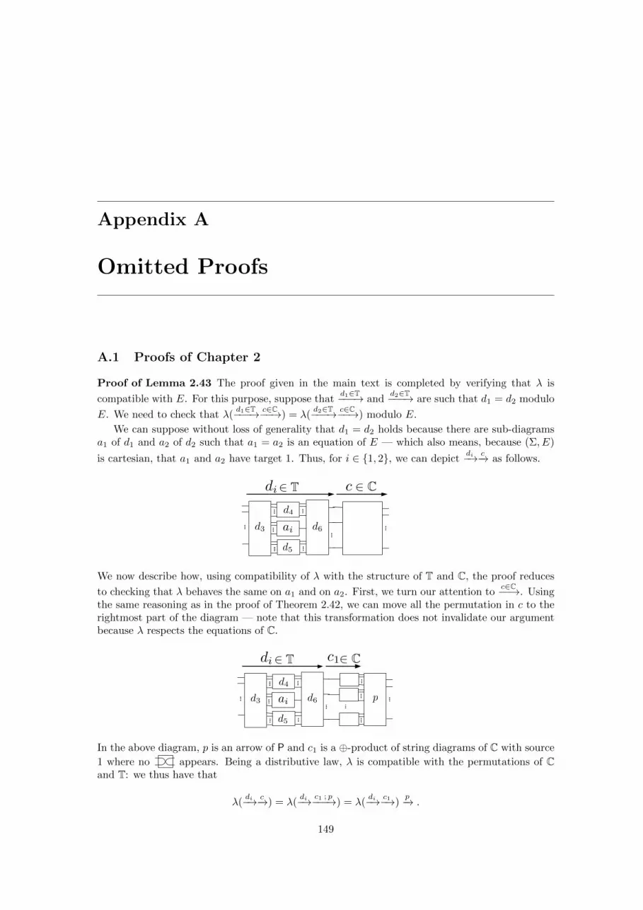
Appendix A
Omitted Proofs
A.1 Proofs of Chapter 2
Proof of Lemma 2.43 The proof given in the main text is completed by verifying that λ is
compatible with E. For this purpose, suppose thatd1∈T−−−→ and
d2∈T−−−→ are such that d1 = d2 modulo
E. We need to check that λ(d1∈T−−−→ c∈C−−→) = λ(
d2∈T−−−→ c∈C−−→) modulo E.
We can suppose without loss of generality that d1 = d2 holds because there are sub-diagramsa1 of d1 and a2 of d2 such that a1 = a2 is an equation of E — which also means, because (Σ, E)
is cartesian, that a1 and a2 have target 1. Thus, for i ∈ {1, 2}, we can depictdi−→ c−→ as follows.
d4
d5
d6d3
2 C2 T
ai
cdi
We now describe how, using compatibility of λ with the structure of T and C, the proof reduces
to checking that λ behaves the same on a1 and on a2. First, we turn our attention toc∈C−−→. Using
the same reasoning as in the proof of Theorem 2.42, we can move all the permutation in c to therightmost part of the diagram — note that this transformation does not invalidate our argumentbecause λ respects the equations of C.
d4
d5
d6d3 p
2 C2 T
ai
di c1
In the above diagram, p is an arrow of P and c1 is a ⊕-product of string diagrams of C with source
1 where no appears. Being a distributive law, λ is compatible with the permutations of Cand T: we thus have that
λ(di−→ c−→) = λ(
di−→ c1 ; p−−−→) = λ(di−→ c1−→)
p−→ .
149
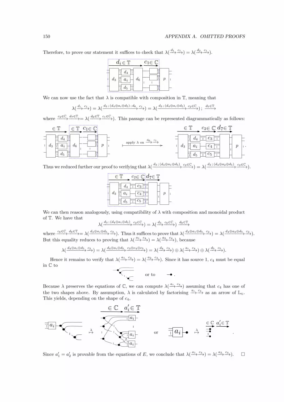
150 APPENDIX A. OMITTED PROOFS
Therefore, to prove our statement it suffices to check that λ(d1−→ c1−→) = λ(
d2−→ c1−→).
d4
d5
d6d3 p
2 C2 T
ai
di c1
We can now use the fact that λ is compatible with composition in T, meaning that
λ(di−→ c1−→) = λ(
d3 ; (d4⊕ai⊕d5) ; d6−−−−−−−−−−−−→ c1−→) = λ(d3 ; (d4⊕ai⊕d5)−−−−−−−−−−→ c2∈C−−−→) ;
d7∈T−−−→
wherec2∈C−−−→ d7∈T−−−→= λ(
d6∈T−−−→ c1∈C−−−→). This passage can be represented diagrammatically as follows:
d4
d5
d6d3 p
2 T 2 T
ai
2 Cc1
� apply λ ond6−→ c1−→ //
d4
d5
d3 p
2 C2 T 2 T
ai
c3
c4
d7
c5
c2
.
Thus we reduced further our proof to verifying that λ(d3 ; (d4⊕a1⊕d5)−−−−−−−−−−→ c2∈C−−−→) = λ(
d3 ; (d4⊕a2⊕d5)−−−−−−−−−−→ c2∈C−−−→).
d4
d5
d3 p
2 C2 T 2 T
ai
c3
c4
d7
c5
c2
We can then reason analogously, using compatibility of λ with composition and monoidal productof T. We have that
λ(d3 ; (d4⊕ai⊕d5)−−−−−−−−−−→ c2∈C−−−→) = λ(
d3−→ c6∈C−−−→)d8∈T−−−→
wherec6∈C−−−→ d8∈T−−−→= λ(
d4⊕ai⊕d5−−−−−−→ c2−→). Thus it suffices to prove that λ(d4⊕a1⊕d5−−−−−−→ c2−→) = λ(
d4⊕a2⊕d5−−−−−−→ c2−→).
But this equality reduces to proving that λ(a1−→ c4−→) = λ(
a2−→ c4−→), because
λ(d4⊕ai⊕d5−−−−−−→ c2−→) = λ(
d4⊕ai⊕d5−−−−−−→ c3⊕c4⊕c5−−−−−−→) = λ(d4−→ c3−→)⊕ λ(
ai−→ c4−→)⊕ λ(d5−→ c5−→).
Hence it remains to verify that λ(a1−→ c4−→) = λ(
a2−→ c4−→). Since it has source 1, c4 must be equalin C to
or to .
Because λ preserves the equations of C, we can compute λ(ai−→ c4−→) assuming that c4 has one of
the two shapes above. By assumption, λ is calculated by factorisingai−→ c4−→ as an arrow of LΣ.
This yields, depending on the shape of c4,
aiλ7→
2 C 2 T
ai
ai
ai
a0i
or aiλ7→
2 C 2 Ta0i
.
Since a′1 = a′2 is provable from the equations of E, we conclude that λ(a1−→ c4−→) = λ(
a2−→ c4−→). �
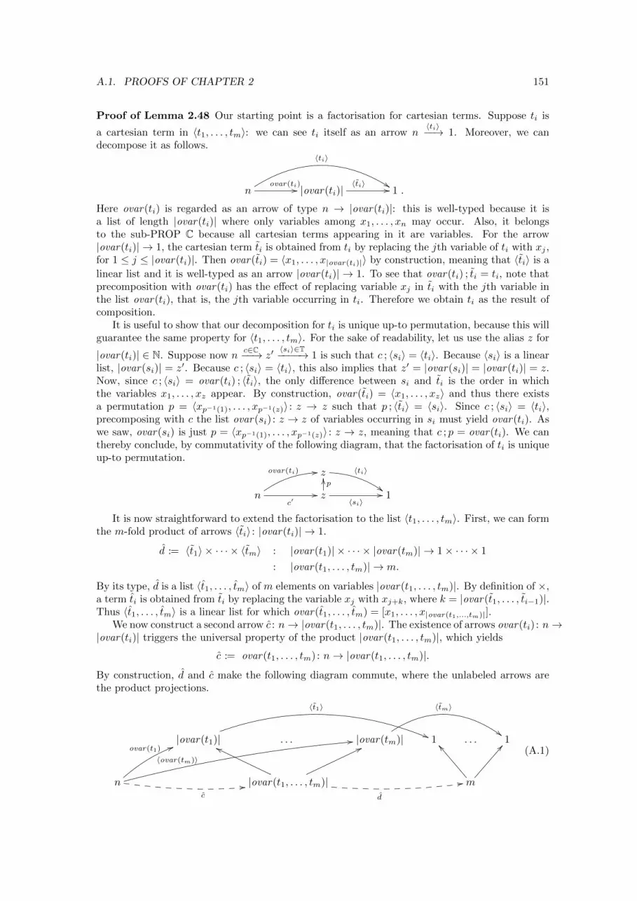
A.1. PROOFS OF CHAPTER 2 151
Proof of Lemma 2.48 Our starting point is a factorisation for cartesian terms. Suppose ti is
a cartesian term in 〈t1, . . . , tm〉: we can see ti itself as an arrow n〈ti〉−−→ 1. Moreover, we can
decompose it as follows.
n
〈ti〉
%%ovar(ti)// |ovar(ti)|〈ti〉 // 1 .
Here ovar(ti) is regarded as an arrow of type n → |ovar(ti)|: this is well-typed because it isa list of length |ovar(ti)| where only variables among x1, . . . , xn may occur. Also, it belongsto the sub-PROP C because all cartesian terms appearing in it are variables. For the arrow|ovar(ti)| → 1, the cartesian term ti is obtained from ti by replacing the jth variable of ti with xj ,for 1 ≤ j ≤ |ovar(ti)|. Then ovar(ti) = 〈x1, . . . , x|ovar(ti)|〉 by construction, meaning that 〈ti〉 is a
linear list and it is well-typed as an arrow |ovar(ti)| → 1. To see that ovar(ti) ; ti = ti, note thatprecomposition with ovar(ti) has the effect of replacing variable xj in ti with the jth variable inthe list ovar(ti), that is, the jth variable occurring in ti. Therefore we obtain ti as the result ofcomposition.
It is useful to show that our decomposition for ti is unique up-to permutation, because this willguarantee the same property for 〈t1, . . . , tm〉. For the sake of readability, let us use the alias z for
|ovar(ti)| ∈ N. Suppose now nc∈C−−→ z′
〈si〉∈T−−−−→ 1 is such that c ; 〈si〉 = 〈ti〉. Because 〈si〉 is a linearlist, |ovar(si)| = z′. Because c ; 〈si〉 = 〈ti〉, this also implies that z′ = |ovar(si)| = |ovar(ti)| = z.Now, since c ; 〈si〉 = ovar(ti) ; 〈ti〉, the only difference between si and ti is the order in whichthe variables x1, . . . , xz appear. By construction, ovar(ti) = 〈x1, . . . , xz〉 and thus there existsa permutation p = 〈xp−1(1), . . . , xp−1(z)〉 : z → z such that p ; 〈ti〉 = 〈si〉. Since c ; 〈si〉 = 〈ti〉,precomposing with c the list ovar(si) : z → z of variables occurring in si must yield ovar(ti). Aswe saw, ovar(si) is just p = 〈xp−1(1), . . . , xp−1(z)〉 : z → z, meaning that c ; p = ovar(ti). We canthereby conclude, by commutativity of the following diagram, that the factorisation of ti is uniqueup-to permutation.
z 〈ti〉
##n
ovar(ti) 00
c′// zpOO
〈si〉// 1
It is now straightforward to extend the factorisation to the list 〈t1, . . . , tm〉. First, we can formthe m-fold product of arrows 〈ti〉 : |ovar(ti)| → 1.
d := 〈t1〉 × · · · × 〈tm〉 : |ovar(t1)| × · · · × |ovar(tm)| → 1× · · · × 1
: |ovar(t1, . . . , tm)| → m.
By its type, d is a list 〈t1, . . . , tm〉 of m elements on variables |ovar(t1, . . . , tm)|. By definition of ×,a term ti is obtained from ti by replacing the variable xj with xj+k, where k = |ovar(t1, . . . , ti−1)|.Thus 〈t1, . . . , tm〉 is a linear list for which ovar(t1, . . . , tm) = [x1, . . . , x|ovar(t1,...,tm)|].
We now construct a second arrow c : n→ |ovar(t1, . . . , tm)|. The existence of arrows ovar(ti) : n→|ovar(ti)| triggers the universal property of the product |ovar(t1, . . . , tm)|, which yields
c := ovar(t1, . . . , tm) : n→ |ovar(t1, . . . , tm)|.By construction, d and c make the following diagram commute, where the unlabeled arrows arethe product projections.
|ovar(t1)|
〈t1〉
((. . . |ovar(tm)|
〈tm〉
##1 . . . 1
n
ovar(t1) 55
〈ovar(tm)〉
00
c
00 |ovar(t1, . . . , tm)|
gg 66
d
11 m
]] AA(A.1)
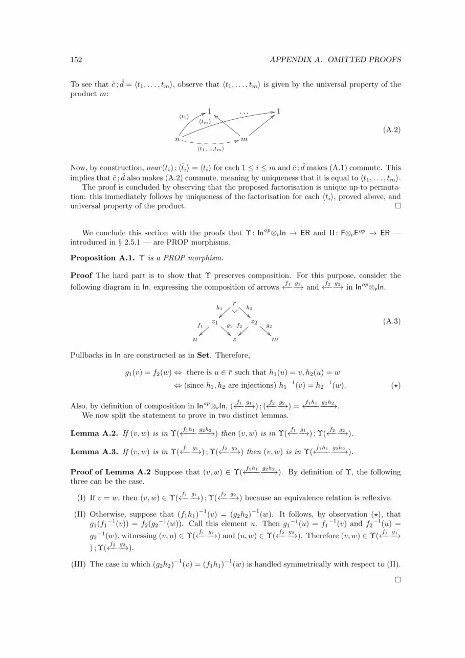
152 APPENDIX A. OMITTED PROOFS
To see that c ; d = 〈t1, . . . , tm〉, observe that 〈t1, . . . , tm〉 is given by the universal property of theproduct m:
1 . . . 1
n
〈t1〉55
〈tm〉
11
〈t1,...,tm〉33 m
bb <<
(A.2)
Now, by construction, ovar(ti) ; 〈ti〉 = 〈ti〉 for each 1 ≤ i ≤ m and c ; d makes (A.1) commute. This
implies that c ; d also makes (A.2) commute, meaning by uniqueness that it is equal to 〈t1, . . . , tm〉.The proof is concluded by observing that the proposed factorisation is unique up-to permuta-
tion: this immediately follows by uniqueness of the factorisation for each 〈ti〉, proved above, anduniversal property of the product. �
We conclude this section with the proofs that Υ: Inop⊗PIn → ER and Π: F⊗PFop → ER —
introduced in § 2.5.1 — are PROP morphisms.
Proposition A.1. Υ is a PROP morphism.
Proof The hard part is to show that Υ preserves composition. For this purpose, consider the
following diagram in In, expressing the composition of arrowsf1←− g1−→ and
f2←− g2−→ in Inop⊗PIn.
rh1
~~h2
z1f1
}}g1
z2f2
~~g2
!!n z m
(A.3)
Pullbacks in In are constructed as in Set. Therefore,
g1(v) = f2(w)⇔ there is u ∈ r such that h1(u) = v, h2(u) = w
⇔ (since h1, h2 are injections) h1−1(v) = h2
−1(w). (?)
Also, by definition of composition in Inop⊗PIn, (f1←− g1−→) ; (
f2←− g2−→) =f1h1←−−− g2h2−−−→.
We now split the statement to prove in two distinct lemmas.
Lemma A.2. If (v, w) is in Υ(f1h1←−−− g2h2−−−→) then (v, w) is in Υ(
f1←− g1−→) ; Υ(f2←− g2−→).
Lemma A.3. If (v, w) is in Υ(f1←− g1−→) ; Υ(
f2←− g2−→) then (v, w) is in Υ(f1h1←−−− g2h2−−−→).
Proof of Lemma A.2 Suppose that (v, w) ∈ Υ(f1h1←−−− g2h2−−−→). By definition of Υ, the following
three can be the case.
(I) If v = w, then (v, w) ∈ Υ(f1←− g1−→) ; Υ(
f2←− g2−→) because an equivalence relation is reflexive.
(II) Otherwise, suppose that (f1h1)−1
(v) = (g2h2)−1
(w). It follows, by observation (?), thatg1(f1
−1(v)) = f2(g2−1(w)). Call this element u. Then g1
−1(u) = f1−1(v) and f2
−1(u) =
g2−1(w), witnessing (v, u) ∈ Υ(
f1←− g1−→) and (u,w) ∈ Υ(f2←− g2−→). Therefore (v, w) ∈ Υ(
f1←− g1−→) ; Υ(
f2←− g2−→).
(III) The case in which (g2h2)−1
(v) = (f1h1)−1
(w) is handled symmetrically with respect to (II).
�
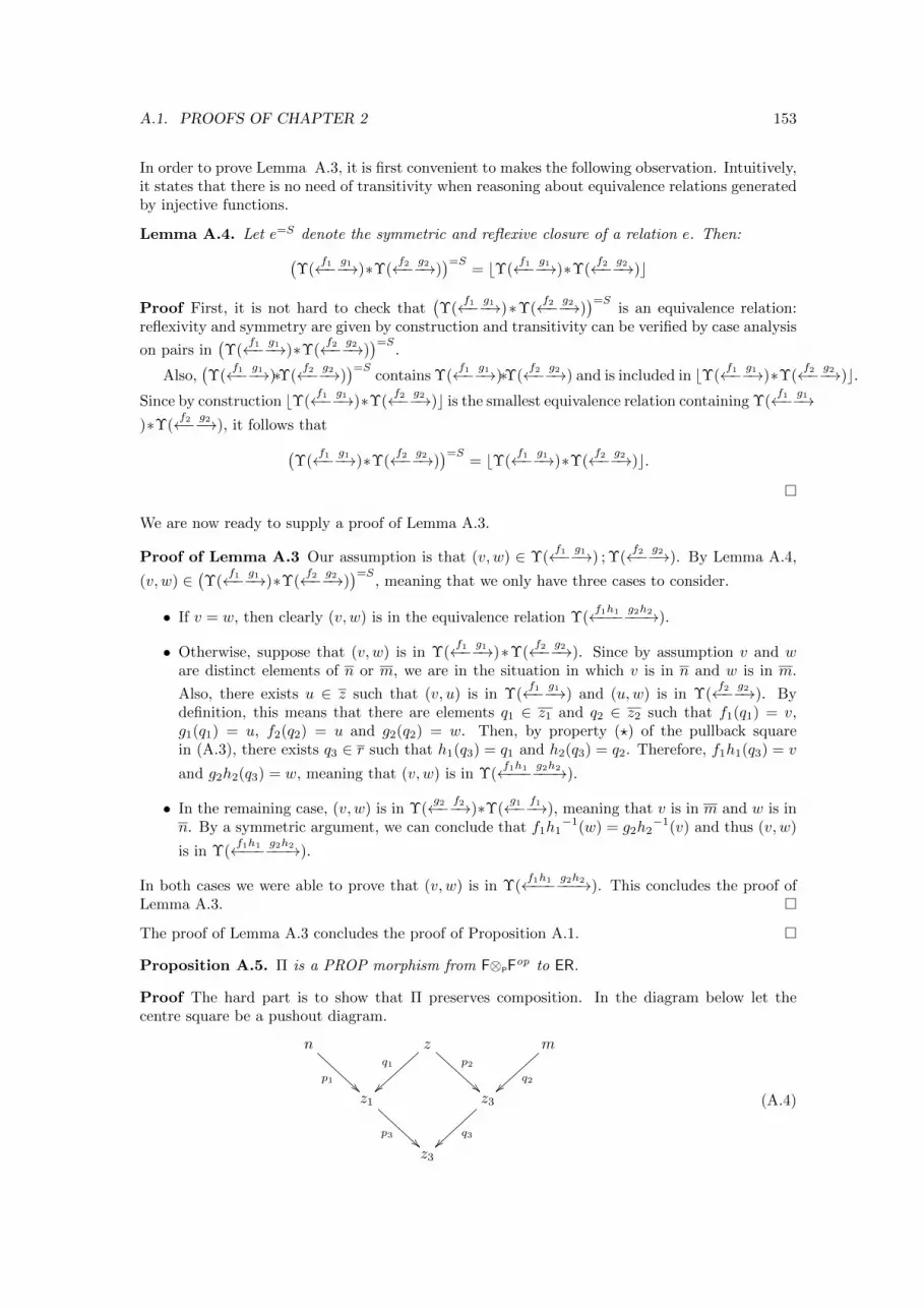
A.1. PROOFS OF CHAPTER 2 153
In order to prove Lemma A.3, it is first convenient to makes the following observation. Intuitively,it states that there is no need of transitivity when reasoning about equivalence relations generatedby injective functions.
Lemma A.4. Let e=S denote the symmetric and reflexive closure of a relation e. Then:
(Υ(
f1←− g1−→)∗Υ(f2←− g2−→)
)=S= bΥ(
f1←− g1−→)∗Υ(f2←− g2−→)c
Proof First, it is not hard to check that(Υ(
f1←− g1−→)∗Υ(f2←− g2−→)
)=Sis an equivalence relation:
reflexivity and symmetry are given by construction and transitivity can be verified by case analysis
on pairs in(Υ(
f1←− g1−→)∗Υ(f2←− g2−→)
)=S.
Also,(Υ(
f1←− g1−→)∗Υ(f2←− g2−→)
)=Scontains Υ(
f1←− g1−→)∗Υ(f2←− g2−→) and is included in bΥ(
f1←− g1−→)∗Υ(f2←− g2−→)c.
Since by construction bΥ(f1←− g1−→)∗Υ(
f2←− g2−→)c is the smallest equivalence relation containing Υ(f1←− g1−→
)∗Υ(f2←− g2−→), it follows that
(Υ(
f1←− g1−→)∗Υ(f2←− g2−→)
)=S= bΥ(
f1←− g1−→)∗Υ(f2←− g2−→)c.
�
We are now ready to supply a proof of Lemma A.3.
Proof of Lemma A.3 Our assumption is that (v, w) ∈ Υ(f1←− g1−→) ; Υ(
f2←− g2−→). By Lemma A.4,
(v, w) ∈(Υ(
f1←− g1−→)∗Υ(f2←− g2−→)
)=S, meaning that we only have three cases to consider.
• If v = w, then clearly (v, w) is in the equivalence relation Υ(f1h1←−−− g2h2−−−→).
• Otherwise, suppose that (v, w) is in Υ(f1←− g1−→)∗Υ(
f2←− g2−→). Since by assumption v and ware distinct elements of n or m, we are in the situation in which v is in n and w is in m.
Also, there exists u ∈ z such that (v, u) is in Υ(f1←− g1−→) and (u,w) is in Υ(
f2←− g2−→). Bydefinition, this means that there are elements q1 ∈ z1 and q2 ∈ z2 such that f1(q1) = v,g1(q1) = u, f2(q2) = u and g2(q2) = w. Then, by property (?) of the pullback squarein (A.3), there exists q3 ∈ r such that h1(q3) = q1 and h2(q3) = q2. Therefore, f1h1(q3) = v
and g2h2(q3) = w, meaning that (v, w) is in Υ(f1h1←−−− g2h2−−−→).
• In the remaining case, (v, w) is in Υ(g2←− f2−→)∗Υ(
g1←− f1−→), meaning that v is in m and w is inn. By a symmetric argument, we can conclude that f1h1
−1(w) = g2h2−1(v) and thus (v, w)
is in Υ(f1h1←−−− g2h2−−−→).
In both cases we were able to prove that (v, w) is in Υ(f1h1←−−− g2h2−−−→). This concludes the proof of
Lemma A.3. �
The proof of Lemma A.3 concludes the proof of Proposition A.1. �
Proposition A.5. Π is a PROP morphism from F⊗PFop to ER.
Proof The hard part is to show that Π preserves composition. In the diagram below let thecentre square be a pushout diagram.
n
p1
zq1
}}
p2
!!
m
q2}}
z1
p3
z3
q3~~
z3
(A.4)
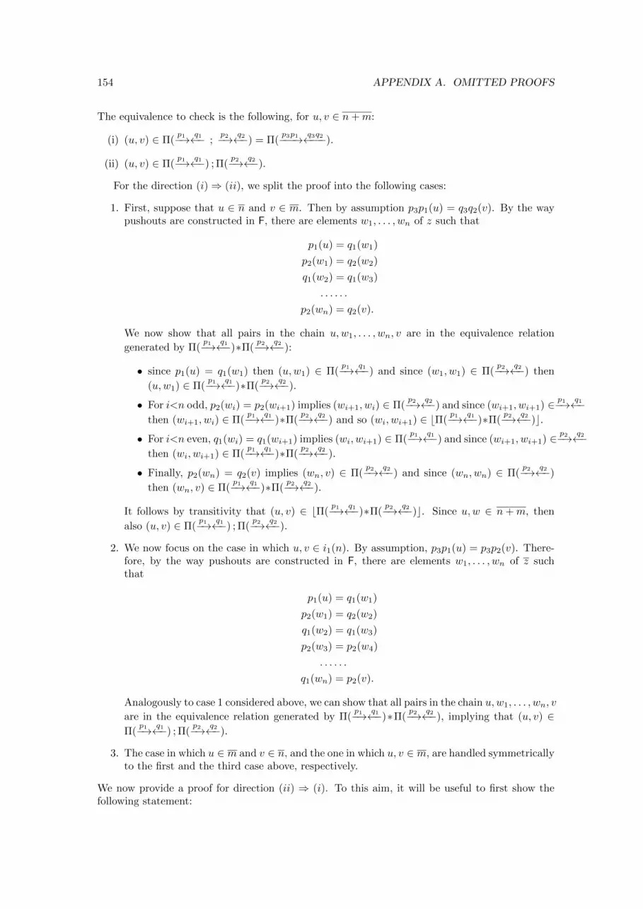
154 APPENDIX A. OMITTED PROOFS
The equivalence to check is the following, for u, v ∈ n+m:
(i) (u, v) ∈ Π(p1−→ q1←− ;
p2−→ q2←−) = Π(p3p1−−−→ q3q2←−−−).
(ii) (u, v) ∈ Π(p1−→ q1←−) ; Π(
p2−→ q2←−).
For the direction (i)⇒ (ii), we split the proof into the following cases:
1. First, suppose that u ∈ n and v ∈ m. Then by assumption p3p1(u) = q3q2(v). By the waypushouts are constructed in F, there are elements w1, . . . , wn of z such that
p1(u) = q1(w1)
p2(w1) = q2(w2)
q1(w2) = q1(w3)
. . . . . .
p2(wn) = q2(v).
We now show that all pairs in the chain u,w1, . . . , wn, v are in the equivalence relation
generated by Π(p1−→ q1←−)∗Π(
p2−→ q2←−):
• since p1(u) = q1(w1) then (u,w1) ∈ Π(p1−→ q1←−) and since (w1, w1) ∈ Π(
p2−→ q2←−) then
(u,w1) ∈ Π(p1−→ q1←−)∗Π(
p2−→ q2←−).
• For i<n odd, p2(wi) = p2(wi+1) implies (wi+1, wi) ∈ Π(p2−→ q2←−) and since (wi+1, wi+1) ∈ p1−→ q1←−
then (wi+1, wi) ∈ Π(p1−→ q1←−)∗Π(
p2−→ q2←−) and so (wi, wi+1) ∈ bΠ(p1−→ q1←−)∗Π(
p2−→ q2←−)c.• For i<n even, q1(wi) = q1(wi+1) implies (wi, wi+1) ∈ Π(
p1−→ q1←−) and since (wi+1, wi+1) ∈ p2−→ q2←−then (wi, wi+1) ∈ Π(
p1−→ q1←−)∗Π(p2−→ q2←−).
• Finally, p2(wn) = q2(v) implies (wn, v) ∈ Π(p2−→ q2←−) and since (wn, wn) ∈ Π(
p2−→ q2←−)
then (wn, v) ∈ Π(p1−→ q1←−)∗Π(
p2−→ q2←−).
It follows by transitivity that (u, v) ∈ bΠ(p1−→ q1←−)∗Π(
p2−→ q2←−)c. Since u,w ∈ n+m, then
also (u, v) ∈ Π(p1−→ q1←−) ; Π(
p2−→ q2←−).
2. We now focus on the case in which u, v ∈ i1(n). By assumption, p3p1(u) = p3p2(v). There-fore, by the way pushouts are constructed in F, there are elements w1, . . . , wn of z suchthat
p1(u) = q1(w1)
p2(w1) = q2(w2)
q1(w2) = q1(w3)
p2(w3) = p2(w4)
. . . . . .
q1(wn) = p2(v).
Analogously to case 1 considered above, we can show that all pairs in the chain u,w1, . . . , wn, v
are in the equivalence relation generated by Π(p1−→ q1←−)∗Π(
p2−→ q2←−), implying that (u, v) ∈Π(
p1−→ q1←−) ; Π(p2−→ q2←−).
3. The case in which u ∈ m and v ∈ n, and the one in which u, v ∈ m, are handled symmetricallyto the first and the third case above, respectively.
We now provide a proof for direction (ii) ⇒ (i). To this aim, it will be useful to first show thefollowing statement:
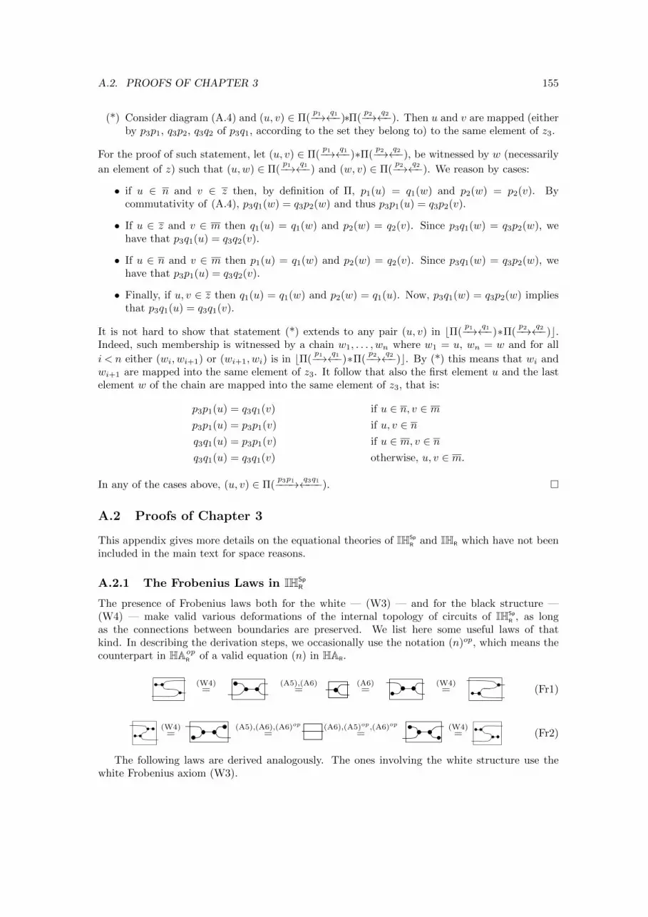
A.2. PROOFS OF CHAPTER 3 155
(*) Consider diagram (A.4) and (u, v) ∈ Π(p1−→ q1←−)∗Π(
p2−→ q2←−). Then u and v are mapped (eitherby p3p1, q3p2, q3q2 of p3q1, according to the set they belong to) to the same element of z3.
For the proof of such statement, let (u, v) ∈ Π(p1−→ q1←−)∗Π(
p2−→ q2←−), be witnessed by w (necessarily
an element of z) such that (u,w) ∈ Π(p1−→ q1←−) and (w, v) ∈ Π(
p2−→ q2←−). We reason by cases:
• if u ∈ n and v ∈ z then, by definition of Π, p1(u) = q1(w) and p2(w) = p2(v). Bycommutativity of (A.4), p3q1(w) = q3p2(w) and thus p3p1(u) = q3p2(v).
• If u ∈ z and v ∈ m then q1(u) = q1(w) and p2(w) = q2(v). Since p3q1(w) = q3p2(w), wehave that p3q1(u) = q3q2(v).
• If u ∈ n and v ∈ m then p1(u) = q1(w) and p2(w) = q2(v). Since p3q1(w) = q3p2(w), wehave that p3p1(u) = q3q2(v).
• Finally, if u, v ∈ z then q1(u) = q1(w) and p2(w) = q1(u). Now, p3q1(w) = q3p2(w) impliesthat p3q1(u) = q3q1(v).
It is not hard to show that statement (*) extends to any pair (u, v) in bΠ(p1−→ q1←−)∗Π(
p2−→ q2←−)c.Indeed, such membership is witnessed by a chain w1, . . . , wn where w1 = u, wn = w and for all
i < n either (wi, wi+1) or (wi+1, wi) is in bΠ(p1−→ q1←−)∗Π(
p2−→ q2←−)c. By (*) this means that wi andwi+1 are mapped into the same element of z3. It follow that also the first element u and the lastelement w of the chain are mapped into the same element of z3, that is:
p3p1(u) = q3q1(v) if u ∈ n, v ∈ mp3p1(u) = p3p1(v) if u, v ∈ nq3q1(u) = p3p1(v) if u ∈ m, v ∈ nq3q1(u) = q3q1(v) otherwise, u, v ∈ m.
In any of the cases above, (u, v) ∈ Π(p3p1−−−→ q3q1←−−−). �
A.2 Proofs of Chapter 3
This appendix gives more details on the equational theories of IHSp
R and IHR which have not beenincluded in the main text for space reasons.
A.2.1 The Frobenius Laws in IHSpR
The presence of Frobenius laws both for the white — (W3) — and for the black structure —(W4) — make valid various deformations of the internal topology of circuits of IHSp
R , as longas the connections between boundaries are preserved. We list here some useful laws of thatkind. In describing the derivation steps, we occasionally use the notation (n)op, which means thecounterpart in HAop
R of a valid equation (n) in HAR.
(W4)=
(A5),(A6)=
(A6)=
(W4)= (Fr1)
(W4)=
(A5),(A6),(A6)op
=(A6),(A5)op,(A6)op
=(W4)= (Fr2)
The following laws are derived analogously. The ones involving the white structure use thewhite Frobenius axiom (W3).
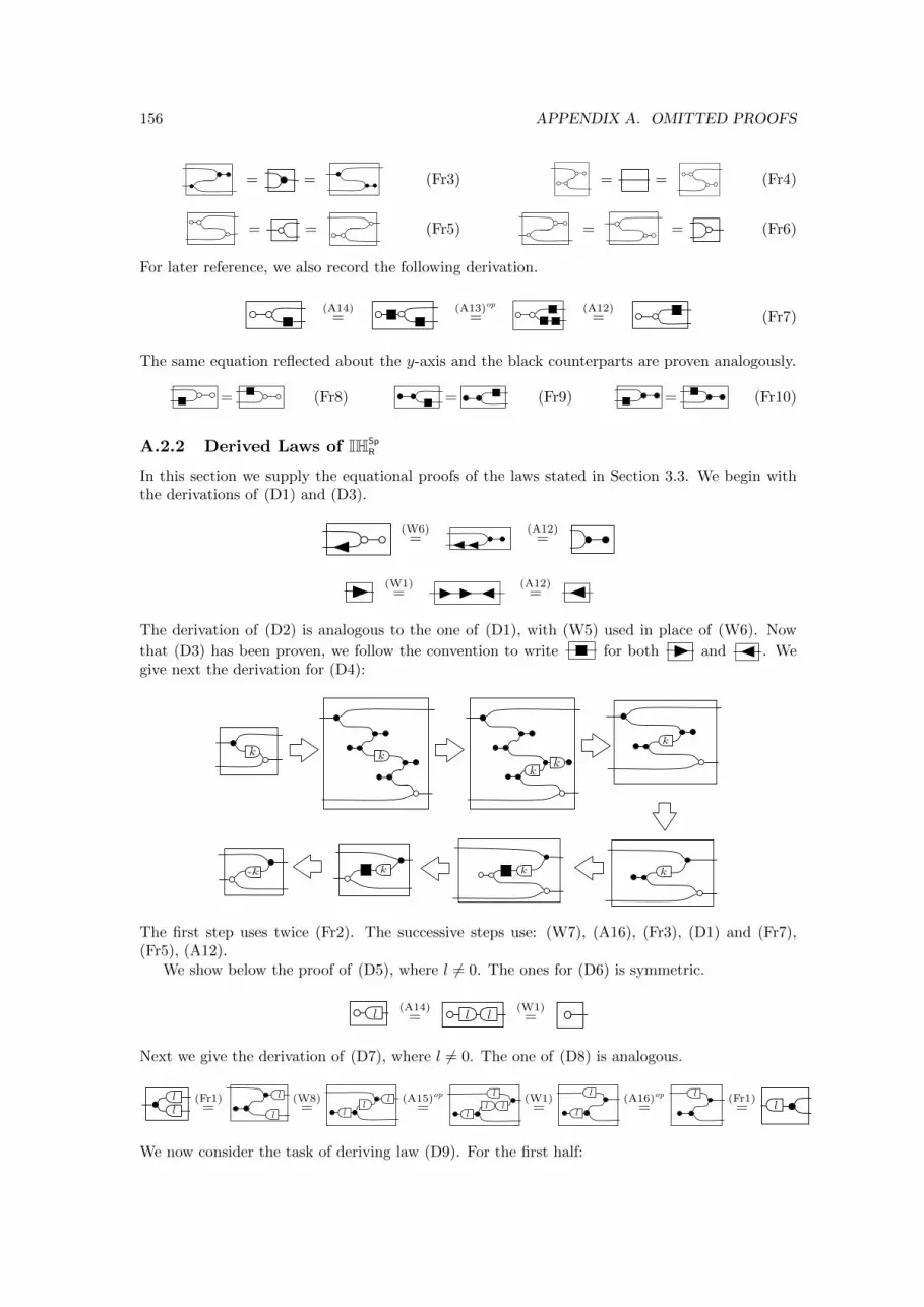
156 APPENDIX A. OMITTED PROOFS
= = (Fr3) = = (Fr4)
= = (Fr5) = = (Fr6)
For later reference, we also record the following derivation.
(A14)=
(A13)op
=(A12)
= (Fr7)
The same equation reflected about the y-axis and the black counterparts are proven analogously.
= (Fr8) = (Fr9) = (Fr10)
A.2.2 Derived Laws of IHSpR
In this section we supply the equational proofs of the laws stated in Section 3.3. We begin withthe derivations of (D1) and (D3).
(W6)=
(A12)=
(W1)=
(A12)=
The derivation of (D2) is analogous to the one of (D1), with (W5) used in place of (W6). Now
that (D3) has been proven, we follow the convention to write for both and . Wegive next the derivation for (D4):
k k
k
kkk-k
kk
The first step uses twice (Fr2). The successive steps use: (W7), (A16), (Fr3), (D1) and (Fr7),(Fr5), (A12).
We show below the proof of (D5), where l 6= 0. The ones for (D6) is symmetric.
l(A14)
= ll(W1)=
Next we give the derivation of (D7), where l 6= 0. The one of (D8) is analogous.
ll
(Fr1)=
l
l
(W8)= l
l
l
(A15)op
= l
l
ll
(W1)=
l
l
(A16)op
=l
(Fr1)= l
We now consider the task of deriving law (D9). For the first half:
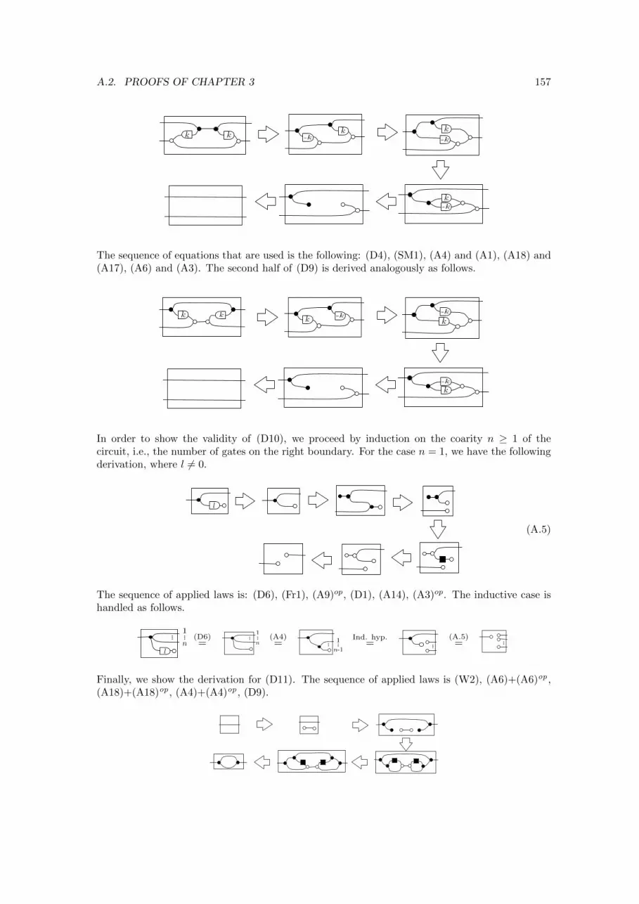
A.2. PROOFS OF CHAPTER 3 157
-kk
-k
k
-k
k
k k
The sequence of equations that are used is the following: (D4), (SM1), (A4) and (A1), (A18) and(A17), (A6) and (A3). The second half of (D9) is derived analogously as follows.
k k -kk
-k
k
-k
k
In order to show the validity of (D10), we proceed by induction on the coarity n ≥ 1 of thecircuit, i.e., the number of gates on the right boundary. For the case n = 1, we have the followingderivation, where l 6= 0.
l
(A.5)
The sequence of applied laws is: (D6), (Fr1), (A9)op, (D1), (A14), (A3)op. The inductive case ishandled as follows.
n
1
l
(D6)= n
1(A4)= 1
n-1
Ind. hyp.=
(A.5)=
Finally, we show the derivation for (D11). The sequence of applied laws is (W2), (A6)+(A6)op ,(A18)+(A18)op , (A4)+(A4)op , (D9).
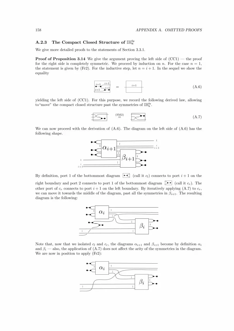
158 APPENDIX A. OMITTED PROOFS
A.2.3 The Compact Closed Structure of IHSpR
We give more detailed proofs to the statements of Section 3.3.1.
Proof of Proposition 3.14 We give the argument proving the left side of (CC1) — the prooffor the right side is completely symmetric. We proceed by induction on n. For the case n = 1,the statement is given by (Fr2). For the inductive step, let n = i + 1. In the sequel we show theequality
i+1
i+1
i+1
i+1 = i+1 (A.6)
yielding the left side of (CC1). For this purpose, we record the following derived law, allowingto“move” the compact closed structure past the symmetries of IHSp
R .
(SM2)= (A.7)
We can now proceed with the derivation of (A.6). The diagram on the left side of (A.6) has thefollowing shape.
↵i+1
�i+1i
1
1
i + 1
ii + 1
By definition, port 1 of the bottommost diagram (call it cl) connects to port i + 1 on the
right boundary and port 2 connects to port 1 of the bottommost diagram (call it cr). The
other port of cr connects to port i + 1 on the left boundary. By iteratively applying (A.7) to cr,we can move it towards the middle of the diagram, past all the symmetries in βi+1. The resultingdiagram is the following:
↵i
�i
Note that, now that we isolated cl and cr, the diagrams αi+1 and βi+1 become by definition αiand βi — also, the application of (A.7) does not affect the arity of the symmetries in the diagram.We are now in position to apply (Fr2):
↵i
�i
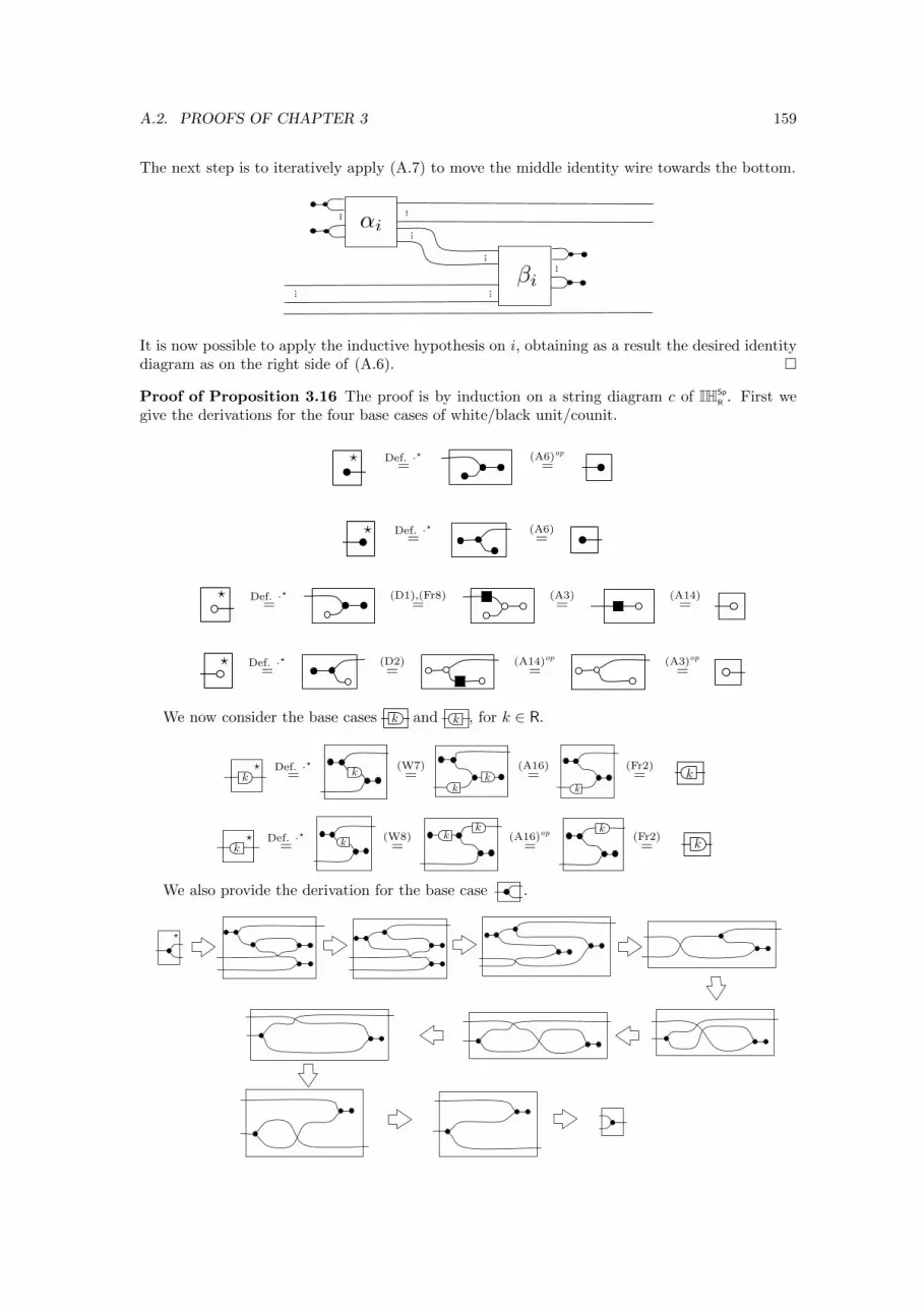
A.2. PROOFS OF CHAPTER 3 159
The next step is to iteratively apply (A.7) to move the middle identity wire towards the bottom.
↵i
�i
It is now possible to apply the inductive hypothesis on i, obtaining as a result the desired identitydiagram as on the right side of (A.6). �
Proof of Proposition 3.16 The proof is by induction on a string diagram c of IHSp
R . First wegive the derivations for the four base cases of white/black unit/counit.
? Def. ·?=
(A6)op
=
? Def. ·?=
(A6)=
? Def. ·?=
(D1),(Fr8)=
(A3)=
(A14)=
? Def. ·?=
(D2)=
(A14)op
=(A3)op
=
We now consider the base cases k and k , for k ∈ R.
?k
Def. ·?= k
(W7)= k
k
(A16)=
k
(Fr2)= k
k? Def. ·?
= k(W8)=
kk (A16)op
=k
(Fr2)= k
We also provide the derivation for the base case .
?
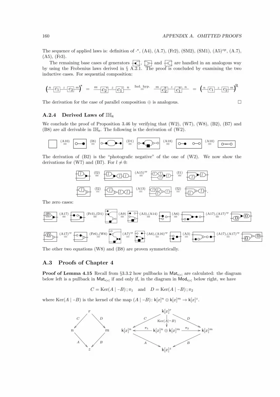
160 APPENDIX A. OMITTED PROOFS
The sequence of applied laws is: definition of ·?, (A4), (A.7), (Fr2), (SM2), (SM1), (A5)op , (A.7),(A5), (Fr3).
The remaining base cases of generators , and are handled in an analogous wayby using the Frobenius laws derived in § A.2.1. The proof is concluded by examining the twoinductive cases. For sequential composition:
n mc1 c2z (?( = nm c1c2
z ?? Ind. hyp.= nm
c1c2z RR = n mc1 c2
z
(( R
The derivation for the case of parallel composition ⊕ is analogous. �
A.2.4 Derived Laws of IHR
We conclude the proof of Proposition 3.46 by verifying that (W2), (W7), (W8), (B2), (B7) and(B8) are all derivable in IHR. The following is the derivation of (W2).
(A10)=
(I8)=
(D1)=
(A18)=
(A10)=
The derivation of (B2) is the “photografic negative” of the one of (W2). We now show thederivations for (W7) and (B7). For l 6= 0:
l (I2)= l
l l(A15)op
= ll
l
l (I1)= l
l
l (I2)= ll
l (A13)= l
ll
l (I2)= l
l .
The zero cases:
0 (A17)=
(Fr3),(D1)=
(A9)=
(A3),(A14)=
(A6)=
(A17),(A17)op
= 0 0
0 (A17)op
=(Fr6),(W6)
=(A7)op
=(A6),(A16)op
=(A3)=
(A17),(A17)op
= 00
The other two equations (W8) and (B8) are proven symmetrically.
A.3 Proofs of Chapter 4
Proof of Lemma 4.15 Recall from §3.3.2 how pullbacks in Matk[x] are calculated: the diagrambelow left is a pullback in Matk[x] if and only if, in the diagram in Modk[x] below right, we have
C = Ker(A | −B) ;π1 and D = Ker(A | −B) ;π2
where Ker(A | −B) is the kernel of the map (A | −B) : k[x]n ⊕ k[x]m → k[x]z.
r
C
��
D
��n
A��
m
B��
z
k[x]r
C
wwKer(A|−B)
��
D
''k[x]n
A''
k[x]n ⊕ k[x]mπ1oo π2 // k[x]m
Bww
k[x]z
A.3. PROOFS OF CHAPTER 4 161
The same holds for pullbacks in Matk[[x]], since k[[x]] is also a PID. Therefore, our proof reduces to
check that, for arbitrary M in Matk[x], Ker(M) = Ker(M).Now, given a matrix M in Matk[x], its kernel can be obtained following the recipe of Propo-
sition 3.31: given an invertible matrix U such that MU is in Hermite Normal Form (HNF), theinitial 0-columns of U yield Ker(M).
By definition, in order to check that a matrix is in HNF, it suffices to verify the position of the0-entries. The embedding · preserves 0: therefore, since MU is in HNF then also MU must be inHNF. To conclude, let v1, . . . ,vr be the initial 0-columns of U , yielding Ker(M). Since MU is inHNF, by Proposition 3.31 the same vectors v1, . . . ,vr, now considered as the first r columns of
U , yield the matrix Ker(M). Therefore Ker(M) = Ker(M). �
For the next proof, it is useful to first fix some notation. The embeddings between k[x], k[[x]]k(x) and k((x)), defined in §4.4, lift to the faithful morphisms of the corresponding PROPs ofmatrices, as summarised below.
Matk[[x]]
� � ν // Matk((x))
Matk[x]
� �
δ//?�
·OO
Matk(x)
� ?
·OO
(A.8)
Proof of Lemma 4.16 By Lemma 3.59, for every H ∈ SVk(x)[n,m] there exists a span nV←−
kW−→ m in Matk[x] such that Φ(n
V←− k W−→ m) = H, i.e.,
H = { (u,v) | u ∈ k(x)n, v ∈ k(x)m, ∃w ∈ k(x)k. δ(V )w = u ∧ δ(W )w = v }.
For 1 ≤ i ≤ k, let vi ∈ k[x]n and wi ∈ k[x]m be the i-th column vectors of V and W , respectively.Then, {(δ(vi), δ(wi)) | 1 ≤ i ≤ k} spans H.
Since [·] makes the rightmost front face of (��
) commute, it maps H into Φ′ ◦Θ(H) that is
{ (u,v) | u ∈ k((x))n, v ∈ k((x))m, ∃w ∈ k((x))k. ν(V )w = u ∧ ν(W )w = v }
which, by (A.8), is
{ (u,v) | u ∈ k((x))n, v ∈ k((x))m, ∃w ∈ k((x))k. δ(V )w = u ∧ δ(W )w = v }.
This space is spanned by {(δ(vi), δ(wi)) | 1 ≤ i ≤ k}. This set is obtained by embedding via · the
generators of H into k((x)). Therefore [·] applied to H yields [H]. �
Proof of Proposition 4.18 The proof is by structural induction on c, following the inductivedefinition of SF in §4.2. If c is in C−→irc then [[c]] = [(ei, Aei)]i≤n for some matrix A ∈ Matk[x][n,m]and clearly any (ordinary) polynomial is rational.
Inductively, suppose that [[c : n+ 1→ m+ 1]] is [(ei, Aei)]i≤n+1 for someA ∈ Matk〈x〉[n+ 1,m+ 1].We need to show that Tr(c) is [(ei, A
′ei)]i≤n for some A′ ∈ Matk〈x〉[n,m].
For this purpose, suppose that v =
(σ1
.
.
.σn+1
)and w =
(τ1...
τm+1
)are k(x)-vectors such that
Av = w. This means that
τ1 = A1,1σ1 +A1,2σ2 + · · ·+A1,n+1σn+1
...τi = Ai,1σ1 +Ai,2σ2 + · · ·+Ai,n+1σn+1
...τm = Am,1σ1 +Am,2σ2 + · · ·+Am+1,n+1σn+1
162 APPENDIX A. OMITTED PROOFS
The semantics of Tr(c) is the subspace corresponding to the solution of the above system ofequations plus
σ1 = x · τ1.
By replacing σ1 with x ·τ1 in the first equation, one can deduce that τ1(1−A1,1 ·x) =∑n+1j=2 A1,jσj .
Note that 1−A1,1 · x 6= 0 since, by assumption, A1,1 6= 1x . Therefore we can safely conclude that
τ1 =
n+1∑
j=2
(A1,j
1−A1,1 · x
)σj
We can now replace σ1 by x ·∑n+1j=2
(A1,j
1−A1,1·x
)σj in the above system of equations and obtain
τi = Ai,1x ·n+1∑
j=2
(A1,j
1−A1,1 · x
)σj +
n+1∑
j=2
Ai,jσj
for all 2 ≤ i ≤ m+ 1. We thus have m equations with n variables (namely σj for 2 ≤ j ≤ n+ 1).These form a matrix A′ with m columns and n rows. In order to conclude, we have to show thatall the entries of this matrix are rationals.
Since A1,1 is a rational we can write it as pk+q·x for some polynomials p, q and scalar k 6= 0. So
1− A1,1 · x = k+(q−p)·xk+q·x and 1
1−A1,1·x = k+q·xk+(q−p)·x which is a rational since k 6= 0. Since rationals
form a ring, i.e., they are closed under + and ·, all the entries of A′ are rationals.The remaining inductive cases are the ones in which c = c1 ; c2 and c = c1 ⊕ c2 for circuits
c1, c2 of SF. The statement is easily verified by functoriality of [[·]] and definition of ⊕ and ; inSVk(x). �
Proof of Proposition 4.36 It is routine to check that 〈·〉 preserves identities and the symmetricmonoidal structure. Thus we focus on showing that 〈·〉 preserves composition. To keep notationsimple, we present the argument for 1-to-1 circuits: the general case does not present any furtherchallenge. Let c1 ∈ Circ[1, 1] and c2 ∈ Circ[1, 1] be circuits and fix fps α = k0k1 . . . and β = l0l1 . . . .It is immediate by definition that the following statements are equivalent.
1. (α, β) is in it(c1) ; it(c2).
2. There exists a fps γ = r0r1 . . . such that (α, γ) is in it(c1) and (γ, β) is in it(c2).
3. For each i ∈ N, there are ri ∈ k, c1-states s1, t1 and c2-states s2, t2 such that s1ki−−→ri
t1 and
s2ri−−→li
t2.
4. For each i ∈ N, there are c1 ; c2-states s1 ; s2 and t1 ; t2 such that s1 ; s2ki−−→li
t1 ; t2.
5. (α, β) is in it(c1 ; c2).
This shows that it(c1) ; it(c2) = it(c1 ; c2). In order to show that ft(c1) ; ft(c2) = ft(c1 ; c2) we canuse an analogous chain of equivalences, where α, β and γ will be finite instead of infinite traces.We can thereby conclude that 〈c1〉 ; 〈c2〉 = 〈c1 ; c2〉. �
For the proof of Theorem 4.39, it is useful to fix the following two lemmas.
Lemma A.6. For c ∈ Circ[n,m], let s be its initial state. Then s0−→0s.
Proof The statement is easily verified by induction on c. �
Lemma A.7.
A.3. PROOFS OF CHAPTER 4 163
• Given c1 ∈ Circ[n, z] and c2 ∈ Circ[z,m], F〈c1 ; c2〉 = F〈c1〉 ;F〈c2〉.
• Given c1 ∈ Circ[n,m] and c2 ∈ Circ[z, r], F〈c1 ⊕ c2〉 = F〈c1〉 ⊕ F〈c2〉.
Proof Let us focus on the first statement. Analogously to Proposition 4.36, we confine ourselvesto presenting the argument for the 1-to-1 case, that is, we take c1 and c2 both in Circ[1, 1]. Fixnotation (f1, g1) := 〈c1〉 ∈ Relk[x] × Relk[[x]][1, 1] and (f2, g2) := 〈c2〉 ∈ Relk[x] × Relk[[x]][1, 1] andsuppose that (σ, τ) is in F
((f1, g1) ; (f2, g2)
). This means that there is (α, β) ∈ g1 ; g2 and z ∈ Z
generating (σ, τ). It follows that there is a fps γ such that (α, γ) is in g1 and (γ, β) is in g2. Definethe fls ρ by ρ(i + z) := γ(i) if i ≥ 0 and ρ(i + z) = 0 otherwise. Then (α, γ) with z generates(σ, ρ) and (γ, β) with z generates (ρ, τ). By definition this means that (σ, ρ) is in F(f1, g1) and(ρ, τ) is in F(f2, g2). Therefore (σ, τ) is in F(f1, g1) ;F(f2, g2).
For the converse direction, suppose that (σ, τ) is an element of F(f1, g1) ;F(f2, g2). Then thereis a fls ρ such that (σ, ρ) is in F(f1, g1) and (ρ, τ) is in F(f2, g2). By definition, this means thatthere are (α, γ) ∈ g1 and z ∈ Z generating (σ, ρ), and (γ′, β) ∈ g2 and z′ ∈ Z generating (ρ, τ).We now distinguish two cases.
• Suppose first that z′ ≤ z. For j < (z−z′), γ′(j) = ρ(j + z′) = 0 because j + z′ < (z−z′) +z′ = z and z is assumed to be smaller or equal than the degree of ρ. For j ≥ (z−z′),γ′(j) = ρ(j + z′) = ρ(j−(z−z′) + z) = γ(j−(z−z′)). Intuitively, this means that γ′ isgiven by prefixing γ with z−z′ elements with value 0. In other words, γ′ = γ · xz−z′ .Now, define the fps α′ by α′(j) = α(j−(z−z′)) for j ≥ (z−z′) and α(j) = 0 otherwise.By construction, α′ = α · xz−z′ . We then want to show that (α′, γ′) is in g2. For this
purpose, let s0k0−−→l0
s1k1−−→l0
. . . be the computation of c from initial state s0 yielding the
trace (α, γ) ∈ it(c). As observed in Lemma A.6, a transition s00−→0s0 is always possible.
Therefore the following is a computation of c, where sj = s0 for all j ≤ z′−z.
s00−→0s1
0−→0. . .
0−→0s(z′−z)
k0−−→l0
s(z′−z)+1k1−−→l1
. . .
By definition of α′ and γ′, such computation yields the trace (α′, γ′) as an element of g2.Since by assumption (γ′, β) is in g2, it follows that (α′, β) is in g1 ; g2. Also notice thatα′(j) = α(j−(z−z′)) = σ(j−(z−z′) + z) = σ(j + z′) for j ≥ (z−z′), and otherwise, forj < (z−z′), α′(j) = 0 = σ(j + z′) because j + z′ < (z−z′) + z′ = z and z is smaller orequal to the degree of σ. Thus (α′, β) and z′ generate (σ, τ). It follows that (σ, τ) is inF((f1, g1) ; (f2, g2)).
• The case in which z < z′ is handled symmetrically: instead of constructing α′, we let β′ beβ · xz′−z. Then one can check that (α, β′) is in g1 ; g2 and, with the choice of the instant z,it generates (σ, τ). It follows that (σ, τ) is in F((f1, g1) ; (f2, g2)).
The proof of the second statement in the lemma is conceptually straightforward, following a similarline of reasoning as the argument for the first statement. �
We split the proof of Theorem 4.39 in three parts.
Proof of Theorem 4.39
Proof of point (a) The proof is by induction on c. We just show two representative base cases:
• if c = , then let σ and τ be fls, say with degree a and b respectively. Pick z smaller than
a and b and let fps α and β be defined by α(i) := σ(i+ z) and β(i) := τ(i+ z) respectively,
for i ∈ N. Then the pair (
(στ
), σ + τ), which is in 〈〈c〉〉, is generated by (
(αβ
), α+ β) and
z. In particular, observe that by definition α+β(i) = σ+ τ(i+ z). Since (
(αβ
), α+β) is in
164 APPENDIX A. OMITTED PROOFS
it(c) then (
(στ
), σ+ τ) is in F〈c〉. This show that 〈〈c〉〉 ⊆ F〈c〉. Conversely, suppose that ρ,
φ1 and φ2 are fls such that (
(φ1
φ2
), ρ) is in F〈c〉. Then there are fps γ, δ1, δ2 and z ∈ Z such
that (
(δ1δ2
), γ) is in 〈c〉 and together with z generates (
(φ1
φ2
), ρ). This means in particular
that γ = δ1 + δ2. Also, for i ≥ 0, ρ(i+ z) = γ(i) = δ1(i) + δ2(i) = φ1(i+ z) + φ2(i+ z). Fori < 0, ρ(i + z) = 0 = φ1(i + z) = φ2(i + z), because z is smaller or equal to the minimum
among the degrees of ρ, φ1 and φ2. This shows that ρ = φ1 +φ2 and therefore (
(φ1
φ2
), ρ) is
in 〈〈c〉〉.
• For c = x , let σ be a fls with degree d. Any element of 〈〈c〉〉 has shape (σ, σ · x). Definethe fps α by putting α(i) := σ(i + d). Clearly, (α, α · x) together with the choice of dfor z ∈ Z generate (σ, σ · x). Also, by definition (α, α · x) is in 〈c〉, meaning that (σ, σ · x)is in F〈c〉. Therefore 〈〈c〉〉 ⊆ F〈c〉. For the converse direction, let (σ, τ) be in F〈c〉. Thismeans that it is generated by some (α, β) ∈ 〈c〉 and z ∈ Z. By definition of 〈c〉, α and βare of shape k0k1k2 . . . and 0k0k1 . . . respectively, that is, β = α · x. For i ≥ 0 we have thatσ(i+ z) = α(i) = β(i+ 1) = τ(i+ 1 + z). For i < 0 we have that σ(i+ z) = 0 = τ(i+ 1 + z).To see this last point, observe that z is by assumption smaller or equal to the degree of σand smaller than the degree of τ , because τ(z) = β(0) = 0. We can thereby conclude thatτ = σ · x and thus (σ, τ) is in 〈〈c〉〉. This shows that F〈c〉 ⊆ 〈〈c〉〉.
The inductive cases of composition by ⊕ and ; are just given by application of the inductivehypothesis, Lemma A.7 and functoriality of 〈〈·〉〉. For instance, for c = c1 ; c2 we have:
F〈c1 ; c2〉 = F〈c1〉 ;F〈c2〉 IH= 〈〈c1〉〉 ; 〈〈c2〉〉 = 〈〈c1 ; c2〉〉.
�
Proof of point (b) Let (f, g) = UF〈c〉. For the infinite traces, we now show that it(c) ⊆ g.
Suppose that (−→α ,−→β ) is an element of it(c). For each fps αj in −→α and βk in−→β , define fls σj and τk
as σj(i) = α(i) and τk(i) = βk(i) for i ≥ 0, and as 0 for i < 0. This gives vectors −→σ and −→τ such
that (−→σ ,−→τ ) is generated by (−→α ,−→β ) for z = 0. It follows that (−→σ ,−→τ ) ∈ F〈c〉 and (−→α ,−→β ) ∈ g.For the finite traces, we need to show that ft(c) ⊆ f . Because c is deadlock free, any trace
(−→α ,−→β ) in ft(c) is the prefix of some infinite trace in it(c). Since we just proved that it(c) ⊆ g,
then (−→α ,−→β ) is also the prefix of some infinite trace in g. It follows by definition of U that (−→α ,−→β )is an element of f . We can thereby conclude that 〈c〉 ⊆ UF〈c〉. �
Proof of point (c) For the sake of readability, we show the proof only for 1-to-1 circuits c ofCirc. The general case is just a more involved formulation of the same argument. For this purpose,let (f, g) = UF〈c〉 and suppose that (α, β) is an element of g, which we want to show to be init(c). By definition of U there are fls σ, τ and z ∈ Z such that (α, β) generates (σ, τ) and (σ, τ) isin F〈c〉. Then, by definition of F, there are also α′, β′ and z′ ∈ Z such that (α′, β′) is in it(c) andgenerates (σ, τ). From this, we shall derive that also (α, β) is in it(c): the idea is that (α′, β′) and(α, β) are the same, modulo a prefix of 0s. We now distinguish two cases.
• First, suppose that z′ ≤ z. Intuitively, this is the case in which (α′, β′) is (α, β) withthe addition of a prefix of 0s at the beginning of the two streams. Indeed, for j < (z−z′),α′(j) = σ(j+z′) = 0 because j+z′ < (z−z′)+z′ = z and z is assumed to be smaller or equalto the degree of σ. Also, for j ≥ (z−z′), α′(j) = σ(j+z′) = σ(j−(z−z′)+z) = α(j−(z−z′)).This shows that, given notation k0k1 . . . for α, we can write α′ as 0 . . . 0k0k1 . . . , where theprefix 0 . . . 0 is of length z−z′. In other words, α′ = α · xz−z′ . With an analogous reasoningwe can calculate that, given notation l0l1 . . . for β, then β′ = 0 . . . 0l0l1 . . . , where the prefix
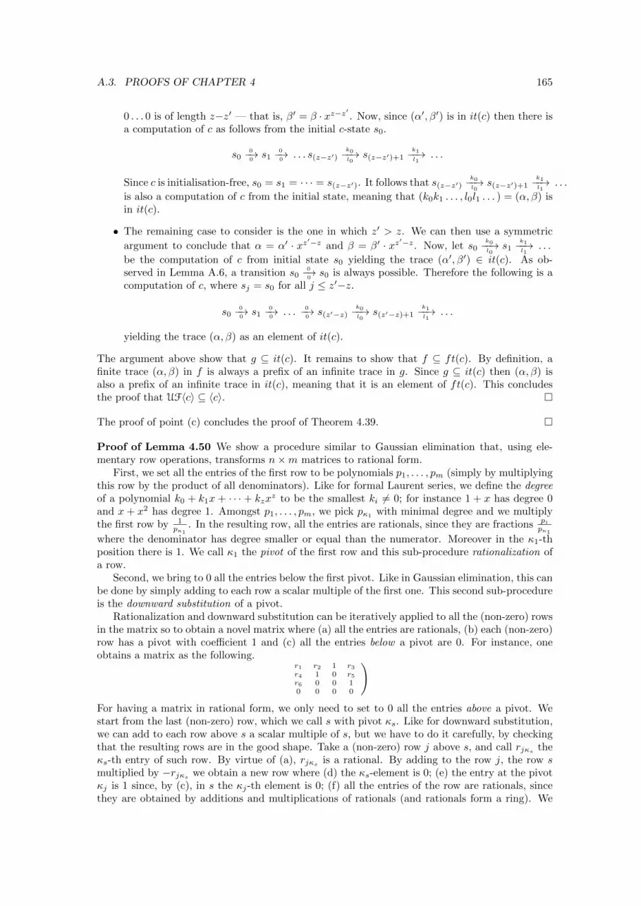
A.3. PROOFS OF CHAPTER 4 165
0 . . . 0 is of length z−z′ — that is, β′ = β · xz−z′ . Now, since (α′, β′) is in it(c) then there isa computation of c as follows from the initial c-state s0.
s00−→0s1
0−→0. . . s(z−z′)
k0−−→l0
s(z−z′)+1k1−−→l1
. . .
Since c is initialisation-free, s0 = s1 = · · · = s(z−z′). It follows that s(z−z′)k0−−→l0
s(z−z′)+1k1−−→l1
. . .
is also a computation of c from the initial state, meaning that (k0k1 . . . , l0l1 . . . ) = (α, β) isin it(c).
• The remaining case to consider is the one in which z′ > z. We can then use a symmetric
argument to conclude that α = α′ · xz′−z and β = β′ · xz′−z. Now, let s0k0−−→l0
s1k1−−→l1
. . .
be the computation of c from initial state s0 yielding the trace (α′, β′) ∈ it(c). As ob-served in Lemma A.6, a transition s0
0−→0s0 is always possible. Therefore the following is a
computation of c, where sj = s0 for all j ≤ z′−z.
s00−→0s1
0−→0. . .
0−→0s(z′−z)
k0−−→l0
s(z′−z)+1k1−−→l1
. . .
yielding the trace (α, β) as an element of it(c).
The argument above show that g ⊆ it(c). It remains to show that f ⊆ ft(c). By definition, afinite trace (α, β) in f is always a prefix of an infinite trace in g. Since g ⊆ it(c) then (α, β) isalso a prefix of an infinite trace in it(c), meaning that it is an element of ft(c). This concludesthe proof that UF〈c〉 ⊆ 〈c〉. �
The proof of point (c) concludes the proof of Theorem 4.39. �
Proof of Lemma 4.50 We show a procedure similar to Gaussian elimination that, using ele-mentary row operations, transforms n×m matrices to rational form.
First, we set all the entries of the first row to be polynomials p1, . . . , pm (simply by multiplyingthis row by the product of all denominators). Like for formal Laurent series, we define the degreeof a polynomial k0 + k1x + · · · + kzx
z to be the smallest ki 6= 0; for instance 1 + x has degree 0and x+ x2 has degree 1. Amongst p1, . . . , pm, we pick pκ1 with minimal degree and we multiplythe first row by 1
pκ1. In the resulting row, all the entries are rationals, since they are fractions pi
pκ1
where the denominator has degree smaller or equal than the numerator. Moreover in the κ1-thposition there is 1. We call κ1 the pivot of the first row and this sub-procedure rationalization ofa row.
Second, we bring to 0 all the entries below the first pivot. Like in Gaussian elimination, this canbe done by simply adding to each row a scalar multiple of the first one. This second sub-procedureis the downward substitution of a pivot.
Rationalization and downward substitution can be iteratively applied to all the (non-zero) rowsin the matrix so to obtain a novel matrix where (a) all the entries are rationals, (b) each (non-zero)row has a pivot with coefficient 1 and (c) all the entries below a pivot are 0. For instance, oneobtains a matrix as the following. (
r1 r2 1 r3r4 1 0 r5r6 0 0 10 0 0 0
)
For having a matrix in rational form, we only need to set to 0 all the entries above a pivot. Westart from the last (non-zero) row, which we call s with pivot κs. Like for downward substitution,we can add to each row above s a scalar multiple of s, but we have to do it carefully, by checkingthat the resulting rows are in the good shape. Take a (non-zero) row j above s, and call rjκs theκs-th entry of such row. By virtue of (a), rjκs is a rational. By adding to the row j, the row smultiplied by −rjκs we obtain a new row where (d) the κs-element is 0; (e) the entry at the pivotκj is 1 since, by (c), in s the κj-th element is 0; (f) all the entries of the row are rationals, sincethey are obtained by additions and multiplications of rationals (and rationals form a ring). We

166 APPENDIX A. OMITTED PROOFS
can repeat this for all the pivots κu and for all the rows above u and we will eventually obtain amatrix where by (f) all the entries are rationals, each row has, by (e), a pivot with entry 1 and allthe entries above and below a pivot are 0 by (c) and (d). �
Appendix B
Works not Included in the Thesis
During the PhD I also worked on other research topics, which are not detailed in this thesisfor reasons of homogeneity. In the following I briefly report on these works and the associatedpublications.
§1 Expressive completeness for fragments of the modal µ-calculus The modal µ-calculus(MC) is a well-balanced specification language for describing and verifying properties of transitionsystems. A landmark result in the area is the Janin-Walukiewicz theorem, stating that MC isthe bisimulation-invariant fragment of monadic second-order logic (MSO). That means, MC isas expressive as MSO on properties not distinguishing between bisimilar transition systems, likecomputationally relevant properties usually do.
The Janin-Walukiewicz theorem has been extended also to finite, transitive and tree models.However, very little is known about analogous expressive completeness results for fragments of MC.In my master thesis I answered this question for the alternation-free fragment of the µ-calculus(AFMC), which is particularly appealing in applications for its computational feasibility. By meansof an automata theoretic construction, I proved that AFMC is the bisimulation-invariant fragmentof well-founded MSO: the latter is the fragment of MSO where, roughly speaking, second-orderquantifiers are only allowed to range over well-founded portions of the model. During my PhD,together with my master thesis supervisors Y. Venema and A. Facchini, we prepared a joint paperon these results which appeared at LICS’13 [49]. Our collaboration continued in another paperappearing at CSL-LICS’14 [38], also with F. Carreiro, in which we tailored a fragment of MCwhere the application of fixpoint operators is restricted by a continuity condition and prove thatit is the bisimulation-inviariant fragment of weak MSO.
• F. Carreiro, A. Facchini, Y. Venema, F. Zanasi - Weak MSO: automata and expressivenessmodulo bisimilarity, CSL-LICS’14.
• A. Facchini, Y. Venema, F. Zanasi - A Characterization Theorem for the Alternation-FreeFragment of the Modal µ-Calculus, LICS’13.
§2 Bialgebraic semantics for logic programming Recent work by E. Komendantskaya andJ. Power [69] introduces a coalgebraic treatment of logic programming. This approach bringsseveral benefits (for instance, allows for reasoning about coinductive programs) but fails to becompositional: intuitively, their semantics is not compatible with substitutions that may occur informulas. In categorical terms, the space of formulas is represented by a presheaf F on a Lawveretheory; a logic program and its semantics should then be coalgebras on F, but they fail to benatural transformations, forcing the authors to introduce laxness in the picture. The drawbacksof the coalgebraic approach were the main motivation for F. Bonchi and me to propose a bialgebraic
167
168 APPENDIX B. WORKS NOT INCLUDED IN THE THESIS
environment for logic programming. We model logic programs as bialgebras on presheaves. Weobtain compositionality with respect to substitutions by applying saturation techniques, previouslyemployed in the setting of nominal process calculi. Categorically, saturation amounts to a certainright Kan extension of the presheaf modeling formulas. The bialgebra structure allows us toachieve also a second form of compositionality, with respect to the conjunction of formulas in agoal. This work appeared in a journal article [26], which extends a conference paper [25] winnerof the Best Paper award at CALCO’13.
• F. Bonchi, F. Zanasi - Bialgebraic Semantics for Logic Programming, Logical Methods inComputer Science, Vol. 11, Issue 2, 2015.
• F. Bonchi, F. Zanasi - Saturated Semantics for Coalgebraic Logic Programming, CALCO’13(Best Paper Award).
§3 A Categorical environment for systems with internal moves Coalgebras has beensuccessful in modeling a wide range of state-based systems. However, they seem to be inadequate todescribe the behaviour of systems where internal transitions play a role — notable examples includeautomata with ε-transitions and labelled transition systems with τ -transitions. In a collaborationwith F. Bonchi, A. Silva and S. Milius, we had the intuition that the gap could be filled byconsidering a more general form of coinduction — usually called parametric corecursion [3] —and the attached body of work on iteration theories and Elgot monads. We developed this ideainto a framework where the type of a system with internal moves is an Elgot monad satisfyingan initial algebra-final coalgebra coincidence. Our work resulted in a paper which I presented atCMCS’14 [19] and a subsequent journal publication [20].
• F. Bonchi, S. Milius, A. Silva, F. Zanasi - Killing Epsilons with a Dagger - A CoalgebraicStudy of Systems with Algebraic Label Structure, Theoretical Computer Science, acceptedfor publication, 2015.
• F. Bonchi, S. Milius, A. Silva, F. Zanasi - How to Kill Epsilons with a Dagger - A CoalgebraicTake on Systems with Algebraic Label Structure - CMCS’14.
Glossary of Symbols
( ) unique element of the 0-dimensional vector space . . . . . . . . . . . . . . . . . . . . . . . . . . . 13I unit object of the monoidal product in a monoidal category . . . . . . . . . . . . . . . . .13B PROP of the theory of bialgebras . . . . . . . . . . . . . . . . . . . . . . . . . . . . . . . . . . . . . . . . . . 18Circ PROP of circuit diagrams . . . . . . . . . . . . . . . . . . . . . . . . . . . . . . . . . . . . . . . . . . . . . . . . . . 114Cu PROP of the theory of counit . . . . . . . . . . . . . . . . . . . . . . . . . . . . . . . . . . . . . . . . . . . . . . 37C PROP of the theory of commutative comonoids . . . . . . . . . . . . . . . . . . . . . . . . . . . . .18Cospan(C) bicategory of objects in C, cospans and cospan morphisms . . . . . . . . . . . . . . . . . . 31ER PROP of equivalence relations . . . . . . . . . . . . . . . . . . . . . . . . . . . . . . . . . . . . . . . . . . . . . .47F PROP of functions . . . . . . . . . . . . . . . . . . . . . . . . . . . . . . . . . . . . . . . . . . . . . . . . . . . . . . . . . 19C−→irc PROP of “functional” circuit diagrams . . . . . . . . . . . . . . . . . . . . . . . . . . . . . . . . . . . . . 114C←−irc PROP of “co-functional” circuit diagrams (opposite of C−→irc ) . . . . . . . . . . . . . . . . 114Fr PROP of the theory of special Frobenius algebras . . . . . . . . . . . . . . . . . . . . . . . . . . .18IFr PROP of the theory of irredundant special Frobenius algebras . . . . . . . . . . . . . . 48IPFr PROP of the theory of irredundant partial special Frobenius algebras . . . . . . . 57In PROP of injective functions . . . . . . . . . . . . . . . . . . . . . . . . . . . . . . . . . . . . . . . . . . . . . . . . 31LΣ,E Lawvere theory generated by a signature Σ and a set E of equations . . . . . . . . 39Mu PROP of the theory of multiplication . . . . . . . . . . . . . . . . . . . . . . . . . . . . . . . . . . . . . . .32Mod(B) bicategory of monads in B, bimodules and bimodule morphisms . . . . . . . . . . . . 26M PROP of the theory of commutative monoids . . . . . . . . . . . . . . . . . . . . . . . . . . . . . . . 18Mnd(C) category of monoids in a monoidal category C . . . . . . . . . . . . . . . . . . . . . . . . . . . . . . 28Mon category of monoids and monoid homomorphisms . . . . . . . . . . . . . . . . . . . . . . . . . . .25PER PROP of partial equivalence relations . . . . . . . . . . . . . . . . . . . . . . . . . . . . . . . . . . . . . . 54PF PROP of partial functions . . . . . . . . . . . . . . . . . . . . . . . . . . . . . . . . . . . . . . . . . . . . . . . . . . 37PFr PROP of the theory of partial special Frobenius algebras . . . . . . . . . . . . . . . . . . . 54J PROP of isomorphisms in a given PROP T (also called the core of T) . . . . . . 34P PROP of permutations . . . . . . . . . . . . . . . . . . . . . . . . . . . . . . . . . . . . . . . . . . . . . . . . . . . . . 19AT Unique PROP morphism from P to a PROP T . . . . . . . . . . . . . . . . . . . . . . . . . . . . . 20SF PROP of orthodox signal flow graphs . . . . . . . . . . . . . . . . . . . . . . . . . . . . . . . . . . . . . . . 115Set category of sets and functions . . . . . . . . . . . . . . . . . . . . . . . . . . . . . . . . . . . . . . . . . . . . . . 23Span(C) bicategory of objects in C, spans and span morphisms . . . . . . . . . . . . . . . . . . . . . . 23Su PROP of surjective functions . . . . . . . . . . . . . . . . . . . . . . . . . . . . . . . . . . . . . . . . . . . . . . . 31Tr(·) trace in IHk[x] defined by feedback loops guarded by a register . . . . . . . . . . . . . . 125U PROP of the theory of unit . . . . . . . . . . . . . . . . . . . . . . . . . . . . . . . . . . . . . . . . . . . . . . . . 32B(x, x) monoidal category of 1-cells x→ x in a bicategory B . . . . . . . . . . . . . . . . . . . . . . . 28⊗D composition of 1-cells along the object D in a bicategory of bimodules . . . . . . 26C[x, y] set of arrows from x to y in a small category C . . . . . . . . . . . . . . . . . . . . . . . . . . . . . 13∼= isomorphism of objects . . . . . . . . . . . . . . . . . . . . . . . . . . . . . . . . . . . . . . . . . . . . . . . . . . . . . 18−→[[·]] polynomial semantics C−→irc → Matk[x] . . . . . . . . . . . . . . . . . . . . . . . . . . . . . . . . . . . . . . . . 116←−[[·]] polynomial semantics C←−irc → Matopk[x] . . . . . . . . . . . . . . . . . . . . . . . . . . . . . . . . . . . . . . . . 117
169
170 GLOSSARY OF SYMBOLS
∅ empty set . . . . . . . . . . . . . . . . . . . . . . . . . . . . . . . . . . . . . . . . . . . . . . . . . . . . . . . . . . . . . . . . . . 19k[[x]] ring of formal power series (streams) . . . . . . . . . . . . . . . . . . . . . . . . . . . . . . . . . . . . . . . 119k(x) field of fractions of polynomials . . . . . . . . . . . . . . . . . . . . . . . . . . . . . . . . . . . . . . . . . . . . .117ft(c) finite traces of the operational semantics of a circuit c of Circ . . . . . . . . . . . . . . . 113it(c) infinite traces of the operational semantics of a circuit c of Circ . . . . . . . . . . . . . 113k((x)) field of formal Laurent series . . . . . . . . . . . . . . . . . . . . . . . . . . . . . . . . . . . . . . . . . . . . . . . 118n the set {1, . . . , n} . . . . . . . . . . . . . . . . . . . . . . . . . . . . . . . . . . . . . . . . . . . . . . . . . . . . . . . . . . .13〈·〉 observable behaviour Circ→ Relk[x] × Relk[[x]] . . . . . . . . . . . . . . . . . . . . . . . . . . . . . . . . 130; sequential composition of arrows in a category . . . . . . . . . . . . . . . . . . . . . . . . . . . . . . 13k[x] ring of polynomials . . . . . . . . . . . . . . . . . . . . . . . . . . . . . . . . . . . . . . . . . . . . . . . . . . . . . . . . . 115k〈x〉 ring of rational fractions of polynomials . . . . . . . . . . . . . . . . . . . . . . . . . . . . . . . . . . . . 119\ difference of sets . . . . . . . . . . . . . . . . . . . . . . . . . . . . . . . . . . . . . . . . . . . . . . . . . . . . . . . . . . . 46σx,y symmetry associated with objects x and y in a symmetric monoidal category 13' equivalence of categories . . . . . . . . . . . . . . . . . . . . . . . . . . . . . . . . . . . . . . . . . . . . . . . . . . . .28−→〈〈·〉〉 denotational stream semantics C−→irc → SVk((x)) . . . . . . . . . . . . . . . . . . . . . . . . . . . . . . . 119〈〈·〉〉 denotational stream semantics Circ→ SVk((x)) . . . . . . . . . . . . . . . . . . . . . . . . . . . . . . . 120⊕ monoidal product in a monoidal category . . . . . . . . . . . . . . . . . . . . . . . . . . . . . . . . . . . 13] disjoint union of sets . . . . . . . . . . . . . . . . . . . . . . . . . . . . . . . . . . . . . . . . . . . . . . . . . . . . . . . 21x/C coslice category of C under x ∈ C . . . . . . . . . . . . . . . . . . . . . . . . . . . . . . . . . . . . . . . . . . .20
Bibliography
[1] Abramsky, S., and Coecke, B. A categorical semantics of quantum protocols. In 19thIEEE Symposium on Logic in Computer Science (LICS 2004), 14-17 July 2004, Turku,Finland, Proceedings (2004), pp. 415–425.
[2] Abramsky, S., and Coecke, B. Categorical quantum mechanics. CoRR abs/1401.4973(2008).
[3] Adamek, J., Milius, S., and Velebil, J. Parametric corecursion and completely iterativemonads. In FICS (2002), Z. Esik and A. Ingolfsdottir, Eds., vol. NS-02-2 of BRICS NotesSeries, University of Aarhus, pp. 2–5.
[4] Arbab, F. Reo: a channel-based coordination model for component composition. MathStruct Comp Sci 14, 3 (2004), 1–38.
[5] Backens, M. The zx-calculus is complete for stabilizer quantum mechanics. New Journalof Physics 16, 9 (2014), 093021.
[6] Backens, M. The zx-calculus is complete for the single-qubit clifford+t group. In Pro-ceedings 11th workshop on Quantum Physics and Logic, Kyoto, Japan, 4-6th June 2014(2014), B. Coecke, I. Hasuo, and P. Panangaden, Eds., vol. 172 of Electronic Proceedings inTheoretical Computer Science, Open Publishing Association, pp. 293–303.
[7] Baez, J. C. Network theory. http://math.ucr.edu/home/baez/networks/, 2014.
[8] Baez, J. C., and Erbele, J. Categories in control. CoRR abs/1405.6881 (2014).
[9] Baez, J. C., and Fong, B. A compositional framework for passive linear circuits. CoRRabs/1504.05625 (2015).
[10] Baez, J. C., and Stay, M. Physics, topology, logic and computation: A rosetta stone.Lecture Notes in Physics 813 (2011), 95–174.
[11] Barnabei, M., Guerrini, C., and Montefusco, L. Some algebraic aspects of signalprocessing. Linear Algebra and its Applications 284, 1-3 (1998), 3 – 17.
[12] Basold, H., Bonsangue, M., Hansen, H., and Rutten, J. (co)algebraic characteri-zations of signal flow graphs. In Horizons of the Mind. A Tribute to Prakash Panangaden,F. van Breugel, E. Kashefi, C. Palamidessi, and J. Rutten, Eds., vol. 8464 of Lecture Notesin Computer Science. Springer International Publishing, 2014, pp. 124–145.
[13] Beauxis, R., and Mimram, S. A non-standard semantics for Kahn networks in continuoustime. In Computer Science Logic, 25th International Workshop / 20th Annual Conferenceof the EACSL, CSL 2011, September 12-15, 2011, Bergen, Norway, Proceedings (2011),pp. 35–50.
171
172 BIBLIOGRAPHY
[14] Beck, J. Distributive laws. In Seminar on Triples and Categorical Homology Theory,B. Eckmann, Ed., vol. 80 of Lecture Notes in Mathematics. Springer Berlin Heidelberg,1969, pp. 119–140.
[15] Benabou, J. Introduction to bicategories. In Reports of the Midwest Category Seminar,vol. 47 of Lecture Notes in Mathematics. Springer Berlin Heidelberg, 1967, pp. 1–77.
[16] Bergman, G. Everybody knows what a Hopf algebra is. Amer. Math. Soc. Contemp. Math.43 (1985), 25–48.
[17] Berstel, J., and Reutenauer, C. Rational series and their languages. EATCS Mono-graphs on Theoretical Computer Science 12 (1988).
[18] Bonchi, F., Bonsangue, M. M., Rutten, J. J. M. M., and Silva, A. Deriving syntaxand axioms for quantitative regular behaviours. In CONCUR 2009 - Concurrency The-ory, 20th International Conference, CONCUR 2009, Bologna, Italy, September 1-4, 2009.Proceedings (2009), pp. 146–162.
[19] Bonchi, F., Milius, S., Silva, A., and Zanasi, F. How to kill epsilons with a dagger- A coalgebraic take on systems with algebraic label structure. In Coalgebraic Methods inComputer Science - 12th IFIP WG 1.3 International Workshop, CMCS 2014, Colocated withETAPS 2014, Grenoble, France, April 5-6, 2014, Revised Selected Papers (2014), pp. 53–74.
[20] Bonchi, F., Milius, S., Silva, A., and Zanasi, F. Killing epsilons with a dagger — acoalgebraic study of systems with algebraic label structure. Theoretical Computer Science(to appear, 2015).
[21] Bonchi, F., Sobocinski, P., and Zanasi, F. A categorical semantics of signal flow graphs.In CONCUR 2014 - Concurrency Theory - 25th International Conference, CONCUR 2014,Rome, Italy, September 2-5, 2014. Proceedings (2014), pp. 435–450.
[22] Bonchi, F., Sobocinski, P., and Zanasi, F. Interacting Hopf algebras. CoRRabs/1403.7048 (2014).
[23] Bonchi, F., Sobocinski, P., and Zanasi, F. Full abstraction for signal flow graphs.In Proceedings of the 42nd Annual ACM SIGPLAN-SIGACT Symposium on Principles ofProgramming Languages, POPL 2015, Mumbai, India, January 15-17, 2015 (2015), pp. 515–526.
[24] Bonchi, F., Sobociski, P., and Zanasi, F. Interacting bialgebras are frobenius. InFoundations of Software Science and Computation Structures, A. Muscholl, Ed., vol. 8412of Lecture Notes in Computer Science. Springer Berlin Heidelberg, 2014, pp. 351–365.
[25] Bonchi, F., and Zanasi, F. Saturated semantics for coalgebraic logic programming. InAlgebra and Coalgebra in Computer Science - 5th International Conference, CALCO 2013,Warsaw, Poland, September 3-6, 2013. Proceedings (2013), pp. 80–94.
[26] Bonchi, F., and Zanasi, F. Bialgebraic semantics for logic programming. Logical Methodsin Computer Science 11 (2015).
[27] Bonsangue, M. M., Hansen, H. H., Kurz, A., and Rot, J. Presenting distributivelaws. In Algebra and Coalgebra in Computer Science - 5th International Conference, CALCO2013, Warsaw, Poland, September 3-6, 2013. Proceedings (2013), pp. 95–109.
[28] Bonsangue, M. M., Rutten, J. J. M. M., and Silva, A. Coalgebraic logic and synthesisof mealy machines. In Foundations of Software Science and Computational Structures, 11thInternational Conference, FOSSACS 2008, Held as Part of the Joint European Conferenceson Theory and Practice of Software, ETAPS 2008, Budapest, Hungary, March 29 - April 6,2008. Proceedings (2008), pp. 231–245.
BIBLIOGRAPHY 173
[29] Borceux, F. Handbook of Categorical Algebra 1 – Basic Category Theory. CambridgeUniv. Press, 1994.
[30] Brookes, S. On the Kahn principle and fair networks. Tech. rep., 1998.
[31] Bruni, R., and Gadducci, F. Some algebraic laws for spans (and their connections withmulti-relations). In RelMiS 2001 (2001), Elsevier.
[32] Bruni, R., Lanese, I., and Montanari, U. A basic algebra of stateless connectors.Theor Comput Sci 366 (2006), 98–120.
[33] Bruni, R., Melgratti, H. C., Montanari, U., and Sobocinski, P. Connector algebrasfor C/E and P/T nets’ interactions. Log Meth Comput Sci 9, 16 (2013).
[34] Burris, S., and Sankappanavar, H. P. A Course in Universal Algebra. Springer, 1981.
[35] Burroni, A. Higher dimensional word problems with applications to equational logic.Theor Comput Sci 115 (1993), 43–62.
[36] Carboni, A., and Walters, R. F. C. Cartesian bicategories I. J Pure Appl Algebra 49(1987), 11–32.
[37] Carqueville, N., and Runkel, I. Orbifold completion of defect bicategories. CoRRabs/1210.6363 (2012).
[38] Carreiro, F., Facchini, A., Venema, Y., and Zanasi, F. Weak MSO: automata andexpressiveness modulo bisimilarity. In Joint Meeting of the Twenty-Third EACSL AnnualConference on Computer Science Logic (CSL) and the Twenty-Ninth Annual ACM/IEEESymposium on Logic in Computer Science (LICS), CSL-LICS ’14, Vienna, Austria, July 14- 18, 2014 (2014), p. 27.
[39] Cheng, E. Iterated distributive laws. Math. Proc. Camb. Philos. Soc. 150, 3 (2011), 459–487.
[40] Cheng, E. Distributive laws for lawvere theories. Algebra Universalis (to appear). availableat http://arxiv.org/abs/1112.3076.
[41] Coecke, B., and Duncan, R. Interacting quantum observables. In Automata, Languagesand Programming, 35th International Colloquium, ICALP 2008, Reykjavik, Iceland, July7-11, 2008, Proceedings, Part II - Track B: Logic, Semantics, and Theory of Programming& Track C: Security and Cryptography Foundations (2008), pp. 298–310.
[42] Coecke, B., and Duncan, R. Interacting quantum observables: categorical algebra anddiagrammatics. New Journal of Physics 13, 4 (2011), 043016.
[43] Cohen, H. A Course in Computational Algebraic Number Theory. Springer, 1993.
[44] Conti, P. Hermite canonical form and Smith canonical form of a matrix over a principalideal domain. 8–16.
[45] Corradini, A., and Gadducci, F. An algebraic presentation of term graphs, via gs-monoidal categories. Applied Categorical Structures 7, 4 (1999), 299–331.
[46] Danos, V., and Regnier, L. The structure of multiplicatives. Archive for MathematicalLogic 28, 3 (1989), 181–203.
[47] de Witt, C. S., and Zamdzhiev, V. The ZX calculus is incomplete for quantum me-chanics. In Proceedings of the 11th workshop on Quantum Physics and Logic, QPL 2014,Kyoto, Japan, 4-6th June 2014. (2014), pp. 285–292.
174 BIBLIOGRAPHY
[48] Eilenberg, S., and Kelly, G. M. Closed categories. In Proceedings of the Conferenceon Categorical Algebra (1966), Springer, pp. 421–562.
[49] Facchini, A., Venema, Y., and Zanasi, F. A characterization theorem for thealternation-free fragment of the modal µ-calculus. In 28th Annual ACM/IEEE Sympo-sium on Logic in Computer Science, LICS 2013, New Orleans, LA, USA, June 25-28, 2013(2013), pp. 478–487.
[50] Fiore, M. P., and Campos, M. D. The algebra of directed acyclic graphs. In AbramskyFestschrift (2013), vol. 7860 of LNCS.
[51] Fritz, T. A presentation of the category of stochastic matrices. CoRR abs/0902.2554(2009).
[52] Girard, J. Linear logic. Theor. Comput. Sci. 50 (1987), 1–102.
[53] Hasegawa, M. Recursion from cyclic sharing: Traced monoidal categories and models ofcyclic lambda calculi. Springer Verlag, pp. 196–213.
[54] Hasuo, I., and Hoshino, N. Semantics of higher-order quantum computation via geometryof interaction. In Proceedings of the 26th Annual IEEE Symposium on Logic in ComputerScience, LICS 2011, June 21-24, 2011, Toronto, Ontario, Canada (2011), pp. 237–246.
[55] Heindel, T., and Sobocinski, P. Being Van Kampen is a universal property. LogicalMethods in Computer Science 7, 1 (2011).
[56] Hildebrandt, T. T., Panangaden, P., and Winskel, G. A relational model of non-deterministic dataflow. Mathematical. Structures in Comp. Sci. 14, 5 (Oct. 2004), 613–649.
[57] Hoare, C. A. R. Communicating sequential processes. Commun. ACM 21, 8 (Aug. 1978),666–677.
[58] Hogben, L. Handbook of Linear Algebra, 1 ed. (Discrete Mathematics and Its Applications).Chapman & Hall/CRC, 2006.
[59] Hyland, M., and Power, J. Symmetric monoidal sketches. In PPDP (2000), pp. 280–288.
[60] Hyland, M., and Power, J. The category theoretic understanding of universal algebra:Lawvere theories and monads. Electronic Notes in Theoretical Computer Science 172 (2007),437–458.
[61] Jacobs, B. Categorical Logic and Type Theory. No. 141 in Studies in Logic and theFoundations of Mathematics. North Holland, Amsterdam, 1999.
[62] Jacobs, B., and Mandemaker, J. Coreflections in algebraic quantum logic. Foundationsof Physics 42, 7 (2012), 932–958.
[63] Joyal, A., and Street, R. The geometry of tensor calculus, i. Adv. Math. 88 (1991),55–112.
[64] Joyal, A., Street, R., and Verity, D. Traced monoidal categories. MathematicalProceedings of the Cambridge Philosophical Society 119 (4 1996), 447–468.
[65] Katis, P., Sabadini, N., and Walters, R. F. C. Span(Graph): an algebra of transitionsystems. In Algebraic Methodology and Software Technology (AMAST ’97) (1997), vol. 1349of LNCS, Springer, pp. 322–336.
[66] Kelly, G. M., and Laplaza, M. L. Coherence for compact closed categories. Journal ofPure and Applied Algebra 19 (1980), 193–213.
BIBLIOGRAPHY 175
[67] Kissinger, A., and Zamdzhiev, V. Quantomatic: A proof assistant for diagrammaticreasoning. CoRR abs/1503.01034 (2015).
[68] Kleene, S. C. Representation of events in nerve nets and finite automata. In AutomataStudies, C. Shannon and J. McCarthy, Eds. Princeton University Press, Princeton, NJ, 1956,pp. 3–41.
[69] Komendantskaya, E., and Power, J. Coalgebraic derivations in logic programming. InCSL (2011), vol. 12 of LIPIcs, Schloss Dagstuhl, pp. 352–366.
[70] Kozen, D. A completeness theorem for kleene algebras and the algebra of regular events.Information and Computation 110 (1994), 366–390.
[71] Lack, S. Composing PROPs. Theor App Categories 13, 9 (2004), 147–163.
[72] Lafont, Y. Interaction nets. In Conference Record of the Seventeenth Annual ACM Sym-posium on Principles of Programming Languages, San Francisco, California, USA, January1990 (1990), pp. 95–108.
[73] Lafont, Y. Equational reasoning with 2-dimensional diagrams. In Term Rewriting,H. Comon and J.-P. Jounnaud, Eds., vol. 909 of Lecture Notes in Computer Science. SpringerBerlin Heidelberg, 1995, pp. 170–195.
[74] Lafont, Y. Interaction combinators. Inf. Comput. 137, 1 (1997), 69–101.
[75] Lafont, Y. Towards an algebraic theory of boolean circuits. J Pure Appl Alg 184 (2003),257–310.
[76] Lahti, B. Signal Processing and Linear Systems. Oxford University Press, 1998.
[77] Lawvere, W. F. Functorial Semantics of Algebraic Theories. PhD thesis, 2004.
[78] Leinster, T. Higher operads, higher categories. No. 298. Cambridge University Press, 2004.
[79] Mac Lane, S. Categorical algebra. B Am Math Soc 71 (1965), 40–106.
[80] Mac Lane, S. Categories for the Working Mathematician. Springer, 1998.
[81] Mason, S. J. Feedback Theory: I. Some Properties of Signal Flow Graphs. MIT ResearchLaboratory of Electronics, 1953.
[82] Milius, S. A sound and complete calculus for finite stream circuits. In Proceedings of the25th Annual IEEE Symposium on Logic in Computer Science, LICS 2010, 11-14 July 2010,Edinburgh, United Kingdom (2010), IEEE Computer Society, pp. 421–430.
[83] Milner, R. A Calculus of Communicating Systems. Springer-Verlag New York, Inc.,Secaucus, NJ, USA, 1982.
[84] Mimram, S. Semantique des jeux asynchrones et reecriture 2-dimensionnelle. PhD thesis,Universite Paris Diderot, 2008.
[85] Mimram, S. The structure of first-order causality. Mathematical Structures in ComputerScience 21 (2 2011), 65–110.
[86] Mimram, S. Towards 3-dimensional rewriting theory. Logical Methods in Computer Science10, 2 (2014).
[87] Mimram, S. Presenting finite posets. In Proceedings 8th International Workshop on Com-puting with Terms and Graphs, Vienna, Austria, July 13, 2014 (2015), A. Middeldorp andF. v. Raamsdonk, Eds., vol. 183 of Electronic Proceedings in Theoretical Computer Science,Open Publishing Association, pp. 1–17.
176 BIBLIOGRAPHY
[88] Panangaden, P. Probabilistic relations. School of Computer Science research reports,University of Birmingham CSR (1998), 59–74.
[89] Pavlovic, D. Monoidal computer I: Basic computability by string diagrams. Inf. Comput.226 (2013), 94–116.
[90] Pavlovic, D., and Escardo, M. H. Calculus in coinductive form. In Proceedings ofthe 13th Annual IEEE Symposium on Logic in Computer Science (Washington, DC, USA,1998), LICS ’98, IEEE Computer Society, pp. 408–417.
[91] Penrose, R. Applications of negative dimension tensors. In Combinatorial Mathematicsand its Applications (1971), D. J. A. Welsh, Ed., Academic Press, pp. 221–244.
[92] Peterson, J. L. Petri nets. ACM Comput. Surv. 9, 3 (Sept. 1977), 223–252.
[93] Pirashvili, T. On the PROP corresponding to bialgebras. Cah. Top. Gom. Diff. Cat XLIII(2002).
[94] Rannou, P. Reecriture de diagrammes et de Σ-diagrammes. PhD thesis, University ofMarseille, 2013.
[95] Rosebrugh, R., and Wood, R. Distributive laws and factorization. Journal of Pure andApplied Algebra 175, 13 (2002), 327 – 353. Special Volume celebrating the 70th birthday ofProfessor Max Kelly.
[96] Rutten, J. J. M. M. A tutorial on coinductive stream calculus and signal flow graphs.Theor. Comput. Sci. 343, 3 (2005), 443–481.
[97] Rutten, J. J. M. M. Rational streams coalgebraically. Logical Methods in ComputerScience 4, 3 (2008).
[98] Sangiorgi, D., and Walker, D. PI-Calculus: A Theory of Mobile Processes. CambridgeUniversity Press, New York, NY, USA, 2001.
[99] Selinger, P. Dagger compact closed categories and completely positive maps. Electr.Notes Theor. Comput. Sci. 170 (2007), 139–163.
[100] Selinger, P. A survey of graphical languages for monoidal categories. Springer LectureNotes in Physics 13, 813 (2011), 289–355.
[101] Shannon, C. E. The theory and design of linear differential equation machines. Tech. rep.,National Defence Research Council, 1942.
[102] Sleep, M. R., Plasmeijer, M. J., and van Eekelen, M. C. J. D., Eds. Term GraphRewriting: Theory and Practice. John Wiley and Sons Ltd., Chichester, UK, 1993.
[103] Sobocinski, P. Representations of Petri net interactions. In CONCUR 2010 - ConcurrencyTheory, 21th International Conference, CONCUR 2010, Paris, France, August 31-September3, 2010. Proceedings (2010), pp. 554–568.
[104] Sobocinski, P. Nets, relations and linking diagrams. In Algebra and Coalgebra in ComputerScience - 5th International Conference, CALCO 2013, Warsaw, Poland, September 3-6,2013. Proceedings (2013), pp. 282–298.
[105] Stefanescu, G. Network Algebra. Discrete Mathematics and Theoretical Computer Sci-ence. Springer London, 2000.
[106] Street, R. The formal theory of monads. J Pure Appl Algebra 2, 1 (2002), 243–265.
[107] Streicher, T. Semantics of type theory : correctness, completeness, and independenceresults. Progress in theoretical computer science. Birkhuser, Boston, 1991.

BIBLIOGRAPHY 177
[108] Sweedler, M. Hopf Algebras. W. A. Benjamin, Inc., 1969.
[109] Wadsley, S., and Woods, N. PROPs for linear systems. CoRR abs/1505.00048 (2015).
[110] Wilf, H. Generatingfunctionology, 3rd ed. A. K. Peters, 2006.
[111] Willems, J. Linear systems in discrete time. In Festschrift on the occasion of the retirementof Okko Bosgra (2009), C. S. P.M.J. van den Hof and P. Heuberger, Eds., pp. 3–12.
[112] Willems, J. C. The behavioural approach to open and interconnected systems. IEEEContr. Syst. Mag. 27 (2007), 46–99.
Related Documents


![Braided Hopf algebras of triangular type · 4 Introduction Braided Hopf algebras appeared in the structure theory of Hopf algebras when Radford [34] generalized the notion of semi-direct](https://static.cupdf.com/doc/110x72/5f1f575c79e5127e2d16584e/braided-hopf-algebras-of-triangular-type-4-introduction-braided-hopf-algebras-appeared.jpg)