INTER-SECTORAL LABOUR MOBILITY IN KOREA: ITS ORIGINS AND RELATIONSHIP WITH UNEMPLOYMENT by Fiona Ai Lin Tan Bachelor of Economics (Hons) (UWA) This thesis is presented for the degree of Doctor of Philosophy of The University of Western Australia Business School University of Western Australia September 2008

Welcome message from author
This document is posted to help you gain knowledge. Please leave a comment to let me know what you think about it! Share it to your friends and learn new things together.
Transcript
INTER-SECTORAL LABOUR MOBILITY IN KOREA:
ITS ORIGINS AND RELATIONSHIP WITH UNEMPLOYMENT
by
Fiona Ai Lin Tan
Bachelor of Economics (Hons) (UWA)
This thesis is presented for the degree of Doctor of Philosophy of
The University of Western Australia
Business School
University of Western Australia
September 2008

i
ABSTRACT
The Asian Financial Crisis was a wake-up call to the South Korean economy that a change
to its economic structure was needed. Prior to the Crisis, South Korea enjoyed healthy
economic growth and low unemployment. With the onset of the Crisis, Korea experienced
severe recession. Unemployment levels soared and turnover in the labour market became
commonplace. The Korean government enacted a series of policies and succeeded in
combating unemployment in the short-term. To the present time, unemployment levels
have been lowered, albeit with job instability and insecurity. A more effective longer-term
solution is needed to increase the resilience of this NIE.
The role of inter-sector labour mobility as a policy tool to combat unemployment using the
relevant determinants of mobility has not been explored in Korea (Asia), although it has
been debated at length in the West since the 1980s. Part of the reason for this lies in the
lack of longitudinal data to facilitate appropriate research. Recently, such data have been
made available by the Korean Labour Institute (KLI). This thesis extends research into the
labour mobility-unemployment relationship to South Korea. The priority is to establish
whether a mobility-unemployment relationship exists in Korea, and to obtain a thorough
understanding of the factors affecting sectoral mobility in this country in order to facilitate
the crafting of potential tools for addressing the unemployment problem.
The thesis is organised into two parts. Prior to the main study, however, the economic
history of Korea is outlined and sectoral labour reallocation patterns are associated with
economic growth. This preliminary work establishes the potential for the detailed research
for the Korean labour market that follows to make contribution to policy solutions to the
unemployment problem along the lines of the earlier research undertaken in Western
countries. Part I, entitled ‘Sectoral Mobility and Unemployment’, details the theoretical
hypotheses and empirical evidence concerning sectoral mobility and unemployment, and
extends the empirical application to Korea. The general finding is that whilst the
hypotheses [Sectoral Shift Hypothesis (SSH), Aggregate Demand Hypothesis (ADH) and
stage-of-the-business-cycle effect] are not relevant for Korea in the pre-Crisis era (1970-
1997), they have some support in the post-Crisis period (1998-2001). However, data
limitations, in the form of the short time period available for analysis, prevent strong
conclusions from being formed. The tentative conclusion is that a new mobility-

ii
unemployment relationship may exist for Korea in the post-Crisis period, thereby giving
rise to the potential for mobility as a policy tool for controlling unemployment. The in-
depth understanding of the factors of sectoral mobility required to implement such policy
provides the basis for the remainder of the thesis.
Part II, titled ‘The Factors Affecting Mobility’, develops a theoretical model for sectoral
mobility, and provides a literature review on other forms of labour mobility (union/non-
union, public-private and rural-urban mobility) as well as an empirical review of sectoral
mobility. These chapters set the stage for the empirical analysis of the determinants of
sectoral mobility for Korea. For the overall workforce, the main conclusion is that sectoral
mobility is a multi-facetted phenomenon involving a spread of factors. Of significance are
the expected and lifetime incomes, which are the pull factors of mobility, the deterrent
effect of the new sector’s unemployment rate and the direct effects of unanticipated sectoral
shocks. The multi-dimensional nature of these factors is replicated in the separate analyses
undertaken for males and females. The main finding is that whilst the monetary variables
and worker/industry characteristics impact male and female mobility differently, sectoral
unemployment and sectoral shock affect male and female mobility similarly.
The thesis is summarised and some policy measures provided in the sypnosis. It is argued
that the ‘new’ mobility-unemployment phenomenon appears to have emerged in Korea
after the Crisis, whereas it had been a feature of Western economies in much earlier time
periods. Traditional monetary and fiscal policies are inadequate when it comes to
combating unemployment in the presence of this mobility-unemployment phenomenon. A
combination of macro-policies, given the relevance of the ADH, and micro-policies, given
the validity of the SSH, is required. The multi-dimensional nature of mobility implies that
the micro policies to control or reduce mobility rates using the relevant variables (to
alleviate unemployment) should cover measures related to monetary wages, labour market
groups and sector performance. The sypnosis notes a dearth of Asian studies on sectoral
mobility, possibly due to the lack of longitudinal data. The collection of quality
longitudinal data for other Asian countries, so that research along the lines conducted in the
thesis could be undertaken for other NIEs, was seen as being of vital importance. With
such data, the standard of research on Asian economies can be at par with that of the
Western countries, and the apparently considerable potential benefits of microeconomic
policies via sectoral mobility for Asia could be realised.
iii
TABLE OF CONTENTS
Page
Abstract
Table of Contents
List of Tables
List of Figures
List of Common Acronyms
Acknowledgements
i
iii
xi
xii
xiii
xv
Chapter
Description
1
1.1
1.1.1
1.1.2
1.1.3
1.1.4
1.2
1.3
INTRODUCTION
Aims of Thesis
Definition of Sectoral Mobility
The Empirical Studies
Sectoral Mobility vis-à-vis Unemployment
The Factors Motivating Mobility
Organisation of the Thesis
Contributions to Labour Economics
1
1
1
1
2
4
5
7
2
2.1
2.2
2.2.1
2.2.2
2.2.3
2.2.4
2.2.5
2.2.6
2.3
2.3.1
2.3.2
2.3.3
2.4
2.4.1
2.4.2
2.4.3
2.5
ECONOMIC HISTORY OF SOUTH KOREA
Introduction
Korea’s Economic History
The Three Kingdoms
Koryo Dynasty
Choson Dynasty (1392-1910)
Japanese Colonial Rule (1910-1945)
Korean War (1950-1953)
Post-war South Korea
Korea’s Economic History in the Post-War Era
The 1970s
The 1980s
The 1990s
Economic Growth, Sectoral Changes and Labour Mobility
The Three Decades: 1970-2000
The 1998-2001 Period
Possible Structural Break during Asian Financial Crisis
Concluding Remarks
10
10
11
11
12
13
13
14
14
15
15
18
19
20
20
25
28
28

iv
Chapter Description Page
PART I:
SECTORAL MOBILITY AND UNEMPLOYMENT
PREAMBLE
29
29
3
3.1
3.2
3.2.1
3.2.2
3.2.3
3.3
3.3.1
3.3.2
3.4
3.5
3.5.1
3.5.2
3.6
3.6.1
3.6.2
3.6.3
3.7
3.7.1
3.7.2
3.7.3
3.8
3.9
THEORETICAL HYPOTHESES CONCERNING
SECTORAL MOBILITY AND UNEMPLOYMENT
Introduction
The Sectoral Shift Hypothesis
Impact of Sectoral Mobility on Aggregate Unemployment
SSH and Supply Shocks
SSH and the Natural Unemployment Rate
Aggregate Demand Hypothesis
U-V Relationship
The σ-U Co-movement Approach
Predicted and Unpredicted Mobility Indices
The Reallocation Timing Hypothesis and Stage-of-the-
Business-Cycle Effect
The Reallocation Timing Hypothesis
The Stage-of-the-Business-Cycle Effect
Conceptual Differences Between the SSH, ADH and RTH
Source of Sectoral Mobility
Chain of Causation
Nature of Unemployment
Methodological Differences
Methods to Test the SSH
Methods to Test the ADH
Methods to Test the RTH and Stage-of-the-Business-Cycle
Effect
Critique of the Mobility Indices
Summary
31
31
32
32
34
36
38
38
40
42
46
46
48
49
49
49
50
50
50
51
54
54
58

v
Chapter
4
4.1
4.2
4.2.1
4.2.2
4.2.3
4.2.4
4.3
4.3.1
4.3.2
4.4
4.4.1
4.4.2
4.4.3
4.5
4.6
4.6.1
4.6.2
4.6.3
4.6.3.1
4.6.3.2
4.6.3.3
4.6.4
4.6.4.1
4.6.4.2
4.6.5
4.6.6
4.6.7
4.7
4.8
Description
THE IMPACT OF SECTORAL MOBILITY ON
UNEMPLOYMENT: A REVIEW OF THE EMPIRICAL
LITERATURE
Introduction
Empirical Review on the SSH
The Raw Lilien Index
The Index Generated by Supply-side Disturbances
Pure Sectoral Shift Measures
The Natural Unemployment Rate Approach
Empirical Findings on the ADH
The Predicted Mobility Indices
The U-V Relationship
Findings on the RTH and Stage-of-the-Business-Cycle
The Horizon Covariance Index
Interaction Variables
Labour Reallocations and Foregone Production
Summary of Empirical Findings
Empirical Application
Type and Frequency of Data
Time Period
Model Estimation
Single-Equation Models
2-Stage Least Squares (2SLS)
Dual-Equation Models
Model Specification
Dependent Variable
Explanatory Variables
Number of σ’s in the Regression Equation
Natural Unemployment Rate Approach
Sectoral Mobility and Gender Unemployment
Summary of Empirical Application
Links with Research on Determinants of Mobility
Page
60
60
60
61
62
62
65
67
67
68
69
69
70
70
71
72
72
73
73
73
80
80
84
84
84
88
89
92
93
94

vi
Chapter Description
Page
5
5.1
5.2
5.2.1
5.2.2
5.3
5.3.1
5.3.2
5.3.3
5.3.4
5.4
5.4.1
5.4.1.1
5.4.1.2
5.4.2
5.4.2.1
5.4.2.2
5.4.3
5.4.3.1
5.4.3.2
5.4.3.3
5.4.3.4
5.4.3.5
5.4.4
5.5
5.5.1
5.5.2
5.6
5.6.1
5.6.2
5.6.3
5.6.4
5.7
SECTORAL MOBILITY AND UNEMPLOYMENT: AN
EMPIRICAL EXAMINATION FOR KOREA
Introduction
Trends in Aggregate and Sectoral Unemployment
Aggregate and Sectoral Unemployment
Sector-specific Employment and Unemployment
Model Framework
Baseline Model
Methodology
Descriptive Statistics
Stationarity
Dual-Equation Modelling
Estimation of Money Growth Equation
Review of Empirical Studies Estimating DMRt
Application to the Korean Case
Specification of Unemployment Equation
Unrestricted to Restricted Models
Preliminary Model Estimation
Structural Change
Prior Knowledge on Korean Unemployment
Tests for Model Stability
Phase I and Phase II
Phase II and Phase III
Accommodation of Structural Change
Re-specification of Unemployment Models
Final Model Estimation
Treatment for Serial Correlation
Sectoral Mobility during the Pre-Crisis Period (1971-1997)
Validity of the Hypotheses
Validity of the SSH
Relevance of the ADH
Applicability of the RTH
Sectoral Movements and Stage-of-the-Business-Cycle Effect
Concluding Remarks
97
97
98
98
98
100
100
100
101
105
106
106
106
108
111
111
114
116
116
116
120
120
123
125
127
127
129
130
131
134
135
136
138

vii
Chapter Description Page
PART II:
THE FACTORS AFFECTING SECTORAL MOBILITY
143
PREAMBLE
143
6
6.1
6.2
6.3
6.3.1
6.3.2
6.3.3
6.4
6.5
6.5.1
6.5.2
6.5.3
6.5.4
6.5.5
6.6
THE THEORETICAL AND CONCEPTUAL ISSUES IN
LABOUR/SECTORAL MOBILITY
Introduction
What is Labour Mobility
Theories of Sectoral/Industrial Mobility
Worker-Employer Mismatch Theory
Sectoral Shock Theory
Bridging Theory
Model of Labour Mobility
Empirical Models of Sectoral Mobility
Probability Choice Models
Simultaneous Equation Models
Vector Auto-regression Models
Sectoral Shock Measures
Time Periods
Summary: Model Application for Current Research
145
145
145
149
149
150
151
151
157
158
162
163
163
164
164
7
7.1
7.2
7.3
7.4
7.5
REVIEW OF THE EMPIRICAL LITERATURE ON
OTHER FORMS OF LABOUR MOBILITY
Introduction
Union versus Non-Union Mobility
Public versus Private Sector Mobility
Rural-Urban Mobility
Summary: Salient Points for Empirical Model
166
166
166
173
179
184
viii
Chapter
Description Page
8
8.1
8.2
8.3
8.3.1
8.3.2
8.3.3
8.3.4
8.4
8.5
8.6
8.7
8.8
EMPIRICAL EVIDENCE: FACTORS MOTIVATING
SECTORAL/INDUSTRIAL MOBILITY
Introduction
Sectoral/Industrial Mobility
Determinants under the Mismatch Theory
Monetary Wages
Macroeconomic Factors
Worker Characteristics
Job/Industry Characteristics
Determinants under Sectoral Shock Theory
Determinants under Bridging Theory
Assessment of Empirical Studies of Sectoral Mobility for
Modelling
Summary of Empirical Studies of Sectoral Mobility
Summary of Lessons Drawn from the Literature
186
186
186
188
194
198
203
220
226
230
231
233
237
9
9.1
9.2
9.2.1
9.2.2
9.2.3
9.2.3.1
9.2.3.2
9.2.3.3
9.2.3.4
9.3
9.4
9.4.1
9.4.1.1
9.4.1.2
9.4.1.3
9.4.2
EMPIRICAL STUDY ON THE DETERMINANTS OF
SECTORAL/INDUSTRIAL MOBILITY IN KOREA
Introduction
Data Sources, Concepts and Coverage
KLIPS Data
Korea NSO Data
The Role of Interim State of Unemployment
Sectoral Labour Flows
Missing Industry Information
Missing Survey Information
Interim States of Unemployment
Generic Model of Sectoral/Industrial Mobility
Descriptive Statistics
Survey Weights
Wave 1 Weights and the Population
Weights for Sample Attrition
Weights for New Entrants
Descriptive Statistics: Complex Statistics
240
240
241
241
245
245
245
247
249
250
251
252
253
254
255
255
256

ix
Chapter
9.5
9.5.1
9.5.2
9.5.3
9.6
9.6.1
9.6.2
9.6.3
9.6.4
9.6.5
9.7
9.7.1
9.7.2
9.8
Description
Derivation of Predicted/Recomputed Variables
Predicted Sectoral Wages
Sector-level Variables
Descriptive Statistics of Predicted/Recomputed Variables
Empirical Analysis: Determinants of Sectoral Mobility
Monetary Variables
Macroeconomic Variables
Worker Characteristics
Industry Characteristics
Sectoral Shock
Extensions of the Model
A Focus on the Initial Industry
Empirical Test: Theories of Sectoral Mobility
Summary
Page
261
262
269
274
275
280
282
283
289
290
291
291
292
298
10 10.1 10.2 10.3 10.4 10.5 10.5.1 10.5.2 10.5.3 10.5.4 10.5.5 10.6 10.6.1 10.6.2 10.6.3 10.7 10.7.1 10.7.2 10.7.3 10.7.4 10.8
GENDER DIFFERENCES IN SECTORAL/MOBILITY IN KOREA Introduction Model and Sample Dataset Validity of Pooling the Dataset Descriptive Statistics for Males and Females Gender Differences in the Determinants of Sectoral Mobility Monetary Variables Macroeconomic Variables Worker Characteristics Industry Characteristics Sectoral Shock A Gender Perspective on Theories of Sectoral Mobility Worker-Employer Mismatch Theory Sectoral Shock Theory Bridging Theory Decomposition Analysis An Overview of the Standard Decomposition Technique Application to Logit Models Decomposition Results Explanatory Power of Observed Variables Concluding Remarks
303 303 304 305 307 311 312 315 316 320 322 323 323 323 324 325 326 327 329 331 334
x
Chapter
Description
Page
11 11.1 11.2 11.3 11.4 11.4.1 11.4.2 11.4.3 11.5
THE SYPNOSIS Introduction Part I: Sectoral Mobility and Unemployment Part II: The Factors Affecting Sectoral Mobility The Policy Implications Policy Measures in Post-Crisis Period Assessment of Policy Measures and Current Situation Policy Recommendations Direction for Future Research
337 337 337 342 354 354 355 356 362
REFERENCES
364
LIST OF APPENDICES* 388
* Available on enclosed CD.

xi
LIST OF TABLES
Table Description Page
Table 2.1 Annual % Change in GDP, CPI and Employment (EMP) and 16
Unemployment Rate (UR)
Table 2.2 GDP by Sector, 1970-2000 21
Table 2.3 Employed Persons by Sector, 1970-2000 23
Table 2.4 GDP at Current Prices by Sector, 1998-2001 26
Table 2.5 Employed Persons by Sector, 1998-2001 27
Table 4.1 Studies on the Impact of Sectoral Mobility on Aggregate 63
Unemployment in the U.S.
Table 4.2 R2 between Actual Unemployment Rate and Natural Unemployment 66
Rate
Table 4.3 Contemporaneous Correlations between Labour Reallocation 71
and Average Value Proxies of Foregone Production
Table 4.4 Unemployment and Money Growth Equations used in Selected 74
Studies of Sectoral Mobility
Table 5.1 Employment and Unemployment By Sector 99
Table 5.2 Symbols of Sectoral Mobility 102
Table 5.3 Descriptive Statistics of Ut, DMRt and σ 103
Table 5.4 Initial Parameter Estimates of σ 115
Table 5.5 Phases in the Korean Labour Market from the CUSUMSQ Test 118
Table 5.6 F- and Harvey-Collier Statistics from Tests of Structural Change 122
Table 5.7 Final Model: Parameter Estimates of σ, D and σD and LM statistic 128
Table 5.8 1971-1997: Parameter Estimates of σ 130
Table 5.9 Parameter Estimates of σ, σSt and/or σStD 137
Table 7.1 Selected Studies of Union/Non-Union Mobility 168
Table 7.2 Selected Studies of Public-Private Sector Mobility 175
Table 7.3 Selected Studies of Rural-Urban Sector Mobility 181
Table 8.1 Probability Choice Studies of Sectoral/Industrial Mobility under 190
Worker-Employer Mismatch Theory
Table 8.2 Wages and Sectoral/Industrial Mobility 197
Table 8.3 Unemployment, Employment, GNP and Sectoral/Industrial Mobility 202
Table 8.4 Age and Sectoral/Industrial Mobility 204
Table 8.5 Gender and Sectoral/Industrial Mobility 206
Table 8.6 Marital Status/Head of Household and Sectoral/Industrial Mobility 207
Table 8.7 Education and Sectoral/Industrial Mobility 208
Table 8.8 On-the-job Training and Sectoral/Industrial Mobility 213
Table 8.9 Occupation and Industrial Mobility 217
Table 8.10 Initial Industry and Industrial Mobility 218
Table 8.11 Employment Status and Industrial Mobility 220
Table 8.12 Working Hours, Product Similarity, Work Similarity and Industrial 223
Mobility
Table 8.13 Sectoral Performance Indicators and Sectoral/Industrial Mobility 226
Table 8.14 Sectoral Shocks and Sectoral/Industrial Mobility under Sectoral Shock 229
Theory
Table 8.15 Assessment of the Explanatory Variables 235

xii
Table Description Page
Table 9.1 Gross and Net Labour Flows based on Sample of 29,474 Observations 246
Table 9.2 Gross and Net Labour Flows based on Sample of 29,474 Observations 248
and the Interim State of Unemployment
Table 9.3 Industry Breakdown of 29,474 Sample with/without Survey Information 249
Table 9.4 Gross and Net Labour Flows based on Sample of 10,691 Observations 251
Table 9.5 Wave 1 Weights 254
Table 9.6 Means and Standard Deviations for Korean workers, Aged 20-64 years 258
Table 9.7 Actual versus Predicted Monetary Variables 269
Table 9.8 Means and Standard Deviations for Predicted and Recomputed
Variables 275
Table 9.9 Unrestricted Model: Logit Regression on Probability of
Sectoral/Industrial Mobility 278
Table 9.10 Main Model: Logit Regression on Probability of Sectoral/Industrial
Mobility 281
Table 9.11 Logit Regression on Probability of Sectoral/Industrial Mobility:
A Focus on the Initial Industry, Selected Coefficients 292
Table 9.12 Logistic Regression of Sectoral/Industrial Mobility on Wages and
Alternative Measures of Sectoral Shock, Selected Coefficients 296
Table 10.1 Logistic Regression of ‘Full’ Model 306
Table 10.2 Means and Standard Deviations for Male and Female workers, Aged
20-64 years 308
Table 10.3 Logistic Regression of Sectoral/Industrial Mobility by Gender 314
Table 10.4 Logistic Regression of Sectoral/Industrial Mobility on the Standard
Error of Wage Distribution and Sectoral Shock for Males and Females 324
Table 10.5 Decomposition Results 330
Table 10.6 Explanatory Power of Observed Characteristics in Decomposition 332
Table 11.1 Micro-policy Targets for Korea 360
LIST OF FIGURES
Figure Description Page
Figure 1.1 Lilien Index (σt) and Annual Unemployment Rate (Ut) 3
Figure 2.1 Korea’s Historical Timeline 11
Figure 2.2 Annual % Change in GDP, 1970-2001 17
Figure 2.3 Annual % Change in Employment and Unemployment Rate, 17
1970-2001
Figure 2.4 Annual % Change in CPI, 1970-2001 18
Figure 5.1 DMRt series 110
Figure 9.1 Probability of Sectoral Mobility and Age 284
Figure 9.2 Probability of Sectoral Mobility and Tenure 285

xiii
LIST OF COMMON ACRONYMS
ABS Australian Bureau of Statistics
ACGR Average Annual Compound Growth Rate
AD Aggregate Demand
ADH Aggregate Demand Hypothesis
APEC Asia-Pacific Economic Cooperation
AR Auto-regression
BLS Bureau of Labor Statistics
CILSS Cöte d’Ivoire Living Standards Survey
CO Cochrane-Orcutt
CPI Consumer Price Index
CPS Current Population Survey
CSO Central Statistical Organisation
CSV Cross-Section Volatility
CUSUM Cumulated Sum of Residuals
CUSUMSQ Cumulated Sum of Squared Residuals
DMR Unanticipated Money Growth
DME Anticipated Money Growth
DOLS Dynamic Ordinary Least Squares
DWS Displaced Workers Survey
ECM Error Correction Models
EP Energy Price Index
ESS Error Sum of Squares
GDP Gross Domestic Product
GIC Government Investment Corporation
GNP Gross National Product
HC Harvey-Collier
HILDA Household, Income and Labour Dynamics in Australia
ILO International Labor Organisation
IMF International Monetary Fund
IQ Intelligence Quotient
IT Information Technology
IV Instrumental Variables
KLI Korean Labor Institute
KLIPS Korea Labor Income Panel Study
LM Lagrange Multiplier
LMAS Labour Market Activity Survey
MLE Maximum Likelihood Estimation
NHWI National Help-Wanted Index
NIE Newly Industrialised Economy
NILF Not In Labour Force
NLS National Labor Survey
NSO National Statistical Office
NSW New South Wales
OECD Organisation for Economic Cooperation and Development
OLS Ordinary Least Squares
PID Personal Identification
PPI Producer Price Index
PSC Post-School Certificate
PSID Panel Study of Income Dynamics
RTH Reallocation Timing Hypothesis
SA South Australia
xiv
SSH Sectoral Shift Hypothesis
SME Small and Medium-sized Enterprises
TSM Time-Series Models
TQ Trade Qualification
UI Unemployment Insurance
U-V Unemployment-Vacancies
VAR Vector-autoregression
WA Western Australia
2SE 2-Step Estimation
2SLS 2-Stage Least Squares
σ-U Mobility-Unemployment
σ-V Mobility-Vacancies
Note: Excludes annotations for variables and mathematical symbols.

xv
ACKNOWLEDGEMENTS
This thesis has moved with me through three continents, seven houses and varied states of
employment. It’s a wonder it is finished. I have several people to be grateful for.
My principal supervisor, Professor Paul Miller; who was instrumental in the evolution of
this thesis. His expertise on the area of labour economics and excellent supervision
throughout the thesis will be treasured. His suggestions on modelling and empirical issues,
conscientious attention in reviewing the hundreds of drafts and empirical results, and clear
suggestions in the written drafts are valued, considering that the study was done long-
distance with minimal face-to-face contact. He is the ideal supervisor one could have.
My coordinating supervisor in my initial country of residence, Dr Chai Tai Tee, from the
Government of Singapore Investment Corporation, who gave direction on the choice of
topic and data collection. He sketched a realistic picture on the effort involved and was
willing to give the moral backup outside of the university.
The Korea Labor Institute for their assistance in the execution of the KLIPS software and in
explaining the survey questionnaires and data items which initially appeared in the Korean
language onscreen. The UWA Economics Programme for providing me with the necessary
resources during my residency at the university. A note of appreciation to Ms Derby Voon
for going through my list of references.
Special thanks to my family. To my mother who has been there for me these years; her
perfect blend of kindness and wisdom never ceases to amaze me. To my husband whose
job stint in the Middle East made this study possible and who became the IT helpdesk at
home. To my brother who assisted in the merging of several datasets. To ‘Moses’, my
little Maltese, my source of fun and amusement.
I thank God, too, for bringing these people to me, for without them, this thesis would not be
complete.
1
CHAPTER 1
INTRODUCTION
1.1 AIMS OF THESIS
1.1.1 Definition of Sectoral Mobility
Labour mobility is an area of labour economics that has generated considerable attention in
studies across the world. It involves labour movements across sectors, and can take various
forms, including between union and non-union sectors, public and private sectors, and rural
and urban sectors. This study examines labour mobility across industries or sectors of the
economy. Such labour movements are termed as „industrial‟, „inter-industrial‟, or more
simply „intersectoral‟ or „sectoral‟ mobility.
1.1.2 The Empirical Studies
There has been widespread interest in the study of sectoral mobility, from the perspective
of its causes and consequences. The latter has been particularly popular as a research topic,
with many studies looking at the links between sectoral mobility and employment and
unemployment. These links have been examined for the U.S. [Lilien (1982), Abraham and
Katz (1986), Blanchard and Diamond (1989), Parker (1992), Palley (1992), Brainard and
Cutler (1993), Davis (1987), Mills, Pelloni and Zervoyianni (1995), Loungani (1986),
Murphy and Topel (1987a) and Lu (1996)], Canada [Neelin (1987) and Samson (1985)],
Europe [Saint-Paul (1997) for France, Garonna and Sica (2000) for Italy], and Asia [Prasad
(1997) for Japan]. The seminal paper was Lilien (1982) on the relationship between
sectoral mobility and unemployment1. The subsequent development of this led to several
hypotheses, namely, the Sectoral Shift Hypothesis (SSH), Aggregate Demand Hypothesis
(ADH), Reallocation Timing Hypothesis (RTH) and stage-of-the-business-cycle effect.
This research has policy significance, as if the underlying relationship holds, inter-sector
mobility could be an instrument in combating unemployment via adjustments of its relevant
determinants2. Putting it figuratively, this is analogous to sculpting a new tool to solve an
old problem.

2
Given the links between mobility and unemployment, and the potential of mobility as a
policy tool, the need to understand the factors that motivate it emerges. Interest in these
only followed nearly a decade later, in the late 1980s and 1990s. The studies covering this
topic are for the U.S. [Loungani and Rogerson (1989), Jovanovic and Moffitt (1990),
McLaughlin and Bils (2001), Brainard and Cutler (1993), Fallick (1993), Thomas (1996b),
Neal (1995), Clark (1998) and Kim (1998)], Canada [Osberg (1991), Osberg, Gordon and
Lin (1994), Vanderkamp (1977) and Altonji and Ham (1990)], Europe [Ottersen (1993) for
Sweden and Gulde and Wolf (1998) for the European Union (France, Italy, Germany and
Spain)] and Asia [Prasad (1997) for Japan and Jayadevan (1997) for India]. Though the
number of studies is by no means sparse, given its belated entry into the field of labour
economics, sectoral mobility can be considered to be an infant topic of research.
1.1.3 Sectoral Mobility vis-à-vis Unemployment
The empirical basis for the research into the links between sectoral mobility and
unemployment can be seen for several continents/countries, namely, Oceania (Australia),
North America (U.S. and Canada), Europe (U.K., Sweden and Finland), and Asia (Japan,
South Korea and Singapore). The indicator of unemployment is its rate (Ut). Inter-sector
labour movements can be represented by the raw Lilien index (ζt), the derivation of which
will be outlined in chapter 33. Inter-sector labour movements and the unemployment rate
both fluctuate for each country over the 1970-2001 period4 (see country charts under Figure
1.1). Of relevance is South Korea, where sectoral mobility moved in tandem with
unemployment, especially during the 1998-20015 post-Crisis period where unemployment
reached 7% in 1998, the highest since 1970.
The various empirical investigations into data like that presented in Figure 1.1 suggest that
a mobility-unemployment relationship exists in most Western countries. The first review
of the aggregate-level data in Figure 1.1 suggests that a mobility-unemployment
relationship may also exist for Korea. Given the potential for this relationship to be
exploited in unemployment policy in Korea, it is important to establish more formally its
strength, and to determine how it arises. Part I of this thesis addresses these issues.

3
Figure 1.1 Lilien Index (ζt) and Annual Unemployment Rate (Ut)
Australia U.S.
0.00
2.00
4.00
6.00
8.00
10.00
12.00
1970
1972
1974
1976
1978
1980
1982
1984
1986
1988
1990
1992
1994
1996
1998
2000
0.00
2.00
4.00
6.00
8.00
10.00
12.00
1970
1972
1974
1976
1978
1980
1982
1984
1986
1988
1990
1992
1994
1996
1998
2000
Canada U.K.
0.00
2.00
4.00
6.00
8.00
10.00
12.00
14.00
1970
1972
1974
1976
1978
1980
1982
1984
1986
1988
1990
1992
1994
1996
1998
2000
0.00
2.00
4.00
6.00
8.00
10.00
12.00
14.00
1971
1973
1975
1977
1979
1981
1983
1985
1987
1989
1991
1993
1995
1997
1999
2001
Note: Methodology for 1999 revised; data not strictly comparable.
Finland Sweden
0.00
2.00
4.00
6.00
8.00
10.00
12.00
14.00
16.00
18.00
1971
1973
1975
1977
1979
1981
1983
1985
1987
1989
1991
1993
1995
1997
1999
2001
0.00
1.00
2.00
3.00
4.00
5.00
6.00
7.00
8.00
9.00
1970
1972
1974
1976
1978
1980
1982
1984
1986
1988
1990
1992
1994
1996
1998
2000
Note: Methodology for 1989 revised; data not strictly comparable. Note: Methodology for 1993 revised; data not strictly comparable.
ζt*100
Ut
Ut
ζt*100
Ut
ζt*100
ζt*100
Ut
Ut
ζt*100
ζt*100
Ut

4
Japan Singapore
0.00
1.00
2.00
3.00
4.00
5.00
6.00
1970 1973 1976 1979 1982 1985 1988 1991 1994 1997 2000
0.00
2.00
4.00
6.00
8.00
10.00
12.00
1974
1976
1978
1980
1982
1984
1986
1988
1990
1992
1994
1996
1998
2000
Note: Sector employment data not available for 1971-1973.
South Korea
0.00
1.00
2.00
3.00
4.00
5.00
6.00
7.00
8.00
1970
1972
1974
1976
1978
1980
1982
1984
1986
1988
1990
1992
1994
1996
1998
2000
Note: For all charts, the x-axis is the year. The y-axis either represents the unemployment rate in percent terms or the
value of the Lilien index. The Lilien index is a measure of sectoral mobility, and it is the most commonly-used index in
empirical studies that focus on sectoral mobility.
1.1.4 The Factors Motivating Mobility
Where a mobility-unemployment relation exists and is to be used by policy makers, the
factors that determine this mobility need to be understood. Part II is dedicated to enhancing
such understanding for Korea for the recent 1998-2001 post-Crisis period. A range of
determinants of worker mobility have been identified in the empirical literature, covering
monetary and macroeconomic variables, worker/job characteristics and unanticipated
ζt*100 Ut
Ut
ζt*100
Ut
ζt*100

5
sectoral shocks. Study of the Korean labour market will include these, and there will be
emphasis on measuring these separately for the different sectors.
If these determinants can be identified formally, there arises the potential for policy to
control mobility via the relevant variables to alleviate unemployment. This thesis therefore
aims to: (i) establish the relationship between mobility and unemployment for Korea; and
(ii) enable a thorough understanding of the determinants of sectoral mobility in order to
provide a sound basis for policy in this area.
1.2 ORGANISATION OF THE THESIS
The thesis consists of an introduction (chapter 1), a prelude (chapter 2), the main body of
research (Parts I and II), and a conclusion (chapter 11). Chapter 2, on „The Economic
History of South Korea‟, introduces the lesser-researched country of Korea and
demonstrates the importance of sectoral mobility in relation to economic growth. Part I
focuses on the issue of sectoral mobility vis-a-vis unemployment and Part II concentrates
on the determinants of sectoral mobility.
Part I, entitled „Sectoral Mobility and Unemployment‟, contains 3 chapters. Chapter 3
outlines theoretical perspectives on hypotheses concerning sectoral mobility and
unemployment. Chapter 4 covers empirical evidence on these hypotheses. An empirical
application to Korea is undertaken in the last chapter of Part I.
The theoretical hypotheses on sectoral mobility and unemployment presented in chapter 3
are the SSH, ADH, RTH and stage-of-the-business-cycle. The chapter documents the
different methods of testing these hypotheses. Conceptual differences among the
hypotheses, in terms of the source of sectoral mobility, the chain of causation, and the
nature of the resultant unemployment, are identified.
The empirical review of the impact of sectoral mobility on unemployment in chapter 4
focuses on findings, modelling techniques, model specification and the set of mobility

6
indices and explanatory variables. This is considered to be the preparatory work for the
empirical application carried out in chapter 5.
Chapter 5 estimates the impact of sectoral mobility on aggregate unemployment for Korea
in the context of the hypotheses outlined in chapter 3. The empirical model is subjected to
stringent econometric testing procedures. Two periods are distinguished in the empirical
work, the pre- and post-Crisis periods. For the earlier period, the main findings show a lack
of relevance of the SSH, ADH and stage-of-the-business-cycle effect for Korea. The
relevance of the RTH could not be ascertained owing to measurement issues associated
with the primary variable used, the horizon covariance index. For the post-Crisis period,
the findings favour the SSH, ADH and stage-of-the-business-cycle effect, but the limited
number of observations in the aggregate-level annual data prevents strong conclusions from
being drawn. Nonetheless, as the findings have revealed that the SSH and ADH could
apply to Korea, sectoral mobility could be a potential policy tool for addressing the
unemployment problem. Knowledge of the determinants of sectoral mobility is needed.
Part II is devoted to providing this information.
The second part of the thesis, entitled „The Factors Affecting Sectoral Mobility‟, contains
the literature review on labour/sectoral mobility and an empirical study of sectoral mobility
in the context of the Korean labour market. It contains five chapters, chapter 6 through to
chapter 10. Chapter 6 highlights the theoretical and conceptual issues in the study of
labour mobility and develops the empirical model. Chapter 7 reviews the literature on the
forms other than sectoral mobility, i.e. union/non-union, public-private and rural-urban
mobility, to extract findings useful for the current work in terms of econometric techniques,
data banks and relevant research questions. Finally, chapter 8 reviews the empirical
evidence on the factors associated with sectoral mobility. Together, chapters 6, 7 and 8 set
the stage, in terms of identifying a model, conceptual issues, econometric techniques,
appropriate explanatory variables and data to be used, for the empirical analysis of the
determinants of sectoral mobility for Korea.
The last two chapters in Part II contain the empirical application for Korea. Chapter 9
presents the generic model of sectoral mobility, descriptive statistics of the explanatory
variables, selected predicted/recomputed monetary and sector-level variables, and empirical

7
results of the determinants of sectoral mobility. The conclusion is that sectoral mobility is
a multi-dimensional phenomenon involving a range of factors. Of special interest are the
expected and lifetime incomes, which act as pull factors of mobility, the deterrent effect of
the new sector‟s unemployment rate and the positive impact of the unpredictable sectoral
shock. Having established the findings for the total workforce, separate analyses are
conducted for males and females in chapter 10.
Chapter 10 provides within- and across-gender group comparisons in terms of mobility
behaviour. The conclusion is that whilst the monetary variables and worker/industry
characteristics affect the mobility of males and females differently, sectoral unemployment
and sectoral shocks impact male and female mobility similarly. The multi-dimensional
nature of these determinants established for the workforce as a whole in chapter 9 is
similarly reflected in the separate analyses for men and women.
The synopsis is chapter 11. The key findings of the empirical work are summarized, and
links between Parts I and II of the research are drawn. Some policy implications
concerning labour mobility are provided and possible avenues for further research for
Korea are suggested.
1.3 CONTRIBUTIONS TO LABOUR ECONOMICS
The major contributions to labour economics can be succinctly stated. These cover
conceptual and empirical issues. On the impact of sectoral mobility on unemployment (i.e.
Part I), the contributions are:
a) The consolidation of the extensive information available on hypotheses on the
mobility-unemployment relationship, including the varied indices used in
empirical research and the way the hypotheses are tested;
b) Development of empirical research through the use of a comprehensive
specification, sophisticated econometric testing, and accommodation of
structural changes to the economy; and

8
c) Conducting research for Asia (Korea in this case), which has been
underrepresented in analyses of the sectoral mobility-unemployment
relationship.
The more notable contributions found in Part II on the determinants of sectoral mobility
include:
a) Raising the sophistication of research on the determinants of sectoral mobility.
This is made possible by drawing out lessons from the study of other forms of
labour mobility for empirical modelling, having a pooled, time-series cross-
sectional dataset at the micro-level, developing a conceptually-advanced model
and having a comprehensive list of variables in the estimating equation.
b) Filling the gap in the research into the determinants of worker mobility for Asia.
The existing studies for Asia are inadequate in quantity (i.e. conducted only for
Japan and India) and quality (i.e. conducted using aggregate-level datasets with
few explanatory variables). The new research in this area applies the lessons
learnt from the West to Korea. The availability of the micro-level dataset
ensures that the research can be carried out to the desired level of sophistication,
comparable with that of recent studies of the developed countries.
c) Extending the coverage of the research by conducting separate analyses for
males and females. This is an important contribution as there are only a few
gender studies, and these only cover the developed countries (e.g. Osberg (1991)
and Osberg, Gordon and Lin (1994) for Canada, and Jovanovic and Moffitt
(1990), Neal (1995) and Thomas (1996b) for the U.S.).
These contributions make the current study a pioneering effort in terms of coverage (to
Asia and the separate male and female labour markets) and the quality of research. It sets
the research on sectoral mobility for South Korea on par with that of the developed
countries.

9
Endnotes:
1. An earlier paper by Vanderkamp (1977) focused on the factors that determine sectoral mobility. Since this
paper did not generate much interest until the late 1980s/early 1990s, the Lilien (1982) paper on the impact of
sectoral mobility is considered to be the origin of the debate.
2. There are many economic, social and political problems associated with unemployment, including loss of
national output and personal hardship. These have been documented elsewhere and will not be discussed here.
3. Aggregate-level employment statistics sourced from the International Labour Organisation (ILO) are used
to compute the raw Lilien index. The Lilien index has been scaled up 100 times to make it comparable to the
unemployment rate in value terms. For all countries except Singapore, the Lilien index has been estimated
over the same nine major industries as that for Korea. The index for Singapore was estimated over 7
industries, with agriculture, mining and utilities being grouped together since 2000-2001 sector employment
data are not available for these industries.
4. The data period is chosen to synchronise with that for the empirical work undertaken in chapter 5.
5. This data period is consistent with that used in the empirical work undertaken on the impact and
determinants of sectoral mobility.
10
CHAPTER 2
THE ECONOMIC HISTORY OF SOUTH KOREA
2.1 INTRODUCTION
South Korea is classified as a Newly Industrialised Economy (NIE), alongside the
economies of Japan, Singapore, Hong Kong and Taiwan. It has experienced phenomenal
economic growth during the post war era, emerging from humble beginnings as a
developing country with a low per capita Gross Domestic Product (GDP) of U.S.$279 in
1970 to attaining developed country status in 1996, with a per capita GDP of U.S.$14,265
in 2004. Its spectacular growth did not come without obstacles, as it had to encounter the
global oil and food crises in the 1970s and it was one of the hardest-hit Asian countries
when the Asian Financial Crisis occurred in the last decade. The country‟s adeptness in
responding to changing economic conditions through industrialisation, protectionism,
financial reform, globalisation and seeking emergency assistance from international bodies
has contributed to its reputation as a dynamic and growing economy. As of 2004, it was
ranked as the world‟s tenth largest economy in gross domestic product1.
This chapter describes the economy of South Korea and traces its economic history. It also
demonstrates the importance of sectoral mobility in relation to economic growth. Whilst the
first aim is for the benefit of readers in providing background information on Korea‟s
economic history and labour market situation, which is imperative for this lesser-researched
Asian country, the second aligns the significance of the study of sectoral mobility itself to
the South Korean economy. The approach is chronological, with the period 1970-2000
categorised into decades, followed by a year-by-year analysis in the more recent period
covering 1998-2001. The purpose of this more detailed coverage of 1998-2001 is to provide
a better understanding of the data period used in the empirical study in chapters 5, 9 and 10.
The chapter is structured as follows. Section 2.2 sketches the history and economy of
Korea up to around 1970. The economic history post-1970 is presented in section 2.3, with
a separate account for each decade. Finally, in section 2.4, it is demonstrated that economic
growth not only depends on the changes in importance of the various sectors of the
11
economy but also on inter-sectoral labour mobility. Hence, labour movements between the
various sectors are tracked together with sectoral economic growth.
2.2 KOREA’S ECONOMIC HISTORY
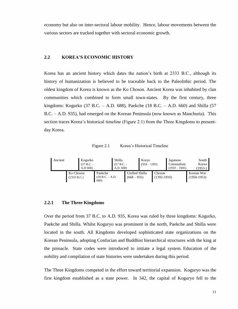
Korea has an ancient history which dates the nation‟s birth at 2333 B.C., although its
history of humanization is believed to be traceable back to the Paleolithic period. The
oldest kingdom of Korea is known as the Ko Choson. Ancient Korea was inhabited by clan
communities which combined to form small town-states. By the first century, three
kingdoms: Kogurko (37 B.C. – A.D. 688), Paekche (18 B.C. – A.D. 660) and Shilla (57
B.C. – A.D. 935), had emerged on the Korean Peninsula (now known as Manchuria). This
section traces Korea‟s historical timeline (Figure 2.1) from the Three Kingdoms to present-
day Korea.
Figure 2.1 Korea‟s Historical Timeline
Ancient Kogurko
(37 B.C. –
A.D 668)
Shilla
(57 B.C. –
A.D. 668)
Koryo
(918 – 1392)
Japanese
Colonialism (1910 – 1945)
South
Korea
(1953-)
Ko Choson
(2333 B.C.)
Paekche (18 B.C. – A.D. 660)
Unified Shilla
(668 – 935)
Choson
(1392-1910)
Korean War
(1950-1953)
2.2.1 The Three Kingdoms
Over the period from 37 B.C. to A.D. 935, Korea was ruled by three kingdoms: Kogurko,
Paekche and Shilla. Whilst Koguryo was prominent in the north, Paekche and Shilla were
located in the south. All Kingdoms developed sophisticated state organizations on the
Korean Peninsula, adopting Confucian and Buddhist hierarchical structures with the king at
the pinnacle. State codes were introduced to initiate a legal system. Education of the
nobility and compilation of state histories were undertaken during this period.
The Three Kingdoms competed in the effort toward territorial expansion. Koguryo was the
first kingdom established as a state power. In 342, the capital of Koguryo fell to the

12
Chinese. After this Paekche amassed power and came into conflict with Koguryo in the
late fourth century. Subsequently Shilla managed to defeat the other two kingdoms, but
was initially unable to control the entire territories of Koguryo and Paekche, which were
under Chinese rule. Eventually Shilla defeated the Chinese in A.D. 676, and became a
unified state covering most of the Korean Peninsula.
The Unified Shilla kingdom (668-935) reached its peak of power and prosperity in the
middle of the eighth century. Education flourished in the government service, the equitable
distribution of land for peasants was put into practice in 722, reservoirs were erected for
rice field irrigation and taxation in kind was collected. Learning was encouraged, resulting
in a new transcription system of Korean words by the use of Chinese characters. However,
in the ninth century, Shilla was troubled by intra-clan conflict around the throne and in
district administration.
2.2.2 Koryo Dynasty
Shilla was destroyed by rebel leaders: Kyon Hwon in 900, Kung Ye in 901 and Wang Kon,
the last rebel of Shilla and founder of the Koryo Dynasty (918-1392). During the Koryo
dynasty, diplomatic relations with the former Shilla aristocracy were maintained, state
defence was strengthened, internal conflicts among royalties were discouraged, the
emancipation of slaves in 956 was instituted, a civil service examination system to recruit
officials by merit was enforced and land allocation to officials was put into practice. These
policies enabled the Dynasty to become a centralized government with the power to make
admonitions to the throne on the part of officials and censorship of royal decisions. With
such internal order, Koryo was long able to withstand frequent invasions by the Liaos (old
tribal league) in the 900s. However, in 1238 the Mongolians invaded Korea. When the
Mongol Empire collapsed in the middle of the 14th
century, the Koryo dynasty was faced
with internal problems, e.g. animosity between Buddhism and Confucianism, opposition to
land reform by land owners and raiding by Japanese pirates in the country.

13
2.2.3 Choson Dynasty (1392-1910)
In 1392, King Kongyang (of the Koryo Dynasty) was forced to abdicate his throne and
General Yi took over. This marked the start of the Choson dynasty (1392-1910). During
the early Choson period (till the 17th century), Confucian ethics were promoted. The early
Choson era was noted for progressive ideas in administration, phonetics, national script,
economics, science, music, medical science and humanistic studies, historical geography,
increases in learning and writing of books, an increasing number of schools as well as the
introduction of the Korean alphabet.
The Choson maintained its political independence and cultural and ethnic identity in spite
of a number of foreign invasions. However, these invasions brought about destruction of
government records, cultural objects and historical documents, the devastation of land,
decrease in population, and the loss of artisans and technicians. The late Choson period
witnessed much social and economic upheaval. Following a particularly destructive war
with Japan in 1592, there were activities to reconstruct, provide medical relief and print
books destroyed during the war. The era also saw the rise of mercantilism, upward social
mobility, introduction of agro-managerial production methods, privatized factories, higher
production of goods for trade and a rise in commercial farming.
2.2.4 Japanese Colonial Rule (1910-1945)
Towards the late 19th
century, Korea became the focus of intense competition among
imperialist nations: China, Japan and Russia. In 1910, Japan annexed Korea. The Japanese
remained in the peninsula until the end of World War II and instituted militarized colonial
rule. Anti-Japanese resistance was evident. These sentiments came to the fore on March 1
1919 with a nationwide demonstration declaring Independence for Korea in the face of
intolerable aggression and oppression by the Japanese colonialists. The demonstration was
forcefully suppressed by the Japanese occupiers.
At the height of the independence movement, a provisional government of Korea was
established in Vladivostok on March 21, in Shanghai on April 11, and in Seoul on April 21.
The provisional government in Seoul proclaimed Korean independence, asking Japan to
withdraw its occupation forces from Korea. It called upon the Korean people to refuse

14
payment of taxes to the Japanese government, reject trials by Japanese courts, and avoid
employment at colonial offices. The Vladivostok, Shanghai and Seoul groups attempted to
integrate and form the Provisional Government on November 4. The Provisional
Government, despite financial difficulties, attempted to fulfill the international obligations
of the Korean people for 27 years until World War II. It declared war on Japan and
cooperated with the Allied Powers during war.
2.2.5 Korean War (1950-1953)
The Japanese surrender in 1945 brought many challenges in Korea. Korea was then faced
with a conflict in ideology. Korea was divided by the U.S. and U.S.S.R., which occupied
the north and south of the 38th
parallel, respectively. The ideological confrontation
inevitably gave rise to a tense military confrontation. North Korean troops invaded and
defeated the unprepared South across the 38th parallel in 1950. South Korea appealed to the
U.N. In response, the Security Council passed a resolution ordering North Korea to
withdraw to the 38th parallel and encouraged all member countries to give military and
medical support to the Republic. This was provided by the U.S. and 15 other nations.
Although the Allied forces initially pushed the North Koreans out of South Korea and
advanced into the north, they were soon forced to retreat by the Communist Chinese in
January 1951. The U.N. forces mounted a counterattack, retaking Seoul on March 12. A
stalemate was reached in the area along the 38th parallel, where the conflict had begun. At
this point, the Soviet Union called for truce negotiations, which began in July 1951, and
dragged on for two years before an agreement was reached on July 27, 1953.
2.2.6 Post-war South Korea
By the time the war ended, two million people had died and the country had been officially
divided between the north and the south. The Republic of Korea in the south has a
democratic government, whilst the Democratic People‟s Republic of Korea in the north is
ruled by a Communist regime. From this point, the research focuses on the Republic of
Korea.
The start of the Republic of Korea‟s growth began in the early 1960s with the introduction
of the First Five-Year Economic Development Plan. A conscious effort was made to turn

15
from inward-looking import substitution to an outward-looking strategy of export
promotion. South Korea exported light manufactured goods, in which the country had a
comparative advantage owing to its low labour costs. Other measures included maintaining
high interest rates to increase domestic savings and encouraging the inflow of foreign
investment. Thus, Korea was a growing economy when it entered the 1970s.
2.3 KOREA’S ECONOMIC HISTORY IN THE POST-WAR ERA
The Korean economy has experienced astounding growth in the past three decades. Owing
to its sophisticated industrial structure and globalisation efforts, it was admitted into the
Organisation for Economic Cooperation and Development (OECD) in 1996, signaling the
country‟s entry into the rank of advanced economies. Double-digit growth has been
consistently recorded: 30% in 1970-1980, 17% in 1980-1990 and 11% in 1990-2000.
Corresponding to high economic growth, employment has been rising steadily, by 4%, 3%
and 2%, over the same periods.
2.3.1 The 1970s
Korea‟s economic performance in the 1970s can be described as phenomenal, with high
economic growth and inflation but stable unemployment. There was an economic boom in
this decade, with GDP increasing at astounding rates of between 24% and 41% (see Table
2.1 and Figure 2.2). This boom in fact started in the mid-1960s when Korea made policy
changes to promote a free trade regime for exports and combined this with selective
protection in the import competing sectors. As a result of the food shortage of 1973 and oil
price shock in 1974, Korea‟s balance of payments deteriorated and she responded by
restructuring exports to higher value-added sophisticated products and diversifying her
trading partners. Moreover, industrial restructuring towards heavy and chemical products
led to a rising demand for investment by firms as well as increased demand for skilled
workers in the urban areas. There was consequently a transfer of labour from agriculture to
industry. Employment grew rapidly from 3.6% in 1970 to 6.2% in 1976, although the
growth slowed to 1% by the end of the decade (Figure 2.3). With the growth in

16
employment, the unemployment rate was kept at reasonably stable levels, and actually
decreased slightly, from 5% in 1970 to 4% in 1979.
Table 2.1 Annual % Change in GDP, CPI and Employment (EMP)
and Unemployment Rates (UR) GDP CPI EMP UR
1970 27.9 16.0 3.6 4.5
1971 24.0 13.5 3.4 4.5
1972 23.5 11.7 4.4 4.5
1973 28.9 3.2 5.4 4.0
1974 41.2 24.3 4.4 4.1
1975 34.6 25.2 2.4 4.1
1976 36.9 15.3 6.2 3.9
1977 28.2 10.1 3.2 3.8
1978 35.0 14.5 4.7 3.2
1979 28.1 18.3 1.4 3.8
1980 21.8 28.7 0.6 5.2
1981 25.4 21.4 2.5 4.5
1982 14.9 7.2 2.5 4.4
1983 17.3 3.4 0.9 4.1
1984 14.3 2.3 -0.5 3.8
1985 11.4 2.5 3.7 4.0
1986 16.7 2.8 3.6 3.8
1987 17.2 3.1 5.5 3.1
1988 18.8 7.1 3.1 2.5
1989 12.2 5.7 4.1 2.6
1990 20.6 8.6 3.0 2.4
1991 21.1 9.3 3.1 2.3
1992 13.5 6.2 1.9 2.4
1993 12.9 4.8 1.2 2.8
1994 16.5 6.3 3.2 2.4
1995 16.7 4.5 2.9 2.0
1996 10.9 4.9 2.2 2.0
1997 8.3 4.4 1.7 2.6
1998 -2.0 7.5 -6.0 6.8
1999 8.6 0.8 1.8 6.3
2000 8.1 2.3 4.3 4.1
2001 5.7 4.1 2.0 3.0 Source: Data on CPI, Employment and UR are from the ILO LaborStat database.
Data on GDP are from the Korea National Statistical Office.

17
Figure 2.2 Annual % Change in GDP, 1970-2001
-8
-4
0
4
8
12
16
20
24
28
32
36
40
44
1970
1972
1974
1976
1978
1980
1982
1984
1986
1988
1990
1992
1994
1996
1998
2000
Figure 2.3 Annual % Change in Employment and Unemployment Rates, 1970-2001
-8
-4
0
4
8
1970
1972
1974
1976
1978
1980
1982
1984
1986
1988
1990
1992
1994
1996
1998
2000
EMPG
UR
Annotation: EMPG: Annual % Employment Growth Rate
UR: Unemployment Rate
%
%
year
year

18
Figure 2.4 Annual % Change in CPI, 1970-2001
0
4
8
12
16
20
24
28
32
1970
1972
1974
1976
1978
1980
1982
1984
1986
1988
1990
1992
1994
1996
1998
2000
This economic progress came at the cost of high inflation (Figure 2.4). Moreover, the
industrial structure was distorted by over-investment in heavy industries and under-
investment in light industries. There was also a high degree of government control which
distorted prices and stifled competition.
2.3.2 The 1980s
Compared to the previous decade, the 1980s was a decade with lower growth, less inflation
and reduced unemployment. The growth in GDP slowed, from 22% in 1980 to 12% in
1989. Inflation rates dropped significantly, from 29% to 6%, over the same period. These
changes were the result of active steps undertaken to reduce inflation, rectify the structural
imbalance in the economy and to promote competition in the 1970s. Many restructured
industrial firms (power-generating, automobile, electrical, electronics, shipping, overseas
construction industries) were forced to merge to reduce excess capacity. There was also a
financial restructuring in the 1980s, as many commercial banks privatized, barriers to entry
into the financial sector were reduced, and financial services were diversified and
streamlined. On the labour front, employment levels rose, with about 2.8 million new jobs
being created during the decade. The rate of unemployment sank to the unprecedented
level of 2.6% by 1989.
%
year
19
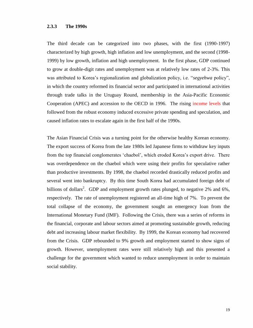
2.3.3 The 1990s
The third decade can be categorized into two phases, with the first (1990-1997)
characterized by high growth, high inflation and low unemployment, and the second (1998-
1999) by low growth, inflation and high unemployment. In the first phase, GDP continued
to grow at double-digit rates and unemployment was at relatively low rates of 2-3%. This
was attributed to Korea‟s regionalization and globalization policy, i.e. “segyehwa policy”,
in which the country reformed its financial sector and participated in international activities
through trade talks in the Uruguay Round, membership in the Asia-Pacific Economic
Cooperation (APEC) and accession to the OECD in 1996. The rising income levels that
followed from the robust economy induced excessive private spending and speculation, and
caused inflation rates to escalate again in the first half of the 1990s.
The Asian Financial Crisis was a turning point for the otherwise healthy Korean economy.
The export success of Korea from the late 1980s led Japanese firms to withdraw key inputs
from the top financial conglomerates „chaebol‟, which eroded Korea‟s export drive. There
was overdependence on the chaebol which were using their profits for speculative rather
than productive investments. By 1998, the chaebol recorded drastically reduced profits and
several went into bankruptcy. By this time South Korea had accumulated foreign debt of
billions of dollars2. GDP and employment growth rates plunged, to negative 2% and 6%,
respectively. The rate of unemployment registered an all-time high of 7%. To prevent the
total collapse of the economy, the government sought an emergency loan from the
International Monetary Fund (IMF). Following the Crisis, there was a series of reforms in
the financial, corporate and labour sectors aimed at promoting sustainable growth, reducing
debt and increasing labour market flexibility. By 1999, the Korean economy had recovered
from the Crisis. GDP rebounded to 9% growth and employment started to show signs of
growth. However, unemployment rates were still relatively high and this presented a
challenge for the government which wanted to reduce unemployment in order to maintain
social stability.

20
2.4 ECONOMIC GROWTH, SECTORAL CHANGES
AND LABOUR MOBILITY
The previous section highlighted that Korea has undergone several phases of boom and
recession in recent times. These have been associated with changes in the importance of
various sectors of the economy. This section illustrates the associations between economic
growth, sectoral changes and labour mobility on a decade-by-decade basis, from 1970 to
2000, with special attention on 1998-2001 to coincide with the period of data collection for
the dataset used in the study of worker mobility in Part II of this thesis. The major
sectors/industries comprise agriculture, mining, manufacturing, utilities, construction,
commerce, transport, storage and communications, financial, business services and real
estate, and community, social and personal services. The classification of these nine
sectors/industries follows that of the empirical study to be undertaken in Part II of this
thesis.
2.4.1 The Three Decades: 1970-2000
The Korean economy at the start of the 1970s was dominated by three sectors: agriculture,
manufacturing and commerce. Together, these sectors contributed more than three-fifths of
total GDP in 1970, with the share of total output for agriculture, manufacturing and
commerce at 29%, 18% and 17%, respectively. At the end of the first decade, as a
consequence of the 1970s oil and food crises, the share of output due to agriculture and
commerce had declined considerably, to 16% and 14%, respectively. Corresponding to
their lower share in total output, the average annual GDP growths of agriculture and
commerce over the first decade were lower, at 22% and 28%, respectively. In comparison,
the share of manufacturing output rose to 24% and the sector experienced a strong average
annual growth of 34% over the decade. The services sector‟s contribution to GDP rose,
especially due to growth in the transport, storage and communications industry (share rose
from 7% to 8%), and the financial, business services and real estate industry (share rose
from 7% to 12%), with the average annual growths at 32% and 36%, respectively. These
high growth rates are reflective of the success of Korea‟s export-oriented policy and the
protectionism in the import sector. Thus, Korea‟s economic growth in the first decade was
associated mainly with strong growth in the manufacturing and services sectors.

21
Table 2.2 GDP by Sector, 1970-2000 1970 1980 1990 2000 1970-1980 1980-1990 1990-2000
% Distribution by Sector Average Annual Growth (%)
Total Gross Value-
Added at Basic Prices1 100.0 100.0 100.0 100.0 29.9 17.1 11.9 Agriculture 29.2 16.2 8.9 4.9 22.4 10.4 5.3 Mining 1.8 1.9 0.8 0.4 31.2 7.6 3.8 Manufacturing 17.8 24.4 27.3 29.4 34.1 18.4 12.7 Utilities 1.4 2.2 2.1 2.6 36.1 17.0 13.9 Construction 5.1 8.0 11.3 8.4 35.9 21.3 8.5 Commerce 16.8 14.2 13.0 10.8 27.7 16.1 9.8 Transport, Storage &
Communications 6.7 8.0 6.8 7.0 32.2 15.3 12.2 Financial, Business
Services & Real Estate 7.3 11.5 14.9 20.1 35.9 20.3 15.3 Community, Social &
Personal Services 13.9 13.7 14.8 16.5 29.7 18.1 13.1
Source: Korea NSO.
1. Whilst overall GDP comprises gross value-added at basic prices plus taxes less subsidies on products, the
latter does not have a sectoral breakdown. As such, „Total‟ refers to total gross value-added at basic prices. This
facilitates the computation of sectoral contributions.
By the second decade, the adverse effects of the global oil and food crises spilled over to
the agricultural and commerce sector where their shares of output declined to 9% and 13%,
respectively. Reflecting the diversification towards heavy and chemical industries during
the post-Crisis period, manufacturing‟s share of output continued to grow steadily, to 27%.
In the services sector, the contribution to GDP was the result of the increases in the
financial, business services and real estate industry (share rose from 12% to 15%) and
community, social and personal services industry (share rose from 14% to 15%). For the
financial industry, the availability of investment funds made the growth in the industry
possible.
In the third decade, the rising importance of services, particularly financial, business
services and real estate, and community, social and personal services industries, was
evident. The share of GDP increased from 15% to 20% for the former and from 15% to
17% for the latter. The success in the financial, business services and real estate industry
was attributed to financial restructuring and globalization efforts. The manufacturing sector
managed to sustain its high share of 29%, and this was probably due to lower costs
associated with the amalgamation of manufacturing industries in the late 1980s. In
contrast, agriculture‟s share of total output continued to fall, to a meager 5%. The

22
commerce sector also registered a declining share of GDP over the decade, although its
drop in relative importance was not as pronounced as the drop in the rural sector.
In terms of sectoral labour shifts, Korea‟s labour force moved from the rural and services
sectors to the manufacturing, construction and commerce sectors over the first decade. The
share of agricultural employment declined from 50% to 34%, whilst notable increases
occurred in manufacturing (13% to 22%), construction (3% to 6%) and commerce (12% to
19%). The proportion of employment remained fairly stable in the other sectors/industries
over the first decade.
Between 1980 and 1990, the composition of the labour force shifted from agriculture to the
manufacturing, commerce and services sectors. Whilst the employment share continued to
drop in agriculture (34% to 18%), it rose in the manufacturing sector, from 22% to 27%,
and from 19% to 22% in the commerce sector. Each of the services industries also
recorded rising shares of employment during the decade.
By the third decade, the sectoral shifts were mainly in the form of movements from the
agricultural and manufacturing sectors towards the commerce and services sectors. The
first two sectors witnessed proportionate declines in the employment whilst the latter two
experienced increases in their relative employment.
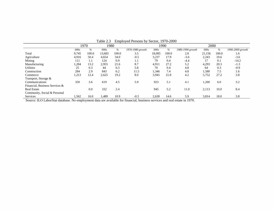
Table 2.3 Employed Persons by Sector, 1970-2000
1970 1980 1990 2000 000s % 000s % 1970-1980 growth 000s % 1980-1990 growth 000s % 1990-2000 growth
Total 9,745 100.0 13,683 100.0 3.5 18,085 100.0 2.8 21,156 100.0 1.6
Agriculture 4,916 50.4 4,654 34.0 -0.5 3,237 17.9 -3.6 2,243 10.6 -3.6
Mining 111 1.1 124 0.9 1.1 79 0.4 -4.4 17 0.1 -14.2
Manufacturing 1,284 13.2 2,955 21.6 8.7 4,911 27.2 5.2 4,293 20.3 -1.3
Utilities 25 0.3 44 0.3 5.8 70 0.4 4.8 64 0.3 -0.9
Construction 284 2.9 843 6.2 11.5 1,346 7.4 4.8 1,580 7.5 1.6
Commerce 1,213 12.4 2,625 19.2 8.0 3,945 21.8 4.2 5,752 27.2 3.8
Transport, Storage &
Communications 350 3.6 619 4.5 5.9 923 5.1 4.1 1,260 6.0 3.2
Financial, Business Services &
Real Estate 0.0 332 2.4 945 5.2 11.0 2,113 10.0 8.4
Community, Social & Personal
Services 1,562 16.0 1,489 10.9 -0.5 2,638 14.6 5.9 3,814 18.0 3.8
Source: ILO LaborStat database. No employment data are available for financial, business services and real estate in 1970.

24
It should be noted that the Table 2.3 data illustrate the net mobility across sectors, and
include the impact of individuals moving from outside the labour market into employment,
and of individuals leaving employment for non-labour market activities. For example,
between 1970 and 1980, there was an increase in employment of 1,671,000 in Korea‟s
manufacturing sector. This is accompanied by employment growth in the mining, utilities,
construction, commerce and services sectors, and a decline in employment in the
agricultural sector. The 1,671,000 people who, on net, joined the manufacturing sector
over this period will generally comprise:
(i) inflows into manufacturing from outside the labour market, Iolm, and from
agriculture (Ia), mining (Im), utilities (Iu), construction (Ict), commerce (Ic) or
services (Is)3;
(ii) outflows from manufacturing to either non-labour market activities, Oolm, or to
work in either agriculture (Oa), mining (Om), utilities (Ou), construction (Oct),
commerce (Oc) or services (Os).
These individual inflows and outflows are the gross flows that combine to generate the net
flows illustrated in Table 2.3.
Hence,
1,671,000 = Inflows – Outflows
= (Iolm + Ia + Im + Iu + Ict + Ic + Is)
- (Oolm + Oa + Om + Ou + Oct + Oc + Os)
Clearly, inflows exceed outflows, and the number of employed persons in the
manufacturing sector has risen. While knowledge of the individual flows would assist
understanding the dynamics of the Korean labour market, the net movements provide a
useful measure of the relative strengths of the various economic sectors.
It can be seen that the growth in the Korean economy not only depends on changes in the
significance of the various sectors but on labour movements between sectors. The data
reveals that the sectoral flows of workers occur in the same direction as that of economic
growth. In the first decade, there was a net movement of labour from the agriculture and
services sectors to the manufacturing4, construction and commerce sectors. The net labour
25
flows were from agriculture to the manufacturing, commerce and services sectors in the
second decade. In the third decade net labour flows occurred mainly from the agricultural
and manufacturing sectors to the commerce and services sectors.
2.4.2 The 1998-2001 period
Throughout 1998-2001, the sectoral shares of GDP (at current prices) and employment
have remained fairly stable. The major contributors to overall GDP have been the
manufacturing sector and financial services industry, with a combined contribution of about
half of the total. In contrast, the mining and utilities sectors contributed a meager share of
less than 5%. In terms of overall employment, whilst the manufacturing remained one of
the largest contributors, and the mining and utilities sectors the lowest, the commerce sector
emerged to have the largest share, displacing the financial industry in this regard.
As compositional changes are not usually obvious within a short span of 4 years, sectoral
changes for 1998-2001 will also be examined using growth data. The earlier section
revealed that the Asian Financial Crisis was associated with a deterioration in both
economic and employment growth, to negative 2% and 6%, respectively, in 1998. Many
sectors recorded declines in GDP, including agriculture, mining, construction and
commerce. Correspondingly, three out of these four sectors with adverse economic
performance experienced declining employment5.
The series of reforms after the Crisis led to rises of 9% in GDP and 2% in employment. All
sectors except mining and construction experienced improvements in economic
performance. In the labour market, it was these two same two sectors, along with the
agricultural sector, where employment failed to recover. The situation in the agricultural
sector probably reflects the continued outflow of surplus labour from the rural to urban
sectors.
Economic recovery continued in 2000, and GDP rose by 8% and employment by 4%. The
growth in performance was seen in all sectors other than construction. Even in the
construction sector, the magnitude of decline slowed considerably, from 7% in 1999 to less

26
than 1% in 2000. Correspondingly, nearly all of the sectors, including construction, had an
increased intake of workers in 2000.
Sustained economic growth was witnessed in 2001, with GDP growing by 6% and
employment by 2%. All sectors other than agriculture and mining displayed positive GDP
growth in 2001. Employment levels increased in all sectors except agriculture,
manufacturing and utilities. The drop in employment in the manufacturing sector reflected
a slowdown in sectoral GDP growth.
In general, a sector‟s significance in employment coincides with its importance in terms of
its value-added contribution. In 1998, many sectors experienced declines in both GDP and
employment. During 1999-2001, with a few exceptions, sectors that had a higher (lower)
GDP growth also had larger (smaller) employment intake for the same year.
Table 2.4 GDP at Current Prices by Sector, 1998-2001 1998 1999 2000 2001 1998 1999 2000 2001
% Distribution by Sector Annual % Growth Total GDP -2.0 8.7 7.6 5.8 Total Gross Value-
Added at Basic Prices 100.0 100.0 100.0 100.0 0.0 7.8 8.7 7.0 Agriculture 5.1 5.2 4.9 4.5 -6.4 11.0 0.9 -0.9 Mining 0.5 0.4 0.4 0.4 -10.6 -0.8 2.8 -0.8 Manufacturing 27.3 28.1 29.4 27.6 3.9 10.9 13.7 0.3 Utilities 2.3 2.5 2.6 2.7 12.0 19.6 10.6 10.9 Construction 10.6 9.2 8.4 8.6 -13.5 -6.9 -1.0 9.9 Commerce 9.2 10.0 10.8 10.8 -7.4 17.7 17.4 6.5 Transport, Storage &
Communications 7.1 7.0 7.0 7.5 6.1 7.5 8.6 14.0 Financial, Business
Services & Real Estate 21.1 20.8 20.1 20.4 3.2 6.2 5.3 8.9 Community, Social &
Personal Services 16.9 16.7 16.5 17.6 3.0 6.3 7.2 14.3
Source: Korea NSO.
1. Total GDP comprises gross value-added at basic prices plus taxes less subsidies on products.
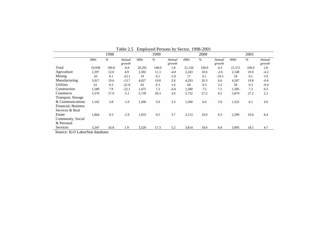
Table 2.5 Employed Persons by Sector, 1998-2001 1998 1999 2000 2001
000s % Annual
growth
000s % Annual
growth
000s % Annual
growth
000s % Annual
growth
Total 19,938 100.0 -6.0 20,291 100.0 1.8 21,156 100.0 4.3 21,572 100.0 2.0
Agriculture 2,397 12.0 4.9 2,302 11.3 -4.0 2,243 10.6 -2.6 2,148 10.0 -4.2
Mining 20 0.1 -23.1 19 0.1 -5.0 17 0.1 -10.5 18 0.1 5.9
Manufacturing 3,917 19.6 -13.7 4,027 19.8 2.8 4,293 20.3 6.6 4,267 19.8 -0.6
Utilities 61 0.3 -21.8 62 0.3 1.6 64 0.3 3.2 58 0.3 -9.4
Construction 1,580 7.9 -22.1 1,475 7.3 -6.6 1,580 7.5 7.1 1,585 7.3 0.3
Commerce 5,570 27.9 -5.1 5,739 28.3 3.0 5,752 27.2 0.2 5,874 27.2 2.1
Transport, Storage
& Communications 1,162 5.8 -1.0 1,200 5.9 3.3 1,260 6.0 5.0 1,322 6.1 4.9
Financial, Business
Services & Real
Estate 1,864 9.3 -2.9 1,933 9.5 3.7 2,113 10.0 9.3 2,290 10.6 8.4
Community, Social
& Personal
Services 3,347 16.8 1.9 3,520 17.3 5.2 3,814 18.0 8.4 3,995 18.5 4.7
Source: ILO LaborStat database.
28
2.4.3 Possible Structural Break during Asian Financial Crisis
At this stage, it is worth mentioning that the Asian Financial Crisis could give rise to a
structural change in the Korean economy and labour market. Looking at the data trends,
there are reasons to suspect that a structural change occurred around 1998. The Korean
economy had been experiencing double-digit growth in GDP throughout the pre-Crisis
period, but the GDP growth rate suddenly dipped to negative 2% in 1998 immediately after
the Crisis occurred. In the Korean labour market, employment had been growing by about
2-3% since the late 1980s but in 1998, the employment growth rate plunged to negative
6%. Unemployment, which had been at a general low of 2-3% since the late 1980s,
suddenly increased to 7% in 1998, the highest in the past 30 years. These trends provide a
priori justification for tests of a structural break in chapter 5.
2.5 CONCLUDING REMARKS
This chapter has traced the economic history of Korea and illustrated how the success of
this Asian country has been associated with the growth of the various economic sectors and
also how it has been associated with inter-sectoral reallocations of labour. The patterns for
the decades covering 1970-2000, as well as for the more specific 1998-2001 period, were
reviewed. It is concluded that labour (and sectoral) mobility should not be ignored in the
analysis of the different phases of the macroeconomy. Labour market flexibility among
various sectors has emerged as a challenging issue, particularly in explaining the rising
unemployment experienced towards the end of the last decade. This has implications for
labour and macro policy. The following chapters introduce and review the recent research
undertaken in several countries on the relationship between sectoral mobility and
unemployment, and the corresponding factors that affect labour (and sectoral) mobility.
Endnotes:
1. See www.korea.net, the official homepage of the Korean government operated by the Korean Information
Service.
2. Prior to 1997, Korea‟s exchange rate regime was managed or pseudo-fixed [Park, Chung and Wang
(2001)].
3. In this section, the three services industries, as distinguished in Table 2.3, namely Transport, Storage &
Communications, Financial, Business Services & Real Estate, and Community, Social & Personal Services
are treated as a single „services‟ sector.
4. This follows the Lewis surplus model of labour transfer from rural areas to the industrialized sector.
5. The exception is agriculture, which experienced higher employment in 1998.
29
PART I: SECTORAL MOBILITY AND UNEMPLOYMENT
PREAMBLE
Part I, entitled „Sectoral Mobility and Unemployment‟, is about the relationship between
inter-sectoral mobility and aggregate unemployment. It introduces the macroeconomic
problem of unemployment and links it to sectoral labour movements. The discovery of the
mobility-unemployment relationship in the late 1980s led to extensive debate, resulting in
the formation of four hypotheses: sectoral shift hypothesis (SSH), aggregate demand
hypothesis (ADH), reallocation timing hypothesis and stage-of-the-business cycle effect.
Part I contains three chapters. The theoretical exposition of the hypotheses on sectoral
mobility and unemployment is found in chapter 3, which includes discussion of the
methods of hypotheses testing and conceptual differences in terms of the source of
mobility, chain of causation, and nature of the resultant unemployment. The empirical
evidence on the hypotheses in chapter 4 focuses on modelling techniques and specification,
the set of mobility indices and findings from studies across the U.S., Europe and Japan.
Chapters 3 and 4 provide the theoretical and empirical foundation from which empirical
work for Korea can be carried out.
The empirical work is presented in chapter 5, where the model is first constructed and then
used to test the four hypotheses in the Korean labour market. The model is subjected to
rigorous econometric procedures involving tests of structural change, collinearity and serial
correlation. The tests for structural change reveal a structural break between the pre- and
post-Crisis (1998-2001) periods. The key findings show a lack of support for the SSH,
ADH and stage-of-the-business-cycle effect for Korea in the pre-Crisis period. For the
post-Crisis period, the empirical results favour the SSH, ADH and stage-of-the-business-
cycle effect, but data limitations prevent the formation of firm conclusions. Nonetheless,
the tentative support for the hypotheses reveals the potential for mobility to be used as a
tool for reducing unemployment, giving rise to the need for an in-depth study of the
determinants of sectoral mobility for Korea. Part I concludes by linking the research on the
impact of mobility with work undertaken on the determinants of sectoral mobility in Part II.

30
31
CHAPTER 3
THEORETICAL HYPOTHESES CONCERNING
SECTORAL MOBILITY AND UNEMPLOYMENT
3.1 INTRODUCTION
Sectoral mobility is an important feature of labour markets across the world. It is also a
phenomenon that has entered most major macroeconomic debates on unemployment, with
numerous studies having examined or questioned its influence on this economic outcome1.
This chapter presents a review of the ways that sectoral mobility has been advanced as a
potential contributor to unemployment.
In a seminal paper, Lilien (1982) introduced the importance of sectoral mobility in
explaining unemployment for the U.S. economy. Using a sectoral shift measure of
employment dispersion, it was shown that nearly half of the rise in aggregate
unemployment during 1948-1980 was attributable to sectoral mobility. This association of
sectoral mobility with unemployment formed the basis for the Sectoral Shift Hypothesis
(SSH). The Aggregate Demand Hypothesis (ADH), introduced by Abraham and Katz
(1986), challenges the SSH, and associates unemployment with aggregate demand
fluctuations, claiming that the sectoral shift measure picks up effects of aggregate demand
rather than inter-industry disturbances. In comparison, the Reallocation Timing Hypothesis
(RTH), mooted by Davis (1987), acknowledges the role of sectoral shifts in explaining
fluctuations in unemployment but argues that sectoral movements are reinforced by past
patterns of labour reallocation and their impact influenced by the stages of the business
cycle (termed as stage-of-the-business-cycle effect). Whilst the SSH and ADH have
triggered a series of debates, the RTH and stage-of-the-business-cycle effect have not
warranted much attention in the literature, apart from the sporadic work of Davis (1987) for
the former and Mills, Pelloni and Zervoyianni (1995) for the latter.
This chapter forms the start of Part I of this thesis, which analyses the relationship between
sectoral mobility and unemployment. It provides a theoretical exposition of the hypotheses
introduced above. The following chapter, chapter 4, supplements this theory with empirical
evidence. Chapter 5 then extends the application to Korea. Chapter 3 proceeds in the

32
following manner. Sections 3.2 to 3.5 outline, in some detail, each hypothesis. The
conceptual and methodological differences between the hypotheses are presented in
sections 3.6 and 3.7. It is shown that there is an array of mobility indices that can be used
to test each hypothesis. Consequently, an attempt is made in section 3.8 to narrow the
range of suitable indices. A summary of these issues is given in section 3.9.
3.2 THE SECTORAL SHIFT HYPOTHESIS
3.2.1 Impact of Sectoral Mobility on Aggregate Unemployment
The SSH asserts a causal role for sectoral mobility in accounting for variations in aggregate
unemployment. This form of mobility can represent pure sectoral shifts and/or sectoral
reallocations arising from a supply-side disturbance that results in more labour being
allocated to some sectors and less to others [Parker (1992)].
Pure sectoral shifts originate from changes in individuals‟ tastes/preferences, desire for
higher wages, non-pecuniary benefits etc., and can occur during periods of stable aggregate
conditions. Frictional unemployment results from pure sectoral shifts as labour markets are
imperfect and labour is not instantaneously responsive [Lilien (1982) and Parker (1992)],
i.e. it takes time for workers to find suitable jobs and employers to find the right employees.
Supply disturbances to the economy can also induce sectoral mobility [Prasad (1997)].
These include changes in technology, oil prices, import competition and war, where
declining sectors reduce their employment requirements and expanding ones increase their
employment intake. Workers from declining sectors may be slow in responding to the
shifts in employment demand owing to industrial attachments, and this can result in higher
aggregate unemployment. At some point, the rise in employment in expanding sectors may
not offset the falling levels in declining sectors. At the aggregate-level, unemployment
increases. The resultant unemployment is regarded as structural.
A proxy statistic to represent the magnitude of sectoral movements was devised by Lilien
(1982), and has been labelled the „raw Lilien index‟ by subsequent authors. It is the

33
weighted standard deviation of the cross-sectoral employment growth rates, expressed
mathematically in the following equation:
N
ζt = [ ∑ (eit / Et)(Δ log (eit ) - Δ log (Et ))2]
½ (3.1)
i =1
where eit is employment in sector i, i = 1,.. , N, in period t and Et is aggregate employment
in period t. The term (eit/Et) is the ith
sector‟s share of total employment at time t, while Δ
log (eit ) and Δ log (Et) represent the rates of growth of employment in sector i and in the
aggregate economy, respectively.
Lilien (1982) computed the raw index over 11 sectors in the U.S., and used this as an
explanatory variable in the following model of the aggregate rate of unemployment in
period t, Ut:
J
Ut = βo + β1 ζt - ∑ β2j DMRt-j + β3 Ut-1 + β4 T + εt (3.2) j =0
where DMRt-j is unanticipated money growth, Ut-1 is the unemployment rate in the
preceding period, T is a time trend variable, εt is the stochastic disturbance term and J
denotes the number of lags for the unanticipated money growth term. The unanticipated
money growth term (DMR) was introduced by Barro (1977), and is the residual of the
following money growth equation:
DMt = α0 + α1DMt-1 + α2DMt-2 + α3FEDVt + α4UNt-1 + DMRt (3.3)
where DMt = log Mt - log Mt-1 is the annual average money growth (of M1) and
UNt-1 = log [U/(1-U)]t-1, where U is the average annual unemployment rate. FEDVt is the
difference between real and normal government expenditure. FEDVt ≡ log (FED)t – [log
(FED)]*t where FED is real government expenditure and [log (FED)]*t refers to the normal
value of this expenditure. Empirically, [log (FED)]*t can be generated from the adaptive
formula: [log (FED)]*t = ρ [log (FED)]t + (1-ρ) [log (FED)]*t-1 with ρ being the adaptive
coefficient. DMR is the difference between the observed DM and the DM predicted from
the regression equation.
34
The results from estimating equation (3.2) showed that nearly half of the unemployment in
the U.S. during the post-war 1948-1980 period was accounted for by sectoral mobility.
This effect was more substantial than that of the unanticipated monetary growth. Lilien
(1982) interpreted the positive ζ-U correlation as evidence that much of aggregate
unemployment is attributed to the process of sectoral labour reallocation.
3.2.2 SSH and Supply Shocks
Supply shocks are argued to lead to sectoral mobility in the SSH and this argument has
been formalized by Loungani (1986) and Mills, Pelloni and Zervoyianni (1995). Loungani
(1986) suggests that it was dramatic oil price shocks requiring an unusually high amount of
labour to be reallocated across industries that increased the unemployment rate in the
1970s. The point of departure for this theory is the representation of sectoral employment
growth. Sectoral employment growth (eit) was decomposed by Loungani (1986) as:
eit = β0Xt + β1Zt + Sit (3.4)
where Xt is a matrix of current and lagged aggregate-level variables, Zt is an unobserved
aggregate shock orthogonal to X and Sit is the residual sectoral component of employment
growth. The residual sectoral components were assumed to have an AR structure:
Sit = ρ1Sit-1 + ρ2Sit-2 + … ρjSit-j + εit (3.5)
The raw Lilien index computed across N sectors was altered to:
N
ζt = [ ∑ (ei /E) (εit)2 / ωt ]
½ (3.6)
i =1
where εit is the residual for each industry i obtained from the regression of equation (3.5).
Each industry‟s residual is weighted by (ei/E), the industry i‟s share of total employment.
Note that there is no time subscript for the term (ei/E) as it refers to a specific time period,
i.e. 1969 in Loungani‟s (1986) case. The denominator, ωt, is the variance over time of an
T
industry‟s residual and can be written as: ωt = ∑ (εit)2 / T where T is the length of the
t =1

35
sample period. Compared to the raw Lilien index in equation (3.1), the difference lies
in this denominator, which denotes the variance over time of an industry‟s residual.
This representation of sectoral employment growth has been modified to reflect the
characteristics of specific supply-side shocks. For example, to construct the Lilien index
generated by oil price shocks, the sectoral employment growth in equation (3.4) can be re-
written as:
eit = β0Xt + β1Pt + β2Zt + Rit (3.7)
where Pt is a matrix of current and lagged changes in oil prices and Rit is the residual
component of sectoral employment growth which is assumed to have an AR structure:
Rit = ρ*1Rit-1 + ρ*2Rit-2 + … ρ*jRit-j + εit (3.8)
for j number of lags. Whilst equation (3.5) captures the residual sectoral component of
employment growth which can include oil price shocks, equation (3.8) is the residual
component of sectoral employment growth that is independent of aggregate demand and oil
price shocks.
Equations (3.7) and (3.8) can then be used to construct the mobility index brought about by
oil price shocks:
N ζt(s) = { ∑ (ei /E) / [(βi – β) Pt ]
2 }
½ (3.9)
i =1
N
where β = ∑ (ei /E) βi with βi being the estimated coefficient of the oil price variable from i =1
the ith
sector‟s regression. The mobility index capturing the effects of the residual (r)
reallocative shocks in period t, ζt(r), that is purged of aggregate demand and supply
influences, is expressed as:
N
ζt(r) = [ ∑ (ei /E) (εit)2 / σt ]
½ (3.10)
i =1
T
where σt = ∑ (εit)2 / T.
i =1

36
Mills, Pelloni and Zervoyianni (1995) purged the raw Lilien index of aggregate supply
influences [change in the logarithm of energy prices (ΔEP) ] by regressing (Δeit - ΔEt ) on
the current and four-period lagged values of ΔEP and (ΔEP)2, respectively, to obtain the
residual series εp1
it and εp2
it. The pure indices purged of ΔEP and (ΔEP)2
can be expressed
as:
N
ζp1
t(up) = [ ∑ (eit / Et) (εp1
it )2]
½ (3.11a)
i =1
N
ζp2
t(up) = [ ∑ (eit / Et) (εp2
it )2]
½ (3.11b)
i =1
The index caused by supply shocks as per equation (3.9), that which is purged of demand
and supply influences as per equation (3.10), and the indices purged of supply influences
from equations (3.11a) and (3.11b) are alternatives to the raw index. Evidence for the SSH
requires these indices to have a positive and significant effect on aggregate unemployment.
3.2.3 SSH and the Natural Unemployment Rate
The SSH emphasizes the role of natural unemployment, which consists of frictional and
structural unemployment. It can be affected by a structural change, e.g. supply shock
where sectoral labour reallocations impact the structural rate, or via pure sectoral shifts
resulting in frictional unemployment2.
The logic of the links between the SSH and the natural rate stems from the view that
aggregate unemployment in the current period t evolves from Ut-1 and the differential
between separations (St) and hires (Ht) in the current period [Palley (1992)]. The
assumptions are that separations depend on the extent of demand shifts between sectors: St
= S(ζt), whilst hires are a constant proportion (k > 0) of Ut-1. The natural (or equilibrium)
unemployment rate is therefore U* = S(ζe)/k, where ζ
e is the expected dispersion of
sectoral demand shocks. If actual ζ exceeds ζe, then an increase in sectoral demand
dispersion arising from a supply shock can cause an increase in the natural unemployment
rate above the expected U*.

37
Lilien (1982) estimated the natural unemployment rate from the results of the regression of
aggregate unemployment as per equation (3.2). The natural unemployment rate in the
current period t, U*t, was expressed as a function of sectoral movements in the preceding
periods and a time trend variable, T:
∞
U*t = ∑ βj2 (β0 + β1ζt-j + β3Tt-j) (3.12)
j=0
where β0, β1, β2 and β3 are the parameter estimates for the constant term, ζt-j, Ut-1 and Tt-j,
respectively.
The U* series is not time invariant and it has changed considerably over 1949-1980. The
correlation coefficient between actual U and U* for this period was 0.74. Since Ut and U*t
both trended upwards during the post-war period, U* might be detrended by replacing T in
equation (3.12) with its average value over the period. Since the trend term is assumed to
capture demographic components of the labour market, the detrended measure would
probably more closely reflect changes owing to pure sectoral movements. The correlation
coefficient between U and the detrended U* was 0.60.
As the unemployment rate (U) is quite highly correlated with the natural rate, and given
that U is influenced by sectoral mobility (ζ), it is expected that sectoral mobility would be a
significant explanatory variable for U*t as well. This provides the foundations of the
SSH‟s recognition of the role of the natural unemployment rate. Several studies have
examined the role of the natural unemployment rate from unemployment models, including
Loungani (1986), Mills, Pelloni and Zervoyianni (1995), Parker (1992) and Samson (1985).
There have been numerous studies examining the credibility of the SSH across a range of
countries. These include Parker (1992), Palley (1992), Brainard and Cutler (1993),
Loungani and Rogerson (1989), Davis (1987), Mills, Pelloni and Zervoyianni (1995),
Loungani (1986), Murphy and Topel (1987a) and Lu (1996) for the U.S., Neelin (1987) and
Samson (1985) for Canada, Saint-Paul (1997) for France, Garonna and Sica (1997, 2000)
for Italy and Prasad (1997) for Japan. The majority of these studies focus on the impact of
sectoral mobility on aggregate unemployment, using unemployment models along the lines
of equation (3.2).
38
However, there appears to be a dearth of studies analyzing the origins of mobility,
particularly supply-side shocks generating sectoral mobility. Davis (1987) used a dummy
variable for periods before and after 1974 to capture the effects of the oil price shock on
unemployment. Brainard and Cutler (1993) regressed oil prices on unemployment. The
coefficient of the dummy variable was significant and positive in Davis (1987), but oil
prices were insignificant in Brainard and Cutler (1993). Although both studies analysed the
effects of a supply-side shock, their limitation is that the impact of a supply-side shock on
mobility is not captured. The exceptions are the unpredicted indices constructed by
Loungani (1986) in equations (3.9) and by Mills, Pelloni and Zervoyianni (1995) in
equations (3.11a) and (3.11b) which cater to analyzing the influence of supply shocks on
mobility.
3.3 AGGREGATE DEMAND HYPOTHESIS
The ADH, advanced by Abraham and Katz (1986), presents a case for aggregate demand
disturbances in explaining unemployment and questions the causal role of sectoral mobility.
Two lines of argument against the SSH were presented, the first being based on the
unemployment and vacancies (U-V) relationship and the second involving the ζ-U co-
movement approach.
3.3.1 U-V Relationship
The central piece of evidence against the SSH involved the U-V relationship. Under pure
sectoral shifts (independent of aggregate disturbances), sectoral mobility produces a
positive ζ-U correlation. This is because such changes to the structural economy will cause
the U-V curve to shift inwards (outwards) and thereby increase (decrease) the job matching
rate. The declining (increasing) inter-sector labour movements are a likely reason for the
inward (outward) shift of the U-V curve. The result is that a decline (rise) in
unemployment caused purely by sectoral labour shifts will be accompanied by a drop (rise)
in job vacancies. In other words, the measured relationship between U and V will be
positive. If the SSH correctly reflects why ζ and U are positively related, then ζ and V
should be positively related as well.
39
Abraham and Katz (1986) contended, however, that the positive ζ-U association generates
a negative ζ-V relationship. A positive (negative) AD shock, for example, that leads to
lower (higher) unemployment results in an increase (decrease) in job vacancies. This can
be construed as a movement along the Beveridge curve which posits a negative U-V
relation in response to aggregate shocks [Blanchard and Diamond (1989)].
To test the U-V argument, the Conference Board‟s3 help-wanted index was used as a proxy
for job vacancies. A normalized help-wanted index (NHWI) was constructed using the
employment weighted average of the number of help-wanted advertisements in 51
metropolitan newspapers and dividing the result by total non-agricultural payroll
employment. A negative U-V relationship was plotted for the U.S. for 1949-1980.
Abraham and Katz (1986) regressed unemployment and job vacancies (the NHWI) on ζt in
the equations below.
Ut = αo + α1 ζt + α2 ζt-1 + α3DMRt + α4DMRt-1 + α5DMRt-2 + α6Ut-1 + α7T + ut (3.13)
NHWIt = αo + α1ζt + α2 ζt-1 + α3DMRt + α4DMRt-1 + α5DMRt-2
+ α6NHWIt-1 + α7T + ut (3.14)
It was found that ζt had a positive impact on U for equation (3.13) but a negative effect on
NHWI for equation (3.14). These co-movements of ζt, U and V provided support for the
ADH. To further validate the ADH, the above regressions [equations (3.13) and (3.14)]
were extended to the U.K. using vacancy data over 1961-1981. The resulting positive ζ-U
and negative ζ-V correlations for Britain provided further support for the ADH.
A few studies have validated the ADH from this perspective, but they only focus on the ζ-
V portion of the U-V argument. Among these are Davis (1987), Brainard and Cutler
(1993) and Palley (1992) for U.S., and Edin and Holmlund (1997) for Sweden. The reason
for the limited number of studies is possibly that there is a lack of data available for
vacancies [Garonna and Sica (2000)] and because the suitability of the NHWI as a proxy
for the job vacancy rate has been questioned [Watcher (1987), Shin (1997a) and Zagosky
(1990)].

40
3.3.2 The σ-U Co-movement Approach
The second line of argument against the SSH was that aggregate demand disturbances
alone generate positive ζ-U co-movements. This argument thus suggests that an adverse
(positive) shock would reduce (increase) employment by a larger magnitude in industries
with an already low (higher) employment growth, thereby enlarging the employment gap
across industries and fostering a positive ζ-U relationship. From this perspective,
unemployment fluctuations could be explained by economy-wide fluctuations and a fall in
aggregate demand. The assumption is that sectors have different cyclical sensitivities in
employment growth [Abraham and Katz (1986), Lu (1996) and Garonna and Sica (2000)]
and are negatively correlated in the trend rate of growth and responsiveness of employment
to cyclical fluctuations. Abraham and Katz (1986) argued that, in comparison, with pure
sectoral shifts all sectors were assumed to have the same trend rate of growth and not to
differ in their sensitivity to cyclical fluctuations. To illustrate, let:
ln e1t = δ + η1T + γ1(ln Yt - ln Y*t) (3.15)
ln e2t = δ + η2T + γ2(ln Yt - ln Y*t) (3.16)
where e1t and e2t are employment in sector 1 and sector 2, respectively, T is a time trend, Yt
is actual GNP, and Y*t is trend GNP. Assume η1 > η2 (sector 1‟s employment grows at a
more rapid trend rate than sector 2‟s employment) and γ1 < γ2 (sector 1‟s employment is
less cyclically responsive than sector 2‟s employment). If it is assumed that the two sectors
start out equal in size, Abraham and Katz (1986) show that the sectoral mobility index for
the two sectors can be approximated as:
ζt = ½ | (η1 - η2 ) + ½ (γ 1 - γ 2 ) ( Δ ln Yt - Δ ln Y*t )| (3.17)
If Ut bears an Okun‟s law relationship4 to the percentage deviation of GNP from its trend,
then as shown by the same authors, unemployment can be expressed as:
Ut = ω + ζ (ln Yt - ln Y*t) (3.18)
41
where ζ < 0. From equation (3.18), unemployment rises during a downturn (actual GNP
growth falls below the trend growth) and falls during an upturn. It can be seen from
equation (3.17) that ζt will rise and fall during a downturn and upturn, respectively. It
follows that ζt and ∆Ut can be positively correlated when their movements are induced by
fluctuations in aggregate demand. The existence of a negative correlation between the
industrial trend rates of growth and their cyclical sensitivities is sufficient to produce a
positive correlation between ζt and ∆Ut.
Empirically, Abraham and Katz (1986) showed, using annual data for 11 major sectors for
the same 1949-1980 period as the Lilien (1982) study5, that AD fluctuations appeared to
generate a positive ζ-U correlation in postwar U.S. First, it was shown, using the
estimating equations below, that there was a positive correlation between ζt and ∆Ut.
Δln eit = δ0i +η2iT + δ1i(Δln Yt - Δln Y*t) + δ2i(Δln Yt-1 - Δln Y*t-1) + εit (3.19)
where eit is the employment in sector i at time t, T is a time trend, Yt is the GNPt series6, ln
Y*t is the trend value of ln (GNP) and the η‟s and δ‟s are the parameters to be estimated.
The lagged term (Δln Yt-1 - Δln Y*t-1) was included to assess if deviations from trend GNP
in the past period would have affected sectoral employment growth. The correlation
between d(ln eit)/dt and the sum of the δ coefficients from the above OLS regression was
-0.571. That is, there was a strong negative correlation between the industries‟ trend
growth rates and their responsiveness in employment to cyclical fluctuations. This
satisfies the condition of a positive ζt-∆Ut relationship as outlined in the paragraph above.
Furthermore, using annual U.S. data for 1949-1980, it was found that ∆Ut and Ut were
positively associated. Thus, an aggregate demand-induced positive correlation between ζt
and ∆Ut could, through a positive association between ∆Ut and Ut, produce a positive ζt-Ut
relation.
There are a number of studies testing the validity of the ADH against the SSH using this ζ-
U co-movement approach by purging the raw Lilien index of aggregate demand
disturbances and applying it as a regressor in aggregate unemployment equations. The
studies include Lu (1996), Palley (1992) and Mills, Pelloni and Zervoyianni (1995) for the

42
U.S., Neelin (1987) for Canada and Garonna and Sica (2000) for Italy. Several techniques
of purging the indices are described below.
3.4 PREDICTED AND UNPREDICTED MOBILITY INDICES
The mobility index has been decomposed into two components in some studies that
examine the ADH. These are: (i) the „unpredicted index‟, which is an index that is purged
of aggregate demand disturbances so that it is indicative of pure sectoral shifts; and (ii) the
„predicted index‟, which is an index that accounts for sectoral mobility generated solely by
shocks to aggregate demand. Variations of these predicted and unpredicted indices have
been proposed. Hence DMR has been used as a proxy for aggregate demand to purge the
raw index of AD disturbances and construct the predicted/unpredicted indices by Garonna
and Sica (2000) and Neelin (1987). Aggregate employment has been used for this purpose
by Lu (1996) and Palley (1992), and DME (anticipated money growth), and DMR and the
ratio of the government deficit to nominal GNP (g) by Mills, Pelloni and Zervoyianni
(1995).
Garonna and Sica‟s (2000) method involves the following steps7.
1. The predicted values of the growth rates in sectoral and total employment are estimated
using the regression equations below.
log eit – log eit-1 = β0 + β1DMRt + β2DMRt-1 + β3T + εit (3.20)
log Et – log Et-1 = β0 + β1DMRt + β2DMRt-1 + β3T + εt (3.21)
where DMR, the unanticipated money growth, is a proxy for swings in aggregate
demand and a one period lag is applied for this variable. The time trend (T) captures
demographic and other changes in the labour market. Since DMR may not capture all of
the aggregate influences on the sectoral employment growth rate, Abraham and Katz
(1986) suggested using the employment weighted average residuals as an independent
variable. Thus, the estimated equations are as follows:

43
log eit – log eit-1 = β0 + β1DMRt + β2DMRt-1 + β3T + β4AvgRest + uit (3.22)
log Et – log Et-1 = β0 + β1DMRt + β2DMRt-1 + β3T + β4AvgRest + ut (3.23)
where AvgRest is the weighted average of the residuals from the estimated regressions
for each sector. The shares of each sector in the total employment are utilized as
weights when forming AvgRest.
Neelin (1987) developed the predicted and unpredicted indices along similar lines as
Garonna and Sica (2000)8. Since quarterly data for Canada are used, equations (3.20) and
(3.21), and the subsequent equations (3.22) and (3.23), were estimated using four time lags
of DMR, compared to the one period lag in Garonna and Sica (2000), where annual data
were used for Italy.
2. In the Garonna and Sica (2000) and Neelin (1987) studies, the fitted growth rates in
sectoral and total employment are obtained from the estimated versions of equations
(3.22) and (3.23), along with the residuals where:
(log (eit) – log (eit-1))a = (log (eit) – log (eit-1))
f + uit
(log (Et) – log (Et-1))a = (log (Et) – log (Et-1))
f + ut
where the fitted and actual growth rates are superscripted with „f‟ and „a‟, respectively.
3. Using the fitted employment growth rates, the predicted index is calculated as:
N
ζt(p) = {∑ (eit / Et) [(log (eit) – log (eit-1))f – (log (Et) – log (Et-1))
f]
2 }
½ (3.24)
i =1
and this index captures the effects of swings in aggregate demand on sectoral mobility.
The unpredicted index, which captures the impact of sector-specific shocks on sectoral
mobility, is computed as:
N
ζt(up) = [∑ (eit / Et) (uit – ut )2]
½ (3.25)
i =1

44
Lu (1996) purged the mobility index of aggregate employment growth and estimated it as
follows:
N
ζa1
t(up) = [∑(eit / Et) ( εit - εt )2]
½ (3.26)
i =1
where εit is the residual of the following regression of the ith
sector‟s growth rate:
J
(log eit – log eit-1) = β0 + ∑ βj Et-j,gr + εit
j = 0
where J is the total number of lags, Et-j,gr is the aggregate employment growth rate, and εt is
the employment-weighted sum of all industries‟ residual employment growth.
Palley (1992) introduced two types of indices: one that was attributable to sector-specific
and sectoral shift factors and another attributable to aggregate factors. The methodology
consisted of estimating the ith
sector‟s regression as follows:
J J
ln(eit - eit-1) = β0 + β1T + ∑β2i,t-j ln(eit-j – eit-j-1) + ∑β3,t-j [ln(Et-j – eit-j) – ln(Et-j-1 – eit-j-1)] + εit j=1 j=0
with T as the trend variable, E as the aggregate growth rate in employment of all industries
except sector i, eit as sector i‟s employment growth in period t for a total of j = 0…J lags,
and εit as the residual term.
The next step involved decomposing the above estimated regression as follows:
J
Zit = βo + β1T + ∑ β2i,t-j ln (eit-j – eit-j-1) + εit (3.27) j=1 J
Yit = ∑ β3,t-j [ln (Et-j – eit-j) – ln (Et-j-1 – eit-j-1)] (3.28) j=0
Zit and Yit are computed using estimates from the ith
sector‟s regression above. Zit depicts
changes in employment in sector i between the current and lagged period as well as
changes in sectoral shift factors. Yit represents the difference between the deviation of
sector i‟s employment from aggregate employment in the current period t and the same
deviation in the past period. In other words, Zit is the component attributed to sectoral
disturbances whereas Yit is that which is attributed to aggregate influences.
45
The mobility index depicting the dispersion in sectoral employment growth attributable to
sectoral factors was estimated as9:
N
ζa2
t(up) = [∑ (eit / Et) (Zit - Zt )2]
½ (3.29)
i=1
N
where Zt = ∑ Zit. i=1
The predicted index which reflected the dispersion in sectoral employment growth rates
attributable to aggregate influences, was computed as:
N
ζa2
t(p) = [∑ ( eit / Et ) ( Yit - Yt )2]
½ (3.30)
i =1
N
where Yt = ∑ ( eit / Et ) Yit. i =1
Mills, Pelloni and Zervoyianni (1995) purged the index separately of DME, DMR and g by
regressing Δeit - ΔEt on the current and four-period lagged values of:
a) DMEt and DMRt to obtain the residual series εm
it, and
b) g to obtain the residual series εgit.
The unpredicted indices purged of monetary shocks and government deficits were then
each constructed as follows:
N
ζm
t(up) = [ ∑ (eit / Et)(εm
it )2]
½ (3.31)
i =1
N
ζgt(up) = [ ∑ (eit / Et)(ε
git )
2] ½
(3.32) i =1
The unpredicted and predicted indices are used to test the SSH and ADH, respectively. A
positive predicted ζ-U correlation renders support for the ADH. A positive relationship
between the unpredicted indices and unemployment provides evidence for the SSH10
.
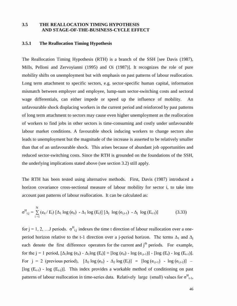
46
3.5 THE REALLOCATION TIMING HYPOTHESIS
AND STAGE-OF-THE-BUSINESS-CYCLE EFFECT
3.5.1 The Reallocation Timing Hypothesis
The Reallocation Timing Hypothesis (RTH) is a branch of the SSH [see Davis (1987),
Mills, Pelloni and Zervoyianni (1995) and Oi (1987)]. It recognizes the role of pure
mobility shifts on unemployment but with emphasis on past patterns of labour reallocation.
Long term attachment to specific sectors, e.g. sector-specific human capital, information
mismatch between employer and employee, lump-sum sector-switching costs and sectoral
wage differentials, can either impede or speed up the influence of mobility. An
unfavourable shock displacing workers in the current period and reinforced by past patterns
of long term attachment to sectors may cause even higher unemployment as the reallocation
of workers to find jobs in other sectors is time-consuming and costly under unfavourable
labour market conditions. A favourable shock inducing workers to change sectors also
leads to unemployment but the magnitude of the increase is asserted to be relatively smaller
than that of an unfavourable shock. This arises because of abundant job opportunities and
reduced sector-switching costs. Since the RTH is grounded on the foundations of the SSH,
the underlying implications stated above (see section 3.2) still apply.
The RTH has been tested using alternative methods. First, Davis (1987) introduced a
horizon covariance cross-sectional measure of labour mobility for sector i, to take into
account past patterns of labour reallocation. It can be calculated as:
N
ζH
t,j = ∑ (eit / Et) [Δ1 log (eit) - Δ1 log (Et)] [Δj log (ei,t-1) - Δj log (Et-1)] (3.33) i =1
for j = 1, 2, …J periods. ζH
t,j indexes the time t direction of labour reallocation over a one-
period horizon relative to the t-1 direction over a j-period horizon. The terms Δ1 and Δj
each denote the first difference operators for the current and jth
periods. For example,
for the j = 1 period, [Δ1log (eit) - Δ1log (Et)] = [log (eit) - log (ei,t-1)] - [log (Et) - log (Et-1)].
For j = 2 (previous period), [Δ2 log (eit) - Δ2 log (Et)] = [log (ei,t-1) - log (ei,t-2)] –
[log (Et-1) - log (Et-2)]. This index provides a workable method of conditioning on past
patterns of labour reallocation in time-series data. Relatively large (small) values for ζH
t-1,

47
ζH
t-2,. indicate that the time t direction of labour reallocation reinforces (reverses) past
patterns of labour reallocation. Reinforcement (reversal) of recent past patterns of labour
reallocation exacerbates (mitigates) skill, location, and informational mismatches between
workers. Davis (1987) estimated the impact of the horizon covariance index using the
following specification of the unemployment equation:
J J J
Ut = βo + β1 DUM74 + ∑β2 ζt + ∑ β3jζH
t-j + ∑ β4j DMEt-j + j=0 j=0 j=0 J
∑ β5j DMRt-j + β6 µt-1 + β7 µt-2 + εt (3.34) j=0
where DUM74 is a dummy variable that equals zero prior to 1974 and one thereafter and
DME is the anticipated money supply growth rate. The error terms, β6µt-1 + β7µt-2 + εt,
follow an AR(2) process. A positive impact for the horizon covariance index on
unemployment was to be interpreted as evidence in favour of the RTH.
The alternative method by Davis (1987) is based on estimating the contemporaneous
correlations between labour reallocation measures and proxies for monetary compensation
and finished goods. According to the RTH, labour mobility and turnover are substitutable
over time. Labour mobility involves unemployment and other forms of foregone
production, which implies that movements in the value of foregone production across
sectors are negatively correlated with unemployment and the pace of labour reallocation.
The two monetary compensation proxies for the cross-sectoral average value of foregone
production are log [compensation index/producer price index (PPI)] and log [compensation
index/consumer price index (CPI)]11
. As these are broad-based measures to proxy for the
average value of foregone production across sectors, they are termed by Davis (1987) as
„cross-sectoral‟.
The deficiencies associated with the monetary compensation measures include the
difficulty in estimating the number of effective hours worked for workers, and the fact that
real wages (under long-term contracts) need not follow short-term movements in the
marginal product of labour. Two alternative proxies based on finished goods were also
adopted, namely, log (manufacturing finished goods inventory at constant prices) and log
(constant prices inventory/manufacturing sales). These are based on the argument that high

48
finished goods inventory levels indicate a lower level of foregone production which triggers
layoffs. Hence, a positive correlation between the finished goods proxies and labour
reallocation should result.
Davis (1987) tested this by letting the raw Lilien index series and the simulated
unemployment series represent the labour reallocation measures. The simulated series is
estimated as per equation (3.34) but without the ζH
t-j component, and with the raw Lilien
index taking its sample values and fixing other regressors in the equation at their sample
means. The proxies of the cross-sectoral average values of monetary compensation and
foregone production discussed above were adopted. A negative correlation between labour
reallocation and the monetary compensation measures and a positive one for the finished
goods were argued to be indicative of confirmation of the fundamental prediction of the
RTH.
3.5.2 The Stage-of-the-Business-Cycle Effect
Whilst the SSH is independent of aggregate economic conditions, the stage-of-the-
business-cycle effect stresses their role in explaining unemployment conditions. During a
recession, there is a tendency for unemployment spells to lengthen and so shocks inducing
sectoral mobility will therefore lead to higher unemployment. Conversely, during an
upturn, unemployment spells tend to be shorter. Consequently, a given rise in sectoral
mobility should result in a smaller increase in unemployment during upturns compared to
downturns. The stage-of-the-business-cycle effect asserts that although the direction of the
ζ-U relation is the same under the SSH and RTH, the magnitude of the increase in
unemployment will be higher during recessions than during boom periods.
The method of testing this type of asymmetric effect involves constructing a multiplicative
interaction variable and testing its effect on unemployment. In Mills, Pelloni and
Zervoyianni (1995), it was the product of the dispersion index, ζt, and S (where S takes
value one when real GNP is below its trend value and 0 otherwise). In Davis (1987), the
interaction variable was the product of RECESS (number of months to recession during the
quarter divided by three) and βζ (where β is the estimated coefficient of ζ). A positive

49
effect of ζt and these interaction variables was to be interpreted as evidence of the stage-of-
the-business-cycle effect.
3.6 CONCEPTUAL DIFFERENCES BETWEEN THE SSH, ADH AND RTH
3.6.1 Source of Sectoral Mobility
Some conceptual differences relating to the role/impact of sectoral mobility on
unemployment are established in this section. Although all hypotheses postulate a positive
ζ-U relationship, there is a difference in the acknowledgement of sectoral mobility as the
cause of unemployment. Whilst the SSH and RTH play up its significance, the ADH
excludes the possibility of this. This difference stems from the source of a sectoral shift. In
the SSH, the shifts are independent of aggregate demand disturbances and can be either
“pure” shifts arising from changes in worker characteristics and sectoral earnings
differentials, or sectoral mobility shifts arising from a supply-side disturbance. In the
ADH, the shifts are derived from pure shocks to aggregate demand, meaning that mobility
is a by-product of an aggregate demand disturbance. Whilst the ADH is based on factors
affecting the macro economy, the SSH has microeconomic foundations. The RTH marries
the two approaches. It is dependent on aggregate economic fluctuations, but it is these
macroeconomic conditions that influence the microeconomic behaviour of individuals.
3.6.2 Chain of Causation
The chain of causation between ζ and U differs between the hypotheses. Whilst it is
sectoral mobility that induces a recession (unemployment) in the SSH and RTH, it is a
recession (generated by an AD disturbance) that causes sectoral movements (which then
lead to unemployment) in the ADH. Although the RTH depends on the stage-of-the-
business-cycle, since past mobility behaviour governs current behaviour, sectoral mobility
is acknowledged as an integral factor generating unemployment. In other words, whilst the
primary cause of unemployment in the SSH and RTH is sectoral mobility, in the ADH it is
the AD disturbance itself.

50
3.6.3 Nature of Unemployment
There is a difference as to how the significance of the components of aggregate
unemployment is perceived amongst the hypotheses. The SSH argues that it is natural
unemployment arising from sectoral movements that causes aggregate unemployment
levels to rise. According to Lilien (1982), “much of the cyclical unemployment is better
described as fluctuations of the natural rate itself”. In contrast, the ADH asserts the role of
cyclical unemployment, since it can be viewed as a form of demand-deficient
unemployment. A negative demand shock would result in cyclical unemployment. The
RTH, however, does not explicitly indicate the nature of the unemployment generated.
3.7 METHODOLOGICAL DIFFERENCES
3.7.1 Methods to Test the SSH
There are methodological differences in the ways the hypotheses have been tested in the
empirical literature. For the SSH, the validation rests upon the statistical significance of the
mobility indices in unemployment models. In relation to the differences in the source of
the sectoral shifts, several measures of the mobility indices have been constructed.
The base measure is the raw Lilien index of equation (3.1). Numerous studies have used
this raw index to test the SSH, namely Lilien (1982), Loungani (1986), Davis (1987), Mills,
Pelloni and Zervoyianni (1995), Loungani and Rogerson (1989), Parker (1992), Palley
(1992), Lu (1996), Neelin (1987), Samson (1985), Saint-Paul (1993), Prasad (1997) and
Brainard and Cutler (1993). Two limitations of the raw index are noted: (a) it captures net
labour flows rather than gross labour flows [Prasad (1997)]; and (b) it assumes that only
pure sectoral shifts affect the dispersion in employment growth rates [Mills, Pelloni and
Zervoyianni (1995)] when aggregate demand and supply shocks could also influence the
dispersion in employment. Owing to these limitations, supply-side and unpredicted
mobility indices have been developed in other studies.

51
The mobility index attributed to supply shocks, introduced by Loungani (1986), is as
expressed in equation (3.9), but it should be noted this index captures only oil price shocks
and not other forms of aggregate supply disturbances. There are variants of the unpredicted
mobility indices intended to capture the sectoral movements from pure sectoral shifts
and/or sector-specific shocks. These indices are purged of aggregate demand disturbances
proxies, namely DMR [equation (3.25)] by Garonna and Sica (2000) and Neelin (1987),
aggregate employment [equations (3.26) and (3.29)] by Lu (1996) and Palley (1992), DMR
and DME [equation (3.31)] and government deficit [equation (32)] by Mills, Pelloni and
Zervoyianni (1995). Others include the index purged of aggregate supply shocks, i.e. an oil
price shock [equations (3.9), (3.11a) and (3.11b)] by Loungani (1986) and Mills, Pelloni
and Zervoyianni (1995).
3.7.2 Methods to Test the ADH
Several methods have been adopted to substantiate the relevance of the ADH, including the
use of predicted mobility indices, ζ-U co-movement approach and the U-V method.
Predicted Mobility Indices
The predicted indices capture the anticipated component of sectoral mobility attributable to
aggregate demand shocks, and their statistical significance in unemployment models is used
to inform on the relevance of the ADH. Two proxies of AD disturbances have been applied
when predicted indices have been constructed, i.e. DMR [equation (3.24)] by Garonna and
Sica (2000) and Neelin (1987) and aggregate employment [equation (3.30)] by Palley
(1992).
The σ-U Co-movement Approach
In the ζ-U co-movement approach, Abraham and Katz (1986) regressed sectoral mobility
on a variable for AD shocks (denoted by deviations of GNP from its trend growth), as per
equation (3.19). First, it was shown that ζt and ∆Ut were positively correlated, given the
negative correlation between the industrial trend growth rates [i.e. d(ln eit)/dt] and their
responsiveness in employment to cyclical fluctuations [i.e. the sum of the δ coefficients

52
from the regression of equation (3.19)]. Second, ΔUt and Ut bore a positive correlation for
the U.S. over 1949-1980 for 11 major sectors. From this, it was concluded that an
aggregate demand-driven ζt-∆Ut correlation could, through a positive ΔUt-Ut relationship,
lead to positive ζ-U co-movements.
The main critique of this method is that there is no direct assessment of the impact of ζ on
U to see if sectoral mobility really does or does not affect aggregate unemployment. As
such, there are limited studies using this method to validate the ADH. The majority of the
studies have used the predicted index approach, as it tackles the issue of whether sectoral
movements (arising from AD shocks) impact U directly.
U-V Method
The U-V correlation was used by Abraham and Katz (1986) to reveal which factors
(aggregate demand disturbances or sectoral shifts) were important in explaining aggregate
unemployment. As mentioned, Abraham and Katz (1986) stated that if the pure SSH
captured why the relationship between ζ and U was positive, that between ζ and V should
be positive, which implies a positive U-V relation. In contrast, the pure ADH suggests
there is a negative U-V relationship. There are, however, doubts over the U-V method
from the theoretical and empirical points of view.
Theoretically, the U-V relation need not be positive under the SSH. A negative U-V
relation is also consistent with the SSH in the presence of asymmetric hiring and firing
costs12
. Thus, by extending Weiss‟ (1984) model to include vacancies, Palley (1992)
illustrated that whilst a negative demand shock to a sector tends to reduce vacancies in that
sector, a positive shock to other sectors, which increases their job vacancies, may not
necessarily offset the decline in vacancies in the sector with the negative shock if it is costly
to hire additional workers in the other sectors. The net effect is an increase in aggregate U
and decline in aggregate V, i.e. a negative U-V relationship. Furthermore, it has been
shown that the correlation between U and V could be negative under the pure SSH and
positive under the pure ADH. Using an equilibrium job matching model, Hosios (1994)
identified circumstances where these particular correlations were possible13
. Under the
SSH, an increase in the price dispersion of output of firms in different sectors could lead to

53
a rise in the number of job searchers, a decline in the actual number of jobs and an increase
in the probability of finding a job, which result in higher unemployment and lower job
vacancies. Under the ADH, an increase in the separation rate could result in a higher
number of workers searching for jobs, leading to a rise in the layoff rate, which causes
higher unemployment and job vacancies.
The criticisms of this empirical approach focus on modelling and measurement issues.
The first lies in the approach to modelling with respect to the posited theoretical
relationship. Abraham and Katz (1986) computed 2 regressions for the U.S. and U.K. as
per equations (3.13) and (3.14). From the resultant positive ζ-U and negative ζ-U
relations, a negative U-V relationship was inferred, suggesting support for the ADH. As
both estimating equations are independent regressions, estimated separately for U on ζ and
V on ζ, respectively, it is not really appropriate to make inference about the U-V
correlation. Since the essence of the positive ζ-U relation is derived from the foundations
of the SSH, it appears that the conclusion arising from the 2 regressions tends to “mix” the
arguments of the ADH and SSH.
The other criticism is that the NHWI used in many studies may be an inadequate proxy for
the vacancy rate. Although Abraham and Katz (1986) concluded that the NHWI tracked
actual vacancies relatively well (by showing that the index and the actual vacancy rate for
Minneapolis/St. Paul were positively correlated with an R2 = 0.8), the evidence is only
based on 1 state. Also, as the NHWI is derived from the number of job advertisements, it is
possible that its increase is attributed to changes in employers‟ advertising practices and
declining newspaper competition [Wachter (1987)] and that the index had not been adjusted
for structural change in the labour market. The 35 per cent reduction of the NHWI by
Abraham and Katz (1986) to accommodate these concerns has been criticized as being
large [Wachter (1987)]. Moreover, since it is based on help-wanted advertising, shifts in
the demand and supply of help-wanted advertising that are unrelated to any change in
vacancies are not considered [Zagorsky (1990)]. Furthermore, even if registered vacancy
data were available for other countries, there may be other vacant jobs not registered with
the authorities14
. For example, adversely affected sectors could reduce job vacancies whilst
favourably affected sectors could recall former workers without relying on registered
advertising [Shin (1997a)].
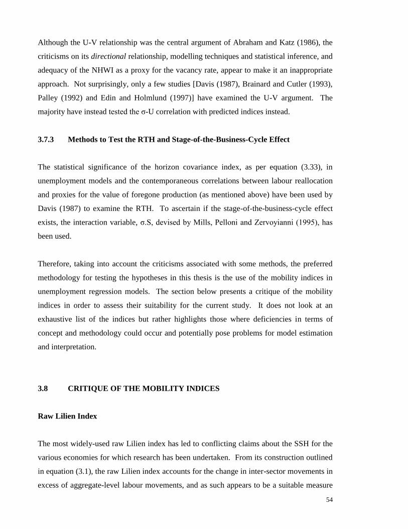
54
Although the U-V relationship was the central argument of Abraham and Katz (1986), the
criticisms on its directional relationship, modelling techniques and statistical inference, and
adequacy of the NHWI as a proxy for the vacancy rate, appear to make it an inappropriate
approach. Not surprisingly, only a few studies [Davis (1987), Brainard and Cutler (1993),
Palley (1992) and Edin and Holmlund (1997)] have examined the U-V argument. The
majority have instead tested the ζ-U correlation with predicted indices instead.
3.7.3 Methods to Test the RTH and Stage-of-the-Business-Cycle Effect
The statistical significance of the horizon covariance index, as per equation (3.33), in
unemployment models and the contemporaneous correlations between labour reallocation
and proxies for the value of foregone production (as mentioned above) have been used by
Davis (1987) to examine the RTH. To ascertain if the stage-of-the-business-cycle effect
exists, the interaction variable, ζ.S, devised by Mills, Pelloni and Zervoyianni (1995), has
been used.
Therefore, taking into account the criticisms associated with some methods, the preferred
methodology for testing the hypotheses in this thesis is the use of the mobility indices in
unemployment regression models. The section below presents a critique of the mobility
indices in order to assess their suitability for the current study. It does not look at an
exhaustive list of the indices but rather highlights those where deficiencies in terms of
concept and methodology could occur and potentially pose problems for model estimation
and interpretation.
3.8 CRITIQUE OF THE MOBILITY INDICES
Raw Lilien Index
The most widely-used raw Lilien index has led to conflicting claims about the SSH for the
various economies for which research has been undertaken. From its construction outlined
in equation (3.1), the raw Lilien index accounts for the change in inter-sector movements in
excess of aggregate-level labour movements, and as such appears to be a suitable measure
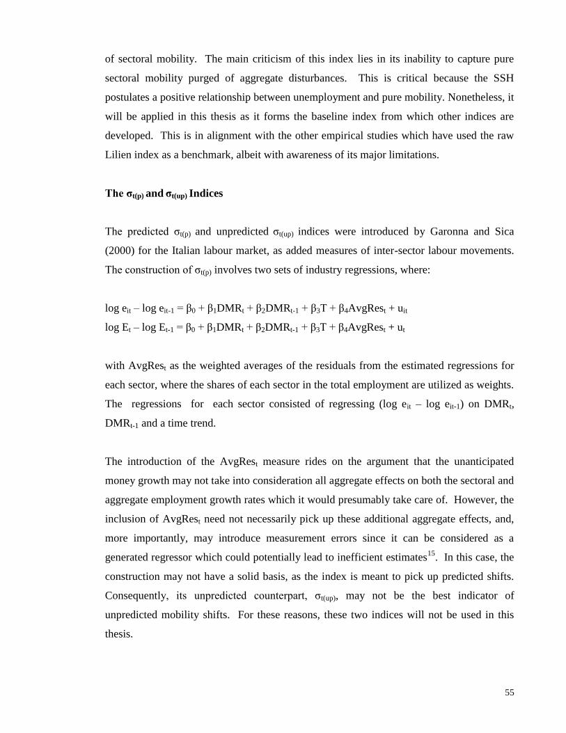
55
of sectoral mobility. The main criticism of this index lies in its inability to capture pure
sectoral mobility purged of aggregate disturbances. This is critical because the SSH
postulates a positive relationship between unemployment and pure mobility. Nonetheless, it
will be applied in this thesis as it forms the baseline index from which other indices are
developed. This is in alignment with the other empirical studies which have used the raw
Lilien index as a benchmark, albeit with awareness of its major limitations.
The σt(p) and σt(up) Indices
The predicted ζt(p) and unpredicted ζt(up) indices were introduced by Garonna and Sica
(2000) for the Italian labour market, as added measures of inter-sector labour movements.
The construction of ζt(p) involves two sets of industry regressions, where:
log eit – log eit-1 = β0 + β1DMRt + β2DMRt-1 + β3T + β4AvgRest + uit
log Et – log Et-1 = β0 + β1DMRt + β2DMRt-1 + β3T + β4AvgRest + ut
with AvgRest as the weighted averages of the residuals from the estimated regressions for
each sector, where the shares of each sector in the total employment are utilized as weights.
The regressions for each sector consisted of regressing (log eit – log eit-1) on DMRt,
DMRt-1 and a time trend.
The introduction of the AvgRest measure rides on the argument that the unanticipated
money growth may not take into consideration all aggregate effects on both the sectoral and
aggregate employment growth rates which it would presumably take care of. However, the
inclusion of AvgRest need not necessarily pick up these additional aggregate effects, and,
more importantly, may introduce measurement errors since it can be considered as a
generated regressor which could potentially lead to inefficient estimates15
. In this case, the
construction may not have a solid basis, as the index is meant to pick up predicted shifts.
Consequently, its unpredicted counterpart, ζt(up), may not be the best indicator of
unpredicted mobility shifts. For these reasons, these two indices will not be used in this
thesis.

56
The σa1
t(up) Index
The ζa1
t(up) of equation (3.26) was used by Lu (1996) in an assessment of the SSH for the
U.S. labour market. The limitation of this index lies in the purging indicator, aggregate
employment, which may not be a strong indicator of aggregate demand per se as it is
negatively related with some other aggregate demand indicators. For example, in the case
of South Korea, it was negatively correlated (correlation coefficient in brackets) with the
ratio of public debt to GDP (-0.299) and ratio of exports to GDP (-0.388). For this reason,
the ζa1
t(up) index will not used in the current work.
The σt(r) Index
The unpredicted ζt(r) index of equation (3.10) was recommended by Loungani (1986) in a
study of the SSH in the U.S. It is a mobility index purged of both aggregate demand (i.e.
unanticipated money supply) and supply (i.e. PPI) factors. Because of this, there is a
concern that the index has been over-purged, and this probably accounts for the
inconsistency of the empirical findings associated with it. Depending on the number of
quarterly lags used, the Loungani (1986) study gave conflicting results, namely, the
estimated impact of the index was positive for ζt-1(r) and ζt-7(r), negative for ζt-3(r) and
ζt-4(r), and insignificant for the other lagged indices. Thus, this measure does seem to be
suitable for empirical work.
The σt(s) Index
Another index introduced by Loungani (1986) is the ζt(s) index of equation (3.9), and it is
the only one reflecting labour movements arising from supply side shocks in the form of oil
prices (PPI). The main concern with this index is its lack of currency. Since there have
only been minute changes in oil prices from 1980 to 2001, the supply shifts are negligible
and there is not much use for the index in the current thesis, particularly if the interest is on
the latter years.

57
The σp1
t(up) and σp2
t(up) Indices
Two SSH indices purged of aggregate supply influences in the form of the energy price
index (EP) are the ζp1
t(up) and ζp2
t(up) applied in the Mills, Pelloni and Zervoyianni (1995)
study for the U.S. economy. Unlike the ζt(s) index, these indices do not reflect movements
from supply influences, but rather movements that have been purged of such. These two
indices will be examined as their plotted series (see Appendix 5C in chapter 5) show
sufficient variability to warrant an examination, and „supply-side‟ indices are needed to
complement the array of the demand-related ones.
Horizon Covariance Index
The horizon covariance index captures inter-sectoral movements from past periods which
are deducted from movements in the present period. The index may not therefore be
suitable for the present study as the present study will be based on annual data and sectoral
movements from up to two years ago may be too distant to exert any influence on current
unemployment. Nonetheless, the use of the index should not be ruled out at this early
stage, as it has won favour in some of the influential literature [see Davis (1987)].
Interaction variable, σtSt
The interaction variable was introduced by Mills, Pelloni and Zervoyianni (1995) to assess
the stage-of-the-business-cycle effect. Given that the Asian Financial Crisis marks a major
turning point in Korea, the interaction variable may not be suitable for the current study.
This is because the post-Crisis era has only 4 annual data points, and because the cycle was
incomplete at the end of the data period examined. However, the interaction variable
should not be omitted at this stage, given the importance of the Asian Financial Crisis.

58
3.9 SUMMARY
This chapter has described the SSH, ADH, RTH and stage-of-the-business-cycle effect and
provided insights into the main conceptual and methodological issues. In summary:
a) The hypotheses not only differ in terms of the presumed impact of sectoral
mobility on unemployment but they also differ conceptually (i.e. source of
sectoral shifts, chain of causation and nature of unemployment) and
methodologically.
b) The method of testing the SSH involves several versions of the mobility index
(raw, supply-side and unpredicted indices purged of aggregate demand and/or
supply disturbances) as regressors in models of unemployment.
c) The methods to test the ADH comprise the ζ-U co-movement approach, U-V
argument and regressing the unemployment rate on a predicted mobility index.
d) The RTH and stage-of-the-business-cycle effect were subject to tests that took
the form of regressing unemployment on the horizon covariance index and
interaction variable, and computing the contemporaneous correlations between
labour reallocation measures and proxies for monetary compensation and
finished goods.
e) The current study will examine the hypotheses using mobility indices (i.e. raw
Lilien index, unpredicted/predicted indices, horizon covariance index and
interaction variable) in unemployment models.
f) Taking into consideration their suitability in terms of concept and methodology,
a total of eleven mobility indices will be utilised in this thesis to test the
hypotheses. They are the SSH indices [ζt, ζa2
t(up), ζm
t(up), ζgt(up), ζ
p1t(up), ζ
p2t(up)],
the ADH indices [ζa2
t(p), ζm
t(p), ζgt(p)], the horizon covariance index (ζH) and the
interaction variable (ζtSt).
The SSH, ADH, RTH and stage-of-the-business-cycle effect have been tested in many
studies in the empirical literature. The findings of these studies, covering various
economies, will be presented and discussed in the following chapter.
59
Endnotes:
1. Other studies examine the role of sectoral shocks on output growth rate [Long, Plosser and Charles (1987), Horvath
(2000) and Norbin and Schlagenhauf (1991)], or sectoral labour mobility on labour productivity [McCombie (1991)] or
sectoral mobility on the recall/retention of jobs [Idson and Valletta (1996)].
2. The other factors influencing the natural rate are labour market distortions (e.g. influence of unions, minimum wage
laws and unemployment insurance) and a change in the profile of the labour force.
3. The Conference Board is an independent global business membership and research organization, and equips businesses
with practical knowledge through issues-oriented research and senior executive meetings.
4. The connection between unemployment and output growth is often formally summarized by the statistical relationship
known as Okun‟s Law. The law relates decreasing unemployment rates with increasing output growth.
5. Abraham and Katz (1986) started the analysis from 1949, rather than 1948 as in Lilien (1982), since 1949 was the
earliest year for which they could obtain data on the help-wanted index.
6. Since Abraham and Katz (1986) stated that „ln Yt is log (GNPt)‟, it can be assumed that it is ln Yt = loge (GNPt), and
hence Yt is the GNPt series.
7. In the process of deriving the predicted and unpredicted indices, some studies have expressed the regression(s) in a
logarithmic series, i.e. as „log‟ [Garonna and Sica (2000), Neelin (1987) and Lu (1996)], whilst others have stated the
series was in natural logarithmic terms [Palley (1992)]. For the studies that do not give the base for the logs, it can be
assumed that they have used natural logs. However, to maintain comparability, this study presents the methodologies
according to the way each empirical study has stated their respective indices.
8. Neelin (1987) mentioned that these predicted and unpredicted indices are analogous to the one used in Lilien (1983).
9. The ζa2t(up) index is a hybrid of predicted and unpredicted indices. The predictive component is captured from the
change in sectoral employment and the unpredicted element arises from the residual component (εit) which presumably
captures pure sectoral influences. Whilst the index has elements of predictability, it is also considered as an index purged
of aggregate demand influences and will be used to test for the SSH in this thesis.
10. Using the average rate of return on capital for industry i in period t, Shin (1997a) computed a cross-sectoral variance
index, ζyit and purged ζy
it by regressing it on the current and lagged growth rates of GNP. However, since the rate of
return on capital is used instead of the employment growth rate, Shin‟s (1997a) study is not relevant to this thesis.
11. These proxies were estimated in logarithmic terms in Davis (1987).
12. Garonna and Sica (2000) also highlighted the role of hiring and firing costs for sectoral shifts in the Italian labour
market.
13. There was no empirical work undertaken for the equilibrium model outlined by Hosios (1994).
14. See Bureau of Labour Market Research, „Structural Change and the Labour Market‟, Research Report no. 11,
Australian Government Publishing Service, Canberra, 1987.
15. Refer to the next chapter for the problem of generated regressors.

60
CHAPTER 4
THE IMPACT OF SECTORAL MOBILITY ON UNEMPLOYMENT:
A REVIEW OF THE EMPIRICAL LITERATURE
4.1 INTRODUCTION
The previous chapter introduced the hypotheses concerning the impact of sectoral mobility
on unemployment: the SSH, ADH, RTH and the stage-of-the-business-cycle effect, and
discussed their conceptual and methodological differences. This chapter aims to review the
related empirical findings on the hypotheses. It then uses this review to indicate how the
empirical application for Korea (chapter 5) might proceed. The organization of the chapter
is as follows. The empirical review is conducted under sections 4.2 to 4.5. Sections 4.6 and
4.7 draw out practical implications for the study of the Korean labour market to be
undertaken in chapter 5, in terms of model specification and estimation. The link to the
microeconomic research on the determinants of sectoral mobility is identified in the
concluding section.
4.2 EMPIRICAL REVIEW ON THE SSH
Sections 4.2 to 4.4 discuss the empirical findings for the various hypotheses with reference
to Table 4.1, which presents the results for the impact of sectoral mobility on
unemployment for the U.S., with those for Canada and Italy reported in the footnote (owing
to the different variables used). Details on these studies are presented here to highlight
differences in the empirical approach. The findings of studies for several other countries –
Japan, Europe and Canada – will also be introduced below. The methodologies in these
studies are generally variants of those employed in the studies for the U.S. listed in Table
4.1. Given the differing hypotheses, and the spread of mobility indicators adopted
within/across the hypotheses, studies with similar indices will be compared under each
hypothesis. This approach establishes conceptual similarity and minimizes the need for
undue explanations where differing results across studies are merely due to conceptual or
methodological dissimilarity. A summary of the findings is found in section 4.5.

61
This section presents the empirical findings for the SSH. Owing to the array of mobility
indices used to test the SSH, the organization of each section is by index-type where the
findings of studies adopting the same type of mobility index are compared. The section
commences with findings from the raw Lilien index – the most commonly-used index, and
ends with the natural unemployment rate approach to testing the hypothesis.
4.2.1 The Raw Lilien Index
Among studies using the raw Lilien index, all for North America and Japan confirm a
positive and significant impact of sectoral mobility on aggregate unemployment. These
include Lilien (1982), Loungani (1986), Parker (1992), Loungani and Rogerson (1989),
Brainard and Cutler (1993), Davis (1987), Mills, Pelloni and Zervoyianni (1995) and Lu
(1996) for the U.S. and Samson (1985) and Neelin (1987) for Canada. Prasad (1997)
computed the raw Lilien index for Japan over 1970-1994 and found a negative relationship
with aggregate employment via graphical analysis, meaning that its impact on
unemployment was probably positive. Similar results were produced when lagged values
of the raw Lilien indices were introduced to cater for long run responses of sectoral
mobility on the macro economy in Lilien (1982), Loungani (1986), Brainard and Cutler
(1993), Davis (1987) and Lu (1996).
For the European economies, the studies acknowledged the role of sectoral mobility on
unemployment but the effect worked in the opposite direction. A negative correlation of the
raw Lilien index with aggregate unemployment was plotted by Saint-Paul (1997) for France
over 1964-1991 and by Garonna and Sica (2000) for Italy for 1952-1994. Rising public
employment in response to higher unemployment and labour market rigidities via
temporary contracts that hampered workers‟ ability to relocate to growth sectors or those
requiring more of specific products/services were the reasons cited for France for this
perverse finding. In Italy, the greater cyclical sensitivity of manufacturing employment vis-
à-vis services employment as compared to the U.S, and firing costs that exceeded hiring
costs (given the high job security) such that unemployment was kept low through sectoral
reallocations (via new hires and pull of new sectors) and interregional mobility were both
argued to have contributed to the negative ζ-U relation.
62
4.2.2 The Index Generated by Supply-side Disturbances
Sectoral movements generated by supply disturbances (oil price shocks) were captured by
an index developed in a single study by Loungani (1986). The lack of similar analyses
reflect the datedness of the 1970s global oil crisis, which has not warranted much research
given the stability of oil prices in latter years. Loungani‟s (1986) index generated by
supply-side disturbances had a positive impact on the unemployment rate for up to 4 lagged
periods.
4.2.3 Pure Sectoral Shift Measures
The pure sectoral shift measures are those that have been purged of the influences of
various aggregate demand and supply variables. With regards to the mobility index purged
of oil price shocks, Mills, Pelloni and Zervoyianni (1995) reported a positive ζ-U
correlation for the U.S. when a one-period lagged version of the mobility index was used.
Again, this is an isolated study which has not generated much interest in the literature,
possibly owing to the datedness of the 1970s oil shock.
Pertaining to the index purged of money growth, the effect on unemployment was positive
for the current period variable and negative for the four-period lagged variable for the U.S.
[Mills, Pelloni and Zervoyianni (1995)] but insignificant for Canada [Neelin (1987)].
When purged of government debt, the index‟s lagged effect was positive for a one-period
lagged variable but negative for a four-period lagged variable [Mills, Pelloni and
Zervoyianni (1995)]1. Conflicting results were produced when the index was purged of
aggregate employment. Palley (1992) reported positive influences for the current and one-
period lagged variables, but Lu (1996) reported an insignificant relationship for all three
lagged indices included in the estimating equation (see Table 4.1). This conflict may
reflect the inappropriateness of using overall employment as a purging tool rather than
specific AD variables.
Loungani (1986) purged the index of aggregate demand (DMR) and supply (oil price
shocks) variables. The one-period and seven-period lagged indices were found to have
significant effects on unemployment. There does not appear to be a convincing argument
for this pattern of significant effects. However, the index may be over-purged, and the
degree of support for the hypothesis under test provided by such results is therefore open to
debate.

Table 4.1 Studies on the Impact of Sectoral Mobility on Aggregate Unemployment in the U.S. Study Lilien (1982) Loungani
(1986)
Parker (1992) Brainard and
Cutler (1993)
Palley (1992) Loungani and
Rogerson
(1989)
Davis
(1987)
Mills, Pelloni and
Zervoyianni
(1995)
Lu
(1996)
Raw Lilien index Over 13
sectors
Over 65
industries
MLE 2SE
ζt 55.9** 0.29** 0.051** 0.0034 0.71+ 0.361**
ζt-1 18.9* 0.40** 0.708** 0.559** 0.37**
ζt-2 0.16 0.467** 0.384** -0.21*
ζt-3 -0.03 -0.136 0.335** 0.04
ζt-4 0.15 -0.123 0.138
ζt-5 0.39** 0.113
ζt-6 0.36** 0.224**
ζt-7 0.46** 0.288**
ζt-8 0.20 0.218**
ζt-9 0.203**
ζt-10 0.138
ζt-11 0.151
ζt-12 0.252**
Δζt 3.856**
Δζt-1 4.690**
Δζt-2 3.333**
Index purged of AD variables
ζmt(up) 2.268**
ζmt-4(up) -1.993**
ζgt-1(up) 4.364**
ζgt-4(up) -2.529*
ζa1t-1(up) 0.09
ζa1t-2(up) 0.32
ζa1t-3(up) -0.07
ζa2t(up) 18.00** 24.15**
ζa2t-1(up) 15.24* 14.72*
ζa2t-2(up) -5.99 -7.61
ζa2t-3(up) 7.91 6.19
Index purged of AS variables
ζp1t-1(up) 3.820**
ζp1t-3(up) -3.519**
ζp2t-3(up) -3.190**
Index purged of AD and AS
variables
ζt(r) 0.24
ζt-1(r) 0.38**
ζt-2(r) 0.10
ζt-3(r) -0.23
ζt-4(r) -0.20
ζt-5(r) 0.06
ζt-6(r) 0.08
ζt-7(r) 0.28**
ζt-8(r) 0.17

64
Table 4.1 Studies on the Impact of Sectoral Mobility on Aggregate Unemployment in the U.S. (continued) Study Lilien (1982) Loungani
(1986)
Parker (1992) Brainard
and Cutler
(1993)
Palley (1992) Loungani and
Rogerson
(1989)
Davis
(1987)
Mills, Pelloni
and
Zervoyianni
(1995)
Lu (1996)
MLE 2SE
Index attributed to AS shocks
ζt(s) 0.60**
ζt-1(s) 0.83**
ζt-2(s) 0.49**
ζt-3(s) 0.47**
ζt-4(s) 0.34**
ζt-5(s) -0.19
ζt-6(s) -0.12
ζt-7(s) 0.07
ζt-8(s) 0.09
Index attributed to Aggregate
shocks
ζat(p) -22.07** -47.42**
ζat-1(p) -21.19** -25.44**
ζat-2(p) -19.00** -14.40
ζat-3(p) -15.89* -13.63
Horizon Covariance Index
Quarterly data series
ζHt-1 0.598**
ζHt-6 0.279**
ζHt-12 0.166**
Annual data series
ζHt-1 -7.9
ζHt-4 28.9*
ζHt-1 6.13
ζHt-3 44.18**
Interaction variable
Quarterly data series
RECESS(βtζt + βt-1ζt-1) 0.172* 5
RECESS ∑ (βiζi ) i=0
0.046
10
RECESS ∑ (βiζi ) i=0
0.077
12
RECESS ∑ (βtζt + βt-1ζt-1) i=0
0.038
∆ (Stζt + St-1ζt-1) 1.210**
** significant at 5% level. * significant at 10% level.
+ : Based on bivariate correlation coefficient.
Note: 1. Although the Lilien indices have been categorized by type (raw, purged of AD/AS/Aggregate variables, pure indices, interaction variable) and by the number of lags, including that for the current period, the indices are not directly comparable across studies. This arises as the impacts of the Lilien indices on unemployment for these studies were based
on different methods of estimation, model specification and number of industries.
2. Findings on coefficients (in brackets) for other countries
Canada: Neelin (1987): Raw Lilien index (31.71) and Index attributed to AD shocks (101.52) were significant at the 5% level. Index purged of AD variables (-7.63) was insignificant.
Samson (1985): Raw Lilien index (81.7) was reported to be significant at the 5% level.
Italy: Garonna and Sica (2000): Index purged of AD variables (0.30) was significant at the 10% level and Index attributed to AD shocks (-0.70) was significant at the 5% level.

65
4.2.4 The Natural Unemployment Rate Approach
The empirical findings on the significance of the natural unemployment rate concur with
the foundations of the SSH (Table 4.2). Thus, the natural unemployment rate explained a
significant portion of the variations in the aggregate unemployment rate in Lilien (1982)
and Mills, Pelloni and Zervoyianni (1995). Furthermore, when alternative indices (index
purged of aggregate demand influences and interaction variables for the stage-of-the-
business-cycle effect) were included in the unemployment equation used to estimate the
natural rate in the latter study, the natural rate accounted for a slightly larger proportion of
the actual rate. Parker (1992) estimated the natural rate as the fitted value of the
unemployment equation with the unanticipated money growth and residual obtained from
the unemployment regression set equal to zero, and plotted this series against that of U. It
was observed that U exceeded U* during 1956-1964. Towards the late 1960s and early
1970s, U declined due to microeconomic factors (labour supply shortage associated with
the Vietnam war) and the U-U* disparity lessened. Given that the natural rate is that which
is attributable solely to microeconomic factors, the narrowing of the U*-U gap implies that
much of the unemployment in the 1970s was accounted for by natural (microeconomic)
factors, i.e. the natural rate. Samson (1985) plotted the U* series against the actual U series
over the 1957-1983 period and found a small deviation of 0.45 between the two series
(based on their average absolute values), implying that the natural rate could explain the
actual series relatively well. Loungani (1986) constructed two measures of the natural rate,
U*t(s) and U
*t(r), where the former was estimated from the regression associated with the
index attributed to the oil shock, and the latter with the unpredicted index. Using quarterly
data for the U.S. over j = 8 lags, these were calculated as:
8
U*t(s) = β0 + ∑ βj ζ t(s)-j and
j=0
8
U*t(r) = β0 + ∑ γj ζ t(r)-j
j=0
where β0 is the intercept estimate from the regressions and βj and γj were each the
estimated coefficients attached to the ζt(s) and ζt(r) variables. It was reported that U*t(s)
accounted for 20% of U, higher than the 5% reported for U*t(r).

66
Table 4.2 R2 between Actual Unemployment Rate and Natural Unemployment Rate
Study Lilien (1982) Mills, Pelloni and
Zervoyianni (1995)
Loungani (1986)
Between Ut and U*t Between ∆Ut and ∆U*t Between Ut and U*t
Index used
Actual
series
Detrended
series
Detrended series
ζt 0.74 0.60 0.52
ζt(s) 0.20
ζt(r) 0.05
ζm
t(up) 0.55
∆(Stζt + St-1ζt-1) 0.57
∆(Stζm
t(up)+St-1ζm
t(up)-1) 0.56
Whilst several studies have supported the general influence U* has on U, namely, Parker
(1992), Loungani (1986) and Samson (1985), a counter argument questioning the influence
of U* was presented by Murphy and Topel (1987a). They made use of a constant natural
rate argument to conclude a lack of support for the SSH. In theory, sectoral movements
under the SSH generate frictional unemployment which should lead to changes in the
natural rate. Using unit-record cross-sectional data for male employees in the U.S., it was
shown that only 2.4-4.0 per cent of the total unemployed were industry movers during
1968-1985, and that this proportion remained virtually constant throughout this period,
implying a constant natural rate of unemployment. Since changes in the natural rate are
implied under the SSH in that U* varies with frictional inter-sector labour movements,
Murphy and Topel (1987a) concluded that the constant natural rate (implied from the non-
varying 2.4-4 per cent) did not concur with the hypothesis. This contrasts with the other
evidence for the U.S., such as Parker (1992) and Lilien (1982), which illustrated a
fluctuating U* series over the period, but it should be noted that two different sets of data
are used to support the evidence for the SSH or lack thereof. Murphy and Topel‟s (1987a)
constant rate is implied from descriptive data covering males only, whilst Parker‟s (1992)
and Lilien‟s (1982) U* series has been estimated formally and covers both males and
females. Furthermore, in response, Lilien (1987) argued that Murphy and Topel (1987a)
misinterpreted the underlying implications of the SSH, where sectoral mobility is generated
by frictional movements as well as economic shocks.2 Thus, whilst Murphy and Topel
(1987a) interpreted inter-industry movements to arise from frictional labour movements,
such sectoral movements can also originate from economic shocks.
67
4.3 EMPIRICAL FINDINGS ON THE ADH
The methodologies to test the ADH comprise the use of predicted mobility indices, the U-V
relationship and ζ-U co-movement approach. The organization of this section is to
evaluate the empirical works according to these methodologies. For the latter approach, the
findings are not assessed since Abraham and Katz (1986) appears to be the single study
using the ζ-U co-movement method, and this has been described in the previous chapter.
4.3.1 The Predicted Mobility Indices
Predicted indices from aggregate demand disturbances have been used to test the ADH.
The two studies adopting this approach have reported opposite results. The ζ-U relation
was positive in Neelin (1987) for Canada but negative in Garonna and Sica‟s (2000)
analysis for Italy. For the latter, the inverse relation was held to reflect the differing
cyclical responsiveness of economic sectors which triggers unemployment, thereby leading
to the deduction that sectoral movements in Italy were generated from an AD disturbance
and that unemployment is cyclical. Thus, whilst the Canadian experience appears to
provide clear support for the ADH via its positive ζ-U relation, the Italian outcome can be
argued to be aligned to the ADH only in terms of the source of sectoral shifts and nature of
unemployment, and certainly not from the evidence of the directional influence of ζ on U.
A predicted index generated by aggregate employment was examined by Palley (1992) for
the U.S. over 1951-1988 for 11 sectors. A negative influence on unemployment from
mobility for the current-period index and indices lagged by three periods was reported.
This does not support the ADH, since the study for the U.S. by Abraham and Katz (1986)
asserted that there should be positive ζ-U co-movements. Since Palley (1992) and
Abraham and Katz (1986) cover the same economy and almost similar time periods but
reveal differing results, the method of filtering involved when constructing this form of
predicted index (i.e. the use of aggregate employment) remains questionable.
68
4.3.2 The U-V Relationship
As explained in the previous chapter, under the SSH the U-V relationship should be
positive, and ζ-U and ζ-V should both be positively related as well. Under the ADH, the
positive ζ-U association generates a negative ζ-V relationship following an aggregate
demand shock and the resulting U-V relation is inverse. In this section the empirical
support for the ADH from the correlation results of U-V and/or ζ-U and/or ζ-V is
examined. Generally, it is shown that the conclusions on the ADH using the U-V
relationship are contradictory.
Davis (1987) plotted the ζ, NHWI and unemployment inflows and outflow series for 1948-
1986. It was shown that: (a) periods of high (low) unemployment inflow and outflow rates
coincided with declining (rising) NHWI levels; and (b) periods of rapid rates of labour
reallocations accompanied high unemployment rates. The negative U and V correlation
and the positive ζ and U relationship appeared to be consistent with the ADH rather than
the SSH.
Brainard and Cutler (1993) estimated the Beveridge Curve by regressing the logarithm of
the vacancy rate against the current and lagged values of a cross-section volatility (CSV)
measure, the raw Lilien index and the unemployment rate3:
15 15
log Vt = β0 + ∑ β1jCSVt-j + ∑ β2jζt-j + β3logUt + εt (4.1) j=0 j=0
for 15 lagged quarters, where the CSV is a variance measure of sectors‟ stock market
excess returns. Whilst CSV and Ut exerted positive and significant influences on job
vacancies, the finding for ζ was ambiguous, being significant and positive for the first two
lagged years and insignificant for the third and fourth lagged years4. As the U-V relation
was negative and the ζ-V relationship ambiguous, the results did not appear to support the
ADH.
Similarly, the significance of the current and lagged values of the predicted and unpredicted
indices in a model of the aggregate vacancy rate (proxied by ratio of NHWI to total non-
agricultural employment) was examined by Palley (1992) using the following equation5:

69
3 3
Vt = β0 + β1T + β2Vt-1 + ∑ β3,t-jζt-j(p) + ∑ β4,t-jζt-j(up) + εt (4.2)
j=0 j=0
The results revealed the unpredicted indices were associated with reductions in the vacancy
rate. This negative ζ-V correlation concurs with the ADH rather than the SSH, which as
noted above asserts a positive ζ-V relation. However, the main criticism is that the
unpredicted indices were insignificant regressors of the vacancy rate even though the
coefficients were negative. The case for the U-V argument in Palley‟s (1992) study is
therefore weak.
The other study supporting the ADH is Edin and Holmlund (1997), using a U-V curve for
Sweden over 1983-1995. The increase in unemployment over the period was characterized
by a movement along the curve rather than a shift. It was concluded that higher
unemployment during 1994-1995 was brought about by aggregate demand shocks in the
form of a decline in public sector labour demand rather than by any mismatch in the
composition of labour demand and supply, suggesting a case for the ADH.
4.4 FINDINGS ON THE RTH AND STAGE-OF-THE-BUSINESS-CYCLE
This section presents the findings on the RTH and stage-of-the-business-cycle effect. The
section is presented according to the measure adopted to test the hypotheses. It begins with
an assessment of results based on the horizon covariance index and interaction variable,
followed by those using labour reallocation and foregone production proxies.
4.4.1 The Horizon Covariance Index
The horizon covariance index used by Davis (1987) to test the RTH was constructed for 8
non-agricultural industries with quarterly data for the U.S. This index, lagged by one, six
and twelve periods, had positive impacts on unemployment for 1953-1986. While this
appears to provide support for the RTH, the strength of this support has been questioned by
Oi (1987). He argued that the regression results of Davis (1987) were quite weak
statistically. Since the RTH has not been tested by any other studies, including Oi (1987),

70
no conclusion can be reached as to its relevance in general, or its potential relevance to the
Korean labour market.
4.4.2 Interaction Variables
To test the stage-of-the-business-cycle effect, Mills, Pelloni and Zervoyianni‟s (1995)
interaction variable, ζtSt, was computed over 30 industries for the U.S. during 1960-1991.
The interaction variable had a positive effect on unemployment. Davis‟ (1987)
RECESS(βtζt + βt-1ζt-1) variable was also significant for the U.S. during 1953 quarter 2 and
1986 quarter 2. These results were argued to be consistent with the stage-of-the-business-
cycle effect, i.e. the ζ-U impact intensifies during recessions and weakens during upturns.
However, Davis‟ (1987) interaction variable is not applicable to the current work in that it
has to be applied to quarterly data.
4.4.3 Labour Reallocations and Foregone Production
Davis (1987) is the single study examining the RTH using correlations between labour
reallocations and foregone production. The labour reallocation measures are the raw Lilien
index series and the simulated unemployment series as per equation (3.34), excluding ζH
t-j,
and with the raw Lilien index taking its sample values whilst fixing other regressors at their
sample means. The proxies for foregone production were log [compensation
index/producer price index (PPI)], log [compensation index/consumer price index (CPI)],
log (manufacturing finished goods inventory at constant prices), log (manufacturing
finished goods/PPI) and log (constant prices inventory/manufacturing sales). Negative
correlations were reported for both labour reallocation measures and the first two proxies
over 1953-1986, whilst positive correlations were reported for the detrended finished goods
measures for different time periods (see Table 4.3). These results were interpreted as
confirming the predictions of the RTH.
Two related criticisms were directed at Davis‟ (1987) conclusion by Oi (1987). First, the
correlations shown are rather small, and second, the R2 never exceeds 0.1. These criticisms
are certainly valid and appear to account for why the method of labour reallocations and
value of foregone production has not been used in other studies. Owing to the dearth of

71
comparison studies, and the criticism of the Davis (1987) study, this approach will not be
applied in this thesis.
Table 4.3 Contemporaneous Correlations between Labour Reallocation
and Average Value Proxies of Foregone Production Proxies for Foregone Production Simulated Unemployment Raw Lilien Index
Contemporaneous Correlation
R2 Contemporaneous Correlation
R2
Log (Compensation Index/PPI)
1953-1986 -0.227 0.009 -0.217 0.012
Log (Compensation Index/CPI)
1953-1986 -0.306 0.000 -0.250 0.004
Log (Manufacturing Finished
Goods Inventory/PPI)
1953-1986 0.091 0.298 0.185 0.033
Log (Manufacturing Finished Goods
Inventory at Constant Prices)
1959-1986 0.212 0.028 0.219 0.023
Log (Inventory at Constant Prices/
Manufacturing Sales)
1961-1985 0.710 0.000 0.359 0.000
Source: Davis (1987).
Note: Davis (1987) stated most correlations were significant at the 5% level except for one correlation.
However, this exception was not singled out.
4.5 SUMMARY OF EMPIRICAL FINDINGS
Based on the above review, the following can be concluded regarding the empirical
relevance of the hypotheses:
a) Empirically, the SSH appears to be supported by studies using the raw Lilien
index, supply-side index and pure indices purged of specific aggregate demand
and supply disturbances. The hypothesis is not a global phenomenon as the
contrasting experiences of European economies suggest that varied labour
market features and sectoral sensitivities influence the way mobility affects
unemployment. Given the widespread empirical acceptance of the SSH, this
thesis will consider the use of the SSH indices in model estimation.

72
b) The ADH appears to have less empirical acceptance compared to the SSH. In
view of the contradictory theories governing the U-V correlation, and the
absence of a direct assessment of the impact of ζ on U, tests of the ADH will be
based on the statistical significance of predicted mobility indices in
unemployment models.
c) The horizon covariance index and interaction variable have been reported as
significant in models of unemployment. Based on this, the current work will
adopt the same index and interaction variable to evaluate if the RTH and stage-
of-the-business-cycle effect hold for Korea.
4.6 EMPIRICAL APPLICATION
This section reviews the empirical methods adopted by the studies of the impact of sectoral
mobility in terms of the data-type and frequency, time periods, and model specification and
estimation. Reference is made to the recommended empirical framework for the thesis.
4.6.1 Type and Frequency of Data
The common form of data adopted in the studies is aggregate-level time-series data. The
majority have used annual data, which have the advantage of removing the effects of
seasonality and thus enabling assessment of the impact of sectoral mobility on structural,
frictional and cyclical unemployment independent of seasonal unemployment. Some
studies have used quarterly data, but these either showed the Lilien index to be insignificant
[Lu (1996)], ended up incorporating numerous lagged indices (6-12 lags) in the regression
to accommodate the longer-run effects of mobility [Loungani (1986), Neelin (1987), Davis
(1987) and Mills, Pelloni and Zervoyianni (1995)], or have had to make adjustment for the
seasonal component in the regression analysis, either by including seasonal dummies as
regressors [Neelin (1987)] or pre-adjusting the dependent variable [Davis (1987)]. Since
sectoral behavioural response is not highly volatile to swings in market activity compared
to a stock market response (where high frequency data are generally used), the use of
annual data for the current study should suffice.

73
4.6.2 Time Period
The majority of the analyses cover 3 decades in order to be able to capture the long run
dynamics of sectoral mobility. The exceptions are Loungani and Rogerson (1989) [1
decade], Samson (1985) and Neelin (1987) [2 decades], Brainard and Cutler (1993), Lu
(1996) and Garonna and Sica (2000) [4 decades] and Davis (1987) [6 decades]. Likewise,
the current work for Korea covers 3 decades, from 1971 to 2001.
4.6.3 Model Estimation
An unemployment regression containing variants of ζ will be the main approach to test the
hypotheses. Table 4.4 provides the model specification and method of estimation of the
unemployment equations in the main studies. Two types of time-series models (TSM) are
applied: single-equation and dual-equation models.
4.6.3.1 Single-Equation Models
The studies adopting a single-equation TSM are of the following general functional form:
J J
Ut = βo + ∑ β1j Xt-j + ∑ β2jUt-j + εt (4.3)
j=0 j=1
where Xt-j represents the current and/or lagged values of the variants of ζ and aggregate
demand/supply variables, and Ut-j represents the lagged values of the dependent variable.
One area of concern is that ζ could be correlated with other explanatory variables and this
poses potential problems of multicollinearity. Another more significant area of concern in
studies with single-equation models is the lack of adequate proxy variables for aggregate
demand/supply disturbances. Lu‟s (1996) GDP growth rate variable does not distinguish
whether it is an AD or AS variable6. Brainard and Cutler‟s (1993) CSV measure captures
the short-run dynamics of a shock and ignores its long-run impact on the labour market.
Aggregate disturbance variables are totally absent from Palley‟s (1992) specification7.
Accommodating such variables frequently involves the inclusion of DMR in the studies.
Since DMR itself is estimated from a money growth equation, this means that the
unemployment model is treated as a second equation, leading to the emergence of dual-
equation models.

74
Table 4.4 Unemployment and Money Growth Equations used
in Selected Studies of Sectoral Mobility Study Country/ Time
Period/Data-
type/Method of
Estimation for
Aggregate
Unemployment
Model Specification
Lilien (1982)
U.S., 1948-1980,
Aggregate-level time-
series annual data.
Method of Estimation
2-step estimation (2SE).
Aggregate Unemployment
1 2
Ut = βo + ∑ β1j ζt-j - ∑ β2j DMRt-j + β3 Ut-1 + β4 T + εt
j=0 j=0
Natural Unemployment Rate
∞
U*t = ∑ βj2 (β0 + β1ζt-j + β4 Tt-j)
j=0
Note: The number of lags in the U*t equation corresponds with those for
the aggregate unemployment equation.
Money Growth Rate
DMt = α0 + α1 DMt-1 + α2DMt-2 + α3FEDVt + α4UNt-1 + DMRt
Abraham
and Katz
(1986)
U.S., 1949-1980,
Aggregate-level time-
series annual data.
Method of Estimation
2SE.
Aggregate Unemployment
1 2
Ut = βo + ∑ β1j ζt-j - ∑ β2j DMRt-j + β3 Ut-1 + β4 T + εt
j=0 j=0
Money Growth Rate
DMt = α0 + α1 DMt-1 + α2DMt-2 + α3FEDVt + α4UNt-1 + DMRt
Loungani
(1986)
U.S., 1947-1982,
Aggregate-level time-
series quarterly data.
Method of Estimation:
2SE.
Aggregate Unemployment
8 8
Regression 1: Ut = βo + ∑ β1j ζt-j - ∑β2j DMRt-j + β3 T + εt
j=0 j=0
8 8
Regression 2: Ut = βo + ∑β1j ζt(s)-j - ∑β2j DMRt-j + β3 T + εt
j=0 j=0
8 8
Regression 3: Ut = βo + ∑β1j ζt(r)-j - ∑β2j DMRt-j + β3 T + εt
j=0 j=0
Natural Unemployment Rate
J
U* t(s) = βo + ∑ β1j ζt(s)-j
j=0
J
U* t(r) = βo + ∑ β1j ζt(r)-j j=0
Note: The number of lags in the U*t equation corresponds with those for
the aggregate unemployment equation. No reason was given as to why the
trend variable was excluded. The U*t was probably meant to solely capture
the amount of unemployment attributable to sectoral movements.
Money Growth Rate
DMt = α0 + α1 DMt-1 + α2DMt-2 + α3FEDVt + α4UNt-1 + DMRt
Note: As the author did not specify the money growth equation, it is
assumed the equation follows that of Barro (1977).
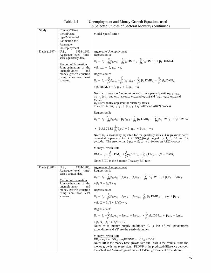
75
Table 4.4 Unemployment and Money Growth Equations used
in Selected Studies of Sectoral Mobility (continued) Study Country/ Time
Period/Data-
type/Method of
Estimation for
Aggregate
Unemployment
Model Specification
Davis (1987) U.S., 1953-1986, Aggregate-level time- series quarterly data. Method of Estimation Joint-estimation of the unemployment and money growth equation using non-linear least squares.
Aggregate Unemployment Regression 1:
12 9 12
Ut = βo + ∑ β1j ζt-j + ∑β2j DMRt-j + ∑ β3j DMEt-j + β4 DUM74 j=0 j=0 j=0
+ β5 μt-1 + β6 μt-2 + εt Regression 2:
12 Ja 9 12
Ut = βo + ∑ β1jζt-j + ∑ β2j ζHt-j - ∑ β3j DMRt-j + ∑ β4j DMEt-j
j=0 j=0 j=0 j=0
+ β5 DUM74 + β6 μt-1 + β7 μt-2 + εt Note: a: J varies as 6 regressions were run separately with ζHt-1, ζHt-6,
ζHt-12, (ζHt-1 and ζHt-12), (ζHt-1, ζHt-6 and ζHt-10) and (ζHt-1, ζHt-4, ζHt-8 and ζHt-10). Ut is seasonally-adjusted for quarterly series. The error terms, βj μt-1 + βj μt-2 + εt, follow an AR(2) process. Regression 3: 12 9 12
Ut = βo + ∑ β1j ζt-j + β2 ζHt-1 + ∑ β3j DMRt-j + ∑ β4j DMEt-j + β5DUM74 j=0 j=0 j=0
J
+ β6RECESS (∑ βjζt-j) + β7 μt-1 + β8 μt-2 + εt j=0
Note: Ut is seasonally-adjusted for the quarterly series. 4 regressions were estimated separately for RECESS(∑βjζt-j) lagged by 1, 5, 10 and 12 periods. The error terms, βjμt-1 + βjμt-2 + εt, follow an AR(2) process. Money Growth Rate 12 4 4
DMt = α0 + ∑α1jDMt-j + ∑α2jBILLt-j + ∑α3jUNt-j + α4T + DMRt j=1 j=1 j=1
Note: BILL is the 3-month Treasury Bill rate.
Davis (1987) U.S., 1924-1985, Aggregate-level time- series, annual data. Method of Estimation Joint-estimation of the unemployment and money growth equation using non-linear least squares.
Aggregate Unemployment Regression 1:
2 2
Ut = βo + ∑ β1j ζt-j + β2ζHt-1 + β3ζHt-4 + ∑ β4j DMRt-j + β5mt + β6mt-1
j=0 j=0
+ β7 Gt + β8 T + εt Regression 2:
2 2
Ut = βo + ∑ β1j ζt-j + β2ζHt-1 + β3ζHt-4 + ∑ β4j DMRt-j + β5mt + β6mt-1
j=0 j=0
+ β7 Gt + β8 T + β9YD + εt Regression 3:
2 2
Ut = βo + ∑ β1j ζt-j + β2ζHt-1 + β3ζHt-3 + ∑ β4j DBRt-j + β5mt + β6mt-1
j=0 j=0
+ β7 Gt + β8T + β9YD + εt
Note: m is money supply multiplier, G is log of real government
expenditure and YD are the yearly dummies. Money Growth Rate DBt = α0 + α1 DBt-1 + α2FEDVPt + α3Ut-1 + DBRt
Note: DB is the money base growth rate and DBR is the residual from the
money growth rate regression. FEDVP is the predicted difference between
the actual and „normal‟ growth rate of federal government expenditure.
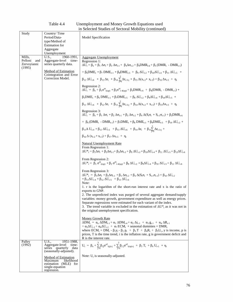
76
Table 4.4 Unemployment and Money Growth Equations used
in Selected Studies of Sectoral Mobility (continued) Study Country/ Time
Period/Data-
type/Method of
Estimation for
Aggregate
Unemployment
Model Specification
Mills, Pelloni and Zervoyianni (1995)
U.S., 1960-1991, Aggregate-level time- series quarterly data. Method of Estimation Cointegration and Error Correction Model.
Aggregate Unemployment
Regression 1: ΔUt = βo + β1 Δζt + β2 Δζt-1 + β3Δζt-2 + β4DMRt-6 + β5 (DMRt - DMRt-1) + β6DMEt + β7 DMEt-1 + β8DMEt-5 + β9 ΔUt-2 + β10ΔUt-4 + β11 ΔUt-5 + 2
β12 ΔUt-6 + β13 Δrt + β14 ∑ Δrt-3-j + β15 Δ(xt-2+ xt-3) + β16 Δxt-5 + εt j=0
Regression 2: ΔUt = βo + β1ζ
mt(up) + β2ζ
mt-4(up) + β3DMRt-6 + β4(DMRt - DMRt-1) +
β5DMEt + β6 DMEt-1 + β7DMEt-5 + β8 ΔUt-2 + β9ΔUt-4 + β10ΔUt-5 + 2
β11 ΔUt-6 + β12 Δrt + β13 ∑ Δrt-3-j + β14 Δ(xt-2 + xt-3) + β15Δxt-5 + εt j=0
Regression 3: ΔUt = βo + β1 Δζt + β2 Δζt-1 + β3 Δζt-2 + β4 Δ(Stζt + St-1ζt-1) + β5DMRt-6
+ β6 (DMRt - DMRt-1) + β7DMEt + β8 DMEt-1 + β9DMEt-5 + β10 ΔUt-2 +
2
β11Δ Ut-4 + β12 ΔUt-5 + β13 ΔUt-6 + β14 Δrt + β15∑ Δrt-3-j +
j=0
β16 Δ (xt-2 + xt-3) + β17 Δxt-5 + εt Natural Unemployment Rate
From Regression 1:
ΔU*t = β1Δζt + β2Δζt-1+ β3Δζt-2 + β9 ΔUt-2 + β10ΔUt-4 + β11 ΔUt-5 + β12ΔUt-6
From Regression 2:
ΔU*t = β1 ζm
t(up) + β2 ζm
t-4(up) + β8 ΔUt-2 + β9ΔUt-4 + β10 ΔUt-5 + β11 ΔUt-6
From Regression 3:
ΔU*t = β1Δζt + β2Δζt-1 + β3 Δζt-2 + β4 Δ(Stζt + St-1ζt-1) + β10 ΔUt-2
+ β11ΔUt-4 + β12 ΔUt-5 + β13 ΔUt-6
Note:
1. r is the logarithm of the short-run interest rate and x is the ratio of
exports to GNP.
2. The unpredicted index was purged of several aggregate demand/supply
variables: money growth, government expenditure as well as energy prices.
Separate regressions were estimated for each variant of the index.
3. The trend variable is excluded in the estimation of ΔU*t as it was not in
the original unemployment specification.
Money Growth Rate
ΔDMt = αo ΔDMt-1 + α1 ΔDMt-4 + α2 Δit-1 + α3 gt-1 + α4 ΔRt-1
+ α5ΔUt-1 + α6ΔUt-2 + α7 ECMt + seasonal dummies + DMRt
where ECMt = DMt - β1yt - β2 pt + β3 T + β4Rt + β5Ut,, y is income, p is
prices, T is the time trend, i is the inflation rate, g is government deficit and
R is the interest rate. Palley (1992)
U.S., 1951-1988, Aggregate-level time-series quarterly data (seasonally-adjusted). Method of Estimation Maximum likelihood estimation (MLE) for single-equation regression.
3 3
Ut = βo + ∑ β1jζa2
t(p)-j + ∑ β2 jζa2
t(up)-j + β3 Tt + β4 Ut-1 + εt
j=0 j=0
Note: Ut is seasonally-adjusted.

77
Table 4.4 Unemployment and Money Growth Equations used
in Selected Studies of Sectoral Mobility (continued) Study Country/ Time
Period/Data-
type/Method of
Estimation for
Aggregate
Unemployment
Model Specification
Parker
(1992)
U.S., 1956-1987,
Aggregate-level time-
series annual data.
Method of Estimation
Joint-estimation of the
unemployment and
money growth equation.
Aggregate Unemployment
Ut = βo + β1 ζt + β2 DMRt + β3 DMRt-1 + β4 DMRt-2 + β5 UIt + β6 MWt
+ β7 MILt + εt
Male Unemployment
UtM = βo + β1 ζt + β2 DMRt + β3 DMRt-1 + β4 DMRt-2 + β5 UIt + β6 MWt
+ β7 MILt + β8 ζrt + εt
Female Unemployment
UtF = βo + β1 ζt + β2 DMRt + β3 DMRt-1 + β4 DMRt-2 + β5 UIt + β6 MWt
+ β7 MILt + β8 ζrt + εt
Natural Unemployment Rate
U*t = βo + β1 ζt + β5 UIt + β6 MWt + β7 MILt
Money Growth Rate
DMt = α0 + α1 DMt-1 + α2DMt-2 + α3DMt-3 + α4FEDVt + α5UNt-1 + DMRt
Note:
1. MW is the ratio of federal minimum wage to economy-wide average
wage, UI is the ratio of unemployment insurance to average wage, MIL is
the number of military personnel per 1000 population and ζrt is the
dispersion measure for inter-regional mobility.
2. Regressions were estimated for the ζ based on inter-sectoral mobility (13
sectors) and inter-industry mobility (65 industries).
3. The dependent variable is the logarithm of Ut..
4. The disturbance term follows an AR(1) process. 5. The natural unemployment rate was estimated from the predictions of
the regression of aggregate unemployment. The trend variable is excluded
in the estimation of U*t as it was not in the original unemployment
specification.
Brainard and
Cutler
(1993)
U.S., 1948-1991,
Aggregate-level time-
series quarterly data.
Method of Estimation:
Single equation
regression.
Regression 1:
4 4
Ut = βo + ∑ β1j ζt-j + ∑ β2j CSVt-j + β3 Ut-1 + εt
j=1 j=1
Regression 2:
2 2
Ut = βo + ∑ β1j ζt-j + ∑ β2j CSVt-j + εt
j=1 j=1
Note: CSV is cross section volatility measure of the stock market.
The number of j lags are expressed in years in regressions 1 and 2.
Quarterly data are used in the regressions but the coefficients are expressed
in years, being the sum of coefficients for the quarters in that year.
Lu (1997) U.S., 1948-1994,
Aggregate-level time-
series annual/quarterly
data.
Method of Estimation:
Single equation
regression.
Regression 1:
3 2
Ut = βo + ∑ β1j ζt-j + ∑ β2j GDPGt-j + β3 Ut-1 + εt
j=0 j=0
Regression 2:
3 2
Ut = βo + ∑ β1j ζa1
t(up)-j + ∑ β2j GDPGt-j + β3 Ut-1 + εt
j=0 j=0
Note: GDPG is the real GDP growth. The regressions were estimated
using annual and quarterly series. The number of j periods refer to years
and quarters.

78
Table 4.4 Unemployment and Money Growth Equations used
in Selected Studies of Sectoral Mobility (continued) Study Country/ Time
Period/Data-
type/Method of
Estimation for
Aggregate
Unemployment
Model Specification
Loungani
and
Rogerson
(1989)
U.S., 1974-1984,
Aggregate-level time-
series annual data.
Method of Estimation:
Correlation Coefficient
Correlation Coefficient between Ut and ζt
Neelin
(1987)
Canada, 1961-1983,
Aggregate-level time-
series quarterly data.
Method of Estimation:
2SE.
Aggregate Unemployment
Regression 1:
4 8 8
Ut = βo + ∑β1jζt-j + ∑β2jDMRt-j + β3T + ∑ β4jUt-j + β5 SDt + εt
j=0 j=0 j=0
Regression 2:
4 4 8 8
Ut= βo +∑β1jζt(p)-j + ∑β2jζt(up)-j + ∑β3jDMRt-j + β4T + ∑ β5jUt-j + β6SDt + εt
j=0 j=0 j=0 j=0
Note: SD is the sum of seasonal dummies. The derivation of SD was not
specified in Neelin (1987).
Money Growth Rate
6 6 6
DMt = α0 + ∑ α1j U.S. GNPt-j + ∑ α2j U.S. Ut-j + ∑ α3jU.S. BILLt-j + j=0 j=0 j=0
6
∑ α4U.S. EXt-j + DMRt j=0
Note: U.S. GNP is the logarithm of real GNP, BILL is the 3-month treasury
bill rate and EX is the logarithm of U.S. exports. The U.S. variables were
included to avoid simultaneity bias.
Samson
(1985)
Canada, 1957-1983, Aggregate-level time-series annual data. Method of Estimation: 2SE.
Aggregate Unemployment Regression 1: Ut = βo + β1 ζt + β2DMRt-1 + β3 Ut-1 + β4T + εt Regression 2: Ut = βo + β1 ζt + β2DMRt-1 + β3 Ut-1 + β4 LFPRWt + εt Note: LFPRW is the ratio of women in labour force to total labour force Regression 3: Ut = βo + β1 ζt + β2DMRt-1 + β3 Ut-1 + β4 U.S. Ut + β5T + εt Regression 4: Ut = βo + β1 ζt + β2DMRt-1 + β3 Ut-1 + β4 U.S. U*t + β5 U.S. MSt
+ β6 U.S. MSt-1 + εt Note: MS is money supply. The sample period for regression 4 is 1957-1980. Natural Unemployment Rate (from Regression 3) U*t = βo + β1 ζt + β3 U*t-1 + β4 U.S. Ut + β5T As initial U*t-1 was not observable, actual U was used for the first observation. The value obtained was substituted back into the equation to generate the next U* until the last observations of ζt, U.S. Ut and T were utilized. Money Growth Rate DMt = α0 + α1 DMt-1 + α2DMt-2 + α3DMt-3 + α4FEDVt + α5Ut-1 + α6 DMtU.S. + DMRt Note: DMtU.S. is the U.S. M1 growth rate.

79
Table 4.4 Unemployment and Money Growth Equations used
in Selected Studies of Sectoral Mobility (continued) Study Country/ Time
Period/Data-
type/Method of
Estimation for
Aggregate
Unemployment
Model Specification
Saint-Paul
(1997)
France, 1964-1991,
Aggregate-level time-
series annual data.
Method of Estimation:
Graphical analysis.
Graphical analysis of Ut versus ζt
Garonna and
Sica (1997,
2000)
Italy, 1952-1994,
Aggregate-level time-
series annual data.
Method of Estimation:
2SE and graphical
analysis.
Aggregate Unemployment
Ut = βo + β1ζt(p) + β2ζt(up) + β3DMRt + β4DMRt-1 + β5Ut-1 + β6Ut-2 + εt
Money Growth Rate
∆Mt = α0 + β1∆Mt-1 + β2∆Mt-2 + β3GEXPVt + β4UEMPt + εt
DMt = α0 + α1 DMt-1 + α2DMt-2 + α3(GEXPDt – GEXPDt*) + α4UNt-1 +
DMRt
Note: ∆M is the actual money growth rate, GEXPV is the difference
between actual public and forecasted expenditure and UEMP is the ratio of
the unemployment rate to the employment rate.
Graphical analysis of Ut versus ζt.
Prasad
(1997)
Japan, 1970-1994,
Aggregate-level time-
series annual data.
Method of Estimation:
Graphical analysis.
Graphical analysis of annual employment growth versus ζt.
Note: Out of the above studies, only Abraham and Katz (1986), Garonna and Sica (2000) and Mills, Pelloni and
Zervoyianni (1995) mentioned using OLS as the method of estimation of the unemployment equation.
It is inferred that Brainard and Cutler (1993) and Lu (1996) employed least squares
regression in their model estimation8, with the underlying classical assumptions leading to
unbiased and consistent parameter estimates. Palley (1992) adopted Maximum Likelihood
Estimation (MLE) since the ζ‟s were generated regressors, and the OLS estimates will
therefore be consistent but inefficient [Pagan (1984) and Oxley and McAleer (1993)]. The
inefficient estimation arises with the predicted index as it is generated from an aggregate
employment equation and may be correlated with the error term of the unemployment
equation. This is not an issue, however, with the unpredicted index, which has been purged
of aggregate influences.
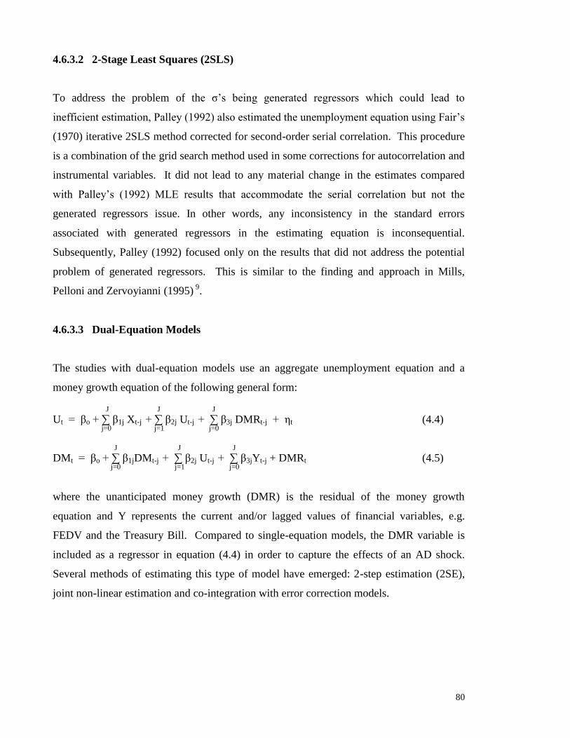
80
4.6.3.2 2-Stage Least Squares (2SLS)
To address the problem of the ζ‟s being generated regressors which could lead to
inefficient estimation, Palley (1992) also estimated the unemployment equation using Fair‟s
(1970) iterative 2SLS method corrected for second-order serial correlation. This procedure
is a combination of the grid search method used in some corrections for autocorrelation and
instrumental variables. It did not lead to any material change in the estimates compared
with Palley‟s (1992) MLE results that accommodate the serial correlation but not the
generated regressors issue. In other words, any inconsistency in the standard errors
associated with generated regressors in the estimating equation is inconsequential.
Subsequently, Palley (1992) focused only on the results that did not address the potential
problem of generated regressors. This is similar to the finding and approach in Mills,
Pelloni and Zervoyianni (1995) 9
.
4.6.3.3 Dual-Equation Models
The studies with dual-equation models use an aggregate unemployment equation and a
money growth equation of the following general form:
J J J
Ut = βo + ∑ β1j Xt-j + ∑ β2j Ut-j + ∑ β3j DMRt-j + εt (4.4)
j=0 j=1 j=0
J J J
DMt = βo + ∑ β1jDMt-j + ∑ β2j Ut-j + ∑ β3jYt-j + DMRt (4.5)
j=0 j=1 j=0
where the unanticipated money growth (DMR) is the residual of the money growth
equation and Y represents the current and/or lagged values of financial variables, e.g.
FEDV and the Treasury Bill. Compared to single-equation models, the DMR variable is
included as a regressor in equation (4.4) in order to capture the effects of an AD shock.
Several methods of estimating this type of model have emerged: 2-step estimation (2SE),
joint non-linear estimation and co-integration with error correction models.

81
2-Step Estimation
The majority of the studies that incorporate an unanticipated money growth variable adopt
Barro‟s (1977) 2-step method of estimation. These include Lilien (1982), Garonna and
Sica (2000), Abraham and Katz (1986), Neelin (1987), Loungani (1986) and Samson
(1985). The 2-step procedure involves the regression of:
i) DM on its lagged values and other variables to obtain DMR, the residual
(Equation 4.5);
ii) Ut on DMR (including other regressors) to estimate the impact of ζ on
unemployment (Equation 4.4).
Three areas of concern pertaining to the 2-step estimation can be noted. First, the 2SE
models share with single-equation models the potential problem of ζ being correlated with
other explanatory variables, as discussed earlier. Second, since DMR forms the unexpected
portion of money growth, it should be uncorrelated with any systematic components of
money growth. However, if the money growth equation is mis-specified (e.g. omission of
variables), DMR could be predictable and if so, capturing the element of a shock is lost in
the test of the hypotheses. Third, DMR, is a generated regressor from the money growth
model, and if measurement errors are neglected, the OLS estimates and standard errors will
be consistent but inefficient.
Lilien (1982) addressed the first problem by testing the orthogonality of DMR vis-à-vis ζ
by regressing ζ on its own lagged values and the current and lagged values of DMR. The
low R2 from the regression showed ζ to be exogenous, i.e. ζ captured the influence of real
variables only. Samson (1985) conducted tests for the correlation of DMR by regressing it
on all the right hand side variables of the DM equation plus its own lagged value. The low
t-statistic for the coefficient of DMRt-1 demonstrated DMR to be unpredictable. The
problem of generated regressors was addressed through joint non-linear estimation, which
has only been followed by Davis (1987) and Parker (1992)10
. The joint non-linear
estimation did not appear to lead to improvements in the quality of estimates, possibly
because cross-equation restrictions need to be adequately identified in accordance with a
clear knowledge of theoretical economic relationships11
. In line with more recent studies,
it will not be pursued in this thesis.

82
Cointegration and Error Correction Models (ECM)
An alternative method is co-integration with error correction models (ECM). The
advantage of this approach is that it incorporates the long run behavioural relationship of
money growth in the short-run co-integrating regression without any loss of efficiency or
consistency. Mills, Pelloni and Zervoyianni (1995) adopted this method to estimate their
model of money growth and unemployment. The money growth (ΔDM) equation was
expressed as an error correction model, i.e.
ΔDMt = βo Δ DMt-1 + β1 Δ DMt-4 + β2 Δ it-1 + β3 gt-1 + β4 Δ Rt-1 + β5 Δ Ut-1 +
β6 Δ Ut-2 + β7 ECMt + seasonal dummies + DMRt (4.6)
where ECMt is the error-correction term, i is the inflation rate, R is the interest rate and g is
the government deficit. The ECM term, expressed as a function of money growth, income
(y), prices (p), time trend (T), interest rates (R) and the unemployment rate (U), was
estimated as:
ECMt = DMt - β1yt - β2 pt + β3 T + β4 Rt + β5 Ut, (4.7)
and incorporated into the money growth equation (4.6). Equation (4.6) is an ECM since
the long run relationship of money growth is distinguished from the short responses of
other variables, ΔUt-j, ΔRt-1, Δit-j and ΔDMt-j. The co-integrating regression was estimated
using Stock and Watson‟s (1993) Dynamic Ordinary Least Squares (DOLS) method. In the
case of a single co-integrating vector with an I(1) system, the DOLS method essentially
involves regressing one variable on other contemporaneous regressors and their
corresponding leads and lags, as well as a constant, using OLS. Since the variables are co-
integrated in the regression and are integrated of the same order, the DOLS estimates are
argued to be asymptotically efficient. The authors have suggested that the methodology
adopted to estimate unanticipated money growth is a “clear improvement on the previous
approaches used to predict money growth in the sectoral shifts literature”.
The impact of ζ on unemployment was assessed using a co-integration equation. In this,
two conditions had to be met to ensure consistent and efficient estimates: (a) all variables

83
had to be stationary; and (b) the regression equation had to contain variables which were
integrated of order zero. Since the ratio of exports to GNP (x) and the logarithm of the
short-run interest rates (r) were I(1) and DME and DMR were both I(0), the first two
variables had to be differenced such that their series became stationary in the co-integrating
regression. The baseline unemployment equation (excluding ζ) was written as:
J J
ΔUt = ∑ β1jΔUt-j + ∑ ( β2j DMEt-j + β3jDMRt-j + β4j Δrt-j + β5j Δ xt-j ) + εt (4.8) j=1 j=0
The hypotheses were tested by including the first difference of the variants of ζ as
regressors. It is noted that in the final model (Table 4.4), the indices were differenced
several times for their series to be stationary.
Cointegration is not recommended for the current study. Mills, Pelloni and Zervoyianni
(1995) had a quarterly data series of about 124 observations, which far exceeds the 31
observations for the current work covering 1971-2001. The relatively short time span,
coupled with the low yearly data frequency, means that cointegration is not really a suitable
technique to apply, especially when studies have shown that increasing data frequency
yields considerable gains in power. Higher frequency data also perform better in tracking
historical relationships between variables [Ramirez and Khan (1999) and Zhou (2001)].
In terms of model estimation, 2SE is the recommended procedure for the current work.
Single-equation models are not relevant given the need to incorporate DMR. 2SLS could
be used to address the problem of generated regressors which may show up under 2SE, but
the choice of instruments is limited, and the findings by Palley (1992) indicate that the
issue is not paramount. Cointegration is not suited for the current study with the small
number (31) of observations. In applying a 2SE procedure, the empirical work of chapter 5
follows numerous reputable studies [Lilien (1982), Garonna and Sica (2000), Abraham and
Katz (1986), Neelin (1987), Loungani (1986) and Samson (1985)]. To assess whether
multicollinearity constitutes a problem, tests based on the DMR vis-à-vis ζ correlation will
be carried out. As economic time-series could be non-stationary, tests of stationarity will
be undertaken.

84
4.6.4 Model Specification
This section reviews the explanatory variables typically employed in the literature in terms
of practical relevance to the Korean economy and feasibility in modelling. Whilst the
model should capture explanatory variables linked to the contrasting predictions of the
hypotheses, there is a need to limit the number of model terms to minimise the chances of
multicollinearity.
4.6.4.1 Dependent Variable
The dependent variable in the majority of studies is the actual unemployment rate for the
current period. The exceptions are Mills, Pelloni and Zervoyianni (1995) and Palley
(1992), each of which treated the first difference and the logarithm of the unemployment
rate as the dependent variable12
. A reason for the former with quarterly data was to ensure
the series was stationary, established via first differencing (or logarithmic transformation)
[Coulson and Robins (1987)]. The logarithmic series was imposed as the series was
positive and the logarithmic transformation ensures that the predictions from the model are
also positive. For this thesis, the dependent variable will be the actual or change in the
unemployment rate, subject to tests of stationarity.
4.6.4.2 Explanatory Variables
In general terms, the explanatory variables employed in previous studies encompass the
mobility indices, lagged dependent variable, aggregate demand/supply, a time trend,
monetary factors and inter-country factors. More specifically, the variables comprise
aggregate demand policy indicators (DMR, DME, GNP, ratio of exports to GNP, short run
interest rate, government expenditure and the M2 multiplier), aggregate supply indicators
(post-1974 oil shock dummy variable), labour force characteristics (military personnel per
1000 population and working women/total labour force), monetary factors (ratio of federal
minimum wage to economy-wide average hourly earnings and ratio of recipients‟ average
weekly unemployment insurance to average weekly earnings of employed workers) and
inter-country influences (U.S. unemployment and U.S. money supply in the unemployment
model for Canada).
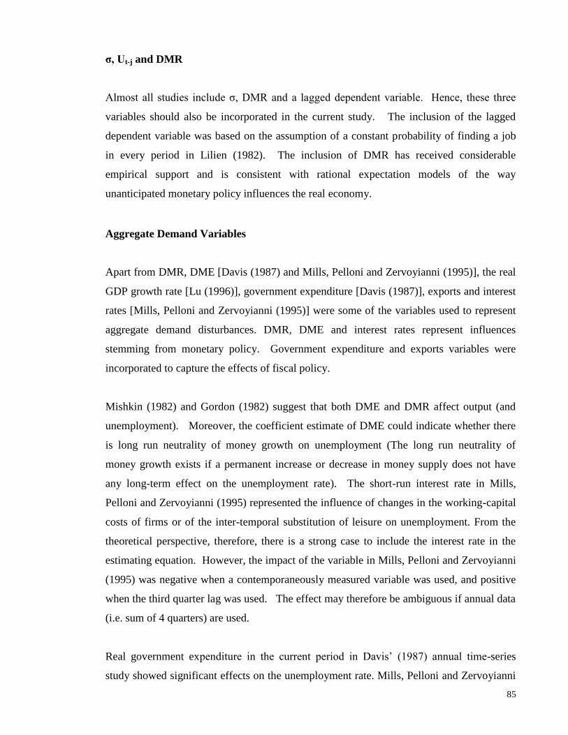
85
σ, Ut-j and DMR
Almost all studies include ζ, DMR and a lagged dependent variable. Hence, these three
variables should also be incorporated in the current study. The inclusion of the lagged
dependent variable was based on the assumption of a constant probability of finding a job
in every period in Lilien (1982). The inclusion of DMR has received considerable
empirical support and is consistent with rational expectation models of the way
unanticipated monetary policy influences the real economy.
Aggregate Demand Variables
Apart from DMR, DME [Davis (1987) and Mills, Pelloni and Zervoyianni (1995)], the real
GDP growth rate [Lu (1996)], government expenditure [Davis (1987)], exports and interest
rates [Mills, Pelloni and Zervoyianni (1995)] were some of the variables used to represent
aggregate demand disturbances. DMR, DME and interest rates represent influences
stemming from monetary policy. Government expenditure and exports variables were
incorporated to capture the effects of fiscal policy.
Mishkin (1982) and Gordon (1982) suggest that both DME and DMR affect output (and
unemployment). Moreover, the coefficient estimate of DME could indicate whether there
is long run neutrality of money growth on unemployment (The long run neutrality of
money growth exists if a permanent increase or decrease in money supply does not have
any long-term effect on the unemployment rate). The short-run interest rate in Mills,
Pelloni and Zervoyianni (1995) represented the influence of changes in the working-capital
costs of firms or of the inter-temporal substitution of leisure on unemployment. From the
theoretical perspective, therefore, there is a strong case to include the interest rate in the
estimating equation. However, the impact of the variable in Mills, Pelloni and Zervoyianni
(1995) was negative when a contemporaneously measured variable was used, and positive
when the third quarter lag was used. The effect may therefore be ambiguous if annual data
(i.e. sum of 4 quarters) are used.
Real government expenditure in the current period in Davis‟ (1987) annual time-series
study showed significant effects on the unemployment rate. Mills, Pelloni and Zervoyianni
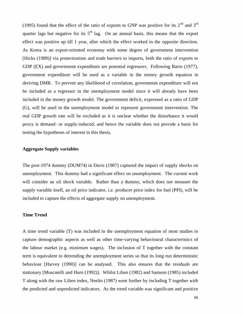
86
(1995) found that the effect of the ratio of exports to GNP was positive for its 2nd
and 3rd
quarter lags but negative for its 5th
lag. On an annual basis, this means that the export
effect was positive up till 1 year, after which the effect worked in the opposite direction.
As Korea is an export-oriented economy with some degree of government intervention
[Hicks (1989)] via protectionism and trade barriers to imports, both the ratio of exports to
GDP (EX) and government expenditure are potential regressors. Following Barro (1977),
government expenditure will be used as a variable in the money growth equation in
deriving DMR. To prevent any likelihood of correlation, government expenditure will not
be included as a regressor in the unemployment model since it will already have been
included in the money growth model. The government deficit, expressed as a ratio of GDP
(G), will be used in the unemployment model to represent government intervention. The
real GDP growth rate will be excluded as it is unclear whether the disturbance it would
proxy is demand- or supply-induced, and hence the variable does not provide a basis for
testing the hypotheses of interest in this thesis.
Aggregate Supply variables
The post-1974 dummy (DUM74) in Davis (1987) captured the impact of supply shocks on
unemployment. This dummy had a significant effect on unemployment. The current work
will consider an oil shock variable. Rather than a dummy, which does not measure the
supply variable itself, an oil price indicator, i.e. producer price index for fuel (PPI), will be
included to capture the effects of aggregate supply on unemployment.
Time Trend
A time trend variable (T) was included in the unemployment equation of most studies to
capture demographic aspects as well as other time-varying behavioural characteristics of
the labour market (e.g. minimum wages). The inclusion of T together with the constant
term is equivalent to detrending the unemployment series so that its long run deterministic
behaviour [Harvey (1990)] can be analysed. This also ensures that the residuals are
stationary [Muscatelli and Hurn (1992)]. Whilst Lilien (1982) and Samson (1985) included
T along with the raw Lilien index, Neelin (1987) went further by including T together with
the predicted and unpredicted indicators. As the trend variable was significant and positive

87
in Lilien (1982) and Neelin (1987) [but not Samson (1985)], it is worth considering this
variable in the current study.
Other Factors
Two studies [Palley (1992) and Samson (1985)] included demographic characteristics of
the labour market: military population in the former and ratio of working women in the
latter. The military population is not relevant to Korea as it was included in Palley (1992)
to proxy the labour supply shortage in the U.S. arising from the 1960s Vietnam war, and no
major wars were fought by Korea during 1971-2001. Samson (1985) used the labour force
participation rate of women in place of the time trend variable, stating that it only captured
demographic changes13
. Given the limited degrees of freedom, and the fact that there are
many possible measures of demographic influences, a parsimonious approach via a time
trend variable is recommended for the current study.
Neelin (1985) included macroeconomic indicators for economies other than that being
studied. Specifically, the U.S. unemployment rate and money supply were considered in an
analysis of the Canadian economy. These variables are not relevant for Korea as they were
specific to Canada which has established ties with the U.S. Palley (1992) included
minimum wages and unemployment insurance14
. As the minimum wage law in Korea was
enacted by the U.N. only from December 1986, and unemployment insurance is not
applicable to all sectors/industries in Korea, these variables will not be used in the current
study covering 1971-2001 for all major sectors. The growth rate in the M2 multiplier in
Davis (1987) was included to control for the effects of the collapse of financial
intermediation during the 1930s [Davis (1987) and Bernanke (1983)]. This variable is
therefore not relevant for the current analysis.
Capital Measures
Brainard and Cutler‟s (1993) measure of a sectoral shock - cross section volatility for 49
industries listed on the stock market - impacted unemployment in the U.S. positively over
1948-1991. Shin‟s (1997a) inter-sectoral shock measure, derived from accounting data on
returns to capital of manufacturing industries, showed a positive impact on unemployment

88
for the U.S. during 1961-1991. Loungani, Rush and Tave (1990) used the stock market
dispersion index of price growth rates among different industries as a proxy for
intersectoral shocks. They showed that the lagged values of this measure had significant
impacts on the unemployment rate. However, the CSV15
, returns to capital measure and
stock market dispersion index cannot be considered as proxies for dispersion in sectoral
employment as they are measures of movements in physical capital rather than human
capital. These studies adopted such indicators to measure the reallocations of sectoral
shocks on the capital market rather than on the labour market. Furthermore, the stock
market measures have been criticized in that the stock prices respond to expected future
shocks rather than current shocks [Shin (1997a)].
In short, the preliminary baseline unemployment equation to test the SSH, ADH, RTH and
stage-of-the-business-cycle effect can be written as follows:
J J J J
Ut = βo + ∑ β1jζt-j + ∑ β2j (DMEt-j + DMRt-j) +∑ β3jDMEt-j +∑ β4jDMRt-j +
j=0 j=0 j=0 j=0
J
∑ β5j Ut-j + β6 EXt-1 + β7Gt-1 + β8 PPI + β9 T + εt (4.9)
j=1
where ζ is a generic index representing the variants of the mobility index, horizon
covariance index and the interaction variable, the term J is the number of lags to be
determined by the statistical significance of the jth
lagged variable16
, and the
inclusion/exclusion of the regressors indicated will be dependent upon tests for
multicollinearity. There may be a need to keep the number of lags to a minimum for an
annual data series like that available for Korea. It may also be necessary to reparameterise
the final unemployment equation to correct for the presence of a unit root via differencing
to ensure the series is stationary.
4.6.5 Number of σ’s in the Regression Equation
The number of regression equations varied among the studies testing the SSH and ADH.
Studies using the raw Lilien index have generally presented a regression equation with a
single sectoral shift variable [Lilien (1982), Samson (1985), Parker (1992), Davis (1987),
Loungani and Rogerson (1989), Neelin (1987), Loungani (1986) and Mills, Pelloni and
89
Zervoyianni (1995)]. A model with either the predicted or unpredicted index was estimated
in Lu (1996), Loungani (1986) and Mills, Pelloni and Zervoyianni (1995). In the latter
study, separate equations were estimated for each unpredicted index purged of different AD
variables. Neelin (1987), Garonna and Sica (2000) and Palley (1992), however, included
both the predicted and unpredicted indices in a single regression equation.
On the RTH, both the raw Lilien index and the horizon covariance index were included in
the unemployment model of Davis (1987). Although the reason for the inclusion of both
indices was not stated, this was probably done to: (i) examine the impact of the current
sectoral mobility in conjunction with its past labour reallocations; or (ii) have a nested
model to see which was preferred. Pertaining to the stage-of-the-business-cycle model, the
specification of Mills, Pelloni and Zervoyianni (1995) involves the inclusion of the raw
Lilien index and the interaction variable. Whilst the coefficient of the raw index captures
the impact on unemployment for periods when GDP does not exceed its trend value, the
coefficient of ζtSt shows the additional impact of the raw index during stages when GDP
exceeds its trend value. The impact of the Lilien index when GDP exceeds its trend value
will be given by the sum of the coefficients of ζt and ζtSt. Where multiple indices are
entered into a single equation, as in the case of ζt and ζH in Davis (1987), and ζt and ζtSt in
Mills, Pelloni and Zervoyianni (1995), their joint and individual significance should be
examined.
4.6.6 Natural Unemployment Rate Approach
There are several ways in which the natural unemployment rate has been computed in the
empirical literature. This section presents these and indicates the approach that will be
taken in the study of the Korean labour market in chapter 5.
Lilien‟s (1982) natural unemployment rate series was computed as:
∞
U*t = ∑ βj2 (β0 + β1ζt-j + β3 Tt-j) (4.10)
j=0
where the natural unemployment rate, U*, was a function of unemployment in the
preceding period, sectoral mobility and a trend term. Whilst estimation of the natural rate

90
seems like a straightforward calculation, there are problems in practice. According to
Samson (1985), the concern is that “if the βj2 is relatively large (greater than 0.5), the
summation cannot be truncated to just a few years because the expression decays too
slowly.” This limitation is of particular concern to the application in chapter 5, since there
are only 31 observations for this research, and so the summation cannot be extended too far
as it would result in a loss of too many observations.
Loungani (1986) presents two models of the natural unemployment rate. The first
comprises the estimated coefficients of the intercept and predicted index. The second
specification contains the intercept and the unpredicted index. These models can be written
as:
J
U*t(s) = βo + ∑ β1j ζt(s)-j
j=0
J
U*t(r) = βo + ∑ β1j ζt(r)-j j=0
There are two limitations of this approach. First, Ut-1, an integral part of many other natural
unemployment rate series, was not used as it was not in the original unemployment model.
Second, the trend variable was excluded even though it was part of the model of
unemployment, and there does not seem to be a reason for this omission. This suggests that
U* was probably just meant to solely capture the amount of unemployment attributable to
mobility.
Parker (1992) set the natural rate to be dependent on the estimated coefficients of an
intercept, the Lilien index, unemployment insurance, minimum wages and military
population ratio. That is, U*t = βo + β1 ζt + β5 UIt + β6 MWt + β7 MILt. The latter three
variables were used as the unemployment model did not have a trend term. Since the
unemployment insurance, minimum wages and military population variable are not relevant
to the unemployment model of the current study (which has a trend term), Parker‟s (1992)
version is not applicable. However, their use by Parker (1992) indicates that the time trend
coefficient should be used when computing U*.

91
Mills, Pelloni and Zervoyianni (1995) computed three versions of the natural rate, with
each of these depicting raw mobility, pure mobility and movements arising from the stages
of the business cycle. They can be depicted as follows:
ΔU*t = β1Δζt + β2Δζt-1 + β3Δζt-2 + β9ΔUt-2 + β10Δ Ut-4 + β11 ΔUt-5 + β12 ΔUt-6
ΔU*t = β1ζt(up) + β2ζt-4(up) + β8ΔUt-2 + β9ΔUt-4 + β10 ΔUt-5 + β11 ΔUt-6
ΔU*t = β1Δζt + β2 Δζt-1 + β3 Δζt-2 + β4 Δ(Stζt + St-1ζt-1) + β10ΔUt-2
+ β11ΔUt-4 + β12 ΔUt-5 + β13 ΔUt-6
The approach taken by Mills et al. (1995) shows that computation of the natural rate need
not be limited to the raw index but rather can be easily extended to the other forms of
mobility indices.
Samson‟s (1985) version (i.e. U*t = βo + β1 ζt + β3 U*t-1 + β4 U.S. Ut + β5 T ) not only
included the intercept, Lilien index and time trend variables, but the U.S. unemployment
rate and lagged value of the Canadian natural unemployment rate as well. For the latter, as
the initial value was not observable, the actual unemployment rate was used instead. The
U* value obtained was then substituted back into the equation to generate subsequent U*
values until all observations of ζt, U.S. Ut and T were used. This method is not feasible for
the current study for two reasons. First, the U.S. unemployment rate is not relevant in the
current study, as noted previously. Second, the method of using actual U for the first
observation will bias the results. Although it is stated in the study that the bias effect
decreases rapidly, this is not the case for Korea since 1970, i.e. the initial observation
period, occurs during the start of the oil crisis when the actual unemployment rate was high,
at 4.5%. A separate estimation of the Korean natural unemployment rate along the lines of
Samson‟s (1985) equation, excluding the U.S. Ut term (i.e. U*t = βo + β1 ζt + β3 U*t-1 +
β4 T ) gave rise to a high estimated natural rate of 2-5% throughout 1970-2001, which is
contrary to the natural rate series of being less than 2% in the empirical literature [Hayafuji,
Ikeda and Yamada (2003)].
What is apparent from most of the studies reviewed above is that U* is intended to capture
sectoral movements (via the ζ‟s) and the trend term (provided it is in the original
specification). Aggregate demand/supply variables are excluded on the premise that the

92
natural U* represents frictional unemployment brought about by inter-sector movements.
Hence, computation of the natural unemployment rate for the current work could be based
on an equation like the following:
U*t = β2 (β0 + β1ζt + β3 T) (4.10‟)
where ζ represents variants of the mobility indices, as in the case of Mills, Pelloni and
Zervoyianni (1995). The number of lags for ζ to determine U*t will be equivalent to those
adopted for the actual unemployment equation.
U* reflects frictional unemployment, and its links to U provide information on the SSH.
A close correlation is expected under this hypothesis as unemployment under the SSH
should be frictional. As such, the correlation coefficient between U*t and Ut has been used
to test the SSH.
In addition, Lilien (1982) and Loungani (1986) analysed the correlation coefficient of the
detrended series of U*t and Ut. The former detrended U*t by replacing the value of the
time trend in equation (4.10) with its average value over the period. It is noted that the
actual aggregate unemployment (Ut) was not detrended. The latter did not specify how U*
was detrended. However, it was reported that whilst U*t(s) accounted for 20% of the
variance of the detrended series, U*t(r) accounted for less than 5%. This approach of
detrending the U*t in Lilien (1982) could be applied to the current work.
It should be emphasized that construction of the natural unemployment rate series will be
undertaken provided the SSH can be shown to be valid in the Korean labour market.
4.6.7 Sectoral Mobility and Gender Unemployment
The review has focused on the impact of sectoral mobility on aggregate unemployment.
Sectoral mobility could have different impacts on the unemployment of men and women as
they differ in their sector-specific skills and experience. Recognising this, Parker (1992)17
analysed the impact of sectoral mobility (and inter-regional mobility, ζrt) on the male

93
unemployment rate (UtM
) and female unemployment rate (UtF) for the U.S. over 1956-1984
using the following estimating equations:
UtM
= βo + β1 ζt + β2 DMRt + β3 DMRt-1 + β4 DMRt-2 +
β5 UIt + β6 MWt + β7 MILt + β8 ζrt + εt (4.11)
UtF = βo + β1 ζt + β2 DMRt + β3 DMRt-1 + β4 DMRt-2 +
β5 UIt + β6 MWt + β7 MILt + β8 ζrt + εt (4.12)
It is noted that none of the explanatory variables are gender specific. It was found that the
raw Lilien index affected both male and female unemployment positively, although the
sectoral mobility appeared to have a stronger effect on males, with the statistically
significant parameter estimates for ζ being 0.0368 and 0.0234 for male and female
unemployment, respectively. Subject to the analysis of aggregate unemployment for
Korea, separate analyses of the impact of sectoral mobility on male and female
unemployment could be undertaken.
4.7 SUMMARY OF EMPIRICAL APPLICATION
The proposed empirical application for Korea can be summarized as follows:
a) The baseline time-series model to test the SSH, ADH, RTH and stage-of-the-
business-cycle effect will be as per equation (4.9). The explanatory variables
will be subject to tests for multicollinearity. All variables will be subject to tests
of stationarity, and differenced if necessary. The number of lags for each
explanatory variable will depend on the statistical significance of the lagged
variables, but lag length will be kept to a minimum for the annual data series
available for Korea.
b) The data to be used are aggregate-level time-series annual data covering 1971-
2001.
c) Compared to the other methods of model estimation, the 2SE procedure is the
recommended approach for the current study.
d) The models adopting the raw Lilien index and predicted and unpredicted indices
will be based on a single regression for each index. When the horizon

94
covariance index and interaction variable are considered, their impacts will be
estimated jointly with that of the raw Lilien index.
e) The natural unemployment rate equation is as specified in equation (4.10‟), with
the number of lags for ζ corresponding to the actual unemployment model. The
correlation coefficient of U* and U will be examined as a further test of the
SSH. Computation of the natural rate series is subject to the SSH being shown
to be valid in the Korean labour market.
f) The impact of sectoral mobility on the male and female unemployment rates
could be assessed separately, based on the model of equation (4.9). The merit of
this extension will, however, depend upon the results from the analysis of the
determinants of aggregate unemployment.
4.8 LINKS WITH RESEARCH ON DETERMINANTS OF MOBILITY
This chapter has provided an assessment of the empirical findings from research on the
impact of sectoral mobility on unemployment. It has used this review material to outline a
framework for a related study of the impact of sectoral mobility in the Korean labour
market. It concludes by linking the research on the impact of sectoral mobility with the
determinants of sectoral mobility, which constitutes the second part of this thesis.
The empirical study of sectoral mobility started with recognition of its impact on
unemployment in the seminal paper by Lilien (1982). This sparked a series of debates on
the SSH, later branching out to the ADH, RTH and stage-of-the-business-cycle effect. The
review of this chapter has drawn attention to the pertinent issues associated with index
construction, model testing and application of the results (e.g. finding U*t).
All studies on the mobility-unemployment relationship use aggregate-level time-series data.
This essentially takes the mobility that leads to unemployment as „given‟, or at best, being
caused by broad indicators of aggregate demand or aggregate supply. But how are these
changes in aggregate-level indicators linked to individual decision making? What
motivates workers to move across sectors of employment? This information needs to be
known if any policy implications drawn from the studies are to be implemented.

95
The next chapter focuses on the assessment of the hypotheses for Korea using the
modelling techniques learnt from the literature. Since aggregate-level data are used, it
serves as a complement to the more detailed and focused work undertaken on the
determinants of mobility using micro-level data in the second part of this thesis.
Endnotes:
1. Mills, Pelloni and Zervoyianni (1995) did not provide a reason for why ζ purged of government debt
influences had a positive effect for a one-period lagged variable and a negative effect for a four-period lagged
variable.
2. Thomas (1996a) suggested Murphy and Topel‟s (1987a) finding of higher unemployment being
accompanied by low levels of inter-industrial mobility was not necessarily inconsistent with the SSH. With
the aid of a theoretical model, he showed that if sectoral shocks led the declining sector to displace workers,
such workers will not switch sectors even if there is a higher probability of a job offer in the expanding (new)
sector if the job offer probability is offset by reservation wage changes that lead workers to accept a job in the
former sector. In this instance, higher unemployment is accompanied by declining sectoral movements.
3. Brainard and Cutler (1993) used the estimation of the Beveridge Curve to conclude if CSV was a
reallocation variable and ζ was an aggregate shock variable. An outward shift of the Beveridge Curve owing
to higher sectoral reallocations (from an increase in CSV) and greater unemployment in some sectors,
accompanied by increased labour demand and job vacancies, would provide evidence of the CSV being a
sectoral reallocation variable. In contrast, aggregate shocks would move the economy along the Beveridge
Curve. As ζ was only significant in explaining short-term unemployment, it was suggested as reflecting
aggregate shocks.
4. The equation is expressed in logarithmic terms as in Brainard and Cutler (1993). Although quarterly data
from 1948-1991 were used, the CSV and ζ coefficients and standard errors were presented in terms of lagged
years for up till 4 years (covering 15 lagged quarters). The coefficients were for the sum of the coefficients
from 4 quarters in that year. The standard errors were for that sum.
5. Palley (1992) reported the coefficients of the mobility indices from a single-equation maximum likelihood
estimation (MLE) and also an Iterative 2-stage least squares estimation (I2SLS). The results from the MLE
and I2SLS were similar.
6. Although Lu (1996) did conduct a regression with DMR and reported the results to be similar.
7. Palley (1992) indicated that the „inclusion (of DMR) would be important if one were interested in
constructing a series for the natural rate and subscribed to the anticipated policy ineffectiveness solution.‟
8. Brainard and Cutler (1993) and Lu (1996) did not specifically mention that the method of estimation was
OLS.
9. Mills, Pelloni and Zervoyianni (1995) looked into the issue of generated regressors and found that it was
not important. They re-estimated the unemployment equation jointly with the money growth equation using
the approach of McKenzie and McAleer (1992), which enables efficient estimates to be obtained. The re-
estimation showed that the standard errors were only slightly larger, and coefficient estimates deviated
slightly from their original estimates, implying that there were no errors made in statistical inference in their
original estimation.
10. Parker (1992) adopted Mishkin‟s (1983) approach of joint estimation.
11. The rational expectations hypothesis implicitly assumes that only unanticipated movements in money
affect real economic variables, e.g. output, unemployment. Since Davis (1987) stated that the cross equation
restrictions are „implied by the forecasting mechanism‟, one of the restrictions could be that only DMR affects
unemployment. Following Barro‟s (1977) study showing that only DMR affects unemployment, it may be
possible to infer the cross-equation restrictions imposed by Davis (1987). From Table 4.4, given Davis‟
(1987) money growth and unemployment equations:
DMt = α0 + α1 DMt-1 + α2DMt-2 + α3BILLt + α4UNt-1 + DMRt (1)
12 9 12
Ut = βo + ∑ β1j ζt-j - ∑β2j DMRt-j + ∑ β3j DMEt-j + β4 DUM74 + β 5 μt-1 + β6 μt-2 + εt (2)
j=0 j=0 j=0
and applying Barro‟s (1977) proposition to equation (1) that DMR is obtained solely from the history of DM
gives:

96
DMt = α0 + α1 DMt-1 + α2DMt-2 + DMRt (3)
The estimated unemployment equation with the estimated DMR from equation (3) should have a poorer fit (as
proven by Barro (1977) for the U.S. for 1946-1973). Substituting into the estimated equation (2), from the ^ ^
condition that DMR ≡ DM - DM, where DM is from the estimated equation (1), the „reduced form‟ unemployment becomes a function of (DMt-1 …..DMt-j), DMEt-j , DUM74, BILLt and UNt-1. The restrictions could be that the parameters associated with DMEt-j, DUM74, BILLt and UNt-1 are zero, such
that Ut = f (DMt-1 …..DMt-j). Davis (1987) did mention that BILLt and UNt-1 did not enter the unemployment
equation except through the money growth equation. Hence, the cross-equation restrictions could be
tantamount to testing the joint hypothesis: H0: α3 = α4 = β3 = β4 = 0.
In the same manner, applying Barro‟s (1977) proposition to Parker‟s (1992) equations below:
DMt = α0 + α1 DMt-1 + α2DMt-2 + α3DMt-3 + α4FEDVt + α5UNt-1 + DMRt
Ut = βo + β1 ζt + β2 DMRt + β3 DMRt-1 + β4 DMRt-2 + β5 UIt + β6 MWt + β7 MILt + εt
gives the reduced form unemployment equation to be a function of (DM t-1 …..DMt-j), FEDVt, UNt-1, UIt, MWt
and MILt. It is possible that the restrictions would be akin to testing the joint hypothesis that the parameters
of FEDVt, UNt-1, UIt, MWt and MILt are zero (i.e. H0: α4 = α5 = β5 = β6 = β7 = 0), such that Ut = f (DMt-1
…..DMt-j).
12. In addition to the actual unemployment series, Palley (1992) applied log and semi-log transformations to
the functional specification. This implies that the logarithmic series of the unemployment rate was also used.
However, only the results of the linear form are reported in the study.
13. Although Samson (1985) argued its inclusion suggests the presence of something studies have not been
able to model.
14. 1986 is close to the year used to distinguish two phases of the Korean economic experience in the current
work (based on tests of structural change conducted in the next chapter). However, since it was revealed that
the estimated relationships were similar across these phases, the implication is that the minimum wage did not
have a major impact on the model of unemployment.
15. The CSV was also criticized by Thomas (1996a). Brainard and Cutler (1993) argued that since the CSV
explained long unemployment spells, it could adequately capture sectoral shocks which had a longer lasting
impact on the macroeconomy. However, Thomas (1996a) argued that given the possibility of sectoral movers
experiencing shorter unemployment spells (since a sectoral shock could raise the probability of a job offer in
the expanding sector), the CSV would prove to be an inadequate measure as it is meant to capture long
unemployment spells.
16. Accordingly, J can vary across variables.
17. The other studies mentioned did not analyse the impact of sectoral mobility on male/female
unemployment. However, Loungani and Rogerson (1989), with the use of micro-data, reported that during
periods of recession, i.e. 1975, higher sectoral movements were observed for U.S. males aged 25 years and
over. The measure for sectoral movements was taken as the sum of the absolute change in sectoral
employment shares.

97
CHAPTER 5
SECTORAL MOBILITY AND UNEMPLOYMENT:
AN EMPIRICAL EXAMINATION FOR KOREA
5.1 INTRODUCTION
Much has been debated about inter-sector labour movements and their impact on
unemployment. A large part of this debate has centered on establishing the empirical
relevance of the hypotheses: the Sectoral Shift Hypothesis (SSH), the Aggregate Demand
Hypothesis (ADH) and the Reallocation Timing Hypothesis (RTH). The literature review
of chapter 4 did not establish firm conclusions on the relative importance of these
hypotheses. Moreover, there was a lack of evidence on the links between unemployment
and worker mobility for South Korea1. Accordingly, the mobility-unemployment debate
needs to be pioneered for this country. This chapter examines the impact of sectoral
mobility on unemployment for the Korean labour market.
Prior to the formal regression analysis, section 5.2 provides an overview of the aggregate
unemployment data and information on sectoral mobility for Korea. The baseline
unemployment model suggested by the literature review is restated, and the mobility
indicators are described, in section 5.3. The methodological framework in section 5.4 gives
special attention to the specification of the unemployment models and mobility indices.
Tests for structural change and serial correlation are used to modify the initial specification
of the models. Section 5.5 presents the results of the final models of unemployment, and
the main conclusions on the validity of the hypotheses for Korea are stated in section 5.6.
For reference purposes, the Appendices provide information on the derivation and plot of
the mobility indices, results from tests of stationarity and multicollinearity,
CUSUM/CUSUMSQ statistics from tests of structural change, and the estimated
unemployment equations.

98
5.2 TRENDS IN AGGREGATE AND SECTORAL UNEMPLOYMENT
The trends in aggregate and sectoral unemployment in Korea are viewed on a decade-by-
decade basis, as fundamental changes appear more obvious when data are examined over
periods of this length. The analysis commences in 1971, since sector unemployment data
are available from that year, and the first decade covers 1971-1980 instead. It will be
demonstrated that unemployment within sectors reflects the overall trend. This is followed
by an examination of changes in sectoral employment vis-à-vis aggregate unemployment. If
a consistent co-movement is detected, e.g. if sector-specific mobility and unemployment
rates move in the same direction, it might be reasonable to expect that sectoral mobility
could lead to an increase in aggregate unemployment.
5.2.1 Aggregate and Sectoral Unemployment
The aggregate unemployment rate fluctuated over 1971-2000, escalating in the first decade,
falling in the second and going up again in the final decade (Table 5.1). Between 1971 and
1980, increased unemployment was experienced in many industries: manufacturing,
construction, commerce, transport, storage and communications, and financial, business
services and real estate. In the second decade, the drop in the overall unemployment rate,
from 5.2% to 2.4%, was mirrored in all sectors/industries. In the third decade, the greater
unemployment experienced in all sectors except mining contributed to the rise in the
overall unemployment rate, from 2.4% to 4.1%. Thus, increases (decreases) in aggregate
unemployment are typically associated with increases (decreases) in unemployment within
each sector/industry.
5.2.2 Sector-specific Employment and Unemployment
As sector employment data are available from the ILO, two informal measures of sector
mobility, namely, changes in the sectoral shares of total employment and average annual
growth in sectoral employment, can be computed2. The data presented in Table 5.1 shows
that the average annual growth in sectoral employment over the decades has no obvious
relationship with changes in sector unemployment rates. Sectoral employment can
sometimes increase whilst the sector unemployment decreases, or vice versa. At other

99
times, employment growth and the unemployment rate in the sector can move in the same
direction. The same observation applies to changes in the share of sectoral employment
and changes in the annual unemployment rate.
Table 5.1 Employment and Unemployment By Sector Employment Share (%) Unemployment Rate (%)
1971 1980 1990 2000 1971 1980 1990 2000
Agriculture 48.4 34.0 17.9 10.6 0.6 0.4 0.2 0.5
Mining 0.9 0.9 0.4 0.1 4.2 3.1 1.3
Manufacturing 13.3 21.6 27.2 20.3 3.9 6.0 1.5 3.1
Utilities 0.2 0.3 0.4 0.3 10.7 6.4 .0 1.5
Construction 3.5 6.2 7.4 7.5 4.7 12.9 2.6 7.3
Commerce 15.6 19.2 21.8 27.2 2.2 3.9 1.6 3.6
Transport, Storage &
Communications 3.7 4.5 5.1 6.0 4.9 5.4 1.4 2.8
Financial, Business Services
& Real Estate 1.3 2.4 5.2 10.0 2.9 4.3 1.5 2.6
Community, Social &
Personal Services 13.0 10.9 14.6 18.0 2.9 2.9 1.1 5.9
Total 100.0 100.0 100.0 100.0 4.5 5.2 2.4 4.1
Average Annual Growth (%)
Employment Unemployment Rate
1971-
1980
1980-
1990
1990-
2000
1971-
1980
1980-
1990
1990-
2000
Agriculture -0.5 -3.6 -3.6 -4.2 -9.7 13.2
Mining 3.4 -4.4 -14.2 -3.1 -8.8
Manufacturing 9.2 5.2 -1.3 5.0 -13.1 7.7
Utilities 6.5 4.8 -0.9 -5.6
Construction 10.3 4.8 1.6 12.0 -14.8 10.8
Commerce 5.8 4.2 3.8 6.8 -8.7 8.6
Transport, Storage &
Communications 5.9 4.1 3.2
1.0 -12.6 7.2
Financial, Business Services
& Real Estate 10.8 11.0 8.4
4.4 -10.3 5.9
Community, Social &
Personal Services 1.4 5.9 3.8
-0.1 -8.9 18.1
Total 3.5 2.8 1.6 1.6 -7.4 5.5
Source: ILO LaborStat database.
Note: Some cells for the mining and utilites sectors are blank as the unemployment data supplied in terms
of thousands was „0‟. As such, the rates/growths cannot be computed.
Hence, this casual inspection of the employment and unemployment data for Korea from
1971 to 2000 does not provide any real indication of either the direction or strength of the
co-movement between worker mobility and unemployment. Whether this is due to the
informality of the approach, or due to the absence of an underlying relationship, cannot be
determined here. With these issues at hand, there is a need for a formal examination of the
links between sectoral mobility and aggregate unemployment.

100
5.3 MODEL FRAMEWORK
5.3.1 Baseline Model
From the literature review of chapter 4, the baseline unemployment equation to test the
SSH, ADH, RTH and stage-of-the-business cycle effect can be restated as:
J J J J
Ut = βo + ∑ β1jζt-j + ∑ β2j(DMEt-j + DMRt-j) +∑ β3jDMEt-j +∑β4jDMRt-j +
j=0 j=0 j=0 j=0
J
∑ β5j Ut-j + β6EXt-1 + β7Gt-1 + β8PPI + β9T + εt (4.9)
j=1
The right-hand-side of equation (4.9) comprises a comprehensive list of feasible
explanatory variables from the empirical review. The key variable depicting sectoral
mobility is ζ, which represents the generic version of variants of the mobility index. The
comprehensive list of indices and representation for the symbols are listed in Table 5.2.
Following the critique of the indices in chapter 3, eleven indices will be utilised in this
chapter to test the hypotheses: SSH indices [i.e. ζt, ζm
t(up), ζgt(up), ζ
a2t(up), ζ
p1t(up), ζ
p2t(up)],
ADH indices [ζa2
t(p), ζm
t(p), ζgt(p)], the horizon covariance index (ζH) and the interaction
variable (ζtSt).
Although the focus is on the mobility indices as an explanation for changes in aggregate
unemployment, the other explanatory variables are important, as their inclusion/exclusion
could lead to misleading statistical inference. A substantial part of this chapter is geared
towards arriving at an appropriate functional specification.
5.3.2 Methodology
The derivation of each ζ adopts the methodology proposed by Lilien (1982), Abraham and
Katz (1986), Parker (1992), Palley (1992), Davis (1987), Mills, Pelloni and Zervoyianni
(1995), Lu (1996), Neelin (1987), Samson (1985) and Loungani (1986) [see chapter 4].
This methodology is applied to Korea using aggregate-level time-series NSO data for 1971-
2001. The formula for index derivation is provided in Appendix 5A. Corresponding with
101
the majority of the studies, annual data are used as some variables are not available on a
quarterly basis.
5.3.3 Descriptive Statistics
The literature review discussed conceptual differences between the various indices which
might account for the variation in the results for the studies conducted to date. To provide
insight into the nature of the indices, each series is plotted for Korea in Appendices 5B and
5C. Each purged index exhibits an oscillating pattern over 1971-2001, reflecting
unpredictability of pure sectoral movements. For each predictive series, since sectoral
labour movements are generated by aggregate demand and/or supply disturbances, a
fluctuating pattern is also observed. A fluctuating pattern is observed for the raw Lilien
index, which incorporates both predicted and unpredicted movements.
The fluctuating pattern in the raw Lilien index has also been reported for other countries,
including the U.S. [see Lilien (1982), Abraham and Katz (1986), Davis (1987), Mills,
Pelloni and Zervoyianni (1995) and Parker (1992)], Canada [Samson (1985)] and Italy
[Garonna and Sica (2000)]. The other studies did not provide the series (numeric or
graphical) for their predicted or unpredicted indices, and hence no comparison with Korea
can be made.
The pair-wise correlations revealed that the unpredicted indices were not highly correlated.
This is not surprising, since these indices have been purged of different demand/supply
factors, and the mobility that each captures should therefore be different.
Similarly, given that the predicted indices are generated by differing demand/supply
variables, the low correlations among them reported in Appendix 5C are to be expected.
This means that each index generally contains independent information.

102
Table 5.2 Symbols of Sectoral Mobility Symbol Description Developed by Used for test
of
ζt Raw mobility index. Lilien (1982) SSH
ζm
t(up) Mobility index purged of anticipated
and unanticipated money growth.
Mills, Pelloni and Zervoyianni (1995) SSH
ζgt(up) Mobility index purged of the share of
government deficit to GDP.
Mills, Pelloni and Zervoyianni (1995) SSH
ζa1
t(up) Mobility index purged of aggregate
employment growth.
Lu (1996) SSH
ζa2
t(up) Mobility index depicting the dispersion
in sectoral employment growth
attributable to sectoral factors.
Palley (1992) SSH
ζp1
t(up) Mobility index purged of changes in the
energy price index (EP).
Mills, Pelloni and Zervoyianni (1995) SSH
ζp2
t(up) Mobility index purged of changes in the
energy price index (EP) and a quadratic
series for changes in EP.
Mills, Pelloni and Zervoyianni (1995) SSH
ζt(r) Mobility index purged of changes in
PPI for fuel and sectoral employment.
Loungani (1986) SSH
ζt(s) Mobility index attributed to changes in
PPI for fuel and sectoral employment.
Loungani (1986) SSH
ζt(up) Mobility index purged of current and
lagged values of unanticipated money
growth, and sectoral and total
employment growth.
Garonna and Sica (2000) SSH
ζa2
t(p) Predicted mobility index whereby the
unanticipated deviations in the inter-
sector labour movements have been
removed from changes in aggregate
employment.
Palley (1992) ADH
ζm
t(p) Mobility index predicted from changes
in the anticipated and unanticipated
money growth.
Derived in this thesis ADH
ζgt(p) Mobility index predicted from changes
in the share of government deficit to
GDP.
Derived in this thesis ADH
ζt(p) Mobility index predicted from (i)
current and lagged values of
unanticipated money growth; and (ii)
sectoral and total employment growth.
Garonna and Sica (2000) ADH
ζH Termed as Horizon Covariance Index.
Mobility index taking into account
sectoral labour reallocations in previous
periods.
Davis (1987) RTH
ζtSt An interaction variable.
ζt is the raw Lilien index; St equals 1
when GDP exceeds trend GDP, and is
defined to equal 0 otherwise.
Mills, Pelloni and Zervoyianni (1995) Stage-of-the-
business-
cycle effect

103
SSH Indices
Table 5.3 presents the descriptive statistics of the indices. Starting with the raw Lilien
index measure, a mean of 0.0274 is recorded, close to the mean of 0.025 in Lilien (1982)
and Abraham and Katz (1986) for the U.S., and 0.02737 in Samson (1985) for Canada.
Table 5.3 Descriptive Statistics of Ut, DMRt and ζ Variable Mean Standard Deviation
Aggregate Unemployment
Ut 3.9257 1.4583
Unanticipated Money Growth
DMRt 0.0010 0.0405
SSH indices
Raw Index
ζt 0.0274 0.0082
Purged of AD Shocks
ζm
t(up) 0.1455 0.0713
ζgt(up) 0.0228 0.0097
ζa2
t(up) 0.3214 0.2700
Purged of AS Shocks
ζp1
t(up) 0.0251 0.0111
ζp2
t(up) 0.0294 0.0109
ADH indices
ζa2
t(p) 0.0266 0.0090
ζm
t(p) 0.1387 0.0739
ζgt(p) 0.0173 0.0033
Horizon Covariance Index
ζH 0.0003 0.0003
Interaction Variable
ζtSt 0.0097 0.0148
The unpredicted indices are sub-components of the raw index. However, there is no
requirement from the construction of the indices for the unpredicted and predicted values to
sum to the raw index: their relative magnitudes will vary according to the impact
(positive/negative) of the specific influence being purged in each instance. All one should
expect is that the means and variances of the additional indices will differ from those of the
raw index.
Among the indices purged of demand influences, ζgt(up) has a lower mean value than the
raw index, presumably reflecting the purging of government factors which have a

104
uniformly positive effect on the underlying employment series. In contrast, the mean value
of ζm
t(up) is larger than the raw index because the values for DMRt and DMEt are negative
for several years. The average value of ζa2
t(up) is larger than that of the raw index, and this
may follow from the greater variability of the within-sector growth than the across-sector
growth in Korea. There is no benchmark for the comparison between this index and the
raw index as the time-series data were not furnished in Palley (1992).
For the indices purged of oil price shocks, namely ζp1
t(up) and ζp2
t(up), only slight deviations
in the mean values from the raw index were found. Considering that the oil shocks occurred
in the 1970s, changes in the oil price (using the producer price index for fuel) are minimal
from 1980 onwards. Hence, the purging of oil price changes should not result in
significantly lower values.
ADH indices
The ADH index that has been investigated most thoroughly is that predicted from changes
in aggregate employment, namely, ζa2
t(p)3. The predicted ζ
a2t(p) had an average value
similar to the raw index, which is not surprising since both account for the deviation of
sectoral employment growth rates from the aggregate rate4.
The current study introduces two further indicators to test the ADH. This is done using
actual aggregate demand indicators, namely, the money supply in the economy and the
ratio of the public deficit to GDP. Sectoral movements predicted from these two indicators
can be denoted by ζm
t(p) and ζgt(p), which form the predicted counterparts of ζ
mt(up) and
ζgt(up), respectively. They can be derived as follows:
N
ζm
t(p) = [ ∑ (eit / Et) ((Δlog(eit ) - Δlog(Et))f)2]
½
i =1
where (Δlog(eit) - Δlog(Et))f) is the fitted value from the industry-specific regressions of
(Δlog(eit ) - Δlog(Et)) on DMRt, DMRt-1, DMEt and DMEt-1.
N
ζgt(p) = [∑ (eit / Et) ((Δlog(eit ) - Δlog(Et))
f)2]
½
i =1
105
where (Δlog(eit ) - Δlog(Et))f is the fitted value from the industry-specific regressions of
(Δlog(eit ) - Δlog(Et)) on Gt and Gt-1. Gt is the ratio of the government deficit to GDP in
period t. Each of the N sector‟s employment in period t is denoted by the sector‟s eit, and
aggregate employment in period t is denoted by Et.
The mean of ζgt(p) is lower than the mean of the raw index, since it only picks up the
predicted components of a mobility shift, and the proxy for fiscal influences used here
appears to have a relatively modest role in this regard. For ζm
t(p), the higher mean reflects
the greater influence of monetary factors on inter-sector movements. Compared to their
unpredicted counterparts, ζm
t(up) and ζgt(up), their mean values are slightly lower, suggesting
that unpredicted events may exert a slightly greater influence on inter-sector movements.
Horizon Covariance Index and Interaction Variable
The horizon covariance index has a substantially smaller average value than the raw index.
This is not surprising as inter-sectoral movements from past periods are deducted from
movements in the present period. The possible unsuitability of the horizon covariance index
for annual data series was noted earlier. Nonetheless, since it is the only index available to
examine the RTH, it should not be ruled out at this stage. Given its considerably smaller
value, the index will be scaled by a factor of 100 in the estimations below.
The lower average value of the interaction variable compared to the raw index merely
illustrates the higher number of periods which saw GDP being above its trend value. In
particular, GDP exceeded its trend value for 20 out of the 31 yearly observations.
5.3.4 Stationarity
The unemployment model encompasses a time-series framework and it is imperative that
the variables are stationary to reduce the likelihood of serial correlation which could lead to
inconsistent and inefficient estimates, and spurious regressions which give high R-squared
values leading to misleading statistical inference. Dickey-Fuller/Augmented Dickey-Fuller
tests for each variable were conducted and the results showing their order of integration are

106
in Appendix 5D. All explanatory variables were stationary, save for DME and PPI, which
became stationary after first-differencing.
5.4 DUAL-EQUATION MODELLING
Following the common practice in this field of research, this thesis adopts a 2-step
estimation procedure to estimate the impact of ζt on Ut. The first step involves estimation
of a money growth equation to obtain DMR, which is then included as a regressor in the
unemployment equation. At the second step, the hypotheses are tested, through analysis of
the links between ζ and Ut, with other variables, including DMRt, held constant.
5.4.1 Estimation of Money Growth Equation
5.4.1.1 Review of Empirical Studies Estimating DMRt
The money growth model used in this thesis is based on the adaptive expectations
framework, outlined in Barro (1977), and this approach has been followed in the relevant
comparison literature, e.g. Lilien (1982), Abraham and Katz (1986), Loungani (1986),
Garonna and Sica (2000), Neelin (1987) and Samson (1985). Whilst the first three studies
make use of the DMRt term revised in Barro (1981), the latter three embark on their own
estimations for Italy and Canada. Mills, Pelloni and Zervoyianni (1995) estimated the
DMRt term using co-integration methods.
This section presents an overview of the studies estimating DMRt. In the Barro estimation,
the specification of money growth is:
DMt = α0 + β1DMt-1+ β2DMt-2 + β3FEDVt + α2UNt-1 + DMRt ,
where money growth (DMt) is computed as DMt = log Mt – log Mt-1, where Mt is the annual
average of M1, FEDVt is the difference between the real (FED) and normal federal
expenditure, i.e. FEDVt ≡ log (FED)t – [log (FED)]*t, and UN is the ratio of the
unemployment rate to the employment rate, i.e. UNt-1 = log [U/(1-U)]t-15
. Since FEDVt is

107
not directly observable, the adaptive expectations hypothesis postulates that it can be
generated from the formula:
[log (FED)]*t = ρ [log (FED)]t + (1-ρ) [log (FED)]*t-1
with ρ being the adaptive coefficient. Based on the average annual growth rate of federal
expenditure in the U.S. from 1949 till 1973, Barro (1977) estimated that the adaptive ρ
coefficient was 0.2, and used this value to compute the expected federal expenditure, and
substituted FEDVt into the money growth equation above to obtain DMRt. With the use of
quarterly data, the money growth model for 1941-1973, with t-values in parentheses, gave a
good fit, with an R-squared of 0.9.
ˆ DMt = 0.087 + 0.024DMt-1+ 0.35DMt-2 + 0.082FEDVt + 0.027UNt-1
(2.81) (1.60) (2.69) (5.47) (2.70)
R-squared = 0.9, Sample size: 132
Using annual data, Samson‟s (1987) specification for the Canadian money growth equation
for 1954-1983 was as follows:
ˆ DMt = -0.01 - 0.05DMt-1 + 0.25DMt-2 + 0.36DMt-3 + 0.35FEDVt + 0.90DMU.S.t + 0.07Ut-1 (-0.1) (-0.3) (1.3) (1.9) (2.6) (2.6) (1.8)
R-squared = 0.48, sample size: 30,
with DMU.S.t being the U.S. money growth. Whilst the Canadian money variables were
insignificant, except for DMt-3 at the 10 per cent level, the U.S. variable was significant,
which suggests that U.S. money growth affected the Canadian money growth more than the
country‟s own.
Neelin‟s (1987) Canadian money growth model over the period 1954:4 till 1984:3 (i.e.
sample size: 116) also included U.S. variables, namely the current and six lagged values of
log real U.S. GNP, the U.S. 3 month treasury-bill rate, log exports and the U.S.
unemployment rate. The results of the money growth model were not reported but it was
indicated that the U.S. variables were included to avoid simultaneity bias6.

108
Though the results were not reported, Garonna and Sica (2000) indicated that their analysis
of the money growth rate7 with the use of annual data over 1952-1994 (i.e. sample size of
43) for Italy comprised the regression of the actual money growth rate (∆Mt) on its two
lagged values, the difference between actual public and forecasted expenditure (GEXPVt)
and the ratio of the unemployment rate to the employment rate (UEMPt), written as:
∆Mt = α0 + β1∆Mt-1 + β2∆Mt-2 + β3GEXPVt + β4UEMPt + εt
with εt as the error term. Using quarterly data from 1960-1991 with 128 observations,
Mills, Pelloni and Zervoyianni‟s (1995) co-integrating equation for the U.S. was:
∆mt = 0.166∆mt-1 + 0.264∆mt-4 + 0.526it-1 - 0.487gt-1 - 0.0051∆Rt-1 + 0.020∆Ut-1
(0.073) (0.069) (0.163) (0.158) (0.0014) (0.009)
+ 0.032∆Ut-2 - 0.104ECMt-1 + seasonal dummies + DMR1,
(0.008) (0.022)
where ECMt = mt - 0.543yt – 1.000pt + 5.685it + 0.027Rt + 0.108Ut
R-squared = 0.92
where m, y and p are the logarithms of M1, real GNP and the GNP deflator, respectively, U
is the logistic transformation of UN, R is the long-run interest rate, i is the inflation rate, g
is the ratio of the government deficit to nominal GDP, and ECM is the error correction term
for the co-integrating equation. The money growth equation (∆mt) was estimated using
OLS and the standard errors are shown in parentheses.
Mills, Pelloni and Zervoyianni‟s (1995) co-integration method with quarterly data cannot
be applied to Korea. More mileage can be obtained from cointegration with high frequency
data. The current study with annual data has a short data span of only 31 observations.
5.4.1.2 Application to the Korean Case
Consolidating the explanatory variables from the above studies, the money equation for
Korea for a total of J lags is:
J DMt = α0 + ∑ β1j DMt-j + β2GEXPDVt* + β3UNt-1 + β4CPINt-1 + β5GDPNt-1
j =1 + β6GNt-1 + DMRt

109
The number of lags (J) is dependent on the statistical significance of the lagged DM
variable. As in Barro (1977), the money equation is expressed in logarithmic terms where:
GEXPDVt* = ρlog(GEXP)t – (1-ρ)log(GEXP)t-1
CPINt = log CPIt – log CPIt-1
GDPNt = log GDPt – log GDPt-1
GNt = log Gt – log Gt-1
with ρ as the adaptive coefficient. The terms CPINt, GDPNt and Gt measure, respectively,
the inflation rate, economic growth and change in the ratio of government deficit to GDP.
The interest rate is excluded since the data series from the Bank of Korea only started from
the 1980s. The term GEXPDVt* measures the difference between real and expected
government expenditure. With regards to ρ, the average annual growth of real government
expenditure for Korea over 1971-2001 is 0.05, and the GEXPDVt* series is presented in
Appendix 5B8. None of the explanatory variables were highly correlated: the pairwise
correlation coefficients did not exceed 0.8. The econometric approach adopted involves
moving from a general to a specific model until all the variables are significant. In
particular, it was found that UNt-1 and DMt-1 could be omitted.
The estimated version of the money equation for Korea over the 1971-2001 period, with the
t-ratios in parentheses, was:
DMt = 0.016 – 0.4141DMt-2 – 1.080GEXPDVt* - 0.570CPINt-1 + 1.717GDPNt-1 (1.06) (-2.44) (-1.79) (-1.70) (5.73)
- 0.150GNt-1 + DMRt
(-2.98)
R-squared = 0.60
Sample size: 31
LM statistic = 3.84
With the exception of the constant term, all of the variables are significant at the 10% level.
The fit of the model (R2 = 0.6) does not match that of the U.S., where the R
2 is 0.90, and
this could be attributed to the greater importance of the lagged dependent variables when
quarterly data are used in the study for the U.S. The model‟s fit is slightly better than the

110
model for Canada in Samson‟s (1985) work, based on annual data and having a similar
number of observations. The LM statistic ( ʅ2(1) = 3.84) indicates the absence of first-order
serial correlation at the 5% level of significance.
The DMR series has been fluctuating over 1971-2001 (Figure 5.1). DMEt, the predictable
portion of money growth, is the fitted values from the regression, and it is used in the
construction of several indices (see Appendix 5A). Since DMRt will be used as a regressor
in the unemployment models, the correlation matrix for DMRt and the other variants of ζ
was computed. DMRt was lowly correlated with these indices: 0.275 for ζt, -0.099 for
ζa2
t(up), 0.112 for ζm
t(up), 0.213 for ζgt(up), 0.099 for ζ
p1t(up), 0.067 for ζ
p2t(up), 0.173 for ζ
a2t(p),
0.041 for ζm
t(p), -0.051 for ζgt(p), -0.140 for ζH and -0.124 for ζtSt. Multicollinearity should
not therefore be a problem in the unemployment model where only these variables are
considered.
Figure 5.1 DMRt Series
-0.10
-0.08
-0.06
-0.04
-0.02
0.00
0.02
0.04
0.06
0.08
0.10
0.12
1972
1974
1976
1978
1980
1982
1984
1986
1988
1990
1992
1994
1996
1998
2000
DMR
year
111
5.4.2 Specification of Unemployment Equation
5.4.2.1 Unrestricted to Restricted Models
The second step involves estimation of the unemployment model. The approach towards
arriving at the final model is, as with the money growth equation, to move from the general
to the specific. The explanatory variables suggested by the literature comprise
(DMR+DME), DMR, ∆DME, ∆PPI, EX, G and U. As each variable was stationary, the
unrestricted model is rewritten as9:
Ut = βo + β1ζ + β2(DMEt + DMRt)+ β3DMRt + β4DMRt-1 + β5∆DME + β6Ut-1
+ β7EXt-1 + β8Gt-1 + β9∆PPI + β10T + εt (4.9‟)
This is likely to be an over-parameterised model10
.
The criteria adopted in this study towards model specification are low multicollinearity, the
absence of serial correlation and a high adjusted R-squared value. Pre-tests to detect
multicollinearity are carried out as serial correlation and the fit of the model are visible only
in the actual model estimation itself. The main practical test is the „R-squared delete‟
regression, a regression of each explanatory variable on all other variables, with a high R-
squared (or multiple correlation coefficient) being indicative of multicollinearity. The rule
of thumb is to delete variables where the R-squared from the individual tests is greater than
or equal to the R-squared of the original model of equation (4.9‟).
The relationships among all the explanatory variables were examined using a two-step
procedure. First, to determine if a pair of variables is highly correlated in the binary sense
(i.e. simple correlations), the benchmark used is a correlation coefficient of at least 0.5.
Second, the R-squared delete regression and its rule of thumb is then applied to variables
with a high correlation coefficient.
A „high‟ degree of correlation exists between DMRt and (DMRt+DMEt), ∆PPI and Ut-1, Gt-1
and T, and EXt-1 and (DMRt+DMEt) [Appendix 5E]. The R-squared delete regression was
first applied to (DMRt+DMEt), since it was highly correlated with the greatest number of

112
variables, with the specification of the estimating equation varying according to ζ. These
auxiliary regressions gave R-squared values greater than those of the original model. The
high value is due to its „high‟ correlation with DMR, with a coefficient of 0.6. Since DMt =
(DMRt+DMEt), this means that the unanticipated component of money growth is
accounting for a substantial portion of the change in actual money growth, and so the
information content of (DMRt+DMEt) itself will be minimal if DMR is included.
The variables with the next greatest number of „high‟ correlations were T, Gt-1 and EXt-1.
The R-squared delete regressions of T with each ζ resulted in R-squared values equal to or
greater than those of the original model (excluding DMRt+DMEt) for all ζ‟s except ζp1
t(up)
and ζtSt. For the latter two indices, the R-squared was only 0.1 point lower than the
original. Hence, T will be dropped from the model.
The regressions for EXt-1 gave R-squared values that were not uniformly greater or lower
than that of the original model (excluding DMRt+DMEt) for the various indices, and given
this, EXt-1 will not be removed at this stage. Also, the variable Gt-1 will not be omitted, as
its regression gave R-squared values that were lower than or equal to the R-squared values
of the original model (excluding DMRt+DMEt).
The R-squared delete regression for each of the ζ‟s gave R-squared values which were
lower than that of the original model [excluding T and (DMRt+DMEt)], indicating that
multicollinearity was not an issue. The independent regressions of Ut-1, Gt-1, EXt-1, ∆PPI
and ∆DME on all variables except T and (DMRt+DMEt) gave R-squared values that were
lower than the R-squared value of the original model.
These preliminary analyses therefore indicate that to minimize multicollinearity, only T and
(DMRt+DMEt) need to be omitted, resulting in the model outlined below.
Ut = βo + β1ζ + β2DMRt + β3DMRt-1 + β4∆DME + β5Ut-1
+ β6EXt-1 + β7∆PPI + β8 Gt-1 + εt (4.9a)
The deterministic behaviour of the explanatory variables of equation (4.9a) varies with the
index type. A preliminary estimation showed a number of insignificant variables for each

113
index. In moving towards a restricted model, one or two insignificant variables are omitted
at a time until the final model shows most variables to be significant. This is done to
ensure that there is no inadvertent omission of a significant variable (Hendry and Krolzig
(2001)]. In this process, those variables that were formerly significant remained so.
Depending on the model fit and the regression‟s standard error, one insignificant variable
can be tolerated. For instance, if model I with all significant variables has a lower fit and
higher standard error than model II with one insignificant variable, then the decision is to
select model II. In this instance, model II will have a higher adjusted R-squared and the
absolute t-value of that one insignificant variable will be greater than one, albeit not
sufficiently high to cross the 95% level of significance. By doing so, this leads to a
different specification for each index, and their restricted models, now termed as equation
(4.9a), are shown below.
For ζt and ζgt(up): Ut = βo + β1ζ + β2DMRt-1 + β3Ut-1 + β4EXt-1 + εt
For ζa2
t(up), ζm
t(up), ζm
t(p), ζgt(p) and ζ
a2t(p):
Ut = βo + β1ζ + β2DMRt-1 + β3Ut-1 + β4∆PPI + εt
For ζp1
t(up): Ut = βo + β1ζ + β2DMRt-1 + β3Ut-1 + β4∆PPI + β5Gt-1 + εt
For ζp2
t(up) and (ζt, ζH*100): Ut = βo + β1ζ + β2DMRt-1 + β3Ut-1 + β4∆PPI + β5 EXt-1 + εt
For (ζt, ζtSt): Ut = βo + β1ζ + β2Ut-1 + β3∆PPI + β4EXt-1 + εt
Compared to other studies using dual-equation models to test the SSH and ADH [Lilien,
(1982), Abraham and Katz (1986), Neelin (1987), Garonna and Sica (2000), Loungani
(1986) and Samson (1985)], the model of equation (4.9a) is more complex in that aggregate
demand (Gt-1, EXt-1) and aggregate supply (∆PPI) variables are included. Nonetheless, the
specification of the empirical studies noted above needs to be considered here for purposes
of comparison (i.e. a benchmark specification). Accounting for the appropriate number of
lags, the benchmark specification applied to Korea is:
Ut = βo + β1ζ + β1DMRt + β2DMRt-1 + β3Ut-1 + β4T + εt (5.1)

114
Hence, two restricted models, in equations (4.9a) and (5.1), will be estimated in this thesis.
These models are non-nested. Whilst the model of equation (5.1) has been adopted in most
empirical studies, the model of equation (4.9a) is an alternative model distinguished by the
inclusion of additional variables. The inclusion of these variables provides a basis for a
more complete understanding of the determinants of unemployment.
5.4.2.2 Preliminary Model Estimation
Having arrived at the restricted models, a preliminary estimation of the models is
undertaken to assess the robustness of the results, in that the statistical significance of
variables should, where appropriate comparisons can be made, be consistent across the
models, identifying problems (e.g. serial correlation) and possibly to narrow to a more
parsimonious specification. As such, no references to the other empirical studies will be
made in this sub-section. Also, establishing consistency in statistical significance is
essential since equation (4.9a) is more encompassing and the statistical significance in
equation (5.1) could be a case of omitted variables bias.
The SSH indices generated mixed results. Under equations (4.9a) and (5.1), ζt had a
significant, positive impact on aggregate unemployment (Table 5.4). Similarly, ζp1
t(up) and
ζp2
t(up), were associated with significant and positive impacts in both equations. For ζgt(up),
the higher the inter-sector labour movements in Korea, the higher the rate of unemployment
under equations (4.9a) and (5.1). ζm
t(up) and ζa2
t(up), however, were insignificant in each of
the equations examined.
The three ADH indices capturing mobility shifts predicted by aggregate demand
disturbances, ζa2
t(p), ζm
t(p) and ζgt(p). were insignificant for equations (4.9a) and (5.1). The
non-significance of ζa2
t(p) could reflect the shortcomings of index construction, as
highlighted earlier. The lack of significance for the ζm
t(p) and ζgt(p) variables suggests that
inter-sector movements brought about as a consequence of public budgetary considerations
or from monetary policy are not the cause of unemployment. As these policies are not
targeted on specific sectors (as measured here in the case of fiscal policy), these findings
are intuitively reasonable.

115
Table 5.4 Initial Parameter Estimates of ζ Regression with: Equation (4.9a) Equation (5.1)
Coefficient Adjusted R2 Coefficient Adjusted R
2
SSH indices ζt 66.279
(3.57) 0.628 63.753
(2.84) 0.567
ζ
mt(up) 2.929
(1.40) 0.509 3.512
(1.54) 0.477
ζ
gt(up) 59.688
(4.44) 0.685
54.755 (3.77)
0.635
ζa2
t(up) 0.957 (1.95)
0.525 1.112 (1.73)
0.489
ζp1
t(up) 57.142 (4.87)
0.719 56.363 (4.34)
0.674
ζp2
t(up) 52.495 (3.96)
0.663 34.266 (2.34)
0.530
ADH indices ζ
a2t(p) 5.766
(0.33) 0.474 -0.764
(-0.04) 0.428
ζ
mt(p) 2.820
(1.38) 0.508 3.060
(1.44) 0.472
ζgt(p) 11.183
(0.40) 0.475 -1.885
(-0.07) 0.428
Horizon Covariance Index ζt 62.432
(3.29) 0.627 69.067
(2.68) 0.553
and ζH*100 -3.841
(-0.73)
2.664
(0.44)
Interaction Variable
ζt 43.708
(2.61)
0.693 54.443
(2.10)
0.559
and ζtSt 31.450
(3.33)
8.560
(0.74)
Note: t-values in parentheses.
The raw Lilien and horizon covariance indices were incorporated into equations (4.9a) and
(5.1). Under each equation, the horizon covariance index was insignificant, corresponding
to the outcome in Davis (1987) for the U.S. using the annual data series for ζHt-1. This could
mean that the horizon covariance index should simply not be applied to annual data.
Likewise, the raw Lilien index was included together with the interaction variable ζtSt in
the current study. The results were inconsistent across the two restricted models. Whilst
the interaction variable showed a positive and significant coefficient under equation (4.9a),
it was insignificant under equation (5.1).
The preliminary estimation of the restricted models for the SSH, ADH and RTH indices
and the interaction variable therefore reveals mixed results. Whilst the estimated impacts
of some indices are consistent under alternative model specifications, the results also show
a lack of robustness of the estimates for other indices. Hence, there arises a need for further

116
consideration of the model. One issue that is an obvious candidate for examination is
structural change. This is examined below.
5.4.3 Structural Change
Considering that the data period extends over 30 years (1971-2001), and the world
economy experienced several shocks during this time (due to rises in oil prices in the
1970s, 1998 Financial Crisis), it is possible that a structural change occurred in the ζ-U
relationship for Korea. If this is the case, the results from Table 5.4 become invalid.
Statistical tests of structural change are applied in this section. Apart from Davis (1987),
who used a dummy variable (DUM74) to incorporate the impact of the oil shock, the other
empirical studies on the ζ-U relation do not consider the possibility of a structural change
in their models.
5.4.3.1 Prior Knowledge on Korean Unemployment
The detection of a structural break requires prior knowledge of a country‟s economic
experiences. Since the model attempts to explain unemployment, the categorization should
be based on the unemployment rate. From Table 2.1 and information on the Korean
economy in chapter 2, 3 distinct stages can be distinguished: Stage 1: 1970-1986
(unemployment of 3-5%); Stage 2: 1987-1997 (2-3%); and Stage 3: 1998-2001 (3-7%).
Since each stage is characterized by such different unemployment rates, there is a
possibility of a structural break between the phases. Armed with this, tests of model
stability, e.g. cumulated sum of residuals (CUSUM) and the squares of the residuals
(CUSUMSQ) tests are conducted.
5.4.3.2 Tests for Model Stability
CUSUM and CUSUMSQ Tests
The CUSUM and CUSUMSQ tests offer a general insight into whether models are stable
(i.e. coefficients remain constant) over time. Whilst a cost of this generality is limited
power, the tests nevertheless are often used to assess if models are stable, and where

117
instability is detected, the approximate dates where the structural change occurred. More
powerful techniques, such as a Chow test, or re-specification through the use of dummy
variables, can then be considered.
Appendix 5F shows the CUSUM and CUSUMSQ statistics for each index in graphical
form. Table 5.5 presents the CUSUM and CUSUMSQ statistics for equations (5.1) and
(4.9a) for the mobility indices. Looking at equation (5.1), the CUSUM stays within the
upper and lower boundaries for all the ζ‟s throughout the 31-year period. The CUSUMSQ,
however, is outside the confidence bounds for all the ζ‟s, suggesting parameter instability.
In the case of the SSH indices, the CUSUMSQ drifted outside the boundaries for the
1990/92-1997 period for ζt, ζm
t(up), ζa2
t(up) and ζp2
t(up). For ζp1
t(up), the CUSUMSQ is outside
the confidence bounds for 1981-1984. For ζg
t(up), the CUSUMSQ moves out of the
boundaries during 1980-1984 and 1996-1997. The ADH indices have a less common
configuration in terms of the time-frame in which the CUSUMSQ has drifted outside of the
confidence intervals, i.e. 1982-1997 for ζa2
t(p), 1970-1985 and 1996-1997 for ζm
t(p) and
1981-1984 and 1995-1997 for ζgt(p). For the horizon covariance index and interaction
variable, the CUSUMSQ shows that parameters are unstable during 1981-1993 and 1991-
1997, respectively. The general outcome is post-1997, where the CUSUMSQ statistic
returned to the confidence bounds for all indices11
.
With regards to the model of equation (4.9a), the CUSUM remains within the upper and
lower confidence intervals for all the ζ‟s for 1971-2001. Unlike the CUSUM statistic, the
CUSUMSQ statistic deviates outside the boundaries for all the ζ‟s, suggesting parameter
instability. Among the SSH indices, the CUSUMSQ is outside the confidence intervals
during 1988-1997 for ζm
t(up), 1983-1997 for ζa2
t(up), 1995-1997 for ζp1
t(up) and 1990-1997
for ζp2
t(up). For ζt and ζgt(up), only two phases are identified, where the CUSUMSQ is
outside the boundaries for the period 1970-1996. Like the SSH indices, the ADH indices
portray varied time intervals in which the CUSUMSQ has drifted outside of the confidence
bounds, i.e. 1985-1997 for ζa2
t(p), 1992-1997 for ζgt(p) and 1990-1997 for ζ
mt(p). The
horizon covariance index showed parameter instability during 1979-1981 and 1991-1997,
whilst the interaction variable exhibited unstable parameters during 1986-1997. The
common outcome is the post-1997 period, where the CUSUMSQ statistic returned back to
the confidence boundaries for nearly all indices.
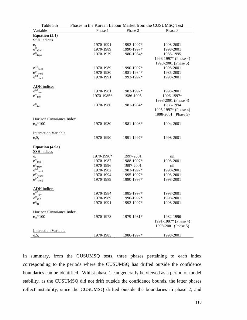
118
Table 5.5 Phases in the Korean Labour Market from the CUSUMSQ Test Variable Phase 1 Phase 2 Phase 3
Equation (5.1)
SSH indices
ζt 1970-1991 1992-1997* 1998-2001
ζm
t(up) 1970-1989 1990-1997* 1998-2001
ζgt(up) 1970-1979 1980-1984* 1985-1995
1996-1997* (Phase 4)
1998-2001 (Phase 5)
ζa2
t(up) 1970-1989 1990-1997* 1998-2001
ζp1
t(up) 1970-1980 1981-1984* 1985-2001
ζp2
t(up) 1970-1991 1992-1997* 1998-2001
ADH indices
ζa2
t(p) 1970-1981 1982-1997* 1998-2001
ζm
t(p) 1970-1985* 1986-1995 1996-1997*
1998-2001 (Phase 4)
ζgt(p) 1970-1980 1981-1984* 1985-1994
1995-1997* (Phase 4)
1998-2001 (Phase 5)
Horizon Covariance Index
ζH*100 1970-1980 1981-1993* 1994-2001
Interaction Variable
ζtSt 1970-1990 1991-1997* 1998-2001
Equation (4.9a)
SSH indices
ζt 1970-1996* 1997-2001 nil
ζm
t(up) 1970-1987 1988-1997* 1998-2001
ζgt(up) 1970-1996 1997-2001 nil
ζa2
t(up) 1970-1982 1983-1997* 1998-2001
ζp1
t(up) 1970-1994 1995-1997* 1998-2001
ζp2
t(up) 1970-1989 1990-1997* 1998-2001
ADH indices
ζa2
t(p) 1970-1984 1985-1997* 1998-2001
ζm
t(p) 1970-1989 1990-1997* 1998-2001
ζgt(p) 1970-1991 1992-1997* 1998-2001
Horizon Covariance Index
ζH*100 1970-1978 1979-1981* 1982-1990
1991-1997* (Phase 4)
1998-2001 (Phase 5)
Interaction Variable
ζtSt 1970-1985 1986-1997* 1998-2001
In summary, from the CUSUMSQ tests, three phases pertaining to each index
corresponding to the periods where the CUSUMSQ has drifted outside the confidence
boundaries can be identified. Whilst phase 1 can generally be viewed as a period of model
stability, as the CUSUMSQ did not drift outside the confidence bounds, the latter phases
reflect instability, since the CUSUMSQ drifted outside the boundaries in phase 2, and

119
returned back to the boundaries in phase 3. Hence, potential structural breaks could occur
between phase 1 and 2, and between phase 2 and 3.
It is worth noting that the phases identified from the CUSUMSQ procedure are closely
associated with the „stages‟ outlined in section 5.4.3.1. Phase 1 covers 1970 till the
mid/late 1980s, close to stage 1 (1970-1986) with an unemployment rate of 3-5%. Phase 2
covers the mid/late 1980s to 1997, corresponding with stage 2 (1987-1997), where the
unemployment rate was 2-3%. Finally, both phase 3 and stage 3 represent the 1998-2001
post-Crisis period.
Harvey-Collier Statistic
The Harvey-Collier (HC) statistic is another test of model stability. For a total of N
observations and k parameters, the statistic is computed as:
r = N
s2
= [1 / (N- k -1)] ∑ (wr - w)2
r = k+1
_________________
where wr = (Ut – xt‟βt-1) / √ [1 + x‟t(X‟t-1Xt-1)-1
xt]
_ r = N
w = [1 / (N- k)] ∑ wr
r = k +1
with Ut being the actual unemployment rate, xt being the (k x 1) vector of regressors
associated with observations of Ut, βt-1 is the estimated regression coefficients computed
using the first (t-1) observations and Xt-1 is the matrix of full rank consisting of regressors
for the first (t-1) observations. The numerator term (Ut – xt‟βt-1) is the tth
recursive residual
and represents the expost forecast error using the former (t-1) observations. The HC
statistic is assessed against the t-distribution with N-k-1 degrees of freedom. If it exceeds
its critical value at a prescribed level of significance (i.e. 5% in this study), the null
hypothesis of model stability is rejected.
The HC is used in conjunction with the CUSUM/CUSUMSQ to check model stability. It is
not used in conjunction with the Chow test since the latter requires prior knowledge of the

120
time point at which the structural change occurs. From Table 5.6, two observations about
the HC statistic can be made. Under equation (4.9a), there is no clear-cut outcome of
parameter stability, since the statistic for some indices suggested stability, whilst that for
others did not. Some consistency is established under the model of equation (5.1), in that
model instability is suggested by the statistic for nearly all the indices.
5.4.3.3 Phase I and Phase II
Whilst the CUSUM results point towards stability, the CUSUMSQ results do not.
Likewise, mixed findings emerge from application of the HC test. This conflict can be
mediated by means of the Chow-test. The Chow-test will be applied to confirm if there
was a structural change between phase 1 and phase 2. The relevant F-statistic uses the error
sum of squares from the regressions of phase 1 (ESS1), phase 2 (ESS2) and for the two
phases (ESS), and can be computed as:
F = (ESS – ESS1 – ESS2) / k
(ESS1 + ESS2) / (n – 2k)
for k regression coefficients and n number of observations from phases 1 and 2. Table 5.6
shows the corresponding F-statistic for each index for each regression equation. The F-
statistic could not be computed for a few of the indices (indicated as „n.a.‟ in Table 5.6)
since the number of observations (n) did not exceed the number of parameters (k) for that
particular phase. Among those that could be computed, as the observed F-statistic did not
exceed the critical F (k, n-2k) at the 5% level for nearly all the indices for equations (5.1)
and (4.9a), it is reasonable to side with the CUSUM results of an absence of a structural
break between phase 1 and phase 2. From phase 1 till phase 2, the unemployment rate has
been 2-5%, with no sudden hikes or dips in this rate over 1970-1997.
5.4.3.4 Phase II and Phase III
Whilst the k parameters can generally be estimated from a phase 2 regression (as n2 > k),
the k parameters cannot be estimated for phase 3, as the k number of parameters exceeds
the number of observations (n3 < k). Consequently, the error sum of squares from the

121
regression of phase 3 (ESS3) will be zero, and the conventional Chow-test cannot therefore
be applied to phase 2 and phase 3. The test of the null hypothesis that the extra n3
observations have a similar structure as that of the first n2 observations is based on the
following F-statistic:
F = (ESS2+3 – ESS2) / n3
ESS2 / (n2 – k)
where ESS2+3 is the error sum of squares from the regression of phase 2 plus phase 3 and n2
and n3 are the number of observations for phases 2 and 3, respectively. If the computed F
statistic exceeds the critical F(n3, n2-k) value, the decision would be to reject the null
hypothesis of a common structural relationship [see Johnston (1984)].
With regards to equation (5.1), the F-statistic to test for a structural break between phases 2
and 3 could not be computed for several indices, as n2 < k or only two phases were
identified via the CUSUM and CUSUMSQ tests. These indices are again indicated as „n.a.‟
in Table 5.6. For the indices that could be computed, the null hypothesis is rejected for
ζa2
t(p) and the horizon covariance index. Given that a structural break was identified for
these two indices, and the corresponding CUSUMSQ and HC statistic suggest parameter
instability for nearly all indices, it is reasonable to suspect that a structural break occurred
between phase 2 and phase 3. From the CUSUMSQ tests, it is reasonable to conclude that
the structural break occurred around 1997/1998.
With regards to equation (4.9a), there is evidence of a structural break between phases 2
and 3 for ζa2
t(up) and ζa2
t(p), as their corresponding F statistic exceeded the critical value.
However, for these two indices, the HC statistics did not provide support for the structural
change hypothesis. Instead, the HC test pointed towards parameter instability for several
other indices (ζp2
t(up), ζm
t(p), ζgt(p), ζH and ζtSt). Nevertheless, given that the CUSUMSQ
result, F-statistic and HC test identified a break in the deterministic relationship for a range
of indices, it is reasonable to accept that a structural change happened between phases 2 and
3.

122
Table 5.6 F- and Harvey-Collier Statistics from Tests of Structural Change Equation (4.9a) Equation (5.1)
Phase I &
II
F
statistics
Phase II
& III
F
statistics
Harvey-
Collier
statistics
Phase I &
II
F
statistics
Phase II
& III
F
statistics
Harvey-
Collier
Statistics
ζt n.a. n.a.2 0.31 n.a. n.a. 2.96*
ζm
t(up) 0.90 2.71 0.72 0.30 8.75 2.24*
ζgt(up) n.a. n.a.
2 0.33 n.a. n.a. 2.66*
ζa2
t(up) 2.06 15.81* 1.07 0.42 8.89 2.76*
ζp1
t(up) n.a. n.a. 0.98 n.a. n.a. 2.58*
ζp2
t(up) 1.68 0.98 3.06* n.a. n.a. 2.90*
ζa2
t(p) 2.01 10.56* 1.00 2.39 9.92* 2.90*
ζm
t(p) 0.32 1.29 2.44* 2.08 3.68 3.27*
ζgt(p) 0.17 0.23 10.97* n.a. n.a. 3.14*
ζH*100 n.a. n.a. 0.78* 6.57* 11.89* 13.15*
ζtSt 1.68 3.42 2.45* n.a. n.a. 4.86*
* The observed statistic exceeds its critical value at the 5% level.
n.a. : not available as n ≤ k for that particular phase.
n.a.2 : not available as only 2 phases were identified.
Whilst it is not the case that each and every test from equations (5.1) and (4.9a) has
indicated that a structural change has occurred, several of the tests [CUSUMSQ and HC for
equation (5.1)] point towards model instability, which suggests the likelihood of a
structural change. Taking into account the prior knowledge (from chapter 2) that the Asian
Currency Crisis marked a dramatic turning point and brought Korea to recession after 1997,
with unemployment reaching 7% in 1998 after low rates of 2-3% in the preceding years, it
is plausible to suspect that the structural break took place in 1998. The use of a post-Crisis
structural dummy variable in the following section will assist in confirming if a change did
occur between phase 2 and phase 312
.
One empirical study found that sectoral labour reallocation shocks played an important role
in the decline of Korea‟s unemployment since the 1960s up till the mid-1990s, although the
study did not preclude the possibility of the importance of other multiple structural
parameters (productivity growth, return to market relative to non-market activities,
bargaining power of workers, real interest rates and matching technology) [Chang, Nam
and Ree (2004)]. This finding strengthens the case of a structural change in the mobility-
unemployment relationship in Korea.

123
5.4.3.5 Accommodation of Structural Change
The identification of a structural break around 1998 necessitates an alteration to the
specification of the unemployment models, accommodated through the use of a post-Crisis
dummy variable:
D = 0 for observations during 1971-1997;
= 1 for observations during 1998-2001.
The structural dummy informs on whether a break actually occurs and also provides,
indirectly, information on its source. The other studies have not accommodated the
consequences of a structural change, even though they cover periods of major change (e.g.
Vietnam war13
). Perhaps the unemployment consequences of these were not as pronounced
as that of the Asian Currency Crisis.
Since there is no prior knowledge pertaining to the source of the structural change, i.e.
whether it is brought about by an intercept shift, changing mobility effect or an alteration to
the effects of other explanatory variables, the ideal procedure would be to interact the
dummy variable with all explanatory variables to identify the source.
The limited number of annual data points in the post-Crisis period, namely 4 years, in
Korea poses constraints. Taking equation (5.1) as an example, the number of interaction
dummies with the explanatory variables (i.e. 5 including the intercept term) exceeds the
number of data points in the post-Crisis period. A feasible approach is to include an
intercept dummy and a mobility interaction dummy for each model. This way, the number
of structural dummies per equation (i.e. 2) stays within the boundary of the number of data
points (observations), and the importance of changes in the impact of the key variable of
interest can still be assessed.
Both the intercept dummy and mobility interaction dummy are included in the model
initially. This approach has the advantage in overcoming any result which may appear to
be sensitive to the order in which the dummies have been inserted in the model14
. Under
the modified approach, equation (5.1) can be converted to:

124
Ut = α1 + α2D + β1ζ + β2ζ D + γ1DMRt + δ1DMRt-1 + λ1Ut-1 + Ω1T + εt (5.1‟)
with α2 measuring the shift in intercept during the Crisis and β2 the additional impact of the
mobility index. The statistical significance of the dummies will assist in pinpointing the
source of structural change. Testing the null hypothesis, i.e. Ho: α2 = 0, is tantamount to
testing the homogeneity of intercepts before and after the structural break, and testing Ho:
β2 = 0 represents testing for a change in the deterministic relationships between mobility
and unemployment.
The pair-wise correlation matrix revealed that D, ζtD, ζm
t(up)D, ζgt(up)D, ζ
a2t(up)D, ζ
p1t(up)D,
ζp2
t(up)D, ζa2
t(p)D, ζm
t(p)D, ζgt(p)D, (ζH*100)D and ζtStD were not highly correlated with
DMRt, DMRt-1, Ut-1 and T, with their respective pair-wise correlation coefficients being
below 0.6.
Each dummy/interaction dummy was retained when it was significant at the 5% level. This
led to the equations below for equation (5.1‟).
Ut = α1 + β1ζt + β2ζtD + γ1DMRt + δ1DMRt-1 + λ1Ut-1 + Ω1T + εt
Ut = α1 + α2D + β1ζm
t(up) + β2ζm
t(up)D + γ1DMRt + δ1DMRt-1 + λ1Ut-1 + Ω1T + εt
Ut = α1 + α2D + β1ζgt(up) + β2ζ
gt(up)D + γ1DMRt + δ1DMRt-1 + λ1Ut-1 + Ω1T + εt
Ut = α1 + β1ζa2
t(up) + β2ζa2
t(up)D + γ1DMRt + δ1DMRt-1 + λ1Ut-1 + Ω1T + εt
Ut = α1 + β1ζp1
t(up) + β2 ζp1
t(up)D + γ1DMRt + δ1DMRt-1 + λ1Ut-1 + Ω1T + εt
Ut = α1 + α2D + β1ζp2
t(up) + β2 ζp2
t(up)D + γ1DMRt + δ1DMRt-1 + λ1Ut-1 + Ω1T + εt
Ut = α1 + β1ζa2
t(p) + β2ζa2
t(p)D + γ1DMRt + δ1DMRt-1 + λ1Ut-1 + Ω1T + εt
Ut = α1 + β1ζm
t(p) + β2ζm
t(p)D + γ1DMRt + δ1DMRt-1 + λ1Ut-1 + Ω1T + εt
Ut = α1 + α2D + β1ζgt(p) + β2ζ
gt(p)D + γ1DMRt + δ1DMRt-1 + λ1Ut-1 + Ω1T + εt
Ut = α1 + β1ζt + β2ζH*100 + β3(ζH*100)D + γ1DMRt + δ1DMRt-1 + λ1Ut-1 + Ω1T + εt
Ut = α1 + β1ζt + β2ζtSt + β3ζtStD + γ1DMRt + δ1DMRt-1 + λ1Ut-1 + Ω1T + εt
The „preferred‟ model for each index from equation (4.9a), after consideration of the
hypotheses that α2 = 0 and β2 = 0, is as follows:
Ut = α1 + β1ζt + β2ζtD + δ1DMRt-1 + λ1Ut-1 + η1EXt-1 + εt (4.9a‟)
Ut = α1 + α2D + β1ζm
t(up) + β2ζm
t(up) D + δ1DMRt-1 + λ1Ut-1 + τ1∆PPI + εt
Ut = α1 + α2D + β1ζgt(up) + β2ζ
gt(up)D + δ1DMRt-1 + λ1Ut-1 + η1EXt-1 + εt

125
Ut = α1 + β1ζa2
t(up) + β2ζa2
t(up) D + δ1DMRt-1 + λ1Ut-1 + τ1∆PPI + εt
Ut = α1 + β1ζp1
t(up) + β2 ζp1
t(up)D + δ1DMRt-1 + λ1Ut-1 + τ1∆PPI + ς1Gt-1 + εt
Ut = α1 + α2D + β1ζp2
t(up) + β2 ζp2
t(up)D + δ1DMRt-1 + λ1Ut-1 + τ1∆PPI + η1EXt-1 + εt
Ut = α1 + α2D + β1ζa2
t(p) + β2ζa2
t(p) D + δ1DMRt-1 + λ1Ut-1 + τ1∆PPI + εt
Ut = α1 + α2D + β1ζm
t(p) + β2ζm
t(p)D + δ1DMRt-1 + λ1Ut-1 + τ1∆PPI + εt
Ut = α1 + α2D + β1ζgt(p) + β2 ζ
gt(p)D + δ1DMRt-1 + λ1Ut-1 + τ1∆PPI + εt
Ut = α1 + α2D + β1ζt + β2ζH*100 + β3(ζH*100)D + δ1DMRt-1 + λ1Ut-1 + τ1∆PPI + η1EXt-1 + εt
Ut = α1 + β1ζt + β2ζtSt + β3ζtStD + λ1Ut-1 + τ1∆PPI + η1EXt-1 + εt
The equations for the various indices indicate dissimilar sources of structural change. This
is not surprising given the differences in the concept and construction of the indices. Under
equation (5.1), the homogeneity of intercepts is revealed for most indices whilst the
heterogeneity of intercepts is apparent in equation (4.9a) for the majority of indices An
alteration in the mobility-unemployment relationship is shown for all indices in both
models.
In general, the statistical significance of the dummy variable and the interaction dummies
agree with the CUSUMSQ results, which suggest model instability. It is possible to
conclude that a structural break occurred between phase 2 and phase 3. The source of
structural change varies among the indices, though this is expected since each index is
constructed to capture different sets of influences.
5.4.4 Re-specification of Unemployment Models
In this section, an attempt is made to tighten the augmented models. This is desirable as the
inclusion of the dummies improved the fit of the model by about 40-50% but resulted in a
few insignificant variables. These changes in the statistical significance are not surprising
given the structural change. In the process of tightening the models, the mobility indices (if
insignificant) will not be omitted as their significance, or lack thereof, is central towards
establishing the claims of the hypotheses.
The re-specified equation (5.1*) was estimated using OLS. A fairly common observation is
that DMRt was insignificant and its omission led to the same or better model fit for ζt,
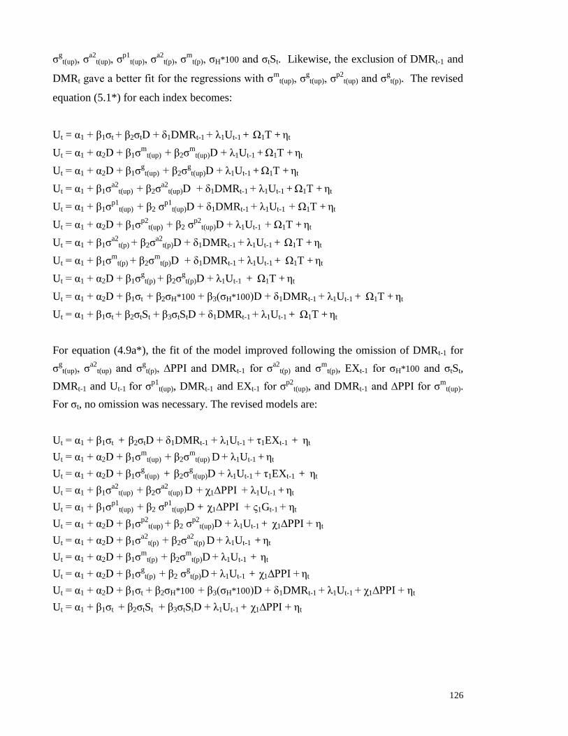
126
ζgt(up), ζ
a2t(up), ζ
p1t(up), ζ
a2t(p), ζ
mt(p), ζH*100 and ζtSt. Likewise, the exclusion of DMRt-1 and
DMRt gave a better fit for the regressions with ζm
t(up), ζgt(up), ζ
p2t(up) and ζ
gt(p). The revised
equation (5.1*) for each index becomes:
Ut = α1 + β1ζt + β2ζtD + δ1DMRt-1 + λ1Ut-1 + Ω1T + εt
Ut = α1 + α2D + β1ζm
t(up) + β2ζm
t(up)D + λ1Ut-1 + Ω1T + εt
Ut = α1 + α2D + β1ζgt(up) + β2ζ
gt(up)D + λ1Ut-1 + Ω1T + εt
Ut = α1 + β1ζa2
t(up) + β2ζa2
t(up)D + δ1DMRt-1 + λ1Ut-1 + Ω1T + εt
Ut = α1 + β1ζp1
t(up) + β2 ζp1
t(up)D + δ1DMRt-1 + λ1Ut-1 + Ω1T + εt
Ut = α1 + α2D + β1ζp2
t(up) + β2 ζp2
t(up)D + λ1Ut-1 + Ω1T + εt
Ut = α1 + β1ζa2
t(p) + β2ζa2
t(p)D + δ1DMRt-1 + λ1Ut-1 + Ω1T + εt
Ut = α1 + β1ζm
t(p) + β2ζm
t(p)D + δ1DMRt-1 + λ1Ut-1 + Ω1T + εt
Ut = α1 + α2D + β1ζgt(p) + β2ζ
gt(p)D + λ1Ut-1 + Ω1T + εt
Ut = α1 + α2D + β1ζt + β2ζH*100 + β3(ζH*100)D + δ1DMRt-1 + λ1Ut-1 + Ω1T + εt
Ut = α1 + β1ζt + β2ζtSt + β3ζtStD + δ1DMRt-1 + λ1Ut-1 + Ω1T + εt
For equation (4.9a*), the fit of the model improved following the omission of DMRt-1 for
ζgt(up), ζ
a2t(up) and ζ
gt(p), ∆PPI and DMRt-1 for ζ
a2t(p) and ζ
mt(p), EXt-1 for ζH*100 and ζtSt,
DMRt-1 and Ut-1 for ζp1
t(up), DMRt-1 and EXt-1 for ζp2
t(up), and DMRt-1 and ∆PPI for ζm
t(up).
For ζt, no omission was necessary. The revised models are:
Ut = α1 + β1ζt + β2ζtD + δ1DMRt-1 + λ1Ut-1 + η1EXt-1 + εt
Ut = α1 + α2D + β1ζm
t(up) + β2ζm
t(up) D + λ1Ut-1 + εt
Ut = α1 + α2D + β1ζgt(up) + β2ζ
gt(up)D + λ1Ut-1 + η1EXt-1 + εt
Ut = α1 + β1ζa2
t(up) + β2ζa2
t(up) D + τ1∆PPI + λ1Ut-1 + εt
Ut = α1 + β1ζp1
t(up) + β2 ζp1
t(up)D + τ1∆PPI + ς1Gt-1 + εt
Ut = α1 + α2D + β1ζp2
t(up) + β2 ζp2
t(up)D + λ1Ut-1 + τ1∆PPI + εt
Ut = α1 + α2D + β1ζa2
t(p) + β2ζa2
t(p) D + λ1Ut-1 + εt
Ut = α1 + α2D + β1ζm
t(p) + β2ζm
t(p)D + λ1Ut-1 + εt
Ut = α1 + α2D + β1ζgt(p) + β2 ζ
gt(p)D + λ1Ut-1 + τ1∆PPI + εt
Ut = α1 + α2D + β1ζt + β2ζH*100 + β3(ζH*100)D + δ1DMRt-1 + λ1Ut-1 + τ1∆PPI + εt
Ut = α1 + β1ζt + β2ζtSt + β3ζtStD + λ1Ut-1 + τ1∆PPI + εt

127
5.5 FINAL MODEL ESTIMATION
5.5.1 Treatment for Serial Correlation
Table 5.7 presents the OLS estimates of the mobility indices from the final specifications.
The LM statistic was used to test for the presence of serially-correlated errors15
. Given the
use of annual data, only first-order serial correlation was considered. First-order serial
correlation was prevalent in equation (5.1*) with ζH and equation (4.9a*) with ζp1
t(up),
ζH*100 and ζtSt. This is of particular concern as the t-values will typically be inflated with
positively correlated error terms. Accordingly, a Cochrane-Orcutt (CO) correction for serial
correlation was applied to the affected equations16
.
Where serial correlation has been detected, the CO estimates are displayed alongside the
OLS estimates. As using CO estimation results in a loss of the first observation, which is
substantial in the current application considering that the dataset is based on only 31 data
points17
, a Prais-Winsten transformation is applied to preserve the first observation,
whereby it is written as:
U1* = U1 (1- ρ2)1/2
; and
X1* = X1 (1- ρ2)1/2
where X denotes the set of explanatory variables in the estimating equation. Compared to
the OLS estimates, there were differences in the size of the parameter estimates and t-
values when the estimates corrected for serial correlation are considered. In particular, the
t-values of several of the OLS estimates were larger in the presence of serial correlation.
Having specified the models to reflect structural change, reduced multicollinearity and
serial correlation, and omitted irrelevant variables, reliable, consistent and efficient CO
estimates can be obtained to examine the validity of the SSH, ADH and RTH hypotheses.
In general, compared to the OLS estimates of Table 5.4, the fit of the model has improved
substantially, with the adjusted R-squared ranging from 0.7 to 0.9. This improvement
arises due to the modelling of structural change.

128
Table 5.7 Final Model: Parameter Estimates of ζ, D and ζD and LM Statistic Regression with: Equation (4.9a*) Equation (5.1*) OLS CO LM statistic OLS CO LM statistic ζt 48.951
(2.923) n.u. 2.13 8.992
(0.470) n.u. 1.62
ζtD 61.209 (3.245)
102.679 (4.942)
ζm
t(up) -2.632 (-1.752)
n.u. 0.93 -2.189 (-1.532)
n.u. 0.15
ζm
t(up) D 33.046 (6.873)
27.576 (5.276)
D -5.957 (-5.574)
ζgt(up) 17.057
(1.226) n.u. 0.48 4.775
(0.388) n.u. 0.33
ζgt(up) D 127.108
(4.639) 120.865
(5.152)
D -2.734 (-3.453)
ζa2
t(up) 0.534 (1.209)
n.u. 1.41 -0.017 (-0.036)
n.u. 0.36
ζa2
t(up) D 3.583 (4.794)
4.453 (5.488)
ζp1
t(up) 41.745 (2.862)
37.936 (3.145)
10.14 9.647 (0.791)
n.u. 1.62
ζp1
t(up) D 40.369 (2.779)
38.484 (3.184)
70.992 (5.488)
ζp2
(up) 4.908 (0.432)
n.u. 0.84 -11.504 (-0.971)
n.u. 0.30
ζp2
(up) D 130.095 (4.954)
131.703 (5.011)
D -3.281 (-3.641)
-2.502 (-2.050)
ζa2
t(p) -9.096 (-0.557)
n.u. 2.19 -34.363 (-2.301)
n.u. 2.10
ζa2
t(p)D 303.477 (3.149)
103.779 (5.272)
D -7.982 (-2.743)
ζm
t(p) -1.698 (-0.933)
n.u. 0.18 -0.317 (-0.181)
n.u. 1.74
ζm
t(p)D 21.052 (4.295)
11.857 (4.461)
D -2.685
(-2.826)
ζgt(p) 19.137
(1.210) n.u. 0.15 -10.173
(-0.645) n.u. 1.59
ζgt(p)D -340.299
(-7.254) -272.188
(-5.095)
D 7.772 (8.010)
7.552 (7.915)
ζt 67.704 (4.115)
48.106 (2.820)
6.30 46.071 (1.920)
19.849 (0.962)
5.97
ζH*100 0.825 (0.165)
0.256 (0.060)
2.746 (0.515)
1.057 (0.244)
ζH*100D 132.806 (3.666)
191.558 (2.229)
165.745 (2.651)
105.074 (1.316)
ζt 20.535 (1.325)
39.579 (2.691)
3.09 11.868 (0.601)
n.u. 1.14
ζtSt 158.621 (3.723)
9.646 (0.954)
-6.115 (-0.712)
ζtStD 158.621 (3.723)
61.011 (3.810)
108.882 (4.793)
Note: t-values in parentheses. n.u.: not undertaken.
129
The regressions with three indices (ζp1
t(up), ζH*100 and ζtSt) had to be corrected for serial
correlation. Comparing the OLS and CO estimates in Table 5.7, the standard errors were
higher for ζp1
t(up) and ζtSt under equation (4.9a*), those for ζH*100 under equations (5.1*)
and (4.9a*) under OLS estimation. A likely reason is that their post-Crisis interaction
dummy variables constitute 4 data points, and perhaps this period is not sufficiently long to
give the higher standard errors under CO estimation. Nonetheless, the standard errors of the
regressions under CO estimation are fairly close to those under OLS estimation. The CO
estimates can be considered to be valid for statistical inference.
It is noted that serial correlation is not prevalent in regression equations with the other
indices, and their OLS estimates are unbiased, consistent and efficient, and valid for
statistical inference. Compared to the OLS estimates of Table 5.4, the fit of the newly
specified models improved, with the adjusted R-squared of at least 0.8. For reference
purposes, the estimating equations of these final unemployment models (as per Table 5.7)
can be found in Appendix 5G.
5.5.2 Sectoral Mobility during the Pre-Crisis Period (1971-1997)
The unemployment equations (5.1*) and (4.9a*) were also estimated for 1971-1997 to
ascertain if the mobility-unemployment relationship found for this truncated data period is
consistent with that established with the larger sample (1971-2001) after accommodating
the structural break. This is a test of the adequacy of the way the structural break has been
modelled. Since the 1998-2001 observations are removed, the interaction variables with D,
and D itself, are excluded. The same equations cannot be estimated for 1998-2001 as the
number of parameters exceeds the number of observations.
The SSH/ADH indices and horizon covariance index, which were insignificant for 1971-
2001, were also insignificant for 1971-1997 in both models, confirming that predicted and
unpredicted mobility as well as past labour reallocations did not cause unemployment
during the pre-Crisis period. Pertaining to the stage-of-the-business-cycle effect, ζtSt
remained insignificant for equations (5.1*) and (4.9a*) for 1971-1997.

130
Thus, where the mobility indices were insignificant variables for 1971-2001, they were also
insignificant for 1971-1997. Likewise, whilst the index [i.e. ζa2
t(p)] was significant for the
full data period under equation (5.1*), it was also significant for the pre-Crisis period. This
implies that modelling of the 1997 structural break using the dummy variable does not
introduce any distortions to the fundamental relationships between mobility and
unemployment over 1971-1997.
Table 5.8 1971-1997: Parameter Estimates of ζ Regression with: Equation
(4.9a*)
Equation
(5.1*)
ζt 16.147
(1.020)
9.619
(0.627)
ζm
t(up) -2.296
(-1.848)
-2.140
(-1.776)
ζgt(up) 6.336
(0.459)
5.038
(0.389)
ζa2
t(up) 0.227
(0.777)
0.047
(0.128)
ζp1
t(up) 14.603
(1.267)
5.289
(0.425)
ζp2
t(up) 6.563
(0.658)
-10.989
(-0.980)
ζa2
t(p) -14.500
(-1.469)
-28.891
(-3.155)
ζm
t(p) -1.563
(-1.312)
-1.172
(-0.879)
ζgt(p) 10.870
(0.728)
-8.213
(-0.550)
ζH*100 0.261
(0.079)
0.854
(0.242)
ζtSt 8.945
(1.325)
-2.148
(-0.293)
1. All figures are OLS except for the CO
estimates (applied with Prais-Winsten
transformation) of ζt, ζm
t(up), ζgt(up), ζ
gt(p) and
ζp2
t(up) under equation (5.1*).
2. t-values in parentheses.
5.6 VALIDITY OF THE HYPOTHESES
The main focus of this analysis is to see if sectoral labour movements generate aggregate
unemployment and this is to be done through examination of the statistical significance of
the mobility indices. With the variety of indices, there arises a need to establish the set of
indices which are robust under the alternative restricted models. Since equations (4.9a*)
and (5.1*) are similar in that: (i) equation (5.1*) has its roots in the basic Lilien approach,

131
while equation (4.9a*) is a more encompassing version of the former equation; and (ii) the
structural change has been modelled into both equations, the result in terms of the
significance of the mobility indices must at least be broadly consistent across these two
models.
5.6.1 Validity of the SSH
Each SSH index has been purged of differing influences and it is important to examine the
validity of the SSH by comparing the findings with studies of similar index type.
Raw Lilien Index
The raw Lilien index was significant under equation (4.9a*) but insignificant under
equation (5.1*). However, its interaction with the dummy variable was significant and
positive for both models. The finding under equation (4.9a*) is consistent with the
numerous studies for North America and Japan reporting a significant positive impact on
unemployment: Lilien (1982), Loungani (1986), Abraham and Katz (1986), Parker (1992),
Loungani and Rogerson (1989), Brainard and Cutler (1993), Davis (1987), Mills, Pelloni
and Zervoyianni (1995) and Lu (1996) for the U.S., Neelin (1987) for Canada and Prasad
(1997) for Japan. It contradicts findings from Europe: France [Saint-Paul (1997)] and Italy
[Garonna and Sica (2000)], which showed mobility to affect unemployment in the opposite
direction. As mentioned in chapter 4, the negative effect has been attributed to labour
market rigidities in France, i.e. temporary contracts and rising public sector employment,
and the high firing costs and differences in cyclical sensitivities in Italy‟s manufacturing
and services sectors.
The sensitivity of the results under the alternative models may, in addition to the potential
omitted variables bias in the two non-nested models, reflect the deficiency of the raw index
in aligning with the concept of the SSH. Several studies have criticized the index and opted
and/or recommended alternative indices to examine the SSH, even though it was reported
to be significant. These include Loungani (1986), Palley (1992), Mills, Pelloni and
Zervoyianni (1995), Lu (1996), Neelin (1985) and Garonna and Sica (2000). It is the intent
of the following sub-sections to do likewise.
132
Pure Sectoral Shifts Purged of AD disturbances
Similar results were produced for ζm
t(up), ζgt(up) and ζ
a2t(up) under equations (5.1*) and
(4.9a*), in that they had an insignificant impact on unemployment. In the unpredicted
sense, a mobility-unemployment relationship did not exist before 1997 in Korea.
Consistency in findings was displayed in the post-1997 findings. All three interaction
variables, i.e. ζm
t(up)D, ζgt(up)D and ζ
a2t(up)D, had positive and significant coefficients under
equations (5.1*) and (4.9a*). The post-Crisis finding agreed with the reports of the
empirical studies in terms of the ζ-U impact, although the data periods differ. Whilst the
findings for the first two were in tandem with Mills, Pelloni and Zervoyianni (1995), that of
ζa2
t(up) replicated the findings of Palley (1992) for the U.S.
The structural change brought about by the Crisis caused a phenomenal change in the way
sectoral mobility affected unemployment. Taking equation (5.1*) with ζgt(up) as an
example, the coefficient estimate during the pre-Crisis period was 4.775 while the post-
Crisis impact, estimated as ∂Ut/∂ζgt(up) = 4.775 + 120.865ζ
gt(up), exceeds that of the pre-
Crisis magnitude. Evaluated at the mean of ζgt(up), it equals 7.500. The onset of the Crisis
led to a much greater influence of mobility movements on unemployment.
The robustness in the result and its concurrence with the empirical literature (in terms of
statistical significance only) seems to point towards the existence of the unpredicted ζ-U
relationship during 1998-2001. For this period, it seems possible to validate the claims of
the SSH for pure mobility purged of demand disturbances.
Pure Sectoral Shifts Purged of Supply Influences
Whilst ζp2
t(up) was insignificant under both equations, ζp1
t(up) was only positive and
significant under equation (4.9a*). Given the lack of robustness in results, not much can be
deduced from the impact of pure shifts purged of supply shocks on unemployment.
Moreover, the insignificant results are in conflict with the outcome for ζp1
t(up) in Mills,
Pelloni and Zervoyianni (1995) for the U.S., but it should be noted that that study covered
the earlier 1961-1991 period, where supply shocks may have been more important.

133
The post-Crisis mobility effect for ζp1
t(up) and ζp2
t(up) showed results similar to those for the
indices purged of AD disturbances, in that both ζp1
t(up)D and ζp2
t(up)D became positive and
significant under both models. In terms of the ζp1
t(up)-U impact, the result is consistent with
Mills, Pelloni and Zervoyianni (1995) for the U.S., although the data periods differ. The
mobility effect was magnified dramatically in the post-Crisis period. The coefficient for
ζp2
t(up) in equation (4.9a*) was 4.908 for the pre-Crisis period but was very much larger
after the Crisis, i.e. ∂Ut/∂ζp2
t(up) = 4.908 + 130.095ζp2
t(up). Evaluated at the mean of ζp2
t(up),
this equals 8.700.
In summary, the post-Crisis findings for Korea suggest that an unpredicted ζ-U relationship
existed. What appears to hold is the following:
a) The impact of unpredicted mobility on unemployment was not felt prior to
1998. This is a common finding across unemployment models with the pure
mobility indices. The finding coincides with results obtained from estimates
based only on 1971-1997 data.
b) Pure sectoral movements purged of demand and supply disturbances seem,
however, to have led to higher aggregate unemployment during the post-Crisis
period. During this period, workers changing sectors will have exacerbated any
unemployment problem. Job replacements may not have been as easy as in the
past as job seekers in this more recent turbulent period will need further time to
acquire skills in the emerging high-skilled jobs, compete with existing workers
with higher productivity, and compete with technology which has made much of
the unskilled labour redundant, i.e. the jobless growth phenomena to be
mentioned in chapter 9.
The claims of the SSH seem valid for the post-Crisis period for Korea, given the robustness
of the results across the various forms of unpredicted indices and the consistency with
related empirical work. However, as highlighted earlier, data limitations in terms of the
low number of observations for the post-Crisis period prevent strong conclusions from
being drawn. The unpredicted ζ-U relationship could be more effectively studied if the
dataset for the post-Crisis period covered a longer time frame.

134
As an added comment, preliminary estimations suggest that much of the unemployment
generated in the post-Crisis period could be non-frictional. As the SSH itself has not been
fully validated, statements about the nature of unemployment generated by pure inter-sector
movements can only be tentative at this stage. For reference purposes, however, a
discussion on the SSH and the natural unemployment rate is provided in Appendix 5H.
5.6.2 Relevance of the ADH
The predicted indices capturing aggregate demand shocks are ζm
t(p), ζgt(p) and ζ
a2t(p). The
former two ADH indices had an insignificant impact on unemployment for equations
(4.9a*) and (5.1*). Thus, from the perspective of mobility predicted from changes in
anticipated money supply and the government deficit to GDP ratio, the ADH is irrelevant to
Korea during the pre-Crisis period. However, whilst the interaction variable of ζm
t(p)D was
positive and significant under both models, the interaction variable of ζgt(p)D gave a
negative and significant result, thereby suggesting that the ADH could only be validated for
Korean mobility arising from changes in the money supply. It also suggests that in the
post-Crisis period, monetary policy would increase the mobility rate as compared to fiscal
policy (via a reduction in the public deficit), which works in the reverse direction.
Where predicted mobility is measured by removing unanticipated deviations in the sectoral
labour movements from changes in aggregate employment [i.e. ζa2
t(p)], the index was
insignificant under equation (4.9a*) but negative and significant in equation (5.1*). Despite
this inconsistency in statistical significance, the fundamental relationship between
unemployment and ζa2
t(p) appears to be inverse - the coefficient in the significant instance is
-34.363 and the point estimate is also negative in the equation with the insignificant
estimate. The inverse relationship continued to prevail during the Crisis period. For
example, from equation (5.1*), the mobility effect on unemployment, i.e. ∂Ut/∂ζa2
t(p) =
-34.363 + 103.779ζa2
t(p), was equal to -31.60 when evaluated at the mean of ζa2
t(p).
It is possible to conclude the lack of relevance of the ADH for Korea in the pre-Crisis
period for predicted mobility arising from changes in the money supply and government
deficit. Though the post-Crisis results indicate a predicted ζ-U correlation, caution must be
exercised in forming conclusions given the limited number of data observations.
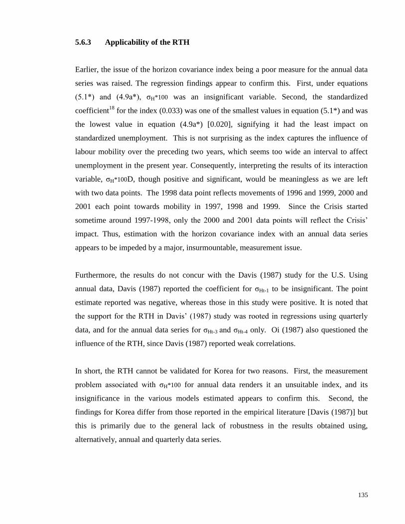
135
5.6.3 Applicability of the RTH
Earlier, the issue of the horizon covariance index being a poor measure for the annual data
series was raised. The regression findings appear to confirm this. First, under equations
(5.1*) and (4.9a*), ζH*100 was an insignificant variable. Second, the standardized
coefficient18
for the index (0.033) was one of the smallest values in equation (5.1*) and was
the lowest value in equation (4.9a*) [0.020], signifying it had the least impact on
standardized unemployment. This is not surprising as the index captures the influence of
labour mobility over the preceding two years, which seems too wide an interval to affect
unemployment in the present year. Consequently, interpreting the results of its interaction
variable, ζH*100D, though positive and significant, would be meaningless as we are left
with two data points. The 1998 data point reflects movements of 1996 and 1999, 2000 and
2001 each point towards mobility in 1997, 1998 and 1999. Since the Crisis started
sometime around 1997-1998, only the 2000 and 2001 data points will reflect the Crisis‟
impact. Thus, estimation with the horizon covariance index with an annual data series
appears to be impeded by a major, insurmountable, measurement issue.
Furthermore, the results do not concur with the Davis (1987) study for the U.S. Using
annual data, Davis (1987) reported the coefficient for ζHt-1 to be insignificant. The point
estimate reported was negative, whereas those in this study were positive. It is noted that
the support for the RTH in Davis‟ (1987) study was rooted in regressions using quarterly
data, and for the annual data series for ζHt-3 and ζHt-4 only. Oi (1987) also questioned the
influence of the RTH, since Davis (1987) reported weak correlations.
In short, the RTH cannot be validated for Korea for two reasons. First, the measurement
problem associated with ζH*100 for annual data renders it an unsuitable index, and its
insignificance in the various models estimated appears to confirm this. Second, the
findings for Korea differ from those reported in the empirical literature [Davis (1987)] but
this is primarily due to the general lack of robustness in the results obtained using,
alternatively, annual and quarterly data series.

136
5.6.4 Sectoral Movements and Stage-of-the-Business-Cycle Effect
The regressions of equations (5.1*) and (4.9a*) showed that ζtSt was an insignificant
variable. This finding for the post-Crisis phase in Korea does not concur with that for a
more stable economic setting reported by Mills, Pelloni and Zervoyianni (1995) for the
U.S. Since there are limitations associated with the raw Lilien index, the variable St was
made to interact with other unpredicted and predicted indices.
Pre-Crisis Finding
To assess if the stage-of-the-business-cycle effect applies to unpredicted sectoral
movements, additional interaction variables were created by multiplying St by each
unpredicted index. Each of the five sets of new variables [(i) ζm
t(up), ζm
t(up)St and
ζm
t(up)St D, (ii) ζgt(up), ζ
gt(up)St and ζ
gt(up)St D, (iii) ζ
a2t(up), ζ
a2t(up)St and ζ
a2t(up)St D, (iv) ζ
p1t(up),
ζp1
t(up)St and ζp1
t(up)St D, and (v) ζp2
t(up), ζp2
t(up)St and ζp2
t(up)St D] was entered into the
regressions of equations (5.1*) and (4.9a*) in place of ζt, ζtSt and ζtStD. The regressions
revealed the unpredicted ζSt‟s to be insignificant (Table 5.9), implying that pure inter-
sector labour movements did not lead to higher aggregate unemployment during the period
1971-2001.
The stage-of-the-business-cycle hypothesis was also tested for mobility predicted by
demand disturbances. For the regressions with the ADH indices, each set of variables, i.e.
ζa2
t(p), ζa2
t(p)St and ζa2
t(p)St D, ζm
t(p), ζm
t(p)St and ζm
t(p)St D and ζgt(p), ζ
gt(p)St and ζ
gt(p)St D, was
entered into equations (5.1*) and (4.9a*) instead of ζt, ζtSt and ζtStD2. The interaction
variables ζa2
t(p)St, ζm
t(p)St and ζgt(p)St were insignificant, suggesting that the business cycle
effect is inapplicable during 1971-2001 for predicted labour movements.
Thus, the stage-of-the-business-cycle argument cannot be extended to predicted and
unpredicted sectoral labour movements. As the SSH and ADH did not exist for most forms
of mobility during 1971-2001, it is not surprising that the stage-of-the-business-cycle effect
does not apply to predicted and unpredicted mobility.
137
Table 5.9 Parameter Estimates of ζ, ζSt and/or ζStD Equation
(4.9a*)
Equation
(5.1*) ζt 39.579*
(2.691) 11.868 (0.601)
ζtSt 9.646 (0.955)
-6.115 (-0.712)
ζtStD 61.011* (3.810)
108.882* (4.793)
ζm
t(up) -1.735 (-1.114)
-1.582 (-1.050)
ζm
t(up)St 1.548 (0.626)
-0.208 (-0.095)
ζm
t(up)StD 10.808* (3.824)
13.553* (4.868)
ζg t(up) 21.176
(1.402) 12.803 (0.958)
ζg t(up)St 8.635
(0.565) -8.604
(-0.983) ζ
g t(up)StD 53.955*
(3.319) 88.535* (5.410)
ζa2
t(up) 0.450 (1.005)
-0.012 (-0.024)
ζa2
t(up)St 1.047 (1.237)
0.161 (0.197)
ζa2
t(up)StD 2.638* (2.448)
4.293* (3.692)
ζp1
t(up) 35.263* (3.604)
11.276 (0.914)
ζp1
t(up)St 9.603 (0.960)
-7.632 (-0.956)
ζp1
t(up)StD 29.660* (2.535)
77.691* (5.244)
ζp2
t(up) 26.182 (1.786)
+
-9.153 (-0.546)
ζp2
t(up)St 6.143 (0.646)
-0.890 (-0.105)
ζp2
t(up)StD 36.470* (3.243)
80.124* (5.243)
ζa2
t(p) 2.438 (0.140)
-37.531* (-2.531)
ζa2
t(p)St 14.901 (0.890)
-15.145 (-1.400)
ζa2
t(p)StD 51.966* (2.306)
125.556* (5.063)
ζm
t(p) -0.149 (-0.081)
-0.309 (-0.173)
ζm
t(p)St 4.173 (1.658)
-0.363 (-0.152)
ζm
t(p)StD 4.476 (1.426)
12.244* (3.299)
ζg t(p) -55.588
(-1.377) -40.205 (-0.943)
ζg t(p)St 43.784
+
(1.772) 10.465 (0.383)
ζg t(p)StD -0.732
(-0.024) 96.677
+
(1.859)
* significant at 5% level. + significant at 10% level.
Note: All are OLSE except for equation (4.9a*) with ζa2
t(p),
ζa2
t(up), ζm
t(up) and ζgt(p), and equation (5.1*) with ζ
gt(p) and
ζm
t(up) which are CO estimates applied with a Prais-Winsten
transformation.

138
Post-Crisis Finding
From the results of the predicted and unpredicted ζStD variables, the majority of the indices
point towards a positive and significant coefficient. Although this may suggest some
evidence in favour of the business-cycle effect during the post-Crisis period, two notable
limitations with regards to the dataset prevent the formation of any conclusion pertaining to
the post-Crisis period. The 4 annual data points for the 1998-2001 period are too few
observations to confidently ascertain if the stage-of-the-business-cycle effect really existed.
This is compounded by the fact that at the end of the data period (2001), the most
pronounced business cycle in the data series was incomplete. Any examination of this
hypothesis for Korea can only be conducted over a longer time frame. This is outside the
scope of this thesis.
5.7 CONCLUDING REMARKS
The impact of sectoral mobility on unemployment with regards to the Korean labour
market was examined in this chapter. This examination was conducted from the
perspective of the four main hypotheses: SSH, ADH, RTH, and the stage-of-the-business-
cycle effect. Owing to the contradictory evidence from the empirical studies, the extensive
list of indices and wealth of explanatory variables gathered from the literature, lengthy,
rigorous steps had to be followed to ensure reliable estimates were obtained prior to
statistical inference.
In terms of specification, the approach was to move from an unrestricted to a restricted
model. As an all-encompassing model would have led to over-parameterisation and
multicollinearity, tests were conducted to determine if any of the regressors were
correlated. It was also necessary to ensure the series of each variable was stationary and to
avoid instability in the regression.
With a time period of 31 years, the likelihood of a change in the deterministic relationship
in the variables within each model would be quite high. This is especially so following
from events like the 1998 Asian Financial Crisis, which led to a severe recession in Korea

139
[The World Bank (1999)]. For the majority of models and indices, the tests indicated a
structural break between 1971-1997 and 1998-2001. The identification of these structural
breaks gave rise to a more appropriate functional form with the creation of dummy and
interaction variables. Serial correlation was detected in several estimating equations and
was corrected with the Cochrane-Orcutt iterative method where applicable. The final
estimates gave rise to a better fit of the models and were considered to be valid for
statistical inference.
The non-uniqueness in model specification meant that robustness of the regression results
under alternative models had to be established a priori. Having established robustness in
the results between the two models [i.e. equations (4.9a*) and (5.1*)], it was possible for
conclusions pertaining to the validity of the SSH, ADH, RTH and stage-of-the-business-
cycle to be reached. However, it was not possible to conclude if the RTH applies to Korea,
owing to the problems in using the horizon covariance index for an annual data series, lack
of congruency with the empirical literature, and lack of robustness in the results of the
related empirical literature.
In terms of the pre-Crisis period, there is a general lack of relevance of the SSH, ADH and
stage-of-the-business-cycle effect for the Korean economy. For the post-Crisis period, the
results tend to support the first two hypotheses, but do not support the stage-of-the-
business-cycle effect.
For the post-1997 period, the limited data (4 observation points) seem to provide evidence
in favour of the post-Crisis effect for the SSH and ADH. However, this limitation (i.e.
short span) of the aggregate-level data prevents the full validation of these two hypotheses,
and it is only when more data become available for the post-Crisis period that appropriate
empirical testing will be possible. The implications of the stage-of-the-business-cycle
effect could not be examined effectively owing to the limited data available (i.e. only 4 data
points). Furthermore, it may not be meaningful to examine this hypothesis when the last
data point reflects a mid-point of the most pronounced cycle in the data series.
Nonetheless, since the aggregate-level data findings have indicated that the SSH/ADH
could apply to Korea, and that the nature of unemployment arising from pure sectoral

140
movements could be non-frictional after the Crisis, it could imply that the SSH/ADH are
new phenomena for Korea. What existed for the developed countries much earlier in the
last century appears to have only started for this NIE in recent years19
.
What we would like do in this current thesis, therefore, is extend the research from
aggregate-level data to longitudinal data using the same period of 1998-2001. Part II of the
thesis therefore uses unit-record data to study the factors that motivate inter-sector mobility.
Such knowledge may be useful when seeking solutions to future unemployment problems
through changes to labour mobility.
Endnotes:
1. South Korea will be referred to as Korea hereinafter.
2. The formal indices of sectoral mobility gathered from the literature review are to be analysed later.
3. A part of the reason is that a substantial portion of the ADH discussions has been centred around the U-V
correlation initiated by Abraham and Katz (1986).
4. Additional measures that were examined but not reported on are ζa1
t(up), ζt(s), ζt(r), ζt(p) and its corresponding
unpredicted series, ζt(up). See chapter 3 for a critique of these indices.
5. DMt and UNt were found to be stationary.
6. In the current study, these U.S. variables will not be included because, unlike Canada, the U.S. and Korean
economies are not integrated. To address the possibility of simultaneity bias, checks on the correlation
between DMRt and the other explanatory variables of the unemployment equation will be carried out. These
checks are undertaken as correlation between variables may indicate simultaneity bias, and if overlooked this
may lead to biased estimation [Barrows (2004)].
7. Garonna and Sica (2000) referred to the series as „money growth rate‟. Since it is an aggregate demand
indicator, it is most likely to be the money supply growth for Italy.
8. Barro (1977) indicated that the growth of the public sector at 5% per year (ρ = 0.2) would not seem to be
permanently sustainable. The Korean case of ρ = 0.05 appears reasonable.
9. The term, ζ, represents the generic sectoral mobility index covering all predicted and unpredicted indices.
It does not have a subscript for time t. The term with the subscript for time t, ζt, is the raw Lilien index. The
change variables denoted by the prefix „∆‟ are with respect to the immediate past period.
10. The similarity is based on the type of the variables as the number of lags and difference operators will
differ depending on tests of stationarity and data frequency in the case for Korea. Since annual data are used,
the number of lags for each variable was kept to a minimum. If not, the influence of a variable lagged by, say,
more than one year becomes dated. For the ζ‟s, the indices lagged by one time period were insignificant for
most regressions under equation (5.1). The DMR was lagged by one time period since DMRt was
insignificant in most regressions. It was not lagged by two periods since the annual data series for the
regressions would start from 1972, meaning a further loss of observations and degrees of freedom.
11. The CUSUM and CUSUMSQ techniques, and the associated significance lines, are often viewed as
„yardsticks‟ rather than formal statistical tests. The timing of any structural change is difficult to pinpoint
accurately using this procedure, and the plots need to be examined in association with prior knowledge. The
point at which the structural change commences is often when the plotted line starts to deviate upwards or
downwards.
12. It should be noted that since the absence of a structural break between phase 1 and phase 2 was
established, the Chow test could also have been conducted for (phase 1 plus phase 2) versus phase 3.
However, this is not necessary given the varied findings above. It would be better to proceed straight to the
structural dummy variable approach to ascertain the occurrence and source of structural change.
13. The only study was Parker (1992), where a military variable was incorporated into the unemployment
model to pick up the manpower influences of the Vietnam war.

141
14. A prior test that involved estimating a model with only the mobility dummy first, followed by the
inclusion of the intercept and mobility dummies, showed the statistical significance of the dummies to alter
according to the order of inclusion.
15. This LM statistic is computed as (N-1)R2, where R
2 comes from the auxiliary regression of the estimated
OLS error term on all explanatory variables together with the lagged value of the estimated error term for
(N-1) observations, with N being the total number of observations.
16. The tightening of the models could equally have been done following a correction for serial correlation
without any material change to the findings. The regressions with ζH and ζtSt under equation (4.9a*) and ζH
under equation (5.1*) were corrected for serial correlation. The findings showed that the intercept dummy
and/or mobility interaction dummies remained insignificant under both equations.
17. Greene (2003) conducted a Lagrange Multiplier test with a sample size of 19.
18. The standardized coefficient in the SPSS program expresses the impact of the independent variable in
terms of standard deviation units, i.e., whether the number of standard deviations the dependent variable
increases or decreases with a one standard deviation increase in the independent variable. The standardized
coefficient is calculated by multiplying the non-standardized coefficient by the ratio of the standard deviations
for the independent and dependent variables. A standardized coefficient of a single independent variable in a
multiple regression will assist in determining whether it has a greater or lesser effect on the dependent
variable as compared to the effects of other independent variables.
19. See „The World Bank (1999) „Republic of Korea: Establishing a New Foundation for Sustainable
Growth‟, Report No. 19595 KO, Nov 2, 1999‟.

142
(This page is left blank intentionally.)
143
PART II: THE FACTORS AFFECTING SECTORAL MOBILITY
PREAMBLE
Part I examined, from the perspective of the four hypotheses: SSH, ADH, RTH, and the
stage-of-the-business-cycle effect, the impact of sectoral mobility on unemployment.
Based on aggregate-level data, the key finding was the significant impact that unpredicted
and predicted sectoral mobility had on aggregate unemployment in Korea during the post-
Crisis 1998-2001 period. The four hypotheses, however, had little relevance for periods
prior to this. The mobility-unemployment relationship therefore appears to be a new
phenomenon in Korea, though it has been a characteristic of developed countries like the
U.S. and Canada for earlier periods. There is a need to understand the sectoral mobility
associated with this type of unemployment in Korea. This is the aim of the research
presented in Part II, where the causal factors of sectoral mobility are analysed using
longitudinal data for Korea for the 1998-2001 period.
The literature review in the next three chapters seeks to gather ideas for the current work
from the research undertaken on various forms of labour mobility. Chapter 6 presents
theoretical and conceptual issues in labour mobility and outlines the proposed empirical
framework. Chapter 7 reviews the literature on forms of labour mobility other than sectoral
mobility and extracts salient points for the current research. Chapter 8 conducts a review of
the empirical evidence on the factors affecting sectoral mobility. Finally, chapters 9 and 10
contain the empirical application for Korea, with emphasis on the overall labour force in
the former and separate analyses for males and females in the latter. The key conclusion is
that sectoral mobility is a multi-facetted phenomenon encompassing a range of factors,
including monetary and macroeconomic variables, worker and industry characteristics, and
the sectoral shock.

144

145
CHAPTER 6
THE THEORETICAL AND CONCEPTUAL ISSUES
IN LABOUR/SECTORAL MOBILITY
6.1 INTRODUCTION
This chapter introduces the main theoretical and conceptual issues in the microeconometric
study of labour mobility. The various forms of labour mobility are defined in section 6.2
and the three theories of sectoral/industrial mobility are presented in section 6.3. A generic
theoretical model describing the main motivations behind labour mobility is outlined in
section 6.4. This model provides a framework within which the empirical literature can be
studied (see chapter 8). It also forms the basis for the empirical analyses presented later in
the thesis (see chapters 9 and 10). While the focus of this thesis is on sectoral or industrial
mobility, the empirical literature reviewed covers other forms of labour mobility, including
union/non-union mobility, public-private sector mobility and rural-urban mobility. The
reason for this broad approach is that research into sectoral/industrial mobility appears less
advanced, and hence there may be much to be learned from careful study of the
econometric techniques, databanks and research questions from these other types of labour
mobility. Then, the empirical models used in study of the various forms of mobility are
presented in section 6.5. A summary of the chapter and the implications for the empirical
model are presented in the final section.
6.2 WHAT IS LABOUR MOBILITY?
Labour mobility is a very general term. It can be applied to movement of labour across
countries, across regions within a country, across occupations, industries or broad sectors of
an economy, such as the union and non-union sectors, government versus non-government
sectors and rural versus urban sectors.
There is a vast amount of literature dealing with the movement of labour across countries:
International migration has been a major research issue for most of the last century [Borjas
146
(1994), Bartel (1989), Chiswick (1991), Chiswick and Miller (1985), Chiswick, Le and
Miller (2008) and Dustmann (1993)]. A range of international migration issues have been
examined in Asia. Seok (1999), for example, examined Korea‟s foreign worker labour
immobility during the post-1997 Asian Financial Crisis, and attributed this to the fact that
small and medium-sized firms preferred to hire migrant labour at lower wages, while these
workers remained as their potential gain in earnings from re-migration did not exceed the
costs of returning to their countries of origin. Chew (1990) investigated issues related to
the brain drain in Singapore and highlighted the number of Singapore emigrations in the
1980s. Manning‟s (1999) study focused on implications of the influx of foreign labour into
Singapore from developing countries. Bartram‟s (2000) study highlighted that, in contrast
to other advanced industrial countries with positive migrant inflow, Japan experienced
negative labour migration in the post-World War II period.
Intra-regional migration is also of importance, with researchers attempting to account for
the rise and decline of parts of a country, the growth and demise of regional concentrations
of specific groups of people, and even patterns of settlement within cities [Tomes and
Robinson (1982a), Antolin and Bover (1997), and Fanni, Galli, Gennari and Rossi (1997)].
There have been a number of studies on intra-regional migration and these have
emphasized various patterns. Rogers and Henning (1999), for example, reported that
during the periods 1975-1980 and 1985-1990, foreign-born Americans showed a slightly
higher likelihood of crossing state boundaries than their native-born counterparts. Cutler,
Glaesar and Vigdor (1999) highlighted a trend for black migration during the period 1980-
1996 from the ghettos to cities/suburbs that previously had a predominantly all-white
population. Jeong (2003) showed that wages and large corporate employment raised the
likelihood of regional mobility in Korea over the period 1995-2002.
Occupational mobility is a popular field of study for economists interested in individual
economic well-being. A person‟s occupation offers a good guide to their economic
standing in society, and changes in the individual‟s occupation over time offer useful
insights into their economic progress. Occupational mobility can also be studied at the
aggregate (group) level where a change in the occupational mix over time can help explain
147
why particular groups fare better than others in the job market. For example, if males are
concentrated in trades occupations, and women in services, a shift in the jobs generated in
the economy away from trades towards services would, ceteris paribus, lead to more
favourable labour market outcomes for females than for males. Similarly, if the scope for
productivity gains differs across occupations, knowing how the occupational mix changes
over time will be fundamental to an appreciation of the origins of economic growth, for
example, whether it is so-called jobless growth or is associated with employment growth.
Examples of studies on occupational mobility include Flyer (1997), Kim (1998),
Greenhalgh and Stewart (1985), Miller (1984) and Chiswick, Lee and Miller (2005). Flyer
(1997) reported that the projected earnings was a positive and significant variable in the
initial occupation choice of college graduates. Greenhalgh and Stewart (1985) showed that
British men experienced greater upward mobility and achieved higher occupational status
than women. Miller (1984) presented a model of job matching and occupational choice,
demonstrating that it was optimal for young workers with lesser work experience to switch
occupations. Kim (1998) found that workers who change occupations experienced smaller
wage gains, were less skilled, lower educated and had lower market experience than
workers who do not change occupations. Chiswick, Lee and Miller (2005) found that
although there was a drop in occupational attainment from the last job in the origin to the
first job in the destination for male immigrants in Australia, upward occupational mobility
was possible with post-immigration investments.
As with occupational mobility, labour mobility across broad sectors of the economy
involves individual behaviour which could have implications for the economy. Sectoral
mobility takes various forms. One of the more common types is mobility between union
and non-union sectors [Heywood (1993) and Hahn (1996)]. Other forms of labour mobility
include that between government and non-government sectors [Borland, Hirschberg and
Lye (1998) and Blank (1985)] and rural and urban sectors [Todaro (1981), Zahn (1971) and
Tcha (1993)]. For the latter form of mobility, Zahn (1971) and Tcha (1993) examined the
determinants of worker movements for Japan and Korea, respectively.
Industrial or sectoral mobility is the main topic for the current study. As mentioned in Part
I of the thesis, one of the reasons for this study is that sectoral or industrial mobility is often
associated with structural changes and cyclical movements in the economy. This link has

148
been drawn in a number of studies. Studies associating sectoral mobility and cyclical
variations in unemployment include Abraham and Katz (1986), Blanchard and Diamond
(1989), Brainard and Cutler (1993), Lilien (1982) and Loungani and Rogerson (1989) for
the U.S. labour market, Garonna and Sica (2000) for the Italian labour market, and Prasad
(1997) on industrial mobility for the Japanese manufacturing sector. One point worth
noting is that these studies adopt aggregate-level time-series data. Interest in the individual
behaviour that leads to sectoral (industrial) mobility commenced around the late 1980s, and
this was facilitated by access to unit-record longitudinal data. Studies taking this approach
include Osberg (1991), Osberg, Gordon and Lin (1994), Vanderkamp (1977) for Canada,
Loungani and Rogerson (1989), McLaughlin and Bils (2001), Fallick (1993) and Neal
(1995) for the U.S.
These studies focus on the conventional definitions of economic sectors/industries.
Alternative definitions using micro-level datasets were developed in other studies. For
example, Thomas (1996b) constructed two sectors: (a) pre-displacement sector, which is
the original sector of employment of displaced workers; and (b) the remainder of the labour
market for Canada. Osberg, Mazany, Apostle and Clairmont (1986) categorized sectors as
central or marginal, where the former consisted of the goods-producing primary sector that
used capital intensive technology, including the resource and construction sectors, and the
latter comprised other manufacturing firms not in the central sector and personal services
industries.
The studies above have primarily been concerned with the movement of labour across
economic sectors of the economy. All the types of mobility considered can be examined
within a common framework. This framework is a standard neo-classical model that
depicts individuals as moving from one state (country, region, occupation or
industry/sector) to another if the gains from moving outweigh the costs. These gains and
costs can be either monetary or non-monetary. A model of mobility is outlined and used as
a basis for a more detailed review of the literature in section 6.4. Prior to that, the theories
pertaining to the origins of sectoral mobility will be presented in the section below.

149
6.3 THEORIES OF SECTORAL/INDUSTRIAL MOBILITY
Three theories on the origins of sectoral mobility emerge from the literature, namely, the
worker-employer mismatch theory, the sectoral shock theory and the bridging theory.
These theories are basically about model specification.
6.3.1 Worker-Employer Mismatch Theory
The worker-employer mismatch theory relies on the mismatch between workers and jobs to
generate sectoral mobility. Mobility is modelled as a function of wages and worker/job
characteristics. Workers change sectors if there is a change between their current and
expected circumstances; in the form of higher perceived wages in the new sector and/or
non-pecuniary benefits in new sector and/or or a better job-match between worker
characteristics and new job requirements. Hence, workers could change sectors if the
following matches occur:
a) workers‟ expected wages match with the prospective employers‟ wage offer;
b) workers‟ expectations of the non-wage benefits of the job, e.g. working hours
and benefits, match with the new job characteristics; and
c) workers‟ individual skill sets, e.g. demographic profile, qualification and
experience, match with employer demands and requirements for the job.
Whether one or all of the above matches occur following a sectoral switch really depends
on the individual worker and employer. For example, whilst one worker will switch sectors
if his skill set meets a firm‟s requirements even if the wages do not, another worker will
require that both his skill set and wage levels are in accordance with expectation before a
sectoral change takes place.
As both workers and employers are heterogeneous, the probability of moving to another
sector will differ across workers. It takes time and resources for workers to acquire
information about available job prospects and for employers to acquire information about
potential applicants. Moreover, there is uncertainty about this job information. The theory

150
suggests that workers will seek to maximize their expected wages based on the information
acquired and make a decision on a sectoral switch. Employers will optimally assign jobs to
workers based on the available information about the workers. Optimizing behaviour
within this framework can generate sectoral mobility for some workers and stability for
others. The theory relies on worker heterogeneity and imperfect information in job markets
to generate mobility and is applicable to all forms of sectoral mobility. Many studies of
union/non-union, public-private and rural-urban mobility and the majority of the studies of
sectoral/industrial mobility are based on this theory.
6.3.2 Sectoral Shock Theory
The sectoral shock theory subscribes to the view that sectoral shocks are responsible for
generating sectoral/industrial mobility. A sectoral shock can take the form of changing
tastes, technology, input price, product demand and productivity. Sector-specific shocks
are believed to affect the pattern of labour demand which leads to sectoral reallocations in
the labour market [Helwege (1992) and Clark (1998)]. For example, after a sectoral shock,
the demand for the product of that sector rises, the wages in that sector rise and this attracts
workers from other sectors, thereby generating labour mobility. There are a number of
studies measuring the impact of a sectoral shock on mobility, namely Gulde and Wolf
(1998), Jovanovic and Moffitt (1990), Brainard and Cutler (1993), Altonji and Ham (1990)
and Clark (1998).
Two distinctions must be made between the worker-employer mismatch and sectoral shock
theories. First, whilst the former relies on worker heterogeneity and imperfect markets to
generate mobility, it is implied in the latter that labour movements can occur even when
workers are homogeneous in a perfectly competitive labour market [Clive and Jovanovic
(1988)]. Specifically, in a perfect market, each homogenous worker is deemed to have an
equal probability of changing sectors [Mincer and Jovanovic (1981)] following a sectoral
shock. Second, there are implications pertaining to the empirical application. The sectoral
shock approach could be used if gross flows were equal to net flows. That is, if sectoral
shocks are the only reason for generating mobility, workers move from one specific sector
to another in response to a sectoral shock. Since the sectoral shock theory rules out other
causes of mobility, it implies that gross flows of labour should be equal to net flows. In
151
contrast, under the mismatch theory, mobility occurs owing to reasons other than a sectoral
shock. Workers move across sectors in both directions, and gross flows can be larger than
net flows.
6.3.3 Bridging Theory
Bull and Jovanovic (1986) argued that labour mobility may be caused by shifts in the
derived demand for labour on the part of firms/sectors and by mismatches between workers
and jobs. Furthermore, Jovanovic and Moffitt (1990) stated that a model that relies solely
on the impact of sectoral shocks on labour demand or concentrates on sector/worker
mismatch is likely to lead to misinterpretation of the empirical results. Hence, the
“bridging” theory subscribes to the view that labour mobility can be modelled in two ways:
via a shift in labour demand and also generated by employer-employee mismatch. This
bridging view was mooted by Clive and Jovanovic (1988) in theory only. The study that
tested this theory was Jovanovic and Moffitt (1990), where wages, worker characteristics
and a sectoral shock variable were incorporated into the mobility equation. Since mobility
is also generated by an employer-employee mismatch, it operates in the presence of
worker/employer heterogeneity and imperfect job markets. Each worker faces an unequal
probability of a sectoral switch.
6.4 MODEL OF LABOUR MOBILITY
The model outlined below is developed as a tool to explain worker movement from one
sector to another. The model has as its starting point the approach taken by Le and Miller
(1998). They developed a model of labour market choice incorporating an individual‟s
current and future earnings streams as well as the non-pecuniary aspects of alternative
employment states. This is a conceptual advance over other models of labour market
choice that are based only on the differential in current earnings associated with alternative
employment states.
Let yai(t) represent the annual earnings of an individual i in sector „a‟ in period t, and ybi(t)
be the annual earnings of the individual in sector „b‟ for period t. The lifetime earnings of
this individual in sectors „a‟ and „b‟ would each be:
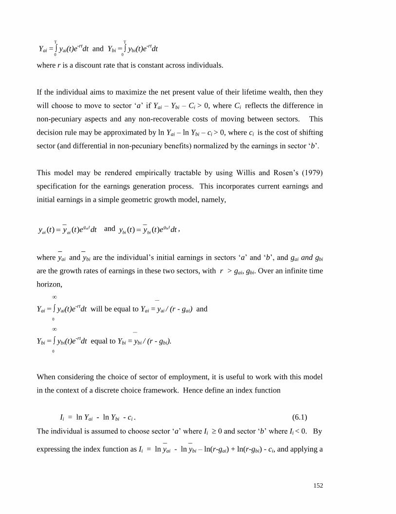
152
T T
Yai = ∫ yai(t)e-rt
dt and Ybi = ∫ ybi(t)e-rt
dt 0 0
where r is a discount rate that is constant across individuals.
If the individual aims to maximize the net present value of their lifetime wealth, then they
will choose to move to sector „a‟ if Yai – Ybi – Ci > 0, where Ci reflects the difference in
non-pecuniary aspects and any non-recoverable costs of moving between sectors. This
decision rule may be approximated by ln Yai – ln Ybi – ci > 0, where ci is the cost of shifting
sector (and differential in non-pecuniary benefits) normalized by the earnings in sector „b‟.
This model may be rendered empirically tractable by using Willis and Rosen‟s (1979)
specification for the earnings generation process. This incorporates current earnings and
initial earnings in a simple geometric growth model, namely,
( ) ( ) aig t
ai aiy t y t e dt and ( ) ( ) big t
bi biy t y t e dt ,
_ _
where yai and ybi are the individual‟s initial earnings in sectors „a‟ and „b‟, and gai and gbi
are the growth rates of earnings in these two sectors, with r > gai, gbi. Over an infinite time
horizon,
∞ __
Yai = ∫ yai(t)e-rt
dt will be equal to Yai = yai / (r - gai) and
0
∞ __
Ybi = ∫ ybi(t)e-rt
dt equal to Ybi = ybi / (r - gbi).
0
When considering the choice of sector of employment, it is useful to work with this model
in the context of a discrete choice framework. Hence define an index function
Ii = ln Yai - ln Ybi - ci . (6.1)
The individual is assumed to choose sector „a‟ where Ii 0 and sector „b‟ where Ii < 0. By
_ _
expressing the index function as Ii = ln yai - ln ybi – ln(r-gai) + ln(r-gbi) - ci, and applying a

153
Taylors series expansion for ln(r-gai) and ln(r-gbi) around the mean values of the arguments,
the following expression may be derived:
1 2 3 4[ln ln ]i ai bi iai biI y y g g c . (6.2)
where the βs are the parameters that will be estimated to show how initial earnings in each
sector and growth rates in earnings in these sectors affect the underlying index that is used
to determine the choice of sector.
The index function could also be expressed in terms of current earnings and growth rates,
_ _
using the fact that ln yai(t) = ln yai + gait and ln ybi(t) = ln ybi + gbit. Thus,
Ii = γ1 + γ2 [ ln yai(t) - ln ybi(t) ] + γ3gai + γ4gbi - ci. (6.3)
The cost of moving between sectors (ci) can be modelled for inclusion in the index
function. Hence write ci = Ziδ, where Zi is a vector of observable variables influencing the
non-monetary differences in employment in sector „a‟ compared with „b‟. It also includes
any costs associated with moving between sectors. A sectoral shock (Si) can also be
incorporated into the model. Thus, substituting ci = Ziδ, and adding Siφ to represent the
sectoral shock, we obtain:
Ii = γ1 + γ2 [ ln yai(t) - ln ybi(t) ] + γ3 gai + γ4 gbi - Ziδ - Siφ. (6.4)
In this index function, which represents the latent tendency to move from sector „b‟ to
sector „a‟, the term ln yai(t) - ln ybi(t) represents the differential in current earnings while the
terms for the growth rates, γ3gai and γ4gbi, provide the foundation for a model that
incorporates future or permanent earnings. Finally, the terms Ziδ and Siφ each represent the
mobility effects associated with the costs of sectoral mobility and a sectoral shock.
In addition to monetary factors, worker and job characteristics, sector-specific shocks have
been reported to affect sectoral/industrial mobility [Gulde and Wolf (1998), Jovanovic and
Moffitt (1990), Brainard and Cutler (1993), Altonji and Ham (1990) and Clark (1998)].

154
Each sector is subject to shocks resulting in the movement of workers (i.e. sectoral
mobility), where workers are expected to move from lower to higher productivity sectors.
Although sector-specific shocks could affect worker wages, a sectoral labour change is
typically argued to occur prior to a change in wages. For example, a productivity shock
will first cause a worker to reallocate to a higher productivity sector before he can expect to
receive higher wages. A non-monetary shock (e.g. change in labour input demand) causing
workers to switch sectors may not necessarily result in a wage change. Therefore, sectoral
shocks cannot be fully reflected in the sectoral wage differential. For this reason, the
sectoral shock variable is introduced into equation (6.7) as a separate explanatory variable.
It was earlier noted that limitations on labour mobility in Korea appear to give rise to
unemployment. This unemployment needs to be incorporated into the Le and Miller
model. The Todaro (1984) model of worker mobility between rural and urban sectors is
useful in this regard, as it explicitly recognized the way unemployment can impinge on the
labour mobility process. In this model, an individual‟s decision to move is based on
considerations of income maximization and the perceived expected earnings stream in the
new sector. Applying Todaro‟s model to a generic form of sectoral mobility, it is assumed
that sector „b‟ is characterized by market clearing, while the higher income sector, sector
„a‟, has an above market-clearing wage and „wait‟ unemployment. If the probability that
the individual secures a job in sector „a‟ at their potential income in period „t‟ is pi(t), then
expected wages are given by the term ( ) ( )i aip t y t . Examples of studies applying the
concept of expected wages include Miller and Neo (2003) in an analysis of U.S. and
Australian labour market flexibility and immigrant adjustment, and Gyourko and Tracy
(1988) in an analysis of public versus private sector wages in union and non-union sectors.
In Miller and Neo (2003), the expected earnings was constructed by adjusting earnings
using the probability of unemployment. Both the earnings and unemployment measures
were from multivariate models of these labour market outcomes. Similarly, in Gyourko
and Tracy (1988), the expected public-sector (private-sector) wage was computed as the
weighted average of the expected public/union (private/union) and public/non-union
(private/non-union) wages. The actual earnings differential of workers from two sectors of
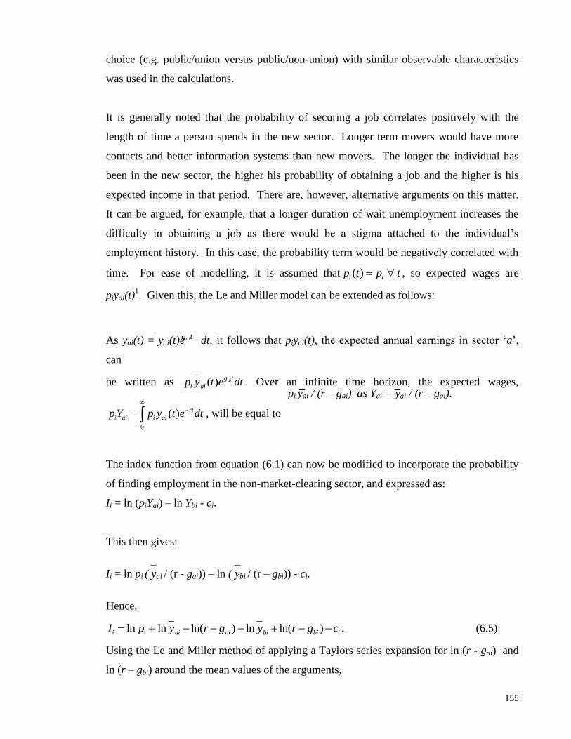
155
choice (e.g. public/union versus public/non-union) with similar observable characteristics
was used in the calculations.
It is generally noted that the probability of securing a job correlates positively with the
length of time a person spends in the new sector. Longer term movers would have more
contacts and better information systems than new movers. The longer the individual has
been in the new sector, the higher his probability of obtaining a job and the higher is his
expected income in that period. There are, however, alternative arguments on this matter.
It can be argued, for example, that a longer duration of wait unemployment increases the
difficulty in obtaining a job as there would be a stigma attached to the individual‟s
employment history. In this case, the probability term would be negatively correlated with
time. For ease of modelling, it is assumed that ( )i ip t p t , so expected wages are
piyai(t)1. Given this, the Le and Miller model can be extended as follows:
_
As yai(t) = yai(t)e dt, it follows that piyai(t), the expected annual earnings in sector „a‟,
can
be written as ( ) aig t
i aip y t e dt . Over an infinite time horizon, the expected wages,
0
( ) rt
i ai i aip Y p y t e dt
, will be equal to
The index function from equation (6.1) can now be modified to incorporate the probability
of finding employment in the non-market-clearing sector, and expressed as:
Ii = ln (piYai) – ln Ybi - ci.
This then gives:
_ _
Ii = ln pi ( yai / (r - gai)) – ln ( ybi / (r – gbi)) - ci.
Hence,
ln ln ln( ) ln ln( )i i ai bi iai biI p y r g y r g c . (6.5)
Using the Le and Miller method of applying a Taylors series expansion for ln (r - gai) and
ln (r – gbi) around the mean values of the arguments,
_ _ pi yai / (r – gai) as Yai = yai / (r – gai).
gait

156
1 2 3 4[ln ln ln ]i i ai bi iai biI p y y g g c . (6.6)
_ _ Given that ln yai(t) = ln yai + gait, ln ybi(t) = ln ybi + gbit and ci = Ziδ, and adding Siφ
which represents the sectoral shock, this gives:
Ii = γ1 + γ2 [ ln pi + ln yai – ln ybi] + γ3 gai + γ4 gbi - Ziδ - Siφ. (6.7)
where ln lni aip y represents the income level the individual expects to receive in the new
sector „a‟. The term [ln ln ln ]i ai bip y y now represents the anticipated differential in
expected current earnings. The term ln pi is reflecting wait unemployment.
Hence, it can be seen from the extended model that the worker movements from sector „b‟
to sector „a‟ are determined by the following:
a) Earnings in sector „a‟ versus sector „b‟, where earnings in the new sector should
be higher than the original sector in order to entice workers to move. This
could be regarded as a pull factor.
b) Lifetime wages in sector „a‟ versus sector „b‟. The new sector‟s permanent
incomes should be higher than the old sector‟s for a sectoral switch to occur.
This could also be treated as a pull factor.
c) Unemployment in sector „a‟ versus sector „b‟, where the level of unemployment
is greater in the high wage sector. This could be viewed as a factor that
moderates the pull factor noted above.
d) Non-monetary factors associated with the costs of mobility, which include a
range of demographic and socio-economic factors.
e) Sectoral shocks, which could lead to sectoral labour rellocations in the labour
market.
The transitory period of wait unemployment takes two forms: voluntary [Kim (1998)] and
involuntary [Thomas (1996b) and Addison and Portugal (1989)]. If individuals are
motivated by the pull factor of higher earnings in the new sector, inter-sectoral movements
are conceived to be voluntary, as mobility arises out of choice. Consequently, any wait
unemployment experienced in the new sector arising from the actions of wealth-
maximising individuals are voluntary. Wait unemployment can be involuntary where the
157
sectoral move arises out of necessity rather than choice. This could happen if individuals
lose their jobs due to employer-initiated actions [Fallick (1993)].
The empirical model of equation (6.7) is applicable to all three theories of sectoral mobility
described in the previous section. Under the mismatch theory, the model caters for wages
(with the inclusion of [ln ln ln ]i ai bip y y , gai and gbi terms) and worker/job
characteristics (subsumed under Zi). Under the bridging theory, the full model applies,
including the Si term, which now incorporates the sectoral shock element as well. In
contrast, the model becomes Ii = γ1 + Siφ under the sectoral shock theory, with Si
representing the stochastic shock.
Although not the focus of the thesis, the model can be generically applied to other forms of
labour mobility, since the terms „a‟ and „b‟ can each represent the employment states in
distinct sectors, i.e. union/non-union, public-private, and rural-urban sectors, or different
regions, e.g. region „a‟ versus region „b‟ and country „a‟ versus country „b‟. The
explanatory variables on the right-hand-side of equation (6.7) can represent the factors
affecting mobility. Nonetheless, regardless of mobility type, it should be noted that the
application of the model of equation (6.7) involves a study at the micro-level and not at the
aggregate level.
6.5 EMPIRICAL MODELS OF SECTORAL MOBILITY
The empirical models used in the analysis of the determinants of labour mobility consist of
single equation probability choice models, simultaneous equation models and competing
risks models. These models have been used in empirical study of union/non-union, public-
private, rural-urban and sectoral/industrial mobility. The first three forms of labour
mobility are of interest in the current thesis for three reasons. First, the theoretical model
used in much of the research is broadly the same as that outlined in section 6.4. In
particular, the typical model incorporates both a sectoral wage advantage and non-
pecuniary determinants. Second, much can be learned in terms of the type of data used.
Third, the econometric techniques and estimating equations cover a range of situations, and
158
this extensive coverage is useful for the empirical study of sectoral mobility, where the
empirical work is less advanced, and hence there is an advantage in being able to relate the
work to research in cognate areas.
A variety of databanks, estimation methods, coverage, dependent variables and explanatory
variables have been used. This section evaluates the relevance and implications for
modelling in the current work in terms of the general functional form, data-type, dependent
variable, coverage and estimation method.
6.5.1 Probability Choice Models
Functional Form
The probability choice models generally comprise one dependent variable and several
regressors, and are a form analogous to equation (6.7), namely:
Ii = Xi + ei (6.8)
where Ii is a latent (unobserved) tendency towards a move from sector „b‟ to sector „a‟, Xi
represents a range of monetary, economic and non-pecuniary explanatory variables, is the
vector of parameters to be estimated and ei is the stochastic disturbance term.
These models have usually been estimated using a probit, logit or linear probability method
of estimation, especially when micro data are used and the nature of the dependent variable
is dichotomous. This can be seen in studies of the other forms of labour mobility, namely,
Christie (1992), Farber and Saks (1980), van der Gaag and Vijverberg (1988), Gyourko and
Tracy (1988), Long (1975) and Long (1976), and in studies of sectoral/industrial mobility
by Osberg (1991), Osberg, Gordon and Lin (1994), Jovanovic and Moffitt (1990) and Neal
(1995). In the majority of studies based on aggregate-level data, ordinary least squares
estimation (OLS) was used2.

159
Although the empirical models in this area of research incorporate a wealth of monetary
and non-pecuniary determinants, they do not account for the lifetime earnings stream of
individuals that were included in the model outlined in section 6.4. In addition, although
several authors have recognized the importance of the expected wage differential, few have
attempted to use such a measure. In this regard, it is noted that while several studies refer
to an expected wage construct, this is a different concept from that developed in section 6.4.
For example, the wages in the union choice literature are computed on the basis of a full-
employment assumption, and hence are “expected” only in the sense that they refer to the
wages that the particular worker could expect to receive in the new sector. There is no
adjustment for wait unemployment. It should be possible, however, to make an adjustment
for unemployment with many datasets, including those for Korea, using the approach
adopted by Miller and Neo (2003).
The probability choice model of equation (6.8) is applicable to the three theories of sectoral
mobility depending on the inclusion of the variables under Xi. Likewise, it applies to the
conceptually-advanced empirical model of equation (6.7) where Xi is identical to
(γ1 + γ2[ln ln ln ]i ai bip y y + γ3 gai + γ4 gbi - Ziδ - Siφ).
Types of Data
Probability choice models have been estimated using four broad types of data. First, there
are micro datasets obtained from cross-sectional surveys. Examples are the union/non-
union and public-private sector studies of Christie (1992), Farber and Saks (1980), Borland
and Ouliaris (1994), Blank (1985), Hartog and Oosterbeek (1993), van der Gaag and
Vijverberg (1988), Gyouko and Tracy (1988), Long (1975) and Long (1976). Among the
various studies of sectoral/industrial mobility, those by Vanderkamp (1977) and Neal
(1995) have used cross-sectional micro datasets. Second, there are longitudinal datasets
which have been mainly used in the study of sectoral/industrial mobility, and these studies
include Osberg (1991), Osberg, Gordon and Lin (1994), Jovanovic and Moffitt (1990),
Loungani and Rogerson (1989), Fallick (1993) and Thomas (1996b). Third, some studies
have used aggregate-level cross-sectional data. These include the studies of public sector
mobility by Utgoff (1983) and rural-urban mobility by Schultz (1971) and Ghatak (1996).

160
Fourth, there are time-series studies conducted at various levels of aggregation. These
include Borland and Ouliaris (1994), Kenyon and Lewis (1997), Sharpe (1971), Carruth
and Disney (1988), Booth (1983), Bain and Elsheikh (1976) and Neumann and Rissman
(1984) for union/non-union mobility, Tcha (1993), Zahn (1971) for rural-urban mobility
and Ottersen (1993), McLaughlin and Bils (2001) and Jayadevan (1997) for
sectoral/industrial mobility.
The use of cross-sectional data has its limitations in that the data are subject to recall error
and their analysis confines the estimation to a single time-point, implying that dynamic or
longitudinal inferences are made on the basis of static analyses. One way of overcoming
these constraints is via the collection of longitudinal data, where workers who switched
industries are interviewed in adjacent time periods, and detailed information (original
industry and new industry) can therefore be collected on the workers who switch
sector/industry. This is illustrated in several studies of industrial mobility where
longitudinal datasets, enabling interviews and re-interviews to be conducted, were available
for analysis. The use of time-series data permits construction of both variables describing
labour market outcomes in previous periods and the lifetime earnings measure that is
central to the model of sectoral mobility employed. A structural change that affects an
economic sector may cause an imbalance in sectoral labour demand and supply. The socio-
demographic determinants of sectoral mobility are likely to be swamped by the
consequences of structural change. For example, in the absence of a structural change,
younger workers may have a higher likelihood of switching sectors if employment
opportunities appear strong in the new sector. However, when a structural change occurs,
e.g. a negative shock impacts the new sector, the new sector‟s performance and
employment levels may be reduced, and this same group of young workers may have a
higher probability of remaining in the old sector.
Aggregate-level data, cross-sectional or otherwise, have the merits of providing a rich
source of information about worker and job characteristics. However, there is a limitation
in that the conceptual models of aggregate-level data may mask the underlying relationship
through an averaging process. The results from the aggregate-level analysis may also be
sensitive to distributional characteristics of the data.

161
Longitudinal data available for the research on Korea are appropriate for the study on
sectoral/industrial mobility. Given the above discussion, this appears to be a strength of
the proposed analysis.
Coverage
A common observation in terms of coverage is that the studies of all forms of labour
mobility, using both aggregate and micro data, focus on employed persons3. The studies
with micro data tend to focus on the employed as full details are available in the data files.
Hence, in the current model, the focus will be on employed persons.
It is observed that several studies have analysed the determinants of sectoral mobility
separately for males and/or females [Osberg (1991), Neal (1995) and Osberg, Gordon and
Lin (1994)]. This is in view of the fact that the behaviour and motivation for mobility of
men and women are held to be different [Simpson (1988), Osberg (1991) and Osberg,
Gordon and Lin (1994)]. Furthermore, the estimated models for male mobility appear to be
statistically (in terms of goodness-of-fit) and economically (sign, magnitude and statistical
significance of particular regressors) superior to the results for females, which could
explain why most studies have focused on males [Osberg, Gordon and Lin (1994), Fallick
(1993) and Thomas (1996b)]. A similar approach will be undertaken for Korea. Separate
regression equations will be estimated for males and females, provided the gender mobility
patterns vary.
Dependent Variable
The dependent variable used in these models is a measured outcome variable that is linked
to the underlying propensity to choose a particular sector. For micro data, empirical work
is based on the individual‟s actual choice of sector in two adjacent time periods. This can
be seen in the sectoral mobility studies of Osberg (1991), Osberg, Gordon and Lin (1994)
and Jovanovic and Moffitt (1990). For aggregate-level data, the empirical work is based on
162
the change in, or proportion in, sectoral employment or the net change in employment of
the original and new sectors. The change variable in aggregate-level studies, e.g. Borland
and Ouliaris (1994), Kenyon and Lewis (1997), Carruth and Disney (1988), Bain and
Elsheikh (1996) and Sharpe (1971) in union/non-union studies and Jayadevan (1997) for
industrial mobility4, can be interpreted to mean that there are higher probabilities of
mobility into those industries characterized by higher employment growth. The proportion
of sectoral employment variable, e.g. Neumann and Rissman (1984) and McLaughlin and
Bils (2001), means that there has been an increase in the net inflow of labour into sector „a‟
when sector „a‟ has a proportionately higher increase in its share of employment between
period t and period t+1, compared to that of sector „b‟. In the current study, the dependent
variable will be a dichotomous variable, based on the actual change in sector/industry, since
micro data are available for the research.
6.5.2 Simultaneous Equation Models
One study that adopted a simultaneous equations approach is Zahn (1971), where equations
for both labour demand and labour supply were considered in the context of rural/urban
mobility. This approach was used as there may be simultaneous feedback between sectoral
movements and sectoral growth/unemployment. For example, lower growth in sector „a‟
might induce out-mobility to sector „b‟, but this out-mobility could also generate lower
growth in sector „a‟. In such an instance, OLS cannot be applied unless the system is
recursive, i.e. where there is a chain of causation from one factor to the next without any
feedback within the current period and the errors are uncorrelated [Booth (1983)]5. Where
these conditions do not hold, OLS will yield biased and inconsistent estimates. However,
most studies have eschewed the simultaneous equations approach in favour of simpler
methods of estimation. For example, Booth (1983), Ashenfelter and Pencavel (1969) and
Addison and Portugal (1989) have introduced lagged endogenous variables as regressors in
their single-equation models6. With these lagged variables, there is a distinction of time
periods and the causation between sectoral growth/unemployment and sectoral mobility can
be separately identified. The errors of the lagged variables will be uncorrelated7 and OLS
will be unbiased and consistent. Thus, the current empirical model will be based on a
single-equation, making use of lagged endogenous variables.

163
6.5.3 Vector Auto-regression Models
The methodology adopted by Prasad (1997) for Japan from 1959 to 1993 was a tri-variate
vector auto-regression model (VAR) of the following form:
et et-1 ε1t
wt = A(L) wt-1 + ε2t (6.9)
pt pt-1 ε3t
where et represents employment growth, wt is the growth in average real wages, pt is
the labour productivity growth rate, t the time index, A(L) is a 3x3 lag polynomial and ε is
the stochastic disturbance term. The VARs were estimated for each sector with one time
lag and a constant term. Although this methodology can be easily applied to aggregate-
level datasets, these VAR models are only useful in determining the correlations of relative
wages and employment. They do not differentiate a single dependent variable from the
independent variables and the chain of causation of variables cannot be ascertained. As
such, VAR models are not recommended for the current research8.
6.5.4 Sectoral Shock Measures
A useful point to note is that Gulde and Wolf (1998), Jovanovic and Moffitt (1990),
Brainard and Cutler (1993), Altonji and Ham (1990) and Clark (1998) measured the impact
of a sectoral shock on sectoral/industrial mobility. Sector-specific shocks, e.g. change in
tastes, technology, input prices, product demand and productivity, are believed to affect the
pattern of labour demand and this leads to sectoral reallocations in the labour market
[Helwege (1992) and Clark (1998)]. Given the existence of sectoral disturbances in the
economy, the empirical model should account for the stochastic shock element. The
technique of measuring sectoral shocks will be discussed in the later part of this thesis.
6.5.5 Time Periods
The data available from the Korean Labour and Income Panel Study (KLIPS) cover a
period of 4 years (1998-2001). This differs from the studies by Osberg (1991) and
Vanderkamp (1977), where regression results were estimated separately for different time

164
periods. As mentioned, the main advantage of using time-series data over a continuous
time horizon, 4 years in this case, is that it facilitates construction of appropriate lagged and
projected labour market outcomes variables for inclusion in the the estimating equation.
6.6 SUMMARY: MODEL APPLICATION FOR CURRENT RESEARCH
Probabilistic choice models appear to be more appropriate for the study of workers‟
movements between alternative employment sectors. From these models, maximum
benefits will be obtained if the following principles can be followed:
a) It is the expected, and not the actual, wage differential that should be applied to
the empirical model.
b) It is the lifetime earnings, and not present earnings, that should be embedded
into the empirical modelling. Individuals are maximisers of long-term income
and are not necessarily motivated to move to a new sector simply for immediate
and temporal gains. In practice, however, many researchers have had to use
only current earnings as the information required to calculate lifetime earnings
(i.e. longitudinal databases) has generally not been available.
c) Longitudinal data should be used where possible. Whilst cross-sectional data
provide a rich source of information on worker/job characteristics, time-series
data enable the assessment of the impact of structural changes on the labour
market and sectoral/industrial mobility. This data-type marries the benefits of
cross-sectional and time-series data.
d) The methods of estimation considered could be probit or logit models since the
dependent variable is dichotomous, and these methods generally yield
comparable results.
e) The dependent variable is a binary variable indicative of an individual‟s change
of sectors/industries.
f) Separate regressions could be estimated for each gender as mobility patterns of
males and females may differ. The extent to which this is necessary to
characterise the patterns of labour mobility in Korea can be tested statistically.
g) The empirical model can be used to test the three theories on sectoral/industrial
mobility: worker-employer mismatch, sectoral shock and bridging hypotheses.
165
This chapter has described the theoretical and conceptual issues of sectoral/labour mobility
for empirical modelling. The intent of the next chapter is to introduce the works on the
other forms of labour mobility, and extract the salient points for the current empirical
exercise.
Endnotes:
1. Furthermore, there is a difficulty in obtaining longitudinal data to model the duration dependence.
2. The exception applied to Loungani and Rogerson (1989) and Vanderkamp (1977) in sectoral/industrial
mobility where micro data were available.
3. The exception applies to Neal (1995) and Ottersen (1993) who concentrated on unemployed workers.
4. The growth rates in output and real wages per worker were the regressors in the equation.
5. Bain and Elsheikh (1976) recognized the problem of simultaneity between union density and price and
wage inflation but did not attempt to correct it in their empirical estimation of union/non-union sectoral
choice.
6. Booth (1983) and Ashenfelter and Pencavel (1969) adopted an instrumental variables (IV) approach where
price inflation was treated as endogenous. Addison and Portugal (1989) also used the IV approach to take
into account simultaneity between unemployment duration and the post displacement wage.
7. The Durbin H-statistic instead of the DW test for autocorrelation should be applied in a model which
contains lagged endogenous variables.
8. There are several studies of sectoral/industrial mobility that use a competing-risks model [Fallick (1993)
and Thomas (1996b)], but they focus on the unemployed. These models are generally based on a reduced-
form equation of the form: hij(t) = g (t, Xi, common components of labour market conditions in the old and
new sectors/industries), where hij is the probability that a worker who was unemployed at the beginning of
period t will make a transition from unemployment to employment in the new industry during period t, and t
is the number of periods of unemployment and Xi represents characteristics for individual i.

166
CHAPTER 7
REVIEW OF THE EMPIRICAL LITERATURE ON
OTHER FORMS OF LABOUR MOBILITY
7.1 INTRODUCTION
The previous chapter provided a theoretical foundation for the empirical modelling of
sectoral/labour mobility. As research on the determinants of sectoral/industrial mobility is
less sophisticated than the analyses of most other forms of mobility, it is possible that much
can be learned from studies of union/non-union, public-private sector and rural-urban
mobility that can assist the planned study of sectoral mobility. Accordingly, the primary
aim of the current chapter is to review studies on these other forms of labour mobility in
order to identify points relevant to the empirical analyses of sectoral mobility presented in
chapters 9 and 10. Section 7.2 covers union/non-union mobility, section 7.3 examines
public-private sector mobility while section 7.4 reviews rural-urban mobility. The final
section presents a summary of findings of relevance to the current empirical work.
7.2 UNION VERSUS NON-UNION MOBILITY
Union/non-union mobility refers to worker movements from the original non-union (union)
sector to the union (non-union) sector1. The rationale is that wealth maximizing individuals
will join the union sector if expected wages in that sector exceed current wages in the non-
union sector, ceteris paribus. As it is anticipated that the union wage will be above market-
clearing levels, there will be involuntary or wait unemployment, and it is the expected
rather than the actual wage in the union sector that will enter into the worker‟s calculations.
The studies on union choice generally adopt a model similar to that of equation (6.7),
except that the component of expected wages has not been factored into the worker‟s
calculations2.
There are numerous empirical studies focused on the determination of union choice, some
of which include Christie (1992), Borland and Ouliaris (1994), Sharpe (1971) and Kenyon
and Lewis (1997) for Australia, Booth (1983), Bain and Elsheikh (1976) and Carruth and
167
Disney (1988) for the U.K., and Neumann and Rissman (1984) and Farber and Saks (1992)
for the U.S. These studies generally relate union choice to monetary, macroeconomic and
non-pecuniary variables.
Table 7.1 outlines the main features of these studies, providing the data source, data-type,
coverage, model specification, method of estimation and relevant findings from the studies.
With regards to the data-type, whilst studies with micro cross-sectional data have generally
included a monetary variable (e.g. sectoral wage advantage) and a wide range of non-
pecuniary factors, the time series analyses with aggregate-level data have focused on the
macroeconomic factors and included lagged dependent variables. The approach to model
specification therefore depends to a certain extent on the type of data available.
The specification of variables is of particular interest to the current research. The effect of
monetary influences is generally captured by the earnings differential between the union
and non-union sectors. This component of the model corresponds to the current wage
advantage in the models of Todaro (1981) and Le and Miller (1998). An assessment of
whether cyclical fluctuations account for union/non-union mobility is generally made by
including the macroeconomic variables of unemployment, prices, wages and employment
rates in the union choice equations. These economic variables are generally included in
time-series analyses either as lagged independent variables or are differenced to the first-,
second- or third-order. This is in line with an earlier paper by Shister (1953), who argued
that both the rate and pattern of economic change were possible causes of unionization.
The influence of lagged dependent variables (i.e. union membership in previous time
periods) was also considered in several studies dealing with aggregate-level data [Sharpe
(1971), Booth (1983), Kenyon and Lewis (1990), Carruth and Disney (1988) and Borland
and Ouliaris (1994)]. There are several reasons for including the lagged dependent
variable. The “saturation effect” suggests that it is more difficult to increase trade union
membership in already highly unionized sectors owing to resistance from the remaining
non-unionised workers [Sharpe (1971) and Booth (1983)], and hence union density in
preceding periods might be expected to exert negative influences on current membership.
Another reason is that owing to reporting delays, union membership in preceding periods
might reflect some of the membership numbers for the current period [Carruth and Disney
(1988)].

168
Table 7.1 Selected Studies of Union/Non-Union Mobility
Study Source/Country/Time
Period, Data-Type and
Coverage
Dependent Variable,
No. of Regressors and
Explanatory Variables
Method of Estimation
and Relevant Findings
Christie (1992)
Source/Country/Time Period Australian National Social Science Survey, 1984. Data-type Unit-record cross-sectional data. Sample of population. Coverage 1,316 full-time and part-time wage earners aged 18 years and over from all Australian states.
Dependent Variable: Probability of union membership. No. of Regressors: 8. Explanatory Variables: Monetary: union/non-union
wage differential.
Socio-economic:
educational qualification,
experience, industry and
occupation.
Demographic: marital
status, sex and state.
Method of Estimation: Logit model. Relevant Findings: Workers are likely to join unions if the expected wages are higher. Males, diploma holders, experienced workers and those in Tasmania have a higher probability of joining unions. Marital status did not have an influential effect on the probability of union membership. Workers from agriculture, manufacturing, construction, wholesale trade, finance and public administration are less likely to join unions. Professionals, administrators, clerical, sales and service workers have a lower chance of union membership.
Farber and Saks (1980)
Source/Country/Time Period Individual votes from National Labor Relations Board elections, U.S., Jan 1972-Sep 1973. Data-type Unit-record cross-sectional data. Random sample of workers from 29 establishments in various industries. Coverage 817 union and non-union workers who were asked to participate in the vote, i.e. whether they preferred to join a union job or not.
Dependent Variable: Probability of an individual voting for a union job. No. of Regressors: 12. Explanatory Variables: Monetary: individual‟s position in intra-firm earnings distribution. Socio-economic: seniority, education, indicators for union causing relationship deterioration, union causing fairness improvement, chances for promotion, difficulty of finding job (DIFF), dissatisfied with job security (DS) and interaction variable (DIFF*DS). Demographic: race, sex, location and age.
Method of Estimation: Probit model. Relevant Findings: Workers who are at the lower end of the intra-firm earnings distribution, feel that they are unfairly treated, feel that chances for promotion in the non-union sector are not good, find difficulty in replacing jobs and are dissatisfied with job security are more likely to vote for unionization. Blacks are more likely to vote for unionization but older workers are not. Seniority, sex, education and location had little impact on the vote. The effects of demographic factors were controlled for in the study.
Borland and Ouliaris (1994)
Source/Country/Time Period Australian union membership data, 1913-1989. Data-type Aggregate-level time-series data. Coverage Total Australian workforce.
Dependent Variable: Change in union membership. No. of Regressors: 6. Explanatory Variables: Macroeconomic: employment in manufacturing and non-manufacturing sectors, UR in period t - UR in period t-2 and RW in period t-1 - RW in period t-3. Lagged dependent variable: union density in period t-1 and union density in period t-3.
Method of Estimation Engel and Granger (1987) method of co-integration using an error correction model. Relevant Findings: Employment in manufacturing and non-manufacturing have significant positive and negative impacts, respectively, on union membership. Unemployment and real wages showed a negative impact on union membership. An increase in union membership in previous periods increases union membership in the current period.

169
Table 7.1 Selected Studies of Union/Non-Union Mobility (continued)
Study Source/Country/Time
Period, Data-Type and
Coverage
Dependent Variable, No.
of Regressors and
Explanatory Variables
Method of Estimation
and Relevant Findings
Kenyon and Lewis (1997)
Source/Country/Time Period The data period covers 1948 to 1995. Data are from the Australian Bureau of Statistics‟ publications, including Trade Union Members and Trade Union Statistics. Data-type Aggregate-level time-series data. Coverage Total Australian workforce.
Dependent Variable: Change in union membership. No. of Regressors: 9. Explanatory Variables: Macroeconomic: RW in period t-1, UR in period t-1, employment in union sector in periods t and t-1, female employment in period t-1 and government employment in period t. Lagged dependent variable: union membership - total civilian employment in period t-1. Political: political dummy variable (1 = Labor Party in power, 0 = otherwise), Accord dummy variable (1 = during 1983-1990, 0 = otherwise) and dummy variable for post-1990 period.
Method of Estimation: OLS. Relevant Findings: Real wages had a positive effect on union membership. Any change in union employment in periods t and t-1, and government employment showed a positive influence. A change in female employment and a net increase in union membership over total employment in the previous period had a negative impact on union membership. Whilst the presence of the Labor party raised union membership, the Accord did not. The addition of a post-1990 dummy variable caused a negative shift in union membership. The unemployment rate had an insignificant effect on union membership.
Sharpe (1971) Source/Country/Time Period The data period covers 1907-1969. Data on union membership, unemployment and real wages obtained from the Labour Report of the Bureau of Census and Statistics. Employment data from the Australian Economic History Review and Yearbook of Commonwealth of Australia. Data-type Aggregate-level time-series data. Coverage Total Australian workforce.
Dependent Variable: Annual growth in trade union membership. No. of Regressors: 5. Explanatory Variables: Macroeconomic: growth in employment in the union sector, UR and RW in period t-1. Lagged dependent variable: Ratio of union membership to employment in period t-1. Political: dummy variable for institutional factors.
Method of Estimation: OLS. Relevant Findings: An increase in union sector employment leads to an increase in union membership. Real wages had an insignificant effect on unionization. The ratio of union membership to total employment in the previous period and the overall unemployment rate had negative effects on union membership. Institution factors exerted a positive impact.
Carruth and Disney (1988)
Source/Country/Time Period The data period covers 1896 to 1984 and are obtained from the following publications: U.K. Department of Employment (DE) Gazette (various issues), DE surveys of Trade Union membership and from the Census of Employment. Data-type Aggregate-level time-series data. Coverage Total British workforce.
Dependent Variable: Change in union membership. No. of Regressors: 10. Explanatory Variables: Macroeconomic: employment, employment, differential between wages and price in period t-1, UR, UR and union membership – employment in period t-1. Lagged dependent variable: union membership in previous periods t-1, t-2, and t-3. Political: dummy variable for political climate (0=Conservative government in power, 1=non-Conservative government).
Method of Estimation: OLS. Relevant Findings: Results are extracted from the model based on real wages after incorporating a dummy variable for political climate. Union membership has a positive effect on membership growth for up to period t-1. Real wages and unemployment have negative effects on the incentive to unionise. Any deceleration/acceleration to the change in unemployment has an offsetting effect. A positive change in employment and the presence of a non-Conservative government raises union density. Union membership net of employment in the previous period had an insignificant effect.
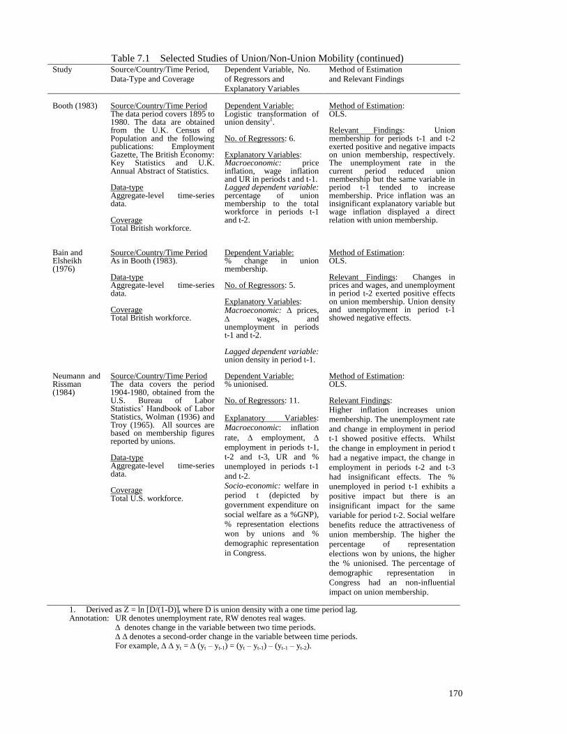
170
Table 7.1 Selected Studies of Union/Non-Union Mobility (continued)
Study Source/Country/Time Period,
Data-Type and Coverage
Dependent Variable, No.
of Regressors and
Explanatory Variables
Method of Estimation
and Relevant Findings
Booth (1983) Source/Country/Time Period
The data period covers 1895 to 1980. The data are obtained from the U.K. Census of Population and the following publications: Employment Gazette, The British Economy: Key Statistics and U.K. Annual Abstract of Statistics. Data-type Aggregate-level time-series data. Coverage Total British workforce.
Dependent Variable: Logistic transformation of union density1. No. of Regressors: 6. Explanatory Variables: Macroeconomic: price inflation, wage inflation and UR in periods t and t-1. Lagged dependent variable: percentage of union membership to the total workforce in periods t-1 and t-2.
Method of Estimation: OLS. Relevant Findings: Union membership for periods t-1 and t-2 exerted positive and negative impacts on union membership, respectively. The unemployment rate in the current period reduced union membership but the same variable in period t-1 tended to increase membership. Price inflation was an insignificant explanatory variable but wage inflation displayed a direct relation with union membership.
Bain and Elsheikh (1976)
Source/Country/Time Period As in Booth (1983). Data-type Aggregate-level time-series data. Coverage Total British workforce.
Dependent Variable: % change in union membership. No. of Regressors: 5. Explanatory Variables: Macroeconomic: prices, wages, and unemployment in periods t-1 and t-2. Lagged dependent variable: union density in period t-1.
Method of Estimation: OLS. Relevant Findings: Changes in prices and wages, and unemployment in period t-2 exerted positive effects on union membership. Union density and unemployment in period t-1 showed negative effects.
Neumann and Rissman (1984)
Source/Country/Time Period The data covers the period 1904-1980, obtained from the U.S. Bureau of Labor Statistics‟ Handbook of Labor Statistics, Wolman (1936) and Troy (1965). All sources are based on membership figures reported by unions. Data-type Aggregate-level time-series data. Coverage Total U.S. workforce.
Dependent Variable: % unionised. No. of Regressors: 11. Explanatory Variables:
Macroeconomic: inflation
rate, employment,
employment in periods t-1,
t-2 and t-3, UR and %
unemployed in periods t-1
and t-2.
Socio-economic: welfare in
period t (depicted by
government expenditure on
social welfare as a %GNP),
% representation elections
won by unions and %
demographic representation
in Congress.
Method of Estimation: OLS. Relevant Findings: Higher inflation increases union
membership. The unemployment rate
and change in employment in period
t-1 showed positive effects. Whilst
the change in employment in period t
had a negative impact, the change in
employment in periods t-2 and t-3
had insignificant effects. The %
unemployed in period t-1 exhibits a
positive impact but there is an
insignificant impact for the same
variable for period t-2. Social welfare
benefits reduce the attractiveness of
union membership. The higher the
percentage of representation
elections won by unions, the higher
the % unionised. The percentage of
demographic representation in
Congress had an non-influential
impact on union membership.
1. Derived as Z = ln [D/(1-D)]t where D is union density with a one time period lag. Annotation: UR denotes unemployment rate, RW denotes real wages.
denotes change in the variable between two time periods. denotes a second-order change in the variable between time periods. For example, yt = (yt – yt-1) = (yt – yt-1) – (yt-1 – yt-2).

171
A range of non-pecuniary influences has been examined in the union choice literature.
Included are the demographic and socio-economic composition of the labour force, in terms
of the age, race, sex, marital status, education, industry, occupation, seniority and
employment status of workers. Several studies have also added what Shister (1954) termed
as a “proximity influence”, which can be viewed as either physical proximity (e.g. rural-
urban-suburb, state), an employer- or employment-specific factor (e.g. relationship with
supervisor, fairness treatment of employee, promotional prospects, job security) or political
proximity, e.g. influence of political party on the union as in Kenyon and Lewis (1997) and
Carruth and Disney (1988).
The empirical findings from this body of research are also of interest, as they can show the
success or otherwise of this approach to modelling. The union/non-union wage differential
was found to have a positive and significant effect on the union choice decision by Christie
(1992). Farber and Saks (1980) went a step further to add a threshold point - workers at the
lower end of the intra-firm earnings distribution (earning less than $0.21/hour above the
infra-firm mean earnings of $0.49/hour) were more likely to join unions. This is consistent
with suggestions in the union literature that unions represent the political interests of lower-
income and disadvantaged persons. For example, see the discussion of the collective voice
“face” of unions in Freeman and Medoff (1984). These and the other studies demonstrate,
therefore, that monetary incentives can be modelled successfully when analyzing worker
mobility.
The studies that have examined the impact of economic variables on the rate of
unionization, however, have produced conflicting results in relation to the possible impact
of unemployment, level of employment and real wages. The relationship between
unemployment and union membership was negative in Borland and Ouliaris (1994), Sharpe
(1971) and Carruth and Disney (1988), but positive in Neumann and Rissman (1984),
Ashenfelter and Pencavel (1969) and Freeman (1989), and insignificant in Kenyon and
Lewis (1997). In the studies by Booth (1983) and Bain and Elsheikh (1976), the
unemployment rate lagged by different time periods also exhibited conflicting results.
Unemployment exerted a negative influence for the current period in Booth (1983) and for
period t-1 in Bain and Elsheikh (1976). The unemployment rate for period t-1 and that for
period t-2 tended to be associated with increased membership in Booth (1983) and Bain and

172
Elsheikh (1976), respectively. In part, the conflicting empirical evidence may reflect the
ambiguous nature of the theoretical predictions. On the one hand, it has been argued that
higher unemployment raises union density because unions are able to increase job security.
On the other hand, if unions are seen as a source of higher unemployment owing to their
wage-setting powers, the incentive to unionise will decline during periods of high
unemployment3.
Similarly, changes in the level of overall employment were found to have a positive effect
on union density in Carruth and Disney (1988), but a negative bearing in Neumann and
Rissman (1984). It should be noted that Sharpe (1971) considered a sectoral breakdown for
the employment variable, with the inclusion of employment in the union sector, which was
found to have a positive impact on union membership. However, as the number of studies
using sector-specific economic indicators is few, no firm conclusions can be formed.
Theoretically, the association of real wage with union choice is indeterminate. It has
generally been argued that this association will be negative, as decreases in wages that lead
to worker dissatisfaction should increase the desire to unionise. However, it is also possible
that workers might join unions to defend real wage gains so that real wages and
unionization will be positively correlated. Given these competing views, it should come as
little surprise that the empirical findings on the union density – real wage relationship are
mixed. Whilst Borland and Ouliaris (1994) and Carruth and Disney (1988)4 concluded that
real wages had a negative effect on union density, Kenyon and Lewis (1990) and Peetz
(1990)5 reported a positive impact. Real wages were found to have an insignificant effect
on unionization in the study by Sharpe (1971).
It was earlier argued that workers seek to maximize their economic wealth and so will join
unions if the perceived union wages are higher. This, however, is tied to a ceteris paribus
assumption that needs to be accommodated in empirical work. Worker characteristics differ
and each labour market exhibits different characteristics. The studies reviewed in Table 7.1
take account of such factors, although the empirical evidence is not always conclusive. For
example, sex and education were found to be significant explanatory variables in Christie‟s
(1992) model for Australia, but not in the study undertaken by Farber and Saks (1980) for
the U.S.
173
There are, however, limitations to these union choice models which the current study
should attempt to overcome. In particular, there appears to be a fundamental oversight
which could explain the conflicting results for business cycle variables. Earlier, it was
observed that sectoral labour movements are determined, in part, by unemployment in
sector „a‟ versus sector „b‟. In the union choice studies, however, an overall unemployment
rate variable is used. That is, there is no distinction as to whether the pool of the
unemployed is generated from the union sector or the non-union sector. This same line of
argument applies to the real wage and employment variables, where empirical studies fail
to differentiate between union/non-union employment and real wages. Kelly and
Richardson (1989) and Booth (1983) have also expressed doubts concerning the
explanatory power of estimating equations based on business cycle models. Sharpe (1971)
also indicated that a disaggregated sectoral unemployment rate might help to explain trade
union growth. The exclusion of these apparently appropriate explanatory variables could
lead to model misspecification, giving rise to misleading results. The empirical review in
chapter 8 addresses this issue6.
7.3 PUBLIC VERSUS PRIVATE SECTOR MOBILITY
Public-private sector mobility is another form of labour mobility7. Both of these sectors are
associated with different characteristics and influences. Whilst the private sector tends to
follow principles of profit-maximisation or cost-minimisation, the public sector is more
often subject to other social, political and non-economic influences. Workers with differing
personal characteristics have differing probabilities of choosing public versus private sector
employment, as they seek the job (or sector) where their specific set of characteristics will
receive the highest rewards. The public-private sector divide resembles more closely the
setting that will be used in the empirical work to be undertaken in this thesis, in that
movement between sectors for public and private sector workers generally involves a
greater set of changes than does movements between sectors for the union and non-union
workers examined above.
Many of the models of public-private sector mobility have a structure that is quite similar to
the empirical model of equation (6.7). Accordingly, this research has included both the
public-private sectoral wage differential and worker/job characteristics as explanatory

174
variables in the estimating equations used. Some examples include Borland, Hirschberg
and Lye (1996) for Australia, Blank (1985), Gyourko and Tracy (1988), Long (1975), Long
(1976) and Utgoff (1983) for the U.S., Hartog and Oosterbeek (1993) for the Netherlands
and van der Gaag and Vijverberg (1988) for Cöte d‟Ivoire.
Table 7.2 overviews the major approaches and findings from research into public-private
sector mobility. The public-private sector studies selected use unit-record cross-sectional
data and incorporate a wealth of monetary and non-pecuniary factors as regressors. The
exception, in this context, is Utgoff (1983) who uses aggregate-level cross-sectional data
and with a smaller number of regressors. However, unlike union/non-union studies with
aggregate-level time-series data, there do not appear to be any studies in the public-private
sector with macroeconomic factors and lagged dependent variables.
The explanatory variables in the private-public sector selection models consist of the
sectoral earnings differential and non-monetary factors. The latter comprises personal
characteristics (sex, age, race, marital status, educational qualification, intelligence quotient
(IQ), veteran status, years and levels of education, past school in non-English speaking
country, school attended, whether born in Asian/non-English speaking country, year of
arrival in Australia, field of study, reading, writing and arithmetic skills, geographic region,
age of youngest child and whether in capital city) and job characteristics (occupation, firm
size, experience and blue-collar versus white-collar status). In addition to these personal
and job characteristics, Hartog and Oosterbeek (1993) added social background indicators,
such as number of siblings, father‟s occupation and father and mother‟s education.

175
Table 7.2 Selected Studies of Public-Private Sector Mobility Study Source/Country/Time
Period, Data-Type and
Coverage
Dependent Variable,
No. of Regressors and
Explanatory Variables
Method of Estimation and Relevant
Findings
Borland, Hirschberg and Lye (1996)
Source/Country/Time Period Australian Bureau of Statistics (ABS) Training and Education Experience Survey 1993. Data-type Unit-record cross-sectional data. Sample of employees. Coverage 5,969 males and 3,376 females aged 15-64 years who were employed full-time as wage and salary earners.
Dependent Variable: Probability of selecting a public sector job. No. of Regressors: 13. Explanatory Variables: Demographic: age, marital status, age of youngest child and whether in capital city. Socio-economic: education level, age minus age left school, experience-squared, year of arrival in Australia, last school attended in non-English speaking country, field of study, whether born in Asian/non-English speaking country and state of residence.
Method of Estimation: Separate probit models for male and female employees. Relevant Findings: Males: The more experienced males residing in Victoria, South Australia (SA) and Western Australia (WA), who have attended a school in a non-English speaking country, arrived in Australia between 1964-1967, 1972-1975, 1986-1987 and 1990-1991, and who have studied Trade Qualification (TQ) in vehicle and food, Post-School Certificate (PSC) in science, computing and agriculture will have a lower likelihood of choosing the public sector. Those who have degrees in law, education, medicine, mathematics, IT, veterinary science, engineering, social sciences and TQ in electricals and electronics, arts, social sciences and crafts, are more likely to choose the public sector. Females: Women with longer job tenures, who are residing in NSW, Victoria, Queensland, SA and WA who arrived in Australia between 1984-1985 have a greater probability of choosing the private sector. Those with children between 0-2 years who have completed degrees in law, education and the social sciences, PSC in education, teacher training, nursing, other health and para-medical, and who arrived in Australia between 1968-1971 and 1972-1975 are more likely to choose the public sector instead.
Blank (1985) Source/Country/Time Period U.S. 1979 Current Population Survey (CPS). Data-type Unit-record cross-sectional data. Random sub-sample of the CPS, i.e. one-fourth of employed heads of households. Coverage 10,908 employed heads of households, of whom 8,344 are in the private sector and 2,564 are in the public sector.
Dependent Variable: Probability of individual being a private sector worker. No. of Regressors: 6. Explanatory Variables: Demographic: sex, race and geographic region. Socio-economic: veteran status, occupation, education level and experience.
Method of Estimation: Probit model. Relevant Findings: For the non-monetary variables, veterans, non-whites, higher-educated persons, workers in services and those in Washington D.C. and with more experience have a higher probability of choosing the public sector. Women showed no statistically distinguishable preference.

176
Table 7.2 Selected Studies of Public-Private Sector Mobility (continued) Study Source/Country/Time
Period, Data-Type and
Coverage
Dependent Variable,
No. of Regressors and
Explanatory Variables
Method of Estimation and Relevant
Findings
Hartog and Oosterbeek (1993)
Source/Country/Time Period Individuals from the Dutch province of Noord-Brabant obtained from addresses in the city population register of the Netherlands in 1983. Data-type Unit-record cross-sectional data. Sample of population. Coverage Males and females from 2,726 addresses in a single province.
Dependent Variable: Probability of selecting a public sector job. No. of Regressors: 8. Explanatory Variables: Monetary: public-private sector wage differential. Demographic: sex (female). Socio-economic: social background (no. of siblings, father‟s occupation, education of father and education of mother), personal characteristics (IQ, education level).
Method of Estimation: Endogenous switching regression model. Relevant Findings: Variables related to social background were unimportant in the determination of public sector employment, except for father‟s education which showed a positive effect. For personal characteristics, vocational and university graduates are more likely to work in the public sector. The higher the IQ, the lower the probability of the individual working in the public sector. Females were less likely to become public servants. The likelihood of public sector employment is higher the larger the predicted wage gain in the public sector.
van der Gaag and Vijverberg (1988)
Source/Country.Time Period Cöte d‟Ívoire Living Standards Survey (CILSS), 1985. Data-type Unit-record cross-sectional data. Sample of households. Coverage 513 wage earners from 1,600 households.
Dependent Variable: Probability of obtaining public sector job. No. of Regressors: 6. Explanatory Variables: Monetary: public-private sector wage differential. Demographic: sex, age and age-squared. Socio-economic: indicators for diploma at elementary, high school, higher and technical diplomas, reading, writing and arithmetic (RRR) skills and years of schooling.
Method of Estimation: Probit model. Relevant Findings: Women are more likely than men to be employed in the public sector. Age (up to 50 years) shows a positive effect on public sector employment. Elementary and high-school diplomas increase the likelihood of a public sector job. Higher and technical diplomas, years of schooling and RRR skills have insignificant effects. The sectoral wage differential is not significantly different from zero.
Gyourko and Tracy (1988)
Source/Country/Time Period U.S. 1977 CPS. Data-type Unit-record cross-sectional data. Sample of population. Coverage Full-time wage earners.
Dependent Variable: Probability of selecting private/union or private/non-union or public/union or public/non-union sector. No. of Regressors: 8. Explanatory Variables: Demographic: marital status, race, gender and region of residence (northeast, central, south and west). Socio-economic: veteran status, seniority status (junior and senior), level of college (1st, 2nd, 3rd and 4th year) and graduate status.
Method of Estimation: Multinomial logit model. The model had 4 distinct labour markets: private/union, private/non-union, public/union and public/non-union sectors. Relevant Findings1: Veterans, juniors,
graduates, those attending higher levels
of college education (3rd-4th year) and
lived in the western region had a higher
chance of selecting a public union/non-
union job. There was no distinct
preference for a public union/non-
union job versus private union/non-
union job for workers who are white,
married, male, seniors, have lower
level of college education (1st and 2nd
year) and lived in the northeast, central
and south regions.

177
Table 7.2 Selected Studies of Public-Private Sector Mobility (continued) Study Source/Country/Time
Period, Data-Type and
Coverage
Dependent Variable,
No. of Regressors and
Explanatory Variables
Method of Estimation and Relevant
Findings
Long (1975) Source/Country/Time Period
U.S. 1970 Census of Population. The reference year is 1969. Data-type Unit-record cross-sectional data. 1-in-1,000 public use sample of the 1970 census data. Coverage 40,578 males aged 14 years and over, of which 3,886 were black.
Dependent Variable: Probability of public sector employment. No. of Regressors: 6. Explanatory Variables: Demographic: indicators for males aged 14 years and over, males aged 18-34 years, workers in the southern region and non-southern region. Socio-economic: white-collar workers and blue-collar workers.
Method of Estimation: Linear probability model. Relevant Findings: The study concentrates on sectoral differences in employment for blacks relative to whites. The probability of public sector employment was higher for black white-collar and blue-collar workers, black males aged 14 years and over, and those aged 18-34 years. In both southern and non-southern regions, blacks were relatively more likely to be employed in the public sector rather than the private sector.
Long (1976) Source/Country/Time Period U.S. 1970 Census of Population. The reference year is 1970. Data-type Unit-record cross-sectional data. 1-in-1,000 public use sample of the 1970 census data. Coverage Male and female employees.
Dependent Variable: Probability of Federal Employment. No. of Regressors: 4. Explanatory Variables: Demographic: marital status (married and single) of workers. Socio-economic: indicators for white-collar workers, and occupation (professionals, managers and administrators).
Method of Estimation: Linear probability model. Relevant Findings: Females are less likely to be employed in the public service. Specifically, females who are white-collar workers, professionals, administrators and managers tend to be under-represented in the public service. Marriage has a negative impact on the probability of public employment among females, while being single had a positive but insignificant effect.
Utgoff (1983) Source/Country/Time Period U.S. 1972 Bureau of Labor Statistics‟ (BLS) data and 1972 Census of Manufactures. Data-type Aggregate-level cross-sectional data. Sample of the population (for BLS data on quit rates). Coverage Government employees.
Dependent Variable: Probability of quitting the public sector. No. of Regressors: 2. Explanatory Variables: Monetary: average hourly earnings. Socio-economic: firm size.
Method of Estimation: OLS. Relevant Findings: Larger firm size and higher average hourly earnings had a negative effect on the probability of quitting the public sector.
1. The Gyourko and Tracy (1988) study had four labour market choices: public union, public/non-union, private
union and private non-union. Since the focus is on the choice between two labour markets (public versus
private sector), the findings presented reflect the most significant result which will be independent of
union/non-union choice.
As argued previously, it would be expected that higher wages in the public sector would
induce wealth maximizing individuals to seek employment in that sector. Hartog and
Oosterbeek (1993) found that the larger the predicted wage gain in the public sector, the
higher the likelihood of public sector employment. In Borland, Hirschberg and Lye (1996),
public sector male and female employees had higher wages than their counterparts in the
private sector, implying that the higher-paid public sector would attract individuals to seek
employment in that sector. However, it has also been argued that there may be non-wage

178
benefits, e.g. job stability, working hours and fringe benefits, that are generally not
considered in the statistical analyses, and the presence of which mean that workers may
prefer the public sector even if monetary wages are higher in the private sector. In the case
of the Ivorian market, the sectoral earnings differential did not have a significant impact on
the choice of sectoral employment. Thus, with the exception of the Ivorian labour market,
the evidence for public-private sector mobility sits comfortably alongside that for
union/non-union choice models. Hence, emphasis can be placed on the estimated impact of
the sectoral wage advantage in both the union choice equation and the public sector/private
sector model.
The findings on education levels were consistent for all the studies represented in Table 7.2,
except for Borland, Hirschberg and Lye (1996). Specifically, public sector choice tended to
be associated with higher education levels, even though the specification of the education
variables differed across studies. In particular, Blank (1985) found that higher-educated
persons in the U.S. had a higher probability of choosing the public sector. Hartog and
Oosterbeek (1993) demonstrated that university graduates in the Netherlands were more
likely to work in the public sector than in the private sector. van der Gaag and Vijverberg
(1988) also found that public sector employees were, on average, better educated than
private sector employees for the Ivorian labour market. Gyourko and Tracy (1988) found
that graduates and persons with higher levels of diplomas had a greater likelihood of
choosing a public sector job. This is not surprising as the public sector has been perceived
as recruiting better educated persons to assist in the planning of policies and evaluation of
programmes.
It has been argued that certain groups, e.g. non-whites and women, may have a higher
probability of choosing the public sector. Non-whites may choose the public sector as the
work practices are less discriminatory. Women may prefer the public service given that the
work environment there is more family friendly, with practices facilitating intermittent
labour market attachment. The findings on the racial divide were consistent for the U.S.
Blacks and other non-whites were found to have a higher probability of choosing public
sector employment in the three studies conducted for the U.S. for the different periods of
analysis [Blank (1985), Long (1975) and Gyourko and Tracy (1988)]. For Australia,
179
being born in an Asian country did not have a significant impact on public-private sector
choice [Borland, Hirschberg and Lye (1996)].
The findings on the role of gender on public sector choice were inconclusive. Whilst van
der Gaag and Vijverberg (1988) and Gyourko and Tracy (1988) found that women were
more likely than men to choose public sector employment, Hartog and Oosterbeek (1993)
and Long (1976) reported that females were less likely to become public servants. Blank
(1985), however, reported that being female had a statistically insignificant impact on
public sector choice. Apart from the fact that the role of women at work varies in
importance across different countries, a possible reason for the mixed evidence could be a
failure to take adequate account of the composition of female employment by occupation,
industry etc. For instance, if the public sector in a country had a higher proportion of
clerical personnel compared to professionals, and if such workers are predominantly
female, then it could be expected that women, on the whole, would have a higher chance of
securing public sector employment, particularly if insufficient account is taken of
occupational structure in the estimations.
A final point to note in relation to the public-private sector selection models is that sectoral
unemployment does not appear to have been recognized in the analyses. This may be due
to data limitations. While datasets are available that contain information on the type of
work (e.g. occupation/industry) that individuals are seeking, and hence facilitate the
estimation of unemployment models for different sectors, this information may not be
available in the datasets used for the studies reviewed in Table 7.2.
7.4 RURAL-URBAN MOBILITY
Rural-urban mobility (or migration) is another type of labour mobility that has been
researched extensively8. Todaro (1969) and Harris and Todaro (1970) hypothesized that
rural-urban mobility is stimulated primarily by rational economic considerations of relative
benefits and costs, and it is mainly the expected urban-rural income differential that will
influence the individual‟s decision to move9. The studies on rural-urban mobility have
mainly been conducted for developing countries with a predominantly agrarian population,
180
i.e. Schultz (1971) for Columbia and Ghatak (1996) for India, as well as NIEs with a
substantial share of rural workers, namely Tcha (1993) for Korea and Zahn (1971) for
Japan. The relevance of these studies to the current analysis lies in the emphasis placed on
the monetary and non-pecuniary determinants.
Table 7.3 summarises the main findings of several studies conducted for the U.S., South
America and Asia. With the exception of Ghatak (1996), the authors have included the
sectoral wage differential as well as macroeconomic (e.g. overall unemployment and
economic growth rate), demographic (e.g. urban-rural population ratios, rural labour supply
and the age-sex distribution of the population) and a rich array of socio-economic (e.g.
education, violence indicators and travel time to city) elements in the rural-urban mobility
function.
These rural-urban studies use aggregate-level data. Whilst the aggregate-level time-series
analyses have incorporated macroeconomic variables, those with cross-sectional data, i.e.
Ghatak (1996) and Schultz (1971), have not. The absence of macroeconomic determinants
for cross-sectional analyses was also observed in the union/non-union and public-private
sector studies. This arises as cross-sectional studies are unable to track the consequences of
a structural change in the macroeconomy. In addition, as in the case of public-sector
studies, the rural-urban studies generally have a fewer number of regressors (6 or less)
when aggregate-level data are applied.
The primary explanatory variable in these studies is the rural-urban wage differential10
.
According to Todaro‟s model and the model outlined in chapter 6, there should be a clear
positive relationship between the wage differential and worker mobility, especially when
the probability of obtaining work in the urban sector is taken into account. However, this
clear theoretical prediction is not reflected in the empirical literature. The studies that are
consistent with the Todarian hypothesis, and report a positive relationship between the
urban-rural income ratio/differential and rural-urban movements, include Tcha (1993) for
the U.S. and Zahn (1971) for Japan. The sectoral wage differential was insignificant in the
study by Ghatak (1996). In contrast, Tcha‟s (1996) findings for the Korean labour force
did not support Todaro‟s hypothesis: he found that Korean villagers were willing to

181
sacrifice higher rural wages for lower incomes in return for better living conditions in urban
areas, provided the expected urban wages were at least 75 per cent of the original rural
income.
Table 7.3 Selected Studies of Rural-Urban Sector Mobility Study Source/Country/Time
Period, Data-Type and
Coverage
Dependent Variable, No.
of Regressors and
Explanatory Variables
Method of Estimation and
Relevant Findings
Tcha (1993)
Source/Country/Time Period Annual data of U.S., 1960-1987. Data-type Aggregate-level time-series data. Sample of population. Coverage U.S. migrants.
Dependent Variable: Net rural-urban migration rate1. No. of Regressors: 4. Explanatory Variables: Monetary: dynastic rural-urban income ratio. Macroeconomic: real growth rate of the economy and overall unemployment rate. Demographic: ratio of the rural population to urban population.
Method of Estimation: OLS (log-linear). Relevant Findings: Dynastic income ratio and economic growth rate had significant positive effects on rural-urban migration. Effects of the overall unemployment rate and ratio of the rural population to urban population were insignificant.
Schultz (1971)
Source/Country/Time Period Columbia, 1951 and 1964. Data-type Aggregate-level cross-sectional data. Sample of 131 Columbian municipalities drawn from 1951 and 1964 Population Census data. Coverage Males and females aged 7-51 years.
Dependent Variable: Net migration rate for rural population2. No. of Regressors: 5. Explanatory Variables: Monetary: rural wage. Socio-economic: school enrolment for children aged 5-9 years and 10-14 years, frequency of political violence and distance to travel to the next city. Demographic: growth rate of rural labour supply.
Method of Estimation: OLS. Relevant Findings: Rural wage has a negative effect on out-migration. An increase in the growth rate of the rural labour supply accelerates out-migration. School children aged 10-14 years are more likely to move to urban areas than those 5-9 years. The effect of greater distance to the next city spurs migration. An increase in rural violence encourages persons to move to urban areas.
Tcha (1993) Source/Country/Time Period Annual data of Korea, 1963-1988. Data-type Aggregate-level time-series data. Sample of population. Coverage Korean migrants.
Dependent Variable: Net rural-urban migration rate1. No. of Regressors: 4. Explanatory Variables: Monetary: dynastic rural-urban income ratio. Macroeconomic: real growth rate of the economy and overall unemployment rate. Demographic: ratio of the rural population to urban population.
Method of Estimation: OLS (log-linear). Relevant Findings: For the income variable, people are willing to move to urban areas until the expected dynastic income is 75% of the rural income. Economic growth rate had a positive effect on migration and the unemployment rate had a negative effect. The result for the ratio of the rural population to urban population was insignificant.

182
Table 7.3 Selected Studies of Rural-Urban Sector Mobility (continued)
Study Source/Country/Time
Period, Data-Type and
Coverage
Dependent Variable, No.
of Regressors and
Explanatory Variables
Method of Estimation and
Relevant Findings
Zahn (1971) Source/Country/Time Period
The data covers the period 1878 to 1937. Agricultural and industrial labour, real output and working age population are obtained from Ohkawa (1957). The capital stock series are estimated from Ohkawa‟s (1957) capital stock estimate and Rosovsky‟s (1961) savings data. Population data are from the Bank of Japan. Data-type Aggregate-level time-series data. Coverage Males and females aged 14 years and over.
Dependent Variable Industrial-agrarian labour force ratio. No. of Regressors Demand equation: 2. Supply equation: 2. Explanatory Variables:
Demand Equation
Industrial-agrarian required labour ratio is expressed as a function of the socio-economic (industrial-agrarian capital stock ratio) and macroeconomic (real output ratio and technical progress) factors.
Supply Equation
Industrial-agrarian labour force ratio is expressed as a function of the monetary (expected urban-rural income ratio) and demographic (an index of the age-sex distribution of the population) factors.
Method of Estimation: Simultaneous equation model using 2-stage least squares estimation. Relevant Findings: Demand Equation The industrial-agrarian real output ratio and technical progress have positive effects on the industrial-agrarian labour ratio. The industrial-agrarian capital stock ratio had a negative effect. Supply Equation An increase in the actual urban-rural wage ratio leads to out-migration. A higher number of working age persons and females both induce out-migration.
Ghatak (1996)
Source/Country/Time Period Census of Population 1971 and 1981 obtained from the Statistical Abstract of the Indian Union. Data-type Aggregate-level cross-sectional data. Coverage Rural and urban population for all Indian States.
Dependent Variable 3 variables: size/growth rate/density of urban population (UP). No. of Regressors: 1. Explanatory variables: Monetary: estimated rural-urban income differential.
Method of Estimation: OLS. Relevant Findings: For these 3 regressions, a higher urban-rural wage differential does not appear to induce out-migration.3
1. The rate is calculated using the actual and expected rural population (RP) data. The expected RP in period t is
calculated by multiplying RP in period t-1 (RPt-1) by the natural population growth rate allowing for births and
deaths (δt). Subtracting the actual RPt from RPt-1(1+ δt) gives net rural-urban migration.
2. Net migration rate is defined as the ratio of a net migration flow in the rural sector to the average size of the
local population. A negative migration rate means a net out-migration from the rural sector, and conversely for
a positive migration rate. 3. According to Ghatak (1996), several factors, i.e. moving costs, expected wages, skill levels, risk-taking
behaviour of individuals and borrowing and liquidity constraints, were not taken into consideration, and this could explain why the Todarian hypothesis was not supported.
The conflicting findings in relation to the estimated impact of the monetary variable could
be due to two factors. Firstly, as in the public-private sector studies, differences exist
between rural-urban work environments, individual preferences, culture of country etc., and
the effects of the monetary element are therefore not expected to be the same for studies

183
conducted in different contexts. Secondly, different measurements of the variable have
been used. Ghatak (1996), for example, computed the rural-urban income ratio using the
estimated agricultural and industrial incomes for India (in Rupees) at current prices, while
Zahn (1971) used the actual urban-rural income differential. In comparison, Tcha (1993)
calculated a dynastic income ratio of the weighted average of blue-collar and white-collar
incomes in the urban area to the income in the rural area, where the weights were chosen
iteratively and were related to time and altruistic discount rates between generations.
Schultz (1971) only considered the push factor of the rural wage as a determinant of
mobility.
The dynastic income ratio used by Tcha (1983) suggests that the wage differential should
account for altruism between generations which has multiplicative effects on a family‟s
decision to migrate. The average of blue-/white-collar incomes was also used in the
dynastic measure as migrants from rural areas typically have insufficient physical and
human capital, and are more likely to use the urban blue-collar income as their expected
income. This type of dynastic income measure is not relevant to analysis of
sectoral/industrial mobility. Whilst rural-urban migration decisions involving inter-regional
movements could cause multi-generational family migration, sectoral/industrial mobility is
usually independent of family migration.
The rural-urban mobility models do not have a sectoral breakdown of the unemployment
rate, unlike that suggested for the current empirical model. Such a breakdown is important
theoretically as sectoral movements could prevail in the presence of higher unemployment
in the new sector where migrants would be underemployed in the informal sector.
Underemployment is, however, difficult to measure, and this measurement problem may
explain the practice (of omitting unemployment rate variables) in applied work. In
comparison, the inclusion of the sectoral unemployment rates in the empirical work is
likely to be important in the current research, and it is practical to include relevant measures
in the estimating equations.
184
Several aspects of the rural-urban migration analyses are of value to the current study.
First, the use of the sectoral wage differential is notable and this variable can be considered
for inclusion in the current work. Second, the use of sectoral performance indicators in
rural-urban studies is an approach that can be followed. In the study of rural-urban
migration, individuals are argued to move from the lower-growth sector to the rapidly
growing sector. The variables indicative of sectoral growth comprise the industrial-
agrarian labour force, capital stock and real output [Zahn (1971)] and growth rate of rural
labour supply [Schultz (1971)]. Whilst the industrial-agrarian labour force ratio acts as a
demand-pull factor, where a higher ratio (e.g. from technology shock) causes urban wages
to rise and pulls people to migrate to urban areas, higher rural labour supply acts as a
supply-side factor causing rural unemployment and pushing people to migrate. For
sectoral/industrial mobility, it would be the growth (declining) sectors that induce workers
to move to (out of) their sectors.
7.5 SUMMARY: SALIENT POINTS FOR EMPIRICAL MODEL
The review of the literature in this chapter has highlighted the following points which
should inform the empirical work to be undertaken in chapters 9 and 10.
a) The determinants of sectoral mobility should be modelled within a framework
comprising a sectoral wage differential and the macroeconomic and non-
monetary factors associated with mobility.
b) A sectoral distinction in the macroeconomic variables, especially on
unemployment, is desirable.
c) The non-pecuniary determinants should also be measured on a sector-by-sector
basis where possible.
d) The type of data to be used affects model specification. The longitudinal data
that are to be used have the advantage that macroeconomic and lagged
dependent variables, which have been demonstrated to be significant
determinants of labour mobility, can be incorporated into the estimating
equation.

185
Endnotes:
1. It is recognized that the worker movement can be from the non-union sector to the union sector or from the
union sector to the non-union sector. For ease of exposition the discussion here is in terms of the former flow
of workers.
2. The sole exception to this appears to be Gyourko and Tracy (1988).
3. See Borland and Ouliaris (1994).
4. Carruth and Disney (1988) incorporated a dummy variable for political climate: 1 when the
Labour/Liberals were in power and 0 for the presence of a Conservative government. The initial regression
in the absence of the political dummy revealed that the real wage had a negligible effect on union
membership.
5. Peetz (1990) presented evidence on workers in the manufacturing sector. Those who experienced a decline
in real wage in the previous two years had a higher desire to unionise.
6. The exception applies to changing price levels, which were found to be directly related to union
membership in Neumann and Rissman (1984), Carruth and Disney (1988) and Bain and Elsheikh (1976). A
possible explanation for the non-conflicting result in this instance is that, unlike real wages and
unemployment, prices are not sector-specific. All individuals/workers, regardless of whether they are union
or non-union members, face similar price levels. It is noted that for Carruth and Disney (1988), the findings
reported are obtained from their nominal inflation model.
7. Private-public sector labour flows do occur, but for ease of exposition the review examines the public-
private sector mobility.
8. While there may be urban-rural labour flows, most literature addresses the more important rural-urban
flow, and this is the focus of this section.
9. Several authors, like Mincer (1978) and Borjas (1990), have questioned the hypothesis that migration
behaviour can be explained solely by the individual‟s income. Mincer (1978) examined decision making
within the family unit, particularly the effect of interactions between husband and wife on the probability of
migration. Borjas (1990) considered the welfare of children as a determinant in the migration function.
10. Earlier studies prior to Todaro [Jorgensen (1967) and Ranis and Fei (1964)] examined rural-urban
mobility using the wage differential.
186
CHAPTER 8
EMPIRICAL EVIDENCE:
FACTORS MOTIVATING SECTORAL/INDUSTRIAL MOBILITY
8.1 INTRODUCTION
This chapter reviews the empirical evidence on the factors motivating sectoral/industrial
mobility. These factors include monetary and macroeconomic characteristics, worker and
job characteristics, and sectoral shocks. Various labour markets are covered. Moreover,
where possible, results for both males and females, as well as for the overall labour force,
are reviewed.
The chapter categorises the studies according to labour mismatch, sectoral shock and
bridging theories. Section 8.2 gives a general introduction to the concept of
sectoral/industrial mobility and introduces the studies covered. Section 8.3 outlines the
impact of explanatory variables under the labour mismatch theory. These variables include
monetary and macroeconomic factors and worker and job characteristics. Section 8.4
focuses on the effects of a sectoral shock on mobility under the shock theory. The
implications from a single study based on the bridging theory are covered in section 8.5.
The impact of the explanatory variables on overall (i.e. both male and female workers)
mobility will first be reviewed. This will be followed by an examination of gender
differences in sectoral labour market outcomes. An assessment of the empirical studies of
sectoral mobility for the purpose of empirical modelling is given in section 8.6. A
summary of the findings is provided in the final section, together with suggestions on the
applicability of the explanatory variables to the current empirical study of Korea.
8.2 SECTORAL/INDUSTRIAL MOBILITY
Sectoral/industrial mobility is the main form of labour mobility of interest to the current
research. It is a complex matter involving a spectrum of factors in the individual‟s decision-
making process, and the costs and benefits involved are usually of far greater importance
than those that need to be considered in union/non-union or intra-sectoral mobility. In the

187
latter forms of mobility, wealth-maximising individuals select jobs similar to their former
jobs/sectors so that much of their human capital can be transferred to the new sector in
return for wage gains. Consequently, the costs of moving, and the wage gains required to
induce mobility, will usually be relatively minor. In comparison, the costs and barriers to
entry in inter-sectoral mobility are greater. As sector-specific skills may not be easily
transferable to other sectors, skills relevant to the new sector will need to be acquired, and
this means the investment costs necessary to facilitate the move may be considerable.
Moreover, limited market knowledge of the new sector may act as a barrier to entry
[Subrahmaniam, Veena and Parikh (1982) and Gallaway (1965)]. There may also be
psychic costs to moving that are of greater importance than in intra-sectoral mobility, e.g.
uncertainty about prospects in the new sector which pose as artificial barriers to entry
[Greenwood (1975), Gallaway (1965) and Vanderkamp (1977)]. These real and artificial
barriers to entry constitute a further cost that workers need to take into account in their
choice of sector/industry.
These issues are prominent in empirical studies of sectoral mobility. Under the labour
mismatch theory, the main studies of sectoral/industrial mobility are Osberg (1991),
Osberg, Gordon and Lin (1994) and Vanderkamp (1977) for Canada, Loungani and
Rogerson (1989), McLaughlin and Bils (2001) and Brainard and Cutler (1993) for the U.S.,
Prasad (1997) for Japan and Jayadevan (1997) for India. These studies covered employed
workers, where sectoral mobility rates of around 13% [U.S. males in Jovanovic and Moffitt
(1990) and Canadian employees in Osberg, Gordon and Lin (1994)] have been reported.
Inter-industrial movements are higher for the unemployed (about two-thirds of the
unemployed who gained employment changed their industry of employment in Thomas
(1996b)1 and Neal (1995)
2), but there are only a small number of studies of their behaviour.
The main contributions are Fallick (1993), Thomas (1996b), Neal (1995) and Kim (1998)
for the U.S.,3 and Ottersen (1993) for Sweden.
The studies of the sectoral shock hypothesis cover a range of countries, including Brainard
and Cutler (1993) and Clark (1998) for the U.S., Gulde and Wolf (1998) for the European
Union (France, Italy, Germany and Spain) and Altonji and Ham (1990) for Canada. The
sole study based on the bridging hypothesis was undertaken by Jovanovic and Moffitt
(1990) for the U.S.

188
8.3 DETERMINANTS UNDER THE MISMATCH THEORY
The aim of this section is to review the determinants covered in the studies of sectoral
mobility under the mismatch theory. Table 8.1 provides a selection of the relevant
empirical literature. The explanatory variables under the bridging theory in Jovanovic and
Moffitt (1990) are also presented so that the variables (excluding the sectoral shock) can be
compared with those under the mismatch theory. These studies are chosen as they cover a
wide range of the monetary, macroeconomic and non-pecuniary factors that appear to be
directly related to the current work. Additionally, the studies cover the main worker
groups, namely, the overall workforce as well as males and/or females. This is relevant to
the separate analyses undertaken later for males and females in the Korean labour market.
The determinants include a sectoral distinction for the monetary variable (e.g. wage
differential between the old and new industries or wages in the original and/or wages in the
new industries, industry per worker real wage growth rate and sectoral wages relative to
total wages) and macroeconomic factors (overall GNP and employment, employment in the
old and new industries, unemployment in the old and new industries and the ratio of
employment in the old industry to that of the new industry). Some of the macroeconomic
factors, e.g. average and real GNP growth, overall employment and unemployment and
unemployment duration, do not have a sectoral breakdown. Most of these variables were
analysed from the perspective of the ways they affected overall mobility. However, the
analysis of the impact of the overall unemployment rate and duration of unemployment
spell was extended to male and female mobility, and the analyses of the effects of wages in
the old/new sector and relative sectoral wages were undertaken for male mobility.
The non-pecuniary factors include worker and job characteristics. The worker
characteristics consist of demographic factors (sex, age, age of entry and marital status) and
socio-economic characteristics (education status, language ability, unionization, head of
household status, having children, skill levels, e.g. white-collar job, job tenure and
employment status). These characteristics are fixed for the worker and so there is no need
to consider sector-specific measures. The examination of the impacts of marital status,
tenure, employment status, occupational status, initial industry and working hours was
carried out for male/female mobility, and that of formal education for male mobility.

189
The job characteristics comprise working hours/weeks, training, industry, industry
performance, occupation, industry size, turnover, output, whether the industry provides
unemployment insurance/social benefits, product/work similarity4, type of job loss (e.g.
advance notification, due to slackness or shift in position) and male-female mix in the
industry. These variables tend to be sector- or industry-specific, and there are quite
considerable variations across industries in these factors. Consequently, it is expected that
most variables will exert greater influence on sectoral mobility than on other forms of
worker mobility. In addition, sector-specific shocks which are believed to affect certain
economic sectors causing sectoral mobility were included in many studies.
These studies either cover the employed or unemployed. As employed workers have greater
access to information markets, i.e. networks in other sectors and capital markets, and face
greater opportunity costs in changing sectors [Pissarides and Wadsworth (1989)], it is
expected that the personal characteristics and market conditions that affect their mobility
will differ from those for the unemployed. Where possible therefore, the empirical
determinants of mobility for these two groups need to be assessed separately.
It was earlier highlighted that several studies examine the determinants of sectoral mobility
separately for males and/or females. However, Osberg (1991) appears to be the only study
that compares the inter-industry mobility patterns of male and female employees. Gender
comparisons regarding the determinants of industrial mobility are therefore limited to the
explanatory variables covered in his study. Many studies focus on male mobility behaviour,
including Osberg (1991), Osberg, Gordon and Lin (1994), and Jovanovic and Moffit (1990)
for the employed, and Neal (1995), Fallick (1993) and Thomas (1996b) for the
unemployed. Other studies have covered either the overall workforce [Vanderkamp
(1977), Loungani and Rogerson (1989) and Ottersen (1993)], industry establishments
[McLaughlin and Bils (2001) and Jayadevan (1997)] or sectoral employment [Prasad
(1997), Gulde and Wolf (1998), Altonji and Ham (1990), Brainard and Cutler (1993) and
Clark (1998)].
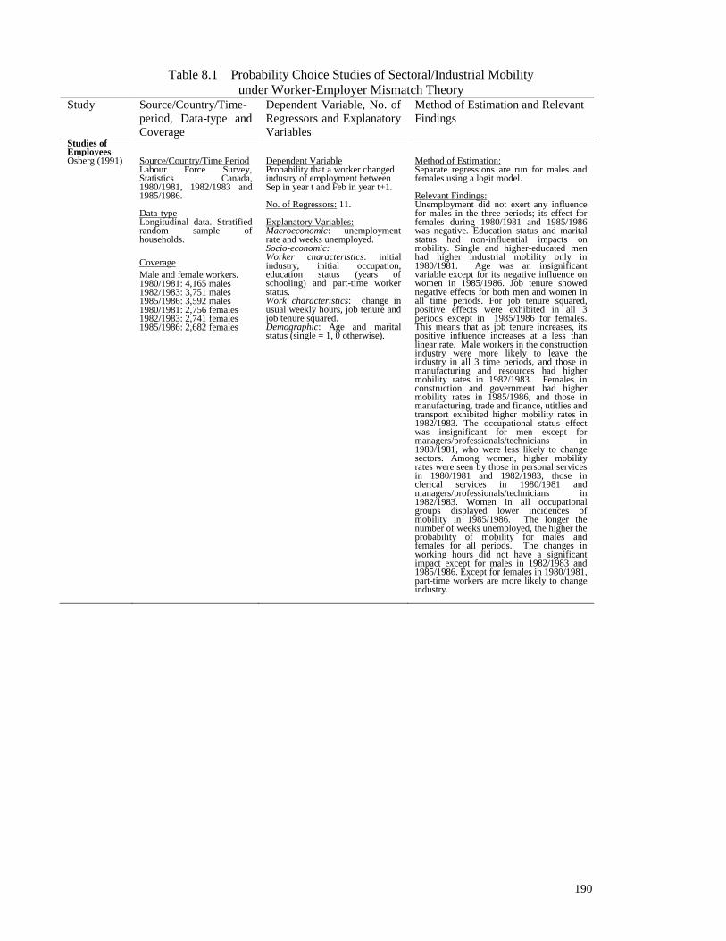
190
Table 8.1 Probability Choice Studies of Sectoral/Industrial Mobility
under Worker-Employer Mismatch Theory Study Source/Country/Time-
period, Data-type and
Coverage
Dependent Variable, No. of
Regressors and Explanatory
Variables
Method of Estimation and Relevant
Findings
Studies of Employees
Osberg (1991) Source/Country/Time Period Labour Force Survey, Statistics Canada, 1980/1981, 1982/1983 and 1985/1986. Data-type Longitudinal data. Stratified random sample of households.
Coverage
Male and female workers. 1980/1981: 4,165 males 1982/1983: 3,751 males 1985/1986: 3,592 males 1980/1981: 2,756 females 1982/1983: 2,741 females 1985/1986: 2,682 females
Dependent Variable Probability that a worker changed industry of employment between Sep in year t and Feb in year t+1. No. of Regressors: 11. Explanatory Variables: Macroeconomic: unemployment rate and weeks unemployed. Socio-economic: Worker characteristics: initial industry, initial occupation, education status (years of schooling) and part-time worker status. Work characteristics: change in usual weekly hours, job tenure and job tenure squared. Demographic: Age and marital status (single = 1, 0 otherwise).
Method of Estimation: Separate regressions are run for males and females using a logit model. Relevant Findings: Unemployment did not exert any influence for males in the three periods; its effect for females during 1980/1981 and 1985/1986 was negative. Education status and marital status had non-influential impacts on mobility. Single and higher-educated men had higher industrial mobility only in 1980/1981. Age was an insignificant variable except for its negative influence on women in 1985/1986. Job tenure showed negative effects for both men and women in all time periods. For job tenure squared, positive effects were exhibited in all 3 periods except in 1985/1986 for females. This means that as job tenure increases, its positive influence increases at a less than linear rate. Male workers in the construction industry were more likely to leave the industry in all 3 time periods, and those in manufacturing and resources had higher mobility rates in 1982/1983. Females in construction and government had higher mobility rates in 1985/1986, and those in manufacturing, trade and finance, utitlies and transport exhibited higher mobility rates in 1982/1983. The occupational status effect was insignificant for men except for managers/professionals/technicians in 1980/1981, who were less likely to change sectors. Among women, higher mobility rates were seen by those in personal services in 1980/1981 and 1982/1983, those in clerical services in 1980/1981 and managers/professionals/technicians in 1982/1983. Women in all occupational groups displayed lower incidences of mobility in 1985/1986. The longer the number of weeks unemployed, the higher the probability of mobility for males and females for all periods. The changes in working hours did not have a significant impact except for males in 1982/1983 and 1985/1986. Except for females in 1980/1981, part-time workers are more likely to change industry.

191
Table 8.1 Probability Choice Studies of Sectoral/Industrial Mobility
under Worker-Employer Mismatch Theory (continued) Study Source/Country/Time-
period, Data-type and
Coverage
Dependent Variable, No. of
Regressors and Explanatory
Variables
Method of Estimation and Relevant
Findings
Studies of Employees
Vanderkamp (1977)
Source/Country/Time Period Canadian Insured Population for years 1965/1966, 1966/1967 and 1967/1968. Data-type Unit-record, cross-sectional data. Sample of Insured Population. Coverage 4,692 employees.
Dependent Variable Proportion of moves from industry i to j. No. of Regressors (linear model): 25. Explanatory Variables: Monetary: wage in original industry (Yi) and wage in new industry (Yj). Macroeconomic: unemployment in original industry (Ui) and unemployment in new industry (Uj). Socio-economic: Worker characteristics: formal education in original industry (EDi), education in new industry (EDj), (EDiEDj)
1/2, unionization in original industry (CAi), unionization in new industry (CAj), (CAiCAj)
1/2, change in occupation, change in province of employment and change in occupation and province of employment. Work characteristics: industry size (Pj), industry turnover and dummy variables for product similarity, location similarity and work similarity. Demographic: age of entry in original industry (Ai), age of entry in new industry (Aj), (AiAj)
1/2, male-female specialization in the original industry (Fi), male-female specialization in the new industry (Fj) and (FiFj)
1/2.
Method of Estimation: OLS for linear mobility model. Relevant Findings from Linear Model: For 1965/1966 and 1966/1967, the lower the wage in the original industry, the higher the likelihood of mobility. Conversely, higher wages in the new industry induce industrial mobility for all three periods. Higher unemployment in the original industry encourages industrial mobility. Unemployment in the new industry did not have a significant effect for 1966/1967 and 1967/1968. The larger the industry size and turnover, the higher the probability of mobility. Education, age of entry and male-female specialisation in the new and original industries displayed negative effects on industrial mobility. However, the effects of the coefficients on (EDiEDj)
1/2, (AiAj)1/2 and
(FiFj)1/2 were positive. Unionization in the
old and new industries had negative effects on mobility except for unionization in the new industry in 1965/1966. The effect of the coefficient on (CAiCAj)
1/2 was positive for 1965/1966 and 1966/1967. The change in occupation and change in occupation and province indicators had negative effects on industrial mobility. However, the change in the province of employment had a positive impact on mobility. The 3 dummy variables for product, location and work similarity showed positive and significant effects on inter-industry mobility.
Osberg, Gordon and Lin (1994)
Source/Country/Time Period 1986-1987 Labour Market Activity Survey (LMAS) extracted from the Labour Force Survey, Statistics Canada. Original interview conducted in Jan/Feb 1987 on labour market activities with a re-interview concerning activities in 1987 being conducted in Jan/Feb 1988. Data-type Longitudinal data. Stratified sample of households. Coverage Prairie and Atlantic male employees aged 16-69 years with hourly wages in both surveys. Initial sample is 8,570 males, out of which 1,095 changed industries.
Dependent Variable Probability of inter-industry mobility. No. of Regressors: 14. Explanatory Variables: Monetary: wage differential. Macroeconomic: no. of weeks unemployed. Socio-economic: Work characteristics: index of job availability, desire for more working weeks per year and desire for more work hours. Worker characteristics: education qualification (elementary, post-secondary, diploma, university), language (French speaking indicator), job tenure, received unemployment insurance indicator, received training in 1986 indicator, received social assistance indicator and used CEC1 in 1986 indicator. Demographic: age (16-19 years, 20-24 years and 25-34 years) and marital status (married).
Method of Estimation: Bivariate probit model of simultaneous choice between 3 states: immobility, inter-regional and inter-industry mobility during 1987. Relevant Findings: The wage differential did not exert any influence on inter-industry mobility. The greater the availability of jobs and the shorter the job tenure, the higher the probability of inter-industry mobility. Persons aged 16-19, 20-24 and 25-34 years, desiring a higher number of working weeks per year and more working hours per week, with a post-secondary education, with longer duration of unemployment and who received unemployment insurance and those who received training in 1986 showed a higher incidence of inter-industry mobility. French speakers, married persons, those with elementary, diploma or university education, those who used CEC and received social assistance displayed insignificant effects on industrial mobility.

192
Table 8.1 Probability Choice Studies of Sectoral/Industrial Mobility
under Worker-Employer Mismatch Theory (continued) Study Source/Country/Time-
period, Data-type and
Coverage
Dependent Variable, No. of
Regressors and Explanatory
Variables
Method of Estimation and Relevant
Findings
Studies of Employees
Jovanovic and Moffitt (1990)
Source/Country/Time Period National Longitudinal Survey of Young Men, U.S., 1968-1981. Data-type Longitudinal data. Survey sample of males. Coverage Male employees aged 14-24 years were interviewed in 1966 and who were 29-39 years in 1981 at the last interview. There are a total of 9,963 observations: 492 (1965-1968), 754 (1968-1970), 628 (1967-1969), 887 (1969-1971), 1,357 (1971-1973), 1,846 (1973-1975), 2,032 (1976-1978) and 1,967 (1978-1980).
Dependent Variable Probability of a sectoral move. No. of Regressors: 2. Explanatory Variables: Monetary: standard deviation of wage distribution. Socio-economic: Worker characteristics: Job experience (5 years, 8 years and 11 years). Aggregate Disturbance term: sectoral shocks.
Method of Estimation 1. Probit mobility equation estimated separately for each year as a function of education, experience, experience-squared, and race. Only the fitted probabilities at 5, 8 and 11 years of job experience are shown for each regression estimated for the years 1968 to 1973, 1975, 1978 and 1980. 2. The probability of a sectoral move was regressed on the standard deviation of the log (wage distribution) and standard deviation of sectoral shocks at 5, 8 and 11 years of job experience. Relevant Findings: 1. The probability of a sectoral move decreased for all experience levels (5 years, 8 years and 11 years of experience). Mobility fell much faster from 1968 to 1973 than from 1973 to 1981. 2. The larger the standard deviation in wages, the higher the probability of a sectoral move for all experience groups. The sectoral shock had a positive impact on the probability of sectoral mobility for workers with 5 and 8 years of work experience.
Loungani and Rogerson (1989)
Source/Country/Time Period U.S. Michigan Panel Study of Income Dynamics (PSID) 1974-1984. Data-type Longitudinal data. Sample of population. Coverage Workers in the labour force covering 26 industries with 8 time periods (208 observations).
Dependent Variable: Proportion of permanent industry switchers. 3 regressions were estimated for sectoral mobility: all sectoral switchers, from goods to services sector, and from services to goods sector. No. of Regressors: 3 Explanatory Variables: Macroeconomic: average real GNP growth between periods t and t+1 and real GNP growth in period t+2. Socio-economic: Worker characteristics: skill-mix (proportion of individuals in skill-intensive industries).
Method of Estimation: OLS. Relevant Findings: The average real GNP growth exerted a negative effect on the proportion of industry switchers from the goods to services sector and a positive effect for workers switching from the services to goods sector. Its impact in the regression for all industry switchers was insignificant. The higher the real GNP growth, the lower the proportion of industry switchers from the goods to services sector and for all industry switchers. The effect on movements from services to the goods sectors was not significant. The skill mix did not have a significant influence on the proportion of industrial switchers.
McLaughlin and Bils (2001)
Source/Country/Time Period U.S. Bureau of Labor Statistics Survey of Establishments, 1964-1995. Time period for business & repair services, personal services and other professional services is 1972-1995. Data-type Panel data. Sample of establishments weighted to represent the aggregate. Coverage U.S. establishments in 22 industries.
Dependent Variable Natural logarithm of the proportion of industry‟s employment to aggregate employment. No. of Regressors: 2. Explanatory Variable: First difference of the natural logarithm of aggregate employment and the time trend variable.
Method of Estimation: OLS. Relevant Findings: Employment fluctuations in construction and all durable manufacturing industries are more than twice the size of aggregate employment fluctuations. Industries that exhibit cyclical movements in employment that are less than half the size of aggregate employment include agriculture, food and tobacco, communication and utilities, public administration, and several service industries.

193
Table 8.1 Probability Choice Studies of Sectoral/Industrial Mobility
under Worker-Employer Mismatch Theory (continued) Study Source/Country/Time-
period, Data-type and
Coverage
Dependent Variable, No. of
Regressors and Explanatory
Variables
Method of Estimation and Relevant
Findings
Studies of Employees
Jayadevan (1997)
Source/Country/Time Period Annual Survey of Industries published by Central Statistical Organisation (CSO) for the years 1973/1974 to 1979/1980, 1980/1981 to 1990/1991. Data-type Panel data. Sample of establishments weighted to represent the aggregate. Coverage Indian establishments in 18 manufacturing industries.
Dependent Variable Growth rate of employment in industry. No. of Regressors: 2. Explanatory Variables: Macroeconomic: output growth rate and real wages per worker growth rate.
Method of Estimation: OLS. Relevant Findings: Industries with higher output growth experienced higher employment growth for the two time periods and industries with higher growth in per worker real wages had lower employment growth for the 1980/1981 to 1990/1991 period.
Studies of the Unemployed
Neal (1995) Source/Country/Time Period U.S. Displaced Workers Survey (DWS), 1984/1986/1988/1990. The DWS was supplemented with the Current Population Survey. Data-type Unit-record, cross-sectional data. Sample of population. Coverage Unemployed males aged 20-61 years at survey dates.
Dependent Variable: Probability of switching industries. No. of Regressors: 12. Explanatory Variables: Macroeconomic: unemployment spell. Socio-economic: Worker characteristics: original industry employment/employment growth, experience, experience-squared, tenure, tenure-squared, years of schooling and occupation. Demographic: race (white), marital status (married) and indicator for persons with children.
Method of Estimation: Probit Model. Relevant Findings: The probability of switching industries was higher the longer the duration of unemployment. Married males, whites and those with a longer job tenure had a lower probability of changing industries. Professionals, craftsmen and operators showed lower probabilities of changing industries. The effects of having children, years of schooling and experience were insignificant. The probability of switching industries was higher the lower the original industry employment and employment growth.
Ottersen (1993)
Source/Country/Time Period Statistics Sweden. Monthly data on the number of layoffs for the years 1978-1987. Data-type Aggregated, time-series data. Coverage Unemployed workers.
Dependent Variable Probability of being hired in the new sector after being laid off from the original sector. No. of Regressors: 3. Explanatory Variables: Work characteristics: number of lay-offs in the original industry. Other variables: Monthly dummy variables and time trend variable.
Method of Estimation OLS. Relevant Findings: The higher the number of layoffs in the original industry, the lower the probability of being hired in the new sector.
1. Osberg, Gordon and Lin (1994) did not specify what CEC stands for. It could be some form of a social funding in Canada, e.g.
Council for Exceptional Children, which aims to assist children/youth with disabilities or those who are exceptionally gifted.
Note: Vanderkamp (1977) also estimated a non-linear mobility equation with multiplicative interaction variables using a composite costs of adjustment variable Vij and interacting it with Yi, Yj, Ui, Uj, Pj and industry turnover. Vij is constructed using variables in the linear
mobility equation weighted by coefficient estimates. Results are not shown.
The structure of this review of each determinant is as follows. First, where possible, a
priori knowledge of the variable‟s impact on mobility will be highlighted. Second, the
empirical findings, irrespective of whether the studies focus on the overall, male or female
mobility, are presented. Separate findings for the employed and unemployed will also be
given where they are available. The review for each explanatory variable will highlight
whether the studies have been extended to the disaggregated analysis by gender. Finally,

194
the variables‟ feasibility in terms of alignment with the theoretical model and applicability
to the current in-depth, unit-record research for the current thesis is considered.
8.3.1 MONETARY WAGES
Overall Wages
A number of studies use overall wages as an explanatory variable even though separate
wage measures for each sector would be preferred. Overall wages was expressed in terms
of the mean income ratio [computed as the ratio of (1963 income + 1964 income) to (1961
income + 1962 income)] in Cox (1971) and in logarithmic terms in Thomas (1996b).
Jovanovic and Moffitt (1990) used the standard deviation derived from a log wage
regression on race, education and experience to test the mismatch theory of sectoral
mobility. The use of the standard deviation follows from their theory, where the probability
of a worker changing jobs was inversely related to the ratio of the costs of moving to the
standard error of the wage distribution.
The empirical findings across studies based on employed workers are consistent (Table
8.2). A positive wage-mobility relationship was found in Cox (1971), where workers who
changed industries had higher incomes than those who did not. Jovanovic and Moffitt
(1990) found that the probability of a sectoral move was higher the larger the standard
deviation of log wages for all levels of work experience (5, 8 and 11 years). An overall
wage variable was included in the study of the unemployed by Thomas (1996b), but was
found to be insignificant.
The absence of a sectoral distinction in the wages variable in the studies noted above is a
major limitation. In the absence of this sectoral distinction, it needs to be assumed that the
overall wages influence mobility via wages in the new or old industry, though the actual
channel of influence cannot be ascertained. Where possible the wages variables should be
constructed on a sector-by-sector basis to enable the origin of its influence to be
established. This ideal practice will be followed in the empirical work for Korea reported
on later in this thesis.
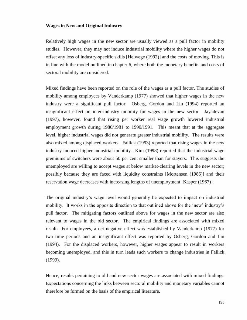
195
Wages in New and Original Industry
Relatively high wages in the new sector are usually viewed as a pull factor in mobility
studies. However, they may not induce industrial mobility where the higher wages do not
offset any loss of industry-specific skills [Helwege (1992)] and the costs of moving. This is
in line with the model outlined in chapter 6, where both the monetary benefits and costs of
sectoral mobility are considered.
Mixed findings have been reported on the role of the wages as a pull factor. The studies of
mobility among employees by Vanderkamp (1977) showed that higher wages in the new
industry were a significant pull factor. Osberg, Gordon and Lin (1994) reported an
insignificant effect on inter-industry mobility for wages in the new sector. Jayadevan
(1997), however, found that rising per worker real wage growth lowered industrial
employment growth during 1980/1981 to 1990/1991. This meant that at the aggregate
level, higher industrial wages did not generate greater industrial mobility. The results were
also mixed among displaced workers. Fallick (1993) reported that rising wages in the new
industry induced higher industrial mobility. Kim (1998) reported that the industrial wage
premiums of switchers were about 50 per cent smaller than for stayers. This suggests the
unemployed are willing to accept wages at below market-clearing levels in the new sector;
possibly because they are faced with liquidity constraints [Mortensen (1986)] and their
reservation wage decreases with increasing lengths of unemployment [Kasper (1967)].
The original industry‟s wage level would generally be expected to impact on industrial
mobility. It works in the opposite direction to that outlined above for the „new‟ industry‟s
pull factor. The mitigating factors outlined above for wages in the new sector are also
relevant to wages in the old sector. The empirical findings are associated with mixed
results. For employees, a net negative effect was established by Vanderkamp (1977) for
two time periods and an insignificant effect was reported by Osberg, Gordon and Lin
(1994). For the displaced workers, however, higher wages appear to result in workers
becoming unemployed, and this in turn leads such workers to change industries in Fallick
(1993).
Hence, results pertaining to old and new sector wages are associated with mixed findings.
Expectations concerning the links between sectoral mobility and monetary variables cannot
therefore be formed on the basis of the empirical literature.

196
There is limited information on whether the impacts of the old and new sector wages differ
for males and females. Only Osberg, Gordon and Lin (1994) examine this issue, and they
focused only on male employees. They found that the old and new sector wages had a non-
influential impact on mobility among males.
It is worth pointing out that the element of expectations is absent in the empirical literature,
which means that the wage variables presented in Table 8.2 will not conform to the
theoretical model exposited in equation (6.7). In addition, most of the studies use the old
and/or new industry wages, and not the sectoral wage differential in their analyses. These
studies are therefore not fully comparable with the analyses to be conducted in chapters 9
and 10, which are based on the expected sectoral wage differential. One exception is
Osberg, Gordon and Lin (1994), who used the wage differential between movers and
stayers. The wage differential has a strong theoretical basis (see chapter 6), and will be
included in the empirical analyses to be conducted below5.
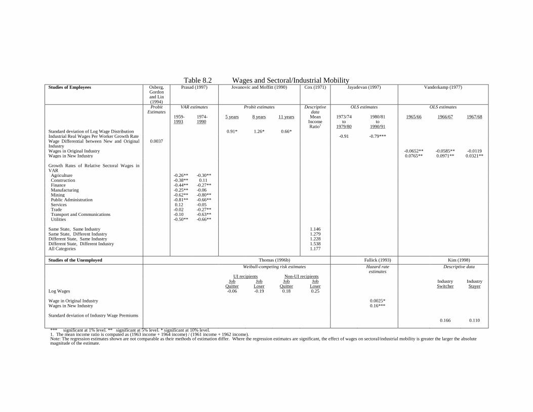
Table 8.2 Wages and Sectoral/Industrial Mobility Studies of Employees Osberg,
Gordon and Lin (1994)
Prasad (1997) Jovanovic and Moffitt (1990) Cox (1971) Jayadevan (1997) Vanderkamp (1977)
Probit Estimates
VAR estimates Probit estimates Descriptive data
OLS estimates OLS estimates
1959-1993
1974-1990
5 years 8 years 11 years Mean Income Ratio1
1973/74 to
1979/80
1980/81 to
1990/91
1965/66 1966/67 1967/68
Standard deviation of Log Wage Distribution 0.91* 1.26* 0.66* Industrial Real Wages Per Worker Growth Rate -0.91 -0.79*** Wage Differential between New and Original Industry
0.0037
Wages in Original Industry -0.0652** -0.0585** -0.0119 Wages in New Industry 0.0765** 0.0971** 0.0321** Growth Rates of Relative Sectoral Wages in VAR
Agriculture -0.26** -0.30** Construction -0.38** 0.11 Finance -0.44** -0.27** Manufacturing -0.25** -0.06 Mining -0.62** -0.80** Public Administration -0.81** -0.66** Services 0.12 -0.05 Trade -0.02 -0.27** Transport and Communications -0.10 -0.63** Utilities -0.50** -0.66** Same State, Same Industry 1.146 Same State, Different Industry 1.279 Different State, Same Industry 1.228 Different State, Different Industry 1.538 All Categories
1.177
Studies of the Unemployed Thomas (1996b) Fallick (1993) Kim (1998)
Weibull-competing risk estimates Hazard rate estimates
Descriptive data
UI recipients Non-UI recipients Job
Quitter Job
Loser Job
Quitter Job
Loser Industry
Switcher Industry Stayer
Log Wages
-0.06 -0.19 0.18 0.25
Wage in Original Industry 0.0025* Wages in New Industry Standard deviation of Industry Wage Premiums
0.16***
0.166 0.110
*** significant at 1% level. ** significant at 5% level. * significant at 10% level. 1. The mean income ratio is computed as (1963 income + 1964 income) / (1961 income + 1962 income). Note: The regression estimates shown are not comparable as their methods of estimation differ. Where the regression estimates are significant, the effect of wages on sectoral/industrial mobility is greater the larger the absolute magnitude of the estimate.

198
8.3.2 MACROECONOMIC FACTORS
Overall Unemployment
No clear links between inter-industry mobility and the overall unemployment rate have
been established in the empirical literature (see Table 8.3). For employees, Osberg (1991)
reported that unemployment had a negative effect only for females during 1980/1981 and
1985/1986. For the unemployed, the overall unemployment rate does not appear to be a
significant influence [Fallick (1993)].
The overall unemployment rate was used by Osberg (1991) in separate analyses of male
and female mobility. The results from these analyses showed that male mobility was not
affected by the overall unemployment rate, but this aggregate-level variable had a negative
effect on female mobility during several of the time periods analysed. In large part the
limited statistical success from the inclusion of the overall unemployment rate in models of
industrial mobility may be because this is not the best measure to capture any of the
influences noted above. A better measure would be to examine the separate roles of
unemployment in the old and new industries.
Unemployment in Old and New Industry
The theoretical model of chapter 6 asserts that higher unemployment in the original
industry induces sectoral movements to the new sector. Amongst employed persons,
higher unemployment in the original industry acted as a push factor for out-mobility in
Vanderkamp (1977) for all three time periods analysed. This is thus consistent with the
implications of the theoretical model. The effect of unemployment in the original sector
was, however, insignificant in Fallick‟s (1993) study of unemployed persons.
Unemployment in the new industry would generally be expected to discourage potential
entrants from moving into the new sector as their chances of securing a job in that sector
are lowered. However, this effect may be small where the wage gap between the sectors is
considerable. The empirical studies reveal mixed results. Unemployment in the new
industry did not exert any influence on the extent of inter-industry mobility among
employed workers in Vanderkamp (1977) in 1966/1967 and 1967/1968. However, there
was a surprising positive coefficient in Vanderkamp‟s (1977) study for 1965/1966.

199
Displaced workers in Fallick‟s (1993) study were not affected by unemployment levels in
the new industry.
The general observation is that studies using the old/new sectors‟ unemployment as
explanatory variables generate conflicting results, and hence predetermined views on the
unemployment-mobility relationship cannot be formed on this basis. In addition, the
literature does not appear to have examined whether sectoral unemployment rate variables
have different impacts on mobility for males and females, or whether within the separate
studies for males and females, the old/new sectors unemployment rate variable should be
defined in a gender-specific way rather than cover both males and females. Nonetheless,
the sectoral distinction in these variables aligns with the theoretical model where the push
or pull factor of mobility can be determined. From this perspective there is merit to their
inclusion in the empirical work in chapters 9 and 10.
Unemployment Spell
The theories/studies of labour mobility other than those of industrial mobility have assumed
either no intervening period of unemployment [Jovanovic and Moffitt (1990), Tobin (1972)
and Mattila (1974)] or that every job change involves an intervening unemployment spell
[Lucas and Prescott (1974)]. In comparison, the role of a spell of unemployment has been
examined in a number of studies of industrial mobility. Theoretically, as the spell
lengthens, workers would be expected to shift their search efforts towards new sectors and
to lower their earnings expectations [Pissarides and Wadsworth (1989)]. A positive effect
of spells of unemployment on industrial mobility among employed workers was reported
by Osberg (1991) and among male employees by Osberg, Gordon and Lin (1984).
The results for the unemployment spell variable in analyses for displaced workers have
been ambiguous. This may be attributed to the different coverage groups (i.e. quitters
versus losers, UI recipients versus non-UI recipients). Unemployed workers in Neal (1995)
and job quitters/losers who did not receive UI and losers who received UI in Thomas
(1996b) were more likely to change industries with a longer duration of unemployment6.
Conversely, the probability of moving sectors decreased with a longer spell among job
quitters who were UI-recipients. A likely reason for this is that since job quitters receive
some monetary compensation from UI, the opportunity cost of unemployment is lower than

200
when UI is not available, which mitigates the expected tendency to shift sectors as an
unemployment spell lengthens.
The analysis of the impact of the duration of unemployment on sectoral mobility has been
extended to separate analysis for males and females in several studies. Longer
unemployment spells were associated with greater mobility for both men and women in
Osberg (1991) during each of the three time periods examined, and for men in Osberg,
Gordon and Lin (1984). In particular, in Osberg (1991), the marginal effect of an
unemployment spell was higher for males in 1982/1983 and higher for females in
1980/1981 and 1985/19867.
Given the diversity of these findings for the unemployment spell variable, particularly for
the group of unemployed individuals for whom the variable should be more relevant, there
is arguably little benefit from including an unemployment spell variable in the empirical
application of chapters 9 and 10.
Overall Economic Growth and Employment
There are alternative viewpoints on the cyclical patterns associated with sectoral mobility
when aggregate indicators are used. Economic growth is usually associated with increases
in the rate of sectoral mobility. This occurs where the greater job availabilities associated
with an upturn encourage workers to switch sectors voluntarily. Alternatively, an economic
downturn can be associated with greater sectoral mobility where job losses/retrenchments
cause workers to seek employment in a new sector. The major study on this issue is
Loungani and Rogerson‟s (1989) analysis over the 1974 to 1984 period using a micro-
dataset for the U.S. Industry switchers in this study were defined as those who were
employed at the time of the base-year interview, i.e. year t, changed industries in year t+1
and who did not return to the original industry by year t+3. It was reported that the average
real GNP growth between years t and t+1 and the real GNP growth in year t+2 (i.e. the
growth rate of real GNP in the year following the initial industry switch) had negative and
significant effects on the proportion of industry switchers from the goods sector to the
services sector. This implies that if the declining goods sector was cyclically more
sensitive, mobility accelerates during a downturn. However, only the average GNP growth
between year t and year t+1 had a positive effect on the proportion of switchers from the
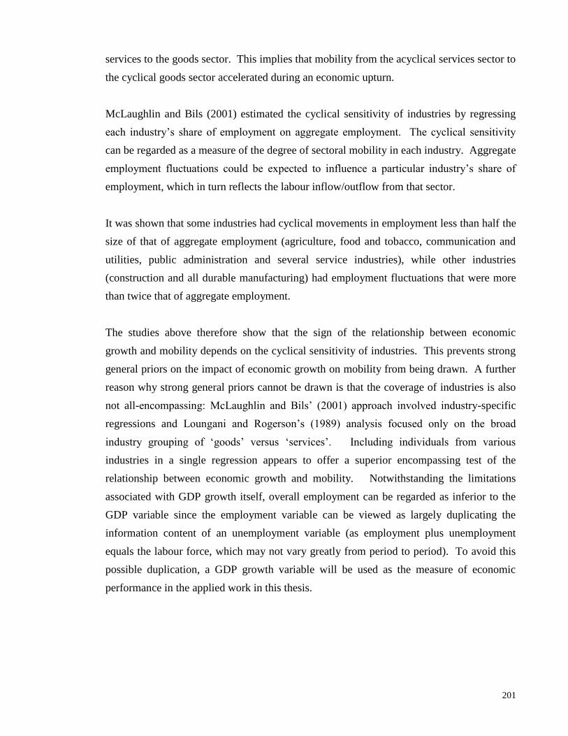
201
services to the goods sector. This implies that mobility from the acyclical services sector to
the cyclical goods sector accelerated during an economic upturn.
McLaughlin and Bils (2001) estimated the cyclical sensitivity of industries by regressing
each industry‟s share of employment on aggregate employment. The cyclical sensitivity
can be regarded as a measure of the degree of sectoral mobility in each industry. Aggregate
employment fluctuations could be expected to influence a particular industry‟s share of
employment, which in turn reflects the labour inflow/outflow from that sector.
It was shown that some industries had cyclical movements in employment less than half the
size of that of aggregate employment (agriculture, food and tobacco, communication and
utilities, public administration and several service industries), while other industries
(construction and all durable manufacturing) had employment fluctuations that were more
than twice that of aggregate employment.
The studies above therefore show that the sign of the relationship between economic
growth and mobility depends on the cyclical sensitivity of industries. This prevents strong
general priors on the impact of economic growth on mobility from being drawn. A further
reason why strong general priors cannot be drawn is that the coverage of industries is also
not all-encompassing: McLaughlin and Bils‟ (2001) approach involved industry-specific
regressions and Loungani and Rogerson‟s (1989) analysis focused only on the broad
industry grouping of „goods‟ versus „services‟. Including individuals from various
industries in a single regression appears to offer a superior encompassing test of the
relationship between economic growth and mobility. Notwithstanding the limitations
associated with GDP growth itself, overall employment can be regarded as inferior to the
GDP variable since the employment variable can be viewed as largely duplicating the
information content of an unemployment variable (as employment plus unemployment
equals the labour force, which may not vary greatly from period to period). To avoid this
possible duplication, a GDP growth variable will be used as the measure of economic
performance in the applied work in this thesis.

202
Table 8.3 Unemployment, Employment, GNP and Sectoral/Industrial Mobility
Studies of Employees Osberg (1991) Osberg,
Gordon and
Lin (1994)
Logit estimates Probit estimates
Males Females
1980/81 1982/83 1985/86 1980/81 1982/83 1985/86
Overall Unemployment Rate -0.0261 -0.0312 0.0028 -0.136*** 0.0255 -0.0651*
No. of Weeks Unemployed 0.0519*** 0.055*** 0.0526*** 0.0537*** 0.0453** 0.0738*** 0.0071**
Vanderkamp (1977) Loungani and Rogerson (1989) McLaughlin and Bils (2001)
OLS estimates
OLS estimates
OLS estimates
1965/66 1966/67 1967/68 All Industry switchers
Goods to services
Services to Goods
Unemployment in Old Industry
0.1006** 0.0708** 0.0706**
Unemployment in New Industry
0.0674** -0.0025 0.0217
Average Real GNP Growth between Periods t and t+1
-0.008 -0.037* 0.076**
Real GNP Growth in Period t+2
-0.040** -0.041** -0.014
Overall Employment in:
Agriculture -1.06***
Mining -0.56
Construction 1.67***
Metals 1.76***
Machinery 1.74***
Transportation Equipment 1.73***
Other Durables 1.21***
Food & Tobacco -0.65***
Textiles, Apparel & Leather 0.33
Paper, Printing & Publishing 0.03
Chemicals, Petroleum & Rubber
0.48***
Transportation 0.35***
Communications and Utilities -0.67***
Wholesale Trade -0.01
Retail Trade -0.11
Finance, Insurance & Real Estate
-0.39***
Business & Repair Services 0.55***
Personal Services -0.33*
Health Services -1.00***
Education -0.59***
Other Professional Services -0.63***
Public Administration -0.53***
Studies of the Unemployed Fallick (1993) Neal (1995)
Hazard rate estimates Probit estimates
Overall Unemployment Rate -0.021
Unemployment in Old Industry
-0.029
Unemployment in New Industry
-0.15
Years since Displacement 0.05**
*** significant at 1% level, ** significant at 5% level, * significant at 10% level.
Note: The regression estimates shown are not comparable as their methods of estimation differ. Where the regression estimates are significant, the effect
of unemployment/employment/GNP on sectoral/industrial mobility is greater the larger the absolute magnitude of the estimate.

203
8.3.3 WORKER CHARACTERISTICS
Age
In general, increasing age is expected to be linked to a lower incidence of sectoral/industrial
mobility. Younger workers are expected to have a higher degree of sectoral mobility as
they have a longer period over which they can gain any rewards associated with the change
of jobs [Creedy and Thomas (1982)]. In comparison, older workers who face greater costs
of moving [Jovanovic and Moffitt (1990)] and have a smaller amount of time to recoup the
costs [Creedy and Thomas (1982)] are expected to be less mobile. Moreover, the chances
of moving are likely to fall with age because of accumulation of sector-specific experience
and knowledge. The ability to learn new job skills required in the new sector also
diminishes with age.
It is observed that age has been viewed in empirical research as a personal characteristic
applicable to all individuals (i.e. age of individual) and with reference to specific industries
(i.e. age of entry into industry). The same expectations apply to both forms of the variable.
A decline in labour mobility with increasing age has been found in many studies [see for
example, Mincer and Jovanovic (1981) and Antolin and Bover (1997)], and has come to be
termed a socioeconomic by-law [Byrne (1975)]. This finding carries over to the literature
on industrial mobility among employed workers (see Table 8.4). Thus, older women had a
lower incidence of industrial mobility in Osberg (1991) in 1985/1986 whilst younger males
had a greater industrial mobility in Cox (1971) and Osberg, Gordon and Lin (1994). Both
the age of entry into the old industry and into the new industry had negative impacts on
industrial mobility in Vanderkamp (1977)8.
Declining mobility with age is also a characteristic of the unemployed. Thus, Thomas
(1996b) reported that younger job quitters (UI and non-UI recipients) and job losers who
did not receive UI aged 16-19 years had higher probabilities of switching industries.
Similarly, older displaced workers in Fallick (1993), and job quitters and losers aged 45-49
years who received UI in Thomas (1996b), were less likely to switch industries.
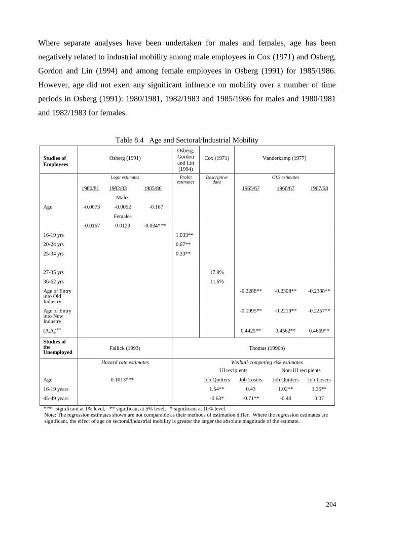
204
Where separate analyses have been undertaken for males and females, age has been
negatively related to industrial mobility among male employees in Cox (1971) and Osberg,
Gordon and Lin (1994) and among female employees in Osberg (1991) for 1985/1986.
However, age did not exert any significant influence on mobility over a number of time
periods in Osberg (1991): 1980/1981, 1982/1983 and 1985/1986 for males and 1980/1981
and 1982/1983 for females.
Table 8.4 Age and Sectoral/Industrial Mobility
Studies of
Employees
Osberg (1991)
Osberg, Gordon
and Lin
(1994)
Cox (1971)
Vanderkamp (1977)
Logit estimates Probit estimates
Descriptive data
OLS estimates
1980/81 1982/83 1985/86 1965/67 1966/67 1967/68
Males
Age -0.0073 -0.0052 -0.167
Females
-0.0167 0.0129 -0.034***
16-19 yrs 1.033**
20-24 yrs 0.67**
25-34 yrs 0.33**
27-35 yrs 17.9%
36-62 yrs 11.6%
Age of Entry into Old Industry
-0.2288** -0.2308** -0.2388**
Age of Entry into New Industry
-0.1995** -0.2219** -0.2257**
(AiAj)1/2 0.4425** 0.4562** 0.4669**
Studies of the Unemployed
Fallick (1993)
Thomas (1996b)
Hazard rate estimates Weibull-competing risk estimates
UI recipients Non-UI recipients
Age -0.1013*** Job Quitters Job Losers Job Quitters Job Losers
16-19 years
45-49 years
1.54**
-0.63*
0.43
-0.71**
1.02**
-0.40
1.35**
0.07
*** significant at 1% level, ** significant at 5% level, * significant at 10% level.
Note: The regression estimates shown are not comparable as their methods of estimation differ. Where the regression estimates are
significant, the effect of age on sectoral/industrial mobility is greater the larger the absolute magnitude of the estimate.

205
From the studies above, the negative age-mobility relationship is nearly always reported for
all labour groups, and this expectation is to be carried over to the empirical analysis later in
this thesis. Either the linear variable of Osberg (1991), the dummy variables of Osberg,
Gordon and Lin (1994) or a quadratic function in age could be used. The dummy variable
and quadratic function in age are more general and therefore appear to offer a sounder
starting point for empirical analysis.
Gender
A gender variable has been included in several studies to capture mobility differences
between men and women. Two forms have been used: as an industry characteristic (e.g.
male/female mix in the industry) and as a personal characteristic. Vanderkamp‟s (1977)
industry characteristic variable reflected male-female specialization. It was computed for
both the original and new industries, and each of these measures was associated with
negative effects on industrial mobility. This was interpreted to mean that a higher
proportion of males relative to females in the original industry acted as a barrier to outward
mobility whilst a higher proportion in the new industry was a barrier to entry. Fallick
(1993) incorporated a dummy variable for females in his study of the unemployed and
reported that they had a higher likelihood of industrial mobility (Table 8.5).
Based on the findings of these empirical studies, as well as patterns established in the
general labour economics literature, a gender difference in mobility behaviour is expected
for the empirical work presented later in this thesis. Moreover, this expectation is a basis
for conducting the separate analyses for males and females. The gender variable will be
used as a personal characteristic rather than as an industry characteristic (i.e. the gender mix
of the industry) as this is the usual practice in recent applied labour economics research.

206
Table 8.5 Gender and Sectoral/Industrial Mobility Study of Employees Study of the Unemployed
Vanderkamp (1977) Fallick (1993)
OLS estimates Hazard rate estimates
1965/67 1966/67 1967/68
As a Personal Characteristic
Female 0.27***
As an Industry Characteristic
Male-female Specialization in Old
Industry (Fi)
-0.0910** -0.0834** -0.0662**
Male-female Specialization in New
Industry (Fj)
-0.0248** -0.0364** -0.0459**
(FiFj)1/2 0.1057** 0.0957** 0.0999**
*** significant at 1% level, ** significant at 5% level.
Note: The regression estimates shown are not comparable as their methods of estimation differ. Where the regression estimates are significant, the effect of gender on sectoral/industrial mobility is greater the larger the
absolute magnitude of the estimate.
Family Indicators: Marital Status, Head of Household and Children
It has been suggested that workers with greater family commitments, e.g. married persons,
heads of households and persons with children, have lower propensities to switch industries
as any adverse consequences (e.g. temporary loss of income) will impact more intensely on
them than on other groups. However, marital status did not exert significant effects on the
propensity to switch sectors for employees in Osberg (1991), except for 1980/1981. Among
the unemployed, married persons displayed lower incidences of mobility in Neal (1995).
The results for unemployed heads of households in Fallick (1993) were as expected, with
lower probabilities of changing industries. However, having children was not associated
with any significant influence on industrial mobility in Neal (1995). The studies that have
examined the determinants of mobility behaviour separately for men and women have
concluded that marital status generally did not have any significant impact on industrial
mobility for either males or females, as seen from Osberg (1991) and Osberg, Gordon and
Lin (1994)9. There is no evidence on whether the impacts of the household head and
children indicators on mobility differ between men and women.
Owing to these conflicting findings and the limited number of studies, preconceived views
about marital status/head of household status vis-à-vis mobility are difficult to arrive at.

207
This contrasts with the situation with respect to marital status and head of household
variables in many other areas of labour market research (e.g. wage determination,
occupational attainment). This difference is likely due to the sparse nature of research on
sectoral mobility at the present time. Accordingly, the marital status and head of household
variables will be used in the current unit-record analysis.
Table 8.6 Marital Status/Head of Household and Sectoral/Industrial Mobility
Studies of Employees Osberg (1991) Osberg, Gordon and
Lin (1994)
Males Females
1980/81 1982/83 1985/86 1980/81 1982/83 1985/86
Marital Status
Single = 1
Otherwise = 0
0.345* 0.209 -0.126 0.862 0.236 0.1005
Married = 1
Otherwise = 0
-0.012
Studies of the Unemployed
Fallick (1993) Neal (1995)
Marital Status
Currently married -0.151**
Head of Household -0.40***
With Children 0.016
*** significant at 1% level, ** significant at 5% level, * significant at 10% level.
Formal Education
The influence of formal education on the probability of moving to a new sector/industry is
indeterminate a priori. Education level is both a stock of acquired skills and a signal of
one‟s ability to learn. Whether these attributes are rewarded more in the original sector
(which would retard mobility) or new sector (which would encourage mobility) is an
empirical matter. This is viewing education as a personal characteristic.
Education can also be viewed as an industry characteristic, measured as the mean education
level or the education composition of the workforce of the industry in question. A highly
educated workforce within an industry could act as a barrier to entry into that industry,
especially if potential entrants view it as lessening their chances for securing higher paid
jobs which are generally associated with higher education.
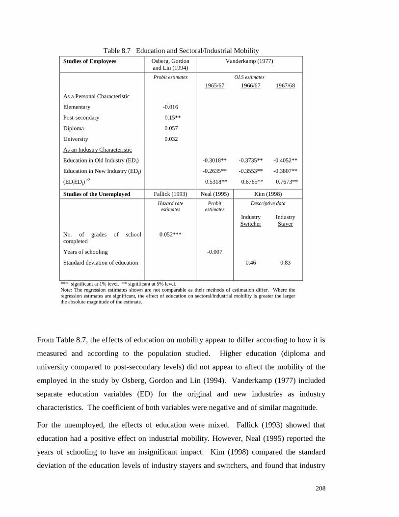
208
Table 8.7 Education and Sectoral/Industrial Mobility
Studies of Employees Osberg, Gordon
and Lin (1994)
Vanderkamp (1977)
Probit estimates OLS estimates
1965/67 1966/67 1967/68
As a Personal Characteristic
Elementary -0.016
Post-secondary 0.15**
Diploma 0.057
University 0.032
As an Industry Characteristic
Education in Old Industry (EDi) -0.3018** -0.3735** -0.4052**
Education in New Industry (EDj) -0.2635** -0.3553** -0.3807**
(EDiEDj)1/2 0.5318** 0.6765** 0.7673**
Studies of the Unemployed Fallick (1993) Neal (1995) Kim (1998)
Hazard rate estimates
Probit estimates
Descriptive data
Industry
Switcher
Industry
Stayer
No. of grades of school
completed
0.052***
Years of schooling -0.007
Standard deviation of education 0.46 0.83
*** significant at 1% level, ** significant at 5% level.
Note: The regression estimates shown are not comparable as their methods of estimation differ. Where the
regression estimates are significant, the effect of education on sectoral/industrial mobility is greater the larger the absolute magnitude of the estimate.
From Table 8.7, the effects of education on mobility appear to differ according to how it is
measured and according to the population studied. Higher education (diploma and
university compared to post-secondary levels) did not appear to affect the mobility of the
employed in the study by Osberg, Gordon and Lin (1994). Vanderkamp (1977) included
separate education variables (ED) for the original and new industries as industry
characteristics. The coefficient of both variables were negative and of similar magnitude.
For the unemployed, the effects of education were mixed. Fallick (1993) showed that
education had a positive effect on industrial mobility. However, Neal (1995) reported the
years of schooling to have an insignificant impact. Kim (1998) compared the standard
deviation of the education levels of industry stayers and switchers, and found that industry

209
switchers have smaller industry dispersions in education. Kim (1998) proposed that the
probability of an industry switch was greater among marginal workers, e.g. low- (high-)
educated workers in high- (low-) wage industries, and the results showed that switchers
were marginal in terms of the smaller standard deviation measure.
There is limited evidence on whether the links between educational attainment and mobility
differ between males and females, and so comment on this is not provided. The superiority
of the education variable as a personal or industry characteristic cannot be determined on
the basis of consistent findings, although the former is more relevant for unit-record
analysis, is consistent with the practice in most recent applied labour market studies, and
has the merit of capturing a personal characteristic that can readily be seen as a policy
variable. For these reasons the level of education of the individual will be included in the
estimating equation used for the study of the Korean labour market.
On-the-job Training
It has been suggested that on-the-job training may be a more appropriate measure of a
worker‟s knowledge of the job than formal education and hence have a greater influence on
labour mobility [Parent (1999)]. On-the-job training can take two forms: general and
firm/sector-specific [Creedy and Thomas (1982) and Becker (1964)]. In general training,
the marginal productivity of trainees is the same across sectors. If the post-training wage is
below the workers‟ improved marginal productivity, it would be economically irrational for
the trained person to remain in the same firm/sector and the likelihood of switching sectors
is greater. In firm/sector-specific training, the worker‟s improved productivity is not
transferable to other firms/sectors. In this situation, an organization would be more willing
to bear some of the costs of training, and Becker (1964) argues that both the costs of, and
returns to, firm/sector specific training will be shared by employer and employee, which
will tend to lock workers into their existing jobs and limit mobility.

210
The fundamental difficulty with on-the-job training compared to formal education is that it
is not easily measured. Most on-the-job skills are acquired through learning-by-doing
[Oatey (1970)] rather than from formal training programmes, and learning-by-doing is
generally not quantifiable. The usual proxy variables of tenure and labour market
experience capture the influence of a range of factors (e.g. life-cycle factors, cohort effects)
and attributing any statistical relationships between these variables and labour mobility to
on-the-job training is therefore difficult.
The proxy measures for on-the-job training considered in the literature are job tenure and
labour market experience [Neal (1995) and Burdett (1978)]. An individual with a longer
job tenure or labour market experience is more likely to switch sectors if the relevant work
experience/training acquired in the years worked represents general training. Offsetting
this are other factors like benefits received. Thus, workers with longer job tenures,
experience and greater training may be less willing to move and give up seniority rights
like job security, pension benefits, seniority-based pay, longer vacation periods and
promotional advantages [Mincer and Jovanovic (1981) and Neal (1995)].
There is an issue of the specification of the tenure/experience variables that also is of
relevance. Some studies use a linear specification for these variables and others a more
general quadratic function. The studies that use a linear specification are reviewed first
below followed by those that present tenure in its quadratic form. For the linear
specification where there are more studies, the findings for job tenure are covered prior to
the findings for experience. For the quadratic functional form, however, there are fewer
studies and the two proxies are dealt with together.
Studies using job tenure as a proxy for on-the-job training have produced consistent results
among employed workers but not among the unemployed. Osberg (1991) reported that job
tenure reduced the likelihood of industrial mobility for all three time periods examined for
males and females. Job tenure was also associated with a reduced likelihood of industrial
mobility for males in Osberg, Gordon and Lin (1994). Thus, the evidence on the links
between tenure and mobility is similar for both male and female workers. The findings,
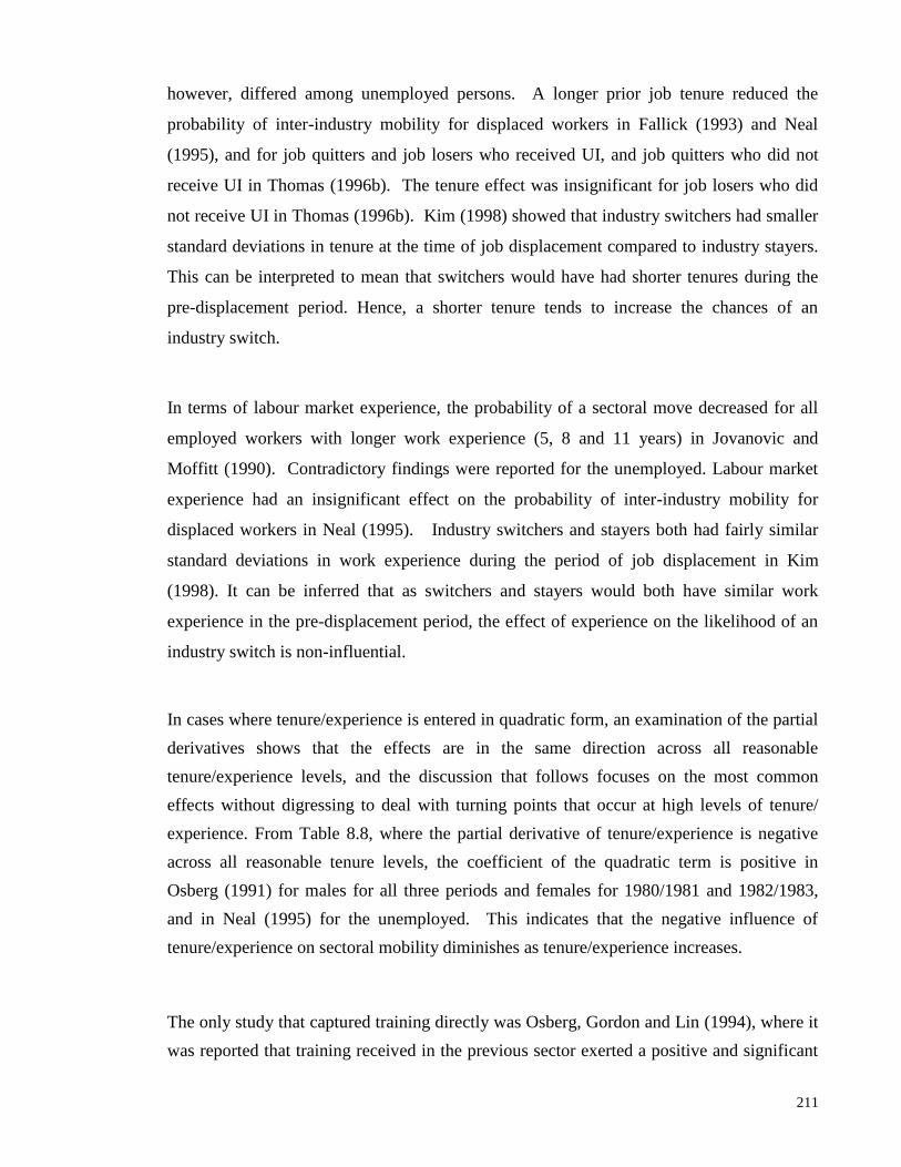
211
however, differed among unemployed persons. A longer prior job tenure reduced the
probability of inter-industry mobility for displaced workers in Fallick (1993) and Neal
(1995), and for job quitters and job losers who received UI, and job quitters who did not
receive UI in Thomas (1996b). The tenure effect was insignificant for job losers who did
not receive UI in Thomas (1996b). Kim (1998) showed that industry switchers had smaller
standard deviations in tenure at the time of job displacement compared to industry stayers.
This can be interpreted to mean that switchers would have had shorter tenures during the
pre-displacement period. Hence, a shorter tenure tends to increase the chances of an
industry switch.
In terms of labour market experience, the probability of a sectoral move decreased for all
employed workers with longer work experience (5, 8 and 11 years) in Jovanovic and
Moffitt (1990). Contradictory findings were reported for the unemployed. Labour market
experience had an insignificant effect on the probability of inter-industry mobility for
displaced workers in Neal (1995). Industry switchers and stayers both had fairly similar
standard deviations in work experience during the period of job displacement in Kim
(1998). It can be inferred that as switchers and stayers would both have similar work
experience in the pre-displacement period, the effect of experience on the likelihood of an
industry switch is non-influential.
In cases where tenure/experience is entered in quadratic form, an examination of the partial
derivatives shows that the effects are in the same direction across all reasonable
tenure/experience levels, and the discussion that follows focuses on the most common
effects without digressing to deal with turning points that occur at high levels of tenure/
experience. From Table 8.8, where the partial derivative of tenure/experience is negative
across all reasonable tenure levels, the coefficient of the quadratic term is positive in
Osberg (1991) for males for all three periods and females for 1980/1981 and 1982/1983,
and in Neal (1995) for the unemployed. This indicates that the negative influence of
tenure/experience on sectoral mobility diminishes as tenure/experience increases.
The only study that captured training directly was Osberg, Gordon and Lin (1994), where it
was reported that training received in the previous sector exerted a positive and significant

212
impact on inter-industry mobility. However, this measure will not be dealt with in the
current work owing to the difficulty in determining a suitable across-the-board measure of
training for individuals in the KLIPS10
.
In summary, consistent results are revealed in the studies of job tenure/experience and
mobility for employed workers. Given the strength of these findings, a negative
relationship between tenure/experience and mobility would be expected in the current
work, both for the aggregate-level analyses and for the separate analyses to be undertaken
for males and females. Given the evidence in favour of non-linear relationships between
mobility and tenure/experience, tenure/experience should be examined using a quadratic
function.

Table 8.8 On-the-job Training and Sectoral/Industrial Mobility
Studies of
Employees
Osberg (1991) Osberg,
Gordon and
Lin (1994)
Jovanovic and Moffitt (1990)
Logit estimates Probit
estimates
Probit estimates
Males Females Probability of a Sectoral Move
1980/81 1982/83 1985/86 1980/81 1982/83 1985/86 1968 1969 1970 1971 1973 1975 1978 1980
Job Tenure -0.0124*** -0.0184*** -0.0139*** -0.258*** -0.0216*** -0.0107** -0.00016**
Job Tenure-squared 0.00002*** 0.000032*** 0.000027*** 0.000057*** 0.000045*** -0.00001
Years of Experience
5 years 0.25 0.25 0.22 0.18 0.20 0.21 0.19 0.15
8 years 0.23 0.28 0.20 0.20 0.16 0.17 0.18 0.15
11 years 0.23 0.20 0.17 0.17 0.15 0.15 0.17 0.14
Received Training
in 1986
0.27**
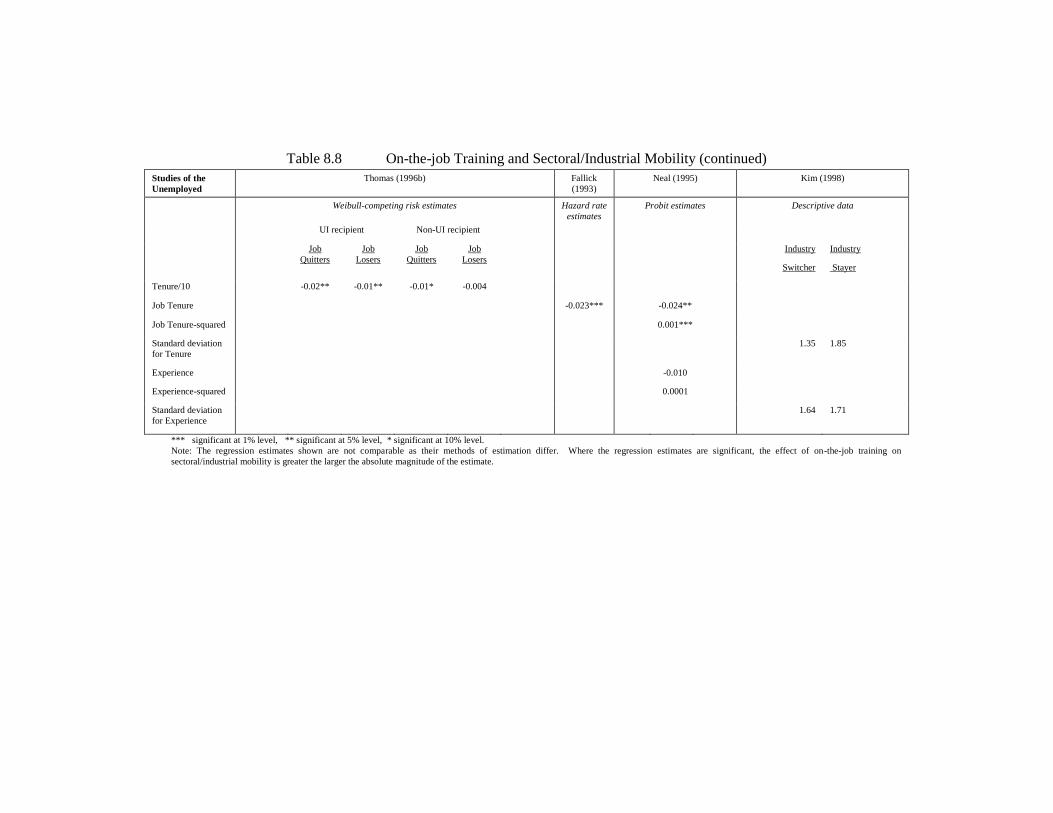
214
Table 8.8 On-the-job Training and Sectoral/Industrial Mobility (continued)
Studies of the
Unemployed
Thomas (1996b) Fallick
(1993)
Neal (1995) Kim (1998)
Weibull-competing risk estimates Hazard rate
estimates
Probit estimates Descriptive data
UI recipient Non-UI recipient
Job
Quitters
Job
Losers
Job
Quitters
Job
Losers
Industry
Switcher
Industry
Stayer
Tenure/10 -0.02** -0.01** -0.01* -0.004
Job Tenure -0.023*** -0.024**
Job Tenure-squared 0.001***
Standard deviation
for Tenure
1.35 1.85
Experience -0.010
Experience-squared 0.0001
Standard deviation
for Experience
1.64 1.71
*** significant at 1% level, ** significant at 5% level, * significant at 10% level.
Note: The regression estimates shown are not comparable as their methods of estimation differ. Where the regression estimates are significant, the effect of on-the-job training on
sectoral/industrial mobility is greater the larger the absolute magnitude of the estimate.

215
Occupation
Occupation is reflective of skill levels, and has been measured in mobility studies by initial
occupation, change in occupation and as a proportion of individuals in skill-intensive
occupations (see Table 8.9). There are alternative viewpoints regarding the industrial
mobility behaviour of skilled and semi-skilled workers. On the one hand, skilled workers
could exhibit „mobility stickiness‟ [Subrahmanian, Veena and Parikh (1982)] if skills are
team-specific and jobs rely on the existing net of workers [Mailath and Postlewaith (1990)
and Chillemi and Gui (1997)] in the original sector. On the other hand, by virtue of their
skill being vital in certain industries [Neal (1995)], skilled workers may be scouted for their
talent, potential injection of new ideas or productivity [Murphy and Topel (1990)]. White-
collar jobs are also more likely to be advertised than blue-collar jobs [Abraham (1987)] and
the rate of mobility for such workers may be higher. The change in occupation was
examined by Vanderkamp (1977), who argued that such changes impose additional costs to
mobility in the form of acquiring new skills and retraining for a different occupation.
The initial occupation was examined by Osberg (1991) for the employed and Neal (1995)
and Fallick (1993) for the unemployed. Osberg (1991) reported that higher probabilities of
industrial mobility were reported by female personal service workers for all three periods
examined (1980/1981, 1982/1983 and 1985/1986), female managers, professionals and
technicians in 1982/1983 and 1985/1986, and female clerical and sales workers in
1980/1981 and 1985/1986. Male managers, professionals and technicians in 1980/1981
were also more likely to change industries. Fallick (1993) reported that displaced workers
who were in the technical, sales or administration, precision production, craft and repairs or
who were operators, fabricators and labourers in the old industry had higher propensities to
switch sectors. In contrast, Neal (1995) reported that unemployed workers who were
professionals, craftsmen and those who were operators were less likely to be industry
switchers. The empirical findings revealed mobility stickiness for job losers who received
UI [Thomas (1996b)]11
. The change in occupation was a deterrent to industrial mobility in
Vanderkamp‟s (1977) empirical work. In terms of the proportion of individuals in skill-
intensive occupations, higher skill levels did not exert any significant effect on sectoral
mobility in Loungani and Rogerson (1989).

216
This mixed evidence therefore does not provide a basis for establishing priors on whether
the mobility behaviour of skilled and unskilled workers will differ. Similarly, as Osberg
(1991) is the only study that addresses whether mobility patterns across occupations differ
for males and females, and the extent to which his findings generalize to other countries
and time periods is not clear, priors for the role that occupation may have in the separate
analyses to be conducted for men and women cannot be formed.
Part of the reason for the conflicting results on the role of occupation in the empirical
literature may be the different variables used (initial occupation, change in occupation,
dummy variables, industry averages). However, it seems that there are grounds for a
reasoned choice in this regard. Between the first two types of variables mentioned above,
the change in occupation is less preferred as it depicts another form of labour mobility,
namely, occupational mobility, and so may potentially be endogenous. In contrast, the
initial occupation variable is exogenous, and has an unambiguous interpretation, and for
this reason is preferred for the empirical work. For consistency with the representation of
other worker characteristics in the model, the initial occupation will be categorized as a
dummy variable (i.e skilled versus unskilled).
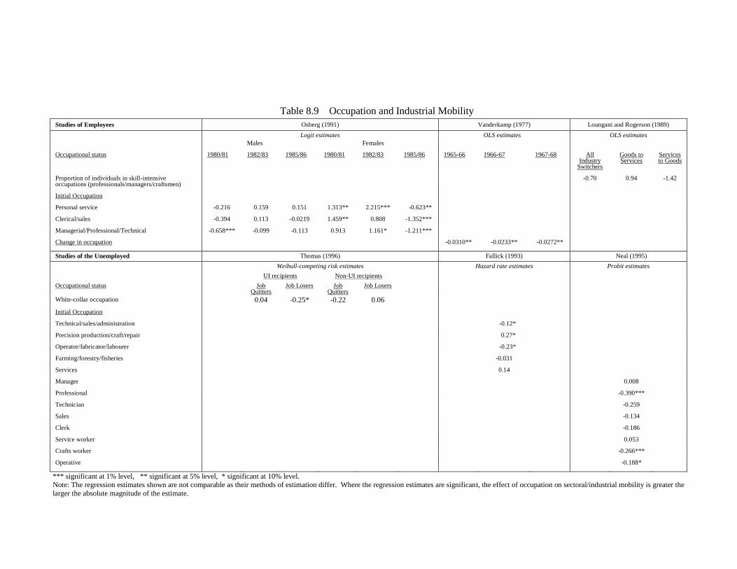
Table 8.9 Occupation and Industrial Mobility
Studies of Employees Osberg (1991) Vanderkamp (1977) Loungani and Rogerson (1989)
Logit estimates OLS estimates OLS estimates
Males Females
Occupational status 1980/81 1982/83 1985/86 1980/81 1982/83 1985/86 1965-66 1966-67 1967-68 All Industry
Switchers
Goods to Services
Services to Goods
Proportion of individuals in skill-intensive occupations (professionals/managers/craftsmen)
-0.70 0.94 -1.42
Initial Occupation
Personal service -0.216 0.159 0.151 1.313** 2.215*** -0.623**
Clerical/sales -0.394 0.113 -0.0219 1.459** 0.808 -1.352***
Managerial/Professional/Technical -0.658*** -0.099 -0.113 0.913 1.161* -1.211***
Change in occupation -0.0310** -0.0233** -0.0272**
Studies of the Unemployed Thomas (1996) Fallick (1993) Neal (1995)
Weibull-competing risk estimates Hazard rate estimates Probit estimates
UI recipients Non-UI recipients
Occupational status Job Quitters
Job Losers Job Quitters
Job Losers
White-collar occupation 0.04 -0.25* -0.22 0.06
Initial Occupation
Technical/sales/administration -0.12*
Precision production/craft/repair 0.27*
Operator/fabricator/labourer -0.23*
Farming/forestry/fisheries -0.031
Services 0.14
Manager 0.008
Professional -0.390***
Technician -0.259
Sales -0.134
Clerk -0.186
Service worker 0.053
Crafts worker -0.266***
Operative -0.188*
*** significant at 1% level, ** significant at 5% level, * significant at 10% level. Note: The regression estimates shown are not comparable as their methods of estimation differ. Where the regression estimates are significant, the effect of occupation on sectoral/industrial mobility is greater the
larger the absolute magnitude of the estimate.
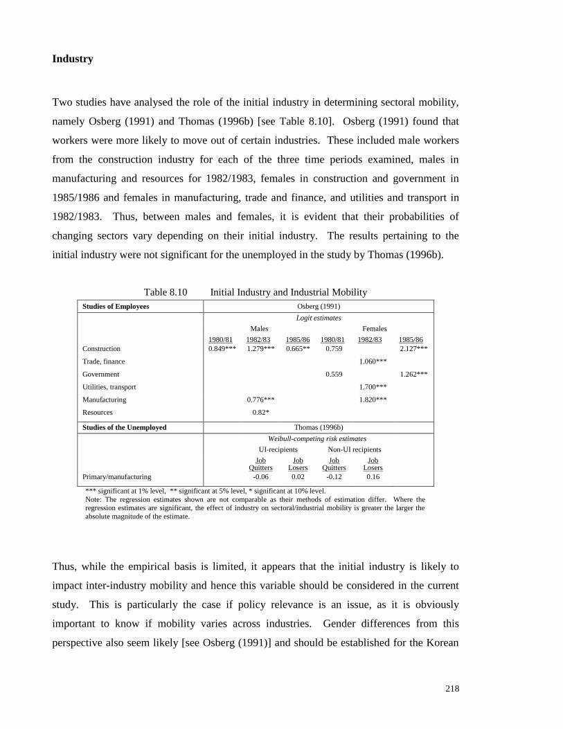
218
Industry
Two studies have analysed the role of the initial industry in determining sectoral mobility,
namely Osberg (1991) and Thomas (1996b) [see Table 8.10]. Osberg (1991) found that
workers were more likely to move out of certain industries. These included male workers
from the construction industry for each of the three time periods examined, males in
manufacturing and resources for 1982/1983, females in construction and government in
1985/1986 and females in manufacturing, trade and finance, and utilities and transport in
1982/1983. Thus, between males and females, it is evident that their probabilities of
changing sectors vary depending on their initial industry. The results pertaining to the
initial industry were not significant for the unemployed in the study by Thomas (1996b).
Table 8.10 Initial Industry and Industrial Mobility
Studies of Employees Osberg (1991)
Logit estimates
Males Females
1980/81 1982/83 1985/86 1980/81 1982/83 1985/86
Construction 0.849*** 1.279*** 0.665** 0.759 2.127***
Trade, finance 1.060***
Government 0.559 1.262***
Utilities, transport 1.700***
Manufacturing 0.776*** 1.820***
Resources 0.82*
Studies of the Unemployed Thomas (1996b)
Weibull-competing risk estimates
UI-recipients Non-UI recipients
Job Quitters
Job Losers
Job Quitters
Job Losers
Primary/manufacturing -0.06 0.02 -0.12 0.16
*** significant at 1% level, ** significant at 5% level, * significant at 10% level.
Note: The regression estimates shown are not comparable as their methods of estimation differ. Where the
regression estimates are significant, the effect of industry on sectoral/industrial mobility is greater the larger the
absolute magnitude of the estimate.
Thus, while the empirical basis is limited, it appears that the initial industry is likely to
impact inter-industry mobility and hence this variable should be considered in the current
study. This is particularly the case if policy relevance is an issue, as it is obviously
important to know if mobility varies across industries. Gender differences from this
perspective also seem likely [see Osberg (1991)] and should be established for the Korean
219
labour market if possible. Hence variables for the initial industry will be included in the
mobility equations used in chapters 9 and 10.
Employment Status, Unionisation, Alternative Sources of Income and Region
A number of other potential determinants of worker mobility have been considered, e.g.
employment status in Osberg (1991), unionization in Vanderkamp (1977), unemployment
insurance in Osberg, Gordon and Lin (1994) and Fallick (1993), social assistance in
Osberg, Gordon and Lin (1994) and region by Vanderkamp (1977) and Thomas (1996b).
The empirical evidence relating to the latter four factors is not reviewed as it is not relevant
to the empirical analyses to be conducted below.
The research on the impact of employment status on sectoral mobility is relevant to the
current work and the finding by Osberg (1991) will be reported here. Osberg (1991)
focused on full-time versus part-time workers, although it seems that other categorizations
could be used, such as employees versus employers, own account workers and workers in
family business. Part-timers and employees are expected to have a higher incidence of
industrial mobility as they are less emotionally attached to their current job/sector than full-
time employees. This was confirmed in Osberg (1991), where male and female part-time
workers were both associated with higher mobility rates (see Table 8.11). Since Osberg
(1991) is the sole study of sectoral mobility that covers employment status, the findings
should not be generalized to other samples. However, the apparent strength of the results,
their accord with intuition, and the policy and social relevance of knowledge of whether
sectoral mobility varies by employment status provide sound reasons for considering an
employment status variable in the study of mobility in the Korean labour market.

220
Table 8.11 Employment Status and Industrial Mobility
Osberg (1991)
Males Females
1980/81 1982/83 1985/86 1980/81 1982/83 1985/86
Part-time worker in initial sector
0.616** 1.145*** 0.876*** -0.138 1.066*** 0.925***
*** significant at 1% level, ** significant at 5% level, * significant at 10% level
8.3.4 JOB/INDUSTRY CHARACTERISTICS
Different sectors are associated with different job characteristics and work environments,
and these differences can impact an individual‟s mobility decision. Consistent with the
implications of the empirical model, as workers have to make ex ante decisions about
switching industries, the decision becomes a function of the expected job/industry
characteristics in addition to the other characteristics discussed above (e.g. expected
wages). Studies of public-private sector mobility in particular have stressed the importance
of the non-monetary aspect in mobility, as the two sectors operate under different work
environments. These non-monetary characteristics might include working hours/weeks,
work/product similarity and industry size and turnover.
Working Hours/Weeks
Variation in working hours/weeks has been noted as a prominent determinant of labour
market mobility in a number of studies [e.g. Arnott, Hosios and Stiglitz (1988)]. Although
employers may require fixed work hours, workers can increase their work hours by
changing sectors and a change in working hours or a desire to change the work hours
should be positively associated with mobility. From Table 8.12, the indicators of this
dimension of labour supply include the change in the individual‟s usual weekly hours
between periods t (original interview) and t+1 (re-interview) in Osberg (1991), and the
individual‟s desire for more working hours/weeks per year in Osberg, Gordon and Lin
(1994). In the latter study, it was envisaged that a greater amount of time that could be
spent at work in the new sector would increase earnings for individuals and thus lead to a

221
higher probability of a sectoral switch. A potential problem in using the change in weekly
hours lies in its non-exogeneity. The labour supply as measured by the change in weekly
hours may change as an individual changes sectors. Hence, the desire to work more hours is
probably a superior variable.
Despite its apparent importance, only two studies have examined the links between
working hours and sectoral mobility. Osberg (1991) reported that an increase in the usual
working week showed a positive effect on the industrial mobility behaviour only for males
in 1982/1983 and 1985/1986. Osberg, Gordon and Lin‟s (1994) results were as expected,
i.e. individuals desiring more working weeks/hours had higher probabilities of a sectoral
change.
In terms of working hours/weeks, the study by Osberg (1991) does not always point
towards a positive relationship between industrial mobility and working hours/weeks. The
empirical findings are thus inconsistent. The evidence also points to the industrial mobility
– working hours relation differing for males and females, with this labour supply factor
being important for males but not for females. Given the inconclusive evidence, and the
fact that the data are not available for all individuals in the KLIPS dataset, the hours data
will not be considered in the thesis.
Product and Work Similarity
Product and work similarity are other factors associated with the work environment. An
individual‟s propensity to change sectors/industries is expected to be higher the greater the
similarity across sectors of the characteristics of the products handled and work
environment. This arises as similarity of the products handled enhances the transferability
across industries of skills and knowledge, and similarity in work environment reduces the
psychic costs of adjustment [Vanderkamp (1977)]. Workers will therefore aim to relocate
to industries that are “close” to their current industry so that much of their human capital
acquired will be transferable [Fallick (1993)]. Vanderkamp (1977) operationalised the
product and work similarity concepts by classifying industries into eleven product groups
(product similarity) and into two work types: light (including mental activity) and heavy

222
(including manual and physical activity). Two dummy variables were used (Dummy = 1 if
the industries had similar product/work, Dummy = 0 otherwise). Positive correlations
between industrial mobility and product/work similarity were reported by Vanderkamp
(1997) for the years 1965/1966, 1966/1967 and 1967/1968, except for work similarity in
1967/1968.
Unfortunately Vanderkamp (1977) appears to be the only study that assesses the impact of
product and work similarity on the sectoral mobility of labour. There do not appear to be
any studies that examine gender differences in this dimension of sectoral mobility. This is
surprising given the intuition behind the inclusion of the variable in Vanderkamp‟s (1977)
study. A likely reason for this is the arbitrary nature of the categorization that needs to be
employed. Product/work similarity variables certainly have potential importance for the
research on Korean sectoral mobility, given that they signify ease of skill transferability
into the new sector. However, application depends on data availability, and the
arbitrariness of the definition noted above is a strong argument against the use of this set of
variables. Accordingly, product and work similarity variables will not be considered
further in this thesis.

Table 8.12 Working Hours, Product Similarity, Work Similarity and Industrial Mobility
Studies of Employees Osberg (1991) Osberg, Gordon
and Lin (1994)
Vanderkamp (1977)
Logit estimates Probit estimates
OLS estimates
Males Females
1980/81 1982/83 1985/86 1980/81 1982/83 1985/86 1965/66 1966/67 1967/68
Change in usual weekly hours
(period t+1 – period t)
-0.00035 0.0373*** 0.0169** 0.0023 0.0041 -0.0107
Desire more weeks per year 0.19**
Desire more hours per week 0.43**
Product Similarity1
(=1 if similar, =0 otherwise)
0.6094** 0.6020** 0.5391**
Work Similarity2
(=1 if similar, =0 otherwise)
0.0451** 0.0490** 0.0302
*** significant at 1% level, ** significant at 5% level. 1. Dummy variable indicating product similarity (Dummy x 10-2). The industries are classified into 11 product groups.
2. Dummy variable indicating work similarity (Dummy x 10-2). The industries are divided according to two types of work effort: light (including mental activity) and heavy (including
manual and physical activity). Note: The regression estimates shown are not comparable as their methods of estimation differ. Where the regression estimates are significant, the effect of the working hours/product
similarity/ work similarity on sectoral/industrial mobility is greater the larger the absolute magnitude of the estimate.

224
Size of Original and New Industries
Industry size is typically measured in empirical studies of worker mobility by the level of
employment or changes in employment and, to the extent that the contractions and
expansions in employment reveal declining or growing trends for specific industries, the
variable can reflect industry performance. Higher employment in the initial industry could
be viewed as a good indication of the industry‟s job market prospects/availability and lower
costs of finding a job in that industry [Neal (1995)]. Thus, a negative correlation between
mobility and employment growth in the old industry, and a positive association between
mobility and size of the new industry, are to be expected.
In terms of the size of the old industry, the expected negative relationship was reported by
both Fallick (1993) and Neal (1995) [see Table 8.13]. However, both of these studies cover
displaced workers only, and this approach does not appear to have been applied to other
groups or in separate analyses of the mobility of male and female employees.
With respect to the size of the new sector, higher employment was shown to be positively
correlated with industrial mobility in Vanderkamp (1977) for the three time periods
analysed. Similarly, lower job availabilities in the new industry (observed from the no-job-
available index) reduced the likelihood of industrial mobility for males in Osberg, Gordon
and Lin (1994). To the extent that lower job availabilities is an indication of lower
employment in a sector, the positive correlation between the new sector‟s size and mobility
is implied in the latter study.
While these findings are interesting, the limited number of studies of employed workers is a
shortcoming of research in this particular area. It prevents strong conclusions from being
drawn, whether for the aggregate labour force or for males and females separately.
Nevertheless, the ready availability of measures of employment size means that the impacts
of size of the original and new industries can be easily addressed in the current empirical
study. In this context, it is noted that the industry size variables (i.e. for original and new)
can be both examined in a single regression model as simultaneity does not appear to be an

225
issue. At any time t, the pool of workers in one industry differs from the pool of workers in
another.
Industry Turnover and Output
It is believed that higher turnover or output for an industry is generally indicative of its
ability to recruit, which raises the probability of finding a job and encourages inter-industry
mobility. However, higher turnover or output may also mean a greater chance of
retrenchment, which would be expected to be a deterrent to industrial mobility.
Vanderkamp (1997) reported a positive and significant relationship between turnover in the
new industry and industrial mobility. Jayadevan (1997) introduced the industrial output
growth rate as a performance indicator in an analysis of the manufacturing sector. Using
establishment data that covered all workers, it was found that a higher growth in output was
positively associated with higher employment growth or a higher net inflow of labour.
Among the unemployed, Ottersen (1993) showed that the number of layoffs in the original
sector was negatively associated with the probability of being hired in the new sector.
The different measures employed in these studies, as well as the vastly different
populations studied, prevents a consensus on the impact of industry performance on
sectoral mobility from emerging. Moreover, analysis of the industry performance –
sectoral mobility relationship has not been conducted for separate samples of males and
females. However, as with some other variables, there is considerable practical/policy
appeal in having knowledge of the links between industry performance and sectoral
mobility. For this reason, the applied work below will consider this relationship. In
assessing the variables, Vanderkamp‟s (1977) turnover indicator has the merit of
distinguishing the old versus new sectors so that the actual channel of influence on mobility
can be determined. However, the information is not about sectoral performance per se but
the sector‟s ability to recruit or retrench. Jayadevan‟s (1997) industry output (or GDP
growth) is a viable indicator as it reflects the economic performance of the sector, but it
lacks the sectoral distinction preferred for the current study and is confined to the
manufacturing sector. Hence, for the current work, it is recommended that a sectoral
performance indicator in the form of GDP growth be adopted with a sectoral distinction.
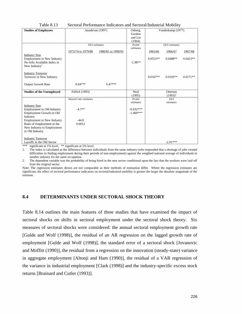
226
Table 8.13 Sectoral Performance Indicators and Sectoral/Industrial Mobility
Studies of Employees Jayadevan (1997) Osberg, Gordon
and Lin
(1994)
Vanderkamp (1977)
OLS estimates Probit
estimates
OLS estimates
1973/74 to 1979/80 1980/81 to 1990/91 1965/66 1966/67 1967/68 Industry Size
Employment in New Industry 0.0553** 0.0488** 0.0423**
No-Jobs Available Index in New Industry1
-1.98**
Industry Turnover Turnover in New Industry 0.0167** 0.0105** 0.0171**
Output Growth Rate 0.64*** 0.47***
Studies of the Unemployed Fallick (1993) Neal
(1995)
Ottersen
(1993)2
Hazard rate estimates Probit
estimates OLS
estimates
Industry Size Employment in Old Industry -4.7** -0.032***
Employment Growth in Old
Industry
-1.460***
Employment in New Industry -44.0
Ratio of Employment in the
New Industry to Employment in Old Industry
0.0012
Industry Turnover Layoffs in the Old Sector -2.01***
*** significant at 1% level, ** significant at 5% level.
1. The index is calculated as the difference between individuals from the same industry (who responded that a shortage of jobs created
difficulties in finding employment during their periods of non-employment) against the weighted national average of individuals in
another industry for the same occupation.
2. The dependent variable was the probability of being hired in the new sector conditional upon the fact that the workers were laid off
from the original sector. Note: The regression estimates shown are not comparable as their methods of estimation differ. Where the regression estimates are
significant, the effect of sectoral performance indicators on sectoral/industrial mobility is greater the larger the absolute magnitude of the estimate.
8.4 DETERMINANTS UNDER SECTORAL SHOCK THEORY
Table 8.14 outlines the main features of three studies that have examined the impact of
sectoral shocks on shifts in sectoral employment under the sectoral shock theory. Six
measures of sectoral shocks were considered: the annual sectoral employment growth rate
[Gulde and Wolf (1998)], the residual of an AR regression on the lagged growth rate of
employment [Gulde and Wolf (1998)], the standard error of a sectoral shock [Jovanovic
and Moffitt (1990)], the residual from a regression on the innovation (steady-state) variance
in aggregate employment [Altonji and Ham (1990)], the residual of a VAR regression of
the variance in industrial employment [Clark (1998)] and the industry-specific excess stock
returns [Brainard and Cutler (1993)].

227
The approach taken varies considerably across these studies. Gulde and Wolf (1998) used
the spatial correlation of the shock measures along the national (i.e. European Union) and
sectoral dimension for both the AR(1) measure of the shock and sectoral employment
growth rates. This correlation technique is not recommended as it merely measures the
association of sectoral shocks amongst countries and various sectors, and not the impact of
a shock as measured under a formal regression. Jovanovic and Moffitt (1990) regressed the
probability of a sectoral move for various groups of workers on a sectoral shock variable,
where the measure of a shock was provided by the standard deviation of residuals from
sector-specific AR(2) regressions of the log annual U.S. employment. Altonji and Ham‟s
(1990) shock variable was derived from the residual of a regression on the innovation
variance in aggregate employment in the Canadian labour market. This innovation
variance was expressed as a function of the variances of the national, provincial, sectoral
and U.S. shocks [derived from the residual of an AR(2) regression of U.S. GNP]. The
impact of the sectoral shock was determined via regression of the shock on each sector‟s
employment growth rate. Clark‟s (1998) model involved estimation in two forms, namely,
a VAR model and error models. The VAR model (for K lags) was estimated as:
K
Xt = ∑ ζk Xt-k + et k=1
where Xt is a vector of regional and industrial employment rates of growth, ζk is the vector
of regression coefficients and et is the error term. The error models were estimated as:
er,t = θrct + ∑ αrt εit + µrt i
ei,t = θict + εit + ∑ βrtµrt r
for industry i and region r, with ct, εit and µrt each representing unobserved national,
industrial and regional shocks. The θ coefficient represents the impact of a national shock.
Whilst the α coefficient measures the impact of the industry i shock in region r, the β
coefficient measures the impact of the region r shock in industry i. In particular, the
response of an industrial (sectoral) shock can be measured by the α coefficient in the error
model.
A concern with the measures adopted in Altonji and Ham (1990) and Clark (1998) is that
the various shock measures (national, provincial and sectoral) may be mutually

228
correlated12
, which could mean potential problems of multicollinearity. Brainard and
Cutler (1993) regressed the excess industrial employment change on the industry specific
excess stock returns. This dependent variable was the sum of residuals over several time
horizons arising from a regression of the change in the logarithm of each industry‟s
employment on a constant and the change in the logarithm of total employment. A concern
with the excess returns measure is that it is a capital measure rather than a labour market
measure. Furthermore, the excess returns variable does not appear to have great
explanatory power (R2 ranged from 0.001 to 0.007).
Despite the differences in methodology, the studies reviewed in Table 8.14 have a common
finding, namely that sector-specific shocks affect sectoral/industrial mobility. Gulde and
Wolf (1998) reported that sectoral shocks to the transport and food industries exhibited the
strongest spatial correlations, while the agricultural and textiles industries had smaller
correlations. Jovanovic and Moffitt (1990) found that sectoral shocks (as measured by the
residual of an AR regression on the lagged growth rate of employment) affected labour
mobility positively for workers with 5 and 8 years of experience. Alternative measures of
sectoral shocks were used (Lilien index and net flows of sectoral employment) but these
had insignificant effects on labour mobility. It was argued that the reason for the poor
performance of these alternative measures is that they include foreseen components of
changes arising from a sectoral shock, compared to the standard error of sectoral shocks
which accounts for the unanticipated effects following an exogenous shock. Altonji and
Ham (1990) established a positive impact of a sectoral shock on each sector‟s employment
growth for most industries up to 5 years, after which the effect dissipated. Clark‟s (1998)
study indicated that sector-specific shocks had a greater influence than the national shock
on the variance of industrial employment. Brainard and Cutler (1993) reported that the
excess stock returns to industry significantly predicted industrial employment growth,
although the effects were small.
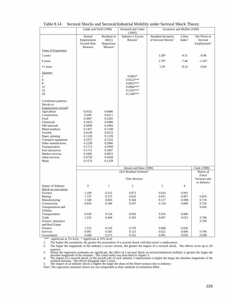
229
Table 8.14 Sectoral Shocks and Sectoral/Industrial Mobility under Sectoral Shock Theory Gulde and Wolf (1998) Brainard and Cutler
(1993) Jovanovic and Moffitt (1990)
Annual
Employment
Growth Rate Measure
Residual of
AR(1)
Regression Measure
Industry‟s Excess
Returns2
Standard deviation
of Sectoral Shocks3
Lilien
Index3
Net Flows in
Sectoral
Employment3
Years of Experience
5 years 3.28* -4.51 -0.96
8 years 2.78*
-7.40 -1.54*
11 years 1.39
-8.23
-0.64
Quarters
1 0.0061* 4 0.0523***
8 0.0815***
12 0.0964***
16 0.1165***
20
0.1340***
Correlation patterns:
Shocks to
Employment Growth1
Agriculture 0.0532 0.0686
Construction 0.449 0.0211
Food 0.3007 0.2505 Chemicals 0.1623 0.0480
NM minerals 0.3099 0.2093
Metal products 0.1457 0.1108 Textiles 0.0136 0.0223
Paper, printing 0.1120 0.1139
Transport equipment 0.2557 0.1252 Other manufactures 0.2228 0.2066
Transportation 0.1713 0.2909
Fuel and power 0.1711 0.2067 Market services 0.1682 0.0815
Other services 0.0730 0.0558
Mean 0.1574 0.1329
Altonji and Ham (1990) Clark (1998)
OLS Residual Estimate4
Time Horizon
Shares of
Fitted Variance due
to Industry
Impact of Industry Shock on own-sector
0 1 2 3 4
Forestry 1.108 0.312 0.073 0.014 0.001 -
Mining 1.737 0.137 0.032 0.011 0.007 0.819 Manufacturing 1.540 0.845 0.364 0.117 -0.006 0.710
Construction 0.654 0.349 0.207 0.124 0.068 0.726
Transportation and
Utilities
0.416
Transportation 0.430 0.124 0.043 0.016 0.006
Trade 1.232 0.449 0.183 0.067 0.023 0.786 Finance, Insurance
and Real Estate
0.709
Finance 1.515 0.516 0.176 0.060 0.020 Services 0.991 0.305 0.123 0.022 0.000 0.709
Government 0.494 0.275 0.161 0.091 0.050 0.938
*** significant at 1% level. * significant at 10% level. 1. The higher the correlation, the greater the association of a sectoral shock with that sector‟s employment.
2. The larger the magnitude of the industry‟s excess returns, the greater the impact of a sectoral shock. The effects occur up to 20
quarters. 3. Where the regression estimates are significant, the effect of a sectoral shock on sectoral/industrial mobility is greater the larger the
absolute magnitude of the estimate. The Lilien index was described in chapter 3. 4. The impact of a sectoral shock on the growth rate of each industry‟s employment is higher the larger the absolute magnitude of the
residual estimate. The effects disappear after 5 years. 5. The impact of an industry shock is higher the larger the share of the fitted variance due to industry. Note: The regression estimates shown are not comparable as their methods of estimation differ.

230
In summary, whilst a range of methods have been used in the literature, several of these
seem less suited to the current study than others. Gulde and Wolf‟s (1998) correlation
technique is unsuitable, as it offers only a measure of association. Moreover, the spatial
component of the shock measure computed across the European countries is not relevant to
the current study which focuses on one country (i.e. Korea). The shock measures in Altonji
and Ham (1989) and Clark (1998) could have multicollinearity problems and Brainard and
Cutler‟s (1993) capital measure may not be relevant where the focus is on labour market
pressures. Thus, it appears that the AR technique employed by Gulde and Wolf (1998) and
Jovanovic and Moffitt (1990) to measure an industrial shock is the preferred approach for
the current work.
8.5 DETERMINANTS UNDER BRIDGING THEORY
The study by Jovanovic and Moffitt (1990) attempted to model sectoral/industrial mobility
based on the bridging theory (refer to Table 8.1). This section will not review the findings
for specific variables from this study since this was done in the sections above. Instead, the
further implications for modelling will be highlighted.
Jovanovic and Moffitt‟s (1990) model included one monetary variable (the standard
deviation of the wage distribution) and the sectoral shock variable. The monetary variable
was constructed by first estimating a log wage regression by year as a function of
education, experience, experience-squared and race. The predicted monetary variable and
sectoral shock were then entered into the mobility regression, which was estimated using
samples of workers at 3 levels of experience, 5, 8 and 11 years.
The main feature of the Jovanovic and Moffitt (1990) study of relevance to the current
study is the inclusion of the variables typically included in tests of the mismatch theory as
well as the sectoral shock variable. This approach will be followed in the empirical
chapters of this thesis.
231
8.6 ASSESSMENT OF EMPIRICAL STUDIES OF
SECTORAL MOBILITY FOR MODELLING
The sections above have reviewed the findings on specific variables in the empirical
literature, and where possible have commented on whether parallel variables should be
included in the empirical application to Korea. The lessons from past research can be
extended to issues associated with data-type, coverage, model specification, variable-type
and method of estimation. Under each of these headings, general observations from
empirical studies are identified below, followed by a critical assessment. Where possible,
links with the theoretical model and studies of other forms of mobility (in chapters 6 and 7)
are made. For reference, Table 8.1 has outlined the features of the studies of
sectoral/industrial mobility pertaining to the source, data-type, coverage, model
specification, dependent variable and method of estimation.
Data-type
Studies of sectoral mobility have been based on three types of data: longitudinal or unit-
record time-series13
, unit-record cross-sectional and aggregate-level datasets. Studies with
longitudinal data include Osberg (1991), Osberg, Gordon and Lin (1994), Jovanovic and
Moffitt (1990) and Loungani and Rogerson (1989), whilst those with cross-sectional data
comprise Vanderkamp (1977) and Neal (1995). The studies using aggregate-level datasets
are McLaughlin and Bils (2001), Jayadevan (1997) and Ottersen (1993).
Chapters 6 and 7 (and Part I) recommended the use of micro-level data for the study of the
factors affecting mobility to facilitate an in-depth understanding. Thus, studies with
aggregate-level data are less favoured since only broad-level patterns can be identified.
Amongst studies with unit-record data, analyses with time-series or cross-sectional data
appear to be equally valuable, as the former is able to cater for a time dimension in the
analyses, and the latter can provide an in-depth profile of industry movers. The KLIPS is a
unit-record longitudinal dataset which marries the two data categories bringing together the
benefits of both into a single estimating equation.

232
Coverage
The studies reviewed in Table 8.1 cover three labour groups5: the overall workforce
[Vanderkamp (1977), Loungani and Rogerson (1989) and Ottersen (1993)], males [Osberg,
Gordon and Lin (1994), Jovanovic and Moffitt (1990) and Neal (1995)] and separate
analyses for males and females [Osberg (1991)]. It is seen that most studies have examined
either the overall or male workforce, save for Osberg (1991). As the mobility patterns of
males and females may differ, chapter 6 recommended that the analyses be disaggregated
by gender. Against this background, the Osberg (1991) study appears to have an advantage
over the others by extending its analysis to female mobility. The current thesis will examine
mobility behaviour for the pooled workforce, and also conduct separate analyses for the
male and female workforces in Korea.
Model Specification
The model specification recommended in the previous chapter involved a mix of monetary
and non-monetary variables. Several studies of sectoral mobility have used such a
specification, namely, Osberg (1991), Vanderkamp (1977), Osberg, Gordon and Lin
(1994), Jovanovic and Moffitt (1990), Loungani and Rogerson (1989) and McLaughlin and
Bils (2001). Jovanovic and Moffitt (1990) is distinguished by also including a stochastic
shock variable. Therefore, in terms of the specification, these studies are more relevant for
the current work than those focusing only on the sectoral shock variable, i.e. Gulde and
Wolfe (1998), Brainard and Cutler (1993), Clark (1998) and Altonji and Ham (1990) [refer
to Table 8.14].
Sectoral Distinction of Variables
One of the points gathered from chapters 6 and 7 was that a sectoral breakdown for both
monetary and non-pecuniary variables was desirable. However, only a few of the studies
listed in Table 8.1 have accommodated this, namely the sectoral wage differential in
Osberg, Gordon and Lin (1994), sectoral wages, size and unemployment in Vanderkamp
(1977) and sectoral performance in Jayadevan (1997). The current study will be based on
sectoral-specific variables where possible.
233
Dependent Variable and Method of Estimation
Chapter 6 indicated that the dependent variable should be binary, indicative of an
individual‟s change of sectors/industries, and this should be analysed with a probit or logit
model. Selected studies, i.e. Osberg (1991), Osberg, Gordon and Lin (1994), Jovanovic
and Moffitt (1990) and Neal (1995), have used the probit or logit model to examine the
probability of a sectoral move. These are more relevant to the empirical model of equation
(6.7) than those studies using the proportion/growth rate of industry movers/moves and
OLS for estimation.
In summary, there is no one single study that accommodates all the relevant features for the
current work. The empirical model is a combination of the features implied from its
theoretical origins (outlined in chapter 6) and extracted from other studies of various forms
of mobility (in chapter 7).
8.7 SUMMARY OF EMPIRICAL STUDIES OF SECTORAL MOBILITY
This chapter has described the various ways worker mobility has been modelled. The
empirical evidence from sectoral/industrial mobility can be succinctly stated. It should be
noted that only variables where at least two studies reported a similar finding are discussed
in this paragraph. The main determinants of sectoral/industrial mobility appear to be overall
wages, unemployment duration, age, tenure, working hours, size of the old/new industry
and sectoral shocks. Among the employed, the variables that were positively associated
with sectoral/industrial mobility were overall wages, working hours, size of the new
industry and sectoral shocks. Unemployment duration, age and tenure were shown to have
a negative impact on mobility. Among the unemployed, only age, tenure and size of old
industry, which had negative effects on industrial mobility, were statistically significant.
Only a few studies reported that separate analyses were conducted for males and females.
Unemployment spell, employment status, working hours/weeks and size of new industry
were positively associated with male mobility, whilst age and tenure had negative impacts.

234
Employment status and unemployment spell had positive influences on female mobility,
whilst age, tenure and the overall unemployment rate had negative effects on female
mobility. The remaining variables considered for the separate gender groups, namely
marital status for both groups and working hours/week for females, were statistically
insignificant.
Table 8.15 lists the explanatory variables used and findings in the studies of
sectoral/industrial mobility. The applicability of these variables with respect to the current
analysis for the Korean workforce is also summarized in this table. Whilst sections 8.3 and
8.4 have reviewed the explanatory variable in terms of conceptual alignment with the
theoretical model and research on sectoral mobility, an assessment of the variables on
issues of measurement and applicability for the Korean labour market, and availability of
data in the KLIPS dataset, is also provided in the table.
Given the varied evidence and few common findings for each explanatory variable, few
firm general conclusions can be drawn. Even fewer can be drawn concerning gender
differences in the determinants of mobility. However, this should not be viewed as overly
alarming, as there are conflicting hypotheses regarding the impact of most variables on
industrial mobility. Thus, the impact of many variables cannot be determined prior to the
empirical application. The analysis on the determinants of industrial mobility in Korea to
be undertaken in chapters 9 and 10 will adopt a comprehensive approach which may enable
comment on the array of findings in the literature to date.

235
Table 8.15 Assessment of the Explanatory Variables
Explanatory Variables Findings Applicability Measurement/Remarks Monetary Variables Overall Wages P (E)
I (U) No
This variable is not recommended as
there is no sectoral distinction.
Wages in the New Sector/Industry
M (E) M (U)
Yes Individual‟s average monthly income in the new sector, adjusted for the chances of finding employment. This variable will be used to compute the expected sectoral wage differential.
Wages in the Original Sector/Industry
M (E) P(U)
Yes Individual‟s average monthly income in the original sector. This variable will be used to compute the expected sectoral wage differential.
Sectoral Wage Differential I (E) Yes Wage differential between individual‟s monthly income in the new sector and individual‟s monthly income in the original sector. This variable will be adjusted for the chances of finding employment.
Wage Growth in the New Sector/Industry
n.r. Yes The annual growth rate of wages (in percentage terms) in the individual‟s new sector/industry.
Wage Growth in the Original Sector/Industry
n.r. Yes The annual growth rate of wages (in percentage terms) in the individual‟s original sector/industry.
Macroeconomic Variables Overall Unemployment N (E)
I (U) No This variable is not recommended as
there is no sectoral distinction.
Unemployment in the New Sector
M (E) Yes The unemployment rate of the individual‟s new sector. A lagged variable should be used if simultaneity occurs with sectoral/industrial mobility.
Unemployment in the Original Sector
P (E) I (U)
Yes The unemployment rate of the individual‟s original sector. A lagged variable should be used if simultaneity occurs with sectoral/industrial mobility.
Unemployment Duration
P (E) M (U)
No The data pertain to the unemployed for aggregate-level datasets.
Overall Economic Growth M Yes Overall GDP growth rate.
Overall Employment M No This variable is not recommended as it should simply capture influences similar to the unemployment variable.
Inflation Rate n.r. No All workers face the same price levels and changes regardless of sectors.

236
Table 8.15 Assessment of the Explanatory Variables (continued)
Explanatory Variables Findings Applicability Measurement/Remarks Worker Characteristics Age N (E)
N (U) Yes Age of individual (in years).
Gender M (E-males)
P (U-females) Yes Gender of individual entered as a
dummy variable for males versus females.
Race n.r. No A racial distinction is not relevant for predominantly mono-cultural societies like Korea.
Language n.r. No The findings were insignificant. Furthermore, the variable is not needed as the common/commercial language in Korea is Korean.
Marital Status P (E) N (U)
Yes Marital status of an individual (married versus non-married) entered as a dummy variable.
Household Head N (U) Yes Household head status of an individual entered as a dummy variable to distinguish if the person was a household head.
Children I (U) No This variable is not recommended as its
effect was found to be insignificant.
Formal Education M (E) M (U)
Yes Education status entered as a dummy variable to distinguish tertiary versus non-tertiary educated workers.
On-the-job Training P (E) No The data on on-the-job training are difficult to quantify.
Tenure N (E) N (U)
Yes Job tenure of the individual measured in years is available.
Initial Industry M (E) I (U)
Yes The initial industry of an individual.
Occupation Status M (E) M (U)
Yes Occupational status of an individual (skilled versus semi-skilled) entered as a dummy variable.
Employment Status M (E) Yes Employment status of an individual [employee versus other workers (employer, own account workers, family workers)] entered as a dummy variable.
Unionisation n.r. No The data are not available for non-employees in Korea.
Region n.r. No The data are only available for region of birth, and not region of present residence.
Alternative Sources of Income
n.r. No The KLIPS had poor data quality as the majority of respondents did not know whether they had social assistance.

237
Table 8.15 Assessment of the Explanatory Variables (continued)
Explanatory Variables Findings Applicability Measurement/Remarks Job/Industry Characteristics Working Hours/Weeks P (E) No There was a relatively high number of
KLIPS respondents who did not indicate their working hours/weeks. Therefore, the number of observations for this variable compared to the other explanatory variables is relatively low.
Product/Work Similarity P (E) No The level of product/work similarity cannot be ascertained from the KLIPS.
Size of Original Industry N (U) Yes Level of industry employment in the individual‟s original industry.
Size of New Industry P (E) I (U)
Yes Sum of industries‟ employment except that of the individual‟s original industry.
Industry Turnover P (E) N (U)
No The separation and accession rates were not available for the agricultural sector.
Performance of Original Industry
n.r. Yes Value-added growth rate of individual‟s original industry.
Performance of New Industry n.r. Yes Value-added growth rate of individual‟s new industry (i.e. all other industries except individual‟s original industry).
Sectoral Shock
P
Yes
Residual of an AR regression on employment that is lagged by one or more time-periods.
Annotation: P : one or more studies reported a positive effect on mobility. N : one or more studies reported a negative effect on mobility. I : one or more studies reported an insignificant effect on mobility. M : Mixed findings among studies/groups/periods. It can refer to differing results among multiple studies and/or
across time periods for same work group in the same study, or for different groups (e.g. males and females) in the same study.
E : Employed persons. U : Unemployed persons. n.r.: The variable was not reviewed. Note: Where neither „E‟ nor „U‟ is indicated, the variable covers the macro-economy.
8.8 SUMMARY OF LESSONS DRAWN FROM THE LITERATURE
Numerous lessons have been drawn from the theoretical and empirical review in the first
three chapters of Part II, covering both sectoral mobility and other forms of mobility.
Chapter 6 provides the theoretical basis for model application and estimation. The
extended Le and Miller (1998) model (as per equation 6.7) is the recommended tool where
conceptual advancements are introduced in the form of the expected sectoral wage
differential and lifetime earnings. Probit- or logit-type regressions are deemed as most
suitable, catering for the use of dichotomous dependent variables which adequately reflect

238
dual mobility states, namely, to move or to stay. Gender analyses on mobility, which are
usually neglected in the literature, could be conducted depending on findings of gender
differences in Korea. The model can be applied to test the three theories of sectoral
mobility covering the worker-employer mismatch, sectoral shock and bridging hypotheses.
Chapter 7 reviews other forms of labour mobility (union/non-union, public-private, rural-
urban) and gives a general framework for specification of the current model. The
recommendations are to establish a model that includes a sectoral wage differential as well
as macroeconomic and non-monetary factors; a sectoral distinction for the unemployment
variable, and sectoral breakdown for non-pecuniary variables where possible. Longitudinal
datasets are superior to cross-sectional datasets as they are a rich data source and cater for
time-series analyses. The latter attribute is desirable for the current study as
macroeconomic and lagged dependent variables, which have been found to be significant
determinants of mobility, can be incorporated into the empirical model.
Chapter 8 is the critical literature review where empirical evidence is canvassed from
studies of sectoral/industrial mobility that could be a yardstick against which analyses of
the determinants of mobility in Korea are assessed. However, varied evidence and
conflicting hypotheses prevent the formation of firm conclusions for each variable. The
determinants reported to be significant covered an array of monetary factors (overall
wages), macroeconomic factors (unemployment duration), worker characteristics (age,
tenure and working hours), job characteristics (size of the old/new industry) and sectoral
shocks. This spread of factors, coupled with the limitation in the number of common
findings, gives rise to the adoption of a comprehensive approach in model specification for
the current work.
The final section of chapter 8 (section 8.7) summarizes the applicability of the explanatory
variables with respect to the current analysis, taking into account issues related to
measurement, the Korean labour market and data availability. The determinants to enter
into worker‟s mobility function are the sectoral wage differential, sectoral wage
growth/unemployment/size/performance, GDP growth, sex, age, marital status, educational
attainment, head of household status, occupational status, employer status, job tenure and
239
the sectoral shock. The investigation into the determinants of sectoral mobility in Korea
begins in chapter 9, followed by the study disaggregated by gender in chapter 10.
Endnotes:
1. Refers to 751 job losers and quitters who changed industries out of a total of 1,089 who went through at
least 1 week of unemployment but gained employment either in the new or old industry.
2. Refers to 1,685 workers who changed industries out of a total of 2,641 employees. The 2,641 were
unemployed in the 5 years before the survey date but they had gained full-time employment at the point of the
survey.
3. Several studies [Podgursky and Swaim (1987), Madden (1987, 1988) and Addison and Portugal (1989)]
recognized the importance of industrial mobility but did not examine this form of worker mobility behaviour.
These studies focused on the wage losses of displaced workers instead.
4. The industry was classified into eleven product groups to distinguish product similarity and two work
groups (light – mental activity, and heavy – manual/physical activity) for classifying work similarity.
5. It is noted that Prasad (1997) examined the correlations between the growth rates in relative sectoral
employment and relative sectoral wages. The relative measures of these variables were the deviations from
the aggregate growth rates. Negative and significant correlations between relative wages and employment
were found in agriculture, construction, finance, manufacturing, mining, public administration and utilities
during the 1959-1993 period. This measure is not suitable for the current study as it is a bi-variate correlation
study, not regression analysis. 6. Results from Thomas (1996b) were inferred from Figures 1 and 2 for a standard worker who receives/does not receive UI according to the route of job separation (quit or loss). The standard worker is one who worked in a service industry in a blue-collar occupation for 2.2 years, did not belong to a union and had an hourly wage rate of $9.16. The results are the probability of the u-r transition from being unemployed in sector „a‟ to being employed in sector „b‟, Mjb (tu), conditional upon the length of the unemployment spell (tu) and job separation status (j). Mjb (tu) = hjb (tu) / [hjb (tu) + hja (tu)], where hj represents the hazard rates of transition. 7. The marginal effect is measured by β*ρ*(1-ρ)*100, where β is the regression coefficient and ρ is the
proportion of industry movers. In Osberg (1991), the marginal effects for males were 0.23, 0.18 and 0.21 for
1980/1981, 1982/1983 and 1985/1986, respectively. For the same corresponding periods, the marginal effects
for females were 0.26, 0.12 and 0.32.
8. It is noted that the coefficient of (AiAj)1/2
was positive.
9. Amongst the unemployed, Neal (1995) reported that married males had a lower likelihood of switching
industries.
10. The KLIPS questionnaire classifies training (excluding regular schooling) according to training in a
private institution, authorized vocational institute, public vocational institution, in-house training by firms etc.
Since there are a variety of training programmes, those who received training would have had different types
of training which may or may not be relevant to the new sector. Furthermore, not all individuals would have
received training, especially the non-employees.
11. This does not support the view in Neal (1995) that switchers forfeit compensation for industry skills.
12. Altonji and Ham (1990) and Clark (1998) made mention of possible correlations between shock measures
but assumed the errors were independently distributed in the models.
13. A number of studies use datasets that follow individuals or firms over time. These can be described as
unit-record time-series datasets. In this thesis, these will be referred to via the usual terminology of
longitudinal or panel datasets.

240
CHAPTER 9
EMPIRICAL STUDY ON THE DETERMINANTS
OF SECTORAL/INDUSTRIAL MOBILITY IN KOREA
9.1 INTRODUCTION
The literature review in chapter 8 indicated that there is a solid empirical foundation for the
understanding of worker mobility. It was suggested that the main determinants of sectoral
labour mobility in the U.S., Canada, Sweden and India are monetary, economic,
demographic and socio-economic factors. However, three gaps in the research were
identified. First, there is a dearth of mobility studies for Asia. This chapter attempts to fill
this void in the literature by modelling mobility behaviour in Korea. Second, there are a
number of inconsistencies in the results reported. For example, there are few common
findings with regards to the relationship between inter-industry mobility and worker
characteristics. The current study will attempt to account for these inconsistencies. Third,
the studies reviewed often focus on one set of variables (e.g. demographic) to the exclusion
of others (e.g. monetary). It is the intent of this chapter to conduct an all-encompassing
formal study covering monetary, economic, demographic and socio-economic factors,
which no other study has done.
The objective of this chapter will therefore be to comprehensively examine the
determinants of sectoral/industrial mobility for the Korean workforce. The chapter is
organized as follows. Section 9.2 introduces the data source, concepts, coverage and time
periods used in the empirical work. A generic model of sectoral/industrial mobility is
presented in Section 9.3. Sections 9.4 and 9.5 present descriptive statistics of the variables
used in the regression analysis of sectoral mobility, as well as selected
predicted/recomputed monetary and sector-level variables. The results of the empirical
analysis of the determinants of sectoral mobility are presented and discussed in Section 9.6.
A series of extensions of the empirical model are considered in Section 9.7. These include
assessing the impact of an individual‟s industry of origin on sectoral mobility as well as an
empirical test of three theories of mobility: worker-employer mismatch, sectoral shock and
bridging theories. A summary of the empirical findings and concluding comments are

241
given in the final section. The list of variables and the rules followed when deriving them
are provided in Appendices 9A and 9B.
9.2 DATA SOURCES, CONCEPTS AND COVERAGE
This chapter is based on both unit-record and aggregate-level data. The unit-record data
were obtained from the Korean Labor and Income Panel Study (KLIPS) conducted by the
Korea Labor Institute (KLI)1. The aggregate-level data were obtained from the Korea
National Statistical Office (NSO).
There are five ideal prerequisites for a micro-level dataset on inter-industry mobility: (i) the
sample should be representative of the working population; (ii) the dataset should be large;
(iii) individuals must be surveyed at least twice; (iv) the data should extend over a fairly
long period; and (v) individuals should report income and industry at the time of the
interview rather than over the past year [McLaughlin and Bils (2001)]. The unit-record
data available in the KLIPS sample satisfy these prerequisites.
9.2.1 KLIPS Data
Although there are several national labour surveys in Korea, i.e. Current Population Survey,
Special Survey of Employment, Survey of Labour Mobility and Basic Survey of Wages,
these are cross-sectional in nature. Cross-sectional data do not cater for the construction of
many of the variables that are prominent in studies of mobility behaviour, and the KLI was
set up to enable the collection of longitudinal data that might overcome these and to
facilitate in-depth study of the labour market and mobility issues. The KLIPS that it has
collected is a longitudinal study of a representative sample of households and individuals
living in urban areas in Korea. It is the first panel survey in Korea on labour-related issues.
The first wave was launched in 1998 in the midst of the Asian Financial Crisis.
The KLIPS sample is an equal probability sample of households from the seven
metropolitan cities and urban areas in eight provinces in Korea. The sampling frame was
from the 1995 Korean mid-term census. Out of 21,675 census unit areas, 951 sampling
unit areas were selected. For each sampling unit, five to six households were randomly
242
chosen. The KLIPS sample yielded 5,000 households in the first wave, with some 13,321
household members aged 15 years and over being successfully interviewed. These 5,000
households represent the original panel in the study.
The study comprises four waves of data that were collected from 1998 till 2001. The initial
sample of households were interviewed in 1998 (wave 1), with follow-up interviews in
1999 (wave 2), 2000 (wave 3) and 2001 (wave 4). New joiners, namely those who have
blood or economic ties to the original panel members, were added to the sample in waves
2-4. Where a panel member moved out and formed an independent household with his/her
new family (e.g. spouse), then the new family members were treated as new joiners to the
original panel. Additionally, if an outside party joins one of the existing households
surveyed (e.g. via marriage), he/she was also included in the interview. Each person is
identified by a unique personal identification number (PID).
The field work for the KLIPS started in May and ended around September each year, with
the majority of household interviews being completed by end-August. Consequently, the
survey reference month is treated as end-June (mid-point) each year.
Any analysis on mobility needs a time dimension to assess if mobility occurred. This paper
looks at the mobility over one year, i.e. between year t-1 and year t. Sectoral/industrial
mobility is defined as having occurred if a person switched industries between year t-1 and
year t. This establishes one of the selection criteria for the current study‟s dataset, namely
that a person must participate in at least two consecutive survey years and have reported
positive incomes and valid data on the industry of employment in the two years. It is
possible to identify such persons by using the PID to match respondents in the datasets of
adjacent years. One advantage in using a one-year time dimension to examine mobility is
that persons who switch industries with longer intervening unemployment spells can be
included in the study.2
As the KLIPS attempts to track members who moved out of the original household, the
KLIPS dataset does not depend on residential stability. Since at the aggregate level, inter-
industry mobility includes inter-industry movers who change their place of residence, this
means that the measure of industrial mobility available for use in this thesis will not
243
underestimate aggregate inter-industry labour mobility. This an advantage over Osberg‟s
(1991) study, for example, where movers were dropped from the original Canadian sample
of households and thus his measure of the dependent variable was the conditional
probability of inter-industry mobility, given residential stability. Since the residential
movers in Canada comprised 3% of the initial sample, if the probabilities of residential and
inter-industry mobility are positively correlated, Osberg‟s (1991) estimate of the probability
of sectoral mobility would be biased downwards.
Notwithstanding these advantages, several limitations of the dataset must be pointed out.
The past year‟s data can be captured fairly accurately for waves 2-4, as respondents, having
been interviewed in the first wave, are aware of the subsequent interviews and will
probably record and report the information at the time of the interview and/or provide an
update of the change of information from the previous year‟s survey. The responses for the
initial wave, however, could be subject to greater recall error as respondents were being
interviewed for the first time and did not know previously that they had to provide answers
to their income/industry over the past year. So the actual dollar income earned or specific
industry group for the initial wave may not be accurate. Nevertheless, there is consistency
in all the waves in the sense that the past year‟s information refers to the past 12 months.
This even applies to the initial wave. Some respondents may have reported a series of jobs
in the past but it is possible to ascertain the previous year‟s income/industry based on the
start dates and quit dates of the previous job. So the data for wave 1 are fixed to a specific
time period of one year, i.e. as at June 1997.
The other limitation lies in the length of the time period available for research. The four-
year time series, though adequate for research on some labour market characteristics (e.g.
unemployment duration), may not be sufficiently long to capture effects on mobility over
an individual‟s working life. Furthermore, as mobility patterns are detected at the same
month every year (i.e. June), it would not be possible to ascertain the seasonal responses in
mobility behaviour. Unless mobility patterns can be tracked quarterly/six-monthly instead
of annually, any seasonal effects on inter-industry mobility should be interpreted with
caution.
To obtain information about individuals during the pre-move period (year t-1) and post-
move period (year t), the data items from the previous wave‟s dataset were appended to the

244
current wave‟s dataset via matching with the PID. The list of data items and their
derivations are supplied in Appendix 9A. Moreover, for the initial 1998 wave, respondents
were asked to provide their previous income, industry, occupation, employment size,
employment status, start dates and quit dates, and so these records could be considered for
inclusion in the set of inter-industry movers for the study below.
The analysis focuses on a subset of the population in the dataset, namely persons aged 20-
64 years. The age group is chosen as the mobility patterns for younger workers (aged less
than 20 years) are affected by schooling behaviour, whilst those for older workers (beyond
64 years) are influenced by retirement behaviour. To model mobility that is affected by
schooling or retirement behaviour is beyond the scope of the thesis. Therefore, the focus is
on workers aged 20-64 years. This is in line with Oi‟s (1987) recommendation to include
adults aged 20-64 years as this offers a „cleaner statistic measuring variations in labour
market activity‟. Respondents with non-positive income, those who did not report either an
old/new industry, and those who did not provide valid data on any other question used in
the analysis are excluded from the sample. Consequently, the sample for the current study
amounts to 10,691 person-year observations covering the period 1998-2001 (about 4 years
per person). In addition, one variable, working hours in the individual‟s original sector, was
excluded owing to its significantly fewer number of observations (6,161).
The structure of the sample dataset varies from that used in past studies. Cross-sectional
analyses of mobility behaviour have been conducted for different periods with periodic
gaps. For instance, Osberg (1991) analysed 3 sets of years: 1980 to 1981, 1982 to 1983 and
1985 to 1986, with a periodic gap between the second and third set. This study‟s panel
dataset combines the mobility records of individuals from 4 consecutive waves: 1997 to
1998, 1998 to 1999, 1999 to 2000 and 2000 to 2001. By repeatedly interviewing the same
respondents over the years, there are no periodic gaps and mobility behaviour can be more
readily analysed in conjunction with the continuous time-series macroeconomic data which
can be embedded into this type of data structure. With the inclusion of relevant time-series
macroeconomic data in micro-level panel data, the explanatory power of the regression
analysis of sectoral mobility is likely to be enhanced.

245
9.2.2 Korea NSO Data
The macroeconomic variables and sectoral indicator variables considered from the
literature review to have influence on mobility decisions, namely: overall/sectoral GDP
growth rate, sectoral/industrial employment size and unemployment rate, and annual
growth rates in sectoral/industrial income, are obtained from the Korea NSO. In addition,
the sectoral shock measure is estimated using industrial employment data from the NSO.
9.2.3 The Role of Interim State of Unemployment
The sample of 10,691 covers employed persons who reported an industry of employment as
at year t-1 and year t. This does not preclude the possibility of such persons being out of
employment between periods t-1 and t. The purpose of this section is to demonstrate that
ignoring any interim states of unemployment does not affect the analysis of sectoral labour
flows. By doing so, the various states of employment/non-employment and the relationship
between gross and net labour flows are highlighted. The approach here is to examine the
inflows and outflows of labour from a larger sample with fewer restrictions, and to compare
these to the proposed final sample of 10,691 observations, where additional restrictions are
imposed to permit a more refined analysis. In addition, this preliminary analysis will
provide the reader with information on how the sample of 10,691 observations evolved.
9.2.3.1 Sectoral Labour Flows
Table 9.1 shows the labour flows based on a sample of persons aged 20-64 years, where
individuals can report either their new or old industry, or both. That is, respondents need
not report all of the information on wages, job tenure, employment status, occupational
status and educational attainment. This gives us a larger sample size of 29,474 person-year
observations. This sample constitutes industry stayers (Es), inter-industry movers,
employed workers in year t-1 who become unemployed, moved out of the labour force or
did not report any industry in year t (denoted by Uo, where the subscript refers to outflows)
as well as the unemployed, those not in the labour force (NILF) or who did not report any
industry in year t-1 who entered into employment and reported their industry in year t
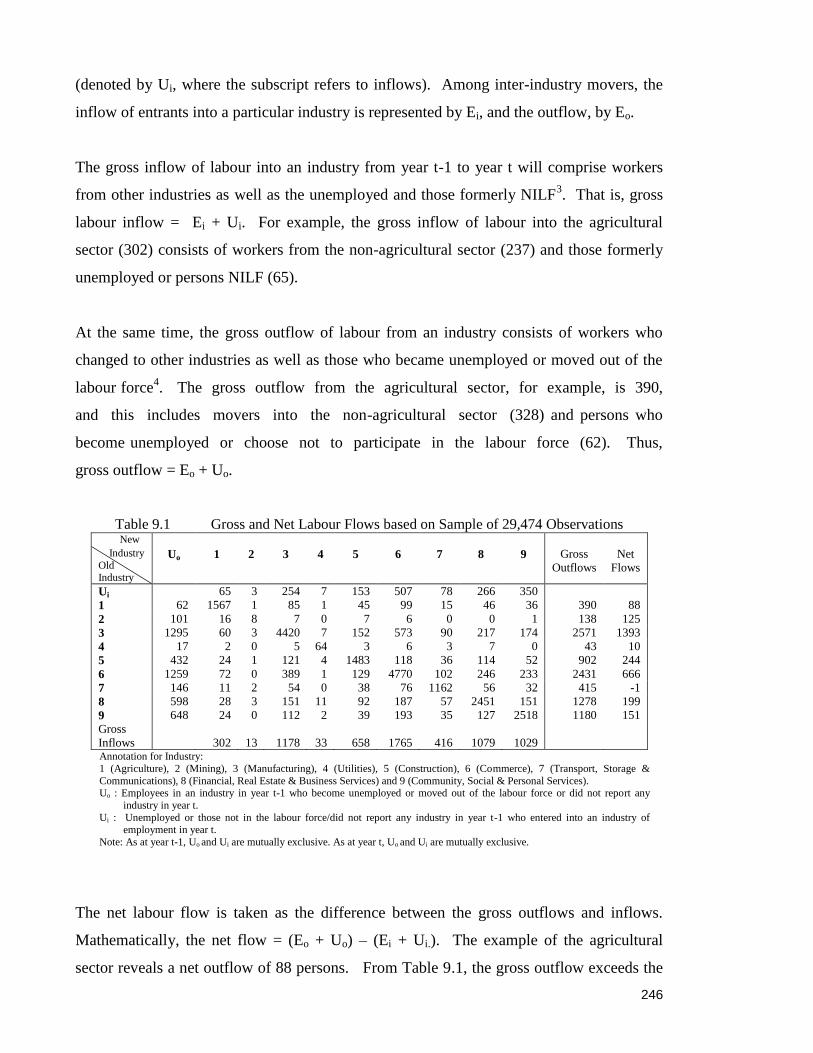
246
(denoted by Ui, where the subscript refers to inflows). Among inter-industry movers, the
inflow of entrants into a particular industry is represented by Ei, and the outflow, by Eo.
The gross inflow of labour into an industry from year t-1 to year t will comprise workers
from other industries as well as the unemployed and those formerly NILF3. That is, gross
labour inflow = Ei + Ui. For example, the gross inflow of labour into the agricultural
sector (302) consists of workers from the non-agricultural sector (237) and those formerly
unemployed or persons NILF (65).
At the same time, the gross outflow of labour from an industry consists of workers who
changed to other industries as well as those who became unemployed or moved out of the
labour force4. The gross outflow from the agricultural sector, for example, is 390,
and this includes movers into the non-agricultural sector (328) and persons who
become unemployed or choose not to participate in the labour force (62). Thus,
gross outflow = Eo + Uo.
Table 9.1 Gross and Net Labour Flows based on Sample of 29,474 Observations New Industry
Old Industry
Uo 1 2 3 4 5 6 7 8 9 Gross
Outflows
Net
Flows
Ui 65 3 254 7 153 507 78 266 350
1 62 1567 1 85 1 45 99 15 46 36 390 88
2 101 16 8 7 0 7 6 0 0 1 138 125
3 1295 60 3 4420 7 152 573 90 217 174 2571 1393
4 17 2 0 5 64 3 6 3 7 0 43 10
5 432 24 1 121 4 1483 118 36 114 52 902 244
6 1259 72 0 389 1 129 4770 102 246 233 2431 666
7 146 11 2 54 0 38 76 1162 56 32 415 -1
8 598 28 3 151 11 92 187 57 2451 151 1278 199
9 648 24 0 112 2 39 193 35 127 2518 1180 151
Gross
Inflows 302 13 1178 33 658 1765 416 1079 1029 Annotation for Industry:
1 (Agriculture), 2 (Mining), 3 (Manufacturing), 4 (Utilities), 5 (Construction), 6 (Commerce), 7 (Transport, Storage &
Communications), 8 (Financial, Real Estate & Business Services) and 9 (Community, Social & Personal Services). Uo : Employees in an industry in year t-1 who become unemployed or moved out of the labour force or did not report any
industry in year t.
Ui : Unemployed or those not in the labour force/did not report any industry in year t-1 who entered into an industry of employment in year t.
Note: As at year t-1, Uo and Ui are mutually exclusive. As at year t, Uo and Ui are mutually exclusive.
The net labour flow is taken as the difference between the gross outflows and inflows.
Mathematically, the net flow = (Eo + Uo) – (Ei + Ui.). The example of the agricultural
sector reveals a net outflow of 88 persons. From Table 9.1, the gross outflow exceeds the

247
gross inflow for all sectors/industries except for transport, storage and communications.
This pattern is not surprising since the data collection was during the post-Asian Financial
Crisis period which witnessed numerous business closures and job losses on an economy-
wide scale. An outflow of labour in nearly all sectors/industries is thus to be expected.
9.2.3.2 Missing Industry Information
The provision of a respondent‟s industry information in period t-1 and period t is a critical
key for the empirical exercise. In the dataset, some workers did not state their industry of
employment in either survey period t-1 or period t. Their numbers are represented by
Uiinterim
and Uointerim
in Table 9.2. From Tables 9.1 and 9.2, Ui = Ui*
+ Uiinterim
and
Uo = Uo* + Uo
interim. From the first equality, Ui
interim denotes persons who did not report any
industry in period t-1 but reported an industry of employment in period t. The Ui* category
comprises persons formerly in non-employment in period t-1 who entered into employment
in period t. For the second equation, Uointerim
are those who had a job/industry reported in
period t-1 but did not provide their industry of employment in period t. The Uo*
category
represents workers formerly in employment in period t-1 who became unemployed or left
the labour force in period t. Since such persons under Uiinterim
and Uointerim
categories did
not report any industry information in one of the time periods, they are excluded from the
final sample.
It is observed that missing industry information does not really affect the comparison of
gross flows and net flows in the KLIPS. Compared to Table 9.1, when Uiinterim
and Uointerim
are ignored, gross outflows still exceed the gross inflows for all sectors/industries in Table
9.2. Furthermore, the labour movements of inter-industry movers (i.e. the Eo‟s and Ei‟s) of
Table 9.2 are very similar to those of Table 9.1. One difference between Table 9.1 and
Table 9.2 is the net flow data for the transport, storage and communications industry, where
the net flow turned positive, from -1 to 5. The small disparity of 6 persons stems from the
difference between Uiinterim
(19) and Uointerim
(13). Thus, from this exercise, the non-
importance of the non-stated industry categories is illustrated.
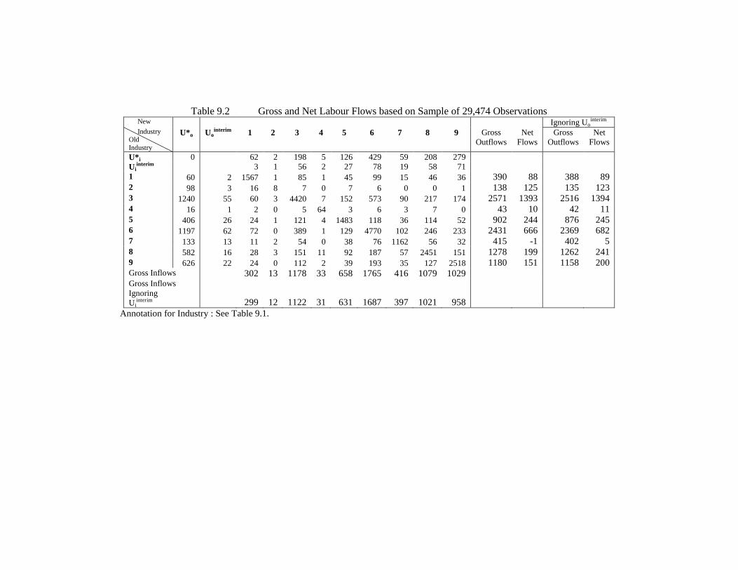
Table 9.2 Gross and Net Labour Flows based on Sample of 29,474 Observations New Ignoring Uo
interim Industry
Old
Industry
U*o Uointerim 1 2 3 4 5 6 7 8 9 Gross
Outflows
Net
Flows
Gross
Outflows
Net
Flows
U*i 0 62 2 198 5 126 429 59 208 279
Uiinterim 3 1 56 2 27 78 19 58 71
1 60 2 1567 1 85 1 45 99 15 46 36 390 88 388 89 2 98 3 16 8 7 0 7 6 0 0 1 138 125 135 123 3 1240 55 60 3 4420 7 152 573 90 217 174 2571 1393 2516 1394 4 16 1 2 0 5 64 3 6 3 7 0 43 10 42 11 5 406 26 24 1 121 4 1483 118 36 114 52 902 244 876 245 6 1197 62 72 0 389 1 129 4770 102 246 233 2431 666 2369 682 7 133 13 11 2 54 0 38 76 1162 56 32 415 -1 402 5 8 582 16 28 3 151 11 92 187 57 2451 151 1278 199 1262 241 9 626 22 24 0 112 2 39 193 35 127 2518 1180 151 1158 200 Gross Inflows 302 13 1178 33 658 1765 416 1079 1029
Gross Inflows
Ignoring
Uiinterim
299 12 1122 31 631 1687 397 1021 958
Annotation for Industry : See Table 9.1.

249
9.2.3.3 Missing Survey Information
It is observed that the sample of 29,474 observations contains respondents who did not
provide information on all of the potential determinants of sectoral mobility to be examined
in the statistical analysis. To effectively conduct the empirical analysis of mobility, the
latter group, numbering 12,544 over the four waves (see top panel of Table 9.3), had their
records removed. Additionally, persons who entered into/out of the states of non-
employment marked out by intervals of one year, or those who did not report an industry of
employment in either period t-1 or period t (U0 and Ui), were also excluded (see section
9.2.3.2). The remaining sample of 10,691 observations in the bottom panel of Table 9.3
consists of stayers (Es) and movers (Eo and Ei) who reported all of the survey information.
Under these sample exclusions, it is can be seen that the comparison of gross outflows and
gross inflows in the sample of 10,691 observations differs from that of the unabridged
sample of 29,474 observations. The net labour flow is now positive for the agricultural,
mining and manufacturing sectors, and negative for utilities, construction, commerce and
the services industries. Therefore, missing survey information on the other explanatory
variables appears to affect the relative sizes of the gross and net flows. Unfortunately, the
importance of this to the statistical analyses conducted below cannot be ascertained, either
through formal modelling5 or by drawing on the literature (where the issue does not seem to
have been discussed).
Table 9.3 Industry Breakdown of 29,474 Sample with/without Survey Information New Industry
Old Industry
Uo 1 2 3 4 5 6 7 8 9 Total
excl. Uo
Ui 65 3 254 7 153 507 78 266 350
Respondents who did not report other survey information*
1 62 1154 1 46 0 17 58 3 16 22 1317
2 101 12 3 5 0 0 2 0 0 0 22
3 1295 45 3 2362 3 76 308 37 91 76 3001
4 17 1 0 2 37 1 3 0 3 0 47
5 432 9 0 61 1 726 54 15 45 28 939
6 1259 46 0 209 0 51 2879 42 110 115 3452
7 146 6 1 21 0 16 36 543 24 9 656
8 598 21 0 62 3 55 90 20 1202 74 1527
9 648 15 0 60 1 20 100 14 58 1315 1583 Total excl. Ui 1309 8 2828 45 962 3530 674 1549 1639 12544

250
Table 9.3 Industry Breakdown of 29,474 Sample with/without
Survey Information (continued) New
Industry
Old Industry
1 2 3 4 5 6 7 8 9 Gross
Outflows
Net
Flows
Respondents who reported all of the required survey information
(based on 10,691 observations)
1 413 39 1 28 41 12 30 14 165 83
2 4 5 2 7 4 1 18 13
3 15 2059 4 76 265 53 126 99 638 180
4 1 2 27 2 3 3 4 15 -3
5 15 1 61 3 757 64 21 69 24 258 -11
6 26 180 1 78 1891 60 136 118 599 -8
7 5 1 33 22 40 619 32 23 156 -51
8 7 3 89 8 37 97 37 1249 77 355 -111
9 9 52 1 19 93 21 69 1203 264 -92 Gross Inflows 147 8 712 25 422 1114 285 732 706
Annotation for Industry, Uo and Ui : See Table 9.1. * : This comprises respondents who reported both their original and new industries but did not provide any information for at least
one of the following variables: old wage, new wage, job tenure or occupation. These records were excluded to obtain the main sample of 10,691 observations.
9.2.3.4 Interim States of Unemployment
The sample of 10,691 observations will include those who may have experienced an
interrupted spell of unemployment between period t-1 and period t. Out of this sample,
there are some 826 workers who encountered an unemployment spell during the interim
period, as shown in Table 9.4. The difference between these workers and the Uiinterim
and
Uointerim
groups is that they reported their industry of employment as at the survey reference
dates. Hence, they can be effectively classified under their industry of employment, as
shown in Table 9.4.
The purpose in this section is to illustrate that even if the 826 persons were excluded, the
main features of the comparison of the gross outflows and gross inflows carry over from
the comparisons shown in Table 9.3. There is a net outflow of labour from the
agricultural, mining and manufacturing sectors, and a net inflow into the utilities,
construction, commerce and services industries. Therefore, ignoring the state of intervening
unemployment does not affect the labour flows in this study of inter-industry mobility.

251
Table 9.4 Gross and Net Labour Flows based on Sample of 10,691 Observations New
Industry
Old
Industry
1 2 3 4 5 6 7 8 9
Interim Unemployment between period t-1 and period t
1 6 0 3 0 1 3 1 0 1
2 0 0 0 0 0 0 0 0 0
3 0 0 170 0 9 14 4 15 4
4 0 0 1 2 1 0 1 0 0
5 0 0 7 0 85 3 5 5 2
6 0 0 16 1 7 147 17 15 6
7 0 0 2 0 0 4 31 4 1
8 0 0 11 0 3 12 2 82 7
9 0 0 5 0 4 9 2 10 85
Number of persons with uninterrupted employment
Gross
Outflows
Net
Flows
1 407 0 36 1 27 38 11 30 13 156 74
2 4 5 2 0 7 4 0 0 1 18 13
3 15 0 1889 4 67 251 49 111 95 592 179
4 1 0 1 25 1 3 2 4 0 12 -5
5 15 1 54 3 672 61 16 64 22 236 -8
6 26 0 164 0 71 1744 43 121 112 537 -25
7 5 1 31 0 22 36 588 28 22 145 -30
8 7 3 78 8 34 85 35 1167 70 320 -97
9 9 0 47 1 15 84 19 59 1118 234 -101
Gross Inflows 82 5 413 17 244 562 175 417 335
Annotation for Industry: See Table 9.1.
9.3 GENERIC MODEL OF SECTORAL/INDUSTRIAL MOBILITY
The generic model of sectoral labour mobility adopted for the study of individuals‟ choice
between two sectors given in the index function of equation (6.7) is restated here:
Ii = γ1 + γ2 [ ln pi + ln yai – ln ybi] + γ3 gai + γ4 gbi - Ziδ - Siφ.
The actual and expected incomes, measured over the individuals‟ lifetimes, represented in
the model are as described earlier. Zi is an all encompassing vector of economic,
demographic and socio-economic factors, Si represents the stochastic shock term, δ is a
vector of coefficients for Zi and θ is the coefficient for Si. This generic model enables us to
test three theories of sectoral mobility: the worker-employer mismatch, sectoral shock and
bridging theories of sectoral mobility that were outlined in chapter 6.
The index, Ii, is a latent variable for the propensity of workers to move across industries. It
is not observed. Rather, what is observed is a binary indicator of whether workers moved

252
(I*i). It takes the value 0 when individual i did not switch sectors/industries, and the value 1
if individual i did switch sectors/industries, between period t-1 and period t. It can be
linked to the latent index Ii as follows: I*i = 1 if Ii ≥ 0 ; I
*i = 0 otherwise.
The dataset classifies the sectors/industries according to the Korean Standard Classification
of Industries. The sectors/industries are categorized into nine major groups: agriculture;
mining; manufacturing; utilities; construction; commerce; transport, storage &
communications; financial, real estate & business services; and community, social &
personal services. Hence, I*i is assigned the value 1 if the respondent switched between
these industry groups.
As mentioned in the literature review, the standard OLS method of estimation is not
recommended. This is because the dependent variable is binary and hence it is not normally
distributed and the distribution of the residual term will be heteroscedastic. This violates
one of the assumptions of OLS regression, and so statistical inference would not be valid.
Therefore, a logit model is used, with the estimates being obtained using the method of
maximum likelihood, similar to Osberg (1991). The logit regression does not require the
dependent variable to be normally distributed. However, it does retain some of the other
requirements of OLS regression: error terms must be independent and the relationship
between the logit of the dependent variable and the explanatory variables must be linear in
coefficients.
9.4 DESCRIPTIVE STATISTICS
This section presents the descriptive statistics of the variables to be included in the current
study. Given the selection criteria described above and the complexity of the KLIPS
survey design, the section first explores the possibility of incorporating survey weights in
the KLIPS sample. This is in line with the theoretical recommendations outlined in several
studies, that survey weighting achieves greater precision in the sample statistics [Kish
(1965), Kish and Frankel (1974), Scott and Watson (1982) and Watson and Fry (2002)].
This also permits an assessment of whether the usage of a longitudinal dataset for Korea
can be aligned with that of the longitudinal datasets of advanced countries which adopt

253
survey weighting [Thompson, Fong, Hammond, Boudreau, Driezen, Hyland, Borland,
Cummings, Hastings, Siahpush, Mackintosh and Laux (2006) for an inter-country tobacco
study, and Watson (2004) and Watson and Fry (2002) for Australia].
9.4.1 Survey Weights
The KLIPS dataset does not have survey weights that accommodate aspects of the survey
design, sample attrition or new entrants. A review of recent studies covering a wealth of
topics using the KLIPS longitudinal data have shown that none have attempted to develop
survey weights to address the issue. These include Nam (2007) on asset distribution, Kim
(2004a) on family background and education, Cho (2005) on household wealth, Sawangfa
(2007) on job satisfaction, Kim (2003) on IT job training, Young (2005) on ageing, Kang
(2004) and Kim (2004b) on university prestige and choice of study, Young (2006) on social
class and gender differentials, Chang and Yang (2007) on non-standard employment, Seong
(2007) on union participation, Son (2007a) and Son (2007b) on job training for women, and
Jung, Moon and Hahm (2007) on age, gender, sector and job satisfaction.
As the weighting of the survey data may affect the precision and/or interpretation of the
regression results, it is the intent of this section to determine whether this might be an issue.
An approach that can be taken in this regard that is within the scope of this thesis is to
construct a series of variable weights, and then compare the descriptive statistics using
these weights with those obtained from non-weighted data.
In terms of constructing survey weights from the current KLIPS dataset, the aims are
twofold: (i) to adjust the basic characteristics of the sample so that they align with the
national benchmark at the time of the wave 1 data collection, and (ii) to account for sample
attrition and cater for new entrants at the subsequent waves 2, 3 and 4. Thereafter, the set
of weighted descriptive statistics will be compared with the non-weighted set to determine
if the weighting process renders a substantive difference to the statistics.

254
9.4.1.1 Wave 1 Weights and the Population
Although the original KLIPS survey consist of 5,000 households, from which individuals
of 20-64 years of age amount to 29,474 person-year observations, this includes individuals
with incomplete information. The final sample for the regression analysis consists of the
10,691 observations with complete information on the variables used in the statistical
analyses. This sample of 10,691 as at wave 1 is treated as the population for the purpose
of developing the survey weights below.
The purpose of the wave 1 weights is to align the sample labour force profile as at wave 1
to that of the national labour force profile. This national benchmark is obtained from
Korean NSO employment data for 1998. Three stratification variables are used when
constructing the weights, namely sex, education status and employment status. The year
1998 is used to coincide with the time the data for wave 1 were gathered.
In the weighting process, individuals‟ basic characteristics (as at wave 1) and initial
industry were assigned an expansion factor, which is the ratio of the national composition
of the labour force to that of the wave 1 sample for the respective variable in question. The
variable is then multiplied by the weighting factor, i.e. X x weighting factor, where X is the
dummy variable (equals 1) for the characteristic in question. Table 9.5 below presents the
weights for the basic characteristics. For example, in the case of females, the weighting
factor is 1.27 (i.e. 0.400/0.315) where the numerator is the 1998 national proportion of
employed females and the denominator is the sample proportion of females as at wave 1.
The individual value for each female is 1 x 1.27.
Table 9.5 Wave 1 Weights Variable Weighting Factor
Sex
- Male
0.88
- Female 1.27
Education Status
- Graduate
1.35
- Non-graduate 0.95
Employment Status
- Employee
0.78
- Employer 1.81 Source: Author‟s calculations from KLIPS dataset and Korean NSO data.

255
In addition to the wave 1 weights, the variables sex, employment status and education
status are also weighted by the probabilities of survival and for being a new entrant as
described below. The methodology for deriving the weighted means and standard
deviations of these socio-demographic variables is found in Appendix 9C.
9.4.1.2 Weights for Sample Attrition
Sample attrition occurs in the KLIPS, though non-response, respondents moving out of the
original household or become out of scope (e.g. missing survey information as described in
the previous section). The surviving pool in the subsequent wave is therefore the cohort of
individuals from the previous wave which did not become out of scope and continued to
exist in the original household. The probabilities of survival in the KLIPS sample were
0.44, 0.35 and 0.38 for waves 2, 3 and 4, respectively6. Weights for each wave were
increased by their wave 1 weight modified by a factor inverse to their probability of
survival in that wave, i.e. P(survivalw).
It is noted that the probabilities of survival are below the norm. This is owing to the
selection criteria and method of data processing adopted. As mentioned, selection involved
the inclusion of individuals 20-64 years, those who took part in consecutive waves in the
original KLIPS survey and those with non-negative incomes and those with complete/valid
survey information for the regression analysis. The processing of the KLIPS dataset,
especially with the data completeness checks, was done irrespective of waves so as to
include more individuals in the sample for the regression analysis. This resulted in a lower
survival rate when examined on a wave-by-wave basis.
9.4.1.3 Weights for New Entrants
To counter-balance the low probabilities of survival, weights are included to account for
new entrants to the KLIPS sample in waves 2, 3 and 4. New entrants exist in the KLIPS
sample because they are either new joiners to the KLIPS survey, e.g. new members to the
household or re-entrants from previous waves. The probability of being a new entrant for
each wave is the proportion of new entrants to the total number of individuals for each
wave. For waves 2, 3 and 4, the probabilities are 0.57, 0.65 and 0.62, respectively. Weights

256
for each wave are modified to a factor inverse to the probability of being a new entrant in
that wave, i.e. P(new entrantw).
For both survivors and new entrants, the weights are computed differently depending on
whether the variable is categorical or continuous. The continuous variables comprise age,
tenure, GDP growth, sectoral shock, the sectoral wage differential as well as the old and
new sector wages, unemployment, wage growth, size and performance. The categorical
variables in the KLIPS are industry mover status, sex, marital status, education status,
employment status, occupational status, head of household status and the initial industry.
Together, the weights of survivors and new entrants are incorporated into the computation
of the descriptive statistics. Given that the KLIPS is a complex sample, the weighted
means and standard deviations are appropriately termed as „complex statistics‟. The
complex statistics are computed differently depending on whether the variable is
continuous or categorical. Appendix 9C lists the methodology for deriving the complex
statistics for both types, taking into account the probabilities of survival and of being a new
entrant.
9.4.2 Descriptive Statistics: Complex Statistics
Table 9.6 presents the descriptive statistics for the weighted and non-weighted series from
the KLIPS sample of 10,691 observations covering the four job waves (1998 till 2001).
The list of explanatory variables is in Appendix 9A. From Table 9.6, the means for the
non-weighted and weighted series are fairly similar for all variables, except for mover
status, which is smaller under the weighted series, pointing towards the lower share of
industry movers in subsequent job waves. The lower share of movers in the latter years
reflects the state of labour market adjustment. Workers are more likely to switch sectors
arising from retrenchments or business closure during the immediate year of the Crisis (i.e.
wave 1) as compared to the latter years.
A smaller standard deviation is noted for most variables, reflecting the greater precision in
estimation under the weighted series. This is to be expected as the variance from a complex
sample (e.g. clustered or stratified) is usually smaller than that under simple random
sampling [Jolliffe (2002/2003)]. This can be summarized using the design effect (deff),

257
which gives the net effect of various complexities of the sample as compared to simple
random sampling. It is „the ratio of the actual variance of a sample to the variance of a
simple random sample of the same number of elements‟ [Kish and Frankel (1973)], and can
be computed as:
deff = Varianceweighted / Variancenon-weighted .
Since the standard deviation rather than the variance is usually used for statistical inference
in regression models, the design effect is often computed in square-root terms, i.e.
____ __________________________
√ deff = √ Varianceweighted / Variancenon-weighted .
From Table 9.6, the design effect is slightly less than 1 for most variables, reflecting the
lower standard deviation under complex sampling. As the design effect is close to 1, this
means that the sample variance under the weighted series only deviates marginally from
that under the non-weighted series. The means of the variables under the two methods of
computation in Table 9.6 are also similar. Thus, the weighting process does not contribute
to a significant difference in the descriptive statistics of the explanatory variables listed.
Hence, the descriptive statistics in this section refer to the non-weighted set.
The majority of workers are industry stayers, which is not surprising as several authors
have highlighted the constraints confronting workers considering change to their industry
of employment. Nonetheless, the share of inter-industry movers is large enough (23%) to
facilitate the study of sectoral mobility, and is quite similar to the mobility rates reported in
Jovanovic and Moffitt (1990) [13%-26%], Osberg (1991) [14%], Osberg, Gordon and Lin
(1994) [13%] and Osberg, Mazany, Apostle and Clairmont (1986) [20%-36%].

258
Table 9.6 Means and Standard Deviations for Korean Workers, Aged 20-64 years
Mean
(or Percent)
Standard
Deviation
Mean (or
Percent)
Standard
Deviation
___
√deff
Non-weighted series Weighted series
Monetary variables
Ln (Expected New Industry Wage) 4.59 0.67 4.61 0.66 0.985
Ln (Original Industry Wage) 4.34 1.03 4.47 0.84 0.816
Growth Rate of New Industry Wage (%) 4.29 6.45 6.48 4.08 0.633
Growth Rate of Original Industry Wage (%) 4.22 6.56 6.46 4.09 0.623
Macroeconomic variables
Unemployment Rate in New Industry in Period t-1 (%) 3.84 2.81 4.60 2.38 0.847
Unemployment Rate in Original Industry in Period t-1 (%) 3.82 2.78 4.57 2.36 0.849
Worker characteristics
Industry Mover (%) 23.1 42.14 16.0 33.36 0.792
Male (%) 64.6 47.82 64.3 47.53 0.994
Age at Former Interview (yrs) 39.7 10.66 40.0 10.39 0.975
Original Job Tenure (yrs) 7.12 8.22 7.42 7.39 0.899
Married Person (%) 73.4 44.18 73.6 43.70 0.989
Household Head (%) 52.9 49.92 55.5 47.91 0.960
Educational Attainment: Graduate (%) 14.6 35.29 16.0 36.35 1.030
Professional/Associate Professional (%) 7.5 26.33 8.1 27.18 1.032
Employee (%) 79.8 40.17 80.3 34.44 0.857
Initial Industry (%)
Agriculture 5.4 22.62 4.5 20.40 0.902
Mining 0.2 4.63 0.2 2.94 0.6351
Manufacturing 25.2 43.43 24.7 43.10 0.993
Utilities 0.4 6.26 0.4 6.28 0.995
Construction 9.5 29.32 9.4 29.11 0.993
Commerce 23.3 42.27 23.2 42.19 0.998
Transport, Storage & Communications 7.2 25.93 7.6 26.44 1.020
Financial, Real Estate & Business Services 15.0 35.71 16.3 36.76 1.029
Community, Social & Personal Services 13.7 34.41 13.7 34.45 1.001
Industry characteristics
Original Industry Size (no.) 3,556 1,573 3,555 1,578 1.003
New Industry Size (no.) 3,533 1,585 3,543 1,579 0.996
Original Industry Growth Rate (%) 5.36 8.33 7.76 5.93 0.7122
New Industry Growth Rate (%) 5.33 8.33 7.73 5.95 0.7142
GDP Growth Rate (%) 4.42 4.15 6.37 0.00
Sectoral Shock
Residual of AR(1) Regression (micro-level) 3.45 100.93 5.02 56.17 0.5573
Residual of AR(1) Regression (by wave) 0.37 0.1335 0.02 0.01 0.0754
Cross-sector Standard Error of Residual
of AR(1) Regression 0.18 0.0954 0.17 0.08 0.839
Sample Size 10,691 10,691
Source: KLIPS dataset, KLI. Note: Since the annual GDP growth rate does not vary within each wave, the weighted standard deviation is zero. Hence, its design
effect cannot be computed. See Appendix 9C.
1. The lower standard deviation (weighted series) is due to fewer individuals in mining. The standard deviation is zero for waves 2 and 3 for new entrants and wave 4 for new entrants/survivors. Hence, the design effect is relatively low.
2. The lower design effect reflects the lower standard deviation (weighted series) for old/new industry growth for new entrants in waves
3 and 4. Since these variables vary by wave only, the standard deviation for each wave merely reflects distributional differences amongst new entrants and survivors.
3. The standard deviations on a by-wave basis are generally less than 100 except for wave 3 for survivors. This accounts for the lower
overall weighted standard deviation of 56. Hence, the design effect is lower. 4. Since the residual is derived from a regression for each wave, the residual on a by-wave basis is negligible. Any deviation within each
wave reflects distributional differences between survivors and new entrants and is negligible. Thus, the descriptive statistics between
the weighted and non-weighted sets differ and the design effect is small.

259
In terms of worker and job characteristics, there are proportionately more males (65%) than
females (35%) in the Korean sample. There are proportionately more married persons
(73%), employees (80%) and household heads (53%) in the sample than the respective
complementary categories (the non-married, non-employees and non-household heads).
There are relatively fewer graduates (15%) and professionals (8%). The typical worker is
40 years of age and has accumulated 7 years of work experience in his original/current job.
The initial industries for most individuals are concentrated in the manufacturing sector
(25%), commerce sector (23%) and financial, real estate and business services industries
(15%).
The monetary indicators favour the new sector/industry. Thus, the new industry‟s expected
wages (in natural logarithms) exceed the old industry‟s actual wages, and the annual
average growth rates in income of the workers‟ new industries are marginally higher than
the rates in their old industries.
On average, the GDP growth rates and employment sizes of workers‟ new industries were
lower than those of their original industries. The lower growth suggests that the influence
of the sector‟s past performance on a sectoral move may not be compelling. The average
lagged annual unemployment rate was slightly higher for new industries. That is, at the
aggregate level, movement to a new sector will involve a trade off of higher unemployment
for higher wages.
It is observed that the comparison of old versus new sector monetary and sector-level
variables remains unchanged under the weighted and non-weighted series. The average
GDP growth rate of the industries of employment reported by Korean workers in the
sample was 4%.
The typical worker experienced a sectoral shock whilst working in their original industry
during 1998-2001. This is revealed by the positive mean values from the alternative
measures of a sectoral shock. There are two approaches to estimating the AR(1) residual
designed to capture the unanticipated effects on sector-specific employment between two
time periods. The first, the residual of an AR(1) regression7 (micro-level), is computed by
regressing the individual industry‟s employment in period t on that of period t-1, and

260
taking the difference between the fitted and estimated values of industry employment for
each individual record. The second AR(1) residual (by wave) was estimated in a similar
fashion to that of Jovanovic and Moffitt (1990). The natural logarithm of the industry‟s
employment AR(1) regression was estimated for each year (i.e. four years) and the
corresponding four standard errors from these regressions were then inserted into the
dataset for each record8. All individual records within the same wave (or year) would have
the same value. It is not surprising that the standard deviation was significantly smaller
than for the first AR(1) measure.
The shock measures are estimated across all sectors/industries of the economy and
comparison data need to be constructed in a similar way9. The positive mean value of the
AR(1) residual (by wave) is comparable in size with Jovanovic and Moffitt‟s (1990) shock
measures, which ranged from 0.006 to 0.031 during 1968-1980 in the U.S.
The third measure of sectoral shock is given by the cross-sector standard error of the
residual of an AR(1) regression of the natural logarithm of industry employment. This
estimates the unobservable effects on sectoral employment independent of the effects on
aggregate employment. For each observation, it is computed as:
[eit/Et x (res(ln eit) – res(ln Et))]1/2
,
where eit is the industry‟s employment, Et is aggregate employment, res(ln eit) is the
residual of an AR(1) regression of industry employment and res(ln Et) is the residual of an
AR(1) regression of aggregate employment.
Table 9.6 shows that the mean value of the cross-sectoral standard error of this AR(1)
residual was 0.18, and this is much smaller than the AR(1) residual (micro-level) measure.
This is due to the fact that it removes the unanticipated effects of a shock on overall
employment, and as such it allows the effect on a specific sector to be examined in
isolation. Therefore, it might be reasonable to expect that this might be the most
appropriate measure for the empirical study.
These descriptive statistics give a preliminary indication of some worker/job and monetary
variables that might be influential in the mobility decision. The patterns between old and

261
new sectors in many of these variables are consistent with expectations. However, in the
case of sectoral growth rates, the new sector‟s rate is lower than the old sector‟s, and for
unemployment rates, the new sector‟s rate is higher. A further examination of these
variables is required. The extent to which patterns more consistent with economic theory
emerge from the study of individual-level data will be examined in the later part of this
chapter.
9.5 DERIVATION OF PREDICTED/RECOMPUTED VARIABLES
As the examination of sectoral mobility involves industry movers and stayers, and the study
focuses on the motivation behind a movement from the old sector to the new, there must be
some observable differences in the explanatory variables for movers and stayers. This
leads to problems for the researcher in the case of stayers, for whom there is no designated
new industry, especially for variables that make use of aggregate-level industry data, and
for the monetary variable which involves computation of the new sector‟s wage, i.e. the
sectoral wage differential. The purpose of this section is to compute suitable values for
these variables for industry stayers.
Sector-level Variables
The potential new sector-level values for industry stayers are not observed for the wage
growth, lagged unemployment rate, sectoral size and sectoral performance variables. If the
current sector values are assigned to the new sector variables, there is a high correlation
between the old-new variables: ga versus gb (0.889), Ua,t-1 versus Ub,t-1 (0.875), sizea versus
sizeb (0.728) and GDPa versus GDPb (0.793). These correlation coefficients are less than
one only because the old and new industries for movers differ.
To overcome this problem, the sector-level variables for movers are constructed using the
average across all industries other than the stayer‟s original industry value as the new
industry values. These re-computed new sector values should not exhibit high correlations
with the values for the old sectors. The remaining explanatory variables, namely the

262
individual characteristics and GDP growth, are not affected as they remain unchanged for
each individual in the sample datasets.
The list of the data items following these changes and their corresponding annotation are
supplied in Appendix 9B.
Sectoral Wage Differential
The issue of determining an appropriate „new sector‟ value also arises for the sectoral wage
differential for stayers, as their old sector wage, but not their potential new sector wage, is
observed. A related issue is that the actual wage data available at the micro-level contain
both an observed predictable element and an unobserved stochastic component. This could
lead to biased estimates if the stochastic component is related to the error term in the
mobility equation.
The possibility of biased estimates with the use of actual wage data can be accommodated
through the use of predicted wages. The variable in question is the expected sectoral wage
differential. For this, the individual‟s new and old sectors‟ wages, and the new sector‟s
unemployment rate, need to be derived to arrive at the wage differential term. For
reference purposes, these derived data items will be termed the „predicted new sector‟s
wage‟, „predicted old sector‟s wage‟, „predicted new sector‟s unemployment rate‟ and
„predicted expected sectoral wage differential‟.
9.5.1 Predicted Sectoral Wages
The computation of the predicted old/new sector‟s wages adopts the methodology of Tomes
and Robinson (1982a) in their estimation of the determination of wages for two different
regions in the context of Canadian interprovincial migration. The methodology of Tomes
and Robinson (1982a) is an example of what Borjas (1980) refers to as using a „clean‟
proxy for a wage variable that has econometric problems associated with it. Offered wages
are usually held to be dependent on personal attributes, and so the wage functions for sector
a (ln yai) and sector b (ln ybi) for an individual i can be constructed as:

263
ln yai = Xiβa + uai (9.1)
ln ybi = Xiβb + ubi (9.2)
where Xi is the set of observable personal characteristics (sex, age, marital status,
educational attainment, head of household status, occupational status, employer status and
job tenure)10
, βa and βb are the vectors of parameters associated with each sector to be
estimated for the corresponding explanatory variables, and uai and ubi are the unobservable
components representing the general ability and other factors applicable to sectors a and b,
respectively, but which are not captured under Xi. The dependent variables, ln yai, and
ln ybi, are the individual‟s actual wages (expressed in natural logarithms) in the new sector
and old sector, respectively.
Since industry movers and stayers each experience different levels of utility from changing
sectors or remaining immobile, the sample is self-selected into mover and stayer sub-
samples, and the estimation of the individual wage equations (9.1) and (9.2) is based on
these truncated samples. Predicted wages are then obtained from the industry-specific
wage regressions for movers and stayers. It is noted that these equations are not corrected
for sample selection bias, as undertaken by Tomes and Robinson (1982a), as there is a lack
of variables in the dataset that can be used as legitimate identifying variables in the
selection equation. Furthermore, there have been recent dissatisfaction with the selection
bias methodology where the correction might reduce the accuracy of coefficient estimates
[Puhani (2000) and Stolzenberg and Relles (1997)].
As several studies have revealed inter-industry wages to vary [Carrington and Zaman
(1994), Dickens and Katz (1987), Gibbons and Katz (1992), Helwege (1992), Keane (1993)
and Krueger and Summers (1987)], and some industries may value particular employee
attributes more highly than others, an industry-specific approach to the estimation of the
wage regressions of equations (9.1) and (9.2) is recommended11
.
Predicted Wage for Movers
As in the case of Tomes and Robinson (1982a), wage regressions are undertaken for each
mover and stayer sub-sample. For movers, the term ln ybi is the actual wage reported by

264
individual i in period t-1 in the old industry and ln yai is the corresponding wage reported in
period t in the new industry. Specifically, as mobility in the KLIPS sample is measured
annually, new (old) sector earnings are based on data reported in the first (previous) year of
each survey wave, i.e. 1998 (1997) for wave 1, 1999 (1998) for wave 2 and 2000 (1999)
and 2001 (2000) for waves 3 and 4, respectively.
To obtain the predicted wages for movers in the new (old) industry, ln yai (ln ybi) is
regressed on the Xi‟s for each industry. The fitted values, ln yap
(ln ybp), constitute the
predicted wages for movers in the new (old) industry. Each mover will have a different
predicted wage for the old/new sector computed for incorporation into the mobility
equation. In this regard, the KLIPS dataset is superior to the Tomes and Robinson (1982a)
data, as wages for movers are estimated before and after a sectoral switch. Therefore, the
predicted wages for movers would be:
ˆ ln ya = Xβa from the new industry; and ˆ ln yb= Xβb from the old industry.
It is noted that incomes in the four years of the survey need not be adjusted to the real
(1998) values using the CPI. Since the final model is about the sectoral wage differential,
the real and actual wage differentials are the same as both old/new sector wages are
adjusted by the same deflator12
. This is in line with empirical studies of sectoral mobility
adopting a sectoral wage differential [Osberg, Gordon and Lin (1994)] or old/new sector
wages [Vanderkamp (1977) and Fallick (1993)] which do not make use of a wage deflator.
In addition, recent studies using the KLIPS wage data (though not about sectoral mobility)
have not adopted real wages in their analyses, including Son (2007a), Son (2007b), Kim
(2003), Kang, Park and Lee (2007) and Kang (2004).
Predicted Wage for Stayers
For stayers, the predicted wages in the old industry are obtained from an industry-specific
regression of ln ybi on Xi. The reported old sector wages are based on the previous year,
namely 1997 for wave 1, 1998 for wave 2, 1999 for wave 3 and 2000 for wave 4. Each
stayer will have a different predicted wage for the old sector.

265
As mentioned earlier, the estimation of predicted wages in the new industry for stayers will
pose a problem since their old and new industries are the same. The dataset gives the actual
wage of period t, and not the potential wage that could be achieved in an alternative
industry. To overcome this limitation, the procedure adopted by Tomes and Robinson
(1982a) is used. They treated the new destination as a single alternative comprising all
destinations other than that in which the individual (stayer) was observed in period t. For
example, for an industry stayer working in the commerce sector, the new sector‟s wage is
the average wage across all sectors other than the commerce sector.
To obtain „ln yai‟ for a typical stayer, the aggregated earnings for stayers reported across all
industries other than the original industry is divided by the number of stayers in all
industries other than the original industry, which is then expressed in natural logarithmic
terms. These averages are argued to provide a general idea of what could be earned
following a sectoral move. Earnings (i.e. ya) are based on data observed in the first year
each survey wave was conducted, i.e. 1998 for wave 1, 1999 for wave 2 and 2000 and 2001
for waves 3 and 4, respectively. Stayers from the various „original‟ industries will have
differing ln yai‟s, but those from the same „original‟ industries (for the same survey wave)
will have similar ln yai‟s.
It should be noted that many observations would have the same value for ln yai for the
obvious reason that earnings in the new sector (ya) are not realized or observed by industry
stayers. The variability within each stayer sub-sample needed for the industry-specific
regression to be feasible arises because stayers from different survey waves will have
dissimilar ln yai‟s.
Having derived stayers‟ new sector wages, industry-specific regressions of ln yai on Xi were
then estimated and used to generate a predicted „new‟ sector wage. The corresponding
fitted values, ln yap, constitute the predicted potential wages for stayers in the new industry.
Since the regression is undertaken on Xi which contains a set of characteristics unique to
each individual, each ln yap value would be unique. Therefore, in the case of stayers, the
predicted wages would be:
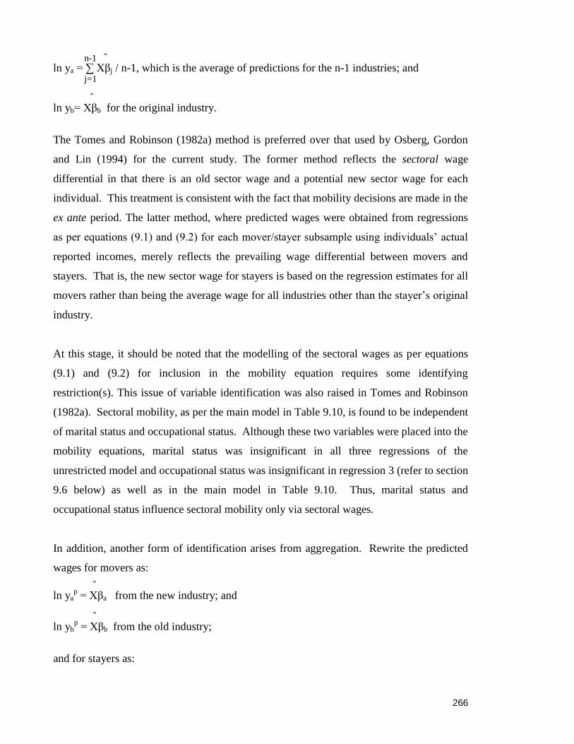
266
n-1 ˆ ln ya = ∑ Xβj / n-1, which is the average of predictions for the n-1 industries; and j=1 ˆ ln yb= Xβb for the original industry.
The Tomes and Robinson (1982a) method is preferred over that used by Osberg, Gordon
and Lin (1994) for the current study. The former method reflects the sectoral wage
differential in that there is an old sector wage and a potential new sector wage for each
individual. This treatment is consistent with the fact that mobility decisions are made in the
ex ante period. The latter method, where predicted wages were obtained from regressions
as per equations (9.1) and (9.2) for each mover/stayer subsample using individuals‟ actual
reported incomes, merely reflects the prevailing wage differential between movers and
stayers. That is, the new sector wage for stayers is based on the regression estimates for all
movers rather than being the average wage for all industries other than the stayer‟s original
industry.
At this stage, it should be noted that the modelling of the sectoral wages as per equations
(9.1) and (9.2) for inclusion in the mobility equation requires some identifying
restriction(s). This issue of variable identification was also raised in Tomes and Robinson
(1982a). Sectoral mobility, as per the main model in Table 9.10, is found to be independent
of marital status and occupational status. Although these two variables were placed into the
mobility equations, marital status was insignificant in all three regressions of the
unrestricted model and occupational status was insignificant in regression 3 (refer to section
9.6 below) as well as in the main model in Table 9.10. Thus, marital status and
occupational status influence sectoral mobility only via sectoral wages.
In addition, another form of identification arises from aggregation. Rewrite the predicted
wages for movers as:
ˆ ln ya
p = Xβa from the new industry; and
ˆ ln yb
p = Xβb from the old industry;
and for stayers as:

267
n-1 ˆ ln ya
p = ∑ Xβj / n-1; and
j=1 ˆ ln yb
p = Xβb for the original industry.
It can be seen that it is this averaging process, in addition to variable identification, which
gives rise to the low correlations between the predicted variables and the other variables
included in the mobility equation.
Predicted New Sector’s Unemployment Rate
The new sector‟s unemployment rate (Uat) can be derived in the same manner as outlined
above for wages via the industry-specific regression of Uat on the individual characteristics
for inter-industry movers. This gives the predicted unemployment rate (Uatp) for movers.
For stayers, the new industry is once again treated as all industries outside the original
industry and the corresponding Uat is the average rate across all industries other than the
stayer‟s original industry. For example, for stayers from commerce, Uat for the new
industry (non-commerce) is computed as:
[UNEMPnon-commerce / (UNEMPnon-commerce + EMPnon-commerce)] x 100,
where UNEMPnon-commerce and EMPnon-commerce are the levels of unemployment and
employment, respectively in all sectors outside commerce. It is noted that the employment
and unemployment data are obtained from the Korean NSO. Published data are used since
these can be considered to be the information available in the marketplace that rational
income-maximizing individuals will make use of to assess their potential mobility
outcomes. The regression of Uat on individual characteristics is undertaken to derive the
predicted rate (Uatp) for stayers.
Each mover/stayer will have a different predicted rate. For movers, the predicted
unemployment rate would be:
ˆ Uat
p = Xβa for the new industry; and
ˆ Ubt
p = Xβb for the original industry.

268
Uatp and Ubt
p for movers are derived via industry-specific regressions using the mover sub-
sample covering four waves of data in the KLIPS.
For stayers, the predicted unemployment rates are:
n-1 ˆ Uat
p = ∑ Xβj / n-1; which is the average of predictions for the n-1 industries; and
j=1 ˆ Ubt
p = Xβb for the industry of origin.
It is noted that the predicted unemployment rates are estimated from industry-specific
regressions using the stayer sub-sample covering four waves of data.
This approach to modelling unemployment rates for inclusion in the mobility equation
embodies the same form of variable identification as was used for wages in that marital
status and occupational status affect inter-sectoral mobility only via the sectoral
unemployment rates. The averaging process of Uat for stayers, another form of
identification, implies that perfect collinearity between the predicted variables and the other
determinants of mobility would never arise.
Predicted Expected Sectoral Wage Differential
With the predicted variables, Uatp, ln yai
p and ln ybi
p, the predicted expected sectoral wage
differential can be computed for each individual as:
ln(pya)p
- lnybp = ln [(1- Uat
p) x yai
p] - ln (ybi
p).
Actual versus Predicted Wage Differential
A comparison between actual (as per the original dataset in Table 9.6) and predicted wages
is undertaken to ensure that the algorithms used to derive the predicted variables have not
altered the basic patterns in the data. The key variable for comparison is the expected
sectoral wage differential. The mean values for the actual and predicted variables are
presented in Table 9.7. It is clear that the use of predicted variables in the empirical work
should not introduce any major distortions, as the mean values of the actual and predicted
variables are fairly similar in magnitude. Thus, the mean values of the actual and predicted

269
expected sectoral wage differential are both higher for movers than for stayers, conforming
to the theory that income-maximising individuals will switch sectors for the monetary
benefit. Moreover, it is observed that the predicted variables have lower standard errors
than the actual variables, attributed in large part to the fact that the stochastic elements
associated with actual wages have been removed.
Table 9.7 Actual versus Predicted Monetary Variables Actual Predicted
Movers
Mean
Standard
Deviation
Mean
Standard
Deviation
Expected New Sector Wages 4.43 0.66 4.37 0.28
Old Sector Wages 3.90 1.33 3.91 0.64
Unemployment Rate 5.43 3.44 5.43 3.06
Expected Sectoral Wage
Differential
0.52 1.35 0.45 0.60
Stayers
Expected New Sector Wages 4.63 0.66 4.81 0.04
Old Sector Wages 4.47 0.88 4.47 0.33
Unemployment Rate 3.88 2.71 3.88 1.84
Expected Sectoral Wage
Differential
0.16 0.76 0.34 0.34
Source: KLIPS dataset
Note: For ease of comparison between actual and predicted variables, the non-
weighted series is presented.
9.5.2 Sector-level Variables
Sectoral Unemployment, Size and Performance
Given the high correlation between the old-new sector-level variables mentioned earlier,
that arises primarily because stayers‟ old and new industries are the same, a rework of the
„new‟ sector variables (the lagged unemployment rate, sectoral size and performance, and
sectoral wage growth) for stayers is in order. Following Tomes and Robinson‟s (1982a)
treatment of the new destination as a single aggregated alternative, the new industry for the
stayers‟ sector-level variables will be all industries other than the original industry. The
sector-level data are obtained from the Korean NSO. As mentioned above, these can be
treated as the data available in the marketplace that income-maximizing agents make use of
in their mobility decisions13
.
270
The new sector‟s size is the average size of all industries other than the stayer‟s original
industry. The new sector‟s GDP growth and lagged unemployment rate are computed
using aggregates for all industries other than the stayer‟s original industry. For instance,
the growth in GDP at current prices across all industries other than agriculture in
period t (GDPnon-agriculture,t) over GDP in period t-1, (GDPnon-agriculture,t-1), is computed as:
[(GDPnon-agriculture,t - GDPnon-agriculture,t-1)/GDPnon-agriculture,t-1] x 100.
The average unemployment rate across all industries other than agriculture is computed as:
[UNEMPnon-agriculture /(UNEMPnon-agriculture + EMPnon-agriculture)] x 100,
where UNEMPnon-agriculture and EMPnon-agriculture each represent the unemployment level and
employment level in all industries other than agriculture. The pair-wise correlations
between these recomputed variables (marked with an asterisk) are substantially lower than
those initially presented: U*a,t-1 versus Ub,t-1 (0.460), size*a versus sizeb (-0.227) and GDP*a
versus GDPb (0.380).
New Sector’s Wage Growth
The descriptive statistics for the annual sectoral wage growth are given in the first two
columns of Table 9.6. Given that the data cover the Asian Financial Crisis period, it is
observed that all industries experienced negative wage growth in 1998. As the wage
growth variable is supposed to represent lifetime earnings, an individual would probably
look at „the industry average‟ rather than a year-on-year measure so that his/her decision
would be more fully informed.
Based on this principle, the wage growth variables were computed using information on the
previous five years. A 5-year period is chosen as it appears to be long enough to average
out the fluctuations observed in the data. Thus, for wave 1, the old/new industry wage
growth rate is computed based on the average annual compound growth rate (ACGR) over
the 1994-1998 period; for wave 2 over the 1995-1999 period; for wave 3 covering 1996-
2000; and for wave 4 extending from 1997 to 2001. For example, for T number of periods
(i.e. 5 in this study), the ACGR for the 1998 wages (y1998
) over the 1994 wages (y1994
) is
computed as follows:

271
ACGR = [(y1998
/ y1994
)1/(T-1)
- 1 ] x 100.
With regards to the new sector, the decision would be whether to move using information
about the new sector‟s future earnings. For each mover, the wage growth is based on the 5-
year average annual compound growth rate in the mover‟s new industry. In line with the
method used for the wage data, fitted values (g*p
at) from a regression of the new sector‟s
wage growth on individual characteristics (sex, age, marital/occupational/employment
status, educational attainment and tenure) are used. This method is similar to Willis and
Rosen (1979), where the wage growth functions for college and non-college attendees were
regressed on individual characteristics. The wage growth regressions are not corrected for
selection bias for the reasons mentioned above. The wage growth effects in the modelling
of worker mobility are identified through marital status and occupational status influencing
mobility only via the wage growth rates. This type of identification is again coupled with
that achieved through the averaging of the predictions for the larger stayers component of
the sample, as discussed in the next paragraph.
In the case of stayers, as their old and new sectors are the same in periods t-1 and t, the
Tomes and Robinson‟s (1982a) treatment of the new sector as an aggregated alternative is
employed. The new sector income is computed as the earnings for all industries other than
the stayer‟s original industry. Stayers for each different year (1998 till 2001) from each
„original‟ industry will have differing earnings. Thereafter, the 5-year average annual
compound growth is applied. For wave 1, the new industry wage growth rate is computed
over 1994-1998, wave 2, over 1995-1999, wave 3 over 1996-2000, and wave 4 over 1997-
2001. Predicted values, obtained from industry-specific regressions of average wage growth
on stayer‟s individual characteristics, are used in the model. In addition to variable
identification, the averaging process of the new wage growth rates for stayers suggests that
the problem of perfect collinearity in the mobility equation that includes the predicted wage
growth variable would be avoided.
Old Sector’s Wage Growth
The lifetime earnings potential in a mover‟s original industry is proxied by using the
average annual wage growth of that old industry over the last five years. Again, fitted

272
values (g*p
bt), from the regression of the old sector‟s wage growth on individual
characteristics, are used in the estimations.
In the case of stayers, since their old and new industries are the same, their annual wage
growth, derived from their reported earnings in period t-1 and period t, is indicative of the
old sector‟s wage growth. It is noted that the use of individual data is in tandem with Willis
and Rosen‟s (1979) estimation of lifetime earnings (conditioned on actual school choices in
the U.S.), which made use of each individual‟s reported initial and latest earnings to
compute a wage growth variable. However, there are anomalies associated with the use of
individual data in the present application, and these will be addressed below.
The average wage growth was an astounding 127.66%, with a large standard deviation of
258.87. These values could perhaps be explained by considering the data period covered,
which is just after the onset of the Asian Financial Crisis when the Korean labour market
underwent tremendous adjustments. These adjustments can be seen in the pattern in the
average wage growth over time. As an example, whilst the average growth was 110.80% in
1998 and 146.96% in 1999, it later tapered to 84.01% in 2000 and 34.00% by 2001. On the
one hand, there are workers who experience phenomenal recovery in actual wages after
apparently suffering major income setbacks during the Crisis period. On the other hand,
there are workers with negative wage growth who failed to recover from the Crisis. Such
outliers should be discarded for the purpose of modelling lifetime wage growth, as this
wage growth would be expected to follow a reasonably steady pattern, and should not
reflect temporary surges or dips arising from external disturbances. The outliers should be
progressively excluded until a reliable growth pattern is achieved.
Given that the 5-year industry average annual wage growth over 1998-2001 using
aggregate-level data is about 6-7%, the KLIPS sample unit-record data spanning all
industries should have a similar average wage growth. To achieve a reliable growth pattern
across respondents in the KLIPS, the top 10% and bottom 5% of outliers had to be removed
in the calculation of lifetime wages. It is noted that more observations from the high-end
growth distribution are removed since the magnitude of wage increases exceeded that of the
decreases, and there are more respondents with positive growth. Additionally, workers who
changed job status between periods were removed in the computation of lifetime wages as
273
their inclusion could distort the annual wage growth rate. These cover a change from part-
time to full-time work and vice versa, or from regular (job contracts exceeding 1 month) to
irregular work (include job contracts of less than 1 month, including daily-rated work) and
vice versa14
.
Removing the top 10%, bottom 5% and individuals with a changed job status gives an
average wage growth of 6.20 with a standard deviation of 25.92 for industry stayers15
. The
average growth in the sample now reflects the industry average of 6-7% with aggregate-
level data. The annual wage growth for each industry was then regressed on the personal
attributes of this sub-set of stayers. The estimated regression equation was then used to
predict a wage for all industry stayers. This enables maximum usage of the dataset. The
average predicted wage growth rate from this exercise is 6.12%, with a much lower
standard deviation of 3.45. This approach to constructing a wage growth variable for
inclusion in the mobility equation identifies the effects of the old sector‟s wage growth via
exclusion restrictions (marital status and occupational status) and through having multiple
(for each industry) equations for generating the predicted variables.
A sensitivity test was conducted to ensure the regression results of the main model
presented later in Table 9.10 are not sensitive to changes in the sample of stayers used to
construct the wage growth variable. An extra 1% of observations at the upper end of the
distribution were removed. The average predicted wage growth rate was then computed
again, and the inclusion of this alternative measure in the main model resulted only in slight
changes to the regression coefficients (of around 1 decimal point). Thus, the results are
robust to this change in the sample used for the underlying regression for the wage growth
calculations for industry stayers.
With this combination of past industry data and the individual-level variables, the pair-wise
correlation coefficient between g*p
at and g*p
bt is 0.007, which is much lower than that for
the aggregate-level, of 0.889.
274
9.5.3 Descriptive Statistics of Predicted/Recomputed Variables
Having derived predicted monetary variables and recomputed the sector-level variables, a
re-look at the descriptive statistics that are to be used in the main model is in order. For
comparative purposes, the non-weighted and weighted series are presented. Similar to the
case for actual data, the design effect is less than 1 for most predicted/recomputed
variables. However, it is usually not much less than 1, implying that little is lost by
focusing on the unweighted data. The description in this section therefore applies to the
non-weighted series.
As in the case for actual variables, the average predicted expected new sector‟s wage was
higher than the average predicted old sector‟s wage. With regards to lifetime earnings, the
average predicted wage growth in the new sector (5.72%) is slightly less than that of the old
sector (6.12%), a pattern different from when the actual variables (as per the first two
columns of Table 9.6) are used. A breakdown revealed that this pattern applied to industry
stayers only. Since stayers constitute most of the sample, this pattern is to some extent the
result of averaging over five years for the new sector compared with the two years for the
old sector. It could also be due to the fact that an arbitrary decision was made by leaving
out the top 10% and bottom 5% to compute the sample 2-year average wage growth in the
old sector, and the descriptive statistics simply reflect the conservative approach taken in
this regard.
The average lagged annual unemployment rate was also slightly higher for the new sectors
when the recomputed rates were used. This is a similar scenario to when the actual
variables were used, suggesting again that a move to the high-wage new sector involves a
trade off for higher unemployment. Conforming to the pattern of Table 9.6, the
recomputed new sector size is smaller than the old sector size, and the recomputed new
sector‟s average growth rate is lower than the old sector‟s, once again suggesting that the
impact of the sector‟s past performance on mobility may not be as great.

275
Table 9.8 Means and Standard Deviations for Predicted and Recomputed Variables
Mean
Standard
Deviation Mean
Standard
Deviation
___
√deff
Monetary variables Non-weighted series Weighted series
ln(pya)p 4.71 0.23 4.74 0.17 0.739
lnybp 4.34 0.48 4.38 0.38 0.792
g*p
at (%) 5.72 0.90 5.74 0.77 0.856
g*p
bt (%) 6.12 3.46 6.15 3.61 1.043
Sector-level variables
U*a,t-1 (%) 4.64 2.12 5.49 1.04 0.4911
Ub,t-1 (%) 3.82 2.78 4.57 2.36 0.849
size*a (no.) 2,432 950 2,365 784 0.825
sizeb (no.) 3,556 1,573 3,555 1,578 1.003
GDP*a (%) 4.59 5.93 6.69 2.63 0.4441
GDPb (%) 5.36 8.33 7.76 5.93 0.712
Sample size 10,691 10,691
Source: KLIPS dataset. Annotations and description of variables are in Appendix 9B.
1. Compared to the weighted series, the high standard deviation for the non-weighted
U*a,t-1 and GDP*a series (and hence their lower design effects) reflects the higher
values in wave 2, the period following the Crisis when Korean workers are in the
initial stages of adjustment. It is noted that the design effects were closer to 1 for the
non-predicted series since aggregate-level data was used.
It can be seen that the predicted/recomputed statistics (non-weighted series) are generally
consistent with the actual variables. Thus, the derivations of predicted and recomputed
variables has not altered the way the mean monetary, macroeconomic and industry
characteristics differ in terms of the old-new sector comparison.
9.6 EMPIRICAL ANALYSIS: DETERMINANTS OF SECTORAL
MOBILITY
Having established the extended Le and Miller (1998) model, a reliable dataset and derived
variables to accommodate econometric issues associated with the original data, the
statistical analysis can be conducted. Prior to examining the determinants of sectoral
mobility, an attempt has to be made to arrive at the main model from the most general
model suggested by the review of past studies. There are three issues: (i) moving from an
unrestricted to a restricted model; (ii) determining if the weighted results should be used;
and (iii) deciding on the most suitable measure of sectoral shock.
Prior to the conduct of unrestricted-to-restricted modelling, a correlation matrix was
computed for all explanatory variables to detect multicollinearity. It was found that the

276
overall GDP growth rate was highly correlated with the new sector‟s performance and
lagged unemployment rate, with a correlation coefficient of at least 0.8. The other
variables were not highly correlated, having correlation coefficients of less than 0.6. To
minimize potential multicollinearity, and given the data shortcomings in that there is a
discrepancy in the time periods [i.e. the GDP growth rate is estimated at year-end (January
till December) whilst mobility (and annual employment) is estimated at mid-year (June
year t-1 till June year t)], and that GDP growth, being measured at yearly intervals, will not
capture any shorter-term cyclical effects, this variable will be excluded from subsequent
specifications.
Table 9.9 lists the estimated coefficients from an unrestricted model, using alternative
measures of a sectoral shock. This unrestricted model is based on a non-linear mobility
relationship for both age and job tenure. The first set of estimates in the left-hand panel is
based on the residual of the industry-specific AR(1) regression (micro level). Those in the
middle panel are based on the residual of the industry-specific AR(1) regression (by wave),
which was adopted by Jovanovic and Moffitt (1990) for the U.S. The third set in the right-
hand side panel is based on the cross-sectoral standard error of residuals from the industry-
specific AR(1) regression16
. It should be noted that the three models presented in Table 9.9
are non-nested and this may make comparison of the models difficult. While a nested
model can include all three shock regressors in the estimating equation, collinearity,
especially between the AR(1) (by wave) and AR(1) (micro level) residuals, prevents this17
.
The determination of the main model and the appropriate shock regressor will have to be
based on the number of significant regressors in the model as well as the overall fit of the
model.
Before the main model is determined, an attempt is made to weight the results and compare
the weighted and non-weighted results. Although the coefficient estimates will not be
seriously affected with complex sampling in large samples, the t-statistic, confidence
intervals and model selection will be biased if these complexities are not taken into
account. The t-statistic (tβ‟) under the complex KLIPS sample can be computed as:
___
tβ‟ = tβ /√deff

277
where tβ is the t-statistic for a regression estimate of β under the assumption of simple
random sampling18
. The weighted t-values are presented in Table 9.9. The comparison is
thus based on the statistical significance of the weighted and non-weighted t-values.
It can be seen that the statistical significance of the explanatory variables does not alter
whether the weighted or non-weighted t-statistic was used. This applies to all three
regressions. The design effect appears to have a modest effect at best. From here, the
logit estimates are therefore based on the non-weighted series. The use of non-weighted
KLIPS data concurs with previous studies, including Nam (2007), Kim (2004a), Cho
(2005), Sawangfa (2007), Kim (2003), Young (2005), Kang (2004), Kim (2004b), Young
(2006), Chang and Yang (2007), Seong (2007), Son (2007a), Son (2007b) and Jung, Moon
and Hahm (2007).
When the residual of an AR(1) regression (micro level) of the individual industry‟s
employment is used, the t-test indicates that sex, age, age-squared, marital status,
employment status, the new sector‟s wage growth and old sector performance did not
significantly influence the probability of a sectoral move at the 5% level. In addition to the
first five variables, the new sector‟s performance and tenure-squared were shown by the
corresponding t-statistic to be insignificant when the AR(1) residual (by wave) was used in
the regression. When the cross-sectoral standard error of residuals from the sector-specific
AR(1) regression of the natural logarithm of annual employment was used, only
occupational status and marital status were not significant influences (at the 5% level) on
the probability of a worker being classified as an inter-sector mover.
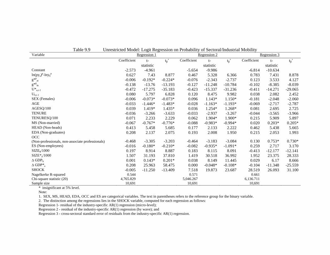
Table 9.9 Unrestricted Model: Logit Regression on Probability of Sectoral/Industrial Mobility Variable Regression 1 Regression 2 Regression 3
Coefficient t-
statistic
tβ‟ Coefficient t-
statistic
tβ‟ Coefficient t-
statistic
tβ‟
Constant -2.573 -4.961 -5.654 -9.986 -6.814 -10.634 ln(pya)
p-lnybp 0.627 7.43 8.877 0.467 5.328 6.366 0.783 7.431 8.878
g*pat -0.006 -0.192* -0.224* -0.076 -2.343 -2.737 0.123 3.533 4.127
g*pbt -0.138 -13.76 -13.193 -0.127 -11.248 -10.784 -0.102 -8.385 -8.039
U*a,t-1 -0.472 -17.275 -35.183 -0.423 -15.337 -31.236 -0.411 -14.271 -29.065 Ub,t-1 0.080 5.797 6.828 0.120 8.475 9.982 0.038 2.082 2.452 SEX (Females) -0.006 -0.073* -0.073* 0.096 1.143* 1.150* -0.181 -2.048 -2.060 AGE -0.033 -1.446* -1.483* -0.028 -1.163* -1.193* -0.069 -2.717 -2.787 AGESQ/100 0.039 1.419* 1.435* 0.036 1.254* 1.268* 0.081 2.695 2.725 TENURE -0.036 -3.266 -3.633 -0.033 -2.937 -3.267 -0.044 -3.565 -3.966 TENURESQ/100 0.071 2.233 2.229 0.062 1.904* 1.900* 0.215 5.909 5.897 MS (Non-married) -0.067 -0.767* -0.776* -0.088 -0.983* -0.994* 0.020 0.203* 0.205* HEAD (Non-heads) 0.413 5.458 5.685 0.177 2.133 2.222 0.462 5.438 5.665 EDA (Non-graduates) 0.208 2.137 2.075 0.193 2.008 1.950 0.215 2.053 1.993 OCC
(Non-professionals, non-associate professionals) -0.468 -3.305 -3.203 -0.464 -3.183 -3.084 0.130 0.753* 0.730* ES (Non-employees) -0.016 -0.180* -0.210* -0.082 -0.935* -1.091* 0.259 2.717 3.170 SIZEb/1000 0.197 8.914 8.887 0.183 8.115 8.091 -0.413 -12.177 -12.141 SIZE*a/1000 1.507 31.193 37.810 1.419 30.518 36.992 1.952 23.375 28.333 ∆ GDPb 0.001 0.143* 0.201* 0.038 8.149 11.445 0.029 6.17 8.666 ∆ GDP*a 0.208 25.963 58.475 0.000 -0.048* -0.108* -0.104 -11.348 -25.559 SHOCK -0.005 -11.250 -13.409 7.518 19.873 23.687 28.519 26.093 31.100 Nagelkerke R-squared 0.544 0.571 0.661
Chi-square statistic (20) 4,765.829 5,046.267 6,136.711
Sample size 10,691 10,691 10,691
* insignificant at 5% level.
Note:
1. SEX, MS, HEAD, EDA, OCC and ES are categorical variables. The text in parentheses refers to the reference group for the binary variable.
2. The distinction among the regressions lies in the SHOCK variable, computed for each regression as follows:
Regression 1- residual of the industry-specific AR(1) regression (micro-level);
Regression 2 - residual of the industry-specific AR(1) regression (by wave); and
Regression 3 - cross-sectoral standard error of residuals from the industry-specific AR(1) regression.

279
In terms of the number of insignificant variables, regression 3 has the lowest number of
such variables (two) compared to regressions 1 and 2 (each with seven insignificant
variables). The model under regression 3 had a better fit than the models under regressions
1 and 2. The Nagelkerke R-squared19
measure is 0.661, compared to 0.544 under
regression 1 and 0.571 under regression 2. Given the higher number of significant
variables and the better fit, regression 3, with the cross-sectoral standard error of residuals
as the sectoral shock, is viewed as superior to the first two regressions. In addition, the
cross-sectoral measure can be considered to be better by looking at the sign and size of the
coefficients. The coefficient for the AR(1) (micro-level) measure was negative, indicating
that using a shock that affects the individual-level (and not the sectoral-level) may not be
suitable. In contrast, both the AR(1) (by wave) and cross-sectoral measures have positive
coefficients, with the latter registering a larger magnitude. Considering the data period
covered, the large magnitude reflects the dramatic impact the Crisis had on mobility via a
disturbance to the economic sectors. Hence, the cross-sectoral standard error of residuals is
regarded as a reasonable measure of a sectoral shock reflective of the period in question.
To arrive at the restricted model of Table 9.10 from regression 3, the insignificant marital
status and occupational status variables are omitted. The restricted model can be
considered to be the main model used in analyzing the determinants of inter-sector
mobility. It will be termed the main model from here. The marginal effect for each
explanatory variable is included to highlight their relative importance on the dependent
variable20
.
With the high number of statistically significant variables, it is not surprising that the
overall goodness-of-fit chi-squared statistic (6,136) rejects the null hypothesis that none of
the independent variables are linearly related to the log odds of the dependent variable. The
good fit of the model can be attributed to the inclusion of the sectoral shock as well as the
macroeconomic time series data. Compared to studies based purely on cross-sectional
studies, the model would appear to be superior in terms of model specification. In addition,
to test whether the model‟s results are sensitive to changes in specification, each predicted
variable (sectoral wage differential or growth) was omitted in turn from the main model. It
was observed that the regression results for the other explanatory variables remained

280
unchanged in coefficient sign and significance. This suggests that the model is robust
under alternative specifications.
9.6.1 Monetary Variables
Expected Sectoral Wage Differential
The expected sectoral/industrial wage differential term is based on the Le and Miller (1998)
model and the Todarian hypothesis, which stipulates that worker movements are influenced
by higher expected earnings in the new sector compared to lower actual earnings in the
original sector. Empirically, the findings concur with the model and hypothesis. The
propensity to move to a new sector is increased the higher the expected industrial wage
differential. Specifically, higher expected wages raise the propensity to move by 13.89
percentage points. This is, for example, about 3 times the estimated partial effect on
mobility of being a non-graduate rather than a graduate. Thus, the role of expectations and
the comparison of the net monetary benefits in the alternative employment state are clearly
evident in the mobility decision for Korean workers.
In order to establish the relative importance of the wage and unemployment components of
the expected wage in the new industry, the main model was estimated with the same set of
explanatory variables but with the actual industrial wage differential21
replacing the
expected wage differential. The results obtained were similar to those reported in Table
9.10, which suggests that workers‟ decisions are based mainly on actual wage differentials.
The reason for this outcome can be seen mathematically. The expected wage variable,
ln [ya(1-Uat)] – ln yb, can be expressed as ln ya – ln yb + ln (1-Uat). As unemployment rates
in the new sector are quite low (on average 4%), the final term in the expected wage
variable will be close to zero. The expected wage differential and actual wage differential
will therefore be quite similar.
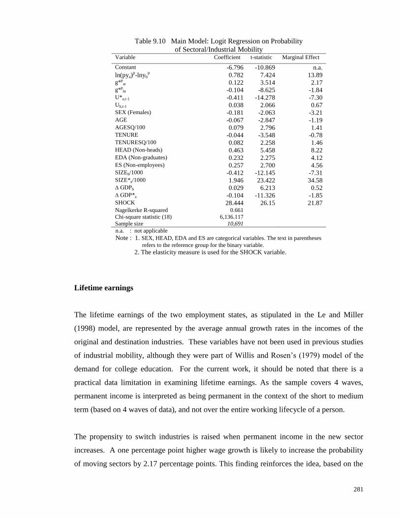
281
Table 9.10 Main Model: Logit Regression on Probability
of Sectoral/Industrial Mobility Variable Coefficient t-statistic Marginal Effect
Constant -6.796 -10.869 n.a.
ln(pya)p-lnyb
p 0.782 7.424 13.89
g*pat 0.122 3.514 2.17
g*pbt -0.104 -8.625 -1.84
U*a,t-1 -0.411 -14.278 -7.30 Ub,t-1 0.038 2.066 0.67 SEX (Females) -0.181 -2.063 -3.21 AGE -0.067 -2.847 -1.19 AGESQ/100 0.079 2.796 1.41 TENURE -0.044 -3.548 -0.78 TENURESQ/100 0.082 2.258 1.46 HEAD (Non-heads) 0.463 5.458 8.22 EDA (Non-graduates) 0.232 2.275 4.12 ES (Non-employees) 0.257 2.700 4.56 SIZEb/1000 -0.412 -12.145 -7.31 SIZE*a/1000 1.946 23.422 34.58 ∆ GDPb 0.029 6.213 0.52 ∆ GDP*a -0.104 -11.326 -1.85 SHOCK 28.444 26.15 21.87 Nagelkerke R-squared 0.661
Chi-square statistic (18) 6,136.117
Sample size 10,691
n.a. : not applicable
Note : 1. SEX, HEAD, EDA and ES are categorical variables. The text in parentheses
refers to the reference group for the binary variable.
2. The elasticity measure is used for the SHOCK variable.
Lifetime earnings
The lifetime earnings of the two employment states, as stipulated in the Le and Miller
(1998) model, are represented by the average annual growth rates in the incomes of the
original and destination industries. These variables have not been used in previous studies
of industrial mobility, although they were part of Willis and Rosen‟s (1979) model of the
demand for college education. For the current work, it should be noted that there is a
practical data limitation in examining lifetime earnings. As the sample covers 4 waves,
permanent income is interpreted as being permanent in the context of the short to medium
term (based on 4 waves of data), and not over the entire working lifecycle of a person.
The propensity to switch industries is raised when permanent income in the new sector
increases. A one percentage point higher wage growth is likely to increase the probability
of moving sectors by 2.17 percentage points. This finding reinforces the idea, based on the
282
relatively high costs of sectoral mobility, of individuals viewing industrial mobility as a
more permanent switch and as being a lifetime decision. In contrast, the likelihood of
changing industries is greater the lower the original industry‟s lifetime income. A one
percentage point lower growth rate in the original sector is likely to increase the occurrence
of moving by 1.84 percentage points. Thus, the lifetime earnings stream is clearly an
important consideration in the mobility decision, with higher permanent income in the new
industry acting as a pull factor and lower permanent wages in the original industry acting as
a push factor of mobility.
It is observed that the probability of a sectoral move is less sensitive to the pull and push
factors of the new and old sectors‟ permanent earnings compared to the current expected
wage differential. In other words, the elasticities of mobility with respect to a change in the
wage growth in the old sector (-0.49) and a change in the wage growth in the new sector
(0.54) is lower (in absolute value) than the elasticity with respect to the expected wage
differential (0.60)22
. Hence, among Korean workers, the lure of new sector wages appears
to have greater weight.
9.6.2 Macroeconomic Variables
Unemployment Rate
The original and new industries‟ unemployment rates were each entered into the workers‟
mobility decision process as lagged variables23
. Strong priors cannot be formed in relation
to the impact of the original and new industries‟ unemployment, as there appears to be only
a single study on employees [Vanderkamp (1977)]24
. In the current study, the higher the
unemployment rate in the original industry, the higher the likelihood of out-mobility. In
particular, every one percentage point increase in the unemployment rate increases the
outflow of labour from the old sector by 0.67 percentage points. This suggests that workers
view the higher chances of unemployment in their original sector as a signal of higher risks,
and hence tend to move out of the sector of origin to look for an alternative job. This
finding is consistent with Vanderkamp‟s (1977) study, which showed a positive
unemployment-mobility relationship in the old sector.
283
The findings of the current study show that higher unemployment in the new sector
deterred sectoral mobility. Specifically, an increase in the new sector‟s unemployment rate
by one percentage point is associated with a reduction in the inflow of labour into the new
sector of 7.30 percentage points. In a sectoral move, most workers move into a new sector
in anticipation of higher wages, but they may have to be unemployed for a while, i.e.
experience some form of wait unemployment before entering into employment in the new
sector. The greater the chances of being unemployed, the lower the workers‟ expected
wages, and the lower will be the chances of a sectoral switch for workers. This result for
Korea concurs with the Todarian hypothesis, which postulates an inverse relationship
between the unemployment rate and probability of obtaining a job in the new sector. It is,
however, contradictory to Vanderkamp‟s (1977) report of a positive unemployment-
mobility correlation for the new sector for the 1965/1966 period.
The old-new sector results are consistent, as lower job availabilities should limit mobility
into the new sector and encourage out-mobility from the old sector. In terms of the
magnitude of the effect of the unemployment rate, the absolute value of the new sector
variable (0.411) is greater than that of the old sector (0.038). Perhaps Korea workers are
more influenced by the lack of job availabilities and are daunted by the possibility of not
securing a job in the new sector.
9.6.3 Worker Characteristics
Gender
The gender variable is measured as a dummy variable indicating if the worker is a male
(= 1) or a female (= 0). The current research reports females to have a lower propensity of
industrial mobility than males. In particular, females are 3.21 percentage points less likely
to move to a new industry than males. The finding is inconsistent with Fallick‟s (1993)
study, which reports that females have higher probabilities of changing industries, but it
supports the general view that male and female mobility patterns differ.

284
Age
Age is entered in the estimating equation in quadratic form. The coefficient on the linear
age variable is negative and the coefficient on age-squared is positive. Thus, the negative
influence of age on sectoral mobility diminishes with rising age, and actually becomes
positive among older age groups. It is noted that the negative age-mobility relationship is
consistent with the findings of the empirical studies among employees: Osberg (1991) for
women in 1985/1986 and Osberg, Gordon and Lin (1994). Among the unemployed, the
negative relation is also portrayed in Thomas (1996b) for younger job quitters (UI and non-
UI recipients) and job losers (non-UI recipients) who had higher probabilities of mobility,
and for older job quitters and losers (UI recipients) who had lower mobility rates. The non-
linearity of the age effect on mobility is illustrated in Figure 9.1. This figure shows the
relationship between age and the probability of mobility for a specific worker profile (male,
graduate, head of household and employer) with monetary, macroeconomic, tenure and
industry variables equal to the sample means. From the calculation of the partial effect,
which measures the slope of the probability function25
, the turning point occurred at 43
years of age.
Figure 9.1 Probability of Sectoral Mobility and Age
0.0000
0.0500
0.1000
0.1500
0.2000
0.2500
0.3000
0.3500
0.4000
20 22 24 26 28 30 32 34 36 38 40 42 44 46 48 50 52 54 56 58 60
Probability
Age (years)

285
Job Tenure
Original job tenure was computed for industry movers and stayers in the current work using
slightly different algorithms. For stayers, the difference (in years) between the start date of
the current (and original) job and survey reference date was taken. For movers, job tenure
was computed as the difference between the start and quit dates of the previous job.
Job tenure was entered in the estimating equation in quadratic form. The coefficient on the
linear tenure variable was negative and the coefficient on tenure-squared was positive.
However, while the tenure-mobility relationship is U-shaped (see Figure 9.2)26
, for most of
the sample the relationship will be negative (as the positive effect holds only after tenure of
27 years). The negative tenure-mobility relation is consistent with a number of reports:
Osberg (1991) for male and female employees in 1980/1981, 1982/1983 and 1985/1986,
Osberg, Gordon and Lin (1994) for male employees, Fallick (1993) and Neal (1995) for
unemployed workers and Thomas (1996b) for job losers and quitters who received UI, and
job quitters who did not receive UI. Thus, this finding suggests that more experienced
workers who have more to sacrifice, e.g. seniority-based pay, longer leave periods and
pension benefits, are less likely to switch sectors.
Figure 9.2 Probability of Sectoral Mobility and Tenure
Probability
0.0000
0.0500
0.1000
0.1500
0.2000
0.2500
0.3000
0.3500
0.4000
1 3 5 7 9 11 13 15 17 19 21 23 25 27 29 31 33 35 37 39 41 43 45 47 49
Tenure (years)

286
Family Indicators: Marital Status and Household Head
A dummy variable was used to indicate if a person was married. The data findings
revealed that little, if any, of the variation in sectoral mobility could be attributed to marital
status. The variable was consequently omitted from the regression analysis. This is a
finding consistent with Osberg (1991) for males in 1982/1983 and 1985/1986, and females
in 1980/1981, 1982/1983 and 1985/1986, and Osberg, Gordon and Lin (1994), but it
contradicts Neal (1995), who showed that married men have a lower likelihood of
switching sectors.
A dummy variable was also used to indicate if the individual is a household head
(1 = household head, 0 = non-head). This household head variable was significant in the
analyses reported in Table 9.10. The probability of changing sectors was lower if the
person was a household head. The marginal effect was 8.22 percentage points. This finding
is consistent with the study of sectoral mobility among unemployed workers in the U.S. by
Fallick (1993), and supports the general view of household heads facing greater risks in
changing sectors owing to greater family commitments.
The significant finding for the household head and the insignificant one for marital status
can be reconciled. Since there can be only one head but more than one married person in
the household (see the descriptive statistics, where about three-quarters of the KLIPS
sample are married persons but only half are household heads), the family burden and risks
associated with changing sectors for a married person are lessened. As such, the mobility
effect will be dissipated for married persons.
Educational Attainment
If education is viewed as an indicator of one‟s learning ability or adaptability, it should
have a positive impact on mobility. If, however, employers favour more practical work
qualifications, such as current job scope, post-school track record and training attended,
then formal education need not have a positive influence on sectoral mobility. The measure
of education available in the survey related to the respondent‟s highest qualification
attained. Accordingly, this study focuses on whether the mobility patterns of graduates and

287
non-graduates differ. This is examined though the use of a dummy variable, set equal to
one for graduate status, and set equal to zero for non-graduates. The results showed that
non-graduates had a higher propensity to switch sectors, with the marginal effect being 4.12
percentage points. In a sense, the current findings are consistent with Kim (1998) who
inferred that lower-educated persons tended to be industry switchers among the
unemployed. The finding is, however, contradictory to Neal (1995) who reported that the
number of years of schooling (and most likely higher education levels) had an insignificant
impact on mobility, and Fallick (1993) who revealed that the number of grades of school
completed (and hence higher education levels) had a positive impact on industrial mobility.
Occupational Status
Inter-sectoral mobility may vary according to the workers‟ skills. In broad terms, the
differences in mobility rates between skilled and unskilled workers will most likely be
closely linked to any skill biases associated with a structural change in the economy. In this
study, the skill indicator is a person‟s occupation. A person is denoted as being skilled if
he/she was a professional or associate professional, and a dummy variable is used to
differentiate these skilled workers from their unskilled counterparts. The results show that
little of the variation in mobility could be attributed to occupational status in Korea. The
variable was subsequently omitted from the regression.
This finding is consistent with some of the results in Osberg (1991). Three occupational
groups were formed in this study: managerial/professional/technical, clerical/sales and
personal services, where the first group can be considered to be skilled workers, and the
latter two groups viewed as unskilled workers. Osberg (1991) reported that occupational
status was an insignificant determinant of the mobility of male workers in the 1982/1983
and 1985/1986 periods.27
However, the current study‟s finding does not concur with
Osberg‟s (1991) report for males in 1980/1981 and females in 1985/1986, where lower
tendencies of mobility among skilled workers were found, and for skilled females in
1982/1983, where higher probabilities of mobility were established. In particular, it must
be noted that the mixed result in Osberg (1991) for the same gender group (females) for
different time periods within an interval of just one year (i.e. 1980/1981 and 1982/1983) is
an area of concern, since few major behavioural changes in the labour force characteristics

288
can be observed within a short time span. There thus appears to be a lack of robustness in
the study of the Canadian labour market. It is also noted that the insignificant result
remained in the current study even when the logistic regression was undertaken for a
different time period, i.e. 1999-2001 (excluding the immediate post-Crisis year of 1998).
Employment Status
The employment status variable was included in the estimating equation to assess if
employees had a higher propensity to change sectors than their non-employee counterparts.
A dummy variable was used to distinguish employees (= 1) from non-employees (self-
employed/unpaid family workers) (= 0). The data revealed that non-employees were more
likely (by 5 percentage points) to move to a new sector. These employers were most likely
to be owners of small firms or business start-ups, with few or no employees, limited
contingency funds and more modest plans, thereby making the firm closure process easier
and the change to a new job/sector more probable.
Since the data period covers 1998-2001, a probable explanation could be associated with
the mid-1997 Asian Financial Crisis. The onset of the Crisis arose from large-scale capital
inflows into the country, and rapid increases in lending in the 1990s to firms which over-
invested at low profitability levels [Radelet and Sachs (1998), Tanzer (1999) and Akyüz
(2000)]. This led to massive debt obligations on the part of firms and eventual bankruptcies
in large conglomerates as well as small and medium-sized establishments (SMEs)
[Gregory, Harvie and Lee (2002)]. It is probable that employers owning the SMEs (which
had lower contingency funds) were the first to encounter the adverse effects of the Crisis.
Results from a separate regression omitting the first wave of observations in the KLIPS
sample showed that the partial effect was higher (7 percentage points). However, when the
first two waves of observations were omitted, employment status became an insignificant
variable. This is reflective of the immediate adverse impact the Crisis had on employers.

289
9.6.4 Industry Characteristics
Sectoral Size
The size of the original industry is measured by its employment size. In the current study,
the larger the size of the individual‟s original industry, the lesser the likelihood of changing
sectors. The elasticity of mobility with respect to an increase in the original industry‟s size
was -0.32. This implies that Korean workers may be reluctant to move out of their initial
sector of employment when it has greater job opportunities. This result is similar to the
negative impact reported by Fallick (1993) and Neal (1995) for their studies on the
unemployed. This similarity of result with the empirical literature should be observed with
some reservation, however, since these comparison studies focus on the unemployed who
may have quite different behavioural responses.
For the new industry, a larger size had a positive effect on sectoral mobility. The elasticity
of mobility with respect to an increase in the new industry‟s size was 1.50. This suggests
that Korean workers could be moving into the new sector because of its employment
opportunities. The result is consistent with the findings reported by Vanderkamp (1977)
and Osberg, Gordon and Lin (1994). It is noted that the result for this explanatory variable
is robust: Even when the finer initial industry data of Table 9.11 are included later in the
model, the coefficient of the new industry size is still positive and significant.
Sectoral Performance
The effect of sectoral performance is pursued in the current study by using the industry‟s
GDP growth rate as an indicator of industry performance28
. The results reveal that the
likelihood of a sectoral move from the old industry was higher the higher the GDP growth
rate of the initial industry. An increase in the growth rate of the original industry by one
percentage point raised the probability of mobility by 0.52 percentage points. This result is
unexpected, although several commentators have drawn attention to so-called jobless
growth as being a characteristic of many modern economies (Burgess and Green (2000)
and Mitchell (2000)]. Under this hypothesis, higher growth in a sector will not require an
increase in labour. This arises as the high growth could be spurred by a technological

290
upgrade or enhanced worker productivity. Moreover, the number of job vacancies arising
from the growth could be insufficient to cater for the rising number of the long-term
unemployed in the sector. Hence, this finding supports the jobless growth hypothesis that
higher growth in the old sector, brought about by technological advancements, leads to
labour obsolescence and a reduction in employment, resulting in out-mobility.
The effect of the new industry‟s GDP growth was negative. Higher growth in the new
industry deterred workers from entering into these industries. The marginal effect was
registered at 1.85 percentage points. This result is unexpected, but like the results for the
old industry‟s growth, is consistent with the jobless growth hypothesis. Better performance
in the new sector arising from a technological upgrade, leading to labour obsolescence, will
be insufficient to cater to more jobs, let alone provide jobs for new entrants into the sector.
Hence, a lower probability of mobility into the new high-growth sector is implied.
There is consistency in argument as the findings for both the old and new industry
performance align with the jobless growth hypothesis. Since the hypothesis is a
characteristic of a developed economy, it points towards the modernization of the Korean
economy.
9.6.5 Sectoral Shock
The sectoral/industrial shock variable is intended to capture unanticipated variations in
labour movements in the particular industry. From Table 9.10, it can be seen that a sectoral
shock resulted in greater sectoral labour reallocations in the Korean labour market. This
finding is consistent with many studies [Gulde and Wolf (1998), Brainard and Cutler
(1993), Jovanovic and Moffitt (1990), Altonji and Ham (1990) and Clark (1998)], which
have demonstrated that sectoral labour movements are not immune to the effects of a
sectoral shock.
It should be emphasized that the effect of the sectoral shock is highly significant in Korea.
The elasticity of sectoral mobility with respect to a change in the sectoral shock is large, at
21.8729
. This large effect is not surprising, given the dramatic impact of the unprecedented
Crisis. When the AR(1) residual (by wave) measure was used under the main model, the
291
elasticity of sectoral mobility with respect to the sectoral shock was still large, at 5.7530
. A
separate regression (not reported here) showed that the explanatory power of the model
dropped substantially, from 0.661 to 0.530 (measured by the Nagelkerke R-squared), when
the shock variable (cross-sectoral measure) was excluded. Therefore, the sectoral shock
variable plays a very important role in accounting for mobility in the Korean labour market.
Korea is an open, export-oriented economy, and unanticipated events affecting the
macroeconomy and labour market would also impact severely on various sectors of the
economy.
9.7 EXTENSIONS OF THE MODEL
This section considers two extensions of the above empirical model. The first extension
focuses on the individual‟s initial industry, in line with the work by Osberg (1991) for the
employed and Thomas (1996b) for the unemployed. The second part of this section
proceeds to test the various theories of sectoral mobility implied in the literature: worker-
employer mismatch, sectoral shock and bridging theories of sectoral mobility.
9.7.1 A Focus on the Initial Industry
The initial industry of an employee was included in the estimating equation to permit
assessment of which industries can be distinguished on the basis of their incidence of
industrial mobility. A set of eight dummy variables indicating the worker‟s original
industry of employment was incorporated in this study. Table 9.11 shows the regression
results for the initial industry variables. It is noted that by including these variables the
explanatory power of the regression improved further, to 0.676.
The results show that the propensity to change sectors varied according to the initial
sector/industry. The propensity of a sectoral move was lower if the worker was from the
construction and commerce sectors. In contrast, the probability of changing sectors was
higher if the worker originated from the agricultural sector and financial, real estate and
business services, and community, social and personal services industries, with the
marginal effects being 23.16 percentage points, 14.59 percentage points and 10.94
percentage points, respectively. The effects associated with initial employment in mining,

292
utilities and transport, storage and communications were insignificant. The variation in the
probability of worker mobility across industries possibly reflects that each industry
possesses different characteristics, like working conditions, job opportunities and
performance.
Table 9.11 Logit Regression on Probability of Sectoral/Industrial Mobility:
A Focus on the Initial Industry, Selected Coefficients Variable Coefficient t-statistic
Marginal
Effect
Agriculture 1.304 4.893 23.16
Mining -0.727 -0.198* -12.92
Utilities -0.430 -0.503* -7.63
Construction -0.461 -2.157 -8.19
Commerce -2.278 -14.391 -40.47
Transport, Storage & Communications -0.129 -0.726* -2.29
Financial, Real Estate & Business Services 0.821 5.304 14.59
Community, Social & Personal Services 0.616 3.665 10.94
Nagelkerke R-squared 0.676
Chi-square statistic (23) 6,329.946
Sample size 10,691 * insignificant at 5% level.
Note: 1. In addition to the initial industry variables, the model contains all variables in Table 9.10
except for the old industry size, sex and employment status. Compared to the other
explanatory variables, the correlation coefficient of the old industry size with each of the
initial industry variables was higher. The inclusion of the old industry size in the regression
would have led to unusually large estimates for the initial industry variables, a possible case
of multicollinearity. The sex and employment status variables were excluded from the
regression as they became insignificant after the inclusion of the initial industry variables.
2. The initial manufacturing sector, which had the largest number of observations, is excluded
from the regression.
9.7.2 Empirical Test: Theories of Sectoral Mobiliy
The three theories of sectoral/industrial mobility, namely the worker-employer mismatch,
sectoral shock and bridging theories, are tested in this section. These theories are about
model specification, and the distinction lies in the inclusion/exclusion of the industrial
shock variable.
The starting point for testing these theories will be the estimation of the main model of
sectoral mobility in Table 9.10. The critical explanatory variable for consideration is the
exogenous industrial shock variable. By singling out this variable, equation (6.7) can be
expressed as:

293
Ii = α + β1X1i + ….. + βkXki + θSi + μi (6.7‟)
where α is the constant term, X1 to Xk represent the k monetary, macroeconomic,
worker/job characteristic regressors, S is the industrial shock measure, and μ is the
stochastic error term. The β‟s and θ are the parameters to be estimated for the X‟s and S,
respectively.
Worker-Employer Mismatch Theory
Under the worker-employee mismatch theory, the emphasis is on the null hypothesis that
the effect of the industrial shock variable is zero (H0 : θ = 0), and this can be tested against
the alternative hypothesis (H1 : θ ≠ 0). The null hypothesis should be rejected under this
theory. The test can be implemented using the t-test. The t-statistic computed for the
industrial shock variable was 26.150 for the main model. As the computed t-statistic far
exceeded its critical value, the null hypothesis should be rejected. That is, the effect of the
sectoral shock cannot be ignored. The worker-employer mismatch theory is thus rejected
for the Korean labour experience.
Sectoral Shock Theory
The sectoral shock theory has an emphasis on the test of the null joint hypothesis that the
joint effects of the monetary, macroeconomic, demographic and socio-economic variables
are zero (H0 : β1 = β2 ….. = βk = 0), and this can be tested against the alternative
hypothesis that at least one of these exogenous variables is significant. This null means
that the industrial shock variable is the sole factor accounting for sectoral movements. A
test can be implemented using the chi-square statistic, computed as twice the difference
between the log likelihoods of the main model and the reduced model. The reduced model
is formed by omitting all variables other than the sectoral shock variable. As the observed
difference in the chi-square statistics between the main model (6,136) and the reduced
model (3,610) was 2,526, much larger than its critical value, the null hypothesis is rejected.
Thus, a model with sole reliance on the industrial shock will be inadequate in analyzing the
determinants of industrial mobility in the Korean labour market.

294
Bridging Theory
Under the bridging theory, testing the determinants of sectoral mobility has a focus on
testing the null hypotheses, i.e. H0 : β1 = β2 ….. = βk = 0 and H0 : θ = 0, that all variables,
including the sectoral shock, are insignificant If this theory is correct, the null hypotheses
should be rejected. The alternative is that at least one of the
monetary/macroeconomic/demographic/socio-economic variables and/or the sectoral shock
is significantly different from zero. Since the results of the main model of Table 9.10
provide strong evidence of significant β‟s and θ, the null hypotheses are rejected. The
Korean experience favours the bridging theory of sectoral mobility.
To assess if the bridging theory holds under an alternative technique, an approach along the
lines of Jovanovic and Moffitt (1990) is followed. This method rests on the assumption
that the effects of worker characteristics on mobility are via wages. Hence, rather than
including all variables in a single equation as per equation (6.7), a wages equation was first
estimated where the log of wages was expressed as a function of worker characteristics.
The standard error of this wage regression was obtained. Similarly, a measure of the
sectoral shock given by the standard deviation of residuals was obtained from an AR(2)
regression of each industry‟s log annual U.S. employment31
. Specifically, for each year
from 1968 to 1980, Jovanovic and Moffitt (1990) used the National Longitudinal Survey of
Young Men to regress log wage on education, experience, experience-squared and race to
obtain the standard errors of the annual wage regressions.
The wage measure is meant to capture the underlying wage deviations independent of
differences in worker characteristics. The sectoral shock is the AR(2) residual (by wave),
termed in the study as the across-sector standard deviation of residuals, and it was obtained
from log annual U.S. industry employment regressions. The binary dependent variable (1 =
mover, 0 = stayer) represented the probability of a sectoral move. It was regressed on the
standard error of the log wage distribution and the sectoral shock variable (i.e. the across-
sector standard deviation of residuals). The wage variable was significant, showing that the
mobility of U.S. workers was influenced by monetary differentials, even after accounting
for personal differences such as race, education and experience. The results showed that
the impact of a sectoral shock was positive and significant. The study concluded that since

295
the standard errors of wages are not constant, sectoral shocks would first affect wages,
which would then affect mobility. The significance of both variables provided support for
the bridging theory.
The Jovanovic and Moffitt (1990) model is implemented in this study as follows. To obtain
the standard error of the log wage distribution, the natural logarithm of individual workers‟
reported wages was first regressed on worker characteristics for each year, from 1998 to
2001. The available characteristics are sex, educational attainment, marital status,
employment status (self-employed or otherwise), age, age-squared, tenure and tenure-
squared. The standard errors from each of the four annual wage regressions were then
obtained, giving four values for each regression. The sectoral shock variable is the AR(1)
residual (by wave). Using the same binary dependent variable (1 = mover, 0 = stayer) as in
the main model to represent the probability of sectoral mobility, the dependent variable is
regressed on these two variables, with the logit estimates being shown in Table 9.12. The
results showed that although the sectoral shock variable was significant, the standard error
of the logarithm of the wage distribution was not.
It should be noted, however, that this technique is not a direct application of Jovanovic and
Moffitt (1990). Compared to Jovanovic and Moffitt (1990), the limited variation in the
wage variable for the Korean case (4 years compared with 13 years) may have accounted
for the weaker result with respect to this variable. Furthermore, the approach to estimation
differed. Jovanovic and Moffitt (1990) estimated the probability function for a typical
worker for each period with the number of observations in parentheses: 1966-1968 (492),
1967-1969 (628), 1968-1970 (754), 1969-1971 (887), 1971-1973 (1,357), 1973-1975
(1,846), 1976-1978 (2,032) and 1978-1980 (1,967). In comparison, estimation in the
current application was for the entire dataset from 1998-2001 covering 10,691
observations.
However, when alternative measures of a sectoral shock were used, namely the cross-
sectoral standard error of residuals from the industry-specific AR(1) regression and the
residual of an AR(1) residual (micro-level) under regressions 2 and 3, respectively, the
wage variable became significant. However, the sectoral shock variable was significant
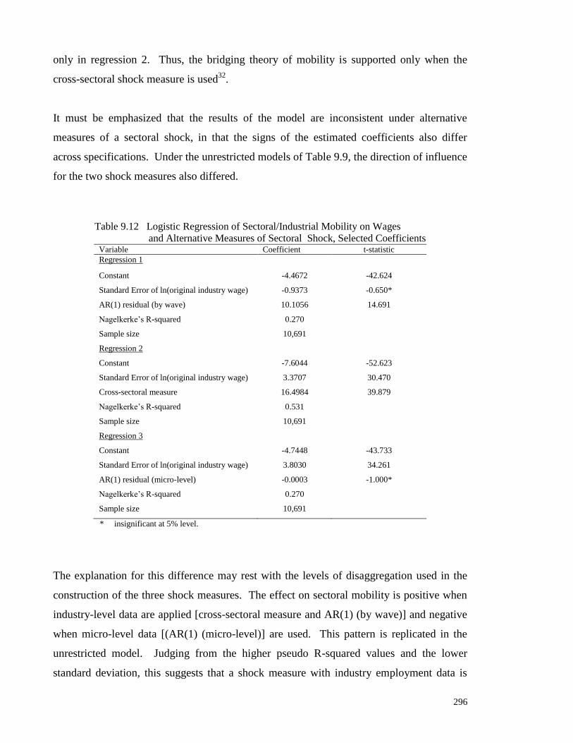
296
only in regression 2. Thus, the bridging theory of mobility is supported only when the
cross-sectoral shock measure is used32
.
It must be emphasized that the results of the model are inconsistent under alternative
measures of a sectoral shock, in that the signs of the estimated coefficients also differ
across specifications. Under the unrestricted models of Table 9.9, the direction of influence
for the two shock measures also differed.
Table 9.12 Logistic Regression of Sectoral/Industrial Mobility on Wages
and Alternative Measures of Sectoral Shock, Selected Coefficients
Variable Coefficient t-statistic
Regression 1
Constant -4.4672 -42.624
Standard Error of ln(original industry wage) -0.9373 -0.650*
AR(1) residual (by wave) 10.1056 14.691
Nagelkerke‟s R-squared 0.270
Sample size 10,691
Regression 2
Constant -7.6044 -52.623
Standard Error of ln(original industry wage) 3.3707 30.470
Cross-sectoral measure 16.4984 39.879
Nagelkerke‟s R-squared 0.531
Sample size 10,691
Regression 3
Constant -4.7448 -43.733
Standard Error of ln(original industry wage) 3.8030 34.261
AR(1) residual (micro-level) -0.0003 -1.000*
Nagelkerke‟s R-squared 0.270
Sample size 10,691
* insignificant at 5% level.
The explanation for this difference may rest with the levels of disaggregation used in the
construction of the three shock measures. The effect on sectoral mobility is positive when
industry-level data are applied [cross-sectoral measure and AR(1) (by wave)] and negative
when micro-level data [(AR(1) (micro-level)] are used. This pattern is replicated in the
unrestricted model. Judging from the higher pseudo R-squared values and the lower
standard deviation, this suggests that a shock measure with industry employment data is
297
better than one estimated at the micro level. The support for this can be seen from a
conceptual standpoint as the measure of a sectoral shock should ideally reflect an external
disturbance impacting a sector as an entity, which the industry data seem to represent. In
contrast, the micro-level AR(1) indicator represents a shock that affects the labour market
at the individual level, which may not necessarily be reflective of the sectoral/industrial
outcome. In addition, between the two measures estimated at industry level, since
regression 2 gave a better fit, this also suggests that the cross-sectoral standard error of
residuals is a better measure.
Another reason for the disparity lies in the correlation of the shock measures with the
standard error of the log wage measure. The AR(1) residual (by wave) and AR(1) residual
(micro-level) are quite highly correlated with the standard error of the log wage
distribution, with the correlations estimated at 0.989 and -0.586. This change in sign also
suggests these two measures have different information content, which is not surprising
since the former is derived from industry-level data whereas the latter is from individual
data. In comparison, the correlation between the wage measure and the cross-sectoral
measure is the lowest, at 0.304. Furthermore, multicollinearity will exist if the AR(1)
residual (by wave) is applied, posing potential problems in statistical inference. Therefore,
owing to its higher pseudo-R-squared value, lower correlation with the log wage
distribution, which minimizes problems in statistical inference, and that the bridging theory
of mobility is supported when it is used, the cross-sectoral standard error of residuals is
deemed to be the better indicator of a sectoral shock.
It is also worth mentioning why Jovanovic and Moffitt‟s (1990) method of model
specification (i.e. two explanatory variables) was not adopted as the main model for the
current thesis. First, it can be seen that the results of the model are inconsistent for the
same wage variable when alternative measures of a sectoral shock were adopted. Second,
the assumption of worker characteristics influencing mobility indirectly is not widely
accepted, as many other studies have demonstrated such effects to be direct. Third, the
sectoral wage differential, a critical deterministic factor, and other industry characteristics,
are ignored in the analysis.

298
9.8 SUMMARY
This chapter provides a study of the determinants of sectoral/industrial mobility in the
Korean labour market. Since sectoral mobility is a complex phenomenon, a wide variety of
monetary, macroeconomic, worker and job characteristics were entered into the mobility
function. The findings are summarized below.
The Korean sectoral mobility experience supports the bridging theory for the overall
workforce. Labour movements occur as a result of monetary, macroeconomic,
demographic and socio-economic factors as well as from a sectoral shock.
The monetary element in the new sector is an important pull factor, with higher expected
wages attracting workers to the new sector. Similarly, higher monetary rewards in the
original sector serve to reduce worker mobility. In terms of lifetime earnings, whilst higher
permanent incomes in the new sector encourage worker mobility, those in the old sector
have a deterrent effect. On the whole, the findings on the monetary variables provide
strong evidence for the theoretical predictions implied by the Le and Miller (1998) model.
Considering that the new industry‟s unemployment rate had a negative effect on mobility
for the overall workforce, it can be viewed as a factor that moderates the monetary pull
factor. Perhaps Korean workers will not change sectors until an employment contract is
secured. Higher unemployment in the new sector will tend to lower workers‟ expectations
of obtaining higher wages, reducing the likelihood of a sectoral switch and lowering the
probability of obtaining a job in the new sector. The Korean experience provides support
for the Todarian hypothesis, in that individuals move for higher expected wages and that
the new sector‟s unemployment rate and probability of gaining new employment are
inversely related. It was also found that rising unemployment in the old sector led to out-
mobility from that sector.
With the exception of age and tenure, the alternative views and reported results from the
literature review do not support clear predictions about the relationships between mobility
and worker characteristics. Several of the findings from the current empirical analysis of
the Korean labour market are similar to those reported in other studies. But where the
findings deviate, the differences seem to be attributable to differences in model
299
specification (where an exogenous shock factor is included), coverage (employees rather
than the unemployed) and measurement issues. An alternative view is that the results
reported here reflect behavioural patterns of sectoral mobility unique to the Korean
experience: inter-industry movers are more likely to be younger non-graduate males who
are not household heads, have lesser work experience and who are non-employees.
Among the industry characteristics, Korean workers are more likely to move out from
smaller-sized sectors and move into larger-sized ones with greater employment
opportunities. In terms of sectoral performance, the workforce is more likely to exit from
high-performance sectors, and they seem to be prevented from entering high-performance
sectors, a finding attributed to the jobless growth hypothesis.
The sectoral shock has been shown to be a highly influential determinant of industrial
mobility, consistent with the bridging theory and the empirical findings reported in other
studies. For the overall pooled sample, the sectoral shock explained a major portion of
sectoral movements from 1998 to 2001 in Korea. For example, if this shock variable was
excluded, the Nagelkerke R-squared is substantially reduced, from 0.661 to 0.530.
This chapter has provided us with an understanding of the motivations behind
sectoral/industrial mobility in the context of the Korean labour market. In a nutshell, it can
be seen that sectoral mobility is a multifaceted phenomenon involving a spread of factors.
Although these factors affect mobility differently when different samples are considered,
there is at least some form of consistency in terms of the monetary incentive and the
influence of the sectoral shock. The results conform to the bridging theory. The bridging
theory of sectoral mobility, covered by one author, gives a broader view on mobility,
combining the effects of labour market characteristics and other unanticipated elements.
The current study has embarked on a more advanced research methodology. The
comprehensive set of factors and model implications sourced from numerous studies,
including those of the other forms of labour mobility, gave a broader dimension to the
research. The availability of a combination of cross-sectional and time-series data has not
only enabled a more in-depth analysis into the wealth of variables explored, but it has also
facilitated inclusion of variables reflecting both past and expected labour market outcomes.
The inclusion of micro- and macro-data improved the explanatory power of the regression.
300
The checking of the potential importance of survey weights to the KLIPS data is unique to
the current work. Apart from these, since potential workers make exante decisions about
the future, the conceptually-advanced model, which rides on expectations and the lifetime
income stream, appears to be highly appropriate in modelling this form of mobility
behaviour.
Endnotes:
1. See www.kli.re.kr. The KLI was founded as a government-sponsored research organization in May
1988. Since its establishment, it has conducted policy-oriented research on a wide range of labour issues. The
key issues include labour market participation and employment, industrial relations, human resource
management, worker welfare, labour laws and regulations. The KLIPS is the first panel survey on labour-
related issues in Korea, and serves as a valuable data source for microeconomic analysis of labour market
activities and transitions. The availability of longitudinal data through the KLIPS facilitates in-depth analytic
studies of labour supply and mobility, including schooling and the school-to-work transitions of youth, job
mobility and labour market transitions, unemployment experience, job training and education, working
conditions and welfare, childcare and female labour force participation, income and consumption, health and
retirement. The survey design and management of the KLIPS is based on the longitudinal surveys conducted
in advanced countries, e.g. U.S. Panel Study of Income Dynamics (PSID) and National Labor Survey (NLS).
2. Osberg (1991) noted that his short period of employment mobility of 6 months may exclude persons with
long intervening spells of unemployment.
3. It also comprises persons who were employed previously but did not provide information on their industry.
4. This also includes persons who did not report an industry in year t.
5. The missing survey information could be addressed, in principle, using the selection bias correction
techniques discussed below. However, the absence of information on key demographic and employment
variables effectively precludes the estimation of a satisfactory selection equation.
6. This means that the attrition rate does not vary according to any demographic or employment
characteristics.
7. An AR(1) regression was used instead of an AR(2), as in Jovanovic and Moffitt (1990), as the first
differenced series of each of the nine sectors/industries employment was stationary.
8. The standard errors of the regression for each regression by year are in parentheses: 1998 (0.5755), 1999
(0.4041), 2000 (0.2783) and 2001 (0.2451).
9. It is noted that the AR(1) residual mean value cannot be compared directly with Gulde and Wolf‟s (1998)
correlation measure since Gulde and Wolf (1998) used it to determine the association of sectoral shocks
amongst countries and various sectors.
10. Tomes and Robinson‟s (1982a) set of observable characteristics comprised schooling, experience, degree,
training, ability, language and urban/rural/farm location.
11. It is noted that wage estimations for the mover and stayer sub-samples were also undertaken by Osberg,
Gordon and Lin (1994), for old wages in period t-1 and new wages in period t, for their study of sectoral
mobility. They estimated the predicted wages for movers and stayers from the regressions of the new wage
(individual‟s 1987 reported income) on personal characteristics and the old wage (individual‟s 1986 reported
income), also on personal characteristics within each mover/stayer subsample. The fitted values formed the
predicted wages and the difference between the predicted wages of movers and those of stayers formed the
wage differential. The difference with the Tomes and Robinson (1982a) methodology is that the new sector
wages for industry stayers is as reported and not the average of all industries outside the stayer‟s original
industry.
12. The real wage differential adjusted to the 1998 deflator (wdiff1 = ln (yai/CPI1998) – ln (ybi/CPI1998)) and the
actual wage differential (wdiff2 = ln yai - ln ybi) are the same as the two ln (CPI) terms offset each other. In
the stricter sense, yat and ybt could be adjusted by different deflators. Since ya is measured at period t and yb at
period t-1, the new difference (newdiff) = ln (yat/CPIt) – ln (ybt/CPIt-1). Since there is no „i‟ term, the
difference between this adjusted variable and actual wages is subsumed into the constant term.
13. It is noted that the sector-level variables were re-computed and not predicted to avoid potential problems
in statistical inference associated with collinearity. If the sector-level variables are predicted from regressions
of U*a,t-1, Ub,t-1, size*a, sizeb, GDP*a and GDPb on the set of individual characteristics (Xi), and the mobility

301
model then consists of these predicted sector-level variables (superscripted with p) in addition to other
variables:
Ii = α + ..+ β1U*p
a,t-1 + β2 Upb,t-1 + β3size*
pa + β4size
pb + β5GDP*
pa + β6GDP
pb + βiXi + μ.
with α and μ being the constant term and error terms, respectively, then as the predicted values are: ^ ^
U*pa,t-1, U
pb,t-1, size*
pa, size*
pb, GDP*
pa, GDP
pb = α + βiXi,
the predicted sector-level variables are linear combinations of the same set of predictors, and so will be highly
collinear. There were numerous pair-wise correlation coefficients exceeding 0.5 including U*pa,t-1 with size*
pa,
GDP*p
a and GDPpb, U
pb,t-1 with size
pb, size
pb with GDP*
pa and GDP
pb as well as GDP*
pa with size
pb and
GDPpb. It is noted that these variables are not perfectly correlated owing to the averaging process. Whilst the
old sector values are obtained from movers‟ and stayers‟ original industries, and the new sector values for
movers are obtained from their new industries, the new sector value for stayers is the average of predictions of
all industries other than the stayers‟ original industry. It is this averaging process that gives the less-than-
perfect correlation.
14. Not all respondents in the KLIPS sample reported job status. The removal of individuals reporting a
changed job status (i.e. part-time to full-time and vice versa, regular to irregular employment and vice versa)
is based on available responses only.
15. Removing the bottom 10% would have given a high average wage growth of 9.65%, which exceeds the
industry average of 6-7%.
16. Some degree of collinearity amongst the three shock measures exists, as shown by the following
correlation matrix:
AR(1) (micro-level) AR(1) (by wave) Cross-sectoral standard
error of residuals from
industry-specific AR(1)
regression
AR(1) (micro-level) 1.000 -0.624 -0.168
AR(1) (by wave) -0.624 1.000 0.306
Cross-sectoral standard
error of residuals from
industry-specific AR(1)
regression
-0.168 0.306 1.000
17. A separate regression using the Lilien index as an alternative measure of industrial shock resulted in ten
insignificant variables, including the expected sectoral wage differential.
18. The formula for tβ‟ follows from Kish (1965) [refer to page 259] where it is mentioned that the effective t-
statistic adjusted for the design effect is: ____
tβ / √deff
19. See Nagelkerke (1991). The Nagelkerke R-squared is a modification of the Cox and Snell statistic to
ensure that it varies from 0 to 1. The Cox and Snell R-squared is an attempt to imitate the interpretation of the
multiple R-squared based on the likelihood, but its maximum can be less than 1, which makes it difficult to
interpret. It is measured by R2 = 1 – exp[-2/n{logL(β) – log L(0)}] where logL(β) and log L(0) denote the log
likelihoods of the fitted and null models, respectively. Nagelkerke‟s R-squared divides Cox and Snell‟s R-
squared by its maximum in order to achieve a measure that ranges from 0 to 1. This maximum is defined as
max(R2) = 1 – exp{2n
-1log L(0)}. The Nagelkerke R-squared = R
2 / max(R
2).
20. The marginal effect of a variable in a logit model (expressed in percentage terms) is given as ρ(1- ρ)β x
100, where ρ is the mean of the dependent variable and β is the estimated logit coefficient. It shows the partial
effect of an exogenous variable on the probability of a sectoral move. For a quadratic term, e.g AGE, the
marginal effect is estimated as (β0 + 2 β1 AGE) ρ (1- ρ).
21. The actual industrial wage differential is computed as ln(Wage in New Sector) – ln(Wage in Original
Sector). The sectoral wages are based on the predicted values.
22. As the comparison of marginal effects can be sensitive to units of measurement, the elasticity measure is
used instead. The elasticity of sectoral mobility with respect to (w.r.t.) a change in the wage growth rate is
computed as: ∂ρ/∂ğ x (ğ/ρ) = marginal effect x (ğ/ρ) where ρ is the probability of sectoral mobility and ğ is
the average wage growth in the original or new sector. The elasticity of mobility w.r.t. a change in the
expected wage differential is derived from the equation:
∂ρ/∂ln(pya/yb) = marginal effect, which gives ∂ρ/∂(pya/yb) x (pya/yb) = marginal effect,
and thus elasticity = marginal effect /ρ.
23. As mentioned in the literature review, the sectoral unemployment rates were included in the mobility
equation as lagged variables. A two-stage least squares test of simultaneity, following the methodology of

302
Addison and Portugal (1989), was undertaken. The logistic regression of the probability of a sectoral move
(Ii) on the new sector‟s unemployment rate in the current period (Uat) showed Uat to be significant and
positive. At the same time, for the Uat equation, out-mobility to the new sector led to further increases in the
new sector‟s unemployment rate. This points towards evidence of simultaneity bias in equations that
incorporate the Uat term. Hence, the sectoral unemployment rates were entered as lagged variables.
24. While a higher unemployment rate in the current sector would reflect poorer job prospects there, it could
also indicate poor job prospects in other sectors as well.
25. For age, the partial effect is measured by [-0.067 + 2(0.079)(Age)] ρ(Age) [1- ρ(Age)] where ρ(Age) is the
probability of changing sectors at a particular age.
26. Figure 9.2 shows the relationship between tenure and the probability of mobility for a specific worker
profile (male, graduate, head of household and employer) with monetary, macroeconomic, age and industry
variables equal to the sample means.
27. Vanderkamp‟s (1977) „change of occupation‟ variable is not directly comparable with this study.
28. One isolated study by Jayadevan (1997) reported a positive correlation between employment growth and
industrial output growth.
29. As the cross sectoral shock variable is measured in natural logarithmic terms, the marginal effect is
computed as ∂ρ/∂ln(X) = ∂ρ/∂X x X, where X is the cross-sectoral standard error of residuals variable, X is
the mean of the cross sectoral shock variable (equals 0.1802) and 505.28 is estimated from the partial effect
formula: β x ρ(1- ρ) x 100; with β being the regression coefficient and ρ being the average probability of a
sectoral move. Since the comparison of marginal effects can be sensitive to units of measurement, the
elasticity measure is used instead. The elasticity of mobility w.r.t. a change in the sectoral shock is derived
from the equation ∂ρ/∂X x X = marginal effect, and thus elasticity = marginal effect / ρ = β x ρ (1- ρ)/ ρ =
28.444 x 0.231(0.769)/0.231 = 21.87.
30. The AR(1) (by wave) residual is measured in natural logarithmic terms. The elasticity of mobility w.r.t. a
change in the sectoral shock, computed as β x ρ(1- ρ)/ρ, is 7.518 x 0.231(0.769)/0.231 = 5.78.
31. No reason was mentioned for why an AR(2) regression of log U.S. employment was used, but it is likely
that the AR(2) series was stationary. The current thesis adopts an AR(1) series for sectoral employment as the
employment series for the 9 major sectors/industries, using annual data, over the period 1998-2001 was tested
and found to be stationary.
32. Numerous studies [Lilien (1982), Abraham and Katz (1986), Loungani (1986), Parker (1992), Lu (1996),
Mills, Pelloni and Zervoyianni (1995) and Garonna and Sica (2000)] use the Lilien index to represent sectoral
movements in their analyses of the impact of sectoral mobility and unemployment. It is noted that the other
measures of sectoral shock, i.e. Lilien index and net labour flow index, are not used here as they are measures
of sectoral reallocations of labour movements and do not focus on the unobservable labour movements.

303
CHAPTER 10
GENDER DIFFERENCES IN SECTORAL MOBILITY IN KOREA
10.1 INTRODUCTION
The preceding chapter examined the determinants of sectoral mobility using data pooled
across males and females. This chapter extends the work by considering males and females
separately. In this way it develops past research, as only a few studies have moved beyond
pooled data to examine mobility patterns, namely, Osberg (1991) and Osberg, Gordon and
Lin (1994) for Canada, and Jovanovic and Moffitt (1990), Neal (1995) and Thomas
(1996b) for the U.S. However, not all of these studies consider both the male and female
workforces, and so there is only limited evidence on gender differences in sectoral
mobility.
The chapter also aims to assess whether the differences in mobility between males and
females are related to differences in individual and industry characteristics or to differences
in gender preferences in the demand for sectors (e.g. labour market attachment) and in the
ways that males and females are treated by firms in hiring/firing decisions. In doing this it
draws upon the wage discrimination literature to provide the analytical framework. From
this perspective, the part of the gender difference in mean mobility rates that can be linked
to differences between males and females in the observable individual and industry
characteristics will be termed the „explained‟ gender mobility differential. Similarly, the
remainder of the gender difference in mobility rates, which presumably arises due to gender
preferences or discrimination, will be termed „unexplained‟ (by the regression model). The
decomposition methods used in this type of work thus give emphasis to the differences
between males and females in the ways sectoral mobility is determined1.
Prior to the empirical analysis of the determinants of mobility and application of the
decomposition technique, brief statements on the empirical model, sample datasets and a
test of whether the male and female samples should be examined separately are presented
in sections 10.2 and 10.3. Section 10.4 outlines the similarities and differences between
males and females in terms of their characteristics that form the basis of the model. The

304
empirical findings from the separate logit models of sectoral mobility for males and
females are discussed in section 10.5. Empirical tests on the three theories of sectoral
mobility are presented in section 10.6. Finally, the decomposition analysis is presented in
section 10.7, followed by a conclusion in section 10.8.
10.2 MODEL AND SAMPLE DATASET
The general model of sectoral labour mobility for the study of individuals‟ choice between
two sectors stated in the previous chapter can be applied to specific gender groups as
follows:
Iim = γ1m + γ2m[ln pim + ln yaim – ln ybim] + γ3mgaim + γ4mgbim- Zimδm - Simθm + vim (10.1)
Iif = γ1f + γ2f[ln pif + ln yaif – ln ybif] + γ3fgaif + γ4fgbif - Zifδf - Sifθf + vif (10.2)
Iim and Iif are the latent (i.e. unobserved) variables for the probability of a sectoral move for
males and females, respectively. The indices, I*
im and I*if, are the observed dependent
variables for males and females, respectively. They indicate whether a sectoral move has
taken place. I*im and I
*if take the value 1 if male/female workers changed sectors, and the
value 0 if a change did not occur. These observed variables are linked to their
corresponding latent indices as shown below:
I*im = 0 if Iim < 0;
= 1 if Iim ≥ 0; and
I*if = 0 if Iif < 0;
= 1 if Iif ≥ 0.
The explanatory variables are as described earlier, with the m and f subscripts each
denoting male and female workers. The terms vim and vif denote the stochastic disturbances
for males and females. As in the estimation for the pooled dataset, the logit method of
estimation will be used in this disaggregated analysis.
The sample dataset for males and females are subsets of the pooled dataset. There are
6,906 person-year observations for the regression for males and 3,785 person-year

305
observations for the regression for females. The list of data items for males and females is
given in Appendix 10A. The general characteristics of the data follow that of the pooled
data in that the re-computed sector-level variables exhibit lower correlations than those
displayed for the original variables2.
10.3 VALIDITY OF POOLING THE DATASET
Prior to the analysis, it would be worthwhile to test if the male and female samples should
be pooled into a single sample. The approach is to make use of a gender dummy variable
(F = 1 for females, F = 0 for males) to test if the individual coefficients differ between the
gender groups. A chi-squared test of whether all coefficients for males are simultaneously
different from the respective coefficients for females is also presented. Thus, to test if the
mobility relationship is the same for both gender groups, the female dummy variable (F) is
inserted in the general equation together with a series of interaction terms (FX‟s):
Ii = γ1 + γ*1F + (β1X1 + β2X2 +……….βkXk) + (β
*1FX1 + β
*2FX2 +……….β
*kFXk) + ui
It can readily be seen that the estimated models for each gender group are:
Males: Ii = γ1 + (β1X1 + β2X2 +……….βkXk) + ui
Females: Ii = (γ1 + γ*1) + (β1+β
*1)X1+ (β2+β
*2)X2 + …….. (βk+β
*k)Xk + ui
Whilst the β‟s will be the estimated coefficients for males, the (β+β*)‟s will be the
coefficients for females. The t-tests of the null hypotheses H0: β*‟
s = 0 will indicate if the
individual slope coefficients for females differ from those for males. The t-test of the null
hypothesis H0: γ*1 =0 will show if the intercepts in the male and female mobility
regressions are similar.
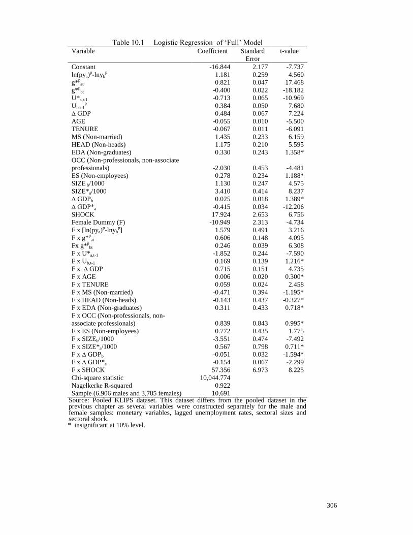
306
Table 10.1 Logistic Regression of „Full‟ Model Variable Coefficient Standard
Error
t-value
Constant -16.844 2.177 -7.737
ln(pya)p-lnyb
p 1.181 0.259 4.560
g*p
at 0.821 0.047 17.468
g*p
bt -0.400 0.022 -18.182
U*a,t-1 -0.713 0.065 -10.969
Ub,t-1p 0.384 0.050 7.680
∆ GDP 0.484 0.067 7.224
AGE -0.055 0.010 -5.500
TENURE -0.067 0.011 -6.091
MS (Non-married) 1.435 0.233 6.159
HEAD (Non-heads) 1.175 0.210 5.595
EDA (Non-graduates) 0.330 0.243 1.358*
OCC (Non-professionals, non-associate
professionals) -2.030 0.453 -4.481
ES (Non-employees) 0.278 0.234 1.188*
SIZE b/1000 1.130 0.247 4.575
SIZE*a/1000 3.410 0.414 8.237
∆ GDPb 0.025 0.018 1.389*
∆ GDP*a -0.415 0.034 -12.206
SHOCK 17.924 2.653 6.756
Female Dummy (F) -10.949 2.313 -4.734
F x [ln(pya)p-lnyb
p] 1.579 0.491 3.216
F x g*pat 0.606 0.148 4.095
Fx g*p
bt 0.246 0.039 6.308
F x U*a,t-1 -1.852 0.244 -7.590
F x Ub,t-1 0.169 0.139 1.216*
F x ∆ GDP 0.715 0.151 4.735
F x AGE 0.006 0.020 0.300*
F x TENURE 0.059 0.024 2.458
F x MS (Non-married) -0.471 0.394 -1.195*
F x HEAD (Non-heads) -0.143 0.437 -0.327*
F x EDA (Non-graduates) 0.311 0.433 0.718*
F x OCC (Non-professionals, non-
associate professionals) 0.839 0.843 0.995*
F x ES (Non-employees) 0.772 0.435 1.775
F x SIZEb/1000 -3.551 0.474 -7.492
F x SIZE*a/1000 0.567 0.798 0.711*
F x ∆ GDPb -0.051 0.032 -1.594*
F x ∆ GDP*a -0.154 0.067 -2.299
F x SHOCK 57.356 6.973 8.225
Chi-square statistic 10,044.774
Nagelkerke R-squared 0.922
Sample (6,906 males and 3,785 females) 10,691 Source: Pooled KLIPS dataset. This dataset differs from the pooled dataset in the previous chapter as several variables were constructed separately for the male and female samples: monetary variables, lagged unemployment rates, sectoral sizes and sectoral shock.
* insignificant at 10% level.

307
Table 10.1 shows the t-statistic for each coefficient. The intercepts in the male and female
regressions are clearly different. There are eight gender interaction terms that are
insignificant at the 10% level, and ten statistically significant interaction variables. In
particular, the individual coefficients for females that are significantly different from the
corresponding coefficient for males are the three monetary variables, lagged new sector‟s
unemployment rate, GDP growth, employee status, tenure, old sector size, new sector
performance and sectoral shock. Furthermore, the chi-square statistic for the test that the
female dummy and interaction terms can be excluded from the model is 550. This exceeds
the critical value and so the hypothesis that there is no significant difference between the
models of worker mobility for males and females is clearly rejected. The industrial
mobility relationship should therefore be estimated separately for males and females.
10.4 DESCRIPTIVE STATISTICS FOR MALES AND FEMALES
This section outlines the similarities and differences between male and female workers in
Korea in terms of the monetary and macroeconomic variables, and worker and job
characteristics that are the basis of the model of industrial mobility. As noted in the
introduction, differences between males and females in these variables may contribute to an
understanding of the reasons for any gender differences in the sectoral mobility of the two
groups.
The means and standard deviations for the KLIPS male sample of 6,906 observations and
the female sample of 3,785 observations covering the four job waves (1998 till 2001) are
listed in Table 10.2. A „t‟ statistic for the test of whether the mean values for each male
and female variable are significantly different from each other is reported in the last column
of the table3.
As in the case of the pooled sample, the majority of male and female workers are industry
stayers, with the mean mobility rates being 23.5% for males and 22.3% for females.
Although the share of movers for men and women do not differ significantly, there could be
differences in the means of the explanatory variables between men and women. If this is
the case, it implies that there must be differences in the estimated coefficients of the
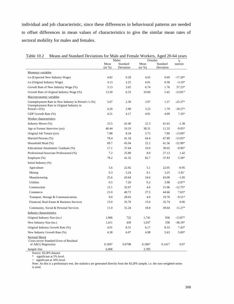
308
individual and job characteristic, since these differences in behavioural patterns are needed
to offset differences in mean values of characteristics to give the similar mean rates of
sectoral mobility for males and females.
Table 10.2 Means and Standard Deviations for Male and Female Workers, Aged 20-64 years Males Females tβ
Mean (or %)
Standard Deviation
Mean (or %)
Standard Deviation
statistic
Monetary variables
Ln (Expected New Industry Wage) 4.82 0.28 4.65 0.69 -17.20*
Ln (Original Industry Wage) 4.13 2.25 4.01 0.58 -3.10*
Growth Rate of New Industry Wage (%) 3.13 3.65 6.74 1.76 57.23*
Growth Rate of Original Industry Wage (%) 13.50 6.33 10.60 5.42 -23.81*
Macroeconomic variables
Unemployment Rate in New Industry in Period t-1 (%) 5.07 2.39 3.97 1.57 -25.37*
Unemployment Rate in Original Industry in
Period t-1(%) 4.20 2.98 3.23 1.79 -18.27*
GDP Growth Rate (%) 4.21 4.17 4.81 4.09 7.10*
Worker characteristics
Industry Mover (%) 23.5 42.40 22.3 41.63 -1.38
Age at Former Interview (yrs) 40.44 10.19 38.31 11.33 -9.95*
Original Job Tenure (yrs) 7.88 8.34 5.72 7.80 -13.09*
Married Persons (%) 78.4 41.18 64.4 47.89 -15.83*
Household Head (%) 69.7 45.94 22.2 41.56 -52.90*
Educational Attainment: Graduate (%) 17.1 37.64 10.0 30.02 -9.96*
Professional/Associate Professional (%) 7.2 25.89 8.0 27.13 1.42
Employee (%) 78.2 41.32 82.7 37.83 5.58*
Initial Industry (%)
Agriculture 5.6 22.92 5.1 22.05 -0.95
Mining 0.3 5.24 0.1 3.25 -1.81+
Manufacturing 25.6 43.64 24.6 43.09 -1.05
Utilities 0.5 7.20 0.2 3.98 -2.87*
Construction 12.1 32.67 4.6 21.06 -12.75*
Commerce 21.0 40.72 27.5 44.66 7.65*
Transport, Storage & Communications 9.0 28.63 4.0 19.70 -9.51*
Financial, Real Estate & Business Services 15.0 35.70 15.0 35.74 0.06
Community, Social & Personal Services 11.0 31.24 18.8 39.04 11.27*
Industry characteristics
Original Industry Size (no.) 1,966 722 1,741 936 -13.87*
New Industry Size (no.) 1,411 439 1,037 558 -38.19*
Original Industry Growth Rate (%) 4.91 8.31 6.17 8.33 7.43*
New Industry Growth Rate (%) 4.38 6.07 4.98 5.63 5.00*
Sectoral Shock
Cross-sector Standard Error of Residual of AR(1) Regression 0.1697 0.0798 0.1867 0.1417
0.07
Sample Size 6,906 3,785
Source: KLIPS dataset. * significant at 5% level.
+ significant at 10% level.
Note: As this is a preliminary test, the statistics are generated directly from the KLIPS sample, i.e. the non-weighted series is used.

309
The Table 10.2 data show that male and female workers differ considerably in terms of
both individual and job characteristics. Among the monetary variables, there were
statistically significant differences between the two groups in terms of the expected
incomes in the new sector, original income and wage growth in both sectors. Males, on
average, reported higher expected and actual earnings. Their expected incomes in the new
sector exceeded those of females by 17 percentage points. Their original incomes were
greater by 13 percentage points. In terms of the old sector‟s lifetime income, male workers
also reported higher earnings than their female counterparts, with their average growth rate
exceeding that of females by 2.9 percentage points. However, the new sector‟s future
earnings for males were lower than those of their female counterparts, by 3.6 percentage
points. So whilst men have greater immediate income gains in the new sector than women,
they would do better in terms of wages growth by remaining in their present sector.
Nonetheless, a breakdown of the data for each gender group revealed that inter-industry
movers had higher future incomes in the new sector than industry stayers.
The descriptive statistics showed that men, on average, experience higher unemployment
than women in both the new and original sectors. For example, the new sector‟s male
unemployment rate was 5.07%, more than 1 percentage point higher than the 3.97% female
rate. The original sector male unemployment rate was 4.20%, which is also greater than the
female rate of 3.23%. Although these data indicate that a higher proportion of men
encounter unemployment, it should be noted that the female unemployment rate can be a
hazy measure. To the extent that females can be „secondary‟ wage earners, they have a
greater tendency to withdraw from the labour force rather than search for work. This
means that the female measured unemployment rate could understate the true
unemployment rate in each sector.
In terms of worker characteristics, there are significant differences between males and
females in terms of age and tenure. The average male (aged 40 with 8 years of experience)
is two years older and has two years more work experience than the average female (aged
38 with 6 years of experience). There are also marked differences in terms of marital
status and head of household status. Whilst 78% of male workers are married and 70%
assume headship in the household, only 64% of females are married with a lower 22%
heading households. In terms of educational attainment, men appear to be more educated,

310
with a considerably higher proportion of graduates (17%) than their female counterparts
(10%).
The variables that do not vary substantially between the two gender groups are employment
status and occupational status. Men have a slightly lower share of employees (at 78%) than
do women (83%). Men and women have similar shares of professionals and associate
professionals, of 7-8%.
In terms of the initial industry, there are differences in the proportional representation by
gender for industries other than mining, manufacturing and financial services. The
industries where males have a higher proportional representation than females are
agriculture (6% versus 5%), utilities, construction (12% versus 5%) and transport and
communications (9% versus 4%). Females were more concentrated in the commerce sector
(28% of females work there compared to 21% of males) and community, social and
personal services (19% for females versus 11% for males).
There are statistically significant differences between men and women in the size of the
original and new industries. Reflecting the greater number of male workers, the average
sizes of both the original and new industries were larger for males than for females.
However, for both gender groups, the new sector‟s size was less than that of the old sector,
suggesting a move towards smaller-sized industries for both groups.
Since there are no gender-specific GDP data, the average GDP growth rate is similar
among males and females, at 4-5%. The statistical difference in GDP growth rates shown
by the t-statistic is mainly due to the uneven distributions of males and females across the
KLIPS sample/sectors. This also applies to sectoral performance, where there is no gender-
specific data, and where the growth rate for the female workforce was slightly higher (by
about 1 percentage point) than that of their male counterparts.
There is, however, also a significant gender difference in the measure of sectoral shock,
given by the cross-sectoral standard error of the residuals of an AR(1) regression4. That is,
an exogenous shock in the original sector has differing magnitudes for the male and female
workforces.

311
The data therefore show that male and female workers differ in terms of both individual
and job characteristics. Given the similarity in the sectoral mobility rates of males and
females, the differences in the mean values of the explanatory variables reported here
suggests that mobility for each gender group is determined by a different set of explanatory
variables. Differences in the behavioural relationships as well as the difference in mean
values of variables will therefore need to be considered in this evaluation of male and
female mobility behaviour.
10.5 GENDER DIFFERENCES IN THE DETERMINANTS
OF SECTORAL MOBILITY
When the model of sectoral mobility was estimated on the separate samples of males and
females, it was found that there were more insignificant variables than in the pooled sample
analysis, an outcome that may be attributed to the smaller sample sizes5. In determining the
final models in this disaggregated anlaysis, three criteria were applied: the fit of the model,
the number of insignificant variables, and having the same variables in the models
estimated for males and females to facilitate the decomposition analysis in the later part of
the chapter.
Prior to conducting the initial gender regressions, a correlation matrix of the explanatory
variables was computed for the separate male and female datasets. The GDP growth rate
was highly correlated with the new sector‟s lagged unemployment rates and new sector
performance, with a coefficient of at least 0.8 in the male dataset. In addition to these two
variables, it was also highly correlated with the old sector‟s lagged unemployment rate in
the female dataset. The remaining correlation coefficients were all more modest, being 0.6
or lower. To minimize the likelihood of multicollinearity and given the measurement issues
about the GDP growth rate raised in the previous chapter (in terms of discrepancy in time
periods and data frequency, and that it is based on a broad-based economy-wide scale), the
GDP growth rate will again be omitted from the estimating equation. It is noted that the
high correlation between age and age-squared, and between tenure and tenure-squared, is to
be expected and they will be retained in the model.

312
The analysis conducted on the separate male and female samples is based on the non-
weighted data. This is undertaken to synchronise with the non-weighted regression results
of the pooled sample, where it was found that the use of weighted statistics led to minimal,
if any, change to the material conclusions. Furthermore, a weighting exercise undertaken
for males and females (not shown) showed that the statistical significance of the variables
remain unchanged regardless of whether the weighted or unweighted t-values were used.
The starting point for this empirical analysis was the estimation for the male and female
samples of the extended model used for the pooled dataset, as set out in Table 10B in
Appendix 10B. This model was characterized by a number of insignificant variables.
Under the initial regression for males, the insignificant variables at the 5% level were age-
squared, tenure, tenure-squared, educational attainment, old sector size and employment
status. Since the squared terms for age and tenure were non-influential, linear specifications
for these variables were tried. Under this linear model, the same variables remained
insignificant save for tenure, which became significant. For the unrestricted female
regression, in addition to the first four variables noted above for males, age and
occupational status were also insignificant at the 5% level. Using a linear specification for
the age and tenure variables for females led to the same variables being insignificant,
except for age6. Hence, linear age- and tenure-mobility relationships are implied by these
gender-specific regressions.
Table 10.3 presents the results of the restricted model when estimated separately for male
and female workers. There is a high number of statistically significant variables in each
model. The models for both samples have a good fit, with the Nagelkerke R-squared being
0.912 for males and 0.908 for females7. The analysis of Table 10.3 will first proceed with
the discussion of the results from the monetary and macroeconomic variables, followed by
individual and job characteristics and the sectoral shock variable.
10.5.1 Monetary variables
There are several studies of sectoral mobility that have provided separate analyses for
males and females. These, however, have not discussed gender differences in the impact of
monetary variables (expected or lifetime wages). Accordingly, any gender differences in
313
the effects of the monetary variables in the current set of empirical analyses will not be able
to be compared with empirical findings reported in the literature. Rather, the discussion
below will be limited to the between-gender differences from the current analysis, with
reference to findings from some single-sex studies where possible.
Expected Sectoral Wage Differential
In the analysis of the data pooled across males and females (chapter 9), the expected
sectoral wage differential had a positive and significant effect on sectoral mobility. This
finding is replicated in the separate analyses for males and females. The higher the
expected wage differential between sectors, the greater the probability of male and female
mobility. The elasticity of mobility with respect to a unit change in the expected wage
differential is 0.61 for men and 1.79 for women. Thus, empirically, the results of the
disaggregate study concur with the Le and Miller (1998) model.
The „actual‟ wage differential variable (results not reported here) yielded results similar to
those reported for the expected wage differential term. Hence, the male regression showed
that the coefficient of actual wages (1.03) was only slightly larger and the fit of the model,
as measured by Nagelkerke R-squared (0.91), was the same as the Table 10.3 result. For
the female regression, the coefficient of „actual‟ wages (1.91) was only slightly smaller
than that reported in Table 10.3, as was the fit of the model (Nagelkerke R-squared at
0.905). The similarity of the findings based on the expected and „actual‟ wage differential
has its basis in the argument advanced in relation to analysis of the pooled data: since
average Uatp rates are quite low for males (5%) and females (4%), the final term in the
expected wages measure [ln yap – ln yb
p + ln (1-Uat
p)] will be close to zero, meaning that
expected wages will be close to actual wages.

314
Table 10.3 Logistic Regression of Sectoral/Industrial Mobility by Gender Variable Males Females
Coefficient t-statistic Marginal
Effect
Coefficient t-statistic Marginal
Effect
Constant -7.526 -8.601 n.a. -18.148 -11.080 n.a.
ln(pya)p-lnyb
p 0.796 3.192 14.32 2.298 7.137 39.81
g*pat 0.714 18.297 12.83 1.099 9.944 19.04
g*p
bt -0.408 -18.779 -7.33 -0.229 -9.238 -3.97
U*a,t-1 -0.366 -9.501 -6.58 -1.401 -10.392 -24.27
Ub,t-1 0.477 11.086 8.57 1.037 9.236 17.97
AGE -0.047 -5.043 -0.84 -0.043 -2.958 -0.74
TENURE -0.061 -5.685 -1.10 -0.003 -0.166* -0.05
MS (Non-married) 1.372 6.053 24.67 0.959 3.437 16.62
HEAD (Non-heads) 1.121 5.330 20.15 1.245 3.804 21.58
OCC
(Non-professionals,
non-associate
professionals) -2.128 -5.257 -38.25 -0.667 -1.379* -11.56
ES (Non-employees) 0.218 0.974* 3.92 1.112 3.669 19.27
SIZEb/1000 0.492 1.940+ 8.85 -2.855 -8.378 -49.46
SIZE*a/1000 2.937 7.702 52.79 3.150 6.729 54.58
∆ GDP*b 0.057 3.706 1.02 0.158 7.871 2.74
∆ GDP*a -0.240 -12.255 -4.32 -0.315 -8.583 -5.46
SHOCK 20.221 6.591 15.47 74.706 13.082 58.05
Nagelkerke R-squared 0.912 0.908
Chi-square statistic (16) 6,426.520 3,410.659
Sample size 6,906 3,785
* insignificant at 5% level.
+ significant at 10% level.
n.a. : not applicable
Note : For the SHOCK variable, the elasticity measure is used. The elasticity of mobility w.r.t. a change in
the sectoral shock is measured as: elasticity = marginal effect / p = β x p(1-p)/p. For males, elasticity =
20.221 x 0.235(0.765)/0.235 = 15.47. For females, elasticity = 74.706 x 0.223(0.777)/0.223 = 58.05.
Lifetime Earnings
For the pooled sample analyses of chapter 9, the effects of the individuals‟ lifetime earnings
streams, as captured by the wage growth terms, were found to differ between sectors. The
probability of moving was raised by higher wage growth in the new sector. For the original
sector‟s wage growth, a move out of the original sector was less likely if the original
sector‟s permanent earnings were higher. The separate analyses undertaken by gender
mirrored these results.
Male workers were more likely to move to the new sector for higher permanent earnings.
For a unit increase in income growth, male mobility increased by 13 percentage points.
Similarly, lifetime earnings in the new sector exerted a positive impact on female mobility
315
behaviour. Females were 19 percentage points more likely to enter into the new sector for
every unit increase in wage growth.
For the original sector, lower lifetime earnings induce male workers to change sectors. For
every unit decrease in income growth, men are 7.33 percentage points more likely to move.
The deterrent effect was also evident among women: women were 3.97 percentage points
more likely to change sectors for every unit decline in the growth rate.
From this examination of the results for the monetary variables, it can be concluded that
both men and women are motivated by the initial monetary gains and are equally
responsive to the prospect of earning higher lifetime incomes in the new sector. The extent
of the impact of lifetime income is also greater in the new sector than the old sector,
judging from the magnitude of the parameter estimates and the marginal effects. The
gender analyses therefore supports one of the predictions of the Le and Miller (1998)
model, that individuals move to alternative employment states in anticipation of higher
lifetime earnings. It also confirms the expectation that higher earnings in the new sector act
as a pull factor and lower earnings in the original industry act as a push factor for male and
female mobility. The consistency of the findings for males and females is reassuring, from
the perspective of informing on the robustness of the results.
10.5.2 Macroeconomic Variables
The macroeconomic variables included in this empirical analysis are the unemployment
rates in the original and new industries. The results obtained for the study of males and
females in the Korean labour market do not appear to have any direct counterparts in the
literature; hence only comparisons with general, aggregate-level, studies can be provided
below.
Sectoral Unemployment Rate
In the analysis of chapter 9, where the sample was pooled across males and females, the
original sector‟s unemployment rate had a positive effect on sectoral mobility. Similarly, in
316
the analyses disaggregated by gender, the old sector‟s unemployment rate had a positive
impact on the likelihood of both males and females moving across sectors. For males, the
marginal effect of a one percentage point increase in the unemployment rate was 8.57
percentage points. For females, the marginal effect was 17.97 percentage points. Thus, it
appears that the original sector‟s unemployment rate acts as a push factor of mobility.
For the new sector‟s lagged unemployment rate, the separate analyses for males and
females replicate the overall sample result that the odds of a move to the new sector are
lowered the higher the new sector‟s unemployment rate. For male workers the marginal
effect was 6.58 percentage points. For female workers, the marginal effect was 24.27
percentage points for every one percent increase in the unemployment rate8. The Table
10.3 results are consistent with the Todarian hypothesis, which asserts a negative
relationship between the unemployment rate and the probability of gaining employment.
These findings for males and females are internally consistent in that lower job
opportunities lead to out-mobility from the old sector and deter mobility into the new
sector. The results for Ub,t-1 (U*a,t-1) also held when U*a,t-1 (Ub,t-1) was omitted from the
estimating gender equations. These features, and the similarity with the findings reported
in chapter 9, point to the results with respect to the macroeconomic variables being quite
robust.
10.5.3 Worker Characteristics
Gender differences in the impact of a number of worker characteristics, i.e. age, job tenure,
family indicators, employment/occupational status and educational attainment variables, are
of interest. Several recent studies have focused on these issues, and they afford a basis,
albeit limited, for comparison in this section. Where applicable, these comparisons will be
highlighted.
Age
The analyses conducted for the pooled sample indicated a non-linear, negative age-mobility
relationship. As noted above, the preliminary examination of the data indicated that the

317
mobility-age relationship for the separate male and female samples were linear. Consistent
with the aggregate-level analysis, however, these relationships were also negative. Among
men, the chances of moving decreased by 0.84 percentage points per additional year of age.
Among women, the probability of moving sectors declined by 0.74 percentage points for
every extra year of age. These gender findings correspond with the negative age-mobility
correlation for males in Osberg, Gordon and Lin (1994) and for females in 1985/1986 in
Osberg (1991). As noted before, this relationship is generally held to arise as older workers
have a shorter working period over which they can derive benefits from a different job
[Creedy and Thomas (1982)] and, due to the experience and knowledge they have acquired
in the original job/sector, they face greater costs in moving [Jovanovic and Moffitt (1990)].
Job Tenure
The analysis of the data pooled across the male and female samples revealed a non-linear,
generally negative tenure-mobility relation. When the analyses were undertaken separately
for males and females, however, the relationship between mobility and job tenure for males
was linear and negative, while that for females was statistically insignificant. However, for
consistency with the analyses for males, a linear specification was used in the estimating
equation for females.
Male workers with lengthy tenures were less likely to switch sectors, with their propensity
to move reducing by 1.10 percentage points per extra year of tenure. This finding conforms
with other studies for males: Osberg (1991), Osberg, Gordon and Lin (1994) and Neal
(1995) all reported a negative tenure effect. However, the insignificant tenure effect for
females differs from Osberg‟s (1991) study, which showed females to have lower mobility
probabilities with rising tenure.
Various suggestions for the difference in the impact of tenure on the mobility behaviour of
males and females can be advanced. These include a greater importance of firm-specific
training for male workers than for female workers, and, in general, a higher opportunity
cost of moving sectors for male workers than for their female counterparts. This could
arise from a higher proportion of older male workers with lengthy tenures holding senior
318
positions, and the high wages of their senior positions, in addition to other non-pecuniary
benefits, may not be readily available in the new sector.
Family Indicators: Marital Status and Household Head
The preliminary analyses in chapter 9 of the data pooled across males and females showed
that marital status was not a significant determinant of the propensity to change sectors.
The marital status variable was subsequently omitted from the estimating equation. The
separate analyses conducted for men and women, however, revealed marital status to be a
significant determinant of mobility. Whilst married men were 24.67 percentage points less
likely than their non-married counterparts to switch industries, females were 16.62
percentage points less likely than their non-married counterparts to change sectors. This
result for males is in line with Neal (1995), who shows married men to have lower
propensities of moving sectors. However, it differs from results reported by Osberg (1991)
for 1982/1983 and 1985/1986, and Osberg, Gordon and Lin (1994), where marital status
did not have a significant effect on sectoral mobility. The finding for females in the current
study, to the extent that married women have greater household responsibilities, comes
across as intuitively reasonable. However, the finding for females does not concur with
Osberg‟s (1991) study, where marital status did not impact on female sectoral mobility in
any of the three phases, 1980/1981, 1982/1983 and 1985/1986, for which the statistical
analyses were undertaken.
In the analysis for the entire sample of workers, heads of households had a lower incidence
of industrial mobility. Given the considerably higher proportion of male heads in the
sample, it is not surprising that this impact is mirrored in male mobility behaviour. Male
heads were 20.15 percentage points less likely to change sectors than males who were not
the household head. This finding aligns with the study of Fallick (1993), which revealed
unemployed male heads to have a lower incidence of industrial mobility, and supports the
view of household heads facing greater risks from an industrial switch arising from their
family responsibilities. Household head status also showed up as a significant deterrent of
female mobility, with the marginal effect being 21.58 percentage points. This could be due
to the fact that females heading households are single parents who are not able to afford to
incur the risks of changing sectors. A breakdown of the data revealed that nearly three-

319
fifths of the 840 female household heads in the sample were single, divorced, widowed or
separated.
Educational Attainment
In the previous chapter where the sample was pooled across male and female workers,
educational attainment was shown to have a significant impact on sectoral mobility, with
graduates being less likely to switch sectors. The preliminary analyses conducted for males
and females revealed that little, if any, of the variation in male or female mobility could be
attributed to educational attainment. The insignificant education variable was therefore
omitted from the estimating equation used in this chapter. The finding for males reported
here is consistent with Osberg, Gordon and Lin (1994) and Neal (1995). In this earlier
study, male elementary/diploma and university degree holders had similar rates of mobility.
There is no readily apparent reason for the different findings for the aggregate-level
analysis and these estimations undertaken on the separate male and female datasets, other
than the size of the sample. In this regard it is noted that the „t‟ on the educational
attainment variable in the aggregate-level analysis was typically around 2, and a halving of
the sample would itself reduce this value by around one-third in the preliminary analysis.
Occupational Status
Occupational status was shown to be an insignificant determinant of mobility in the overall
sample in chapter 9, and the variable was omitted from main set of analyses in that chapter.
The disaggregated gender analysis revealed a similar finding for women. Thus, among
Korean females, occupational status did not exert any impact on gender mobility. This
finding is consistent with the some of the results reported by Osberg (1991), where the
likelihood of a sectoral change was not significantly different for women in clerical and
sales occupations in 1982/1983 and for female managers, professionals and technicians in
1980/1981.
In the analyses undertaken separately in this thesis for males, however, skilled workers had
a higher likelihood of moving sectors, with their chances being 38.25 percentage points
greater than that of their unskilled counterparts. This finding is consistent with the results
320
in Osberg (1991), where men in the higher-skilled managerial/professional/technical
occupations were found to have a higher probability of mobility for 1980/1981. This
finding for males in Korea supports the view of skill levels being vital to certain industries‟
operations [Neal (1995)] and workers with vital skills will be more likely to switch to
industries requiring such skills. Also, the finding supports the idea of skilled workers being
scouted for their talent and productivity [Murphy and Topel (1990)] and they will
consequently have a higher likelihood of switching sectors. The finding for females,
however, reflects mobility stickiness. Skilled females could be in more specialized
occupations which limit their range of alternatives and thus results in limited mobility.
Employment Status
In the analysis of the data pooled across males and females, non-employees had a greater
likelihood than employees of moving to new sectors/industries. This finding was replicated
in the analysis for females. Specifically, females who were non-employees were 19.27
percentage points more likely than employees to move across sectors. Among males,
however, employment status did not have a significant effect on mobility. It is not clear
why this variable should have different effects for men and women. The Asian Financial
Crisis adversely affected businesses and caused many employers/business owners to close
down. It could be that female employers/business owners were more likely to be in small
firms: such businesses have emerged as significant avenues for the economic empowerment
of women in the Asia-Pacific, as their flexibility in operations with minimum technology
and capital start-ups, and family-based nature favour women‟s decision to participate in the
labour force9. With limited access to resources and business networks, however, these
small businesses may have been more vulnerable and the hardest hit by the Crisis. The
mobility literature does not provide any evidence in this regard.
10.5.4 Industry Characteristics
The industry characteristics considered for inclusion in the model of sectoral mobility are
industry size and sectoral performance. Whilst the findings linking industry size to sectoral
mobility in the separate samples of males and females can be compared with findings from
the empirical literature, no comparison appears possible for sectoral performance.

321
Sectoral Size
In the previous chapter, the aggregate-level analyses revealed that a larger size of the
original sector reduced the probability of a sectoral move. This result carried over to the
separate study of female workers. The elasticity of female mobility with respect to an
increase in the size of the original sector was -2.22. In contrast, the original sector size
increased the likelihood of male mobility, with the corresponding elasticity of mobility at
0.38. The finding for males contradicts that in Neal (1995), where it was reported that the
industry size had a negative effect on mobility (although the study pertains to displaced
workers).
To account for the contrasting results between men and women, the female variable for the
original sectoral size was placed into the estimating equation for males. The coefficient of
this alternative variable was negative but insignificant, compared to the positive one when
the male variable was used. This suggests that a reason for the conflicting results is the
gender differences in the industrial composition, with males being concentrated in the
construction sector and females being concentrated in the commerce sector and in
community, social and personal services industries. In other words, it is not so much size
per se that is important, but it is the size of particular sectors of the economy.
The aggregate-level analyses also indicated that the probability of a sectoral move was
higher the larger the size of the new sector, and it was suggested that Korean workers
moved for greater employment opportunities. The separate analyses for males and females
reinforce this result. The elasticity of mobility in response to an increase in the new sector
size for females (2.45) was slightly larger than for males (2.25). This finding corresponds
with Osberg, Gordon and Lin (1994), where a positive association between male mobility
and industry size was reported, and it portrays the idea of workers moving in response to
employment availabilities in the new sector.
Sectoral Performance
The GDP by sector variable cannot be constructed separately for men and women. Hence
differences between men and women in this variable will only reflect gender differences in

322
the distribution of workers across industries. The earlier study of the overall sample showed
that stronger growth in the original sector raised the likelihood of a sectoral move.
Likewise, the gender studies replicated this finding, with higher growth in the original
sector increasing the probabilities of both male and female mobility, with the marginal
effects being 1.02 percentage points for males and 2.74 percentage points for females. As
in the case of the result from the study of the pooled sample, it appears that both male and
female mobility support the jobless growth hypothesis. This may be associated with the
technological advances in Korea, where the high-performing original sector has limited job
vacancies associated with the growth thereby leading to higher out-mobility rates.
For the new sector, better performance reduced the likelihood of a sectoral switch in the
aggregate-level analyses, and the disaggregated analyses conducted here revealed similar
results for both males and females. That is, a higher (lower) GDP growth rate reported in
the new industry decreased (increased) the probability of moving industries for males and
females. The marginal effects were -4.32 percentage points for males and -5.46 percentage
points for females. These findings are consistent with the jobless growth hypothesis, where
the high-performing new sectors with technological advancements have fewer job
opportunities, and hence the chances of a sectoral switch to the new sectors are lowered.
10.5.5 Sectoral Shock
The effect of the sectoral shock was large, positive, and significant for the overall
workforce. This result was mirrored in the analyses conducted for the separate samples of
males and females. The elasticity of mobility with respect to a change in the sectoral shock
variable was 15.47 for males and 58.05 for females. This finding for males is similar to the
result reported by Jovanovic and Moffitt (1990), who demonstrated the sectoral shock to
have a positive impact on the probability of male sectoral mobility10
. When this exogenous
sector shock variable was omitted from the regressions, the fit under the male model
dropped from 0.912 to 0.905, and that under the female model dropped from 0.908 to
0.761. It can thus be seen that the effect of the sectoral shock variable is greater among
female workers than among male workers, which is also reflected in the gender difference
in the coefficients of the sectoral shock variable given in Table 10.3.
323
10.6 A GENDER PERSPECTIVE ON THEORIES OF SECTORAL MOBILITY
The objective of this section is to assess the empirical relevance of the three theories of
sectoral mobility outlined earlier to the separate samples of male and female workers. The
tests of null hypothesis under each theory are the same as in the previous chapter.
10.6.1 Worker-Employer Mismatch Theory
With the regression for males, the t-statistic for the coefficient of the industrial shock, θ,
was 6.60. With the regression for females, the t-statistic for H0: θ = 0 was 13.08. Thus, the
null hypothesis of H0: θ = 0 is rejected for both gender groups. That is, the sectoral shock
is a significant factor in accounting for both male and female mobility patterns. For the
Korean workforce, gender models that are based on the worker-employer mismatch theory
and disregard the sectoral shock effect on mobility would be inadequate in accounting for
sectoral labour movements.
10.6.2 Sectoral Shock Theory
From the results displayed in Table 10.3, fourteen variables in the equation for males are
significantly different from zero at the 5% level. The chi-square statistics for the test of
whether all the non-sectoral shock variables add to the explanatory power of the model was
4,339. This exceeds the critical value and so the null hypothesis that these non-sectoral
shock variables are not important is rejected. The pure sectoral shock theory cannot be
applied to the study of male mobility. For the regression for females, there were fourteen
significant variables at the 5% level. The test of the null that all the non-sectoral shock
variables did not contribute to the explanatory power of the model yielded a test statistic of
1,599, which is far higher than the critical value. As in the case of the study of male
mobility, the pure sectoral shock theory is not applicable to the analysis of female mobility
behaviour.

324
10.6.3 Bridging Theory
Table 10.3 shows that the monetary, macroeconomic, demographic, socio-economic and
sectoral shock variables are significant in explaining male and female mobility. The
mismatch theory (i.e. testing H0 : θ = 0) and sectoral shock theory (i.e. testing H0 : β1 = β2
….. = βk = 0) are rejected for both groups and it appears that gender movements are best
described using the bridging theory.
The validity of these results was checked using the approach along the lines of the
Jovanovic and Moffitt‟s (1990) method that was discussed in Chapter 9. This involved
regressing the probability of a sectoral move on the standard error of the log wage
distribution and the sectoral shock. The wage and sectoral shock measures were significant
for both the male and female regressions, as shown in Table 10.4. It can be concluded,
therefore, that the bridging theory of sectoral mobility, that was previously held to apply to
the pooled data regression, applies also to the study of male and female mobility.
Table 10.4 Logistic Regression of Sectoral/Industrial Mobility on the Standard
Error of Wage Distribution and Sectoral Shock for Males and Females Variable Coefficient t-statistic
Male Regression
Constant -7.714 -42.810 Standard Error of ln(original industry wage) 3.167 25.256 Standard Error of Sectoral Shock 19.134 28.542 Nagelkerke‟s R-squared 0.498 Female Regression Constant -7.580 -28.128 Standard Error of ln(original industry wage) 2.778 12.518 Standard Error of Sectoral Shock 17.371 23.036 Nagelkerke‟s R-squared 0.622
Source: KLIPS dataset
Whilst the model specification of the above approach is similar to Jovanovic and Moffitt
(1990), the method is not a direct application in terms of data (4 years for the Korean case
compared with 13 years), difference in the sectoral shock variable (i.e. cross-sectoral
measure in this case), estimation of the probability function for males and females using
data for the entire sample period rather than using a series of sub-periods. With regards to
325
the latter, the current application was based on the male and female datasets of 6,906 and
3,785 observations respectively. Jovanovic and Moffitt (1990), however, estimated the
probability function for a typical worker for each period with the number of observations in
parentheses: 1966-1968 (492), 1967-1969 (628), 1968-1970 (754), 1969-1971 (887), 1971-
1973 (1,357), 1973-1975 (1,846), 1976-1978 (2,032) and 1978-1980 (1,967).
10.7 DECOMPOSITION ANALYSIS
The empirical analysis in the preceding section examined the determinants of sectoral
mobility by gender using a logit model developed from equations (10.1) and (10.2). Male
and female workers in Korea have different mobility behaviour, in that their sectoral
mobility is influenced by different sets of explanatory variables, and by different amounts
for particular explanatory variables. In particular, there is a statistically significant
difference in the intercept coefficients of the male and female regressions as well as in the
coefficients of the majority of the explanatory variables, namely, the monetary variables,
lagged new sector‟s unemployment rate, GDP growth, employee status, tenure, old sector
size, new sector performance and sectoral shock (Table 10.1). The aim of this section is
therefore to explore these gender differences more formally and in greater depth via a
decomposition technique.
From equations (10.1) and (10.2), the predicted probability of moving sectors for males (m)
and females (f) can be expressed as:
^ ^
movem = 1 / (1 + e-Im) , where Im = Xm βm
for males, and for females as:
^ ^
movef = 1 / (1 + e-If) , where If = Xf βf .
In this formulation, X is the all-encompassing vector of explanatory variables, including ^
the constant, and β is the associated logit regression coefficients. These two equations
indicate that the differences in the probability of a worker, male or female, moving will be
linked to differences in either the values of the explanatory variables or the estimated logit
326
coefficients. Differences in the latter will be due to the personal preferences of males and
females in their demand for sectors, or employer/industry preferences to recruit/retain male
or female workers. The aim of the decomposition explored in this section is to link
differences in the mobility rates of males and females to differences in the estimated logit
coefficients, and to differences between males and females in the values of the explanatory
variables.
This type of decomposition is widely used in the gender discrimination literature. It has its
intellectual roots in the studies of Blinder (1973) and Oaxaca (1973). These earlier studies
were based on regression equations estimated by ordinary least squares, and refinements
are necessary in this application to accommodate the non-linear, non-separable nature of
the logit model. These refinements are outlined in section 10.7.2. The results of the
decomposition analysis are presented in section 10.7.3.
10.7.1 An Overview of the Standard Decomposition Technique
Consider a linear probability mobility model, where the mobility outcome M takes the
value of 1 if a change of sectors occurs and 0 otherwise. The mobility outcome, evaluated
at the sample mean values of the regression variables, can be expressed as:
_ _ ^ Mm = Xm βm (10.3) _ _ ^
Mf = Xf βf (10.4) _ _
where for males (m) and females (f), Mm and Mf denote the average probability of _ _
sectoral mobility, Xm and Xf are the sample mean values of characteristics, and
^ ^
βm and βf are the estimates from the linear probability models.
If females receive the same return to their characteristics as males, the average hypothetical
mobility outcome for females will be:
_ _ ^
Mf* = Xf βm (10.5)
To obtain the impact of endowments on the difference in the average mobility outcomes
between males and females, equation (10.5) is subtracted from equation (10.3) to give

327
equation (10.6). The impact of the estimated coefficients on the difference in the mobility
outcome in equation (10.7) is derived by subtracting equation (10.4) from equation (10.5).
_ _ _ _ ^ Mm - Mf* = (Xm - Xf ) βm (10.6)
_ _ _ ^ ^ Mf* - Mf = Xf ( βm - βf ) (10.7)
The decomposition of the overall gap between the male and female outcomes can be
derived by adding equations (10.6) and (10.7) to give
_ _ _ _ ^ _ ^ ^
Mm - Mf = (Xm - Xf ) βm + Xf ( βm – βf ) (10.8)
The first component of the decomposition on the right-hand side of the above equation is
the part of the gap on the left-hand side due to differences in the endowments of males and
females. The second part is attributed to differences between males and females in the
parameter estimates. Equation (10.8) can be considered to be the standard model for
decomposition of differences in the labour market outcomes of males and females.
10.7.2 Application to Logit Models
The decomposition technique outlined above requires the underlying regression model to
be additive. It can be used with a linear probability model. However, modifications are
needed if the technique is to be used in conjunction with a logit or probit model. In the case
of these non-linear probability models (logit, probit), an appropriate method is the Farber
(1990) procedure. The starting point for this method is the average predicted probability
P(Xi βi) for the sample of individuals (i = males, females). This can be expressed as:
^ n ^
P(Xi βi) = 1/n ∑ F (Xij βi) (10.9) j=1
^
where Xij is a vector of the characteristics of the jth
individual in the ith
sample, βi is the logit
estimates from the sample dataset for group i, n is the number of individuals in the sample
and F( . ) is the cumulative distribution function. Applying this notation, the difference in
^ ^
the probability of sectoral mobility between males and females, i.e. P(Xmβm) - P(Xf βf), can
be decomposed as:

328
^ ^ ^ ^ ^ ^
P(Xmβm) - P(Xf βf) = [P(Xmβf) - P(Xf βf)] + [P(Xmβm) - P(Xmβf)] (10.10)
The first bracketed term on the right-hand side of the equation is the component of the
difference in rates of mobility of males and females due to the difference in the values of
their observable attributes, evaluated at the coefficient for females. In other words, it is the
portion of this mobility rate differential that can be explained by variations in the
characteristics of males in comparison to those of females if the mobility outcomes were
determined in accordance with the estimated female mobility behaviour. The second
bracketed term shows the portion of the mobility rate differential that is attributable to
differences between males and females in the way that each worker characteristic impacts
on mobility behaviour. This „behavioural‟ component is evaluated using the characteristic
of males. It is the unexplained component of the difference in mobility outcomes. It
generally reflects either or both of the following:
a) The difference between male and female preferences (since some parameter
estimates are for individual characteristics);
b) The unequal treatment of males and females in industry labour market practices
(since some regression coefficients are associated with industry characteristics).
The well-known index number problem in the Blinder (1973) decomposition can be
accommodated in the current study by also decomposing the differences in the probability
of sectoral mobility between males and females using:
^ ^ ^ ^ ^ ^
P(Xmβm) - P(Xf βf) = [P(Xmβm) - P(Xf βm)] + [P(Xfβm) - P(Xfβf)] (10.11)
This decomposition simply uses different weights from that outlined in equation (10.10).
Compared to the earlier method, the mobility rate differential due to differences in male
and female characteristics (i.e. first bracketed term on the right-hand side of the equation) is
evaluated as if the mobility outcomes were determined by the equation estimates for males
instead of those for females. That is, the explained difference due to gender differences in
characteristics is evaluated using the coefficients for males. In terms of the unexplained
difference (i.e. second bracketed term on the right-hand side of the equation), equation
(10.11) uses the endowments for females rather than those of males as the weighting
variable. Thus, the component gives the difference between the mobility outcomes of

329
males and females that is due to differences in the preferences of the two groups and/or the
unequal treatment of males and females by industry sources, evaluated using the
characteristics for female workers.
For the current research, the decomposition of the difference in the sectoral mobility rates
of males and females will be conducted using both equations (10.10) and (10.11).
10.7.3 Decomposition Results
The data for the application of the decomposition methods are from the same KLIPS
sample datasets for males and females used in the multivariate analyses presented earlier in
this chapter. The difference in the average probabilities of sectoral mobility can be
obtained from Table 10.2 or computed using the algorithm in the left-hand side of
equations (10.10) and (10.11). The explained and unexplained components were computed
using the estimated β coefficients and associated characteristics of each person in the
particular (male or female) sample. The terms on the right-hand side of equations (10.10)
and (10.11) were obtained as follows. First, predicted values for each individual were
computed for the male sample, where the characteristics for each record were multiplied by
the estimated βm and βf.
^ ^ These values were divided by the male sample size to give P(Xmβm) and P(Xmβf).
Likewise, from the female sample, the characteristics for every female record was
multiplied by the estimated βm and βf and predicted probabilities of mobility obtained.
^ ^ The average of these predicted values over the female sample gives P(Xfβm) and P(Xfβf).
Table 10.5 presents the decompositions of the difference in the average probability of
mobility between males and females. The left-hand panel of this table is for equation
(10.10) and the right-hand panel is for equation (10.11). As noted in section 10.4, males
have a 1.2 percentage point higher probability of mobility than females. This is the figure
presented in the first row of the Table (i.e. 0.012).

330
Table 10.5 Decomposition Results Variable Equation (10.10):
Farber Method
Equation (10.11):
Farber Method
Total Difference
P(Xmβm)-P(Xfβf)
0.012
0.012
Total Explained (due to characteristics)
P(Xmβf)-P(Xfβf)
P(Xmβm)-P(Xfβm)
-0.037
-0.113
Total Unexplained (due to coefficients)
P(Xmβm)-P(Xmβf)
P(Xfβm)-P(Xfβf)
0.049
0.125
Source : KLIPS gender datasets
The explained component is the portion due entirely to the differential between the
observed attributes of males and females. This component is negative under both methods,
but of different magnitude. If the mobility outcomes were determined according to the
estimates obtained for females, the probability of moving sectors for males would be 3.7
percentage points less than that of their female counterparts. If the mobility outcomes were
evaluated according to the estimates obtained for males, the endowment effect would be
-11.3. That is, ceteris paribus, the probability of switching sectors for males would be 11.3
percentage points less than that of females. This means that males have relatively less of
those characteristics associated with higher probabilities of moving in the logit model, and
they have relatively more of those characteristics associated with lower probabilities of
moving in the statistical analyses presented in Table 10.3.
The unexplained portion of the decomposition is positive under the two methods. It is 0.049
when equation (10.10) is used and 0.125 when equation (10.11) is used. In other words, for
the same set of male (or female) characteristics, males are more likely to switch sectors
than females. The results of the unexplained difference under both methods suggest that
the sectoral mobility behaviour of males is more sensitive to changes in worker and/or
industry circumstances than is the case for females. This either points towards differences
in preferences (e.g. males have stronger desire to change sectors, females prefer to remain
in the same sector owing to family commitments) or the unequal treatment in industry
practices between the sexes (e.g. employer reluctance to recruit females).

331
The greater ceteris paribus sectoral mobility among male workers in Korea than among
their female counterparts could be consistent with several scenarios. First, sectoral mobility
may be „good‟ in that it is associated with economic progress, and employers in the new
sector may be nepotistic towards males or discriminatory towards females in Korea.
Second, sectoral mobility may be „bad‟, being forced upon workers as a result of adverse
events. In this case, males may simply prefer to risk changing sectors whilst their female
counterparts may simply prefer to avoid the risks of a sectoral switch.
10.7.4 Explanatory Power of Observed Variables
The decomposition presented above does not assess the portion of the explained difference
attributable to each of the observed characteristics. Several studies have examined the
explanatory power of the individual observed characteristics, including Even and
Macpherson (1993), Doiron and Riddell (1994) and Nielsen (1998). This study adopts the
method of Even and Macpherson (1993). The portion of the explained difference from
equation (10.10) due to differences between males and females in the kth
explanatory
variable can be defined as:
_ ^ _ ^ _ _ ^ _ _ ^
[P(Xmβf)-P(Xfβf)] x [(Xmk – Xfk) βfk]/[(Xm – Xf) βf] (10.12)
_ ^ _ ^
where [P(Xmβf) - P(Xfβf)] is the explained difference evaluated at the coefficients for
^ _ _
females (βf) and, for the kth
explanatory variable, Xmk and Xfk are the mean values for
^
males and females, respectively, and βfk is the respective logit coefficient from the female
regression.
The method of Even and Macpherson (1993) can be modified to examine the explained
difference as per equation (10.11). Given that the explained difference is determined from
_ ^ _ ^
[P(Xmβm) - P(Xfβm)], the male regression coefficient is used in place of the female one.
That is, the portion of the explained difference due to the gender difference in the kth
explanatory variable can be written as:
_ ^ _ ^ _ _ ^ _ _ ^
[P(Xmβm)-P(Xfβm)] x [(Xmk – Xfk) βmk]/[(Xm – Xf) βm] (10.13)
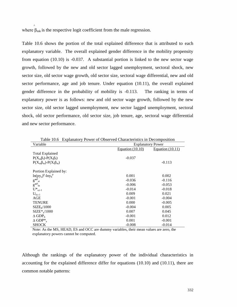
332
^
where βmk is the respective logit coefficient from the male regression.
Table 10.6 shows the portion of the total explained difference that is attributed to each
explanatory variable. The overall explained gender difference in the mobility propensity
from equation (10.10) is -0.037. A substantial portion is linked to the new sector wage
growth, followed by the new and old sector lagged unemployment, sectoral shock, new
sector size, old sector wage growth, old sector size, sectoral wage differential, new and old
sector performance, age and job tenure. Under equation (10.11), the overall explained
gender difference in the probability of mobility is -0.113. The ranking in terms of
explanatory power is as follows: new and old sector wage growth, followed by the new
sector size, old sector lagged unemployment, new sector lagged unemployment, sectoral
shock, old sector performance, old sector size, job tenure, age, sectoral wage differential
and new sector performance.
Table 10.6 Explanatory Power of Observed Characteristics in Decomposition Variable Explanatory Power
Equation (10.10) Equation (10.11)
Total Explained
P(Xmβf)-P(Xfβf)
P(Xmβm)-P(Xfβm)
-0.037
-0.113
Portion Explained by:
ln(pya)p-lnyb
p 0.001 0.002
g*p
at -0.036 -0.116
g*p
bt -0.006 -0.053
U*a,t-1 -0.014 -0.018
Ub,t-1 0.009 0.021
AGE -0.001 -0.004
TENURE 0.000 -0.005
SIZEb/1000 -0.004 0.005
SIZE*a/1000 0.007 0.045
∆ GDPb -0.001 0.012
∆ GDP*a 0.001 -0.001
SHOCK -0.008 -0.014
Note: As the MS, HEAD, ES and OCC are dummy variables, their mean values are zero, the
explanatory powers cannot be computed.
Although the rankings of the explanatory power of the individual characteristics in
accounting for the explained difference differ for equations (10.10) and (10.11), there are
common notable patterns:

333
(a) The new and old sector wage growths account for a considerable portion of the
gender difference, as compared to the sectoral wage differential. This implies
that expected lifetime incomes play a greater role than the expected wage
sectoral wage differential in accounting for the gender difference.
(b) The individual characteristics of age and job tenure have considerably lower
explanatory power as they rank below the monetary, macroeconomic, monetary
and most sector-level variables.
(c) The sectoral shock contributes only a moderate amount to the explained
component, meaning that unanticipated events play some, albeit, slight, role in
the difference between the male and female mobility outcomes.
Finally, it is noted that the negativity of the total explained difference reinforces certain
patterns in the data. It supports the conclusion that men have relatively less of those
characteristics associated with higher probabilities of moving (Xm < Xf and βk > 0), as
depicted from the new sector wage growth, the old sector performance and the sectoral
shock under both equations (10.10) and (10.11), and relatively more of those characteristics
associated with lower probabilities of moving (Xm > Xf and βk < 0), as seen from the new
sector unemployment rate, old sector wage growth and age and job tenure. However, there
are other patterns which reinforce the data for females. First, women with relatively low
mean values in the observable attributes are associated with higher probabilities of mobility
(Xm > Xf and βk > 0), as is the case for the sectoral wage differential and old sector
unemployment rate. Second, women with relatively higher mean values in their attributes
are associated with lower likelihoods of switching sectors (Xm < Xf and βk < 0), as seen in
the new sector performance. Nonetheless, given the higher number of variables supporting
the effect for males (7) as compared to that for females (3), this implies that the reinforcing
effect for males is stronger than that for females in accounting for the total explained
difference.

334
10.8 CONCLUDING REMARKS
This chapter has extended the study of the determinants of inter-industry mobility by
considering males and females separately. The same empirical model and dataset that were
employed in chapter 9 are used for this disaggregated analysis. In general, the complexity
of this form of mobility for both males and females manifests itself in the array of
monetary, macroeconomic, demographic and socio-economic and sectoral shock variables
which were found to exert significant influences. The mobility patterns of both males and
females appear to be consistent with the bridging theory of sectoral mobility.
The results of the initial, expected and future monetary factors from the pooled dataset were
reflected in the analyses conducted separately for males and females. The mobility
decisions of both men and women are sensitive to the expectation of earning higher
incomes in the new sector. The future earnings potential also has a strong influence for
both males and females. Whilst the prospect of higher lifetime earnings entices workers
into the new sector, lower future wages induces out-mobility from workers‟ original sector
of employment. In general, it can be concluded that the results for males and females
support the theoretical model that places emphasis on the role that monetary factors play in
determining worker mobility across sectors. The consistency of the results for males and
females is appealing in terms of informing the importance of the monetary incentive in
inter-sectoral mobility decisions.
The higher the new industry‟s unemployment rate, the lower the likelihood of mobility for
the overall workforce. The separate analyses conducted for males and females mirrored
this result. This implied inverse relationship between the new sector‟s unemployment rate
and the probability of gaining new employment and the idea of workers moving for higher
expected gains suggests some alignment of the results of this chapter with the Todarian
hypothesis. The original sector‟s unemployment rate acts as a push factor of male and
female mobility, with a higher unemployment rate leading to out-mobility.
The majority of the results for worker characteristics from the analyses of the data pooled
across males and females carried across to the analyses conducted separately for males and
females. Among males, the variables where this was the case were age, tenure and head of
335
household status. Thus, among male workers, the industry movers tended to be younger,
skilled, non-married, non-heads of households with shorter work experience. Educational
attainment and employment status did not appear to exert any influence on male mobility.
Among females, the results for age, head of household status and employment status were
the same as for the aggregate-level analysis. Female industry movers tended to be younger,
single/widowed/separated/divorced, non-employees and non-heads of households.
Educational attainment, occupational status and job tenure were insignificant variables in
the study of female mobility.
In terms of sector size, the pooled data analyses suggested that Korean workers tend to be
squeezed out from the smaller sized sectors and enter into larger ones. Whilst this entry
behaviour carries over to both males and females, the exit tendency is evident among
female workers only. These results support the idea of worker mobility being affected by
job opportunities. The overall workforce is also more likely to exit from high-performance
industries. However, high-performance sectors are not associated with higher „in‟ mobility
rates. The deterrence of entry into the better performing industries reported in chapter 9 is
mirrored in the disaggregated analyses of the current chapter, and it is consistent with the
so-called jobless growth hypothesis. However, since there are no data on sectoral
performance disaggregated by gender, this interpretation should be treated with some
caution.
The sectoral shock has been shown to be a highly influential determinant of industrial
mobility in the pooled sample, accounting for a large portion of sectoral movements from
1998 to 2001. The analyses disaggregated by gender conducted in this chapter revealed that
shocks were highly significant in each set of analyses, although the influence appears to be
stronger on female mobility.
The regressions undertaken separately for males and females point towards differences in
the determinants of their sectoral mobility. The results of the decomposition presented in
section 10.7 show that male workers in Korea have higher average propensities to switch
sectors than their female counterparts. The explained difference reveals males to have
relatively less (more) of those characteristics associated with higher (lower) probabilities of
changing sectors in the logit model of mobility. The variable that has the greatest

336
explanatory power under both decomposition methods employed is the new sector wage
growth. The unexplained difference showed that for the same set of given male (or female)
endowments, male workers have a greater likelihood of changing sectors than their female
counterparts. That is, in terms of sectoral mobility behaviour, males are more sensitive to
changes in worker and/or industry characteristics than females.
This chapter improves the current understanding of the determinants of male and female
sectoral mobility. The major contribution lies in the study to the lesser-researched labour
markets of Asia, South Korea in this case, and in the more informative approach towards
examining the gender differences in labour market outcomes via decomposition techniques.
Endnotes:
1. This technique has been used in comparisons of gender groups [Blinder (1973), Blinder (1976), Oaxaca
(1973) and Cotton (1988)], unionized/non-unionised groups [Farber (1990) and Even and Macpherson
(1993)] and racial groups [Masters (1974), Smith and Welch (1989) and Reimers (1983)].
2. Formerly, the pair-wise correlations for the original variables were ga versus gb (0.932 for males, 0.852 for
females), Ua,t-1 versus Ub,t-1 (0.879 for males, 0.928 for females), sizea versus sizeb (0.730 for males, 0.733 for
females) and GDPa versus GDPb (0.777 for males, 0.819 for females). The pair-wise correlations for the re-
computed variables were g*p
at versus g*p
bt (-0.404 for males and -0.202 for females), U*a,t-1 versus Ub,t-1 (0.484
for males, 0.621 for females), size*a versus sizeb (-0.206 for males, -0.255 for females) and GDP*a versus
GDPb (0.369 for males, 0.398 for females).
3. The observed tβ statistic arises from a simple regression of Y = α + βX + v, where Y is the variable in
question, α (constant term) represents the mean value for the variable for males, X is a gender dummy
variable that takes a value of 0 for males and 1 for females, and hence β is the difference between the mean Y
values of males and females, and v is the stochastic error term. The tβ statistic will indicate whether male and
female characteristics are significantly different.
4. The pooled data results in the previous chapter have shown the cross-sectoral standard error of the residuals
of an AR(1) regression to be the more appropriate indicator.
5. Owing to the smaller sample sizes, the initial industry variables were not explored in the male and female
models.
6. While the tenure variable was insignificant, it is retained in the specification to be consistent with the
model for males. To maintain the same set of explanatory variables for the decomposition analysis of the
mean outcomes of males and females, a few insignificant variables were retained in either gender model: job
tenure and occupational status for females and employment status for males.
7. The same strategies for identification are used in this chapter as were discussed for the analysis for the data
pooled across males and females in the previous chapter. First, education status was used in the estimation of
the predicted new/old sector wages, unemployment rate and lifetime wages but not in the restricted gender
mobility models. Second, the aggregation process, where the new sector variables (wages, wage growth and
unemployment rates) are aggregated across all industries other than stayers‟ original industries, minimizes the
likelihood of perfect collinearity.
8. When the lagged old and new sectors‟ unemployment rates for males were each placed into the equation
for females, the marginal effects were smaller in absolute magnitude, at 2.27 percentage points and 4.70
percentage points, respectively. Although there was a change in the directional impact of the new sector male
unemployment rate, given its smaller marginal effect, it could mean that the female unemployment rate is a
less reliable measure than the male unemployment rate.
9. Refer to: United Nations Economic and Social Commission for Asia and the Pacific (1999) „Emerging
Issues and Developments at the Regional Level: Socio-Economic Measures to Alleviate Poverty in Rural and
Urban Areas - Empowerment of Women in Asia and the Pacific‟, Fifty-Fifth Session, 22-28 Apr 1999,
Bangkok, ESCAP Paper Number 1133, Feb 1999.
10. Jovanovic and Moffitt (1990) did not study the impact of the sectoral shock on female sectoral mobility.

337
CHAPTER 11
THE SYPNOSIS
11.1 INTRODUCTION
The main aims of this thesis were to: (i) provide an in-depth understanding of sectoral
mobility; (ii) extend the coverage of the study of sectoral mobility to the lesser-researched
labour markets of Asia; (iii) provide analyses disaggregated by gender to facilitate gender
comparisons within a single dataset; and (iv) provide an empirical basis that policy makers
could use in a focus on worker mobility as a way of reducing unemployment.
There were two parts to the thesis. Part I examined sectoral mobility from the perspective
of its impact on unemployment for the Korean economy. Part II provided a detailed study
of the determinants of sectoral mobility for the overall, male and female labour forces.
This chapter is the sypnosis to the entire thesis. Section 11.2 is the summary for Part I while
section 11.3 outlines the main findings for Part II. Notable links between the two parts are
established in section 11.4. These links are used to provide directions for further research
and policy implications in the conclusion section.
11.2 PART I: SECTORAL MOBILITY AND UNEMPLOYMENT
The thesis opened with its introduction (chapter 1) and preview of Korea‟s economic
history (chapter 2). Following this, Part I (chapters 3 to 5) studied the impact sectoral
mobility had on unemployment. This covered the hypotheses related to the topic, namely,
the sectoral shift hypothesis (SSH), aggregate demand hypothesis (ADH), reallocation
timing hypothesis (RTH) and stage-of-the-business-cycle effect, from both theoretical and
empirical perspectives. It also presented an application of this line of work to the Korean
labour market.
338
The Hypotheses
The SSH was developed by Lilien (1982) who postulated that there was a direct
relationship between sectoral mobility and aggregate unemployment. Under this
hypothesis, the form of mobility which leads to unemployment was that which originated
from pure sectoral shifts purged of aggregate demand/supply disturbances, and/or sectoral
reallocations arising from a supply-side disturbance. The empirical finding from Lilien‟s
(1982) study for the U.S., undertaken for 11 economic sectors covering 1948-1980, clearly
supported his view.
Subsequent developments of the links between sectoral mobility and unemployment have
questioned the source of the mobility and have also looked at the role of past sectoral
reallocations and the stage of the business cycle. Thus, Abraham and Katz (1986) put
forward the ADH. Whilst this also maintains that there will be a positive relation between
mobility and unemployment, it was argued that the relevant form of mobility was that
predicted from aggregate demand influences. Abraham and Katz (1986) tested this
hypothesis using the same 11 economic sectors and time period used in the Lilien (1982)
study. The RTH, advanced by Davis (1987), is an extension of the SSH which
acknowledges the role of mobility on unemployment, but adds that past sectoral
reallocations of labour induced by economic shocks also lead to higher unemployment. The
stage-of-the-business-cycle effect, introduced by Mills, Pelloni and Zervoyianni (1995),
suggests a higher magnitude of increase in unemployment following sectoral mobility shifts
during recessions as compared to boom periods. So whilst the SSH is independent of
aggregate economic conditions, the latter three hypotheses stress the importance of
aggregate economic conditions in accounting for the ζ-U relationship1.
The Empirical Review and Model
Chapters 3 and 4 presented the literature review on sectoral mobility vis-à-vis
unemployment. Studies conducted in the U.S., Canada, Europe and Asia were covered.
The theoretical hypotheses were expounded in chapter 3 and the empirical studies were
reviewed in chapter 4. The theoretical portion provided insights into both conceptual and
methodological issues. Distinct differences between the hypotheses were noted, in the role

339
of sectoral mobility on unemployment, concept (i.e. source of sectoral shifts, chain of
causation and nature of unemployment) and methods of testing. Of special significance to
the empirical modelling were the different methods (regression, U-V relationship, ζ-U co-
movement approach, graphical techniques and natural unemployment rate approach) and
mobility indices (taken to be the regressors in unemployment models) adopted for each
hypothesis. Whilst tests of the SSH made use of the raw Lilien index, the supply-side
index and pure/unpredicted indices purged of aggregate demand and/or supply
disturbances, those conducted for the ADH, RTH and stage-of-the-business-cycle effect
each involved indices predicted from aggregate demand factors, the horizon covariance
index and interaction variables2.
The empirical literature revealed a widespread, though not global, acceptance of the SSH in
the North American and Asian studies based on the raw Lilien index, supply-side index and
pure indices. The divergent finding established for Europe was thought to be associated
with different sectoral sensitivities and labour market features. In particular, an inverse
relationship between mobility and unemployment was reported by Garonna and Sica (2000)
for Italy for 1952-1994 and by Saint-Paul (1997) for France over 1964-1991. In Garonna
and Sica‟s (2000) study, the divergent finding was attributed to interregional mobility,
lower cyclical sensitivity of manufacturing-services employment in the U.S. as compared to
Italy, and firing costs exceeding hiring costs. Labour market rigidities (temporary jobs,
public sector employment) that impeded worker movements to sectors with higher growth
or requiring more specialized labour was the reason cited for the atypical finding for
France. Compared to the SSH, the ADH had much less empirical support, with conflicting
results being reported by studies adopting the various forms of predictive indices. It was
only the Canadian study by Neelin (1987) which supported the ADH. The differing cyclical
responsiveness of economic sectors was once again the reason advanced for the non-
positive ζ-U relation for Italy in Garonna and Sica (2000). Palley‟s (1992) study of the
U.S. economy for nearly the same time period (1951-1988) as Abraham and Katz (1986)
reported a negative influence of predicted mobility on unemployment. It has been argued
that this finding was likely to be associated with limitations of the method of filtering the
predicted index. There is, however, empirical support for the RTH and the stage-of-the-
business-cycle effect. However, the literature dealing with these is sparse, and is
essentially confined to the originators themselves.

340
For the purpose of empirical modelling for Korea, there are several important lessons from
the empirical literature. These include the need to develop a baseline unemployment model
with a comprehensive set of explanatory variables and predictive and unpredicted mobility
indices, and the need to use rigorous econometric testing (e.g. stability and stationarity
tests) if unbiased and consistent estimates are to be obtained3.
The Mobility-Unemployment Relationship in Korea
The empirical examination for the Korean labour market of the impact of mobility on
unemployment was presented in chapter 5. It was primarily geared towards testing the
SSH, ADH, RTH and stage-of-the-business-cycle effect for Korea. A thorough econometric
procedure that involved assessing the suitability of each mobility index, considering
measurement errors, testing for stationarity, multicollinearity, structural change, model
specification, and serial correlation, and conducting regression analyses for truncated
periods was employed. Conclusions were based on the robustness of results under
alternative models. Special attention was paid to the use of dummy variables to cater for
the structural break that occurred in 1998 during the Asian Financial Crisis. This aligned
the econometric models to economic realities.
Pre-Crisis Finding
The empirical analyses revealed a general lack of applicability of the SSH, ADH and stage-
of-the-business-cycle effect for Korea for the pre-Crisis period. With regards to the RTH,
however, measurement issues associated with the horizon covariance index limited the
research that could be done in the current study.
The results for the SSH were consistent across the models based on the various predicted
index measures. Similar findings were established from the regression models for the full
data period (1971-2001) that accommodate structural change and the models for the
truncated 1971-1997 period. The lack of relevance of the ADH for Korea applied to
mobility predicted from changes in the money supply and government deficit. Hence,
neither predicted nor unpredicted sectoral mobility led to higher unemployment in the pre-
Crisis phase in Korea.

341
The analysis of the data revealed that the stage-of-the-business cycle effect did not
influence the way that pure mobility shifts impacted unemployment during the pre-Crisis
period. This finding was established for the various forms of pure mobility shifts purged of
aggregate demand and supply influences, as well as the predicted mobility arising from
changes in the money supply, government deficit and aggregate employment.
Post-Crisis Finding
If validation of the hypotheses was based on regression findings and robustness of the
results alone, then the claims of the SSH, ADH and stage-of-the-business-cycle effect are
supported during the post-Crisis period. In other words, pure mobility purged of aggregate
demand and supply influences, and mobility predicted from changes in money supply and
the public debt, led to higher unemployment in Korea.
However, it was noted in chapter 5 that too much should not be read into these conclusions.
The low number of observations for the period made statistical inference problematic, even
though there was a well-tested and comprehensive model in place. This constraint of a
limited number of observations also restricted the effective examination of the stage-of-the-
business-cycle effect, since the most pronounced business cycle in Korea‟s recent history
has not yet been complete. There is a need for further assessment of these hypotheses once
a longer time series is available.
Nonetheless, Part I ended on an optimistic note. The strength of the regression findings in
relation to the SSH/ADH was argued to demonstrate their potential for use in
unemployment policy. What had occurred in the West in the last millennium seems to be
making its mark in Asia from 1998. Therefore, the lessons learnt from the West and the
benefits of a new microeconomic policy for addressing sectoral mobility in Asia could be
immense. To address the topic of sectoral mobility, the thesis recommended a micro-level
study of the factors motivating sectoral mobility. This provided the focus for Part II of the
thesis.

342
11.3 PART II: THE FACTORS AFFECTING SECTORAL MOBILITY
Part II (chapters 6-10) focused on the factors that motivate labour mobility. It presented a
literature review on labour mobility. To obtain a broader perspective on the topic, the
review covered union/non-union, public-private sector and rural-urban mobility, as well as
the sectoral mobility that is the focus of this thesis. Part II then provided an empirical
application to the Korean economy of a model of sectoral mobility. Equations were
estimated for the overall workforce and for separate samples of male and female workers.
Building the Empirical Model
The second part (chapter 6) began by introducing a model based on Le and Miller (1998)
which marries the concepts of the expected wage differential and wait unemployment.
Moreover, rather than focus on contemporary measures, the model was based on lifetime
earnings streams. This reflects the fact that individuals maximise long-term incomes. The
model has the added ability to differentiate between the influences of income and
unemployment in the two sectors in this study. The model accommodates both monetary
and non-monetary factors as well. Chapter 6 closed with proposals for the current
empirical work. The model proposed has a dichotomous dependent variable (to be
analysed using a logit or probit procedure), with explanatory variables to cater for a range
of factors affecting sectoral mobility. It makes use of a longitudinal database, which
provides a wealth of information on worker/job characteristics and enables an assessment
of mobility covering multiple periods. The proposed model is also sufficiently general to
enable an investigation of gender differences in the determinants of sectoral mobility.
Assembling the Factors
Chapter 7 presented a review of the literature on other forms of labour mobility. This was
not exhaustive but it nevertheless supplied a number of prominent pointers for the current
work. These included the importance of including a sectoral wage differential in the
estimating equation together with the macroeconomic and non-pecuniary factors that have
been included in most studies to date. It also suggested that the macroeconomic (e.g.
343
unemployment) and non-pecuniary variables should be measured separately for the two
sectors. These suggestions were incorporated into the model estimated in chapter 9.
Chapter 8 contains the review of the sectoral mobility literature. The chapter outlined the
findings reported for a range of variables, and explored the feasibility of each variable for
inclusion in the current work. The determinants of sectoral mobility explored comprised the
monetary (overall wages, wages in the old/new sector, wage growth in the old/new sector),
macroeconomic (overall unemployment, unemployment in the old/new sector,
unemployment duration, overall economic growth, overall employment and inflation rate),
worker characteristics (age, gender, race, language, marital status, household head status,
with children indicator, formal education, on-the-job training/tenure, initial industry,
occupational status, employment status, unionization, region and alternative sources of
income), job characteristics (working hours/weeks, product/work similarity, size of old/new
industry, industry turnover and sectoral performance indicators) and sectoral shocks.
Findings from Empirical Studies
The review revealed a low degree of consistency in findings across the studies. In this
context, consistency refers to the situation where at least two studies reported a similar
result for the variable in question. Even given this rather weak definition, only about half
(i.e. eight) of the above-mentioned explanatory variables had „consistent‟ results. Among
employees, sectoral mobility was positively associated with overall wages, working hours,
size of the new industry and sectoral shocks, and negatively related with age, tenure and
unemployment duration. Among the unemployed, two variables appeared to be
systematically related to mobility in a negative manner, namely age, tenure and size of old
industry4.
In terms of male mobility, whilst age had a negative effect on mobility, unemployment
spell, employment status, working hours/weeks and size of new industry had positive
effects. For female mobility, employment status and unemployment spell were associated
with positive influences, whilst age and the overall unemployment rate affected mobility
negatively. For both groups, job tenure was associated with a negative impact while

344
marital status was typically an insignificant regressor. The other insignificant variable
included working hours/weeks for females.
Given the low level of consistency, limited number of studies spread across differing
groups (i.e. employed, unemployed, male, female, job loser/quitter) and even conflicting
hypotheses regarding the impact of most variables on sectoral mobility, clear priors
pertaining to the impact of the determinants of sectoral mobility were not established for
most variables. In this light, the choice of variables for inclusion in the current study was
based mainly on feasibility in terms of data availability from the KLIPS dataset. For the
study of overall, male and female mobility, the set of factors therefore included wages in
the old/new sector, wage growth in the old/new sector, unemployment in the old/new
sector, GDP growth, age, gender (for study on the overall workforce only), marital status,
household head status, educational status, tenure, occupational status, employment status,
initial industry, size of old/new sector, sectoral GDP growth and sectoral shock.
Building the Data/Dataset
The all-encompassing empirical modelling of the factors that motivate Korean sectoral
mobility was carried out in chapter 9. The value assigned to a good dataset for empirical
analysis should not be understated and one-sixth of the chapter was committed to
establishing the credentials of the KLIPS dataset. The micro-level KLIPS contained the
information required to construct the monetary variables and description of worker
characteristics. This was supplemented with NSO data for the macroeconomic factors, job
characteristics and sectoral shock. The combination of the micro- and macro-level data
enhanced the explanatory power of the regression.
The benefits of the KLIPS dataset included the fact that it comprised data from four waves
(1998 till 2001), which facilitated analysis of the influences of both lagged and expected
influences on inter-sectoral worker mobility, was an equal probability sample of households
- which minimized sampling bias, had a good coverage across seven metropolitan cities in
eight provinces, was independent of residential stability so that individuals who moved
in/out of households were traced thereby maintaining continuity in the survey information,
and included persons with intervening unemployment spells which prevented loss of

345
individual records. A section in chapter 9 was dedicated to illustrating the non-importance
of these interim unemployment states with regards to the study of labour mobility. The
KLIPS dataset satisfied the five ideal pre-requisites outlined in the literature [McLaughlin
and Bils (2001)], of being a large dataset, representative of the working population,
surveying the individuals at least twice, extending over a fairly long period, and ensuring
that the data items on income and industry are provided at the point of the interview rather
than over the past year.
The subset of the KLIPS dataset used in the statistical analysis comprised 10,691 persons in
the working-age group (20-64 years) from 4 waves of data collection. This purged sample
was obtained after respondents with non-positive income, those with missing information
on their old/new industry, and those with invalid information on other questions used in the
model were excluded.
The limitations of the KLIPS dataset were also pointed out. The information on the past
year‟s income in the initial wave may be subject to recall error since the survey had just
commenced. Also, the 4 years‟ worth of information may be insufficient to capture an
individual‟s mobility over his/her working life. The reader should, however, bear in mind
that the KLIPS is Korea‟s first panel data for labour issues and it nonetheless provides a
good start for research.
Deriving Reliable Variables
The descriptive overview revealed that the share of industry movers (23%) was comparable
with the mobility rate in other empirical studies. The descriptive statistics also showed that
the old versus new sector variables aligned to expectations. The exceptions were sectoral
growth where their new sector rates were lower, and unemployment where the new sector
rates were higher. In terms of the latter, the old-new sector pattern is consistent with the
theoretical model involving wait unemployment where workers switch sectors and
experience wait unemployment.
Special attention was paid to ensuring the derivation of the variables was appropriate. An
important issue in this regard is the similarity of the old and new sector variables (e.g.

346
wage, unemployment, wage growth, sector size and performance) for stayers. This led to
very high correlations of old-new sector variables. As multicollinearity may be associated
with misleading inference, ways of circumventing the problem had to be implemented. This
included Tomes and Robinson‟s (1982a) method of treating the new sector as a single
potential alternative destination for the sector-level variables, predicting the sectoral wage
differential and unemployment via industry-specific regressions on personal characteristics
to remove the stochastic element, and estimating lifetime wages with a 5-year moving
average growth to average out year-on-year fluctuations. Consideration was also given to
the influence of outliers when constructing the lifetime wages variable. In the process of
deriving the predicted variables, the issue of model identification was addressed. Armed
with a conceptually-advanced model, a reliable dataset containing variables constructed in
ways that minimize the possibility of misleading inference, the regression equations were
estimated.
Given the complexities of the KLIPS sample, an attempt to assess the importance of survey
weighting was made. The comparison showed that the application of weights did not
change the material conclusions: the statistical significance of the explanatory variables
under the weighted and non-weighted series remained unaltered. The use of non-weighted
KLIPS data is in line with previous studies, i.e. Nam (2007), Kim (2004a), Cho (2005),
Sawangfa (2007), Kim (2003), Young (2005), Kang (2004), Kim (2004b), Young (2006),
Chang and Yang (2007), Seong (2007), Son (2007a), Son (2007b) and Jung, Moon and
Hahm (2007). Nonetheless, the checking of the potential importance of survey weighting is
unique to the current work. The final model was derived using the general-to-specific
modelling strategy.
The Determinants of Worker Mobility in Korea
The empirical results revealed the multi-dimensional nature of sectoral mobility in the
Korean labour market. The bridging theory, which suggests that mobility is a consequence
of monetary, macroeconomic, demographic and socio-economic factors as well as a
consequence of sectoral shocks, received support in the empirical analysis. The main
findings were:5

347
Consistent with the theoretical implications of the Le and Miller (1998) model,
the probability of a sectoral move was higher the greater the expected sectoral
wage differential.
Higher lifetime incomes in the new sector were a pull factor in the model of
mobility, and lower permanent incomes in the old sector were a push factor in
this model. The elasticities of mobility with respect to a change in the lifetime
income are lower than the elasticity with respect to the expected wage
differential.
There was an increased chance of out-mobility if lagged unemployment in the
old sector was higher. This finding was consistent with Vanderkamp‟s (1977)
study for the U.S. labour market. This suggests that Korean workers associate
higher unemployment with high risks and hence tend to move out of the old
sector.
Higher unemployment in the new sector deterred mobility. This intuitively
reasonable finding contrasts with results for the U.S. reported by Vanderkamp
(1977). The result in the current study supports the Todarian hypothesis which
postulates an inverse relationship between the unemployment rate and the
probability of obtaining a job in the new sector. It also implies that the greater
the chance of unemployment, the lower the expected wage and the lower the
chance of a sectoral switch.
In contrast to Fallick‟s (1993) study, females were found to have a higher
propensity towards industrial mobility than males. Nonetheless, this supports the
general view that mobility patterns differ between males and females.
A negative influence of age on sectoral mobility was established for most
workers in the Korean labour market. This negative effect diminishes with
rising age, and the age effect was predicted to become positive after 43 years of
age. The negative age-mobility relationship is consistent with empirical reports.
In general, higher mobility rates were reported for younger persons [younger
male employees in Cox (1971) and Osberg, Gordon and Lin (1994), and
younger job quitters (UI and non-UI recipients) and job losers (non-UI
recipients) in Thomas (1996b)] and lower mobility rates among older persons
[older women in Osberg (1991) for 1985/1986, older displaced workers in
Fallick (1993) and older job quitters and losers who received UI].

348
Individuals with longer job tenures have a lower probability of industrial
mobility. This relationship is likely to arise because the opportunity costs of
switching sectors are greater among those who have been with firms for longer,
due presumably to seniority-based pay, longer leave periods and pension
benefits, among other factors. This finding is in line with the results of Osberg
(1991) for males and females in 1980/1981, 1982/1983 and 1985/1986, Osberg,
Gordon and Lin (1994) for male employees, Fallick (1993) and Neal (1995) for
unemployed workers and Thomas (1996) for job losers and quitters who
received UI and job quitters who did not receive UI.
Marital status did not have any bearing on overall worker mobility in Korea.
This result is in line with the reports of Osberg (1991) for males in 1982/1983
and 1985/1986 and females in 1980/1981, 1982/1983 and 1985/1986, and
Osberg, Gordon and Lin (1994), but it is inconsistent with the Neal (1995) study
for married males. In tandem with Fallick (1993), household heads had a lower
chance of changing sectors, supporting the view that household heads have
greater family responsibilities which deter them from switching sectors.
Educational attainment had a significant effect on mobility, with non-graduates
being shown to have a higher propensity to switch sectors. This finding is
consistent with Kim (1998), who inferred that industry switchers tended to have
lower education levels. The finding however contradicts Neal (1995) who
revealed that higher education levels (represented by the number of years of
schooling) had an insignificant impact on mobility, and Fallick (1993) who
reported that higher education levels (represented by the number of grades of
school completed) had a positive effect on mobility.
Occupational status had an insignificant effect on sectoral mobility in Korea.
This finding is consistent with some results in the study by Osberg (1991),
where it was reported that occupational status was an insignificant determinant
of male mobility during 1982/1983 and 1985/1986. However, it differs from the
results in the same study for males during 1980/1981 and for skilled females
during 1982/1983 and 1985/1986.
Employers were more likely than employees to change sectors, especially
during the Crisis period. Those changing sectors are possibly owners of small

349
firms or new businesses with few employees and minimum funds. These
characteristics would have made closing their businesses and changing to a new
job/sector easier.
A larger-sized original industry had a negative effect on sectoral mobility. This
was held to imply that Korean workers may not be willing to change sectors
owing to plentiful job opportunities in the original sector. This finding was
similar to the results reported by Fallick (1993) and Neal (1995). However, as
these studies were for the unemployed, the comparisons should be noted with
caution.
Conforming to the results in the studies by Vanderkamp (1977) and Osberg,
Gordon and Lin (1994), a larger-size new industry raises the odds of a sectoral
switch. This suggests that Korean workers are changing sectors for employment
opportunities in the new industries.
The probability of out-mobility increased when the GDP growth increased in the
original industry in Korea. This result is unexpected, although it supports the
jobless growth hypothesis, where high growth could be attributed to an upgrade
in technology or worker productivity which leads to labour obsolescence and
thus results in a sectoral switch.
Higher growth in the new industry was shown to deter worker mobility. This
finding also supports the jobless growth hypothesis, whereby the advancements
in technology and worker productivity possibly limit the creation of jobs and
thus reduce the likelihood of mobility into the new high-growth sectors.
A sectoral shock is likely to generate greater sectoral labour reallocations in the
Korean labour market, a finding consistent with Gulde and Wolf (1998),
Brainard and Cutler (1993), Jovanovic and Moffitt (1990), Altonji and Ham
(1990) and Clark (1998).
Given the varied industry characteristics in terms of working conditions, job
opportunities and performance among other factors, the propensity to change
sectors depended on the worker‟s initial sector/industry. It was lower if the
worker was originally based in the construction and commerce sectors, and
higher if he/she came from agriculture, financial, real estate and business
services, and community, social and personal services. The effect was

350
insignificant if mining, utilities and transport, storage and communications were
the sectors/industries of origin.
The Factors Affecting the Mobility of Males and Females
Chapter 10 extended the analysis of mobility for the Korean labour market by conducting
separate analyses for males and females. These disaggregated analyses were based on the
same model, dataset, statistical methodology and procedures for creating variables as for
the initial set of analyses on data pooled across males and females. The review of the
descriptive statistics pointed towards distinct gender differences in terms of the explanatory
variables. These differences would be expected, a priori, to lead to differences in the
sectoral mobility of males and females. Tests confirmed that the relationships between
worker and industry characteristics and the sectoral mobility of males and females should
be estimated separately. The major findings are summarized below.
With the pooled data analyses, the probability of a sectoral move was raised
when the expected sectoral wage differential increased. Similarly, both male
and female mobility were also positively related to the differential in the
expected wages for the two sectors. The findings for males and females are
consistent with the theoretical implications of the Le and Miller (1998) model.
Higher lifetime wages in the new sector tended to act as a pull factor and raised
the odds of a sectoral move for both males and females. Corresponding to the
pooled data finding, both groups therefore can be viewed as income-maximising
individuals who change employment states in expectation of higher lifetime
wages.
Lower permanent earnings in the old sector, however, were established as a
push factor of both male and female mobility. This finding is also similar to
that reported in the analysis of the pooled data.
Higher unemployment in the original sector was found to be a push factor in the
analysis of both male and female mobility. This finding from the disaggregated
analysis replicated the study of the pooled data.
The probability of a sectoral switch was lower the higher the new sector‟s
unemployment rate for both males and females. As in the case of overall
351
mobility, the gender analysis supports the Todarian hypothesis of a negative
association between the unemployment rate and probability of gaining
employment.
The negative influence of age on mobility established in the analysis of the data
pooled across males and females was reflected in the separate analyses
undertaken for males and females. Thus, both older men and women have a
lower probability of changing sectors than their younger counterparts. These
gender results coincide with the reports of Osberg, Gordon and Lin (1994) for
males and the analysis in Osberg (1991) for females in 1985/1986.
The negative tenure-mobility relationship documented in the analyses for the
pooled sample carried across to the study of male mobility. This finding for
males corresponds with the results reported by Osberg (1991), Osberg, Gordon
and Lin (1994) and Neal (1995). The tenure effect was insignificant for
females. This finding for females contrasts with the results in Osberg (1991),
where there was a negative relation between tenure and mobility. The gender
difference in the tenure effect can be attributed to: a greater importance of firm-
specific training for males, a higher opportunity cost of switching sectors for
males and perhaps a higher proportion of older male workers with lengthy
tenures holding senior positions with high wages and other non-pecuniary
benefits.
The disaggregated analysis revealed that, among both males and females,
married persons have a lower chance of changing sectors. This finding differed
from the analysis of the pooled data in chapter 9, and supports the view that
married persons have greater family responsibilities and are thus prevented from
changing sectors. The result for males aligns with Neal‟s (1995) study but it
contrasts with the studies of Osberg (1991) for 1982/1983 and 1985/1986, and
Osberg, Gordon and Lin (1994), where the marital status effect was
insignificant. The finding for females differed from that in Osberg‟s (1991)
study, where the marital status variable was insignificant for females for
1980/1981, 1982/1983 and 1985/1986.
The separate analyses undertaken for males and females replicated the
aggregated study, where household heads were associated with a lower
352
propensity to change sectors. The finding for males is in line with Fallick‟s
(1993) study of unemployed males. In the case of females, the majority of
household heads (three-fifths) in the KLIPS are single parents (single, divorced,
widowed or separated), for whom the financial burdens of job change may be
particularly daunting.
The analysis of the pooled sample showed that non-graduates had a higher
incidence of mobility than graduates, although the effect was of marginal
significance. The analysis for the smaller separate samples of males and
females suggests little, if any, of the variation in mobility was associated with
educational attainment. The insignificance of the graduate status variable
among males is consistent with the findings reported by Osberg, Gordon and
Lin (1994) and Neal (1995). A possible reason for this may be that tenure and
practical training are more important in the job match process than formal
education for men and women in Korea.
Whilst skilled males were shown to have a lower probability of moving sectors,
the skill effect was non-influential among females. This finding for females
reflected the results of the aggregated study which showed the occupational
status variable to be an insignificant determinant of mobility. Nonetheless, the
result for males supports the view of skill levels being critical to certain
industries‟ operations and of skilled workers being scouted for their talent. The
findings for both males and females are consistent with some of the results
reported in Osberg (1991): the analyses for 1980/1981 for males and the
analyses for 1980/1981 and 1982/1983 for females.
The pooled study revealed that non-employees had a greater propensity to
change sectors, particularly during the Crisis where many businesses were
forced to close down. The disaggregated study attributed this to female non-
employees: the effect of the variable for non-employee status on male mobility
was insignificant.
The pooled study revealed that a larger-size old industry reduced the odds of a
sectoral switch. In the analyses conducted separately for males and females, a
larger-size original sector lowered the odds of a sectoral move for females but
the effect was insignificant for males. This latter result contrasts with Neal‟s
353
(1995) negative result for the original sector size for the unemployed.
Corresponding to the pooled result, a larger-sized new sector raised the odds of
a sectoral move for both males and females. This result suggests that workers
may move in response to employment availabilities in the new sector. The
finding for males corresponds with the results reported by Osberg, Gordon and
Lin (1994). In comparison, males appear to be lured by greater employment
opportunities in the new sector rather than in the old.
Sectoral GDP growth variables were included in the analysis, but it was noted
that these will largely capture differences in the distribution of the male and
female workforces across industries. It was therefore suggested that the results
should be treated with caution. The old sector growth variable displayed a
positive correlation with male/female mobility whilst the new sector growth had
a negative relationship with male/female mobility. These results reflect the
finding from the pooled study.
A sectoral shock was shown to lead to more intense male and female labour
movements across sectors. This result is similar to that reported on the basis of
the study of the pooled sample.
In summary, the vast majority of the results for the separate samples of males and females
mirror those of the pooled data, particularly those associated with variables that were
stressed in the theoretical model, i.e. the monetary variables (expected sectoral wage
differential, sectoral lifetime incomes), macroeconomic variables (sectoral unemployment)
and sectoral shock variable. The robustness of these results across the pooled and
disaggregated analyses therefore gives a high degree of confidence in the analyses of
sectoral mobility.
The Gender Decomposition Result
The analyses conducted in chapter 10 on the separate samples of male and female workers
revealed that the factors affecting sectoral mobility differed between men and women. The
decomposition results showed that male workers in Korea have slightly higher average
probabilities of sectoral mobility than their female counterparts. The explained difference
shows that men have relatively less (more) of those characteristics associated with a higher

354
(lower) likelihood of switching sectors. The variable that contributed most to the explained
difference is the new sector wage growth. In terms of the unexplained difference, it was
found that for a similar set of male (or female) endowments, males had a higher chance of a
sectoral switch than females. That is, in terms of sectoral mobility behaviour, males are
more sensitive to changes in worker and/or industry characteristics than females.
11.4 THE POLICY IMPLICATIONS
Policy implications are presented in this section. The aim is to assess the current policy
measures in Korea in the post-Crisis era and see if further recommendations could be made
from this study of sectoral mobility.
11.4.1 Policy Measures in Post-Crisis Period
In chapter 2 it was reported that the unemployment levels, which had been low before
1997, soared during the Crisis. The Financial Crisis was an indication that Korea‟s
economic and labour market structure required a fundamental revision [Cheon and Jung
(2004)]. A Tripatite Commission, consisting of Government, Union and Employer‟s
Association, was formed to oversee and implement the revision.
The revisions comprised an IMF rescue package which involved restructuring industry and
various unemployment measures. Industrial restructuring applied to the chaebols, financial
sector and government investment corporations (GICs). There was a reduced reliance on
state-funding, a push for reforms to the ownership, supervision and accounting practices of
corporations, privatization of GICs and innovations in the public sector.
The comprehensive unemployment package comprised active measures to maintain and
create jobs [Jeong (2002)] and measures for the unemployed [Cheon and Kim (2004) and
Yoo (2005)]. Under the active measures, job maintenance included providing support for
employment adjustment and creation, introducing childcare centres at work and assisting in
job information and having mutual aid programmes for construction workers. Job creation
involved introducing jobs in SMEs, implementing training programmes (i.e. government-

355
supported internships, human resource development at SMEs, forest-cultivation
programmes) and establishing databases on public sector jobs and social welfare services to
supply information on temporary relief work for the unemployed.
The measures assisting the unemployed consisted of income support to the poor via
unemployment loans/benefits and wage guarantees, vocational training for re-employment
of the unemployed and female-householders, expansion of job security offices, and the
establishment of centres for working women. Each measure catered to different groups,
including those displaced as a result of dismissal, those who have difficulty with finding a
job, those who have become unemployed as a result of business closures or bankruptcies,
those from SMEs not covered by employment insurance, the middle-aged, elderly or non-
regular workers [Yoo (2005)].
11.4.2 Assessment of Policy Measures and Current Situation
The restructuring of the corporate/financial sector was prompt and the unemployment
measures were successful in that they appeared to help reduce unemployment for thousands
[Jeong (2002)]. The unemployment rate dropped from 7% in 1998 to 3% by 2001. These
measures were, however, short-term ones enacted by Korea to help overcome the Crisis.
Although Korea is in the aftermath of the Crisis, there are lingering effects. The prompt
restructuring of industry carried with it a social cost [Yoo (2005)]. Unemployment became
higher than the pre-Crisis levels, owing in part to the retraction of jobs in large companies
which have downsized and outsourced their business activities in response to industrial
restructuring. Job instability has increased as workers are re-employed into lower quality,
non-regular jobs, face recurrent unemployment and precarious earnings (as wages have
become more flexible) [Cheon and Jung (2004)]6. Job prospects are not glamorous for
youth owing to the higher demand for experienced personnel, and they are dim for elderly
women. There is a skill mismatch in the labour market: high-skilled jobs are shrinking as
a result of restructuring and there is a need to fill low-skilled work. The higher-educated
seem to have little desire to work in these lower-skilled jobs.

356
11.4.3 Policy Recommendations
KLI’s Long term Plan Required
The emergency measures were implemented to provide a short-term solution to the Crisis.
However, given the lingering effects of the Crisis noted above, a longer-term plan is
required. One such long-term plan has been recommended by the Korean Labor Institute
(KLI) [Jeong (2002)]. In summary, the basis of this plan is to:
a) Improve the quality of the labour force via investments in
vocational/professional training and labour market information and provision of
wage/promotion incentives.
b) Emphasise the importance of regional labour markets with a call for regional
unemployment data to be made available.
c) Assist younger unemployed workers via smooth transition from school to work,
creating job opportunities and increasing job market information.
d) Create more opportunities for public works programmes, e.g. IT jobs for
younger workers, forest cultivation/public road works for older workers.
e) Enhance work conditions for non-standard workers by catering for social
insurance and leave, improving administration and supervision, ensuring wage
equality for comparable work, identifying jobs which can be converted to
regular jobs, and providing vocational training to convert to regular jobs.
These recommendations are geared towards maintaining low levels of unemployment and
reducing job instability. These policies could be expanded to incorporate the implications
derived from the findings of Parts I and II of this thesis.
Combination of Macro- and Micro-policies
Part I of this thesis showed that the SSH and ADH applied to Korea over 1998-2001, but
given the short period, any policy inference is tentative. From this, a combination of macro-
and micro-level policies is implied. First, the relevance of the ADH to the Korean
economy points towards the adoption of macro-policy. The findings indicated that mobility
predicted from changes in money supply and government debt were significant
357
determinants of unemployment. Aggregate demand policies, via tight controls on the
money supply and a reduction in the public debt to reduce unemployment, would therefore
be relevant. The mechanism is that these lead to smaller predicted inter-sector labour
movements, which our empirical evidence has shown will alleviate unemployment.
Second, the applicability of the SSH suggests that macro-policies are insufficient.
Implementation of these in isolation would lead to a problem where the „government
cannot perfectly identity the characteristics of agents to implement the first-best re-
distributive policy‟ [Andersen (1997)]. Remedial action is required at the micro-level.
Possible Micro-policy Targets
The microeconomic analyses of Part II of this thesis form the basis for appropriate policy
responses. Prior to the identification of policy targets, the nature of unemployment in
relation to the type of mobility must be established. From the SSH, frictional
unemployment, occurring as a consequence of pure sectoral shifts, is not the problem as
mobility is regarded as part of reallocating resources to better sectors following a successful
job match.
The problem arises if there is an inefficient reallocation of labour resources. The SSH and
ADH suggest unemployment accompanies the reallocation of resources in response to
demand and supply shocks. Structural and cyclical unemployment generated from mobility
attributed to demand and supply shocks (SSH and ADH) would be the area of concern.
The situation is worsened if unemployment becomes prolonged and is coupled with job
instability. There may be a role for policy in encouraging better initial job matches and this
can be achieved through identifying characteristics of the labour force and sectors that are
associated with lower mobility so that the labour force can be made more resilient to
shocks. Sectoral mobility arising from these shocks should be minimized so that
unemployment is kept at low levels. This is where empirical findings on the determinants
of mobility become relevant. The SSH and ADH asserted a positive mobility-
unemployment relationship, and from this the main impetus is to reduce sectoral mobility
to lower non-frictional unemployment for Korea.

358
Table 11.1 lists the possible targets derived from the empirical findings on the determinants
of mobility. From the pooled and disaggregated analyses, the target groups are also
indicated. That is, in order to reduce mobility rates, the following targets and measures
could be introduced:
a) Narrow the expected sectoral wage differential gap.
This can best be done by raising the income levels of low-wage sectors via
increases in output and turnover. Ceteris paribus, this would mean that
prevailing rewards in high-wage sectors may no longer be sufficient to entice
worker movements across sectors.
b) Increase permanent incomes in low-wage sectors whilst maintaining7 permanent
incomes in high-wage sectors.
This can be achieved by emphasizing the concept of lifetime employment in all
sectors via skills upgrading for workers, funding businesses and encouraging
higher output and turnover in industries.
c) Enhance job stability for females.
By introducing more non-casual female employment, encouraging skills-
training and education for women, women would be better able to see a career
progression in their existing jobs which could encourage job stability.
d) Encourage young workers/inexperienced men to remain in their original sectors.
For younger persons, the recommendations by Jeong (2002), to create more job
opportunities and improve job information, clearly apply. In addition, official
recruitment policies in the public service for fresh graduates could be enacted so
that younger persons can look forward to a longer-term career path [Addison
(1997)]. For the more inexperienced male workers, a balance between
seniority- and performance-based wage systems should be established so they
can foresee a longer-term progression in their careers, thereby discouraging
them from considering a sectoral switch.
e) Encourage married men/women and household heads to return to the workforce
or to remain in their existing jobs.
This could be achieved by continuing to develop alternative arrangements in
family rearing (like childcare centres) for working married men/women and
household heads. This was first implemented as an emergency measure during
the Crisis period and should be ongoing for longer-term success.

359
f) Raise the standard of formal education.
This recommendation involves continuing with the training programmes and
vocational training for re-employment of the unemployed that were
implemented during the post-Crisis period as a short-term solution. These
should be ongoing to achieve longer-term success.
g) Provide career incentives for skilled men.
Under this initiative, it is envisaged that corporations could give incentives for
existing skilled male workers to remain in their current establishments, either
via monetary or non-pecuniary benefits. For newly recruited skilled male
workers, a progression in their career path could be made known in order to
increase job satisfaction and discourage job quits.
h) Promote entrepreneurship in existing sectors and assist employers in their
businesses to prevent business closures.
Under this proposal, funding could be provided for new business start-ups. In
other words, SMEs should be given more recognition [Garonna and Sica
(2000)]. This was enacted as an immediate measure in the Crisis period and
should be ongoing for longer-term success. In addition, there could be some
funding backup if new businesses are on the verge of failure so that business
owners need not resort to a sectoral switch. For female enterpreneurs, additional
maternity leave and childcare cover could be provided to encourage business
start-ups.
i) Raise GDP growth of all sectors by raising labour productivity8.
The main issue under this recommendation is to cater for multi-sector
production by increasing labour productivity in all sectors. As the phenomenon
of the jobless growth hypothesis appears to be at play in the Korean economy,
the focus should be to increase labour productivity in all sectors by increasing
the skill and technical competency of workers from all sectors in order to ease
mobility rates.
j) Make sectors more resilient so they can better respond to sectoral shocks.
The measures under item (i) can be applied to the sectors to achieve this further
objective.
k) Reduce out-mobility rates of workers in agriculture, and financial, business
services and real estate, and community, social and personal services industries.
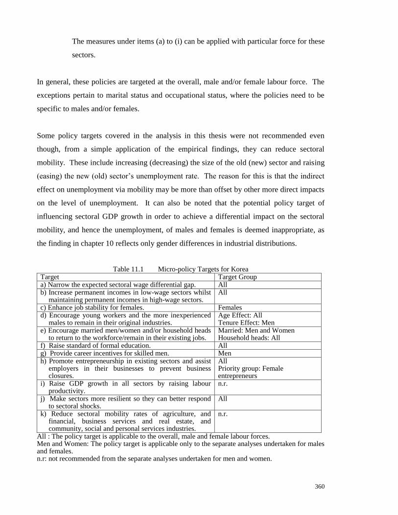
360
The measures under items (a) to (i) can be applied with particular force for these
sectors.
In general, these policies are targeted at the overall, male and/or female labour force. The
exceptions pertain to marital status and occupational status, where the policies need to be
specific to males and/or females.
Some policy targets covered in the analysis in this thesis were not recommended even
though, from a simple application of the empirical findings, they can reduce sectoral
mobility. These include increasing (decreasing) the size of the old (new) sector and raising
(easing) the new (old) sector‟s unemployment rate. The reason for this is that the indirect
effect on unemployment via mobility may be more than offset by other more direct impacts
on the level of unemployment. It can also be noted that the potential policy target of
influencing sectoral GDP growth in order to achieve a differential impact on the sectoral
mobility, and hence the unemployment, of males and females is deemed inappropriate, as
the finding in chapter 10 reflects only gender differences in industrial distributions.
Table 11.1 Micro-policy Targets for Korea Target Target Group a) Narrow the expected sectoral wage differential gap. All b) Increase permanent incomes in low-wage sectors whilst
maintaining permanent incomes in high-wage sectors. All
c) Enhance job stability for females. Females d) Encourage young workers and the more inexperienced
males to remain in their original industries. Age Effect: All Tenure Effect: Men
e) Encourage married men/women and/or household heads to return to the workforce/remain in their existing jobs.
Married: Men and Women Household heads: All
f) Raise standard of formal education. All g) Provide career incentives for skilled men. Men h) Promote entrepreneurship in existing sectors and assist
employers in their businesses to prevent business closures.
All Priority group: Female entrepreneurs
i) Raise GDP growth in all sectors by raising labour productivity.
n.r.
j) Make sectors more resilient so they can better respond to sectoral shocks.
All
k) Reduce sectoral mobility rates of agriculture, and financial, business services and real estate, and community, social and personal services industries.
n.r.
All : The policy target is applicable to the overall, male and female labour forces. Men and Women: The policy target is applicable only to the separate analyses undertaken for males and females. n.r: not recommended from the separate analyses undertaken for men and women.
361
It is envisaged that these policies would aid in reducing the social costs of higher
unemployment as well as the job instability mentioned above. Whilst unemployment can be
alleviated via a mix of macro- and micro-policies, job stability could be achieved by
moderating mobility through the micro measures stated.
Integration of Policies with KLI’s Recommendation
Several of the policy measures stated above are inter-linked with the KLI‟s long-term plan.
The KLI‟s recommendation of investment in vocational training is related to the suggested
measures of training to increase lifetime incomes, moderating mobility amongst women
and younger workers, and raising the level of education of the workforce in general [items
(b), (c), (d) and (f)]. The measures to encourage younger workers to remain in the original
sectors are also applicable to the KLI‟s suggestion to tackle youth unemployment [item
(d)]. The measures to lower female mobility, encourage married women to work or remain
in their jobs can be related to the KLI‟s plan to improve job prospects for elderly women
[items (c) and (e)]. Lastly, whilst the suggestion to create IT jobs for younger persons is
related to the measures for moderating mobility rates of young workers [item (d)], the
forest cultivation public works programme for older workers will assist in reducing
mobility rates for workers in agriculture [item (k)].
Of interest to note also is that several suggestions from the KLI to tackle job instability
have the implied result of reducing sectoral mobility, which is the very goal the policies
from this study are geared at. The provision of wage incentives could prevent workers
from switching sectors (since higher wages in the existing jobs reduce mobility) and
assisting disadvantaged workers (young, elderly women, older workers and workers in non-
regular jobs) could discourage them from switching jobs/sectors, thereby lowering mobility
rates and subsequently alleviating unemployment problems.
Therefore, it can be seen that the policy targets derived from this study are in line with the
KLI‟s long-term plan. An integrated effort is thus required to combat the social costs of
unemployment in Korea.

362
11.5 DIRECTION FOR FUTURE RESEARCH
Part I of the thesis provided some preliminary insight into the positive mobility-
unemployment relationship for Korea from the perspectives of the SSH and ADH. Part II
augmented the research via an in-depth analysis of the factors that motivate sectoral
mobility. The thesis has reported an ample range of findings which can provide a basis for
further research.
The empirical support for the SSH/ADH and stage-of-the-business-cycle effect for Korea
was rather tentative owing to the limited amount of data available. The results suggest that
the „new‟ mobility-unemployment phenomenon appears to have just started in the post-
Crisis period for Korea, whereas it had been a feature of the labour markets of Western
countries since the 1980s. Future studies should examine the validity of these hypotheses
for Korea when more data are available. The benefit of this is that if the validity of the
hypotheses for Korea can be established with a higher degree of certainty, then the micro-
policies derived from the findings on the factors that motivate mobility can be implemented
with greater confidence. The year 1998 appears to have been a structural break and the
economy appears to be at a significant turning point. The traditional monetary and fiscal
policies are deemed insufficient. So a policy combination of micro- and macro-policies for
sectoral mobility could be an innovative tool in the new millennium.
There appears to be a dearth of studies for this type of research for Asia, possibly the
consequence of a lack of longitudinal data available for research. Some studies, like Prasad
(1997) who examined the mobility-unemployment relationship for the manufacturing sector
in Japan using informal graphical techniques, are informative but appear to fall short of the
rigor required in research that is to lead to the development of policy. In the case of Korea,
the KLIPS is the first panel study for labour issues, so it is a useful starting point. The
study of sectoral mobility could be extended to the NIEs (Japan, Hong Kong, Singapore
and Taiwan) and the rest of Asia so that the standard of research can be more aligned with
that of the Western countries. This is attainable if datasets like the KLIPS become
available for research in other developing countries. If similar research on sectoral mobility
can be undertaken for other countries in Asia, the lessons learnt from the West, and the
benefits of a new microeconomic policy via sectoral mobility for Asia, could be immense.

363
Endnotes:
1. Since the nature of unemployment was not expounded in the empirical application, it is not mentioned here.
2. The other methods are not mentioned owing to their unsuitability for the current work, namely the ζ-U co-
movement approach and U-V argument for the ADH, and computing contemporaneous correlations between
labour reallocation measures and the average value of foregone production for the RTH. In the case of the
former, there is an absence of a direct assessment of predicted mobility on unemployment. In the latter, the
seemingly non-existent correlations make the method not worthwhile.
3. The chapter suggested that separate analyses might be undertaken for males and females. Since it was not
undertaken owing to the findings obtained for the overall study, it was not mentioned.
4. No distinction in the mobility behaviour of the overall, male or female labour groups is made here.
5. Where no references are provided alongside the findings of the current study, it means that there was no
study that adopted the relevant variable.
6. In Cheon and Jung (2004), wages are more performance-based rather than seniority-based. However, this
change is only partial and the Korean employment system retains traits which separates it from the West, such
as honorary retirement, and seniority-based wages, especially for blue-collar workers in large companies and
union members.
7. According to the empirical result, the target should be to reduce permanent incomes in high-wage sectors.
However, owing to wage inflation and individuals‟ constant demand for higher wages, a lowering of the
lifetime incomes is not desired in the longer term. Hence the next best alternative is to maintain permanent
income levels in the already high-wage sectors.
8. According to the empirical results, to reduce mobility, the target should be to lower the GDP growth of the
old sector, and raise the GDP growth of new sector. Since a lower GDP growth is undesirable, and given the
phenomenon of the jobless growth hypothesis in Korea, the better alternative is to cater for multi-sector
production by raising labour productivity.
364
REFERENCES
Abraham, K. (1983) „Structural/Frictional vs. Deficient Demand Unemployment: Some
New Evidence‟, American Economic Review, vol. 73(4), pp. 708-724.
Abraham, K. (1987) „Help-wanted Advertising, Job Vacancies and Unemployment‟,
Brookings Papers on Economic Activity, vol. 1987(1), pp. 207-243.
Abraham, K. and Katz, L. (1986) „Cyclical Unemployment: Sectoral Shifts or Aggregate
Disturbances?‟, Journal of Political Economy, vol. 94(3), pp. 507-522.
Addison, J. (1997) „The U.S. Labour Market: Structure and Performance‟, article in
„Structural Changes and Labor Market Flexibility: Experience in OECD Countries‟,
edited by Horst Siebert, Mohr, Tübingen, pp. 187-222.
Addison, J. and Portugal, P. (1989) „Job Displacement, Wage Changes and Duration of
Unemployment‟, Journal of Labor Economics, vol. 7(3), pp. 281-301.
Akyüz, Y. (2000) „Causes and Sources of the Asian Financial Crisis‟, UNCTAC Geneva,
Paper presented at the host Country Event, Symposium on Economic and Financial
recovery in Asia, UNCTAD X Bangkok, 17 Feb 2000.
Alogoskoufis, G. and Smith, R. (1991) „On Error Correction Models: Specification,
Interpretations, Estimation‟, Journal of Economic Surveys, vol. 5(1), pp. 97-128.
Altonji, J. and Ham, J. (1990) „Variation in Employment Growth in Canada: The Role of
External, National, Regional and Industrial Factors‟, Journal of Labor Economics,
vol. 8(1), S198-S236.
Andersen, T. (1997) „Structural Changes and Barriers in the Danish Labour Market‟, article
in Structural Changes and Labor Market Flexibility: Experience in OECD Countries,
edited by Horst Siebert, Mohr, Tübingen, pp. 123-149.
Anderson, J. (1979) „Determinants of Bargaining Outcomes in the Federal Government of
Canada‟, Industrial and Labor Relations Review, vol. 32(2), pp. 224-241.
Antolin, P. and Bover, O. (1997) „Regional Migration in Spain: The Effect of Personal
Characteristics and of Unemployment, Wage and House Price Differentials using
pooled Cross-sections‟, Oxford Bulletin of Economics and Statistics, vol. 59(2), pp.
215-235.
Arnott, R., Hosios, A. and Stiglitz, J. (1988) „Implicit Contracts, Labor Mobility and
Unemployment‟, American Economic Review, vol. 78(5), pp. 1046-1066.
Ashenfelter, O. and Pencavel, J. (1969) „American Trade Union Growth: 1900-1960‟,
Quarterly Journal of Economics, vol. 83(3), pp. 434-448.

365
Austria, M. and Martin, W. (1995) „Macroeconomic Instability and Growth in the
Philippines, 1950-1987: A Dynamic Approach‟, Singapore Economic Review, vol.
40(1), pp. 65-81.
Bain, G. and Elsheikh (1976) Union Growth and the Business Cycle, Basil Blackwell,
Oxford.
Barro, R. J. (1977) „Unanticipated Money Growth and Unemployment in the United
States‟, American Economic Review, vol. 67(2), pp. 101-115.
Barro, R. J. (1980) „Inter-temporal Substitution and the Business Cycle‟ NBER working
paper no. 490, National Bureau of Economic Research.
Barrows, G. (2004) „Isolating Trade‟s Effects on Growth‟, paper submitted for the 2004
Moffatt Prize in Economics, Economics at About.Com (http://economics.about.com).
Bartel, A. (1989) „Where do the New U.S. Immigrants Live?‟, Journal of Labor
Economics, vol. 7 (4), pp. 371-391.
Bartel, A. and Koch, M. (1991) Internal Migration of U.S. Migrants’, Immigration, Trade
and the Labor Market, University of Chicago Press, United States.
Bartram, D. (2000) „Japan and Labor Migration: Theoretical and Methodological
Implications of Negative Cases', International Migration Review, vol. 34 (1), pp. 5-
32.
Becker, G. (1964) Human Capital: A Theoretical and Empirical Analysis with Special
Reference to Education, New York and London: Columbia University Press, 1964.
Becker, G. (1993) „Nobel Lecture: The Economic Way of Looking at Behaviour‟, Journal
of Political Economy, vol. 101(3), pp. 385-409.
Beggs, J. and Chapman, B. (1988) „Labor Turnover Bias in Estimating Wages‟, Review of
Economics and Statistics, vol. 70(1), pp. 117-123.
Bernanke, N. (1983) „Non-monetary Effects of the Financial Collapse in the Propagation of
the Great Depression‟, American Economic Review, vol. 73(3), pp. 257-293.
Bernstein, I. (1954) „The Growth of American Unions‟, American Economic Review, vol.
44(3), pp. 301-318.
Blackburn, M, and Neumark, D. (1992) „Unobserved Ability, Efficiency Wages and Inter-
industry Wage Differentials‟, Quarterly Journal of Economics, vol. 107(4), pp. 1421-
1436.
Blan, D. (1991) „Search for Non-wage Job Characteristics: A Test of the Reservation Wage
Hypothesis‟, Journal of Labor Economics, 1991, vol. 9(2), pp. 186-205.

366
Blanchard, O. and Diamond, P. (1989) „The Beveridge Curve‟, Brookings Papers on
Economic Activity, vol. 1989(1), pp. 1-60.
Blanchard, O. and Quah, D. (1989) „The Dynamic Effects of Aggregate Demand and
Supply Disturbances‟, American Economic Review, vol. 79(4), pp. 655-673.
Blank, R. (1985) „An Analysis of Workers‟ Choice Between Employment in the Public and
Private Sectors‟, Industrial and Labor Relations Review, vol. 38(2), pp. 211-224.
Bleany, M. (1992) „Sectoral Rigidities, Wage Inertia and Expectations‟, Australian
Economic Papers, vol. 31(59), pp. 303-310..
Blinder, A. (1973) „Wage-Discrimination: Reduced Form and Structural Variables‟,
Journal of Human Resources, vol. 8(4), pp. 436-455.
Blinder, A. (1976) „On Dogmatism in Human Capital‟, Journal of Human Resources, vol.
11(1), pp. 8-22.
Bradshaw, Y. and Naonan, R. (1997) „Urbanization, Economic Growth and Women‟s
Labour Force Participation. A Theoretical and Empirical Reassessment‟, Cities in the
Development World: Issues, changes and policy, Oxford University Press 1997.
Brainard, S. and Cutler, D. (1993) „Sectoral Shifts and Cyclical Unemployment
Reconsidered‟, Quarterly Journal of Economics, vol. 108(1), pp. 219-243.
Brown, P. and Browne, M. (1962) „Earnings in Industries of the United Kingdom, 1948-
1959‟, The Economic Journal, vol. 72(287), pp. 517-549.
Brown, R., Moon, M. and Zoloth, B. (1980) „Occupational Attainment and Segregation by
Sex‟, Industrial and Labor Relations Review, vol. 33(4), pp. 506-517.
Booth, A. (1983) „A Reconsideration of Trade Union Growth in the United Kingdom‟,
British Journal of Industrial Relations, vol. 21(3), pp. 377-391.
Borjas, G. (1980) „The Relationship Balance Between Wage and Weekly Hours of Work:
The Role of Division Bias‟, Journal of Human Resources, vol. 15(3), pp. 409-423.
Borjas, G. (1982) „The Politics of Employment Discrimination in the Federal Bureaucracy‟,
Journal of Law and Economics, vol. 25(2), pp. 271-299.
Borjas, G. (1990) „The Intergenerational Mobility of Immigrants‟, mimeo, University of
Chicago, 1990.
Borjas, G. (1994) „The Economics of Immigration‟, Journal of Economic Literature, vol.
32(4), pp. 1667-1717.
Borland, J., Hirschberg, J. and Lye, J. (1998) „Earnings of Public Sector and Private Sector
Employees in Australia: Is There a Difference?‟, Economic Record, vol. 74(224), pp.
36-53.

367
Borland, J. and Ouliaris, S. (1994) „The Determinants of Australian Trade Union
Membership‟, Journal of Applied Econometrics, vol. 9(4), pp. 453-468.
Bound, J. and Krueger (1991) „The Extent of Measurement Error in Longitudinal Earnings
Data: Do Two Wrongs Make a Right?‟, Journal of Labor Economics, vol. 9(1), pp. 1-
24.
Bull, C. and Jovanovic, B. (1988) „Mismatch versus Derived Demand Shift as Causes of
Labour Mobility‟, Review of Economic Studies, vol. 55(1), pp. 169-175.
Burdett, K. (1978) „A Theory of Employee Job Search and Quit Rates‟, American
Economic Review, vol. 68(1), pp. 212-220.
Bureau of Labour Market Research, „Structural Change and the Labour Market‟, Research
Report no. 11, Australian Government Publishing Services, Canberra, 1987.
Burgess, J. and Green, R. H. (2000) „Is Growth the Answer? in S. Bell (ed.) The
Unemployment Crisis in Australia: Which Way Out?, Cambridge University Press,
Cambridge, pp. 125-148.
Byrne, J. (1975) „Occupational Mobility‟, Monthly Labor Review, vol. 98, pp. 53-59.
Callagham, G. (1997) Flexibility, Mobility and the Labour Market, Ashgate Publishing Ltd.
Carrington, W. and Zaman, A. (1994) „Interindustry Variation in the Costs of Job
Displacement‟, Journal of Labor Economics, vol. 2(2), pp. 243-275.
Carruth, A. and Disney, R. (1988) „Where Have Two Million Trade Union Members
Gone?‟, Economica, vol. 55(217), pp. 1-19.
Chaison, G. and Dhavale, D. (1992) „The Choice Between Union Membership and Free-
Rider Status‟, Journal of Labor Research, vol. 13(4), pp. 355-369.
Chan, W. (1996) „Intersectoral Mobility and Short-Run Labor Market Adjustments‟,
Journal of Labor Economics, vol. 14(3), pp. 454-471.
Chang, Jiyeun and Yang, Sukyung (2007) „Non-standard Employment from the Social
Exclusion Perspective‟, working paper, Korea Labor Institute, Jun 2007.
Chang, Y., Jaeryang, N. and Changyong, R. (2004) „Trends in unemployment rates in
Korea: A search-matching model interpretation‟, Journal of the Japanese and
International Economies, 18(2), pp. 241-263.
Cheon, Byung-You and Jung, Ee-hwan (2004) „Economic Crisis and the Changes in the
Employment Systems in East Asia: The Cases of Japan and Korea‟, working paper,
Korea Labor Institute, Jun 2004, pp. 1-27.
Cheon, Byung You and Kim, Sungteak (2004) „Labor Market Policies to Meet Challenges
in the Korean Labor Market after the 1997 Financial Crisis‟, paper prepared for

368
International Conference on International Perspectives on Labor Market Institutions,
Seoul, Korea, Jul 19-20 2004, pp. 1-49.
Cho, Sang-Wook (2005) „Household Wealth Accumulation and Portfolio Choices in
Korea‟, Job Market paper, University of Minnesota, Oct 2005, pp. 1-43.
Choo, H. (1989) „The Asian Newly Industrialising Economies (NIEs): Are Economic
Miracles really Miraculous?‟, Singapore Economic Review, vol 34(1), pp. 2-12.
Chew, S. (1990) „Brain Drain in Singapore: Issues and Prospects‟, Singapore Economic
Review, Oct 1990, vol. 35(2), pp. 55-77.
Chillemi, O. and Gui, B. (1997) „Team Human Capital and Worker Mobility‟, Journal of
Labor Economics, vol. 15(4), pp. 567-85.
Chirco, A. and Colombo, C. (1996) „The AD-AS Model and Its Solutions: Some New
Results in a Disequilibrium Perspective‟, Australian Economic Papers, vol. 35(67),
pp. 263-281.
Chiswick, B. (1991) „Speaking, Reading and Earnings among Low-skilled Migrants‟,
Journal of Labor Economics, vol. 9(2), pp. 149-170.
Chiswick, B., Le, A. and Miller, P. (2008) „How Immigrants Fare Across the Earnings
Distribution in Australia and the United States‟, Industrial and Labor Relations
Review, vol. 61(3), pp. 353-373.
Chiswick, B., Lee, Y. L. and Miller, P. (2005) „Longitudinal Analysis of Immigrant
Occupational Mobility: A Test of the Immigrant Assimilation Hypothesis‟,
International Migration Review, vol. 39(2), pp. 332-353.
Chiswick, B. and Miller, P. (1985) „Immigrant Generation and Income in Australia‟,
Economic Record, vol. 61 (173), pp. 540-573.
Chiswick, B. and Miller, P. (1994) „The Determinants of Post-Immigration Investments in
Education‟, Economics of Education Review, vol. 13(2), pp. 163-177.
Choy, K. (1999) „Sources of Macroeconomic Fluctuations in Singapore: Evidence from A
Structural VAR model‟, Singapore Economic Review, Apr 1999, vol. 44(1), pp. 74-
98.
Christie, V. (1992) „Union Wage Effects and the Probability of Union Membership‟,
Economic Record, vol. 68(200), pp. 43-56.
Chuma, J. (1997) „Structural Change and the State of the Labour Market in Japan‟, article
in „Structural Changes and Labor Market Flexibility: Experience in OECD
Countries‟, edited by Horst Siebert, Mohr, Tübingen, pp. 257-289.

369
Clark, T. (1998) „Employment Fluctuations in U.S. Regions and Industries: The Roles of
National, Region-specific, and Industry-specific Shocks‟, Journal of Labor
Economics, vol. 16(1), pp. 202-229.
Clive, B. and Jovanovic, B. (1988) „Mismatch versus Derived-Demand Shift as Causes of
Labour Mobility‟, Review of Economic Studies, vol. 55(1), pp. 169-175.
Coe, D. (1990) „Insider-Outsider Influences on Industry Wages (Evidence from fourteen
Industrialised Countries), Empirical Economics, vol. 15(2), pp. 163-183.
Conlon, R. (1992) „Determinants of Manufacturing Industry Exports: A Comparative Study
of Australia, republic of Korea, Singapore and Taiwan‟, Australian Economic Papers,
vol. 31(59), pp. 427-442.
Cotton, J. (1988) „On the Decomposition of Wage Differentials‟, Review of Economics and
Statistics, vol. 70(2), pp. 236-243.
Coulson, N. and Robins, R. (1987) „A Test of the First-Difference Transformation in Time
Series Models‟, Review of Economics and Statistics, vol. 69(4), pp. 723-726.
Cox, D. (1971) „The Effect of Geographic and Industry Mobility on Income: A Further
Comment‟, Journal of Human Resources, vol. 6(4), pp. 525-527.
Creedy, J. (1974) „Labour Mobility, Earnings and Unemployment. Selected Papers – Inter-
regional Mobility: A Cross-section Analysis‟, Scottish Journal of Political Economy,
vol. 21(1), pp. 41-53.
Creedy, J. and Thomas, R. (1982) The Economics of Labor, Butterworths, London.
Cutler, D., Glaeser, E. and Vigdor, J. (1999) „The Rise and Decline of the American
Ghetto‟, Journal of Political Economy, vol. 107(3), pp. 455-506.
Dalziel, P. (1993) „Classical and Keynesian Unemployment in a Simple Disequilibrium
AS-AD Framework‟, Australian Economic Papers, vol. 32(60), pp. 40-52.
Darby, M., Haltiwanger, J. and Plant, M. (1985) „Unemployment Rate Dynamics and
Persistent Unemployment under Rational Expectations‟, American Economic Review,
vol. 75(4), pp. 614-637.
Davidson, C., Martin, L. and Matusz, S. (1988) „The Structure of Simple General
Equilibrium Models with Frictional Unemployment‟, Journal of Political Economy,
vol. 96(6), pp. 1267-1293.
Davis, S. (1987) „Fluctuations in the Pace of Labor Reallocation‟, Carnegie-Rochester
Conference Series on Public Policy 27, pp. 335-402.
Diamond, P. (1981) „Mobility Costs, Frictional Unemployment and Efficiency‟, Journal of
Political Economy, vol. 89(4), pp. 798-812.

370
Dickens, W. and Katz, L. (1987) „Inter-Industry Wage Differences and Industry
Characteristics‟, article in Unemployment and the Structure of Labor Markets, edited
by Lang, K. and Leonard, J., Basil Blackwell, Oxford, pp. 48-89.
Disney, R. (1990) „Explanations of the Decline in Trade Union Density in Britain: an
Appraisal‟, British Journal of Industrial Relations, vol. 28(2), pp. 165-177.
Dixon, R. (1982) „The Rate of Exploitation and the Wage Share as Weighted Sums of
Sectoral Measures‟, Australian Economic Papers, vol. 21(39), pp. 421-424.
Doeringer, P. and Piore, M. (1971) Internal Labour Markets and Manpower Analysis,
Lexington Books, D.C. Heath, Lexington , Mass.
Doiron, D. and Riddell, W. (1994) „The Impact of Unionisation on Male-Female Earnings
Differences in Canada‟, Journal of Human Resources, vol. 29(2), pp. 504-534.
Doucouliagos, C. (1997) „The Aggregate Demand for Labour in Australia: A Meta-
Analysis‟, Australian Economic Papers, vol. 36(69), pp. 224-242.
Duetsch, L. (1974-1975) „Structural Performance and the Net Rate of Entry into
Manufacturing Industries, Southern Economic Journal vol. 41, 1974-1975.
Dustmann, C. (1993) „Earnings Adjustment of Temporary Immigrants‟, Journal of Political
Economy, vol. 6 (2), pp. 153-168.
Edin, P. and Holmlund, B. (1997) „Sectoral Structural Change and the State of the Labour
Market in Sweden‟, article in „Structural Changes and Labor Market Flexibility:
Experience in OECD Countries‟, edited by Horst Siebert, Mohr, Tübingen, pp. 89-
122.
Ehrenberg, R. (1973) „The Demand for State and Local Government Employees‟, American
Economic Review, vol. 63(3), pp. 366-379.
Eickstein, O. and Wilson, T. (1967) „The Determination of Money Wages in American
Industry: Reply‟, Quarterly Journal of Economics, vol. 81(4), pp. 690-694.
Eisemann, D. (1956) „Inter-industry Wage Changes, 1939-1947‟, Review of Economics and
Statistics, vol. 38(4), pp. 445-458.
Eriksson, G. (1991) „Human Capital Investments and Labor Mobility‟, Journal of Labor
Economics, vol. 9(3), pp. 236-254.
Evans, S. and Lewis, P. (1986) „Demand, Supply and Adjustment of Farm Labour in
Australia‟, Australian Economic Papers, vol. 25(47), pp. 236-246.
Even, W. and MacPherson, D. (1993) „The Decline of Private Sector Unionism and the
Gender Wage Gap‟, Journal of Human Resources, vol. 28, pp. 279-296.

371
Faini, R., Galli, G., Gennari, P. and Rossi, F. (1997) „An Empirical Puzzle: Falling
Migration and Growing Unemployment Differentials among Italian Regimes‟,
European Economic Review, 41(3), pp. 571-579.
Fallick, B. (1992) „Job Security and Job Search in More than One Labor Market‟,
Economic Inquiry, vol. 30(4), pp. 742-745.
Fallick, B. (1993) „The Industrial Mobility of Displaced Workers‟, Journal of Labor
Economics, vol. 11(2), pp. 302-323.
Fair R.C. (1970) „The Estimation of Simultaneous Equation Models with Lagged
Endogenous Variables and First Order Serially Correlated Errors‟, Econometrica, vol.
38(3), pp. 507-516.
Farber, H. (1990) „The Decline of Unionisation in the United States: What Can Be Learned
from Recent Experience‟, Journal of Labor Economics, vol. 8, S75-105.
Farber, H. and Saks, D. (1980) „Why Workers Want Unions: The Role of Relative Wages
and Job Characteristics‟, Journal of Political Economy, vol. 88(2), pp. 349-369.
Farkas, G. and England, P. (1988) Industries, Firms and Jobs: Sociological and Economic
Approaches, Plenum Press, New York.
Finnie, R. and Garneau, G. (1997) „Earnings Patterns By Age and Sex‟, Canadian
Economic Observer, Vol. 10(10), Feature Article.
Flyer, F. (1997) „The Influence of Higher Moments of Earnings Distributions in Career
Decisions‟, Journal of Labor Economics, 1997, vol. 15(4), pp. 689-713.
Freeman, R. (1989) „On the Divergence of Unionism Among Developed Countries‟ NBER
working paper no. 2817, National Bureau of Economic Research.
Freeman, R. and Medoff, J. (1984) What Do Unions Do? Basic Books, New York.
Gallaway, L. (1963) „Labor Mobility, Resource Allocation and Structural Unemployment‟
American Economic Review, vol. 55(3), pp. 531-532.
Gallaway, L. (1965) „Structural Unemployment: Reply‟, American Economic Review, vol.
55(3), pp. 527-531.
Garbarino, J. (1950) „A Theory of Interindustry Wage Structure Variation‟, Quarterly
Journal of Economics, vol. 64(2), pp. 282-305.
Garonna, P. and Sica, F. (1997) „Intersectoral Labour Reallocations and Flexibility
Mechanisms in Post-war Italy‟, article in „Structural Changes and Labor Market
Flexibility: Experience in OECD Countries‟, edited by Horst Siebert, Mohr,
Tübingen, pp. 51-88.
372
Garonna, P. and Sica, F. (2000) „Inter-sectoral Labour Reallocations and Unemployment in
Italy‟, Labour Economics, vol. 7(6), pp. 711-728.
Gerwin, D. (1969) „Compensation Decisions in Public Organisations‟, Industrial Relations,
vol. 8(2), pp. 174-184.
Ghatak, A. (1996) „Labour Migration in the Indian States and the Todarian Hypothesis‟,
Asian Economic Review, vol. 38(2), pp. 212-228.
Gibbons, R. and Katz, L. (1992) „Does Unmeasured Ability Explain Inter-industry Wage
Differentials?‟, Review of Economic Studies, vol. 59(3), pp. 515.535.
Gordon, R. (1982) „Price Inertia and Policy Ineffectiveness in the U.S.‟ Journal of Political
Economy, vol. 90 (6), pp. 1087-1117.
Goss, E. and Schoening, N. (1974) „Search Time, Unemployment and the Migration
Decision‟, Journal of Human Resources, vol. 19(4), pp. 570-579.
Green, D. (1999) „Immigrant Occupational Attainment: Assimilation and Mobility Over
Time‟, Journal of Labor Economics, vol. 17(1), pp. 49-79.
Greene W. (2003) „Econometric Analysis‟, fourth edition, Prentice Hall.
Greenhalgh, C. and Stewart, M. (1985) „The Occupational Status and Mobility of British
Men and Women‟, Oxford Economic Activity, vol. 37(1), pp. 40-71.
Greenwood, M. (1975) „Research on Internal Migration in the United States: A Survey‟,
Journal of Economic Literature, vol. 5(3), pp. 397-433.
Gregory, G., Harvie, C. and Lee, H.H. (2002) „Korean SMEs in the Wake of the Financial
Crisis: Strategies, Constraints, and Performance in a Global Economy‟, paper no. 50
on CD, The 47th International Council for Small Business World Conference, San
Juan, Puerto Rico, 16-19 Jun, 2002.
Groshen, E. (1991) „Sources of Intra-Industry Wage Dispersion: How much Do Employers
Matter?‟, Quarterly Journal of Economics, Aug 1991, vol. 106, Issue 3, p. 869-884.
Groshen, E. (1991) „Five Reasons Why Wages Vary Among Employers‟, Industrial
Relations, vol. 30(3), pp. 350-381.
Gujarati, D. (1995) Basic Econometrics, 3rd
Edition, McGraw Hill, New York.
Gulde, A. and Wolf, H. (1998) „The Changing Skill Structure of Employment in German
Manufacturing: A Peek Inside the Industry Black Box‟, article in Globalisation,
Technological Change and Labour Markets, edited by Stanley W. Black, Kenver
Academic Publishers.
Gunderson, M. (1979) „Earnings Differentials between the Public and Private Sectors‟,
Canadian Journal of Economics, vol. 12(2), pp. 228-242.
373
Gunderson, M. (1980) „Public Sector Compensation in Canada and the U.S.‟, Industrial
Relations, vol. 19(3), pp. 257-271.
Gyourko, J, and Tracy, J. (1988) „An Analysis of Public and Private Sector Wages
Allowing for Endogenous Choices of Both Government and Union Status‟, Journal of
Labor Economics, vol. 6(2), pp. 229-253.
Hahn, J. (1996) „Pecuniary Mobility Costs in a Two-sector Model‟, Seoul Journal of
Economics, vol. 9(2), pp. 163-174.
Hall, R. (1975) „The Rigidity of Wages and the Persistence of Unemployment‟, Brookings
Papers on Economic Activity, vol. 1975(2), pp. 301-335.
Hall, J. (1991) „Notes and Comments: Sectoral Transformation and Economic Decline:
Views from Berkeley and Cambridge‟, Cambridge Journal of Economics, vol.15(2),
pp. 229-237.
Hall, P. and Treadgold, M. (1982) „Aggregate Demand Curves: A Guide to Use and
Abuse‟, Australian Economic Papers, vol. 21(38), pp. 37-48.
Hall, R. and Yellen, J. (1989) „The Beveridge Curve: Comments and Discussion‟,
Brookings Papers on Economic Activity, vol. 1989(1), pp. 61-76.
Hamilton, J. (1988) „A Neo-classical Model of Unemployment and the Business Cycle‟,
Journal of Political Economy, vol. 96(3), pp. 593-617.
Hansen, B. (1970) „Excess Demand, Unemployment, Vacancies and Wages‟, Quarterly
Journal of Economics, vol. 84(1), pp. 1-23.
Harris, J. and Todaro, M. (1970) „Migration, Unemployment and Development: A Two-
Sector Analysis‟, American Economic Review, 60(1), pp. 128-149.
Hartog, J. and Oosterbeek, H. (1993) „Public and Private Sector Wages in the Netherlands‟,
European Economic Review, 37(1), pp. 97-114.
Hartog, J. and Theeuwes, J. (1997) „The Dutch Response to Dynamic Challenges in the
Labour Market‟, article in Structural Changes and Labor Market Flexibility:
Experience in OECD Countries, edited by Horst Siebert, Mohr, Tübingen, pp. 151-
184.
Harvey, A. (1990) The Econometric Analysis of Time Series, 2nd
edition, BPCC Wheaton
Ltd., Exeter.
Hayafuji, T., Ikeda, M. and Yamada, H. (2003) „South Korea‟s Next Step‟, Apr 2003, SPP
542 International Financial Policy (extracted from www-personal.umich.edu).
Hayworth, C. and Rasmusseu, D. (1971) „Human Capital and Inter-industry Wages in
Manufacturing‟, Review of Economics and Statistics, vol. 53(4), pp. 376-380.

374
Heckman, J. and Sedlacek, G. (1985) „Heterogeneity, Aggregation and Market Wage
Functions: An Empirical Model of Self-Selection in the Labor Market‟, Journal of
Political Economy, vol. 93(6), pp 1077-1125.
Helwege, J. (1992) „Sectoral Shifts and Interindustry Wage Differentials‟, Journal of Labor
Economics, vol. 10(1), pp. 55-84.
Hendry, D. H. and Krolzig, H.-M (2001), Automatic Econometric Model Selection using
PcGets, Timberlake Consultants Ltd., London.
Henstridge, J. (2001) „The Household, Income and Labour Dynamics in Australia (HILDA)
Survey: Weighting and Imputation‟, HILDA Project Discussion Paper Series, Jul
2001, no. 3/01.
Heywood, J. (1993) „Efficient Labour Bargains, Unemployment and Non-union Wages: A
Two-sector Model‟, Australian Economic Papers, vol. 32(61), pp. 214-230.
Hicks, G. (1989) „The Four Little Dragons: An Enthusiast‟s Reading Guide‟, Asian-Pacific
Economic Literature, vol. 3(2), pp. 35-49.
Higgins, M. and Williamson, J. (1997) „Age Structure Dynamics in Asia and Dependence
on Foreign Capital‟, Population and Development Review, vol. 23(2), pp. 261-293.
Hill, J. (1984) „Australian Union Density Rates 1976-1982‟, Journal of Industrial
Relations, vol. 26(4), pp. 435-450.
Holtz-Eakin, D. and Rosen, H. (1991) „Municipal Labor Demand in the Presence of
Uncertainty: An Econometric Approach‟, Journal of Labor Economics, vol. 9(3), pp.
276-293.
Horn, S. (2004) „Guide to Standard Errors for Cross Section Estimates‟, HILDA Project
Technical Paper Series, Jan 2004, no. 1/04.
Horvath, M. (1998) „Cyclicality and Sectoral Linkages: Aggregate Fluctuations from
Independent Sectoral Shocks‟, Review of Economic Dynamics, vol. 1(4), pp. 781-808.
Horvath, M. (2000) „Sectoral Shocks and Aggregate Fluctuations‟, Journal of Monetary
Economics, vol. 45(1), pp. 69-106.
Hosios, A. (1994) „Unemployment and Vacancies with Sectoral Shifts‟, American
Economic Review, vol. 84(1), pp. 124-144.
Idson, T. and Valleta, R. (1996) „Seniority, Sectoral Decline and Employee Retention: An
Analysis of Layoff Unemployment Spells‟, Journal of Labor Economics, vol. 14(4),
pp. 654-676.
Jaffe, A., Day, L. and Adams, W. (1964) Disabled Workers in the Labor Market, The
Bedminster Press, New Jersey.
375
Jayadevan, C. (1997) „Inter-industrial Differences in Employment Growth Rates of
Organised Manufacturing Industry in India‟, Asian Economic Review, vol. 39(1), pp.
15-27.
Jeong, Insoo (2002) „Unemployment Schemes during the Financial Crisis in Korea:
Achievements and Evaluations‟, working paper, Korea Labor Institute, Dec 2002, pp.
71-94.
Jeong, Insoo (2003) „Interregional Labor Mobility‟, working paper, Korea Labor Institute,
May 2003.
Johnston, J. (1984) Econometric Methods, McGraw-Hill Book Company, Singapore.
Jolliffe, D. (2002/2003) „Estimating Sampling Variance from the Current Population
Survey: A Synthetic Design Approach to Correcting Standard Errors‟, Journal of
Economic and Social Measurement, vol. 28(4), pp. 239-261.
Jorgensen, D. (1967) „Surplus Agricultural Labour and the Development of a Dual
Economy‟, Oxford Economic Papers, vol. 19(3), pp. 288-312.
Jovanovic, B. (1979) „Job Matching and the Theory of Turnover‟, Journal of Political
Economy, vol. 87(5), pp. 972-990.
Jovanovic, B. and Moffitt, R. (1990) „An Estimate of a Sectoral Model of Labor Mobility‟,
Journal of Political Economy, vol. 98(4), pp. 827-852.
June, Ee-hwan and Cheon, Byung-You (2004) „Economic Crisis and the Changes in
Employment Systems in East Asia: The Cases of Japan and Korea‟, working paper,
Korea Labor Institute, Jun 2004, pp. 1-27.
Jung, Kwangho, Moon, M. Jae and Hahm, Sung Deul (2007) „Do Age, Gender and Sector
Affect Job Satisfaction? Results from the Korean Labor and Income Panel Data‟,
Review of Public Personnel Administration, vol 27(2), pp. 125-146.
Kang, C. (2004) „University Prestige and Choice of Major Field: Evidence from South
Korea‟, manuscript prepared for Presentation at the 2004 Far Eastern Meeting of the
Econometric Society, pp. 1-38.
Kang, C., Park, C. and Lee, M. (2007) „Effects of Ability Mixing in High School on
Adulthood Earnings: Quasiexperimental Evidence from South Korea‟, Journal of
Population Economics, vol. 20(2), pp. 269-297.
Kasper, H. (1967) „The Asking Price of Labour and the Duration of Unemployment‟,
Review of Economics and Statistics, vol. 49(2), pp. 165-172.
Katz, L. and Summers, L. (1989) „Industry Rents: Evidence and Implications‟, Brookings
Papers on Economic Activity. Microeconomics, vol. 1989(1), pp. 209-290.

376
Keane, M. (1993) „Individual Heterogeneity and Interindustry Wage Differentials‟, Journal
of Human Resources, vol. 28(1), pp. 134-161.
Kelly, J. and Richardson, R. (1989) „Annual Review Article 1988‟, British Journal of
Industrial Relations, vol. 27(1), pp. 133-154.
Kenyon, P. and Lewis, P. (1997) „The Decline in Trade Union Membership: What Role did
the Accord Play?‟, Murdoch University, Feb 1997, working paper no. 156.
Kim, D. (1998) „Reinterpreting Industry Premiums: Match-specific Productivity‟, Journal
of Labor Economics, vol. 16(3), pp. 479-504.
Kim, Hong-Kyun (2003) „Effect of IT Job Training on Employment and Wage Premium:
Evidence from Korea Panel Data‟, The Developing Economies, XLI-4, pp. 461-483.
Kim, K. (2004a) „The Effects of Family Background on Educational Continuation: From
Middle School to Graduate School‟ paper presented for COE Workshop, Feb 2,
Sendai, Japan and at KLIPS Conference, Feb 11, Seoul, Korea, pp. 334-354.
Kim, K. (2004b) „Expanded Opportunity, Persistent Inequality: Social Class and Gender
Differentials in School Transitions in Korea‟, paper prepared for the presentation at
the Association Coreene d‟Etudes Politiques Francaise‟s International Conference,
Nov 10, Seoul, Korea, 2004, pp. 1-27.
Kingston, G. and Layton, A. (1986) „The Tax Smoothing Hypothesis: Some Australian
Empirical Results‟, Australian Economic Papers, vol. 25(47), pp. 247-251.
Kish, L. (1965) Survey Sampling, John Wiley and Sons, New York.
Kish, L. and Frankel, M. (1974) „Inference from Complex Samples‟, originally published in
Journal of the Royal Statistical Society 36, Ser. B, 1-22, and republished as chapter 8
in Leslie Kish, Selected Papers (editors: Klaton, G.. and Heeringa, S.), John Wiley
and Sons, Hoboken 2002.
Korea Labor Institute, Questionnaire for Households, Korean Labor and Income Panel
Study, 1998.
Korea Labor Institute, Questionnaire for Paid Workers, Korean Labor and Income Panel
Study, 1998.
Korea Labor Institute, Questionnaire for the Unemployed, Korean Labor and Income Panel
Study, 1998.
Korea Labor Institute, Questionnaire for Households, Korean Labor and Income Panel
Study, 1999.
Korea Labor Institute, Questionnaire for Individuals, Korean Labor and Income Panel
Study, 1999.

377
Korea Labor Institute, Questionnaire for New Respondents, Korean Labor and Income
Panel Study, 1999.
Korea Labor Institute, Questionnaire for Households, Korean Labor and Income Panel
Study, 2000.
Korea Labor Institute, Questionnaire for Individuals, Korean Labor and Income Panel
Study, 2000.
Korea Labor Institute, Questionnaire for Households, Korean Labor and Income Panel
Study, 2001.
Korea Labor Institute, Questionnaire for Individuals, Korean Labor and Income Panel
Study, 2001.
Krongkaew, M. (1994) „Income Distribution in East Asian Developing Countries: An
Update‟, Asian-Pacific Economic Literature, vol. 8(2), pp. 58-73.
Krueger, A. and Summers, L. (1987) „Reflections on the Inter-industry Wage Structure‟,
NBER working paper no. 1960, National Bureau of Economic Research.
Krueger, A. and Summers, L. (1988) „Efficiency Wages and the Inter-industry Wage
Structure‟, Econometrica, vol. 56(2), pp. 259-293.
Krugman, P. (1981) „Intraindustry Specialization and the Gains from Trade‟, Journal of
Political Economy, vol. 89(5), pp. 959-974.
Lamberton, D. (1994) „The Information Revolution in the Asian-Pacific Region‟, Asian-
Pacific Economic Literature, Nov 1994, vol. 8(2), pp. 31-57.
Lang, K. (1989) „Trade Liberalisation of the New Zealand Labour Market‟, Research
Monograph 53, Oct 1989, New Zealand Institute of Economic Research.
Lanyard, R., Nickell, S. and Jackman, R. (1991) „Unemployment: Macroeconomic
Performance of the Labour Market‟, Oxford University Press, United Kingdom.
Le, A, (1999) „Empirical Studies of Self-Employment‟, Journal of Economic Surveys, vol.
13(4), pp. 381-416.
Le, A. and Miller, P. (1998) „Pitfalls in Including Current Earnings in Labour Market
Choice Estimating Equations‟, Australian Economic Papers, vol. 37(4), pp. 414-419.
Le, A. and Miller, P. (2004) „School Leaving Decisions in Australia: A Cohort Analysis‟,
Education Economics, vol. 12(1), pp. 39-65.
Lee, P. and Townsend, P. (1994) „A Study of Inequality, Low Incomes and Unemployment
in London, 1985-1992‟, International Labor Review, vol. 133(5-6), pp. 579-595.
378
Levine, D. (1991) „Just-Cause Employment Policies in the Presence of Worker Adverse
Selection‟, Journal of Labor Economics, vol. 9(3), pp. 294-305.
Lilien, D. (1980) „The Cyclical Pattern of Temporary Layoffs in United States
Manufacturing‟, Review of Economics and Statistics, vol. 51(1), pp. 24-31.
Lilien, D. (1982) „Sectoral Shifts and Cyclical Unemployment‟, Journal of Political
Economy, vol. 90(4), pp. 777-793.
Lilien, D. (1983) „A Sectoral Model of the Business Cycle‟, paper presented at the Hoover
Institute Conference, Jan 1983.
Lilien, D. (1987), comment in Murphy, K. and Topel, R. (1987a) „The Evolution of
Unemployment in the United States: 1968-1985‟, University of Chicago and National
Bureau of Economic Research.
Long, J. (1975) „Public-Private Sectoral Differences in Employment Discrimination‟,
Southern Economic Journal, vol. 42(1), pp. 89-96.
Long, J. (1976) „Employment Discrimination in the Federal Sector‟, Journal of Human
Resources, vol. 11(1), pp. 86-97.
Long, J., Plosser, J and Charles, I. (1983) „Real Business Cycles‟, Journal of Political
Economy, vol. 91(1), pp. 39-69.
Long, J., Plosser, J and Charles, I. (1987) „Sectoral versus Aggregate Shocks in the
Business Cycle‟, American Economic Review, vol. 77(2), pp. 333-336.
Loungani, P. (1986) „Oil Price Shocks and Dispersion Hypothesis‟, Review of Economics
and Statistics, vol. 18(3), pp. 517-530.
Loungani, P. and Rogerson, R. (1989) „Cyclical Fluctuations and Sectoral Reallocation.
Evidence from the PSID‟, Journal of Monetary Economics, vol. 23(2), pp. 259-273.
Loungani, P., Rush, M. and Tave, W. (1990) „Stock Market Dispersion and
Unemployment‟, Journal of Monetary Economics, 25(3), pp. 367-388.
Lu, J. (1996) „A Reconsideration of the Inter-industry Employment Dispersion‟, Economic
Letters, vol. 50(2), pp. 203-208.
Lucas, R. and Prescott, J. (1974) „Equilibrium Search and Unemployment‟, Journal of
Economic Theory, vol. 7(2), pp. 188-209.
Madden, J. (1987) „Gender Differences in the Cost of Displacement: An Empirical Test of
Discrimination in the Labor Market‟, American Economic Review, vol. 77(2), pp.
246-251.
Madden, J. (1988) „The Distribution of Economic Losses among Displaced Workers:
Measurement Methods Matter‟, Journal of Human Resources, vol. 23(1), pp. 93-107.

379
Mailath, G. and Postlewaith, A. (1990) „Workers Versus Firms: Bargaining over a Firm‟s
Value‟, Review of Economic Studies, vol. 57(3), pp. 369-380.
Manning, C. (1999) „Labour Markets in the ASEAN-4 and the NIEs‟, Asian-Pacific
Economic Literature, vol. 13(1), pp. 50-68.
Masters, S. (1974) „The Effect of Educational Differences and Labor Market
Discrimination on the Relative Earnings of Black Males‟, Journal of Human
Resources, vol. 9(3), pp. 342-360.
Mattila, J. (1974) „Job Quitting and Fricitonal Unemployment‟, American Economic
Review, Mar 1974, vol, 64(1), pp. 235-279.
McCombie, J. (1991) „The Productivity Growth Slowdown of the Advanced Countries and
the Inter-sectoral Relocations of Labor‟, Australian Economic Papers, vol. 39(56), pp.
70-85.
McCormick, B. (1997) „Regional Unemployment and Labour Mobility in the U.K.‟,
European Economic Review, vol. 41(3-5), pp. 581-589.
McGuire, T. and Rapping, L. (1967) „The Determination of Money Wages in American
Industry: Comment‟, Quarterly Journal of Economics, vol. 81(4), pp. 684-689.
McLaughlin, K. and Bils, M. (2001) „Interindustry Mobility and the Cyclical Upgrading of
Labour‟, Journal of Labor Economics, 2001, vol. 19(1), pp. 94-135.
Medoff, J. (1983) „U.S. Labor Markets: Imbalance Wage Growth, and Productivity in the
1970s‟, Brookings Papers on Economic Activity, vol. 1983(1), pp. 87-128.
Miller, P. and Neo, L. (2003) „Labour Market Flexibility and Immigrant Adjustment‟,
Economic Record, Vol. 79(246), pp. 336-356.
Miller, P. and Rummery, S. (1991) „Male-Female Wage Differentials in Australia: A
Reassessment‟, Australian Economic Papers, vol. 30(56), pp. 50-69.
Miller, R. (1984) „Job Matching and Occupational Choice‟, Journal of Political Economy,
vol. 92(6), pp. 1086-1120.
Mills, T., Pelloni, G. and Zervoyianni, A. (1995) „Unemployment Fluctuations in the
United States: Further Tests of the Sectoral Shift Hypothesis‟, Review of Economics
and Statistics, vol. 77(2), pp. 294-304.
Mincer, J. (1978) „Family Migration Decisions‟, Journal of Political Economy, vol. 86(5),
pp. 749-773.
Mincer, J. and Jovanovic, B. (1981) „Labor Mobility and Wages‟, Studies in Labor
Markets, University of Chicago Press, Chicago Studies 1981, National Bureau of
Economic Research.

380
Mishkin, F. (1982) „Does Anticipated Monetary Policy Matter? An Econometric
Investigation‟, Journal of Political Economy, vol. 90(1), pp. 22-51.
Mishkin, F. (1983) „A Rational Expectations Approach to Macroeconometrics. Testing
Policy in Effectiveness and Efficient Market Models‟, NBER and University of
Chicago Press, Chicago.
Mitchell, W. F. (2000) „The Causes of Unemployment‟, article in The Unemployment
Crisis in Australia: Which Way Out?, edited by S. Bell, Cambridge University Press,
Cambridge, pp. 21-48.
Montgomery, J. (1991) „Equilibrium Wage Dispersion and Interindustry Wage
Differentials‟, Quarterly Journal of Economics, 106(1), pp. 163-179.
Mortensen, D. (1986) „Job Search and Labor Market Analysis‟, in Handbook of Labor
Economics, vol. 2, edited by O. Ashenfelter and R. Layard, Elsevier Science
Publishers BV., pp. 849-919.
Murphy, K. and Topel, R. (1987a) „The Evolution of Unemployment in the United States,
1968-1985‟, University of Chicago and National Bureau of Economic Research,
reprint no. 1209.
Murphy, K. and Topel, R. (1987b) „Unemployment, Risk and Earnings: Testing for
Equalizing Wage Differences in the Labor Market‟, in Unemployment and the
Structure of Labor Market, edited by Lang, K. and Leonard, J., Basil Blackwell, New
York, pp. 103-140.
Murphy, K. and Topel, R. (1990) „Efficiency Wages Reconsidered: Theory and Evidence‟,
in Y. Weiss and G. Fishelson: Advance in the Theory and Measurement of
Unemployment, New York: St. Martin‟s Press, pp. 204-240.
Muscatelli, V. A. and Hurn, S. (1992) „Cointegration and Dynamic Time Series Models‟,
Journal of Economic Surveys, vol. 6(1), pp. 1-43.
Nagelkerke, N. J. D. (1991) „A Note on a General Definition of the Coefficient of
Determination‟ Biometrika, vol. 78(3), pp. 691-692.
Nam, Sang-Ho (2007) „Asset Distribution and Asset-poverty in Korea‟, Korea Institute for
Health and Social Affairs, pp. 1-25.
Neal, D. (1995) „Industry-Specific Human Capital: Evidence from Displaced Workers‟,
Journal of Labor Economics, vol. 13(4), pp. 653-677.
Neal, D. (1999) „The Complexity of Job Mobility Among Young Men‟, Journal of Labor
Economics, vol. 17(2), pp. 237-261.
Neelin, J. (1987) „Sectoral Shifts and Canadian Unemployment‟, Review of Economics and
Statistics, vol. 69(4), pp. 718-723.

381
Neumann, G. and Rissman, E. (1984) „Where have all the Union Members Gone?‟ Journal
of Labor Economics, vol. 2(2), pp. 175-192.
Nielsen, H. (1998) „Discrimination and Detailed Decomposition in a Logit Model‟,
Economic Letters, vol. 61, 1998, pp. 115-120.
Nickell, S. (1997) „Structural Change and the British Labour Market‟, article in Structural
Changes and Labor Market Flexibility: Experience in OECD Countries, edited by
Horst Siebert, Mohr, Tübingen, pp. 3-28.
Norbin, S. and Schlagenhauf (1988) „An Inquiry into the Sources of Macroeconomic
Fluctuations‟, Journal of Monetary Economics, vol. 22(1), pp. 43-70.
Oatey, M. (1970) „The Economics of Training: with respect to the Firm‟, British Journal of
Industrial Relations, vol. 8(1), pp. 1-21.
Oaxaca, R. (1973) „Male-Female Wage Differentials in Urban Labour Markets‟,
International Economic Review, vol. 14(3), pp. 693-709.
Ogawa, N. and Ermisch, J. (1996) „Family Structure, Home Time Demands and the
Employment Patterns of Japanese Married Women‟, Journal of Labor Economics,
vol. 14(4), pp. 677-702.
Ohkawa, K. (1957) The Growth Rate of the Japanese Economy since 1878, Kinokuniya
Bookstore Co. Ltd., Tokyo.
Oi, W. (1987) „Comments on the Relation Between Unemployment and Sectoral Shifts‟,
Carnegie-Rochester Conference Series on Public Policy 27, North Holland, pp. 403-
420.
Oliveira-Martins, J. (1994) „Market Structure, Trade and Industry Wages‟, OECD
Economic Studies, Spring 1994, no. 22, pp. 131-154.
Osberg, L. (1991) „Unemployment and Interindustry Labour Mobility in Canada in the
1980s‟, Applied Economics, vol. 23(11), pp. 1707-1717.
Osberg, L., Gordon, D. and Lin, Z. (1994) „Inter-regional Migration and Inter-industry
Labour Mobility in Canada: A Simultaneous Approach‟, Canadian Journal of
Economics, vol. 27(1), pp. 58-80.
Osberg, L., Manzany, R., Apostle, R. and Clairmont, D. (1986) „Job Mobility, Wage
Determination and Market Segmentation in the Presence of Sample Selection Bias‟,
Canadian Journal of Economics, vol. 19(2), pp. 319-346.
Osberg, L. and Phipps, S. (1993) „Labour Supply with Quantity Constraints: Estimates
from a Large Sample of Canadian Workers‟, Oxford Economic Papers, vol. 45(2), pp.
261-291.

382
Osburn, J. (2000) „Interindustry Wage Differentials: Patterns and Possible Sources‟,
Monthly Labor Review, Feb 2000, Bureau of Labor Statistics, Washington.
Ottersen, E. (1993) „Sectoral Shocks and Structural Unemployment. An Empirical
Analysis‟, European Economic Review, vol. 37(1), pp. 115-133.
Oxley, L. and McAleer, M. (1993) „Econometric Issues in Macroeconomic Models with
Generated Regressors‟, Journal of Economic Surveys, vol. 7(1), pp. 1-40.
Pagan A. (1984) „Econometric Issues in the Analysis of Regressions with Generated
Regressors‟, International Economic Review, vol. 25(1), pp. 221-247.
Palley, T. (1992) „Sectoral Shifts and Cyclical Unemployment: A Reconsideration‟,
Economic Inquiry, vol. 30(1), p. 117-133.
Parent, D. (1999) „Wages and Mobility: The Impact of Employer-provided Training‟,
Journal of Labor Economics, vol. 17(2), pp. 298-317.
Park, Y. , Chung, C. and Wang Y. (2001), „Fear of Floating: Korea‟s Exchange Rate
Policy after the Crisis‟, Journal of the Japanese and International Economies, vol.
15(2), pp. 225-251.
Parker, J. (1992) „Structural Unemployment in the United States: The Effects of Inter-
industry and Inter-regional dispersion‟, Economic Inquiry, vol. 30(1), pp. 101-116,
Parnes, H. (1965) „Employment and Economic Growth‟, American Economic Review, vol.
55(1/2), pp. 270-272.
Peetz, D. (1990) „Declining Union Density‟, Journal of Industrial Relations, vol. 32(2), pp.
197-223.
Pekkala, S. and Tero, H. (2002) „Unemployment and Migration: Does Moving Help?‟
Scandinavian Journal of Economics, vol. 104(4), pp. 621-639.
Perry, L. (1991) „A Comment on Aggregate Demand‟, Australian Economic Papers, vol.
30(57), pp. 278-286.
Pissarides, C. (1985) „Short-Run Equilibrium Dynamics of Unemployment, Vacancies and
Real Wages‟, American Economic Review, vol. 75(4), pp. 676-690.
Pissarides, C. and Wadsworth, J. (1989) „Unemployment and the Inter-regional Mobility of
Labour‟, The Economic Journal, vol. 99(397), pp. 739-755.
Podgursky, M. and Swaim, P. (1987) „Job Displacement and Earnings Loss: Evidence from
the Displaced Worker Survey‟, Industrial and Labor Relations Review, vol. 41(1), pp.
17-29.
Prasad, E. (1997) „Sectoral Shifts and Structural Change in the Japanese Economy:
Evidence and Interpretation‟, Japan and the World Economy, vol. 9(3), pp. 293-313.
383
Price, R. and Bain, G. (1983) „Union Growth in Britain: Retrospect and Prospect‟, British
Journal of Industrial Relations, vol. 21(1), pp. 46-68.
Puhani, P. A. (2000) "The Heckman Correction for Sample Selection and its Critique",
Journal of Economic Surveys, vol. 14(1), pp. 53-68.
Qian, W. (1996) Rural Urban Migration and its Impact on Economic Development in
China, Ashgate Publishing Ltd.
Radelet, S. and Sachs, S. (1998) The Onset of the East Asian Financial Crisis, NBER
working paper no. 6680, National Bureau of Economic Research.
Ramirez, M. and Khan, S. (1999) „Cointegration Analysis of Purchasing Power Parity:
1973-96‟, International Advances In Economic Research, vol. 5(3), pp. 369-385.
Ranis, G. and Fei, J. (1964) Development of the Labor-Surplus Economy: Theory and
Policy, R.D. Irwin, Homewood, Ill.
Rao, B. (1991) „What is the Matter with Aggregate Demand and Aggregate Supply‟,
Australian Economic Papers, vol. 30(57), pp. 264-277.
Reimers, C. (1983) „Labor Market Discrimination against Hispanic and Black‟, Review of
Economics and Statistics, vol. 65(4), pp. 570-579.
Robinson, C. (1995) „Union Incidence in the Public and Private Sectors‟, Canadian Journal
of Economics, vol. 28(4b), pp. 1056-1076.
Rogers, A. and Henning, S. (1999) „The Internal Migration Patterns of Foreign-born and
Native-born Populations in the United States: 1975-80 and 1985-90‟, International
Migration Review, vol. 33(2), pp. 403-429.
Rogerson, R. (1987) „An Equilibrium Model of Sectoral Reallocation‟, Journal of Political
Economy, vol. 95(4), pp. 824-834.
Rosovsky, H. (1961) Capital Formation in Japan, 1868-1940, The Free Press of Glencoe,
New York.
Ross, A. and Goldner, W. (1950) „Forces Affecting the Industry Wage Structure‟,
Quarterly Journal of Economics, vol. 64(2), pp. 254-281.
Rotemberg, J. (1987) The New Keynesian Microfoundations, Sloan School of Management
and National Bureau of Economic Research, Massachusetts.
Riddell, C. (1986) Adapting to Change: Labour Market Adjustment in Canada, University
of Toronto Press, Canada.
Riddell, W. (1997) „Structural Change and Adjustment in the Canadian Labour Market‟,
article in Structural Changes and Labor Market Flexibility: Experience in OECD
Countries, edited by Horst Siebert, Mohr, Tübingen, pp. 223-256.
384
Ruser, J. (1991) „Workers‟ Compensation and Occupational Injuries and Illnesses‟, Journal
of Labor Economics, vol. 9(4), pp. 325-350.
Saint-Paul, G. (1997) „Labour Rigidities and the Performance of the French Economy‟,
article in Structural Changes and Labor Market Flexibility: Experience in OECD
Countries, edited by Horst Siebert, Mohr, Tübingen, pp. 29-50.
Saito, M. (1971) „An Inter-industry Study of Price Formation‟, Review of Economics and
Statistics, vol. 53(1), pp. 11-25.
Samson, L. (1985) „A Study of the Impact of Sectoral Shifts on Aggregate Unemployment
in Canada‟, Canadian Journal of Economics, vol. 18(3), pp. 518-530.
Sawangfa, Onnicha (2007) „Does Job Switching Lead to Greater Satisfaction?: Evidence
from South Korea‟, Jul 2007 (www.ppdoconference.org).
Schioppa, F. (1991) „A Cross-Country Comparison of Sectoral Mismatch in the 1980s‟,
article in Mismatch and Labour Mobility, edited by F. Schioppa, Cambridge
University Press, United Kingdom, pp. 1-43.
Schultz, T. (1971) „Rural-urban Migration in Columbia‟, Review of Economics and
Statistics, vol. 53(2), pp. 157-163.
Scott, A. and Holt, D. (1982) „The Effect of Two-Stage Sampling on Ordinary Least
Squares Methods‟, Journal of the American Statistical Association, vol. 77(380), pp.
848-854.
Seok, Hyunho (1999) „International Labor Migration and Financial Crisis in Korea‟,
Development and Society, vol. 28(1), pp. 139-165.
Seong, J. (2007) „Trends of Union Participation among Non-union Employees –
Introducing the data from the Supplement Questionnaire to the 8th
KLIPS‟, working
paper, Korea Labour Institute, Feb 2007.
Sharpe, I. (1971) „The Growth of Australian Trade Unions: 1907-1969‟, Journal of
Industrial Relations, vol. 13(2), pp. 138-154.
Shin, K. (1997a) „Inter- and Intrasectoral Shocks: Effects on the Unemployment Rate‟,
Journal of Labor Economics vol. 15(2), pp. 376-401.
Shin, K. (1997b) „Sectoral Shocks and Movement Costs: Effects on Employment and
Welfare‟, Journal of Economic Dynamics and Control, 21(2-3), pp. 448-471.
Shister, J. (1953) „The Logic of Union Growth‟, Journal of Political Economy, vol. 61(5),
pp. 413-433.
Simpson, W. (1988) „Job Mobility and the Wage-gap between Single Males and Females‟,
mimeo, University of Manitoba.

385
Slichter, S. (1950) „Notes on the Structure of Wages‟, Review of Economics and Statistics,
vol. 32(1), pp. 80-91.
Smith, J. and Welch, F. (1989) „Black Economic Progress after Myrdal‟, Journal of
Economic Literature, vol. 27(2), pp. 519-564.
Son, Jaehee (2007a) „Reappraising the Job-Training Effect on Labor Market Outputs of
Korean Women‟, Department of Economics, University of California, pp. 1-31.
Son, Jaehee (2007b) „The Effect of Job Training on the Labor Market Outcomes of Women
in Korea: Empirical Analysis with Panel Data, 1998-2005‟, Department of
Economics, University of California, pp. 1-36.
Stock, J. and Watson, M. (1993) „A Simple Estimation of Cointegrating Vectors in Higher
Order Intergrated Systems‟, Econometrica, vol. 61(4), pp. 783-820.
Stoilov, V. (1965) „Structural Unemployment: Comment‟, American Economic Review,
vol. 55(3), pp. 527-531.
Stolzenberg, Ross M. and Relles, Daniel A. (1997) "Tools for Intuition about Sample
Selection Bias and its Correction", American Sociological Review, vol. 62(3), pp.
494-507.
Subrahmanian, K., Veena, D. and Parikh, B. (1982) Construction Labour Market: A Study
in Ahmedabad, Concept Publishing Company, New Delhi.
Tanzer, C. (1999) „The Asian Crisis and the Search for a New Global Financial
Architecture‟, paper submitted for the Global Policy Forum.
Tcha, M. (1993) „Altruistic Migration – Evidence for Korea and the U.S.A.‟, University of
Western Australia, Department of Economics, Discussion Paper 93.07.
The World Bank (1999), „Republic of Korea: Establishing a New Foundation for
Sustainable Growth‟, Report No. 19595 KO, Nov 2 1999.
Thomas, J. (1996a) „Sectoral Shifts and the Mobility of Displaced Workers: When are
Microdata Useful?‟ Economic Letters, vol. 52(3), pp. 337-343.
Thomas, J. (1996b) „An Empirical Model of Sectoral Movements by Unemployed
Workers‟, Journal of Labor Economics, vol. 14(1), pp. 126-153.
Thompson, M., Fong, G., Hammond, D., Boudreau, C., Driezen, P., Hyland, A., Borland,
R., Cummings, K., Hastings, G., Siahpush M., Mackintosh A. and Laux F. (2006),
„Methods of the International Tobacco Control (ITC) Four Country Survey‟, Research
Paper, Apr 2006, produced online by BMJ Publishing Group Ltd of the BMA,
assisted by Stanford University's HighWire Press (see www.tobaccocontrol.bmj.com).

386
Tobin, J. (1972) „Inflation and Unemployment‟, American Economic Review, vol. 62(1),
pp. 1-18.
Todaro, M. (1969) „A Model of Labour-Migration and Urban Unemployment in Less
Developed Countries‟, American Economic Review, vol. 59(1), pp. 138-148.
Todaro, M. (1981) Economic Development in the Third World, Longman, Inc., New York.
Tomes, N. and Robinson, C. (1982a) „Self-selection and Interprovincial Migration in
Canada‟, Canadian Journal of Economics, vol. 15(3), pp. 474-502.
Tomes, N. and Robinson, C. (1982b) „Family Labour Supply and Fertility: a Two-regime
Model‟, Canadian Journal of Economics, vol. 15(4), pp. 706-783.
Tomes, N. and Robinson, C. (1984) „Union Wage Differentials in the Public and Private
Sectors: A Simultaneous Equations Specification‟, Journal of Labor Economics, vol.
2(1), pp. 106-127.
Topel, R. (1986) „Local Labour Markets‟, Journal of Political Economy, vol. 94(3), S111-
S143.
Troy, L. (1965) Trade Union Membership, 1897-1962, National Bureau of Economic
Research, New York.
United Nations Economic and Social Council (1999) „Implementation of the International
Covenant on Economic, Social and Cultural Rights: Addendum: Republic of Korea‟,
State Party Report No. E/1990/5/Add. 19, United Nations, 5 Jan 1994.
United Nations Economic and Social Commission for Asia and the Pacific (1999)
„Emerging Issues and Developments at the Regional Level: Socio-Economic
Measures to Alleviate Poverty in Rural and Urban Areas - Empowerment of Women
in Asia and the Pacific‟, Fifty-Fifth Session, 22-28 Apr 1999, Bangkok, ESCAP Paper
Number 1133, Feb 1999.
Utgoff, K. (1983) „Compensation Levels and Quit Rates in the Public Sector‟, Journal of
Human Resources, vol. 18(3), pp. 394-406.
Vanderkamp, J. (1971) „Migration Flows, Their Determinants and the Effects of Return
Migration‟, Journal of Political Economy, vol. 79(5), pp. 1012-1031.
Vanderkamp, J. (1977) „Industrial Mobility: Some Further Results‟, Canadian Journal of
Economics, vol. 10(3), pp. 462-472.
van der Gaag, J. and Vijverberg, W. (1988) „A Switching Regression Model for Wage
Determinants in the Public and Private Sectors of a Developing Country‟, Review of
Economics and Statistics, vol. 70(2), pp. 244-252.
Wachter, M. (1970) „Cyclical Variation in the Interindustry Wage Structure‟, American
Economic Review, vol. 60(1), pp. 75-84.

387
Wachter, M. (1987) „Help-wanted Advertising, Job Vacancies and Unemployment.
Comments and Discussion‟, Brookings Papers on Economic Activity, vol. 1987(1),
pp. 244-248.
Wannell, T. (1992) „Firm Size and Employment: Recent Canadian Trends‟, Canadian
Economic Observer, Vol. 5(3), Feature Article.
Watson, N. (2004) „Wave 2 Weighting‟, HILDA Project Technical Paper Series no. 4/04,
Jul 2004.
Watson, N. and Fry, T. (2002) „The Household, Income and Labour Dynamics in Australia
(HILDA) Survey: Wave 1 Weighting‟, HILDA Project Technical Paper Series no.
3/02, Sep 2002.
Weiss, L. (1984) „Sectoral Shifts and Assymmetric Adjustment Costs‟, mimeo, University
of Chicago, Illinois.
Willis, R. and Rosen, S. (1979) „Education and Self-Selection‟, Journal of Political
Economy, vol. 87(5), part 2, S7-S36.
Wolman, L. (1936) Ebb and Flow in Trade Unionism, National Bureau of Economic
Research, New York.
Yellen, J. (1984) „Efficiency Wage Models of Unemployment‟, American Economic
Review, vol. 74(2), Papers and Proceedings of the Ninety-sixth Annual Meeting of the
American Economic Association, May 1984, pp. 200-205.
Yoo, Kil-Sang (2005) „Financial Crisis and Unemployment Measures: The Experience of
Korea‟, working paper, Korea Labor Institute, Dec 2005.
Young, Jun-Chun (2005) „Population Aging, Fiscal Policies, and National Saving:
Prediction for Korean Economy‟, Department of Economics, University of Incheon,
pp. 1-29.
Young, Jun-Chun (2006) „Fiscal Impacts of Taxation on Pension in Aging Korea: A
Generational Accounting Approach‟, Department of Economics, University of
Incheon, May 2006, pp. 1-30.
Zagorsky, J. (1990) „Can Shifty Beveridge Curves be Trusted? New Findings in the
Unemployment-Vacancy Relationship‟, working paper, Boston University, Boston.
Zahn, F. (1971) „Sectoral Labour Migration and Sustained Industrialisation in the Japanese
Development Experience‟, Review of Economics and Statistics, vol. 53(3), pp. 283-
287.
Zhou, S. (2001) „The Power of Cointegration Tests versus Data Frequency and Time
Spans‟, Southern Economic Journal, vol. 67(3), pp. 906-921.
Related Documents