Inter-and Intrasite Correlations of Large-Scale Parameters From Macrocellular Measurements at 1800 MHz

Inter and Intra-Site Correlation of Large ScaleParameters from Macro Cellular Measurements at

1800MHzNiklas Jalden, Per Zetterberg, Bjorn Ottersten, Laura Garcia

Electrical EngineeringRoyal institute of Technology

100 44 StockholmEmail: (niklas.jalden,per.zetterberg,bjorn.ottersten)@ee.kth.se

Abstract—Herein, the inter- and intra-site correlation prop-erties of shadow fading and power-weighted angular spreadat both the mobile station and the base station are studiedutilizing narrow band multi-site MIMO measurements in the1800MHz band. The influence of the distance between two basestations on the correlation is studied in an urban environment.Measurements have been conducted for two different situations,widely separated as well as closely positioned base stations. Novelresults regarding the correlation of the power-weighted anglespread between base station sites with different separations arepresented. Furthermore, the measurements and analysis pre-sented herein confirm the autocorrelation and cross-correlationproperties of the shadow fading and the angle spread that havebeen observed in previous studies.

I. I NTRODUCTION

As the demand for higher data rates increases faster than theavailable spectrum, more efficient spectrum utilization meth-ods are required. Multiple antennas at both the receiver andthetransmitter, so-called Multiple Input Multiple Output (MIMO)systems, is one technique to achieve high spectral efficiency,[1], [2]. Since multi-antenna communication systems exploitthe spatial characteristics of the propagation environment,accurate channel models incorporating spatial parametersarerequired to conduct realistic performance evaluations. Sincefuture systems may reuse frequency channels within the samecell to increase system capacity, the characterization of thecommunication channel, including correlation propertiesofspatial parameters, becomes more critical. Several measure-ment campaigns have been conducted to develop accuratepropagation models for the design, analysis, and simulationof MIMO wireless systems [3], [4], [5], [6], [7], [8], [9].Most of these studies are based on measurements of a singleMIMO link (one mobile and one base station). Thus, thesemeasurements may not capture all necessary aspects requiredfor multiuser MIMO systems. From the measurement datacollected, several parameters describing the channel charac-teristics can be extracted. This work primarily focusses onextracting some key parameters that capture the most essentialcharacteristics of the environment, and that later can be used togenerate realistic synthetic channels with the purpose of linklevel simulations. To evaluate system performance with several

base stations (BS) and mobile stations (MS), it has generallybeen assumed that all parameters describing the channels areindependent from one link (single BS to single MS) to another,[10], [3]. However, correlation between the channel parametersof different links may certainly exist, for example, when oneBS communicates with two MSs that are located in the samevicinity, or vice versa. In this case, the radio signals propagateover very similar environments and hence, parameters such asshadow fading and/or spread in angle of arrival should be verysimilar. This has also been experimentally observed in somework where the autocorrelation of so called large scale (LS)isstudied. These LS parameters, such as shadow-fading, delay-spread, and angle spread, are shown to have autocorrelationthat decreases exponentially with a decorrelation distance ofsome tenths of meters [11], [12]. High correlation of these pa-rameters is expected if the MS moves within a small physicalarea. We believe that this may also be the case for multiple BSsthat are closely positioned. The assumption that the channelparameters for different links are completely independentmayresult in over/under estimation of the performance of the multi-user systems. Previous studies [13], [14], [15] have inves-tigated the shadow fading correlation between two separatebase station sites and found substantial correlation for closelylocated base stations. However, the inter-site correlation ofangle spreads has not been studied previously. Herein, multisite MIMO measurements have been conducted to addressthis issue. We investigate the existence of correlation betweenLS parameters on separate links using data collected in twoextensive narrow band measurement campaigns. The intra-siteand inter-site correlation of the shadow fading and the power-weighted angle spread at the base and mobile stations areinvestigated. The analysis provides unique correlation resultsfor base and mobile station angle spreads as well as log-normal(shadow) fading.

The paper is structured as follows; in Section II we give ashort introduction to the concept of large scale parametersandin Section III some relevant previous research is summarized.The two measurement campaigns are presented in Section IV.In Section V we state the assumptions on the channel modelwhile Section VI describes the estimation procedure. The

results are presented in Section VII and conclusions are drawnin Section VIII.

II. I NTRODUCTION TOLARGE SCALE PARAMETERS

The wireless channel is very complex and consists of timevarying multipath propagation and scattering. We considerchannel modelling that aims at characterizing the radio mediafor relevant scenarios. One approach is to conduct measure-ments and ”condense” the information of typical channels intoa parameterized model that captures the essential statistics ofthe channel, and later create synthetic data with the sameproperties for evaluating link and system level performanceetc. Large scale (LS) parameters are based on this concept.The term large scale parameters was used [3] for a collectionof quantities that can be used to describe the characteristicsof a MIMO channel. This collection of parameters are termedlarge scale because they assumed to be constant over ”large”areas of several wavelengths. Further, these parameters areassumed to depend on the local environment or the transmitterand receiver. Some of the possible LS parameters are listedbelow:

• Shadow fading• Angle of Arrival (AoA) Angle spread• Angle of Departure (AoD) Angle spread• AoA Elevation spread• AoD Elevation spread• Cross polarization ratio• Delay spread

This paper investigates only the shadow fading and the anglespread parameters. Shadow fading describes the variation inthe received power around some local mean, which depends onthe distance between the transmitter and receiver, see SectionVI-A. The power-weighted angle spread describes the the sizeof the sector or area from which the majority of the poweris received. The spread parameter will be different for thetransmitter (Tx) and receiver (Rx) sides of the link, since anglespread largely depends on the amount of local scattering, seefurther in Section V. A description of the other LS parametersmay be found in [3].

III. PREVIOUS WORK

An early paper by Graziano [13] investigates the correlationof shadow fading in an urban macro-cellular environmentbetween one MS and two BSs. The correlation is found tobe approximately 0.7-0.8 for small angles (α < 10o), whereα is defined as displayed in Fig. 1. Later, Weitzen arguedin [14] that the correlation for the shadow fading can bemuch less than 0.7 even for small angles, in disagreementwith the results presented by Graziano. This was illustratedby analyzing measurement data collected in the downtownBoston area using one custom made MS and several pairs ofBSs from an existing personal communication system. Theseresults are reasonable since in most current systems the BSsites are widely spread over an area. If the angleα separatingthe two BSs is small, the relative distance is large, and asmall relative distance corresponds to a large angle separation.

x

x

BS

BS

1

2

x

MS

α

d

d1

2

Fig. 1. Model of the cross-correlation as a function of the relative distanceand angle separation, also proposed in [16].

A more appropriate model for the correlation of the shadowfading parameter is to assume that it is a function of therelative distanced = log

10

d1

d2

between the two BSs and theangleα separating them as proposed in [16]. The distancesd1 and d2 are defined as in Fig. 1. Further studies on thecorrelation of shadow fading between several sites can befound in for example [15], [17], [18], and [19].

The angular spread parameter has been less studied. In[12] the autocorrelation of the angle spread at a single basestations is studied and found to be well modelled by anexponential decay, and the angle spread is further found tobe negatively correlated with shadow fading. However, tothe authors’ knowledge, the inter-site correlation of the anglespread at the MS or BS has not been studied previously.Herein, we extend the analysis performed on the 2004 datain [20]. We also investigate data collected in 2005 and findsubstantial correlation between the shadow fading but lessbetween the angular spreads. The low correlation of the spatialparameters may be important for future propagation modelling.The angle spread at the mobile station is studied and adistribution proposed. Further, we find that the correlationbetween the base station and mobile station angular spreads(of the same link) is significant for elevated base stations butvirtually zero for base stations just above rooftop.

IV. M EASUREMENT CAMPAIGNS

Two multiple-site MIMO measurement campaigns havebeen conducted by KTH in the Stockholm area using cus-tom built multiple antenna transmitters and receivers. Thesemeasurements were carried out in the summer of 2004 andthe autumn of 2005 and will in the following be refereed toas the 2004 and 2005 campaigns.

Because of measurement equipment shortcomings the mea-sured MIMO channels have unknown phase rotations. Thisis due to small unknown frequency offsets. In the 2004campaign, these phase rotations are introduced at the mobileside and therefore the relation between the measured channeland the true channel is given by

Hmeasured, 2004= ΛfHtrue, (1)

where Λf = diag(exp(j2πf1t), . . . , exp(j2πfnt)) andf1, ..., fn are unknown. Similarly the campaign of 2005 has

unknown phase rotations at the base station side1 resulting inthe following relation

Hmeasured, 2005= HtrueΛf . (2)

The frequencies changed up 5Hz per second. However, the es-timators that will be used are designed with these shortcomingsin mind.

A. Measurement Hardware

The hardware used for these measurements is the sameas the hardware described in [21] and [22]. The transmittercontinuously sends a unique tone on each antenna on the1800MHz band. The tones are separated 1kHz from the eachother. The receiver down-converts the signal to an intermediatefrequency of 10kHz, samples and stores the data on disk. Thisdata is later post-processed to extract the channel matrices.The system bandwidth is 9.6kHz, which allows narrow-bandchannel measurements with high sensitivity. The off-line andnarrow-band features simplify the system operation, sinceneither real-time constrains nor broadband equalization arerequired. For a thorough explanation of the radio frequencyhardware, [23] may be consulted.

B. Antennas

In both measurements campaigns, Huber-Suhner dual-polarized planar antennas with slanted linear polarization(±45o), SPA 1800/85/8/0/DS, were used at both the transmitterand the receiver. However, only one of the polarizations(+45o) was actually used in these measurements. The antennaswere mounted in different structures on the mobile and basestations as described below. For more information on theantenna radiation patterns etc, see [24].

1) Base station array: At the base station, the antennaelements were mounted on a metal plane to form a uniformlinear array with 0.56 wavelength (λ) spacing. In the 2004campaign, an array of four by four elements were used atthe BS. However, the ”columns” were combined using 4:1combiners to produce four elements with higher vertical gain.The base stations in the 2005 campaign were only equippedwith 2 elements.

2) Mobile station array: At the mobile side the fourantenna elements were mounted on separate sides of a woodenbox as illustrated in Fig. 2. This structure is similar to theuniform linear array using four elements. A wooden box isused so that the antenna radiation patterns are unaffected bythe structure.

C. 2004 Campaign

Uplink measurements where made using one 4-element box-antenna transmitter at the MS, see Fig. 2, and three 4-elementuniform linear arrays (ULA), with antenna elements spaced0.56λ apart, at the receiving BSs. The BSs, covered 3 sectorson two different sites. Site 1, Karhuset-A, hade one sector

1In the 2004 campaign the phase rotations are due to drifting and unlockedlocal oscillators in the four mobile transmitters while in the 2005 campaignthey are due to drifting sample-rates in the D/A and A/D converters.

Tx1

Tx2

Tx3

Tx4Ref

Fig. 2. Mobile station box antenna.M

S

4

1

2

3

Kårhuset

Vanadis

∆

∆

∆

Fig. 3. Measurement geography, and travelled route for 2004campaign.

while site 2, Vanadis, had two sectors, B and C, separated some20 meters and with boresights offset 120-degrees in angle. Wedefine a sector by the area seen from the BS boresight±60o.The environment where the measurements where conductedcan be characterized as typical European urban with mostly sixto eight storey stone buildings and occasional higher buildingsand church towers. Fig. 3 shows the location of the base stationsites and the route covered by the MS. The BS sectors aredisplayed by the dashed lines in the figure, and the arrowindicates the antenna pointing direction. Sector A is thus thearea seen between the dashed lines to the west of site Karhuset.Sector B and sector C are the areas southeast and northeastof site Vanadis respectively. A more complete description ofthe transmitter hardware and measurement conditions can befound in [25].

D. 2005 Campaign

In contrast to the previous campaign, the 2005 campaigncollected data in the downlink. Two BSs with two antennaseach were employed (the same type of antenna elements wereused as in the 2004 campaign), each transmitting, simultane-ously, one continuous tone separated 1kHz in the 1800MHzband. The two base stations were located on the same roof

∆

Fig. 4. Measurement map and travelled route for the 2005 campaign.

separated 50 meters, with identical boresight and thereforecovering almost the same sector. The characteristics of theenvironment in the measured area are the same as 2004. Theroutes were different but with some small overlap. The MSwas equipped with the 4-element box antenna as was usedin 2004, see Fig. 2, to get a closer comparison between thetwo campaigns. In Fig. 4 we see the location of the two BSs(in the upper left corner) and the measured trajectory whichcovered a distance of about 10km. The arrow in the figureindicates the pointing direction of the base station antennas.The campaign measurements were conducted during two days,and the difference in color of the MS routes depicts which areawas measured which day. The setups were identical on thesetwo days.

V. PRELIMINARIES

Assume we have a system withM Tx antennas at thebase station andK Rx antennas at the mobile station. Lethk,m(t) denote the narrow-band MIMO channel between thek:th receiver antenna and them:th transmitter antenna. Thenarrow-band MIMO channel matrix is then defined as

H(t) =

h1,1(t) h1,2(t) . . . h1,M (t)

h2,1(t). . .

......

. . ....

hK,1(t) . . . . . . hK,M (t)

. (3)

The channel is assumed to be composed ofN propagationrays. Then:th ray has angle of departureθk, angle of arrivalαk, gaingk, and Doppler frequencyfk. The steering vector2

of the transmitter given byaTx(θk) and that of the receiver is

2The steering vectora(θ) can be seen a complex-valued vector of lengthequal to the number of antenna elements in the array. The absolute value ofthek:th element is the square root of the antenna gain of that element and thephase the phase shift of the element relative some common reference point.Ie. ak(θ) =

√

ak(θ)ejφk .

aRx(αk). Thus, the channel is given by

H =N

∑

k=1

gkej2πfkta

Rx(αk)(aTx(θk))H . (4)

The ray parameters (θk, αk, gk, and fk) are assumed to beslowly varying and approximately constant for a distance of30λ. Below, we define the shadow fading and the base stationand the mobile station angle spread.

A. Shadow fading

The measured channel matrices are normalized so that theyare independent of the transmitted power. The received power,PRx, at the MS is defined as:

PRx = E|H|2PTx =

N∑

k=1

|gk|2| aBS(θk)|2| aMS , (αk)|2PTx

(5)wherePTx is the transmit power. The ratio of the received andthe transmitted powers is commonly assumed to be related asas: [26]:

PRx

PTx

=K

RnSSF , (6)

whereK is a constant, proportional to the squared norms ofthe steering vectors that depend on the gain at the receiverand transmitter antennas as well as the carrier frequency, basestation height etc. The distance separating the transmitter andreceiver is denotedR. The variableSSF describes the slowvariation in power, usually termed shadow fading, and is duetoobstacles and obstruction in the propagation path. Expressing(6) in decibels (dB) and rearranging the terms in the pathloss which describe the difference in transmitted and receivedpower, we have:

L = 10 log10

(PTx) − 10 log10

(PRx)

= n10 log10(R) − 10 log10(K) − 10 log10(SSF ), (7)

where the logarithm is taken with base ten. Thus, the pathloss is assumed to be linearly decreasing with log-distanceseparating the transmitter and receiver when measured in dB.

B. Base station power-weighted angle spread

The power-weighted angle spread at the base station,σ2

AS,BS,is defined as

σ2

AS,BS =N

∑

k=1

pk(θk − θ)2 , (8)

wherepk = |gk|2 is the power of thek:th ray and the mean

angleθ is given by.

θ =

N∑

k=1

pkθk . (9)

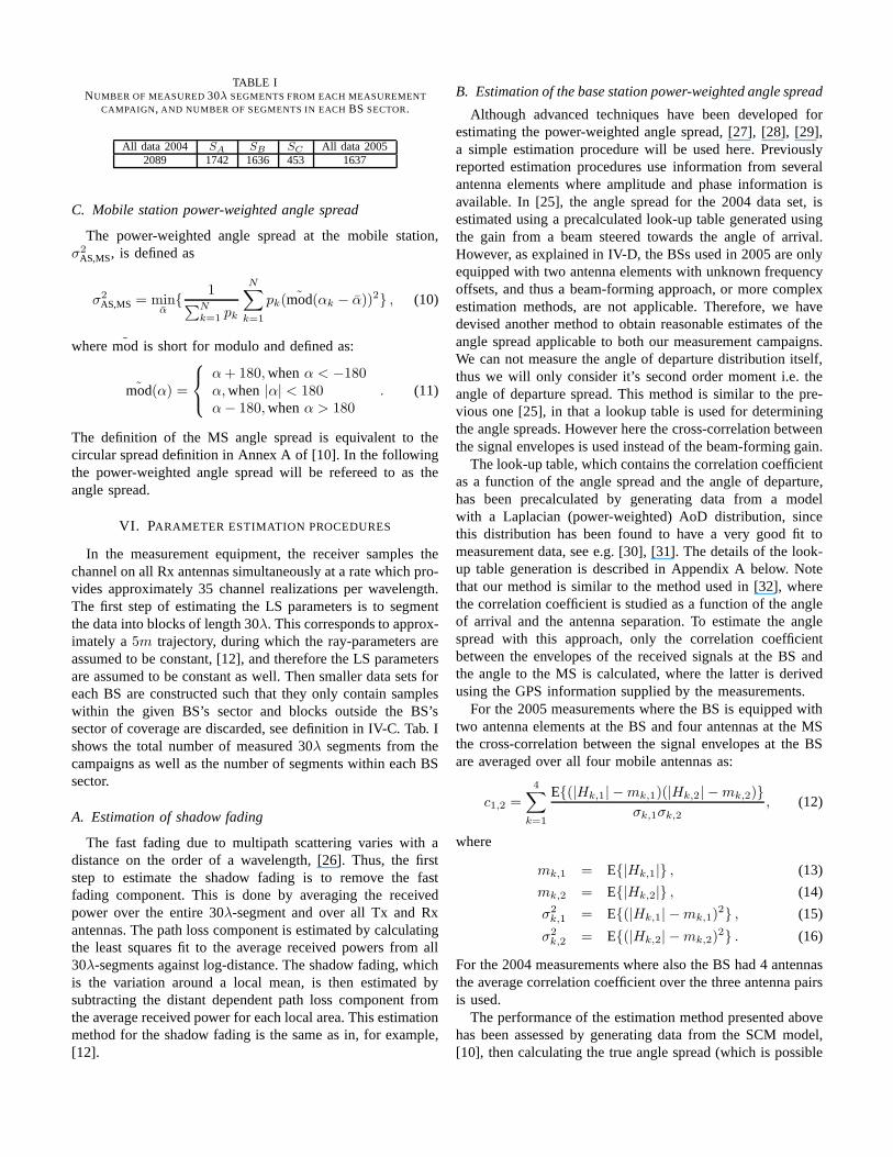
TABLE INUMBER OF MEASURED30λ SEGMENTS FROM EACH MEASUREMENT

CAMPAIGN, AND NUMBER OF SEGMENTS IN EACHBS SECTOR.

All data 2004 SA SB SC All data 20052089 1742 1636 453 1637

C. Mobile station power-weighted angle spread

The power-weighted angle spread at the mobile station,σ2

AS,MS, is defined as

σ2

AS,MS = minα

{1

∑Nk=1

pk

N∑

k=1

pk(mod(αk − α))2} , (10)

wheremod is short for modulo and defined as:

mod(α) =

α + 180, whenα < −180α, when |α| < 180α − 180, whenα > 180

. (11)

The definition of the MS angle spread is equivalent to thecircular spread definition in Annex A of [10]. In the followingthe power-weighted angle spread will be refereed to as theangle spread.

VI. PARAMETER ESTIMATION PROCEDURES

In the measurement equipment, the receiver samples thechannel on all Rx antennas simultaneously at a rate which pro-vides approximately 35 channel realizations per wavelength.The first step of estimating the LS parameters is to segmentthe data into blocks of length 30λ. This corresponds to approx-imately a5m trajectory, during which the ray-parameters areassumed to be constant, [12], and therefore the LS parametersare assumed to be constant as well. Then smaller data sets foreach BS are constructed such that they only contain sampleswithin the given BS’s sector and blocks outside the BS’ssector of coverage are discarded, see definition in IV-C. Tab. Ishows the total number of measured 30λ segments from thecampaigns as well as the number of segments within each BSsector.

A. Estimation of shadow fading

The fast fading due to multipath scattering varies with adistance on the order of a wavelength, [26]. Thus, the firststep to estimate the shadow fading is to remove the fastfading component. This is done by averaging the receivedpower over the entire 30λ-segment and over all Tx and Rxantennas. The path loss component is estimated by calculatingthe least squares fit to the average received powers from all30λ-segments against log-distance. The shadow fading, whichis the variation around a local mean, is then estimated bysubtracting the distant dependent path loss component fromthe average received power for each local area. This estimationmethod for the shadow fading is the same as in, for example,[12].

B. Estimation of the base station power-weighted angle spread

Although advanced techniques have been developed forestimating the power-weighted angle spread, [27], [28], [29],a simple estimation procedure will be used here. Previouslyreported estimation procedures use information from severalantenna elements where amplitude and phase information isavailable. In [25], the angle spread for the 2004 data set, isestimated using a precalculated look-up table generated usingthe gain from a beam steered towards the angle of arrival.However, as explained in IV-D, the BSs used in 2005 are onlyequipped with two antenna elements with unknown frequencyoffsets, and thus a beam-forming approach, or more complexestimation methods, are not applicable. Therefore, we havedevised another method to obtain reasonable estimates of theangle spread applicable to both our measurement campaigns.We can not measure the angle of departure distribution itself,thus we will only consider it’s second order moment i.e. theangle of departure spread. This method is similar to the pre-vious one [25], in that a lookup table is used for determiningthe angle spreads. However here the cross-correlation betweenthe signal envelopes is used instead of the beam-forming gain.

The look-up table, which contains the correlation coefficientas a function of the angle spread and the angle of departure,has been precalculated by generating data from a modelwith a Laplacian (power-weighted) AoD distribution, sincethis distribution has been found to have a very good fit tomeasurement data, see e.g. [30], [31]. The details of the look-up table generation is described in Appendix A below. Notethat our method is similar to the method used in [32], wherethe correlation coefficient is studied as a function of the angleof arrival and the antenna separation. To estimate the anglespread with this approach, only the correlation coefficientbetween the envelopes of the received signals at the BS andthe angle to the MS is calculated, where the latter is derivedusing the GPS information supplied by the measurements.

For the 2005 measurements where the BS is equipped withtwo antenna elements at the BS and four antennas at the MSthe cross-correlation between the signal envelopes at the BSare averaged over all four mobile antennas as:

c1,2 =

4∑

k=1

E{(|Hk,1| − mk,1)(|Hk,2| − mk,2)}

σk,1σk,2

, (12)

where

mk,1 = E{|Hk,1|} , (13)

mk,2 = E{|Hk,2|} , (14)

σ2

k,1 = E{(|Hk,1| − mk,1)2} , (15)

σ2

k,2 = E{(|Hk,2| − mk,2)2} . (16)

For the 2004 measurements where also the BS had 4 antennasthe average correlation coefficient over the three antenna pairsis used.

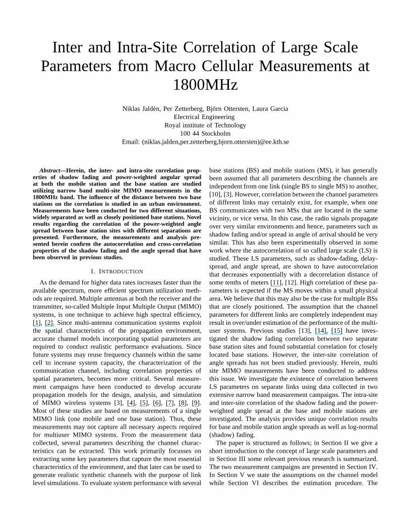
The performance of the estimation method presented abovehas been assessed by generating data from the SCM model,[10], then calculating the true angle spread (which is possible

0 0.2 0.4 0.6 0.8 1 1.2 1.4 1.60

0.2

0.4

0.6

0.8

1

1.2

1.4

1.6

log10 true angle spread

log1

0 es

timat

ed a

ngle

spr

ead

Fig. 5. Performance of the angle spread estimator on SCM generated data.

on the simulated data since all rays are known) and theestimated angle spread using the method described above.The results of this comparison are shown in Fig. 5. From theestimates in the figure, it is readily seen that the angle spreadestimate is reasonably unbiased, with a standard deviationof0.1 log-degrees.

C. Estimation of the mobile station power-weighted anglespread

At the mobile station, an estimate of the power-weightedangle spread will be extracted from the power levels of thefour MS antennas. Accurate estimate can not be expected,however, the MS angle spread is usually very large due to richscattering at ground level in this environment and reasonableestimates can still be obtained as will be seen.

A first attempt is to use a four ray model where the AOAsof the four rays are identical to the boresights of the four MSantennas i.eαn = 90o(n − 2.5). The power of the four raysp1,. . . ,p4, are obtained from the power of the four antennasi.e. the Euclidean norm of the rows of the channel matricesH. These estimates obtained by averaging the fast fading over30λ segments. From the powers the angle spread is calculatedusing the circular model defined in (11) resulting in

σ2

AS,MS-fe = minα

{1

∑

4

n=1pn

4∑

n=1

pn(mod(90(n − 2.5)− α))2}

(17)where (.)fe is short for first-estimate. As explained in Annex Aof [10], the angle spread should be invariant to the direction ofthe antenna, hence, knowledge of the moving direction of theMS is not required. The performance of the estimate is firstevaluated by simulating a large number of widely differentcases, using the SCM model, and estimating the spread basedon four directional antennas as proposed here. The result isshown in Fig. 6. The details of the simulation are describedin Appendix B.

The results show that the angle spread is often over-estimated using the proposed method. However, as indicated

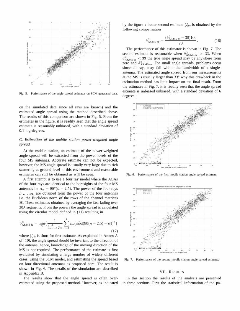
by the figure a better second estimate (.)se is obtained by thefollowing compensation

σ2

AS,MS-se=(σ2

AS,MS-fe− 30)100

70. (18)

The performance of this estimator is shown in Fig. 7. Thesecond estimate is reasonable whenσ2

AS,MS-se > 33. Whenσ2

AS,MS-se < 33 the true angle spread may be anywhere fromzero andσ2

AS,MS-se. For small angle spreads, problems occursince all rays may fall within the bandwidth of a single-antenna. The estimated angle spread from our measurementsat the MS is usually larger than 33o why this drawback in theestimation method has little impact on the final result. Fromthe estimates in Fig. 7, it is readily seen that the angle spreadestimate is unbiased unbiased, with a standard deviation of6degrees.

30 40 50 60 70 80 90 1000

10

20

30

40

50

60

70

80

90

100

First estimate of MS angle spread

Tru

e an

gle

spre

ad

EstimatesFitted line y=(x30)*100/70

Fig. 6. Performance of the first mobile station angle spread estimate.

0 10 20 30 40 50 60 70 80 90 1000

10

20

30

40

50

60

70

80

90

100

Second estimate of MS anglespread

Tru

e an

gleS

prea

d

Performance of second MS anglespread estimate

EstimatesLine y=x

Fig. 7. Performance of the second mobile station angle spread estimate.

VII. R ESULTS

In this section the results of the analysis are presentedin three sections. First the statistical information of thepa-

TABLE IIPARAMETERSα AND β FOR THE BETA BEST FIT DISTRIBUTION TO THE

ANGLE SPREAD AT THE MOBILE.

2004:A 2004:B 2004:C 2005:1 2005:2α 8.69 5.74 4.22 6.85 7.07β 2.85 2.36 2.44 2.72 2.77

rameters is shown and then their autocorrelation and cross-correlation properties are displayed.

A. Statistical properties

The first and the second order statistics of the LS parametersare estimated and shown in Tab. III. The standard deviationof the shadow fading is given in dB while the angle spreadat the BS is given in logarithmic degrees. Further, the MSangle spread is given in degrees. The mean value of theshadow fading component is not tabulated since it is zeroby definition. As seen from the histograms in Fig. 8, whichshows the statistics of the LS parameters for site 2004:B, theshadow fading and log-angle spread can be well modelled witha normal distribution. This agrees with observations reportedin [26], [12]. The angle spread at the mobile on the other handis better modelled by a scaled beta distribution, defined as:

f(x, α, β) =1

B(α, β)(x

η)α−1(1 −

x

η)β−1 , (19)

where η = 360√12

is a normalization constant, equal to themaximum possible angle spread. The best fit shape parametersα and β for each of the measurement sets are tabulated inTab. II. The parameterB(α, β) is a constant which dependson α andβ such that

∫ η

0f(x, α, β)dx = 1. The distributions

for the parameters from all the other measured sites are similar,with statistics given in Tab. III. From the table it is seenthat the angle spread clearly depends on the height of theBS. The highest elevated BS, 2004:B, has the lowest anglespread and correspondingly, the BS at rooftop level, 2004:A,has the largest angle spread. The mean angle spreads at thebase station are quite similar to the typical urban sites in [12](0.74-0.95) and to those of the SCM urban macro model (0.81-1.18) [10]. Furthermore, the standard deviation of the anglespread and the shadow fading, Tab III found here are somewhatsmaller than those of [12]. One explanation for this could bethat the measured propagation environments in 2004 and 2005are more uniform than those measured in [12].

B. LS autocorrelation

The rate of change of the LS parameters is investigatedby estimating the autocorrelation as a function of distancetravelled by the MS. The autocorrelation functions for the largescale parameters are shown in Fig. 9 and 10. The correlationcoefficient between two variables is calculated as explainedin Appendix X-C. Note that the autocorrelation functionscan be well approximated by an exponential function withdecorrelation distances as seen in Tab IV. The decorrelationdistance is defined as the distance for which the correlationhas decreased toe−1. Furthermore, it can be noted that

20 0 200

0.01

0.02

0.03

0.04

0.05

0.06

0.07

0.08

0.09Shadow fading

dB 0 0.5 1 1.5

0

0.2

0.4

0.6

0.8

1

1.2

1.4

1.6

1.8

2Angle spread at BS

Log10

(degrees) 0 50 100

0

0.005

0.01

0.015

0.02

0.025Angle spread at MS

degrees

Fig. 8. Histograms of the estimated large scale parameters for site 2004:B.

TABLE IVAVERAGE DECORRELATION DISTANCE IN METERS FOR THE ESTIMATED

LARGE SCALE PARAMETERS.

SF σAS,BS σAS,MSddecorr (m) 113 88 32

these distances are very similar for the 2004 and the 2005measurements, which is reasonable since the environments aresimilar. The exponential model has been proposed before, see[12], for the shadow fading and angle spread at the BS. Theresults shown herein indicate that this is a good model for theangle spread at the MS as well.

0 100 200 300 400 5000. 4

0. 2

0

0.2

0.4

0.6

0.8

1

Distance (m)

Cor

rela

tion

Site:A SFSite:A AS

BS

Site:B SFSite:B AS

BS

Site:05 SFSite:05 AS

BS

Fig. 9. Autocorrelation of the shadow fading and the angle spread at thebase station for both measurements.

C. Intra-site correlation

The intra-site correlation coefficient between different largescale parameters at the same site are calculated for the twoseparate measurement campaigns. In Tab. V and VI thecorrelation coefficients for the two base stations, sector AandB, from 2004 are shown respectively. The last sector (C) is not

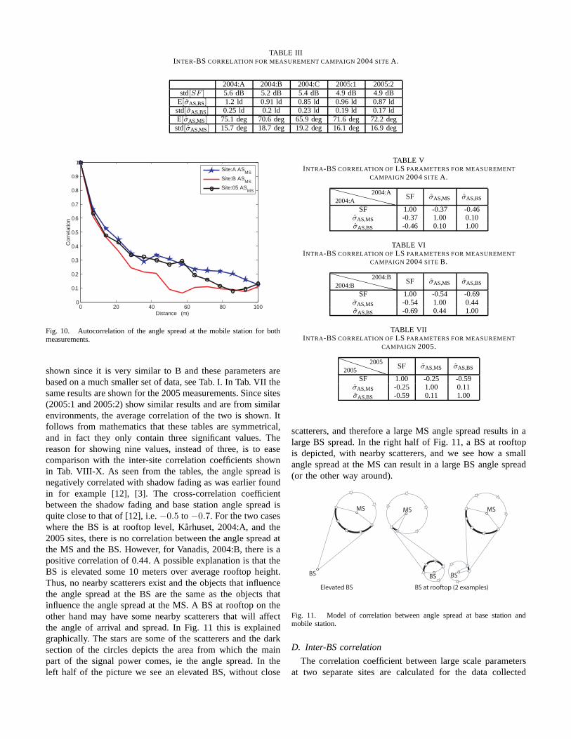
TABLE IIIINTER-BS CORRELATION FOR MEASUREMENT CAMPAIGN2004SITE A.

2004:A 2004:B 2004:C 2005:1 2005:2std[SF ] 5.6 dB 5.2 dB 5.4 dB 4.9 dB 4.9 dB

E[σAS,BS] 1.2 ld 0.91 ld 0.85 ld 0.96 ld 0.87 ldstd[σAS,BS] 0.25 ld 0.2 ld 0.23 ld 0.19 ld 0.17 ldE[σAS,MS] 75.1 deg 70.6 deg 65.9 deg 71.6 deg 72.2 deg

std[σAS,MS] 15.7 deg 18.7 deg 19.2 deg 16.1 deg 16.9 deg

0 20 40 60 80 1000

0.1

0.2

0.3

0.4

0.5

0.6

0.7

0.8

0.9

1

Distance (m)

Cor

rela

tion

Site:A AS

MS

Site:B ASMS

Site:05 ASMS

Fig. 10. Autocorrelation of the angle spread at the mobile station for bothmeasurements.

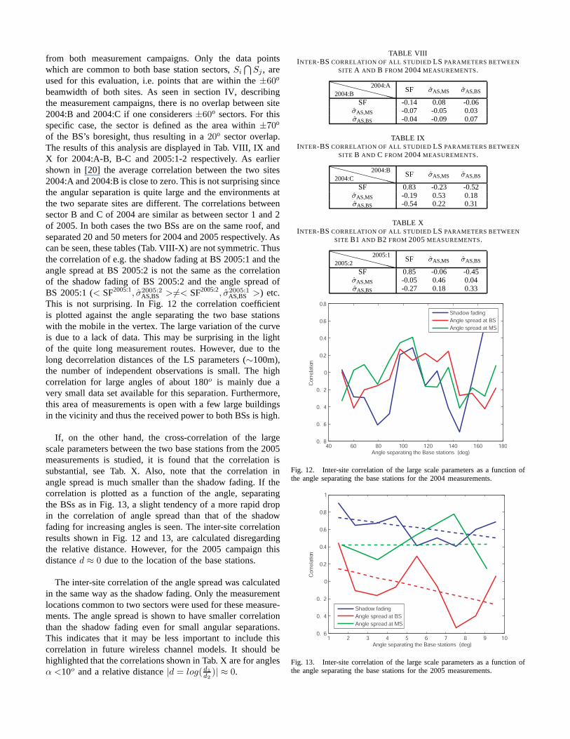
shown since it is very similar to B and these parameters arebased on a much smaller set of data, see Tab. I. In Tab. VII thesame results are shown for the 2005 measurements. Since sites(2005:1 and 2005:2) show similar results and are from similarenvironments, the average correlation of the two is shown. Itfollows from mathematics that these tables are symmetrical,and in fact they only contain three significant values. Thereason for showing nine values, instead of three, is to easecomparison with the inter-site correlation coefficients shownin Tab. VIII-X. As seen from the tables, the angle spread isnegatively correlated with shadow fading as was earlier foundin for example [12], [3]. The cross-correlation coefficientbetween the shadow fading and base station angle spread isquite close to that of [12], i.e.−0.5 to −0.7. For the two caseswhere the BS is at rooftop level, Karhuset, 2004:A, and the2005 sites, there is no correlation between the angle spreadatthe MS and the BS. However, for Vanadis, 2004:B, there is apositive correlation of 0.44. A possible explanation is that theBS is elevated some 10 meters over average rooftop height.Thus, no nearby scatterers exist and the objects that influencethe angle spread at the BS are the same as the objects thatinfluence the angle spread at the MS. A BS at rooftop on theother hand may have some nearby scatterers that will affectthe angle of arrival and spread. In Fig. 11 this is explainedgraphically. The stars are some of the scatterers and the darksection of the circles depicts the area from which the mainpart of the signal power comes, ie the angle spread. In theleft half of the picture we see an elevated BS, without close

TABLE VINTRA-BS CORRELATION OFLS PARAMETERS FOR MEASUREMENT

CAMPAIGN 2004SITE A.

XX

XX

XX

XX2004:A

2004:ASF σAS,MS σAS,BS

SF 1.00 -0.37 -0.46σAS,MS -0.37 1.00 0.10σAS,BS -0.46 0.10 1.00

TABLE VIINTRA-BS CORRELATION OFLS PARAMETERS FOR MEASUREMENT

CAMPAIGN 2004SITE B.

XX

XX

XX

XX2004:B

2004:BSF σAS,MS σAS,BS

SF 1.00 -0.54 -0.69σAS,MS -0.54 1.00 0.44σAS,BS -0.69 0.44 1.00

TABLE VIIINTRA-BS CORRELATION OFLS PARAMETERS FOR MEASUREMENT

CAMPAIGN 2005.

PP

PP

PP2005

2005SF σAS,MS σAS,BS

SF 1.00 -0.25 -0.59σAS,MS -0.25 1.00 0.11σAS,BS -0.59 0.11 1.00

scatterers, and therefore a large MS angle spread results inalarge BS spread. In the right half of Fig. 11, a BS at rooftopis depicted, with nearby scatterers, and we see how a smallangle spread at the MS can result in a large BS angle spread(or the other way around).

Elevated BS BS at rooftop (2 examples)

MS

BSBS

MS MS

BS

Fig. 11. Model of correlation between angle spread at base station andmobile station.

D. Inter-BS correlation

The correlation coefficient between large scale parametersat two separate sites are calculated for the data collected

from both measurement campaigns. Only the data pointswhich are common to both base station sectors,Si

⋂

Sj , areused for this evaluation, i.e. points that are within the±60o

beamwidth of both sites. As seen in section IV, describingthe measurement campaigns, there is no overlap between site2004:B and 2004:C if one considerers±60o sectors. For thisspecific case, the sector is defined as the area within±70o

of the BS’s boresight, thus resulting in a20o sector overlap.The results of this analysis are displayed in Tab. VIII, IX andX for 2004:A-B, B-C and 2005:1-2 respectively. As earliershown in [20] the average correlation between the two sites2004:A and 2004:B is close to zero. This is not surprising sincethe angular separation is quite large and the environments atthe two separate sites are different. The correlations betweensector B and C of 2004 are similar as between sector 1 and 2of 2005. In both cases the two BSs are on the same roof, andseparated 20 and 50 meters for 2004 and 2005 respectively. Ascan be seen, these tables (Tab. VIII-X) are not symmetric. Thusthe correlation of e.g. the shadow fading at BS 2005:1 and theangle spread at BS 2005:2 is not the same as the correlationof the shadow fading of BS 2005:2 and the angle spread ofBS 2005:1 (< SF2005:1, σ2005:2

AS,BS > 6=< SF2005:2, σ2005:1

AS,BS >) etc.This is not surprising. In Fig. 12 the correlation coefficientis plotted against the angle separating the two base stationswith the mobile in the vertex. The large variation of the curveis due to a lack of data. This may be surprising in the lightof the quite long measurement routes. However, due to thelong decorrelation distances of the LS parameters (∼100m),the number of independent observations is small. The highcorrelation for large angles of about 180o is mainly due avery small data set available for this separation. Furthermore,this area of measurements is open with a few large buildingsin the vicinity and thus the received power to both BSs is high.

If, on the other hand, the cross-correlation of the largescale parameters between the two base stations from the 2005measurements is studied, it is found that the correlation issubstantial, see Tab. X. Also, note that the correlation inangle spread is much smaller than the shadow fading. If thecorrelation is plotted as a function of the angle, separatingthe BSs as in Fig. 13, a slight tendency of a more rapid dropin the correlation of angle spread than that of the shadowfading for increasing angles is seen. The inter-site correlationresults shown in Fig. 12 and 13, are calculated disregardingthe relative distance. However, for the 2005 campaign thisdistanced ≈ 0 due to the location of the base stations.

The inter-site correlation of the angle spread was calculatedin the same way as the shadow fading. Only the measurementlocations common to two sectors were used for these measure-ments. The angle spread is shown to have smaller correlationthan the shadow fading even for small angular separations.This indicates that it may be less important to include thiscorrelation in future wireless channel models. It should behighlighted that the correlations shown in Tab. X are for anglesα <10o and a relative distance|d = log(d1

d2

)| ≈ 0.

TABLE VIIIINTER-BS CORRELATION OF ALL STUDIEDLS PARAMETERS BETWEEN

SITE A AND B FROM 2004MEASUREMENTS.

XX

XX

XX

XX2004:B

2004:ASF σAS,MS σAS,BS

SF -0.14 0.08 -0.06σAS,MS -0.07 -0.05 0.03σAS,BS -0.04 -0.09 0.07

TABLE IXINTER-BS CORRELATION OF ALL STUDIEDLS PARAMETERS BETWEEN

SITE B AND C FROM 2004MEASUREMENTS.

XX

XX

XX

XX2004:C

2004:BSF σAS,MS σAS,BS

SF 0.83 -0.23 -0.52σAS,MS -0.19 0.53 0.18σAS,BS -0.54 0.22 0.31

TABLE XINTER-BS CORRELATION OF ALL STUDIEDLS PARAMETERS BETWEEN

SITE B1 AND B2 FROM 2005MEASUREMENTS.

XX

XX

XX

XX2005:2

2005:1SF σAS,MS σAS,BS

SF 0.85 -0.06 -0.45σAS,MS -0.05 0.46 0.04σAS,BS -0.27 0.18 0.33

40 60 80 100 120 140 160 1800. 8

0. 6

0. 4

0. 2

0

0.2

0.4

0.6

0.8

Angle separating the Base stations (deg)

Corr

ela

tion

Shadow fading

Angle spread at BS

Angle spread at MS

Fig. 12. Inter-site correlation of the large scale parameters as a function ofthe angle separating the base stations for the 2004 measurements.

1 2 3 4 5 6 7 8 9 100. 6

0. 4

0. 2

0

0.2

0.4

0.6

0.8

1

Angle separating the Base stations (deg)

Co

rre

latio

n

Shadow fading

Angle spread at BS

Angle spread at MS

Fig. 13. Inter-site correlation of the large scale parameters as a function ofthe angle separating the base stations for the 2005 measurements.

VIII. C ONCLUSION

We studied the correlation properties of the three large scaleparameters shadow fading, base station power-weighted anglespread, and mobile station power-weighted angle spread. Twolimiting cases were considered, namely when the base stationsare widely separated,∼ 900m and when they are closelypositioned, some 20-50 meters apart.

The results in [12] on the distribution and autocorrelationofshadow fading and base station angle spread were confirmedalthough the standard deviations of the angular spread andshadow fading were slightly smaller in our measurements. Thehigh inter-base station shadow fading correlation, when basestations are close, as observed in [13] was also confirmedin this analysis. Our results also show that angular spreadcorrelation exists at both the base station and the mobile stationif the base station separation is small. However, the correlationin angular spread is significantly smaller than the correlationof the shadow fading. Thus it is less important to model thiseffect. For widely separated base stations, our results show thatthe base station and mobile station angular spreads as well asthe shadow fading are uncorrelated.

The angle spread at the mobile was analyzed and a scaledbeta distribution was shown to fit the measurements well.Further, we have also found that the base station and mo-bile station angular spreads are correlated for elevated basestations but uncorrelated for base station just above rooftop.Correlation can be expected if the scatters are only locatedclose to the mobile station, which is the case for macro-cellularenvironments, as illustrated in Fig. 11.

In the future, it will be of interest to assess also theregion in between the two limiting cases studied herein. Notethat the limiting case of distances of 20-50 meters has apractical interest. For instance, the sectors of three-sectorsites are sometimes not co-located but placed on differentedges of a roof. The two base stations may also belong todifferent operators and the properties studied here could thenbe important when studying adjacent carrier interference.

IX. A CKNOWLEDGEMENTS

This work was sponsored partly within the Antenna Centerof Excellence (FP6-IST 508009), the WINNER project IST-2003-507581, and wireless@KTH.

X. A PPENDIX

A. Appendix A

The Laplacian angle of departure distribution is given by

PA(θ) = Ce−|θ−θ0|

σAoD , (20)

whereθ0 is the nominal direction of the mobile andσAoD isangle-of-departure spread. The variableC is a constant suchthat

∫ π

−πPA(θ)dθ = 1. When generating data the channel

covariance matrix is first estimated as

R =

∫ 180o

θ=−180o

PA(θ)a(θ)a∗(θ)dθ (21)

wherea(θ) is the array steering vector which is given by

a(θ) = p(θ)[1, exp(−j2πdspacingsin(θ))]T (22)

andp(θ) is the (amplitude) antenna element diagrams of thearray anddspacing is the spacing between the antenna elementsgiven in wavelengths. In our case the element diagrams areapproximated by

p2(θ) = max(101.4 cos2(θ), 10−0.2), (23)

and the antenna element spacing is 0.56 wavelengths. Theprocedure for calculating the look-up table is then 1) Fixangle spread and nominal angle of arrival, 2) Calculate thecovariance matrixR and it’s eigendecomposition, 3) Generatedata from the model and calculate the envelope correlation.

The choice of Laplacian (power-weighted ) AoD distribu-tion over other, for example Gaussian, does only affect theestimation results marginally, due to the short antenna spacingdistance. This is further explained in [33].

B. Appendix B

To test the estimator of the (power-weighted) RMS anglespread at the mobile-station side, some propagation channelswere generated. Each channel had random number of clusterswhich was equally distributed between 1 and 10. The AOAof each cluster is uniformly distributed between0o and360o.The power of the clusters are log-normally distributed witha standard deviation of 8dB. Each cluster is modelled withbetween 1 and 100 rays (all with equal power) which areuniformly distributed within the cluster width. The clusterwidths are uniform distributed between 0 and 10 degrees.One thousand propagation (completely independent) channelsare drawn from this model. The powers of the four antennasare calculated based on the power of the rays, their angleof arrival, and the antenna pattern. The true angle spread isfirst estimated as described in Annex A of [10], and then theestimation method described in Section VI-C, is applied.

C. Appendix C

The correlation coefficient between two variables is definedby the normalized covariance as:

ρ =< a, b >=E[ab] − mamb

√

(E[a2] − m2a)(E[b2] − m2

b)(24)

At all times when calculating the cross-correlation between LSparameters, even for small subsets of data, like when analyzingthe correlation as a function of angular separation betweenBSs, the mean values are global. Hence the valuesma andmb are calculated using the full data set of each BSs sectorrespectively. If the mean values would be estimated locallyitequal to assuming the parameters are locally zero mean, andthis is not what we are studying. What we want to investigateis: given that one parameter is large (or small) is the other onethis as well.

REFERENCES

[1] G. Foschini and M. G. Telatar, “On limits of wireless communications ina fading environmen when using multiple antennas,”Wireless PersonalCommunications, vol. 6, no. 3, pp. 311–335, 1998.

[2] I. Telatar, “Capacity of multi-antenna gaussian channels,” EuropeanTelecomunication Transactions, vol. 10, no. 6, pp. 585–596, Dec. 1999.

[3] D. Baum and H. E.-S. et al., “IST-WINNER D5.4, final reporton linkand system level channel models,” Oct. 2005, http://www.ist-winner.org/.

[4] D. Chizhik, J. Ling, P. Wolniansky, R. Valenzuela, N. Costa, andK. Huber, “Multiple-input-multiple-output measurementsand modelingin manhattan,” IEEE Journal on Selected Areas in Communication,vol. 21, no. 3, pp. 321–331, Apr. 2003.

[5] V. Eiceg, H. Sampath, and S. Catreux-Erceg, “Dual-polarization versussingle-polarization MIMO channel measurement results andmodeling,”IEEE Transactions on Wireless Communications, vol. 5, no. 1, pp. 28–33, Jan. 2006.

[6] P. Kyritsi, D. Cox, R. Valenzuela, and P. Wolniansky, “Correlation anal-ysis based on MIMO channel measurements in an indoor environment,”IEEE Journal on Selected Areas in Communications, vol. 21, no. 5, pp.713–720, Jun. 2003.

[7] M. Steinbauer, A. Molisch, and E. Bonek, “The double-directional radiochannel,”IEEE Antennas and Propagation Magazine, vol. 43, no. 4, pp.51–63, Aug. 2001.

[8] R. Stridh, K. Yu, B. Ottersten, and P. Karlsson, “MIMO channel capacityand modeling issues on a measured indoor radio channel at 5.8GHz,”IEEE Transactions on Wireless Communications, vol. 4, no. 3, pp. 895–903, May 2005.

[9] J. Wallace and M. Jensen, “Time-varying MIMO channels: Measure-ment, analysis, and modeling,”IEEE Transactions on Antennas andPropagation, vol. 11, no. 1, pp. 3265–3273, Nov. 2006.

[10] 3GPP-SCM, “Spatial channel model for multiple input multi-ple output (MIMO) simulations.” TR.25.966 v.6.10, Sep. 2003,http://www.3gpp.org/.

[11] M. Gudmundson, “Correlation model for shadow fading inmobile radiosystems,”IEEE Electronic Letters, vol. 27, no. 23, pp. 2145–2146, Nov.1991.

[12] A. Algans, K. Pedersen, and P. Morgensen, “Experimental analysis of thejoint properties of azimuth spread, delay spread and shadowing fading.”IEEE Journal on Selected Areas in Communication, vol. 20, no. 3, pp.523–531, Apr. 2002.

[13] V. Graziano, “Propagation correlation at 900MHz,”IEEE Transactionon Vehicular Technology, vol. VT-27, no. 4, Nov. 1978.

[14] J. Witzen and T. Lowe, “Measurement of angular and distance correla-tion properties of log-normal shadowing at 1900MHz and its applicationto design of PCS systems,”IEEE Transaction on Vehicular Technology,vol. 51, no. 2, Mar. 2002.

[15] A. Mawira, “Models for the spatial correlation functions of the (log-)normal component of the variability of the VHF/UHF field strength inurban environment,”PIMRC, pp. 436–440, 1992.

[16] K. Zayana and B. Guisnet, “Measurements and modelisation of shadow-ing cross-correlations between two base-stations,”ICUPC, vol. 1, Oct.1998.

[17] E. Perahia, D. Cox, and S. Ho, “Shadow fading cross correlation betweenbasestations,”VTC, vol. 1, pp. 313–317, May 2001.

[18] H. Arnold, D. Cox, and R. Murray, “Macroscopic diversity performancemeasured in the 800-MHz portable radio communications environment,”IEEE Transactions on Antennas and Propagation, vol. 36, no. 2, pp.277–281, Feb. 1988.

[19] T. Klingenbrunn and P. Mogensen, “Modelling cross-correlated shad-owning in network similations,”VTC, 1999.

[20] N. Jalden, P. Zetterberg, M. Bengtsson, and B. Ottersten, “Analysis ofmulti-cell MIMO measurements in an urban macro cell environment,”URSI GA, Jun. 2005.

[21] L. Garcia, N. Jalden, B. Lindmark, P. Zetterberg, and L. D. Haro,“Measurements of MIMO capacity at 1800MHz with in- and outdoortransmitter locations,”EuCAP 2006, Jul. 2006.

[22] ——, “Measurements of MIMO indoor channels at 1800MHz withmultiple indoor and outdoor base stations,”Eurasip Journal on WirelessCommunication and Networking, Nov. 2007.

[23] P. Zetterberg,WIreless DEvelopment LABoratory (WIDELAB) equip-ment base, Signal Sensors and Systems (KTH), http://www.ee.kth.se/,Aug. 2003, iR-SB-IR-0316.

[24] “http://www.hubersuhner.com/.”

[25] P. Zetterberg, N. Jalden, K. Yu, and M. Bengtsson, “Analysis of MIMOmulti-cell correlations and other propagation issues based on urbanmeasurements,”IST mobile summit 2005, Jun. 2005.

[26] T. Rappaport,Wireless Communications: Principles and practice. Up-per Saddle River, New Jersey 07458: Prentice-Hall Inc., 1996.

[27] T. Trump and B. Ottersten, “Estimation of nominal direction of arrivaland angular spread using an array of sensors,”IEEE Transactions onSignal Processing, vol. 50, pp. 57–69, 1996.

[28] M. Bengtsson and B. Ottersten, “Low-complexity estimators for dis-tributed sources,”IEEE Transactions on Signal Processing, vol. 48,no. 8, pp. 2185–2194, 2000.

[29] M. Tapio, “Direction and spread estimation of spatially distributedsignals via the power azimuth spectrum,”ICASSP 02, vol. 3, pp. III–3005– III–3008, 2002.

[30] K. Pedersen, P. Mogensen, and B. Fleury, “A stochastic model ofthe temporal and azimuthal dispersion seen at the base station inoutdoor propagation environments,”IEEE Transactions on VehicularThecnology, vol. 49, no. 2, pp. 437–447, Mar. 2000.

[31] K. I. Pedersen, P. Mogensen, and J. Ramiro-Moreno, “A stochasticmodel of the temporal and azimuthal dispersion seen at the base stationin outdoor propagation,”IEEE Transactions on Vehicular Technology,vol. 49, no. 2, pp. 437–447, Mar. 2000.

[32] F. Adachi, M. Feeny, and A. Williamson, “Crosscorrelation betweenenvelopes of 900 MHz signals received at a mobile radio base stationsite.” IEE Proceedings, vol. 133, no. 6, pp. 506–512, Oct. 1986.

[33] N. Jalden, “Analysis of radio channel measurements using multiple basestations,” Licenciate Thesis, Royal Institute of Technology, May 2007.