Faculdade de Engenharia da Universidade do Porto Intelligent Traffic Signal Control Cristina Alexandra Teixeira Vilarinho SUBMITTED IN PARTIAL FULFILMENT OF THE REQUIREMENTS FOR THE DEGREE OF PH.D. IN TRANSPORTATION SYSTEMS SUPERVISOR: JOSÉ Pedro TAVARES CO- SUPERVISOR: ROSALDO J. F. ROSSETTI Porto, December 2019

Welcome message from author
This document is posted to help you gain knowledge. Please leave a comment to let me know what you think about it! Share it to your friends and learn new things together.
Transcript
Faculdade de Engenharia da Universidade do Porto
Intelligent Traffic Signal Control
Cristina Alexandra Teixeira Vilarinho
SUBMITTED IN PARTIAL FULFILMENT OF THE REQUIREMENTS FOR THE DEGREE OF
PH.D. IN TRANSPORTATION SYSTEMS
SUPERVISOR: JOSÉ Pedro TAVARES
CO- SUPERVISOR: ROSALDO J. F. ROSSETTI
Porto, December 2019

ii
© Cristina Vilarinho, 2019

iii
Co-funded by:

iv

v
Acknowledgments
I would like to take this opportunity to express my profound gratitude to my supervisors Professor José
Pedro Tavares and Professor Rosaldo Rossetti from the Faculty of Engineering of University of Porto
(FEUP). Professor José Pedro Tavares gave me the opportunity to work in the European project CiViTAS-
ELAN project and pursue my studies in the doctoral program. His knowledge and friendship, in the past
ten years, have been crucial for my academic and personal development.
A word of appreciation goes to SVC/DEC, namely Professor Carlos Rodrigues, Professor António Couto and
Professor Sara Ferreira, for their support and for the opportunities I received to develop my knowledge
and experience; I also would like to thank Mrs. Guilhermina Castro for the administrative support.
To MIT Portugal Program and Staff, thank you for the opportunity to learn with the best in Portugal and to
make an internship at the MIT. I would like to thank Professor Carolina Osorio for hosting me during my
stay in Boston
Many thanks to all my colleagues and friends from FEUP’s Traffic Analysis Laboratory for the excellent
work environment: António Lobo, Marco, Juliana, André, Murilo and Gustavo. These words extend to my
colleagues and friends from MIT Transportation Systems Doctoral Program: Marcos, Liliana and Teresa.
I also want to acknowledge all my colleagues and friends at Municipality of Porto, for encouraging me to
complete my doctoral program. A special word of appreciation for Bruno Eugénio for giving me the
conditions needed for the “final sprint”.
During the past seven years, a lot of things happened in my life. I would like to express my gratitude to Tia
Margarida who gave me so much. To my parents, Laura and Vilarinho, my sister Sílvia and my brother-in-
law João Pedro, thank you for believing in me. José Nuno and Júlia thank you for your patience and
unconditional support, I would not have achieved this goal without your love. For my longtime friends
who always have been there for me, I would like to thank their support.
I am also thankful to the Portuguese Foundation for Science and Technology, for awarding me MIT
Portugal scholarship SFRH/BD/51977/2012. I want to acknowledge FEUP and the Research Centre for
Territory, Transports and Environment (CITTA) for providing the resources needed to develop this work.
This journey was only possible thanks to the help of many people which contributed in so many ways.
Thank you all!

vi
vii
Abstract
Traffic in a city is very much affected by traffic lights. They are not the only pieces in this puzzle, but they
are important elements of traffic management.
Traffic lights have the power to improve the safety at intersections, which are considered critical elements
of the network, avoiding traffic conflicts between the different vehicle and pedestrian movements by
managing time in space. In order to avoid the dangerous conflicts and to optimize the control, people
have to wait for the green light, spending valuable time and building up frustration, while vehicles keep
consuming fuel and producing hazardous emissions.
In this research a novel traffic signal control is developed. Instead of using the traditional vehicle-based
optimization perspective, in which the approach is to look at the vehicle traffic condition as dependent on
standard metrics such as vehicle flow and vehicle delay, a novel person-based strategy is instead adopted.
It seems to be an interesting possibility to look into the traffic conditions distinguishing vehicles with
different occupancy, allowing a control based on people present/expected at the intersection.
The traffic signal control is viewed as a problem of efficient allocation of an available resource (green
light) to consumers (traffic lights), where all traffic streams at an intersection “compete" for the green
time period. To generate a disruptive traffic control strategy, the traditional concepts of traffic control
such as the cycle length, the maximum green period and a fixed phase sequence were abandoned.
Therefore, the proposed traffic signal control system settings design is less restrictive and more flexible
than traditional systems.
For this purpose, a novel auction-based intersection-control mechanism for traffic signal control is
developed. The present methodology includes a negotiation process, involving all the traffic streams so as
to manage the green time between them. The proposed routine decides on a time period (auction
frequency), an extension or an ending to the present green period, based on the recurrent demand and
aiming at minimizing person’s delay. In case of ending the green light, a second decision is made in order
to select which traffic streams should receive the green light. Negotiation process is very dynamic, and
reinitiates in short intervals (i.e. just a few seconds).
For the negotiation process, a set of initial traffic control settings is defined a priori. Two approaches for
finding the initial control settings are developed, respectively without (ITC_No_Plan) and with (ITC_Plan)
traffic signal plan design. The ITC_No_Plan approach is simpler and more direct than the ITC_Plan
approach, but more disruptive.
The global architecture of the proposed traffic control system is designed using a Multi-Agent System
approach for isolated intersections. Each intersection operates independently from other intersections, so
each intersection has the freedom and flexibility to calculate and implement any traffic control settings.
Decisions about the traffic light status of each traffic stream take into account the current traffic data in
all traffic streams, independent of their traffic light color. As a result, this strategy can react to non-
schedulable events or unpredictable events without human intervention.
The findings from the microscopic traffic simulation of different scenarios are encouraging and suggest
that there is value in viewing signal control based on persons instead of vehicles. The ITC_No_Plan traffic
signal control strategy has a better performance in low demands. For medium/high demands the results
are somewhat disappointing. The ITC_Plan traffic signal control strategy has a more balanced
performance.

viii
In the proposed traffic control strategy, average delay time is reduced on the arm with the highest value,
distributing and balancing the delay among all intersection arms. As a consequence, the arms with low
average delay tend to increase. The benefit for the network will be bigger when the most delayed arms
have a high relative demand.
Keywords: traffic signal control, traffic signal plan design, person-based mobility, auction mechanism,
agent base modeling
ix
Resumo
Os sinais luminosos têm impacto na circulação rodoviária de uma cidade. Estes não são as únicas peças do
“quebra-cabeças”, mas são sem dúvida elementos importantes na gestão de tráfego.
Os sinais luminosos têm a capacidade de melhorar a segurança rodoviária nas interseções, consideradas
elementos críticos da rede viária, evitando os movimentos conflituantes de todos os utilizadores através
da coordenação das dimensões espacial e temporal. De modo a evitar conflito de correntes de tráfego
incompatíveis e otimizar a capacidade de escoamento da intersecção, os utilizadores têm de aguardar
pela indicação do sinal verde, o que pode ter implicações na expectativa dos utilizadores e no consumo
energético com o consequente impacto no ambiente.
Neste trabalho foi desenvolvida uma nova abordagem de controlo de tráfego. Em vez da tradicional
otimização centrada no veículo, onde se analisam as condições de circulação deste tendo em atenção, por
exemplo, a maximização da capacidade ou minimização do atraso, propõe-se uma nova estratégia
baseada nas “pessoas”. De facto, parece ser uma abordagem interessante olhar para as condições de
circulação distinguindo os veículos de acordo com a sua ocupação, permitindo que o controlo de tráfego
se faça com base no tráfego de pessoas presente/expectável na interseção.
O controlo de tráfego é visto como um problema de alocação eficiente dos recursos disponíveis (sinal com
a cor verde) aos consumidores (sinais luminosos), onde todas as correntes de tráfego na intersecção
competem pelo sinal com a cor verde. De modo a criar uma estratégia de controlo de tráfego disruptiva,
as variáveis tradicionais utilizadas no controlo de tráfego tais como o ciclo, o tempo de verde máximo e a
sequência fixa das fases foram abandonadas. Deste modo, o sistema de controlo de tráfego proposto é
menos restritivo e mais flexível que os sistemas tradicionais.
Com este objetivo é desenvolvido um novo sistema de controlo de tráfego baseado num mecanismo de
“leilão”. A presente metodologia inclui um processo de negociação, envolvendo todas as correntes de
tráfego de modo a gerir o tempo de verde entre elas. Em cada momento de leilão é decidido se se aplica a
extensão do tempo de verde da presente fase ou o término desta fase, com base na procura de tráfego
existente e com o objetivo de minimizar o atraso das pessoas. Em caso de decisão de terminar a presente
fase, uma segunda decisão é necessária sobre qual a nova fase a iniciar. O processo de negociação é
muito dinâmico, e inicia-se em intervalos curtos (poucos segundos).
Para o processo de negociação é definido a priori um conjunto de valores iniciais para as variáveis de
controlo de tráfego. São desenvolvidas duas abordagens para encontrar os valores iniciais para o controlo
de tráfego, sem (ITC_No_Plan) e com (ITC_Plan) desenho de plano de regulação da interseção. A
abordagem ITC_No_Plan é mais simples e direta do que a abordagem ITC_Plan, mas mais disruptiva.
A arquitetura global do sistema de controlo de tráfego proposto utiliza uma abordagem de Sistema Multi-
Agente para interseções isoladas. Cada interseção opera independentemente das outras interseções,
tendo liberdade e flexibilidade para calcular e implementar quaisquer valores para as variáveis de
controlo de tráfego.
As decisões sobre o estado da sinalização luminosa de cada corrente de tráfego são tomadas com base na
informação de todas as correntes de tráfego, independentemente da cor do seu sinal. Assim, esta
estratégia consegue reagir a eventos não planeados ou imprevisíveis sem intervenção humana.
Os resultados obtidos dos diferentes cenários, testados em ambiente de simulação microscópica de
tráfego, são animadores e sugerem que há viabilidade no controlo de sinal com base em pessoas em vez

x
de veículos. A estratégia do sistema de controlo de tráfego ITC_No_Plan tem melhor desempenho em
volumes de procura menores. Para volumes de tráfego médios/altos, os resultados são de qualidade
inferior. A estratégia do sistema de controle de tráfego ITC_Plan tem um desempenho mais equilibrado.
Na estratégia de controlo de tráfego proposta, o ramo da interseção com maior valor de atraso vê sempre
o seu valor ser reduzido, distribuindo e equilibrando o atraso entre todos os ramos da interseção. Assim
os ramos com menor atraso nas abordagens tradicionais tendem a aumentar o atraso com a estratégia
proposta. O benefício para a rede será superior nos casos em que os ramos com maior atraso tenham
uma procura relativa elevada.
Palavras-chave: controlo de tráfego, planos de regulação, mobilidade das pessoas, mecanismos de leilão,
modelação baseada no agente

xi
Table of Contents
Acknowledgments ............................................................................................................................... v
Abstract ............................................................................................................................................ vii
Resumo .............................................................................................................................................. ix
Table of Contents ............................................................................................................................... xi
List of Tables ..................................................................................................................................... xv
List of Figures .................................................................................................................................. xvii
Glossary ........................................................................................................................................... xix
List of Abbreviations ......................................................................................................................... xxi
1. Introduction ................................................................................................................................ 1
1.1. MOTIVATION ...................................................................................................................................... 1
1.2. PROBLEM DESCRIPTION ........................................................................................................................ 3
1.3. OBJECTIVES ........................................................................................................................................ 4
1.4. RESEARCH QUESTIONS ......................................................................................................................... 5
1.5. THESIS ORGANIZATION ......................................................................................................................... 9
2. Literature Review ...................................................................................................................... 11
2.1. TRAFFIC SIGNAL CONTROL GOAL .......................................................................................................... 11
2.2. TRAFFIC CONTROL SETTINGS OVERVIEW ................................................................................................ 12
2.2.1. SIGNAL PLAN DESIGN ..................................................................................................................... 12
2.2.2. SIGNAL PLAN TIMING ..................................................................................................................... 14
2.2.3. SUMMARY ................................................................................................................................... 19
2.3. TRAFFIC SIGNAL CONTROL STRATEGIES OVERVIEW .................................................................................. 20
2.3.1. CONTEXT ..................................................................................................................................... 20
2.3.2. LOGIC ......................................................................................................................................... 25
2.3.3. OPTIMIZATION .............................................................................................................................. 27
2.3.4. OPERATION .................................................................................................................................. 28
2.3.5. SUMMARY ................................................................................................................................... 28
2.4. OPTIMIZATION METHODS AT ISOLATED INTERSECTIONS ............................................................................ 30
2.4.1. EARLY METHODS .......................................................................................................................... 30
2.4.2. ACTUATED METHODS ..................................................................................................................... 33
xii
2.4.3. CLASSICAL OPTIMIZATION METHOD ................................................................................................. 36
2.4.4. HEURISTIC METHOD ...................................................................................................................... 39
2.4.5. ARTIFICIAL INTELLIGENCE METHOD................................................................................................... 44
2.4.6. SUMMARY ................................................................................................................................... 58
3. Methodology ............................................................................................................................. 61
3.1. MULTI-AGENT SYSTEM CONCEPTUAL MODEL ........................................................................................ 62
3.1.1. SCENARIO DESCRIPTION .................................................................................................................. 65
3.1.2. EARLIER REQUIREMENTS PHASE ....................................................................................................... 66
3.1.3. ANALYSIS PHASE ........................................................................................................................... 67
3.1.4. DESIGN PHASE .............................................................................................................................. 74
3.1.5. DETAILED DESIGN.......................................................................................................................... 79
3.1.6. THEORETICAL EXAMPLE .................................................................................................................. 80
3.2. INITIAL CONTROL SETTINGS ................................................................................................................. 83
3.2.1. TRAFFIC SIGNAL PLAN DESIGN ......................................................................................................... 83
3.2.2. TRAFFIC SIGNAL TIMING PLAN ......................................................................................................... 86
3.2.3. CONTROL SETTINGS SELECTION ........................................................................................................ 89
3.3. GREEN TIME NEGOTIATION ................................................................................................................. 91
3.3.1. BACKGROUND .............................................................................................................................. 92
3.3.2. NEGOTIATION ............................................................................................................................... 93
3.4. METHOD FRAMEWORK .................................................................................................................... 101
3.5. COMPARING SYSTEMS ...................................................................................................................... 106
4. Simulation Experiments and Analysis ....................................................................................... 111
4.1. CASE STUDY DESCRIPTION ................................................................................................................. 111
4.2. PERFORMANCE MEASURES ............................................................................................................... 117
4.3. EVALUATION APPROACHES ................................................................................................................ 119
4.4. RESULTS AND DISCUSSION ................................................................................................................ 119
4.5. SUMMARY ..................................................................................................................................... 131
5. Conclusion ............................................................................................................................... 133
5.1. SUMMARY OF RESEARCH WORK ........................................................................................................ 133
5.2. CONTRIBUTION ............................................................................................................................... 135
5.3. FUTURE WORK ............................................................................................................................... 137
References ...................................................................................................................................... 139
xiii
Appendix A ..................................................................................................................................... 147
INPUT DATA EXAMPLE .................................................................................................................................. 147
Appendix B ...................................................................................................................................... 149
RESULTS BY SIMULATION RUN ........................................................................................................................ 149
Results of scenario A by simulation run .............................................................................................. 150
Results of scenario B by simulation run .............................................................................................. 152
Results of scenario C by simulation run .............................................................................................. 154
Results of scenario D by simulation run .............................................................................................. 156
Results of scenario E by simulation run............................................................................................... 158
Results of scenario F by simulation run ............................................................................................... 160
Results of scenario G by simulation run .............................................................................................. 162
Appendix C ...................................................................................................................................... 165
RESULTS BY ARM ......................................................................................................................................... 165
Results of scenario A by arm ............................................................................................................... 167
Results of scenario B by arm ............................................................................................................... 168
Results of scenario C by arm ............................................................................................................... 170
Results of scenario D by arm ............................................................................................................... 172
Results of scenario E by arm ............................................................................................................... 174
Results of scenario F by arm ............................................................................................................... 176
Results of scenario G by arm ............................................................................................................... 178

xiv
xv
List of Tables
Table 1 - Minimum Value for Green Time ..................................................................................................... 15
Table 2 - Maximum Value for Green Time .................................................................................................... 16
Table 3 – Yellow interval ............................................................................................................................... 16
Table 4 – All-Red Clearance Interval ............................................................................................................. 17
Table 5 – Clearance time for pedestrian traffic signal .................................................................................. 17
Table 6 – Minimum Cycle Length .................................................................................................................. 18
Table 7 – Characteristics of traffic signal control strategies ......................................................................... 20
Table 8 – Resources description .................................................................................................................... 70
Table 9 – Role Model ..................................................................................................................................... 75
Table 10 – Protocol model example “InformPlanEvent” .............................................................................. 78
Table 11 – Input data for signal timing calculation ....................................................................................... 88
Table 12 – Characteristics of the proposed traffic signal control strategy ................................................. 101
Table 13 - Resume of the proposed traffic control ..................................................................................... 104
Table 14 - Differences and similarities of proposed traffic control compared with other systems ............ 108
Table 15 – Case Studies: Intersection Geometry ........................................................................................ 114
Table 16 – Case Studies: Demand Profile .................................................................................................... 114
Table 17 – Scenarios composition ............................................................................................................... 116
Table 18 - Case Studies: Traffic Signal Plan Design ..................................................................................... 120
Table 19 – Case Studies: Negotiation Outcomes No Plan ........................................................................... 129
Table 20 – Case Studies: Negotiation Outcomes Plan ................................................................................ 130

xvi

xvii
List of Figures
Figure 1 – Control elements definitions and relationships ........................................................................... 13
Figure 2 – Example of phase sequence with a dual-ring controller based on intersection of Figure 1 ........ 14
Figure 3 – Control strategy: centralized (A), decentralized (B) and distributed (C1, C2) .............................. 22
Figure 4 – Green time extension ................................................................................................................... 26
Figure 5– Optimization algorithms ................................................................................................................ 27
Figure 6 – Akçelik method: a) Critical movement search diagram, and b) possible critical path ................. 32
Figure 7 – Gap reduction timing (Kell and Fullerton, 1982) .......................................................................... 34
Figure 8 – Rolling Horizon adaptation of Gartner (1984) .............................................................................. 38
Figure 9 – Improta and Cantarella (1984) formulation ................................................................................. 39
Figure 10 – Hill-Climbing algorithm ............................................................................................................... 40
Figure 11 – Tabu Search algorithm (Cantarella et al., 2006) ......................................................................... 41
Figure 12 – Simulated annealing algorithm .................................................................................................. 42
Figure 13 – Flowchart of ant colony algorithm ............................................................................................. 43
Figure 14 – Genetic algorithm (Cantarella et al., 2006) ................................................................................ 45
Figure 15 – Fuzzy control............................................................................................................................... 47
Figure 16 – A processing element modeled by MCCulloch-Pitts (Yegnanarayana, 2009) ............................ 49
Figure 17 – “Learner” environment interaction ............................................................................................ 51
Figure 18 – Case-based reasoning cycle (Abdulhai et al., 2003) ................................................................... 56
Figure 19 – Challenges of traffic signal control at isolated intersection. ...................................................... 61
Figure 20 – Multi-agent Systems methodologies based on Wooldridge (2009) ........................................... 63
Figure 21 – Gaia methodology (Zambonelli et al., 2003) .............................................................................. 64
Figure 22 – Scenario description ................................................................................................................... 65
Figure 23 – Actors and goals diagram for the traffic signal control model. Beyond individual goals, actors
share softgoals and goals, on a cooperative basis. ....................................................................................... 66
Figure 24 – Collaboration diagram of traffic signal control intersection ...................................................... 72
Figure 25 – Environment and preliminary role association. Operations allowed in the environment and the
roles allowed to do it..................................................................................................................................... 73
Figure 26 – Organization structure for the entire system ............................................................................. 74
Figure 27 – Full agent model in a UML diagram............................................................................................ 78
Figure 28 – Choreography Diagram .............................................................................................................. 79
Figure 29 – Business Interaction Model ........................................................................................................ 80
Figure 30 – Proposed multi-agent system control scheme: (a) Each traffic stream in the intersection, and
(b) The agents and their communications .................................................................................................... 81
xviii
Figure 31 – Two hypotheses of events during operation of traffic stream agents: Hypothesis A: a new
topology due to roadwork, and Hypothesis B: Auditor evaluates possible actions ...................................... 82
Figure 32 – Intersection geometry: index and input data ............................................................................. 84
Figure 33 – Example of how to create phases .............................................................................................. 85
Figure 34 – Impact of possible temporary events ......................................................................................... 86
Figure 35 – Signal Plan Settings selection ..................................................................................................... 90
Figure 36 – Green Time Negotiation: Decisions ............................................................................................ 92
Figure 37 – Green time period negotiation scheme ..................................................................................... 94
Figure 38 – Green time Negotiation: When occurs? ..................................................................................... 95
Figure 39 – Delay time, Waiting time and Queue length diagram ................................................................ 96
Figure 40 – Traffic delay prediction formulation .......................................................................................... 98
Figure 41 – Message flow of the proposed Traffic Signal Control .............................................................. 102
Figure 42 – Communication between the several components ................................................................. 113
Figure 43 – Case studies map ...................................................................................................................... 113
Figure 44 – Demand profile I (Vilarinho et al., 2017) .................................................................................. 115
Figure 45 – Demand profile II to III .............................................................................................................. 115
Figure 46 –Demand profile IV to VII extracted from a 24 hours traffic distribution (source Tavares and
Pereira (2015)) ............................................................................................................................................ 116
Figure 47 – Empirical cdf’s of Scenario A .................................................................................................... 122
Figure 48 – Empirical cdf’s of Scenario B .................................................................................................... 123
Figure 49 – Empirical cdf’s of Scenario C .................................................................................................... 123
Figure 50 – Empirical cdf’s of Scenario D .................................................................................................... 124
Figure 51 – Empirical cdf’s of Scenario E ..................................................................................................... 124
Figure 52 – Empirical cdf’s of Scenario F ..................................................................................................... 125
Figure 53 – Empirical cdf’s of Scenario G .................................................................................................... 125
Figure 54 – Average travel time of scenario A by simulation run ............................................................... 127
Figure 55 – Results of scenario A by arm .................................................................................................... 128
xix
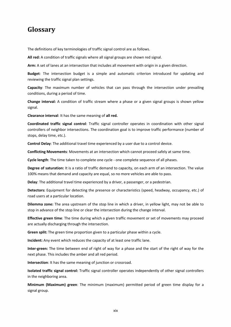
Glossary
The definitions of key terminologies of traffic signal control are as follows.
All red: A condition of traffic signals where all signal groups are shown red signal.
Arm: A set of lanes at an intersection that includes all movement with origin in a given direction.
Budget: The intersection budget is a simple and automatic criterion introduced for updating and
reviewing the traffic signal plan settings.
Capacity: The maximum number of vehicles that can pass through the intersection under prevailing
conditions, during a period of time.
Change interval: A condition of traffic stream where a phase or a given signal groups is shown yellow
signal.
Clearance interval: It has the same meaning of all red.
Coordinated traffic signal control: Traffic signal controller operates in coordination with other signal
controllers of neighbor intersections. The coordination goal is to improve traffic performance (number of
stops, delay time, etc.).
Control Delay: The additional travel time experienced by a user due to a control device.
Conflicting Movements: Movements at an intersection which cannot proceed safely at same time.
Cycle length: The time taken to complete one cycle - one complete sequence of all phases.
Degree of saturation: It is a ratio of traffic demand to capacity, on each arm of an intersection. The value
100% means that demand and capacity are equal, so no more vehicles are able to pass.
Delay: The additional travel time experienced by a driver, a passenger, or a pedestrian.
Detectors: Equipment for detecting the presence or characteristics (speed, headway, occupancy, etc.) of
road users at a particular location.
Dilemma zone: The area upstream of the stop line in which a driver, in yellow light, may not be able to
stop in advance of the stop line or clear the intersection during the change interval.
Effective green time: The time during which a given traffic movement or set of movements may proceed
are actually discharging through the intersection.
Green split: The green time proportion given to a particular phase within a cycle.
Incident: Any event which reduces the capacity of at least one traffic lane.
Inter-green: The time between end of right of way for a phase and the start of the right of way for the
next phase. This includes the amber and all red period.
Intersection: It has the same meaning of junction or crossroad.
Isolated traffic signal control: Traffic signal controller operates independently of other signal controllers
in the neighboring area.
Minimum (Maximum) green: The minimum (maximum) permitted period of green time display for a
signal group.
xx
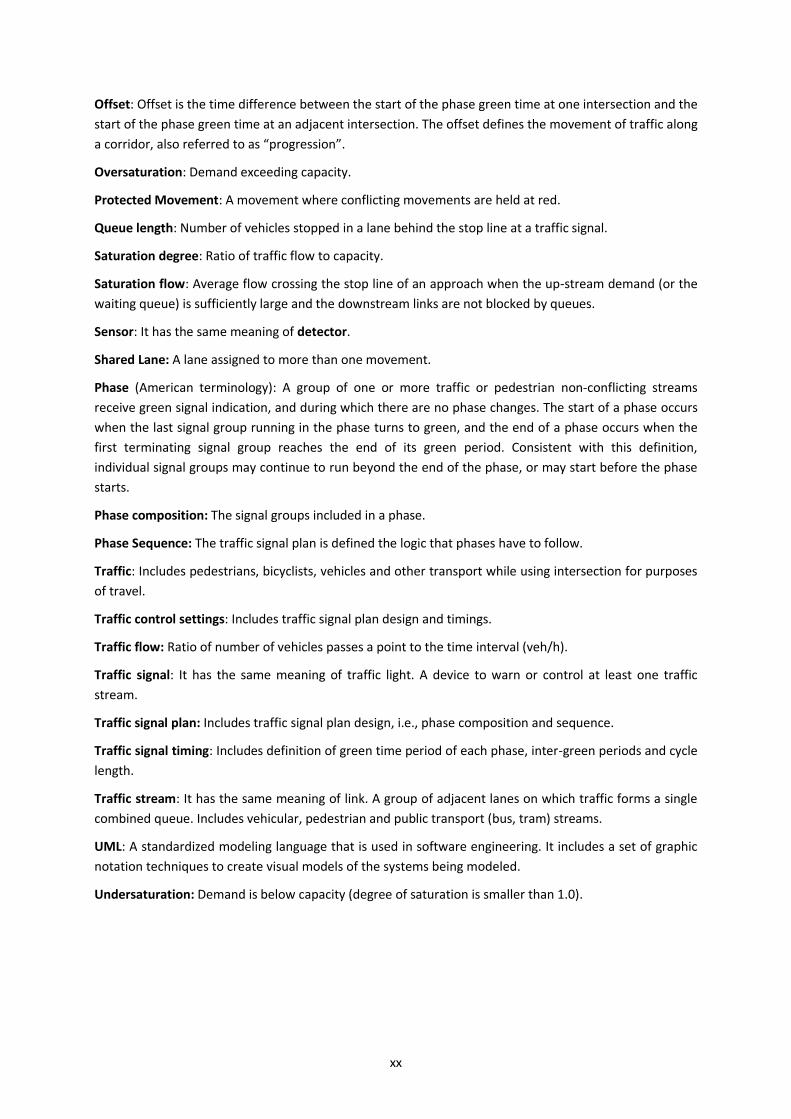
Offset: Offset is the time difference between the start of the phase green time at one intersection and the
start of the phase green time at an adjacent intersection. The offset defines the movement of traffic along
a corridor, also referred to as “progression”.
Oversaturation: Demand exceeding capacity.
Protected Movement: A movement where conflicting movements are held at red.
Queue length: Number of vehicles stopped in a lane behind the stop line at a traffic signal.
Saturation degree: Ratio of traffic flow to capacity.
Saturation flow: Average flow crossing the stop line of an approach when the up-stream demand (or the
waiting queue) is sufficiently large and the downstream links are not blocked by queues.
Sensor: It has the same meaning of detector.
Shared Lane: A lane assigned to more than one movement.
Phase (American terminology): A group of one or more traffic or pedestrian non-conflicting streams
receive green signal indication, and during which there are no phase changes. The start of a phase occurs
when the last signal group running in the phase turns to green, and the end of a phase occurs when the
first terminating signal group reaches the end of its green period. Consistent with this definition,
individual signal groups may continue to run beyond the end of the phase, or may start before the phase
starts.
Phase composition: The signal groups included in a phase.
Phase Sequence: The traffic signal plan is defined the logic that phases have to follow.
Traffic: Includes pedestrians, bicyclists, vehicles and other transport while using intersection for purposes
of travel.
Traffic control settings: Includes traffic signal plan design and timings.
Traffic flow: Ratio of number of vehicles passes a point to the time interval (veh/h).
Traffic signal: It has the same meaning of traffic light. A device to warn or control at least one traffic
stream.
Traffic signal plan: Includes traffic signal plan design, i.e., phase composition and sequence.
Traffic signal timing: Includes definition of green time period of each phase, inter-green periods and cycle
length.
Traffic stream: It has the same meaning of link. A group of adjacent lanes on which traffic forms a single
combined queue. Includes vehicular, pedestrian and public transport (bus, tram) streams.
UML: A standardized modeling language that is used in software engineering. It includes a set of graphic
notation techniques to create visual models of the systems being modeled.
Undersaturation: Demand is below capacity (degree of saturation is smaller than 1.0).
xxi
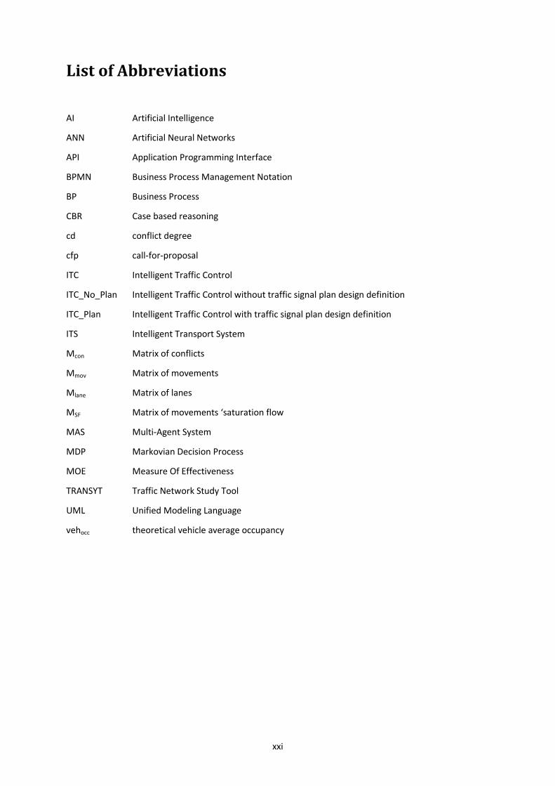
List of Abbreviations
AI Artificial Intelligence
ANN Artificial Neural Networks
API Application Programming Interface
BPMN Business Process Management Notation
BP Business Process
CBR Case based reasoning
cd conflict degree
cfp call-for-proposal
ITC Intelligent Traffic Control
ITC_No_Plan Intelligent Traffic Control without traffic signal plan design definition
ITC_Plan Intelligent Traffic Control with traffic signal plan design definition
ITS Intelligent Transport System
Mcon Matrix of conflicts
Mmov Matrix of movements
Mlane Matrix of lanes
MSF Matrix of movements ‘saturation flow
MAS Multi-Agent System
MDP Markovian Decision Process
MOE Measure Of Effectiveness
TRANSYT Traffic Network Study Tool
UML Unified Modeling Language
vehocc theoretical vehicle average occupancy

xxii
1
1. Introduction
The aim of this chapter is to introduce the research questions of the work carried out in this thesis, and to
present a brief description of the problem at hand along with the motivational aspects laying the grounds
upon which this study is established.
The main idea of this research work was to develop a strategy for controlling traffic lights that relies on
the flexibility and the maximal level of freedom in the design of traffic plan settings, while guaranteeing
efficiency under different conditions. As a result, this strategy should react to either non-schedulable or
unpredictable events without human intervention.
The chapter ends with a brief overview of the structure of the thesis.
1.1. Motivation
Transportation has always been a critical component of human society. Connecting places, transportation
is the “lifeblood” of the economy, bringing goods from producers to local market, taking people to their
homes to workplaces or leisure activities.
Since the second half of the last century, the traffic congestion problem has become predominant all over
the world due to the rapid increase in the number of vehicles of all transportation modes (Papageorgiou
et al., 2003). The traffic congestion appears when too many vehicles are attempting to use a common
transportation infrastructure with a limited capacity. Traffic congestion leads to the queuing phenomenon
and consequently yields excessive delays, degrading in several cases the use of the available
infrastructure, increasing fuel consumption and pollution, and many times causing irreversible
environmental damage.
In the recent past, one of the ways for improving traffic flow within urban environments has been focused
on the investment towards the construction of more road infrastructures increasing capacity. This
strategy, however, implies a high economic penalty and also consumes a large amount of the limited
space available within an urban area.
Another possible solution is improving the use of the available infrastructure via suitable application of
traffic management strategies at intersections. The intersections are often known as the bottleneck of
urban transportation systems (Chen and Cheng, 2010). Traffic signal control is considered to be a
competitive strategy for ensuring good operation of the intersection, improving mobility and addressing
environmental issues in urban networks (Park and Schneeberger, 2003). It also steers up some strategic
traffic management possibilities such as prioritization and promotion of different groups of travelers such
as pedestrians or bus passengers by providing appropriate facilities. Additionally, it can be used to
implement limitations of capacity for motor vehicles to manage traffic growth (Heydecker, 2004).
Nevertheless, the inefficient operation of traffic lights is a common problem certainly experienced by all
drivers, passengers, and pedestrians. This problem causes excessive and unnecessary delay, annoying
road users and affecting negatively the local economy. It also incurs in costs at different levels of the
urban network, such as increased fuel consumption, travel time, traffic emissions, and noise to mention
only but a few. In this way, a reliable and efficient operation of the traffic network is thus of crucial
importance for our society.
The optimization of traditional traffic signal timings represents a large effort and cost for traffic control
agencies. As a result, the number of times that the plans are updating is often limited by the agency
2
resources available for this task. In order to diminish the needed resources, there are traffic systems with
the capability of automatically changing signal timing in response to actual traffic variations. These
systems provide more effective control of traffic and require fewer resources to update the plans. Usually
the adaptive traffic control is based on sensors installed underneath the pavement close to the
intersection.
The research community has focused on the optimization of traffic signal plans that regulate traffic flow
at the intersection. Permission for one or more traffic streams to move on at the intersection is granted
during green time. In the present work the traffic stream is the base unit and can be defined as a single or
a group of movements in adjacent lanes on which traffic forms up a single combined queue and shares
the same traffic light according to the intersection topology, namely the geometric layout and the lanes
assigned to each movement. Hence traffic streams can be grouped into all possible ways outperforming
static phase composition resulting from offline traffic plan design control strategies.
Although there has been a relatively successful effort in optimizing traffic control by the research
community, these attempts often feature some shortcomings during control operation. First, traffic
control systems are often blind to the surrounding environment of the intersection; indeed, many
optimization approaches operate offline, using historically measured data to determine optimal traffic
control settings, thus missing changes to traffic state as traffic patterns do not remain static over time.
Other systems have some information collected in real time; however, they do not distinguish between
different traffic users and their needs.
Another issue commonly addressed in research is the use of centralized traffic control architectures. In a
control system with many intersections, the design of real-time signal plan updates is often an impossible
task; the communication network tends to be complex and recurrent system failures can result in
significant degradation of performance due to their interdependencies, which suggests an isolated control
strategy to be preferable.
Since industry is moving towards a period of abundance of traffic data, collected in real time by road
sensors (e.g. Smartphones applications, Bluetooth, Wi-Fi, GSM signal of mobile phones) or/and
vehicle/infrastructures communication, it seems that traffic signal control could take more advantage of
such significantly higher granularity of data.
Road sensors, widely spread over the network, have the limitation of giving only vehicle information at a
fixed location. However, new initiatives known as vehicle-infrastructure communication allow the wireless
transmission of the positions, headings, and speeds of vehicles for use by the traffic controller (Goodall et
al., 2013). As it is relatively a new technology, market penetration is not yet large enough, and it will take
some time until all vehicles can benefit from such communication platform.
Lastly, many approaches are evaluated in too simple scenarios which are not representative enough of
real-world traffic situations (e.g., a constantly varying demand or a complex network structure). In
general, current traffic signal control approaches are characterized by their lack of flexibility in their
control systems, constraining the definition of new green time values or new plan design structures.
Indeed, their self-rigidity is responsible for constraining the effectiveness of these strategies.
In spite of much research on the optimization of traffic plans, it is also important to pursue the target of
maintaining the system optimized and respecting the traffic management strategy adopted throughout
the operation period. Basically, after designing the best suitable traffic signal control given a demand it is
necessary to update the system according to the recurrent demand throughout the day, which may
experience slight differences or significant fluctuations. Such variations in demand can occur even within
3
very short intervals of time due to incidents, even within periods when demand is normally constant. In
such cases, the operation of traffic signal control with fixed traffic signal settings or with low flexibility to
adopt new settings may incur in sub-optimal operation.
The present research will thus tackle the shortcomings described above in order to develop a new traffic
control system more efficient, benefiting all road users.
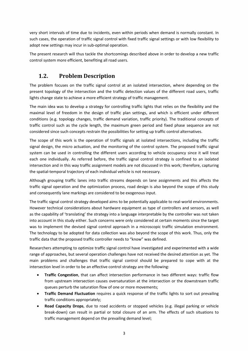
1.2. Problem Description
The problem focuses on the traffic signal control at an isolated intersection, where depending on the
present topology of the intersection and the traffic detection values of the different road users, traffic
lights change state to achieve a more efficient strategy of traffic management.
The main idea was to develop a strategy for controlling traffic lights that relies on the flexibility and the
maximal level of freedom in the design of traffic plan settings, and which is efficient under different
conditions (e.g. topology changes, traffic demand variation, traffic priority). The traditional concepts of
traffic control such as the cycle length, the maximum green period and fixed phase sequence are not
considered since such concepts restrain the possibilities for setting up traffic control alternatives.
The scope of this work is the operation of traffic signals at isolated intersections, including the traffic
signal design, the micro actuation, and the monitoring of the control system. The proposed traffic signal
system can be used in controlling the different users according to vehicle occupancy since it will treat
each one individually. As referred before, the traffic signal control strategy is confined to an isolated
intersection and in this way traffic assignment models are not discussed in this work; therefore, capturing
the spatial-temporal trajectory of each individual vehicle is not necessary.
Although grouping traffic lanes into traffic streams depends on lane assignments and this affects the
traffic signal operation and the optimization process, road design is also beyond the scope of this study
and consequently lane markings are considered to be exogenous input.
The traffic signal control strategy developed aims to be potentially applicable to real-world environments.
However technical considerations about hardware equipment as type of controllers and sensors, as well
as the capability of ‘translating’ the strategy into a language interpretable by the controller was not taken
into account in this study either. Such concerns were only considered at certain moments since the target
was to implement the devised signal control approach in a microscopic traffic simulation environment.
The technology to be adopted for data collection was also beyond the scope of this work. Thus, only the
traffic data that the proposed traffic controller needs to “know” was defined.
Researchers attempting to optimize traffic signal control have investigated and experimented with a wide
range of approaches, but several operation challenges have not received the desired attention as yet. The
main problems and challenges that traffic signal control should be prepared to cope with at the
intersection level in order to be an effective control strategy are the following:
Traffic Congestion, that can affect intersection performance in two different ways: traffic flow
from upstream intersection causes oversaturation at the intersection or the downstream traffic
queues perturb the saturation flow of one or more movements;
Traffic Demand Fluctuation requires a quick response of the traffic lights to sort out prevailing
traffic conditions appropriately;
Road Capacity Drops, due to road accidents or stopped vehicles (e.g. illegal parking or vehicle
break-down) can result in partial or total closure of an arm. The effects of such situations to
traffic management depend on the prevailing demand level;

4
Different Users, as the mix of different types of road users in sharing some space at intersection
raises operation challenge, due to their different characteristics (e.g. size, capacity, pollution
emissions) and conflicting interests. There can also be specific local policies such as prioritizing
public transport or favoring mobility of sustainable modes.
1.3. Objectives
In this research work, there are two problems of particular interest: one is how to design traffic signal
plans while exploring all possible solutions for phase composition; the other is how to maintain traffic
signal plan settings updated to meet the recurrent traffic demand of different users.
For the first problem, the major challenge is to develop a simple framework for traffic signal plan design
able to consider any intersection geometry with a few inputs. The second problem is to find the
optimization methodology for the computation of traffic control settings and the approach to update and
review its settings in real time.
The specific objectives of this research are thus listed as follows:
To study the viability of using a new programming logic for traffic signal control at intersections,
as a better alternative to the traditional traffic signal control methodologies. The proposed
strategy was developed in order to be more flexible and autonomous without compromising the
safety of road users.
To implement a microscopic view of the proposed traffic control strategy. This microscopic
perspective subdivides the control of the isolated intersection into sub-problems, such that the
combination of all the solutions of the sub-problems together yields the solution of the original
overall control problem. The coordination and the negotiation between traffic streams of the
same intersection should be accounted for so as to prevent negative effects to the local
optimization.
To incorporate the number of people (i.e., both inside vehicles and pedestrians) at the
intersection in the traffic control strategy. The traditional approach in traffic signal control is to
look at the traffic condition from the perspective of vehicle flow or vehicle delay. The possibility
of looking at the traffic condition distinguishing between vehicles with different occupancy,
public transport, bicycles, and pedestrians represents a potential opportunity for enhanced traffic
control. From the perspective of social welfare, it is reasonable and should be more important
and valuable to minimize “people’s” delays or other person-based measure rather than vehicle-
specific metrics. The same reasoning can be applied to vehicle types. In this way, green light could
be given according to traffic composition instead of vehicle volumes.
To investigate the minimum constraints to include on the proposed traffic control strategy.
Constraints, and its values (e.g.: the minimum green time, the maximum green time, the
maximum cycle length, the inter-green), are adopted due to reasons of operation, comfort
and/or safety.
To define the criteria for updating and reviewing the traffic signal plan settings. The process
should be simple and automatic in order to be performed in real time without human control.
To test the performance of developed strategy under different scenarios, such as different
intersection geometries and traffic demand profiles, so as to quantify the reliability and
robustness of the strategy.
To evaluate the performance of the proposed traffic control strategy, a set of baseline scenarios,
derived from well-established methods, is used as reference for assessment and comparison.
5
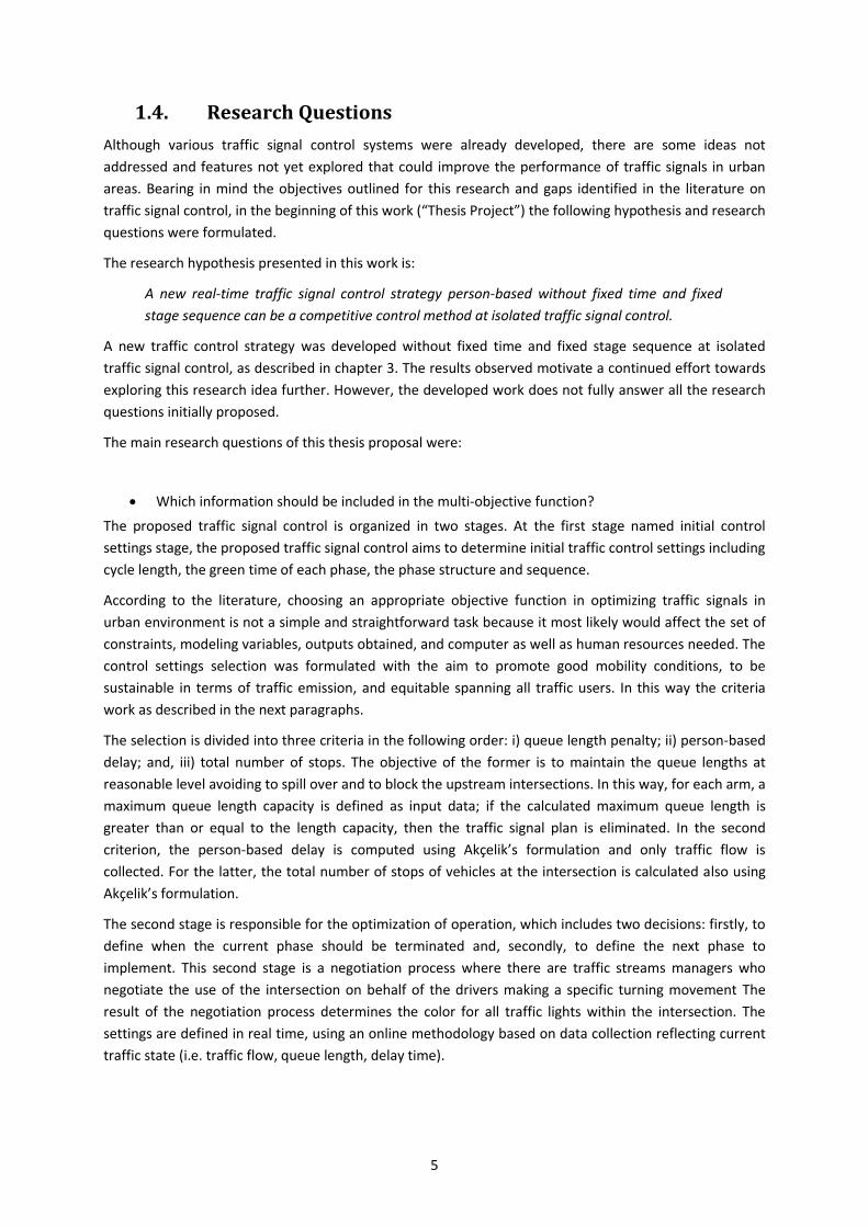
1.4. Research Questions
Although various traffic signal control systems were already developed, there are some ideas not
addressed and features not yet explored that could improve the performance of traffic signals in urban
areas. Bearing in mind the objectives outlined for this research and gaps identified in the literature on
traffic signal control, in the beginning of this work (“Thesis Project”) the following hypothesis and research
questions were formulated.
The research hypothesis presented in this work is:
A new real-time traffic signal control strategy person-based without fixed time and fixed
stage sequence can be a competitive control method at isolated traffic signal control.
A new traffic control strategy was developed without fixed time and fixed stage sequence at isolated
traffic signal control, as described in chapter 3. The results observed motivate a continued effort towards
exploring this research idea further. However, the developed work does not fully answer all the research
questions initially proposed.
The main research questions of this thesis proposal were:
Which information should be included in the multi-objective function?
The proposed traffic signal control is organized in two stages. At the first stage named initial control
settings stage, the proposed traffic signal control aims to determine initial traffic control settings including
cycle length, the green time of each phase, the phase structure and sequence.
According to the literature, choosing an appropriate objective function in optimizing traffic signals in
urban environment is not a simple and straightforward task because it most likely would affect the set of
constraints, modeling variables, outputs obtained, and computer as well as human resources needed. The
control settings selection was formulated with the aim to promote good mobility conditions, to be
sustainable in terms of traffic emission, and equitable spanning all traffic users. In this way the criteria
work as described in the next paragraphs.
The selection is divided into three criteria in the following order: i) queue length penalty; ii) person-based
delay; and, iii) total number of stops. The objective of the former is to maintain the queue lengths at
reasonable level avoiding to spill over and to block the upstream intersections. In this way, for each arm, a
maximum queue length capacity is defined as input data; if the calculated maximum queue length is
greater than or equal to the length capacity, then the traffic signal plan is eliminated. In the second
criterion, the person-based delay is computed using Akçelik’s formulation and only traffic flow is
collected. For the latter, the total number of stops of vehicles at the intersection is calculated also using
Akçelik’s formulation.
The second stage is responsible for the optimization of operation, which includes two decisions: firstly, to
define when the current phase should be terminated and, secondly, to define the next phase to
implement. This second stage is a negotiation process where there are traffic streams managers who
negotiate the use of the intersection on behalf of the drivers making a specific turning movement The
result of the negotiation process determines the color for all traffic lights within the intersection. The
settings are defined in real time, using an online methodology based on data collection reflecting current
traffic state (i.e. traffic flow, queue length, delay time).
6
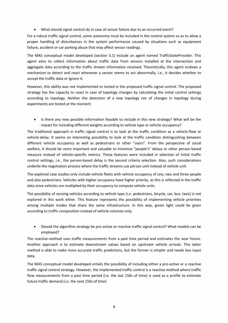
What should signal control do in case of sensor failure due to an occurred event?
For a robust traffic signal control, some autonomy must be included in the control system so as to allow a
proper handling of disturbances in the system performance caused by situations such as equipment
failure, accident or car parking abuse that may affect sensor readings.
The MAS conceptual model developed (section 3.1) include an agent named TrafficStateProvider. This
agent aims to collect information about traffic data from sensors installed at the intersection and
aggregate data according to the traffic stream information received. Theoretically, this agent endows a
mechanism to detect and react whenever a sensor seems to act abnormally, i.e., it decides whether to
accept the traffic data or ignore it.
However, this ability was not implemented or tested in the proposed traffic signal control. The proposed
strategy has the capacity to react in case of topology changes by calculating the initial control settings
according to topology. Neither the detection of a new topology nor of changes in topology during
experiments are tested at the moment.
Is there any new possible information feasible to include in this new strategy? What will be the
impact for including different weights according to vehicle type or vehicle occupancy?
The traditional approach in traffic signal control is to look at the traffic condition as a vehicle-flow or
vehicle-delay. It seems an interesting possibility to look at the traffic condition distinguishing between
different vehicle occupancy as well as pedestrians or other “users”. From the perspective of social
welfare, it should be more important and valuable to minimize “people’s” delays or other person-based
measure instead of vehicle-specific metrics. These features were included in selection of initial traffic
control settings, i.e., the person-based delay is the second criteria selection. Also, such considerations
underlie the negotiation process where the traffic streams use person unit instead of vehicle unit.
The explored case studies only include vehicle fleets with vehicle occupancy of one, two and three people
and also pedestrians. Vehicles with higher occupancy have higher priority, as this is reflected in the traffic
data since vehicles are multiplied by their occupancy to compute vehicle units.
The possibility of sensing vehicles according to vehicle type (i.e. pedestrians, bicycle, car, bus, taxis) is not
explored in this work either. This feature represents the possibility of implementing vehicle priorities
among multiple modes that share the same infrastructure. In this way, green light could be given
according to traffic composition instead of vehicle volumes only.
Should the algorithm strategy be pro-active or reactive traffic signal control? What models can be
employed?
The reactive-method uses traffic measurements from a past time period and estimates the near future.
Another approach is to estimate downstream values based on upstream vehicle arrivals. This latter
method is able to make more accurate traffic predictions, but the former is simpler and needs less input
data.
The MAS conceptual model developed entails the possibility of including either a pro-active or a reactive
traffic signal control strategy. However, the implemented traffic control is a reactive method where traffic
flow measurements from a past time period (i.e. the last 150s of time) is used as a profile to estimate
future traffic demand (i.e. the next 150s of time)
7
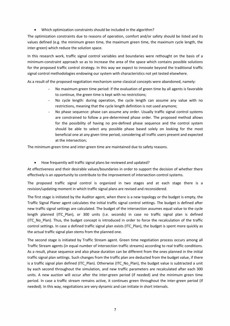
Which optimization constraints should be included in the algorithm?
The optimization constraints due to reasons of operation, comfort and/or safety should be listed and its
values defined (e.g. the minimum green time, the maximum green time, the maximum cycle length, the
inter-green) which reduce the solution space.
In this research work, traffic signal control variables and boundaries were rethought on the basis of a
minimum-constraint approach so as to increase the area of the space which contains possible solutions
for the proposed traffic control strategy. In this way we expect to innovate beyond the traditional traffic
signal control methodologies endowing our system with characteristics not yet tested elsewhere.
As a result of the proposed negotiation mechanism some classical concepts were abandoned, namely:
- No maximum green time period: if the evaluation of green time by all agents is favorable
to continue, the green time is kept with no restrictions;
- No cycle length: during operation, the cycle length can assume any value with no
restrictions, meaning that the cycle length definition is not used anymore;
- No phase sequence: phase can assume any order. Usually traffic signal control systems
are constrained to follow a pre-determined phase order. The proposed method allows
for the possibility of having no pre-defined phase sequence and the control system
should be able to select any possible phase based solely on looking for the most
beneficial one at any given time period, considering all traffic users present and expected
at the intersection;
The minimum green time and inter-green time are maintained due to safety reasons.
How frequently will traffic signal plans be reviewed and updated?
At effectiveness and their desirable values/boundaries in order to support the decision of whether there
effectively is an opportunity to contribute to the improvement of intersection control systems.
The proposed traffic signal control is organized in two stages and at each stage there is a
revision/updating moment in which traffic signal plans are revised and reconsidered.
The first stage is initiated by the Auditor agent, when there is a new topology or the budget is empty, the
Traffic Signal Planer agent calculates the initial traffic signal control settings. The budget is defined after
new traffic signal settings are calculated. The budget of the intersection assumes equal value to the cycle
length planned (ITC_Plan), or 300 units (i.e. seconds) in case no traffic signal plan is defined
(ITC_No_Plan). Thus, the budget concept is introduced in order to force the recalculation of the traffic
control settings. In case a defined traffic signal plan exists (ITC_Plan), the budget is spent more quickly as
the actual traffic signal plan stems from the planned one.
The second stage is initiated by Traffic Stream agent. Green time negotiation process occurs among all
Traffic Stream agents (in equal number of intersection traffic streams) according to real traffic conditions.
As a result, phase sequence and also phase duration can be different from the ones planned in the initial
traffic signal plan settings. Such changes from the traffic plan are deducted from the budget value, if there
is a traffic signal plan defined (ITC_Plan). Otherwise (ITC_No_Plan), the budget value is subtracted a unit
by each second throughout the simulation, and new traffic parameters are recalculated after each 300
units. A new auction will occur after the inter-green period (if needed) and the minimum green time
period. In case a traffic stream remains active, it continues green throughout the inter-green period (if
needed). In this way, negotiations are very dynamic and can initiate in short intervals.
8
What method(s) should be used for traffic signal plan optimization? Should traffic conditions at
an intersection guide the definition of the optimization strategy?
Optimization methods that can be applied in such systems can be divided into two groups, namely
classical optimization and heuristic optimization (and artificial intelligence). A discussion about the
potential of using each method should be attempted. This research question also entails investigating
whether the selection of the optimization strategy should adapt to the intersection layout and to traffic
demand.
The global architecture of the proposed traffic control system is designed using a Multi-Agent System
approach for isolated intersections and the traffic signal control is viewed as a problem of efficient
allocation of an available resource (green light) to consumers (traffic lights), where all traffic streams at an
intersection compete for the green time period. For this purpose, a novel auction-based intersection-
control mechanism for traffic signal control is developed. The present methodology underlies the
negotiation process, involving all traffic streams to manage the green time between them. The proposed
routine decides on a time period (auction frequency), an extension or an ending of the present green
period, based on recurrent demand and aiming at minimizing the person’s delay. In case of ending the
green light, a second decision is made in order to select which traffic streams should receive the green
light. Negotiations are very dynamic, and initiate in short intervals (i.e., just a few seconds). This
mechanism adopts a first-price, single-item auction.
Which scenarios will be employed to test the strategy?
The performance of the developed strategy should be tested under varied operational situations such as
different intersection layouts, different traffic demands and other events, so as to quantify the reliability
and robustness of the strategy.
The proposed traffic signal control is tested in seven scenarios with different intersection geometries
(number of approaches, number of lanes and pedestrian crossings) and traffic demand profiles. The
selected geometry layouts are from four real-world intersections in the city of Porto, Portugal. To test the
ability of the proposed approach to respond to different demand conditions, the experiments also include
different demand profiles for pedestrians and vehicles, with different vehicle occupancy of one, two and
three people. The traffic demand profiles applied are both from real-world traffic data collection and from
synthetic traffic data.
Which methods that may be used to compare and evaluate the developed strategy?
One or more existing strategies should be selected as the baseline in order to quantify the reliability of
the developed strategy.
Three established approaches for validation of the proposed strategy were defined which are commonly
implemented in real-world signalized intersections. These approaches work as baselines and are used to
allow comparisons with the proposed strategy. A description of each of such baseline approaches is
presented below as follows.

9
- Baseline 1: Fixed operation TRANSYT. In this approach, traffic signal control plans were
calculated with a well-established software named TRANSYT (Binning, 2014) For the
cases of scenarios with two intersections, the traffic signal plans are coordinated, sharing
a common cycle length that minimizes the amount of overall delay in the system. The
offset required is then computed for progression. Once the operation of the
intersections is fixed, traffic signal plans remains coordinated;
- Baseline 2: Actuated operation TRANSYT. The traffic signal plans were designed
following the approach above (Fixed operation TRANSYT), but now considering the
control operation in actuated time. During actuated time operation, traffic signal control
loses coordination, being caught when a new cycle length is adopted;
- Baseline 3: Real-world. This approach tries to reproduce the strategy implemented in
real-world environment. In two intersections, the actuated time operation with traffic
signal plans according with the period of the day is performed. In the other two
intersections, the real-world control is a centralized strategy in order to reproduce the
operation, it was selected the fixed operation with different cycles according with the
period of the day.
Can local optimization be “extrapolated” to the network optimization?
Lastly, the impact of the developed algorithm on the network optimization level should also be
investigated. Although the scope of this research work is focused on isolated intersections where each
intersection operates independently from each other, six of the seven developed scenarios tested two
intersections. However, the present research did not explore the present question further.
1.5. Thesis Organization
The structure of this research work includes five chapters.
Chapter 1 provides an introduction to the thesis and includes the description of the author’s motivations
as well as the objectives to be pursued in this research work.
Chapter 2 introduces the concepts of traffic signal control in terms of the main goal, elements, signal plan
design approaches, constraints, control strategies, and scope. The chapter also includes the review of the
state of the art on traffic signal control methods used in isolated intersection approaches.
Chapter 3 presents the design of the methodology used for developing the proposed traffic control, going
beyond the boundaries of current paradigms in traffic light control, i.e., each cycle and phase sequence
are independent; the adopted values for variables and plan design depend entirely on the actual traffic
conditions – they are not influenced by values of previous cycles. The control strategy design follows a
MAS perspective that was selected after an extensive review, as discussed in chapter 2. This chapter also
provides the description of the green-time negotiation process in order to maintain traffic control settings
updated, referred as the inspiration for the approach.
In order to test and validate the proposed traffic control, Chapter 4 begins with the description of the
selected virtual environment and the communication protocol developed to link the traffic simulation
model and the algorithm using an API module. The chapter also provides the descriptions of case studies,
including geometry and demand profiles. The performance of the two methods proposed for traffic
control is compared with the performance of baseline scenarios, where traffic control plans were

10
calculated with an established benchmark. The chapter also presents a description of measures of
effectiveness selected for performance analysis discussion.
Chapter 5 draws conclusions, highlighting major contributions and remarking most important findings
from this thesis, and closes the document with a discussion on potential directions for further research.
11
2. Literature Review
The goal of this chapter is mainly to provide background information regarding the concepts and main
approaches used. As well as a perspective on the research carried out by the community regarding traffic
signal control strategies. Although there is an effort to give a comprehensive description, the main goal is
to give the important information in order to give an understandable view of these scientific topics and
the rationale for using them. The chapter is structured as follows.
The first part of the present chapter is dedicated to introducing the traffic signal control for single
intersection in an urban network context, defining relevant concepts and presenting a generalized
overview of a general traffic control plan. First, section 2.1 introduces the traffic control paradigm, giving
some information regarding the history and the evolution of reasons for traffic control implementation.
Section 2.2 gives an overview of traffic control settings, divided in traffic signal plan and timings, used in
traditional methods and the choices made regarding control elements to include in the traffic control
proposed on chapter 3. Lastly, in section 2.3 traffic signal control strategies are presented according with
four characteristics: context, control, optimization and operation.
The second part of the chapter, section 2.4, is reserved for description of optimization methods for the
computation of the optimal signal settings of a traffic signal plan at isolated intersections. The section is
divided in three classes of methods. Their advantages and disadvantages are presented as well as their
historic evaluation.
2.1. Traffic Signal Control Goal
Traffic lights have the power to improve the safety at intersections, avoiding traffic conflicts between the
different vehicles and pedestrian movements by managing time in space. In order to avoid the dangerous
conflicts and to optimize the control, people have to wait for the green light, in the meantime lose time
which implies some frustration and vehicles consumes fuel and produce more emissions.
The objectives of signal control vary in accordance with the history time and the current policy of traffic
management authority.
The traffic signal control as it is known today has its base in the manual operation made by signalman of
police authority. The first automatic traffic light made its appearance in the beginning of the XX century.
At this time the goal of the traffic light was to improve the safety, avoiding accidents between vehicles
and pedestrians at intersections, through assigning alternative the right of way of conflicting movements
by displaying standard color code.
Over the years with the increase of traffic demand and congestion, the impact of traffic light in terms of
efficiency of network operation, for the same level of safety was realized by research community. So
besides grouping conflicting movements in different times to guarantee the safety operation of an
intersection, there also must be a strategy to split green time and movements grouping in order to lead to
the optimal operation.
In conclusion, the primary purpose of traffic control is the road safety, which in any case cannot be
forgotten or ignored. However signal timing offers the opportunity to improve the mobility and contribute
to environmental benefits if an efficient and relevant control methodology is employed.
In this research work, besides the basic goal of safety, traffic control’s proposed aim is to improve person
mobility at intersections. In a perspective of society management, it should be more important and
valuable to minimize “people” delays or other person-based measure, instead of vehicle measures. In this
12
way, green light could be given according to the number of persons waiting instead of the number of
vehicles.
2.2. Traffic Control Settings Overview
As stated in section 1.3, this research work studies the viability of using a new programming logic for
traffic signal control settings at intersections, more flexible and autonomous without compromising safety
of road users. Although, present work wants to be disruptive, breaking with the traditional concepts of
traffic control, in order to provide context there is described below the control elements typically used by
research community.
Traffic control settings include traffic signal plan and timings. For traffic signal control plan is needed the
specification of geometric layout of the intersection in order to define the compatible signal groups, the
phase composition, and the phase sequence. For traffic signal timing, besides the definition of approach
for green time split addressed in section 2.4, there is a need to define boundaries for timing variables.
These variables are much affected by the geometric layout, the traffic vehicles characteristics and the
drivers’ behavior.
Traffic light control uses three colors for road traffic and two colors for pedestrian. The sequence and
meaning of the colors slightly vary between countries, but the general purpose is the same and is
consistent inside the country. The traffic controller includes the three intervals: the permissive, the
change and the clearance using for that the green, the yellow /flashing green and the red for all traffic
lights, respectively.
2.2.1. Signal Plan Design
The following information is to be provided as part of signal plan design: phase composition and phase
sequence.
Traffic signal control regulates the traffic flow in the intersection, or more precisely, in the stop line. The
permission for traffic crossing from one or more lanes (or traffic streams) of one intersection approach is
granted during recurring intervals. Each period of access to the intersection for a particular set of lanes (or
traffic streams) is referred to as a phase.
The definition of term “phase” requires particular explanation. In literature review of traffic control,
“stage” and “phase” terms gave rise to some confusion because there are employed with conflicting
meanings. In countries such as USA and Australia, the term “phase” is employed to express the concept of
“stage” and reverse. As well, to give rise to confusion some countries use a similar term (e.g. “fase” in
Portuguese) which has similarities in spelling increasing the possibilities of misuse. Another point is from
the fact that in simple traffic control the two terms can be swapped without consequence because in
some specific cases they can truly have the same meaning. In more complex traffic control where the
number of phases is not equal to the number of signal groups (stages), the correct use of both terms is
important. In this document, there is used the American terminology and the term “stage” is replaced by
“signal group” in order to simplify and avoid confusion.
Geometric layout
A geometric layout of an intersection is composed by a number of approaches and a crossing area. An
approach may have one or two directions, with one or more lanes each. The base unit is the traffic stream
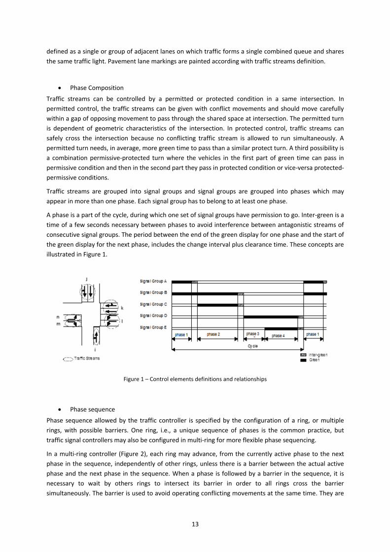
13
defined as a single or group of adjacent lanes on which traffic forms a single combined queue and shares
the same traffic light. Pavement lane markings are painted according with traffic streams definition.
Phase Composition
Traffic streams can be controlled by a permitted or protected condition in a same intersection. In
permitted control, the traffic streams can be given with conflict movements and should move carefully
within a gap of opposing movement to pass through the shared space at intersection. The permitted turn
is dependent of geometric characteristics of the intersection. In protected control, traffic streams can
safely cross the intersection because no conflicting traffic stream is allowed to run simultaneously. A
permitted turn needs, in average, more green time to pass than a similar protect turn. A third possibility is
a combination permissive-protected turn where the vehicles in the first part of green time can pass in
permissive condition and then in the second part they pass in protected condition or vice-versa protected-
permissive conditions.
Traffic streams are grouped into signal groups and signal groups are grouped into phases which may
appear in more than one phase. Each signal group has to belong to at least one phase.
A phase is a part of the cycle, during which one set of signal groups have permission to go. Inter-green is a
time of a few seconds necessary between phases to avoid interference between antagonistic streams of
consecutive signal groups. The period between the end of the green display for one phase and the start of
the green display for the next phase, includes the change interval plus clearance time. These concepts are
illustrated in Figure 1.
Figure 1 – Control elements definitions and relationships
Phase sequence
Phase sequence allowed by the traffic controller is specified by the configuration of a ring, or multiple
rings, with possible barriers. One ring, i.e., a unique sequence of phases is the common practice, but
traffic signal controllers may also be configured in multi-ring for more flexible phase sequencing.
In a multi-ring controller (Figure 2), each ring may advance, from the currently active phase to the next
phase in the sequence, independently of other rings, unless there is a barrier between the actual active
phase and the next phase in the sequence. When a phase is followed by a barrier in the sequence, it is
necessary to wait by others rings to intersect its barrier in order to all rings cross the barrier
simultaneously. The barrier is used to avoid operating conflicting movements at the same time. They are
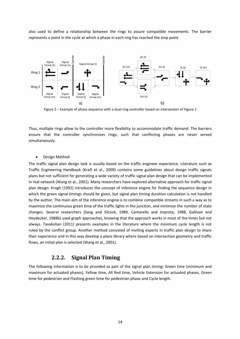
14
also used to define a relationship between the rings to assure compatible movements. The barrier
represents a point in the cycle at which a phase in each ring has reached the stop point.
a) b)
Figure 2 – Example of phase sequence with a dual-ring controller based on intersection of Figure 1
Thus, multiple rings allow to the controller more flexibility to accommodate traffic demand. The barriers
ensure that the controller synchronizes rings, such that conflicting phases are never served
simultaneously.
Design Method
The traffic signal plan design task is usually based on the traffic engineer experience. Literature such as
Traffic Engineering Handbook (Kraft et al., 2009) contains some guidelines about design traffic signals
plans but not sufficient for generating a wide variety of traffic signal plan design that can be implemented
in real network (Wang et al., 2001). Many researchers have explored alternative approach for traffic signal
plan design. Krogh (1992) introduces the concept of inference engine for finding the sequence design in
which the green signal timings should be given, but signal plan timing duration calculation is not handled
by the author. The main aim of the inference engine is to combine compatible streams in such a way as to
maximize the continuous green time of the traffic lights in the junction, and minimize the number of state
changes. Several researchers (Sang and Silcock, 1989, Cantarella and Improta, 1988, Gallivan and
Heydecker, 1988b) used graph approaches, knowing that the approach works in most of the times but not
always. Tavakolian (2011) presents examples in the literature where the minimum cycle length is not
ruled by the conflict group. Another method consisted of inviting experts in traffic plan design to share
their experience and in this way develop a plans library where based on intersection geometry and traffic
flows, an initial plan is selected (Wang et al., 2001).
2.2.2. Signal Plan Timing
The following information is to be provided as part of the signal plan timing: Green time (minimum and
maximum for actuated phases), Yellow time, All Red time, Vehicle Extension for actuated phases, Green
time for pedestrian and Flashing green time for pedestrian phase and Cycle length.
Ring 1
Ring 2
Signal
Group (k)
Signal
Group (n)
Signal
Group (m)
ba
rrie
r
Signal
Group (l)
v
v
Signal
Group (j)
Signal Group (l) ba
rrie
r
Signal
Group (m)
(k) (m)
v
vv
(n) (l)
(k) (l)
(l) (m)(l) (j)
(m) (n)
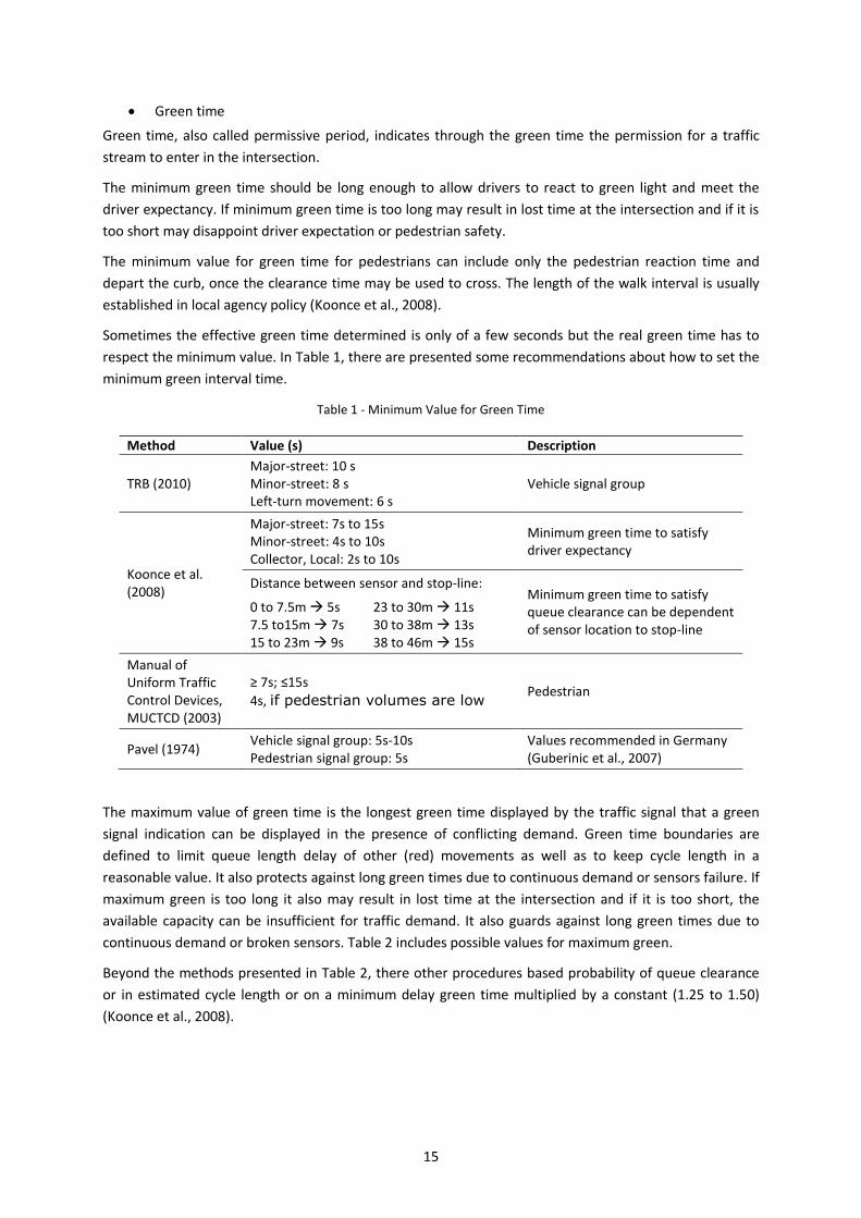
15
Green time
Green time, also called permissive period, indicates through the green time the permission for a traffic
stream to enter in the intersection.
The minimum green time should be long enough to allow drivers to react to green light and meet the
driver expectancy. If minimum green time is too long may result in lost time at the intersection and if it is
too short may disappoint driver expectation or pedestrian safety.
The minimum value for green time for pedestrians can include only the pedestrian reaction time and
depart the curb, once the clearance time may be used to cross. The length of the walk interval is usually
established in local agency policy (Koonce et al., 2008).
Sometimes the effective green time determined is only of a few seconds but the real green time has to
respect the minimum value. In Table 1, there are presented some recommendations about how to set the
minimum green interval time.
Table 1 - Minimum Value for Green Time
Method Value (s) Description
TRB (2010) Major-street: 10 s Minor-street: 8 s Left-turn movement: 6 s
Vehicle signal group
Koonce et al. (2008)
Major-street: 7s to 15s Minor-street: 4s to 10s Collector, Local: 2s to 10s
Minimum green time to satisfy driver expectancy
Distance between sensor and stop-line: Minimum green time to satisfy queue clearance can be dependent of sensor location to stop-line
0 to 7.5m 5s 7.5 to15m 7s 15 to 23m 9s
23 to 30m 11s 30 to 38m 13s 38 to 46m 15s
Manual of Uniform Traffic Control Devices, MUCTCD (2003)
≥ 7s; ≤15s
4s, if pedestrian volumes are low Pedestrian
Pavel (1974) Vehicle signal group: 5s-10s Pedestrian signal group: 5s
Values recommended in Germany (Guberinic et al., 2007)
The maximum value of green time is the longest green time displayed by the traffic signal that a green
signal indication can be displayed in the presence of conflicting demand. Green time boundaries are
defined to limit queue length delay of other (red) movements as well as to keep cycle length in a
reasonable value. It also protects against long green times due to continuous demand or sensors failure. If
maximum green is too long it also may result in lost time at the intersection and if it is too short, the
available capacity can be insufficient for traffic demand. It also guards against long green times due to
continuous demand or broken sensors. Table 2 includes possible values for maximum green.
Beyond the methods presented in Table 2, there other procedures based probability of queue clearance
or in estimated cycle length or on a minimum delay green time multiplied by a constant (1.25 to 1.50)
(Koonce et al., 2008).
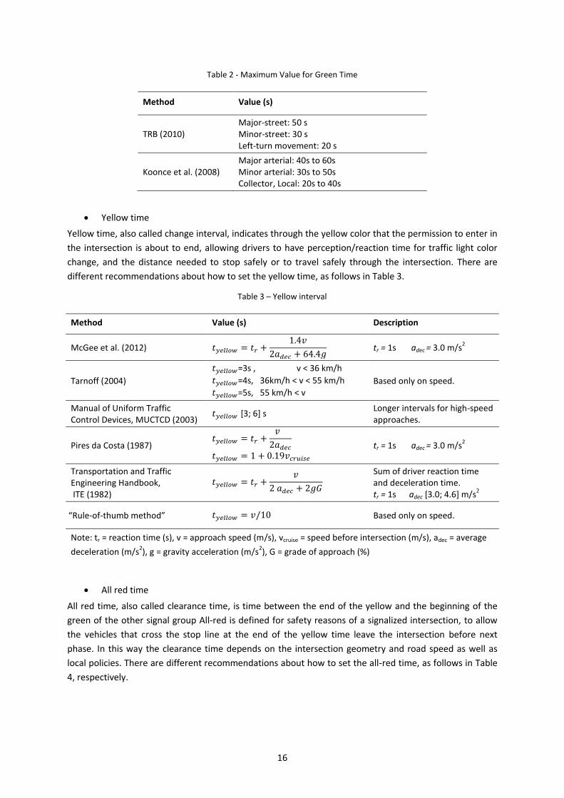
16
Table 2 - Maximum Value for Green Time
Method Value (s)
TRB (2010) Major-street: 50 s Minor-street: 30 s Left-turn movement: 20 s
Koonce et al. (2008) Major arterial: 40s to 60s Minor arterial: 30s to 50s Collector, Local: 20s to 40s
Yellow time
Yellow time, also called change interval, indicates through the yellow color that the permission to enter in
the intersection is about to end, allowing drivers to have perception/reaction time for traffic light color
change, and the distance needed to stop safely or to travel safely through the intersection. There are
different recommendations about how to set the yellow time, as follows in Table 3.
Table 3 – Yellow interval
Method Value (s) Description
McGee et al. (2012)
tr = 1s adec = 3.0 m/s
2
Tarnoff (2004)
=3s , v < 36 km/h
=4s, 36km/h < v < 55 km/h
=5s, 55 km/h < v Based only on speed.
Manual of Uniform Traffic Control Devices, MUCTCD (2003)
[3; 6] s Longer intervals for high-speed approaches.
Pires da Costa (1987)
tr = 1s adec = 3.0 m/s
2
Transportation and Traffic Engineering Handbook, ITE (1982)
Sum of driver reaction time and deceleration time. tr = 1s adec [3.0; 4.6] m/s
2
“Rule-of-thumb method” Based only on speed.
Note: tr = reaction time (s), v = approach speed (m/s), vcruise = speed before intersection (m/s), adec = average
deceleration (m/s2), g = gravity acceleration (m/s
2), G = grade of approach (%)
All red time
All red time, also called clearance time, is time between the end of the yellow and the beginning of the
green of the other signal group All-red is defined for safety reasons of a signalized intersection, to allow
the vehicles that cross the stop line at the end of the yellow time leave the intersection before next
phase. In this way the clearance time depends on the intersection geometry and road speed as well as
local policies. There are different recommendations about how to set the all-red time, as follows in Table
4, respectively.
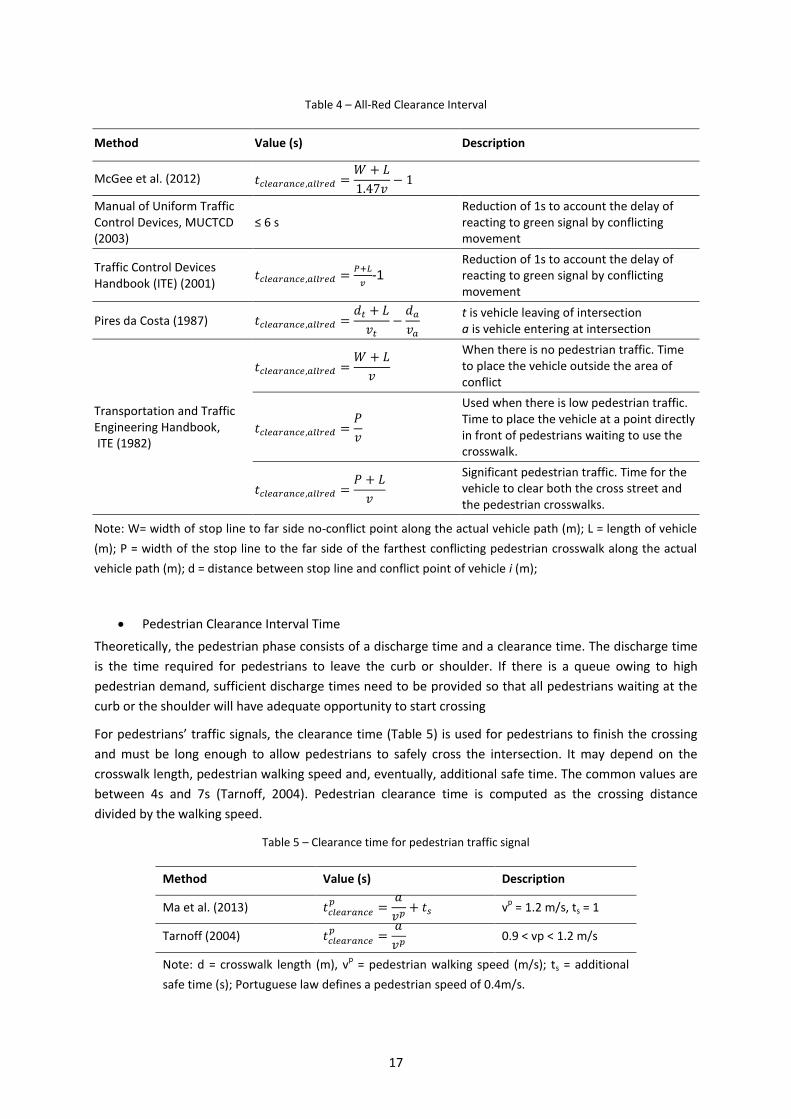
17
Table 4 – All-Red Clearance Interval
Method Value (s) Description
McGee et al. (2012)
Manual of Uniform Traffic Control Devices, MUCTCD (2003)
≤ 6 s Reduction of 1s to account the delay of reacting to green signal by conflicting movement
Traffic Control Devices Handbook (ITE) (2001)
-1
Reduction of 1s to account the delay of reacting to green signal by conflicting movement
Pires da Costa (1987)
t is vehicle leaving of intersection a is vehicle entering at intersection
Transportation and Traffic Engineering Handbook, ITE (1982)
When there is no pedestrian traffic. Time to place the vehicle outside the area of conflict
Used when there is low pedestrian traffic. Time to place the vehicle at a point directly in front of pedestrians waiting to use the crosswalk.
Significant pedestrian traffic. Time for the vehicle to clear both the cross street and the pedestrian crosswalks.
Note: W= width of stop line to far side no-conflict point along the actual vehicle path (m); L = length of vehicle
(m); P = width of the stop line to the far side of the farthest conflicting pedestrian crosswalk along the actual
vehicle path (m); d = distance between stop line and conflict point of vehicle i (m);
Pedestrian Clearance Interval Time
Theoretically, the pedestrian phase consists of a discharge time and a clearance time. The discharge time
is the time required for pedestrians to leave the curb or shoulder. If there is a queue owing to high
pedestrian demand, sufficient discharge times need to be provided so that all pedestrians waiting at the
curb or the shoulder will have adequate opportunity to start crossing
For pedestrians’ traffic signals, the clearance time (Table 5) is used for pedestrians to finish the crossing
and must be long enough to allow pedestrians to safely cross the intersection. It may depend on the
crosswalk length, pedestrian walking speed and, eventually, additional safe time. The common values are
between 4s and 7s (Tarnoff, 2004). Pedestrian clearance time is computed as the crossing distance
divided by the walking speed.
Table 5 – Clearance time for pedestrian traffic signal
Method Value (s) Description
Ma et al. (2013)
v
p = 1.2 m/s, ts = 1
Tarnoff (2004)
0.9 < vp < 1.2 m/s
Note: d = crosswalk length (m), vp = pedestrian walking speed (m/s); ts = additional
safe time (s); Portuguese law defines a pedestrian speed of 0.4m/s.
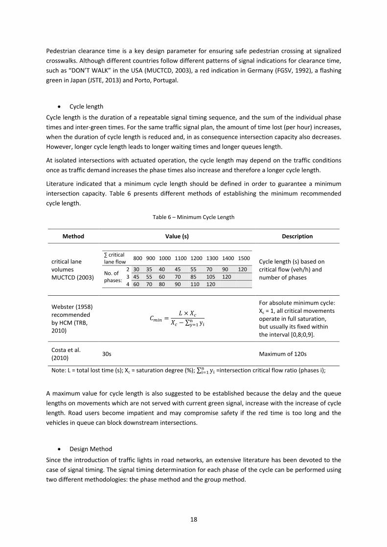
18
Pedestrian clearance time is a key design parameter for ensuring safe pedestrian crossing at signalized
crosswalks. Although different countries follow different patterns of signal indications for clearance time,
such as “DON’T WALK” in the USA (MUCTCD, 2003), a red indication in Germany (FGSV, 1992), a flashing
green in Japan (JSTE, 2013) and Porto, Portugal.
Cycle length
Cycle length is the duration of a repeatable signal timing sequence, and the sum of the individual phase
times and inter-green times. For the same traffic signal plan, the amount of time lost (per hour) increases,
when the duration of cycle length is reduced and, in as consequence intersection capacity also decreases.
However, longer cycle length leads to longer waiting times and longer queues length.
At isolated intersections with actuated operation, the cycle length may depend on the traffic conditions
once as traffic demand increases the phase times also increase and therefore a longer cycle length.
Literature indicated that a minimum cycle length should be defined in order to guarantee a minimum
intersection capacity. Table 6 presents different methods of establishing the minimum recommended
cycle length.
Table 6 – Minimum Cycle Length
Method Value (s) Description
critical lane volumes MUCTCD (2003)
∑ critical lane flow
800 900 1000 1100 1200 1300 1400 1500
No. of phases:
2 30 35 40 45 55 70 90 120
3 45 55 60 70 85 105 120
4 60 70 80 90 110 120
Cycle length (s) based on critical flow (veh/h) and number of phases
Webster (1958) recommended by HCM (TRB, 2010)
For absolute minimum cycle: Xc = 1, all critical movements operate in full saturation, but usually its fixed within the interval [0,8;0,9].
Costa et al. (2010)
30s Maximum of 120s
Note: L = total lost time (s); Xc = saturation degree (%); =intersection critical flow ratio (phases i);
A maximum value for cycle length is also suggested to be established because the delay and the queue
lengths on movements which are not served with current green signal, increase with the increase of cycle
length. Road users become impatient and may compromise safety if the red time is too long and the
vehicles in queue can block downstream intersections.
Design Method
Since the introduction of traffic lights in road networks, an extensive literature has been devoted to the
case of signal timing. The signal timing determination for each phase of the cycle can be performed using
two different methodologies: the phase method and the group method.
19
In the phase-based method, the signal groups are divided into a number of phases before calculation.
Each signal group has to belong to at least one phase. For the signal timing purpose, it is considered the
traffic flow of the representative traffic stream of each phase. A priori it must be defined: the phase
sequence, the inter-green time between phases (yellow and all red times), the traffic flows and the
saturation flows. The optimal green splits and the cycle length are calculated (Yagar, 1974, Allsop, 1972,
Allsop, 1971, Webster, 1958). The usual goal of this type of control is to minimize the total delay or to
maximize the intersection capacity. The phase-based description is often used as the basis for
optimization methods for signal timings. A number of constraints are applied to ensure that green time
interval of each phase exceeds a minimum acceptable value, an adequate capacity is provided, and the
cycle length lies in a suitable range. In this method, phases cannot normally be eliminated from or
introduced into the sequence by any automatic process because of the difficulties that this would cause
with the associated inter-greens (Heydecker, 1996).
While, in the group-based method (Gallivan and Heydecker, 1988a, Heydecker and Dudgeon, 1987,
Improta and Cantarella, 1984), each traffic stream is associated independently of the phase. The group-
based provides a higher degree of flexibility for the specification of traffic signal. The group-based method
determines the cycle length, the green time duration for each signal group and phasing combination,
respecting the compatibility of traffic streams defined a priori. The traffic flows and saturation flows are
still information known a priori. The optimal signal timing is evaluated according to the possible sets of
different signal groups (Akçelik, 1989). The group-based model requires a preliminary decision about the
definition of the traffic streams and their assignment to the lanes.
Lam et al. (1997) and (Wong and Wong (2003)), have extended the group-based approach to lane-based,
where the lane markings and the traffic streams are not known a priori. In lane-based method, the design
of junction geometry, lane allocation and signal timings can be performed together. In Lam et al. (1997)
method, the signal timing is not integrated. In contrast with other methods, this method can only be used
“once” because intersection layout once defined will not be updated shortly.
Groupbased control has been more explored since it is more flexible than the phasebased control.
Therefore it is better able to adapt to traffic conditions and to bring considerable benefits in complex
intersections (Heydecker and Dudgeon, 1987). The main disadvantage comes from the fact that this
flexibility requires a greater number of variables and constraints.
These methods are used to determine the signal timings plans, which can be implemented as fixed timed
or vehicle-actuated.
2.2.3. Summary
In conclusion, traffic signal control usually defines fixed traffic signal plans and boundaries for values of
cycle length, green time and inter-green. Constraints and its values are adopted due to reasons of
operation, comfort and/or safety.
In this research work, traffic signal control variables and boundaries were rethought, on the minimum
constraints focus in order to increase the area of the space which contains possible solutions for the
proposed traffic control strategy and to break with the traditional traffic signal control methodologies.
Traffic stream is defined as the base unit, instead of signal group or phase, for proposed traffic signal
control.
For signal plan design there is no fixed plan, no phase sequence and, no fixed phase composition. The
proposed method is able to select any possible phase respecting only the inter-green period.
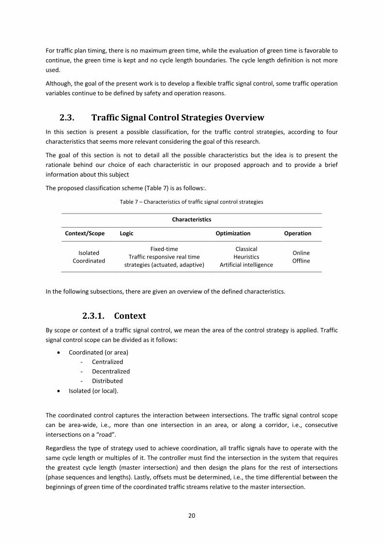
20
For traffic plan timing, there is no maximum green time, while the evaluation of green time is favorable to
continue, the green time is kept and no cycle length boundaries. The cycle length definition is not more
used.
Although, the goal of the present work is to develop a flexible traffic signal control, some traffic operation
variables continue to be defined by safety and operation reasons.
2.3. Traffic Signal Control Strategies Overview
In this section is present a possible classification, for the traffic control strategies, according to four
characteristics that seems more relevant considering the goal of this research.
The goal of this section is not to detail all the possible characteristics but the idea is to present the
rationale behind our choice of each characteristic in our proposed approach and to provide a brief
information about this subject
The proposed classification scheme (Table 7) is as follows:.
Table 7 – Characteristics of traffic signal control strategies
Characteristics
Context/Scope Logic Optimization Operation
Isolated Coordinated
Fixed-time Traffic responsive real time
strategies (actuated, adaptive)
Classical Heuristics
Artificial intelligence
Online Offline
In the following subsections, there are given an overview of the defined characteristics.
2.3.1. Context
By scope or context of a traffic signal control, we mean the area of the control strategy is applied. Traffic
signal control scope can be divided as it follows:
Coordinated (or area)
- Centralized
- Decentralized
- Distributed
Isolated (or local).
The coordinated control captures the interaction between intersections. The traffic signal control scope
can be area-wide, i.e., more than one intersection in an area, or along a corridor, i.e., consecutive
intersections on a “road”.
Regardless the type of strategy used to achieve coordination, all traffic signals have to operate with the
same cycle length or multiples of it. The controller must find the intersection in the system that requires
the greatest cycle length (master intersection) and then design the plans for the rest of intersections
(phase sequences and lengths). Lastly, offsets must be determined, i.e., the time differential between the
beginnings of green time of the coordinated traffic streams relative to the master intersection.
21
Coordinated control started by static logic, which consists of finding the appropriate traffic signal plans
and timings to optimize traffic flow. This results in the so-called “green wave method” that flows through
the main streets of a city, allowing the consecutive traffic signals to switch with an offset equivalent to the
expected vehicle travel time between intersections ideally enabling vehicles to drive through them
without facing a red light. Thus, waves of green light “move” through the street at the same speed as the
vehicles.
Computer tools for generating coordinated timing plans were developed, generally, with one of two
different types of main goals: maximization of the bandwidth (green wave extension) of the progression,
or minimization of the overall delay and stops (French and French, 2006). Bandwidth optimization
techniques, such as MAXBAND (Little et al., 1981), PASSER II (Chang and Messer, 1991), and PASSER IV
(Chaudhary et al., 2002), use traffic volumes, distance between traffic signals and desired travel speed to
determine the optimum width of progression band that can be accommodated onto an arterial. Because
bandwidth optimization techniques are attempting to provide as wide of a progression band as possible,
they generally result in longer cycle lengths so as to permit larger amounts of traffic to pass through an
intersection during the green interval. The second approach, such as TRANSYT-7F (McTrans, 2010) and
TRANSYT - Traffic Network Study Tool (Robertson, 1969), uses models to find a common cycle length that
minimizes the amount of overall delay in the system and then computes the offset required for
progression. As a result, these optimization techniques generally produce cycle lengths that are shorter
than those produced by bandwidth optimization techniques. Because these two approaches are
attempting to develop signal timing plans to achieve different design objectives (maximize bandwidth
versus minimize delay), they can result in significantly different signal timing plans for similar traffic
conditions.
On the one hand, the main advantage of coordination is achieved when most of the traffic flows in the
direction of the green wave. On the other hand, disadvantages can be of three types. First, since only one
traffic corridor can have “green waves”, the vehicles flowing in the opposite directions of the green wave
may or will be delayed. Second, once coordination behavior is static, current state of the traffic is
generally disregarded. In fact, if there is a high traffic density, vehicles entering a green wave will be
stopped by vehicles ahead of them or by vehicles that turned into the corridor, and once a vehicle misses
the green wave, it will have to wait the whole duration of the red light to enter the next green wave
(Gershenson and Rosenblueth, 2012). Lastly, when traffic densities are very low, vehicles might arrive too
quickly at the next intersection, having to stop at each intersection (Gershenson and Rosenblueth, 2012).
To overcome the aforementioned disadvantages, a number of dynamic coordination strategies were
developed, so traffic signal control could react to incidents. In order to be able to respond to real-time
varying traffic conditions, such strategies require sensors to collect traffic data, which are incorporated
into the control system. Dynamic traffic control strategies are more reliable and efficient, but demand a
big engineering effort and more expenses due to higher installation and maintenance costs (Papageorgiou
et al., 2003).
Concerning dynamic coordination there are three main approaches, namely centralized, decentralized
and distributed, as presented in Figure 3 and described below.
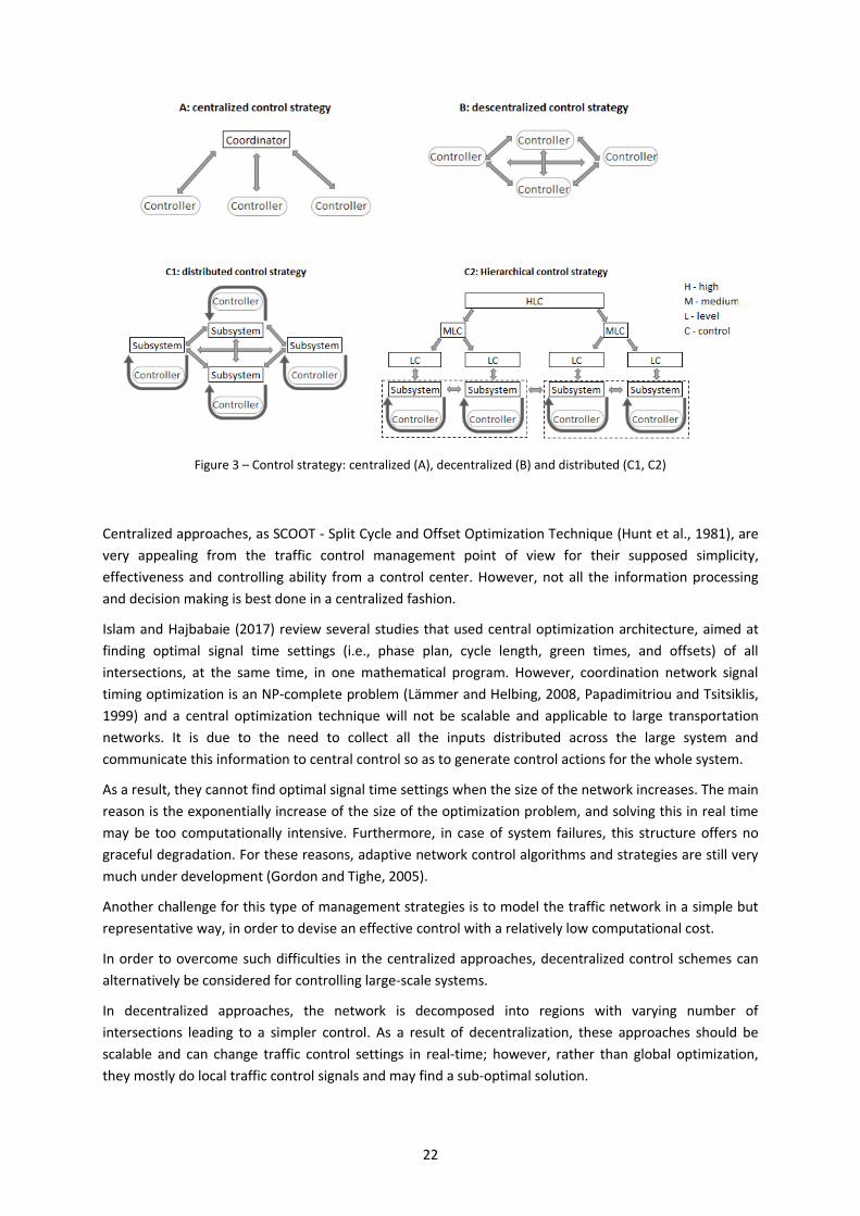
22
Figure 3 – Control strategy: centralized (A), decentralized (B) and distributed (C1, C2)
Centralized approaches, as SCOOT - Split Cycle and Offset Optimization Technique (Hunt et al., 1981), are
very appealing from the traffic control management point of view for their supposed simplicity,
effectiveness and controlling ability from a control center. However, not all the information processing
and decision making is best done in a centralized fashion.
Islam and Hajbabaie (2017) review several studies that used central optimization architecture, aimed at
finding optimal signal time settings (i.e., phase plan, cycle length, green times, and offsets) of all
intersections, at the same time, in one mathematical program. However, coordination network signal
timing optimization is an NP‐complete problem (Lämmer and Helbing, 2008, Papadimitriou and Tsitsiklis,
1999) and a central optimization technique will not be scalable and applicable to large transportation
networks. It is due to the need to collect all the inputs distributed across the large system and
communicate this information to central control so as to generate control actions for the whole system.
As a result, they cannot find optimal signal time settings when the size of the network increases. The main
reason is the exponentially increase of the size of the optimization problem, and solving this in real time
may be too computationally intensive. Furthermore, in case of system failures, this structure offers no
graceful degradation. For these reasons, adaptive network control algorithms and strategies are still very
much under development (Gordon and Tighe, 2005).
Another challenge for this type of management strategies is to model the traffic network in a simple but
representative way, in order to devise an effective control with a relatively low computational cost.
In order to overcome such difficulties in the centralized approaches, decentralized control schemes can
alternatively be considered for controlling large-scale systems.
In decentralized approaches, the network is decomposed into regions with varying number of
intersections leading to a simpler control. As a result of decentralization, these approaches should be
scalable and can change traffic control settings in real-time; however, rather than global optimization,
they mostly do local traffic control signals and may find a sub-optimal solution.
23
The ALLONS-D (Porche and Lafortune, 1999) is probably the most well-known software with decentralized
architecture. They decomposed the network to the intersection level and used dynamic programming
based on tree searching algorithm to select the phase receiving green signal at each time interval. The
intersections do not coordinate explicitly their decisions; on the contrary, due to the incorporation of data
from upstream, there is an implicit coordination among intersections in arterial. For network application,
authors proposed a two-layer hierarchy approach. The application of such hierarchical version in arterial
scope has improved system performance when compared to unbiased (i.e., with unity weights for all
phases) decentralized controllers. However, ALLONS-D is computationally expensive and cannot solve the
problem in real time (Islam and Hajbabaie, 2017).
The self-organizing traffic signals use a decentralized optimization scheme, which enables global
coordination of the traffic streams on road networks (Placzek, 2014). The global coordination is adaptively
achieved by local interactions between vehicles and traffic signals, generating flexible green waves based
on traffic demand. Self-organization systems are defined as elements that interact in order to achieve
dynamically a global function or behavior. This function or behavior is not imposed by either one single or
a few elements, nor it is determined hierarchically. It is however achieved autonomously as the elements
interact with one another. Traffic signals are called self-organizing because each traffic signal control
makes a decision based only on local information about its own state (Gershenson and Rosenblueth,
2012). This gives time for other vehicles to join them. As more vehicles join the group, vehicles will wait
less time behind red lights. With a sufficient number of vehicles, the red lights will turn green even before
they reach the intersection, generating “green corridors” (Gershenson, 2004). If there are no vehicles
approaching a red light, the complementary one can stay green.
This method is self-organizing because the global performance is determined by the local rules followed
by each traffic signal: they are “unaware” of the state of other intersections and still manage to achieve
global coordination. The method uses a similar idea to the one used by Porche and Lafortune (1999) but
with a much simpler implementation, without prediction of arrivals at intersections, or communication
between traffic signals or fixed cycles lengths.
Recent approaches make use of intelligent agents to act upon the traffic system in a completely
decentralized fashion. In general, a decentralized signal control system can be modeled as MAS which
each signal controller is considered as an agent, i.e., each intersection operates individually and
autonomously without coordinating explicitly with other agents. Due to the ease of implementation and
the development of cheap communication devices, there have been increasing efforts for promoting
decentralized signal control systems based on the MAS metaphor.
In fact, in a decentralized multi-agent system, the agents are scattered all over the environment. Each
agent has a limited sensing capability because of the range and coverage of the sensors connected to it,
which limits the view available to each agent in the environment.
The emerging technology of autonomous vehicles even furthers the possibility of sharing and exploring
information of vehicles and their environment to improve control performance. So decentralized
approaches have been gaining territory in literature once each intersection determines its own control
policy based on the information received from other vehicles on the road (Dresner and Stone, 2008,
Vasirani and Ossowski, 2012).
In case of strong interactions among the subsystems, the local optimization of each system can lead to
conflicts. In order to overcome these conflicts, the distributed strategy decomposes the traffic signal time
optimization problem into several interconnected sub-problems. Therefore, the difference to
decentralized approaches is that it allows sub-systems to exchange some information about constraints
24
and variables, and to share resources. In a typical case, the information propagates from intersection to
intersection with a decreasing weight. By doing so, it can yield coordination among the controllers and
achieve better system performance. However, this approach poses many challenges such as coordination
increasing the computational complexity and the communication overhead, as well as the associated
costs.
Another way of doing the distributed control, namely the hierarchical approach, is to include a central
control unit. The control is distributed among the multilevel hierarchy of subsystem as shown in Figure 3.
The underlying concept of most hierarchical approaches is to handle slow-varying and wide-area-level
decisions at upper levels and perform real-time and small-area computations in lower levels (Islam and
Hajbabaie, 2017). As a result, the upper and lower levels may have objective functions that compete with
each other. This approach decomposes the system structure in such a way, so as to improve the
computational efficiency. Therefore, designing signal control methods with a reasonable balance between
these levels is quite challenging and laborious (Dion and Hellinga, 2001).
The most widely-used hierarchical approach is SCATS - Sydney Coordinated Adaptive Traffic System (Sims
and Dobinson, 1979, Lowrie, 1990), where an intersection, in each sub-network, is set to be the critical
one, and cycle lengths and splits are optimized for this particular intersection. There are other systems
known but less widely used such as: RHODES - Real-Time Hierarchical Optimized Distributed and Effective
System (Head et al., 1992, Mirchandani and Head, 2001), OPAC - Optimization Policies for Adaptive
Control (Liao, 1998) and UTOPIA - Urban Traffic Optimization by Integrated Automation (Mauro and Di
Taranto, 1989). The algorithms above use pre-specified plans for the traffic signals phases. Therefore,
these control systems have limitations in finding the phase composition, the sequence and the traffic
signal times.
The second main type of scope is isolated control strategy, which only captures the traffic conditions
around the intersection. Therefore, the green time periods assignment is independent from other traffic
signals, allowing the flexibility to assume the optimal cycle length and traffic signal plan. This means that
the control algorithm can be much simpler and have a higher degree of freedom to choose traffic control
settings than coordinated control counterparts (Kronborg et al., 1997) awarding to this type of control a
worthy advantage.
Albeit only in last years, the research community has given more attention to coordination than to
isolated intersections; isolated control at intersection is still quite present in cities. The number of isolated
traffic signal control intersections exceeds 50% of the implemented equipment’s in a large number of
countries throughout the world (Guberinic et al., 2007). Nowadays, in Municipality of Porto (Portugal),
57% of traffic control follows an isolated control approach. Therefore, it is also important to develop good
algorithms for traffic signal control at isolated intersections.
The main drawback of isolated approaches is not being able to capture the interaction between
intersections, as coordinated control does. In case of saturated conditions when adjacent intersections
are close, the traffic queues forming up at downstream intersections spill back and deteriorate the
performance of upstream intersections. To overcome this, very closely spaced intersections can be in
practice considered a single traffic junction in terms of traffic control due to the large influence that many
of them have on each other.
There are a few systems purposely designed for optimizing isolated intersection operation in literature,
such as MOVA - Microprocessor Optimized Vehicle Activation (Vincent and Peirce, 1988) and SOS - Self
Optimized Signal Control (Kronborg et al., 1997).
25
2.3.2. Logic
There is a wide range of logic by which traffic signal can be controlled. Control logic means how the
controller responds to local conditions. The types of traffic signal control logic can be divided as it follows:
fixed-time;
traffic responsive:
- actuated control;
- adaptive control.
The first traffic signal control developed was controlled by fixed-time. In the fixed-time control, the green
times and the phase sequence are fixed. The green time calculation is computed based on historical traffic
data collected under the assumption that traffic arrival is uniform. Although several fixed plans can be
performed for different times of the day the traffic signal control executes them in blindness without
regard to the actual traffic conditions. To determine when to change timing plans is used a tool based on
the time-of-day or the day-of-week schedule. This strategy can be described as an optimization problem
solved offline, once it is developed using historical traffic data. The traffic signal usually provides an
efficient operation during peak traffic periods, once traffic settings are generally projected for this period.
Out of this period, mainly at night, is common to observe vehicles or pedestrians stopped for no reason
because there is no traffic in conflicting movements. In some cities to avoid unnecessary delay, in the
night, the traffic light becomes flashing yellow. Chandra (2009) has noted some benefit to switching off
traffic signals or introducing flashing yellow.
Fixed-time control is able to provide efficient coordination with adjacent intersection with the same type
of control, since begin and end of green time are predictable. Another advantage is the absence of
sensors which simplify maintenance and reduce operation problems.
On the other hand, fixed-time control cannot react and adapt to traffic demand changes and fluctuations
in traffic flows such as accidents, unplanned roadwork or random traffic arrives.
Despite their important role in traffic management, the traffic signals, once installed, are often not
proactively managed. Maintenance activities are frequently delayed or cancelled, in reaction to shrinking
budgets and staffs.
There are several examples of established software packages for fixed-time signal plans such as the
TRANSYT (Robertson, 1969). The traffic signal plans obtained from the software packages usually serve to
provide a benchmark for analytical studies and a reference library of plan designs for operation.
Traffic responsive control is another option for traffic signal control, which is a strategy more suitable
when traffic demand varies broadly within a day, such traffic signal operation depends on the actual
traffic flow demand. There are generally two kind of traffic responsive control: the actuated control and
the adaptive control.
The main idea of actuated control is to detect the vehicle presence through sensors, placed in the traffic
signal system, and to adapt the control operation to traffic demand fluctuation. The information collected
is used to decide if green time signal is extended to allow the vehicles to go through its journey or end the
phase depending on the current traffic demand. So the cycle length and green time allocation is unknown
in advance, thus this value can be different cycle by cycle. The process is based on some parameters
(weights): maximum green time, minimum green time and vehicle extension, for each signal group.
During the minimum green time the traffic signal is green whether there is traffic demand or not. After
minimum green time, actuated control uses the gap-seek logic to respond to traffic fluctuations, the
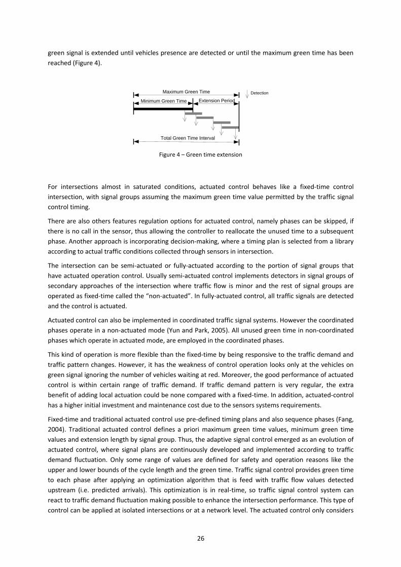
26
green signal is extended until vehicles presence are detected or until the maximum green time has been
reached (Figure 4).
Figure 4 – Green time extension
For intersections almost in saturated conditions, actuated control behaves like a fixed-time control
intersection, with signal groups assuming the maximum green time value permitted by the traffic signal
control timing.
There are also others features regulation options for actuated control, namely phases can be skipped, if
there is no call in the sensor, thus allowing the controller to reallocate the unused time to a subsequent
phase. Another approach is incorporating decision-making, where a timing plan is selected from a library
according to actual traffic conditions collected through sensors in intersection.
The intersection can be semi-actuated or fully-actuated according to the portion of signal groups that
have actuated operation control. Usually semi-actuated control implements detectors in signal groups of
secondary approaches of the intersection where traffic flow is minor and the rest of signal groups are
operated as fixed-time called the “non-actuated”. In fully-actuated control, all traffic signals are detected
and the control is actuated.
Actuated control can also be implemented in coordinated traffic signal systems. However the coordinated
phases operate in a non-actuated mode (Yun and Park, 2005). All unused green time in non-coordinated
phases which operate in actuated mode, are employed in the coordinated phases.
This kind of operation is more flexible than the fixed-time by being responsive to the traffic demand and
traffic pattern changes. However, it has the weakness of control operation looks only at the vehicles on
green signal ignoring the number of vehicles waiting at red. Moreover, the good performance of actuated
control is within certain range of traffic demand. If traffic demand pattern is very regular, the extra
benefit of adding local actuation could be none compared with a fixed-time. In addition, actuated-control
has a higher initial investment and maintenance cost due to the sensors systems requirements.
Fixed-time and traditional actuated control use pre-defined timing plans and also sequence phases (Fang,
2004). Traditional actuated control defines a priori maximum green time values, minimum green time
values and extension length by signal group. Thus, the adaptive signal control emerged as an evolution of
actuated control, where signal plans are continuously developed and implemented according to traffic
demand fluctuation. Only some range of values are defined for safety and operation reasons like the
upper and lower bounds of the cycle length and the green time. Traffic signal control provides green time
to each phase after applying an optimization algorithm that is feed with traffic flow values detected
upstream (i.e. predicted arrivals). This optimization is in real-time, so traffic signal control system can
react to traffic demand fluctuation making possible to enhance the intersection performance. This type of
control can be applied at isolated intersections or at a network level. The actuated control only considers
Minimum Green Time
Total Green Time Interval
Extension Period
Maximum Green Time Detection
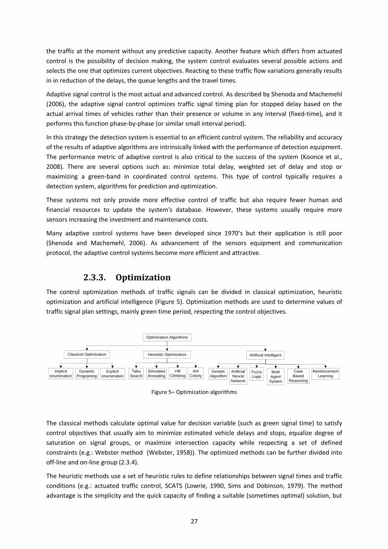
27
the traffic at the moment without any predictive capacity. Another feature which differs from actuated
control is the possibility of decision making, the system control evaluates several possible actions and
selects the one that optimizes current objectives. Reacting to these traffic flow variations generally results
in in reduction of the delays, the queue lengths and the travel times.
Adaptive signal control is the most actual and advanced control. As described by Shenoda and Machemehl
(2006), the adaptive signal control optimizes traffic signal timing plan for stopped delay based on the
actual arrival times of vehicles rather than their presence or volume in any interval (fixed-time), and it
performs this function phase-by-phase (or similar small interval period).
In this strategy the detection system is essential to an efficient control system. The reliability and accuracy
of the results of adaptive algorithms are intrinsically linked with the performance of detection equipment.
The performance metric of adaptive control is also critical to the success of the system (Koonce et al.,
2008). There are several options such as: minimize total delay, weighted set of delay and stop or
maximizing a green-band in coordinated control systems. This type of control typically requires a
detection system, algorithms for prediction and optimization.
These systems not only provide more effective control of traffic but also require fewer human and
financial resources to update the system's database. However, these systems usually require more
sensors increasing the investment and maintenance costs.
Many adaptive control systems have been developed since 1970’s but their application is still poor
(Shenoda and Machemehl, 2006). As advancement of the sensors equipment and communication
protocol, the adaptive control systems become more efficient and attractive.
2.3.3. Optimization
The control optimization methods of traffic signals can be divided in classical optimization, heuristic
optimization and artificial intelligence (Figure 5). Optimization methods are used to determine values of
traffic signal plan settings, mainly green time period, respecting the control objectives.
Figure 5– Optimization algorithms
The classical methods calculate optimal value for decision variable (such as green signal time) to satisfy
control objectives that usually aim to minimize estimated vehicle delays and stops, equalize degree of
saturation on signal groups, or maximize intersection capacity while respecting a set of defined
constraints (e.g.: Webster method (Webster, 1958)). The optimized methods can be further divided into
off-line and on-line group (2.3.4).
The heuristic methods use a set of heuristic rules to define relationships between signal times and traffic
conditions (e.g.: actuated traffic control, SCATS (Lowrie, 1990, Sims and Dobinson, 1979). The method
advantage is the simplicity and the quick capacity of finding a suitable (sometimes optimal) solution, but
Optimization Algorithms
Classical Optimization Heuristic Optimization
Implicit
enumeration
Dynamic
Programing
Explicit
enumeration
Genetic
Algorithm
Simulated
Annealing
Artificial Intelligent
Hill
ClimbingArtificial
Neural
Network
Tabu
Search
Ant
ColonyFuzzy
LogicMulti
Agent
System
Reinforcement
Learning
Case
Based
Reasoning
28
control performance is not optimized. Although the aim is to find a high quality solution, heuristics want
to find a “good” solution.
Heuristic search is capable of finding suitable and/or optimal solutions for phase/ signal group timing
more quickly than ordinal exhaustive enumeration.
In recent years, the optimization methods begin to apply artificial intelligence (AI) techniques to solve the
complicated traffic control problem. This approach is based in human-like and nature-like decision
process. The development of AI approaches to traffic signal control is one of the new and promising
research areas that use the existing urban capacity. Researchers have been focused on developing traffic
control computers that are capable of learning from experience about the way that humans do through
AI.
These methods employed for the estimation of the optimal signal settings for isolated intersections will
be described in more detail in section 2.4.
2.3.4. Operation
The traffic signal control methods can be divided as it follows:
Offline (or static)
Online (or dynamic)
In offline operation, traffic signal plans are developed based on historical traffic data. Traffic signal control
may be run based on a unique stored plan, or vary according to the time-of-day (both fixed-time) or select
a plan from library previous stored using sensor information to select a different plan.
The online operation adjusts the timing plan based on data collection of traffic flow conditions. Due to the
nature of traffic, fluctuations and unexpected situations are always happening, which could lead to
decreased traffic control accuracy. Actual traffic flows are measured through the sensors and the values
of the parameters are adapted. A computer traffic control system is used to calculate the new traffic
signal plan and implement or adjust the current plan in short time intervals such as each phase, cycle or
when a different plan is needed (Gordon and Tighe, 2005). Traffic adaptive control generates traffic signal
plan in dynamically or real-time.
Hybrid operation combines online and offline optimization. The UTOPIA (Mauro and Di Taranto, 1989)
software is an example of this approach, it has a hierarchy system that has an area level and a local level;
the area controller generates a reference plan, and local controllers adapt this reference plan.
2.3.5. Summary
Traffic signal control is a high-importance topic due to its impact in economy, environment and society,
affecting people and freight transport. This topic has been studied by many researchers in last decades.
The traffic signal timing and plan design are time consuming tasks, requiring an experienced traffic
engineer so if these tasks become automated a large benefit will be achieved.
There is a wide range of traffic signal control strategies and each one is characterized by some advantages
and disadvantages.
Looking at the control context, traffic signal control of an isolated intersection is simpler in development
and in implementation than coordinated control. However, in case of saturated conditions when adjacent
29
intersections are close each other, but not enough to consider a single one, the traffic queue of
downstream intersection blocks the performance of upstream intersection and, the isolated control might
not deal with the problem.
As Bazzan (2009) pointed out coordinated control also presents some limitations. In case of changes in
traffic patterns, the optimization of control synchronization may face difficulties in handling with
situations of high traffic flow demand because the situation becomes even more complex. The
implementation of a new cycle length or a different offset cannot be introduced immediately since it is
necessary the implementation of a transition time period to adjust the traffic control settings, which it will
probably brings same disturbance to the system with the risk of large queues formation. Therefore,
coordination approaches restrict the flexibility of the system.
As shown previously (Lämmer and Helbing, 2008, Papadimitriou and Tsitsiklis, 1999), traffic signal time
optimization for a road network is an NP-Complete problem and a central approach is not able to yield
the optimal solution in a reasonable amount of time. For that reason, the centralized traffic control
methods are based on adaptation of some pre-calculated signalization schedules, i.e., an optimization of
signalization cycle length, offset and split (Hamilton et al., 2013). So centralized strategy has no flexibility
to design and implement new traffic signal control settings.
The emerging technology of connected autonomous vehicles has been focusing on the development of
decentralized approaches. By taking advantage of vehicles’ “intelligence”, traffic signal control receives
information from vehicles, therefore improving the decision based only on local information. In general, a
decentralized signal control system can be modeled as a multi-agent system in which each signal
controller is considered as an agent (Jin and Ma, 2017). In such a way, the scope level has return to the
intersection level in decentralized strategies, especially due to the freedom and flexibility that they allow.
As a downside characteristic however, the decentralized approaches are much prone to finding sub-
optimal signal time settings.
The distributed approaches decompose the problem in several interconnected sub-problems. Still these
approaches pose many challenges such as coordination, increasing computation complexity and
appropriate communication infrastructure, as well as the associated costs. The hierarchical approaches
will be able to find solutions faster, require significant investment in infrastructure to provide
communication between a central unit and each local optimizer. This strategy has no flexibility to design
and implement the best traffic signal control settings because of a central unit that imposes some
limitations.
So, isolated intersection control seems adequate to be used in our application domain, because each
intersection operates independently from other intersections, so each intersection has the freedom and
flexibility to calculate and implement any traffic control settings.
Looking at logic control, the fact of many traffic controllers rely on fixed traffic signal, they fail to address
the real time traffic flow conditions. While many intelligent control approaches have been developed to
solve this problem, they are typically implemented and tested within small and simple traffic simulations.
The fixed-time control has the advantage of being less prone to error. Traditional actuated control defines
a priori maximum green time values, minimum green time values and extension length by signal group.
Thus, the adaptive signal control emerged as an evolution of actuated control, where signal plans are
continuously developed and implemented according to traffic demand fluctuation. Only some values
ranges are defined for safety and operation reasons like the upper and lower bounds of the cycle length
and the green time. Thus, the traffic responsive control seems adequated to be used in our application
30
domain, because, as it stated traffic signal should be able to respond to real-time varying traffic
conditions.
Looking at control optimization, there are significant differences between the optimization algorithms
revealing a diversity of existing approaches for dealing with the optimal signal control problem. The
classical optimization method is used in traffic control to find the optimal values of control settings;
however it has some difficulty in leading with complex intersections and real-time traffic signal setting
adjustments. Heuristics methods are developed to find “good” solutions avoiding an exhaustive
enumeration, but the solution found may not be “optimal”. The artificial intelligence methods are similar
to heuristic methods but they try to reproduce human-like intelligence in order to be more flexible and
autonomous. However, these methods are described as a closed black-box, making comprehension and
generalization difficult (Cai, 2009). In addition, this problem raises ethical issues of responsibility, to put
the safety of road users into hands of controller that sometimes it is hard to understand its logic
operation.
Looking at control operation, it is important to ensure adaptability of traffic control settings (signal group
plan and timings) at any time. In this case, where traffic flow is monitorized and the values of the
parameters are adapted, is named online strategy. The opposite case, where the above parameters
calculated beforehand, is named offline, and it is an easier option. So, as mentioned before the proposed
traffic signal control system should be updated frequently to meet the current traffic demand of the
different traffic users.
In this way the proposed strategy defines an optimal approach for controlling traffic signals that relies on
the flexibility and the maximal level of freedom in the design of traffic control settings, and no fixed plan
and phase composition have to be undertaken. The control system should be updated frequently to meet
the current traffic demand of the different traffic users.
2.4. Optimization Methods at Isolated Intersections
This section is dedicated to introducing the methods employed for the estimation of the optimal signal
settings of a traffic signal plan, with emphasis at isolated intersections. In general, a phase plan is
designed and the optimization requires a search method and an objective function to evaluate the
performance. This topic was introduced in section 2.3.3. Another section goal is to present the rationale
behind the choice to use optimization method in our proposed approach.
The following sections present several methods towards estimating the optimal signal settings.
2.4.1. Early Methods
As research work on the topic of traffic signal control is mandatory to introduce the simple and efficient
method of estimating the signal settings, developed by Webster followed by Akçelik.
Webster’s method (Webster, 1958) resulted from the first detailed study for isolated intersections and
became standard reference method in literature of fixed-methods.
This method is the basis of several methods that followed (TRB, 2010, Akçelik, 1989) and many times is
used as a benchmark for traffic control performance for isolated intersections. This popularity is due to
the simplicity in determining “optimal” fixed-time signal timings: cycle length and green signal timings
split, based on a phase structure and a phase sequence pre-specified.

31
Webster used field observations and computer simulation to develop a cycle-optimization equation to
minimize intersection delay. The total traffic delay was measured by counting the number of vehicles and
time spent in queue (vehicle x seconds) and then computing the average delay, obtained dividing the total
delay by the number of arrivals.
From the computation results, which were carried out for a variety of random traffic flows arrivals,
saturation flows and traffic signal plans, Webster developed an empirical equation to express the traffic
delay on a single traffic stream of an intersection (Eq.1).
1)
Where for each traffic stream i:
D [s] is average delay per vehicle; q [veh/s] is traffic flow; C [s] is cycle length; g [s] is effective green; y [] is
the ratio flow factor; x [] is the degree of saturation.
The first term of Webster’s equation represents an estimate of delay experienced by vehicles assuming
uniform arrivals, the second term is an additional delay caused by randomness in the traffic flow pattern
and finally, the third term is a kind of adjustment factor that is responsible for fitting the theoretical
curve.
Through the derivation of this delay formula, in order to minimize the total delay experienced by all
vehicles, Webster found that the theoretical optimum cycle length, in seconds, could be express by (Eq.
2):
2)
Where for each cycle:
L [s] is the total lost time, and the most saturated traffic stream by phase (yi) is the one used to calculate
the phase duration.
The suggested method for green time split consists in distributing the available green time in proportion
to the critical flow factors on each phase (Eq. 3). The total green time is equal to the cycle length minus
the lost time per cycle.
3)
Where:
gi [s] is the effective green period of phase i.

32
It is assumed in this formulation that vehicles arrive in a truly random distribution at the intersection. In
practice, these rarely hold and thus the cycle length determined will only be close to the optimum.
Another assumption of this formulation is the system is working under-saturated traffic condition. So
near-saturated or saturated conditions, the formula estimates long cycle lengths. In the oversaturated,
where critical flow ratio is equal to or greater than one the Webster method is infeasible and cycle length
usually assumes the maximum value defined by the user.
Akçelik (1989) introduced the concept of group-based control. In this way the lost time, the green time
ratio and the traffic flow ratio are defined as the sum of the critical group instead of traditional phase.
The signal groups responsible for computing the signal timings of the intersection are called critical signal
groups (Figure 6 – b), which is a critical path. The critical signal group search method is presented as a
procedure which automatically satisfies the minimum green time constraints and allows the use of
different degrees of saturation. First all paths should be identified calculating the total time for each path
and second finding the path which gives the largest value. The process involves the elimination of non-
overlap signal group with smallest green time needs. The critical signal group identification is based on
the green signal time needs in every signal group and respecting the conflicts between them. The traffic
stream with the highest flow rate is selected to represent the signal group. If green signal time allocation
respects the capacity allocation, then all signal groups should have their capacity needs satisfied.
a + b
Figure 6 – Akçelik method: a) Critical movement search diagram, and b) possible critical path
In case of all signal groups are non-overlapping, there will be one signal group per phase. An overlapping
signal group is a signal group which receives the right of way during more than one single phase, example
of the signal group 3 and 4 in Figure 6 – a. In Figure 6, the nodes are phases and the links are signal
groups.
The method is applicable to both isolated and coordinated intersections. Another feature is that a signal
group may receive green signal during non-consecutive phases within one cycle (needs two lost times).
The traditional methods, for cycle length determination, use as criteria the delay minimization (Webster,
1958). The vehicle stops are also an important measure because it is related with fuel consumption and
emissions. Akçelik (1989) introduced the stop penalty parameter (k) - 0.4 for minimum fuel consumption,
0.2 for minimum cost of delay time and travel time and 0 for minimum delay in addition to delay. The
results are close to solution given by Webster formula. The cycle approximate optimal time calculation
uses the expression (Eq. 4):
A B C D1 2 5
3
A6
4
A B C D1 A6
4
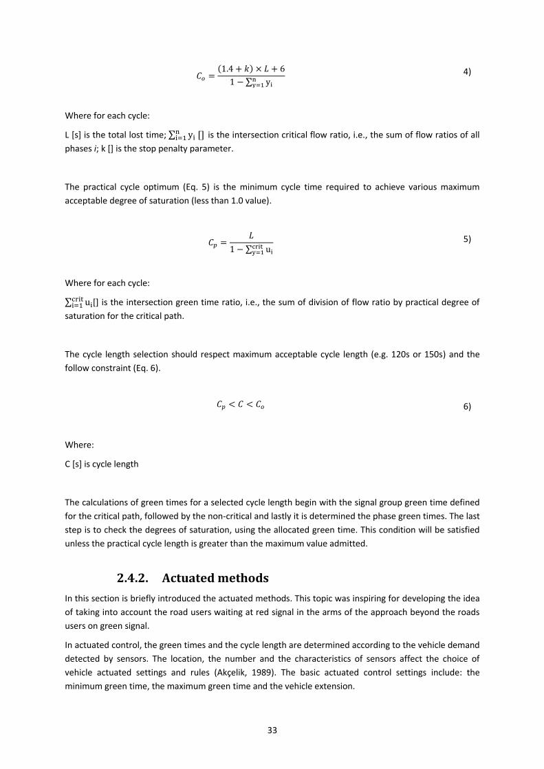
33
4)
Where for each cycle:
L [s] is the total lost time; [] is the intersection critical flow ratio, i.e., the sum of flow ratios of all
phases i; k [] is the stop penalty parameter.
The practical cycle optimum (Eq. 5) is the minimum cycle time required to achieve various maximum
acceptable degree of saturation (less than 1.0 value).
5)
Where for each cycle:
[] is the intersection green time ratio, i.e., the sum of division of flow ratio by practical degree of
saturation for the critical path.
The cycle length selection should respect maximum acceptable cycle length (e.g. 120s or 150s) and the
follow constraint (Eq. 6).
6)
Where:
C [s] is cycle length
The calculations of green times for a selected cycle length begin with the signal group green time defined
for the critical path, followed by the non-critical and lastly it is determined the phase green times. The last
step is to check the degrees of saturation, using the allocated green time. This condition will be satisfied
unless the practical cycle length is greater than the maximum value admitted.
2.4.2. Actuated methods
In this section is briefly introduced the actuated methods. This topic was inspiring for developing the idea
of taking into account the road users waiting at red signal in the arms of the approach beyond the roads
users on green signal.
In actuated control, the green times and the cycle length are determined according to the vehicle demand
detected by sensors. The location, the number and the characteristics of sensors affect the choice of
vehicle actuated settings and rules (Akçelik, 1989). The basic actuated control settings include: the
minimum green time, the maximum green time and the vehicle extension.

34
Basically, the green time duration of each phase is adjusted based on the vehicle extension time and the
gap detected between vehicles crossing the sensor. A minimum green time is given to clear the possible
vehicles queued between the stop line and the sensor. The green time is extended by resetting the
extension time every time a vehicle is recorded after the minimum green time expires. If the sensor
detects another vehicle within this extension time, the green time is extended again, by the length of the
extension time until the last vehicle has passed. The green time can be extended until the maximum
green time value (see Figure 4 in section 2.3.2).
In case of no vehicles detected on a particular approach, in some controllers is possible to skip over the
phase with no vehicles assigned and move directly to the next phase following the phase sequence. The
main disadvantage of using this actuated control is that it looks only at the vehicles on green while not
taking into account the number of vehicles waiting at red signal in other approaches of intersection.
A further enhancement of actuated control is the volume-density (Pacelli et al., 2000, Kell and Fullerton,
1982). For volume-density operation, sensors are placed further back the intersection stop-line given
earlier detection information to controller. The minimum green time duration and the vehicle extension
assume a value according to the distance between sensor and stop-line in order to clear a possible
installed queue in this distance. Since the distance is relatively long, resulting in a vehicle extension
superior to the desired maximum, the gap-reduction concept is introduced which reduces the vehicle
extension value (Figure 7). The “time before reduction” starts during green signal when a conflicting signal
group requires the green time. At the end of “time before reduction”, there is a linear reduction from the
“initial” vehicle extension value to the “minimum” defined. From that point minimum vehicle extension
value control actuation until the maximum green value is reached.
Figure 7 – Gap reduction timing (Kell and Fullerton, 1982)
The volume-density rule induces the probability to end the current phase as the green time increases
allowing to keep the green phase shorter than the one that would occur if the gap setting was fixed at its
initial setting.
Another type of volume-density rule (Pacelli et al., 2000) is to use upstream sensors to count vehicles as
they enter the queue, and then adjust the length of minimum green time to satisfy the discharge
requirements of the number of vehicles known to be in queue. The disadvantage of this method is the
difficulty of sensor placement, it should be far enough of the stop-line to capture all the vehicles in queue.
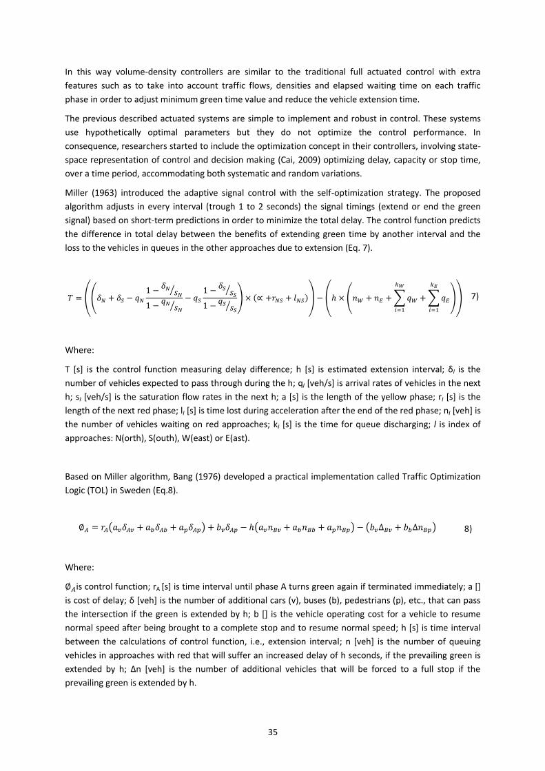
35
In this way volume-density controllers are similar to the traditional full actuated control with extra
features such as to take into account traffic flows, densities and elapsed waiting time on each traffic
phase in order to adjust minimum green time value and reduce the vehicle extension time.
The previous described actuated systems are simple to implement and robust in control. These systems
use hypothetically optimal parameters but they do not optimize the control performance. In
consequence, researchers started to include the optimization concept in their controllers, involving state-
space representation of control and decision making (Cai, 2009) optimizing delay, capacity or stop time,
over a time period, accommodating both systematic and random variations.
Miller (1963) introduced the adaptive signal control with the self-optimization strategy. The proposed
algorithm adjusts in every interval (trough 1 to 2 seconds) the signal timings (extend or end the green
signal) based on short-term predictions in order to minimize the total delay. The control function predicts
the difference in total delay between the benefits of extending green time by another interval and the
loss to the vehicles in queues in the other approaches due to extension (Eq. 7).
7)
Where:
T [s] is the control function measuring delay difference; h [s] is estimated extension interval; δl is the
number of vehicles expected to pass through during the h; qI [veh/s] is arrival rates of vehicles in the next
h; sI [veh/s] is the saturation flow rates in the next h; a [s] is the length of the yellow phase; rI [s] is the
length of the next red phase; lI [s] is time lost during acceleration after the end of the red phase; nI [veh] is
the number of vehicles waiting on red approaches; kI [s] is the time for queue discharging; l is index of
approaches: N(orth), S(outh), W(east) or E(ast).
Based on Miller algorithm, Bang (1976) developed a practical implementation called Traffic Optimization
Logic (TOL) in Sweden (Eq.8).
8)
Where:
is control function; rA [s] is time interval until phase A turns green again if terminated immediately; a []
is cost of delay; δ [veh] is the number of additional cars (v), buses (b), pedestrians (p), etc., that can pass
the intersection if the green is extended by h; b [] is the vehicle operating cost for a vehicle to resume
normal speed after being brought to a complete stop and to resume normal speed; h [s] is time interval
between the calculations of control function, i.e., extension interval; n [veh] is the number of queuing
vehicles in approaches with red that will suffer an increased delay of h seconds, if the prevailing green is
extended by h; ∆n [veh] is the number of additional vehicles that will be forced to a full stop if the
prevailing green is extended by h.
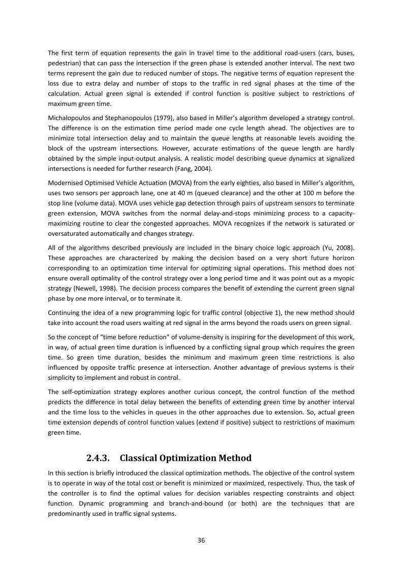
36
The first term of equation represents the gain in travel time to the additional road-users (cars, buses,
pedestrian) that can pass the intersection if the green phase is extended another interval. The next two
terms represent the gain due to reduced number of stops. The negative terms of equation represent the
loss due to extra delay and number of stops to the traffic in red signal phases at the time of the
calculation. Actual green signal is extended if control function is positive subject to restrictions of
maximum green time.
Michalopoulos and Stephanopoulos (1979), also based in Miller’s algorithm developed a strategy control.
The difference is on the estimation time period made one cycle length ahead. The objectives are to
minimize total intersection delay and to maintain the queue lengths at reasonable levels avoiding the
block of the upstream intersections. However, accurate estimations of the queue length are hardly
obtained by the simple input-output analysis. A realistic model describing queue dynamics at signalized
intersections is needed for further research (Fang, 2004).
Modernised Optimised Vehicle Actuation (MOVA) from the early eighties, also based in Miller’s algorithm,
uses two sensors per approach lane, one at 40 m (queued clearance) and the other at 100 m before the
stop line (volume data). MOVA uses vehicle gap detection through pairs of upstream sensors to terminate
green extension, MOVA switches from the normal delay-and-stops minimizing process to a capacity-
maximizing routine to clear the congested approaches. MOVA recognizes if the network is saturated or
oversaturated automatically and changes strategy.
All of the algorithms described previously are included in the binary choice logic approach (Yu, 2008).
These approaches are characterized by making the decision based on a very short future horizon
corresponding to an optimization time interval for optimizing signal operations. This method does not
ensure overall optimality of the control strategy over a long period time and it was point out as a myopic
strategy (Newell, 1998). The decision process compares the benefit of extending the current green signal
phase by one more interval, or to terminate it.
Continuing the idea of a new programming logic for traffic control (objective 1), the new method should
take into account the road users waiting at red signal in the arms beyond the roads users on green signal.
So the concept of “time before reduction” of volume-density is inspiring for the development of this work,
in way, of actual green time duration is influenced by a conflicting signal group which requires the green
time. So green time duration, besides the minimum and maximum green time restrictions is also
influenced by opposite traffic presence at intersection. Another advantage of previous systems is their
simplicity to implement and robust in control.
The self-optimization strategy explores another curious concept, the control function of the method
predicts the difference in total delay between the benefits of extending green time by another interval
and the time loss to the vehicles in queues in the other approaches due to extension. So, actual green
time extension depends of control function values (extend if positive) subject to restrictions of maximum
green time.
2.4.3. Classical Optimization Method
In this section is briefly introduced the classical optimization methods. The objective of the control system
is to operate in way of the total cost or benefit is minimized or maximized, respectively. Thus, the task of
the controller is to find the optimal values for decision variables respecting constraints and object
function. Dynamic programming and branch-and-bound (or both) are the techniques that are
predominantly used in traffic signal systems.
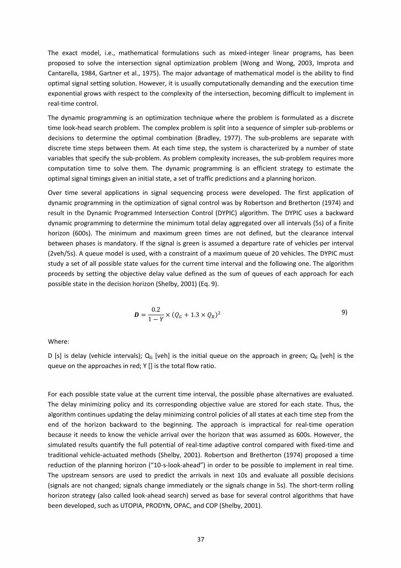
37
The exact model, i.e., mathematical formulations such as mixed-integer linear programs, has been
proposed to solve the intersection signal optimization problem (Wong and Wong, 2003, Improta and
Cantarella, 1984, Gartner et al., 1975). The major advantage of mathematical model is the ability to find
optimal signal setting solution. However, it is usually computationally demanding and the execution time
exponential grows with respect to the complexity of the intersection, becoming difficult to implement in
real-time control.
The dynamic programming is an optimization technique where the problem is formulated as a discrete
time look-head search problem. The complex problem is split into a sequence of simpler sub-problems or
decisions to determine the optimal combination (Bradley, 1977). The sub-problems are separate with
discrete time steps between them. At each time step, the system is characterized by a number of state
variables that specify the sub-problem. As problem complexity increases, the sub-problem requires more
computation time to solve them. The dynamic programming is an efficient strategy to estimate the
optimal signal timings given an initial state, a set of traffic predictions and a planning horizon.
Over time several applications in signal sequencing process were developed. The first application of
dynamic programming in the optimization of signal control was by Robertson and Bretherton (1974) and
result in the Dynamic Programmed Intersection Control (DYPIC) algorithm. The DYPIC uses a backward
dynamic programming to determine the minimum total delay aggregated over all intervals (5s) of a finite
horizon (600s). The minimum and maximum green times are not defined, but the clearance interval
between phases is mandatory. If the signal is green is assumed a departure rate of vehicles per interval
(2veh/5s). A queue model is used, with a constraint of a maximum queue of 20 vehicles. The DYPIC must
study a set of all possible state values for the current time interval and the following one. The algorithm
proceeds by setting the objective delay value defined as the sum of queues of each approach for each
possible state in the decision horizon (Shelby, 2001) (Eq. 9).
9)
Where:
D [s] is delay (vehicle intervals); QG [veh] is the initial queue on the approach in green; QR [veh] is the
queue on the approaches in red; Y [] is the total flow ratio.
For each possible state value at the current time interval, the possible phase alternatives are evaluated.
The delay minimizing policy and its corresponding objective value are stored for each state. Thus, the
algorithm continues updating the delay minimizing control policies of all states at each time step from the
end of the horizon backward to the beginning. The approach is impractical for real-time operation
because it needs to know the vehicle arrival over the horizon that was assumed as 600s. However, the
simulated results quantify the full potential of real-time adaptive control compared with fixed-time and
traditional vehicle-actuated methods (Shelby, 2001). Robertson and Bretherton (1974) proposed a time
reduction of the planning horizon (“10-s-look-ahead”) in order to be possible to implement in real time.
The upstream sensors are used to predict the arrivals in next 10s and evaluate all possible decisions
(signals are not changed; signals change immediately or the signals change in 5s). The short-term rolling
horizon strategy (also called look-ahead search) served as base for several control algorithms that have
been developed, such as UTOPIA, PRODYN, OPAC, and COP (Shelby, 2001).
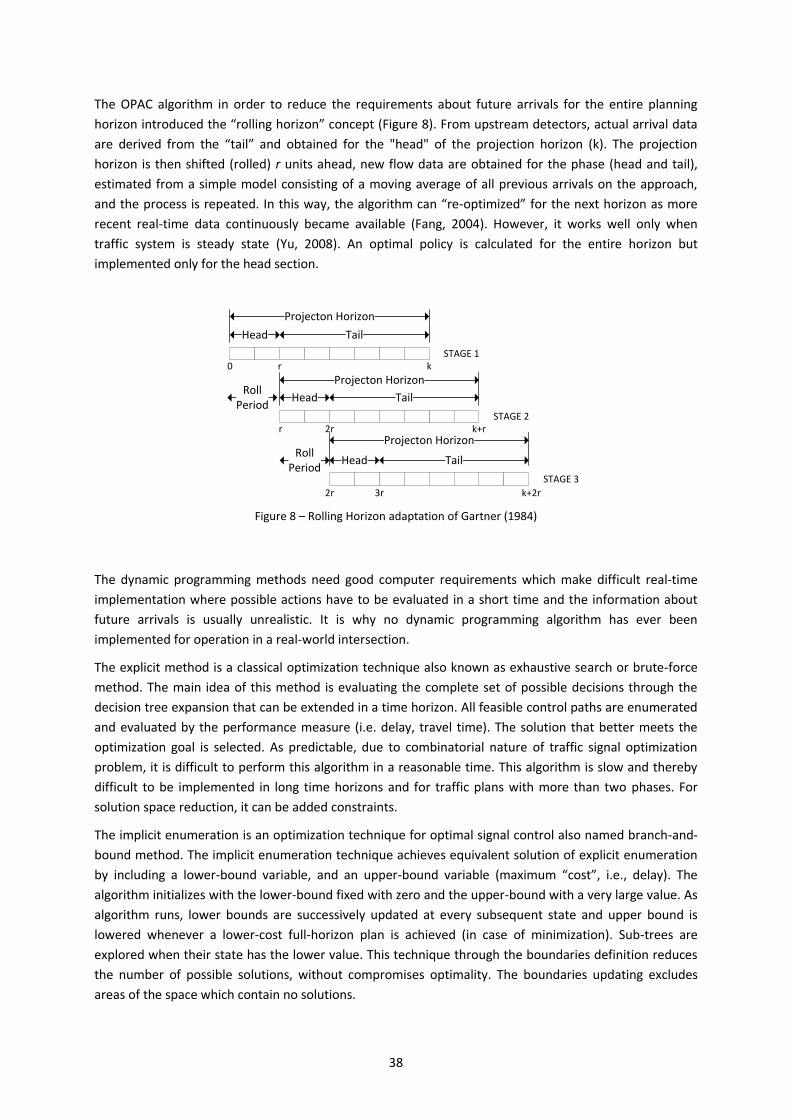
38
The OPAC algorithm in order to reduce the requirements about future arrivals for the entire planning
horizon introduced the “rolling horizon” concept (Figure 8). From upstream detectors, actual arrival data
are derived from the “tail” and obtained for the "head" of the projection horizon (k). The projection
horizon is then shifted (rolled) r units ahead, new flow data are obtained for the phase (head and tail),
estimated from a simple model consisting of a moving average of all previous arrivals on the approach,
and the process is repeated. In this way, the algorithm can “re-optimized” for the next horizon as more
recent real-time data continuously became available (Fang, 2004). However, it works well only when
traffic system is steady state (Yu, 2008). An optimal policy is calculated for the entire horizon but
implemented only for the head section.
Figure 8 – Rolling Horizon adaptation of Gartner (1984)
The dynamic programming methods need good computer requirements which make difficult real-time
implementation where possible actions have to be evaluated in a short time and the information about
future arrivals is usually unrealistic. It is why no dynamic programming algorithm has ever been
implemented for operation in a real-world intersection.
The explicit method is a classical optimization technique also known as exhaustive search or brute-force
method. The main idea of this method is evaluating the complete set of possible decisions through the
decision tree expansion that can be extended in a time horizon. All feasible control paths are enumerated
and evaluated by the performance measure (i.e. delay, travel time). The solution that better meets the
optimization goal is selected. As predictable, due to combinatorial nature of traffic signal optimization
problem, it is difficult to perform this algorithm in a reasonable time. This algorithm is slow and thereby
difficult to be implemented in long time horizons and for traffic plans with more than two phases. For
solution space reduction, it can be added constraints.
The implicit enumeration is an optimization technique for optimal signal control also named branch-and-
bound method. The implicit enumeration technique achieves equivalent solution of explicit enumeration
by including a lower-bound variable, and an upper-bound variable (maximum “cost”, i.e., delay). The
algorithm initializes with the lower-bound fixed with zero and the upper-bound with a very large value. As
algorithm runs, lower bounds are successively updated at every subsequent state and upper bound is
lowered whenever a lower-cost full-horizon plan is achieved (in case of minimization). Sub-trees are
explored when their state has the lower value. This technique through the boundaries definition reduces
the number of possible solutions, without compromises optimality. The boundaries updating excludes
areas of the space which contain no solutions.
Head Tail
Projecton Horizon
STAGE 1
Head Tail
Projecton Horizon
STAGE 2
Head Tail
Projecton Horizon
STAGE 3
RollPeriod
RollPeriod
0 r
2rr
2r
k
k+r
k+2r3r
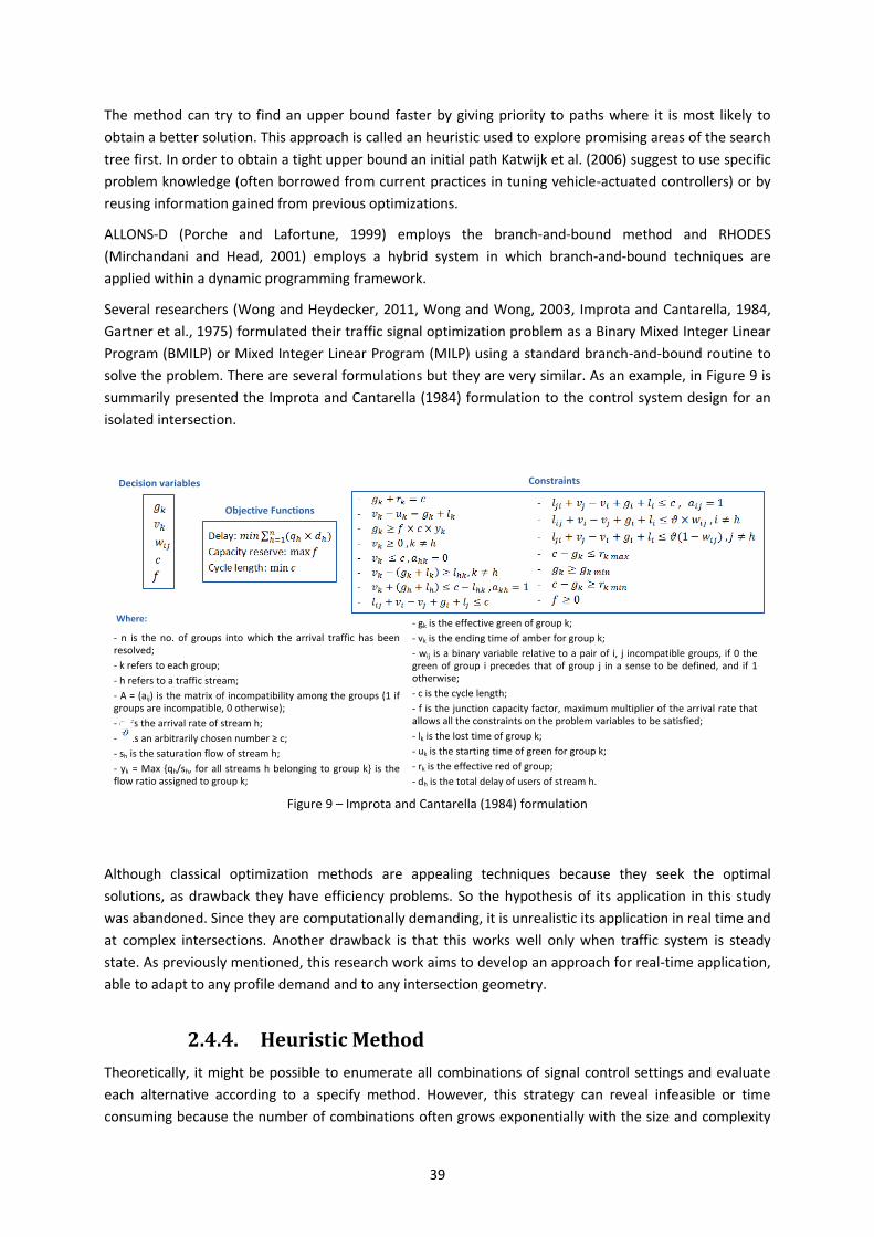
39
The method can try to find an upper bound faster by giving priority to paths where it is most likely to
obtain a better solution. This approach is called an heuristic used to explore promising areas of the search
tree first. In order to obtain a tight upper bound an initial path Katwijk et al. (2006) suggest to use specific
problem knowledge (often borrowed from current practices in tuning vehicle-actuated controllers) or by
reusing information gained from previous optimizations.
ALLONS-D (Porche and Lafortune, 1999) employs the branch-and-bound method and RHODES
(Mirchandani and Head, 2001) employs a hybrid system in which branch-and-bound techniques are
applied within a dynamic programming framework.
Several researchers (Wong and Heydecker, 2011, Wong and Wong, 2003, Improta and Cantarella, 1984,
Gartner et al., 1975) formulated their traffic signal optimization problem as a Binary Mixed Integer Linear
Program (BMILP) or Mixed Integer Linear Program (MILP) using a standard branch-and-bound routine to
solve the problem. There are several formulations but they are very similar. As an example, in Figure 9 is
summarily presented the Improta and Cantarella (1984) formulation to the control system design for an
isolated intersection.
Figure 9 – Improta and Cantarella (1984) formulation
Although classical optimization methods are appealing techniques because they seek the optimal
solutions, as drawback they have efficiency problems. So the hypothesis of its application in this study
was abandoned. Since they are computationally demanding, it is unrealistic its application in real time and
at complex intersections. Another drawback is that this works well only when traffic system is steady
state. As previously mentioned, this research work aims to develop an approach for real-time application,
able to adapt to any profile demand and to any intersection geometry.
2.4.4. Heuristic Method
Theoretically, it might be possible to enumerate all combinations of signal control settings and evaluate
each alternative according to a specify method. However, this strategy can reveal infeasible or time
consuming because the number of combinations often grows exponentially with the size and complexity
- n is the no. of groups into which the arrival traffic has been resolved;
- k refers to each group;
- h refers to a traffic stream;
- A = (aij) is the matrix of incompatibility among the groups (1 if groups are incompatible, 0 otherwise);
- qh is the arrival rate of stream h;
- is an arbitrarily chosen number ≥ c;
- sh is the saturation flow of stream h;
- yk = Max {qh/sh, for all streams h belonging to group k} is the flow ratio assigned to group k;
Decision variables Constraints
Objective Functions
Where: - gk is the effective green of group k;
- vk is the ending time of amber for group k;
- wij is a binary variable relative to a pair of i, j incompatible groups, if 0 the green of group i precedes that of group j in a sense to be defined, and if 1 otherwise;
- c is the cycle length;
- f is the junction capacity factor, maximum multiplier of the arrival rate that allows all the constraints on the problem variables to be satisfied;
- lk is the lost time of group k;
- uk is the starting time of green for group k;
- rk is the effective red of group;
- dh is the total delay of users of stream h.
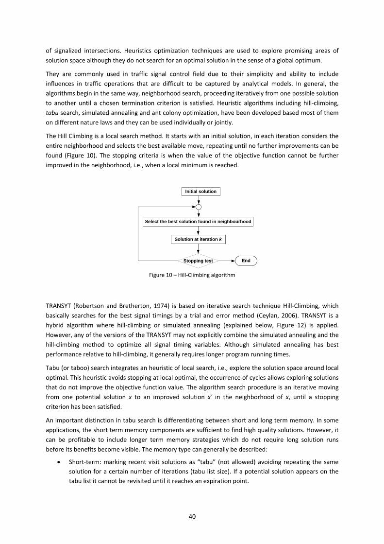
40
of signalized intersections. Heuristics optimization techniques are used to explore promising areas of
solution space although they do not search for an optimal solution in the sense of a global optimum.
They are commonly used in traffic signal control field due to their simplicity and ability to include
influences in traffic operations that are difficult to be captured by analytical models. In general, the
algorithms begin in the same way, neighborhood search, proceeding iteratively from one possible solution
to another until a chosen termination criterion is satisfied. Heuristic algorithms including hill-climbing,
tabu search, simulated annealing and ant colony optimization, have been developed based most of them
on different nature laws and they can be used individually or jointly.
The Hill Climbing is a local search method. It starts with an initial solution, in each iteration considers the
entire neighborhood and selects the best available move, repeating until no further improvements can be
found (Figure 10). The stopping criteria is when the value of the objective function cannot be further
improved in the neighborhood, i.e., when a local minimum is reached.
Figure 10 – Hill-Climbing algorithm
TRANSYT (Robertson and Bretherton, 1974) is based on iterative search technique Hill-Climbing, which
basically searches for the best signal timings by a trial and error method (Ceylan, 2006). TRANSYT is a
hybrid algorithm where hill-climbing or simulated annealing (explained below, Figure 12) is applied.
However, any of the versions of the TRANSYT may not explicitly combine the simulated annealing and the
hill-climbing method to optimize all signal timing variables. Although simulated annealing has best
performance relative to hill-climbing, it generally requires longer program running times.
Tabu (or taboo) search integrates an heuristic of local search, i.e., explore the solution space around local
optimal. This heuristic avoids stopping at local optimal, the occurrence of cycles allows exploring solutions
that do not improve the objective function value. The algorithm search procedure is an iterative moving
from one potential solution x to an improved solution x' in the neighborhood of x, until a stopping
criterion has been satisfied.
An important distinction in tabu search is differentiating between short and long term memory. In some
applications, the short term memory components are sufficient to find high quality solutions. However, it
can be profitable to include longer term memory strategies which do not require long solution runs
before its benefits become visible. The memory type can generally be described:
Short-term: marking recent visit solutions as “tabu” (not allowed) avoiding repeating the same
solution for a certain number of iterations (tabu list size). If a potential solution appears on the
tabu list it cannot be revisited until it reaches an expiration point.
Initial solution
Select the best solution found in neighbourhood
Solution at iteration k
Stopping test End
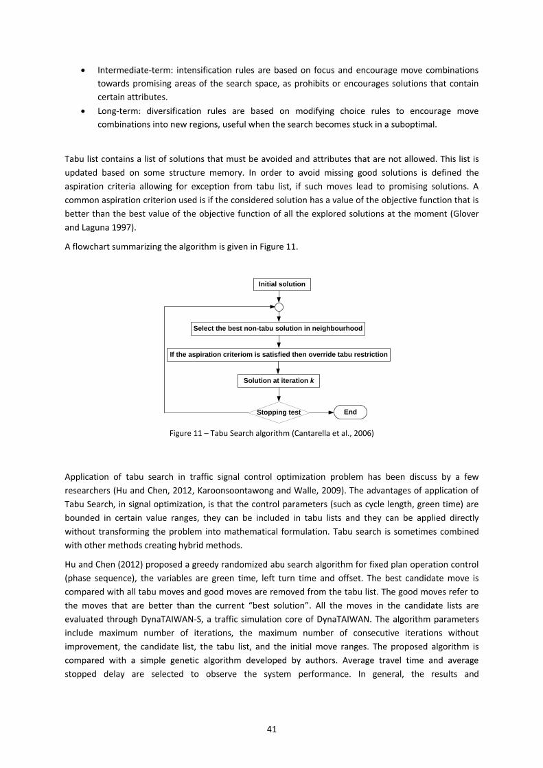
41
Intermediate-term: intensification rules are based on focus and encourage move combinations
towards promising areas of the search space, as prohibits or encourages solutions that contain
certain attributes.
Long-term: diversification rules are based on modifying choice rules to encourage move
combinations into new regions, useful when the search becomes stuck in a suboptimal.
Tabu list contains a list of solutions that must be avoided and attributes that are not allowed. This list is
updated based on some structure memory. In order to avoid missing good solutions is defined the
aspiration criteria allowing for exception from tabu list, if such moves lead to promising solutions. A
common aspiration criterion used is if the considered solution has a value of the objective function that is
better than the best value of the objective function of all the explored solutions at the moment (Glover
and Laguna 1997).
A flowchart summarizing the algorithm is given in Figure 11.
Figure 11 – Tabu Search algorithm (Cantarella et al., 2006)
Application of tabu search in traffic signal control optimization problem has been discuss by a few
researchers (Hu and Chen, 2012, Karoonsoontawong and Walle, 2009). The advantages of application of
Tabu Search, in signal optimization, is that the control parameters (such as cycle length, green time) are
bounded in certain value ranges, they can be included in tabu lists and they can be applied directly
without transforming the problem into mathematical formulation. Tabu search is sometimes combined
with other methods creating hybrid methods.
Hu and Chen (2012) proposed a greedy randomized abu search algorithm for fixed plan operation control
(phase sequence), the variables are green time, left turn time and offset. The best candidate move is
compared with all tabu moves and good moves are removed from the tabu list. The good moves refer to
the moves that are better than the current “best solution”. All the moves in the candidate lists are
evaluated through DynaTAIWAN-S, a traffic simulation core of DynaTAIWAN. The algorithm parameters
include maximum number of iterations, the maximum number of consecutive iterations without
improvement, the candidate list, the tabu list, and the initial move ranges. The proposed algorithm is
compared with a simple genetic algorithm developed by authors. Average travel time and average
stopped delay are selected to observe the system performance. In general, the results and
Initial solution
Select the best non-tabu solution in neighbourhood
Solution at iteration k
Stopping test End
If the aspiration criteriom is satisfied then override tabu restriction
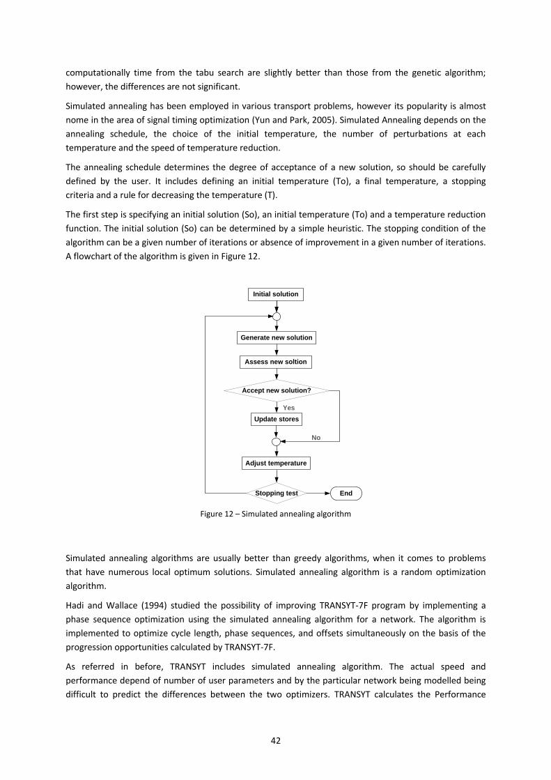
42
computationally time from the tabu search are slightly better than those from the genetic algorithm;
however, the differences are not significant.
Simulated annealing has been employed in various transport problems, however its popularity is almost
nome in the area of signal timing optimization (Yun and Park, 2005). Simulated Annealing depends on the
annealing schedule, the choice of the initial temperature, the number of perturbations at each
temperature and the speed of temperature reduction.
The annealing schedule determines the degree of acceptance of a new solution, so should be carefully
defined by the user. It includes defining an initial temperature (To), a final temperature, a stopping
criteria and a rule for decreasing the temperature (T).
The first step is specifying an initial solution (So), an initial temperature (To) and a temperature reduction
function. The initial solution (So) can be determined by a simple heuristic. The stopping condition of the
algorithm can be a given number of iterations or absence of improvement in a given number of iterations.
A flowchart of the algorithm is given in Figure 12.
Figure 12 – Simulated annealing algorithm
Simulated annealing algorithms are usually better than greedy algorithms, when it comes to problems
that have numerous local optimum solutions. Simulated annealing algorithm is a random optimization
algorithm.
Hadi and Wallace (1994) studied the possibility of improving TRANSYT-7F program by implementing a
phase sequence optimization using the simulated annealing algorithm for a network. The algorithm is
implemented to optimize cycle length, phase sequences, and offsets simultaneously on the basis of the
progression opportunities calculated by TRANSYT-7F.
As referred in before, TRANSYT includes simulated annealing algorithm. The actual speed and
performance depend of number of user parameters and by the particular network being modelled being
difficult to predict the differences between the two optimizers. TRANSYT calculates the Performance
Initial solution
Generate new solution
Update stores
Stopping test End
Assess new soltion
Adjust temperature
Yes
Accept new solution?
No

43
Index (PI) of the network for an initial set of signal timings. Next, the program alters the timings as
dictated to by the optimizer logic and recalculates the PI of the network. If the PI is reduced, these timings
replace the currently best set of timings.
Ant colony is a recent method inspired by the observation of real ant colonies (Baskan et al., 2009). The
main idea is the communication between the ants by means of chemical pheromone trails, which enables
them to find shortest paths between their nest and food sources. This behavior of real ant colonies is
exploited to solve optimization problems. The algorithm is based on search of each ant; they search only
around the best solution of the previous iteration with reduced search space.
Each ant probabilistically prefers to follow the direction rich in pheromone. Once all ants generate a
solution, then global pheromone updating rule is applied in two phases; an evaporation phase, where a
fraction of the pheromone evaporates, and a reinforcement phase, where each ant deposits an amount of
pheromone which is proportional to the fitness (Figure 13). This process is repeated until stopping criteria
is met. The pheromone update phase is located after the initialization phase, meaning that the quantity of
pheromone intensifies in each iteration within the reduced search space. Thus, global optimum is
searched within the reduced search space using best values obtained from new ant colony in the previous
iteration.
Figure 13 – Flowchart of ant colony algorithm
Haldenbilen et al. (2013) applied the algorithm to an area traffic control to optimize traffic signal timings
at coordinated signalized network and TRANSYT-7F to calculate the performance index for a given set of
signal settings. The decision variables are green times of phases, the offset and cycle length. The study
concludes that ant-colony algorithm provides an alternative to the hill-climbing and genetic optimization,
used by Ceylan (2006), described on section 2.4.5.
The main advantage of heuristic approach over classical optimization is that traffic signal control variables
search usually starts with an initial solution and goal state, considering irrelevant or unreachable parts of
the state space. The optimal solution is not guaranteed, but the results are usually close to the global
optimum. Generally, heuristic approach requires that problem fit in its structure, as consequence it is
moving away from the nature of the problem. From this point of view, it loses the clearness of the
solution.
Generate a solution
Evaporation phase
Stopping test End
Pheromone update
Initial solution
Creates ants: size of ant colony (m), search space value (β) for each decision variable
Reinforcement phase
44
2.4.5. Artificial Intelligence Method
In recent years, the optimization methods begin to apply artificial intelligence (AI) techniques to solve
traffic control problem. This approach is based in human-like and nature-like decision process.
There is an expressive number of publications using various AI techniques in traffic control (van Zuylen,
2012, Wiering et al., 2004, Bielli et al., 1991). AI attempts to replicate the human ways of reasoning,
learning, reacting adaptively and communicating (Kasabov, 1996). The method advantage is the capacity
of finding suitable and/or optimal solutions for phase timing more quickly than other methods. However,
several of these methods are described as a closed black-box, making comprehension and generalization
difficult raising ethical issues of responsibilities (Cai, 2009).
As explained by Kasabov (1996) the use of heuristic search techniques belongs to AI area. However, in
scientific community is common to separate the heuristics from artificial intelligence area, but the
concept boundaries are not tight defined.
In this section, AI area is considered the knowledge engineering such as fuzzy logic or machine learning.
There are models, methods, and basic technologies for representing and processing knowledge and for
building intelligent knowledge-based systems. The basic issues in knowledge engineering are
representation, inference, learning, generalization, interaction, explanation, validation and adaptation
(Kasabov, 1996):
Representation: process of transforming existing problem knowledge to some of the known
knowledge engineering schemes;
Inference: process of matching current facts from the domain space to the existing knowledge
and inferring new facts (e.g. fuzzy inference, neural inference);
Learning: process of obtaining new knowledge and improve the system. It is a step toward
adaptation. The principal methods to learning are: learning through examples (typical for neural
networks and some machine learning methods), learning by being told (typical for fuzzy systems)
and learning by doing (typical system starts with little system knowledge);
Generalization: process of matching new, unknown input data with the problem knowledge, i.e.,
reacting properly to new situations;
Interaction: means communication between a system and the environment. It is an important
issue for a system to adapt to a new situation. This is the spirit of the agent-based approach;
Explanation: means tracing, in a contextually comprehensible way, the process of inferring the
solution, and reporting it;
Validation: process of testing how good the solutions produced by a system with the results
obtained either by experts or by other systems;
Adaptation: process of changing a system during its operation in a dynamically changing
environment. Without adaptation there is no intelligence.
In this field, genetic algorithms are a heuristic optimization model based on natural selection and
evolution theory. The search method for a solution is random and iterative tending to converge to an
optimal solution. Genetic algorithm has the ability to move out of local optimal.
This algorithm is different of other optimization techniques in some aspects: uses a probabilistic transition
rule to guide the search towards high performance regions of the search space, work with codes of the
parameter set and search from a population of strings rather than use point-to-point method and hence
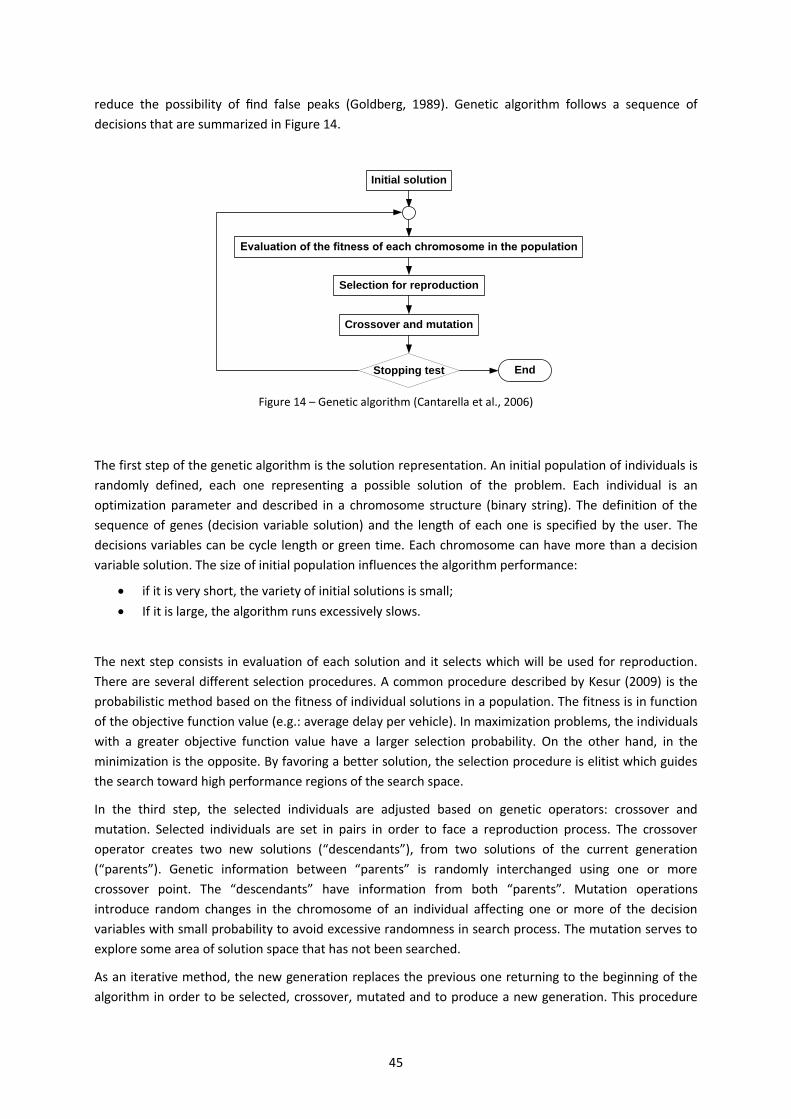
45
reduce the possibility of find false peaks (Goldberg, 1989). Genetic algorithm follows a sequence of
decisions that are summarized in Figure 14.
Figure 14 – Genetic algorithm (Cantarella et al., 2006)
The first step of the genetic algorithm is the solution representation. An initial population of individuals is
randomly defined, each one representing a possible solution of the problem. Each individual is an
optimization parameter and described in a chromosome structure (binary string). The definition of the
sequence of genes (decision variable solution) and the length of each one is specified by the user. The
decisions variables can be cycle length or green time. Each chromosome can have more than a decision
variable solution. The size of initial population influences the algorithm performance:
if it is very short, the variety of initial solutions is small;
If it is large, the algorithm runs excessively slows.
The next step consists in evaluation of each solution and it selects which will be used for reproduction.
There are several different selection procedures. A common procedure described by Kesur (2009) is the
probabilistic method based on the fitness of individual solutions in a population. The fitness is in function
of the objective function value (e.g.: average delay per vehicle). In maximization problems, the individuals
with a greater objective function value have a larger selection probability. On the other hand, in the
minimization is the opposite. By favoring a better solution, the selection procedure is elitist which guides
the search toward high performance regions of the search space.
In the third step, the selected individuals are adjusted based on genetic operators: crossover and
mutation. Selected individuals are set in pairs in order to face a reproduction process. The crossover
operator creates two new solutions (“descendants”), from two solutions of the current generation
(“parents”). Genetic information between “parents” is randomly interchanged using one or more
crossover point. The “descendants” have information from both “parents”. Mutation operations
introduce random changes in the chromosome of an individual affecting one or more of the decision
variables with small probability to avoid excessive randomness in search process. The mutation serves to
explore some area of solution space that has not been searched.
As an iterative method, the new generation replaces the previous one returning to the beginning of the
algorithm in order to be selected, crossover, mutated and to produce a new generation. This procedure
Evaluation of the fitness of each chromosome in the population
Crossover and mutation
Stopping test End
Selection for reproduction
Initial solution
46
will be repeated until the new population reached the defined condition or the maximum number of
iterations (equal to generations) defined.
Since the first step on genetic algorithms, many new operators (elitist method, uniform crossover, ranking
and tournament selection), alternative algorithms (steady state genetic algorithm, CHC) and encodings
(gray encoding, real coding and operators) have been introduced (Kesur, 2007). (Yun and Park (2005))
selected three stopping criteria: the maximum number of generations, the lack of improvement in the
fitness of the best solution over 10 generations and no difference between the fitness of best solution and
the average fitness of all solutions over 10 generations. Since the genetic algorithm is a heuristic search
method, the modifications are usually evaluated empirically by comparing the performance of several
independent replications of the search algorithm with and without the modification.
Genetic algorithm belongs to the evolutionary algorithms. Evolutionary algorithms have the advantage of
not stucked in local optimal due to the random search. However, of all the evolutionary algorithms, the
genetic algorithm is the only successfully applied in the traffic signal control system for commercial
distribution (Park et al., 1999). In fact, genetic algorithm has been applied in the traffic signal control field
in to optimize cycle length, phase sequence, green times and/or offset (Kesur, 2009, Teklu et al., 2007,
Ceylan and Bell, 2004, Sun et al., 2003, Park and Schneeberger, 2003).
Park and Schneeberger (2003) provided a thorough application of genetic algorithms to optimize all
timing variables besides the number and structure of signal phases. Several optimization criteria were
considered and measures of effectiveness were computed by a traffic simulation model. Park (1998)
found that the genetic algorithm provides effective optimization for hypothetical signal networks and
outperformed the TRANSYT-7 hill climbing procedure. For a simplified two signal network, the genetic
algorithm found a solution with delay only 1% larger than that of a full enumerative search.
Sun et al. (2003) applied genetic algorithm approach with a multi-objective function for minimum delay
and stops at an isolated intersection. The decision variable selected where green time and cycle length for
a two phase intersection. Delay and stops were calculated using analytical formulation. The multi-
objective genetic algorithm has potential to be used in intersection signal timing optimization under
uniform and stochastic traffic arrival patterns.
Ceylan and Bell (2004) applied genetic algorithm approach to solve traffic signal control and traffic
assignment problems. The scope of the study was a network with the following decision variables: cycle
length, green time split and the offsets. The objective function was a weighted sum of a linear
combination between delay and number of stops per unit time for all traffic streams. The model
converged to the optimal solution independent of the initial signal timings.
Kesur (2009) explored adjustments to the genetic algorithms for fixed time traffic signals. The
modifications are tested on the traffic signal optimization problem, on two network (nine and fourteen
signalized intersections), considering under-saturated and oversaturated scenarios. The encoding problem
is enhanced including the structure and sequence of the signal phases to be optimized. Signal
optimization was performed using a delay minimization strategy. The enhanced algorithm offers delay
reductions between 13% and 30%, depending of the scenario, comparing with traditional genetic
algorithm application.
TRANSYT-7F is an adaptation of original TRANSYT 7 software product where it is introduced the genetic
algorithm optimization method rather than the hill-climbing. Although the genetic algorithm is
mathematically better suited for determining the absolute or global optimal solution, relative to hill-
climbing optimization, it generally requires longer program running times.
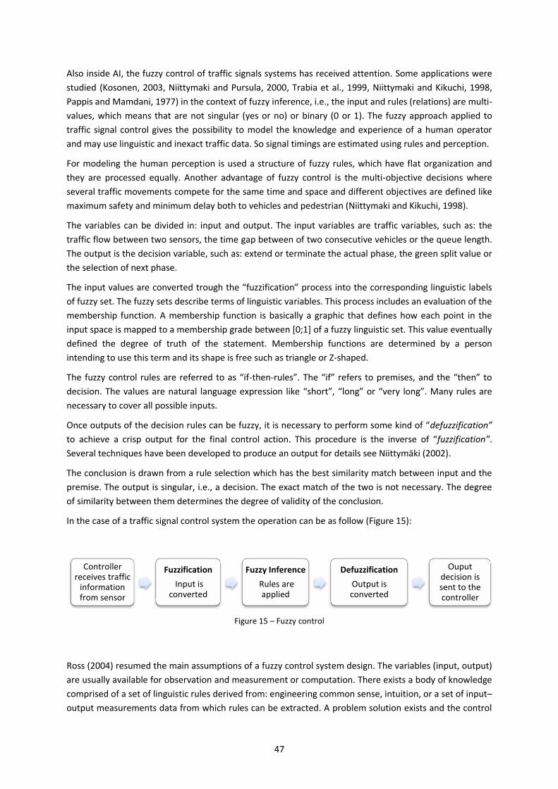
47
Also inside AI, the fuzzy control of traffic signals systems has received attention. Some applications were
studied (Kosonen, 2003, Niittymaki and Pursula, 2000, Trabia et al., 1999, Niittymaki and Kikuchi, 1998,
Pappis and Mamdani, 1977) in the context of fuzzy inference, i.e., the input and rules (relations) are multi-
values, which means that are not singular (yes or no) or binary (0 or 1). The fuzzy approach applied to
traffic signal control gives the possibility to model the knowledge and experience of a human operator
and may use linguistic and inexact traffic data. So signal timings are estimated using rules and perception.
For modeling the human perception is used a structure of fuzzy rules, which have flat organization and
they are processed equally. Another advantage of fuzzy control is the multi-objective decisions where
several traffic movements compete for the same time and space and different objectives are defined like
maximum safety and minimum delay both to vehicles and pedestrian (Niittymaki and Kikuchi, 1998).
The variables can be divided in: input and output. The input variables are traffic variables, such as: the
traffic flow between two sensors, the time gap between of two consecutive vehicles or the queue length.
The output is the decision variable, such as: extend or terminate the actual phase, the green split value or
the selection of next phase.
The input values are converted trough the “fuzzification” process into the corresponding linguistic labels
of fuzzy set. The fuzzy sets describe terms of linguistic variables. This process includes an evaluation of the
membership function. A membership function is basically a graphic that defines how each point in the
input space is mapped to a membership grade between [0;1] of a fuzzy linguistic set. This value eventually
defined the degree of truth of the statement. Membership functions are determined by a person
intending to use this term and its shape is free such as triangle or Z-shaped.
The fuzzy control rules are referred to as “if-then-rules”. The “if” refers to premises, and the “then” to
decision. The values are natural language expression like “short”, “long” or “very long”. Many rules are
necessary to cover all possible inputs.
Once outputs of the decision rules can be fuzzy, it is necessary to perform some kind of “defuzzification”
to achieve a crisp output for the final control action. This procedure is the inverse of “fuzzification”.
Several techniques have been developed to produce an output for details see Niittymäki (2002).
The conclusion is drawn from a rule selection which has the best similarity match between input and the
premise. The output is singular, i.e., a decision. The exact match of the two is not necessary. The degree
of similarity between them determines the degree of validity of the conclusion.
In the case of a traffic signal control system the operation can be as follow (Figure 15):
Figure 15 – Fuzzy control
Ross (2004) resumed the main assumptions of a fuzzy control system design. The variables (input, output)
are usually available for observation and measurement or computation. There exists a body of knowledge
comprised of a set of linguistic rules derived from: engineering common sense, intuition, or a set of input–
output measurements data from which rules can be extracted. A problem solution exists and the control
Controller receives traffic
information from sensor
Fuzzification
Input is converted
Fuzzy Inference
Rules are applied
Defuzzification
Output is converted
Ouput decision is sent to the controller

48
engineer is responsible for looking a good solution, not necessarily the optimal one. The problems of
stability and optimality are not addressed explicitly, once such issues are still open problems in fuzzy
controller design.
The main advantages claimed for expressing control laws in this way are that it enables to capture the
knowledge of how the system should work in linguistic terms as well as serving multi-objective. However,
fuzzy logic basically has the same main disadvantage as the heuristic approaches, namely the rule-base
should be as complete as possible, while missing an important rule or over-valuing another has a
significant impact on the signal operation.
Pappis and Mamdani (1977) performed the first theoretical simulation study of a fuzzy logic controller
with random vehicle arrivals and no turning movements, at isolated intersection. Fuzzy rules were
developed for evaluating the green time extension until maximum green time. The selected performance
criterion was delay minimization using the Webster analytical approach and the fuzzy controller showed
slightly better results comparing with a traditional traffic actuated controller.
Trabia et al. (1999) performed a fuzzy logic-based traffic signal controller for an isolated four arm
intersection with through and left turning movements. Fuzzy rule was also defined to make adjustments
to signal timing: extend or terminate, in response to traffic conditions. Using vehicle sensors, the traffic
signal controller measures approach traffic flows and estimates queues length. The intersection
performance is based on delay minimization and proportion of stopped vehicles. Intersection controlled
by fuzzy logic produces less delay while maintaining the proportion of stopped vehicles comparing with an
actuated controller.
Niittymaki and Kikuchi (1998) tested fuzzy logic controller at a signalized pedestrian crossing where was
made a compromise between two opposing objectives, minimum pedestrian delay and minimum vehicle
delay, in accordance with the level of pedestrians and vehicles volumes.
Niittymaki and Pursula (2000) developed a fuzzy control named FUSICO (Fuzzy Signal Control) for two
phase isolated intersections, where signal timings are optimized. The FUSICO was evaluated and
implemented in Finland (Niittymaki, 1999) and comparing with the vehicle-actuated signal control, the
performance improved 10% to 20%. FUSICO is an algorithm of multi-phase control decision which
includes the traffic situation, phase sequence and the green extension. FUSICO control algorithm gave a
smaller number of stops than the traditional extension principle of actuated control or the (Pappis and
Mamdani, 1977) approach reducing fuel consumption and increasing traffic safety. The author tested
public transport priority in fuzzy control and results were promising.
Murat and Gedizlioglu (2005) used fuzzy logic to control signal traffic timing and phase sequence based on
traffic flows. An isolated four-arm intersection is compared with Niittymäki (2002) model of actuated
traffic control with respect to delay. For signal timing, the input parameters are: the longest queues
length in red signal, the vehicles arrivals to junction during green time and remaining unused rate of green
time. For the phase sequence, input parameters are: again the longest of the queues during red signal,
the longest vehicle queue in next phase and red time of the longest queue.
The fuzzy logic highlights from other methods are the fact of some traffic signal configurations using fuzzy
control have already been tested and implemented in real-world networks. However, the fuzzy logic
control has the shortcoming of using static rules which can imply than further updates to the system need
traffic expert displacement (McKenney and White, 2013). Also, it can be difficult to generate effective rule
for intersection with a high number of possible phases, but Niittymaki and Pursula (2000) believes on the
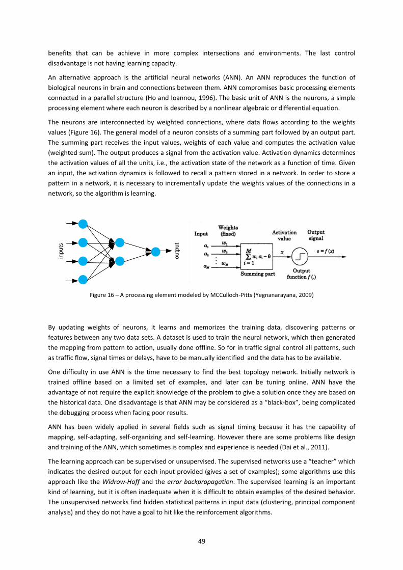
49
benefits that can be achieve in more complex intersections and environments. The last control
disadvantage is not having learning capacity.
An alternative approach is the artificial neural networks (ANN). An ANN reproduces the function of
biological neurons in brain and connections between them. ANN compromises basic processing elements
connected in a parallel structure (Ho and Ioannou, 1996). The basic unit of ANN is the neurons, a simple
processing element where each neuron is described by a nonlinear algebraic or differential equation.
The neurons are interconnected by weighted connections, where data flows according to the weights
values (Figure 16). The general model of a neuron consists of a summing part followed by an output part.
The summing part receives the input values, weights of each value and computes the activation value
(weighted sum). The output produces a signal from the activation value. Activation dynamics determines
the activation values of all the units, i.e., the activation state of the network as a function of time. Given
an input, the activation dynamics is followed to recall a pattern stored in a network. In order to store a
pattern in a network, it is necessary to incrementally update the weights values of the connections in a
network, so the algorithm is learning.
Figure 16 – A processing element modeled by MCCulloch-Pitts (Yegnanarayana, 2009)
By updating weights of neurons, it learns and memorizes the training data, discovering patterns or
features between any two data sets. A dataset is used to train the neural network, which then generated
the mapping from pattern to action, usually done offline. So for in traffic signal control all patterns, such
as traffic flow, signal times or delays, have to be manually identified and the data has to be available.
One difficulty in use ANN is the time necessary to find the best topology network. Initially network is
trained offline based on a limited set of examples, and later can be tuning online. ANN have the
advantage of not require the explicit knowledge of the problem to give a solution once they are based on
the historical data. One disadvantage is that ANN may be considered as a “black-box”, being complicated
the debugging process when facing poor results.
ANN has been widely applied in several fields such as signal timing because it has the capability of
mapping, self-adapting, self-organizing and self-learning. However there are some problems like design
and training of the ANN, which sometimes is complex and experience is needed (Dai et al., 2011).
The learning approach can be supervised or unsupervised. The supervised networks use a “teacher” which
indicates the desired output for each input provided (gives a set of examples); some algorithms use this
approach like the Widrow-Hoff and the error backpropagation. The supervised learning is an important
kind of learning, but it is often inadequate when it is difficult to obtain examples of the desired behavior.
The unsupervised networks find hidden statistical patterns in input data (clustering, principal component
analysis) and they do not have a goal to hit like the reinforcement algorithms.
inp
uts
ou
tpu
t
50
Saito and Fan (2000) developed an approach that uses ANN to evaluate the level of service of signalized
intersections and an artificial intelligence-based search model that would determine optimal signal
timing. The two inputs of the ANN are: the traffic environment data (lay-out and traffic demand) and the
range of cycle length (user boundaries) that will be analyzed for optimal signal timing that minimizes the
vehicle delay at intersections in the traffic network. The system is tested at an isolated two-phase
intersection.
Spall and Chin (1997) used ANN to map traffic patterns to define signal timings, and used perturbation
algorithm to obtain reinforcement signal to adjust neural weights. ANN is also used to map future traffic
arrival pattern in order to define the green time extension for the current phase.
Azzam ul et al. (2008) developed a neural network based traffic signal controller in order to generate real-
time signal timing according to traffic conditions for each intersection. Fifty traffic demand patterns and
their signal timings based on HCM formula (TRB, 2010) were taught to ANN. Once the ANN is trained,
weights are optimized after its learning phase, it was able to generate signal timing plans for the current
traffic conditions in real time. This method eliminated the need of memory for timing plans storage and
misclassification of current traffic conditions.
There are three typical cases of application of ANN in traffic control field (Liu, 2007):
ANN used to model, learning and controlling;
ANN generalization capability is used based on other methods such as fuzzy control was used to
map membership functions. The combination of a neural network and fuzzy logic is called a
neuro-fuzzy system. Neuro-fuzzy system uses the human-like reasoning of fuzzy system and the
powerful computing ability of neural networks, avoiding the drawbacks of using only one system
(Bingham, 2001).
ANN is combined with other methods to improve their generalization capability. So the learning
process should converge to the global optimal point.
ANNs have been successfully used in many aspects in traffic signal control, but some problems like how to
choose structure of the ANNs, how to train the ANN are still present. Most of the time, design and
training of the ANNs are complex and experience needed.
Reinforcement Learning is learning from interaction with uncertain environment in order to maximize a
reward (goal-oriented). The learning is made online. The learner instead of a target output has an
objective of getting as much reward as possible. The search is a trial-and-error where the “learner” must
discover which actions yield the most reward by trying them via experiences. As well as consider a
possible delayed reward, scarifying a short-term gain for greater long-term gains. These two
characteristics, trial-and-error search and delayed reward, are the two most important distinguishing
features of reinforcement learning (Sutton and Barto, 1998).
In reinforcement learning is necessary to find a trade-off between exploration and exploitation.
Exploitation is about what “learner” already knows in order to get a reward and exploration is to try new
actions in order to make better action selections in the future. The systems are evaluated whether the
previous control action was good or not. If the action had good consequences, the tendency to produce
that action is strengthened.
The reinforcement learning problem is described as learning a policy from interaction to achieve a goal.
The “learner” and “decision maker” is sometimes named agent. The principal elements of the
reinforcement learning are:
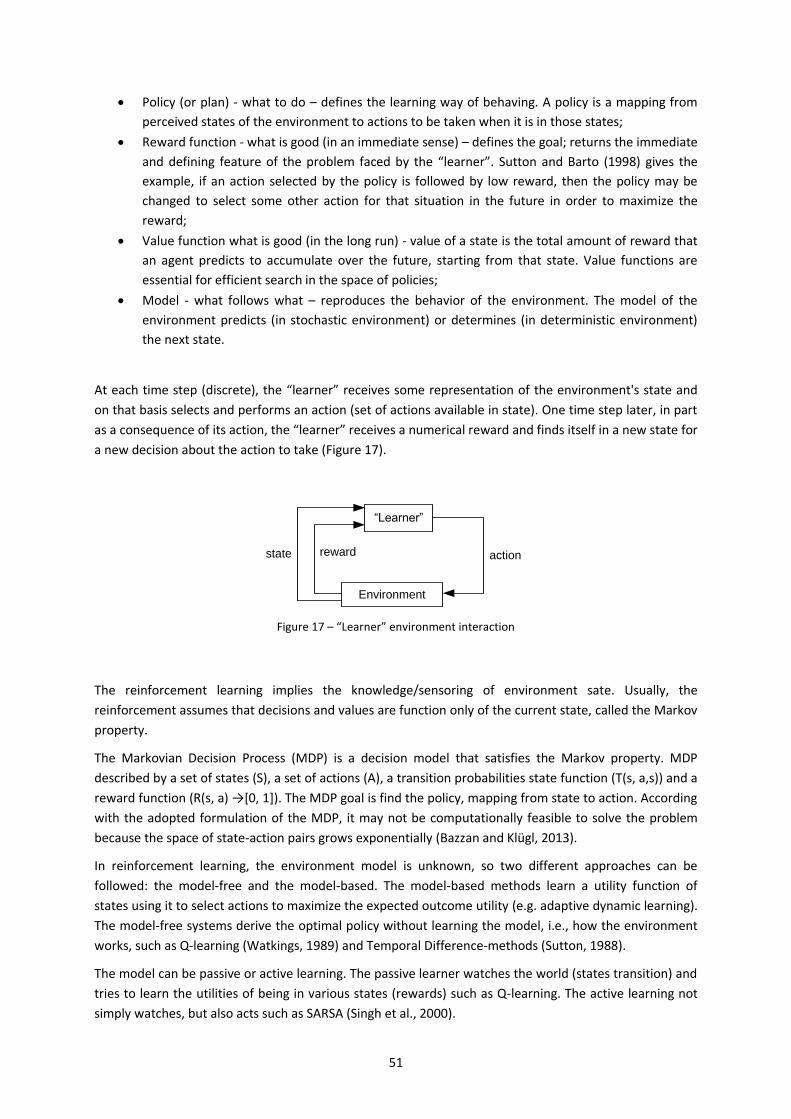
51
Policy (or plan) - what to do – defines the learning way of behaving. A policy is a mapping from
perceived states of the environment to actions to be taken when it is in those states;
Reward function - what is good (in an immediate sense) – defines the goal; returns the immediate
and defining feature of the problem faced by the “learner”. Sutton and Barto (1998) gives the
example, if an action selected by the policy is followed by low reward, then the policy may be
changed to select some other action for that situation in the future in order to maximize the
reward;
Value function what is good (in the long run) - value of a state is the total amount of reward that
an agent predicts to accumulate over the future, starting from that state. Value functions are
essential for efficient search in the space of policies;
Model - what follows what – reproduces the behavior of the environment. The model of the
environment predicts (in stochastic environment) or determines (in deterministic environment)
the next state.
At each time step (discrete), the “learner” receives some representation of the environment's state and
on that basis selects and performs an action (set of actions available in state). One time step later, in part
as a consequence of its action, the “learner” receives a numerical reward and finds itself in a new state for
a new decision about the action to take (Figure 17).
Figure 17 – “Learner” environment interaction
The reinforcement learning implies the knowledge/sensoring of environment sate. Usually, the
reinforcement assumes that decisions and values are function only of the current state, called the Markov
property.
The Markovian Decision Process (MDP) is a decision model that satisfies the Markov property. MDP
described by a set of states (S), a set of actions (A), a transition probabilities state function (T(s, a,s)) and a
reward function (R(s, a) →[0, 1]). The MDP goal is find the policy, mapping from state to action. According
with the adopted formulation of the MDP, it may not be computationally feasible to solve the problem
because the space of state-action pairs grows exponentially (Bazzan and Klügl, 2013).
In reinforcement learning, the environment model is unknown, so two different approaches can be
followed: the model-free and the model-based. The model-based methods learn a utility function of
states using it to select actions to maximize the expected outcome utility (e.g. adaptive dynamic learning).
The model-free systems derive the optimal policy without learning the model, i.e., how the environment
works, such as Q-learning (Watkings, 1989) and Temporal Difference-methods (Sutton, 1988).
The model can be passive or active learning. The passive learner watches the world (states transition) and
tries to learn the utilities of being in various states (rewards) such as Q-learning. The active learning not
simply watches, but also acts such as SARSA (Singh et al., 2000).
“Learner”
Environment
state reward action
52
Some researchers such as (Camponogara and Kraus (2003), Bingham (2001), Wiering (2000)) applied the
reinforcement learning in traffic control environment. The “learner” can be the road-user or the traffic
light (Wiering et al., 2004). The objective of the learning can be to minimize the vehicular delay (Bingham,
2001) or the queue length (Costa and Bastos, 2012) caused by the signal control policy.
Wiering (2000) used reinforcement learning for different kinds of global communication between traffic
lights. The results show that the reinforcement learning algorithms can outperform fixed traffic light
controllers.
Box and Waterson (2013) developed a temporal difference learning for a signalized junction controller
that learns its own strategies through experience without need priori information. The control decision is
performed using an ANN. The method of weights learn were tested through supervised learning with a
human trainer developed by Box and Waterson (2012) and reinforcement learning by temporal difference
(TD) in terms of delays. Tests on intersection models show both methods of training were approximately
equivalent but TD did not outperform human training. The TD method has the advantages of not be
human expert dependent for training which is less costly and not limited to his knowledge. The
performance improvement of the system control during TD training was characterized by long periods of
stagnation punctuated and some points where performance suddenly increased making it difficult to
know if the best possible performance under TD training has been reached and if performance may
improve further with more training.
Multi-agent system (MAS) is usually an AI system that uses combinations of AI techniques and other
heuristic methods. It is widely used by researchers all over the world to solve complex problems.
The application of MAS to the traffic signal control problem is characterized by decomposition of the
system into multiple agents. Each agent tries to optimize its own behavior and might be able to
communicate with other agents. The communication can also be seen as a negotiation process in which
agents, while optimizing its own goals can also consider other agent´s goals. The final decision is usually a
trade-off between the agent’s own preferences against those of others agents (Kosonen, 2003). Multi-
agent control is decentralized, meaning that there is not necessarily any central level of control and that
each agent operates individually and locally. The communication and negotiation with other agents is
usually limited to neighborhood of agent increasing robustness (McKenney and White, 2013). The
neighborhood can be based on physical distance or on other things.
MAS have been suggested for many transportation problems such as traffic control (Bazzan and Klügl,
2013). The inherent distribution allows for a natural decomposition of the system into multiple agents.
Although, in a traffic network, many actors can be considered autonomous agents (Bazzan, 2009), such as
drivers, pedestrians, traffic experts, traffic lights, intersections or traffic signal controllers, the most
common approach is one in which each agent represent an intersection control (Kosonen, 2003).
A MAS might have additional attributes that enable it to solve problems by itself, understand information,
learn, and evaluate alternatives. Here, several broad approaches are reviewed that have been used to
create intelligent traffic signal controllers using MAS.
Roozemond and Rogier (2000) and Roozemond (2001) proposed a proactive and real-time traffic signal
control, adjusting traffic signal plans to the traffic environment based on internal rules. As the system has
three types of agents: intersection traffic signaling agents (ITSAs), road segment agents (RSAs), and
authority agents. The ITSAs manage the intersection control in order to maximize traffic flow helped by
RSAs. Traffic data gathered by the system is used to make predictions having a pro-active behavior.

53
Authority agents control several intersections and handle the possible contradictions actions in ITSAs
agents or unexpected system wide traffic control situations.
In 2001, Ferreira et al. (2001) proposed a decentralized traffic control for urban traffic network. Each
agent optimizes an intersection’s signal control on the basis of its local states (signal group values and
time elapsed since the last traffic light change), sensors in the traffic lanes, and adjacent intersection
agents ‘opinions. The output is the definition of next signal group to be green signal. This control
approach was simulated with real-world data in a microscopic traffic simulator and yielded better results
than fixed or adaptive control.
Choy et al. (2003) presented a hierarchical MAS for real-time coordinated signal control in an urban traffic
network. The traffic network is divided in zones where each zone has several intersections. In line with
Roozemond (2001) work explained before, there are three level of agents: the lowest level of intersection
controller agents (ICAs), the middle level of zone controller agents (ZCAs), and the highest level of
regional controller agents (RCAs). One RCA controls all of the ZCAs and a ZCA controls several pre-defined
ICAs. The MAS includes online learning to adapt to changing traffic demands. The system was tested in a
microscopic traffic simulator and it was achieved a reduction in average delay time and total stop time
comparing with a fixed-traffic signal control.
Kosonen (2003) presented the perspective of each signal group operating individually as an agent,
negotiating with other signal groups about the control strategy for a single intersection using fuzzy
inference. Each agent is a signal group that changes its lights to green when required by the traffic flow
and when other agents permit it. The MAS traffic signal control is applied only to decide when to extend
or to terminate the active green time duration. The negotiation between agents is made through fuzzy
inference. Each signal group collects the traffic flow and the total queue length during the red signal. The
system, called HUTSIG, is incorporated in a microscopic traffic simulator called HUTSIM. The HUTSIG was
compared with traditional vehicle actuated control and self-optimization strategy. The preliminary results
showed better performance of MAS than vehicle actuated. However, the self-optimization strategy seems
to produce less delays especially with high traffic flows. Kosonen (2003) suggested that agents could also
negotiate with other upstream and downstream intersections. He concluded that as intersection
complexity increases (for example, the number of lanes, pedestrian crossings, and public transport
priorities), the advantages of flexible multi-agent control become clearer.
In Choy (2005) is presented a real-time traffic control for coordinated application in a large urban traffic
network. There were developed three new MAS different approaches where each agent in the system is a
local traffic signal controller for one intersection in the traffic network. The new systems were developed
by applying AI concepts (e.g., fuzzy logic, neural network) and other relevant algorithms. The first MAS is a
hierarchical multi-agent system, each agent “learns” online to adapt itself to the changing problem and
agents cooperated among different hierarchies. The second is the application of simultaneous
perturbation stochastic approximation (SPSA-NN), based on multi-agent system where concepts of
stochastic approximation theorems, neural networks and fuzzy logic are combined. The last is the
cooperative ensemble of agents, like the last system is non-hierarchical and has a dynamic nature of the
cooperative zones. In the MAS, each agent is an intersection controller and the first MAS has two more
agent layers: the middle layer comprises the zone controller agents and the highest level comprises one
regional controller agent. Each MAS has been implemented and simulations compared. For a complete
benchmark, it was also compared with the local system control (GLIDE used in Singapore). The three MAS
presented above outperformed the GLIDE in all of the simulation scenarios.
54
Chen et al. (2005) developed a decentralized traffic signal control with multi-agent architecture named
the Adaptive and Cooperative Traffic Light Agent Model (ACTAM). The system includes three components:
intelligent intersection agent who communicates and changes information with adjacent intelligent
intersection agents to generate traffic signal plan; real time traffic flow sensor used to monitor and traffic
light. Also includes a forecast module in order to predict traffic flows. The traffic control is able to modify
cycle length, green time duration and offset. The ACTAM control system was implemented and compared
with fixed traffic signal control performing a reduction of 37% of delay time.
Yang et al. (2005) developed a multi-level hierarchical MAS for urban network traffic signal control, in
real-time. The system mainly includes three types of agents: central agent (CTA), area agent (ARA) and
intersection agent (ISA). The system used reinforcement learning for local traffic optimal control and
genetic algorithm to achieve global optimization by modifying the parameters of the reinforcement
learning. The traffic control optimizes parameters, such as cycle time, offset and green split. For approach
validation, a simple and fictions network was tested using traffic simulation tool. The author concludes
the efficiency of the approach. However, in the paper is not clear the baseline control characteristics,
named as general control.
Dresner and Stone (2008) view cars as an “enormous” MAS involving millions of heterogeneous agents.
The authors assume the perspective that human drivers will be replaced by autonomous driving vehicles.
Their system has two types of agents: the driver agent, which controls the vehicle, and the arbiter agent,
which is placed at each intersection with the role of managing it. Driver agents approaching the
intersection request the intersection manager for a reservation of “green time interval”, including
parameters such as time of arrival, speed of arrival and vehicle characteristics. The intersection manager
decides whether to accept or to reject requested reservations according to an intersection control policy.
This approach is called reservation-based intersection control. The authors developed a simulation
environment to validate the MAS approach and demonstrated the approach´s potential to significantly
outperform current intersection control technology — traffic lights and stop signs.
Vasirani and Ossowski (2011) extended the Dresner and Stone approach to network intersections. Their
approach is market-based in that driver agents (that are buyers) trade with the infrastructure agents (that
are sellers) in a virtual marketplace, purchasing reservations to cross intersections. Drivers reserve space
and time at an intersection to be able to cross it safely. The drivers have an incentive to choose an
alternative of the shortest paths. The intersection manager agents coordinate their pricing within a team
of intersection managers.
In summary, since the beginning of this century, the interest in application of MAS to traffic control has
been increasing. Furthermore, the promising results already achieved by several authors have helped to
establish that agent-based approaches are suited to traffic management control.
There are several approaches that have been used to create intelligent traffic signal controllers using
MAS. Some works has argued that the communication capabilities of MASs can be used to accomplish
traffic signal coordination (Bazzan and Klügl, 2013, Katwijk et al., 2006, Choy et al., 2003, Hernández et al.,
1999). The favorite communication approach is the exchange of data about traffic states and control
actions. However, there is no consensus on the best configuration for a traffic managing MAS and its
protocol (Bazzan and Klügl, 2013). To solve conflicts between agents besides communication approaches,
work has addressed three areas:
the hierarchical structure, so that conflicts are resolved at an upper level;
teaching the agents to learn how to control;
how the agents become self-organized.
55
Many authors make use of a hierarchical structure in which higher-level agents can monitor lower-level
agents and intervene when necessary. In some approaches (Choy et al., 2003, Hernández et al., 1999),
there is no communication between agents at the same level. Roozemond and Rogier (2000) and
Roozemond (2001) proposed a hierarchical MAS in which each agent seeks its own optimal solution but
could be influenced by both surrounding and higher level. The higher-level agents must resolve conflicts
between lower-level agents that they cannot solve by themselves. The authoritative agent controls,
coordinates and seeks a global optimum of a group of intersections. Traffic gathered by the system are
used to made prediction and exercise proactive behavior. As mentioned before, Choy et al. (2003)
presented a hierarchical MAS for real-time coordinated signal control in an urban traffic network. The
traffic network is divided in zones, each of which has several intersections. In common with Roozemond
(2001) work, there are three levels of agents. The system was tested in a microscopic traffic simulator and
achieved a reduction in average delay time and total vehicle-stopped time compared with a fixed traffic
signal control.
The second and third approaches, respectively, need time to learn or self-organized, which could be
incompatible with the environment’s dynamics. Agents learning to control is a popular approach related
to traffic signal control. One or more agents learn a policy for mapping states to actions by observing the
environment and selecting actions; the reinforcement learning technique is the most popular method
used (Bazzan et al., 2010, Bazzan, 2009, Wiering et al., 2004). In 2001, Ferreira et al. (2001) proposed
decentralized traffic signal control for urban traffic intersections at each intersection of the network.
The approach of self-organizing agents is a progressive system win which agents interact to communicate
information and make decisions. Agents need is not imposed by hierarchical elements but it is achieved
dynamically during the agent interactions that produce feedback to the system. In this sense, Oliveira and
Bazzan (2006) proposed an approach based on swarm intelligence. Bazzan (2005) also applied
evolutionary game theory in which each intersection is an agent and traffic signal agents act in a dynamic
environment having only local knowledge.
Most of reviewed MASs have focused their attention on networks controllers, with or without
coordination, rather than on isolated intersections. Perhaps authors agree with Bazzan (2009) that major
challenges lie in control of arterial and networks.
Almost of MAS outputs centers on signal timing and operation parameters such as cycle length and green
split or decisions about green time extensions. Another issue is that traffic control approaches focus on
private vehicles (except Kosonen (2003)) as the major component of traffic, and might be missing
important aspects of urban traffic such as public transport and soft modes (pedestrians and cyclists).
Although many actors in a traffic network can be considered as an autonomous agent (Bazzan, 2009) like
such drivers, pedestrians, traffic experts, traffic lights, intersections or traffic signal controller, the most
common approach is the one where each agent represents an intersection control. However, there is no
consensus about the best configuration of the traffic managing multi-agent system (Van Katwijk et al.,
2005).
Case-Based Reasoning (CBR) appeared in the 1980s. The CBR idea is situations that have a tendency to
occur more than once as well as previous experiences can be used to solve new ones which shares
similarities with previous experiments. The idea is inspired in the way that humans solve their problems
by remembering a previous similar experience and reuse their knowledge of that situation. The
methodology has four steps:

56
Retrieve –find the most similar case(s), for a giving similarity threshold of some kind, to solving
the current situation;
Reuse – suggest the information and knowledge from the previous case(s) that can be transferred
to solve the new situation. The differences between the past and at the current case are also
identified;
Revise – after mapping previous case(s) and test the solution, if the achieved solution is not
correct, the revise process gives an opportunity for learning from failure (revise);
Retain – incorporate the parts of this experience likely to be useful for future problem solving are
stored as new case. This process involves selecting what information to retain, in what form to
retain it, how to index the case for later retrieval from similar case and how to integrate the new
case in memory structure.
The approach can be defined as identify the current problem, find the past similar cases, suggest a
solution, evaluate the proposed solution and update the system by learning from this solution (Figure 18).
Figure 18 – Case-based reasoning cycle (Abdulhai et al., 2003)
As highlight by Aamodt and Plaza (1994) CBR approach has two main differences from other major AI
approaches:
Instead of relying exclusively on general knowledge of a problem domain, or making associations
along generalized relationships between problem descriptors and conclusions, CBR is able to
utilize the specific knowledge of previously experienced, concrete problem situations (cases). A
new problem is solved by finding a similar past case, and reusing it in the new problem situation,
instead of just finding the closest possible match;
Uses an incremental approach, sustained learning, a new experience is retained each time a
problem has been solved, making it immediately available for future problems.
Wang et al. (2001) developed a system, named TIMELY, to generate an initial signal plan design for the
traffic signal controller and then simulate traffic delay and adjust automatically the traffic signal plan
accordingly to the results. Traffic signal plan includes the sequence of signal phase changes and the
57
duration of each green signal at an isolated intersection. The system use CBR approach for finding a good
initial traffic signal plan design. The system tries to mimic the human strategy. Traffic engineers were
invited to design traffic signal plans for intersections and the plans are stored in a library. To generate a
new traffic signal plan, TIMELY searches in the library a similar case. If it retrieves a case, its traffic plan is
reused without modifications. Traffic flow of approaches and intersection geometry are the parameters
used for looking similarity between cases. This strategy is used offline for planning.
Schutter et al. (2003) developed a MAS that uses CBR to assist urban traffic control in evaluating or
predicting the effects of control measures when unexpected events occur such as traffic accidents. This
system should help the operators to decide in a uniform and structured way to unusual situations. The
library of cases is built offline with the support of a traffic simulator and traffic engineers. The current
traffic situation is then compared with the cases in library and based on similarity parameters. If a case is
retrieved, a prediction can be made about the effects of a given control scenario. The role of the fuzzy
decision support system in this set-up is to suggest whether a particular local traffic control measure
should be activated or not. The traffic network is divided in several sub-networks. For each sub-network is
searched a case, based on traffic demand. The use of multiple case bases to deal with larger network
makes the system scalable. The proposed approach is much faster than straightforward traffic simulation
so that it can be used for on-line and real-time evaluation of a large number of different control scenarios.
In 2008, Li and Zhao (2008) propose an approach to real-time traffic control based on CBR. A new case is
defined based on current traffic information. The system looks for similar cases in the library. If a similar
case is retrieved, the case is reused as the solution of the new case. If no similar case is found, the system
uses actuated control and a new solution is created. The implemented solution is evaluated based on
current traffic data. In case of solution is considered successful by traffic congestion reduction, the case
solution will be retained by the system. The CBR strategy was validated against fixed time control.
Kheradmandi (2012) studied the application of case-based reasoning for controlling a pedestrian crossing
and compared in terms of efficiency, safety and user-friendliness. Pedestrians’ behavior intention near
crossing is interpreted enabling the system to take faster decisions, because the system does not need to
wait for the pedestrians to execute the signaling, however the intention interpretation has showed low
reliability. Various descriptive features related to the vehicles and pedestrians approaching the
intersection were used to build the case structure for the case-based system. Both systems showed
promising results.
Andersen (2012) presented a system that uses case-based reasoning to predict the traffic flow, which is
then used to calculate signal plans for use in an intersection. Traffic situations are described trough
different features such as time of the day, day of the week, weather, and road surface friction. When a
case is retrieved, a signal plan is calculated based on traffic predicted, the case features, and general
domain knowledge which is incorporated into the algorithm. The system is evaluated by comparing the
simulation results of the CBR-system to fixed signal plans, which have been used in intersection on earlier
occasions. The author concluded that case-based reasoning is a possible approach for this domain, but the
system has some possible improvements that should be made during future work.
In summary, CBR is not widely used in traffic control domain, only a few works find were developed in last
decade. The results already achieved were promising, being expected to continue the research of traffic
control using CBR. As can be seen, this strategy is different from other AI approaches presented because
instead of extracting general knowledge, the system uses specific knowledge of previous cases. And also,
it is open to incorporate new successful experienced cases in the database being able to update system to
new situations. However, solution space of the method is quite limited by the initial information provided.

58
Application of AI to develop traffic signal control brings flexibility, autonomy, and robustness to overcome
nonlinearity and randomness of the traffic systems. The common idea is to simulate the intelligence of
nature to solve traffic signal control problem. Traffic signal control actions can be taken based on real-
time traffic conditions or historical reasoning. Researchers have conducted a lot of work for applications
of AI and the developed approaches show some good results in comparison with traditional methods, it
becomes apparent that AI are effective solutions for traffics signal control problem. On the other hand,
there is no criterion to determine which AI technology is more suitable or how to apply these
methodologies, in the field of traffic signal control. These problems are usually left for researchers, which
means that people will make choices depending on their own fields, views, and experiences. Also, solution
space of the method AI is quite limited by the initial information provided, which means that is totally
effect by people experience.
2.4.6. Summary
As described before, there are several optimization strategies for traffic signal control which
demonstrates the interest of the research community for the topic. Some algorithms are of simpler and
easier implementation compared to others, but all reveal positive results in their applications as well as
potential. The decision about which traffic control strategy to select may depend on: intersection
complexity, the objectives of strategy, computational effort needed and traffic demand characteristics.
The simplest methodology for traffic signal timing (e.g. Webster or Akçelik methods) makes several
assumptions, including the existence of a default value for saturation flow according with movement type.
Usually the assumed value “reflects typical” conditions ignoring the current situation. The assumed
saturation flow has a large impact in green signal time distribution by each phase.
The mathematical programming of traffic signal control problem has the advantage of finding the best
traffic signal plan for the traffic situation described. However, its implementation in real time is hard (time
demanding), being more suitable as a planning strategy than for traffic operation. The dynamic
programming can be efficient because, it optimizes for the whole horizon but implements only for the
first time step and the rest of the horizon is re-evaluated. However, the intersection complexity obliges
the use of longer time steps due to computational reasons, which may compromise the real-time capture
of traffic situation. The explicit enumeration is difficult to implement and its resolution is slow for complex
intersections. The branch and bound is an implicit enumeration of all possible signaling decisions in the
solution space that is time consuming. Most of real-time optimization algorithms of commercial software
use some method to reduce the computational effort by adding some restrictive constraints or stop
criterion.
Thus, the main advantage of heuristic approach over classical optimizations is that traffic signal control
variables search usually starts with an initial solution and goal state, considering irrelevant or unreachable
parts of the state space. However, the optimal solution is not guaranteed but the results are usually close
to the global optimum.
Application of AI to develop traffic signal control brings flexibility, autonomy, and robustness to overcome
nonlinearity and randomness of traffic systems. Genetic algorithm strategy introduces a new coding
system for variables codification – chromosome approach. The main advantages of the system are the
capability of making the search space discrete even when the variables are continuous and look for
multiple solutions in search spaces and they also use stochastic solutions of individual solution, stochastic
crossover and mutation. Fuzzy control has been developed due to their capacity in incorporating human
knowledge as a set of rules. Traffic in general is controlled by rules, which makes fuzzy control a plausible
59
choice for traffic control problem. A drawback is the fact of need maintenance of traffic expert in order to
update rule to actual environment. ANNs are often used in association with other methods for traffic
signal timing. Reinforcement learning is different from supervised learning methods such as neural
networks. For supervised learning methods, there must be a set of training pairs (input, expected output).
The training is to optimize the weights of neural networks such that the outputs from neural networks are
as close to the expected outputs as possible. The reinforcement learning method has the advantage of
learning the traffic control relationships from the interactions between agents and environment. The
implementation of a MAS approach seems to be a step forward to create a system more autonomous and
cooperative in real-time control without sacrificing safety of road users and compromising operation by a
significant computational effort. CBR is a recent technique used to learn and to solve problems based on
past “cases”.
As heuristics techniques, AI methods have also the drawback of never be able to guarantee the “optimal”
solution. Also in some methods, it is hard to understand the way the method gets insight into the problem
and the nature of the solution, unlike what it happens when using mathematical programming methods.
So, AI methods are sometimes considered as a “black-box”, and it is complicated to know how to do the
debugging process when facing poor results. Other problem, it is the methods being based on knowledge,
so it may be influenced by people choices, which are depending on their own fields, views, and
experiences. Besides AI application, in traffic control, has been widely researched, the most published
applications are mainly theoretical and there are not many methods applied in real-world networks.
In summary, most of the described traffic control methods do not optimize all traffic control settings, such
as parameters of signal timing (cycle lengths, green signal times) and of signal plan design (phase
structure, phase sequence). A common approach is a traffic signal plan defined a priori and the system
controls how to perform small adjustment like decreasing, increasing or moving forward a green time of a
traffic signal phase.
Research community has given more attention to traffic signal control of coordinated networks than
isolated control. There has been an effort to present, in this section, optimization methods for isolated
intersection in real-time control sometimes was difficult and often coordination research works were
presented. For example, in ant colony algorithms, there was not found to any application for real-time
traffic control at isolated intersection. The main reason pointed out is the control at isolated intersection
is considered an “easy” case and it is “more challenging” to coordinate several controllers.
As it could be seen in this review, there are promising methods but most of them are only tested in traffic
simulation environment using intersection prototype with standard geometry and traffic demand. Real-
world intersections can be more challenging.
For validation of the approach, several traffic control strategies described used a well-established
algorithm TRANSYT. This software is used for offline optimization traffic signal controller for fixed time
operation. The main drawback of this software is traffic plans (design and timing) calculation use a static
and historical traffic demand.

60
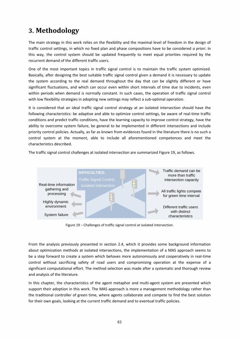
61
3. Methodology
The main strategy in this work relies on the flexibility and the maximal level of freedom in the design of
traffic control settings, in which no fixed plan and phase compositions have to be considered a priori. In
this way, the control system should be updated frequently to meet equal priorities required by the
recurrent demand of the different traffic users.
One of the most important topics in traffic signal control is to maintain the traffic system optimized.
Basically, after designing the best suitable traffic signal control given a demand it is necessary to update
the system according to the real demand throughout the day that can be slightly different or have
significant fluctuations, and which can occur even within short intervals of time due to incidents, even
within periods when demand is normally constant. In such cases, the operation of traffic signal control
with low flexibility strategies in adopting new settings may reflect a sub-optimal operation.
It is considered that an ideal traffic signal control strategy at an isolated intersection should have the
following characteristics: be adaptive and able to optimize control settings, be aware of real-time traffic
conditions and predict traffic conditions, have the learning capacity to improve control strategy, have the
ability to overcome system failure, be general to be implemented in different intersections and include
priority control policies. Actually, as far as known from evidences found in the literature there is no such a
control system at the moment, able to include all aforementioned competences and meet the
characteristics described.
The traffic signal control challenges at isolated intersection are summarized Figure 19, as follows.
Figure 19 – Challenges of traffic signal control at isolated intersection.
From the analysis previously presented in section 2.4, which it provides some background information
about optimization methods at isolated intersections, the implementation of a MAS approach seems to
be a step forward to create a system which behaves more autonomously and cooperatively in real-time
control without sacrificing safety of road users and compromising operation at the expense of a
significant computational effort. The method selection was made after a systematic and thorough review
and analysis of the literature.
In this chapter, the characteristics of the agent metaphor and multi-agent system are presented which
support their adoption in this work. The MAS approach is more a management methodology rather than
the traditional controller of green time, where agents collaborate and compete to find the best solution
for their own goals, looking at the current traffic demand and to eventual traffic policies.
Traffic Signal Control,
Isolated Intersection
All traffic lights compete
for green time interval
DIFFICULTIES:
Highly dynamic
environment
Real-time information
gathering and
processing
Traffic demand can be
more than traffic
intersection capacity
Different traffic users
with distinct
characteristicsSystem failure
62
In section 3.1 each phase of the conceptual model proposed for traffic control is presented, using a
methodology called GAIA (Zambonelli et al., 2003). This will allow the reader to better understand the
concepts together with the proposed methodology and, at the same time, become acquainted with the
system developed for the traffic signal control approach.
As mentioned before, the intersection control problem uses the MAS approach as described in (Vilarinho
et al., 2016). The proposed traffic signal control is organized in two stages (Vilarinho et al., 2017) whose
main goal is to improve people mobility at intersections, as described in sections 3.2 and 3.3. At a first
stage, the proposed traffic signal control aims to determine initial traffic control settings including phase
composition and the respective green time periods, presented in detail in section 3.2. Two approaches for
finding the initial settings were developed, respectively one with and another without traffic plan design.
The second stage is responsible for the optimization of operation, which includes two decisions: firstly, to
define when the current phase should be terminated and secondly to define the next phase to be
implemented. This second stage is a negotiation process, as described in section 3.3. The intersection
control problem is treated as an auction-based mechanism where there are traffic stream managers who
negotiate the use of the intersection on behalf of the drivers making a specific turning movement. The
result of such a negotiation process determines the color for all traffic lights within the intersection.
The optimization framework using MAS, organized in two stages, is presented in section 3.4. In this
section the main message flow among the implemented agents is explained, as well as their identification
of the traffic data needs for the proposed traffic control.
To conclude this chapter, section 3.5 points out the differences and similarities between the proposed
approach presented in this chapter and the existing systems described in the chapter before.
3.1. Multi-Agent System Conceptual Model
Before presenting the architecture of the multi-agent system, it is important to point out the
characteristics of MAS that make us adopt it to model this problem: - Why use the Multi-Agent System
Paradigm?
The MAS paradigm may provide an ideal method to deal with this traffic control problem. Adler and Blue
(2002) concluded that MAS can enhance the design and analysis of problem domains in dynamic
environments, when agents need to interact with each other and the domain is geographically
distributed. For traffic management, Zheng et al. (2013) pointed out three characteristics as the most
appealing for MAS application in the domain of traffic management, which are:
Autonomy: agents decide by themselves how to relate data to commands to achieve goals;
Collaboration: agents are capable of interacting with other agents;
Reactivity: agents perceive changes in the system and respond in a timely manner, which is one
of the most appealing characteristics for MAS application.
The application of MAS to the traffic signal control problem is characterized by the interaction among
many agents that are trying to make a decision each one in a cooperative way. Agents in MAS could have
some additional attributes that enable them to solve problems by themselves, to understand information
and to learn and to evaluate alternatives. The problem-solving component of an intelligent agent can be a
simple rule-based system, a neural network, or some set of fuzzy rules (Zheng et al., 2013).
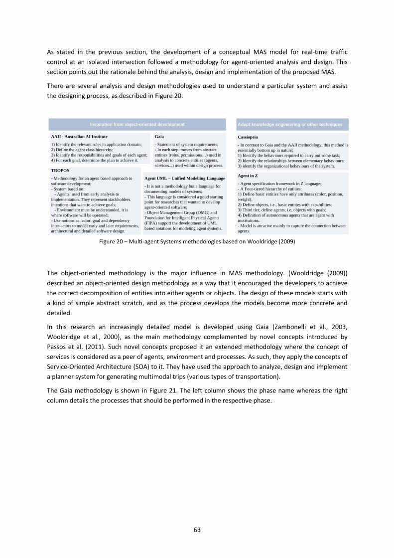
63
As stated in the previous section, the development of a conceptual MAS model for real-time traffic
control at an isolated intersection followed a methodology for agent-oriented analysis and design. This
section points out the rationale behind the analysis, design and implementation of the proposed MAS.
There are several analysis and design methodologies used to understand a particular system and assist
the designing process, as described in Figure 20.
Figure 20 – Multi-agent Systems methodologies based on Wooldridge (2009)
The object-oriented methodology is the major influence in MAS methodology. (Wooldridge (2009))
described an object-oriented design methodology as a way that it encouraged the developers to achieve
the correct decomposition of entities into either agents or objects. The design of these models starts with
a kind of simple abstract scratch, and as the process develops the models become more concrete and
detailed.
In this research an increasingly detailed model is developed using Gaia (Zambonelli et al., 2003,
Wooldridge et al., 2000), as the main methodology complemented by novel concepts introduced by
Passos et al. (2011). Such novel concepts proposed it an extended methodology where the concept of
services is considered as a peer of agents, environment and processes. As such, they apply the concepts of
Service-Oriented Architecture (SOA) to it. They have used the approach to analyze, design and implement
a planner system for generating multimodal trips (various types of transportation).
The Gaia methodology is shown in Figure 21. The left column shows the phase name whereas the right
column details the processes that should be performed in the respective phase.
AAII - Australian AI Institute
1) Identify the relevant roles in application domain;
2) Define the agent class hierarchy;
3) Identify the responsibilities and goals of each agent;
4) For each goal, determine the plan to achieve it.
Inspiration from object-oriented development Adapt knowledge engineering or other techniques
Gaia
- Statement of system requirements;
- In each step, moves from abstract
entities (roles, permissions…) used in
analysis to concrete entities (agents,
services...) used within design process.
Agent UML – Unified Modelling Language
- It is not a methodology but a language for
documenting models of systems;
- This language is considered a good starting
point for researches that wanted to develop
agent-oriented software;
- Object Management Group (OMG) and
Foundation for Intelligent Physical Agents
(FIPA) support the development of UML
based notations for modeling agent systems.
Cassiopeia
- In contrast to Gaia and the AAII methodology, this method is
essentially bottom up in nature;
1) Identify the behaviours required to carry out some task;
2) Identify the relationships between elementary behaviours;
3) identify the organizational behaviours of the system.
Agent in Z
- Agent specification framework in Z language;
- A Four-tiered hierarchy of entities:
1) Define basic entities have only attributes (color, position,
weight);
2) Define objects, i.e., basic entities with capabilities;
3) Third tier, define agents, i.e, objects with goals;
4) Definition of autonomous agents that are agent with
motivations.
- Model is attracive mainly to capture the connection between
agents.
TROPOS
- Methodology for an agent based approach to
software development;
- System based on:
- Agents: used from early analysis to
implementation. They represent stackholders
intentions that want to achieve goals;
- Environment must be understanded, it is
where software will be operated;
- Use notions as: actor, goal and dependency
inter-actors to model early and later requirements,
architectural and detailed software design.

64
Figure 21 – Gaia methodology (Zambonelli et al., 2003)
Before further discussing the Gaia’s scope, the scenario under study must be understood by describing
the operation of a traffic signal at an isolated intersection.
A brief explanation of each phase of the proposed methodology is presented, as follows:
Requirements (section 3.1.2): The goal of this phase is to understand the requirements. The
artifacts of this phase are the requirements model and the actor, goal and dependency diagrams.
Analysis (section3.1.3): Afterwards, the Gaia process starts with an analysis phase wherein the
goal is to collect and establish the organization’s specifications—namely, an organization’s goal,
environmental model, preliminary role model, preliminary interaction model, and rules. The
analysis phase can rely on the output produced by an early requirements engineering phase, and
it is aimed at understanding what the MAS must be.
Architectural Design (section 3.1.4): The analysis phase’s output is the basis for the second
phase—design, which can be logically decomposed into an architectural design phase and a
detailed design phase. The architectural design identifies an efficient and reliable way to
structure the MAS organization and it completes accordingly the preliminary roles and interaction
models. The design phase is where decisions about the actual characteristics of the MAS must be
made.
Detailed Design (section 3.1.5): Once the system’s overall architecture is identified together with
its completed roles and interaction model, the detailed design phase can begin. The methodology
ends with the final diagram of the agent model’s detailed design. This model is a guideline for the
implementation of the agents.
In the next subsection of 3.1, each of the phases of this method is detailed.
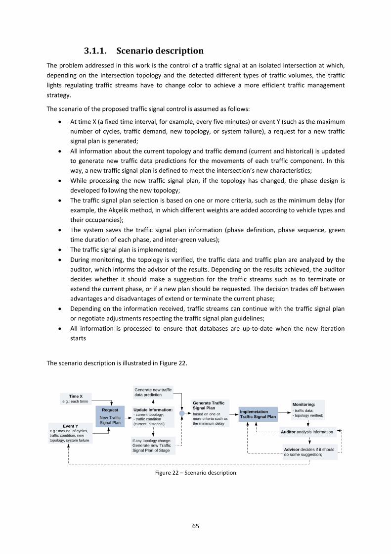
65
3.1.1. Scenario description
The problem addressed in this work is the control of a traffic signal at an isolated intersection at which,
depending on the intersection topology and the detected different types of traffic volumes, the traffic
lights regulating traffic streams have to change color to achieve a more efficient traffic management
strategy.
The scenario of the proposed traffic signal control is assumed as follows:
At time X (a fixed time interval, for example, every five minutes) or event Y (such as the maximum
number of cycles, traffic demand, new topology, or system failure), a request for a new traffic
signal plan is generated;
All information about the current topology and traffic demand (current and historical) is updated
to generate new traffic data predictions for the movements of each traffic component. In this
way, a new traffic signal plan is defined to meet the intersection’s new characteristics;
While processing the new traffic signal plan, if the topology has changed, the phase design is
developed following the new topology;
The traffic signal plan selection is based on one or more criteria, such as the minimum delay (for
example, the Akçelik method, in which different weights are added according to vehicle types and
their occupancies);
The system saves the traffic signal plan information (phase definition, phase sequence, green
time duration of each phase, and inter-green values);
The traffic signal plan is implemented;
During monitoring, the topology is verified, the traffic data and traffic plan are analyzed by the
auditor, which informs the advisor of the results. Depending on the results achieved, the auditor
decides whether it should make a suggestion for the traffic streams such as to terminate or
extend the current phase, or if a new plan should be requested. The decision trades off between
advantages and disadvantages of extend or terminate the current phase;
Depending on the information received, traffic streams can continue with the traffic signal plan
or negotiate adjustments respecting the traffic signal plan guidelines;
All information is processed to ensure that databases are up-to-date when the new iteration
starts
The scenario description is illustrated in Figure 22.
Figure 22 – Scenario description
Event Ye.g.: max no. of cycles,
traffic condition, new
topology, system failure
Time X
e.g.: each 5min
Update Information:- current topology;
- traffic condition
(current, historical).
Generate new traffic
data prediction
If any topology change:
Generate new Traffic
Signal Plan of Stage
Generate Traffic
Signal Plan
based on one or
more criteria such as
the minimum delay
Implemetation
Traffic Signal Plan
Monitoring:
- traffic data;
- topology verified;
Advisor decides if it should
do some suggestion;
AudItor analysis information
Request
New Traffic
Signal Plan
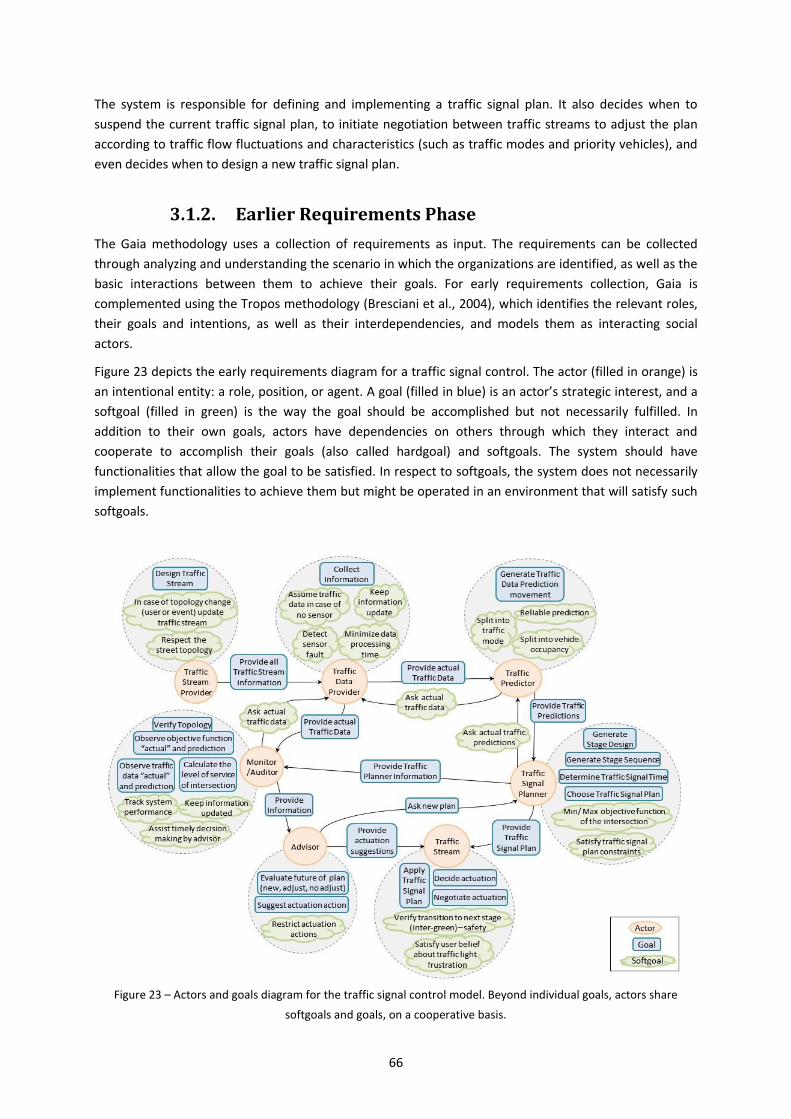
66
The system is responsible for defining and implementing a traffic signal plan. It also decides when to
suspend the current traffic signal plan, to initiate negotiation between traffic streams to adjust the plan
according to traffic flow fluctuations and characteristics (such as traffic modes and priority vehicles), and
even decides when to design a new traffic signal plan.
3.1.2. Earlier Requirements Phase
The Gaia methodology uses a collection of requirements as input. The requirements can be collected
through analyzing and understanding the scenario in which the organizations are identified, as well as the
basic interactions between them to achieve their goals. For early requirements collection, Gaia is
complemented using the Tropos methodology (Bresciani et al., 2004), which identifies the relevant roles,
their goals and intentions, as well as their interdependencies, and models them as interacting social
actors.
Figure 23 depicts the early requirements diagram for a traffic signal control. The actor (filled in orange) is
an intentional entity: a role, position, or agent. A goal (filled in blue) is an actor’s strategic interest, and a
softgoal (filled in green) is the way the goal should be accomplished but not necessarily fulfilled. In
addition to their own goals, actors have dependencies on others through which they interact and
cooperate to accomplish their goals (also called hardgoal) and softgoals. The system should have
functionalities that allow the goal to be satisfied. In respect to softgoals, the system does not necessarily
implement functionalities to achieve them but might be operated in an environment that will satisfy such
softgoals.
Figure 23 – Actors and goals diagram for the traffic signal control model. Beyond individual goals, actors share
softgoals and goals, on a cooperative basis.
67
3.1.3. Analysis Phase
The goal of the analysis phase is to develop an overview of the system and capture its structure,
considering the requirements model. Dividing the system into sub organizations helps to find system
entities with specific goals that interact with other system entities and require competencies that are not
needed in other parts of the system. The following processes are the characterization of the environment
model, followed by the definition of the preliminary role model, and the preliminary interaction model,
which are the outputs of this phase are the preliminary role and interaction models, as well as, the
environment model.
The first process to be performed in the Analysis phase is to subdivide the system into sub-organizations.
From the diagram of the early requirements (see Figure 23), it was identified seven actors (circles). Here,
the goals and softgoals of the actors (dashed circles) are described, as well as are their dependencies.
TrafficStreamProvider aims to design a traffic stream. Each traffic stream is described by movements and
lanes assigned to each movement. To achieve its goal, it was defined two softgoals:
Respect the intersection topology.
Keep the topology information updated in case of topology changes —permanently if new
geometry or lane marks were defined, or temporarily during roadwork— or events such as
accidents or car parking abuse in which lane capacity is affected.
The actor should provide all traffic stream information to TrafficDataProvider to be able to exploit the
sensor data.
TrafficDataProvider aims to collect information about traffic data from sensors installed at a signalized
intersection and aggregate data according to the traffic stream information received. The
TrafficDataProvider’s goal is defined upon four subgoals:
Keep traffic data information updated by collecting data at each time interval;
Minimize data processing time when dependent actors are waiting for the information;
If no sensor is installed in an intersection sector, the actor should assume the historical traffic
data;
If a sensor seems to act strangely, the actor should decide whether to assume the traffic data or
ignore the road supply (lane).
TrafficPredictor requests recent traffic data from this actor and makes its own traffic predictions as
described next. Monitor/Advisor also requests traffic data from this actor and uses them for early
detection of possible problems and improvements at the intersection control.
TrafficPredictor focuses on generating a traffic data prediction for each movement in order to optimize
signal control for imminent demand. The strategy could include traffic measurements from a past time
period and the current time and use them to estimate the near future. The generated traffic prediction
should be both reliable for future traffic such as arrivals and queues and comprehensive, with total values

68
and splits into traffic modes such as pedestrian, private vehicle, and bus. Traffic splitting is requested so
traffic priority policies can be implemented and used to weight objective functions.
The actor requests recent traffic data from TrafficDataProvider and makes its own traffic predictions.
TrafficSignalPlanner requests this actor for recent traffic predictions and uses them to optimize the traffic
signal plan.
TrafficSignalPlanner has four main objectives:
Generate phase design. This involves searching possible signal group sets that can run
concurrently while respecting a set of safety constraints;
Generate phase sequence. Once possible phase designs are defined, this step compiles strategic
groupings of phases to have signal plans designed;
Determine traffic signal times. For each traffic signal plan, the green time durations, inter-green
duration, and cycle lengths are calculated.
Choose traffic signal plan, based on a given criterion or a weighted combination of different
criteria.
We defined two softgoals for the objective of choosing a traffic signal plan. Traffic signal plan selection is
based on the best objective function. The signal control objectives can be divided by:
Efficiencies related to the intersection operation, such as minimization of delay times, queue
lengths, or stops;
Environmental impact of traffic; and
Accessibility for vulnerable users (that are pedestrians and cyclists) or priority road users.
Second, plan design and timing should be conducted respecting some operational constraints, such as
topology, minimum green, and maximum and minimum cycle lengths.
The actor requests TrafficPredictor for recent traffic predictions and uses these to optimize its traffic
signal plan. It provides the selected plan to Traffic-Stream to be applied. Advisor asks for a new plan
search if the current plan is not adequate to remain active. Finally, Monitor/Auditor receives information
from the traffic planner, such as traffic predictions and the objective function, so that it can monitor it
independently.
TrafficStream has three main goals:
Apply the traffic signal plan. Each traffic stream assumes a signal state (red, yellow, or green)
according to the plan or the current actuation action, if it has been defined;
Negotiate actuation. Traffic streams cooperate to find possible actuation actions following the
advisor’s suggestions;
Decide actuation. Traffic stream actors together decide upon an actuation action to implement.
To accomplish its goal, the actor aims to do two things. First, it should verify transition to the next phase.
If the next phase is new, the actor should verify details about the phase transition and whether any signal
group can keep the green without compromising safety. Second, the actor should satisfy user beliefs
69
about the traffic light to prevent frustration. If a new phase is defined differently from planned, the actor
should guarantee that no movement is neglected due to system errors.
The actor receives the selected traffic signal plan from TrafficSignalPlanner to apply it, as well as actuation
suggestions from Advisor to guide the negotiation phase. If negotiations are needed, TrafficStream actors
discuss these among themselves.
Advisor has two main objectives. The first is to evaluate the future of plan (that is, choose a possible
action depending on information received from Monitor/Auditor and find a new plan, adjust the current
plan, or continue the implementation). The second objective is to suggest actuation action, if the Advisor
decided to adjust the plan through actuation. In this case, the actor prepares a recommendation to guide
the actuation process. The second objective implies the softgoal of formulating a recommendation that
will restrict the solution space for actuation negotiation.
The actor provides actuation suggestions to TrafficStream. It requests a new plan search from
TrafficSignalPlanner if the current plan is not adequate to remain active. Monitor/Auditor sends monitor
information to this actor.
Monitor/Auditor has four main objectives: to verify the topology (check whether any topology change
has occurred and if so, report it to the Advisor), observe traffic data (actual and predicted), observe
objective function, and calculate the level of service of the intersection. The data acquired through
monitoring are used to evaluate whether the Advisor should ask for any plan change. The objectives have
three subgoals:
Systematically and routinely collect data to keep information updated;
Track system performance by evaluating and learning to improve practices and activities in the
future;
Assist Advisor’s timely decision-making to exploit every opportunity to improve the intersection
system.
The actor requests recent traffic data from TrafficDataProvider both to allow early detection of possible
problems and to further implement improvements at the intersection control. It receives traffic planner
information, such as traffic predictions and the objective function from TrafficSignalPlanner. It also sends
monitor information to the Advisor.
The second process of the analysis phase is to define the environment. Modeling the environment is a
major activity in agent-oriented methodologies. The environment model can be viewed in its simplest
form as a list of resources that the MAS can exploit, control, or consume when working toward its goal.
The resources can be information (such as a database) or a physical entity (such as a sensor). Six resources
were defined for the proposed traffic signal control: topology, traffic sensor, traffic database, traffic
prediction, traffic signal plan, and traffic light. The resources are identified by name and characterized by
their types of actions, in Table 8, along with a brief description to complete the model.
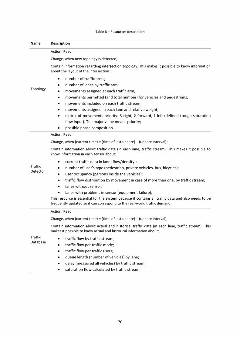
70
Table 8 – Resources description
Name Description
Topology
Action: Read
Change, when new topology is detected;
Contain information regarding intersection topology. This makes it possible to know information about the layout of the intersection:
number of traffic arms;
number of lanes by traffic arm;
movements assigned at each traffic arm;
movements permitted (and total number) for vehicles and pedestrians;
movements included on each traffic stream;
movements assigned in each lane and relative weight;
matrix of movements priority: 3 right, 2 forward, 1 left (defined trough saturation
flow input). The major value means priority;
possible phase composition.
Traffic Detector
Action: Read
Change, when (current time) = (time of last update) + (update interval);
Contain information about traffic data (in each lane, traffic stream). This makes it possible to know information in each sensor about:
current traffic data in lane (flow/density);
number of user’s type (pedestrian, private vehicles, bus, bicycles);
user occupancy (persons inside the vehicles);
traffic flow distribution by movement in case of more than one, by traffic stream;
lanes without sensor;
lanes with problems in sensor (equipment failure);
This resource is essential for the system because it contains all traffic data and also needs to be frequently updated so it can correspond to the real-world traffic demand.
Traffic Database
Action: Read
Change, when (current time) = (time of last update) + (update interval);
Contain information about actual and historical traffic data (in each lane, traffic stream). This makes it possible to know actual and historical information about:
traffic flow by traffic stream;
traffic flow per traffic mode;
traffic flow per traffic users;
queue length (number of vehicles) by lane;
delay (measured all vehicles) by traffic stream;
saturation flow calculated by traffic stream;
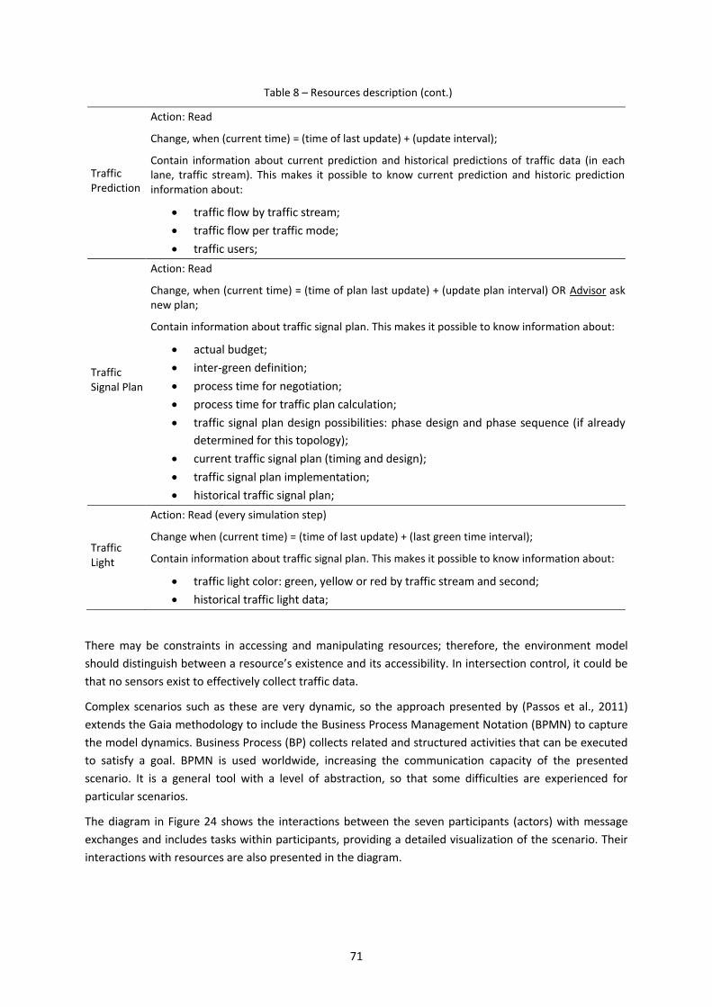
71
Table 8 – Resources description (cont.)
Traffic Prediction
Action: Read
Change, when (current time) = (time of last update) + (update interval);
Contain information about current prediction and historical predictions of traffic data (in each lane, traffic stream). This makes it possible to know current prediction and historic prediction information about:
traffic flow by traffic stream;
traffic flow per traffic mode;
traffic users;
Traffic Signal Plan
Action: Read
Change, when (current time) = (time of plan last update) + (update plan interval) OR Advisor ask new plan;
Contain information about traffic signal plan. This makes it possible to know information about:
actual budget;
inter-green definition;
process time for negotiation;
process time for traffic plan calculation;
traffic signal plan design possibilities: phase design and phase sequence (if already
determined for this topology);
current traffic signal plan (timing and design);
traffic signal plan implementation;
historical traffic signal plan;
Traffic Light
Action: Read (every simulation step)
Change when (current time) = (time of last update) + (last green time interval);
Contain information about traffic signal plan. This makes it possible to know information about:
traffic light color: green, yellow or red by traffic stream and second;
historical traffic light data;
There may be constraints in accessing and manipulating resources; therefore, the environment model
should distinguish between a resource’s existence and its accessibility. In intersection control, it could be
that no sensors exist to effectively collect traffic data.
Complex scenarios such as these are very dynamic, so the approach presented by (Passos et al., 2011)
extends the Gaia methodology to include the Business Process Management Notation (BPMN) to capture
the model dynamics. Business Process (BP) collects related and structured activities that can be executed
to satisfy a goal. BPMN is used worldwide, increasing the communication capacity of the presented
scenario. It is a general tool with a level of abstraction, so that some difficulties are experienced for
particular scenarios.
The diagram in Figure 24 shows the interactions between the seven participants (actors) with message
exchanges and includes tasks within participants, providing a detailed visualization of the scenario. Their
interactions with resources are also presented in the diagram.
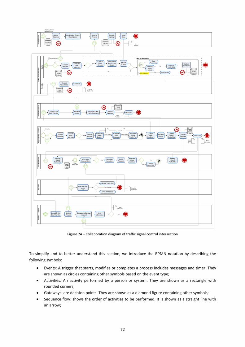
72
Figure 24 – Collaboration diagram of traffic signal control intersection
To simplify and to better understand this section, we introduce the BPMN notation by describing the
following symbols:
Events: A trigger that starts, modifies or completes a process includes messages and timer. They
are shown as circles containing other symbols based on the event type;
Activities: An activity performed by a person or system. They are shown as a rectangle with
rounded corners;
Gateways: are decision points. They are shown as a diamond figure containing other symbols;
Sequence flow: shows the order of activities to be performed. It is shown as a straight line with
an arrow;
Traffic
Database
Tra
ffic
Da
ta P
rov
ide
r
Topology
Tra
ffic
Str
ea
mT
raff
ic P
red
icto
rS
ign
al T
raff
ic P
lan
ne
rT
raff
ic S
tre
am
Consult
Detector
Traffic
Detector
Generate Data
Traffic Prediction
Cyclic event (ms)
topology change:
predict or event
Update
Database
Update
Database
Send Notice Recent
Data UpdateSend
Data
Actual
Traffic Data
Sensor
fault ?
No
Yes
Assume
traffic data
Data
Processing
All movements
Ga
the
rP
rov
ide
r Consult
Recent Data
Traffic
Database
Consult Traffic
Data Provider
Receive
Answer
Send Data
Traffic
Prediction
Update
Database
Receive
Answer
Search
Best Plan
Generate
Stage
Sequence
Choose
Signal
Traffic Plan
Generate
Stage
Design
New
topology
Determine
Signal
Traffic Plan
Stage Design Plan Design
Inicializar
Consult
topology
Consult
Traffic
Stream
Consult
topology
Topology
Receive
Answer
No
Mo
nit
or
/ A
ud
ito
r
Execute
Signal
Traffic Plan
Yes
No
Data Processing
Consult
Traffic
Predictor
Yes
Stage
green time
Evaluate plan
future
Send Information
Yes
Define
intergreenNo
Update
Signal
Traffic Plan
Negotiate
Actuation
No change
Ask new Traffic Plan
Evaluate
new
topology
Traffic
Light
Evaluate
New
topology
Send Data
Traffic
Prediction
Receive
Answer
Traffic
Signal
PlanUpdate
Database Send Data
Signal
Traffic
Plan
Send Notice
Recent Data
UpdateChange
sensor
status
No
Yes Send Notice
Ad
vis
or
Plan
Information
Evaluate traffic data
receivedSend
InformationNo
Yes
Consult Traffic
Data Provider
Receive
Answer
Information
from advisorYes
No
Decide
Actuation
Evaluate:
stage
continue
Actuation
Suggestion
Audit
Information
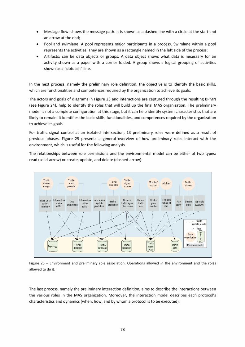
73
Message flow: shows the message path. It is shown as a dashed line with a circle at the start and
an arrow at the end;
Pool and swimlane: A pool represents major participants in a process. Swimlane within a pool
represents the activities. They are shown as a rectangle named in the left side of the process;
Artifacts: can be data objects or groups. A data object shows what data is necessary for an
activity shown as a paper with a corner folded. A group shows a logical grouping of activities
shown as a “dotdash” line.
In the next process, namely the preliminary role definition, the objective is to identify the basic skills,
which are functionalities and competences required by the organization to achieve its goals.
The actors and goals of diagrams in Figure 23 and interactions are captured through the resulting BPMN
(see Figure 24), help to identify the roles that will build up the final MAS organization. The preliminary
model is not a complete configuration at this stage, but it can help identify system characteristics that are
likely to remain. It identifies the basic skills, functionalities, and competences required by the organization
to achieve its goals.
For traffic signal control at an isolated intersection, 13 preliminary roles were defined as a result of
previous phases. Figure 25 presents a general overview of how preliminary roles interact with the
environment, which is useful for the following analysis.
The relationships between role permissions and the environmental model can be either of two types:
read (solid-arrow) or create, update, and delete (dashed-arrow).
Figure 25 – Environment and preliminary role association. Operations allowed in the environment and the roles
allowed to do it.
The last process, namely the preliminary interaction definition, aims to describe the interactions between
the various roles in the MAS organization. Moreover, the interaction model describes each protocol’s
characteristics and dynamics (when, how, and by whom a protocol is to be executed).
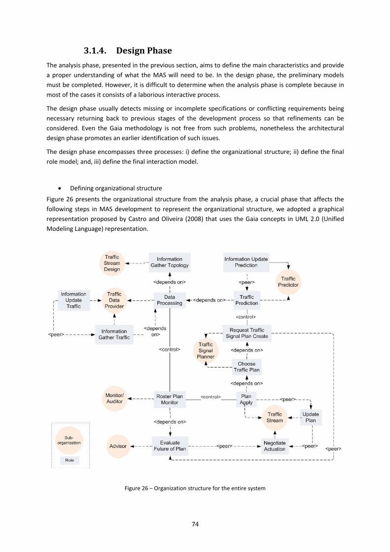
74
3.1.4. Design Phase
The analysis phase, presented in the previous section, aims to define the main characteristics and provide
a proper understanding of what the MAS will need to be. In the design phase, the preliminary models
must be completed. However, it is difficult to determine when the analysis phase is complete because in
most of the cases it consists of a laborious interactive process.
The design phase usually detects missing or incomplete specifications or conflicting requirements being
necessary returning back to previous stages of the development process so that refinements can be
considered. Even the Gaia methodology is not free from such problems, nonetheless the architectural
design phase promotes an earlier identification of such issues.
The design phase encompasses three processes: i) define the organizational structure; ii) define the final
role model; and, iii) define the final interaction model.
Defining organizational structure
Figure 26 presents the organizational structure from the analysis phase, a crucial phase that affects the
following steps in MAS development to represent the organizational structure, we adopted a graphical
representation proposed by Castro and Oliveira (2008) that uses the Gaia concepts in UML 2.0 (Unified
Modeling Language) representation.
Figure 26 – Organization structure for the entire system
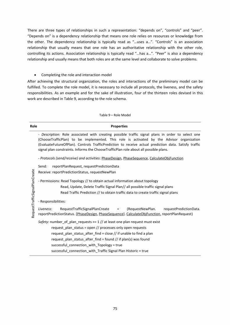
75
There are three types of relationships in such a representation: “depends on”, “controls” and “peer”.
“Depends on” is a dependency relationship that means one role relies on resources or knowledge from
the other. The dependency relationship is typically read as “…uses a…”. “Controls” is an association
relationship that usually means that one role has an authoritative relationship with the other role,
controlling its actions. Association relationship is typically read “…has a…”. “Peer” is also a dependency
relationship and usually means that both roles are at the same level and collaborate to solve problems.
Completing the role and interaction model
After achieving the structural organization, the roles and interactions of the preliminary model can be
fulfilled. To complete the role model, it is necessary to include all protocols, the liveness, and the safety
responsibilities. As an example and for the sake of illustration, four of the thirteen roles devised in this
work are described in Table 9, according to the role schema.
Table 9 – Role Model
Role Properties
Req
ues
tTra
ffic
Sign
alP
lan
Cre
ate
- Description: Role associated with creating possible traffic signal plans in order to select one
(ChooseTrafficPlan) to be implemented. This role is activated by the Advisor organization
(EvaluateFutureOfPlan). Controls TrafficPrediction to receive actual prediction data. Satisfy traffic
signal plan constraints. Informs the ChooseTrafficPlan role about all possible plans.
- Protocols (send/receive) and activities: PhaseDesign, PhaseSequence, CalculateObjFunction
Send: reportPlanRequest, requestPredictionData
Receive: reportPredictionStatus, requestNewPlan
- Permissions: Read Topology // to obtain actual information about topology
Read, Update, Delete Traffic Signal Plan// all possible traffic signal plans
Read Traffic Prediction // to obtain traffic data to create traffic signal plans
- Responsibilities:
Liveness: RequestTrafficSignalPlanCreate = (RequestNewPlan. requestPredictionData.
reportPredictionStatus. [PhaseDesign, PhaseSequence]. CalculateObjFunction. reportPlanRequest)
Safety: number_of_plan_requests >= 1 // at least one plan request must exist
request_plan_status = open // processes only open requests
request_plan_status_after_find = close // if unable to find a plan
request_plan_status_after_find = found // if plan(s) was found
successful_connection_with_Topology = true
successful_connection_with_Traffic Signal Plan Historic = true
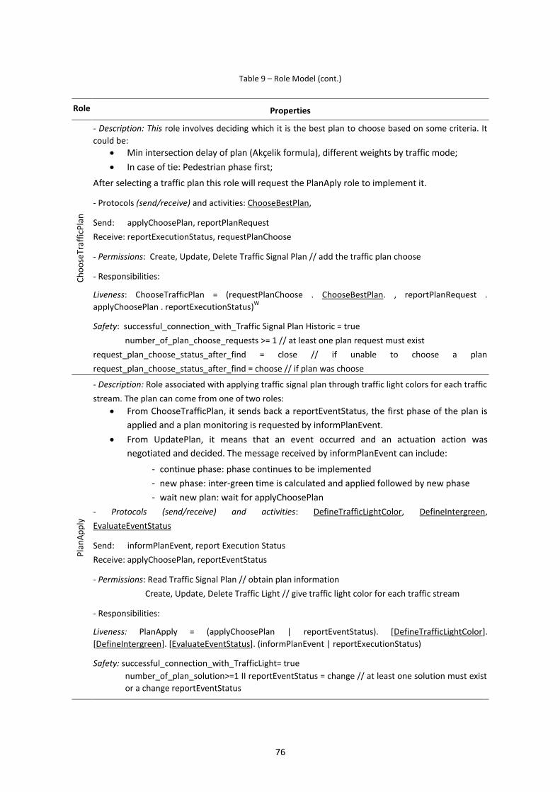
76
Table 9 – Role Model (cont.)
Role Properties
Ch
oo
seTr
affi
cPla
n
- Description: This role involves deciding which it is the best plan to choose based on some criteria. It
could be:
Min intersection delay of plan (Akçelik formula), different weights by traffic mode;
In case of tie: Pedestrian phase first;
After selecting a traffic plan this role will request the PlanAply role to implement it.
- Protocols (send/receive) and activities: ChooseBestPlan,
Send: applyChoosePlan, reportPlanRequest
Receive: reportExecutionStatus, requestPlanChoose
- Permissions: Create, Update, Delete Traffic Signal Plan // add the traffic plan choose
- Responsibilities:
Liveness: ChooseTrafficPlan = (requestPlanChoose . ChooseBestPlan. , reportPlanRequest .
applyChoosePlan . reportExecutionStatus)W
Safety: successful_connection_with_Traffic Signal Plan Historic = true
number_of_plan_choose_requests >= 1 // at least one plan request must exist
request_plan_choose_status_after_find = close // if unable to choose a plan
request_plan_choose_status_after_find = choose // if plan was choose
Pla
nA
pp
ly
- Description: Role associated with applying traffic signal plan through traffic light colors for each traffic
stream. The plan can come from one of two roles:
From ChooseTrafficPlan, it sends back a reportEventStatus, the first phase of the plan is
applied and a plan monitoring is requested by informPlanEvent.
From UpdatePlan, it means that an event occurred and an actuation action was
negotiated and decided. The message received by informPlanEvent can include:
- continue phase: phase continues to be implemented
- new phase: inter-green time is calculated and applied followed by new phase
- wait new plan: wait for applyChoosePlan
- Protocols (send/receive) and activities: DefineTrafficLightColor, DefineIntergreen,
EvaluateEventStatus
Send: informPlanEvent, report Execution Status
Receive: applyChoosePlan, reportEventStatus
- Permissions: Read Traffic Signal Plan // obtain plan information
Create, Update, Delete Traffic Light // give traffic light color for each traffic stream
- Responsibilities:
Liveness: PlanApply = (applyChoosePlan | reportEventStatus). [DefineTrafficLightColor].
[DefineIntergreen]. [EvaluateEventStatus]. (informPlanEvent | reportExecutionStatus)
Safety: successful_connection_with_TrafficLight= true
number_of_plan_solution>=1 II reportEventStatus = change // at least one solution must exist
or a change reportEventStatus
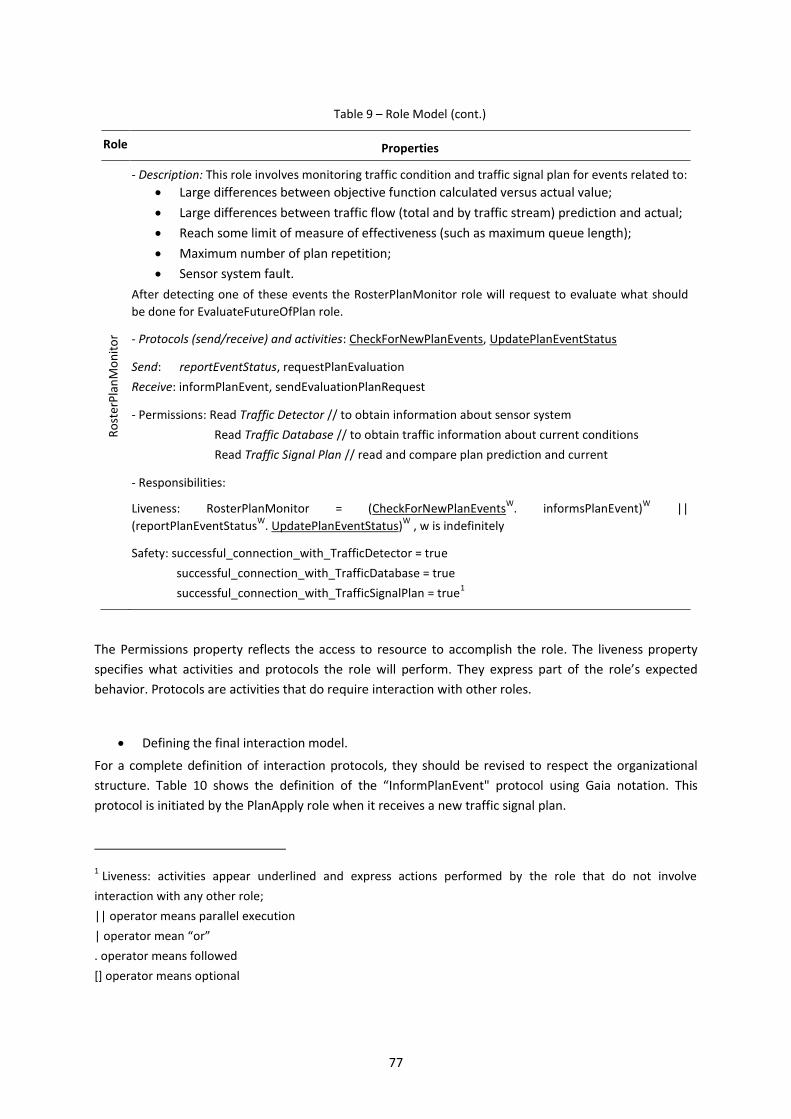
77
Table 9 – Role Model (cont.)
Role Properties
Ro
ster
Pla
nM
on
ito
r
- Description: This role involves monitoring traffic condition and traffic signal plan for events related to:
Large differences between objective function calculated versus actual value;
Large differences between traffic flow (total and by traffic stream) prediction and actual;
Reach some limit of measure of effectiveness (such as maximum queue length);
Maximum number of plan repetition;
Sensor system fault.
After detecting one of these events the RosterPlanMonitor role will request to evaluate what should
be done for EvaluateFutureOfPlan role.
- Protocols (send/receive) and activities: CheckForNewPlanEvents, UpdatePlanEventStatus
Send: reportEventStatus, requestPlanEvaluation
Receive: informPlanEvent, sendEvaluationPlanRequest
- Permissions: Read Traffic Detector // to obtain information about sensor system
Read Traffic Database // to obtain traffic information about current conditions
Read Traffic Signal Plan // read and compare plan prediction and current
- Responsibilities:
Liveness: RosterPlanMonitor = (CheckForNewPlanEventsW
. informsPlanEvent)W
||
(reportPlanEventStatusW
. UpdatePlanEventStatus)W
, w is indefinitely
Safety: successful_connection_with_TrafficDetector = true
successful_connection_with_TrafficDatabase = true
successful_connection_with_TrafficSignalPlan = true1
The Permissions property reflects the access to resource to accomplish the role. The liveness property
specifies what activities and protocols the role will perform. They express part of the role’s expected
behavior. Protocols are activities that do require interaction with other roles.
Defining the final interaction model.
For a complete definition of interaction protocols, they should be revised to respect the organizational
structure. Table 10 shows the definition of the “InformPlanEvent" protocol using Gaia notation. This
protocol is initiated by the PlanApply role when it receives a new traffic signal plan.
1 Liveness: activities appear underlined and express actions performed by the role that do not involve
interaction with any other role;
|| operator means parallel execution
| operator mean “or”
. operator means followed
[] operator means optional
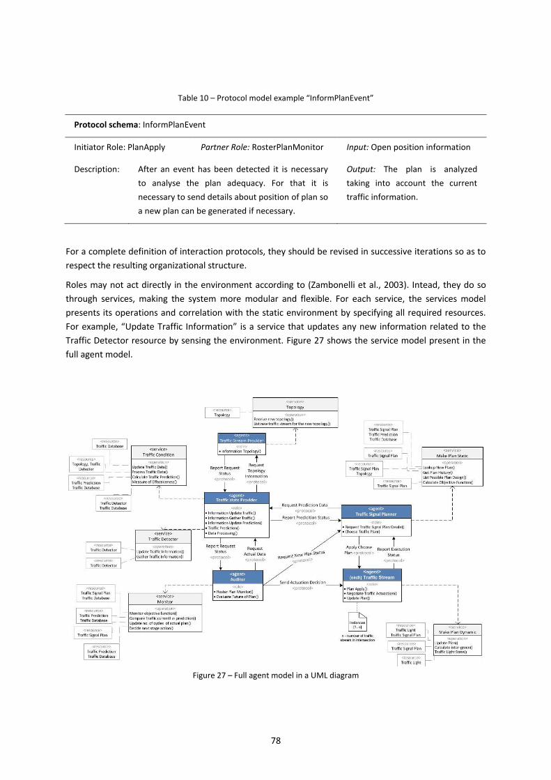
78
Table 10 – Protocol model example “InformPlanEvent”
Protocol schema: InformPlanEvent
Initiator Role: PlanApply Partner Role: RosterPlanMonitor Input: Open position information
Description: After an event has been detected it is necessary
to analyse the plan adequacy. For that it is
necessary to send details about position of plan so
a new plan can be generated if necessary.
Output: The plan is analyzed
taking into account the current
traffic information.
For a complete definition of interaction protocols, they should be revised in successive iterations so as to
respect the resulting organizational structure.
Roles may not act directly in the environment according to (Zambonelli et al., 2003). Intead, they do so
through services, making the system more modular and flexible. For each service, the services model
presents its operations and correlation with the static environment by specifying all required resources.
For example, “Update Traffic Information” is a service that updates any new information related to the
Traffic Detector resource by sensing the environment. Figure 27 shows the service model present in the
full agent model.
Figure 27 – Full agent model in a UML diagram
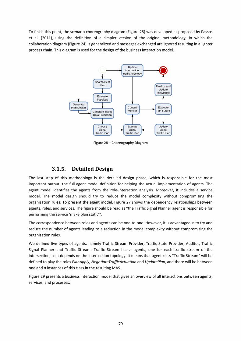
79
To finish this point, the scenario choreography diagram (Figure 28) was developed as proposed by Passos
et al. (2011), using the definition of a simpler version of the original methodology, in which the
collaboration diagram (Figure 24) is generalized and messages exchanged are ignored resulting in a lighter
process chain. This diagram is used for the design of the business interaction model.
Figure 28 – Choreography Diagram
3.1.5. Detailed Design
The last step of this methodology is the detailed design phase, which is responsible for the most
important output: the full agent model definition for helping the actual implementation of agents. The
agent model identifies the agents from the role-interaction analysis. Moreover, it includes a service
model. The model design should try to reduce the model complexity without compromising the
organization rules. To present the agent model, Figure 27 shows the dependency relationships between
agents, roles, and services. The figure should be read as “the Traffic Signal Planner agent is responsible for
performing the service ‘make plan static’”.
The correspondence between roles and agents can be one-to-one. However, it is advantageous to try and
reduce the number of agents leading to a reduction in the model complexity without compromising the
organization rules.
We defined five types of agents, namely Traffic Stream Provider, Traffic State Provider, Auditor, Traffic
Signal Planner and Traffic Stream. Traffic Stream has n agents, one for each traffic stream of the
intersection, so it depends on the intersection topology. It means that agent class “Traffic Stream” will be
defined to play the roles PlanApply, NegotiateTrafficActuation and UpdatePlan, and there will be between
one and n instances of this class in the resulting MAS.
Figure 29 presents a business interaction model that gives an overview of all interactions between agents,
services, and processes.
Update
information:
traffic, topology
Generate Traffic
Data Prediction
Search Best
Plan
Generate
Plan Design Consult
Monitor
Choose
Signal
Traffic Plan
Execute
Signal
Traffic Plan
Update
Signal
Traffic Plan
Evaluate
Topology
Finalize and
Update
knowledge
Evaluate
Pan Future
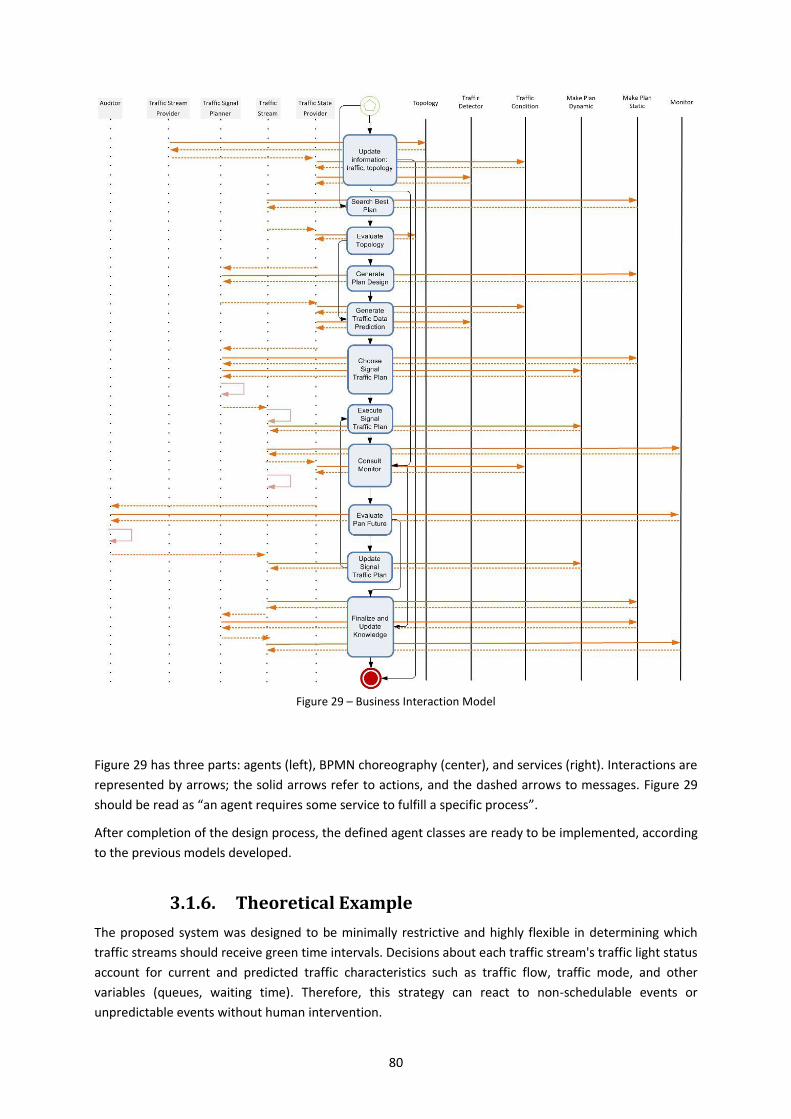
80
Figure 29 – Business Interaction Model
Figure 29 has three parts: agents (left), BPMN choreography (center), and services (right). Interactions are
represented by arrows; the solid arrows refer to actions, and the dashed arrows to messages. Figure 29
should be read as “an agent requires some service to fulfill a specific process”.
After completion of the design process, the defined agent classes are ready to be implemented, according
to the previous models developed.
3.1.6. Theoretical Example
The proposed system was designed to be minimally restrictive and highly flexible in determining which
traffic streams should receive green time intervals. Decisions about each traffic stream's traffic light status
account for current and predicted traffic characteristics such as traffic flow, traffic mode, and other
variables (queues, waiting time). Therefore, this strategy can react to non-schedulable events or
unpredictable events without human intervention.
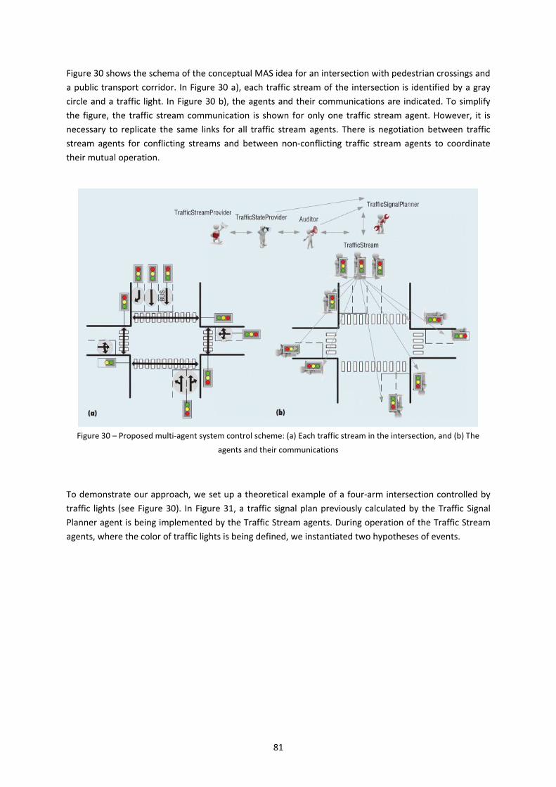
81
Figure 30 shows the schema of the conceptual MAS idea for an intersection with pedestrian crossings and
a public transport corridor. In Figure 30 a), each traffic stream of the intersection is identified by a gray
circle and a traffic light. In Figure 30 b), the agents and their communications are indicated. To simplify
the figure, the traffic stream communication is shown for only one traffic stream agent. However, it is
necessary to replicate the same links for all traffic stream agents. There is negotiation between traffic
stream agents for conflicting streams and between non-conflicting traffic stream agents to coordinate
their mutual operation.
Figure 30 – Proposed multi-agent system control scheme: (a) Each traffic stream in the intersection, and (b) The
agents and their communications
To demonstrate our approach, we set up a theoretical example of a four-arm intersection controlled by
traffic lights (see Figure 30). In Figure 31, a traffic signal plan previously calculated by the Traffic Signal
Planner agent is being implemented by the Traffic Stream agents. During operation of the Traffic Stream
agents, where the color of traffic lights is being defined, we instantiated two hypotheses of events.
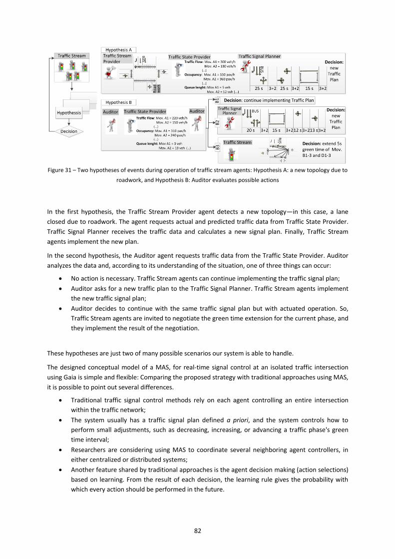
82
Figure 31 – Two hypotheses of events during operation of traffic stream agents: Hypothesis A: a new topology due to
roadwork, and Hypothesis B: Auditor evaluates possible actions
In the first hypothesis, the Traffic Stream Provider agent detects a new topology—in this case, a lane
closed due to roadwork. The agent requests actual and predicted traffic data from Traffic State Provider.
Traffic Signal Planner receives the traffic data and calculates a new signal plan. Finally, Traffic Stream
agents implement the new plan.
In the second hypothesis, the Auditor agent requests traffic data from the Traffic State Provider. Auditor
analyzes the data and, according to its understanding of the situation, one of three things can occur:
No action is necessary. Traffic Stream agents can continue implementing the traffic signal plan;
Auditor asks for a new traffic plan to the Traffic Signal Planner. Traffic Stream agents implement
the new traffic signal plan;
Auditor decides to continue with the same traffic signal plan but with actuated operation. So,
Traffic Stream agents are invited to negotiate the green time extension for the current phase, and
they implement the result of the negotiation.
These hypotheses are just two of many possible scenarios our system is able to handle.
The designed conceptual model of a MAS, for real-time signal control at an isolated traffic intersection
using Gaia is simple and flexible: Comparing the proposed strategy with traditional approaches using MAS,
it is possible to point out several differences.
Traditional traffic signal control methods rely on each agent controlling an entire intersection
within the traffic network;
The system usually has a traffic signal plan defined a priori, and the system controls how to
perform small adjustments, such as decreasing, increasing, or advancing a traffic phase's green
time interval;
Researchers are considering using MAS to coordinate several neighboring agent controllers, in
either centralized or distributed systems;
Another feature shared by traditional approaches is the agent decision making (action selections)
based on learning. From the result of each decision, the learning rule gives the probability with
which every action should be performed in the future.

83
Our approach is distinct from other efforts to the extent that each traffic stream is an agent and each
signalized intersection builds upon independent MASs. Thus, the multitude of agents designed for isolated
intersections creates, manages, and evolves its own traffic signal plans. Therefore, this proposed multi-
agent control brings up the benefit of phased designs and sequences being formed as needed instead of
being established a priori. The system structure is flexible and can adapt traffic control decisions to
predictions and react to unexpected traffic events.
3.2. Initial Control Settings
The initial control settings stage aims to find a traffic signal plan including phase composition definition
and respective green time periods. In the MAS perspective, this stage occurs occasionally when the
“Auditor agent” decides that a new traffic signal plan is needed (e.g. due to new topology, empty budget,
and so forth).
In this research, traffic signal control variables and boundaries were rethought accounting for the
minimum constraints so as to increase the area of the space which contains possible solutions of the
proposed traffic control strategy and to innovate upon the traditional traffic signal control methodologies.
Traffic stream is defined as the base unit of the proposed traffic signal control, instead of signal group or
phase element.
The settings are defined in real-time, using an online methodology based on data collection of traffic state
(i.e. traffic flow, queue length, delay time).
In the following section we are going to present the approach of traffic signal plan design (3.2.1) and
timing plan calculation (3.2.2) in more detail, and for last the selection method used to choose the traffic
signal plan to be implemented.
3.2.1. Traffic Signal Plan Design
The proposed traffic signal plan design is based on enumeration. All possible signal plans are
automatically designed for each intersection grouping the maximum compatible traffic streams by phase.
In this way, all traffic streams that can run at same time are allowed to be part of a phase bringing more
flexibility to the real-time traffic control.
The traffic signal plan design includes four processes: i) define the parameter indexes; ii) define the input
data; iii) define phase composition; and, iv) define possible traffic signal plan designs.
The method was developed to be implemented in any intersection geometry without requiring much
effort in parameterization (as detailed in Figure 32);
Every intersection is described as having n traffic arms and are numbered consecutively in
counterclockwise direction from any traffic arm;
each arm i is described by having l approaching lanes, where i [1; n], and are also numbered
consecutively from the right to left hand;
The number of exit lanes was discarded since they are not considered in the algorithm;
Turning movements are described as a vector (m,n) where m is origin arm and n is destination
arm in total of p movements.
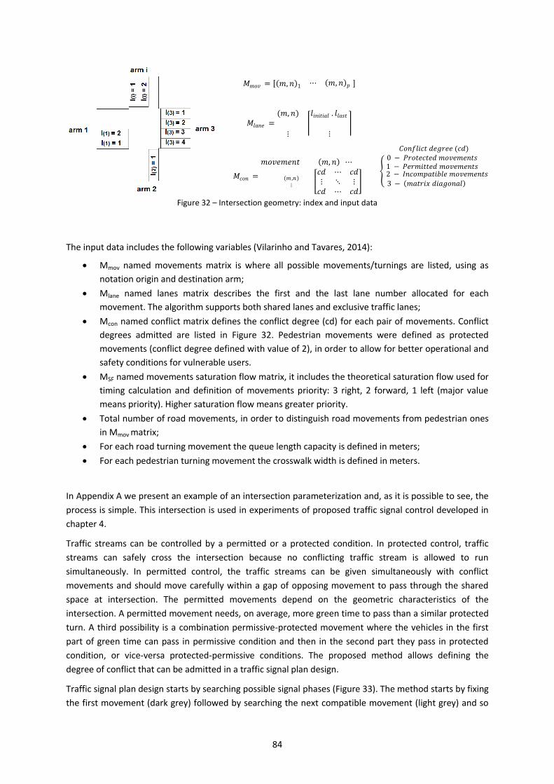
84
Figure 32 – Intersection geometry: index and input data
The input data includes the following variables (Vilarinho and Tavares, 2014):
Mmov named movements matrix is where all possible movements/turnings are listed, using as
notation origin and destination arm;
Mlane named lanes matrix describes the first and the last lane number allocated for each
movement. The algorithm supports both shared lanes and exclusive traffic lanes;
Mcon named conflict matrix defines the conflict degree (cd) for each pair of movements. Conflict
degrees admitted are listed in Figure 32. Pedestrian movements were defined as protected
movements (conflict degree defined with value of 2), in order to allow for better operational and
safety conditions for vulnerable users.
MSF named movements saturation flow matrix, it includes the theoretical saturation flow used for
timing calculation and definition of movements priority: 3 right, 2 forward, 1 left (major value
means priority). Higher saturation flow means greater priority.
Total number of road movements, in order to distinguish road movements from pedestrian ones
in Mmov matrix;
For each road turning movement the queue length capacity is defined in meters;
For each pedestrian turning movement the crosswalk width is defined in meters.
In Appendix A we present an example of an intersection parameterization and, as it is possible to see, the
process is simple. This intersection is used in experiments of proposed traffic signal control developed in
chapter 4.
Traffic streams can be controlled by a permitted or a protected condition. In protected control, traffic
streams can safely cross the intersection because no conflicting traffic stream is allowed to run
simultaneously. In permitted control, the traffic streams can be given simultaneously with conflict
movements and should move carefully within a gap of opposing movement to pass through the shared
space at intersection. The permitted movements depend on the geometric characteristics of the
intersection. A permitted movement needs, on average, more green time to pass than a similar protected
turn. A third possibility is a combination permissive-protected movement where the vehicles in the first
part of green time can pass in permissive condition and then in the second part they pass in protected
condition, or vice-versa protected-permissive conditions. The proposed method allows defining the
degree of conflict that can be admitted in a traffic signal plan design.
Traffic signal plan design starts by searching possible signal phases (Figure 33). The method starts by fixing
the first movement (dark grey) followed by searching the next compatible movement (light grey) and so
𝑀𝑚𝑜 = 𝑚, 1 ⋯ 𝑚, 𝑝
𝑀 𝑒 =(𝑚, )
⋮
𝑖 𝑖 𝑖 .
⋮
𝑀𝑐𝑜 =
𝑚𝑜 𝑒𝑚𝑒 𝑚, ⋯
𝑚 ,
⋮ 𝑐 ⋯ 𝑐 ⋮ ⋱ ⋮𝑐 ⋯ 𝑐
𝑜 𝑓 𝑖𝑐 𝑒 𝑒𝑒 (𝑐 )
0 𝑜 𝑒𝑐 𝑒 𝑚𝑜 𝑒𝑚𝑒 1 𝑒 𝑚𝑖 𝑒 𝑚𝑜 𝑒𝑚𝑒
2 𝐼 𝑐𝑜𝑚𝑝 𝑖 𝑒 𝑚𝑜 𝑒𝑚𝑒
3 𝑚 𝑖 𝑖 𝑜
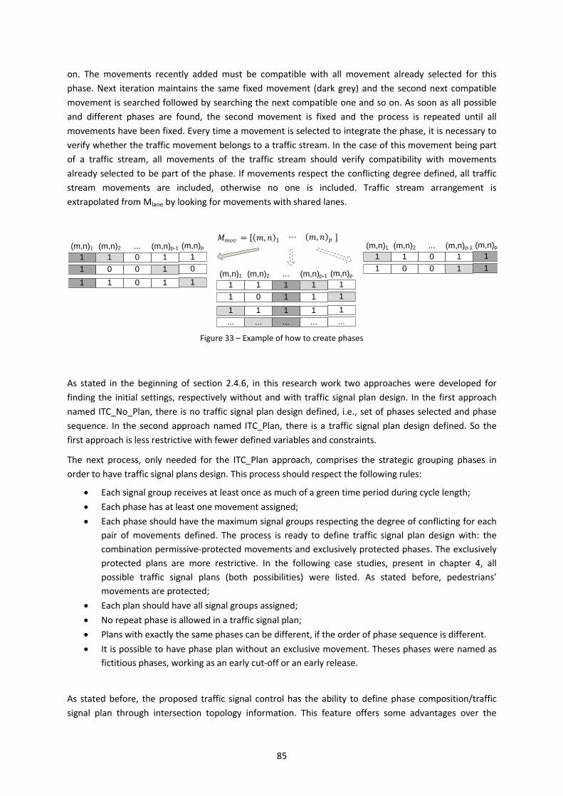
85
on. The movements recently added must be compatible with all movement already selected for this
phase. Next iteration maintains the same fixed movement (dark grey) and the second next compatible
movement is searched followed by searching the next compatible one and so on. As soon as all possible
and different phases are found, the second movement is fixed and the process is repeated until all
movements have been fixed. Every time a movement is selected to integrate the phase, it is necessary to
verify whether the traffic movement belongs to a traffic stream. In the case of this movement being part
of a traffic stream, all movements of the traffic stream should verify compatibility with movements
already selected to be part of the phase. If movements respect the conflicting degree defined, all traffic
stream movements are included, otherwise no one is included. Traffic stream arrangement is
extrapolated from Mlane by looking for movements with shared lanes.
Figure 33 – Example of how to create phases
As stated in the beginning of section 2.4.6, in this research work two approaches were developed for
finding the initial settings, respectively without and with traffic signal plan design. In the first approach
named ITC_No_Plan, there is no traffic signal plan design defined, i.e., set of phases selected and phase
sequence. In the second approach named ITC_Plan, there is a traffic signal plan design defined. So the
first approach is less restrictive with fewer defined variables and constraints.
The next process, only needed for the ITC_Plan approach, comprises the strategic grouping phases in
order to have traffic signal plans design. This process should respect the following rules:
Each signal group receives at least once as much of a green time period during cycle length;
Each phase has at least one movement assigned;
Each phase should have the maximum signal groups respecting the degree of conflicting for each
pair of movements defined. The process is ready to define traffic signal plan design with: the
combination permissive-protected movements and exclusively protected phases. The exclusively
protected plans are more restrictive. In the following case studies, present in chapter 4, all
possible traffic signal plans (both possibilities) were listed. As stated before, pedestrians’
movements are protected;
Each plan should have all signal groups assigned;
No repeat phase is allowed in a traffic signal plan;
Plans with exactly the same phases can be different, if the order of phase sequence is different.
It is possible to have phase plan without an exclusive movement. Theses phases were named as
fictitious phases, working as an early cut-off or an early release.
As stated before, the proposed traffic signal control has the ability to define phase composition/traffic
signal plan through intersection topology information. This feature offers some advantages over the
𝑀𝑚𝑜 = 𝑚, 1 ⋯ 𝑚, 𝑝
(m,n)1 (m,n)2
1 1
... (m,n)p-1
0 1
1 0 0 1
1 1 0 1
(m,n)p
1
0
1(m,n)1 (m,n)2
1 1
... (m,n)p-1
1 1
1 0 1 1
1 1
... ...
1 1
... ...
(m,n)p
1
1
1
...
(m,n)1 (m,n)2
1 1
... (m,n)p-1
0 1
1 0 0 1
(m,n)p
1
1
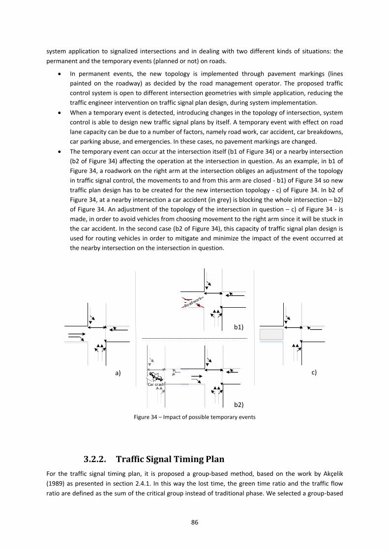
86
system application to signalized intersections and in dealing with two different kinds of situations: the
permanent and the temporary events (planned or not) on roads.
In permanent events, the new topology is implemented through pavement markings (lines
painted on the roadway) as decided by the road management operator. The proposed traffic
control system is open to different intersection geometries with simple application, reducing the
traffic engineer intervention on traffic signal plan design, during system implementation.
When a temporary event is detected, introducing changes in the topology of intersection, system
control is able to design new traffic signal plans by itself. A temporary event with effect on road
lane capacity can be due to a number of factors, namely road work, car accident, car breakdowns,
car parking abuse, and emergencies. In these cases, no pavement markings are changed.
The temporary event can occur at the intersection itself (b1 of Figure 34) or a nearby intersection
(b2 of Figure 34) affecting the operation at the intersection in question. As an example, in b1 of
Figure 34, a roadwork on the right arm at the intersection obliges an adjustment of the topology
in traffic signal control, the movements to and from this arm are closed - b1) of Figure 34 so new
traffic plan design has to be created for the new intersection topology - c) of Figure 34. In b2 of
Figure 34, at a nearby intersection a car accident (in grey) is blocking the whole intersection – b2)
of Figure 34. An adjustment of the topology of the intersection in question – c) of Figure 34 - is
made, in order to avoid vehicles from choosing movement to the right arm since it will be stuck in
the car accident. In the second case (b2 of Figure 34), this capacity of traffic signal plan design is
used for routing vehicles in order to mitigate and minimize the impact of the event occurred at
the nearby intersection on the intersection in question.
Figure 34 – Impact of possible temporary events
3.2.2. Traffic Signal Timing Plan
For the traffic signal timing plan, it is proposed a group-based method, based on the work by Akçelik
(1989) as presented in section 2.4.1. In this way the lost time, the green time ratio and the traffic flow
ratio are defined as the sum of the critical group instead of traditional phase. We selected a group-based
b1)
c)
b2)
Car crash
a)

87
control once it is more flexible than phase-based control and, consequently, able to adapt to traffic
conditions.
For each possible traffic signal plan design the signal timing calculation is performed. Akçelik approach is
based on critical movement search where it begins by identifying all possible paths, followed by
calculating the total time for each path and finally finding the critical path, which represents the one with
the largest time value.
The signal groups responsible for determining the signal timings of the intersection are called critical
signal groups. In case all signal groups are non-overlapping, there will be one signal group in each phase.
An overlap signal group is a signal group which receives the right of way during more than one single
phase.
A critical movement identification method is presented as a procedure which automatically satisfies the
green signal time needs (and minimum green time constraints) in every signal group and respecting the
conflicts between them and it allows the use of different degrees of saturation. The critical movement
search is therefore a matter of identifying all paths calculating the total time for each path and finding the
path which gives the largest value. The process involves the elimination of non-overlap signal group with
smallest time needs. The method is applicable to both isolated and coordinated intersections. Another
feature is that a signal group may receive green signal during non-consecutive stages within one cycle
(needs two lost times).
Once critical movements are identified, critical lost time, critical flow rate and critical green time ratio are
defined as the sum of the critical path. The sum of all critical movements time is the cycle length.
The cycle length value should be in the range between practical cycle length (Cp) and optimal cycle length
(Co), without exceeding the maximum cycle length (Cmax) (Table 11). In the case the cycle falls out of these
limits, cycle length assumes nearest acceptable value. Optimal cycle length determination uses as criteria
the traditional method of delay minimization (Webster, 1958) (Eq. 4). The practical cycle optimum (Eq. 5)
is the minimum cycle time required to achieve various maximum acceptable degree of saturation (less
than 1.0 value). These cycle lengths calculations use critical movements’ parameters as input values.
All identified paths are calculated again using the new cycle length value. If critical path is the same as
before and respects the cycle length range, green time durations are determined. Otherwise critical path
process is repeated until convergence is achieved.
The calculations of green times for a selected cycle length begins with the signal group green time defined
for the critical path, followed by the non-critical signal group and lastly to determine the phase green time
durations. The last step is to check the degrees of saturation, using the allocated green time. This
condition will be satisfied unless the practical cycle length is greater than the maximum value admitted.
For the same traffic signal plan, the amount of time lost (per hour) increases when the duration of cycle
length is reduced and, as a consequence intersection capacity also decreases. However, longer cycle
length leads to longer waiting times and longer queue lengths.
For signal timing calculation, input data includes the minimum green time, practical degree of saturation,
saturation flow, maximum cycle length and inter-green; values can be defined for each signal group or
intersection scope. Since this is a middle step of our method, so as not to require more computational
effort and custom parameterization, we opted for the intersection scope for the input data definition.
Further details about parameters of the proposed traffic control are presented in Table 11.
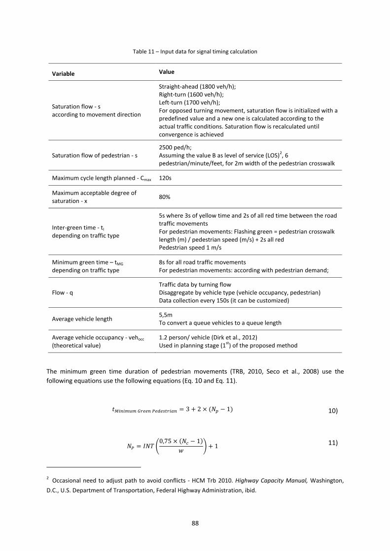
88
Table 11 – Input data for signal timing calculation
Variable Value
Saturation flow - s according to movement direction
Straight-ahead (1800 veh/h); Right-turn (1600 veh/h); Left-turn (1700 veh/h); For opposed turning movement, saturation flow is initialized with a predefined value and a new one is calculated according to the actual traffic conditions. Saturation flow is recalculated until convergence is achieved
Saturation flow of pedestrian - s 2500 ped/h; Assuming the value B as level of service (LOS)
2, 6
pedestrian/minute/feet, for 2m width of the pedestrian crosswalk
Maximum cycle length planned - Cmax 120s
Maximum acceptable degree of saturation - x
80%
Inter-green time - tI depending on traffic type
5s where 3s of yellow time and 2s of all red time between the road traffic movements For pedestrian movements: Flashing green = pedestrian crosswalk length (m) / pedestrian speed (m/s) + 2s all red Pedestrian speed 1 m/s
Minimum green time – tMG depending on traffic type
8s for all road traffic movements For pedestrian movements: according with pedestrian demand;
Flow - q Traffic data by turning flow Disaggregate by vehicle type (vehicle occupancy, pedestrian) Data collection every 150s (it can be customized)
Average vehicle length 5,5m To convert a queue vehicles to a queue length
Average vehicle occupancy - vehocc
(theoretical value) 1.2 person/ vehicle (Dirk et al., 2012) Used in planning stage (1
st) of the proposed method
The minimum green time duration of pedestrian movements (TRB, 2010, Seco et al., 2008) use the
following equations use the following equations (Eq. 10 and Eq. 11).
10)
𝐼
11)
2 Occasional need to adjust path to avoid conflicts - HCM Trb 2010. Highway Capacity Manual, Washington,
D.C., U.S. Department of Transportation, Federal Highway Administration, ibid.
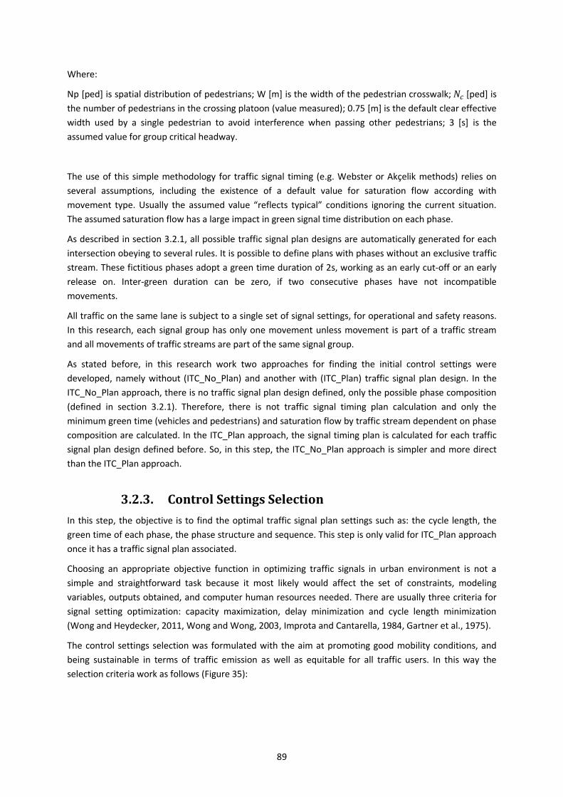
89
Where:
Np [ped] is spatial distribution of pedestrians; W [m] is the width of the pedestrian crosswalk; [ped] is
the number of pedestrians in the crossing platoon (value measured); 0.75 [m] is the default clear effective
width used by a single pedestrian to avoid interference when passing other pedestrians; 3 [s] is the
assumed value for group critical headway.
The use of this simple methodology for traffic signal timing (e.g. Webster or Akçelik methods) relies on
several assumptions, including the existence of a default value for saturation flow according with
movement type. Usually the assumed value “reflects typical” conditions ignoring the current situation.
The assumed saturation flow has a large impact in green signal time distribution on each phase.
As described in section 3.2.1, all possible traffic signal plan designs are automatically generated for each
intersection obeying to several rules. It is possible to define plans with phases without an exclusive traffic
stream. These fictitious phases adopt a green time duration of 2s, working as an early cut-off or an early
release on. Inter-green duration can be zero, if two consecutive phases have not incompatible
movements.
All traffic on the same lane is subject to a single set of signal settings, for operational and safety reasons.
In this research, each signal group has only one movement unless movement is part of a traffic stream
and all movements of traffic streams are part of the same signal group.
As stated before, in this research work two approaches for finding the initial control settings were
developed, namely without (ITC_No_Plan) and another with (ITC_Plan) traffic signal plan design. In the
ITC_No_Plan approach, there is no traffic signal plan design defined, only the possible phase composition
(defined in section 3.2.1). Therefore, there is not traffic signal timing plan calculation and only the
minimum green time (vehicles and pedestrians) and saturation flow by traffic stream dependent on phase
composition are calculated. In the ITC_Plan approach, the signal timing plan is calculated for each traffic
signal plan design defined before. So, in this step, the ITC_No_Plan approach is simpler and more direct
than the ITC_Plan approach.
3.2.3. Control Settings Selection
In this step, the objective is to find the optimal traffic signal plan settings such as: the cycle length, the
green time of each phase, the phase structure and sequence. This step is only valid for ITC_Plan approach
once it has a traffic signal plan associated.
Choosing an appropriate objective function in optimizing traffic signals in urban environment is not a
simple and straightforward task because it most likely would affect the set of constraints, modeling
variables, outputs obtained, and computer human resources needed. There are usually three criteria for
signal setting optimization: capacity maximization, delay minimization and cycle length minimization
(Wong and Heydecker, 2011, Wong and Wong, 2003, Improta and Cantarella, 1984, Gartner et al., 1975).
The control settings selection was formulated with the aim at promoting good mobility conditions, and
being sustainable in terms of traffic emission as well as equitable for all traffic users. In this way the
selection criteria work as follows (Figure 35):
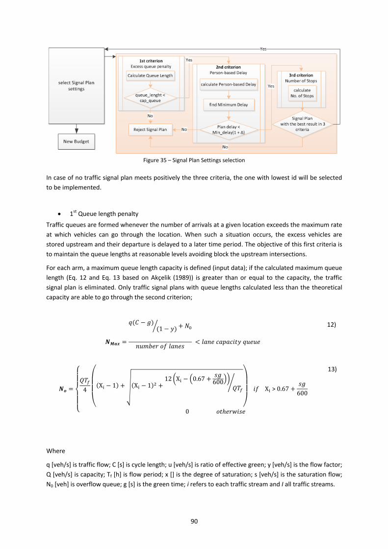
90
Figure 35 – Signal Plan Settings selection
In case of no traffic signal plan meets positively the three criteria, the one with lowest id will be selected
to be implemented.
1st Queue length penalty
Traffic queues are formed whenever the number of arrivals at a given location exceeds the maximum rate
at which vehicles can go through the location. When such a situation occurs, the excess vehicles are
stored upstream and their departure is delayed to a later time period. The objective of this first criteria is
to maintain the queue lengths at reasonable levels avoiding block the upstream intersections.
For each arm, a maximum queue length capacity is defined (input data); if the calculated maximum queue
length (Eq. 12 and Eq. 13 based on Akçelik (1989)) is greater than or equal to the capacity, the traffic
signal plan is eliminated. Only traffic signal plans with queue lengths calculated less than the theoretical
capacity are able to go through the second criterion;
𝑚 𝑒 𝑜𝑓 𝑒 𝑒 𝑐 𝑝 𝑐𝑖 𝑒 𝑒
12)
𝑜 𝑒 𝑖 𝑒
𝑖𝑓
13)
Where
q [veh/s] is traffic flow; C [s] is cycle length; u [veh/s] is ratio of effective green; y [veh/s] is the flow factor;
Q [veh/s] is capacity; Tf [h] is flow period; x [] is the degree of saturation; s [veh/s] is the saturation flow;
N0 [veh] is overflow queue; g [s] is the green time; i refers to each traffic stream and I all traffic streams.
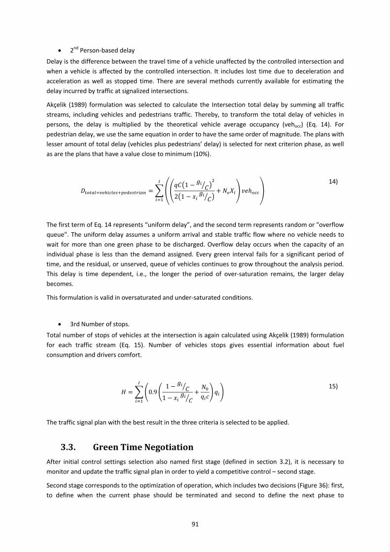
91
2nd Person-based delay
Delay is the difference between the travel time of a vehicle unaffected by the controlled intersection and
when a vehicle is affected by the controlled intersection. It includes lost time due to deceleration and
acceleration as well as stopped time. There are several methods currently available for estimating the
delay incurred by traffic at signalized intersections.
Akçelik (1989) formulation was selected to calculate the Intersection total delay by summing all traffic
streams, including vehicles and pedestrians traffic. Thereby, to transform the total delay of vehicles in
persons, the delay is multiplied by the theoretical vehicle average occupancy (vehocc) (Eq. 14). For
pedestrian delay, we use the same equation in order to have the same order of magnitude. The plans with
lesser amount of total delay (vehicles plus pedestrians’ delay) is selected for next criterion phase, as well
as are the plans that have a value close to minimum (10%).
𝑒
14)
The first term of Eq. 14 represents “uniform delay”, and the second term represents random or "overflow
queue". The uniform delay assumes a uniform arrival and stable traffic flow where no vehicle needs to
wait for more than one green phase to be discharged. Overflow delay occurs when the capacity of an
individual phase is less than the demand assigned. Every green interval fails for a significant period of
time, and the residual, or unserved, queue of vehicles continues to grow throughout the analysis period.
This delay is time dependent, i.e., the longer the period of over-saturation remains, the larger delay
becomes.
This formulation is valid in oversaturated and under-saturated conditions.
3rd Number of stops.
Total number of stops of vehicles at the intersection is again calculated using Akçelik (1989) formulation
for each traffic stream (Eq. 15). Number of vehicles stops gives essential information about fuel
consumption and drivers comfort.
𝑐
15)
The traffic signal plan with the best result in the three criteria is selected to be applied.
3.3. Green Time Negotiation
After initial control settings selection also named first stage (defined in section 3.2), it is necessary to
monitor and update the traffic signal plan in order to yield a competitive control – second stage.
Second stage corresponds to the optimization of operation, which includes two decisions (Figure 36): first,
to define when the current phase should be terminated and second to define the next phase to
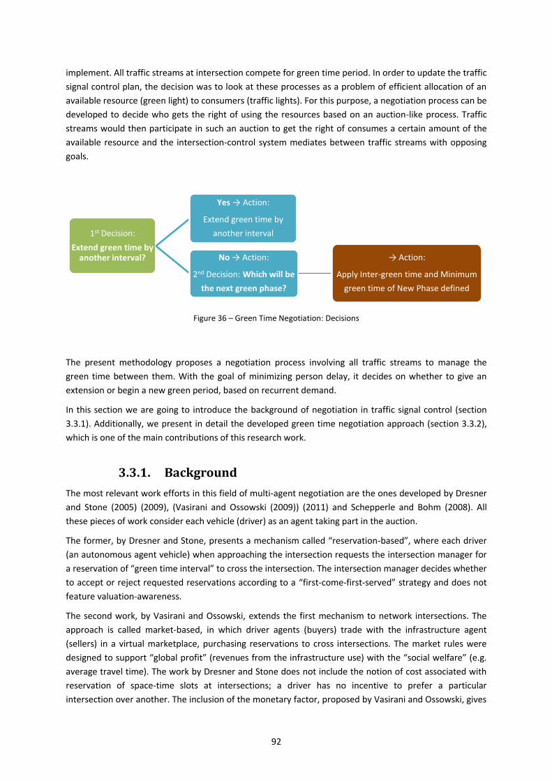
92
implement. All traffic streams at intersection compete for green time period. In order to update the traffic
signal control plan, the decision was to look at these processes as a problem of efficient allocation of an
available resource (green light) to consumers (traffic lights). For this purpose, a negotiation process can be
developed to decide who gets the right of using the resources based on an auction-like process. Traffic
streams would then participate in such an auction to get the right of consumes a certain amount of the
available resource and the intersection-control system mediates between traffic streams with opposing
goals.
Figure 36 – Green Time Negotiation: Decisions
The present methodology proposes a negotiation process involving all traffic streams to manage the
green time between them. With the goal of minimizing person delay, it decides on whether to give an
extension or begin a new green period, based on recurrent demand.
In this section we are going to introduce the background of negotiation in traffic signal control (section
3.3.1). Additionally, we present in detail the developed green time negotiation approach (section 3.3.2),
which is one of the main contributions of this research work.
3.3.1. Background
The most relevant work efforts in this field of multi-agent negotiation are the ones developed by Dresner
and Stone (2005) (2009), (Vasirani and Ossowski (2009)) (2011) and Schepperle and Bohm (2008). All
these pieces of work consider each vehicle (driver) as an agent taking part in the auction.
The former, by Dresner and Stone, presents a mechanism called “reservation-based”, where each driver
(an autonomous agent vehicle) when approaching the intersection requests the intersection manager for
a reservation of “green time interval” to cross the intersection. The intersection manager decides whether
to accept or reject requested reservations according to a “first-come-first-served” strategy and does not
feature valuation-awareness.
The second work, by Vasirani and Ossowski, extends the first mechanism to network intersections. The
approach is called market-based, in which driver agents (buyers) trade with the infrastructure agent
(sellers) in a virtual marketplace, purchasing reservations to cross intersections. The market rules were
designed to support “global profit” (revenues from the infrastructure use) with the “social welfare” (e.g.
average travel time). The work by Dresner and Stone does not include the notion of cost associated with
reservation of space-time slots at intersections; a driver has no incentive to prefer a particular
intersection over another. The inclusion of the monetary factor, proposed by Vasirani and Ossowski, gives
1st Decision:
Extend green time by another interval?
Yes → Action:
Extend green time by
another interval
No → Action:
2nd Decision: Which will be
the next green phase?
→ Action:
Apply Inter-green time and Minimum
green time of New Phase defined

93
drivers an incentive to explore alternatives to the shortest paths, and provides intersection managers with
an effective way to control the system.
Schepperle and Bohm (2008) propose an approach that takes into account valuation by the drivers. There,
driver-assistance agents can exchange the time slots that have been allocated to them. Their focus is on
single intersections. The initial procedure proposed consists of the following process: vehicles contact the
intersection; vehicles acquire an initial time slot to cross the intersection; if not satisfied a vehicle can try
to acquire a better time slot, this time from another vehicle; vehicles cross intersection. In the second
step, an auction takes place among vehicles that do not yet possess a time slot.
In section 2.4.2, the adaptive signal control with the self-optimization strategy is briefly introduced where
the control function predicts the difference in total delay between the benefits of extending green time
by another interval and the loss to the vehicles in queues, in the other approaches, due to this green
extension. This topic was inspiring for developing the idea of taking into account the road users waiting at
red signal, on the arms of the approach beyond the roads users on green signal.
The concept of “time before reduction” of volume-density (actuated operation) was also inspiring for
proposed control in way of actual green time duration is influenced by a conflicting signal group, which
requires the green time. So green time duration, besides the traditional minimum and maximum green
time restrictions is also influenced by opposite traffic presence at intersection.
Based on Miller algorithm, Bang (1976) developed a practical implementation called Traffic Optimization
Logic (TOL), in Sweden, where the gain in travel time to the additional road-users (cars, buses, pedestrian)
that can pass the intersection if the green phase is extended, another interval is calculated, as also the
benefit due to reduced number of stops. On the other hand, the negative impact is calculated represent
the loss due to extra delay and number of stops to the traffic in red signal phases. Actual green signal is
extended if control function is positive subject to restrictions of maximum green time.
The self-optimization strategy explores another curious concept, the control function of the method
predicts the difference in total delay between the benefits of extending green time by another interval
and the loss to the vehicles in queues in the other approaches due to extension. So actual green time
extension depends of control function values also subject to restrictions of maximum green time. Each
traffic signal control makes a decision based only on local information its own state, they are “unaware”
of the state of other intersections.
Continuing the idea of a new programming logic for traffic control (objective 1), the new method should
take into account the road users waiting at red signal in the arms beyond the road users on green signal.
The decision process compares the benefit of extending the current green signal phase by one more
interval, or to terminate it. In case of terminating the current green time, the next phase to apply is
decided based on the most benefit predicted. This approach is described in detail in the following section
(3.3.2).
3.3.2. Negotiation
The negotiation process developed is presented in this section, in order to decide who gets the right of
using the available resource (green light) based on an auction-like process. Traffic streams would then
participate in this auction to get the right of consuming a certain amount of the available resource and the
intersection-control system mediates between traffic streams with opposing goals.
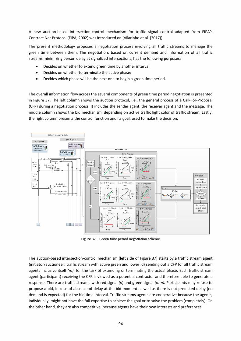
94
A new auction-based intersection-control mechanism for traffic signal control adapted from FIPA’s
Contract Net Protocol (FIPA, 2002) was introduced on (Vilarinho et al. (2017)).
The present methodology proposes a negotiation process involving all traffic streams to manage the
green time between them. The negotiation, based on current demand and information of all traffic
streams minimizing person delay at signalized intersections, has the following purposes:
Decides on whether to extend green time by another interval;
Decides on whether to terminate the active phase;
Decides which phase will be the next one to begin a green time period.
The overall information flow across the several components of green time period negotiation is presented
in Figure 37. The left column shows the auction protocol, i.e., the general process of a Call-For-Proposal
(CFP) during a negotiation process. It includes the sender agent, the receiver agent and the message. The
middle column shows the bid mechanism, depending on active traffic light color of traffic stream. Lastly,
the right column presents the control function and its goal, used to make the decision.
Figure 37 – Green time period negotiation scheme
The auction-based intersection-control mechanism (left side of Figure 37) starts by a traffic stream agent
(initiator/auctioneer: traffic stream with active green and lower id) sending out a CFP for all traffic stream
agents inclusive itself (m), for the task of extending or terminating the actual phase. Each traffic stream
agent (participant) receiving the CFP is viewed as a potential contractor and therefore able to generate a
response. There are traffic streams with red signal (n) and green signal (m-n). Participants may refuse to
propose a bid, in case of absence of delay at the bid moment as well as there is not predicted delay (no
demand is expected) for the bid time interval. Traffic streams agents are cooperative because the agents,
individually, might not have the full expertise to achieve the goal or to solve the problem (completely). On
the other hand, they are also competitive, because agents have their own interests and preferences.
95
This mechanism employs a first-price, single-item auction. The initiator agent receives j proposals of the
traffic streams. At this time, the initiator agent evaluates all proposals, firstly it groups them in phases
according to previous selected traffic plan (see section 3.2), and a traffic stream bid can be included in
more than one “bid phase”. Finally, it uses an evaluation function and chooses the winner proposals
through an accept-proposal message. The winners are the traffic streams agents which perform the “bid
phase” with the highest delay value. The problem is solved as a Winner Selection Problem (WSP).
In case of active green phase group wins, the traffic streams with green signal are extended by another
green time interval and the traffic stream agents of the selected proposal receive an accept proposal and
the remaining agents receive a reject proposal act. Note that a new auction will occur as the new
extension period terminates with new update input data (Figure 38).
In case of a red phase group wins, they receive an accept proposal message from the initiator, whereas
the other traffic stream agents that are not in the selected phase receive a reject proposal act. The active
green phase is terminated and after the inter-green period (if needed), the traffic streams of the win
phase receive the green signal. In this case, a new auction will occur after the minimum green time period
is accomplished (Figure 38).
Figure 38 – Green time Negotiation: When occurs?
Each traffic stream agent makes a bid based on total person-delay, experienced and predicted based on
current demand. The delay was selected because it is perhaps the most important parameter used by
transportation professionals to evaluate the performance of signalized intersection (Dion et al., 2004).
However, delay is also a parameter that is not easily determined. There are several ways to estimate it
(Kang, 2000, Dion et al., 2004), it was selected a deterministic queue model where the arrival and
departure traffic flow rates can be taken as known constants so that the total delay can be calculated as
the area of a polygon between the arrival (traffic flow) and departure (saturation flow) curves. In analytic
models for predicting delay, there are three distinct components of delay, namely, uniform delay, random
delay, and overflow delay. Before explaining these, first a delay representation diagram is useful for
illustrating these components (Figure 39).
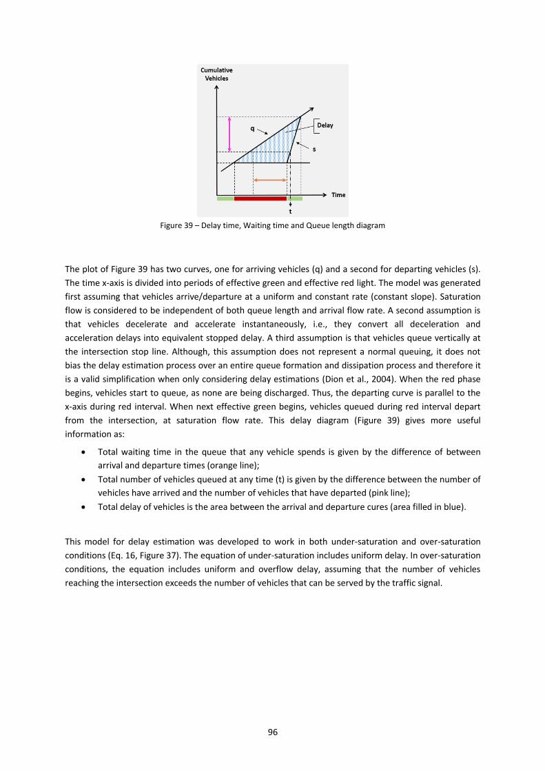
96
Figure 39 – Delay time, Waiting time and Queue length diagram
The plot of Figure 39 has two curves, one for arriving vehicles (q) and a second for departing vehicles (s).
The time x-axis is divided into periods of effective green and effective red light. The model was generated
first assuming that vehicles arrive/departure at a uniform and constant rate (constant slope). Saturation
flow is considered to be independent of both queue length and arrival flow rate. A second assumption is
that vehicles decelerate and accelerate instantaneously, i.e., they convert all deceleration and
acceleration delays into equivalent stopped delay. A third assumption is that vehicles queue vertically at
the intersection stop line. Although, this assumption does not represent a normal queuing, it does not
bias the delay estimation process over an entire queue formation and dissipation process and therefore it
is a valid simplification when only considering delay estimations (Dion et al., 2004). When the red phase
begins, vehicles start to queue, as none are being discharged. Thus, the departing curve is parallel to the
x-axis during red interval. When next effective green begins, vehicles queued during red interval depart
from the intersection, at saturation flow rate. This delay diagram (Figure 39) gives more useful
information as:
Total waiting time in the queue that any vehicle spends is given by the difference of between
arrival and departure times (orange line);
Total number of vehicles queued at any time (t) is given by the difference between the number of
vehicles have arrived and the number of vehicles that have departed (pink line);
Total delay of vehicles is the area between the arrival and departure cures (area filled in blue).
This model for delay estimation was developed to work in both under-saturation and over-saturation
conditions (Eq. 16, Figure 37). The equation of under-saturation includes uniform delay. In over-saturation
conditions, the equation includes uniform and overflow delay, assuming that the number of vehicles
reaching the intersection exceeds the number of vehicles that can be served by the traffic signal.

97
𝐼𝑓 𝑒 𝑜 𝑒 𝑖𝑜
𝑒 𝑖 𝑒 𝑒 𝑖𝑜
16)
Where:
n [veh] is number of vehicles in queue at decision moment; q [veh/s] is the traffic flow; s [veh/s] is the
saturation flow; t [s] is time of decision.
As the aim of this negotiation is to distribute green light time between traffic streams, in a “social
welfare” way, the delay equations are person-based, i.e., each traffic variable of equations such as traffic
flow (q), saturation flow (s) and queue length (ni) were converted to the unit person () instead of
vehicles, using the sensing vehicle occupation as a converter. The initial queue length at the beginning of
the evaluation period is obtained by measuring the real queue length and vehicle occupation. Therefore,
this proposed model is time dependent.
The bidding mechanism is divided into two types of bids: the green bids and the red bids (Figure 37).
Green bids are made by traffic streams that are receiving the green light (Eq. 17). There are two
green bid cases:
First case: continue the active green phase, i.e., green light is extended by another green time
interval; and their bid value is the actual delay added of the difference between prediction of the
delay if they lose the green in next phase (“lost future”) and prediction of the delay if green light
is extended (“win present”). In the first term of the Eq. 18 delay is calculated to extension time
(tc) and the second term is to period during inter-green and minimum green time (tI+tMG);
Second case: continue the active green in a new phase, i.e., actual phase is terminated but traffic
stream continues green in the next phase and inter-green period; The bid value is the actual delay
plus the difference between prediction of the delay if they lose the green in next phase (“lost
future” Eq. 19) and prediction of the delay if they win the green in next phase (“win present”),
both delays are calculated for during minimum green time and inter-green time (tI+tMG);
Red bid is made by traffic streams that are receiving the red light. The bid value is the actual delay
plus the prediction of the delay if they win the green in next phase (“win”) (Eq. 20).
The delay prediction was formulated (Figure 40) based on the area of a polygon between the arrival
(traffic flow) and departure (saturation flow) curves (see the plot of Figure 39). For the “win” bid
component is necessary to determine the saturation condition, if the traffic stream is undersaturated or
oversaturated, in order to select the equation to adopt. In the green bid case, the t variable in seconds
can be extension time (tc) or the sum of minimum green time (tMG) with inter-green time (tI) depending of
the case (see Figure 37). The minimum green time and the inter-green time is customized according to the
traffic stream characteristics (vehicle or pedestrian).
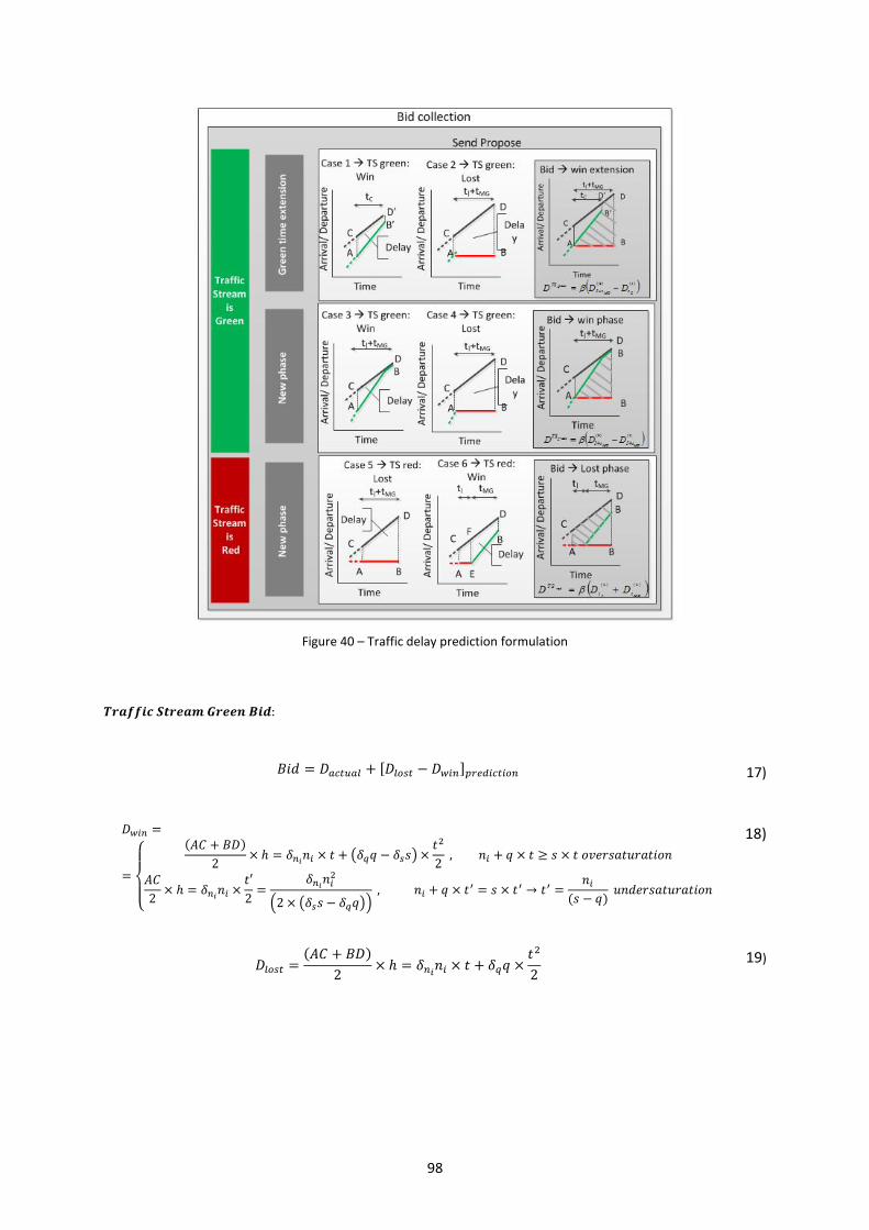
98
Figure 40 – Traffic delay prediction formulation
𝑖 17)
𝑜 𝑒 𝑖𝑜
𝑒 𝑖𝑜
18)
19)
99
𝑖 20)
21)
22)
𝑜 𝑒
𝑒 𝑖𝑜
23)
Where:
D predication [s x person] is total delay predicted for all persons in a traffic stream and for time of decision; D
actual [s x person] is total delay experienced for all persons in a traffic stream; [person] is vehicle
occupancy; ni [veh] is number of vehicles in queue at decision moment (measured); q [veh/s] is traffic
flow (measured); s [veh/s] is saturation flow (calculated during stage 1); t [s] is time of decision, depends
of the case see details in Figure 40; tI [s] is inter-green time; tMG [s] is minimum green time period.
Each traffic stream makes a bid based on total person-delay (Eq. 17, Eq. 20), experienced and predicted,
and actual traffic light color. The bids of each traffic stream agent are aggregated on “bid phase”,
following these rules:
In case of method ITC_Plan, the “bid phase” aggregates bids of traffic stream according to
selected traffic signal plan. There are “bid phases” in equal number of traffic signal plan phases;
In case of method ITC_No_Plan, the “bid phase” aggregates bids according to possible phase
composition. There are “bid phases” in equal number of possible phases.
The bid of traffic streams with green color, i.e., “green bids” have two possible values: extend green time
by another interval (case 1 and 2) and begin a new phase (case 3 and 4) as stated before, depending on
the phase that refers. If the “bid phase” is the active phase, the traffic stream bid is the actual delay plus
the prediction of difference in total delay between the loss of green time and the benefit of extending
green time by another interval for vehicles in this traffic stream. Otherwise, i.e., the “bid phase” is not the
active one but the traffic stream continues green, the bid is the actual delay plus the prediction of
difference in total delay between the loss of green time and the benefit of winning the next phase for
vehicles in this traffic stream.
100
Red bid is the actual delay plus the prediction of difference in total delay between the loss of green time
and the benefit of extending green time for vehicles in this traffic stream (Eq. 20).
The “bid phase” selection follows the maximization revenue formulation (Eq. 24). The winners are the
traffic streams (Traffic Stream agents) which perform the “bid phase” with the higher delay value.
𝑀
24)
Where:
DTS[s] is traffic delay of traffic stream at the decision moment; p [id] is index of phase; TS [id] is index of
traffic stream; i [id] is index of traffic stream of a phase; m [id] is index of number of traffic streams of a
phase.
In case of winning the active green phase, the active traffic streams with green light are extended by
another interval. A new auction will occur as the new extension period terminates with new update input
data (see Figure 38).
In case of a red phase wins, the active green phase is terminated and after the inter-green period (if
needed), the traffic streams of the win phase receive the green phase (see Figure 38). In this case, a new
auction will occur after the inter-green period (if needed) and the minimum green time period. In case of
continuing the active traffic stream, it continues green along inter-green period (if needed). In this way
negotiations are very dynamic and initiate in short intervals, just a few seconds.
The proposed approach allows updating traffic signal control and brings up the benefit of phase designs
and phases being changed as needed instead of being fixed to an a priori traffic signal control plan or a
fixed library of plans. The system structure is flexible and has the capacity to adapt the traffic signal
control, reacting to unexpected traffic events such as changes in traffic flow or topology, without
requiring human interaction. All road users are taken into account, even those waiting at red signal. The
green time assignment is decided by Traffic Stream agents at same control level where no agent has more
powerful control than others. Nonetheless, it is used stationary agents which it offers many advantages
over using vehicles as the focal point of the auction (Tumer and Agogino, 2007). The proposed traffic
signal control system requires a new traffic detecting system in order to collect real-time information
about vehicle occupancy, queue length and traffic user arrivals at intersection.
As a result of this proposed negotiation mechanism some classical concepts were abandoned as:
No maximum green time period is defined: if the evaluation of green time by all agents is
favorable to continue, the green time is kept with no restrictions;
No cycle length: during operation, the cycle length can assume any value with no restrictions, i.e.,
the cycle length concept is lost;
No phase sequence: phase can assume any order. Usually traffic signal control systems are
constrained to follow a pre-determined phase order. The proposed method gives the possibility
of having no pre-defined phase order. So the control system should be able to select any possible
phase based on the most beneficial phase at any given time period considering all traffic users
presented and expected at intersection;
101
No control levels: the green time is decided by agents at same level. There is any agent with more
power of control than others;
A traffic signal control system concerned about the person, independently of the selected
transportation mode (car, bus, pedestrian). In traffic signal control systems, the typically
approach of control is to look at the traffic condition as vehicle flow or vehicle delay;
Pedestrian green light is given according to its delay, instead of using only the minimum values.
Although, the goal of the present work is to develop a flexible traffic signal control, some traffic operation
variables continue to be defined in proposed traffic control system by safety and operation reasons (see
section 3.2).
The maximum value for green time and cycle length is used to assure that all traffic streams are served in
an acceptable time period. Road users become impatient and may compromise safety if the red time is
too long and the vehicles in queue can block downstream intersections. However, we choose not to
include these constraints in the proposed traffic signal control in order to have more flexibility in control.
We believe that traffic signal control will find an equilibrium, avoiding red light for traffic streams too
long, without having the constraint defined.
3.4. Method Framework
In this chapter, a new approach for real-time traffic signal control is proposed, using Multi-agent
architecture and an auction mechanism, at isolated intersections. As mentioned before, at isolated traffic
control each intersection control is independent, it is “unaware” of the state of other intersections. Thus
allows a simpler control algorithm than for coordinated intersections and also more flexibility to green
time assignment. The vision is presented in the following paragraph:
The traffic signal control system is designed to be as minimally restrictive as possible and highly flexible in
determining which traffic streams should receive the green time at each time interval. Several traffic
streams compete for the same green time. Decisions about the traffic light status of each traffic stream
take into account the current traffic data such as the traffic flow, the number of road users, queue lengths
and delay time in all traffic streams, independent of their traffic light color. As a result, this strategy can
react to non-schedulable events or unpredictable events without human intervention.
In short, following the classification presented in section 2.3, the proposed traffic signal control can be
classified as defined in Table 12
Table 12 – Characteristics of the proposed traffic signal control strategy
Characteristics of Proposed Traffic Signal Control
Context/Scope Logic Optimization Operation
Isolated Traffic responsive real time strategy Artificial intelligence Online
It is proposed to represent the traffic signal control problem using a MAS metaphor, replacing traffic
signal control design, the control monitoring and updating, by intelligent agents as shown in Figure 41.
From the MAS conceptual model (section 3.1), we developed and implemented our proposed traffic signal
control, with the exception of four items. A brief summary of these items not included in the experiments,
follows:
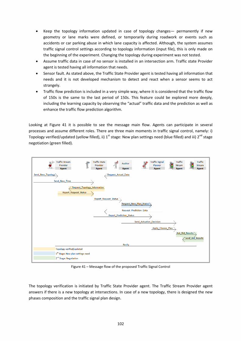
102
Keep the topology information updated in case of topology changes— permanently if new
geometry or lane marks were defined, or temporarily during roadwork or events such as
accidents or car parking abuse in which lane capacity is affected. Although, the system assumes
traffic signal control settings according to topology information (input file), this is only made on
the beginning of the experiment. Changing the topology during experiment was not tested.
Assume traffic data in case of no sensor is installed in an intersection arm. Traffic state Provider
agent is tested having all information that needs.
Sensor fault. As stated above, the Traffic State Provider agent is tested having all information that
needs and it is not developed mechanism to detect and react when a sensor seems to act
strangely.
Traffic flow prediction is included in a very simple way, where it is considered that the traffic flow
of 150s is the same to the last period of 150s. This feature could be explored more deeply,
including the learning capacity by observing the “actual” traffic data and the prediction as well as
enhance the traffic flow prediction algorithm.
Looking at Figure 41 it is possible to see the message main flow. Agents can participate in several
processes and assume different roles. There are three main moments in traffic signal control, namely: i)
Topology verified/updated (yellow filled), ii) 1st stage: New plan settings need (blue filled) and iii) 2nd stage
negotiation (green filled).
Figure 41 – Message flow of the proposed Traffic Signal Control
The topology verification is initiated by Traffic State Provider agent. The Traffic Stream Provider agent
answers if there is a new topology at intersections. In case of a new topology, there is designed the new
phases composition and the traffic signal plan design.
103
The 1st stage is initiated by Auditor agent, when there is a new topology or the budget is empty, the
Traffic Signal Planer agent calculates the new traffic signal plan settings (returning to the beginning of first
stage explained in detail section 3.2). The budget is defined after new traffic signal settings are calculated.
The budget of intersection assumes equal value to the cycle length planned (ITC_Plan), or 300 units in
case of no traffic signal defined (ITC_No_Plan).
The 2nd stage is initiated by Traffic Stream agent; Green time negotiation process (details in section 3.3)
occurs between all Traffic Stream agents (in equal number of intersection traffic streams) according to
real traffic conditions. As a result, the phase sequence and also the phase duration can be different from
the one planned in the initial traffic signal plan settings. Those changes from the traffic plan are deducted
in the budget value (Eq. 25), if there is a traffic signal defined (ITC_Plan). Otherwise (ITC_No_Plan), the
budget value is subtracted a unit by each second of simulation, as resulted the new traffic settings
parameters are calculated in each 300s.
𝑒
𝑒 𝑖𝑓 𝑒 𝑐 𝑖 𝑒 𝑝 𝑒 𝑒 𝑚𝑖 𝑒
𝑒
𝑖𝑓 𝑒 𝑖 𝑒 𝑝 𝑒 25)
Where:
t [s] is actual period; tgreen [s] is green time value; m [id] is the previous phase; n [id] is the new phase.
Although, the traffic signal plan is updated according to traffic conditions during the green time
negotiation process. The traffic signal control settings defined beforehand influence negotiation, such as
the saturation flow values, the minimum green times, the traffic signal plan design (phase composition
and sequence). So, the budget concept is introduced in order to force to calculate again the traffic control
settings. In case of having a defined traffic signal plan (ITC_Plan), the budget is spent more quickly as the
actual traffic signal plan departs from the planned one.
In the search of a “minimal restrictive and highly flexible” traffic signal control system, the traffic signal
plan design, i.e. the possibility of changing phase sequence and phase composition is developed and
tested in two different ways (as summarized in Table 13).
ITC_Plan: Traffic signal control operation is actuated. By the time a decision is to terminate the
actual green time, the green time can be assigned to any phase of the active traffic signal plan
(defined during the first stage). The selected phase is the one that gives the most beneficial
contribution to the intersection performance. So, a new traffic signal plan design can be assumed,
i.e. with different phase sequence (Vilarinho et al., 2017).
ITC_No_Plan: Traffic signal control operation is also actuated. By the time a decision is to
terminate the actual green time, the green time can be assigned to any phase composition. Again
the selected phase is the one that gives the most beneficial contribution to the intersection
performance. So, there is no traffic signal plan constraint: any possible phase composition can be
selected at each decision moment.

104
Table 13 - Resume of the proposed traffic control
Stage ITC_Plan – with a Traffic Signal Plan ITC_No_Plan – without a Traffic Signal Plan
1st
For each traffic signal plan determines:
green time periods for vehicles and pedestrians’ movements;
cycle length;
saturation flow by traffic stream. Result: Find a traffic signal plan in terms of phase composition and sequence, concerning:
Good mobility conditions
Sustainability in terms of traffic emissions
Equitability for all traffic users.
Update: when intersection budget ≤ 0
All traffic signal parameters are determined again using traffic flow collected from last 150s;
A new traffic signal plan is selected and the intersection budget is updated to the cycle length value;
Budget: changes from the traffic plan are deducted in budget value;
For each phase determines:
minimum green time for vehicles and pedestrians’ movements;
saturation flow by traffic stream, dependent on phase composition
Result: Phase selection uses 2
nd stage method
Update: when intersection budget ≤ 0
All traffic signal parameters are determined again using traffic flow collected from last 150s;
Intersection budget is updated to 300 units;
Budget value is subtracted in 1 unit by each second of simulation;
2nd
Decision:
when current phase is terminated;
define the next phase to implement from the active traffic plan;
Negotiation process:
Bid by traffic stream;
Bid are organized by phase;
Decision:
when current phase is terminated;
define the next phase from all possible phases to implement;
Negotiation process:
Bid by traffic stream and by phase (due to saturation flow);
Bid are organized by phase;
Result: Maximum bid (phase) wins the green time
Although, the goal of the present work is to develop a flexible traffic signal control, some traffic operation
variables continue to be defined by safety and operation reasons like: possible phase composition,
minimum green time and inter-green period. The maximum value for green time and cycle length are not
more used in the proposed traffic signal control. The minimum green time of pedestrians is defined
according with their demand.
As mentioned before, the proposed traffic control receives “information from the simulation model”, in its
implementation at real-world environment that information should be collected by sensors. The proposed
traffic control is quite dependent on traffic data in order to find the optimal control according to the
actual traffic conditions. The proposed control system requires a detecting system in order to collect real-
time information about the vehicle occupancy, the queue length and the traffic user arrivals at
intersection.
105
The industry is moving towards a period of abundance of traffic data, collected in real-time, by road
sensors (Smartphones applications, Bluetooth, Wi-Fi, GSM signal of mobile phones) or/and vehicle
(V)/infrastructures (I) communication (V2V and V2I), it seems that traffic signal control could take more
advantage of higher granularity of data.
The road sensors, widely spread over the network, have the limitation of giving only vehicle information
at a fixed location. However, new initiatives known as vehicle-infrastructure communication allow the
wireless transmission of the positions, headings, and speeds of vehicles for use by the traffic controller
(Goodall et al., 2013). As it is a new technology, it will take some time until reach a penetration rate
where vehicles can benefit from such communication platform.
Dealing with the technology to adopt data collection is beyond the scope of this work. Thus, we only
defined the traffic data that the proposed traffic controller needs to “know”, as follows
Traffic flow /vehicles and pedestrians, in each traffic stream, by the next turning movement;
Vehicle occupancy, i. e., number of people in each vehicle;
Delay time of each vehicle due to the traffic light;
Number of vehicles in queue, i.e. vehicles with speed < 0.1 km/h.
In MAS, there is interaction between agents. In order for agents to interact, there must be some
standardized mechanism for communication - communication protocol.
The proposed communication protocol consists of a fixed set of message types, each with various fields
for storing information, as well as rules that must be obeyed concerning the sending and receiving of
these messages, as well as the actions that may or may not be taken by an agent that has received or sent
them.
This subject is introduced in section 3.1 and shown in detail in Figure 41.
The message has always the same structure, which is:
Sender id
Receiver id
Message type
This communication protocol supports agents that act as organizers and/or respondents, assuming more
than one role (initiator and participant) with different problem solving methods and bid strategies. There
are ten types of messages that can be sent by the five agents type of the MAS. Some messages are
depending on each other and sometimes of its content.
Request Actual Data - An Auditor agent sends the REQUEST message to a Traffic State agent,
every second (or simulation step). Each request asks the actual traffic data;
Request Topology Information - A Traffic State agent sends the REQUEST message to a Traffic
Stream Provider agent, every second (or simulation step). Each request asks if there is a new
topology at the intersection;
Report Request Status - This message is a response to a REQUEST message. It does not mean that
the proposal transmitted by the sender agent is accept. Although, it means that the REQUEST
arrived to the receiver agent. The message is sent in two cases;
106
- Traffic Stream Provider agent responds to Traffic State agent (message Request Topology
information). The message includes a Boolean variable, “true” in case of a new topology
at intersection, and “false” in opposite case;
- Traffic State agent responds to Auditor Agent (message Request Actual Data), after
update “Traffic Database” resource;
Request New Plan Status - An Auditor agent sends the REQUEST message to a Traffic Signal
Planner agent in two cases. The message includes a Boolean variable which values depend on
intersection budget value, “true” in case of positive request of new traffic settings (budget ≤ 0),
and “false” in opposite case (budget > 0);
Request Prediction Data - A Traffic Signal Planner agent sends the REQUEST message to a Traffic
State Provider agent. This message is only sent, if a positive request for a new plan has been
asked;
Report Prediction Status - A Traffic State Provider agent sends a response to a Traffic Signal
Planner agent’s REQUEST message (Request Prediction Data). The traffic variables are updated
with information of last 150s in order to help the planning of traffic control settings;
Apply Choose Plan - In the event of a new traffic setting is available, i.e., in message Request New
Plan Status, the Boolean variable is true. A Traffic Signal Planner agent sends the REQUEST
message to a Traffic Stream in order to consider the new traffic signal control settings;
Send Actuation Decision - In the event of maintaining traffic settings, i.e., in message Request
New Plan Status, the Boolean variable is false. An Auditor agent send the REQUEST message
asking to apply actuation to a Traffic Stream agent. Traffic stream will verify if it time to negotiate
(Figure 38), if positive negotiation will start, else traffic light color maintains unchanged;
Ask Bid Result - In the event of negotiation stage occur decided by a Traffic Stream agent. A
Traffic Stream agent (traffic stream with active green and lower id) sends the REQUEST message
to all Traffic Stream agents of the intersection. Each traffic stream agent makes a bid based on
total person-delay experienced and predicted;
Send Bid Result - All Traffic Stream agents sends a response to a Traffic Stream agent’s (traffic
stream with active green and lower id) REQUEST message (Ask Bid Result). Each traffic stream
agent sends its bid value and the traffic light color decision is based on those values.
The methodology proposed does not have a central unit or the ability to communicate with other
intersections. It is based on MASs, in which each traffic stream of the intersection is considered as an
agent. So, agents communicate only between them at the same intersection, i.e., isolated control
approach.
3.5. Comparing Systems
The purpose of this section is to summarize the differences and similarities between proposed traffic
control system, described along this chapter (chapter 2.4.6), and traffic control systems already
developed and mostly implemented in real environment, described on section 2.4.
As presented on section 1.3, this research work has two problems of particular interest: one is to design
the traffic signal plan exploring all possible solutions for phase composition; the other is to maintain the
traffic signal control settings updated to meet the current traffic demand of the different users.
For the first problem, the major challenge is developing a simple framework for traffic signal plan design
able to consider any intersection geometry with few data inputs. For the second problem is to find
107
suitable optimization method for traffic control plan settings calculation as well as an approach for
updating and reviewing its settings in real-time.
The proposal of a new traffic control system raises a natural question of understanding: “What are the
differences and similarities of this system compared with existing systems?”. Table 14 presents a
comparative analysis. For the sake of space and in order to avoid an extensive discussion on the
similarities and the differences, which is out of scope in this study, only a selected range of existing
systems is considered, but the sufficient number of systems to allow a proper support to the decisions
made throughout the process of designing the proposed approach herein presented.
Probably, the most widely-used adaptive traffic control system are the SCOOT - Split Cycle and Offset
Optimization Technique (Hunt et al., 1981) and the SCATS - Sydney Coordinated Adaptive Traffic System
(Lowrie, 1990, Sims and Dobinson, 1979). There are other systems known to be operational but les used
such as: the RHODES - Real-Time Hierarchical Optimized Distributed and Effective System (Head et al.,
1992, Mirchandani and Head, 2001), the OPAC - Optimization Policies for Adaptive Control (Liao, 1998),
the PRODYN - Programmation Dynamique (Henry et al., 1984) and the ALLONS-D D (Porche and Lafortune,
1999). It was also included in the revision two systems purposely designed for isolated intersection
operation because it is the focus of the scope. The two systems are: the MOVA - Microprocessor
Optimized Vehicle Activation (Vincent and Peirce, 1988) and the SOS - Self-Optimized Signal Control
(Kronborg et al., 1997).
As it can be concluded from Table 14, the proposed traffic signal control shares some similarities and
differences with already developed methods. In common, they have the actuation operation. Actuated
operation consists of intervals where phases are invoked and extended by another green interval
according to vehicles sensors. In the proposed control, we also include the capacity of delay estimation
for each traffic stream. Besides varying the cycle length and the green times in response to detectors, the
actuated control can change the sequence of phases.
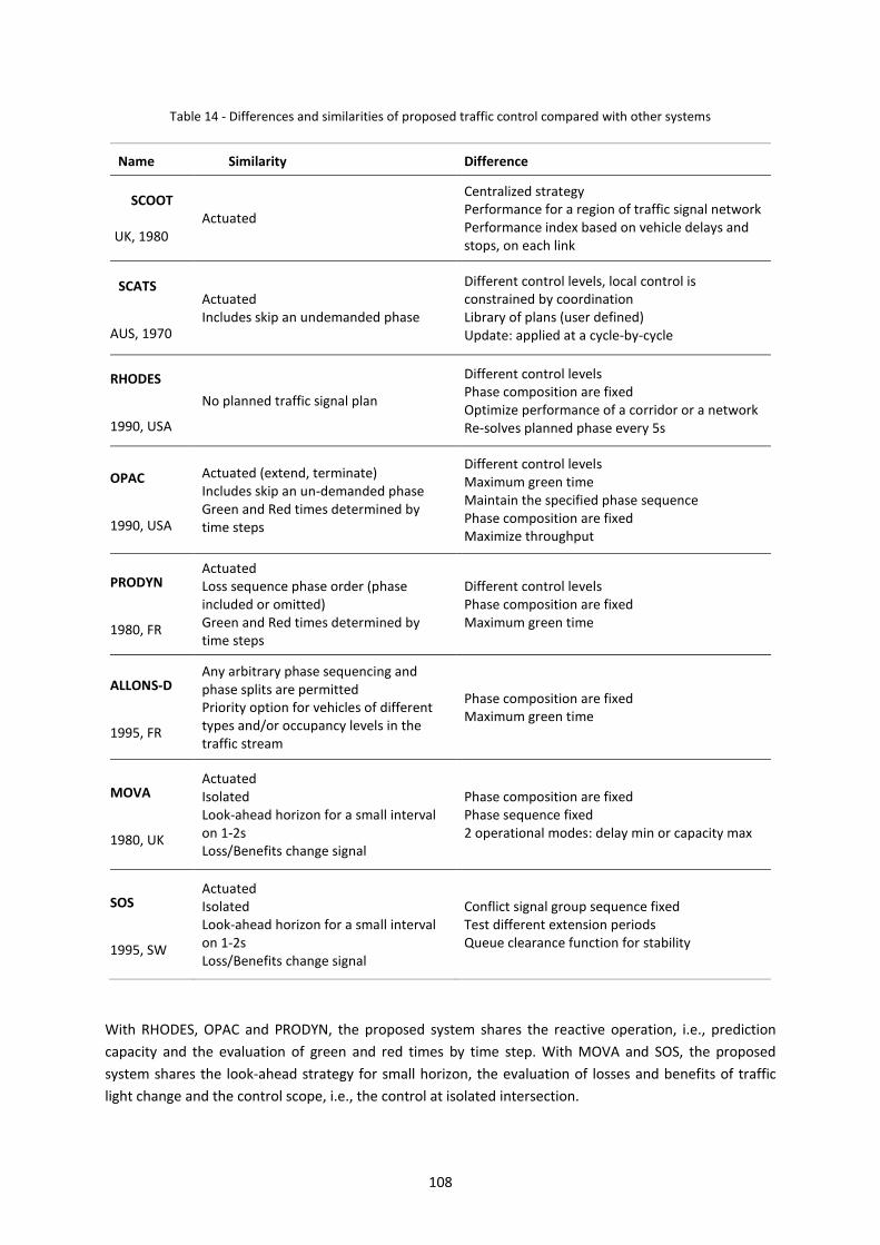
108
Table 14 - Differences and similarities of proposed traffic control compared with other systems
Name Similarity Difference
SCOOT
UK, 1980 Actuated
Centralized strategy Performance for a region of traffic signal network Performance index based on vehicle delays and stops, on each link
SCATS
AUS, 1970
Actuated Includes skip an undemanded phase
Different control levels, local control is constrained by coordination Library of plans (user defined) Update: applied at a cycle-by-cycle
RHODES
1990, USA
No planned traffic signal plan
Different control levels Phase composition are fixed Optimize performance of a corridor or a network Re-solves planned phase every 5s
OPAC
1990, USA
Actuated (extend, terminate) Includes skip an un-demanded phase Green and Red times determined by time steps
Different control levels Maximum green time Maintain the specified phase sequence Phase composition are fixed Maximize throughput
PRODYN
1980, FR
Actuated Loss sequence phase order (phase included or omitted) Green and Red times determined by time steps
Different control levels Phase composition are fixed Maximum green time
ALLONS-D
1995, FR
Any arbitrary phase sequencing and phase splits are permitted Priority option for vehicles of different types and/or occupancy levels in the traffic stream
Phase composition are fixed Maximum green time
MOVA
1980, UK
Actuated Isolated Look-ahead horizon for a small interval on 1-2s Loss/Benefits change signal
Phase composition are fixed Phase sequence fixed 2 operational modes: delay min or capacity max
SOS
1995, SW
Actuated Isolated Look-ahead horizon for a small interval on 1-2s Loss/Benefits change signal
Conflict signal group sequence fixed Test different extension periods Queue clearance function for stability
With RHODES, OPAC and PRODYN, the proposed system shares the reactive operation, i.e., prediction
capacity and the evaluation of green and red times by time step. With MOVA and SOS, the proposed
system shares the look-ahead strategy for small horizon, the evaluation of losses and benefits of traffic
light change and the control scope, i.e., the control at isolated intersection.
109
There are identified as major differences/advantages of the proposed control against the reviewed ACTS,
the following characteristics:
No control levels: the green time is decided by agents at same level. There is no any agent with
more power of control;
No maximum green time period is defined a priori, while the evaluation of green time is
favorable to continue, the green time is kept;
No cycle length: during operation. The cycle length concept is not used;
No phase sequence: phase can assume any order. Usually traffic control systems are constrained
to follow a pre-determined phase order;
No phase composition fixed: the following phase or green light can be assumed by any possible
set of traffic streams (ITC_No_Plan method);
Person based traffic control. The vehicles occupancy is distinguished allowing a control based on
people present/expected at intersection. In this way, green light can be given according to the
number of persons instead of favoring the number of vehicles.
Pedestrians delay is included in objective function of proposed traffic control methodology;
Possible to change intersection topology: is another feature that distinguishes the proposed
strategy against reviewed systems. Usually, the traffic signal plan design is only included in offline
systems, where traffic signal plans are designed for static conditions, such as the TRANSYT
(Robertson, 1969). The proposed traffic control is an online system with the capacity of create all
possible traffic signal plans design (phase composition and sequence), with few data inputs and
only based on the local geometric lay-out.
However, as it would be expected this work also includes limitations comparing to existing systems, the
main feature is the absence of coordination or sequencing of traffic signals. In coordination, the platoons
or groups of vehicles can travel through a series of intersections with minimal or no stopping. For
coordinate the green time in a set of intersections, additional parameters are used such as: cycle, i.e.,
time needed to serve all phases; and offset - time from a reference point, such as the start of green phase
at one intersection, to the same reference point at the other intersections. In proposed method, green
time period will be provided, independently of green time assignment on nearby intersections.

110
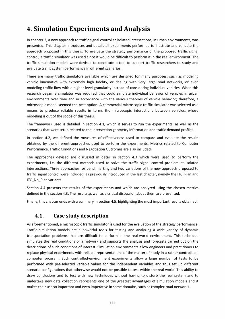
111
4. Simulation Experiments and Analysis
In chapter 3, a new approach to traffic signal control at isolated intersections, in urban environments, was
presented. This chapter introduces and details all experiments performed to illustrate and validate the
approach proposed in this thesis. To evaluate the strategy performance of the proposed traffic signal
control, a traffic simulator was used since it would be difficult to perform it in the real environment. The
traffic simulation models were devised to constitute a tool to support traffic researchers to study and
evaluate traffic system performance in different scenarios.
There are many traffic simulators available which are designed for many purposes, such as modeling
vehicle kinematics with extremely high fidelity, or dealing with very large road networks, or even
modeling traffic flow with a higher-level granularity instead of considering individual vehicles. When this
research began, a simulator was required that could simulate individual behavior of vehicles in urban
environments over time and in accordance with the various theories of vehicle behavior; therefore, a
microscopic model seemed the best option. A commercial microscopic traffic simulator was selected as a
means to produce reliable results in terms the microscopic interactions between vehicles, whose
modeling is out of the scope of this thesis.
The framework used is detailed in section 4.1, which it serves to run the experiments, as well as the
scenarios that were setup related to the intersection geometry information and traffic demand profiles.
In section 4.2, we defined the measures of effectiveness used to compare and evaluate the results
obtained by the different approaches used to perform the experiments. Metrics related to Computer
Performance, Traffic Conditions and Negotiation Outcomes are also included.
The approaches devised are discussed in detail in section 4.3 which were used to perform the
experiments, i.e. the different methods used to solve the traffic signal control problem at isolated
intersections. Three approaches for benchmarking and two variations of the new approach proposed to
traffic signal control were included, as previously introduced in the last chapter, namely the ITC_Plan and
ITC_No_Plan variants.
Section 4.4 presents the results of the experiments and which are analyzed using the chosen metrics
defined in the section 4.3. The results as well as a critical discussion about them are presented.
Finally, this chapter ends with a summary in section 4.5, highlighting the most important results obtained.
4.1. Case study description
As aforementioned, a microscopic traffic simulator is used for the evaluation of the strategy performance.
Traffic simulation models are a powerful tools for testing and analyzing a wide variety of dynamic
transportation problems that are difficult to perform in the real-world environment. This technique
simulates the real conditions of a network and supports the analysis and forecasts carried out on the
descriptions of such conditions of interest. Simulation environments allow engineers and practitioners to
replace physical experiments with reliable representations of the matter of study in a rather controllable
computer program. Such controlled-environment experiments allow a large number of tests to be
performed with pre-selected variable values for the independent variables and thus set up different
scenario configurations that otherwise would not be possible to test within the real world. This ability to
draw conclusions and to test with new techniques without having to disturb the real system and to
undertake new data collection represents one of the greatest advantages of simulation models and it
makes their use so important and even imperative in some domains, such as complex road networks.

112
Aimsun (2013) was the microscopic traffic simulator selected for this research. AIMSUN means Advanced
Interactive Microscopic Simulator for Urban and Non-Urban Networks and has been developed by
Universidad Politecnica Catalunya and Transportation Simulation System of Barcelona, Spain (Barceló,
2002). This simulator has proven to be very useful in testing new traffic control systems and management
policies based on traditional technologies, as well as in analyzing the viability for the of Intelligent
Transport Systems (ITSs). The SMARTEST project (Barceló et al., 1999) classified Aimsun as high-
applicability and suitable for different networks (urban, highways).
Simulations run under Aimsun can be classified as hybrid processes. At each simulation step, the
simulation cycle updates the event scheduling list (traffic light changing does not depend on the
conclusion of other activities). After this updating process, a set of loops starts to update the states of the
entities (links and nodes), as well as of vehicles. The last tasks include instantiating new vehicles,
collecting statistics, and updating the simulation clock (Aimsun, 2013).
For traffic signal control modeling, the Aimsun micro-simulator uses fictitious stopped vehicles, which are
instantiated and placed at the stop line when the light turns red, and are eliminated when it turns green
(Aimsun, 2013). This strategy basically generalizes the car-following model implemented in Aimsun to
support the simulation of traffic lights relying on the same model.
Three different types of traffic signal control can be defined in Aimsun, namely pre-timed, actuated, and
external. There are some customization options as well, such as coordination/synchronization of a system
of traffic-light controllers, implementation of actuated parameters (e.g. minimum green time, rest in red,
allowance gap, passage gap, recall), and implementation of multi-ringer or pre-emption controllers,
depending on the selected traffic signal control type.
Aimsun was chosen because it is a sturdier traffic simulator providing the possibility of customization
through its Application Programming Interface (Aimsun’s API module), which ultimately leverages traffic
light control with a lot of potential to be enhanced.
The Aimsun’s API module allows it to interface with virtually any external application that may need
access to some internal data of Aimsun and to modify the simulation state during simulation runtime,
since it provides external and legacy applications with direct access to the simulation functions. The
interaction between Aimsun and its API module is performed by a set of functions provided by the
interface of Aimsun (2011).
To test with the proposed traffic signal control on the microscopic simulator, it was necessary to develop
a communication protocol to link the implemented approach to Aimsun (Vilarinho et al., 2013). The traffic
signal control strategy is carried out by a multi-agent framework leveraging MAS-based simulation over
multiple microscopic simulators, coined TraSMAPI (Timóteo et al.). This tool was developed in an
abstraction level in order to be independent from the simulator used, which allows modelers to test the
same approach in different traffic simulation software without changing their solution code. For each
coupled traffic simulator, TraSMAPI implements a dedicated communication module, which interconnects
it in real time with the simulator’s API. The C/C++ programming language was used to link the dedicated
TraSMAPI’s communication module (implemented in Java) to the Aimsun’s API. The designed traffic signal
control strategy was coded in Java. In short the overall information flow between the several components
of the proposed solution is presented in Figure 42.
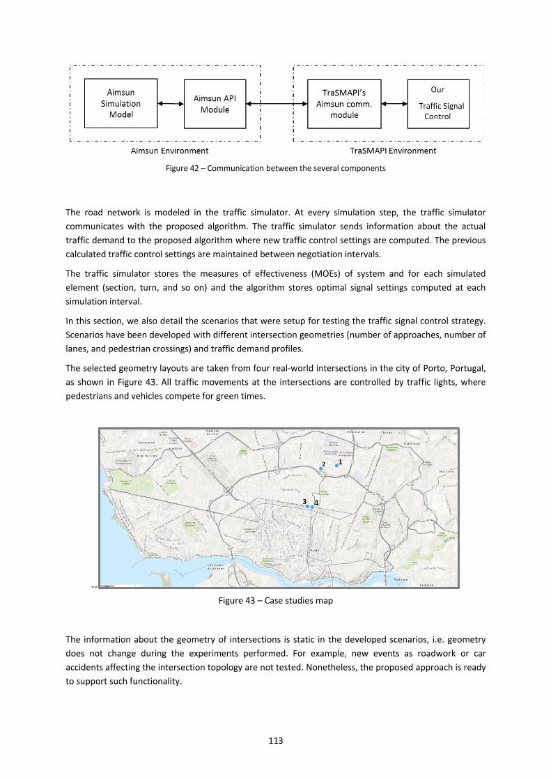
113
Figure 42 – Communication between the several components
The road network is modeled in the traffic simulator. At every simulation step, the traffic simulator
communicates with the proposed algorithm. The traffic simulator sends information about the actual
traffic demand to the proposed algorithm where new traffic control settings are computed. The previous
calculated traffic control settings are maintained between negotiation intervals.
The traffic simulator stores the measures of effectiveness (MOEs) of system and for each simulated
element (section, turn, and so on) and the algorithm stores optimal signal settings computed at each
simulation interval.
In this section, we also detail the scenarios that were setup for testing the traffic signal control strategy.
Scenarios have been developed with different intersection geometries (number of approaches, number of
lanes, and pedestrian crossings) and traffic demand profiles.
The selected geometry layouts are taken from four real-world intersections in the city of Porto, Portugal,
as shown in Figure 43. All traffic movements at the intersections are controlled by traffic lights, where
pedestrians and vehicles compete for green times.
--
Figure 43 – Case studies map
The information about the geometry of intersections is static in the developed scenarios, i.e. geometry
does not change during the experiments performed. For example, new events as roadwork or car
accidents affecting the intersection topology are not tested. Nonetheless, the proposed approach is ready
to support such functionality.
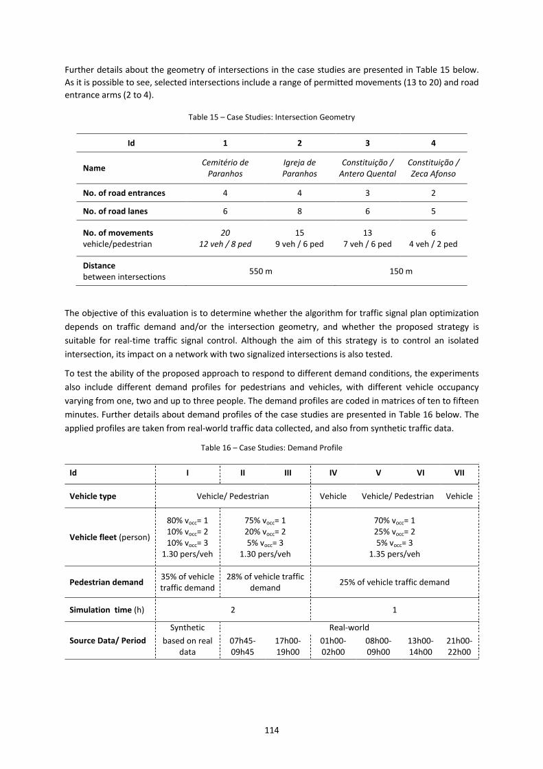
114
Further details about the geometry of intersections in the case studies are presented in Table 15 below.
As it is possible to see, selected intersections include a range of permitted movements (13 to 20) and road
entrance arms (2 to 4).
Table 15 – Case Studies: Intersection Geometry
Id 1 2 3 4
Name Cemitério de
Paranhos Igreja de Paranhos
Constituição / Antero Quental
Constituição / Zeca Afonso
No. of road entrances 4 4 3 2
No. of road lanes 6 8 6 5
No. of movements vehicle/pedestrian
20 12 veh / 8 ped
15 9 veh / 6 ped
13 7 veh / 6 ped
6 4 veh / 2 ped
Distance between intersections
550 m 150 m
The objective of this evaluation is to determine whether the algorithm for traffic signal plan optimization
depends on traffic demand and/or the intersection geometry, and whether the proposed strategy is
suitable for real-time traffic signal control. Although the aim of this strategy is to control an isolated
intersection, its impact on a network with two signalized intersections is also tested.
To test the ability of the proposed approach to respond to different demand conditions, the experiments
also include different demand profiles for pedestrians and vehicles, with different vehicle occupancy
varying from one, two and up to three people. The demand profiles are coded in matrices of ten to fifteen
minutes. Further details about demand profiles of the case studies are presented in Table 16 below. The
applied profiles are taken from real-world traffic data collected, and also from synthetic traffic data.
Table 16 – Case Studies: Demand Profile
Id I II III IV V VI VII
Vehicle type Vehicle/ Pedestrian Vehicle Vehicle/ Pedestrian Vehicle
Vehicle fleet (person)
80% vocc= 1 10% vocc= 2 10% vocc= 3
1.30 pers/veh
75% vocc= 1 20% vocc= 2 5% vocc= 3
1.30 pers/veh
70% vocc= 1 25% vocc= 2 5% vocc= 3
1.35 pers/veh
Pedestrian demand 35% of vehicle traffic demand
28% of vehicle traffic demand
25% of vehicle traffic demand
Simulation time (h) 2 1
Source Data/ Period
Synthetic Real-world
based on real data
07h45-09h45
17h00-19h00
01h00-02h00
08h00-09h00
13h00-14h00
21h00-22h00
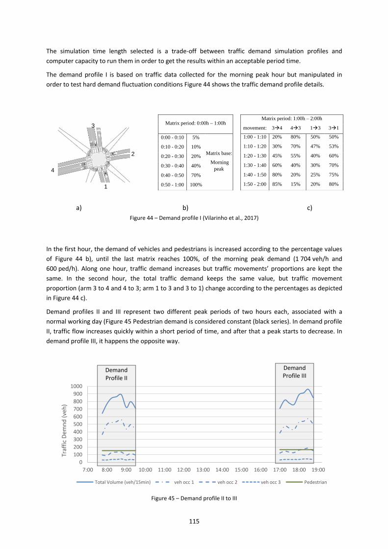
115
The simulation time length selected is a trade-off between traffic demand simulation profiles and
computer capacity to run them in order to get the results within an acceptable period time.
The demand profile I is based on traffic data collected for the morning peak hour but manipulated in
order to test hard demand fluctuation conditions Figure 44 shows the traffic demand profile details.
a) b) c)
Figure 44 – Demand profile I (Vilarinho et al., 2017)
In the first hour, the demand of vehicles and pedestrians is increased according to the percentage values
of Figure 44 b), until the last matrix reaches 100%, of the morning peak demand (1 704 veh/h and
600 ped/h). Along one hour, traffic demand increases but traffic movements’ proportions are kept the
same. In the second hour, the total traffic demand keeps the same value, but traffic movement
proportion (arm 3 to 4 and 4 to 3; arm 1 to 3 and 3 to 1) change according to the percentages as depicted
in Figure 44 c).
Demand profiles II and III represent two different peak periods of two hours each, associated with a
normal working day (Figure 45 Pedestrian demand is considered constant (black series). In demand profile
II, traffic flow increases quickly within a short period of time, and after that a peak starts to decrease. In
demand profile III, it happens the opposite way.
Figure 45 – Demand profile II to III
0
100
200
300
400
500
600
700
800
900
1000
7:00 8:00 9:00 10:00 11:00 12:00 13:00 14:00 15:00 16:00 17:00 18:00 19:00
Traf
fic
Dem
nd
(ve
h)
Total Volume (veh/15min) veh occ 1 veh occ 2 veh occ 3 Pedestrian
Matrix period: 0:00h – 1:00h Matrix period: 1:00h – 2:00h
movement: 34 43 13 31
0:00 - 0:10 5%
Matrix base:
Morning
peak
1:00 - 1:10 20% 80% 50% 50%
0:10 - 0:20 10% 1:10 - 1:20 30% 70% 47% 53%
0:20 - 0:30 20% 1:20 - 1:30 45% 55% 40% 60%
0:30 - 0:40 40% 1:30 - 1:40 60% 40% 30% 70%
0:40 - 0:50 70% 1:40 - 1:50 80% 20% 25% 75%
0:50 - 1:00 100% 1:50 - 2:00 85% 15% 20% 80%
Demand Profile II
Demand Profile III
1
2
3
4
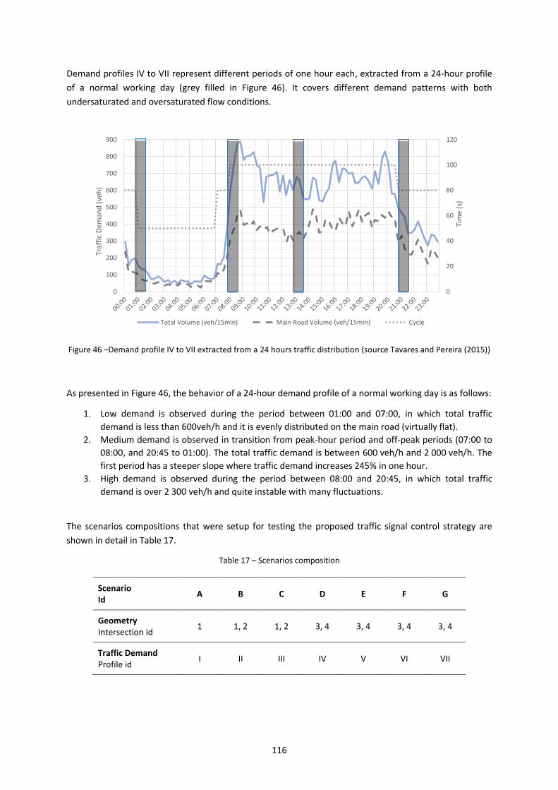
116
Demand profiles IV to VII represent different periods of one hour each, extracted from a 24-hour profile
of a normal working day (grey filled in Figure 46). It covers different demand patterns with both
undersaturated and oversaturated flow conditions.
Figure 46 –Demand profile IV to VII extracted from a 24 hours traffic distribution (source Tavares and Pereira (2015))
As presented in Figure 46, the behavior of a 24-hour demand profile of a normal working day is as follows:
1. Low demand is observed during the period between 01:00 and 07:00, in which total traffic
demand is less than 600veh/h and it is evenly distributed on the main road (virtually flat).
2. Medium demand is observed in transition from peak-hour period and off-peak periods (07:00 to
08:00, and 20:45 to 01:00). The total traffic demand is between 600 veh/h and 2 000 veh/h. The
first period has a steeper slope where traffic demand increases 245% in one hour.
3. High demand is observed during the period between 08:00 and 20:45, in which total traffic
demand is over 2 300 veh/h and quite instable with many fluctuations.
The scenarios compositions that were setup for testing the proposed traffic signal control strategy are
shown in detail in Table 17.
Table 17 – Scenarios composition
Scenario Id
A B C D E F G
Geometry Intersection id
1 1, 2 1, 2 3, 4 3, 4 3, 4 3, 4
Traffic Demand Profile id
I II III IV V VI VII
0
20
40
60
80
100
120
0
100
200
300
400
500
600
700
800
900
Tim
e (s
)
Traf
fic
Dem
and
(ve
h)
Total Volume (veh/15min) Main Road Volume (veh/15min) Cycle
117
Important further details about the case studies also include:
Free flow Speed: 50 km/h;
Time step duration: 1 s;
Reaction time: 1.10 s;
Warm-up: 15 minutes of where traffic lights operate on a fixed-time basis. Time does not count
as simulation time goes on. Data of this period is ignored in the results;
Number of simulation runs performed per approach and scenario: 25. A sensitive analysis was
performed for 50 simulation runs; however, 25 simulation runs show to be sufficient to yield
statistically significant results. The traffic simulator performs 25 runs on average.
Finally, it is important to point out that all the scenarios characterized in this section, i.e. the geometry,
the traffic demand profiles, and the different details about the case studies (listed above) are tested with
equal parameters for all approaches. This will allow us to compare the different approaches and fairly
compare the results obtained from each of them.
4.2. Performance Measures
The performance of control strategy is quantified and evaluated using typical measures of effectiveness
relevant for traffic operation. Metrics or performance measures are essential to evaluate the experiments
results and compare the different approaches used (see section 4.3). The system is analyzed both at the
arm and at network system levels. In the former, it is possible to understand if the solution is balanced or
if the improvements are related to a specific arm, whereas the latter gives an overall picture of how
healthy the system is performing as a whole. The performance measures can be distinguished by road
user type, such as pedestrians and vehicles with occupancy of one, two, and three people.
Two metrics were defined regarding the Computational Performance, whereas six metrics were related to
Traffic Conditions and five metrics were related to Negotiation Outcomes. Each performance metric is
described below in order to allow a better understanding of the results presented in section 4.4. Note
that the term “vehicle” encompasses all vehicles independently of their occupancy, and the pedestrians
as well.
Computer Performance Metrics – these metrics are only available for the proposed traffic control
(ITC_No_Plan and ITC_Plan) and are monitored by the algorithm itself. Results regarding computational
performance are available in section 4.4.
Execution time for phase composition (seconds) – time spent in the computation of phase
composition (see section 3.2.1). In the experiments, this step is performed only once by run time;
Execution time for possible plan design (seconds) – time spent in the design computation of
possible traffic signal plans (see 3.2.1). In the experiments, this step is performed only in the
ITC_Plan approach, and once by run time.
Traffic conditions – these metrics depend highly on the measure of effectiveness (MOE) computed by the
traffic simulator. This performance measure is evaluated both at the network and at the arm levels. The
statistical data is presented as “global” results if concerned with the whole simulation period, and as
“periodic” if concerned with a certain time period, which was defined as an interval of two minutes and a
118
half (2min 30s). The selected metrics for the whole network are different from those for the arms because
the traffic simulator uses different units in each case, and it is not clear how it computes some of such
metrics.
Network Average Travel Time (seconds per vehicle) - average travel time experienced by each
vehicle (includes pedestrians and vehicles, with different vehicle occupancy of one, two, and
three people) that have crossed the network. In section 4.4, the results are available for all
simulation periods. In Appendix B, the results are available for each simulation run and period
(2min30s interval) which provides us with the possibility of observing the metric evolution over
time and the variability between simulation runs;
Network Average People Travel Time (seconds per person) - it is a variation of the previous
metric where the subject is “people”, i.e., average travel time experienced by each person that
has crossed the network, for all simulation periods (results in section 4.4). This metric was
chosen to evaluate the impact of the person-based optimization method devised in this work;
Network Total Number of vehicles (vehicles) – total number of vehicles that have crossed the
network until certain time period (x-axis) (results in Appendix B). The aim of this metric is to show
the demand served over time;
Arm Average Delay Time (seconds per vehicle) - it represents the average delay time per vehicle.
This is the difference between the expected travel time – the time it would take to traverse the
arm under ideal conditions – and the effective travel time. It is calculated as the average over all
vehicles during all simulation periods (results in Appendix C);
Arm Average Number of stops (times per vehicle) - it represents the average number of stops
per vehicle while travelling on the arms during all simulation periods (results in Appendix C);
Arm Total Number of vehicles (vehicles) - it represents the total number of vehicles that have
crossed the arm during all simulation periods (results in Appendix C). The aim of this metric is to
show the demand achieved and its weight in the whole network.
Negotiation Outcomes - these metrics are only available for the proposed traffic signal control. The
algorithm itself records the signal settings determined by the designed approach. The results are available
in section 4.4.
Maximum green time (seconds) – it represents the average maximum green time interval of all
simulation runs. The results are presented for each proposed traffic control approach;
Average green time (seconds) – it represents the arithmetic average of green time intervals of all
simulation runs. The results are presented for each proposed traffic control approach;
Phase changing (number) – it is the average number of times in which a phase is terminated and
a new one is initiated. The results are presented as an average of all simulation runs, for each
proposed traffic control approach;
Plan changing (number) – it is the average number of times in which a traffic signal plan is
terminated. The traffic signal plan is stopped due to budget reasons (explained on section 3.4), so
the next plan can be the same if it is the most beneficial for the intersection. The metric is an
average of all simulation runs and only applicable to the ITC_Plan approach;
Negotiation time (seconds)– it is the average time spent in the negotiation process (explained in
section 3.3) for all simulation runs. The negotiation step is performed several times during a
simulation run.
119
These performance metrics were deemed to be the most appropriated for this work given the specificities
of the application domain, especially when measured for a variety of traffic demand levels and
geometries. Note that it may not be useful to directly compare the metrics as measured in the traffic
simulator with real-world values, as the simulator is not designed to replicate the exact constants of the
real world. Instead, we use them to compare various mechanisms and policies tested within the traffic
simulator.
4.3. Evaluation Approaches
Three established approaches for validation of the proposed strategy were defined which are commonly
implemented in real-world signalized intersections. These approaches work as a baseline for comparison
of the proposed strategy. A description of each one follows.
Baseline 1: Fixed operation TRANSYT.
In this approach, the traffic signal control plan is calculated with a well-established software named
TRANSYT (Binning, 2014) This software is used for offline optimization of traffic signal plans, for fixed-time
operation. The main drawback of this software is that the traffic signal plan calculation (design and
timing) uses static and historical traffic demand. We opted for the 15-minute matrix with high demand of
the whole simulation period for traffic signal plan optimization. For the cases of scenarios with two
intersections, the traffic signal plans are coordinated, sharing a common cycle length that minimizes the
amount of overall delay in the system and then compute the offset required for progression. Once the
operation of intersections is fixed, traffic signal plans remain coordinated;
Baseline 2: Actuated operation TRANSYT.
The traffic signal plans were designed following the approach above (Fixed operation TRANSYT). The
difference is that the control system operates in actuated time. During actuated-time operation, the
traffic signal control losses coordination, and only regains it when a new cycle length is adopted;
Baseline 3: Real-world.
This approach tries to reproduce the strategy implemented in the real-world environment. Regarding the
intersections defined before (Table 15), intersections 1 and 2 have an actuated-time operation with traffic
signal plans defined according to the period of the day. Intersections 3 and 4, in the real-world
environment, are controlled by a dynamic centralized strategy. To reproduce such behavior, the fixed-
operation with different cycles was selected according to the period of the day, as shown in Figure 46.
Since its dynamic operation would be difficult to replicate, a coordination approach resorting to fixed-
time operation was adopted.
Finally, the parameters used in the traffic simulation model are the same for these approaches and for the
proposed traffic signal control strategy.
4.4. Results and Discussion
Results of the experiments for the approaches defined in the previous section, as well as, the traffic signal
control strategy presented in chapter 2, section 2.4.6, are summarized in the following figures (Figure 47
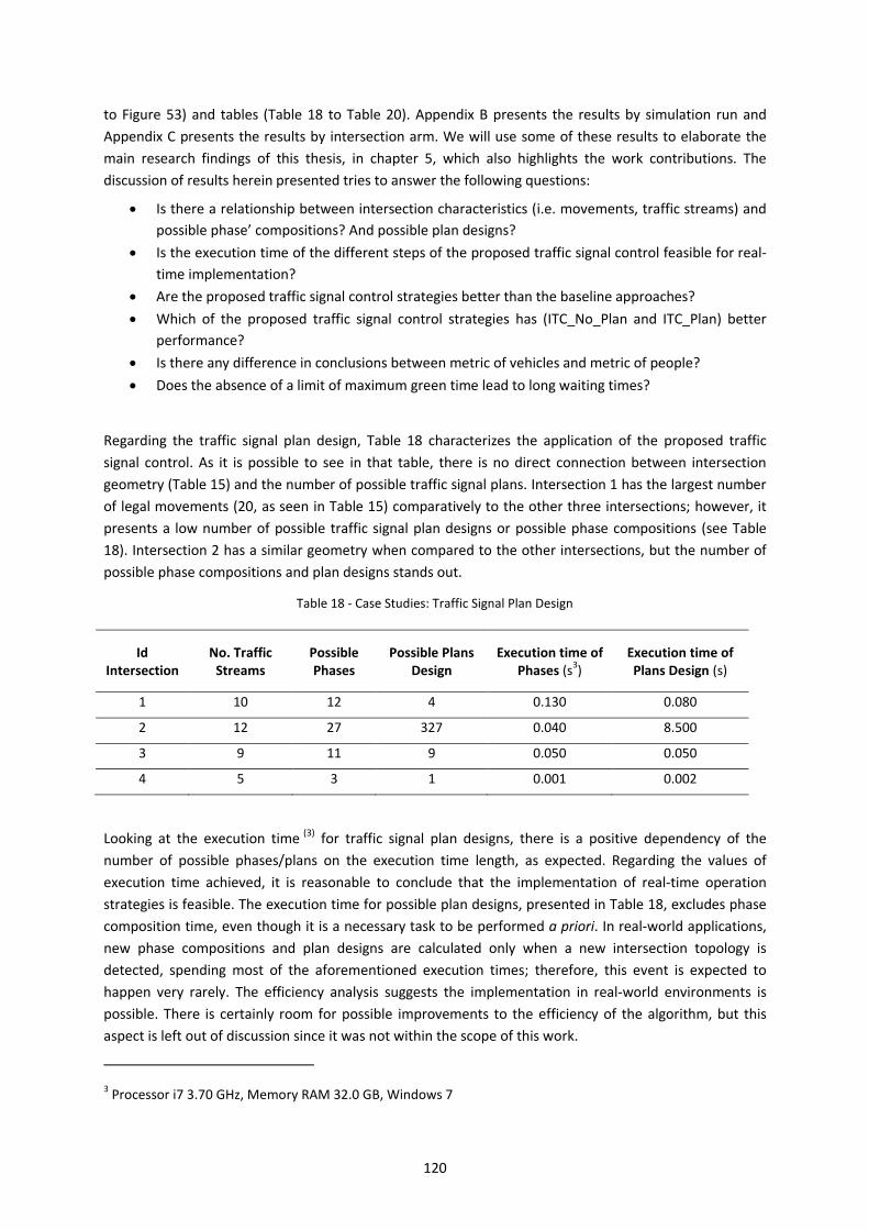
120
to Figure 53) and tables (Table 18 to Table 20). Appendix B presents the results by simulation run and
Appendix C presents the results by intersection arm. We will use some of these results to elaborate the
main research findings of this thesis, in chapter 5, which also highlights the work contributions. The
discussion of results herein presented tries to answer the following questions:
Is there a relationship between intersection characteristics (i.e. movements, traffic streams) and
possible phase’ compositions? And possible plan designs?
Is the execution time of the different steps of the proposed traffic signal control feasible for real-
time implementation?
Are the proposed traffic signal control strategies better than the baseline approaches?
Which of the proposed traffic signal control strategies has (ITC_No_Plan and ITC_Plan) better
performance?
Is there any difference in conclusions between metric of vehicles and metric of people?
Does the absence of a limit of maximum green time lead to long waiting times?
Regarding the traffic signal plan design, Table 18 characterizes the application of the proposed traffic
signal control. As it is possible to see in that table, there is no direct connection between intersection
geometry (Table 15) and the number of possible traffic signal plans. Intersection 1 has the largest number
of legal movements (20, as seen in Table 15) comparatively to the other three intersections; however, it
presents a low number of possible traffic signal plan designs or possible phase compositions (see Table
18). Intersection 2 has a similar geometry when compared to the other intersections, but the number of
possible phase compositions and plan designs stands out.
Table 18 - Case Studies: Traffic Signal Plan Design
Id Intersection
No. Traffic Streams
Possible Phases
Possible Plans Design
Execution time of Phases (s
3)
Execution time of Plans Design (s)
1 10 12 4 0.130 0.080
2 12 27 327 0.040 8.500
3 9 11 9 0.050 0.050
4 5 3 1 0.001 0.002
Looking at the execution time (3) for traffic signal plan designs, there is a positive dependency of the
number of possible phases/plans on the execution time length, as expected. Regarding the values of
execution time achieved, it is reasonable to conclude that the implementation of real-time operation
strategies is feasible. The execution time for possible plan designs, presented in Table 18, excludes phase
composition time, even though it is a necessary task to be performed a priori. In real-world applications,
new phase compositions and plan designs are calculated only when a new intersection topology is
detected, spending most of the aforementioned execution times; therefore, this event is expected to
happen very rarely. The efficiency analysis suggests the implementation in real-world environments is
possible. There is certainly room for possible improvements to the efficiency of the algorithm, but this
aspect is left out of discussion since it was not within the scope of this work.
3 Processor i7 3.70 GHz, Memory RAM 32.0 GB, Windows 7

121
Regarding traffic conditions, and to evaluate the performance of the proposed traffic signal control, 25
replications of each scenario (see Table 17) were run and compared against evaluation approaches.
The cumulative distribution functions (cdf’s) of average travel time of vehicles (s/veh) and people
(s/person) are presented in Figure 47 to Figure 53, each of which presenting the results of one of the
scenarios in alphabetical order.
In scenario A which presents only one intersection (intersection 1), due to the characteristics of traffic
demand being so different during simulation period, besides the plots of the two-hours period (Figure 47
a) and b)), the plot for the first hour (Figure 47 c) and d)) and the second simulation hour (Figure 47 e)
and f)) are also presented separately.
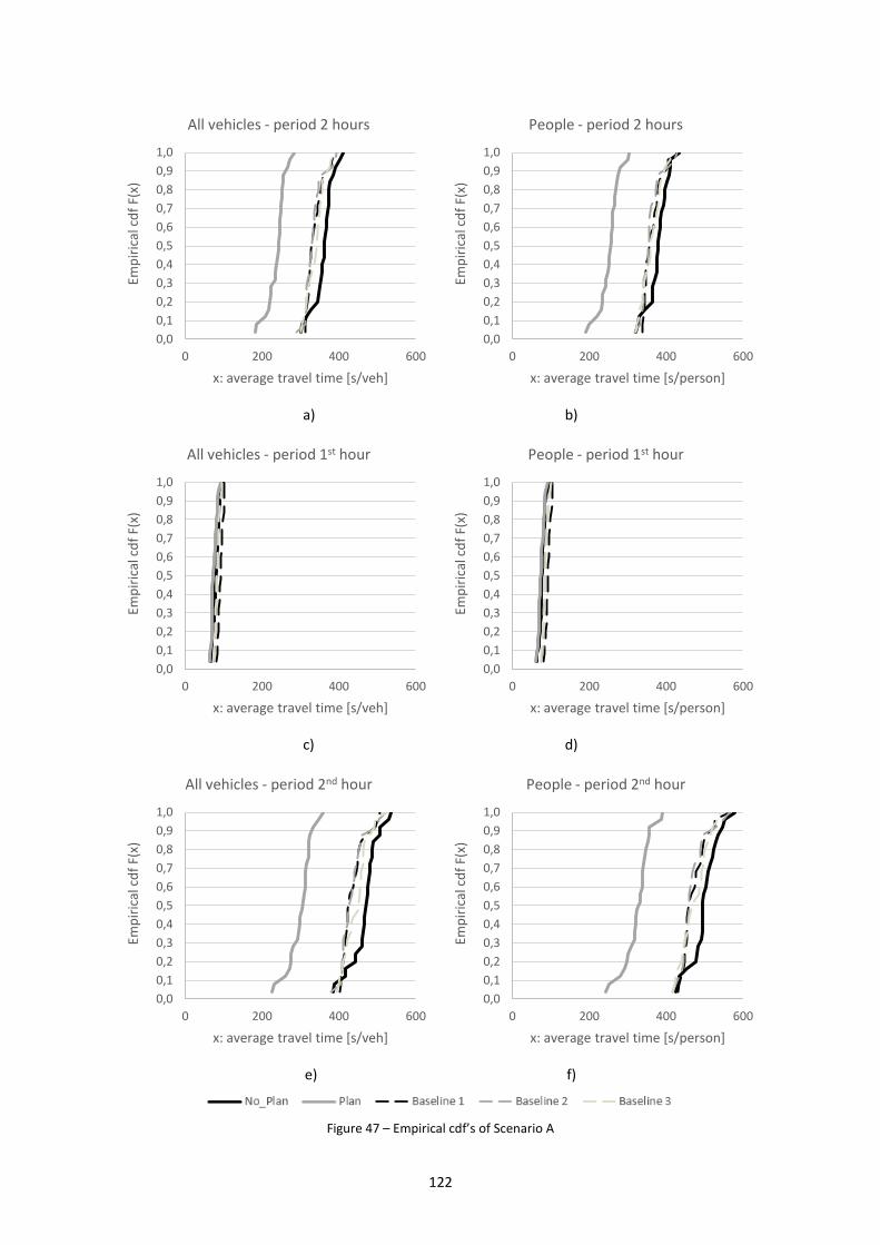
122
a) b)
c) d)
e) f)
Figure 47 – Empirical cdf’s of Scenario A
0,0
0,1
0,2
0,3
0,4
0,5
0,6
0,7
0,8
0,9
1,0
0 200 400 600
Emp
iric
al c
df
F(x)
x: average travel time [s/veh]
All vehicles - period 2 hours
0,0
0,1
0,2
0,3
0,4
0,5
0,6
0,7
0,8
0,9
1,0
0 200 400 600
Emp
iric
al c
df
F(x)
x: average travel time [s/person]
People - period 2 hours
0,0
0,1
0,2
0,3
0,4
0,5
0,6
0,7
0,8
0,9
1,0
0 200 400 600
Emp
iric
al c
df
F(x)
x: average travel time [s/veh]
All vehicles - period 1st hour
0,0
0,1
0,2
0,3
0,4
0,5
0,6
0,7
0,8
0,9
1,0
0 200 400 600
Emp
iric
al c
df
F(x)
x: average travel time [s/person]
People - period 1st hour
0,0
0,1
0,2
0,3
0,4
0,5
0,6
0,7
0,8
0,9
1,0
0 200 400 600
Emp
iric
al c
df
F(x)
x: average travel time [s/veh]
All vehicles - period 2nd hour
0,0
0,1
0,2
0,3
0,4
0,5
0,6
0,7
0,8
0,9
1,0
0 200 400 600
Emp
iric
al c
df
F(x)
x: average travel time [s/person]
People - period 2nd hour
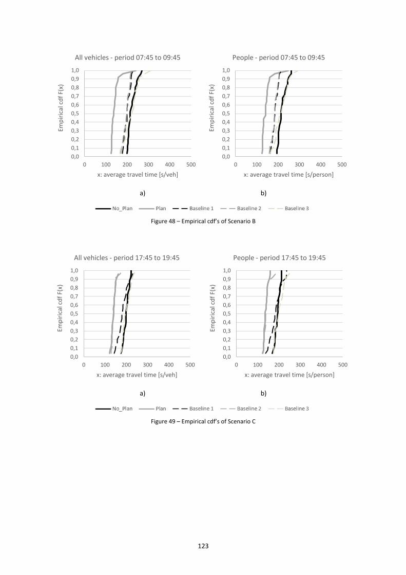
123
a) b)
Figure 48 – Empirical cdf’s of Scenario B
a) b)
Figure 49 – Empirical cdf’s of Scenario C
0,0
0,1
0,2
0,3
0,4
0,5
0,6
0,7
0,8
0,9
1,0
0 100 200 300 400 500
Emp
iric
al c
df
F(x)
x: average travel time [s/veh]
All vehicles - period 07:45 to 09:45
0,0
0,1
0,2
0,3
0,4
0,5
0,6
0,7
0,8
0,9
1,0
0 100 200 300 400 500
Emp
iric
al c
df
F(x)
x: average travel time [s/person]
People - period 07:45 to 09:45
0,0
0,1
0,2
0,3
0,4
0,5
0,6
0,7
0,8
0,9
1,0
0 100 200 300 400 500
Emp
iric
al c
df
F(x)
x: average travel time [s/veh]
All vehicles - period 17:45 to 19:45
0,0
0,1
0,2
0,3
0,4
0,5
0,6
0,7
0,8
0,9
1,0
0 100 200 300 400 500
Emp
iric
al c
df
F(x)
x: average travel time [s/person]
People - period 17:45 to 19:45
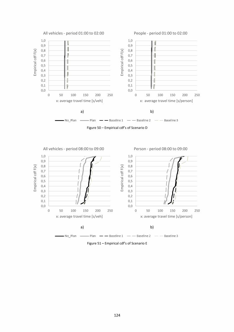
124
a) b)
Figure 50 – Empirical cdf’s of Scenario D
a) b)
Figure 51 – Empirical cdf’s of Scenario E
0,0
0,1
0,2
0,3
0,4
0,5
0,6
0,7
0,8
0,9
1,0
0 50 100 150 200 250
Emp
iric
al c
df
F(x)
x: average travel time [s/veh]
All vehicles - period 01:00 to 02:00
0,0
0,1
0,2
0,3
0,4
0,5
0,6
0,7
0,8
0,9
1,0
0 50 100 150 200 250
Emp
iric
al c
df
F(x)
x: average travel time [s/person]
People - period 01:00 to 02:00
0,0
0,1
0,2
0,3
0,4
0,5
0,6
0,7
0,8
0,9
1,0
0 50 100 150 200 250
Emp
iric
al c
df
F(x)
x: average travel time [s/veh]
All vehicles - period 08:00 to 09:00
0,0
0,1
0,2
0,3
0,4
0,5
0,6
0,7
0,8
0,9
1,0
0 50 100 150 200 250
Emp
iric
al c
df
F(x)
x: average travel time [s/person]
Person - period 08:00 to 09:00
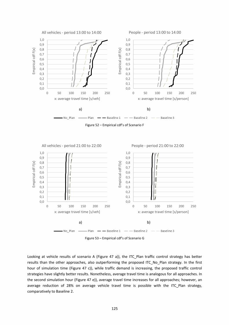
125
a) b)
Figure 52 – Empirical cdf’s of Scenario F
a) b)
Figure 53 – Empirical cdf’s of Scenario G
Looking at vehicle results of scenario A (Figure 47 a)), the ITC_Plan traffic control strategy has better
results than the other approaches, also outperforming the proposed ITC_No_Plan strategy. In the first
hour of simulation time (Figure 47 c)), while traffic demand is increasing, the proposed traffic control
strategies have slightly better results. Nonetheless, average travel time is analogous for all approaches. In
the second simulation hour (Figure 47 e)), average travel time increases for all approaches; however, an
average reduction of 28% on average vehicle travel time is possible with the ITC_Plan strategy,
comparatively to Baseline 2.
0,0
0,1
0,2
0,3
0,4
0,5
0,6
0,7
0,8
0,9
1,0
0 50 100 150 200 250
Emp
iric
al c
df
F(x)
x: average travel time [s/veh]
All vehicles - period 13:00 to 14:00
0,0
0,1
0,2
0,3
0,4
0,5
0,6
0,7
0,8
0,9
1,0
0 50 100 150 200 250
Emp
iric
al c
df
F(x)
x: average travel time [s/person]
People - period 13:00 to 14:00
0,0
0,1
0,2
0,3
0,4
0,5
0,6
0,7
0,8
0,9
1,0
0 50 100 150 200 250
Emp
iric
al c
df
F(x)
x: average travel time [s/veh]
All vehicles - period 21:00 to 22:00
0,0
0,1
0,2
0,3
0,4
0,5
0,6
0,7
0,8
0,9
1,0
0 50 100 150 200 250
Emp
iric
al c
df
F(x)
x: average travel time [s/person]
People - period 21:00 to 22:00
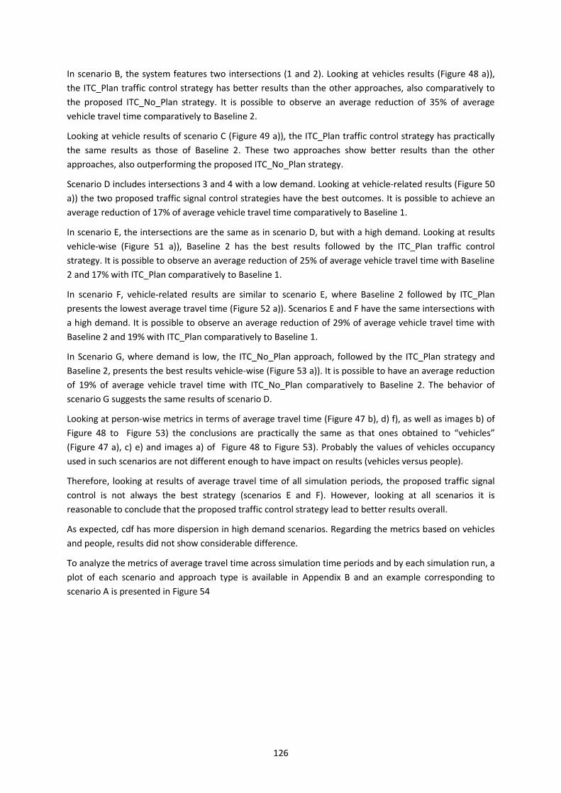
126
In scenario B, the system features two intersections (1 and 2). Looking at vehicles results (Figure 48 a)),
the ITC_Plan traffic control strategy has better results than the other approaches, also comparatively to
the proposed ITC_No_Plan strategy. It is possible to observe an average reduction of 35% of average
vehicle travel time comparatively to Baseline 2.
Looking at vehicle results of scenario C (Figure 49 a)), the ITC_Plan traffic control strategy has practically
the same results as those of Baseline 2. These two approaches show better results than the other
approaches, also outperforming the proposed ITC_No_Plan strategy.
Scenario D includes intersections 3 and 4 with a low demand. Looking at vehicle-related results (Figure 50
a)) the two proposed traffic signal control strategies have the best outcomes. It is possible to achieve an
average reduction of 17% of average vehicle travel time comparatively to Baseline 1.
In scenario E, the intersections are the same as in scenario D, but with a high demand. Looking at results
vehicle-wise (Figure 51 a)), Baseline 2 has the best results followed by the ITC_Plan traffic control
strategy. It is possible to observe an average reduction of 25% of average vehicle travel time with Baseline
2 and 17% with ITC_Plan comparatively to Baseline 1.
In scenario F, vehicle-related results are similar to scenario E, where Baseline 2 followed by ITC_Plan
presents the lowest average travel time (Figure 52 a)). Scenarios E and F have the same intersections with
a high demand. It is possible to observe an average reduction of 29% of average vehicle travel time with
Baseline 2 and 19% with ITC_Plan comparatively to Baseline 1.
In Scenario G, where demand is low, the ITC_No_Plan approach, followed by the ITC_Plan strategy and
Baseline 2, presents the best results vehicle-wise (Figure 53 a)). It is possible to have an average reduction
of 19% of average vehicle travel time with ITC_No_Plan comparatively to Baseline 2. The behavior of
scenario G suggests the same results of scenario D.
Looking at person-wise metrics in terms of average travel time (Figure 47 b), d) f), as well as images b) of
Figure 48 to Figure 53) the conclusions are practically the same as that ones obtained to “vehicles”
(Figure 47 a), c) e) and images a) of Figure 48 to Figure 53). Probably the values of vehicles occupancy
used in such scenarios are not different enough to have impact on results (vehicles versus people).
Therefore, looking at results of average travel time of all simulation periods, the proposed traffic signal
control is not always the best strategy (scenarios E and F). However, looking at all scenarios it is
reasonable to conclude that the proposed traffic control strategy lead to better results overall.
As expected, cdf has more dispersion in high demand scenarios. Regarding the metrics based on vehicles
and people, results did not show considerable difference.
To analyze the metrics of average travel time across simulation time periods and by each simulation run, a
plot of each scenario and approach type is available in Appendix B and an example corresponding to
scenario A is presented in Figure 54

127
a) No Plan b) Plan
c) Baseline 1 d) Baseline 2 e) Baseline 3
Figure 54 – Average travel time of scenario A by simulation run
The main conclusions are as follows.
In scenario A, as discussed above, the average travel time is low and steady in the first hour of the
simulation time. In the second hour though, the traffic demand is heavier which yields an increase of the
average travel time. The proposed method ITC_Plan presents the best results when compared with plots
of other approaches, where the average travel time increases in an exponential way.
In scenario B, more vehicles have crossed the network with the ITC_Plan traffic control strategy than with
other strategies. The reason for this behavior is the increase of intersection capacity due to the traffic
control strategy. The average travel time in the ITC_Plan plot presents the best results and the series are
very flat when compared with the plot of other approaches, in the same scenario.
In scenario C, the number of traffic users who crossed the network is very similar in all approaches. As
referred before, the ITC_Plan traffic control strategy presents practically the same results as of Baseline 2.
Looking at results in Appendix B, these two approaches present better outcome, but the ITC_Plan series
are more evenly distributed, yielding a virtually flat curve.
0
500
1000
1500
2000
2500
3000
3500
0
100
200
300
400
500
600
700
800
900
1000
1 6 11 16 21 26 31 36 41 46
Traf
fic
cou
nt
[veh
]
aver
age
trav
el t
ime
[s/v
eh]
x: time interval [2m30s]
All traffic users- Period 2 hours
0
500
1000
1500
2000
2500
3000
3500
0
100
200
300
400
500
600
700
800
900
1000
1 6 11 16 21 26 31 36 41 46
Traf
fic
cou
nt
[veh
]
aver
age
trav
el t
ime
[s/v
eh]
x: time interval [2min30s]
All traffic users - Period 2 hours
0
500
1000
1500
2000
2500
3000
3500
0
100
200
300
400
500
600
700
800
900
1000
1 9 17 25 33 41
Traf
fic
cou
nt
[veh
]
aver
age
trav
el t
ime
[s/v
eh]
x: time interval [2min30s]
All traffic users - Period 2 hours
0
500
1000
1500
2000
2500
3000
3500
0
100
200
300
400
500
600
700
800
900
1000
1 11 21 31 41
Traf
fic
cou
nt
[veh
]
aver
age
trav
el t
ime
[s/v
eh]
x: time interval [2min30s]
All traffic users - Period 2 hours
0
500
1000
1500
2000
2500
3000
3500
0
100
200
300
400
500
600
700
800
900
1000
1 9 17 25 33 41
Traf
fic
cou
nt
[veh
]
aver
age
trav
el t
ime
[s/v
eh]
x: time interval [2min30s]
All traffic users - Period 2 hours
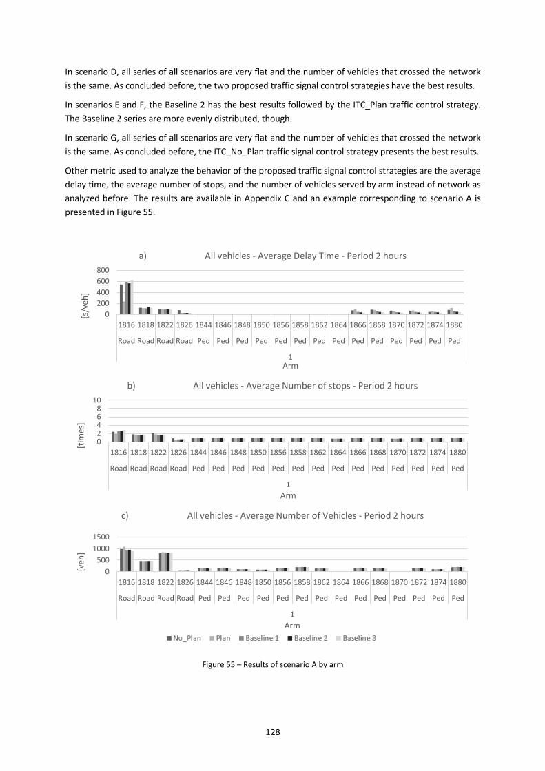
128
In scenario D, all series of all scenarios are very flat and the number of vehicles that crossed the network
is the same. As concluded before, the two proposed traffic signal control strategies have the best results.
In scenarios E and F, the Baseline 2 has the best results followed by the ITC_Plan traffic control strategy.
The Baseline 2 series are more evenly distributed, though.
In scenario G, all series of all scenarios are very flat and the number of vehicles that crossed the network
is the same. As concluded before, the ITC_No_Plan traffic signal control strategy presents the best results.
Other metric used to analyze the behavior of the proposed traffic signal control strategies are the average
delay time, the average number of stops, and the number of vehicles served by arm instead of network as
analyzed before. The results are available in Appendix C and an example corresponding to scenario A is
presented in Figure 55.
Figure 55 – Results of scenario A by arm
0
200
400
600
800
1816 1818 1822 1826 1844 1846 1848 1850 1856 1858 1862 1864 1866 1868 1870 1872 1874 1880
Road Road Road Road Ped Ped Ped Ped Ped Ped Ped Ped Ped Ped Ped Ped Ped Ped
1
[s/v
eh]
Arm
a) All vehicles - Average Delay Time - Period 2 hours
0 2 4 6 8
10
1816 1818 1822 1826 1844 1846 1848 1850 1856 1858 1862 1864 1866 1868 1870 1872 1874 1880
Road Road Road Road Ped Ped Ped Ped Ped Ped Ped Ped Ped Ped Ped Ped Ped Ped
1
[tim
es]
Arm
b) All vehicles - Average Number of stops - Period 2 hours
0
500
1000
1500
1816 1818 1822 1826 1844 1846 1848 1850 1856 1858 1862 1864 1866 1868 1870 1872 1874 1880
Road Road Road Road Ped Ped Ped Ped Ped Ped Ped Ped Ped Ped Ped Ped Ped Ped
1
[veh
]
Arm
c) All vehicles - Average Number of Vehicles - Period 2 hours
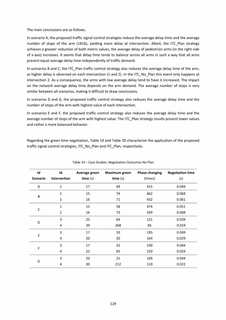
129
The main conclusions are as follows.
In scenario A, the proposed traffic signal control strategies reduce the average delay time and the average
number of stops of the arm (1816), yielding more delay at intersection. Albeit, the ITC_Plan strategy
achieves a greater reduction of both metric values, the average delay of pedestrian arms (in the right side
of x-axis) increases. It seems that delay time tends to balance across all arms in such a way that all arms
present equal average delay time independently of traffic demand.
In scenarios B and C, the ITC_Plan traffic control strategy also reduces the average delay time of the arm,
as higher delay is observed on each intersection (1 and 2). In the ITC_No_Plan this event only happens at
intersection 2. As a consequence, the arms with low average delay tend to have it increased. The impact
on the network average delay time depends on the arm demand. The average number of stops is very
similar between all scenarios, making it difficult to draw conclusions.
In scenarios D and G, the proposed traffic control strategy also reduces the average delay time and the
number of stops of the arm with highest value of each intersection.
In scenarios E and F, the proposed traffic control strategy also reduces the average delay time and the
average number of stops of the arm with highest value. The ITC_Plan strategy results present lower values
and rather a more balanced behavior.
Regarding the green time negotiation, Table 19 and Table 20 characterize the application of the proposed
traffic signal control strategies, ITC_No_Plan and ITC_Plan, respectively.
Table 19 – Case Studies: Negotiation Outcomes No Plan
Id
Scenario
Id
Intersection
Average green
time (s)
Maximum green
time (s)
Phase changing
(times)
Negotiation time
(s)
A 1 17 49 415 0.044
B 1 15 74 462 0.069
2 16 71 432 0.061
C 1 15 58 474 0.051
2 16 73 439 0.069
D 3 25 64 131 0.039
4 39 268 85 0.019
E 3 17 33 195 0.049
4 20 20 164 0.029
F 3 17 32 190 0.044
4 22 65 150 0.024
G 3 20 21 169 0.044
4 30 212 110 0.022
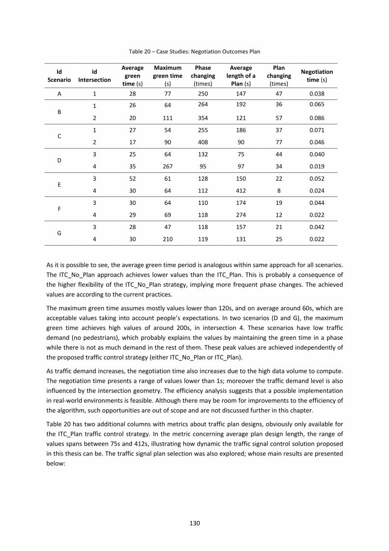
130
Table 20 – Case Studies: Negotiation Outcomes Plan
Id Scenario
Id Intersection
Average green
time (s)
Maximum green time
(s)
Phase changing (times)
Average length of a
Plan (s)
Plan changing (times)
Negotiation time (s)
A 1 28 77 250 147 47 0.038
B 1 26 64 264 192 36 0.065
2 20 111 354 121 57 0.086
C 1 27 54 255 186 37 0.071
2 17 90 408 90 77 0.046
D 3 25 64 132 75 44 0.040
4 35 267 95 97 34 0.019
E 3 52 61 128 150 22 0.052
4 30 64 112 412 8 0.024
F 3 30 64 110 174 19 0.044
4 29 69 118 274 12 0.022
G 3 28 47 118 157 21 0.042
4 30 210 119 131 25 0.022
As it is possible to see, the average green time period is analogous within same approach for all scenarios.
The ITC_No_Plan approach achieves lower values than the ITC_Plan. This is probably a consequence of
the higher flexibility of the ITC_No_Plan strategy, implying more frequent phase changes. The achieved
values are according to the current practices.
The maximum green time assumes mostly values lower than 120s, and on average around 60s, which are
acceptable values taking into account people’s expectations. In two scenarios (D and G), the maximum
green time achieves high values of around 200s, in intersection 4. These scenarios have low traffic
demand (no pedestrians), which probably explains the values by maintaining the green time in a phase
while there is not as much demand in the rest of them. These peak values are achieved independently of
the proposed traffic control strategy (either ITC_No_Plan or ITC_Plan).
As traffic demand increases, the negotiation time also increases due to the high data volume to compute.
The negotiation time presents a range of values lower than 1s; moreover the traffic demand level is also
influenced by the intersection geometry. The efficiency analysis suggests that a possible implementation
in real-world environments is feasible. Although there may be room for improvements to the efficiency of
the algorithm, such opportunities are out of scope and are not discussed further in this chapter.
Table 20 has two additional columns with metrics about traffic plan designs, obviously only available for
the ITC_Plan traffic control strategy. In the metric concerning average plan design length, the range of
values spans between 75s and 412s, illustrating how dynamic the traffic signal control solution proposed
in this thesis can be. The traffic signal plan selection was also explored; whose main results are presented
below:
131
Intersection 1, when the sole intersection of the network (scenario A) its choice switches
between two traffic signal plans. In the two-intersection network scenario (B and C), intersection
1 selects mostly the same traffic plan design;
Intersection 2 chooses among several traffic signal plans. In scenario B, the average selected set
has 13 traffic signal plans, in which the same traffic signal plan is chosen 6 times at most. In
scenario C, the average selected set has 17 traffic signal plans, in which the same traffic signal
plan is selected 17 times at most.
Intersection 3 may select mostly among 3 traffic signal plans, in which the distribution of traffic
plans selected is different among all scenarios, as well as the most selected one.
Intersection 4 always selects a unique plan. So, in this case it is easy to conclude that every time
the intersection calculates new traffic plan settings its choice falls always upon the same traffic
signal plan.
4.5. Summary
This chapter presented the experiments carried out in this research work. The setup for each of the
selected scenarios was introduced, regarding both the intersection geometry and the traffic demand
profiles. The performance metrics used to evaluate the experiments were defined, which include the
Computer Performance metrics, the Traffic Conditions metrics, and the Negotiation Outcomes metrics.
The three evaluation approaches (named baselines), used to compare our strategy were introduced as
well.
The results were presented and followed by a thorough discussion about their interpretation. The main
conclusions regarding the questions introduced earlier on are summarized below:
Just by looking at intersection geometry, it is not possible to know the number of viable phase
compositions or possible traffic signal plan designs;
The execution time of the negotiation process, i.e. the time taken to decide on whether to extend
or to terminate the active green time interval, as well as on the next phase to implement takes
much less than one second. The execution times for phase composition and plan design are also
promising, taking much less than 1 second. One exception was observed, however: the traffic
plan design of 327 plans (intersection 2) took 8.5s. Nevertheless, the process of phase
composition and plan design occurs only when there is a new topology, which is not frequent.
There are certainly room for improving the efficiency of the algorithm; however, such
opportunities are not discussed at this point since they were not within the scope of this research
work;
The proposed traffic signal control strategies achieved good results. The Baseline 2 approach
(actuated operation TRANSYT) achieved better results in two of the seven scenarios
comparatively to the results of the proposed traffic control and other two baselines, in terms of
average travel time for the whole simulation time. The negotiation process implemented in the
proposed traffic control reduces average delay time in the arm with high value, distributing and
balancing the delay among all intersection arms. As a consequence, the arms with low average
delay tend to have it increased. The impact on the network average delay time depends on the
traffic demand level of the arm;
The ITC_No_Plan strategy has a better performance in low demands. The results are
disappointing for medium/high demands, though. The ITC_Plan strategy presents a more
balanced performance;

132
The results of average travel time by vehicle and by people were practically the same with minor
differences between them;
In the proposed traffic signal control strategy, a few traditional variables were discarded including
the maximum green time. The results showed adequate maximum green time even without an
established limit. Only in the low traffic demand level, the green time achieved higher values but
probably due to the absence of cars on the opposite arms, so the active phase remained in green.
The next chapter concludes the presentation of this research work by providing a summary of the main
findings and highlighting the most important contributions of this thesis. The limitations of our proposal
as well as directions for future work are also presented.
133
5. Conclusion
In this research, the problem of Traffic Signal Control at isolated intersections in urban environment is
addressed. Traffic lights have the power to improve the safety at intersections, avoiding traffic conflicts
between the different vehicle and pedestrian movements by managing time in space. In order to avoid
dangerous conflicts and to optimize the control performance, the different users have to wait for the
green light, meanwhile losing time which implies some frustration and increased vehicle fuel consumption
as well as CO₂ and other greenhouse gas emissions.
This chapter summarizes the work carried out, in section 5.1, and provides highlights on the main
contributions achieved, in section 5.2. It concludes presenting some directions for future research in
section 5.3.
5.1. Summary of Research Work
This research work proposes a new real-time traffic signal control strategy that relies on the flexibility and
the maximal level of freedom in the design of traffic control settings, where no fixed plan and phase
compositions have to be undertaken. In this way, the control system should be updated frequently so as
to meet equitable priority requirements imposed by the recurrent demand of the different traffic users.
Instead of using the traditional vehicle-based optimization perspective, in which the approach is to look at
the vehicle traffic condition as dependent on standard metrics such as vehicle flow and vehicle delay, a
person-based strategy is instead adopted. It represents an interesting opportunity allowing us to look into
the traffic condition, distinguishing vehicles with different occupancy leveraging a control based on
people present/expected at the intersection. The people metrics are considered independently of the
selected transportation mode (car, bus, pedestrian). In the perspective of a rather societal management,
it should be more important and valuable to minimize “people’s” delays or other person-based metrics
instead of the traditional vehicle performance measures. In this way, green light is given according to the
person volume instead of the vehicle volume.
The global architecture of the proposed traffic signal control system is designed using a Multi-Agent
System approach, for isolated intersections. Each intersection is “unaware” of the state of other
intersections, operating independently from other intersections. So each one has the freedom and
flexibility to calculate and implement any traffic control settings. Thus it allows control algorithms simpler
than the ones for coordinated intersections, which are also more flexible in terms of green time
assignment.
The proposed approach is more of a management methodology than the traditional control of green
time, where agents collaborate and compete to find the best solution for their own goals, looking at the
recurrent traffic demand and possible traffic policies that may apply.
The initial control settings stage aims to find a traffic signal plan including phase composition definition
and respective green time periods. In the MAS perspective, this stage occurs occasionally when the
“Auditor agent” decides that a new traffic signal plan is needed (e.g., due to new topology or empty
budget). The traffic proposed signal plan design is based on enumeration. All possible signal plans are
automatically designed for each intersection grouping the maximum compatible traffic streams by phase.
In this way, all traffic streams that can run at same time are allowed to be part of a phase bringing more
flexibility to the real-time traffic control. For each possible traffic signal plan design, the signal timing
calculation is performed. Akçelik’s approach is based on critical movement search where it begins by

134
identifying all possible paths, followed by calculating the total time for each path and finally finding the
critical path which represents the one with the largest time value. For the traffic signal plan selection, a
multi-objective framework is applied with the aim of promoting good mobility conditions, being
sustainable in terms of traffic emission and equitable for all traffic users. The multi-objective formulations
use the following metrics, in this order: queue length, person-based delay, and number of stops.
Two approaches for finding the initial control settings were developed, one without (ITC_No_Plan) and
another with (ITC_Plan) traffic signal plan design, respectively. In the ITC_No_Plan approach, there is no
traffic signal plan design defined; only the composition of possible phases is instead considered.
Therefore, there is no traffic signal timing plan calculation, but rather only the minimum green time
(vehicles and pedestrians) and saturation flow by traffic stream dependent on phase composition are
computed. In the ITC_Plan approach, the timing plan is calculated for each traffic signal plan design
defined before respectively. So, the ITC_No_Plan approach is simpler and more direct than the ITC_Plan
alternative.
After the selection of initial control settings also named first stage, it is necessary to monitor and update
the traffic signal plan in order to yield a competitive control, so a second stage of the approach was
developed.
The second stage developed corresponds to the optimization of operation, which includes two decisions:
firstly, to define when the current phase should be terminated and secondly to define the next phase to
implement. All traffic streams at intersection compete for green time period. In order to update the traffic
signal control plan, the decision was to look at these processes as a problem of efficient allocation of an
available resource (green light) to consumers (traffic lights). For this purpose, a novel auction-based
intersection-control mechanism for traffic signal control is developed. The present methodology underlies
a negotiation process, involving all the traffic streams to manage the green time between them. The
proposed routine decides on a time period (auction frequency), an extension or an ending of the present
green period, based on current demand and aiming at minimizing the person’s delay. In case of
terminating the green light, a second decision is made in order to select which traffic streams should
receive the green light. The negotiation process is very dynamic and initiates in short intervals (i.e. just a
few seconds).
Decisions about the traffic light status of each traffic stream take into account the current traffic data
such as the traffic flow, the number of road users, the queue lengths, and the delay time in all traffic
streams, independently of their traffic light color. As a result, this strategy can react to non-schedulable
events or unpredictable events without human intervention, and takes into account the traffic streams
with red light.
In this research work, traffic signal control variables and boundaries were rethought with focus on the
minimum constraints so as to increase the area of the space which contains possible solutions of the
proposed traffic control strategy, and to innovate further beyond the traditional traffic signal control
methodologies. As a result, cycle length and maximum green time were discarded. The results showed
adequate maximum green time even without an established limit. Only in low traffic demand levels, the
green time achieved higher values, probably due to the absence of demand in the opposite arms, so the
active phase remained in green.
This traffic signal control strategy was developed in the Java programming language, reporting to
TraSMAPI framework, and the assessment was conducted in a microscopic traffic simulation model. To
include the proposed traffic signal control, communication protocol to link it to the traffic simulation
model was developed. TraSMAPI implements a dedicated communication module, which interconnects
135
with the simulator’s API in real time. The C/C++ programming language was used to link the dedicated
TraSMAPI’s communication module (in Java) to the Aimsun’s API. At every simulation step, the traffic
simulator communicates with the proposed traffic signal control strategy to receive traffic light colors
(green, yellow or red) of all traffic streams to simulate. In the opposite direction, the algorithm of the
proposed traffic control strategy requests data from the simulation model in order to feed its functions.
The execution time needed by the model to make decisions (negotiation process, traffic signal plan
design) is also promising, taking mostly much less than one second. Nonetheless, there is still room to
improve the efficiency of the algorithm since such sort of optimization was not a primary objective of this
research work.
For testing the traffic signal control strategy, seven scenarios were developed, with different intersection
geometries (e.g. number of approaches, number of lanes, and pedestrian crossings) and several traffic
demand profiles were considered. The ITC_No_Plan traffic signal control strategy has a better
performance in low demands. For medium/high demands the results are disappointing though. The
ITC_Plan traffic signal control strategy nonetheless presents a more balanced performance.
The proposed traffic signal control strategies achieved good results. In two of the seven scenarios, the
Baseline 2 approach (i.e. actuated operation TRANSYT) achieved better results than the proposed traffic
control and other two baselines, in terms of the average travel time metric for all simulation time. The
negotiation process implemented in the proposed traffic control system reduces average delay time on
the arm with highest value, distributing and balancing the delay among all intersection arms. As a
consequence, the arms with low average delay tend to increase it. The impact on the network average
delay time depends on the traffic demand level of the arms. Results in terms of average travel time by
vehicle and by people were practically the same with minor differences between them.
5.2. Contribution
The main scientific contributions of this thesis result from the development of the traffic signal control
model, as well as from the implementation of case studies and analysis of results. The related work efforts
were identified with respect to the current state of the art by highlighting the major
differences/advantages of the proposed control against the traffic control systems reviewed in chapter 2.
The main differences of the work performed are listed below:
No control levels
Traffic signal control strategy was developed based on a multi-agent architecture for real-time
signal control at isolated traffic intersections where each traffic stream is an agent and each
signalized intersection builds upon an independent multi-agent system. Agents at same level
negotiate and decide the green time to implement. There is no agent with more power of control
than others. Each agent/traffic stream operates individually and autonomously, cooperating with
the other agents while performing their tasks;
Negotiation Process
Traffic streams can share information with each other; vehicles and traffic streams are
“connected”. All traffic streams compete for green time independently of their traffic color
status;
No Maximum Green Time
No maximum green time period is defined a priori. Whenever the evaluation of the green time is
favorable to continue, the green time is thus kept;

136
No Cycle length
No cycle length is defined a priori during operation. The cycle length concept is not used anymore
since phase can assume any order;
No phase sequence
Phase can assume any order. Usually traffic control systems are constrained to follow a pre-
determined phase order. The proposed method gives the possibility of having no pre-defined
phase order. So the control system is able to select any possible phase based on the most
beneficial phase at any given time period considering all traffic users currently present and
expected at the intersection instead of being established a priori;
No phase composition fixed
During the decision time of the negotiation process no phase composition is fixed. The following
phase or green light can be assumed by any possible set of traffic streams (ITC_No_Plan method).
To gain green light it has to be the more advantageous solution for users;
Person-based traffic control method
For existing traffic signal control systems, the typical approach is to look at traffic conditions as a
vehicle-flow or a vehicle-delay problem. It seems an interesting possibility to look at the traffic
conditions distinguishing vehicles with different occupancy allowing a control based on people
present/expected at an intersection. In a perspective of socially aware management, it should be
more important and valuable to minimize “people’s” delays or other person-based measure
rather than favoring vehicle performance measures. In this way, green light could be given
according to the number of people in the system instead of the number of vehicles;
Pedestrians delay
Pedestrian delay is included in the objective function of the proposed traffic control
methodology. Traffic signals generally aim at minimizing average vehicle delay whereas
pedestrian delay is not taken into account and sometimes completely neglected. Usually green
light is given only based on the minimum values and often in case of exclusive pedestrian phase,
the phase is skipped if there is no demand (i.e. no phase request). Such strategy can be
admissible when pedestrian demand is low, such as in rural areas or high-speed roads. However,
in urban areas, with a high demand of pedestrians, a strategy that only optimizes vehicle flows
makes pedestrians feel forgotten and less important by the traffic signal and consequently by city
policies;
Possible to change intersection topology
The possibility of changing intersection topology is another feature included in the proposed
strategy as compared with reviewed systems. Usually, the traffic signal plan design is only
included in offline systems, where traffic signal plans are designed for static conditions. The
proposed traffic control is an online system with the capacity of creating all possible traffic signal
plan designs (i.e. phase composition and sequence), with just a few data inputs and only based on
the local geometric layout of the intersection. In this way the traffic control strategy is able to
accommodate and account for any changes to the geometry of the intersection;
137
Single intersection
According to the literature review, recent advances have been made towards improved and
optimized coordination systems. In this research work, a proposed strategy is devised for single
intersection, which gives more freedom to the definition of traffic control settings. In this
approach, results were better than plans developed in the TRANSYT software with fixed
operation;
Criteria for updating and reviewing the traffic signal plan settings
The budget in the negotiation process is a simple and automatic criterion for updating and
reviewing the traffic signal plan settings. The process is able to be performed in real time without
human control.
In conclusion of this topic, the major contributions of this research work for traffic signal control are:
More flexibility and freedom is given to the system for changing phase composition and
managing the green time at each single intersection. The phase composition and timing are not
fixed;
Focus is given to people mobility in real time. Traffic controller responds to measured conditions,
such as number of people waiting and for how long, instead of using historical data about
vehicles;
In the devised online strategies, traffic control settings are determined and calculated at a
frequency dictated by existing traffic conditions and predefined settings;
The traffic signal control management approach at isolated intersection is conceived as a multi-
agent system. This is an innovative view where each traffic stream is an agent, rather than
modeling the whole intersection as an agent, as in most traditional approaches encountered in
the literature;
The control strategy is viewed as a problem of efficient allocation of an available resource (green
light) to consumers (traffic signals), leveraged on a bid-based control strategy in which all traffic
streams at an intersection compete for the green time period. For this purpose, this research
introduced a novel auction-based intersection-control mechanism;
Minimizing delay is the goal of the auction. Such an approach can reduce the waiting time for
vehicles, smooth the traffic flow at intersections, and reduce the exhaust emissions. In brief, this
method not only improves the efficiency of the road transport system, but also reduces fuel
consumption and gas emissions.
The stakeholders who may benefit from the use of these new regulation strategies for traffic light control
developed in this research work include, but are not limited to, road users, road management entities,
and society in general, benefiting from a better quality of life and a more sustainable environment.
5.3. Future Work
Regarding future work, there are several interesting lines of research that, even though they have already
been referred to in some previous chapters, are important enough to be pointed out again here,
representing potential opportunities for further development and future contributions.
Regarding the methodology
Albeit the conceptual model of the proposed strategy includes the following competences such as the
ability to predict traffic conditions, to learn and adopt so as to improve control strategies, the ability to
138
overcome system failures was not included in developed algorithms. Therefore, it would be potentially
beneficial to:
- Develop a mechanism to assume traffic data in case of no sensor is installed on an
intersection arm;
- Include detection of sensor faults and failures, and react when a sensor seems to act
abnormally by inferring all needed information from other alternative sources;
- Enhance traffic prediction algorithms. Traffic flow prediction is currently included in a
very simple way, in which it considers that traffic flow for 150s is the same as the last
period of 150s. This feature could be explored deeply further, including the
implementation of learning capacity by observing “actual” traffic data so as to enhance
traffic flow prediction algorithms.
The negotiation process developed is based on traffic flow, queue length, and saturation flow. It would be
beneficial to test new negotiation methodologies with different variables reflecting, for instance, vehicle
trip or vehicle/person information and characteristics. Testing different ways of including information
about saturation flow is another future step to be pursued, since this approach is very dependent on
theoretical values. Empirical approaches to define practical and operational thresholds and limits would
certainly be enlightening.
Although the scope of this research work is on isolated intersections, negotiation processes could include
information about traffic streams of adjacent intersections as well, for instance in the case they have been
shut down for any given reason.
Regarding the Case Study
Ideally, to be able to fully test the capacities of the proposed traffic control and analyze its full potential,
further testing should be carried out on the following case studies:
- Include vehicles of public transport with demand formed up by different user profiles in
order to evaluate if this control strategy promotes prioritization of public transport as it
is expected;
- Include topology changing of layout geometry in order to evaluate the capacity of the
traffic control strategy in calculating new phase compositions and traffic signal plan
designs during simulation period. Topology should be updated in case of topology
changes —permanently if new geometry or lane marks are defined, or temporarily
during roadwork or events such as accidents or car parking abuse in which lane capacity
may be considerably affected.
Regarding the Proposed Traffic Signal Control Results
Results obtained suggest the application of ITC_No_Plan in low traffic demand and of ITC_Plan in
medium/high demand regimes. Therefore, it would be highly beneficial to further analyze such
relationships to decide when to apply each strategy according to the recurrent traffic demand.
139
References
Aamodt, A. & Plaza, E. 1994. Case-based reasoning: Foundational issues, methodological variations, and system approaches. AI communications, 7, 39-59.
Abdulhai, B., Pringle, R. & Karakoulas, G. J. 2003. Reinforcement learning for True Adaptive traffic signal control. Journal of Transportation Engineering-Asce, 129, 278-285.
Adler, J. L. & Blue, V. J. 2002. A cooperative multi-agent transportation management and route guidance system. Transportation Research Part C: Emerging Technologies, 10, 433-454.
Aimsun 2011. Aimsun Microsimulator API Manual, TSS. 7.0 ed. Barcelona, Spain: Transport Simulation System. Aimsun 2013. Aimsun 7 Users’ Manual. In: Systems, T. T. S. (ed.) 7 ed. Barcelona, Spain. Akçelik, R. 1989. Traffic Signals: Capacity and Timing Analysis. Australian Road Research Board. Allsop, R. E. 1971. SIGSET: a computer program for calculating traffic signal settings. Traffic Engineering &
Control, 13, 58-60. Allsop, R. E. 1972. Estimating the traffic capacity of a signalized road junction. Transportation Research, 6, 245-
255. Andersen, O., J. 2012. How Case-based Reasoning can be used to predict and improve Traffic Flow in Urban
Intersections. Norwegian University of Science and Technology. Azzam Ul, A., Sadeeq, U. M., Ahmed, J. & Riaz Ul, H. Traffic responsive signal timing plan generation based on
neural network. Automation Science and Engineering, 2008. CASE 2008. IEEE International Conference on, 23-26 Aug. 2008 2008. 833-838.
Bang, K. L. 1976. Optimal Control of Isolated Traffic Signals. Transportation Research Record, 597. Barceló, J. 2002. Microscopic Traffic Simulator: a tool for the analysis and assessment of ITS system. . TSS -
Transport Simulation System. Barcelona. Barceló, J., Bernauer, E., Breheret, L., Canepari, G., Taranto, C., Ferrer, J., Fox, K., Gabard, J. F. & Liu, R. 1999.
SMARTEST - Simulation Modelling Applied to Road Transport European Scheme Tests. In: D6, S. D. (ed.). European Commission Funds.
Baskan, O., Haldenbilen, S., Ceylan, H. & Ceylan, H. 2009. A new solution algorithm for improving performance of ant colony optimization. Applied Mathematics and Computation, 211, 75-84.
Bazzan, A. L. C. 2005. A distributed approach for coordination of traffic signal agents. Autonomous Agents and Multi-Agent Systems, 10, 131-164.
Bazzan, A. L. C. 2009. Opportunities for multiagent systems and multiagent reinforcement learning in traffic control. Autonomous Agents and Multi-Agent Systems, 18, 342-375.
Bazzan, A. L. C., De Oliveira, D. & Da Silva, B. C. 2010. Learning in groups of traffic signals. Engineering Applications of Artificial Intelligence, 23, 560-568.
Bazzan, A. L. C. & Klügl, F. 2013. A review on agent-based technology for traffic and transportation. The Knowledge Engineering Review, 29, 375-403.
Bielli, M., Ambrosino, G., Boero, M. & Mastretta, M. 1991. Artificial intelligence techniques for urban traffic control. Transportation Research Part A: General, 25.
Bingham, E. 2001. Reinforcement learning in neurofuzzy traffic signal control. European Journal of Operational Research, 131, 232-241.
Binning, J. C. 2014. Transyt 15 User Guide. In: Limited, T. (ed.). E. Wokingham Berkshire, United Kingdom,. Box, S. & Waterson, B. 2012. An automated signalized junction controller that learns strategies from a human
expert. Engineering Applications of Artificial Intelligence, 25, 107-118. Box, S. & Waterson, B. 2013. An automated signalized junction controller that learns strategies by temporal
difference reinforcement learning. Engineering Applications of Artificial Intelligence, 26, 652-659. Bradley, H., And Magnant 1977. Dynamic Programming. Applied Mathematical Programming. Addison-Wesley. Bresciani, P., Perini, A., Giorgini, P., Giunchiglia, F. & Mylopoulos, J. 2004. Tropos: An agent-oriented software
development methodology. Autonomous Agents and Multi-Agent Systems, 8, 203-236. Cai, C. 2009. Adaptive Traffic Signal Control Using Approximate Dynamic Programming Phd Thesis, University
College of London. Camponogara, E. & Kraus, W. 2003. Distributed learning agents in urban traffic control. Progress in Artificial
Intelligence, 2902, 324-335. Cantarella, G. E. & Improta, G. 1988. Capacity factor or cycle time optimization for signalized junctions: a graph
theory approach. Transportation Research Part B: Methodological, 22, 1-23. Cantarella, G. E., Pavone, G. & Vitetta, A. 2006. Heuristics for urban road network design: Lane layout and
signal settings. European Journal of Operational Research, 175, 1682-1695.
140
Castro, A. & Oliveira, E. 2008. The rationale behind the development of an airline operations control centre using Gaia-based methodology. International Journal of Agent-Oriented Software Engineering, 2, 350-377.
Ceylan, H. 2006. Developing combined genetic algorithm-Hill-climbing optimization method for area traffic control. Journal of transportation engineering, 132, 663-671.
Ceylan, H. & Bell, M. G. H. 2004. Traffic signal timing optimisation based on genetic algorithm approach, including drivers’ routing. Transportation Research Part B: Methodological, 38, 329-342.
Chandra, A. 2009. Economic impact of traffic signals. Report. London: Greater London Authority. Chang, E. C. & Messer, C. J. 1991. Arterial signal timing optimization using PASSER II-90-Program user's manual,
Texas Transportation Institute, College Station, Texas United States Chaudhary, N. A., Kovvali, V., Chu, C., Kim, J. & Alam, S. 2002. Guidelines for selecting signal timing software.
Technical Report 0-4020-P2. U.S. Department of Transportation, Federal Highway Administration.: Texas Transportation Institute.
Chen, B. & Cheng, H. H. 2010. A review of the applications of agent technology in traffic and transportation systems. Transactions on Intelligent Transport System, 11, 485-497.
Chen, R., Chen, D. & Lin, S. 2005. ACTAM: Cooperative multi-agent system architecture for urban traffic signal control.
Choy, M., Cheu, R., Srinivasan, D. & Logi, F. 2003. Real-Time Coordinated Signal Control Through Use of Agents with Online Reinforcement Learning. Transportation Research Record: Journal of the Transportation Research Board, 1836, 64-75.
Choy, M. C. 2005. Cooperative, hybrid multi-agent systems for distributed, real-time traffic signal control National University of Singapore.
Costa, A. P., Seco, Á. J. M. & Vasconcelos, A. L. 2010. Sinais Luminosos. Manual de Planeamento das Acessibilidades e da Gestão Viária. Porto: Comissão de Coordenação e Desenvolvimento Regional do Norte.
Costa, G. & Bastos, G. 2012. Semáforo inteligente-uma aplica¸cão de aprendizagem por reforço. XIX Congresso Brasileiro de Automática.
Dai, Y., Hu, J., Zhao, D. & Zhu, F. Neural network based online traffic signal controller design with reinforcement training. Intelligent Transportation Systems (ITSC), 2011 14th International IEEE Conference on Intelligent Transportation Systems, 5-7 Oct. 2011 2011 Washington, USA. 1045-1050.
Dion, F. & Hellinga, B. A methodology for obtaining signal coordination within a distributed real-time network signal control system with transit priority. Transportation Research Board 80th Annual Meeting, 2001 Washington D.C., USA. 31.
Dion, F., Rakha, H. & Kang, Y.-S. 2004. Comparison of delay estimates at under-saturated and over-saturated pre-timed signalized intersections. Transportation Research Part B: Methodological, 38, 99-122.
Dirk, E., Davor, K., Marko, M., Stefica, M., Begga Van, C., Jana, V., Vilarinho, C., Tavares, J. & Eliene Van, A. 2012. CIVITAS ELAN Final Evaluation Report, ELAN Deliverable No. 10.11.
Dresner, K. 2009. Autonomous Intersection Management. PhD thesis, University of Texas. Dresner, K. & Stone, P. 2005. Multiagent traffic management: an improved intersection control mechanism.
Proceedings of the fourth international joint conference on Autonomous agents and multiagent systems. The Netherlands: ACM.
Dresner, K. M. & Stone, P. 2008. A Multiagent Approach to Autonomous Intersection Management. J. Artif. Intell. Res.(JAIR), 31, 591-656.
Fang, F. 2004. Optimal adaptive signal control for diamond interchanges using dynamic programming. Doctor of Philosophy, Pennsylvania State University.
Ferreira, E. D., Subrahmanian, E. & Manstetten, D. Intelligent agents in decentralized traffic control. Intelligent Transportation Systems. Proceedings. 2001 IEEE, 2001. IEEE, 705-709.
Fgsv 1992. Guidelines for Traffic Signals RiLSA, Cologne, Germany. Fipa 2002. FIPA Contract Net Interaction Protocol Specification. In: Sc00029h (ed.).
http://www.fipa.org/specs/fipa00029/SC00029H.pdf. French, L. J. & French, M. S. 2006. Benefits of signal timing optimization and ITS to corridor operations. PA,
USA: Pennsylvania Department of Transportation. Gallivan, S. & Heydecker, B. 1988a. Optimising the control performance of traffic signals at a single junction.
Transportation Research Part B: Methodological 22, 357-370. Gallivan, S. & Heydecker, B. G. 1988b. Optimising the control performance of traffic signals at a single junction.
Transportation Research Part B: Methodological, 22, 357-370. Gartner, N., Little, J. & Gabbay, H. 1975. Optimization of traffic signal settings by mixed-integer linear
programming. Transportation Sciences, 321-343.
141
Gartner, N. H. 1984. Development of demand-responsive strategies for urban traffic control. In: P., T.-C. (ed.) System Modelling and Optimization. Berlin, Heidelberg: Springer.
Gershenson, C. 2004. Self-organizing traffic lights. arXiv preprint nlin/0411066. Gershenson, C. & Rosenblueth, D. A. 2012. Self-Organizing Traffic Lights at Multiple-Street Intersections.
Complexity, 17, 23-39. Goldberg, D. E. 1989. Genetic algorithms in search, optimization, and machine learning, Addison-wesley
Reading Menlo Park. Goodall, N., Smith, B. & Park, B. 2013. Traffic signal control with connected vehicles. Transportation Research
Record: Journal of the Transportation Research Board, 2381, 65-72. Gordon, R. & Tighe, W. 2005. Traffic Control Systems Handbook. Washington: Federal Highway Administration. Guberinic, S., Senborn, G. & Lazic, B. 2007. Optimal traffic control: urban intersections, CRC Press. Hadi, M. A. & Wallace, C. E. 1994. Optimization of signal phasing and timing using cauchy simulated annealing.
Transportation Research Record. Haldenbilen, S., Baskan, O. & Ozan, C. 2013. An Ant Colony Optimization Algorithm for Area Traffic Control. In:
Barbosa, D. H. (ed.) Ant Colony Optimization - Techniques and Applications. InTech. Hamilton, A., Waterson, B., Cherrett, T., Robinson, A. & Snell, I. 2013. The evolution of urban traffic control:
changing policy and technology. Transportation Planning and Technology, 36, 24-43. Head, K. L., Mirchandani, P. B. & Sheppard, D. 1992. Hierarchical framework for real-time traffic control.
Transportation Research Record, 1360, 82-88. Henry, J.-J., Farges, J.-L. & Tuffal, J. The PRODYN real time traffic algorithm. In: Systems, C. I. T., ed. IFAC Control
in Transportation Systems Conference, 1984 Federal Republic of Germany. 305-310. Hernández, J., Cuena, J. & Molina, M. 1999. Real-time traffic management through knowledge-based models:
The TRYS approach. ERUDIT Tutorial on Intelligent Traffic Management Models, Helsinki, Finland. Heydecker, B. G. 1996. A decomposition approach for signal optimisation in road networks. Transportation
Research Part B: Methodological, 30, 99-114. Heydecker, B. G. 2004. Objectives, stimulus and feedback in signal control of road traffic. Its Journal, 8, 63-76. Heydecker, B. G. & Dudgeon, I. W. 1987. Calculation of signal settings to minimise delay at a junction.
Transportation and Traffic Theory Ho, F. S. & Ioannou, P. 1996. Traffic flow modeling and control using artificial neural networks. Ieee Control
Systems Magazine, 16, 16-26. Hu, T. & Chen, L. 2012. Traffic Signal Optimization with Greedy Randomized Tabu Search Algorithm. Journal of
Transportation Engineering, 138, 1040-1050. Hunt, P., Robertson, D., Bretherton, R. & Winton, R. 1981. SCOOT-a traffic responsive method of coordinating
signals. In: Laboratory, T. (ed.). Improta, G. & Cantarella, G. E. 1984. Control system design for an individual signalized junction. Transportation
Research Part B: Methodological, 18, 147-167. Islam, S. M. a. B. A. & Hajbabaie, A. 2017. Distributed coordination and optimization for signal timing in
connected transportation networks. Transportation Research Part C Emerging Technologies, 80, 272-285.
Ite 1982. Transportation and Traffic Engineering Handbook, NJ, USA, Englewood Cliffs. Jin, J. & Ma, X. 2017. A Decentralized Traffic Light Control System Based on Adaptive Learning. IFAC-
PapersOnLine, 50, 5301-5306. Jste 2013. Manual on Traffic Signal Control Revised Edition, Tokyo, Japan, Japan Society of Traffic Engineers. Kang, Y.-S. 2000. Delay, stop and queue estimation for uniform and random traffic arrivals at fixed-time
signalized intersections. PhD thesis, Virginia Polytechnic Institute and State University. Karoonsoontawong, A. & Walle, S. T. 2009. Application of reactive tabu search for combined dynamic user
equilibrium and traffic signal optimization problem. Transportation Research Record: Journal of the Transportation Research Board, 2090, 29-41.
Kasabov, N. K. 1996. Foundations of neural networks, fuzzy systems, and knowledge engineering, Cambridge, Massachusetts, Marcel Alencar.
Katwijk, R., Schutter, B. & Hellendoorn, H. 2006. Look-ahead traffic adaptive control of a single intersection – A taxonomy and a new hybrid algorithm [Online]. Rotterdam, The Netherlands.
Kell, J. & Fullerton, I. 1982. Manual of traffic signal design, Institute of Transportation Engineers, Prentice-Hall. Kesur, K. B. 2007. Advances In Genetic Algorithm Optimization Of Traffic Signals. Master Advances In Genetic
Algorithm Optimization Of Traffic Signals, University of the Witwatersrand. Kesur, K. B. 2009. Advances in Genetic Algorithm Optimization of Traffic Signals. Journal of Transportation
Engineering-Asce, 135, 160-173.

142
Kheradmandi, O. 2012. Controlling a Signal-regulated Pedestrian Crossing using Case-based Reasoning. Norwegian University of Science and Technology.
Koonce, P., Rodegerdts, L., Lee, K., Quayle, S., Beaird, S., Braud, C., Bonneson, J., Tarnoff, P. & Urbanik, T. 2008. Traffic Signal Timing Manual. Washington: Federal Highway Administration.
Kosonen, I. 2003. Multi-agent fuzzy signal control based on real-time simulation. Transportation Research Part C-Emerging Technologies, 11, 389-403.
Kraft, W. H., Homburger, W. S. & Pline, J. L. 2009. Traffic engineering handbook, Washington USA, Institute of Transportation Engineers.
Krogh, C. 1992. SPGEN: An inference engine for Signal Plan GENeration. 2nd International OECD Workshop on Knowledge-based expert systems in transportation. Montreal, Quebec, Canada.
Kronborg, P., F., D. & Edholm, J. 1997. SOS - Self Optimising Signal Control. Sweden: TFK - Transport Research Institute.
Lam, W., Poon, A. & Mung, G. 1997. Integrated Model for Lane-Use and Signal-Phase Designs. Journal of Transportation Engineering, 123, 114-122.
Lämmer, S. & Helbing, D. 2008. Self-Control of Traffic Lights and Vehicle Flows in Urban Road Networks. Journal of Statistical Mechanics Theory and Experiment, 2008.
Li, Z. & Zhao, X. A case-based reasoning approach to urban intersection control. Intelligent Control and Automation, 2008. WCICA 2008. 7th World Congress on, 25-27 June 2008 2008. 7113-7118.
Liao, L. C. 1998. A review of the Optimized Policies for Adaptive Control strategy (OPAC), California, USA, Institute of Transportation Studies, University of California at Berkeley.
Little, J. D., Kelson, M. D. & Gartner, N. H. 1981. MAXBAND: A versatile program for setting signals on arteries and triangular networks. Transport Research Record, 795, 40-46.
Liu, Z. 2007. A Survey of Intelligence Methods in Urban Traffic Signal Control. IJCSNS International Journal of Computer Science and Network Security, vol. 7.
Lowrie, P. 1990. SCATS, Sydney Co-Ordinated Adaptive Traffic System: A traffic responsive method of controlling urban traffic. Roads and Traffic Authority NSW, Darlinghurst, NSW Australia, 2.
Ma, W., Liu, Y. & Head, K. L. 2013. Optimization of pedestrian phase patterns at signalized intersections: a multi-objective approach. Journal of Advanced Transportation, n/a-n/a.
Mauro, V. & Di Taranto, C. 1989. UTOPIA. IFAC Symposium of Control Communications in Transportation. Pergamon Press, Oxford.
Mcgee, H., Moriarty, K., Eccles, K., Liu, M., Vienna, V., Gates, T., Detroit, M., Retting, R. & Arlington, V. 2012. Guidelines for Timing Yellow and All-Red Intervals at Signalized Intersections. In: 731, N. R. (ed.) Transportation Research Board. Washington DC.
Mckenney, D. & White, T. 2013. Distributed and adaptive traffic signal control within a realistic traffic simulation. Engineering Applications of Artificial Intelligence, 26, 574-583.
Mctrans 2010. TRANSYT-7F Users Guide Manual, Florida, USA, University of Florida. Michalopoulos, P. G. & Stephanopoulos, G. 1979. An algorithm for real-time control of critical intersections.
Traffic Engineering & Control, 20, 9-15. Miller, A. J. 1963. A computer control system for traffic networks. 2nd Intern. Symposium on Traffic Theory
London, UK. Mirchandani, P. & Head, L. 2001. A real-time traffic signal control system: architecture, algorithms, and
analysis. Transportation Research Part C: Emerging Technologies, 9, 415-432. Muctcd 2003. Manual on Uniform Traffic Control Devices for Streets and Highways In: Edition (ed.) Part 4,
Highway Traffic Signal. Washington, DC, USA: Federal Highway Administration,. Murat, Y. S. & Gedizlioglu, E. 2005. A fuzzy logic multi-phased signal control model for isolated junctions.
Transportation Research Part C-Emerging Technologies, 13, 19-36. Newell, G. F. 1998. The rolling horizon scheme of traffic signal control. Transportation Research Part A: Policy
and Practice, 32, 39-44. Niittymaki, J. 1999. Using Fuzzy Logic to Control Traffic Signals at Multi-phase Intersections. Computational
Intelligence. Niittymäki, J. 2002. Fuzzy Traffic Signal Control - Principles and Applications. Niittymaki, J. & Kikuchi, S. 1998. Application of fuzzy logic to the control of a pedestrian crossing signal.
Intelligent Transportation Systems, Automated Highway Systems, Traveler Information, and Artificial Intelligence, 30-38.
Niittymaki, J. & Pursula, M. 2000. Signal control using fuzzy logic. Fuzzy Sets and Systems, 116, 11-22. Oliveira, D. & Bazzan, A. L. C. 2006. Traffic lights control with adaptive group formation based on swarm
intelligence. Ant Colony Optimization and Swarm Intelligence, Proceedings, 4150, 520-521.
143
Pacelli, M., Messer, C. & Urbanik, T. 2000. Development of an actuated traffic control proccess utilizing real-time estimated volume feedback. Texas: Texas Transportation Institute.
Papadimitriou, C. H. & Tsitsiklis, J. N. 1999. The complexity of optimal queuing network control. Mathematics of Operations Research, 24, 293-305.
Papageorgiou, M., Diakaki, C., Dinopoulou, V., Kotsialos, A. & Wang, Y. B. 2003. Review of road traffic control strategies. Proceedings of the IEEE, 91, 2043-2067.
Pappis, C. P. & Mamdani, E. H. 1977. Fuzzy Logic-Controller for a Traffic Junction. Ieee Transactions on Systems Man and Cybernetics, 7, 707-717.
Park, B. 1998. Development of Genetic Algorithm-based Signal Optimization Program for Oversaturated Intersections. Ph.D. thesi.
Park, B., Messer, C. J. & Urbanik Ii, T. 1999. Traffic signal optimization program for oversaturated conditions: genetic algorithm approach. Transportation Research Record, 133-142.
Park, B. & Schneeberger, J. D. 2003. Evaluation of traffic signal timing optimization methods using a stochastic and microscopic simulation program, Virginia Transportation Research Council.
Passos, L. S., Rossetti, R. J. & Gabriel, J. An Agent Methodology for Processes, the Environment, and Services. 2011 14th International Ieee Conference on Intelligent Transportation Systems (ITSC), 2011. IEEE, 2124-2129.
Pavel, G. 1974. Planen von Signalanlagen für den Strassenverkehr. Kirschbaum Verlag, Bonn-Bad Godesberg. Pires Da Costa, A. H. 1987. Cruzamentos Regulados por Sinais Luminosos. PhD, Universidade do Porto. Placzek, B. 2014. A self-organizing system for urban traffic control based on predictive interval microscopic
model. Enineering Applications of Artificial Intelligence, 34, 75-84. Porche, I. & Lafortune, S. 1999. Adaptive Look-ahead Optimization of Traffic Signals. ITS Journal - Intelligent
Transportation Systems Journal, 4, 209-254. Robertson, D. I. 1969. TRANSYT: A Traffic Network Study Tool Crowthorne: Road Research Laboratory. Robertson, D. I. & Bretherton, R. D. Optimum control of an intersection for any known sequence of vehicular
arrivals. Second IFAC-IF1P-IFORS Symposium on 'Traffic Control and Transportation Systems', 1974 Monte Carlo, Monaco.
Roozemond, D. A. 2001. Using intelligent agents for pro-active, real-time urban intersection control. European Journal of Operational Research, 131, 293-301.
Roozemond, D. A. & Rogier, J. L. Agent controlled traffic lights. ESIT 2000; European Symposium on Intelligent Techniques, 2000. Citeseer.
Ross, T. J. 2004. Fuzzy Logic with Engineering Applications, West Sussex , England, John Wiley & Sons Ltd. Saito, M. & Fan, J. Z. 2000. Artificial neural network-based heuristic Optimal Traffic Signal Timing. Computer-
Aided Civil and Infrastructure Engineering, 15, 281-291. Sang, A. P. & Silcock, J. P. 1989. SIGSIGN user manual. Steer Davies and Gleave Ltd and Transport Studies Group,
University College London. Schepperle, H. & Bohm, K. Auction-Based Traffic Management: Towards Effective Concurrent Utilization of
Road Intersections. Ieee Joint Conference on E-Commerce Technology (Cec'08) and Enterprise Computing, E-Commerce and E-Services (Eee'08), July 21-24 2008. 105-112.
Schutter, B., Hoogendoorny, S. P., Schuurmanz , H. & Stramigiolix, S. 2003. A Multi-Agent Case-Based Traffic Control Scenario Evaluation System. Intelligent Transportation Systems, IEEE Transactions on, 1, 678-683.
Seco, Á., Macedo, J. & Costa, A. P. D. 2008. Peões. Manual de Planeamento das Acessibilidades e da Gestão Viária. Porto, Potugal: Comissão de Coordenação e Desenvolvimento Regional do Norte.
Shelby, S. G. 2001. Design and evaluation of real-time adaptive traffic signal control algorithms. PhD, University of Arizona.
Shenoda, M. & Machemehl, R. 2006. Development of a Phase-by-Phase, Arrival-Based, Delay-Optimized Adaptive Traffic Signal Control Methodology with Metaheuristic Search. Center for Transportation Research University of Texas at Austin.
Sims, A. & Dobinson, K. SCAT the Sydney coordinated adaptive traffic system: philosophy and benefits. International Symposium on Traffic Control Systems, 1979, Berkeley, California, USA, 1979.
Singh, S., Jaakkola, T., Littman, M. L. & Szepesvari, C. 2000. Convergence results for single-step on-policy reinforcement-learning algorithms. Machine Learning, 38, 287-308.
Spall, J. C. & Chin, D. C. 1997. Traffic-responsive signal timing for system-wide traffic control. Transportation Research Part C: Emerging Technologies, 5, 153-163.
Sun, D., Benekohal, R. F. & Waller, S. T. Multiobjective traffic signal timing optimization using non-dominated sorting genetic algorithm. Intelligent Vehicles Symposium, 2003. Proceedings. IEEE, 2003. IEEE, 198-203.
144
Sutton, R. S. & Barto, A. G. 1998. Reinforcement Learning: An Introduction, Bradford Book. Tarnoff, P. J. 2004. Traffic signal clearance intervals. Ite Journal-Institute of Transportation Engineers, 74, 20-24. Tavakolian, P. 2011. Optimal sequencing of traffic streams at a signalized junction. Civil Engineering Master's
Theses, Northeastern University. Tavares, J. P. & Pereira, J. 2015. Modelação da rede viária "Constituição". In: Porto, F. D. E. D. U. D. (ed.). Teklu, F., Sumalee, A. & Watling, D. 2007. A genetic algorithm approach for optimizing traffic control signals
considering routing. Computer-Aided Civil and Infrastructure Engineering, 22, 31-43. Timóteo, I., Araújo, M. R., Rossetti, R. J. F. & Oliveira, E. C. TraSMAPI: An API oriented towards Multi-Agent
Systems real-time interaction with multiple Traffic Simulators. 2010. IEEE, 1183-1188. Trabia, M. B., Kaseko, M. S. & Ande, M. 1999. A two-stage fuzzy logic controller for traffic signals.
Transportation Research Part C: Emerging Technologies, 7, 353-367. Trb 2010. Highway Capacity Manual, Washington, D.C., U.S. Department of Transportation, Federal Highway
Administration. Tumer, K. & Agogino, A. 2007. Distributed agent-based air traffic flow management. Proceedings of the 6th
international joint conference on Autonomous agents and multiagent systems. Honolulu, Hawaii: ACM. Van Katwijk, R., Van Koningsbruggen, P., De Schutter, B. & Hellendoorn, J. 2005. A test bed for multi-agent
control systems in road traffic management. Applications of Agent Technology in Traffic and Transportation. Springer.
Van Zuylen, H. 2012. Artificial Intelligence Applications to Critical Transportation Issues. In: 2012 (ed.) Artificial Intelligence and Advanced Computing Committee Transportation Research Board. Washington, DC.
Vasirani, M. & Ossowski, S. A market-inspired approach to reservation-based urban road traffic management. Proceedings of The 8th International Conference on Autonomous Agents and Multiagent Systems-Volume 1, 2009. International Foundation for Autonomous Agents and Multiagent Systems, 617-624.
Vasirani, M. & Ossowski, S. 2011. A computational market for distributed control of urban road traffic systems. Intelligent Transportation Systems, IEEE Transactions on, 12, 313-321.
Vasirani, M. & Ossowski, S. 2012. A Market-Inspired Approach for Intersection Management in Urban Road Traffic Networks. Journal of Artificial Intelligence Research, 43, 621-659.
Vilarinho, C., Soares, G., Macedo, J., Tavares, J. P. & Rossetti, R. J. F. 2013. Capability-Enhanced AIMSUN with Real-Time Signal Timing Control. Procedia - Social and Behavioral Sciences, EWGT2013 – 16th Meeting of the EURO Working Group on Transportation, 262-221.
Vilarinho, C. & Tavares, J. P. 2014. Real-time traffic signal settings at an isolated signal control intersection Transportation Research Procedia (TRPRO264), 1021-1030 (in press).
Vilarinho, C., Tavares, J. P. & Rossetti, R. J. F. 2016. Design of a Multiagent System for Real-Time Traffic Control. IEEE Intelligent Systems, 31, 68-80.
Vilarinho, C., Tavares, J. P. & Rossetti, R. J. F. 2017. Intelligent Traffic Lights: Green Time Period Negotiaton. Transportation Research Procedia, 22, 325-334.
Vincent, R. A. & Peirce, J. R. 1988. MOVA: Traffic Responsive, Self-optimising Signal Control for Isolated Intersections, Transport and Road Research Laboratory Traffic Management Division.
Wang, L., Hayes, C. C. & Penner, R. R. 2001. Automated phase design and timing adjustment for signal phase design. Applied Intelligence, 15, 41-55.
Webster, F. V. 1958. Traffic Signal Settings. Road Research Technical Paper. HMSO, London. Wiering, M., Veenen, J., Vreeken, J. & Koopman, A. 2004. Intelligent Traffic Light Control. Technical Report
Dept. of Information and Computing Sciences. Utrecht University. Wiering, M. A. 2000. Multi-agent reinforcement learning for traffic light control. Proceedings of the
Seventeenth International Conference on Machine Learning (ICML’2000), 1151–1158. Wong, C. K. & Heydecker, B. G. 2011. Optimal allocation of turns to lanes at an isolated signal-controlled
junction. Transportation Research Part B-Methodological, 45, 667-681. Wong, C. K. & Wong, S. C. 2003. Lane-based optimization of signal timings for isolated junctions. Transportation
Research Part B-Methodological, 37, 63-84. Wooldridge, M. 2009. An introduction to multiagent systems, John Wiley & Sons. Wooldridge, M., Jennings, N. R. & Kinny, D. 2000. The Gaia methodology for agent-oriented analysis and
design. Autonomous Agents and Multi-Agent Systems, 3, 285-312. Yagar, S. 1974. Capacity of a signalized road junction: critique and extensions. Transportation Research, 8, 137-
147. Yang, Z.-S., Chen, X., Tang, Y.-S. & Sun, J.-P. Intelligent cooperation control of urban traffic networks. Machine
Learning and Cybernetics, 2005. Proceedings of 2005 International Conference on, 18-21 Aug. 2005 2005. 1482-1486 Vol. 3.
Yegnanarayana, B. 2009. Artificial Neural Networks, PHI Learning.

145
Yu, X.-H. 2008. Decentralized Adaptive Signal Control for Traffic Networks. In: Inweldi, P. (ed.) Decentralized Adaptive Signal Control for Traffic Networks.
Yun, I. & Park, B. 2005. Stochastic Optimization Method for Coordinated Actuated Signal Systems. Research Report No. UVACTS-15-0-102. Center for Transportation Studies at the University of Virginia.
Zambonelli, F., Jennings, N. R. & Wooldridge, M. 2003. Developing multiagent systems: The Gaia methodology. Acm Transactions on Software Engineering and Methodology, 12, 317-370.
Zheng, H., Son, Y.-J., Chiu, Y.-C., Head, L., Feng, Y., Xi, H., Kim, S. & Hickman, M. 2013. A Primer for Agent-Based Simulation and Modeling in Transportation Applications.

146
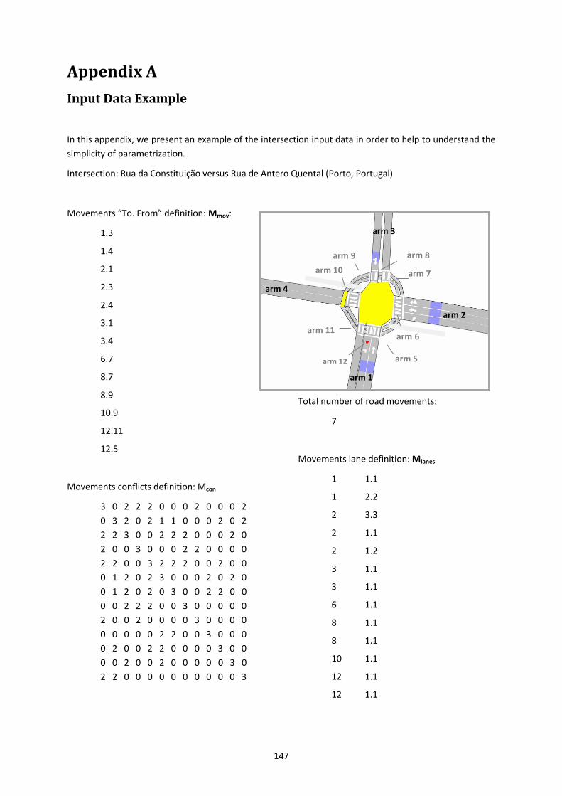
147
Appendix A
Input Data Example
In this appendix, we present an example of the intersection input data in order to help to understand the
simplicity of parametrization.
Intersection: Rua da Constituição versus Rua de Antero Quental (Porto, Portugal)
Movements “To. From” definition: Mmov:
1.3
1.4
2.1
2.3
2.4
3.1
3.4
6.7
8.7
8.9
10.9
12.11
12.5
Movements conflicts definition: Mcon
3 0 2 2 2 0 0 0 2 0 0 0 2
0 3 2 0 2 1 1 0 0 0 2 0 2
2 2 3 0 0 2 2 2 0 0 0 2 0
2 0 0 3 0 0 0 2 2 0 0 0 0
2 2 0 0 3 2 2 2 0 0 2 0 0
0 1 2 0 2 3 0 0 0 2 0 2 0
0 1 2 0 2 0 3 0 0 2 2 0 0
0 0 2 2 2 0 0 3 0 0 0 0 0
2 0 0 2 0 0 0 0 3 0 0 0 0
0 0 0 0 0 2 2 0 0 3 0 0 0
0 2 0 0 2 2 0 0 0 0 3 0 0
0 0 2 0 0 2 0 0 0 0 0 3 0
2 2 0 0 0 0 0 0 0 0 0 0 3
Total number of road movements:
7
Movements lane definition: Mlanes
1 1.1
1 2.2
2 3.3
2 1.1
2 1.2
3 1.1
3 1.1
6 1.1
8 1.1
8 1.1
10 1.1
12 1.1
12 1.1
arm 1
arm 4
arm 5
arm 11
arm 12
arm 10
arm 2
arm 3
arm 7
arm 8 arm 9
arm 6
arm 5
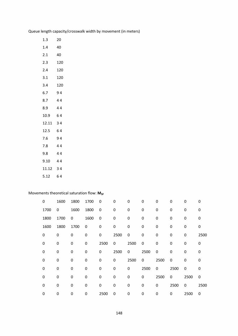
148
Queue length capacity/crosswalk width by movement (in meters)
1.3 20
1.4 40
2.1 40
2.3 120
2.4 120
3.1 120
3.4 120
6.7 9 4
8.7 4 4
8.9 4 4
10.9 6 4
12.11 3 4
12.5 6 4
7.6 9 4
7.8 4 4
9.8 4 4
9.10 4 4
11.12 3 4
5.12 6 4
Movements theoretical saturation flow: MSF
0 1600 1800 1700 0 0 0 0 0 0 0 0
1700 0 1600 1800 0 0 0 0 0 0 0 0
1800 1700 0 1600 0 0 0 0 0 0 0 0
1600 1800 1700 0 0 0 0 0 0 0 0 0
0 0 0 0 0 2500 0 0 0 0 0 2500
0 0 0 0 2500 0 2500 0 0 0 0 0
0 0 0 0 0 2500 0 2500 0 0 0 0
0 0 0 0 0 0 2500 0 2500 0 0 0
0 0 0 0 0 0 0 2500 0 2500 0 0
0 0 0 0 0 0 0 0 2500 0 2500 0
0 0 0 0 0 0 0 0 0 2500 0 2500
0 0 0 0 2500 0 0 0 0 0 2500 0
149
Appendix B
Results by Simulation Run
In section 4.4, the results are available for all simulation period. In this appendix, we present some
additional results that have been referred during this research work, here the results of average travel
time are available for each simulation run and time interval. This presentation gives the possibility to
observe the metric evolution along time and the variability between the twenty-five simulation runs.
Each scenario between A to G has five plots. Each plot is about a traffic signal control approach, where the
first two are the proposed strategies and the follow three plots are baseline approaches (details in section
4.3). They are listed as below:
a) No Plan
b) Plan
c) Baseline 1
d) Baseline 2
e) Baseline 3
In the following plots, each green line is a simulation run and it shows the evolution of the average travel
time (left y-axe) of traffic users (includes vehicles and pedestrians) across simulation time, each time
interval has two-minutes and thirty-seconds. The black line represents the total cumulative number of
traffic users (includes vehicles and pedestrians) that have exited the intersection(s) (right y-axe), in each
time interval. The black line helps to compare if the traffic signal control approach served the same
amount of traffic demand than others.
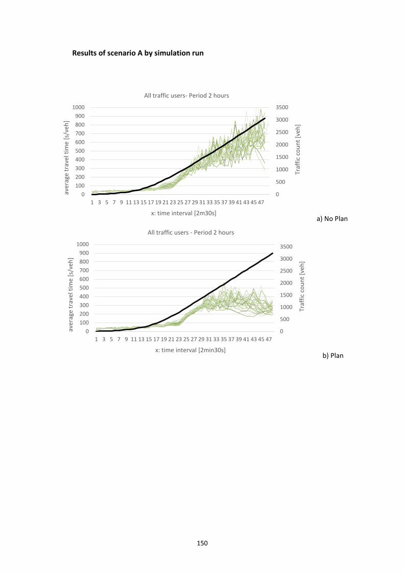
150
Results of scenario A by simulation run
a) No Plan
b) Plan
0
500
1000
1500
2000
2500
3000
3500
0
100
200
300
400
500
600
700
800
900
1000
1 3 5 7 9 11 13 15 17 19 21 23 25 27 29 31 33 35 37 39 41 43 45 47
Traf
fic
cou
nt
[veh
]
aver
age
trav
el t
ime
[s/v
eh]
x: time interval [2m30s]
All traffic users- Period 2 hours
0
500
1000
1500
2000
2500
3000
3500
0
100
200
300
400
500
600
700
800
900
1000
1 3 5 7 9 11 13 15 17 19 21 23 25 27 29 31 33 35 37 39 41 43 45 47
Traf
fic
cou
nt
[veh
]
aver
age
trav
el t
ime
[s/v
eh]
x: time interval [2min30s]
All traffic users - Period 2 hours
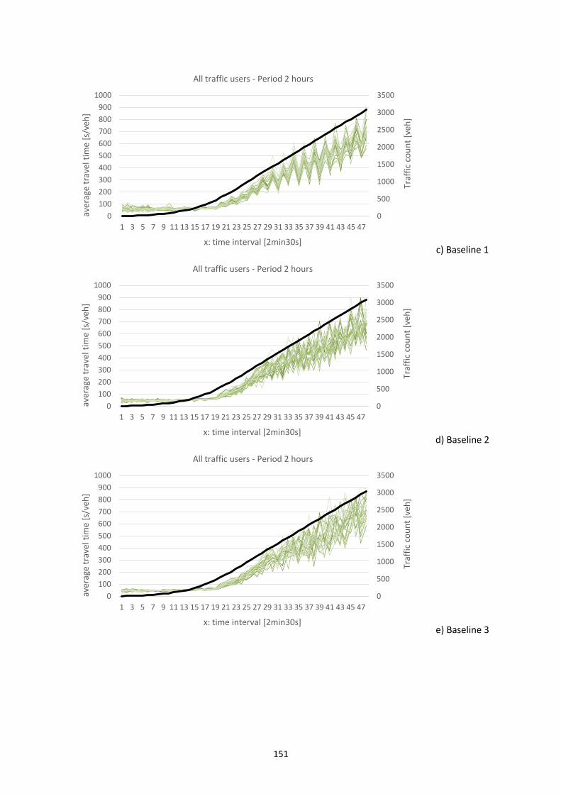
151
c) Baseline 1
d) Baseline 2
e) Baseline 3
0
500
1000
1500
2000
2500
3000
3500
0
100
200
300
400
500
600
700
800
900
1000
1 3 5 7 9 11 13 15 17 19 21 23 25 27 29 31 33 35 37 39 41 43 45 47
Traf
fic
cou
nt
[veh
]
aver
age
trav
el t
ime
[s/v
eh]
x: time interval [2min30s]
All traffic users - Period 2 hours
0
500
1000
1500
2000
2500
3000
3500
0
100
200
300
400
500
600
700
800
900
1000
1 3 5 7 9 11 13 15 17 19 21 23 25 27 29 31 33 35 37 39 41 43 45 47
Traf
fic
cou
nt
[veh
]
aver
age
trav
el t
ime
[s/v
eh]
x: time interval [2min30s]
All traffic users - Period 2 hours
0
500
1000
1500
2000
2500
3000
3500
0
100
200
300
400
500
600
700
800
900
1000
1 3 5 7 9 11 13 15 17 19 21 23 25 27 29 31 33 35 37 39 41 43 45 47
Traf
fic
cou
nt
[veh
]
aver
age
trav
el t
ime
[s/v
eh]
x: time interval [2min30s]
All traffic users - Period 2 hours
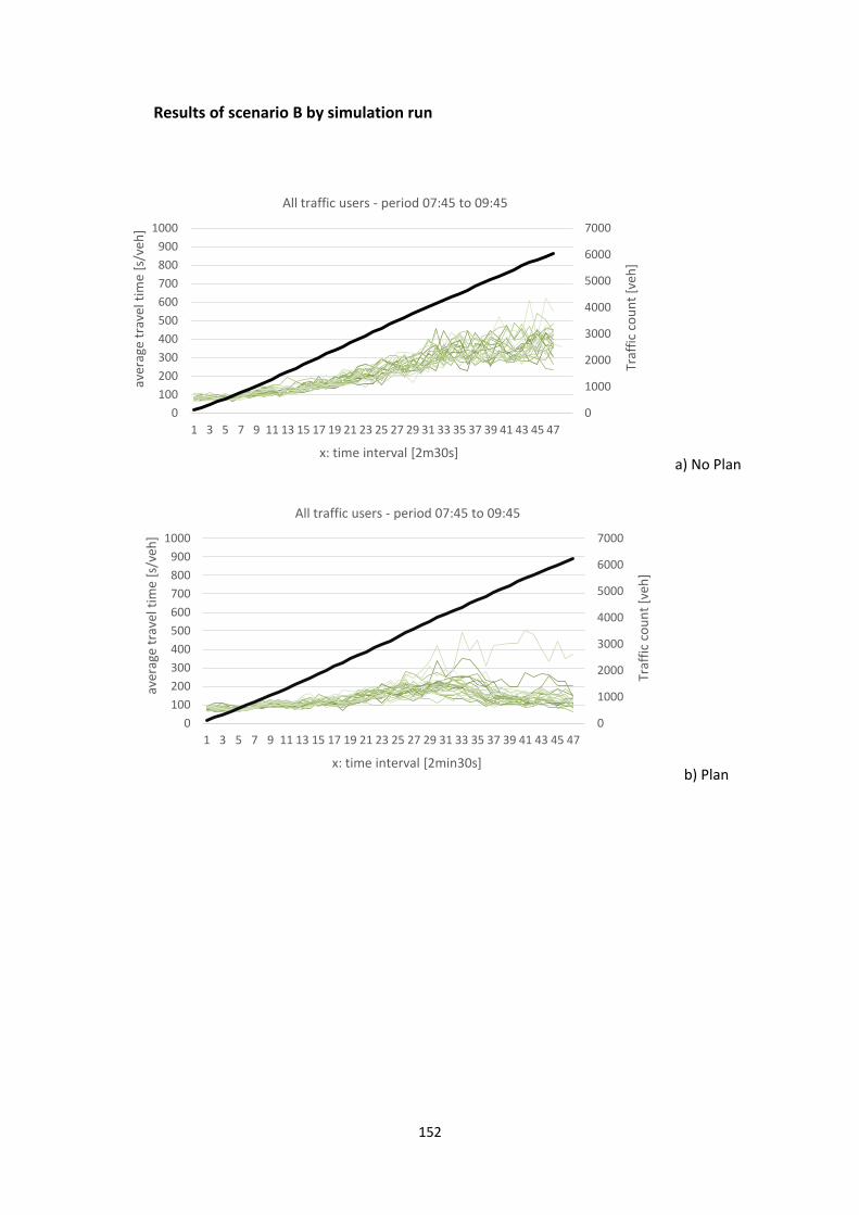
152
Results of scenario B by simulation run
a) No Plan
b) Plan
0
1000
2000
3000
4000
5000
6000
7000
0
100
200
300
400
500
600
700
800
900
1000
1 3 5 7 9 11 13 15 17 19 21 23 25 27 29 31 33 35 37 39 41 43 45 47
Traf
fic
cou
nt
[veh
]
aver
age
trav
el t
ime
[s/v
eh]
x: time interval [2m30s]
All traffic users - period 07:45 to 09:45
0
1000
2000
3000
4000
5000
6000
7000
0
100
200
300
400
500
600
700
800
900
1000
1 3 5 7 9 11 13 15 17 19 21 23 25 27 29 31 33 35 37 39 41 43 45 47
Traf
fic
cou
nt
[veh
]
aver
age
trav
el t
ime
[s/v
eh]
x: time interval [2min30s]
All traffic users - period 07:45 to 09:45
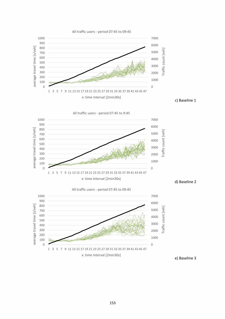
153
c) Baseline 1
d) Baseline 2
e) Baseline 3
0
1000
2000
3000
4000
5000
6000
7000
0
100
200
300
400
500
600
700
800
900
1000
1 3 5 7 9 11 13 15 17 19 21 23 25 27 29 31 33 35 37 39 41 43 45 47
Traf
fic
cou
nt
[veh
]
aver
age
trav
el t
ime
[s/v
eh]
x: time interval [2min30s]
All traffic users - period 07:45 to 09:45
0
1000
2000
3000
4000
5000
6000
7000
0
100
200
300
400
500
600
700
800
900
1000
1 3 5 7 9 11 13 15 17 19 21 23 25 27 29 31 33 35 37 39 41 43 45 47
Traf
fic
cou
nt
[veh
]
aver
age
trav
el t
ime
[s/v
eh]
x: time interval [2min30s]
All traffic users - period 07:45 to 9:45
0
1000
2000
3000
4000
5000
6000
7000
0
100
200
300
400
500
600
700
800
900
1000
1 3 5 7 9 11 13 15 17 19 21 23 25 27 29 31 33 35 37 39 41 43 45 47
Traf
fic
cou
nt
[veh
]
aver
age
trav
el t
ime
[s/v
eh]
x: time interval [2min30s]
All traffic users - period 07:45 to 09:45
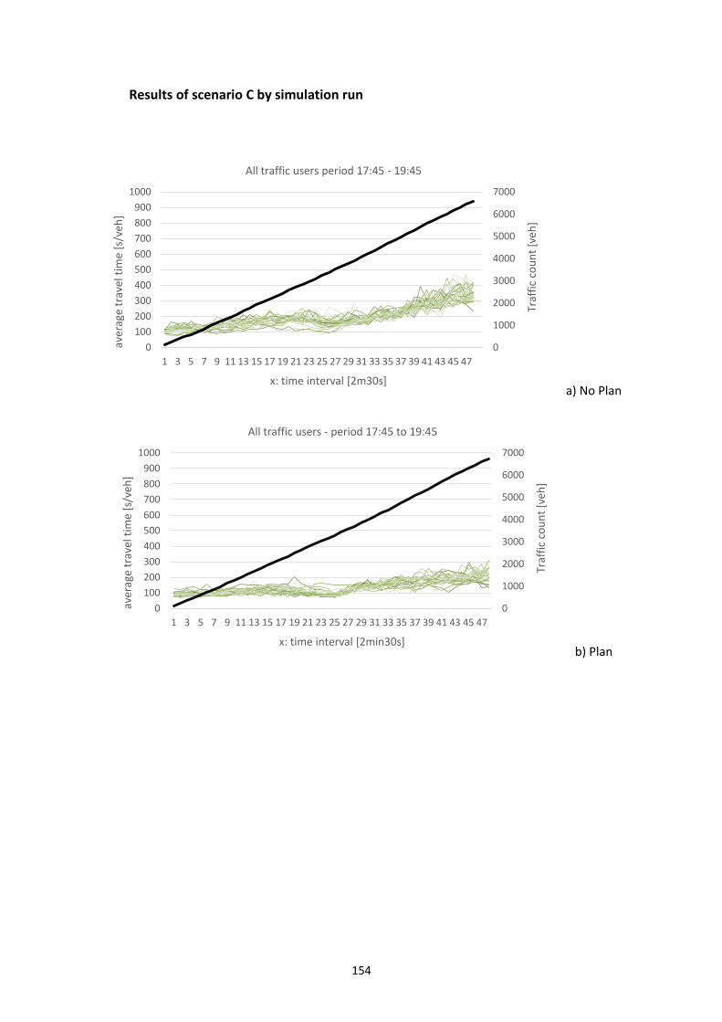
154
Results of scenario C by simulation run
a) No Plan
b) Plan
0
1000
2000
3000
4000
5000
6000
7000
0
100
200
300
400
500
600
700
800
900
1000
1 3 5 7 9 11 13 15 17 19 21 23 25 27 29 31 33 35 37 39 41 43 45 47
Traf
fic
cou
nt
[veh
]
aver
age
trav
el t
ime
[s/v
eh]
x: time interval [2m30s]
All traffic users period 17:45 - 19:45
0
1000
2000
3000
4000
5000
6000
7000
0
100
200
300
400
500
600
700
800
900
1000
1 3 5 7 9 11 13 15 17 19 21 23 25 27 29 31 33 35 37 39 41 43 45 47
Traf
fic
cou
nt
[veh
]
aver
age
trav
el t
ime
[s/v
eh]
x: time interval [2min30s]
All traffic users - period 17:45 to 19:45
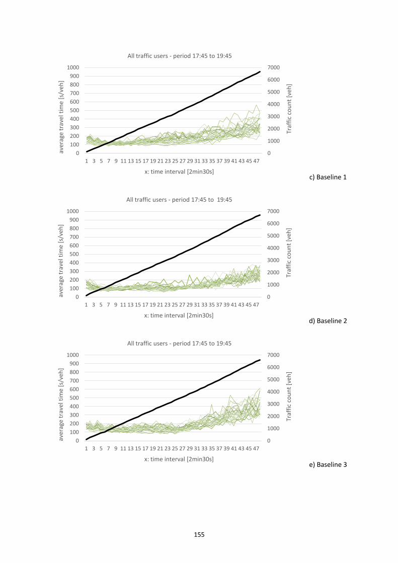
155
c) Baseline 1
d) Baseline 2
e) Baseline 3
0
1000
2000
3000
4000
5000
6000
7000
0
100
200
300
400
500
600
700
800
900
1000
1 3 5 7 9 11 13 15 17 19 21 23 25 27 29 31 33 35 37 39 41 43 45 47
Traf
fic
cou
nt
[veh
]
aver
age
trav
el t
ime
[s/v
eh]
x: time interval [2min30s]
All traffic users - period 17:45 to 19:45
0
1000
2000
3000
4000
5000
6000
7000
0
100
200
300
400
500
600
700
800
900
1000
1 3 5 7 9 11 13 15 17 19 21 23 25 27 29 31 33 35 37 39 41 43 45 47
Traf
fic
cou
nt
[veh
]
aver
age
trav
el t
ime
[s/v
eh]
x: time interval [2min30s]
All traffic users - period 17:45 to 19:45
0
1000
2000
3000
4000
5000
6000
7000
0
100
200
300
400
500
600
700
800
900
1000
1 3 5 7 9 11 13 15 17 19 21 23 25 27 29 31 33 35 37 39 41 43 45 47
Traf
fic
cou
nt
[veh
]
aver
age
trav
el t
ime
[s/v
eh]
x: time interval [2min30s]
All traffic users - period 17:45 to 19:45
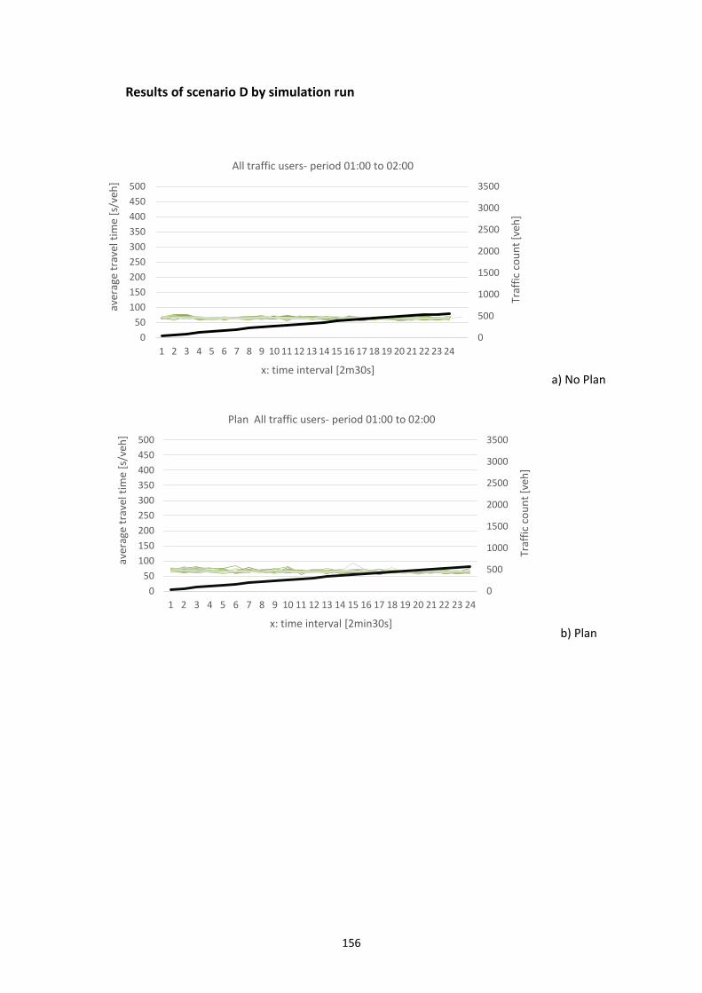
156
Results of scenario D by simulation run
a) No Plan
b) Plan
0
500
1000
1500
2000
2500
3000
3500
0
50
100
150
200
250
300
350
400
450
500
1 2 3 4 5 6 7 8 9 10 11 12 13 14 15 16 17 18 19 20 21 22 23 24
Traf
fic
cou
nt
[veh
]
aver
age
trav
el t
ime
[s/v
eh]
x: time interval [2m30s]
All traffic users- period 01:00 to 02:00
0
500
1000
1500
2000
2500
3000
3500
0
50
100
150
200
250
300
350
400
450
500
1 2 3 4 5 6 7 8 9 10 11 12 13 14 15 16 17 18 19 20 21 22 23 24
Traf
fic
cou
nt
[veh
]
aver
age
trav
el t
ime
[s/v
eh]
x: time interval [2min30s]
Plan All traffic users- period 01:00 to 02:00
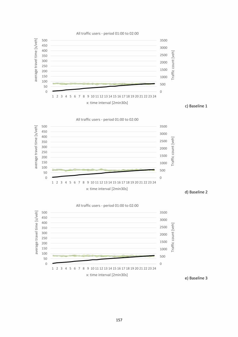
157
c) Baseline 1
d) Baseline 2
e) Baseline 3
0
500
1000
1500
2000
2500
3000
3500
0
50
100
150
200
250
300
350
400
450
500
1 2 3 4 5 6 7 8 9 10 11 12 13 14 15 16 17 18 19 20 21 22 23 24
Traf
fic
cou
nt
[veh
]
aver
age
trav
el t
ime
[s/v
eh]
x: time interval [2min30s]
All traffic users - period 01:00 to 02:00
0
500
1000
1500
2000
2500
3000
3500
0
50
100
150
200
250
300
350
400
450
500
1 2 3 4 5 6 7 8 9 10 11 12 13 14 15 16 17 18 19 20 21 22 23 24
Traf
fic
cou
nt
[veh
]
aver
age
trav
el t
ime
[s/v
eh]
x: time interval [2min30s]
All traffic users - period 01:00 to 02:00
0
500
1000
1500
2000
2500
3000
3500
0
50
100
150
200
250
300
350
400
450
500
1 2 3 4 5 6 7 8 9 10 11 12 13 14 15 16 17 18 19 20 21 22 23 24
Traf
fic
cou
nt
[veh
]
aver
age
trav
el t
ime
[s/v
eh]
x: time interval [2min30s]
All traffic users - period 01:00 to 02:00
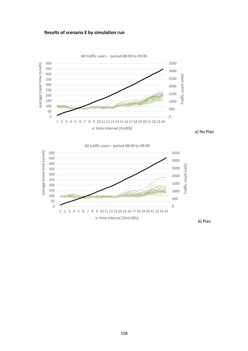
158
Results of scenario E by simulation run
a) No Plan
b) Plan
0
500
1000
1500
2000
2500
3000
3500
0
50
100
150
200
250
300
350
400
450
500
1 2 3 4 5 6 7 8 9 10 11 12 13 14 15 16 17 18 19 20 21 22 23 24
Traf
fic
cou
nt
[veh
]
aver
age
trav
el t
ime
[s/v
eh]
x: time interval [2m30s]
All traffic users - period 08:00 to 09:00
0
500
1000
1500
2000
2500
3000
3500
0
50
100
150
200
250
300
350
400
450
500
1 2 3 4 5 6 7 8 9 10 11 12 13 14 15 16 17 18 19 20 21 22 23 24
Traf
fic
cou
nt
[veh
]
aver
age
trav
el t
ime
[s/v
eh]
x: time interval [2min30s]
All traffic users - period 08:00 to 09:00
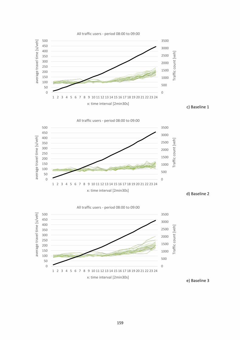
159
c) Baseline 1
d) Baseline 2
e) Baseline 3
0
500
1000
1500
2000
2500
3000
3500
0
50
100
150
200
250
300
350
400
450
500
1 2 3 4 5 6 7 8 9 10 11 12 13 14 15 16 17 18 19 20 21 22 23 24
Traf
fic
cou
nt
[veh
]
aver
age
trav
el t
ime
[s/v
eh]
x: time interval [2min30s]
All traffic users - period 08:00 to 09:00
0
500
1000
1500
2000
2500
3000
3500
0
50
100
150
200
250
300
350
400
450
500
1 2 3 4 5 6 7 8 9 10 11 12 13 14 15 16 17 18 19 20 21 22 23 24
Traf
fic
cou
nt
[veh
]
aver
age
trav
el t
ime
[s/v
eh]
x: time interval [2min30s]
All traffic users - period 08:00 to 09:00
0
500
1000
1500
2000
2500
3000
3500
0
50
100
150
200
250
300
350
400
450
500
1 2 3 4 5 6 7 8 9 10 11 12 13 14 15 16 17 18 19 20 21 22 23 24
Traf
fic
cou
nt
[veh
]
aver
age
trav
el t
ime
[s/v
eh]
x: time interval [2min30s]
All traffic users - period 08:00 to 09:00
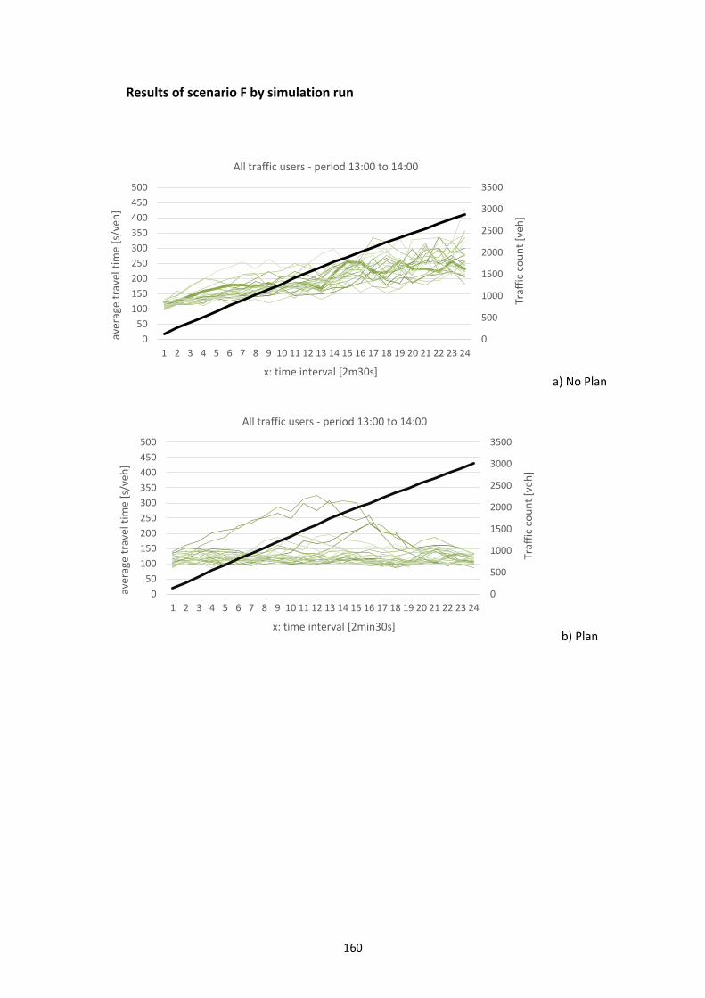
160
Results of scenario F by simulation run
a) No Plan
b) Plan
0
500
1000
1500
2000
2500
3000
3500
0
50
100
150
200
250
300
350
400
450
500
1 2 3 4 5 6 7 8 9 10 11 12 13 14 15 16 17 18 19 20 21 22 23 24
Traf
fic
cou
nt
[veh
]
aver
age
trav
el t
ime
[s/v
eh]
x: time interval [2m30s]
All traffic users - period 13:00 to 14:00
0
500
1000
1500
2000
2500
3000
3500
0
50
100
150
200
250
300
350
400
450
500
1 2 3 4 5 6 7 8 9 10 11 12 13 14 15 16 17 18 19 20 21 22 23 24
Traf
fic
cou
nt
[veh
]
aver
age
trav
el t
ime
[s/v
eh]
x: time interval [2min30s]
All traffic users - period 13:00 to 14:00
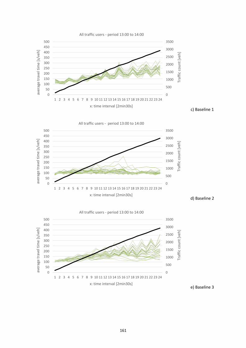
161
c) Baseline 1
d) Baseline 2
e) Baseline 3
0
500
1000
1500
2000
2500
3000
3500
0
50
100
150
200
250
300
350
400
450
500
1 2 3 4 5 6 7 8 9 10 11 12 13 14 15 16 17 18 19 20 21 22 23 24
Traf
fic
cou
nt
[veh
]
aver
age
trav
el t
ime
[s/v
eh]
x: time interval [2min30s]
All traffic users - period 13:00 to 14:00
0
500
1000
1500
2000
2500
3000
3500
0
50
100
150
200
250
300
350
400
450
500
1 2 3 4 5 6 7 8 9 10 11 12 13 14 15 16 17 18 19 20 21 22 23 24
Traf
fic
cou
nt
[veh
]
aver
age
trav
el t
ime
[s/v
eh]
x: time interval [2min30s]
All traffic users - period 13:00 to 14:00
0
500
1000
1500
2000
2500
3000
3500
0
50
100
150
200
250
300
350
400
450
500
1 2 3 4 5 6 7 8 9 10 11 12 13 14 15 16 17 18 19 20 21 22 23 24
Traf
fic
cou
nt
[veh
]
aver
age
trav
el t
ime
[s/v
eh]
x: time interval [2min30s]
All traffic users - period 13:00 to 14:00
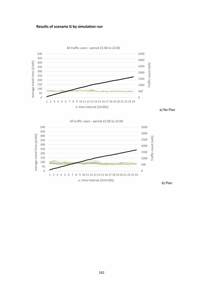
162
Results of scenario G by simulation run
a) No Plan
b) Plan
0
500
1000
1500
2000
2500
3000
3500
0
50
100
150
200
250
300
350
400
450
500
1 2 3 4 5 6 7 8 9 10 11 12 13 14 15 16 17 18 19 20 21 22 23 24
Traf
fic
cou
nt
[veh
]
aver
age
trav
el t
ime
[s/v
eh]
x: time interval [2m30s]
All traffic users - period 21:00 to 22:00
0
500
1000
1500
2000
2500
3000
3500
0
50
100
150
200
250
300
350
400
450
500
1 2 3 4 5 6 7 8 9 10 11 12 13 14 15 16 17 18 19 20 21 22 23 24
Traf
fic
cou
nt
[veh
]
aver
age
trav
el t
ime
[s/v
eh]
x: time interval [2min30s]
All traffic users - period 21:00 to 22:00
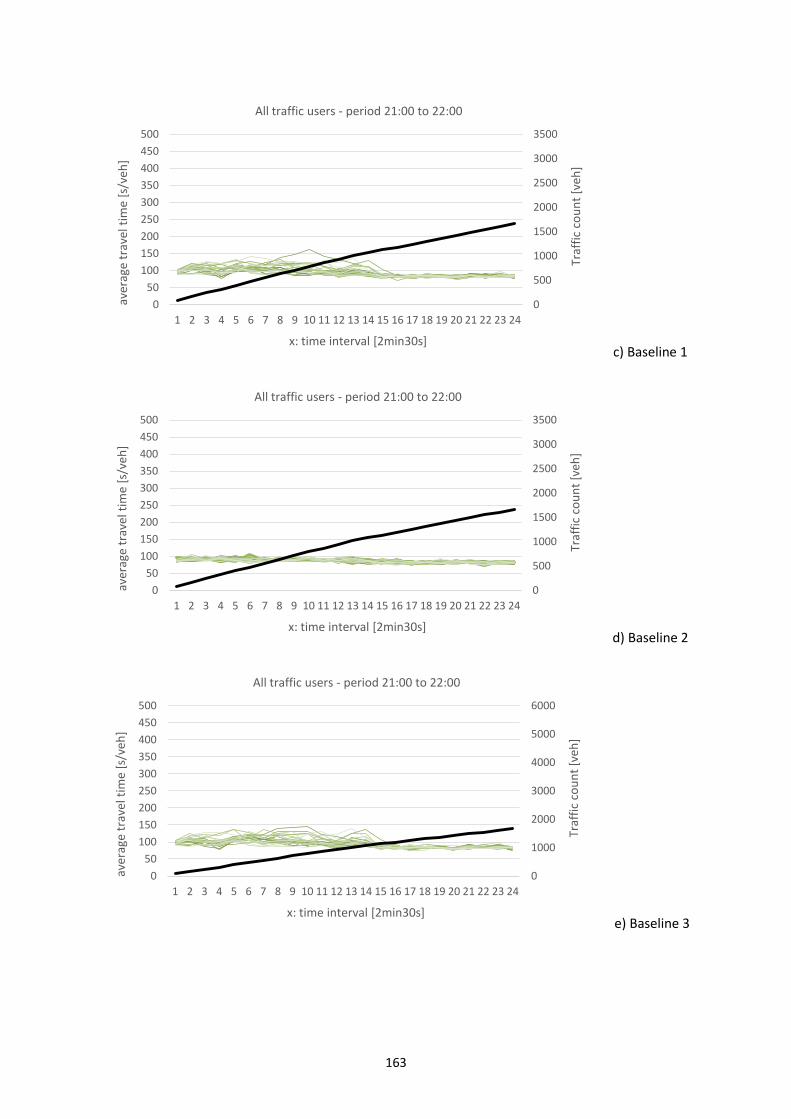
163
c) Baseline 1
d) Baseline 2
e) Baseline 3
0
500
1000
1500
2000
2500
3000
3500
0
50
100
150
200
250
300
350
400
450
500
1 2 3 4 5 6 7 8 9 10 11 12 13 14 15 16 17 18 19 20 21 22 23 24
Traf
fic
cou
nt
[veh
]
aver
age
trav
el t
ime
[s/v
eh]
x: time interval [2min30s]
All traffic users - period 21:00 to 22:00
0
500
1000
1500
2000
2500
3000
3500
0
50
100
150
200
250
300
350
400
450
500
1 2 3 4 5 6 7 8 9 10 11 12 13 14 15 16 17 18 19 20 21 22 23 24
Traf
fic
cou
nt
[veh
]
aver
age
trav
el t
ime
[s/v
eh]
x: time interval [2min30s]
All traffic users - period 21:00 to 22:00
0
1000
2000
3000
4000
5000
6000
0
50
100
150
200
250
300
350
400
450
500
1 2 3 4 5 6 7 8 9 10 11 12 13 14 15 16 17 18 19 20 21 22 23 24
Traf
fic
cou
nt
[veh
]
aver
age
trav
el t
ime
[s/v
eh]
x: time interval [2min30s]
All traffic users - period 21:00 to 22:00

164
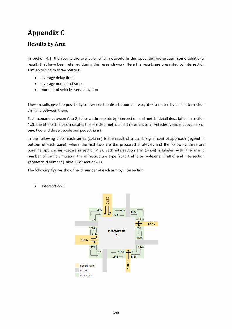
165
Appendix C
Results by Arm
In section 4.4, the results are available for all network. In this appendix, we present some additional
results that have been referred during this research work. Here the results are presented by intersection
arm according to three metrics:
average delay time;
average number of stops
number of vehicles served by arm
These results give the possibility to observe the distribution and weight of a metric by each intersection
arm and between them.
Each scenario between A to G, it has at three plots by intersection and metric (detail description in section
4.2), the title of the plot indicates the selected metric and it referrers to all vehicles (vehicle occupancy of
one, two and three people and pedestrians).
In the following plots, each series (column) is the result of a traffic signal control approach (legend in
bottom of each page), where the first two are the proposed strategies and the following three are
baseline approaches (details in section 4.3). Each intersection arm (x-axe) is labeled with: the arm id
number of traffic simulator, the infrastructure type (road traffic or pedestrian traffic) and intersection
geometry id number (Table 15 of section4.1).
The following figures show the id number of each arm by intersection.
Intersection 1
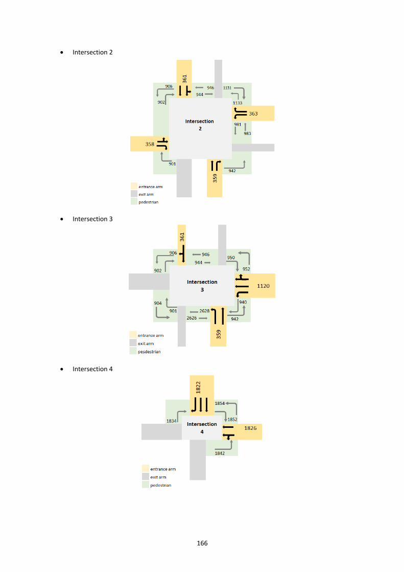
166
Intersection 2
Intersection 3
Intersection 4
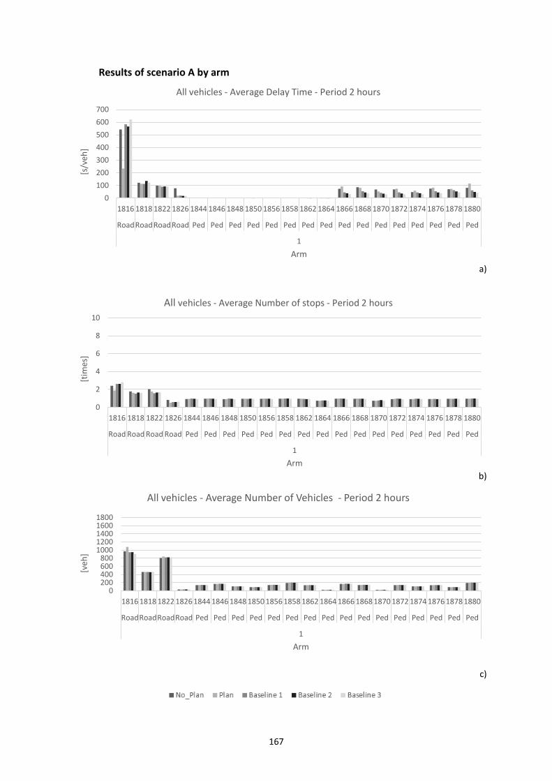
167
Results of scenario A by arm
a)
b)
c)
0
100
200
300
400
500
600
700
1816 1818 1822 1826 1844 1846 1848 1850 1856 1858 1862 1864 1866 1868 1870 1872 1874 1876 1878 1880
Road Road Road Road Ped Ped Ped Ped Ped Ped Ped Ped Ped Ped Ped Ped Ped Ped Ped Ped
1
[s/v
eh]
Arm
All vehicles - Average Delay Time - Period 2 hours
0
2
4
6
8
10
1816 1818 1822 1826 1844 1846 1848 1850 1856 1858 1862 1864 1866 1868 1870 1872 1874 1876 1878 1880
Road Road Road Road Ped Ped Ped Ped Ped Ped Ped Ped Ped Ped Ped Ped Ped Ped Ped Ped
1
[tim
es]
Arm
All vehicles - Average Number of stops - Period 2 hours
0 200 400 600 800
1000 1200 1400 1600 1800
1816 1818 1822 1826 1844 1846 1848 1850 1856 1858 1862 1864 1866 1868 1870 1872 1874 1876 1878 1880
Road Road Road Road Ped Ped Ped Ped Ped Ped Ped Ped Ped Ped Ped Ped Ped Ped Ped Ped
1
[veh
]
Arm
All vehicles - Average Number of Vehicles - Period 2 hours
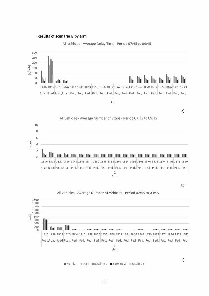
168
Results of scenario B by arm
a)
b)
c)
0
50
100
150
200
250
300
1816 1818 1822 1826 1844 1846 1848 1850 1856 1858 1862 1864 1866 1868 1870 1872 1874 1876 1878 1880
Road, 1
Road, 1
Road, 1
Road, 1
Ped, 1
Ped, 1
Ped, 1
Ped, 1
Ped, 1
Ped, 1
Ped, 1
Ped, 1
Ped, 1
Ped, 1
Ped, 1
Ped, 1
Ped, 1
Ped, 1
Ped, 1
Ped, 1
[s/v
eh]
Arm
All vehicles - Average Delay Time - Period 07:45 to 09:45
0
2
4
6
8
10
1816 1818 1822 1826 1844 1846 1848 1850 1856 1858 1862 1864 1866 1868 1870 1872 1874 1876 1878 1880
Road, 1
Road, 1
Road, 1
Road, 1
Ped, 1
Ped, 1
Ped, 1
Ped, 1
Ped, 1
Ped, 1
Ped, 1
Ped, 1
Ped, 1
Ped, 1
Ped, 1
Ped, 1
Ped, 1
Ped, 1
Ped, 1
Ped, 1
[tim
es]
Arm
All vehicles - Average Number of Stops - Period 07:45 to 09:45
0 200 400 600 800
1000 1200 1400 1600 1800
1816 1818 1822 1826 1844 1846 1848 1850 1856 1858 1862 1864 1866 1868 1870 1872 1874 1876 1878 1880
Road, 1
Road, 1
Road, 1
Road, 1
Ped, 1
Ped, 1
Ped, 1
Ped, 1
Ped, 1
Ped, 1
Ped, 1
Ped, 1
Ped, 1
Ped, 1
Ped, 1
Ped, 1
Ped, 1
Ped, 1
Ped, 1
Ped, 1
[veh
]
Arm
All vehicles - Average Number of Vehicles - Period 07:45 to 09:45
1
1
1
1
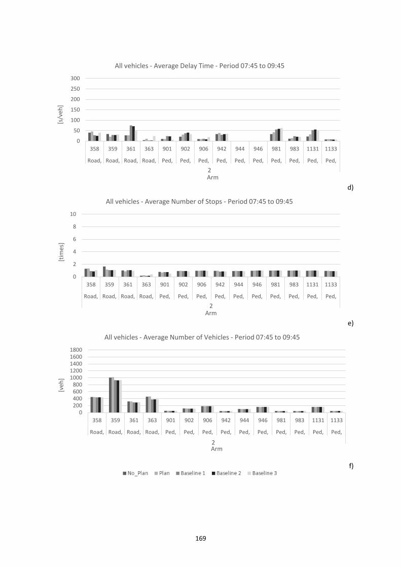
169
d)
e)
f)
0
50
100
150
200
250
300
358 359 361 363 901 902 906 942 944 946 981 983 1131 1133
Road, 2
Road, 2
Road, 2
Road, 2
Ped, 2
Ped, 2
Ped, 2
Ped, 2
Ped, 2
Ped, 2
Ped, 2
Ped, 2
Ped, 2
Ped, 2
[s/v
eh]
Arm
All vehicles - Average Delay Time - Period 07:45 to 09:45
0
2
4
6
8
10
358 359 361 363 901 902 906 942 944 946 981 983 1131 1133
Road, 2
Road, 2
Road, 2
Road, 2
Ped, 2
Ped, 2
Ped, 2
Ped, 2
Ped, 2
Ped, 2
Ped, 2
Ped, 2
Ped, 2
Ped, 2
[tim
es]
Arm
All vehicles - Average Number of Stops - Period 07:45 to 09:45
0 200 400 600 800
1000 1200 1400 1600 1800
358 359 361 363 901 902 906 942 944 946 981 983 1131 1133
Road, 2
Road, 2
Road, 2
Road, 2
Ped, 2
Ped, 2
Ped, 2
Ped, 2
Ped, 2
Ped, 2
Ped, 2
Ped, 2
Ped, 2
Ped, 2
[veh
]
Arm
All vehicles - Average Number of Vehicles - Period 07:45 to 09:45
2 2
2
2
2
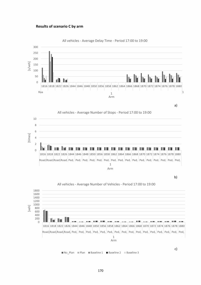
170
Results of scenario C by arm
a)
b)
c)
0
50
100
150
200
250
300
1816 1818 1822 1826 1844 1846 1848 1850 1856 1858 1862 1864 1866 1868 1870 1872 1874 1876 1878 1880
Road, 1 Road, 1 Road, 1 Road, 1 Ped, 1 Ped, 1 Ped, 1 Ped, 1 Ped, 1 Ped, 1 Ped, 1 Ped, 1 Ped, 1 Ped, 1 Ped, 1 Ped, 1 Ped, 1 Ped, 1 Ped, 1 Ped, 1
[s/v
eh]
Arm
All vehicles - Average Delay Time - Period 17:00 to 19:00
0
2
4
6
8
10
1816 1818 1822 1826 1844 1846 1848 1850 1856 1858 1862 1864 1866 1868 1870 1872 1874 1876 1878 1880
Road, 1
Road, 1
Road, 1
Road, 1
Ped, 1
Ped, 1
Ped, 1
Ped, 1
Ped, 1
Ped, 1
Ped, 1
Ped, 1
Ped, 1
Ped, 1
Ped, 1
Ped, 1
Ped, 1
Ped, 1
Ped, 1
Ped, 1
[tim
es]
Arm
All vehicles - Average Number of Stops - Period 17:00 to 19:00
0 200 400 600 800
1000 1200 1400 1600 1800
1816 1818 1822 1826 1844 1846 1848 1850 1856 1858 1862 1864 1866 1868 1870 1872 1874 1876 1878 1880
Road, 1
Road, 1
Road, 1
Road, 1
Ped, 1
Ped, 1
Ped, 1
Ped, 1
Ped, 1
Ped, 1
Ped, 1
Ped, 1
Ped, 1
Ped, 1
Ped, 1
Ped, 1
Ped, 1
Ped, 1
Ped, 1
Ped, 1
[veh
]
Arm
All vehicles - Average Number of Vehicles - Period 17:00 to 19:00
1
1
1
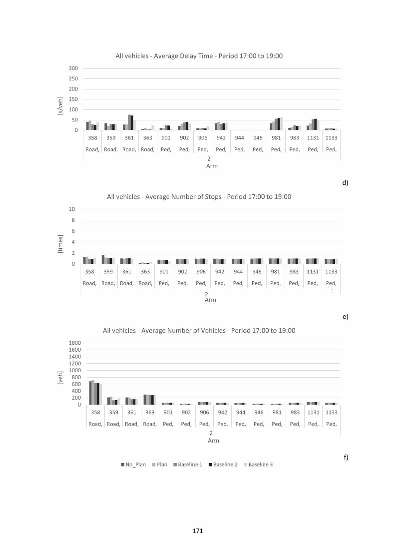
171
d)
e)
f)
0
50
100
150
200
250
300
358 359 361 363 901 902 906 942 944 946 981 983 1131 1133
Road, 2
Road, 2
Road, 2
Road, 2
Ped, 2
Ped, 2
Ped, 2
Ped, 2
Ped, 2
Ped, 2
Ped, 2
Ped, 2
Ped, 2
Ped, 2
[s/v
eh]
Arm
All vehicles - Average Delay Time - Period 17:00 to 19:00
0
2
4
6
8
10
358 359 361 363 901 902 906 942 944 946 981 983 1131 1133
Road, 2
Road, 2
Road, 2
Road, 2
Ped, 2
Ped, 2
Ped, 2
Ped, 2
Ped, 2
Ped, 2
Ped, 2
Ped, 2
Ped, 2
Ped, 2
[tim
es]
Arm
All vehicles - Average Number of Stops - Period 17:00 to 19:00
0 200 400 600 800
1000 1200 1400 1600 1800
358 359 361 363 901 902 906 942 944 946 981 983 1131 1133
Road, 2
Road, 2
Road, 2
Road, 2
Ped, 2
Ped, 2
Ped, 2
Ped, 2
Ped, 2
Ped, 2
Ped, 2
Ped, 2
Ped, 2
Ped, 2
[veh
]
Arm
All vehicles - Average Number of Vehicles - Period 17:00 to 19:00
2
2 2
2
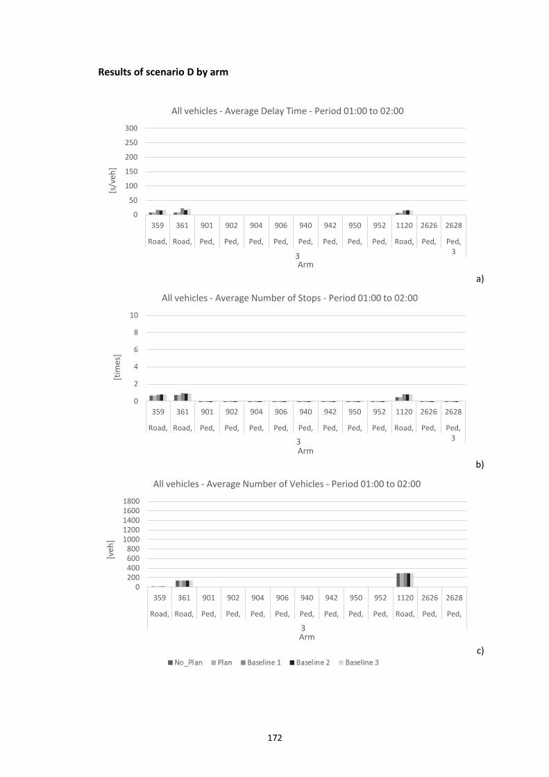
172
Results of scenario D by arm
a)
b)
c)
0
50
100
150
200
250
300
359 361 901 902 904 906 940 942 950 952 1120 2626 2628
Road, 3
Road, 3
Ped, 3
Ped, 3
Ped, 3
Ped, 3
Ped, 3
Ped, 3
Ped, 3
Ped, 3
Road, 3
Ped, 3
Ped, 3
[s/v
eh]
Arm
All vehicles - Average Delay Time - Period 01:00 to 02:00
0
2
4
6
8
10
359 361 901 902 904 906 940 942 950 952 1120 2626 2628
Road, 3
Road, 3
Ped, 3
Ped, 3
Ped, 3
Ped, 3
Ped, 3
Ped, 3
Ped, 3
Ped, 3
Road, 3
Ped, 3
Ped, 3
[tim
es]
Arm
All vehicles - Average Number of Stops - Period 01:00 to 02:00
0 200 400 600 800
1000 1200 1400 1600 1800
359 361 901 902 904 906 940 942 950 952 1120 2626 2628
Road, 3
Road, 3
Ped, 3
Ped, 3
Ped, 3
Ped, 3
Ped, 3
Ped, 3
Ped, 3
Ped, 3
Road, 3
Ped, 3
Ped, 3
[veh
]
Arm
All vehicles - Average Number of Vehicles - Period 01:00 to 02:00
3
3
3

173
d)
e)
f)
0
50
100
150
200
250
300
1822 1826 1834 1842 1852 1854
Road, 4 Road, 4 Ped, 4 Ped, 4 Ped, 4 Ped, 4
[s/v
eh]
Arm
All vehicles - Average Delay Time - Period 01:00 to 02:00
0
2
4
6
8
10
1822 1826 1834 1842 1852 1854
Road, 4 Road, 4 Ped, 4 Ped, 4 Ped, 4 Ped, 4
[tim
es]
Arm
All vehicles - Average Number of Stops - Period 01:00 to 02:00
0 200 400 600 800
1000 1200 1400 1600 1800
1822 1826 1834 1842 1852 1854
Road, 4 Road, 4 Ped, 4 Ped, 4 Ped, 4 Ped, 4
[veh
]
Arm
All vehicles - Average Number of Vehicles - Period 01:00 to 02:00
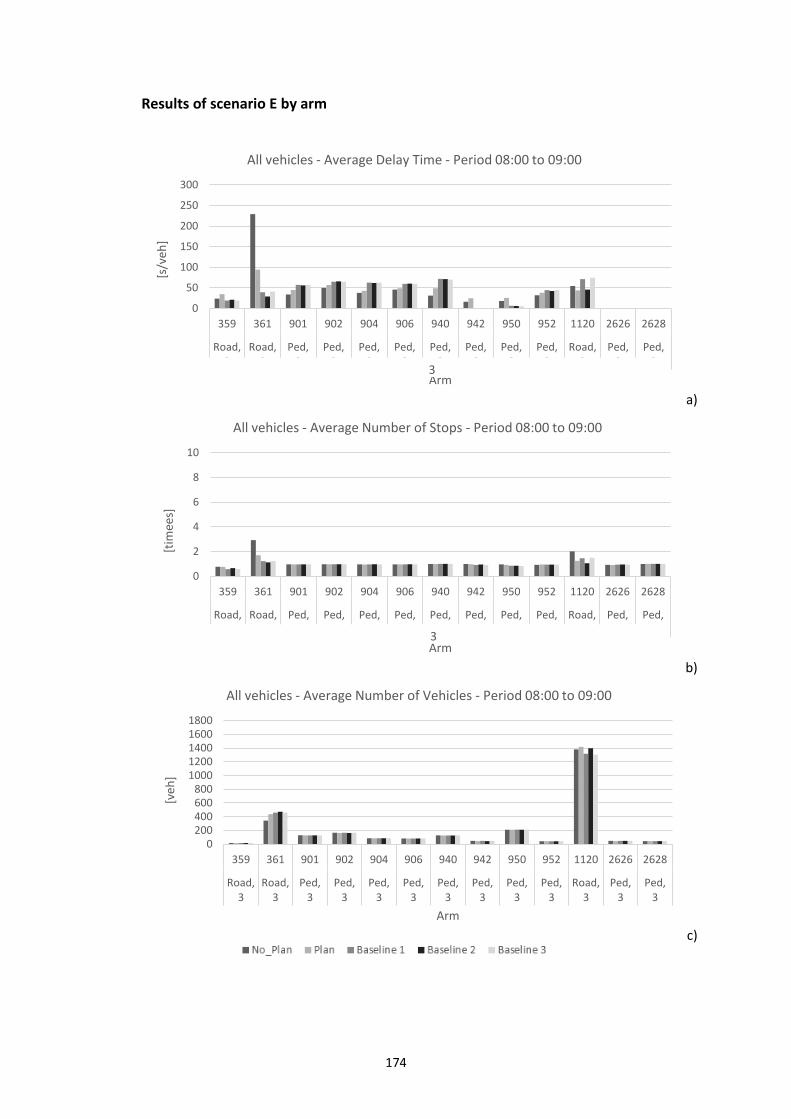
174
Results of scenario E by arm
a)
b)
c)
0
50
100
150
200
250
300
359 361 901 902 904 906 940 942 950 952 1120 2626 2628
Road, 3
Road, 3
Ped, 3
Ped, 3
Ped, 3
Ped, 3
Ped, 3
Ped, 3
Ped, 3
Ped, 3
Road, 3
Ped, 3
Ped, 3
[s/v
eh]
Arm
All vehicles - Average Delay Time - Period 08:00 to 09:00
0
2
4
6
8
10
359 361 901 902 904 906 940 942 950 952 1120 2626 2628
Road, 3
Road, 3
Ped, 3
Ped, 3
Ped, 3
Ped, 3
Ped, 3
Ped, 3
Ped, 3
Ped, 3
Road, 3
Ped, 3
Ped, 3
[tim
ees]
Arm
All vehicles - Average Number of Stops - Period 08:00 to 09:00
0 200 400 600 800
1000 1200 1400 1600 1800
359 361 901 902 904 906 940 942 950 952 1120 2626 2628
Road, 3
Road, 3
Ped, 3
Ped, 3
Ped, 3
Ped, 3
Ped, 3
Ped, 3
Ped, 3
Ped, 3
Road, 3
Ped, 3
Ped, 3
[veh
]
Arm
All vehicles - Average Number of Vehicles - Period 08:00 to 09:00
3
3
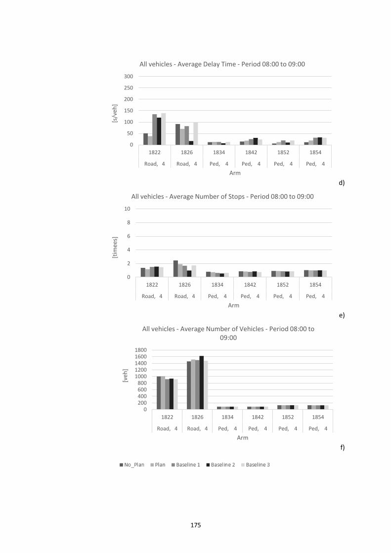
175
d)
e)
f)
0
50
100
150
200
250
300
1822 1826 1834 1842 1852 1854
Road, 4 Road, 4 Ped, 4 Ped, 4 Ped, 4 Ped, 4
[s/v
eh]
Arm
All vehicles - Average Delay Time - Period 08:00 to 09:00
0
2
4
6
8
10
1822 1826 1834 1842 1852 1854
Road, 4 Road, 4 Ped, 4 Ped, 4 Ped, 4 Ped, 4
[tim
ees]
Arm
All vehicles - Average Number of Stops - Period 08:00 to 09:00
0 200 400 600 800
1000 1200 1400 1600 1800
1822 1826 1834 1842 1852 1854
Road, 4 Road, 4 Ped, 4 Ped, 4 Ped, 4 Ped, 4
[veh
]
Arm
All vehicles - Average Number of Vehicles - Period 08:00 to 09:00
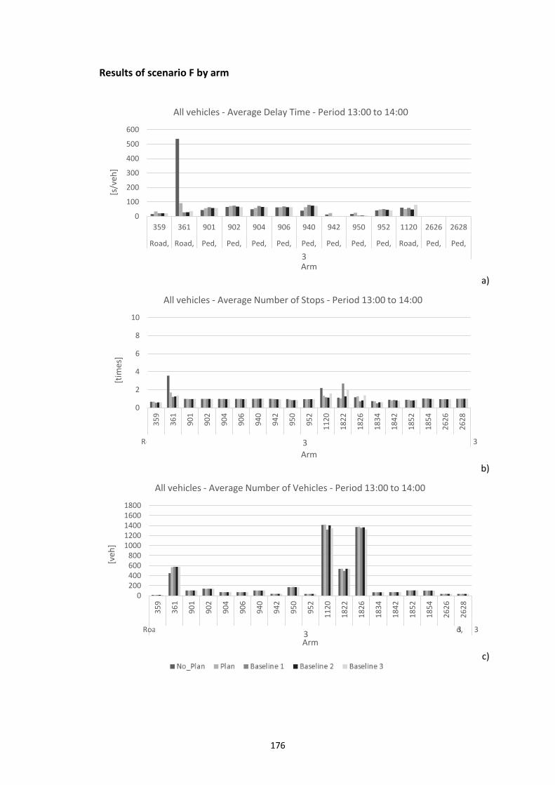
176
Results of scenario F by arm
a)
b)
c)
0
100
200
300
400
500
600
359 361 901 902 904 906 940 942 950 952 1120 2626 2628
Road, 3
Road, 3
Ped, 3
Ped, 3
Ped, 3
Ped, 3
Ped, 3
Ped, 3
Ped, 3
Ped, 3
Road, 3
Ped, 3
Ped, 3
[s/v
eh]
Arm
All vehicles - Average Delay Time - Period 13:00 to 14:00
0
2
4
6
8
10
35
9
36
1
90
1
90
2
90
4
90
6
94
0
94
2
95
0
95
2
11
20
18
22
18
26
18
34
18
42
18
52
18
54
26
26
26
28
Road, 3 Road, 3 Ped, 3 Ped, 3 Ped, 3 Ped, 3 Ped, 3 Ped, 3 Ped, 3 Ped, 3 Road, 3 Road, 4 Road, 4 Ped, 4 Ped, 4 Ped, 4 Ped, 4 Ped, 3 Ped, 3
[tim
es]
Arm
All vehicles - Average Number of Stops - Period 13:00 to 14:00
0 200 400 600 800
1000 1200 1400 1600 1800
35
9
36
1
90
1
90
2
90
4
90
6
94
0
94
2
95
0
95
2
11
20
18
22
18
26
18
34
18
42
18
52
18
54
26
26
26
28
Road, 3 Road, 3 Ped, 3 Ped, 3 Ped, 3 Ped, 3 Ped, 3 Ped, 3 Ped, 3 Ped, 3 Road, 3 Road, 4 Road, 4 Ped, 4 Ped, 4 Ped, 4 Ped, 4 Ped, 3 Ped, 3
[veh
]
Arm
All vehicles - Average Number of Vehicles - Period 13:00 to 14:00
3
3
3
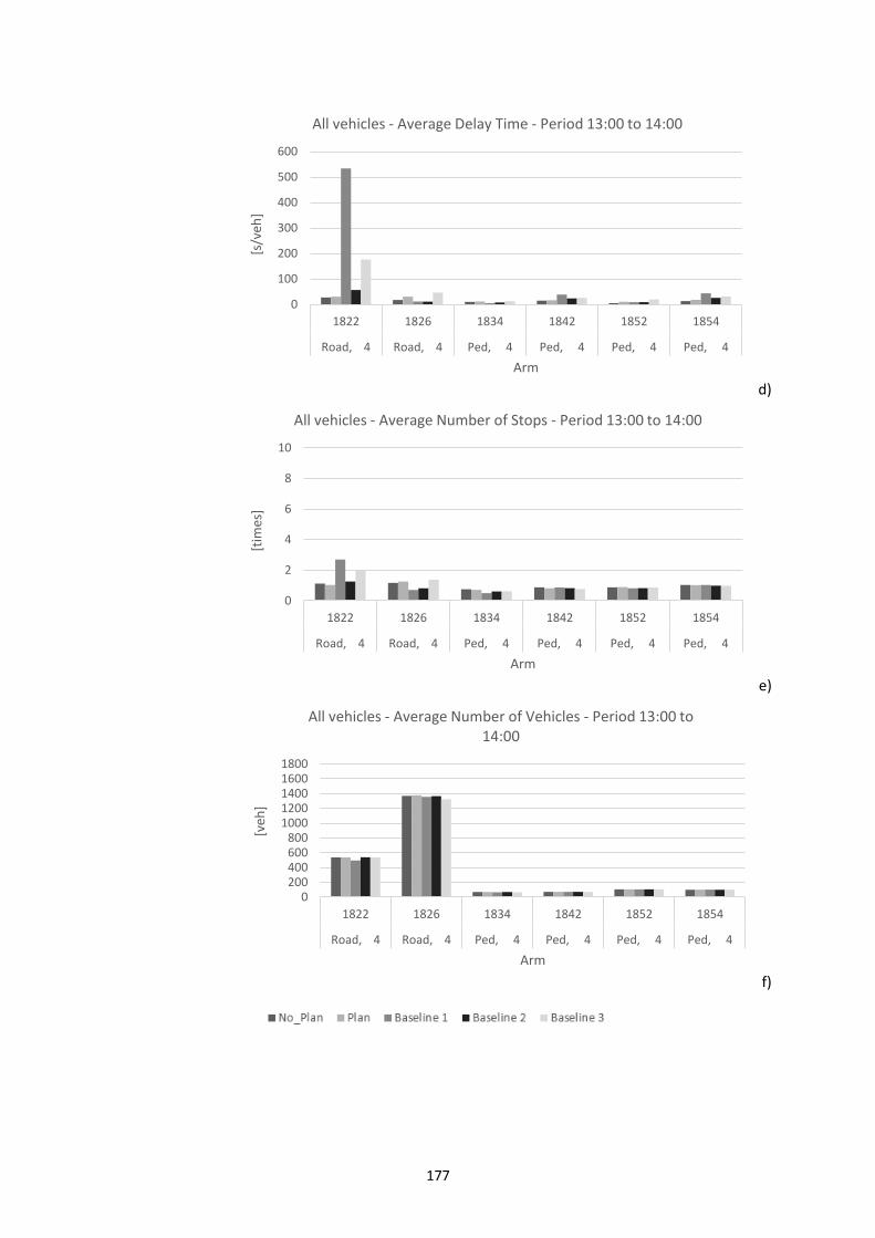
177
d)
e)
f)
0
100
200
300
400
500
600
1822 1826 1834 1842 1852 1854
Road, 4 Road, 4 Ped, 4 Ped, 4 Ped, 4 Ped, 4
[s/v
eh]
Arm
All vehicles - Average Delay Time - Period 13:00 to 14:00
0
2
4
6
8
10
1822 1826 1834 1842 1852 1854
Road, 4 Road, 4 Ped, 4 Ped, 4 Ped, 4 Ped, 4
[tim
es]
Arm
All vehicles - Average Number of Stops - Period 13:00 to 14:00
0 200 400 600 800
1000 1200 1400 1600 1800
1822 1826 1834 1842 1852 1854
Road, 4 Road, 4 Ped, 4 Ped, 4 Ped, 4 Ped, 4
[veh
]
Arm
All vehicles - Average Number of Vehicles - Period 13:00 to 14:00
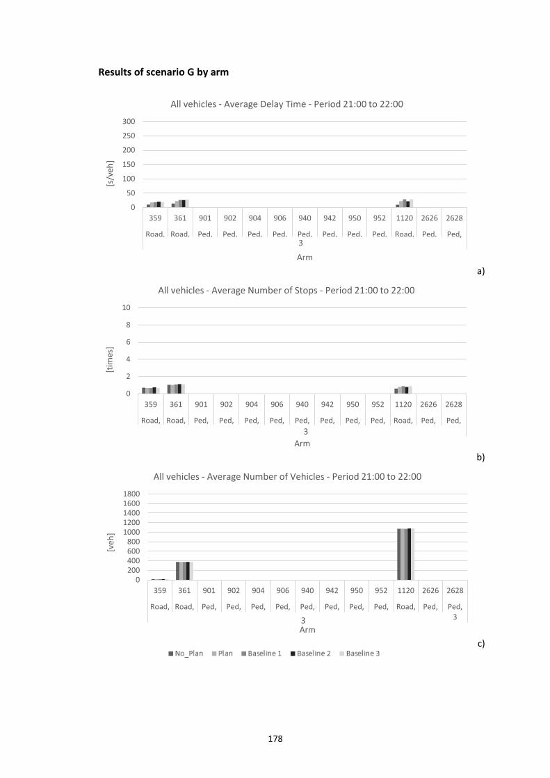
178
Results of scenario G by arm
a)
b)
c)
0
50
100
150
200
250
300
359 361 901 902 904 906 940 942 950 952 1120 2626 2628
Road, 3
Road, 3
Ped, 3
Ped, 3
Ped, 3
Ped, 3
Ped, 3
Ped, 3
Ped, 3
Ped, 3
Road, 3
Ped, 3
Ped, 3
[s/v
eh]
Arm
All vehicles - Average Delay Time - Period 21:00 to 22:00
0
2
4
6
8
10
359 361 901 902 904 906 940 942 950 952 1120 2626 2628
Road, 3
Road, 3
Ped, 3
Ped, 3
Ped, 3
Ped, 3
Ped, 3
Ped, 3
Ped, 3
Ped, 3
Road, 3
Ped, 3
Ped, 3
[tim
es]
Arm
All vehicles - Average Number of Stops - Period 21:00 to 22:00
0 200 400 600 800
1000 1200 1400 1600 1800
359 361 901 902 904 906 940 942 950 952 1120 2626 2628
Road, 3
Road, 3
Ped, 3
Ped, 3
Ped, 3
Ped, 3
Ped, 3
Ped, 3
Ped, 3
Ped, 3
Road, 3
Ped, 3
Ped, 3
[veh
]
Arm
All vehicles - Average Number of Vehicles - Period 21:00 to 22:00
3 4
3
3
3
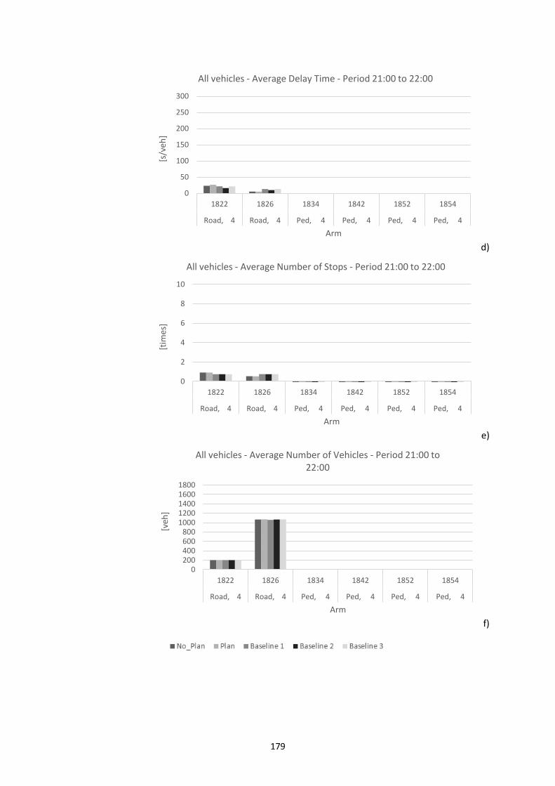
179
d)
e)
f)
0
50
100
150
200
250
300
1822 1826 1834 1842 1852 1854
Road, 4 Road, 4 Ped, 4 Ped, 4 Ped, 4 Ped, 4
[s/v
eh]
Arm
All vehicles - Average Delay Time - Period 21:00 to 22:00
0
2
4
6
8
10
1822 1826 1834 1842 1852 1854
Road, 4 Road, 4 Ped, 4 Ped, 4 Ped, 4 Ped, 4
[tim
es]
Arm
All vehicles - Average Number of Stops - Period 21:00 to 22:00
0 200 400 600 800
1000 1200 1400 1600 1800
1822 1826 1834 1842 1852 1854
Road, 4 Road, 4 Ped, 4 Ped, 4 Ped, 4 Ped, 4
[veh
]
Arm
All vehicles - Average Number of Vehicles - Period 21:00 to 22:00
Related Documents