INTELLIGENT DISTRIBUTION NETWORK USING LOAD ...

Journal of Engineering Science and Technology 8th EURECA 2017 Special Issue August (2018) 17 - 27 © School of Engineering, Taylor’s University

17

INTELLIGENT DISTRIBUTION NETWORK USING LOAD INFORMATION MANAGEMENT

MOHAMMAD HAFIZ1, ARAVIND CV1,*, CHARLES R SARIMUTHU2

1School of Engineering, Taylor’s University, Taylor's Lakeside Campus,

No. 1 Jalan Taylor's, 47500, Subang Jaya, Selangor DE, Malaysia 2Monash University, Subang Jaya, Selangor DE, Malaysia

*Corresponding Author: [email protected]

Abstract

Power systems operation is widely monitored through load flow analyses. The

three main methods used in these analyses are Newton-Raphson (NR), Gauss-

Seidel and Fast-Decoupled method. These methods involve long calculations and

numerous iteration which leads to an increase in computation time. However, fast

analyses are required for an efficient power system protection scheme. Therefore,

an alternative method which consumes much lesser time to compute and able to

provide accurate results are necessary. In this paper, the accuracy of Artificial

Neural Network (ANN) is studied by comparing numerical and analytical results

for an IEEE 14-bus power system network model. The study is done by varying

the load parameters at bus 6 and the output voltages (in per unit values) of all the

buses are recorded for ANN training and testing purposes. The ANN is coded

using the MATLAB software and the result obtained is compared with the

analytical and simulation results. Findings from this study suggest that the ANN

could possibly be an alternative method for load flow solutions.

Keywords: Artificial neural network, Load flow, Matlab, Newton-Raphson, Power

quality.

18 M. Hafiz et al.

Journal of Engineering Science and Technology Special Issue 8/2018

1. Introduction

Power system operation needs to be monitored to determine whether the system is

in stable condition. Without monitoring, the stability of the power system will be

compromised as the system needs to be underspecified limit in both normal and

emergency operation. Therefore, load flow analysis by way of calculating the

electrical parameters of a distribution system is required to determine the power

system’s performance and the system’s steady-state. Without load flow analysis, it

is difficult to ensure whether the system is operating within the permissible

threshold values or not. In addition to that, load flow analysis is also essential to

determine the losses occurred in the system [1]. The load flow analysis method is

used to find the voltage magnitude and other electrical parameters. The calculation

of load flow analysis requires network data such as the bus data, line data and

transformer specifications [1-3].

The three common load flow methods are Fast-Decoupled, Newton-Raphson,

and Gauss-Seidel method [4]. However, these three methods have their own

limitations. For example, the Newton-Raphson load flow method is able to

compute fast if the initial guess value is close to the actual value. Whereas, the

Gauss-Seidel method is considered not suitable to be used in large systems due

to the involvement of complex algorithms. Meanwhile, the Fast-Decoupled

method will not produce accurate values if the voltage in any bus is low [5]. The

development of Artificial Intelligence (AI) had created the possibility for it to

replace the conventional load flow methods [6]. Thus, Artificial Neural Network

(ANN), a type of AI is proposed to solve the load flow in this paper. ANN is

developed by following the structure of the brain where the brain’s neuron is

considered as the equivalent of the ANN’s Processing Element [7]. The

processing speed range of the brain is about 10-100ms while for ANN it is 10-

100 nanoseconds. The learning method of ANN is similar to AI which utilizes

machine learning.

ANN consists of supervised, unsupervised and reinforcement training.

Supervised training is used to find the trend of the data provided and its results

are validated using another set of data [8]. The unsupervised training groups the

training data by finding out the similarity of each data statistically [9]. Unlike

supervised and unsupervised learning, the reinforcement training requires actual

data [10].

2. System Network Design

The basic model of Artificial Neural Network (ANN) consists of three types of the

layer, which are the input, output and hidden layers as shown in Fig. 1. below [11].

The input layer of the ANN is represented by the number of input of the ANN

application which is also the same case with the output layer. However, the size of

the hidden layer must be able to compensate the size of the data used for the

training. The ANN is used to perform load flow analysis for the IEEE 14-bus

system. This model system is based on the approximation of the American Power

System [12]. The IEEE 14-bus system is connected with 5 generators and 11 loads

as shown in Fig. 2.

Intelligent Distribution Network using Load Information Management . . . . 19


Fig. 1. The basic structure of ANN [11].

Fig. 2. IEEE 14-bus model [12].

Simulink model of IEEE 14-bus system is modeled using the data obtained from

[13]. In order to verify whether the model is built correctly or not, the model in default

condition where the P=11.2 and Q=7.5 are simulated and the voltage value (in p.u)

for all the 14-buses is collected and compared with the voltage reference from [13].

20 M. Hafiz et al.


After the model verification, the simulation proceeds where one of the bus is

real (P) and reactive (Q) power for the load is manipulated. The voltage level at all

the buses is recorded to be used for the training and testing of the ANN. For this

research, the real and reactive power of the load connected at bus 6 is chosen to be

manipulated where the value of real power is increased from 10MW to 100MW

while the reactive power is changed accordingly to maintain a power factor of 0.9.

The calculation of the real and reactive power is based on the power triangle as

shown in Fig. 3.

Fig. 3. Power triangle.

After the data of the output voltage is recorded, the data is made into two sets

where one of the set will be used to train the ANN, while another set of data will

be used to test the accuracy of the ANN. The ANN is coded using Matlab where

all the parameters of the ANN are included in the coding such as the learning rate,

hidden layer, epoch, error rate and the training function.

The ANN training is started where the input is set as real and reactive power for

a load connected at bus 6 while the designated output data is the voltage level of all

the 14 buses. The output produced by the ANN is compared with the results

recorded from the simulation. If the error is too high (>5%), then the coding will

be reconfigured or more data will be added to increase the ANN training.

If the ANN produces satisfactory results, then the next step is to compare the ANN

result with the result produced by one of the conventional load flow methods. In this

research, Newton-Raphson method is chosen as this method although complex it

produces a reliable result and can be used regardless of the size of the buses [14]

The test data of real (P) and reactive (Q) value is used for the Newton-Raphson

calculation where the real and reactive power of load connected at bus 6 load is

varied while maintaining the power factor of 0.9 as done with the Simulink

simulation. The voltage levels at all 14 buses are recorded.

3. Results and Discussion

3.1. Simulink model

Table 1 shows the error or differences between the voltage levels produced by

simulation when in default condition compared with the IEEE 14 Bus System data

sheet from [13].



Table 1. Difference between simulation voltage and data sheet [13].

Bus

Number

Simulated Voltage

(p.u)

Data Sheet voltage

(p.u)

%

difference

Bus 1 1.012 1.06 4.53

Bus 2 1.004 1.045 3.92

Bus 3 0.978 1.01 3.17

Bus 4 0.990 1.00 1.00

Bus 5 0.995 1.00 0.50

Bus 6 0.997 1.00 0.30

Bus 7 0.994 1.00 0.60

Bus 8 0.984 1.00 1.60

Bus 9 0.981 1.00 1.90

Bus 10 0.978 1.00 2.20

Bus 11 0.978 1.00 2.20

Bus 12 0.981 1.00 1.90

Bus 13 0.975 1.00 2.50

Bus 14 0.986 1.00 1.40

In Simulink, the real and reactive power for a load connected at bus 6 is adjusted

where the power factor is maintained as 0.9. The 10 training cases are shown in

Table 2.

Table 2. Training cases for the ANN.

Train Case P (MW) Q (Mvar)

1 10 4.8

2 20 9.7

3 30 14.5

4 40 19.4

5 50 24.2

6 60 29.1

7 70 33.9

8 80 38.8

9 90 43.6

10 100 48.4

The produced voltage values at all the buses are recorded and used for the

Artificial Neural Network (ANN) training. Another set of real and reactive power

is used to test the ANN’s performance as shown in Table 3.

Table 3. Test case for the ANN.

Test Case P (MW) Q (Mvar)

1 25 12.1

2 45 21.8

3 60 29.1

4 65 31.5

5 85 41.2

22 M. Hafiz et al.


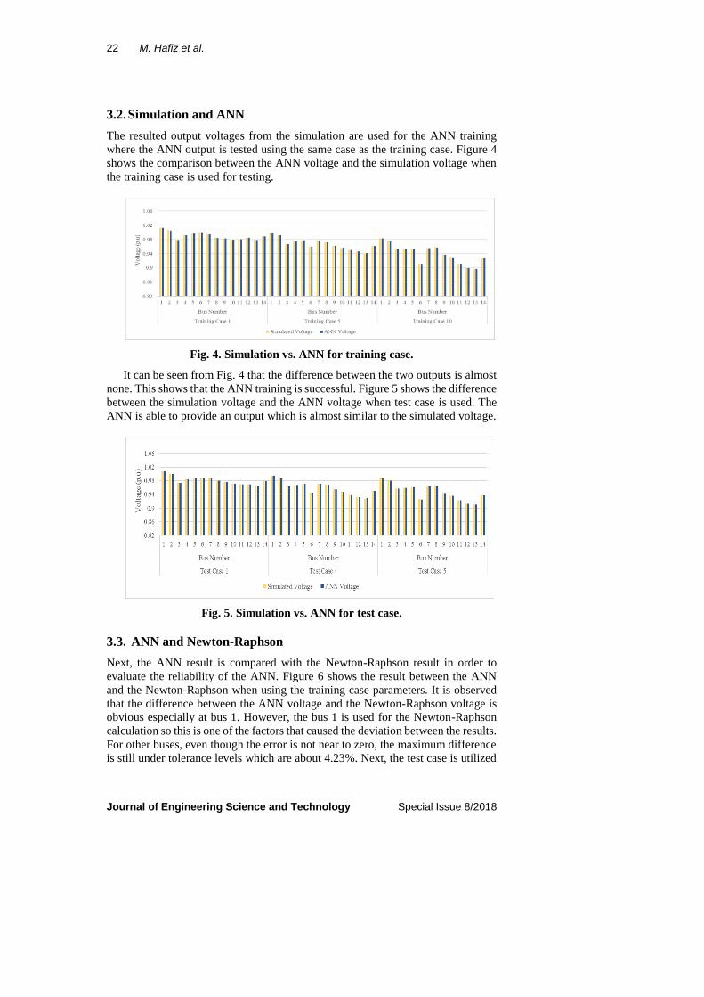
3.2. Simulation and ANN

The resulted output voltages from the simulation are used for the ANN training

where the ANN output is tested using the same case as the training case. Figure 4

shows the comparison between the ANN voltage and the simulation voltage when

the training case is used for testing.

Fig. 4. Simulation vs. ANN for training case.

It can be seen from Fig. 4 that the difference between the two outputs is almost

none. This shows that the ANN training is successful. Figure 5 shows the difference

between the simulation voltage and the ANN voltage when test case is used. The

ANN is able to provide an output which is almost similar to the simulated voltage.

Fig. 5. Simulation vs. ANN for test case.

3.3. ANN and Newton-Raphson

Next, the ANN result is compared with the Newton-Raphson result in order to

evaluate the reliability of the ANN. Figure 6 shows the result between the ANN

and the Newton-Raphson when using the training case parameters. It is observed

that the difference between the ANN voltage and the Newton-Raphson voltage is

obvious especially at bus 1. However, the bus 1 is used for the Newton-Raphson

calculation so this is one of the factors that caused the deviation between the results.

For other buses, even though the error is not near to zero, the maximum difference

is still under tolerance levels which are about 4.23%. Next, the test case is utilized



in order to evaluate the performance of the ANN compared to the Newton-Raphson

where the result is shown in Fig.7. Similar to the condition where training case is

used, the error is noticed when the test case is used. The highest error is still under

tolerance where the maximum error is 3.8%.

Fig. 6. ANN vs. Newton-Raphson for training case.

Fig. 7. ANN vs. Newton-Raphson for test case.

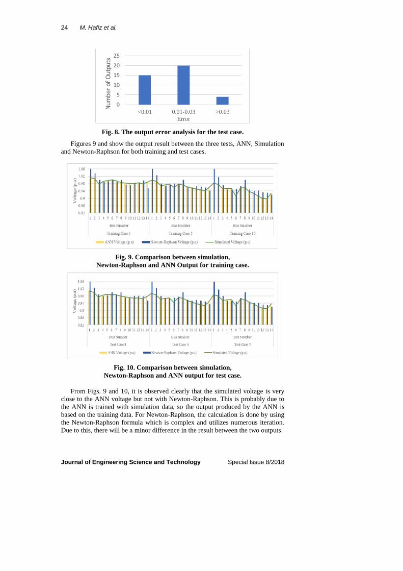
3.4. Error Analysis

Figure 8 shows the summary of the error difference for the test case where it can

see that from 39 output (total is 42 but bus 1 output is excluded), most output falls

between 0.01 to 0.03 error, followed by below 0.01 and only four output is more

than 0.03. However, none had exceeded the tolerance level which is 0.05. So, it can

be concluded that the ANN output showed a positive result.

24 M. Hafiz et al.


Fig. 8. The output error analysis for the test case.

Figures 9 and show the output result between the three tests, ANN, Simulation

and Newton-Raphson for both training and test cases.

Fig. 9. Comparison between simulation,

Newton-Raphson and ANN Output for training case.

Fig. 10. Comparison between simulation,

Newton-Raphson and ANN output for test case.

From Figs. 9 and 10, it is observed clearly that the simulated voltage is very

close to the ANN voltage but not with Newton-Raphson. This is probably due to

the ANN is trained with simulation data, so the output produced by the ANN is

based on the training data. For Newton-Raphson, the calculation is done by using

the Newton-Raphson formula which is complex and utilizes numerous iteration.

Due to this, there will be a minor difference in the result between the two outputs.

0

5

10

15

20

25

<0.01 0.01-0.03 >0.03N

um

ber

of

Outp

uts

Error



3.5. Performance of ANN Compared to Newton-Raphson

In terms of time, Newton-Raphson is able to complete the computation instantly

after the Matlab code is run to produce 14 bus output for only 1 case while the ANN

produced 14 bus output for all the cases within one second. For accuracy, the ANN

can produce a very accurate result with error difference that is close to 0 as long as

the training data supplied to the ANN is accurate.

3.6. ANN Parameters

The ANN parameter could affect the accuracy of the result produced. However,

since the size of the bus is quite small, some of the parameters do not affect the

results greatly. The epoch which also known as a number of iterations is set as 8000

but the ANN managed to finish its training within 3 iterations due to the size of the

bus. Learning rate is basically how fast the ANN is able to change its parameter.

According to [15], the trial-and-error approach could be used to find the optimal

learning rate. Just like epoch, since the number of buses is small, the learning rate

did not make a big impact on the finding as it gave the same output regardless of

the learning rate. The ANN training is done in 1 second when the learning rate is

set to 0.001. The ‘error’ in the ANN configuration basically set the accuracy of the

ANN with respect to the decimal point. As for the training function, Trainlm is

selected from other function named Trainlm, Traingdx and Trainoss just to name a

few as it gave a low mean square error (MSE) and perfect to be used in a small-

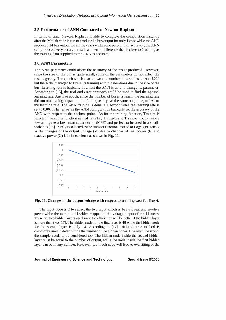
scale bus [16]. Purely is selected as the transfer function instead of Logsig or Tansig

as the changes of the output voltage (V) due to changes of real power (P) and

reactive power (Q) is in linear form as shown in Fig. 11.

Fig. 11. Changes in the output voltage with respect to training case for Bus 6.

The input node is 2 to reflect the two input which is bus 6’s real and reactive

power while the output is 14 which mapped to the voltage output of the 14 buses.

There are two hidden layers used since the efficiency will be better if the hidden layer

is more than two [17]. The hidden node for the first layer is 48 while the hidden node

for the second layer is only 14. According to [17], trial-and-error method is

commonly used in determining the number of the hidden nodes. However, the size of

the sample needs to be considered too. The hidden node inside the second hidden

layer must be equal to the number of output, while the node inside the first hidden

layer can be in any number. However, too much node will lead to overfitting of the

26 M. Hafiz et al.


regression line while too less will hinder the ANN to learn the data. So, in this work

trial-and-error method is used until the best output is produced.

4. Conclusions

As a conclusion, ANN can be used to solve load flow just like the conventional

load flow method as the difference between the two methods is still under

acceptable level. It is noted that ANN can only produce an accurate result if the

parameter of the ANN is configured correctly and a large amount of data is used

for training purposes. Finally, for better ANN performance, a database which

consists of bus data under various conditions can be used as a platform to train

the ANN to solve load flow problem.

Nomenclatures

R Real Power

Q Reactive Power

S Apparent Power

Abbreviations

AI Artificial Intelligence

ANN Artificial Neural Network

MSE Mean Square Error

References

1. AVO Training Institute. (2012). Go with the flow: The importance of load flow

studies. Retrieved November 18, 2016, from http://www.avotraining.com/go-

with-the-flow-the-importance-of-load-flow-studies/.

2. Kundur, P. (1994). Power system stability and control. New York: McGraw-Hill.

3. Glover, J.D.; and Sarma, M.S. (2002). Power system analysis and design.

Thomson Learning.

4. Singhal, K. (2014). Comparison between load flow analysis methods in power

system using MATLAB. International Journal of Scientific & Engineering

Research, 5(5), 1412-2014.

5. Bokka, N. (2010). Comparison of power flow algorithms for inclusion in on-

line power systems operation tools. University of New Orleans.

6. Pannu, A. (2015). Artificial intelligence and its application in different areas.

International Journal of Engineering and Innovative Technology (IJEIT),

4(10), 79-84.

7. Dillon, S.; Edwin, K.W.; Kochs, H.D.; and Taud, R.J. (1978). Integer

programming approach to the problem of optimal unit commitment with

probabilistic reserve determination. IEEE Transactions on Power Apparatus

and Systems, 97(6), 2154-2166.

8. Eberhart, R.C.; and Shi, Y. (2007). Computational intelligence: Concept to

implementations, Elsevier, 2(6), 20-24.

9. MathWorks. (2016). Supervised Learning. The MathWorks, Inc. Retrieved

November 18, 2016, https://www.mathworks.com/discovery/supervisedle

arning.html?requestedDomain=www.mathworks.com&requestedDomain=w

ww.mathworks.com.



10. Dayan, P. (2000). Unsupervised learning. MIT, Cambridge.

11. Lee, M. (2005). Reinforcement learning. Retrieved November 18, 2016,

Available:https://webdocs.cs.ualberta.ca/~sutton/book/ebook/node7.html.

12. Burger, J.T. (2016). A basic introduction to neural networks. The University

of Wisconsin-Madison.

13. Illinois Center for a Smarter Electric Grid (ICSEG) (2016). IEEE 14-Bus

System. Information Trust Institute. Retrieved November 18, 2016,

:http://icseg.iti.illinois.edu/ieee-14-bus-system/.

14. Bala, P.; and Dalai, S. (2017). Random forest-based fault analysis method in

IEEE 14 bus system. Proceedings of the 3rd International Conference on

Condition Assessment Techniques in Electrical Systems (CATCON),

Rupnagar, 2017, 407-411.

15. Kailay, A.K.; and Brar, Y.S. (2015). Identification of best load flow

calculation method for IEEE-30 BUS system using MATLAB. International

Journal of Electrical and Electronics Research, 3(3), 155-161.

16. Bengio, Y. (2012). Practical recommendations for gradient-based training of

deep architectures. Lecture Notes in Computer Science, 7700, 437-478.

17. San Diego State University. Summary. Retrieved January 22, 2017,

http://www.rohan.sdsu.edu/doc/matlab/toolbox/nnet/backpr14.html.

INTELLIGENT DISTRIBUTION NETWORK USING LOAD ...

Documents