ISSN 1055-1425 December 1997 This work was performed as part of the California PATH Program of the University of California, in cooperation with the State of California Business, Transportation, and Housing Agency, Department of Transportation; and the United States Department of Transportation, Federal Highway Administration. The contents of this report reflect the views of the authors who are responsible for the facts and the accuracy of the data presented herein. The contents do not necessarily reflect the official views or policies of the State of California. This report does not constitute a standard, specification, or regulation. Report for MOU 291 CALIFORNIA PATH PROGRAM INSTITUTE OF TRANSPORTATION STUDIES UNIVERSITY OF CALIFORNIA, BERKELEY Integration of Fault Detection and Identification into a Fault Tolerant Automated Highway System UCB-ITS-PRR-97-52 California PATH Research Report Randal K. Douglas, Walter H. Chung, Durga P. Malladi, Robert H. Chen, Jason L. Speyer and D. Lewis Mingori University of California, Los Angeles

Welcome message from author
This document is posted to help you gain knowledge. Please leave a comment to let me know what you think about it! Share it to your friends and learn new things together.
Transcript

ISSN 1055-1425
December 1997
This work was performed as part of the California PATH Program of theUniversity of California, in cooperation with the State of California Business,Transportation, and Housing Agency, Department of Transportation; and theUnited States Department of Transportation, Federal Highway Administration.
The contents of this report reflect the views of the authors who are responsiblefor the facts and the accuracy of the data presented herein. The contents do notnecessarily reflect the official views or policies of the State of California. Thisreport does not constitute a standard, specification, or regulation.
Report for MOU 291
CALIFORNIA PATH PROGRAMINSTITUTE OF TRANSPORTATION STUDIESUNIVERSITY OF CALIFORNIA, BERKELEY
Integration of Fault Detection andIdentification into a Fault TolerantAutomated Highway System
UCB-ITS-PRR-97-52California PATH Research Report
Randal K. Douglas, Walter H. Chung, Durga P. Malladi,Robert H. Chen, Jason L. Speyer and D. Lewis MingoriUniversity of California, Los Angeles

Integration of Fault Detection and Identiflcation
into a Fault Tolerant Automated Highway System
Randal K. Douglas, Walter H. Chung, Durga P. Malladi, Robert H. Chen,
Jason L. Speyer and D. Lewis Mingori
Mechanical and Aerospace Engineering DepartmentUniversity of California, Los Angeles
Los Angeles, California 90095


Integration of Fault Detectionand Identiflcation into a
Fault Tolerant Automated Highway System
Randal K. Douglas, Walter H. Chung, Durga P. Malladi,
Robert H. Chen, Jason L. Speyer and D. Lewis Mingori
Mechanical and Aerospace Engineering DepartmentUniversity of California, Los Angeles
Los Angeles, California 90095
December 5, 1997


Integration of Fault Detection and Identiflcation into aFault Tolerant Automated Highway System
Randal K. Douglas, Walter H. Chung, Durga P. Malladi, Robert H. Chen, Jason L. Speyerand D. Lewis Mingori
Mechanical and Aerospace Engineering DepartmentUniversity of California, Los Angeles
Los Angeles, California 90095
December 5, 1997
Abstract
This report is a continuation of the work of (Douglas et al. 1996) which concerns vehicle
fault detection and identification and describes a vehicle health management approach based
on analytic redundancy. A point design of fault detection filters and parity equations is
developed for the vehicle longitudinal mode. Data from analytically redundant sensors and
actuators are fused in a way that unique, identifiable static patterns emerge in response to a
fault. Sensor noise, process disturbances, system parameter variations, unmodeled dynamics
and nonlinearities can distort these static patterns. A Shiryayev probability ratio test that
has been extended to multiple hypotheses examines the filter and parity equation residuals
and generates the probability of the presence of a fault. Tests in a high-fidelity vehicle
simulation where nonlinearities and road variations are significant are very encouraging. A
preliminary design of a range sensor fault monitoring system is outlined as an application of
a new decentralized fault detection filter. This system combines dynamic state information
already generated by the existing filter designs with inter-vehicle analytic redundancy.
Keywords. Automated Highway Systems, Automatic Vehicle Monitoring, Fault Detection
and Fault Tolerant Control, Reliability, Sensors, Vehicle Monitoring.
v


Integration of Fault Detection and Identiflcation into aFault Tolerant Automated Highway System
Award No. 65X817, M.O.U. 291
Executive Summary
This report is a continuation of the work of (Douglas et al. 1996) which concerns vehicle
fault detection and identification and describes a vehicle health management approach based
on analytic redundancy. A point design of fault detection filters and parity equations is
developed for the vehicle longitudinal mode. Data from analytically redundant sensors and
actuators are fused in a way that unique, identifiable static patterns emerge in response to a
fault. Sensor noise, process disturbances, system parameter variations, unmodeled dynamics
and nonlinearities can distort these static patterns. A Shiryayev probability ratio test that
has been extended to multiple hypotheses examines the filter and parity equation residuals
and generates the probability of the presence of a fault. Tests in a high-fidelity vehicle
simulation where nonlinearities and road variations are significant are very encouraging. A
preliminary design of a range sensor fault monitoring system is outlined as an application of
a new decentralized fault detection filter. This system combines dynamic state information
already generated by the existing filter designs with inter-vehicle analytic redundancy.
vii

Contents
Abstract . . . . . . . . . . . . . . . . . . . . . . . . . . . . . . . . . . . . . . . . . . v
Executive Summary . . . . . . . . . . . . . . . . . . . . . . . . . . . . . . . . . . . vii
List of Figures . . . . . . . . . . . . . . . . . . . . . . . . . . . . . . . . . . . . . . xi
List of Tables . . . . . . . . . . . . . . . . . . . . . . . . . . . . . . . . . . . . . . . xiii
Chapter 1 Introduction . . . . . . . . . . . . . . . . . . . . . . . . . . . . . . . . 1
Chapter 2 Vehicle Model . . . . . . . . . . . . . . . . . . . . . . . . . . . . . . . 72.1 Linear Model . . . . . . . . . . . . . . . . . . . . . . . . . . . . . . . . . . . 8
2.1.1 Linear Model Reduction . . . . . . . . . . . . . . . . . . . . . . . . . 92.1.2 Vehicle Measurements . . . . . . . . . . . . . . . . . . . . . . . . . . 10
2.2 Suspension Model . . . . . . . . . . . . . . . . . . . . . . . . . . . . . . . . . 112.2.1 Suspension Model With Suspension Length State . . . . . . . . . . . 122.2.2 Suspension Model With Suspension Force State . . . . . . . . . . . . 132.2.3 Example . . . . . . . . . . . . . . . . . . . . . . . . . . . . . . . . . . 15
2.3 Manifold Temperature Model . . . . . . . . . . . . . . . . . . . . . . . . . . 16
ix

x Contents
Chapter 3 Fault Detection By Analytic Redundancy . . . . . . . . . . . . . 173.1 Analytic Redundancy . . . . . . . . . . . . . . . . . . . . . . . . . . . . . . 18
3.1.1 Beard-Jones Fault Detection Filter Background . . . . . . . . . . . . 193.1.2 Fault Modelling . . . . . . . . . . . . . . . . . . . . . . . . . . . . . . 213.1.3 Special Design Considerations . . . . . . . . . . . . . . . . . . . . . . 23
Ill-conditioned fault direction . . . . . . . . . . . . . . . . . . . . . . 23Output separability . . . . . . . . . . . . . . . . . . . . . . . . . . . 23Zero steady-state fault residual . . . . . . . . . . . . . . . . . . . . . 25
3.1.4 Fault Assignment to Multiple Fault Detection Filters . . . . . . . . . 273.1.5 Fault Detection Filter Design For Sensors . . . . . . . . . . . . . . . 303.1.6 Fault Detection Filter Design For Actuators . . . . . . . . . . . . . . 35
3.2 Algebraic Redundancy . . . . . . . . . . . . . . . . . . . . . . . . . . . . . . 373.3 Structure . . . . . . . . . . . . . . . . . . . . . . . . . . . . . . . . . . . . . 38
Chapter 4 Fault Detection Filter Evalution . . . . . . . . . . . . . . . . . . . 414.1 Residual Scaling . . . . . . . . . . . . . . . . . . . . . . . . . . . . . . . . . 424.2 Smooth Road . . . . . . . . . . . . . . . . . . . . . . . . . . . . . . . . . . . 424.3 Rough Road . . . . . . . . . . . . . . . . . . . . . . . . . . . . . . . . . . . . 44
Chapter 5 Residual Processing . . . . . . . . . . . . . . . . . . . . . . . . . . . 555.1 Residual Processor Design . . . . . . . . . . . . . . . . . . . . . . . . . . . . 565.2 Simulations . . . . . . . . . . . . . . . . . . . . . . . . . . . . . . . . . . . . 585.3 Conclusions . . . . . . . . . . . . . . . . . . . . . . . . . . . . . . . . . . . . 60
Chapter 6 A Game Theoretic Fault Detection Filter . . . . . . . . . . . . . 636.1 The Approximate Detection Filter Design Problem . . . . . . . . . . . . . . 65
6.1.1 Modeling the Detection Problem . . . . . . . . . . . . . . . . . . . . 656.1.2 Modeling Failures . . . . . . . . . . . . . . . . . . . . . . . . . . . . . 686.1.3 Constructing the Failure Signal . . . . . . . . . . . . . . . . . . . . . 69
6.2 A Game Theoretic Solution to the Approximate Detection Filter DesignProblem . . . . . . . . . . . . . . . . . . . . . . . . . . . . . . . . . . . . . . 746.2.1 The Disturbance Attenuation Problem . . . . . . . . . . . . . . . . . 746.2.2 The Differential Game Solution . . . . . . . . . . . . . . . . . . . . . 756.2.3 Steady-State Results . . . . . . . . . . . . . . . . . . . . . . . . . . . 79
6.3 Applications . . . . . . . . . . . . . . . . . . . . . . . . . . . . . . . . . . . . 806.3.1 Accelerometer Fault Detection in an F16XL . . . . . . . . . . . . . . 80
Aircraft Dynamics Model . . . . . . . . . . . . . . . . . . . . . . . . 80Full-Order Filter Design . . . . . . . . . . . . . . . . . . . . . . . . . 81

Contents xi
Analysis . . . . . . . . . . . . . . . . . . . . . . . . . . . . . . . . . . 83
6.3.2 Position Sensor Fault Detection for a Simple Rocket, ATime-Varying System . . . . . . . . . . . . . . . . . . . . . . . . . . 86
Rocket Dynamics Model . . . . . . . . . . . . . . . . . . . . . . . . . 86
Full-Order Filter Design . . . . . . . . . . . . . . . . . . . . . . . . . 88
Analysis . . . . . . . . . . . . . . . . . . . . . . . . . . . . . . . . . . 90
Chapter 7 The Asymptotic Game Theoretic Fault Detection Filter . . . . 93
7.1 Finding the Limiting Solution: Singular Differential Game Theory . . . . . . 94
7.2 Conditions for the Nonpositivity of the Game Cost . . . . . . . . . . . . . . 95
7.3 The Solution to the Singular Differential Game . . . . . . . . . . . . . . . . 98
7.4 The Relationship Between the Limiting Game Filter and Detection Filters . 110
7.4.1 A Reduced-Order Detection Filter from the Limiting Game Solution 110
7.4.2 The Invariant Subspace Structure of the Limiting Case Filter . . . . 115
7.5 Revisited: Accelerometer Fault Detection in an F-16XL . . . . . . . . . . . . 121
Chapter 8 A Parameter Robust Game Theoretic Fault Detection Filter . 125
8.1 Parameter Robustness and FDI . . . . . . . . . . . . . . . . . . . . . . . . . 125
8.2 Parameter Robustness versus FDI . . . . . . . . . . . . . . . . . . . . . . . . 127
8.3 A Disturbance Attenuation Problem with Parameter Variations . . . . . . . 128
8.3.1 The Modified Disturbance Attenuation Problem . . . . . . . . . . . 128
8.3.2 Equivalence to the H∞ Measurement Feedback Control Problem . . 136
8.4 The Robust Game Theoretic Fault Detection Filter in the Limit . . . . . . . 138
8.5 Example: Accelerometer Fault Detection in an F16XL with ModelUncertainty . . . . . . . . . . . . . . . . . . . . . . . . . . . . . . . . . . . . 143
8.5.1 Problem Statement . . . . . . . . . . . . . . . . . . . . . . . . . . . . 143
8.5.2 Parameter Robust Filter Design . . . . . . . . . . . . . . . . . . . . . 145
Chapter 9 A Decentralized Fault Detection Filter . . . . . . . . . . . . . . . 151
9.1 Decentralized Estimation Theory and its Application to FDI . . . . . . . . . 152
9.1.1 The General Solution . . . . . . . . . . . . . . . . . . . . . . . . . . 152
9.1.2 Implications for Detection Filters . . . . . . . . . . . . . . . . . . . . 156
9.2 Range Sensor Fault Detection in a Platoon of Cars . . . . . . . . . . . . . . 157
9.2.1 Problem Statement . . . . . . . . . . . . . . . . . . . . . . . . . . . . 157
9.2.2 System Dynamics and Failure Modeling . . . . . . . . . . . . . . . . 158
9.2.3 Decentralized Fault Detection Filter Design . . . . . . . . . . . . . . 167

xii Contents
Chapter 10 Multiple Model Adaptive Estimation . . . . . . . . . . . . . . . . 17110.1 Problem Statement . . . . . . . . . . . . . . . . . . . . . . . . . . . . . . . . 17310.2 MMAE Algorithm . . . . . . . . . . . . . . . . . . . . . . . . . . . . . . . . 174
10.2.1 Beta Dominance . . . . . . . . . . . . . . . . . . . . . . . . . . . . . 17610.3 Adaptive Kalman Filter Algorithm . . . . . . . . . . . . . . . . . . . . . . . 17710.4 Performance of AKF Algorithm . . . . . . . . . . . . . . . . . . . . . . . . . 180
10.4.1 Underlying Assumptions of MHSSPRT . . . . . . . . . . . . . . . . . 18110.4.2 Convergence of the Posterior Probability . . . . . . . . . . . . . . . . 18310.4.3 Convergence of the Posterior Error Covariance . . . . . . . . . . . . 190
10.5 Simulations . . . . . . . . . . . . . . . . . . . . . . . . . . . . . . . . . . . . 19910.5.1 Example 1 . . . . . . . . . . . . . . . . . . . . . . . . . . . . . . . . . 19910.5.2 Example 2 . . . . . . . . . . . . . . . . . . . . . . . . . . . . . . . . . 20010.5.3 Example 3 . . . . . . . . . . . . . . . . . . . . . . . . . . . . . . . . . 20210.5.4 Example 4 . . . . . . . . . . . . . . . . . . . . . . . . . . . . . . . . . 204
10.6 Conclusions . . . . . . . . . . . . . . . . . . . . . . . . . . . . . . . . . . . . 20410.7 Proofs . . . . . . . . . . . . . . . . . . . . . . . . . . . . . . . . . . . . . . . 206
10.7.1 Proof A . . . . . . . . . . . . . . . . . . . . . . . . . . . . . . . . . . 20610.7.2 Proof B1 . . . . . . . . . . . . . . . . . . . . . . . . . . . . . . . . . 20810.7.3 Proof B2 . . . . . . . . . . . . . . . . . . . . . . . . . . . . . . . . . 20910.7.4 Proof B3 . . . . . . . . . . . . . . . . . . . . . . . . . . . . . . . . . 210
Chapter 11 Fault Detection and Identification Using Linear QuadraticOptimization . . . . . . . . . . . . . . . . . . . . . . . . . . . . . . . 213
11.1 Problem Formulation . . . . . . . . . . . . . . . . . . . . . . . . . . . . . . . 21411.2 On Line Filter . . . . . . . . . . . . . . . . . . . . . . . . . . . . . . . . . . . 21911.3 The Steady State Filter . . . . . . . . . . . . . . . . . . . . . . . . . . . . . 22011.4 Proofs . . . . . . . . . . . . . . . . . . . . . . . . . . . . . . . . . . . . . . . 222
Proof A . . . . . . . . . . . . . . . . . . . . . . . . . . . . . . . . . . . . . . 222Proof B . . . . . . . . . . . . . . . . . . . . . . . . . . . . . . . . . . . . . . 223
Chapter 12 Model Input Reduction . . . . . . . . . . . . . . . . . . . . . . . . . 22712.1 Notation . . . . . . . . . . . . . . . . . . . . . . . . . . . . . . . . . . . . . . 22812.2 Input-Output Mappings and Model Input Reduction . . . . . . . . . . . . . 229
12.2.1 Output Point of View . . . . . . . . . . . . . . . . . . . . . . . . . . 22912.2.2 Input Point of View . . . . . . . . . . . . . . . . . . . . . . . . . . . 23012.2.3 Output and Intput Point of View . . . . . . . . . . . . . . . . . . . . 232
12.3 Application to Disturbance Direction Estimation . . . . . . . . . . . . . . . 23312.4 Extension to Parameter Variation Model Reduction . . . . . . . . . . . . . . 235

Contents xiii
12.5 Conclusions . . . . . . . . . . . . . . . . . . . . . . . . . . . . . . . . . . . . 237
Chapter 13 Conclusions . . . . . . . . . . . . . . . . . . . . . . . . . . . . . . . . 239
Appendix A Fault Detection Filter Design Data . . . . . . . . . . . . . . . . 241
References . . . . . . . . . . . . . . . . . . . . . . . . . . . . . . . . . . . . . . . . . 245


List of Figures
Figure 1.1 A System View of Vehicle Health Management . . . . . . . . . . . . . . 2
Figure 2.1 Simplified suspension and tire model . . . . . . . . . . . . . . . . . . . . 11
Figure 3.1 Fault Signatures . . . . . . . . . . . . . . . . . . . . . . . . . . . . . . . 25Figure 3.2 Fault Signatures . . . . . . . . . . . . . . . . . . . . . . . . . . . . . . . 27Figure 3.3 Fault Signatures . . . . . . . . . . . . . . . . . . . . . . . . . . . . . . . 28Figure 3.4 Singular value frequency response from all faults to throttle residual . . 37Figure 3.5 Fault Signatures . . . . . . . . . . . . . . . . . . . . . . . . . . . . . . . 39
Figure 4.1 Residuals for fault detection filter one . . . . . . . . . . . . . . . . . . . 45Figure 4.2 Residuals for fault detection filter one . . . . . . . . . . . . . . . . . . . 45Figure 4.3 Residuals for fault detection filter two . . . . . . . . . . . . . . . . . . . 46Figure 4.4 Residuals for fault detection filter three . . . . . . . . . . . . . . . . . . 46Figure 4.5 Residual for fault detection filter four . . . . . . . . . . . . . . . . . . . 47Figure 4.6 Residual for fault detection filter five . . . . . . . . . . . . . . . . . . . . 47Figure 4.7 Residual for fault detection filter six . . . . . . . . . . . . . . . . . . . . 48Figure 4.8 Residuals for fault detection filter one when there is no fault . . . . . . . 49
xv

xvi List of Figures
Figure 4.9 Residuals for fault detection filter one when a +2 deg throttle actuatorfault occurs . . . . . . . . . . . . . . . . . . . . . . . . . . . . . . . . . . 49
Figure 4.10 Residuals for fault detection filter one when a -2 deg throttle actuatorfault occurs . . . . . . . . . . . . . . . . . . . . . . . . . . . . . . . . . . 50
Figure 4.11 Residuals for fault detection filter one when a brake actuator fault occurs 50Figure 4.12 Residuals for fault detection filter one when a manifold air mass sensor
fault occurs . . . . . . . . . . . . . . . . . . . . . . . . . . . . . . . . . . 51Figure 4.13 Residuals for fault detection filter one when a manifold temperature sensor
fault occurs . . . . . . . . . . . . . . . . . . . . . . . . . . . . . . . . . . 51Figure 4.14 Residuals for fault detection filter two . . . . . . . . . . . . . . . . . . . 52Figure 4.15 Residuals for fault detection filter three . . . . . . . . . . . . . . . . . . 52Figure 4.16 Residual for fault detection filter four . . . . . . . . . . . . . . . . . . . 53Figure 4.17 Residual for fault detection filter five . . . . . . . . . . . . . . . . . . . . 53Figure 4.18 Residual for fault detection filter six . . . . . . . . . . . . . . . . . . . . 54
Figure 5.1 Ramp fault in manifold air mass sensor . . . . . . . . . . . . . . . . . . 60Figure 5.2 Probability of a fault in the manifold temperature sensor as a ramp fault
in manifold air mass sensor is applied . . . . . . . . . . . . . . . . . . . 61Figure 5.3 Ramp fault in throttle actuator . . . . . . . . . . . . . . . . . . . . . . . 61Figure 5.4 Ramp fault in Brake actuator . . . . . . . . . . . . . . . . . . . . . . . . 62Figure 5.5 Ramp fault in Vertical accelerometer . . . . . . . . . . . . . . . . . . . . 62
Figure 6.1 F-16XL example: singular value plot of accelerometer fault transmissionvs. wind gust transmission . . . . . . . . . . . . . . . . . . . . . . . . . . 84
Figure 6.2 F-16XL example: target fault transmission vs. sensor noise transmission 85Figure 6.3 Rocket example: failure signal response . . . . . . . . . . . . . . . . . . . 90
Figure 7.1 Reduced-Order Detection Filter Performance for the F-16XL Example . 122
Figure 8.1 F-16XL example: signal transmission in the parameter robust gametheoretic fault detection filter with a 15% shift in eigenvalues . . . . . . 147
Figure 8.2 F-16XL example: signal transmission in the standard game theoretic faultdetection filter with a 15% shift in eigenvalues . . . . . . . . . . . . . . . 148
Figure 9.1 A two-car platoon with a range sensor . . . . . . . . . . . . . . . . . . . 157Figure 9.2 Platoon example: signal transmission in the local detection filter on car #
1 . . . . . . . . . . . . . . . . . . . . . . . . . . . . . . . . . . . . . . . . 168Figure 9.3 Platoon example: signal transmission in the local detection filter on car #
2 . . . . . . . . . . . . . . . . . . . . . . . . . . . . . . . . . . . . . . . . 168
List of Figures xvii
Figure 9.4 Platoon example: signal transmission in the global detection filter . . . . 169Figure 9.5 Platoon example: failure signal response of the decentralized fault
detection filter . . . . . . . . . . . . . . . . . . . . . . . . . . . . . . . . 169
Figure 10.1 Multiple Model Adaptive Estimation - Lainiotis Filters . . . . . . . . . . 175Figure 10.2 Adaptive Kalman Filter Algorithm . . . . . . . . . . . . . . . . . . . . . 177Figure 10.3 Off-line computation of Λ kj , Λ ki and Ski . . . . . . . . . . . . . . . . . 200Figure 10.4 Adaptive Kalman Filter Performance - Change from H0 to H1 . . . . . 201Figure 10.5 E [ | δ Pki | ] vs. tk . . . . . . . . . . . . . . . . . . . . . . . . . . . . . . 202Figure 10.6 Adaptive Kalman Filter Performance - Change from H0 to H2 . . . . . 203Figure 10.7 E [ | δ Pki | ] vs. tk . . . . . . . . . . . . . . . . . . . . . . . . . . . . . . 204Figure 10.8 Adaptive Kalman Filter Performance - Change from H0 to H1 . . . . . 205Figure 10.9 E [ | δ Pki | ] vs. tk . . . . . . . . . . . . . . . . . . . . . . . . . . . . . . 206Figure 10.10Adaptive Kalman Filter Performance - Change from H0 to H2 . . . . . 207Figure 10.11E [ | δ Pki | ] vs. tk . . . . . . . . . . . . . . . . . . . . . . . . . . . . . . 208


List of Tables
Table 5.1 Faults organized into analytically redundant groups . . . . . . . . . . . . 56Table 5.2 Fault hypotheses for residual processing . . . . . . . . . . . . . . . . . . . 57Table 5.3 Applied faults for residual processor testing . . . . . . . . . . . . . . . . . 59
xix


Chapter 1
Introduction
This report is a continuation of the work of (Douglas et al. 1996) which concerns vehicle
fault detection and identification and describes a vehicle health management approach based
on analytic redundancy. A system view of vehicle health management is summarized by
Figure 1.1. Vehicle dynamics, which could be a high-fidelity nonlinear simulation or a
real vehicle, are driven by throttle, brake and steering commands, various unmeasured
exogenous influences such as road variations and wind and faults. Sensors measure a possible
nonlinear function of the dynamic states and are corrupted by noise, biases and faults of
their own. A fault detection module uses the sensor measurements and known dynamic
inputs to produce a conditional probability of a fault hypothesis. The fault hypothesis
is generated in two stages. First, a residual generator formed as a combination of linear
observers and algebraic parity equations produces a static pattern uniquely identified with
a given fault or no-fault condition. Since the static patterns are only clearly identifiable
in nominal operating conditions, the second stage, a residual processor, interogates the
1

2 Chapter 1: Introduction
residual and matches it to one of many known patterns. The pattern matching is done with
a probabilistically based algorithm so the residual processor produces a fault hypothesis
probability rather than a simple binary announcement. A simple threshold mapping could
be added very easily to produce a binary announcement if that were needed. A fault
hypothesis probability is passed to a vehicle health monitoring and reconfiguration system.
These components determine the impact of the possible fault on safe vehicle operation
and adjust control laws if necessary to accomodate a degraded operating condition. These
components are being developed by the UC Berkeley team.
DetectionFilters
ResidualProcessing
ThresholdSelection
ResFault
Declaration
Faults
Commands
Health ManagementSystem
ControllerReconfiguration
Decision
SystemInformation
¥ Vehicle¥ Platoon
PlantDisturbances
Inputsand
Outputs
Controller
Redundancy Management
Figure 1.1: A System View of Vehicle Health Management.
Chapters 2, 3, 4 and 5 describe a fault detection and identification system that is
designed to meet the requirements of a module in a comprehensive health monitoring and
reconfiguration system under development at UC Berkeley. The system is a point design. It
is designed to detect faults in sensors and actuators associated with the longitudinal motion
of the modeled vehicle. The vehicle has a nominal operating speed of 25 meters per second
and is travelling straight ahead. The nonlinear vehicle and road model used for simulation
and the reduced-order linear models used for fault detection filter design are described in
Chapter 2. The fault detection filter design is discussed in Chapter 3. The performance
of the fault detection filter is evaluated in Chapter 4. Finally, a residual processor design

Chapter 1: Introduction 3
based on a multiple hypothesis Shiryayev sequential probability ratio test is described in
Chapter 5.
In Chapters 6, 7 and 8 a new disturbance attenuation approach to fault detection filter
design is described. First reported in chapter 9 of (Douglas et al. 1996), this is a completely
rewritten presentation with many improvements. Here, a differential game is defined where
one player is the state estimate and the adversaries are all the exogenous signals except
for the fault to be detected. By treating faults as disturbances to be attenuated, the usual
invariant subspace structure associated with fault detection filters is not present except
in the limit. By treating model uncertainty as another element in the differential game,
sensitivity to parameter variations can be reduced.
Also introduced is the notion of a fault detection filter for time-varying systems. This
is especially important in applications where a vehicle follows a maneuver such as a merge
or a split. While first considered in the game theoretic filter derivation, it is expected that
the Beard-Jones fault detection filter definition will be extended to time-varying systems in
the same way.
In Chapter 9 a decentralized fault detection filter is described. This filter is the result
of combining the game theoretic fault detection filter of Chapters 6, 7 and 8 and introduced
by Chung in (Chung and Speyer 1996) and (Chung and Speyer 1998) with the decentralized
filtering algorithm introduced by Speyer in (Speyer 1979) and extended by Willsky et al.
in (Willsky et al. 1982). This approach to health monitoring is well suited to large-scale
systems as it breaks the problem into smaller pieces and is easily scalable to the dimensions
of the problem. For systems of interest to PATH, such as the multi-car platoons which
will populate advanced highway systems, a decentralized approach may be the ideal way
to monitor sensors that measure quantities defined by relative vehicle motion, for example,
the range and range rate between a vehicle and the vehicle immediately ahead of it. An
example illustrates the application of a decentralized fault detection filter to the health
monitoring of a range sensor.
In Chapter 10 an approach to fault detection is described that combines the residual

4 Chapter 1: Introduction
generation and residual processing components into a single coherent design. This is a
specialization of a class of adaptive estimation problems where a system is an undetermined
element of a set of system models.
A common approach to adaptive estimation is the Multiple Model Adaptive Estimation
algorithm as first proposed by (Magill 1965) and later generalized by (Lainiotis 1976) to
form the framework of partitioned algorithms. Here the problem domain is restricted to
linear stochastic systems with time-invariant parametric uncertainty. With the parametric
uncertainty expressed as a set of hypotheses, the multiple model estimation algorithm is
formed as a joint estimation and system identification algorithm consisting of a bank of
Kalman filters, each matched to one hypothesis, and an identification subsystem, which may
be interpreted as a sub-optimal multiple hypothesis Wald’s sequential probability ratio test.
In addition to a system state estimate, a product of the algorithm is a set of probabilities,
conditioned on the measurement history, that the hypotheses match the true system, that
is, the system underlying the measurement history. As shown in (Athans 1977), there is no
proof that the probability of the hypothesis associated with the ’true’ system will converge
to one. Furthermore, the algorithm exhibits beta dominance (Menke and Maybeck 1995),
which arises out of incorrect system modeling and leads to irregular residuals. Finally, the
algorithm is computationally intensive since filters for each hypothesis are propagated.
A new approach to adaptive estimation is based on a single adaptive Kalman filter where
time-varying system model parameters are updated by feeding back the posterior probability
of each hypothesis conditioned on the residual process. It is shown that the expected value
of the true posterior probability converges to one and, under certain assumptions, the
expected value of the norm of the difference between the constructed error covariance and
the true posterior error covariance converges to a lower bound. It is also shown that in
the presence of modeling errors, the filter converges to the hypothesis which maximizes a
certain information function. The application to fault detection and identification follows
the use the dynamics of a multiple hypothesis Shiryayev sequential probability ratio test,
an algorithm that explicitly allows for parametric transitions in the system model.

Chapter 1: Introduction 5
In Chapter 11 a new approach to the residual generation problem for fault detection
and identification based on linear quadratic optimization is presented. A quadratic cost
encourages the input observability of a fault that is to be detected and the unobservability
of disturbances, sensor noise and a set of faults that are to be isolated. Since the filter is
not constrained to form unobservability subspace structures, adjustment of the quadratic
cost could realize improved performance as reduced sensor noise and dynamic disturbance
components in the residual and reduced sensitivity to parametric variations. In the present
form, the filter detects a single fault so the structure could also be described as that of an
unidentified input observer. A bank of filters are constructed when multiple faults are to
be detected.
In Chapter 12 a new model input reduction algorithm is presented. This work was
motivated by the need for improved disturbance direction modeling for fault detection filter
design. Another application is to control blending but that is not used here. In disturbance
decoupling problems where the disturbance is meant to model neglected higher-order or
nonlinear dynamics, determination of the direction from first principles is not always possible
or practical. When the disturbance direction is found empirically, typically several directions
are found, each one associated with a different operating point, and a suitable representative
direction must be chosen. The problem is complicated further when the rank of the
disturbance map is not known, that is, when it is not clear how many directions should
be chosen from the empirically derived set.


Chapter 2
Vehicle Model
In this chapter, vehicle models are developed for the design and evaluation of fault
detection filters. A high-fidelity six degree of freedom nonlinear vehicle model described
in last year’s report (Douglas et al. 1996) allows for arbitrary variations in road slope and
road noise. An object-oriented vehicle simulation is implemented in C++ and is currently
hosted on an Apple Macintosh PowerPC 8100 computer.
Linear models for the longitudinal vehicle dynamics are derived numerically from the
nonlinear vehicle simulation using a central differences method. The models are described
in Section 2.1 and the derivation method is described in (Douglas et al. 1996). Model order
reduction issues related to the suspension model are discussed in Section 2.2.
The manifold temperature measurement model is discussed in Section 2.3. To monitor
the health of the manifold temperature sensor, an analytically redundant relationship for
the manifold temperature has to be found. Since the temperature enters the engine model
as a constant, a state model would introduce an unobservable integrator. An alternative is
to let the temperature be a known, that is measured, input to the engine.
7

8 Chapter 2: Vehicle Model
2.1 Linear Model
The linearized longitudinal dynamics of the vehicle are derived numerically from high-fidelity
nonlinear simulation using a central differences method. The nonlinear model and the
central differences method are described in detail in (Douglas et al. 1996). The linearization
is done at a single nominal operating point of 25 meters per second, about 56 miles
per hour, where the car is travelling straight ahead. Since the car is not in a turn,
the linear longitudinal dynamics decouple completely from the linear lateral dynamics.
The longitudinal model has thirteen states and three inputs. Two of the inputs, throttle
and brake actuator commands are regarded as controls. The third input is the manifold
temperature and is regarded as a known, that is measured, exogenous input.
States: ma : Manifold air mass.
ωe : Engine speed.
vx : Longitudinal velocity.
z : Vertical position.
vz : Vertical velocity.
θ : Pitch angle.
q : Pitch rate.
ωf : Sum of front wheel speeds.
ωr : Sum of rear wheel speeds.
Ff : Sum of front suspension forces.
Fr : Sum of rear suspension forces.
α : Throttle state.
Tb : Brake state.
Control inputs: uα : Throttle command.
uTb : Brake command.

2.1 Linear Model 9
Exogenous input: ωTm : Manifold temperature.
The lateral model states and inputs are given for completeness although they are not used.
States: vy : Lateral velocity.
φ : Roll angle.
p : Roll rate.
r : Yaw rate.
ωf : Difference of front wheel speeds.
ωr : Difference of rear wheel speeds.
Ff : Difference of front suspension forces.
Fr : Difference of rear suspension forces.
γ : Steering state.
Control inputs: uγ : Steering command.
2.1.1 Linear Model Reduction
The thirteenth-order longitudinal model has eigenvalues: −215.62, −160.79, −136.03±1.67i,
−90.91, −31.56, −26.26, −2.00±6.55i, −1.32±5.56i, −1.25 and −0.0418. Observe that five
of these eigenvalues are significantly faster than the rest. By inspection of the eigenvectors,
it is determined that the fast eigenvalues are associated with the states ωf , ωr, Ff , Fr and
α.
A model order reduction is done by dynamic truncation with a steady-state correction.
First, the derivatives of the fast states ωf , ωr, Ff , Fr and α are set to zero. Then, the linear
dynamic equations are solved for the fast states in terms of the remaining states: ma, ωe,
vx, z, vz, θ, q and Tb. The result is substituted into the state equations of the remaining
states. This process is described in more detail in Section 2.3 of (Douglas et al. 1996).
The eigenvalues of the eighth-order reduced-order longitudinal model are −33.01, −25.87,
−2.08 ± 6.45i, −1.44 ± 5.47i, −1.25 and −0.0451 which are close to the eigenvalues of the

10 Chapter 2: Vehicle Model
full-order longitudinal model. Also the frequency responses of the reduced and full-order
models are close to each other.
The reduced-order linear longitudinal dynamics data are given in Appendix A.
2.1.2 Vehicle Measurements
There are thirteen sensors on the car.
yma : Manifold air mass sensor.
yωe : Engine speed sensor.
yTm : Manifold temperature sensor.
ypm : Manifold pressure sensor.
yvx : Longitudinal velocity sensor.
yax : Longitudinal accelerometer.
yaz : Vertical accelerometer.
yωfl : Front left wheel speed sensor.
yωfr : Front right wheel speed sensor.
yωrl : Rear left wheel speed sensor.
yωrr : Rear right wheel speed sensor.
yα : Throttle sensor.
yTb : Brake sensor.
Since the dynamics naturally decompose into longitudinal and lateral components, the
following processed wheel speed sensors form a more natural set of measurements:
yωf : Sum of front wheel speeds.
yωr : Sum of rear wheel speeds.
yωf : Difference of front wheel speeds.
yωr : Difference of rear wheel speeds.

2.2 Suspension Model 11
For the longitudinal dynamics, the wheel speed difference sensors yωf and yωr are not
relevant. Also, the throttle and brake sensors yα and yTb measure control inputs rather
than states. The manifold temperature sensor yTm measures an exogenous input. Finally,
the manifold pressure ypm and manifold air mass yma are linearly dependent. Thus, there
are only seven sensors that provide measurements linearly related to the vehicle longitudinal
states: yma , yωe , yvx , yax , yaz , yωf and yωr
The reduced-order linear longitudinal measurement data are given in Appendix A.
2.2 Suspension Model
The suspension system is modelled as a nonlinear spring and linear damper. The tire is
a mass and linear spring. Since the mass of the tire is very small relative to the car,
the tire model is simplified to a linear spring as shown in Figure 2.1. It is possible to
C1 D1
Kt
mg
r
x1
x2
x3
Figure 2.1: Simplified suspension and tire model.
express the dynamics of the suspension model using either suspension force or suspension
length as states. Although both realizations are meant to model the same physical system,
their reduced-order linearized dynamics can be very different. In the following sections,

12 Chapter 2: Vehicle Model
two representations of the suspension model and their reduced-order linearized models are
derived. In Section 2.2.1, suspension length is used as the suspension state. In Section 2.2.2,
suspension force is used as the suspension state. Section 2.2.3 provides more discussion and
a numerical example is given to illustrate the modelling difficulty.
2.2.1 Suspension Model With Suspension Length State
In this section, the suspension model uses suspension length as the state. The suspension
force Fs acting on each wheel is given by
Fs = −C1(x3 − x30)[1 + C2(x3 − x30)4]−D1x3 +mg (2.1)
where x30 is the length of the suspension system when a nominal load mg is applied.
Compare this with Equation 2.3 of (Douglas et al. 1996).
The force Ft transmitted to the suspension by the tire spring is given by
Ft = −Kt(x2 − x3 − r − x10) (2.2)
where Kt is the tire spring stiffness and x10 is the nominal tire radius. Since the tire is
massless, the tire spring force is equal to the suspension force.
Ft = Fs (2.3)
Put (2.1) and (2.2) into (2.3),
x3 =1D1
[−(Kt + C1)x3 +Ktx2 − C1C2(x3 − x30)5 −Ktr + (mg + C1x30 −Ktx10)] (2.4)
An equation of motion for the chassis given by
mx2 = Kt(−x2 + x3 + r + x10) (2.5)
provides another relation between x2 and x3.
The dynamics (2.4, 2.5) after a linearization become
d
dt
x2
x2
x3
=
0 1 0−Kt
m 0 Ktm
KtD1
0 −Kt+C1D1
x2
x2
x3
+
0Ktm
−KtD1
r
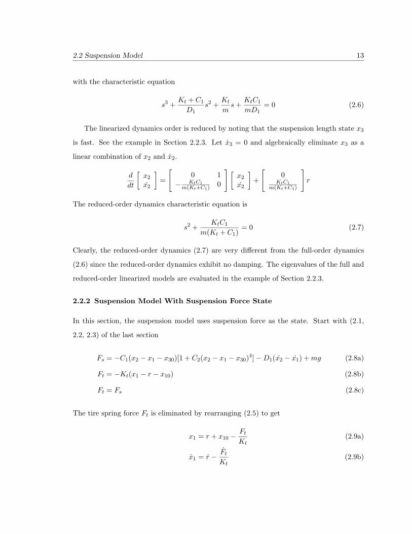
2.2 Suspension Model 13
with the characteristic equation
s3 +Kt + C1
D1s2 +
Kt
ms+
KtC1
mD1= 0 (2.6)
The linearized dynamics order is reduced by noting that the suspension length state x3
is fast. See the example in Section 2.2.3. Let x3 = 0 and algebraically eliminate x3 as a
linear combination of x2 and x2.
d
dt
[x2
x2
]=
[0 1
− KtC1m(Kt+C1) 0
] [x2
x2
]+
[0
KtC1m(Kt+C1)
]r
The reduced-order dynamics characteristic equation is
s2 +KtC1
m(Kt + C1)= 0 (2.7)
Clearly, the reduced-order dynamics (2.7) are very different from the full-order dynamics
(2.6) since the reduced-order dynamics exhibit no damping. The eigenvalues of the full and
reduced-order linearized models are evaluated in the example of Section 2.2.3.
2.2.2 Suspension Model With Suspension Force State
In this section, the suspension model uses suspension force as the state. Start with (2.1,
2.2, 2.3) of the last section
Fs = −C1(x2 − x1 − x30)[1 + C2(x2 − x1 − x30)4]−D1(x2 − x1) +mg (2.8a)
Ft = −Kt(x1 − r − x10) (2.8b)
Ft = Fs (2.8c)
The tire spring force Ft is eliminated by rearranging (2.5) to get
x1 = r + x10 −FtKt
(2.9a)
x1 = r − FtKt
(2.9b)

14 Chapter 2: Vehicle Model
and then combining (2.8a), (2.8c) and (2.9) as
F =Kt
D1{−F +mg − C1(x2 − r − x10 − x30 +
F
Kt)
[1 + C2(x2 − r − x10 − x30 +F
Kt)4]−D1(x2− r)}
where F4= Fs. An equation of motion for the chassis is given by combining (2.5) with (2.8b)
and (2.8c)
mx2 = F
The linearized model is
d
dt
x2
x2
F
=
0 1 00 0 1
m
−KtC1D1
−Kt −Kt+C1D1
x2
x2
F
+
0 00 0
KtC1D1
Kt
[ rr
]with the characteristic equation
s3 +Kt + C1
D1s2 +
Kt
ms+
KtC1
mD1= 0 (2.10)
which is the same as (2.6) as expected.
Again, since the suspension force state F is fast, the reduced-order linearized model is
derived by letting F = 0 and algebraically eliminating F as a linear combination of x2 and
x2.
d
dt
[x2
x2
]=
[0 1
− KtC1m(Kt+C1) − KtD1
m(Kt+C1)
] [x2
x2
]+
[0 0
KtC1m(Kt+C1)
KtD1m(Kt+C1)
] [rr
]
The reduced-order dynamics characteristic equation is
s2 +KtD1
m(Kt + C1)s+
KtC1
m(Kt + C1)= 0 (2.11)
This reduced-order model includes a damping term and is probably a more realistic model
than the reduced-order model of Section 2.2.1. However, note that this model regards road
displacement r and road displacement rate r as two independent inputs. In the physical
system being modelled, they are not independent. The eigenvalues of this model are also
evaluated in Section 2.2.3.

2.2 Suspension Model 15
2.2.3 Example
Here is a numerical example of a suspension model. The parameters are obtained from the
vehicle simulation code from U.C. Berkeley.
m = 393.25 kg Mass of a quarter car.
Kt = 190632Nm
Tire spring constant.
C1 = 17000Nm
Suspension spring constant.
D1 = 1500N · sm
Suspension damper constant.
The eigenvalues of both full-order models in Section 2.2.1 and 2.2.2 are the same: −135.13,
−1.64± 6.16i. The eigenvalues of the reduced-order model in Section 2.2.1 are ±6.30i and
the eigenvalues of the reduced-order model in Section 2.2.2 are −1.75 ± 6.05i. The light
damping of the force-state model of Section 2.2.2 is more realistic so this model is considered
to be a better representation of the suspension dynamics.
Remark 1. If the model reduction is done by balanced realization and truncation, the
length-state and force-state realizations should have similar reduced-order linear models.
Balanced realization and truncation, discussed in detail in (Douglas et al. 1996), truncates
the least observable and controllable modes as determined by inspection of the observability
and controllability Grammians. By this method, the truncated modes are not necessarily
the fast modes so that the eigenvalues of the reduced-order model might be very different
from those of the full-order model. Further, when fast modes are truncated, the simple
state truncation with steady-state correction method illustrated in Sections 2.2.1 and 2.2.2
produces results that are dependent on the state basis. Regarding a balanced realization
as just another basis, it is possible that for some problems, a balanced realization does not
provide a best reduced-order model. Best is problem dependent but is generally determined
by comparing the full and reduced-order frequency responses and eigenstructures.

16 Chapter 2: Vehicle Model
2.3 Manifold Temperature Model
In the engine model the manifold temperature is taken to be a constant. If a manifold
temperature sensor is to be monitored for a fault, two sensor models are possible. One model
has the manifold temperature as an engine state and appends an integrator to the engine
dynamics. Another model considers the manifold temperature as a measured exogenous
input.
Since manifold temperature changes are on a much longer time scale than the engine
dynamics, it is a natural choice to model the manifold temperature as a constant. With a
constant manifold temperature as an engine state, an integrator is appended to the engine
dynamics. [xxTm
]=[A BTm0 0
] [xxTm
]+[B0
]u
y =[C 00 1
] [xxTm
]where xTm is the manifold temperature state and x are the rest of the states. A problem
with this model is that the observability Grammian is ill-defined because the eigenvalue at
the origin is associated with a measured state, the temperature xTm .
An alternate model has the temperature as a known, that is measured, input to the
engine.
x = Ax+Bu+BTmωTm
yx = Cx
yω = ωTm
This approach avoids the observability Grammian problem and seems more reasonable in
that the manifold temperature is an environmental factor which cannot be controlled.

Chapter 3
Fault Detection By Analytic Redundancy
Analytic redundancy is an approach to health monitoring that compares dissimilar
instruments using a detailed system model. The approach is to find dynamic or algebraic
relationships between sensors and actuators. That is, information provided by a monitored
sensor is, in some form, also provided by other sensors or, through the dynamics, by actuator
commands. In automated vehicles, these requirements preclude monitoring nonredundant
sensors such as obstacle detection or lane position sensors. The information provided by
a radar or infrared sensor designed to detect objects in the vehicle’s path has no dynamic
correlation with other sensors on the vehicle. A sensor that detects the vehicle’s position in
a lane is the only sensor that can provide this information. Actuators that do no observable
action are also difficult to monitor. For example, the health of a power window actuator is
easily monitored by the driver. But, unless specialized sensors are installed, no other part
of the car is affected by the operation of this actuator and there is no analytic redundancy.
A range sensor is another example of a sensor for which a vehicle has no redundant
information. In some configurations, range information is provided by several different
17

18 Chapter 3: Fault Detection By Analytic Redundancy
types of sensors, for example, radar and optical range sensors. In this type of design, the
sensor measurements are fused at the vehicle regulation layer. So, for the purposes of vehicle
control and fault detection, the range sensors are regarded as providing a single synthesized,
and nonredundant, measurement.
Analytic dynamic redundancy requires a detailed model of the dynamic relationship
between sensors and actuator commands. This information is encoded in a fault detection
filter that detects and isolates faults by producing a static pattern in a linear observer
residual. Most sensors and actuators associated with the vehicle longitudinal dynamics
are monitored this way. Fault detection filter design is described in Section 3.1. Algebraic
redundancy provides a simple algebraic parity equation that must be satisfied. For example,
since the throttle actuator dynamics are very fast, the throttle actuator command minus
the throttle actuator position is nominally zero. Parity equation design is described in 3.2.
The fault detection and isolation system is summarized in Section 3.3.
3.1 Analytic Redundancy
Eleven sensors and two actuators are to be monitored. The sensors are the manifold air mass
sensor yma , engine speed sensor yωe , manifold temperature sensor yTm , manifold pressure
sensor ypm, longitudinal velocity sensor yvx and accelerometer yax , vertical accelerometer
yaz , the sum of front wheel speed sensors yωf , the sum of rear wheel speed sensors yωr ,
throttle sensor yα and brake sensor yTb . The two actuators are the throttle uα and brake
uTb . Three of the sensors yα, yTb and ypm, are monitored with algebraically redundant
information. Hence, eight sensors and two actuators are included in the fault detection
filter design.
A very brief review of the fault detection filter is provided in Section 3.1.1. Section 3.1.2
describes the sensor and actuator fault models. Section 3.1.3 discusses several design
considerations that are specific to the longitudinal vehicle dynamics health monitoring
problem. Section 3.1.4 discusses how multiple faults are grouped among several filters. The
fault detection filter designs are sensor and actuator fault groups described in Sections 3.1.5

3.1 Analytic Redundancy 19
and 3.1.6.
3.1.1 Beard-Jones Fault Detection Filter Background
A detailed review of fault detection filter design is provided in Appendix A of last year’s
report (Douglas et al. 1996). For a thorough background, several references are available,
a few of which are (Douglas 1993), (White and Speyer 1987) and (Massoumnia 1986).
Consider a linear time-invariant system with q failure modes and no disturbances or
sensor noise
x = Ax+Bu+q∑i=1
Fimi (3.1a)
y = Cx+Du (3.1b)
The system variables x, u, y and the mi belong to real vector spaces and the system maps
A, B, C, D and the Fi are of compatible dimensions. Assume that the input u and the
output y both are known. The Fi are the failure signatures. They are known and fixed and
model the directional characteristics of the faults. The mi are the failure modes and model
the unknown time-varying amplitude of faults. The mi do not have to be scalar values.
A fault detection filter is a linear observer that, like any other linear observer, forms a
residual process sensitive to unknown inputs. Consider a full-order observer with dynamics
and residual
˙x = (A+ LC)x+Bu− Ly (3.2a)
r = Cx+Du− y (3.2b)
Form the state estimation error e = x− x and the dynamics and residual are
e = (A+ LC)e−q∑i=1
Fimi
r = Ce
In steady-state, the residual is driven by the faults when they are present. If the system
is (C,A) observable, and the observer dynamics are stable, then in steady-state and in the

20 Chapter 3: Fault Detection By Analytic Redundancy
absence of disturbances and modeling errors, the residual r is nonzero only if a fault has
occurred, that is, if some mi is nonzero. Furthermore, when a fault does occur, the residual
is nonzero except in certain theoretically relevant but physically unrealistic situations. This
means that any stable observer can detect the presence of a fault. Simply monitor the
residual and when it is nonzero a fault has occurred.
In addition to detecting a fault, a fault detection filter provides information to determine
which fault has occurred. An observer such as (3.2) becomes a fault detection filter when
the observer gain L is chosen so that the residual has certain directional properties that
immediately identify the fault. The gain is chosen to partition the residual space where each
partition is uniquely associated with one of the design fault directions Fi. A fault is identified
by projecting the residual onto each of the residual subspaces and then determining which
projections are nonzero.
In a detection filter, the state estimation error in response to a fault in the direction
Fi remains in a state subspace T ∗i , an unobservability subspace or detection space. See
Appendix A of last year’s report (Douglas et al. 1996) for details. The ability to identify
a fault, to distinguish one fault from another, requires, for an observable system, that the
detection spaces be independent. Thus, the number of faults that can be detected and
identified by a fault detection filter is limited by the size of the state space and the sizes of
the detection spaces associated with each of the faults. If the problem considered has more
faults than can be accommodated by one fault detection filter, then a bank of filters will
have to be constructed.
For a fault Fi, the approach to finding the detection space T ∗i is to find the minimal
(C,A)-invariant subspaceW∗i that contains Fi and then to find the invariant zero directions
of the triple (C,A, Fi), if any. With the invariant zero directions denoted by V i, the minimal
unobservability subspace T ∗i is given by
T ∗i =W∗i + V i
Before the fault detection filter design (3.2) can begin, a system model with faults has
to be found with the form (3.1). This is discussed in the next section.
3.1 Analytic Redundancy 21
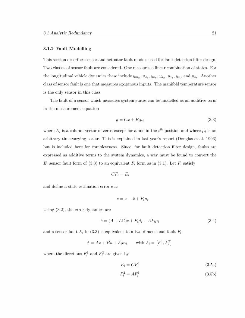
3.1.2 Fault Modelling
This section describes sensor and actuator fault models used for fault detection filter design.
Two classes of sensor fault are considered. One measures a linear combination of states. For
the longitudinal vehicle dynamics these include yma , yωe , yvx , yax , yaz , yωf and yωr . Another
class of sensor fault is one that measures exogenous inputs. The manifold temperature sensor
is the only sensor in this class.
The fault of a sensor which measures system states can be modelled as an additive term
in the measurement equation
y = Cx+ Eiµi (3.3)
where Ei is a column vector of zeros except for a one in the ith position and where µi is an
arbitrary time-varying scalar. This is explained in last year’s report (Douglas et al. 1996)
but is included here for completeness. Since, for fault detection filter design, faults are
expressed as additive terms to the system dynamics, a way must be found to convert the
Ei sensor fault form of (3.3) to an equivalent Fi form as in (3.1). Let Fi satisfy
CFi = Ei
and define a state estimation error e as
e = x− x+ Fiµi
Using (3.2), the error dynamics are
e = (A+ LC)e+ Fiµi −AFiµi (3.4)
and a sensor fault Ei in (3.3) is equivalent to a two-dimensional fault Fi
x = Ax+Bu+ Fimi with Fi =[F 1i , F
2i
]where the directions F 1
i and F 2i are given by
Ei = CF 1i (3.5a)
F 2i = AF 1
i (3.5b)
22 Chapter 3: Fault Detection By Analytic Redundancy
An interpretation of the effect of a sensor fault on observer error dynamics follows from
(3.4) where F 1i is the sensor fault rate µi direction and F 2
i is the sensor fault magnitude
µi direction. This interpretation suggests a possible simplification when information about
the spectral content of the sensor fault is available. If it is known that a sensor fault has
persistent and significant high frequency components, such as in the case of a noisy sensor,
the fault direction could be approximated by the F 1i direction alone. Or, if it is known
that a sensor fault has only low frequency components, such as in the case of a bias, the
fault direction could be approximated by the F 2i direction alone. For example, if a sensor
were to develop a bias, a transient would be likely to appear in all fault directions but, in
steady-state, only the residual associated with the faulty sensor should be nonzero.
A linear model partitioned to isolate first-order actuator dynamics can be expressed as
[xxa
]=[A B0 −ω
] [xxa
]+[
0ω
]u+Bωω
where xa is a vector of actuator states and ω is an exogenous input. Typically, exogenous
inputs are dynamic disturbances such as road noise and wind gusts and are not known or
measured. However, as described in Section 2.3, the manifold temperature is modelled as a
dynamic input and is measured. A fault in this sensor is modelled as a direction given by
the associated column of the Bω matrix.
A fault in a control input is also modeled as an additive term in the system dynamics.
In the case of a fault appearing at the input of an actuator, that is the actuator command,
the fault has the same direction as the associated column of the [0, ω]T matrix. A fault
appearing at the output of an actuator, the actuator position, has the same direction as the
associated column of the [BT , 0]T matrix. In the vehicle model, the actuator dynamics are
relatively fast and, in an approximation made here, are removed from the system model.
Thus, the control inputs are applied directly to the system through a column of the B
matrix.

3.1 Analytic Redundancy 23
3.1.3 Special Design Considerations
Several design considerations arise that are specific to the longitudinal vehicle dynamics
health monitoring problem. One problem is a conditioning problem that arises from the
model order reduction done in Section 2.1. Another concerns the output separability of the
modeled faults. A third problem concerns a reasonable expectation that a fault detection
filter should produce a nonzero fault residual for as long as a modeled fault is present.
Ill-conditioned fault direction
For all sensor and throttle actuator faults described in Section 3.1.2, the detection or
minimal unobservability subspaces are given by the fault directions themselves, that is,
T ∗i =W∗i + V i = ImFi
For example, for the brake actuator, T ∗i = ImFi because CFuTb 6= 0, (Douglas et al. 1996).
However, CFuTb 6= 0 only holds for the reduced, eighth-order model. For the full-order
model, CFuTb = 0 so FuTb should be considered as a very weakly observable direction. For
fault detection filter design, the brake actuator unobservability subspace is taken to be the
second-order space given by
T ∗uTb = Im[FuTb , AFuTb
]Output separability
The output separability design requirement states that the residuals produced by design
faults be pairwise linearly independent. Faults that are not output separable generate
co-linear residuals and cannot be isolated. Output separability of two faults Fi and Fj is
determined by
CT ∗i ∩ CT ∗j = 0 (3.6)
which may be checked by the column independence of realizations for CT i and CT j .
24 Chapter 3: Fault Detection By Analytic Redundancy
Performing the check (3.6) reveals that two pairs of faults are not output separable.
The throttle actuator uα and manifold air mass sensor yma faults are not output separable
and the manifold temperature sensor yTm and manifold air mass sensor yma faults are not
output separable. The problem is summarized as
T ∗uα = Fuα
T ∗yTm = FyTm
T ∗yma =[Fyma AFyma
]Fuα = Fyma
FyTm = AFyma
First, consider the throttle actuator and manifold air mass sensor faults where CFuα =
CFyma indicates that they cannot be isolated. As explained in Section 3.1.2, the direction
of the air mass sensor fault magnitude is AFyma while the direction of the fault rate is Fyma .
The throttle actuator and air mass sensor faults become output separable if only the sensor
fault magnitude direction is used. This design decision could allow a noisy but zero mean
sensor fault to remain undetected through the direction CAFyma . Also, since the throttle
fault detection space is spanned by Fuα = Fyma , an air mass sensor fault rate will stimulate
the throttle fault residual. However, a throttle actuator fault could never stimulate the
air mass sensor fault residual. In summary, as long as the air mass sensor fault spectral
components are low frequency, the throttle actuator and manifold air mass sensor faults
should be detectable and isolatable.
Next, consider the manifold temperature and air mass sensor faults where CFyTm =
CAFyma indicates that they cannot be isolated. Since AFyma represents the fault magnitude
direction, this direction can not be dropped from the detection space. One remedy is
to design a second fault detection filter that does not take the manifold air mass as a
measurement. Such a filter will be unaffected by air mass sensor faults but will respond to
manifold temperature sensor faults. A problem with this fix is that the throttle actuator and
temperature sensor faults are not output separable without an air mass sensor measurement.
3.1 Analytic Redundancy 25
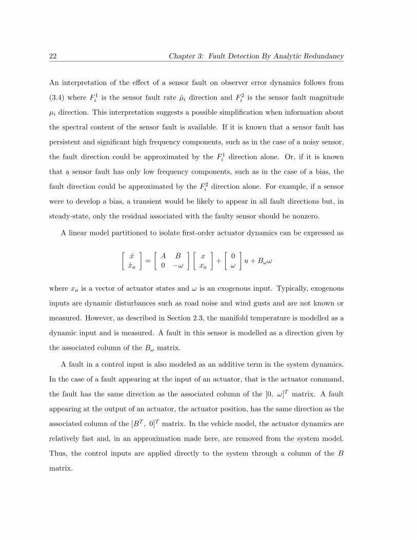
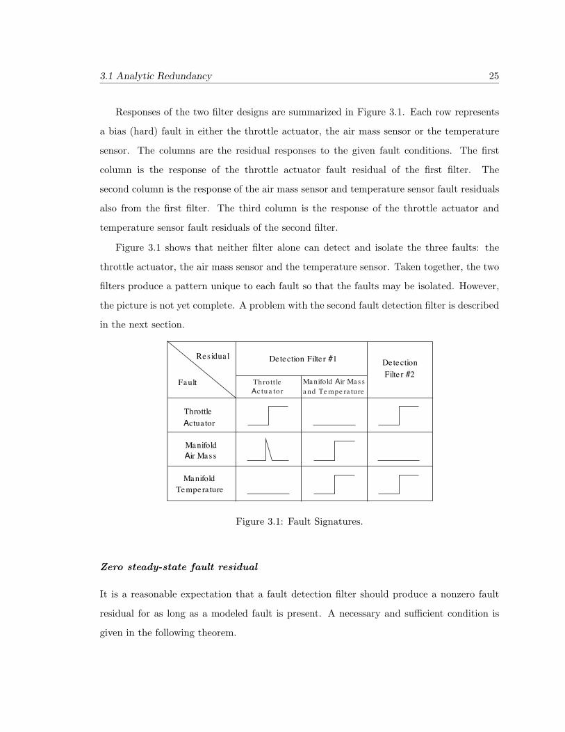
Responses of the two filter designs are summarized in Figure 3.1. Each row represents
a bias (hard) fault in either the throttle actuator, the air mass sensor or the temperature
sensor. The columns are the residual responses to the given fault conditions. The first
column is the response of the throttle actuator fault residual of the first filter. The
second column is the response of the air mass sensor and temperature sensor fault residuals
also from the first filter. The third column is the response of the throttle actuator and
temperature sensor fault residuals of the second filter.
Figure 3.1 shows that neither filter alone can detect and isolate the three faults: the
throttle actuator, the air mass sensor and the temperature sensor. Taken together, the two
filters produce a pattern unique to each fault so that the faults may be isolated. However,
the picture is not yet complete. A problem with the second fault detection filter is described
in the next section.
Tempera tureManifold
Air MassManifold
Actua torThrottle
Detection Filte r #1 DetectionFilte r #2
Fault
Res idua l
Thro ttle Ma nifold Air Ma s sa nd Te mpe ra tureAc tu a to r
Figure 3.1: Fault Signatures.
Zero steady-state fault residual
It is a reasonable expectation that a fault detection filter should produce a nonzero fault
residual for as long as a modeled fault is present. A necessary and sufficient condition is
given in the following theorem.

26 Chapter 3: Fault Detection By Analytic Redundancy
Theorem 3.1. A necessary and sufficient condition for a fault detection filter residual to
hold a non-zero steady-state value in response to a bias fault is CA−1F 6= 0, that is,
C(sI −A− LC)−1F |s=0 = 0 ⇔ CA−1F = 0
Proof. Let F4= (A+ LC)−1F . (⇒)
F = (A+ LC)F = AF because CF = C(A+ LC)−1F = 0.
⇒ F = A−1F
⇒ CA−1F = CF = 0
(⇐)
AF + LCF = F
⇒ F = A−1F because CA−1F = 0 and (A+ LC) is unique.
⇒ C(A+ LC)−1F = CF = CA−1F = 0
Since CA−1FyTm = 0, the second fault detection filter will not see the temperature sensor
faults in the steady state. When a temperature bias fault occurs, the residual responds
with only a transient. Figure 3.1 is corrected in Figure 3.2 to illustrate the transitory
response. Once again, the fault patterns for the three faults are not unique, at least not in
steady-state.
Since a second fault detection filter no longer fixes the output separability problem,
another fix is needed. An algebraic relation between the manifold pressure and manifold
air mass is useful
manifold pressure− 19.9635 ∗manifold air mass = 0 (3.7)
This convenient relation arises from the perfect gas law. The magic number 19.9635 includes
the gas constant, a nominal temperature and the manifold volume. Equation (3.7) is a

3.1 Analytic Redundancy 27
Tempera tureManifold
Air MassManifold
Actua torThrottle
Detection Filte r #1 DetectionFilte r #2
Fault
Res idua l
Thro ttle Ma nifold Air Ma s sa nd Te mpe ra tureAc tu a to r
Figure 3.2: Fault Signatures.
parity equation that is satisfied when the manifold pressure and manifold air mass sensors
are working and is not satisfied when either sensor has failed. The parity equation by itself
cannot isolate a fault.
By combining the parity equation (3.7) with the first fault detection filter of the last
section, a residual pattern unique to each fault is formed and the faults may be isolated. The
faults are the throttle actuator, the air mass sensor, the temperature sensor and the manifold
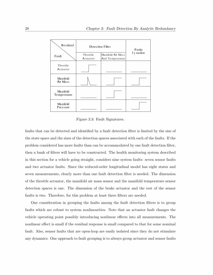
pressure sensor. The residual patterns are summarized in Figure 3.3 Each row represents
a bias (hard) fault in either the throttle actuator, the air mass sensor, the temperature
sensor or the manifold pressure sensor. The columns are the residual responses to the given
fault conditions. The first column is the response of the throttle actuator fault residual of
the first filter. The second column is the response of the air mass sensor and temperature
sensor fault residuals also from the first filter. The third column is the response of the parity
equation for the manifold air mass and pressure sensors. The parity equation is discussed
further in Section 3.2.
3.1.4 Fault Assignment to Multiple Fault Detection Filters
The ability to identify a fault, to distinguish one fault from another, requires for an
observable system that the detection spaces be independent. Therefore, the number of
28 Chapter 3: Fault Detection By Analytic Redundancy
ManifoldPressure
ManifoldAir Mass
ManifoldTempera ture
Detection Filte rParity
EquationFault
Res idua l
Ma nifold Air Ma s sAnd Te mpe ra ture
Thro ttleAc tu a to r
Thro ttleAc tu a to r
Figure 3.3: Fault Signatures.
faults that can be detected and identified by a fault detection filter is limited by the size of
the state space and the sizes of the detection spaces associated with each of the faults. If the
problem considered has more faults than can be accommodated by one fault detection filter,
then a bank of filters will have to be constructed. The health monitoring system described
in this section for a vehicle going straight, considers nine system faults: seven sensor faults
and two actuator faults. Since the reduced-order longitudinal model has eight states and
seven measurements, clearly more than one fault detection filter is needed. The dimension
of the throttle actuator, the manifold air mass sensor and the manifold temperature sensor
detection spaces is one. The dimension of the brake actuator and the rest of the sensor
faults is two. Therefore, for this problem at least three filters are needed.
One consideration in grouping the faults among the fault detection filters is to group
faults which are robust to system nonlinearities. Note that an actuator fault changes the
vehicle operating point possibly introducing nonlinear effects into all measurements. The
nonlinear effect is small if the residual response is small compared to that for some nominal
fault. Also, sensor faults that are open-loop are easily isolated since they do not stimulate
any dynamics. One approach to fault grouping is to always group actuator and sensor faults

3.1 Analytic Redundancy 29
with different fault detection filters.
Usually an attempt is made to group as many faults as possible in each filter. When
full-order filters are used, this approach minimizes the number of filters needed. When
reduced-order filters are used, this approach minimizes the order of each complementary
space and, therefore, the order of each reduced-order filter. Note that each fault included in
a fault detection filter design imposes more constraints on the filter eigenvectors. Sometimes,
the objective of obtaining well-conditioned filter eigenvectors imposes a tradeoff between
robustness and the reduced-order filter size.
With all the considerations above in mind, now we should decide how many fault
detection filters are needed and which faults should go together. Robustness to nonlinearities
requires all the actuator faults to be in the same filter. The output separability consideration
of Section 3.1.3 requires the throttle actuator and manifold air mass sensor fault to be in
the same filter. Thus, one fault detection filter has the throttle actuator uα, brake actuator
uTb and manifold air mass sensor yma . Note that this filter is also sensitive to faults in the
manifold temperature sensor yTm since manifold temperature and manifold air mass sensor
faults are not output separable.
The six remaining sensor faults, yωe , yvx , yax , yaz , yωf and yωr are assigned to two more
fault detection filters. Each filter has three faults. There are ten different combinations
for these two filters and they are all non-mutually detectable which means the invariant
zeros arising from the fault combinations will be the eigenvalues of the filters, that is, some
poles of the filters cannot be assigned. In six of these cases, the invariant zeros, hence the
fixed poles, are in the right-half plane resulting in an unstable fault detection filter. The
remaining four configurations are stable. Each stable case has been designed and tested.
The most robust combination is to put yωe , yax and yωf into the second filter and put yvx ,
yaz and yωr into the third filter. Here, most robust is taken to mean the filter with left
eigenvectors that are least ill-conditioned. This hedges against eigenstructure sensitivity to
small variations in system parameters. The three fault detection filters are

30 Chapter 3: Fault Detection By Analytic Redundancy
Fault detection filter 1.
uα : Throttle actuator.
uTb : Brake actuator.
yma : Manifold air mass sensor.
yTm : Manifold temperature sensor.
Fault detection filter 2.
yωe : Engine speed sensor.
yax : Longitudinal accelerometer.
yωf : Sum of front wheel speed sensors.
Fault detection filter 3.
yvx : Longitudinal velocity sensor.
yaz : Vertical accelerometer.
yωr : Sum of rear wheel speed sensors.
3.1.5 Fault Detection Filter Design For Sensors
In this and the following sections, Beard-Jones fault detection filters have been designed
using eigenstructure assignment while ensuring that the eigenvectors are not ill-conditioned.
The essential feature of a fault detection filter is the detection space structure embedded
in the filter dynamics. A left eigenvector assignment design algorithm explicitly places
eigenvectors to span these subspaces. An eigenvector assignment design algorithm also
has to balance the objective of having well-conditioned eigenvectors for robustness against
the objective of each fault being highly input observable for fault detection performance.
System disturbances, sensor noise and system parameter variations are not considered in
the fault detection filter designs described in this report. Note that they are considered
in performance evaluation. For such a benign environment, the filter designs are based on

3.1 Analytic Redundancy 31
spectral considerations only; there is little else that can be used to distinguish a good design
from a bad design.
Since the calculations are somewhat long and they are the similar for each detection
filter, the calculation details are given for only the first and third fault detection filters. In
this section, the fault detection filter is designed for the third fault group which has the
longitudinal velocity sensor yvx , the vertical accelerometer yaz and the sum of rear wheel
speed sensors yωr . In next section, a filter is designed for the first fault group which has the
throttle actuator uα, the brake actuator uTb and the manifold air mass sensor yma . Note
once again that the manifold air mass sensor yma is not output separable with respect to
the manifold temperature sensor yTm .
The eight state reduced-order longitudinal model derived in Section 2.1 is used. The
dimension of each detection space was found in Section 3.1.4 as
νyvx = dim T ∗yvx = 2
νyaz = dim T ∗yaz = 2
νyωr = dim T ∗yωr = 2
The dimension of the fault detection filter complementary space T 0 is also needed. The
complementary space is any subspace independent of the detection spaces that completes
the state-space.
X = T ∗yvx ⊕ T∗yaz⊕ T ∗yωr ⊕ T 0
Thus the dimension of T 0 is two
ν0 = n− νyvx − νyaz − νyωr= 8− 2− 2− 2
= 2
Next define the complementary faults sets. There are three faults Fyvx , Fyaz and Fyωr

32 Chapter 3: Fault Detection By Analytic Redundancy
so there are four complementary fault sets which are:
Fyvx =[Fyaz , Fyωr
](3.8a)
Fyaz =[Fyvx , Fyωr
](3.8b)
Fyωr =[Fyvx , Fyaz
](3.8c)
F0 =[Fyvx , Fyaz , Fyωr
](3.8d)
Now choose the filter closed-loop eigenvalues. As discussed in Section 3.1.4, these three
faults are not mutually detectable. Therefore the invariant zero −14.52 has to be one of
the eigenvalues of the complementary subspace. Since the system model includes no sensor
noise, no disturbances and no parameter variations, there is little basis for preferring one
set of detection filter closed-loop eigenvalues over another. The poles are chosen here to
give a reasonable response time but are not unrealistically fast. The assigned eigenvalues
are
Λyvx = {−3,−4}
Λyaz = {−3,−4}
Λyωr = {−3,−4}
Λ0 = {−3,−14.52}
The next step is to find the closed-loop fault detection filter left eigenvectors. For each
eigenvalue λij ∈ Λi, the left eigenvectors vij generally are not unique and must be chosen
from a subspace as vij ∈ Vij where Vij and another space Wij are found by solving[AT − λijI CT
F Ti 0
] [VijWij
]=[
00
](3.9)
There are eight Vij associated with eight eigenvalues. To help desensitize the fault detection
filter to parameter variations, the left eigenvectors are chosen from vij ∈ Vij as the set with
the greatest degree of linear independence. The degree of linear independence is indicated
by the smallest singular value of the matrix formed by the left eigenvectors. Upper bounds

3.1 Analytic Redundancy 33
on the singular values of the left eigenvectors are given by the singular values of
V = [V01 , V02 , Vyvx1, Vyvx2
, Vyaz1 , Vyaz2 , Vyωr1 , Vyωr2 ]
These singular values are
σ(V ) = {2.83, 2.50, 1.69, 1.41, 1.32, 0.333, 0.080, 0.0088} (3.10)
If the left eigenvector singular value upper bounds were small, then all possible combinations
of detection filter left eigenvectors would be ill-conditioned and the filter eigenstructure
would be sensitive to small parameter variations. Since (3.10) indicates that the upper
bounds are not small, continue by looking for a set of fault detection filter left eigenvectors
that are reasonably well-conditioned. For this case, one possible set of left eigenvectors
from the set V nearly meets the upper bound and should be well-conditioned. The singular
values of this set of left eigenvectors are
σ(V ) = {1.95, 1.12, 1.00, 1.00, 0.92, 0.285, 0.063, 0.00691}
Since the difference between the largest and the smallest singular values is only three orders
of magnitude, the detection filter gain will be reasonably small and the filter eigenstructure
should not be sensitive to small parameter variations.
The fault detection filter gain L is found by solving
V TL = W T (3.11)
where V is the matrix of left eigenvectors as found above, and W is a matrix of vectors wij[AT − λijI CT
F Ti 0
] [vijwij
]=[
00
]If the left eigenvector vij is a linear combination of the columns of Vij , wij is the same linear
combination of the columns of Wij where Vij and Wij are from (3.9).
To complete the detection filter design, output projection matrices Hyvx , Hyaz and Hyωr
are needed to project the residual along the respective output subspaces CT ∗yvx , CT ∗yaz and
34 Chapter 3: Fault Detection By Analytic Redundancy
CT ∗yωr . What this means is that, for example, T ∗yvx becomes the unobservable subspace
of the pair (HyvxC,A + LC). Remember that by the definition of the complementary
faults (3.8), faults Fyaz and Fyωr lie in T ∗yvx and fault Fyvx does not. The effect is that the
projected residual is driven by fault Fyvx and only fault Fyvx .
A projection Hi is computed by first finding a basis for the range space of CT ∗i where
again, T ∗i is any basis for the detection space T ∗i . This is done by finding the left singular
vectors of CT ∗i . Denote this basis for now as hi. Then Hi is given by
Hi = I − hihTi
In summary, a fault detection filter for the system with sensor faults Eyvx , Eyaz and
Eyωr
x = Ax+Bu+BTmωTm
y = Cx+Du+ Eyvxµyvx + Eyazµyaz + Eyωrµyωr
is equivalent to a fault detection filter for the system with faults Fyvx , Fyaz and Fyωr
x = Ax+Bu+BTmωTm + Fyvxmyvx + Fyazmyaz + Fyωrmyωr
y = Cx+Du
and has the form
˙x = (A+ LC)x+ (B + LD)u+BTmyTm − Ly
zyvx = Hyvx (Cx+Du− y)
zyaz = Hyaz (Cx+Du− y)
zyωr = Hyωr (Cx+Du− y)
where L, Hyvx , Hyaz and Hyωr are shown in Appendix A.
A fault detection filter design for the second fault group is carried out in the similar way
and is not shown here. However, the filter gain L and projections Hyωe , Hyax and Hyωfare
shown in Appendix A.
3.1 Analytic Redundancy 35
3.1.6 Fault Detection Filter Design For Actuators
In next section, a fault detection filter is designed for the first fault group which has the
throttle actuator uα, the brake actuator uTb and the manifold air mass sensor yma . Note
once again that the manifold air mass sensor yma is not output separable with respect to
the manifold temperature sensor yTm .
The design procedure is similar to the previous section but does have a twist. As
discussed in Section 3.1.3, a reduced-order manifold air mass sensor fault is used to achieve
output separability with the throttle actuator fault. Also manifold air mass and manifold
temperature sensor faults cannot be isolated.
The dimension of each detection space was found in Section 3.1.4 as
νuα = dim T ∗uα = 1
νuTb = dim T ∗uTb = 2
νyma = dim T ∗yma = 1
and the dimension of the fault detection filter complementary space T 0 where
X = T ∗uα ⊕ T∗uTb⊕ T ∗yma ⊕ T 0
is four
ν0 = n− νuα − νuTb − νyma= 8− 1− 2− 1
= 4
Next define the complementary faults sets. There are three faults Fuα , FuTb and Fyma
so there are four complementary fault sets which are:
Fuα =[FuTb , Fyma
](3.12a)
FuTb =[Fuα , Fyma
](3.12b)
Fyma =[Fuα , FuTb
](3.12c)
F0 =[Fuα , FuTb , Fyma
](3.12d)

36 Chapter 3: Fault Detection By Analytic Redundancy
Now choose the fault detection filter closed-loop eigenvalues. Since these three faults are
mutually detectable, all eigenvalues are freely assignable.
Λuα = {−3}
ΛuTb = {−3, −4}
Λyma = {−3}
Λ0 = {−3, −4, −5, −6}
The next step is to find the closed-loop fault detection filter left eigenvectors. The left
eigenvectors vij for each eigenvalue λij ∈ Λi generally are not unique and must be chosen
from a subspace as vij ∈ Vij where Vij is found by solving[AT − λijI CT
F Ti 0
] [VijWij
]=[
00
](3.13)
There are eight Vij associated with eight eigenvalues. Upper bounds on the singular values
of the left eigenvectors are given by the singular values of
V = [V01 , V02 , V03 , V04 , Vuα , VuTb1 , VuTb2 , Vyma ]
These singular values are
σ(V ) = {2.83, 2.83, 2.82, 1.98, 1.41, 0.290, 0.174, 0.021} (3.14)
Since (3.14) indicates that the upper bounds are not small, continue by looking for a set
of fault detection filter left eigenvectors that are reasonably well-conditioned. One possible
choice has the following singular values
σ(V ) = {1.46, 1.41, 1.35, 1.00, 1.00, 0.235, 0.056, 0.0028}
Since these singular values are quite close to their respective upper bounds, the detection
filter gain should not be large and the filter eigenstructure should not be sensitive to small
parameter variations. As in Section 3.1.5, the fault detection filter gain L is found by solving
V TL = W T (3.15)

3.2 Algebraic Redundancy 37
where the columns of V and W are found from (3.13). Output projection matrices Huα ,
HuTb, Hyma and HyTm are found in the same way as for the sensor fault example of
Section 3.1.5. The filter gain L and projections Huα , HuTb, Hyma and HyTm are shown
in Appendix A
A note should be made regarding the throttle actuator fault residual. By the definition
of the complementary faults (3.12), FuTb and Fyma lie in T ∗uα while Fuα does not. The effect
is that the projected residual is not driven by fault FuTb or Fyma . Now recall that Fyma is a
reduced-order approximation for Eyma so the throttle actuator residual is not only driven by
Fuα , but also the part of Eyma not modeled by Fyma . As shown in Figure 3.4, the throttle
actuator residual can only isolate faults well at low frequency while other residuals isolate
all faults.
10-3
10-2
10-1
100
101
102
103
-350
-300
-250
-200
-150
-100
-50
0
rad/s
db
Figure 3.4: Singular value frequency response from all faults to throttle residual.
3.2 Algebraic Redundancy
Algebraic parity equations provide a second component to the fault detection and isolation
system. The following algebraically redundant pairs are available: the throttle sensor yα

38 Chapter 3: Fault Detection By Analytic Redundancy
and throttle actuator, the brake sensor yTb and brake actuator uTb and the manifold pressure
sensor ypm and manifold air mass sensor yma. Three parity equations are defined:
1. 0 = Throttle sensor yα− Throttle actuator uα
2. 0 = Brake sensor yTb− Brake actuator uTb
3. 0 = Manifold pressure sensor ypm− Manifold air mass sensor yma ∗ 19.9635
None of the parity equations can by itself identify a fault. But by combining the parity
equations with the first fault group detection filter of Section 3.1.4, a unique residual pattern
is presented allowing each fault to be isolated. The patterns are summarized in Figure 3.5.
Each row of Figure 3.5 represents a bias (hard) fault in either the throttle actuator,
the throttle sensor, the brake actuator, the brake sensor, the manifold air mass sensor,
the manifold temperature sensor or the manifold pressure sensor. The columns are the
residual responses to the given fault conditions. The first column is the response of the
throttle actuator fault residual of the first filter. The second column is the response of the
brake actuator fault residual of the first filter. The third column is the response of the air
mass sensor and temperature sensor residuals of the first filter. The fourth, fifth and sixth
columns are responses of the first, second and third parity equations.
3.3 Structure
Combining the fault detection filters of Section 3.1 and parity equations in Section 3.2, a
set of six analytic redundancy relationships either dynamic or algebraic are presented. The
designs are given in Appendix A.
Fault detection filter 1.
uα : Throttle actuator.
uTb : Brake actuator.
yma : Manifold air mass sensor.
yTm : Manifold temperature sensor.

3.3 Structure 39
ThrottleActua tor
ThrottleSensor
BrakeActua tor
BrakeSensor
Air Mass
Tempera ture
Pressure
Manifold
Manifold
Manifold
Fault
Res idua l Parity Parity
Equation
#2
ParityEquation
#3
Beard-JonesFault Detection Filte r #1
Thro ttleAc tu a to r
Bra keAc tu a to r
Air Ma s sa nd
Te mpe ra ture
Equa tion
#1
Figure 3.5: Fault Signatures.
Fault detection filter 2.
yωe : Engine speed sensor.
yax : Longitudinal accelerometer.
yωf : Sum of front wheel speed sensors.
Fault detection filter 3.
yvx : Longitudinal velocity sensor.
yaz : Vertical accelerometer.
yωr : Sum of rear wheel speed sensors.

40 Chapter 3: Fault Detection By Analytic Redundancy
Parity equation 1.
yα : Throttle sensor.
uα : Throttle actuator.
Parity equation 2.
yTb : Brake sensor.
uTb : Brake actuator.
Parity equation 3.
ypm : Manifold pressure sensor.
yma : Manifold air mass sensor.

Chapter 4
Fault Detection Filter Evalution
Fault detection filter performance is evaluated using the nonlinear simulation
discussed in Section 2. The fault detection filters designed in Sections 3 are tested on smooth
and rough roads and at an off-nominal condition. The off-nominal operating condition is
with the vehicle travelling straight ahead at 27 meters per second. Recall that the fault
detection filters were designed for the vehicle traveling straight ahead at 25 meters per
second. Performance is evaluated with respect to robustness to model nonlinearities and
road noise. A smooth road model has no irregularities at all and a rough road model has
roughness similar to what would be found on a reasonably well maintained freeway.
With the filters operating at an off-nominal condition, it is expected that the residuals
will be nonzero but small even when no fault is present. Section 4.1 discusses the issue of
when a residual is small and when a residual is large enough to indicate that a fault has
occurred. Section 4.2 discusses the detection filter performance when the vehicle operates
on smooth roads. Section 4.3 discusses the detection filter performance when the vehicle
operates on rough roads.
41
42 Chapter 4: Fault Detection Filter Evalution
4.1 Residual Scaling
Since most residuals are not zero, as is to be expected, the natural question to ask is what
magnitude residual should be considered small. The answer lies in comparing the size of
a nonzero residual due to non-linearities and the size of a nonzero residual due to a fault.
A residual scaling factor is chosen such that when a fault is introduced into the linearized
dynamics the magnitude of the corresponding reduced-order fault detection filter residual
is one. Since all residuals generated by the off-nominal operating condition have magnitude
less than 0.12, they should not be easily mistaken for residuals generated by a fault.
Of course, the size of the residual is proportional to the size of the fault. The size of the
fault used for finding the residual scaling factors is determined as follows. For most sensors,
the size of the fault is given by the difference in magnitude between the sensor output at
the nominal and off-nominal steady state operating conditions. For accelerometers, the
output is zero in any steady state condition and another method has to be used. The value
0.5 msec2 ≈ 0.05g is chosen as a reasonable value for an accelerometer bias fault.
4.2 Smooth Road
In this section, the fault detection filters of Section 3 are tested on smooth, flat roads at
an off-nominal operating point, that is, the vehicle operates in a steady state condition but
not the same one used to generate the linearized dynamics. This is achieved by letting the
car run at 27 meters per second rather than the nominal 25 meters per second. The road
is flat and smooth so only vehicle nonlinearities corrupt the filter residuals. If the vehicle
dynamics were linear, the increased throttle setting would have only a transient effect, if
any, on the linear fault detection filter state estimates. The state estimate errors and the
filter residuals would asymptotically go to zero. Since the vehicle dynamics are not linear
and the vehicle operating condition is not the same as it would be if the dynamics were
linear, the filter state estimates and the residuals are not zero.
The performance of the fault detection filter for the first fault group which includes
throttle and brake actuator faults, manifold air mass and temperature sensor faults is shown
4.2 Smooth Road 43
in Figures 4.1 and 4.2. A throttle fault is simulated by sending a two-degree incremental
or decremental step throttle command after two seconds to the nonlinear simulation but
not to the fault detection filter. This increases or decreases the speed of the car by about 2
meters per second or 4.5 miles per hour. Even though a throttle fault stimulates the vehicle
nonlinear dynamics and the residuals associated with other faults, Figure 4.1 shows that
both positive and negative throttle faults are clearly identifiable from other faults.
A brake fault is simulated by applying a brake torque just large enough to slow the
vehicle from 25 meters per second to 23 meters per second. This changes the vehicle steady
state operating point by the same amount as a minus two degree throttle fault. Figure 4.1
shows that the brake fault is clearly identified. It is important to note that when any of the
faults from the first fault design group occur, the residuals associated with a fault detection
filter designed for other faults have no meaning. This is why only four residuals are shown
in each plot of Figures 4.1 and 4.2.
A few interesting observations that follow from the discussion of Section 3.1.3 are
illustrated in Figure 4.2. First, since one direction of the throttle actuator fault corresponds
to the air mass sensor fault rate, a bias fault in the air mass sensor causes a transient response
in the throttle actuator residual. Because the transient dies out quickly, there should be no
problem distinguishing throttle actuator and air mass sensor faults as long as the air mass
sensor faults have only low frequency components. Second, since manifold air mass and
temperature sensor faults are not output separable, the fault detection filter has the same
residual response for both faults. However, the throttle actuator and manifold temperature
sensor faults are output separable so there is no transient in the throttle residual when a
manifold temperature fault occurs. Finally, note that the fault detection filter does not
respond to the manifold pressure sensor fault because the filter does not use a manifold
pressure measurement.
Figure 4.3 shows the magnitudes of the residuals for the fault detection filter derived
from the second fault design group: the engine speed sensor, the longitudinal accelerometer
and the sum of front wheel speed sensors. For each test, a sensor bias fault is added after two

44 Chapter 4: Fault Detection Filter Evalution
seconds. Only one sensor fault is added at a time since simultaneous faults are not allowed.
As with the first detection filter tests, when any of the sensor faults from the second fault
design group occur, the residuals of fault detection filters designed for other faults have no
meaning. This is why only three residuals are shown in each plot of Figures 4.3 and 4.4.
Distinguishing a meaningful residual from a non-meaningful residual is left to the residual
processing system . The residual associated with the fault quickly approaches one and other
residuals in the fault group remain unaffected.
Figure 4.4 shows the residuals for the three fault detection filters derived from the third
fault design group: the longitudinal velocity sensor, the vertical accelerometer and the sum
of the rear wheel speed sensors. Residual scaling factors are chosen in the same way as for
the first fault design group. The fault detection filter performance indicated by Figure 4.4
is the same as that indicated by Figure 4.3.
Figure 4.5 shows the residual from the parity equation derived for the fourth fault design
group: the throttle actuator and throttle sensor. Note that there is only one residual. The
scaling factor is chosen in the same way as for the other fault design groups. As discussed
in Section 3.1, a nonzero residual could mean that either or both components have failed.
Figures 4.6 and 4.7 show the residuals from parity equations derived for the fifth, the
brake actuator and brake sensor, and sixth, manifold air mass and temperature sensor, fault
design groups. They are similar to Figure 4.5.
4.3 Rough Road
Tests performed on the fault detection filters in this section closely follow those of the last
section except that the road is no longer smooth. The same types and sizes of faults are
used here as in Section 4.2.
To start, residuals for fault detection filter one in the no-fault case are illustrated
in Figure 4.8. Since actuator faults stimulate the nonlinear vehicle dynamics, alter the
operating point and cause all residuals to respond, plots of all residuals are provided when
actuator faults are simulated. Figures 4.9, 4.10, 4.11, 4.12 and 4.13 show each residual as a
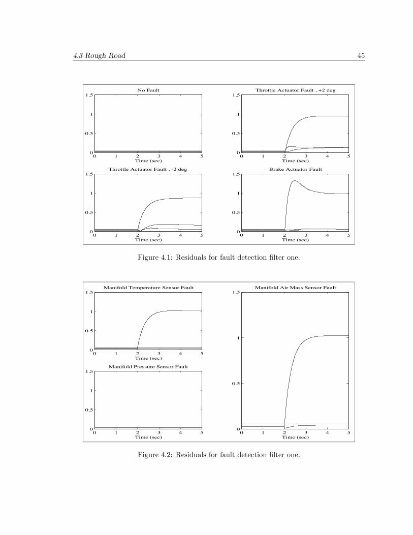
4.3 Rough Road 45
0 1 2 3 4 50
0.5
1
1.5No Fault
Time (sec)0 1 2 3 4 5
0
0.5
1
1.5Throttle Actuator Fault , +2 deg
Time (sec)
0 1 2 3 4 50
0.5
1
1.5Throttle Actuator Fault , -2 deg
Time (sec)0 1 2 3 4 5
0
0.5
1
1.5Brake Actuator Fault
Time (sec)
Figure 4.1: Residuals for fault detection filter one.
0 1 2 3 4 50
0.5
1
1.5Manifold Air Mass Sensor Fault
Time (sec)
0 1 2 3 4 50
0.5
1
1.5Manifold Temperature Sensor Fault
Time (sec)
0 1 2 3 4 50
0.5
1
1.5Manifold Pressure Sensor Fault
Time (sec)
Figure 4.2: Residuals for fault detection filter one.

46 Chapter 4: Fault Detection Filter Evalution
0 1 2 3 4 50
0.5
1
1.5No Fault
Time (sec)0 1 2 3 4 5
0
0.5
1
1.5Engine Speed Sensor Fault
Time (sec)
0 1 2 3 4 50
0.5
1
1.5Longitudinal Accelerameter Fault
Time (sec)0 1 2 3 4 5
0
0.5
1
1.5Sum of Front Wheel Speed Sensor Fault
Time (sec)
Figure 4.3: Residuals for fault detection filter two.
0 1 2 3 4 50
0.5
1
1.5No Fault
Time (sec)0 1 2 3 4 5
0
0.5
1
1.5Longitudinal Velocity Sensor Fault
Time (sec)
0 1 2 3 4 50
0.5
1
1.5Vertical Acelerameter Fault
Time (sec)0 1 2 3 4 5
0
0.5
1
1.5Sum of Rear Wheel Speed Sensor Fault
Time (sec)
Figure 4.4: Residuals for fault detection filter three.

4.3 Rough Road 47
0 1 2 3 4 50
0.5
1
1.5No Fault
Time (sec)0 1 2 3 4 5
0
0.5
1
1.5Throttle Actuator Fault , +2 deg
Time (sec)
0 1 2 3 4 50
0.5
1
1.5Throttle Actuator Fault , -2 deg
Time (sec)0 1 2 3 4 5
0
0.5
1
1.5Throttle Sensor Fault
Time (sec)
Figure 4.5: Residual for fault detection filter four.
0 2 40
0.5
1
1.5No Fault
Time (sec)0 2 4
0
0.5
1
1.5Brake Actuator Fault
Time (sec)0 2 4
0
0.5
1
1.5Brake Sensor Fault
Time (sec)
Figure 4.6: Residual for fault detection filter five.

48 Chapter 4: Fault Detection Filter Evalution
0 2 40
0.5
1
1.5No Fault
Time (sec)0 2 4
0
0.5
1
1.5Manifold Pressure Sensor Fault
Time (sec)0 2 4
0
0.5
1
1.5Manifold Air Mass Sensor Fault
Time (sec)
Figure 4.7: Residual for fault detection filter six.
separate plot for clarity.
Figure 4.14 shows the residuals for fault detection filter two derived from the second
fault group. Figure 4.14 illustrates a visually obvious contrast between cases where no fault
occurs and where a step fault occurs in the engine speed sensor, longitudinal accelerometer
and the sum of front wheel speed sensors.
Figure 4.15 shows the residuals for fault detection filter three derived from the third
fault group. Figures 4.16, 4.17 and 4.18 show the residuals for parity equations derived for
the third, fourth and sixth fault groups. They are the same as on a smooth road.

4.3 Rough Road 49
0 0.5 1 1.5 2 2.5 3 3.5 4 4.5 50
0.5
1
1.5Throttle Actuator Residual
0 0.5 1 1.5 2 2.5 3 3.5 4 4.5 50
0.5
1
1.5Brake Actuator Residual
0 0.5 1 1.5 2 2.5 3 3.5 4 4.5 50
0.5
1
1.5Manifold Air Mass and Temperature Residual
Time (sec)
Figure 4.8: Residuals for fault detection filter one when there is no fault.
0 0.5 1 1.5 2 2.5 3 3.5 4 4.5 50
0.5
1
1.5Throttle Actuator Residual
0 0.5 1 1.5 2 2.5 3 3.5 4 4.5 50
0.5
1
1.5Brake Actuator Residual
0 0.5 1 1.5 2 2.5 3 3.5 4 4.5 50
0.5
1
1.5Manifold Air Mass and Temperature Residual
Time (sec)
Figure 4.9: Residuals for fault detection filter one when a +2 deg throttle actuator faultoccurs.
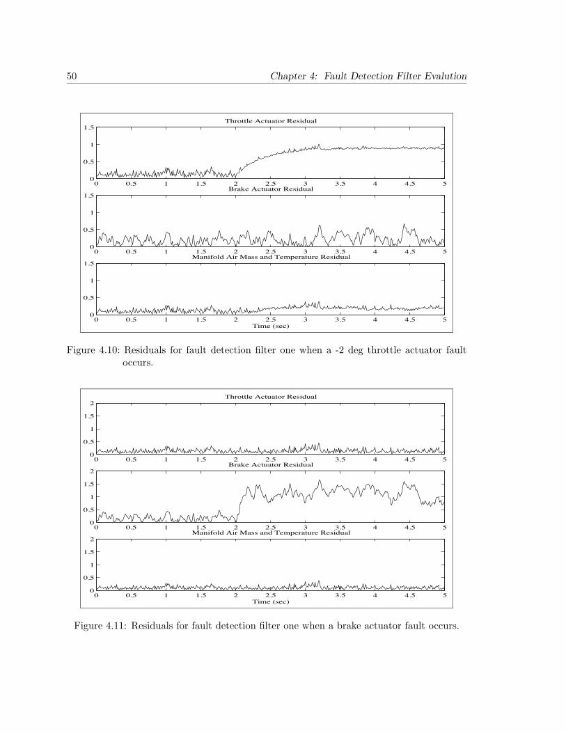
50 Chapter 4: Fault Detection Filter Evalution
0 0.5 1 1.5 2 2.5 3 3.5 4 4.5 50
0.5
1
1.5Brake Actuator Residual
0 0.5 1 1.5 2 2.5 3 3.5 4 4.5 50
0.5
1
1.5Manifold Air Mass and Temperature Residual
Time (sec)
0 0.5 1 1.5 2 2.5 3 3.5 4 4.5 50
0.5
1
1.5Throttle Actuator Residual
Figure 4.10: Residuals for fault detection filter one when a -2 deg throttle actuator faultoccurs.
0 0.5 1 1.5 2 2.5 3 3.5 4 4.5 50
0.5
1
1.5
2Throttle Actuator Residual
0 0.5 1 1.5 2 2.5 3 3.5 4 4.5 50
0.5
1
1.5
2Brake Actuator Residual
0 0.5 1 1.5 2 2.5 3 3.5 4 4.5 50
0.5
1
1.5
2Manifold Air Mass and Temperature Residual
Time (sec)
Figure 4.11: Residuals for fault detection filter one when a brake actuator fault occurs.
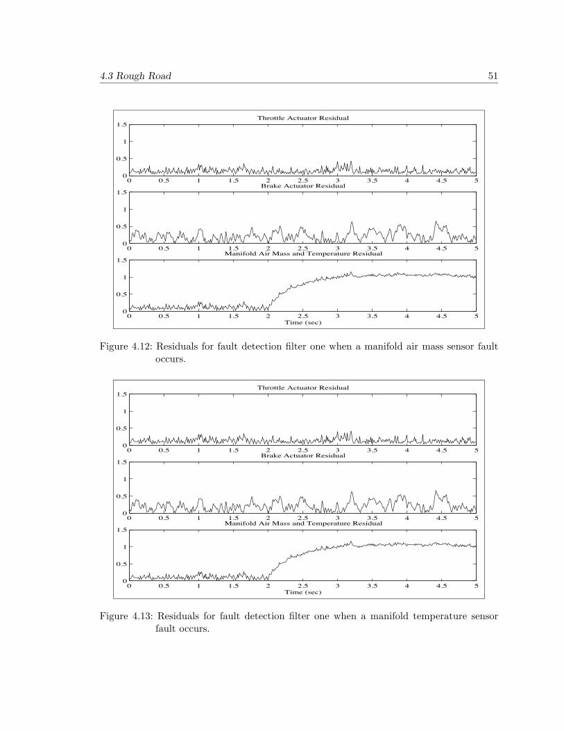
4.3 Rough Road 51
0 0.5 1 1.5 2 2.5 3 3.5 4 4.5 50
0.5
1
1.5Throttle Actuator Residual
0 0.5 1 1.5 2 2.5 3 3.5 4 4.5 50
0.5
1
1.5Brake Actuator Residual
0 0.5 1 1.5 2 2.5 3 3.5 4 4.5 50
0.5
1
1.5Manifold Air Mass and Temperature Residual
Time (sec)
Figure 4.12: Residuals for fault detection filter one when a manifold air mass sensor faultoccurs.
0 0.5 1 1.5 2 2.5 3 3.5 4 4.5 50
0.5
1
1.5Throttle Actuator Residual
0 0.5 1 1.5 2 2.5 3 3.5 4 4.5 50
0.5
1
1.5Brake Actuator Residual
0 0.5 1 1.5 2 2.5 3 3.5 4 4.5 50
0.5
1
1.5Manifold Air Mass and Temperature Residual
Time (sec)
Figure 4.13: Residuals for fault detection filter one when a manifold temperature sensorfault occurs.

52 Chapter 4: Fault Detection Filter Evalution
0 1 2 3 4 50
0.5
1
1.5No Fault
0 1 2 3 4 50
0.5
1
1.5No Fault
0 1 2 3 4 50
0.5
1
1.5No Fault
Time (sec)
0 1 2 3 4 50
0.5
1
1.5Engine Speed Sensor Fault
0 1 2 3 4 50
0.5
1
1.5Longitudinal Accelerameter Fault
0 1 2 3 4 50
0.5
1
1.5Sum of Front Wheel Speed Sensor Fault
Time (sec)
Figure 4.14: Residuals for fault detection filter two.
0 1 2 3 4 50
0.5
1
1.5No Fault
0 1 2 3 4 50
0.5
1
1.5
2No Fault
0 1 2 3 4 50
0.5
1
1.5No Fault
Time (sec)
0 1 2 3 4 50
0.5
1
1.5Longitudinal Velocity Sensor Fault
0 1 2 3 4 50
0.5
1
1.5
2Vertical Accelerameter Fault
0 1 2 3 4 50
0.5
1
1.5Sum of Rear Wheel Speed Sensor Fault
Time (sec)
Figure 4.15: Residuals for fault detection filter three.
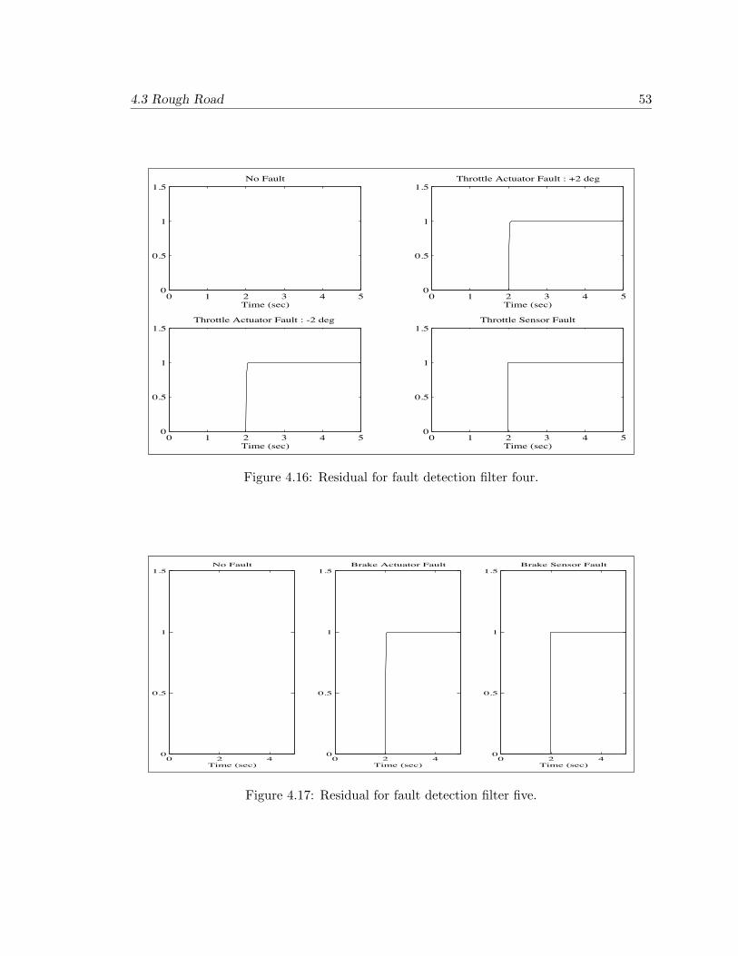
4.3 Rough Road 53
0 1 2 3 4 50
0.5
1
1.5No Fault
Time (sec)0 1 2 3 4 5
0
0.5
1
1.5Throttle Actuator Fault : +2 deg
Time (sec)
0 1 2 3 4 50
0.5
1
1.5Throttle Actuator Fault : -2 deg
Time (sec)0 1 2 3 4 5
0
0.5
1
1.5Throttle Sensor Fault
Time (sec)
Figure 4.16: Residual for fault detection filter four.
0 2 40
0.5
1
1.5No Fault
Time (sec)0 2 4
0
0.5
1
1.5Brake Actuator Fault
Time (sec)0 2 4
0
0.5
1
1.5Brake Sensor Fault
Time (sec)
Figure 4.17: Residual for fault detection filter five.

54 Chapter 4: Fault Detection Filter Evalution
0 2 40
0.5
1
1.5Manofold Air Mass Sensor Fault
Time (sec)0 2 4
0
0.5
1
1.5Manifold Pressure Sensor Fault
Time (sec)0 2 4
0
0.5
1
1.5No Fault
Time (sec)
Figure 4.18: Residual for fault detection filter six.

Chapter 5
Residual Processing
A primary objective of any analytic redundancy management scheme is to generate
residuals with sufficient statistics and to analyze these signals. The fault detection filters
perform this task by constraining the residual to respond in a known and fixed direction
for each fault, thereby aiding the fault isolation process. However, in the presence of
nonlinearities and process uncertainties, the directional properties of the residual process
are no longer well defined. Further analysis of the signals is needed.
In this scenario, fault isolation may be viewed as a pattern recognition problem. The
residual processor could be a Bayesian neural network whose input is the residual process
and the outputs, in some sense, approximate the posteriori probabilities of each fault
(Douglas et al. 1995). However, the Bayesian neural network, while easy to implement, is
not easily amenable to mathematical analysis. Moreover, due to feedback, the performance
deteriorates in the presence of noise at the input.
A better approach is to use a Sequential Probability Ratio Test (SPRT). We derived a
multiple hypothesis Shiryayev SPRT by adopting a dynamic programming viewpoint and
55

56 Chapter 5: Residual Processing
Fault detection filter 1: Throttle actuatorBrake actuatorManifold air mass sensorManifold temperature sensor
Fault detection filter 2: Engine speed sensorLongitudinal accelerometerFront wheel symmetric speed sensor
Fault detection filter 3: Longitudinal velocity sensorVertical accelerometerRear wheel symmetric speed sensor
Parity equation 1: Throttle actuatorThrottle sensor
Parity equation 2: Brake actuatorBrake sensor
Parity equation 3: Manifold air mass sensorManifold pressure sensor
Table 5.1: Faults organized into analytically redundant groups.
showed that for a certain criterion of optimality, it detects and isolates a fault in minimum
time (Malladi and Speyer 1996, Malladi and Speyer 1997). The fault isolation problem is
now solved by assuming that each fault corresponds to a particular hypothesis. The multiple
hypothesis Shiryayev SPRT is described in detail in last year’s report (Douglas et al. 1996)
and in (Malladi and Speyer 1996) and (Malladi and Speyer 1997). The notation of this
chapter is the same as in Chapter 7 of (Douglas et al. 1996).
5.1 Residual Processor Design
As discussed in Sections 3.1.4 and 3.2, sensor and actuator faults are organized into the
analytically redundant groups of Table 5.1. The combined residual processes, xk ∈ R12,
from the fault detection filters and parity equations are considered to be the measurement
sequence for the Shiryayev sequential probability ratio test. The measurement sequence is
assumed to have a Gaussian distribution and be conditionally independent, that is, once a
fault occurs, the measurement process is independent.
There are 14 hypotheses {H0 . . .H13}, including the no-fault case. For convenience,
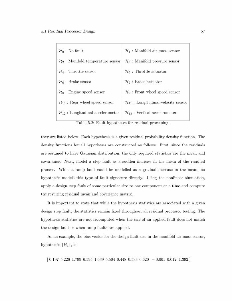
5.1 Residual Processor Design 57
H0 : No fault H1 : Manifold air mass sensor
H2 : Manifold temperature sensor H3 : Manifold pressure sensor
H4 : Throttle sensor H5 : Throttle actuator
H6 : Brake sensor H7 : Brake actuator
H8 : Engine speed sensor H9 : Front wheel speed sensor
H10 : Rear wheel speed sensor H11 : Longitudinal velocity sensor
H12 : Longitudinal accelerometer H13 : Vertical accelerometer
Table 5.2: Fault hypotheses for residual processing.
they are listed below. Each hypothesis is a given residual probability density function. The
density functions for all hypotheses are constructed as follows. First, since the residuals
are assumed to have Gaussian distribution, the only required statistics are the mean and
covariance. Next, model a step fault as a sudden increase in the mean of the residual
process. While a ramp fault could be modelled as a gradual increase in the mean, no
hypothesis models this type of fault signature directly. Using the nonlinear simulation,
apply a design step fault of some particular size to one component at a time and compute
the resulting residual mean and covariance matrix.
It is important to state that while the hypothesis statistics are associated with a given
design step fault, the statistics remain fixed throughout all residual processor testing. The
hypothesis statistics are not recomputed when the size of an applied fault does not match
the design fault or when ramp faults are applied.
As an example, the bias vector for the design fault size in the manifold air mass sensor,
hypothesis {H1}, is
[ 0.197 5.226 1.799 6.595 1.639 5.504 0.448 0.533 6.620 − 0.001 0.012 1.392 ]

58 Chapter 5: Residual Processing
while the covariance matrix is
0.011 0.016 0.008 0.018 −0.001 0.008 0.002 0.005 . . .0.016 11.26 0.113 0.070 0.104 0.135 −0.003 −0.015 . . .0.008 0.113 0.158 0.575 0.205 0.721 0.033 0.037 . . .0.018 0.070 0.575 2.142 0.756 2.668 0.121 0.132 . . .−0.001 0.104 0.205 0.756 0.318 1.074 0.043 0.042 . . .
0.008 0.135 0.721 2.668 1.074 3.692 0.151 0.156 . . .0.002 −0.003 0.033 0.121 0.043 0.151 0.008 0.008 . . .0.005 −0.015 0.037 0.132 0.042 0.156 0.008 0.013 . . .0.018 0.072 0.577 2.148 0.758 2.675 0.121 0.132 . . .
0.0001 −0.001 0.0004 −0.0001 0.001 0.002 0.0001 0.001 . . .0.001 −0.017 0.001 0.003 0.002 0.007 0.0002 0.001 . . .−0.001 −0.026 −0.003 −0.010 −0.002 −0.011 −0.001 −0.001 . . .
. . . 0.018 0.0001 0.001 −0.001
. . . 0.072 −0.001 −0.017 −0.026
. . . 0.577 0.0004 0.001 −0.003
. . . 2.148 −0.0001 0.003 −0.010
. . . 0.758 0.001 0.002 −0.002
. . . 2.675 0.002 0.007 −0.011
. . . 0.121 0.0001 0.0002 −0.001
. . . 0.132 0.001 0.001 −0.001
. . . 2.154 −0.0001 0.003 −0.010
. . . −0.0001 0.010 0.001 0.0002
. . . 0.003 0.001 0.010 −0.001
. . . −0.010 0.0002 −0.001 0.010
5.2 Simulations
The statistics of the residual process {x} are exactly modeled by the Shiryayev sequential
probability ratio test as
Under Hi : x ∼ N (mi,Λi)
where mi and Λi are a known mean and covariance. Therefore it is not surprising that
when a hard fault of the same magnitude as the design step fault is applied in the nonlinear
simulation, the residual processor isolates the fault almost immediately. However, real
faults have an unknown magnitude and never match the design case so it seems reasonable
to evaluate the residual processor by applying ramp faults to the nonlinear simulation.

5.2 Simulations 59
Manifold air mass sensor: x3 derived from fault detection filter 1
Throttle actuator: x1 derived from fault detection filter 1
Brake actuator: x11 derived from parity equation 2
Vertical accelerometer: x8 derived from fault detection filter 3
Table 5.3: Applied faults for residual processor testing.
To illustrate typical results, ramp faults in the manifold air mass sensor, throttle
actuator, vertical accelerometer and brake actuator are considered. Figures 5.1, 5.3, 5.4
and 5.5 show the residuals given in Table 5.3.
Figure 5.1 shows a 10 second simulation of a ramp fault applied to the manifold air mass
sensor. The size of the fault is gradually increased from zero at two seconds to the design
size of 0.07 kg/s at seven seconds. It is seen that the posteriori probability of a fault in the
manifold air mass sensor, hypothesis H1, becomes one at around five seconds.
Figure 5.2 shows the posteriori probability of a fault in the manifold temperature sensor,
hypothesis H2. The probability increases initially, but goes back to zero as the fault size in
the manifold air mass sensor increases.
Figure 5.3 shows a ten second simulation of a ramp fault applied to the throttle actuator.
The size of the fault is gradually increased from zero at two seconds to the design size of two
degrees at seven seconds. In this case, the posteriori probability of a fault in the throttle
actuator, hypothesis H5, increases to one at around three seconds.
Figure 5.4 shows a ten second simulation of a ramp fault applied to the brake actuator.
The size of the fault is gradually increased from zero at two seconds to the design size of
fifty at seven seconds. Here, the posteriori probability of a fault in the brake actuator,
hypothesis H7, increases to one at around three seconds.
In Figure 5.5, a ten second simulated ramp fault is applied to the vertical accelerometer.
The size of the fault is gradually increased from zero at two seconds to the design size
of 0.5 msec2 at seven seconds. Here, the posteriori probability of a fault in the vertical

60 Chapter 5: Residual Processing
0 5 10
0.5
1
1.5
2
Air
Mas
s
Sensors
0 5 10
0.2
0.4
0.6
Thr
ottle
Actuators
0 5 10
-0.2
0
0.2
Bra
ke
0 5 10
0.2
0.4
0.6
Z A
ccel
erom
eter
0 5 100
0.5
1
Pro
b. o
f H0
0 5 100
0.5
1P
rob.
of A
ir M
ass
Figure 5.1: Ramp fault in manifold air mass sensor.
accelerometer, hypothesis H13, increases to one at around three seconds.
5.3 Conclusions
The simulation studies clearly illustrate the efficacy of a health monitoring scheme which
blends a classical fault detection filters approach with hypothesis testing ideas.
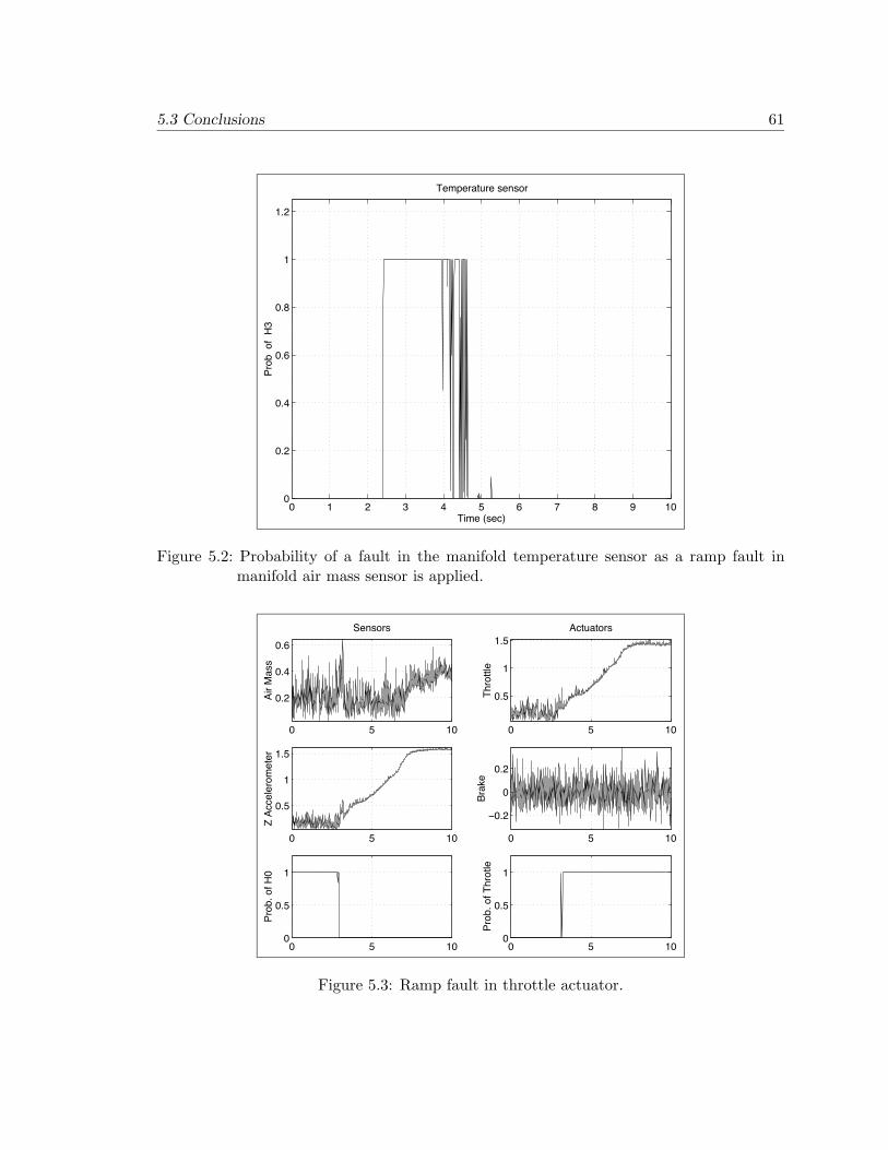
5.3 Conclusions 61
0 1 2 3 4 5 6 7 8 9 100
0.2
0.4
0.6
0.8
1
1.2
Time (sec)
Pro
b o
f H
3
Temperature sensor
Figure 5.2: Probability of a fault in the manifold temperature sensor as a ramp fault inmanifold air mass sensor is applied.
0 5 10
0.2
0.4
0.6
Air
Mas
s
Sensors
0 5 10
0.5
1
1.5
Thr
ottle
Actuators
0 5 10
-0.2
0
0.2
Bra
ke
0 5 10
0.5
1
1.5
Z A
ccel
erom
eter
0 5 100
0.5
1
Pro
b. o
f H0
0 5 100
0.5
1
Pro
b. o
f Thr
otle
Figure 5.3: Ramp fault in throttle actuator.

62 Chapter 5: Residual Processing
0 5 10
0.2
0.4
0.6A
ir M
ass
Sensors
0 5 10
0.2
0.4
0.6
Thr
ottle
Actuators
0 5 100
20
40
Bra
ke
0 5 10
0.1
0.2
0.3
0.4
Z A
ccel
erom
eter
0 5 100
0.5
1
Pro
b. o
f H0
0 5 100
0.5
1P
rob.
of B
rake
Figure 5.4: Ramp fault in Brake actuator.
0 5 10
0.2
0.4
0.6
0.8
1
Air
Mas
s
Sensors
0 5 10
0.2
0.4
0.6
0.8
1
Thr
ottle
Actuators
0 5 10
-0.2
0
0.2
Bra
ke
0 5 10
0.2
0.4
0.6
0.8
Z A
ccel
erom
eter
0 5 100
0.5
1
Pro
b. o
f H0
0 5 100
0.5
1
Pro
b. o
f Z
Figure 5.5: Ramp fault in Vertical accelerometer.

Chapter 6
A Game Theoretic Fault Detection Filter
The fault detection filter was introduced by Beard (Beard 1971) in his doctoral thesis
and later refined by Jones (Jones 1973) who gave it a geometric interpretation. Since then,
the fault detection filter has undergone many refinements. White (White and Speyer 1987)
derived an eigenstructure assignment design algorithm. Massoumnia (Massoumnia 1986)
used advances in geometric theory to derive a complete and elegant geometric version of a
fault detection filter and derived a reduced-order fault detector (Massoumnia et al. 1989).
Most recently, Douglas robustified the filter to parameter variations (Douglas 1993) and
(Douglas and Speyer 1996) and also derived a version of the filter which bounds disturbance
transmission (Douglas and Speyer 1995). The fault detection filter background and design
methods discussed in Appendices A,B and C of last year’s report (Douglas et al. 1996) as
well as the application to vehicle fault detection of Sections 2 through 4 all follow from
these sources.
Common to all of these sources is an underlying structure of independent, invariant
subspaces. Most design algorithms, an exception being (Douglas and Speyer 1995), rely
63

64 Chapter 6: A Game Theoretic Fault Detection Filter
on spectral methods, that is, specifying eigenvalues and eigenvectors, since these methods
lead directly to the needed filter structure. Spectral methods, however, also limit the
applicability of fault detection filters to linear, time-invariant systems and filters designed
by these methods can have poor robustness to parameter variations (Lee 1994).
For these reasons, we take a different approach to detection filter design. We look at the
fault detection process as a disturbance attenuation problem and convert the process into
a differential game which leads to the final design. The game is one in which the player is
a state estimate and the adversaries are all of the exogenous signals, save the fault to be
detected. The player attempts to exclude the adversaries from a specified portion of the
state-space much in the same way that the invariant subspace structure of the fault detection
filter restricts state trajectories when driven by faults. The end result is an H∞-type filter
which bounds disturbance transmission.
Since fault detection filters block transmission, it would seem reasonable to expect that
in the limiting case when the H∞ transmission bound is brought to zero, the game filter
no longer approximates, but actually becomes a fault detection filter. We will prove that
this is indeed the case. For linear time-invariant (LTI) systems, we will show, in fact,
that the game filter becomes a Beard-Jones fault detector in the sense of (Douglas 1993):
faults other than the one to be detected are restricted to a subspace which is invariant and
unobservable.
The method developed here has wider applicability than current techniques since time-
invariance is never assumed in the game solution. Thus, for a class of time-varying systems,
results analogous to the LTI case exist in the limit as disturbance bounds are taken to
zero. It is also possible with this method to deal with model uncertainty by treating it as
another element in the differential game (Chichka and Speyer 1995, Mangoubi et al. 1994).
In this manner, sensitivity to parameter variations can be reduced. Finally, by using a game
theoretic approach, the designer has the freedom to choose the extent to which the game
filter behaves as an H∞ filter and the extent to which it behaves like a detection filter. This
flexibility is unique to this method of fault detection filter design.

6.1 The Approximate Detection Filter Design Problem 65
The development of game theoretic estimation closely followed the development of game
theoretic control theory. The most notable and the most cited (and most unreadable) work
in the latter was the paper by Doyle et al. (Doyle et al. 1989). The ascendant of the work
presented here is the paper by Rhee and Speyer (Rhee and Speyer 1991) which derived the
two Riccati solution of (Doyle et al. 1989) via the calculus of variations. It is hard to credit
the first derivation of the game theoretic estimator, though (Banavar and Speyer 1991) or
(Yaesh and Shaked 1993) are probable candidates.
In Section 6.1, we motivate the disturbance attenuation approach to FDI by showing
how it approximates the actions of a detection filter. In Section 6.2, we solve a disturbance
attenuation problem patterned after the fault detection process. The game theoretic fault
detection filter is a product of this solution. In Sections 6.3.1 and 6.3.2, we demonstrate
the effectiveness of the new filter with a pair of examples.
6.1 The Approximate Detection Filter Design Problem
6.1.1 Modeling the Detection Problem
The general class of systems that we will look at are linear, observable, possibly time-varying,
and driven by noisy measurements:
x(t) = Ax(t) +Bu(t),
y(t) = Cx(t) + v. (6.1)
We will also assume that our state matrices have sufficient smoothness to guarantee the
existence of derivatives various order.
Beard (Beard 1971) showed that failures in the sensors and actuators, and unexpected
changes in the plant dynamics can be modeled as additive signals:
x = Ax+Bu+ F1µ1 + · · ·+ Fqµq. (6.2)
Let n be the dimension of the state-space. The n × pi matrix, Fi, i = 1 · · · q, is called a
failure map and represents the directional characteristics of the ith fault. The pi×1 vector,

66 Chapter 6: A Game Theoretic Fault Detection Filter
µi, is the failure signal and represents the time dependence of the failure. It will always
be assumed that each Fi is monic, i.e. Fiµi 6= 0 for µi 6= 0. We will look at Fi and µi in
more detail in Section 6.1.2, and we will show the importance of the monicity assumption
in Section 6.1.3. Throughout this paper, we will refer to µ1 as the “target fault” and the
other faults, µj , j = 2 · · · q, as the “nuisance faults”. Without loss of generality, we can
represent the entire set of nuisance faults with a single map and vector:
x = Ax+Bu+ F1µ1 + F2µ2.
Suppose that it is desired to detect the occurrence of the failure, µ1, in spite of the
measurement noise, v, and the possible presence of the nuisance faults, µ2. As described
earlier, a detection filter-based solution to this problem,
˙x = Ax+ L(y − Cx), (6.3)
works by keeping the reachable subspaces of µ1 and µ2 in separate and nonintersecting
invariant subspaces. Thus, with a properly chosen projector, H, we can project the filter
residual, (y−Cx), onto the orthogonal complement of the invariant subspace containing µ2
and get a signal,
z = H(y − Cx), (6.4)
such that
z = 0 when µ1 = 0 and µ2 is arbitrary. (6.5)
To be useful for FDI, z must also be such that
z 6= 0 when µ1 6= 0. (6.6)
If we restrict ourselves to time-invariant systems, (6.6) will be equivalent to requiring that
the transfer matrix between µ1(s) and z(s)1 be left-invertible. Left-invertibility, however, is
1µ1(s) and z(s) are the Laplace transforms of the time-domain signals µ1(t) and z(t).
6.1 The Approximate Detection Filter Design Problem 67
a severe restriction, and has no analog for the general time-varying systems that considered
here. Previous researchers (Douglas 1993, Massoumnia et al. 1989) have, in fact, only
required that the mapping from µ1(t) to z(t) be input observable, i.e. z 6= 0 for any µ1 that
is a step input. It is then argued (Massoumnia et al. 1989) that with input observability
z will be nonzero for “almost any” µ1, since µ1 is unlikely to remain in the kernal of the
mapping to z for all time.
We formulate the approximate detection filter problem by requiring input observability
and relaxing the requirement for strict blocking that is implied by (6.5). We, instead, only
require that the transmission of the nuisance fault be bounded above by a pre-set level,
γ > 0:
‖z‖2‖µ2‖2
≤ γ. (6.7)
Equation (6.7) is clearly a disturbance attenuation problem, and it is an H∞ problem if
we assume L2 norms for µ2 and z in (6.7). We refer to the solution to the approximate
detection filter problem as the game theoretic fault detection filter.
Remark 2. Detection filters typically make no assumptions about the time dependence
of nuisance faults. The L2 assumption that we make above is, thus, a new restriction. We
will, however, recover the full generality of the detection filter in the limiting case when we
take the disturbance attenuation bound to zero.
Remark 3. The terms, “H∞” and “game theoretic,” are used interchangeably throughout
this chapter. Doyle (Doyle et al. 1989) showed that the solution to the infinite-horizon
linear quadratic game (Mageirou 1976) provides a fundamental solution to many H∞-norm
minimizing problems, all other solutions being expressible in terms of this solution and a
free parameter2, Q. Other researchers established a direct equivalence between the two
problems by using a disturbance attenuation interpretation of the H∞ problem to recover
Doyle’s result with the calculus of variations (Rhee and Speyer 1991) and with dynamic
2The free parameter, Q, is a real rational transfer function matrix.

68 Chapter 6: A Game Theoretic Fault Detection Filter
programming (Basar and Bernhard 1995)3. These researchers, moreover, derive significant
extensions of theH∞ result, obtaining solutions for finite-horizon problems and time-varying
systems. The differential game approach to solving H∞ problems has since been revisited
by a number of researchers (Limebeer et al. 1992, Mills and Bryson 1994) and has led
to new results in estimation (Banavar and Speyer 1991, Yaesh and Shaked 1993), robust
control (Ghaoui et al. 1992), robust estimation (DeSouza et al. 1992, Mangoubi 1995), and
adaptive control (Chichka and Speyer 1995). The differential game approach has even made
its way into textbooks such as (Green and Limebeer 1995).
6.1.2 Modeling Failures
In this section, we will show how to construct failure maps and signals for each type of
failure. Existing methods (Beard 1971, Douglas 1993, White and Speyer 1987) exist for
time-invariant systems. For actuator faults and plant changes, these methods can be
extended “as is” to time-varying systems. In the actuator fault case, this means that the
map is taken to be the corresponding column of the input matrix. In the plant fault case,
the map is similarly derived by pulling out the corresponding entries in the state matrix.
The failure signals in both cases can be found by choosing an appropriate time function4.
Sensor faults require a generalization of the time-invariant result. Because these failures
enter the system through the measurements, we can initially model them as an additive
input in the measurement equation:
y = Cx+ Ejµj . (6.8)
C is an m × n matrix, and Ej is an m × 1 unit vector with a one at jth position, which
corresponds to a failure in the jth sensor.
Following (Douglas 1993), we determine the sensor failure map by finding the input to
the plant which drives the error state in the same way that µj will in (6.8). This is elegantly
accomplished by a Goh transformation on the error space (Jacobson 1971). Defining the
3This approach was significantly extended by Chichka and Speyer in (Chichka and Speyer 1995).4For example, hard failures or saturation failures can be modeled as step inputs.
6.1 The Approximate Detection Filter Design Problem 69
estimation error, e, as x− x, the filter residual is then
r4= y − Cx = Ce
when there is no sensor noise (6.1). When a sensor failure occurs,
r = Ce+ Ejµj . (6.9)
Let fj be the solution to Ej = Cfj . The transformation begins by defining a new error
state,
e4= e+ fiµi, (6.10)
which allows us to rewrite (6.9) as r = Ce. Assuming a generic form for the observer, (6.3),
and a homogeneous dynamic system, x = Ax, we differentiate e,
˙e = e+ fjµj + fjµj
= Ae+ LCe+Afjµj −Afjµj + fjµj + fjµj
= (A+ LC)e+[fj (Afj − fj)
]{ µj−µj
},
to get a differential equation for the transformed error trajectory. Clearly, the equivalent
input is one which enters the system through
Fj =[fj f∗j
], (6.11)
where f∗j = Afj − fj . When the system is time-invariant, fj = 0 and (6.11) will match
the time-invariant failure map given in (Beard 1971) and (White and Speyer 1987). For
our purposes, finding Fj is the key result. The actual time history of the failure signal is
not important and so undue importance should not be attached to the “equivalent” input,[µTj −µTj
]T .
6.1.3 Constructing the Failure Signal
We complete our formulation of the disturbance attenuation problem for fault detection by
constructing a projector, H, which determines the failure signal, z, (6.4). For time-invariant
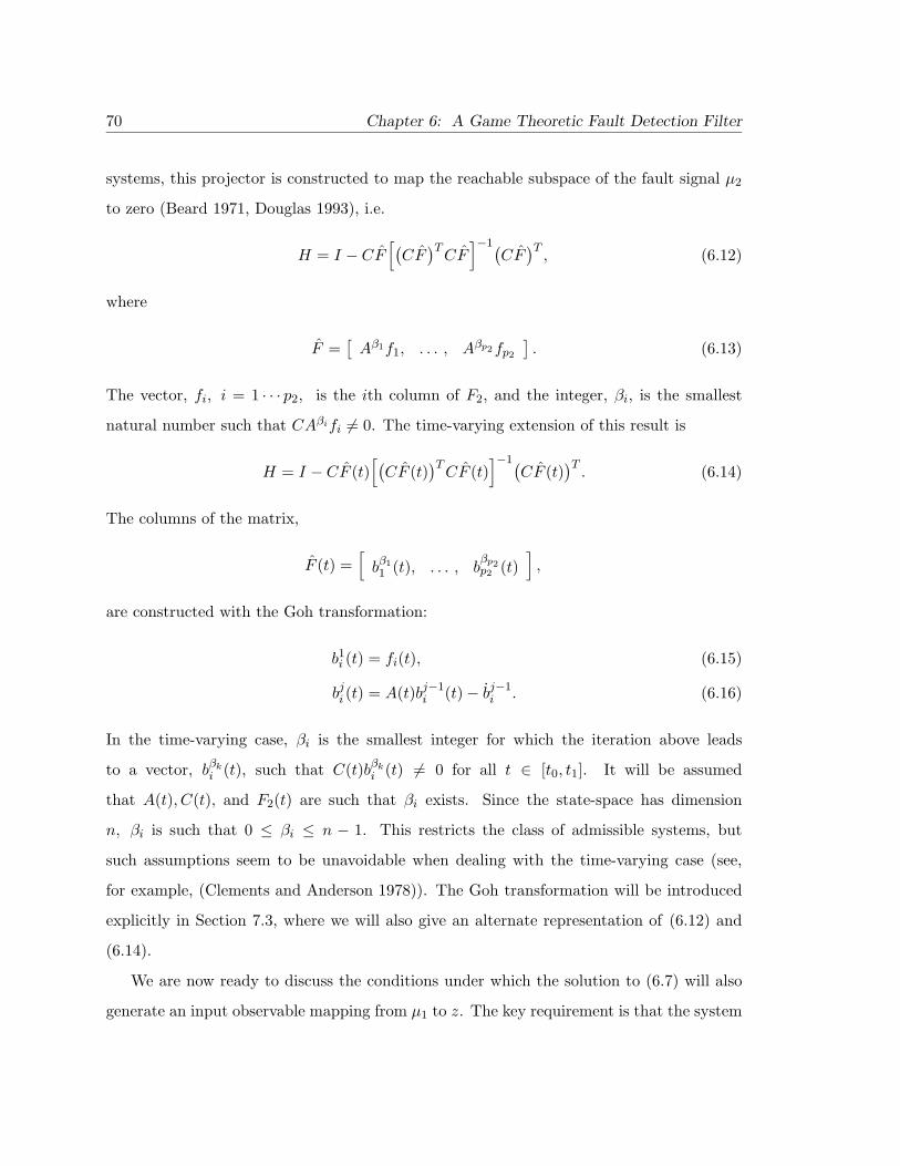
70 Chapter 6: A Game Theoretic Fault Detection Filter
systems, this projector is constructed to map the reachable subspace of the fault signal µ2
to zero (Beard 1971, Douglas 1993), i.e.
H = I − CF[(CF)TCF]−1(
CF)T, (6.12)
where
F =[Aβ1f1, . . . , Aβp2fp2
]. (6.13)
The vector, fi, i = 1 · · · p2, is the ith column of F2, and the integer, βi, is the smallest
natural number such that CAβifi 6= 0. The time-varying extension of this result is
H = I − CF (t)[(CF (t)
)TCF (t)
]−1(CF (t)
)T. (6.14)
The columns of the matrix,
F (t) =[bβ11 (t), . . . , b
βp2p2 (t)
],
are constructed with the Goh transformation:
b1i (t) = fi(t), (6.15)
bji (t) = A(t)bj−1i (t)− bj−1
i . (6.16)
In the time-varying case, βi is the smallest integer for which the iteration above leads
to a vector, bβki (t), such that C(t)bβki (t) 6= 0 for all t ∈ [t0, t1]. It will be assumed
that A(t), C(t), and F2(t) are such that βi exists. Since the state-space has dimension
n, βi is such that 0 ≤ βi ≤ n − 1. This restricts the class of admissible systems, but
such assumptions seem to be unavoidable when dealing with the time-varying case (see,
for example, (Clements and Anderson 1978)). The Goh transformation will be introduced
explicitly in Section 7.3, where we will also give an alternate representation of (6.12) and
(6.14).
We are now ready to discuss the conditions under which the solution to (6.7) will also
generate an input observable mapping from µ1 to z. The key requirement is that the system

6.1 The Approximate Detection Filter Design Problem 71
be output separable. That is, F1 and F2 must be linearly independent and remain so when
mapped to the output space by C and A. For time-invariant systems, the test for output
separability is
rank[CAδ1 f1, . . . , CAδp1 fp1 , CAβ1f1, . . . , CAβp2fp2
]= p1 + p2. (6.17)
As in (6.13), fi is the ith column of F2, and βi is the the smallest integer such that CAβifi 6=
0. Similarly, fj is the jth column of F1, and δj is the smallest integer such that Aδj fj 6= 0.
The integer sum, p1 + p2, is the total number of columns in F1 and F2.
For time-varying systems, the output separability test becomes
rank[C(t)bδ11 (t), . . . , C(t)bδp1p1 (t), C(t)bβ1
1 (t), . . . , C(t)bβp2p2 (t)]
= p1 + p2, ∀t ∈ [t0, t1], (6.18)
where the vectors, bβii and bδjj , are found from the iteration defined by (6.15) and (6.16).
The initial vector, b1j , is set equal to the jth column of F1, and b1i is initialized as the ith
column of F2.
The following proposition connects output separability to input observability and shows
the importance of the monicity assumption:
Proposition 6.1. Suppose that we have an approximate detection filter which satisfies
(6.7) and generates the failure signal, z, given by (6.4). If F1 and F2 are output separable
and F1 is monic, then the mapping, µ1(t) 7→ z(t), is input observable.
Proof. The input observability of the mapping, µ1(t) 7→ z(t), is equivalent (Douglas 1993,
Massoumnia et al. 1989) to requirement that F1 be monic and that its image not intersect
the unobservable subspace of (HC,A). We have already assumed the former. To show the
latter, let us assume the converse, i.e. that there exists a vector,
ξ1(t) =p1∑i=1
αifi(t), (6.19)

72 Chapter 6: A Game Theoretic Fault Detection Filter
such that
H(t)C(t)Φ(t, τ)ξ1(τ) = 0, ∀ t and τ ≤ t. (6.20)
The vector, fi, is the ith column of F1, and the coefficient, αi, is a real number. At least
one αi is nonzero. Φ(t, τ) is the state transition matrix of A(·) from τ to t.
Equation (6.20) implies that ξ1(t) ∈ KerH(t)C(t), since we can set τ = t and get
Φ(t, t) = I. Since the vectors, fi, are independent by the monicity assumption, this implies
that
fi(t) ∈ KerH(t)C(t), ∀ i = 1, · · · , p1. (6.21)
Now, if one of these vectors, say fi0(t), is not also in KerC(t), then (6.21) can hold only if
Cfi0(t) is linearly dependent upon the vectors, Cbβii , which form the projector, H(t). This,
in turn, would imply that the output separability test, (6.18), will fail, which implies the
proposition. Thus, for argument’s sake, let us suppose that all the fi lie in KerC(t), so that
we can continue with the proof.
Now, because we have assumed that the underlying matrices are smooth enough to allow
for derivatives of arbitrary order, a necessary and sufficient condition for (6.20) is that the
derivatives of HCΦξ1 be zero for all t and τ . Thus,
d
dτ[H(t)C(t)Φ(t, τ)ξ1(τ)] = H(t)C(t)Φ(t, τ)
[−A(τ)ξ1(τ) + ξ1(τ)
]= H(t)C(t)Φ(t, τ)ξ2(τ) = 0, ∀ t, τ,
(6.22)
where ξ24= − Aξ1 + ξ1. Again, setting τ = t in (6.22) implies that ξ2(t) ∈ KerH(t)C(t).
From the definition of ξ1 and the iteration formulas (6.15,6.16), we can rewrite ξ2 as
ξ2 = α1b21 + . . .+ αp1 b
2p1. (6.23)
The same arguments as before will lead us to the conclusion that either b2j (t) ∈ KerC(t),∀j, t
or that our proposition holds. We will again assume the former for argument’s sake.

6.1 The Approximate Detection Filter Design Problem 73
In the general case, we consider the vector, ξk, which is the kth iteration of formula,
ξj = −Aξj−1 + ξj−1, (6.24)
in which the initial vector, ξ1, is given by (6.19)5. We can also write ξk as
ξk =p1∑i=1
αibki (t),
where bki is the kth step of the iteration (6.15,6.16) with b1i taken to be fi, the ith column
of F1. Previously, we saw for the case, k = 1, that
H(t)C(t)Φ(t, τ)ξk(τ) = 0, ∀ t and τ ≤ t (6.25)
implies
C(t)bki (t) = 0, ∀ i, t, (6.26)
H(t)C(t)Φ(t, τ)ξk+1(τ) = 0, ∀ t and τ ≤ t, (6.27)
where ξk+14= − Aξk + ξk is the next step in the iteration (6.24). The arguments used for
k = 1 are independent of the particular value of k, which means that (6.26,6.27) hold for
all k. Thus, by induction, we can claim that ξ1 unobservable through (HC,A) implies that
all of the vectors bik(t), i = 1 . . . n−1, k = 1 . . . p1 from (6.15,6.16) lie in the kernal of C(t).
This, implies that the output separability test matrix,
[Cbδ11 , . . . , Cb
δp1p1 , Cbβ1
1 , . . . , Cbβp2p2
],
will fail to be full-rank. Therefore, the contrapositive argument,
image F2 ∩KerHC 6= 0 =⇒ F1 and F2 not output separable,
implies our proposition.
5Note that this formula is simply the Goh transformation.

74 Chapter 6: A Game Theoretic Fault Detection Filter
Remark 4. Although output separability is a necessary condition for the existence of
Beard-Jones filters (Beard 1971, Douglas 1993), Edelmayer et al. (Edelmayer et al. 1996),
show that even without output separability it is still possible to find approximate detection
filters which can distinguish the target input from nuisance inputs. There is no guarantee,
however, that this will always be the case, and our example in Chapter 8 will show that the
loss of output separability severely reduces our ability to distinguish the two faults.
Remark 5. A property of the unknown input observer such as described by (Frank 1990,
Patton and Chen 1992, Saif and Guan 1993), and its approximations, such as the filter we
are about to derive, is the ability to distinguish only one fault out of a set of faults. In
general, this is a disadvantage when compared to the Beard-Jones Fault Detection Filter
which can identify several faults. An exception to this rule, however, is in the number of
faults which can be included in the nuisance set. In the unknown input observer, any fault
which is output separable from the target fault can be included, though a minimal set that
spans the range of the nuisance set may have to be used as the failure map in order to
preserve monicity. In a Beard-Jones Filter, all of the faults in the model will be target
faults at one point or another and so they must be pairwise output separable. This severely
limits the number of faults which can be included in a single Beard-Jones Filter6.
6.2 A Game Theoretic Solution to the Approximate Detection FilterDesign Problem
6.2.1 The Disturbance Attenuation Problem
We now turn our attention to the disturbance attenuation problem implied by (6.7). We
begin by defining a disturbance attenuation function,
Daf =
∫ t1t0‖HC(x− x)‖2Qdt∫ t2
t1
[‖µ2‖2M−1 + ‖v‖2
V −1
]dt+ ‖x(t0)− x0‖2P0
, (6.28)
6In general, one can include, at most, only as many faults as there are measurements in thesystem (Douglas 1993, Massoumnia et al. 1989).

6.2 A Game Theoretic Solution to the Approximate Detection Filter Design Problem 75
which is a ratio of the outputs to the disturbances (Rhee and Speyer 1991). Equation (6.28)
is patterned roughly after (6.7). We have added the sensor noise, v, and the initial error,
x(t0)− x0, to the set of disturbance signals to incorporate tradeoffs for noise rejection and
settling time into the problem. M,V,Q, and P0 are weighting matrices. Note that we do not
include the target fault, µ1, at this stage of the design problem, since we are now focusing
on nuisance blocking. Our only concern with µ1 is that it be visible at the output, which is
what Proposition 6.1 guarantees.
The disturbance attenuation problem is to find the estimate, x, so that for all µ2,
v ∈ L2[t1, t2], x(t0) ∈ Rn,
Daf ≤ γ,
where γ ∈ R is called the disturbance attenuation bound. Since Daf is defined with L2
norms, the disturbance attenuation problem is equivalent to a suboptimal H∞ problem.
(C,A) will always be assumed to be an observable pair.
To solve this problem, we convert (6.28) into a cost function,
J =∫ t1
t0
[‖HC(x− x)‖2Q − γ
(‖µ2‖2M−1 + ‖y − Cx‖2V −1
)]dt− ‖x(t0)− x0‖2Π0
, (6.29)
where we have used (6.1) to rewrite the measurement noise term. Note that we have also
rewritten the initial error weighting, defining Π04= γ−1P0. The disturbance attenuation
problem is then solved via the differential game,
minx
maxy
maxµ2
maxx(t0)
J ≤ 0, (6.30)
subject to
x = Ax+ F2µ2, (6.31)
y = Cx+ v.

76 Chapter 6: A Game Theoretic Fault Detection Filter
6.2.2 The Differential Game Solution
We will solve the differential game in two steps beginning with the subproblem,
maxµ2
maxx(t0)
J ≤ 0,
subject to (6.31) with y and x fixed. The first step in this solution is to append the problem
constraints, which are the system dynamics, (6.31), to the cost, (6.29), through a Lagrange
multiplier, λT :
J =∫ t1
t0
[‖HC(x− x)‖2Q − γ
(‖µ2‖2M−1 + ‖y − Cx‖2V −1)
+ λT (Ax+ F2µ2 − x)]dt− ‖x(t0)− x0‖2Π0
.
Integrate λT x by parts,
J =∫ t1
t0
[‖HC(x− x)‖2Q − γ
(‖µ2‖2M−1 + ‖y − Cx‖2V −1
)+ λT
(Ax+ F2µ2
)+ λTx
]dt− ‖x(t0)− x0‖2Π0
+ λ(t0)Tx(t0)− λ(t1)Tx(t1), (6.32)
and then take the variation of (6.32) with respect to µ2 and x(t0):
δJ =∫ t1
t0
{[(x− x)TCTHQHC + γ(y − Cx)TV −1C + λT + λTA
]δx
+[−γµT2 M−1 + λTF2
]δµ2
}dt− λ(t1)T δx(t1)
−[(x(t0)− x0)TΠ0 − λ(t0)T
]δx(t0). (6.33)
Note that since H is a projector, H = HT = H2. Equation (6.33) implies that the first-order
necessary conditions to maximize (6.29) with respect to x(t0) and µ2 are

6.2 A Game Theoretic Solution to the Approximate Detection Filter Design Problem 77
µ∗2 =1γMF T2 λ, (6.34)
−λ = ATλ+ CTHQHC(x− x) + γCTV −1(y − Cx), (6.35)
λ(t1) = 0, (6.36)
λ(t0) = Π0
[x∗(t0)− x0
]. (6.37)
The asterisks in (6.34) and (6.37) denote that the extremizing value for the given variable is
being used. By substituting the maximizing strategy for µ2, (6.34), into the state equation
(6.31), we get a nonhomogeneous two-point boundary value problem (TPBVP),
{x
λ
}=[
A 1γF2MF T2
−CT (HQH − γV −1)C −AT]{
xλ
}+{
0CTHQHCx− γCTV −1y
}, (6.38)
by coupling (6.31) with (6.35). We will assume solutions x∗ and λ∗ to (6.38) such that
λ∗ = Π(x∗ − xp). (6.39)
The vector, xp, is a measurement-dependent variable which will reduce to the optimal state
estimate in the second-half of this game. If we take
Π(t0) = Π0, (6.40)
xp(t0) = x0, (6.41)
then (6.39) will match the boundary condition for λ at t0, (6.37). By differentiating (6.39)
and substituting in the equations for x and λ from (6.38), we get
0 =[Π +ATΠ + ΠA+
1γ
ΠF2MF T2 Π + CT(HQH − γV −1
)C]x∗
− Πxp −Πxp −ATΠxp − CTHQHCx+ γCTV −1y. (6.42)

78 Chapter 6: A Game Theoretic Fault Detection Filter
Now, add and subtract γCTV −1Cx and [ΠA+CT (HQH−γV −1)C]xp to (6.42) and collect
terms:
0 =[Π +ATΠ + ΠA+
1γ
ΠF2MF T2 Π + CT(HQH − γV −1
)C](x∗ − xp)
−Πxp + ΠAxp −[CT(HQH − γV −1
)C](x− xp) + γCTV −1(y − Cx). (6.43)
We, thus, find that (6.39) solves the TPBVP identically if
−Π = ATΠ + ΠA+1γ
ΠF2MF T2 Π + CT (HQH − γV −1)C, (6.44)
Πxp = ΠAxp −[CT (HQH − γV −1)C
](x− xp) + γCTV −1(y − Cx). (6.45)
Equation (6.44) is clearly a Riccati equation, and its boundary condition is given by (6.40).
Equation (6.45) looks like an estimator equation, except that it propagates the intermediate
variable, xp, and not the state estimate, x.
Substituting the maximizing values for µ2 and x(t0), (6.34,6.37), into the original cost
function, (6.29), gives us
J =∫ t1
t0
[‖x− x‖2CTHQHC − ‖λ‖21
γF2MFT2
− γ‖y − Cx‖2V −1
]dt− ‖λ(t0)‖2
Π−10. (6.46)
The second half of the game is then
minx
maxy
J ≤ 0,
subject to (6.45). By adding the identically zero term,
‖λ(t0)‖2Π(t0)−1 − ‖λ(t1)‖2Π(t1)−1 +∫ t1
t0
d
dt‖λ(t)‖2Π−1dt = 0,
to (6.46) and applying the boundary conditions for λ, (6.36,6.37), we get
J =∫ t1
t0
[‖x− x‖2CTHQHC − ‖λ‖21
γF2MFT2
− γ‖y − Cx‖2V −1
+ λTΠ−1λT + λT Π−1λ+ λTΠ−1λ]dt. (6.47)

6.2 A Game Theoretic Solution to the Approximate Detection Filter Design Problem 79
If we substitute the differential equation for λ from (6.38) into (6.47), we then have
J =∫ t1
t0
{‖x− x‖2CTHQHC + λT (−AΠ−1 −Π−1AT − F2MF T2 + Π−1)λ
− (x− x)TCTHQHCΠ−1λ− λTΠ−1CTHQHC(x− x)
− γ[‖y − Cx)‖2V −1 + (y − Cx)TV −1CΠ−1λ+ λTΠ−1CTV −1(y − Cx)
]}dt. (6.48)
From (6.44), the differential equation for Π−1 is
Π−1 = −Π−1ΠΠ−1 = Π−1AT +AΠ−1 +1γF2MF T2
+ Π−1CT (HQH − γV −1)CΠ−1, (6.49)
which, when substituted into the second term in (6.48), gives us
J =∫ t1
t0
[‖Π−1λ− (x− x)‖2CTHQHC − γ‖CΠ−1λ+ (y − Cx)‖2V −1
]dt. (6.50)
Substituting the optimal value for λ, (6.39), into (6.50) then leads to
J =∫ t1
t0
[‖x− xp‖2CTHQHC − γ‖y − Cxp‖2V −1
]dt. (6.51)
From (6.51), the minimizing strategy for x and the maximizing strategy for y are clearly
x∗ = xp, (6.52)
y∗ = Cxp.
This implies that our game optimal estimate, x, is found from
˙x = Ax+ γΠ−1CTV −1(y − Cx), x(t0) = x0, (6.53)
which is simply the extremizing value of x, (6.52), applied to (6.45) and (6.41). Π is found
by propagating (6.44) with the initial condition, (6.40).
Remark 6. The derivation presented in this section follows that presented by Banavar
and Speyer (Banavar and Speyer 1991).

80 Chapter 6: A Game Theoretic Fault Detection Filter
6.2.3 Steady-State Results
In many cases, it is desired to extend finite-time solutions of game theoretic problems to
the steady-state condition. Whenever it is possible to find a steady-state solution to the
disturbance attenuation problem, the optimal estimator will be given by (6.53) with Π being
the solution of the algebraic Riccati equation (Green and Limebeer 1995),
0 = ATΠ + ΠA+1γ
ΠF2MF T2 Π + CT(HQH − γV −1
)C. (6.54)
However, unlike the algebraic Riccati equation of linear-quadratic optimal control problems,
there are no conditions which guarantee the existence of a unique, nonnegative definite,
stabilizing solution to the steady-state Riccati equation (6.54), except in the special case
where A is asymptotically stable (Green and Limebeer 1995).
6.3 Applications
This section demonstrates the effectiveness of the new game theoretic fault detection filter
with a pair of examples.
6.3.1 Accelerometer Fault Detection in an F16XL
In this application, the F16XL example of (Douglas and Speyer 1996) is re-examined. The
objective is to detect a normal accelerometer fault in the presence of wind gusts and sensor
noise.
Aircraft Dynamics Model
The aircraft dynamics are linearized about trimmed level flight at 10,000 ft altitude and
Mach 0.9. For simplicity, a reduced-order, five-state model of the longitudinal dynamics
(including a first-order wind gust model) is considered:
x = Ax+Bwgwwg,
y = Cx+ v.
The five components of the state vector are

6.3 Applications 81
x =
uwqθwg
long. velocity (ft/sec)normal velocity (ft/sec)pitch rate (deg/sec)pitch (deg)wind gust (ft/sec)
with the measurements,
y =
qθAzAx
pitch rate (deg/sec)pitch (deg)long. acceleration (ft/sec2)normal acceleration (ft/sec2).
(6.55)
The input, wwg, is windgust and v is the sensor noise. The system matrices are
A =
−.0674 .0430 −.8886 −.5587 .0430.0205 −1.4666 16.5800 −.0299 −1.4666.1377 −1.6788 −.6819 0 −1.6788
0 0 1 0 00 0 0 0 −1.1948
, (6.56)
BTwg =
[0 0 0 0 2.0156
], (6.57)
and
C =
0 0 1 0 00 0 0 1 0
0.0139 1.0517 0.1485 −0.0299 0−0.0677 0.0431 0.0171 0 0
. (6.58)
Full-Order Filter Design
Following the modeling techniques described in Section 6.1, we convert the accelerometer
fault into an input to the system,
x = Ax+ FAzµAz + Fwgµwg,
y = Cx+ v,

82 Chapter 6: A Game Theoretic Fault Detection Filter
where
FAz =
0.6003 00.9429 −1.3706
0 −1.50030 00 0
.
In order to distinguish the accelerometer fault from the windgust disturbance, we model the
windgust as the nuisance fault. Hence, Fwg is simply Bwg and µwg is the wind gust input,
wwg. A quick check shows that FAz and Fwg are output separable. Finally, we generate the
residual projector, H. Since CFwg = 0, we must go through the Goh iteration one time to
find that
F = AFwg.
The projector is then
H = I − CAFwg[(CAFwg)TCAFwg
]−1(CAFwg)T
=
0.5330 0 −0.4982 −0.0264
0 1 0 0−0.4982 0 0.4685 −0.0281−0.0264 0 −0.0281 0.9985
.(6.59)
The full-order filter design problem boils down to finding a solution to the game Riccati
equation, (6.44), that leads to acceptable filter performance. Acceptable, in this example,
means that the filter transmits the target fault and attenuates the nuisance fault so that
there is good separation between the respective transmission levels. Since the inverse of Π
is used in the filter gain, we directly solve for this inverse using the steady-state version of
(6.49),
0 = Π−1AT +AΠ−1 +1γF2MF T2 + Π−1CT
(HQH − γV −1
)CΠ−1, (6.60)
with

6.3 Applications 83
γ = 5× 10⁻⁷, Q = M = I, γ−1V =
1 0 0 00 1 0 00 0 10, 000 00 0 0 1
. (6.61)
The solution to (6.60) is
Π−1 = 105 ×
0.000001 −0.000050 −0.000053 −0.000000 0.002291−0.000050 0.001603 0.001661 0.000009 −0.077892−0.000053 0.001661 0.001704 0.000010 −0.088760−0.000000 0.000009 0.000010 0.000000 −0.0000200.002291 −0.077892 −0.088760 −0.000020 9.219357
. (6.62)
The peculiar form of γ−1V is necessitated by the fact that, in the true system, the target
fault is a sensor fault which appears in the measurements,
y = Cx+ EAzµAz ,
and, as a result, directly feeds through to the failure signal:
z = H(y − Cx) = HCe+HEAzµAz .
Analysis
The effect of this feedthrough can be seen in Figure 6.1, which is a plot of the singular values
of the transfer function matrix between µAz and µwg and the failure signal, z. As Figure 6.1
shows, the direct feedthrough of the target fault prevents its transmission from rolling off
at higher frequencies and detrimentally effects its DC gain, as evidenced by the dashed-dot
line which depicts the performance of a filter designed with γ−1V = I. By choosing γ−1V
as in (6.61), the contribution of the accelerometer channel is minimized because its gain and
bandwidth are kept small. In terms of detection performance, it can been seen that that
the filter does a good job of separating the target fault from nuisance fault transmissions
when the filter is designed with the weightings, (6.61).
Our choice of γV −1, (6.61), and the solution Π−1, (6.62), to (6.60) also result in high-gain
feedback for the other sensor channels (see Remark 6.3.1). High gain means high bandwidth
84 Chapter 6: A Game Theoretic Fault Detection Filter
10-2
10-1
100
101
102
-140
-120
-100
-80
-60
-40
-20
0Singular Value Plot of Game Theoretic Filter
Mag
nitu
de (
db)
Frequency
Figure 6.1: F-16XL example: singular value plot of accelerometer fault transmission vs.wind gust transmission (solid line - output due to µAz ; dashed line - output dueto µwg; dashed-dot line - output due to µAz for filter with γV −1 = I).

6.3 Applications 85
which works against our ability to quench noise coming through these channels. As shown
in Figure 6.2, sensor noise is transmitted to the failure signal at distressingly amplified
levels. Ideally, we would like to be able to reverse this situation, i.e. keep the high gain on
the accelerometer channel and turn down the gain on the other channels to reject noise.
10-2
10-1
100
101
102
-140
-120
-100
-80
-60
-40
-20
0
20Singular Value Plot of Game Theoretic Filter
Mag
nitu
de (
db)
Frequency
Figure 6.2: F-16XL example: target fault transmission vs. sensor noise transmission (Thesolid line represents the accelerometer fault and the dash-dot line representssensor noise from all four channels. The dashed line is the windgust input).
It should be noted that, with a different measurement suite, we might be able to mitigate
the detrimental effects of the direct feedthrough term. With our current measurement set,
(6.55), there are no other sensors that can observe the portion of the state-space covered
by accelerometer, and so there is nothing to compensate for the loss of this measurement.
Thus, augmenting the sensor set may be needed to improve our ability to health monitor
the system. This, of course, reduces some of the advantage to using analytical redundancy.
Finally, we note that we may not always be able to choose such an extreme form for
γ−1V and still get a solution to the game Riccati equation. In those cases, one simply
86 Chapter 6: A Game Theoretic Fault Detection Filter
has to do the best that one can and rely on residual post-processing to help with failure
identification.
Remark 7. The result that our solution is a high-gain filter, while not predicted, should not
be altogether surprising; since, as we will show in Chapter 7, we are asymptotically imposing
an invariant subspace structure on our filter. Previous work on asymptotic structures,
such as “almost invariant subspaces” (Willems 1981) and “almost disturbance decoupling”
(Ozcetin et al. 1992), also report high-gain feedback.
6.3.2 Position Sensor Fault Detection for a Simple Rocket, A Time-VaryingSystem
In this section, we present, quite likely, the first example ever given for detection filtering
applied to a time-varying system. Our example is taken from (Rugh 1996) and is a rocket
moving in the vertical plane. The problem is to detect a fault in the rocket position sensor
without triggering a false alarm due to uncertainty in the rocket motor mass rate.
Rocket Dynamics Model
Consider a rocket moving in the vertical plane with height, h(t), and velocity, v(t). The
rocket is propelled against gravity, g, by thrust generated from expelled fuel mass:
Fthrust = −Veu(t),
u(t) = m(t).
The variable, m, is the rate of change of the mass due to spent fuel, and Ve is the exit
velocity of the fuel through the nozzle.
Kinematics gives us h(t) = v(t), and Newton’s Second Law of Motion gives us
v(t) = −g +Veu(t)m(t)
.
Defining x14= h, x2
4= v, and x3
4=m, we get
6.3 Applications 87
x1(t)x2(t)x3(t)
= f(t) =
x2(t)−g + Veu(t)/x3(t)
u(t)
(6.63)
as our state equation. If we assume that the mass rate, u(t), is nominally a constant, i.e.
u(t) = u0, then integrating each of the state equations in turn gives us
x1(t)x2(t)x3(t)
=
−g
2 t2 + m0Ve
u0
[(1 + u0
m0t
)ln(
1 + u0m0t
)− u0
m0t
]−gt+ Ve ln
(1 + u0
m0t
)m0 + u0t
(6.64)
as the nominal solution to (6.63). The scalar constant, m0, is the initial mass of the rocket.
If the true mass rate of the rocket, however, is u(t) = u0 + δu(t) (where δu is some “small”,
time-varying perturbation), then the system will be perturbed away from the nominal state,
i.e. x(t) = x(t) + δx(t). Using a Taylor expansion of (6.63) about (6.64) and neglecting
terms higher than first-order, we find that the behavior of the system about the nominal
trajectory can be described by
δx =
0 1 00 0 − Veu0
(m0+u0t)2
0 0 0
δx(t) +
0Ve
m0+u0t
1
δu(t).
For this example, we will assume that we have sensors that measure the height and velocity
of the rocket so that
y(t) =[
1 0 00 1 0
]δx.
With these measurements, our system is observable.
Full-Order Filter Design
Suppose that we want to detect a position sensor fault in spite of uncertainty about the
mass rate input, u(t). We can apply the game theoretic detection filter to this problem by
treating the perturbation, δu(t), as the nuisance fault:

88 Chapter 6: A Game Theoretic Fault Detection Filter
F2(t) =
0Ve
m0+u0t
1
, µ2(t) = δu(t).
To check for output separability, we also need to find the failure map for the position sensor
fault. As described in Section 6.1.2, we begin with
y = Cx+ Eµ1,
where ET =[
1 0]. The first column of the sensor failure map is found as the solution
to the equation,
E = Cf.
It can easily be verified that fT =[
1 0 0]. The second column is found from Af − f ,
which in this case turns out to be zero. Thus, we only need a single column failure map for
the position sensor. The output separability test is then
M(t) =[CF2 Cf
]=[
0 1Ve
m0+u0t0
]which is full rank so long u0t 6= −m0 (note that u0 is a negative quantity since it represents
the rate of mass loss). Finally, we get
H = I − CF2
[(CF2)TCF2
]−1F T2 C
T
=[
1 00 1
]−{
0Ve
m0+u0t
}(m0 + u0t)2
V 2e
[0 Ve
m0+u0t
]
=[
1 00 0
]as the failure signal projector.
The detection filter is obtained by propagating the equations,
˙δx = Aδx+ PCTV −1(y − Cδx),
P = PAT +AP − CT (V −1 −HQH)C +1γF2MF T2 .

6.3 Applications 89
A failure is then declared whenever the failure signal,
z = H(y − Cδx),
exceeds some a priori chosen threshold. After some trial and error, the following values for
the weighting matrices were chosen:
V =[.2 00 .045
], Q =
[.01 00 1
], P (t0) =
10 0 00 10 00 0 10
, M = 10, 000,
along with γ = 0.25. The initial conditions were arbitrarily picked to be
δx(t0) =
000
, e(t0) =
0−0.30.2
. (6.65)
A nonzero initial error state was chosen to demonstrate the filter’s convergence properties.
The physical parameters of the rocket were taken from (Sutton 1986, pg. 263–264) and are
the characteristics of the first-stage Minuteman Missile Motor:
m0 = 50, 550 lb−mass, u0 = −855lb−mass
sec, Ve = −5180
ftsec
.
Q and V were chosen to maximize the low frequency transmission of the target fault;
though, in this example, we were limited in our choices for Q and V by the existence of a
finite escape time for the Riccati solution. The escape time turned out to be a function of
these weightings.
Analysis
The rocket dynamics along with the filter were simulated from t0 = 0 seconds to t1 = 25
seconds. In Figure 6.3, the response of the failure signal generated by the time-varying
game theoretic fault detection filter is displayed for a hard failure of the position sensor at
t = 10 seconds and for a step bias in the mass rate also occurring at t = 10 seconds.

90 Chapter 6: A Game Theoretic Fault Detection Filter
0 5 10 15 20 25-5
-4
-3
-2
-1
0x 10
-4
Time Seconds
Sig
nal M
agni
tude
Failure Signal Response to Nuisance Failure (Mass Rate Bias)
0 5 10 15 20 250
0.2
0.4
0.6
0.8
1
Time Seconds
Sig
nal M
agni
tude
Failure Signal Response to Target Failure (Position Sensor)
Figure 6.3: Rocket example: failure signal response (failures occur at t = 10 seconds).
The detrimental effect of the direct feedthrough can clearly be seen in this figure. The
response to the target fault has a transient quality which dies away noticeably after t = 15
seconds. The magnitude of the target fault response, however, is still quite a bit greater
than the nuisance fault transmission and remains so for a substantial period of time. Thus,
a reasonably designed post-processing scheme should be able to detect and declare a sensor
fault. We should note that, as with the previous example, a different sensor suite might
improve our ability to detect a position sensor fault; since, with the current set, the position
bias is unobservable to the velocity sensor.
The initial response at the beginning of Figure 6.3 is the transient response of the filter
to the nonzero initial condition, (6.65). It must be noted that in this example the Riccati
matrix loses definiteness past t = 50 seconds. For this application, however, this may not
be a liability, since the rocket motor is on for only a brief period of time.

Chapter 7
The AsymptoticGame Theoretic Fault Detection Filter
The asymptotic properties of the game theoretic fault detection filter are examined
in this chapter. In Section 7.1, we show how the limiting case disturbance attenuation
problem can be made into a singular differential game. In Section 7.2, we derive sufficient
conditions for a nonpositive cost in the original game and in the singular game. These
conditions turn out to be the key to our understanding of the asymptotic game theoretic
fault detection filter. In Section 7.3, we solve the singular game; and, in Section 7.4, we
explore the relationship between this solution and a pair of long standing detection filter
structures: the unknown input observer and the reduced-order residual generator. The
latter we accomplish by deriving our own reduced-order filter out of the singular game
solution. We conclude in Section 7.5 by returning to the example of Section 6.3.1 and
applying the new reduced-order filter.
91

92 Chapter 7: The Asymptotic Game Theoretic Fault Detection Filter
7.1 Finding the Limiting Solution: Singular Difierential Game Theory
We motivated the disturbance attenuation problem of Chapter 6 by formulating it in such
a way as to approximate the detection filter problem. It is clear, however, that when the
disturbance attenuation bound is zero the two problems are equivalent. It is logical to
then ask whether the solution to the disturbance attenuation problem likewise becomes a
detection filter at this limit. The answer to this question is by no means obvious, since it
is not clear that a limiting case solution even exists.
It is a well-known phenomena of game Riccati equations such as (6.44) that positive
semi-definite, symmetric solutions exist only for values of γ larger than a critical value, γcrit.
This would seem to immediately imply the nonexistence of limiting solutions. However, we
can prevent the onset of the γcrit phenomenon by taking the weighting, V , to zero along
with γ so that their product, γV −1, does not disappear in the limit. This, in and of itself,
does not resolve the existence question, but it does turn the limiting case problem into a
singular optimization problem since the game cost loses the input term, γ‖µ2‖2M−1 , i.e.
J∗ = limγ→0
J =∫ t1
t0
[‖x− x‖2CTHQHC − ‖y − Cx‖2V −1
]dt− ‖x(t0)− x‖2Π0
. (7.1)
We define V −1 4= limγ→0 γV−1 and Π0
4= limγ→0 Π0. This is a problem that we can solve.
Remark 8. Singular optimization theory has a rich legacy dating back to the beginning
of the modern control period. Much of the work from this period is summarized nicely in
the book by Bell and Jacobson (Bell and Jacobsen 1973), which is the source for many of
the singular optimal control techniques that we will use in this chapter. We should note
that a significant portion of this book originally appeared in (Jacobson and Speyer 1971).
Other important summaries from this period can be found in the survey article by Jacobson
(Jacobson 1971) and in the book by Bryson and Ho (Bryson and Ho 1975). The original
work on singular estimation, is due to Bryson and his students (Bryson and Johansen 1965,
Mehra and Bryson 1968). In more recent times, singular optimal control theory has taken
on a geometric flavor, e.g (Schumacher 1985, Stoorvogel 1991, Willems et al. 1986).

7.2 Conditions for the Nonpositivity of the Game Cost 93
7.2 Conditions for the Nonpositivity of the Game Cost
In this section, we will determine the properties of the limiting case filter by converting the
nonpositivity condition on the game cost, (6.30), into an equivalent linear matrix inequality
condition. The latter falls out when we manipulate the cost function to look like a simple
quadratic,
J(x, x(t0), µ2, v) =∫ t1
t0
ξTWξdt.
The vector, ξ, consists of linear combinations of the game elements. Nonpositivity of the cost
then hinges on the sign definiteness of W . In singular optimal control theory, W is called the
“dissipation matrix,” because its nonnegative definiteness ensures that the system will be
dissipative (Bell and Jacobsen 1973, Clements and Anderson 1978, Schumacher 1983). For
our purposes, W needs to be nonpositive definite, or opposite in sign to the dissipation
matrix, in order to guarantee a nonpositive game cost. A nonpositive game cost, in
turn, implies that the disturbance attenuation objective is satisfied, giving us a sufficiency
condition for an attenuating solution.
This sufficiency condition, however, is strongly tied to the game solution. Results from
the game solution are used1 in several places to construct W , and the sufficiency condition
is really nothing more than the first half of the saddle point inequality that is implicit in
every differential game,
J(x∗, x(t0), µ2, µ3, v) ≤ J(x∗, x∗(t0), µ∗2, µ∗3, v∗) = 0 ≤ J(x, x∗(t0), µ∗2, µ
∗3, v∗).
As before, the asterisk indicates that the game optimal strategy is being used for that
element.
We begin by appending the dynamics of the system, (6.31), to the cost, (6.29), through
the Lagrange multiplier2, (x− x)TΠ:
1One can think of this as x playing its optimal strategy before the adversaries get to play theirs.2Note that this form of the Lagrange multiplier comes from the TPBVP solution in Section 6.2,
(6.39).

94 Chapter 7: The Asymptotic Game Theoretic Fault Detection Filter
J =∫ t1
t0
[‖x− x‖2CTHQHC − γ‖µ2‖2M−1 − γ‖y − Cx‖2V −1 +
(x− x)TΠ(Ax+ F2µ2 − x)]dt− ‖x(t0)− x0‖2Π0
. (7.2)
Add and subtract (x− x)TΠAx and (x− x)TΠ ˙x to (7.2) and collect terms to get
J =∫ t1
t0
{‖x− x‖2ΠA+CTHQHC − γ‖µ2‖2M−1
− γ‖y − Cx‖2V −1 + (x− x)TΠF2µ2 − (x− x)TΠ(x− ˙x)
+ (x− x)T[ΠAx−Π ˙x
]}dt− ‖x(t0)− x0‖2Π0
.
Integrate (x− x)TΠ(x− ˙x) in the above by parts and substitute the state equation, (6.31),
into the appropriate places. Add and subtract xTATΠ(x− x) to the result and collect terms
to get
J =∫ t1
t0
{‖x− x‖2
Π+ΠA+ATΠ+CTHQHC− γ‖µ2‖2M−1
+ (x− x)TΠF2µ2 + µT2 FT2 Π(x− x)− γ‖y − Cx‖2V −1
+ (x− x)T[−Π ˙x+ ΠAx
]+[−Π ˙x+ ΠAx
]T(x− x)
}dt
− ‖x(t0)− x0‖2Π0−Π(t0) − ‖x(t1)− x(t1)‖2Π(t1). (7.3)
Finally, by expanding ‖y − Cx‖2V −1 into ‖(y − Cx) − C(x − x)‖2V −1 and collecting terms,
(7.3) can be rewritten as
J =∫ t1
t0
{‖x− x‖2
Π+ΠA+ATΠ+CTHQHC− γ‖µ2‖2M−1
+ (x− x)TΠF2µ2 + µT2 FT2 Π(x− x)− γ‖y − Cx‖2V −1
+ (x− x)T[−Π ˙x+ ΠAx+ γCTV −1(y − Cx)
]+[−Π ˙x+ ΠAx+ γCTV −1(y − Cx)
]T(x− x)
}dt
− ‖x(t0)− x0‖2Π0−Π(t0) − ‖x(t1)− x(t1)‖2Π(t1). (7.4)

7.2 Conditions for the Nonpositivity of the Game Cost 95
Using the estimator equation, (6.53), we can eliminate the third and fourth lines in (7.4).
The remainder can then be compactly written as
J =∫ t1
t0
[ξTW (Π)ξ − γ‖y − Cx‖2V −1
]dt− ‖x(t0)− x0‖2Π0−Π(t0) − ‖x(t1)− x(t1)‖2Π(t1),
where
ξ4={
(x− x)µ2
}and
W (Π)4=[
Π +ATΠ + ΠA+ CT(HQH − γV −1
)C ΠF2
F T2 Π −γM−1
]. (7.5)
Thus, for matrices Π ≥ 0 such that
W (Π) ≤ 0,
Π0 −Π(t0) ≥ 0, (7.6)
Π(t1) ≥ 0, (7.7)
we will have J ≤ 0. For γ > 0, it is easy to see that the Riccati equation, (6.44), of the
previous section is embedded in W (Π)3; but, unlike (6.44), W (Π) can be evaluated in the
limit, γ → 0. In fact, from (7.5), it is clear that the sufficient conditions for the limiting
case cost, J∗ (7.1), to be nonpositive are:
ΠF2 = 0, (7.8)
Π +ATΠ + ΠA+ CT(HQH − V −1
)C ≤ 0. (7.9)
The boundary conditions are (7.7) and a modification of (7.6) to account for a possible
jump in the value of Π from t0 to t+0 (we will show this in the next section).
3In fact, the solution of (6.44) is the solution of W (Π) which minimizes its rank(Schumacher 1983).

96 Chapter 7: The Asymptotic Game Theoretic Fault Detection Filter
Equation (7.8) clearly shows that, in the limit, the Riccati matrix, Π, obtains a nontrivial
null space which contains the image of the nuisance map, F2. Moreover, those familiar with
singular optimal control theory will recognize (7.8) and (7.9) as conditions seen previously
for the singular linear quadratic regulator (Bell and Jacobsen 1973).
7.3 The Solution to the Singular Difierential Game
In this section, we solve the singular differential game obtained in Section 7.1. The key
result will be a Riccati equation for the limiting case problem. We will find, in subsequent
sections, that the solution to this equation is central to understanding the structure of the
limiting case game theoretic fault detection filter.
To get our Riccati equation, we must recast the limiting case problem to look like
the differential game solved in Section 6.2. This is done with the Goh transformation,
which is the same technique that was used in Section 6.1 to construct various elements of
the disturbance attenuation problem. The transformation begins when we define a new
nuisance fault vector, φ1, and a new state vector, α1:
φ1(t)4=∫ t
t0
µ2(τ) dτ, (7.10)
α14= x− F2φ1. (7.11)
Differentiating (7.11) gives us
α1 = Aα1 +B1φ1, (7.12)
B14=AF2 − F2. (7.13)
Equation (7.12) is the new state equation. The need for the subscript on B1 will become
obvious later. Substituting (7.10) and (7.11) into the limiting case game cost (7.1) gives us
J∗ =∫ t1
t0
[‖α1 − x‖2CTHQHC − ‖y − Cα1‖2V −1
+ (y − Cα1)T V −1CF2φ1 + φT1 FT2 C
T V −1(y − Cα1)
− ‖φ1‖2FT2 CT V −1CF2
]dt− ‖α1(t0) + F2φ1(t+0 )− x0‖2Π0
. (7.14)

7.3 The Solution to the Singular Differential Game 97
At first glance, the term, φ1(t+0 ), may seem odd, since φ1(t) is defined to be the integral
of µ2 from t0 to t. However, µ2 need not be an L2 function, or even a function at all,
since it no longer appears in the game cost, (7.1). Thus, we must be able to account
for impulsive jumps in φ1 at t0. Classical results from singular optimization theory, in
fact, contain many examples of control inputs (Bell and Jacobsen 1973) or state estimates
(Bryson and Johansen 1965, Mehra and Bryson 1968) that are impulsive at the initial time.
If F T2 CT V −1CF2 > 0, we have a new differential game,
minx
maxy
maxφ1
maxα1(t0)
J∗ ≤ 0,
subject to (7.12). This is the essentially the same game that we examined in Section 6.2, the
only difference being new cross-terms between the nuisance input and measurement noise.
We should note that we are only able to recover the game from Section 6.2, because the
projector, H, (6.12,6.14), has been constructed so that HCF2 = 0. Without this property,
there would be cross-terms involving x and φ1 in the cost, (7.14), which changes the game.
Begin by appending the state dynamics (7.12) to the cost (7.14) with a Lagrange
multiplier λT :
J∗ =∫ t1
t0
[‖α1 − x‖2CTHQHC − ‖y − Cα1‖2V −1 − ‖φ1‖2FT2 CT V −1CF2
+ (y − Cα1)T V −1CF2φ1 + φT1 FT2 C
T V −1(y − Cα1)
+ λT (Aα1 +B1φ1 − α1)]dt− ‖α1(t0) + F2φ1(t+0 )− x0‖2Π0
. (7.15)
By maximizing (7.15) with respect to α1(t0) and φ1, the first-order necessary conditions are
λ = −ATλ+ CT V −1CF1φ1 − CT V −1(y − Cα1)− CTHQHC(α1 − x), (7.16)
φ1 =(F T2 C
T V −1CF2
)−1BT
1 λ+(F T2 C
T V −1CF2
)−1F T2 C
T V −1(y − Cα1), (7.17)
λ(t+0 ) = Π0
[α1(t0) + F2φ1(t0)− x0
], (7.18)
λ(t1) = 0,
φ1(t+0 ) =(F T2 Π0F2
)−1F T2 Π0
[α1(t0)− x0
]. (7.19)

98 Chapter 7: The Asymptotic Game Theoretic Fault Detection Filter
Note that (7.19) results when we maximize the initial error term, ‖α1(t0)+F2φ1(t+0 )−x0‖2Π0,
with respect to φ1(t+0 ). Substituting this term into (7.18) gives us
λ(t+0 ) =[Π0 − Π0F2
(F T2 Π0F2
)−1F T2 Π0
](α1(t0)− x0
). (7.20)
Using (7.17), we can rewrite our state equation, (7.12), and our co-state equation, (7.16),
as
α1 =[A−B1
(F T2 C
T V −1CF2
)−1F T2 C
T V −1C]α1
+B1
(F T2 C
T V −1CF2
)−1BT
1 λ+B1
(F T2 C
T V −1CF2
)−1F T2 C
T V −1y, (7.21)
λ =−[A−B1
(F T2 C
T V −1CF2
)−1F T2 C
T V −1C]Tλ− CTHQHC(α− x)
− CT[V −1 − V CF2
(F T2 C
T V −1CF2
)−1F T2 C
T V −1](y − Cα). (7.22)
It will turn out that our notation can be greatly simplified if we rearrange the term in
front of (y − Cα) in (7.22),
V −1−V −1CF2
(F T2 C
T V −1CF2
)−1F T2 C
T V −1
=V −12
[I − V − 1
2CF2
(F T2 C
T V −1CF2
)−1F T2 C
T V −12
]V −
12 .
(7.23)
Since the term inside the square brackets on the right hand side of (7.23) is a projector, we
can rewrite (7.23) as
V −1−V −1CF2
(F T2 C
T V −1CF2
)−1F T2 C
T V −1
=V −12
[I − V − 1
2CF2
(F T2 C
T V −1CF2
)−1F T2 C
T V −12
]×[I − V − 1
2CF2
(F T2 C
T V −1CF2
)−1F T2 C
T V −12
]V −
12 .
Pulling the V −12 terms through the projectors and in towards the center gives us

7.3 The Solution to the Singular Differential Game 99
V −1−V −1CF2
(F T2 C
T V −1CF2
)−1F T2 C
T V −1
=[I − V −1CF2
(F T2 C
T V −1CF2
)−1F T2 C
T]
× V −1[I − CF2
(F T2 C
T V −1CF2
)−1F T2 C
T V −1]
=HTV −1H,
where we have defined
H4= I − CF2
(F T2 C
T V −1CF2
)−1F T2 C
T V −1. (7.24)
Aside from greatly condensing our equations, H has the same effect as a projector since it
is idempotent, i.e. H2 = H. Thus, its eigenvalues will be either one or zero. H, in fact,
maps vectors onto the same subspace as H, since HCF2 = 0. If V is of the form, νI, then
H is identically H. This becomes evident if one looks at (6.14) or (6.12) and substitutes F2
in for F .
Using (7.24), we can write (7.21) and (7.22) compactly as a two-point boundary value
problem,
{α1
λ
}=
[A B1
(F T2 C
T V −1CF2
)−1BT
1
CT(HTV −1H −HQH
)C −AT
]{α1
λ
}
+{B1
(F T2 C
T V −1CF2
)−1F T2 C
T V −1y
−CT (H)T V −1Hy + CTHQHCx
}.
The matrix A is defined to be
A4=A−B1
(F T2 C
T V −1CF2
)−1F T2 C
T V −1C.
If we assume a solution of the form,
λ = S(α1 − αp), (7.25)
where αp is analogous to xp from Section 6.2, then differentiating (7.25) gives us

100 Chapter 7: The Asymptotic Game Theoretic Fault Detection Filter
− S = S[A−B1
(F T2 C
T V −1CF2
)−1F T2 C
T V −1C]
+[A−B1
(F T2 C
T V −1CF2
)−1F T2 C
T V −1C]TS
+ CT(HQH −HT
V −1H)C + SB1
(F T2 C
T V −1CF2
)−1BT
1 S (7.26)
and
Sαp = SAαp + SB1
(F T2 C
T V −1CF2
)−1F T2 C
T V −1(y − Cαp)
+ CTHQHC(αp − x) + CT (H)T V −1H(y − Cαp) (7.27)
with the boundary conditions,
S(t+0 ) = Π0 − Π0F2
(F T2 Π0F2
)−1F T2 Π0, (7.28)
αp(t+0 ) = x0.
The boundary conditions fall out when we match (7.25) with the boundary condition for λ
at t+0 , (7.20). Note that
S(t+0 )F2 = Π0F2 − Π0F2
(F T2 Π0F2
)−1F T2 Π0F2 = Π0F2 − Π0F2 = 0, (7.29)
which shows that S(t) takes an impulsive jump at t0. Equation (7.26) is sometimes referred
to in singular optimal control literature as the Goh Riccati equation. The existence of the
game optimal estimator, (7.27), will hinge upon the existence of a nonnegative definite,
symmetric solution to this equation. To get the final form of (7.27), we need to solve the
second half of the game,
minx
maxy
J∗ ≤ 0,
J∗ =∫ t1
t0
[‖α1 − x‖CTHQHC − ‖y − Cα1‖HT
V −1H
− ‖α1 − αp‖SB1(FT2 CT V −1CF2)−1BT1 S
]dt
− ‖α1(t+0 )− x0‖Π0−Π0F2(FT2 Π0F2)−1FT2 Π0.
7.3 The Solution to the Singular Differential Game 101
J∗ is the singular game cost, (7.14), with the extremizing value of φ1 - including φt(t+0 ) -
substituted into the appropriate places. For simplicity, we define
e = α1 − x,
v = y − Cα1,
r = α1 − αp,
so that the game is now
mine
maxvJ∗ ≤ 0,
J∗ =∫ t1
t0
[‖e‖CTHQHC − ‖v‖HT
V −1H− ‖r‖SB1(FT2 C
T V −1CF2)−1BT1 S
]dt
− ‖r(t+0 )‖Π0−Π0F2(FT2 Π0F2)−1FT2 Π0, (7.30)
subject to
S ˙r = S(α1 − αp)
={S[A−B1
(F T2 C
T V −1CF2
)−1F T2 C
T V −1C]
+ SB1
(F T2 C
T V −1CF2
)−1BT
1 S
+ CT(HQH −HT
V −1H)C
}r − CT (H)T V −1Hv − CTHQHCe. (7.31)
After appending (7.31) to (7.30) through the Lagrange multiplier, ψT , and taking the first
variation, we find that the first-order necessary conditions to extremize the cost with respect
to e and r are
0 =CTHQHC(e− r), (7.32)
0 =HTV −1H(v + Cr), (7.33)
Sψ =S[A−B1
(F T2 C
T V −1CF2
)−1F T2 C
T V −1C]ψ
+ SB1
(F T2 C
T V −1CF2
)−1BT
1 Sr, (7.34)
0 =(
Π0 − Π0F2
(F T2 Π0F2
)−1F T2 Π0
)[ψ(t+0 )− r(t+0 )
](7.35)

102 Chapter 7: The Asymptotic Game Theoretic Fault Detection Filter
Because of (7.28), (7.35) can be rewritten as
0 = S(t+0 )[ψ(t+0 )− r(t+0 )
]. (7.36)
Using (7.31–7.33), we get
S ˙r ={S[A−B1
(F T2 C
T V −1CF2
)−1F T2 C
T V −1C]
+ SB1
(F T2 C
T V −1CF2
)−1BT
1 S
}r
+[CT (H)T V −1HC − CTHQHC
](r − ψ). (7.37)
Equations (7.36) tells us that
ψ = r mod KerS at t = t+0
which implies that
ψ = r mod KerHC (= KerHC) at t = t+0 ,
since KerS = KerHC at t = t+0 (7.29). Equation (7.37), therefore, simplifies to
S ˙r = S[A−B1
(F T2 C
T V −1CF2
)−1F T2 C
T V −1C
+ SB1
(F T2 C
T V −1CF2
)−1BT
1 S]r (7.38)
at t = t+0 , which is the same equation as (7.34). Hence,
ψ = r mod KerS
over the entire time interval since they are equal (mod ker S) at t+0 and are propagated by
the same equations for t > t+0 . This means that
e = r mod KerS, ∀ t,

7.3 The Solution to the Singular Differential Game 103
which implies that
x = αp mod KerS, ∀ t.
The optimal estimate is, thus, given by
S ˙x = SAx+ SB1
(F T2 C
T V −1CF2
)−1F T2 C
T V −1(y − Cx)
+ CT (H)T V H(y − Cx), (7.39)
where S is the solution of (7.26). While it is possible to generate an estimate from (7.39)
in full-order form, it may not be practical since S is not invertible. We will see in the next
section, however, that an easily implementable reduced-order estimator can be derived from
these results.
If F T2 CT V −1CF2 fails to be positive definite, we will still have a singular problem and our
results from above will be invalid, since (7.26) requires that the inverse, (F T2 CT V −1CF2)−1,
exists. We must, therefore, continue to transform our problem until it is nonsingular. The
way we proceed, however, depends on the type of singularity that we are dealing with.
1. If F T2 CT V −1CF2 is totally singular, i.e. equal to zero, we can repeat the Goh
transformation,
φ2(t) =∫ t
t0
φ1(τ)dτ,
α2 = α1 −B1φ1,
α2 = Aα2 +B2φ2,
B2 = AB1 − B1, (7.40)
since we have the same problem that we started out with.
2. If F T2 CT V −1CF2 is only partially singular, that is, singular but nonzero, we can always
assume that this quantity takes the form,
F2CT V −1CF2 =
[Qa 00 0
],

104 Chapter 7: The Asymptotic Game Theoretic Fault Detection Filter
where Qa is positive definite. This assumption is reasonable since we can reshuffle
the state-space if needed (Moylan and Moore 1971). In fact, we can also group the
nuisance input, φ1, accordingly:
α1 = Aα1 +Ba1φ
a1 +Bb
1φb1,
so that the game cost is singular with respect to φb1, but not φa1. The transformation
proceeds on φb1 only:
φb2(t) =∫ t
t0
φb1(τ) dτ
α2 = α1 −Bb1φ
b2.
The new input matrix is then
B2 =[Ba
1 ABb1 − Bb
1
], (7.41)
and the new game is formed as before.
In both cases, we can stop with the transformation process if BT1 C
T V −1CB1 is positive
definite. Otherwise, we must continue the transformation in the appropriate manner. When
we finally get a Bk such that BTk−1C
T V −1CBk−1 is positive definite, the differential game
will be
minx
maxy
maxφk
maxαk(t0)
J∗ ≤ 0,
J∗ =∫ t1
t0
[‖αk − x‖2CTHQHC − ‖y − Cαk‖2V −1
+ (y − Cαk)T V −1CBk−1φk + φTkBTk−1C
T V −1(y − Cαk)
− ‖φk‖2BTk−1CT V −1CBk−1
]dt− ‖αk(t0) +Bφ(t+0 )− x0‖2Π0
,
subject to
αk = Aαk +Bkφk,

7.3 The Solution to the Singular Differential Game 105
where
αk = x+Bφ(t+0 ).
B is a matrix formed by eliminating the redundant columns of the composite matrix,[F2 · · · Bk−1
], and φ(t+0 ) is the corresponding vector,
[φT1 · · · φTk
]T , with the
redundant elements eliminated. These columns and elements must be removed to avoid
accounting for the same signal more than once. The potential for repeating elements
exists, because in the partially singular case the columns of Bj−1 which correspond to
the nonsingular inputs (denoted Baj ) are simply carried over unchanged to the next input
matrix, Bj , e.g. (7.41).
The corresponding Goh Riccati equation for the general problem is
− S = S[A−Bk
(BTk−1C
T V −1CBk−1
)−1BTk−1C
T V −1C]
+[A−Bk
(BTk−1C
T V −1CBk−1
)−1BTk−1C
T V −1C]TS
+ CT(HQH −HT
V −1H)C + SBk
(BTk−1C
T V −1CBk−1
)−1BTk S (7.42)
with the boundary condition,
S(t+0 ) = Π0 − Π0B(BT Π0B)−1
BT Π0. (7.43)
The general form of the estimator is
S ˙x = SAx+ SBk(BTk−1C
T V −1CBk−1
)−1BTk−1C
T V −1(y − Cx)
+ CT (H)T V −1H(y − Cx). (7.44)
Implicit in the general form of the Goh Riccati equation is the assumption that the
projector, H, will be such that HCBi = 0, ∀i < k − 1, where k is the iteration step which
leads to a nonsingular problem. If one examines the construction of H, however, he will
see that this is always indeed the case. Bk−1 is constructed by operating on the columns of
the nuisance map, F2, with the Goh transformation until they lie outside the kernal of C

106 Chapter 7: The Asymptotic Game Theoretic Fault Detection Filter
(7.13,7.40,7.41). This is the same way that the matrices, F or F (t), from the definition of
H, (6.14,6.12), are derived. Thus, one could equivalently define H as
H = I − CBk−1
[(CBk−1)TCBk−1
]−1(CBk−1)T
and H as
H = I − CBk−1
[BTk−1C
T V −1CBk−1
]−1BTk−1C
T V −1. (7.45)
We can relate the Goh Riccati equation to our game Riccati equation and to the limiting
case analysis through the following theorem taken directly from (Bell and Jacobsen 1973):
Theorem 7.1. The solution to (7.42), S, is such that
SBi−1 = 0, ∀t ∈ [t0, t1], (7.46)
S + SA+ATS + CT(HQH − V −1
)C ≤ 0. (7.47)
Proof. Rewrite (7.42) as
S + SA+ATS + CT(HQH −HT
V −1H)C =
− SBk(BTk−1C
T V −1CBk−1
)−1BTk S + SBk
(BTk−1C
T V −1CBk−1
)−1BTk−1C
T V −1C
+ CT V −1CBk−1
(BTk−1C
T V −1CBk−1
)−1BTk S. (7.48)
Using (7.45), we can expand H in (7.48) and collect terms to get
S + SA+ATS + CT(HQH − V −1
)C = −
[SBk − CT V −1CBk−1
]×(BTk−1C
T V −1CBk−1
)−1[BTk S −BT
k−1CT V −1C
]. (7.49)
Equation (7.49) clearly implies our first claim, (7.47). To prove our second claim, (7.46),
we first rearrange (7.49) as

7.3 The Solution to the Singular Differential Game 107
S = −SA−ATS − CT(HQH − V −1
)C −
[SBk − CT V −1CBk−1
]×(BTk−1C
T V −1CBk−1
)−1[BTk S −BT
k−1CT V −1C
]. (7.50)
Multiply both sides of (7.50) by BTk−1 and then subtract BT
k−1S from both sides of the result
to get
−BTk−1S − BT
k−1S = −BTk−1SA− BT
k−1S +BTk−1A
TS
−BTk−1C
TV−1C −
[BTk−1SBk −BT
k−1CTV−1CBT
k−1
]×(BTk−1C
TV−1CB−1
k−1
)−1[BTk S −BT
k−1CTV−1C].
If we collect terms, making use of the fact that Bk = ABk−1 − Bk−1, we get
d
dt
[BTk−1S
]=
−BTk−1S
[A+Bk
(BTk−1C
T V −1CBk−1
)−1(BTk S −BT
k−1CT V −1C
)]. (7.51)
Equation (7.51) is a homogeneous differential equation in the BTk−1S. The boundary
condition to (7.51) is derived from (7.43), where we make use of fact that S(t+0 ) is a projector
that maps Bk−1 to zero since B contains the columns of Bk−1:
BTk−1S(t+0 ) = BT
k−1Π0 −BTk−1Π0B(BT Π0B
)−1BT Π0 = 0. (7.52)
Equations (7.51) and (7.52) together imply (7.46).
The same arguments used to prove Theorem 7.1 are used in (Moylan and Moore 1971)
to show that (7.46) implies SF2 = 0, ∀t ∈ [t0, t1]. Hence, the Goh Riccati solution satisfies
all of the sufficient conditions for nonpositivity.
Remark 9. Equations (7.19) and (7.52) show that the nuisance input acts impulsively at
t0 to move the error trajectory onto the singular arc defined by (7.46). The projector, H,

108 Chapter 7: The Asymptotic Game Theoretic Fault Detection Filter
restricts z to this singular arc so that the transformed game becomes the same game that
was solved in Section 6.2, except restricted to the singular arc. In this sense, S is the limit
of Π on the singular arc.
Remark 10. The requirement that BTi C
T V −1CBi be invertible is the Generalized
Legendre-Clebsch Condition (Bell and Jacobsen 1973). Note that taking V to zero along
with γ so that γV −1 has a nonzero limit is crucial to satisfying this condition.
7.4 The Relationship Between the Limiting Game Filter and DetectionFilters
7.4.1 A Reduced-Order Detection Filter from the Limiting Game Solution
The results that we will present in this subsection are most easily derived for time-invariant
systems. We will, therefore, limit ourselves to this case to simplify the presentation.
To begin, we consider the initial condition, S(t0), (7.43), to the Goh Riccati equation,
(7.42). This matrix is symmetric, nonnegative definite with a nontrivial nullspace which
means that there exists a nonsingular, orthonormal transformation, Γ, such that
ΓTS(t0)Γ =[S(t0) 0
0 0
]. (7.53)
S(t0) is positive definite and symmetric. Applying the same transformation to our system
matrices, gives us
CΓ =[C1 C2
], ΓTAΓ =
[A11 A12
A21 A22
],
ΓTBk−1 =[D1
D2
], ΓTBk =
[G1
G2
].
Note that since SBk−1 = 0, applying the transformation, Γ, within the product, SBk−1,
gives us ΓTSΓΓTBk−1 = SD1 = 0, which implies that D1 = 0 since S is positive definite.
Hence,
ΓTBk−1 =[
0D2
].
7.4 The Relationship Between the Limiting Game Filter and Detection Filters 109
We can apply this transformation to the estimator state,
η ={η1
η2
}= ΓT x,
to get a reduced-order estimator by transforming (7.44):
[S 00 0
]{ ˙η1˙η2
}=[S 00 0
] [A11 A12
A21 A22
]{η1
η2
}+{CT1CT2
}HTV −1H
(y −
[C1 C2
]{ η1
η2
})
−[S 00 0
] [G1
G2
]([0 DT
2
] [ CT1CT2
]V −1
[C1 C2
] [ 0D2
])−1
×[
0 DT2
] [ CT1CT2
]V −1(y − C1η1 − C2η2). (7.54)
From (7.54), we get a pair of equations:
S ˙η1 =SA11η1 + SA12η2 + CT1 (H)T V −1H(y − C1η1 − C2η2)
− SG1
(DT
2 CT2 V−1C2D2
)−1DT
2 CT2 V−1(y − C1η1 − C2η2), (7.55)
0 =CT2 (H)T V −1H(y − C1η1 − C2η2). (7.56)
Since the residual signal, y − C1η1 − C2η2, is arbitrary, (7.56) implies that
HC2 = 0. (7.57)
Since KerS ⊂ KerHC at t+0 by construction (7.29), we can take a vector, ξ ∈ KerS(t+0 ),
and then pre- and post-multiply (7.42) by ξT and ξ respectively to get ξT S(t+0 )ξ = 0. This
implies that
ΓT S(t+0 )Γ =
[˙S 00 0
].
Thus, if we apply the Goh transformation to the Goh Riccati equation, (7.42), we get three
equations:

110 Chapter 7: The Asymptotic Game Theoretic Fault Detection Filter
0 =CT2(HQH −HT
V −1H)C2, (7.58)
0 =S[A12 −G1
(DT
2 CT2 V−1C2D2
)−1DT
2 CT2 V−1C2
]+ CT1
(HQH −HT
V −1H)C2, (7.59)
˙S =S[A11 −G1
(DT
2 CT2 V−1C2D2
)−1DT
2 CT2 V−1C1
]+[A11 −G1
(DT
2 CT2 V−1C2D2
)−1DT
2 CT2 V−1C1
]TS
+ SG1
(DT
2 CT2 V−1C2D2
)−1GT1 S + CT1
(HQH −HT
V −1H)C1. (7.60)
Equation (7.60) is a reduced-order Goh Riccati equation with a boundary condition taken
from (7.53). Equations (7.57) and (7.58) imply that
HC2 = 0. (7.61)
By applying (7.57,7.61) to (7.59), we find that
S[A12 −G1
(DT
2 CT2 V−1C2D2
)−1DT
2 CT2 V−1C2
]= 0
which means that
A12 −G1
(DT
2 CT2 V−1C2D2
)−1DT
2 CT2 V−1C2 = 0, (7.62)
since S is positive definite. Together (7.57,7.61, and 7.62) reduce (7.55) to
˙η1 = A11η1 +G1
(DT
2 CT2 V−1C2D2
)−1DT
2 CT2 V−1(y − C1η1)
+ S−1CT1 (H)T V −1H(y − C1η1). (7.63)
Equations (7.57), (7.61), and (7.62) also imply that for all t ∈ [t0, t1], the kernal of the Goh
Riccati matrix does not increase or decrease in size. Thus, the Goh Riccati equation, (7.42),
reduces to (7.60).

7.4 The Relationship Between the Limiting Game Filter and Detection Filters 111
To get the error equation, we define
η ={η1
η2
}4= ΓTαk, e1
4= η1 − η1, e2
4= η2 − η2.
If we transform the state dynamics, (6.31), and the measurements, (6.1), we get
η1 =A11η1 +A12η2 +G1φk, (7.64)
η2 =A21η1 +A22η2 +G2φk,
y =Cαk + CBφ+ v = C1η1 + C2η2 + C2D2φk + v. (7.65)
The expression on the furthest right hand side of (7.65) results from the fact that the only
columns in B which lie outside the kernal of C are those which correspond to Bk−1. Using
(7.63–7.65), the error equation for our reduced-order estimator is
e1 =[A11 −G1
(DT
2 CT2 V−1C2D2
)−1DT
2 CT1 V−1C1 − S−1CT1 (H)T V −1HC1
]e1
+[A12 −G1
(DT
2 CT2 V−1C2D2
)−1DT
2 CT2 V−1C2
]η2 +G1φk
−G1
(DT
2 CT2 V−1C2D2
)−1DT
2 CT2 V−1C2(D2φk + v)
− S−1CT1 (H)T V −1H(C2D2φk + v). (7.66)
By using (7.57) and (7.62), (7.66) can be further simplified to
e1 =[A11 −G1
(DT
2 CT2 V−1C2D2
)−1DT
2 CT1 V−1C1 − S−1CT1 (H)T V −1HC1
]e1
−[G1
(DT
2 CT2 V−1C2D2
)−1DT
2 CT2 V−1C2 + S−1CT1 (H)T V −1H
]v. (7.67)
Equation (7.67) clearly shows that the error, e1, is not influenced by the nuisance fault. In
practice, however, we will not be able to monitor e1 directly, since our information about
the system comes from the filter residual, (y − Cη1), which is not free from the influence

112 Chapter 7: The Asymptotic Game Theoretic Fault Detection Filter
of η2. The use of the projector, H, on this residual, however, will eliminate this influence.
The failure signal for the reduced-order filter is then
z = H(y − C1η1).
It is fairly easy to show:
Theorem 7.2. The reduced-order estimator, (7.63), is asymptotically stable.
Proof. From (7.67), it is clear that the stability of the reduced-order estimator depends
on the eigenvalues of the closed-loop matrix,
Acl = A11 −G1
(DT
2 CT2 V−1C2D2
)−1DT
2 CT1 V−1C1 − S−1CT1 (H)T V −1HC1. (7.68)
We can show that Acl is Hurwitz, i.e. its eigenvalues are in the open left-half plane, by
rewriting (7.60) as
˙S + SAcl + ATclS = −CT1(HQH +H
TV −1H
)C1
− SG1
(DT
2 CT2 V−1C2D2
)−1GT1 S. (7.69)
The first term on the right-hand side of (7.69) is negative semi-definite. The second
term is negative definite, since S and (DT2 C
T2 V−1C2D2)−1 are positive definite and G1
has independent columns by construction. Therefore,
˙S + SAcl + ATclS < 0.
Lyapunov’s Stability Theorem (Khalil 1996) then implies that Acl is Hurwitz.
Remark 11. The reduced-order filter that we find here is similar to the “residual
generator” introduced by Massoumnia et al. in (Massoumnia et al. 1989) and establishes
an important link between our limiting case results and classical detection filters. A stronger
link will be established shortly when we show the equivalence between the limiting solution
and the unknown input observer.

7.4 The Relationship Between the Limiting Game Filter and Detection Filters 113
Remark 12. The difficulty in deriving a reduced-order filter for the time-varying case
lies in finding a way to transform S so that the reduced-order estimator, (7.63), and the
reduced-order Riccati equation, (7.60), remain valid over the entire time interval. Note that
Theorem 7.1, Equation (7.46), gives insight on how to form the transformation matrix and
(Oshman and Bar-Itzhack 1985) gives similar insights on the propagation structure.
Remark 13. Taking the limit of γV −1 allows us to give a rigorous accounting of the
measurement uncertainty, v, in the lower-dimensional subspace determined by the singular
arc. The authors of (Massoumnia et al. 1989) claim that they can choose a reduced-order
filter structure to deal with such issues, though their analyses do not explicitly consider
sensor noise, making it unclear how such noise projects onto their reduced state-space.
7.4.2 The Invariant Subspace Structure of the Limiting Case Filter
Unknown input observers work by placing the image of the nuisance failure map into the
unobservable subspace. We will show that the asymptotic game filter works in the same
way. Getting to this result, however, will require that we first introduce some concepts from
geometric control theory (Basile and Marro 1992, Wonham 1985).
Geometric control theory gets its name from its use of abstract subspaces and operators,
without specific bases, to define and solve problems in systems theory. Of particular
importance in this theory are subspaces which are invariant with respect to operators.
If we consider a system, (6.1,6.31), defined by the triple, (C,A, F2), and let X denote the
state-space, then a subspace W ⊂ X is said to be A-invariant if for every x ∈ W, Ax ∈ W.
This can be equivalently symbolized as AW ⊂W. W is said to be (C,A)-invariant if there
exists an output injection feedback matrix, L, such that (A+ LC)W ⊂W.
Another important element in geometric control theory, and in control theory in general,
is the concept of invariant zeros. Invariant zeros are the complex numbers, λ, which cause
the matrix,
P (λ) =[A− λI F2
C 0
],

114 Chapter 7: The Asymptotic Game Theoretic Fault Detection Filter
to lose column rank (Macfarlane and Karcanias 1976). Associated with each zero is an
invariant zero direction, z, such that[A− λI F2
C 0
]{zw
}= 0. (7.70)
By (Moore and Laub 1978), when (7.70) holds, the vector w is such that w = Kz for
some matrix K. Invariant zeros behave like multivariable analogs to the transfer function
zeros of classical control theory. They play a fundamental role in determining the limits
of performance for optimal control systems (Francis 1979, Kwakernaak and Sivan 1972,
Shaked 1990), and they are also essential to defining special (C,A)-invariant subspaces,
called (C,A)-unobservability subspaces, which are used in Beard-Jones Fault Detection
Filters (Douglas 1993, Massoumnia 1986) and in reduced-order residual generators (see
(Massoumnia et al. 1989) and Remark (7.4.2)) for design.
The following theorem tells us that KerS is a (C,A)-invariant subspace, and it also
tells us something of KerS’s invariant zero structure. The second claim will require the
following lemma:
Lemma 7.3. Let λ and z be an invariant zero and zero direction for the triple, (C,A, F2).
Let W ⊂ X be a (C,A)-invariant subspace with the image of F2 contained in W and let L
be any map such that (A + LC)W ⊂ W. Then z 6∈ W implies that λ is an eigenvalue of
(A+ LC) restricted to the factor space, X/W.
Proof. See (Douglas 1993), Proposition 2.9
Theorem 7.4.
1. KerS is a (C,A)-invariant subspace.
2. The invariant zero directions corresponding to the right-half plane and jω-axis zeros
of (C,A, F2) lie in KerS.
7.4 The Relationship Between the Limiting Game Filter and Detection Filters 115
Proof. Consider the “state matrix,”
Acl = SA− SBk(BTk−1C
T V −1CBk−1
)−1BTk−1C
T V −1C + CT (H)T V HC,
of the full-order estimator found from the singular game solution, (7.44). If we pre- and
post-multiply Acl by ΓT and Γ respectively, we get
ΓTAclΓ =[S 00 0
] [Acl A12
A21 A22
], (7.71)
where Acl is as defined in (7.68) and
A124=A12 −G1
(DT
2 CT2 V−1C2D2
)−1DT
2 CT2 V−1C2,
A214=A21 −G2
(DT
2 CT2 V−1C2D2
)−1DT
2 CT2 V−1C1,
A224=A22 −G2
(DT
2 CT2 V−1C2D2
)−1DT
2 CT2 V−1C2.
From (7.62), A12 = 0, which means that (7.71) simplifies to
ΓTAclΓ =[S 00 0
] [Acl 0A21 A22
]. (7.72)
Equation (7.72) clearly implies that KerS is (C,A)-invariant, since the error e, if it initially
lies in KerS, must be of the form,
e(t0) ={
0e(t0)
},
in the basis corresponding to the transformation, Γ. In the absence of exogenous inputs,
(7.72) implies that e(t) will then be propagated by way of
e(t) =[S 00 0
]{0
A22 e(t)
}.

116 Chapter 7: The Asymptotic Game Theoretic Fault Detection Filter
This clearly shows that the error trajectory will never leave KerS.
The second part of our theorem follows from Lemma 7.3. Applied to our case, this
lemma tells us that any zero directions which do not lie in KerS will show up as eigenvalues
of the submatrix, Acl, in (7.72). We have just shown in Theorem 7.2, however, that Acl is
asymptotically stable. Therefore these zero directions cannot lie outside of KerS.
Since the image of F2 lies in KerS, the following theorem implies that the limiting case
game filter has the structure of an unknown input observer:
Theorem 7.5. KerS is contained in the unobservable subspace of (HC,A), where H is
the projector defined by (6.12) or (6.14).
Proof. Let ξ be a constant vector which lies in KerS at t = t+0 . Define
ΓT ξ ={
0ξ
}and pre- and post-multiply the Goh Riccati equation, (7.42), by ξT and ξ respectively to
get
0 = ξT Sξ + ξTCT(HQH −HT
V H)Cξ. (7.73)
However,
ξTΓΓT SΓΓT ξ =[
0 ξT] [ ˙S 0
0 0
]{0ξ
}= 0, (7.74)
which implies that
ξTCT(HQH −HT
V H)Cξ = 0. (7.75)
Since HC and HC project onto the same space4, we can define ξ4=HCξ = HCξ and then
rewrite (7.75) as
‖ξ‖2Q−V −1 = 0.
4See the discussion which follows (7.24).

7.4 The Relationship Between the Limiting Game Filter and Detection Filters 117
So long as Q 6= V −1, this implies that ‖ξ‖ = 0, which, in turn, implies that
ξ ∈ KerHC = KerHC. (7.76)
We will now consider the general case. We define the vector, ξk, to be
ξk4=[A−Bk
(BTk−1C
T V −1CBk−1
)−1BTk−1C
T V −1C]kξ
and assume that ξk ∈ KerS. Note that this implies that
Γξk ={
0ξk
}which, in turn, means that Sξk = 0, since we can transform Sξk into a form similar to (7.74).
ξk lying in the kernals of both S and S then implies that ξk also lies in KerHC since we
can pre- and post-multiply the Goh Riccati equation, (7.42), by ξTk and ξk respectively to
get
ξTk CT(HQH −HT
V H)Cξk = 0.
Thus, if we post-multiply, (7.42) by ξk, the remainder,
0 = S[A−Bk
(BTk−1C
T V −1CBk−1
)−1Bk−1C
T V −1C]ξk
= S[A−Bk
(BTk−1C
T V −1CBk−1
)−1Bk−1C
T V −1C]k+1
ξ,
tells us that
ξk+14=[A−Bk
(BTk−1C
T V −1CBk−1
)−1Bk−1C
T V −1C]k+1
ξ
lies in the kernal of S. The same arguments as before then lead to ξk+1 ∈ Ker S and
ξk+1 ∈ KerHC. Thus, ξk lying the the kernal of S implies it also lies in the kernal of HC
and that ξk+1 lies in the kernal of S. By induction, we can claim that this holds for all k,
in particular, k = 0, . . . , n− 1, so that

118 Chapter 7: The Asymptotic Game Theoretic Fault Detection Filter
HCξ = 0,
HC[A−Bk
(BTk−1C
T V −1CBk−1
)−1Bk−1C
T V −1C]ξ = 0,
... =...
HC[A−Bk
(BTk−1C
T V −1CBk−1
)−1Bk−1C
T V −1C]n−1
ξ = 0.
This leads us to the conclusion that our original vector, ξ, lies in the unobservable subspace
of (HC,A − Bk(BTk−1C
T V −1CBk−1)−1Bk−1CT V −1C). Since output injection feedback
cannot change the observability of a system, ξ lies in the unobservable subspace of (HC,A).
Since ξ is an arbitrary vector in KerS, this implies the proposition.
Remark 14. The fault-embedding state subspace of the residual generator described
by (Massoumnia et al. 1989) is a (C,A)-unobservability subspace. These subspaces are
distinguished by the fact that they contain all of the invariant zero directions associated
with the triple, (C,A, F2). This characteristic allows for complete eigenvalue assignment
on both the (C,A)-unobservability subspace and the associated factor space. The authors
of (Massoumnia et al. 1989) claim that this not only ensures the stability of their residual
generator, but that it also enables them to address other design issues such as sensor noise
rejection (see Remark 7.4.1). Our invariant subspace, KerS, on the other hand, can only
be said to be (C,A)-invariant, since we cannot account for all of the invariant zeros with
Theorem 7.4. The game theoretic filter, however, provides the analyst the freedom to adjust
his designs through the use of the weighting matrices, and it has also been shown to be
asymptotic stable (Theorem 7.2).
Remark 15. The proof to Theorem 7.4 is patterned after the proof to Lemma 3.1(b) from
(Limebeer and Halikias 1988). It is also possible to prove the second part of Theorem 7.4
using the proof given in Part 3 of Appendix B in (Francis 1979). Other reported results
concerning the null space of Riccati solutions are cited in (Saberi et al. 1995).
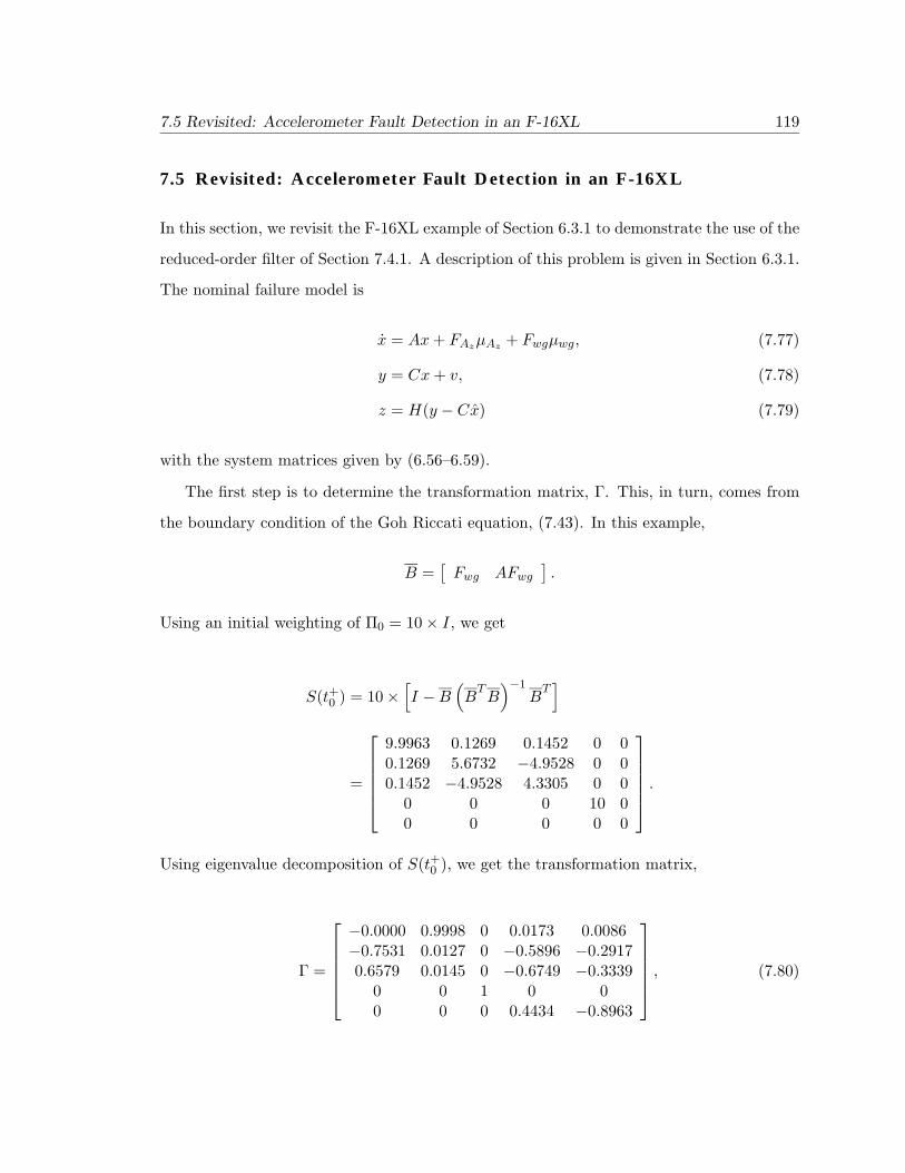
7.5 Revisited: Accelerometer Fault Detection in an F-16XL 119
7.5 Revisited: Accelerometer Fault Detection in an F-16XL
In this section, we revisit the F-16XL example of Section 6.3.1 to demonstrate the use of the
reduced-order filter of Section 7.4.1. A description of this problem is given in Section 6.3.1.
The nominal failure model is
x = Ax+ FAzµAz + Fwgµwg, (7.77)
y = Cx+ v, (7.78)
z = H(y − Cx) (7.79)
with the system matrices given by (6.56–6.59).
The first step is to determine the transformation matrix, Γ. This, in turn, comes from
the boundary condition of the Goh Riccati equation, (7.43). In this example,
B =[Fwg AFwg
].
Using an initial weighting of Π0 = 10× I, we get
S(t+0 ) = 10×[I −B
(BTB)−1
BT]
=
9.9963 0.1269 0.1452 0 00.1269 5.6732 −4.9528 0 00.1452 −4.9528 4.3305 0 0
0 0 0 10 00 0 0 0 0
.
Using eigenvalue decomposition of S(t+0 ), we get the transformation matrix,
Γ =
−0.0000 0.9998 0 0.0173 0.0086−0.7531 0.0127 0 −0.5896 −0.29170.6579 0.0145 0 −0.6749 −0.3339
0 0 1 0 00 0 0 0.4434 −0.8963
, (7.80)

120 Chapter 7: The Asymptotic Game Theoretic Fault Detection Filter
by using the eigenvectors of S(t+0 ) as the columns of Γ. By applying (7.80) to the F-16XL
model (7.77–7.79) and (6.56–6.59), we get a decomposition of the system and a steady-state
solution to the reduced-order Goh Riccati equation, (7.60),
S =
0.0637 0.0341 0.83870.0341 0.0577 0.48140.8387 0.4814 11.1811
. (7.81)
Our choice of weightings is
V =
2 0 0 00 2 0 00 0 200 00 0 0 2
, Q = I.
0 0.5 1 1.5 2 2.5 3 3.5 4 4.5 5-6
-4
-2
0
2
4x 10
-5
Time (Seconds)
Mag
nitu
de
Reduced-Order Filter Residual Response to Nuisance Fault Input
0 0.5 1 1.5 2 2.5 3 3.5 4 4.5 5-0.5
0
0.5
Time (Seconds)
Mag
nitu
de
Reduced-Order Filter Residual Response to Target Fault Input
Figure 7.1: Reduced-Order Detection Filter Performance for the F-16XL Example.
Figure 7.1 shows that the resulting reduced-order filter effectively blocks the nuisance
fault transmission while preserving the target fault transmission. If one compares the Goh
Riccati solution, (7.81), to the game Riccati solution used in Section 6.3.1, (6.62), he will
notice that the reduced-order filter does not necessarily lead to a high-gain filter. Looking

7.5 Revisited: Accelerometer Fault Detection in an F-16XL 121
back on the discussion on high-gain feedback in Section 6.3.1, this is an important aspect
of the reduced-order filter.


Chapter 8
A Parameter RobustGame Theoretic Fault Detection Filter
A game theoretic fault detection filter which is robust to uncertainty in the plant
dynamics is derived and analyzed in this chapter. In Section 8.1, we discuss the various
strategies that have been used to robustify detection filters. In Section 8.2, we discuss how
fault detection and parameter robustness can act as competing objectives and in Section 8.3
we formulate a new disturbance attenuation problem in which plant parameter variations
are modeled as additional disturbances. The parameter robust detection filter falls out from
the problem solution. In Section 8.4, we analyze the limiting case properties of the new
filter, and in Section 8.5 we work through an example which compares the performance of
filters designed with and without an accounting of model uncertainty.
8.1 Parameter Robustness and FDI
A fundamental issue in fault detection and identification is the sensitivity of the given
method to plant parameter variations. Detection filters and other analytical redundancy
123
124 Chapter 8: A Parameter Robust Game Theoretic Fault Detection Filter
techniques rely on accurate representations of the systems that they monitor. FDI under
modeling error, however, is still an open question.
For unknown input observers, it has been proposed to treat model uncertainty as another
disturbance, for example, (Patton and Chen 1992). Using standard design techniques, the
uncertainty disturbance is then embedded in the unobservable subspace along with the other
inputs in the disturbance set. In general however, it is not always possible to separate the
effects of parameter variations from the target fault. Thus, some, (Ding and Frank 1989),
have proposed filters which maximize the ratio of the fault transmission to disturbance
transmission with model uncertainty, again, thrown into the disturbance set. Still others
(Viswanadham and Minto 1988) have considered bounding the effect of model perturbations
on the estimation error using stable factorization and H∞ optimization.
Beard-Jones detection filters (Douglas 1993, Massoumnia 1986, White and Speyer 1987)
are difficult to robustify because of their reliance upon geometric methods. Schemes have
been introduced which robustify the detection filter to ill-conditioning in the eigenstructure
(Douglas and Speyer 1996) and to exogenous disturbances (Douglas and Speyer 1995); but,
to date, no significant progress has been made in handling plant parameter robustness. We
should note that it is possible to model plant uncertainty as an additional fault as in
(Patton and Chen 1992), but this approach, as shown in Section 8.5, leads to a filter with
poor performance if the plant uncertainty is not output separable from the target fault.
Approximate detection filter designs, such as the game theoretic fault detection filter,
can be robustified via the method of DeSouza et al. Here, plant parameter variations are
formulated as an additional element in the disturbance attenuation problem. The resulting
filter is still an H∞ filter, but one with the added property of parameter robustness. In this
chapter, we will apply the methods of (DeSouza et al. 1992) to derive a parameter robust
version of the game theoretic filter introduced in Chapter 6.
Remark 16. We must acknowledge the work of Edelmayer et al. who derive a pair
of robust H∞ detection filters in (Edelmayer et al. 1994). Their first approach uses the
DeSouza method (as we will do), and their second is a modification of their original filter

8.2 Parameter Robustness versus FDI 125
which was first presented in (Edelmayer et al. 1996). We contribute further analysis on the
filter which arises from the DeSouza construction, including an analysis of its asymptotic
properties. We will also show that the two filters proposed by Edelmayer et al. are actually
variations on the same theme, the second being a simplification of the first.
Remark 17. The benefit of DeSouza’s approach is that it provides an easy and elegant
way to incorporate parameter robustness into the design problem. Classic detection filter
structures already have the freedom to incorporate features into their designs beyond basic
FDI objectives (Douglas 1993, Massoumnia et al. 1989). However, it is not always clear how
to make use of this freedom. An analogous situation is the well-known “Q-parameterization”
of H∞ or H2 solutions (Doyle et al. 1989). Existence of this design freedom is well-known;
finding a way to use it is not. See the discussion in (Iwasake and Skelton 1994)).
Remark 18. A good survey of the robust FDI problem is given in (Frank 1994).
8.2 Parameter Robustness versus FDI
Suppose that instead of the system described by (6.2), we have one in which there is
uncertainty in the plant:
x =(A+ ∆A
)x+Bu+ F1µ1 + F2µ2. (8.1)
Clearly if we attempt to monitor (8.1) with a fault detection filter designed for the nominal
model, A, the error equation (e4= x− x),
e =(A+ LC
)e+ ∆Ax+ F1µ1 + F2µ2 + Lv, (8.2)
will be biased by the uncertainty term. Equation (8.2), however, suggests that we can
deal with modeling uncertainty by simply defining F34= ∆A and µ3
4= x. If F3 is output
separable from F1, conventional detection filter designs are applicable, since the effect
of plant uncertainty is completely decoupled from the target fault input. In general,
however, F1 and F3 will not be output separable, and non-output separable faults cannot
be distinguished by a detection filter (Beard 1971).

126 Chapter 8: A Parameter Robust Game Theoretic Fault Detection Filter
Output separability is not a necessary condition, however, for approximate detection
filters like the game theoretic fault detection filter (Edelmayer et al. 1996). Thus, we can
still design a filter which treats the plant parameter variations as another nuisance fault,
though the loss of this property eliminates the only guarantee we have that the target fault
will be visible at the output (Proposition 6.1). Our only recourse, therefore, is to proceed
with a design and attempt to find the best tradeoff between target fault transmission,
nuisance fault attenuation, and plant parameter robustness.
8.3 A Disturbance Attenuation Problem with Parameter Variations
8.3.1 The Modified Disturbance Attenuation Problem
This section repeats the derivation and analysis of Chapter 6 with the additional element
of model uncertainty. Start with a system described by (8.1) and measurements given by
the additive noise model, (6.1). As before, the disturbance attenuation function is
Daf =
∫ t1t0‖HC(x− x)‖2Qdt∫ t1
t0
[‖µ2‖2M−1 + ‖v‖2
V −1
]dt+ ‖x(t0)− x0‖2P−1
0
,
where M,V,Q, and P0 are weighting matrices. As in Chapter 6, the disturbance attenuation
problem is to find an estimator so that for all adversaries, µ2, v ∈ L2 [t1, t2], x(t0) ∈ Rn,
Daf ≤ γ. (8.3)
We solve (8.3) by converting it into a differential game,
minx
maxv
maxµ2
maxx(t0)
J ′ ≤ 0,
J ′ =∫ t1
t0
[‖HC(x− x)‖2Q − γ
(‖µ2‖2M−1 + ‖v‖2V −1
)]dt− ‖x(t0)− x0‖2Π0
,
subject to (8.1). Π04= γP−1
0 . Following DeSouza, we assume that the plant uncertainty,
∆A, can be decomposed as
∆A = F3ΛG. (8.4)

8.3 A Disturbance Attenuation Problem with Parameter Variations 127
F3 and G are known matrices of dimension, n × r and r × n, respectively. Λ is an r × rmatrix whose elements are unknown L2[t0, t1] functions. Defining
µ34= ΛGx,
we get a new dynamical equation,
x = Ax+Bu+ F1µ1 + F2µ2 + F3µ3. (8.5)
Additionally, we will augment the output, z,
z ={HC(x− x)√
εGx
},
so that the disturbance attenuation function is now
D∗af =
∫ t1t0
[‖HC(x− x)‖2Q + ε‖Gx‖2
]dt∫ t2
t1
[‖µ2‖2M−1 + ‖µ3‖2N−1 + ‖v‖2
V −1
]dt+ ‖x(t0)− x0‖2P−1
0
. (8.6)
To solve the disturbance attenuation problem, we convert (8.6) into the cost function,
J =∫ t1
t0
[‖HC(x− x)‖2Q + ε‖Gx‖2 − γ
(‖µ2‖2M−1
+ ‖µ3‖2N−1 + ‖v‖2V −1
)]dt− ‖x(t0)− x0‖2Π0
,
where Π04= γP−1
0 , and solve the differential game,
minx
maxv
maxµ2
maxµ3
maxx(t0)
J ≤ 0,
subject to
x = Ax+ F2µ2 + F3µ3. (8.7)
Note that we have eliminated a pair of elements from Equation (8.5). As in Chapter 6,
µ1 is taken to be zero in the the derivation of the solution, since it is the target fault and

128 Chapter 8: A Parameter Robust Game Theoretic Fault Detection Filter
should not be attenuated. We also take u to be zero for convenience. When the plant model
is perfectly known, it is possible to simply subtract out known signals such as u to nullify
their effects. However, in the case of model uncertainty, such signals can have a significant
impact upon filter performance (DeSouza et al. 1992). The inclusion of the control input
is an obvious extension of the work that we present here.
The following proposition, modified from (DeSouza et al. 1992), shows that the solution
to the new game also solves the original game under a mild restriction:
Proposition 8.1. If Λ is such that ‖Λ‖∞ ≤ 1√γ ‖N−
12 ‖∞
, then for any ε > 0,
maxv
maxµ2
maxµ3
maxx(t0)
J ′ ≤ maxv
maxµ2
maxµ3
maxx(t0)
J.
Proof. If one simply compares the terms in J ′ and J , he would find that:
J = J ′ + ε[‖Gx‖2 − γ‖ΛGx‖2N−1
]Now,
γ‖ΛGx‖2N−1 = γ‖N− 12 ΛGx‖2
≤ γ‖N− 12 Λ‖2∞‖Gx‖2
≤ γ‖N− 12 ‖2∞‖Λ‖2∞‖Gx‖2.
Thus, ‖Λ‖∞ ≤ 1√γ ‖N−
12 ‖∞
implies the proposition.
As in Chapter 6, rewrite the sensor noise term, ‖v‖2V −1 , as the equivalent ‖y−Cx‖2V −1 :
J =∫ t1
t0
[‖HC(x− x)‖2Q + ε‖Gx‖2 − γ
(‖µ2‖2M−1 + ‖µ3‖2N−1
+ ‖y − Cx‖2V −1
)]dt− ‖x(t0)− x0‖2Π0
, (8.8)
so that the game becomes
minx
maxy
maxµ2
maxµ3
maxx(t0)
J ≤ 0.

8.3 A Disturbance Attenuation Problem with Parameter Variations 129
The differential game solution comes in two steps, beginning with
maxµ2
maxµ3
maxx(t0)
J ≤ 0.
We start by appending the system dynamics, (8.7), to the cost function, (8.8), through a
Lagrange multiplier, λT ,
J =∫ t1
t0
[‖HC(x− x)‖2Q + ε‖Gx‖2 − γ
(‖µ2‖2M−1 + ‖µ3‖2N−1 + ‖y − Cx‖2V −1
)+ λT
(Ax+ F2µ2 + F3µ3 − x
)]dt− ‖x(t0)− x0‖2Π0
,
and then integrate λT x by parts:
J =∫ t1
t0
[‖HC(x− x)‖2Q + ε‖Gx‖2
− γ(‖µ2‖2M−1 + ‖µ3‖2N−1 + ‖y − Cx‖2V −1
)+ λT
(Ax+ F2µ2 + F3µ3
)+ λTx
]dt
− ‖x(t0)− x0‖2Π0+ λ(t0)Tx(t0)− λ(t1)Tx(t1). (8.9)
Taking the first variation of (8.9) with respect to µ2, µ3 and x(t0), then gives us
µ∗2 =1γMF T2 λ, (8.10)
µ∗3 =1γNF T3 λ, (8.11)
−λ = ATλ+ εGTGx+ CTHQHC(x− x) + γCTV −1(y − Cx), (8.12)
λ(t1) = 0, (8.13)
λ(t0) = Π0
[x(t0)∗ − x0
](8.14)
as the first-order necessary conditions for the maximization of J . The asterisk is indicative
of the extremizing value of the variable. Substituting (8.10) and (8.11) into our dynamics,
(8.7), and combining the result with (8.12), gives us a two point boundary value problem,

130 Chapter 8: A Parameter Robust Game Theoretic Fault Detection Filter
{x
λ
}=[
A 1γ
(F2MF T2 + F3NF
T3
)−CT
(HQH − γV −1
)C − εGTG −AT
]{xλ
}
+{
0CTHQHCx− γCTV −1y
}, (8.15)
with initial conditions,
x∗(t0) = x0 + Π−10 λ(t0), (8.16)
λ∗(t1) = 0.
Following Chapter 6, we will assume solutions, x∗ and λ∗, to (8.15) such that
λ∗ = Π(x∗ − xp). (8.17)
If we take
Π(t0) = Π0, (8.18)
xp(t0) = x0, (8.19)
then (8.17) is in agreement with the boundary condition for λ, (8.14), at the initial time,
t0. In Chapter 6 we found that, in the absence of model uncertainty, xp is equivalent to the
optimal state estimate. With model uncertainty, however, xp will act like the state variable
in the second half of the game solution.
As we did in Chapter 6, we can substitute our assumed solution, (8.17), into the TPBVP,
(8.15), and manipulate the equations to find that the TPBVP is solved identically if
− Π = ATΠ + ΠA+1γ
Π(F2MF T2 + F3NF
T3
)Π
+ CT(HQH − γV −1
)C + εGTG (8.20)
and

8.3 A Disturbance Attenuation Problem with Parameter Variations 131
Πxp = ΠAxp + εGTGxp − CTHQHC(x− xp) + γCTV −1(y − Cxp). (8.21)
Equation (8.20) is an estimator Riccati equation and its boundary condition is given by
(8.18). The boundary condition for (8.21) is given by (8.19). We will often need the inverse
of Π in derivations and applications. Thus, we can alternatively propagate
Π−1 = AΠ−1 + Π−1AT + Π−1CT(HQH − γV −1
)CΠ−1
+ εΠ−1GTGΠ−1 +1γ
(F2MF T2 + F3NF
T3
). (8.22)
The second half of our solution begins by substituting the game optimal values of µ2,
µ3, and x(t0), (8.10,8.11,8.16), into the cost function, (8.8). The new cost, J , is then
J =∫ t1
t0
[‖x− x‖2CTHQHC + ε‖Gx‖2 − ‖λ‖21
γ(F2MFT2 +F3NFT3 )
− γ‖y − Cx‖2V −1
]dt− ‖λ(t0)‖2
Π−10. (8.23)
Add the identically zero term,
0 = ‖λ(t0)‖2Π(t0)−1 − ‖λ(t1)‖2Π(t1)−1 +∫ t1
t0
d
dt‖λ(t)‖2Π−1dt,
to (8.23) and use the inverse Riccati equation, (8.22), the boundary condition for Π at t0,
(8.18), and the boundary condition for λ at t1, (8.13), to get
J =∫ t1
t0
[‖x− x‖2CTHQHC + ε‖Gx‖2 − γ‖y − Cx‖2V −1
− (x− x)TCTHQHCΠ−1λ− λTΠ−1CTHQHC(x− x)− ελTΠ−1GTGx
− εxTGTGΠ−1λ+ (y − Cx)TV −1CΠ−1λ+ λTΠ−1CTV −1(y − Cx)
+ ελTΠ−1GTGΠ−1λ+ λTΠ−1CT(HQH − γV −1
)CΠ−1λ
]dt. (8.24)

132 Chapter 8: A Parameter Robust Game Theoretic Fault Detection Filter
We can group all the terms in (8.24) into three quadratics,
J =∫ t1
t0
[‖(x− x)−Π−1λ‖2CTHQHC + ε‖x−Π−1λ‖2GTG
− γ‖(y − Cx) + CΠ−1λ‖2V −1
]dt, (8.25)
and then use the solution, (8.17), to replace λ in (8.25). This leaves us with
J =∫ t1
t0
[‖xp − x‖2CTHQHC + ε‖xp‖2GTG − γ‖y − Cxp‖2V −1
]dt. (8.26)
The game is now
minx
maxy
J ≤ 0,
subject to (8.21). As in the first subproblem, we find the solution to this game by appending
the dynamics, (8.21), to the cost, (8.26), through a Lagrange multiplier, ρT :
J =∫ t1
t0
{‖xp − x‖2CTHQHC + ε‖xp‖2GTG − γ‖y − Cxp‖2V −1
+ ρT[Axp + εΠ−1GTGxp −Π−1CTHQHC(x− xp)
+ γΠ−1CTV −1(y − Cxp)− xp]}dt. (8.27)
After integrating ρT xp by parts, we get
δJ =∫ t1
t0
{[(xp − x)TCTHQHC + εxTpG
TG+ γ(y − Cxp)TV −1C + ρTA
+ ερTΠ−1GTG+ ρTΠ−1CTHQHC − γρTΠ−1CTV −1C + ρT]δxp
+[−(xp − x)TCTHQHC − ρTΠ−1CTHQHC
]δx+
[−γ(y − Cxp)TV −1
+ γρTΠ−1CTV −1]δy
}dt+ ρT (t0)δxp(t0)− ρT (t1)δxp(t1) (8.28)

8.3 A Disturbance Attenuation Problem with Parameter Variations 133
by taking the variation of (8.27) with respect to y and x. Note that δxp(t0) = 0, because
xp is fixed at t0 by the boundary condition, (8.19). From (8.28), the first order necessary
conditions to extremize (8.26) with respect to x and y are
x∗ = xp + Π−1ρ mod KerHC, (8.29)
y∗ = C(xp + Π−1ρ), (8.30)
ρ =[−(A+ εΠ−1GTG
)T − CT (HQH − γV −1)CΠ−1
]ρ
− CTHQHC(xp − x)− γCTV −1(y − Cxp)− εGTGxp, (8.31)
ρ(t1) = 0. (8.32)
If we substitute (8.29) and (8.30)1 into (8.21) and (8.31), we get
xp =(A+ εΠ−1GTG
)xp −Π−1CT
(HQH − γV −1
)CΠ−1ρ, (8.33)
ρ = −(A+ εΠ−1GTG
)Tρ− εGTGxp, (8.34)
which is a homogeneous two-point boundary value problem in xp and ρ with boundary
conditions, (8.19) and (8.32). Using the sweep method, we take
ρ = Sxp (8.35)
and substitute (8.35) into (8.29) to get
x∗ =(I + Π−1S
)xp (8.36)
as the optimal estimate. The vector, xp, is propagated by
xp =(A+ εΠ−1GTG−Π−1CTHQHCΠ−1S
)xp + γΠ−1CTV −1(y − Cxp), (8.37)
1We can ignore any differences between x and xp that lie in kerHC since these differences willnot show up at our controlled output, z.

134 Chapter 8: A Parameter Robust Game Theoretic Fault Detection Filter
which is the result of substituting (8.36) into (8.21). S is found by propagating
− S =(A+ εΠ−1GTG
)TS + S
(A+ εΠ−1GTG
)− SΠ−1CT
(HQH − γV −1
)CΠ−1S + εGTG (8.38)
from the terminal condition,
S(t1) = 0. (8.39)
Equation (8.38) is found by differentiating (8.35) and using (8.33) and (8.34) where needed.
Equation (8.39) is determined from (8.32) and (8.35).
Remark 19. If we take ε = 0, S will be identically zero since (8.38) will be an unforced
differential equation with zero as its boundary condition. Thus, from (8.36), x = xp, and
the robust game theoretic fault detection filter simplifies to
˙x = Ax+ γΠ−1CTV −1(y − Cx),
−Π = ATΠ + ΠA+1γ
Π(F2MF T2 + F3NF
T3
)Π + CT
(HQH − γV −1
)C,
Π(t0) = Π0.
This is identical to the results of Chapter 6, except that we still have the map, F3, which
corresponds to plant uncertainty. Thus, the filter is still robustified, though in a much
simpler way. As it turns out, this is Edelmayer’s alternative approach robustifying the
approximate detection filter (see Remark 8.1 and (Edelmayer et al. 1994)). Our results,
however, show that this “alternative” is just DeSouza’s method with ε = 0.
8.3.2 Equivalence to the H∞ Measurement Feedback Control Problem
The robust game theoretic fault detection filter requires the solutions to two differential
Riccati equations: one that is integrated forward in time, (8.20), and one that is integrated
backwards in time, (8.38). This is strikingly similar to the “two Riccati” solution to the

8.3 A Disturbance Attenuation Problem with Parameter Variations 135
H∞ measurement feedback problem given in (Doyle et al. 1989, Green and Limebeer 1995,
Rhee and Speyer 1991). We will now show that the robust approximate detection filter
problem and the H∞ measurement feedback control problem are one in the same problem.
We begin by making the following definitions:
x4= xp, Q
4= εGTG, A
4=A+ εΠ−1GTG,
u4= xp − x, R
4= CTHQHC, B
4= Π−1CTHQHC,
w4= y − Cxp, W
4= γV −1, Γ
4= γΠ−1CTV −1.
Assume for argument’s sake that R = CTHQHC is invertible. Substituting these definitions
into the cost function for the second half of the game, (8.26), gives us
J =∫ t1
t0
[‖x‖2
Q+ ‖u‖2R − ‖w‖W
]dt.
If we also make these substitutions into the differential equation for xp, (8.37), we then get
˙x = Ax+Bu+ Γw. (8.40)
Our game is now given by the following which is subject to (8.40):
minu
maxw
J ≤ 0,
This is the classic, linear quadratic differential game. If we apply our definitions to the
well-known feedback solution for the game (Basar and Bernhard 1995, Mageirou 1976),
u = −R−1BTSx, (8.41)
−S =ATS + SA− S(BR−1BT − ΓTW−1Γ
)S +Q, (8.42)
we find that we recover the differential game solutions of Section 8.3. That is, from (8.41),
we get the optimal state estimate, (8.36):
u = −R−1BTSx
=⇒ xp − x = −(CTHQHC
)−1(CTHQHC
)Π−1Sxp
=⇒ x =(I + Π−1S
)xp,

136 Chapter 8: A Parameter Robust Game Theoretic Fault Detection Filter
and from (8.42) we get the our second Riccati equation, (8.38):
−S = ATS + SA− S(BR−1BT − ΓW−1ΓT
)S +Q
=⇒ −S =(A+ εΠ−1GTG
)TS + S
(A+ εΠ−1GTG
)− S
[Π−1CTHQHC
(CTHQHC
)−1CTHQHCΠ−1
−(γΠ−1CTV −1
)(γ−1V
)(γV −1CΠ−1
)]S + εGTG
=⇒ −S =(A+ εΠ−1GTG
)TS + S
(A+ εΠ−1GTG
)− SΠ−1CT
(HQH − γV −1
)CΠ−1S + εGTG.
Thus, if we think of the first half of the differential game as giving us an estimator, the
equivalence between the second-half and the classic linear quadratic game implies that the
entire game is equivalent to H∞ measurement feedback problem.
Remark 20. The results presented here imply that the results derived by DeSouza
(DeSouza et al. 1992) are also equivalent to a variation of the H∞ measurement feedback
problem. This equivalence, to our knowledge, has not been recognized previously.
8.4 The Robust Game Theoretic Fault Detection Filter in the Limit
In Chapter 7, it was shown that in the limit, γ → 0, the game theoretic fault detection
filter becomes an unknown input observer in that it obtains the same invariant subspace
structure. In this section, we will examine whether the parameter robust filter derived in
the previous section also possesses this limiting property. As in Chapter 7, we will begin by
trying to find the conditions which guarantee that the game cost will be nonpositive. These
fall out after we manipulate the cost function to look like a single quadratic,
J(x, x(t0), µ2, µ3, v) =∫ t1
t0
ξTWξdt.
A nonpositive definite W ensures a nonpositive cost which ensures an attenuating solution.
We begin with the cost function as given by (8.8),
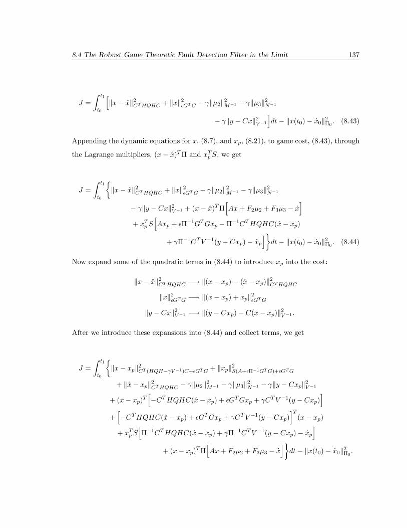
8.4 The Robust Game Theoretic Fault Detection Filter in the Limit 137
J =∫ t1
t0
[‖x− x‖2CTHQHC + ‖x‖2εGTG − γ‖µ2‖2M−1 − γ‖µ3‖2N−1
− γ‖y − Cx‖2V −1
]dt− ‖x(t0)− x0‖2Π0
. (8.43)
Appending the dynamic equations for x, (8.7), and xp, (8.21), to game cost, (8.43), through
the Lagrange multipliers, (x− x)TΠ and xTp S, we get
J =∫ t1
t0
{‖x− x‖2CTHQHC + ‖x‖2εGTG − γ‖µ2‖2M−1 − γ‖µ3‖2N−1
− γ‖y − Cx‖2V −1 + (x− x)TΠ[Ax+ F2µ2 + F3µ3 − x
]+ xTp S
[Axp + εΠ−1GTGxp −Π−1CTHQHC(x− xp)
+ γΠ−1CTV −1(y − Cxp)− xp]}dt− ‖x(t0)− x0‖2Π0
. (8.44)
Now expand some of the quadratic terms in (8.44) to introduce xp into the cost:
‖x− x‖2CTHQHC −→ ‖(x− xp)− (x− xp)‖2CTHQHC‖x‖2εGTG −→ ‖(x− xp) + xp‖2εGTG
‖y − Cx‖2V −1 −→ ‖(y − Cxp)− C(x− xp)‖2V −1 .
After we introduce these expansions into (8.44) and collect terms, we get
J =∫ t1
t0
{‖x− xp‖2CT (HQH−γV −1)C+εGTG + ‖xp‖2S(A+εΠ−1GTG)+εGTG
+ ‖x− xp‖2CTHQHC − γ‖µ2‖2M−1 − γ‖µ3‖2N−1 − γ‖y − Cxp‖2V −1
+ (x− xp)T[−CTHQHC(x− xp) + εGTGxp + γCTV −1(y − Cxp)
]+[−CTHQHC(x− xp) + εGTGxp + γCTV −1(y − Cxp)
]T(x− xp)
+ xTp S[Π−1CTHQHC(x− xp) + γΠ−1CTV −1(y − Cxp)− xp
]+ (x− xp)TΠ
[Ax+ F2µ2 + F3µ3 − x
]}dt− ‖x(t0)− x0‖2Π0
.

138 Chapter 8: A Parameter Robust Game Theoretic Fault Detection Filter
Add and subtract (x− xp)TΠAxp and (x− xp)TΠxp to the above and collect terms to get
J =∫ t1
t0
{‖x− xp‖2ΠA+CT (HQH−γV −1)C+εGTG + ‖xp‖2S(A+εΠ−1GTG)+εGTG
+ ‖x− xp‖2CTHQHC − γ‖µ2‖2M−1 − γ‖µ3‖2N−1 − γ‖y − Cxp‖2V −1
+ (x− xp)T[−Πxp + ΠAxp − CTHQHC(x− xp) + εGTGxp + γCTV −1(y − Cxp)
]+[−CTHQHC(x− xp) + εGTGxp + γCTV −1(y − Cxp)
]T(x− xp)
+ xTp S[Π−1CTHQHC(x− xp) + γΠ−1CTV −1(y − Cxp)− xp
]+ (x− x)TΠ
(F2µ2 + F3µ3
)− (x− xp)TΠ(x− xp)
}dt− ‖x(t0)− x0‖2Π0
. (8.45)
The third line of (8.45) can be eliminated by using (8.21), which comes from the first half
of the game solution derived in Section 8.3. We now integrate the terms, (x−xp)TΠ(x− xp)
and xTp Sxp, in (8.45) by parts so that the cost now becomes
J =∫ t1
t0
{‖x− xp‖2Π+ΠA+CT (HQH−γV −1)C+εGTG
+ ‖x− xp‖CTHQHC
+[−Πxp − CTHQHC(x− xp) + εGTGxp + γCTV −1(y − Cxp)
]T(x− xp)
+ (x− xp)TΠ(F2µ2 + F3µ3
)+ xTΠ(x− xp) + xTp Sxp − γ‖y − Cxp‖2V −1
+ xTp S[Π−1CTHQHC(x− xp) + γΠ−1CTV −1(y − Cxp)
]− γ‖µ2‖2M−1
− γ‖µ3‖2N−1 + ‖xp‖2S+S(A+εΠ−1GTG)+εGTG
}dt+ ‖xp(t0)‖2S(t0) − ‖xp(t1)‖2S(t1)
− ‖x(t0)− x0‖2Π0+ ‖x(t0)− xp(t0)‖2Π(t0) − ‖x(t1)− xp(t1)‖2Π(t1). (8.46)
The first two terms on the last line of (8.46) can be combined by using the boundary
condition for xp at t0, (8.19). Moreover, if we insert the state equation for x, (8.7), and xp,
(8.21), into the third line of (8.46), we get

8.4 The Robust Game Theoretic Fault Detection Filter in the Limit 139
J =∫ t1
t0
{‖x− xp‖2Π+ΠA+CT (HQH−γV −1)C+εGTG
+ ‖x− xp‖2CTHQHC
+[−Πxp − CTHQHC(x− xp) + εGTGxp + γCTV −1(y − Cxp)
]T(x− xp)
− γ‖µ2‖2M−1 − γ‖µ3‖2N−1 + ‖xp‖2S+S(A+εΠ−1GTG)+(A+εΠ−1GTG)TS+εGTG
+ (x− xp)TΠ(F2µ2 + F3µ3
)+(Ax+ F2µ2 + F3µ3
)TΠ(x− xp)− γ‖y − Cxp‖2V −1
+[−Π−1CTHQHC(x− xp) + γΠ−1CTV −1(y − Cxp)
]TSxp
+ xTp S[−Π−1CTHQHC(x− xp) + γΠ−1CTV −1(y − Cxp)
]}dt
+ ‖xp(t0)‖2S(t0) − ‖x(t0)− x0‖2Π0−Π(t0) − ‖xp(t1)‖2S(t1) − ‖x(t1)− xp(t1)‖2Π(t1).
Now, add and subtract xTpATΠ(x − xp) to the above and collect terms so that we end up
with
J =∫ t1
t0
{‖x− xp‖2Π+ΠA+ATΠ+CT (HQH−γV −1)C+εGTG
+ ‖x− xp‖CTHQHC
+[−Πxp + ΠAxp − CTHQHC(x− xp) + εGTGxp + γCTV −1(y − Cxp)
]T(x− xp)
+ ‖xp‖2S+S(A+εΠ−1GTG)+(A+εΠ−1GTG)TS+εGTG− γ‖µ2‖2M−1 − γ‖µ3‖2N−1
+ (x− xp)TΠ(F2µ2 + F3µ3
)+(F2µ2 + F3µ3
)TΠ(x− xp)− γ‖y − Cxp‖2V −1
+[−Π−1CTHQHC(x− xp) + γΠ−1CTV −1(y − Cxp)
]TSxp
+ xTp S[−Π−1CTHQHC(x− xp) + γΠ−1CTV −1(y − Cxp)
]}dt
+ ‖xp(t0)‖2S(t0) − ‖x(t0)− x0‖2Π0−Π(t0) − ‖xp(t1)‖2S(t1) − ‖x(t1)− xp(t1)‖2Π(t1). (8.47)
Using (8.21), we can eliminate the second line of (8.47). The remainder can then be
compactly written as
J =∫ t1
t0
ξTWξdt+ ‖xp(t0)‖2S(t0) − ‖x(t0)− x0‖2Π0−Π(t0)
− ‖xp(t1)‖2S(t1) − ‖x(t1)− xp(t1)‖2Π(t1),

140 Chapter 8: A Parameter Robust Game Theoretic Fault Detection Filter
where
ξ =
(x− xp)µ2
µ3
xp(x− xp)
(y − Cxp)
.
The matrix, W , has the form,
W =[W1(Π) 0
0 W2(S)
],
in which
W1(Π)4=
L1(Π) ΠF2 ΠF3
F T2 Π −γM−1 0F T3 Π 0 −γN−1
, (8.48)
L1(Π)4= Π +ATΠ + ΠA+ CT
(HQH − γV −1
)C + εGTG
and
W2(S)4=
L2(S) −SΠ−1CTHQHC γSΠ−1CTV −1
−CTHQHCΠ−1S CTHQHC 0γV −1CΠ−1S 0 −γV −1
,
L2(S)4= S +
(A+ εΠ−1GTG
)TS + S
(A+ εΠ−1GTG
)+ εGTG.
Therefore, for matrices Π > 0 and S > 0 such that
W1(Π) ≤ 0,
W2(S) ≤ 0,
Π0 −Π(t0) ≥ 0,
S(t0) = 0 or x0 = 0,
S(t1) ≥ 0,
Π(t1) ≥ 0,

8.5 Example: Accelerometer Fault Detection in an F16XL with Model Uncertainty 141
the cost, J , will be nonpositive.
In the special case, ε = 0, we know from Remark 8.3.1 that S will be zero, which allows
us to ignore W2(S) altogether. The limiting conditions for γ → 0 then come from (8.48)
and are
ΠF2 = 0, (8.49)
ΠF3 = 0, (8.50)
L1(Π) ≤ 0. (8.51)
Equations (8.49–8.51) are identical to the conditions found in Chapter 7 for the standard
problem with no model uncertainty, which is what we would expect. Note that (8.49) and
(8.50) clearly show that, in the limit, the Riccati matrix, Π, obtains a nontrivial null space
which contains the image of the nuisance failure maps, F2 and F3. This, in turn, implies
that a limiting solution does not exist for the case, ε 6= 0, since W2(S) requires that an
inverse exist for Π. Thus, robustifying the game theoretic fault detection filter destroys the
limiting property found in Chapter 7. The loss of this asymptotic property can be thought
of as a vivid example of the tradeoff between fault detection and parameter robustness.
8.5 Example: Accelerometer Fault Detection in an F16XL with ModelUncertainty
8.5.1 Problem Statement
To show how the robust game theoretic detection filter can be used for fault detection and
identification, we once again revisit the F-16XL example introduced in Chapter 6. In this
section, we will add model uncertainty to the problem. A description of the states and the
measurements is given in Section 6.3.1. The nominal failure model is given by
x = Ax+ FAzµAz + Fwgµwg,
y = Cx+ v,
z = H(y − Cx).

142 Chapter 8: A Parameter Robust Game Theoretic Fault Detection Filter
The system matrices are given by (6.56–6.59). To complete our model, incorporate plant
uncertainty into the equations. In this example, we will assume that the system eigenvalues
are only known to within a certain range. The perturbation in A corresponding to this
uncertainty is found by decomposing A into its eigenvalues and eigenvectors:
A = XDX−1.
X is a matrix whose columns are the eigenvectors of A; D is a diagonal matrix whose
diagonal elements are the corresponding eigenvalues. ∆A is then obtained by perturbing
the eigenvalues by 10%, reforming the matrix, and taking the difference from the nominal
A:
A = V (1.1×D)V −1,
∆A = A−A.
We do not need all of the elements of ∆A, however. Since any element in the fifth column of
∆A enters the system in the same way as the nuisance fault, µwg, it is redundant to include
these perturbations. Also, the fourth state, θ, is the integral of the third state, q. There is
no uncertainty in this dynamic relationship (since an integral is always an integral), and so
we can eliminate the corresponding element in ∆A, to get
∆A =
−0.0067 0.0043 −0.0889 0 00.0020 −0.1467 1.6580 0 00.0138 −0.1679 −0.0682 0 0
0 0 0 0 00 0 0 0 0
.Now implicit in this perturbation model is a perturbation size, 10 %. We remove this
assumption when we decompose ∆A into the form given by (8.4). We must also point out
that we are only interested in finding the map, F3, since this represents the way in which
the plant uncertainty drives the system. By using the singular value decomposition,
∆A = USV T ,
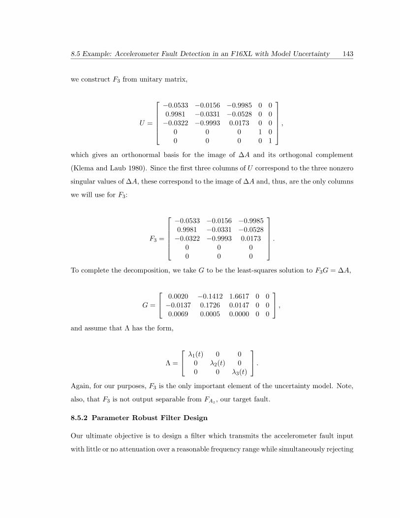
8.5 Example: Accelerometer Fault Detection in an F16XL with Model Uncertainty 143
we construct F3 from unitary matrix,
U =
−0.0533 −0.0156 −0.9985 0 00.9981 −0.0331 −0.0528 0 0−0.0322 −0.9993 0.0173 0 0
0 0 0 1 00 0 0 0 1
,which gives an orthonormal basis for the image of ∆A and its orthogonal complement
(Klema and Laub 1980). Since the first three columns of U correspond to the three nonzero
singular values of ∆A, these correspond to the image of ∆A and, thus, are the only columns
we will use for F3:
F3 =
−0.0533 −0.0156 −0.99850.9981 −0.0331 −0.0528−0.0322 −0.9993 0.0173
0 0 00 0 0
.To complete the decomposition, we take G to be the least-squares solution to F3G = ∆A,
G =
0.0020 −0.1412 1.6617 0 0−0.0137 0.1726 0.0147 0 00.0069 0.0005 0.0000 0 0
,and assume that Λ has the form,
Λ =
λ1(t) 0 00 λ2(t) 00 0 λ3(t)
.Again, for our purposes, F3 is the only important element of the uncertainty model. Note,
also, that F3 is not output separable from FAz , our target fault.
8.5.2 Parameter Robust Filter Design
Our ultimate objective is to design a filter which transmits the accelerometer fault input
with little or no attenuation over a reasonable frequency range while simultaneously rejecting

144 Chapter 8: A Parameter Robust Game Theoretic Fault Detection Filter
sensor noise and the windgust disturbance. Additionally, the filter must also be insensitive
to uncertainty in the eigenvalues, and it must be stable. To achieve this design goal, we
have the parameters, γ and ε, and the weighting matrices: Q, V , M , and N .
A critical element in our design is the value chosen for the parameter, ε. As we discussed
in Remark 8.3.1, with ε = 0, the robust game theoretic detection filter simplifies to standard
game theoretic fault detection filter of Chapter 6. With ε 6= 0, additional elements appear in
the estimator equation which bias the estimate in anticipation of variations in the plant. We
will, therefore, look at two different designs: one with ε = 0 and the other with ε nonzero.
After much trial and error, in which target fault transmission was traded off for nuisance
fault attenuation, the following weightings,
V =
1 0 0 00 1 0 00 0 4000 00 0 0 1
, N =
10 0 00 10 00 0 10
Q = I, M = 1000, (8.52)
were used along with γ = 0.0015 and ε = 0.000005. These values were found to give the
best design for nonzero ε. The corresponding Riccati solutions are
Π−1 = 105 ×
0.4723 −0.0065 0.0019 −0.0012 0.0393−0.0065 0.0004 0.0006 0.0001 −0.01380.0019 0.0006 0.0011 0.0000 −0.0162−0.0012 0.0001 0.0000 0.0034 −0.00020.0393 −0.0138 −0.0162 −0.0002 1.0895
,
S = 10−5 ×
0.0006 −0.0054 −0.0010 0.0001 −0.0045−0.0054 0.0699 −0.0262 −0.0011 0.0597−0.0010 −0.0262 0.5650 0.0012 −0.05970.0001 −0.0011 0.0012 0.0171 −0.0003−0.0045 0.0597 −0.0597 −0.0003 0.0729
.
If we take ε = 0, we find that the best results come when we keep all other parameters
as before, with the exception of γ, which we change to 0.0000005. For this case, the
corresponding Riccati solutions are

8.5 Example: Accelerometer Fault Detection in an F16XL with Model Uncertainty 145
Π−1 = 108 ×
0.1406 −0.0019 0.0005 0.0000 0.0134−0.0019 0.0000 0.0000 0.0000 −0.00060.0005 0.0000 0.0000 0.0000 −0.00100.0000 0.0000 0.0000 0.0010 −0.00000.0134 −0.0006 −0.0010 −0.0000 2.0780
,
S = 0.
10-2
10-1
100
101
-20
-15
-10
-5
0
Mag
nitu
de (
db)
Frequency
Robust Filter Performance with epsilon = 0.000005, 15 % Perturbation
10-2
10-1
100
101
-20
-15
-10
-5
0
Mag
nitu
de (
db)
Frequency
Robust Filter Performance with epsilon = 0, 15 % Perturbation
Figure 8.1: F-16XL example: signal transmission in the parameter robust game theoreticfault detection filter with a 15% Shift in eigenvalues (The accelerometer fault andnominal windgust transmission are represented by the solid line. The windgustis the lower of the two. The dash-dot line corresponds to windgust transmissionwhen modeled eigenvalues are in error by 15%. The dashed line corresponds totransmission under a -15% modeling error).
Figure 8.1 shows the performance of both filters for the nominal plant and for a perturbed
plant with a 15% shift in the eigenvalues. As we saw from before, the direct feedthrough
of the target fault has a very pronounced effect on target fault transmission. There is no
high frequency roll-off, and the low frequency transmission is degraded. This degradation

146 Chapter 8: A Parameter Robust Game Theoretic Fault Detection Filter
10-3
10-2
10-1
100
101
102
-80
-70
-60
-50
-40
-30
-20
-10
0Singular Value Plot of Game Theoretic Filter
Mag
nitu
de (
dB)
Frequency
Figure 8.2: F-16XL example: signal transmission in the standard game theoretic faultdetection filter with a 15% shift in eigenvalues (The accelerometer fault andnominal windgust transmission are represented by the solid line. The windgustis the lower of the two. The dash-dot line corresponds to windgust transmissionwhen modeled eigenvalues are in error by 15%. The dashed line corresponds totransmission under a -15% modeling error).
is mitigated somewhat by choosing the particular form of weighting, V , seen in (8.52).
We also note that the accelerometer fault transmission is invariant under plant parameter
changes. This is because the accelerometer fault comes in through the measurements and,
as a result, only drives the filter.
From Figure 8.1, we can see that the loss of the output separability property severely
degrades our ability to both maintain target fault sensitivity and achieve good separation
between the target fault and nuisance fault. This separation is particularly poor in the low
frequency region. Experience with this example has shown that little can be done to improve
the low frequency separation without severely degrading low frequency accelerometer fault
transmission. Figure 8.1 also shows that the ε parameter has a negligible, perhaps even
detrimental, effect upon the filter design. This result is due to the sensitivity of the Riccati
solution, S, to the values of ε and γ used in the problem. It was found that S will quickly

8.5 Example: Accelerometer Fault Detection in an F16XL with Model Uncertainty 147
lose its symmetry property when more aggressive values of ε and γ are used. This hurts the
performance of the robust filter by preventing the additional elements of the filter associated
with ε and S from having an impact on the design. It also prevents the designer from using
lower values of γ to improve nominal performance.
If one compares Figure 8.1 to Figure 8.2, which shows the performance of the filter
designed in Chapter 6 under a 15% perturbation, he will see that the parameter robust
filter achieves its robustness at the cost of nominal performance. The original filter design
from Chapter 6, in fact, has far superior low frequency performance, even under plant
parameter variations. This is critical for detecting “hard failures,” which look like step
inputs.


Chapter 9
A Decentralized Fault Detection Filter
For many of the larger scale systems of interest to PATH, such as multi-car platoons, the
design of a fault detection filter may best be done using a decentralized scheme, particularly
for the monitoring of sensors which measure relative states between cars. By this, we refer
to a filter that is formed indirectly by combining the state estimates generated by several
”local” estimators to form an estimate of the overall, or ”global,” system. This is distinct
from the standard approach, which is to design a single filter directly for the ”global”
system.
For large-scale systems, a decentralized filter may offer several advantages over using just
a single filter. First, by decentralizing the problem one simplifies it by decomposing it down
into a collection of smaller problems. Second, there are times when the decentralized point
of view reflects the actual physical structure of the system, such as a platoon of automated
cars. Third, the element of scalability is introduced into the fault detection filter with a
decentralized approach. When a car joins the platoon, for instance, there is a step change
149

150 Chapter 9: A Decentralized Fault Detection Filter
in the order of the problem. If the system is being monitored with a single filter, it may
be impossible to make a graceful adjustment. Finally, fault tolerance can be built into
the system by checking for faults in the local sensors and actuators prior to allowing their
outputs to be passed onto the global level as suggested by (Kerr 1985).
9.1 Decentralized Estimation Theory and its Application to FDI
The decentralized fault detection filter is the result of combining the game theoretic fault
detection filter of the Chapter 6 with the decentralized filtering algorithm introduced by
Speyer in (Speyer 1979) and extended by Willsky et al. in (Willsky et al. 1982). For
completeness, we will review the basics of decentralized estimation theory in this section.
The general theory was first presented in (Chung and Speyer 1995) which was research
sponsored in part by the PATH program.
9.1.1 The General Solution
Consider the following system driven by process disturbances, w, and sensor noise, v,
x = Ax+Bw, x(0), x ∈ Rn, (9.1)
y = Cx+ v, y ∈ Rm. (9.2)
for which it is desired to derive an estimate of x. The standard approach is a full-order
observer,
˙x = Ax+ L(y − Cx), x(0) = 0, (9.3)
which we will call a centralized estimator. An alternative to this method is to derive the
estimated with a decentralized estimator. In the decentralized approach, x is found by
combining estimates based upon “local” models,
xj = Ajxj +Bjwj , xj ∈ Rnj , (j = 1...N), (9.4)
yj = Ejxj + vj , yj ∈ Rmj , (j = 1...N), (9.5)
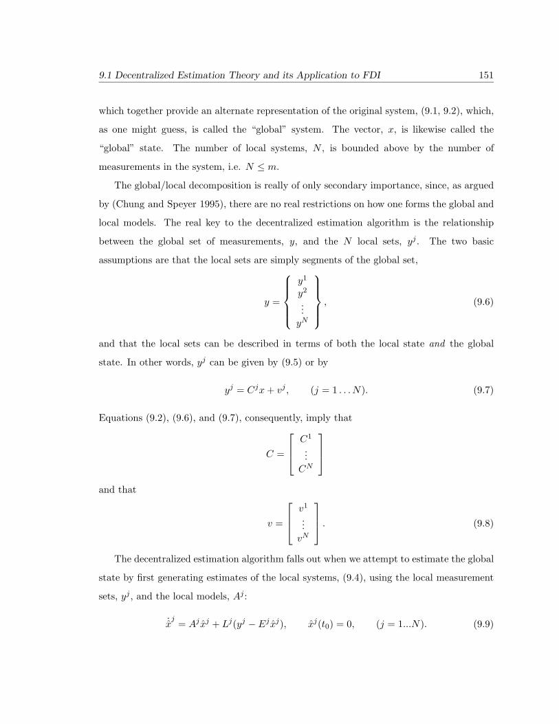
9.1 Decentralized Estimation Theory and its Application to FDI 151
which together provide an alternate representation of the original system, (9.1, 9.2), which,
as one might guess, is called the “global” system. The vector, x, is likewise called the
“global” state. The number of local systems, N , is bounded above by the number of
measurements in the system, i.e. N ≤ m.
The global/local decomposition is really of only secondary importance, since, as argued
by (Chung and Speyer 1995), there are no real restrictions on how one forms the global and
local models. The real key to the decentralized estimation algorithm is the relationship
between the global set of measurements, y, and the N local sets, yj . The two basic
assumptions are that the local sets are simply segments of the global set,
y =
y1
y2
...yN
, (9.6)
and that the local sets can be described in terms of both the local state and the global
state. In other words, yj can be given by (9.5) or by
yj = Cjx+ vj , (j = 1 . . . N). (9.7)
Equations (9.2), (9.6), and (9.7), consequently, imply that
C =
C1
...CN
and that
v =
v1
...vN
. (9.8)
The decentralized estimation algorithm falls out when we attempt to estimate the global
state by first generating estimates of the local systems, (9.4), using the local measurement
sets, yj , and the local models, Aj :
˙xj
= Aj xj + Lj(yj − Ej xj), xj(t0) = 0, (j = 1...N). (9.9)
152 Chapter 9: A Decentralized Fault Detection Filter
The global state estimate, x, is then found via
x =N∑j=1
(Gj xj + hj
). (9.10)
where hj is a measurement-dependent variable propagated by
hj = Φhj + (ΦGj − Gj −GjΦj)xj , hj(0) = 0. (9.11)
The constituent matrices are defined as
Φ := A−N∑j=1
GjLjCj ,
Φj := Aj − LjEj .
The Gj matrices are chosen “blending matrices”. In (Chung and Speyer 1995) it was found
that in order for the dectralized esimation algorithm, (9.10,9.11), to generate the same
estimate, x, as a standard centralized estimator, (6.3), the blending matrices have to be
related to the gain of the centralized estimator and the gains of the local estimators through
the equation:
L =[G1 . . . GN
]L1 0 · · · 00 L2 · · · 0...
.... . .
...0 0 · · · LN
. (9.12)
L is the gain for the global estimator, and Lj is the gain for the jth local estimator. This
is simply the requirement that a solution exists to a linear algebraic equation. In general,
however, this condition can not be met because of an insufficient number of equations with
which to solve for the unknowns.
There is, however, one general class of estimator for which (9.12) is satified almost
automatically. This class is comprised of estimators which take their gains from Riccati
solutions, that is Kalman filters (Speyer 1979, Willsky et al. 1982) or H∞-norm bounding
filters (Jang and Speyer 1994). In this case, the local gains are found from
Lj = P j(Ej)T (V j)−1, (9.13)

9.1 Decentralized Estimation Theory and its Application to FDI 153
where, in the case of the Kalman Filter, the matrix, P j is the solution of the Riccati
equation:
P j = AjP j + P j(Aj)T +BjW j(Bj)T − P j(Ej)T (V j)−1EjP j ,
P j(0) = P j0 .
The initial condition, P j0 , is chosen by the analyst based upon his knowledge of the system.
In the global system, the global gain is
L = PCTV −1
where
V =
V 1 0 · · · 00 V 2 0 0... 0
. . ....
0 · · · · · · V N
, (9.14)
is restricted to a block diagonal form comprised of the local weightings, V j , and P is the
solution to the global Riccati equation,
P = AP + PAT +BWBT − PCTVCP, P (0) = P0.
. The blending matrix solution is then,
Gj = P (Sj)T (P j)−1 j = 1, . . . , N, (9.15)
where Sj is any matrix such that
Cj = EjSj . (9.16)
One can, in fact, always take Sj = (Ej)†Cj where (Ej)† is the pseudo-inverse of Ej
(Willsky et al. 1982). Note that the solutions for Gj will always exist for Riccati-based
observers so long as P j is invertible or, equivalently, positive-definite. This will always be
the case if the triples, (Cj , Aj , Bj), are controllable and observable for each of the local
systems.

154 Chapter 9: A Decentralized Fault Detection Filter
9.1.2 Implications for Detection Filters
The analysis of the previous section implies that will we be able to form a decentralized
fault detection filter in the general case only if we are able to find a Riccati-based observer
which is equivalent to a Beard-Jones Filter or unknown input observer. The most direct
way to achieve this is to find a linear-quadratic optimization problem which is equivalent
to the fault detection and identification problem. This is an analog of the famous inverse
optimal control problem first posed by Kalman (Kalman 1964). In (Chung 1997), however,
a counterexample was given which showed that FDI observers do not correspond one-to-one
with linear-quadratic problems.
Another way to address this problem, of course, is to use the Riccati-based game
theoretic fault detection filter that we have painstaking developed in the previous three
chapters. This filter is entirely suitable for use in the decentralized estimation algorithm.
One might, in fact, take the following steps to use the game theoretic fault detection filter
in this way:
1. Identify the sensors and actuators which must be monitored at the global level, i.e.
define the target faults for the global filter.
2. Identify the faults which should be included in the global nuisance set. The remaining
faults should be monitored at the local levels.
3. Derive global and local models for the system including failure maps. (Chung 1997)
contains a brief discussion about this process. In Section 9.2, we will demonstrate one
method in which the local models are derived from the global model via a minimum
realization.
4. Design game theoretic fault detection filters for the local and global systems. Solve
the corresponding Riccati equations and store the solutions for later use.
5. Determine the blending solutions, Gj , from Equation (9.15).

9.2 Range Sensor Fault Detection in a Platoon of Cars 155
6. Propagate the local estimates, xj , and vectors, hj , and then use the decentralized
estimation algorithm (9.10) to derive a global estimate, x.
7. Determine the global failure signal from (y − Cx) where y is the total measurement
set, C is the global measurement matrix, and x is the global fault detection filter
estimate just derived.
We will now apply these steps in an example.
9.2 Range Sensor Fault Detection in a Platoon of Cars
Car #2
Range
Car #1 X
Z
Figure 9.1: A two-car platoon with a range sensor.
9.2.1 Problem Statement
We will now examine the utility of the decentralized approach to FDI by working through
an example. The problem that we will look at involves the detection of failures within
a system of two cars traveling as a platoon. See Figure 9.1. The cars are controlled to
maintain a uniform speed and constant separation.
The platoon is the central component of automated highway schemes in which groups of
cars line up single file and travel as a unit, thereby eliminating the possibility of individual
vehicles impeding one another (Douglas et al. 1995, Douglas et al. 1996). With careful
coordination, these platoons will allow traffic to move with much the same order and
protocol as electrical signals on the Internet. The viability of the platooning scheme,
however, will depend on many factors, not the least of which are reliability and safety.

156 Chapter 9: A Decentralized Fault Detection Filter
The FDI schemes that we have examined to this point are capable of monitoring
individual cars, but may not be ideal for monitoring elements that deal with the interactions
between cars. For example, to maintain uniform speed throughout the platoon and to keep
the spacing between the cars constant, additional sensors will be needed to measure the
relative speed and the relative distance, or “range”, between the cars. In order to detect
a failure in the range sensor using analytic redundancy, however, it is necessary to have a
dynamic relationship between the range sensor and other sensors on the vehicles. Range,
however, involves the dynamics of both of the cars and so would require a higher-order
model for its detection filter.
While this is not necessarily prohibitive, it does not make use of the many different
state estimates that are already being propagated throughout the platoon. The sensors on
each of the cars, for instance, will be monitored by detection filters, and it is more than
likely that a state estimate would also be generated by the vehicles’ control loops. Given
these pre-existing estimates, it seems logical to make use of the decentralized estimation
algorithm to carry out range sensor fault detection.
9.2.2 System Dynamics and Failure Modeling
Our example starts with the car model used in (Douglas et al. 1995). In this model, the
nonlinear, six degree-of-freedom dynamics of an representative automobile are linearized
about a straight, level path at a speed of 25 meters/sec (roughly 56 miles per hour).
The linearized equations are found to decouple nicely into latitudinal and longitudinal
dynamics, much like an airplane. Moreover, the linearized equations can be further reduced
by eliminating “fast modes” and actuator states. For simplicity, we will only use the
longitudinal dynamics which we represent as
x = ALx,
y = CLx.

9.2 Range Sensor Fault Detection in a Platoon of Cars 157
The vehicle states are
x =
ma
ωevxvzzqθ
engine air mass (kg)engine speed (rad/sec)long. velocity (m/sec)vertical velocity (m/sec)vertical position (m)pitch rate (rad/sec)pitch (rad)
(9.17)
and are propagated by the state matrix,
AL = 103 ×
−0.0226 −0.0001 0 0 0 0 00.3070 −0.0354 0.3974 −0.2381 −2.6980 −3.7530 −0.3311
0 0.0001 −0.0008 0.0006 0.0068 0.0168 0.00150 −0.0000 0.0000 −0.0036 −0.0404 −0.0091 −0.00080 0 0 0.0010 0 0 00 0 0 0 0 0 0.00100 −0.0000 0.0002 −0.0006 −0.0072 −0.0396 −0.0036
. (9.18)
The measurements are
y =
ma
ωevxvzqωfωr
engine air mass (kg)engine speed (rad/sed)long. acceleration (m/sec2)heave acceleration (m/sec2)pitch rate (rad/sec)front symmetric wheel speed (rad/sec)rear symmetric wheel speed (rad/sec)
(9.19)
with the corresponding measurement matrix,
CL =
1 0 0 0 0 0 00 1 0 0 0 0 00 0.0713 −0.8177 0.5934 6.7786 16.8068 1.51620 −0.0020 0.0221 −3.5646 −40.4210 −9.0765 −0.81410 0 0 0 0 0 10 0 7.1220 −4.5806 −51.9152 58.8718 5.19440 0.0888 5.9738 −3.5782 −40.5542 −56.4109 −4.9773
. (9.20)
The rear and front symmetric wheel speeds are states that were eliminated when the fast
modes were factored out of the linearized system.

158 Chapter 9: A Decentralized Fault Detection Filter
In order to build a detection filter for the range sensor, we need to use (9.17–9.20) to
build state space models for the platoon,
η = Aη + F1µ1 + F2µ2,
y = Cη,
and the two cars,
η1 = A1η1 + F 11 µ
11 + F 1
2 µ12,
y1 = E1η1,
η2 = A2η2 + F 21 µ
21 + F 2
2 µ22,
y2 = E2η2.
We will build up our models with the following steps:
1. Using (9.17–9.20), we will derive the global state matrices, A and C.
2. Using the modelling techniques described in (Douglas 1993), we will determine the
failure maps, Fi.
3. We will then obtain the local state matrices, Ai, Ei, and F ij , from the minimum
realization of the triples (C1, A, F2) and (C2, A, F2).
Our general strategy is to derive the global equation first and then get the local equations
from decompositions based upon observability and controllability. While this is by no means
the only way to obtain the global and local representations of a system, it is a logical method
that can be applied to any problem.
The obvious way the get the global matrices, A and C, is to form block diagonal
composite matrices with AL and CL repeated on the diagonal, i.e.
A′ =[AL 00 AL
], C ′ =
[CL 00 CL
].
9.2 Range Sensor Fault Detection in a Platoon of Cars 159
This, however, is not sufficient, since there is no way to describe the range, R, between the
two vehicles with the given states, (9.17). Range is the relative distance between the cars,
R = x1 − x2,
where xi is the longitudinal displacement of car i. Displacement, however, is not a state of
the vehicle (9.17). We must, therefore, add a range state to the platoon dynamics, using
the equation,
R = v1x − v2
x.
The end result is that the platoon will be a fifteen-state system,
η =
m1a
ω1e
v1x
v1z
z1
q1
θ1
m2a
ω2e
v2x
v2z
z2
q2
θ2
R
engine air mass (kg) - Car#1engine speed (rad/sec) - Car#1long. velocity (m/sec) - Car#1vertical velocity (m/sec) - Car#1vertical position (m) - Car#1pitch rate (rad/sec) - Car#1pitch (rad) - Car#1engine air mass (kg) - Car#2engine speed (rad/sec) - Car#2long. velocity (m/sec) - Car#2vertical velocity (m/sec) - Car#2vertical position (m) - Car#2pitch rate (rad/sec) - Car#2pitch (rad) - Car#2Range (m).
The corresponding state matrix is
A =
AL 00 AL
E1 −E1
, (9.21)
E1 =[
0 0 1 0 0 0 0].
The measurement matrix is
C =
CL 0
0CL 00 1
=[C1 00 C2
], (9.22)
160 Chapter 9: A Decentralized Fault Detection Filter
where C1 and C2 can be inferred from (9.22). Finally, the local measurement sets are
y1 =
m1a
ω1e
v1x
v1z
q1
ω1f
ω1r
engine air mass (kg)- Car#1engine speed (rad/sed)- Car#1long. acceleration (m/sec2)- Car#1heave acceleration (m/sec2)- Car#1pitch rate (rad/sec)- Car#1front symmetric wheel speed (rad/sec) - Car#1rear symmetric wheel speed (rad/sec) - Car#1.
and
y2 =
m2a
ω2e
v2x
v2z
q2
ω2f
ω2r
R
engine air mass (kg)- Car#2engine speed (rad/sed)- Car#2long. acceleration (m/sec2)- Car#2heave acceleration (m/sec2)- Car#2pitch rate (rad/sec)- Car#2front symmetric wheel speed (rad/sec) - Car#2rear symmetric wheel speed (rad/sec) - Car#2range (rad/sec).
Our ultimate objective is to design a filter which will detect a range sensor fault in the
presence of potential failures in the other sensors.
In an actual health monitoring system, we would design the global filter to block out
all of the nuisance faults that are output separable from the range sensor fault and then
rely upon the local filters to monitor the remaining faults. Given the size of our example,
however, the full analysis required to do a detailed design would clutter our presentation.
We will, therefore, limit ourselves to constructing only one local filter and will choose simple
nuisance sets at both the global and local levels.
For this example, we choose to monitor the front symmetric wheel speed sensor at the
local level. The nuisance set is then chosen to be the engine air mass sensor and the heave
accelerometer. At the global level, the range sensor has already been designated as the
target fault. We, therefore, complete the problem definition by choosing the engine speed
sensor and longitudinal accelerometer as the global nuisance set. There is no particular
significance attached to any of our choices for the nuisance and target sets, aside from the
choice of the range sensor as the global target fault.
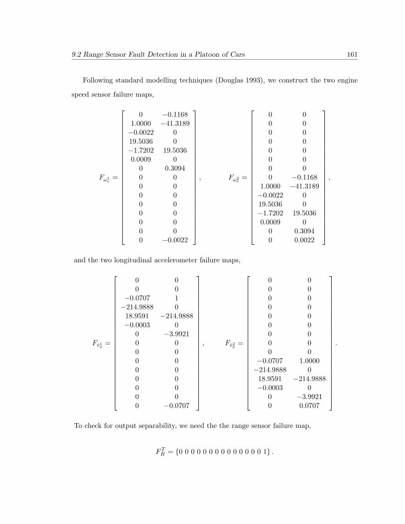
9.2 Range Sensor Fault Detection in a Platoon of Cars 161
Following standard modelling techniques (Douglas 1993), we construct the two engine
speed sensor failure maps,
Fω1e
=
0 −0.11681.0000 −41.3189−0.0022 019.5036 0−1.7202 19.50360.0009 0
0 0.30940 00 00 00 00 00 00 00 −0.0022
, Fω2e
=
0 00 00 00 00 00 00 00 −0.1168
1.0000 −41.3189−0.0022 019.5036 0−1.7202 19.50360.0009 0
0 0.30940 0.0022
,
and the two longitudinal accelerometer failure maps,
Fv1x
=
0 00 0
−0.0707 1−214.9888 0
18.9591 −214.9888−0.0003 0
0 −3.99210 00 00 00 00 00 00 00 −0.0707
, Fv2x
=
0 00 00 00 00 00 00 00 00 0
−0.0707 1.0000−214.9888 0
18.9591 −214.9888−0.0003 0
0 −3.99210 0.0707
.
To check for output separability, we need the the range sensor failure map,
F TR = {0 0 0 0 0 0 0 0 0 0 0 0 0 0 1} .

162 Chapter 9: A Decentralized Fault Detection Filter
For the local filters, we need the need the airmass sensor failure maps,
Fm1a
=
1 −22.56050 307.02980 00 00 00 00 00 00 00 00 00 00 00 00 0
, Fm2a
=
0 00 00 00 00 00 00 01 −22.56050 307.02980 00 00 00 00 00 0
,
and the heave accelerometer sensor failure maps,
Fv1z
=
0 00 0
−0.1767 0−7.8747 10.6698 −7.8747−0.0007 0
0 0.01970 00 00 00 00 00 00 00 −0.1767
, Fv2z
=
0 00 00 00 00 00 00 00 00 0
−0.1767 0−7.8747 10.6698 −7.8747−0.0007 0
0 0.01970 0.1767
.
Finally, to check for output separability in the local filters, we will need the front wheel
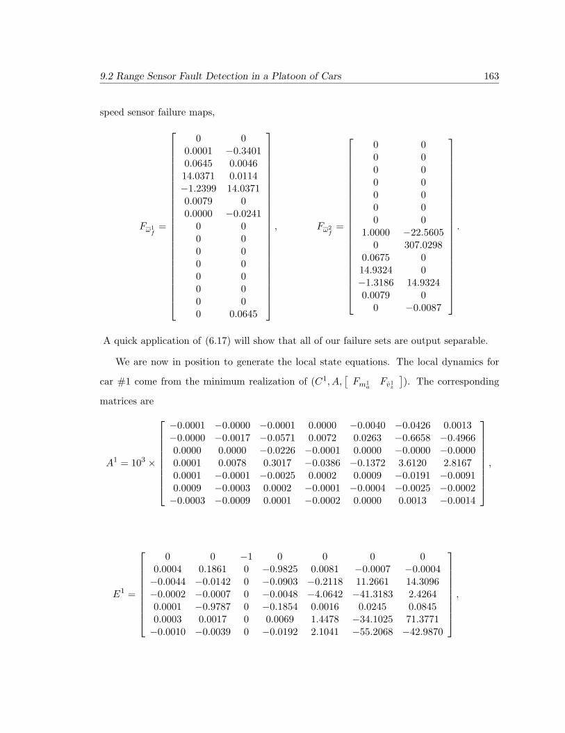
9.2 Range Sensor Fault Detection in a Platoon of Cars 163
speed sensor failure maps,
Fω1f
=
0 00.0001 −0.34010.0645 0.004614.0371 0.0114−1.2399 14.03710.0079 00.0000 −0.0241
0 00 00 00 00 00 00 00 0.0645
, Fω2f
=
0 00 00 00 00 00 00 0
1.0000 −22.56050 307.0298
0.0675 014.9324 0−1.3186 14.93240.0079 0
0 −0.0087
.
A quick application of (6.17) will show that all of our failure sets are output separable.
We are now in position to generate the local state equations. The local dynamics for
car #1 come from the minimum realization of (C1, A,[Fm1
aFv1
z
]). The corresponding
matrices are
A1 = 103 ×
−0.0001 −0.0000 −0.0001 0.0000 −0.0040 −0.0426 0.0013−0.0000 −0.0017 −0.0571 0.0072 0.0263 −0.6658 −0.49660.0000 0.0000 −0.0226 −0.0001 0.0000 −0.0000 −0.00000.0001 0.0078 0.3017 −0.0386 −0.1372 3.6120 2.81670.0001 −0.0001 −0.0025 0.0002 0.0009 −0.0191 −0.00910.0009 −0.0003 0.0002 −0.0001 −0.0004 −0.0025 −0.0002−0.0003 −0.0009 0.0001 −0.0002 0.0000 0.0013 −0.0014
,
E1 =
0 0 −1 0 0 0 00.0004 0.1861 0 −0.9825 0.0081 −0.0007 −0.0004−0.0044 −0.0142 0 −0.0903 −0.2118 11.2661 14.3096−0.0002 −0.0007 0 −0.0048 −4.0642 −41.3183 2.42640.0001 −0.9787 0 −0.1854 0.0016 0.0245 0.08450.0003 0.0017 0 0.0069 1.4478 −34.1025 71.3771−0.0010 −0.0039 0 −0.0192 2.1041 −55.2068 −42.9870
,

164 Chapter 9: A Decentralized Fault Detection Filter
F 1m1a
=
0 0.12130 57.12301 −22.56050 −301.65860 2.49800 −0.20410 −0.1202
, F 1
v1z
=
7.9031 −1.6879−0.0007 −0.0213
0 0−0.0048 −0.0057−0.1760 −0.7911−0.0068 −7.4136−0.0003 −2.1388
.
A model for Car #2 is similarly found as a minimal realization of (C2, A,[Fm2
aFv2
z
]).
The corresponding matrices are
A2 = 103 ×
−0.0003 −0.0003 0.0010 −0.0000 0.0000 0.0000 0.0000 −0.00000.0003 0.0003 0.0000 0.0010 −0.0000 −0.0000 −0.0000 0.0000−0.0125 −0.0121 −0.0015 −0.0008 −0.0000 0.0000 0.0000 0.0000−0.0283 −0.0275 −0.0021 −0.0030 0.0000 0.0081 0.0067 −0.00010.1951 0.1939 −0.0024 0.0389 −0.0002 −0.1529 −0.1262 0.00270.0039 0.0046 0.0004 0.0005 −0.0000 −0.0213 −0.0184 0.0000−0.0041 −0.0048 −0.0004 −0.0005 0.0000 0.0228 0.0178 −0.0000−2.6548 −2.6391 0.0323 −0.5294 −0.3044 2.0805 1.7175 −0.0578
,
E2 =
−0.0000 0.0000 1.0000 −0.0000 0.0000 0.0000 −0.0000−0.0004 0.1861 0 −0.9825 0.0081 −0.0007 0.00040.0044 −0.0142 −0.0000 −0.0903 −0.2118 11.2661 −14.30960.0002 −0.0007 −0.0000 −0.0048 −4.0642 −41.3183 −2.4264−0.0001 −0.9787 0 −0.1854 0.0016 0.0245 −0.0845−0.0003 0.0017 0 0.0069 1.4478 −34.1025 −71.37710.0010 −0.0039 0 −0.0192 2.1041 −55.2068 42.9870
,
F 2m2a
=
0 00 00 00 0
0.9973 0.00020 00 0
0.0733 −307.8575
, F 2
v2z
=
0 00 00 00 00 0
−5.0327 −4.92826.0961 −6.2254
0 0
.

9.2 Range Sensor Fault Detection in a Platoon of Cars 165
With all of these system matrices in place, we can now form the residual projectors, H,
(6.12) needed generate the failure signal, z. In the global filter, we define
F =[Fω1
eFv1
xFω2
eFv2
x
]so that the projector for the global filter is
H = I − CF[(CF )TCF
]−1(CF )T .
In the local filters, we define
F i =[F imia
F iviz
]i = 1, 2
so that the projector is
H i = I − CF i[(CF i)TCF i
]−1(CF i)T .
We do not show either of these matrices explicitly because of their size.
9.2.3 Decentralized Fault Detection Filter Design
We will first design filters for the local systems. For simplicity, we will once again use the
steady-state version of the game theoretic fault detection filter. The design process boils
down to finding the design weightings which give the best tradeoff between target fault
transmission and nuisance fault attenuation. For this example, it was found that
M1 = 10× I7, V 1 = diag[
1 1 10 1 1 1 1],
Q1 = I7, γ = 0.18
leads to the filter for Car #1 depicted in Figure 9.2. The minimum separation over frequency
is only 35 dB, but the filter has particularly good separation in the low frequency range.
For Car #2, the same weightings, adjusted for the different dimensions of the Car #2
dynamics,
M2 = 10× I8, V 2 = diag[
1 1 10 1 1 1 1 1],
Q2 = I8, γ = 0.18,

166 Chapter 9: A Decentralized Fault Detection Filter
10-1
100
101
102
103
-120
-100
-80
-60
-40
-20
0
Singular Value Plot of Local Game Theoretic Filter #1
Mag
nitu
de (
db)
Frequency
Figure 9.2: Platoon example: signal transmission in the local detection filter on car# 1 (accelerometer fault transmission shown with solid line, nuisance faulttransmission shown with dashed line).
10-1
100
101
102
103
-120
-100
-80
-60
-40
-20
0
Singular Value Plot of Local Game Theoretic Filter #2
Mag
nitu
de (
db)
Figure 9.3: Platoon example: signal transmission in the local detection filter on car# 2 (accelerometer fault transmission shown with solid line, nuisance faulttransmission shown with dashed line).

9.2 Range Sensor Fault Detection in a Platoon of Cars 167
10-1
100
101
102
103
-120
-100
-80
-60
-40
-20
0
Singular Value Plot of Global Game Theoretic Filter
Mag
nitu
de (
db)
Frequency
Figure 9.4: Platoon example: signal transmission in the global detection filter (positionsensor fault transmission shown with solid line, nuisance fault transmissionshown with dashed line).
0 0.5 1 1.5 2 2.5 3 3.5 4 4.5 5-0.03
-0.02
-0.01
0
0.01
0.02
0.03Residual Signal for Nuisance Fault Input
Sig
nal M
agni
tude
Time (secs)
0 0.5 1 1.5 2 2.5 3 3.5 4 4.5 5-0.2
0
0.2
0.4
0.6
0.8
1
Residual Signal for Target Fault Input
Sig
nal M
agni
tude
Time (secs)
Figure 9.5: Platoon example: failure signal response of the decentralized fault detectionfilter (Nuisance fault is a step failure in the longitudinal accelerometer on car #1).

168 Chapter 9: A Decentralized Fault Detection Filter
lead to a filter with the performance depicted in Figure 9.3.
Finally, we turn to the global system. The decentralized fault detection filter for range
sensor health monitoring in the platoon is found by solving,
0 = Π−1AT +AΠ−1 +1γF2MF T2 + Π−1CT (HQH − γV −1)CΠ−1, (9.23)
which is simply a variation of (6.54). The weightings,
γV −1 = I17, Q = I17,
M = 100× I8, γ = 0.18.
were used in the design. The resulting filter has the properties depicted in Figure 9.4. The
decentralized estimator should also exhibit this level of performance. As a check, a simple
time domain simulation was run comparing the response of the residual signal when the
system is driven by the target fault (a step failure of the range sensor) to when it is driven
by a nuisance fault (a step failure of the longitudinal accelerometer on Car #1). Because
we are using Riccati-based estimators, the blending matrices, Gj , are given by (9.15). The
connecting matrices, Sj , are taken to be the pseudo-inverses of Ej . The remaining vectors
and matrices that form the decentralized estimation algorithm are as given in Section 9.1.
As Figure 9.5 shows, the resulting decentralized fault detection filter does a good job of
distinguishing the target fault from the nuisance fault.
It must be noted that we have assumed that the lead car will transmit its measurements,
y1, its local state estimates, η2, and the vector, h1, back to car #2 so that the latter can
form the global estimate via the decentralized estimation algorithm. Transmission issues
and limitations, quite obviously, open up the potential for new problems. We have also
assumed that each car will have stored on-board the needed Riccati solutions for all likely
scenarios.

Chapter 10
Multiple Model Adaptive Estimation
A class of adaptive estimation problems is considered where an unknown system
model is assumed to correspond to one of a number of specified models and the model
uncertainty is summarized as a time-varying parametric uncertainty. In particular, we
concern ourselves with estimation in linear stochastic systems with time-varying parameters.
Early attempts to solve this problem produced the Multiple Model Adaptive Estimation
(MMAE) algorithm, first proposed by (Magill 1965) then generalized by (Lainiotis 1976)
to form the framework of partitioned algorithms. This algorithm addresses the most basic
adaptive estimation problem, estimation in a linear stochastic system with time-invariant
parametric uncertainty. It is a joint estimation and system identification algorithm with of
a bank of Kalman filters, each matched to one hypothesis and an identification subsystem,
which may be construed as the dynamics of a sub-optimal multiple hypothesis Wald’s
Sequential Probability Ratio Test (WSPRT). We denote the underlying dynamics of the
WSPRT by Fwki , which is defined as the posterior probability of hypothesis Hi conditioned
169

170 Chapter 10: Multiple Model Adaptive Estimation
on the residual history up to tk. The use of Fwki is motivated by the implicit assumption
that we are dealing with a time-invariant parametric uncertainty. However, as stated in
(Athans 1977), there is no rigorous proof that the posterior probability associated with the
true model will converge to unity. Moreover, apart from being computationally intensive,
this algorithm suffers from beta dominance (Menke and Maybeck 1995), which arises out of
incorrect system modeling and leads to irregular residuals.
Recently, there have been efforts to improve the performance of the MMAE algorithm
(Maybeck and Hanlon 1995). Recall that the recursive relation for the generation of Fwki
does not allow for transitions from one hypothesis to another: It can be shown that if the
conditional probability of a particular hypothesis becomes unity/zero, it stays at unity/zero
irrespective of what the correct hypothesis is. To avoid this, the recursive relation was
modified by upper and lower bounding the conditional probabilities of all hypotheses.
Secondly, in an effort to remove beta dominance, the conditional density functions were
altered by removing the covariance term from the denominator. The probabilities still sum
to one, though the “density” functions are no longer scaled. However, there appears to be
no rigorous theoretical justification for both these procedures.
We develop a new algorithm based on a single adaptive Kalman filter wherein the
time-varying parameters are updated by feeding back the posterior probability of each
hypothesis conditioned on the residual process. It is then shown that the expected value
of the true posterior probability converges to unity and, under certain assumptions, the
expected value of the norm of the difference between the constructed error covariance and
the true posteriori error covariance converges to a lower bound. It is also shown that in the
presence of modeling errors, the filter converges to the hypothesis which maximizes a certain
information function. We also make a comment about the extension of the MMAE algorithm
by using the dynamics F ski of a multiple hypothesis Shiryayev sequential probability ratio
test (MHSSPRT), which explicitly allows for transitions to occur.
This chapter is organized as follows. In Section 10.1, we form the framework of the
time-varying parameter estimation problem. In Section 10.2, we highlight the salient

10.1 Problem Statement 171
features of the MMAE scheme. In Section 10.3, we develop the adaptive Kalman filter
algorithm and in Section 10.4, we derive the properties of this scheme. In Section 10.5, we
compare the two algorithms in various numerical simulations. Finally, in Section 10.6,
we conclude by summarizing the adaptive Kalman filter algorithm and its theoretical
properties.
10.1 Problem Statement
Consider a linear time-varying stochastic system:
xk+1 = Akxk + bk + wk (10.1a)
yk = Ckxk + dk + vk (10.1b)
wherein xk ∈ Rn is the state, yk ∈ Rs is the measurement, bk ∈ Rn and dk ∈ Res are bias
vectors. Matrices Ak and Ck have the appropriate dimensions. Under each hypothesis Hi,the process noise {wk} and measurement noise {vk} sequences are white, with the following
statistics:
vk ∼ N (0, Vi) Ak = Aki bk = bi (10.2)
wk ∼ N (0,Wi) Ck = Cki dk = di (10.3)
Note that instead of being parameterized, the noise statistics and other model parameters
are hypothesized. Clearly they are equivalent.
Now, as a particular application, we can reduce the problem of detection and isolation of
the occurrence of a change in a correlated measurement sequence, by assuming an ARMA
model for the measurement process. Assuming the AR-coefficients to be time-varying, we
can formulate a state-space equivalent of the ARMA process as:
xk+1 = Akxk + bk + wk (10.4a)
yk = Ckxk + dk + vk (10.4b)
wherein yk ∈ Rs is the measurement, Ck = [yk−1| . . . |yk−n] is the measurement matrix,
xk ∈ Rn are the AR-coefficients, Ak is a given matrix and bk and dk are appropriate bias

172 Chapter 10: Multiple Model Adaptive Estimation
vectors. Again, from (10.2–10.3), the process and sensor noise sequences are white with
different statistics under different hypotheses.
The problem may be stated as follows. Identify the current system model in minimum
time by detecting and isolating a change in the measurement process. As stated earlier, all
existing algorithms have an embedded identification subsystem construed as the recursive
relation for Fwki. It is assumed that no change occurs in the measurement process when the
test is in progress. However, in our AKF algorithm, we explicitly model the probability of a
transition from one hypothesis to another thereby allowing for time-varying hypotheses and
using the recursive relation for F ski (Malladi and Speyer 1996, Malladi and Speyer 1997).
We also extend the MMAE algorithm to time-varying hypotheses by using this F ski instead
of the bounded Fwki. Finally, we develop sufficient conditions for the convergence of this
adaptive filter structure.
10.2 MMAE Algorithm
The Multiple Model Adaptive Estimation algorithm and its variations are widely applied
to linear stochastic system parameter estimation (Athans 1977, Menke and Maybeck 1995).
Let there be L+ 1 linear, discrete-time stochastic dynamic system models, each generating
measurements corrupted by white noise. It follows that the available measurement sequence
may be assumed to correspond to one of the m different hypotheses. The sensor and
process noise statistics vary with each hypothesis. One can then construct a bank of L+ 1
discrete-time Kalman filters, each matched to one hypothesis, generating a white residual
process provided the corresponding hypothesis is the true one. The residual process becomes
the input to the recursive relation for Fwki, which generates the posterior probability of
each hypothesis, conditioned on the measurement sequence. This leads to a neat parallel
structure shown in Figure 10.1.

10.2 MMAE Algorithm 173
KalmanFilter
1
KalmanFilter
2
KalmanFilter
L
Posteriori
Probability
Updateyk
rk0
rk1
rkL
Fk0w
FkLw
Fk1w
Figure 10.1: Multiple Model Adaptive Estimation - Lainiotis Filters.
The update equations for a generic Kalman filter for hypothesis Hi are
Ski = CkiMkiCTki + Vi (10.5a)
Kki = MkiCTkiS−1ki (10.5b)
xki = xki +Kki[yk − Ckixki − dki] (10.5c)
Pki = [I −KkiCki]Mki (10.5d)
rki = yk − Ckixki − dki (10.5e)
Rki4= [r1i . . . rki] (10.5f)
Rk4= [Rk1 . . .RkM ] (10.5g)
wherein Mki is the apriori error covariance matrix, Pki is the posteriori covariance matrix,
xki is the apriori state estimate and xki is the posteriori state estimate at time tk. The
propagation equations are
xk+1,i = Akixki + bki (10.6a)
Mk+1,i = AkiPkiATki +Wi (10.6b)

174 Chapter 10: Multiple Model Adaptive Estimation
In the cited literature and in the figure, Fwki is generated. However, allowing transitions
from one hypothesis to another, we generate F ski
F skj4= P (Hj/Rk)
The overall posteriori state estimate and error covariance become
x∗k =∑j
xkjFskj (10.7a)
P ∗k =∑j
{Pkj + (x∗k − xkj)(x∗k − xkj)T }F skj (10.7b)
Remark 21. The noise characteristics of each filter are time-invariant.
Remark 22. As the number of hypotheses grows, the algorithm becomes computationally
intensive, as one needs to compute all the time-varying filter gains. To alleviate this problem,
sometimes the steady-state gains of each Kalman filter are used, instead of the time-varying
gains (Athans 1977). But this can lead to convergence to the wrong hypothesis.
Remark 23. There is no rigorous proof that in the posterior probability associated with
the correct hypothesis will converge to unity.
Remark 24. The recursive relation for F ski or Fwki assumes that the residual sequence
is conditionally independent, but when Hi is true, Rkj is not conditionally independent
for allj 6= i. Hence the generated Fwki or F ski is always wrong no matter what the correct
hypothesis is.
Remark 25. Under certain circumstances (Athans 1977), the algorithm leads to the
convergence to the wrong hypothesis. This phenomenon has been termed as beta dominance
in (Menke and Maybeck 1995).
10.2.1 Beta Dominance
Let Hi be true. Then, one would expect the residual process rki to be small while the
residuals of the mismatched Kalman filters to be large. If for some reason this doesn’t

10.3 Adaptive Kalman Filter Algorithm 175
happen, for example, if the wrong noise statistics are chosen, it can be shown that the
posterior probability of Hi might actually decrease, depending upon Skj for all j. Refer to
Section 10.7.1 for the proof.
10.3 Adaptive Kalman Filter Algorithm
We formulate an algorithm based on a structure which uses a single adaptive Kalman filter
in conjunction with the recursive relation for F ski. Consider Figure 10.2. An approximate
posterior probability Fki of each hypothesis conditioned on the residual history is generated
and fed back to the filter. All the bias vectors and system matrices, including the process
and sensor noise statistics, are updated in the following way:
Adaptive
Kalman
Filter
Posteriori
Probability
Update
Delay
ykrk Fk
Figure 10.2: Adaptive Kalman Filter Algorithm.
vk ∼ N (0, Vk) wk ∼ N (0,Wk) Rk4= [r0 r1 . . . rk] (10.8)
Fkj4= approximate F skj Fk
4= [Fk0 Fk1 . . . FkL]T (10.9)
Ak =∑j
FkjAj bk =∑j
Fkjbj Wk =∑j
FkjWj (10.10)
Ck =∑j
Fk−1,jCj dk =∑j
Fk−1,jdj Vk =∑j
Fk−1,jVj (10.11)
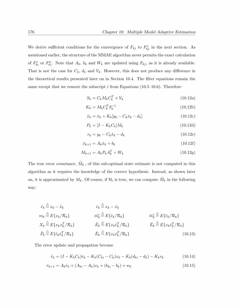
176 Chapter 10: Multiple Model Adaptive Estimation
We derive sufficient conditions for the convergence of Fkj to F skj in the next section. As
mentioned earlier, the structure of the MMAE algorithm never permits the exact calculation
of F ski or Fwki. Note that Ak, bk and Wk are updated using Fkj , as it is already available.
That is not the case for Ck, dk and Vk. However, this does not produce any difference in
the theoretical results presented later on in Section 10.4. The filter equations remain the
same except that we remove the subscript i from Equations (10.5–10.6). Therefore
Sk = CkMkCTk + Vk (10.12a)
Kk = MkCTk S−1k (10.12b)
xk = xk +Kk[yk − Ckxk − dk] (10.12c)
Pk = [I −KkCk]Mk (10.12d)
rk = yk − Ckxk − dk (10.12e)
xk+1 = Akxk + bk (10.12f)
Mk+1 = AkPkATk +Wk (10.12g)
The true error covariance, Mk , of this sub-optimal state estimate is not computed in this
algorithm as it requires the knowledge of the correct hypothesis. Instead, as shown later
on, it is approximated by Mk. Of course, if Hi is true, we can compute Mk in the following
way:
ek4= xk − xk ek
4= xk − xk
mk4= E{xk/Rk} me
k4= E{ek/Rk} me
k4= E{ek/Rk}
Xk4= E{xkxTk /Rk} Ek
4= E{xkeTk /Rk} Ek
4= E{xkeTk /Rk}
Pk4= E{ekeTk /Rk} Ek
4= E{xkeTk /Rk} (10.13)
The error update and propagation become
ek = (I −KkCk)ek −Kk(Cki − Ck)xk −Kk(dki − dk)−Kkvk (10.14)
ek+1 = Akek + (Aki −Ak)xk + (bki − bk) + wk (10.15)

10.3 Adaptive Kalman Filter Algorithm 177
and the difference equations become
Pk = (I −KkCk)Mk(I −KkCk)T +Kk(Cki − Ck)Xk(Cki − Ck)TKTk
+Kk(dki − dk)(dki − dk)TKTk +KkViK
Tk
− 2(I −KkCk)ETk (Cki − Ck)TKTk − 2(I −KkCk)me
k(dki − dk)TKTk
+ 2Kk(Cki − Ck)mk(dki − dk)TKTk
(10.16)
Mk+1 = AkPkATk + (Aki −Ak)Xk(Aki −Ak)T + (bki − bk)(bki − bk)T +Wi
+ 2AkETk (Aki −Ak)T + 2Akmek(bki − bk)T
+ 2(Aki −Ak)mk(bki − bk)T(10.17)
Xk+1 = AkiXkATki + bkib
Tki +Wi + 2Akimkb
Tki (10.18)
Ek = Ek(I −KkCk)T −Xk(Cki − Ck)TKTk −mkKk(dki − dk) (10.19)
Ek+1 = AkiEkATk +AkiXk(Aki −Ak)T +Akm
ekbTki
+Akimk(bki − bk)T + (Aki −Ak)mkbTki + bki(bki − bk)T +Wi
(10.20)
mk+1 = Akimk + bki (10.21)
mek = (I −KkCk)me
k −Kk(Cki − Ck)mk −Kk(dki − dk) (10.22)
mek+1 = Akm
ek + (Aki −Ak)mk + (bki − bk) (10.23)
The initial conditions become:
X0 = P0 + x0xT0 E0 = P0
m0 = x0 me0 = 0
These equations are computationally intensive, but can be computed off-line to assess
the performance of the AKF algorithm for specific applications. In certain cases, the off-line
computation becomes necessary to analyze the steady-state behavior of the AKF algorithm,
in particular, its convergence to the correct hypothesis.
Given Hi, the true distribution of rk is
fki(rk)4= fk(rk/Hi,Rk−1) (10.24)
E[rk/Hi,Rk−1] = (Cki − Ck)xk + (dki − dk)4= bki (10.25)
E[rkrTk /Hi,Rk−1] = CkiMkCTki + Vi
4= Ski (10.26)

178 Chapter 10: Multiple Model Adaptive Estimation
Therefore,
(rk/Hi,Rk−1) ∼ N (bki, Ski) (10.27)
However, since the correct hypothesis is unknown, the AKF algorithm is designed
to approximate the true error covariance Mk with the error “covariance” Mk , which is
computed on-line from (10.12d) and (10.12g). In Section 10.4, this assumption is justified
by showing that under certain conditions, E{Mk/Hi} →Mki, where Mki is the apriori error
covariance corresponding to the ith filter in the MMAE algorithm. It is also shown that
E{Mk/Hi} → M∗k , wherein M∗k is the exact apriori error covariance derived from (10.7b)
and E{Mk/Hi} → Mk. At each tk, we assume
E[rk/Hi,Rk−1] = 0
E[rkrTk /Hi,Rk−1] = CkiMkCTki + Vi
4= Λki (10.28)
Under the Gaussian assumption, we explicitly construct the density function fki(·) as
fki(rk)4= Approx. fki(rk)
(rk/Hi,Rk−1) ∼ N (0,Λki) (10.29)
We make a crucial observation that {rk} is no longer an independent residual process.
Now, F ski requires the knowledge of the density functions fki(·). Since we approximate
these functions with fki(·), F ski has been approximated by Fki.
Note that, by removing the parallel structure of the MMAE approach while retaining the
time-varying filter gain, the AKF algorithm is computationally less intensive, especially if
the number of hypotheses is large. Further, following the argument used in Section 10.7.1,
it can be shown that beta dominance cannot exist in this structure as there is only one
residual process here.
10.4 Performance of AKF Algorithm
The following sections consider the convergence and robustness properties of the AKF
algorithm and prove the following:

10.4 Performance of AKF Algorithm 179
• If hypothesis Hi is true, then the generated posterior probability of Hj (called Fkj)
decreases monotonically in time for all j 6= i, that is, Fk+1,j ≤ Fkj ∀j 6= i.
• If hypothesis Hi is true, then the posterior error covariance Pk of the AKF algorithm
converges to Pki of the “correct” filter from the MMAE algorithm.
• If hypothesis Hi is true but not included in the set of probable hypotheses, Θ4= {Hj},
then, the generated posterior probability converges to that hypothesis Hm ∈ Θ which
maximizes a particular information function.
10.4.1 Underlying Assumptions of MHSSPRT
We briefly rederive the MHSSPRT (Malladi and Speyer 1996, Malladi and Speyer 1997) by
defining the following notation:
πi4= P (Hi)
pi4= Apriori probability of change from H0 to Hi from tk to tk+1, for all k
fki(·)4= Approximate probability density function of rk conditioned on Hi and Rk−1
fk0(·) 4= Approximate probability density function of rk conditioned on H0 and Rk−1
L+ 14= Number of hypotheses
θi4= Time of occurence of Hi
At stage t1
P (θi ≤ t1/r1) =P (r1/θi ≤ t1)P (θi ≤ t1)
P (r1)(10.30)
P (r1) =L∑i=1
P (r1/θi ≤ t1)P (θi ≤ t1) + P (r1/θi > t1)P (θi > t1)
P (θi ≤ t1) = P (θi ≤ t0) + P (θi = t1/θi > t0)
= πi + pi(1− πi)P (r1/θi ≤ t1) = f1i(r1)dr1 (10.31)
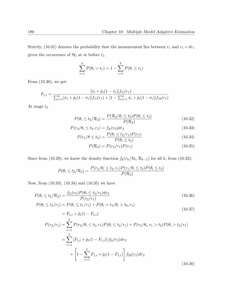
180 Chapter 10: Multiple Model Adaptive Estimation
Strictly, (10.31) denotes the probability that the measurement lies between r1 and r1 + dr1
given the occurrence of Hi at or before t1.
L∑i=1
P (θi > t1) = 1−L∑i=1
P (θi ≤ t1)
From (10.30), we get:
F1,i =[πi + pi(1− πi)]f1i(r1)∑L
i=1[πi + pi(1− πi)]f1i(r1) + [1−∑L
i=1 πi + pi(1− πi)]f10(r1)
At stage t2
P (θi ≤ t2/R2) =P (R2/θi ≤ t2)P (θi ≤ t2)
P (R2)(10.32)
P (r2/θi ≤ t2, r1) = f2i(r2)dr2 (10.33)
P (r1/θ ≤ t2) =P (θi ≤ t2/r1)P (r1)
P (θi ≤ t2)(10.34)
P (R2) = P (r2/r1)P (r1) (10.35)
Since from (10.29), we know the density function fk(rk/Hi,Rk−1) for all k, from (10.32):
P (θi ≤ t2/R2) =P (r2/θi ≤ t2, r1)P (r1/θi ≤ t2)P (θi ≤ t2)
P (R2)
Now, from (10.33), (10.34) and (10.35) we have
P (θi ≤ t2/R2) =f2i(r2)P (θi ≤ t2/r1)dr2
P (r2/r1)(10.36)
P (θi ≤ t2/r1) = P (θi ≤ t1/r1) + P (θi = t2/θi > t0, r1)
= F1,i + pi(1− F1,i)(10.37)
P (r2/r1) =L∑i=1
P (r2/θi ≤ t2, r1)P (θi ≤ t2/r1) + P (r2/θi, r1 > t2)P (θi > t2/r1)
=L∑i=1
[F1,i + pi(1− F1,i)] f2i(r2)dr2
+
[1−
L∑i=1
F1,i + pi(1− F1,i)
]f20(r2)dr2
(10.38)

10.4 Performance of AKF Algorithm 181
Clearly, by induction, we can now write the recursive relation for Fk+1,i in terms of Fk,i as
Fk+1,i =[Fk,i + pi(1− Fk,i)] fk+1,i(rk+1)∑L
i=1 [Fk,i + pi(1− Fk,i)] fk+1,i(rk+1) +[1−
∑Li=1 Fk,i + pi(1− Fk,i)
]fk+1,0(rk+1)
(10.39)
F0,i = πi (10.40)
Nowhere have we made any assumptions about the independence of the residual process.
From (10.29), we explicitly construct fki(·) for all i and at each tk. This approximates F ski
by Fki as mentioned in the earlier section. In the next section, we derive sufficient conditions
for the convergence of Fki and the associated error covariance.
10.4.2 Convergence of the Posterior Probability
We seek to prove that when Hi is true, the posterior probabilities of all hypotheses Hj for
all j 6= i decrease. We define the following:
F 4= {f(r/H) : H ∈ Θ} (10.41)
J ji(k)4= E [ln{fkj(rk)}/Hi,Rk−1] (10.42)
ρjmi4= max
kE
[[fkj(rk)fkm(rk)
]t/Hi,Rk−1
]for some t ∈ (0, 1)
4= max
kρjmi(Rk−1)
(10.43)
Assumption 10.1. The family of density functions F is identifiable, that is,
f(r/Hi) = f(r/Hj) ⇔ θi = θj ∀r
This assumption is invoked to prove Claim 10.1.
Claim 10.1. By Assumption 10.1, beta dominance cannot exist in the AKF algorithm.
Proof. Refer to Section 10.7.2.
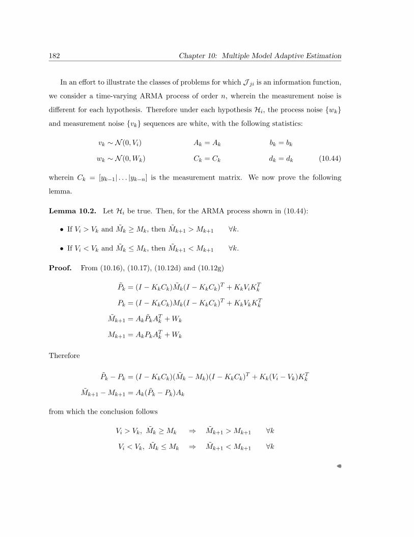
182 Chapter 10: Multiple Model Adaptive Estimation
In an effort to illustrate the classes of problems for which J ji is an information function,
we consider a time-varying ARMA process of order n, wherein the measurement noise is
different for each hypothesis. Therefore under each hypothesis Hi, the process noise {wk}and measurement noise {vk} sequences are white, with the following statistics:
vk ∼ N (0, Vi) Ak = Ak bk = bk
wk ∼ N (0,Wk) Ck = Ck dk = dk (10.44)
wherein Ck = [yk−1| . . . |yk−n] is the measurement matrix. We now prove the following
lemma.
Lemma 10.2. Let Hi be true. Then, for the ARMA process shown in (10.44):
• If Vi > Vk and Mk ≥Mk, then Mk+1 > Mk+1 ∀k.
• If Vi < Vk and Mk ≤Mk, then Mk+1 < Mk+1 ∀k.
Proof. From (10.16), (10.17), (10.12d) and (10.12g)
Pk = (I −KkCk)Mk(I −KkCk)T +KkViKTk
Pk = (I −KkCk)Mk(I −KkCk)T +KkVkKTk
Mk+1 = AkPkATk +Wk
Mk+1 = AkPkATk +Wk
Therefore
Pk − Pk = (I −KkCk)(Mk −Mk)(I −KkCk)T +Kk(Vi − Vk)KTk
Mk+1 −Mk+1 = Ak(Pk − Pk)Ak
from which the conclusion follows
Vi > Vk, Mk ≥Mk ⇒ Mk+1 > Mk+1 ∀k
Vi < Vk, Mk ≤Mk ⇒ Mk+1 < Mk+1 ∀k

10.4 Performance of AKF Algorithm 183
As a consequence, from (10.12a), (10.26) and (10.28)
Vi > Vj ⇒ Λkj < Λki < Ski ∀k
Vi < Vj ⇒ Λkj > Λki > Ski ∀k (10.45)
We could consider another class of problems similar to (10.44) wherein the hypotheses differ
only in the process noise statistics, that is, under Hi
wk ∼ N (0,Wi) (10.46)
We now prove the following lemma.
Lemma 10.3. Let Hi be true. Then, for the process shown in (10.46)
• If Wi > Wk and Mk ≥Mk, then Mk+1 > Mk+1 ∀k.
• If Wi < Wk and Mk ≤Mk, then Mk+1 < Mk+1 ∀k.
Proof. The proof is very similar to the one of Lemma 10.2. From (10.16), (10.17),
(10.12d) and (10.12g)
Pk = (I −KkCk)Mk(I −KkCk)T +KkVkKTk
Pk = (I −KkCk)Mk(I −KkCk)T +KkVkKTk
Mk+1 = AkPkATk +Wi
Mk+1 = AkPkATk +Wk
Therefore
Pk − Pk = (I −KkCk)(Mk −Mk)(I −KkCk)T
Mk+1 −Mk+1 = Ak(Pk − Pk)Ak + (Wi −Wk)
from which the conclusion follows
Wi > Wk, Mk ≥Mk ⇒ Mk+1 > Mk+1 ∀k
Wi < Wk, Mk ≤Mk ⇒ Mk+1 < Mk+1 ∀k

184 Chapter 10: Multiple Model Adaptive Estimation
So, from (10.12a), (10.26) and (10.28):
Wi > Wj ⇒ Λkj < Λki < Ski ∀k
Wi < Wj ⇒ Λkj > Λki > Ski ∀k
These results are used in proving the following claim.
Claim 10.4. If the state estimate bias is sufficiently small and
Λkj < Λki < Ski or Λkj > Λki > Ski ∀k
then J ji is an information function. Therefore, when Hi is true:
J ii(k) > J ji(k) ∀j 6= i , ∀k (10.47)
Proof. See Section 10.7.3.
Remark 26. Claim 10.4 assumes that convergence to the wrong hypothesis has occurred
and proves that under certain conditions, the filter cannot remain in the wrong hypothesis.
The conditions spelt out are sufficient but not necessary. Moreover for the processes shown
in (10.44) and (10.46), the state estimate is unbiased and from Lemmas 10.2 and 10.3,
Claim 10.4 is always valid.
Lemma 10.5. Let Hi be true and Hm ∈ Θ be such that:
Jmi(k)4= max
jJ ji(k) ∀Hj ∈ Θ ∀k (10.48)
Then
ρjmi < 1 ∀j 6= m
Proof. See Section 10.7.4.

10.4 Performance of AKF Algorithm 185
For the classes of problems that we consider, in view of Claim 10.4 and Lemma 10.5, if
Hi ∈ Θ then Hi ≡ Hm and
ρjii < 1 (10.49)
From now on, we only consider the classes of problems for which Claim 10.4 is valid.
We now proceed to prove the following theorem.
Theorem 10.6. Let the family F be identifiable and Hi ∈ Θ be true. Then
E[Fk,j/Hi] < E[Fk−1,j/Hi] ∀j 6= i (10.50)
Proof. Let hypothesis Hi ∈ Θ be true. Since Fkj ≤ 1, we have
Fkj ≤ F tkj for some t ∈ (0, 1) (10.51)
This is a crucial observation and is invoked to use ρjii < 1 from (10.49). All the terms in
the denominator of the recursive relation (10.40) are positive. Therefore we get
Fkj ≤[Fk−1,j + pj(1− Fk−1,j)] fkj(rk)[Fk−1,i + pi(1− Fk−1,i)] fki(rk)
φji4=Fk−1,j + pj(1− Fk−1,j)Fk−1,i + pi(1− Fk−1,i)
(10.52)
We note that the density functions fkj(·) are the approximate conditional density functions
as defined in (10.29). Assume that pj = p for all j. Let
Fk−1,j ≥ Fk−1,i ∀j 6= i, ∀k ≤ N
Then
φji =p+ (1− p)Fk−1,j
p+ (1− p)Fk−1,j
=Fk−1,j
Fk−1,i·
(1− p) + pFk−1,j
(1− p) + pFk−1,i
≤ Fk−1,j
Fk−1,i
(10.53)

186 Chapter 10: Multiple Model Adaptive Estimation
From (10.51), (10.52), (10.53):
Fkj ≤[Fk−1,j
Fk−1,i
]t [fkj(rk)fki(rk)
]t≤[Fk−2,j
Fk−2,i
]t [fk−1,j(rk−1)fk−1,i(rk−1)
]t [fkj(rk)fki(rk)
]t≤[πjπi
]t [f1j(r1)f1i(r1)
]t. . .
[fkj(rk)fki(rk)
]t(10.54)
We note that fki(rk) are the constructed density functions fk(rk/Hi,Rk−1) in (10.26). Take
the expectation conditioned on Hi
E[Fkj/Hi] ≤[πjπi
]tE
[[f1j(r1)f1i(r1)
]t. . .
[fkj(rk)fki(rk)
]t/Hi
]
=[πjπi
]t ∫ [f1j(r1)f1i(r1)
]t. . .
[fkj(rk)fki(rk)
]tfki(Rk/Hi)dRk
4=[πjπi
]tIk
(10.55)
where Ik is the integral. Now
fki(Rk/Hi) = fki(rk/Rk−1,Hi)fk−1,i(rk−1/Rk−2,Hi) . . . f1i(r1/Hi)
Ik =∫ [
f1j(r1)f1i(r1)
]t. . .
[fk−1,j(rk−1)fk−1,i(rk−1)
]tfk−1,i(Rk−1/Hi)dRk−1
×∫ [
fkj(rk)fki(rk)
]tfki(rk/Rk−1,Hi)drk
=∫ [
f1j(r1)f1i(r1)
]t. . .
[fk−1,j(rk−1)fk−1,i(rk−1)
]tfk−1,i(Rk−1/Hi)dRk−1ρjii(Rk−1)
≤ Ik−1ρjii
Therefore, from (10.55):
E [Fk,j/Hi] ≤[πjπi
]tρkjii (10.56)
From Claim 10.4 and Lemma 10.5, ρjii < 1. Hence, the posterior probability rapidly
decreases as k →∞ and the assumption of Fk−1,j ≥ Fk−1,i for all j 6= i and for all k is no

10.4 Performance of AKF Algorithm 187
longer valid. Let Fk−1,j ≤ Fk−1,i for all j 6= i and for all k ≥ N . Then
φji =Fk−1,j
Fk−1,i· 1 + p(1/Fk−1,j − 1)
1 + p(1/Fk−1,j − 1)
≤ Fk−1,j
Fk−1,i[1 + p(1/Fk−1,j − 1)]
≤ Fk−1,j
Fk−1,i+ p
(1− Fk−1,j)Fk−1,i
≤ Fk−1,j
Fk−1,i+ p
(10.57)
Following the argument used above, we get:
F tkj ≤(Fk−1,j
Fk−1,i+ p
)t [fkj(rk)fki(rk)
]t≤[(
Fk−1,j
Fk−1,i
)t+ pt
] [fkj(rk)fki(rk)
]t(Fk−1,j
Fk−1,i
)t≤[(
Fk−2,j
Fk−2,i
)t+ pt
] [fk−1,j(rk−1)fk−1,i(rk−1)
]tTherefore:
F tkj ≤[Fk−2,j
Fk−2,i
]t [fkj(rk)fk−1,j(rk−1)fki(rk)fk−1,i(rk−1)
]t+ pt
[fkj(rk)fk−1,j(rk−1)fki(rk)fk−1,i(rk−1)
]t+ pt
[fkj(rk)fki(rk)
]t(10.58)
Again, taking an expectation conditioned on Hi and from (10.43)
E[Fkj/Hi] ≤ E[[FNjFNi
]t/Hi
]ρk−Njii + pt
(ρjii + ρ2
jii + . . .+ ρk−Njii
)4= εk
(10.59)
εk+1 − εk = ρk−Njii E
[(FNjFNi
)t/Hi
](ρjii − 1) + ρk+1−N
jii pt
< 0 ∀k ≥ Nk
(10.60)
Hence
ε < . . . < εk+1 < εk < εk−1 < . . . ∀k ≥ Nk (10.61)
Clearly, for the WSPRT, p = 0, and hence, the lower bound ε = 0.

188 Chapter 10: Multiple Model Adaptive Estimation
Corollary 10.7. Let the family F be identifiable, Hi 6∈ Θ be true. Then
E[Fk,j/Hi] < E[Fk−1,j/Hi] ∀j 6= m (10.62)
where Hm maximizes the information function defined in (10.48).
Proof. The proof remains essentially the same as at appropriate places we replace the
subscript i by m, except that now ρjmi < 1. The corollary is relevant to the robustness
issues associated with any multiple model adaptive estimation scheme.
10.4.3 Convergence of the Posterior Error Covariance
Let Hi be true. We now compare the posteriori error covariance matrices of the adaptive
filter and the “true” filter matched to Hi in the MMAE algorithm. From (10.5–10.6) and
(10.12a–10.12g)
Pki = (I −KkiCki)Mki (10.63)
Pk = (I −KkCk)Mk (10.64)
Mk −Mki = Ak−1Pk−1ATk−1 −Ak−1,iPk−1,iA
Tk−1,i + (Wk−1 −Wi) (10.65)
Therefore
Pk − Pki = (I −KkCk)(Mk −Mki)(I −KkiCki)T
+ (I −KkCk)MkCTkiK
Tki −KkCkMki(I −KkiCki)T
= (I −KkCk)(Mk −Mki)(I −KkiCki)T +Gki
(10.66)
Now from the definitions of Kk and Kki in (10.5b) and (10.12b)
Gki = KkiCkiMk −KkCkMkCTkiK
Tki −KkCkMki +KkiCkiMkiC
Tk K
Tk
= MkiCTkiS−1ki CkiMk −MkC
Tk S−1k CkMkC
TkiS−1ki CkiMki −
MkCTk S−1k CkMki +MkiC
TkiS−1ki CkiMkiC
Tk S−1k CkMk
= Mki
[CTkiS
−1ki Cki − CkS−1
k Ck − CTkiS−1ki Cki (Mk −Mki)CTk S
−1k Ck
]Mk
Now
CTkiS−1ki Cki − CkS−1
k Ck = CTki(S−1ki − S−1
k
)Ck −
(CTk S
−1k + CTkiS
−1ki
)(Ck − Cki)

10.4 Performance of AKF Algorithm 189
Therefore
Gki = MkiCTki
[S−1ki − S−1
k − S−1ki Cki (Mk −Mki)CTk S
−1k
]CkMk
−Mki
(CTk S
−1k + CTkiS
−1ki
)(Ck − Cki)Mk
= MkiCTkiS−1ki
[Sk − Ski − Cki (Mk −Mki)CTk
]S−1k CkMk
−Mki
(CTk S
−1k + CTkiS
−1ki
)(Ck − Cki)Mk
= Kki
(CkMkC
Tk + Vk − CkiMkiC
Tki − Vi − CkiMkC
Tk + CkiMkiC
Tk
)Kk
−Mki
(CTk S
−1k + CTkiS
−1ki
)(Ck − Cki)Mk
= Kki (Vk − Vi)Kk +Kki (Ck − Cki)(MkC
Tk + CkiMki
)KTk
−Mki
(CTk S
−1k + CTkiS
−1ki
)(Ck − Cki)Mk
(10.67)
Similarly from (10.65)
Mk −Mki = Ak−1 (Pk−1 − Pk−1,i)ATk−1,i
+ (Ak−1,iPk−1,i +Ak−1Pk−1) (Ak−1 −Ak−1,i)T + (Wk−1 −Wi)
and from (10.65–10.67)
Pk − Pki = (I −KkCk)Ak−1(Pk−1 − Pk−1,i)ATk−1i(I −KkiCki)T
+ (I −KkCk)(Ak−1,iPk−1,i +Ak−1Pk−1)(Ak−1 −Ak−1,i)T (I −KkiCki)T
+ (I −KkCk)(Wk−1 −Wi)(I −KkiCki)T +Kki(Vk − Vi)Kk
+Kki(Ck − Cki)(MkCTk + CkiMki)KT
k
−Mki(CTk S−1k + CTkiS
−1ki )(Ck − Cki)Mk (10.68)
The filter equations are
xki = (I −KkiCki)Ak−1,ixk−1,i +Kki(yk − Ckibk−1,i − dki)
xk = (I −KkCk)Ak−1xk−1 +Kk(yk − Ckbk−1 − dk)
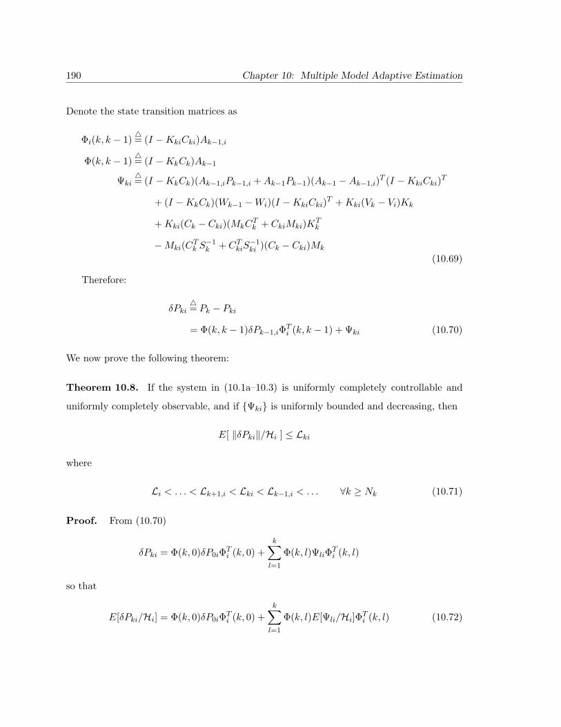
190 Chapter 10: Multiple Model Adaptive Estimation
Denote the state transition matrices as
Φi(k, k − 1)4= (I −KkiCki)Ak−1,i
Φ(k, k − 1)4= (I −KkCk)Ak−1
Ψki4= (I −KkCk)(Ak−1,iPk−1,i +Ak−1Pk−1)(Ak−1 −Ak−1,i)T (I −KkiCki)T
+ (I −KkCk)(Wk−1 −Wi)(I −KkiCki)T +Kki(Vk − Vi)Kk
+Kki(Ck − Cki)(MkCTk + CkiMki)KT
k
−Mki(CTk S−1k + CTkiS
−1ki )(Ck − Cki)Mk
(10.69)
Therefore:
δPki4= Pk − Pki
= Φ(k, k − 1)δPk−1,iΦTi (k, k − 1) + Ψki (10.70)
We now prove the following theorem:
Theorem 10.8. If the system in (10.1a–10.3) is uniformly completely controllable and
uniformly completely observable, and if {Ψki} is uniformly bounded and decreasing, then
E[ ‖δPki‖/Hi ] ≤ Lki
where
Li < . . . < Lk+1,i < Lki < Lk−1,i < . . . ∀k ≥ Nk (10.71)
Proof. From (10.70)
δPki = Φ(k, 0)δP0iΦTi (k, 0) +
k∑l=1
Φ(k, l)ΨliΦTi (k, l)
so that
E[δPki/Hi] = Φ(k, 0)δP0iΦTi (k, 0) +
k∑l=1
Φ(k, l)E[Ψli/Hi]ΦTi (k, l) (10.72)
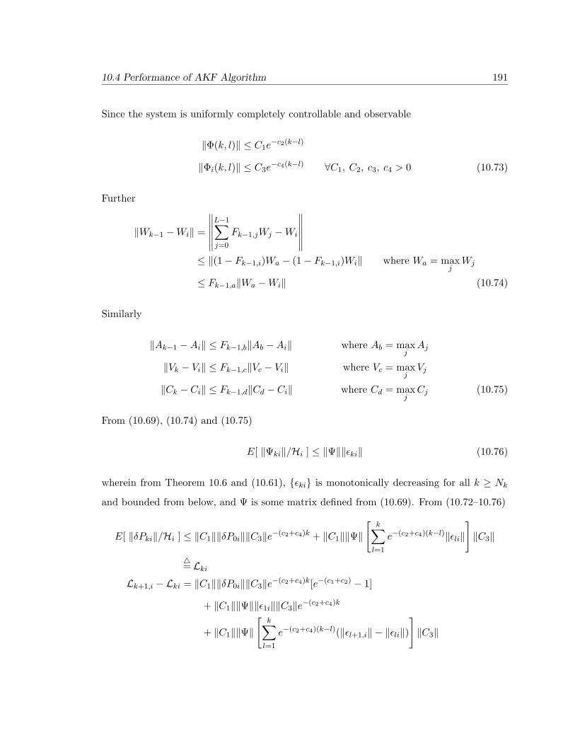
10.4 Performance of AKF Algorithm 191
Since the system is uniformly completely controllable and observable
‖Φ(k, l)‖ ≤ C1e−c2(k−l)
‖Φi(k, l)‖ ≤ C3e−c4(k−l) ∀C1, C2, c3, c4 > 0 (10.73)
Further
‖Wk−1 −Wi‖ =
∥∥∥∥∥∥L−1∑j=0
Fk−1,jWj −Wi
∥∥∥∥∥∥≤ ‖(1− Fk−1,i)Wa − (1− Fk−1,i)Wi‖ where Wa = max
jWj
≤ Fk−1,a‖Wa −Wi‖ (10.74)
Similarly
‖Ak−1 −Ai‖ ≤ Fk−1,b‖Ab −Ai‖ where Ab = maxjAj
‖Vk − Vi‖ ≤ Fk−1,c‖Vc − Vi‖ where Vc = maxjVj
‖Ck − Ci‖ ≤ Fk−1,d‖Cd − Ci‖ where Cd = maxjCj (10.75)
From (10.69), (10.74) and (10.75)
E[ ‖Ψki‖/Hi ] ≤ ‖Ψ‖‖εki‖ (10.76)
wherein from Theorem 10.6 and (10.61), {εki} is monotonically decreasing for all k ≥ Nk
and bounded from below, and Ψ is some matrix defined from (10.69). From (10.72–10.76)
E[ ‖δPki‖/Hi ] ≤ ‖C1‖‖δP0i‖‖C3‖e−(c2+c4)k + ‖C1‖‖Ψ‖[
k∑l=1
e−(c2+c4)(k−l)‖εli‖]‖C3‖
4= Lki
Lk+1,i − Lki = ‖C1‖‖δP0i‖‖C3‖e−(c2+c4)k[e−(c1+c2) − 1]
+ ‖C1‖‖Ψ‖‖ε1i‖‖C3‖e−(c2+c4)k
+ ‖C1‖‖Ψ‖[
k∑l=1
e−(c2+c4)(k−l)(‖εl+1,i‖ − ‖εli‖)]‖C3‖

192 Chapter 10: Multiple Model Adaptive Estimation
so that
Lk+1,i − Lki < 0 ∀k ≥ Nk
Hence
Li < . . . < Lk+1,i < Lki < Lk−1,i < . . . ∀k ≥ Nk
Remark 27. Note that the lower bound is governed by the factor p of the MHSSPRT as
it controls the lower bound of the sequence {εki}, as shown in Theorem 10.6. This theorem,
based upon our adaptive filter structure, shows that the apriori “covariance” assumed for
the conditional density function of the residual fki(rk) approaches the true apriori error
covariance, that is, E{Mk/Hi} → Mki. As a special case, consider the Wald SPRT, where
p = 0. From Theorem 10.6, it can be seen that for ρ < 1
εk ∼ ερk
so that
E[ ‖δPki‖/Hi ] ≤
‖C1‖‖δP0i‖‖C3‖e−(c2+c4)k + ‖C1‖‖Ψ‖[ρk+1e(c2+c4)(k+1) − e(c2+c4)k
ρec2+c4 − 1
]‖C3‖
and
E[ ‖δPki‖/Hi ] = 0 as k →∞ (10.77)
So, for the Wald SPRT, Li = 0. The adaptive filter converges exactly to the “true” filter
of the MMAE scheme.
The assumptions in the AKF algorithm may be justified in yet another way, by looking
at the exact expressions for the overall state estimate and posteriori error covariance, as

10.4 Performance of AKF Algorithm 193
developed in the MMAE algorithm. Recall from (10.7a) and (10.7b)
x∗k =∑j
xkjFkj
P ∗k =∑j
[Pkj + (x∗k − xkj)(x∗k − xkj)T ]Fkj
Let
δP ∗k4= P ∗k − Pk (10.78)
We now show that the expected value of δP ∗k conditioned on any hypothesis decreases as
k →∞.
Theorem 10.9. If the system in (10.1a–10.3) is uniformly completely controllable and
uniformly completely observable, then
E[ ‖δP ∗k ‖/Hi ] ≤ L∗ki ∀Hi
where
L∗i < . . . < L∗k+1,i < L∗ki < L∗k−1,i < . . . ∀k ≥ Nk
Proof. From the above equations
δP ∗k =∑j
[(Pkj − Pk) + (x∗k − xkj)(x∗k − xkj)T ]Fkj
=∑j
[δPkj + (x∗k − xkj)(x∗k − xkj)T ]Fkj
=∑j 6=i
[δPkj + (x∗k − xkj)(x∗k − xkj)T ]Fkj
+ [δPki + (x∗k − xki)(x∗k − xki)T ]Fki
(10.79)
Taking the norm and using an analysis similar to (10.75)
δP ∗k ≤∑j 6=i
[‖δPkj‖+ ‖(x∗k − xkj)(x∗k − xkj)T ‖
]Fkj
+[‖δPki‖+ ‖(x∗k − xki)(x∗k − xki)T ‖
]Fki
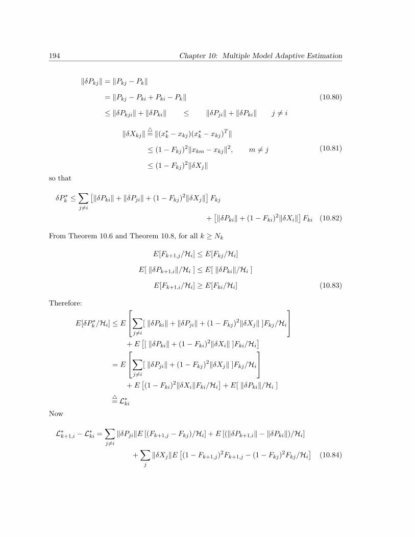
194 Chapter 10: Multiple Model Adaptive Estimation
‖δPkj‖ = ‖Pkj − Pk‖
= ‖Pkj − Pki + Pki − Pk‖
≤ ‖δPkji‖+ ‖δPki‖ ≤ ‖δPji‖+ ‖δPki‖ j 6= i
(10.80)
‖δXkj‖4= ‖(x∗k − xkj)(x∗k − xkj)T ‖
≤ (1− Fkj)2‖xkm − xkj‖2, m 6= j
≤ (1− Fkj)2‖δXj‖
(10.81)
so that
δP ∗k ≤∑j 6=i
[‖δPki‖+ ‖δPji‖+ (1− Fkj)2‖δXj‖
]Fkj
+[‖δPki‖+ (1− Fki)2‖δXi‖
]Fki (10.82)
From Theorem 10.6 and Theorem 10.8, for all k ≥ Nk
E[Fk+1,j/Hi] ≤ E[Fkj/Hi]
E[ ‖δPk+1,i‖/Hi ] ≤ E[ ‖δPki‖/Hi ]
E[Fk+1,i/Hi] ≥ E[Fki/Hi] (10.83)
Therefore:
E[δP ∗k /Hi] ≤ E
∑j 6=i
[ ‖δPki‖+ ‖δPji‖+ (1− Fkj)2‖δXj‖ ]Fkj/Hi
+ E
[[ ‖δPki‖+ (1− Fki)2‖δXi‖ ]Fki/Hi
]= E
∑j 6=i
[ ‖δPji‖+ (1− Fkj)2‖δXj‖ ]Fkj/Hi
+ E
[(1− Fki)2‖δXi‖Fki/Hi
]+ E[ ‖δPki‖/Hi ]
4= L∗ki
Now
L∗k+1,i − L∗ki =∑j 6=i‖δPji‖E [(Fk+1,j − Fkj)/Hi] + E [(‖δPk+1,i‖ − ‖δPki‖)/Hi]
+∑j
‖δXj‖E[(1− Fk+1,j)2Fk+1,j − (1− Fkj)2Fkj/Hi
](10.84)

10.4 Performance of AKF Algorithm 195
Consider the function:
E[(1− Fkj)2Fkj/Hi
]= E[Fkj/Hi] + E[F 3
kj/Hi]− 2E[F 2kj/Hi]
≤ 2E[Fkj/Hi]− 2E[F 2kj/Hi]
Now
E[F 2kj/Hi] ≥ (E[Fkj/Hi])2
which implies that
E[(1− Fkj)2Fkj/Hi
]≤ 2
{E[Fkj/Hi]− (E[Fkj/Hi])2
}4= ϕ(E[Fkj/Hi])
Since ϕ(·) is an increasing function in the interval [0, 1/2) and a decreasing function in the
interval (1/2, 1], it follows from (10.83) and (10.84) that
E[(1− Fk+1,j)2Fk+1,j/Hi] ≤ E[(1− Fkj)2Fkj/Hi] ∀j 6= i
E[(1− Fk+1,i)2Fk+1,i/Hi] ≤ E[(1− Fki)2Fki/Hi]
so that
L∗k+1,i − L∗ki ≤ 0 k ≥ Nk (10.85)
and
L∗i < . . . < L∗k+1,i < L∗ki < L∗k−1,i < . . . ∀k ≥ Nk
Clearly the posteriori “covariance” of the AKF algorithm approaches the exact posteriori
error covariance as computed in the MMAE algorithm.
Finally, we analyze the difference between the assumed error “covariance” Pk and the
exact error covariance Pk. Let Hi be true. From (10.12d), (10.16) and (10.17)
δPki4= Pk − Pk (10.86)
= (I −KkCk)Ak(Pk−1 − Pk−1)ATk (I −KkCk)T + Ψk
= Φ(k, k − 1)δPk−1Φ(k, k − 1)T + Ψk (10.87)

196 Chapter 10: Multiple Model Adaptive Estimation
wherein:
Ψk = Kk[(Vk − Vi)− (Ck − Cki)Xk(Ck − Cki)T + (dk − dki)(dk − dki)T
+ 2(Ck − Cki)mk(dki − dk)T ]KTk
− (I −KkCk)[2ETk (Ck − Cki)T − 2mek(dk − dki)T ]KT
k
+ (I −KkCk)[(Wk−1 −Wi)− (Ak−1 −Ak−1,i)Xk−1(Ak−1 −Ak−1,i)T
− (bk−1,i − bk−1)(bk−1,i − bk−1)T + 2Ak−1ETk−1(Ak−1 −Ak−1,i)T
+ 2Ak−1mek−1(bk−1 − bk−1,i)T
− 2(Ak−1 −Ak−1,i)mk−1(bk−1 − bk−1,i)T ](I −KkCk)T
We now prove that the expected value of δPki conditioned on Hi decreases as k →∞.
Theorem 10.10. If the system in (10.1a–10.3) is uniformly completely controllable and
uniformly completely observable, then
E[ ‖δPki‖/Hi ] ≤ Lki, ∀Hi
wherein:
Li < . . . < Lk+1,i < Lki < Lk−1,i < . . . ∀k ≥ Nk
Proof. From (10.87)
δPki = Φ(k, 0)δP0iΦT (k, 0) +k∑l=1
Φ(k, l)ΨliΦT (k, l)
so that
E[δPki/Hi] = Φ(k, 0)δP0iΦT (k, 0) +k∑l=1
Φ(k, l)E[Ψli/Hi]ΦT (k, l)
The rest of the proof follows that of Theorem 10.8.
This concludes our analysis to justify the structure of the AKF algorithm. Under Hi,we derived sufficient conditions for the convergence of Fki to F ski and Pk to Pk, Pki, and P ∗k .
In the next section, we test the AKF algorithm in a few numerical simulations

10.5 Simulations 197
10.5 Simulations
10.5.1 Example 1
Consider a scalar dynamic system:
xk+1 = Akxk + bk + wk
yk = Ckxk + dk + vk
wherein under each hypothesis
H0 : Ak = −0.5, bk = 0.0, Ck = 1.0, dk = 0.0
vk ∼ N (0, 1.0), wk ∼ N (0, 0.001)
H1 : Ak = −0.6, bk = 0.25, Ck = 1.25, dk = 0.25
vk ∼ N (0, 2.0), wk ∼ N (0, 0.001)
H2 : Ak = −0.7, bk = 0.50, Ck = 1.50, dk = 0.50
vk ∼ N (0, 3.0), wk ∼ N (0, 0.001)
The Adaptive Kalman Filter algorithm was compared to the MMAE algorithm. In the
MMAE approach, Fwki was replaced by F ski to allow for transitions from one hypothesis to
another. Of course, from our earlier discussion, it is clear that the recursive relation is not
strictly F ski but an approximation to it. In order to design the AKF algorithm, it is essential
to consider scenarios when a particular hypothesis is true and the filter is “matched” to
the wrong hypothesis. An off-line computation of the true residual error covariance was
conducted for all scenarios. It is seen from Figure 10.3 that when Hi is true and the filter
is matched to Hj , either Λkj < Λki < Ski or Λkj > Λki > Ski. Moreover the matrix Bki
in the exponential term is always positive definite and so, from Section 10.7.3, the system
satisfies Claim 10.4. This implies that the filter cannot remain matched to Hj .
We now test the AKF algorithm. At t = 40 sec, the hypothesis was changed from H0
to H1. The posterior probabilities of the three hypotheses are shown in Figure 10.4. The
bold line denotes the AKF approach while the dotted line denotes the MMAE approach.
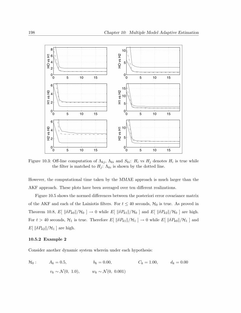
198 Chapter 10: Multiple Model Adaptive Estimation
0 5 10 150
2
4
6
8H
O v
s H
1
0 5 10 150
5
10
HO
vs
H2
0 5 10 150
2
4
6
H1
vs H
0
0 5 10 150
5
10
15
H1
vs H
2
0 5 10 150
2
4
6
H2
vs H
0
0 5 10 150
5
10
H2
vs H
1
Figure 10.3: Off-line computation of Λkj , Λki and Ski: Hi vs Hj denotes Hi is true whilethe filter is matched to Hj : Λki is shown by the dotted line.
However, the computational time taken by the MMAE approach is much larger than the
AKF approach. These plots have been averaged over ten different realizations.
Figure 10.5 shows the normed differences between the posteriori error covariance matrix
of the AKF and each of the Lainiotis filters. For t ≤ 40 seconds, H0 is true. As proved in
Theorem 10.8, E[ ‖δPk0‖/H0 ] → 0 while E[ ‖δPk1‖/H0 ] and E[ ‖δPk2‖/H0 ] are high.
For t > 40 seconds, H1 is true. Therefore E[ ‖δPk1‖/H1 ] → 0 while E[ ‖δPk0‖/H1 ] and
E[ ‖δPk2‖/H1 ] are high.
10.5.2 Example 2
Consider another dynamic system wherein under each hypothesis:
H0 : Ak = 0.5, bk = 0.00, Ck = 1.00, dk = 0.00
vk ∼ N (0, 1.0), wk ∼ N (0, 0.001)

10.5 Simulations 199
0 10 20 30 40 50 60 70 80 900
0.5
1
Adaptive Kalman Filter vs Lainiotis filters
Pro
b of
H0
0 10 20 30 40 50 60 70 80 900
0.5
1
Pro
b of
H1
0 10 20 30 40 50 60 70 80 900
0.5
1
Pro
b of
H2
Time
Figure 10.4: Adaptive Kalman Filter Performance - Change from H0 to H1.
H1 : Ak = 0.6, bk = 0.25, Ck = 1.25, dk = 0.25
vk ∼ N (0, 1.5), wk ∼ N (0, 0.001)
H2 : Ak = 0.7, bk = 0.50, Ck = 1.50, dk = 0.50
vk ∼ N (0, 2.0), wk ∼ N (0, 0.001)
Again, we compared the Adaptive Kalman Filter to the MMAE algorithm. At t = 3 sec, the
hypothesis was changed from H0 to H2. The posterior probabilities of the three hypotheses
are shown in Figure 10.6. The plots have been averaged over ten different realizations.
Figure 10.7 shows the normed differences between the posteriori error covariance matrix
of the AKF and each of the Lainiotis filters.

200 Chapter 10: Multiple Model Adaptive Estimation
0 10 20 30 40 50 60 70 80 900
0.2
0.4
Difference between Error CovariancesH
0
0 10 20 30 40 50 60 70 80 900
0.2
0.4
H1
0 10 20 30 40 50 60 70 80 900
1
2
H2
Time
Figure 10.5: E[|δPki|] vs. tk.
10.5.3 Example 3
Consider three hypotheses wherein:
H0 :vk ∼ N (0, 1.0)
H1 :vk ∼ N (0, 1.5)
H2 :vk ∼ N (0, 2.0)
A fourth order ARMA measurement process was simulated thus:
yk = 0.1 · [ yk−1 − yk−2 + yk−3 − yk−4 ] + vk
Since the order of the ARMA process typically is unknown, a fifth order ARMA model
was assumed for the measurement process. The assumed system model is the same as

10.5 Simulations 201
0 1 2 3 4 5 6 7 8 90
0.5
1
Adaptive Kalman Filter vs Lainiotis filters
Pro
b of
H0
0 1 2 3 4 5 6 7 8 90
0.5
1
Pro
b of
H1
0 1 2 3 4 5 6 7 8 90
0.5
1
Pro
b of
H2
Time
Figure 10.6: Adaptive Kalman Filter Performance - Change from H0 to H2.
(10.1a–10.3) and for all Hj
A = I Wj = 0.001 ∗ I d = 0
Ck = [yk−1| . . . |yk−5] b = [0 0 0 0 0]T
Recall from Lemma 10.2 and Section 10.7.3 that for ARMA processes, Claim 10.4 is always
valid thereby obviating any off-line computation. At t = 40 sec, the hypothesis was changed
fromH0 toH1. The posterior probabilities of the three hypotheses are shown in Figure 10.8.
The plots have been averaged over ten different realizations. Figure 10.9 shows the normed
differences between the posteriori error covariance matrix of the AKF and each of the
Lainiotis filters.

202 Chapter 10: Multiple Model Adaptive Estimation
0 1 2 3 4 5 6 7 8 90
0.5
1Difference between Error Covariances
H0
0 1 2 3 4 5 6 7 8 90
0.5
1
H1
0 1 2 3 4 5 6 7 8 90
0.5
1
H2
Time
Figure 10.7: E[|δPki|] vs. tk.
10.5.4 Example 4
For the same system, the hypothesis was changed from H0 to H2 at t = 40 seconds. The
posterior probabilities of the three hypotheses are shown in Figure 10.10. Again the plots
have been averaged over ten different realizations. Figure 10.11 shows the normed differences
between the posteriori error covariance matrix of the AKF and each of the Lainiotis filters.
10.6 Conclusions
An AKF algorithm and sufficient conditions for its convergence have been developed for
adaptive estimation in linear time-varying stochastic dynamic systems. In the simulated
examples, it performs comparably to the modified MMAE algorithm, while significantly

10.6 Conclusions 203
0 10 20 30 40 50 60 70 80 900
0.5
1
Adaptive Kalman Filter vs Lainiotis filters
Pro
b of
H0
0 10 20 30 40 50 60 70 80 900
0.5
1
Pro
b of
H1
0 10 20 30 40 50 60 70 80 900
0.5
1
Pro
b of
H2
Time
Figure 10.8: Adaptive Kalman Filter Performance - Change from H0 to H1.
reducing the computational intensity. It has also been shown that for a class of problems, the
expected value of the true posterior probability conditioned on the residual history converges
to unity. In its most general form, an off-line computation is necessary to investigate the
convergence of the true posterior probability. Under assumptions of uniform complete
controllability and observability, the expected value of the norm of the difference between
the constructed error covariance and the true posteriori error covariance converges to a
lower bound. This lower bound is determined by the apriori probability of change from
one hypothesis to another in the MHSSPRT. In the presence of modeling errors, the AKF
algorithm has been shown to converge to the hypothesis which maximizes a particular
information function, while the MMAE algorithm might show beta dominance.
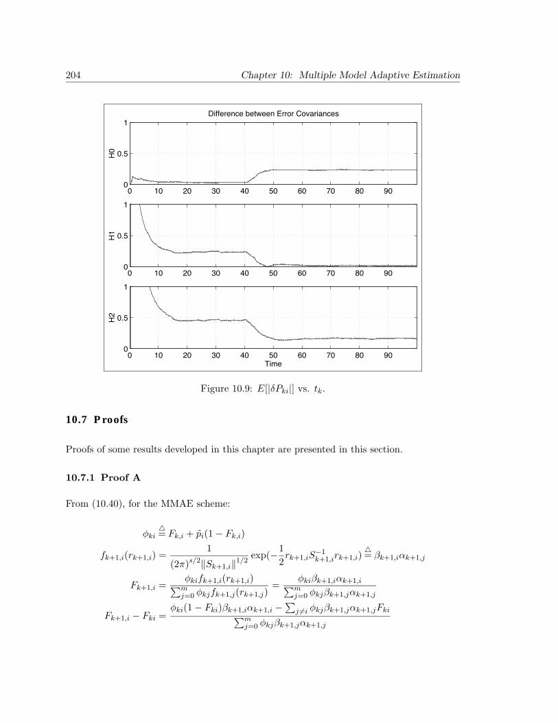
204 Chapter 10: Multiple Model Adaptive Estimation
0 10 20 30 40 50 60 70 80 900
0.5
1Difference between Error Covariances
H0
0 10 20 30 40 50 60 70 80 900
0.5
1
H1
0 10 20 30 40 50 60 70 80 900
0.5
1
H2
Time
Figure 10.9: E[|δPki|] vs. tk.
10.7 Proofs
Proofs of some results developed in this chapter are presented in this section.
10.7.1 Proof A
From (10.40), for the MMAE scheme:
φki4= Fk,i + pi(1− Fk,i)
fk+1,i(rk+1,i) =1
(2π)s/2‖Sk+1,i‖1/2exp(−1
2rk+1,iS
−1k+1,irk+1,i)
4= βk+1,iαk+1,j
Fk+1,i =φkifk+1,i(rk+1,i)∑mj=0 φkjfk+1,j(rk+1,j)
=φkiβk+1,iαk+1,i∑mj=0 φkjβk+1,jαk+1,j
Fk+1,i − Fki =φki(1− Fki)βk+1,iαk+1,i −
∑j 6=i φkjβk+1,jαk+1,jFki∑m
j=0 φkjβk+1,jαk+1,j
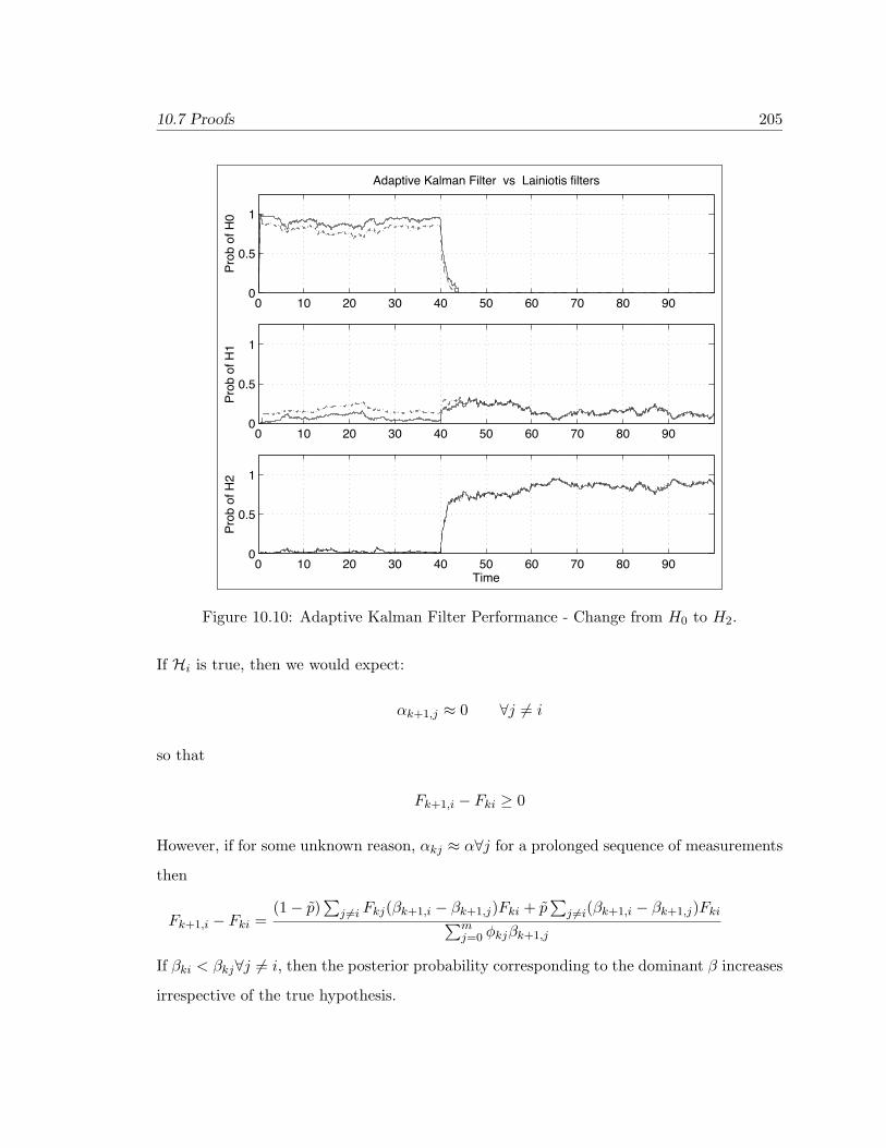
10.7 Proofs 205
0 10 20 30 40 50 60 70 80 900
0.5
1
Adaptive Kalman Filter vs Lainiotis filters
Pro
b of
H0
0 10 20 30 40 50 60 70 80 900
0.5
1
Pro
b of
H1
0 10 20 30 40 50 60 70 80 900
0.5
1
Pro
b of
H2
Time
Figure 10.10: Adaptive Kalman Filter Performance - Change from H0 to H2.
If Hi is true, then we would expect:
αk+1,j ≈ 0 ∀j 6= i
so that
Fk+1,i − Fki ≥ 0
However, if for some unknown reason, αkj ≈ α∀j for a prolonged sequence of measurements
then
Fk+1,i − Fki =(1− p)
∑j 6=i Fkj(βk+1,i − βk+1,j)Fki + p
∑j 6=i(βk+1,i − βk+1,j)Fki∑m
j=0 φkjβk+1,j
If βki < βkj∀j 6= i, then the posterior probability corresponding to the dominant β increases
irrespective of the true hypothesis.

206 Chapter 10: Multiple Model Adaptive Estimation
0 10 20 30 40 50 60 70 80 900
0.5
1Difference between Error Covariances
H0
0 10 20 30 40 50 60 70 80 900
0.5
1
H1
0 10 20 30 40 50 60 70 80 900
0.5
1
H2
Time
Figure 10.11: E[|δPki|] vs. tk.
10.7.2 Proof B1
For the AKF algorithm, there is only one residual process. Hence, if for some reason,
αkj ≈ α for all j for a prolonged sequence of measurements this implies that
rTk+1[Sk+1,i − Sk+1,j ]rk+1 = 0
and
Sk+1,i ≡ Sk+1,j ∀k
This violates the identifiability assumption of the family F . Moreover, since now βki ≡
βkj∀j, one β cannot dominate over the other.
10.7 Proofs 207
10.7.3 Proof B2
From (10.42):
J ji(k)4= E [ln {fkj(rk)} /Hi,Rk−1]
Let Hi be true. Then
J ji(k)− J ii(k) =∫
ln{fkj(rk)fki(rk)
}fki(rk)drk
Since lnx ≤ x− 1
J ji(k)− J ii(k) ≤∫ {
fkj(rk)fki(rk)
− 1}fki(rk)drk
≤{∫ {
fkj(rk)fki(rk)
}fki(rk)drk
}− 1 ∀j 6= i
4= Ik − 1
From (10.25), (10.26) and (10.28),
Ik4=‖Λki‖1/2‖Λk‖1/2‖Λkj‖1/2‖Sk‖1/2
exp{−aki
2
}where
aki4= bTki[Ski + (Λ−1
kj − Λ−1ki )−1]−1bki
= bTkiBkibki
and
Λ−1k
4= S−1
k + Λ−1kj − Λ−1
ki
with Λ−1k > 0 for the integral to exist.
Now, it must be true that either Λkj < Λki < Ski or Λkj > Λki > Ski for all k. Clearly,
the integral always exists and Λk > 0. Since the bias terms are small, neglect the exponential
term aki. However, note that if
Λkj < Λki ⇒ Bki > 0
⇒ aki > 0 ∀bki
⇒ exp{−aki
2
}< 1

208 Chapter 10: Multiple Model Adaptive Estimation
Hence, in certain cases, the bias terms need not be small. Anyway, by removing the
exponential term from Ik, we can show that
Ik = ‖Λ−1ki Λkj + Λ−1
ki Sk − Λ−1ki ΛkjΛ−1
ki Sk‖−1/2
≤ 1
with the equality sign if and only if Λki = Λkj or Λki = Sk for all k. The former situation
violates the identifiability assumption while the latter assumes that Mk = Mk for all k in
which case the algorithm has already converged. Therefore:
J ji(k)− J ii(k) ≤ 0
Now, the equality sign in holds if and only if fki(·) = fkj(·) almost everywhere. Since we
assumed the family F to be identifiable, the J ji(k) is strictly less than J ii(k)∀j 6= i and
∀k.
10.7.4 Proof B3
The proof follows the analysis in (Liporace 1971). Let Hi 6∈ Θ be true. We first prove that
whenever J ji(k) < Jmi(k) ∀k the following holds true
E
[{fkj(rk)fkm(rk)
}t/Hi,Rk−1
]4= ρjmi(Rk−1) < 1 forsomet ∈ (0, 1) ∀k
By definition:
J ji(k)− Jmi(k) = E
[ln{fkj(rk)fkm(rk)
}/Hi,Rk−1
]= E
[limt→0
({fkj(rk)fkm(rk)
}t− 1
)t−1/Hi,Rk−1
]Using the Lebesgue dominated convergence theorem, the limit and expectation may be
interchanged. Therefore, for any δ ∈ (0, 1), there exists a t ∈ (0, 1) such that
limt→0
t−1
(E
[{fkj(rk)fkm(rk)
}t/Hi,Rk−1
]− 1
)≤ [J ji(k)− Jmi(k)] (1− δ)
E
[{fkj(rk)fkm(rk)
}t/Hi,Rk−1
]≤ 1 + t(1− δ) [J ji(k)− Jmi(k)]
< 1

10.7 Proofs 209
The same analysis can be carried out ∀k, that is, for any realization of Rk
ρjmi(Rk−1) < 1 ∀k
⇒ ρjmi4= max
kρjmi(Rk−1) < 1


Chapter 11
Fault Detection and IdentificationUsing Linear Quadratic Optimization
A new approach to the residual generation problem for fault detection and identification
based on linear quadratic optimization is presented. A quadratic cost encourages the input
observability of a fault that is to be detected and the unobservability of disturbances, sensor
noise and a set of faults that are to be isolated. Since the filter is not constrained to form
unobservability subspace structures, adjustment of the quadratic cost could realize improved
performance as reduced sensor noise and dynamic disturbance components in the residual
and reduced sensitivity to parametric variations. In the present form, the filter detects a
single fault so the structure could also be described as that of an unidentified input observer.
A bank of filters are constructed when multiple faults are to be detected.
211

212 Chapter 11: Fault Detection and Identification Using Linear Quadratic Optimization
11.1 Problem Formulation
Consider a dynamic system described by the equations
x = Ax+B1u1 +B2u2; x(t0) = x0 (11.1)
y = Cx+ w (11.2)
In (11.1) and (11.2), y is a p×1 measurement vector, w is the p×1 measurement error, and
u1 and u2 are unknown disturbance inputs representing faults. Our goal is to derive a fault
detection filter which processes the measurement y(t) and produces a scalar output h(t)
which is small if u1 is zero and large only if u1 is different from zero. Thus the filter should
respond to a non zero input u1, but not to the inputs u2, w, and x0. In this development
we shall consider filters in the form:
h(t1) = fT[y(t1)−
∫ t1
t0
CMT (τ, t1)y(τ)dτ]
(11.3)
Procedures for choosing the matrix f(t1) and the p×n matrix M(τ, t1) are developed below.
A filter with the properties described above can be used to detect a fault corresponding to
u1. The roles of u1 and u2 can be interchanged to detect faults corresponding to u2.
Introduce an n× n square matrix Z(t; t1) satisfying
d
dtZ(t; t1) = −ATZ(t; t1) + CTM(t; t1); Z(t1; t1) = I (11.4)
Form ZTx and differentiate with respect to t.
d
dt(ZTx) = ZTx+ ZT x
= [−ZTA/
+MTC]x+ ZT [Ax/
+B1u1 +B2u2]
= MTCx+ ZTB1u1 + ZTB2u2
(11.5)
Substitute (11.2) into (11.5).
d
dt(ZTx) = MT (y − w) + ZTB1u1 + ZTB2u2 (11.6)
11.1 Problem Formulation 213
Integrate (11.6) from t0 to t1.
ZT (t1; t1)x(t1)− ZT (t0; t1)x(t0)
=∫ t1
t0
MT (τ ; t1)y(τ)dτ −∫ t1
t0
MT (τ ; t1)w(τ)dτ
+∫ t1
t0
ZT (τ ; t1)B1u1dτ +∫ t1
t0
ZT (τ ; t1)B2u2dτ
(11.7)
Using Z(t1; t1) = I and rearranging (11.7) we get
x(t1)−∫ t1
t0
MT (τ ; t1)y(τ)dτ = ZT (t0; t1)x(t0)−∫ t1
t0
MT (τ ; t1)w(τ)dτ
+∫ t1
t0
ZT (τ ; t1)B1u1dτ +∫ t1
t0
ZT (τ ; t1)B2u2dτ (11.8)
Multiply (11.8) from the left by fTC where f is a vector to be determined. For the time
being, regard f as given. Later we will have more to say about choosing f .
fTCx (t1)− fT∫ t1
t0
CMTwdτ = fT [y (t1)− w (t1)]− fT∫ t1
t0
CMTwdτ
= h (t1)− fTw (t1)
= fTCZT (t0; t1)x(t0)−∫ t1
t0
fTCMTwdτ
+∫ t1
t0
fTCZTB1u1dτ +∫ t1
t0
fTCZTB2u2dτ
(11.9)
Thus
h (t1) = fTCZT (t0; t1)x (t0) + fTw (t1)
+∫ t1
t0
[fTCZ(τ, t1) (B1u1 +B2u2)− fTCMT (τ, t1)w
]dτ (11.10)
Note that h(t1) in Equation (11.9) is a scalar. We want to choose f and M such that h(t1)
is responsive to u1, but not to u2, w and x0. To accomplish this, set up the cost function
J =fTC
{ZT (t0; t1)WZ(t0) +
∫ t1t0
[ZTB2Q2B
T2 Z +MTRM
]dτ}CT f + fTV f
fTC{∫ t1
t0ZTB1Q1BT
1 Zdt}CT f
(11.11)
Equation (11.11) is subject to
d
dtZ(t; t1) = −AT z(t; t1) + CTM(t; t1); Z(t1; t1) = I (11.12)

214 Chapter 11: Fault Detection and Identification Using Linear Quadratic Optimization
The cost function J penalizes the impulse response of h(t1) due to the input u2, but seeks
to maximize the impulse response of h(t1) due to the input u1. The cost function also
penalizes impulse response of the filter itself, and the response due to initial conditions. We
want to choose M and f such that J is minimized.
In subsequent work it will be useful to express J in a slightly different form. To this
end, add and subtract to the numerator of (11.12) γ2 times the denominator of (11.12).
Thus
J =
f ′C{Z ′(t0; t1)WZ(t0; t1) +
∫ t1t0
[Z ′QZ +M ′RM ] dτ + γ2∫ t1t0Z ′B1Q1B
′1Zdτ
}C ′f + f ′V f
f ′C[∫ t1t0Z ′B1Q1B′1Zdτ
]C ′f
= γ2 +f ′V f + f ′C
{Z ′(t0; t1)WZ(t0; t1) +
∫ t1t0
[Z ′QZ +M ′RM ] dτ}C ′f
f ′C[∫ t1t0Z ′B1Q1B′1Adτ
] (11.13)
where
Q = B2Q2BT2 − γ2B1Q1B
T1 (11.14)
Equation (11.1) can be cast into a still more convenient form by introducing a symmetric
n× n matrix P (t) which satisfies the matrix Riccati equation:
P = PAT +AP − PCTR−1CP +Q; P (t0) = W (11.15)
Next form ZTPZ and differentiate. Using (11.12) and (11.15) one obtains
d
dt(ZTPZ) =ZTQZ +MTCPZ
+ ZTPCTM − ZTPCTR−1CPZ
(11.16)
Integrating both sides of (11.16) leads to
ZT (t0; t1)P (t1)Z(t0; t1)− ZT (t0; t1)P (t0)Z(t0; t1) =∫ t1
t0
[ZTQZ +MTCPZ + ZTPCTM − ZTPCTR−1CPZ]dt (11.17)

11.1 Problem Formulation 215
After some rearrangement, (11.17) can be written as
ZT (t0; t1)WZ(t0; t1) +∫ t1
t0
(ZTQZ +MTRM)dt =
ZT (t1; t1)P (t1)Z(t1; t1) +∫ t1
t0
[M −R−1CPZ]TR[M −R−1CPZ]dt (11.18)
Comparing (11.1) and (11.18) and using the fact that Z(t1; t1) = I we see that J becomes
J = γ2 +fTC
{P (t1) +
∫ t1t0
[M −R−1CPZ]TR[M −R−1CPZ]dτ}CT f + f ′V f
f ′C{∫ t1
t0Z ′B1Q1B′1Zdτ
}C ′f
= γ2 +f ′ [CP (t1)C ′ + V ] f
f ′C{∫ t1
t0Z ′B1Q1B′Zdτ
}C ′f
+f ′C
{∫ t1t0
[M −R−1CPZ
]′R[M −R−1CPZ
]dτ}C ′f
f ′C{∫ t1
t0Z ′B1Q1B′1Zdτ
}C ′f
(11.19)
There are three quantities to be chosen in evaluating (11.19). They are γ2, M(τ, t1) and
f . For any particular values of f and γ2 which are selected, J is minimized by choosing
M(τ, t1) to satisfy
M(τ ; t1) = R−1CP (τ)Z(τ ; t1) (11.20)
With this choice J becomes:
J = γ2 +f ′ [CP (t1)C ′ + V ] f
f ′C[∫ t1t0Z ′B1Q1B′1zdτ
]C ′f
(11.21)
Now let’s work on simplifying the demonimator of (11.21). Introduce S(t) defined as
S(t)4=∫ t
t0
Z ′(τ ; t)B1Q1B′1Z(τ, t)dt (11.22)
It can be shown (see Section 11.4) that S(t) is the solution of the time varyng Lyapunov
equation
S(t) = ACL(t)S(t) + S(t)A′CL(t) +B1Q1B′1 (11.23)
S(t0) = 0 (11.24)
ACL(t) = A−K(t)C; K(t) = P (t)C ′R−1 (11.25)

216 Chapter 11: Fault Detection and Identification Using Linear Quadratic Optimization
Using S(t), J can be expressed as
J = γ2 +f ′ [CP (t1)C ′ + V ] f
f ′CS(t1)C ′f(11.26)
Recall that this expression for J assumes that M(τ ; t1) has been chosen to satisfy (11.20).
Only γ2 and f remain to be chosen. These parameters may be determined by a numerical
search procedure which may be summarized as follows:
1. Select a value for γ2 starting with γ2 = 0 and gradually increasing γ2.
2. For each value of γ2 start with P (t0) = W , and solve the Riccati equation forward in
time to obtain P (t), t0 ≤ t ≤ t1. P (t1) is also determined in this step.
3. Using P (t) from step 2, determine ACL(t) from (11.25). Then use ACL(t) to solve
Equations (11.23 – 11.24) for S(t1).
4. Form the real symmetric matrices N1 = CP (t1)C ′ + V , N2 = CS(t1)C ′, J may be
expressed as
J = γ2 +f ′N1f
f ′N2f
Solve the generalized eigenvalue problem
[N1 + λ2
iN2
]ξi = 0
Choose f as the eigenvector corresponding to the smallest eigenvalue of this system,
and normalize f such that f ′N2f = 1. Then f ′N1f = λ2min, and
J = γ2 + λ2min+
5. Gradually increase γ2 and repeat steps 1-4 until one of the following two events occurs:
a. The eigenvalues of the Hamiltonian (i.e., the filter eigenvalues) move onto the
imaginary axis. When this occurs γ2 cannot be increased further because the
filter would then become unstable.

11.2 On Line Filter 217
b. J passes through a smooth minimum (dJ/dγ2 = 0) at which point one of the
eigenvalues found in step 4 becomes zero. In this case f is chosen such that
fTCP (t1)CT f = 0
Thus,
J = γ2
The value of γ which results in either (a) or (b) will lead to the minimum value
of J .
6. Once the minimizing value of γ2 has been found, use this value to compute Q and
hence P (t). See (11.14), (11.12). Then using (11.12) and (11.20), the equation for
Z(t; t1) becomes
Z(t; t1) =[−A′ + C ′R−1CP (t)
]Z(t, t1); Z(t1; t1) = I
Solve (6) backward in time to obtain Z(τ ; t1), t0 ≤ t ≤ t1.
7. Let
M(τ, t1) = R−1CP (τ)Z(τ, t1)
8. Using f from step 4, construct the filter as
ho(t1) = fT[y(t1)−
∫ t1
t0
CM ′(τ, t1)y(τ)dτ]
(11.27)
11.2 On Line Filter
To develop an online version of the filter, let
ξ(t)4=∫ t
t0
MT (τ, t)y(τ)dτ (11.28)
where
M(τ, t) = R−1CP (τ)Z(τ, t) (11.29)

218 Chapter 11: Fault Detection and Identification Using Linear Quadratic Optimization
dZ(τ, t)dτ
=(−AT + CTR−1CP (τ)
)Z(τ, t) (11.30)
Z(t, t) = I (11.31)
After some manipulation it can be shown [AM-1, Appendix B] that ξ satisfies the equation
ξ = Aξ + PCTR−1[y − Cξ]; ξ(t0) = 0 (11.32)
Thus, the filter given in (11.27) can also be expressed as
ho(t1) = fT [y(t1)− Cξ(t1)] (11.33)
where ξ(t1) is obtained from (11.32).
11.3 The Steady State Filter
In most cases, the fault detection filter will be implemented as a steady state filter, i.e.,
a linear filter in which the coefficient matrices are constant. Assume the pair (A,C) is
detectable and that
limto→−∞
P (t0) = 0 (11.34)
The steady state filter is then obtained as
ho(t1) = fT [y(t1)− Cξ(t1)] (11.35)
ξ = Aξ + PCTR−1[y − Cξ]; ξ(t0) = 0 (11.36)
In (11.35) and (11.36), P satisfies
PAT +AP − PCTR−1CP +Q = 0 (11.37)
and f is chosen as described in step 4 of section 2.

11.3 The Steady State Filter 219
It is often instructive to look at a frequency domain expression for the steady state filter.
To obtain such an expression, take the Laplace transform of (11.36). This yields:
sξ =[A− PCTR−1C
]ξ + PCTR−1y (11.38)
Letting
K4= PCTR−1 (11.39)
this becomes
ξ = (sI −A+KC)−1Ky (11.40)
Substitute (11.40) into the transform of (11.29).
h = f t[I − C(sI −A+KC)−1K
]y (11.41)
After defining Φ as
Φ4= (sI −A)−1 (11.42)
Equation (11.41) can be written:
h = fT (I + CΦK)−1y (11.43)
The frequency domain expression for y is:
y = CΦB1u1 + CΦB2u2 + w (11.44)
Thus,
h = fT (I + CΦK)−1CΦB1u1
+ fT (I + CΦK)−1CΦB2u2 + fT (I + CΦK)−1w(11.45)
Equation (11.45) can be used to study the frequency response functions from u1, u2, and w
to h. This will be illustrated by two examples.

220 Chapter 11: Fault Detection and Identification Using Linear Quadratic Optimization
11.4 Proofs
Proofs of some results developed in this chapter are presented in this section.
Proof A
Given
S(t)4=∫ t
t0
Z ′(τ ; t)B1Q1B′1Z(τ ; t)dτ (11.46)
The derivative of S with respect to t becomes
S(t) = Z ′(t; t)B1Q1B′1(t, t)
+∫ t
t0
d
dt
[Z ′(τ ; t)
]B1Q1B
′1Z(τ ; t) + Z ′(τ ; t)B1Q1B
′1
d
dtZ(τ ; t)dt (11.47)
Using (11.12) and (11.20) we obtain
d
dtZ(t; t1) = −
[A′ − C ′R−1CP (t)
]Z(t; t1); Z(t1; t1) = I (11.48)
Let
K(t)4= P (t)C ′R−1 (11.49)
ACL(t)4=A(t)−K(t)C (11.50)
Then
d
dtZ(t; t1) = −A′CL(t)Z(t; t1); A(t1; t1) = I (11.51)
Z(t, t1) is a transition matrix. Thus,
Z(t1, t)Z(t; t1) = I
Z(t1; t)Z(t; t1) + Z(t1; t)Z(t; t1) = 0
Z(t1; t)Z(t; t1)− Z(t1; t)A′CL(t)Z(t; t1) = 0
Z(t1, t) = Z(t1, t)A′CL(t)
Z(t1, t) = ACL(t)Z ′(t1, t)
(11.52)

11.4 Proofs 221
Substitution of τ for t1 gives:
d
dtZ ′(τ, t) = ACL(τ)Z ′(τ, t) (11.53)
d
dtZ(τ, t) = Z(τ, t)A′CL(τ) (11.54)
Substitute (11.53) and (11.54) into (11.47) and note that Z(t, t) = I. This yields:
S(t) = B1Q1B′1 +
∫ t
t0
ACL(t)Z ′(τ, t)B1Q1B′1Z(τ, t)dτ
+∫ t
t0
Z ′(τ, t)B1Q1B′1Z′(τ, t)B1Q1B
′1Z(τ, t)A′CL(t)dτ
= B1Q1B′1 +ACL(t)S(t) + S(t)A′CL(t)
(11.55)
Hence, S(t) is the solution of the equation
S(t) =ACL(t)S(t) + S(t)A′CL(t) +B1Q1B′1
S(t0) =0(11.56)
Proof B
ξ(t) = MT (t, t)y(t) +∫ t
t0
d
dtMT (τ, t)y(τ)dτ (11.57)
M(t; t) = R−1CP (t)Z(t; t) = R−1CP (t) (11.58)
d
dtM ′(τ, t) =
d
dtZ ′(τ, t)P (τ)C ′R−1 (11.59)
Since Z(τ, t) is a transition matrix,
Z(τ, t)Z(t, τ) = I (11.60)
so
d
dtZ(τ, t)Z(t, τ) + z(τ, t)
d
dtZ(t, τ) = 0 (11.61)

222 Chapter 11: Fault Detection and Identification Using Linear Quadratic Optimization
Using (11.4) we get
d
dtZ(τ, t)Z(t, τ) + Z(τ, t)
[−A′Z(t, τ) + C ′M(t, τ)
]= 0 (11.62)
d
dtZ(τ, t)Z(t, τ)− Z(τ, t)A′Z(t, τ) + Z(τ, t)C ′R−1CP (t)Z(t, τ) = 0 (11.63)
d
dtZ(τ, t) =Z(τ, t)A′ − Z(τ, t)C ′R−1CP (t)
=Z(τ, t)[A′ − C ′R−1CP (t)
] (11.64)
From (11.59) and (11.64),
d
dtM ′(τ, t) =
[A− P (t)C ′R−1C
]Z ′(τ, t)P (τ)C1R−1 (11.65)
Substitute (11.58) and (11.65) into (11.57)
ξ(t) = P (t)C ′R−1y(t) +∫ t
t0
[A− P (t)C ′R−1C
]Z ′(τ, t)P (τ)C ′R−1y(τ)dτ
= A
∫ t
t0
Z ′(τ, t)P (τ)C ′R−1y(τ)dτ
+ P (t)C ′R−1
[y(τ)− C
∫ t
t0
Z ′(τ, t)P (τ)C ′R−1y(τ)dτ]
= A
∫ t
t0
M ′(τ, t)y(τ)dτ − P (t)C ′R−1
[y(t)− C
∫ t
t0
M ′(τ, t)y(τ)dτ]
= Aξ − PC ′R−1[y − Cξ]
(11.66)
h = f ′1y =∫ t1
t0
f ′2CM′ydτ
Z = −A′Z + C ′M ; Z(t1) = I
x(t1)−∫M ′ydτ = Z ′(t0)x(t0)−
∫ t1
t0
M ′wdτ +∫ t1
t0
Z ′B1u1dτ +∫ t1
t0
Z ′B2u2dτ
11.4 Proofs 223
f ′2Cx(t1)−∫ t1
t0
f ′2CM′ydτ + f ′1y − f ′1y
= f ′2Z′(t0)x(t0)−
∫ t1
t0
f ′2CM′wdτ +
∫ t1
t0
f ′2CZ′B1u1dτ +
∫ t1
t0
f ′2CZ′B2u2dτ
= f ′2(y − w)− f ′1y + f ′1y − f ′2CM ′ydτ
= h(t1)− f ′2w + (f ′2 − f ′1)y
h(t1) = f ′2w + (f ′2 − f ′1)y + f ′2Z′(t0)x(t0)

Chapter 12
Model Input Reduction
Two examples of linear system input-order reduction problems are control blending and
disturbance direction identification problems. In control blending problems, system input
dimension is reduced to facilitate control design and implementation. Typically, the system
has dynamically redundant actuators which are to be mapped to a smaller set of generalized
controls and an associated control mapping.
In disturbance decoupling problems where the disturbance is meant to model neglected
higher-order or nonlinear dynamics, determination of the direction from first principles
is not always possible or practical. When the disturbance direction is found empirically,
typically several directions are found, each one associated with a different operating point,
and a suitable representative direction must be chosen. The problem is complicated further
when the rank of the disturbance map is not known, that is, when it is not clear how many
directions should be chosen from the empirically derived set.
One approach to model input reduction, appealing at first, is to inspect, pairwise, the
angle between each rank one input direction. If all the angles are small it might seem
225

226 Chapter 12: Model Input Reduction
reasonable to choose any one direction or an average of all of them as a rank-one direction
representative of the set (Patton and Chen 1992). However, given that the input directions
form a linearly independent set, the angles depend on the chosen state-space basis. For
m ≤ n linearly independent input directions where n is the dimension of the state-space,
state transformations may be found that make the pairwise angles between the directions
arbitrarily close to zero or 90 deg. It is, therefore, not clear whether the rank of the input
map should be 1 or m or something in between.
A second approach is to group the input directions into a single multi-input mapping
and to consider the singular values of this map (Sobel and Lallman 1989). If Bi is a linear
system input map and B = [B1, . . . , Bm] an aggregate mapping, a reduced rank map is
formed by combining the left singular vectors associated with the largest singular values of
B, that is, once a threshold is chosen for what is to be considered a small singular value.
However, this approach amounts to the first since the left singular vectors and singular
values of B depend on the basis chosen for the state-space unless, of course, only unitary
transformations on the state-space are allowed.
The underlying difficulty with both approaches is that the dynamics and input-output
characteristics of the system are neglected. The following section introduces some notation.
Section 12.2 presents an approach to model input reduction based on maximizing a system
Hankel norm. Section 12.3 illustrates an application to a disturbance direction identification
problem. A numerical example is included. Section 12.4 discusses an extension to input and
output order reduction as applied to an internal feedback loop parameter variation model.
12.1 Notation
Let G be a linear time-invariant system with k inputs
x = Ax+B1u1 + · · ·+Bkuk
y = Cx
All system variables belong to real vector spaces x ∈ X , ui ∈ U i and y ∈ Y with n = dimX ,
mi = dimU i and p = dimY. Define an aggregate control u ∈ U = U1⊕· · ·⊕Uk and control

12.2 Input-Output Mappings and Model Input Reduction 227
mapping B = [B1, . . . , Bk] where m = dimU . Also, define a reduced-input system G(q) as
x = Ax+Bqu
y = Cx
where q : R 7→ Rm and ‖q‖ = 1.
12.2 Input-Output Mappings and Model Input Reduction
The following sections build towards a Hankel norm maximization approach to model input
reduction. Section 12.2.1 considers only the system output dynamic characteristics, that is,
the pair (C,A) in forming a model input reduction problem. Section 12.2.2 considers only
the system input dynamic characteristics, that is, the pair (A,B). Section 12.2.3 considers
both system input and output characteristics in the triple (C,A,B) and a Hankel norm cost
function is formed.
12.2.1 Output Point of View
Consider the output of the system y(t) for t ∈ [0,∞) generated only by a state initial
condition x(0) = x0. The L2 norm of y(t) is given by
‖y‖2L2[0,∞)=∫ ∞
0xT0 e
ATτCTCeAτx0dτ = xT0 Lox0
where Lo, the observability gramian, is found as a solution to a steady-state Lyapunov
equation
0 = ATLo + LoA+ CTC
Now, define a reduced-order input map as B = Bq where q : R 7→ Rm and ‖q‖ = 1, that
is, a dimension m input is to be reduced to a dimension one input. If the state initial
condition x0 is restricted to ImB as x0 = Bq, a model input reduction problem is to find
q that maximizes ‖y‖
maxqJo = qTBT
∫ ∞0
eATτCTCeAτdτBq
= qTBTLoBq
(12.1)

228 Chapter 12: Model Input Reduction
This is solved as an eigenvalue problem
Jomax = λmax
(BTLoB
)with q taken to be the associated eigenvector. Since only the observability of the system
pair (C,A) is considered, no weighting is given to the control energy required to reach the
initial state x0.
12.2.2 Input Point of View
Having found an initial state direction x0 ∈ ImB, note that the control energy required to
reach x0 by applying a control ω(t) over t ∈ (−∞, 0] could be arbitrarily large. A well-known
result (Doyle et al. 1989) is that for a given state x0, the smallest signal ω ∈ L(−∞, 0] that
produces x0 has a norm given by
infω
{‖ω‖2|x(0) = x0
}= xT0 L
−1c x0
where Lc is the controllability gramian,
Lc =∫ 0
−∞e−AτBBT e−A
Tτdτ
also found as a solution to a steady-state Lyapunov equation
0 = ALc + LcAT +BBT
A best initial state x0 is considered here as one requiring the smallest signal ω ∈ L2(−∞, 0].
supω
‖x0‖2Rn‖ω‖2L2(−∞,0]
= maxx0
xT0 x0
xT0 L−1c x0
= λmax (Lc)
where λmax (Lc) is the largest eigenvalue of Lc and x0 is the associated eigenvector
Lcx0 = λmaxx0
A model input reduction problem that follows is to find q, ‖q‖ = 1 and the reduced-input
map B = Bq by solving the following maximization problem
Jcmax = maxq
maxx0
xT0 x0
xT0
[∫ 0−∞e
−AτBqqTBTe−ATτdτ]−1x0
= maxq
maxx0
xT0∫ 0−∞ e
−AτBqqTBT e−ATτdτx0
xT0 x0
(12.2)
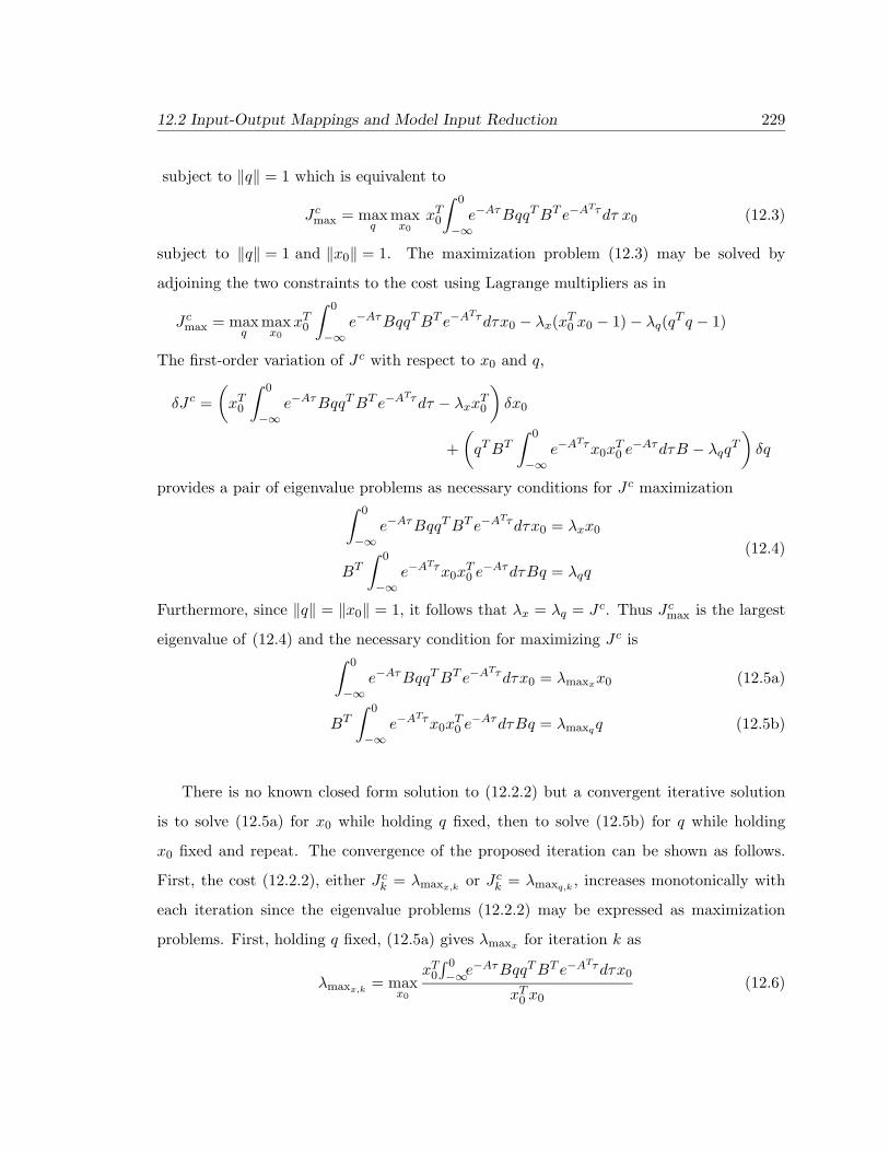
12.2 Input-Output Mappings and Model Input Reduction 229
subject to ‖q‖ = 1 which is equivalent to
Jcmax = maxq
maxx0
xT0
∫ 0
−∞e−AτBqqTBT e−A
Tτdτ x0 (12.3)
subject to ‖q‖ = 1 and ‖x0‖ = 1. The maximization problem (12.3) may be solved by
adjoining the two constraints to the cost using Lagrange multipliers as in
Jcmax = maxq
maxx0
xT0
∫ 0
−∞e−AτBqqTBT e−A
Tτdτx0 − λx(xT0 x0 − 1)− λq(qT q − 1)
The first-order variation of Jc with respect to x0 and q,
δJc =(xT0
∫ 0
−∞e−AτBqqTBT e−A
Tτdτ − λxxT0)δx0
+(qTBT
∫ 0
−∞e−A
Tτx0xT0 e−AτdτB − λqqT
)δq
provides a pair of eigenvalue problems as necessary conditions for Jc maximization∫ 0
−∞e−AτBqqTBT e−A
Tτdτx0 = λxx0
BT
∫ 0
−∞e−A
Tτx0xT0 e−AτdτBq = λqq
(12.4)
Furthermore, since ‖q‖ = ‖x0‖ = 1, it follows that λx = λq = Jc. Thus Jcmax is the largest
eigenvalue of (12.4) and the necessary condition for maximizing Jc is∫ 0
−∞e−AτBqqTBT e−A
Tτdτx0 = λmaxxx0 (12.5a)
BT
∫ 0
−∞e−A
Tτx0xT0 e−AτdτBq = λmaxqq (12.5b)
There is no known closed form solution to (12.2.2) but a convergent iterative solution
is to solve (12.5a) for x0 while holding q fixed, then to solve (12.5b) for q while holding
x0 fixed and repeat. The convergence of the proposed iteration can be shown as follows.
First, the cost (12.2.2), either Jck = λmaxx,k or Jck = λmaxq,k , increases monotonically with
each iteration since the eigenvalue problems (12.2.2) may be expressed as maximization
problems. First, holding q fixed, (12.5a) gives λmaxx for iteration k as
λmaxx,k = maxx0
xT0∫ 0−∞e
−AτBqqTBT e−ATτdτx0
xT0 x0(12.6)

230 Chapter 12: Model Input Reduction
Now, holding x0 fixed, (12.5b) gives λmaxq for iteration k + 1 as
λmaxq,k+1= max
q
qTBT∫ 0−∞e
−ATτx0xT0 e−Aτdτ Bq
xT0 x0
= maxq
xT0∫ 0−∞e
−AτBqqTBT e−ATτdτ x0
xT0 x0
(12.7)
Therefore,
λmaxq,k+1≥ λmaxx,k ≥ λmaxq,k−1
≥ · · · ≥ λmaxx,1
Clearly, as long as ‖q‖ = ‖x0‖ = 1, the cost Jck is bounded above. Thus Jck approaches a
limit and the iteration must converge.
limk→∞
Jck = Jcmax
While the uniqueness of the limit is not guaranteed, the experience of the authors has shown
that in several practical applications the limit achieved is close to the upper bound given
by λmax (Lc) of the full-input system.
This approach is a dual to that of Section 12.2.1 in the sense that only the controllability
of the system pair (A,B) is considered. No weight is given to the energy required to
reconstruct the initial state x0 from the output pair (C,A).
12.2.3 Output and Intput Point of View
Both input (12.1) and output (12.2.2) considerations are combined by maximizing the
Hankel norm of the system triple G4= (C,A,Bq) as in
Jmax = maxq
ΓG(q)
= maxq
supω
‖y‖2L2[0,∞)
‖ω‖2L2(−∞,0]
= maxq
maxx0
xT0 Lox0
xT0
[∫ 0−∞e
−AτBqqTBT e−ATτdτ]−1x0
= maxq
maxx0
xT0∫ 0−∞ e
−AτBqqTBT e−ATτdτ x0
xT0 L−1o x0

12.3 Application to Disturbance Direction Estimation 231
Necessary conditions for this problem are a pair of eigenvalue problems similar to (12.2.2)
but with the premultiplication of an observability gramian
Lo
∫ 0
−∞e−AτBqqTBT e−A
Tτdτx0 = λmaxxx0 (12.8a)
BT
∫ 0
−∞e−A
Tτx0xT0 e−AτdτBq = λmaxqq (12.8b)
An iterative solution to (12.8) that is similar to that for (12.2.2) has been successfully
applied.
12.3 Application to Disturbance Direction Estimation
Parametric uncertainties in a linear system model can often be modeled as scalar or low
dimensional unknown inputs. Given the disturbance direction, a disturbance decoupling or
bounding controller may be constructed to provide robustness to variations in the unknown
system parameters. In practice, identifying this direction has its own uncertainty in the
sense that usually a set of directions is formed from which a representative direction is
chosen. For the purpose of illustration, an observer based method (Patton and Chen 1992)
for identifying a disturbance direction is outlined below.
Consider a linear time invariant system with a scalar disturbance d
x = Ax+Bu+ Ed
The vector E is unknown and represents the direction of uncertainty acting on the system
model. The direction E may be estimated by defining Ed = w, and forming an observer
to estimate w. First, assume that w is a slowly time varying vector of dimension n. Then
append it to the state vector to form a 2n-dimensional system[xw
]=[A I0 0
] [xw
]+[B0
]u (12.9)
Since (12.9) is a system model, full state information may be assumed so that the observation
relation is
y =[I 0
] [ xw
](12.10)

232 Chapter 12: Model Input Reduction
An observer based on the model (12.9, 12.10) is used to estimate w. The measurements
provided to the observer are from the full higher-order or nonlinear system or simulation.
It is assumed that constant controls u are applied so that the observer eventually reaches
a steady-state and an estimate for w, that is w, becomes a constant. The disturbance
direction E is a normalized w. In general, the direction E found will depend on the size
and direction of the control vector u applied to the nonlinear plant. Thus a system model
with several disturbance directions is formed as
x = Ax+Bu+[E1 E2 . . . Em
]d1d2...dm
The problem now is to determine an appropriate reduced dimension and range for the
disturbance distribution matrix [E1, E2, . . . , Em].
A numerical example follows from the longitudinal dynamics of an automobile linearized
as the vehicle is driven on a straight and level road at a constant speed 25 m/s. A small
slope in the road appears as a disturbance in the dynamics. Thus the model becomes
x = Ax+Bu+ E1d1 + E2d2 + E3d3 + E4d4
y = Cx
The states are engine manifold air mass, engine speed, longitudinal and vertical velocity,
vertical position, the sum of two front wheel speeds and the sum of two rear wheel speeds.
The control inputs are throttle and brake commands. The disturbance directions E =
[E1, E2, E3, E4] are found for road slopes of −1, −2, −3 and 0 degrees respectively when
the brake is held fixed at the trim value and the throttle is held fixed slightly away from
the trim value. Data for the system are as follows.
A =
−0.0521 −0.2213 0.2681 −0.0121 0.0136 0.0084 −0.0078−0.3007 −8.0277 19.0734 −1.1013 0.0795 0.2471 0.0378−0.3263 −19.7571 −51.0638 −3.2675 −4.8766 −2.4258 0.0040
0.0454 2.4036 15.7922 −2.1857 6.4655 −0.2062 0.04950.0219 1.1136 8.6428 −7.1817 −0.6526 −0.2171 0.93160.0116 0.5928 3.8335 −1.0926 −0.6513 −0.9851 5.96280.0154 0.7868 4.8494 −1.4900 −1.0329 −6.5688 −2.5996
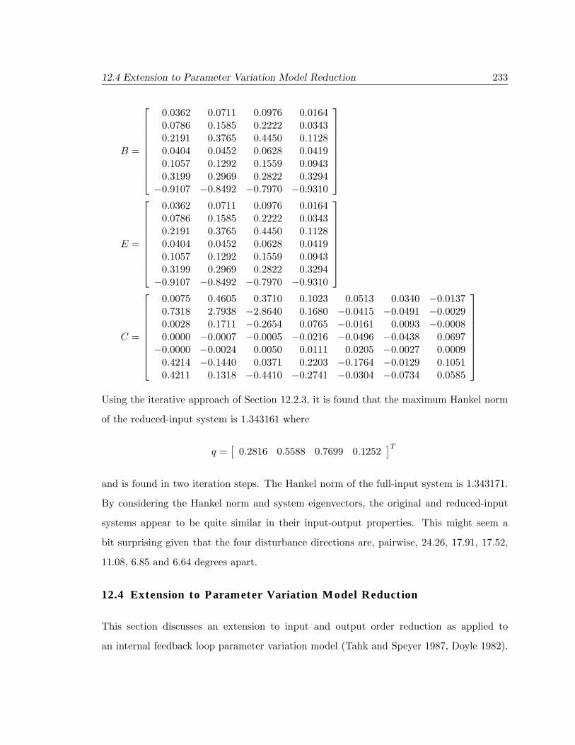
12.4 Extension to Parameter Variation Model Reduction 233
B =
0.0362 0.0711 0.0976 0.01640.0786 0.1585 0.2222 0.03430.2191 0.3765 0.4450 0.11280.0404 0.0452 0.0628 0.04190.1057 0.1292 0.1559 0.09430.3199 0.2969 0.2822 0.3294−0.9107 −0.8492 −0.7970 −0.9310
E =
0.0362 0.0711 0.0976 0.01640.0786 0.1585 0.2222 0.03430.2191 0.3765 0.4450 0.11280.0404 0.0452 0.0628 0.04190.1057 0.1292 0.1559 0.09430.3199 0.2969 0.2822 0.3294−0.9107 −0.8492 −0.7970 −0.9310
C =
0.0075 0.4605 0.3710 0.1023 0.0513 0.0340 −0.01370.7318 2.7938 −2.8640 0.1680 −0.0415 −0.0491 −0.00290.0028 0.1711 −0.2654 0.0765 −0.0161 0.0093 −0.00080.0000 −0.0007 −0.0005 −0.0216 −0.0496 −0.0438 0.0697−0.0000 −0.0024 0.0050 0.0111 0.0205 −0.0027 0.0009
0.4214 −0.1440 0.0371 0.2203 −0.1764 −0.0129 0.10510.4211 0.1318 −0.4410 −0.2741 −0.0304 −0.0734 0.0585
Using the iterative approach of Section 12.2.3, it is found that the maximum Hankel norm
of the reduced-input system is 1.343161 where
q =[
0.2816 0.5588 0.7699 0.1252]T
and is found in two iteration steps. The Hankel norm of the full-input system is 1.343171.
By considering the Hankel norm and system eigenvectors, the original and reduced-input
systems appear to be quite similar in their input-output properties. This might seem a
bit surprising given that the four disturbance directions are, pairwise, 24.26, 17.91, 17.52,
11.08, 6.85 and 6.64 degrees apart.
12.4 Extension to Parameter Variation Model Reduction
This section discusses an extension to input and output order reduction as applied to
an internal feedback loop parameter variation model (Tahk and Speyer 1987, Doyle 1982).

234 Chapter 12: Model Input Reduction
Within the context of an uncertain parameter block variation model ∆ of the form
x = Ax+Bu+Bωω
y = Cx
z = Czx
ω = ∆z
consider a model input and output reduction problem posed as follows. Find qω and qz with
‖qω‖ = ‖qz‖ = 1 such that the system triple
G4=(qTz Cz, A,Bωqω
)maximizes the Hankel norm
Jmax = maxqω
maxqz
ΓG(qω, qz)
= maxqω maxqz
maxx0
xT0 Lox0
xT0 L−1c x0
= maxqω
maxqz
λmax(LcLo)
where
Lc =∫ 0
−∞e−AτBωqωq
TωB
Tω e−ATτdτ
Lo =∫ ∞
0eA
TτCTz qzqTz Cze
Aτdτ
This problem is also solved iteratively. First, hold qz fixed and solve for qω, then hold
qω fixed and solve for qz. The former problem is the same problem as that in Section 12.2.3;
the latter is the dual. Necessary conditions that follow are
LoLcx01 = λmaxx01x01 (12.11a)
BTω
∫ 0
−∞e−A
Tτx01xT01e−AτdτBωqω = λmaxqω qω (12.11b)
and
LcLox02 = λmaxx02x02 (12.12a)
Cz
∫ ∞0eAτx02x
T02e
ATτdτCTz qz = λmaxqz qz (12.12b)

12.5 Conclusions 235
The proposed iteration is to solve (12.11a) and (12.11b) holding qz fixed until x01 and
qω are found. Then, holding qω fixed, solve (12.12a) and (12.12b) iteratively for x02 and
qz. The stopping condition is when Jmax = λmaxx01 = λmaxx02 within some tolerance. Note
that with both qω and qz as one-dimensional mappings, ∆ is a scalar.
12.5 Conclusions
A reduced-input system problem is formed from the point of view of preserving system
input-output properties. Necessary conditions for maximizing a reduced-input system
Hankel norm are stated and an iterative solution is proposed. An application to disturbance
direction identification is illustrated with a numerical example. Finally, an extension to
include applications to internal feedback loop parameter variation models is developed.


Chapter 13
Conclusions
Analytic redundancy continues to be a viable approach to vehicle health monitoring.
The fault detection filters and parity equations developed here as a point design for the
longitudinal mode are tested in a high-fidelity vehicle simulation where nonlinearities and
road variations are significant. The designed static patterns emerge clearly and quickly
in response to a fault. The residual processor, a multiple hypothesis Shiryayev sequential
probability ratio test, examines the filter and parity equation residuals and generates the
probability of the presence of a fault. This system also works well, responding to soft failures
in the presence of dynamic disturbances and vehicle nonlinearites. Sensor noise has been
omitted pending development of higher fidelity sensor models.
The design as presented is intended to be packaged as a module of a comprehensive
health monitoring and reconfiguration system under development at UC Berkeley. Further
development of this module should involve testing with empirically derived data and the
design and implementation of a software interface compatible with the system at Berkeley.
237

238 Chapter 13: Conclusions
A preliminary design of a range sensor fault monitoring system is sketched as an
application of a new decentralized fault detection filter structure. This system combines
dynamic state information already generated by the existing filter designs with inter-vehicle
analytic redundancy. This approach will be more fully tested as a high-fidelity multi-vehicle
simulation becomes available.
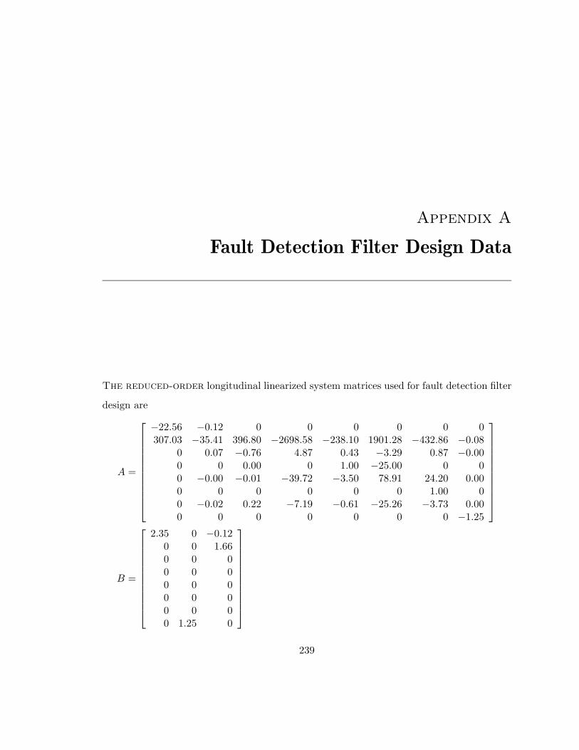
Appendix A
Fault Detection Filter Design Data
The reduced-order longitudinal linearized system matrices used for fault detection filter
design are
A =
−22.56 −0.12 0 0 0 0 0 0307.03 −35.41 396.80 −2698.58 −238.10 1901.28 −432.86 −0.08
0 0.07 −0.76 4.87 0.43 −3.29 0.87 −0.000 0 0.00 0 1.00 −25.00 0 00 −0.00 −0.01 −39.72 −3.50 78.91 24.20 0.000 0 0 0 0 0 1.00 00 −0.02 0.22 −7.19 −0.61 −25.26 −3.73 0.000 0 0 0 0 0 0 −1.25
B =
2.35 0 −0.120 0 1.660 0 00 0 00 0 00 0 00 0 00 1.25 0
239

240 Appendix A. Fault Detection Filter Design Data
C =
1.00 0 0 0 0 0 0 00 1.00 0 0 0 0 0 00 0 1.00 0 0 0 0 00 0.07 −0.76 4.87 0.43 −3.29 0.87 −0.000 −0.00 −0.01 −39.72 −3.50 78.91 24.20 −0.000 0 7.10 −45.34 −4.00 146.48 2.83 −0.000 0.09 5.96 −40.56 −3.58 28.58 −6.51 −0.00
D =
0 0 00 0 00 0 00 0 00 0 00 0 00 0 0
The filter gain L and the output projection matrices Huα , HuTb, Hyma and HyTm for the
first fault detection filter are as follows.
L =
19.56 0.12 0.00 0.00 −0.00 −0.00 0.00−307.03 523.06 −334.41 −6277.18 8.39 3.99 −832.46−0.00 11.97 −11.36 −156.00 0.20 0.10 −18.91
0.00 0.00 −1.96 −0.10 −0.06 0.19 0.030.00 −0.07 −7.21 −0.00 −1.17 −0.08 0.83−0.00 −0.00 0.01 −0.01 −0.02 −0.02 0.03
0.00 −3.51 1.38 46.16 −0.26 0.32 5.26−0.00 −60.65 19.39 784.64 −2.29 0.07 96.37
Huα =
0.93 0.07 −0.02 0.11 0.16 −0.10 −0.110.07 0.01 −0.00 0.01 0.00 0.03 −0.05−0.02 −0.00 0.99 0.04 0.05 −0.03 −0.04
0.11 0.01 0.04 0.16 −0.28 −0.12 −0.180.16 0.00 0.05 −0.28 0.62 0.23 0.28−0.10 0.03 −0.03 −0.12 0.23 0.73 −0.35−0.11 −0.05 −0.04 −0.18 0.28 −0.35 0.55
HuTb=
0 0.00 0 0.00 −0.00 0 0.000.00 0.01 0 −0.07 0.00 0 −0.09
0 0 1.00 0 0 0 00.00 −0.07 0 1.00 0.00 0 −0.01−0.00 0.00 0 0.00 1.00 0 0.00
0 0 0 0 0 1.00 00.00 −0.09 0 −0.01 0.00 0 1.00

Appendix A. Fault Detection Filter Design Data 241
Hyma = HyTm =
0 0 0 0 0 0 00 0.08 −0.02 0.13 0.16 −0.07 −0.160 −0.02 1.00 0.00 0.00 −0.00 −0.000 0.13 0.00 0.35 −0.02 −0.28 −0.360 0.16 0.00 −0.02 0.97 0.01 0.030 −0.07 −0.00 −0.28 0.01 0.86 −0.190 −0.16 −0.00 −0.36 0.03 −0.19 0.74
The filter gain L and the output projection matrices Hyωe , Hyax , Hyωffor the second fault
detection filter are as follows.
L =
18.56 0.12 −0.00 0.00 0.00 −0.00 0.00−307.03 38.32 −0.00 −0.00 −0.00 0.00 −66.53
0.01 −0.00 −3.00 −1.00 0.00 0.00 0.000.75 0.01 0.16 −0.04 0.04 0.21 −0.132.16 −0.00 4.11 −0.01 −0.61 −0.00 −0.08−0.01 −0.00 −0.13 −0.02 −0.03 −0.02 0.05
0.54 0.03 0.02 0.36 −0.12 0.33 −0.380.01 −95.97 32.35 1230.72 −3.58 0.10 151.14
Hyωe =
1.00 −0.00 −0.00 0.00 0.00 −0.00 −0.00−0.00 1.00 −0.00 0.00 0.00 0.00 −0.00−0.00 −0.00 0.99 0.00 0.09 −0.00 −0.02
0.00 0.00 0.00 −0.00 0.00 −0.00 −0.000.00 0.00 0.09 0.00 0.01 −0.00 −0.00−0.00 0.00 −0.00 −0.00 −0.00 0.00 0.00−0.00 −0.00 −0.02 −0.00 −0.00 0.00 0.00
Hyax =
1.00 0.00 0.00 −0.04 0.06 −0.00 −0.060.00 0.00 −0.00 0.00 0.00 −0.00 −0.000.00 −0.00 1.00 0.00 −0.00 −0.00 0.00−0.04 0.00 0.00 0.03 0.18 −0.00 −0.03
0.01 0.00 −0.00 0.18 0.94 −0.00 −0.17−0.00 −0.00 −0.00 −0.00 −0.00 0.00 0.00−0.01 −0.00 0.00 −0.03 −0.17 0.00 0.03
Hyωf=
1.00− 0.000.000.00− 0.010.03− 0.04−0.000− 0.00− 0.000.000.000.00
0.00− 0.000.990.000.05− 0.05− 0.020.00− 0.000.000.00− 0.00− 0.00− 0.00
−0.010.000.05− 0.000.580.470.150.030.00− 0.05− 0.000.470.390.12−0.040.00− 0.02− 0.000.150.120.04

242 Appendix A. Fault Detection Filter Design Data
The filter gain L and the output projection matrices Hyvx , Hyaz , Hyωr for the third fault
detection filter are as follows.
L =
1.96 0.12 −0.00 0.00 −0.00 −0.00 0.00−307.03 38.32 −0.00 0.01 −0.00 0.00 −66.53−0.00 0.00 −3.01 −1.01 0.00 −0.00 0.00
0.00 0.07 −1.11 −0.52 −0.06 0.34 −0.100.00 0.38 −0.02 −3.38 −1.14 0.56 0.01−0.00 −0.00 −0.24 −0.06 −0.03 −0.04 0.05
0.00 0.03 0.26 0.39 −0.15 0.36 −0.350.00 −94.97 14.68 1234.19 −3.10 1.68 151.15
Hyvx =
1.00 −0.00 −0.00 0.00 −0.00 −0.00 0.00−0.00 0.00 −0.00 −0.03 0.00 −0.01 0.00−0.00 −0.00 1.00 0.00 −0.00 −0.00 0.00
0.00 −0.03 0.00 0.90 −0.00 0.30 −0.00−0.00 0.00 −0.00 −0.00 −0.00 −0.00 −0.00−0.00 −0.01 −0.00 0.30 −0.00 0.10 −0.00
0.00 0.00 0.00 −0.00 −0.00 −0.00 −0.00
Hyaz =
1.00 0.00 0.00 0.00 −0.00 0.00 0.000.00 0.03 −0.00 −0.08 0.02 0.16 −0.000.00 −0.00 −0.00 0.00 −0.00 −0.00 −0.000.00 −0.08 0.00 0.99 0.07 0.00 0.00−0.00 0.02 −0.00 0.07 0.03 0.16 −0.00
0.00 0.15 −0.00 0.00 0.16 0.95 −0.000.00 −0.00 −0.00 0.00 −0.00 −0.00 −0.00
Hyωf=
1.00 −0.00 0.00 −0.00 −0.00 0.0 0.00−0.00 1.00 0.00 −0.00 0.00 0.00 0.00
0.00 0.00 −0.00 −0.00 −0.00 −0.00 −0.00−0.00 −0.00 −0.00 0.99 −0.00 0.01 0.12−0.00 0.00 −0.00 −0.00 0 −0.00 −0.00
0.00 0.00 −0.00 0.01 −0.00 0.00 0.000.00 0.00 −0.00 0.12 −0.00 0.00 0.01
References
Athans, M. 1977. The Stochastic Control of the F-8C Aircraft using a Multiple Model
Adaptive Control Method : Equilibrium Flight. IEEE Transactions on Automatic
Control, Vol. 5:768–780.
Basar, T. and P. Bernhard 1995. H∞ Control and Other Minimax Problems. Birkhauser,
New York, 2rd edition.
Banavar, R. N. and J. L. Speyer 1991. An Linear-Quadratic Game Approach to
Estimation and Smoothing. In Proceedings of the American Control Conference,
pages 2818–2822.
Basile, G. and G. Marro 1992. Controlled and Conditioned Invariants in Linear System
Theory. Prentice-Hall.
Beard, R. V. 1971. Failure Accomodation in Linear Systems through Self-Reorganization.
PhD thesis, Department of Aeronautics and Astronautics, Massachusetts Institute
of Technology, Cambridge, MA.
243

244 References
Bell, D. J. and D. H. Jacobsen 1973. Singular Optimal Control. Academic Press.
Bryson, A. E. and Y. C. Ho 1975. Applied Optimal Control. New York: Hemisphere.
Bryson, A. E. and D. Johansen 1965. Linear Filtering for Time-Varying Systems Using
Measurements Containing Colored Noise. IEEE Transactions on Automatic Control,
Vol. AC-10, No. 1:4–10.
Chichka, D. F. and J. L. Speyer 1995. An Adaptive Controller Based on
Disturbance Attenuation. IEEE Transactions on Automatic Control, Vol. AC-40,
No. 7:1220–1233.
Chung, W. H. 1997. Game Theoretic and Decentralized Estimation for Fault Detection.
PhD thesis, University of California, Los Angeles.
Chung, W. H. and J. L. Speyer 1995. A General Framework for Decentralized Estimation.
In Proceedings of the 1995 American Controls Conference, Seattle, WA. ACC.
Chung, W. H. and J. L. Speyer 1996. A Game Theoretic Filter for Fault Detection and
Isolation. In Proceedings of the 13th Triennial IFAC World Congress.
Chung, W. H. and J. L. Speyer 1998. A Game Theoretic Fault Detection Filter. To be
published in the IEEE Transactions on Automatic Control.
Clements, D. J. and B. D. O. Anderson 1978. Singular Optimal Control: The
Linear-Quadratic Problem, volume 5 of Lecture Notes in Control and Information
Sciences. Springer-Verlag.
DeSouza, C., U. Shaked, and M.-Y. Fu 1992. Robust H∞ Filtering with Parametric
Uncertainty and Deterministic Input Signal. In Proceedings of the 31st Conference
on Decision and Control, pages 2305–2310, Tuscon, AZ.
Ding, X. and P. M. Frank 1989. Fault Detection via Optimally Robust Detection Filters.
In Proceedings of the 28th Conference on Decision and Control, pages 1767–1772,
Tampa, FL. IEEE.
References 245
Douglas, R. K. 1993. Robust Fault Detection Filter Design. PhD thesis, The University of
Texas at Austin, Austin, TX.
Douglas, R. K. and J. L. Speyer 1995. An H∞ Bounded Fault Detection Filter. In
Proceedings of the American Controls Conference.
Douglas, R. K. and J. L. Speyer 1996. Robust Fault Detection Filter Design. AIAA Journal
of Guidance, Control, and Dynamics, Vol. 19, No. 1:214–218.
Douglas, R. K., J. L. Speyer, D. L. Mingori, R. H. Chen, D. P. Malladi, and W. H. Chung
1995. Fault Detection and Identification with Application to Advanced Vehicle
Control Systems. Research Report UCB-ITS-PRR-95-26, University of California,
Los Angeles, MAE Dept. and California PATH.
Douglas, R. K., J. L. Speyer, D. L. Mingori, R. H. Chen, D. P. Malladi, and W. H. Chung
1996. Fault Detection and Identification with Application to Advanced Vehicle
Control Systems: Final Report. Research Report UCB-ITS-PRR-96-25, University
of California, Los Angeles, MAE Dept. and California PATH.
Doyle, J. C. 1982. Analysis of Feedback Systems with Structured Uncertainties. In
Proceedings of the IEE. Part D, No. 6.
Doyle, J. C., K. Glover, P. P. Khargonekar, and B. A. Francis 1989. State-Space Solutions to
Standard H2 and H∞ Control Problems. IEEE Transactions on Automatic Control,
Vol. AC-34, No. 8:831–847.
Edelmayer, A., J. Bokor, and L. Keviczky 1994. An H∞ Filtering Approach to Robust
Detection of Failures in Dynamical Systems. In Proceedings of the 33rd IEEE
Conference on Decision and Control, Lake Buena Vista, Florida.
Edelmayer, A., J. Bokor, and L. Keviczky 1996. H∞ Detection Filter Design for Linear
Systems: Comparison of Two Approaches. In Proceedings of the 13th Triennial IFAC
World Congress, San Francisco, California.
246 References
Francis, B. A. 1979. The Optimal Linear-Quadratic Time-Invariant Regulator with Cheap
Control. IEEE Transactions on Automatic Control, Vol. 24, No. 4:616–621.
Frank, P. M. 1990. Fault Diagnosis in Dynamic Systems Using Analytical and
Knowledge-based Redundancy – A Survey and Some New Results. Automatica,
Vol. 26, No. 3:459–474.
Frank, P. M. 1994. Enhancement of Robustness in Observer-Based Fault Detection.
International Journal of Control, Vol. 59, No. 4:955–981.
Ghaoui, L. E., A. Carrier, and A. E. Bryson 1992. Linear Quadratic Minimax Controllers.
AIAA Journal of Guidance, Control, and Dynamics, Vol. 15, No. 4:953–961.
Green, M. and D. J. N. Limebeer 1995. Linear Robust Control. Prentice-Hall.
Iwasake, T. and R. E. Skelton 1994. All Controllers for the General H∞ Control
Problem: LMI Existence Conditions and State Space Formulas. Automatica, Vol. 30,
No. 8:1307–1317.
Jacobson, D. H. 1971. Totally Singular Quadratic Optimization Problems. IEEE
Transactions on Automatic Control, Vol. AC-16, No. 6:651–658.
Jacobson, D. H. and J. L. Speyer 1971. Necessary and Sufficient Conditions for Optimality
for Singular Control Problems: A Limit Approach. Journal of Mathematical Analysis
and Applications, Vol. 34, No. 2:239–266.
Jang, J. and J. L. Speyer 1994. Decentralized Game-Theoretic Filters. In Proceedings of
the American Control Conference, pages 3379–3384, Baltimore, MD. ACC.
Jones, H. L. 1973. Failure Detection in Linear Systems. PhD thesis, Department of
Aeronautics and Astronautics, Massachusetts Institute of Technology, Cambridge,
MA.
Kalman, R. E. 1964. When is a Linear Control System Optimal. Transactions of the ASME,
Journal of Basic Engineering, Series D, Vol. 86:51–50.

References 247
Kerr, T. 1985. Decentralized Filtering and Redundancy Management/Failure Dectection
for Multisensor Integrated Naviagtion Systems. In Proceedings of the ION National
Technical Meeting. Institute of Navigation.
Khalil, H. K. 1996. Nonlinear Systems. Prentice-Hall Inc., 2nd edition.
Klema, V. C. and A. J. Laub 1980. The Singular Value Decomposition: Its Computation and
Some Applications. IEEE Transactions on Automatic Control, Vol. AC-25, No. 2.
Kwakernaak, H. and R. Sivan 1972. The Maximally Achievable Accuracy of Linear Optimal
Regulators and Linear Optimal Filters. IEEE Transactions on Automatic Control,
Vol. AC-17, No. 1:79–86.
Lainiotis, D. G. 1976. Partitioning : A Unified Framework for Adaptive Systems :
Estimation. Proceedings of the IEEE, Vol. 64:1126–1143.
Lee, G. H. 1994. Least-Squares and Minimax Methods for Filtering, Identification and
Detection. PhD thesis, University of California, Los Angeles.
Limebeer, D. and G. Halikias 1988. A Controller Degree Bound for Hinf Problems of the
Second Kind. SIAM Journal of Control and Optimization, Vol. 26, No. 3:646–677.
Limebeer, D. J. N., B. D. O. Anderson, P. P. Khargoneger, and M. Green 1992. A Game
Theoretic Approach to H∞ Control for Time-Varying Systems. SIAM Journal of
Control and Optimization, Vol. 30, No. 2:262–283.
Liporace, L. A. 1971. Variance of Bayes Estimates. IEEE Transactions on Information
Theory, Vol. 17:665–669.
Macfarlane, A. G. J. and N. Karcanias 1976. Poles and Zeros of Linear Multivariable
Systems: A Survey of the Algebraic, Geometric and Complex-variable Theory.
International Journal of Control, Vol. 24, No. 1:33–74.
Mageirou, E. F. 1976. Values and Strategies for the Infinite Time Linear Quadratic Games.
IEEE Transactions on Automatic Control, Vol. 21, No. 9:547–550.

248 References
Magill, D. T. 1965. Optimal Adaptive Estimation of Sampled Processes. IEEE Transactions
on Automatic Control, Vol. 10:434–439.
Malladi, D. P. and J. L. Speyer 1996. A Generalized Shiryayev Sequential Probability Ratio
Test for Change Detection and Isolation. In Proceedings of the 35th Conference on
Decision and Control. IEEE.
Malladi, D. P. and J. L. Speyer 1997. A Generalized Shiryayev Sequential Probability
Ratio Test for Change Detection and Isolation. Submitted for publication in the
IEEE Transactions on Automatic Control.
Mangoubi, R. S. 1995. Robust Estimation and Failure Detection for Linear Systems. PhD
thesis, Department of Aeronautics and Astronautics, Massachusetts Institute of
Technology, Cambridge, MA.
Mangoubi, R. S., B. D. Appleby, and G. C. Verghese 1994. Stochastic Interpretation of
H∞ and Robust Estimation. In Proceedings of the 33rd Conference on Decision and
Control, pages 3943–3948. IEEE.
Massoumnia, M.-A. 1986. A Geometric Approach to the Synthesis of Failure Detection
Filters. IEEE Transactions on Automatic Control, Vol. AC-31, No. 9:839–846.
Massoumnia, M.-A., G. C. Verghese, and A. S. Willsky 1989. Failure Detection and
Identification. IEEE Transactions on Automatic Control, Vol. AC-34, No. 3:316–321.
Maybeck, P. S. and P. D. Hanlon 1995. Performance Enhancement of a Multiple Model
Adaptive Estimator. IEEE Transactions on Aerospace and Electronic Systems,
Vol. 31:1240–1253.
Mehra, R. K. and A. E. Bryson 1968. Linear Smoothing Using Measurements Containing
Correlated Noise with an Application to Inertial Navigation. IEEE Transactions on
Automatic Control, Vol. AC-13, No. 5:496–503.

References 249
Menke, T. E. and P. S. Maybeck 1995. Sensor/Actuator Failure Detection in the Vista
F-16 by Multiple Model Adaptive Estimation. IEEE Transactions on Aerospace and
Electronic Systems, Vol. 31:1218–1228.
Mills, R. A. and A. E. Bryson 1994. Calculus of Variations Derivation of the Minimax
Linear-Quadratic (H∞) Controller. AIAA Journal of Guidance, Control, and
Dynamics, Vol. 17, No. 1:153–160.
Moore, B. C. and A. J. Laub 1978. Computation of Supremal (A,B)-Invariant and
Controllability Subspaces. IEEE Transactions on Automatic Control, Vol. AC-23,
No. 5.
Moylan, P. J. and J. B. Moore 1971. Generalizations of Singular Optimal Control Theory.
Automatica, Vol. 7:591–598.
Oshman, Y. and I. Y. Bar-Itzhack 1985. Eigenfactor Solution of the Matrix Riccati Equation
- A Continuous Square Root Algorithm. IEEE Transactions on Automatic Control,
Vol. AC-30, No. 10:971–978.
Ozcetin, H., A. Saberi, and P. Sannuti 1992. Design forH∞ Almost Disturbance Decoupling
Problem with Internal Stability via State or Measurement Feedback - Singular
Perturbation Approach. International Journal of Control, Vol. 55, No. 4:901–944.
Patton, R. J. and J. Chen 1992. Robust Fault Detection of Jet Engine Sensor Systems Using
Eigenstructure Assignment. AIAA Journal of Guidance, Control, and Dynamics,
Vol. 15, No. 6.
Rhee, I. and J. L. Speyer 1991. A Game Theoretic Approach to a Finite-Time Disturbance
Attenuation Problem. IEEE Transactions on Automatic Control, Vol. AC-36,
No. 9:1021–1032.
Rugh, W. J. 1996. Linear System Theory. Prentice-Hall Inc., 2nd edition.
250 References
Saberi, A., Z. Lin, and A. A. Stoorvogel 1995. H2 Almost Disturbance Decoupling Problem
with Internal Stability. In Proceedings of the American Control Conference, pages
3414–3418, Seattle, WA.
Saif, M. and Y. Guan 1993. A New Approach to Robust Fault Detection
and Identification. IEEE Transactions on Aerospace and Electronic Systems,
Vol. AES-29, No. 3:685–695.
Schumacher, J. M. 1983. The Role of the Dissapation Matrix in Singular Optimal Control.
System and Control Letters, Vol. 2, No. 3:262–266.
Schumacher, J. M. 1985. A Geometric Approach to the Singular Filtering Problem. IEEE
Transactions on Automatic Control, Vol. AC-30, No. 11:1075–1082.
Shaked, U. 1990. H∞-Minimum Error State Estimation of Linear Stationary Processes.
IEEE Transactions on Automatic Control, Vol. AC-35, No. 5.
Sobel, K. M. and F. J. Lallman 1989. Eigenstructure Assignment for the Control of Highly
Augmented Aircraft. AIAA Journal of Guidance, Control, and Dynamics, Vol. 12,
No. 3.
Speyer, J. L. 1979. Computation and Transmission Requirements for a Decentralized
Linear-Quadratic-Gaussian Control Problem. IEEE Transactions on Automatic
Control, Vol. AC-24, No. 2.
Stoorvogel, A. A. 1991. The Singular H∞ Control Problem with Dynamic Measurement
Feedback. SIAM Journal of Control and Optimization, Vol. 29, No. 1:160–184.
Sutton, G. P. 1986. Rocket Propulsion Elements: An Introduction to the Engineering of
Rockets. Wiley-Interscience, 5th edition.
Tahk, M. and J. L. Speyer 1987. Modeling of Parameter Variations and Asymptotic LQG
Synthesis. IEEE Transactions on Automatic Control, Vol. AC-32, No. 9.

References 251
Viswanadham, N. and K. D. Minto 1988. Robust Observer Design with Application to Fault
Detection. In Proceedings of the American Controls Conference, pages 1393–1399,
Atlanta, GA.
White, J. E. and J. L. Speyer 1987. Detection Filter Design: Spectral Theory and
Algorithms. IEEE Transactions on Automatic Control, Vol. AC-32, No. 7:593–603.
Willems, J., A. Ditapci, and L. M. Silverman 1986. Singular Optimal Control: A Geometric
Approach. SIAM Journal of Control and Optimization, Vol. 24, No. 2:323–337.
Willems, J. C. 1981. Almost Invariant Subspaces: An Approach to High Gain Feedback
Design – Part I: Almost Controlled Invariant Subspaces. IEEE Transactions on
Automatic Control, Vol. AC-26, No. 1:235–252.
Willsky, A. S., M. G. Bello, D. A. Castanon, B. C. Levy, and G. C. Verghese 1982.
Combining and Updating of Local Estimates and Regional Maps Along Sets of
One-Dimensional Tracks. IEEE Transactions on Automatic Control, Vol. AC-27,
No. 4:799–813.
Wonham, W. M. 1985. Linear Multivariable Control: A Geometric Approach.
Springer-Verlag, New York, 3rd edition.
Yaesh, I. and U. Shaked 1993. Game Theory Approach to Finite-Time Horizon Optimal
Estimation. IEEE Transactions on Automatic Control, Vol. 38, No. 6:957–963.
Related Documents