Integration of diffraction images and data reduction

Data processing

Integration of diffraction images and data reduction

Phil Evans APS May 2008MRC Laboratory of Molecular BiologyCambridge UK

Assumptions

It is helpful if you understand (at least something about)

• Diffraction from a crystal & the Laue equations

• Reciprocal lattice

• Ewald construction – diffraction geometry

These are topics I don’t have time to discuss today

Crystal

h k l I σ(I)

h k l F σ(F)

Data collection

Images

Integration

Scaling & merging (data reduction)

Diffraction geometryStrategy

Indexing

Space group determinationQuality assessment

Data collection & processing

Decisions

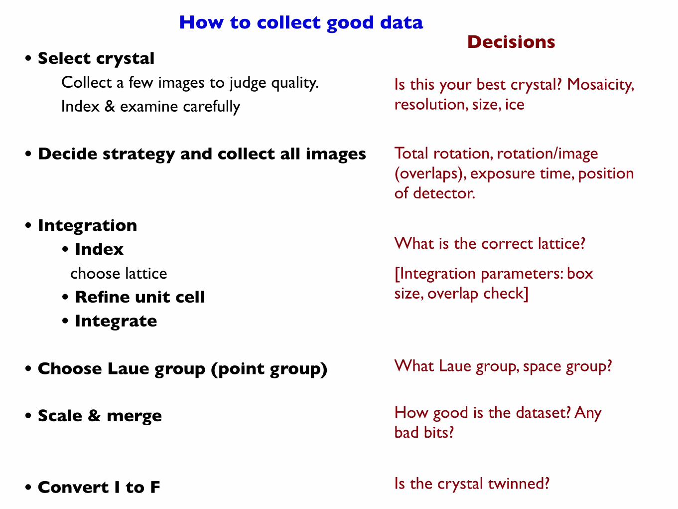
Is this your best crystal? Mosaicity, resolution, size, ice

Total rotation, rotation/image (overlaps), exposure time, position of detector.

How good is the dataset? Any bad bits?

Is the crystal twinned?

What is the correct lattice?

[Integration parameters: box size, overlap check]

What Laue group, space group?

• Select crystalCollect a few images to judge quality.Index & examine carefully

• Decide strategy and collect all images

• Integration• Index choose lattice• Refine unit cell• Integrate

• Choose Laue group (point group)

• Scale & merge

• Convert I to F

How to collect good data

What is a good crystal?

• Single only one lattice

check by indexing pattern and looking for unpredicted spots

• Diffracts to high angle

• Large the diffracted intensity is proportional to the number of unit cells in the beam, so not much gain for a crystal much larger than beam (typically 50–200µm). Smaller crystals may freeze better (lower mosaicity)

• Low mosaicity better signal/noise

• Good freeze no ice, minimum amount of liquid (low background), low mosaicityOptimise cryo procedure

• The best that you have! (the least worst)

The quality of the crystal determines the quality of the dataset.

Beware of pathological cases

Some bad ones

Phi = 0° Phi = 90°

Always check diffraction in two orthogonal images !

Additional spots present, not resolved

Results in instability in refinement of detector parameters.

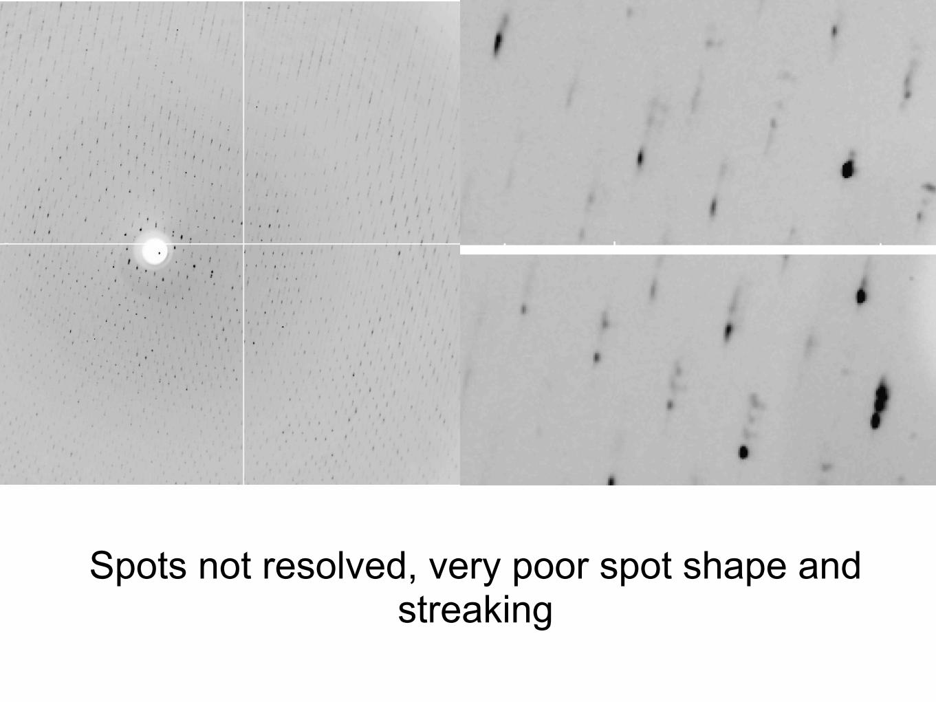
Spots not resolved, very poor spot shape and streaking

Index Strategy Integrate

Scale/Merge

Detwin Convert I to F

(---------------------MOSFLM---------------------)

SCALA

TRUNCATE

Data

Integration and scaling in CCP4

POINTLESSdetermine Laue group & space group, sort

Tools

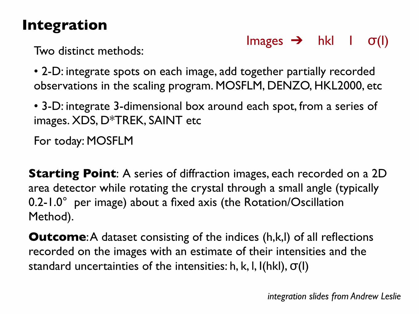
Starting Point: A series of diffraction images, each recorded on a 2D area detector while rotating the crystal through a small angle (typically 0.2-1.0° per image) about a fixed axis (the Rotation/Oscillation Method).

Outcome: A dataset consisting of the indices (h,k,l) of all reflections recorded on the images with an estimate of their intensities and the standard uncertainties of the intensities: h, k, l, I(hkl), σ(I)

Integration

Two distinct methods:

• 2-D: integrate spots on each image, add together partially recorded observations in the scaling program. MOSFLM, DENZO, HKL2000, etc

• 3-D: integrate 3-dimensional box around each spot, from a series of images. XDS, D*TREK, SAINT etc

For today: MOSFLM

integration slides from Andrew Leslie

Images ➔ hkl I σ(I)

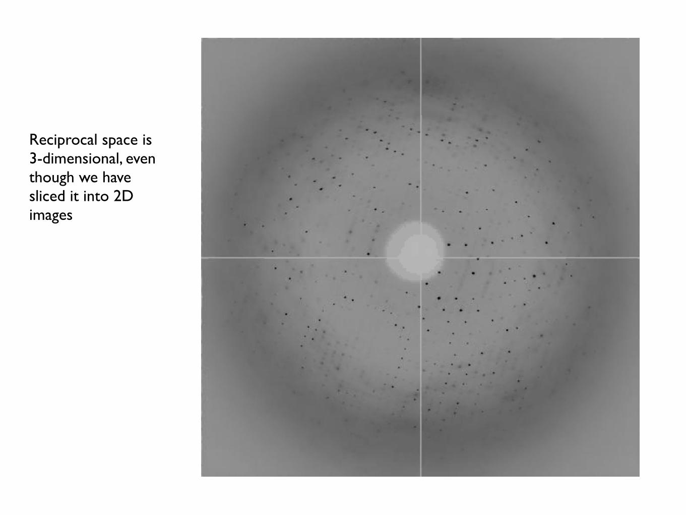
Reciprocal space is 3-dimensional, even though we have sliced it into 2D images

Note that a series of images samples the full 3-dimensional reciprocal space, Bragg diffraction and any other phenomena, all scattering from crystal and its environment.

In practice, defects in the crystals (or detectors) make integration far from trivial, eg weak diffraction, crystal splitting, anisotropic diffraction, diffuse scattering, ice rings/spots, high mosaicity, unresolved spots, overloaded spots, zingers/cosmic rays, etc, etc.

We want to calculate the intensity of each spot: then working backwards –

• The simplest method is draw a box around each spot, add up all the numbers inside, & subtract the background (or better, fit profile)

• To do this, we must know where the spot is: this needs

– the unit cell of the crystal

– the orientation of the crystal relative to the camera

– the exact position of the detector

• To find the unit cell and crystal orientation, we must index the diffraction pattern

– this can be done by finding spots on one or more images

Integration

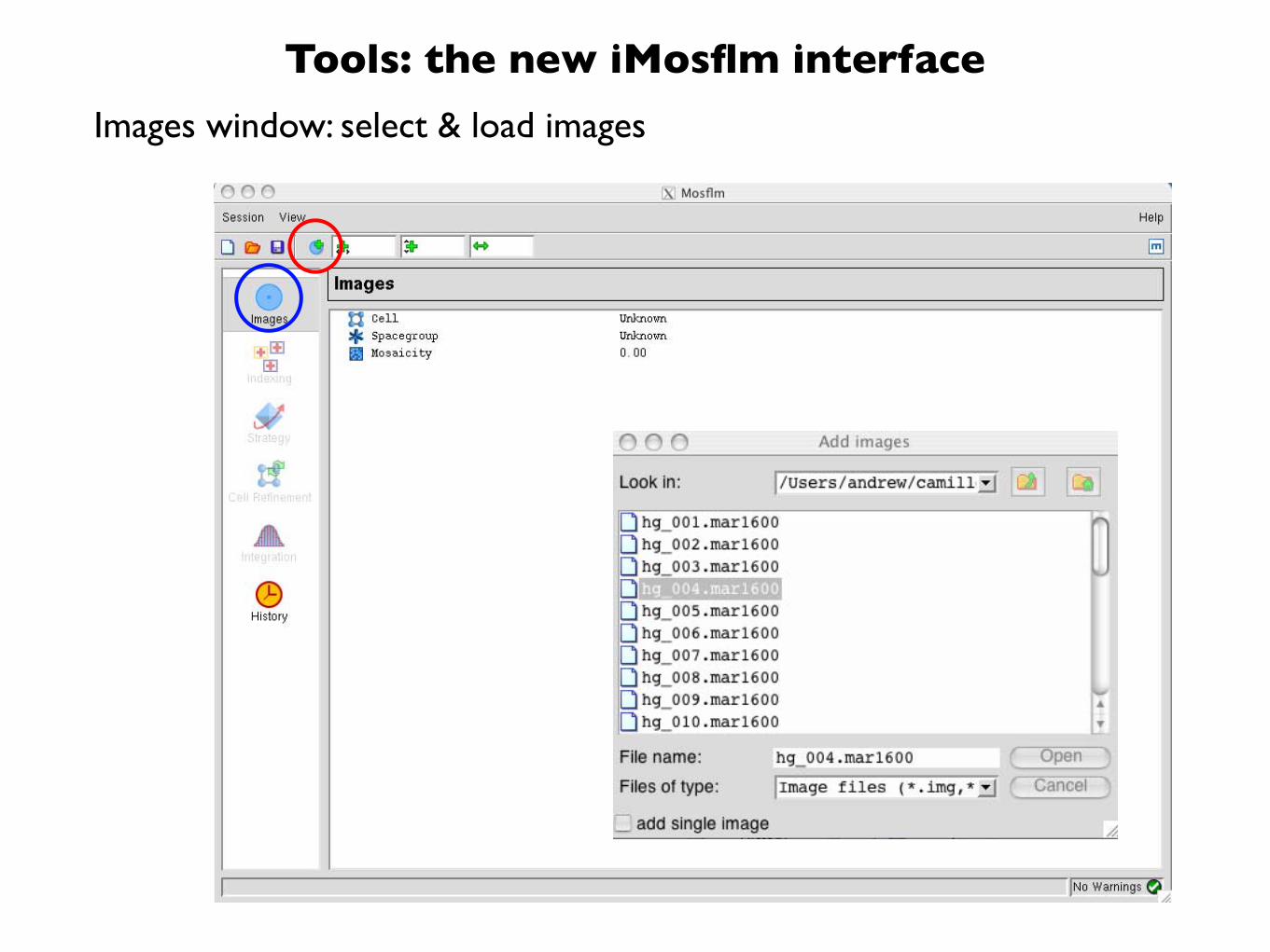
Tools: the new iMosflm interface

Images window: select & load images

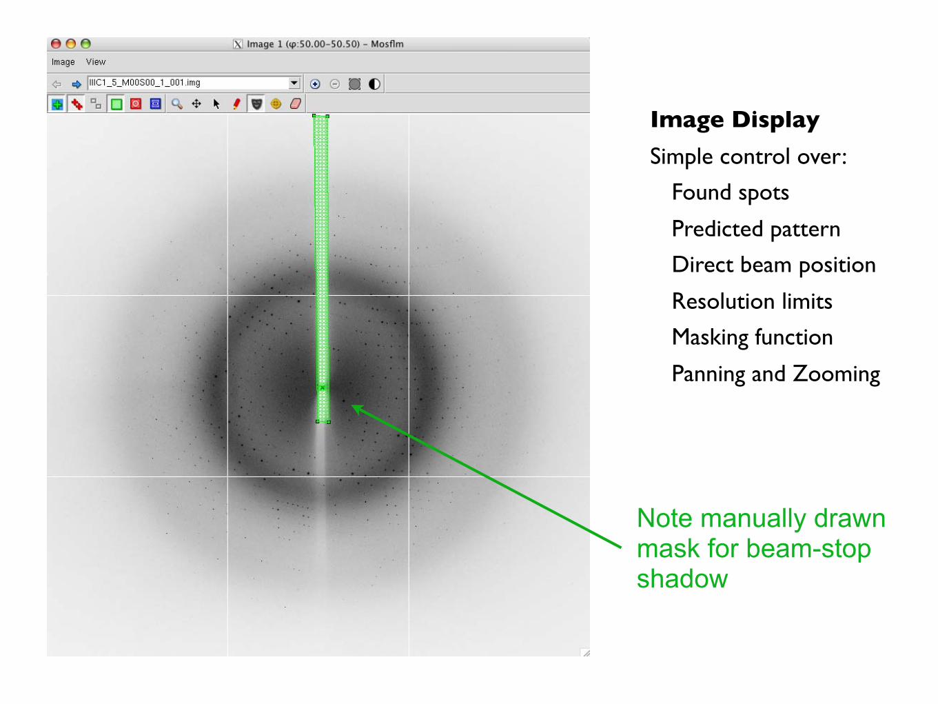
Image Display

Simple control over:

Found spots

Predicted pattern

Direct beam position

Resolution limits

Masking function

Panning and Zooming

Note manually drawn mask for beam-stop shadow

Integration procedure in iMosflm

1. Find spotswhat is a spot? should have uniform shape, not streak

2. Index find lattice which fits spots

3. Estimate mosaicity improve estimate later

4. Check prediction, on images remote in φ (90° away) is the indexing correct?

5. Refine cell use two wedges at 90°, or more in low symmetry

6. Mask backstop shadow not (yet) done automatically by program

7. Integrate one (or few) image to check resolution etc

8. Integrate all images run in background for speed

Strategy option, for use before data collection

Indexing

If we know the main beam position on the image, we can count spots from the centre

To do it properly, we need to put the spots into 3 dimensions, knowing the rotation of the crystal for this image

a*

b*

(3,1,0)l=0

l=1l=2

Back-project each spot on to Ewald sphere, then rotate back into zero-φ frame

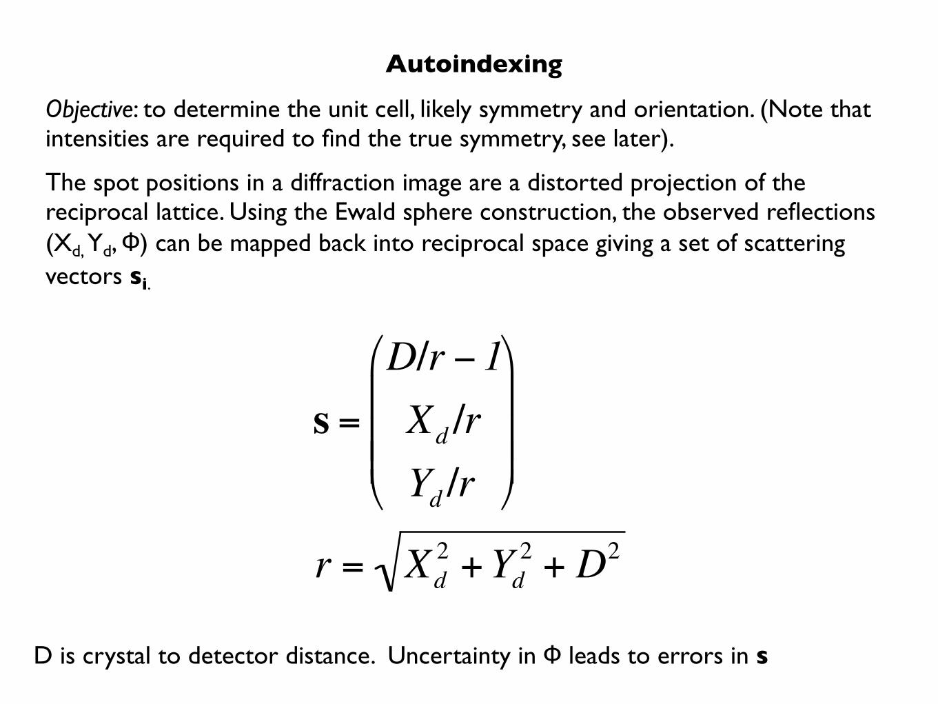
Autoindexing

Objective: to determine the unit cell, likely symmetry and orientation. (Note that intensities are required to find the true symmetry, see later).

The spot positions in a diffraction image are a distorted projection of the reciprocal lattice. Using the Ewald sphere construction, the observed reflections (Xd, Yd, Φ) can be mapped back into reciprocal space giving a set of scattering vectors si.

€

s =

D/r − 1Xd /rYd /r

r = Xd2 +Yd

2 + D2

D is crystal to detector distance. Uncertainty in Φ leads to errors in s

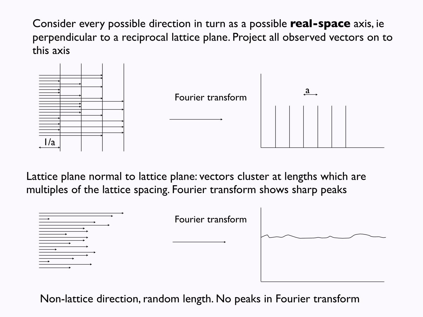
Lattice plane normal to lattice plane: vectors cluster at lengths which are multiples of the lattice spacing. Fourier transform shows sharp peaks

Consider every possible direction in turn as a possible real-space axis, ie perpendicular to a reciprocal lattice plane. Project all observed vectors on to this axis

Fourier transform

1/a

a

Non-lattice direction, random length. No peaks in Fourier transform

Fourier transform

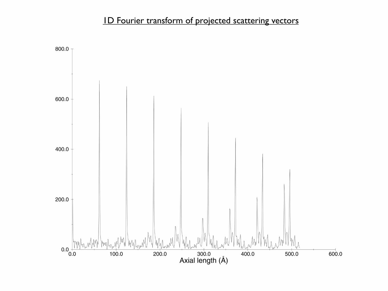
1D Fourier transform of projected scattering vectors

In the 2D example shown, the black cell corresponds to the reduced cell, while the red or blue cells may have been found in the autoindexing.

Pick three non-coplanar directions which have the largest peaks in the Fourier transforms to define a lattice.

This is not necessarily the simplest lattice (the “reduced cell”)

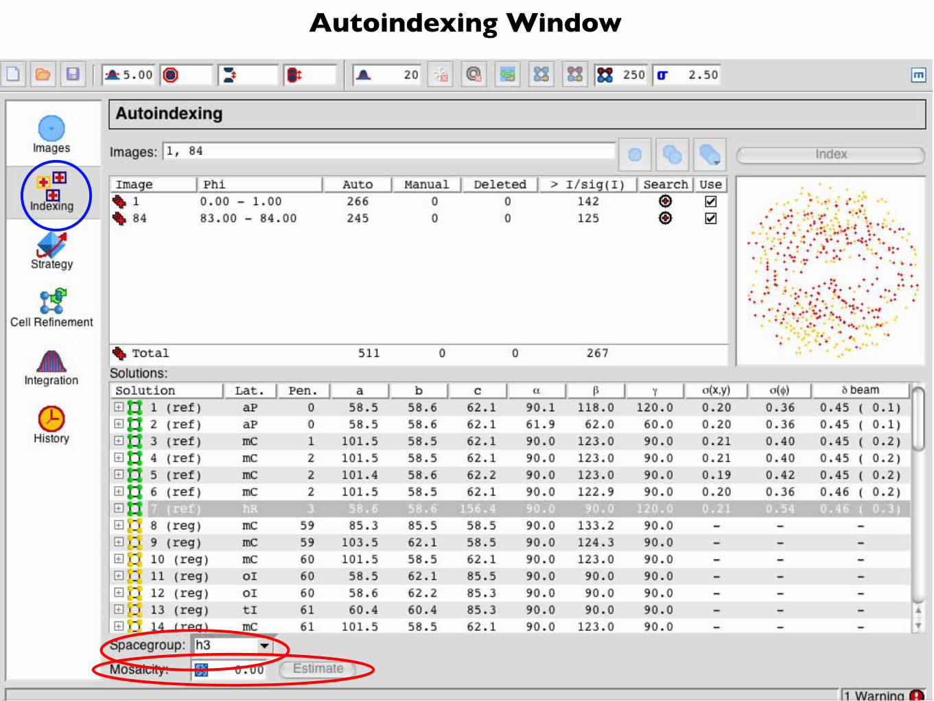
Autoindexing Window

A “penalty” is associated with each solution, which reflects how well the determined cell obeys the constraints for that lattice type.

• If nothing is known about the crystal, choose an initial solution in the following way:– correct solutions usually have penalties < ~20, often < 10 and

rarely > 30: also the errors (σ[x,y] & σ[φ] should be small)– note where there is a sharp drop in the penalty in this case

below solution 8. – pick the solution with the highest symmetry with a penalty

lower than the sharp drop, in this case, solution 7.

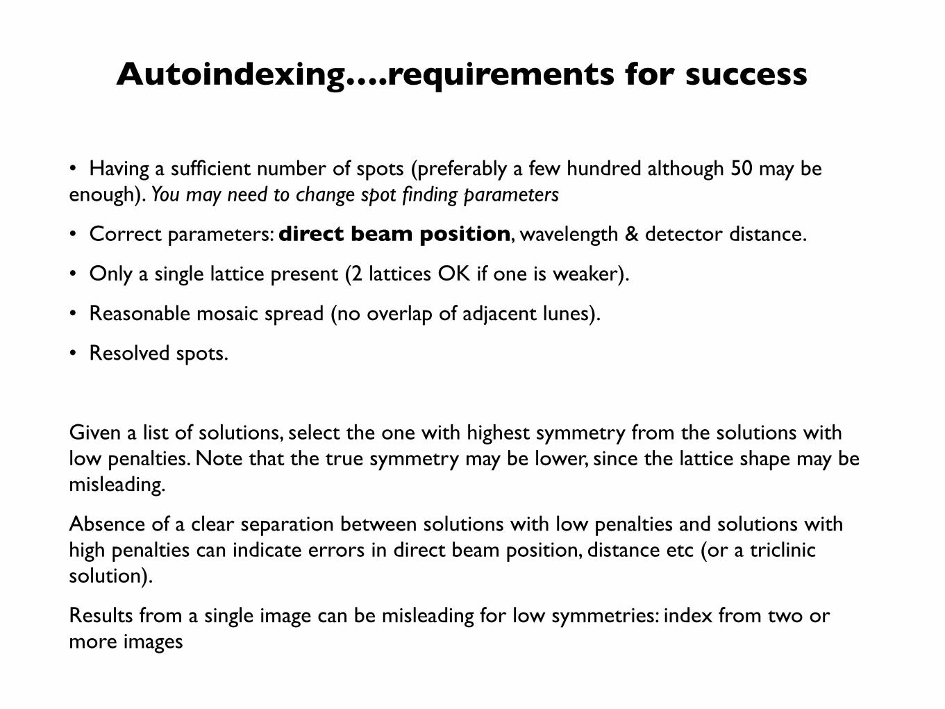
• Having a sufficient number of spots (preferably a few hundred although 50 may be enough). You may need to change spot finding parameters

• Correct parameters: direct beam position, wavelength & detector distance.

• Only a single lattice present (2 lattices OK if one is weaker).

• Reasonable mosaic spread (no overlap of adjacent lunes).

• Resolved spots.

Given a list of solutions, select the one with highest symmetry from the solutions with low penalties. Note that the true symmetry may be lower, since the lattice shape may be misleading.

Absence of a clear separation between solutions with low penalties and solutions with high penalties can indicate errors in direct beam position, distance etc (or a triclinic solution).

Results from a single image can be misleading for low symmetries: index from two or more images

Autoindexing….requirements for success

How do we know that the indexing is correct?

Check by predicting the pattern on several images at different φ angles

The pattern should match reasonably well

The prediction should explain all spots:

unpredicted spots may indicate

• incorrect mosaicity

• multiple lattices (split crystal)

• superlattice (pseudo-symmetry)

Note that the list of solutions given by Mosflm are in fact all the same solution, with different lattice symmetries imposed, so that if the triclinic solution (number 1) is wrong, then all the others are too

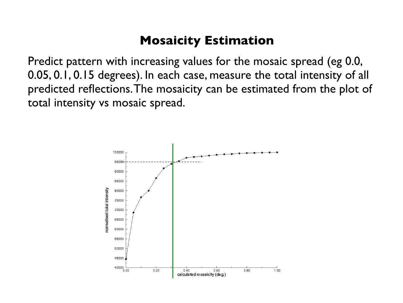
Mosaicity Estimation

Predict pattern with increasing values for the mosaic spread (eg 0.0, 0.05, 0.1, 0.15 degrees). In each case, measure the total intensity of all predicted reflections. The mosaicity can be estimated from the plot of total intensity vs mosaic spread.

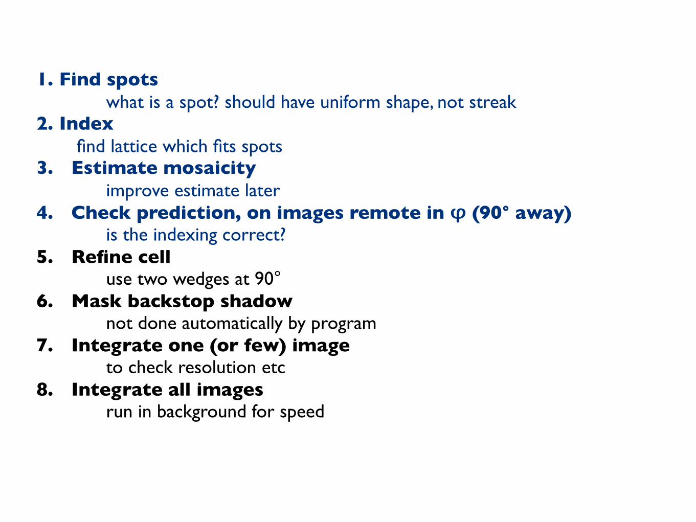
1. Find spotswhat is a spot? should have uniform shape, not streak

2. Index find lattice which fits spots

3. Estimate mosaicity improve estimate later

4. Check prediction, on images remote in φ (90° away) is the indexing correct?

5. Refine cell use two wedges at 90°

6. Mask backstop shadow not done automatically by program

7. Integrate one (or few) image to check resolution etc

8. Integrate all images run in background for speed

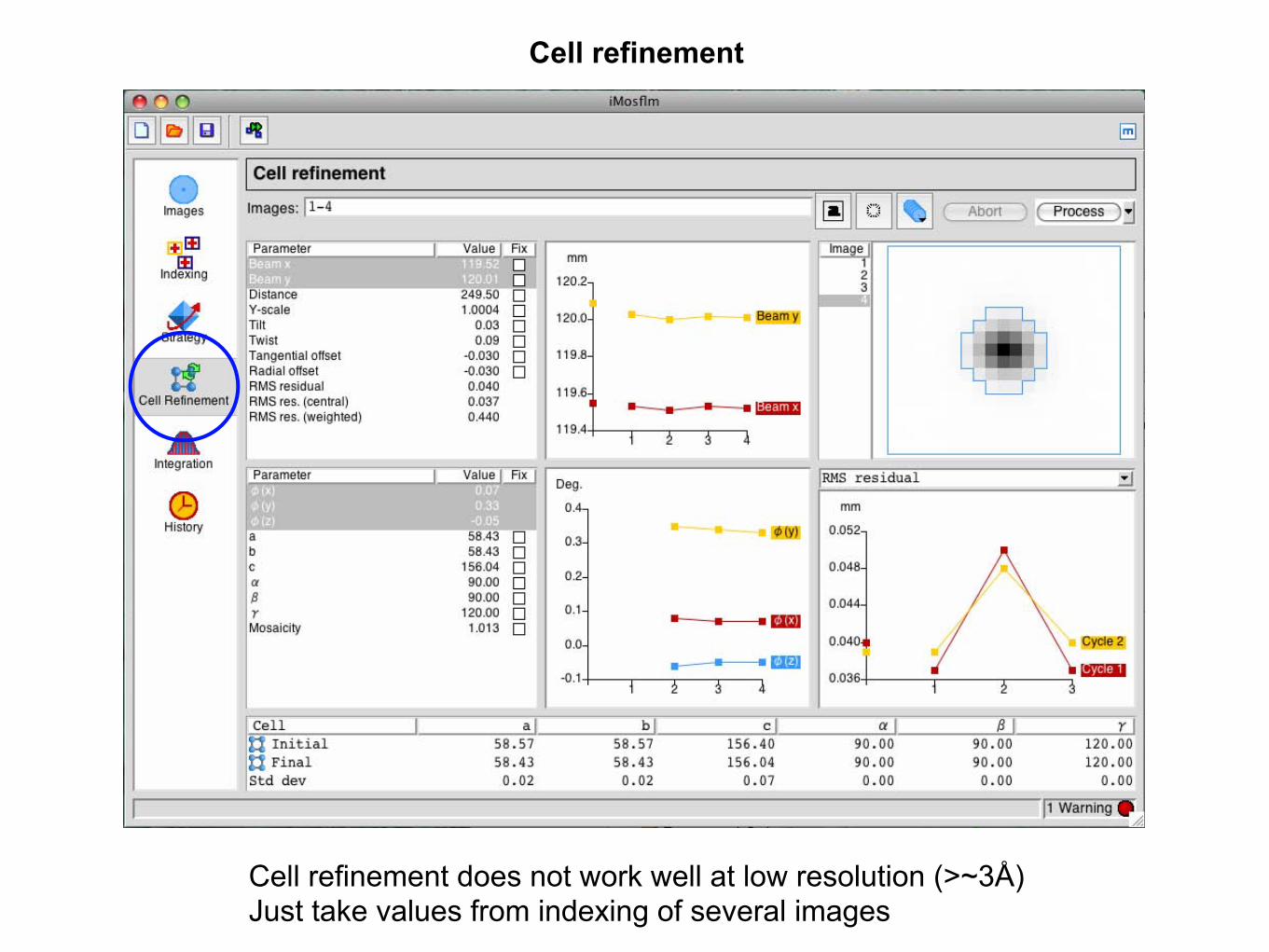
Cell refinement

Cell refinement does not work well at low resolution (>~3Å)Just take values from indexing of several images

Generally, once an orientation matrix and cell parameters have been derived from the autoindexing procedures described, these parameters are refined further using different algorithms.

Parameters to be refined:

1) Crystal parameters: Cell dimensions, orientation, mosaic spread.

2) Detector parameters: Detector position, orientation and (if appropriate) distortion parameters.

3) Beam parameters (possibly): Orientation, beam divergence.

Parameter Refinement

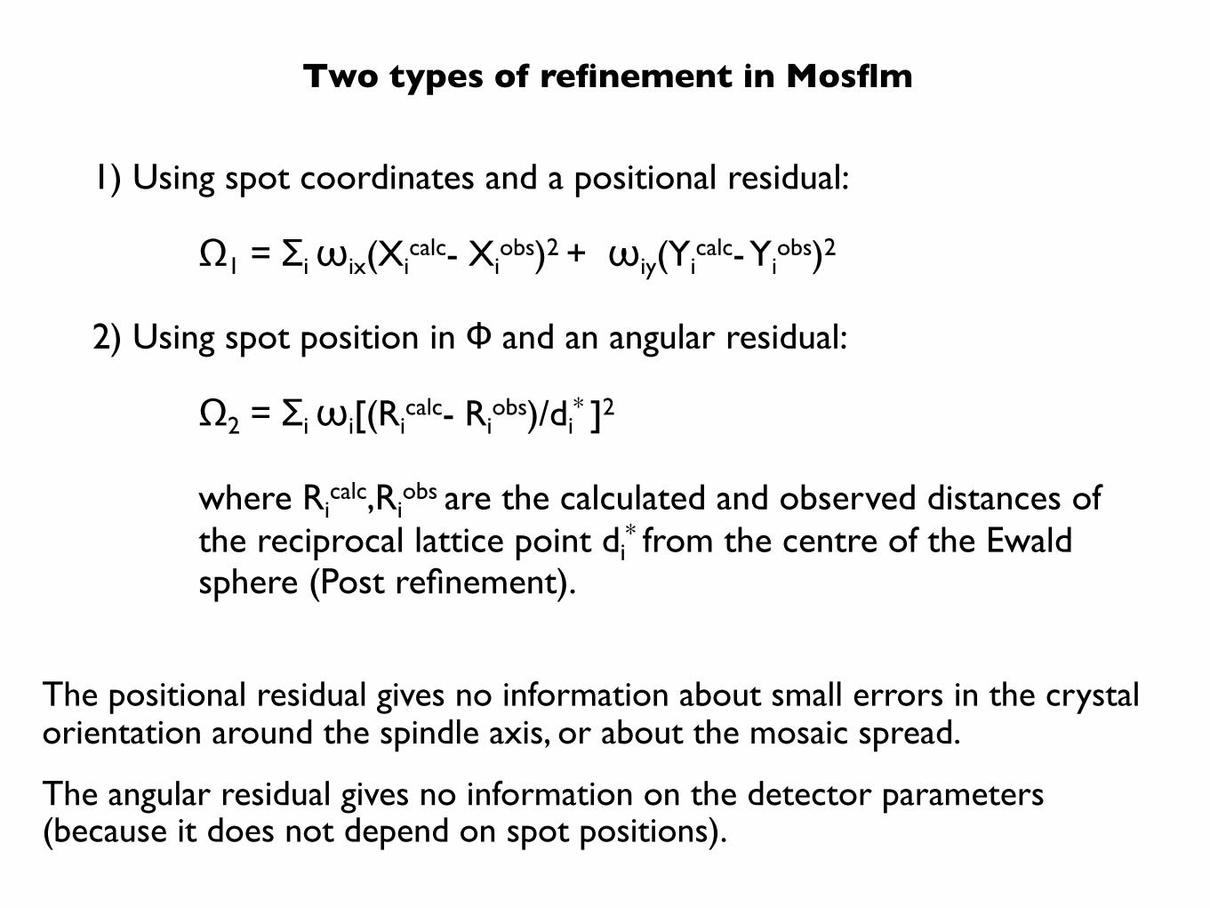
The positional residual gives no information about small errors in the crystal orientation around the spindle axis, or about the mosaic spread.

The angular residual gives no information on the detector parameters (because it does not depend on spot positions).

Two types of refinement in Mosflm

1) Using spot coordinates and a positional residual:

Ω1 = Σi ωix(Xicalc- Xi

obs)2 + ωiy(Yicalc- Yi

obs)2

2) Using spot position in Φ and an angular residual:

Ω2 = Σi ωi[(Ricalc- Ri

obs)/di* ]2

where Ricalc,Ri

obs are the calculated and observed distances of the reciprocal lattice point di

* from the centre of the Ewald sphere (Post refinement).

A fully-recorded spot is entirely recorded on one image

Partials are recorded on two or more images

“Fine-sliced” data has spots sampled in 3-dimensions

illustrations from Elspeth Garman

Fully recorded and partially recorded reflections

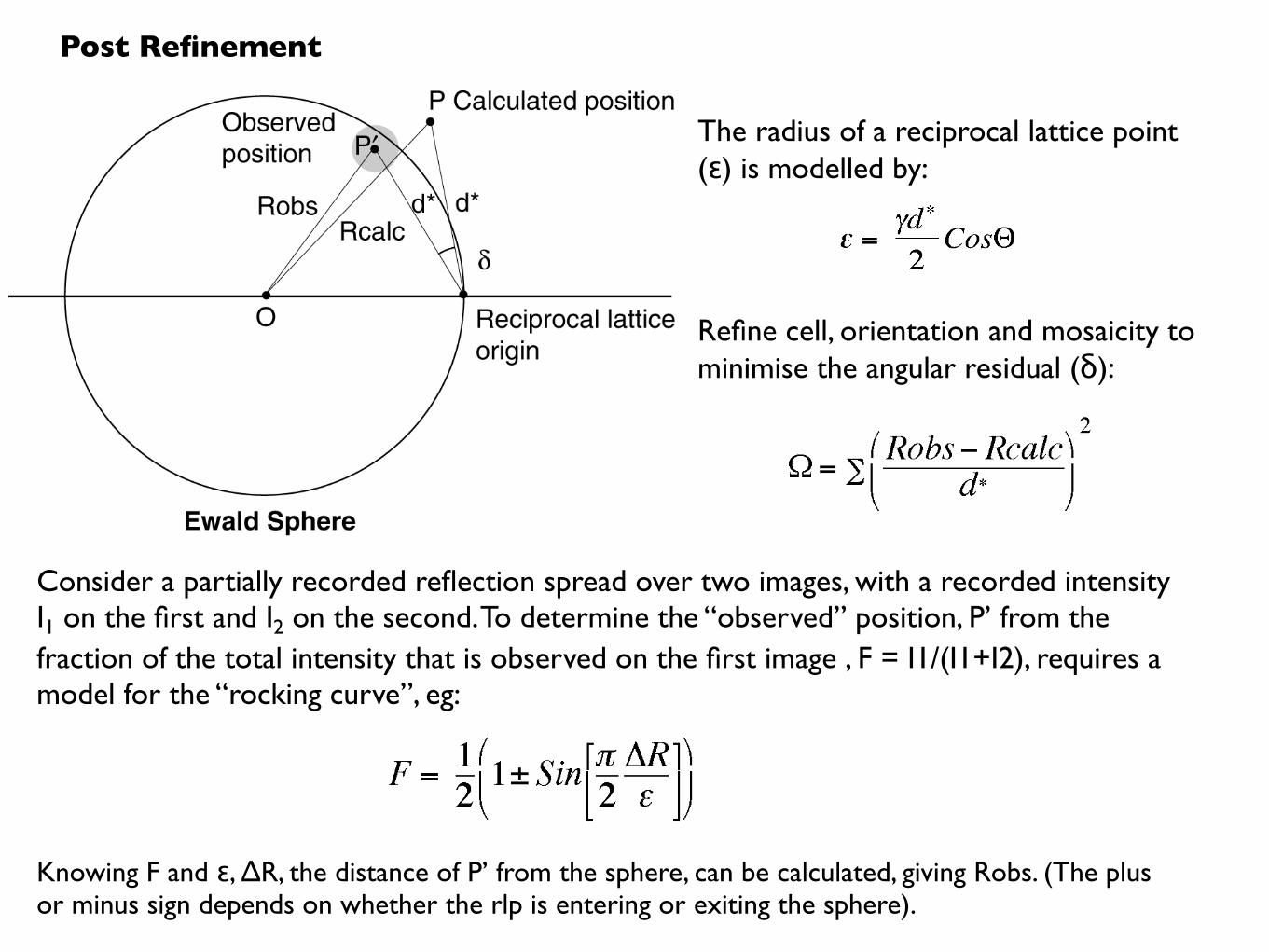
The radius of a reciprocal lattice point (ε) is modelled by:

Consider a partially recorded reflection spread over two images, with a recorded intensity I1 on the first and I2 on the second. To determine the “observed” position, P’ from the fraction of the total intensity that is observed on the first image , F = I1/(I1+I2), requires a model for the “rocking curve”, eg:

Knowing F and ε, ΔR, the distance of P’ from the sphere, can be calculated, giving Robs. (The plus or minus sign depends on whether the rlp is entering or exiting the sphere).

Post Refinement

Refine cell, orientation and mosaicity to minimise the angular residual (δ):

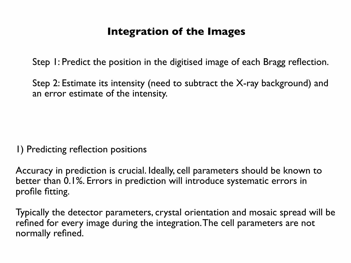
Step 1: Predict the position in the digitised image of each Bragg reflection.

Step 2: Estimate its intensity (need to subtract the X-ray background) and an error estimate of the intensity.

Integration of the Images

1) Predicting reflection positions

Accuracy in prediction is crucial. Ideally, cell parameters should be known to better than 0.1%. Errors in prediction will introduce systematic errors in profile fitting.

Typically the detector parameters, crystal orientation and mosaic spread will be refined for every image during the integration. The cell parameters are not normally refined.

shift/click

Run pointless & scala with default options

Integration window

Summation integration:Sum the pixel values of all pixels in the peak area of the mask, and then subtract the sum of the background values calculated from the background plane for the same pixels.

Profile fitting:Assume that the shape or profile (in 2 or 3 dimensions) of the spots is known. Then determine the scale factor which, when applied to the known spot profile, gives the best fit to be observed spot profile. This scale factor is then proportional to the profile fitted intensity for the reflection. Minimise: R = Σ ωi (Xi - KPi)2

Xi is the background subtracted intensity at pixel iPi is the value of the standard profile at the corresponding pixelωi is a weight, derived from the expected variance of Xi

K is the scale factor to be determined

Summation integration and Profile Fitting

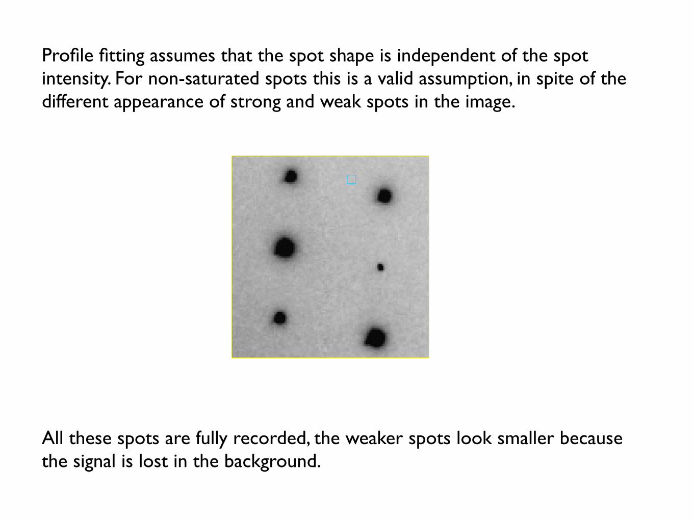
Profile fitting assumes that the spot shape is independent of the spot intensity. For non-saturated spots this is a valid assumption, in spite of the different appearance of strong and weak spots in the image.

All these spots are fully recorded, the weaker spots look smaller because the signal is lost in the background.

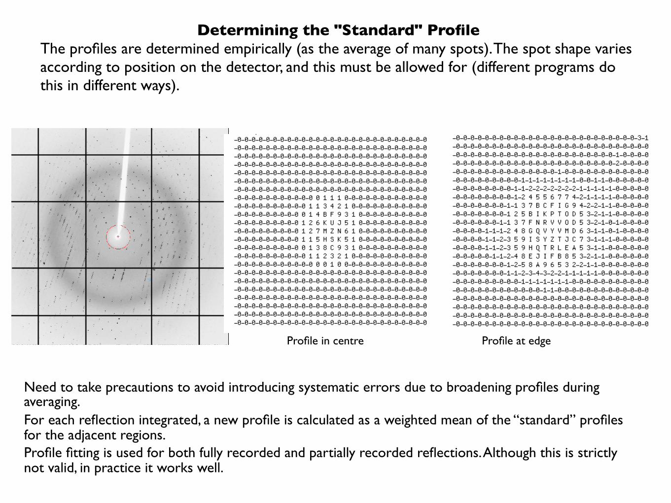
Determining the "Standard" ProfileThe profiles are determined empirically (as the average of many spots). The spot shape varies according to position on the detector, and this must be allowed for (different programs do this in different ways).

Need to take precautions to avoid introducing systematic errors due to broadening profiles during averaging.For each reflection integrated, a new profile is calculated as a weighted mean of the “standard” profiles for the adjacent regions.Profile fitting is used for both fully recorded and partially recorded reflections. Although this is strictly not valid, in practice it works well.

Profile in centre Profile at edge

Standard Deviation Estimates

For summation integration or profile fitted partially recorded reflections, a standard deviation can be obtained based on Poisson statistics.

For profile fitted intensities the goodness of fit of the scaled standard profile to the true reflection profile can be used for fully recorded reflections.

These will generally underestimate the true errors, and should be modified accordingly at the merging step (see later) so that they reflect the actual differences between multiple (symmetry-related) measurements. It is important to get realistic estimates of the errors in the intensities.

1) Autoindexing, preferably using two orthogonal images, will give the crystal cell parameters, orientation and a suggestion of the lattice symmetry. Using this information an initial estimate of the mosaicity can be obtained.

2) Post refinement requires the integration of a series of images, and uses the observed distribution of intensity of partially recorded reflections over those images to refine the unit cell and mosaic spread. Best carried out prior to integration of the data set.

3) During integration of the entire data set, the cell parameters are normally fixed, but the detector parameters, crystal orientation and mosaic spread are refined to ensure the best prediction of spot positions.

4) Intensities are estimated by both summation integration and profile fitting, but generally the profile fitted values are used for structure solution.

Summary of the steps in data integration

Label will probably change

Strategy window

Data collection strategy

• Total rotation range

Ideally 180° (or 360° in P1 to get full anomalous data)

Use programs (eg Mosflm) to give you the smallest required range (eg 90° for orthorhombic, or 2 x 30°) and the start point.

• Rotation/image: not necessarily 1°!

good values are often in range 0.25° - 0.5°, minimize overlap and background

• Time/image depends on total time available

• Detector position: further away to reduce background and improve spot resolution

Compromise between statistics (enough photons/reflection, and multiplicity) and radiation damage. Radiation damage is the big problem.

Radiation damage controls the total time available for crystal exposure.

Two Cases:

Anomalous scattering, MAD

High redundancy is better than long exposures (eliminates outliers)

Split time between all wavelengths, be cautious about radiation damage, reduce time & thus resolution if necessary

Collect Bijvoet pairs close(ish) together in time: align along dyad or collect inverse-beam images

Recollect first part of data at end to assess radiation damage

Data for refinement

Maximise resolution: longer exposure time (but still beware of radiation damage)

High multiplicity less important, but still useful

Use two (or more) passes with different exposure times (ratio ~10) if necessary to extend range of intensities (high & low resolution)

Short wavelength (<1Å) to minimise absorption

Collect symmetry mates at different times and in different geometries, to get best average (even with higher Rmerge!). Rotate about different axes.

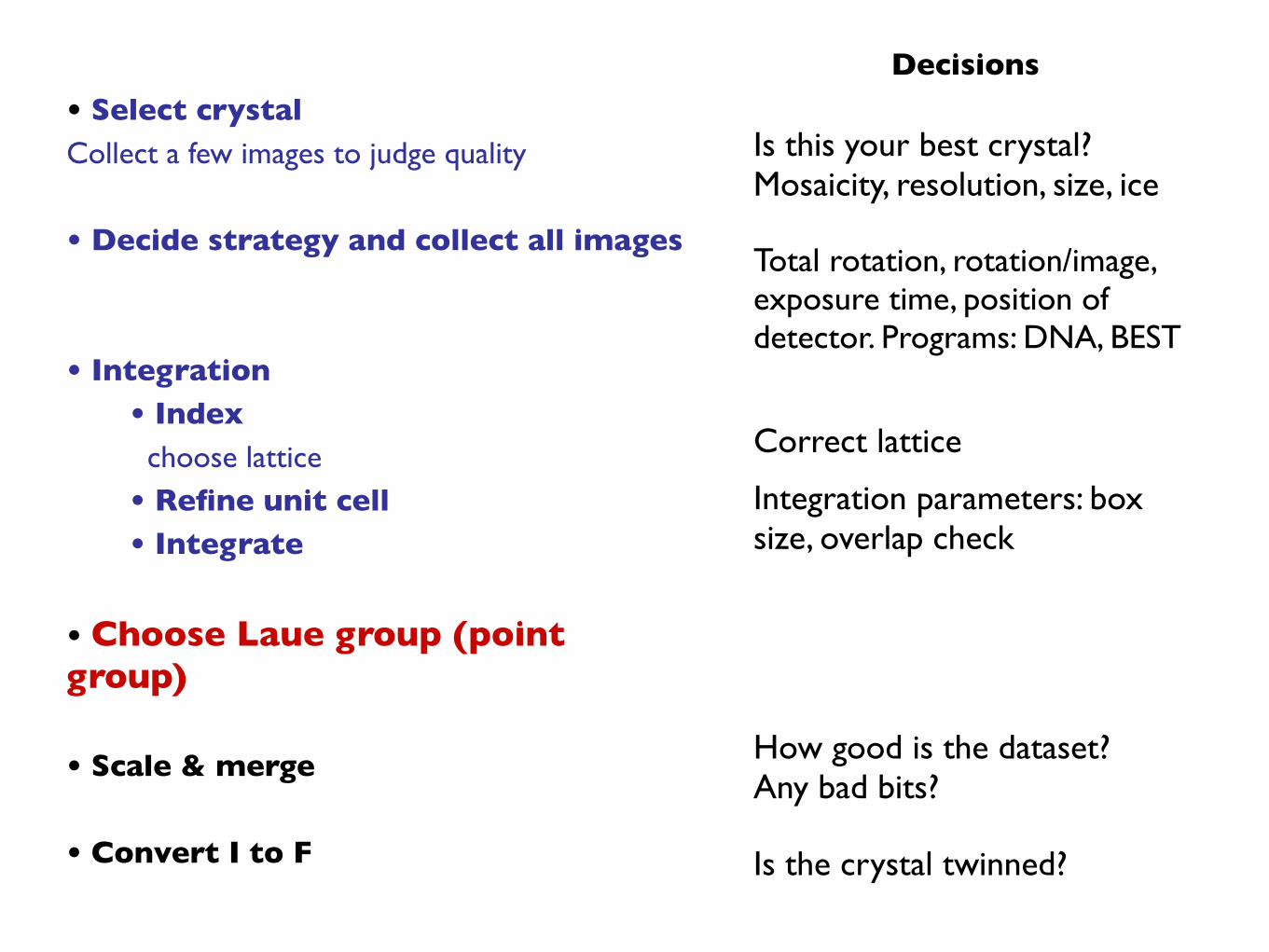
Decisions

• Select crystalCollect a few images to judge quality

• Decide strategy and collect all images

• Integration• Index choose lattice• Refine unit cell• Integrate

• Choose Laue group (point group)

• Scale & merge

• Convert I to F

Is this your best crystal? Mosaicity, resolution, size, ice

Total rotation, rotation/image, exposure time, position of detector. Programs: DNA, BEST

How good is the dataset? Any bad bits?

Is the crystal twinned?

Correct lattice

Integration parameters: box size, overlap check

Determination of Space group

The space group symmetry is only a hypothesis until the structure is solved, since it is hard to distinguish between true crystallographic and approximate (non-crystallographic) symmetry.

By examining the diffraction pattern we can get a good idea of the likely space group.

It is also useful to find the likely symmetry as early as possible, since this affects the data collection strategy.

Stages in space group determination

1. Lattice symmetry – crystal class The crystal class imposes restrictions on cell dimensions, and this information is needed for indexing & accurate image prediction

Cubic – a=b=c α=β=γ=90°Hexagonal/trigonal – a=b α=β=90°, γ=120°Tetragonal – a=b α=β=γ=90°Orthorhombic – α=β=γ=90°Monoclinic – α=γ=90°Triclinic – no restrictions

However, these restrictions may occur accidentally, or from pseudo-symmetry, so we need to score deviations between experimental cell dimensions and ideal values: for this we need estimates of the errors. Various penalty functions have been used.

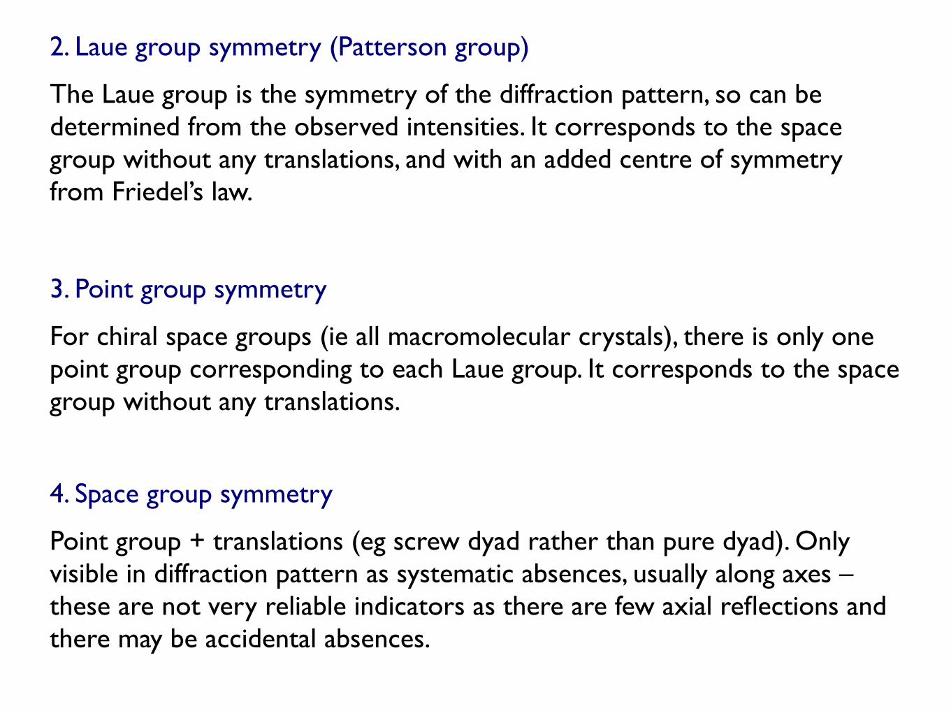
2. Laue group symmetry (Patterson group)

The Laue group is the symmetry of the diffraction pattern, so can be determined from the observed intensities. It corresponds to the space group without any translations, and with an added centre of symmetry from Friedel’s law.

3. Point group symmetry

For chiral space groups (ie all macromolecular crystals), there is only one point group corresponding to each Laue group. It corresponds to the space group without any translations.

4. Space group symmetry

Point group + translations (eg screw dyad rather than pure dyad). Only visible in diffraction pattern as systematic absences, usually along axes – these are not very reliable indicators as there are few axial reflections and there may be accidental absences.

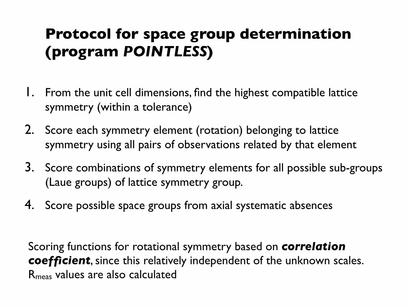
Protocol for space group determination (program POINTLESS)

1. From the unit cell dimensions, find the highest compatible lattice symmetry (within a tolerance)

2. Score each symmetry element (rotation) belonging to lattice symmetry using all pairs of observations related by that element

3. Score combinations of symmetry elements for all possible sub-groups (Laue groups) of lattice symmetry group.

4. Score possible space groups from axial systematic absences

Scoring functions for rotational symmetry based on correlation coefficient, since this relatively independent of the unknown scales. Rmeas values are also calculated

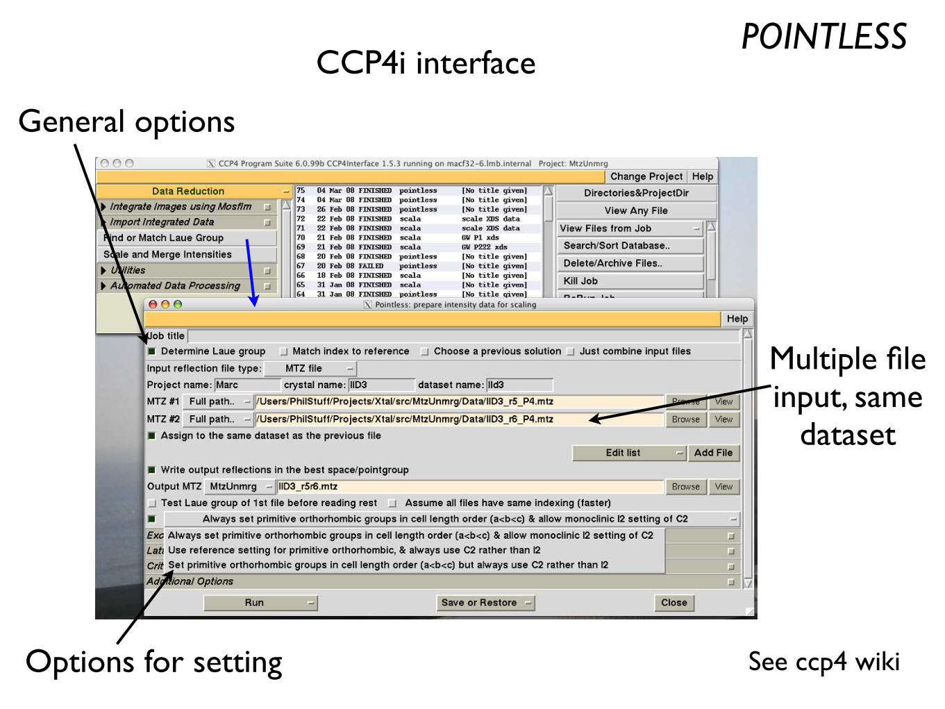
POINTLESSCCP4i interface

Multiple file input, same

dataset

Options for setting

General options

See ccp4 wiki

Example: a confusing case in C222:

Unit cell 74.72 129.22 184.25 90 90 90

This has b ≈ √3 a so can also be indexed on a hexagonal lattice, lattice point group P622 (P6/mmm), with the reindex operator:

h/2+k/2, h/2-k/2, -l

Conversely, a hexagonal lattice may be indexed as C222 in three distinct ways, so there is a 2 in 3 chance of the indexing program choosing the wrong one

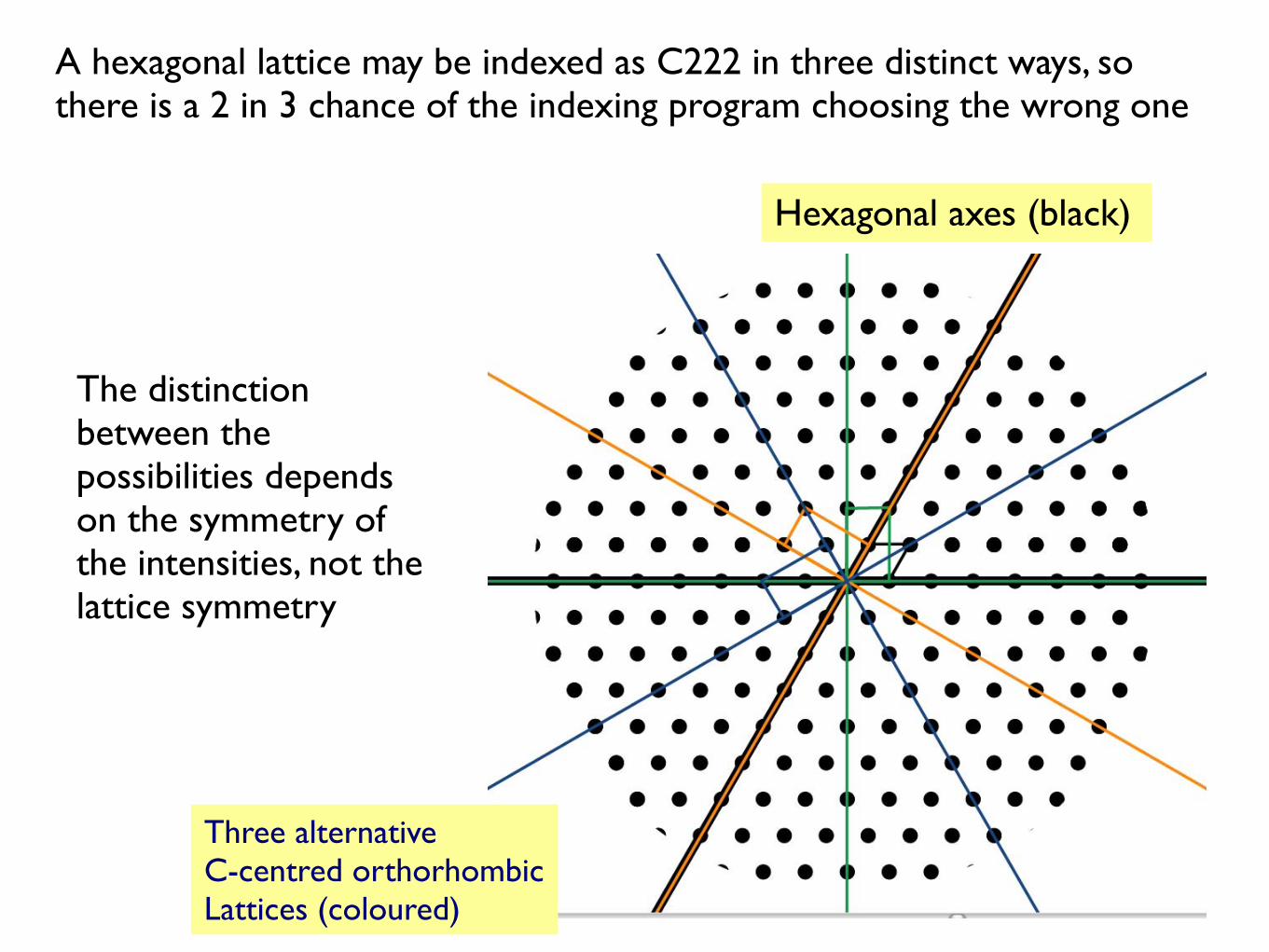
A hexagonal lattice may be indexed as C222 in three distinct ways, so there is a 2 in 3 chance of the indexing program choosing the wrong one

Hexagonal axes (black)

Three alternativeC-centred orthorhombicLattices (coloured)

The distinction between the possibilities depends on the symmetry of the intensities, not the lattice symmetry

Score each symmetry operator in P622

Only the orthorhombic symmetry operators are present

Correlation coefficient on E2 Rfactor (multiplicity weighted)

Nelmt Lklhd Z-cc CC N Rmeas Symmetry & operator (in Lattice Cell)

1 0.808 5.94 0.89 9313 0.115 identity 2 0.828 6.05 0.91 14088 0.141 *** 2-fold l ( 0 0 1) {-h,-k,+l} 3 0.000 0.06 0.01 16864 0.527 2-fold ( 1-1 0) {-k,-h,-l} 4 0.871 6.33 0.95 10418 0.100 *** 2-fold ( 2-1 0) {+h,-h-k,-l} 5 0.000 0.53 0.08 12639 0.559 2-fold h ( 1 0 0) {+h+k,-k,-l} 6 0.000 0.06 0.01 16015 0.562 2-fold ( 1 1 0) {+k,+h,-l} 7 0.870 6.32 0.95 2187 0.087 *** 2-fold k ( 0 1 0) {-h,+h+k,-l} 8 0.000 0.55 0.08 7552 0.540 2-fold (-1 2 0) {-h-k,+k,-l} 9 0.000 -0.12 -0.02 11978 0.598 3-fold l ( 0 0 1) {-h-k,+h,+l} {+k,-h-k,+l} 10 0.000 -0.06 -0.01 17036 0.582 6-fold l ( 0 0 1) {-k,+h+k,+l} {+h+k,-h,+l}

Z-score(CC)“Likelihood”

A clear preference for Laue group Cmmm

Net Z(CC) Likelihood

Correlation coefficient & R-factor

Cell deviation

Net Z(CC) scores are Z+(symmetry in group) - Z-(symmetry not in group)

Likelihood allows for the possibility of pseudo-symmetry

Laue Group Lklhd NetZc Zc+ Zc- CC CC- Rmeas R- Delta ReindexOperator

> 1 C m m m *** 0.991 6.00 6.12 0.12 0.93 0.02 0.12 0.56 0.1 [1/2h-1/2k,3/2h+1/2k,l]> 2 C 1 2/m 1 0.367 5.00 6.13 1.13 0.95 0.17 0.10 0.48 0.1 [3/2h+1/2k,-1/2h+1/2k,l]> 3 C 1 2/m 1 0.365 4.55 6.04 1.49 0.95 0.22 0.09 0.46 0.1 [1/2h-1/2k,3/2h+1/2k,l]> 4 P 1 2/m 1 0.250 4.88 5.99 1.11 0.91 0.17 0.14 0.49 0.0 [1/2h+1/2k,l,1/2h-1/2k] 5 P -1 0.031 4.27 5.94 1.67 0.89 0.25 0.12 0.44 0.0 [-1/2h+1/2k,-1/2h-1/2k,l] 6 C 1 2/m 1 0.000 2.45 4.18 1.73 0.08 0.26 0.54 0.44 0.1 [3/2h-1/2k,1/2h+1/2k,l] 7 C 1 2/m 1 0.000 1.62 3.40 1.79 0.08 0.27 0.56 0.43 0.1 [-1/2h-1/2k,3/2h-1/2k,l] 8 C 1 2/m 1 0.000 0.60 2.55 1.95 0.01 0.29 0.56 0.42 0.0 [-k,h,l] 9 C 1 2/m 1 0.000 0.57 2.52 1.96 0.01 0.29 0.53 0.43 0.0 [h,k,l] 10 P -3 0.000 0.75 2.68 1.93 -0.02 0.29 0.60 0.42 0.1 [1/2h-1/2k,1/2h+1/2k,l] 11 C m m m 0.000 2.60 3.80 1.20 0.44 0.18 0.38 0.47 0.1 [-1/2h-1/2k,3/2h-1/2k,l]=12 C m m m 0.000 0.94 2.59 1.65 0.26 0.25 0.42 0.46 0.0 [h,k,l] 13 P 6/m 0.000 0.83 2.54 1.70 0.24 0.26 0.45 0.44 0.1 [1/2h-1/2k,1/2h+1/2k,l] 14 P -3 m 1 0.000 0.72 2.46 1.74 0.24 0.26 0.45 0.44 0.1 [1/2h-1/2k,1/2h+1/2k,l] 15 P -3 1 m 0.000 -0.57 1.79 2.36 0.10 0.35 0.52 0.39 0.1 [1/2h-1/2k,1/2h+1/2k,l] 16 P 6/m m m 0.000 2.09 2.09 0.00 0.25 0.00 0.44 0.00 0.1 [1/2h-1/2k,1/2h+1/2k,l]

Reindexing

Systematic absences

For a Pq axis along say c (index l), axial reflections are only present if l = (p/q)n where n is an integer

eg 21 2n 2,4,6,…

31 3n 3,6,9,…

41,43 4n 4,8,12,… 42 2n 2,4,6,…

61, 65 6n 6,12,18,… 62, 64 3n 3,6,9,… 63 2n 2,4,6,…

BUT we may only have observed a few of the axial reflections, so be careful …

Zone Number PeakHeight SD Probability ReflectionCondition

1 screw axis 2(1) [c] 109 0.878 0.083 0.747 00l: l=2n

Spacegroup TotProb SysAbsProb Reindex Conditions

<C 2 2 21> ( 20) 1.063 0.747 00l: l=2n (zones 1) .......... <C 2 2 2> ( 21) 0.360 0.253

Screw axis along 00l shows space group is C2221

PeakHeight from Fourier analysis1.0 is perfect screw “Probability” of screw

Screws detected by Fourier analysis of I/σ

Alternative indexing

If the true point group is lower symmetry than the lattice group, alternative valid but non-equivalent indexing schemes are possible, related by symmetry operators present in lattice group but not in point group (these are also the cases where merohedral twinning is possible)

eg if in space group P3 there are 4 different schemes (h,k,l) or (-h,-k,l) or (k,h,-l) or (-k,-h,-l)

For the first crystal, you can choose any scheme

For subsequent crystals, the autoindexing will randomly choose one setting, and we need to make it consistent: POINTLESS will do this for you by comparing the unmerged test data to a merged reference dataset

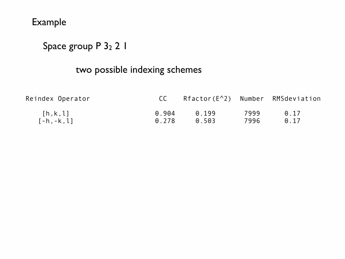
Reindex Operator CC Rfactor(E^2) Number RMSdeviation

[h,k,l] 0.904 0.199 7999 0.17 [-h,-k,l] 0.278 0.503 7996 0.17

Example

Space group P 32 2 1

two possible indexing schemes

POINTLESS

Consistent indexing to reference file (merged or unmerged)

Example in space group H3 (R3 hexagonal setting)

Scaling and Data Quality

|F|2 I

Experiment

|F|2I

lots of effects (“errors”)

Model of experiment

Parameterise experiment

Our job is to invert the experiment

Scaling and Merging

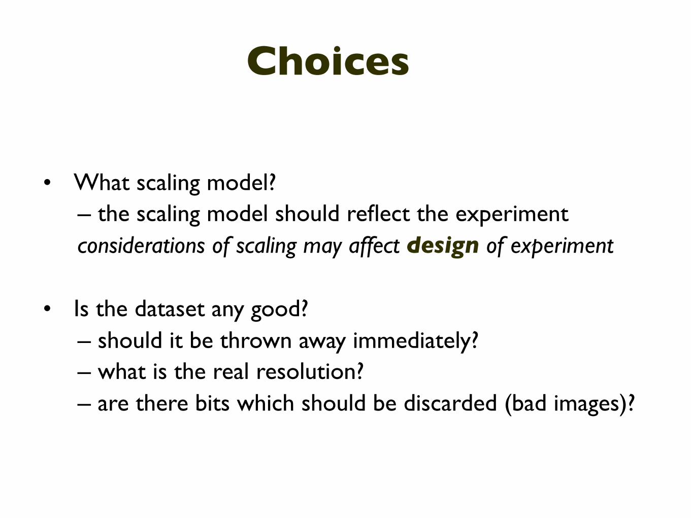
Choices

• What scaling model?– the scaling model should reflect the experimentconsiderations of scaling may affect design of experiment

• Is the dataset any good?– should it be thrown away immediately?– what is the real resolution?– are there bits which should be discarded (bad images)?

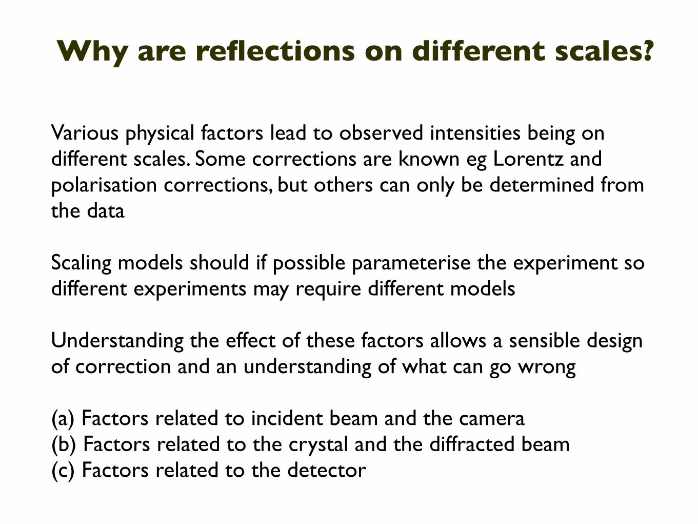
Why are reflections on different scales?

Various physical factors lead to observed intensities being on different scales. Some corrections are known eg Lorentz and polarisation corrections, but others can only be determined from the data

Scaling models should if possible parameterise the experiment so different experiments may require different models

Understanding the effect of these factors allows a sensible design of correction and an understanding of what can go wrong

(a) Factors related to incident beam and the camera(b) Factors related to the crystal and the diffracted beam(c) Factors related to the detector

Factors related to incident Xray beam

(a) incident beam intensity: variable on synchrotrons and not normally measured. Assumed to be constant during a single image, or at least varying smoothly and slowly (relative to exposure time). If this is not true, the data will be poor

(b) illuminated volume: changes with φ if beam smaller than crystal

(c) absorption in primary beam by crystal: indistinguishable from (b)

(d) variations in rotation speed and shutter synchronisation. These errors are disastrous, difficult to detect, and (almost) impossible to correct for: we assume that the crystal rotation rate is constant and that adjacent images exactly abut in φ. Shutter synchronisation errors lead to partial bias which may be positive, unlike the usual negative bias

Factors related to crystal and diffracted beam

(e) Absorption in secondary beam - serious at long wavelength (including CuKα), worth correcting for MAD data

(f) radiation damage - serious on high brilliance sources. Not easily correctable unless small as the structure is changing

Maybe extrapolate back to zero time?

The relative B-factor is largely a correction for radiation damage

Factors related to the detector

• The detector should be properly calibrated for spatial distortion and sensitivity of response, and should be stable. Problems with this are difficult to detect from diffraction data.

• The useful area of the detector should be calibrated or told to the integration program

– Calibration should flag defective pixels and dead regions eg between tiles

– The user should tell the integration program about shadows from the beamstop, beamstop support or cryocooler (define bad areas by circles, rectangles, arcs etc)

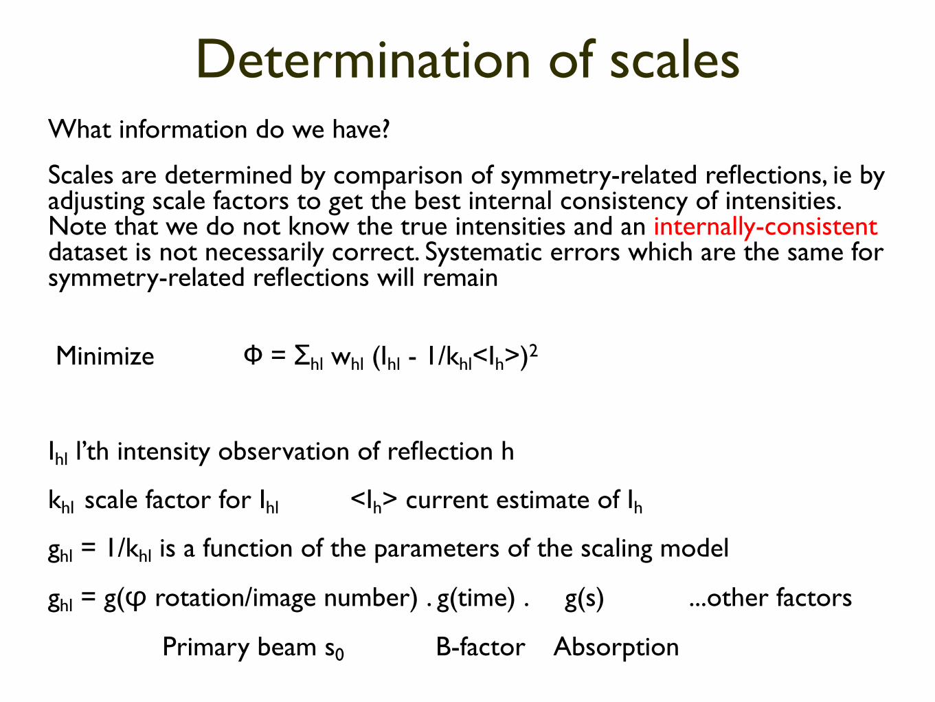
Determination of scalesWhat information do we have?

Scales are determined by comparison of symmetry-related reflections, ie by adjusting scale factors to get the best internal consistency of intensities. Note that we do not know the true intensities and an internally-consistent dataset is not necessarily correct. Systematic errors which are the same for symmetry-related reflections will remain

Minimize Φ = Σhl whl (Ihl - 1/khl<Ih>)2

Ihl l’th intensity observation of reflection h

khl scale factor for Ihl <Ih> current estimate of Ih

ghl = 1/khl is a function of the parameters of the scaling model

ghl = g(φ rotation/image number) . g(time) . g(s) ...other factors

Primary beam s0 B-factor Absorption

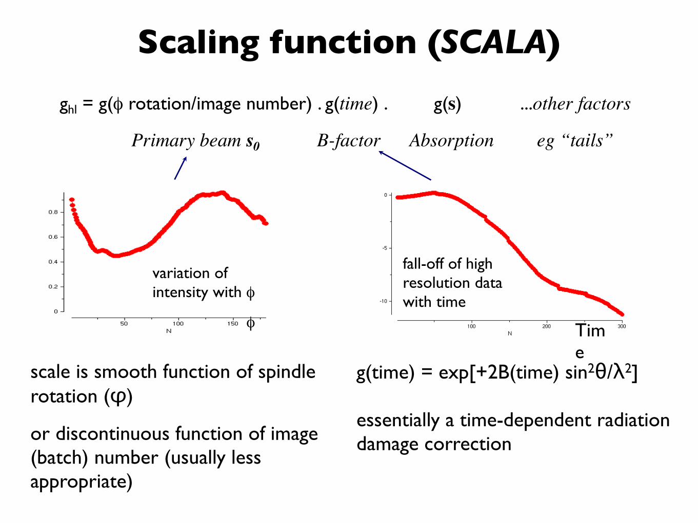
ghl = g(φ rotation/image number) . g(time) . g(s) ...other factors

Primary beam s0 B-factor Absorption eg “tails”

Scaling function (SCALA)

scale is smooth function of spindle rotation (φ)

or discontinuous function of image (batch) number (usually less appropriate)

g(time) = exp[+2B(time) sin2θ/λ2]

essentially a time-dependent radiation damage correction

Time

fall-off of high resolution data with time

variation of intensity with φ

φ

Sample dataset: Rotating anode (RU200, Osmic mirrors, Mar345) Cu Kα (1.54Å)100 images, 1°, 5min/°, resolution 1.8Å

Rmerge

No AbsCorr

AbsCorr

No AbsCorr

AbsCorr<I>/sd

Correction improves the data

corrected

uncorrected

Phasing power

expressed as sum of spherical harmonics g(θ,φ) = ΣlΣm Clm Ylm(θ,φ)

Secondary beam correction (absorption)

scale as function of secondary beam direction (θ,φ)

This depends on the strategy of data collection, thus affects the strategy

Note that determination of scaling parameters depends on symmetry-related observations having different scales. If all observations of a reflection have the same value of the scale component, then there is no information about that component and it remain as a systematic error in the merged data (this may well be the case for absorption for instance)

Thus to get intensities with the lowest absolute error, the symmetry-related observations should be measured in as different way as possible (eg rotation about multiple axes). This will increase Rmerge, but improve the estimate of <I>.

Conversely, to measure the most accurate differences for phasing (anomalous or dispersive), observations should be measured in as similar way as possible

How well are the scales determined?

For multiple-wavelength datasets, it is best to scale all wavelengths together simultaneously. This is then a local scaling to minimise the difference between datasets, reducing the systematic error in the anomalous and dispersive differences which are used for phasing

Other advantages of simultaneous scaling:-

• rejection of outliers with much higher reliability because of higher multiplicity (but with the danger of eliminating real signal)

• correlations between ΔFanom and ΔFdisp indicate the reliability of the phasing signal

• (very) approximate determination of relative f" and relative Δf' values

Scaling datasets together

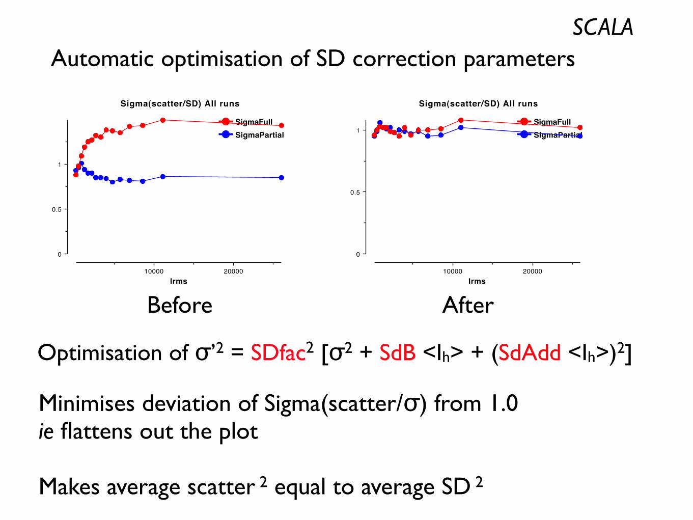
SCALAAutomatic optimisation of SD correction parameters

SigmaFullSigmaPartial

Sigma(scatter/SD) All runs

Irms10000 20000

0

0.5

1

SigmaFullSigmaPartial

Sigma(scatter/SD) All runs

Irms10000 20000

0

0.5

1

Before After

Optimisation of σ’2 = SDfac2 [σ2 + SdB <Ih> + (SdAdd <Ih>)2]

Minimises deviation of Sigma(scatter/σ) from 1.0ie flattens out the plot

Makes average scatter 2 equal to average SD 2

• What is the overall quality of the dataset? How does it compare to other datasets for this project?

• What is the real resolution? Should you cut the high-resolution data?

• Are there bad batches (individual duff batches or ranges of batches)?

• Was the radiation damage such that you should exclude the later parts?

• Is the outlier detection working well?

• Is there any apparent anomalous signal?

Questions about the data

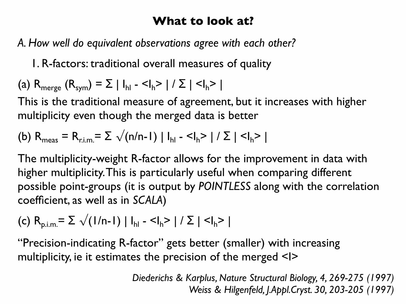
What to look at?

A. How well do equivalent observations agree with each other?

1. R-factors: traditional overall measures of quality

(a) Rmerge (Rsym) = Σ | Ihl - <Ih> | / Σ | <Ih> |

This is the traditional measure of agreement, but it increases with higher multiplicity even though the merged data is better

(b) Rmeas = Rr.i.m.= Σ √(n/n-1) | Ihl - <Ih> | / Σ | <Ih> |

The multiplicity-weight R-factor allows for the improvement in data with higher multiplicity. This is particularly useful when comparing different possible point-groups (it is output by POINTLESS along with the correlation coefficient, as well as in SCALA)

(c) Rp.i.m.= Σ √(1/n-1) | Ihl - <Ih> | / Σ | <Ih> |

“Precision-indicating R-factor” gets better (smaller) with increasing multiplicity, ie it estimates the precision of the merged <I>

Diederichs & Karplus, Nature Structural Biology, 4, 269-275 (1997) Weiss & Hilgenfeld, J.Appl.Cryst. 30, 203-205 (1997)

2. Intensities and standard deviations: what is the real resolution?

(a) Corrected σ’(Ihl)2 = SDfac2 [σ2 + SdB <Ih> + (SdAdd <Ih>)2]

The corrected σ’(I) is compared with the intensities: the most useful statistic is < <I>/ σ(<I>) > (labelled Mn(I)/sd in table) as a function of resolution

This statistic shows the improvement of the estimate of <I> with multiple measurements. It is the best indicator of the true resolution limit

< <I>/ σ(<I>) > greater than ~ 2 (or so)

Maybe lower for anisotropic data, 1.5 to 1.0

(b) Correlation between half datasets (random halves)

Resolution

Cor

rela

tion

coef

ficie

nt

Correlation of <I> indicating a resolution limit

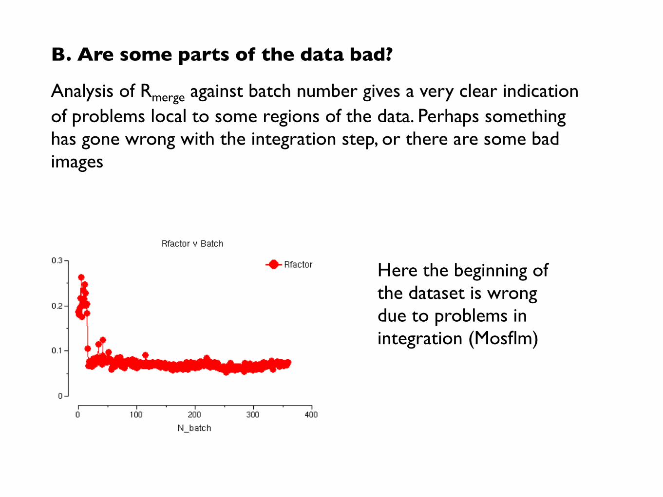
B. Are some parts of the data bad?

Analysis of Rmerge against batch number gives a very clear indication of problems local to some regions of the data. Perhaps something has gone wrong with the integration step, or there are some bad images

Here the beginning of the dataset is wrong due to problems in integration (Mosflm)

A case of severe radiation damage: B-factor should be small (not more than -10, and even that is large)

-10

Outliers

Detection of outliers is easiest if the multiplicity is high

Removal of spots behind the backstop shadow does not work well at present: usually it rejects all the good ones, so tell Mosflm where the backstop shadow is

Scala also has facilities for omitting regions of the detector (rectangles and arcs of circles)

Inspect the ROGUES file to see what is being rejected (at least occasionally)

The ROGUES file contains all rejected reflections (flag "*", "@" for I+- rejects, "#" for Emax rejects) TotFrc = total fraction, fulls (f) or partials (p) Flag I+ or I- for Bijvoet classes DelI/sd = (Ihl - Mn(I)others)/sqrt[sd(Ihl)**2 + sd(Mn(I))**2] h k l h k l Batch I sigI E TotFrc Flag Scale LP DelI/sd d(A) Xdet Ydet Phi (measured) (unique) -2 -2 0 2 2 0 1220 24941 2756 1.03 0.95p I- 2.434 0.031 -1.1 30.40 1263.7 1103.2 210.8 -4 2 0 2 2 0 1146 9400 2101 0.63 0.99p *I+ 3.017 0.032 -6.7 30.40 1266.4 1123.3 151.3 4 -2 0 2 2 0 1148 27521 2972 1.08 1.09p I- 2.882 0.032 0.0 30.40 1058.8 1130.0 153.2 2 -4 0 2 2 0 1075 29967 2865 1.13 0.92p I+ 2.706 0.032 1.1 30.40 1060.9 1106.6 94.4 Weighted mean 27407

Reasons for outliers

• outside reliable area of detector (eg behind shadow)

specify backstop shadow, calibrate detector

• ice spots

do not get ice on your crystal!

• zingers

• bad prediction (spot not there)

improve prediction

• spot overlap

lower mosaicity, smaller slice, move detector back

deconvolute overlaps

• multiple lattices

find single crystal

Ice rings

Rejects lie on ice rings (red)(ROGUEPLOT

in Scala)

Position of rejects on detector

Detection of anomalous signal

0

2

4

-2

-4

0 2 4-2-4(expected)

(obs

erve

d)

Peak

Edge Remote

Are the differences greater than would be expected from the errors?

Test using a Normal Probability Plot: a slope > 1.0 means a significant difference

Differences are largest at the peak wavelength

Are the different measurements of the anomalous difference correlated?

Correlation between wavelengths (MAD)

Resolution Resolution

Cor

rela

tion

coef

ficie

nt

Cor

rela

tion

coef

ficie

nt

Correlation between half datasets at peak wavelength

3.5Å 3.5Å

Correlation of <I> indicating resolution limit

This can be used to set the useful resolution for finding anomalous scatterers

Centric, no anomalous

Another way of looking at correlations: scatter plot of Δanom1 v. Δanom2

Correlated differences Uncorrelated native

Resolution3.5Å

Ratio of distribution width along to width across

diagonal ~= signal/noise

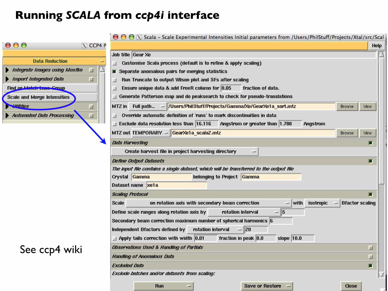
Running SCALA from ccp4i interface

See ccp4 wiki

Intensity distributions and their pathologies

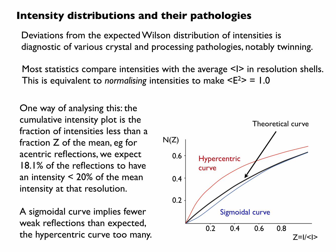
One way of analysing this: the cumulative intensity plot is the fraction of intensities less than a fraction Z of the mean, eg for acentric reflections, we expect 18.1% of the reflections to have an intensity < 20% of the mean intensity at that resolution.

A sigmoidal curve implies fewer weak reflections than expected, the hypercentric curve too many.

Deviations from the expected Wilson distribution of intensities is diagnostic of various crystal and processing pathologies, notably twinning.

0.4

0.2

0.6

0.40.2 0.6 0.8Z=I/<I>

N(Z)

Theoretical curve

Sigmoidal curve

Hypercentric curve

Most statistics compare intensities with the average <I> in resolution shells. This is equivalent to normalising intensities to make <E2> = 1.0

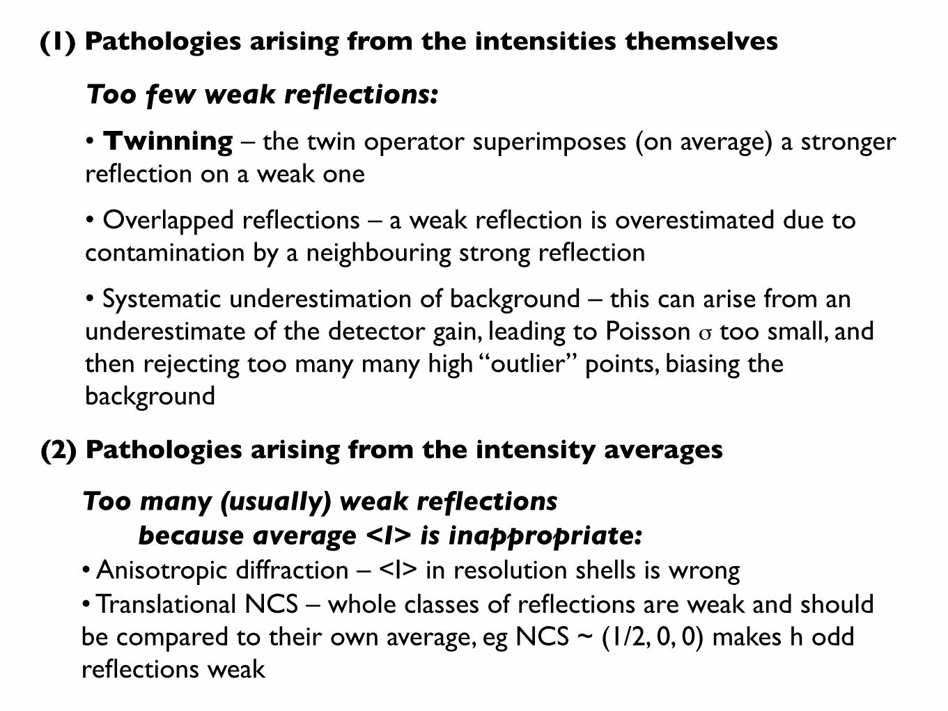
(1) Pathologies arising from the intensities themselves

(2) Pathologies arising from the intensity averages

Too few weak reflections:

• Twinning – the twin operator superimposes (on average) a stronger reflection on a weak one

• Overlapped reflections – a weak reflection is overestimated due to contamination by a neighbouring strong reflection

• Systematic underestimation of background – this can arise from an underestimate of the detector gain, leading to Poisson σ too small, and then rejecting too many many high “outlier” points, biasing the background

Too many (usually) weak reflections because average <I> is inappropriate:• Anisotropic diffraction – <I> in resolution shells is wrong• Translational NCS – whole classes of reflections are weak and should be compared to their own average, eg NCS ~ (1/2, 0, 0) makes h odd reflections weak

Example from Jan Löwe

apparent point group 422a=64.3Å, c=198.8Å, dimer/ASU,

35kDa, 2.0Å

Structure solved on untwinned crystal by MADMolecular replacement (difficult, large conformational change)Refined in CNS 1.1 with α=0.5, P41

422 has no possibility of twinning,must be lower point group (4).

Merohedral twinning (exact overlap of lattices) is possible if the true point group is lower symmetry than the lattice point group.

Intensity statistics show too few weak reflections (and too few strong ones)

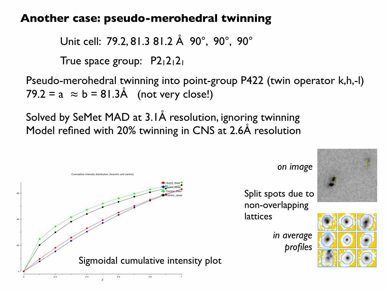
Another case: pseudo-merohedral twinning

Acent_theor

Acent_obser

Centric_theor

Centric_obser

Cumulative intensity distribution (Acentric and centric)

Z

0 0.2 0.4 0.6 0.8 1

0

20

40

60

Unit cell: 79.2, 81.3 81.2 Å 90°, 90°, 90°

True space group: P212121

Pseudo-merohedral twinning into point-group P422 (twin operator k,h,-l)79.2 = a ≈ b = 81.3Å (not very close!)

Split spots due to non-overlapping lattices

on image

in average profiles

Solved by SeMet MAD at 3.1Å resolution, ignoring twinningModel refined with 20% twinning in CNS at 2.6Å resolution

Sigmoidal cumulative intensity plot

References:

ccp4 wiki (www.ccp4wiki.org)

CCP4 Study Weekends

Many useful papers

Acta Cryst. D62, part 1, 1-123 (2006)

Data collection and analysis

Acta Cryst. D55, part 10, 1631-1772 (1999)

Data collection and processing

Acknowledgements

Andrew Leslie – slides

Mosflm team:Present:Andrew LeslieHarry Powell mosflmLuke Kontogiannis imosflm

Past:Geoff Battye imosflm

Pointless:Ralf Grosse-Kunstleve cctbxKevin Cowtan clipper, simplex, C++ adviceMartyn Winn & CCP4 gang ccp4 librariesPeter Briggs ccp4iAirlie McCoy C++ advice, code etc