Integrating using tables (Sect. 8.5) Remarks on: Using Integration tables. Reduction formulas. Computer Algebra Systems. Non-elementary integrals. Limits using L’Hˆ opital’s Rule (Sect. 7.5).

Welcome message from author
This document is posted to help you gain knowledge. Please leave a comment to let me know what you think about it! Share it to your friends and learn new things together.
Transcript
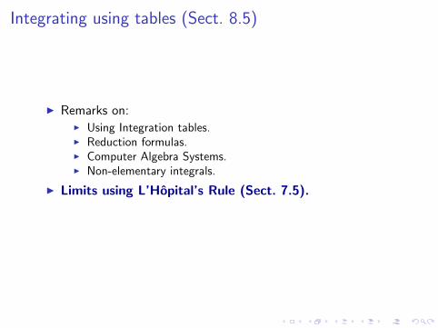
Integrating using tables (Sect. 8.5)
I Remarks on:I Using Integration tables.I Reduction formulas.I Computer Algebra Systems.I Non-elementary integrals.
I Limits using L’Hopital’s Rule (Sect. 7.5).
Integrating using tables (Sect. 8.5)
I Remarks on:I Using Integration tables.I Reduction formulas.I Computer Algebra Systems.I Non-elementary integrals.
I Limits using L’Hopital’s Rule (Sect. 7.5).
Using Integration tables
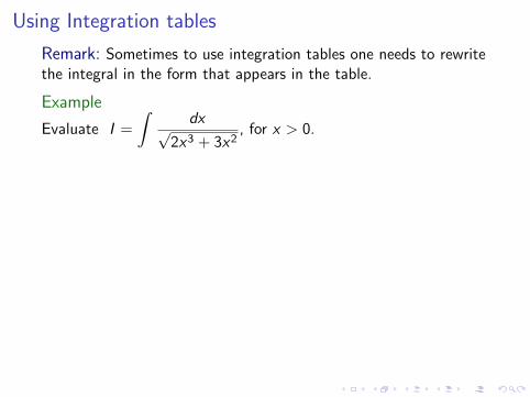
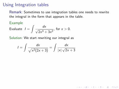
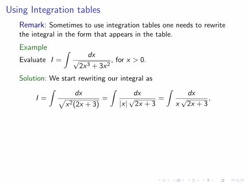
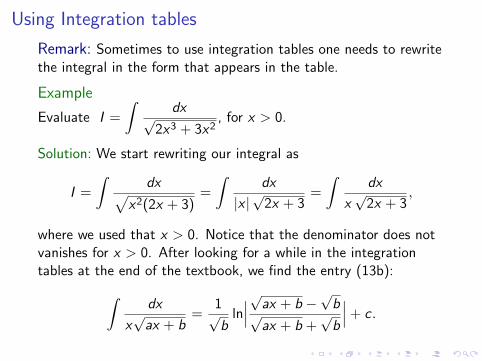
Remark: Sometimes to use integration tables one needs to rewritethe integral in the form that appears in the table.
Example
Evaluate I =
∫dx√
2x3 + 3x2, for x > 0.
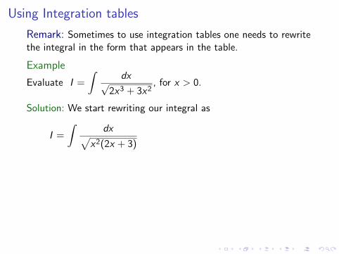
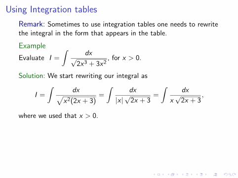
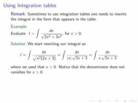
Solution: We start rewriting our integral as
I =
∫dx√
x2(2x + 3)=
∫dx
|x |√
2x + 3=
∫dx
x√
2x + 3,
where we used that x > 0. Notice that the denominator does notvanishes for x > 0. After looking for a while in the integrationtables at the end of the textbook, we find the entry (13b):∫
dx
x√
ax + b=
1√b
ln∣∣∣√ax + b −
√b
√ax + b +
√b
∣∣∣ + c .
Using Integration tables
Remark: Sometimes to use integration tables one needs to rewritethe integral in the form that appears in the table.
Example
Evaluate I =
∫dx√
2x3 + 3x2, for x > 0.
Solution: We start rewriting our integral as
I =
∫dx√
x2(2x + 3)
=
∫dx
|x |√
2x + 3=
∫dx
x√
2x + 3,
where we used that x > 0. Notice that the denominator does notvanishes for x > 0. After looking for a while in the integrationtables at the end of the textbook, we find the entry (13b):∫
dx
x√
ax + b=
1√b
ln∣∣∣√ax + b −
√b
√ax + b +
√b
∣∣∣ + c .
Using Integration tables
Remark: Sometimes to use integration tables one needs to rewritethe integral in the form that appears in the table.
Example
Evaluate I =
∫dx√
2x3 + 3x2, for x > 0.
Solution: We start rewriting our integral as
I =
∫dx√
x2(2x + 3)=
∫dx
|x |√
2x + 3
=
∫dx
x√
2x + 3,
where we used that x > 0. Notice that the denominator does notvanishes for x > 0. After looking for a while in the integrationtables at the end of the textbook, we find the entry (13b):∫
dx
x√
ax + b=
1√b
ln∣∣∣√ax + b −
√b
√ax + b +
√b
∣∣∣ + c .
Using Integration tables
Remark: Sometimes to use integration tables one needs to rewritethe integral in the form that appears in the table.
Example
Evaluate I =
∫dx√
2x3 + 3x2, for x > 0.
Solution: We start rewriting our integral as
I =
∫dx√
x2(2x + 3)=
∫dx
|x |√
2x + 3=
∫dx
x√
2x + 3,
where we used that x > 0. Notice that the denominator does notvanishes for x > 0. After looking for a while in the integrationtables at the end of the textbook, we find the entry (13b):∫
dx
x√
ax + b=
1√b
ln∣∣∣√ax + b −
√b
√ax + b +
√b
∣∣∣ + c .
Using Integration tables
Remark: Sometimes to use integration tables one needs to rewritethe integral in the form that appears in the table.
Example
Evaluate I =
∫dx√
2x3 + 3x2, for x > 0.
Solution: We start rewriting our integral as
I =
∫dx√
x2(2x + 3)=
∫dx
|x |√
2x + 3=
∫dx
x√
2x + 3,
where we used that x > 0.
Notice that the denominator does notvanishes for x > 0. After looking for a while in the integrationtables at the end of the textbook, we find the entry (13b):∫
dx
x√
ax + b=
1√b
ln∣∣∣√ax + b −
√b
√ax + b +
√b
∣∣∣ + c .
Using Integration tables
Remark: Sometimes to use integration tables one needs to rewritethe integral in the form that appears in the table.
Example
Evaluate I =
∫dx√
2x3 + 3x2, for x > 0.
Solution: We start rewriting our integral as
I =
∫dx√
x2(2x + 3)=
∫dx
|x |√
2x + 3=
∫dx
x√
2x + 3,
where we used that x > 0. Notice that the denominator does notvanishes for x > 0.
After looking for a while in the integrationtables at the end of the textbook, we find the entry (13b):∫
dx
x√
ax + b=
1√b
ln∣∣∣√ax + b −
√b
√ax + b +
√b
∣∣∣ + c .
Using Integration tables
Remark: Sometimes to use integration tables one needs to rewritethe integral in the form that appears in the table.
Example
Evaluate I =
∫dx√
2x3 + 3x2, for x > 0.
Solution: We start rewriting our integral as
I =
∫dx√
x2(2x + 3)=
∫dx
|x |√
2x + 3=
∫dx
x√
2x + 3,
where we used that x > 0. Notice that the denominator does notvanishes for x > 0. After looking for a while in the integrationtables at the end of the textbook, we find the entry (13b):∫
dx
x√
ax + b=
1√b
ln∣∣∣√ax + b −
√b
√ax + b +
√b
∣∣∣ + c .
Using Integration tables
Example
Evaluate I =
∫dx√
2x3 + 3x2, for x > 0.
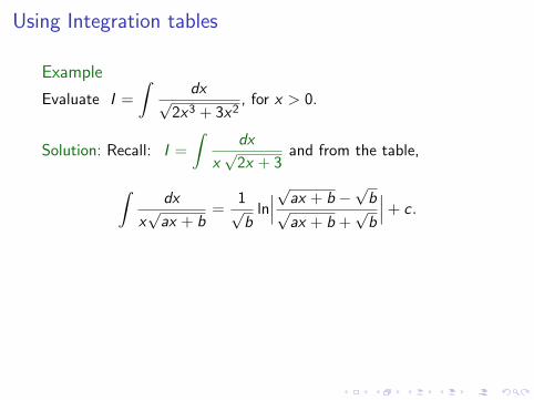
Solution: Recall: I =
∫dx
x√
2x + 3and from the table,
∫dx
x√
ax + b=
1√b
ln∣∣∣√ax + b −
√b
√ax + b +
√b
∣∣∣ + c .
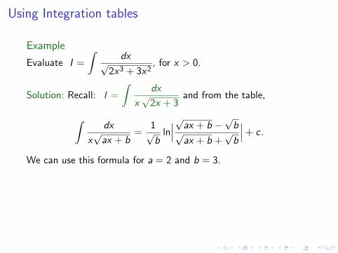
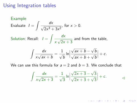
We can use this formula for a = 2 and b = 3. We conclude that∫dx
x√
2x + 3=
1√3
ln∣∣∣√2x + 3−
√3
√2x + 3 +
√3
∣∣∣ + c . C
Using Integration tables
Example
Evaluate I =
∫dx√
2x3 + 3x2, for x > 0.
Solution: Recall: I =
∫dx
x√
2x + 3and from the table,
∫dx
x√
ax + b=
1√b
ln∣∣∣√ax + b −
√b
√ax + b +
√b
∣∣∣ + c .
We can use this formula for a = 2 and b = 3.
We conclude that∫dx
x√
2x + 3=
1√3
ln∣∣∣√2x + 3−
√3
√2x + 3 +
√3
∣∣∣ + c . C
Using Integration tables
Example
Evaluate I =
∫dx√
2x3 + 3x2, for x > 0.
Solution: Recall: I =
∫dx
x√
2x + 3and from the table,
∫dx
x√
ax + b=
1√b
ln∣∣∣√ax + b −
√b
√ax + b +
√b
∣∣∣ + c .
We can use this formula for a = 2 and b = 3. We conclude that∫dx
x√
2x + 3=
1√3
ln∣∣∣√2x + 3−
√3
√2x + 3 +
√3
∣∣∣ + c . C
Integrating using tables (Sect. 8.5)
I Remarks on:I Using Integration tables.I Reduction formulas.I Computer Algebra Systems.I Non-elementary integrals.
I Limits using L’Hopital’s Rule (Sect. 7.5).
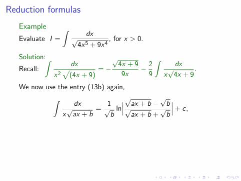
Reduction formulas
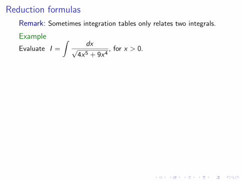
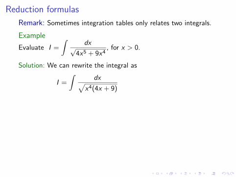
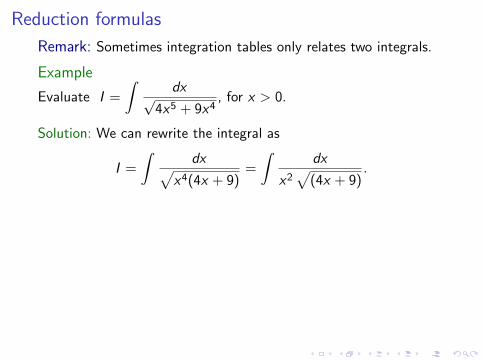
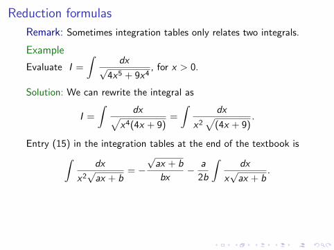
Remark: Sometimes integration tables only relates two integrals.
Example
Evaluate I =
∫dx√
4x5 + 9x4, for x > 0.
Solution: We can rewrite the integral as
I =
∫dx√
x4(4x + 9)=
∫dx
x2√
(4x + 9).
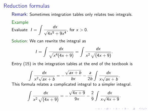
Entry (15) in the integration tables at the end of the textbook is∫dx
x2√
ax + b= −
√ax + b
bx− a
2b
∫dx
x√
ax + b.
This formula relates a complicated integral to a simpler integral.∫dx
x2√
(4x + 9)= −
√4x + 9
9x− 2
9
∫dx
x√
4x + 9.
Reduction formulas
Remark: Sometimes integration tables only relates two integrals.
Example
Evaluate I =
∫dx√
4x5 + 9x4, for x > 0.
Solution: We can rewrite the integral as
I =
∫dx√
x4(4x + 9)=
∫dx
x2√
(4x + 9).
Entry (15) in the integration tables at the end of the textbook is∫dx
x2√
ax + b= −
√ax + b
bx− a
2b
∫dx
x√
ax + b.
This formula relates a complicated integral to a simpler integral.∫dx
x2√
(4x + 9)= −
√4x + 9
9x− 2
9
∫dx
x√
4x + 9.
Reduction formulas
Remark: Sometimes integration tables only relates two integrals.
Example
Evaluate I =
∫dx√
4x5 + 9x4, for x > 0.
Solution: We can rewrite the integral as
I =
∫dx√
x4(4x + 9)
=
∫dx
x2√
(4x + 9).
Entry (15) in the integration tables at the end of the textbook is∫dx
x2√
ax + b= −
√ax + b
bx− a
2b
∫dx
x√
ax + b.
This formula relates a complicated integral to a simpler integral.∫dx
x2√
(4x + 9)= −
√4x + 9
9x− 2
9
∫dx
x√
4x + 9.
Reduction formulas
Remark: Sometimes integration tables only relates two integrals.
Example
Evaluate I =
∫dx√
4x5 + 9x4, for x > 0.
Solution: We can rewrite the integral as
I =
∫dx√
x4(4x + 9)=
∫dx
x2√
(4x + 9).
Entry (15) in the integration tables at the end of the textbook is∫dx
x2√
ax + b= −
√ax + b
bx− a
2b
∫dx
x√
ax + b.
This formula relates a complicated integral to a simpler integral.∫dx
x2√
(4x + 9)= −
√4x + 9
9x− 2
9
∫dx
x√
4x + 9.
Reduction formulas
Remark: Sometimes integration tables only relates two integrals.
Example
Evaluate I =
∫dx√
4x5 + 9x4, for x > 0.
Solution: We can rewrite the integral as
I =
∫dx√
x4(4x + 9)=
∫dx
x2√
(4x + 9).
Entry (15) in the integration tables at the end of the textbook is∫dx
x2√
ax + b= −
√ax + b
bx− a
2b
∫dx
x√
ax + b.
This formula relates a complicated integral to a simpler integral.∫dx
x2√
(4x + 9)= −
√4x + 9
9x− 2
9
∫dx
x√
4x + 9.
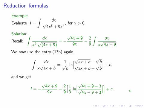
Reduction formulas
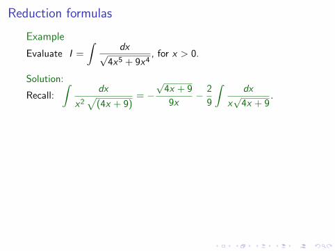
Example
Evaluate I =
∫dx√
4x5 + 9x4, for x > 0.
Solution:
Recall:
∫dx
x2√
(4x + 9)= −
√4x + 9
9x− 2
9
∫dx
x√
4x + 9.
We now use the entry (13b) again,∫dx
x√
ax + b=
1√b
ln∣∣∣√ax + b −
√b
√ax + b +
√b
∣∣∣ + c ,
and we get
I = −√
4x + 9
9x− 2
9
[1
3ln
∣∣∣√4x + 9− 3√4x + 9 + 3
∣∣∣] + c . C
Reduction formulas
Example
Evaluate I =
∫dx√
4x5 + 9x4, for x > 0.
Solution:
Recall:
∫dx
x2√
(4x + 9)= −
√4x + 9
9x− 2
9
∫dx
x√
4x + 9.
We now use the entry (13b) again,∫dx
x√
ax + b=
1√b
ln∣∣∣√ax + b −
√b
√ax + b +
√b
∣∣∣ + c ,
and we get
I = −√
4x + 9
9x− 2
9
[1
3ln
∣∣∣√4x + 9− 3√4x + 9 + 3
∣∣∣] + c . C
Integrating using tables (Sect. 8.5)
I Remarks on:I Using Integration tables.I Reduction formulas.I Computer Algebra Systems.I Non-elementary integrals.
I Limits using L’Hopital’s Rule (Sect. 7.5).
Computer Algebra Systems
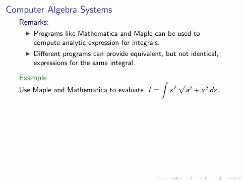
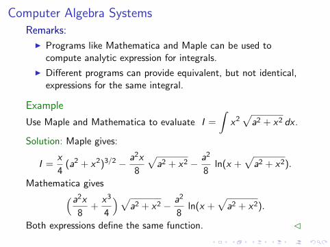
Remarks:
I Programs like Mathematica and Maple can be used tocompute analytic expression for integrals.
I Different programs can provide equivalent, but not identical,expressions for the same integral.
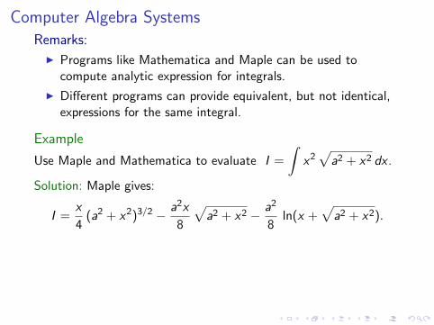
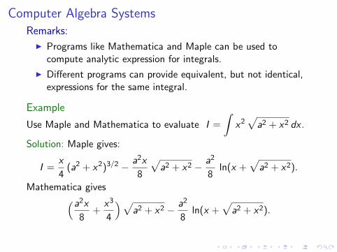
Example
Use Maple and Mathematica to evaluate I =
∫x2
√a2 + x2 dx .
Solution: Maple gives:
I =x
4(a2 + x2)3/2 − a2x
8
√a2 + x2 − a2
8ln(x +
√a2 + x2).
Mathematica gives(a2x
8+
x3
4
) √a2 + x2 − a2
8ln(x +
√a2 + x2).
Both expressions define the same function. C
Computer Algebra Systems
Remarks:
I Programs like Mathematica and Maple can be used tocompute analytic expression for integrals.
I Different programs can provide equivalent, but not identical,expressions for the same integral.
Example
Use Maple and Mathematica to evaluate I =
∫x2
√a2 + x2 dx .
Solution: Maple gives:
I =x
4(a2 + x2)3/2 − a2x
8
√a2 + x2 − a2
8ln(x +
√a2 + x2).
Mathematica gives(a2x
8+
x3
4
) √a2 + x2 − a2
8ln(x +
√a2 + x2).
Both expressions define the same function. C
Integrating using tables (Sect. 8.5)
I Remarks on:I Using Integration tables.I Reduction formulas.I Computer Algebra Systems.I Non-elementary integrals.
I Limits using L’Hopital’s Rule (Sect. 7.5).
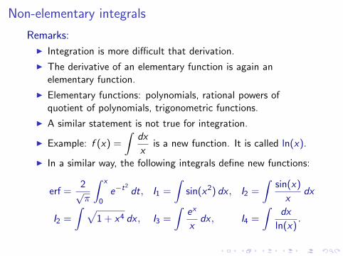
Non-elementary integrals
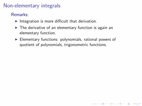
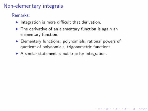
Remarks:
I Integration is more difficult that derivation.
I The derivative of an elementary function is again anelementary function.
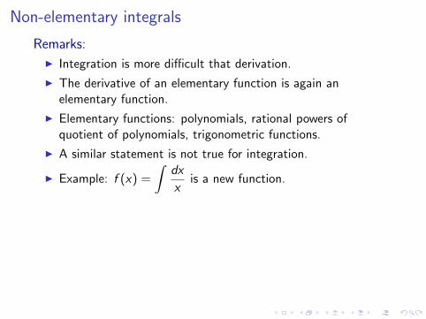
I Elementary functions: polynomials, rational powers ofquotient of polynomials, trigonometric functions.
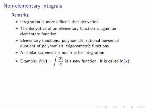
I A similar statement is not true for integration.
I Example: f (x) =
∫dx
xis a new function. It is called ln(x).
I In a similar way, the following integrals define new functions:
erf =2√π
∫ x
0e−t2
dt, I1 =
∫sin(x2) dx , I2 =
∫sin(x)
xdx
I2 =
∫ √1 + x4 dx , I3 =
∫ex
xdx , I4 =
∫dx
ln(x).
Non-elementary integrals
Remarks:
I Integration is more difficult that derivation.
I The derivative of an elementary function is again anelementary function.
I Elementary functions: polynomials, rational powers ofquotient of polynomials, trigonometric functions.
I A similar statement is not true for integration.
I Example: f (x) =
∫dx
xis a new function.
It is called ln(x).
I In a similar way, the following integrals define new functions:
erf =2√π
∫ x
0e−t2
dt, I1 =
∫sin(x2) dx , I2 =
∫sin(x)
xdx
I2 =
∫ √1 + x4 dx , I3 =
∫ex
xdx , I4 =
∫dx
ln(x).
Non-elementary integrals
Remarks:
I Integration is more difficult that derivation.
I The derivative of an elementary function is again anelementary function.
I Elementary functions: polynomials, rational powers ofquotient of polynomials, trigonometric functions.
I A similar statement is not true for integration.
I Example: f (x) =
∫dx
xis a new function. It is called ln(x).
I In a similar way, the following integrals define new functions:
erf =2√π
∫ x
0e−t2
dt, I1 =
∫sin(x2) dx , I2 =
∫sin(x)
xdx
I2 =
∫ √1 + x4 dx , I3 =
∫ex
xdx , I4 =
∫dx
ln(x).
Non-elementary integrals
Remarks:
I Integration is more difficult that derivation.
I The derivative of an elementary function is again anelementary function.
I Elementary functions: polynomials, rational powers ofquotient of polynomials, trigonometric functions.
I A similar statement is not true for integration.
I Example: f (x) =
∫dx
xis a new function. It is called ln(x).
I In a similar way, the following integrals define new functions:
erf =2√π
∫ x
0e−t2
dt, I1 =
∫sin(x2) dx , I2 =
∫sin(x)
xdx
I2 =
∫ √1 + x4 dx , I3 =
∫ex
xdx , I4 =
∫dx
ln(x).
Integrating using tables (Sect. 8.5)
I Remarks on:I Using Integration tables.I Reduction formulas.I Computer Algebra Systems.I Non-elementary integrals.
I Limits using L’Hopital’s Rule (Sect. 7.5).
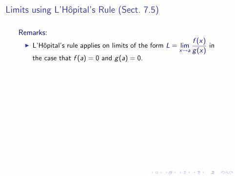
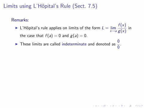
Limits using L’Hopital’s Rule (Sect. 7.5)
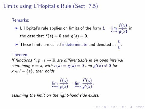
Remarks:
I L’Hopital’s rule applies on limits of the form L = limx→a
f (x)
g(x)in
the case that f (a) = 0 and g(a) = 0.
I These limits are called indeterminate and denoted as0
0.
TheoremIf functions f , g : I → R are differentiable in an open intervalcontaining x = a, with f (a) = g(a) = 0 and g ′(x) 6= 0 forx ∈ I − {a}, then holds
limx→a
f (x)
g(x)= lim
x→a
f ′(x)
g ′(x),
assuming the limit on the right-hand side exists.
Limits using L’Hopital’s Rule (Sect. 7.5)
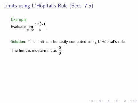
Example
Evaluate limx→0
sin(x)
x.
Solution: This limit can be easily computed using L’Hopital’s rule.
The limit is indeterminate,0
0. But,
limx→0
sin(x)
x= lim
x→0
cos(x)
1= 1.
We conclude limx→0
sin(x)
x= 1. C
Limits using L’Hopital’s Rule (Sect. 7.5)
Example
Evaluate limx→0
sin(x)
x.
Solution: This limit can be easily computed using L’Hopital’s rule.
The limit is indeterminate,0
0. But,
limx→0
sin(x)
x= lim
x→0
cos(x)
1= 1.
We conclude limx→0
sin(x)
x= 1. C
Limits using L’Hopital’s Rule (Sect. 7.5)
Example
Evaluate limx→0
sin(x)
x.
Solution: This limit can be easily computed using L’Hopital’s rule.
The limit is indeterminate,0
0.
But,
limx→0
sin(x)
x= lim
x→0
cos(x)
1= 1.
We conclude limx→0
sin(x)
x= 1. C
Limits using L’Hopital’s Rule (Sect. 7.5)
Example
Evaluate limx→0
sin(x)
x.
Solution: This limit can be easily computed using L’Hopital’s rule.
The limit is indeterminate,0
0. But,
limx→0
sin(x)
x
= limx→0
cos(x)
1= 1.
We conclude limx→0
sin(x)
x= 1. C
Limits using L’Hopital’s Rule (Sect. 7.5)
Example
Evaluate limx→0
sin(x)
x.
Solution: This limit can be easily computed using L’Hopital’s rule.
The limit is indeterminate,0
0. But,
limx→0
sin(x)
x= lim
x→0
cos(x)
1
= 1.
We conclude limx→0
sin(x)
x= 1. C
Limits using L’Hopital’s Rule (Sect. 7.5)
Example
Evaluate limx→0
sin(x)
x.
Solution: This limit can be easily computed using L’Hopital’s rule.
The limit is indeterminate,0
0. But,
limx→0
sin(x)
x= lim
x→0
cos(x)
1= 1.
We conclude limx→0
sin(x)
x= 1. C
Limits using L’Hopital’s Rule (Sect. 7.5)
Example
Evaluate limx→0
sin(x)
x.
Solution: This limit can be easily computed using L’Hopital’s rule.
The limit is indeterminate,0
0. But,
limx→0
sin(x)
x= lim
x→0
cos(x)
1= 1.
We conclude limx→0
sin(x)
x= 1. C
Limits using L’Hopital’s Rule (Sect. 7.5)
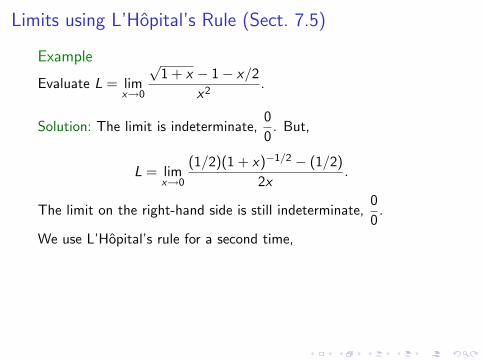
Example
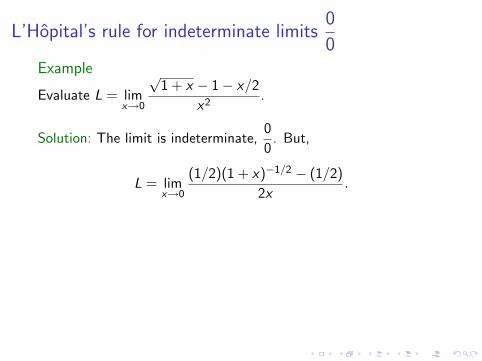
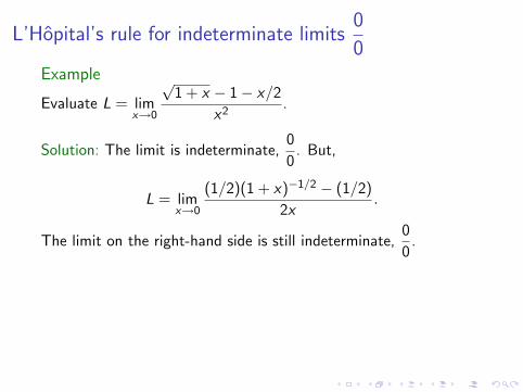
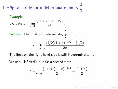
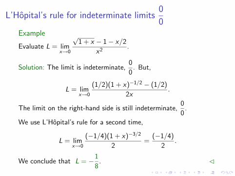
Evaluate L = limx→0
√1 + x − 1− x/2
x2.
Solution: The limit is indeterminate,0
0. But,
L = limx→0
(1/2)(1 + x)−1/2 − (1/2)
2x.
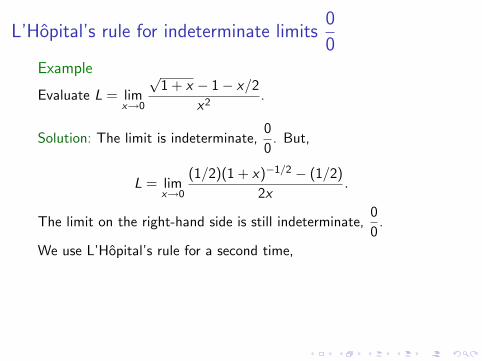
The limit on the right-hand side is still indeterminate,0
0.
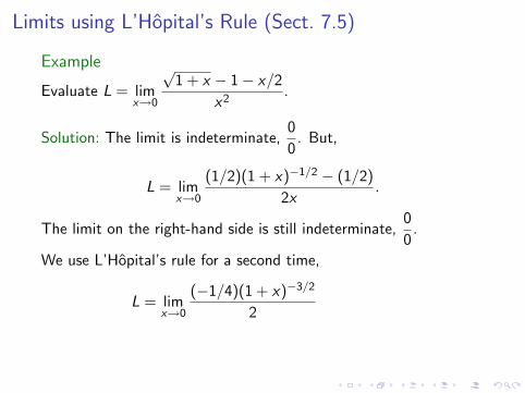
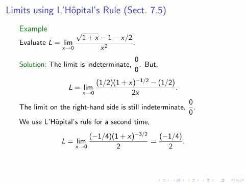
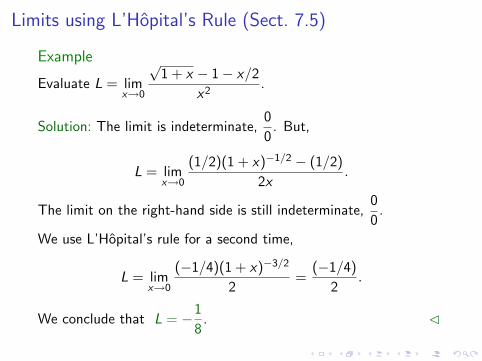
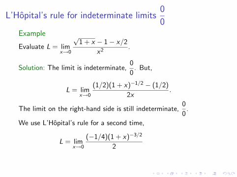
We use L’Hopital’s rule for a second time,
L = limx→0
(−1/4)(1 + x)−3/2
2=
(−1/4)
2.
We conclude that L = −1
8. C
Limits using L’Hopital’s Rule (Sect. 7.5)
Example
Evaluate L = limx→0
√1 + x − 1− x/2
x2.
Solution: The limit is indeterminate,0
0.
But,
L = limx→0
(1/2)(1 + x)−1/2 − (1/2)
2x.
The limit on the right-hand side is still indeterminate,0
0.
We use L’Hopital’s rule for a second time,
L = limx→0
(−1/4)(1 + x)−3/2
2=
(−1/4)
2.
We conclude that L = −1
8. C
Limits using L’Hopital’s Rule (Sect. 7.5)
Example
Evaluate L = limx→0
√1 + x − 1− x/2
x2.
Solution: The limit is indeterminate,0
0. But,
L = limx→0
(1/2)(1 + x)−1/2 − (1/2)
2x.
The limit on the right-hand side is still indeterminate,0
0.
We use L’Hopital’s rule for a second time,
L = limx→0
(−1/4)(1 + x)−3/2
2
=(−1/4)
2.
We conclude that L = −1
8. C
Limits using L’Hopital’s Rule (Sect. 7.5)
Example
Evaluate L = limx→0
√1 + x − 1− x/2
x2.
Solution: The limit is indeterminate,0
0. But,
L = limx→0
(1/2)(1 + x)−1/2 − (1/2)
2x.
The limit on the right-hand side is still indeterminate,0
0.
We use L’Hopital’s rule for a second time,
L = limx→0
(−1/4)(1 + x)−3/2
2=
(−1/4)
2.
We conclude that L = −1
8. C
Limits using L’Hopital’s Rule (Sect. 7.5)
Example
Evaluate L = limx→0
√1 + x − 1− x/2
x2.
Solution: The limit is indeterminate,0
0. But,
L = limx→0
(1/2)(1 + x)−1/2 − (1/2)
2x.
The limit on the right-hand side is still indeterminate,0
0.
We use L’Hopital’s rule for a second time,
L = limx→0
(−1/4)(1 + x)−3/2
2=
(−1/4)
2.
We conclude that L = −1
8. C
Limits using L’Hopital’s Rule (Sect. 7.5)
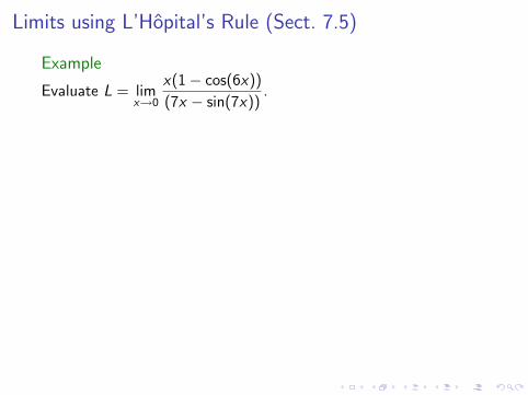
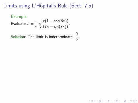
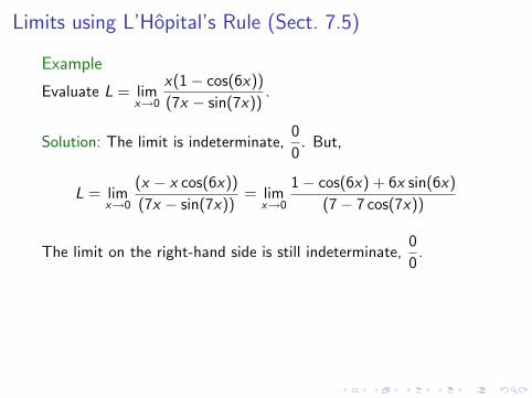
Example
Evaluate L = limx→0
x(1− cos(6x))
(7x − sin(7x)).
Solution: The limit is indeterminate,0
0. But,
L = limx→0
(x − x cos(6x))
(7x − sin(7x))= lim
x→0
1− cos(6x) + 6x sin(6x)
(7− 7 cos(7x))
The limit on the right-hand side is still indeterminate,0
0.
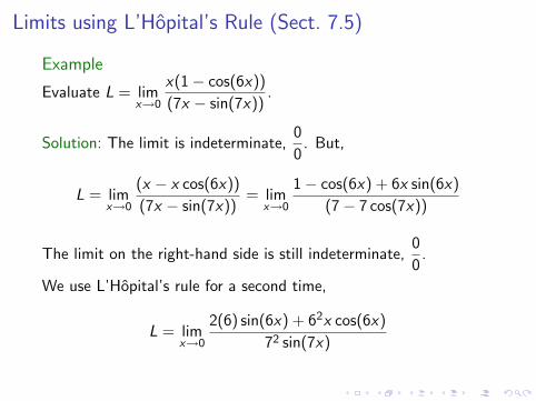
We use L’Hopital’s rule for a second time,
L = limx→0
2(6) sin(6x) + 62x cos(6x)
72 sin(7x)
Limits using L’Hopital’s Rule (Sect. 7.5)
Example
Evaluate L = limx→0
x(1− cos(6x))
(7x − sin(7x)).
Solution: The limit is indeterminate,0
0.
But,
L = limx→0
(x − x cos(6x))
(7x − sin(7x))= lim
x→0
1− cos(6x) + 6x sin(6x)
(7− 7 cos(7x))
The limit on the right-hand side is still indeterminate,0
0.
We use L’Hopital’s rule for a second time,
L = limx→0
2(6) sin(6x) + 62x cos(6x)
72 sin(7x)
Limits using L’Hopital’s Rule (Sect. 7.5)
Example
Evaluate L = limx→0
x(1− cos(6x))
(7x − sin(7x)).
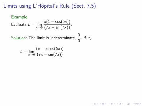
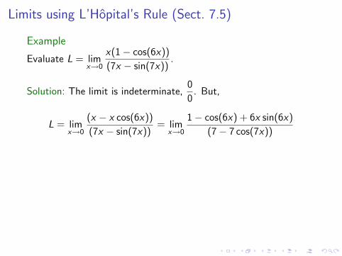
Solution: The limit is indeterminate,0
0. But,
L = limx→0
(x − x cos(6x))
(7x − sin(7x))
= limx→0
1− cos(6x) + 6x sin(6x)
(7− 7 cos(7x))
The limit on the right-hand side is still indeterminate,0
0.
We use L’Hopital’s rule for a second time,
L = limx→0
2(6) sin(6x) + 62x cos(6x)
72 sin(7x)
Limits using L’Hopital’s Rule (Sect. 7.5)
Example
Evaluate L = limx→0
x(1− cos(6x))
(7x − sin(7x)).
Solution: The limit is indeterminate,0
0. But,
L = limx→0
(x − x cos(6x))
(7x − sin(7x))= lim
x→0
1− cos(6x) + 6x sin(6x)
(7− 7 cos(7x))
The limit on the right-hand side is still indeterminate,0
0.
We use L’Hopital’s rule for a second time,
L = limx→0
2(6) sin(6x) + 62x cos(6x)
72 sin(7x)
Limits using L’Hopital’s Rule (Sect. 7.5)
Example
Evaluate L = limx→0
x(1− cos(6x))
(7x − sin(7x)).
Solution: The limit is indeterminate,0
0. But,
L = limx→0
(x − x cos(6x))
(7x − sin(7x))= lim
x→0
1− cos(6x) + 6x sin(6x)
(7− 7 cos(7x))
The limit on the right-hand side is still indeterminate,0
0.
We use L’Hopital’s rule for a second time,
L = limx→0
2(6) sin(6x) + 62x cos(6x)
72 sin(7x)
Limits using L’Hopital’s Rule (Sect. 7.5)
Example
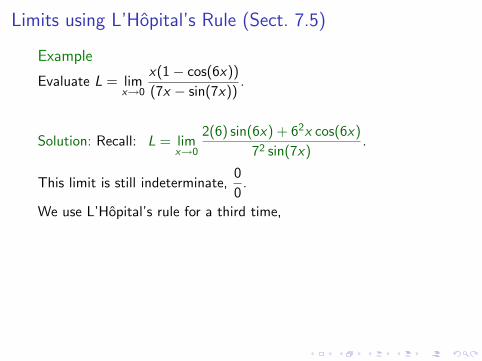
Evaluate L = limx→0
x(1− cos(6x))
(7x − sin(7x)).
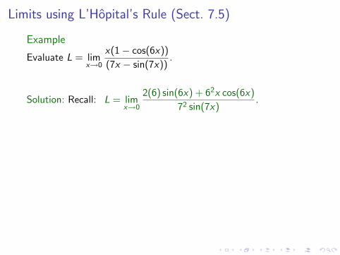
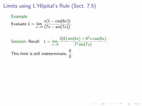
Solution: Recall: L = limx→0
2(6) sin(6x) + 62x cos(6x)
72 sin(7x).
This limit is still indeterminate,0
0.
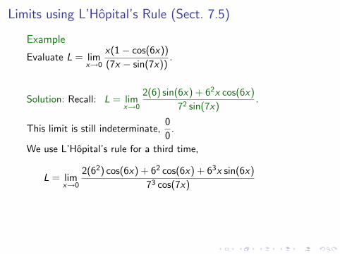
We use L’Hopital’s rule for a third time,
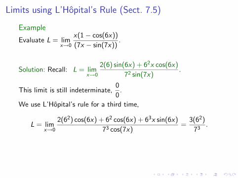
L = limx→0
2(62) cos(6x) + 62 cos(6x) + 63x sin(6x)
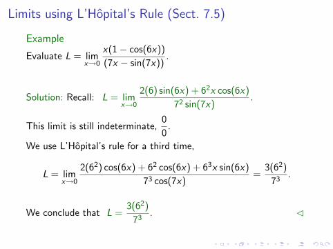
73 cos(7x)=
3(62)
73.
We conclude that L =3(62)
73. C
Limits using L’Hopital’s Rule (Sect. 7.5)
Example
Evaluate L = limx→0
x(1− cos(6x))
(7x − sin(7x)).
Solution: Recall: L = limx→0
2(6) sin(6x) + 62x cos(6x)
72 sin(7x).
This limit is still indeterminate,0
0.
We use L’Hopital’s rule for a third time,
L = limx→0
2(62) cos(6x) + 62 cos(6x) + 63x sin(6x)
73 cos(7x)
=3(62)
73.
We conclude that L =3(62)
73. C
Limits using L’Hopital’s Rule (Sect. 7.5)
Example
Evaluate L = limx→0
x(1− cos(6x))
(7x − sin(7x)).
Solution: Recall: L = limx→0
2(6) sin(6x) + 62x cos(6x)
72 sin(7x).
This limit is still indeterminate,0
0.
We use L’Hopital’s rule for a third time,
L = limx→0
2(62) cos(6x) + 62 cos(6x) + 63x sin(6x)
73 cos(7x)=
3(62)
73.
We conclude that L =3(62)
73. C
Limits using L’Hopital’s Rule (Sect. 7.5)
Example
Evaluate L = limx→0
x(1− cos(6x))
(7x − sin(7x)).
Solution: Recall: L = limx→0
2(6) sin(6x) + 62x cos(6x)
72 sin(7x).
This limit is still indeterminate,0
0.
We use L’Hopital’s rule for a third time,
L = limx→0
2(62) cos(6x) + 62 cos(6x) + 63x sin(6x)
73 cos(7x)=
3(62)
73.
We conclude that L =3(62)
73. C
Limits using L’Hopital’s Rule (Sect. 7.5)
I Review: L’Hopital’s rule for indeterminate limits0
0.
I Indeterminate limit∞∞
.
I Indeterminate limits ∞ · 0 and ∞−∞.
I Overview of improper integrals (Sect. 8.7).
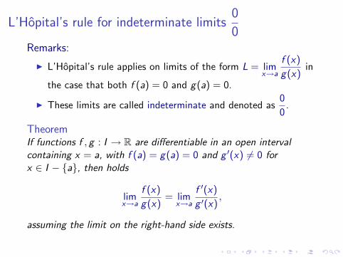
L’Hopital’s rule for indeterminate limits0
0Remarks:
I L’Hopital’s rule applies on limits of the form L = limx→a
f (x)
g(x)in
the case that both f (a) = 0 and g(a) = 0.
I These limits are called indeterminate and denoted as0
0.
TheoremIf functions f , g : I → R are differentiable in an open intervalcontaining x = a, with f (a) = g(a) = 0 and g ′(x) 6= 0 forx ∈ I − {a}, then holds
limx→a
f (x)
g(x)= lim
x→a
f ′(x)
g ′(x),
assuming the limit on the right-hand side exists.
L’Hopital’s rule for indeterminate limits0
0Example
Evaluate L = limx→0
√1 + x − 1− x/2
x2.
Solution: The limit is indeterminate,0
0. But,
L = limx→0
(1/2)(1 + x)−1/2 − (1/2)
2x.
The limit on the right-hand side is still indeterminate,0
0.
We use L’Hopital’s rule for a second time,
L = limx→0
(−1/4)(1 + x)−3/2
2=
(−1/4)
2.
We conclude that L = −1
8. C
L’Hopital’s rule for indeterminate limits0
0Example
Evaluate L = limx→0
√1 + x − 1− x/2
x2.
Solution: The limit is indeterminate,0
0.
But,
L = limx→0
(1/2)(1 + x)−1/2 − (1/2)
2x.
The limit on the right-hand side is still indeterminate,0
0.
We use L’Hopital’s rule for a second time,
L = limx→0
(−1/4)(1 + x)−3/2
2=
(−1/4)
2.
We conclude that L = −1
8. C
L’Hopital’s rule for indeterminate limits0
0Example
Evaluate L = limx→0
√1 + x − 1− x/2
x2.
Solution: The limit is indeterminate,0
0. But,
L = limx→0
(1/2)(1 + x)−1/2 − (1/2)
2x.
The limit on the right-hand side is still indeterminate,0
0.
We use L’Hopital’s rule for a second time,
L = limx→0
(−1/4)(1 + x)−3/2
2=
(−1/4)
2.
We conclude that L = −1
8. C
L’Hopital’s rule for indeterminate limits0
0Example
Evaluate L = limx→0
√1 + x − 1− x/2
x2.
Solution: The limit is indeterminate,0
0. But,
L = limx→0
(1/2)(1 + x)−1/2 − (1/2)
2x.
The limit on the right-hand side is still indeterminate,0
0.
We use L’Hopital’s rule for a second time,
L = limx→0
(−1/4)(1 + x)−3/2
2
=(−1/4)
2.
We conclude that L = −1
8. C
L’Hopital’s rule for indeterminate limits0
0Example
Evaluate L = limx→0
√1 + x − 1− x/2
x2.
Solution: The limit is indeterminate,0
0. But,
L = limx→0
(1/2)(1 + x)−1/2 − (1/2)
2x.
The limit on the right-hand side is still indeterminate,0
0.
We use L’Hopital’s rule for a second time,
L = limx→0
(−1/4)(1 + x)−3/2
2=
(−1/4)
2.
We conclude that L = −1
8. C
L’Hopital’s rule for indeterminate limits0
0Example
Evaluate L = limx→0
√1 + x − 1− x/2
x2.
Solution: The limit is indeterminate,0
0. But,
L = limx→0
(1/2)(1 + x)−1/2 − (1/2)
2x.
The limit on the right-hand side is still indeterminate,0
0.
We use L’Hopital’s rule for a second time,
L = limx→0
(−1/4)(1 + x)−3/2
2=
(−1/4)
2.
We conclude that L = −1
8. C
L’Hopital’s rule for indeterminate limits0
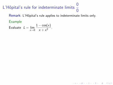
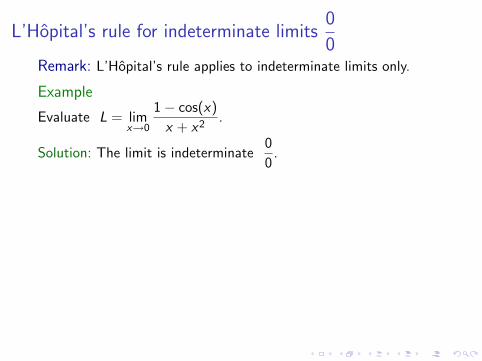
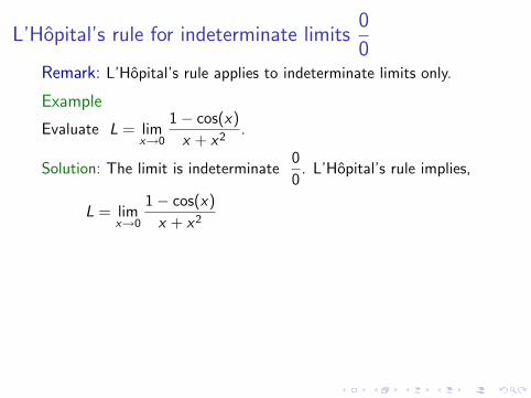
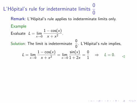
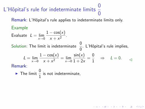
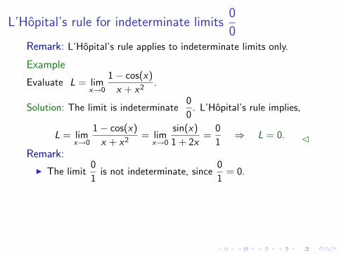
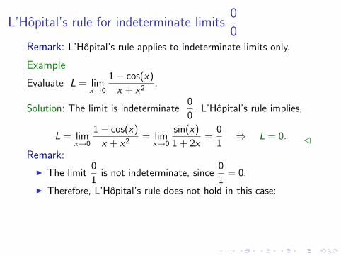
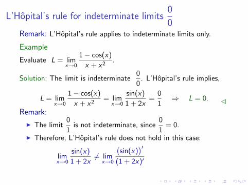
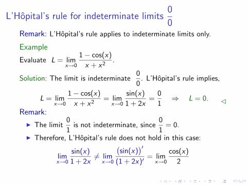
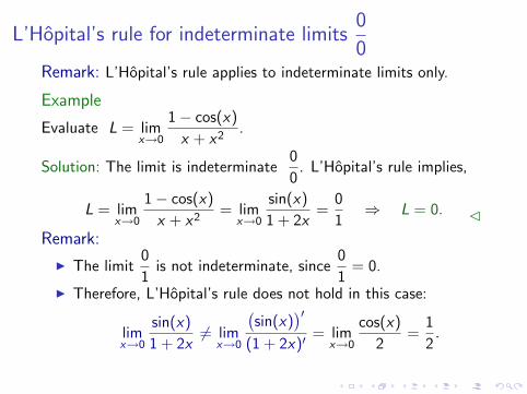
0Remark: L’Hopital’s rule applies to indeterminate limits only.
Example
Evaluate L = limx→0
1− cos(x)
x + x2.
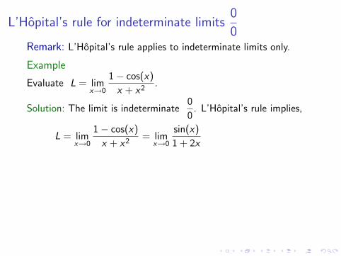
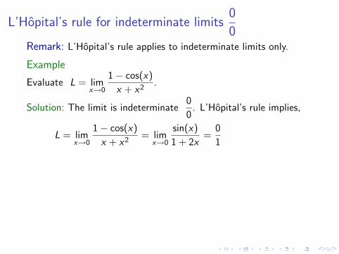
Solution: The limit is indeterminate0
0. L’Hopital’s rule implies,
L = limx→0
1− cos(x)
x + x2= lim
x→0
sin(x)
1 + 2x=
0
1⇒ L = 0. C
Remark:
I The limit0
1is not indeterminate, since
0
1= 0.
I Therefore, L’Hopital’s rule does not hold in this case:
limx→0
sin(x)
1 + 2x6= lim
x→0
(sin(x)
)′(1 + 2x)′
= limx→0
cos(x)
2=
1
2.
L’Hopital’s rule for indeterminate limits0
0Remark: L’Hopital’s rule applies to indeterminate limits only.
Example
Evaluate L = limx→0
1− cos(x)
x + x2.
Solution: The limit is indeterminate0
0.
L’Hopital’s rule implies,
L = limx→0
1− cos(x)
x + x2= lim
x→0
sin(x)
1 + 2x=
0
1⇒ L = 0. C
Remark:
I The limit0
1is not indeterminate, since
0
1= 0.
I Therefore, L’Hopital’s rule does not hold in this case:
limx→0
sin(x)
1 + 2x6= lim
x→0
(sin(x)
)′(1 + 2x)′
= limx→0
cos(x)
2=
1
2.
L’Hopital’s rule for indeterminate limits0
0Remark: L’Hopital’s rule applies to indeterminate limits only.
Example
Evaluate L = limx→0
1− cos(x)
x + x2.
Solution: The limit is indeterminate0
0. L’Hopital’s rule implies,
L = limx→0
1− cos(x)
x + x2
= limx→0
sin(x)
1 + 2x=
0
1⇒ L = 0. C
Remark:
I The limit0
1is not indeterminate, since
0
1= 0.
I Therefore, L’Hopital’s rule does not hold in this case:
limx→0
sin(x)
1 + 2x6= lim
x→0
(sin(x)
)′(1 + 2x)′
= limx→0
cos(x)
2=
1
2.
L’Hopital’s rule for indeterminate limits0
0Remark: L’Hopital’s rule applies to indeterminate limits only.
Example
Evaluate L = limx→0
1− cos(x)
x + x2.
Solution: The limit is indeterminate0
0. L’Hopital’s rule implies,
L = limx→0
1− cos(x)
x + x2= lim
x→0
sin(x)
1 + 2x
=0
1⇒ L = 0. C
Remark:
I The limit0
1is not indeterminate, since
0
1= 0.
I Therefore, L’Hopital’s rule does not hold in this case:
limx→0
sin(x)
1 + 2x6= lim
x→0
(sin(x)
)′(1 + 2x)′
= limx→0
cos(x)
2=
1
2.
L’Hopital’s rule for indeterminate limits0
0Remark: L’Hopital’s rule applies to indeterminate limits only.
Example
Evaluate L = limx→0
1− cos(x)
x + x2.
Solution: The limit is indeterminate0
0. L’Hopital’s rule implies,
L = limx→0
1− cos(x)
x + x2= lim
x→0
sin(x)
1 + 2x=
0
1
⇒ L = 0. C
Remark:
I The limit0
1is not indeterminate, since
0
1= 0.
I Therefore, L’Hopital’s rule does not hold in this case:
limx→0
sin(x)
1 + 2x6= lim
x→0
(sin(x)
)′(1 + 2x)′
= limx→0
cos(x)
2=
1
2.
L’Hopital’s rule for indeterminate limits0
0Remark: L’Hopital’s rule applies to indeterminate limits only.
Example
Evaluate L = limx→0
1− cos(x)
x + x2.
Solution: The limit is indeterminate0
0. L’Hopital’s rule implies,
L = limx→0
1− cos(x)
x + x2= lim
x→0
sin(x)
1 + 2x=
0
1⇒ L = 0. C
Remark:
I The limit0
1is not indeterminate, since
0
1= 0.
I Therefore, L’Hopital’s rule does not hold in this case:
limx→0
sin(x)
1 + 2x6= lim
x→0
(sin(x)
)′(1 + 2x)′
= limx→0
cos(x)
2=
1
2.
L’Hopital’s rule for indeterminate limits0
0Remark: L’Hopital’s rule applies to indeterminate limits only.
Example
Evaluate L = limx→0
1− cos(x)
x + x2.
Solution: The limit is indeterminate0
0. L’Hopital’s rule implies,
L = limx→0
1− cos(x)
x + x2= lim
x→0
sin(x)
1 + 2x=
0
1⇒ L = 0. C
Remark:
I The limit0
1is not indeterminate,
since0
1= 0.
I Therefore, L’Hopital’s rule does not hold in this case:
limx→0
sin(x)
1 + 2x6= lim
x→0
(sin(x)
)′(1 + 2x)′
= limx→0
cos(x)
2=
1
2.
L’Hopital’s rule for indeterminate limits0
0Remark: L’Hopital’s rule applies to indeterminate limits only.
Example
Evaluate L = limx→0
1− cos(x)
x + x2.
Solution: The limit is indeterminate0
0. L’Hopital’s rule implies,
L = limx→0
1− cos(x)
x + x2= lim
x→0
sin(x)
1 + 2x=
0
1⇒ L = 0. C
Remark:
I The limit0
1is not indeterminate, since
0
1= 0.
I Therefore, L’Hopital’s rule does not hold in this case:
limx→0
sin(x)
1 + 2x6= lim
x→0
(sin(x)
)′(1 + 2x)′
= limx→0
cos(x)
2=
1
2.
L’Hopital’s rule for indeterminate limits0
0Remark: L’Hopital’s rule applies to indeterminate limits only.
Example
Evaluate L = limx→0
1− cos(x)
x + x2.
Solution: The limit is indeterminate0
0. L’Hopital’s rule implies,
L = limx→0
1− cos(x)
x + x2= lim
x→0
sin(x)
1 + 2x=
0
1⇒ L = 0. C
Remark:
I The limit0
1is not indeterminate, since
0
1= 0.
I Therefore, L’Hopital’s rule does not hold in this case:
limx→0
sin(x)
1 + 2x6= lim
x→0
(sin(x)
)′(1 + 2x)′
= limx→0
cos(x)
2
=1
2.
L’Hopital’s rule for indeterminate limits0
0Remark: L’Hopital’s rule applies to indeterminate limits only.
Example
Evaluate L = limx→0
1− cos(x)
x + x2.
Solution: The limit is indeterminate0
0. L’Hopital’s rule implies,
L = limx→0
1− cos(x)
x + x2= lim
x→0
sin(x)
1 + 2x=
0
1⇒ L = 0. C
Remark:
I The limit0
1is not indeterminate, since
0
1= 0.
I Therefore, L’Hopital’s rule does not hold in this case:
limx→0
sin(x)
1 + 2x6= lim
x→0
(sin(x)
)′(1 + 2x)′
= limx→0
cos(x)
2=
1
2.
Limits using L’Hopital’s Rule (Sect. 7.5)
I Review: L’Hopital’s rule for indeterminate limits0
0.
I Indeterminate limit∞∞
.
I Indeterminate limits ∞ · 0 and ∞−∞.
I Overview of improper integrals (Sect. 8.7).
Indeterminate limit∞∞
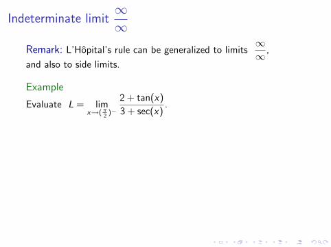
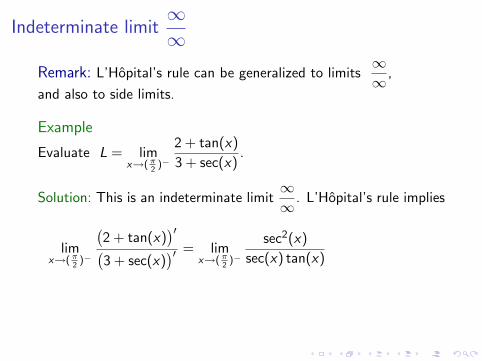
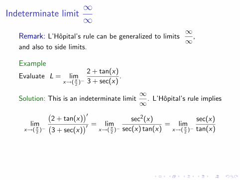
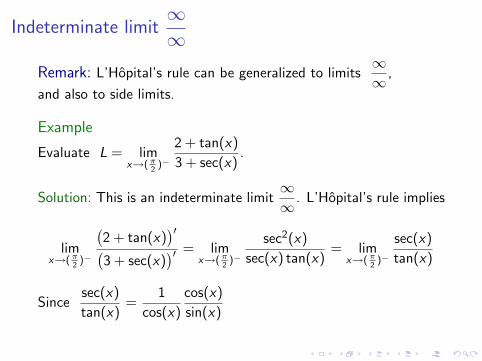
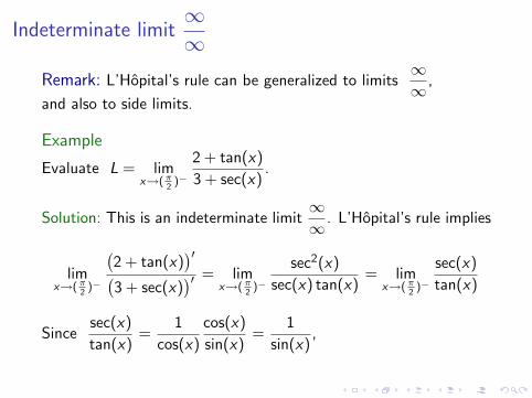
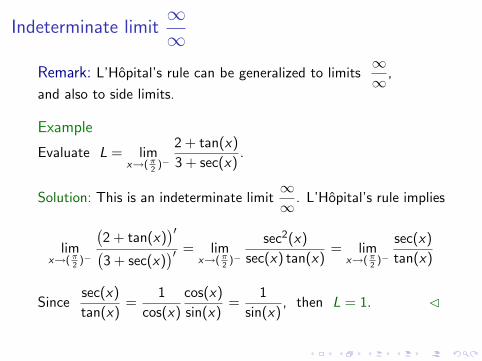
Remark: L’Hopital’s rule can be generalized to limits∞∞
,
and also to side limits.
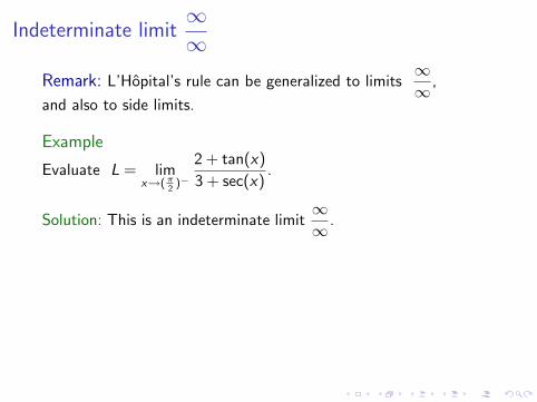
Example
Evaluate L = limx→(π
2)−
2 + tan(x)
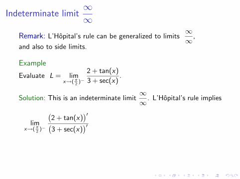
3 + sec(x).
Solution: This is an indeterminate limit∞∞
. L’Hopital’s rule implies
limx→(π
2)−
(2 + tan(x)
)′(3 + sec(x)
)′ = limx→(π
2)−
sec2(x)
sec(x) tan(x)= lim
x→(π2)−
sec(x)
tan(x)
Sincesec(x)
tan(x)=
1
cos(x)
cos(x)
sin(x)=
1
sin(x), then L = 1. C
Indeterminate limit∞∞
Remark: L’Hopital’s rule can be generalized to limits∞∞
,
and also to side limits.
Example
Evaluate L = limx→(π
2)−
2 + tan(x)
3 + sec(x).
Solution: This is an indeterminate limit∞∞
.
L’Hopital’s rule implies
limx→(π
2)−
(2 + tan(x)
)′(3 + sec(x)
)′ = limx→(π
2)−
sec2(x)
sec(x) tan(x)= lim
x→(π2)−
sec(x)
tan(x)
Sincesec(x)
tan(x)=
1
cos(x)
cos(x)
sin(x)=
1
sin(x), then L = 1. C
Indeterminate limit∞∞
Remark: L’Hopital’s rule can be generalized to limits∞∞
,
and also to side limits.
Example
Evaluate L = limx→(π
2)−
2 + tan(x)
3 + sec(x).
Solution: This is an indeterminate limit∞∞
. L’Hopital’s rule implies
limx→(π
2)−
(2 + tan(x)
)′(3 + sec(x)
)′
= limx→(π
2)−
sec2(x)
sec(x) tan(x)= lim
x→(π2)−
sec(x)
tan(x)
Sincesec(x)
tan(x)=
1
cos(x)
cos(x)
sin(x)=
1
sin(x), then L = 1. C
Indeterminate limit∞∞
Remark: L’Hopital’s rule can be generalized to limits∞∞
,
and also to side limits.
Example
Evaluate L = limx→(π
2)−
2 + tan(x)
3 + sec(x).
Solution: This is an indeterminate limit∞∞
. L’Hopital’s rule implies
limx→(π
2)−
(2 + tan(x)
)′(3 + sec(x)
)′ = limx→(π
2)−
sec2(x)
sec(x) tan(x)
= limx→(π
2)−
sec(x)
tan(x)
Sincesec(x)
tan(x)=
1
cos(x)
cos(x)
sin(x)=
1
sin(x), then L = 1. C
Indeterminate limit∞∞
Remark: L’Hopital’s rule can be generalized to limits∞∞
,
and also to side limits.
Example
Evaluate L = limx→(π
2)−
2 + tan(x)
3 + sec(x).
Solution: This is an indeterminate limit∞∞
. L’Hopital’s rule implies
limx→(π
2)−
(2 + tan(x)
)′(3 + sec(x)
)′ = limx→(π
2)−
sec2(x)
sec(x) tan(x)= lim
x→(π2)−
sec(x)
tan(x)
Sincesec(x)
tan(x)=
1
cos(x)
cos(x)
sin(x)=
1
sin(x), then L = 1. C
Indeterminate limit∞∞
Remark: L’Hopital’s rule can be generalized to limits∞∞
,
and also to side limits.
Example
Evaluate L = limx→(π
2)−
2 + tan(x)
3 + sec(x).
Solution: This is an indeterminate limit∞∞
. L’Hopital’s rule implies
limx→(π
2)−
(2 + tan(x)
)′(3 + sec(x)
)′ = limx→(π
2)−
sec2(x)
sec(x) tan(x)= lim
x→(π2)−
sec(x)
tan(x)
Sincesec(x)
tan(x)=
1
cos(x)
cos(x)
sin(x)
=1
sin(x), then L = 1. C
Indeterminate limit∞∞
Remark: L’Hopital’s rule can be generalized to limits∞∞
,
and also to side limits.
Example
Evaluate L = limx→(π
2)−
2 + tan(x)
3 + sec(x).
Solution: This is an indeterminate limit∞∞
. L’Hopital’s rule implies
limx→(π
2)−
(2 + tan(x)
)′(3 + sec(x)
)′ = limx→(π
2)−
sec2(x)
sec(x) tan(x)= lim
x→(π2)−
sec(x)
tan(x)
Sincesec(x)
tan(x)=
1
cos(x)
cos(x)
sin(x)=
1
sin(x),
then L = 1. C
Indeterminate limit∞∞
Remark: L’Hopital’s rule can be generalized to limits∞∞
,
and also to side limits.
Example
Evaluate L = limx→(π
2)−
2 + tan(x)
3 + sec(x).
Solution: This is an indeterminate limit∞∞
. L’Hopital’s rule implies
limx→(π
2)−
(2 + tan(x)
)′(3 + sec(x)
)′ = limx→(π
2)−
sec2(x)
sec(x) tan(x)= lim
x→(π2)−
sec(x)
tan(x)
Sincesec(x)
tan(x)=
1
cos(x)
cos(x)
sin(x)=
1
sin(x), then L = 1. C
Indeterminate limit∞∞
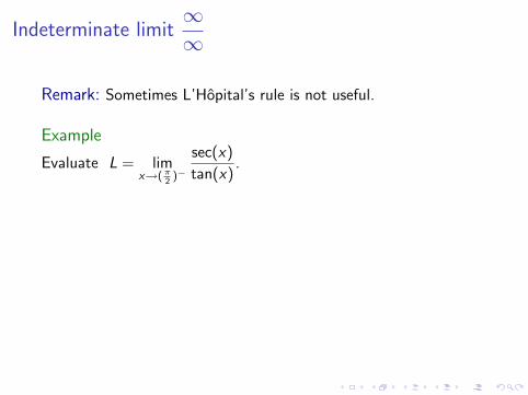
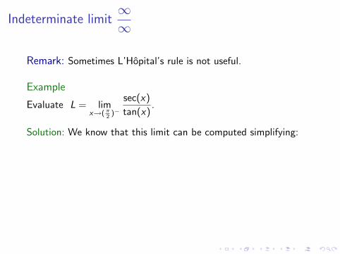
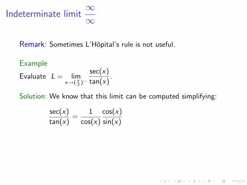
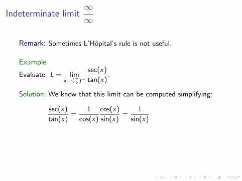
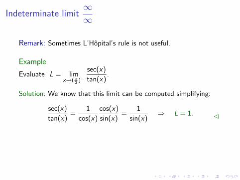
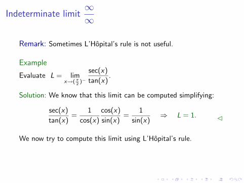
Remark: Sometimes L’Hopital’s rule is not useful.
Example
Evaluate L = limx→(π
2)−
sec(x)
tan(x).
Solution: We know that this limit can be computed simplifying:
sec(x)
tan(x)=
1
cos(x)
cos(x)
sin(x)=
1
sin(x)⇒ L = 1. C
We now try to compute this limit using L’Hopital’s rule.
Indeterminate limit∞∞
Remark: Sometimes L’Hopital’s rule is not useful.
Example
Evaluate L = limx→(π
2)−
sec(x)
tan(x).
Solution: We know that this limit can be computed simplifying:
sec(x)
tan(x)=
1
cos(x)
cos(x)
sin(x)=
1
sin(x)⇒ L = 1. C
We now try to compute this limit using L’Hopital’s rule.
Indeterminate limit∞∞
Remark: Sometimes L’Hopital’s rule is not useful.
Example
Evaluate L = limx→(π
2)−
sec(x)
tan(x).
Solution: We know that this limit can be computed simplifying:
sec(x)
tan(x)=
1
cos(x)
cos(x)
sin(x)
=1
sin(x)⇒ L = 1. C
We now try to compute this limit using L’Hopital’s rule.
Indeterminate limit∞∞
Remark: Sometimes L’Hopital’s rule is not useful.
Example
Evaluate L = limx→(π
2)−
sec(x)
tan(x).
Solution: We know that this limit can be computed simplifying:
sec(x)
tan(x)=
1
cos(x)
cos(x)
sin(x)=
1
sin(x)
⇒ L = 1. C
We now try to compute this limit using L’Hopital’s rule.
Indeterminate limit∞∞
Remark: Sometimes L’Hopital’s rule is not useful.
Example
Evaluate L = limx→(π
2)−
sec(x)
tan(x).
Solution: We know that this limit can be computed simplifying:
sec(x)
tan(x)=
1
cos(x)
cos(x)
sin(x)=
1
sin(x)⇒ L = 1. C
We now try to compute this limit using L’Hopital’s rule.
Indeterminate limit∞∞
Remark: Sometimes L’Hopital’s rule is not useful.
Example
Evaluate L = limx→(π
2)−
sec(x)
tan(x).
Solution: We know that this limit can be computed simplifying:
sec(x)
tan(x)=
1
cos(x)
cos(x)
sin(x)=
1
sin(x)⇒ L = 1. C
We now try to compute this limit using L’Hopital’s rule.
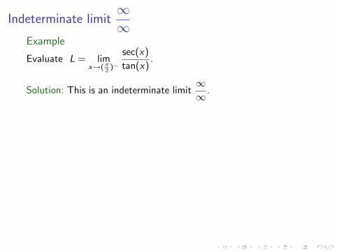
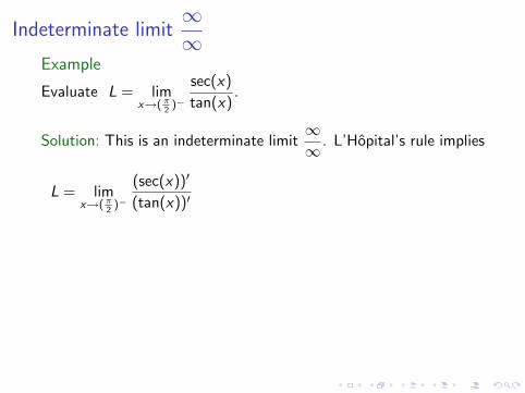
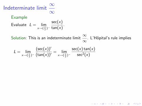
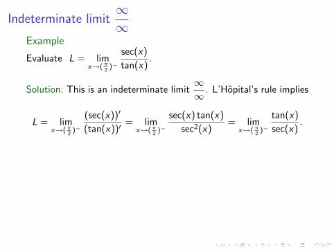
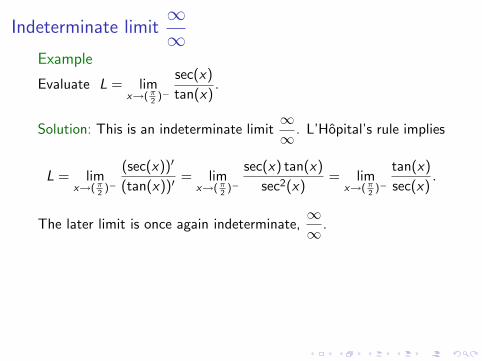
Indeterminate limit∞∞
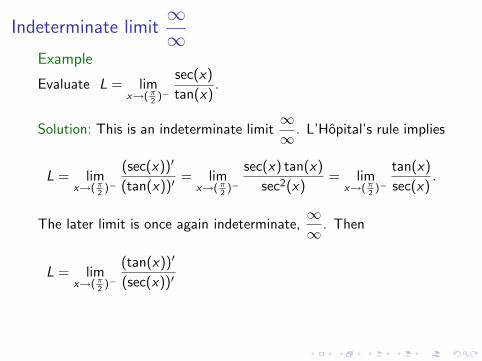
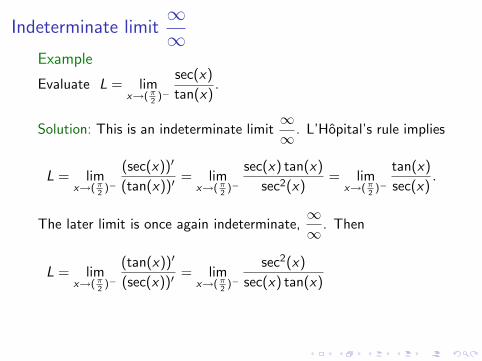
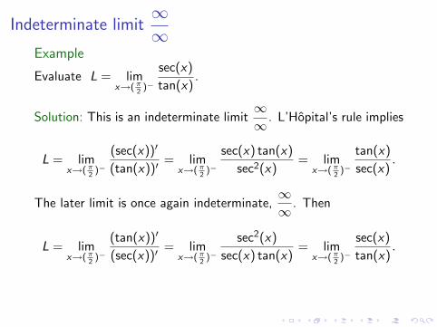
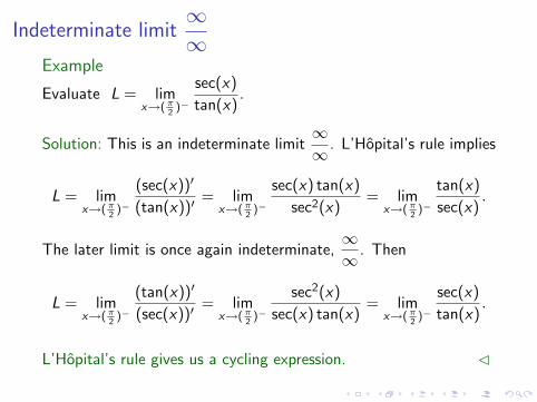
Example
Evaluate L = limx→(π
2)−
sec(x)
tan(x).
Solution: This is an indeterminate limit∞∞
.
L’Hopital’s rule implies
L = limx→(π
2)−
(sec(x))′
(tan(x))′= lim
x→(π2)−
sec(x) tan(x)
sec2(x)= lim
x→(π2)−
tan(x)
sec(x).
The later limit is once again indeterminate,∞∞
. Then
L = limx→(π
2)−
(tan(x))′
(sec(x))′= lim
x→(π2)−
sec2(x)
sec(x) tan(x)= lim
x→(π2)−
sec(x)
tan(x).
L’Hopital’s rule gives us a cycling expression. C
Indeterminate limit∞∞
Example
Evaluate L = limx→(π
2)−
sec(x)
tan(x).
Solution: This is an indeterminate limit∞∞
. L’Hopital’s rule implies
L = limx→(π
2)−
(sec(x))′
(tan(x))′
= limx→(π
2)−
sec(x) tan(x)
sec2(x)= lim
x→(π2)−
tan(x)
sec(x).
The later limit is once again indeterminate,∞∞
. Then
L = limx→(π
2)−
(tan(x))′
(sec(x))′= lim
x→(π2)−
sec2(x)
sec(x) tan(x)= lim
x→(π2)−
sec(x)
tan(x).
L’Hopital’s rule gives us a cycling expression. C
Indeterminate limit∞∞
Example
Evaluate L = limx→(π
2)−
sec(x)
tan(x).
Solution: This is an indeterminate limit∞∞
. L’Hopital’s rule implies
L = limx→(π
2)−
(sec(x))′
(tan(x))′= lim
x→(π2)−
sec(x) tan(x)
sec2(x)
= limx→(π
2)−
tan(x)
sec(x).
The later limit is once again indeterminate,∞∞
. Then
L = limx→(π
2)−
(tan(x))′
(sec(x))′= lim
x→(π2)−
sec2(x)
sec(x) tan(x)= lim
x→(π2)−
sec(x)
tan(x).
L’Hopital’s rule gives us a cycling expression. C
Indeterminate limit∞∞
Example
Evaluate L = limx→(π
2)−
sec(x)
tan(x).
Solution: This is an indeterminate limit∞∞
. L’Hopital’s rule implies
L = limx→(π
2)−
(sec(x))′
(tan(x))′= lim
x→(π2)−
sec(x) tan(x)
sec2(x)= lim
x→(π2)−
tan(x)
sec(x).
The later limit is once again indeterminate,∞∞
. Then
L = limx→(π
2)−
(tan(x))′
(sec(x))′= lim
x→(π2)−
sec2(x)
sec(x) tan(x)= lim
x→(π2)−
sec(x)
tan(x).
L’Hopital’s rule gives us a cycling expression. C
Indeterminate limit∞∞
Example
Evaluate L = limx→(π
2)−
sec(x)
tan(x).
Solution: This is an indeterminate limit∞∞
. L’Hopital’s rule implies
L = limx→(π
2)−
(sec(x))′
(tan(x))′= lim
x→(π2)−
sec(x) tan(x)
sec2(x)= lim
x→(π2)−
tan(x)
sec(x).
The later limit is once again indeterminate,∞∞
.
Then
L = limx→(π
2)−
(tan(x))′
(sec(x))′= lim
x→(π2)−
sec2(x)
sec(x) tan(x)= lim
x→(π2)−
sec(x)
tan(x).
L’Hopital’s rule gives us a cycling expression. C
Indeterminate limit∞∞
Example
Evaluate L = limx→(π
2)−
sec(x)
tan(x).
Solution: This is an indeterminate limit∞∞
. L’Hopital’s rule implies
L = limx→(π
2)−
(sec(x))′
(tan(x))′= lim
x→(π2)−
sec(x) tan(x)
sec2(x)= lim
x→(π2)−
tan(x)
sec(x).
The later limit is once again indeterminate,∞∞
. Then
L = limx→(π
2)−
(tan(x))′
(sec(x))′
= limx→(π
2)−
sec2(x)
sec(x) tan(x)= lim
x→(π2)−
sec(x)
tan(x).
L’Hopital’s rule gives us a cycling expression. C
Indeterminate limit∞∞
Example
Evaluate L = limx→(π
2)−
sec(x)
tan(x).
Solution: This is an indeterminate limit∞∞
. L’Hopital’s rule implies
L = limx→(π
2)−
(sec(x))′
(tan(x))′= lim
x→(π2)−
sec(x) tan(x)
sec2(x)= lim
x→(π2)−
tan(x)
sec(x).
The later limit is once again indeterminate,∞∞
. Then
L = limx→(π
2)−
(tan(x))′
(sec(x))′= lim
x→(π2)−
sec2(x)
sec(x) tan(x)
= limx→(π
2)−
sec(x)
tan(x).
L’Hopital’s rule gives us a cycling expression. C
Indeterminate limit∞∞
Example
Evaluate L = limx→(π
2)−
sec(x)
tan(x).
Solution: This is an indeterminate limit∞∞
. L’Hopital’s rule implies
L = limx→(π
2)−
(sec(x))′
(tan(x))′= lim
x→(π2)−
sec(x) tan(x)
sec2(x)= lim
x→(π2)−
tan(x)
sec(x).
The later limit is once again indeterminate,∞∞
. Then
L = limx→(π
2)−
(tan(x))′
(sec(x))′= lim
x→(π2)−
sec2(x)
sec(x) tan(x)= lim
x→(π2)−
sec(x)
tan(x).
L’Hopital’s rule gives us a cycling expression. C
Indeterminate limit∞∞
Example
Evaluate L = limx→(π
2)−
sec(x)
tan(x).
Solution: This is an indeterminate limit∞∞
. L’Hopital’s rule implies
L = limx→(π
2)−
(sec(x))′
(tan(x))′= lim
x→(π2)−
sec(x) tan(x)
sec2(x)= lim
x→(π2)−
tan(x)
sec(x).
The later limit is once again indeterminate,∞∞
. Then
L = limx→(π
2)−
(tan(x))′
(sec(x))′= lim
x→(π2)−
sec2(x)
sec(x) tan(x)= lim
x→(π2)−
sec(x)
tan(x).
L’Hopital’s rule gives us a cycling expression. C
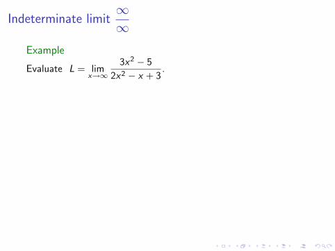
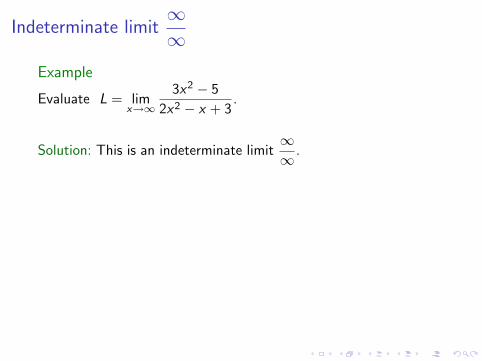
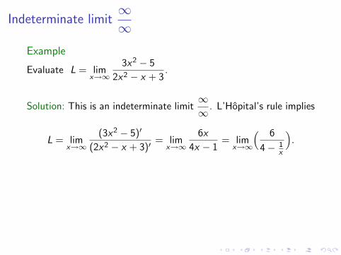
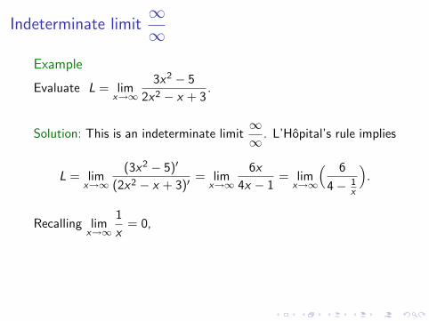
Indeterminate limit∞∞
Example
Evaluate L = limx→∞
3x2 − 5
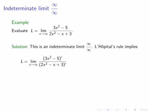
2x2 − x + 3.
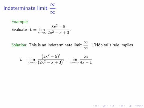
Solution: This is an indeterminate limit∞∞
. L’Hopital’s rule implies
L = limx→∞
(3x2 − 5)′
(2x2 − x + 3)′= lim
x→∞
6x
4x − 1= lim
x→∞
( 6
4− 1x
).
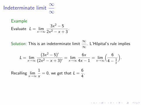
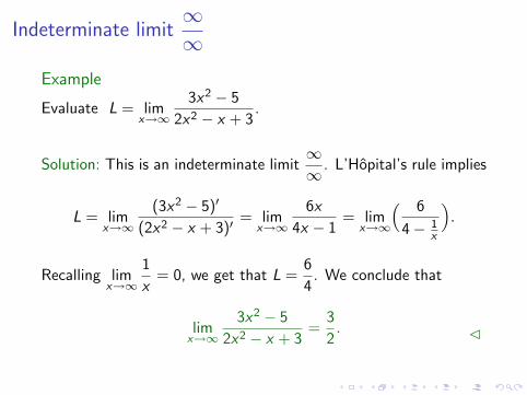
Recalling limx→∞
1
x= 0, we get that L =
6
4. We conclude that
limx→∞
3x2 − 5
2x2 − x + 3=
3
2. C
Indeterminate limit∞∞
Example
Evaluate L = limx→∞
3x2 − 5
2x2 − x + 3.
Solution: This is an indeterminate limit∞∞
.
L’Hopital’s rule implies
L = limx→∞
(3x2 − 5)′
(2x2 − x + 3)′= lim
x→∞
6x
4x − 1= lim
x→∞
( 6
4− 1x
).
Recalling limx→∞
1
x= 0, we get that L =
6
4. We conclude that
limx→∞
3x2 − 5
2x2 − x + 3=
3
2. C
Indeterminate limit∞∞
Example
Evaluate L = limx→∞
3x2 − 5
2x2 − x + 3.
Solution: This is an indeterminate limit∞∞
. L’Hopital’s rule implies
L = limx→∞
(3x2 − 5)′
(2x2 − x + 3)′
= limx→∞
6x
4x − 1= lim
x→∞
( 6
4− 1x
).
Recalling limx→∞
1
x= 0, we get that L =
6
4. We conclude that
limx→∞
3x2 − 5
2x2 − x + 3=
3
2. C
Indeterminate limit∞∞
Example
Evaluate L = limx→∞
3x2 − 5
2x2 − x + 3.
Solution: This is an indeterminate limit∞∞
. L’Hopital’s rule implies
L = limx→∞
(3x2 − 5)′
(2x2 − x + 3)′= lim
x→∞
6x
4x − 1
= limx→∞
( 6
4− 1x
).
Recalling limx→∞
1
x= 0, we get that L =
6
4. We conclude that
limx→∞
3x2 − 5
2x2 − x + 3=
3
2. C
Indeterminate limit∞∞
Example
Evaluate L = limx→∞
3x2 − 5
2x2 − x + 3.
Solution: This is an indeterminate limit∞∞
. L’Hopital’s rule implies
L = limx→∞
(3x2 − 5)′
(2x2 − x + 3)′= lim
x→∞
6x
4x − 1= lim
x→∞
( 6
4− 1x
).
Recalling limx→∞
1
x= 0, we get that L =
6
4. We conclude that
limx→∞
3x2 − 5
2x2 − x + 3=
3
2. C
Indeterminate limit∞∞
Example
Evaluate L = limx→∞
3x2 − 5
2x2 − x + 3.
Solution: This is an indeterminate limit∞∞
. L’Hopital’s rule implies
L = limx→∞
(3x2 − 5)′
(2x2 − x + 3)′= lim
x→∞
6x
4x − 1= lim
x→∞
( 6
4− 1x
).
Recalling limx→∞
1
x= 0,
we get that L =6
4. We conclude that
limx→∞
3x2 − 5
2x2 − x + 3=
3
2. C
Indeterminate limit∞∞
Example
Evaluate L = limx→∞
3x2 − 5
2x2 − x + 3.
Solution: This is an indeterminate limit∞∞
. L’Hopital’s rule implies
L = limx→∞
(3x2 − 5)′
(2x2 − x + 3)′= lim
x→∞
6x
4x − 1= lim
x→∞
( 6
4− 1x
).
Recalling limx→∞
1
x= 0, we get that L =
6
4.
We conclude that
limx→∞
3x2 − 5
2x2 − x + 3=
3
2. C
Indeterminate limit∞∞
Example
Evaluate L = limx→∞
3x2 − 5
2x2 − x + 3.
Solution: This is an indeterminate limit∞∞
. L’Hopital’s rule implies
L = limx→∞
(3x2 − 5)′
(2x2 − x + 3)′= lim
x→∞
6x
4x − 1= lim
x→∞
( 6
4− 1x
).
Recalling limx→∞
1
x= 0, we get that L =
6
4. We conclude that
limx→∞
3x2 − 5
2x2 − x + 3=
3
2. C
Limits using L’Hopital’s Rule (Sect. 7.5)
I Review: L’Hopital’s rule for indeterminate limits0
0.
I Indeterminate limit∞∞
.
I Indeterminate limits ∞ · 0 and ∞−∞.
I Overview of improper integrals (Sect. 8.7).
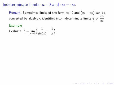
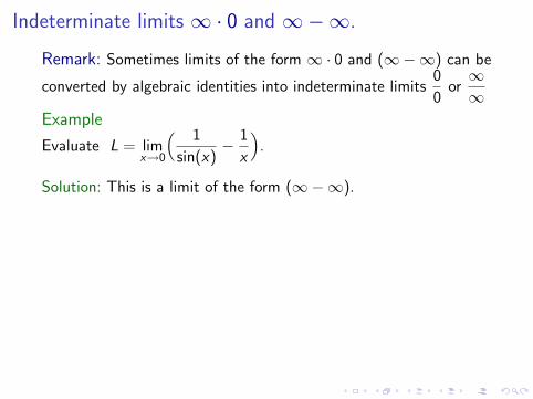
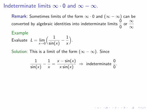
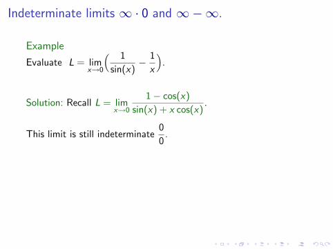
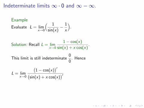
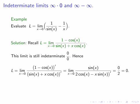
Indeterminate limits ∞ · 0 and ∞−∞.
Remark: Sometimes limits of the form ∞ · 0 and (∞−∞) can be
converted by algebraic identities into indeterminate limits0
0or∞∞
Example
Evaluate L = limx→0
( 1
sin(x)− 1
x
).
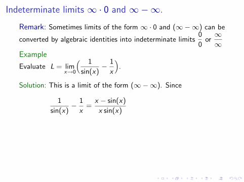
Solution: This is a limit of the form (∞−∞). Since
1
sin(x)− 1
x=
x − sin(x)
x sin(x)⇒ indeterminate
0
0.
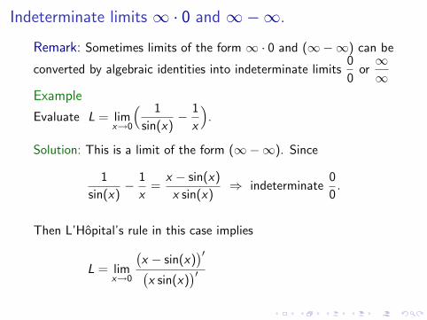
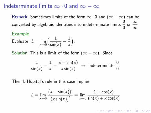
Then L’Hopital’s rule in this case implies
L = limx→0
(x − sin(x)
)′(x sin(x)
)′ = limx→0
1− cos(x)
sin(x) + x cos(x)
Indeterminate limits ∞ · 0 and ∞−∞.
Remark: Sometimes limits of the form ∞ · 0 and (∞−∞) can be
converted by algebraic identities into indeterminate limits0
0or∞∞
Example
Evaluate L = limx→0
( 1
sin(x)− 1
x
).
Solution: This is a limit of the form (∞−∞).
Since
1
sin(x)− 1
x=
x − sin(x)
x sin(x)⇒ indeterminate
0
0.
Then L’Hopital’s rule in this case implies
L = limx→0
(x − sin(x)
)′(x sin(x)
)′ = limx→0
1− cos(x)
sin(x) + x cos(x)
Indeterminate limits ∞ · 0 and ∞−∞.
Remark: Sometimes limits of the form ∞ · 0 and (∞−∞) can be
converted by algebraic identities into indeterminate limits0
0or∞∞
Example
Evaluate L = limx→0
( 1
sin(x)− 1
x
).
Solution: This is a limit of the form (∞−∞). Since
1
sin(x)− 1
x=
x − sin(x)
x sin(x)
⇒ indeterminate0
0.
Then L’Hopital’s rule in this case implies
L = limx→0
(x − sin(x)
)′(x sin(x)
)′ = limx→0
1− cos(x)
sin(x) + x cos(x)
Indeterminate limits ∞ · 0 and ∞−∞.
Remark: Sometimes limits of the form ∞ · 0 and (∞−∞) can be
converted by algebraic identities into indeterminate limits0
0or∞∞
Example
Evaluate L = limx→0
( 1
sin(x)− 1
x
).
Solution: This is a limit of the form (∞−∞). Since
1
sin(x)− 1
x=
x − sin(x)
x sin(x)⇒ indeterminate
0
0.
Then L’Hopital’s rule in this case implies
L = limx→0
(x − sin(x)
)′(x sin(x)
)′ = limx→0
1− cos(x)
sin(x) + x cos(x)
Indeterminate limits ∞ · 0 and ∞−∞.
Remark: Sometimes limits of the form ∞ · 0 and (∞−∞) can be
converted by algebraic identities into indeterminate limits0
0or∞∞
Example
Evaluate L = limx→0
( 1
sin(x)− 1
x
).
Solution: This is a limit of the form (∞−∞). Since
1
sin(x)− 1
x=
x − sin(x)
x sin(x)⇒ indeterminate
0
0.
Then L’Hopital’s rule in this case implies
L = limx→0
(x − sin(x)
)′(x sin(x)
)′
= limx→0
1− cos(x)
sin(x) + x cos(x)
Indeterminate limits ∞ · 0 and ∞−∞.
Remark: Sometimes limits of the form ∞ · 0 and (∞−∞) can be
converted by algebraic identities into indeterminate limits0
0or∞∞
Example
Evaluate L = limx→0
( 1
sin(x)− 1
x
).
Solution: This is a limit of the form (∞−∞). Since
1
sin(x)− 1
x=
x − sin(x)
x sin(x)⇒ indeterminate
0
0.
Then L’Hopital’s rule in this case implies
L = limx→0
(x − sin(x)
)′(x sin(x)
)′ = limx→0
1− cos(x)
sin(x) + x cos(x)
Indeterminate limits ∞ · 0 and ∞−∞.
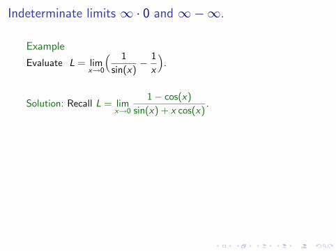
Example
Evaluate L = limx→0
( 1
sin(x)− 1
x
).
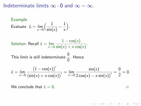
Solution: Recall L = limx→0
1− cos(x)
sin(x) + x cos(x).
This limit is still indeterminate0
0. Hence
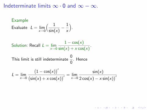
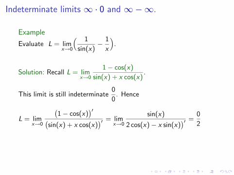
L = limx→0
(1− cos(x)
)′(sin(x) + x cos(x)
)′ = limx→0
sin(x)
2 cos(x)− x sin(x))′ =
0
2= 0.
We conclude that L = 0. C
Indeterminate limits ∞ · 0 and ∞−∞.
Example
Evaluate L = limx→0
( 1
sin(x)− 1
x
).
Solution: Recall L = limx→0
1− cos(x)
sin(x) + x cos(x).
This limit is still indeterminate0
0.
Hence
L = limx→0
(1− cos(x)
)′(sin(x) + x cos(x)
)′ = limx→0
sin(x)
2 cos(x)− x sin(x))′ =
0
2= 0.
We conclude that L = 0. C
Indeterminate limits ∞ · 0 and ∞−∞.
Example
Evaluate L = limx→0
( 1
sin(x)− 1
x
).
Solution: Recall L = limx→0
1− cos(x)
sin(x) + x cos(x).
This limit is still indeterminate0
0. Hence
L = limx→0
(1− cos(x)
)′(sin(x) + x cos(x)
)′
= limx→0
sin(x)
2 cos(x)− x sin(x))′ =
0
2= 0.
We conclude that L = 0. C
Indeterminate limits ∞ · 0 and ∞−∞.
Example
Evaluate L = limx→0
( 1
sin(x)− 1
x
).
Solution: Recall L = limx→0
1− cos(x)
sin(x) + x cos(x).
This limit is still indeterminate0
0. Hence
L = limx→0
(1− cos(x)
)′(sin(x) + x cos(x)
)′ = limx→0
sin(x)
2 cos(x)− x sin(x))′
=0
2= 0.
We conclude that L = 0. C
Indeterminate limits ∞ · 0 and ∞−∞.
Example
Evaluate L = limx→0
( 1
sin(x)− 1
x
).
Solution: Recall L = limx→0
1− cos(x)
sin(x) + x cos(x).
This limit is still indeterminate0
0. Hence
L = limx→0
(1− cos(x)
)′(sin(x) + x cos(x)
)′ = limx→0
sin(x)
2 cos(x)− x sin(x))′ =
0
2
= 0.
We conclude that L = 0. C
Indeterminate limits ∞ · 0 and ∞−∞.
Example
Evaluate L = limx→0
( 1
sin(x)− 1
x
).
Solution: Recall L = limx→0
1− cos(x)
sin(x) + x cos(x).
This limit is still indeterminate0
0. Hence
L = limx→0
(1− cos(x)
)′(sin(x) + x cos(x)
)′ = limx→0
sin(x)
2 cos(x)− x sin(x))′ =
0
2= 0.
We conclude that L = 0. C
Indeterminate limits ∞ · 0 and ∞−∞.
Example
Evaluate L = limx→0
( 1
sin(x)− 1
x
).
Solution: Recall L = limx→0
1− cos(x)
sin(x) + x cos(x).
This limit is still indeterminate0
0. Hence
L = limx→0
(1− cos(x)
)′(sin(x) + x cos(x)
)′ = limx→0
sin(x)
2 cos(x)− x sin(x))′ =
0
2= 0.
We conclude that L = 0. C
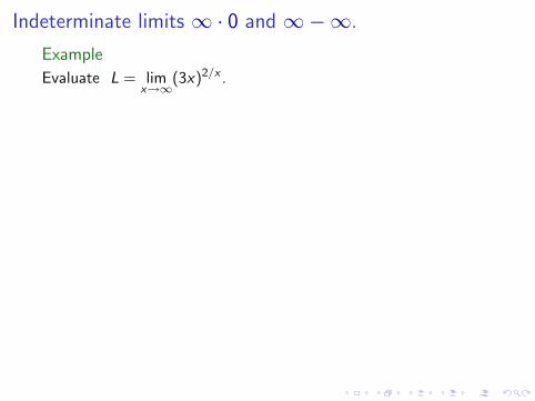
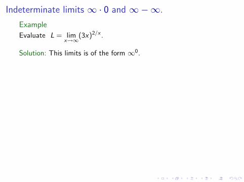
Indeterminate limits ∞ · 0 and ∞−∞.
Example
Evaluate L = limx→∞
(3x)2/x .
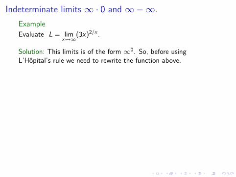
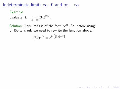
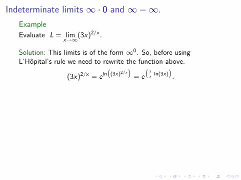
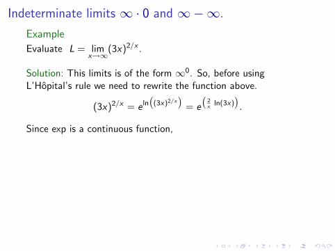
Solution: This limits is of the form ∞0. So, before usingL’Hopital’s rule we need to rewrite the function above.
(3x)2/x = e ln((3x)2/x
)= e
(2x
ln(3x)).
Since exp is a continuous function, holds
limx→∞
(3x)2/x = e limx→∞(
2x
ln(3x))
= e limx→∞(
2 ln(3x)x
).
The exponent, is an indeterminate limit ∞∞ . L’Hopital’s rule implies
limx→∞
2 ln(3x)
x= lim
x→∞
(2 ln(3x)
)′(x)′
= limx→∞
2/x
1= 0.
We conclude that L = e0, that is, L = 1. C
Indeterminate limits ∞ · 0 and ∞−∞.
Example
Evaluate L = limx→∞
(3x)2/x .
Solution: This limits is of the form ∞0.
So, before usingL’Hopital’s rule we need to rewrite the function above.
(3x)2/x = e ln((3x)2/x
)= e
(2x
ln(3x)).
Since exp is a continuous function, holds
limx→∞
(3x)2/x = e limx→∞(
2x
ln(3x))
= e limx→∞(
2 ln(3x)x
).
The exponent, is an indeterminate limit ∞∞ . L’Hopital’s rule implies
limx→∞
2 ln(3x)
x= lim
x→∞
(2 ln(3x)
)′(x)′
= limx→∞
2/x
1= 0.
We conclude that L = e0, that is, L = 1. C
Indeterminate limits ∞ · 0 and ∞−∞.
Example
Evaluate L = limx→∞
(3x)2/x .
Solution: This limits is of the form ∞0. So, before usingL’Hopital’s rule we need to rewrite the function above.
(3x)2/x = e ln((3x)2/x
)= e
(2x
ln(3x)).
Since exp is a continuous function, holds
limx→∞
(3x)2/x = e limx→∞(
2x
ln(3x))
= e limx→∞(
2 ln(3x)x
).
The exponent, is an indeterminate limit ∞∞ . L’Hopital’s rule implies
limx→∞
2 ln(3x)
x= lim
x→∞
(2 ln(3x)
)′(x)′
= limx→∞
2/x
1= 0.
We conclude that L = e0, that is, L = 1. C
Indeterminate limits ∞ · 0 and ∞−∞.
Example
Evaluate L = limx→∞
(3x)2/x .
Solution: This limits is of the form ∞0. So, before usingL’Hopital’s rule we need to rewrite the function above.
(3x)2/x = e ln((3x)2/x
)
= e
(2x
ln(3x)).
Since exp is a continuous function, holds
limx→∞
(3x)2/x = e limx→∞(
2x
ln(3x))
= e limx→∞(
2 ln(3x)x
).
The exponent, is an indeterminate limit ∞∞ . L’Hopital’s rule implies
limx→∞
2 ln(3x)
x= lim
x→∞
(2 ln(3x)
)′(x)′
= limx→∞
2/x
1= 0.
We conclude that L = e0, that is, L = 1. C
Indeterminate limits ∞ · 0 and ∞−∞.
Example
Evaluate L = limx→∞
(3x)2/x .
Solution: This limits is of the form ∞0. So, before usingL’Hopital’s rule we need to rewrite the function above.
(3x)2/x = e ln((3x)2/x
)= e
(2x
ln(3x)).
Since exp is a continuous function, holds
limx→∞
(3x)2/x = e limx→∞(
2x
ln(3x))
= e limx→∞(
2 ln(3x)x
).
The exponent, is an indeterminate limit ∞∞ . L’Hopital’s rule implies
limx→∞
2 ln(3x)
x= lim
x→∞
(2 ln(3x)
)′(x)′
= limx→∞
2/x
1= 0.
We conclude that L = e0, that is, L = 1. C
Indeterminate limits ∞ · 0 and ∞−∞.
Example
Evaluate L = limx→∞
(3x)2/x .
Solution: This limits is of the form ∞0. So, before usingL’Hopital’s rule we need to rewrite the function above.
(3x)2/x = e ln((3x)2/x
)= e
(2x
ln(3x)).
Since exp is a continuous function,
holds
limx→∞
(3x)2/x = e limx→∞(
2x
ln(3x))
= e limx→∞(
2 ln(3x)x
).
The exponent, is an indeterminate limit ∞∞ . L’Hopital’s rule implies
limx→∞
2 ln(3x)
x= lim
x→∞
(2 ln(3x)
)′(x)′
= limx→∞
2/x
1= 0.
We conclude that L = e0, that is, L = 1. C
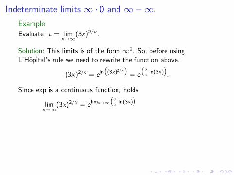
Indeterminate limits ∞ · 0 and ∞−∞.
Example
Evaluate L = limx→∞
(3x)2/x .
Solution: This limits is of the form ∞0. So, before usingL’Hopital’s rule we need to rewrite the function above.
(3x)2/x = e ln((3x)2/x
)= e
(2x
ln(3x)).
Since exp is a continuous function, holds
limx→∞
(3x)2/x = e limx→∞(
2x
ln(3x))
= e limx→∞(
2 ln(3x)x
).
The exponent, is an indeterminate limit ∞∞ . L’Hopital’s rule implies
limx→∞
2 ln(3x)
x= lim
x→∞
(2 ln(3x)
)′(x)′
= limx→∞
2/x
1= 0.
We conclude that L = e0, that is, L = 1. C
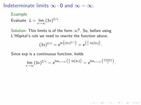
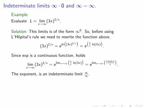
Indeterminate limits ∞ · 0 and ∞−∞.
Example
Evaluate L = limx→∞
(3x)2/x .
Solution: This limits is of the form ∞0. So, before usingL’Hopital’s rule we need to rewrite the function above.
(3x)2/x = e ln((3x)2/x
)= e
(2x
ln(3x)).
Since exp is a continuous function, holds
limx→∞
(3x)2/x = e limx→∞(
2x
ln(3x))
= e limx→∞(
2 ln(3x)x
).
The exponent, is an indeterminate limit ∞∞ .
L’Hopital’s rule implies
limx→∞
2 ln(3x)
x= lim
x→∞
(2 ln(3x)
)′(x)′
= limx→∞
2/x
1= 0.
We conclude that L = e0, that is, L = 1. C
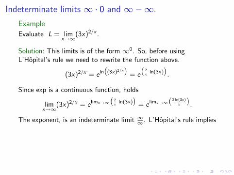
Indeterminate limits ∞ · 0 and ∞−∞.
Example
Evaluate L = limx→∞
(3x)2/x .
Solution: This limits is of the form ∞0. So, before usingL’Hopital’s rule we need to rewrite the function above.
(3x)2/x = e ln((3x)2/x
)= e
(2x
ln(3x)).
Since exp is a continuous function, holds
limx→∞
(3x)2/x = e limx→∞(
2x
ln(3x))
= e limx→∞(
2 ln(3x)x
).
The exponent, is an indeterminate limit ∞∞ . L’Hopital’s rule implies
limx→∞
2 ln(3x)
x= lim
x→∞
(2 ln(3x)
)′(x)′
= limx→∞
2/x
1= 0.
We conclude that L = e0, that is, L = 1. C
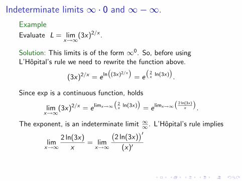
Indeterminate limits ∞ · 0 and ∞−∞.
Example
Evaluate L = limx→∞
(3x)2/x .
Solution: This limits is of the form ∞0. So, before usingL’Hopital’s rule we need to rewrite the function above.
(3x)2/x = e ln((3x)2/x
)= e
(2x
ln(3x)).
Since exp is a continuous function, holds
limx→∞
(3x)2/x = e limx→∞(
2x
ln(3x))
= e limx→∞(
2 ln(3x)x
).
The exponent, is an indeterminate limit ∞∞ . L’Hopital’s rule implies
limx→∞
2 ln(3x)
x= lim
x→∞
(2 ln(3x)
)′(x)′
= limx→∞
2/x
1= 0.
We conclude that L = e0, that is, L = 1. C
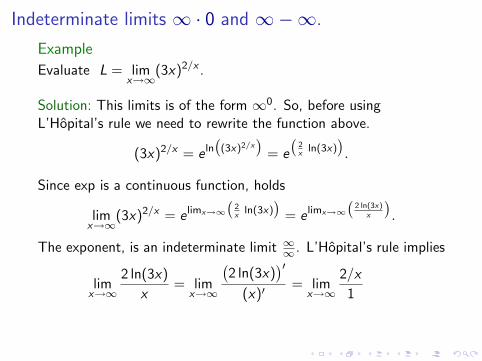
Indeterminate limits ∞ · 0 and ∞−∞.
Example
Evaluate L = limx→∞
(3x)2/x .
Solution: This limits is of the form ∞0. So, before usingL’Hopital’s rule we need to rewrite the function above.
(3x)2/x = e ln((3x)2/x
)= e
(2x
ln(3x)).
Since exp is a continuous function, holds
limx→∞
(3x)2/x = e limx→∞(
2x
ln(3x))
= e limx→∞(
2 ln(3x)x
).
The exponent, is an indeterminate limit ∞∞ . L’Hopital’s rule implies
limx→∞
2 ln(3x)
x= lim
x→∞
(2 ln(3x)
)′(x)′
= limx→∞
2/x
1
= 0.
We conclude that L = e0, that is, L = 1. C
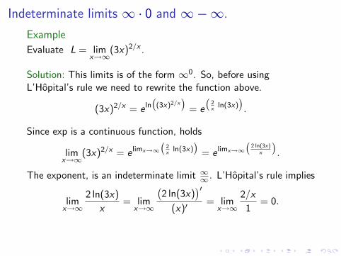
Indeterminate limits ∞ · 0 and ∞−∞.
Example
Evaluate L = limx→∞
(3x)2/x .
Solution: This limits is of the form ∞0. So, before usingL’Hopital’s rule we need to rewrite the function above.
(3x)2/x = e ln((3x)2/x
)= e
(2x
ln(3x)).
Since exp is a continuous function, holds
limx→∞
(3x)2/x = e limx→∞(
2x
ln(3x))
= e limx→∞(
2 ln(3x)x
).
The exponent, is an indeterminate limit ∞∞ . L’Hopital’s rule implies
limx→∞
2 ln(3x)
x= lim
x→∞
(2 ln(3x)
)′(x)′
= limx→∞
2/x
1= 0.
We conclude that L = e0, that is, L = 1. C
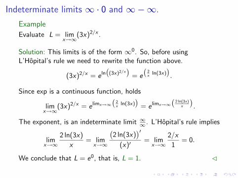
Indeterminate limits ∞ · 0 and ∞−∞.
Example
Evaluate L = limx→∞
(3x)2/x .
Solution: This limits is of the form ∞0. So, before usingL’Hopital’s rule we need to rewrite the function above.
(3x)2/x = e ln((3x)2/x
)= e
(2x
ln(3x)).
Since exp is a continuous function, holds
limx→∞
(3x)2/x = e limx→∞(
2x
ln(3x))
= e limx→∞(
2 ln(3x)x
).
The exponent, is an indeterminate limit ∞∞ . L’Hopital’s rule implies
limx→∞
2 ln(3x)
x= lim
x→∞
(2 ln(3x)
)′(x)′
= limx→∞
2/x
1= 0.
We conclude that L = e0, that is, L = 1. C
Limits using L’Hopital’s Rule (Sect. 7.5)
I Review: L’Hopital’s rule for indeterminate limits0
0.
I Indeterminate limit∞∞
.
I Indeterminate limits ∞ · 0 and ∞−∞.
I Overview of improper integrals (Sect. 8.7).
Overview of improper integrals (Sect. 8.7)
Remarks:
I L’Hopital’s rule is useful to compute improper integrals.
I Improper integrals are the limit of definite integrals when oneendpoint if integration approaches ±∞.
DefinitionThe improper integral of a continuous function f : [a,∞) → R is∫ ∞
af (x) dx = lim
b→∞
∫ b
af (x) dx .
The improper integral of a continuous function f : (−∞, b] → R is∫ b
−∞f (x) dx = lim
a→−∞
∫ b
af (x) dx .
The improper integral of a continuous function f : (−∞,∞) → R,∫ ∞
−∞f (x) dx =
∫ c
−∞f (x) dx +
∫ ∞
cf (x) dx .
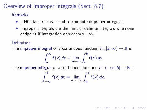
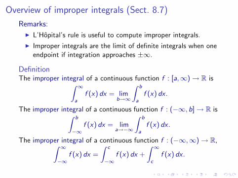
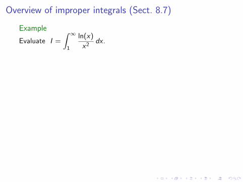
Overview of improper integrals (Sect. 8.7)
Example
Evaluate I =
∫ ∞
1
ln(x)
x2dx .
Solution: This is an improper integral:∫ ∞
1
ln(x)
x2dx = lim
b→∞
∫ b
1
ln(x)
x2
Integrating by parts, u = ln(x), and dv = dx/x2,∫ b
1
ln(x)
x2dx =
(−1
x
)ln(x)
∣∣∣b1−
∫ b
1
(1
x
)(−1
x
)dx
∫ b
1
ln(x)
x2dx = − ln(b)
b+
∫ b
1
dx
x2= − ln(b)
b− 1
x
∣∣∣b1.
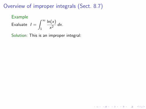
Overview of improper integrals (Sect. 8.7)
Example
Evaluate I =
∫ ∞
1
ln(x)
x2dx .
Solution: This is an improper integral:
∫ ∞
1
ln(x)
x2dx = lim
b→∞
∫ b
1
ln(x)
x2
Integrating by parts, u = ln(x), and dv = dx/x2,∫ b
1
ln(x)
x2dx =
(−1
x
)ln(x)
∣∣∣b1−
∫ b
1
(1
x
)(−1
x
)dx
∫ b
1
ln(x)
x2dx = − ln(b)
b+
∫ b
1
dx
x2= − ln(b)
b− 1
x
∣∣∣b1.
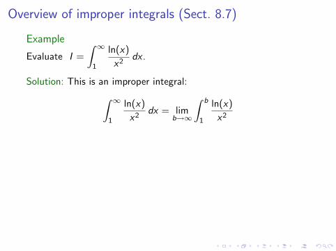
Overview of improper integrals (Sect. 8.7)
Example
Evaluate I =
∫ ∞
1
ln(x)
x2dx .
Solution: This is an improper integral:∫ ∞
1
ln(x)
x2dx = lim
b→∞
∫ b
1
ln(x)
x2
Integrating by parts, u = ln(x), and dv = dx/x2,∫ b
1
ln(x)
x2dx =
(−1
x
)ln(x)
∣∣∣b1−
∫ b
1
(1
x
)(−1
x
)dx
∫ b
1
ln(x)
x2dx = − ln(b)
b+
∫ b
1
dx
x2= − ln(b)
b− 1
x
∣∣∣b1.
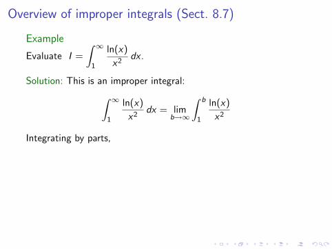
Overview of improper integrals (Sect. 8.7)
Example
Evaluate I =
∫ ∞
1
ln(x)
x2dx .
Solution: This is an improper integral:∫ ∞
1
ln(x)
x2dx = lim
b→∞
∫ b
1
ln(x)
x2
Integrating by parts,
u = ln(x), and dv = dx/x2,∫ b
1
ln(x)
x2dx =
(−1
x
)ln(x)
∣∣∣b1−
∫ b
1
(1
x
)(−1
x
)dx
∫ b
1
ln(x)
x2dx = − ln(b)
b+
∫ b
1
dx
x2= − ln(b)
b− 1
x
∣∣∣b1.
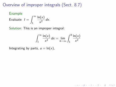
Overview of improper integrals (Sect. 8.7)
Example
Evaluate I =
∫ ∞
1
ln(x)
x2dx .
Solution: This is an improper integral:∫ ∞
1
ln(x)
x2dx = lim
b→∞
∫ b
1
ln(x)
x2
Integrating by parts, u = ln(x),
and dv = dx/x2,∫ b
1
ln(x)
x2dx =
(−1
x
)ln(x)
∣∣∣b1−
∫ b
1
(1
x
)(−1
x
)dx
∫ b
1
ln(x)
x2dx = − ln(b)
b+
∫ b
1
dx
x2= − ln(b)
b− 1
x
∣∣∣b1.
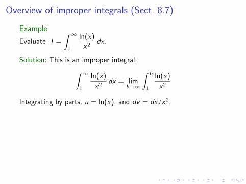
Overview of improper integrals (Sect. 8.7)
Example
Evaluate I =
∫ ∞
1
ln(x)
x2dx .
Solution: This is an improper integral:∫ ∞
1
ln(x)
x2dx = lim
b→∞
∫ b
1
ln(x)
x2
Integrating by parts, u = ln(x), and dv = dx/x2,
∫ b
1
ln(x)
x2dx =
(−1
x
)ln(x)
∣∣∣b1−
∫ b
1
(1
x
)(−1
x
)dx
∫ b
1
ln(x)
x2dx = − ln(b)
b+
∫ b
1
dx
x2= − ln(b)
b− 1
x
∣∣∣b1.
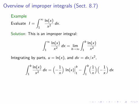
Overview of improper integrals (Sect. 8.7)
Example
Evaluate I =
∫ ∞
1
ln(x)
x2dx .
Solution: This is an improper integral:∫ ∞
1
ln(x)
x2dx = lim
b→∞
∫ b
1
ln(x)
x2
Integrating by parts, u = ln(x), and dv = dx/x2,∫ b
1
ln(x)
x2dx =
(−1
x
)ln(x)
∣∣∣b1−
∫ b
1
(1
x
)(−1
x
)dx
∫ b
1
ln(x)
x2dx = − ln(b)
b+
∫ b
1
dx
x2= − ln(b)
b− 1
x
∣∣∣b1.
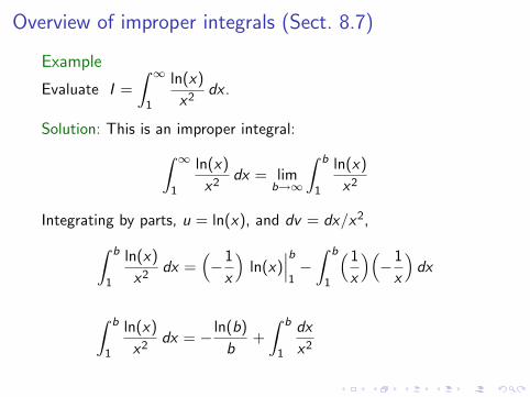
Overview of improper integrals (Sect. 8.7)
Example
Evaluate I =
∫ ∞
1
ln(x)
x2dx .
Solution: This is an improper integral:∫ ∞
1
ln(x)
x2dx = lim
b→∞
∫ b
1
ln(x)
x2
Integrating by parts, u = ln(x), and dv = dx/x2,∫ b
1
ln(x)
x2dx =
(−1
x
)ln(x)
∣∣∣b1−
∫ b
1
(1
x
)(−1
x
)dx
∫ b
1
ln(x)
x2dx = − ln(b)
b+
∫ b
1
dx
x2
= − ln(b)
b− 1
x
∣∣∣b1.
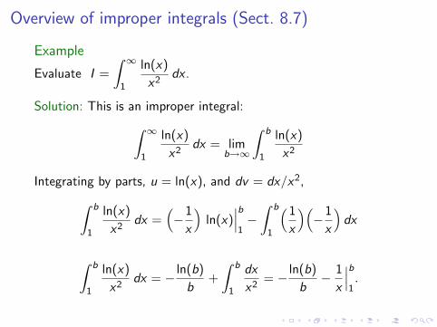
Overview of improper integrals (Sect. 8.7)
Example
Evaluate I =
∫ ∞
1
ln(x)
x2dx .
Solution: This is an improper integral:∫ ∞
1
ln(x)
x2dx = lim
b→∞
∫ b
1
ln(x)
x2
Integrating by parts, u = ln(x), and dv = dx/x2,∫ b
1
ln(x)
x2dx =
(−1
x
)ln(x)
∣∣∣b1−
∫ b
1
(1
x
)(−1
x
)dx
∫ b
1
ln(x)
x2dx = − ln(b)
b+
∫ b
1
dx
x2= − ln(b)
b− 1
x
∣∣∣b1.
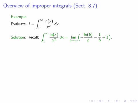
Overview of improper integrals (Sect. 8.7)
Example
Evaluate I =
∫ ∞
1
ln(x)
x2dx .
Solution: Recall:
∫ ∞
1
ln(x)
x2dx = lim
b→∞
(− ln(b)
b− 1
b+ 1
).
The first limit on the right-hand side is indeterminate∞∞
.
L’Hopital’s rule implies
limb→∞
ln(b)
b= lim
b→∞
(ln(b))′
(b)′= lim
b→∞
(1/b)
1= 0.
Therefore, the improper integral is given by∫ ∞
1
ln(x)
x2dx = 0− 0 + 1 ⇒
∫ ∞
1
ln(x)
x2dx = 1. C
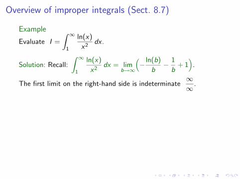
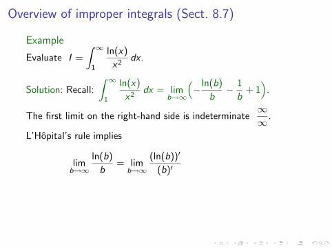
Overview of improper integrals (Sect. 8.7)
Example
Evaluate I =
∫ ∞
1
ln(x)
x2dx .
Solution: Recall:
∫ ∞
1
ln(x)
x2dx = lim
b→∞
(− ln(b)
b− 1
b+ 1
).
The first limit on the right-hand side is indeterminate∞∞
.
L’Hopital’s rule implies
limb→∞
ln(b)
b= lim
b→∞
(ln(b))′
(b)′
= limb→∞
(1/b)
1= 0.
Therefore, the improper integral is given by∫ ∞
1
ln(x)
x2dx = 0− 0 + 1 ⇒
∫ ∞
1
ln(x)
x2dx = 1. C
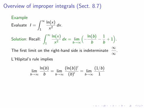
Overview of improper integrals (Sect. 8.7)
Example
Evaluate I =
∫ ∞
1
ln(x)
x2dx .
Solution: Recall:
∫ ∞
1
ln(x)
x2dx = lim
b→∞
(− ln(b)
b− 1
b+ 1
).
The first limit on the right-hand side is indeterminate∞∞
.
L’Hopital’s rule implies
limb→∞
ln(b)
b= lim
b→∞
(ln(b))′
(b)′= lim
b→∞
(1/b)
1
= 0.
Therefore, the improper integral is given by∫ ∞
1
ln(x)
x2dx = 0− 0 + 1 ⇒
∫ ∞
1
ln(x)
x2dx = 1. C
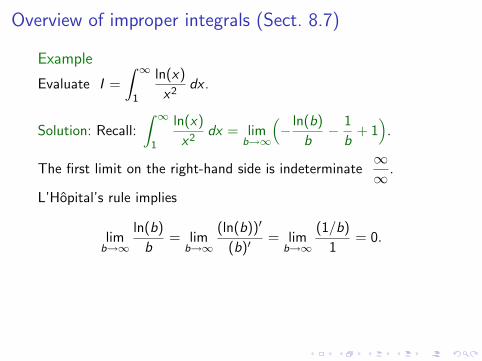
Overview of improper integrals (Sect. 8.7)
Example
Evaluate I =
∫ ∞
1
ln(x)
x2dx .
Solution: Recall:
∫ ∞
1
ln(x)
x2dx = lim
b→∞
(− ln(b)
b− 1
b+ 1
).
The first limit on the right-hand side is indeterminate∞∞
.
L’Hopital’s rule implies
limb→∞
ln(b)
b= lim
b→∞
(ln(b))′
(b)′= lim
b→∞
(1/b)
1= 0.
Therefore, the improper integral is given by∫ ∞
1
ln(x)
x2dx = 0− 0 + 1 ⇒
∫ ∞
1
ln(x)
x2dx = 1. C
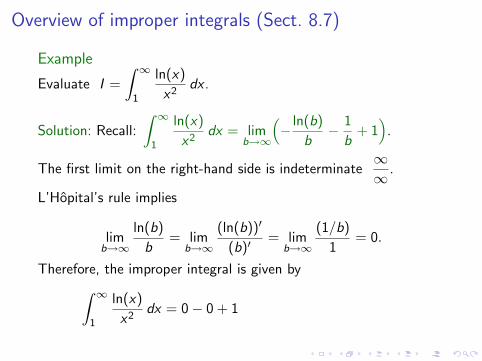
Overview of improper integrals (Sect. 8.7)
Example
Evaluate I =
∫ ∞
1
ln(x)
x2dx .
Solution: Recall:
∫ ∞
1
ln(x)
x2dx = lim
b→∞
(− ln(b)
b− 1
b+ 1
).
The first limit on the right-hand side is indeterminate∞∞
.
L’Hopital’s rule implies
limb→∞
ln(b)
b= lim
b→∞
(ln(b))′
(b)′= lim
b→∞
(1/b)
1= 0.
Therefore, the improper integral is given by∫ ∞
1
ln(x)
x2dx = 0− 0 + 1
⇒∫ ∞
1
ln(x)
x2dx = 1. C
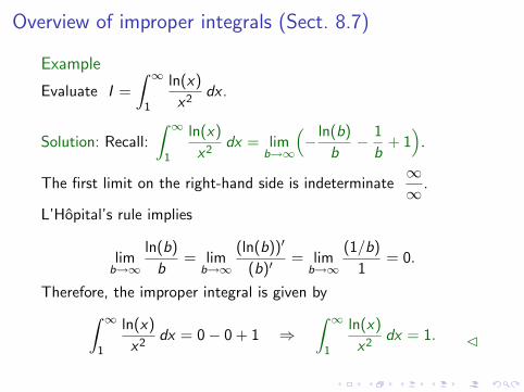
Overview of improper integrals (Sect. 8.7)
Example
Evaluate I =
∫ ∞
1
ln(x)
x2dx .
Solution: Recall:
∫ ∞
1
ln(x)
x2dx = lim
b→∞
(− ln(b)
b− 1
b+ 1
).
The first limit on the right-hand side is indeterminate∞∞
.
L’Hopital’s rule implies
limb→∞
ln(b)
b= lim
b→∞
(ln(b))′
(b)′= lim
b→∞
(1/b)
1= 0.
Therefore, the improper integral is given by∫ ∞
1
ln(x)
x2dx = 0− 0 + 1 ⇒
∫ ∞
1
ln(x)
x2dx = 1. C
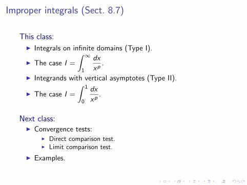
Improper integrals (Sect. 8.7)
This class:
I Integrals on infinite domains (Type I).
I The case I =
∫ ∞
1
dx
xp.
I Integrands with vertical asymptotes (Type II).
I The case I =
∫ 1
0
dx
xp.
Next class:I Convergence tests:
I Direct comparison test.I Limit comparison test.
I Examples.
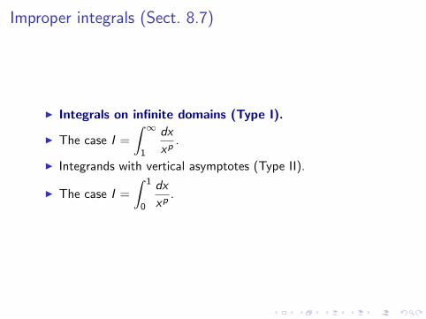
Improper integrals (Sect. 8.7)
I Integrals on infinite domains (Type I).
I The case I =
∫ ∞
1
dx
xp.
I Integrands with vertical asymptotes (Type II).
I The case I =
∫ 1
0
dx
xp.
Integrals on infinite domains (Type I)
Remark: Improper integrals are the limit of definite integrals whenone endpoint if integration approaches ±∞.
Definition (Type I)
Improper integrals of Type I are integrals of continuous functionson infinite domains; these include:The improper integral of a continuous function f on [a,∞),∫ ∞
af (x) dx = lim
b→∞
∫ b
af (x) dx .
The improper integral of a continuous function f on (−∞, b],∫ b
−∞f (x) dx = lim
a→−∞
∫ b
af (x) dx .
The improper integral of a continuous function f on (−∞,∞),∫ ∞
−∞f (x) dx =
∫ c
−∞f (x) dx +
∫ ∞
cf (x) dx .
Integrals on infinite domains (Type I)
Remark: Improper integrals are the limit of definite integrals whenone endpoint if integration approaches ±∞.
Definition (Type I)
Improper integrals of Type I are integrals of continuous functionson infinite domains;
these include:The improper integral of a continuous function f on [a,∞),∫ ∞
af (x) dx = lim
b→∞
∫ b
af (x) dx .
The improper integral of a continuous function f on (−∞, b],∫ b
−∞f (x) dx = lim
a→−∞
∫ b
af (x) dx .
The improper integral of a continuous function f on (−∞,∞),∫ ∞
−∞f (x) dx =
∫ c
−∞f (x) dx +
∫ ∞
cf (x) dx .
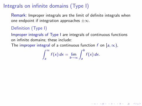
Integrals on infinite domains (Type I)
Remark: Improper integrals are the limit of definite integrals whenone endpoint if integration approaches ±∞.
Definition (Type I)
Improper integrals of Type I are integrals of continuous functionson infinite domains; these include:The improper integral of a continuous function f on [a,∞),∫ ∞
af (x) dx = lim
b→∞
∫ b
af (x) dx .
The improper integral of a continuous function f on (−∞, b],∫ b
−∞f (x) dx = lim
a→−∞
∫ b
af (x) dx .
The improper integral of a continuous function f on (−∞,∞),∫ ∞
−∞f (x) dx =
∫ c
−∞f (x) dx +
∫ ∞
cf (x) dx .
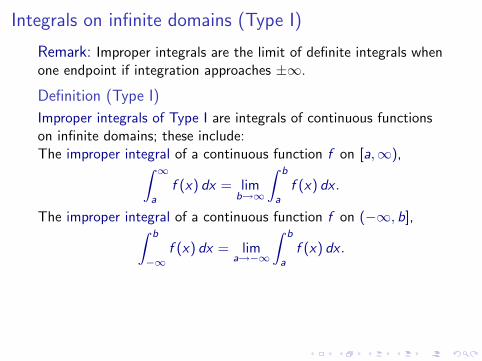
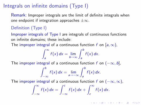
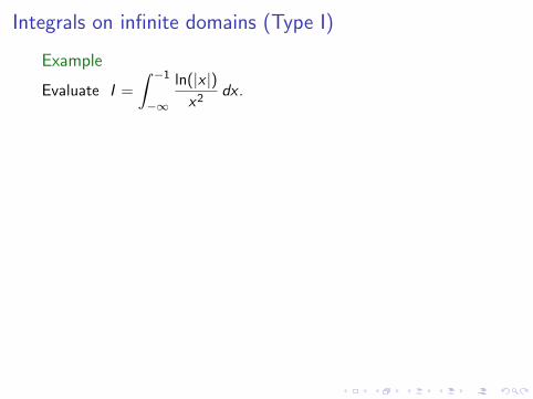
Integrals on infinite domains (Type I)
Example
Evaluate I =
∫ −1
−∞
ln(|x |)x2
dx .
Solution: This is an improper integral:∫ −1
−∞
ln(|x |)x2
dx = lima→−∞
∫ −1
a
ln(|x |)x2
Integrating by parts, u = ln(|x |), and dv = dx/x2,∫ −1
a
ln(|x |)x2
dx =(−1
x
)ln(|x |)
∣∣∣−1
a−
∫ −1
a
(1
x
)(−1
x
)dx
∫ −1
a
ln(|x |)x2
dx =ln(|a|)
a+
∫ −1
a
dx
x2=
ln(|a|)a
− 1
x
∣∣∣−1
a.
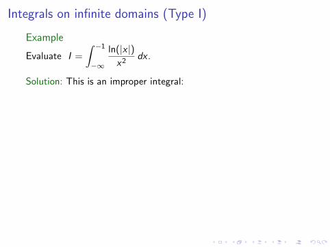
Integrals on infinite domains (Type I)
Example
Evaluate I =
∫ −1
−∞
ln(|x |)x2
dx .
Solution: This is an improper integral:
∫ −1
−∞
ln(|x |)x2
dx = lima→−∞
∫ −1
a
ln(|x |)x2
Integrating by parts, u = ln(|x |), and dv = dx/x2,∫ −1
a
ln(|x |)x2
dx =(−1
x
)ln(|x |)
∣∣∣−1
a−
∫ −1
a
(1
x
)(−1
x
)dx
∫ −1
a
ln(|x |)x2
dx =ln(|a|)
a+
∫ −1
a
dx
x2=
ln(|a|)a
− 1
x
∣∣∣−1
a.
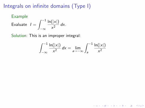
Integrals on infinite domains (Type I)
Example
Evaluate I =
∫ −1
−∞
ln(|x |)x2
dx .
Solution: This is an improper integral:∫ −1
−∞
ln(|x |)x2
dx = lima→−∞
∫ −1
a
ln(|x |)x2
Integrating by parts, u = ln(|x |), and dv = dx/x2,∫ −1
a
ln(|x |)x2
dx =(−1
x
)ln(|x |)
∣∣∣−1
a−
∫ −1
a
(1
x
)(−1
x
)dx
∫ −1
a
ln(|x |)x2
dx =ln(|a|)
a+
∫ −1
a
dx
x2=
ln(|a|)a
− 1
x
∣∣∣−1
a.
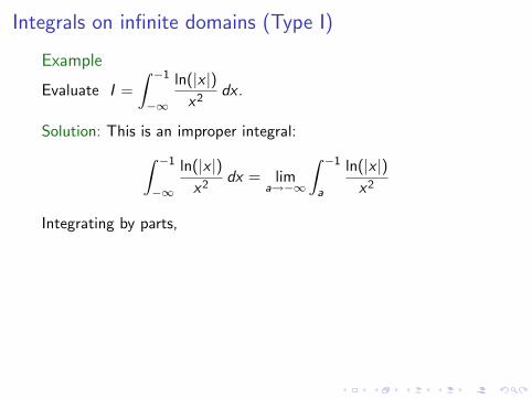
Integrals on infinite domains (Type I)
Example
Evaluate I =
∫ −1
−∞
ln(|x |)x2
dx .
Solution: This is an improper integral:∫ −1
−∞
ln(|x |)x2
dx = lima→−∞
∫ −1
a
ln(|x |)x2
Integrating by parts,
u = ln(|x |), and dv = dx/x2,∫ −1
a
ln(|x |)x2
dx =(−1
x
)ln(|x |)
∣∣∣−1
a−
∫ −1
a
(1
x
)(−1
x
)dx
∫ −1
a
ln(|x |)x2
dx =ln(|a|)
a+
∫ −1
a
dx
x2=
ln(|a|)a
− 1
x
∣∣∣−1
a.
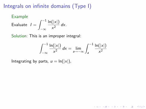
Integrals on infinite domains (Type I)
Example
Evaluate I =
∫ −1
−∞
ln(|x |)x2
dx .
Solution: This is an improper integral:∫ −1
−∞
ln(|x |)x2
dx = lima→−∞
∫ −1
a
ln(|x |)x2
Integrating by parts, u = ln(|x |),
and dv = dx/x2,∫ −1
a
ln(|x |)x2
dx =(−1
x
)ln(|x |)
∣∣∣−1
a−
∫ −1
a
(1
x
)(−1
x
)dx
∫ −1
a
ln(|x |)x2
dx =ln(|a|)
a+
∫ −1
a
dx
x2=
ln(|a|)a
− 1
x
∣∣∣−1
a.
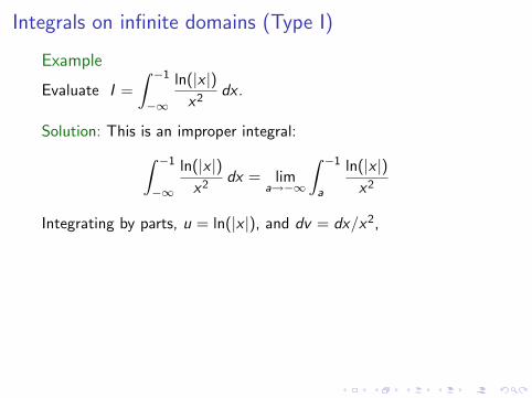
Integrals on infinite domains (Type I)
Example
Evaluate I =
∫ −1
−∞
ln(|x |)x2
dx .
Solution: This is an improper integral:∫ −1
−∞
ln(|x |)x2
dx = lima→−∞
∫ −1
a
ln(|x |)x2
Integrating by parts, u = ln(|x |), and dv = dx/x2,
∫ −1
a
ln(|x |)x2
dx =(−1
x
)ln(|x |)
∣∣∣−1
a−
∫ −1
a
(1
x
)(−1
x
)dx
∫ −1
a
ln(|x |)x2
dx =ln(|a|)
a+
∫ −1
a
dx
x2=
ln(|a|)a
− 1
x
∣∣∣−1
a.
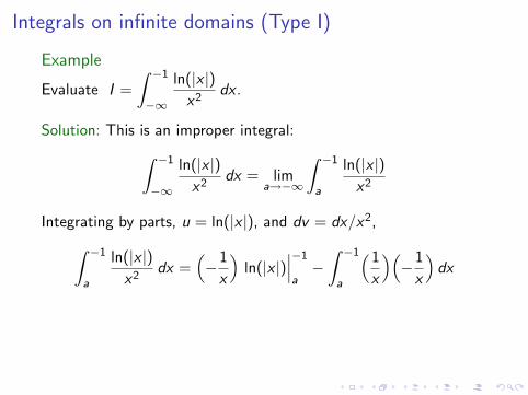
Integrals on infinite domains (Type I)
Example
Evaluate I =
∫ −1
−∞
ln(|x |)x2
dx .
Solution: This is an improper integral:∫ −1
−∞
ln(|x |)x2
dx = lima→−∞
∫ −1
a
ln(|x |)x2
Integrating by parts, u = ln(|x |), and dv = dx/x2,∫ −1
a
ln(|x |)x2
dx =(−1
x
)ln(|x |)
∣∣∣−1
a−
∫ −1
a
(1
x
)(−1
x
)dx
∫ −1
a
ln(|x |)x2
dx =ln(|a|)
a+
∫ −1
a
dx
x2=
ln(|a|)a
− 1
x
∣∣∣−1
a.
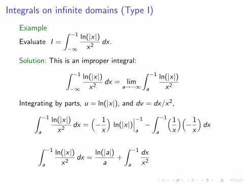
Integrals on infinite domains (Type I)
Example
Evaluate I =
∫ −1
−∞
ln(|x |)x2
dx .
Solution: This is an improper integral:∫ −1
−∞
ln(|x |)x2
dx = lima→−∞
∫ −1
a
ln(|x |)x2
Integrating by parts, u = ln(|x |), and dv = dx/x2,∫ −1
a
ln(|x |)x2
dx =(−1
x
)ln(|x |)
∣∣∣−1
a−
∫ −1
a
(1
x
)(−1
x
)dx
∫ −1
a
ln(|x |)x2
dx =ln(|a|)
a+
∫ −1
a
dx
x2
=ln(|a|)
a− 1
x
∣∣∣−1
a.
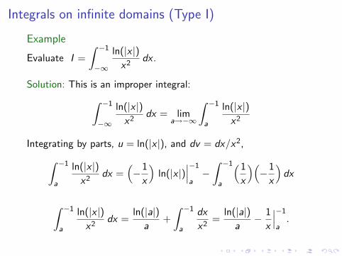
Integrals on infinite domains (Type I)
Example
Evaluate I =
∫ −1
−∞
ln(|x |)x2
dx .
Solution: This is an improper integral:∫ −1
−∞
ln(|x |)x2
dx = lima→−∞
∫ −1
a
ln(|x |)x2
Integrating by parts, u = ln(|x |), and dv = dx/x2,∫ −1
a
ln(|x |)x2
dx =(−1
x
)ln(|x |)
∣∣∣−1
a−
∫ −1
a
(1
x
)(−1
x
)dx
∫ −1
a
ln(|x |)x2
dx =ln(|a|)
a+
∫ −1
a
dx
x2=
ln(|a|)a
− 1
x
∣∣∣−1
a.
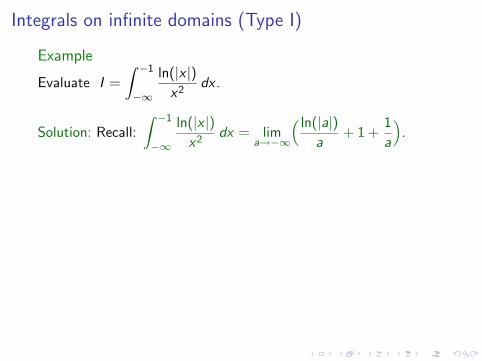
Integrals on infinite domains (Type I)
Example
Evaluate I =
∫ −1
−∞
ln(|x |)x2
dx .
Solution: Recall:
∫ −1
−∞
ln(|x |)x2
dx = lima→−∞
( ln(|a|)a
+ 1 +1
a
).
The first limit on the right-hand side is indeterminate −∞∞
.
L’Hopital’s rule implies
lima→−∞
ln(|a|)a
= lima→−∞
(ln(|a|))′
(a)′= lim
a→−∞
(1/a)
1= 0.
Therefore, the improper integral is given by∫ −1
−∞
ln(|x |)x2
dx = 0 + 1 + 0 ⇒∫ −1
−∞
ln(|x |)x2
dx = 1. C
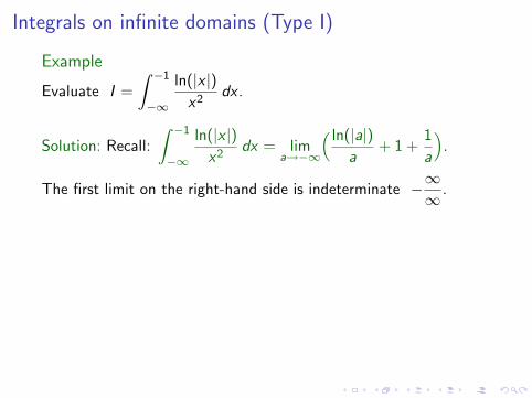
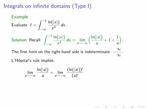
Integrals on infinite domains (Type I)
Example
Evaluate I =
∫ −1
−∞
ln(|x |)x2
dx .
Solution: Recall:
∫ −1
−∞
ln(|x |)x2
dx = lima→−∞
( ln(|a|)a
+ 1 +1
a
).
The first limit on the right-hand side is indeterminate −∞∞
.
L’Hopital’s rule implies
lima→−∞
ln(|a|)a
= lima→−∞
(ln(|a|))′
(a)′
= lima→−∞
(1/a)
1= 0.
Therefore, the improper integral is given by∫ −1
−∞
ln(|x |)x2
dx = 0 + 1 + 0 ⇒∫ −1
−∞
ln(|x |)x2
dx = 1. C
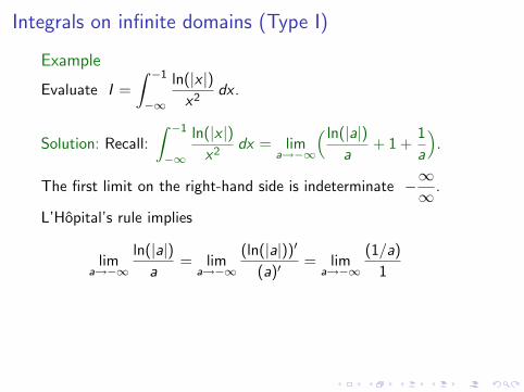
Integrals on infinite domains (Type I)
Example
Evaluate I =
∫ −1
−∞
ln(|x |)x2
dx .
Solution: Recall:
∫ −1
−∞
ln(|x |)x2
dx = lima→−∞
( ln(|a|)a
+ 1 +1
a
).
The first limit on the right-hand side is indeterminate −∞∞
.
L’Hopital’s rule implies
lima→−∞
ln(|a|)a
= lima→−∞
(ln(|a|))′
(a)′= lim
a→−∞
(1/a)
1
= 0.
Therefore, the improper integral is given by∫ −1
−∞
ln(|x |)x2
dx = 0 + 1 + 0 ⇒∫ −1
−∞
ln(|x |)x2
dx = 1. C
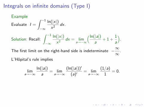
Integrals on infinite domains (Type I)
Example
Evaluate I =
∫ −1
−∞
ln(|x |)x2
dx .
Solution: Recall:
∫ −1
−∞
ln(|x |)x2
dx = lima→−∞
( ln(|a|)a
+ 1 +1
a
).
The first limit on the right-hand side is indeterminate −∞∞
.
L’Hopital’s rule implies
lima→−∞
ln(|a|)a
= lima→−∞
(ln(|a|))′
(a)′= lim
a→−∞
(1/a)
1= 0.
Therefore, the improper integral is given by∫ −1
−∞
ln(|x |)x2
dx = 0 + 1 + 0 ⇒∫ −1
−∞
ln(|x |)x2
dx = 1. C
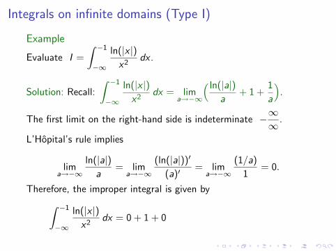
Integrals on infinite domains (Type I)
Example
Evaluate I =
∫ −1
−∞
ln(|x |)x2
dx .
Solution: Recall:
∫ −1
−∞
ln(|x |)x2
dx = lima→−∞
( ln(|a|)a
+ 1 +1
a
).
The first limit on the right-hand side is indeterminate −∞∞
.
L’Hopital’s rule implies
lima→−∞
ln(|a|)a
= lima→−∞
(ln(|a|))′
(a)′= lim
a→−∞
(1/a)
1= 0.
Therefore, the improper integral is given by∫ −1
−∞
ln(|x |)x2
dx = 0 + 1 + 0
⇒∫ −1
−∞
ln(|x |)x2
dx = 1. C
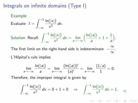
Integrals on infinite domains (Type I)
Example
Evaluate I =
∫ −1
−∞
ln(|x |)x2
dx .
Solution: Recall:
∫ −1
−∞
ln(|x |)x2
dx = lima→−∞
( ln(|a|)a
+ 1 +1
a
).
The first limit on the right-hand side is indeterminate −∞∞
.
L’Hopital’s rule implies
lima→−∞
ln(|a|)a
= lima→−∞
(ln(|a|))′
(a)′= lim
a→−∞
(1/a)
1= 0.
Therefore, the improper integral is given by∫ −1
−∞
ln(|x |)x2
dx = 0 + 1 + 0 ⇒∫ −1
−∞
ln(|x |)x2
dx = 1. C
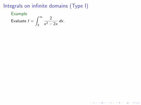
Integrals on infinite domains (Type I)
Example
Evaluate I =
∫ ∞
3
2
x2 − 2xdx .
Solution: Recall: I = limb→∞
∫ b
3
2
x2 − 2xdx .
First integrate, then the limit. For the integral, partial fractions:
2
x2 − 2x=
2
x(x − 2)=
a
x+
b
(x − 2)⇒ 2 = a(x − 2) + bx .
Then a = −1, and b = 1. Hence∫ b
3
2
x2 − 2xdx = −
∫ b
3
dx
x+
∫ b
3
dx
x − 2=
[− ln x + ln(x − 2)
]∣∣∣b3.
∫ b
3
2
x2 − 2xdx = ln(1/b) + ln(b − 2) + ln(3).
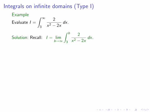
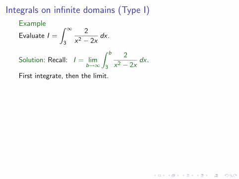
Integrals on infinite domains (Type I)
Example
Evaluate I =
∫ ∞
3
2
x2 − 2xdx .
Solution: Recall: I = limb→∞
∫ b
3
2
x2 − 2xdx .
First integrate, then the limit.
For the integral, partial fractions:
2
x2 − 2x=
2
x(x − 2)=
a
x+
b
(x − 2)⇒ 2 = a(x − 2) + bx .
Then a = −1, and b = 1. Hence∫ b
3
2
x2 − 2xdx = −
∫ b
3
dx
x+
∫ b
3
dx
x − 2=
[− ln x + ln(x − 2)
]∣∣∣b3.
∫ b
3
2
x2 − 2xdx = ln(1/b) + ln(b − 2) + ln(3).
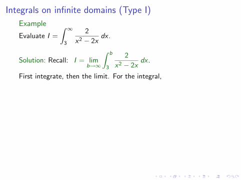
Integrals on infinite domains (Type I)
Example
Evaluate I =
∫ ∞
3
2
x2 − 2xdx .
Solution: Recall: I = limb→∞
∫ b
3
2
x2 − 2xdx .
First integrate, then the limit. For the integral,
partial fractions:
2
x2 − 2x=
2
x(x − 2)=
a
x+
b
(x − 2)⇒ 2 = a(x − 2) + bx .
Then a = −1, and b = 1. Hence∫ b
3
2
x2 − 2xdx = −
∫ b
3
dx
x+
∫ b
3
dx
x − 2=
[− ln x + ln(x − 2)
]∣∣∣b3.
∫ b
3
2
x2 − 2xdx = ln(1/b) + ln(b − 2) + ln(3).
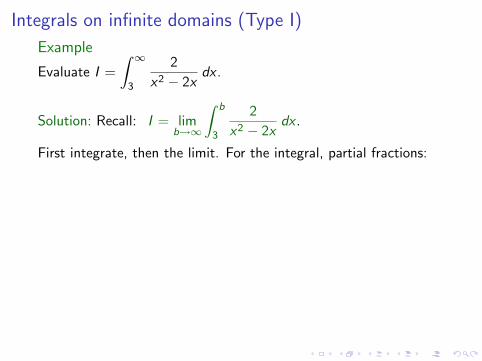
Integrals on infinite domains (Type I)
Example
Evaluate I =
∫ ∞
3
2
x2 − 2xdx .
Solution: Recall: I = limb→∞
∫ b
3
2
x2 − 2xdx .
First integrate, then the limit. For the integral, partial fractions:
2
x2 − 2x=
2
x(x − 2)=
a
x+
b
(x − 2)⇒ 2 = a(x − 2) + bx .
Then a = −1, and b = 1. Hence∫ b
3
2
x2 − 2xdx = −
∫ b
3
dx
x+
∫ b
3
dx
x − 2=
[− ln x + ln(x − 2)
]∣∣∣b3.
∫ b
3
2
x2 − 2xdx = ln(1/b) + ln(b − 2) + ln(3).
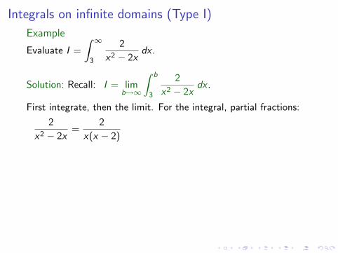
Integrals on infinite domains (Type I)
Example
Evaluate I =
∫ ∞
3
2
x2 − 2xdx .
Solution: Recall: I = limb→∞
∫ b
3
2
x2 − 2xdx .
First integrate, then the limit. For the integral, partial fractions:
2
x2 − 2x=
2
x(x − 2)
=a
x+
b
(x − 2)⇒ 2 = a(x − 2) + bx .
Then a = −1, and b = 1. Hence∫ b
3
2
x2 − 2xdx = −
∫ b
3
dx
x+
∫ b
3
dx
x − 2=
[− ln x + ln(x − 2)
]∣∣∣b3.
∫ b
3
2
x2 − 2xdx = ln(1/b) + ln(b − 2) + ln(3).
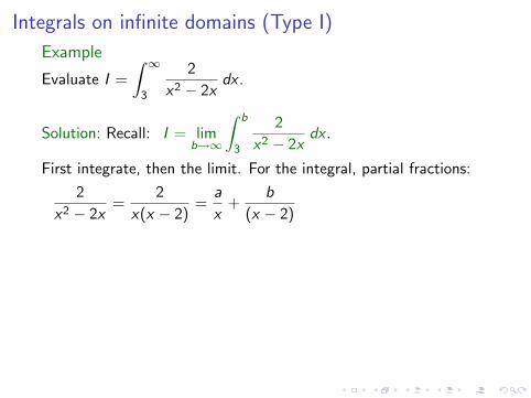
Integrals on infinite domains (Type I)
Example
Evaluate I =
∫ ∞
3
2
x2 − 2xdx .
Solution: Recall: I = limb→∞
∫ b
3
2
x2 − 2xdx .
First integrate, then the limit. For the integral, partial fractions:
2
x2 − 2x=
2
x(x − 2)=
a
x+
b
(x − 2)
⇒ 2 = a(x − 2) + bx .
Then a = −1, and b = 1. Hence∫ b
3
2
x2 − 2xdx = −
∫ b
3
dx
x+
∫ b
3
dx
x − 2=
[− ln x + ln(x − 2)
]∣∣∣b3.
∫ b
3
2
x2 − 2xdx = ln(1/b) + ln(b − 2) + ln(3).
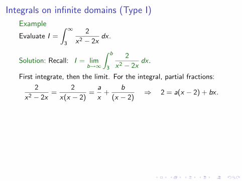
Integrals on infinite domains (Type I)
Example
Evaluate I =
∫ ∞
3
2
x2 − 2xdx .
Solution: Recall: I = limb→∞
∫ b
3
2
x2 − 2xdx .
First integrate, then the limit. For the integral, partial fractions:
2
x2 − 2x=
2
x(x − 2)=
a
x+
b
(x − 2)⇒ 2 = a(x − 2) + bx .
Then a = −1, and b = 1. Hence∫ b
3
2
x2 − 2xdx = −
∫ b
3
dx
x+
∫ b
3
dx
x − 2=
[− ln x + ln(x − 2)
]∣∣∣b3.
∫ b
3
2
x2 − 2xdx = ln(1/b) + ln(b − 2) + ln(3).
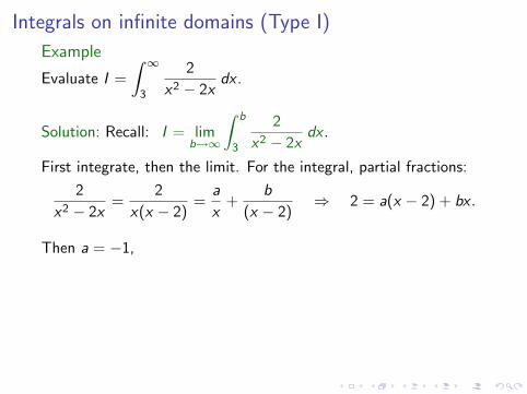
Integrals on infinite domains (Type I)
Example
Evaluate I =
∫ ∞
3
2
x2 − 2xdx .
Solution: Recall: I = limb→∞
∫ b
3
2
x2 − 2xdx .
First integrate, then the limit. For the integral, partial fractions:
2
x2 − 2x=
2
x(x − 2)=
a
x+
b
(x − 2)⇒ 2 = a(x − 2) + bx .
Then a = −1,
and b = 1. Hence∫ b
3
2
x2 − 2xdx = −
∫ b
3
dx
x+
∫ b
3
dx
x − 2=
[− ln x + ln(x − 2)
]∣∣∣b3.
∫ b
3
2
x2 − 2xdx = ln(1/b) + ln(b − 2) + ln(3).
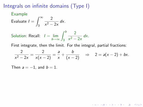
Integrals on infinite domains (Type I)
Example
Evaluate I =
∫ ∞
3
2
x2 − 2xdx .
Solution: Recall: I = limb→∞
∫ b
3
2
x2 − 2xdx .
First integrate, then the limit. For the integral, partial fractions:
2
x2 − 2x=
2
x(x − 2)=
a
x+
b
(x − 2)⇒ 2 = a(x − 2) + bx .
Then a = −1, and b = 1.
Hence∫ b
3
2
x2 − 2xdx = −
∫ b
3
dx
x+
∫ b
3
dx
x − 2=
[− ln x + ln(x − 2)
]∣∣∣b3.
∫ b
3
2
x2 − 2xdx = ln(1/b) + ln(b − 2) + ln(3).
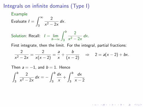
Integrals on infinite domains (Type I)
Example
Evaluate I =
∫ ∞
3
2
x2 − 2xdx .
Solution: Recall: I = limb→∞
∫ b
3
2
x2 − 2xdx .
First integrate, then the limit. For the integral, partial fractions:
2
x2 − 2x=
2
x(x − 2)=
a
x+
b
(x − 2)⇒ 2 = a(x − 2) + bx .
Then a = −1, and b = 1. Hence∫ b
3
2
x2 − 2xdx = −
∫ b
3
dx
x+
∫ b
3
dx
x − 2
=[− ln x + ln(x − 2)
]∣∣∣b3.
∫ b
3
2
x2 − 2xdx = ln(1/b) + ln(b − 2) + ln(3).
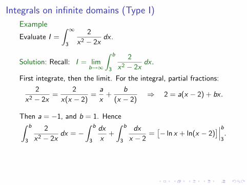
Integrals on infinite domains (Type I)
Example
Evaluate I =
∫ ∞
3
2
x2 − 2xdx .
Solution: Recall: I = limb→∞
∫ b
3
2
x2 − 2xdx .
First integrate, then the limit. For the integral, partial fractions:
2
x2 − 2x=
2
x(x − 2)=
a
x+
b
(x − 2)⇒ 2 = a(x − 2) + bx .
Then a = −1, and b = 1. Hence∫ b
3
2
x2 − 2xdx = −
∫ b
3
dx
x+
∫ b
3
dx
x − 2=
[− ln x + ln(x − 2)
]∣∣∣b3.
∫ b
3
2
x2 − 2xdx = ln(1/b) + ln(b − 2) + ln(3).
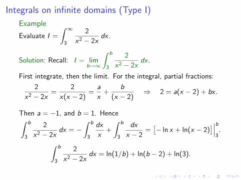
Integrals on infinite domains (Type I)
Example
Evaluate I =
∫ ∞
3
2
x2 − 2xdx .
Solution: Recall: I = limb→∞
∫ b
3
2
x2 − 2xdx .
First integrate, then the limit. For the integral, partial fractions:
2
x2 − 2x=
2
x(x − 2)=
a
x+
b
(x − 2)⇒ 2 = a(x − 2) + bx .
Then a = −1, and b = 1. Hence∫ b
3
2
x2 − 2xdx = −
∫ b
3
dx
x+
∫ b
3
dx
x − 2=
[− ln x + ln(x − 2)
]∣∣∣b3.
∫ b
3
2
x2 − 2xdx = ln(1/b) + ln(b − 2) + ln(3).
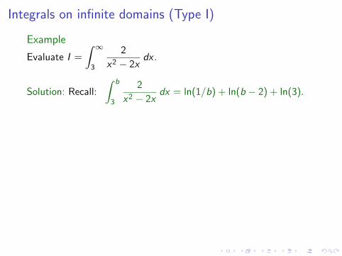
Integrals on infinite domains (Type I)
Example
Evaluate I =
∫ ∞
3
2
x2 − 2xdx .
Solution: Recall:
∫ b
3
2
x2 − 2xdx = ln(1/b) + ln(b − 2) + ln(3).
Therefore, the improper integral is
I = limb→∞
[ln
(b − 2
b
)+ ln(3)
].
The natural log function is continuous,
I = ln(
limb→∞
b − 2
b
)+ ln(3) = ln(1) + ln(3).
We then conclude that I = ln(3). C
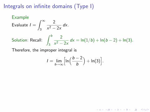
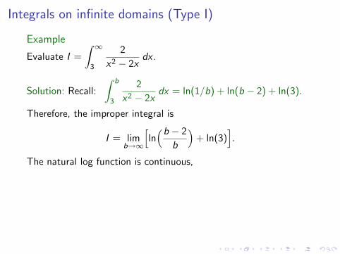
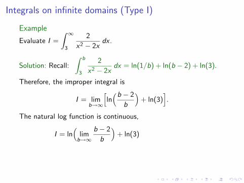
Integrals on infinite domains (Type I)
Example
Evaluate I =
∫ ∞
3
2
x2 − 2xdx .
Solution: Recall:
∫ b
3
2
x2 − 2xdx = ln(1/b) + ln(b − 2) + ln(3).
Therefore, the improper integral is
I = limb→∞
[ln
(b − 2
b
)+ ln(3)
].
The natural log function is continuous,
I = ln(
limb→∞
b − 2
b
)+ ln(3)
= ln(1) + ln(3).
We then conclude that I = ln(3). C
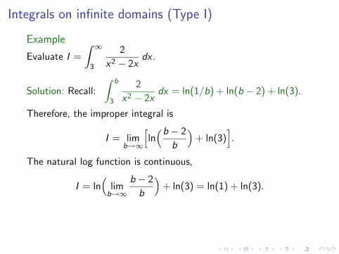
Integrals on infinite domains (Type I)
Example
Evaluate I =
∫ ∞
3
2
x2 − 2xdx .
Solution: Recall:
∫ b
3
2
x2 − 2xdx = ln(1/b) + ln(b − 2) + ln(3).
Therefore, the improper integral is
I = limb→∞
[ln
(b − 2
b
)+ ln(3)
].
The natural log function is continuous,
I = ln(
limb→∞
b − 2
b
)+ ln(3) = ln(1) + ln(3).
We then conclude that I = ln(3). C
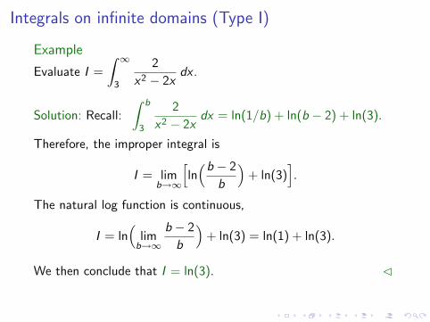
Integrals on infinite domains (Type I)
Example
Evaluate I =
∫ ∞
3
2
x2 − 2xdx .
Solution: Recall:
∫ b
3
2
x2 − 2xdx = ln(1/b) + ln(b − 2) + ln(3).
Therefore, the improper integral is
I = limb→∞
[ln
(b − 2
b
)+ ln(3)
].
The natural log function is continuous,
I = ln(
limb→∞
b − 2
b
)+ ln(3) = ln(1) + ln(3).
We then conclude that I = ln(3). C
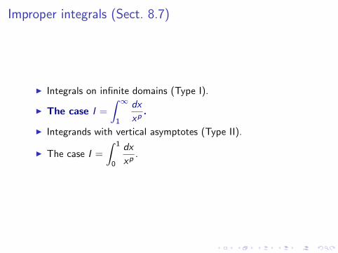
Improper integrals (Sect. 8.7)
I Integrals on infinite domains (Type I).
I The case I =
∫ ∞
1
dx
xp.
I Integrands with vertical asymptotes (Type II).
I The case I =
∫ 1
0
dx
xp.
The case I =
∫ ∞
1
dx
xp
Example
Evaluate I =
∫ ∞
1
dx
xpfor p > 0.
Solution: We first compute the integral, then take the limit.
For p 6= 1, holds I = limb→∞
∫ b
1x−p dx = lim
b→∞
[ x (−p+1)
(−p + 1)
∣∣∣b1
].
I =(−1)
(p − 1)
[lim
b→∞
1
b(p−1)− 1
]⇒
I diverges p < 1,
I =1
p − 1p > 1.
In the case p = 1 the integral diverges since I = limb→∞
ln(b). C
The case I =
∫ ∞
1
dx
xp
Example
Evaluate I =
∫ ∞
1
dx
xpfor p > 0.
Solution: We first compute the integral, then take the limit.
For p 6= 1, holds I = limb→∞
∫ b
1x−p dx
= limb→∞
[ x (−p+1)
(−p + 1)
∣∣∣b1
].
I =(−1)
(p − 1)
[lim
b→∞
1
b(p−1)− 1
]⇒
I diverges p < 1,
I =1
p − 1p > 1.
In the case p = 1 the integral diverges since I = limb→∞
ln(b). C
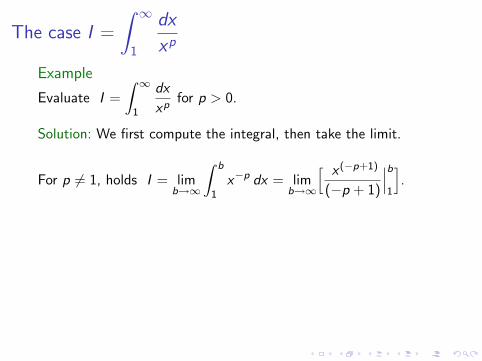
The case I =
∫ ∞
1
dx
xp
Example
Evaluate I =
∫ ∞
1
dx
xpfor p > 0.
Solution: We first compute the integral, then take the limit.
For p 6= 1, holds I = limb→∞
∫ b
1x−p dx = lim
b→∞
[ x (−p+1)
(−p + 1)
∣∣∣b1
].
I =(−1)
(p − 1)
[lim
b→∞
1
b(p−1)− 1
]⇒
I diverges p < 1,
I =1
p − 1p > 1.
In the case p = 1 the integral diverges since I = limb→∞
ln(b). C
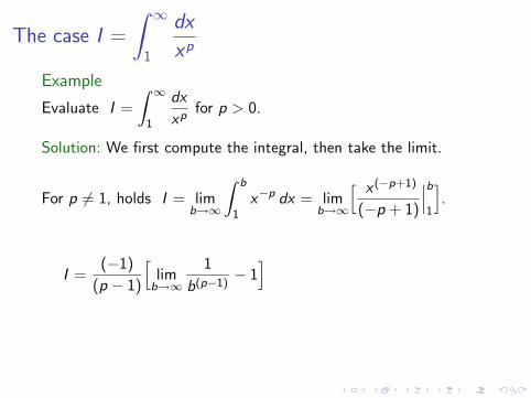
The case I =
∫ ∞
1
dx
xp
Example
Evaluate I =
∫ ∞
1
dx
xpfor p > 0.
Solution: We first compute the integral, then take the limit.
For p 6= 1, holds I = limb→∞
∫ b
1x−p dx = lim
b→∞
[ x (−p+1)
(−p + 1)
∣∣∣b1
].
I =(−1)
(p − 1)
[lim
b→∞
1
b(p−1)− 1
]
⇒
I diverges p < 1,
I =1
p − 1p > 1.
In the case p = 1 the integral diverges since I = limb→∞
ln(b). C
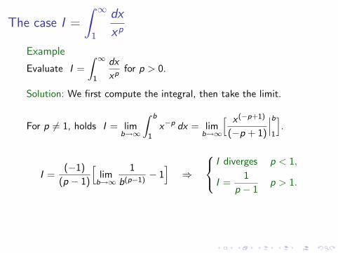
The case I =
∫ ∞
1
dx
xp
Example
Evaluate I =
∫ ∞
1
dx
xpfor p > 0.
Solution: We first compute the integral, then take the limit.
For p 6= 1, holds I = limb→∞
∫ b
1x−p dx = lim
b→∞
[ x (−p+1)
(−p + 1)
∣∣∣b1
].
I =(−1)
(p − 1)
[lim
b→∞
1
b(p−1)− 1
]⇒
I diverges p < 1,
I =1
p − 1p > 1.
In the case p = 1 the integral diverges since I = limb→∞
ln(b). C
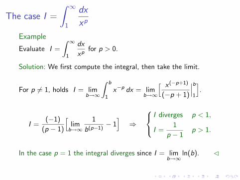
The case I =
∫ ∞
1
dx
xp
Example
Evaluate I =
∫ ∞
1
dx
xpfor p > 0.
Solution: We first compute the integral, then take the limit.
For p 6= 1, holds I = limb→∞
∫ b
1x−p dx = lim
b→∞
[ x (−p+1)
(−p + 1)
∣∣∣b1
].
I =(−1)
(p − 1)
[lim
b→∞
1
b(p−1)− 1
]⇒
I diverges p < 1,
I =1
p − 1p > 1.
In the case p = 1 the integral diverges since I = limb→∞
ln(b). C
Improper integrals (Sect. 8.7)
I Integrals on infinite domains (Type I).
I The case I =
∫ ∞
1
dx
xp.
I Integrands with vertical asymptotes (Type II).
I The case I =
∫ 1
0
dx
xp.
Integrands with vertical asymptotes (Type II)
Definition (Type II)
Improper integrals of Type II are integrals of functions with verticalasymptotes within the integration interval;
these include:
If f is continuous on (a, b] and discontinuous at a, then∫ b
af (x) dx = lim
c→a+
∫ b
cf (x) dx .
If f is continuous on [a, b) and discontinuous at b, then∫ b
af (x) dx = lim
c→b−
∫ c
af (x) dx .
If f is continuous on [a, c) ∪ (c , b] and discontinuous at c , then∫ b
af (x) dx =
∫ c
af (x) dx +
∫ b
cf (x) dx .
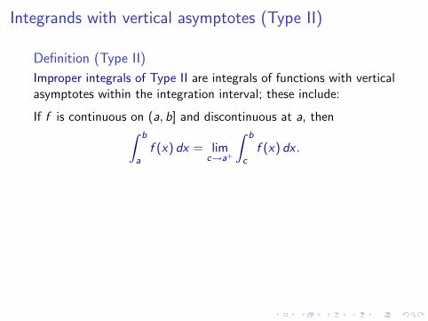
Integrands with vertical asymptotes (Type II)
Definition (Type II)
Improper integrals of Type II are integrals of functions with verticalasymptotes within the integration interval; these include:
If f is continuous on (a, b] and discontinuous at a, then∫ b
af (x) dx = lim
c→a+
∫ b
cf (x) dx .
If f is continuous on [a, b) and discontinuous at b, then∫ b
af (x) dx = lim
c→b−
∫ c
af (x) dx .
If f is continuous on [a, c) ∪ (c , b] and discontinuous at c , then∫ b
af (x) dx =
∫ c
af (x) dx +
∫ b
cf (x) dx .
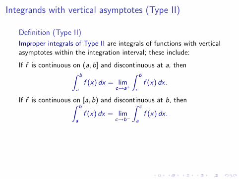
Integrands with vertical asymptotes (Type II)
Definition (Type II)
Improper integrals of Type II are integrals of functions with verticalasymptotes within the integration interval; these include:
If f is continuous on (a, b] and discontinuous at a, then∫ b
af (x) dx = lim
c→a+
∫ b
cf (x) dx .
If f is continuous on [a, b) and discontinuous at b, then∫ b
af (x) dx = lim
c→b−
∫ c
af (x) dx .
If f is continuous on [a, c) ∪ (c , b] and discontinuous at c , then∫ b
af (x) dx =
∫ c
af (x) dx +
∫ b
cf (x) dx .
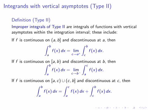
Integrands with vertical asymptotes (Type II)
Definition (Type II)
Improper integrals of Type II are integrals of functions with verticalasymptotes within the integration interval; these include:
If f is continuous on (a, b] and discontinuous at a, then∫ b
af (x) dx = lim
c→a+
∫ b
cf (x) dx .
If f is continuous on [a, b) and discontinuous at b, then∫ b
af (x) dx = lim
c→b−
∫ c
af (x) dx .
If f is continuous on [a, c) ∪ (c , b] and discontinuous at c , then∫ b
af (x) dx =
∫ c
af (x) dx +
∫ b
cf (x) dx .
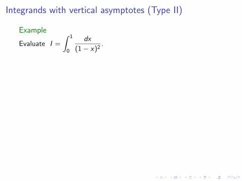
Integrands with vertical asymptotes (Type II)
Example
Evaluate I =
∫ 1
0
dx
(1− x)2.
Solution: Recall: I = limc→1−
∫ c
0(1− x)−2 dx .
We first integrate, then we take the limit. The integral is∫ c
0(1− x)−2 dx = (1− x)−1
∣∣∣c0
=1
(1− c)− 1.
We now take the limit,
I = limc→1−
1
(1− c)− 1.
We conclude that I diverges. C
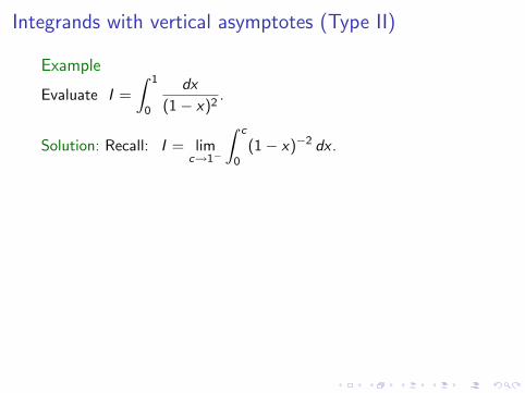
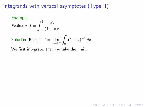
Integrands with vertical asymptotes (Type II)
Example
Evaluate I =
∫ 1
0
dx
(1− x)2.
Solution: Recall: I = limc→1−
∫ c
0(1− x)−2 dx .
We first integrate, then we take the limit.
The integral is∫ c
0(1− x)−2 dx = (1− x)−1
∣∣∣c0
=1
(1− c)− 1.
We now take the limit,
I = limc→1−
1
(1− c)− 1.
We conclude that I diverges. C
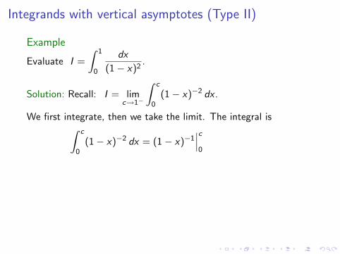
Integrands with vertical asymptotes (Type II)
Example
Evaluate I =
∫ 1
0
dx
(1− x)2.
Solution: Recall: I = limc→1−
∫ c
0(1− x)−2 dx .
We first integrate, then we take the limit. The integral is∫ c
0(1− x)−2 dx = (1− x)−1
∣∣∣c0
=1
(1− c)− 1.
We now take the limit,
I = limc→1−
1
(1− c)− 1.
We conclude that I diverges. C
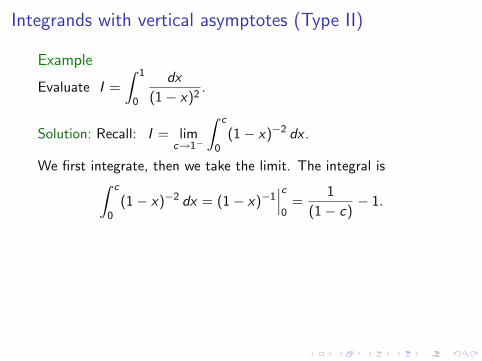
Integrands with vertical asymptotes (Type II)
Example
Evaluate I =
∫ 1
0
dx
(1− x)2.
Solution: Recall: I = limc→1−
∫ c
0(1− x)−2 dx .
We first integrate, then we take the limit. The integral is∫ c
0(1− x)−2 dx = (1− x)−1
∣∣∣c0
=1
(1− c)− 1.
We now take the limit,
I = limc→1−
1
(1− c)− 1.
We conclude that I diverges. C
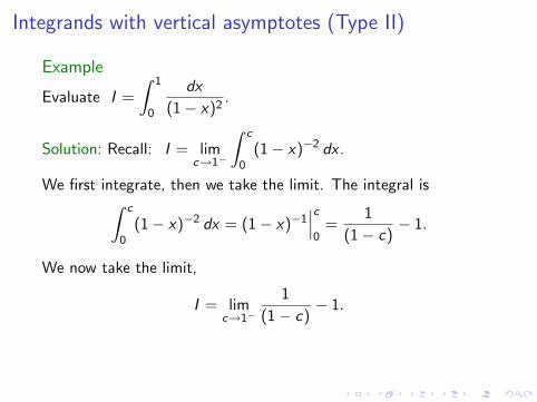
Integrands with vertical asymptotes (Type II)
Example
Evaluate I =
∫ 1
0
dx
(1− x)2.
Solution: Recall: I = limc→1−
∫ c
0(1− x)−2 dx .
We first integrate, then we take the limit. The integral is∫ c
0(1− x)−2 dx = (1− x)−1
∣∣∣c0
=1
(1− c)− 1.
We now take the limit,
I = limc→1−
1
(1− c)− 1.
We conclude that I diverges. C
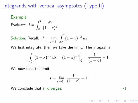
Integrands with vertical asymptotes (Type II)
Example
Evaluate I =
∫ 1
0
dx
(1− x)2.
Solution: Recall: I = limc→1−
∫ c
0(1− x)−2 dx .
We first integrate, then we take the limit. The integral is∫ c
0(1− x)−2 dx = (1− x)−1
∣∣∣c0
=1
(1− c)− 1.
We now take the limit,
I = limc→1−
1
(1− c)− 1.
We conclude that I diverges. C
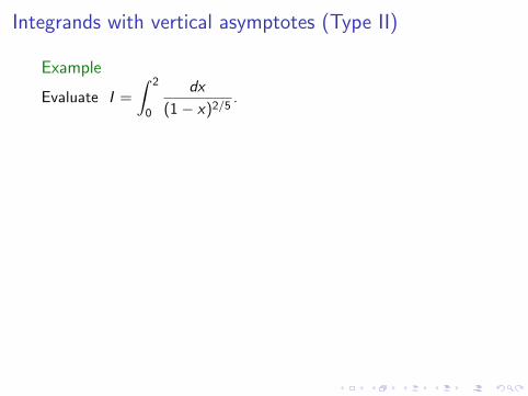
Integrands with vertical asymptotes (Type II)
Example
Evaluate I =
∫ 2
0
dx
(1− x)2/5.
Solution:
Recall:
∫ 2
0
dx
(1− x)2/5=
∫ 1
0
dx
(1− x)2/5+
∫ 2
1
dx
(1− x)2/5.
The first integral is given by∫ 1
0
dx
(1− x)2/5= lim
c→1−
∫ c
0(1− x)−2/5 dx = lim
c→1−−5
3(1− x)3/5
∣∣∣c0,
∫ 1
0
dx
(1− x)2/5= −5
3lim
c→1−(1− c)3/5 +
5
3=
5
3.
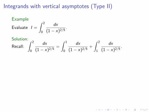
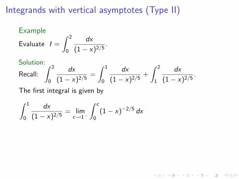
Integrands with vertical asymptotes (Type II)
Example
Evaluate I =
∫ 2
0
dx
(1− x)2/5.
Solution:
Recall:
∫ 2
0
dx
(1− x)2/5=
∫ 1
0
dx
(1− x)2/5+
∫ 2
1
dx
(1− x)2/5.
The first integral is given by∫ 1
0
dx
(1− x)2/5= lim
c→1−
∫ c
0(1− x)−2/5 dx
= limc→1−
−5
3(1− x)3/5
∣∣∣c0,
∫ 1
0
dx
(1− x)2/5= −5
3lim
c→1−(1− c)3/5 +
5
3=
5
3.
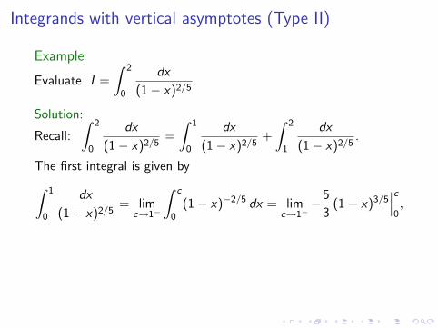
Integrands with vertical asymptotes (Type II)
Example
Evaluate I =
∫ 2
0
dx
(1− x)2/5.
Solution:
Recall:
∫ 2
0
dx
(1− x)2/5=
∫ 1
0
dx
(1− x)2/5+
∫ 2
1
dx
(1− x)2/5.
The first integral is given by∫ 1
0
dx
(1− x)2/5= lim
c→1−
∫ c
0(1− x)−2/5 dx = lim
c→1−−5
3(1− x)3/5
∣∣∣c0,
∫ 1
0
dx
(1− x)2/5= −5
3lim
c→1−(1− c)3/5 +
5
3=
5
3.
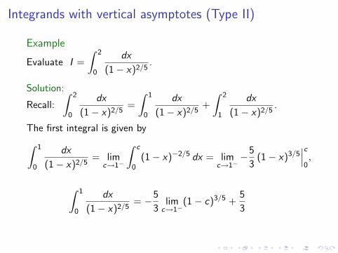
Integrands with vertical asymptotes (Type II)
Example
Evaluate I =
∫ 2
0
dx
(1− x)2/5.
Solution:
Recall:
∫ 2
0
dx
(1− x)2/5=
∫ 1
0
dx
(1− x)2/5+
∫ 2
1
dx
(1− x)2/5.
The first integral is given by∫ 1
0
dx
(1− x)2/5= lim
c→1−
∫ c
0(1− x)−2/5 dx = lim
c→1−−5
3(1− x)3/5
∣∣∣c0,
∫ 1
0
dx
(1− x)2/5= −5
3lim
c→1−(1− c)3/5 +
5
3
=5
3.
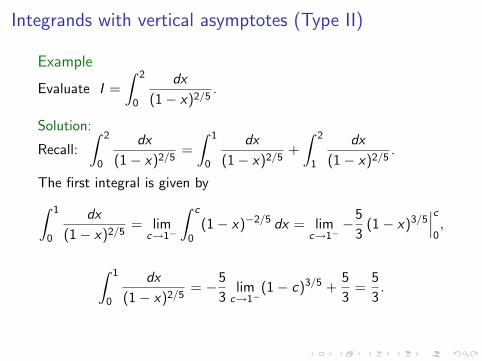
Integrands with vertical asymptotes (Type II)
Example
Evaluate I =
∫ 2
0
dx
(1− x)2/5.
Solution:
Recall:
∫ 2
0
dx
(1− x)2/5=
∫ 1
0
dx
(1− x)2/5+
∫ 2
1
dx
(1− x)2/5.
The first integral is given by∫ 1
0
dx
(1− x)2/5= lim
c→1−
∫ c
0(1− x)−2/5 dx = lim
c→1−−5
3(1− x)3/5
∣∣∣c0,
∫ 1
0
dx
(1− x)2/5= −5
3lim
c→1−(1− c)3/5 +
5
3=
5
3.
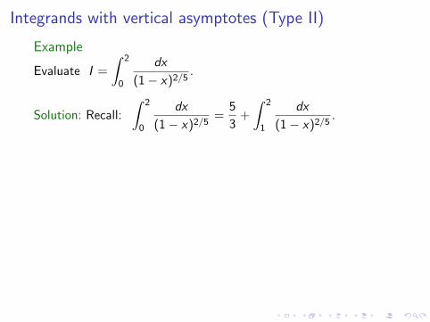
Integrands with vertical asymptotes (Type II)
Example
Evaluate I =
∫ 2
0
dx
(1− x)2/5.
Solution: Recall:
∫ 2
0
dx
(1− x)2/5=
5
3+
∫ 2
1
dx
(1− x)2/5.
The second integral is given by∫ 2
1
dx
(1− x)2/5= lim
c→1+
∫ 2
c(1− x)−2/5 dx = lim
c→1+−5
3(1− x)3/5
∣∣∣2c,
∫ 2
1
dx
(1− x)2/5=
5
3+
5
3lim
c→1+(1− c)3/5 =
5
3.
We conclude: I =10
3. C
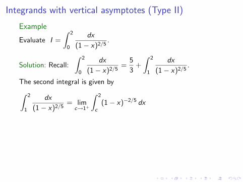
Integrands with vertical asymptotes (Type II)
Example
Evaluate I =
∫ 2
0
dx
(1− x)2/5.
Solution: Recall:
∫ 2
0
dx
(1− x)2/5=
5
3+
∫ 2
1
dx
(1− x)2/5.
The second integral is given by∫ 2
1
dx
(1− x)2/5= lim
c→1+
∫ 2
c(1− x)−2/5 dx
= limc→1+
−5
3(1− x)3/5
∣∣∣2c,
∫ 2
1
dx
(1− x)2/5=
5
3+
5
3lim
c→1+(1− c)3/5 =
5
3.
We conclude: I =10
3. C
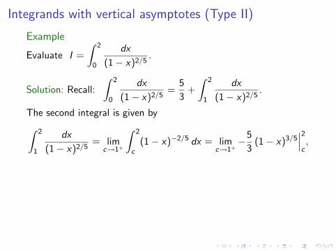
Integrands with vertical asymptotes (Type II)
Example
Evaluate I =
∫ 2
0
dx
(1− x)2/5.
Solution: Recall:
∫ 2
0
dx
(1− x)2/5=
5
3+
∫ 2
1
dx
(1− x)2/5.
The second integral is given by∫ 2
1
dx
(1− x)2/5= lim
c→1+
∫ 2
c(1− x)−2/5 dx = lim
c→1+−5
3(1− x)3/5
∣∣∣2c,
∫ 2
1
dx
(1− x)2/5=
5
3+
5
3lim
c→1+(1− c)3/5 =
5
3.
We conclude: I =10
3. C
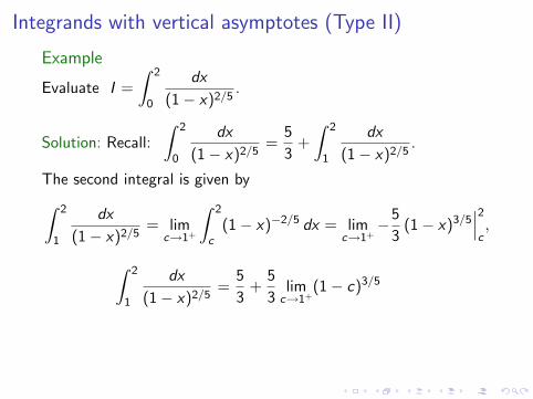
Integrands with vertical asymptotes (Type II)
Example
Evaluate I =
∫ 2
0
dx
(1− x)2/5.
Solution: Recall:
∫ 2
0
dx
(1− x)2/5=
5
3+
∫ 2
1
dx
(1− x)2/5.
The second integral is given by∫ 2
1
dx
(1− x)2/5= lim
c→1+
∫ 2
c(1− x)−2/5 dx = lim
c→1+−5
3(1− x)3/5
∣∣∣2c,
∫ 2
1
dx
(1− x)2/5=
5
3+
5
3lim
c→1+(1− c)3/5
=5
3.
We conclude: I =10
3. C
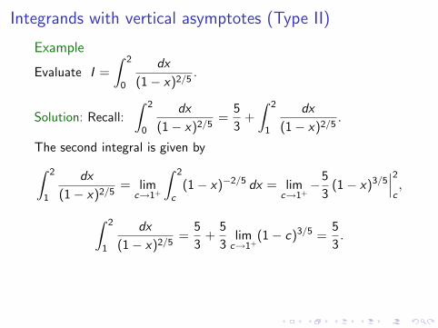
Integrands with vertical asymptotes (Type II)
Example
Evaluate I =
∫ 2
0
dx
(1− x)2/5.
Solution: Recall:
∫ 2
0
dx
(1− x)2/5=
5
3+
∫ 2
1
dx
(1− x)2/5.
The second integral is given by∫ 2
1
dx
(1− x)2/5= lim
c→1+
∫ 2
c(1− x)−2/5 dx = lim
c→1+−5
3(1− x)3/5
∣∣∣2c,
∫ 2
1
dx
(1− x)2/5=
5
3+
5
3lim
c→1+(1− c)3/5 =
5
3.
We conclude: I =10
3. C
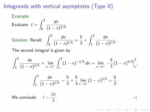
Integrands with vertical asymptotes (Type II)
Example
Evaluate I =
∫ 2
0
dx
(1− x)2/5.
Solution: Recall:
∫ 2
0
dx
(1− x)2/5=
5
3+
∫ 2
1
dx
(1− x)2/5.
The second integral is given by∫ 2
1
dx
(1− x)2/5= lim
c→1+
∫ 2
c(1− x)−2/5 dx = lim
c→1+−5
3(1− x)3/5
∣∣∣2c,
∫ 2
1
dx
(1− x)2/5=
5
3+
5
3lim
c→1+(1− c)3/5 =
5
3.
We conclude: I =10
3. C
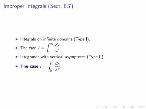
Improper integrals (Sect. 8.7)
I Integrals on infinite domains (Type I).
I The case I =
∫ ∞
1
dx
xp.
I Integrands with vertical asymptotes (Type II).
I The case I =
∫ 1
0
dx
xp.
The case I =
∫ 1
0
dx
xp
Example
Evaluate I =
∫ 1
0
dx
xpfor p > 0.
Solution: We first compute the integral, then take the limit.
For p 6= 1, holds I = lima→0+
∫ 1
ax−p dx = lim
a→0+
[ x (−p+1)
(−p + 1)
∣∣∣1a
].
I =(−1)
(p − 1)
[1− lim
a→0+
1
a(p−1)
]⇒
I =1
1− pp < 1,
I diverges p > 1.
In the case p = 1 the integral diverges since I = lima→0+
ln(a). C

The case I =
∫ 1
0
dx
xp
Example
Evaluate I =
∫ 1
0
dx
xpfor p > 0.
Solution: We first compute the integral, then take the limit.
For p 6= 1, holds I = lima→0+
∫ 1
ax−p dx
= lima→0+
[ x (−p+1)
(−p + 1)
∣∣∣1a
].
I =(−1)
(p − 1)
[1− lim
a→0+
1
a(p−1)
]⇒
I =1
1− pp < 1,
I diverges p > 1.
In the case p = 1 the integral diverges since I = lima→0+
ln(a). C
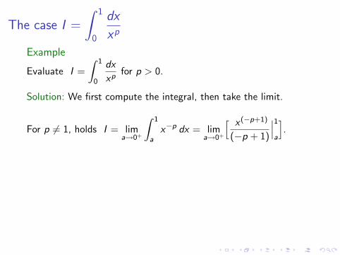
The case I =
∫ 1
0
dx
xp
Example
Evaluate I =
∫ 1
0
dx
xpfor p > 0.
Solution: We first compute the integral, then take the limit.
For p 6= 1, holds I = lima→0+
∫ 1
ax−p dx = lim
a→0+
[ x (−p+1)
(−p + 1)
∣∣∣1a
].
I =(−1)
(p − 1)
[1− lim
a→0+
1
a(p−1)
]⇒
I =1
1− pp < 1,
I diverges p > 1.
In the case p = 1 the integral diverges since I = lima→0+
ln(a). C
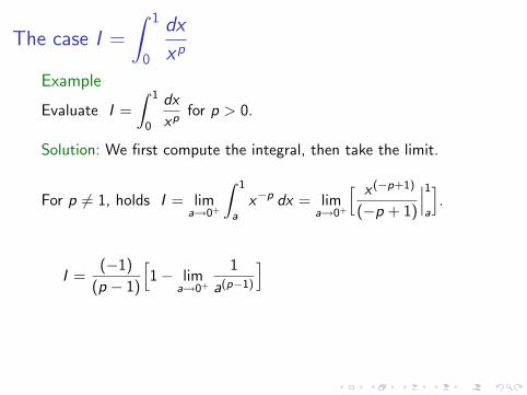
The case I =
∫ 1
0
dx
xp
Example
Evaluate I =
∫ 1
0
dx
xpfor p > 0.
Solution: We first compute the integral, then take the limit.
For p 6= 1, holds I = lima→0+
∫ 1
ax−p dx = lim
a→0+
[ x (−p+1)
(−p + 1)
∣∣∣1a
].
I =(−1)
(p − 1)
[1− lim
a→0+
1
a(p−1)
]
⇒
I =1
1− pp < 1,
I diverges p > 1.
In the case p = 1 the integral diverges since I = lima→0+
ln(a). C
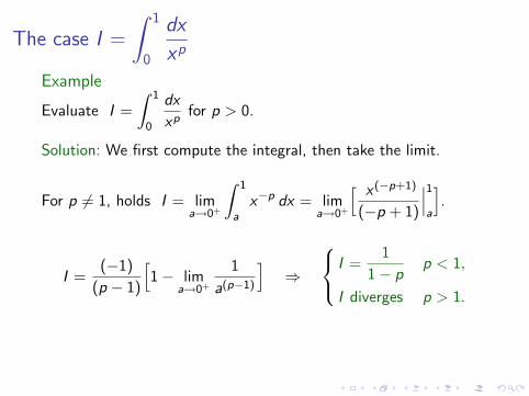
The case I =
∫ 1
0
dx
xp
Example
Evaluate I =
∫ 1
0
dx
xpfor p > 0.
Solution: We first compute the integral, then take the limit.
For p 6= 1, holds I = lima→0+
∫ 1
ax−p dx = lim
a→0+
[ x (−p+1)
(−p + 1)
∣∣∣1a
].
I =(−1)
(p − 1)
[1− lim
a→0+
1
a(p−1)
]⇒
I =1
1− pp < 1,
I diverges p > 1.
In the case p = 1 the integral diverges since I = lima→0+
ln(a). C
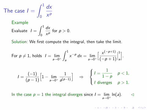
The case I =
∫ 1
0
dx
xp
Example
Evaluate I =
∫ 1
0
dx
xpfor p > 0.
Solution: We first compute the integral, then take the limit.
For p 6= 1, holds I = lima→0+
∫ 1
ax−p dx = lim
a→0+
[ x (−p+1)
(−p + 1)
∣∣∣1a
].
I =(−1)
(p − 1)
[1− lim
a→0+
1
a(p−1)
]⇒
I =1
1− pp < 1,
I diverges p > 1.
In the case p = 1 the integral diverges since I = lima→0+
ln(a). C
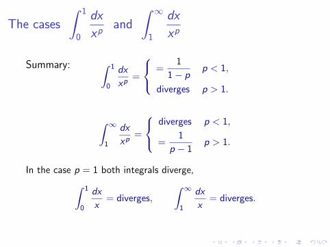
The cases
∫ 1
0
dx
xpand
∫ ∞
1
dx
xp
Summary: ∫ 1
0
dx
xp=
=1
1− pp < 1,
diverges p > 1.
∫ ∞
1
dx
xp=
diverges p < 1,
=1
p − 1p > 1.
In the case p = 1 both integrals diverge,∫ 1
0
dx
x= diverges,
∫ ∞
1
dx
x= diverges.
Related Documents