Integrating optical satellite data and airborne laser scanning in habitat classification for wildlife management

1

Pre-print of published version 1 2

Reference: 3 Nijland, W., Coops, N.C., Nielsen, S.E., Stenhouse, G., 2015. Integrating optical satellite data and 4

airborne laser scanning in habitat classification for wildlife management. International Journal of 5

Applied Earth Observation and Geoinformation 38, 242–250. 6

DOI 7

http://dx.doi.org/10.1016/j.jag.2014.12.004 (published online February 2014) 8

9 Disclaimer: 10 The PDF document is a copy of the final version of this manuscript that was subsequently 11 accepted by the journal for publication. The paper has been through peer review, but it has not 12 been subject to any additional copy-editing or journal specific formatting (so will look different 13 from the final version of record, which may be accessed following the DOI above depending on 14 your access situation). 15

16

Integrating optical satellite data and Airborne Laser Scanning in 17

habitat classification for wildlife management 18

19

W. Nijland1, N.C. Coops1, S.E. Nielsen2, G. Stenhouse3 20

21

1Department of Forest Resources Management, University of British Columbia, 2424 Main Mall, 22

Vancouver BC, V6T 1Z4, Canada 23

2Department of Renewable Resources, University of Alberta, 751 Generals Services Building, 24

Edmonton AB, T6G 2H1, Canada 25

3Foothills Research Institute, Box 6330, Hinton AB, T7V 1X6, Canada 26

ABSTRACT 27

Wildlife habitat selection is determined by a wide range of factors including food availability, 28

shelter, security and landscape heterogeneity all of which are closely related to the more readily 29

mapped landcover types and disturbance regimes. Regional wildlife habitat studies often used 30

moderate resolution multispectral satellite imagery for wall to wall mapping, because it offers a 31

favourable mix of availability, cost and resolution. However, certain habitat characteristics such as 32

2

canopy structure and topographic factors are not well discriminated with these passive, optical 33

datasets. Airborne Laser Scanning (ALS) provides highly accurate three dimensional data on canopy 34

structure and the underlying terrain, thereby offers significant enhancements to wildlife habitat 35

mapping. In this paper, we introduce an approach to integrate ALS data and multispectral images to 36

develop a new heuristic wildlife habitat classifier for western Alberta. Our method combines ALS 37

direct measures of canopy height, and cover with optical estimates of species (conifer vs deciduous) 38

composition into a decision tree classifier for habitat- or landcover types. We believe this new 39

approach is highly versatile and transferable, because class rules can be easily adapted for other 40

species or functional groups. We discuss the implications of increased ALS availability for habitat 41

mapping and wildlife management and provide recommendations for integrating multispectral and 42

ALS data into wildlife management. 43

44

3

INTRODUCTION 45

Wildlife respond to a large number of factors when selecting habitat, involving complex behavioral 46

decisions which are made at multiple spatial scales (Ciarniello et al., 2007; Herfindal et al., 2009; 47

Johnson et al., 2002). Broad scale spatial variation in biodiversity is thought to respond to three 48

major drivers; climatic stability, productivity, and habitat structure (MacArthur, 1972) – with 49

empirical evidence demonstrating the importance of each of these variables (Coops et al., 2008). 50

Bioclimatic models are often applied to estimate broad-scale distribution of species (Guisan and 51

Zimmermann, 2000; Rahbek and Graves, 2001; Willis and Whittaker, 2002). However, at finer 52

spatial scales land cover, disturbance, and habitat heterogeneity are more important factors 53

affecting local distribution and habitat selection of species (Iverson and Prasad, 1998; Thuiller, 54

2004). 55

The vertical and horizontal structure of vegetation plays a critical role in defining suitable wildlife 56

habitat and can do so in a variety of ways. For certain species, vegetation structure drives food 57

quality, diversity, and availability (Hamer and Herrero, 1987; Johnson et al., 2002; Månsson et al., 58

2007). Access to high quality forage in early successional stage forest stands, deciduous overstorey 59

stands, or open areas with grass, forb, herb and berry species (Allen et al., 1987; Dussault et al., 60

2005; Munro et al., 2006) decrease energy required for foraging and digestion in grizzly bear (Ursus 61

arctos), and thus maximise energy intake (White, 1983). Vegetation structure also provides 62

protection and/or cover which provides security against predation and can protect species from 63

heat stress when ambient temperature exceeds optimal levels (Schwab and Pitt, 1991), or deep 64

snow during winter; with snow accumulation often adversely impacting species mobility and food 65

intake, and thus the survival and reproductive rates (Cederlund et al., 1991; Mech and McRoberts, 66

1987; Post and Stenseth, 1998). Vegetation structure is also inextricably linked to disturbances; 67

especially fire, harvesting, and insect defoliation. As a result, disturbances potentially increase 68

future habitat suitability for bears (Nielsen et al., 2008; Nielsen, Munro et al., 2004; Rempel et al., 69

1997; Stewart et al., 2012). Heterogeneity in vegetation structure also provides access to forest 70

edges, where forage and protection are amplified (i.e., the cover-food edge concept) which is a key 71

habitat type selected by many species (Courtois et al., 2002; Dussault et al., 2005; Stewart et al., 72

2013), although edges can also represent attractive sinks where survival is low (Nielsen et al., 2006; 73

Nielsen, Boyce et al., 2004). 74

4

Grizzly bears have diverse seasonal habitat requirements with three distinct foraging seasons, 75

hypophagia, early hyperphagia, and later hyperphagia (Nielsen et al., 2006). In hypophagia they 76

forage on roots (such as alpine sweetvetch), early herbaceous material and ungulate kills, in early 77

hyperphagia their main diet is green herbaceous material (such as cow parsnip, sedges, and 78

horsetails)_with some insect matter, whereas in late hyperphagia berries make up a the majority of 79

their diet (Hamer and Herrero, 1987; Munro et al., 2006). The optimal habitat for grizzly bears 80

therefore changes significantly throughout the season and contains herbaceous areas, wetlands, 81

and open forest, as well as proximity to forest stands for other habitat requirements including 82

bedding and hiding cover.Over the past 40 years, since the launch of the first Earth observation 83

satellites, satellite-based image classification techniques have been used to map species habitat and 84

has become an important tool in large area mapping and management of wildlife habitat 85

(McDermid et al., 2005; Wang et al., 2009). The Landsat series of sensors in particular have set the 86

standard for regional classification projects because of their combination of spatial and spectral 87

resolution, consistent long term record, and excellent data availability (Cohen and Goward, 2004; 88

Franklin and Wulder, 2002; Leimgruber et al., 2005). However, considerable limitations exist in the 89

application of optical satellite imagery specifically involving the detection of detailed forest 90

structural characteristics beyond initial canopy closure (Franklin et al., 2003; Wang et al., 2009). 91

The issue of signal saturation on optical remote sensing imagery with increasing leaf area is well 92

known. Studies have shown both theoretically and practically that estimation of canopy parameters 93

can be difficult beyond a leaf area index of 3 – 5 (Baret and Guyot, 1991; Song, 2012; Turner et al., 94

1999) and that canopy parameter estimation also varies between conifer and deciduous canopy 95

types (Song, 2012). As a result while classification schemes often recognize the importance of forest 96

structure in the class definition (Franklin and Wulder, 2002; McDermid et al., 2009; Wulder et al., 97

2008a), they are often generalized or have considerable uncertainty in forest density classes caused 98

by the inherent limitations of the optical sensor system. 99

Many have tried to bridge the gap between the need for structural information and the inability of 100

direct optical classification to provide this information. Solutions may include the use of ancillary 101

data, texture information, object based analysis, post classification procedures, or other remotely 102

sensed data like radar (Lu and Weng, 2007; Roberts et al., 2007). The most common source of 103

ancillary data is elevation models (Franklin et al., 2002; Johnson et al., 2003; McDermid et al., 2009) 104

and topographic derivatives like slope and aspect. Texture information is used in the form of gray-105

level co-occurrence matrices (Franklin et al., 2002), spatial autocorrelation (Magnussen et al., 106

2004), or variogram functions (Zhang et al., 2004), based on homogeneity assumptions within the 107

5

forest stand and the information content of shaded vs sunlit parts in the canopy. In post 108

classification methods the fine scale patterning of simple land-cover types (e.g. treed, herb, bare) or 109

vegetation indices can be used to define habitat classes (Sluiter et al., 2004). Radar in particular is 110

able to partially penetrate vegetation canopies, but the efficacy in detecting structure is highly 111

dependent on the microwave wavelength, vegetation height and moisture content (Imhoff et al., 112

1997). All of these potential solutions can improve classification results in certain cases, but can be 113

laborious, costly and require extensive training data or manual steps which may lead to interpreter-114

related differences and locally optimised but regionally less applicable results. 115

Airborne Laser Scanning (ALS) uses discrete return small footprint airborne lidar to map the 116

elevation of the ground surface and canopy elements. ALS provides high accuracy measurement of 117

canopy heights and density through the separation of the terrain model from canopy returns. 118

Terrain height and landforms are used to model hydrological and soil processes (White et al., 2012) 119

and are shown to be key drivers of plant species distribution (Nijland et al., 2014).The potential of 120

ALS to detect structural forest characteristics has been shown in many studies, and it has quickly 121

become an operational technology for estimation of forest height, cover and structure around the 122

world (Lim et al., 2008; Wulder Bater et al., 2008). ALS data can provide specific information on 123

forest structure, such as understory and midstory cover assessment, topographic morphological 124

variables, such as slope and aspect, as well as the presence of old, tall trees or snags. As a result, the 125

use of ALS technology has increased for assessments of wildlife habitat. Hyde et al. (2005) utilized 126

ALS data to characterize montane forest canopy structure in the Sierra National Forest for large-127

area habitat mapping. They found that the accurate prediction of canopy height, canopy cover, and 128

biomass was an important prerequisite predicting wildlife habitat showing significant promise in 129

its use. Vierling et al. (2008) provide a review of the current status of ALS remote sensing and 130

habitat characterization and conclude that, although a growing number of studies highlight interest 131

in ALS advances, few studies have actually used the data to quantitatively address these 132

relationships. 133

Western Alberta, Canada is a highly dynamic region where widespread resources extraction from 134

the forestry and fossil fuels industries occurs on important habitat for species at risk (Roever et al., 135

2008). Coal, oil, gas, and timber extraction, in addition to related population growth, urban 136

development and expanding demands for outdoor recreation impact biodiversity through habitat 137

alteration and fragmentation (Schneider et al., 2003). Western Alberta represents the eastern limit 138

of grizzly bear habitat in Southern Canada (Nielsen et al., 2009) and has an important population of 139

woodland caribou (Tarandus rangifer) (Bradshaw and Hebert, 1996; Festa-Bianchet et al., 2011). 140

6

Effective management of wildlife habitat is of paramount importance for sustainable support of 141

both ecological values and resource extraction in the region. To support wildlife and habitat 142

management we need a detailed account of habitat status and a thorough understanding of the 143

habitat requirements of different key species. The availability of accurate habitat maps is crucial for 144

both objectives. 145

In this research we introduce an approach to integrate ALS and multispectral satellite images to 146

develop a new heuristic wildlife habitat classifier for western Alberta. The classifier uses vegetation 147

structure, species composition, and terrain characteristics derived from available ALS and 148

multispectral data directly in a decision tree. We evaluate the accuracy of the habitat layers and 149

discuss the added value of the created products for the classification. Based on our results we look 150

at implications of increased ALS availability for habitat mapping and wildlife management, and 151

make recommendations on the application of ALS in regional habitat mapping efforts. 152

METHODS 153

Study area 154

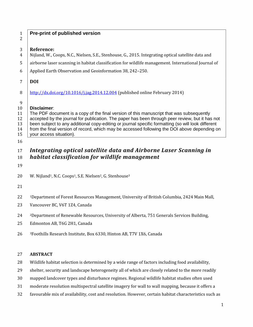
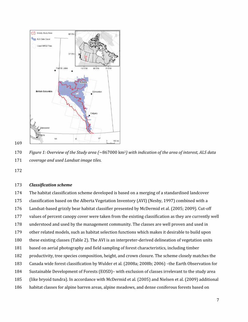
Our focus areas encompasses the western Rocky Mountains in Alberta, Canada constrained by the 155

Upper and Lower foothills Natural subregions, with the higher elevations in the Alpine natural 156

subregion (Downing and Pettapiece, 2006) (Figure 1). Elevations range from 700 to 3000m ASL 157

with steep montane topography in the west, transitioning to a gently rolling landscape in the 158

eastern parts of the area. The natural vegetation in the sub-alpine areas is forested with Lodgepole 159

Pine (Pinus Contorta), White Spruce (Picea glauca), and Trembling Aspen (Populus tremuloides) as 160

the dominant tree species. The area has extensive resource extraction of underground resources 161

(coal, oil, and natural gas) and forest harvesting. This results in a mosaic of mature forest, regrowth 162

forest and barren or recovering areas. 163

Our focus species for the habitat assessment is the grizzly bear which was designated as a 164

threatened species within Alberta with considerable pressures on the population from human 165

caused mortality, and habitat changes associated with forest management, resource extraction, and 166

natural disturbances (Festa-Bianchet, 2010). The provincial government has a provincial grizzly 167

bear recovery plan underway for this species. 168

7

169

Figure 1: Overview of the Study area (~867000 km2) with indication of the area of interest, ALS data 170

coverage and used Landsat image tiles. 171

172

Classification scheme 173

The habitat classification scheme developed is based on a merging of a standardised landcover 174

classification based on the Alberta Vegetation Inventory (AVI) (Nesby, 1997) combined with a 175

Landsat-based grizzly bear habitat classifier presented by McDermid et al. (2005; 2009). Cut-off 176

values of percent canopy cover were taken from the existing classification as they are currently well 177

understood and used by the management community. The classes are well proven and used in 178

other related models, such as habitat selection functions which makes it desirable to build upon 179

these existing classes (Table 2). The AVI is an interpreter-derived delineation of vegetation units 180

based on aerial photography and field sampling of forest characteristics, including timber 181

productivity, tree species composition, height, and crown closure. The scheme closely matches the 182

Canada wide forest classification by Wulder et al. (2008a; 2008b; 2006) –the Earth Observation for 183

Sustainable Development of Forests (EOSD)– with exclusion of classes irrelevant to the study area 184

(like bryoid tundra). In accordance with McDermid et al. (2005) and Nielsen et al. (2009) additional 185

habitat classes for alpine barren areas, alpine meadows, and dense coniferous forests based on 186

8

their relevance for grizzly bear were included. Alpine meadows have specific food resources like 187

Alpine Sweetvetch (Hedisarum alpinum) (Coogan et al., 2012; Nijland et al., 2012), plus both alpine 188

meadows and alpine barren areas are expected to be stable, while meadow and barren landcover 189

types in lowlands are often the result of disturbances and may quickly develop more vegetation 190

cover. Dense coniferous forest are separated as a distinct class because of their relevance for 191

denning sites (Ciarniello et al., 2005; Pigeon et al., 2014), but usually lower yield of fruiting species 192

(Nielsen Munro et al., 2004). These classes were not separated previously, because they were not 193

reliably detected in previously used multispectral classifiers. They are more likely however to be 194

successfully separated using topographical and canopy structure information from ALS. We chose 195

to split them from existing classes to allow for a backwards compatible generalization of the newly 196

created habitat types with existing maps. 197

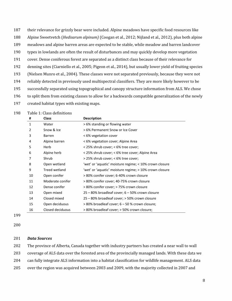
Table 1: Class definitions 198 # Class Description

1 Water > 6% standing or flowing water

2 Snow & Ice > 6% Permanent Snow or Ice Cover

3 Barren < 6% vegetation cover

4 Alpine barren < 6% vegetation cover; Alpine Area

5 Herb < 25% shrub cover; < 6% tree cover;

6 Alpine herb < 25% shrub cover; < 6% tree cover; Alpine Area

7 Shrub > 25% shrub cover; < 6% tree cover;

8 Open wetland ‘wet’ or ‘aquatic’ moisture regime; < 10% crown closure

9 Treed wetland ‘wet’ or ‘aquatic’ moisture regime; > 10% crown closure

10 Open conifer > 80% conifer cover; 6-40% crown closure

11 Moderate conifer > 80% conifer cover; 40-75% crown closure

12 Dense conifer > 80% conifer cover; > 75% crown closure

13 Open mixed 25 – 80% broadleaf cover; 6 – 50% crown closure

14 Closed mixed 25 – 80% broadleaf cover; > 50% crown closure

15 Open deciduous > 80% broadleaf cover; 6 – 50 % crown closure;

16 Closed deciduous > 80% broadleaf cover; > 50% crown closure;

199

200

Data Sources 201

The province of Alberta, Canada together with industry partners has created a near wall to wall 202

coverage of ALS data over the forested area of the provincially managed lands. With these data we 203

can fully integrate ALS information into a habitat classification for wildlife management. ALS data 204

over the region was acquired between 2003 and 2009, with the majority collected in 2007 and 205

9

2008. Data from different acquisitions was acquired, thinned, and distributed as 1 x 1m gridded 206

products including a bare earth layer, and a full feature (top of canopy) layer. Figure 1 shows the 207

extent of ALS coverage in the study area, cover is near complete for the core grizzly range with the 208

exception of the Rocky Mountain national park lands managed by the Federal government. Prior to 209

classification, the 1m products were generalized to 25x25m grid metrics in FUSION (McGaughey, 210

2014), with metrics including maximum canopy height, and returns above 2 m. The bare earth 211

product was used to create a 25m digital terrain model (DTM) and slope layers. In addition to these 212

ALS products, a depth to groundwater layer was also developed from the bare earth model using a 213

hydrological modelling process described in White et al. (2012). 214

A Landsat Thematic Mapper mosaic based on data acquired in the summers of 2008–2010 was also 215

developed. All scenes were processed to surface reflectance by the USGS using their standard image 216

preprocessing procedures (Masek et al., 2006; USGS, 2013) . In addition to summer images a leaf-off 217

mosaic was created using snow free images acquired in October and November, for this mosaic less 218

cloud-free images were available which was compensated for by including Landsat 7 ETM+ (SLC-219

off) images and a wider range of years (2007–2011). The leaf-off mosaic was used only to improve 220

the conifer model; all other classes were derived from the ALS and the Summer mosaic. 221

Reference data 222

Field reference data were collected during a field campaign in 2013. During the campaign 102 223

variable radius plots were established using a structurally guided sampling scheme based on 224

species composition and vegetation height. The centre point located using GPS. At each plot, habitat 225

class, vegetation height (using a vertex III hypsometer (Haglof Sweden AB)), vegetated cover (using 226

a spherical densitometer), soil wetness (dry|mesic|wet), and canopy species composition were 227

recorded. Reference data were used to evaluate the ALS based models of canopy structure, and to 228

build the regression model for percent conifer cover for use in the classification. 229

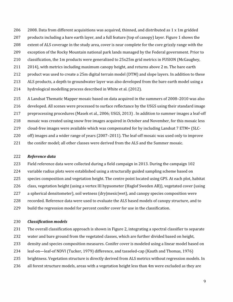
Classification models 230

The overall classification approach is shown in Figure 2, integrating a spectral classifier to separate 231

water and bare ground from the vegetated classes, which are further divided based on height, 232

density and species composition measures. Conifer cover is modeled using a linear model based on 233

leaf-on—leaf-of NDVI (Tucker, 1979) difference, and tasseled-cap (Kauth and Thomas, 1976) 234

brightness. Vegetation structure is directly derived from ALS metrics without regression models. In 235

all forest structure models, areas with a vegetation height less than 4m were excluded as they are 236

10

not considered as forest in our classification. The hydrologic model for depth-to-water-table is 237

described in White et al. (2012) and uses topographic routing of water over the terrain surface 238

together with fixed area for flow initiation to derive the water table height. The parts of the study 239

area that have no ALS data present are in-filled using a standard maximum likelihood classifier on 240

the Landsat visible, near infrared and short wave infrared spectral bands, DTM , and Percent 241

Conifer layers. We evaluate the agreement between our integrated classification with the 242

classification without ALS data using an equalized random sample of 1000 points per class taken 243

from the area where both classifications area available. While this cannot be interpreted as a 244

validation of our results, the comparison reflects on the improvement our integrated classification 245

provides over a more traditional classifier. 246

247

Figure 2: Classification flow chart 248

249

RESULTS 250

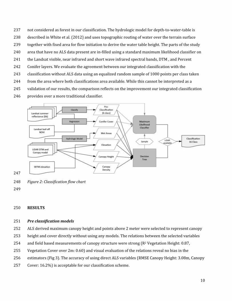
Pre classification models 251

ALS derived maximum canopy height and points above 2 meter were selected to represent canopy 252

height and cover directly without using any models. The relations between the selected variables 253

and field based measurements of canopy structure were strong (R2 Vegetation Height: 0.87, 254

Vegetation Cover over 2m: 0.60) and visual evaluation of the relations reveal no bias in the 255

estimators (Fig 3). The accuracy of using direct ALS variables (RMSE Canopy Height: 3.08m, Canopy 256

Cover: 16.2%) is acceptable for our classification scheme. 257

11

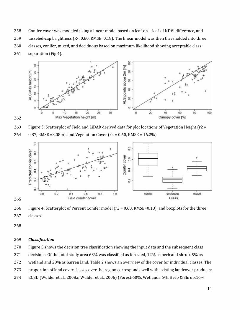
Conifer cover was modeled using a linear model based on leaf-on—leaf-of NDVI difference, and 258

tasseled-cap brightness (R2: 0.60, RMSE: 0.18). The linear model was then thresholded into three 259

classes, conifer, mixed, and deciduous based on maximum likelihood showing acceptable class 260

separation (Fig 4). 261

262

Figure 3: Scatterplot of Field and LiDAR derived data for plot locations of Vegetation Height (r2 = 263

0.87, RMSE =3.08m), and Vegetation Cover (r2 = 0.60, RMSE = 16.2%). 264

265

Figure 4: Scatterplot of Percent Conifer model (r2 = 0.60, RMSE=0.18), and boxplots for the three 266

classes. 267

268

Classification 269

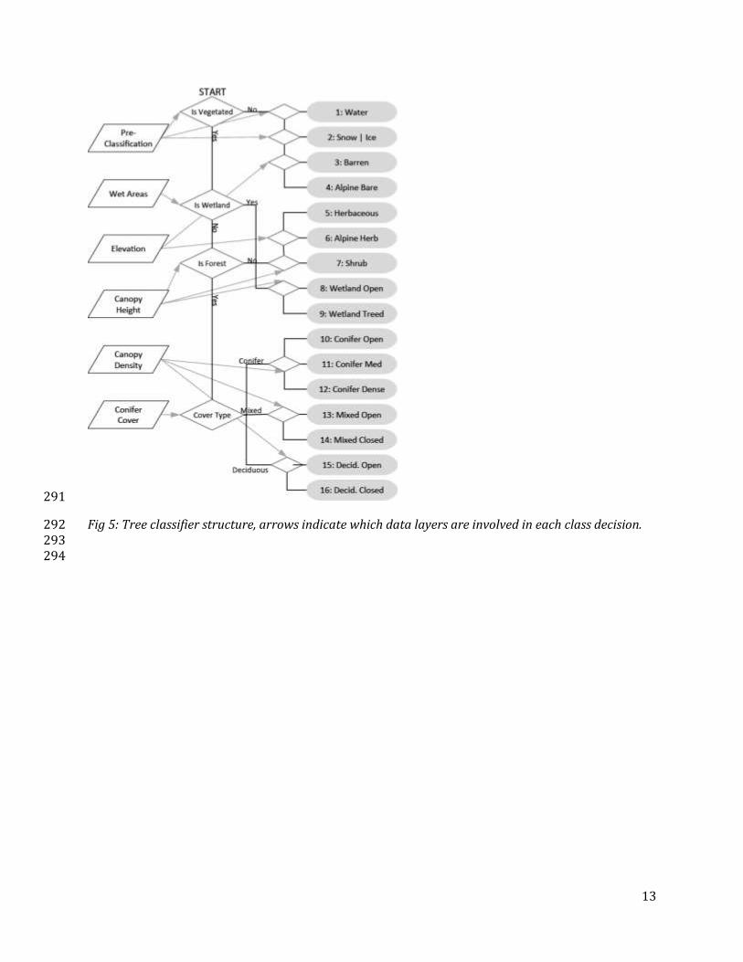
Figure 5 shows the decision tree classification showing the input data and the subsequent class 270

decisions. Of the total study area 63% was classified as forested, 12% as herb and shrub, 5% as 271

wetland and 20% as barren land. Table 2 shows an overview of the cover for individual classes. The 272

proportion of land cover classes over the region corresponds well with existing landcover products: 273

EOSD (Wulder et al., 2008a; Wulder et al., 2006) (Forest:60%, Wetlands:6%, Herb & Shrub:16%, 274

12

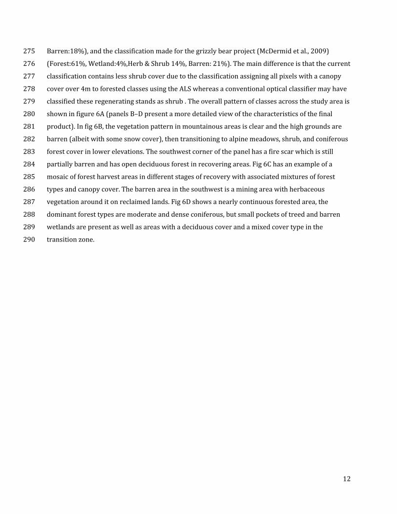
Barren:18%), and the classification made for the grizzly bear project (McDermid et al., 2009) 275

(Forest:61%, Wetland:4%,Herb & Shrub 14%, Barren: 21%). The main difference is that the current 276

classification contains less shrub cover due to the classification assigning all pixels with a canopy 277

cover over 4m to forested classes using the ALS whereas a conventional optical classifier may have 278

classified these regenerating stands as shrub . The overall pattern of classes across the study area is 279

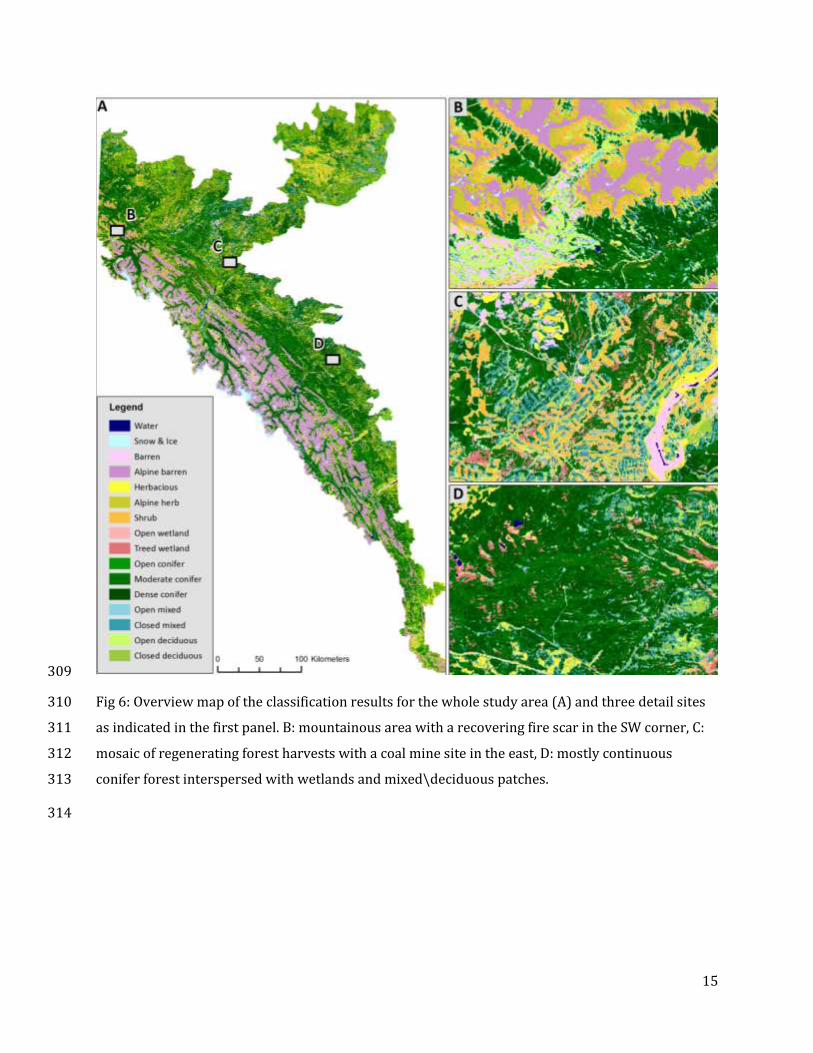
shown in figure 6A (panels B–D present a more detailed view of the characteristics of the final 280

product). In fig 6B, the vegetation pattern in mountainous areas is clear and the high grounds are 281

barren (albeit with some snow cover), then transitioning to alpine meadows, shrub, and coniferous 282

forest cover in lower elevations. The southwest corner of the panel has a fire scar which is still 283

partially barren and has open deciduous forest in recovering areas. Fig 6C has an example of a 284

mosaic of forest harvest areas in different stages of recovery with associated mixtures of forest 285

types and canopy cover. The barren area in the southwest is a mining area with herbaceous 286

vegetation around it on reclaimed lands. Fig 6D shows a nearly continuous forested area, the 287

dominant forest types are moderate and dense coniferous, but small pockets of treed and barren 288

wetlands are present as well as areas with a deciduous cover and a mixed cover type in the 289

transition zone. 290

13

291

Fig 5: Tree classifier structure, arrows indicate which data layers are involved in each class decision. 292 293 294

14

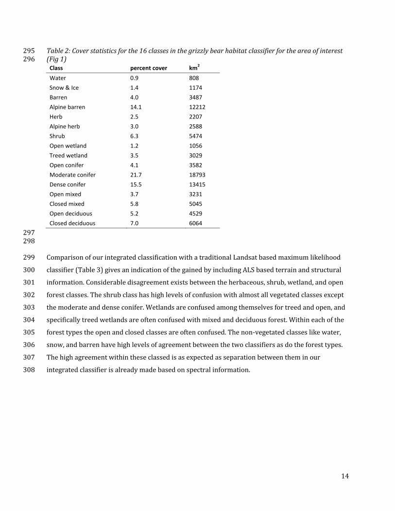
Table 2: Cover statistics for the 16 classes in the grizzly bear habitat classifier for the area of interest 295 (Fig 1) 296

Class percent cover km2

Water 0.9 808

Snow & Ice 1.4 1174

Barren 4.0 3487

Alpine barren 14.1 12212

Herb 2.5 2207

Alpine herb 3.0 2588

Shrub 6.3 5474

Open wetland 1.2 1056

Treed wetland 3.5 3029

Open conifer 4.1 3582

Moderate conifer 21.7 18793

Dense conifer 15.5 13415

Open mixed 3.7 3231

Closed mixed 5.8 5045

Open deciduous 5.2 4529

Closed deciduous 7.0 6064

297 298

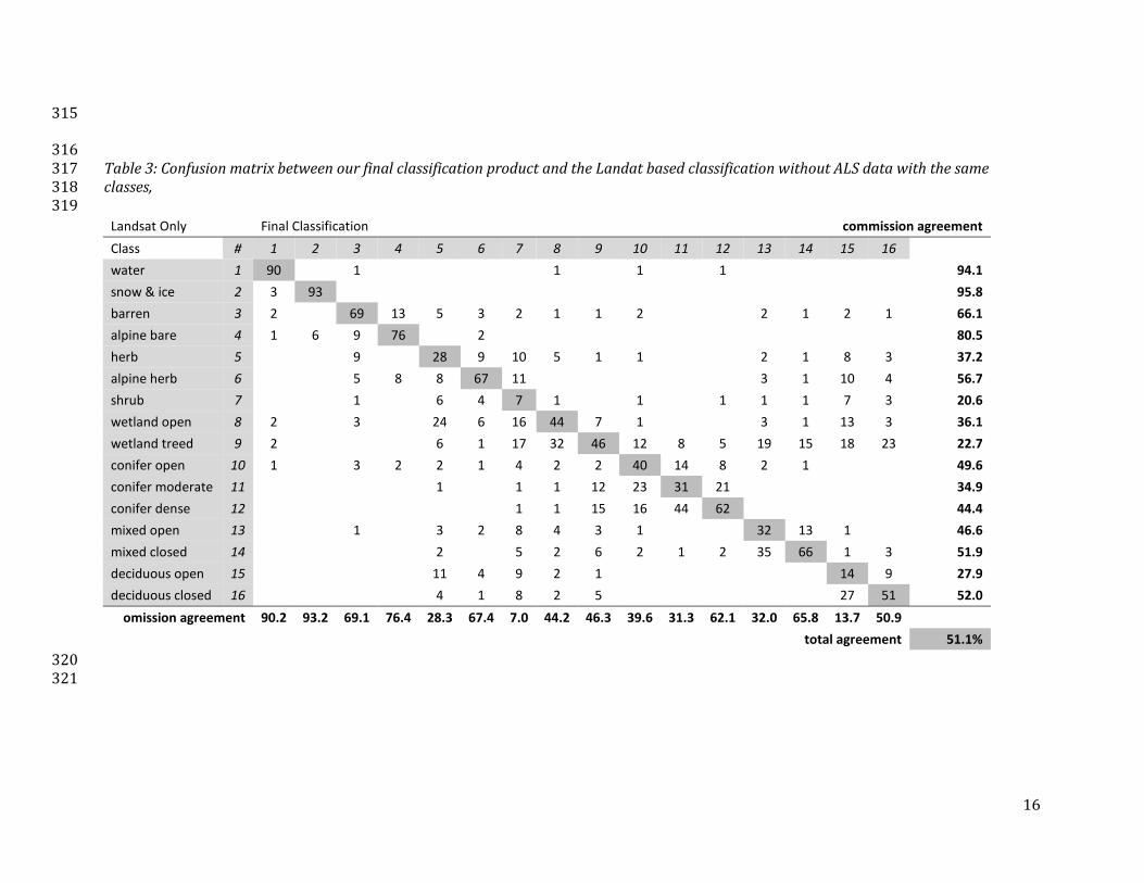
Comparison of our integrated classification with a traditional Landsat based maximum likelihood 299

classifier (Table 3) gives an indication of the gained by including ALS based terrain and structural 300

information. Considerable disagreement exists between the herbaceous, shrub, wetland, and open 301

forest classes. The shrub class has high levels of confusion with almost all vegetated classes except 302

the moderate and dense conifer. Wetlands are confused among themselves for treed and open, and 303

specifically treed wetlands are often confused with mixed and deciduous forest. Within each of the 304

forest types the open and closed classes are often confused. The non-vegetated classes like water, 305

snow, and barren have high levels of agreement between the two classifiers as do the forest types. 306

The high agreement within these classed is as expected as separation between them in our 307

integrated classifier is already made based on spectral information. 308

15

309

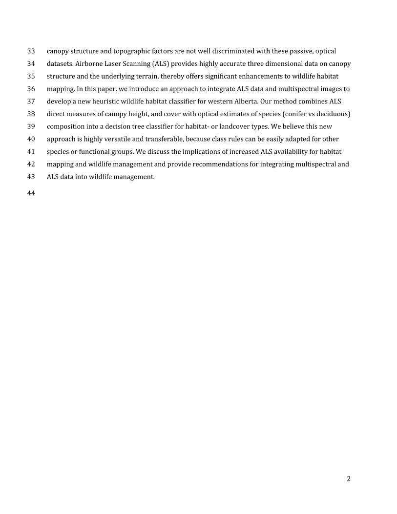
Fig 6: Overview map of the classification results for the whole study area (A) and three detail sites 310

as indicated in the first panel. B: mountainous area with a recovering fire scar in the SW corner, C: 311

mosaic of regenerating forest harvests with a coal mine site in the east, D: mostly continuous 312

conifer forest interspersed with wetlands and mixed\deciduous patches. 313

314

16

315

316 Table 3: Confusion matrix between our final classification product and the Landat based classification without ALS data with the same 317 classes, 318 319

Landsat Only

Final Classification

commission agreement

Class # 1 2 3 4 5 6 7 8 9 10 11 12 13 14 15 16

water 1 90

1

1

1

1

94.1

snow & ice 2 3 93

95.8

barren 3 2

69 13 5 3 2 1 1 2

2 1 2 1 66.1

alpine bare 4 1 6 9 76

2

80.5

herb 5

9

28 9 10 5 1 1

2 1 8 3 37.2

alpine herb 6

5 8 8 67 11

3 1 10 4 56.7

shrub 7

1

6 4 7 1

1

1 1 1 7 3 20.6

wetland open 8 2

3

24 6 16 44 7 1

3 1 13 3 36.1

wetland treed 9 2

6 1 17 32 46 12 8 5 19 15 18 23 22.7

conifer open 10 1

3 2 2 1 4 2 2 40 14 8 2 1

49.6

conifer moderate 11

1

1 1 12 23 31 21

34.9

conifer dense 12

1 1 15 16 44 62

44.4

mixed open 13

1

3 2 8 4 3 1

32 13 1

46.6

mixed closed 14

2

5 2 6 2 1 2 35 66 1 3 51.9

deciduous open 15

11 4 9 2 1

14 9 27.9

deciduous closed 16

4 1 8 2 5

27 51 52.0

omission agreement 90.2 93.2 69.1 76.4 28.3 67.4 7.0 44.2 46.3 39.6 31.3 62.1 32.0 65.8 13.7 50.9

total agreement 51.1%

320 321

17

DISCUSSION 322

Traditional spectral classifiers rely on training data (for supervised classifications), or the 323

discretion of the interpreter (for labeling unsupervised clustering), and maximise class separability 324

for classes that are spectrally different. By adding ancillary data sources such as terrain 325

information, by stratifying datasets, or including the spatial domain into the classification it is 326

possible to improve the classification accuracy. 327

Availability of ALS data into habitat classifications allow more direct estimates of vegetation 328

structure in the classification scheme which has been shown to be of direct relevance to habitat 329

evaluation and wildlife management (Vierling et al., 2008). By using ALS data in combination with 330

optical data direct information on vegetation characteristics can be integrated using a heuristic-331

based classifier that directly employs the class definitions as set based on the management needs. 332

Our results indicate that users can gain considerable accuracy improvements over solely Landsat-333

based classifications (Table 3). 334

335

Integrating ALS derived structural information into habitat classifications allows habitat 336

classification to be tailored for specific species or functional groups. In this approach we used 337

continuous input layers for which the class rules can be adapted to create new products without the 338

need of additional input data. ALS supports this system specifically by providing information 339

difficult to obtain using passive optical sensing systems such as small scale topographical features 340

and vertical vegetation structure. Improvements are also possible for classes which describe the 341

understory which can be detected from ALS, but often have non-unique spectral signatures because 342

of canopy cover. Key habitats where the fusion of ALS and optical data are likely to be beneficial 343

include: 344

Wetland areas: moist soils and wetland areas are often not spectrally unique in the overstorey from 345

drier forests or herbal vegetation as multispectral images are much more sensitive for vegetation 346

density and vigor then individual species (Baker et al., 2006; Johnston and Barson, 1993). However, 347

understory cover and associated resources for animals are fundamentally different. The terrain 348

detail ALS data provide enables accurate mapping of topographically wet areas (White et al., 2012) 349

and separates them from other habitat types. 350

Alpine areas: Alpine meadows and barren terrain are spectrally similar to lower barren or herbal 351

areas but provide different functions and resources to wildlife (Munro et al., 2006). Lowland areas 352

18

with no forest cover are usually transient and result from disturbances, while alpine areas have 353

more stable vegetation cover. The ALS-derived elevation model can be used to separate alpine 354

areas by elevation threshold, or using an automated alpine tree-line detection algorithm as 355

employed in Coops et al. (2013). 356

Forest-cover density: Canopy closure is a crucial habitat driver as it relates to understory 357

composition, fruit productivity (Hamer, 1996; Nielsen et al., 2010; Nielsen Munro et al., 2004), and 358

providing cover from adverse climate and snowfall (Mech and McRoberts, 1987; Schwab and Pitt, 359

1991). Optical methods saturate beyond LAI > 3-5 m2/m2 and may have ambiguous results 360

depending on different species compositions. ALS cover measures are consistent over both 361

deciduous and coniferous species and do not saturate at densities found in temperate or boreal 362

forests. ALS therefore allows for the more detailed and consistent separation of canopy density 363

classes. 364

Species composition: ALS has limited potential for the classification of specific species or the 365

separation of coniferous vs. deciduous vegetation cover (Wulder Bater et al., 2008). Neither do 366

commonly used height metrics separate low herbaceous vegetation and barren areas. We are 367

fortunate that these classes are already reliably separated using multispectral images similarly to 368

separating water bodies from terrestrial habitats. To maximise the separation of deciduous vs. 369

coniferous vegetation cover, we use a combination of leaf-on and leaf-off images which leads to 370

reliable separation of these forest types. Integrating both ALS and optical data sources, we 371

demonstrate the possibility of a complete heuristic habitat classification scheme for wildlife habitat 372

that can be easily adapted for the needs of specific species. 373

We recognise ALS is not ubiquitously available over all jurisdictions; however, this is quickly 374

changing. Through the combined effort of industry and provincial government an almost wall to 375

wall ALS coverage of the forested areas in Alberta has been acquired. This paper demonstrates how 376

valuable these types of data are, not only in engineering and resource management, but also for 377

improving wildlife management and supporting ecological values and other benefits of forests. The 378

current map product is created for regional applications and uses a raster resolution of 25m for 379

summarizing the ALS derived canopy metrics. The generalization of data to this 25m grid size 380

facilitated integration with multispectral images and minimised the impact of different survey 381

configurations of the merged large area ALS dataset. The approach of using naïve estimators from 382

ALS to represent vegetation structure does produce relatively high RMSE values, but the 383

relationship is highly transferable and has minimal bias. Loss in detail compared to the state of the 384

19

art in laser scanning is in exchange for the gain in integration of ALS and multispectral satellite data 385

for large area applications supporting more effective habitat and wildlife management. 386

CONCLUSIONS 387

In this paper we present a new habitat classification for grizzly bear management in Alberta, 388

Canada. We combine optical satellite images and ALS into a heuristic, decision tree based habitat 389

classifier. Based on the integrated use of optical and ALS data we are able to describe the major 390

axes of landscape variability including species composition and vegetation structure and to use 391

these data directly in the landcover classifier. The classifier allows for more detailed habitat classes 392

in alpine areas, wetlands and overstory density and structure and represents a step forward from 393

currently available products. This proposed system is versatile in the sense that the class rules can 394

be easily adapted for other species or functional groups without the need of additional inputs or 395

training data. Integration of multispectral satellite images and ALS enables an adaptable 396

classification system that supports informed decision making for wildlife management. 397

ACKNOWLEDGEMENTS 398

Funding for this research was generously provided by the grizzly bear program of the Foothills 399

Research Institute located in Hinton, Alberta, Canada, with additional information available at: 400

www.foothillsri.ca. Additional funds were provided by an NSERC Discovery grants to Dr. Nicholas 401

Coops and Dr. Scott Nielsen. Lidar data was made available by the Government of Alberta. The 402

authors thank Adam Erickson and Ilia Parshakov for their help with the field program, and Dr. 403

Txomin Hermosilla for his assistance Landsat data compositing. The two anonymous reviewers are 404

acknowledged for their constructive contribution to the manuscript. 405

REFERENCES 406

Allen, A.W., Jordan, P.A., Terrell, J.W., 1987. Habitat suitability index models: Moose, Lake Superior 407 region. U.S. Dep. Inter. Fish Wildl. Serv. Biol. Rep. 82, 60. 408

Baker, C., Lawrence, R., Montagne, C., Patten, D., 2006. Mapping wetlands and riparian areas using 409 Landsat ETM+ imagery and decision-tree-based models. Wetlands 26, 465–474. 410

Baret, F., Guyot, G., 1991. Potentials and limits of vegetation indices for LAI and APAR assessment. 411 Remote Sens. Environ. 35, 161–173. 412

Bradshaw, C., Hebert, D., 1996. Woodland caribou population decline in Alberta: fact or fiction? 413 Rangifer, Special Issue 9, 223-224. 414

Cederlund, G., Sand, H., Pehrson, Å., 1991. Body mass dynamics of moose calves in relation to winter 415 severity. J. Wildl. Manage. 55, 675–81. 416

20

Ciarniello, L.M., Boyce, M.S., Heard, D.C., Seip, D.R., 2005. Denning behavior and den site selection of 417 grizzly bears along the Parsnip River, British Columbia, Canada. Ursus 16, 47–58. 418

Ciarniello, L.M., Boyce, M.S., Seip, D.R., Heard, D.C., 2007. Grizzly bear habitat selection is scale 419 dependent. Ecol. Appl. 17, 1424–40. 420

Cohen, W.B., Goward, S.N., 2004. Landsat’s role in ecological applications of remote sensing. 421 Bioscience 54, 535–45. 422

Coogan, S., Nielsen, S., Stenhouse, G., 2012. Spatial and temporal heterogeneity creates a “brown 423 tide” in root phenology and nutrition. ISRN Ecol. 618257, 1–10. 424

Coops, N.C., Morsdorf, F., Schaepman, M.E., Zimmermann, N.E., 2013. Characterization of an alpine 425 tree line using airborne LiDAR data and physiological modeling. Glob. Chang. Biol. 3808–21. 426

Coops, N.C., Wulder, M.A., Duro, D., Han, T., Berry, S.L., 2008. The development of a Canadian 427 dynamic habitat index using multi-temporal satellite estimates of canopy light absorbance. 428 Ecol. Indic. 8, 754–66. 429

Courtois, R., Dussault, C., Potvin, F., Daigle, G., 2002. Habitat selection by moose (Alces alces) in 430 clear-cut landscapes. Alces 38, 177–92. 431

Downing, D.J., Pettapiece, W.W., 2006. Natural regions and subregions of Alberta. Gov. Alberta Publ. 432 T/852. 433

Dussault, C., Ouellet, J.P., Courtois, R., Huot, J., Breton, L., Jolicoeur, H., 2005. Linking moose habitat 434 selection to limiting factors. Ecography (Cop.). 28, 619–628. 435

Festa-Bianchet, M., 2010. Status of the Grizzly Bear ( Ursus arctos ) in Alberta : Update 2010. 436 Alberta Wildl. Status Rep. 37, 56. 437

Festa-Bianchet, M., Ray, J.C., Boutin, S., Côté, S.D., Gunn, A., 2011. Conservation of caribou (Rangifer 438 tarandus) in Canada: an uncertain future. Can. J. Zool. 89, 419–434. 439

Franklin, S.E., Hall, R.J., Smith, L., Gerylo, G.R., 2003. Discrimination of conifer height, age and crown 440 closure classes using Landsat-5 TM imagery in the Canadian Northwest Territories. Int. J. 441 Remote Sens. 24, 1823–34. 442

Franklin, S.E., Peddle, D.R., Dechka, J.A., Stenhouse, G.B., 2002. Evidential reasoning with Landsat 443 TM, DEM and GIS data for landcover classification in support of grizzly bear habitat 444 mapping. Int. J. Remote Sens. 23, 4633–52. 445

Franklin, S.E., Wulder, M.A., 2002. Remote sensing methods in medium spatial resolution satellite 446 data land cover classification of large areas. Prog. Phys. Geogr. 26, 173–205. 447

Guisan, A., Zimmermann, N.E., 2000. Predictive habitat distribution models in ecology. Ecol. Modell. 448 135, 147–86. 449

Hamer, D., 1996. Buffaloberry Fruit Production in Fire-Successional Bear Feeding Sites. J. Range 450 Manag. 49, 520–529. 451

Hamer, D., Herrero, S., 1987. Grizzly bear food and habitat in the front ranges of Banff National Park, 452 Alberta, in: Zager, P. (Ed.), Proceedings of 7th International Conference on Bear Research 453 and Management. International Association of Bear Research and Management, 454 Williamsburg, Va, U.S.A and Plityice Lakes, Yugoslavia, February and March 1986., pp. 199–455 213. 456

21

Herfindal, I., Tremblay, J.P., Hansen, B.B., Solberg, E.J., Heim, M., Saether, B.E., 2009. Scale 457 dependency and functional response in moose habitat selection. Ecography (Cop.). 32, 849–458 859. 459

Hyde, P., Dubayah, R., Peterson, B., Blair, J.B., Hofton, M., 2005. Mapping forest structure for wildlife 460 habitat analysis using waveform lidar : Validation of montane ecosystems. Sierra. 461

Imhoff, M.F., Sisk, T.D., Milne, A., Morgan, G., Orr, T., 1997. Remotely sensed indicators of habitat 462 heterogeneity: use of synthetic aperature radar in mapping vegetation strucutre and bird 463 habitat. Remote Sens. Environ. 60, 217–227. 464

Iverson, L.R., Prasad, A.M., 1998. Predicting abundance of 80 tree species following climate change 465 in the eastern United States. Ecol. Monogr. 68, 465–85. 466

Johnson, C.J., Alexander, N.D., Wheate, R.D., Parker, K.L., 2003. Characterizing woodland caribou 467 habitat in sub-boreal and boreal forests. For. Ecol. Manage. 180, 241–248. 468

Johnson, C.J., Parker, K.L., Heard, D.C., Gillingham, M.P., 2002. A Multiscale Behavioral Approach to 469 Understanding the Movements of Woodland Caribou. Ecol. Appl. 12, 1840–1860. 470

Johnston, R., Barson, M., 1993. Remote sensing of Australian wetlands: An evaluation of Landsat TM 471 data for inventory and classification. Mar. Freshw. Res. 44, 235. 472

Kauth, R.J., Thomas, G.S., 1976. The Tasselled Cap -- A Graphic Description of the Spectral-Temporal 473 Development of Agricultural Crops as Seen by LANDSAT, in: Symposium on Machine 474 Processing of Remotely Sensed Data. pp. 41–51. 475

Leimgruber, P., Christen, C.A., Laborderie, A., 2005. The impact of Landsat satellite monitoring on 476 conservation biology. Environ. Monit. Assess. 106, 81–101. 477

Lim, B., Brown, S., Schlamadinger, B., 2008. Carbon accounting for forest harvesting and wood 478 products: review and evaluation of different approaches. Environ. Sci. Policy 2, 207–216. 479

Lu, D., Weng, Q., 2007. A survey of image classification methods and techniques for improving 480 classification performance. Int. J. Remote Sens. 28, 823–870. 481

MacArthur, R., 1972. Geographical ecology: patterns in the distribution of species. Harper & Row, 482 New York. 483

Magnussen, S., Boudewyn, P., Wulder, M.A., 2004. Contextual classification of Landsat TM images to 484 forest inventory cover types. Int. J. Remote Sens. 25, 2421–40. 485

Månsson, J., Andrén, H., Pehrson, Å., Bergström, R., 2007. Moose browsing and forage availability: a 486 scale-dependent relationship? Can. J. Zool. 85, 372–80. 487

Masek, J.G., Vermote, E.F., Saleous, N.E., Wolfe, R., Hall, F.G., Huemmrich, K.F., Gao, F., Kutler, J., Lim, 488 T.K., 2006. A Landsat surface reflectance dataset for North America, 1990-2000. Geosci. 489 Remote Sens. Lett. IEEE 3, 68–72. 490

McDermid, G.J., Franklin, S.E., Ledrew, E.F., 2005. Remote sensing for large-area habitat mapping. 491 Prog. Phys. Geogr. 29, 449-74. 492

McDermid, G.J., Hall, R.J., Sanchez-Azofeifa, G.A., Franklin, S.E., Stenhouse, G.B., Kobliuk, T., LeDrew, 493 E.F., 2009. Remote sensing and forest inventory for wildlife habitat assessment. For. Ecol. 494 Manage. 257, 2262–69. 495

McGaughey, R.J., 2014. FUSION/LDV: Software for LIDAR Data Analysis and Visualization. United 496 States Department of Agriculture, Forest Service Pacific Northwest. 497

22

Mech, L., McRoberts, R., 1987. Relationship of deer and moose populations to previous winters’ 498 snow. J. Anim. Ecol. 56, 615–27. 499

Munro, R.H.M., Nielsen, S.E., Price, M.H., Stenhouse, G.B., Boyce, M.S., 2006. Seasonal and diel 500 patterns of grizzly bear diet and activity in west-central Alberta. J. Mammal. 87, 1112–21. 501

Nesby, R. (1997). Alberta Vegetation Inventory. Final Version, 2.2. Alberta Environmental 502 Protection: Edmonton, Alberta, Canada. 503

Nielsen, S., Boyce, M., Stenhouse, G.B., 2004. Grizzly bears and forestry I. Selection of clearcuts by 504 grizzly bears in west-central Alberta. For. Ecol. Manage. 199, 51−65. 505

Nielsen, S., Cranston, J., Stenhouse, G., 2009. Identification of priority areas for grizzly bear 506 conservation and recovery in Alberta, Canada. J. Conserv. Plan. 5, 38–60. 507

Nielsen, S., Graham, K., Larsen, T., Mckay, T., Munro, R., 2010. Chapter 6: Grizzly bear habitat 508 productivity models for the Yellowhead, Swan Hills, Grande Cache and Chinchaga 509 population units of Alberta. Methods, page 60. From: Karine Pigeon, 2010. Denning 510 Behaviour, Thermoregulation, And Environmental Variables, In: G. Stenhouse and K. 511 Graham (eds). Foothills Research Institute Grizzly Bear Program, 2009. Annual Report. 512 Hinton, Alberta. 513

Nielsen, S., Stenhouse, G.B., Boyce, M., 2006. A habitat-based framework for grizzly bear 514 conservation in Alberta. Biol. Conserv. 130, 217–229. 515

Nielsen, S.E., Munro, R.H.M., Bainbridge, E.L., Stenhouse, G.B., Boyce, M.S., 2004. Grizzly bears and 516 forestry: II. Distribution of grizzlybear foods in clearcuts of west-central Alberta, Canada. 517 For. Ecol. Manage. 199, 67–82. 518

Nielsen, S.E., Stenhouse, G.B., Beyer, H.L., Huettmann, F., Boyce, M.S., 2008. Can natural disturbance-519 based forestry rescue a declining population of grizzly bears? Biol. Conserv. 141, 2193–520 2207. 521

Nijland, W., Coops, N.C., Coogan, S.C.P., Bater, C.W., Wulder, M.A., Nielsen, S.E., McDermid, G., 522 Stenhouse, G.B., 2012. Vegetation phenology can be captured with digital repeat 523 photography and linked to variability of root nutrition in Hedysarum alpinum. Appl. Veg. 524 Sci. 1–8. 525

Nijland, W., Nielsen, S.E., Coops, N.C., Wulder, M.A., Stenhouse, G.B., 2014. Fine-spatial scale 526 predictions of understory species using climate- and LiDAR-derived terrain and canopy 527 metrics. J. Appl. Remote Sens. 8, 083572. 528

Pigeon, K.E., Nielsen, S.E., Stenhouse, G.B., Côté, S.D., 2014. Den selection by grizzly bears on a 529 managed landscape. J. Mammal. 95, 559–571. 530

Post, E., Stenseth, N.C., 1998. Largescale climatic fluctuation and population dynamics of moose and 531 white tailed deer. J. Anim. Ecol. 426–32. 532

Rahbek, C., Graves, G.R., 2001. Multiscale assessment of patterns of avian species richness. Proc. 533 Natl. Acad. Sci. U.S.A. 98, 4534–9. 534

Rempel, R.S., Elkie, P.C., Rodgers, A.R., Gluck, M.J., 1997. Timber-management and natural-535 disturbance effects on moose habitat: landscape evaluation. J. Wildl. Manage. 61, 517–24. 536

Roberts, J., Tesfamichael, S., Gebreslasie, M., van Aardt, J., Ahmed, F., 2007. Forest structural 537 assessment using remote sensing technologies: an overview of the current state of the art. 538 South. Hemisph. For. J. 69, 183–203. 539

23

Roever, C.L., Boyce, M., Stenhouse, G.B., 2008. Grizzly bears and forestry II: Grizzly bear habitat 540 selection and conflicts with road placement. For. Ecol. Manage. 256, 1262–1269. 541

Schneider, R., Stelfox, J.B., Boutin, S., Wasel, S., 2003. Managing the Cumulative Impacts of Land Uses 542 in the Western Canadian Sedimentary Basin: A Modeling Approach. Conserv. Ecol. 7, 8. 543

Schwab, F., Pitt, M., 1991. Moose selection of canopy cover types related to operative temperature, 544 forage, and snow depth. Can. J. Zool. 69, 3071-77. 545

Sluiter, R., de Jong, S.M., van der Kwast, H., Walstra, J., 2004. Chapter 15: A Contextual Approach to 546 Classify Mediterranean Heterogeneous Vegetation using the Spatial Reclassification Kernel 547 (SPARK) and DAIS7915 Imagery. 291–310. 548

Song, C., 2012. Optical remote sensing of forest leaf area index and biomass. Prog. Phys. Geogr. 37, 549 98–113. 550

Stewart, B.P., Nelson, T. a., Laberee, K., Nielsen, S.E., Wulder, M. a., Stenhouse, G., 2013. Quantifying 551 grizzly bear selection of natural and anthropogenic edges. J. Wildl. Manage. 77, 957–64. 552

Stewart, B.P., Nelson, T.A., Wulder, M.A., Nielsen, S.E., Stenhouse, G., 2012. Impact of disturbance 553 characteristics and age on grizzly bear habitat selection. Appl. Geogr. 34, 614–25. 554

Thuiller, W., 2004. Patterns and uncertainties of species’ range shifts under climate change. Glob. 555 Chang. Biol. 10, 2020–27. 556

Tucker, C.J., 1979. Red and photographic infrared linear combinations for monitoring vegetation. 557 Remote Sens. Environ. 8, 127–150. 558

Turner, D.P., Cohen, W.B., Kennedy, R.E., Fassnacht, K.S., Briggs, J.M., 1999. Relationships between 559 leaf area index and Landsat TM spectral vegetation indices across three temperate zone 560 sites. Remote Sens. Environ. 70, 52–68. 561

USGS, 2013. Landsat Climate Data Record (CDR) surface reflectance product guide. v 3.4. 562

Vierling, K.T., Vierling, L.A., Gould, W.A., Martinuzzi, S., Clawges, R.M., 2008. Lidar: shedding new 563 light on habitat characterization and modeling. Front. Ecol. Environ. 6, 90–98. 564

Wang, K., Franklin, S.E., Guo, X., He, Y., McDermid, G.J., 2009. Problems in remote sensing of 565 landscapes and habitats. Prog. Phys. Geogr. 33, 747–768. 566

White, B., Ogilvie, J., Campbell, D.M.H., Hiltz, D., Gauthier, B., Chisholm, H.K., Wen, H.K., Murphy, 567 P.N.C., Arp, P.A., 2012. Using the Cartographic Depth-to-Water Index to Locate Small 568 Streams and Associated Wet Areas across Landscapes. Can. Water Resour. J. 37, 333–347. 569

White, R.G., 1983. Foraging Patterns and Their Multiplier Effects on Productivity of Northern 570 Ungulates. Oikos. 40, 377. 571

Willis, K.J., Whittaker, R.J., 2002. Ecology--Species diversity--scale matters. Science. 295, 1245–8. 572

Wulder, M.A., Bater, C.C.W., Coops, N.C., Hilker, T., White, J.C., 2008. The role of LiDAR in sustainable 573 forest management. For. Chron. 84, 807–826. 574

Wulder, M.A., White, J.C., Cranny, M.M., Hall, R.J., Luther, J.E., Beaudoin, A., Goodenough, D.G., 575 Dechka, J.A., 2008a. Monitoring Canada’ s forests . Part 1: Completion of the EOSD land cover 576 project. Can. J. Remote Sens. 34, 549–562. 577

Wulder, M.A., White, J.C., Han, T., Coops, N.C., Cardille, J.A., Holland, T., Grills, D., 2008b. Monitoring 578 Canada’s forests. Part 2: National forest fragmentation and pattern. Can. J. 34, 563–584. 579

24

Wulder, M.A., Dechka, J.A., Gillis, M.D., Luther, J.E., Hall, R.J., Beaudoin, A., Franklin, S.E., 2006. 580 Operational mapping of the land cover of the forested area of Canada with Landsat data: 581 EOSD land cover program. For. Chron. 79, 1075–1083. 582

Zhang, C., Franklin, S.E., Wulder, M.A., 2004. Geostatistical and texture analysis of airborne-acquired 583 images used in forest classification. Int. J. Remote Sens. 25, 859−865. 584

585