Integrating Bionenergetics, Spatial Scales and Population ...animalsciencey.ucdavis.edu/Instream/Nisbet-Anderson presentation.pdf · Integrating Bionenergetics, Spatial Scales and

Integrating Bionenergetics, Spatial Scales and Population Dynamics for Environmental Flow Assessments

Roger M. Nisbet1, Kurt E. Anderson2, Laure Pecquerie1, Lee Harrison1

1. University of California, Santa Barbara2. University of California, Riverside an

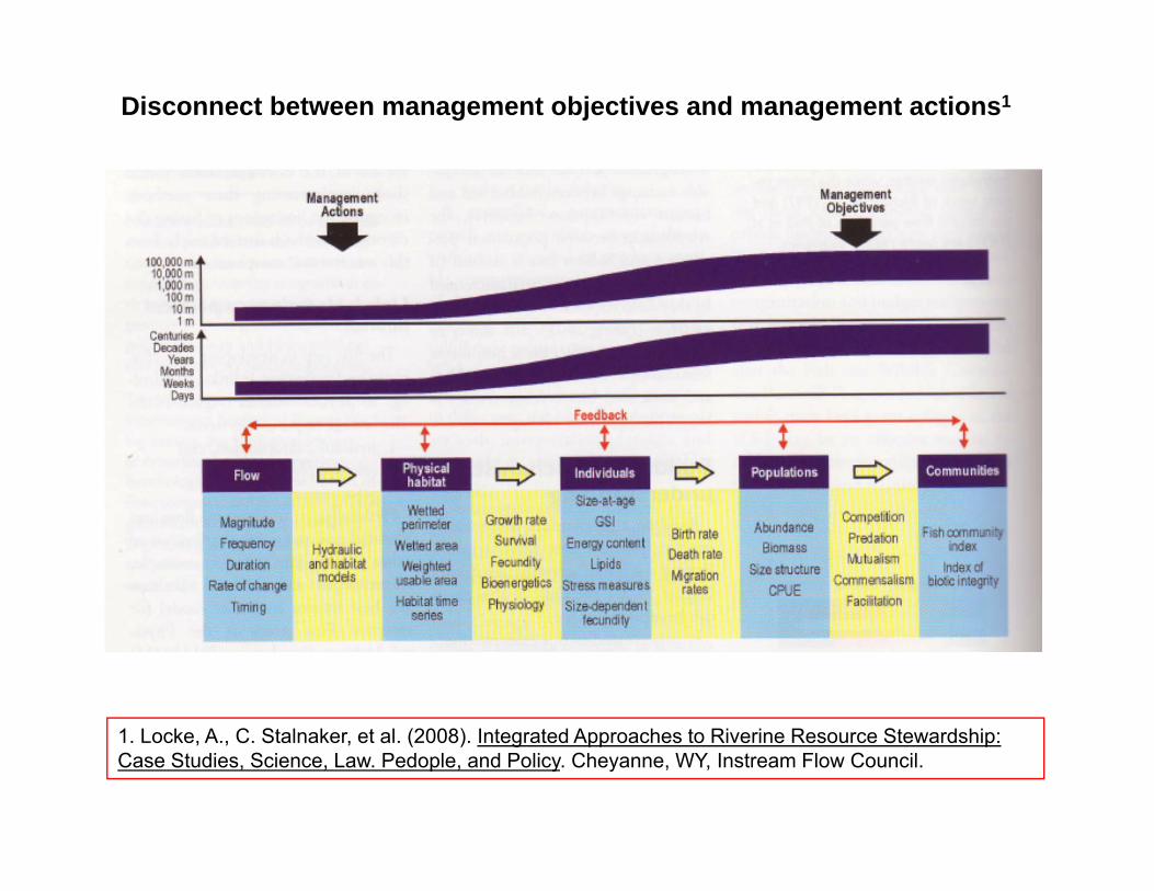
Disconnect between management objectives and management actions1

1. Locke, A., C. Stalnaker, et al. (2008). Integrated Approaches to Riverine Resource Stewardship: Case Studies, Science, Law. Pedople, and Policy. Cheyanne, WY, Instream Flow Council.

Ecological Dynamics and Instream Flow Assessments

Starting point1: “tools lacking recognition of the many dynamic feedbacks among physical and biological components of the river environment are unlikely to provide sufficient descriptions of how population or community viability will respond to changes in the flow regime.”

Recommendations included: • improving bioenergetic-based models of population dynamics to allow them

to address flow variability in streams and rivers and

• testing methods to understand the effects of spatial variability on population and community responses to changes in flow regime.

Current research:Our contribution relates to these recommendations:• Full life cycle Dynamic Energy Budget (DEB) model of Pacific salmon• Food distribution models for riverine life stages

1. Anderson et al. 2006. Ecological dynamics and the management of instream flow needs in rivers and streams. Frontiers in Ecology and Environment 4: 309-318.

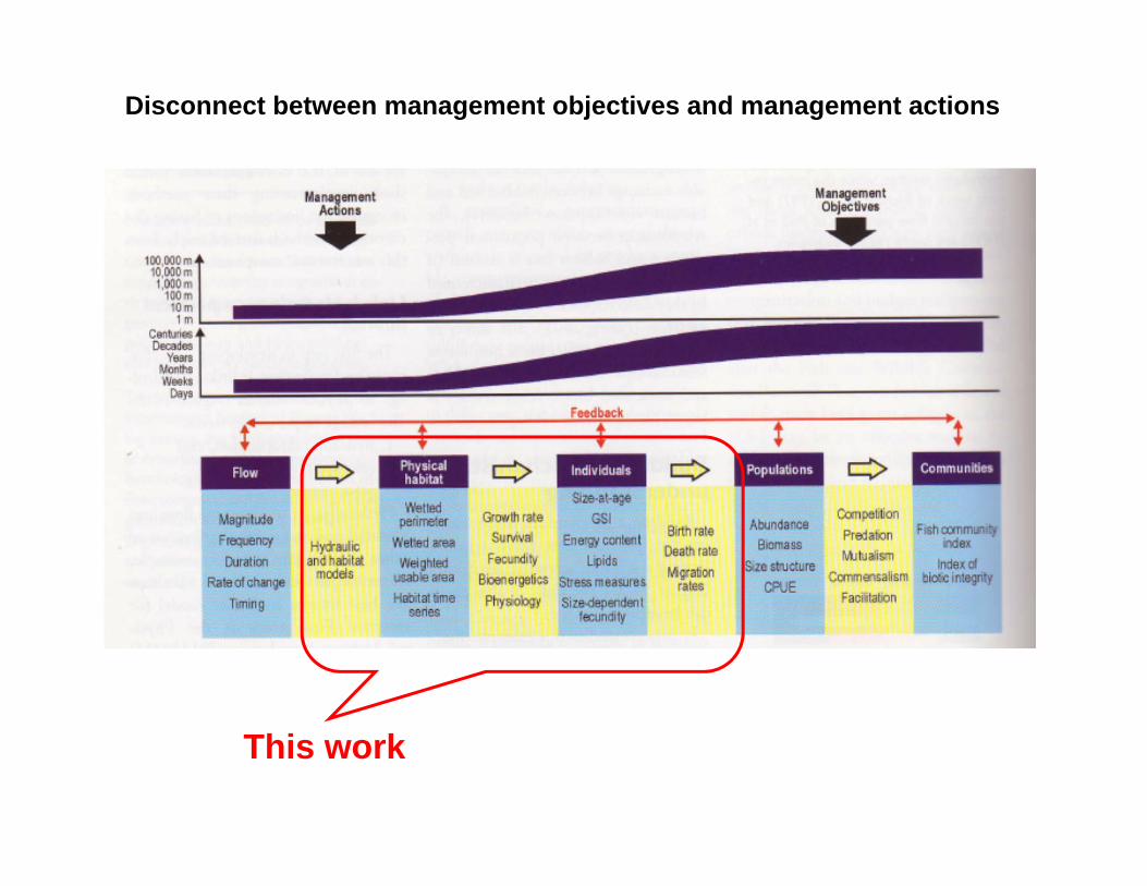
Disconnect between management objectives and management actions

This work

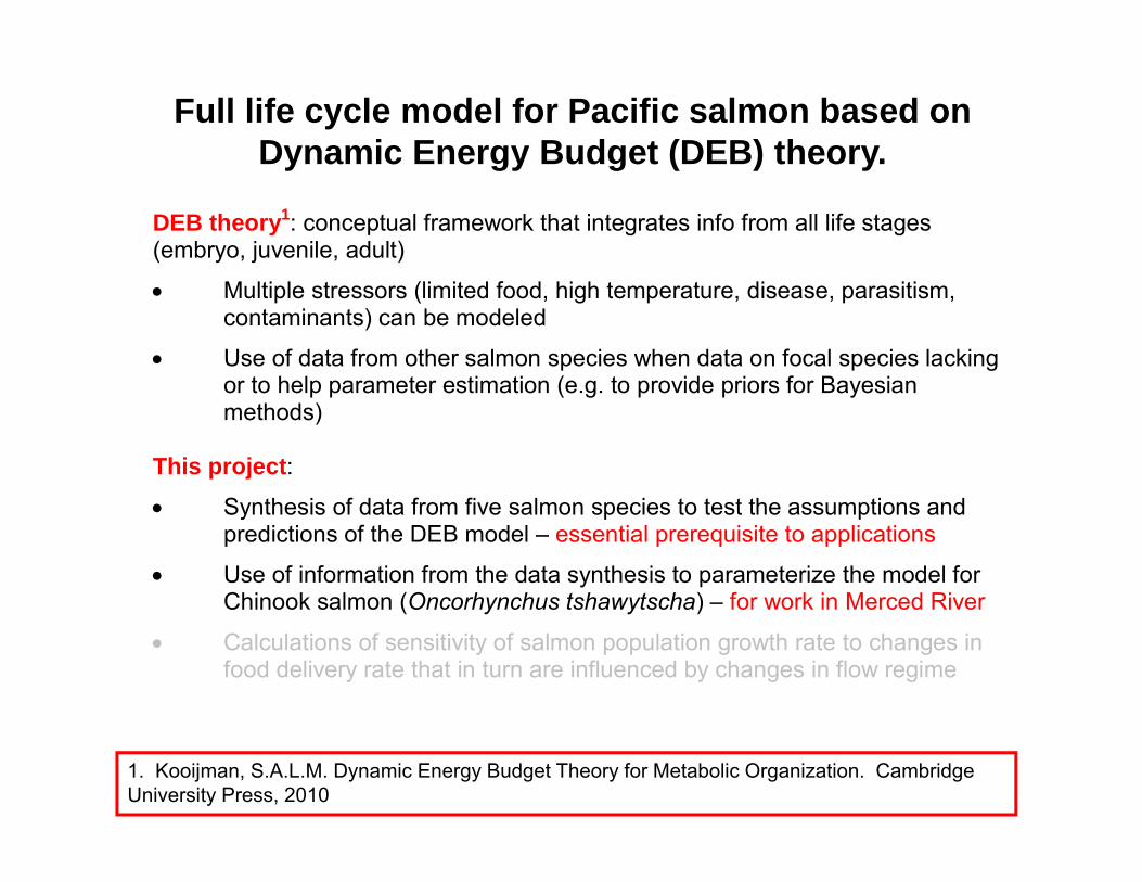
Full life cycle model for Pacific salmon based on Dynamic Energy Budget (DEB) theory.

1. Kooijman, S.A.L.M. Dynamic Energy Budget Theory for Metabolic Organization. Cambridge University Press, 2010

DEB theory1: conceptual framework that integrates info from all life stages (embryo, juvenile, adult)

Multiple stressors (limited food, high temperature, disease, parasitism, contaminants) can be modeled

Use of data from other salmon species when data on focal species lackingor to help parameter estimation (e.g. to provide priors for Bayesian methods)

This project: Synthesis of data from five salmon species to test the assumptions and

predictions of the DEB model – essential prerequisite to applications

Use of information from the data synthesis to parameterize the model for Chinook salmon (Oncorhynchus tshawytscha) – for work in Merced River

Calculations of sensitivity of salmon population growth rate to changes in food delivery rate that in turn are influenced by changes in flow regime

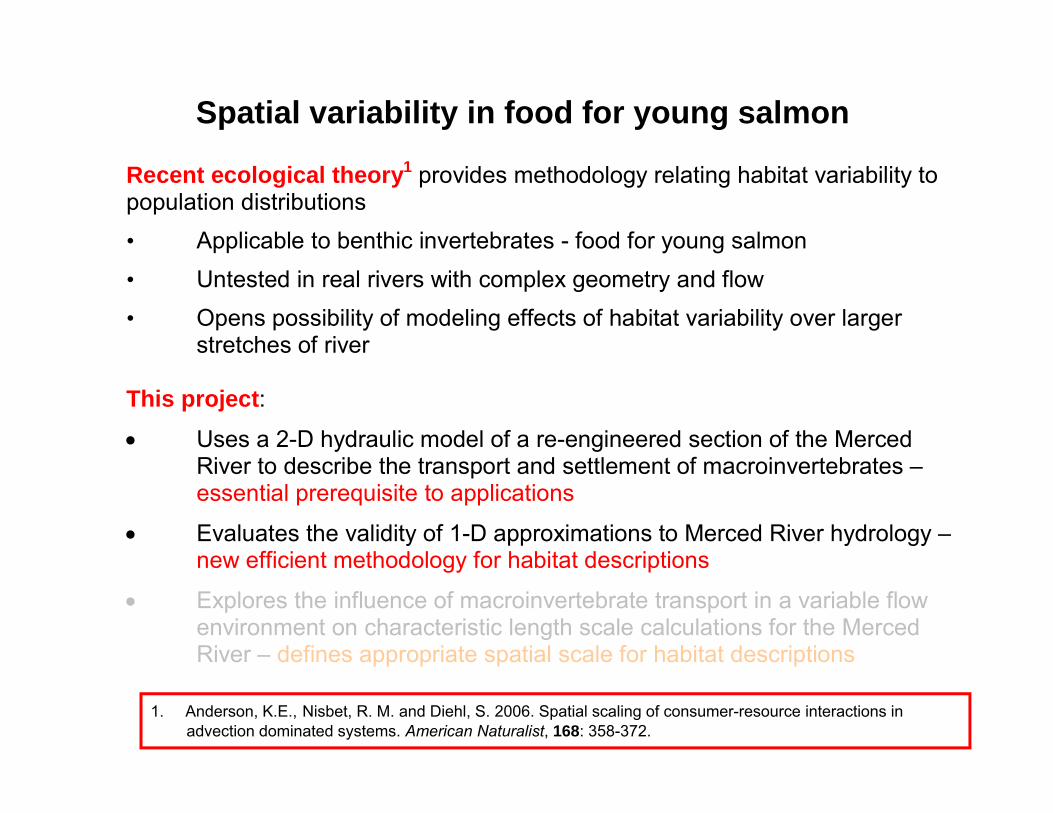
Spatial variability in food for young salmon

Recent ecological theory1 provides methodology relating habitat variability to population distributions • Applicable to benthic invertebrates - food for young salmon • Untested in real rivers with complex geometry and flow • Opens possibility of modeling effects of habitat variability over larger

stretches of river This project: Uses a 2-D hydraulic model of a re-engineered section of the Merced

River to describe the transport and settlement of macroinvertebrates –essential prerequisite to applications

Evaluates the validity of 1-D approximations to Merced River hydrology –new efficient methodology for habitat descriptions

Explores the influence of macroinvertebrate transport in a variable flow environment on characteristic length scale calculations for the Merced River – defines appropriate spatial scale for habitat descriptions

1. Anderson, K.E., Nisbet, R. M. and Diehl, S. 2006. Spatial scaling of consumer-resource interactions in advection dominated systems. American Naturalist, 168: 358-372.

Part II

Modeling the life cycle of Pacific salmon using Dynamic Energy Budget (DEB) theory

1. Motivations for considering DEB theory

2. Properties of the model distinct from other approaches

3. Validation of the model (inter- and intra-species levels)

4. Questions we will address with the model

Danner et al., [2010]

River conditions impact all life stages

Oxygen limitations

Temperature rise

Food limitations

Temperature rise

Contaminants

Habitats lossParasitism, disease

Migration barriers

Migration barriers

Flow speed

Danner et al., [2010]

River conditions impact all life stages

Oxygen limitations

Temperature rise

Food limitations

Temperature rise

Contaminants

Habitats lossParasitism, disease

Migration barriers

Migration barriers

Flow speed

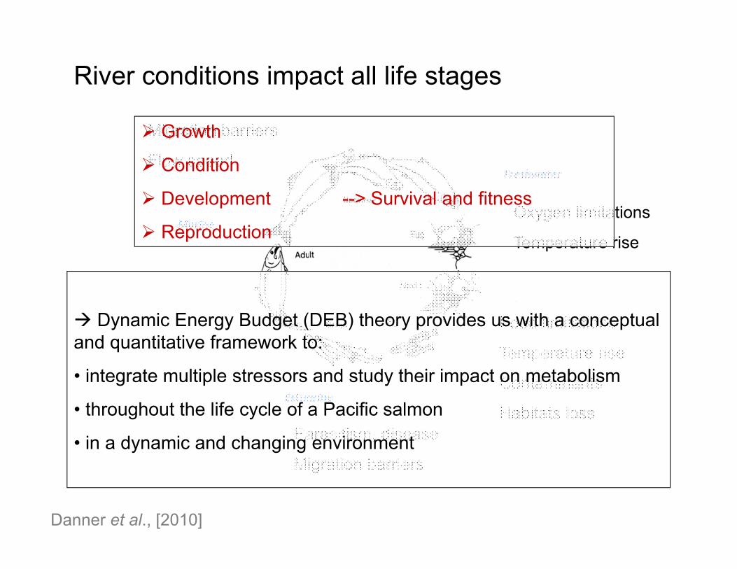
Growth

Condition

Development --> Survival and fitness

Reproduction

Dynamic Energy Budget (DEB) theory provides us with a conceptual and quantitative framework to:

• integrate multiple stressors and study their impact on metabolism

• throughout the life cycle of a Pacific salmon

• in a dynamic and changing environment

maturity

1-maturity

maintenance

development

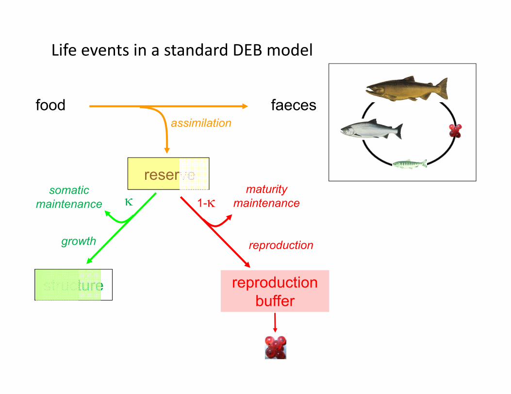
food faecesassimilation

reserve

structure

somaticmaintenance

growth

Life events in a standard DEB model

reproductionbuffer

reproduction

maturity

1-maturity

maintenance

development

food faecesassimilation

reserve

structurestructure

somaticmaintenance

growth

reproductionbuffer

reproduction

maturity

1-maturity

maintenance

development

maturitymaturity

1-maturity

maintenance

development

1-maturity

maintenance

development

food faecesassimilation

food faecesassimilation

reserve

structurestructure

somaticmaintenance

growth

reproductionbuffer

reproduction

reproductionbuffer

reproduction

Model simulations

INPUTS DEB MODEL

Food density

Temperature

Flow

Weight

Fecundity / egg size

OUTPUTS

Length

Properties of the model distinct from other approachesSame parameters for all stages – 12 parameters + 6 for migrations

• Chinook embryo model (Beer and Anderson, 1997): Weight and age at emergence as a function of temperature;12 parameters

Large number of processes: consumption, growth and maintenance + development and reproduction + mortality when limited resources (oxygen, food)• Wisconsin model (Madejian et al., 2004), Net-rate of energy intake

(NREI) (Hayes et al., 2007): consumption, growth and maintenance

Maternal effect: egg size depends on female condition

Rules for parameter variations among related species

Calibration and validation of the model

Inter-species level:• Standard DEB model• Parameter variation (genetic variability)• Length at spawning for parameter variation:

Pink < sockeye < coho < chum < Chinook• Embryo stage (egg weight, fry length and age)• Adult stage (female length, fecundity and egg weight)

Intra-species level:• Limited number of new rules and parameters (time window for

migration decision)• Variations in environmental conditions (phenotypic variability)• Age, length and weight when migrating ocean (smolts) river (returning adults)

Results (1): Inter-species level

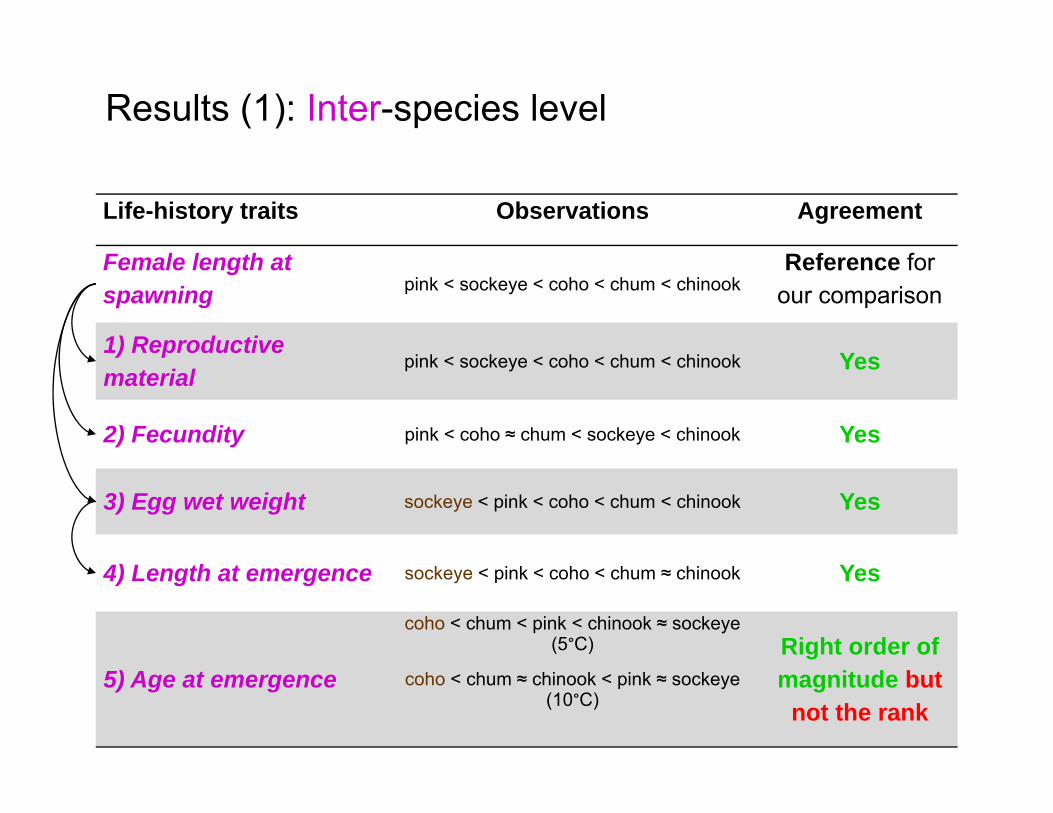
Life-history traits Observations Agreement

Female length at spawning pink < sockeye < coho < chum < chinook

Reference for our comparison

1) Reproductive material

pink < sockeye < coho < chum < chinook Yes

2) Fecundity pink < coho ≈ chum < sockeye < chinook Yes

3) Egg wet weight sockeye < pink < coho < chum < chinook Yes

4) Length at emergence sockeye < pink < coho < chum ≈ chinook Yes

5) Age at emergence

coho < chum < pink < chinook ≈ sockeye (5°C)

coho < chum ≈ chinook < pink ≈ sockeye (10°C)

Right order of magnitude but

not the rank

Results (1): Inter-species level

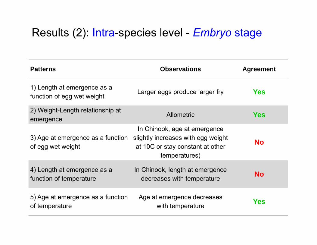
Results (2): Intra-species level - Embryo stage

Patterns Observations Agreement

1) Length at emergence as a function of egg wet weight

Larger eggs produce larger fry Yes

2) Weight-Length relationship at emergence

Allometric Yes

3) Age at emergence as a function of egg wet weight

In Chinook, age at emergence slightly increases with egg weight at 10C or stay constant at other

temperatures)

No

4) Length at emergence as a function of temperature

In Chinook, length at emergence decreases with temperature No

5) Age at emergence as a function of temperature

Age at emergence decreases with temperature Yes

Patterns Observations Agreement

6) Female length and age as a function of growth history during the ocean stage

Individuals that grow faster return at a smaller size and a younger age Yes

7) Female condition as a function of the duration and/or distance of the spawning migration

Female condition decreases with the length of the spawning migration Yes

8) Female condition as a function of female length at spawning

Larger individuals are in better condition after spawning migration Yes

9) Fecundity as a function of female length

Fecundity increases with length Yes

10) Egg wet weight as a function of female length

Egg weight increases with female length Yes

Results (2): Intra-species level - Adult stage

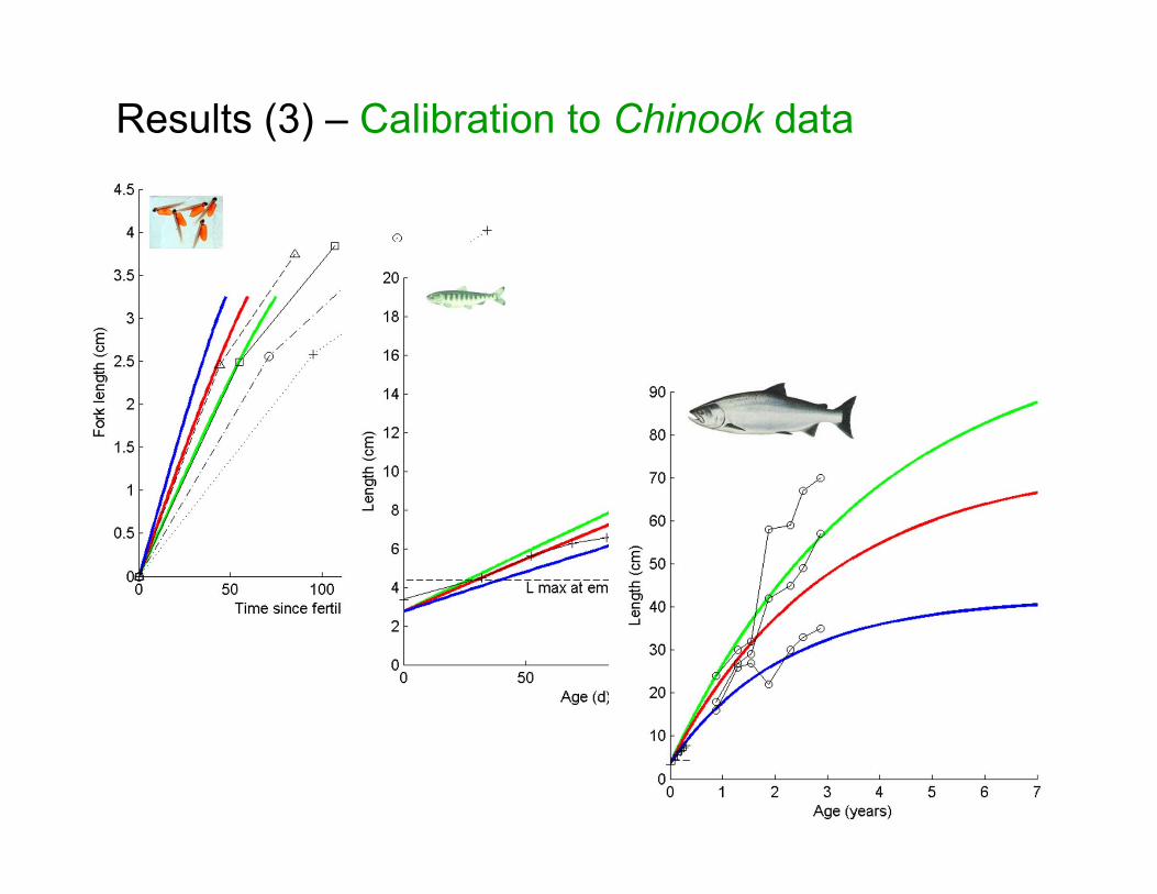
Results (3) – Calibration to Chinook data

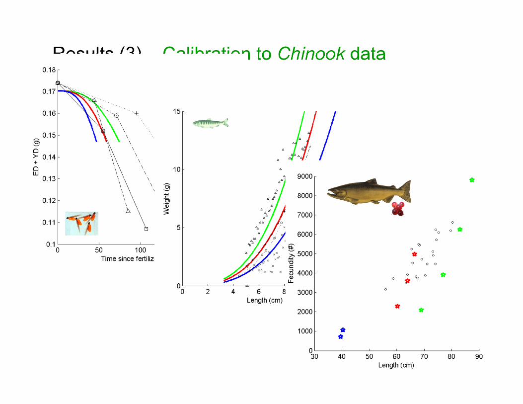
Results (3) – Calibration to Chinook data

Summary Part II

• We have a generic model for the life cycle of a Pacific salmon

• We need more details for the impact of temperature on metabolic processes (cf Coho embryo development for instance)

• Model captures most of the variation in life-history traits among the 5 species of Pacific salmon in North-America

• Model captures patterns at the intra-species level and variation in age and length at migration in particular

• Good fit of the model to Chinook data

Further developments

Short-term: • Include more data for Chinook model (Bayesian framework)• Juveniles: individual growth AND development rates in varying

flow conditions• Eggs: oxygen limitations• Analyzing otolith and scale patterns to reconstruct individual food

histories

Long-term:• Coupling with 2D model (river, coastal ocean)• Adults: survival during migration, female condition after

migration• Long-term population growth rates (individual growth, stage

transitions, fecundity, survival)• Application to Steelhead

Part III

Spatial variability in food delivery for juvenile salmonids

1. Goals

2. Modeling framework

3. Calibration/validation of 2D flow model

4. Flow-Drift Simulations

Project Goals Spatial variability in food for juvenile salmon

1.Formulate 2D numerical models of flow and transport of macroinvertebrates

– Improve food delivery functions in Bioenergetics/DEB models

– Test in simple river under range of flows

2. 2D results used as input to simpler 1D flow and drift model that can be applied over larger spatial scales (Anderson)

Field SiteRobinson Reach, Merced River

o Recently re-engineered reach of the Merced River, CA.

o Single-thread, meandering planform, with alternating deep pools and shallow riffles.

o Utilized existing topographic and hydraulic data sets that were collected with collaborators Tom Dunne (UCSB) and Carl Legleiter (U Wyoming).

Flow ModelingMIKE 21 Code (DHI)

o Model Inputs– Topography– Roughness– Discharge– Stage

o Outputs– Depth– Velocity

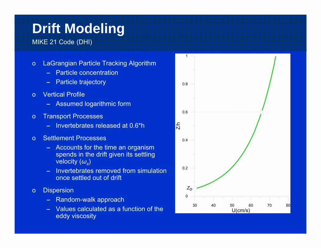
Drift ModelingMIKE 21 Code (DHI)

o LaGrangian Particle Tracking Algorithm– Particle concentration– Particle trajectory

o Vertical Profile– Assumed logarithmic form

o Transport Processes– Invertebrates released at 0.6*h

o Settlement Processes– Accounts for the time an organism

spends in the drift given its settling velocity (ωs)

– Invertebrates removed from simulation once settled out of drift

o Dispersion– Random-walk approach– Values calculated as a function of the

eddy viscosity

30 40 50 60 70 80U(cm/s)

0

0.2

0.4

0.6

0.8

1

Z/h

Zo

Modeling Approacho Input “bugs” into upstream

boundary

o Compute drift concentration and particle pathways

o Utilize a range of settling velocity (ωs) and dispersion (D) values from the literature.

Runs:1. Baseflow (6.4 m3/s)2. 0.75*Bankfull Q (32.5

m3/s)3. For each Q, 12 runs

varying ωs and D

Bugs

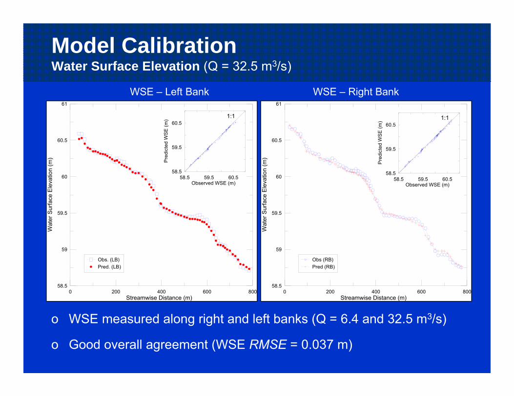
Model CalibrationWater Surface Elevation (Q = 32.5 m3/s)

o WSE measured along right and left banks (Q = 6.4 and 32.5 m3/s)

o Good overall agreement (WSE RMSE = 0.037 m)

WSE – Left Bank WSE – Right Bank

0 200 400 600 800Streamwise Distance (m)

58.5

59

59.5

60

60.5

61

Wat

er S

urfa

ce E

leva

tion

(m)

Obs (RB)Pred (RB)

58.5 59.5 60.5Observed WSE (m)

58.5

59.5

60.5

Pre

dict

ed W

SE (m

) 1:1

0 200 400 600 800Streamwise Distance (m)

58.5

59

59.5

60

60.5

61

Wat

er S

urfa

ce E

leva

tion

(m)

Obs. (LB)Pred. (LB)

58.5 59.5 60.5Observed WSE (m)

58.5

59.5

60.5

Pre

dict

ed W

SE

(m) 1:1

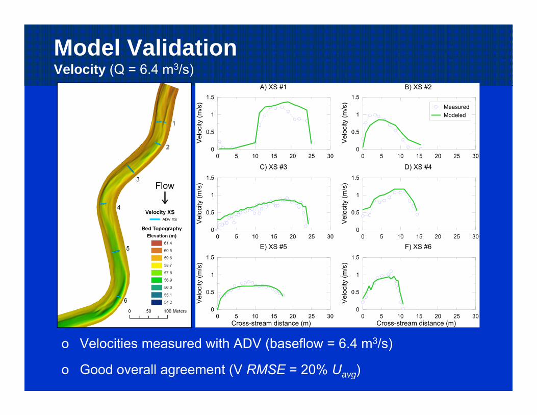
Model ValidationVelocity (Q = 6.4 m3/s)

0 10 20 305 15 250

0.5

1

1.5

Vel

ocity

(m/s

)

0 10 20 305 15 250

0.5

1

1.5

Vel

ocity

(m/s

)

0 10 20 305 15 250

0.5

1

1.5

Vel

ocity

(m/s

)

0 10 20 305 15 250

0.5

1

1.5

Vel

ocity

(m/s

)

0 10 20 305 15 25Cross-stream distance (m)

0

0.5

1

1.5

Vel

ocity

(m/s

)

0 10 20 305 15 25Cross-stream distance (m)

0

0.5

1

1.5

Vel

ocity

(m/s

)

MeasuredModeled

A) XS #1

C) XS #3

E) XS #5

B) XS #2

D) XS #4

F) XS #6

o Velocities measured with ADV (baseflow = 6.4 m3/s)

o Good overall agreement (V RMSE = 20% Uavg)

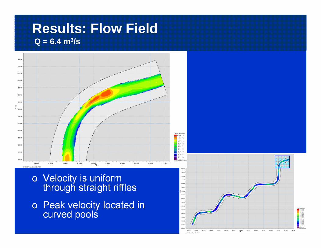
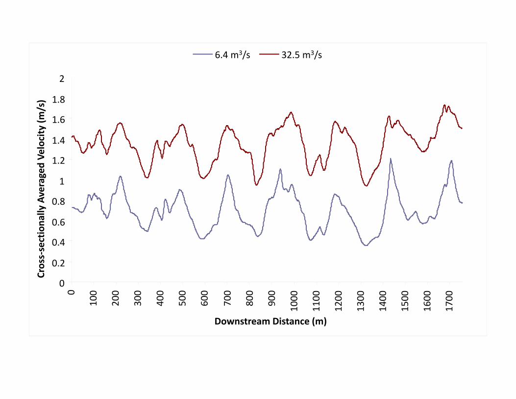
Results: Flow FieldQ = 6.4 m3/s

o Velocity is uniform through straight riffles

o Peak velocity located in curved pools

Results: Flow FieldQ = 32.5 m3/s

o Similar spatial distribution of velocity as low flow run

o Velocity magnitudes are greater

Q (m3/s)

s 

(m/s)LEV (m2/s)

D h  and D v

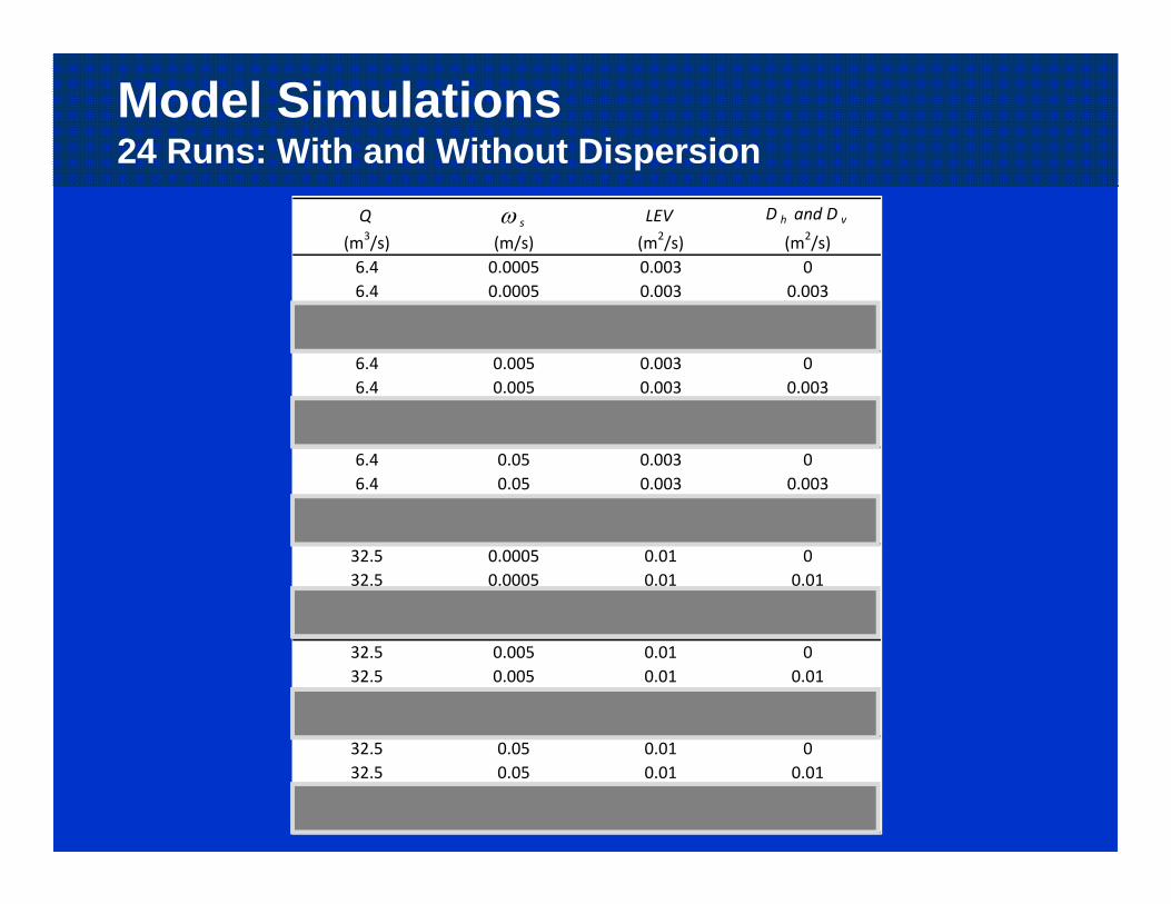
(m2/s)6.4 0.0005 0.003 06.4 0.0005 0.003 0.0036.4 0.0005 0.003 0.0156.4 0.0005 0.003 0.036.4 0.005 0.003 06.4 0.005 0.003 0.0036.4 0.005 0.003 0.0156.4 0.005 0.003 0.036.4 0.05 0.003 06.4 0.05 0.003 0.0036.4 0.05 0.003 0.0156.4 0.05 0.003 0.0332.5 0.0005 0.01 032.5 0.0005 0.01 0.0132.5 0.0005 0.01 0.0532.5 0.0005 0.01 0.132.5 0.005 0.01 032.5 0.005 0.01 0.0132.5 0.005 0.01 0.0532.5 0.005 0.01 0.132.5 0.05 0.01 032.5 0.05 0.01 0.0132.5 0.05 0.01 0.0532.5 0.05 0.01 0.1

Model Simulations24 Runs: With and Without Dispersion

0 400 800 1200 1600 2000Streamwise Distance (m)

0

5

10

15

20

Num

ber I

ndiv

idua

ls

Low flow (w/Disp)Low Flow (no/Disp)High Flow (w/Disp)High Flow (no/Disp)

0 400 800 1200 1600 2000Streamwise Distance (m)

0

5

10

15

20

Num

ber I

ndiv

idua

ls

0 400 800 1200 1600 2000Streamwise Distance (m)

0

5

10

15

20

Num

ber I

ndiv

idua

ls

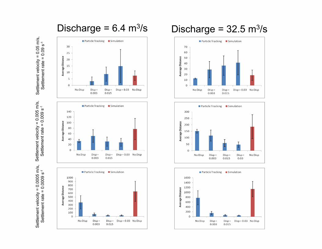
Dispersal DistancesVariable Q, D and ωs

o Travel distances decrease with higher settling velocity

o Without dispersion– Particles settle out over

a small range of distances.

o At low flow– Dispersion increases the

average dispersal distance and the variance.

o At high flow– Dispersion decreases

the mean dispersal distance.

A) ωs = 0.05 (m/s)

B) ωs = 0.005 (m/s)

C) ωs = 0.0005 (m/s)

Model SimulationsRole of Dispersion

Q (m3/s)

s 

(m/s)LEV (m2/s)

D h  and D v

(m2/s)6.4 0.0005 0.003 06.4 0.0005 0.003 0.0036.4 0.0005 0.003 0.0156.4 0.0005 0.003 0.036.4 0.005 0.003 06.4 0.005 0.003 0.0036.4 0.005 0.003 0.0156.4 0.005 0.003 0.036.4 0.05 0.003 06.4 0.05 0.003 0.0036.4 0.05 0.003 0.0156.4 0.05 0.003 0.0332.5 0.0005 0.01 032.5 0.0005 0.01 0.0132.5 0.0005 0.01 0.0532.5 0.0005 0.01 0.132.5 0.005 0.01 032.5 0.005 0.01 0.0132.5 0.005 0.01 0.0532.5 0.005 0.01 0.132.5 0.05 0.01 032.5 0.05 0.01 0.0132.5 0.05 0.01 0.0532.5 0.05 0.01 0.1

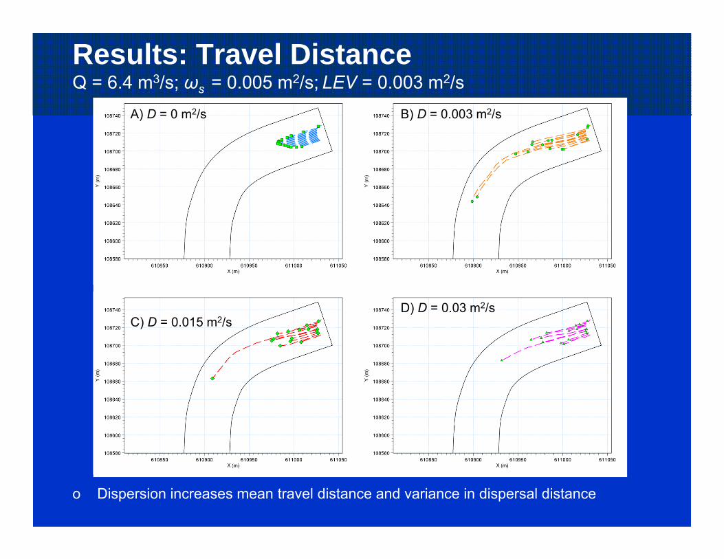
Results: Travel DistanceQ = 6.4 m3/s; ωs = 0.005 m2/s; LEV = 0.003 m2/s

o Dispersion increases mean travel distance and variance in dispersal distance

A) D = 0 m2/s B) D = 0.003 m2/s

C) D = 0.015 m2/sD) D = 0.03 m2/s

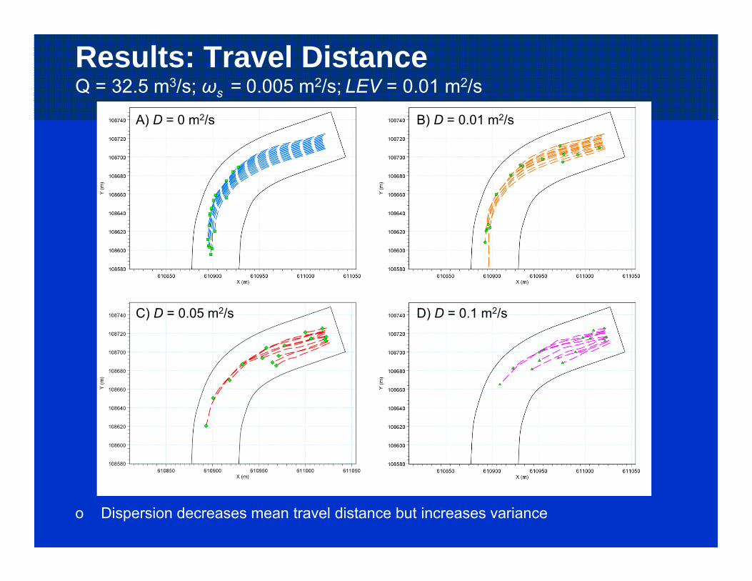
Results: Travel DistanceQ = 32.5 m3/s; ωs = 0.005 m2/s; LEV = 0.01 m2/s

A) D = 0 m2/s B) D = 0.01 m2/s

C) D = 0.05 m2/s D) D = 0.1 m2/s

o Dispersion decreases mean travel distance but increases variance

2D Flow-Drift Summary

o We have a validated 2D flow model of the Merced River

o Model is capable of computing drift transport and settlement at low and high flows

o Preliminary Results:1. Invert pathways dictated by high velocity core.2. Invert travel distances:

– ↑ with flow velocity – ↓ decrease with higher ωs

3. Dispersion increases the variance in dispersal distances.

Kurt will discuss 1D flow-drift transport

Part IV: Flow regime and spatial scales of population response

0

0.2

0.4

0.6

0.8

1

1.2

1.4

1.6

1.8

20

100

200

300

400

500

600

700

800

900

1000

1100

1200

1300

1400

1500

1600

1700

Downstream Distance (m)

Cross‐sectiona

lly Averaged Ve

locity (m

/s)

6.4 m3/s 32.5 m3/s

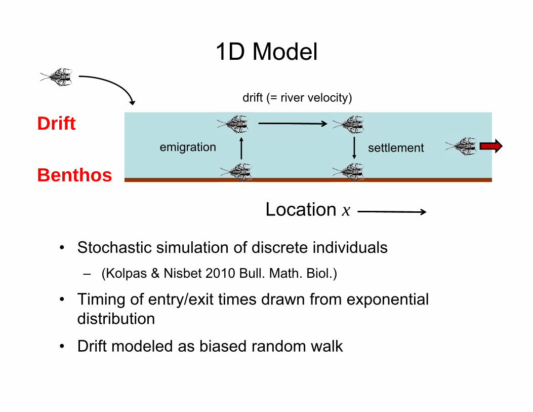
Location x

• Stochastic simulation of discrete individuals– (Kolpas & Nisbet 2010 Bull. Math. Biol.)

• Timing of entry/exit times drawn from exponential distribution

• Drift modeled as biased random walk

1D Model

Drift

Benthosemigration settlement

drift (= river velocity)

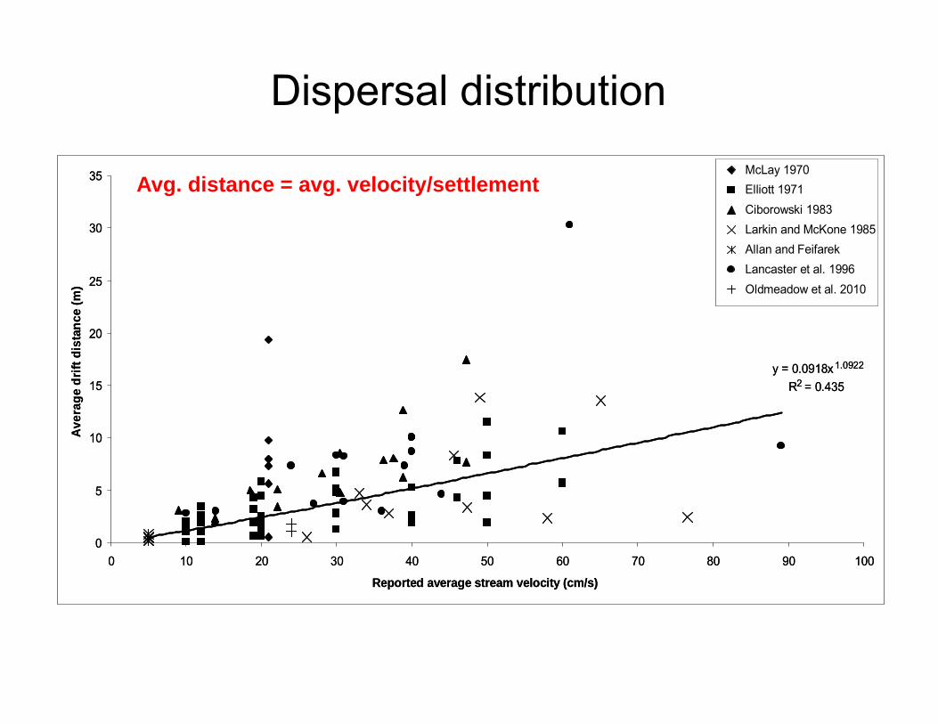
Dispersal distribution

0

0.2

0.4

0.6

0.8

1

0 5 10 15 20 25

Prop

ortio

n of

Pop

ulat

ion

in th

e D

rift

Distance Downstream

xvelocitysettlementexp

Dispersal distribution

0

0.2

0.4

0.6

0.8

1

0 5 10 15 20 25

Prop

ortio

n of

Pop

ulat

ion

in th

e D

rift

Distance Downstream

Dispersal function determined by hydrology

xvelocitysettlementexp

Dispersal distribution

y = 0.0918x1.0922

R2 = 0.435

0

5

10

15

20

25

30

35

0 10 20 30 40 50 60 70 80 90 100

Reported average stream velocity (cm/s)

Aver

age

drift

dis

tanc

e (m

)

McLay 1970Elliott 1971Ciborowski 1983Larkin and McKone 1985Allan and FeifarekLancaster et al. 1996Oldmeadow et al. 2010

y = 0.0918x1.0922

R2 = 0.435

0

5

10

15

20

25

30

35

0 10 20 30 40 50 60 70 80 90 100

Reported average stream velocity (cm/s)

Aver

age

drift

dis

tanc

e (m

)

McLay 1970Elliott 1971Ciborowski 1983Larkin and McKone 1985Allan and FeifarekLancaster et al. 1996Oldmeadow et al. 2010

Avg. distance = avg. velocity/settlement

0

50

100

150

200

250

300

350

400

450

500

0 500 1000 1500 2000 2500 3000 3500 4000 4500 5000

Time (10 sec.)

Tota

l Ind

ivid

uals

0

50

100

150

200

250

300

350

400

450

500

0 500 1000 1500 2000 2500 3000 3500 4000 4500 50002

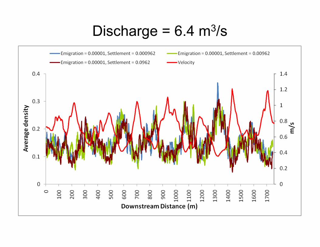
Discharge = 6.4 m3/s

Discharge = 32.5 m3/s

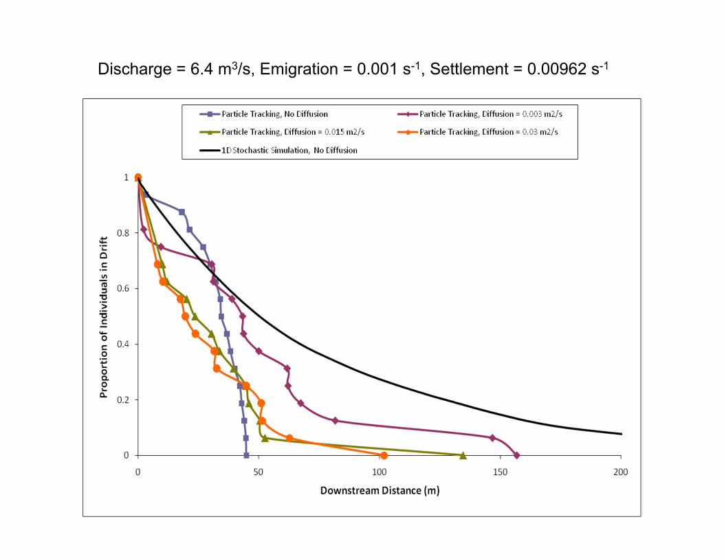
Discharge = 6.4 m3/s, Emigration = 0.001 s-1, Settlement = 0.00962 s-1

Discharge = 6.4 m3/s Discharge = 32.5 m3/sS

ettle

men

t vel

ocity

= 0

.05

m/s

,S

ettle

men

t rat

e =

0.09

s-1

Set

tlem

ent v

eloc

ity =

0.0

05 m

/s,

Set

tlem

ent r

ate

= 0.

009

s-1S

ettle

men

t vel

ocity

= 0

.000

5 m

/s,

Set

tlem

ent r

ate

= 0.

0009

s-1

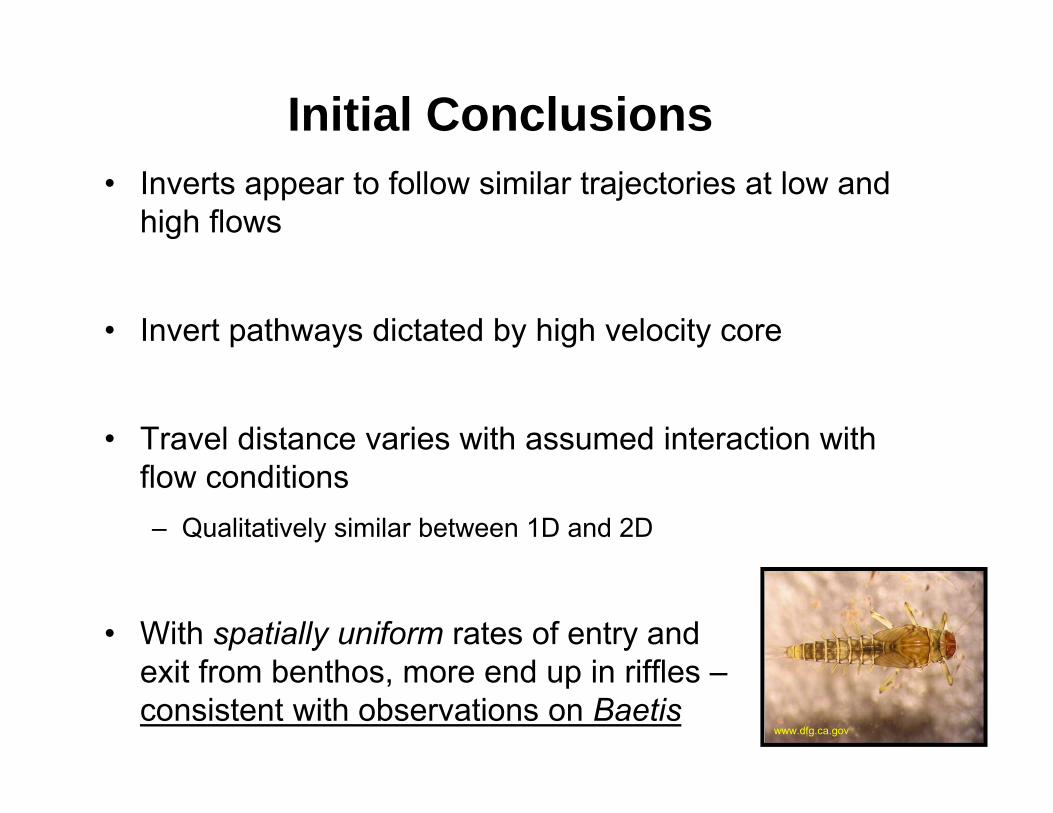
Initial Conclusions• Inverts appear to follow similar trajectories at low and

high flows

• Invert pathways dictated by high velocity core

• Travel distance varies with assumed interaction with flow conditions– Qualitatively similar between 1D and 2D

• With spatially uniform rates of entry and exit from benthos, more end up in riffles –consistent with observations on Baetis

www.dfg.ca.gov

Food delivery• Tests of 1D model in more complex hydrology

• Complex structure (e.g. woody debris, boulders, gravel augmentation)

• Representation of “behavior” in inverts (entry/exit)

• Characteristic length scales to guide appropriate resolution of habitat descriptions

http://www.usbr.gov

http://www.fs.fed.us

http://www.flyfishingtraditions.com

Disconnect between management objectives and management actions1

This talk

Spatial and temporal variation in habitat quality

Fish growth and survival under variability

2D Hydraulic Models, 1D

SimplificationsDEB Theory

Flow, abiotichabitat descriptors,

drift sampling

Fish life histories, links to variability

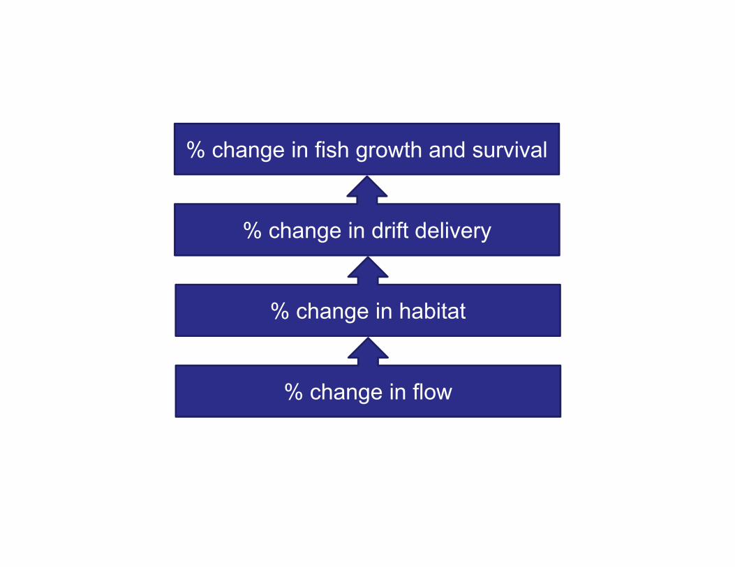
% change in flow

% change in habitat

% change in drift delivery

% change in fish growth and survival

AcknowledgementsThanks to:

Alison KolpasJonathan SarhadMargaret SimonJohn WilliamsBrad CardinaleLindsey AlbertsonTom DunneLeah JohnsonBas KooijmanCarl LegleiterAleksandra WydzgaDale KerperJulio ZysermanAlison Amenta

Funding:

California Energy Commission Public Interest Energy Research Program

National Science Foundation

Calfed Bay-Delta Authority Science Program

UC-Riverside