INTEGRATED WATER RESOURCES MANAGEMENT ... - CORE

I

INTEGRATED WATER RESOURCES MANAGEMENT

MODELLING FOR THE OLDMAN RIVER BASIN

USING SYSTEM DYNAMICS APPROACH

A Thesis

Submitted to the College of Graduate Studies and Research

In Partial Fulfillment of the Requirements for the

Degree of Master of Science

in the School of Environment and Sustainability

University of Saskatchewan,

Saskatoon, Saskatchewan, Canada

By

Hamideh Hosseini Safa

© Copyright Hamideh Hosseini Safa, December, 2015. All Rights Reserved

I

PERMISSION TO USE

In presenting this thesis in partial fulfilment of the requirements for a Postgraduate degree

from the University of Saskatchewan, it is agreed that the Libraries of this University may make

it freely available for inspection. Permission for copying of this thesis in any manner, in whole or

in part, for scholarly purposes may be granted by the professors who supervised this thesis work

or, in their absence, by the Head of the School of Electrical and Computer Engineering or the Dean

of the College of Graduate Studies and Research at the University of Saskatchewan. Any copying,

publication, or use of this thesis, or parts thereof, for financial gain without the written permission

of the author is strictly prohibited. Proper recognition shall be given to the author and to the

University of Saskatchewan in any scholarly use which may be made of any material in this thesis.

Request for permission to copy or to make any other use of material in this thesis in whole or in

part should be addressed to:

Head of the School of Environment and Sustainability,

University of Saskatchewan,

117 Science Place,

Saskatoon, Saskatchewan,

Canada, S7N 5C8.

II

ABSTRACT

Limited freshwater supply is the most important challenge in water resources management,

particularly in arid and semi-arid basins. However, other variations in a basin, including climate

change, population growth, and economic development intensify this threat to water security. The

Oldman River Basin (OMRB), located in southern Alberta, Canada, is a semi-arid basin and

encompasses several water challenges, including uncertain water supply as well as increasing,

uncertain water demands (consumptive irrigation, municipal, and industrial demands, and non-

consumptive hydropower generation, and environmental demands). Reservoirs, of which the

Oldman River Reservoir is the largest in the basin, are responsible for meeting most of demands,

and, protecting the basin’s economy. The OMRB has also faced extreme natural events, floods and

droughts, in the past, which reservoir management plays a critical role to adapt to. The complexity

of the climate, hydrology, and water resource system and water governance escalates the

challenges in the basin. These factors are highly interconnected and establish dynamic, non-linear

behavior, which requires an integrated, feedback-based tool to investigate. Integrated water

resources (IWRM) modelling using system dynamics (SD) is such an approach to tackle the

different water challenges and understand their non-linear, dynamic pattern. In this research study

the Sustainability-oriented Water Allocation, Management, and Planning (SWAMPOM) model for

the Oldman River Basin is developed. SWAMPOM comprises a water allocation model, dynamic

irrigation demand, instream flow needs (IFN), and economic evaluation sub-models. The water

allocation model allocates water to all the above-mentioned demands at a weekly time step from

1928 to 2001, and under different water availability scenarios. Meeting irrigation demands relies

on the crop water requirement (CWR), which is calculated under different climatic conditions by

III

the dynamic irrigation demand sub-model. This sub-model estimates the weekly irrigation demand

for main crops planted in the basin. SWAMPOM also computes environmental demands or instream

flow need (IFN) for the Oldman River, and allocates water to rivers to meet IFN under different

policy scenarios and uncertain water supply. Finally, the major water-related economic benefit in

the basin, earned by agriculture and hydropower generation, is computed by the economic

evaluation sub-model. The results show that SWAMPOM could reasonably satisfy the demands at

a weekly time step and provide an adequate estimation of the crop water requirement under

different hydrometeorological conditions. Based on the SWAMPOM’s results, the average annual

irrigation demand is 306 mm over the historical time period from 1928 to 2001 in the main

irrigation districts. The average weekly instream flow need of the Oldman River is calculated to

be approximately 20.5 m3/s, which can be met in more than 97% of weeks in the historical time

period. Average annual water-related economic benefit was computed to be 192.5 M$ in the

OMRB. It decreased to 82.8 M$ in very dry years, and increased up to 328.6 M$ in very wet years.

This research also developed different sets of Oldman Reservoir’s operation zones,

resulting in trade-offs between the optimal economic benefit, water allocated to the ecosystem,

minimum floodwater and minimum flood frequency. This helps decision makers to decide how

much water should be stored in the reservoir to meet a specific objective while not sacrificing

others. A multi-objective performance assessment, Pareto curve approach, is applied to identify

the optimal trade-offs between the four objective functions (OFs), and 18 different optimal, or

close to optimal sets of operating zones are provided. The decision regarding the operating zones

depends on decision makers’ preference for higher economic benefit, water allocated to IFN, or

flood security. However, the set of operating zones with minimum floodwater causes 11 less flood

events; the operating zones with maximum economic benefits result in 4.1% more financial gain;

IV

and the zones with maximum water allocated to IFN lead to 10.1% more ecosystem protection in

the whole 74 years, compared to current zones.

V

ACKNOWLEDGMENTS

It is my honor to take this chance to thank many people who made this thesis possible with

their help, inspiration and motivation.

First, I am grateful to my supervisors, Professor Howard Wheater and Professor Amin

Elshorbagy, for their patience, invaluable support and guidance throughout my research program

at the University of Saskatchewan. I have learnt several important lessons on the skills and values

of conducting research under their supervision. I would also like to express my gratitude toward

my committee members, Dr. Ken Belcher and Dr. Andrew Ireson, for the valuable suggestions

and feedbacks.

This thesis would not have been possible without the financial support of Canada

Excellence Research Chair in Water Security at the University of Saskatchewan, and the School

of Environment and Sustainability.

My deepest love and gratitude go to my parents for their unconditional care and support

through my entire life. I would also like to send profound appreciation and love to my sister for

her support, advice, and kindness during the hard times.

VI

TABLE OF CONTENTS

PERMISSION TO USE ................................................................................................................... I

ABSTRACT .................................................................................................................................... II

ACKNOWLEDGMENTS ............................................................................................................. V

CHAPTER 1, INTRODUCTION ................................................................................................... 1

1. 1. Background ......................................................................................................................... 1

1. 2. Statement of Problem .......................................................................................................... 2

1. 3. Research Purpose ................................................................................................................ 7

CHAPTER 2, LITERATURE REVIEW ........................................................................................ 9

2. 1. Integrated Water Resources Management Modeling .......................................................... 9

2. 2. Uncertain Water Supply and Demand ............................................................................... 17

2. 3. Balancing Economic and Environmental Protection Objectives While Avoiding

Flooding .................................................................................................................................... 18

CHAPTER 3, MATERIALS AND METHODS .......................................................................... 22

3. 1. Case Study: The Oldman River Basin............................................................................... 23

3. 2. Water Resources Management Model (WRMM) ............................................................. 28

3. 3. System Dynamics Approach ............................................................................................. 33

3. 4. An IWRM Model using SD Approach (SWAMPOM) ....................................................... 37

3. 4. 1. Water Allocation Model .......................................................................................................... 38

3. 4. 2. Dynamic Irrigation Demand Sub-model ................................................................................. 45

3. 4. 3. Instream Flow Needs Sub-Model............................................................................................ 47

3. 4. 4. Economic Evaluation Sub-Model ........................................................................................... 49

CHAPTER 4, RESULTS AND DISCUSSION ............................................................................ 51

VII

4. 1. Performance of Water Allocation Model .......................................................................... 51

4. 1. 1. Water Allocation to Consumptive Water Components ........................................................... 52

4. 1. 2. Water Allocation to Non-Consumptive Water Components ................................................... 57

4. 1. 3. Performance of Reservoirs’ Operation.................................................................................... 60

4. 2. Performance of Dynamic Irrigation Demand Sub-model ................................................. 64

4. 3. Performance of Instream Flow Need Sub-Model ............................................................. 68

4. 4. Performance of Economic Evaluation Sub-Model............................................................ 71

4. 5. Effect of Simultaneously Changing Oldman Flow and the IFN Percent of Natural Flow

Component on Water Allocated to IFN and the Basin’s Economy .......................................... 73

4. 6. Pareto Front, a Method to Study Environmental and Economic Goals under Flood

Protection Condition ................................................................................................................. 77

4. 6. 1. Pareto Front Approach ............................................................................................................ 78

4. 6. 2. Optimal Sets of Operating Zones using Pareto Front Approach ............................................. 80

4. 6. 3. Best Sets of Operating Zones for the Oldman River Reservoir .............................................. 90

CHAPTER 5, CONCLUSION...................................................................................................... 93

5. 1. Summary of the Study ....................................................................................................... 93

5. 2. Conclusion of the Research Study .................................................................................... 95

5. 3. Future Work ...................................................................................................................... 97

REFERENCES ............................................................................................................................. 99

Appendix A ................................................................................................................................. 113

Appendix B ................................................................................................................................. 115

VIII

LIST OF FIGURES

Figure 1.1: Schematic of the scope of the IWRM model ............................................................... 5

Figure 2.1: Schematic map of the OMRB in the WRMM. ........................................................... 16

Figure 3.1: The Oldman River Basin (OWC, 2010) ..................................................................... 24

Figure 3.2: The percentage of water allocated to water sectors in the OMRB. ............................ 25

Figure 3.3: Schematic map of the Oldman River Basin (OMRB) as built in WRMM. ................ 29

Figure 3.4: Penalty zones for various water components ............................................................. 30

Figure 3.5: Simple water system to explain WRMM operation procedure .................................. 32

Figure 3.6: Positive and negative causal links (a), and an example of Reinforcing (positive; b) and

balancing (negative, c) loops ........................................................................................................ 34

Figure 3.7: Stock-flow Diagram. .................................................................................................. 35

Figure 3.8: Some dynamic mechanisms in the environmental sub-system. ................................. 36

Figure 3.9: Some dynamic mechanisms in the human sub-system .............................................. 37

Figure 3.10: Schematic map for the minor units in the OMRB system. ....................................... 39

Figure 3.11: Schematic map of the hydropower plant within the OMRB. ................................... 40

Figure 3.12: Different sections of the Oldman River ................................................................... 42

Figure 3.13: Stock-flow diagram for the Oldman river Basin ...................................................... 43

Figure 3.14: The Oldman River Reservoir operating zones ......................................................... 44

Figure 4.1: Average weekly headwaters flow originating from the Rocky Mountain ................. 52

Figure 4.2: Average weekly rivers flow emanating from Montana, US ....................................... 52

Figure 4.3: Water allocated to the minor units by SWAMPOM versus that by WRMM ............... 53

Figure 4.4: Water allocated to NLID by SWAMPOM and WRMM (a) and in 1988 (b) ............... 54

IX

Figure 4.5: Scatter plot of water allocated to PID (a), RCID (b), SMRID (c), TID (d) by SWAMPOM

and WRMM. ................................................................................................................................. 55

Figure 4.6: Scatter plot of water allocated to irrigation field 341 (a), and 324 (b) by SWAMPOM

and WRMM. ................................................................................................................................. 56

Figure 4.7: Scatter plot of water allocated to irrigation field 657 (a), and 690 (b) by SWAMPOM

and WRMM. ................................................................................................................................. 56

Figure 4.8: Water allocated to the major units by SWAMPOM versus that by WRMM ............... 57

Figure 4.9: Scatter plot of water allocated to the hydropower plant by SWAMPOM and

WRMM ......................................................................................................................................... 58

Figure 4.10: Water allocated to the hydropower plant by SWAMPOM and WRMM in 1931 ...... 58

Figure 4.11: Water allocated to the Willow Creek River (a), and the section 6 of the Oldman River

(b) by SWAMPOM compared to this by WRMM .......................................................................... 59

Figure 4.13: Scatter plot of the Oldman Reservoir water level (a) and the amount of water released

from the reservoir (b) by simulating SWAMPOM and WRMM from 1928 to 2001. .................... 61

Figure 4.14: the result of WRMM and SWAMPOM in the Oldman Reservoir water level (a) and

the reservoir outflow (b) ............................................................................................................... 61

Figure 4.15: Water level and water released from the reservoir compared to the monthly historical

data ................................................................................................................................................ 62

Figure 4.16: Schematic map of the Chain Lake, Divpond and Pine Coulee Reservoirs’ location 63

Figure 4.17: Scatter plots of Chain Lake, Divpond and Pine Coulee reservoirs water level between

SWAMPOM and WRMM’s results ................................................................................................ 64

Figure 4.18: Irrigation Demands calculated by SWAMPOM and Obtained from WRMM for

Lethbridge Northern Irrigation Districts ....................................................................................... 65

X

Figure 4.19: Weekly irrigation demand of NLID, SMRID, TID, RCID, and PID from 1996 to

2001............................................................................................................................................... 67

Figure 4.20: Weekly IFN of the six sections of the Oldman River from 1996 to 2001 calculated

by SWAMPOM and WRMM ......................................................................................................... 69

Figure 4.21: Amount of water allocated to IFN for the section 1 of the Oldman River by

SWAMPOM and WRMM from 1996 to 2001 ............................................................................... 70

Figure 4.22: Number of weeks that WRMM and SWAMPOM could not meet IFN from 1928 to

2000............................................................................................................................................... 70

Figure 4.23: Annual economic benefit in the OMRB from 1928 to 2001 .................................... 71

Figure 4.24: Average annual streamflow (m3/s) from 1928 to 2000 ............................................ 72

Figure 4.25: Average annual temperature (oC) from 1928 to 2000 .............................................. 72

Figure 4.26: Crop water demands from 1928 to 2001 .................................................................. 73

Figure 4.27: Annual Eta/ET0 from 1928 to 2001 .......................................................................... 73

Figure 4.28: Water allocated to IFN under 6 scenarios WAIFN (0.8, 0.8), WAIFN (0.8, 1.2),

WAIFN (1, 0.8), WAIFN (1, 1.2), WAIFN (1.15, 0.8), WAIFN (1.15, 1.2), from 1996 to

2001............................................................................................................................................. ..75

Figure 4.29: The number of the week that SWAMPOM could not meet the IFN in 74 years under

12 scenarios ................................................................................................................................... 76

Figure 4.30: Effect of changing the Oldman flow and IFN percent of natural flow component on

the economic benefit under two scenarios of S (0.8, 1.2) and S (1.15, 1.2) ................................. 77

Figure 4.31: The Oldman River Reservoir operating zones ......................................................... 78

Figure 4.32: Pareto surface and Pareto front of economy and IFN objectives ............................. 81

XI

Figure 4.33: Flood control zones (a) and middle operating zones (b) of each point on the

PFEI .............................................................................................................................................. 82

Figure 4.34: Operating zones causing the maximum economic benefit (orange curves) and the

maximum water allocated to IFN (green curves) on the PFEI ..................................................... 83

Figure 4.35: PSEF1 and PFEF1 .................................................................................................... 83


PFEF1 ........................................................................................................................................... 84

Figure 4.37: Operating zones causing the maximum economic benefit (orange curves) and the

minimum floodwater (blue curves) on the PFEF1 ........................................................................ 85

Figure 4.38: PSIF1 and PFIF1 ...................................................................................................... 85


PFIF1............................................................................................................................................. 86

Figure 4.40: Operating zones with the maximum water allocated to IFN (green curves) and the

minimum floodwater (blue curves) on the PFIF1 ......................................................................... 87

Figure 4.41: PSEF2 and PFEF2 .................................................................................................... 87


PFEF2 ........................................................................................................................................... 88

Figure 4.43: Operating zones with the maximum economic benefit (orange curves) and the

minimum flood frequency (blue curves)....................................................................................... 89

Figure 4.44: PSIF2 and PFIF2 ...................................................................................................... 90

Figure 4.45: Flood control zones (a) and middle operating zones (b) of points on the PFIF2 ..... 90

Figure 4.46: Operating zones with the maximum water allocate to IFN (green curves) and the

minimum flood frequency (blue curves) on the PFIF2 ................................................................. 91

XII

Figure 4.47: Five sets of operating zones, not causing major loss in four objective functions .... 92

Figure B.1: Irrigation demand of Ross Creek ID (RCID) from 1928 to 1995............................ 115

Figure B.2: Irrigation demand of Northern Lethbridge irrigation district (NLID) from 1928 to

1995............................................................................................................................................. 116

Figure B.3: Irrigation demand of St. Mary River and Taber IDs (SMRID&TID) from 1928 to

1995............................................................................................................................................. 117

XIII

LIST OF TABLES

Table 3.1: Percent exceedance natural flow for some rivers in the OMRB ................................. 48

Table 3.2: IFN percent of natural flow component for some rivers in the OMRB ....................... 49

Table 4.1: Averaged Percentage Error between Irrigation Demands calculated by SWAMPOM and

Obtained from WRMM for Each Irrigation District ..................................................................... 66

1

CHAPTER 1

INTRODUCTION

1. 1. Background

Water is an essential source of life. The earliest human civilizations arose near rivers where

fresh surface water was abundant. Later, advances in technology and human capability of building

water structures helped to transport water and provided more water accessibility. However, the

availability of clean and fresh water has been limited (Hinrichsen and Tacio, 2011). Nowadays,

approximately 1.7 billion people live in areas where water availability, climate change, population

growth and economic development are provoking water resources problems (IPCC, 2007). Arid

and semi-arid basins, in particular, face more threats to water security. Besides water shortage in

such basins, specific climatic and hydrological conditions, complex water governance and

complex water systems may increase the challenges in water management. These challenges are

extremely interconnected, and a dynamic, closed-loop behavior is dominant on their interaction,

so that a past behavior of a water component affects its future behavior (Ahmad and Simonovic,

2000), and also the future behavior of the whole water system. To address all these challenges and

investigate their dynamic connections in a basin, an integrated, feedback-based insight is required

for water managers.

The Oldman River Basin (OMRB), located in southern Alberta, a sub-basin of the South

Saskatchewan River Basin, encompasses almost all the above-mentioned threats to water security

faced worldwide. In addition to water supply and water demand uncertainty, the complexity of the

basin’s water resources system and specific climatic and hydrological conditions exacerbate the

2

challenges of the OMRB’s water management. While a water resources management model

(WRMM) has been developed for all sub-basins of the South Saskatchewan River Basin (Alberta

Environment, 2002), it may not integrally examine all water problems in the basin, and is only

designed to allocate water to users. However, in addition to meeting all users’ water demands in

the basin, it is important to balance human and environmental uses, maintain sustainable aquatic

ecosystems and economic uses, and adapt to extreme natural events, like droughts and floods.

WRMM also is an optimization-based model, which is not capable of capturing interactions and

feedback loops among the variables of the water resource system. There is therefore a need to

develop an integrated model for the Oldman River Basin that addresses all water resources threats,

and explores their dynamic impacts on the water system. This is the main purpose of this thesis.

A dynamic integrated model also enables the participation of decision makers in solving

water challenges in a basin, and facilitates scrutinizing the effect of different water policies on a

water system. It helps the decision makers to reach decisions on water allocation to each sector in

different water systems facing different water problems under different meteorological and

hydrological conditions. In a water resource system, which is highly regulated with infrastructure,

like dams, reservoir operation has a critical importance to balance all water security objectives. To

meet these objectives, reservoir operating rules should be optimally identified. This is a further

objective of this thesis.

1. 2. Statement of Problem

Water availability in terms of quantity and quality has dictated its use, but other factors,

including hydrological and ecological conditions, climate variability, socio-political conditions,

and policy and governance controls on water management are involved to solve water challenges

3

(Biswas, 2008). These factors are connected and follow a complex, non-linear behavior. As an

example, extreme natural events related to water, including floods and droughts, have affected the

economy and society. During drought conditions, tensions between water users, specifically

between human uses and environmental flow needs, increase and respecting environmental flow

needs will be necessary. Where water resources cross provincial/international borders, balance

between upstream and downstream water users is another important issue and socio-political

conditions play a crucial role to keep this balance (Wheater and Gober, 2013).

To tackle these water security threats multiple water resources management models have

been developed, but more comprehensive, holistic, multidisciplinary tools have been

recommended (Norman et al., 2011). The models should not only address all water management

challenges, but also present the sensitivity of water resources systems to different climatic and

non-climatic “What-if” scenarios (Gober, 2013). Integrated water resources management (IWRM)

is such an approach that has been proposed to study human system, environment, and economy all

together (Biswas, 1978; Gallego-Ayala, 2013). Mitchell (1990) argued that IWRM should consider

ecological systems, interaction between the climate, land, and water, and connections between

water and socio-economic development. Therefore, IWRM should investigate all physical,

economic, political, social, and legislative aspects of a water system (Molina et al., 2010).

There are two types of views to analyze complex systems like water resources systems,

event-oriented or linear causal thinking, and closed-loop or non-linear causal thinking. In linear

thinking, the connection between the components of a system is unidirectional to create an

outcome, and the outcome has no feedback to the input (Bagheri, 2006). In addition, it is assumed

that there is no interaction between future state and current state of the system in linear thinking

(Mirchi et al., 2012). However, in complex water resource systems, components are interconnected

4

and feedback loops characterize the system’s structure. In fact, closed-loop or non-linear causal

thinking controls the behavior of such complex systems. Hence, it is necessary to develop IWRM

models in an environment that can reflect the dynamic, loop-based interactions among different

components of the water systems. System dynamics (SD) is such approach to scrutinize the

behavior of systems in various aspects like management, environmental change, politics, economic

behavior, and engineering (Bagheri, 2006). The SD approach can determine how change in one

area of a system affects other areas, and also the whole system. Therefore, it is a practical, user-

friendly simulation environment for the incorporation of decision makers and stakeholders to

examine the effect of their policies on the water system, even in the future with a delay.

IWRM models that cover all water resource system aspects and components, and improve

decision making under uncertainty, have not been widely developed in Canada so far (Norman et

al., 2011). Thus, there is a need to develop such an all-inclusive IWRM model in a dynamic

environment.

In order to implement the IWRM modeling approach, the Oldman River Basin (OMRB)

was chosen as a case study in this thesis. The OMRB, as a semi-arid basin, has an average annual

precipitation less than 490 mm (AMEC, 2009) and the natural flow of the Oldman River in the

headwaters is about 56 m3/s. The basin has 10 large Irrigation Districts (IDs), which are the largest

water consumers. The OMRB encompasses several threats to water security faced worldwide.

Uncertain water supply as well as increasing and uncertain water demand in the basin, mostly as a

result of global warming, population growth, and agricultural development, are the main sources

of water challenges. Furthermore, the complexity of the climate and hydrology, and the complexity

of the water resource system and water governance escalate these challenges (These complexities

and characteristics of the basin will be thoroughly discussed in chapter 3). The IWRM model

5

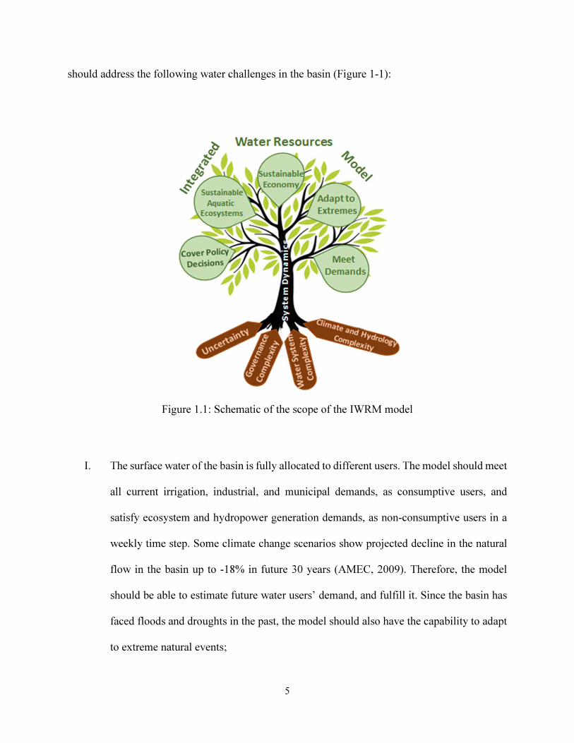
should address the following water challenges in the basin (Figure 1-1):

Figure 1.1: Schematic of the scope of the IWRM model

I. The surface water of the basin is fully allocated to different users. The model should meet

all current irrigation, industrial, and municipal demands, as consumptive users, and

satisfy ecosystem and hydropower generation demands, as non-consumptive users in a

weekly time step. Some climate change scenarios show projected decline in the natural

flow in the basin up to -18% in future 30 years (AMEC, 2009). Therefore, the model

should be able to estimate future water users’ demand, and fulfill it. Since the basin has

faced floods and droughts in the past, the model should also have the capability to adapt

to extreme natural events;

6

II. Among water users, agriculture has special importance for the economy of the OMRB

and Canada. The basin has 10 large Irrigation Districts (IDs) that require careful

consideration in the water allocation. The amount of water allocated to IDs is based on

crop water requirement (CWR), which is affected by climate change increasing the

demands in the OMRB (Pomeroy et al., 2009). The model should estimate the CWR and

address the impact of changes in water supply on the water allocated to irrigation

districts, crop production efficiency, and finally on the basin’s economy under different

what-if scenarios of water availability.

III. Flow regulation and off-stream water diversion change the flow regime, and endanger

sustainable aquatic ecosystems in the basin. It is recommended that river flows should

not be less than a specific amount of water in each week. This amount of water is defined

as instream flow need (IFN). The model should be capable of calculating IFN, and

allocating enough water to rivers to meet IFN under current hydrological conditions.

There are different methods to compute IFN, like the fish rule curve (FRC) and the

Alberta desktop method (ADM). In common approaches of estimating IFN in Alberta, a

percent of natural flow is allocated to ecosystem and maintained in the rivers. This

percentage value is called the “IFN percent of natural flow component”. It is different for

each section of the Oldman River, but it is 75% on average. Satisfying IFN under

different policy scenarios of uncertain water supply is within the scope of this thesis.

Furthermore, this percentage value for each section of the Oldman River will be changed

and IFNs will be calculated. Afterwards, the impact of this change on the water allocated

to IFN, and also on the basin’s economy will be investigated under different scenarios of

water supply availability.

7

IV. Water resources in the basin are highly regulated. There are four important dams, which

are responsible for meeting the demands of the majority of users in the basin and support

sustainable economic development and aquatic environment. Among them, the Oldman

River Reservoir, which is the largest reservoir in the basin, has also the task of providing

the water requirement of the Saskatchewan apportionment channel. The minimum water

demand of this channel is 42.5 m3/s which is met by the Bow and Reddeer Rivers, besides

the Oldman River. Hence, not only does the Oldman reservoir’s operation play a crucial

role in managing the water in the basin, but it is also important to secure flows to the

downstream province of Saskatchewan. This role becomes critical under specific

hydrometeorological conditions, like drought or floods, to keep balance between the

basin’s economy and ecosystem while preventing floods and decreasing drought effects.

Therefore, reservoir operating zones should be most-optimally identified. This research

also aims to provide decision makers with guidelines, including different sets of

operation zones resulting in trade-offs between the optimal economic benefit, water

allocated to the ecosystem, and flood protection. Using these guidelines, decision makers

can easily decide how much water should be stored in the reservoir to meet a specific

objective while not sacrificing others.

1. 3. Research Purpose

The purpose of this research is to improve decision making under uncertain water supply

and demand by developing an integrated water resources management model for the Oldman River

Basin. The specific objectives are to:

8

I. Develop an integrated water resources management model, including water allocation

model, dynamic irrigation demand, economic evaluation, and instream flow needs (IFNs)

sub-models;

II. Investigate the impacts of changing water availability and IFN’s policy on the basin’s

economy and water allocated to IFNs; and

III. Analyze alternative sets of operating zones for the Oldman River Reservoir using multi-

objective performance assessment, the Pareto approach, to identify the most-optimal

economic benefits and water allocation to IFN, while avoiding flooding.

9

CHAPTER 2

LITERATURE REVIEW

This literature review is mostly focused on integrated water resources management

(IWRM) modelling. First of all, IWRM models and some approaches applied to develop them will

be described. Then, uncertainty in water supply and demand will be discussed. The last part of this

chapter will assess the Pareto approach as a solution to balance economic development,

environmental protection, and flood security objectives.

2. 1. Integrated Water Resources Management Modeling

While there are several definitions of IWRM, Biswas (2009) argued that the most

comprehensive is the Global Water Partnership’s definition. The Global Water Partnership (2000)

defined IWRM as “a process which promotes the coordinated development and management of

water, land and related resources, in order to maximize the resultant economic and social welfare

in an equitable manner without compromising the sustainability of vital ecosystems”. Considering

this definition, IWRM requires a model which not only covers the physical processes (Motando,

2002), but also can represent system feedbacks, and interaction between the physical processes

and socio-economic issues. Nikolic et al (2012) also discussed that an IWRM model should have

suitable spatial and temporal scales and engage stakeholders in decision making.

So far various integrated water resources management models have been developed across

the globe. Molina et al. (2010) proposed an integrated water management model using Object-

10

Oriented Bayesian Networks (OOBNs) for the Altiplano region of Murcia in Southern Spain. They

built a Decision Support System (DSS) to engage stakeholders and assess the effects of a range of

management strategies on a complex water system supplied by groundwater from four aquifers.

Graveline et al. (2014) also developed an integrated model, which linked physical processes to

regulatory and economic issues in Gallego catchment, Spain, to evaluate the effects of water

scarcity under global changes on the future state of water. As Harou et al. (2009) argued, such

integrated models, which capture hydrologic, engineering, environmental, and economic aspects

of water resource systems on a regional scale within a coherent framework are called hydro-

economic models. Integrated hydro-economic models represent the interactions between water and

the economy, and the impact of economic water use on water availability and quality in the short

and long term (Brouwer and Hofkes, 2008). In some research, these models have been extended,

and other aspects of water management problems have been added to them. For instance, Cia et

al. (2003) developed an integrated hydrologic-agronomic-economic model to manage the water in

the Syr Darya River basin in Central Asia. Their model had more characteristics of an IWRM

model and included flow and pollutant transport and balance in the basin, irrigation and drainage

processes, economic evaluation of pollution control and water conservation, infrastructure

improvement with consideration of investment, and institutional rules and policies that govern

water allocation. Guan and Hubacek (2008) developed a hydro-economic accounting framework

for the North of China to evaluate the linkages between the economy and the hydro-ecosystem.

They measured the amount of return flows of different qualities to the respective hydro-sectors,

quantified the amount of freshwater that had been contaminated in the regional hydro-ecosystem,

examined the impacts of wastewater on the regional hydro-ecosystem, and tracked the sources of

water inputs to every economic sector. On a smaller scale, California as an arid state in the USA

11

needed a holistic hydro-economic-engineering model to address the water challenges (Draper et

al. 2003). Hence, a model was developed by Draper et al. (2003) to operate surface and

groundwater resources and allocate water over the historical hydrologic record considering the

economic values of agricultural and urban water use, within physical, environmental, and selected

policy constraints. They used an optimization approach to develop their hydro-economic model.

Varela-Ortega et al. (2011) also used a combination of optimization and hydrologic models

(WEAP) in an arid basin in Spain to examine the spatial and temporal impacts of water and

agricultural policies under different climate scenarios. They aimed to recover groundwater

resources and conserve rural livelihoods in the basin. In Canada, Ferreyra et al. (2008) applied an

IWRM framework to analyze agro-environmental policies for secure water quality in the Province

of Ontario. A triangulation strategy was followed, including participant observation, document

analysis and semi-structured interviews. They argued that agro-environmental programs should be

constructed within “expanded arenas” as a task for IWRM and concluded that source water

protection in agricultural areas of Ontario needs more flexible ways of connecting to existing social

and political policies.

To implement the IWRM approach, both optimization and simulation models were applied.

Optimization is typically used to maximize economic efficiency (Alvarez et al, 2004; and

Moghadasi et al 2010), and/or minimize the risk in environmental conservation (Fang et al, 2010;

Chang et al, 2011). Cia et al. (2002) used quantitative indicators of sustainability to improve the

decision-making process with an optimization model applied to the Syr Darya River Basin in

central Asia. Their aim was to manage the water in the irrigation-dominated river basins so that

crop water requirements and municipal and industrial water demands are met while negative

environmental consequences are minimized. Since IWRM needs a broader, multi-faced modeling,

12

a combination of economic and environmental objectives are more useful. As an example, Wang

et al (2009) developed a multi-objective optimization model considering economic, social, and

environmental objectives to meet eco-environmental water demand for allocating water resources

in a river basin over the long term. They also built a forecasting model to predict domestic and

industrial water demands.

Optimization models might be helpful to identify the decision-variable values, which

produce the best plan. But, they are based on the assumptions incorporated in the model. Often

these assumptions are limiting. In these cases the solutions resulting from optimization models

should be examined in more detail, maybe through simulation models, to improve the values of

the decision-variables (Loucks and Van Beek, 2005). Simulation models can address “what-if”

scenarios to evaluate alternative design and/or operating policies (Loucks and Van Beek, 2005).

For instance, George et al. (2011) linked a simulation-based allocation model with a social cost-

benefit economic model to analyze different policy scenarios for water allocation and surface and

groundwater resource availability in the Krishna Basin, India. Another important characteristic of

simulation models to manage water resources is that they allow investigation of the effect of future

changes in the water resources systems (Heinz et al., 2007). Therefore, many studies have preferred

simulation models to examine the water system behavior under different policies and scenarios

(Marques et al., 2006; Kalbus et al, 2011). Another research by Molina et al. (2011) is one example

of applying simulation models in integrated water resources management. They simulated an

integration of hydrological, economic and social factors using a Groundwater Flow Model (GFM)

and a Decision Support System (DSS) based on an object-oriented Bayesian Networks approach

for a region in Murcia in Spain. They selected some management strategies to evaluate the possible

impacts caused by future water management actions on the water system. In a study by Gober et

13

al (2010), a simulation, hierarchical model (WaterSim) has been developed to examine the effect

of different climate conditions and policy choices on water supply and demand conditions in

Phoenix, USA. Their model allows for the participation of policy makers and residents in decision

processes considering the uncertainties of climate change. Simulation results show significant

threats to Phoenix's water security due to global warming and population growth (Gober et al.,

2010).

So far various simulation IWRM models have been developed worldwide, allowing model

developers and policy makers to investigate alternative “science- and policy-based” scenarios.

Nonetheless, there is a strong need to explore simulation models that not only represent complex

dynamic water resource systems in a realistic way, but also allow the involvement of end users in

model development (Ahmad and Simonovic, 2000; Loucks and Van Beek, 2005; Cai et al. 2012;

Beddington, 2013).

As mentioned earlier in chapter 1, system dynamics (SD) is a simulation environment that

is valuable for representing complex systems in a way that can facilitate the engagement of

stakeholders in the decision-making process. For example, SD was used to propose a water

allocation agreement among five states of the Mexican Republic and the national water authorities

(Hinojosa-Huerta et al., 2001). SD also is quite suitable for multidisciplinary and multi-actor

problems in integrated water resources management (Winz et al, 2009). Davies and Simonovic

(2011) examined five water resources experiments to show several benefits of a feedback-based

modeling approach. Their experiments included “wastewater treatment”, “reuse programs”,

“irrigation expansion”, “animal product consumption” and “alternative dilution factor values”.

Their modelling was focused on the nature and structure of the connections between “water

resources” and “socio-economic and environmental change”. The results of the five simulations

14

determined the influences of water stress in water quality and water quantity on the water system

in the basin. Gastelum et al. (2010) used an SD approach in the Conchos Basin in Mexico to

analyze the effect of different water allocation scenarios on water delivery in the United States and

agricultural production within the Basin. To analyze the effectiveness of various supply and

demand policies in meeting socio-economic and ecological requirements, Wang et al. (2011)

developed a dynamic simulation model of a water system in Yulin City, China. Their results show

that the most sustainable strategy for saving the economic and ecological status of the region is

demand management instruments and conservation measures. Hassanzadeh et al. (2014)

developed a modeling framework for IWRM called SWAMPSK (Sustainability-oriented Water

Allocation, Management, and Planning), including an irrigation demand sub-model and a cost-

revenue evaluation, using the SD approach for the Saskatchewan portion of the South

Saskatchewan River Basin in western Canada. Different evapotranspiration equations were

applied to estimate the crop water requirement, and they found that the water resources system is

sensitive to the selection of these equations. They also simulated SWAMPSK under multiple what-

if scenarios based on irrigation expansion and warming climate and concluded that the agricultural

expansion leads to a small decline in hydropower production, and obviously results in an increase

in the basin’s economic benefit. Besides SWAMPSK, there are parallel works for developing

SWAMPBOW (SWAMP for the Bow River Basin; Gonda (2015)) and SWAMPOM (SWAMP for

the Oldman River Basin) which is the main objective of this thesis.

As Mirchi et al. (2012) concluded, system dynamics, as a systems thinking approach,

enables integrated understanding of water resources systems in a reliable qualitative and

quantitative bases for policy selection, and strategic decision making, while avoiding unsustainable

management strategies. It is a multi-disciplinary, multi-sectoral, and participatory approach that

15

can capture the big picture of the problem using feedback loops (Mirchi, 2013). Hence, it is

practical to carry out a conceptual, strategic, sustainable water resources model.

For the Oldman River Basin, which is the case study in this research, an IWRM model

which addresses hydrologic, engineering, environmental, and economic aspects of water resources

systems, and examines the dynamic behavior of components and the whole system has not

developed so far. However, Alberta Environment (2002) has been using an optimization-based

Water Resources Management Model (WRMM) for the South Saskatchewan River Basin to

allocate water to users based on the physical characteristics of the water resource system, water

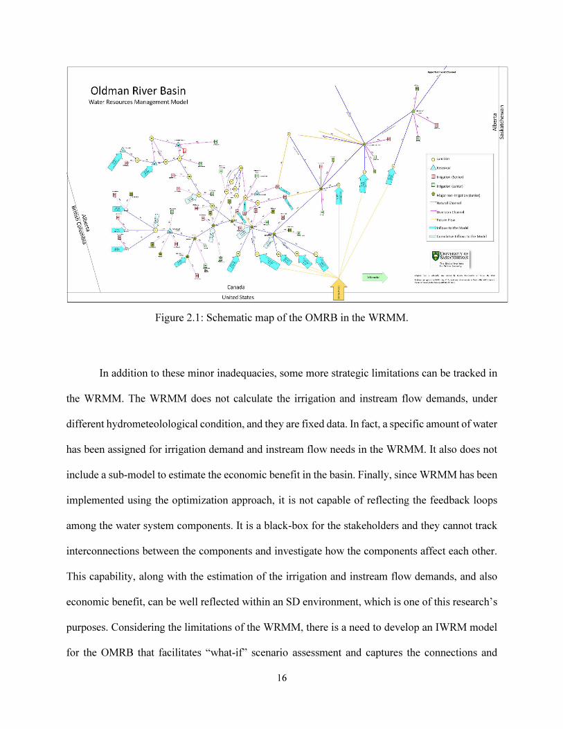
supply, water demand, and operating policies. But, it has some structural limitations. First, it

applies negative flow in some points in the water system. The model uses the cumulative amount

of water flow in some parts of the basin (shown with big light blue fletchers in figure 2-1) and the

amount of local flow is not given in these parts. Therefore, to calculate the amount of local flow

in these points, the cumulative flow should subtract from the flows in the previous points. In some

weeks, the calculated local flows have negative values. Second, some inflows are assumed in the

model, but there are no such flows in the basin (Blue narrow fletchers in figure 2-1). If some of

them are deleted, the model cannot be executed. Third, the WRMM solver can become infeasible,

for example when the annual flow volume decreases and/or increases by more than 25% and/or

the timing of the peak flow is shifted 4 weeks or more (Nazemi et al., 2013). Another minor

inadequacy of WRMM is the imprecise dead storage level assumed for some reservoirs found by

Sheer et al. (2013). For instance, the dead storage level in McGregor is assumed so low that

irrigators could not pull water at that level.

16

Figure 2.1: Schematic map of the OMRB in the WRMM.

In addition to these minor inadequacies, some more strategic limitations can be tracked in

the WRMM. The WRMM does not calculate the irrigation and instream flow demands, under

different hydrometeolological condition, and they are fixed data. In fact, a specific amount of water

has been assigned for irrigation demand and instream flow needs in the WRMM. It also does not

include a sub-model to estimate the economic benefit in the basin. Finally, since WRMM has been

implemented using the optimization approach, it is not capable of reflecting the feedback loops

among the water system components. It is a black-box for the stakeholders and they cannot track

interconnections between the components and investigate how the components affect each other.

This capability, along with the estimation of the irrigation and instream flow demands, and also

economic benefit, can be well reflected within an SD environment, which is one of this research’s

purposes. Considering the limitations of the WRMM, there is a need to develop an IWRM model

for the OMRB that facilitates “what-if” scenario assessment and captures the connections and

17

feedbacks among the water system variables. This model is implemented within an SD

environment.

2. 2. Uncertain Water Supply and Demand

The magnitude and timing of river flows are changing, mainly because of variations in

meteorological variables, including precipitation and temperature, and snowpack and glacier melt

(Groisman et al., 2001; Milly et al., 2005; Wheater and Gober, 2013). The major reason for these

changes is climate variability and climate change. Such variations in river discharge can result in

failure to meet the demands (Payne et al. 2004; Archer et al. 2010; Nazemi et al. 2013). Nazemi et

al. (2013) demonstrated that changes in the Alberta rivers flow regime mean that Alberta might

not be able to meet all demands. Vano et al. (2010) simulated the effects of earlier snowmelt runoff

and reduced summer flows on irrigated agriculture. They show that earlier snowmelt leads to

increased water delivery limitations and economic losses. On a big scale, Palmer et al. (2010)

mapped possible changes in river flows and water stress in basins worldwide. Their projections

indicated that nearly one billion people live in areas likely to require proactive or reactive

management intervention to mitigate water stress. Otherwise, these changes result in risks to

ecosystems and economic losses. Since the Oldman River Basin has experienced such changes in

the pattern and characteristics of the river flows (Tanzeeba and Gan, 2012), it is essential to analyze

how changes in hydrologic patterns affect meeting the various water demands and the basin’s

economy.

Another important factor, which affects agricultural productivity and then the basin’s

economy, is how much water is required by planted crops in the IDs and how much water is

available to allocate. Hence, a model should be developed to estimate the irrigation demand. Crop

18

water requirement is the amount of water, which a crop requires for maximum yield. To estimate

irrigation demand, different reference evapotranspiration equations (ETo) have been used such as

the Penman-Monteith equation (Monteith, 1965), Priestley and Taylor (Priestley and Taylor,

1972), Hargreaves (Hargreaves, 1973), modified Hargreaves (Hargreaves et al., 1985); Hargreaves

and Samani (Hargreaves and Samani, 1985); and Maulé (Maulé et al., 2006). Among them, the

Penman-Monteith equation calculates the crop water requirement with higher accuracy, but using

this equation requires meteorological data that may not be available in all regions (Hassanzadeh et

al., 2014). Thus, simple equations have been used in recent studies. Hassanzadeh et al. (2014)

compared some simple equations, such as Maulé’s and Farmer’s equations (Farmer et al. 2011) to

estimate the ETo for the South Saskatchewan River (SSR) Basin. They found that the irrigation

demand model is sensitive to the selection of the ETo equations. Also, they showed that the results

of the Farmer’s equation are closer to Penman-Monteith equation’s results. Alberta Agriculture,

Food and Rural Development (2013) developed an Irrigation Management Model, which uses an

ASCE standardized equation, a modified Penman equation, to calculate the reference

evapotranspiration. The model estimates the irrigation demands for the most popular crops planted

in Alberta. These irrigation demands are an input of Alberta’s WRMM. Since SWAMPOM is an

emulation of WRMM, the modified Penman equation will be also applied to estimate ETo in this

thesis.

2. 3. Balancing Economic and Environmental Protection Objectives While

Avoiding Flooding

Water resources management faces both increasing attention to environmental flow

requirements and economic growth. This involves complex decision making to allocate water.

19

Changes in water supply availabilities and water demands can accelerate the competition between

human and ecosystem needs. Pahl-Wostl (2007) introduced a conceptual framework to analyze the

management regimes of river basins at the global scale that follows a “learning to manage by

managing to learn” plan. It was concluded that adaptive water management regimes that consider

all characteristics of river basins, specifically environment and economy, are required.

Besides such conceptual frameworks, mathematical models are used to meet economic and

environmental protection objectives together. Qureshi et al. (2007) developed an optimization

model to analyze the effect of reallocating Murray River Basin water from agriculture to the

environment on the economy. The model was simulated under multiple stochastic weather

scenarios with and without the possibility of interregional water trade. The results showed a

decrease in economic benefit through increasing water allocation to the environment. Cia (2008)

also developed an optimization model, which maximized the economic benefit to holistically

manage water resources in a basin-scale.

In addition to optimization models with one objective function, there are multicriterion

decision methods, which investigate multiple objectives. Lee (2012) used a combination of game

theory and multi-objective optimization to balance water quality protection and economic

development objectives in the Tseng-Wen reservoir, Taiwan. They aimed to manage land use

patterns, therefore, geographic information system (GIS) has been used to spatially organize the

geographical data of land use types within the watershed. The Pareto curve approach is another

multicriterion decision method that typically follows an optimization method with two or more

objective functions (OFs). However, it is practical when the optimization problem involves

multiple conflicting objective functions, and there is no single, feasible solution to optimize all

objectives together (Augusto et al., 2012). Like other optimization models, one or more parameters

20

are relaxed and optimal objective functions are calculated. In the Pareto curve approach these OFs

can be for example, economic benefits and ecosystem targets. Calculated objective functions are

plotted in a two dimensional Pareto surface, with the axes showing economic benefit and

ecosystem objectives. However, the number of objective functions may increase, and the Pareto

curve would change into a higher-dimensional plot. The front of such a plot shows an optimal

management plan, which is called the Pareto front. The Pareto approach has several applications

in hydrology (to find a set of optimal values for hydrological model’s parameters), system

management, and hydropower plants (Beven, 2006; Vahidinas and Jadid, 2010; Capon-Garcıa et

al., 2011; Vijayalakshmi, 2014). As an example, Ouattara et al. (2012) applied the Pareto approach

to study simultaneously ecological and economic issues in hydropower plant utilities management.

Genetic algorithms and a decision making tool, called ARIANETM were used to find Pareto

surfaces. They found five Pareto fronts based on the annual hydropower generation cost and five

emitted pollutants.

In the last decade, the Pareto approach has been applied in water resources management,

and reservoir operation. Suen and Eheart (2006) used the Pareto approach to operate a reservoir in

the Dahan River Basin in Taiwan. They aimed to find the optimal trade-off between human water

needs and environmental flow regime. Their main goal was to calculate environmental flow needs

under different flow magnitude, duration, frequency, and timing conditions. They also defined an

objective function, a human needs objective function, to compute the agricultural, and municipal

water demands. In another study by Le Ngo et al. (2007), the Pareto curve has been applied to

maximize hydropower generation, and minimize flooding in order to reach the optimal control

strategies for the Hoa Binh reservoir operation, in Vietnam. Castelletti et al (2013) also focused

on the hydropower generation, and flood control in the Hoa Binh reservoir. They projected a novel

21

multi-objective Reinforcement Learning algorithm to compute an approximation of the Pareto

front in one single run. Some researches focused on only reservoir flood control operation.

Delelegn et al. (2011) used the Pareto approach to minimize the urban flood damage, and Li et al.

(2010) used it to optimize the peak flood discharge. They applied a multi-objective shuffled frog

leaping algorithm (MOSFLA) to find closer solutions to the Pareto front. On the other hand, Liu

et al (2011) found that the Pareto approach is very useful to maximize the hydropower generation

in cascade reservoirs. To the best of this author’s knowledge, the Pareto approach with multiple

objective functions (more than two OFs) has not been applied for reservoir basin management and

making a guideline for decision makers to find the best plan based on their priorities on different

water management objectives. In most studies, the objective was to find an optimal trade-off

between the two objectives, resulting in a two-dimensional Pareto front. In this thesis, the aim is

to manage the Oldman River Reservoir in order to overcome the most important water

management criticism, and reach the optimal economic benefit and water allocated to the instream

flow needs, minimum floodwater and flood frequency through generating a four-dimensional

Pareto front.

22

CHAPTER 3

MATERIALS AND METHODS

As mentioned earlier, this research aims to develop an integrated water resources

management model for the Oldman River Basin (SWAMPOM), to address the water security

challenges under uncertain water supply. This will be achieved through the following steps:

I. Developing a simulation-based water allocation model for the Oldman River Basin

(OMRB), through emulation of the existing optimization-based Water Resources

Management Model (WRMM);

II. Adding model functionality, in particular, developing dynamic irrigation demand,

instream flow need (IFN), and economic evaluation sub-models;

III. Generating a set of feasible scenarios to analyze the impact of water supply uncertainty

and change in the IFN percent of the natural flow component, on the basin’s economy;

and

IV. Analyzing alternative sets of operating zones for the Oldman River Reservoir using

multi-objective performance assessment to identify optimal trade-offs between the

economic benefits, water allocation to environmental flows and flood control safety

objectives.

To develop the SWAMPOM, system dynamics (SD), as a modeling approach and object-

based simulation environment, is used. SD facilitates engaging different water policies in a

modelling process while capturing the dynamic feedback loops dominating the behavior of a

complex water resources system (Ford, 1997; Sterman, 2001). This chapter is organized as

23

follows: The chapter begins with an explanation of the Oldman River Basin (Section 3.1), followed

by a brief description of WRMM as a source of data on water supply, water demand, operating

rules, and allocation priorities (Section 3.2). Section 3.3 explains the SD approach employed to

develop the model. Finally, Section 3.4 provides a comprehensive description of SWAMPOM

including an explanation of the water allocation model, and economic evaluation, instream flow

needs, and dynamic irrigation demand sub-models.

3. 1. Case Study: The Oldman River Basin

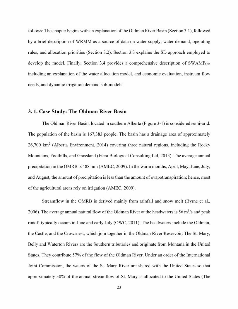
The Oldman River Basin, located in southern Alberta (Figure 3-1) is considered semi-arid.

The population of the basin is 167,383 people. The basin has a drainage area of approximately

26,700 km2 (Alberta Environment, 2014) covering three natural regions, including the Rocky

Mountains, Foothills, and Grassland (Fiera Biological Consulting Ltd, 2013). The average annual

precipitation in the OMRB is 488 mm (AMEC, 2009). In the warm months, April, May, June, July,

and August, the amount of precipitation is less than the amount of evapotranspiration; hence, most

of the agricultural areas rely on irrigation (AMEC, 2009).

Streamflow in the OMRB is derived mainly from rainfall and snow melt (Byrne et al.,

2006). The average annual natural flow of the Oldman River at the headwaters is 56 m3/s and peak

runoff typically occurs in June and early July (OWC, 2011). The headwaters include the Oldman,

the Castle, and the Crowsnest, which join together in the Oldman River Reservoir. The St. Mary,

Belly and Waterton Rivers are the Southern tributaries and originate from Montana in the United

States. They contribute 57% of the flow of the Oldman River. Under an order of the International

Joint Commission, the waters of the St. Mary River are shared with the United States so that

approximately 30% of the annual streamflow of St. Mary is allocated to the United States (The

24

State of Saskatchewan River Basin, 2006). The Oldman River and the Bow River join to form the

South Saskatchewan River. Climate change scenarios show a range of projected change in the

natural flow in the basin from -18% to +4% by 2050 (AMEC, 2009).

Figure 3.1: The Oldman River Basin (OWC, 2010)

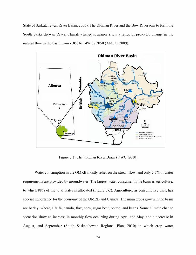
Water consumption in the OMRB mostly relies on the streamflow, and only 2.5% of water

requirements are provided by groundwater. The largest water consumer in the basin is agriculture,

to which 88% of the total water is allocated (Figure 3-2). Agriculture, as consumptive user, has

special importance for the economy of the OMRB and Canada. The main crops grown in the basin

are barley, wheat, alfalfa, canola, flax, corn, sugar beet, potato, and beans. Some climate change

scenarios show an increase in monthly flow occurring during April and May, and a decrease in

August, and September (South Saskatchewan Regional Plan, 2010) in which crop water

25

requirements are high. Such predictions negatively affect the desire of irrigation districts to

expand. After agriculture, urban centers (3%), industry (1%) and stock water (1%) are the next

largest water consumers in the basin (Figure 3-2). Industrial water is mainly consumed for food

and beverage production. Hydropower is also an important non-consumptive water user which has

been classified as “other users” in figure 3-2. Hydropower generation is small in the basin and

reaches a maximum amount of 32 MWhr in May.

Consumptive water users, such as agriculture, urban centers and industry, reduce the

quantity and/or quality of flow, while non-consumptive users like hydropower plant, and instream

flow needs, do not cause any overall diminishment in river flow (Adelsman, 1996).

Figure 3.2: The percentage of water allocated to water sectors in the OMRB.

Competition among water users has increased due to urbanization, agricultural expansion,

and industrial development. Currently, 100% of the surface flow is allocated to consumptive and

non-consumptive users, and it escalates water challenges in the basin. Moreover, degraded water

quality and ecosystems are additional challenges for water management in the basin. The basin is

a complex human-environmental system with interconnections between terrestrial and aquatic

26

environments, climate, human activities on land, and water management. In general, the growing

complexity of the water system and future uncertainty are the main sources of water resources

challenges in the basin (Wheater and Gober, 2013):

I. Climate and Hydrology: The temperature in the OMRB ranges widely, between -40

and 35 oC. Large areas of the basin are covered by the Rocky Mountains, thus,

characterizing the precipitation amount and phase is difficult. The dominant form of

precipitation in the basin is snow. Rainfall, specifically on the snow-covered areas, also

plays an important role in the basin’s hydrology. Blowing snow, snow sublimation, and

snow accumulation are other factors affecting the water balance in the basin (Wheater

and Gober, 2013). Flows in the Oldman River greatly change from year to year, with

coefficient of variation of up to 55% and flow regulation and water use significantly

affect the flow (AMEC, 2009). While climate change scenarios project an increase in

precipitation in the OMRB, a decline in the natural flow is expected due to an increase

in air temperature leading to a rise in evaporation (Tanzeeba and Gan, 2012) and change

in snowmelt contribution to streamflow. The basin experienced extreme natural events

in recent decades, including floods (e.g., 2005, 2011, and 2013 floods) and droughts

(1999-2004). Warming climate is causing Rocky Mountain glaciers to retreat, hence,

the magnitude and timing of river flows are changing (Gober and Wheater, 2013).

II. Water Resources System: The water resources system is complex in the OMRB; it

includes more than 100 components such as, irrigation districts, hydropower plant, as

well as industrial and municipal centers. In addition, there are six important dams, of

which the Oldman reservoir is the biggest with full storage capacity of approximately

900 MCM. Water management, flow regulation, flood and erosion control, recreation,

27

and conservation are the main purposes of Oldman reservoir construction (Federal

Government, 2003). The reservoir supplies irrigation demands and environmental flow

requirements and also meets apportionment requirements for the Saskatchewan

province, especially in the dry months. In severe consecutive drought years, the

Oldman Reservoir is depleted to the minimum level after one and half years and takes

time to recover (South Saskatchewan Regional Plan, 2010).

III. Water Governance: Water allocation in the basin is based on the principle of “first in

time, first in right” and the use of water (surface water or groundwater) requires a

license from the Government of Alberta. However, the federal government has a

responsibility to provide the water requirement of First Nation’s land (Wheater and

Gober, 2013), and first nations have first order to receive water in all water

consumption purposes.

In addition, the OMRB -also the Bow River Basin- has inter-provincial commitments

to transfer 50% of the natural flows to Saskatchewan via an apportionment channel

(Prairie Provinces Water Board, 2011). But, flows have been very close to this limit in

consecutive dry years and there are concerns to meet the agreement under drought

conditions (Wheater and Gober, 2013).

Although hydrologic characteristics and water management problems in Alberta have been

frequently studied, a few studies focused on the Oldman River Basin particularly. As an example,

Byrne et al. (2006) addressed current and future water quantity and water quality issues in the

OMRB. They discussed that global warming has resulted in a declining trend in alpine and prairie

snow pack accumulation affecting streamflow within the OMRB. Their results show that net water

supplies are decreasing in the basin, and may possibly lead to a decline in surface water quality;

28

and finally they emphasized the need for holistic water resources management. Nevertheless, a

comprehensive study capturing the water challenges of the basin has not been done. However, the

Water Resources Management Model, WRMM, has been developed to allocate the water to all

basins in Alberta (Alberta Environment, 2002). The WRMM’s data and operating policies have

been used to make the IWRM model for the OMRB here (SWAMPOM). Thus, it is necessary that

a brief description of the WRMM is provided and it will appear in the next section.

3. 2. Water Resources Management Model (WRMM)

WRMM, developed by Alberta Environment, is an optimization-based model that attempts

to optimally allocate water to the South Saskatchewan River Basin based on operating rules, and

water supply and demand (Alberta Environment, 2010). To allocate the water to the users, WRMM

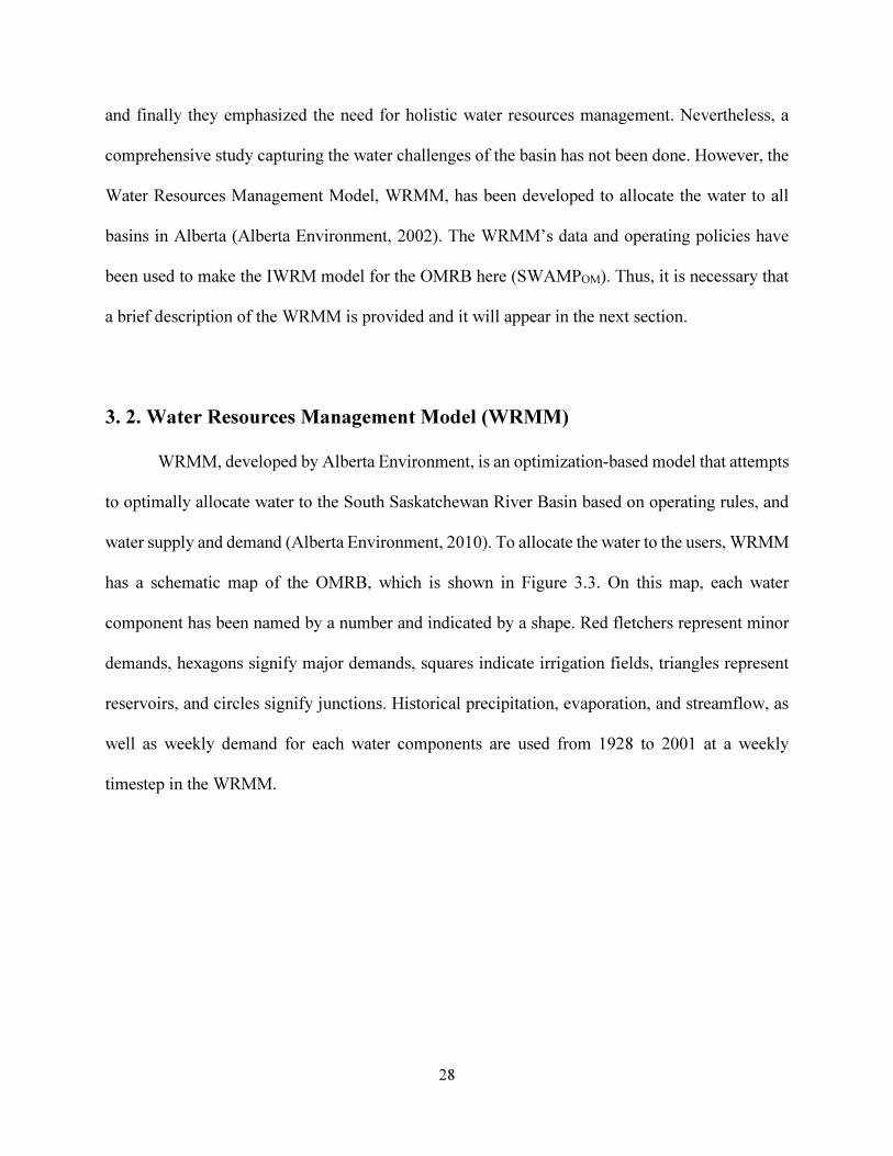
has a schematic map of the OMRB, which is shown in Figure 3.3. On this map, each water

component has been named by a number and indicated by a shape. Red fletchers represent minor

demands, hexagons signify major demands, squares indicate irrigation fields, triangles represent

reservoirs, and circles signify junctions. Historical precipitation, evaporation, and streamflow, as

well as weekly demand for each water components are used from 1928 to 2001 at a weekly

timestep in the WRMM.

29

Figure 3.3: Schematic map of the Oldman River Basin (OMRB) as built in WRMM.

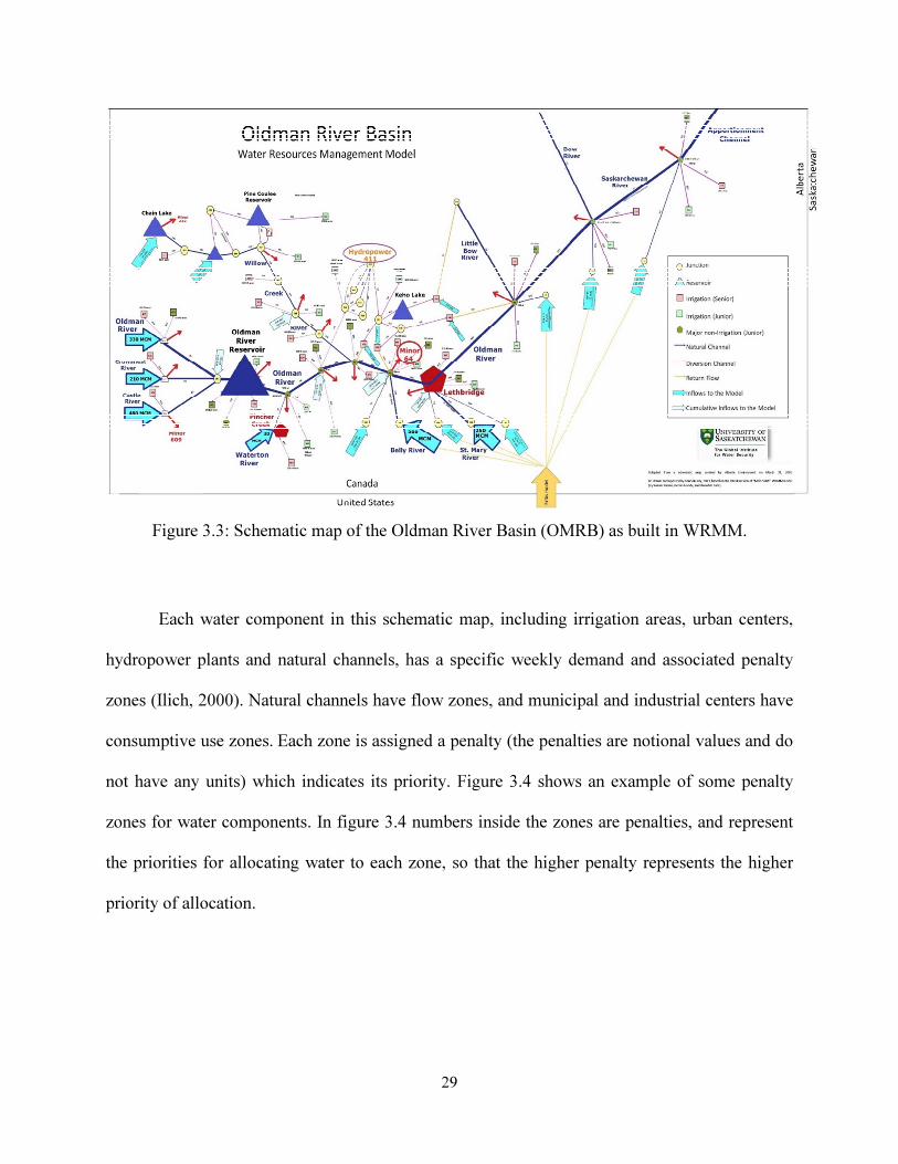
Each water component in this schematic map, including irrigation areas, urban centers,

hydropower plants and natural channels, has a specific weekly demand and associated penalty

zones (Ilich, 2000). Natural channels have flow zones, and municipal and industrial centers have

consumptive use zones. Each zone is assigned a penalty (the penalties are notional values and do

not have any units) which indicates its priority. Figure 3.4 shows an example of some penalty

zones for water components. In figure 3.4 numbers inside the zones are penalties, and represent

the priorities for allocating water to each zone, so that the higher penalty represents the higher

priority of allocation.

30

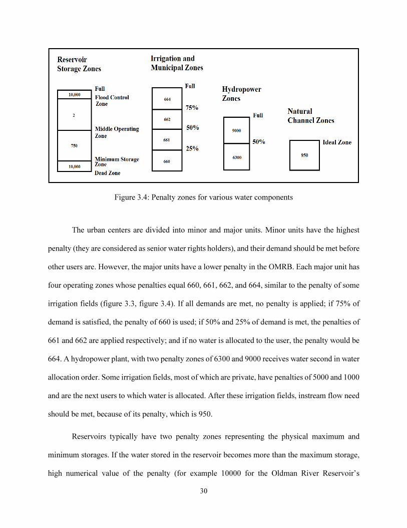
Figure 3.4: Penalty zones for various water components

The urban centers are divided into minor and major units. Minor units have the highest

penalty (they are considered as senior water rights holders), and their demand should be met before

other users are. However, the major units have a lower penalty in the OMRB. Each major unit has

four operating zones whose penalties equal 660, 661, 662, and 664, similar to the penalty of some

irrigation fields (figure 3.3, figure 3.4). If all demands are met, no penalty is applied; if 75% of

demand is satisfied, the penalty of 660 is used; if 50% and 25% of demand is met, the penalties of

661 and 662 are applied respectively; and if no water is allocated to the user, the penalty would be

664. A hydropower plant, with two penalty zones of 6300 and 9000 receives water second in water

allocation order. Some irrigation fields, most of which are private, have penalties of 5000 and 1000

and are the next users to which water is allocated. After these irrigation fields, instream flow need

should be met, because of its penalty, which is 950.

Reservoirs typically have two penalty zones representing the physical maximum and

minimum storages. If the water stored in the reservoir becomes more than the maximum storage,

high numerical value of the penalty (for example 10000 for the Oldman River Reservoir’s

31

maximum storage, figure 3.4) is specified. This high numerical penalty is also applied for physical

minimum storage, so that if the water stored in the Oldman Reservoir, for instance, becomes less

than minimum storage, a penalty of 10000, is specified. Reservoirs may have other penalty zones

between the maximum and minimum storage. The Oldman reservoir has two additional penalty

zones, including a flood control operating zone and middle operating zone whose penalties are

equal to 10,000 and 750, respectively. These additional penalty zones may be higher or lower than

the downstream users’ penalties. Therefore, depending on these two penalty zones and water users’

demand and water users’ penalty, the reservoir releases water (Ilich, 1992).

The WRMM utilizes linear programming optimization to minimize water shortage/surplus

multiplied by the penalty:

�� = �∑(�� ∗ |� �� −� �� |) (3.1)

WRMM also has some constraints to allocate the water. For instance, the water allocated

to irrigation fields, majors, minors and hydropower cannot be more than their demands. The mass

balance equation is used to calculate the amount of water stored in reservoirs:

“Storage = Inflow + Precipitation-Evaporation - Water Allocated to Consumers (Minors, Majors,

Irrigation Fields) - Water Allocated to Hydropower - Water Allocated to IFN” (3.2)

To clarify how WRMM mathematically works, it is explained by a simple water system

(figure 3.5). This system includes a reservoir (blue triangle in figure 3.5) with two penalty zones

of maximum and minimum water storages, an urban center (red hexagon), an irrigation field (green

square), and one natural channel, all with one penalty zone. The system also has a diversion

channel which does not have any penalty. The values of the penalty zones have been indicated

inside each water component in figure 3.5. The irrigation field has a demand of 20 m3/week with

32

a penalty value of 600 (if it is not met); the demand of the urban center is 10 m3/week with a

penalty of 650, and the natural channel’s demand is 15 m3/week and its penalty value is 900. The

reservoir is the source to allocate the water to the components. However, the water storage in the

reservoir should not be less than minimum or maximum level, otherwise a penalty of 1000 is

specified. Therefore, the objective function of this simple system would be:

�� min 650 ∗ �|10 � �1|� � 600 ∗ �|20 � �2|� � 900 ∗ �|15 � �3|�� (3.3)

Figure 3.5: Simple water system to explain WRMM operation procedure

where x1, x2, and x3 are water allocated to the urban center, irrigation field, and natural channel,

respectively. If the water level in the reservoir goes above the maximum or below the minimum

33

storage, a penalty of 1000 is added to equation 3.3. If WRMM has enough water to allocate to all

users, the objective function would be zero. Under water scarcity conditions, it allocates more

water to the natural channel to minimize the objective, because its penalty is higher than others.

After the natural channel, the urban center, followed by the irrigation field, are set in water

allocation order.

3. 3. System Dynamics Approach

System Dynamics (SD) is a simulation environment based on the systems thinking

approach being able to combine theory and methods to analyze the dynamic behavior of complex

systems (Forrester, 1961; Ford, 1999; Bagheri, 2006). Not only does SD represent processes and

related components in isolation, but it also describes the interactions and feedback loops among

them over time. It represents a visualization of the connections between the components of a

system (Osgood, 2004). SD facilitates understanding of how change in one area of the system

results in changes in other areas. Sometimes interaction among the simple components can lead to

a complex dynamic pattern in the behavior of the whole system, and the resulting pattern is

possibly different than what would be expected through studying each component of the system

separately (Osgood, 2004). In fact, the complex behaviors of a system usually originate from the

feedbacks among the components, not from the complexity of the components themselves

(Sterman, 2000). The socio-economic and environmental systems mostly follow this kind of

complex dynamic patterns; therefore, they can be studied using the SD approach.

To understand feedback processes and determine the dynamics of a system, causal loop

diagrams (CLDs) are used. A CLD is a powerful graphical tool to visualize the relationships among

the components and their interactions with each other (Forrester, 1961; Ford, 1999; Bagheri, 2006).

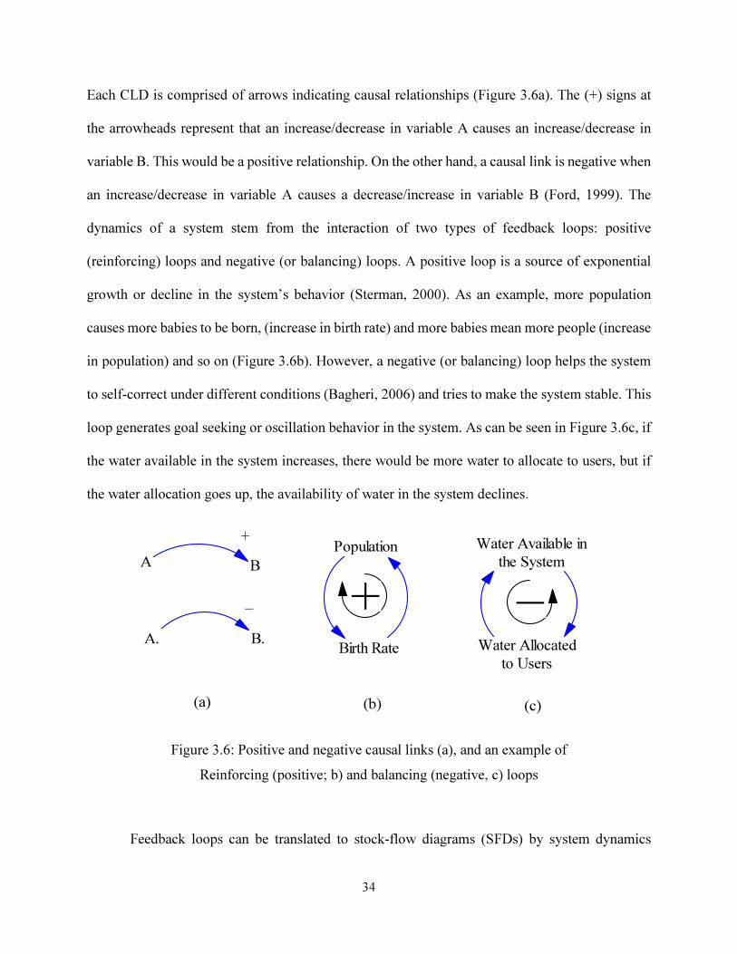
34

Each CLD is comprised of arrows indicating causal relationships (Figure 3.6a). The (+) signs at

the arrowheads represent that an increase/decrease in variable A causes an increase/decrease in

variable B. This would be a positive relationship. On the other hand, a causal link is negative when

an increase/decrease in variable A causes a decrease/increase in variable B (Ford, 1999). The

dynamics of a system stem from the interaction of two types of feedback loops: positive

(reinforcing) loops and negative (or balancing) loops. A positive loop is a source of exponential

growth or decline in the system’s behavior (Sterman, 2000). As an example, more population

causes more babies to be born, (increase in birth rate) and more babies mean more people (increase

in population) and so on (Figure 3.6b). However, a negative (or balancing) loop helps the system

to self-correct under different conditions (Bagheri, 2006) and tries to make the system stable. This

loop generates goal seeking or oscillation behavior in the system. As can be seen in Figure 3.6c, if

the water available in the system increases, there would be more water to allocate to users, but if

the water allocation goes up, the availability of water in the system declines.

Figure 3.6: Positive and negative causal links (a), and an example of

Reinforcing (positive; b) and balancing (negative, c) loops

Feedback loops can be translated to stock-flow diagrams (SFDs) by system dynamics

A B

A. B.

Population

Birth Rate

Water Available in

the System

Water Allocated

to Users

(a) (b) (c)

+

_

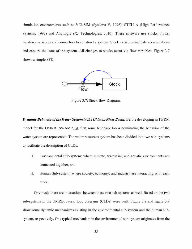
35

simulation environments such as VENSIM (Systems V, 1996), STELLA (High Performance

Systems, 1992) and AnyLogic (XJ Technologies, 2010). These software use stocks, flows,

auxiliary variables and connectors to construct a system. Stock variables indicate accumulations

and capture the state of the system. All changes to stocks occur via flow variables. Figure 3.7

shows a simple SFD.

Figure 3.7: Stock-flow Diagram.

Dynamic Behavior of the Water System in the Oldman River Basin: Before developing an IWRM

model for the OMRB (SWAMPOM), first some feedback loops dominating the behavior of the

water system are represented. The water resources system has been divided into two sub-systems

to facilitate the description of CLDs:

I. Environmental Sub-system: where climate, terrestrial, and aquatic environments are

connected together, and

II. Human Sub-system: where society, economy, and industry are interacting with each

other.

Obviously there are interactions between these two sub-systems as well. Based on the two

sub-systems in the OMRB, causal loop diagrams (CLDs) were built. Figure 3.8 and figure 3.9

show some dynamic mechanisms existing in the environmental sub-system and the human sub-

system, respectively. One typical mechanism in the environmental sub-system originates from the

Stock

Flow

-

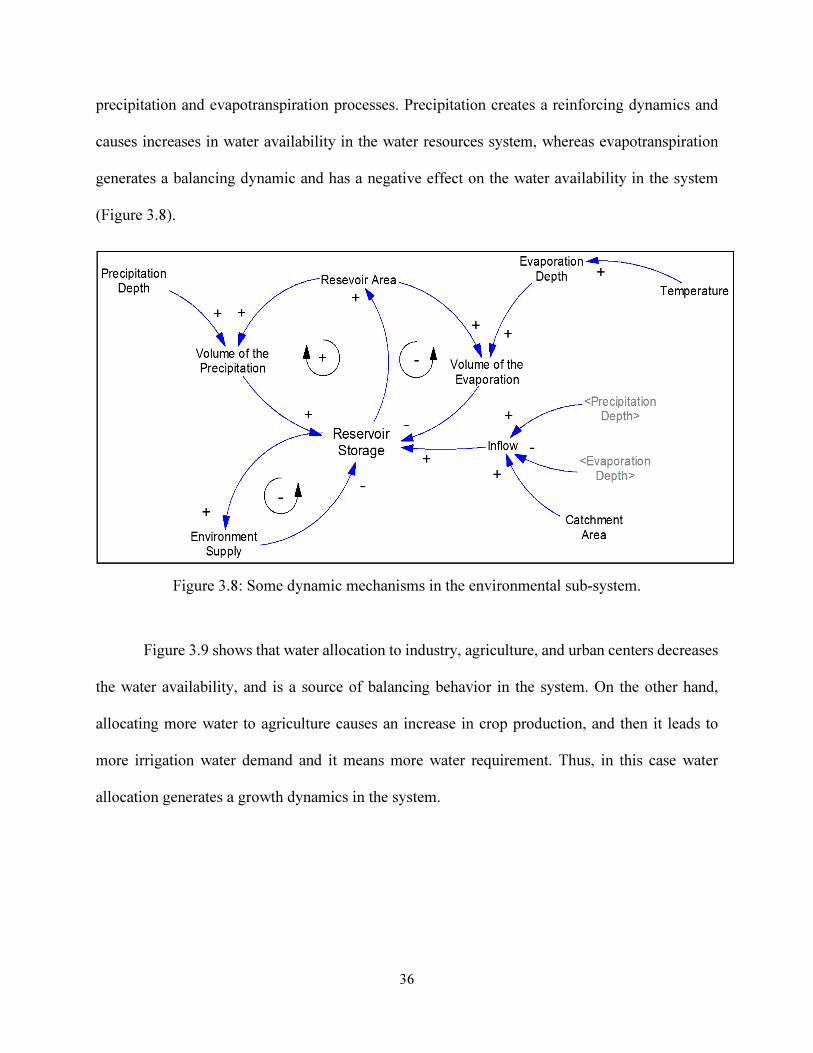
36

precipitation and evapotranspiration processes. Precipitation creates a reinforcing dynamics and

causes increases in water availability in the water resources system, whereas evapotranspiration

generates a balancing dynamic and has a negative effect on the water availability in the system

(Figure 3.8).

Figure 3.8: Some dynamic mechanisms in the environmental sub-system.

Figure 3.9 shows that water allocation to industry, agriculture, and urban centers decreases

the water availability, and is a source of balancing behavior in the system. On the other hand,

allocating more water to agriculture causes an increase in crop production, and then it leads to

more irrigation water demand and it means more water requirement. Thus, in this case water

allocation generates a growth dynamics in the system.

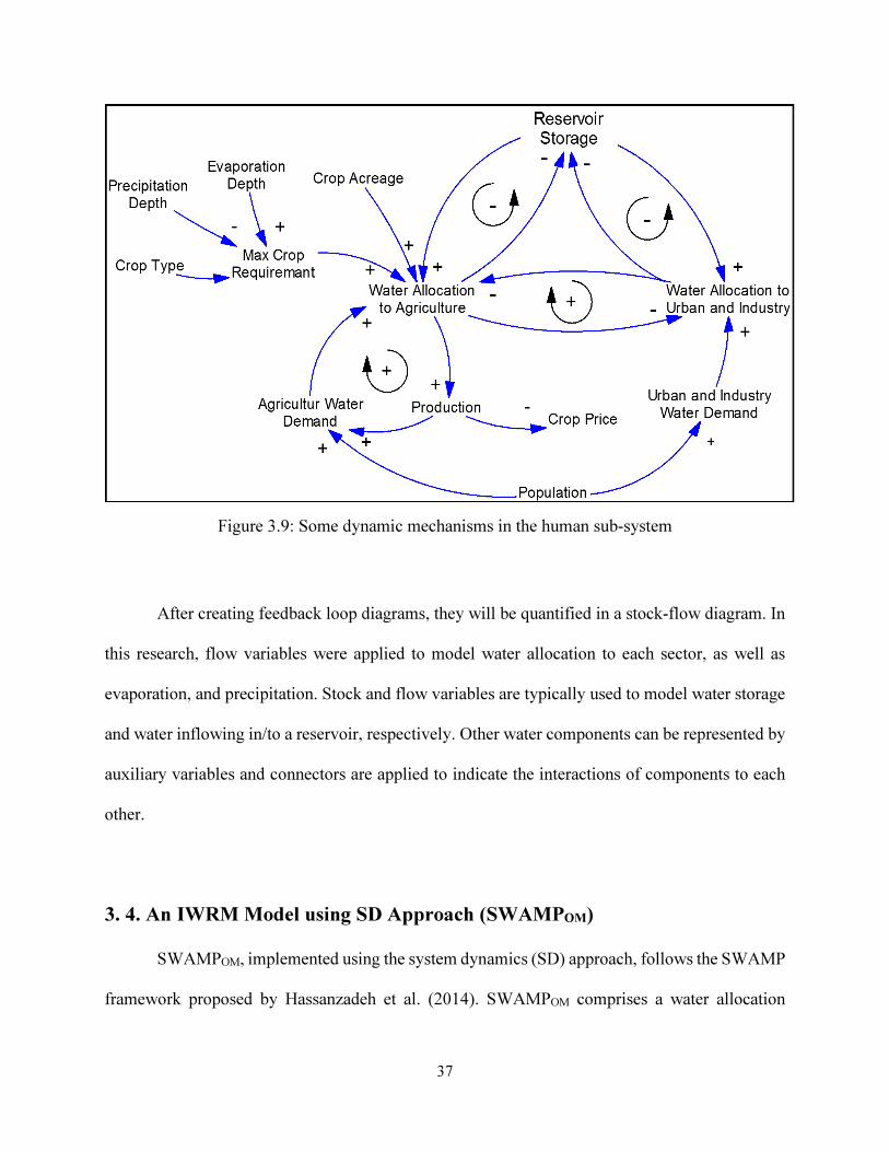
37

Figure 3.9: Some dynamic mechanisms in the human sub-system

After creating feedback loop diagrams, they will be quantified in a stock-flow diagram. In

this research, flow variables were applied to model water allocation to each sector, as well as

evaporation, and precipitation. Stock and flow variables are typically used to model water storage

and water inflowing in/to a reservoir, respectively. Other water components can be represented by

auxiliary variables and connectors are applied to indicate the interactions of components to each

other.

3. 4. An IWRM Model using SD Approach (SWAMPOM)

SWAMPOM, implemented using the system dynamics (SD) approach, follows the SWAMP

framework proposed by Hassanzadeh et al. (2014). SWAMPOM comprises a water allocation

38

model and economic evaluation, instream flow needs, and dynamic irrigation demand sub-models.

The water allocation model is an emulation of Water Resources Management Model (WRMM)

and the dynamic irrigation demand and economic evaluation sub-models are developed using the

same approach used in the SWAMPSK model (Hassanzadeh et al., 2014).

Input data (water demand and water supply) and operating policies (penalty zones) required

to make the water allocation model are derived from the WRMM input files. Like WRMM, each

water user receives the water based on its specific weekly demand; but, the penalty zones in

WRMM only specify the priority of the users to receive the water in the SWAMPOM’s water

allocation model. A user with a higher penalty obtains the water first. As mentioned in previous

sections, there is one important hydropower plant in the basin and it has the highest priority after

minor units. According to WRMM’s penalty values, some irrigation districts, most of which are

private, ranks as third in water allocation order, and afterwards instream flow need (IFN) receives

the water (Alberta Environment, 2010). To allocate water to users, it is assumed that each user gets

the water from the nearest river (in the case of tributaries) or river reach (in the case of main river

abstractions). If the nearest river reach cannot meet the entire demand, the next upstream reach is

responsible to provide the water. When all rivers, which can allocate the water to the user, do not

have enough water to satisfy the demand, the nearest reservoir releases the water to meet the rest

of the user’s demand. All water components and water supplies modeled in SWAMPOM are shown

in figure 3.3.

3. 4. 1. Water Allocation Model

In this section how water is allocated to each component in the OMRB’s water system will

be described in detail. As can be seen in figure 3.3 and 3.10, red fletchers indicate minor units to

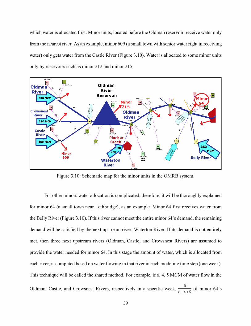
39

which water is allocated first. Minor units, located before the Oldman reservoir, receive water only

from the nearest river. As an example, minor 609 (a small town with senior water right in receiving

water) only gets water from the Castle River (Figure 3.10). Water is allocated to some minor units

only by reservoirs such as minor 212 and minor 215.

Figure 3.10: Schematic map for the minor units in the OMRB system.

For other minors water allocation is complicated, therefore, it will be thoroughly explained

for minor 64 (a small town near Lethbridge), as an example. Minor 64 first receives water from

the Belly River (Figure 3.10). If this river cannot meet the entire minor 64’s demand, the remaining

demand will be satisfied by the next upstream river, Waterton River. If its demand is not entirely

met, then three next upstream rivers (Oldman, Castle, and Crowsnest Rivers) are assumed to

provide the water needed for minor 64. In this stage the amount of water, which is allocated from

each river, is computed based on water flowing in that river in each modeling time step (one week).

This technique will be called the shared method. For example, if 6, 4, 5 MCM of water flow in the

Oldman, Castle, and Crowsnest Rivers, respectively in a specific week, �

�� of minor 64’s

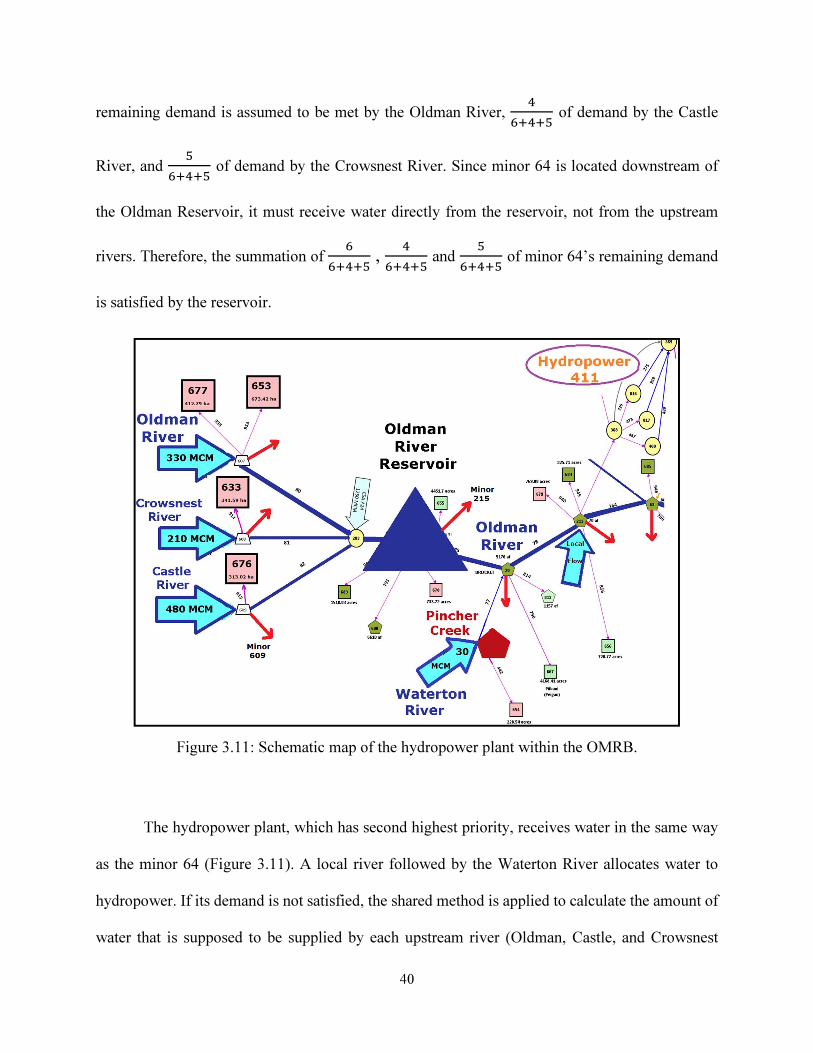
40

remaining demand is assumed to be met by the Oldman River, �

�� of demand by the Castle

River, and �

�� of demand by the Crowsnest River. Since minor 64 is located downstream of

the Oldman Reservoir, it must receive water directly from the reservoir, not from the upstream

rivers. Therefore, the summation of �

�� ,

�

�� and

�

�� of minor 64’s remaining demand

is satisfied by the reservoir.

Figure 3.11: Schematic map of the hydropower plant within the OMRB.

The hydropower plant, which has second highest priority, receives water in the same way

as the minor 64 (Figure 3.11). A local river followed by the Waterton River allocates water to

hydropower. If its demand is not satisfied, the shared method is applied to calculate the amount of

water that is supposed to be supplied by each upstream river (Oldman, Castle, and Crowsnest

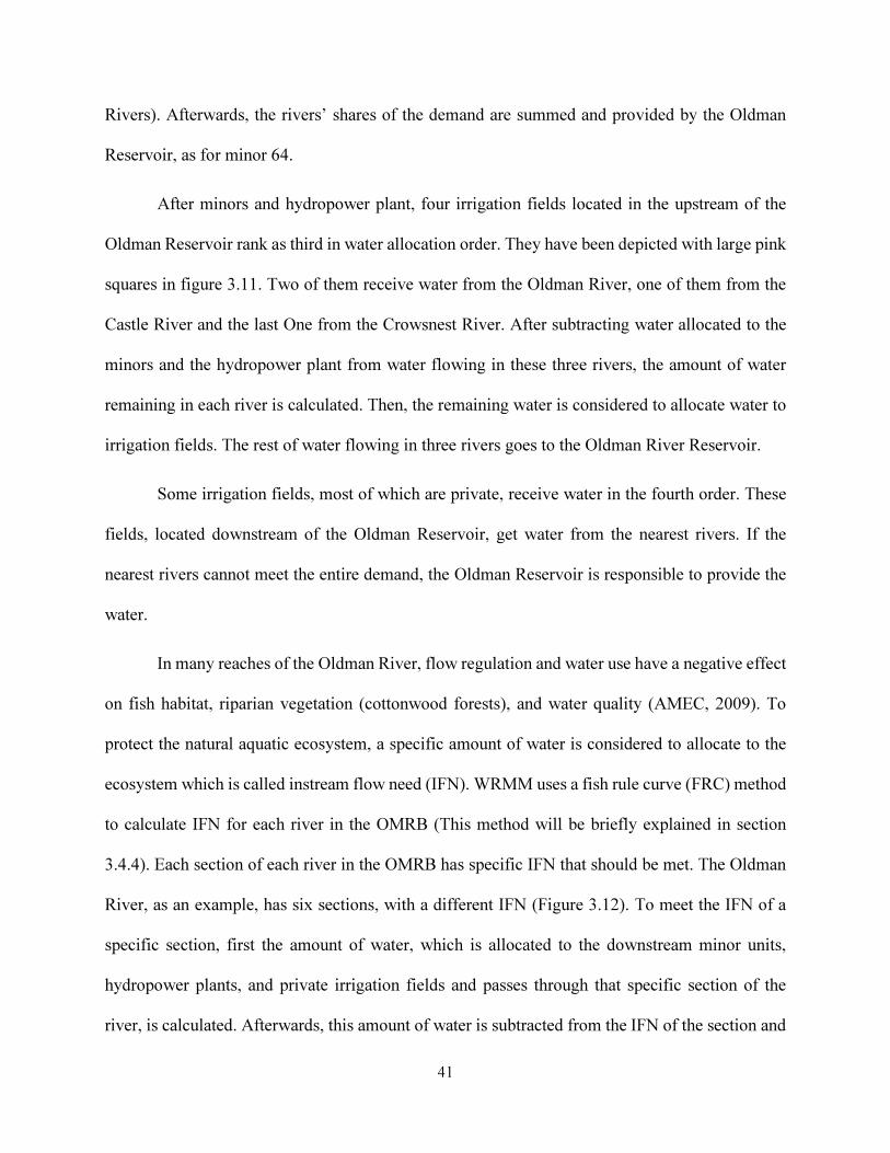
41

Rivers). Afterwards, the rivers’ shares of the demand are summed and provided by the Oldman

Reservoir, as for minor 64.

After minors and hydropower plant, four irrigation fields located in the upstream of the

Oldman Reservoir rank as third in water allocation order. They have been depicted with large pink

squares in figure 3.11. Two of them receive water from the Oldman River, one of them from the

Castle River and the last One from the Crowsnest River. After subtracting water allocated to the

minors and the hydropower plant from water flowing in these three rivers, the amount of water

remaining in each river is calculated. Then, the remaining water is considered to allocate water to

irrigation fields. The rest of water flowing in three rivers goes to the Oldman River Reservoir.

Some irrigation fields, most of which are private, receive water in the fourth order. These

fields, located downstream of the Oldman Reservoir, get water from the nearest rivers. If the

nearest rivers cannot meet the entire demand, the Oldman Reservoir is responsible to provide the

water.

In many reaches of the Oldman River, flow regulation and water use have a negative effect

on fish habitat, riparian vegetation (cottonwood forests), and water quality (AMEC, 2009). To

protect the natural aquatic ecosystem, a specific amount of water is considered to allocate to the

ecosystem which is called instream flow need (IFN). WRMM uses a fish rule curve (FRC) method

to calculate IFN for each river in the OMRB (This method will be briefly explained in section

3.4.4). Each section of each river in the OMRB has specific IFN that should be met. The Oldman

River, as an example, has six sections, with a different IFN (Figure 3.12). To meet the IFN of a

specific section, first the amount of water, which is allocated to the downstream minor units,

hydropower plants, and private irrigation fields and passes through that specific section of the

river, is calculated. Afterwards, this amount of water is subtracted from the IFN of the section and

42

the remaining IFN is computed. Like other mentioned water users, the remaining IFN is first

satisfied by the nearest rivers or river reaches, and then the Oldman River Reservoir provides the

water.

The last water users to receive the water are the rest of irrigation fields and major units.

These users follow the method applied to the private irrigation fields to meet their demand.

Figure 3.12: Different sections of the Oldman River

Reservoir Operation: To release the water from the reservoir, two penalty zones, indicating the

physical maximum and minimum storage zones have been considered. The reservoirs may have

additional penalty zones for active storage (Ilich, 1992). The penalty zones and the downstream

users’ water demand (which is not met by the downstream rivers) and the downstream users’

penalty control the amount of water released from the reservoir. To estimate the amount of water

stored in the reservoir, the mass balance equation is used (equation 3.2).

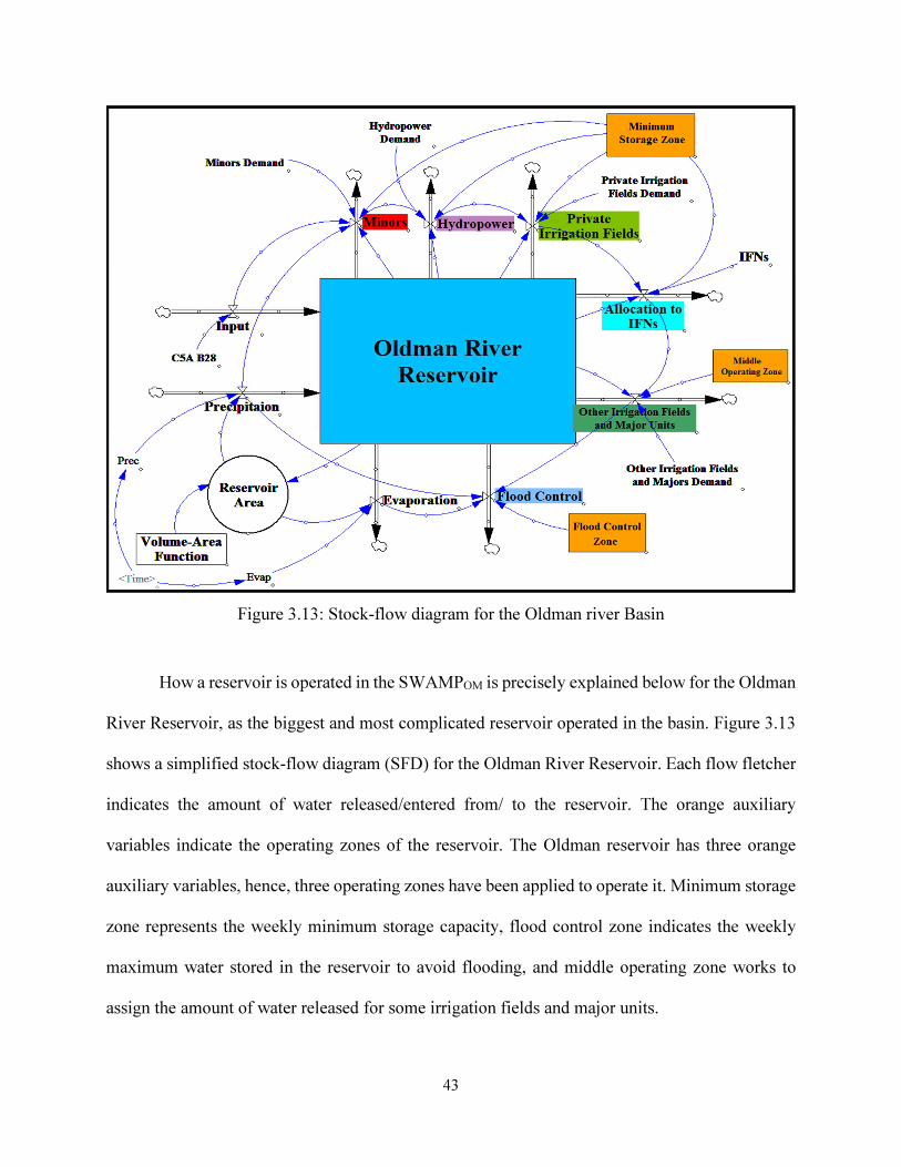
43

Figure 3.13: Stock-flow diagram for the Oldman river Basin

How a reservoir is operated in the SWAMPOM is precisely explained below for the Oldman

River Reservoir, as the biggest and most complicated reservoir operated in the basin. Figure 3.13

shows a simplified stock-flow diagram (SFD) for the Oldman River Reservoir. Each flow fletcher

indicates the amount of water released/entered from/ to the reservoir. The orange auxiliary

variables indicate the operating zones of the reservoir. The Oldman reservoir has three orange

auxiliary variables, hence, three operating zones have been applied to operate it. Minimum storage

zone represents the weekly minimum storage capacity, flood control zone indicates the weekly

maximum water stored in the reservoir to avoid flooding, and middle operating zone works to

assign the amount of water released for some irrigation fields and major units.

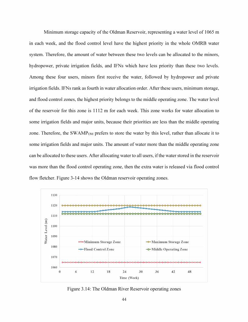
44

Minimum storage capacity of the Oldman Reservoir, representing a water level of 1065 m

in each week, and the flood control level have the highest priority in the whole OMRB water

system. Therefore, the amount of water between these two levels can be allocated to the minors,

hydropower, private irrigation fields, and IFNs which have less priority than these two levels.

Among these four users, minors first receive the water, followed by hydropower and private

irrigation fields. IFNs rank as fourth in water allocation order. After these users, minimum storage,

and flood control zones, the highest priority belongs to the middle operating zone. The water level

of the reservoir for this zone is 1112 m for each week. This zone works for water allocation to

some irrigation fields and major units, because their priorities are less than the middle operating

zone. Therefore, the SWAMPOM prefers to store the water by this level, rather than allocate it to

some irrigation fields and major units. The amount of water more than the middle operating zone

can be allocated to these users. After allocating water to all users, if the water stored in the reservoir

was more than the flood control operating zone, then the extra water is released via flood control

flow fletcher. Figure 3-14 shows the Oldman reservoir operating zones.

Figure 3.14: The Oldman River Reservoir operating zones

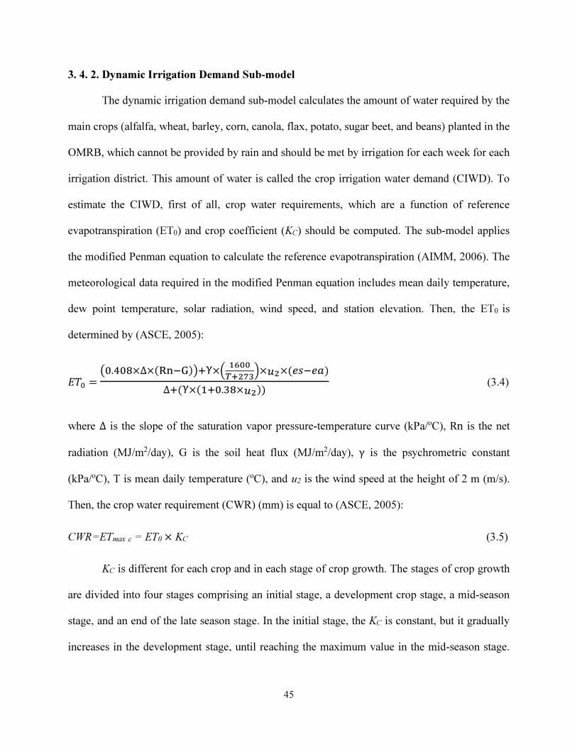
45

3. 4. 2. Dynamic Irrigation Demand Sub-model

The dynamic irrigation demand sub-model calculates the amount of water required by the

main crops (alfalfa, wheat, barley, corn, canola, flax, potato, sugar beet, and beans) planted in the

OMRB, which cannot be provided by rain and should be met by irrigation for each week for each

irrigation district. This amount of water is called the crop irrigation water demand (CIWD). To

estimate the CIWD, first of all, crop water requirements, which are a function of reference

evapotranspiration (ET0) and crop coefficient (KC) should be computed. The sub-model applies

the modified Penman equation to calculate the reference evapotranspiration (AIMM, 2006). The

meteorological data required in the modified Penman equation includes mean daily temperature,

dew point temperature, solar radiation, wind speed, and station elevation. Then, the ET0 is

determined by (ASCE, 2005):

�� = ��.��×∆×�� ×� ��

��×��×(��)∆�( ×��.��×��)

(3.4)

where ∆ is the slope of the saturation vapor pressure-temperature curve (kPa/oC), Rn is the net

radiation (MJ/m2/day), G is the soil heat flux (MJ/m2/day), γ is the psychrometric constant

(kPa/oC), T is mean daily temperature (oC), and u2 is the wind speed at the height of 2 m (m/s).

Then, the crop water requirement (CWR) (mm) is equal to (ASCE, 2005):

CWR=ETmax c = ET0× KC (3.5)

KC is different for each crop and in each stage of crop growth. The stages of crop growth

are divided into four stages comprising an initial stage, a development crop stage, a mid-season

stage, and an end of the late season stage. In the initial stage, the KC is constant, but it gradually

increases in the development stage, until reaching the maximum value in the mid-season stage.

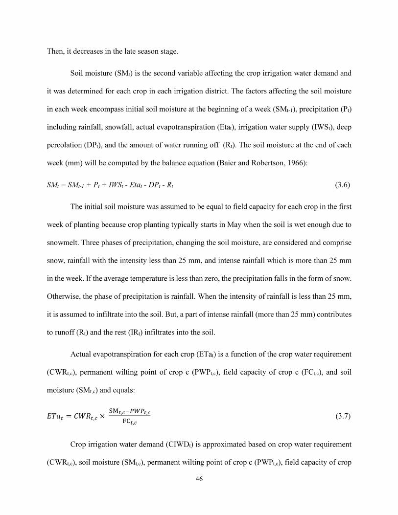
46

Then, it decreases in the late season stage.

Soil moisture (SMt) is the second variable affecting the crop irrigation water demand and

it was determined for each crop in each irrigation district. The factors affecting the soil moisture

in each week encompass initial soil moisture at the beginning of a week (SMt-1), precipitation (Pt)

including rainfall, snowfall, actual evapotranspiration (Etat), irrigation water supply (IWSt), deep

percolation (DPt), and the amount of water running off (Rt). The soil moisture at the end of each

week (mm) will be computed by the balance equation (Baier and Robertson, 1966):

SMt = SMt-1 + Pt + IWSt - Etat - DPt - Rt (3.6)

The initial soil moisture was assumed to be equal to field capacity for each crop in the first

week of planting because crop planting typically starts in May when the soil is wet enough due to

snowmelt. Three phases of precipitation, changing the soil moisture, are considered and comprise

snow, rainfall with the intensity less than 25 mm, and intense rainfall which is more than 25 mm

in the week. If the average temperature is less than zero, the precipitation falls in the form of snow.

Otherwise, the phase of precipitation is rainfall. When the intensity of rainfall is less than 25 mm,

it is assumed to infiltrate into the soil. But, a part of intense rainfall (more than 25 mm) contributes

to runoff (Rt) and the rest (IRt) infiltrates into the soil.

Actual evapotranspiration for each crop (ETat) is a function of the crop water requirement

(CWRt,c), permanent wilting point of crop c (PWPt,c), field capacity of crop c (FCt,c), and soil

moisture (SMt,c) and equals:

�� = ��,� × ��,��,�

��,�

(3.7)

Crop irrigation water demand (CIWDt) is approximated based on crop water requirement

(CWRt,c), soil moisture (SMt,c), permanent wilting point of crop c (PWPt,c), field capacity of crop

47

c (FCt,c), as well as irrigation efficiency of each irrigation district (IEid). The dynamic irrigation

demand sub-model tries to keep soil moisture between permanent wilting point and field capacity

in the root depth of the crop, while meeting the crop water requirement in each week. Therefore,

CIWDt is equal to (AIMM, 2006):

�� = �� ,��,��(��,��,�)/�

��

(3.8)

The equations applied to calculate ∆, Rn, u2, γ, Rt, and IRt, are explained in Appendix A.

3. 4. 3. Instream Flow Needs Sub-Model

So far, instream flow needs (IFN) for the Oldman River Basin have been calculated using

a fish rule curve (FRC) method, which meets the local minimum flow requirement for fish habitat

(AMEC, 2009). The FRC method calculates IFN based on the weighted usable area (WUA) of the

river as a function of the discharge (WUA curve) and the available natural supply of water. The

wetted usable area of a river is defined based on its suitability for use by aquatic organisms

(Clipperton et al., 2003). In this method IFN changes depending not only on the WUA curve, but

also on the hydrologic conditions (wet, dry, average) during a specific period (Clipperton et al.,

2003). WRMM applies the IFN determined by FRC method. In WRMM different sections have

been defined for each river and each section has a specific IFN. In the first stage of modeling, these

data were used as the instream flow needs in SWAMPOM.

Recently, Alberta Environment has been using a new method, the Alberta Desktop Method

(ADM), which requires weekly/monthly naturalized hydrological data, to determine the

environmental flows (Locke and Paul, 2011). This has been applied in this thesis. In this method,

first an ecosystem base flow (EBF) component is calculated, so that a percent exceedance natural

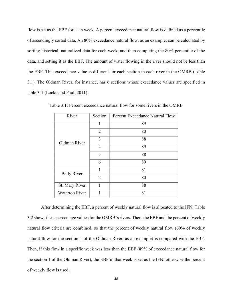
48

flow is set as the EBF for each week. A percent exceedance natural flow is defined as a percentile

of ascendingly sorted data. An 80% exceedance natural flow, as an example, can be calculated by

sorting historical, naturalized data for each week, and then computing the 80% percentile of the

data, and setting it as the EBF. The amount of water flowing in the river should not be less than

the EBF. This exceedance value is different for each section in each river in the OMRB (Table

3.1). The Oldman River, for instance, has 6 sections whose exceedance values are specified in

table 3-1 (Locke and Paul, 2011).

Table 3.1: Percent exceedance natural flow for some rivers in the OMRB

After determining the EBF, a percent of weekly natural flow is allocated to the IFN. Table

3.2 shows these percentage values for the OMRB’s rivers. Then, the EBF and the percent of weekly

natural flow criteria are combined, so that the percent of weekly natural flow (60% of weekly

natural flow for the section 1 of the Oldman River, as an example) is compared with the EBF.

Then, if this flow in a specific week was less than the EBF (89% of exceedance natural flow for

the section 1 of the Oldman River), the EBF in that week is set as the IFN; otherwise the percent

of weekly flow is used.

River Section Percent Exceedance Natural Flow

Oldman River

1 89

2 80

3 88

4 89

5 88

6 89

Belly River 1 81

2 80

St. Mary River 1 88

Waterton River 1 81

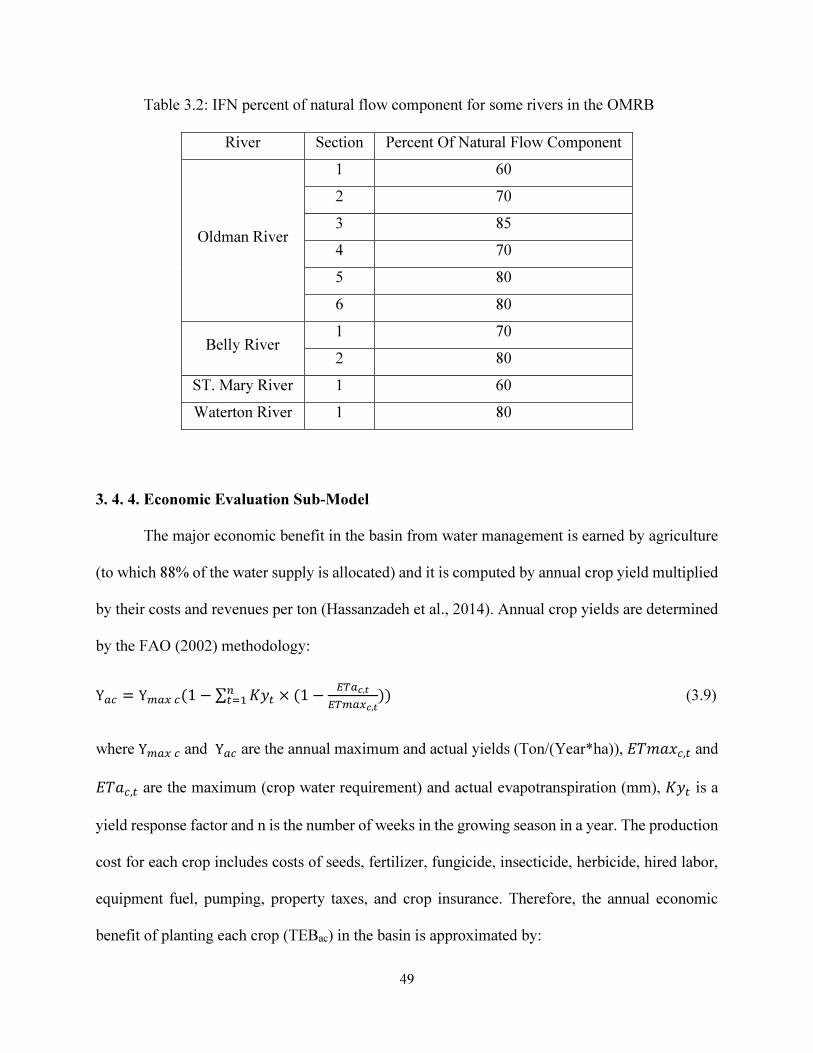
49

Table 3.2: IFN percent of natural flow component for some rivers in the OMRB

3. 4. 4. Economic Evaluation Sub-Model

The major economic benefit in the basin from water management is earned by agriculture

(to which 88% of the water supply is allocated) and it is computed by annual crop yield multiplied

by their costs and revenues per ton (Hassanzadeh et al., 2014). Annual crop yields are determined

by the FAO (2002) methodology:

Y�� = Y��(1 − ∑ �� × (1 −��,�

��,�))

�� (3.9)

where Y�� and Y�� are the annual maximum and actual yields (Ton/(Year*ha)), �� ,� and

�� ,� are the maximum (crop water requirement) and actual evapotranspiration (mm), �� is a

yield response factor and n is the number of weeks in the growing season in a year. The production

cost for each crop includes costs of seeds, fertilizer, fungicide, insecticide, herbicide, hired labor,

equipment fuel, pumping, property taxes, and crop insurance. Therefore, the annual economic

benefit of planting each crop (TEBac) in the basin is approximated by:

River Section Percent Of Natural Flow Component

Oldman River

1 60

2 70

3 85

4 70

5 80

6 80

Belly River 1 70

2 80

ST. Mary River 1 60

Waterton River 1 80

50

�� = (!�� × ��"�� (ℎ ) × ��" �#��$$ ��⁄ &) −(��"��'��(�$$ (ℎ ∗ !� �)⁄ & × ��"�� (ℎ )) (3.10)

The total irrigation area in the OMRB is about 123,420 ha. SWAMPOM uses the crop

market prices and production costs in 2006 to calculate agricultural economic benefit from 1928

to 2001. The second source of water-based economic benefit in the OMRB is hydropower. Annual

hydropower Generation (MWh) multiplied by revenue and cost results in economic benefit from

this sector. Annual hydropower generation (MWh) (P) can be calculated by

� = �×(��)×��×��×�.��

�� (3.11)

where Q is flow in hydropower channel (m3/s), H is the average head available for power

generation (m), HL is the head loss at the rated head and flow (m), 9.907 is a coefficient of

changing units to metric, and TE and GE are turbine and generator efficiencies. Multiplication of

generated hydropower (P) (MWh) by revenues results in economic benefit for this sector

($/MWh). Since there was no access to the market price of hydropower generation for the Oldman

plant, the market price for the power generation in the Lake Diefenbaker Reservoir in 2010 is

applied in this sub-model.

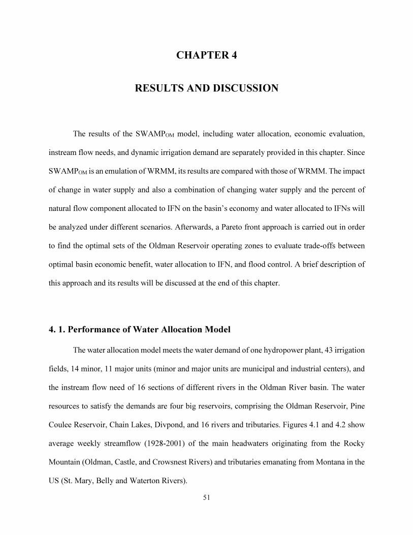
51

CHAPTER 4

RESULTS AND DISCUSSION

The results of the SWAMPOM model, including water allocation, economic evaluation,

instream flow needs, and dynamic irrigation demand are separately provided in this chapter. Since

SWAMPOM is an emulation of WRMM, its results are compared with those of WRMM. The impact

of change in water supply and also a combination of changing water supply and the percent of

natural flow component allocated to IFN on the basin’s economy and water allocated to IFNs will

be analyzed under different scenarios. Afterwards, a Pareto front approach is carried out in order

to find the optimal sets of the Oldman Reservoir operating zones to evaluate trade-offs between

optimal basin economic benefit, water allocation to IFN, and flood control. A brief description of

this approach and its results will be discussed at the end of this chapter.

4. 1. Performance of Water Allocation Model

The water allocation model meets the water demand of one hydropower plant, 43 irrigation

fields, 14 minor, 11 major units (minor and major units are municipal and industrial centers), and

the instream flow need of 16 sections of different rivers in the Oldman River basin. The water

resources to satisfy the demands are four big reservoirs, comprising the Oldman Reservoir, Pine

Coulee Reservoir, Chain Lakes, Divpond, and 16 rivers and tributaries. Figures 4.1 and 4.2 show

average weekly streamflow (1928-2001) of the main headwaters originating from the Rocky

Mountain (Oldman, Castle, and Crowsnest Rivers) and tributaries emanating from Montana in the

US (St. Mary, Belly and Waterton Rivers).

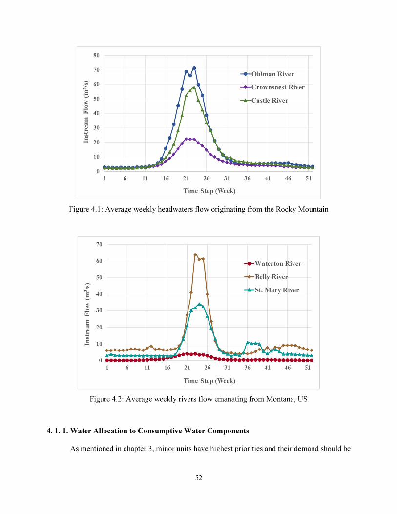
52

Figure 4.1: Average weekly headwaters flow originating from the Rocky Mountain

Figure 4.2: Average weekly rivers flow emanating from Montana, US

4. 1. 1. Water Allocation to Consumptive Water Components

As mentioned in chapter 3, minor units have highest priorities and their demand should be

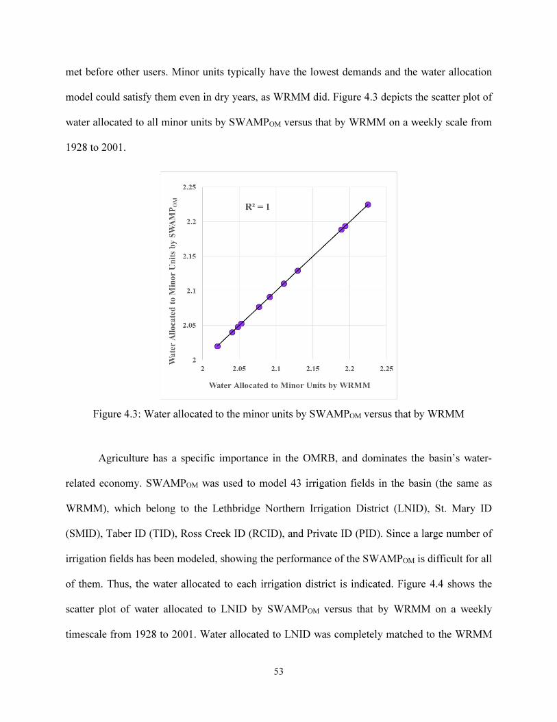
53

met before other users. Minor units typically have the lowest demands and the water allocation

model could satisfy them even in dry years, as WRMM did. Figure 4.3 depicts the scatter plot of

water allocated to all minor units by SWAMPOM versus that by WRMM on a weekly scale from

1928 to 2001.

Figure 4.3: Water allocated to the minor units by SWAMPOM versus that by WRMM

Agriculture has a specific importance in the OMRB, and dominates the basin’s water-

related economy. SWAMPOM was used to model 43 irrigation fields in the basin (the same as

WRMM), which belong to the Lethbridge Northern Irrigation District (LNID), St. Mary ID

(SMID), Taber ID (TID), Ross Creek ID (RCID), and Private ID (PID). Since a large number of

irrigation fields has been modeled, showing the performance of the SWAMPOM is difficult for all

of them. Thus, the water allocated to each irrigation district is indicated. Figure 4.4 shows the

scatter plot of water allocated to LNID by SWAMPOM versus that by WRMM on a weekly

timescale from 1928 to 2001. Water allocated to LNID was completely matched to the WRMM

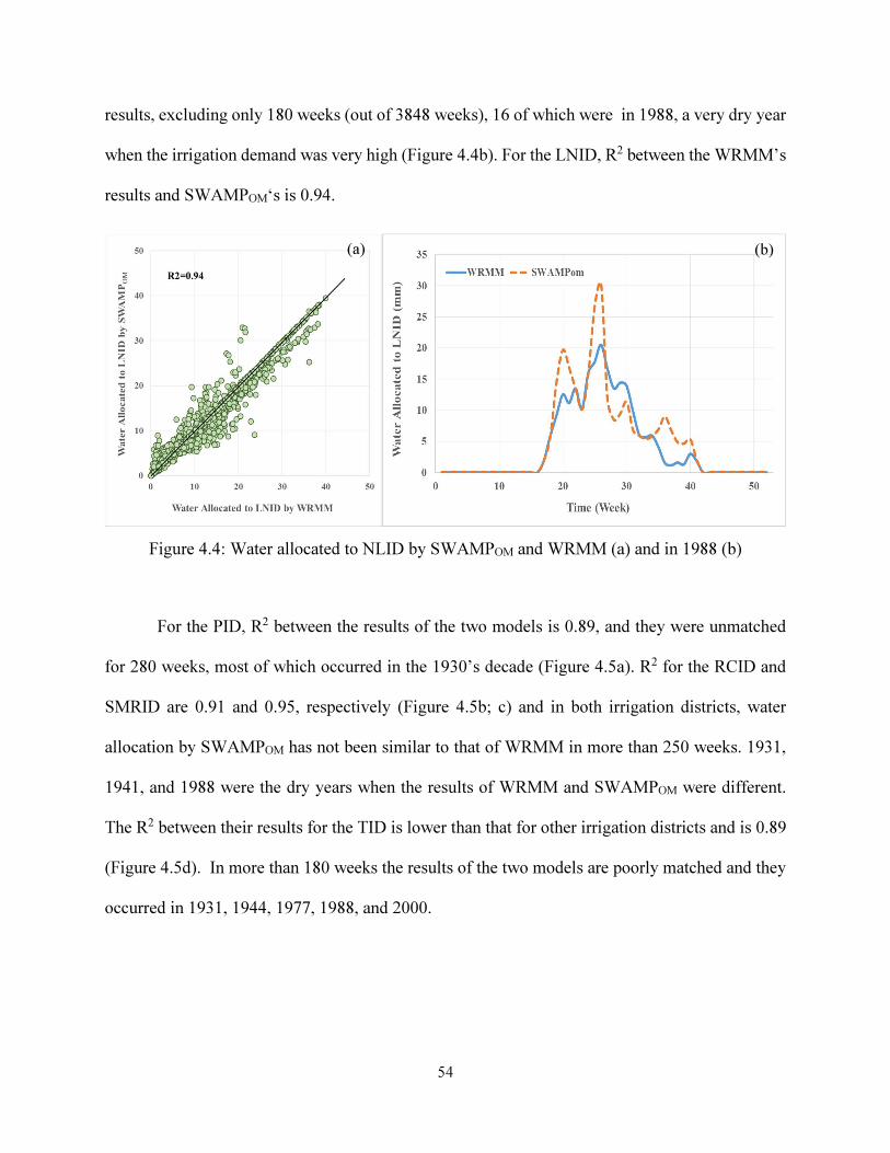
54

results, excluding only 180 weeks (out of 3848 weeks), 16 of which were in 1988, a very dry year

when the irrigation demand was very high (Figure 4.4b). For the LNID, R2 between the WRMM’s

results and SWAMPOM‘s is 0.94.

Figure 4.4: Water allocated to NLID by SWAMPOM and WRMM (a) and in 1988 (b)

For the PID, R2 between the results of the two models is 0.89, and they were unmatched

for 280 weeks, most of which occurred in the 1930’s decade (Figure 4.5a). R2 for the RCID and

SMRID are 0.91 and 0.95, respectively (Figure 4.5b; c) and in both irrigation districts, water

allocation by SWAMPOM has not been similar to that of WRMM in more than 250 weeks. 1931,

1941, and 1988 were the dry years when the results of WRMM and SWAMPOM were different.

The R2 between their results for the TID is lower than that for other irrigation districts and is 0.89

(Figure 4.5d). In more than 180 weeks the results of the two models are poorly matched and they

occurred in 1931, 1944, 1977, 1988, and 2000.

(a) (b)

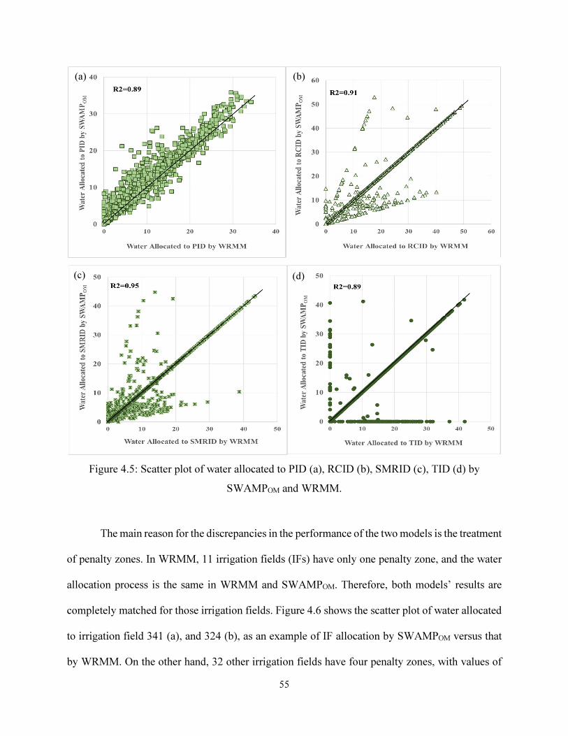
55

Figure 4.5: Scatter plot of water allocated to PID (a), RCID (b), SMRID (c), TID (d) by

SWAMPOM and WRMM.

The main reason for the discrepancies in the performance of the two models is the treatment

of penalty zones. In WRMM, 11 irrigation fields (IFs) have only one penalty zone, and the water

allocation process is the same in WRMM and SWAMPOM. Therefore, both models’ results are

completely matched for those irrigation fields. Figure 4.6 shows the scatter plot of water allocated

to irrigation field 341 (a), and 324 (b), as an example of IF allocation by SWAMPOM versus that

by WRMM. On the other hand, 32 other irrigation fields have four penalty zones, with values of

(a) (b)

(c) (d)

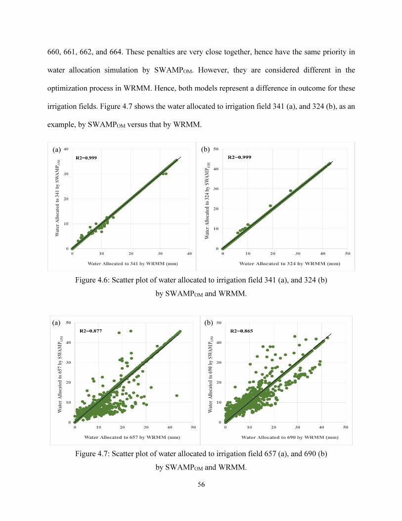
56

660, 661, 662, and 664. These penalties are very close together, hence have the same priority in

water allocation simulation by SWAMPOM. However, they are considered different in the

optimization process in WRMM. Hence, both models represent a difference in outcome for these

irrigation fields. Figure 4.7 shows the water allocated to irrigation field 341 (a), and 324 (b), as an

example, by SWAMPOM versus that by WRMM.

Figure 4.6: Scatter plot of water allocated to irrigation field 341 (a), and 324 (b)

by SWAMPOM and WRMM.

Figure 4.7: Scatter plot of water allocated to irrigation field 657 (a), and 690 (b)

by SWAMPOM and WRMM.

(a) (b)

(a) (b)

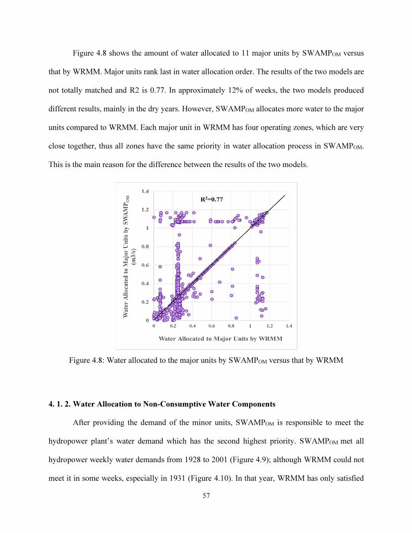
57

Figure 4.8 shows the amount of water allocated to 11 major units by SWAMPOM versus

that by WRMM. Major units rank last in water allocation order. The results of the two models are

not totally matched and R2 is 0.77. In approximately 12% of weeks, the two models produced

different results, mainly in the dry years. However, SWAMPOM allocates more water to the major

units compared to WRMM. Each major unit in WRMM has four operating zones, which are very

close together, thus all zones have the same priority in water allocation process in SWAMPOM.

This is the main reason for the difference between the results of the two models.

Figure 4.8: Water allocated to the major units by SWAMPOM versus that by WRMM

4. 1. 2. Water Allocation to Non-Consumptive Water Components

After providing the demand of the minor units, SWAMPOM is responsible to meet the

hydropower plant’s water demand which has the second highest priority. SWAMPOM met all

hydropower weekly water demands from 1928 to 2001 (Figure 4.9); although WRMM could not

meet it in some weeks, especially in 1931 (Figure 4.10). In that year, WRMM has only satisfied

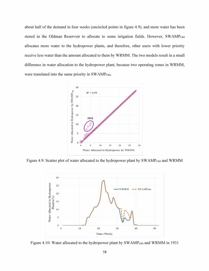
58

about half of the demand in four weeks (encircled points in figure 4.9), and more water has been

stored in the Oldman Reservoir to allocate to some irrigation fields. However, SWAMPOM

allocates more water to the hydropower plants, and therefore, other users with lower priority

receive less water than the amount allocated to them by WRMM. The two models result in a small

difference in water allocation to the hydropower plant, because two operating zones in WRMM,

were translated into the same priority in SWAMPOM.

Figure 4.9: Scatter plot of water allocated to the hydropower plant by SWAMPOM and WRMM

Figure 4.10: Water allocated to the hydropower plant by SWAMPOM and WRMM in 1931

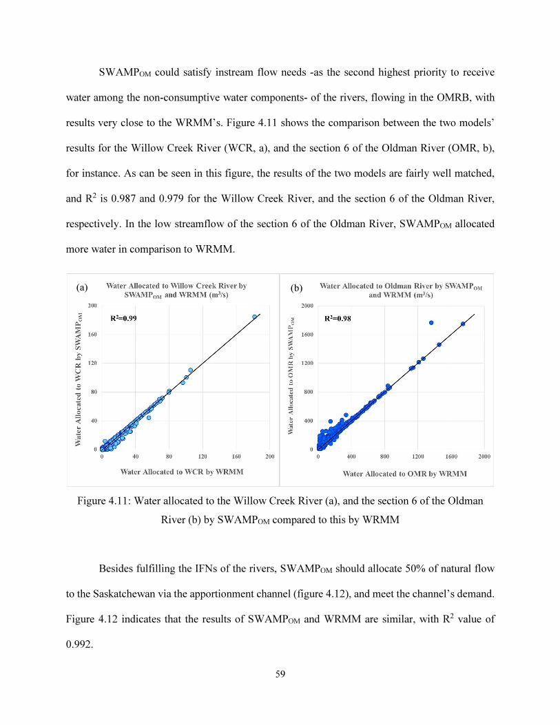
59

SWAMPOM could satisfy instream flow needs -as the second highest priority to receive

water among the non-consumptive water components- of the rivers, flowing in the OMRB, with

results very close to the WRMM’s. Figure 4.11 shows the comparison between the two models’

results for the Willow Creek River (WCR, a), and the section 6 of the Oldman River (OMR, b),

for instance. As can be seen in this figure, the results of the two models are fairly well matched,

and R2 is 0.987 and 0.979 for the Willow Creek River, and the section 6 of the Oldman River,

respectively. In the low streamflow of the section 6 of the Oldman River, SWAMPOM allocated

more water in comparison to WRMM.

Figure 4.11: Water allocated to the Willow Creek River (a), and the section 6 of the Oldman

River (b) by SWAMPOM compared to this by WRMM

Besides fulfilling the IFNs of the rivers, SWAMPOM should allocate 50% of natural flow

to the Saskatchewan via the apportionment channel (figure 4.12), and meet the channel’s demand.

Figure 4.12 indicates that the results of SWAMPOM and WRMM are similar, with R2 value of

0.992.

(a) (b)

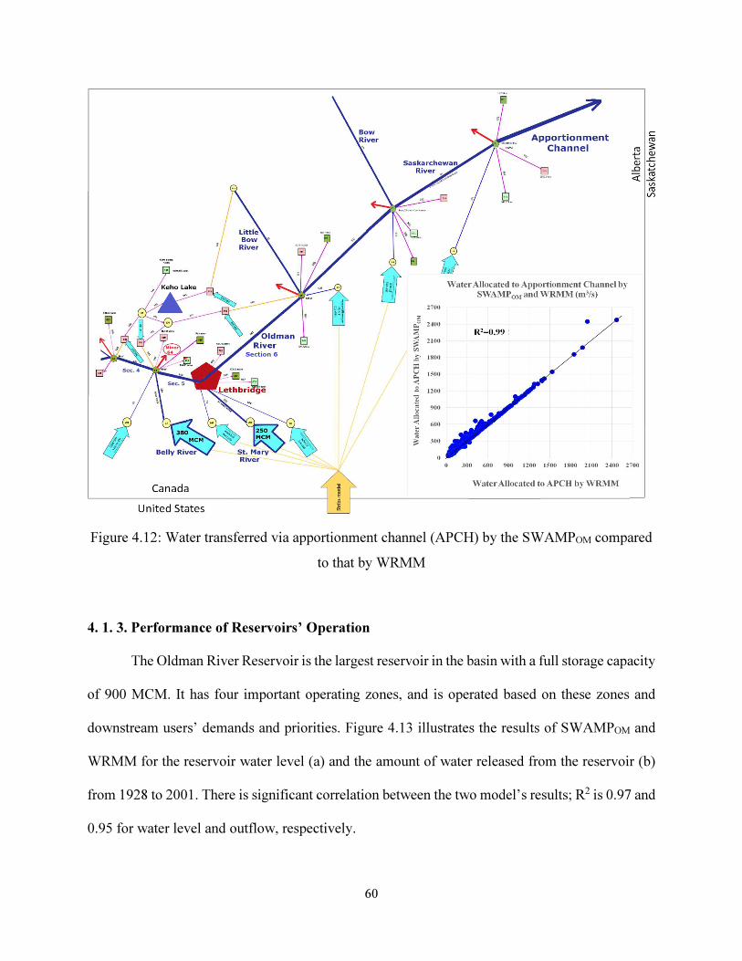
60

Figure 4.12: Water transferred via apportionment channel (APCH) by the SWAMPOM compared

to that by WRMM

4. 1. 3. Performance of Reservoirs’ Operation

The Oldman River Reservoir is the largest reservoir in the basin with a full storage capacity

of 900 MCM. It has four important operating zones, and is operated based on these zones and

downstream users’ demands and priorities. Figure 4.13 illustrates the results of SWAMPOM and

WRMM for the reservoir water level (a) and the amount of water released from the reservoir (b)

from 1928 to 2001. There is significant correlation between the two model’s results; R2 is 0.97 and

0.95 for water level and outflow, respectively.

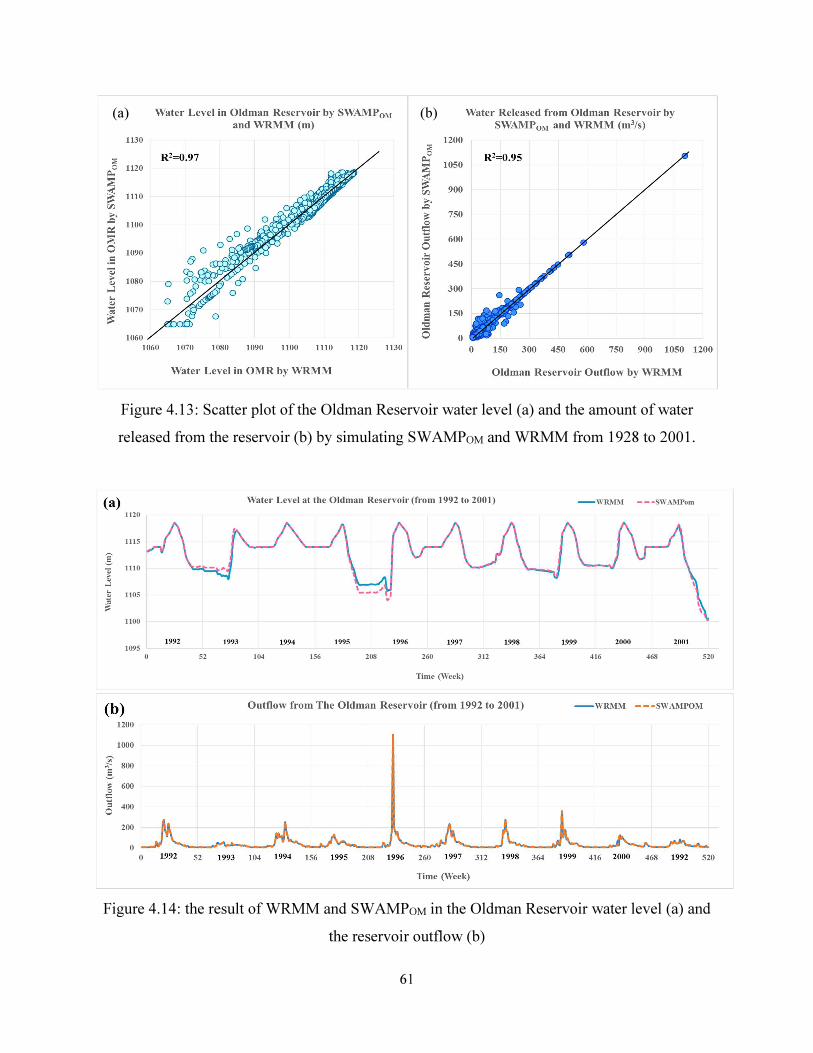
61

Figure 4.13: Scatter plot of the Oldman Reservoir water level (a) and the amount of water

released from the reservoir (b) by simulating SWAMPOM and WRMM from 1928 to 2001.

Figure 4.14: the result of WRMM and SWAMPOM in the Oldman Reservoir water level (a) and

the reservoir outflow (b)

(a) (b)

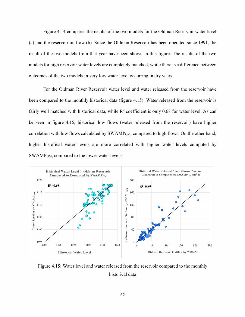
62

Figure 4.14 compares the results of the two models for the Oldman Reservoir water level

(a) and the reservoir outflow (b). Since the Oldman Reservoir has been operated since 1991, the

result of the two models from that year have been shown in this figure. The results of the two

models for high reservoir water levels are completely matched, while there is a difference between

outcomes of the two models in very low water level occurring in dry years.

For the Oldman River Reservoir water level and water released from the reservoir have

been compared to the monthly historical data (figure 4.15). Water released from the reservoir is

fairly well matched with historical data, while R2 coefficient is only 0.68 for water level. As can

be seen in figure 4.15, historical low flows (water released from the reservoir) have higher

correlation with low flows calculated by SWAMPOM, compared to high flows. On the other hand,

higher historical water levels are more correlated with higher water levels computed by

SWAMPOM, compared to the lower water levels.

Figure 4.15: Water level and water released from the reservoir compared to the monthly

historical data

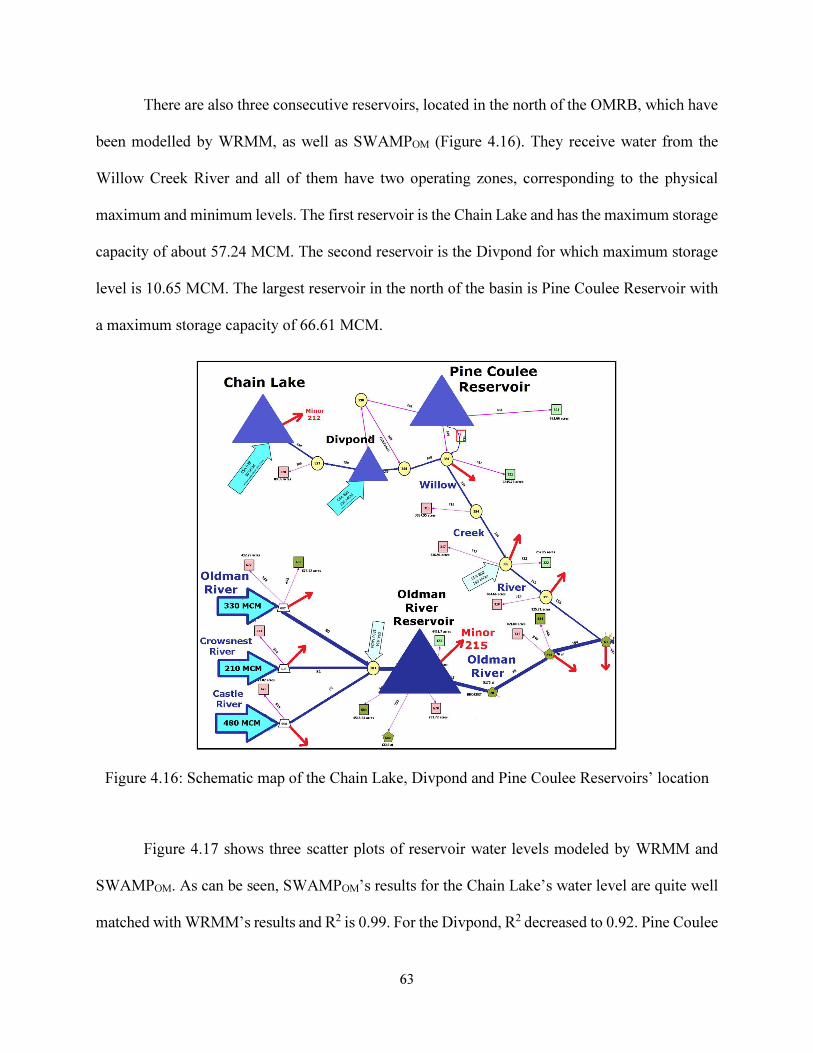
63

There are also three consecutive reservoirs, located in the north of the OMRB, which have

been modelled by WRMM, as well as SWAMPOM (Figure 4.16). They receive water from the

Willow Creek River and all of them have two operating zones, corresponding to the physical

maximum and minimum levels. The first reservoir is the Chain Lake and has the maximum storage

capacity of about 57.24 MCM. The second reservoir is the Divpond for which maximum storage

level is 10.65 MCM. The largest reservoir in the north of the basin is Pine Coulee Reservoir with

a maximum storage capacity of 66.61 MCM.

Figure 4.16: Schematic map of the Chain Lake, Divpond and Pine Coulee Reservoirs’ location

Figure 4.17 shows three scatter plots of reservoir water levels modeled by WRMM and

SWAMPOM. As can be seen, SWAMPOM’s results for the Chain Lake’s water level are quite well

matched with WRMM’s results and R2 is 0.99. For the Divpond, R2 decreased to 0.92. Pine Coulee

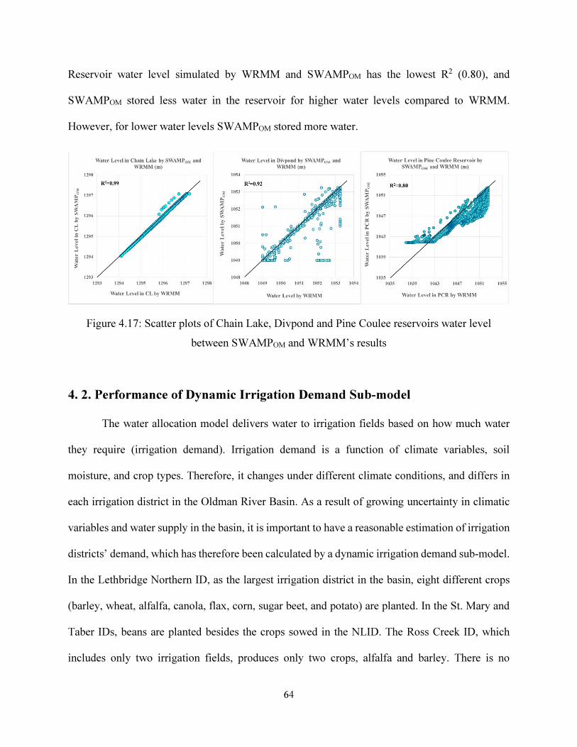
64

Reservoir water level simulated by WRMM and SWAMPOM has the lowest R2 (0.80), and

SWAMPOM stored less water in the reservoir for higher water levels compared to WRMM.

However, for lower water levels SWAMPOM stored more water.

Figure 4.17: Scatter plots of Chain Lake, Divpond and Pine Coulee reservoirs water level

between SWAMPOM and WRMM’s results

4. 2. Performance of Dynamic Irrigation Demand Sub-model

The water allocation model delivers water to irrigation fields based on how much water

they require (irrigation demand). Irrigation demand is a function of climate variables, soil

moisture, and crop types. Therefore, it changes under different climate conditions, and differs in

each irrigation district in the Oldman River Basin. As a result of growing uncertainty in climatic

variables and water supply in the basin, it is important to have a reasonable estimation of irrigation

districts’ demand, which has therefore been calculated by a dynamic irrigation demand sub-model.

In the Lethbridge Northern ID, as the largest irrigation district in the basin, eight different crops

(barley, wheat, alfalfa, canola, flax, corn, sugar beet, and potato) are planted. In the St. Mary and

Taber IDs, beans are planted besides the crops sowed in the NLID. The Ross Creek ID, which

includes only two irrigation fields, produces only two crops, alfalfa and barley. There is no

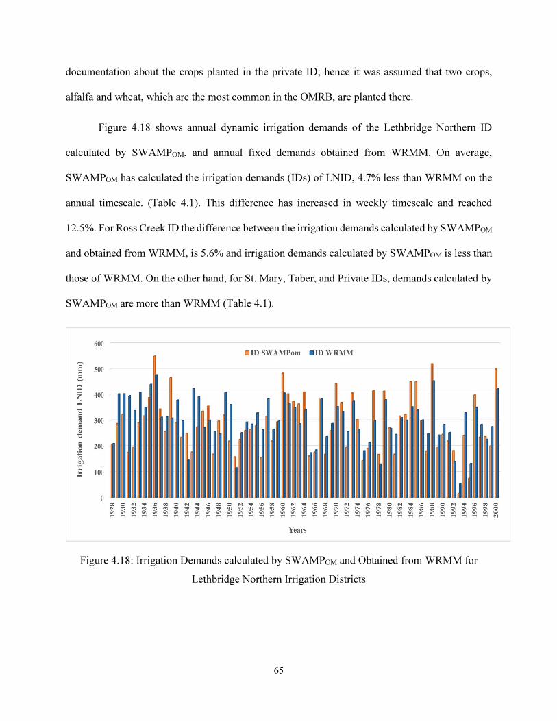
65

documentation about the crops planted in the private ID; hence it was assumed that two crops,

alfalfa and wheat, which are the most common in the OMRB, are planted there.

Figure 4.18 shows annual dynamic irrigation demands of the Lethbridge Northern ID

calculated by SWAMPOM, and annual fixed demands obtained from WRMM. On average,

SWAMPOM has calculated the irrigation demands (IDs) of LNID, 4.7% less than WRMM on the

annual timescale. (Table 4.1). This difference has increased in weekly timescale and reached

12.5%. For Ross Creek ID the difference between the irrigation demands calculated by SWAMPOM

and obtained from WRMM, is 5.6% and irrigation demands calculated by SWAMPOM is less than

those of WRMM. On the other hand, for St. Mary, Taber, and Private IDs, demands calculated by

SWAMPOM are more than WRMM (Table 4.1).

Figure 4.18: Irrigation Demands calculated by SWAMPOM and Obtained from WRMM for

Lethbridge Northern Irrigation Districts

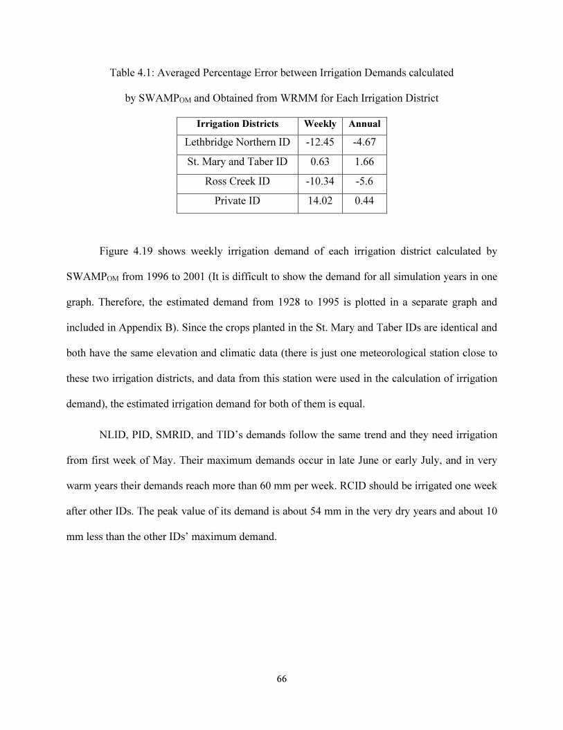
66

Table 4.1: Averaged Percentage Error between Irrigation Demands calculated

by SWAMPOM and Obtained from WRMM for Each Irrigation District

Irrigation Districts Weekly Annual

Lethbridge Northern ID -12.45 -4.67

St. Mary and Taber ID 0.63 1.66

Ross Creek ID -10.34 -5.6

Private ID 14.02 0.44

Figure 4.19 shows weekly irrigation demand of each irrigation district calculated by

SWAMPOM from 1996 to 2001 (It is difficult to show the demand for all simulation years in one

graph. Therefore, the estimated demand from 1928 to 1995 is plotted in a separate graph and

included in Appendix B). Since the crops planted in the St. Mary and Taber IDs are identical and

both have the same elevation and climatic data (there is just one meteorological station close to

these two irrigation districts, and data from this station were used in the calculation of irrigation

demand), the estimated irrigation demand for both of them is equal.

NLID, PID, SMRID, and TID’s demands follow the same trend and they need irrigation

from first week of May. Their maximum demands occur in late June or early July, and in very

warm years their demands reach more than 60 mm per week. RCID should be irrigated one week

after other IDs. The peak value of its demand is about 54 mm in the very dry years and about 10

mm less than the other IDs’ maximum demand.

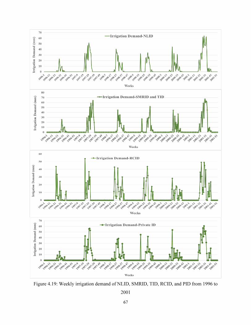
67

Figure 4.19: Weekly irrigation demand of NLID, SMRID, TID, RCID, and PID from 1996 to

2001

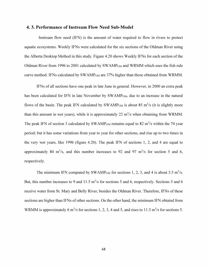
68

4. 3. Performance of Instream Flow Need Sub-Model

Instream flow need (IFN) is the amount of water required to flow in rivers to protect

aquatic ecosystems. Weekly IFNs were calculated for the six sections of the Oldman River using

the Alberta Desktop Method in this study. Figure 4.20 shows Weekly IFNs for each section of the

Oldman River from 1996 to 2001 calculated by SWAMPOM and WRMM which uses the fish rule

curve method. IFNs calculated by SWAMPOM are 37% higher than those obtained from WRMM.

IFNs of all sections have one peak in late June in general. However, in 2000 an extra peak

has been calculated for IFN in late November by SWAMPOM, due to an increase in the natural

flows of the basin. The peak IFN calculated by SWAMPOM is about 85 m3/s (it is slightly more

than this amount in wet years), while it is approximately 22 m3/s when obtaining from WRMM.

The peak IFN of section 3 calculated by SWAMPOM remains equal to 82 m3/s within the 74 year

period; but it has some variations from year to year for other sections, and rise up to two times in

the very wet years, like 1996 (figure 4.20). The peak IFN of sections 1, 2, and 4 are equal to

approximately 84 m3/s, and this number increases to 92 and 97 m3/s for section 5 and 6,

respectively.

The minimum IFN computed by SWAMPOM for sections 1, 2, 3, and 4 is about 5.5 m3/s.

But, this number increases to 9 and 11.5 m3/s for sections 5 and 6, respectively. Sections 5 and 6

receive water from St. Mary and Belly River, besides the Oldman River. Therefore, IFNs of these

sections are higher than IFNs of other sections. On the other hand, the minimum IFN obtaind from

WRMM is approximately 6 m3/s for sections 1, 2, 3, 4 and 5, and rises to 11.5 m3/s for sections 5.

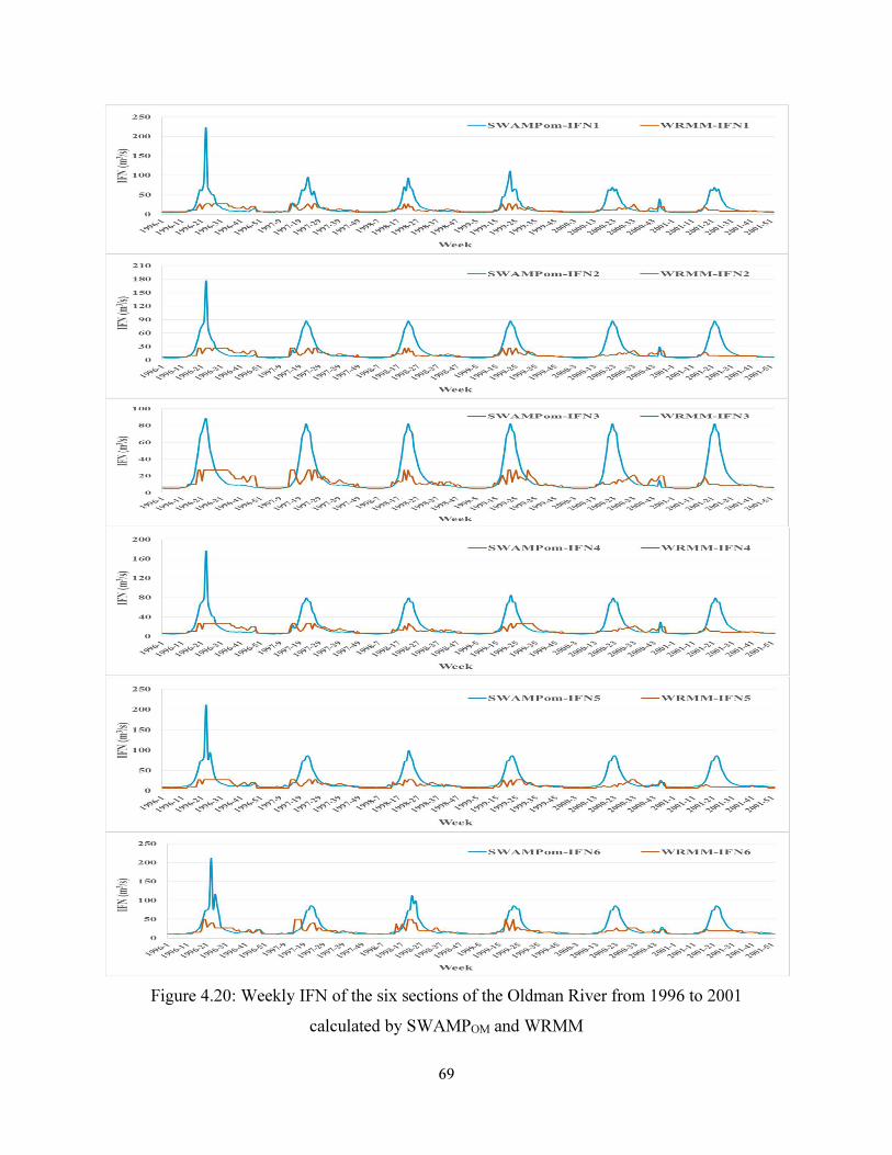
69

Figure 4.20: Weekly IFN of the six sections of the Oldman River from 1996 to 2001

calculated by SWAMPOM and WRMM

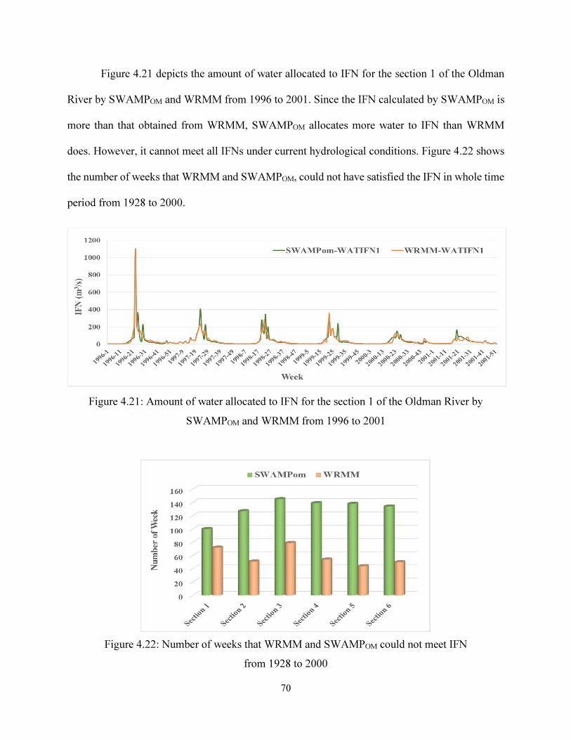
70

Figure 4.21 depicts the amount of water allocated to IFN for the section 1 of the Oldman

River by SWAMPOM and WRMM from 1996 to 2001. Since the IFN calculated by SWAMPOM is

more than that obtained from WRMM, SWAMPOM allocates more water to IFN than WRMM

does. However, it cannot meet all IFNs under current hydrological conditions. Figure 4.22 shows

the number of weeks that WRMM and SWAMPOM, could not have satisfied the IFN in whole time

period from 1928 to 2000.

Figure 4.21: Amount of water allocated to IFN for the section 1 of the Oldman River by

SWAMPOM and WRMM from 1996 to 2001

Figure 4.22: Number of weeks that WRMM and SWAMPOM could not meet IFN

from 1928 to 2000

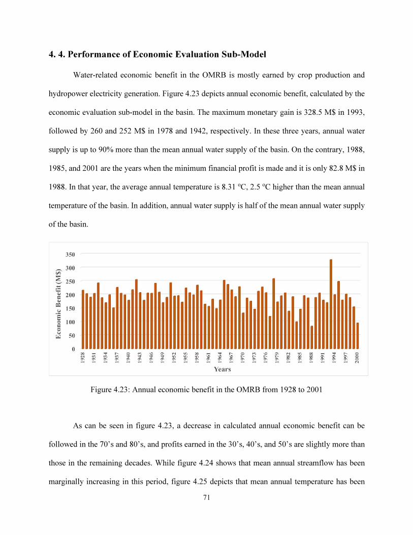
71

4. 4. Performance of Economic Evaluation Sub-Model

Water-related economic benefit in the OMRB is mostly earned by crop production and

hydropower electricity generation. Figure 4.23 depicts annual economic benefit, calculated by the

economic evaluation sub-model in the basin. The maximum monetary gain is 328.5 M$ in 1993,

followed by 260 and 252 M$ in 1978 and 1942, respectively. In these three years, annual water

supply is up to 90% more than the mean annual water supply of the basin. On the contrary, 1988,

1985, and 2001 are the years when the minimum financial profit is made and it is only 82.8 M$ in

1988. In that year, the average annual temperature is 8.31 oC, 2.5 oC higher than the mean annual

temperature of the basin. In addition, annual water supply is half of the mean annual water supply

of the basin.

Figure 4.23: Annual economic benefit in the OMRB from 1928 to 2001

As can be seen in figure 4.23, a decrease in calculated annual economic benefit can be

followed in the 70’s and 80’s, and profits earned in the 30’s, 40’s, and 50’s are slightly more than

those in the remaining decades. While figure 4.24 shows that mean annual streamflow has been

marginally increasing in this period, figure 4.25 depicts that mean annual temperature has been

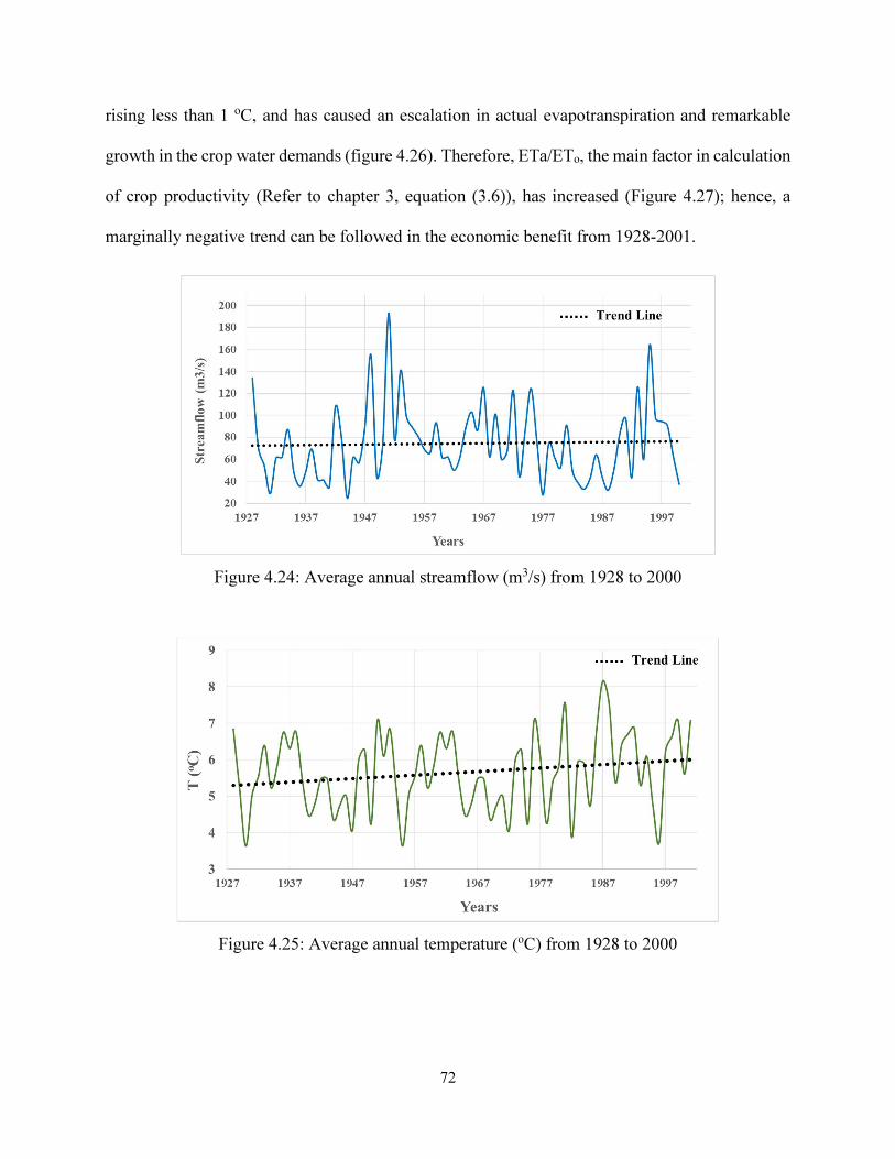
72

rising less than 1 oC, and has caused an escalation in actual evapotranspiration and remarkable

growth in the crop water demands (figure 4.26). Therefore, ETa/ETo, the main factor in calculation

of crop productivity (Refer to chapter 3, equation (3.6)), has increased (Figure 4.27); hence, a

marginally negative trend can be followed in the economic benefit from 1928-2001.

Figure 4.24: Average annual streamflow (m3/s) from 1928 to 2000

Figure 4.25: Average annual temperature (oC) from 1928 to 2000

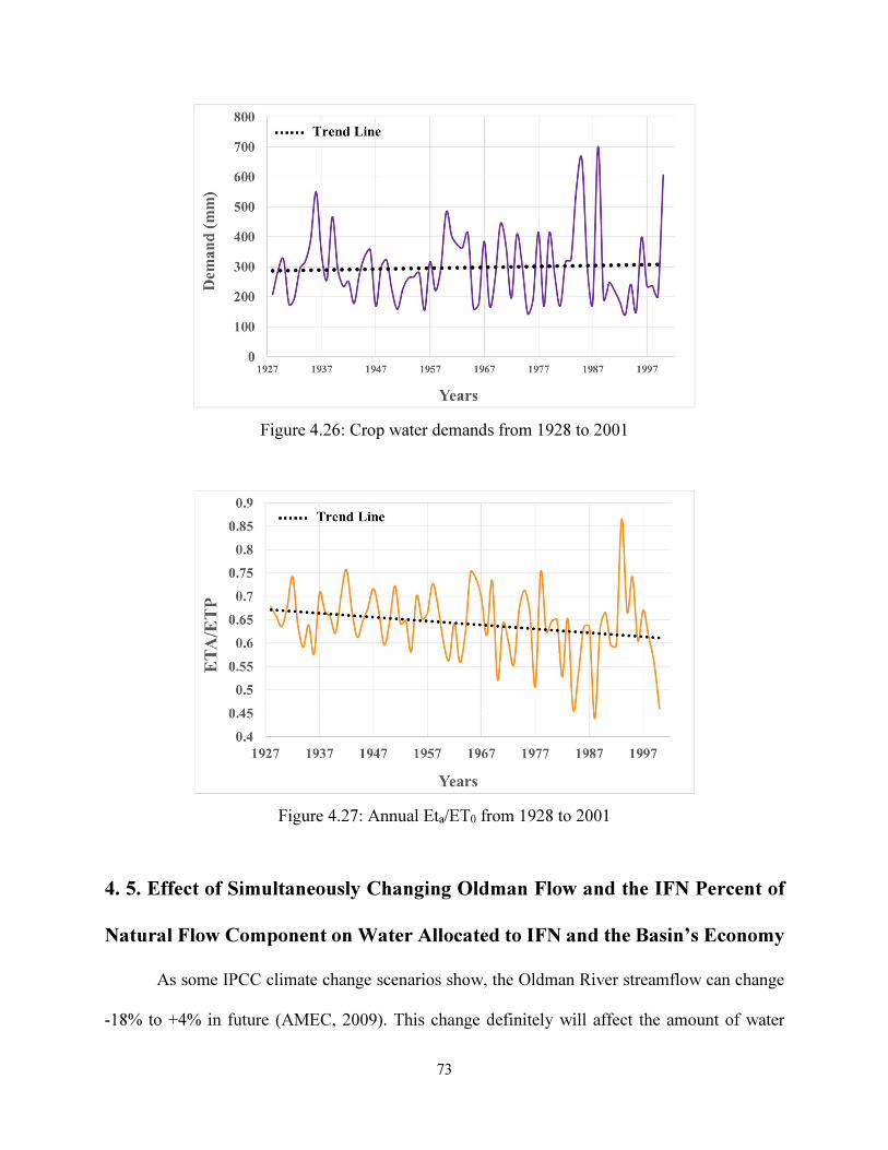
73

Figure 4.26: Crop water demands from 1928 to 2001

Figure 4.27: Annual Eta/ET0 from 1928 to 2001

4. 5. Effect of Simultaneously Changing Oldman Flow and the IFN Percent of

Natural Flow Component on Water Allocated to IFN and the Basin’s Economy

As some IPCC climate change scenarios show, the Oldman River streamflow can change

-18% to +4% in future (AMEC, 2009). This change definitely will affect the amount of water

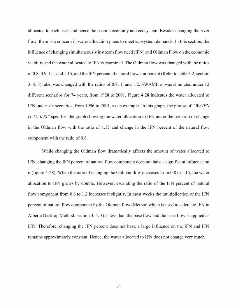
74

allocated to each user, and hence the basin’s economy and ecosystem. Besides changing the river

flow, there is a concern in water allocation plans to meet ecosystem demands. In this section, the

influence of changing simultaneously instream flow need (IFN) and Oldman Flow on the economic

viability and the water allocated to IFN is examined. The Oldman flow was changed with the ratios

of 0.8, 0.9, 1.1, and 1.15, and the IFN percent of natural flow component (Refer to table 3.2, section

3. 4. 3), also was changed with the ratios of 0.8, 1, and 1.2. SWAMPOM was simulated under 12

different scenarios for 74 years, from 1928 to 2001. Figure 4.28 indicates the water allocated to

IFN under six scenarios, from 1996 to 2001, as an example. In this graph, the phrase of “WAIFN

(1.15, 0.8)” specifies the graph showing the water allocation to IFN under the scenario of change

in the Oldman flow with the ratio of 1.15 and change in the IFN percent of the natural flow

component with the ratio of 0.8.

While changing the Oldman flow dramatically affects the amount of water allocated to

IFN, changing the IFN percent of natural flow component does not have a significant influence on

it (figure 4-28). When the ratio of changing the Oldman flow increases from 0.8 to 1.15, the water

allocation to IFN grows by double. However, escalating the ratio of the IFN percent of natural

flow component from 0.8 to 1.2 increases it slightly. In most weeks the multiplication of the IFN

percent of natural flow component by the Oldman flow (Method which is used to calculate IFN in

Alberta Desktop Method; section 3. 4. 3) is less than the base flow and the base flow is applied as

IFN. Therefore, changing the IFN percent does not have a large influence on the IFN and IFN

remains approximately constant. Hence, the water allocated to IFN does not change very much.

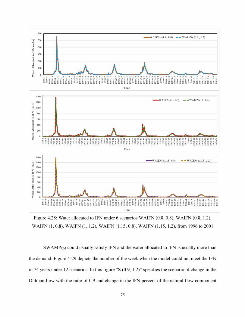
75

Figure 4.28: Water allocated to IFN under 6 scenarios WAIFN (0.8, 0.8), WAIFN (0.8, 1.2),

WAIFN (1, 0.8), WAIFN (1, 1.2), WAIFN (1.15, 0.8), WAIFN (1.15, 1.2), from 1996 to 2001

SWAMPOM could usually satisfy IFN and the water allocated to IFN is usually more than

the demand. Figure 4-29 depicts the number of the week when the model could not meet the IFN

in 74 years under 12 scenarios. In this figure “S (0.9, 1.2)” specifies the scenario of change in the

Oldman flow with the ratio of 0.9 and change in the IFN percent of the natural flow component

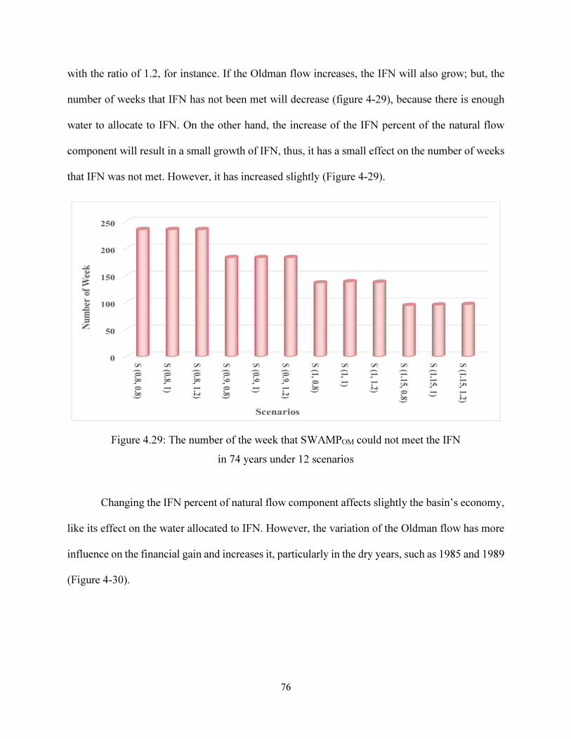
76

with the ratio of 1.2, for instance. If the Oldman flow increases, the IFN will also grow; but, the

number of weeks that IFN has not been met will decrease (figure 4-29), because there is enough

water to allocate to IFN. On the other hand, the increase of the IFN percent of the natural flow

component will result in a small growth of IFN, thus, it has a small effect on the number of weeks

that IFN was not met. However, it has increased slightly (Figure 4-29).

Figure 4.29: The number of the week that SWAMPOM could not meet the IFN

in 74 years under 12 scenarios

Changing the IFN percent of natural flow component affects slightly the basin’s economy,

like its effect on the water allocated to IFN. However, the variation of the Oldman flow has more

influence on the financial gain and increases it, particularly in the dry years, such as 1985 and 1989

(Figure 4-30).

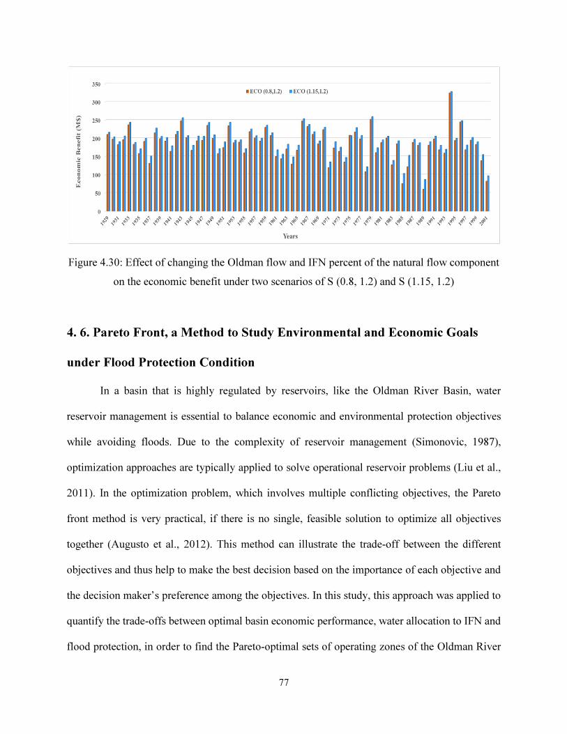
77

Figure 4.30: Effect of changing the Oldman flow and IFN percent of the natural flow component

on the economic benefit under two scenarios of S (0.8, 1.2) and S (1.15, 1.2)

4. 6. Pareto Front, a Method to Study Environmental and Economic Goals

under Flood Protection Condition

In a basin that is highly regulated by reservoirs, like the Oldman River Basin, water

reservoir management is essential to balance economic and environmental protection objectives

while avoiding floods. Due to the complexity of reservoir management (Simonovic, 1987),

optimization approaches are typically applied to solve operational reservoir problems (Liu et al.,

2011). In the optimization problem, which involves multiple conflicting objectives, the Pareto

front method is very practical, if there is no single, feasible solution to optimize all objectives

together (Augusto et al., 2012). This method can illustrate the trade-off between the different

objectives and thus help to make the best decision based on the importance of each objective and

the decision maker’s preference among the objectives. In this study, this approach was applied to

quantify the trade-offs between optimal basin economic performance, water allocation to IFN and

flood protection, in order to find the Pareto-optimal sets of operating zones of the Oldman River

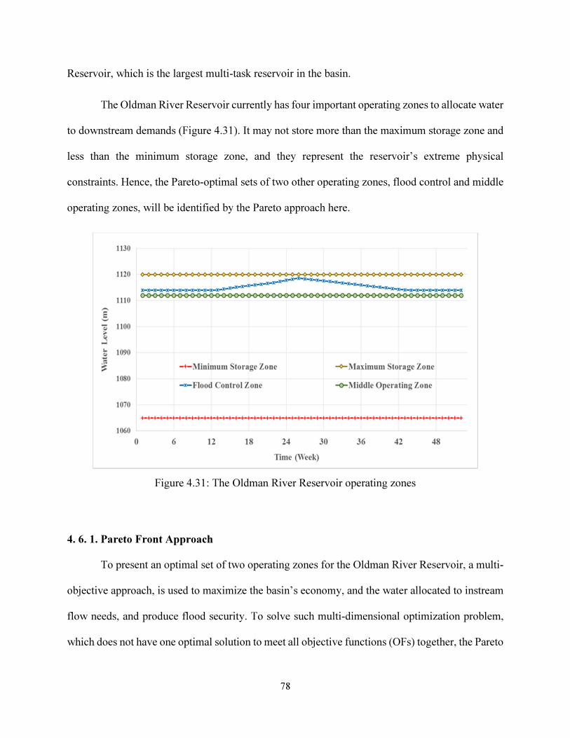
78

Reservoir, which is the largest multi-task reservoir in the basin.

The Oldman River Reservoir currently has four important operating zones to allocate water

to downstream demands (Figure 4.31). It may not store more than the maximum storage zone and

less than the minimum storage zone, and they represent the reservoir’s extreme physical

constraints. Hence, the Pareto-optimal sets of two other operating zones, flood control and middle

operating zones, will be identified by the Pareto approach here.

Figure 4.31: The Oldman River Reservoir operating zones

4. 6. 1. Pareto Front Approach

To present an optimal set of two operating zones for the Oldman River Reservoir, a multi-

objective approach, is used to maximize the basin’s economy, and the water allocated to instream

flow needs, and produce flood security. To solve such multi-dimensional optimization problem,

which does not have one optimal solution to meet all objective functions (OFs) together, the Pareto

79

front approach is very useful. The Pareto front is a framework to evaluate a set of decision variables

with multi-dimensional outputs assuming that improvement in one dimension will result in being

worsen in another (Legriel et al., 2010). It represents trade-offs between objective functions, which

is very practical in decision making process. To find optimal Oldman Reservoir operating zones,

the Pareto approach requires to optimize three objective functions, economic, environmental

(IFN), and flood OFs, simultaneously. Since both the amount of floodwater and flood frequency

are very important, two objective functions were defined to protect the basin from flooding.

Equations 4.1 to 4.4 represent objective functions which have been assigned:

��) = min *∑ *( ��)

��+��

�� + /74 (4.1)

�� ) = min∑ ∑ ,(�� ,�� ,�)

�� ,�- /(74 × 52)��

�� (4.2)

)��)(1) = min∑ ∑ *(�� !�,��)

�+ /(74 × 52)��

�� (4.3)

)��)$2& = )��)��.'�� = min/∑ ∑ 0'��1)��(��

�� 2 (4.4)

where i and j are the year and week index respectively, Max EB is the maximum economic benefit

which can be earned in a year, EBi is the actual economic benefit in year i, IFN OMRi,j is the

average weekly instream flow need of the Oldman River, WAIFN OMRi,j is the average weekly

water allocated to IFN, Outflowi,j is the average weekly water released from the Oldman Reservoir,

and FT is flood threshold.

The economic objective function aims to minimize the difference between the maximum

and actual economic benefit. To calculate Max EB, it is assumed that crop’s annual yield would

be maximum. Then, economic benefit for each crop is calculated using equation 3.10 and 3.11

Maximum hydropower generation in the basin is 32 MWh. Multiplication of this maximum

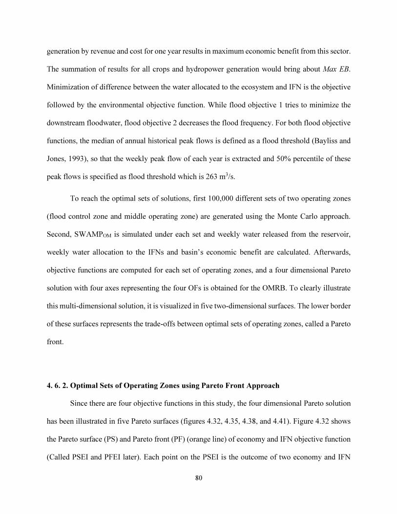
80

generation by revenue and cost for one year results in maximum economic benefit from this sector.

The summation of results for all crops and hydropower generation would bring about Max EB.

Minimization of difference between the water allocated to the ecosystem and IFN is the objective

followed by the environmental objective function. While flood objective 1 tries to minimize the

downstream floodwater, flood objective 2 decreases the flood frequency. For both flood objective

functions, the median of annual historical peak flows is defined as a flood threshold (Bayliss and

Jones, 1993), so that the weekly peak flow of each year is extracted and 50% percentile of these

peak flows is specified as flood threshold which is 263 m3/s.

To reach the optimal sets of solutions, first 100,000 different sets of two operating zones

(flood control zone and middle operating zone) are generated using the Monte Carlo approach.

Second, SWAMPOM is simulated under each set and weekly water released from the reservoir,

weekly water allocation to the IFNs and basin’s economic benefit are calculated. Afterwards,

objective functions are computed for each set of operating zones, and a four dimensional Pareto

solution with four axes representing the four OFs is obtained for the OMRB. To clearly illustrate

this multi-dimensional solution, it is visualized in five two-dimensional surfaces. The lower border

of these surfaces represents the trade-offs between optimal sets of operating zones, called a Pareto

front.

4. 6. 2. Optimal Sets of Operating Zones using Pareto Front Approach

Since there are four objective functions in this study, the four dimensional Pareto solution

has been illustrated in five Pareto surfaces (figures 4.32, 4.35, 4.38, and 4.41). Figure 4.32 shows

the Pareto surface (PS) and Pareto front (PF) (orange line) of economy and IFN objective function

(Called PSEI and PFEI later). Each point on the PSEI is the outcome of two economy and IFN

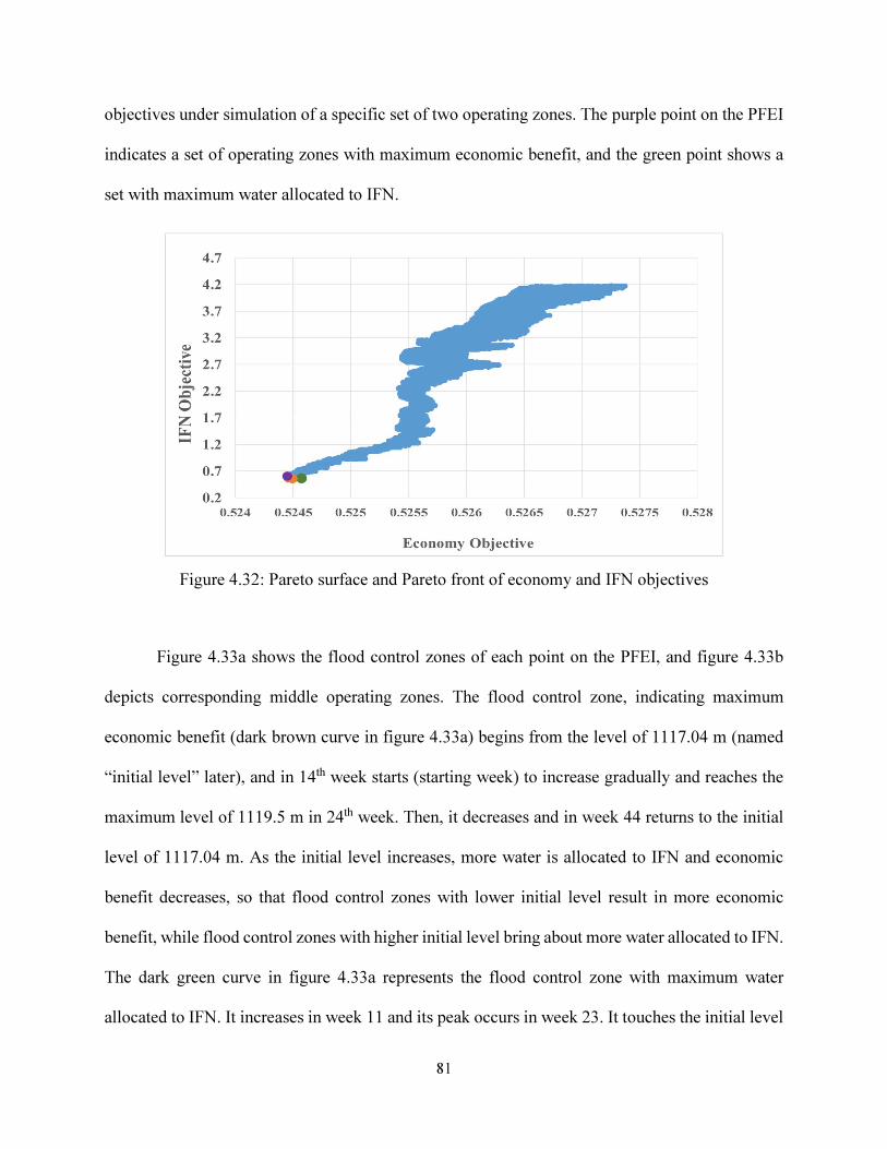
81

objectives under simulation of a specific set of two operating zones. The purple point on the PFEI

indicates a set of operating zones with maximum economic benefit, and the green point shows a

set with maximum water allocated to IFN.

Figure 4.32: Pareto surface and Pareto front of economy and IFN objectives

Figure 4.33a shows the flood control zones of each point on the PFEI, and figure 4.33b

depicts corresponding middle operating zones. The flood control zone, indicating maximum

economic benefit (dark brown curve in figure 4.33a) begins from the level of 1117.04 m (named

“initial level” later), and in 14th week starts (starting week) to increase gradually and reaches the

maximum level of 1119.5 m in 24th week. Then, it decreases and in week 44 returns to the initial

level of 1117.04 m. As the initial level increases, more water is allocated to IFN and economic

benefit decreases, so that flood control zones with lower initial level result in more economic

benefit, while flood control zones with higher initial level bring about more water allocated to IFN.

The dark green curve in figure 4.33a represents the flood control zone with maximum water

allocated to IFN. It increases in week 11 and its peak occurs in week 23. It touches the initial level

82

of 1117.32 m in week 44 again. As can be seen in figure 4-34a, the flood control zones resulting

in more water allocation to IFN, start to increase two/three weeks earlier than the zones resulting

in more economic gains. The middle operating zones, which are meeting the economy objective,

have lower levels than the middle operating zones which are satisfying the IFN objective function.

Figure 4.33: Flood control zones (a) and middle operating zones (b) of each point on the PFEI

Figure 4-34 shows the operating zones causing the maximum economic benefit (orange

curves; according to the purple point on the PFEI) and the maximum water allocated to IFN (green

curves; according to the green point on the PFEI).

(a) (b)

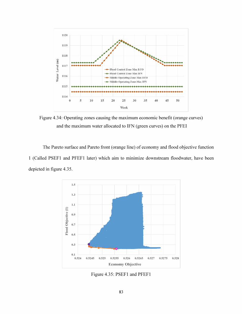
83

Figure 4.34: Operating zones causing the maximum economic benefit (orange curves)

and the maximum water allocated to IFN (green curves) on the PFEI

The Pareto surface and Pareto front (orange line) of economy and flood objective function

1 (Called PSEF1 and PFEF1 later) which aim to minimize downstream floodwater, have been

depicted in figure 4.35.

Figure 4.35: PSEF1 and PFEF1

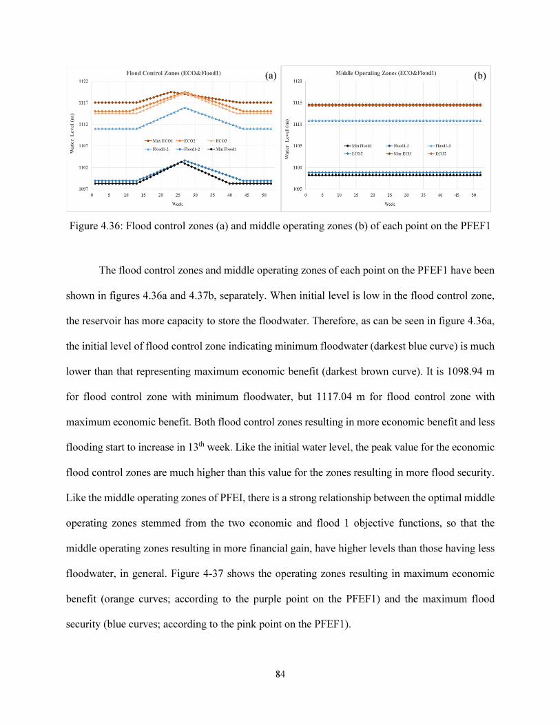
84

Figure 4.36: Flood control zones (a) and middle operating zones (b) of each point on the PFEF1

The flood control zones and middle operating zones of each point on the PFEF1 have been

shown in figures 4.36a and 4.37b, separately. When initial level is low in the flood control zone,

the reservoir has more capacity to store the floodwater. Therefore, as can be seen in figure 4.36a,

the initial level of flood control zone indicating minimum floodwater (darkest blue curve) is much

lower than that representing maximum economic benefit (darkest brown curve). It is 1098.94 m

for flood control zone with minimum floodwater, but 1117.04 m for flood control zone with

maximum economic benefit. Both flood control zones resulting in more economic benefit and less

flooding start to increase in 13th week. Like the initial water level, the peak value for the economic

flood control zones are much higher than this value for the zones resulting in more flood security.

Like the middle operating zones of PFEI, there is a strong relationship between the optimal middle

operating zones stemmed from the two economic and flood 1 objective functions, so that the

middle operating zones resulting in more financial gain, have higher levels than those having less

floodwater, in general. Figure 4-37 shows the operating zones resulting in maximum economic

benefit (orange curves; according to the purple point on the PFEF1) and the maximum flood

security (blue curves; according to the pink point on the PFEF1).

(a) (b)

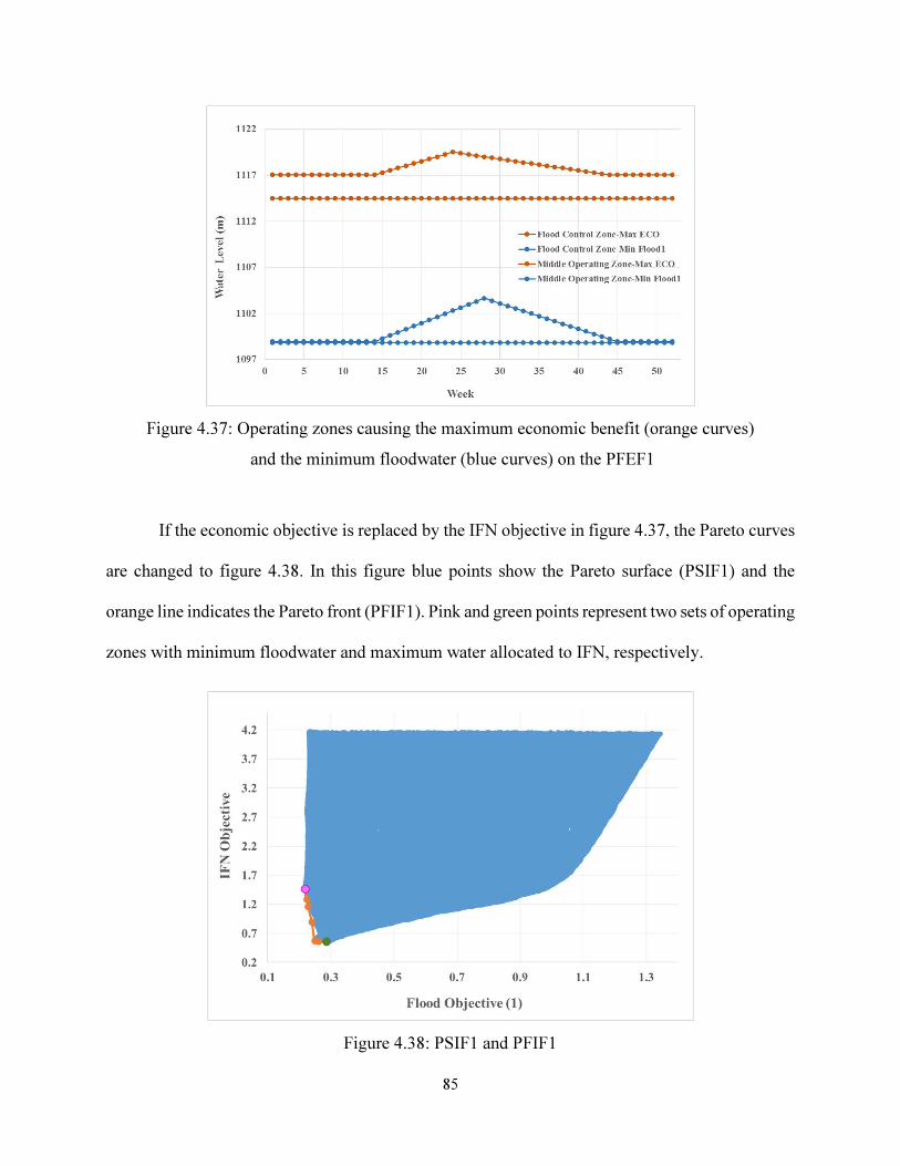
85

Figure 4.37: Operating zones causing the maximum economic benefit (orange curves)

and the minimum floodwater (blue curves) on the PFEF1

If the economic objective is replaced by the IFN objective in figure 4.37, the Pareto curves

are changed to figure 4.38. In this figure blue points show the Pareto surface (PSIF1) and the

orange line indicates the Pareto front (PFIF1). Pink and green points represent two sets of operating

zones with minimum floodwater and maximum water allocated to IFN, respectively.

Figure 4.38: PSIF1 and PFIF1

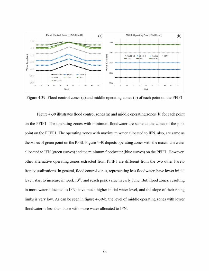
86

Figure 4.39: Flood control zones (a) and middle operating zones (b) of each point on the PFIF1

Figure 4-39 illustrates flood control zones (a) and middle operating zones (b) for each point

on the PFIF1. The operating zones with minimum floodwater are same as the zones of the pink

point on the PFEF1. The operating zones with maximum water allocated to IFN, also, are same as

the zones of green point on the PFEI. Figure 4-40 depicts operating zones with the maximum water

allocated to IFN (green curves) and the minimum floodwater (blue curves) on the PFIF1. However,

other alternative operating zones extracted from PFIF1 are different from the two other Pareto

front visualizations. In general, flood control zones, representing less floodwater, have lower initial

level, start to increase in week 13th, and reach peak value in early June. But, flood zones, resulting

in more water allocated to IFN, have much higher initial water level, and the slope of their rising

limbs is very low. As can be seen in figure 4-39-b, the level of middle operating zones with lower

floodwater is less than those with more water allocated to IFN.

(a) (b)

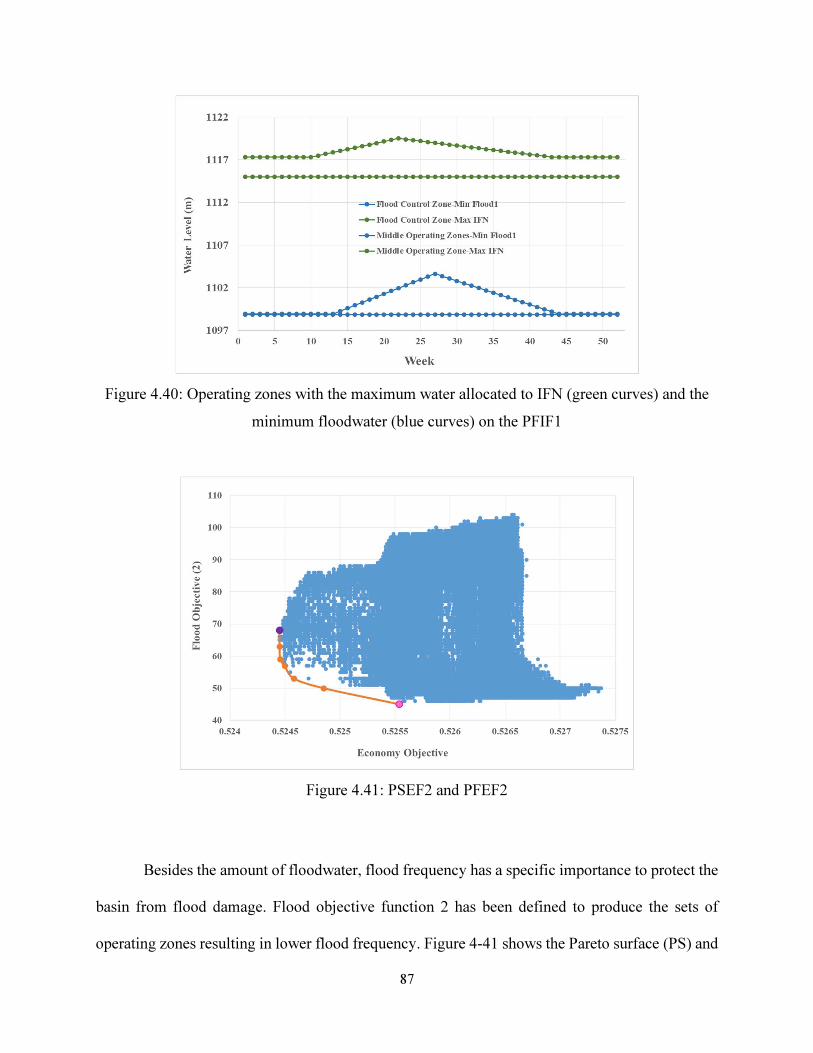
87

Figure 4.40: Operating zones with the maximum water allocated to IFN (green curves) and the

minimum floodwater (blue curves) on the PFIF1

Figure 4.41: PSEF2 and PFEF2

Besides the amount of floodwater, flood frequency has a specific importance to protect the

basin from flood damage. Flood objective function 2 has been defined to produce the sets of

operating zones resulting in lower flood frequency. Figure 4-41 shows the Pareto surface (PS) and

88

Pareto front (PF) (orange line) of economy and flood 2 objective functions, PSEF2 and PFEF2.

Figure 4.42: Flood control zones (a) and middle operating zones (b) of each point on the PFEF2

Flood control zones and middle operating zones causing points on PFEF2 have been shown

in figure 4.42. The initial level of flood control zone with minimum flood frequency is 1097.18 m,

about one m more than that with minimum floodwater. This curve begins to increase in week 14th,

and in the middle of June touches the peak value of 1101.73, which is 1.9 m lower than the peak

level of flood zone with minimum floodwater. It returns to the initial level three weeks earlier than

the flood zone with minimum floodwater. Overall, the initial level of flood control zones resulting

in less flood frequency is lower than those causing more economic benefit, and their middle

operating zones are lower than those with more financial benefit. Operating zones with the

maximum economic benefit (orange curves), producing the purple point on the PFEF2 and the

minimum flood frequency (45 flood events in 74 years; blue curves), generating the pink point on

the PFEF2, are depicted on figure 4.43.

(a) (b)

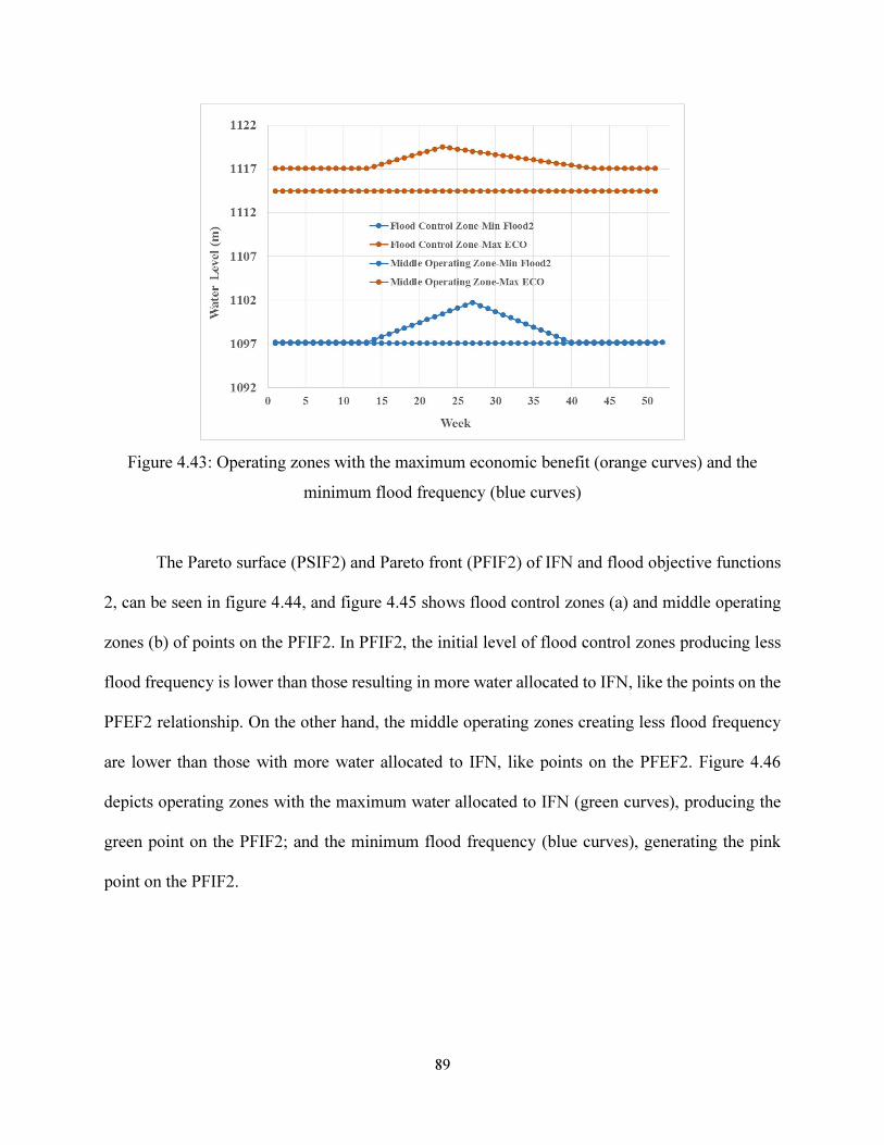
89

Figure 4.43: Operating zones with the maximum economic benefit (orange curves) and the

minimum flood frequency (blue curves)

The Pareto surface (PSIF2) and Pareto front (PFIF2) of IFN and flood objective functions

2, can be seen in figure 4.44, and figure 4.45 shows flood control zones (a) and middle operating

zones (b) of points on the PFIF2. In PFIF2, the initial level of flood control zones producing less

flood frequency is lower than those resulting in more water allocated to IFN, like the points on the

PFEF2 relationship. On the other hand, the middle operating zones creating less flood frequency

are lower than those with more water allocated to IFN, like points on the PFEF2. Figure 4.46

depicts operating zones with the maximum water allocated to IFN (green curves), producing the

green point on the PFIF2; and the minimum flood frequency (blue curves), generating the pink

point on the PFIF2.

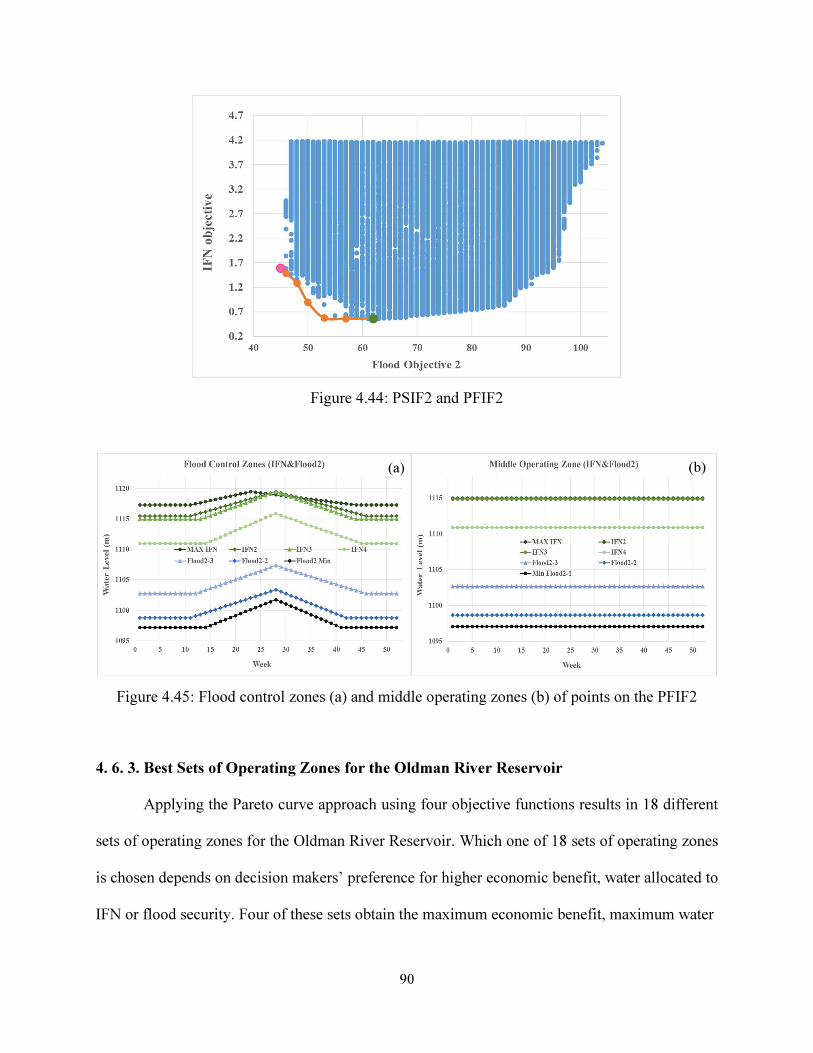
90

Figure 4.44: PSIF2 and PFIF2

Figure 4.45: Flood control zones (a) and middle operating zones (b) of points on the PFIF2

4. 6. 3. Best Sets of Operating Zones for the Oldman River Reservoir

Applying the Pareto curve approach using four objective functions results in 18 different

sets of operating zones for the Oldman River Reservoir. Which one of 18 sets of operating zones

is chosen depends on decision makers’ preference for higher economic benefit, water allocated to

IFN or flood security. Four of these sets obtain the maximum economic benefit, maximum water

(a) (b)

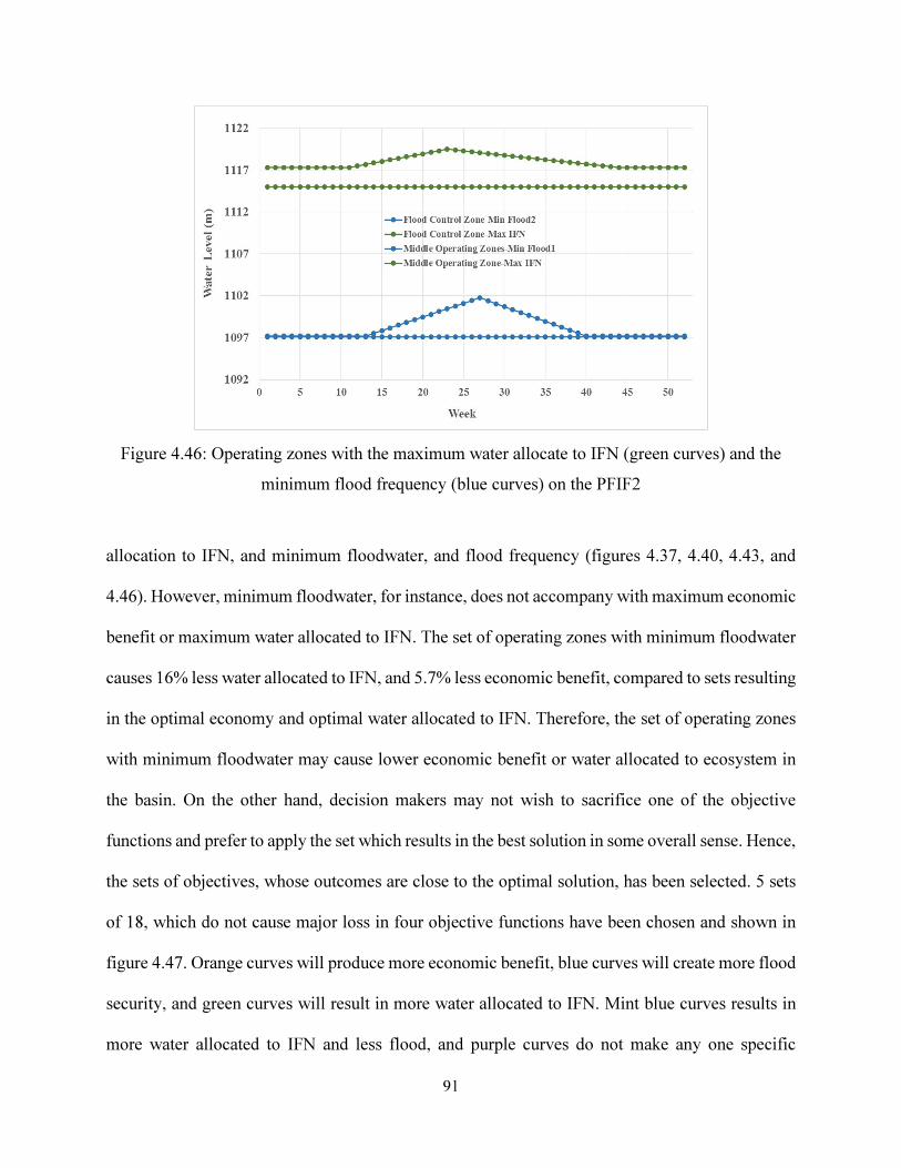
91

Figure 4.46: Operating zones with the maximum water allocate to IFN (green curves) and the

minimum flood frequency (blue curves) on the PFIF2

allocation to IFN, and minimum floodwater, and flood frequency (figures 4.37, 4.40, 4.43, and

4.46). However, minimum floodwater, for instance, does not accompany with maximum economic

benefit or maximum water allocated to IFN. The set of operating zones with minimum floodwater

causes 16% less water allocated to IFN, and 5.7% less economic benefit, compared to sets resulting

in the optimal economy and optimal water allocated to IFN. Therefore, the set of operating zones

with minimum floodwater may cause lower economic benefit or water allocated to ecosystem in

the basin. On the other hand, decision makers may not wish to sacrifice one of the objective

functions and prefer to apply the set which results in the best solution in some overall sense. Hence,

the sets of objectives, whose outcomes are close to the optimal solution, has been selected. 5 sets

of 18, which do not cause major loss in four objective functions have been chosen and shown in

figure 4.47. Orange curves will produce more economic benefit, blue curves will create more flood

security, and green curves will result in more water allocated to IFN. Mint blue curves results in

more water allocated to IFN and less flood, and purple curves do not make any one specific

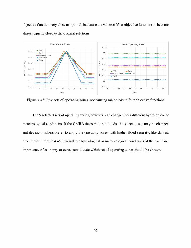
92

objective function very close to optimal, but cause the values of four objective functions to become

almost equally close to the optimal solutions.

Figure 4.47: Five sets of operating zones, not causing major loss in four objective functions

The 5 selected sets of operating zones, however, can change under different hydrological or

meteorological conditions. If the OMRB faces multiple floods, the selected sets may be changed

and decision makers prefer to apply the operating zones with higher flood security, like darkest

blue curves in figure 4.45. Overall, the hydrological or meteorological conditions of the basin and

importance of economy or ecosystem dictate which set of operating zones should be chosen.

93

CHAPTER 5

CONCLUSION

In this chapter, first a summary of this study, including purpose, methodology, and the

SWAMPOM model that has been developed here, is provided. Then the conclusions of results and

analysis are presented, and finally possible future studies are discussed.

5. 1. Summary of the Study

This thesis focused on the development of an integrated water resources management

(IWRM) model using the system dynamics (SD) approach for the Oldman River Basin (OMRB),

located in southern Alberta, Canada. The SD approach can reflect interconnection between various

components of a water system and represent dynamic loops controlling the complex behavior of

the system. Since the OMRB is a semi-arid basin and faces multiple water resources challenges,

including water shortage, uncertain water supply and water demand, flooding and drought, specific

climatic and hydrological conditions, complex water governance and complex water systems, an

IWRM model is required to address all these challenges and investigate their dynamic connections

in the basin. Thus, an IWRM, called SWAMPOM, including a water allocation model, dynamic

irrigation demand, instream flow needs (IFN) and economic evaluation sub-models, has been

developed for the OMRB. The water allocation sub-model is an emulation of an existing water

resources management model, WRMM, which has been developed by Alberta Environment

(2002). The data and operating policies required for the development of the water allocation sub-

model have been derived from the WRMM. This sub-model meets current/future consumptive

94

irrigation, industrial, and municipal demands, and satisfies non-consumptive ecosystem and

hydropower generation demands, operating on a weekly time step. Meeting irrigation demands

relies on the crop water requirement, which is affected by climate variations. Therefore, it should

be estimated under varying climatic conditions, hence the need for the dynamic irrigation demand

sub-model. This sub-model computes the crop water requirement for the main crops (barley,

wheat, alfalfa, canola, flax, corn, sugar beet, potato, and beans) planted in 43 irrigation fields,

which belong to five irrigation districts (Lethbridge Northern ID, St. Mary ID, Taber ID, Ross

Creek ID, and Private ID). The sustainability of the aquatic ecosystem is another important concern

in the basin. SWAMPOM calculates instream flow need (IFN) for six sections of the Oldman River

using the Alberta Desktop method (Locke and Paul, 2011), and allocates enough water to rivers to

meet IFN under different policy scenarios of uncertain water supply. In the OMRB the major

water-related economic benefit, which is computed by the economic evaluation sub-model, is

earned by agriculture and hydropower generation.

Water resources in the OMRB are highly regulated by infrastructure, like dams, of which

the Oldman River Reservoir is the largest. This reservoir plays a critical role to meet the demands

and keep a balance between the basin’s economy and ecosystem while preventing floods and

decreasing drought effects. This research also has aimed to produce different sets of Oldman

Reservoir operation zones, resulting in trade-offs among four objective functions; the optimal

economic benefit, water allocated to the ecosystem, and minimum floodwater and flood frequency;

so that decision makers can decide how much water should be stored in the reservoir to meet a

specific objective while not sacrificing others. A multi-objective performance assessment, using a

Pareto curve approach, has been applied to identify the optimal trade-offs between the four

objective functions, and define 18 different sets of operating zones. Each set results in an optimal

95

value of one, or more objective functions, but a global optimum for all objectives together is not

achievable. The preference of decision makers, for example for higher economic benefit, water

allocated to IFN or flood security, can determine which set of operation zones should be selected.

5. 2. Conclusion of the Research Study

To conclude, the SWAMPOM can address most water challenges in the Oldman River

Basin. SWAMPOM not only reflects the dynamic, loop-based interactions among different

components of the water resource system, but it also facilitates analyzing the sensitivity of the

water system to different “What-if” scenarios of water availability and IFN’s policy. In addition,

it enables the participation of decision makers in solving water problems in a basin. The following

points can also be deduced:

I. The comparison between the SWAMPOM’s results and WRMM’s shows that

SWAMPOM could reasonably represent all irrigation, industrial, municipal, ecosystem,

and hydropower generation demands at a weekly time step. SWAMPOM could meet

86% of irrigation demands, 81% of industrial and municipal demand, 94% of

ecosystem needs, and 100% of hydropower demands in the whole time period, from

1928 to 2001;

II. Comparison between the historical water levels and those computed by SWAMPOM

for the Oldman River Reservoir shows that the two data series are better matched for

higher water levels. However, the same comparison for the water released from the

reservoir indicates higher correlation between historical low flows and those

calculated by SWAMPOM.

III. While there is a difference between irrigation demand estimated by WRMM and

96

SWAMPOM, SWAMPOM could provide an adequate estimation of the crop water

requirement under different hydrometeorological conditions. Based on the

SWAMPOM’s results, the average annual irrigation demand is 306 mm over the

whole time period from 1928 to 2001 in the main irrigation districts, which increases

to 714 mm in dry years and decreases to 92 mm in wet years. However, this value

equals 319 mm in WRMM’s database;

IV. SWAMPOM is promising as a tool to secure the aquatic ecosystem in the OMRB. The

average weekly instream flow need of the Oldman River was estimated to be

approximately 20.5 m3/s by the Alberta Desktop method using the IFN sub-model.

However, it is specified as 12.3 m3/s in WRMM, which applies the Fish Rule curves

method. Under the current hydrometeorological conditions, SWAMPOM could meet

entire IFN for more than 97% of weeks in the whole time period, from 1928 to 2001;

V. Average annual economic benefit, mostly earned by crop production and hydropower

generation, was computed to be 192.5 M$ on average in the OMRB. It decreased to

82.8 M$ in very dry years, and increased to 328.6 M$ in very wet years;

VI. Increase in river flow resulted in a large effect on water allocated to IFNs, specifically

in wet years, and an influence on the basin’s economy in dry years, in particular.

However, changing the IFN percent of natural flow component did not have a

significant influence on both economic benefits and water allocated to IFN; and

VII. Water allocation and water-related economy in the OMRB are sensitive to the Oldman

River Reservoir operation. Using a Pareto curve approach under four objective

functions of maximum economic benefit, maximum water allocated to the ecosystem,

minimum floodwater, and minimum flood frequency, 18 different, optimal, or close

97

to optimal sets of operating zones were calculated for the Reservoir. Operating zones

is chosen based on decision makers’ preference for higher economic benefit, water

allocated to IFN or flood protection. However, the set of operating zones with

minimum floodwater caused 11 less flood events; the operating zones with maximum

economy resulted in 4.1% more financial gain; and the zones with maximum water

allocated to IFN led to 10.1% more ecosystem protection in the whole 74 years,

compared to current zones.

5. 3. Future Work

Some of the possible additional research studies, associated with the SWAPMOM and

optimal operating zones, are as follows:

I. Since SWAMPOM is an emulation of WRMM, and hence simplified to some extent,

only some of the WRMM’s polices (for example, penalty zones) have been applied in

the SWAMPOM. Therefore, the two model results are not quite matched for some water

components. Adding all WRMM’s policies would be useful to increase the correlation

between two model results;

II. While SWAMPOM is an integrated water resources management model, it does not

model all the basin’s characteristics. Hydrological modeling and groundwater

management can be added to the SWAMPOM, in order to more comprehensively

address water management in the basin;

III. Water resources and water management in the Oldman, Bow, Red Deer, and South

Saskatchewan are connected together. Developing SWAMP for other basins, and

linking them can be the next step to have holistic water management in three prairie

98

provinces of Alberta, Saskatchewan, and Manitoba (Currently SWAMP has been

developed for Oldman, Bow, and Saskatchewan portion of South Saskatchewan river

basins);

IV. In this study, sustainable economy, ecosystem protection and flood protection were

assessed using the Pareto approach. However, another important concern in the basin

is drought. Defining a drought objective function and minimizing the drought effects

in the basin could be a possible future scope.

99

REFERENCES

Adelsman H. (1996). Water Resources Program Policy, Consumptive and Non-consumptive

Water Use, Coordination & Hydrology Section. Effective Date: 10-31-91.

Ahmad S., and Simonovic S. P. (2000). “Modeling Reservoir Operations for Flood Management

Using System Dynamics”, ASCE Journal of Computing in Civil Engineering, Vol.14, No. 3,

190-198.

AIMM (2006). Alberta Irrigation Management Manual. Irrigation Management Branch, Irrigation

and Farm Water Division. 2006.

Alberta Agriculture, Food and Rural Development (2013). Alberta Irrigation Management

Manual.

Alberta Environment. (2002). Water Resources Management Model (WRMM), Government of

Alberta, Edmonton, Alberta.

Alberta Environment. (2010), South Saskatchewan Regional Plan: Water Quantity and Quality

Modelling Results, Govt. of Alberta, Edmonton, Alberta, pp 89.

Alberta Environment. (2014). http://www.environment.alberta.ca/apps/basins/default.aspx.

Álvarez J. F. O., Valero J. A. d. J., Martín-Benito J. M. T. and Mata E. L. (2004). An economic

optimization model for irrigation water management. Irrigation Science May 2004, Vol. 23

(2), 61-75.

AMEC. (2009). South Saskatchewan River Basin in Alberta: Water Supply Study. Alberta

Agriculture and Rural Development. Lethbridge, Alberta.

100

Archer D. R., Forsythe H. J., Fowler S. and Shah M. (2010). Sustainability of water resources

management in the Indus Basin under changing climatic and socio economic conditions.

Hydrol. Earth Syst. Sci., 14, 1669-1680, 2010.

ASCE (2005). Standardized Reference Evapotranspiration Equation. EWRI of the ASCE, 59 pp.

Augusto O. B., Bennis F. and Caro S. (2012). A new method for decision making in multi-objective

optimization problems. Brazilian Operations Research Society, Pesquisa Operacional (2012)

32(2): 331-369.

Bagheri A. (2006). Sustainable Development Implementation in Urban Water Systems. PhD

dissertation, Lund University, Sweden.

Baier W. and Robertson G. W. (1966). A New Versatile Soil Moisture Budget. Canadian Journal

of Plant Science, V46:299-315.

Bayliss A, and Jones R. (1993). Peaks-over-threshold flood database: Summary statistics and

seasonality. IH Report No. 121. Institute of Hydrology: Wallingford, UK; 61.

Beddington J. (2013). Catalysing sustainable water security: role of science, innovation and

partnerships. Philosophical Transactions of the Royal Society A: Mathematical, Physical and

Engineering Sciences, 371(2002), 20120414.

Beven K. (2006). Rainfall-Runoff Modelling: The Primer. John Wiley& Sons.

Biswas A. K. (1978). United Nations Water Conference: Summary and Main Documents (Oxford:

Pergamon Press).

Biswas A. k. (2008). Integrated water resources management: Is it working? Water Resources

development Journal. Vol. 24. (1): 5-22.

101

Biswas A. K. (2009). Water Management: Some Personal Reflections. Water International,

December 2009.

Brouwer R. and Hofkes M. (2008). Integrated hydro-economic modelling: Approaches, key issues

and future research directions. Ecological Economics. Vol. 66, Issue 1, 16-22.

Byrne J., Kienzle S., Johnson D., Duke G., Gannon V., Selinger B. and Thomas J. (2006). Current

and future water issues in the Oldman River Basin of Alberta, Canada. Water Science

Technology, 53 (10): 327-340.

Cai X., Rosegrant M. W. and Ringler C. (2003). Physical and economic efficiency of water use in

the river basin: Implications for efficient water management. Water Resources Research,

39(1).

Cai X., Vogel R. and Ranjithan R. (2012). The Role of Systems Analysis in Watershed

Management. Journal of Water Resources Planning and Management. doi:

10.1061/(ASCE)WR. 1943-5452.0000341.

Capon-Garcıa E., Bojarski A. D., Espuna A., and Puigjaner L. (2011). Multi-objective

Optimization of Multiproduct Batch Plants Scheduling Under Environmental and Economic

Concerns. Process Systems Engineering. 57(10): 2766-2782.

Castelletti A., Pianosi F. and Restelli M. (2013). A multiobjective reinforcement learning approach

to water resources systems operation: Pareto frontier approximation in a single run. Water

Resources Research, Vol. 49, 3476–3486.

Chang N., Rivera B. J. and Wanielista P. M. (2011). Optimal design for water conservation and

energy savings using green roofs in a green building under mixed uncertainties. Journal of

Cleaner Production, Vol. 19, Issue 11, July 2011, 1180-1188.

102

Cia X. (2008). Implementation of holistic water resources-economic optimization models for river

basin management e Reflective experiences. Environmental Modelling & Software 23

(2008), 2-18.

Cia X., McKinney D. C. and Lasdon L. S. (2002). A framework for sustainability analysis in water

resources management and application to the Syr Darya Basin. WATER RESOURCES

RESEARCH, VOL. 38, NO. 6, 1085, 1-13, 10.1029/2001WR000214, 2002.

Clipperton G. K., Koning C. W., Locke A. G.H., Mahoney J., and Quazi B. (2003). Instream Flow

Needs Determinations for the South Saskatchewan River Basin, Alberta, Canada. ISBN No.

0-7785-3045-0. Pub No. T/719.

Davies E. G. R., and Simonovic S. P. (2011). Global water resources modeling with an integrated

model of the social–economic–environmental system. Advances in Water Resources, 34(6):

684-700.

Delelegn S.W., Pathirana A., Gersonius B., Adeogun A.G., and Vairavamoorthy K. (2011). Multi-

Objective Optimization of Cost-Benefit of Urban Flood Management using a 1D2D Coupled

Model. Water Science & Technology, DOI: 10.2166/wst.2011.290. 1-9.

Draper A., Jenkins M., Kirby K., Lund J., and Howitt R. (2003). Economic-Engineering

Optimization for California Water Management. J. Water Resources Planning Management,

129(3), 155-164.

Fang Q. X. Mab L., Green T. R., Yu Q., Wang T. D. and Ahuja L. R. (2010). Water resources and

water use efficiency in the North China Plain: Current status and agronomic management

options. Agricultural Water Management, 97 (2010) 1102-1116.

FAO. (2002). Deficit Irrigation Practices. Water Reports No. 22. Rome.

103

Farmer W., Strzepek K., Schlosser C. A., Droogers P. and Gao X. (2011). A Method for

Calculating Reference Evapotranspiration on Daily Time Scales. MIT Joint Program on the

Science and Policy of Global Change.

Federal Government (2003). Follow-up actions arising from the federal environmental assessment

and approval of the Oldman River Dam project. http://www.oag-

bvg.gc.ca/internet/English/pet_092B_e_28806.html.

Ferreyra, C., de Loë R. C., and Kreutzwiser R. D. (2008). Imagined communities, contested

watersheds: challenges to integrated water resources management in agricultural areas.

Journal of Rural Studies 24: 304-321.

Fiera Biological Consulting Ltd (Fiera). (2013). Oldman Watershed Headwaters Indicator Project

– Draft Report (Version 2013.3). Edmonton, Alberta. Fiera Biological Consulting Report

#1346.

Ford A. (1999). Modeling the Environment. Island Press: Covelo, California.

Forrester W. J. (1961). Industrial Management. The M.I.T. Press. Cambridge, MA, USA.

Gallego-Ayala J. (2013). Trends in integrated water resources management research: a literature

review. Water Policy, 15(4), 628.

Gastelum R.J., Valdés J. B. and Stewart S. (2010). A system dynamics model to evaluate

temporary water transfers in the Mexican Conchos Basin. Water Resources Management.

24(11): 1285-1311.

George B., Malano H., Davidson B., Hellegers P., Bharati L. and Massuel S. (2011). An integrated

hydro-economic modelling framework to evaluate water allocation strategies II: Scenario

assessment. Agricultural Water Management, 98(5), 747-758.

104

Global Water Partnership (GWP). (2000). Integrated Water Resources Management. (TAC

background paper; no. 4). Stockholm, Sweden. Online at

http://www.gwpforum.org/gwp/library/Tacno4.pdf.

Gober P. (2013). Getting outside the water box: The need for new approaches to water planning

and policy, Water Resources Management., 27, 955–957.

Gober P., and Wheater H. S. (2013). Socio-hydrology and the science-policy interface: a case

study of the Saskatchewan River Basin. Hydrology and Earth System Sciences Discussions,

10(5): 6669-6693.

Gober P., Kirkwood C. W., Balling R. C., Ellis A. W. and Deitrick S. (2010). Water planning

under climatic uncertainty in Phoenix: why we need a new paradigm. Annals of the

Association of American Geographers 100(2): 356-372.

Graveline N., Majone B., Van Duinen R. and Ansink E. (2014). Hydro-economic modeling of

water scarcity under global change: an application to the Gallego river basin (Spain). Reg

Environ Change (2014) 14: 119-132.

Groisman P. Y., Knight R. W. and Karl T. R. (2001). Heavy precipitation and high streamflow in

the contiguous United States: Trends in the twentieth century. Bulletin of the American

Meteorological Society, 82(2), 219-246.

Guan D. and Hubacek K. (2008). A new and integrated hydro-economic accounting and analytical

framework for water resources: A case study for North China. Journal of Environmental

Management. Vol. 88, Issue 4, 1300-1313.

Hargreaves G. H. (1973). The Estimation of Potential and Crop Evapotranspiration. American

Society of Agricultural Engineers.

105

Hargreaves G. H. and Samani Z. A. (1985). Reference crop evapotranspiration from temperature.

Applied Engineering in Agriculture, 1(2): 96-99.

Hargreaves G. L., Hargreaves G. H., and Riley J. P. (1985). Agricultural benefits for Senegal River

basin. Journal of irrigation and Drainage Engineering, 111(2): 113-124.

Harou J. J., Pulido-Velazquez M., Rosenberg D. E., Medellín-Azuara J., Lund J. R., and Howitt

R. E. (2009). Hydro-economic models: Concepts, design, applications, and future prospects.

Journal of Hydrology, 375(3-4), 627-643.

Hassanzadeh E., Elshorbagy A., Wheater H. and Gober P. (2014). Managing water in complex

systems: An integrated water resources model for Saskatchewan, Canada. Environmental

Modelling & Software, 58 (2014): 12-26.

Heinz I., Pulido-Velazquez M., Lund J. R. and Andreu J. (2007). Hydro-economic modeling in

river basin management: implications and applications for the European water framework

directive. Water resources management, 21(7), 1103-1125.

High Performance Systems (1992). Stella II: an introduction to systems thinking. High

Performance Systems, Inc, Hanover, New Hampshire.

Hinojosa-Huerta, O., DeStefano S., and Shaw W. W. (2001). Distribution and abundance of the

Yuma Clapper Rail (Rallus longirostris yumanensis) in the Colorado River delta. Mexico

Journal of arid Environments, 49: 171-182.

Hinrichsen D., and Tacio H. D. (2011) The Coming Freshwater Crisis is Already Here. Economics

and Globalization. Jul 7, 2011.

Ilich, N. (1992). Improvement of the return flow allocation in the Water Resources Management

Model of Alberta Environment. Canadian Journal of Civil Engineering 20, 613-621.

106

Ilich E. (2000). Enhancements of the Water Resources Management Model through an Improved

Communication with Users. M.Sc. Thesis, University of Manitoba, 2000.

IPCC. (2007). Freshwater Resources and their management. In Climate Change 2007: Impacts,

Adaptation and Vulnerability. Contribution of Working Group II to the Fourth Assessment

Report of the Intergovernmental Panel on Climate Change, pp. 173-210. Cambridge, UK:

Cambridge University Press.

Kalbus E., Kalbacher T., Kolditz O., Krüger E., Seegert J., Röstel G., Teutsch G., Borchardt D.

and Krebs P. (2011). Integrated Water Resources Management under different hydrological,

climatic and socio-economic conditions. Environmental Earth Sciences. March 2012, 65(5):

1363-1366.

Le Ngo L., Madsen H. and Rosbjerg D. (2007). Simulation and optimization modelling approach

for operation of the Hoa Binh reservoir, Vietnam. Journal of Hydrology. 336(3-4): 269-281.

Lee C. S. (2012). Multi-objective game-theory models for conflict analysis in reservoir watershed

management. Chemosphere 87 (2012), 608-613.

Legriel J., Le Guernic C., Cotton S., and Maler O. (2010) Approximating the Pareto Front of Multi-

criteria Optimization Problems. J. Esparza and R. Majumdar (Eds.): TACAS 2010, LNCS

6015, pp. 69–83, 2010 Springer.

Li Y., Zhou J., Zhang Y., Qin H. and Liu L. (2010). ”Novel Multiobjective Shuffled Frog Leaping

Algorithm with Application to Reservoir Flood Control Operation.” J. Water Resources

Planning Management, 136 (2), 217–226.

Liu P., Guo S., Xu X. and Chen J. (2011). Derivation of Aggregation-Based Joint Operating Rule

Curves for Cascade Hydropower Reservoirs. Water Resources Management, (2011)

107

25:3177–3200 DOI 10.1007/s11269-011-9851-9.

Locke A. and Paul A. (2011). A desktop for establishing environmental flows in Alberta rivers

and streams. Alberta Environment and Alberta Sustainable Resource Development. April

2011.

Loucks, D.P. and van Beek, E. (2005). Water Resources Systems Planning and Management: An

Introduction to Methods, Models and Applications. UNESCO Press, Paris.

Marques G. F., Lund J. R., Leu M. R., Jenkins M., Howitt R., Harter T. and Burke S. (2006).

Economically driven simulation of regional water systems: Friant-Kern, California. Journal

of water resources planning and management, 132(6), 468-479.

Matondo, J. I. (2002). A comparison between conventional and integrated water resources

planning and management. Physics and Chemistry of the Earth, Parts A/B/C, 27(11-22),

831–838.

Maulé C., Helgason W., McGinn S. and Cutforth H. (2006). Estimation of standardized reference

evapotranspiration on the Canadian prairies using simple models with limited weather data.

Can. Biosystem. Engineering. 48 (1): 1-11.

Milly P. C., Dunne K. A. and Vecchia A. V. (2005). Global pattern of trends in streamflow and

water availability in a changing climate. Nature, 438(7066), 347-350.

Mirchi A. (2013). System Dynamics Modeling as a Quantitative-Qualitative Framework for

Sustainable Water Resources Management: Insights for Water Quality Policy in the Great

Lakes Region. PhD Dissertation, Michigan Technological University, 2013.

Mirchi A., Madani K., Watkins Jr D. and Ahmad S. (2012). Synthesis of System Dynamics Tools

for Holistic Conceptualization of Water Resources Problems. Water Resources Management.

108

July 2012, 26(9), 2421-2442.

Mitchell B. (1990). Integrated Water Management: International Experiences and Perspectives,

Belhaven Press, London, 1990.

Moghaddasi M., Morid S., Araghinejad S. and Agha Alikhani M. (2010). Assessment of irrigation

water allocation based on optimization and equitable water reduction approaches to reduce

agricultural drought losses: The 1999 drought in the Zayandeh RUD irrigation system

(IRAN). Irrigation and Drainage Vol. 59, Issue 4, 377-387.

Molina J. L., Bromleyb J., García-Arósteguia J. L., Sullivanb C., and Benaventec J. (2010).

Integrated water resources management of overexploited hydrogeological systems using

Object-Oriented Bayesian Networks. Environmental Modelling & Software. Vo. 25, Issue 4,

383-397.

Molina J., Garcia-Arostegui J. L., Bromley J. and Benavente J. (2011). Integrated Assessment of

the European WFD Implementation in Extremely Overexploited Aquifers Through

Participatory Modelling. Water Resources Management. 25: 3343-3370.

Monteith J. L. (1965). Evaporation and the environment, the state and movement of water in living

organisms. XIX the Symposium.

Nazemi A., Wheater H. S., Chun K. P. and Elshorbagy A. (2013). A stochastic reconstruction

framework for analysis of water resource system vulnerability to climate-induced changes in

river flow regime. Water Resources Research. 49(1): 291–305.

Nikolic V. V., Simonovic S. P. and Milicevic D. B. (2012). Analytical Support for Integrated

Water Resources Management: A New Method for Addressing Spatial and Temporal

Variability. Water Resources Management, 27(2), 401–417.

109

Norman E. S., Bakker K., and Dunn G. (2011). Recent developments in Canadian water policy:

an emerging water security paradigm. Canadian Water Resources Journal, 36(1), 53-66.

Osgood N. (2004). Representing heterogeneity in complex feedback system modeling:

computational resource and error scaling. 22nd international conference of the system

dynamics society. July 2004, Oxford, UK.

OWC (2011). Oldman Watershed Council Strategic Plan, 2011–2013.

Pahl-Wostl, C. (2007). Transition towards adaptive management of water facing climate and

global change. Water Resources Management, 21(1): 49–62.

Palmer, M. A., Menninger H. L. and Bernhardt E. (2010). River restoration, habitat heterogeneity

and biodiversity: A failure of theory or practice?, Freshwater Biology, 55, 205-222.

Payne J. T., Wood A. W., Hamlet A. F., Palmer R. N. and Lettenmaier D. P. (2004). Mitigating

the Effects of Climate Change on the Water Resources of the Columbia River Basin. Climatic

Change, 62(1-3), 233-256.

Pomeroy J.W., Fang X. and Williams B. (2009). Impacts of Climate Change on Saskatchewan’s

Water Resources., University of Saskatchewan., Saskatchewan, 46pp.

Prairie Provinces Water Board, (2011). Master Agreement on Apportionment.

http://www.ppwb.ca/.

Priestley C. H. B. and Taylor R. J. (1972). On the assessment of surface heat flux and evaporation

using large-scale parameters. Monthly weather review, 100(2): 81-92.

Quattara A., Pibouleau L., Azzaro-Pantel C., Domenech S., Baudet P., Yao B. (2012). Economic

and environmental strategies for process design. Computers & Chemical Engineering

Volume 36, 10 January 2012, Pages 174-188.

110

Qureshi M. E., Connor J., Mac Kirby, and Mainuddin M. (2007). Economic assessment of

acquiring water for environmental flows in the Murray Basin. The Australian Journal of

Agricultural and Resource Economics, 51, pp. 283-303.

Sheer A. M. S., Nemeth M. W., Sheer D. P., Van Ham M., Kelly M., Hill D. and Lebherz S. D.

(2013). Developing a New Operations Plan for the Bow River Basin Using Collaborative

Modeling for Decision Support. JAWRA Journal of the American Water Resources

Association, 49(3), 654-668.

Simonovic S. (1987). The Implicit Stochastic Model for Reservoir Yield Optimization. Water

Resources Research, 23(12): 2159-2165.

South Saskatchewan Regional Plan, (2010). ISBN No. 978-0-7785-9165-8. Pub No. I/457. Printed

July 2010.

Sterman J. D. (2000). Business Dynamics: Systems Thinking and Modeling for a Complex World.

McGraw-Hill Higher Education.

Suen J. and Eheart W. J. (2006). Reservoir management to balance ecosystem and human needs:

Incorporating the paradigm of the ecological flow regime. Water Resources Research, Vol.

42, 2-9, W03417.

Systems V (1996). Vensim user’s guide. Ventana Systems Inc, Belmont, Massachusetts.

Tanzeeba S. and Gan T. (2012). Potential impact of climate change on the water availability of

South Saskatchewan River Basin. Climatic Change. May 2012, 112(2): 355-386.

The State of Saskatchewan River Basin (2006). Chapter Eight. The Bow and Oldman River Sub-

basin.

Vahidinas V. and Jadid S. (2010). Normal boundary intersection method for suppliers’ strategic

111

bidding in electricity markets: An environmental/economic approach. Energy Conversion

and Management 51 (2010) 1111-1119.

Vano J. A., Scott M. J., Voisin N., Stöckle C. O., Hamlet A. F., Mickelson K. E. B., Elsner M. M.

and Lettenmaier D. P. (2010). Climate change impacts on water management and irrigated

agriculture in the Yakima River Basin, Washington, USA. Climatic Change, 102(1-2): 287-

317.

Varela-Ortega C., Blanco-Gutie I., Swartz H. C., and Downing T. E. (2011). Balancing

groundwater conservation and rural livelihoods under water and climate uncertainties: An

integrated hydro-economic modeling framework. Global Environmental Change 21 (2011)

604-619.

Vijayalakshmi R. (2014). Solution for Environmental/Economic Dispatch Problem using

Differential Evolution. International Journal of Emerging Technology and Advanced

Engineering. Volume 4, Special Issue 3, 300-306, February 2014.

Wang X., Sunb Y., Songc L. and Meid C. (2009). An eco-environmental water demand based

model for optimizing water resources using hybrid genetic simulated annealing algorithms.

Part I. Model development. Journal of Environmental Management, Vol. 90, Issue 8, 2628-

2635.

Wang X., Zhang J., Liu J. and Wang G. (2011). Water resources planning and management based

on system dynamics: a case study of Yulin city. Environment, Development and

Sustainability, 13(2): 331-351.

Wheater H., and Gober P. (2013). Water security in the Canadian Prairies: science and

management challenges. Philosophical Transactions of the Royal Society A: Mathematical,

112

Physical and Engineering Sciences, 371(2002), 20120409.

Winz I., Brierley G. and Trowsdale S. (2009). The Use of System Dynamics Simulation in Water

Resources Management. Water Resources Management. 23:1301–1323. DOI

10.1007/s11269-008-9328-7.

XJ Technologies. (2010). AnyLogic 6.5 User’s Guide, ⟨http://www.xjtek .com⟩ (Jan. 8, 2010).

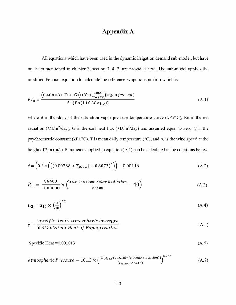
113

Appendix A

All equations which have been used in the dynamic irrigation demand sub-model, but have

not been mentioned in chapter 3, section 3. 4. 2, are provided here. The sub-model applies the

modified Penman equation to calculate the reference evapotranspiration which is:

�� = ��.��×∆×�� ×� ��

��×��×(��)∆�( ×��.��×��)

(A.1)

where ∆ is the slope of the saturation vapor pressure-temperature curve (kPa/oC), Rn is the net

radiation (MJ/m2/day), G is the soil heat flux (MJ/m2/day) and assumed equal to zero, γ is the

psychrometric constant (kPa/oC), T is mean daily temperature (oC), and u2 is the wind speed at the

height of 2 m (m/s). Parameters applied in equation (A.1) can be calculated using equations below:

∆= ,0.2 ∗ */$0.00738 × � "�&+ 0.80722�+-− 0.00116 (A.2)

�� = �� × ��.��×��×��×�� ! ��

"�� − 40� (A.3)

�� = �� × * ��+�.� (A.4)

γ = � �!"#"!��%×&%'(� )�*"!+*��*��.�,,×��%�-%��%(#.� (�*"/�%"(- (A.5)

Specific Heat =0.001013 (A.6)

��("ℎ��(('�� = 101.3 × *#$��%��&.�'(�$�.��'�×��")�� (*

$��%��&.�'(+�.��'

(A.7)

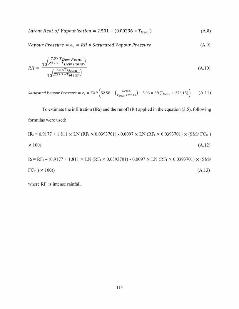
114

3 ��4� ��15 "�'��6 �� = 2.501 − $0.00236 × � "�& (A.8)

5 "�'��(('�� = �� = �4 × 7 �'� ��5 "�'��(('�� (A.9)

�4 = ��

�.×�� .��

��.×�� .��

(A.10)

#$%&'$%()*$+,&'-'(..&'( = ( = /0- 152.58 − 2 �� .�

��.��3− 5.03 × 4567�� + 273.1589 (A.11)

To estimate the infiltration (IRt) and the runoff (Rt) applied in the equation (3.5), following

formulas were used:

IRt = 0.9177 + 1.811 × LN (RFI ×0.0393701) - 0.0097 × LN (RFI × 0.0393701) × (SMt/ FCtc )

× 100) (A.12)

Rt = RFI – (0.9177 + 1.811 × LN (RFI ×0.0393701) - 0.0097 × LN (RFI × 0.0393701) × (SMt/

FCtc ) × 100)) (A.13)

where RFI is intense rainfall.

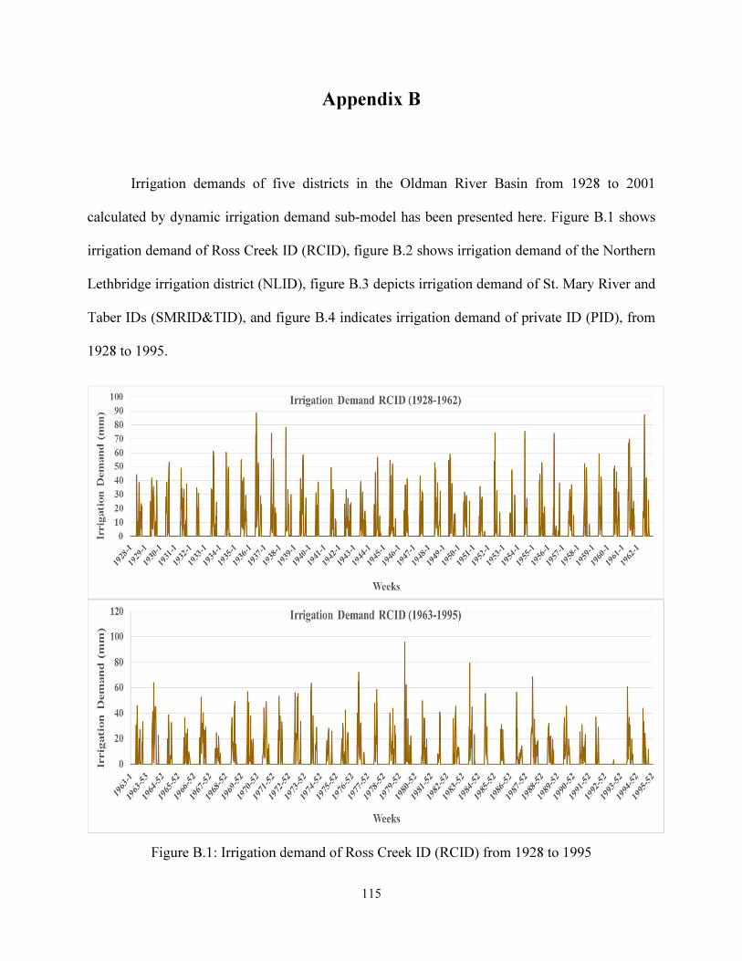
115

Appendix B

Irrigation demands of five districts in the Oldman River Basin from 1928 to 2001

calculated by dynamic irrigation demand sub-model has been presented here. Figure B.1 shows

irrigation demand of Ross Creek ID (RCID), figure B.2 shows irrigation demand of the Northern

Lethbridge irrigation district (NLID), figure B.3 depicts irrigation demand of St. Mary River and

Taber IDs (SMRID&TID), and figure B.4 indicates irrigation demand of private ID (PID), from

1928 to 1995.

Figure B.1: Irrigation demand of Ross Creek ID (RCID) from 1928 to 1995

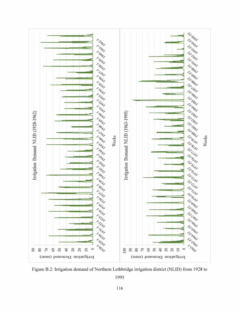
116

Figure B.2: Irrigation demand of Northern Lethbridge irrigation district (NLID) from 1928 to

1995

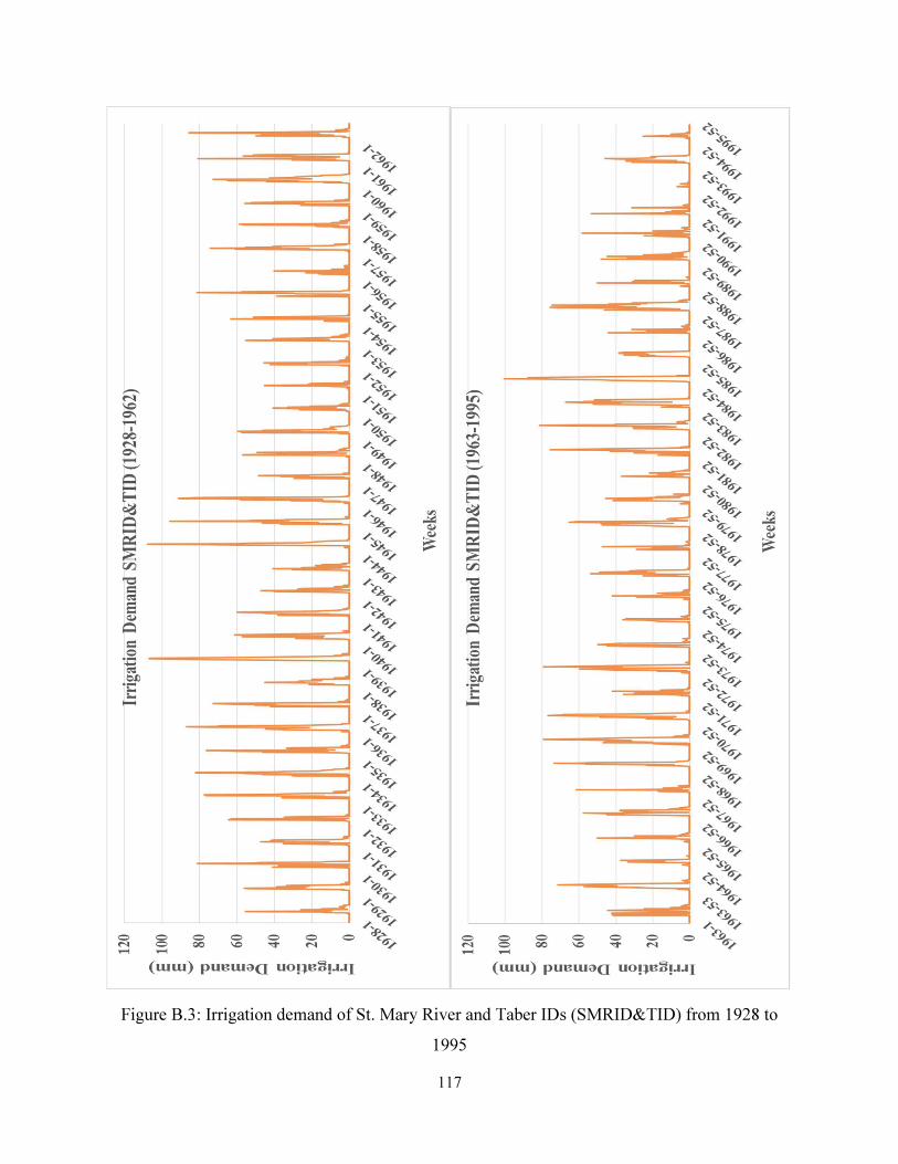
117

Figure B.3: Irrigation demand of St. Mary River and Taber IDs (SMRID&TID) from 1928 to

1995

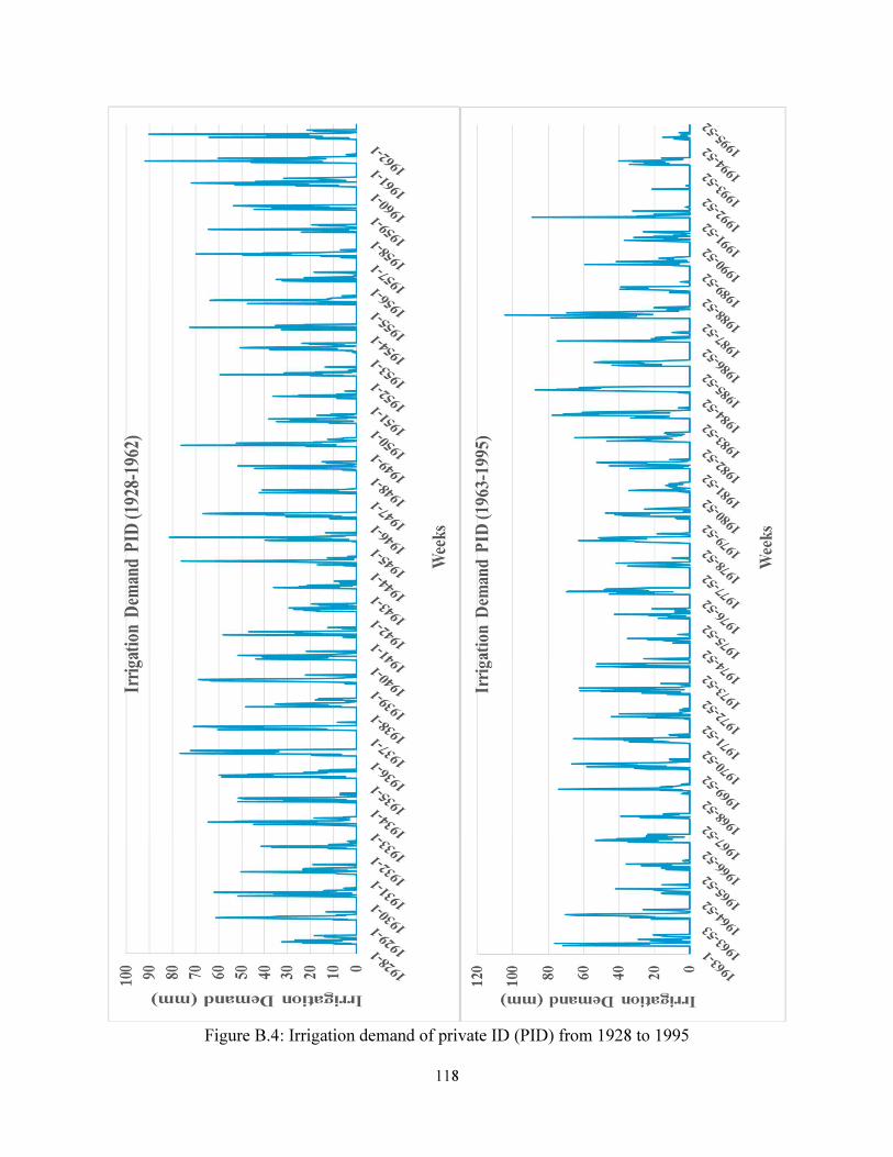
118

Figure B.4: Irrigation demand of private ID (PID) from 1928 to 1995