Integrated Stereovision for an Autonomous Ground · PDF fileIntegrated Stereovision for an Autonomous Ground Vehicle Competing in the Darpa Grand Challenge ... valuable experience

ISSN 0280-5316 ISRN LUTFD2/TFRT--5760--SE

Integrated Stereovision for an Autonomous Ground Vehicle

Competing in the Darpa Grand Challenge

Marie Göransson Erik Johannesson

Department of Automatic Control Lund University December 2005

3

Acknowledgements This work was carried out at the Department of Control and Dynamical Systems at California Institute of Technology, California, USA, in cooperation with the Department of Automatic Control, LTH, Lund University, Sweden. First of all, we would like to thank Professor Richard M. Murray at the Department of Control and Dynamical Systems, California Institute of Technology, and Professor Anders Rantzer at the Department of Automatic Control, LTH, Lund University, for giving us the opportunity of doing our master thesis in this exciting project at the California Institute of Technology. We would like to express our gratitude to all students in Team Caltech for their help, support and friendliness. It was fun working with all of you. Especially Jeremy Gillula, Kristo Kriechbaum and Lars Cremean provided a lot of valuable experience and insight into the problems we were facing. A special thanks to Pietro Perona, Professor of Electrical Engineering at the California Institute of Technology, who gave important advice in the field of computer vision. Also, a special thanks to Tony and Sandie Fender who made our desert experience much more pleasurable by providing us with excellent food. Thanks to Maria Koeper for handling purchasing matters with efficiency and care. Last, but not least, we would like to thank our families and friends in Sweden, for their continuous and valuable support throughout our stay in California.

4

Figure 1: Alice, the vehicle that raced in the DARPA Grand Challenge 2005 for Team

Caltech.

5

1 About this Master Thesis......................................................................................6 1.1 Outline ..........................................................................................................6 1.2 Distribution of Work .....................................................................................6

2 Background..........................................................................................................8 2.1 DARPA Grand Challenge..............................................................................8 2.2 History of Team Caltech................................................................................9

3 Team Caltech and Alice .....................................................................................10 3.1 Team Caltech organization ..........................................................................10

3.1.1 Team Structure .....................................................................................10 3.1.2 Team Operations...................................................................................11

3.2 System Architecture ....................................................................................12 4 Stereovision Theory ...........................................................................................17

4.1 Camera Calibration......................................................................................17 4.2 Stereovision Processing ...............................................................................19

5 The Stereovision System ....................................................................................22 5.1 Hardware.....................................................................................................22 5.2 Software ......................................................................................................23

6 Method of Development.....................................................................................26 6.1 Definition Phase ..........................................................................................26 6.2 Implementation Phase..................................................................................26 6.3 Test Phase ...................................................................................................27 6.4 Further Improvements .................................................................................28

7 Solved Problems.................................................................................................29 7.1 Hardware Configuration ..............................................................................29 7.2 Calibration...................................................................................................30

7.2.1 A Bug ...................................................................................................30 7.2.2 The Calibration Target ..........................................................................31

7.3 Camera Focus..............................................................................................32 7.4 Exposure Control.........................................................................................33 7.5 Sun Blocking...............................................................................................35 7.6 Noise Filtering.............................................................................................36 7.7 Processing Parameter Settings .....................................................................38 7.8 Processing Speed.........................................................................................41

7.8.1 Subwindowing......................................................................................42 7.8.2 Coordinate transformations ...................................................................42

7.9 Dynamic Subwindow ..................................................................................43 7.10 Obstacle Detection and Spatial Filtering ....................................................43

8 Events ................................................................................................................49 8.1 Preliminary/Critical Implementation Review ...............................................49 8.2 National Qualifying Event ...........................................................................49 8.3 Grand Challenge Event................................................................................51

9 Conclusions........................................................................................................54 9.1 Possible Future Work ..................................................................................54

Dictionary ................................................................................................................56 Bibliography ............................................................................................................58

6

1 About this Master Thesis This report describes work carried out by the authors for Team Caltech during the time from the middle of June 2005 until the Grand Challenge Event on October 8th, 2005. Compared to conventional master theses written at LTH, this work differs in a number of aspects:

• Team-based project – All the work was done in the context of an extensive project, in a team consisting of a large number of students. On the project level, the primary goal was to win the DARPA Grand Challenge. However, most of the team members had personal goals related to their own specific research project. Naturally there could be priority conflicts between these goals and team members often had to work on matters important for the whole team, but not relevant for their own research. The nature of the project also conveyed a dependency on the work of others. Development could be hindered because of errors or delays caused by someone else. On the other hand, other team members contributed with important help and advice.

• Strict deadline – Because the Grand Challenge Event was set for a certain date, time was limited. This made it necessary to ensure robustness in basic operations before development of advanced functionality.

• Extremely applied project – Making everything work in reality was of highest importance, considering the project’s primary goal. This required a lot of time being devoted to tests and solving application-specific problems of lesser interest to research.

This report presents the most relevant work performed by the authors. Other work required by the team, but not strictly related to this master thesis, influenced the ability to concentrate on the work described here.

1.1 Outline

Because of what has been said, the structure of this master thesis differs slightly from what is usual at LTH. This report is laid out as follows. The first part (chapters 2 & 3) describes the background of the project, the team organization and the system architecture. The second part (chapters 4 & 5) describes the stereovision system in theory and practice. This is followed by a description of how the work was performed (chapter 6), and a presentation of problems and solutions (chapter 7). The major events during the time period are treated (chapter 8) before the final conclusions are given (chapter 9). A dictionary is provided to simplify understanding.

1.2 Distribution of Work

Erik Johannesson focused on enabling basic operation of the stereovision system. This included working with the following:

• Hardware configuration1 (section 7.1)

1 This work was carried out in cooperation with Jeremy Gillula.

7

• Camera focus (section 7.3) • Noise filtering (section 7.6) • Processing parameter settings (section 7.7) • Processing speed (section 7.8) • Spatial filtering (section 7.9)

Marie Göransson focused on enabling satisfactory operation of the stereovision system under certain special conditions. This included working with the following:

• Exposure control (section 7.4) • Sun blocking (section 7.5) • Dynamic subwindow (section 7.8)

To some extent, the authors cooperated while solving problems in all of the above-mentioned matters. However, the authors worked together with the following tasks:

• Calibration (section 3.2) • Testing (no particular section)

8

2 Background

2.1 DARPA Grand Challenge

In 2003, the U.S Congress asked the Department of Defense (DoD) to make one third of the ground military forces automated by 2015. In response, the Defense Advanced Research Project Agency (DARPA) created a race for autonomous ground vehicles with the purpose to generate research and development in the field. DARPA is the central research and development organization of the DoD in the USA and the race was named DARPA Grand Challenge. Here is a summary of the basic rules and challenges in the DARPA Grand Challenge:

• The team that developed an autonomous ground vehicle that finished the designated route first within 10 hours would win the DARPA Grand Challenge and the grand prize.

• The challenging route was announced to be no more than 175 miles over desert terrain. This required an average speed of 17,5 miles per hour (equivalent to an average speed of slightly less than 30 kilometers per hour) to make the route in less then 10 hours.

• Only publicly available signals (e.g. GPS) were allowed to use for navigation. Otherwise, each vehicle had to be fully autonomous, navigating the route and determining its own path around obstacles using cameras, LADARs and other terrain sensors.

• No communication, except for the emergency stop safety radio and tracking system (E-stop) supplied by DARPA, was allowed. E-stop was used by DARPA as a start/stop actuator of the vehicles as well as for receiving position-track data.

• The vehicles had to find and follow the pre-defined route, avoid obstacles, and negotiate turns. The route was to be received only two hours before the race, given as a Route Data Definition File (RDDF). The RDDF was to contain several waypoints, each specified with latitude, longitude, corridor width in which the vehicle had to stay and speed limit for that section. The route would include a number of different types of terrain such as paved roads, dry lake beds, twisting mountain pathways, and rough off-road desert.

Figure 2: Different types of terrain that occurred in the DARPA Grand Challenge.

9

DARPA Grand Challenge brought together individuals and organizations from a number of different academic and geographical backgrounds in the pursuit of a technical challenge that no one had ever solved before. The Grand Challenge was organized for the first time on 13th March 2004. 15 out of the 100 registered teams emerged and attempted the race. The course went from Barstow, California, to Primm, Nevada, and the prize money was $1,000,000. However, the price went unclaimed as the best vehicle only made about 7.36 of the 142 miles course. DARPA immediately announced a second Grand Challenge, and increased the grand prize to $2,000,000. [2, 3, 5,14]

2.2 History of Team Caltech

Team Caltech was formed in March 2003 to compete in the DARPA Grand Challenge 2004. Representing Team Caltech in the 2004 Grand Challenge was a heavily modified 1996 Chevrolet Tahoe named “Bob”. Bob was fully automated and equipped with a sensing system that included two stereo camera pairs, 2 LADAR units, a GPS/IMU package and one color firewire camera. Bob completed 1.3 miles in the race before he drove into a barbed wire fence and got stuck. Building upon the experiences from the 2004 Grand Challenge, Team Caltech reorganized with a new plan and new vehicle. The goal was simple – victory in the 2005 DARPA Grand Challenge! In December 2004 Team Caltech acquired a new vehicle that was named Alice. Alice is a 2005 Ford E-350 van, modified by the team’s sponsor Sportsmobile for off-road usage. A further description of Alice is located in the System Architecture section. The selection process for the DARPA Grand Challenge 2005 consisted of several different steps In February and March 2005 Team Caltech submitted applications including among other things a vehicle specification sheet and a video of Alice. She was then selected for a site visit from DARPA representatives in May 2005. The site visit included a demonstration of Alice and an interview of the team. Alice had to show safe autonomous operation, e.g. navigation through waypoints as well as obstacle avoidance. She performed well and in June 2005 DARPA announced that Team Caltech was one of the 43 teams selected for the National Qualifying Event in September 2005. [11, 13]

10

3 Team Caltech and Alice

3.1 Team Caltech organization

3.1.1 Team Structure

Team Caltech consisted of a broad range of students from different disciplines and with different experience levels. The team was composed primarily of undergraduate students. In total, 50 undergraduate students have been working on the project. In the summer of 2005, 28 undergraduates, 3 high school students, 4 graduate students and 3 professors were involved in the project, working to prepare Alice for the DARPA Grand Challenge 2005. Team Caltech was organized in three race teams and six additional teams, where the race teams constituted the primary organization structure. Each race team was responsible for some set of software and/or hardware required. The race teams; the Terrain Team, Planning Team and Vehicle Team, and their responsibilities are described in table 1. Each race team was composed by a number of undergraduate students supervised by a graduate student working as a team coordinator and a professor who functioned as an advisor. To ensure that everything was done in a timely manner, to resolve cross-team issues and to keep the project moving forward, Team Caltech also had an Integrated Product Team (IPT). The IPT consisted of the team coordinators, the advisors and some undergraduate students. Because of the desire to have the students making all decisions, the IPT functionality was more about coordination than team management. Each additional team was responsible for a certain set of tasks not specifically related to software or hardware on Alice. The additional teams and their responsibilities are summarized in the right column in table 1. [8, 10, 11]

Table 1: Structure of Team Caltech.

11

3.1.2 Team Operations

The development was performed in a Linux environment and all code was written in C/C++. Team Caltech utilized the following development tools:

• Bugzilla - a database for managing bugs, developed in the Mozilla project. Bugzilla was used to report and assign bugs to appropriate team members, and to keep track of them. It was for example very helpful to see what all team members worked on or planned to work on.

• Subversion – a source code management tool that allows multiple users to simultaneously work on the same set of code. Using this tool, it was possible to log and compare changes in the code.

• Wiki – A wiki page was used for general documentation such as meeting notes, field test plans, hardware and software documentation and team status.

In the beginning of the summer, about 10 new students joined the team (authors included). Therefore the first week was used for getting new team members up to speed, including an introduction to the development tools. Milestones and test plan for the period until the race in October were also worked out during this week. Team Caltech used a spiral development process to guide the efforts. Spirals were phases of three weeks and each spiral added a new layer of functionality that future layers could build upon. The spiral development method was useful for this project, since it required multiple modules, depending on one another, to be developed in parallel. Any given module could always depend on the level of functionality of the other modules in a previous spiral. Goals were set for each spiral and separated into weekly goals for every race team. An extensive test plan was created, to achieve development and testing of individual modules and full integration. Finally all tasks and objectives were assigned to individuals or sub teams. To achieve the milestones and follow the time line, Team Caltech utilized:

• Field tests Team Caltech spent 3-5 days of testing most weeks during the summer. Most of this time was spent on desert testing, although local testing on a parking lot close to Caltech was done sometimes. During autonomous testing, a safety driver was always seated in the driver seat and prepared to take control over Alice by switching from automatic to manual mode. The test manager of the week – usually one of the graduate students, organized the field test. This person was responsible for setting the objectives for the test, tracking the preparations and maintaining the schedule during the test. Students chosen to participate in each test were selected based on which modules would be tested.

• GOTChA charts A GOTChA chart is a simple project management tool that aims to summarize what a project is about and how it will be accomplished. A GOTChA chart has four elements:

o Goals – a high level description of what you want to accomplish. o Objectives – specific goals that you can measure if they have been

completed or not. They should support the overall goals, but they should be more concrete.

o Technical Challenges – a list of problems that might prevent you from accomplishing the goals and objectives.

12

o Approach – a list of activities and strategies that you plan to implement to solve the technical challenges.

An example of a simple GOTChA chart for completing this Master thesis can be seen in table 2.

• Team meetings

Every Monday, the whole team met at a project meeting. The field test manager from the previous week summarized what had been accomplished and what needed further work. The overall team status was checked and compared with the timeline set in the beginning of the summer. The test plan of the current week was updated and the objectives were changed with respect to the results of previous week’s field test and the priority of each module. GOTChA charts were used a lot in the meetings to describe the status of the project. Also each race team had a separate meeting every Monday. In these meetings, all bugs assigned to the team were discussed and the distribution of work within the team was shifted around if needed.

• Bugs

As mentioned above, Bugzilla was a very useful tool for keeping track of all the bugs in the project. It also ensured that no two separate team members worked on the same bug without each other’s knowledge. Furthermore it provided valuable historical data on bugs that were worked on for longer periods of time.

• Review sessions

The team invited industrial and academic experts to review the overall progress. This was done twice during the summer, on two occasions known as the PIR and CIR. These events are described later in the Event section. The experts submitted requests for action for any issue or concern that they felt needed work or attention. This put pressure on the team to achieve results and come up with answers for the next review session and also helped to guide and focus on the goal. [8, 10]

Goals:

- Complete the Master thesis.

Technical Challenges:

- Getting log data from Alice that

have not yet been collected. - Finishing the report on time.

Objectives:

- Complete the final version of

the report on the 22nd of November.

- Hold a presentation on the

29th of November.

Approach:

- Contact the team members that

are studying at Caltech and have access to the log data.

- Create a detailed time-plan for

writing the report.

Table 2: Example of a GOTChA chart.

3.2 System Architecture

Alice is a 2005 Ford E-350 van that has been modified for off-road driving. The modifications include suspension and transmission, as well as electrical power and air handling systems. Both the steering and brake actuators are possible to disable via the throttle switch on the dashboard. When disabled, Alice is in manual operation and completely road-legal. Alice is intended to function as a mobile workstation and the interior is therefore designed as a software development lab. Three team members (safety driver not included) can be safely seated and are able to do code development

13

while Alice is running. Alice’s software systems run on six Dell PowerEdge servers and one quad-core IBM operation-based servers, all running Gentoo Linux. A 4-user KVM (keyboard, video, mouse) switch is used to access the servers, allowing any of the servers to be reached from any of the workstations within Alice. The servers are located in a shock-isolated and climate-controlled computer box.

Figure 3: Throttle switches on the dashboard.

Figure 4: Workstations in the back of Alice.

Figure 5: Alice’s software architecture. (Courtesy of Jeremy Gillula)

Team Caltech’s software architecture is shown in figure 5. State estimation is accomplished through the combination of two differential GPS units, one Navcom SF2050G and one Novatel ProPak-LBplus, to measure absolute position and a Northrop Grumman LN-200 Inertial Measurement Unit (IMU) to measure relative

14

position and orientation. The outputs from these state sensors are combined through Kalman filtering to generate an optimal estimation of state. All modules running on Alice are then able to receive the state information.

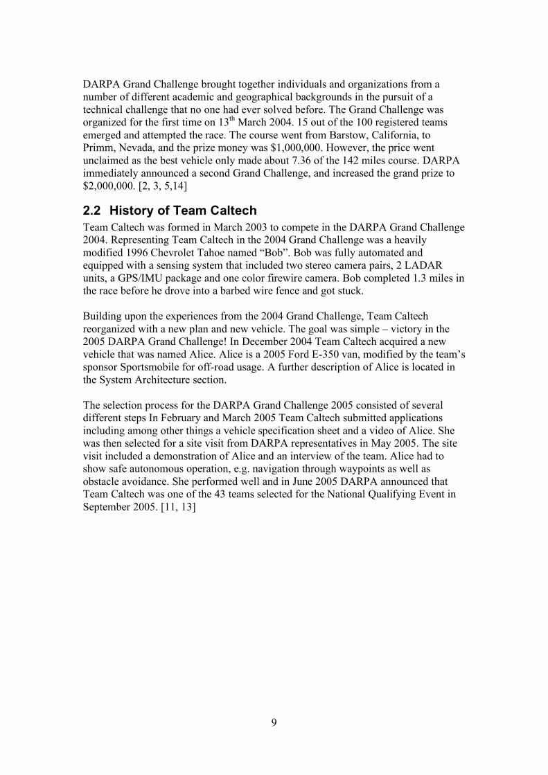
Figure 6: Alice, with terrain sensors marked.

Alice is provided with a variety of terrain sensors with overlapping ranges and capabilities to get a sense of the surrounding terrain. The LADAR units are the main terrain sensors Alice makes use of. A LADAR scans over a certain set of angles in a scan plane and the range is measured for each pulse using the time it takes for it to return. Five LADAR units are mounted on Alice. One SICK LMS-221-30206 is placed on the roof, together with a SICK LMS 291-S14 and a Riegl LMS Q-120i LADAR. Another SICK LMS-221-30206 is enclosed in the front bumper and a SICK LMS 291-S05 is placed on top of the bumper. The LADARs on the roof all have different maximum ranges and are also pointed out at different distances (30, 40 and 65 meters on flat ground). The SICK LADAR in the front bumper is pointed straightforward to detect obstacles independent of range. The one on the top of the bumper is pitched down such that it provides data from the ground just in front of Alice. For the stereovision system, two pairs of Point Grey Dragonfly cameras are used. A detailed description about the stereovision system is in the Stereovision section. A color camera mounted on Alice feeds a road-finding algorithm and is therefore named the Road-finding camera in figure 5. This algorithm uses dominant pixel orientations within an image to estimate direction and location of a possible road.

15

The mapping module creates elevation maps of the terrain using data from each LADAR and stereo pair. These maps, with a cell size of 0.4 x 0.4 m, are then processed to make cost maps for each sensor. Each cell in the cost map contains the maximum recommended speed for that area. This speed is determined by elevation differences to adjacent cells. The cost maps are then fused with the data from the road-finding algorithm and the given RDDF to generate a final speed limit map for evaluation by the planning software. Navigation is accomplished using a deliberative planner. The planned trajectories are optimal in the sense that they constitute the shortest path, in time, through current map, while satisfying dynamical feasibility constraints for the vehicle. The vehicle is approximated by a kinematic bicycle model and the constraints are determined by commercially available algorithms. The trajectory returned by the planner module includes the northing and easting UTM coordinates, and the first and second time derivatives. The trajectory following algorithm includes separate control algorithms for the steering and the throttle and brake actuators. The control signals are then sent to the actuator control module, which translates the commands and passes them to the actuators. The system also includes a supervisory controller module that receives status info from all the other modules. Its objective is to modify the system operations if a fault is detected. In this context, a fault is defined as a state where Alice does not perform as intended. An example is if Alice comes to a stop caused by something that was not detected by the sensors and therefore not expected. A major element of the software infrastructure is the GUI and the logging module. These features allow fast and easy determination of conditions that lead to errors as well as off-line testing of software on logged sensor data. The GUI, which is shown in figure 7, provides the user with the elevation and cost maps from each terrain sensor as well as the final speed limit map.

16

Figure 7: The GUI, here showing a final speed limit map. The blue rectangles represent

Alice. The blue lines and the circle are the RDDF corridor and a waypoint. The red

curve is the traversed path, the violet curve is the current planned trajectory and the

green curve represents the current steering angle. Notice that Alice is heading towards a

ditch.

17

4 Stereovision Theory The goal of computer vision (or machine vision) is to derive information about the real world, given a set of images and possibly some other information, such as facts about the cameras that took the images. Computer vision is a rich and active research field, covering a wide range of theoretical and applied problems, of which only a small subset is relevant here. By stereovision we refer to a special case of a computer vision system, where cameras are used in pairs to generate simultaneous images of the same scene from different locations. Together with information about the cameras, extracted in the process of camera calibration, it is possible to reconstruct a three-dimensional model of the objects seen by the cameras. The output from a stereovision system can be used for navigation and obstacle detection, e.g. on robotic vehicles. Although LADARs seem to be the standard sensor in such applications, stereovision has emerged as a useful alternative and complement. [15] On Alice, the purpose of the stereovision system is to complement the LADAR sensors and add to the overall mapping and obstacle detection ability. Compared to stereovision, the LADARs have higher accuracy and run with a greater frequency. However, there are some disadvantages due to the fact that they only scan along one plane at a time. Stereovision on the other hand processes full images allowing coverage of an extended area in every instant, even when the vehicle is not moving. Also, the cameras usually see the full height of obstacles, regardless of what range it is at (this is not true for LADARs). These advantages of stereovision can be substantial in certain situations, such as when passing turns or crests, or driving over rough parts (where the vibrations can cause the LADARs to miss parts of the terrain). Considering the application there is a lot of interesting theory to mention, although a full description of the theoretical framework and all the related results is out of the scope of this thesis. In this section only a brief introduction to the theory behind stereovision will be given, with the purpose of providing the reader with a basic understanding of the underlying principles of the system, as well as an understanding of the described problems and their solutions. We first give an introduction to camera calibration and then describe how stereovision processing is performed.

4.1 Camera Calibration

To reconstruct a three-dimensional model with the use of images, it is necessary to have a model of the camera (i.e. how the camera projects points in the world to points in the image). The standard model is the pinhole camera, which is given by the projection equation

!

s ˜ m = A R t[ ] ˜ M

where s is a scale factor,

!

˜ m is the image coordinates and

!

˜ M is the world coordinates.

The two latter are written using homogenous coordinates, such that

!

˜ m = u v 1( )T

(1)

18

and

!

˜ M = X Y Z 1( )T

. The matrix

!

R t[ ] , called the extrinsic parameters, is

composed of a rotation matrix R and a translational vector t, describing the placement of the camera relative to the world coordinates. The matrix

!

A =

" # u0

0 $ v0

0 0 1

%

&

' ' '

(

)

* * *

is called the camera intrinsic matrix and contains the internal parameters of the camera: (u0,v0) are the coordinates of the principal point (where the focal point is projected), ! and " are scale factors in image u and v axes, and # is a measure of the

skewness of the image axes. The " parameter is equal to the focal length f of the

camera, which is sometimes factored out of ! and #.

In addition to the pinhole camera model, it is usually necessary to take into account some nonlinear effects in the camera lens, especially radial distortion that “bends” the image in the sides. Radial distortion is significant for most cameras, in particular for those with a wide field of view. Radial distortion is modeled by transforming the image coordinates according to a nonlinear function of the distance to the principal point. The resulting camera model describes the relation between world and image coordinates as a composition of transformations that contain a number of parameters, as seen above. The parameters are often divided into intrinsic, such as focal length, radial distortion constants, etc., and extrinsic, which is essentially the position of the camera. Camera calibration is the process of determining (estimating) these parameters. Camera calibration is usually performed by taking a number of images of a known geometry, usually a planar target with a texture that facilitates extraction of some unique points (such as a checkerboard pattern). By fitting the parameters to the known geometry along with the resulting images, the parameters can be estimated. The procedure often involves an initial closed-form solution that is further refined by nonlinear optimization. When calibrating a pair of stereo cameras, it is also necessary to find the geometrical relationship between the cameras. The camera frame is then considered equivalent to the coordinate frame of the left camera. The problem of finding the relationship between that coordinate frame and the world coordinate frame is here defined as external calibration, while all the other parameters are said to be covered by internal

calibration. Internal calibration of stereo cameras can be performed as usual with a checkerboard target, although of course two separate images are taken for each placement of the target. [7, 9, 12, 16]

(2)

19

Figure 8: El Mirage dry lake bed, where most of the external calibration was done.

Here, external calibration was performed afterwards. The rotation of the left camera was found by placing the vehicle in a (approximately) known environment: a dry lake bed, which was the flattest ground available. The pitch and roll parameters where adjusted while the resulting elevation maps were inspected – a non-flat map indicated an error in the parameters. The yaw parameter was assumed to be zero. The translation of the left camera was estimated using a tape measure.

4.2 Stereovision Processing

Once a stereo pair is calibrated, it is possible to find the world coordinates for any point, given the corresponding image coordinates in both images, by using the camera models and triangulation (i.e. solving a system of two projection equations). The main problem lies in finding the corresponding image coordinates in the other image, for a given point in one of the images. This is known as the correspondence problem, and is by no means trivial. In the ideal stereo setting, the cameras are placed such that the image planes are parallel and the images are lined up with each other. Also the focal lengths are the same and the focal points are horizontally aligned. In this special geometry, every point has the same vertical image coordinates in both images. This greatly facilitates the correspondence problem since search is only necessary along the horizontal axis.

20

Figure 9: The ideal stereo setting (from [7], with permission). (X,Y,Z) is the camera

frame, (u, v) and (u’, v’) coordinates in the left and right images, f the focal length,

CX,CY the (identical) image planes and TX the baseline. S is an arbitrary point, which in

this setting is projected such that v = v’.

Unfortunately, in reality the conditions of the ideal stereo setting are not fulfilled. But since we have information about the deviation from the ideal setting (given by calibration) this can be compensated for by image rectification. The rectification step consists of multiplying both images with their respective rectification matrix, a 3x3 matrix, which corresponds to an affine transformation determined by the calibration. The result is an image pair that adheres to the requirements of the ideal stereo setting. The matching of a point in one image with a point in the other image is usually done using correlation methods. E.g. corresponding points can be found by minimization of

!

M d( ) = Il x,y( ) " Ir x " d,y( )( )2

x,y( )#$

%

or some similar expression, where $ denotes the correlation window (usually a

square), Il and Ir the intensities in the left and right images, and d, the relative difference in the horizontal image coordinate, is called the disparity. Since the images are irregular, the minimization is done by evaluation of all possible values of d, with some upper bound (obviously d is always zero or positive since the point is located in front of the cameras). The minimum value is often required to be below a certain threshold for a match to be considered. Thus, a match is not always found. Once a match is found, the disparity is used to calculate the location of the point in the camera frame, from which it can be transformed into world coordinates as discussed above. There are plenty of parameters that can be used to control the way the correlation method works, and they all have different effects on the accuracy, noise level, robustness and speed of the processing. Some of the parameters that can be altered are

(3)

21

the size of the correlation window, the threshold level for a successful match and the bounds on the disparity search. Further, it is possible to scale down the image to a lower resolution and do the correlation on several scales. This is called multi-scale processing. It is also frequent to use some kind of additional error filter, such as the left/right check. This check requires a match to be verified by also being the optimal match when the optimization above is instead performed from the right image to the left image (this is done by exchanging the left and right indices in equation 3). [7, 9, 15]

22

5 The Stereovision System

5.1 Hardware

Four IEEE-1394 (Firewire) digital cameras are used. The cameras are produced by Point Grey and the model name is Dragonfly. The CCD is a Sony 1/3”, the resolution is 640x480, black & white version. The circuit board, which is placed in a black metal case, can be seen in figure 9.

Figure 10: The Dragonfly Firewire camera from Point Grey.

Figure 11: The Fujinon TF2.8DA-8 (left) and the Kowa LM8JC lenses, used for short

and long range respectively.

The cameras are arranged in two stereo pairs, known as the short range and the long range pair. The baselines, the distances between two cameras in a pair, are approximately 0.6 and 1.5 meters respectively. The short range cameras are equipped with Fujinon TF2.8DA-8 lenses, with a focal length of 2.8 mm. The field of view is approximately 89° horizontally and 69° vertically. The long range cameras are

equipped with Kowa LM8JC lenses, with a focal length of 8 mm. The horizontal field of view is approximately 34.5° with the 1/3” CCD. To achieve focus with these lenses

and cameras, it is necessary to use extension rings and spacers. To each lens is attached a C-Mount extension tube, 5 mm, from Edmund Optics. The short range lenses also have a 1 mm Pentax spacer. To compensate for reflexes caused by indirect sunlight, linear polarized filters were placed in front of the long range lenses. Unfortunately, no filters could be found that fit with the short range lenses.

23

Figure 12: The camera casing and the whole camera mount.

The cameras, including the original metal case, are placed in aluminum boxes, which are tightly screwed to a 1.5 meters wide aluminum bar. The bar is mounted on the vehicle above the windshield as seen in figure 12. The purpose of this setting is to preserve calibration, i.e. the exact placement of the cameras, while driving in rough terrain. In figure 12, left picture, a brown pipe is visible above the lens. This is the lens cleaning system, which removes dust from the lenses by exerting a burst of air approximately twice every minute. Dirt on the lenses and inside the cameras (on the glass covering the CCD) was cleared by using optic cleaning solution (methanol) applied to a sheet of lens cleaning paper.

5.2 Software

The software module that takes care of the stereovision processing is called StereoFeeder. A flowchart of the processing can be seen in figure 13, where the green boxes represent data that is generated by StereoFeeder. Most of the steps follow the presentation given in the theory section. To give a full view, some of the mapping functions (yellow boxes) have also been included even though they are not managed by StereoFeeder. Most processing steps (rectification, correlation and reprojection) are performed by a stereo processing engine. The engine is included in the software package Small Vision

System (SVS), developed by SRI International. This software contains, along with some stand-alone applications for simple stereovision applications, an API that lets the user integrate the computational algorithms of the processing engine with their own software. The API includes function for the above processing steps, as well as for setting the parameters that are used in the processing. SVS also includes an application for stereo camera calibration, which was used in the project. [7]

24

Figure 13: Flowchart of the major steps in stereovision processing.

Even though SVS handles most of the computations, all the intermediate data is available for display or manipulation (although sometimes a creative solution was required to get access to or manipulate the data in a certain way). Had this not been possible it would have been absolutely necessary to acquire or develop a new processing engine. As will be seen, some major improvements of the processing was necessary in order to make it work acceptably. The StereoFeeder code is organized in three different C++ classes:

• StereoSource handles the generation of images: Communication with the firewire driver, or the loading of logged image sequences into memory.

• StereoProcess is a wrapper class around the processing engine; it handles all communication with the API.

• StereoFeeder is the main class. It takes care of integration with other modules and the user interface. It uses functions in the other classes to perform the steps in the processing flow.

Video Stream

Firewire camera driver

Image Pair

Internal Calibration

Rectification

Rectified Image Pair

Disparity Map

Correlation Algorithm

3D Points (Camera Frame)

3D Points (UTM Frame)

Reprojection Transformation

Elevation Map

Elevation Fusion

Cost Fusion

Cost Map

External Calibration & Vehicle State

25

Figure 14: StereoFeeder user interface.

The current user interface of StereoFeeder can be seen in figure 14. When running the module, it is also possible to show the rectified images and the disparity image in separate windows. This is to be used for testing only since the displaying decreases the processing speed.

26

6 Method of Development This section gives an idea of how the stereovision development described in this report was done in context of the project. To maintain flexibility, no strict plan was laid out in advance for how to solve a problem. In general, the described process was adopted although there were deviations in some cases. Such deviations could be caused by different structure of the problems or varying requirements and deadlines at project level.

Figure 15: The three development phases and their major components.

6.1 Definition Phase

The main source where problems originated was the test plan. The test plan described, for each week, a set of tests that would be performed, as well as specific functionality that was supposed to be demonstrated during the test. The test plan highly affected which problems were worked on as well as the order. The problems in the test plan mostly concerned new functionality. Another major source of new problems was the field test notes. During each field test, any issues or suggestions for improvements were entered in the notes and later assigned to the person responsible for the relevant module or functionality. Most often, the problems discovered in field tests were related to errors in existing functionality. Correction of such errors generally had a higher priority than the addition of new functionality. During this phase, a Bugzilla entry was created for tracking and the problem was assigned. The assignee then started to think about how to solve the problem, using help from other, more experienced, team members and expert advisors. The result of these discussions and some information searching was a preliminary solution idea. If needed, this idea was also discussed with team members responsible for anything that would be affected by the solution, e.g. if their module was to interface with new code. The length of this phase varied greatly for the specific problems discussed in this report. Most often, time did not allow for finding, developing and comparing many possible solutions. The most simple one was often the one used.

6.2 Implementation Phase

In some cases it was desired to do a concept test of the solution before it was actually implemented in the module. For example, an algorithm could be implemented in

Definition - Problem recognition

- Information search

- Discussion

- Solution idea

Implementation - Concept test

- Implement

- Debug

- Simulate

Test - Stand-alone

- Open loop

- Closed loop

- Log data analysis

27

Matlab and tested offline on log data, before adding it to the module. Also, an algorithm could be developed in a stand-alone program that was tested on live data, before integration with the existing system. These approaches made it easier and faster to find some errors and to refine the functionality, because of the isolation. The obvious disadvantage was that the algorithm also had to be implemented twice. Nevertheless, this method proved important. Due to the complexity of the system it was important to verify that no other functionality was affected by the addition of new code. Therefore the code was continuously tested during the implementation. Correct operation of algorithms was verified using output of status messages and variable values, as well as simulations using log data. When needed, debugging was performed using the GDB debugger.

6.3 Test Phase

Due to the applied nature of the project, the test phase constituted a major part of the work. It was essential that reliable operations of all the modules could be guaranteed in race-like conditions. The first tests were often performed in the garage. If Alice was unavailable the cameras could be unmounted and connected to another computer. That way stereovision could be tested on its own. When testing in the field, new code was often first tested in open loop, meaning that the output of the stereovision module was not forwarded to the mapping module. The output was instead inspected visually using the GUI, while the vehicle was either driven manually or autonomously using only the LADAR sensors. The purpose of open loop testing was to determine if it was safe to use a new version of the stereovision module for autonomous driving. If the output was acceptable, closed loop testing followed. During these tests it was sometimes desired to see how the output of the stereovision module affected the overall performance. This was achieved by evaluating performance of the whole system when different sensor configurations were used. At other times it was desired to see how some new piece of functionality in the stereovision module contributed to its output. Running different versions of the module under similar conditions usually did this. In some instances, additional improvements such as parameter tweaking, was done during testing. However, it was usually better to collect a set of log data to analyze back at campus for further improvements. The advantage with log data was that different parameters or implementations could be tested under the exact same conditions. However, in closed loop testing, it was possible to immediately know how the whole system reacted to a certain change. The difficult and uncomfortable conditions in which the field tests were carried out (such as very high temperatures, lack of cold water, long test runs with few breaks) naturally resulted in tests being less efficient or systematic than otherwise possible. Also, the testing time was sometimes limited, because of practical reasons or other tests having higher priority.

28

6.4 Further Improvements

Depending on the results of the field tests and the prioritization of other tasks, further refinement of the solution could be done. If it was found that the tested solution was insufficient to solve the problem, this could involve improvement of the idea behind the solution (a move back to the definition phase). If it on the other hand was found that the code did not behave as desired even though there was nothing wrong with the principle behind it, further work was devoted to the implementation (a move back to the implementation phase). Further improvements also included solving bugs found in the existing code.

29

7 Solved Problems In the beginning of the summer, stereovision was not ready for usage. There was a stereovision module with code that had been used on Bob. However, stereovision had never been tested on Alice and the system architecture had undergone substantial changes since the vehicle change. Only one, uncalibrated, camera pair was mounted. The cameras were out of focus and had bad aperture settings. To make stereovision work, many problems had to be solved, and a lot of testing had to be done. The problems, and their solutions, are described in the following subsections. The presentation generally starts with a description of the problem, followed by the solution and its motivation. The outcome is also discussed, when appropriate.

7.1 Hardware Configuration

When discussing camera calibration, it was realized that the existing Pentax lenses were inappropriate for rough driving. The lenses were not at all sturdy, when attached to the camera they could in fact be slightly bent using only light pressure from the side. If the lenses move relative to the camera, the calibration is degraded. Because of this, it was decided to purchase new lenses. Acquiring new lenses also allowed a choice of new focal lengths. All of the old lenses had a focal length of 2.8 mm, which is quite short. A short focal length gives a wide field of view, resulting in lower resolution if the number of pixels, determined by the cameras CCD, remains constant. Since there were two camera pairs, it was decided that one of the pairs was to be used for short range stereovision, and the other for long range stereovision. The range at which the camera pairs operate well is not only determined by focal length, but also by the baseline. A wider baseline gives a larger difference between the images, increasing the disparity values at every range. When the resolution is increased in disparity, so is the operating range. However, a wider baseline makes the correspondence problem more difficult, since the images are less similar. It also makes calibration more difficult since the calibration target has to be further away to be inside both images, resulting in a lower accuracy. The relation between range and disparity is given by

!

r =bf

dm=bf

dpw

where b is the baseline, f the focal length, dm the disparity in meters, and d the disparity in pixels. pw is the pixel width. [7] If this equation is rewritten and differentiated, it leads to an expression for range resolution, the smallest discernable range difference:

!

"r =r2

bf"dm =

pwr2

bf"d

(4)

(5)

30

Here, %r is the range resolution and %d is a change in disparity. The equation can be

modified with regards to sub-pixel accuracy by simply multiplying the pixel width with the inverse of the resolution (2 for 0.5 sub-pixel accuracy etc.). The SVS manual states that the processing engine interpolates disparities to 1/16th of a pixel, but a value of ! was used in the calculations since the actual accuracy was thought to be lower. It was desired that stereovision would have a range resolution of at least 0.2 m at maximum operating range. In relation to the total sensor coverage, maximum operating ranges of 10 and 40 m for short and long range respectively seemed appropriate. After testing some different values and expert consultation it was decided to use the values in table 3.

Parameter Short range Long range

f 2.8 mm 8 mm

b 0.6 m 1.5 m

Table 3: Hardware configuration parameters.

The actual lenses purchased are described in the Hardware subsection of The Stereovision System section. The chosen parameters worked well, and the new lenses were more mechanically robust than the old ones.

7.2 Calibration

7.2.1 A Bug

Most of the bugs that were fixed are not explicitly described in this report. However there was one bug that deserves a presentation, since it had a significant impact. When starting to test stereovision it was discovered that the generated disparity images were of very low quality, not to say completely faulty. They seemed to mostly consist of spurious objects as well as random noise. The conclusion was that the calibration was off. Numerous recalibrations were performed, all with similar results. The mean pixel errors, an error measure that the calibration software computes by projecting the estimated position of the calibration target and comparing with the actual image, were around 0.15, which is satisfactory (according to expert advisors, values below 0.2 are acceptable). Nevertheless, the problem remained. A lot of effort was put into adjusting the processing parameters. It was sometimes possible to get disparity images, in which objects were identifiable, but there were still a lot of noise and strange errors, e.g. some distant mountains were identified as being quite close. Using the stand-alone stereo processing application to test the calibration, it was found that it was possible to get high quality disparity images. This led to the suspicion that something was wrong in the code. Debugging started with use of artificial images for processing. That way it would be easier to characterize the nature

31

of the error. One hypothesis was that the left and right images were somehow mixed up, although no substantial difference could be noticed when switched. Finally, a test was made to see if the calibration parameters actually made any difference, by entering completely unreasonable numbers in the configuration file. It was discovered that this made no difference at all. Once realized that the calibration had no effect, it was easy to find the bug: The line of code that called the function that performs rectification had been commented out by mistake. It was a simple problem to fix, but not knowing what caused the problem did cost a lot of valuable time.

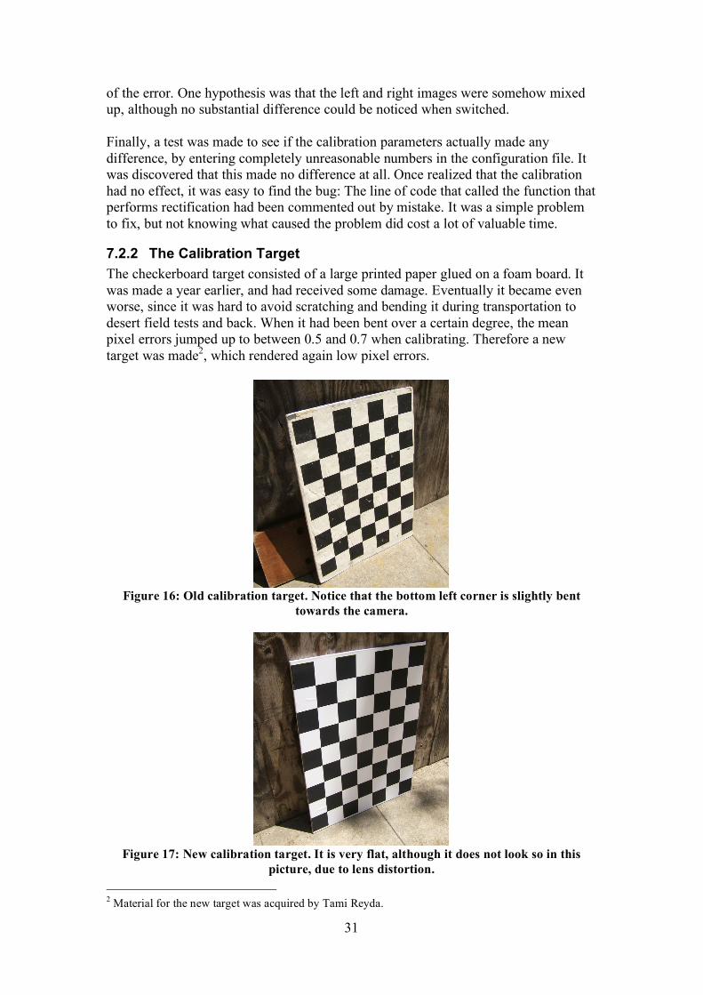
7.2.2 The Calibration Target

The checkerboard target consisted of a large printed paper glued on a foam board. It was made a year earlier, and had received some damage. Eventually it became even worse, since it was hard to avoid scratching and bending it during transportation to desert field tests and back. When it had been bent over a certain degree, the mean pixel errors jumped up to between 0.5 and 0.7 when calibrating. Therefore a new target was made2, which rendered again low pixel errors.

Figure 16: Old calibration target. Notice that the bottom left corner is slightly bent

towards the camera.

Figure 17: New calibration target. It is very flat, although it does not look so in this

picture, due to lens distortion.

2 Material for the new target was acquired by Tami Reyda.

32

7.3 Camera Focus

Initially, the camera focus was manually set before calibration. Adjusting the focus changes the focal length, which makes a recalibration necessary. This was easy in theory but harder in practice. A knob on the lens had to be turned while looking at the resulting image and, more or less, arbitrarily deciding on a good setting. Usually, this had to be done standing on Alice’s hood in daylight while looking at a laptop screen, trying not to be in front of the camera. To improve the resulting focus a semi-automatic focus-setting process was developed. The idea was to have an objective measure of the quality of the focus setting, for a certain range. Such a measure could typically be related to image contrast. If the measure is computed continuously in real-time, it would be possible to look at a plot and see if a small movement of the knob led to better or worse focus. A program was implemented in Matlab that loads the newest image file in a directory and computes a contrast measure in a given rectangle within the image. The program lets the user define the rectangle at startup. The contrast measure is the sum of the 100 largest, in absolute values, intensities in the image that is generated by convolution of the original image with the matrix

!

C =

0 "1 0

"1 4 "1

0 "1 0

#

$

% % %

&

'

( ( (

The reason for not using the average value of all the values within the rectangle is that the proposed measure was less sensitive to natural variations in intensity.

Figure 18: The graph shows the focus measure (no averaging) computed on the area

inside the red rectangle as the focus knob is turned from one endpoint to the other and

back. The measure has a much higher value when the image is sharply focused.

When used in practice, the rectangle where the measure is computed was defined over an area covered by an object, e.g. a house wall with texture, at a distance close to the desired operating range. In order to make the plot less sensitive to noise, the contrast measure was averaged over 10 images. For each change in the focus setting, the plot was observed to see if the focus had become better or worse, and a maximum could quickly be reached.

(6)

33

7.4 Exposure Control

Exposure is the total amount of light allowed to reach the CCD of the camera, and it is controlled by shutter speed and lens aperture. Slower shutter speed and greater lens aperture produce greater exposure. The lens aperture was set mechanically by turning a knob on the lens. With a set aperture, the exposure was thus controlled by the shutter speed. The driver for the Dragonfly cameras allowed manual or automatic exposure control. Manual exposure control let the user set the shutter speed. In automatic control, the camera software controlled the exposure through the shutter speed, based on the average brightness of the whole image. In the beginning, automatic control was used by default. This caused problems when facing the sun. In this situation the sky became extremely bright in the image and to compensate, the exposure was controlled such that the ground became almost black. This resulted in images with small intensity variations, which makes it more difficult for the correlation algorithm to find any matches. The difference between figure 19 and 20 can be seen clearly, even if it’s cloudy and the sky is not as bright as it could be.

Figure 19: Using automatic exposure control, not facing the sun.

Figure 20: Using automatic exposure control, facing the sun.

Changing to manual exposure solved the problem and an alternative controller was implemented to compute the exposure. It was shown, through testing, that a simple

34

proportional gain controller was enough. The region of interest, which is the same as the subwindow described later, excluded the sky and therefore enabled for a more appropriate measurement value to be selected for the controller. This value chosen was the average brightness of the subwindow. The reference value was chosen as the intensity value just between black and white, 128.0, since the intensity is described by an integer in the range 0-255. The controller computed the exposure as:

!

u(t) = u(t "1) + K(yref " y(t))

where t is the index number of the grabbed image, u the exposure, K the controller gain, yref the reference value and y the measurement value. A sufficient controller gain was found by analyzing the step responses for different values of the gain. Letting the automatic exposure stabilize, when facing the sun, and then changing to manual exposure control created the step response. The value of the gain that corresponded to the fastest stabilization of the measurement value was chosen as the controller gain. The control algorithm was only operating on the left image, since this made the calculations faster. To enable use of the same exposure on the right camera, the apertures had to be the same size. This condition was assured by testing if the measurement values from both cameras were the same, for some different light conditions. Only using the average brightness value might seem simple but through testing this was shown to be sufficient. Figure 21 and 22 shows the result when facing the sun. The exposure control also worked well when turning away from the sun. The images also show sun glare, which is discussed in next section.

Figure 21: Region of interest while facing the sun, using automatic exposure.

Figure 22: Similar conditions as in figure 21, but using the implemented exposure

control.

(7)

35

7.5 Sun Blocking

When facing the sun there might be glare effects as can be seen in figures 21-23. Complex reflections within the camera optics in combination with the aperture give rise to circular glare while reflections from reflective surfaces and direct sun light appear as straight lines. In worst case, the sun glare could be misinterpreted as obstacles by the stereo processing algorithm. Since sun glare can arise in many different shapes, it was hard to find a general solution. Adding polarization filters to the camera lenses eliminated glare caused by reflection from other objects, e.g. vehicles. Unfortunately, as said in the hardware section, no filters could be found for the short range lenses. The remaining glare was unfortunately not that easy to remove. Implementing an algorithm that kept track of the position of the sun relative to the cameras solved the problem. Spherical polar coordinates, & and ', were used for the relative position. A certain area, %' ( %& with

the sun in the center, was selected to be set to zero intensity i.e. painted black. If part of the area was in the cameras’ field of view, the overlapping area was painted black in the left image. The parameters %' and %& was chosen such that, if the sun was in

the center of the field, the whole left image was painted black. Also, tests were done to make sure that the left image never showed any sun glare while not eliminating too much valuable information. Since the region was painted black in the left image, while remaining unmodified in the right image, the correlation algorithm could not find any matches in this region.

Figure 23: Left (on top) and right image from short range cameras when facing the sun

and sun covering was active.

The solution worked, however it was not optimal since a lot of useful information was disregarded. Far from all images contained sun glare, even when Alice was facing the sun. Unfortunately, there was not enough time to find a solution where the images first were analyzed if they contained sun glare or not. If that had been done, the sun blocking could have been used only when necessary. Figure 23 shows black-painted areas in the left images, covering the sun glare.

36

7.6 Noise Filtering

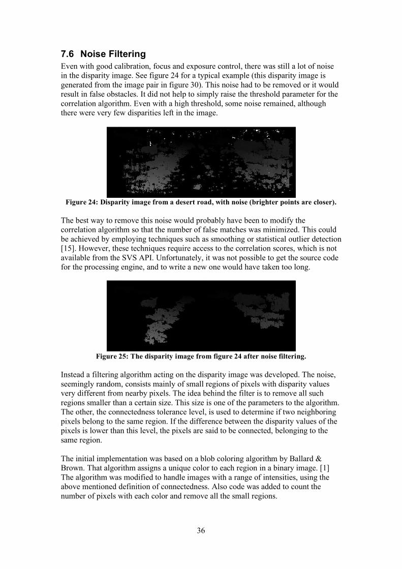
Even with good calibration, focus and exposure control, there was still a lot of noise in the disparity image. See figure 24 for a typical example (this disparity image is generated from the image pair in figure 30). This noise had to be removed or it would result in false obstacles. It did not help to simply raise the threshold parameter for the correlation algorithm. Even with a high threshold, some noise remained, although there were very few disparities left in the image.

Figure 24: Disparity image from a desert road, with noise (brighter points are closer).

The best way to remove this noise would probably have been to modify the correlation algorithm so that the number of false matches was minimized. This could be achieved by employing techniques such as smoothing or statistical outlier detection [15]. However, these techniques require access to the correlation scores, which is not available from the SVS API. Unfortunately, it was not possible to get the source code for the processing engine, and to write a new one would have taken too long.

Figure 25: The disparity image from figure 24 after noise filtering.

Instead a filtering algorithm acting on the disparity image was developed. The noise, seemingly random, consists mainly of small regions of pixels with disparity values very different from nearby pixels. The idea behind the filter is to remove all such regions smaller than a certain size. This size is one of the parameters to the algorithm. The other, the connectedness tolerance level, is used to determine if two neighboring pixels belong to the same region. If the difference between the disparity values of the pixels is lower than this level, the pixels are said to be connected, belonging to the same region. The initial implementation was based on a blob coloring algorithm by Ballard & Brown. That algorithm assigns a unique color to each region in a binary image. [1] The algorithm was modified to handle images with a range of intensities, using the above mentioned definition of connectedness. Also code was added to count the number of pixels with each color and remove all the small regions.

37

The Ballard & Brown algorithm has a drawback in that it is quite time-consuming. At first glance, the time complexity of the algorithm looks linear in the number of pixels since it only processes each pixel once (top-down, left to right). However, it requires keeping track of equivalences between different colors: If the algorithm encounters a pixel that connects two regions (of different color), it has to repaint one of the regions or consider the colors equivalent. From looking at printouts, it was learned that this happened very often. Thus, it was essential to implement this re-coloring in a very efficient manner. Three different implementations were written in C++ and tested on real data. The first version used the standard Vector class to manage the coloring. Each color had its own vector in which the pixel indices were stored. When two colors were recognized as equivalent, all the elements of one vector were moved to the other. The second version used instead the Set data structure to represent the equivalences. An array was used to hold pointers to sets containing numbers representing the colors. Each color had its own pointer, but two pointers would point to the same set if the colors were equivalent. When two colors were considered equivalent, the union was taken of the relevant sets and the pointers updated to point to it. It turned out that both of these implementations increased the processing time with approximately 15 %, which was unacceptable given the simplicity of the filter. The final implementation used a simple recursive flood-filling algorithm. When a new region was encountered, it was given a new color, and the recursive coloring function was called for all of the adjacent pixels that within the connectedness tolerance level. This implementation was of linear time complexity and was much faster than the others. It was actually so fast that it reduced the processing time for a frame. This was possible because fewer reprojections and coordinate transformations had to be done after the filter had been applied. The result when the filter was applied to the disparity image in figure 24 can be seen in figure 25. All the noise from the old image seems to have disappeared, with the loss of some useful data as well. This was the result with the final settings for the two parameters. Similar images for other parameter settings can be seen in figures 25-29, with the parameters specified in table 4.

Figure Region size

threshold

Connectedness

tolerance level

25 350 8

26 50 8

27 1200 8

28 350 4

29 350 16

Table 4: Parameter settings for the noise filters used in figures 26-29.

38

Figure 26: The disparity image from figure 24 after noise filtering. For this image, the

filter’s region size threshold is 50 and the connectedness tolerance level is 8.







7.7 Processing Parameter Settings

The SVS API makes it possible to adjust some parameters involved in the stereo processing. The parameters are:

• Window size – The size of the correlation window. More specifically it is the length of the side as the window is a square. A small value can give more detail but is more noise-sensitive. A large window gives smoother disparity images but less detail.

39

• Number of disparities – The number of points at which the correlation score is calculated. A larger number means that the volume in space where points can be matched is made larger. On the other hand this increases processing time.

• Threshold – A value indicating how good the best correlation score has to be in order for it to be considered a match. Here, higher threshold means fewer matches, as opposed to the presentation in the theory section.

• Uniqueness – A value indicating how much better the best correlation has to be than all the other scores, for it to be considered a match. Higher uniqueness value means fewer matches. This filter is supposed to be useful near edges of objects.

• Multi-scale – A binary parameter that determines if multi-scale processing is active or not.

Also, there are the two parameters for the disparity noise filter that were discussed in the previous subsection. See [7] for more detailed information about the parameters. How these parameters influence the result is shown in figures 31-35, where the same image pair (figure 30) has been processed with different settings. The disparity noise filter was not used in the generation of these disparity images, since it makes it difficult to see the effects of the individual parameters.

Figure 30: Short range image pair from a typical desert road.

Figure 31: Disparity images generated from the image pair in figure 30, with the

processing parameter “window size” set to 7, 9 and 15 respectively. (Brighter points are

closer.)

40


processing parameter “number of disparities” set to 32 and 128 respectively. Note that

the color scales are different in the two images.


processing parameter “threshold” set to 0, 11 and 20 respectively. Note that a lot of the

noise remains even as the matches become fewer.


processing parameter “uniqueness” set to 10, 25 and 38 respectively. This parameter

seems to be more useful than “threshold” in terms of signal/noise ratio.

Figure 35: Disparity images generated from the image pair in figure 30, with multi-scale

processing off and on respectively.

41

To find the optimal set of parameters or, more realistically, a good one, log data was used to test different configurations. This problem can be regarded as a multidimensional optimization problem. However, it was not clear how to evaluate the performance of different parameter settings objectively. It would have been possible to formulate a cost function to be minimized by a good setting, but that approach was not considered to contribute enough to be worth the time it would have taken to develop it. Instead a trial and error-scheme, with more or less sophisticated guessing, was used. The objective was to achieve a good compromise between getting as much good data as possible, while keeping the amount of noise to a minimum. The amount of noise was critical since spurious obstacles in the map could severely decrease the speed, and/or cause Alice to make faulty decisions. The performance of a configuration was determined by inspection of disparity images as well as elevation maps. Since some parameters have a more fundamental impact on the result, while others are simply used to remove certain points, the former were fixated first. Correlation window size and multi-scale belong to this group. Once they were set, it was easier to set the others. The threshold and uniqueness parameters had to be configured while also taking the disparity noise filter into account. The final parameters were chosen to be slightly different for the short and the long range camera pairs. This was mainly because they operate at different ranges, and have different relationships between disparity and range. For example, the Noise filter connectedness tolerance level is lower for long range since a certain difference in disparity corresponds to a greater range difference when at a greater range. Parameter Final Value

Window size 9

Number of disparities 128

Threshold 11

Unique 25

Multiscale On

Noise filter threshold 350

Noise filter connectedness tolerance level 8

Table 5: Short range processing, final parameter values.

Parameter Final Value

Window size 9

Number of disparities 128

Threshold 15

Unique 25

Multiscale On

Noise filter threshold 300

Noise filter connectedness tolerance level 6

Table 6: Long range processing, final parameter values.

7.8 Processing Speed

The frame rate was somewhere between 5 and 10 Hz, depending on the number of matches. This was considered too low for the speeds at which Alice would be driving at. A frame rate of 5 Hz is equivalent to a processing time of 0.2 s, meaning that Alice could travel two meters between two consecutive frames, assuming a speed of 10 m/s.

42

Taking into account the time needed for mapping and planning, this produced a reaction-time that was too long. Two actions were taken to increase the processing speed: Subwindowing was implemented, and the coordinate transformation code was reimplemented. As a result, the frame rate increased to rates averaging between 10 and 18 Hz.

7.8.1 Subwindowing

A simple way to increase the processing speed is to reduce the amount of data that is processed. In this case it meant only processing a part of the image. This reduction could be done without any significant loss in valuable information, since some parts of the image (the sky and the engine hood) were of no interest. In theory this was very simple to implement. The subwindow was defined as a rectangle, whose location was made easily adjustable. The problem was to make it work together with the SVS processing engine, since it is made to work with images of a certain format. In the implementation that was written, the correlation algorithm was given only the image part inside the subwindow rectangle. The generated disparity image was then pasted into another, empty, disparity image in order for the reprojection into 3D-coordinates to be correct. The processing time for a frame was approximately linearly dependent on the image size. This means that a subwindow with half the size of the original image resulted in the processing time being almost halved. Almost, because of some overhead processing in each frame.

Parameter Short range Long range

Vertical offset from top 180 120

Subwindow height 240 170

Table 7: Vertical subwindow parameters.

All subwindows were chosen to have the same width as the original image. The vertical parameters can be seen in table 7. The subwindow was set to be larger for the short range pair since it has a wider field of view. Also the region of interest was smaller in the long range images since they operate at greater range.

7.8.2 Coordinate transformations3

The existing code that managed the coordinate transformation from camera frame to UTM coordinates was inefficient. For each point, a function was called that first transformed the point into the vehicle coordinate frame and then to UTM coordinates. This required two matrix multiplications (3x3) and two vector additions on top of the overhead caused by the large number of function calls. A new transformation function was written that, using external calibration and vehicle state information generated a single 4x4 matrix that performs the complete transformation (this was possible since the coordinates were rewritten in homogenous form by the addition of a 4th element set to 1). The transformation was now instead

3 This work was done in cooperation with Jeremy Leibs

43

performed by multiplication of this transformation matrix with a matrix containing the vectors representing all the points. The new implementation was significantly faster than the old one, at least when many points were processed. When testing the implementation, zero values were used for threshold and uniqueness in the stereo processing algorithm. With those settings, the processing time could drop by approximately 15%. With normal parameter settings, the difference was closer to 5%.

7.9 Dynamic Subwindow

The part of the image containing the sky was usually removed by subwindowing, but not when going upwards, i.e. pitch was positive. This meant that a large part of the image could be of the sky, again making the exposure setting a problem. To solve this problem a dynamic subwindow was implemented. The algorithm received the pitch from the state module and moved the subwindow a number of pixels proportional to pitch value. If pitch was negative, the original sub window was used since there was no reason to look higher in the image when going downhill. The result is shown is figures 36 and 37. As can be seen, with the pitch control inactive half of the subwindow consists of sky when going uphill. In this case Alice was not facing the sun. Had she been, the ground would probably have been totally black, resulting in very little or no data in this area.

Figure 36: Left image from the long range cameras, dynamic subwindow is inactive.

Alice’s pitch is positive, resulting in the sky taking up a large portion of the image.

Figure 37: Left image from long range cameras, dynamic subwindow is active. The pitch

is compensated for by vertical movement of the subwindow.

7.10 Obstacle Detection and Spatial Filtering

With all the above mentioned solutions implemented, a lot of further testing was done to confirm robust performance of stereovision. The first test performed was an obstacle avoidance test, which was quite successful. Using only short range stereo,

44

Alice was able to detect and navigate around most of the obstacles with a performance similar to that when only using LADAR sensors. The best performance was achieved when using both stereovision and LADARs. An example from this test can be seen in figures 38 and 39.

Figure 38: Obstacle detection and navigation test. The object to the right is a model of a

so called Tank Trap. The smaller obstacles are crate lids.

Figure 39: Disparity image corresponding to figure 38. The Tank Trap model and one of

the lids are visible, as well as some bushes to the left. (Brighter points are closer.)

Some resulting maps from the tests, all from a mountain road, can be seen in figures 40-44 (note that the scale is inverted so that blue indicates higher elevation than red). All maps in this section were produced in approximately the same location. From the elevation map generated by the short range stereo pair, it was clear that the range accuracy was very low at distances above the operating range (approximately 10 m). This resulted in maps where distant objects were smeared. The problem was not as evident for the long range stereo pair.

45

Figure 40: Elevation map from short range stereovision. (40 m between grid lines. Blue

cells are above Alice, red cells are below.)

Figure 41: Elevation map from long range stereovision. (10 m between grid lines. Blue

cells are above Alice, red cells are below.)

To remove the negative effects of low resolution beyond the operating range, a constraint, or a 3D point filter, was implemented. After the reprojection step in the stereo processing flow, all points with a range outside some given interval were removed by this filter. The minimum and the maximum ranges were implemented as adjustable parameters. In addition to removing uncertain points far away, the filter was also used to eliminate occasional points detected on the hood of Alice. The parameter settings can be seen in table 8. The maximum allowed range for the long range pair corresponds to the maximum operating range. For the short range pair, the maximum range was chosen to be higher since the accuracy proved to be fine a bit beyond the theoretical range.

46

Further testing was carried out, while the mapping algorithms and parameters were adjusted to make the best possible maps using the stereovision data. This involved controlling how sensitive the recommended speed in each map cell should be to variations in elevation, as well as adjusting how data from the different sensors would be fused. See [6] for a detailed description of the mapping module and algorithms. One observation from these tests, was that stereovision sometimes only detected points on one side of the road, due to the texture on that side being more irregular. Because the mapping module recommends a low speed for cells with no data, the planned trajectories were more often on the side with more texture. This bias to drive on a certain side of the road was considered negative, since the best thing to do is often to have a straight course in the middle of the road. Further testing established that stereovision sometimes generated spurious obstacles in the map. These obstacles almost always appeared as holes, up to five meters deep, and often in the middle of a road. Log data showed that the erroneous holes appeared when there were multiple regions in the images that looked similar. Thus, the problem was not caused by a software bug, but rather by good correlation scores for erroneous disparities. A parallel wheel track on the road is one cause to this. The correlation algorithm then often mismatched points in one track with points in another. Since the correlations were very strong for these false matches, the problem could not simply be solved by increasing the threshold. Although some of them could be removed with a smaller correlation window size (this change is included in the previously mentioned parameter settings), the phenomenon persisted. The situation was discussed and the conclusion was that the best thing to do was to sacrifice some data in order to get rid of the false obstacles. A decision was taken to only use stereovision for positive obstacle detection. This meant that stereovision would only report objects found above ground level. Considering the discussion in the theory section about how LADAR and stereovision sensors differ and complement each other, the change seemed natural. The LADARs have higher accuracy and are thus suitable for generating dense elevation maps. Stereovision has lower accuracy, but the advantage of always seeing obstacles at their full height. Consequently, there was little reason to use stereovision for mapping the ground. The change was implemented as an addition to the previously mentioned 3D point filter. Constraints on the altitude relative to the ground were put on the points such that points outside a given interval would not be processed. The allowed interval was parameterized just as for the range constraints. The used parameters can be seen in table 8. Some margin, determined by testing, was used in order to decrease the amount of detected points on the ground. To not detect any ground points at all was not possible since there were a lot of hills. The selected parameters were tested during many hours of driving, and they worked well. Obviously, no more false negative obstacles were detected, and the bias towards parts of the ground with more texture only appeared when driving uphill. A negative effect of the 3D point filter was that obstacle detection was impaired when driving

47

downhill. A positive side effect of the filter came with the ability to set the maximum relative altitude. This prevented stereovision from claiming that a tunnel was a tall obstacle.

Parameter Short range pair Long range pair

Min. range 2.0 10.0

Max. range 15.0 40.0

Min. relative altitude 0.3 0.4

Max. relative altitude 3.0 5.0

Table 8: 3D point filter parameters.

Figure 42: Elevation map from short range stereovision, using the 3D point filter that

removes certain points. (4 m between grid lines. Blue cells are above Alice, red cells are

below.)

Figure 43: Elevation map from long range stereovision, using the 3D point filter that

removes certain points. (10 m between grid lines. Blue cells are above Alice, red cells are

below.)

48

Figures 42 and 43 show examples of elevation maps when driving uphill, with the 3D point filter active. Figure 44 shows an example of a good elevation map, short range pair, from the same location as in figure 42. Here the minimum relative altitude was set to -1, enabling mapping of the ground. Had it not been for the two problems mentioned above, this is the kind of map quality that should have been expected.

Figure 44: Elevation map from short range stereovision. The 3D point filter that

removes certain points is used, although with a lower minimum relative altitude

constraint than usual. This map is very smooth and accurate. (Blue cells are above Alice,

red cells are below.)

To solve the problems related to driving uphill or downhill, the 3D point filter was modified to take Alice’s pitch into account when calculating the relative altitude. It seemed natural to assume that the ground plane has the same pitch as Alice, and the objective was to remove points with respect to their altitude relative to the ground. However, this extension was removed, since it turned out that it counteracted the original purpose of the filter. Because of shaking, Alice’s pitch was constantly changing also when driving on flat roads. When the pitch was negative this meant that there was a risk of again detecting false negative obstacles.

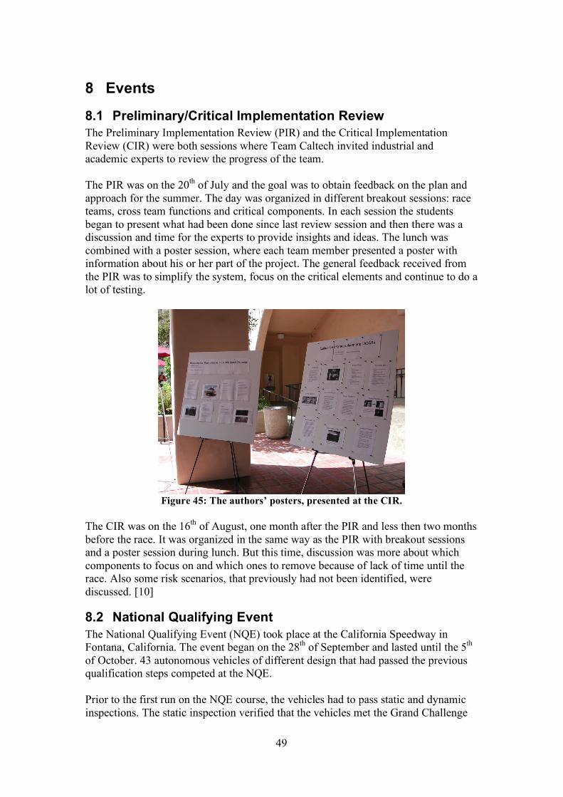
49

8 Events

8.1 Preliminary/Critical Implementation Review

The Preliminary Implementation Review (PIR) and the Critical Implementation Review (CIR) were both sessions where Team Caltech invited industrial and academic experts to review the progress of the team. The PIR was on the 20th of July and the goal was to obtain feedback on the plan and approach for the summer. The day was organized in different breakout sessions: race teams, cross team functions and critical components. In each session the students began to present what had been done since last review session and then there was a discussion and time for the experts to provide insights and ideas. The lunch was combined with a poster session, where each team member presented a poster with information about his or her part of the project. The general feedback received from the PIR was to simplify the system, focus on the critical elements and continue to do a lot of testing.

Figure 45: The authors’ posters, presented at the CIR.

The CIR was on the 16th of August, one month after the PIR and less then two months before the race. It was organized in the same way as the PIR with breakout sessions and a poster session during lunch. But this time, discussion was more about which components to focus on and which ones to remove because of lack of time until the race. Also some risk scenarios, that previously had not been identified, were discussed. [10]

8.2 National Qualifying Event

The National Qualifying Event (NQE) took place at the California Speedway in Fontana, California. The event began on the 28th of September and lasted until the 5th of October. 43 autonomous vehicles of different design that had passed the previous qualification steps competed at the NQE. Prior to the first run on the NQE course, the vehicles had to pass static and dynamic inspections. The static inspection verified that the vehicles met the Grand Challenge

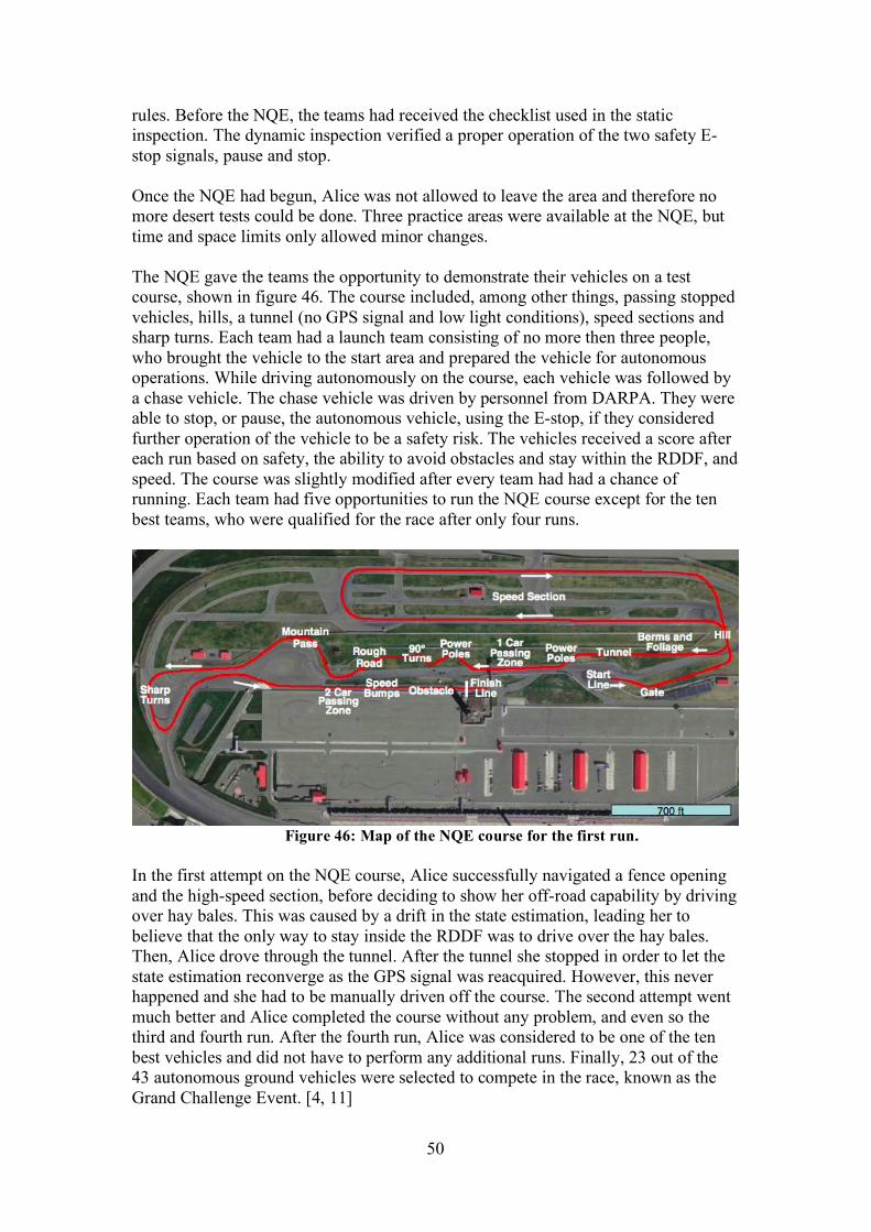
50

rules. Before the NQE, the teams had received the checklist used in the static inspection. The dynamic inspection verified a proper operation of the two safety E-stop signals, pause and stop. Once the NQE had begun, Alice was not allowed to leave the area and therefore no more desert tests could be done. Three practice areas were available at the NQE, but time and space limits only allowed minor changes. The NQE gave the teams the opportunity to demonstrate their vehicles on a test course, shown in figure 46. The course included, among other things, passing stopped vehicles, hills, a tunnel (no GPS signal and low light conditions), speed sections and sharp turns. Each team had a launch team consisting of no more then three people, who brought the vehicle to the start area and prepared the vehicle for autonomous operations. While driving autonomously on the course, each vehicle was followed by a chase vehicle. The chase vehicle was driven by personnel from DARPA. They were able to stop, or pause, the autonomous vehicle, using the E-stop, if they considered further operation of the vehicle to be a safety risk. The vehicles received a score after each run based on safety, the ability to avoid obstacles and stay within the RDDF, and speed. The course was slightly modified after every team had had a chance of running. Each team had five opportunities to run the NQE course except for the ten best teams, who were qualified for the race after only four runs.

Figure 46: Map of the NQE course for the first run.

In the first attempt on the NQE course, Alice successfully navigated a fence opening and the high-speed section, before deciding to show her off-road capability by driving over hay bales. This was caused by a drift in the state estimation, leading her to believe that the only way to stay inside the RDDF was to drive over the hay bales. Then, Alice drove through the tunnel. After the tunnel she stopped in order to let the state estimation reconverge as the GPS signal was reacquired. However, this never happened and she had to be manually driven off the course. The second attempt went much better and Alice completed the course without any problem, and even so the third and fourth run. After the fourth run, Alice was considered to be one of the ten best vehicles and did not have to perform any additional runs. Finally, 23 out of the 43 autonomous ground vehicles were selected to compete in the race, known as the Grand Challenge Event. [4, 11]

51

Figure 47: Alice successfully passing the first challenge on the NQE course, a fence

opening.

8.3 Grand Challenge Event

The DARPA Grand Challenge 2005 begun the 8th of October at 06.40 a.m. The vehicles started in 5-10 minutes intervals. Team members and supporters could follow the race through dynamic 3D maps and a status board, as well as by watching the start and finish. As can be seen in figure 48, the 131.6-mile course was a loop and both the start and finish line were located in Primm, Nevada. The most difficult challenge of the course was the mountain pass where a wrong turn would have caused the vehicle to plunge 100 feet over a sheer cliff. This section was in the last part of the course. It was recorded and the spectators could watch a part of it in real-time.

Figure 48: Course map.

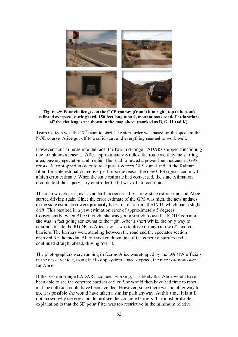
52

Figure 49: Four challenges on the GCE course; (from left to right, top to bottom)

railroad overpass, cattle guard, 150-feet long tunnel, mountainous road. The locations

off the challenges are shown in the map above (marked as B, G, H and K).

Team Caltech was the 17th team to start. The start order was based on the speed at the NQE course. Alice got off to a solid start and everything seemed to work well. However, four minutes into the race, the two mid-range LADARs stopped functioning due to unknown reasons. After approximately 8 miles, the route went by the starting area, passing spectators and media. The road followed a power line that caused GPS errors. Alice stopped in order to reacquire a correct GPS signal and let the Kalman filter, for state estimation, converge. For some reason the new GPS signals came with a high error estimate. When the state estimate had converged, the state estimation module told the supervisory controller that it was safe to continue. The map was cleared, as is standard procedure after a new state estimation, and Alice started driving again. Since the error estimate of the GPS was high, the new updates to the state estimation were primarily based on data from the IMU, which had a slight drift. This resulted in a yaw estimation error of approximately 5 degrees. Consequently, when Alice thought she was going straight down the RDDF corridor, she was in fact going somewhat to the right. After a short while, the only way to continue inside the RDDF, as Alice saw it, was to drive through a row of concrete barriers. The barriers were standing between the road and the spectator section reserved for the media. Alice knocked down one of the concrete barriers and continued straight ahead, driving over it. The photographers were running in fear as Alice was stopped by the DARPA officials in the chase vehicle, using the E-stop system. Once stopped, the race was now over for Alice. If the two mid-range LADARs had been working, it is likely that Alice would have been able to see the concrete barriers earlier. She would then have had time to react and the collision could have been avoided. However, since there was no other way to go, it is possible she would have taken a similar path anyway. At this time, it is still not known why stereovision did not see the concrete barriers. The most probable explanation is that the 3D point filter was too restrictive in the minimum relative

53

altitude. The concrete barriers are higher than 0.3 m, but were not detected. Although it can be seen in the logs that stereovision detects objects on the hillside behind the barriers (to the right in figure 50). Thus, there may have been an error in the calculations resulting in a more restrictive minimum relative altitude. [10, 11]

Figure 50: Alice going off-road in the DARPA Grand Challenge 2005.

(Photograph courtesy of Will Heltsley)

Five out of the 23 competing vehicles completed the entire course. “Stanley”, entered by the Stanford University, finished the course in the shortest elapsed time under 10 hours – 6 hours, 53 minutes and 58 seconds, and therefore won the $2 million prize. This means that Stanley had an average speed of 19.1 mph (30.7 km/h). Two vehicles entered by Carnegie-Mellon University, “Sandstorm” and “Highlander” finished close after, 7 hours 4 minutes and 7 hours 14 minutes respectively. Also, the Gray Team’s “KAT-5” finished under 10 hours – 7 hours, 30 minutes. The fifth autonomous vehicle completing the course was Oshkosh Truck’s 16-ton “TerraMax”, but the elapsed time exceeded the 10-hour limit. The status board showing the final results of all competing teams can be seen in figure 51. [5, 11]

Figure 51: Final results of DARPA Grand Challenge 2005.

54

9 Conclusions At the start of this master thesis project, stereovision was far from ready to use. All the necessary hardware had not been acquired. The basic software had been implemented earlier, but only used and tested on Bob. Several problems were solved to make stereovision work on Alice, and a lot of testing was performed to ensure robust operations. Even though time was limited, requiring solutions to be simple and time efficient to implement, the effort was successful. Eventually, stereovision reached a satisfactory data quality and reliability, and could thus be integrated into the system. Although the LADAR units remained the main terrain sensors, stereovision made an important contribution by improving the overall ability to detect obstacles. Unfortunately, this was not enough to prevent the crash that stopped Alice. Implementations were generally of an ad hoc nature, meaning that some of the problems could have been handled more efficiently, had more time been available. E.g. a lot of the problems were likely the result of flaws in the stereo processing engine. If this had been known from the beginning, a probable course of work would have been to replace this software. This master thesis resulted in many valuable experiences. Working as members of a team competing in the DARPA Grand Challenge proved to be an excellent opportunity to improve engineering skills. It is the firm belief of the authors that every engineering student should at least once work in a large project of this kind. To work at this level of application, develops the ability to handle practical issues, which is often required of an engineer.

9.1 Possible Future Work

To increase the value of stereovision sensors on Alice, a lot of improvements can be done to enhance the accuracy of data and the processing speed. A possible improvement would be to find an alternative to the SVS stereo processing engine, either by purchasing some alternative software or by implementing a new engine from scratch. The processing algorithms could then be customized for this application and there would be no need for ad hoc fixes. If the processing engine was also implemented on a Graphical Processing Unit (GPU), speed could be dramatically improved. This would allow use of cameras with higher resolution, rendering in an increase in accuracy. If a gimbaled platform was mounted on Alice, the stereo cameras could be placed on it. The cameras would then be stabilized, decreasing accuracy losses caused by vibrations. Also, the platform could be moved such that the sensors are directed to an area of interest. This would improve map coverage, especially in hilly terrain. One idea was to put markers on Alice’s hood and use them to verify that the external camera calibration was correct. Since the hood is in the field of view of the short

55

range stereo cameras, the markers should always remain in the same position. Possibly, the markers could also have been used to estimate the new external parameters if a camera would moves. However, this was never implemented due to time constraints. Another possible improvement would be to implement a sensor health module that would detect and report sensor failures. The module would analyze the accuracy and reliability of data from both LADAR and stereovision sensors, reporting to the supervisory controller or mapping module if something seems to be wrong with any of the sensors. E.g. that long range stereovision generates map data that is not at all similar to that provided by the other sensors, and that it should no longer be trusted.

56

Dictionary Alice The autonomous ground vehicle competing for Team Caltech

in DARPA Grand Challenge 2005. Bugzilla A bug reporting tool developed in the Mozilla project, used to

report, track and assign bugs to appropriate team members.

Calibration In the context of computer vision, the process of estimating the parameters that determine how the camera maps 3D points to images.

Correspondence The problem of finding the different locations of a point in the Problem images taken by two cameras in a stereo setting. CCD Charged-coupled device, a sensor containing grids of pixels,

used for recording images in digital cameras.

CIR Critical Implementation Review, a session when Team Caltech invited industrial and academic experts to review the progress of the team. See also PIR.

Correlation An algorithm that tries to solve the correspondence problem by Algorithm optimizing a correlation measure on a stereo image pair.

DARPA Defense Advanced Research Project Agency, an agency of the United States Department of Defense responsible for the development of new military technology.

DGC DARPA Grand Challenge, a competition for autonomous ground vehicles.

Disparity For a point in the real world, the disparity is defined as the relative difference in horizontal location of the point in two rectified stereo images.

E-stop Emergency stop, a safety radio and tracking system used by DARPA as a start/stop actuator of the vehicles as well as for receiving position-track data.

GCE Grand Challenge Event, the final event (the race) in the DARPA Grand Challenge.

GDB GNU Debugger, the standard debugger for the GNU software

system, used to debug the C++ code.

GPS Global Positioning System, a satellite navigation system used for determining precise locations on Earth.

57

IMU Inertial Measurement Unit, an internal navigation system that detects attitude (i.e. roll, pitch and yaw rates) and motion to find the change from the initial position.

LADAR Laser Detection and Ranging, a common sensor in robotics. It consists of a laser and a rotating mirror and measures reflection time to estimate ranges.

NQE National Qualifying Event, the final qualification round in the DARPA Grand Challenge.

PIR Preliminary Implementation Review, a session when Team Caltech invited industrial and academic experts to review the progress of the team. See also CIR.

RDDF Route Data Definition File, containing a number of waypoints, each specified with latitude, longitude, corridor and a speed limit. It defines a corridor in which the vehicle is allowed to operate.

Rectification The process of transforming stereo images such that they

appear to be generated by a pair of cameras in an ideal stereo setting.

Subwindow In this report, the section of an image that was used for stereovision processing.

SVS Small Vision System, a software package including the stereo processing engine and calibration application used in this project.

UTM Universal Transverse Mercator, a grid-based method of

specifying locations on the surface of the Earth. Wiki A special kind of web pages that can be easily edited by the

users.

58

Bibliography [1] Ballard, D. & Brown, C. (1982): Computer Vision. Englewood Cliffs, NJ:

Prentice-Hall. Retrieved 19th of August 2005 from http://homepages.inf.ed.ac.uk/rbf/BOOKS/BANDB/bandb.htm

[2] Clingman, R. RDDF 2004. Retrieved 26th of October 2005 from

http://www.robosuv.com/html/rddf_2004.html [3] DARPA (2005): DARPA Grand Challenge 2005, Emergency Stop System

Preliminary Guidance. Retrieved 30th of October from www.darpa.mil/grandchallenge/Estop_Guidance.pdf

[4] DARPA (2005): DARPA Grand Challenge 2005, National Qualification

Event. Retrieved 25th of October from http://www.darpa.mil/grandchallenge/NQE_Handout.pdf

[5] DARPA Grand Challenge 2005 official web site. Retrieved 30th of October

from http://www.grandchallenge.org. [6] Gillula, J. (2005): Data Fusion From Multiple Sensors: Real-Time Mapping on

an Unmanned Ground Vehicle. California Institute of Technology, Summer Undergraduate Research Fellowship, final report.

[7] Konolige, K. & Beymer, D. (2005): SRI Small Vision System. User’s manual

(also including Calibration Addendum). [8] Murray, R. et al (2005): DARPA Technical Paper: Team Caltech. Retrieved

25th of October 2005 from http://www.darpa.mil/grandchallenge/TechPapers/teamcaltech.pdf

[9] Oskarsson, M. & Berthilsson. R (2005): Föreläsningsanteckningar i

Datorseende. Course notes, FMA270, LTH, Lund University. [10] Team Caltech internal wiki pages. Retrieved 1st of November 2005 from

http://gc.caltech.edu/wiki [11] Team Caltech official web site. Retrieved 26th of October 2005 from

http://team.caltech.edu [12] Tsai, R. (1987): A Versatile Camera Calibration Technique for High-

Accuracy 3D Machine Vision Metrology Using Off-the-Shelf TV Cameras and

Lenses. IEEE Journal of Robotics and Automation, Vol. RA-3, No. 4 August 1987, pp 323-344.

[13] van Gogh, D. et al (2004): Technical Paper, DARPA Grand Challenge.

Retrieved 26th of October 2005 from http://www.darpa.mil/grandchallenge04/TeamTechPapers/TeamCaltechFinalTP.pdf

59

[14] Wikipedia article DARPA Grand Challenge. Retrieved 2nd of November 2005 from http://en.wikipedia.org/wiki/DARPA_Grand_Challenge.

[15] Xiong, Y. & Matthies, L. (1997): Error Analysis of a Real-Time Stereo

System. IEEE Conference on Computer Vision and Pattern Recognition, 1997, pp. 1087-1093.

[16] Zhang, Z. (1998): A Flexible New Technique for Camera Calibration. IEEE

Transactions on Pattern Analysis and Machine Intelligence, 22(11):1330-1334, 2000.

Integrated Stereovision for an Autonomous Ground · PDF fileIntegrated Stereovision for an Autonomous Ground Vehicle Competing in the Darpa Grand Challenge ... valuable experience

Documents