integrated life cycle sustainability performance assessment

INTEGRATED LIFE CYCLE SUSTAINABILITY PERFORMANCE ASSESSMENT

FRAMEWORK FOR RESIDENTIAL MODULAR BUILDINGS

by

Mohammad Kamali

B.Sc., Sharif University of Technology (SUT), 2004

M.Sc., Tarbiat Modares University (TMU), 2008

A THESIS SUBMITTED IN PARTIAL FULFILLMENT

OF THE REQUIREMENTS FOR THE DEGREE OF

DOCTOR OF PHILOSOPHY

in

THE COLLEGE OF GRADUATE STUDIES

(Civil Engineering)

THE UNIVERSITY OF BRITISH COLUMBIA

(Okanagan)

June 2019

© Mohammad Kamali, 2019

ii

The following individuals certify that they have read, and recommend to the College of Graduate

Studies for acceptance, a thesis/dissertation entitled:

INTEGRATED LIFE CYCLE SUSTAINABILITY PERFORMANCE ASSESSMENT

FRAMEWORK FOR RESIDENTIAL MODULAR BUILDINGS

submitted by Mohammad Kamali in partial fulfillment of the requirements of

the degree of Doctor of Philosophy .

Dr. Kasun Hewage, School of Engineering

Supervisor

Dr. Rehan Sadiq, School of Engineering

Supervisory Committee Member

Dr. Shahria Alam, School of Engineering

Supervisory Committee Member

Dr. Anas Chaaban, School of Engineering

University Examiner

Dr. Mohamed Al-Hussein, University of Alberta

External Examiner

iii

Abstract

Due to the rapid global growth of sustainable construction strategies, it is important to assess the

sustainability of buildings constructed by different methods. In the past few decades, the

construction industry has been exposed to the process of industrialization and experimenting off-

site construction methods. Modular construction, as the primary method of off-site construction,

came into practice as an alternative to conventional on-site construction. This method has been

claimed to offer many advantages over conventional construction. However, the continued

expansion of modular construction highly depends on the quantification and evaluation of its

sustainability and the claimed advantages.

In this research, an integrated life cycle sustainability performance assessment framework for

single-family residential modular buildings was developed. To this end, the results of a

comprehensive literature review, various methodologies and tools, and extensive data collection,

were integrated to develop a multi-level decision support framework (DSF). The overall

framework commences with the identification and selection of the most applicable sustainability

performance criteria (SPCs) for comparing the performance of modular buildings versus

conventional buildings. To develop a sustainability index for each selected SPC, relevant

sustainability performance indicators (SPIs and sub-SPIs) have been determined, calculated, and

aggregated using suitable multi-criteria decision analysis (MCDA) methods and life cycle

assessment (LCA). Subsequently, the same methodology has been used to develop the

sustainability indices to represent the performance of a given modular building at higher levels

including environmental sustainability, economic sustainability, and overall sustainability. To

enable comparisons of the developed indices with the industry’s performance benchmarks,

suitable sustainability performance scales (SPSs) have been established at the corresponding

levels.

This research, which integrated life cycle thinking and decision making, helps the construction

industry and governments to make informed decisions on the selection of the most sustainable

construction methods by taking into account the regional circumstances. In addition, it assists

with identification of the underperforming environmental and economic areas over the life cycle

of modular buildings to apply relevant corrective actions on similar projects. Moreover, the

methodology outlined in this research can be adopted for sustainability assessment of other

practices, processes, or products in the construction filed or any other fields.

iv

Lay Summary

This study involves the promotion of sustainable construction across Canada with the focus on

British Columbia. Although modular construction as the primary method of off-site construction

has been claimed to offer many sustainability advantages over conventional on-site construction,

limited studies were undertaken to quantitatively compare the sustainability of these construction

methods. The main contribution of this thesis is to address the research gap by developing a

holistic assessment framework by which the life cycle environmental and economic performance

of single-family residential modular buildings are compared with the performance benchmarks

of conventional buildings. The developed framework is presented in the form of a decision

support framework (DSF) and demonstrated through two case study modular buildings. Results

of this thesis will assist the construction decision makers, such as governmental organizations

and developers, with the selection of optimal construction methods and also identification and

improvement of underperforming areas of modular buildings.

v

Preface

I, Mohammad Kamali, conceived and developed all the contents presented in this thesis under

the supervision of Dr. Kasun Hewage. I wrote all the manuscripts from this research work and

the doctoral thesis. The research supervisor has reviewed the manuscripts and the thesis and

provided critical feedback to improve these documents. In addition, third authors of the three-

author articles, Dr. Rehan Sadiq and Dr. Abbas S. Milani, have reviewed the corresponding

manuscripts and provided constructive feedback to improve them. Nine journal and three

conference articles are currently published, under review, or will be submitted for possible

publication, based on the research work presented in this thesis. Details of the aforementioned

articles are provided below.

1. A version of Chapter 2 has been published in Proceedings of the Canadian Society for Civil

Engineering International Construction Specialty Conference (6th CSCE/CRC) entitled

“Sustainability performance assessment: A life cycle based framework for modular

buildings” (Kamali and Hewage 2017a).

2. A version of Chapter 3 has been published in Renewable & Sustainable Energy Reviews

entitled “Life cycle performance of modular buildings: A critical review” (Kamali and

Hewage 2016).

3. A version of Chapter 4 has been published in Journal of Cleaner Production entitled

“Development of performance criteria for sustainability evaluation of modular versus

conventional construction methods” (Kamali and Hewage 2017b).

4. A version of Chapter 4 has been published in Proceedings of the Modular and Offsite

Construction (MOC15) Summit & 1st International Conference on the Industrialization of

Construction (ICIC) entitled “A framework for comparative evaluation of the life cycle

sustainability of modular and conventional buildings” (Kamali and Hewage 2015a)

5. A version of Chapter 4 has been published in Proceedings of the Canadian Society for Civil

Engineering International Construction Specialty Conference (ICSC15) entitled

“Performance indicators for sustainability assessment of buildings” (Kamali and Hewage

2015b).

6. A version of Chapters 5 has been published in Building and Environment entitled “Life cycle

sustainability performance assessment framework for residential modular buildings:

Aggregated sustainability indices” (Kamali et al. 2018).

7. A version of Chapter 5 will be submitted for possible publication in Sustainable Cities and

vi

Society entitled “Environmental sustainability benchmarking of modular homes – Part I:

Performance quantification” (Kamali et al. 2019a).

8. A version of Chapter 6 will be submitted for possible publication in Sustainable Cities and

Society entitled “Environmental sustainability benchmarking of modular homes – Part II:

Performance assessment” (Kamali et al. 2019b).

9. A version of Chapter 5 will be submitted for possible publication in Journal of Cleaner

Production entitled “Economic sustainability benchmarking of modular homes – Part I:

Performance quantification” (Kamali et al. 2019c).

10. A version of Chapter 6 will be submitted for possible publication in Journal of Cleaner

Production entitled “Economic sustainability benchmarking of modular homes – Part II:

Performance assessment” (Kamali et al. 2019d).

11. A version of Chapter 7 is under review in Energy and Buildings entitled “Comparing

environmental impacts of different construction methods: Cradle-to-gate LCA for residential

buildings in BC, Canada” (Kamali et al. 2019e).

12. A research article consisting of an overall integrated framework developed in this thesis will

be submitted for possible publication in Clean Technologies and Environmental Policy

entitled “Towards sustainable buildings: Conceptualization to implementation of a multi-

level decision support framework for off-site versus on-site construction methods” (Kamali

and Hewage 2019f).

I secured the approval of UBC’s Behavioral Research Ethics Board (UBC BREB No: H14-

02361, Project title: Sustainability of Modular Construction) for all the surveys and interviews

conducted in this research.

vii

Table of Contents

Abstract ..................................................................................................................... iii

Lay Summary ............................................................................................................ iv

Preface ........................................................................................................................ v

Table of Contents ..................................................................................................... vii

List of Tables ........................................................................................................... xiv

List of Figures ......................................................................................................... xvi

List of Abbreviations .............................................................................................. xix

Acknowledgements ................................................................................................ xxii

Dedication .............................................................................................................. xxiv

Chapter 1 Introduction ........................................................................................... 1

1.1 Background and Motivation .................................................................................. 1

1.2 Research Gap ......................................................................................................... 3

1.3 Goal and Objectives .............................................................................................. 4

1.4 Meta Language ...................................................................................................... 5

1.5 Thesis Structure ..................................................................................................... 6

Chapter 2 Research Methodology.......................................................................... 8

2.1 Phase 1 ................................................................................................................. 10

2.2 Phase 2 ................................................................................................................. 10

2.3 Phase 3 ................................................................................................................. 11

2.4 Phase 4 ................................................................................................................. 12

2.5 Phase 5 ................................................................................................................. 13

2.6 Phase 6 ................................................................................................................. 13

Chapter 3 Literature Review ................................................................................ 15

3.1 Background .......................................................................................................... 15

3.2 Building Sustainability Assessment Methods ..................................................... 18

3.2.1 Sustainability Assessment Systems .................................................................................. 18

3.2.2 Sustainability Assessment Standards ............................................................................... 20

3.2.3 Sustainability Assessment Tools ...................................................................................... 21

3.3 Benefits and Challenges of Modular Construction ............................................. 22

3.3.1 Benefits of Modular Construction .................................................................................... 22

viii

3.3.2 Challenges of Modular Construction ............................................................................... 25

3.4 Life Cycle Performance of Modular Buildings ................................................... 28

3.4.1 Life Cycle Phases of Buildings ........................................................................................ 28

3.4.2 Life Cycle Performance Studies of Modular Buildings ................................................... 29

3.5 Summary .............................................................................................................. 38

Chapter 4 Identification and Selection of Sustainability Performance

……………Criteria ................................................................................................. 40

4.1 Background .......................................................................................................... 40

4.2 Detailed Methodology ......................................................................................... 43

4.2.1 SPC Compilation .............................................................................................................. 44

4.2.2 Survey Design .................................................................................................................. 44

4.2.3 Survey Implementation .................................................................................................... 45

4.2.4 Methods of Data Analysis ................................................................................................ 46

4.3 Sustainability Performance Criteria .................................................................... 48

4.4 Ranking the TBL Sustainability Performance Criteria ....................................... 50

4.4.1 Survey Respondents ......................................................................................................... 51

4.4.2 Reliability Analysis .......................................................................................................... 54

4.4.3 Environmental Criteria Ranking ...................................................................................... 54

4.4.4 Economic Criteria Ranking .............................................................................................. 56

4.4.5 Social Criteria Ranking .................................................................................................... 58

4.4.6 Effect of Professional Experience on Ranking Results .................................................... 61

4.5 Summary .............................................................................................................. 63

Chapter 5 Development of Aggregated Sustainability Indices ......................... 66

5.1 Background .......................................................................................................... 66

5.2 Detailed Methodology ......................................................................................... 66

5.2.1 Determination of indicators under SPCs .......................................................................... 68

5.2.2 Performance Level Functions for Indicators .................................................................... 69

5.2.3 Aggregated Sustainability Indices .................................................................................... 71

5.3 Environmental SPCs ............................................................................................ 72

5.3.1 Energy Performance and Efficiency Strategies (EP) ....................................................... 74

5.3.1.1 Envelope insulation (EP1) ......................................................................................... 76

5.3.1.2 Air infiltration (EP2) ................................................................................................. 78

ix

5.3.1.3 Windows and glass doors (EP3) ................................................................................ 78

5.3.1.4 Space heating and cooling equipment (EP4) ............................................................. 79

5.3.1.5 Heating and cooling distribution system (EP5) ......................................................... 81

5.3.1.6 Efficient hot water equipment (EP6) ......................................................................... 81

5.3.1.7 Efficient lighting (EP7) ............................................................................................. 83

5.3.1.8 Efficient appliances (EP8) ......................................................................................... 84

5.3.1.9 Residential refrigerant management (EP9)................................................................ 84

5.3.1.10 Relative importance of the SPIs under EP ............................................................... 85

5.3.2 Regional Materials (RM) ................................................................................................. 85

5.3.2.1 Local materials in exterior wall (RM1) ..................................................................... 86

5.3.2.2 Local materials in floor (RM2) .................................................................................. 87

5.3.2.3 Local materials in foundation (RM3) ........................................................................ 88

5.3.2.4 Local materials in interior walls and ceiling (RM4) .................................................. 88

5.3.2.5 Local materials in landscape (RM5) .......................................................................... 88

5.3.2.6 Local materials in roof (RM6) ................................................................................... 89

5.3.2.7 Local materials in roof, floor, and wall (RM7) ......................................................... 90

5.3.2.8 Local materials in other components (RM8) ............................................................. 90

5.3.2.9 Relative importance of the SPIs under RM ............................................................... 91

5.3.3 Construction Waste Management (CWM) ....................................................................... 91

5.3.3.1 Efficient material consumption plans (CWM1) ........................................................ 93

5.3.3.2 Construction waste diversion (CWM2) ..................................................................... 95

5.3.3.3 Construction waste reuse (CWM3) ........................................................................... 96

5.3.3.4 Relative importance of the SPIs under CWM ........................................................... 96

5.3.4 Renewable and Environmentally Preferable Products (REP) .......................................... 97

5.3.4.1 Exterior wall content (REP1) .................................................................................... 98

5.3.4.2 Floor content (REP2) ................................................................................................. 99

5.3.4.3 Foundation content (REP3) ..................................................................................... 100

5.3.4.4 Interior wall and ceiling content (REP4) ................................................................. 100

5.3.4.5 Landscape content (REP5) ...................................................................................... 100

5.3.4.6 Roof content (REP6) ............................................................................................... 101

5.3.4.7 Roof, floor, and wall content (REP7) ...................................................................... 101

5.3.4.8 Other components’ content (REP8) ......................................................................... 102

x

5.3.4.9 Relative importance of the SPIs under REP ............................................................ 103

5.3.5 Site Disruption and Appropriate Strategies (SD) ........................................................... 103

5.3.5.1 Construction activity pollution prevention (SD1) ................................................... 104

5.3.5.2 Efficient landscaping (SD2) .................................................................................... 105

5.3.5.3 Heat island effects (SD3) ......................................................................................... 106

5.3.5.4 Rainwater management (SD4)................................................................................. 107

5.3.5.5 Efficient pest control (SD5) ..................................................................................... 109

5.3.5.6 Relative importance of the SPIs under SD .............................................................. 109

5.3.6 Renewable Energy Use (RE) .......................................................................................... 110

5.3.6.1 Renewable electricity (RE1) .................................................................................... 111

5.3.6.2 Renewable space heating (RE2) .............................................................................. 112

5.3.6.3 Renewable water heating (RE3) .............................................................................. 113

5.3.6.4 Relative importance of the SPIs under RE .............................................................. 114

5.3.7 Greenhouse Gas Emissions (GE) ................................................................................... 114

5.3.7.1 Life cycle assessment .............................................................................................. 115

5.3.7.2 Definition of goal and scope .................................................................................... 116

5.3.7.3 Required data for inventory analysis ....................................................................... 117

5.3.7.4 Life cycle impact assessment .................................................................................. 120

5.3.7.5 Development of environmental impact indices ....................................................... 123

5.3.8 Material Consumption in Construction (MCC) ............................................................. 126

5.4 Economic SPCs ................................................................................................. 127

5.4.1 Integrated Management (IM) ......................................................................................... 132

5.4.1.1 Integrated design processes (IM1) ........................................................................... 132

5.4.1.2 Life cycle cost (IM2) ............................................................................................... 135

5.4.1.3 Commissioning (IM3) ............................................................................................. 137

5.4.1.4 Relative importance of the SPIs under IM .............................................................. 139

5.4.2 Durability of Building (DB) ........................................................................................... 139

5.4.2.1 Roofing and openings (DB1) ................................................................................... 140

5.4.2.2 Foundation waterproofing (DB2) ............................................................................ 141

5.4.2.3 Cladding (DB3) ....................................................................................................... 142

5.4.2.4 Barriers (DB4) ......................................................................................................... 143

5.4.2.5 Relative importance of the SPIs under DB .............................................................. 145

xi

5.4.3 Adaptability of Building (AB) ....................................................................................... 145

5.4.3.1 Expandability (AB1)................................................................................................ 147

5.4.3.2 Dismantlability (AB2) ............................................................................................. 150

5.4.3.3 Record keeping (AB3) ............................................................................................. 151

5.4.3.4 Relative importance of the SPIs under AB .............................................................. 152

5.4.4 Design and Construction Time (DCT) ........................................................................... 152

5.4.4.1 Design time (DCT1) ................................................................................................ 153

5.4.4.2 Construction time (DCT2) ....................................................................................... 154

5.4.4.3 Relative importance of the SPIs under DCT ........................................................... 155

5.4.5 Design and Construction Costs (DCC) .......................................................................... 155

5.4.5.1 Design cost (DCC1) ................................................................................................ 156

5.4.5.2 Construction cost (DCC2) ....................................................................................... 156

5.4.5.3 Relative importance of the SPIs under DCC ........................................................... 157

5.4.6 Operational Costs (OC) .................................................................................................. 157

5.4.6.1 Running costs (OC1) ............................................................................................... 158

5.4.7 Maintenance Costs (MC) ............................................................................................... 159

5.4.7.1 Repair and replacement costs (MC1) ...................................................................... 160

5.4.8 End of Life Costs (EC) ................................................................................................... 160

5.4.9 Investment and Related Risks (IRR) .............................................................................. 162

5.4.9.1 Profitability of investment (IRR1) ........................................................................... 163

5.5 Development of Sustainability Indices ............................................................. 164

5.5.1 Sustainability Indices for SPCs (Level 3) ...................................................................... 165

5.5.2 Sustainability Indices for Sustainability Dimensions (Level 2) ..................................... 165

5.5.3 Overall Sustainability Index (Level 1) ........................................................................... 167

5.6 Summary ............................................................................................................ 168

Chapter 6 Integrated Framework for Sustainability Assessment of

……………Modular Buildings ............................................................................. 169

6.1 Background ........................................................................................................ 169

6.2 Detailed Methodology ....................................................................................... 170

6.2.1 Data Collection ............................................................................................................... 171

6.2.1.1 Design and implementation of Survey B ................................................................. 173

6.2.1.2 Design and implementation of Survey C ................................................................. 173

xii

6.2.1.3 Design and implementation of Survey D ................................................................ 175

6.2.2 Monte Carlo Simulation Analyses ................................................................................. 176

6.2.2.1 Probability distribution of a random variable .......................................................... 177

6.2.2.2 Selection of probability distribution type ................................................................ 178

6.2.3 Establishment of Sustainability Performance Scales ..................................................... 180

6.2.4 Development of Decision Support Framework .............................................................. 182

6.3 Sustainability Performance Scales for Environmental SPCs ............................ 182

6.3.1 SPS for Energy Performance and Efficiency Strategies ................................................ 184

6.3.2 SPS for Regional Materials ............................................................................................ 186

6.3.3 SPS for Construction Waste Management ..................................................................... 188

6.3.4 SPS for Renewable and Environmentally Preferable Products ...................................... 189

6.3.5 SPS for Site Disruption and Appropriate Strategies ...................................................... 191

6.3.6 SPS for Renewable Energy Use ..................................................................................... 193

6.3.7 SPS for Greenhouse Gas Emissions ............................................................................... 194

6.4 Sustainability Performance Scales for Economic SPCs ................................... 195

6.4.1 SPS for Integrated Management .................................................................................... 195

6.4.2 SPS for Durability of Building ....................................................................................... 197

6.4.3 SPS for Adaptability of Building ................................................................................... 199

6.4.4 SPS for Design and Construction Time ......................................................................... 201

6.4.5 SPS for Design and Construction Costs ......................................................................... 203

6.4.6 SPS for Operational Costs .............................................................................................. 204

6.4.7 SPS for Maintenance Costs ............................................................................................ 205

6.4.8 SPS for Investment and Related Risks ........................................................................... 206

6.5 Sustainability Performance Scales for Sustainability Dimensions ................... 208

6.6 Sustainability Performance Scale for Overall Sustainability ............................ 210

6.7 Proposed Decision Support Framework ............................................................ 212

6.7.1 Quantification Process .................................................................................................... 214

6.7.2 Assessment Process ........................................................................................................ 214

6.8 Summary ............................................................................................................ 215

Chapter 7 Validation of the Integrated Sustainability Assessment

……………Framework ......................................................................................... 217

7.1 Background ........................................................................................................ 217

xiii

7.2 Performance Evaluation of the Case Study Buildings at Different Levels ....... 218

7.2.1 Description of Case Study Modular Buildings .............................................................. 218

7.2.2 Data Collection for Development of Sustainability Indices ........................................... 219

7.2.3 Sustainability Indices ..................................................................................................... 220

7.2.4 Performance Evaluation at Different Levels .................................................................. 223

7.2.4.1 Sensitivity analysis ............................................................................................ 227

7.3 Performance Evaluation of the Case Study Buildings with respect to the

…..GE SPC .............................................................................................................. 230

7.3.1 Data Collection for Inventory Analysis ......................................................................... 230

7.3.2 Impact Assessment ......................................................................................................... 232

7.3.3 Environmental Impact Indices ....................................................................................... 236

7.4 Summary ............................................................................................................ 240

Chapter 8 Conclusions and Recommendations ................................................ 241

8.1 Summary and Conclusions ................................................................................ 241

8.2 Originality and Contribution ............................................................................. 244

8.3 Research Limitations ......................................................................................... 246

8.4 Recommendations for Future Research ............................................................ 247

References ............................................................................................................... 248

Appendices.............................................................................................................. 274

Appendix A: Evaluation of SPCs against ‘Applicability’ and ‘Measurability’ ...... 274

A.1 Criteria for evaluation of SPCs ........................................................................................ 274

A.2 Survey implementation..................................................................................................... 275

A.3 ELECTRE 1 MCDA method ........................................................................................... 275

A.4 Ranking the SPC categories ............................................................................................. 279

A.5 Calculation example for final ranking of the economic SPCs ......................................... 281

A.6 Sensitivity analysis ........................................................................................................... 284

Appendix B: First Step Study .................................................................................. 287

Appendix C: TOPSIS MCDA Method .................................................................... 289

Appendix D: Establishment of a Suitable PLF for ‘Construction waste reuse’ ..... 291

Appendix E: Renewable Energy Sources and Net-zero Energy Buildings ............ 293

xiv

List of Tables

Table 3.1 Number of relevant documents used in this research ................................................... 18

Table 3.2 Worldwide known examples of sustainability rating systems ...................................... 20

Table 3.3 Summary of the advantages and disadvantages of modular construction .................... 27

Table 3.4 Environmental LCAs associated with modular buildings ............................................ 31

Table 4.1 Primary potential sustainability performance criteria developed in this research ........ 50

Table 4.2 Survey dissemination details and the rate of valid responses ....................................... 51

Table 4.3 Reliability coefficients for different SPC categories .................................................... 54

Table 4.4 Ranking of the environmental sustainability performance criteria ............................... 55

Table 4.5 Ranking of the economic sustainability performance criteria ...................................... 57

Table 4.6 Ranking of the social sustainability performance criteria ............................................ 59

Table 5.1 Importance levels of the selected environmental and economic SPCs ......................... 68

Table 5.2 Environmental SPCs and corresponding indicators ...................................................... 73

Table 5.3 ER and U-factor requirements for windows and glass doors in different zones .......... 79

Table 5.4 Weight set for the SPIs under the EP SPC .................................................................... 85

Table 5.5 Weight set for the SPIs under the RM SPC .................................................................. 91

Table 5.6 Efficient framing items ................................................................................................. 94

Table 5.7 Weight set of the SPIs under the RM SPC ................................................................. 103

Table 5.8 Renewable water heating systems .............................................................................. 114

Table 5.9 Functional equivalent set of LCA in this research ...................................................... 117

Table 5.10 Required data for inventory analysis ........................................................................ 118

Table 5.11 Weights of the main contributing chemicals to eco-toxicity .................................... 122

Table 5.12 Weighting schemes for environmental impact measures ......................................... 125

Table 5.13 Economic SPCs and corresponding indicators ......................................................... 131

Table 5.14 Relative importance weights of the selected environmental and economic SPCs ... 167

Table 7.1 Performance levels, weighted values, PISs, and NISs for the SPIs of the EP SPC .... 221

Table 7.2 Separation measures and sustainability indices at different levels for Mod1 ............. 222

Table 7.3 Separation measures and sustainability indices at different levels for Mod2 ............. 223

Table 7.4 Results of LCIA for the benchmarking buildings ....................................................... 233

Table 7.5 Environmental impact measures and their normalized effects on life cycle phases ... 237

Table 7.6 Environmental impact indices for the benchmarking buildings ................................. 238

Table A.1 Net outranking of the environmental sustainability performance criteria ................. 280

Table A.2 Net outranking of the economic sustainability performance criteria ......................... 281

Table A.3 Net outranking of the social sustainability performance criteria ............................... 281

Table A.4 The rating matrix for the economic category ............................................................. 282

xv

Table A.5 The normalized weighted rating matrix for the economic category .......................... 282

Table A.6 The concordance sets for SPCs in the economic category ........................................ 283

Table A.7 The discordance sets for SPCs in the economic category .......................................... 283

Table A.8 The concordance index for SPCs in the economic category ...................................... 284

Table A.9 The discordance index for SPCs in the economic category ....................................... 284

Table B.1 Standard deviations (σ) of scores for the environmental SPC category .................... 287

Table B.2 Standard deviations (σ) of scores for the economic SPC category ............................ 287

Table B.3 Standard deviations (σ) of scores for the social SPC category .................................. 288

xvi

List of Figures

Figure 1.1 Thesis chapters and associated objectives ..................................................................... 6

Figure 2.1 Research methodology followed in the research phases ............................................... 9

Figure 3.1 Time savings in modular construction. Reproduced from

…………..Kamali and Hewag (2016) Used with permission from © Elsevier ........................... 22

Figure 3.2 Life cycle of modular buildings versus conventional buildings. Adapted from

…………..Kamali and Hewage (2017). Used with permission from © Elsevier ........................ 29

Figure 4.1 The hierarchy of sustainability criteria. Adapted from

…………..Kamali and Hewage (2017). Used with permission from © Elsevier ........................ 42

Figure 4.2 Methodology adopted in Chapter 4 ............................................................................. 43

Figure 4.3 Professional experience of the survey participants. Reproduced from

…………..Kamali and Hewage (2017b). Used with permission from © Elsevier ...................... 53

Figure 4.4 Number of TBL SPCs assigned each of the importance levels. Reproduced from


Figure 4.5 Influence of the participants’ experience on rank order of (a) Environmental SPCs;

………….(b) Economic SPCs; (c) Social SPCs. Reproduced from


Figure 5.1 Methodology used in Chapter 5 .................................................................................. 67

Figure 5.2 SPIs and sub-SPIs associated with ‘Energy performance and efficiency strategies’ .. 75

Figure 5.3 SPIs and sub-SPIs related to ‘Regional materials’ ...................................................... 86

Figure 5.4 Construction waste management hierarchy ................................................................. 92

Figure 5.5 SPIs and sub-SPIs associated with ‘Construction waste management’ ...................... 93

Figure 5.6 SPIs and sub-SPIs under ‘Renewable and environmentally preferable products’ ...... 98

Figure 5.7 SPIs and sub-SPIs associated with ‘Site disruption and appropriate strategies’ ....... 104

Figure 5.8 SPIs associated with ‘Renewable energy use’ ........................................................... 111

Figure 5.9 Hierarchy of AHP-based framework and contributing parameters ........................... 124

Figure 5.10 SPIs and sub-SPIs associated with ‘Integrated management’ ................................. 132

Figure 5.11 Costs of two systems of cooling over 60 years of building life span ...................... 136

Figure 5.12 SPIs and sub-SPIs associated with ‘Durability of building’ ................................... 140

Figure 5.13 SPIs and sub-SPIs associated with ‘Adaptability of building’ ................................ 147

Figure 6.1 Performance benchmarking to identify the performance gap of a product ............... 169

Figure 6.2 Methodology used in Chapter 6 ................................................................................ 171

Figure 6.3 Probability distributions of discrete random variables (PMF) and continuous

…………..random variables (PDF) ............................................................................................ 178

Figure 6.4 Proposed evaluation scale and PL thresholds for performance categories ................ 182

xvii

Figure 6.5 Probability distributions of the indicators under the EP SPC .................................... 185

Figure 6.6 (a) Probability distribution of the EP SPC; (b) Corresponding SPS ......................... 186

Figure 6.7 Probability distributions of the indicators under the RM SPC .................................. 187

Figure 6.8 (a) Probability distribution of the RM SPC; (b) Corresponding SPS ........................ 188

Figure 6.9 Probability distributions of the indicators under the CWM SPC .............................. 188

Figure 6.10 (a) Probability distribution of the CWM SPC; (b) Corresponding SPS .................. 189

Figure 6.11 Probability distributions of the indicators under the REP SPC ............................... 190

Figure 6.12 (a) Probability distribution of the REP SPC; (b) Corresponding SPS..................... 191

Figure 6.13 Probability distributions of the indicators under the SD SPC ................................. 192

Figure 6.14 (a) Probability distribution of the SD SPC; (b) Corresponding SPS ....................... 193

Figure 6.15 Probability distributions of the indicators under the RE SPC ................................. 193

Figure 6.16 (a) Probability distribution of the RE SPC; (b) Corresponding SPS ....................... 194

Figure 6.17 Probability distributions of the indicators under the IM SPC ................................. 196

Figure 6.18 (a) Probability distribution of the IM SPC; (b) Corresponding SPS ....................... 197

Figure 6.19 Probability distributions of the indicators under the DB SPC ................................. 198

Figure 6.20 (a) Probability distribution of the DB SPC; (b) Corresponding SPS ...................... 199

Figure 6.21 Probability distributions of the indicators under the AB SPC ................................. 200

Figure 6.22 (a) Probability distribution of AB SPC; (b) Corresponding SPS ............................ 201

Figure 6.23 Probability distributions of the indicators under the DCT SPC .............................. 202

Figure 6.24 (a) Probability distribution of the DCT SPC; (b) Corresponding SPS .................... 203

Figure 6.25 Probability distributions of the indicators under the DCC SPC .............................. 203

Figure 6.26 (a) Probability distribution of the DCC SPC; (b) Corresponding SPS .................... 204

Figure 6.27 (a) Probability distribution of the OC SPC; (b) Corresponding SPS ...................... 205

Figure 6.28 (a) Probability distribution of the MC SPC; (b) Corresponding SPS ...................... 206

Figure 6.29 Probability distributions of the indicators under the IRR SPC................................ 207

Figure 6.30 (a) Probability distribution of the IRR SPC; (b) Corresponding SPS ..................... 207

Figure 6.31 (a) Probability distribution of the historical environmental performance of

……………buildings; (b) Corresponding SPS .......................................................................... 209

Figure 6.32 (a) Probability distribution of the historical economic performance of


Figure 6.33 (a) Probability distribution of the overall sustainability performance of


Figure 6.34 Proposed DSF for life cycle sustainability assessment of residential

……………modular buildings ................................................................................................... 213

Figure 7.1 Floor plans of the case study modular buildings (Mod1 and Mod2) ........................ 219

xviii

Figure 7.2 Sustainability performance benchmarking of the case study buildings (Level 1) ..... 224

Figure 7.3 Environmental and economic performance benchmarking of the case study

…………..buildings (Level 2) .................................................................................................... 225

Figure 7.4 Sustainability performance benchmarking of the case study buildings with

…………..respect to environmental SPCs (Level 3).................................................................. 226

Figure 7.5 Sustainability performance benchmarking of the case study buildings with

…………..respect to economic SPCs (Level 3) ......................................................................... 227

Figure 7.6 Sensitivity analysis results (a) Energy performance and efficiency strategies; (b)

…………..Renewable and environmentally preferable products; (c) Site disruption and

…………..appropriate strategies ................................................................................................ 229

Figure 7.7 Floor plan of the case study conventional building (Conv) ...................................... 231

Figure 7.8 Global warming potential, Acidification potential, Human health effect, and

…………..Eutrophication potential due to construction of the benchmarking buildings .......... 234

Figure 7.9 Ozone depletion potential, Smog potential, Fossil fuel consumption, and

…………..Eco-toxicity effect due to construction of the benchmarking buildings ................... 235

Figure 7.10 Cradle-to-grate index (CTGi) for different building alternatives ............................ 239

Figure A.1 Net Concordance (Cp) and net discordance (Dp) indices for SPCs;

…………..(a) Environmental category; (b) Economic category; (c) Social category.

…………..Reproduced from Kamali et al. (2018). Used with permission from © Elsevier ..... 280

Figure A.2 Net outranking of (a) Environmental category; (b) Economic category; (c) Social

…………..category, for different weight sets of the evaluation criteria. Reproduced from

…………..Kamali et al. (2018). Used with permission from © Elsevier .................................. 285

Figure E.1 US energy consumption by energy source in 2017. Reproduced from EIA (2018).

…………..Used with permission from © U.S. Energy Information Administration ................. 294

xix

List of Abbreviations

A Affordability AB Adaptability of Building ABB Aesthetic options and Beauty of Building AFUE Annual Fuel Utilization Efficiency AHP Analytic Hierarchy Process AL Air Leakage AP Acidification Potential ASCE American Society of Civil Engineers ASHRAE American Society of Heating, Refrigerating, and Air-conditioning Engineers AT Alternative Transportation BC British Columbia BEES Building for Environmental and Economic Sustainability C&D Construction and demolition waste CD Community Disturbance CHC Cultural and Heritage Conservation CI Consistency Index CO2eq Carbon dioxide equivalents CR Consistency Ratio CWM Construction Waste Management DB Durability of Building DCC Design and Construction Costs DCT Design and Construction Time DM Decision Maker DSF Decision Support Framework EC End of life Costs EE Eco-toxicity Effect EF Energy Factor EIFS Exterior Insulation Finishing Systems ELECTRE Elimination and Choice Translating Reality EO Expert Opinions EP Energy Performance and efficiency strategies E-P Eutrophication Potential EPA Environmental Protection Agency ER Energy Rating FFC Fossil Fuel Consumption FSC-certified Forest Stewardship Council certified FU Functionality and Usability of the physical space GE Greenhouse gas Emissions GHG Greenhouse Gases GWP Global Warming Potential HDD Heating Degree Days HHE Human Health Effect HO Health, comfort, and well-being of Occupants HSPF Heat Seasonal Performance Factor HVAC Heating, Ventilation, and Air Conditioning IECC International Energy Conservation Code ILE Influence on the Local Economy

xx

IM Integrated Management IRR Investment and Related Risks ISD Influence on local Social Development ISO International Organization for Standardization ISW Industrial Solid Waste LBC Living Building Challenge LCA Life Cycle Assessment LCC Life Cycle Cost LCI Life Cycle Inventory LCIA Life Cycle Impact Assessment LCSA Life Cycle Sustainability Assessment LEED Leadership in Energy & Environmental Design MBI Modular Building Institute MC Maintenance Costs MCC Material Consumption in Construction MCS Monte Carlo Simulation MEF Modified Energy Factor MSW Municipal Solid Waste NAA Neighborhood Accessibility and Amenities NIS Negative-Ideal Solution NZEB Net-Zero Energy Building OC Operational Costs ODP Ozone Depletion Potential PAF Potentially Affected Fraction of species in an environment PDF Probability Density Function PIS Positive-Ideal Solution PL Performance Level PLF Performance Level Function PMF Probability Mass Function POI Profitability of Investment PV Photovoltaic RE Renewable Energy use REP Renewable and Environmentally preferable Products RESNET Residential Energy Services NETwork RM Regional (local) Materials ROI Return on Investment RSI R-value Systeme International SD Site Disruption and appropriate strategies SEER Seasonal Energy Efficiency Ratio SI Severity Index SP Smog Potential SPCs Sustainability Performance Criteria SPIs Sustainability Performance Indicators SPS Sustainability Performance Scale SPSS Statistical Package for Social Sciences SS Site Selection SSB Safety and Security of Building TBL Triple Bottom Line TOPSIS Technique for Order Preference by Similarity to Ideal Solution TRACI Tool for the Reduction and Assessment of Chemical other environmental

xxi

Impacts UAS User Acceptance and Satisfaction UBC University of British Columbia WE Water and wastewater Efficiency strategies WF Water Factor WGR Waste Generation Rate WHS Workforce Health and Safety

xxii

Acknowledgements

All praises be to the ALLAH Almighty who gave me the strength to materialize this research in

the present form. I would like to express my sincere appreciation to my advisor, Dr. Kasun

Hewage, who believed in me, trusted in my abilities, encouraged me to grow as a researcher, and

strive for the best. Dr. Hewage has been an inspiration as long as I have known him and I am

deeply grateful that I had the chance to work under his supervision for my PhD at The University

of British Columbia (UBC). Dr. Hewage is an outstanding mentor and a passionate researcher

and I am extremely thankful for his wisdom, patience, kindness, passion for success, and

research vision. You have been an incredible mentor for me during my challenging research

journey.

I would like to thank Dr. Rehan Sadiq and Dr. Shahria Alam for kindly being on my doctoral

committee and for their motivation and support. I am forever grateful to Dr. Sadiq because

despite his busy schedule, he always had the time to discuss my research. His priceless advice

and critical comments definitely enhanced the quality of my work. I would also like to thank Dr.

Abbas Milani for his encouragement and invaluable creative comments. His friendly and

approachable personality permitted me to access his precious time whenever I needed it

throughout my research.

The input from many individuals, organizations, and firms was vital for the successful

completion of this research project. I would like to thank all participants of the multiple surveys

and interviews throughout the study period. Without their feedback and shared experiences, the

extensive data collection would not have been successfully completed. Special thanks go to

Michael Jacobs (Dilworth Homes), Lloyd Dehart (Moduline Industries), and James Stevenson

(Champion Home Builders).

I would like to thank all my friends and colleagues in and out of UBC including the research

team of the Project Life Cycle Management Laboratory. I appreciate the kind support of Dr.

Husnain Haider, Dr. Joanne Taylor, Dr. Navid Hossaini, and Haibo Feng. Moreover,

appreciation is due to faculty and staff at UBC. In particular, I would like to thank Shannon

Hohl, who supported me on several occasions during my study period, Lori Walter, who

affectionately guided me in technical writing skills, and Lisa Shearer, who effectively facilitated

the research ethics approvals.

I would like to express my special thanks to my dear family who have provided unconditional

love and support while I have been away from them. I am forever indebted to my mother and

father for their care throughout my life, for all of their prayers, and for teaching me to be a

faithful and good person. Words cannot express how eternally grateful I am to them. I am also

xxiii

grateful to my mother-in-law, deceased father-in-law, and my brothers and sisters for the many

sacrifices that they have made on my behalf. Your prayers helped to sustain me. Finally, I want

to express my deepest appreciation to my beloved wife, Nassiba. Despite your extremely busy

life with your own PhD research at UBC and our endearing child, Mohiaddin, you always

encouraged our partnership and inspired me in the moments when there was no one to answer

my queries. Nassiba, without your love, patience, and immense support within the past years, it

would have been impossible to accomplish my goal at this stage of the life journey. I am

extremely happy and excited to continue this incredible journey with you.

xxiv

Dedication

Lovingly dedicated to

My parents

&

My beloved wife, Nassiba

1

Chapter 1 Introduction

This chapter briefly discusses the problem statement, research motivation, research gap and

questions, research goal and the associated specific objectives. In addition, an overview of the

thesis structure to achieve the research objectives is provided.

1.1 Background and Motivation

Sustainability is defined as a set of processes aimed at delivering efficient built assets in the

long-term (Egan 1998). It is adopting a strategic view of enhancing the impacts of human

developments on the environment by satisfying the requirements of people today without

undermining the ability of next generations to meet their own needs (Brundtland Commission

1987). A rigorous analysis of the evolution of the sustainability concept in the scientific

community was conducted by Bettencourt and Kaur (2011). The authors assembled a large body

of scientific publications between 1974 and 2010 that contained the words ‘sustainability’ and/or

‘sustainable development’ in their abstract, title, or keywords. Overall, they found 20,000 papers,

authored by about 37,000 authors found in 174 countries. This is a large amount of publications,

which testifies to the extraordinary growth of interest in sustainability assessment over time.

These figures alone say a lot about how urgent and global the topic of sustainability is, and how

much it has developed.

There is a significant demand for development of new buildings and infrastructure to

accommodate the rapidly increasing population of the world (Lim et al. 2015). It is estimated

that the construction industry contributes to 13% of global economy and employment of over

110 million workers around the world (Ajayi and Oyedele 2018; Economy Watch 2010).

However, this industry accounts for significant environmental, economic, and social impacts

(Han et al. 2017) by consuming approximately half of the global resources (Achal et al. 2015).

The construction industry is the largest consumer of material resources (40- 60% of the total raw

material extractions), water, and energy (40% of energy consumption). It also accounts for

significant amount of CO2 emissions to the environment (up to 39% of the total emissions) and

largest waste to landfills (Bilal et al. 2016; Edwards 2014; Ahn et al. 2009; Achal et al. 2015;

Bribian et al. 2011). Thus, the construction development should be accompanied by careful

considerations to reduce its negative burdens on the environment and societies.

Achieving sustainability is one of the most challenging contemporary concerns, which means

using natural resources to fulfil current generation needs while not threatening future

generations’ quality of life. Sustainable construction, in particular, aims at reducing the

2

environmental impact of a building over its entire lifetime, while optimizing its economic

viability and the comfort and safety of its occupants. In other words, the built environment

including buildings can result in momentous environmental, economic, and social impacts

(namely triple bottom line or TBL) as the primary dimensions of sustainable construction (Sev

2009). Therefore, the construction industry can actively contribute to the sustainability agenda by

means of sustainable construction (Lim et al. 2015). Consequently, there has been a paradigm

shift in the construction industry over the last few years and the sustainable construction is

grabbing more attention globally among construction stakeholders such as firms and clients

(Valdes-vasquez et al. 2012). Nonetheless, the lack of broad knowledge on sustainability in

terms of methodologies and expected long term benefits is still a significant hindering factor of

construction of sustainable buildings (Ahn et al. 2013; Cotgrave and Kokkarinen 2011; Chong et

al. 2009). One of the most effective solution to achieve the goals of sustainable construction is to

intensify sustainability knowledge and expertise within the construction industry (Shelbourn et

al. 2006). In addition, the public awareness of the life cycle advantages of sustainability can play

an important role towards expansion of sustainable construction.

Three industrial revolutions have already occurred. During the past few years, digital progress

has transformed whole industries, ushering in a new technological era now known as the Fourth

Industrial Revolution. New technologies can address both consumer needs and companies’

sustainability and productivity. New technologies in the construction industry, such as building

information modeling (BIM), prefabrication and modularization, and automated and robotic

equipment, can significantly affect the entire construction industry. Although this industry still

follows its traditional approach, it has been exposed to the process of industrialization and

experimenting different methods of construction. As a result, off-site construction came into

practice as a potential alternative to conventional on-site (also called traditional, site-built, stick-

built) construction which shows signs of revolutionizing the housing market. Off-site

construction refers to the process of manufacturing and preassembling building elements,

components, or modules prior to their installation on the final project site (Goodier and Gibb

2007). Modular construction, as the primary method of off-site construction, is fast evolving as

an effective alternative to conventional (on-site) construction. A modular building comprises a

set of modules that are built in an off-site fabrication center, delivered to the construction site,

assembled, and placed on a permanent foundation. Each modular building normally has multi-

rooms consisting of three-dimensional modules. The modules are built and pre-assembled in

factory environments and all the mechanical, electrical, plumbing, and trim work is done

(O’Brien et al. 2000). Upon the completion by the manufacturer, these units are shipped to the

site for installation on foundations much like a site-built building (Cameron and Di Carlo 2007).

3

About 85% to 90% of the modular construction work is done off-site and the remaining (10% to

15%), including the foundation and utility hookups, is done on the final building location on site

(Kawecki 2010).

It is imperative to comprehensively assess the life cycle sustainability performance of different

construction methods because of the importance of sustainable construction. This can be

accomplished by analyzing and comparing the sustainability performance of buildings

constructed using on-site and off-site construction methods. Therefore, the motivation behind the

proposed research is to compare and contrast the comparative sustainability performance of

residential modular vs. conventional buildings over their life cycle.

1.2 Research Gap

During the past few years, new methods of construction have been gaining attention as effective

alternatives to conventional methods in the pursuit of sustainable construction. In this regard, the

topic of off-site construction has been of major interest due to push towards minimizing

construction and demolition waste and increasing sustainability in construction industry (Yeheyis

et al. 2013). Modular construction, as the primary method of off-site construction, is a rapidly

growing technique that can be applied to different types of buildings, such as residential single

and multi-family buildings, educational centers and student housing, hospitals, offices, hotels,

and so forth. It has been reported in the published literature that modular construction offers

various benefits over the traditional construction (Arif and Egbu 2010; Kamali and Hewage

2016). However, despite the claimed advantages, the application of modular construction is still

limited in practice. For example, buildings in the developing countries are rarely constructed

using off-site and modular construction methods (Mao et al. 2015). The use of modular

construction in the building sector of the developed countries is more than that of the developing

countries; however, it is not still extensive (Quale et al. 2012).

A key reason for the limited application of modular construction is the clients’ reluctance to fully

accept innovative construction techniques’ added benefits to a project (Pasquire and Gibb 2002).

According to the literature, the public's negative perception of the off-site construction methods

is one of the significant challenges to modular construction. This is because of the difficulty of

ascertaining the advantages that modular construction provides over the conventional methods.

For example, modular and prefabricated homes are usually believed as trailers, mobile homes, or

manufactured houses (Boyd et al. 2013; Haas et al. 2000). However, similar to conventional

buildings, modular buildings are permanent structures that are built according to codes, which

are more restrictive than the codes for temporary and transportable trailers. Not only for the

4

public, but also for many of those involved in the construction industry, the benefits of off-site

construction techniques have not been well understood. Therefore, decisions on the selection of

off-site construction methods are mostly made according to anecdotal evidence rather than solid

analytical evidence (Na 2007; Pasquire and Gibb 2002; Blismas et al. 2006).

Published peer-reviewed literature on the topic of life cycle sustainability performance of

modular construction is very limited. Only few studies addressed the environmental performance

of modular buildings. No significant published study was found on the other key dimensions of

sustainability (i.e., economic and social).

Based on the above noted concerns, the following specific research questions emerged in this

research:

i. How can the claimed benefits of modular buildings be quantitatively investigated?

ii. What are the most significant sustainability criteria when comparing modular and

conventional buildings?

iii. How can the life cycle performance of residential modular buildings be assessed using

objective indices?

iv. How can the underperforming areas of modular buildings be managed to improve their

performance?

v. How can the most sustainable building option be prioritized between the modular and

conventional options?

It is envisaged that a comprehensive sustainability performance assessment of residential

modular buildings over the entire life cycle can fill the research gap by answering the above

stated questions.

1.3 Goal and Objectives

The primary goal of this research is to improve sustainable construction by developing a

methodical and practically applicable life cycle based sustainability performance assessment

framework for single-family modular buildings in North America. In this research, the

environmental and economic dimensions of sustainability are analyzed and the social dimension

is left for future research. In other words, this research addresses the enviro-economic

assessment of residential modular buildings. The following are the specific objectives of this

research:

1- Identify and prioritize appropriate sustainability performance criteria (SPCs) for modular

5

buildings;

2- Develop sustainability indices for benchmarking the performance of modular buildings.

3- Establish suitable sustainability performance assessment scales.

4- Develop a holistic decision support framework for sustainability assessment of residential

modular buildings.

5- Evaluate the performance evaluation of modular buildings in the Okanagan, British

Columbia, Canada.

1.4 Meta Language

There are diverse models, techniques and methods that have been used in this research each

involved specific and technical vocabularies. However, certain principles and terminologies can

have broad meanings. Therefore, it is important to properly understand the terminology

developed for this research in order to appreciate the integrated concept of sustainability

performance assessment for residential modular buildings. For the purpose of consistent

understanding, the specific terms used in this thesis are specifically defined as follows:

- Conventional/traditional construction: These terms have been interchangeably used and

referred to on-site construction method (also called site-built and stick-built).

- Conventional/traditional buildings: These terms have been interchangeably used and referred

to buildings constructed by on-site construction method.

- Technique, method, and methodology: These terms have been interchangeably used for any

calculation methods such as multi-criteria decision analysis (MCDA) methods. In addition, the

‘technique’ and ‘method’ represented the on-site and off-site construction methods such as

modular construction method.

- Framework: A framework is, or contains, a (not completely detailed) structure or system for the

realization of a defined result/goal. In this research, framework referred to holistic methods (e.g.,

framework for holistic sustainability assessment, framework for identification of sustainability

criteria).

- Decision support framework (DSF): This term represented the integrated sustainability

performance assessment framework developed in this research. It is a system of methods,

modules, calculation tools, and different frameworks to aid decision making.

- Benchmarking: This term referred to the performance comparisons of a given building with the

6

least/most desirable performances of other buildings.

1.5 Thesis Structure

The thesis contains eight chapters to achieve the aforementioned research objectives. Figure 1.1

illustrates the organization of the thesis chapters and their interconnections with the research

objectives. Chapter 1 describes the problem statement, research motivation, research gap and

questions, research goal and objectives, and thesis structure.

Chapter 1: Introduction

Objective 1

Chapter 3: Literature Review

Chapter 4: Identification and Selection of Sustainability

Performance Criteria

Objective 2

Chapter 5: Development of Aggregated Sustainability Indices

Objectives 3 & 4

Chapter 6: Integrated Framework for Sustainability Assessment of

Modular Buildings

Objective 5

Chapter 7: Validation of the

Integrated Sustainability

Assessment Framework

Chapter 8: Conclusions and Recommendations

Chapter 2: Methodology

Figure 1.1 Thesis chapters and associated objectives

Chapter 2 briefly overviews the methodology adopted in this research. Then, Chapter 3 presents

a comprehensive literature review on the sustainability assessment methods, the advantages and

challenges of modular buildings, and the existing studies performed on life cycle sustainability

7

assessment (LCSA) of these buildings. Chapter 4 compiles and ranks the primary potential

sustainability performance criteria (SPCs) for the performance assessment of residential modular

buildings. Next chapter, Chapter 5, focuses on quantification of the selected SPCs by

establishing a method to develop sustainability indices at different levels (i.e., SPC level,

sustainability dimension level, and overall sustainability level). Chapter 6 establishes suitable

sustainability performance scales for benchmarking the performance of a modular building using

the sustainability indices. In addition, this chapter incorporates the research outcomes into an

integrated sustainability assessment framework (i.e., decision support framework, DSF). Then,

Chapter 7 validates the developed integrated sustainability assessment framework using case

study analyses of modular buildings in the Okanagan, British Columbia, Canada. Finally,

Chapter 8 discusses the research conclusions, contributions, limitations, and provides

recommendations for future research.

8

Chapter 2 Research Methodology

A part of this chapter has been published in Proceedings of the Canadian Society for Civil

Engineering International Construction Specialty Conference (6th CSCE/CRC) entitled

“Sustainability performance assessment: A life cycle based framework for modular buildings”

(Kamali and Hewage 2017a).

An overview of the research methodology is illustrated in Figure 2.1. To achieve the research

objectives, six methodological phases have been completed. The detailed methodologies have

been provided in the following individual chapters.

9

Phase 1- TBL sustainability performance criteria

Compilation of potential SPCs

Document analysis

Review of sustainability rating systems and published articles

Review of modular vs. conventional construction

Experts feedback

Prioritization of SPCs

Survey A design (Likert scale)

Survey A implementation (construction practitioners)

Reliabil ity analysis

Ranking analysis (Severity Indices, importance levels)

Environmental SPCs Economic SPCs Social SPCs

Phase 2- Sustainability performance indicators

Identification of SPIs & sub-SPIs, data variables, weights,

least/most desirable performances

Review sustainability rating systems and published articles

Expert consultations

Survey B design (Delphi method)

Survey B implementation (designers, builders)

Establish performance level functions (PLFs) for indicators

Establishment of PLFs for SPIs & sub-SPIs

Simple weighted average (SWA) MCDA method

Performance level (PL) concept

Phase 3- Sustainability indices

Development of indices for:

SPCs (Level 3)

TOPSIS MCDA method, LCA

Sustainability dimensions (Level 2) Weights of SPCs (Survey 1) TOPSIS MCDA method

Overall sustainability (Level 1) Weights of sustainability dimensions (Survey 1) TOPSIS MCDA method

Phase 4- Sustainability performance scales

Surveys B & C design (Delphi method)

Surveys B & C implementation (building sustainability

rating experts, designers, builders)

Probability distributions for SPIs and sub-SPIs (triangular)

SPS establishment for SPCs, sustainability dimensions, & overall sustainability(@Risk s Monte Carlo, Athena s LCA)

Phase 5- Decision support framework

Develop an integrated multi-level DSF

Incorporate the deliverables into an integrated framework

DSF procedure

Collect data from the subject building project (survey design & implementation)

Calculate indicators

Develop sustainability indices (Levels 1, 2, 3)

Benchmark performance at different levels & take actions for sustainability improvement Case study of two modular buildings in the Okanagan, Canada

Surveys D & E design

Surveys D & E implementation (case study homebuilders)

Develop sustainability indices (Levels 1, 2, 3)

Benchmark performance at different levels & take actions for sustainability improvement

Start

Finish

Phase 6- DSF validation

Figure 2.1 Research methodology followed in the research phases

10

2.1 Phase 1

The first phase of this research identified, ranked, and selected suitable sustainability

performance criteria (SPCs) for residential modular buildings (Objective 1). There are different

performance areas that can significantly contribute to the life cycle sustainability of buildings,

such as energy, material, cost, and so forth. To efficiently evaluate the sustainability of a

building, each area can be broken down into a number of assessment criteria, namely

sustainability performance criteria (SPCs) in this research. Although, a breadth of literature is

available on performance areas for conventional buildings, there is still a gap exists for

identification and prioritization of suitable SPCs for performance assessment of residential

modular buildings. In this regard, first, the literature regarding rating systems and other

published studies were reviewed and experts were consulted to compile the primary potential

SPCs and group them into the TBL sustainability categories (i.e., environmental, economic, and

social). These SPCs were then incorporated into a questionnaire survey (Survey A) using the

LiveCycle Designer tool. Survey A was designed and conducted to capture the construction

industry feedback on ‘applicability’ (relevance) of the compiled SPC categories for sustainability

assessment of residential modular buildings. The survey sample population was mainly

construction experts in North America who had experience in construction processes and had

diverse professional backgrounds. Each SPC was rated using a five-point Likert scale. The data

collected through Survey A was analyzed using two standard analyses of reliability analysis and

ranking analysis and the Severity Index (SI) scores of the SPCs were calculated with the help of

SPSS statistical software. Subsequently, all the SPCs were assigned importance levels ranging

from ‘Extremely Low’ to ‘Extremely High’ (according to their SI scores) and ranked within each

sustainability category.

In this research, all the environmental and economic SPCs with the importance level of

‘Medium’ and above were selected for evaluation of modular buildings. As mentioned before,

the social sustainability assessment of modular buildings is beyond the scope of this research.

Phase 1 was completed in Chapter 4. In section 4.2 of that chapter, the above methodology has

been explained in detail.

2.2 Phase 2

Phases 2 and 3 collectively addressed Objective 2 of the research. Phase 2 sought suitable

measurable sustainability performance indicators (SPIs) under each selected SPC by which it can

be calculated. It is not unlikely that an SPI itself consists of a number of sub-SPIs. Similar to

what was done for compiling SPCs, a literature review and also expert interviews were carried

11

out to determine suitable SPIs (and sub-SPIs), their data variables, their least/most desirable

performance values, and also their relative importance weights. In the cases of some SPCs and

the associated SPIs, the information regarding the least/most desirable performance values was

not available in the literature or, even if available, should be determined locally due to sensitivity

of the information to the region in which buildings are constructed (i.e., locality sensitive

criteria). To collect the required information of such cases, a questionnaire survey (Survey B)

was designed and implemented based on the Delphi method along with expert interviews.

The approach followed in this research involved choosing simple and easy-to-use measurement

methods for SPIs (and sub-SPIs) by which each indicator can be calculated by having the

minimum amount of data including quantitative and qualitative. By using the determined data

variables of each indicator (SPI, sub-SPI) and their ranges, the measurement method of the

indicator was formulated. To this end, a performance level function (PLF) was established for

each SPI and sub-SPI by which its performance can be calculated using the collected data, and

presented in a normalized form based on a performance level (PL) between 0 and 100. The PLs

of 0 and 100 represent the least and most desirable performances of the subject indicator,

respectively, which were already determined through the aforementioned literature review and

expert consultations/survey.

Phase 2 was completed in Chapter 5. The detailed methodology of this phase has been provided

in the methodology section of that chapter (i.e., section 5.2).

2.3 Phase 3

The next step of the research was to develop aggregated sustainability indices for benchmarking

the performance of modular buildings. Using a bottom-up approach, this research developed

sustainability indices at the following levels:

Level 3: SPCs;

Level 2: Environmental performance and economic performance; and

Level 1: Overall sustainability performance.

At Level 3, a sustainability index was developed for each SPC through an aggregation process by

combining the calculated SPIs (PL values) and their relative importance weights. The required

weights of SPIs were determined through the literature review and expert opinions. For the

aggregation process, the Technique for Order of Preference by Similarity to Ideal Solution

(TOPSIS) multi-criteria decision analysis (MCDA) method was used, which is based on the

relative closeness to the best performance and relative remoteness from the worst performance.

12

Similarly, at Level 2, a sustainability index for the environmental performance (ENVRi) and a

sustainability index for the economic performance (ECONi) were developed by aggregating the

developed sustainability indices of all SPCs associated with each sustainability dimension and

their weights. The above stated Severity Index scores of the SPCs were used to calculate their

weights.

In the same way, at Level 1, the overall sustainability index (OVERALLi) was derived by

aggregating the environmental and economic sustainability indices developed above and the

weights of these sustainability dimensions. These weights were determined based on the

construction practitioners’ feedback in the same Survey A described above.

In addition to the previous phase, Phase 3 was also completed in Chapter 5. The detailed

methodology of this phase has been described in section 5.2.

2.4 Phase 4

In order to evaluate the performance of a modular building, the developed sustainability indices

should be compared with the industry’s performance benchmarks of similar conventional

buildings. In this phase, suitable sustainability performance scales (SPSs) were established for

SPCs, sustainability dimensions, and overall sustainability (Objective 3). The following data

sources can be utilized to collect the required data and establish such SPSs:

A database that contains the historical performance of conventional buildings with respect

to each SPCs and the associated SPIs and sub-SPIs.

Opinions of experienced experts on the historical performance of conventional buildings

with respect to each SPCs and the associated SPIs and sub-SPIs.

Because the former data source was not available in the literature for many of the criteria and

indicators, an attempt was made to create the latter data source. Subsequently, two surveys

including Survey B (the same survey that explained under Phase 2 with added questions) and

Survey C were designed and implemented based on the Delphi method to capture the

construction experts’ feedback on the historical performance of buildings with respect to the sub-

SPIs and SPIs. The collected data was used to construct the probability distributions of the sub-

SPIs and SPIs. Subsequently, these distributions were used to generate the probability

distributions of the corresponding SPCs using the Monte Carlo simulation (MCS) method. The

@Risk software was employed to perform the MCS analyses. Similarly, the generated

probability distributions of the SPCs were used as input of new analyses to generate the

probability distributions of the sustainability dimensions. This method continued to develop the

13

probability distribution of the overall sustainability.

Eventually, using the results of distributions associated with each Level, the corresponding SPSs

were established by assigning four performance categories including Low, Fair, Good, and

Excellent to index range between 0 and 100. Therefore, the performance of a given modular

building can be benchmarked by comparing the developed index and the corresponding SPS. It

should be stressed that, it was not possible to establish a SPS for the ‘Greenhouse gas emissions

(GE)’ SPC. However, in this research, the review benchmarking method was used to compare

the GE performance of the modular and conventional buildings based on the results of the life

cycle assessment (LCA) method. The required data for LCA of the case study modular and

conventional buildings was collected separately using a separate survey (Survey D) and then the

Athena software was used for the LCA analyses.

Phase 4 was completed in Chapter 6 and the above methodology has been explained in details

under section 6.2.

2.5 Phase 5

In response to Objective 4, in this phase, all the research outcomes were incorporated into an

integrated sustainability assessment framework as a multi-level decision support framework

(DSF) that can be used to comprehensively assess the sustainability of residential modular

buildings. The developed DSF integrated the individual frameworks used to fulfill Objectives 1

to 3 of the research. Despite the bottom-up approach used when developing the sustainability

indices and sustainability performance scales (SPSs) above, the sustainability performance

assessment process follows a top-bottom approach. The assessment starts at Level 1 (i.e., overall

sustainability performance of the subject building) and can continue up to Level 3 (i.e.,

performance of the subject building with respect to each SPC) depending on the purpose and

scope of assessment determined by the decision maker (DM).

Similar to Phase 4, Phase 5 was also completed in Chapter 6. Thus, the detailed methodology of

Phase 5 can be found in section 6.2.

2.6 Phase 6

In this phase, the developed DSF was validated by two case study modular buildings in the

Okanagan, British Columbia, Canada (Objective 5). To collect the data required for calculating

the sub-SPIs and SPIs, another survey (Survey E) was designed and conducted. Four modular

homebuilders in the Okanagan were contacted and requested for participation in Survey E. Two

14

of them participated and completed the survey. In some cases, the participating homebuilders

were provided with more details or clarifications on the requested data through a number of in

person meetings or phone calls. The collected data was used in the established PLFs to calculate

the PLs of sub-SPIs and SPIs. Subsequently, for each modular building, the aggregated

sustainability indices were developed using the TOPSIS MCDA method. As explained above,

these indices were then used for performance benchmarking of the two modular buildings at

different levels by comparing them with the corresponding SPSs. Consequently, the

underperforming areas were explored and given high priorities for improvement actions.

As stated earlier, to benchmark the performance of modular buildings with respect to the GE

SPC, LCA analyses needed to be performed. In this regard, Survey D was designed and

conducted to collect the required data. In addition to the two participating modular homebuilders

above, one conventional homebuilder in the Okanagan also participated. Subsequently, LCA was

performed for the three buildings (two modular and one conventional) and their global warming

potential (GWP) values as the main environmental impact incurred by greenhouse gas emissions

(i.e., GE SPC) were calculated and benchmarked. In addition to GWP comparisons, seven

additional environmental impact measures were calculated including smog potential, ozone

depletion potential, and so forth. These calculated measures along with their relative importance

weights were aggregated using an AHP-based framework (Analytic Hierarchy Process) to

develop a set of environmental impact indices for each building. Comparisons of these indices

comparatively revealed the environmental impacts of the buildings at their material production

phase, the construction phase, and the overall cradle-to-gate (before occupancy).

15

Chapter 3 Literature Review

A part of this chapter has been published in Renewable & Sustainable Energy Reviews entitled

“Life cycle performance of modular buildings: A critical review” (Kamali and Hewage 2016).

This chapter contains a state-of-the-art literature review of sustainability assessment methods for

buildings, benefits and challenges of modular construction, and studies conducted for life cycle

sustainability assessment of modular buildings.

3.1 Background

Conventionally, a building is constructed on the construction site after the design phase and a

contractor is hired to build it. This process is commonly known as “on-site”, “site-built”, “stick-

built”, “conventional”, or “traditional” construction. Since the late 19th century, this method of

construction has been the accepted construction method and nowadays it accounts for a

significant portion of the housing industry (Zenga and Javor 2008). However, in the past few

decades, the construction industry has been exposed to the process of industrialization; therefore,

it has experienced different methods of construction. As a result, off-site construction came into

practice as an alternative to the on-site method.

Off-site construction refers to the process of manufacturing and preassembling of building

elements, components, or modules prior to their installation on the final project site (Goodier and

Gibb 2007). Based on the degree of work off the project site (i.e., building’s final location), off-

site construction is categorized into the following levels (Gibb and Pendlebury 2006):

• Component subassembly: Small-scale elements are assembled in factory environments

(e.g., windows);

• Non-volumetric preassembly: Items are assembled in factory environments to form non-

volumetric units before installation on project sites (e.g., cladding panels);

• Volumetric preassembly: Similar to the previous level, items are assembled in factory

environments but they form volumetric units (i.e., units enclose usable space) before

installation on project sites. Units are usually fully finished internally (e.g., toilet pods); and

• Complete (modular) construction: Items are assembled in factory environments to form fully

finished modules. Whole buildings are formed by a number of modules.

Modular buildings are a set of modules that are built in an off-site fabrication center, delivered to

16

the construction site, assembled, and placed on the permanent foundation. A modular building

normally has multi-rooms consisting of three-dimensional modules. The modules are built and

preassembled in factory environments and all the mechanical, electrical, plumbing, and trim

work is done (O’Brien et al. 2000). Upon completion by the manufacturer, these units are

shipped to the project site for installation on foundations, much like a site-built project (Kawecki

2010; Cameron and Di Carlo 2007). About 85% to 90% of the modular construction is done off

the construction site and the remaining work (10% to 15%), including foundations and utility

hookups, is done on site (Kawecki 2010).

Modular construction, as one of the off-site construction methods, is fast evolving and effective

alternative to traditional on-site construction. The application of modular construction is found

mainly in general building construction, particularly apartment buildings, schools, hotels, student

housing, hospitals, offices, single-family developments, correctional facilities, floating projects,

and other buildings where units are repetitive (Annan 2008; Moon 2014). The technique is used

in North America, Japan, and parts of Europe (Annan 2008; Li et al. 2013).

In general, the adaptation of off-site construction methods in developing countries has not been

as fast as that of developed countries (Mao et al. 2015). However, despite the many well-

documented benefits that can be derived from the use of these methods of construction, their

applications are still limited. For example, the US modular industry accounts for only 2% to 3%

of the total new single-family houses and equal or less than 1% of the total new multi-family

houses between 2000 and 2014 (USCB 2016). A key reason for clients’ reluctance to accept

innovated construction techniques is the difficulty of ascertaining the benefits that off-site

construction adds to a project (Pasquire and Gibb 2002). For many of those involved in the

construction process, the benefits of off-site construction techniques were not well understood

(Na 2007). As a result, decisions surrounding off-site construction techniques are largely made

based on anecdotal evidence rather than rigorous data (Pasquire and Gibb 2002; Blismas et al.

2006; Blismas and Wakefield 2009).

It is claimed that modular construction provides a wide range of environmental, economic, and

social advantages; thus, it can contribute to achieving the goals of sustainability (Ahn and Kim

2014; Nahmens and Ikuma 2012). These advantages, can justify the use of modular construction

by the construction industry practitioners as an effective alternative, more than in the past. To

gain a deeper understanding of the modular construction’s overall sustainability compared to its

conventional counterpart, it is imperative to investigate the sustainability performance of

modular buildings over the entire life cycle.

This chapter presents a thorough state-of-the-art literature review regarding modular buildings

17

and sustainability. The following sections review the:

Existing methods for sustainability assessment of buildings (Study 1)

Key benefits and challenges of modular construction (Study 2)

Research studies that have been carried out to evaluate the life cycle performance of

modular buildings (Study 3)

In each of these independent studies, first, different types of documents such as journal papers,

theses, public reports, and so forth, were searched. Then, through a screening process, the

abstract/prefaces/conclusion of the found documents were reviewed to narrow them down to the

most relevant documents. Finally, the refined documents were carefully reviewed.

In all Studies 1, 2, and 3, combinations of suitable keywords were searched in three different

document categories using the following search databases:

Books and academic theses: UBC library database was used to find an initial list of books

and academic theses. The abstracts/prefaces were reviewed and irrelevant documents were

discarded.

Journal and conference articles: “Compendex Engineering Village” database and ASCE

library were searched to find journal and conference articles. The search was also limited to

articles that were published after the year 2000. These articles were further refined by

reviewing their abstracts and conclusions.

Governmental/institutional reports: The World Wide Web was used to find governmental or

institutional reports and publications, which provided information related to the study they

were searched for.

Combinations of keywords ‘sustainability assessment’, ‘building’, ‘sustainability performance’,

‘criteria’, ‘indicators’, ‘method’, ‘system’, ‘tool’, ‘standard’, and ‘framework’ were searched in

the above search databases to find appropriate documents related to the sustainability assessment

methods for buildings (Study 1). In the case of the next study (Study 2), combinations of

keywords ‘modular construction’, ‘modular building’, ‘benefit’, ‘challenge’, and ‘advantage’

were searched to compile a list of documents which provided information related to the benefits

and challenges of modular construction. Similarly, combinations of keywords ‘modular

construction’, ‘modular building’, ‘life cycle performance’, and ‘life cycle assessment’ have

been searched to find appropriate documents which reported the studies that have been

performed on sustainability assessment of modular buildings (Study 3). Refined count of

documents used in the process of literature review is listed in Table 3.1.

18

Table 3.1 Number of relevant documents used in this research

Reference category Study 1 Study 2 Study 3

Book, Thesis 2 13 8

Journal/Conference article 14 36 32

Governmental/Institutional report 46 13 4

The final refined documents under each study were reviewed and findings have been reported in

the following sections.

3.2 Building Sustainability Assessment Methods

Currently, diverse assessment methods are used to evaluate the sustainability performance of

buildings. However, they are different in terms of objectives, scope, and assessment aspects.

Some of these methods have been developed for residential buildings, whereas others have been

tailored for commercial buildings. The focus area of the methods is also different ranging from

only one phase (e.g., the design and construction phase) to the entire life cycle. In addition, a

number of sustainability methods evaluate the performance of a building with respect to only one

or two criteria associated with one sustainability dimension (e.g., CO2 emissions that is related to

the environmental dimension). The scoring systems are also different. While some sustainability

assessment methods assign points to buildings’ performance, others evaluate buildings using the

calculated values of criteria (e.g., global warming potential).

During this review, the existing sustainability assessment methods were classified, based on their

objectives, characteristics, and structures. Consequently, the following categories recommended

by some references (IHOBE 2010) have been realized to effectively classify the existing

sustainability assessment methods:

Sustainability assessment systems

Sustainability assessment standards

Sustainability assessment tools

Each of these sustainability assessment method categories is discussed below. It should be noted

that in cases where a document was presented in a language other than English, supportive

English-language documents were searched to explore the content of the original document.

3.2.1 Sustainability Assessment Systems

The sustainability assessment systems (simply called systems) involve methods to evaluate the

performance of a building from sustainability point of view, which is usually beyond the

minimum performance required in building codes. In many of these systems, there are a number

19

of assessment categories, such as materials or energy, which are used to evaluate the

performance of the building with respect to them. Each category comprises a set of relevant

performance criteria such as waste management or quality of insulation that collectively address

the sustainability performance of the building with regard to the parent category. Similarly, each

criterion itself may consist of a number of sub-criteria by which the parent criterion can be

quantified. Therefore, the assessment process commences by collecting data of the building to

quantify the sub-criteria and criteria. It then continues by scoring the quantified sub-criteria and

criteria and determining the building’s performance in each assessment category. Subsequently,

all the scores are summed up and the overall performance of the whole building is determined by

assigning performance indices such as ‘Poor’, ‘Good’, ‘Excellent’, and so forth. Some of the

assessment systems take further steps and certify the building based on its performance. In

addition to less environmental impacts by a building that assigned ‘Good’ and higher

performance index (or any equivalent terms used in different systems), it is beneficial to both

developer/builder and client/user since it provides a positive perception of the building.

The sustainability assessment systems are usually voluntarily and developed by either

governmental or non-governmental organizations to be used internationally or exclusively for

buildings are constructed in a country depending on the geographical and socio-economic

circumstances. Therefore, they are regularly updated to include every changes in the

circumstances such as new technologies such as energy efficient strategies, and assessment

methodologies such as the life cycle assessment (LCA) method. They have been developed for

different types of buildings such as residential, commercial, and even urban development

projects (Bernardi et al. 2013; Ferreira et al. 2014). In addition, the systems have been mostly

designed to evaluate the performance of new buildings (i.e., new designs); however, in some

cases there are systems that address existing buildings (i.e., renovations, extensions).

The sustainability assessment systems are dissimilar in terms of the life cycle phase coverage.

The main priority is mostly the use phase followed by the construction phase; therefore, limited

attention is paid to the end of life phase. Furthermore, the sustainability assessment systems

consider different aspects of the building’s sustainability performance related to the TBL

sustainability dimensions, i.e., environmental, economic, and social. The primary focus of

systems are on the environmental dimension, even though some economic and social criteria are

also addressed. The documents reviewed in this section showed that the sustainability assessment

systems are the most comprehensive methods among the three method categories.

Rating systems (also called sustainability rating systems and green building rating systems) are

among the well-known sustainability assessment systems that were developed to assist with the

20

management of “green” or “environmentally friendly” building projects. During the past few

years, rating systems have had a vital role in informing on progress in sustainability practices

(Siew et al. 2013). These systems are mostly qualitative tools that deal with sustainability

performance of buildings by providing a set of performance criteria and scoring each building

project based on those criteria (Castro-Lacouture et al. 2009). Rating systems examine the

performance of a “whole building” and allow comparison of different buildings (Fowler and

Rauch 2006). However, they suffer from not addressing all the sustainability dimensions and all

the life cycle phases. Moreover, the use of these systems in many cases is complicated, time-

consuming, and expensive. Table 3.2 lists a number of well-known rating systems.

Table 3.2 Worldwide known examples of sustainability rating systems

Rating System Country Launched Organization(s)

LEED International 1998 US Green Building Council (USGBC)

Green Globes US and Canada 2002 Green Building Initiative (GBI), BOMA Canada, ECD Energy and

Environment Canada

LBC International 2006 International Living Future Institute

BREEAM International 1990 Building Research Establishment (BRE)

SBTool International 1996 International Initiative for a Sustainable Built Environment (iiSBE)

CASBEE Japan 2001 Japan Green Build Council (JaGBC)

Green Star Australia 2003 Green Building Council Australia (GBCA)

ESGB China 2006 Ministry of Housing and Urban Rural development of the People's

Republic of China (MOHURD)

BCA-GM Singapore 2005 National Environment Agency

HK BEAM Hong Kong 1996 BEAM Society

3.2.2 Sustainability Assessment Standards

Sustainability assessment standards (simply called standards) are intended to investigate if the

performance of buildings is within the pre-defined minimum requirement. The standards are not

as comprehensive as the systems. They are not also capable of assessing the performance of the

given building with respect to all the life cycle phases, all sustainability dimensions, and even all

aspects within a sustainability dimension. They only address limited performances of buildings,

mainly energy related aspects. For example, a number of standards evaluate the greenhouse gas

(GHG) emissions of buildings in the use phase.

The sustainability assessment standards are not geared towards extensive sustainability

assessment or certification. However, they are useful when the performance of the subject

building with regard to a specific aspect is concerned. If the results of applying a standard shows

high performance of a building with respect to the investigated criterion, it does not necessarily

mean that the building is a sustainable product. This is because the performance of the building

with respect to all relevant criteria associated with all TBL and also all life cycle phases has not

21

been investigated. However, such a building can be considered a potential candidate to be a

sustainable building; therefore, it needs to be tested by a comprehensive method such as a

sustainability assessment system.

3.2.3 Sustainability Assessment Tools

Similar to the sustainability assessment standards, the sustainability assessment tools (simply

called tools) are not intended to comprehensively assess the sustainability performance of

buildings. As the name implies, the tools can be interpreted as means to support the required

calculations or measurements indicated in the sustainability assessment systems and standards. In

other words, tools provide a methodical framework such as inventory databases, methodologies,

among others, to calculate a specific measure or output such as global warming potential using

the required data of the given building.

Tools usually do not provide any scoring system, minimum performance requirements,

performance levels, or certification types by which the outputs can be interpreted. If the tools are

not categorized as an independent sustainability assessment method category, they can be

considered as strong support tools for the systems and standards to calculate some of the criteria

included in them. For example, LCA is recently becoming a significant criterion and has been

included in a number of systems. However, the methodology how to perform an effective LCA

study for a building is not included within the same systems. This should be conducted

separately using a suitable LCA tool such as Athena or SimaPro and the output is then used as

input for the intended system in order to score, compare, or interpret the performance of the

subject building with regard to this input. In addition, in many cases, tools are employed in the

design phase to assist with the selection of building materials, local service options (energy

types, supply systems, equipment), material transportation means, and waste management

strategies (Ali and Al Nsairat 2009). Examples of known tool are Athena (for LCA), BEES (for

LCA), SimaPro (for LCA), TRNSYS (for energy simulation), eQuest (for energy simulation),

One Click LCA (for both LCA and LCC), among others.

The other important point is that the output of a tool (LCA output, embodied energy, and so

forth) is sensitive and can significantly be affected from a country to another. Therefore, the

databases or data inventories included in a tool should be in accordance with the circumstances

of the region it is intended to be used, otherwise the output will be wrong or very inaccurate.

There are cases where a huge database is compiled and embedded in a tool by which the region

differences are addressed. For example, the Athena LCA software includes the inventory

database for different locations in North America.

22

3.3 Benefits and Challenges of Modular Construction

According to Pasquire and Gibb (2002), advantages and disadvantages of off-site methods in the

construction industry should be clearly identifiable and accessible to all construction

practitioners, including architects, engineers, contractors, and end users,. Although monetary

measures are able to be linked to profitability, they are inadequate to evaluate other benefits such

as productivity, safety and wider human factors (Blismas et al. 2006). In fact, the main focus of

the traditional performance evaluation frameworks when choosing the construction method is on

direct cost. Therefore, other significant advantages that lead to the added value and enhanced

sustainability of a building project are generally overlooked (Li et al. 2014).

3.3.1 Benefits of Modular Construction

The significant benefits of modular construction are briefly discussed in this section.

Schedule

One of the most important benefits of modular construction is fast turnaround between “ground

breaking” and occupancy. As Figure 3.1 demonstrates, site preparation and building construction

activities take place simultaneously in modular construction as opposed to conventional

construction (Kawecki 2010; Haas et al. 2000). In addition, the risk of delays due to weather

extremes (Na 2007; NAHB 2006; Celine 2009), vandalism, and site theft (Mah 2011; Cartwright

2011) are minimal in modular construction.

Design EngineeringPermits andApprovals

Site Preparation and Foundations

Construction on Site

Design EngineeringPermits andApprovals

Site Preparation and Foundations

Construction at Factory Plant

Installation on Site

Time Savings

Construction Phase in Modular Construction

Construction Phase in Convrntional Construction

Figure 3.1 Time savings in modular construction. Reproduced from Kamali and Hewage (2016).

Used with permission from © Elsevier

Modularization may be a key option for cases where construction deadlines are often inflexible,

such as for the education sector, or for projects on active sites (e.g., an extension of a hospital

complex constructing a new building) (McGraw-Hill Construction 2011).

23

Modular construction can save around 40% of construction time compared with traditional

construction (Mah 2011; Lawson and Ogden 2010; Smith 2011; MBI 2012a). As an example,

Zenga and Javor (2008) revealed that the time needed for completion of a regular modular house

was only four months, while a similar conventionally constructed home needed 14 months. In

addition, it took 10 months for designing, engineering, and permitting for the modular project,

and 21 months for the conventional project. As construction on site is labor-intensive, this time

saving can considerably cut down the final cost of a project (Said et al. 2014).

Some literature stated that when the number of stories increases in a modular project (e.g., multi-

family vs. single-family buildings), the time savings decreases considerably because the project

becomes more complicated and subsequently extra engineering and communication as well as

more work in the jobsite are required (Ramaji and Memari 2015). However, the completion time

of modular buildings is still less than similar conventional buildings even though the project is a

high-rise building (Cartz and Crosby 2007).

Cost

Off-site methods could yield a lower overall project cost due to many related factors (Haas et al.

2000; Lawson et al. 2012; Kozlovská et al. 2014). According to a study by the Construction

Industry Institute (CII), quoted in some literature, there was up to 10% savings on the overall

cost and up to 25% savings on the on-site labor cost in some modular construction projects (Na

2007; Haas and Fagerlund 2002). Time savings in modular construction can effectively

contribute to the economy of modular buildings (i.e., “time is money”). Manufacturing numerous

modules simultaneously can save costs because materials can be ordered in bulk and labor and

machinery transportation can be reduced (Quale et al. 2012; Chiu 2012). In addition, modular

construction decreases the number of laborers on site, which results in less labor congestion

leading to higher craft productivity (Na 2007; Haas et al. 2000). Moreover, cost reductions could

be achieved by other factors, such as on-site overhead reduction, avoidance of weather extremes,

standardization of design, high level of energy efficiency, and higher efficiency in installation

(Haas et al. 2000; Cartwright 2011; Haas and Fagerlund 2002).

However, some literature emphasized that the impact of using off-site construction on project

costs is not very clear due to a variety of contributing variables (Chiang et al. 2006; Pan et al.

2011; Lawson and Ogden 2008). For example, the lack of access to confidential financial

information of projects and the use of modern equipment are among the unknown variables (Na

2007). In addition, according to Schoenborn (2012), if the cost sources of modular construction

are not efficiently managed, modular buildings can be more expensive than traditional buildings.

24

For example, cost savings due to the time savings in modular construction can be offset by the

costs associated with the transportation or extra engineering requirements.

On-site safety

The fatality rate in the construction industry has not changed in recent years, even with the

overall construction slowdown (Buckley and Ichniowski 2010). Due to the ever-changing nature

of on-site work, safety in modular construction is higher since around 85% of the work is done

off the project site. Workplace accidents, working at height, congestion, severe weather,

dangerous activities, and neighboring construction operations can be reduced by transferring the

main construction work to factories with easier and highly repetitive site operations (Na 2007; Li

et al. 2013; Haas et al. 2000; McGraw-Hill Construction 2011; Haas and Fagerlund 2002; Chiu

2012; Cartz et al. 2007). According to Lawson et al. (2012), on-site reportable accidents in

modular construction can be 80% less than traditional construction (Lawson et al. 2012).

Product quality

Higher quality can be achieved with the use of modular construction due to the controlled

manufacturing facilities in which the components and modules are built. Construction under

factory conditions, repetitive processes and operations, and automated machinery, can result in a

higher level of product quality (Douglas 2006; Haas et al. 2000; Cartz et al. 2007; Rogan et al.

2000; Ambler 2013). In addition, due to smaller tasks in assembly lines, workers become skilled

relatively fast (work specialization). In fact, the learning curve is simple, causing less product

damage or defects. Moreover, as the modules should have enough strength and load bearing

standards when transported by trucks, high quality materials which are durable, lightweight, and

resistant to weather are required. Furthermore, reduced material exposure to harsh weather on

site can lead to better finished building quality (O’Brien et al. 2000; Cameron, and Di Carlo

2007; Celine 2009; Cartwright 2011; Haas and Fagerlund 2002; Chiu 2012).

Workmanship and productivity

Modular construction and prefabrication require less skilled workmanship on site as the work is

less complicated (Blismas et al. 2006; Rogan et al. 2000; Gibb and Isack 2003). In addition,

productivity is higher in modular projects due to highly organized operations and possibility of

better supervision, reduced time interval between different trades, and workforce stability in

modular industry (Celine 2009). Moreover, in manufacturing environments, many parallel

activities and operations can continue without any interruption, which can result in higher

productivity (Haas et al. 2000; Lu 2009).

25

Environmental performance

Modular construction have been claimed to offer several environmental benefits. Less waste is

one of the most important benefits due to more precise purchasing, planning, and cutting of

materials, and also appropriate recycling opportunities (Na 2007; Cameron and Di Carlo 2007;

Celine 2009; Lawson et al. 2012; MBI 2012b). According to a report by McGraw-Hill

Construction (2011), 76% of the research respondents believed that modular construction can

reduce the construction waste. This is because in a modular factory environment it is easier to

control, reuse, recycle, and dispose of generated waste (Zenga and Javor 2008; Kawecki 2010;

Cartz et al. 2007). In addition, at the end of the modular buildings’ life cycle, modules can be

disassembled, relocated, or refurbished to be used in other projects instead of disposal (Li and Li

2013). Although less waste is generated, to ensure the required structural strength of modular

buildings about 10% to 15% more materials are consumed (Cameron and Di Carlo 2007).

Furthermore, while the traditional methods disturb the project site and surrounding area through

on-site construction time, noise, dust, congestion, and waste, modular construction performs

better by providing minimal project site disturbance (Na 2007; Celine 2009; Kozlovská et al.

2014; DiGiovanni et al. 2012; Jeng et al. 2011).

On-site reduction of GHG emissions is another benefit of modular systems (Mah 2011; Amiri et

al. 2013; Lu and Korman 2010). Reduced construction time leads to less energy consumption,

fewer workers’ trips, fewer trips by suppliers and subcontractors to the construction sites (due to

material delivery in bulk to the factory plants) (Cameron and Di Carlo 2007).

3.3.2 Challenges of Modular Construction

The main challenges of modular construction are briefly described in this section.

Project planning

A significant challenge of prefabrication, preassembly, and modularization is the need for

intensive pre-project planning and engineering. Modular design is significantly different from

conventional design. In addition to the complexity of modules’ design itself, further

considerations are needed when incorporating different components within a module, and then

when modules are lifted and transported to the project site, placed on the foundation, and joined

to form the final building (O’Connor et al. 2016). All these must be considered carefully before

the start of component manufacturing and assembly. Complex modules need more engineering

design because of the subsequent complexity of interfaces. A clear scope is needed in advance as

it is hard to make any changes later during the construction phase (Celine 2009; Haas and

26

Fagerlund 2002; Lu 2009; Jaillon and Poon 2010).

Transportation restraints

Transportation logistics has a vital role in feasibility of modular systems. Before taking any

design step, the modular project team should investigate the limitations of module transportation

in the area (O’Connor et al. 2016; Jameson 2007). In addition to studying the general

transportation regulations, special traffic control allowance requirements (e.g., staging areas) for

heavily populated areas should be checked (NMHC 2016). Generally, it is not possible to

transport manufactured houses or completed modules to distant locations because it is costly and

requires complex arrangements (Lu 2009; Boyd et al. 2013; Martinez and Jardon 2008; Velamati

2012; Naqvi et al. 2014). Usually modular manufactures have a maximum limit of distance for

transportation (Cameron and Di Carlo 2007). The modules’ dimensional constraint is another

transportation barrier, which can be dictated by the transportation regulations of each country

(Mah 2011). The transportation method and route can restrict size, weight, and dimensions of

modules (Haas and Fagerlund 2002; Wei et al. 2014). In addition, time delays may be caused by

the need for permits for oversized components, or customs delays at borders when transporting

internationally (Velamati 2012; Cameron and Di Carlo 2007).

Negative perceptions

Much literature noted the public’s negative perception of off-site construction methods. This is a

significant factor that hinders the fast development of off-site construction techniques all around

the world. As an example, modular and prefabricated homes are usually believed to be or similar

to mobile homes (manufactured houses) in the US; however, they are completely different

(O’Brien et al. 2000; Haas et al. 2000; Boyd et al. 2013; Rahman 2013; Blismas et al. 2007; BRE

2001). The end users’ (clients’) lack of awareness on the benefits and different options offered

by off-site construction techniques can influence the market demand, and subsequently, the

development of these techniques (Mao et al. 2015).

High initial cost and site constraints

A considerable amount of initial capital is needed to set up appropriate machinery to run a

modular manufacturing plant (Rahman 2013; Chiang et al. 2006; Celine 2009; Lawson et al.

2012). In addition, local economy is a determining factor to initiate modular construction

services in an area. In those areas, where the labor is cheap, new methods of construction may

not be possible. Likewise, the lack of availability of knowledgeable and experienced experts,

such as engineers and designers who have enough experience for modular systems is a limitation

27

(Jaillon and Poon 2010; Haas and Fagerlund 2002; Celine 2009). For example, for Chinese

developers, finding off-site construction consultants, suppliers, and contractors, is a major

difficulty (Mao et al. 2015).

Coordination and communication

There is a need for an increased, more detailed, and more effective coordination in all stages of a

modular building project, including pre-project planning, procurement, supply chain scheduling,

installation and construction, and delivery. Frequent communication among all stakeholders

(owners, engineers, designers, suppliers, and contractors) is required to provide access to the

necessary information such as decisions, designs, transportation requirements, and schedules (Na

2007; Haas and Fagerlund 2002; Rahman 2013; O’Connor et al. 2016).

Table 3.3 summarizes the key benefits and challenges of modular construction discussed above.

Table 3.3 Summary of the advantages and disadvantages of modular construction

Parameters Description

Adva

nta

ges

Time - simultaneous construction work and site preparation

- no work disruption due to weather extremes

- less vandalism and site theft due to a shorter schedule

Cost - labor transportation reduction

- machinery transportation reduction

- ordering bulk materials and receiving volume discounts

- saving due to on-site labor reduction

- less site overhead and congestion

- reduced interest charges due to fast construction

- avoidance of costly delays due to weather or site severe conditions

- distribution of overheads, admins, and technician costs over quantity

production

On-site safety - reduction in elevated work and dangerous activities

- reduction in on-site workforce congestion

- less workforce exposure to neighboring construction operations

- less workforce exposure to severe weather

- less working time on-site

Product quality - controlled manufacturing facilities

- highly engineered fabrication

- repetitive processes and operations

- automated machinery

- specialized skilled workforce

- using high quality materials to withstand transportation

- less material exposure to harsh weather on-site

28

Parameters Description

Workmanship and productivity - less skilled workforce requirement

- highly organized operations

- better supervision

- less time intervals

- workforce stability

Environmental Performance - waste generation reduction

- potential for waste management

- less disturbance on-site such as noise and dust

- efficient land resources use

- reduction in GHG emissions

Dis

adva

nta

ges

Project planning - need for more pre-project planning

- extra engineering effort

- hard to make changes later

Transportation Restraints - modules’ dimensional constraints

- hard to transport modules far away

- time delays due to late transit permits for oversized components

- customs delays in borders when transporting internationally

Negative perception - negative perception of new construction methods

Site constraints - availability of cheap labor in the area

- availability of knowledgeable experts such as engineers and designers in the

area

Coordination and communication - need for an increased and more detailed coordination in all stages of a project

- more communication among all stakeholders

Initial cost - need for large initial investment to run modular services

Reproduced from Kamali and Hewage (2016). Used with permission from © Elsevier

3.4 Life Cycle Performance of Modular Buildings

As stated earlier, the literature mentioned various benefits offered by modular construction.

However, suitable studies that can prove these benefits using real data and analyses are limited.

This section presents the current studies on the life cycle performance of modular construction.

3.4.1 Life Cycle Phases of Buildings

In general, the life cycle of conventional buildings consists of four main phases; the production

phase, the design and construction phase, the use phase (also called occupancy or operation

phase), and finally, the end of life phase. Similarly, in case of modular buildings, there are four

phases. However, as shown in Figure 3.2, the tasks in the design and construction phase are

different from conventional buildings and comprises building design, module fabrication,

transportation of modules to the project site, and assembly on the project site. Materials and

energy are consumed in all activities under the life cycle phase of a building such as raw material

29

extracting and processing, product and component manufacturing, transportation of products and

components, and energy used for heating, cooling, and lighting. While there are some identical

tasks in the life cycle of conventional and modular buildings, there are also many differences,

which can be opportunities for reducing the consumption of materials and energy.

Material Production

Construction on Site

Occupancy End of Life

Material Production

Assembly on Site

Occupancy End of LifeModule

Fabrication

Transport

TransportTransport

Life Cycle of a Conventional Building

Life Cycle of a Modular Building

Design

Design

Figure 3.2 Life cycle of modular buildings versus conventional buildings. Adapted from Kamali and

Hewage (2017). Used with permission from © Elsevier

It is evident that among the life cycle phases of a building, the use phase has a substantial

contribution to environmental impacts (Quale et al. 2012; Scheuer et al. 2003; Sartori and

Hestnes 2007). Depending on the design and type of a building, energy consumption in the use

phase accounts for over 70% of the total life cycle energy consumption (Ortiz et al. 2009;

Keoleian et al. 2000; ODEQ 2010; Scheuer et al. 2003; Monahan and Powell 2011).

Due to more efficient technologies, including design strategies and materials, and

environmentally friendly energy resources (e.g., wind and solar resources), buildings are

becoming more energy efficient over their occupancy phase. Consequently, other life cycle

phases have been growing in importance. According to Gustavsson and Joelsson (2010), the first

two phases (i.e., the production phase and the design and construction phase) in an optimally

energy efficient building are responsible for around 60% of the total energy used during the life

cycle. In addition, for such a building, the embodied energy, and the equivalent embodied

carbon, become very important because more energy is required to build high-level insulation

systems, additional technologies are incorporated into practice, and heavier mass materials are

used. It was suggested that the proportion of the embodied energy could be anywhere from 9%

up to 46% for low energy buildings (Monahan and Powell 2011; Thormark 2002).

3.4.2 Life Cycle Performance Studies of Modular Buildings

The literature shows that all the life cycle performance studies for modular buildings have been

30

performed in recent years as listed in Table 3.4. These studies have been limited to the

environmental life cycle performance analyses rather than all TBL sustainability dimensions.

31

Table 3.4 Environmental LCAs associated with modular buildings

Study Case Studies Building Type Location Principal Structure Floor Area

(m2)

Lifespan

(year)

Investigated

Indicator(s)

Assessed Life

Cycle Phase(s)

Software or

Method

Kim (2008) modular and

conventional

single-family one-

story residential

US wood 135 50 embodied energy,

operational energy,

CO2 emissions, waste

generation

material acquisition,

module fabrication,

site assembly, use

SimaPro,

BEES, eQuest

Al-Hussein

et al. (2009)

modular and

conventional

multi-family four-

story residential

Canada wood 2500 NA CO2 emissions module fabrication,

site assembly

NA

Kawecki

(2010)

modular Residential US wood NA NA CO2 emissions module fabrication,

site assembly

NA

Monahan

and Powell

(2011)

modular and

conventional

single-family two-

story residential

UK wood (modular),

masonry

(conventional)

91 NA embodied energy,

CO2 emissions


module fabrication,

site assembly

SimaPro

Aye et al.

(2012)

modular and

conventional

buildings

multi-family eight-

story residential

Australia wood (modular), steel

(modular), concrete

(conventional)

3943 50 embodied energy,

operational energy,

CO2 emissions, end of

life waste reuse

full life cycle SimaPro,

TRNSYS

Quale et al.

(2012)

modular and

conventional

single-family two-

story residential

US wood 186 NA embodied energy,

CO2 emissions, other

environmental

impacts


module fabrication,

site assembly, use

SimaPro,

BEES

Faludi et al.

(2012)

modular one-story commercial

(community center)

US steel 465 50 embodied energy,

operational energy,

CO2 emissions, other

environmentalimpacts

full life cycle SimaPro,

EnergyPlus,

eQuest,

EcoIndicator

Paya-Marin

et al. (2013)

modular one-story educational

(school)

Ireland

(UK)

wood 120 50 embodied energy,

operational energy,

CO2 emissions


module fabrication,

site assembly, use

IES-VE,

Hammond

Reproduced from Kamali and Hewage (2016). Used with permission from © Elsevier

32

Each study had its own approach, scope, and case studies. Some studies compared the

environmental performance of modular versus conventional buildings, while others solely focused

on comparing different modular buildings. Type of buildings (residential, commercial), their

principal structure (wood, steel, masonry), and their size were also different between the studies.

Similarly, the studies covered different life cycle phases (ranging from only one phase to full life

cycle) and different indicators, and used different methods to perform the analyses. The following

section presents the life cycle performance studies associated with modular construction.

Kim (2008)

Kim (2008) performed an LCA on a one-story single-family modular house and a traditional

stick-built house in Michigan, US, to investigate the environmental impacts due to different

construction techniques over the lifetime of 50 years. The functional unit was considered the

usable area (135 m2). The modular home was modeled based on real data provided by the

modular manufacturer. Since it is difficult to find a conventional home with an identical size and

comparable conditions, the industry’s average data for the same volume and floor area was used

to analyze the conventional home. Kim used a life cycle approach to compare the total energy

consumption (including embodied and operational energies), resource use, GHG emissions, and

waste generation between the two case study buildings. For the modular home, material

acquisition, module fabrication, site assembly, and occupancy, were taken into account.

Similarly, for the conventional home, the material acquisition, construction, and occupancy

phases were included in the assessment process. For both buildings, the end of life phase, as well

as maintenance/renovation related tasks were considered to be outside of the research scope. As

mentioned earlier, the design, module fabrication, and site assembly in modular construction are

comparable to the design and construction phase in conventional construction. SimaPro and

BEES databases were used for the LCA of material and energy consumption before the use

phase and eQuest was used to simulate the energy consumption during the use phase.

Kim’s study confirmed that the use phase is the dominant phase in terms of energy consumption

and accounts for 94.8% and 93.2% of the total life cycle energy for modular and conventional

buildings, respectively. However, the energy consumption of the modular home was 4.6% less

compared to its conventional counterpart. In terms of GHG emissions, the use phase alone

emitted more than 95% of the total life cycle emissions in both cases, but still the modular

building performed better. The total emissions was presented as the global warming potential in

CO2 equivalent (CO2-eq)and was shown to be 5% more for the conventional home. Moreover, it

was estimated that the on-site construction process generates solid waste up to 2.5 times more

33

than the off-site modular construction process.

Al-Hussein et al. (2009)

In 2009, Al-Hussein et al. focused on the construction phase of modular and conventional

buildings and compared their CO2 equivalent emissions. They analyzed a 42-suite multi-family

four-story residential modular building located in Alberta, Canada. All the construction activities

needed for this building and a similar conventional building, such as material delivery

transportation, workforce trips, equipment usage, and winter heating, were identified and the

associated data was collected separately. Subsequently, the CO2 emissions from each of these

activities were quantified. However, the CO2 quantification, related to the embodied energy of

the building materials, was not taken into account. The authors’ analyses showed that modular

processes led to a 43% reduction in CO2 emissions compared to on-site processes (Al-Hussein et

al. 2009).

Kawecki (2010)

Kawecki (2010) chose a different approach to compute the carbon emissions during production

of a modular building. The author quantified the carbon footprint of factory production output, as

measured by home, module, and square foot of fabrication, based on observations and data

collection during one month in a modular home fabrication company in Pennsylvania, US. All

energy consumed for the manufacturing process in the fabrication plant as well as the delivery

and installation of the modules on site were taken into account. However, the embodied energy,

associated with materials and material delivery to the factory (i.e., production phase), and the

construction waste were considered outside of the study scope. Furthermore, only CO2 emissions

were measured and the other greenhouse gases were excluded.

The carbon emissions for a 130 m2, two-module home was estimated to be 3051 kg of CO2-eq.

The study stated that if the modular factory produces at its full capacity (80 modules per month),

for the same home, the CO2-eq will be decreased from 3051 to 2620 kg. In addition, the

researcher compared a three-module residential home with a similar stick-built home and

suggested that the modular home produces 30% and, at optimum production rate (80 modules

per month), 38% less carbon than the conventional home.

In terms of CO2 emission sources during the manufacturing period, electricity was found to be

the predominant energy source. Records revealed that energy consumption due to electricity is

approximately a fixed amount. It means that high production output can lead to cost saving and

carbon footprint reduction for each production unit such as a module or a modular home.

34

Monahan and Powell (2011)

A partial LCA, from cradle-to-gate, was conducted in Monahan and Powell’s work (2011). They

evaluated the carbon footprints associated with different amounts of embodied energy resulting

from different construction approaches. The researchers in this study quantified the embodied

energy and the associated embodied carbon for a low energy modular home that was constructed

in 2008 in Norfolk, UK. A novel panelized modular timber frame larch cladding system was

analyzed in this building. The researchers also modelled two further scenarios to compare the

LCA results. The first model was again a panelized modular timber frame but with steel cladding

and the second model was a traditional masonry building. All the case study buildings were two-

story houses with the same internal floor areas. Each scenario considered the following factors:

carbon emissions caused by embodied energies in materials and components, transportation of

the materials and modules to the construction site, waste generated on site, transportation of the

waste to landfills, and the energy used on-site during construction.

For the first scenario, the total embodied energy was estimated 5.7 GJ/m2 of floor area which

equates to approximately 405 kg CO2/m2. It is important to state that 82% of the total embodied

carbon was due to materials, of which, minerals alone accounted for 45%. In the case of the

modular timber frame brick cladding, the embodied energy and carbon were quantified as 7.7

GJ/m2 and 535 kg CO2/m2, respectively. This means that 35% more embodied energy was

consumed and 32% more embodied carbon was produced compared to the first scenario. The

conventional case study home was the worst scenario where the embodied energy and embodied

carbon increased 35% and 51%, respectively, compared to the low energy modular scenario.

Monahan and Powell (2011) argued that this considerable difference in the embodied energy and

the consequent carbon emissions was due to the use of materials with relatively high embodied

carbon (concrete, brick, and blocks) in the second and third scenarios. For example, in the

conventional case study, 67% of the total carbon had embodied in the walls, foundations, and

substructure. In addition, the first scenario home had a lighter structure frame; consequently, less

sub-structural support was required, which leads to less foundation materials. In terms of

transportation of module or materials to the project site, the study suggested that it only accounts

for 2% of the total embodied carbon, which was not significant.

Aye et al. (2012)

Aye et al. (2012) quantified and compared the embodied and operational energy of three

residential buildings including a prefabricated steel-framed modular building, a prefabricated

wood-frame modular building, and a concrete-frame conventional building. The buildings were

35

assumed to be located in Melbourne, Australia. The resulting GHG emissions and the potential

areas to manage the generated waste were also investigated. Each building was an eight-story

multi-family with the gross floor area of 3943 m2. The researchers conducted a full LCA study

(i.e., cradle-to-grave) by including all life cycle phases of the buildings. The embodied energy

was excluded from the study scope because of potential material replacement over the life time.

SimaPro database (Australian version) was used for the embodied energy quantifications and

TRNSYS was used for energy simulations.

The total embodied energy for the steel-frame modular case study was reported around 50%

more than the concrete-frame conventional case, while the total mass of the latter building was

much more than the former building (four times). The total embodied energy for the steel-frame

modular, wood-frame modular, and concrete-frame conventional case studies was calculated as

14.4, 10.5, and 9.6 GJ/m2, respectively. According to the authors, this was due to higher energy-

intensive steel manufacturing processes compared to concrete. For all the construction

techniques, the greatest material volume consumed in external walls (followed by the floor

panels), accounting for the total material volume of 39%, 47% and 49% for the concrete-frame

conventional, wood-frame modular, and steel-frame modular buildings, respectively. It meant

that these assemblies were potential assemblies for waste reduction through the use of more

durable materials as well as implementing a better construction waste management strategies

such as reuse and recycling.

As known, the total life cycle energy is the combination of embodied and operational energy.

The study showed that there is only a minor variance in energy use during the occupancy period

among different construction methods. The estimated life cycle energy, in the case of the steel-

frame modular building, was 36 GJ/m2, which was greater than that of the concrete building (30

GJ/m2). The embodied energy represented at least 32% of the total life cycle energy for the case

study buildings, which revealed the importance of suitable strategies to reduce the embodied

energy in the design, material use, and end of life stages. Regarding greenhouse emissions, the

study indicated that the steel-frame modular building emitted 13% more over the life cycle

compared to the conventional building. The percentage of GHG emissions associated with the

embodied energy ranged between 21% and 27% of the total emissions for all the case studies. If

the embodied emissions due to replacement of potential materials and components over the use

phase were taken into account, this percentage became even higher.

According to the researchers, although in their study the conventional building consumed less

energy than the two modular buildings; however, new construction methods, such as modular

technique, are capable to provide better environmental impacts through using less embodied

36

energy-intensive materials and including reuse strategy in the initial building designs. Therefore,

less embodied energy requirements and subsequent GHG emissions can be achievable.

Quale et al. (2012)

The next study regarding environmental LCA of modular building was conducted by Quale et al.

in 2012. The researchers focused on the construction phase of modular and traditional buildings

and quantified the energy consumption from cradle to end of construction (i.e., cradle-to-gate),

and compared the consequent environmental impacts between the two construction methods. The

case study buildings included three residential modular buildings and five conventional buildings

all were two-story wood-frame homes with the floor area of 186 m2. The required data such as

utility bills, worker transportation, materials and waste information, employee and construction

schedules, and so forth, was taken from three residential modular companies based on their

completed projects. Finding two versions of a building constructed with two different techniques

is impossible. Thus, after compiling the specifications for the modular buildings, conventional

homebuilders were asked to provide the data if they were going to build on-site buildings in the

same region using the same specifications.

The embodied energy for modular case studies was estimated in different categories including

material quantities, material transportation, and labor transportation, along with the energy

consumed in the modular factory, when transporting modules, and assembling them on the

project site. For the conventional buildings, material quantities, material transportation, and labor

transportation were considered along with the energy consumption on-site. SimaPro database

was used for LCA analyses. Subsequently, a set of environmental impacts including GHG

emissions, non-cancer, carcinogens, acidification, eutrophication, criteria pollutants, eco-toxicity,

water, smog, and finally, ozone depletion were estimated for each of the case study buildings.

The results of GHG emissions for the modular and conventional buildings showed that, on

average, modular buildings have lower environmental impacts compared to their counterparts.

Average GHG emissions for modular buildings was estimated to be nearly 6 tonnes of CO2-eq

less than that of traditional buildings per 186 m2 home. Furthermore, energy consumption on-site

and labor transportation significantly contributed to GHG emissions in conventional

construction, which revealed the potential areas to reduce the environmental burdens. In addition

to the carbon footprint, other impacts were moderately higher in case of conventional buildings.

Faludi et al. (2012)

Faludi et al. (2012) conducted a life cycle assessment to compare only modular buildings at

37

different levels of energy efficiency technologies in their operation phase. As mentioned earlier,

there is a positive trend toward design and construction of new systems of “zero- energy” or low

energy buildings. As energy demand in buildings is becoming more efficient over the operation

phase, due higher efficiency technologies and more environmentally friendly energy resources,

the energy consumption within the production phase and the design and construction phase is

becoming more important than it was before. Therefore, designers and architects should take into

account all these phases to optimize the energy impacts in the operation phase. This can be

achieved through the use of higher efficiency technologies in the occupancy phase and also by

choosing efficient materials and other embodied energy resources in the production phase and

the design and construction phase.

As stated by the authors, the work aimed to clarify the top design priorities for the design of

higher sustainable modular buildings. The case study building was a 465 m2 commercial modular

building (new community center) with a steel frame built in San Francisco, US. Three scenarios

for energy consumption systems were defined for this study. (1) average Northern California

energy use; (2) “as built” building in which 30% of the energy is supplied by rooftop

photovoltaics, and remaining by grid electricity; (3) a net zero energy system (photovoltaics

supply 100% of energy). The LCA was performed for each of these scenario buildings by

including the whole life cycle from the material production phase to the end of life phase using

the SimaPro software. For energy modeling in the use phase, both eQuest and EnergyPlus

software were used.

The LCA results showed that energy consumption in the operation phase had the greatest

impacts. The next important area for reducing the environmental impacts was construction

materials choices. However, once a building is approaching net zero energy (third scenario),

material choices and manufacturing become the top priority area, which makes the largest

environmental impacts. As seen in this study, 55% of the total GHG emissions was associated

with the material embodied energy.

Another important result of this work was that GHG emissions are not necessarily well

correlated with other environmental impacts. A good example is the concrete used in foundation,

which represented the 3rd highest greenhouse impact but the 7th highest total life cycle impact. In

addition, the results of the study demonstrated that any decisions in design stage of a modular

project can be rationally prioritized and directed based on the LCA results to reduce the total

environmental impacts. For instance, while eliminating the under-floor cooling and heating

system is beneficial in terms of reducing the material impact intensively, it can increase the

energy consumption within the operation phase.

38

Paya-Marin et al. (2013)

Similar to the study performed by Faludi et al. (2012), in another work by Paya-Marin et al.

(2013), the life cycle performance of two modular schools were assessed to compare their energy

and environmental impacts. Two 120 m2 school buildings with different materials and energy

system were investigated. The first one was a typical modular school called “Standard building”

built in Northern Ireland, UK. The other one was called “Eco building”, which was modeled with

different materials, HVAC (Heating, ventilation, and air conditioning) system, lighting system.

In addition, a photovoltaic (PV) was modeled to supply a portion of the school’s energy.

The results of the LCA stated that the embodied carbon in the case of the standard building was

60% more than that of the Eco building. Likewise, the Eco building emitted 48% less GHG

emissions annually. It can also be understood from this study that there is no difference between

modular and convention al buildings in terms of the capability to accommodate energy efficient

technologies, such as low-emissivity windows, thermal insulation, efficient HVAC systems, and

daylighting controls.

3.5 Summary

In this chapter, a state-of-the-art literature review was conducted and presented. In the first part

of this chapter, the existing sustainability assessment methods were reviewed. These methods

can be classified into three categories of sustainability assessment systems, sustainability

assessment standards, and sustainability assessment tools. The sustainability assessment systems

involve methods to evaluate the performance of a building from sustainability point of view,

which is usually beyond the minimum performance required in building codes. In contrast,

sustainability assessment standards are intended to investigate if the performance of buildings is

within the pre-defined minimum requirement (e.g., building codes). Similar to sustainability

assessment standards, sustainability assessment tools are not intended to comprehensively assess

the sustainability performance of buildings. They provide means to support the required

calculations or measurements indicated in the sustainability assessment systems and standards.

Consequently, the sustainability assessment systems are the most comprehensive methods as

they are capable to evaluate the sustainability of a building by choosing suitable sustainability

criteria related to different TBL dimensions of sustainability and also different life cycle phases.

The (environmental) sustainability rating systems are good examples under this category.

However, they suffer from not addressing all the TBL and all the life cycle phases. Moreover,

the use of these systems in many cases is complicated, time-consuming, and expensive.

In the second part, the advantages and disadvantages of modular buildings were investigated.

39

Higher speed of construction, better productivity and workmanship, cost savings, higher safety,

higher product control and quality, and less environmental impacts, were found the most

noticeable advantages of modular construction. In addition, prefabricated and modular

techniques have more potential to reuse a proportion of buildings at the end of the use phase in

new projects, which can lead to reduction in waste sent to landfills. However, amongst the

challenges faced by modular construction were transportation constraints, more complicated

engineering and planning processes, need for more coordination and communication, higher

initial investment, and more importantly, people’s negative perceptions of new construction

methods. A few research projects in the last years focused on the benefits and challenges of

using new construction methods such as modular building. Nevertheless, most of the literature

stated the positive and negative aspects of modular construction qualitatively, not quantitatively.

For example, there have been no clear and sound cost analyses, such as life cycle cost analyses,

which prove that modular buildings are preferable when compared with similar traditional

buildings (from an economic point of view). More importantly, cost should be defined clearly.

Cost as a monetary measurement cannot be a solid decision making criterion for comparing

different construction methods. For example, the speed of work offered by modular construction

can lead to considerable but indirect cost savings.

The last part of this chapter, reviewed the current studies on the life cycle performance of

modular construction. Few studies have been conducted to evaluate the environmental

performance of modular buildings by performing life cycle assessment (LCA) analyses. By

reviewing these LCA studies, it can be seen that each study focused on a particular aspect of

LCA and no comprehensive study was available that enabled comparisons of modular and

conventional buildings. For example, some studies focused only on the construction phase, and

some quantified and compared limited criteria such as partial embodied energy, among others.

One of the reasons behind having fewer and incomprehensive studies could be the fact that the

modular construction method is relatively new compared to conventional methods. Therefore,

there is limited information and data based on real projects supported by modular homebuilders

to perform various analyses.

Due to the rapid global growth of sustainable construction strategies, the continued expansion of

new construction techniques such as modular construction highly depends on the quantification

of its sustainability and the offered advantages (Lawson and Ogden 2010). Thus, as the findings

of the literature review in this chapter showed, effective measurement systems or comprehensive

frameworks are needed by which the life cycle sustainability performance of modular buildings

with respect to TBL sustainability dimensions can be quantitatively evaluated.

40

Chapter 4 Identification and Selection of Sustainability Performance Criteria

Parts of this chapter have been published in:

- Journal of Cleaner Production entitled “Development of performance criteria for sustainability

evaluation of modular versus conventional construction methods” (Kamali and Hewage 2017b).

- Proceedings of the Modular and Offsite Construction (MOC15) Summit & 1st International

Conference on the Industrialization of Construction (ICIC) entitled “A framework for

comparative evaluation of the life cycle sustainability of modular and conventional buildings”

(Kamali and Hewage 2015a)

- Proceedings of the Canadian Society for Civil Engineering International Construction

Specialty Conference (ICSC15) entitled “Performance indicators for sustainability assessment of

buildings” (Kamali and Hewage 2015b).

In this chapter, suitable environmental, economic, and social sustainability criteria are identified

and ranked for sustainability assessment of residential modular buildings.

4.1 Background

Sustainability is defined as a set of processes aimed at delivering efficient built assets in the

long-term (Egan 1998). It is adopting a strategic view of enhancing the impacts of human

developments on the environment by satisfying the requirements of people today without

undermining the ability of next generations to meet their own needs (Brundtland Commission

1987). As stated before, sustainability considers key TBL dimensions, i.e., environmental,

economic, and social, as the main impact dimensions with respect to the above stated

developments (WCED 1987).

The built environment and the associated processes significantly influence the TBL dimensions

of sustainability (Sev 2009). For example, approximately 40% of the total energy consumption in

the US is due to the built environment (Pérez-Lombard et al. 2008; DOE 2008). In Canada, this

percentage is 33%, and the built environment also accounts for around 50% of the natural

resources consumption (Industry Canada 2011). Traditionally, projects’ specific objectives, such

as cost and time, were the primary focus areas of many studies in the past. However, because of

the heightened awareness of diverse life cycle impacts of buildings on the environment and

society, attention to sustainability has been increasing rapidly and ‘sustainable construction’ has

become a significant factor in recent years (Atkinson 1999; Du Plessis 2002; Kandil et al. 2010).

41

Sustainable construction, whether in relation to new or existing buildings, deals with a variety of

proactive processes and strikes a balance between the sustainability dimensions by addressing

the associated criteria over the life cycle of a construction project (Douglas 2006).

An optimal construction method selection for each building project has a vital role in achieving

the goals of sustainability. According to Wey and Wu (2008), negative environmental and

financial impacts, such as resource waste and cost overruns, are the results of choosing

inappropriate construction methods. The process of selecting a construction method amongst

different options is still made based on anecdotal evidence rather than addressing the life cycle

impacts of each option (Pasquire and Gibb 2002; Blismas et al. 2006). Therefore, it is imperative

to comparatively assess the life cycle sustainability performance of different construction

methods (Kamali and Hewage 2015a).

As far as the sustainability of modular construction is concerned, a literature review in the

previous chapter indicated a few studied that assessed the life cycle sustainability performance of

modular buildings. However, their main focus was on the environmental sustainability and no

comprehensive studies were found on the economic life cycle assessment or social life cycle

assessment of modular buildings. It is also important to note that even within the environmental

dimension, no studies were found that considered all the life cycle phases and also addressed all

aspects of the environmental performance (i.e., environmental impacts and resource

conservation) by using all significant criteria. For example, it is difficult to compare the

environmental profiles of different construction methods if the comparative assessment is based

only on a single life cycle phase or a single (even though widely used) environmental indicator.

The results of the previous studies on life cycle assessment of modular buildings emphasized that

the use of modular construction can lead to less environmental impacts compared to traditional

construction. However, as mentioned before, in a sustainable building, all applicable TBL

sustainability criteria should be sufficiently addressed during the entire life cycle. Setting

sustainability goals is important; however, meeting them is more important. According to

Douglas (2006), the best way to measure as to whether or not sustainability targets have been

met is to use established criteria and indicators. In this research, the most significant step for

assessing the life cycle sustainability performance of buildings is to develop suitable

sustainability evaluation criteria (SECs) which address the TBL sustainability dimensions.

Within each sustainability dimension, there are different areas that can significantly contribute to

the overall sustainability of buildings, such as energy, material, cost, and so forth. To evaluate

the sustainability of a building, each area can be broken down into a number of assessment

criteria, called sustainability performance criteria (SPCs) in this research. For example,

42

‘material’ can be represented by material consumption, waste management, and so forth. In

general, SPCs are employed to assess the sustainability of a product or process. As shown in

Figure 4.1, SECs comprise the TBL sustainability categories, i.e., environmental, economic, and

social, in which each category includes a number of SPCs associated with different life cycle

phases of a building. Each SPC itself can be presented by a number of measurable sub-criteria,

called sustainability performance indicators (SPIs). For example, ‘Construction waste

management’ is an SPC within the environmental category of sustainability that can include

different SPIs such as waste diversion, reuse, and so forth. Note that ‘En.’, ‘Ec.’, and ‘So.’ in

Figure 4.1 stand for the environmental, economic, and social dimensions of sustainability,

respectively.

Sustainability Evaluation Criteria

(SEC)

Environmental Economic

En1 En2 En(i) ...

Sustainability dimensions

SPIs & sub-SPIs

En1.1En1.1.1En1.1.2En1.1.3

En1.2..

En2.1En2.2En2.2.1En2.2.2

.

.

En(i).1En(i).1.1En(i).1.2

En(i).2..

...

Ec1 Ec2 Ec(j) ...

Ec1.1Ec1.1.1Ec1.1.2

Ec1.2..

Ec2.1Ec2.2

.

.

.

Ec(j).1Ec(j).2

.

.

.

...

Social

So1 So2 So(k) ...

So1.1So1.2

.

.

.

So2.1So2.2So2.2.1So2.2.2So2.2.3

.

.

So(k).1So(k).1.1So(k).1.2

So(k).2...

...

SPCs

Figure 4.1 The hierarchy of sustainability criteria. Adapted from Kamali and Hewage (2017). Used

with permission from © Elsevier

Numerous sustainability assessment criteria and indicators have been reported in the literature

for the built environment (Braganca et al. 2010; Chen et al. 2010; Alwaer and Clements-Croome

2010; Mwasha et al. 2011; Pan et al. 2012; Kim and Kim 2016); however, many of them may not

be suitable for the subject construction projects in a study. Therefore, to efficiently appraise the

sustainability performance of every construction project, first, a set of appropriate SPCs that suit

the circumstances of the project, should be identified and selected. Similarly, several criteria

have primarily been developed for sustainability evaluation of conventional buildings that should

be reviewed in the context of modular buildings. To this end, this chapter identified and ranked

the most appropriate SPCs for life cycle sustainability assessment of residential modular

buildings.

43

4.2 Detailed Methodology

The methodical framework used in identification and prioritization of SPCs is presented in

Figure 4.2. The methodology in this chapter included different steps. First, the primary potential

SPCs under key sustainability dimension categories were compiled. Then, a survey was designed

and conducted to capture the construction industry’s feedback on applicability of the compiled

SPC categories for sustainability assessment of residential modular buildings. Finally, the data

collected through the survey was analyzed to rank the SPCs within each sustainability category.

Initial screening of existing SPCs for buildings

Rating systems Journal papers Modular vs. coventional

Compiling primary potential SPC categories

Environmental Category Economic Category Social Category

Expert opinions

Appraisal of SPCs against applicability for sustainability assessment of modular buildings

(Survey A/interviews)

Applicability

Energy performance (EP)

Construction waste management (CWM)

Ranking SPCs based on importance levels

(Reliabil ity and Ranking analyses)

EPCWM

.

.

.

DCTDCC

.

.

.

WHSCD

.

.

.

En

viro

nm

en

tal

cate

gory

Eco

no

mic

cat

ego

ry

Soci

al c

ate

gory

Design & Construction time (DCT)

. . .

Design & Construction costs (DCC)

. . .

Workforce health & safety (WHS)

Affordability (A)

. . .

Figure 4.2 Methodology adopted in Chapter 4

44

4.2.1 SPC Compilation

A list of commonly used SPCs was developed based on a state-of-the-art literature review on the

sustainability evaluation of building construction projects as well as experts’ feedback. The

derived SPCs were categorized into the TBL sustainability categories, i.e., environmental

category, economic category, and social category.

4.2.2 Survey Design

In order to identify the most appropriate SPCs for sustainability assessment of a modular

building project, the potential SPCs should be evaluated against suitable evaluation criteria. In

general, performance criteria/indicators should have the following major characteristics (ADB

2012; Giff and Crompvoets 2008; Lundin and Morrison 2002; Lee 2010; Haider et al. 2014):

- Applicable. The criteria should be relevant for performance assessment of a product or process

and should address its major aspects and objectives;

- Adequate. The criteria should be sufficient to assess the intended function of a product or

process. In other words, they should be the minimum number necessary and cost-effective for

performance assessment;

- Understandable. The criteria should be clear, unambiguous, and easy to understand to all;

especially, for those who are not experts;

- Measurable. The criteria should be measurable quantitatively or qualitatively in order to

facilitate comparisons;

- Verifiable. The criteria should be scientifically sound and can be independently verified.

However, depending on the field of assessment, the above list should be carefully refined to

choose the most appropriate evaluation criteria for deciding the suitability of SPCs. In this

research, ‘understandability’ of the SPCs has been met by clearly defining and describing them

in the screening process. Since the SPC categories were compiled using the literature of

residential conventional buildings, their ‘applicability’ for sustainability assessment of similar

modular buildings should be investigated. In the case of ‘measurability’, the availability and

accuracy of the required data for calculation of the SPCs should be checked. As mentioned

before, a SPC can be measured by determining suitable measurable SPIs (and sub-SPIs). This

means that the measurability of the SPC depends on the measurability of the corresponding SPIs,

which have been carefully determined in this thesis (Chapter 5). Similarly, the ‘adequacy’ and

‘verifiability’ of each SPC depends on the adequacy and verifiability of the corresponding SPIs.

Therefore, the construction experts’ feedback on the adequacy, measurability, and verifiability of

45

the compiled SPCs cannot provide certain information in this regard (unless they exactly know

each and every SPIs under the SPCs). Therefore, in this research, the suitability of the compiled

SPC categories for sustainability assessment of residential modular buildings is evaluated against

the ‘applicability’ evaluation criterion only.

In this step, a questionnaire survey, Survey A, was designed to investigate the industrial

perceptions and expectations on the sustainability criteria that are suitable (applicable) for

performance assessment of modular versus conventional buildings. Description of the

‘applicability’ evaluation criterion used in the questionnaire was as follows:

Applicability: How important and relevant is the SPC when assessing the sustainability of

modular versus conventional buildings?

Survey A was designed using the compiled SPC categories. In order to provide the survey

participants an easy to use and interactive environment, the Adobe LiveCycle Designer survey

design tool was used. The survey’s purpose, benefits, duration, confidentiality, guidance on

completion, contact information, and consent form were provided in the first page of the

questionnaire. Two major sections were then included in the questionnaire. The first section

concerned the potential respondent’s profile information, such as the profession, the years of

experience, and the nature of the organization. In the second section, the derived TBL SPCs

along with a clear description of each SPC were listed and the respondent was asked to outline

his/her view by scoring the applicability (importance) of each SPC when comparing the

sustainability of modular and conventional construction methods. In other words, depending on

the capability of each SPC for making a difference in the sustainability of these two construction

methods, the construction professionals’ opinions were captured using a 5-point ordinal Likert

scale ranging from ‘Very Low’ to ‘Very High’. Point 1 (i.e., ‘Very Low’) meant the given SPC

is the least important, hence it can make a minor difference or none when the two method’s

sustainability is compared. Conversely, point 5 (i.e., ‘Very High’) was considered as extremely

important, and the SPC has significantly different values/amounts in each construction method.

At the end of the questionnaire, respondents were asked to suggest any supplementary criteria if

they were not already mentioned in the SPC list.

4.2.3 Survey Implementation

First, the survey potential participants were identified. Key construction practitioners, such as

architects, engineers, construction managers, and manufacturers, as well as academically

affiliated experts (who were originally engineers/architects) were considered as the potential

participants for Survey A and informal interviews. These experts had experience in both modular

46

and conventional building projects. The main focus of the research was on the US and Canadian

construction industry.

In this research, direct and indirect methods were used to contact the potential participants. Under

the indirect contact method, modular industry related organizations (e.g., associations/institutions)

were searched to ask for participation in the survey by distributing the questionnaire to their

members. The Modular Building Institute (MBI) helped to contact the potential respondents.

Founded in 1983, the MBI is the international non-profit trade association serving modular

construction. MBI members are manufacturers, contractors, engineers, architects, and dealers

(MBI 2014). In addition, the 2015 MOC & 1st ICIC conference planning committee was asked for

their assistance. In the case of the direct contact method, a list of construction practitioners and

academically affiliated experts, who have been involved in both modular and conventional

construction processes, were identified and included in the potential participants list.

Upon completion of the contact list, the questionnaire was disseminated to the above potential

respondents, either by delivering online (i.e., emailing the interactive version), or delivering

offline (i.e., distributing the paper version). After all the questionnaires were delivered, two

follow up reminders were sent. In addition, a number of experienced participants were selected

and interviewed during the 2015 MOC & 1st ICIC conference to obtain deeper understanding of

the survey results and the rationale behind the SPCs scoring.

4.2.4 Methods of Data Analysis

After receiving all the completed forms, the next critical step was to analyze the collected data.

In this research, two standard analyses, i.e., reliability analysis and ranking analysis that have

been used in many previous studies were chosen for data analysis. These methods were found

suitable for determining the applicability of sustainability criteria when two products or

processes, e.g., two construction methods, are compared (Chen et al. 2010).

Reliability analysis is used to examine how well different items (here SPCs) in a questionnaire

measure the same concept. This analysis was performed to test the reliability of Survey A. To

this end, Cronbach's alpha measure, also named the reliability coefficient, was used to verify

how closely the derived sustainability criteria (SPCs) used in the questionnaire relate to each

other. The value range of Cronbach's alpha is between 0 and 1, in which the greater values

indicate higher internal consistency reliability of the SPCs. According to Nunnally (1978),

reliability coefficients greater than 0.70 are considered as acceptable. To calculate Cronbach's

alphas, Statistical Package for Social Sciences (SPSS) was used.

Subsequently, the collected data was analyzed using the ranking analysis to rank the developed

47

SPCs. As mentioned earlier, in this study a 5-point ordinal Likert scale was used to score the

importance (applicability) of SPCs. In ordinal scales, scoring is based on the rank order of

criteria and the exact difference between two points is not known. For example, point 4 is more

important than point 3; however, it cannot be quantified exactly how much more important.

According to Johnson and Bhattacharyya (1996), when using descriptive statistics (e.g., Likert

scales), non-parametric methods should be used to rank the items rather than parametric statistics

(means, standard deviations, etc.). Therefore, the Severity Index (SI) method was used to rank

the SPCs according to their applicability (importance) since the scoring system was ordinal in

nature. The SI is calculated as (Idrus and Newman 2002):

Severity Index (SI) = ( ∑ 𝑤𝑖 .

𝑓𝑖𝑛

5𝑖=1 .100%)

𝑎 [4.1]

where 𝑖 is the score of each SPC ranging from 1 to 5 assigned by the survey respondents; 𝑤𝑖 is

the weight of the assigned score (1 is the least important and 5 is the extremely important); 𝑓𝑖 is

the total frequency of the score 𝑖; 𝑛 is the total number of the completed questionnaires; and 𝑎 is

the highest weight which is 5 in this survey. SI values ranged between 0 and 100%.

In this procedure, the frequency analysis was first carried out to obtain the percentage ratings of

the different selection factors. This was performed with the help of SPSS. The percentage ratings

(given as ‘valid percentage’ by SPSS) were then used to calculate the severity indices via the

above equation. The term 𝑓𝑖 . 100%/𝑛 is the valid percentage as calculated by SPSS.

All the SPCs were ranked (based on their severity index values) under the overall TBL SPCs

(i.e., all 32 SPCs) as well as within each associated sustainability dimension categories, i.e., the

environmental category, the economic category, and the social category. Subsequently, each SPC

was assigned an importance level according to the following severity scale:

Extremely High (EH): SI ≥ 95.00 %

Very High (VH): 85.00 % ≤ SI < 95.00 %

High (H): 75.00 % ≤ SI < 85.00 %

Medium (M): 65.00 % ≤ SI < 75.00 %

Low (L): 55.00 % ≤ SI < 65.00 %

Very Low (VL): 45.00 % ≤ SI < 55.00 %

Extremely Low (EL): SI < 45.00 %

Those SPCs that were assigned as either ‘Extremely High’, ‘Very High’, ‘High’, or ‘Medium’ by

48

the participants were considered as the critical sustainability criteria. In other words, they were

considered potential criteria that are capable of making a considerable difference between the

sustainability of modular and conventional buildings.

4.3 Sustainability Performance Criteria

As mentioned above, a comprehensive literature review, five interviews, and the results of

Chapter 3, were analyzed to develop appropriate TBL SPCs and to be included in Survey A. A

content‐analysis based literature review was conducted to develop the most commonly used TBL

sustainability criteria for residential buildings. Content analysis is a qualitative type of document

analysis, which is a systematic method to review and evaluate different documents. In other

words, content analysis is the process of collecting and organizing information related to the

primary research questions (Bowen 2009). Holsti (1969) provided a broad definition of content

analysis as, "any technique for making inferences by objectively and systematically identifying

specified characteristics of messages". All forms of documents, including electronic and printed,

such as letters, books, survey reports, organizational papers, advertisements, and so forth, can be

used as references (Holsti 1969).

First, a preliminary list of building sustainability criteria was developed based on the review of

the following source categories:

1- The sustainable building rating systems (simply called rating systems) that are mainly

intended to be used internationally, such as LEED (Leadership in Energy and Environmental

Design), Green Globes, BREEAM (Building Research Establishment Environmental Assessment

Method), LBC (Living Building Challenge), among others. Rating systems that were developed

to assist in the management of “green” or “environmentally friendly” building projects have a

vital role in informing on progress in sustainability practices (Siew et al. 2013). As described in

the previous chapter, rating systems are good examples of sustainability assessment systems that

mostly deal with the environmental sustainability of buildings by providing a set of performance

criteria and scoring each building project based on those criteria. Rating systems examine the

performance of a “whole building” and allow comparison of different buildings (Fowler and

Rauch 2006; Smith et al. 2006).

2- Other published literature related to sustainable construction and sustainability of buildings.

This source category included published journal and conference papers that provided and

discussed relevant sustainability criteria for one or more sustainability dimensions. The

University of British Columbia (UBC) library databases, Compendex Engineering Village, and

American Society of Civil Engineers (ASCE), were used to retrieve the appropriate journal and

49

conference articles. Key words used were combinations of: ‘building’, ‘sustainability’,

‘performance’, ‘life cycle’, ‘indicator’, ‘criteria’, ‘evaluation’, and ‘assessment’. These articles

were further refined by reviewing abstracts and conclusions.

Through the reviewing and screening processes, in the first round of screening, a long list of

sustainability criteria were developed regardless of their sustainability dimensions,

terminologies, and relationships. In the second round, attention paid to criteria’s sustainability

dimensions; therefore, they were placed in the correct sustainability category (i.e., either

environmental, economic, or social). Through the third round, those criteria with the same

meaning but different terminology were merged into a one criterion. Then, those criteria that had

relationships or overlaps were combined or modified. In this regard, a number of main criteria

(i.e., SPCs) were developed in which other criteria can be represented under them. The final step

was to narrow the SPC list down by identifying the frequency of each SPC in the reviewed

literature. To refine the SPC list, the instructions below were applied to further refine the SPC

list (Kamali and Hewage 2015b):

Environmental dimension: Rating systems were intended to mainly address the

environmental performance of buildings. Moreover, they were developed based on many

academic and industry experts’ opinions. Therefore, more attention was paid to the rating

systems than journal/conference articles. In this regard, if a SPC was used in more than

half of the reviewed rating systems, the SPC is selected regardless of its frequency in the

second source category (i.e. journal/conference articles). If not, the frequency count in all

references, including the rating systems and articles, should be more than 50% in order

for a SPC to be selected.

Economic and social dimensions: Despite the many studies about the environmental

performance, few studies addressed the economic and social performance of buildings.

Therefore, if the frequency count of a SPC in all documents, including the rating systems

and articles, was more than 20%, the SPC is selected.

In addition, in the development of questionnaire, five academic researchers were provided with

the compiled SPC categories and their feedback was received. Eventually, based on the literature

reviews conducted in this chapter and Chapter 3 and also the interviews, the final developed TBL

sustainability criteria including 11 environmental SPCs, 9 economic SPCs, and 12 social SPCs,

were incorporated into Survey A. Table 4.1 lists the final TBL SPCs along with their acronyms.

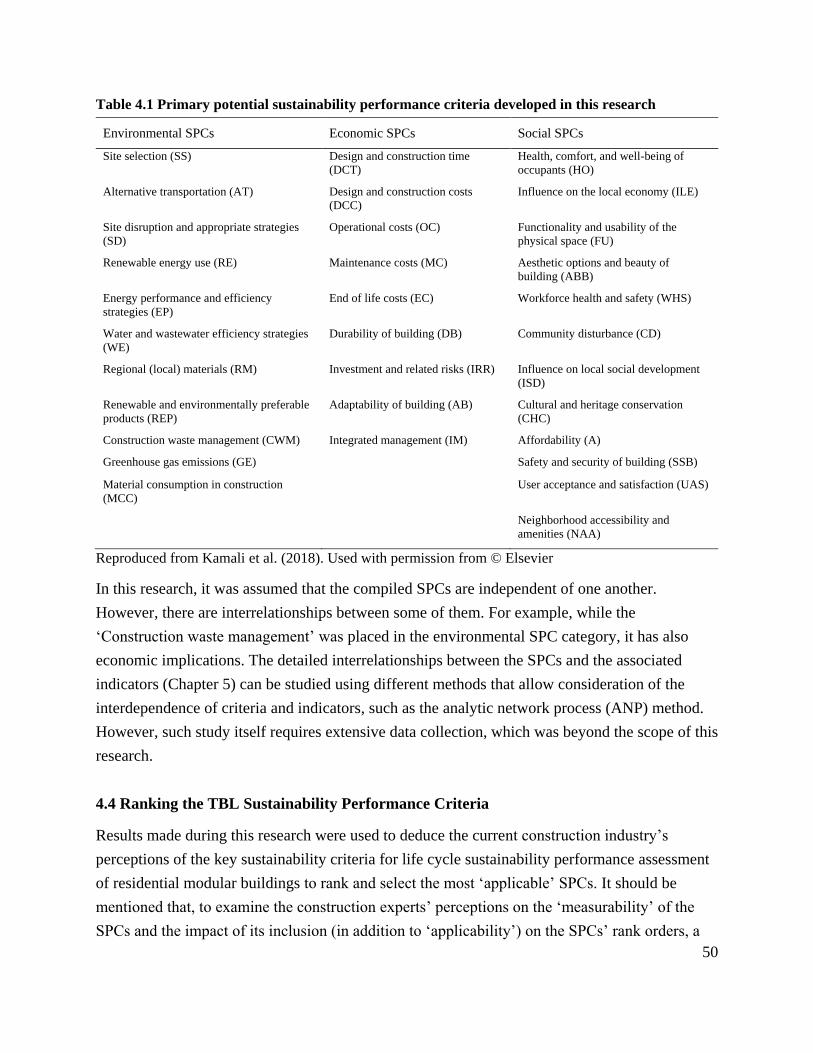
50

Table 4.1 Primary potential sustainability performance criteria developed in this research

Environmental SPCs Economic SPCs Social SPCs

Site selection (SS) Design and construction time

(DCT)

Health, comfort, and well-being of

occupants (HO)

Alternative transportation (AT) Design and construction costs

(DCC)

Influence on the local economy (ILE)

Site disruption and appropriate strategies

(SD)

Operational costs (OC) Functionality and usability of the

physical space (FU)

Renewable energy use (RE) Maintenance costs (MC) Aesthetic options and beauty of

building (ABB)

Energy performance and efficiency

strategies (EP)

End of life costs (EC) Workforce health and safety (WHS)

Water and wastewater efficiency strategies

(WE)

Durability of building (DB) Community disturbance (CD)

Regional (local) materials (RM) Investment and related risks (IRR) Influence on local social development

(ISD)

Renewable and environmentally preferable

products (REP)

Adaptability of building (AB) Cultural and heritage conservation

(CHC)

Construction waste management (CWM) Integrated management (IM) Affordability (A)

Greenhouse gas emissions (GE) Safety and security of building (SSB)

Material consumption in construction

(MCC)

User acceptance and satisfaction (UAS)

Neighborhood accessibility and

amenities (NAA)

Reproduced from Kamali et al. (2018). Used with permission from © Elsevier

In this research, it was assumed that the compiled SPCs are independent of one another.

However, there are interrelationships between some of them. For example, while the

‘Construction waste management’ was placed in the environmental SPC category, it has also

economic implications. The detailed interrelationships between the SPCs and the associated

indicators (Chapter 5) can be studied using different methods that allow consideration of the

interdependence of criteria and indicators, such as the analytic network process (ANP) method.

However, such study itself requires extensive data collection, which was beyond the scope of this

research.

4.4 Ranking the TBL Sustainability Performance Criteria

Results made during this research were used to deduce the current construction industry’s

perceptions of the key sustainability criteria for life cycle sustainability performance assessment

of residential modular buildings to rank and select the most ‘applicable’ SPCs. It should be

mentioned that, to examine the construction experts’ perceptions on the ‘measurability’ of the

SPCs and the impact of its inclusion (in addition to ‘applicability’) on the SPCs’ rank orders, a

51

supplementary study was conducted. This supplementary study conducted additional surveys to

evaluate the SPCs against both ‘applicability’ and ‘measurability’, and employed the Analytic

Hierarchy Process (AHP) and the Elimination and Choice Translating Reality (ELECTRE)

MCDA methods to analyze the surveys and rank the SPCs (see Appendix A for details). When

comparing the results of investigating the ‘applicability’ only, with the results of investigating

both the ‘applicability’ and ‘measurability’, it was evident that the rank order of some SPCs have

been changed locally but the overall trend remained the same in both studies. As discussed

earlier, the ‘measurability’ of the complied SPCs are ensured in the next chapter when

determining suitable measurable SPIs under each selected SPC. Therefore, the empirical

evidence from the study of ranking the SPCs based on their applicability only was reported in

this section.

4.4.1 Survey Respondents

A total number of 51 experts responded to the research participation requests, i.e., the initial

invitation and two follow-up reminder emails. Among the received questionnaire forms, 46

completed forms were properly filled out and returned; therefore, they were included in the

analyses. In addition, the survey overall response rate including direct and indirect questionnaire

delivery contact methods, was 21.9% (Table 4.2).

Table 4.2 Survey dissemination details and the rate of valid responses

Contact method No. of delivered forms No. of received forms No. of valid forms Response rate (%)

Indirect 134 14 13 9.7

Direct 76 37 33 43.4

Total 210 51 46 21.9

Reproduced from Kamali and Hewage (2017b). Used with permission from © Elsevier

There are two primary variables of measurement: (1) Continuous, and (2) Categorical. For

example, if a researcher plans to use a seven-point scale to measure ‘job satisfaction’ or the

extent to which the respondents are agreed with a phrase, these are continuous variables. In

contrast, if the researcher wants to determine if the respondents differ by gender or educational

level, these are certain categorical variables (Bartlett et al. 2001). For each type of measurement

variables, a sample size calculation formula was proposed by Cochran (1977). In this research,

since the applicability of the TBL SPCs was measured, the measured variables are continuous as

opposed to categorical and a five-point Likert scale was used for measurement. Therefore, the

Cochran’s formula for continuous variables that has been used in many studies (e.g., Antar 2012;

Karami et al. 2015; Sushi et al. 2016, among others) was used to determine the adequate sample

size in this survey:

52

𝑛 =𝑧𝛼/22 ∗ 𝑠2

𝑑2 [4.2]

where n is the sample size.

zα/2= confidence coefficient for the selected confidence level (1-α) and associated alpha level (α)

in each tail. The alpha level indicates the level of risk the researcher is willing to take that true

margin of error may exceed the acceptable margin of error.

s = estimate of the standard deviation in the population.

d = acceptable margin of error for mean (d = number of points on primary scale × error

researcher is willing to except).

According to the literature, the commonly used confidence levels are 90% and 95%. In addition,

a commonly acceptable value for the margin of error is 5% (Olson and Kellogg 2014; Méda et al.

2014; Ferguson and Takane 1989). In this study, the confidence level was initially set at 90%

(i.e., α/2 = 5% and zα/2 = 1.64) and the acceptable margin of error was selected as 5%. However,

the final sample size was good enough to make conclusions with 95% confidence level as

explained below.

According to Bartlett et al. (2001) a critical component of sample size formulas is the estimation

of the standard deviation in the primary variables of interest in the study. The researcher does not

have direct control over the standard deviation and must incorporate variance estimates into

research design. Cochran (1977) listed four strategies of estimating population variances for

sample size determinations: (1) take the sample in two steps, and use the results of the first step

(i.e., the variance observed in the first step data) to determine how many additional responses are

needed to attain an appropriate sample size; (2) use a pilot study results; (3) use data from

previous studies of the same or a similar population; or (4) estimate or guess the structure of the

population assisted by some logical mathematical results. In this study, the first strategy was

adopted, which provided early indications on the needed sample size. In the first step, 13

completed questionnaires were taken and the standard deviations of the respondents’ scores for

all the TBL SPCs were calculated. The results revealed that the standard deviations ranged

between 0.51 and 0.96. Appendix B provides the collected data in the first step study and

corresponding standard deviations. Therefore, using Equation [4.2], the required sample size n

was obtained between 𝑛 =1.642∗ 0.512

(5∗0.05)2= 11.19 and 𝑛 =

1.642∗ 0.962

(5∗0.05)2= 39.65. By rounding these

values up to their next highest integer, the minimum required sample size to assess the selected

SPCs came to be between 12 and 40. In other words, certain SPCs had relatively low standard

deviation in the first step study, which required low sample size. Hence, a minimum sample size

53

of 40 is acceptable to draw conclusions out of all the SPCs. This minimum sample size was

calculated based on the confidence level and the margin of error of 90% and 5%, respectively.

However, Cochran’s sample size calculation and correction formulas (Bartlett et al. 2001)

revealed that, even with a more precise confidence level (i.e., 95%), the sample size of 46 valid

questionnaires is adequate to be used in the analyses.

The first main section of the questionnaire searched for the respondent’s background

information. The participants were affiliated with diverse types of organizations (mainly in North

America), e.g., engineering companies, modular manufacturers, general contractors, academic

institutions, among others. The number of employees in the organizations were also different.

For instance, 43% of the organizations had at least 500 employees. The participants were also

from different professions. For example, 9 completed forms were received from construction

managers, 6 from engineers, 4 from architects, 16 from academic researchers (originally

engineers/architects), and so forth. A number of respondents had rich experience in two or even

more professions. In addition, the survey participants had different years of professional

experience, ranging from 5 (and fewer) to over 35. While only below 7% of the respondents

were younger industry practitioners with less than 5 years of experience, 32% had between 5 and

15 years, 36% had between 16 and 30 years, and 25% had over 30 years professional experience

as indicated in Figure 4.3 The respondents’ involvement in modular building projects were also

sought in order to examine the extent to which the respondents were familiar with modular

processes. The questionnaire data showed that most of the experts have been involved in a

number of modular building projects. For example, 25% of them had contributed to over 55

modular projects.

Figure 4.3 Professional experience of the survey participants. Reproduced from Kamali and

Hewage (2017b). Used with permission from © Elsevier

The number of respondents, along with their diverse professions, organizations, professional

Below 5 yr.7% 5 - 10 yr.

9%

11 - 15 yr.23%

16 - 20 yr.16%

21 - 25 yr.13%

26 - 30 yr.7%

31 - 35 yr.9%

Over 35 yr.16%

54

experience, and history of involvement in both modular and conventional building projects

ensured that the results of this survey can adequately represent the construction industry’s

feedback.

4.4.2 Reliability Analysis

As stated in the methodology section, a reliability analysis was conducted to examine the internal

consistency of Survey A. The data collected through the completed forms was fed into the SPSS

software as input and four rounds of reliability analyses were performed. The analyses included

one analysis that considered all SPCs as a whole set of sustainability criteria (overall TBL SPCs),

and three independent analyses that separately considered the SPCs associated with the

sustainability categories (i.e., environmental, economic, and social). As discussed previously, a

minimum reliability coefficient of 0.70 ensures that adequate internal consistency of a test exists.

The resulted Cronbach’s alpha values are shown in Table 4.3, which are much higher than the

minimum reliability coefficient recommended by Nunnally (1978). The reliability coefficient

values for the overall TBL SPC set, environmental SPC set, economic SPC set, and social SPC

set indicate strong internal consistency of Survey A.

Table 4.3 Reliability coefficients for different SPC categories

Sustainability category SPC count Cronbach’s alpha

Environmental 11 0.899

Economic 9 0.837

Social 12 0.883

Overall TBL SPCs 32 0.944


4.4.3 Environmental Criteria Ranking

Similar to the reliability analysis, four rounds of ranking analyses were conducted to analyze the

data collected through Survey A. Based on the output of the SPSS software (i.e., valid

percentage values) and Equation [4.1], severity index (SI) values were obtained. These SI values

were used to identify the rank of all the SPCs under the overall TBL SPCs as well as within their

associated sustainability categories. According to the SI value of a SPC, its importance level was

assigned using the severity scale defined earlier ranging from ‘Extremely High’ to ‘Extremely

Low’.

It is worth to mention that to ensure the validity of the SPC rankings based on their SI values, the

collected data was analyzed one more time using the ELECTRE MCDA method (see Appendix

A for the step-by step procedure of the ELECTRE method). The results of the ELECTRE

55

analyses showed identical rank orders for SPCs in all the three sustainability categories.

The overall rank order of each SPC within the environmental category is shown in Table 4.4. All

of the environmental SPCs were assigned as ‘High’ to ‘Medium’ importance, except three SPCs.

As Table 4.4 illustrates, there was no ‘Extremely High’ and ‘Very High’ level SPCs; however, 4

SPCs were ranked ‘High’ level criteria with SI values ranging from 76.10% to 81.47%. These

highly addressed criteria included ‘Construction waste management’, ‘Energy performance and

efficiency strategies’, ‘Material consumption in construction’, and ‘Greenhouse gas emissions’.

Table 4.4 Ranking of the environmental sustainability performance criteria

Environmental category SI (%) Rank in

category

Rank in overall

TBL SPCs

Level of

Importance

Construction waste management (CWM) 81.47 1 6 H

Energy performance and efficiency strategies (EP) 80.96 2 7 H

Material consumption in construction (MCC) 79.58 3 8 H

Greenhouse gas emissions (GE) 76.10 4 13 H

Site disruption and appropriate strategies (SD) 73.66 5 19 M

Renewable and environmentally preferable products (REP) 70.73 6 22 M

Regional (local) materials (RM) 67.33 7 24 M

Renewable energy use (RE) 66.90 8 25 M

Site selection (SS) 63.35 9 28 L

Water and wastewater efficiency strategies (WE) 62.44 10 29 L

Alternative transportation (AT) 52.76 11 32 VL


The most significant criterion among the top prioritized environmental SPCs was ‘Construction

waste management (CWM)’ (SI = 81.47%) which was also considered as highly ranked criterion

in the overall TBL SPCs (6th among all 32 SPCs). Supporting this, the literature reveals that

modular construction has the potential capability of providing more efficient waste management

strategies, contrary to conventional construction. In other words, modular construction has

shown better waste management results in terms of control (reduce), reuse, recycle, and waste

disposal in manufacturing centers (Zenga and Javor 2008; Kawecki 2010; Cartz and Crosby

2007). For example, materials can be precisely cut in modular factory environments, which

results in less construction waste. Furthermore, in modular construction, different modules have

the capability to be used in new building projects by disassembling, relocating, or refurbishing

them at the end of life phase of buildings, compared to conventional buildings where a

considerable amount of generated waste is sent directly to landfills (Li and Li 2013). However,

because the fabricated modules need to be safely transported to the final project sites, in order to

fulfill the “required structural strength” for transportation, around 10-15% additional materials

are used (in interface such as walls) compared to traditional construction (Cameron and Di Carlo

56

2007). This is probably why the respondents concerned about the ‘Material consumption in

construction (MCC)’. While the construction waste can be reduced when using modular

construction, additional materials are used for structural integrity and also when transporting the

modules to the final building location.

The second ‘High’ importance level SPC highlighted by the respondents was ‘Energy

performance and efficiency strategies (EP)’, with a SI value very close to the first ranked SPC. It

was also ranked 7th among all the TBL SPCs. The literature shows that the occupancy phase is

the dominant phase in terms of environmental impacts (Quale et al. 2012; Scheuer et al. 2003;

Sartori and Hestnes 2007) with over 70% of the total energy consumption (Ortiz et al. 2009;

Scheuer et al. 2003; Keoleian et al. 2000). Having access to more efficient technologies,

buildings are becoming more energy efficient over their operation phase. Consequently, other

life cycle phases, such as the construction phase and the end of life phase are growing in

importance (Gustavsson and Joelsson 2010). However, the use phase still is prevailing in terms

of energy consumption and environmental impacts. Two reasons may be offered as to why the

respondents chose ‘Energy performance and efficiency strategies’ as one of the most important

SPCs: i) the overall importance of energy efficiency in the use phase of a building, and ii) the

modular and conventional buildings’ dissimilar designs and installations of operational energy

efficiency systems, e.g., insulation and quality of construction in factory environment.

As discussed in Chapter 3, modular and conventional buildings are mainly different in their

design and construction phases. Therefore, the ‘Greenhouse gas emissions (GE)’, which

represents the environmental impacts of the construction process, was observed among the

‘High’ important SPCs.

In the bottom of Table 4.4 the ‘Low’ or ‘Very Low’ important SPCs were located including ‘Site

selection’, ‘Water and wastewater efficiency strategies’, and ‘Alternative transportation’. The

construction experts believed that there is no significant difference between modular and

conventional buildings with respect to these SPCs; therefore, they assigned the lowest scores to

these SPCs among all the environmental SPCs. The low ranks of ‘Site selection’ and ‘Alternative

transportation’ was anticipated because these criteria are mainly related to the building location

and are not dependent on the construction method by which the building is constructed.

Noticeably, ‘Alternative transportation’ was also rated as the least important criterion (32th)

among all the TBL SPCs.

4.4.4 Economic Criteria Ranking

The outcomes resulting from the ranking analysis of the economic criteria are reflected in Table

57

4.5. Based on the values of the severity indices, among the nine SPCs in the economic category,

two SPCs, four SPCs, and three SPCs placed in the ‘Very High’, ‘High’, and ‘Medium’ levels,

respectively.

The first top ranked (‘Very High’) economic SPC, as anticipated, was ‘Design and construction

time (DCT)’ with the SI value of 87.24%. This SPC was ranked second under the overall TBL

SPCs, which indicates the importance of this criterion among all the SPCs as well. These results

are consistent with the findings of Chen et al. (2010). As reported in Chapter 2, a significant

difference between the modular and conventional construction methods is the fast turnaround

between the breaking of ground and occupancy in the case of the former method. Unlike the

conventional processes, construction of a building (manufacturing modules) and preparation of

the final project site (foundations, etc.) can be performed simultaneously (Kawecki 2010; Haas et

al. 2000), which can lead to approximately 40% savings in the construction time (Mah 2011;

Lawson and Ogden 2010; Smith 2011; MBI 2012a). The resulted time savings can greatly

contribute to project cost savings when using modular processes. In other words, speed of

construction can enhance the economic positive impacts since the developers/contractors can

rapidly deliver the finished buildings to end users (clients or potential buyers) and start new

projects. On the other hand, the end users can occupy their buildings faster and eliminate

unnecessary expenses such as rental. Furthermore, this can help the economy of the community

the buildings are built.

Table 4.5 Ranking of the economic sustainability performance criteria

Economic category SI (%) Rank in

category

Rank in overall

TBL SPCs

Level of

Importance

Design and construction time (DCT) 87.24 1 2 VH

Design and construction costs (DCC) 86.38 2 3 VH

Durability of building (DB) 78.52 3 9 H

Integrated management (IM) 77.56 4 10 H

Investment and related risks (IRR) 77.09 5 11 H

Operational costs (OC) 76.06 6 14 H

Adaptability of building (AB) 74.76 7 16 M

Maintenance costs (MC) 74.52 8 17 M

End of life costs (EC) 66.36 9 26 M


The next major economic concern of the respondents was ‘Design and construction costs’ (SI =

86.38%). This SPC was found to be at 3rd rank under the overall TBL SPCs. As shown in Table

4.5, the costs associated with the design and construction phase of a building, such as design,

coordination, materials, and labor, grabbed the attention of the respondents more than the costs

associated with the other life cycle phases. The possible reason could be the costs associated with

58

the initial phases of a building’s life cycle can be perceived as short-term costs; therefore, they

are more perceptible (tangible) costs. Interestingly, the costs related to the end of life phase are

long-term costs and rated as the least important SPC under the economic category (with SI value

of 66.36), even though it is still a ‘Medium’ importance level criterion. Accordingly, it can be

observed from Table 4.5 that ‘Operational costs’ and ‘Maintenance costs’, which are both mid-

term costs, were assigned close SI values and located somewhere between ‘Design and

construction costs’ and ‘End of life costs’.

Although some literature pointed out that the economic impacts of using off-site construction

methods are not evident (Chiang et al. 2006; Pan et al. 2011; Lawson and Ogden 2008), there are

various attributes that can lead to cost savings when these methods are used (Haas et al. 2000;

Lawson et al. 2012). Moreover, the cost reduction spots can be different in different life cycle

phases of a building. For example, due to concurrent fabrication of several modules, less

workforce and machinery transportation are needed. In addition, the required materials are

purchased in bulk and therefore less expensive (Chiu 2012).

The modular construction can effectively influence the other SPCs from the economic point of

view, such as ‘Durability of building’. The modular construction method offers higher quality

than the traditional counterpart due to controlled manufacturing environment (Cartz and Crosby

2007; Rogan et al. 2000). Furthermore, higher finished building quality can be achieved due to

“less material exposure to harsh weather” on the final project site. In addition, high quality,

lightweight, and durable materials are utilized in the construction of each module itself (O’Brien

et al. 2000; Celine 2009; Cartwright 2011; Haas and Fagerlund 2002). Moreover, as mentioned

before, extra materials are used in building interface (mostly walls) to ensure the structural

integrity of the whole buildings when connecting the modules on the final project site. All of

these can yield greater durability of modular buildings.

4.4.5 Social Criteria Ranking

Results of the final preferences for the SPCs within the social category are presented in Table

4.6. Among the twelve social SPCs, only three SPCs were rated either ‘Very Low’ or ‘Low’,

while nine SPCs were placed in either ‘Medium’, ‘High’, or ‘Very High’ importance levels.

Noticeably, the top three social criteria were also among the top five overall TBL SPCs, which

implies the construction industry’s increased perception of the role of social criteria in the overall

sustainability of different construction methods.

The ‘Construction workforce health and safety’ SPC was the only criterion that was ranked first

among both the overall TBL SPCs and the category it belonged to (i.e., social category). This

59

SPC was a ‘Very High’ importance SPC with an impressive SI value of 91.25%, which was

higher than the SI values of the top ranked economic and environmental SPCs. This indicated the

significance of the health and safety of the workers to the overall sustainability of a building

from the construction experts’ perspectives, and pointed to their belief that the modular and

conventional processes can provide extremely different degrees of labor health and safety in

building projects. As stated in the previous chapter, on-site reportable accidents can be decreased

up to 80% using off-site construction processes (Lawson et al. 2012). By performing the main

work in manufacturing centers (rather than on the final project sites) working at height,

dangerous activities, severe weather, congestion, workplace accidents, and neighboring

construction operations can be decreased (McGraw-Hill Construction 2011; Na 2007; Li et al.

2013; Haas and Fagerlund 2002).

It is a significant observation that ‘Construction workforce health and safety’ was of paramount

importance to the respondents; however, ‘Health, comfort and well-being of occupants’ is not.

Even though the latter was recorded as ‘Medium’ importance criterion, which shows this SPC is

a relatively important one, its rank within the social category is not as high as expected.

Table 4.6 Ranking of the social sustainability performance criteria

Social category SI (%) Rank in

category

Rank in overall

TBL SPCs

Level of

Importance

Workforce health and safety (WHS) 91.25 1 1 VH

Community disturbance (CD) 83.45 2 4 H

Safety and security of building (SSB) 81.92 3 5 H

User acceptance and satisfaction (UAS) 76.56 4 12 H

Affordability (A) 75.14 5 15 H

Functionality and usability of the physical space (FU) 74.12 6 18 M

Influence on the local economy (ILE) 73.11 7 20 M

Aesthetic options and beauty of building (ABB) 72.64 8 21 M

Health, comfort, and well-being of occupants (HO) 70.22 9 23 M

Influence on local social development (ISD) 64.47 10 27 L

Neighborhood accessibility and amenities (NAA) 60.06 11 30 L

Cultural and heritage conservation (CHC) 53.06 12 31 VL


The SPC named ‘Community disturbance’ was ranked second and fourth under the social

category and the overall TBL SPCs, respectively. The respondents believed that there is an

enormous difference between modular and traditional construction in terms of minimizing the

social impacts of on-site construction activities on the project site and surrounding local

communities, which can be justifiable according to the literature. As mentioned previously, when

using modular construction, the majority of the project work (85-90%) is performed in

manufacturing centers (Kawecki 2010). Thus, construction noise, dust, light pollution, traffic

60

congestion (due to materials, machinery, and workforce transportation) are reduced significantly,

resulting in less community disturbance.

When the results of all ranking analyses (Tables 4.4 to 4.6) were simultaneously evaluated for

the environmental, economic, and social categories, the 32 TBL SPCs were assigned importance

levels as shown in Figure 4.4. According to the SI values, no SPC was rated as ‘Extremely High’

or ‘Extremely Low’ importance.

Figure 4.4 Number of TBL SPCs assigned each of the importance levels. Reproduced from Kamali

and Hewage (2017b). Used with permission from © Elsevier

It should be emphasized that, as some respondents asserted, ‘Very Low’ or ‘Low’ importance

rankings for a SPC does not mean that it is not important by itself, but rather it means there is no

considerable difference in that SPC between modular and conventional construction methods. In

other words, this SPC cannot significantly contribute to comparatively assessing and

distinguishing the overall sustainability of the two construction buildings.

It can be understood from the construction industry experts’ feedback that the social and

economic criteria play more important roles than the environmental ones when the sustainability

of modular construction versus traditional construction is concerned. This was investigated from

two different approaches; considering the top ranked SPCs within the overall TBL SPCs and

comparing the SI value averages of the ‘High’ and ‘Very High’ important SPCs within each

sustainability dimension category. According to Tables 4.4 to 4.6, among the top 5 SPCs in the

overall TBL SPCs, the first, fourth, and fifth belong to the social category and the second and

third belong to the economic category, while the top ranked SPC within the environmental

category ranked sixth in the overall TBL SPCs. In addition, using the second approach, the

average SI values within the ‘Very High’ and ‘High’ importance SPCs for the social category,

the economic category, and the environmental category, have been 81.66%, 80.48 %, and

79.52%, respectively, which also supports the above idea.

Furthermore, comparison of the relative frequency of ‘Very High’ and ‘High’ level SPCs in each

Environmental category

Economic category

Social category

2

1

4

4

4

4

3

4

2

2

1

1

Extremely high important SPC

Very high important SPC

High important SPC

Medium important SPC

Low important SPC

Very low important SPC

Extremely low important SPC

61

sustainability dimension category demonstrated the fact that among the TBL sustainability

dimensions, the economic dimension was still the governing concern of the construction industry

practitioners (even though the top SPC within the overall TBL SPCs is a social one) followed by

the social dimension. Approximately 67% of the economic criteria were rated as ‘Very High’

and ‘High’ importance, which was noticeable compared to the cases of social and environmental

criteria (42% and 33%, respectively). In addition, when the total SI value averages (regardless of

the importance levels of SPCs) of the three sustainability dimension categories were compared,

again, the economic dimension (SI average=78%) was superior to both cases of the social

dimension and environmental dimension.

4.4.6 Effect of Professional Experience on Ranking Results

As stated, the data collected through the survey showed that the research participants had diverse

professional characteristics, such as the number of employees in their firms, professional

experience, and history of involvement in modular projects. Thus far, all the analyses were

conducted based on the assumption that the opinions of the research participants were equally

important, regardless of their different profile characteristics. That is, all respondents’ feedback

had equal weight when conducting different analyses. For example, a respondent’s opinion with

5 years of professional experience and a respondent’s opinion with over 35 years were

considered equal. Among the diverse profile characteristics of the respondents, some can have an

impact on the results, but some cannot. For example, the number of employees in the

organization in which a respondent belongs cannot necessarily guarantee the robustness of

his/her opinions as there are many knowledgeable experts working in small firms, and vice versa.

In this research, professional experience, as one of the respondents’ profile characteristics that

potentially can influence the results, was further investigated. The participants were divided into

two groups including experts with less or equal than 20 years and experts with over 20 years of

professional experience. The first group included 25 junior to highly experienced experts and the

second group included 21 extremely high (i.e., associate) experts. Figure 4.5 illustrate the results

of the ranking analysis for these two groups of participants within the environmental, the

economic, and the social categories, respectively. Furthermore, in each case, the previous results,

where all of the respondents’ opinions were considered equal, are shown for easier comparisons.

An impressive consistency can be found out when comparing the social SPC rankings by all

respondents with respondents with less than 20 years of experience and respondents with over 20

62

Figure 4.5 Influence of the participants’ experience on rank order of (a) Environmental SPCs; (b)

Economic SPCs; (c) Social SPCs. Reproduced from Kamali and Hewage (2017b). Used with

permission from © Elsevier

1

2

3

4

5

6

7

8

9

10

11

2

1

3

5

4

6

7

8

9

10

11

1

3

2

4

6

7

9

5

8

10

11

CWM EP MCC GE SD REP RM RE SS WE AT

(a)All respondents

Years of experience ≤ 20

Years of experience > 20

Ran

k

SPC

1

2

3

4

5

6

7

8

9

1

2

5

4

8

6

3

7

9

1

2

3

5

4

6

7

8

9

DCT DCC DB IM IRR OC AB MC EC

(b)

SPC

Ran

k

12

34

56

78

910

1112

12

34

5

8

67

910

1112

12

34

65

78

910

1112

WHS CD SSB UAS A FU ILE ABB HO ISD NAA CHC

(c)

SPC

Ran

k

63

years of experience. As demonstrated in Figure 4.5c, all three groups assigned the same ranks to

the top ranked SPCs, i.e., WHS, CD, SSB, and UAS. The groups also identically ranked the

bottom SPCs, i.e., HO, ISO, NAA, and CHC. This shows the fact that respondents’ professional

experience does not influence the rating of the top and bottom SPCs. However, there are some

discrepancies between SPC rankings in the cases of the middle SPCs. For example, FU was

ranked by all respondents as the sixth social SPC, while respondents with less than 20 years of

experience and respondents with over 20 years of experience ranked it as the eighth and fifth

SPC, respectively.

In the case of the economic category, similarly, unanimity exists between the opinions of the

respondents (regardless of their different professional experience) when they ranked DCT and

DCC as the top SPCs and also EC as the bottom SPC. Nevertheless, there were minor

inconsistencies in the ranks of the middle economic SPCs, in which the two groups with the

different experience range dissimilarly prioritized these SPCs (Figure 4.5b).

The environmental category is where less consistency can be seen in terms of SPC ranking by

the two respondent groups (Figure 4.5a). While all respondent groups were agreed on the ranks

of the bottom SPCs, different rankings were seen in the cases of the top and middle SPCs in the

category. However, the rank order changes locally. For example, the CWM SPC was ranked first

by all respondents and the group with over 20 years of experience; however, the group with less

experience ranked it as the second SPC.

4.5 Summary

Off-site construction has increasingly been used as alternative for conventional construction

during the last few years. One of the main methods of off-site construction is modular

construction, which offers various advantages that can effectively contribute to sustainable

construction. In order to assess and compare the life cycle sustainability performance of modular

construction with conventional construction the triple bottom line (TBL) sustainability

dimensions, i.e., economic, environmental, and social, should be addressed. The sustainability

evaluation criteria (SECs) comprise the TBL sustainability categories i.e., environmental,

economic, and social, in which each category includes diverse sustainability performance criteria

(SPC) associated with different life cycle phases of a building. Each SPC itself consists of a

number of measurable sustainability performance indicators (SPI) by which the SPC can be

measured. Moreover, a SPI might include a number of sub-SPIs. There is no published study on

sustainability criteria identification for the life cycle performance assessment of residential

modular buildings. Thus, in this chapter, the most applicable (important) TBL SPCs were

64

identified, by which the life cycle sustainability performance of residential modular buildings

can be evaluated.

Following a comprehensive literature review, 11 environmental SPCs, 9 economic SPCs, and 12

social SPCs were developed. Using these TBL SPCs, a questionnaire survey (Survey A) captured

the construction industry practitioners’ perceptions of the most applicable sustainability criteria

for comparing the sustainability of modular and conventional buildings.

Ranking analysis using the Severity Index (SI) method was the primary technique used for data

analysis. Based on each SPC’s SI value, it was assigned an importance level according to a

severity scale ranging from ‘Extremely High’ to ‘Extremely Low’. Results of analyses showed

that among all the 32 TBL SPCs, 15 SPCs were rated as either ‘Very High’ or ‘High’ importance

criteria (there were no ‘Extremely High’ importance SPCs) which account for 45% of all SPCs.

In addition, 11 SPCs were assigned as ‘Medium’ importance level, and 6 SPCs were among

either ‘Low’ or ‘Very Low’ importance level criteria (there were no ‘Extremely Low’

importance SPCs). This should be mentioned that to ensure the validity of the SPC rankings

based on the Severity Index method analyses, the collected data through the survey was analyzed

one more time using the ELECTRE 1 MCDA method, which produced the same rank orders for

SPCs in all the three sustainability categories.

The top ranked SPCs within the environmental category, ‘Construction waste management’ and

‘Energy performance and efficiency strategies’, were the sixth SPC and seventh SPC,

respectively, under the overall TBL SPCs. ‘Design and construction time’ and ‘Design and

construction costs’ in the economic category were highlighted as the top concerns of the

respondents. These two SPCs were also significant among all 32 TBL SPCs as they ranked

second and third, respectively. Within the social category, ‘Construction workforce health and

safety’ along with ‘Community disturbance’ were designated as the main concerns. More

importantly, the former was rated the top criterion within the overall TBL SPCs as well and the

latter was fourth, which indicates the overall sustainability importance of these social SPCs.

According to the construction industry practitioners, the economic criteria still play the most

significant role in distinguishing the sustainability of two construction methods. Nevertheless,

the social dimension of sustainability grabbed more attention compared to the environmental

dimension.

The impact of the research participants’ professional experience on the rank order of SPCs was

examined. In both the economic and the social categories, there were impressive consistencies of

SPC rankings assigned by respondents with less than 20 years and over 20 years of professional

experience. However, in the case of the environmental SPCs, there were some inconsistencies of

65

the rankings by these two groups of respondents. In addition, the impact of the SPC evaluation

criteria on the rank order of SPCs was investigated. The main evaluation criterion of

‘applicability’ was used when analyzing the expert’s feedback to rank the SPCs. However,

another analysis was conducted by including both the evaluation criteria of ‘applicability’ and

‘measurability’ with the help of ELECTRE 1 method to rank the SPCs. The results of ELECTRE

analyses showed the same overall rankings but locally different rankings for SPCs in all the three

sustainability categories. (see Appendix A for details)

The results of this chapter can assist the construction industry experts to gain in-depth

understanding of the most significant TBL sustainability criteria when comparing the

performance a residential modular building with the performance of similar conventional one.

By identification of applicable SPCs, all sustainability dimensions can be analyzed over the life

cycle of building projects and different stakeholders’ concerns can be addressed, which can lead

to sustainable construction.

66

Chapter 5 Development of Aggregated Sustainability Indices

A part of this chapter has been published in Building and Environment entitled “Life cycle

sustainability performance assessment framework for residential modular buildings: Aggregated

sustainability indices” (Kamali et al. 2018).

Parts of this chapter will be submitted for possible publication in:

- Sustainable Cities and Society entitled “Environmental sustainability benchmarking of modular

homes – Part I: Performance quantification” (Kamali et al. 2019a).

- Journal of Cleaner Production entitled “Economic sustainability benchmarking of modular

homes – Part I: Performance quantification” (Kamali et al. 2019c).

In this chapter, suitable sustainability indicators associated with each selected SPC are

determined. In addition, a method to develop sustainability indices for performance evaluation of

residential buildings is proposed.

5.1 Background

In the previous chapter, the TBL SPCs have been compiled and ranked within the sustainability

categories (i.e., environmental, economic, and social) according to their applicability for

sustainability assessment of modular buildings. Those SPCs that were assigned the importance

level of either ‘Very High’, ‘High’, or ‘Medium’ by the construction experts have been

considered the key sustainability criteria and suitable for life cycle sustainability assessment

(LCSA) of residential modular buildings. Therefore, all the SPCs within the environmental and

economic categories with the importance level of ‘Medium’ and higher were selected.

The primary focus of this chapter is on quantification of the selected SPCs (i.e., development of

sustainability indices). To this end, in the first part of this chapter, suitable measurable indicators

under each SPC were determined. In addition, suitable measurement functions were established

to calculate the determined indicators. Subsequently, in the second part of the chapter, the

methodology to develop a set of sustainability indices was proposed by which the performance

of a given modular building can be evaluated.


The methodology followed in this chapter comprised different steps as illustrated in Figure 5.1.

These steps that lead to development of aggregated sustainability indices have been explained in

67

details as follows.

Establishing performance level functions (PLFs) for sub-SPIs/SPIs

(Literature/expert opinions)

Introducing the concept of

Performance Level (PL)

Determining measurable indicators under selected SPCs

(Literature/expert communications)

SPIs and sub-SPIs

Data variables associated with sub-SPIs/SPIs

Importance weights of sub-SPIs/SPIs

Developing aggregated sustainability indices

(MCDA methods)

Sustainability index for (TOPSIS method):

each SPC (Level 3)

each sustainability dimension (Level 2)

overall sustainability (Level 1)

CWMi EPi DCTi DCCi . . .. . .

ENVRi ECONi

OVERALLi

Least/most desirable values of sub-SPIs/SPIs (Literature/Survey B with Delphi method)

Ranges of data variables correspond to least/most desirable performances

PLFs for sub-SPIs/SPIs

Figure 5.1 Methodology used in Chapter 5

68

5.2.1 Determination of indicators under SPCs

As stated in Chapter 4, among the 11 SPCs within the environmental category, 8 SPCs were

prioritized by the construction practitioners as ‘Medium’ and higher importance criteria and the

remaining SPCs received the importance level equal or worse than ‘Low’. In the case of the

economic criteria, all the 9 SPCs received the importance level of ‘Medium’ and above. Table

5.1 lists the environmental and economic SPCs with the importance level of ‘Medium’ and up

which were selected for sustainability assessment of modular buildings in this research. The table

also shows the acronyms of SPCs that were used sometimes in this thesis for simplicity purposes.

Table 5.1 Importance levels of the selected environmental and economic SPCs

Environmental category Level of

Importance Economic category

Level of

Importance

Construction waste management (CWM) H Design and construction time (DCT) VH

Energy performance and efficiency strategies (EP) H Design and construction costs (DCC) VH

Material consumption in construction (MCC) H Durability of building (DB) H

Greenhouse gas emissions (GE) H Integrated management (IM) H

Site disruption and appropriate strategies (SD) M Investment and related risks (IRR) H

Renewable and environmentally preferable products (REP) M Operational costs (OC) H

Regional (local) materials (RM) M Adaptability of building (AB) M

Renewable energy use (RE) M Maintenance costs (MC) M End of life costs (EC) M

As discussed before, each SPC may consist of a number of indicators called sustainability

performance indicators (SPIs) in this research. Similarly, a SPI itself can comprise a number of

sub-SPIs. Therefore, to measure each selected SPC, relevant SPIs and sub-SPIs should be

determined, calculated, and combined. In this step of the methodology, a literature review along

with expert consultations were carried out to determine suitable SPIs and sub-SPIs, their required

measurement data (i.e., data variables), their performance benchmark values, and also their

relative importance weights.

Similar to what has been done for compiling SPCs, the literature regarding rating systems and

other published studies were reviewed. Through a few screening processes, all SPIs and sub-SPIs

related to a SPC were recognized, listed, renamed, and refined. The approach followed in this

research involved choosing simple and easy-to-use measurement methods for the indicators by

which each indicator can be calculated by having the minimum amount of data including

quantitative and qualitative. Therefore, in cases where the same indicator existed in different

references with (different names and) different methods of measurement, the one that provided

easiest method and needed less data was selected.

In this study, the determined SPIs associated with a SPC have been denoted by the acronyms of

69

the SPC followed immediately by an integer starting at 1 and ending at n (successive integers),

where n is the total number of SPIs. For example, if the acronyms of a hypothetical SPC is ABC

and it comprises two SPIs, these SPIs are denoted by ABC1 and ABC2. Similarly, the same

method has been used for symbolizing the sub-SPIs under SPIs with only one difference that the

integer denoting the sub-SPI comes after a hyphen. In the same example, if the ABC1 SPI

consists of three sub-SPIs, they are denoted by ABC1-1, ABC1-2, and ABC1-3.

5.2.2 Performance Level Functions for Indicators

After determination of suitable indicators (i.e., SPIs and sub-SPIs), their measurement methods

were formulated. In this research, a performance level function (PLF) was established for each

indicator by which the performance of the subject building with respect to that indicator can be

calculated and presented in a dimensionless and normalized way. Depending on the nature of the

possible outcomes of a SPI (or sub-SPI), the corresponding PLF can be either a continuous

function or a discrete function. In other words, the calculated possible SPI values can be either

finite (discrete) or infinite (continuous). For example, if a SPI measures the amount of generated

waste during the construction of a building, the possible outcomes can be any real value for the

generated waste. Thus, the corresponding PLF will be a continuous function. A continuous PLF

itself can be a single function or a piecewise function. On the contrary, if a SPI measures

whether a number of specific conditions or items are met in the same project, the possible

outcomes cannot be infinite (measurement is based on Yes/No answers). Therefore, the

associated PLF will be a discrete step function that is, in fact, a step function is a piecewise

function containing all constant "pieces" (Roberts 2018).

Regardless of the form of a PLF (discrete vs continuous), it is important to discuss the unit of its

outcomes, i.e., the unit of measurement for the calculated indicator. As stated earlier, the

calculated SPIs related to a SPC are combined with their relative importance weights to develop

a sustainability index for the SPC. However, the calculated SPIs are not necessarily of the same

unit of measurement. For instance, while all the SPIs under the SPC ‘Regional materials (RM)’

are of the same unit (i.e., percentage of regional content), the SPIs under the SPC ‘Construction

waste management (CWM)’ are of different units of measurement. Therefore, instead of directly

combining SPIs with different units of measurement, first, they should be converted to a

common unit and normalized. This is performed automatically by the PLF of each indicator

when it calculates the indicator. This research introduced and employed the concept of

performance level (PL) as a common unit to enable the calculated indicator to be normalized. PL

is a dimensionless unit ranged between 0 and 100. The PL values of 0 and 100 for an indicator

are representatives of the least and most desirable performances (i.e., benchmark values) of the

70

indicator, respectively. In other words, a PLF calculates an indicator using the collected data and

then transforms the calculated indicator into a PL between 0 and 100.

To develop a PLF for an indicator, its least and most desirable performance values along with the

corresponding data variable values should be determined. In this research, the least desirable

performance (i.e., PL = 0) of an indicator corresponds to the data variable value at which the

performance of the subject building with regard to the indicator is considered as the worst in the

literature or by experts. For example, the LEED rating system assigns no point for the waste

generation rate (WGR) more than 4.0 lb/ft2. It is possible for a building project to generate more

amount of waste; however, the WGR = 4.0 lb/ft2 is the lower bound threshold equivalent to the

least desirable performance (PL = 0) of the subject building with regard to the ‘Construction

waste diversion’ SPI. Similarly, the most desirable performance (PL = 100) is equivalent to the

data variable at which the performance of the subject building is considered the best. In the

above example, the best performance has been defined as having the WGR of 0.5 lb/ft2 or less.

Therefore, the upper bound waste threshold is set at WGR = 0.5 lb/ft2 equivalent to the most

desirable performance of the subject building with regard to the ‘Construction waste diversion’

SPI (PL = 100). In some projects, it might be possible to generate even less waste; however, any

WGR less than the 0.5 lb/ft2 will receive the same PL = 100. In other words, in cases where the

quantity of the data variable of a SPI (or sub-SPI) lies outside the applicable range (0.5 lb/ft2 <

WGR < 4.0 lb/ft2 in this example), the performance levels of 0 and 100 are assigned for all

performances worse and better than the least and most desirable performances, respectively.

It should be stressed that when searching for the least/most desirable performance values of an

indicator and the corresponding data variable thresholds (i.e., data variable boundary conditions),

the priority was the sources that reflected regional information. In this regard, because the case

study modular buildings assessed in this research were located in the Okanagan, BC, the priority

was to use the information specific to this region. For example, if the information about the range

of a data variable of a SPI was available for the entire Canada, the entire BC, and the Okanagan,

the latter was used in developing the PLF for the SPI.

In the cases of some economic SPCs, such as ‘Design and construction costs’, the least and most

desirable performance values of the associated SPIs are sensitive to the construction

circumstances in the region in which the subject building in designed and constructed. Therefore,

the least/most desirable performances should be obtained locally. For such SPCs (henceforth

locality sensitive SPCs), a questionnaire survey (Survey B), was designed based on the Delphi

method and implemented to collect this information from the construction firms located in the

Okanagan, BC. In general, the Delphi method is a robust technique to reach consensus on

71

problems or questions that cannot be resolved in a single meeting by experts. In this method, a

number of experts provide their opinions on an issue through an interactive process (i.e., a few

rounds of questioning) until they reach consensus (Stewart 2001). The collected data in the first

round (initial opinions) is collated and distributed between the experts again for their review.

This process continues until the last round where the consensus is reached by the experts on the

answer or solution of the issue (Stitt-Gohdes and Crews 2004; Aigbavboa 2015).

5.2.3 Aggregated Sustainability Indices

As discussed earlier, using a bottom-up approach, this research develops sustainability indices at

the following levels:

Level 3: Sustainability indices for SPCs (e.g., CWMi, EPi);

Level 2: Sustainability indices for sustainability dimensions (ENVRi and ECONi); and

Level 1: Overall sustainability index (OVERALLi).

In the case of Level 3, the sustainability performance indices for SPCs are developed through

calculating and combining the associated SPIs. Through a suitable aggregation process (i.e.,

MCDA methods), the performance levels (PLs) of all the SPIs associated with a SPC, that have

been already calculated using the developed PLFs and their weights are aggregated to calculate

the sustainability index for the SPC. As for Level 2, once the sustainability indices for SPCs are

derived, an index for each of the sustainability dimensions (i.e., environmental and economic) is

developed. To this end, similar to the methodology used in Level 3, the sustainability indices of

the SPCs associated with a sustainability dimension (e.g., environmental) and their weights are

aggregated to develop the sustainability index for the sustainability dimension. Similarly, the

overall sustainability index at Level 1 is derived by aggregating the environmental and economic

sustainability indices and their weight. The overall sustainability index represents the life cycle

performance of the subject building with regard to both the environmental and economic

dimensions. As stated before, the social assessment is out of the scope of this research.

In this research, the Technique for Order Preference by Similarity to Ideal Solution (TOPSIS)

MCDA method was used as the aggregation process to develop the sustainability indices at

different levels. The TOPSIS method, which is based on the relative closeness to the best

performance (i.e., positive-ideal solution, PIS) and relative remoteness from the worst

performance (i.e., negative-ideal solution, NIS), provides a more realistic benchmarking

approach (Yoon and Hwang 1995). A step-by-step procedure of the TOPSIS method followed in

this study has been described in Appendix C.

72

5.3 Environmental SPCs

In this section, suitable indicators, i.e., SPIs and sub-SPIs, under each environmental SPC were

determined and the performance level functions (PLFs) were established. To this end, for each of

the eight selected environmental SPCs (Table 5.1), an attempt was made to determine relevant

measurable indicators along with their relative importance weights. Then, by determining the

performance benchmarks (i.e., the least and most desirable performance values) and the

corresponding data variable ranges, the PLFs were established for all the indicators.

Different building codes and standards have been increasing the requirements for environmental

performances in recent years. However, according to the literature, meeting these requirements

implies a satisfactory environmentally performing building, not necessarily an environmentally

sustainable building. Therefore, to attain sustainability, further requirements beyond the

minimum requirements should be considered and met during the design and construction phase.

As discussed earlier in Chapter 3, rating systems are the most comprehensive sustainability

assessment systems whose focus is on the environmental dimension of sustainability. During the

literature review to determine suitable indicators under each SPC, it was realized that rating

systems are adequately address different aspects of the environmental performance of buildings

(i.e., energy, materials, among others) by providing and evaluating relevant indicators.

Therefore, in determining suitable SPIs and sub-SPIs under the environmental SPCs, the primary

sources included different rating systems such as LEED, BREEAM, and Green Globes, with

focus on rating systems tailored for Canadian construction circumstances such as LEED Canada

for Homes. The LEED rating system has been distinguished as an excellence source for green

building in over 155 countries. Since 2004, over 7600 building projects have applied for LEED

certification, which is the second highest number of LEED projects worldwide (CaGBC 2018).

However, in establishing the least/most desirable performance values and the corresponding data

variable ranges for the SPIs and sub-SPIs and development of the corresponding PLFs,

additional sources such as the governmental and institutional codes and standards, journal

articles, among others, have also been reviewed. Moreover, this research benefited from experts’

opinions during these processes to gain better understanding and, more importantly, to

adjust/tweak the findings to accommodate the construction circumstances in BC, Canada where

the case study modular buildings have been located.

Except only one SPC (i.e., ‘Material consumption in construction’), this research successfully

determined suitable indicators under each environmental SPC and established their

corresponding PLFs. In total, 81 indicators have been determined under the environmental SPCs

including 37 SPIs and 44 sub-SPIs as summarized in Table 5.2. This table also lists the sources

73

used to identify the measurement method of each indicator and establish the corresponding PLF.

Details are provided in the following sections.

Table 5.2 Environmental SPCs and corresponding indicators

SPIs sub-SPIs Sources

Energy performance and efficiency strategies (EP)

EP1 Envelope insulation EP1-1 R-value Lit.., LEED, BCBCC

EP1-2 Quality of insulation installation Lit., LEED, RESNET

EP2 Air infiltration Lit., NRC, LEED

EP3 Windows and glass doors ENERY STAR, NRC, LEED

EP4 Space heating and cooling equipment EP4-1 Heating equipment ENERY STAR, NRC, LEED

EP4-2 Cooling equipment ENERY STAR, NRC, LEED

EP5 Heating & cooling distribution system LEED, EO

EP6 Efficient hot water equipment EP6-1 Hot water distribution system LEED, Green Globes

EP6-2 Pipe insulation LEED, Green Globes

EP6-3 Hot water equipment LEED, Green Globes

EP7 Efficient lighting ENERGY STAR, LEED

EP8 Efficient appliances ENERGY STAR, LEED

EP9 Residential refrigerant management LEED

Regional materials (RM)

RM1 Local materials in exterior walls RM1-1 Framing/wall structure LBC, LEED, EO

RM1-2 Siding or masonry LBC, LEED, EO

RM2 Local materials in floor RM2-1 Floor framing LBC, LEED, EO

RM2-2 Floor flooring LBC, LEED, EO

RM3 Local materials in foundation LBC, LEED, EO

RM4 Local materials in interior walls/ceiling RM4-1 Framing of interior walls LBC, LEED, EO

RM4-2 Gypsum board LBC, LEED, EO

RM5 Local materials in landscape LBC, LEED, EO

RM6 Local materials in roof RM6-1 Roof framing LBC, LEED, EO

RM6-2 Roof roofing LBC, LEED, EO

RM7 Local materials in roof, floor, and wall RM7-1 Cavity insulation LBC, LEED, EO

RM7-2 Sheathing LBC, LEED, EO

RM8 Local materials in other components RM8-1 Adhesives and sealant LBC, LEED, EO

RM8-2 Counters LBC, LEED, EO

RM8-3 Doors LBC, LEED, EO

Construction waste management (CWM)

CWM1 Efficient material consumption plans CWM1-1 Detailed framing plans Lit., Green Globes, LEED,EO

CWM1-2 Efficient framing Lit., Green Globes, LEED,EO

CWM2 Construction waste diversion Lit., NAHB, Green Globes, LEED, EO

CWM3 Construction waste reuse CWM3-1 Reuse of façades Lit., Green Globes, EO

CWM3-2 Reuse of structural systems Lit., Green Globes, EO

CWM3-3 Reuse of non-structural elements Lit., Green Globes, EO

74


Renewable and environmentally preferable products (REP)

REP1 Exterior wall content REP1-1 Framing/wall structure LEED, EO

REP1-2 Siding or masonry LEED, EO

REP2 Floor content REP2-1 Floor framing LEED, EO

REP2-2 Floor flooring LEED, EO

REP3 Foundation content LEED, EO

REP4 Interior wall and ceiling content REP4-1 Framing of interior walls LEED, EO

REP4-2 Paints and coatings LEED, EO

REP5 Landscape content LEED, EO

REP6 Roof content REP6-1 Roof framing LEED, EO

REP6-2 Roof roofing LEED, EO

REP7 Roof, floor, and wall content REP7-1 Cavity insulation LEED, EO

REP7-2 Sheathing LEED, EO

REP8 Other components’ content REP8-1 Cabinets LEED, EO

REP8-2 Counters LEED, EO

REP8-3 Doors LEED, EO

Site disruption and appropriate strategies (SD)

SD1 Construction activity pollution

prevention LEED, EO

SD2 Efficient landscaping SD2-1 Landscape design Lit., LEED, EO

SD2-2 Conventional turf LEED, EO

SD2-3 Drought-tolerant plants LEED, EO

SD3 Heat island effects Lit., LEED, EO

SD4 Rainwater management SD4-1 Permeable site LEED, EO

SD4-2 Erosion management LEED, EO

SD4-3 Roof runoff management LEED, EO

SD5 Efficient pest control LEED, EO

Renewable energy use (RE)

RE1 Renewable electricity Lit., LEED, NRC, BC Hydro

RE2 Renewable space heating Lit., NRC

RE3 Renewable water heating Lit., NRC. LEED

Greenhouse gas emissions (GE)

GE1 Global warming potential and other

impact measures Lit., ISO, TRACI

Note: Lit. = literature; LEED = Leadership in Energy and Environmental Design; LBC = Living Building Challenge; BREEAM

= Building Research Establishment Environmental Assessment Method; NRC = National Research Council Canada; NAHB =

National Association of Homebuilders Research Center; ISO = International Organization for Standardization; TRACI = Tool for

the Reduction and Assessment of Chemical and Other Environmental Impacts; EO = expert opinions.

5.3.1 Energy Performance and Efficiency Strategies (EP)

Decisions regarding energy performance need to be made early in the design stage to achieve an

energy-efficient, cost-effective, and comfortable building (Straube 2017). Currently, energy

75

considerations and minimum performance requirements have been included in many building

codes and standards such as the North American codes. This has been initiated many years ago.

For example, ASHRAE published one of the first building energy standards, ASHRAE Standard

90.1, in 1975 (Hunn et al. 2010). In Canada, the first national standard for energy performance of

buildings (i.e., National Energy Code for Buildings, NECB) was released in 1997. As public

awareness and concerns about the negative environmental consequences of the built environment

increased, the environmental sustainability considerations in buildings has grown significantly.

This led to emerging environmental and energy rating systems. As mentioned above, building

codes seek the minimum requirements for energy performance in buildings. This is why green

building systems (i.e., rating systems) set stringent performance targets for buildings (Straube

2017). Currently, such systems are grabbing more attention, and have responded to the demand

for environmentally sustainable buildings that perform more efficient than buildings that are

designed and constructed based on minimum requirements of codes (NAIMA Canada 2018).

Energy performance and efficiency strategies (EP) SPC has been included in almost all of the

sources discussed the environmental sustainability of buildings. The intent of this SPC is to

investigate and improve the overall energy performance of buildings throughout their use phase.

Figure 5.2 shows the determined SPIs and sub-SPIs under this SPC.

EP1-1 R-value

EP1 Envelope insulation

EP1-2 Quality of

insulation installation

EP2 Air infiltration

EP3 Windows and glass doors

EP4-1 Heating equipment

EP4 Space heating and

cooling equipment

EP4-2 Cooling equipment

EP5 Heating and cooling

distribution system

EP6-1 Hot water distribution

system

EP6 Efficient hot water

equipment

EP6-2 Pipe insulation

EP6-3 Hot water equipment

EP7 Efficient lighting

EP8 Efficient appliances

EP9 Residential refrigerant

management

Energy Performance

and Efficiency Strategies

(EP)

Figure 5.2 SPIs and sub-SPIs associated with ‘Energy performance and efficiency strategies’

76

5.3.1.1 Envelope insulation (EP1)

Insulation in a building is one of the most significant energy related factors that can efficiently

reduce energy consumption and the subsequent costs. The key role of insulation is to save energy

by keeping the building warm in winters and cool in summers. Simultaneously, insulation

reduces the noise level and provides more comfort to the occupants (NAIMA Canada 2013). In

addition, to the literature mentioned that insulation can be considered as the most cost-effective

way to lower energy bills. That is, a highly insulated and air-sealed building will require less air

conditioning, protecting the owner from potential future costs (NAIMA Canada 2018).

The SPI ‘Envelope insulation (EP1)’ looks for selecting and installing insulation such that the

heat transfer and thermal bridging are reduced which results in energy conservation. EP1 consists

of two sub-SPIs: ‘EP1-1 R-value’ and ‘EP1-2 Quality of insulation installation’.

R-value (EP1-1)

To define the insulation properties of a building, the term R-value (also called Resistance-value)

is used. R-value indicates the resistance level of different materials or assemblies at energy

absorption. A material or assembly with higher R-value shows better insulation properties. The

insulation properties can also be presented by effective insulation or RSI (R-value Systeme

International). Both R-value and RSI measure the materials resistance to the passage of heat;

however, they former is presented in imperial system and the latter is the metric equivalent as:

R-value = 5.678 × RSI [5.1]

This sub-SPI is evaluated based on the amounts of the R-values exceed the minimum values

required by the International Energy Conservation Code (IECC) or local codes such as British

Columbia Building Code (BCBC), depending on the location of the subject building (i.e., climate

zone). The updated version of BCBC requires calculation of the ‘effective’ R-value instead of

the ‘nominal’ R-value (BCBCC 2014).

Nominal R-values, which are provided by the manufacturers, are usually different (higher) that

the R-values in reality. Therefore, to obtain the actual insulation properties (i.e., thermal

resistances) of an assembly, the effective R-values are calculated by including not only

insulation, but all individual components such as framing, sheathing, cladding, and so forth.

The minimum effective R-value requirements for the above-ground assemblies of the Okanagan

buildings (without heat recovery ventilators, HRVs) including ceilings, walls, and floor are

49.23, 17.49, and 26.52, respectively (BCBCC 2014). These R-values were considered as the

lower bound boundary conditions when establishing the PLFs. The adjacent region required

higher minimum effective R-value requirements of 59.22, 21.86, and 28.50, respectively that

77

were considered as the upper bound boundary conditions. Therefore, the effective insulation

performances of ceilings, walls, and floors, are presented as:

PLEP1-1-ceilings = 8.01(𝑅 − 𝑣𝑎𝑙𝑢𝑒) − 374.23 49.23 ≤ 𝑅 − 𝑣𝑎𝑙𝑢𝑒 ≤ 59.22

PLEP1-1-walls = 18.31(𝑅 − 𝑣𝑎𝑙𝑢𝑒) − 300.18 17.49 ≤ 𝑅 − 𝑣𝑎𝑙𝑢𝑒 ≤ 21.86 [5.2]

PLEP1-1-floor = 40.40(𝑅 − 𝑣𝑎𝑙𝑢𝑒) − 1051.50 26.52 ≤ 𝑅 − 𝑣𝑎𝑙𝑢𝑒 ≤ 28.50

Consequently, the EP1-1 sub-SPI is calculated using the following PLF:

PLEP1 = 0.33PLEP1-1-ceilings + 0.33PLEP1-1-walls + 0.33PLEP1-1-floor [5.3]

Quality of insulation installation (EP1-2)

Residential Energy Services Network (RESNET) has published a major revision of the Home

Energy Rating System (HERS) standards regarding the quality of insulation in buildings. The

installed insulation have been categorized into three grades as follows (RESNET 2013):

Grade I- The best installation that includes almost no gaps or compression. Incomplete fill or

compression is allowed up to only 2% of the insulation surface area.

Grade II- The second best installation that allows for up to 2% of missing insulation (gaps)

and up to 10% compression over the insulation surface area.

Grade III- The bottom grade in which insulation gaps exceed 2% and compression exceeds

10%. The insulated surface area is considered un-insulated for anything worse than this grade.

As seen above, ‘missing insulation’ and ‘compression and incompletely filled areas’ are the

governing parameters when assigning the insulation installation grade. Missing insulation means

that there are gaps in the insulation that influence the heat flows through the building envelope

and cause more heat losses. The other parameter, compression, is a common issue when using

fiberglass batts for insulation since they usually are not cut to the proper size.

Grade 1 provides an energy-efficient insulation in a building. Any sub-par insulation leads to

underperforming building with respect to energy consumption (Insulation Institute 2018).

Depending on the installed insulation grade described above, the performance level of this sub-

SPI is calculated using the PLF below:

PLEP1-2 = 10 + 30𝑖 𝑖 = 1, 2, 3 [5.4]

Where i is 1, 2, or 3 equivalent to Grade III, Grade II, and Grade I, respectively.

The EP1-1 and EP1-2 are of equal importance (CaGBC 2009). Therefore, the following PLF can

be used to measure the performance level of the parent SPI:

78

PLEP1 = 0.5×PLEP1-1 + 0.5×PLEP1-2 [5.5]

5.3.1.2 Air infiltration (EP2)

Energy waste due to uncontrolled leakage of air through conditioned spaces should be

minimized. Through the EP2 SPI, the amount of air leakage (AL) in the building is calculated

and presented in ACH@50PA unit (or equivalent units). The higher the AL value is, the more air

leakage in the building. The performance level of a building with respect to air infiltration is

determined according to the climate zone that the subject building is located (Straube 2017).

The climate zones have been defined according to Heating Degree Days (HDD) as the average

annual temperature. HDD is sum of the degrees of the average daily temperature for all days in a

year under 18 °C. Lower HDD values indicate warmer areas. According to Natural Resources

Canada, as of February 2015, the following climate zones have been determined for Canada

(NRC 2018a):

Zone 1: HDDs < 3500

Zone 2: 3500 ≤ HDDs < 6000

Zone 3: HDDs ≥ 6000

LEED Canada for Homes (CaGBC 2009) provided three different applicable ranges for air

leakage in these three climate zones. Lower Mainland (e.g., Vancouver) and a part of the

Okanagan, BC (e.g., Kelowna, Penticton) are located in Zone 1. Therefore, the air leakage range

applicable in the climate Zone 1 has been used to develop the PLF for this SPI. Consequently,

the following PLF can be used to calculate the EP2 performance of the subject building:

PLEP2 = {−133.34(𝐴𝐿) + 466.69 3.0 ≤ 𝐴𝐿 ≤ 3.5−66.66(𝐴𝐿) + 266.65 2.5 ≤ 𝐴𝐿 ≤ 3.0

[5.6]

where AL is the air leakage of the subject building in ACH@50PA.

5.3.1.3 Windows and glass doors (EP3)

Although windows and glass doors do not consume energy, they are important candidates for

heat loss (NRC 2010). Hence, design and installation of high performance windows and glass

doors can significantly reduce the energy waste in buildings. The EP3 SPI checks the type of

ENERGY STAR certified windows and glass doors designed and installed in a building with

respect to the corresponding climate zone. Windows and doors may comply based on either their

U-factor (also known as U-value) or energy rating (ER). Higher U-factor values (W/m2•K)

indicate fast heat loss. ER is a dimensionless measure that consists of U-factor, air leakage, and

the potential solar gain. Windows and glass doors with higher ER values are more efficient

79

products and can save more energy in buildings (NRC 2010; NRC 2016).As of 2015, the

minimum requirements (i.e., minimum ER values and maximum U-factor values) for ENERGY

STAR qualified windows and glass doors in different climate zones of Canada were revised and

became more stringent (NRC 2010; NRC 2014). Table 5.3 compares the previous and updated

minimum requirements for ENERGY STAR qualified windows and glass doors.

Table 5.3 ER and U-factor requirements for windows and glass doors in different zones

Climate

Zone

outdated minimum

ER (unit-less)

updated minimum

ER (unit-less)

outdated maximum

U-factor (W/m2•K)

updated maximum

U-factor (W/m2•K)

1 21 25 1.8 1.6

2 25 29 1.6 1.4

3 29 34 1.4 1.2

Using the thresholds of U-factor or ER in Zone 1, the PLF below was established for this SPI:

PLEP3 ={−333.35(𝑈 − 𝑓𝑎𝑐𝑡𝑜𝑟) + 533.36 1.4 ≤ 𝑈 − 𝑓𝑎𝑐𝑡𝑜𝑟 ≤ 1.6

−166.65(𝑈 − 𝑓𝑎𝑐𝑡𝑜𝑟) + 300 1.2 ≤ 𝑈 − 𝑓𝑎𝑐𝑡𝑜𝑟 ≤ 1.4 [5.7]

PLEP3 ={16.67(𝐸𝑅) − 416.75 25 ≤ 𝐸𝑅 ≤ 296.67(𝐸𝑅) − 126.75 29 ≤ 𝐸𝑅 ≤ 34

[5.8]

5.3.1.4 Space heating and cooling equipment (EP4)

This SPI intends to minimize the energy consumption due to buildings’ heating and cooling

systems. The indicator consists of two sub-SPIs: ‘EP4-1 Heating equipment’ and ‘EP4-2 Cooling

equipment’. To calculate the performance level of this SPI, the performance level of each sub-

SPI is evaluated according to the type of HVAC system for heating and cooling in the building

(GBI 2015; CaGBC 2009).

Heating equipment (EP4-1)

The primary heating systems in buildings are:

- Central AC and air source heat pumps (henceforth heat pumps);

- Furnaces;

- Boilers; and

- Ground-source heat pumps

However, according to the experts in this study, ground-source heat systems are seldom installed

in buildings in BC; therefore, these systems have not been described in this section.

Heat pumps provide comfort for building occupants by heating the building in winters and

cooling it in summers. The heating efficiency of a heat pump is often described by heat seasonal

80

performance factor (HSPF). High efficient heat pumps are those with higher HSPF values.

According to Natural Resources Canada, as of 2006, new minimum HSPF requirement of 6.7

was set for heat pumps in Canada (NRC 2004; NRC 2017a). However, rating systems, such as

LEED Canada for Homes (CaGBC 2009), require higher values of HSPF as the minimum

efficiency requirements, which was used for establishing the PLF for heat pumps in this research.

Consequently, if a heat pump was used in a building, the PL of its heating equipment can be

calculated as:

PLEP4-1 = 125(𝐻𝑆𝑃𝐹) − 1025 8.2 ≤ 𝐻𝑆𝑃𝐹 ≤ 9.0 [5.9]

Furnaces and boilers only have the capability of heating. The heating efficiency of furnaces (also

boilers) are described by annual fuel utilization efficiency (AFUE) that measures the heat a

building receives compared to the fuel that the corresponding furnace (or boiler) consumes. For

example, a furnace with 75% AFUE, is able to convert 75% of the fuel that it receives (25% of

the fuel is lost). The minimum requirement AFUE for furnaces and boilers were determined as

90% and 85%, respectively (CaGBC 2009; NRC 2017b; NRC 2018b). Therefore, in case a

furnace is installed as the heating equipment, the PL of this sub-SPI can be calculated as:

PLEP4-1 ={25(𝐴𝐹𝑈𝐸) − 2250 90 ≤ 𝐴𝐹𝑈𝐸 ≤ 9216.667(𝐴𝐹𝑈𝐸) − 1483.3 92 ≤ 𝐴𝐹𝑈𝐸 ≤ 95

[5.10]

Similarly, if a boiler is installed, the PL of this sub-SPI is calculated as:

PLEP4-1 ={25(𝐴𝐹𝑈𝐸) − 2125 85 ≤ 𝐴𝐹𝑈𝐸 ≤ 8716.667(𝐴𝐹𝑈𝐸) − 1400 87 ≤ 𝐴𝐹𝑈𝐸 ≤ 90

[5.11]

Cooling equipment (EP4-2)

The central AC, heat pumps, and ground-source heat pumps, have also the capability of cooling.

As stated above, furnaces and boilers only have the capability of heating. To measure the cooling

performance of an AC or a heat pump, seasonal energy efficiency ratio (SEER) is used. Higher

efficient AC and heat pumps are those with higher SEER values. The minimum SEER

requirement specified by Natural Resources Canada is 13 (NRC 2004; NRC 2017a); however,

the more stringent minimum SEER value of 14 recommended by LEED Canada for Homes

(CaGBC 2009) were used to develop the PLF for this sub-SPI as:

PLEP4-2 = 50(𝑆𝐸𝐸𝑅) − 700 14 ≤ 𝑆𝐸𝐸𝑅 ≤ 16 [5.12]

The performance of a building with respect to the EP4 SPI is measured based on the performance

of associated sub-SPIs (i.e., EP4-1 and EP4-2). Depending on the PL values of heating and

cooling equipment installed, the performance level of the SPI can be calculated as:

81

PLEP4 = 0.5×PLEP4-1 + 0.5×PLEP4-2 [5.13]

5.3.1.5 Heating and cooling distribution system (EP5)

This SPI seeks to reduce energy associated with thermal bridges or leaks in buildings’ heating

and cooling distribution systems. Generally, there are two types of heating and cooling

distribution systems: the forced-air systems and the non-ducted HVAC systems (e.g., Hydronic

systems). According to the experts in this research, the latter type is not commonly used in

residential buildings in BC. Therefore, the PLF for the EP5 SPI was established based on

meeting any of the following conditions associated with the forced-air systems (CaGBC 2009):

a - If the tested duct leakage rate ≤ 0.08 cmm (3.0 cfm) at 25 Pascals per 9.2 m2 (100 ft2) of

conditioned floor area;

b - If the tested duct leakage rate is ≤ 0.03 cmm (1.0 cfm) at 25 Pascals per 9.2 m2 (100 ft2) of

conditioned floor area;

c - If all ductwork such as the air-handler unit is installed within the conditioned envelope and

envelope leakage is minimized;

d - If all ductwork such as the air-handler is visible within conditioned spaces (i.e., no

ductwork hidden in chases, floors, walls, ceilings).

Consequently, the PL of the SPI is obtained as:

PLEP5 = {0 𝑛𝑜𝑛𝑒67 𝑐𝑜𝑛𝑑𝑖𝑡𝑖𝑜𝑛 𝑎100 𝑒𝑖𝑡ℎ𝑒𝑟 𝑜𝑓 𝑐𝑜𝑛𝑑𝑖𝑡𝑖𝑜𝑛𝑠 𝑏, 𝑐, 𝑑

[5.14]

5.3.1.6 Efficient hot water equipment (EP6)

The energy consumption due to buildings’ hot-water systems can be reduced through design

improvement of the hot water system and the layout of the fixtures. This SPI consists of three

sub-SPIs: ‘EP6-1 Hot water distribution system’, ‘EP6-2 Pipe insulation’, and ‘EP6-3 Hot water

equipment’ (CaGBC 2009; GBI 2015).

Hot water distribution system (EP6-1)

A building shows its best performance with regard to this sub-SPI if either of the following hot

water distribution systems is installed (CaGBC 2009):

System 1. Structured plumbing system

System 2. Central manifold distribution system

82

System 3. Compact design of conventional system

The following PLF can be used to measure the PL of this sub-SPI:

PLEP6-1 = {0 𝑛𝑜𝑛𝑒100 𝑜𝑛𝑒 𝑜𝑓 𝑆𝑦𝑠𝑡𝑒𝑚𝑠 1, 2, 3

[5.15]

Pipe insulation (EP6-2)

Insulation of domestic hot water piping can play an important role is reducing energy consumed

for heating water. This can be fully obtained by implementing insulation of all hot water piping

using international/local standards (e.g., RSI-0.7). To sufficiently insulate the bends, proper

insulation of all piping elbows is required. The PL of this sub-SPI can be calculated as:

PLEP6-2 = {0 𝑛𝑜 𝑖𝑛𝑠𝑢𝑙𝑎𝑡𝑖𝑜𝑛 𝑜𝑓 𝑑𝑜𝑚𝑒𝑠𝑡𝑖𝑐 ℎ𝑜𝑡 𝑤𝑎𝑡𝑒𝑟 𝑝𝑖𝑝𝑖𝑛𝑔100 𝑖𝑛𝑠𝑢𝑙𝑎𝑡𝑖𝑜𝑛 𝑜𝑓 𝑎𝑙𝑙 𝑑𝑜𝑚𝑒𝑠𝑡𝑖𝑐 ℎ𝑜𝑡 𝑤𝑎𝑡𝑒𝑟 𝑝𝑖𝑝𝑖𝑛𝑔

[5.16]

Hot water equipment (EP6-3)

This sub-SPI checks the availability of a domestic hot water equipment in buildings. In general,

there are three types of domestic hot water equipment that are used in residential buildings

including gas water heaters, electric water heaters, and drain water heat recovery. However, in

the case of each equipment, the performance vary depending on meeting a number of

specifications/conditions. Each domestic hot water equipment along with the corresponding PLF

is described below.

Gas water heaters. If a gas water heater is installed in the subject building, existence of any of

the following conditions is checked:

a- High-efficiency storage water heater: EF ≥ 0.53 (300 liters / 80 gallons)

b- Storage or tank-less water heater: EF ≥ 0.8

c- Combination of water and space heaters: CAE ≥ 0.8

Where EF is the energy factor and CAE is the combined annual efficiency. These measures can

be found in the manual of the equipment provided by the manufacturer. Consequently, the

function below can be used to calculate the PL of the EP6-3 sub-SPI:

PLEP6-3 = {0 𝑛𝑜𝑛𝑒33 𝑐𝑜𝑛𝑑𝑖𝑡𝑖𝑜𝑛 𝑎67 𝑒𝑖𝑡ℎ𝑒𝑟 𝑜𝑓 𝑐𝑜𝑛𝑑𝑖𝑡𝑖𝑜𝑛𝑠 𝑏 𝑎𝑛𝑑 𝑐

[5.17]

Electric water heaters. If this equipment is installed in a building, the performance of the

building is measured according to meeting any of the following conditions:

a- High-efficiency storage water heater: EF ≥ 0.89 (300 liters / 80 gallons)

83

b- Tank-less water heater: EF ≥ 0.99

c- Heat pump water heater (ground- or air-sourced): EF ≥ 2.0

Where EF is the energy factor. The following PLF can be used to obtain the PL of EP6-3:

PLEP6-3 = {

0 𝑛𝑜𝑛𝑒33 𝑐𝑜𝑛𝑑𝑖𝑡𝑖𝑜𝑛 𝑎67 𝑐𝑜𝑛𝑑𝑖𝑡𝑖𝑜𝑛 𝑏100 𝑐𝑜𝑛𝑑𝑖𝑡𝑖𝑜𝑛 𝑐

[5.18]

Drain water heat recovery. If this equipment is installed, the performance level of the sub-SPI is

measured according to meeting the following condition:

a- Heat exchanger that captures waste heat from drain water and pre-heats domestic hot water.

The PLF for EP6-3 was established as:

PLEP6-3 = {0 𝑛𝑜𝑛𝑒33 𝑐𝑜𝑛𝑑𝑖𝑡𝑖𝑜𝑛 𝑎

[5.19]

From the PLFs of the three hot water equipment, it can be observed that only the electric water

heaters can potentially provide full performance level of 100 (by meeting its c condition).

Once the performance level for each the three sub-SPIs under the EP6 SPI is obtained, the

performance of the subject building with respect to this SPI can be measured as:

PLEP6 = 0.33×PLEP6-1 + 0.17×PLEP6-2 + 0.5×PLEP6-3 [5.20]

5.3.1.7 Efficient lighting (EP7)

Buildings’ interior and exterior lighting can consume a large amount of energy if non-efficient

equipment is used. The energy performance of a building with respect to this SPI is assessed

according to installation of the following lighting equipment (CaGBC 2009):

Interior lighting. Install 5-7 ENERGY STAR labeled light fixtures or ENERGY STAR labeled

compact fluorescent light bulbs (CFLs) in high use rooms.

Exterior lighting. All exterior lighting except emergency and lighting required by code for health

and safety purposes must have either motion sensor controls or integrated solar electric cells.

Advanced Lighting Package 1. Install ENERGY STAR Advanced Lighting Package using only

ENERGY STAR labeled fixtures. The package consists of at least 60% ENERGY STAR

qualified hard-wired fixtures and 100% ENERGY STAR qualified ceiling fans (if any).

Advanced Lighting Package 2. Install ENERGY STAR labeled lamps in 80% of the fixtures

throughout the home. ENERGY STAR labeled CFLs are acceptable. All ceiling fans must be

84

ENERGY STAR labeled.

Consequently, the performance level of this SPI is calculated as:

PLEP7 =

{

0 𝑛𝑜𝑛𝑒17 𝐼𝑛𝑡𝑒𝑟𝑖𝑜𝑟 𝑙𝑖𝑔ℎ𝑡𝑖𝑛𝑔33 𝐸𝑥𝑡𝑒𝑟𝑖𝑜𝑟 𝑙𝑖𝑔ℎ𝑡𝑖𝑛𝑔50 𝐵𝑜𝑡ℎ 𝑖𝑛𝑡𝑒𝑟𝑖𝑜𝑟 𝑎𝑛𝑑 𝑒𝑥𝑡𝑒𝑟𝑖𝑜𝑟 𝑙𝑖𝑔ℎ𝑡𝑖𝑛𝑔 𝑠𝑡𝑟𝑎𝑡𝑒𝑔𝑖𝑒𝑠100 𝑡ℎ𝑟 𝑜𝑓𝑎𝑑𝑣𝑎𝑛𝑐𝑒𝑑 𝑙𝑖𝑔ℎ𝑡𝑎𝑖𝑛𝑔 𝑝𝑎𝑐𝑘𝑎𝑔𝑒𝑠 1, 2

[5.21]

5.3.1.8 Efficient appliances (EP8)

Major appliances including refrigerators, dishwashers, and clothes washers, consume a large

amount of energy throughout the use phase of buildings. To reduce the energy consumption

associated with appliances, this SPI verifies the performance of installed appliances. Use of the

following high efficiency appliances can save energy significantly (CaGBC 2009):

a. ENERGY STAR labeled refrigerator(s).

b. ENERGY STAR labeled dishwasher(s) that use 6.0 gallons or less per cycle.

c. ENERGY STAR labeled clothes washer(s).

d- Clothes washer(s) with modified energy factor (MEF) ≥ 2.0 and water factor (WF) < 5.5.

Therefore, the performance of a building with respect to this SPI is calculated as:

PLEP8 =

{

0 none

17 either b, c

33 either a, d, bc

50 either ab, ac, bd

67 either ab, abc

84 abd100 a, b, c, d

[5.22]

5.3.1.9 Residential refrigerant management (EP9)

This SPI deals with testing air-conditioning refrigerant in order to ensure suitable performance

and minimize environmental impacts. A building shows highest performance level if either of the

following refrigerant condition is met (CaGBC 2009):

a. Refrigerants are not needed because of passive cooling design.

b. An HVAC system with a non-HCFC refrigerant is installed.

Thus, the performance level function of the EP9 SPI is calculates as:

85

PLEP9 = {0 𝑛𝑜𝑛𝑒100 𝑒𝑖𝑡ℎ𝑒 𝑜𝑓 𝑐𝑜𝑛𝑑𝑖𝑡𝑖𝑜𝑛𝑠 𝑎, 𝑏

[5.23]

5.3.1.10 Relative importance of the SPIs under EP

In this research, the calculated PLs for the SPIs and their weights are aggregated through an

aggregation process to develop a sustainability index for the corresponding SPC. The weights of

the SPIs can be determined by reviewing different sources in the literature and mainly by

focusing on those sources that the SPIs adopted from. In the case of the EP SPC, since all the

SPIs are available in both US and Canadian versions of LEED for homes, the corresponding

weights were determined by normalization of the maximum scores assigned to each SPI to the

total score of all SPIs as listed in Table 5.4 (CaGBC 2009).

Table 5.4 Weight set for the SPIs under the EP SPC

SPI Weight SPI Weight SPI Weight

EP1 0.072 EP4 0.143 EP7 0.107

EP2 0.107 EP5 0.107 EP8 0.107

EP3 0.107 EP6 0.214 EP9 0.036

Sum = 1

5.3.2 Regional Materials (RM)

A building project consists of different assemblies such as foundation, floors, walls, roof,

landscape, and so forth. Each assembly itself may include one or more components. For

example, exterior walls comprise the framing/wall structure and siding/masonry, among others.

Different materials and products have been used to produce each component of a building;

therefore, a building is a combination of various materials. Materials and products that are

extracted, processed, manufactured, and transported within the same region in which a building

is constructed, can positively contribute to the environmental performance of the building from

both resource preservation and environmental impacts points of view. For example, a

considerable amount of energy is consumed to transport materials and products from the

manufacturing centers to the project sites of buildings (CaGBC 2009). Furthermore, the use of

regional materials and products can assist with the reduction of construction costs and

improvement of the economic impacts.

The SPC ‘Regional Materials (RM)’ consists of eight SPIs representing different assemblies in a

building. In cases where an assembly comprises more than one component, suitable sub-SPIs

were developed under that assembly each representing a component. Exception was RM8, where

the RM8-1, RM8-2, and RM8-3 were components that did not necessarily belong to a specific

assembly. This is why RM8 was named ‘Local materials in other components’. Figure 5.3

86

illustrates the SPIs and sub-SPIs under the RM SPC.

In this research, the local (regional) distance has been defined as 800 km and 2400 km from the

project site if materials and products are transported by truck and train, respectively (ILFI 2014;

CaGBC 2009).

RM1-1 Framing/wall

structure

RM1 Local materials in

exterior walls

RM1-2 Siding or masonry


foundation

RM8-1 Adhesives and

sealant


other components

RM8-2 Counters

RM8-3 Doors


landscape

Regional Materials

(RM)

RM2-1 Floor framing

RM2 Local materials in floor

RM2-2 Floor flooring

RM4-1 Framing of

interior walls


interior walls and ceiling

RM4-2 Gypsum board

RM6-1 Roof framing

RM6 Local materials in roof

RM6-2 Roof roofing

RM7-1 Cavity insulation


roof, floor, and wall

RM7-2 Sheathing

Figure 5.3 SPIs and sub-SPIs related to ‘Regional materials’

5.3.2.1 Local materials in exterior wall (RM1)

The RM1 SPI examines whether local materials have been used in the exterior walls assembly of

a building. This SPI includes two sub-SPIs: ‘RM1-1 Framing/wall structure’ and ‘RM1-2 Siding

or masonry’.

Framing/wall structure (RM1-1)

The performance of the RM1-1 sub-SPI is measured according to the local content of the exterior

wall framing/structure (LWFr). If the local materials account for 90% and more, the performance

87

level is the best. In other words, if LWFr = 0%, then PL = 0; and if LWFr = 90% and up, then PL

= 100. Therefore, the following linear PLF can be used to calculate this sub-SPI:

PLRM1-1 = 111.11(𝐿𝑊𝐹𝑟) 0 ≤ 𝐿𝑊𝐹𝑟 ≤ 90% [5.24]

Siding or masonry (RM1-2)

Similarly, the performance of the second sub-SPI, RM1-2, is in its highest level when the local

content of the siding or masonry component of the exterior walls (LWSi) accounts for at least

90%. Consequently, the performance of this sub-SPI is calculated using the PLF below:

PLRM1-2 = 111.11(𝐿𝑊𝑆𝑖) 0 ≤ 𝐿𝑊𝑆𝑖 ≤ 90% [5.25]

To calculate the PL of the parent SPI, the PL values of the two sub-SPIs and their weights should

be combined. According to LEED Canada for Homes (CaGBC 2009), the relative importance

weights of RM1-1 and RM1-2 are equal. Thus, the PL of the RM1 SPI can be calculated as:

PLRM1 = 0.5×PLRM1-1 + 0.5×PLRM1-2 [5.26]

5.3.2.2 Local materials in floor (RM2)

The extent to which local materials have been used in a building’s floors is investigated using

this SPI. The SPI includes sub-SPIs that represent the floor components: ‘RM2-1 Floor framing’

and ‘RM2-2 Floor flooring’.

Floor framing (RM2-1)

The performance of RM2-1 is calculated based on the local material content of the floor framing

(LFFr). Subsequently, the PLF for this sub-SPI is presented as:

PLRM2-1 = 111.11(𝐿𝐹𝐹𝑟) 0 ≤ 𝐿𝐹𝐹𝑟 ≤ 90% [5.27]

Floor flooring (RM2-2)

The performance of the second sub-SPI under RM2 is measured according to the local content of

the flooring component of the building floors (LFFl). Therefore, the performance of this sub-SPI

is obtained using the following function:

PLRM2-2 = 125(𝐿𝐹𝐹𝑙) 0 ≤ 𝐿𝐹𝐹𝑙 ≤ 80% [5.28]

To measure the PL of the RM2 SPI, the PL values of RM2-1 and RM2-2 and their weights

should be aggregated. The weights of RM1-1 and RM1-2 have been specified as 0.333 and

0.667, respectively (CaGBC 2009). Therefore, the PLF for this SPI was established as:

PLRM2 = 0.333×PLRM2-1 + 0.667×PLRM2-2 [5.29]

88

5.3.2.3 Local materials in foundation (RM3)

Foundation is an important assembly of a building, which contains a large amount of materials.

According to the literature, the performance level of a building with respect to this SPI is 50 if its

foundation contains up to 30% of regional materials. However, the full performance (PL = 100)

will occur if this percentage reaches 50% (CaGBC 2009). These boundary conditions were used

to develop a piecewise PLF for the RM3 SPI as:

PLRM3 = {166.67(𝐿𝐹𝑜) 0 ≤ 𝐿𝐹𝑜 ≤ 30%

250(𝐿𝐹𝑜) − 25 30% ≤ 𝐿𝐹𝑜 ≤ 50% [5.30]

Where LFo is the local content of foundation.

5.3.2.4 Local materials in interior walls and ceiling (RM4)

This SPI examines what percentage of the materials used in interior walls and ceiling of a

building are local. RM4 consists of two sub-SPIs for its components: ‘RM4-1 Framing of interior

walls’ and ‘RM4-2 Gypsum board’.

Framing of interior walls (RM4-1)

The performance of this sub-SPI is obtained according to the percentage of local materials used

in the framing component of the interior walls (LIWFr) as:

PLRM4-1 = 111.11(𝐿𝐼𝑊𝐹𝑟) 0 ≤ 𝐿𝐼𝑊𝐹𝑟 ≤ 90% [5.31]

Gypsum board (RM4-2)

Likewise, RM4-2 measures the performance of the subject building according to the local

gypsum board content of the interior walls in the building (LIWGy). According to the experts, a

building performs excellent if 85% of the gypsum board material used in the interior walls and

ceiling have been extracted, processed, and manufactured locally. Thus, the performance of this

sub-SPI can be calculated as:

PLRM4-2 = 117.65(𝐿𝐼𝑊𝐺𝑦) 0 ≤ 𝐿𝐼𝑊𝐺𝑦 ≤ 85% [5.32]

The relative importance weights of RM4-1 and RM4-2 came to be equal. Consequently, the

following PLF can be used to calculate the PL of the parent SPI:

PLRM4 = 0.5×PLRM4-1 + 0.5×PLRM4-2 [5.33]

5.3.2.5 Local materials in landscape (RM5)

This SPI is measured according to the local material content of the landscape (LLa) including

deck or patio. A deck is an outdoor platform (flat surface) without a roof often elevated from the

89

ground that usually extends from the building. On the other hand, a patio is a typically paved

space located directly on the ground, which can be connected or disconnected from the building.

According to the experts and the literature, the materials used in a building landscape are mostly

local. This is in accordance with the strict requirements for the percentage of local materials in

landscaping. According to LEED, a percentage of at least 90% is required for local materials of a

landscape by which the associated building performs excellent (i.e., if LLa ≥ 90%, then PL =

100) (USGBC 2018; CaGBC 2009). However, the consulted experts in this research believed

that even a more strict percentage of regional materials is recommended for landscaping in BC.

Therefore, the boundary condition of LLa = 95% was used when developing the PLF for this

SPI. Consequently, the PL of a building with respect to the RM5 SPI can be presented as:

PLRM5 = 105.26(𝐿𝐿𝑎) 0 ≤ 𝐿𝐿𝑎 ≤ 95% [5.34]

5.3.2.6 Local materials in roof (RM6)

The RM6 SPI examines the extent to which the roof assembly materials and products were

supplied locally. This SPI includes two sub-SPIs: ‘RM6-1 Roof framing’ and ‘RM6-2 Roof

roofing’.

Roof framing (RM6-1)

The performance of RM6-1 is calculated based on the local content percentage in the roof

framing (LRFr). The best performance occurs when LRFr accounts for 90% or more. Therefore,

the following PLF was established for this sub-SPI:

PLRM6-1 = 111.11(𝐿𝑅𝐹𝑟) 0 ≤ 𝐿𝑅𝐹𝑟 ≤ 90% [5.35]

Roof roofing (RM6-2)

According to the literature and expert opinions, the boundary conditions for RM6-2 were

determined depending on the local content of the roof roofing (LRRo) as: PL = 0 when LRRo =

0%, and PL = 100 when LRRo = 70% and up. Consequently, the performance of RM6-2 can be

presented using the following PLF:

PLRM6-2 = 142.86(𝐿𝑅𝑅𝑜) 0 ≤ 𝐿𝑅𝑅𝑜 ≤ 70% [5.36]

The weights of RM6-1 and RM6-2 came to be equal (CaGBC 2009). Therefore, the performance

of the corresponding SPI can be calculated as:

PLRM6 = 0.5×PLRM6-1 + 0.5×PLRM6-2 [5.37]

90

5.3.2.7 Local materials in roof, floor, and wall (RM7)

The intent of this SPI is to investigate the local materials used for ‘Cavity insulation (RM7-1)’

and ‘Sheathing (RM7-2)’ of a building’s walls, roof, and floors. Cavity insulation is employed to

reduce the heat loss from buildings surfaces (mainly walls) by filling the air space with materials

that prevent or reduce heat transfer. Sheathing is a board or panel as a layer of buildings’

different assemblies such as wall, floor, and roof to reinforce them, offer weather resistance, and

provide a smooth surface that allows the next layer of materials to apply. Sheathing can be made

from different materials such as gypsum, engineered timber, plywood, and so forth.

Cavity insulation (RM7-1)

The performance of a building with respect to RM7-1 is calculated based on the local content of

the cavity insulation (not rigid foam insulation) (LCIn) of roof, floor, and walls. The boundary

conditions are: PL = 0 and PL = 100 when LCIn = 0% and LCIn = 20%, respectively. Therefore,

the PLF for this sub-SPI was established as:

PLRM7-1 = 500(𝐿𝐶𝐼𝑛) 0 ≤ 𝐿𝐶𝐼𝑛 ≤ 20% [5.38]

Sheathing (RM7-2)

Similarly, the performance of a building with respect to RM7-2 is measured based on the local

content of the floor, roof, and wall’s sheathing (LSh). The boundary conditions are: PL = 0 when

LSh = 0%, and PL = 100 when LSh = 65% and up. Therefore, the following PLF was established

for this sub-SPI:

PLRM7-2 = 153.85(𝐿𝑆ℎ) 0 ≤ 𝐿𝑆ℎ ≤ 65% [5.39]

When the PL values of RM7-1 and RM7-2 are obtained, the PL of the corresponding RM7 SPI

can be calculated as:

PLRM7 = 0.5×PLRM7-1 + 0.5×PLRM7-2 [5.40]

5.3.2.8 Local materials in other components (RM8)

The RM8 SPI evaluates the regional material content in other important components of a

building that have not been addressed in the previous SPIs and sub-SPIs. This SPI comprises

three sub-SPIs: ‘RM8-1 Adhesives and sealant’, ‘RM8-2 Counters’, and ‘RM8-3 Doors’.

Adhesives and sealant (RM8-1)

The PL of RM8-1 is measured based on the local content of adhesives and sealant in a building

(LAd). Based on the expert opinions, the boundary conditions specified to score this indicator

were tweaked to suit buildings constructed in BC as PL = 0 if LAd = 0%; and PL = 100 if LAd =

91

40% and up. Hence, the following PLF was established to evaluate this sub-SPI:

PLRM8-1 = 250(𝐿𝐴𝑑) 0 ≤ 𝐿𝐴𝑑 ≤ 40% [5.41]

Counters (RM8-2)

Likewise, the boundary conditions for evaluation of the local material content of the building’s

counters (LCo) including kitchens and bathrooms were revised according to the construction

circumstances in BC. Consequently, the PLF below was established to measure RM8-2:

PLRM8-2 = 125(𝐿𝐶𝑜) 0 ≤ 𝐿𝐶𝑜 ≤ 80% [5.42]

Doors (RM8-3)

The PL of this indicator is measured based on the local content of the building doors and trims

(LDo), excluding garage or insulated doors as (CaGBC 2009):

PLRM8-3 = 111.11(𝐿𝐷𝑜) 0 ≤ 𝐿𝐷𝑜 ≤ 90% [5.43]

By having the calculated PLs and weights of the three sub-SPIs, the corresponding SPI can be

calculated. The weights of all sub-SPIs have been reported equal in the literature and this was

confirmed by the experts in this research (CaGBC 2009). Therefore, the PL of RM8 can be

measured as:

PLRM8 = 0.333×PLRM8-1 + 0.333×PLRM8-2 + 0.333×PLRM8-3 [5.44]

5.3.2.9 Relative importance of the SPIs under RM

As stated before, the calculated performance levels of the determined SPIs and their relative

importance weights are aggregated through an aggregation process to develop the sustainability

indices for the corresponding SPCs. The weights of the above-discussed SPIs under the RM SPC

were determined using the literature with the focus on the sources that the SPIs adopted from as

listed in Table 5.5.

Table 5.5 Weight set for the SPIs under the RM SPC


RM1 0.118 RM4 0.118 RM7 0.118

RM2 0.176 RM5 0.058 RM8 0.176

RM3 0.118 RM6 0.118

Sum = 1

5.3.3 Construction Waste Management (CWM)

Construction is not an environmentally responsible activity and the generated waste results in

negative environmental impacts (Boiral and Henri 2012; Lu and Tam 2013; Coelho and de Brito

92

2012). Construction and demolition waste (C&D) is defined as the waste generated during the

construction, renovation, and demolition of a building (Kofoworola and Gheewala 2009). C&D

waste consists of damaged or surplus materials and products during construction activities. In

addition, all temporarily materials and products that are used on or off the project final location

or during the transportation of modules from the factory to the final project site are considered as

C&D waste (Roche and Hegarty 2006). The waste generated in the use phase of a building is

mostly municipal waste (except the waste due to renovation, maintenance, and repair); therefore,

the C&D waste and its management is mainly related to the design and construction phase and

the end of life phase.

The SPC ‘Construction waste management (CWM)’ is a significant criterion in performance

evaluation of building projects. The findings in the previous chapter showed that, this SPC was

considered the top concerns of the construction practitioners when comparing the performance of

on-site construction and off-site construction (see Table 4.4 in Chapter 4). The CWM SPC

evaluates a building’s performance with respect to implementation of the ‘reduce’, reuse’, and

‘recycle’ strategies (also known as 3Rs) as the most construction waste management priorities as

shown in Figure 5.4 (Wang et al. 2010). In other words, the intent of this SPC is to investigate if

during the life cycle of a building, strategies such as reducing the waste generation, reusing the

products or components in other building projects, and recycling have been performed. However,

since the recycling strategy has been addressed under the ‘Renewable and environmentally

preferable products (REP)’ SPC, this strategy was not repeated under CWM to avoid double

counting. In addition to 3Rs, there are two more waste management strategies including ‘recover

or incinerate’ and ‘landfill or dispose’. These strategies are the least preferable strategies (Figure

5.4); therefore, were not discussed under the CWM SPC in this research.

Figure 5.4 Construction waste management hierarchy

93

In determining suitable indicators under the CWM SPC, a total of three SPIs: ‘CWM1 Efficient

material consumption plans’, ‘CWM2 Construction waste diversion’, and ‘CWM3 Construction

waste reuse’ were determined among which two SPIs comprised a number of sub-SPIs as

illustrated in Figure 5.5. CWM1 and CWM2 address the waste management related to the design

and construction phase, while CWM3 addresses the waste management at the end of life phase.

CWM1-1 Detailed

framing plans

CWM1 Efficient material

consumption plans

CWM1-2 Efficient

framing

CWM2 Construction waste

diversion

CWM3-1 Reuse of

façades

CWM3 Construction

waste reuse

CWM3-2 Reuse of

structural systems

CWM3-3 Reuse of non-

structural elements

Construction Waste

Management

(CWM)

Figure 5.5 SPIs and sub-SPIs associated with ‘Construction waste management’

5.3.3.1 Efficient material consumption plans (CWM1)

The CWM1 SPI considers the reduce strategy in the design stage of the life cycle’s design and

construction phase. Many studies emphasized that the ‘reduce’ strategy is the most effective

factor in the process of waste management for reduction of waste disposal and the associated

environmental burdens (Esin and Cosgun 2007; Wang et al. 2010; Peng et al. 1997). The main

advantages of the reduce strategy are: (a) generating less waste; and (b) avoiding the costs of

waste recycling and waste transportation and disposal (Poon 2007). Considerations of suitable

plans earlier in the design stage will limit the consumption of unnecessary construction materials

in the construction stage that helps to increase resource conservation and the subsequent

environmental and economic performances. This SPI consists of two sub-SPIs: ‘CWM1-1

Detailed framing plans’ and ‘CWM1-2 Efficient framing’.

Detailed framing plans (CWM1-1)

Detailed framing explains the minimum material requirements for construction of different

components in a building; hence, it can save a considerable amount of resources during

construction. To measure the performance of a building with regard to this sub-SPI, the

94

following measures are evaluated (GBI 2015; CaGBC 2009):

a- In the design stage, detailed framing documents including the plans and the work scope is

available. The documents should include all the details for use on the building project site such

as the precise locations of all framing members in different assemblies (e.g., walls, floors, and

roof) along with their spacing and sizes.

b- If measure ‘a’ is implemented, then existence of detailed cut list and also the lumber order

documents associated with the framing plans and/or the work scopes (measure ‘a’) is checked.

Depending on meeting the above measures, the PL of this sub-SPI is obtained by the PLF below:

PLCWM1-1 = {0 𝑛𝑜𝑛𝑒50 𝑎100 𝑏𝑜𝑡ℎ 𝑎 𝑎𝑛𝑑 𝑏

[5.45]

Efficient framing (CWM1-2)

Efficient framing can lead to less material consumption; therefore, it can effectively contribute to

less waste generation. This sub-SPI investigates whether the efficient framing items have been

implemented during the construction stage o buildings. As seen in Table 5.6, the efficient

framing items were categorized into two groups, G1 and G2. Implementation of an item from the

G1 group has more contribution to waste reduction when compared to implementation of an item

from the G2 group. The performance of a given building with respect to this sub-SPI can be

determined by checking the implemented items under G1 and G2.

Table 5.6 Efficient framing items

G1 G2

Precut framing packages Joist spacing in ceiling ≥ 16” (40 cm) oc

Open-web floor trusses Finger-jointed framing materials

Structural insulated panel (SIP) walls Joist spacing in floors ≥ 16” (40 cm) oc

Structural insulated panel (SIP) roof Joist spacing in roof ≥ 16” (40 cm) oc

Structural insulated panel (SIP) floors Implement any two of the following:

- size headers for actual loads

- ladder blocking/drywall clips

- two-stud corners

Stud spacing ≥ 16” (40 cm) oc

Note. oc = on center

Therefore, the PLF below can be used to calculate the performance level of CWM1-2:

PLCWM1-2 = 𝑀𝑖𝑛{33.3𝑖 + 16.7𝑗, 100} 𝑖 = 1, 2, … , 6 and 𝑗 = 0, 1, 2, … , 5 [5.46]

Where i and j are the number items under G1 and G2, respectively, which have been

incorporated in the design of the subject building.

95

To calculate the PL of the CWM1 SPI, the calculated PLs of the two sub-SPIs and their weights

are aggregated. According to LEED Canada for Homes (CaGBC 2009), the relative importance

weights of CWM1-1 and CWM1-2 came to be 0.4 and 0.6, respectively. Therefore, the following

PLF was established to measure the CWM1 SPI:

PLCWM1 = 0.4×PLCWM1-1 + 0.6×PLCWM1-2 [5.47]

5.3.3.2 Construction waste diversion (CWM2)

This SPI also addresses the ‘reduce’ strategy of CWM. Although suitable ‘reduce’ factors might

have been incorporated into the design of a building, the actual waste generated during the

construction stage should be investigated. Waste generation rate (WGR) is a common measure to

evaluate waste management in the construction stage (Bakshan et al. 2015). WGR is calculated

by dividing the total weight of the generated waste during construction by the total floor area of

the building (Wang et al. 2019; Formoso et al. 2002).

Different methods have been used to collect the data of waste in construction projects including

direct observation (Poon et al. 2001), surveys (Treloar et al. 2003; McGregor et al. 1993; Tam et

al. 2007), collecting data of waste loads transported by trucks (Poon et al. 2004), contractors'

waste records (Skoyles 1976), and on-site sorting and weighing the generated waste (Bossink

and Brouwer 1996). In terms of waste classification method, some studies classified the

generated waste into different categories (e.g., Treloar et al. 2003; Bossink and Brouwers 1996),

while other studies viewed the generated waste as a single category (e.g., Poon et al. 2004). In

this research, the latter approach has been used when calculating WGR.

The CWM2 SPI seeks reduction of waste generated during the construction of a building (BRE

2016; CaGBC 2009; GBI 2015) to a level below the construction industry average. The average

waste generated by new construction is 3.9 lb per 1 ft2 of the building floor area (19 kg/1m2)

(Merlino 2011; Monroe 2008; CaGBC 2009). The SPI is measured using the WGR data variable.

Since waste is a cost criterion (as opposed to benefit), the PLF for this SPI is expected to be a

monotonically decreasing function that means the more construction waste is generated, the

worse performance level is assigned. The average construction waste of 3.9 lb/ft2 was rounded

up to 4.0 lb/ft2 as the lower bound boundary condition corresponding to the least desirable

performance (PL = 0). Different minimum (i.e., optimum) values for construction waste have

been reported in different studies. However, the most rigorous amount was 0.5 lb/ft2 (CaGBC

2009) that was chosen as the upper bound boundary condition (PL = 100). Consequently, the

following PLF to calculate the PL this SPI was established:

96

PLCWM2 ={−16.68 (𝑊𝐺𝑅) + 66.67 3.0 ≤ 𝑊𝐺𝑅 ≤ 4.0−33.33 (𝑊𝐺𝑅) + 116.67 0.5 ≤ 𝑊𝐺𝑅 ≤ 3.0

[5.48]

If WGR in a building project came to be any amount more than 4.0 lb/ft2, the same PL = 0 is

assigned. Likewise, the PL = 100 is assigned for all outstanding WGR under 0.5 lb/ft2.

5.3.3.3 Construction waste reuse (CWM3)

The intent of this SPI is to investigate the construction waste management at the end of the

building lifetime. Implementation of ‘reuse’ strategy can prolong the life cycle of existing

buildings, reduce resource consumption and also waste, maintain cultural resources, and decrease

the environmental burdens due to new building projects. Nevertheless, according to the literature

and expert views, this strategy is not appropriately incorporated into the design and implemented

in the construction of buildings in today’s construction industry since there is no systematic

supply chain for reused components (structural and non-structural). However, on rare occasions,

some parts of the existing old buildings are reused in new projects.

To identify which parts and components of a new building (i.e., subject building) will be used

again in another building project, it is required to wait until the end of the building’s lifetime

(e.g., 50 or 60 years) which is not possible. To have an estimate, it can be assumed that the

amount of parts and components that are taken from existing old buildings at the end of their life

and reused in a new building is the same as the amount of reused parts and components of this

building at the end of its life in new projects. This is not a faultless assumption because the old

buildings which are now at the end of their lifetime have been designed and constructed many

years ago which cannot be in accordance with today’s new designs and technologies in terms of

reusable parts and components. However, this assumption, at least, can provide an idea of the

‘reuse’ capability of a building in practice. In the case of modular buildings, even this imperfect

assumption is not applicable. As known, modular construction has been evolved in the last few

decades. Consequently, approximately no modular buildings have reached the end of life to

observe if any parts or components are reused in new modular buildings. This was confirmed

with the data provided by the modular homebuilders for the case study modular projects in this

research where none of the modular case study buildings benefited from reused components or

elements. Thus, the CWM3 SPI was eliminated and the CWM SPC is calculated based on only

CWM1 and CWM2 SPIs. However, the determined sub-SPIs under the CWM3 SPI and the

corresponding PLFs have been provided in Appendix D.

5.3.3.4 Relative importance of the SPIs under CWM

To calculate the sustainability index for CWM, the PLs of the associated SPIs and their relative

97

importance weights should be combined. It should be noted that the ideas for measurement of

CWM1 and CWM2 were borrowed from LEED (CaGBC 2009; USGBC 2018). Likewise, the

initial measurement method for CWM3 was adopted from Green Globes for multi-family

buildings (GBI 2015; GBI 2014). However, this SPI was not included as one of the SPIs under

CWM. Therefore, the weights of CWM1 and CWM2 came to be 0.625 and 0.375, respectively.

5.3.4 Renewable and Environmentally Preferable Products (REP)

Renewable and environmentally preferable products are products that are built using materials

that have less environmental impacts. For example, virgin materials that have already been

extracted, processed, and used in a product, can be recycled (i.e., renewed) and used again in a

new product or project. Another example is to use certified lumbar in the construction of a

building. The use of environmentally responsible materials in different products and components

of a building can significantly reduce the demand for raw materials, which can result in

enormous resource conservation. This can also mitigate the negative environmental impacts due

to reduction in the energy required to extract and process new materials even though the

preparation of the used materials to be recycled or reused requires energy (BRE 2016).

The ‘Renewable and environmentally preferable products (REP)’ SPC examines the use of

environmentally friendly materials in buildings and includes eight SPIs as shown in Figure 5.6.

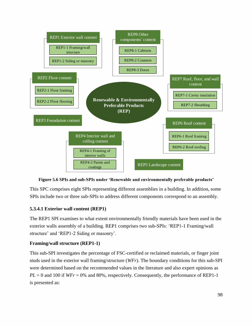
98

REP1-1 Framing/wall

structure

REP1 Exterior wall content

REP1-2 Siding or masonry

REP3 Foundation content

REP8-1 Cabinets

REP8 Other

components content

REP8-2 Counters

REP8-3 Doors

REP5 Landscape content

Renewable & Environmentally

Preferable Products

(REP)

REP2-1 Floor framing

REP2 Floor content

REP2-2 Floor flooring

REP4-1 Framing of

interior walls

REP4 Interior wall and

ceiling content

REP4-2 Paints and

coatings

REP6-1 Roof framing

REP6 Roof content

REP6-2 Roof roofing

REP7-1 Cavity insulation

REP7 Roof, floor, and wall

content

REP7-2 Sheathing

Figure 5.6 SPIs and sub-SPIs under ‘Renewable and environmentally preferable products’

This SPC comprises eight SPIs representing different assemblies in a building. In addition, some

SPIs include two or three sub-SPIs to address different components correspond to an assembly.

5.3.4.1 Exterior wall content (REP1)

The REP1 SPI examines to what extent environmentally friendly materials have been used in the

exterior walls assembly of a building. REP1 comprises two sub-SPIs: ‘REP1-1 Framing/wall

structure’ and ‘REP1-2 Siding or masonry’.

Framing/wall structure (REP1-1)

This sub-SPI investigates the percentage of FSC-certified or reclaimed materials, or finger joint

studs used in the exterior wall framing/structure (WFr). The boundary conditions for this sub-SPI

were determined based on the recommended values in the literature and also expert opinions as

PL = 0 and 100 if WFr = 0% and 80%, respectively. Consequently, the performance of REP1-1

is presented as:

99

PLREP1-1 = 125(𝑊𝐹𝑟) 0 ≤ 𝑊𝐹𝑟 ≤ 80% [5.49]

Siding or masonry (REP1-2)

Likewise, the performance level of REP1-2 is 100 when the recycled, reclaimed, or FSC-

certified materials used in the siding or masonry component of the exterior walls (WSi) accounts

for 70% and up. Thus, the PL of this sub-SPI is obtained by means of the following function:

PLREP1-2 = 142.85(𝑊𝑆𝑖) 0 ≤ 𝑊𝑆𝑖 ≤ 70% [5.50]

To calculate the PL of the parent SPI, the PLs of the associated sub-SPIs should be calculated

and combined with their relative importance weights. The weights of REP1-1 and REP1-2 came

to be equal (CaGBC 2009); therefore, the performance of REP1 can be calculated as:

PLREP1 = 0.5×PLREP1-1 + 0.5×PLREP1-2 [5.51]

5.3.4.2 Floor content (REP2)

The amount of environmentally responsible materials consumed in the construction of floors is

evaluated by this SPI. The SPI includes two sub-SPIs: ‘REP2-1 Floor framing’ and ‘REP2-2

Floor flooring’ that address two components of the floor assembly.

Floor framing (REP2-1)

The performance of REP2-1 is calculated based on the extent to which the FSC-certified or

reclaimed materials have been used in the floor framing (FFr). According to the experts, the

upper boundary for the percentage of FFr, which corresponds to PL = 100, was set at 70%.

Therefore, the PLF for this sub-SPI was presented as:

PLREP2-1 = 142.86(𝐹𝐹𝑟) 0 ≤ 𝐹𝐹𝑟 ≤ 70% [5.52]

Floor flooring (REP2-2)

The performance of the second sub-SPI under REP2 is measured according to the percentage of

the floor’s flooring that contains environmentally responsible materials (FFl) such as cork,

linoleum FSC-certified or reclaimed wood, bamboo, sealed concrete, recycled materials, or any

combination of them. The boundary conditions were set similar to the previous sub-SPI.

Consequently, the performance of this sub-SPI is obtained using the following PLF:

PLREP2-2 = 142.86(𝐹𝐹𝑙) 0 ≤ 𝐹𝐹𝑙 ≤ 70% [5.53]

In addition, the weights of REP2-1 and REP2-2 have been specified as 0.333 and 0.667,

respectively (CaGBC 2009). Hence, the performance of REP2 can be calculated as:


100

5.3.4.3 Foundation content (REP3)

This SPI focuses on the content of a building foundation. The data variable to calculate the

performance level of this SPI is Fo which indicates what percentage of the foundation content is

supplemental cementious materials. According to the literature, the foundation performs

moderately (PL = 50) if it contains 30% of supplemental cementious materials. However, its

performance reaches PL = 100 when it increases to 50% (CaGBC 2009). These boundary

conditions were used to develop a piecewise PLF for the SPI as:

PLREP3 = {166.67(𝐹𝑜) 0 ≤ 𝐹𝑜 ≤ 30%

250(𝐹𝑜) − 25 30% ≤ 𝐹𝑜 ≤ 50% [5.55]

5.3.4.4 Interior wall and ceiling content (REP4)

The REP4 SPI evaluates the performance of the subject building with regard to REP content of

its interior walls and ceiling. The SPI consists of two sub-SPIs including ‘REP4-1 Framing of

interior walls’ and ‘REP4-2 Paints and coatings’.

Framing of interior walls (REP4-1)

The performance of the first sub-SPI is obtained according to the percentage of FSC-certified or

reclaimed materials used in the framing component of the interior walls (IWFr) as:

PLREP4-1 = 125(𝐼𝑊𝐹𝑟) 0 ≤ 𝐼𝑊𝐹𝑟 ≤ 80% [5.56]

Paints and coatings (REP4-2)

The performance of the second sub-SPI is evaluated based on the extent to which recycled paint

that satisfies Green Seal standard (i.e., GS-43) or any other standard is used in painting and

coating of the interior walls and ceiling (IWPa). By applying the boundary conditions for the

IWPa data variable, the following PLF was established to calculate this sub-SPI:

PLREP4-2 = 111.11(𝐼𝑊𝑃𝑎) 0 ≤ 𝐼𝑊𝑃𝑎 ≤ 90% [5.57]

Furthermore, the relative importance weights of the two sub-SPIs came to be equal (CaGBC

2009). Consequently, the performance level of the corresponding SPI can be calculated as:


5.3.4.5 Landscape content (REP5)

The performance of REP5 is measured according to the amount of recycled, FSC-certified or

reclaimed content in the building’s landscape including the deck or patio (La). While the

literature requires high percentages of the environmentally friendly materials at which the

101

building presents its best performance (i.e., up to La = 90%); the experts in this research believed

that even La = 70% can be considered as the best performance for this SPI in British Columbia.

Hence, the performance level of the subject building with respect to REP5 can be calculated

using the PLF below:

PLREP5 = 142.86(𝐿𝑎) 0 ≤ 𝐿𝑎 ≤ 70% [5.59]

5.3.4.6 Roof content (REP6)

This SPI examines the amount of the roof content that were supplied by REP materials. REP6

consists of two sub-SPIs including ‘REP6-1 Roof framing’ and ‘REP6-2 Roof roofing’.

Roof framing (REP6-1)

The performance of this sub-SPI is calculated based on the FSC-certified content of the roof

framing (RFr). The least and most desirable performances take place when the RFr percentage in

the roof structure reaches 0% and 60%, respectively. Therefore, the PLF presented below can be

used to calculate REP6-1:

PLREP6-1 = 250(𝑅𝐹𝑟) 0 ≤ 𝑅𝐹𝑟 ≤ 40% [5.60]

Roof roofing (REP6-2)

According to the literature and expert opinions, the boundary conditions for REP6-2 were

determined based on the recycled content of the roof roofing (RRo) as PL = 0 when RRo = 0%

and PL = 100 when RRo = 75%. Therefore, the PL of this sub-SPI is calculated as:

PLREP6-2 = 133.33(𝑅𝑅𝑜) 0 ≤ 𝑅𝑅𝑜 ≤ 75% [5.61]

The weights of REP6-1 and REP6-2 came to be equal (CaGBC 2009). Thus, the performance

level of the corresponding SPI is obtained using the PLF below:


5.3.4.7 Roof, floor, and wall content (REP7)

This SPI investigates the use of environmentally responsible materials when performing cavity

insulation and sheathing of the roof, floor, and wall assemblies.

Cavity insulation (REP7-1)

The performance of REP7-1 is calculated based on percentage of recycled materials used for

cavity insulation (not rigid foam insulation) (CIn). The boundary conditions are: if CIn = 0%

then PL = 0; and if CIn = 20% and more, then PL = 100. Thus, the following PLF was

102

established to calculate the PL of this sub-SPI:

PLREP7-1 = 500(𝐶𝐼𝑛) 0 ≤ 𝐶𝐼𝑛 ≤ 20% [5.63]

Sheathing (REP7-2)

Likewise, using REP7-2, the amount of recycled, FSC- certified or reclaimed materials used for

sheathing of the roof, floor, and wall assemblies (Sh), is evaluated. By applying the boundary

conditions for the Sh data variable, the following linear PLF was established for calculating the

performance level of this sub-SPI:

PLREP7-2 = 166.67(𝑆ℎ) 0 ≤ 𝑆ℎ ≤ 60% [5.64]

Once the PLs of the two sub-SPIs are calculated, the PL of the parent SPI can be calculated as:


5.3.4.8 Other components’ content (REP8)

Cabinets, counters, and doors are components that are installed in a building at the final stages of

the construction phase and account for considerable amount of materials in the building. The

REP8 SPI examines the environmentally responsible materials in these components using three

sub-SPIs.

Cabinets (REP8-1)

The first sub-SPI investigates the percentage of the recycled, FSC-certified or reclaimed, and

composite materials in the building’s cabinets (Ca). Based on expert consultations, the boundary

conditions for Ca data variable were adjusted to suit the construction circumstances in BC as: if

Ca = 0%, then PL = 0; and if Ca = 75% and up, then PL = 100. Therefore, the PL of REP8-1 can

be calculated as:

PLREP8-1 = 133.33(𝐶𝑎) 0 ≤ 𝐶𝑎 ≤ 75% [5.66]

Counters (REP8-2)

By the second sub-SPI, the recycled, FSC-certified or reclaimed, and composite materials in the

building’s counters (Co) including kitchens and bathrooms is investigated. The boundary

conditions for the Co variable were set as: if Co = 0%, then PL = 0; and if Co = 70% and up,

then PL = 100. Subsequently, the function below can be used to measure the PL of REP8-2:

PLREP8-2 = 142.86(𝐶𝑜) 0 ≤ 𝐶𝑜 ≤ 70% [5.67]

103

Doors (REP8-3)

Through this sub-SPI, the use of environmentally friendly materials in doors and trims (Do),

excluding garage or insulated doors, is checked. The same boundary conditions reported in

LEED Canada for Homes, i.e., if Do = 0%, then PL = 0; and if Do = 80% and up, then PL = 100,

were used to develop the PLF for this sub-SPI as follows:

PLREP8-3 = 125(𝐷𝑜) 0 ≤ 𝐷𝑜 ≤ 80% [5.68]

By having the calculated PLs and weights of the three sub-SPIs, the parent SPI can be calculated.

The weights of all sub-SPIs have been reported equal in the literature and this was confirmed by

the experts in this research (CaGBC 2009). Therefore, the performance of REP8 can be

measured as:

PLREP8 = 0.333×PLREP8-1 + 0.333×PLREP8-2 + 0.333×PLREP8-3 [5.69]

5.3.4.9 Relative importance of the SPIs under REP

The weights of the discussed REP SPIs have been determined using the literature by the focus on

the sources these SPIs adopted from. Table 5.7 lists the relative importance weighs of the eight

SPIs under REP.

Table 5.7 Weight set of the SPIs under the RM SPC


REP1 0.118 REP4 0.118 REP7 0.118

REP2 0.176 REP5 0.058 REP8 0.176

REP3 0.118 REP6 0.118

Sum = 1

5.3.5 Site Disruption and Appropriate Strategies (SD)

Construction projects such as building projects may have negative environmental and social

impacts on the project site. The social impacts of the construction activities consist of negative

consequences on surrounding neighborhoods and families, such as construction noise, traffic

congestion, and dust, among others (Kamali and Hewage 2017b). The social impacts of building

construction on the project site were discussed earlier in the previous chapter under the SPC

‘Community disturbance (CD)’. This SPC was ranked 2nd among the social SPCs which

indicates the experts’ concern about the influence of choosing on-site and off-site construction

methods on the project surroundings (see Table 4.6 in Chapter 4). However, as stated before, the

social performance assessment is beyond the scope of this research. As for the environmental

impacts, appropriate strategies should be implemented to minimize the site disruption due to the

construction activities. Examples of such strategies are promoting natural biodiversity (e.g.,

104

providing adequate open space), planning for stormwater management, avoiding blocking fresh

air or sunlight or natural waterways for adjacent developments, and so forth.

Different sources have addressed site disruption as one of the key criteria towards sustainable

construction that needs to be carefully addressed (REAP 2014; BRE 2016; CaGBC 2009;

USGBC 2018; GBI 2014). The ‘Site disruption and appropriate strategies (SD)’ SPC in this

research; therefore, is intended to decrease the negative environmental impacts of residential

single-family building projects on the final project site. As illustrated in Figure 5.7, this SPC

comprises five SPIs, some of which consist of a number of sub-SPIs.

SD1 Construction activity

pollution prevention

SD2-1 Landscape design

SD2 Efficient landscaping

SD2-2 Conventional turf

SD2-3 Drought-tolerant

plantsSD3 Heat island effects

Site Disruption and

Appropriate Strategies

(SD)

SD4-1 Permeable site

SD4 Rainwater

management

SD4-2 Erosion

management

SD4-3 Roof runoff

management

SD5 Efficient pest control

Figure 5.7 SPIs and sub-SPIs associated with ‘Site disruption and appropriate strategies’

At first, it might seem that there should not be a difference between the modular and

conventional construction methods with respect to this SPC. However, due to short duration of

on-site activities, modular construction might have different impacts than conventional

construction in terms of site disruption. As seen in the previous chapter, the participating experts

were concerned if suitable strategies are implemented in modular building projects to minimize

such impacts by rating the SD SPC as a ‘Medium’ importance criterion which is more applicable

than ‘Low’ (see Table 4.4 in Chapter 4).

5.3.5.1 Construction activity pollution prevention (SD1)

A building is constructed on a lot, which means the natural land should be replaced with man-

made buildings. Therefore, the construction of a building and the corresponding activities can

cause long-term environmental impacts (i.e., damage and pollution) on the project site. This SPI

examines suitable actions that if implemented, these impacts can be minimized.

105

Every building project is constructed on either not previously developed site or previously

developed site. Depending on whether the project site is previously developed or not, the

following pollution prevention actions should be checked to identify the performance of a

building with respect to this SPI (USGBC 2018; CaGBC 2009):

Not previously developed sites

a) Develop a tree/plant preservation plan with “no-disturbance” zones outlined on both

drawings and site.

b) Leave the minimum of 40% of buildable lot area (excluding under roof area) as undisturbed.

Previously developed sites

c) - Develop a tree/plant preservation plan with “no-disturbance” zones outlined on both

drawings and site.

- Restore the undisturbed portion of the lot by undoing any previous soil compaction.

- Remove existing invasive plants.

- Use drought-tolerant turf in the landscape design (no turf in densely shaded areas or

areas with more than 4:1 slope). In addition, use mulch or soil amendments as appropriate.

Moreover, till all compacted soil (e.g., by construction equipment) to at least 6 inches.

d) Build on site with a lot area of less than 0.06 hectares (600 m2), or with a housing density of

one units per 0.06 hectares.

Consequently, the PL of this SPI can be measured by the following PLF:

PLSD1 = 50𝑛 + 100𝑚 𝑛 = 0, 1, 2;𝑚 = 0, 1 [5.70]

Where n is the number of implemented actions (‘a’ and ‘b’) implemented on previously

developed sites and m is 1 if either ‘c’ or ‘d’ was implemented on not previously developed sites.

5.3.5.2 Efficient landscaping (SD2)

The SD2 SPI considers the design of landscape features by which invasive species are avoided

and demand for water and synthetic chemicals is minimized. The SPI includes three sub-SPIs:

‘SD2-1 Landscape design’, ‘SD2-2 Conventional turf’, and ‘SD2-3 Drought-tolerant plants’.

Landscape design (SD2-1)

This sub-SPI investigates if any of the following landscape design items have been incorporated

in the design of a building (USGBC 2018; CaGBC 2009):

a - Any turf must be drought-tolerant.

106

b - Do not use turf in densely shaded areas.

c - Do not use turf in areas with a slope of 4:1.

d - Add mulch or soil amendments as appropriate.

e - Till all compacted soil (e.g., by construction equipment) to at least 6 inches.

If at least four of the above requirements have been considered in a building design, its

performance is excellent. Thus, the PLF for this SD2-1 was established as:

PLSD2-1 = 25𝑛 𝑛 = 0, 1, 2, 3, 4 [5.71]

Where n is the number of items ‘a’ to ‘e’ that have been included in the building’s design.

Conventional turf (SD2-2)

The second sub-SPI under SD2 seeks reduction of the use of traditional (chemical) turf (even

drought-tolerant turf) in the softscape. Conventional lawns, as opposed to natural lawns, need

significant amounts of energy and water while polluting water and air and making noise. This

means the less conventional turf used in the landscape softscape results in better long-term

performances; hence, the corresponding PLF should be a monotonically decreasing function. The

maximum percentage of conventional turf (CT%) provided by LEED has been tweaked with the

help of experts as: if CT = 60% or more, then PL = 0, and if CT = 20% or less, then PL = 100.

Subsequently, the following PLF was developed to calculate the PL of the SD2-2 sub-SPI:

PLSD2-2 = −1.667(𝐶𝑇%) + 133.34 20 ≤ 𝐶𝑇% ≤ 80 [5.72]

Drought-tolerant plants (SD2-3)

The last sub-SPI under SD2 discusses installation of drought-tolerant plants that can result in less

environmentally negative impacts. The boundary conditions determined for the percentage of

drought-tolerant plants (DTP%) in the building’s landscape as: if DTP = 0%, then PL = 0, and if

DTP = 90% or more, then PL = 100. Consequently, the PL of SD2-3 is obtained as:

PLSD2-3 = 1.111(𝐷𝑇𝑃%) 0 ≤ 𝐷𝑇𝑃% ≤ 90 [5.73]

After calculating the PLs of the three sub-SPIs above, the PL of the corresponding SPI can be

measured. The weights of SD2-1, SD2-2, and SD2-3, have been determined as 0.286, 0.428, and

0.286, respectively (CaGBC 2009). Therefore, the SD2 SPI is calculated as:

PLSD2 = 0.286×PLSD2-1 + 0.428×PLSD2-2 + 0.286×PLSD2-3 [5.74]

5.3.5.3 Heat island effects (SD3)

In the past few decades, the urban areas have been significantly developed by replacing open and

107

permeable lands with different buildings and infrastructure. Therefore, the urban areas have

become warmer than their rural surroundings forming an island of higher temperatures called

heat island (EPA 2018a). The temperature differences between urban surfaces (e.g., pavements,

roofs) and the air range between 27 to 50°C in the summer, while there is no difference between

the temperature of the surfaces and the air in rural areas. Heat island has negative impacts on

human, microclimates, and wildlife habitats (Berdahl and Bretz 1997; EPA 2018a).

To minimize the heat island impacts, a number of landscape features can be designed at the

design stage of a building such as shading hardscapes around the building. The intent of the SD3

SPI is to assure consideration of such landscape features. According to both Canadian and US

versions of LEED for single-family homes (USGBC 2018; CaGBC 2009), implementation of

either of the following options can satisfy the requirement for reduction of the heat island effects:

Option 1- Use trees or other plantings by which shading is provided for over half of the patios,

sidewalks, and driveways within 50 ft of the building.

Option 2- Install non-absorptive materials such as light-colored, high-albedo materials, or

vegetation-covered hardscapes (white concrete, open pavers, materials with solar reflectance

index ≥ 0.29) for over half of the patios, sidewalks, and driveways within 50 ft of the building.

Consequently, the PLF for this SPI was established as:

PLSD3 = 100𝑛 𝑛 = 0, 1 [5.75]

Where n is 1 if either of the Options 1 or 2 has been considered and implemented.

5.3.5.4 Rainwater management (SD4)

Site features should be incorporated in the design stage such that the erosion and runoff volume

from the project site is minimized. This SPI investigates whether a building meets the

requirements for suitable rainwater management. It consists of three sub-SPIs including ‘SD4-1

Permeable site’, ‘SD4-2 Erosion management’, and ‘SD4-3 Roof runoff management’.

Permeable site (SD4-1)

This sub-SPI checks the permeable portion of the building’s lot. The lot should be designed in a

way that the majority of the buildable land (excluding the area under roof) is permeable or

designed to capture water runoff for infiltration on the lot. Areas that are considered permeable

land include (CaGBC 2009):

a. Vegetative landscape (e.g., trees, grass).

b. Permeable paving, installed by an experienced professional. Permeable paving must include

108

porous above-ground materials (e.g., open pavers, engineered products) and a 6-inch porous

subbase, also the base layer must be designed to ensure proper drainage away from the home.

c. Impermeable surfaces that are designed to direct all runoff toward an appropriate permanent

infiltration feature (e.g., vegetated swale, on-site rain garden, or rainwater cistern).

According to the literature and expert consultations, the boundary conditions for the percentage

of permeable land (PeL%) were set and then the following PLF was established for SD4-1:

PLSD4-1 = 2.5(𝑃𝑒𝐿%) − 150 60 ≤ 𝑃𝑒𝐿% ≤ 100 [5.76]

Erosion management (SD4-2)

This indicator determines whether suitable measures for permanent erosion controls have been

designed. A building shows excellent performance if either of the following measures has been

designed and implemented (USGBC 2018; CaGBC 2009):

Option 1- In case the site is located on a steep slope, install terracing and retaining walls to

decrease the long-term runoff effects.

Option 2- Plant one tree, four 19-litre (5-gallon) shrubs, or 4.6 square meters of native

groundcover per 46 m2 of disturbed lot area (including area under roof).

Thus, the performance level of this SPI can be measured using the PLF below:

PLSD4-2= 100𝑘 𝑘 = 0, 1 [5.77]

Where k is 1 if either Options 1 or 2 for permanent erosion controls has been implemented.

Roof runoff management (SD4-3)

To control and manage the runoff from the roof of a building, appropriate strategies should be

followed. The third sub-SPI under the SD4 SPI, evaluates the performance of a building with

respect to such strategies. Following are a number of measures that if designed and installed, the

quality management of runoff from the building roof is achieved:

a. Installation of vegetated roof with roof coverage ≥ 50%.

b. Installation of vegetated roof with roof coverage ≥ 100%..

c. Installation of permanent stormwater controls such as vegetated swales, on-site rain garden,

dry well, or rainwater cistern.

d. Site design by licensed landscape designer or engineering professional such that all water

runoff from the building is managed through an on-site design element.

Consequently, the PL of the building with respect to SD4-2 can be presented as:

109

PLSD4-3 = 𝑀𝑖𝑛{100, 25𝑖 + 50𝑗 + 100𝑘} 𝑖 = 0, 1; 𝑗 = 0, 1, 2; 𝑘 = 0, 1 [5.78]

Where i is 1 if measure ‘a’ was met, j is the number of measures ‘b’ and ‘c’ that were met, and k

is 1 if measure ‘d’ was met.

Eventually, the calculated PLs of these sub-SPIs and their weights are combined to evaluate the

performance of the subject building with respect to the SD4 SPI as:

PLSD4 = 0.571×PLSD4-1 + 0.143×PLSD4-2 + 0.286×PLSD4-3 [5.79]

5.3.5.5 Efficient pest control (SD5)

This SPI deals with the design features by which the need for pest control chemicals is

minimized to reduce the pest problem and also the risk of exposure to poisons (USGBC 2018).

The performance the building with respect to the SD5 indicator is calculated based on

implementation of the measures specified below (CaGBC 2009):

a- All wood (e.g., siding, structure) should be more than 1ft above soil.

b- All external cracks, joints, penetrations, edges, and entry points should be sealed with

caulking. Use rodent- proof and corrosion-proof screens (e.g., copper or stainless-steel mesh)

where openings cannot be caulked or sealed.

c- Use no wood-to-concrete connections or separate any exterior wood-to-concrete connections

(e.g., at posts, deck supports, stair stringers) with metal or plastic fasteners or dividers.

d- Install landscaping such that all parts of mature plants are at least 2 ft from the building.

Therefore, the following PLF was established to calculate the PL of SD5:

PLSD5 = 25𝑛 𝑛 = 0, 1, 2, 3, 4 [5.80]

Where n is the number of implemented pest control measures (listed above) on the project site.

5.3.5.6 Relative importance of the SPIs under SD

The SPIs used under the SD SPC have been mentioned in different sources using diverse

wording and descriptions. However, since all of the five SPIs are available in both Canadian and

the US versions of LEED, these references were used to determine the weights of these SPIs. In

doing so, the weight of each SPI has been determined by normalization of the maximum

available points of the SPI to the total available points of all five SPIs. Therefore, the weights of

SD1, SD2, SD3, SD4, and SD5, came to be 0.056, 0.389, 0.056, 0.389, and 0.111, respectively.

110

5.3.6 Renewable Energy Use (RE)

The ‘Renewable energy use (RE)’ SPC evaluates the performance of residential buildings with

respect to the use of renewable energy sources during the use phase. In addition to the negative

environmental consequences of non-renewable natural resource consumption, such as land, air,

and water pollution, another important result is negative social impacts such as health and

occupational issues (Palaniappan 2009). Despite finite fossil fuels, renewable energy sources

regenerate. There are various forms of renewable energy sources including solar, hydropower,

geothermal, biomass, and wind (EIA 2018).

Currently, Canada ranked first globally in the production and use of renewable energy due to its

diverse renewable resources to generate a significant portion of the total energy need. Canada

obtained 17.4% of its primary energy supply from renewable sources in 2016 (currently 18.9%),

while the world average was around 13% (NRC 2018c; NRC 2017c).

In buildings, renewable energies can be used for space heating, water heating, and electricity

(e.g., lighting, appliances) (NRC 2017c). The ultimate goal of using renewable energy sources in

buildings is to reach the level of net-zero energy building (NZEB), also called zero-energy

building and zero net energy. In a NZEB, the total annual energy consumed by a building

approximately equals the renewable energy generated on site or supplied off site by renewable

energy sources (Pless and Torcellini 2010; Peterson et al. 2015; Torcellini et al. 2006). Detailed

definitions and classifications of NZEB buildings have been provided in Appendix E.

Although NZEB homes are technically feasible, they are not yet affordable and common for

average homebuyers (NRC 2018c). Consequently, a building’s performance with regard to the

RE SPC is evaluated based on the renewable energy share of the total energy consumption in

regular (not custom made or luxurious) single-family buildings that can be produced on-site or

purchased off-site. Three SPIs were recognized under this SPC: ‘RE1 Renewable electricity’,

‘RE2 Renewable space heating’, and ‘RE3 Renewable water heating’ as shown in Figure 5.8.

111

Figure 5.8 SPIs associated with ‘Renewable energy use’

5.3.6.1 Renewable electricity (RE1)

The intent of this SPI is to reduce the demand for non-renewable energy in residential buildings

by increasing the use of renewable electricity. The province of BC has the potential to be the

world leader in evolving sustainable energy technologies as effective energy alternatives (Evans

2008). When it comes to electricity, almost 95% of the power supply is renewable sources

including both large-scale and small-scale hydroelectric power (BC’s big dams and rivers),

significant potential for wind power, geothermal, and marine energy (NEB 2017; BCSEA 2018;

BC Hydro 2018). However, this does not mean that 95% of every home’s electricity in BC is

supplied by renewable sources, because the portion of renewable sources to generate electricity

are different among the electricity providers. Furthermore, in almost everywhere in BC that a

building is built, the choice of an electricity provider is limited to only one and this is

independent from the construction method. Installation of renewable electricity generation

systems in a building can reduce the dependency on the electricity supplied by official providers.

This offers three advantages. The first advantage is to increase the building’s renewable

electricity sources, which results in less environmental impacts due to electricity consumption.

The second advantage, however, is economic. Many electricity providers around the world bill

their residential electric customers on a multiple-tier rate. For example, ForticBC, as an

electricity provider in parts of the Okanagan, has set a two-tire rate for the electricity cost, which

means that if a building consumes above a certain amount, each unit of electricity will cost more

than regular price. Therefore, using renewable electricity generation systems can offset a portion

of power need in a building. Lastly, as the third advantage, it raises the building’s value.

Solar energy is a significant renewable energy source that each building can use to supply the

RE1 Renewable electricity

RE2 Renewable space heating

RE3 Renewable water heating

Renewable Energy Use

(RE)

112

energy needed for heating and electricity (NRC 2017c). Solar power systems, also called

photovoltaic or PV systems, are the main renewable electricity generation systems. These

systems convert sunlight to electricity PV arrays that can be placed on or beside the building

(Hayter and Kandt 2011). In 2019, BC has been ranked as Canada’s seventh province for solar

power (Energyhub 2019). The Okanagan Valley in BC is amongst the best regions for solar

power systems within the province (due to its sunny days) where it is possible to offset all of the

power needs in the summer and a sizeable portion in the winter. Although the cost of a PV

system has significantly dropped in the past few years (BC Hydro 2018), it is not still a desirable

option. However, in a long term view, it is economical because PV systems have a warranty of

25-30 years and the payback of a typical system is approximately 12 years, which means 13-18

years (and more) of free electricity (Terratek Energy 2017).

To evaluate the performance of a building with regard to this SPI, both the energy supplied by

the renewable electricity generation systems (other than BC power supply) and the annual

reference electrical load should be estimated. The annual reference electric load can be estimated

by the HERS Reference Home or the EnerGuide reference for average size homes. Thus, the

building’s renewable electric load ratio (REL%) is calculated as:

REL% = 𝐴𝑛𝑛𝑢𝑎𝑙 𝑒𝑙𝑒𝑐𝑡𝑟𝑖𝑐𝑖𝑡𝑦 𝑠𝑢𝑝𝑝𝑙𝑖𝑒𝑑 𝑏𝑦 𝑟𝑒𝑛𝑒𝑤𝑎𝑏𝑙𝑒 𝑒𝑛𝑒𝑟𝑔𝑦 𝑠𝑜𝑢𝑟𝑐𝑒𝑠

𝐴𝑛𝑛𝑢𝑎𝑙 𝑒𝑙𝑒𝑐𝑡𝑟𝑖𝑐𝑖𝑡𝑦 𝑐𝑜𝑛𝑠𝑢𝑚𝑝𝑡𝑖𝑜𝑛 𝑖𝑛 𝑟𝑒𝑓𝑒𝑟𝑒𝑛𝑐𝑒 ℎ𝑜𝑚𝑒 [5.81]

Consequently, using the upper boundary condition of REL% = 30% for PL = 100 (CaGBC

2009), the following PLF was proposed to measure the RE1 SPI:

PLRE1 = 3.33(𝑅𝐸𝐿%) 0 ≤ 𝑅𝐸𝐿% ≤ 30 [5.82]

5.3.6.2 Renewable space heating (RE2)

Another application of renewable energy is heating the internal space of buildings. According to

Natural Resources Canada, in 2015, approximately 40.8% of the energy consumed for space

heating in BC residential buildings was supplied by renewable energy sources and the remaining

was supplied by non-renewable energy sources mainly natural gas (52.1%) and heating oil

(3.4%) (NRC 2015a). Therefore, there is a large room for replacing non-renewable energy

sources (fuel-source options) by renewable sources (electricity, solar) for space heating in BC.

Solar energy is an important source that each building can use to supply the energy needed for

heating and electricity. Space heating by solar energy is gaining attention in some parts of the

world. For example, the Solar Thermal Industry Federation in Europe anticipated that up to 50%

of all space heating will be provided via stored solar heat by 2030 (NRC 2017c). However, in

Canada, solar thermal systems are installed mostly for water heating instead of space heating.

113

This is probably why these systems have not been appreciated in rating systems such as LEED

Canada for Homes, whereas the use of solar hot water and solar power systems in a building can

earn up to approximately 2.5% and 8% of the total available credits in LEED, respectively.

According to BC Hydro (2018), based on the climate conditions, a solar thermal system may be

less economical than other fuel-sources for space heating of Canadian buildings. To decide

whether a solar thermal system is a suitable option for a residential building, a number of factors

should be considered including utility rate for heating, the duration of heating season, and the

surface area of roof and south facing wall to install the heat collector panels (Hayter and Kandt

2011). As stated before, solar systems can effectively installed in the Okanagan because of its

numerous hot and sunny days. For example, Kelowna sees more sunny days than almost any

other Canadian city, with over 300 days of sunshine (2000 sunlight hours) each year

(Environment Canada 2018). Therefore, solar thermal systems for space heating can be a

potential option in the Okanagan to offset a portion of energy required for heating homes.

During the screening process to determine the measurement method of the RE3 SPI, no studies

or reports were found that discussed and evaluated the solar thermal systems for space heating.

Therefore, the following PLF was proposed as a basis to calculate the PL this SPI:

PLRE2 = 100n n = 0, 1 [5.83]

Where n is 1 if a solar thermal system is installed in the building.

5.3.6.3 Renewable water heating (RE3)

Water heating consumes a significant portion of the total energy consumption in buildings

(including residential) worldwide. In 2015, the energy used for water heating in residential

buildings in Canada and its BC province has been reported as 18.7% and 25.1% of the total

energy consumption of these buildings, respectively (NRC 2015b; NRC 2015c).

According to Natural Resources Canada, in 2015, less than 25% of the energy required for water

heating of the BC residential buildings was supplied by renewable energy sources (NRC 2015d).

Solar systems for water heating use the sun's energy as an alternative energy source to electricity

or gas, to heat water with zero pollution, zero fuel costs, and insignificant operation and

maintenance costs. These systems are able to supply up to approximately 80% of hot water

demand. Although the application of the solar heating is still limited, e.g., maximum 1% of the

potential water heating market in the US (Walker 2016), it has begun to grow in the past few

years. For example, Solar BC (2008) reported at least 540 residential solar hot water systems in

BC before 2008 and this number is expected to continue rising. Aside from solar systems, high

efficiency electric water heating systems can also be another renewable water heating option in

114

BC. It might appear contradictory to efforts undertaken above to use solar power systems in

order to offset a portion of the electricity supplied by electricity providers. However, using

electric water heating systems is more sustainable than non-renewable energy sources for water

heating since approximately 95% of the electricity in BC supplied by renewable energy sources

(NEB 2017; BCSEA 2018; BC Hydro 2018).

Consequently, the RE3 SPI can be evaluated based on installation of any of the water heating

systems under the three groups listed in Table 5.8.

Table 5.8 Renewable water heating systems

Group Water heating system

G1 - High-efficiency storage electric water heater with EF (energy efficiency) ≥ 0.89 (300 litres / 80 gallons)

- Solar heat exchanger that absorbs waste heat from drain water to pre-heat domestic hot water

G2 - Tank less electric water heater with EF ≥ 0.99

- Solar water heater (with preheat tank) that supplies 40% ≤ annual domestic hot water load ≤ 60%

G3 - Electric heat pump water heater (ground- or air-sourced) with EF ≥ 2.0

- Solar water heater (with preheat tank) that supplies annual domestic hot water load ≥ 60%

The following PLF can be used to calculate this SPI:

PLRE3 =

{

0 𝑛𝑜𝑛𝑒 𝑜𝑓 𝑠𝑦𝑠𝑡𝑒𝑚𝑠 33.3 𝑜𝑛𝑒 𝑜𝑓 𝐺1 𝑠𝑦𝑠𝑡𝑒𝑚𝑠66.7 𝑜𝑛𝑒 𝑜𝑓 𝐺2 𝑠𝑦𝑠𝑡𝑒𝑚𝑠100 𝑜𝑛𝑒 𝑜𝑓 𝐺3 𝑠𝑦𝑠𝑡𝑒𝑚𝑠

[5.84]

5.3.6.4 Relative importance of the SPIs under RE

The RE performance of a building can be calculated by combining the calculated PLs of the

associated SPIs and their weights. According to the literature and expert consultations, the

weights of ER1, ER2, and ER3, were determined as 0.667, 0.133, and 0.2, respectively.

5.3.7 Greenhouse Gas Emissions (GE)

Human intensive activities such as production of different products, deforestation and land-use

changes, consumption of finite natural resources (e.g., fossil fuels), and transportation, lead to the

emissions of so-called greenhouse gases (GHGs) that cause negative environmental impacts. A

huge amount of GHG emissions (up to 50% of the global release) is due to the activities related to

the building sector (CIWMB 2000). Therefore, quantification of GHG emissions can assist with

the identification and management of responsible decisions, activities, and operations in this

sector. This leads to the environmental impact mitigation, quality asset management, and cost

savings and (BC ECCS 2017).

In Canada, GHG emissions have increased by 16.7% from 1990 to 2016 (BC ECCS 2018; CCC

115

2016). However, Canadian provinces accounted for different shares of the total GHG emissions.

According to BC ECCS (2018), the GHG emissions in BC has increased by 17.6%, which is

above the average national increase.

Global warming is among the most important environmental impacts resulted by GHGs (Asif et

al. 2007). The global warming potential (GWP) measure, also called “carbon footprint” or

“embodied carbon results”, is used to quantify the role of a GHG substance in climate change.

According to the literature, not only global warming, but other environmental impacts such as

ozone depletion, smog, and so forth, are also important and should be paid attention to. Thus, the

SPC ‘Greenhouse gas emissions (GE)’ analyzes a number of important environmental impacts

incurred in the material production phase and the construction phase (collectively called cradle-to-

gate) of modular and conventional buildings. To this end, this research measured the selected

environmental impacts using the life cycle assessment (LCA) method and then developed a set of

environmental impact indices using an AHP-based framework. The developed impact indices can

be used for comparisons of the environmental impacts of selecting different construction method

(i.e., modular versus conventional) during cradle-to-gate of their life cycle.

5.3.7.1 Life cycle assessment

According to the US Environmental Protection Agency (EPA 2001), the life cycle assessment

(LCA) is a “cradle-to-grave” approach that investigates the environmental impacts of a product or

process during the apparently separate but practically inter-dependent life cycle phases. LCA is an

important analytical method for estimating the environmental impacts caused by all stages of a

life cycle phase, even those not included in many traditional assessments, such as raw materials

acquisition, materials transportation, end of life disposal, and so forth (Trusty 2010; SAIC 2006;

ISO 2006a). Consequently, LCA provides a holistic picture of a product/process’s environmental

impacts, which can assist the decision makers with making informed decisions on trade-off

between different product and process options. For example, LCA quantify and reports GWP to

indicate the extent to which a building, over its lifetime, may contribute to climate change. It is

important to note that, depending on the goal and scope of a research study, a partial LCA is

conducted by covering limited number a product’s life cycle phases and also particular

activities/tasks within the covered phases.

The LCA methodology consists of the following four stages (ISO 2006a; ISO 2006b):

1- Goal and scope definition;

2- Life cycle inventory (LCI) analysis;

3- Life cycle impact assessment (LCIA); and

116

4- Interpretation.

Stage 1 consists of defining the objectives, functional unit, and system boundary of the LCA

study. In the case of buildings, according to BS EN 15978 (BSI 2011), a functional equivalent is

“the quantified functional requirements and/or technical requirements for a building or an

assembled system (part of works) for use as a basis for comparison.” In other words, the

functional equivalent is a set of design criteria that both buildings must have in common to

ensure an apples-to-apples comparison (Bowick and O'Connor 2017).

Stage 2 involves collecting the required data and calculating the related inputs and outputs using

the LCI database. In Stage 3 the potential environmental impacts categories, such as GWP, based

on the results of the previous stage (i.e., LCI analysis) are calculated. Finally, in Stage 4 the

results of LCI and LCIA analyses are interpreted (ISO 2006a; ISO 2006b).

LCA is a complicated process in the construction industry including the building sector. It is not

an easy task to collect the necessary data and produce generalizable results, mainly due to the

highly “decentralized nature” of the construction industry, various material types, jobsite

specifications, different assembly methods, and so forth (Malin 2005; Kohler and Moffatt 2003;

Priemus 2005).

5.3.7.2 Definition of goal and scope

The first stage of every LCA study is to define the study objectives, functional unit, and system

boundary. The objective of the LCA in this research was to analyze, compare, and contrast the

environmental impacts of single-family buildings constructed by traditional on-site and modular

off-site construction methods. The benchmarking case study buildings included two modular and

one conventional single-family buildings designed and constructed in the Okanagan, BC. The

LCA was partial which covered the cradle-to-gate life cycle of the buildings including the

material production phase and the construction phase. In other words, the LCA performed in this

study included the materials and energy associated with the production of raw materials to the

finished building and excluded the materials and energy associated with the use and end of life

phases. Therefore, any materials and energy required for the operations (i.e., utilities, furniture,

and appliances), maintenance (i.e., repair, replacement, renovation), and end of life (i.e., waste

management strategies) of the case study buildings were not included in the LCA process. The

functional unit was set at the construction of 1 ft2 of average-quality single-family building in the

Okanagan, BC (Table 5.9).

117

Table 5.9 Functional equivalent set of LCA in this research

Functional criteria

Building type single-family residential

Structure system one story, wood

Location Okanagan, BC

Service life (yrs.) 60

Functional unit 1 ft2 of the total floor area

Total floor area (ft2) under 3000

Covered life cycle phases production phase, construction phase

5.3.7.3 Required data for inventory analysis

After defining the goal and scope of the study, the next step was to collect the material and

energy data of the case study buildings for inventory analysis. The inventory flows should

appropriately reflect the regional or national practices for a product or service. Since the general

focus of this research is on the residential buildings located in Canada, the Athena Impact

Estimator for Buildings software (v5.3.0111) was utilized for the life cycle inventory (LCI) and

the subsequent life cycle impact assessment (LCIA) of the LCA in this research. Developed by

Athena Sustainable Material Institute, the Athena LCI database has been designed to evaluate

buildings based on the LCA methodology. Athena has developed a set of regional databases for

key building materials, products, processes, and energy information, applicable to typical

commercial, industrial, and residential buildings in different locations throughout North America

(Athena 2018; Bowick and O'Connor 2017).

In this research, the activities related to the material production phase and the design and

construction phase (henceforth the construction phase) were categorized into four activity

categories as:

Material production phase: (A1) Material extraction and process; and (A2) Material

transportation.

Construction phase: (A3) Construction and installation; and (A4) Product and worker

transportation.

To perform the inventory analysis, the data of material and energy associated with these activity

categories should be collected for each benchmarking building from the corresponding

homebuilder. The required data variables (raw data) of each activity category have been

summarized in Table 5.10 and described as follows.

118

Table 5.10 Required data for inventory analysis

Construction method Activity category Data variable

Conventional & modular A1, A2 Materials and products (types, quantities)

Conventional A3 On-site energy (machinery, heating, cooling)

Conventional A4 Worker transport (number, workdays, commute modes)

Material/product transport (supplier-site distances, transport modes)

Modular A3 Off-site energy (machinery in factory, heating, cooling)

On-site energy (machinery for site work, heating, cooling)

Modular A4 Worker transport to factory (number, workdays, commute modes)

Worker transport to site (number, workdays, commute modes

Material/product transport to factory (supplier-factory distances,

transport modes)

Module transport (factory-site distance, transportation mode)

Material production phase

As mentioned above, the material production phase accounts for energy consumed in the

following activity categories:

A1) Material extraction and process. First, the primary resources (i.e., raw materials) such as

wood and iron ores are harvested/extracted. Then, they are converted into processed materials

and engineered products usable for certain construction purposes such as lumbar plates, steel

bars, windows, and so forth.

A2) Material transportation. The extracted raw materials are shipped to the manufacturing plant

gates for processing.

It is important to mention that the information about the energy used for the above activity

categories in a region (e.g., BC) is embedded in the Athena LCI database. Therefore, the required

data variables (raw data) are the bill of materials/products and their quantities used in the case

study buildings.

Construction phase

The materials and products produced in the previous phase should be transported to the project

site for construction of the building. Because the construction phase substantially differs between

the conventional and modular construction methods, the activity categories correspond to this

phase (A3 and A4) comprise different tasks in the case of each construction method.

The construction phase of conventional construction accounts for energy consumed in the

following activity categories:

A3) Construction and installation. This category comprises all on-site activities lead to the

construction of the final building on the project site (e.g., foundation, structure, flooring, roofing,

119

finishing). The data variable for A4 includes the energy consumption (natural gas, electricity,

etc.) on the project site during construct of the building including operation of construction

equipment (e.g., crawler crane, skid loader) and operation of the office (e.g., heating, cooling).

The Athena LCI database is able to calculate the energy correspond to the operation of

construction equipment. However, the energy consumed for operation of the office should be

calculated separately and fed into the software.

A4) Product and worker transportation. This category includes the delivery of the processed

materials and products to the project site as well as the workforce commuting to and from the

project site. Based on the bill of materials and the location of a building project, the Athena LCI

database calculates the energy correspond to the material and product transportation. However,

estimation of the energy consumed for employee transportation is out of the scope of the

software. This energy should be calculated separately based on the number of workers on-site,

the number of their working days, and their commute modes, and fed into the software.

The construction phase of modular construction accounts for energy consumed in the following

activity categories:

A3) Construction and installation. The category includes all off-site activities towards fabrication

of the building’s modules in the modular manufacturing center (i.e., modular factory) and on-site

activities related to the site work. Because of the differences of the activities under A3 between

conventional and modular construction methods, the corresponding energy can also be

significantly different. The Athena LCI database does not have the capability to calculate this

energy for modular construction. Therefore, the energy related to A3 for a modular building

project should be calculated separately. In this regard, the data of energy consumed off-site

during the fabrication of modules in the modular factory such as machinery and heating, and also

on-site during the site work such as foundation and module installations are required.

This should be stressed that, calculation of the energy consumed in the factory for manufacturing

the modules of a specific modular building project is not an easy task. This is because in a

modular factory, multiple modules are manufactures simultaneously which do not necessarily

belong to one project. To resolve this issue, the total annual energy consumed in the factory can

be divided by the total annual production (i.e., total floor area) to obtain the off-site energy

associated with production of 1 ft2 of a modular building.

A4) Product and worker transportation. This category comprises the delivery of the required

materials and products to modular factory and the delivery of the completed modules to the

project site as well as the employee’s commute to and from work (off-site and on-site). In this

regard, the data variables associated with A4 include the number of workers off-site (the modular

120

factory) and on-site (the project site), the number of their working days, and their commute

modes. In addition, the distances between the product manufacturing plant gates and the modular

factory, the bill of materials/products consumed, and their transportation modes are required.

Furthermore, the distance between the modular factory and the project site as well as the truck

type to ship the modules are required.

5.3.7.4 Life cycle impact assessment

The Athena’s LCIA methodology used to calculate the environmental impact measures is based

on the US EPA’s Tool for the Reduction and Assessment of Chemical and Other Environmental

Impacts (TRACI) impact assessment method (Bowick and O'Connor 2017; Bare et al. 2012).

Consequently, eight impact measures including global warming potential, eutrophication

potential, acidification potential, ozone depletion potential, human health effect, smog potential,

fossil fuel consumption, and eco-toxicity effect were calculated as described below.

Global warming potential

Global warming is among the most important environmental impact categories, which is the

consequences of a long-term accumulation of GHGs in the higher layer of atmosphere (Asif et al.

2007). Global warming indicates the extent to which such human activities and the subsequent

GHGs may contribute to climate change (Bowick and O'Connor 2017). The primary global

warming’ GHG contributors are carbon dioxide (CO2), methane (CH4), and nitrous oxide (N2O).

While historically CO2 has gained more attention, studies showed that CH4 and N2O contribute

much more than CO2 to climate change (Hermann 2017). To quantify the role of a GHG

substance in climate change, the global warming potential (GWP) measure, also called “carbon

footprint” or “embodied carbon”, is used. It is common to express the GWP of CH4, N2O and

other GHGs based of their equivalent GWP of CO2 that is called carbon dioxide equivalent or

CO2eq (Demirel 2014). In other words, GWP is the ratio of the climate change caused by a GHG

substance to the climate change caused by the same mass of CO2 (Azapagic et al. 2003).

Consequently, the GWP of all GHGs can be calculated and summed up based on kilograms of

CO2eq.

Acidification potential

Acidification is a regional impact that has human health impact. It occurs when high

concentrations of NOx and SO2 are attained. Acidification potential (AP) is a measure to quantify

this impact, which is represented, based on the contributions of SO2, NOx, HCl, NH3, and HF to

the potential acid deposition to form H+ ions. It is common to represent the AP of these

121

substances based on their equivalent AP of SO2 that is called SO2eq. The equivalent AP of a

substance is the ratio of AP caused by a substance to AP caused by the same mass of SO2

(Azapagic et al. 2003). Therefore, the AP for all of these substances can be calculated and

summed up based on kilograms of SO2eq.

Human health effect

Human health effect (HHE) due to particulate matters of various sizes (PM10 and PM2.5) have a

considerable impact on human respiratory system. The US EPA identified “particulates” as the

top cause of human health deterioration, due to its impact on the human respiratory system

(asthma, bronchitis, acute pulmonary disease). Athena uses TRACI’s "Human Health

Particulates from Mobile Sources" characterization factor on an equivalent PM2.5 basis, to

calculate the sum of particulate matters released by different activities during life cycle of

buildings (Athena 2016).

Eutrophication potential

The eutrophication potential (E-P) measure is defined as the potential of nutrients to cause over-

fertilization of water and soil, which can result in increased growth of biomass (Azapagic et al.

2003). When a previously scarce or limiting nutrient is added to a water body, it leads to the

proliferation of aquatic photosynthetic plant life. This may lead to a chain of further

consequences ranging from foul odors to the death of fish. Emissions of chemicals such as NOx,

NH4+, N, PO4

3-, P, and COD, are the main contributors to eutrophication. E-P result is expressed

on an equivalent mass of nitrogen (N) basis, kg Neq (Athena 2016). The equivalent E-P of N for

these chemicals can be found in the literature (Azapagic et al. 2003).

Ozone depletion potential

The ozone depletion potential (ODP) measure indicates the potential of emissions of

chlorofluorohydrocarbons (CFCs) and chlorinated hydrocarbons (HCs) for depleting the ozone

layer (Azapagic et al. 2003). This impact measure is expressed based on kilograms of CFC-11

using other chemicals’ equivalent ODP of CFC-11.

Smog potential

Photochemical smog is defined as “a mixture of pollutants that are formed when nitrogen oxides

and volatile organic compounds (VOCs) react to sunlight, creating a brown haze above cities.”

(SA EPA 2004). This is a symptom of photochemical ozone creation potential (POCP). While

ozone is not emitted directly, it is a product of interactions of volatile organic compounds

122

(VOCs) and nitrogen oxides (NOx). The smog potential (SP) measure is represented based on a

mass of equivalent O3 basis (kg O3eq).

Fossil fuel consumption

Fossil fuel consumption (FFC) refers to the fossil fuel energy types including coal, diesel,

feedstock, gasoline, heavy fuel oil, LPG (propane), and natural gas that are consumed as the

embodied energy throughout the life cycle of a building. However, since the LCA in this study is

cradle-to-gate, the calculated FFC represents the embodied energy consumption in the material

production phase and the construction phase of the case study buildings. FFC is expressed in

mega joules (MJ).

Eco-toxicity effect

Eco-toxicity involves the identification and quantification of the impacts of toxic chemicals on

nonhuman organisms, populations, or communities. Therefore, less consumption of toxic

chemicals and materials in different products can significantly reduce the eco-toxicity effects

(EF). Various chemicals can affect the ecosystem; however, according to the Eco-indicator 99

impact assessment method, the eco-toxicity impact of a chemical is determined based on its

damage factor, i.e., potentially affected fraction of species in an environment (PAF, in m2year

per kg) (Goedkoop and Spriensma 2001; Viveros Santos et al. 2018). Diverse high PAF

chemicals have been reported in the literature (Goedkoop and Spriensma 2001). However, the

results of the inventory analysis in this research showed that during the material production and

the construction phases of the case study buildings, only seven high PAF chemicals have been

released to the environment. Therefore, these toxic substances were considered as the main

contributors to eco-toxicity in this research and their PAF values (reported in Eco-indicator 99)

were used to determine their importance weights as shown in Table 5.11.

Table 5.11 Weights of the main contributing chemicals to eco-toxicity

Toxic substance PAF (m2yearkg-1) Normalized weight

Arsenic 1.14E+02 0.011

Cadmium 4.80E+03 0.451

Chromium 6.87E+02 0.065

Copper 1.47E+03 0.138

Mercury 1.97E+03 0.185

Nickel 1.43E+03 0.134

Zinc 1.63E+02 0.015

Therefore, eco-toxicity effect of a give building can be calculated as:

𝐸𝐸 = ∑ (𝑚𝑠𝑘 × 𝑤𝑠𝑘)7𝑘=1 [5.85]

123

Where msk is the mass of substance k calculated by inventory analysis and wsk is the normalized

weight of the substance (Table 5.11).

5.3.7.5 Development of environmental impact indices

By performing LCIA, each of environmental impact measures can be quantified and compared

individually between the modular and conventional buildings to benchmark their performance

with respect to the corresponding environmental impact. In addition to such comparisons, it is

useful to collectively compare the overall environmental impact using a single measure, which is

based on all the eight environmental impact measures.

To this end, this research developed a set of environmental impact indices for buildings. An

AHP-based framework was used to aggregate various environmental impact measures into a set

of unified indices for the buildings under study. The analytic hierarchy process (AHP) is one of

the known and widely used MCDA methods to solve complex decision making problems

consisting of numerous parameters, i.e., various criteria (attributes) and few alternatives.

Invented by Saaty (1980), AHP is able to combine qualitative and quantitative criteria in a

systematic decision making framework (Wedley 1990). In an AHP framework, the pairwise

comparison method is used for determining the relative importance (weight) of a parameter, such

as a criterion or an alternative, with regard to other parameters (Golden et al. 1989). The first

critical step in construction of an AHP-based framework is to determine suitable parameters to

be placed in different levels as the AHP hierarchy including primary goal, criteria and attributes

(sub-criteria), and alternatives. Figure 5.9 illustrates the proposed AHP-based framework in the

present study and the hierarchy of different contributing parameters.

124

Environmental sustainability of

construction methods

Material production phase Construction phase

GWP AP HHE

Level 2:main criteria

Building 1 Building 2 Building n

E-P SP ODP FFC EE

Level 1:primary goal

Level 3:attributes

Level 4:building alternatives ...

Figure 5.9 Hierarchy of AHP-based framework and contributing parameters

By using the proposed AHP-based framework, three environmental impact indices were

developed for each case study building as described below.

Material production phase index (MPPi): This index represents the environmental

performance of each case study building in the material production phase of its life cycle. For

the alternative building A, MPPi is calculated as:

𝑀𝑃𝑃𝑖𝐴 = ∑ (𝑤𝑚𝑖 × 𝐸𝑚𝑖→𝑀𝑃𝑃 𝑜𝑓 𝐴)8𝑖=1 [5.86]

where wmi is the relative importance weight of the ith measure (e.g., GWP) with respect to other

impact measures and Emi → MPP of A is the normalized effect of the ith measure on the material

production phase of building A.

Construction phase index (CPi): This index represents the environmental performance of each

case study building in the construction phase of its life cycle. For the alternative building A,

CPi is obtained as:

𝐶𝑃𝑖𝐴 = ∑ (𝑤𝑚𝑖 × 𝐸𝑚𝑖→𝐶𝑃 𝑜𝑓 𝐴)8𝑖=1 [5.87]

where wmi is the weight of the ith measure with respect to other impact measures and Emi → CP of A

is the normalized effect of the ith measure on the construction phase of building A.

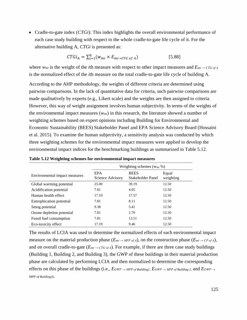
125

Cradle-to-gate index (CTGi): This index highlights the overall environmental performance of

each case study building with respect to the whole cradle-to-gate life cycle of it. For the

alternative building A, CTGi is presented as:

𝐶𝑇𝐺𝑖A = ∑ (𝑤𝑚𝑖 × 𝐸𝑚𝑖→𝐶𝑇𝐺 𝑜𝑓 𝐴)8𝑖=1 [5.88]

where wmi is the weight of the ith measure with respect to other impact measures and Emi → CTG of A

is the normalized effect of the ith measure on the total cradle-to-gate life cycle of building A.

According to the AHP methodology, the weights of different criteria are determined using

pairwise comparisons. In the lack of quantitative data for criteria, such pairwise comparisons are

made qualitatively by experts (e.g., Likert scale) and the weights are then assigned to criteria.

However, this way of weight assignment involves human subjectivity. In terms of the weights of

the environmental impact measures (wmi) in this research, the literature showed a number of

weighting schemes based on expert opinions including Building for Environmental and

Economic Sustainability (BEES) Stakeholder Panel and EPA Science Advisory Board (Hossaini

et al. 2015). To examine the human subjectivity, a sensitivity analysis was conducted by which

three weighting schemes for the environmental impact measures were applied to develop the

environmental impact indices for the benchmarking buildings as summarized in Table 5.12.

Table 5.12 Weighting schemes for environmental impact measures

Weighting schemes (wmi %)

Environmental impact measures EPA

Science Advisory

BEES

Stakeholder Panel

Equal

weighting

Global warming potential 25.00 39.19 12.50

Acidification potential 7.81 4.05 12.50

Human health effect 17.19 17.57 12.50

Eutrophication potential 7.81 8.11 12.50

Smog potential 9.38 5.41 12.50

Ozone depletion potential 7.81 2.70 12.50

Fossil fuel consumption 7.81 13.51 12.50

Eco-toxicity effect 17.19 9.46 12.50

The results of LCIA was used to determine the normalized effects of each environmental impact

measure on the material production phase (Emi → MPP of A), on the construction phase (Emi → CP of A),

and on overall cradle-to-gate (Emi → CTG of A). For example, if there are three case study buildings

(Building 1, Building 2, and Building 3), the GWP of these buildings in their material production

phase are calculated by performing LCIA and then normalized to determine the corresponding

effects on this phase of the buildings (i.e., EGWP → MPP of Building1, EGWP → MPP of Building 2, and EGWP →

MPP of Building3).

126

It should be stressed that although the impact measures are cost criteria by nature (i.e., the higher

the value of an impact measure, the worse the environmental performance of the building), the

impact measures have been considered as the benefit criteria in the proposed framework and the

associated equations above. Therefore, this was considered when normalizing the quantities of

the impact measures to obtain the normalized effects. For example, a building with higher

quantity of an impact measure (e.g., GWP) in its construction phase will contribute to the

corresponding environmental impact less than other buildings.

5.3.8 Material Consumption in Construction (MCC)

Efficient consumption of energy, materials, and natural resources are collectively called

“resource efficiency” that leads to products and services with less resource consumption and less

environmental burdens over the entire life cycle (Ruuska and Häkkinen 2014). The construction

industry is amongst the key contributors to resource consumption and the associated

environmental impacts. As discussed earlier, the construction industry is the largest consumer of

material resources (40- 60% of the total raw material extractions), energy (40% of the total

energy consumption) and largest waste to landfills (Bilal et al. 2016; Edwards 2014; Ahn et al.

2009; Achal et al. 2015; Bribian et al. 2011). For example, the building sector is one of the three

key sectors in the European Union that needs to improve the resource efficiency since it can

influence about 40% of the energy consumption, about 35% the GHG emissions, and over 50%

of all extracted materials (European Commission 2011).

Material efficiency, as the wise consumption of materials, is among the most significant resource

efficiency strategies in the construction industry that can play roles in different aspects. Material

efficiency is effective consumption of natural material resources, reduction of waste, and

recycling. In addition to resource depletion due to inefficient material consumption, limited

availability of materials can produce negative economic impacts. Furthermore, as discussed in

the previous sections, activities related to extraction of primary resources (i.e., raw materials)

and the manufacturing of products and processed materials for building construction can be labor

and energy intensive, which result in negative economic and environmental impacts. Moreover,

material mining and extracting may alternate land use, which has its negative impacts (Ruuska

and Häkkinen 2014). Therefore, efficient material consumption in the construction phase of

buildings can significantly contribute to sustainability and needs to be considered and addressed

earlier in the design stage.

Among the above-mentioned aspects that can be influenced by material efficiency, investigation

of the material resource depletion is the main intent of the ‘Material consumption in construction

(MCC)’ SPC. When it comes to quantification of this SPC, the total materials of different kinds

127

consumed in a building including the materials directly used as the processed materials or the

materials used in different products of the building should be quantified based on functional unit

of the building. In addition, the least and most desirable amount of each material type per

functional unit should be established. However, buildings use diverse materials with different

weight/volume and corresponding waste percentages. Therefore, it is not an easy task to compare

the performance of two buildings (even the same size) from the material consumption point of

view. This might be the reason why the studies that have been conducted to address material

efficiency did not directly compare the amount of materials used in their case study buildings. As

a result, no studies were found that provided the least and most desirable performances for

different building material types. Similarly, due to the same reasons, experts were unable to

provide such performance benchmarks.

Instead, many studies considered the strategies that can result in less consumption of materials.

In this regard, to evaluate material depletion, strategies such as waste prevention, reuse of

components, use of renewable and recycled materials, were found more reasonable than direct

quantification of the consumed materials. In other words, the more implementation of such

strategies, the more resource preservations, regardless of the type of materials. The SPCs

correspond to such strategies (i.e., CWM, REP) have already been prioritized in Chapter 4 and

then, earlier in this chapter, suitable PLFs were developed for their quantification. Therefore,

because 1) The performance benchmarks of this SPI are not available; and 2) Other related SPCs

(CWM, REP) sufficiently (and indirectly) addressed the MCC SPC in this research; there is no

need to develop a sustainability index for this SPC.

It is worth to mention that, the MCC SPC was initially was selected because different references

had emphasized the importance of material consumption in construction of buildings and also

because the experts participating in Survey A had rated this SPC as a ‘High’ importance criterion

for sustainability assessment of modular buildings. However, similar to other SPCs, the

measurability of this SPC had been left for this phase of the research to examine the availability

of suitable measurable indicators and corresponding performance benchmarks.

5.4 Economic SPCs

Economic dimension is another key dimension of a sustainable building. Efficient performance

of a building with respect to suitable criteria (SPCs) that can sufficiently represent this

dimension, can offer significant economic benefits (e.g., added value) or provide ways to avoid

unexpected expenses (e.g., repair costs). In this section, similar to what was performed above for

the environmental SPCs, an attempt was made to determine appropriate measurement methods

128

that lead to development of sustainability indices for the selected economic SPCs (Table 5.1).

The selected economic SPCs in this research can be classified into two types: direct-impact and

indirect-impact. The direct-impact economic SPCs are those that directly deal with costs

throughout a building’s life cycle and are calculated and expressed in the form of monetary

values. Four of the economic SPCs are direct-impact including ‘Design and construction costs

(DCC)’, ‘Operational costs (OC)’, ‘Maintenance costs (MC)’, and ‘End of life costs (EC)’.

Nevertheless, the indirect-impact economic SPCs indirectly deal with the life cycle costs and are

not calculated and expressed based on monetary values. The remaining five SPCs are indirect-

impact including ‘Integrated management (IM)’, ‘Durability of building (DB)’, ‘Adaptability of

building (AB)’, ‘Design and construction time’, and ‘Investment and related risks’.

High locality sensitive SPCs

As discussed in the Methodology section, the information regarding the least and most desirable

performance values and corresponding ranges of data variables for the SPIs under some of the

economic SPCs can be significantly dissimilar in different regions (locality sensitive SPCs). For

example, even though the cities of Vancouver and Kelowna both are located in the same

province of BC, the construction costs per functional unit (1 ft2 of the total area) can be different.

Among all the economic SPCs, six SPCs were recognized to be locality sensitive including:

- Design and construction time (DCT);

- Design and construction costs (DCC);

- Operational costs (OC);

- Maintenance costs (MC);

- End of life costs (EC); and

- Investment and related risks (IRR)

In this research, an attempt was made to collect local information to establish suitable PLFs for

the determined indicators under each of these SPCs. In this regard, the literature was searched to

find information relevant to the Okanagan construction circumstances. In addition, a

questionnaire survey, Survey B, was designed and conducted based on the Delphi method to

collect the required information related to the single-family residential buildings with the total

floor area of less than 3000 ft2. This total area upper limit was chosen because, based on expert

consultations during the design of this survey, residential buildings over 3000 ft2 are generally

custom built with higher quality than typical average-quality single-family houses; therefore, the

performance information can be different.

First, a list of experienced design and construction firms whose main expertise lied in design and

129

construction of conventional residential buildings (single-family houses) in the Okanagan, BC,

has been complied along with their contact information. Then, they have been contacted via both

emails and in-person meetings in their offices to discuss the research, request for participation,

and deliver the survey forms. Initially, eleven construction firms showed interest in the research.

However, when they were informed about the data collection methodology and requirement for

follow up meetings (Delphi method), six firms withdrew from participation and the remaining

five firms continued their participation in the research. In two of the participating firms, a group

of experts completed one questionnaire as the representative of their collective opinions. In

addition, one independent expert who had been involved in different building projects in the

Okanagan, joint the research. Therefore, in total, six questionnaire forms were completed during

the course of survey administration. In addition to the participating experts, two additional

experts who did not have time to participate in all steps of the survey provided their opinions

within a single interview.

The expertise of the participating firms lied in different aspects of residential buildings. For

example, one of the firms was specialized mainly in the design not construction, even though the

corresponding expert was knowledgeable about the economic data of construction. The other

firms were specialized mainly in construction; however, they well knew the design costs since

they have been dealing with the design phase of their projects. Furthermore, four of the experts

were also presidents of their firms, which means they had access to all information required to

complete the survey. The professional experience of the experts from the participating firms

ranged from 6 to 40 years with the average of 23 years. Despite limited number of experts, their

comprehensive experience and also their involvement in diverse residential building projects in

the Okanagan ensured the validity of the collected data.

Depending on the desire and schedule of the participants, the data was collected in each round

using a combination of different methods including asking the survey questions through

individual interviews, phone calls (Keil et al. 2013), or delivering the survey forms and

collecting the completed forms after a few days (Pirdashti et al. 2011; Juwana et al. 2010). In the

first round of data collection, the required information was explained to the experts, the

questionnaire forms were delivered, and if requested, they were given a few days to provide their

answers. Subsequently, the collected data was reviewed by the survey administrator to recognize

and list possible ambiguous answers that needed clarifications. For example, while the cost data

was required to be provided per 1 ft2 as a functional unit of single-family residential buildings,

some of the participants provided the total cost without mentioning the total floor area of the

building they referred to. Therefore, the corresponding participants were contacted to clarify

such answers before including them in the pool of answers. Subsequently, the answers provided

130

by experts ware averaged as the new answers. In the second round, the experts were provided

with these new answers and asked to review and, if required, revise/modify them. The same

method was followed until the third round where the consensus was reached on all the answers.

Consequently, the results of Survey B were used to establish the PLFs for the SPIs associated

with the above listed SPCs. It should be mentioned that, within the same survey (Survey B), the

participants were asked a number of additional questions related to the next phases of this

research that have been explained in the next chapter.

Less locality sensitive SPCs

Despite the above-mentioned SPCs, the least/most desirable performances of buildings with

respect to other economic SPCs including ‘Integrated management (IM)’, ‘Durability of building

(DB)’; and ‘Adaptability of building (AB)’ are approximately similar throughout BC. For these

SPCs, the same process that has been performed earlier in this chapter to establish the PLFs for

the environmental SPCs was used. Therefore, first, relevant measurable indicators (SPIs and sub-

SPIs) along with their relative importance weights were determined. Then, for each indicator, the

least and most desirable performance values and corresponding ranges of data variables have

been established. In this regard, different sources including rating systems and published articles

and reports were reviewed. In addition, experienced experts in the construction industry were

consulted. Subsequently, a PLF has been established for each indicator by which the

performance of the subject building with respect to that indicator can be calculated and presented

with a PL between 0 and 100.

Except only one SPC (i.e., EC), this research successfully determined suitable indicators under

each economic SPC and established the corresponding PLFs. In total, 37 indicators were

determined under the economic SPCs including 17 SPIs and 20 sub-SPIs as summarized in Table

5.13. The table also lists the sources used to identify the measurement method of an indicator and

subsequently to establish the corresponding PLF. Details are provided in the following sections.

131

Table 5.13 Economic SPCs and corresponding indicators


Integrated management (IM)

IM1 Integrated design processes IM1-1 Pre-design meetings BREEAM, Green Globes, EO

IM1-2 Performance goals BREEAM, Green Globes, EO

IM1-3 Progress meetings BREEAM, Green Globes, EO

IM2 Life cycle cost IM2-1 Elemental life cycle cost BREEAM, EO

IM2-2 Component level life cycle cost BREEAM, EO

IM3 Commissioning IM3-1 Commissioning schedule and responsibilities BREEAM, Green Globes, EO

IM3-2 Whole building commissioning BREEAM, Green Globes, EO

IM3-3 Training and handover LEED, BREEAM, EO

Durability of building (DB)

DB1 Roofing and openings DB1-1 Roofing membrane assemblies Lit., Green Globes

DB1-2 Envelope flashings Lit., Green Globes

DB1-3 Roof and wall openings Lit., Green Globes

DB2 Foundation waterproofing Lit., Green Globes

DB4 Barriers DB4-1 Air barriers Lit., Green Globes

DB4-2 Vapor retarders Lit., Green Globes

DB3 Cladding DB3-1 Exterior wall cladding systems Lit., Green Globes

DB3-2 Rain screen wall cladding Lit., Green Globes

Adaptability of building (AB)

AB1 Expandability AB1-1 Lateral expandability Lit., EO

AB1-2 Vertical expandability Lit., EO

AB2 Dismantlability Lit., EO

AB3 Record keeping Lit., EO

Design and construction time (DCT)

DCT1 Design time Lit., EO

DCT2 Construction time Lit., EO

Design and construction costs (DCC)

DCC1 Design cost Lit., EO

DCC2 Construction cost Lit., EO

Operational costs (OC)

OC1 Running costs Lit., EO

Maintenance costs (MC)

MC1 Repair and replacement costs Lit., EO

Investment and related risks (IRR)

IRR1 Return on investment IRR1-1 Sale price Lit., EO

IRR1-2 Design cost Lit., EO

IRR1-3 Construction cost Lit., EO

Note: Lit. = literature; LEED = Leadership in Energy and Environmental Design; BREEAM = Building Research Establishment

Environmental Assessment Method; EO = expert opinions.

132

5.4.1 Integrated Management (IM)

Integrated management (IM) during the design and construction of a building can effectively

help the project’s economic performance. The IM SPC encourages sustainable management

practices with respect to design, construction, commissioning, and handover of a building by

setting and implementing suitable sustainability objectives to avoid extra costs later in the use

phase of the building. This SPC consists of three SPIs: ‘IM1 Integrated design processes’, ‘IM2

Life cycle cost’, and ‘IM3 Commissioning’. Each of these SPIs comprises a number of sub-SPIs

as demonstrated in Figure 5.10.

IM1-1 Pre-design meetings

IM1 Integrated design

processes

IM1-2 Performance goals

IM1-3 Progress meetings

Integrated Management

(IM)

IM2-1 Elemental life cycle cost

IM2 Life cycle cost

IM2-2 Component level life

cycle cost

IM3-1 Commissioning

schedule and responsibilities

IM3 Commissioning

IM3-2 Whole building

commissioning

IM3-3 Training and handover

Figure 5.10 SPIs and sub-SPIs associated with ‘Integrated management’

5.4.1.1 Integrated design processes (IM1)

The aim of this SPI is to ensure that the environmental and functional objectives of the building

are satisfied in a cost-efficient manner through the cooperation of different disciplines involved

in the project. In other words, it looks for an integrated design process that enhances the building

performance (BRE 2016). This SPI is split into three sub-SPIs: ‘IM1-1 Pre-design meetings’,

‘IM1-2 Performance goals’, and ‘IM1-3 Progress meetings’ (GBI 2014; GBI 2015; BRE 2016).

Pre-design meetings (IM1-1)

A significant factor that influences the design and construction of a sustainable building that can

also meet the needs of the end-users (clients) is to establish all goals at the beginning of the

133

design process. In addition, involvement of the project team members throughout the project is

another significant factor. In other words, the project team should know the established basic

goals and the associated criteria and also the responsibility of each member for ensuring that

each criterion is successfully addressed.

To this end, attendance of the representatives of main design disciplines in pre-design planning

sessions is important. Such sessions can be in the form of one or more “all hands” project

meetings, design charrettes, or workshops during pre-design of the project. The number of such

meetings in a project depends on size and complexity of the building as well as the desired

sustainability goals. For example, a minimum seven meetings or workshops is recommended by

the Whole Systems Integrated Process Guide, while ASHRAE does not mention a required

meeting number but emphasizes that the project team should use a charrette process to determine

the optimal building arrangement. Regardless of meetings number, this is vital that all key

project team members arrange and hold collaborative meetings earlier in the design stage and

continue through the use phase of the building.

The performance of a building project with respect to this sub-SPI is evaluated according to the

involvement of the following key design disciplines and stakeholders in collaborative meetings

during the design stage (GBI 2015):

- Owner’s representative

- Architect

- Green building expert or sustainable design coordinator

- Civil engineer

- Electrical engineer

- Mechanical engineer – HVAC

- Structural engineer

Consequently, the PLF below can be used to calculate the performance level of IM1-1:

PLIM1-1 = 25𝑛 𝑛 = 0, 1, . . , 4 [5.89]

Where n is the number of key disciplines involved in “all hands” project meetings, design

charrettes, or workshops.

Performance goals (IM1-2)

This sub-SPI considers the establishment of qualitative design goals and performance metrics.

The project team should review the applicable sustainability criteria available in the literature

such as rating systems or other standards. Subsequently, during “all hands” meetings or design

134

charrettes, the project designers should identify the performance standards and the corresponding

indicators by which the project success can be evaluated.

The performance levels of this sub-SPI is identified based on establishment of qualitative design

goals and performance metrics for any or all of the following items:

- Site design

- Envelope

- Materials efficiency

- Indoor environment

- Energy efficiency

- Renewable energy (percentage of total energy)

- Greenhouse gas emissions and life cycle impact

- Water conservation, efficiency, and reuse

- Construction waste management

The performance level of this sub-SPI can be calculated using the following PLF:

PLIM1-2 = 16.67𝑛 𝑛 = 0, 1, . . , 6 [5.90]

Where n is the number of items whose qualitative green design goals and quantitative

performance metrics have been established at the pre-design stage.

Progress meetings (IM1-3)

The intent of holding progress meetings throughout the design process by all the project

stakeholders is to review performance goals and modify them if necessary, refine language

regarding performance goals outcomes into plans and specifications, realize and correct possible

missing requirements, and define and track the responsibilities.

The performance level of this sub-SPI is calculated according to holding progress meetings

before completion of each of the following design stages:

a- Concept design stage: Where the general scope, initial design, and the relationships between

various components are defined. In addition, the cost and timeline are established.

b- Design development stage: Where detailed plans and drawings that show the main elements

such as electrical, mechanical, structural, plumbing systems, and so forth, are produced.

c- Construction documents stage: Where the finalized drawings that show detailed

specifications of all systems and components are generated.

Subsequently, the following PLF can be used to measure the sub-SPI IM1-3:

135

PLIM1-3 = 33.33𝑛 𝑛 = 0, 1, 2, 3 [5.91]

Where n is the number of the project design stages listed above for which progress meetings

have been held prior to their completion.

Eventually, the PL of the parent SPI is calculated by aggregating the PLs of all three associated

sub-SPIs and their relative importance relationships as:

PLIM1 = 0.25×PLIM1-1 + 0.5×PLIM1-2 +0.25×PLIM1-3 [5.92]

5.4.1.2 Life cycle cost (IM2)

The IM2 SPI seeks enhancing economic sustainability by using life cycle cost (LCC) analysis at

the design stage of a building (BRE 2016). LCC considers the whole life cycle costs from the

design to the end of life to ensure that the systems and specifications designed are based on the

lowest costs and highest value for money. This SPI comprises two sub-SPIs ‘IM2-1 Elemental

life cycle cost’ and ‘IM2-2 Component level life cycle cost’ (BRE 2016). By implementing these

sub-SPIs, different alternative systems, elements, and component, can be compared and

appraised to optimize the life cycle cost plan.

Elemental life cycle cost (IM2-1)

The LCC models can be used to perform a whole building elemental life cycle cost analysis at

the concept design stage. The outcomes provide a prediction of cash flow for the whole building.

The elemental LCC models can include (BRE 2016):

Construction costs including initial capital expenditure, other construction related costs,

and client definable costs.

Maintenance costs including major and minor replacement and repairs, allowances for

unscheduled repairs.

Operational costs including fuel, water and drainage, rates, and other local charges.

End of life costs including deconstruction, demolition, recycling, landfilling.

The performance level of the subject building with respect to the IM2-1 sub-SPI is assigned

based on meeting the conditions outlined below:

a- Conducting an elemental LCC (such as construction costs, maintenance costs, operational

costs) at the concept design stage together with any design option appraisals.

b- If the elemental LCC was performed, does it predict the future replacement costs at particular

time from the start of the use phase required by the client such as 20, 40, or 50 years?

c- If the elemental LCC plan was performed, does it provide maintenance and operational cost

136

estimates?

d- Was it demonstrated, using appropriate examples provided by the analysis team that how the

results of the performed elemental LCC was utilized to modify the design of systems and

specification to minimize the life cycle costs?

The performance level of IM2-1 can be measured by the following PLF:

PLIM2-1 = 25𝑛 + 25𝑛𝑚 𝑛 = 0, 1; 𝑚 = 0, 1, 2, 3 [5.93]

Where n is 1 if the condition ‘a’ was met and m is the number of conditions ‘b’, ‘c’, and ‘d’ that

were met.

Component level life cycle cost (IM2-2)

This sub-SPI considers the component level LCC that are performed by the end of the design

development stage. The main component types to perform LCC options appraisal include (BRE

2016):

Envelope, such as roofing, windows, and cladding.

Services such as heating, cooling, and controls.

Finishes such as floors, walls, and ceilings.

External spaces such as alternative hard landscaping and boundary protection

Figure 5.11 illustrates an example for the cost of two cooling systems over 60 years (in real

discounted costs).

Figure 5.11 Costs of two systems of cooling over 60 years of building life span

The performance level for the IM2 sub-SPI is calculated according to performing a component

137

level LCC options appraisal for any of the aforementioned component types as:

PLIM2-2 = 20𝑛 + 20𝑚 𝑛 = 0, 1, . . , 4; 𝑚 = 0, 1 [5.94]

Where n is the number of component types that LCC were performed for, and m is 1 if the design

team demonstrated, using appropriate examples, that how the results of the component level

LCC used to modify the designed systems and specification to minimize the life cycle costs.

When the PLs of the two sub-SPIs are obtained, the PL of the corresponding IM2 SPI is obtained

using the function below:

PLIM2 = 0.67×PLIM2-1 + 0.33×PLIM2-2 [5.95]

5.4.1.3 Commissioning (IM3)

This SPI encourages the design, construction, and calibration of the building systems in a way

that they operate as intended (GBI 2015) and reflect the needs of the building occupants (BRE

2016). The SPI consists of three sub-SPIs: ‘IM3-1 Commissioning schedule and responsibilities’,

‘IM3-2 Whole building commissioning’, and ‘IM3-3 Training and handover’ (BRE 2016).

Commissioning schedule and responsibilities (IM3-1)

Commissioning and testing are performed by the main contractor/builder of a building according

to a schedule that has been established in the design phase. Such schedule specifies the standards

that all commissioning activities are performed based on, such as national best practice

commissioning codes or any other accepted standards (where applicable). The schedule includes

a timeline for commissioning and recommissioning activities regarding services and control

systems and also testing and inspecting the fabric (e.g., roof, floors, columns, walls, windows,

and doors).

The performance level of the IM3-1 sub-SPI is calculated based on meeting the following:

a- Is there a schedule of commissioning and testing that specifies all the activities required by the

standards such as national best practice commissioning codes or any other suitable standards?

b- Is an individual from the project team chosen to monitor and program the pre-commissioning,

commissioning, and testing activities?

The PLF for this sub-SPI is:

PLIM3-1 = 50𝑛 𝑛 = 0, 1, 2 [5.96]

Where n is the number of conditions ‘a’ and ‘b’ that was met.

138

Whole building commissioning (IM3-2)

The integrity and quality of the building envelope and systems is ensured by completion of pre-

commissioning, commissioning, testing, and inspection activities in accordance with the

schedule outlined above.

The performance of this sub-SPI is measured based on commissioning the following envelope

and systems of the building at the pre-design, design, and construction stages (BRE 2016):

C1- HVAC and refrigeration systems and their controls;

C2- Building envelope (roofing assemblies, windows and doors, waterproofing assemblies, and

cladding/skin);

C3- Structural systems;

C4- Fire protection system;

C5- Plumbing system;

C6- Electrical system; and

C7- Lighting system and their controls.

The following PLF can be used to calculate the IM3-2 sub-SPI:

PLIM3-2 = {𝑀𝑎𝑥 (25𝑛 + 12.5𝑚), 100} 𝑛 = 0, 1, 2; 𝑚 = 0, 1, 2, . . , 5 [5.97]

Where n is the number of the building envelope and systems ‘C1’ and ‘C2’, and m is the number

of the building envelope and systems ‘C3’ to ‘C7’ that have been commissioned.

Training and handover (IM3-3)

Building end users (occupants) should know how to use the building’s systems and equipment

such that they operate in an effective manner as intended. The performance of a building with

regard to this sub-SPI is measured based on meeting the following conditions (BRE 2016):

a- Before handover of the building, a building or home user guide is developed and delivered to

the end user(s).

b- Around handover of the building, a training session is schedule that includes the items below:

- The building’s design objectives;

- The aftercare activities by the builder/contractor such as any scheduled seasonal

commissioning and post occupancy testing;

- Explanation and description of installed systems and key features, controls and their interface,

to end user(s);

- Explanation of the developed user guide and other relevant building documentation; and

139

- Maintenance information and requirements of the building.

The following PLF can be used to measure the performance of this sub-SPI:

PLIM3-3 = 50𝑛 + 10𝑚 𝑛 = 0, 1; 𝑚 = 1, 2, . . , 5 [5.98]

Where n is 1 if the condition ‘a’ was met and m is the number of items under condition ‘b’ that

were met.

Finally, the PL of the IM3 SPI is calculated by combining the PLs of the three sub-SPIs as:

PLIM3 = 0.25×PLIM3-1 + 0.5×PLIM3-2 + 0.25×PLIM3-3 [5.99]

5.4.1.4 Relative importance of the SPIs under IM

To calculate the sustainability index for the IM SPC, both the PLs of the associated SPIs and

their importance weights are required. According to the BREEAM rating system, the weights of

the IM1, IM2, and IM3 SPIs came to be 0.364, 0.272, and 0.364, respectively (BRE 2016).

5.4.2 Durability of Building (DB)

Durability is another indirect-impact criterion that can influence the economic performance of

buildings. Durability is a building capability to perform its intended function during the use

phase with minimal unexpected requirements for repair or maintenance expenses (CaGBC 2009).

The quality of materials and products used in a building along with the quality of construction

and installation (off-site and on-site) activities play a significant role in the overall durability of

the building. In a durable building, suitable design and specification measures are considered

such that the degradation of materials and components during the lifetime of the building and the

subsequent replacements and repairs are minimized (ILFI 2014; BRE 2016).

To this end, the ‘Durability of building (DB)’ is a SPC that considers the incorporation of

measures for adequate protection of exposed elements and landscape of a building to prolong its

life; thus, reduce economic impacts associated with damage and wear and tear. The DB SPC

comprises four SPIs some of which include a number of sub-SPIs as illustrated in Figure 5.12.

140

DB1-1 Roofing membrane

assemblies

DB1 Roofing and openings

DB1-2 Envelope flashings

DB1-3 Roof and wall

openings

Durability of Building

(DB)

DB2 Foundation waterproofing

DB3-1 Exterior wall cladding

systems

DB3 Cladding

DB3-2 Rain screen wall

cladding

DB4-1 Air barriers

DB4 Barriers

DB4-2 Vapor retarders

Figure 5.12 SPIs and sub-SPIs associated with ‘Durability of building’

5.4.2.1 Roofing and openings (DB1)

The aim of this SPI is to implement roofing/opening design measures to enhance the

performance and durability. This indicator comprises three sub-SPIs: ‘DB1-1 Roofing membrane

assemblies’, ‘DB1-2 Envelope flashings’, and ‘DB1-3 Roof and wall openings’ (GBI 2015).

Roofing membrane assemblies (DB1-1)

The performance of the subject building with respect to this sub-SPI is evaluated based on

implementation of the following items:

a- Roofing membrane assemblies and systems should be installed in accordance with the

instructions by the corresponding manufacturers.

b- The installed roofing membrane assemblies and systems should be inspected by

professionals by the manufacturers or a third-party roofing expert.

The performance level of DB1-1 is calculated as:

PLDB1-1 = 50𝑛 𝑛 = 0, 1, 2 [5.100]

Where n is the number of items listed above that have been implemented while constructing and

commissioning the roof assemblies of the subject building.

Envelope flashings (DB1-2)

Flashings and sheet metals act as a defense line to protect a building envelope against moisture.

This sub-SPI ensures the quality installation of the envelope flashing by checking the items

below (GBI 2015):

141

a- Envelope flashings and sheet metal assemblies should be installed in accordance with the

instructions by the industry best practices.

b- The installed envelope flashings and sheet metal assemblies should be inspected as per

prescribed industry protocol or by a third-party expert.

Consequently, the PLF below can be used to calculate the performance level of DB1-2:

PLDB1-2 = 50𝑚 𝑚 = 0, 1, 2 [5.101]

Where m is the number of implemented items ‘a’ and ‘b’.

Roof and wall openings (DB1-3)

To ensure the quality of the products correspond to a buildings’ roof and windows openings, the

following conditions should be examined (GBI 2015):

a- All products associated with wall and roof openings such as windows and doors, should

include moisture management designs.

b- These products should inspected against water penetration in accordance with industry best

practices.

Subsequently, the following PLF can be used to measure the DB1-3 sub-SPI:

PLDB1-3 = 50𝑘 𝑘 = 0, 1, 2 [5.102]

Where k is the number of conditions ‘a’ and ‘b’ that have been satisfied.

When all the three sub-SPIs have been calculated, the parent DB1 SPI is calculated by

aggregating the calculated PLs and their weights as:

PLDB1 = 0.3×PLDB1-1 + 0.3×PLDB1-2 + 0.4×PLDB1-3 [5.103]

5.4.2.2 Foundation waterproofing (DB2)

The intent of this indicator is to investigate if the foundation waterproofing design measures have

been implemented to enhance the durability of the foundation; hence, the whole building. The

performance is evaluated cumulatively using the following measures (GBI 2015):

a- Newly installed foundation systems for conditioned spaces are constructed with slab-on-

ground vapor retarders in accordance with industry best practices.

b- Newly installed foundation systems for conditioned spaces are constructed such that all

slabs on grade will be positioned directly over vapor retarders and capillary-break base courses.

c- The installed foundations should be field-inspected conforming to industry protocol.

142

It is important to note that, in addition to the above stated foundation waterproofing measures,

the literature provided more measures. However, they have not mentioned in this study because

either they were irrelevant to residential buildings or, according to experts, they were not

applicable to the construction circumstances in BC.

Subsequently, the following PLF can be used to calculate the performance level of the DB2 SPI:

PLDB2 = 25𝑚 + 50𝑛 𝑚 = 0, 1, 2; 𝑛 = 0, 1 [5.104]

Where m is the number of measures ‘a’ and ‘b’ that have been implemented and n is 1 if measure

‘c’ was met.

5.4.2.3 Cladding (DB3)

Cladding is the application of a layer of non-structural material (cladding) over the layer of

another material (usually the load bearing materials). The primary purpose of cladding is to

enhance the aesthetics of a building’s walls. However, it also offers resistance and protection

leading to enhanced durability of structural materials (Jacobs 2017). The aim of the DB3 SPI is

to examine the implementation of adequate cladding measures. This SPI included two sub-SPIs:

‘DB3-1 Exterior wall cladding systems’ and ‘DB3-2 Rain screen wall cladding’ (GBI 2015).

Exterior wall cladding systems (DB3-1)

The sub-SPI is measured based on the following measures (GBI 2015):

a- Has one of the following cladding systems been installed as per industry best practices?

- Install Exterior Insulation Finishing Systems (EIFS) as water-managed systems conforming

to the instructions by the corresponding manufacturers.

- Install masonry veneer cladding conforming to industry technical instructions.

- Install aluminum framed glazing systems conforming to the instructions by the

manufacturers. The systems should be warranted by the corresponding manufacturers.

b- If the answer to measure ‘a’ is YES, has the installed cladding system been inspected as per

the appropriate prescribed industry protocols?

c- Have joint sealers been installed and field-inspected in accordance with industry best practice?

The performance of the subject building with respect to DB3-1 is calculated as:

PLDB3-1 = 33.3𝑛 𝑛 = 0, 1, 2, 3 [5.105]

Where n is the number of above states measures that have been satisfied when implementation of

the eexterior wall cladding.

143

Rain screen wall cladding (DB3-2)

The performance level of this sub-SPI is measured using the following measures (GBI 2015):

a- Do the construction documents indicate that exterior rain screen wall cladding systems

specified over framed walls are to be installed with the following items?

- Primary and secondary line of defense.

- An air barrier.

- A means for incidental bulk water intrusion to escape the cladding system assembly.

b- Are the rain screen cladding assemblies installed in accordance with AAMA 508-07

laboratory testing requirements or any other accepted standard?

The PLF for this sub-SPI was established as:

PLDB3-2 = 25𝑘 + 25𝑙 𝑘 = 0, 1, 2, 3; 𝑙 = 0, 1 [5.106]

Where k is the number of implemented items listed under measure ‘a’ and l is 1 if measure ‘b’

has been met.

Once the PLs of the two sub-SPIs are obtained, the PL of the DB3 SPI can be calculated as:

PLDB3 = 0.6×PLDB3-1 + 0.4×PLDB3-2 [5.107]

5.4.2.4 Barriers (DB4)

This indicator appraises the quality implementation of barrier design measures, which can lead to

enhanced durability of the subject building. The DB4 SPI includes two sub-SPIs: ‘DB4-1 Air

barriers’ and ‘DB4-2 Vapor retarders’ (GBI 2015).

Air barriers (DB4-1)

Air barriers are used to decrease the uncontrolled air movement from the envelope. The

performance of a building with respect to this sub-SPI is assessed according to the following

measures (GBI 2015):

a- If installation of a continuous air barrier has been incorporated in the design stage, indicate of

any of the following practices have been considered:

- An airtight and flexible joint between the air barrier material and adjacent assemblies.

- The designed air barrier is able to withstand combined design winds (negative and positive),

stack and fan pressures without displacement or damage.

- The designed air barrier is able to withstand structural movement and also no displacement

due to full load.

144

- Connection details of the air barrier between different assemblies and components, such as

foundation and walls, wall and roof, walls and windows, and so forth, are available in the

construction documents.

b- Is the designed continuous air barrier for the opaque building envelope in accordance with the

relevant local building code or either of the following standards?

- ASTM E2178-11 Standard Test Method for material testing;

- ASTM E2357-11 Standard Test Method for assembly testing;

- ASTM E779-03 or equivalent method for building testing.

Consequently, the PLF below has been established to calculate DB4-1:

PLDB4-1 = 12.5𝑖 + 50𝑗 𝑖 = 0, 1, 2, 3, 4; 𝑗 = 0, 1 [5.108]

Where i is the number of practices listed under measure ‘a’ that have been implemented and j is

1 if any of the standards mentioned under measure ‘b’ was followed.

Vapor retarders (DB4-2)

Uncontrolled moisture in the indoor air of a building can result in serious problems. If such

moisture enters the ceiling or walls, it can create a suitable environment for the mold and mildew

growth, which results in health issues, degradation of the building’s structural integrity, damage

of the materials, and negative impacts on the thermal efficiency and indoor air quality (Al-

Homoud 2005). To minimize the moisture (i.e., movement of water due to vapor diffusion),

vapor retarders are utilized. Vapor retarders are elements made by special materials such as

treated papers, plastic sheets, among others, that are designed and installed in assemblies of a

building to retard the passage of water vapor (Al-Homoud 2005; Lstiburek 2004).

The DB4-2 sub-SPI is evaluated using the following measures (GBI 2015):

a- Install the interior side of framed walls with a Class I or II vapor retarder conforming to the

relevant local building code or (in absence) and an accepted international code such as Energy

Conservation Code 2012.

b- Install on the walls of unvented crawl spaces insulation that is permanently fastened to the

walls and extends downward from the floor to the finished grade level, and then vertically and/or

horizontally for at least an additional 60 cm.

c- Use a continuous Class I vapor retarder to cover exposed earth in unvented crawl space

foundations and implement the items below:

- all joints of the vapor retarder are overlapped by 15 cm and are sealed or taped; and

145

- the edges of the vapor retarder extend at least 15 cm up the stem wall and are attached to the

stem wall.

Consequently, the PLF below can be used to calculate the performance level of DB4-2:

PLDB4-2 = 33.3𝑛 𝑚 = 0, 1, 2, 3 [5.109]

Where n is the number of vapor retarder measures ‘a’, ‘b’, and ‘c’ that have been implemented.

Once the PLs of these two sub-SPIs have been calculated, the PL of the corresponding SPI is

measured using the equation below:

PLDB4 = 0.571×PLDB4-1 + 0.429×PLDB4-2 [5.110]

5.4.2.5 Relative importance of the SPIs under DB

According to the scoring system provided by Green Globes (GBI 2015), the weights of DB1,

DB2, DB3, and DB4, were determined as 0.417, 0.083, 0.208, and 0.292, respectively. These

weights and the calculated PLs are used to develop a sustainability index for the DB SPC.

5.4.3 Adaptability of Building (AB)

Buildings, as a significant share of the built environment, are built mainly to meet the society and

people’s requirements. It is possible that these requirements change during the use phase of

buildings (Fernandez 2003; Moffatt and Russell 2001). Buildings should be able to sufficiently

respond the changes such as needs of owners/users, legislative requirements, new technical and

functional technologies, and so forth (Mansfield 2009; Manewa et al. 2016; Fernandez 2003;

Greden 2005). According to Energy Research Group (1999), any underperforming building with

respect to comfort conditions, energy efficiency, or environmental impact can be a potential

nominee for adaptation. Therefore, it is important to consider such possible changes in the design

and construction of buildings (Heidrich et al. 2017).

Adaptability refers to the capability of accommodating minor and major changes in a building

(Grammenos and Russell 1997). In other words, adaptable buildings are designed at the design

and construction phase of the life cycle in a way that they can accommodate future changes as

easy as possible and at lowest costs to meet the evolving user needs as well as statutory

requirements (Edmonds and Gorgolewski 2000).

According to Douglas (2006), adaptation and maintenance are classified as the two primary

elements of building performance management. Based on this classification, adaptation is

interpreted as performance adjustment that leads to optimum performance or maximum standard.

On the contrary, since the performance of every building decreases over time, maintenance is

146

interpreted as performance upkeep (i.e., preserve) that returns the performance to its original

condition (i.e., early days of the use phase). The economic life of a building can be extended by

performing both adaptation and maintenance rather than only maintenance. In addition, the

cycles of these two major forms of intervention are different for residential and commercial

buildings, which is much shorter in the case of commercial buildings. Residential buildings, such

as single-family and multi-family, have a relatively long lifespan with few major interventions

(i.e. adaptations) during their use phase.

The SPC ‘Adaptability of building (AB)’ recognises and encourages measures to accommodate

possible changes in the occupancy phase and even in the end of life phase of buildings. However,

not all the adaptability strategies are applicable for every building project since each project has

its unique circumstances; therefore, a limited number of strategies can represent the level of

adaptability of a building (Estaji 2017). For example, convertibility (i.e., allowing for changes in

the building main use) has been introduced as one of the important contributors to adaptability

(Douglas 2006). However, it is not a common practice to convert a residential dwelling to a

commercial building because of the rigidity of the structures and layouts (Moffatt and Russell

2001). Thus, in this research, only those changes and corresponding adaptability strategies that

are common and most relevant to residential buildings have been considered when determining

suitable indicators under the AB SPC.

It is important to mention that, ideally, suitable indicators (i.e., adaptability measures and

strategies) and standardized assessment methods are required by which the level of adaptability

in a building can be rated. However, the lack of specific methods and indicators in the literature

makes it difficult to measure adaptability of residential buildings and create benchmarks for

comparison purposes. This study attempted to initiate the establishment of a baseline for suitable

indicators under this SPC and corresponding benchmarks by rationally reviewing and

summarizing the information available in the literature and expert feedback. The main reviewed

documents included Heidrich et al. 2017; Gosling et al. 2008; Moffatt and Russell 2001; Sumer

1997; CMHC 2004; Greden 2005; Israelsson and Hansson 2009; Estaji 2017; Douglas 2006;

Fernandez 2003; Mansfield 2009; Manewa et al. 2016; Energy Research Group (1999), Heidrich

et al. 2017; Grammenos and Russell (1997) and Edmonds and Gorgolewski (2000).

Eventually, the total number of three SPIs were determined under the AB SPC as the most

relevant adaptability strategies for residential buildings as shown in Figure 5.13. However, the

proposed SPIs and associated measures can be modified/revised in the future to represent the

most relevant adaptability performance indicators for residential buildings. It is also worth to

mention that this SPC examined potential adaptability of buildings; however, since each building

147

is unique and the level of adaptation can be completely different, depending on circumstances

and needs, a detailed feasibility study is required before implementation of actual adaptations.

AB2 Dismantlability

Adaptability of Building

(AB)

AB1-1 Lateral expandability

AB1 Expandability

AB1-2 Vertical expandability

AB3 Record keeping

Figure 5.13 SPIs and sub-SPIs associated with ‘Adaptability of building’

5.4.3.1 Expandability (AB1)

Expandability means allowing for increases in volume or capacity of a building to accommodate

new needs of end users. As stated earlier, conversions to other uses (e.g., residential to

commercial) are not common. However, conversions to the same use by expanding or re-

configuring the building space is not uncommon. This kind of conversion might require

substantial changes in internal parts of the building. For example, converting a building unit into

two smaller units requires the design and installation of additional separating walls and floors.

In general, two forms of expansions are performed within same-use conversions: lateral and

vertical. The former form is more common and practical than the latter form. The AB1 SPI

consists of two sub-SPIs: ‘AB1-1 Lateral expandability’ and ‘AB1-2 Vertical expandability’.

Lateral expandability (AB1-1)

Increasing the spatial capacity of a building is one of the most visible forms of adaptation. This

form of adaptation is implemented by adding a horizontal space to the existing building, which

can provide facilities that are not existent in the building or provide additional space for

accommodation. Another reason for lateral expansion is that it is an effective solution to re-

configure and rearrange the existing space in order to accommodate the new living patterns.

Examples of lateral expansion are creating facilities such as granny flats or study rooms by

extending or re-configuring the existing building.

In addition to responding the evolving needs of the occupants, expansions can increase the

148

property values, which is a significant factor for this form of adaptation. Furthermore, expensive

process of moving elsewhere to a larger property (i.e., economic impact) and the associated

stressful activities and emotional subsequences (i.e., social impacts) can convince house owners

to extend their property rather than relocating.

To evaluate a building’s performance with respect to this sub-SPI the inclusion of provisions for

future lateral expansions at the design stage is examined by the following measures:

- The building is located and oriented in a way that there is sufficient space around all or part

of it for horizontal extensions.

- There are means of access and exit regarding the site and building during the lateral extension

activities in order to make less interruption to the surroundings people (e.g., noise, dust).

- Lateral expansions do not disturb the neighborhood access to light, view, and so forth.

- The connections between materials and components facilitate disassembly required for

extensions or re-configurations of the space (e.g., prefabricated components, bolted

connections).

- Substructure (foundation) has been adequately over-designed to accommodate additional

loads due to lateral expansion.

Three possibilities have been considered when evaluating each of the measures above including:

The measure has not been incorporated in the design stage;

The measure has moderately been incorporated; or

The measure has highly been incorporated.

For example, it is likely that the foundation of the given building was over-designed in such a

level that allows only small to medium extensions or re-configurations which means that the

associated measure was moderately met. Subsequently, the PLF below was established to

calculate the PL of this sub-SPI:

PLAB1-1 = 25𝑖 + 12.5𝑗 𝑖 and 𝑗 = 0, 1, 2, 3, 4 [5.111]

Where i and j are the number of the above lateral expandability measures that have been highly

and moderately incorporated in the design of the building, respectively.

Vertical expandability (AB1-2)

Vertical expansions are less common and more expensive than lateral expansions because it is

more complicated. For example, vertical expansion needs staircases (to facilitate access to the

new accommodation) and creating new roof openings or separating floor to provide access

149

between the old and new sections. This reduces slightly the usable space on the floor

immediately below the new level. Building services can be affected by this form of adaptation, in

particular, when the added space requires separate bathroom and/or toilet facilities. Furthermore,

in some cases, there are requirements to strengthen the existing structure. Moreover, the design

of the building foundation should be over-designed such to ensure its strength to bear the added

vertical facilities (e.g., new story). However, the foundation of buildings is mostly over-designed

and fewer buildings require such substructure strengthening.

Typically, there are two forms of vertical adaptation including roof expansions and basement

expansions. The following are possible types of upward and downward vertical expansions or

conversions:

New basement

Creation of recess area at front and/or rear to permit daylight and ventilation.

New mansard roof providing habitable space on existing flat roof or on top of new story

with skylights or dormers.

Additional top story with flat roof to modern durability and thermal standards.

Additional top story with new pitched roof, possibly containing skylights.

Vertical expansions are usually upward since there is almost available space upward that allows

expansions. For example, roof space conversions are still a very common type of vertical

expansion that provided the required extra space at a reasonable cost. Although downward

expansions (i.e., basement adaptation) have been grabbing attention in the past few years, they

are not still popular since they are significantly more expensive than upward expansions. In

addition to the ncost factor, implementation of downward expansions is much more complicated

than vertical expansions such as the need for soil condition testing.

A building’s performance with regard to this sub-SPI is assessed based on considerations of the

following measures at the design stage:

- There are means of access and exit regarding the site and the building during the vertical

expansion activities to make less interruption to the surroundings people (e.g., noise, dust)

- Vertical expansions do not disturb the neighborhood access to light, view, and so forth.

- The flat-roof construction and detailing facilitate disassembles required for extensions or re-

configurations of the space (e.g., prefabricated components, bolted connections).

- Substructure (foundation) has been adequately over-designed.

- Soil conditions can accommodate the extra loading associated with expansion (new basement

150

or additional story).

Consequently, the PLF below can be used to calculate the performance level of the given

building with respect to this sub-SPI:

PLAB1-2 = 25𝑖 + 12.5𝑗 𝑖 and 𝑗 = 0, 1, 2, 3, 4 [5.112]

Where i and j are the number of the above vertical expandability measures that have been highly

and moderately considered at the design stage of the given building, respectively.

Eventually, when the PLs of the above sub-SPIs have been obtained, the PL of the AB1 SPI is

calculated as:

PLAB1 = 0.6×PLAB1-1 + 0.4×PLAB1-2 [5.113]

5.4.3.2 Dismantlability (AB2)

This SPI considers damsmantlability of residential buildings. Dismantlability refers to the

capability of a building’s products, components, and assemblies, to be disassembled during the

use phase (where applicable) and at the end of life phase in a safe, efficient, and speedy way (in

part or in whole).

Due to continuous advancements in energy efficiency and governmental energy efficiency and

enhanced building performance policies, building codes and standards are continually changing

every few years. In addition, the occupants’ expectations of buildings are increasing. These

reasons increase the demand for new technologies in buildings. Deficiencies in buildings and

their services occur because sometimes they are not capable to meet some of the user

requirements and also new technological advancements. Moreover, wear and tear as well as

deterioration of the building products and components require refurbishment in some parts of the

building. Thus, the dismantlability capability of buildings is significant since it can provide

easier and cost-effective possibilities to accommodate such technology upgrades and

refurbishments also implementation of other adaptability strategies such as expandability.

Furthermore, when a building reaches its end of life, it is important that its parts can be easily

taken apart and the corresponding materials, products, and components, are reusable or

recyclable (i.e., reprocessable) as much as possible. This is mostly achievable in the case of

buildings that are dismantlable. In addition to the resource reservation benefit and corresponding

reduction in the environmental impacts resulted from the dismantability adaptation strategy, it

also offers economic benefits of offsetting the end of life costs by implementation of waste

management’s reuse and recycling strategies.

In order for a building to perform well with regard to this SPI, it should be designed for

151

disassembly by incorporating suitable design techniques at the design stage. The performance of

a building with respect to the AB2 SPI can be evaluated by meeting the measures below:

- Use of mechanical connections such as bolt and nut fasteners should be preferred to less

mechanical connections such as screws or nails and chemical connections such as adhesives

and glues, where possible.

- Use of standard sized materials and products should be maximized to promote reuse.

- Use of recyclable materials and products should be maximized.

- Use of modular and prefabricated components and systems should be maximized, where

possible.

- Use systems and components that are capable of accommodating potential increased

performance requirements (e.g., anticipating future advanced HVAC systems).

- Strong interconnections between different layers including structure, services (heating,

plumbing, etc.), and scenery (partitioning, ceiling, finishes) should be avoided.

- Number of different types of components should be minimized.

Depending on the degree of meeting the above measures (i.e., none, moderate, high), the

performance level of the given building with regard to dismantlability is calculated as:

PLAB2 = 20𝑘 + 10𝑙 𝑘 and 𝑙 = 0, 1, 2, 3, 4, 5 [5.114]

Where k and l are the number of the above measures that have been highly and moderately

incorporated in the design of the building, respectively.

5.4.3.3 Record keeping (AB3)

Availability of the explicit information on the building components and systems can assist with

effective decision making with regard to adaptation options in future when the building

experience its use and end of life phases. This can significantly prevent costly probing exercises

to explore potential components and systems for changes.

The performance level of this SPI is assigned based on the availability of the following

information categories:

a- Information regarding the degree of connections (i.e., levels of intervention) between the

building layers such as site (geographic setting, urban location), main structure (foundation and

load bearing elements), services (heating, plumbing, pipes, ducts, cables), scenery (fittings,

partitioning, ceiling, finishes), and set (e.g. furniture).

152

b- Information regarding the adaptability options that have been designed for the building’s

future changes.

Accordingly, the PLF for this SPI was established as:

PLAB3 = 33.3𝑛 + 33.3𝑚 𝑛 = 0, 1, 2; 𝑚 = 0, 1 [5.115]

Where n is 1 and 2 if at the end of design phase, the information category ‘a’ is moderately and

fully available, respectively, and m is 1 if the information category ‘b’ is available.

5.4.3.4 Relative importance of the SPIs under AB

To develop a sustainability index for this SPC, in addition to the PLs of the three SPIs, their

weights are also required. As stated above, adaptability and the associated indicators have not

been well studied and established in the literature. Therefore, this research attempted to develop

relevant indicators as a baseline to address the adaptability of residential buildings. Similarly, no

studies were found that indicated the priorities of different features of adaptability by which their

relative importance weights can be derived. Consequently, in this research, equal weights were

assigned to the three SPIs under the AB SPC. Throughout this research, a number of experts that

were met for different parts of the research were also communicated about this proposed weight

set. Almost all consulted exerts confirmed equal weight set is a reasonable start point. However,

the weight set can modified/revised based on future adaptability studies of single-family

residential buildings.

5.4.4 Design and Construction Time (DCT)

The ‘Design and construction time (DCT)’ SPC considers the duration of residential building

projects. This criterion is one of the indirect-impact economic SPCs and can significantly

influence the project’s economic performance.

As reported earlier in Chapter 4, this SPC was ranked first and second within the economic SPCs

and the overall TBL SPCs, respectively. This showed the importance of the project schedule in

construction experts’ view. A significant difference between the modular and conventional

construction methods is the fast turnaround between the breaking of ground and occupancy in the

case of the former method. Unlike the conventional processes, construction of a building

(manufacturing modules) and preparation of the final project site (foundations, etc.) can be

performed simultaneously (Kawecki 2010; Haas et al. 2000), which can offer up to 40% savings

in the construction time (Mah 2011; Lawson and Ogden 2010; Smith 2011; MBI 2012a). The

resulted time saving can greatly contribute to project cost savings when using modular processes.

In other words, speed of construction can enhance the economic performance since the

153

developers/contractors can deliver the finished buildings to the end users (clients or potential

buyers) faster and start new projects. On the other hand, the end users can occupy their buildings

faster and eliminate unnecessary expenses such as rental. Furthermore, this can help the

economy of the community the buildings are built.

Two SPIs have been determined under DCT including ‘DCT1 Design time’ and ‘DCT2

Construction time’. To establish a PLF for each of these SPIs, the information related to the least

and most desirable performance values of design and construction time is required. However,

because this information is dependent on the regulations and construction conditions within the

region in which the building is constructed, it should be acquired locally. As described earlier in

this chapter, in the cases of such locality sensitive SPCs, Survey B was designed and

implemented based on the Delphi method to collect the required data from the construction firms

in the Okanagan, BC. The details of Survey B and its implementation (design, participants,

rounds of data collection) have already been described; therefore, are not repeated in this and

next sections that discuss other locality sensitive SPCs. In addition to Survey B, the literature

(such as local websites) was searched to support the findings from this survey.

It is also important to mention that the total design and construction time can be significantly

different for building projects with different total floor area. Hence, the collected data was

transformed to the time per functional unit of 1 ft2 when establishing the PLFs for the SPIs under

the DCT SPC. Similarly, the PLFs for the SPIs associated with ‘Design and construction costs

(DCC)’, ‘Operational costs (OC)’, and ‘Maintenance costs (MC)’ were based on cost per 1 ft2 of

single-family buildings. Although the values of these SPCs do not change strictly linear with

respect to building size, the experts suggested that the values follow approximately linear for

single-family buildings with total floor areas under 3000 ft2.

5.4.4.1 Design time (DCT1)

The design phase consists of the concept design stage, design development stage, and

construction documents stage. In this research, the time required to obtain the required permits

(i.e., permit stage) was also considered under this SPI. To determine the performance

benchmarks for the design of conventional single-family buildings (up to 3000 ft2 total floor

area), the following questions were included in the questionnaire:

- What is the most desirable duration (i.e., the best time performance or the fastest duration) to

receive legal permissions and design a single-family building without losing the design

quality?

- What is the least desirable duration (i.e., the worst time performance or the longest duration)

154

to receive legal permissions and design a single-family building without losing the design

quality?

It is worth to mention that, for any uncommon reason, the design time can be much longer that

the least desirable time. For example, there is a possibility that a design firm does not have

enough human resources at the time or had unpredictable number of design offers in a specific

time of the year. In contrast, a design process for a building might be very fast in exceptional

conditions. However, the survey’s participants were asked to exclude such exceptions and

consider regular conditions when assigning the least and most desirable time periods.

The least and most desirable performance values for the design time came to be 0.032 day/ft2 and

0.016 day/ft2, respectively. Consequently, the data variable (i.e., design time) range was

determined and the PLF below was established by which the performance level of this SPI can

be measured:

PLDCT1 =−6250𝐷𝑇 + 200 0.016 ≤ 𝐷𝑇 ≤ 0.032 [5.116]

Where DT is the design time per 1 ft2 of the subject building (day/ft2).

5.4.4.2 Construction time (DCT2)

The construction phase comprises all the activities to construct a building based on the design

documents. As emphasized above, this phase is completely different between construction of a

conventional building and a modular building. To identify the performance benchmarks for the

construction duration of single-family buildings described before, the following questions were

included in the questionnaire:

- What is the most desirable time (i.e., the best time performance or the fastest duration) to

construct a single-family building without losing the construction quality?

- What is the least desirable time (i.e., the worst time performance or the longest duration) to

construct a single-family building without losing the construction quality?

It is also possible that the construction duration becomes unreasonably short or long due to

exceptional reasons (e.g., harsh weather). However, experts provided their opinions by

considering regular construction circumstances in the Okanagan.

Consequently, the least and most desirable construction durations were obtained as 0.137 day/ft2

and 0.101 day/ft2, respectively. Accordingly, the following PLF was established for this SPI:

PLDCT2 =−2777.8𝐶𝑇 + 380.56 0.101 ≤ 𝐶𝑇 ≤ 0.137 [5.117]

Where CT is the time of constructing 1 ft2 of the subject building (day/ft2).

155

5.4.4.3 Relative importance of the SPIs under DCT

To develop a sustainability index for this SPC, the performance levels of the corresponding SPIs

along with their weights are required. Although the data variable of both DCT1 and DCT2 SPIs

are of the same unit (i.e., day/ft2), their contributions to the parent DCT SPC are different; thus

they have different importance weights. According to the results of Survey B, DCT1 and DCT2

account for 18% and 82% of a building project’s total duration, respectively. Therefore, 0.18 and

0.82 were considered as the weights of DCT1 and DCT2, respectively, when developing the

sustainability index for the DCC SPC.

5.4.5 Design and Construction Costs (DCC)

The DCC SPC investigates the economic performance of residential buildings in terms of the

design and construction costs. This SPC is also one of the direct-impact economic SPCs. The

design and construction of a building comprises the following cost items:

- Design including permits;

- Materials/products;

- Material/product/module transportations;

- Workforce;

- Equipment (machinery); and

- Office (off-site and on-site)

The costs associated with the design and construction phase of buildings are amongst major

concerns of both construction practitioners (designers, engineers, contractors, developers) and

users (occupants, clients) and can have a significant influence on the construction method

selection. Supporting this, the DCC SPC ranked second and third under the economic SPCs and

overall TBL SPCs, respectively (Chapter 4). Furthermore, this SPC ranked first among the

direct-impact SPCs. This indicates that the costs associated with the design and construction

phase of a building’s life cycle grabbed more attention of the experts than the costs associated

with other phases when comparing conventional and modular construction methods. Some

literature and modular manufacturers discussed that using the latter method involves less costs

compared to the former method (Haas et al. 2000; Lawson et al. 2012). For example, due to

concurrent fabrication of several modules, less workforce and machinery transportation are

needed. In addition, the required materials are purchased in bulk and therefore less expensive

(Chiu 2012). However, this should be analytically investigated by adopting appropriate

methodology and performing case study analyses of real projects. This was performed in this

research by comparing the performance of modular building projects with the benchmark values

156

of similar conventional building.

To facilitate quantification of the DCC SPC, two relevant SPIs were recognized: ‘DCC1 Design

cost and ‘DCC2 Construction cost’. However, because the performance of this SPC is sensitive

to the regional construction conditions (i.e., locality sensitive), the performance levels of its SPIs

should be calculated based on local cost data (i.e., the Okanagan, BC). Therefore, to establish a

PLF for each of these SPIs, the information regarding the least and most desirable performance

values of design and construction costs was collected through conducting the same Survey B

described earlier.

5.4.5.1 Design cost (DCC1)

The intent of this SPI is to calculate the performance of a given building with respect to its

design cost. To determine the performance benchmarks for the design cost of conventional

single-family buildings described before, the following questions were incorporated in the

questionnaire:

- What is the best (cheapest) design cost (including conceptual planning, design, and permits)

of a single-family building without losing the design quality?

- What is the worst (most expensive) design cost (including conceptual planning, design, and

permits) of a single-family building without losing the design quality?

Finally, the least and most desirable design cost for 1 ft2 of average-quality conventional single-

family buildings in the Okanagan came to be 10.33 $/ft2 and 5.17 $/ft2, respectively.

Subsequently, the data variable (i.e., design cost) range was finalized and the following PLF was

established to calculate the PL of this SPI:

PLDCC1 =−19.38𝐷𝐶 + 200.19 5.17 ≤ 𝐷𝐶 ≤ 10.33 [5.118]

Where DC is the design cost of 1 ft2 of the subject building ($/ft2).

5.4.5.2 Construction cost (DCC2)

The construction phase comprises all the activities to construct a building based on the design

documents. As emphasized above, this phase is completely different between construction of a

conventional building and a modular building. To identify the performance benchmarks for the

construction cost of single-family buildings in the Okanagan, the participating experts in Survey

B were asked the following questions:

- What is the best (cheapest) construction cost (including all the off-site and on-site work) of a

single-family building without losing the construction quality?

157

- What is the worst (most expensive) construction cost (including all the off-site and on-site

work) of a single-family building without losing the construction quality?

Consequently, the least and most desirable construction costs were obtained as 287.21 $/ft2 and

202.68 $/ft2, respectively. Accordingly, the data variable (i.e., construction cost) range was

determined and the following PLF was established for this SPI:

PLDCC2 =−1.183𝐶𝐶 + 339.77 202.68 ≤ 𝐶𝐶 ≤ 287.21 [5.119]

Where CC is the construction cost of 1 ft2 of the subject building ($/ft2).

5.4.5.3 Relative importance of the SPIs under DCC

Although both DCC1 and DCC2 SPIs are monetary indicators whose data variables are of the

same unit (i.e., $/ft2), their contributions to the DCC SPC are different; thus they have different

importance weights. Results of Survey B indicated that DCC1 and DCC2 account for 3% and

97% of the total design and construction costs, respectively. Consequently, the values of 0.03

and 0.97 have been considered as the weights of DCC1 and DCC2, respectively, when

developing the sustainability index for the parent DCC SPC.

5.4.6 Operational Costs (OC)

Operational and maintenance costs are a part of buildings’ life cycle costs. The quality of

construction and the energy efficient equipment installed in a building during the design and

construction phase has impacts on its operational performance during the use phase. This,

consequently, can influence the economic performance of the building in terms of operational

expenses. According to APEGBC/ACEC (2009), the long-term costs of operations and

maintenance of infrastructure or building assets can be over 80% of the asset’s lifetime costs.

This shows the pivotal role of the engineering designs and the efficiency strategies incorporated

in the design phase because it is during this phase that construction, operational, and

maintenance cost savings can be most easily achieved.

In general, operational costs comprise two cost categories including 1) running costs such as

energy bills; and 2) managing costs such as rental, insurances, local taxes and charges, and so

forth (Krstić and Marenjak 2012; ISO 2008). In determining suitable SPIs under the OC SPC, at

first glance, it appears that two SPIs each covering one of the above expense categories can be

determined under the OC SPC. However, some expenses within the second cost category are

mostly applicable for commercial, industrial, and multi-family buildings, not single-family

buildings. Even those applicable expenses, such as rental and insurance, are regular expenses in

every building and are not related to the design and construction of buildings; thus, the

158

construction method (conventional and modular) has minimal impact on such expenses.

Consequently, in this research, the first expense category has been considered as the only

relevant SPI and named ‘OC1 Running costs’.

Because OC is also among the locality sensitive SPCs for which its SPI should be evaluated

using local information, the required data for establishment of the PLF for this SPI was collected

through the same Survey B. It should be pointed out that it is not an easy task to accurately

calculate the ‘Operational costs’ and ‘Maintenance costs’ of a new building for its entire life

span (e.g., 60 years) earlier in the design phase. These costs can only be estimated, otherwise it is

required to observe and record these costs every year within the whole life span of the new

building, which is not practical and applicable in this research or any similar research. Likewise,

it is difficult to say what will be the ‘End of life costs’ after 50-60 years. Thus, in this research,

the information regarding the annual OC and also MC of the existing buildings that have been

constructed within the past few years with similar construction techniques (materials, services)

were used to establish the PLFs for the SPIs under these SPCs. In other words, when

implementing Survey B, the experts were asked to provide the estimated least and most desirable

annual operational costs and maintenance costs of recently designed and built buildings in the

Okanagan. Two reasons can be offered why the assumed buildings should be relatively new:

1) Buildings that have been built in the past few years have benefited from the same construction

method and standards including type and quality of materials, heating and cooling technologies,

among others, whereas old buildings have been constructed many years ago with different

technologies and standards. Therefore, the provided estimates of OC and MC for the former

buildings can be more similar (realistic) to new designs than the latter buildings.

2) As known, modular construction are relatively new method and not well-established

compared to conventional construction. Therefore, the existing modular building have been

constructed in the past few years and the OC and OM estimates provided by the modular builders

for their case study modular buildings can be based on similar existing modular buildings.

5.4.6.1 Running costs (OC1)

This SPI evaluates the economic performance of the given building with respect to operational

costs due to utility consumption. The data variable for this SPI has been defined as running costs

(RC) which is the costs of utilities (energy and water). It is also important to note that energy and

water consumptions are assessed and represented for the building as a whole rather than for

individual systems or components of the building (Gardner 2013).

To estimate the least and most performance of single-family buildings in the Okanagan with

159

respect to the OC1 SPI, the following questions were included in the survey:

- What is the best (cheapest) annual running costs including the utilities (energy, water) of a

single-family building?

- What is the worst (most expensive) annual running costs including the utilities (energy,

water) of a single-family building?

Consequently, the least and most desirable performance values for utility costs were obtained as

1.51 $/ft2/year and 0.80 $/ft2/year, respectively. Consequently, the PLF below was established to

calculate the OC1 SPI:

PLOC1 =−140.85𝑅𝐶 + 212.68 0.80 ≤ 𝑅𝐶 ≤ 1.51 [5.120]

Where RC is the annual running costs per 1 ft2 of the subject building ($/ft2/year).

5.4.7 Maintenance Costs (MC)

Maintenance costs comprise the costs of materials, systems, and labor and any associated

services that are required to keep the building performance level in (or return it to) the state that

it functions as it was intended and designed. Sufficient maintenance leads to prolong the service

life of a building (Che-Ghani et al. 2016). As mentioned earlier, maintenance and operational

costs account for significant portion of the total life cycle costs of buildings and awareness

towards planning these costs is increasing (Krstić and Marenjak 2012).

Around 90% of the use phase of a building needs active maintenance, otherwise the full service

of the building cannot be attained (Olanrewaju et al. 2011). One short-term solution to reduce a

building’ life cycle costs is to ignore maintenance expenses; however, in the long-term much

more costs will be required for repairs and replacements (Che-Ghani et al. 2016). Several factors

can influence a building’s maintenance costs such as construction method, quality of materials,

and performance of installed service equipment (Ali et al. 2010; El-Haram and Horner 2002; Al-

Hammad et al. 1997). According to Krstić and Marenjak (2012), maintenance costs can be

classified in the following groups:

- Statutory periodic inspections;

- Replacement or repairs of degraded materials and elements; and

- Reactive maintenance

All these groups are usually applicable to commercial and big residential buildings (e.g., high-

rise, multi-family). However, according to experts, the second group is the most common and

main contributor to maintenance costs in the case of typical single-family buildings including

160

detached, semi-attached, and attached houses. Therefore, in this research, in determining suitable

SPIs under the MC SPC, the ‘MC1 Repair and replacement costs’, was considered as the only

relevant SPI. In addition, because MC is one of the locality sensitive SPCs, the required data for

establishment of the PLF for this SPI was collected through implementation of Survey B.

5.4.7.1 Repair and replacement costs (MC1)

This SPI consists of the costs associated with repairing the buildings components and services

such as repair of the heating system or replacing the degraded materials and components such as

painting. It is ideal to have specific sub-SPIs that can represent different aspects of maintenance.

However, this was not possible because the experts were only able to provide an estimate for

annual maintenance costs of the whole buildings (not individual expenses). In addition, as

described in the previous section, suitable assumptions were made in this research through which

the experts were able to estimate the operational and maintenance costs based on the

performance of recently buildings (the assumptions are not repeated again).

In order to acquire the local information for maintenance costs of single-family buildings in the

Okanagan, the participating experts were asked the following questions:

- What is the best (cheapest) annual repair and replacement costs of a single-family building?

- What is the worst (most expensive) annual repair and replacement costs of a single-family

building?

Finally, the least and most desirable performance values have been obtained as 1.45 $/ft2/year

and 0.51 $/ft2/year, respectively. Therefore, the PLF below was established to calculate MC1:

PLMC1 =−106.38𝑅𝐶𝐶 + 154.26 0.51 ≤ 𝑅𝑅𝐶 ≤ 1.45 [5.121]

Where RRC is the data variable of the annual repair and replacement costs per 1 ft2 of the subject

building ($/ft2/year).

5.4.8 End of Life Costs (EC)

Poor construction and use of buildings are important issues that increase the need for renovation

of existing buildings and construction of new buildings. This results in consumption of huge

energy and raw materials and generation of an enormous amount of C&D waste. In addition,

because landfill disposal and incineration costs are low, much of the generated waste is sent

directly to landfills and not recycled. Therefore, appropriate strategies for resource (material)

efficiency in the design and construction phase and for waste management at the end of life

phase of buildings should be implemented. As for resource efficiency in the design and

construction phase, strategies such as waste prevention, use of recycled content, and reuse of

161

components/materials from old projects in new projects, adaptability, and durability can

effectively contribute to resource efficiency. These strategies have already been discussed earlier

in present and previous chapters within the corresponding SPCs. Similarly, suitable waste

management strategies can be implemented at the end of life phase of old buildings such that

their components can be disassembles and reused in new projects and also the materials and

products can be sent to recycling centers instead of landfills.

The EC SPC deals with the material efficiency at the end of life phase of buildings. However,

even with considerations of effective strategies for material efficiency management in the design

of a building, there is no guarantee to implement such strategies when the building reaches the

end of its life. For example, even if a building has been designed for disassembly (e.g.,

prefabricated components), the reuse strategy is not implemented in majority of cases due to lack

of an established and connected system by which the dismantled components can be reused in

new projects. In addition, as stated above, due to the low costs of landfill disposal and

incineration, there is less incentive for developers or contractors to implement the recycle

strategy; therefore, much of the solid waste is not recycled.

Based on the above discussion, the end of life economic performance of a building is very

difficult to be measured. This was confirmed when Survey B was conducted in this research to

collect the data related to this SPC from the local firms (builders). According to the participating

firms in Survey B, in almost all projects that a new building is to be built in a site where there is

already an old building, they hire sub-contractors or waste management firms to perform the

demolition tasks. The experts were only able to provide the demolition cost they pay. However,

they did not have clear ideas on what happen to the materials and components of the demolished

building in terms of implementing waste management strategies. Therefore, consensus was not

made on the answers. Obtaining such detailed information is not easy and requires extensive data

collection from sub-contractors or waste management firms who involve in construction and

demolition projects, which is beyond the scope of this research. Even such data is available the

same assumptions made for the OC and MC SPCs cannot be made for this SPC since this

information cannot provide a reasonable estimate for end of life costs of new buildings. This is

because old buildings were built over 50 (and more) years ago with different technologies,

components, materials, and so forth, which are completely different than today’s. Therefore, the

end of life data of old buildings cannot be generalized and then conclude that the same end of life

strategies will be implemented for new buildings after around 50 years at their end of life phases.

In other words, due to significant differences in the construction technologies, old buildings that

are now at the end of their life are not suitable representatives for new buildings in terms of end

of life costs. Even if it is assumed that, the data of old buildings can represent the end of life

162

costs of new buildings, no data of old modular buildings is available to be used for new modular

buildings. This is because no modular building has reached the end of its life for which the

implementation of waste management strategies and the associated costs could be observed and

recorded.

Interestingly, this SPC was ranked the lowest among the economic SPCs by the construction

practitioners (Chapter 4) which confirmed the above discussion from another perspective. This

implied that, although modular buildings offer more potential waste management capabilities at

their end of life, there is not a significant difference between the associated end of life costs of a

conventional and a modular building in the current construction practices.

Based on the above discussion, measurement of the EC SPC and subsequently, the EC

performance benchmarking of modular buildings have been relinquished in this research. It is

worth to remind that, similar discussion was already made earlier in this chapter to justify why

the ‘Construction waste reuse’ SPI cannot be a suitable SPI under the CWM SPC.

5.4.9 Investment and Related Risks (IRR)

This SPC evaluates investment on single-family building projects and the associated risks.

Although this is mainly of the investors (e.g., developers, construction firms) interest to ensure

the economic viability of a construction project before investment, the IRR SPC is considered as

one of the important sustainability criteria. This is because investments in profitable projects can

improve the whole economy of societies, especially when taking into account the high economic

impacts of the building sector (e.g., worker employment, material market, building market).

A construction project is deemed economically feasible, if the expected profit meets or exceeds a

pre-determined level of return on the investor’s initial investment (Mohamed and McCowan

2001). The procedure of exploring this involves a degree of forecasting; therefore, decisions are

frequently made based on past experience, either rationally or intuitively with some degree of

uncertainty, and thus are made under risk (Moselhi and Deb 1993). In the case of big projects

that involve long-term investments either in construction or later in operation (depending on the

type of contract), such as infrastructure projects or high-rise commercial buildings, the total

uncertainty is significant. Therefore, a detailed feasibility study is required before making any

decisions on such investments.

However, in the case of small projects, such as single-family houses in which the construction

and sale occur, in most of the cases, within a year, investments are short-term. Therefore, there is

no need to predict and compare all the uncertainty related to the investment parameters such as

interest rate, inflation, depreciation, tax rate, and operation life. Thus, the degree of uncertainty is

163

not significant and could be minimal using past experience of similar projects in the region.

Therefore, in this research, only one SPI that can adequately evaluate the investments on single-

family building projects was determined under the IRR SPC as ‘IRR1 Profitability of

investment’.

5.4.9.1 Profitability of investment (IRR1)

This SPI investigates the profitability of a building project. Return on investment (ROI) is a

common performance measure employed to evaluate the efficiency of a proposed investment by

assessing its potential benefit (i.e., profit) (Misra and Mondal 2011; Giel and Issa 2011). To

calculate ROI, the ratio of potential profits received as a result of an investment over the

investment’s cost(s) is taken and the result is expressed as a percentage or ratio (Giel and Issa

2011; Feibel 2003):

ROI = Gain from investment−Cost of investment

Cost of investment [5.122]

In the case of a building project, the above formula can be translated to the following:

ROI = 𝑆𝑃−𝐷𝐶𝐶

𝐷𝐶𝐶 [5.123]

Where SP is a building’s sale price and DCC is the corresponding design and construction cost.

It should be mentioned that, the DCC term in the above equation is the same DCC SPC that was

discussed and the corresponding PLF was established earlier in this chapter.

Similarly, to establish a suitable PLF for SP, the associated least and most desirable sale

performances were determined by including the following questions in Survey B:

- What is the least desirable sale price of single-family buildings, which delivers minimum or

even negative profit?

- What is the most desirable sale price of single-family buildings, which delivers maximum

profit?

Consequently, based on the survey findings, the least desirable sale (PL = 0) and the most

desirable sale (PL = 100) are achieved when the constructed building is sold for S = 336.11 $/ft2

and S = 283.63 $/ft2, respectively. Therefore, the following PLF was established to calculate the

performance level of the SP:

PLSP = 1.906𝑆 − 540.45 283.63 ≤ 𝑆 ≤ 336.11 [5.124]

In an attempt to establish a straightforward and linear PLF for the IRR1 SPI, in the first step, the

164

ROI formula (Equation [5.123]) was simplified to ‘profitability of investment (POI)’ as:

POI = SP - DCC [5.125]

Which implies that a building project is profitable only when SP>DCC.

In the next step, the least and most desirable values for POI were determined using the boundary

conditions of SP and DCC. That is, the most desirable POI is achieved when the sale price is the

highest and the design and construction costs is the lowest. Contrary, the least desirable POI

occurs when the sale price is the lowest and design and construction costs is the highest.

However, as stated before, the indicators in this research are of two types: benefit indicators and

cost indicators. For benefit indicators (e.g., SP), an increasing trend is desirable, while for cost

indicators (e.g., DCC), a decreasing trend is desirable. In other words, the PL of 100 for a benefit

indicator and a cost indicator is equivalent to their highest and lowest values, respectively.

Therefore, when using the PL values of the SP and DCC indicators, Equation [5.125] should be

revised as:

Revised POI = SP + DCC [5.126]

Eventually, by considering the above stated boundary conditions, the following PLF was

established for the IRR1 SPI:

PLIRR1 = 𝑅𝑒𝑣𝑖𝑠𝑒𝑑 𝑃𝑂𝐼

2= 0.5𝑆𝑃 + 0.016𝐷𝐶𝐶1 + 0.484𝐷𝐶𝐶2 [5.127]

Where SP, DCC1, and DCC2 are the sale price, the design cost, and the construction cost per 1

ft2 of a single-family building which are presented in their PL values. For example, the PL = 100

will be obtained for IRR when SP, DCC1, and DCC2 all are at the most desirable level (i.e., PL

= 100) is 100. In contrast, the PL = 0 will be obtained for IRR when SP, DCC1, and DCC2, all

are at their least desirable level (PL = 0).

5.5 Development of Sustainability Indices

In this section, the process of sustainability index development is discussed in details. As

explained earlier in the methodology section, using a bottom-up approach, the proposed

framework in this research develops aggregated sustainability indices at the following levels:

Level 3: Sustainability indices for SPCs;

Level 2: Sustainability indices for sustainability dimensions; and

Level 1: Overall sustainability index.

The developed sustainability indices are used to benchmark the performance of the subject

165

modular building. In this research, the aggregated sustainability indices for a given modular

building are developed through systematic implementation of the TOPSIS MCDA method (see

Appendix C for the detailed descriptions). The TOPSIS method, which is based on the relative

closeness to the best performance and relative remoteness from the worst performance, provides

a more realistic benchmarking approach.

5.5.1 Sustainability Indices for SPCs (Level 3)

For a subject building, first, the required data to calculate the PLs of all indicators (sub-SPIs and

subsequently SPIs) related to a SPC is collected. The PL values are calculated using the

performance level functions (PLFs) of the indicators established earlier in this chapter. Second,

the sustainability performance index for each SPC is developed through the TOPSIS aggregation

process by combining the calculated SPIs and their weights. This should be mentioned that in

this chapter, at the end of each section that discussed a SPC and the corresponding SPIs, the

weights of the SPIs were determined and presented.

The outcomes of the aggregation process are the sustainability indices for the environmental and

economic SPCs (Level 3). Each index is denoted by adding the letter “i” to the end of the

acronyms of the corresponding SPC such as EPi, CWMi, DCTi, and so forth. Similar to the

performance levels of SPIs, the sustainability index for a SPC is presented in the form of a

normalized value between 0 and 100, which represents the performance of the subject building

with respect to the SPC.

It is necessary to remind that the sustainability index for the GE SPC has been developed using a

separate methodology. As explained earlier in this chapter, the LCA method along with an AHP-

based framework was used to develop a set of environmental impact indices. Since, the method

of performance evaluation of modular building with respect to the GE SPC is different from the

method used for all other SPCs, this SPC was excluded from the process of development the

sustainability indices at Level 2 and then Level 1 below.

5.5.2 Sustainability Indices for Sustainability Dimensions (Level 2)

After developing the sustainability indices for the environmental and economic SPCs, the

assessor might be interested in evaluating the performance of the subject building with regard to

any of the sustainability dimensions. In this research, the sustainability index for a sustainability

dimension (Level 2) is developed using the same aggregation process (TOPSIS method).

Subsequently, the developed sustainability indices of the SPCs associated with the intended

sustainability dimension and the relative importance weights of the SPCs are aggregated.

166

To determine the weights of the SPCs within each sustainability category, the results of the

ranking analyses conducted in Chapter 4 were used. As reported in that chapter, Survey A was

designed and conducted to capture the construction industry’s feedback on applicability of the

compiled SPC categories for sustainability assessment of residential modular buildings. Then,

using the ranking analysis, the severity index (SI) of each SPC was calculated. Subsequently, the

SPCs were ranked within their sustainability category based on their SI values and an importance

level was assigned to each SPC according to the following severity scale (Tables 4.4-4.6):

Extremely High (EH): SI ≥ 95.00 %

Very High (VH): 85.00 % ≤ SI < 95.00 %

High (H): 75.00 % ≤ SI < 85.00 %

Medium (M): 65.00 % ≤ SI < 75.00 %

Low (L): 55.00 % ≤ SI < 65.00 %

Very Low (VL): 45.00 % ≤ SI < 55.00 %

Extremely Low (EL): SI < 45.00 %

The SI values of the SPCs were used to determine the weights of SPCs within the environmental

and economic SPC categories. In the above severity scale, the minimum SI value for a SPC (i.e.,

the lower bound) by which an importance level of ‘Low’ can be assigned had been defined as SI

= 45%. In other words, it can be assumed that if the SI value for a SPC came to be less than 45%,

the SPC has no importance (i.e., ‘Extremely Low’) in the sustainability assessment process of

modular buildings. Considering this, the weights of the SPCs were calculated. It is important to

note that, since the ‘Material consumption in construction (MCC)’ and ‘End of life costs (EC)‘

were eliminated from the selected SPCs, the weights of the environmental and economic SPCs

have been readjusted. Similarly, if for any reason, such as the study scope, data collection

limitations, assessor/decision maker’s preference, and so forth, a limited number of SPCs are

selected for assessment, the weights of the selected SPCs should be readjusted by excluding the

eliminated SPCs. The normalized weights of the environmental and economic SPCs were listed

in Table 5.14.

167

Table 5.14 Relative importance weights of the selected environmental and economic SPCs

Environmental category Weight Economic category Weight

Construction waste management (CWM) 0.214 Design and construction time (DCT) 0.157

Energy performance and efficiency strategies (EP) 0.210 Design and construction costs (DCC) 0.152

Site disruption and appropriate strategies (SD) 0.168 Durability of building (DB) 0.123

Renewable and environmentally preferable 0.150 Integrated management (IM) 0.120

products (REP) Investment and related risks (IRR) 0.117

Regional (local) materials (RM) 0.130 Operational costs (OC) 0.114

Renewable energy use (RE) 0.128 Adaptability of building (AB) 0.109

Maintenance costs (MC) 0.108

In addition, because the social sustainability assessment of modular buildings is outside the

scope of this research, the weights of the social SPCs were not included in this table.

Aggregation of the calculated SPCs (i.e., sustainability indices of SPCs) and their weight

develops the sustainability indices for the environmental and economic dimensions, which are

denoted by ENVRi and ECONi, respectively. Each of these indices, similar to the indices at Level

3, is represented between 0 and 100 and provides a picture of the subject modular building’s

performance with regard to the corresponding sustainability dimension.

5.5.3 Overall Sustainability Index (Level 1)

The inputs of the last aggregation process are the sustainability indices for environmental and

economic dimensions of sustainability (ENVRi and ECONi) along with the relative importance

weights of these dimensions and the output is the overall sustainability index named OVERALLi.

This index represents the life cycle sustainability performance of the subject modular building.

To determine the required weights of the sustainability dimensions, within the same survey

explained in Chapter 4 (Survey A), the construction practitioners had been asked to assign

weights to the TBL sustainability dimensions. Subsequently, the weights of the environmental,

economic, and social dimensions came to be 0.361, 0.406, and 0.233, respectively. The weight of

economic dimension came to be higher than the weights of both environmental and social

dimensions perhaps because the economic aspect of construction projects is always one of the

main concerns of construction practitioners. Remarkably, this result is consistent with the results

of the survey for SPC ranking where the economic SPCs were rated higher than other

environmental and social SPCs by the construction experts.

Since in this research only the environmental and economic performances of modular buildings

have been investigated, the weights of these two dimensions were readjusted and normalized to

use in the above aggregation process. Consequently, the weights of the environmental and

economic dimensions were determined as 0.471 and 0.529, respectively.

168

5.6 Summary

This chapter discussed the development of sustainability indices for performance benchmarking

of residential modular buildings. First, suitable measurable indicators (i.e., SPIs and sub-SPIs)

associated with each selected environmental and economic SPC were determined. For all

indicators, their measurement methods, their weights, their least and most desirable performance

values (benchmarks), and corresponding ranges of data variables were determined using the

literature and experts’ opinions (surveys and interviews). Subsequently, a performance level

function (PLF) was established for each indicator by which its performance can be calculated,

normalized, and represented based on a performance level (PL) between 0 and 100.

To evaluate the performance of a given modular building, suitable sustainability indices should

be developed. To this end, the required data specified under each sub-SPI and SPI should be

collected from the subject modular building project. Then, using the established PLFs, the PLs of

the indicators are calculated. Eventually, the calculated PLs of the indicators associated with

each SPC and their weights are combined through the TOPSIS MCDA aggregation process to

develop the sustainability indices for the SPCs (Level 3). Using a bottom-up approach, the

sustainability indices can be developed at upper levels for each sustainability dimension (Level

2) and for the overall sustainability (Level 1) by performing similar aggregation process. The

developed sustainability indices are then compared to the performance benchmarks of the

corresponding conventional residential buildings. These performance benchmarks can be

established and presented in the forms of sustainability performance scales at each level to

facilitate such comparisons (Chapter 6).

Development of the sustainability indices using the methods established in this chapter depends

on the scope of study and also on the availability of the required data related to the subject

building. Therefore, depending on circumstances of the subject building, the decision maker

(DS) or assessor might choose a limited number of SPCs for quantification and assessment.

169

Chapter 6 Integrated Framework for Sustainability Assessment of Modular Buildings

Parts of this chapter will be submitted for possible publication in:

- Sustainable Cities and Society entitled “Environmental sustainability benchmarking of modular

homes – Part II: Performance assessment” (Kamali et al. 2019b).

- Journal of Cleaner Production entitled “Economic sustainability benchmarking of modular

homes – Part II: Performance assessment” (Kamali et al. 2019d).

In this chapter, the sustainability performance scales (SPSs) are established. In addition, as the

main output of this thesis, a multi-level decision support framework is developed that can be

used to comprehensively assess the sustainability performance of residential modular buildings.

6.1 Background

The primary goal of this research is to improve sustainable construction by developing a

methodical and practically applicable life cycle sustainability performance assessment

framework for residential modular buildings. The adopted performance assessment methodology

is to compare (i.e., benchmark) the environmental and economic performances of modular

buildings with the corresponding performances of their conventional counterpart. Different

definitions have been provided for benchmarking. In general, benchmarking is applied to a wide

variety of activities, products, services, and practices, to compare the current performance level

with others and/or learn from them to identify, adapt, and adopt practices to improve the

performance as illustrated in Figure 6.1 (Camp 1989; Stapenhurst 2009).

Performance of similar products

Performance of the subject

product

Performance gap to reach Excellent

performance

Excellent

Poor

Figure 6.1 Performance benchmarking to identify the performance gap of a product

170

In recent years, benchmarking studies have been directed to evaluate the performance of a

product or service by comparing it with the performance of its counterpart(s) or with its own

historical performance, as appropriate, using a set of key performance criteria/indicators (also

named KPC, KPI, PC, PI) (Thomas and Thomas 2008). Performance criteria/indicators as early

warning signs provide useful information to reduce uncertainty and to take appropriate actions to

improve the performance of a product, process, or service (Kerzner 2017; Lu et al. 2015).

Similar to other industries, in the construction industry, researchers have showed increasing

interest in adaptation of benchmarking methods based on evaluation of a set of performance

criteria (Cheung 2010; Horta et al. 2009). Lin et al. (2011) evaluated the success of construction

projects by performance benchmarking using a set of indicators. Hegazy and Hegazy (2012)

developed a benchmarking model based on financial performance indicators to assess the

business performance of construction firms. In another study, Horta et al. (2009) integrated KPIs

and data development analysis to benchmark the performance the construction industry.

Benchmarking studies with performance indicators have also performed to examine the success

of construction waste management (Ball and Taleb 2011).

In this research, a benchmarking method based on analyzing performance criteria/indicators was

chosen to assess the life cycle sustainability of residential modular buildings. In this regard, first,

suitable sustainability performance criteria (SPCs) for residential modular buildings were

identified, prioritized, and selected (Chapter 4). Subsequently, an attempt was made to determine

suitable measurable sustainability performance indicators (SPIs and sub-SPIs) under each

selected SPC. Afterwards, the aggregated sustainability indices were developed that represented

the performance of the subject building at different levels, i.e., SPC (Level 1), sustainability

dimension (Level 2), and the overall sustainability (Level 3) (Chapter 5). In order to evaluate the

performance of a modular building, the developed sustainability indices should be compared

with the performance benchmarks of similar conventional buildings. To this end, the first part of

this chapter established a set of sustainability performance scales (SPSs) to represent the

performance benchmarks of conventional buildings at the aforementioned levels. Establishment

of these SPSs was the last requirement for life cycle sustainability performance assessment of

residential modular buildings in this research. Thus, the second part of this chapter incorporated

all research outcomes (i.e., methodologies, frameworks, and deliverables) into an integrated

sustainability assessment framework as a multi-level decision support framework (DSF).


Figure 6.2 illustrates the methodology steps used in this chapter that leads to establishment of

171

sustainability performance scales (SPSs) and development of the decision support Framework

(DSF) for residential modular buildings. These steps have been explained in detail in this section.

Establishing sustainability performance scales (SPSs)

(Data analyses)

Collecting data for establishment of sustainability performance scales

(Literature/expert opinions)

Performance of conventional buildings with respect to sub-SPIs/SPIs

Probability distributions for locality sensitive sub-SPIs/SPIs (Survey B using Delphi method)

Probability distribution for other sub-SPIs/ SPIs (Survey C using Delphi method)

Development of a holistic decision support framework (DSF)

Incorporate the deliverables into an integrated sustainability assessment framework as a multi-level DSF for modular buildings

SPSs for (Monte Carlo simulation with @Risk):

each SPC (except GE SPC) (Level 3)

each sustainability dimension (Level 2)

overall sustainability (Level 1)

Weights of sub-SPIs/SPIs (from Chapter 5)

Performance of conventional buildings with respect to CO2 emissions

Available performance benchmarks (Literature review of LCA studies)

Data from local projects to perform LCA (Survey D)

SPS for (LCA with Athena):

GE SPC (Level 3)

Figure 6.2 Methodology used in Chapter 6

6.2.1 Data Collection

As discussed before, the SPCs are assessment areas that can comprise a number of measurable

indicators, i.e., SPIs, and sub-SPIs. Typically, a SPC cannot be directly calculated unless the

172

associated measurable indicators are determined. Similarly, it is not usually expected to

explicitly find the performance benchmarks of a SPC in the literature. However, by ascertaining

the performance benchmarks of the associated SPIs and sub-SPIs and then combining these

performances using suitable methods, the performance benchmarks of the SPC can be

established. To collect the required data, the following potential data sources can be used:

A database that contains the historical performance of single-family conventional

buildings with respect to each SPI and sub-SPI.

Opinions of experienced experts on the historical performance of single-family

conventional buildings with respect to each SPI and sub-SPI.

Because the first data source was not available in the literature for many of the indicators, an

attempt was made to collect the required data using the second data source. In this regard, two

questionnaire surveys, i.e., Survey B and Survey C, were designed by which experts’ feedback

on the historical performance of buildings with respect to the sub-SPIs and SPIs (developed in

the previous chapter) has been captured. Both surveys were designed and conducted according to

the Delphi method. The Delphi method has been described in the previous chapter and is not

repeated in this section.

Usually, experts can provide certain information when they are asked specific questions rather

than broad questions. For example, an expert might have an idea on the historical performance of

buildings with regard to the amount of ‘generated waste’. However, he/she might not have an

assured opinion on the performance of buildings with respect to a broader indicator such as

‘waste management strategies’ that itself consists of a number of indicators including the

‘generated waste’. The concept of ‘independency’ can shed a light on this. Independent

indicators are defined in this research as those that there are not any indicators attached to them;

therefor, their values can be measured independently using their PLFs by having the data of their

data variables. In this regard, all the sub-SPIs in this research are independent indicators and the

associated SPIs are dependent. However, in some cases, there are not any sub-SPIs attached to a

SPI; thus, such SPIs are also independent indicators that can be directly measured using their

PLFs by having the data of their data variables. In other words, the independent indicators ask

the most specific questions on the associated data variable. Therefore, the approach in the design

of both Survey B and Survey C was to include all the independent indicators in these

questionnaires. Subsequently, by using the collected data through these surveys, the

performances of conventional buildings with respect to all independent indicators were

determined. Then, the performances of conventional buildings with respect to the dependent SPIs

were determined by combining the performances of the corresponding sub-SPIs using a suitable

173

simulation method. The same process continued to determine the performances of conventional

buildings with respect to the SPCs (Level 3), sustainability dimensions (Level 2), and overall

sustainability (Level 1).

In this research, the only SPC among all the selected environmental and economic SPCs for

which the experts were not able to explicitly provide the information regarding the performance

benchmarks of its SPIs was ‘Greenhouse gas emissions (GE)’. This was anticipated since such

information is obtained based on the results of LCA studies, which are not usually performed and

reported for single-family buildings. Therefore, it was not possible to establish a sustainability

performance scale (SPS) for the GE SPC. As mentioned in the previous chapter, a different

methodology based on LCA analyses was used to benchmark the GE performance of modular

buildings. Therefore, a separate survey (Survey D) was designed and implemented to collect the

data required for the LCA analyses.

6.2.1.1 Design and implementation of Survey B

The main difference between Surveys B and C is the type of SPCs and the associated SPIs and

sub-SPIs incorporated in each survey. As discussed before, some of the economic SPCs, such as

‘Design and construction costs (DCC)’, are high locality sensitive and the information regarding

their performance should be collected locally based on the construction conditions and

circumstances of the region the buildings are constructed. Therefore, the questions regarding this

type of SPCs were included in Survey B. It is important to remind that this survey is the same

Survey B conducted in the Chapter 5. As mentioned before, Survey B was initially designed to

determine the least and most desirable performances of conventional buildings with respect to

the SPIs correspond to the locality sensitive SPCs to establish the associated performance level

functions (PLFs). To establish the sustainability performance scales for these SPCs, the questions

regarding the historical performance of single-family conventional buildings with respect to the

independent indicators under these SPCs were also included in the same survey. Since the same

participating experts also provided their feedback to these additional questions during the same

rounds of the Delphi method, the descriptions of this survey are not repeated again (see Section

5.4 for details).

6.2.1.2 Design and implementation of Survey C

As discussed before, in cases where the data on the performance of buildings is available for the

world, country, province, and city, the priority is to use the local data (e.g., city) for

establishment of the performance benchmarks. This is because more local data provides more

realistic picture of the historical performance of buildings in the region. However, according to

174

the rating systems, the performance of buildings that are constructed in areas with similar

construction conditions and climate zone, are almost the same for the most of the environmental

criteria. This might be the reason why these systems established their scoring systems for

broader areas such as the whole country mostly based on the climate zones than provinces and

cities. Consequently, it is not necessarily required to collect the data for establishment of

benchmarks of such environmental and economic criteria from the local experts and every

experienced expert who is familiar with the performance of buildings in the areas with similar

construction conditions and the same climate zone can assist.

In this research, Survey C was designed to collect the information regarding the performance of

single-family conventional buildings with respect to the all independent sub-SPIs and SPIs

associated with the selected environmental SPCs and those economic SPCs that are not high

locality sensitive (i.e., IM, DB, AB). Since the case study modular buildings in this research have

been designed and constructed in the Okanagan, this survey asked about the performance of the

conventional buildings constructed in the Okanagan and other areas in BC with similar

construction conditions and the same climate zone.

In the first section of Survey C, general descriptions of the survey (e.g., objective, benefits,

duration, completion instructions, confidentiality, and contact information) along with the

consent form were included. Then, in the second section, the main questions regarding the

performance of conventional buildings with respect to the independent sub-SPIs and SPI under

the above stated SPCs were included. The total number of these independent indicators came to

be 81, which caused Survey C to be a lengthy survey. However, it had been designed in a way

that the format and type of questions were straightforward and easy to follow. The data variables

and their applicable ranges of the SPIs and sub-SPIs have already been developed in the previous

chapter. Subsequently, the experts were asked to provide their feedback on the most likely value

(i.e., expected value) of each data variable within its applicable range based on the performance

of conventional buildings. It should be added that in cases where the performance benchmarks of

buildings with respect to a SPI or a sub-SPIs could be different in different parts of the BC

province (despite the same climate zones), an attempt was made to collect information specific to

the Okanagan.

In search for the data and also suitable experts to participate in this survey, Canada Green

Building Council (CaGBC) and BC Housing were initially contacted by emails. Since 2002,

CaGBC has been promoting environmentally sustainable buildings and community development.

BC Housing organization is a provincial crown corporation under the Ministry of Municipal

Affairs and Housing that, since 1967, has been developing, managing, and administering a wide

175

range of housing options across the province of BC. CaGBC did not provide any information

regarding the sustainability performances of the building projects mentioning that the

information of different building projects is private and subject to confidentiality. However, BC

Housing cooperated in the research. Following call sessions and in-person meetings with

officials at BC Housing’s central office in Vancouver, BC, a number of experts were introduced

and their contact information was received. The experts were then contacted, the research were

explained, and their participation were requested. Three experts showed interest in the research.

They were all knowledgeable professionals who have been involved in many building projects in

BC. Furthermore, they were experienced in the field of green and sustainable buildings and also

rating systems such as LEED. To consolidate the results of the survey, one construction firm

(comprised an expert team) and one individual expert who have been involved in many building

projects in the Okanagan were requested to participate. In addition, the search found a report

published by BC Housing that discussed the most likely performance values of buildings with

respect to a number of indicators determined in this research (BC Housing 2018). However,

according to BC Housing officials and the participating experts, the report was not accurate such

that BC Housing officials even mentioned that they decided to remove it from their website.

Thus, the focus was mainly on the information provided by the participating experts.

Similar method used in Survey B was also used in Survey C to collect the required data.

Therefore, the details of the Delphi method is not repeated again (see Section 5.4 for details).

Eventually, within three rounds of data collection, the consensus was reached on the most likely

performance values and the probabilities of possible outcomes of the independent indicators.

6.2.1.3 Design and implementation of Survey D

The performance of modular and conventional buildings with respect to the GE SPC can be

evaluated by conducting LCA studies and comparing the calculated environmental impact

measures (e.g., GWP) due to each construction method. Such LCA studies for single-family

buildings in the Okanagan or even in BC were not available in the literature and have not been

conducted and reported by any local or provincial organization/construction firm. Only one LCA

benchmarking study has been conducted in BC, which was for benchmarking multi-family

buildings (Bowick and O'Connor 2017). Therefore, as stated before in Chapter 5, to gain a

realistic understanding of the GE performance of single-family buildings, the LCA analyses were

conducted for three case study buildings (including one conventional and two modular) in the

Okanagan. To collect the required data for LCA analyses from the local homebuilders of these

three benchmarking buildings, a separate survey, i.e., Survey D, was designed and conducted

The details of the required data and the LCA software used in this study (Athena) have already

176

been explained in the past section (Sections 5.3.7.1 to 5.3.7.4).

Similar to all other surveys designed in this research, general descriptions of the survey (e.g.,

objective, benefits, duration, completion instructions, confidentiality, and contact information)

and the consent statement were included in the first section of Survey D. Then, in the second

section, the general information of the building project for which the data is provided (size,

number of stories, location, life span, and so forth) was asked followed by the questions about

the project’s data required for the LCA study.

6.2.2 Monte Carlo Simulation Analyses

The collected data via the surveys provided the past performance benchmarks of conventional

buildings with respect to each of the independent sub-SPIs and SPIs. In the next step, the

performance benchmarks of the sub-SPIs should be combined to develop the performance

benchmarks of the corresponding SPIs. Similarly, the performance benchmarks of the SPIs

should be combined to develop the performance benchmarks of the associated SPCs. However,

simple aggregation of these performance benchmarks involves many uncertainties, thus can be

misleading. To overcome these uncertainties, using a bottom-up approach, the performance of

buildings with respect to each SPI can be generated by randomly and repeatedly aggregating the

performance of related sub-SPIs. Similarly, the performance benchmarks of each SPC can be

simulated using the generated benchmarks of the related SPIs. This process can continue up to

generating the overall sustainability performance benchmarks of buildings.

There are various methods of simulation. One of the effective and highly used methods is the

Monte Carlo simulation (MCS) method. Developed in the 1940's, MCS is a method of analysis

that employs statistical sampling techniques to generate probabilistic approximations of the

solution of a mathematical model or equation (EPA 1997). The core idea of the MCS method is

to use random samples of parameters (i.e., random variables) or inputs to explore the behavior of

a system or process. One of the most important parts of every MCS analysis is to construct

appropriate probability distributions of the contributing parameters (i.e., random variables) of the

system to ensure the validity of the outputs.

To this end, in this research, the collected data via the survey was used to construct suitable

probability distributions of the independent indicators. Then, the generated probability

distributions of all sub-SPIs under a SPI have been combined using the MCS technique to

generate the probability distribution of the SPI. Similarly, the probability distributions of all SPIs

related to a SPC were aggregated to generate the probability distribution of the SPC. It is

important to note that the probability distributions of the SPIs under a SPC can be a combination

177

of the probability distributions generated as the output of the previous MCS analyses (i.e.,

dependent SPIs) and the probability distributions constructed directly based on the results of the

surveys (i.e., independent SPIs). In the same way, the generated distributions of SPCs were used

as the input of new analyses to generate the distributions at a higher level, i.e., probability

distributions of the environmental and economic performances of conventional buildings.

Eventually, these two probability distributions were combined to simulate the overall

sustainability performance of conventional buildings in the past years.

6.2.2.1 Probability distribution of a random variable

The number of possible outcomes of a random variable may be finite, countable infinite, and

infinite. A discrete random variable X is a variable whose possible outcomes are obtained by

counting and can be listed as a sequence (i.e., xi = x1, x2,…). Possible outcomes of a discrete

random variable should be either finite such as the number of heads when flipping three coins, or

countable infinite such as the set of all nonnegative integers. Whereas, a continuous variable is a

variable whose possible outcomes are obtained by measuring such as the height of students in a

class. Possible outcomes of a continuous random variable are infinite and can be any real value

in an interval of values (Starnes et al. 2010).

The probabilities of occurrence of possible outcomes of a random variable can be formulated by

a probability function. In the cases of continuous random variables, such function is called

probability density function (PDF) that represent the probability that the random variable falls

within an interval. In the cases of discrete random variables, such function is called probability

mass function (PMF) rather than probability density function since it expresses the probability of

occurrence of each possible outcome of the random variable (EPA 1997). In other words, while a

PMF assigns probabilities to precise values of possible outcomes, a PDF assigns probabilities to

intervals that are lying between any two precise values of outcomes (Stewart 2011).

The PMFs and PDFs can be visualized in graphical form called probability distribution (also

called probability histogram) by which the possible outcomes of a random variable and

corresponding probabilities (likelihoods) are illustrated. As shown in Figure 6.3, the horizontal

axis of the probability distribution for a PMF represents the possible outcomes of the discrete

variable X (i.e., X= 0, 1, 2, 3, 4, 5, 6, 7, 8, 9), and the vertical axis represents the corresponding

probabilities, P(X). All probabilities assigned by a PMF must be nonnegative and between zero

and one. They must also add up to the total probability of 1.

On the contrary, a continuous random variable X may take any value (i.e., any real number)

within a defined range. Therefore, the probability of X having any precise value within that

178

range is extremely small because a total probability of 1 must be distributed between an infinite

number of values. That is, the probability that a continuous random variable X is exactly equal to

a certain value of outcome is zero. As illustrated in Figure 6.3, the vertical axis of the probability

distribution of the continuous variable X (i.e., f(X)), does not represent probabilities; whereas,

the integral of f(X) represents the probability that a random variable falls within an interval, i.e.,

P(X) = ∫f(X). In other words, the probability of an interval lying between two precise values of X

is obtained by calculating the area under the part of the curve associated with the interval.

Therefore, the total area under the curve must be 1 since it states the probability of occurrence of

all possible outcomes (Starnes et al. 2010).

Figure 6.3 Probability distributions of discrete random variables (PMF) and continuous random

variables (PDF)

6.2.2.2 Selection of probability distribution type

As stated earlier, one of the most significant parts of every MCS analysis is to construct

appropriate probability distributions of the contributing data variables as the input of the

analysis. Various types of common probability distributions for both discrete and continuous

random variables are available with different characteristics, advantages, and weaknesses.

However, selection of the most suitable distribution depends on the type and availability of data

for the data variables in a study.

The random variables in this study are the independent indicators (sub-SPIs and SPIs). For each

indicator, a suitable probability distribution types should be selected that is capable to effectively

present the historical performance of buildings based on the collected data (i.e., experts’

opinions). As discussed before, the PLF of an indicator calculates and presents its performance

level (i.e., possible outcome) in a value between PL = 0 and PL = 100. However, an indicator is

either a discrete or a continuous random variable. That is, the possible outcomes of a discrete

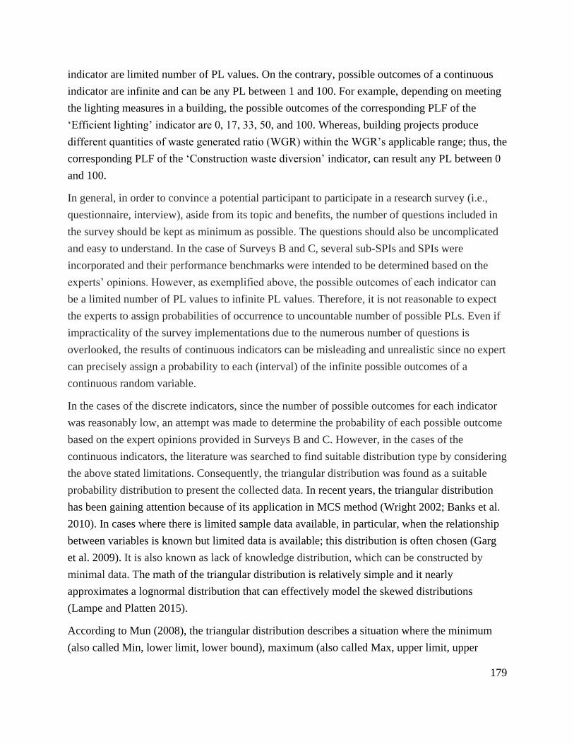
179

indicator are limited number of PL values. On the contrary, possible outcomes of a continuous

indicator are infinite and can be any PL between 1 and 100. For example, depending on meeting

the lighting measures in a building, the possible outcomes of the corresponding PLF of the

‘Efficient lighting’ indicator are 0, 17, 33, 50, and 100. Whereas, building projects produce

different quantities of waste generated ratio (WGR) within the WGR’s applicable range; thus, the

corresponding PLF of the ‘Construction waste diversion’ indicator, can result any PL between 0

and 100.

In general, in order to convince a potential participant to participate in a research survey (i.e.,

questionnaire, interview), aside from its topic and benefits, the number of questions included in

the survey should be kept as minimum as possible. The questions should also be uncomplicated

and easy to understand. In the case of Surveys B and C, several sub-SPIs and SPIs were

incorporated and their performance benchmarks were intended to be determined based on the

experts’ opinions. However, as exemplified above, the possible outcomes of each indicator can

be a limited number of PL values to infinite PL values. Therefore, it is not reasonable to expect

the experts to assign probabilities of occurrence to uncountable number of possible PLs. Even if

impracticality of the survey implementations due to the numerous number of questions is

overlooked, the results of continuous indicators can be misleading and unrealistic since no expert

can precisely assign a probability to each (interval) of the infinite possible outcomes of a

continuous random variable.

In the cases of the discrete indicators, since the number of possible outcomes for each indicator

was reasonably low, an attempt was made to determine the probability of each possible outcome

based on the expert opinions provided in Surveys B and C. However, in the cases of the

continuous indicators, the literature was searched to find suitable distribution type by considering

the above stated limitations. Consequently, the triangular distribution was found as a suitable

probability distribution to present the collected data. In recent years, the triangular distribution

has been gaining attention because of its application in MCS method (Wright 2002; Banks et al.

2010). In cases where there is limited sample data available, in particular, when the relationship

between variables is known but limited data is available; this distribution is often chosen (Garg

et al. 2009). It is also known as lack of knowledge distribution, which can be constructed by

minimal data. The math of the triangular distribution is relatively simple and it nearly

approximates a lognormal distribution that can effectively model the skewed distributions

(Lampe and Platten 2015).

According to Mun (2008), the triangular distribution describes a situation where the minimum

(also called Min, lower limit, lower bound), maximum (also called Max, upper limit, upper

180

bound), and most likely (also called Mode, likely, expected) outcomes of a random variable are

known. The Mode falls between the Min and Max values, forming a triangular-shaped

distribution, which shows that values near the minimum and maximum are less likely to occur

compared to values near the most likely value.

In this research, the Min and Max parameters in the triangular distribution are PL = 0 and PL =

100 correspond to the least and most desirable performance values of each SPI (and sub-SPI),

respectively. These lower and upper bounds have been determined in the past chapter when

establishing the PLFs of each indicator. Therefore, the only data required for construction of the

probability distribution of a continuous indicator was its most likely PL value that has been

obtained based on the experts’ feedback in Surveys B and C.

6.2.3 Establishment of Sustainability Performance Scales

As discussed before, to benchmark the performance of the subject modular building, the

sustainability indices that were developed at different levels should be compared with the

performance of similar conventional buildings at the corresponding levels. Therefore, to

facilitate such comparisons, a set of sustainability performance scales (SPSs) correspond to

different levels (Levels 3, 2, and 1) are required.

After the probability distributions of the independent sub-SPIs and SPIs were constructed, the

MCS analyses through multiple rounds were conducted to generate the probability distributions

of the corresponding parent indicators and criteria. To this end, the @Risk software as a

powerful tool for MCS analysis was used. This software is an add-in to Microsoft Excel that lets

the user to perform MCS and provides virtually all possible outcomes for a system or process

and how likely they are to occur. As explained earlier, the outputs of the MCS analyses at each

level were a set of probability distributions that represent the historical performance of

conventional buildings at that level. For example, the results of the MCS analyses at SPC level

(i.e., Level 3) were a set of probability distributions, each of which represented the (simulated)

performance of buildings with respect to a SPC.

To establish appropriate SPSs, a suitable evaluation scale should be used to divide the total range

of possible PL outcomes of each distribution (0 ≤ PL ≤ 100) into a number of common

performance categories, such as Poor to Excellent or Low to Outstanding. In this regard, the

literature with the focus on the sustainability rating systems was searched to check the existing

evaluation scales for performance evaluation of buildings. Each sustainability performance

system has its own method of scoring and evaluation scales. For example, the LEED rating

system assigns points when each of its criteria is met by an average-sized building project. The

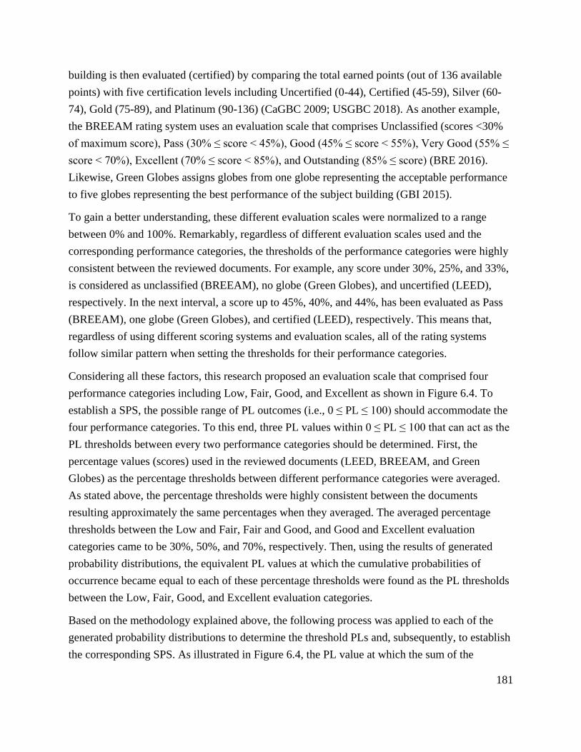
181

building is then evaluated (certified) by comparing the total earned points (out of 136 available

points) with five certification levels including Uncertified (0-44), Certified (45-59), Silver (60-

74), Gold (75-89), and Platinum (90-136) (CaGBC 2009; USGBC 2018). As another example,

the BREEAM rating system uses an evaluation scale that comprises Unclassified (scores <30%

of maximum score), Pass (30% ≤ score < 45%), Good (45% ≤ score < 55%), Very Good (55% ≤

score < 70%), Excellent (70% ≤ score < 85%), and Outstanding (85% ≤ score) (BRE 2016).

Likewise, Green Globes assigns globes from one globe representing the acceptable performance

to five globes representing the best performance of the subject building (GBI 2015).

To gain a better understanding, these different evaluation scales were normalized to a range

between 0% and 100%. Remarkably, regardless of different evaluation scales used and the

corresponding performance categories, the thresholds of the performance categories were highly

consistent between the reviewed documents. For example, any score under 30%, 25%, and 33%,

is considered as unclassified (BREEAM), no globe (Green Globes), and uncertified (LEED),

respectively. In the next interval, a score up to 45%, 40%, and 44%, has been evaluated as Pass

(BREEAM), one globe (Green Globes), and certified (LEED), respectively. This means that,

regardless of using different scoring systems and evaluation scales, all of the rating systems

follow similar pattern when setting the thresholds for their performance categories.

Considering all these factors, this research proposed an evaluation scale that comprised four

performance categories including Low, Fair, Good, and Excellent as shown in Figure 6.4. To

establish a SPS, the possible range of PL outcomes (i.e., 0 ≤ PL ≤ 100) should accommodate the

four performance categories. To this end, three PL values within 0 ≤ PL ≤ 100 that can act as the

PL thresholds between every two performance categories should be determined. First, the

percentage values (scores) used in the reviewed documents (LEED, BREEAM, and Green

Globes) as the percentage thresholds between different performance categories were averaged.

As stated above, the percentage thresholds were highly consistent between the documents

resulting approximately the same percentages when they averaged. The averaged percentage

thresholds between the Low and Fair, Fair and Good, and Good and Excellent evaluation

categories came to be 30%, 50%, and 70%, respectively. Then, using the results of generated

probability distributions, the equivalent PL values at which the cumulative probabilities of

occurrence became equal to each of these percentage thresholds were found as the PL thresholds

between the Low, Fair, Good, and Excellent evaluation categories.

Based on the methodology explained above, the following process was applied to each of the

generated probability distributions to determine the threshold PLs and, subsequently, to establish

the corresponding SPS. As illustrated in Figure 6.4, the PL value at which the sum of the

182

probabilities of occurrence for all PLs between PL = 0 and this PL, became 30% was determined

as the PL threshold between the Low and Fair performance categories. Likewise, the PL

thresholds between the Fair and Good performance categories was determined as the PL value at

which the sum of probabilities of occurrence between PL = 0 and this PL, reached 50%.

Eventually, the PL threshold between the Good and Excellent performance categories was the PL

at which the cumulative probabilities of occurrence between PL = 0 and this PL became 70%.

Low

P(PL) < 30%

0 least desirable

Fair

30% P(PL) < 50%

Good

50% P(PL) < 70%

Excellent

70% P(PL)

100 most desirable

Performance Level (PL)

? ? ?

Figure 6.4 Proposed evaluation scale and PL thresholds for performance categories

The results were a set of SPSs for each SPC (Level 3), each sustainability dimension (Level 2),

and for the overall sustainability (Level 1) that can be used to benchmark the performance of

modular buildings at different levels.

6.2.4 Development of Decision Support Framework

By establishment of the SPSs, all the planned phases in this research for environmental and

economic sustainability performance assessment of modular building were completed (see

Figure 2.1 in Chapter 2 for details). Subsequently, to facilitate a holistic life cycle sustainability

assessment process, all the research frameworks, methodologies, and deliverables, were

incorporated into a single comprehensive sustainability assessment framework. The developed

framework was proposed in the form of a multi-level decision support framework (DSF).

6.3 Sustainability Performance Scales for Environmental SPCs

As stated before, Survey C was implemented to investigate the past performance of conventional

buildings in the Okanagan (and other regions in BC with the same climate zone and construction

condition) with respect to all of environmental (and some of the economic) SPCs. The experts

assigned the most likely PL outcome of each discrete and continuous indicator included in the

survey. The data provided by the experts in each round of data collection was reviewed and

183

revised/modified by each expert in the next round until the consensus was reached on the data at

the end of the third round. This data was used to construct the probability distributions of the

independent indicators correspond to each environmental SPC.

In the case of the continuous indicators, the most likely PL values were used to construct the

corresponding triangular probability distributions. These distributions were then provided to the

participating experts in the next round for their review. In the case of the discrete indicators, as

discussed before, it was difficult for the experts to assign a probability to each and every possible

PL outcomes of the indicators. In this research, the most likely PL outcome of each discrete

indicator was used to estimates the probabilities of other possible outcomes. To this end, it was

assumed that the probability distribution of a discrete indicator follows a discrete triangular

shape. The main difference between a continuous triangular distribution and a discrete triangular

distribution is in their possible outcomes. In the former distribution, the number of PL outcomes

is infinite, whereas in the latter distribution, the number of PL outcomes is (countable) finite.

Therefore, the rough estimate of the probability of each possible outcome in a discrete indicator

can be obtained by calculating the corresponding area under the triangular curve. These rough

estimate probabilities along with the corresponding rough distribution in graphical format were

then provided to the participating experts for their feedback (revising or approving the proposed

estimated probabilities).

To obtain the probability distribution of buildings with respect to each environmental SPCs, the

methodology described earlier was followed by performing two rounds of MCS analyses. In the

first round, the constructed probability distributions of the sub-SPIs related to each SPI were fed

into the @Risk software as the input data along with their weights. A MCS analysis was

performed separately for each SPI using the software’s maximum iteration number of 100000.

Consequently, the probability distribution of each SPI was generated.

As stated earlier, in some cases, there were no sub-SPIs under a SPI; therefore, the probability

distributions of such SPIs had been constructed directly based on the survey results (similar to

sub-SPIs). Thus, the input data of the second round of analyses were a combination of the

probability distributions of SPIs generated by the first round analyses (i.e., output data) and the

probability distributions of SPIs constructed directly by the survey results. In addition, the

weights of the SPIs were entered. Eventually, by separately running the second round of the

MCS analyses, the probability distribution of each environmental SPC was produced.

As the last step, the methodology explained to establish a SPS was applied to the generated

probability distributions of the SPCs to establish the corresponding SPSs. In the following

sections, the results of the data analyses and the established SPSs for the environmental SPCs

184

have been presented.

6.3.1 SPS for Energy Performance and Efficiency Strategies

Among all the indicators determined under the EP SPC in Chapter 5, 17 indicators were

independent including 6 SPIs and 11 sub-SPIs. Therefore, according to the approach adopted in

this research, the questions regarding the past performances of conventional buildings with

regard to these independent indicators were asked from the experts. Consequently, a probability

distribution was constructed for each indicator as illustrated in Figure 6.5.

185

Figure 6.5 Probability distributions of the indicators under the EP SPC

The graphical form of the results of the Monte Carlo analyses for the EP SPC is presented in

0.0 100.0

f(X

)

PL

EP1-1-ceilings

0.0 100.0

f(X

)

PL

EP1-1-walls

0.0 100.0

f(X

)

PL

EP1-1-floor

0.00

0.20

0.40

0.60

0 50 100

Pro

bab

ility

PL

EP1-2

0.0 100.0f(

X)

PL

EP2

0.0 100.0

f(X

)

PL

EP3

0.0 100.0

f(X

)

PL

EP4-1 AC & heat pumps

0.0 100.0

f(X

)

PL

EP4-1 furnaces

0.0 100.0

f(X

)

PL

EP4-1 boilers

0.0 100.0

f(X

)

PL

EP4-2

0.00

0.20

0.40

0.60

0 50 100

Pro

bab

ility

PL

EP5

0.00

0.20

0.40

0.60

0.80

0 100

Pro

bab

ility

PL

EP6-1

0.00

0.20

0.40

0.60

0.80

0 100

Pro

bab

ility

PL

EP6-2

0.00

0.10

0.20

0.30

0.40

0.50

0 33.3 66.7 100

Pro

bab

ility

PL

EP6-3

0.00

0.10

0.20

0.30

0.40

0.50

0 25 50 100

Pro

bab

ility

PL

EP7

0.00

0.10

0.20

0.30

0 16.7 33.3 50 66.7 83.3 100

Pro

bab

ility

PL

EP8

0.00

0.20

0.40

0.60

0.80

0 100

Pro

bab

ility

PL

EP9

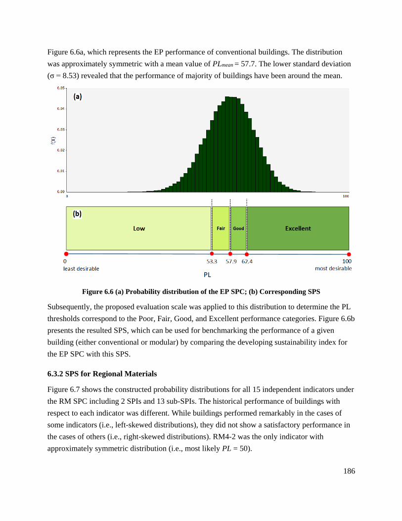
186

Figure 6.6a, which represents the EP performance of conventional buildings. The distribution

was approximately symmetric with a mean value of PLmean = 57.7. The lower standard deviation

(σ = 8.53) revealed that the performance of majority of buildings have been around the mean.

Figure 6.6 (a) Probability distribution of the EP SPC; (b) Corresponding SPS

Subsequently, the proposed evaluation scale was applied to this distribution to determine the PL

thresholds correspond to the Poor, Fair, Good, and Excellent performance categories. Figure 6.6b

presents the resulted SPS, which can be used for benchmarking the performance of a given

building (either conventional or modular) by comparing the developing sustainability index for

the EP SPC with this SPS.

6.3.2 SPS for Regional Materials

Figure 6.7 shows the constructed probability distributions for all 15 independent indicators under

the RM SPC including 2 SPIs and 13 sub-SPIs. The historical performance of buildings with

respect to each indicator was different. While buildings performed remarkably in the cases of

some indicators (i.e., left-skewed distributions), they did not show a satisfactory performance in

the cases of others (i.e., right-skewed distributions). RM4-2 was the only indicator with

approximately symmetric distribution (i.e., most likely PL = 50).

187

Figure 6.7 Probability distributions of the indicators under the RM SPC

By conducting the MCS analyses, the behavior of buildings with regard to the use of regional

materials was simulated as demonstrated in Figure 6.8a. Because there was a balance between

the number of left-skewed and right-skewed distributions of the contributing indicators, a

centrally symmetric distribution was anticipated for the generated distribution of the RM SPC.

0.0 100.0

f(X

)

PL

RM1-1

0.0 100.0

f(X

)

PL

RM1-2

0.0 100.0

f(X

)

PL

RM2-1

0.0 100.0

f(X

)

PL

RM2-2

0.0 100.0f(

X)

PL

RM3

0.0 100.0

f(X

)

PL

RM4-1

0.0 100.0

f(X

)

PL

RM4-2

0.0 100.0

f(X

)

PL

RM5

0.0 100.0

f(X

)

PL

RM6-1

0.0 100.0

f(X

)

PL

RM6-2

0.0 100.0

f(X

)

PL

RM7-1

0.0 100.0

f(X

)

PL

RM7-2

0.0 100.0

f(X

)

PL

RM8-1

0.0 100.0

f(X

)

PL

RM8-2

0.0 100.0

f(X

)

PL

RM8-3

188

Figure 6.8 (a) Probability distribution of the RM SPC; (b) Corresponding SPS

By applying the proposed evaluation scale, the corresponding SPS for this SPC was established

as shown in Figure 6.8b. The lower standard deviation of σ = 5.9 indicated that the RM

performance of most of the buildings in BC have been around the mean.

6.3.3 SPS for Construction Waste Management

The CWM SPC included two SPIs, one of them was independent and the other one consisted of

two sub-SPIs. The constructed probability distributions for the independent indicators were

constructed based on the experts’ opinions as exhibited in Figure 6.9.

Figure 6.9 Probability distributions of the indicators under the CWM SPC

Figure 6.10 shows the historical behaviour of conventional buildings in terms of waste

0.00

0.15

0.30

0.45

0 50 100

Pro

bab

ility

PL

CWM1-1

0.00

0.05

0.10

0.15

0.20

0.25

0 16.7 33.3 50 66.7 83.3 100

Pro

bab

ility

PL

CWM1-2

0.0 100.0

f(X

)

PL

CWM2

189

management as well as the corresponding SPS.

Figure 6.10 (a) Probability distribution of the CWM SPC; (b) Corresponding SPS

Through the first round of simulation analyses, the probability distribution of the dependent SPI

(CWM1) was obtained. Then, through the second round, the probability distribution of the parent

CWM SPC was generated by combing the distributions of the two SPIs (Figure 6.10a). The

resulted distribution was approximately a normal distribution. Dissimilar to the distribution for

the RM SPI, higher standard deviation in this distribution (σ = 15.6) indicated that the single-

family building projects performed differently in terms of waste management by covering all the

possible PLs. This was also confirmed by the developed SPS (Figure 6.10b) where the PL

intervals associated with the central performance categories (i.e., Fair and Good) were wider

compared to the cases of EP and RM SPCs above.

6.3.4 SPS for Renewable and Environmentally Preferable Products

As demonstrated in Figure 6.11, all the probability distributions of all 15 independent indicators

under the REP SPC were right-skewed (i.e., the most likely PL < 50). This indicated the limited

application of renewable and environmentally friendly materials (e.g., recycled materials) in

different components of single-family buildings. According to the experts in this research, most

of the building projects in BC still utilize fewer environmentally responsible materials such as

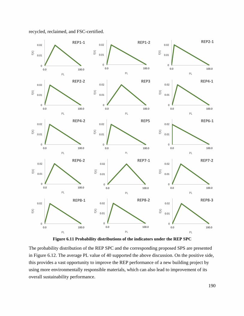
190

recycled, reclaimed, and FSC-certified.

Figure 6.11 Probability distributions of the indicators under the REP SPC

The probability distribution of the REP SPC and the corresponding proposed SPS are presented

in Figure 6.12. The average PL value of 40 supported the above discussion. On the positive side,

this provides a vast opportunity to improve the REP performance of a new building project by

using more environmentally responsible materials, which can also lead to improvement of its

overall sustainability performance.

0.0 100.0

f(X

)

PL

REP1-1

0.0 100.0

f(X

)

PL

REP1-2

0.0 100.0

f(X

)

PL

REP2-1

0.0 100.0

f(X

)

PL

REP2-2

0.0 100.0

f(X

)

PL

REP3

0.0 100.0

f(X

)

PL

REP4-1

0.0 100.0

f(X

)

PL

REP4-2

0.0 100.0

f(X

)

PL

REP5

0.0 100.0

f(X

)

PL

REP6-1

0.0 100.0

f(X

)

PL

REP6-2

0.0 100.0

f(X

)

PL

REP7-1

0.0 100.0

f(X

)

PL

REP7-2

0.0 100.0

f(X

)

PL

REP8-1

0.0 100.0

f(X

)

PL

REP8-2

0.0 100.0

f(X

)

PL

REP8-3

191

Figure 6.12 (a) Probability distribution of the REP SPC; (b) Corresponding SPS

As illustrated in the proposed SPS (Figure 6.12b), if a building’s sustainability index for this

SPC reaches as low as PL = 36.9, it will show moderate performance which can quickly reach

the Good performance and even Excellent performance by a small improvement in its

performance. This is remarkable especially when comparing this SPS with the SPSs proposed for

some other SPCs. For example, the PL threshold between the Good and Excellent performance

categories (PL = 43.1) for the REP SPC, was even less than the PL threshold between the Poor

and Fair performance categories for the RM SPC (PL = 50.6).

6.3.5 SPS for Site Disruption and Appropriate Strategies

The SD SPC is one the environmental SPCs that its independent indicators are mostly discrete

meaning that the number of possible PL outcomes is finite (countable). Figure 6.13 shows the

constructed probability distributions for the nine indicators under this SPC. It can be observed

fro the distributions that the performances of single-family buildings projects on the project site

with respect to different aspects of ‘site disruption’ have not followed the same trend. In the

cases of some indicators, such as SD2-2 and SD4-2, buildings historically showed better

performance compared to some other indicators such as SD3.

192

Figure 6.13 Probability distributions of the indicators under the SD SPC

Figure 6.14a illustrates the performance of buildings with respect to the SD SPC. The

distribution is a centrally symmetric distribution (PLmean = 49.9) with a relatively high standard

deviation. The proposed SPS for benchmarking the SD performance of a building (either

conventional or modular) is presented in Figure 6.14b.

0.00

0.10

0.20

0.30

0.40

0.50

0 50 100

Pro

bab

ility

PL

SD1

0.00

0.10

0.20

0.30

0 25 50 75 100

Pro

bab

ility

PL

SD2-1

0.0 100.0

f(X

)

PL

SD2-2

0.0 100.0

f(X

)

PL

SD2-3

0.00

0.20

0.40

0.60

0.80

0 100P

rob

abili

ty

PL

SD3

0.0 100.0

f(X

)

PL

SD4-1

0.00

0.20

0.40

0.60

0.80

0 100

Pro

bab

ility

PL

SD4-2

0.00

0.10

0.20

0.30

0 25 50 75 100

Pro

bab

ility

PL

SD4-3

0.00

0.10

0.20

0.30

0 25 50 75 100

Pro

bab

ility

PL

SD5

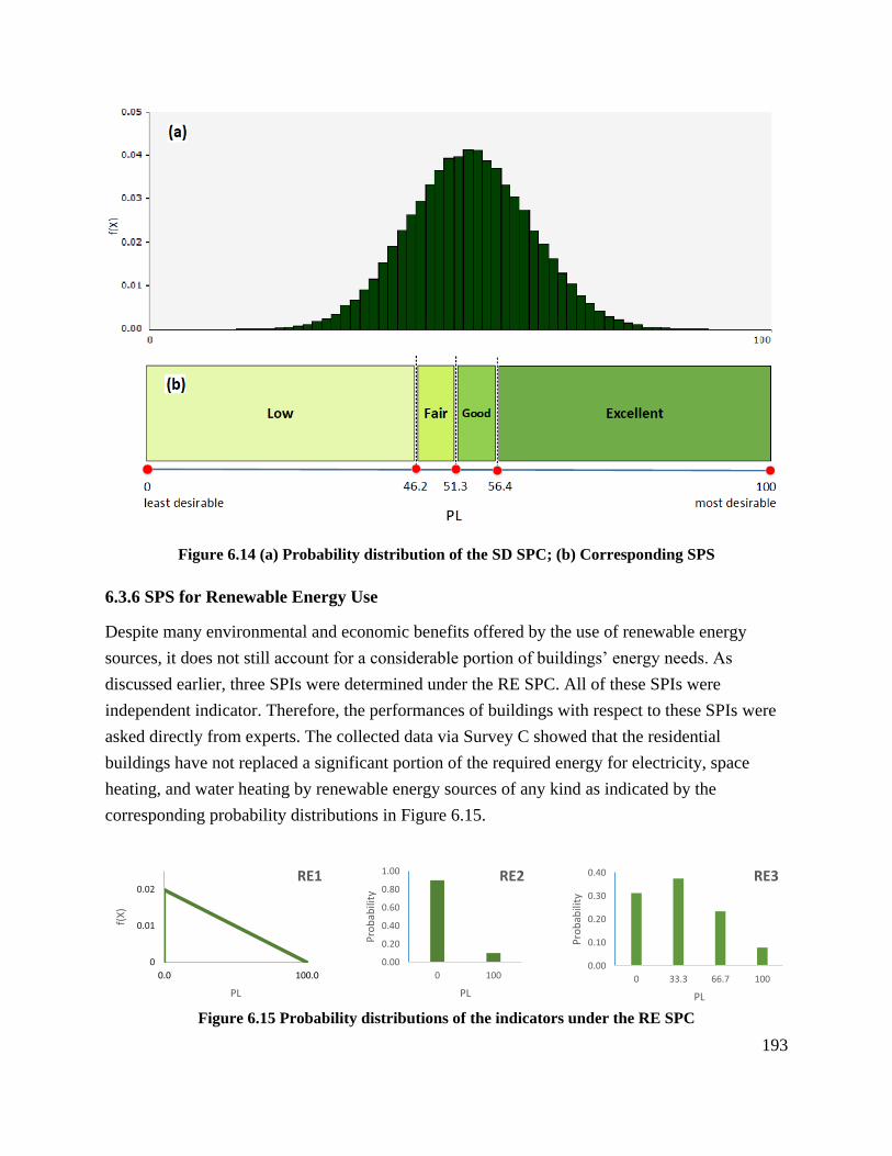
193

Figure 6.14 (a) Probability distribution of the SD SPC; (b) Corresponding SPS

6.3.6 SPS for Renewable Energy Use

Despite many environmental and economic benefits offered by the use of renewable energy

sources, it does not still account for a considerable portion of buildings’ energy needs. As

discussed earlier, three SPIs were determined under the RE SPC. All of these SPIs were

independent indicator. Therefore, the performances of buildings with respect to these SPIs were

asked directly from experts. The collected data via Survey C showed that the residential

buildings have not replaced a significant portion of the required energy for electricity, space

heating, and water heating by renewable energy sources of any kind as indicated by the

corresponding probability distributions in Figure 6.15.

Figure 6.15 Probability distributions of the indicators under the RE SPC

0.0 100.0

f(X

)

PL

RE1

0.00

0.20

0.40

0.60

0.80

1.00

0 100

Pro

bab

ility

PL

RE2

0.00

0.10

0.20

0.30

0.40

0 33.3 66.7 100

Pro

bab

ility

PL

RE3

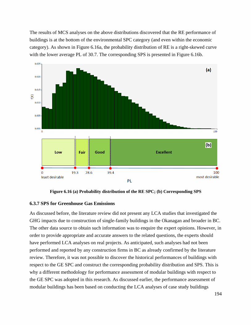
194

The results of MCS analyses on the above distributions discovered that the RE performance of

buildings is at the bottom of the environmental SPC category (and even within the economic

category). As shown in Figure 6.16a, the probability distribution of RE is a right-skewed curve

with the lower average PL of 30.7. The corresponding SPS is presented in Figure 6.16b.

Figure 6.16 (a) Probability distribution of the RE SPC; (b) Corresponding SPS

6.3.7 SPS for Greenhouse Gas Emissions

As discussed before, the literature review did not present any LCA studies that investigated the

GHG impacts due to construction of single-family buildings in the Okanagan and broader in BC.

The other data source to obtain such information was to enquire the expert opinions. However, in

order to provide appropriate and accurate answers to the related questions, the experts should

have performed LCA analyses on real projects. As anticipated, such analyses had not been

performed and reported by any construction firms in BC as already confirmed by the literature

review. Therefore, it was not possible to discover the historical performances of buildings with

respect to the GE SPC and construct the corresponding probability distribution and SPS. This is

why a different methodology for performance assessment of modular buildings with respect to

the GE SPC was adopted in this research. As discussed earlier, the performance assessment of

modular buildings has been based on conducting the LCA analyses of case study buildings

195

(including modular and conventional), developing a set of environmental impact indices, and

comparing these indices between these buildings. In other words, the environmental impacts due

to construction of a modular building is compared with the environmental impacts due to

construction of other similar modular and conventional buildings. This method of benchmarking

is called ‘review benchmarking’ method (Stapenhurst 2009). In contrast, in the cases of all other

SPCs, the performance of a modular building has been evaluated by comparing the developed

sustainability indices with the established SPSs (i.e., the historical performance of similar

conventional buildings).

The details of the data collection process for LCA studies to address the GE SPC have been

described in Chapter 7 where the case study analyses were performed.

6.4 Sustainability Performance Scales for Economic SPCs

Similar to the environmental SPCs, the experts’ feedback was used for construction of suitable

probability distributions of the independent indicators under the economic SPCs. As stated

before, some of the economic SPCs are more and some are less locality sensitive criteria.

Therefore, the data related to the performance of buildings with respect to the indicators

associated with the former SPCs and latter SPCs was collected separately using Survey B and

Survey C, respectively.

The same methodology followed to conduct the MCS analyses, develop the probability

distributions, and establish SPSs for the environmental SPCs was used in the case of the

economic SPCs. Therefore, the detailed descriptions of the methodology are not repeated in this

section and only the results are presented and discussed.

6.4.1 SPS for Integrated Management

The IM SPC included three SPIs each of them consisted of a number of sub-SPIs. Therefore, the

independent indicators were only the sub-SPIs for which the data of the historical performance of

single-family buildings was collected and the corresponding probability distributions were

constructed. Because all sub-SPIs are discrete variables, the values on the y-axis of the

probability distributions of a sub-SPI indicates the probabilities of its possible PL outcomes

(Figure 6.17).

196

Figure 6.17 Probability distributions of the indicators under the IM SPC

Figure 6.18a illustrates the results of the final round of the simulation analyses for the probability

distribution of the performance of buildings related to the IM SPC. The distribution is

approximately normal and centralized (PLmean = 45.9). Using the proposed evaluation scale

discussed in the methodology section, the PL threshold values for different evaluation categories

were determined and the SPS for benchmarking the IM performance of buildings was established

(Figure 6.18b).

0.00

0.10

0.20

0.30

0.40

0 25 50 75 100

Pro

bab

ility

PL

IM1-1

0.00

0.10

0.20

0.30

0 16.7 33.3 50 66.7 83.3 100

Pro

bab

ility

PL

IM1-2

0.00

0.15

0.30

0.45

0 33.3 66.7 100

Pro

bab

ility

PL

IM1-3

0.00

0.10

0.20

0.30

0.40

0 25 50 75 100

Pro

bab

ility

PL

IM2-1

0.00

0.10

0.20

0.30

0 20 40 60 80 100P

rob

abili

ty

PL

IM2-2

0.00

0.10

0.20

0.30

0.40

0.50

0 50 100

Pro

bab

ility

PL

IM3-1

0.00

0.05

0.10

0.15

0.20

0

12

.5 25

37

.5 50

62

.5 75

87

.5

10

0

Pro

bab

ility

PL

IM3-2

0.00

0.05

0.10

0.15

0.200

10

20

30

40

50

60

70

80

90

10

0

Pro

bab

ility

PL

IM3-3

197

Figure 6.18 (a) Probability distribution of the IM SPC; (b) Corresponding SPS

6.4.2 SPS for Durability of Building

The durability feature in a building can offer both environmental and economic advantages. The

environmental benefit of durability is mainly the less demand for repairs and renovation of

existing buildings and also construction of new buildings which result in resource efficiency.

However, as stated before, resource efficiency has already been considered within the

environmental SPCs. Therefore, the DB SPC was included under the economic category to

address the economic benefit of durability. The past performance of single-family buildings with

regard to durability indicators have been demonstrated in Figure 6.19.

198

Figure 6.19 Probability distributions of the indicators under the DB SPC

A few rounds of MCS analyses were performed by using the above distributions as the input of

analyses to discover the historical performance of buildings in terms of durability (Figure 6.20a).

Because all the contributing indicators have been discrete variables, the number of possible PL

outcomes of the parent DB SPC was also finite. This is why not all the PLs between 0 and 100

have been among the possible outcomes of this SPC as shown in Figure 6.20a.

0.00

0.15

0.30

0.45

0 50 100

Pro

bab

ility

PL

DB1-1

0.00

0.20

0.40

0.60

0 50 100

Pro

bab

ility

PL

DB1-2

0.00

0.20

0.40

0.60

0 50 100

Pro

bab

ility

PL

DB1-3

0.00

0.10

0.20

0.30

0.40

0 25 50 75 100

Pro

bab

ility

PL

DB2

0.00

0.15

0.30

0.45

0 33.3 66.7 100P

rob

abili

tyPL

DB3-1

0.00

0.10

0.20

0.30

0 25 50 75 100

Pro

bab

ility

PL

DB3-2

0.00

0.05

0.10

0.15

0.20

0

12

.5 25

37

.5 50

62

.5 75

87

.5

10

0

Pro

bab

ility

PL

DB4-1

0.00

0.10

0.20

0.30

0.40

0 33.3 66.7 100

Pro

bab

ility

PL

DB4-2

199

Figure 6.20 (a) Probability distribution of the DB SPC; (b) Corresponding SPS

Figure 6.20b presents the developed SPS for this SPC. It can be observed that the Fair

performance category started at PL = 50, which is a relatively high threshold. This means that

majority of the single-family conventional buildings in BC have considered and implemented

suitable durability strategies in the design stage such that the PL of the DB SPC for a new

building design should be at least 50 in order for the building to perform Fair.

6.4.3 SPS for Adaptability of Building

As discussed in Chapter 5, adaptability of buildings, in particular residential low-rise buildings,

is one of the criteria that has not been widely addressed in the literature. In an attempt to

investigate the adaptability performance of single-family buildings and establish the

corresponding benchmarks, this research determined three relevant SPIs, which can serve as a

basis for future research. Similar to the IM SPC above, all the SPIs and sub-SPIs under the AB

SPC are discrete; therefore, the corresponding probability distributions are discrete. The

constructed probability distributions for the independent indicators are illustrated in Figure 6.21.

From these distributions, it can be concluded that the single-family buildings in BC have not

shown a high level of adaptability. This was anticipated because (1) adaptability requires

additional costs in the design and construction of buildings; (2) the necessity and benefits of

200

adaptability that can offset the extra costs have not still been documented and well understood. It

should also be stressed that, not all the building projects, in particular residential buildings,

require high level of adaptability. However, this is an additional economic value if a building has

be prepared to accommodate future changes that can be either the users’ needs or technological

changes.

Figure 6.21 Probability distributions of the indicators under the AB SPC

The performance of single-family buildings with respect to the IM SPC has been simulated by

combining the probability distributions of the associated SPIs as shown in Figure 6.22a. This is a

right-skewed distribution that indicates lower performance of buildings with respect to

adaptability compared to the above-discussed economic SPCs. This can also be concluded from

the developed SPS for this SPC (Figure 6.22b). However, on the positive side, a new building

(either modular or conventional) can show higher AB performance easier that other SPCs by

incorporating a number of adaptability measures discussed before into its design. As

demonstrated in the established SPS, the PL threshold between the Low and Fair was as low as

PL = 32.5. Even a PL value close to 50 (PL = 47.8) represents the Excellent adaptability

performance of a building.

0.00

0.05

0.10

0.15

0.20

0 12.5 25 37.5 50 62.5 75 87.5 100

Pro

bab

ility

PL

AB1-1

0.00

0.10

0.20

0.30

0 12.5 25 37.5 50 62.5 75 87.5 100

Pro

bab

ility

PL

AB1-2

0.00

0.05

0.10

0.15

0.20

0 10 20 30 40 50 60 70 80 90 100

Pro

bab

ility

PL

AB2

0.00

0.20

0.40

0.60

0 33.3 66.7 100

Pro

bab

ility

PL

AB3

201

Figure 6.22 (a) Probability distribution of AB SPC; (b) Corresponding SPS

6.4.4 SPS for Design and Construction Time

Unlike to the IM, DB, and AB SPCs, the remaining economic SPCs in this research, i.e., DCT,

DCC, OC, MC, and IRR, are highly sensitive to the local construction conditions. Hence, the

data related to the historical performances of buildings with respect to these SPCs was collected

based on local experts in the Okanagan, BC (Survey B). The results of data analyses have been

provided in the following sections.

As reported in Chapter 4, the duration of a building project was located on top of the economic

criteria by the construction practitioners, which indicated the vital role of the DCT SPC in the

economy of the project (i.e., time is money). Using the collected information, the triangular

distributions of the design time (DCT1) and the construction time (DCT2) were produced as

illustrated in Figure 6.23. The distribution of the DCT1 SPI shows that most of the single-family

buildings have been designed longer than the average applicable time range (i.e., most likely

PLDCT1 < 50). On the contrary, the buildings showed better performance in terms of the

construction duration (i.e., most likely PLDCT2 > 50).

202

Figure 6.23 Probability distributions of the indicators under the DCT SPC

Figure 6.24a shows the probability distribution of the DCT SPC. It should be mentioned that,

although the distributions of the contributing SPIs were symmetrically balanced (one is right-

skewed and the other is left-skewed), the resulted distribution for the parent SPC was not

symmetric. This was because of the difference in the applied weights for the DCT1 and DCT2

when performing MCS analyses, which was significantly higher for DCT2. For example, a

simple mistake in any of the construction activities can delay the project comparable with the

total design time.

The proposed SPS for this SPC is presented in Figure 6.24b. Compared to the previously

discussed SPCs, the PL threshold values for different performance categories have moved ahead.

This means that the conventional building projects in the Okanagan, performed relatively fast in

terms of the design and construction duration. Therefore, a new building project should be on

time enough to be evaluated Good or Excellent. In addition, because of higher standard deviation

in the probability distribution of the SPC, each of the performance categories included a wider

range of possible PLs.

0.00 100.00

f(X

)

PL

DCT1

0.00 100.00

f(X

)

PL

DCT2

203

Figure 6.24 (a) Probability distribution of the DCT SPC; (b) Corresponding SPS

6.4.5 SPS for Design and Construction Costs

Similar to the duration of building projects, the costs associated with the design and construction

phase can contribute significantly to the projects’ economy. As reported earlier, the DCC ranked

second within the economic SPC category. Based on the participating experts’ opinions (Survey

B), the cost performances of single-family building projects in the Okanagan have been

identified and translated into suitable probability distributions for the DCC1 and DCC2 SPIs

(Figure 6.25). From these distributions, it can be observed that majority of the building projects

have been designed with the cost close to the average design cost. However, the construction

cost for most of the projects has been cheaper than the average cost.

Figure 6.25 Probability distributions of the indicators under the DCC SPC

0.00 100.00

f(X

)

PL

DCC1

0.00 100.00

f(X

)

PL

DCC2

204

Aggregation of the above distributions resulted in the distribution of the parent DCC as presented

in Figure 6.26a. This distribution is left-skewed indicating high performance of buildings in

terms of overall design and construction costs. Using this distribution and the proposed

evaluation scale discussed in the methodology section, the corresponding SPS was established

(Figure 6.26b). The SPS shows relatively higher PL thresholds for the performance categories.

For example, in order for a project to perform excellent, its performance should be at least PL =

67.5 which is a high threshold compared to all Excellent thresholds in other SPSs.

Figure 6.26 (a) Probability distribution of the DCC SPC; (b) Corresponding SPS

6.4.6 SPS for Operational Costs

As mentioned in Chapter 5, this SPC comprised only one SPI, which is the running costs (OC1).

Therefore, the performance of buildings with respect to operational costs was determined based

of their performance with respect to running costs. The results of the survey in the form of the

probability distribution is presented in Figure 6.27a. The OC distribution is slightly left-skewed

indicating that operational costs in many of the single-family buildings in the Okanagan have

been less than the average costs (i.e., most likely PLOC > 50). The corresponding SPS for

benchmarking the new building projects has been presented in Figure 6.27b.

205

Figure 6.27 (a) Probability distribution of the OC SPC; (b) Corresponding SPS

6.4.7 SPS for Maintenance Costs

Similar to the OC SPC, the MC SPC consisted of only one SPI (MC1). Thus, the probability

distribution of MC followed the same as the probability distribution of the MC1 SPI (i.e., repair

and replacement costs) as illustrated in Figure 6.28a. It can be observed from the constructed

distribution that the performance of buildings in the Okanagan with respect to maintenance costs

follow a symmetric pattern (PLmean = 50.4).

The corresponding SPS for benchmarking the MC performance of a building was established and

presented in Figure 6.28b. Comparison of the SPSs proposed for the OC and MC SPCs revealed

that the PL thresholds for different performance category in the latter SPS were marginally less

than the corresponding PL thresholds in the former SPS. This is because, according to the

experts, single-family buildings showed slightly higher performances in terms of the operational

costs.

206

Figure 6.28 (a) Probability distribution of the MC SPC; (b) Corresponding SPS

6.4.8 SPS for Investment and Related Risks

In addition to the OC and MC SPC, the IRR SPC also comprised one SPI, i.e., IRR1. Therefore,

the probability distribution of this SPC was the same as its single SPI. As detailed in Chapter 5,

the PLF for the IRR1 SPI included three data variables. The number of data variables of different

PLFs is not important; however, it is important to note that each of these three data variables in

the PLF of the IRR1 SPI has itself been a SPI. In other words, these SPIs now play the roles of

data variables in the PLF of IRR1. According to Chapter 5, the three data variables of this SPI

were DCC1, DCC2, and SP. DCC1and DCC2 have been the SPIs under the ‘design and

construction (DCC)’ SPC. In addition, SP is the sale price of the finished single-family

buildings. The probability distributions of DCC1 and DCC2 have been constructed and presented

earlier in the related section (see Figure 6.25). Similarly, the probability distribution for SP was

constructed based on the experts’ opinions. This distribution along with the repetition of the

distributions of DCC1 and DCC2 are shown in Figure 6.29.

207

Figure 6.29 Probability distributions of the indicators under the IRR SPC

These distributions were fed into the simulation software as the input data to generate the

distribution of the IRR SPC as presented in Figure 6.30a. The resulted distribution was a

centralized symmetric distribution.

Figure 6.30 (a) Probability distribution of the IRR SPC; (b) Corresponding SPS

0.00 100.00

f(X

)

PL

DCC1

0.00 100.00

f(X

)

PL

DCC2

0.00 100.00

f(X

)

PL

SP

208

Using the proposed evaluation scale, a SPS for benchmarking the performances of single-family

buildings with respect to profitability of the project was established (Figure 6.30b). The SPS was

an approximately symmetric scale as anticipated from the probability distribution of IRR. For

example, the upper limit for the Low performance category (PL = 43) and the lower limit for the

Excellent performance category (PL = 58.5) were nearly symmetric.

6.5 Sustainability Performance Scales for Sustainability Dimensions

In the previous sections, the historical performances of single-family buildings in BC (with the

focus on the Okanagan) with regard to each environmental and economic SPC were explored and

the corresponding SPSs were established for performance benchmarking at Level 3 (i.e., SPC

level). In the present section, similar methodology was used to identify the past performance of

these buildings with respect to each of the environmental and economic dimensions and establish

the corresponding SPSs at Level 2. To this end, the probability distributions of the SPCs along

with their importance weights were combined by performing the MCS analyses to produce the

probability distributions of the environmental and economic performances of buildings.

Figure 6.31a exhibits the historical environmental performances of the BC single-family

buildings. The mean of the generated distribution is approximately a centrally symmetric

distribution (PLmean = 48.6). Furthermore, the smaller standard deviation of σ = 4.8 highlighted

the fact that majority of the buildings performed closer to the mean and fewer buildings

performed very low or very high.

The proposed evaluation scale was applied on the probability distribution of the environmental

performance to determine the PL thresholds for different evaluation categories (Poor, Fair, Good,

and Excellent) and establish the corresponding SPS as shown in Figure 6.31b. As stated above,

majority of the buildings showed Fair and Good environmental performance. This pointed to the

fact that meeting the environmental strategies/measures discussed within different indicators

under the environmental SPCs was easy up to the PL values close to mean. However, it was

difficult for the building project to address strategies/measures such that their performance level

go beyond the mean.

209

Figure 6.31 (a) Probability distribution of the historical environmental performance of buildings;

(b) Corresponding SPS

The probability distribution of the performance of buildings with respect to the economic

dimension of sustainability is demonstrated in Figure 6.32a. Similar trend to that of the

environmental performance can be seen in the case of the economic performance. However, the

mean was slightly higher than the mean of the environmental performance which indicated a

marginally better average performance. Nevertheless, the higher standard deviation of 6.7

pointed out that although the PLmean for the economic performance is bigger than that of the

environmental performance, there are more variations in the PL of different buildings with

respect to the economic performance. This is the main reason why in the established SPS, the PL

intervals associated with the Fair and Good performance categories are wider compared to the

corresponding PL intervals in the environmental SPS (Figure 6.32b).

210

Figure 6.32 (a) Probability distribution of the historical economic performance of buildings; (b)

Corresponding SPS

In general, the PL threshold to present a moderate performance was not a small value in both the

environmental and economic (59.9 and 47.5, respectively). However, this does not mean that

reaching such PL values in a building is difficult since the historical performances of existing

buildings showed. It is also worth to state that due to narrow intervals of the Fair and Good

evaluation categories, slightly improvement of the underperforming SPIs and sub-SPIs in the

designs and construction of new building can enhance the overall environmental and economic

performance levels to Excellent level. However, this might not be easy to implement and also

can be cost effective as highlighted by the generated probability distributions.

6.6 Sustainability Performance Scale for Overall Sustainability

The overall life cycle sustainability performance of single-family buildings can be explored

211

using the corresponding environmental and economic performances. In this regard, using the

same MCS method, the probability distributions of the environmental and economic dimensions

combined to explore the overall sustainability performance of single-family buildings in BC.

Figure 6.33a illustrates the results of the simulation analyses for the overall sustainability. This

centrally symmetric distribution (PLmean = 49.9) highlighted the fact that, on average, half of the

available PLs for overall sustainability has been met by the buildings. In addition, the standard

deviation of σ = 4.1 shows that the PL of the majority of buildings have been around the mean.

Figure 6.33b presents the established SPS for benchmarking the overall sustainability (Level 1).

Because the probability distribution is centrally symmetric, the mean PL value and the PL

threshold between the Fair and the Good performance categories were coincident. To benchmark

the overall sustainability performance of a building, the overall sustainability index (OVERALLi)

should be calculated (see Chapter 5) and compared to the performance categories in the proposed

SPS. Consequently, to improve the sustainability performance, the contributing factors, such as

underperforming SPCs, should be improved identified and improved.

Figure 6.33 (a) Probability distribution of the overall sustainability performance of buildings; (b)

Corresponding SPS

212

6.7 Proposed Decision Support Framework

The primary objective of this research is to develop a decision-support framework for

sustainability performance assessment of residential modular buildings based on the life cycle

thinking approach. In this research, this was accomplished by incorporating the developed

frameworks, methodologies, and deliverables, resulted from all the previous phases of the

research into a single comprehensive sustainability assessment framework. The resulted

framework is in the form of a multi-level decision support framework (DSF) as presented in

Figure 6.34.

The proposed DSF comprises a bottom-up quantification approach and a top-bottom assessment

approach. The quantification process starts at calculation of the most independent indicators (i.e.,

sub-SPIs) and continues up to calculation of the most dependent level, i.e., the overall

sustainability index, for the subject building. On the contrary, the assessment process starts at the

highest level, i.e., the overall sustainability, and continues down to benchmark the performance

of the subject building at lower levels.

It should be stressed that it is not necessary to follow all the components of the proposed DSF

and evaluate the sustainability performance of the subject building at all levels. Nevertheless, the

user or decision maker (DM) might decide to choose a specific level and focus on that.

Therefore, it is only required to follow and implement the corresponding components. For

example, the DM wants to benchmark only the energy performance of the subject building.

Consequently, only the data required for quantification of the indicators under the EP SPC

should be collected to develop the sustainability index for this SPC (i.e., EPi) and evaluate it

using the corresponding sustainability performance scale (SPS).

213

Collect the required data to calculate sub-SPIs and SPIs

Calculate the PLs of sub-SPIs and SPIs using the associated PLFs

Develop sustainability indices at Level 3, Levels 2, & Level1 using MCDA

Performance assessment at Level 1:

compare OVERALLi with corresponding SPS

Is the overall sustainability performance of

building within the DM s desirable level?

Yes

No


compare ENVRi and ECONi with corresponding SPSs

Are both environmental and economic

sustainability performances of building within the

DM s desirable level?

Yes

No


compare EPi, CWMi, DCCi, with corresponding SPSs

Are all the SPCs performances within the

DM s desirable level?

Yes

Th

e su

stai

nab

ilit

y p

erf

orm

ance

of

the

subje

ct m

odu

lar

bu

ildin

g i

s w

ithin

the

des

ired

lev

el

Acti

on

s ar

e r

equir

ed t

o im

pro

ve

the

sust

ainabil

ity p

erfo

rman

ce o

f th

e su

bje

ct m

odu

lar

bu

ildin

g

Yes but overall

sustainability improvement

is desired

Desired sustainability performance objectives are achieved for the building

END

Yes but sustainability

improvement of Envr/Econ

is desired

Yes but sustainability

improvement of SPC(s)

is desired

No

Check indicators

Figure 6.34 Proposed DSF for life cycle sustainability assessment of residential modular buildings

214

6.7.1 Quantification Process

The quantification process commences by collecting the data of the subject modular building

project that is required to calculate all the indicators (i.e., SPIs and sub-SPIs) associated with the

selected environmental and economic SPCs. Each sub-SPI and SPI is then calculated and

presented in a performance level (PL) between 0 and 100 using the established performance level

function (PLF).

As soon as the indicators are calculated, the next step is to combine the PLs of the indicators and

their relative importance weights using a suitable aggregation process (TOPSIS MCDA method)

which results in development of a sustainability index for each SPC (Level 3), i.e., EPi, CWMi,

DCCi, and so forth. The same aggregation process is used to combine the sustainability indices

of the SPCs and their weights to develop sustainability indices for environmental and economic

sustainability dimensions (Level 2), i.e., ENVRi and ECONi. Similarly, the overall sustainability

index, i.e., OVERALLi, is developed by combining ENVRi and ECONi and the weights of the

environmental and economic dimensions (Level 1).

6.7.2 Assessment Process

In the assessment process, the performance of the subject building is benchmarked. The process

commences at the overall sustainability level (Level 1) by comparing the corresponding

sustainability index (i.e., OVERALLi) with the established SPS for this level. If the performance

falls within the performance category that the DM desires, the assessment process is completed.

However, if the performance is lower than the desired level, or if it is desirable but the DM still

wishes to investigate the contributing criteria to further improve the overall sustainability

performance of the building, the assessment process continues by moving to the next level

(Level 2). At this level, the performance of the subject building with respect to the environmental

and economic sustainability dimensions is benchmarked by comparing the developed

sustainability indices (i.e., ENVRi and ECONi) with the corresponding SPSs. Consequently, the

underperforming sustainability dimensions that caused the overall sustainability performance of

the building to be lower than the DM’s desired level are investigated. This can be due to low

performance of the building with respect to both or one of the sustainability dimensions. Even if

the latter occurs, the DM might also want to improve the performance of the building with

respect to both sustainability dimensions. Therefore, the assessment process shifts to Level 3

where the low performing SPCs are identified by comparing the sustainability indices with the

corresponding SPSs. To improve each underperforming SPC, the associated SPIs and sub-SPIs

are investigated. Finally, appropriate decisions are made to improve the low performing

indicators.

215

It should be mentioned that, the quantification and assessment processes of the proposed DSF

have been explained above by assuming that a modular building design is under study to identify

its performance levels at different levels and to recognize the underperforming areas that need

improvements. However, if no changes can be made in the design and construction of the

building, the described processes can be still useful. This is because identification of the low and

high performing areas of the subject modular building can assist with improvement of the

sustainability of similar modular projects in the future by considering suitable design and

construction features. In addition, identification of the high performing areas can help the DM to

avoid unnecessary investments on such areas, and instead, to allocate costs to improve the

performances of underperforming areas. Furthermore, the proposed DSF can also be used for

comparisons of two or more buildings that are to be constructed by either modular or

conventional methods. The results can assists with selection of the most sustainable construction

options.

In general, it is recommended that decision makers, first, define their preferences and limitations,

such as sustainability performance desired levels, priority sustainability dimension, cost

constraints, time constraints, technological constraints, and so forth, before starting the

assessment process. By defining the preferences and limitations in advance, the results of the

sustainability performance benchmarking by the proposed DSF can assist with informed decision

options.

6.8 Summary

In order to performance benchmarking a modular building, the developed sustainability indices

at different levels (Chapter 5) should be compared to the corresponding benchmarks. Therefore,

in the first part of this chapter, suitable sustainability performance scales (SPSs) were established

at the corresponding levels. In this regards, three surveys were conducted to capture experts’

opinions on the performances of the single-family buildings with respect to the independent

indicators under each SPC. Subsequently, using the collected data, suitable probability

distributions were constructed for these indicators. Then, these distributions were used as the

inputs of the MCS to generate the probability distributions of the SPCs. Similar analyses were

performed to generate the distributions of the sustainability dimensions and the overall

sustainability. Subsequently, a suitable evaluation scale was chosen based on the literature

review and applied to each of the produced distributions. Finally, the SPSs were established at

different levels (SPCs, sustainability dimensions, and overall sustainability) each of which

included four evaluation categories: Poor, Fair, Good, and Excellent. The developed

sustainability indices can be benchmarked at each of the three levels using the corresponding

216

SPSs.

In the second part of Chapter 6, all the frameworks, methodologies, and deliverables of the

research were incorporated into a single framework as a comprehensive decision support

framework (DSF) for sustainability assessment of residential modular buildings. The proposed

DSF can assist with exploration and improvement of the low sustainability performing areas over

the life cycle of a new modular building design. It can also assists with making informed

decisions on selection of the best method of construction (modular vs. conventional).

217

Chapter 7 Validation of the Integrated Sustainability Assessment Framework

A part of this chapter is under review in:

- Energy and Buildings entitled “Comparing environmental impacts of different construction

methods: Cradle-to-gate LCA for residential buildings in BC, Canada” (Kamali et al. 2019e).

In this chapter, the proposed multi-level decision support framework (DSF) are validated using

case study of modular buildings in British Columbia, Canada.

7.1 Background

In Chapter 6, all the deliverables of this research were merged into an integrated sustainability

assessment framework as a multi-level decision support framework (DSF). In the present

chapter, application of the proposed DSF was illustrated with two case study modular buildings

designed and constructed in the Okanagan, BC, Canada.

As mentioned previously, the proposed DSF can be used in different ways. In other words,

depending on the scope and aim of a study, the user or decision maker (DM) can select to assess

the performance of the subject building at all levels or even only a particular SPC. The scope of

the case study analysis in this chapter is to benchmark the case study modular building projects

at all levels.

In the first part of this chapter, all the components of the proposed DSF were carefully

implemented to develop the sustainability indices for two case study modular buildings. The

developed indices were then used to evaluate the environmental and economic performances of

the case study buildings.

In the second part of this chapter, the performances of the case study modular buildings with

respect to the GE SPC were evaluated. It is necessary to remind that, the method of index

development and performance evaluation in the case of the GE SPC was different from the other

SPCs and was based on LCA studies. Therefore, the associated analyses and assessment process

for this SPC was provided separately.

The detailed descriptions of the case study buildings, data collection, criteria quantification, and

sustainability assessment are presented in the following sections.

218

7.2 Performance Evaluation of the Case Study Buildings at Different Levels

7.2.1 Description of Case Study Modular Buildings

Four modular homebuilders in the Okanagan that build single-family homes were contacted by

emails and phone calls and invited to participate in the research. In addition, they were met in

person at their offices to discuss about the requested data of their building projects. Three

homebuilders showed interest and a number of additional meeting were held with each of them

to discuss the details of the questions and clarify ambiguities. However, after a number of

meetings, two of these homebuilders did not participate due to their tight schedule and limited

human resources. Eventually, two homebuilders (henceforth Mod1-builder and Mod2-builder)

provided the requested data for two of their modular building projects (henceforth Mod1 and

Mod2). Both Mod1-builder and Mod2-builder are known modular homebuilders in Canada that

design and construct diverse modular buildings with the total annual floor areas of 408,000 ft2

and 300,000 ft2, respectively. The completed modules of their buildings are transported to

different locations throughout BC and placed on permanent foundations to form the final

products. However, in the process of research participation invitation, the participating

homebuilders were requested to provide the data for one of their common single-family houses

for which the final site is within the Okanagan.

The floor plans of the case study modular buildings are presented in Figure 7.1. As highlighted

by dashed lines, Mod1 and Mod2 comprise three and two modules, respectively. With the total

floor area of 1480 ft2 (138 m2), Mod1 consists of three bedrooms, two bathrooms, one living

room, one dining room, one kitchen, and one den. The Mod2 building is a bigger house with the

total floor area of 1782 ft2 (165 m2) that includes three bedrooms, two bathrooms, one living

room, one family room, one dining room, one kitchen, one WIC, and one den.

219

Up

Up

Bedroom 1

Living Room

Kitchen

Bedroom 3

Bedroom 2

Den

Walk-in

Bedroom 1Bedroom 2 Bedroom 3 Living Room

KitchenFamily Room

Den

W.I.C.

Up

Up

Mod1

Mod2

2'-6 3/4"

Figure 7.1 Floor plans of the case study modular buildings (Mod1 and Mod2)

7.2.2 Data Collection for Development of Sustainability Indices

To quantify different indicators and develop the corresponding SPCs, the data of the case study

buildings should be available. To facilitate the process of data collection, a questionnaire survey

(Survey E) was designed by including all the questions related to the required data. Survey E

consisted of two main sections. After description of the survey (e.g., research objective and

benefits, confidentiality, duration, consent statement, and so forth), in the first section, general

questions about the case study building such as location, size, frame type, floor plan, were

220

included. Then, in the second section, the questions related to the required data for analyses were

asked. It should be stated that, the name of the indicators associated with the questions and also

their calculation methods were not disclosed. As seen in Chapter 5, several indicators (sub-SPIs

and SPIs) have been determined under the environmental and economic questions.

Consequently, several questions were needed to be included in the questionnaire to collect the

required data for quantification of the indicators. This is why the page count of Survey E came to

be over 30 pages. However, it had been designed in a way that the format and type of questions

were straightforward and easy to follow. Thus, the participating homebuilders did not complain

about the length of the questionnaire.

As mentioned above, Mod1-builder and Mod2-builder participated in Survey E by providing the

data of one common modular building project they produce. After the initial meetings, the

questionnaire was sent to them. Then, during a number of follow up and clarification meetings at

their offices (i.e., modular manufacturing centers) in Kelowna and Penticton, BC, the answers to

all questions were collected. It should be mentioned that, since some of the questions were

related to the site activities such as site preparation and foundation, the answers to such questions

were asked by the participating homebuilders from their contractors who perform these

activities.

7.2.3 Sustainability Indices

In this section, the aggregated sustainability indices for SPCs (Level 3), sustainability

dimensions (Level 2), and overall sustainability (Level 1) have been developed separately for

each case study building. First, the performance levels (PLs) of all the sub-SPIs were calculated

by putting the collected data in their established performance level functions (PLFs). Then, these

PLs were put into the PLFs of the corresponding SPIs to obtain their PLs. Subsequently, the

aggregated sustainability indices for SPCs (Level 3) were developed by aggregating the

calculated PLs of the SPIs and their weights through step-by-step implementation of the TOPSIS

MCDA method. Detailed descriptions of the steps and equations of TOPSIS can be found in

Appendix C. Similar process were followed to develop the sustainability indices at Level 2 (i.e.,

sustainability dimensions) and Level 1 (overall sustainability).

Due to space limitations, only the details of the sustainability index calculation steps for the

‘Energy performance and efficiency strategies (EP)’ SPC of Mod1 are presented. However,

results for all the sustainability indices have been included for both case study buildings.

Step 1: Determine the weights of SPIs. The relative importance weights of the SPIs under the

EP SPC that have already been determined in Chapter 5 are presented in Table 7.1.

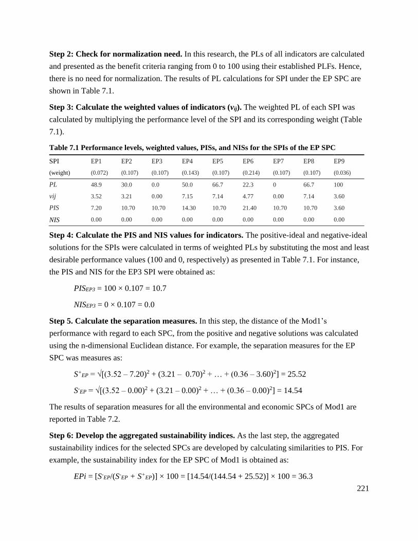
221

Step 2: Check for normalization need. In this research, the PLs of all indicators are calculated

and presented as the benefit criteria ranging from 0 to 100 using their established PLFs. Hence,

there is no need for normalization. The results of PL calculations for SPI under the EP SPC are

shown in Table 7.1.

Step 3: Calculate the weighted values of indicators (vij). The weighted PL of each SPI was

calculated by multiplying the performance level of the SPI and its corresponding weight (Table

7.1).

Table 7.1 Performance levels, weighted values, PISs, and NISs for the SPIs of the EP SPC

SPI EP1 EP2 EP3 EP4 EP5 EP6 EP7 EP8 EP9

(weight) (0.072) (0.107) (0.107) (0.143) (0.107) (0.214) (0.107) (0.107) (0.036)

PL 48.9 30.0 0.0 50.0 66.7 22.3 0 66.7 100

vij 3.52 3.21 0.00 7.15 7.14 4.77 0.00 7.14 3.60

PIS 7.20 10.70 10.70 14.30 10.70 21.40 10.70 10.70 3.60

NIS 0.00 0.00 0.00 0.00 0.00 0.00 0.00 0.00 0.00

Step 4: Calculate the PIS and NIS values for indicators. The positive-ideal and negative-ideal

solutions for the SPIs were calculated in terms of weighted PLs by substituting the most and least

desirable performance values (100 and 0, respectively) as presented in Table 7.1. For instance,

the PIS and NIS for the EP3 SPI were obtained as:

PISEP3 = 100 × 0.107 = 10.7

NISEP3 = 0 × 0.107 = 0.0

Step 5. Calculate the separation measures. In this step, the distance of the Mod1’s

performance with regard to each SPC, from the positive and negative solutions was calculated

using the n-dimensional Euclidean distance. For example, the separation measures for the EP

SPC was measures as:

S+EP = √[(3.52 – 7.20)2 + (3.21 – 0.70)2 + … + (0.36 – 3.60)2] = 25.52

S-EP = √[(3.52 – 0.00)2 + (3.21 – 0.00)2 + … + (0.36 – 0.00)2] = 14.54

The results of separation measures for all the environmental and economic SPCs of Mod1 are

reported in Table 7.2.

Step 6: Develop the aggregated sustainability indices. As the last step, the aggregated

sustainability indices for the selected SPCs are developed by calculating similarities to PIS. For

example, the sustainability index for the EP SPC of Mod1 is obtained as:

EPi = [S-EP/(S-

EP + S+EP)] × 100 = [14.54/(144.54 + 25.52)] × 100 = 36.3

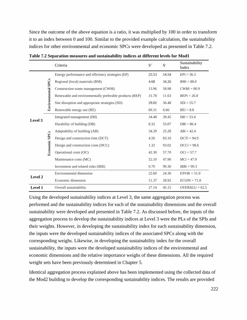
222

Since the outcome of the above equation is a ratio, it was multiplied by 100 in order to transform

it to an index between 0 and 100. Similar to the provided example calculation, the sustainability

indices for other environmental and economic SPCs were developed as presented in Table 7.2.

Table 7.2 Separation measures and sustainability indices at different levels for Mod1

Criteria S+ S- Sustainability

Index

Level 3

En

vir

on

men

tal

SP

Cs

Energy performance and efficiency strategies (EP) 25.53 14.54 EPi = 36.3

Regional (local) materials (RM) 4.68 34.26 RMi = 88.0

Construction waste management (CWM) 13.96 58.98 CWMi = 80.9

Renewable and environmentally preferable products (REP) 31.78 11.63 REPi = 26.8

Site disruption and appropriate strategies (SD) 29.02 36.48 SDi = 55.7

Renewable energy use (RE) 69.31 6.66 REi = 8.8

Eco

nom

ic S

PC

s

Integrated management (IM) 34.48 39.45 IMi = 53.4

Durability of building (DB) 8.32 53.07 DBi = 86.4

Adaptability of building (AB) 34.29 25.28 ABi = 42.4

Design and construction time (DCT) 4.50 83.10 DCTi = 94.9

Design and construction costs (DCC) 1.32 93.02 DCCi = 98.6

Operational costs (OC) 42.30 57.70 OCi = 57.7

Maintenance costs (MC) 52.10 47.90 MCi = 47.9

Investment and related risks (IRR) 0.70 99.30 IRRi = 99.3

Level 2 Environmental dimension 22.60 24.36 ENVRi = 51.9

Economic dimension 11.37 28.92 ECONi = 71.8

Level 1 Overall sustainability 27.14 45.15 OVERALLi = 62.5

Using the developed sustainability indices at Level 3, the same aggregation process was

performed and the sustainability indices for each of the sustainability dimensions and the overall

sustainability were developed and presented in Table 7.2. As discussed before, the inputs of the

aggregation process to develop the sustainability indices at Level 3 were the PLs of the SPIs and

their weights. However, in developing the sustainability index for each sustainability dimension,

the inputs were the developed sustainability indices of the associated SPCs along with the

corresponding weighs. Likewise, in developing the sustainability index for the overall

sustainability, the inputs were the developed sustainability indices of the environmental and

economic dimensions and the relative importance weighs of these dimensions. All the required

weight sets have been previously determined in Chapter 5.

Identical aggregation process explained above has been implemented using the collected data of

the Mod2 building to develop the corresponding sustainability indices. The results are provided

223

in Table 7.3.

Table 7.3 Separation measures and sustainability indices at different levels for Mod2

Criteria S+ S- Sustainability

Index

Level 3

En

vir

on

men

tal

SP

Cs

Energy performance and efficiency strategies (EP) 22.24 18.93 EPi = 46.0

Regional (local) materials (RM) 8.72 31.62 RMi = 78.4

Construction waste management (CWM) 12.49 67.32 CWMi = 84.4

Renewable and environmentally preferable products (REP) 36.73 0.00 REPi = 0.0

Site disruption and appropriate strategies (SD) 35.64 30.17 SDi = 45.8

Renewable energy use (RE) 68.34 13.34 REi = 16.3

Eco

nom

ic S

PC

s

Integrated management (IM) 27.50 40.61 IMi = 59.6

Durability of building (DB) 8.32 53.07 DBi = 86.4

Adaptability of building (AB) 32.04 28.68 ABi = 47.2

Design and construction time (DCT) 10.12 82.38 DCTi = 89.1

Design and construction costs (DCC) 2.70 93.00 DCCi = 97.2

Operational costs (OC) 84.50 15.50 OCi = 15.5

Maintenance costs (MC) 73.40 26.60 MCi = 26.6

Investment and related risks (IRR) 23.50 76.50 IRRi = 76.5

Level 2 Environmental dimension 23.88 24.22 ENVRi = 50.4

Economic dimension 15.80 24.36 ECONi = 60.7

Level 1 Overall sustainability 31.30 39.90 OVERALLi = 56.0

7.2.4 Performance Evaluation at Different Levels

After the sustainability indices were developed, the life cycle performance of each case study

modular building can be benchmarked. According to the proposed DSF in this research, the

assessment process is performed by comparing the developed sustainability indices at each level

with the corresponding sustainability performance scales (SPSs). As discussed in Chapter 6, the

SPSs were established based on the historical performances of single-family conventional

buildings in BC with the focus on the Okanagan.

Figure 7.2 compares the overall sustainability performance of the case study buildings with the

industry’s benchmarks. It can be observed from this figure that although both buildings showed

Excellent sustainability performance, Mod1 showed a better performance compared to Mod2

whose performance is slightly better than Good.

224

L

F G

E

OVERALLi

56.0

62.5

00.0

100.0

Mod1 Mod2

Figure 7.2 Sustainability performance benchmarking of the case study buildings (Level 1)

As discussed before, Excellent overall performance of a building does not necessarily indicate

that the same Excellent performance occurs in lower levels (Levels 2 and 3). Therefore, to

understand the performance of the case study buildings with respect to each of the sustainability

dimensions, the assessment process moved to Level 2. The DM might wish to find out which

sustainability dimension needs urgent attention to fall into the desired performance category.

Furthermore, even both sustainability dimensions are within the DM’s desirable levels, he/she

might want to improve the performance of one or both dimensions in order to further improve

the overall sustainability. In other words, it might be a situation that the performance of the

subject building with respect to both environmental and economic sustainability is acceptable;

however, by implementation of a number of strategies at lower costs, the performance at Level 2

can be improved which can result in the improvement of the overall sustainability.

The environmental and economic performances of the buildings have been compared with the

corresponding SPSs in Figure 7.3. It can be observed from the figure that not only the overall

sustainability performance of Mod1 is better than Mod2, but also both individual sustainability

dimensions. Nevertheless, although both ENVRi and ECONi of Mod1 were located in the

Excellent performance category, the ECONi is close to the lower threshold of this category. On

the other hand, the ENVRi of Mod2 is slightly less than ENVRi of Mod1 very close to the upper

threshold of the Good performance category.

225

L

F G

E

ENVRi50.451.9

00.0

100.0

Mod1 Mod2

L

F G

E

ECONi

56.0

71.8

00.0

100.0

Mod1 Mod2

Figure 7.3 Environmental and economic performance benchmarking of the case study buildings

(Level 2)

In the next step, the assessment process was continued at Level 3 where the sustainability

performances of Mod1 and Mod2 with respect to each SPC were evaluated. Figures 7.4 and 7.5

demonstrate the performance of the case study buildings with respect to the environmental SPCs

and economic SPCs, respectively.

It can be observed from Figure 7.4 that ‘Regional materials (RM)’ and ‘Construction waste

management (CWM)’ are the two areas that the Mod1 building has shown Excellent

performance. In addition, this building performed close to Excellent in terms of ‘Site disruption

and appropriate strategies (SD)’. However, in the other three SPCs, the building have shown a

Poor performance. Similarly, the Mod2 building also showed an Excellent performance for the

RM and CWM SPCs. However, in the remaining areas, its performance has not been

satisfactory.

When the performances of the two buildings are compared with each other (i.e., review

benchmarking), as opposed to what was observed previously at Level 2, the Mod2 building

performed higher than Mod1 in terms of some environmental SPCs. For example, although both

buildings have implemented suitable construction waste management strategies, Mod2 obtained

a higher CWMi. Similarly, even though both Mod1 and Mod2 have fallen into the Low

performance category in the cases of the EP and RE SPCs, the corresponding sustainability

indices for the latter building are higher.

226

L

F

G

E

CWMi

84.4

80.9

00.0

100.0

Mod1 Mod2

L

F G

E

RMi

78.488.0

00.0

100.0

Mod1 Mod2

L

F G

E

EPi46.0

36.3

00.0

100.0

Mod1 Mod2

L

F G

E

SDi45.8

55.7

00.0

100.0

Mod1 Mod2

L

F

G

E

REi

16.38.8

00.0

100.0

Mod1 Mod2

L

F G

E

REPi

00.0

26.8

00.0

100.0

Mod1 Mod2

Figure 7.4 Sustainability performance benchmarking of the case study buildings with respect to

environmental SPCs (Level 3)

Comparisons of the performances of the case study buildings with respect to the economic SPCs

have been presented in Figure 7.5. It can be observed from this figure that, in general, the

sustainability indices for both Mod1 and Mod2 have fallen in high performance categories such

as Excellent and Good. Except the ‘Maintenance costs (MC)’ and to some extent the

‘Operational costs (OC)’, both modular buildings performed remarkably. In the cases of five

SPCs including IM, DB, DCT, DCC, and IRR, the corresponding sustainability indices were

very high indicating outstanding economic performances. Among these five SPCs, an excellent

performance for the ‘Design and construction time (DCT)’ was anticipated because fast

construction is among the most cited benefits of modular construction in the literature.

Supporting this, the DCT SPC was ranked 1st among the economic SPC category and 2nd among

the TBL SPCs by the construction practitioners previously in this research (see the results of

Chapter 4). When comparing the performances of Mod1 and Mod2 with each other, each

building showed a better performance with respect to a number of economic SPCs.

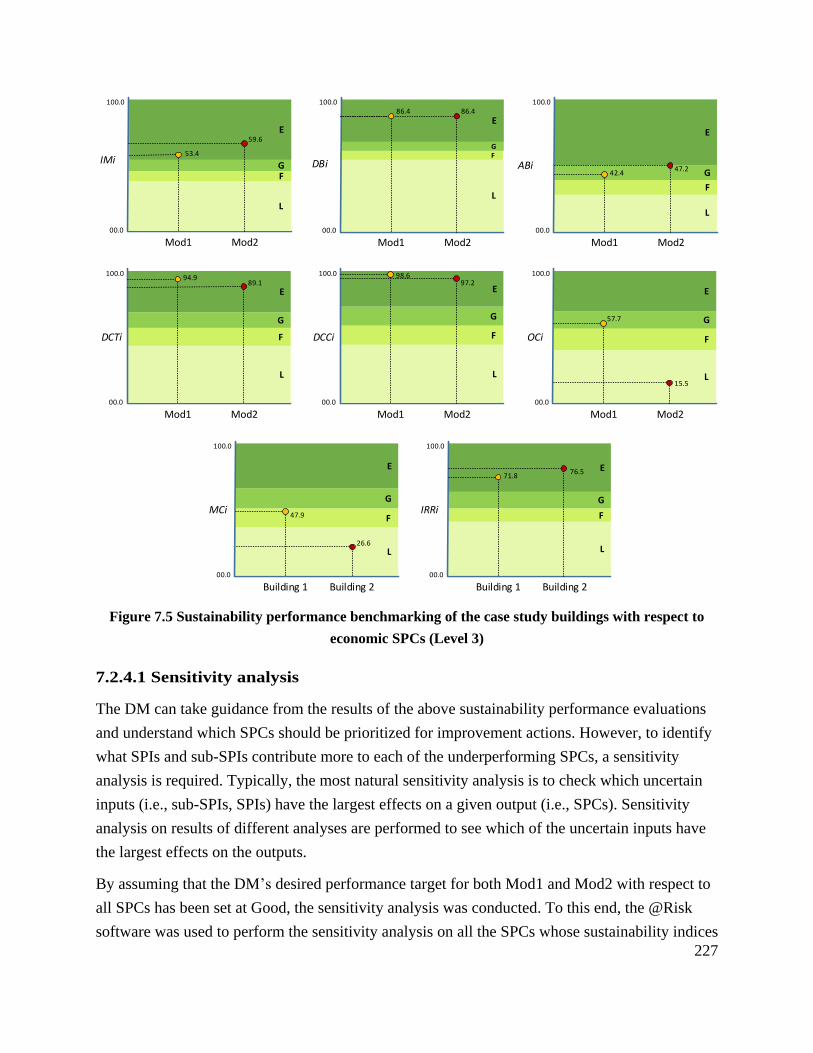
227

L

F

G

E

ABi 47.242.4

00.0

100.0

Mod1 Mod2

L

F G

E

DBi

86.486.4

00.0

100.0

Mod1 Mod2

L

F G

E

IMi

59.6

53.4

00.0

100.0

Mod1 Mod2

L

F

G

E

DCCi

97.298.6

00.0

100.0

Mod1 Mod2

L

F

G

E

OCi

15.5

57.7

00.0

100.0

Mod1 Mod2

L

F

G

E

DCTi

89.194.9

00.0

100.0

Mod1 Mod2

L

F

G

E

IRRi

76.571.8

00.0

100.0

Building 1 Building 2

L

F

G

E

MCi

26.6

47.9

00.0

100.0

Building 1 Building 2

Figure 7.5 Sustainability performance benchmarking of the case study buildings with respect to

economic SPCs (Level 3)

7.2.4.1 Sensitivity analysis

The DM can take guidance from the results of the above sustainability performance evaluations

and understand which SPCs should be prioritized for improvement actions. However, to identify

what SPIs and sub-SPIs contribute more to each of the underperforming SPCs, a sensitivity

analysis is required. Typically, the most natural sensitivity analysis is to check which uncertain

inputs (i.e., sub-SPIs, SPIs) have the largest effects on a given output (i.e., SPCs). Sensitivity

analysis on results of different analyses are performed to see which of the uncertain inputs have

the largest effects on the outputs.

By assuming that the DM’s desired performance target for both Mod1 and Mod2 with respect to

all SPCs has been set at Good, the sensitivity analysis was conducted. To this end, the @Risk

software was used to perform the sensitivity analysis on all the SPCs whose sustainability indices

228

fell into either the Poor or Fair performance categories.

From Figure 7.4, it can be observed that, both buildings showed a Poor environmental

performance in terms of EP, REP, and RE SPCs. In addition, Mod2 also performed

unsatisfactory with respect to the SD SPC. Figure 7.6 presents the results of the sensitivity

analysis for the EP, REP, and SD SPCs in the form of tornado charts. In a tornado chart, the

longest bars are at the top of the chart. In addition, the longer the bar, the more effect the

corresponding uncertain input has on the output. It should be mentioned that the sensitivity

analysis can be performed for each of the Good and Excellent performing SPCs if the DM wants

to investigate the top priority indicators for further improvement of thse SPCs.

The indicators correspond to top bars in Figure 7.6a including the EP5 and EP7 SPIs and also the

EP6-3 and EP6-1 sub-SPIs should be given high priority to improve the performance of the

‘Energy performance and efficiency strategies’ SPC. Similarly, from Figure 7.6b, it can be seen

that the REP2-2 sub-SPI and REP3 SPI are among the top concerns to improve the performance

of the ‘Renewable and environmentally preferable products’ SPC. The remaining indicators have

not a significant difference in their contributions to this SPC. In the same way, Figure 7.6c can

be used to rank the indicators under the ‘Site disruption and appropriate strategies’ for

sustainability performance improvement actions.

229

Figure 7.6 Sensitivity analysis results (a) Energy performance and efficiency strategies; (b)

Renewable and environmentally preferable products; (c) Site disruption and appropriate strategies

230

In the cases of the economic SPCs, as shown in Figure 7.5, the MC performance of Mod1 and

Mod2 have performed Fair and Poor, respectively. Furthermore, Mod2 did not show a

satisfactory performance with respect to OC (i.e., Poor performance). Since both the OC and MC

SPCs consisted of only one SPI, the results of the sensitivity analysis showed 100% contribution

of each SPI to the corresponding output SPC. Therefore, to improve the MC performance, both

Mod1-builder and Mod2-builder should investigate the reasons for high maintenance costs and

make appropriate remedy decisions to apply in new buildings. For example, it could be due to

inappropriate installation of different equipment in the building that resulted in the need for

service and repairs. Similarly, Mod2-builder needs to find out the reasons for the higher running

costs in the use phase. This could be because of the quality of insulations, low performance of

some appliances, and so forth.

7.3 Performance Evaluation of the Case Study Buildings with respect to the GE SPC

7.3.1 Data Collection for Inventory Analysis

The methodology used in this research to develop the environmental impact indices has already

been explained in Chapters 5 and 6 (see sections 5.3.7 and 6.3.7 for details); therefore, detailed

explanations are not repeated. As stated earlier, in this study, two modular single-family

buildings (i.e., Mod1 and Mod2) along with one conventional single-family building (henceforth

Conv) were evaluated in terms of environmental impacts due to construction of these buildings.

Figure 7.7 illustrates the floor plan of the Conv building. The total floor area of this building is

1568 ft2 (146 m2), which includes three bedrooms, two bathrooms, one living room, one dining

room, one kitchen, one WIC, and one den.

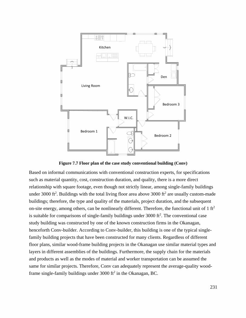
231

Kitchen Up

Den

W.I.C.

Living Room

Bedroom 3

Bedroom 1Bedroom 2

Up

Figure 7.7 Floor plan of the case study conventional building (Conv)

Based on informal communications with conventional construction experts, for specifications

such as material quantity, cost, construction duration, and quality, there is a more direct

relationship with square footage, even though not strictly linear, among single-family buildings

under 3000 ft2. Buildings with the total living floor area above 3000 ft2 are usually custom-made

buildings; therefore, the type and quality of the materials, project duration, and the subsequent

on-site energy, among others, can be nonlinearly different. Therefore, the functional unit of 1 ft2

is suitable for comparisons of single-family buildings under 3000 ft2. The conventional case

study building was constructed by one of the known construction firms in the Okanagan,

henceforth Conv-builder. According to Conv-builder, this building is one of the typical single-

family building projects that have been constructed for many clients. Regardless of different

floor plans, similar wood-frame building projects in the Okanagan use similar material types and

layers in different assemblies of the buildings. Furthermore, the supply chain for the materials

and products as well as the modes of material and worker transportation can be assumed the

same for similar projects. Therefore, Conv can adequately represent the average-quality wood-

frame single-family buildings under 3000 ft2 in the Okanagan, BC.

232

As stated before, a questionnaire survey (Survey D) was conducted to collect the required data of

the two modular and one conventional case study buildings from the corresponding

homebuilders for inventory analysis (LCI) (see Table 5.10 in Chapter 5). In addition, a copy of

the design drawings of each building was requested. Subsequently, using the received design

drawings, different assemblies, their dimensions, and the materials and products used in each

assembly were calculated and entered into the Athena software as the input raw data. The

software performed inventory analysis and calculated the energy associated with the material

production phase (i.e., A1 and A2) and the construction phase (i.e., A3 and A4) of each building.

As discussed before, the software was not able to calculate the energy related to a number of

tasks under the activity categories A3 and A4. However, if these energy consumptions are

separately calculated, Athena is capable of performing LCIA to calculate the corresponding

impact measures. Therefore, for such tasks under the activity categories A3 and A4, the

associated energy consumptions were separately modeled and calculated based on the

information provided by the homebuilders in the questionnaire forms. For example, the energy

consumed in the modular factory for machinery, office, heating, and cooling to construct Mod1

was calculated using the annual energy bills and the total annual module production (ft2)

provided by the Mod1-builder. The calculated energy values were then fed into the software for

LCIA.

7.3.2 Impact Assessment

Based on the results of the inventory analysis, the life cycle impact assessment (LCIA) was

performed by the Athena Impact Estimator to calculate the environmental impact measures.

Table 7.4 presents the results of LCIA for the case study buildings. The environmental impacts

due to material and energy consumption in the material production phase (i.e., activity categories

A1 and A2) and the construction phase (i.e., activity categories A3 and A4) of the buildings have

been provided separately. In addition, the accumulative values of the impact measures for both of

these life cycle phases have been included in the table that indicate the cradle-to-gate

environmental impacts of each building. The results were normalized to the functional unit (i.e.,

1 ft2 of the total floor area of buildings) that enables valid comparisons between the buildings.

Except the eco-toxicity effect, all the impact measures have been generated directly by the

impact assessment. The eco-toxicity measure, as explained earlier, was calculated for each

building by aggregating the mass of the identified toxic substances and their weights (Equation

[5.85]), and then normalized and reported.

233

Table 7.4 Results of LCIA for the benchmarking buildings


(A1 & A2)

Construction phase

(A3 & A4)

Cradle-to-gate

(A1 - A4)

LCA impact measures unit Conv Mod1 Mod2 Conv Mod1 Mod2 Conv Mod1 Mod2

Global warming potential kg CO2eq 5.14E+00 4.85E+00 4.66E+00 4.65E+00 3.75E+00 5.11E+00 9.79E+00 8.60E+00 9.78E+00

Acidification potential kg SO2eq 3.78E-02 3.95E-02 3.77E-02 2.09E-02 1.74E-02 2.88E-02 5.87E-02 5.69E-02 6.65E-02

Human health effect kg PM2.5eq 8.08E-03 1.09E-02 1.05E-02 1.15E-03 9.40E-04 1.40E-03 9.23E-03 1.19E-02 1.19E-02

Eutrophication potential kg Neq 2.53E-03 2.52E-03 2.44E-03 4.95E-04 4.07E-04 8.09E-04 3.02E-03 2.93E-03 3.25E-03

Ozone depletion potential kg CFC11eq 6.77E-08 4.09E-08 3.61E-08 1.07E-10 7.31E-11 1.10E-10 6.78E-08 4.09E-08 3.62E-08

Smog potential kg O3eq 5.49E-01 5.38E-01 5.21E-01 1.71E-01 1.49E-01 3.42E-01 7.20E-01 6.88E-01 8.63E-01

Fossil fuel consumption MJ 1.08E+02 1.01E+02 9.88E+01 6.43E+01 4.90E+01 7.27E+01 1.72E+02 1.50E+02 1.71E+02

Eco-toxicity effect mg 1.02E+00 1.04E+00 1.00E+00 9.66E-01 6.89E-01 1.03E+00 1.98E+00 1.73E+00 2.03E+00

234

To enable visual comparisons, the comparative graphical illustrations of the impact measures are

also presented in Figure 7.8 and Figure 7.9. From these figures, two significant observations can

be drawn. First, the performance of buildings in terms of each individual impact measure can be

compared and contrasted to determine which building, and the corresponding construction

method, is more environmentally responsible.

Figure 7.8 Global warming potential, Acidification potential, Human health effect, and

Eutrophication potential due to construction of the benchmarking buildings

Besides, the impact contribution proportion of the material production phase and the construction

phase to the overall cradle-to-gate can be realized. This latter observation is useful especially to

determine the dominant phase in the case of each impact measure. For examples, the ODP

contribution of the construction phase to the overall cradle-to-gate is very small compared to the

material production phase (similarly, HHE). Therefore, although the ODP values in the

construction phase are significantly different between the Conv, Mod1, and Mod2 buildings, the

0

1

2

3

4

5

6

7

8

9

10

11

Materialproduction phase

Constructionphase

Cradle-to-gate

GWP

Conv

Mod1

Mod2

kgC

O2

eq

0

0.01

0.02

0.03

0.04

0.05

0.06

0.07


Constructionphase

Cradle-to-gate

APConv

Mod1

Mod2

kgSO

2 e

q

0

0.003

0.006

0.009

0.012

0.015


Constructionphase

Cradle-to-gate

HHEConv

Mod1

Mod2

kgP

M2

.5 e

q

0

0.001

0.002

0.003

0.004


Constructionphase

Cradle-to-gate

E-PConv

Mod1

Mod2

kgN

eq

235

material production phase is the main source of judgment for the performances of these

buildings.

Figure 7.9 Ozone depletion potential, Smog potential, Fossil fuel consumption, and Eco-toxicity

effect due to construction of the benchmarking buildings

As can be seen in Figures 7.8 and 7.9, the Mod1 building showed a better performance in terms

of all impact measures compared to the Conv and Mod2 buildings in the construction phase.

However, in the case of some impact measures, this building showed lower performance than

Conv, Mod2, or both Conv and Mod2 in the material production phase. As mentioned above, the

contribution of each impact measure to the material production phase and the construction phase

can significantly influence the overall cradle-to-gate environmental performance of these

buildings. Although Mod1 did not perform better than other buildings for some impact measures,

it can be observed from the figures that this building still ranked first when comparing its

performance over the entire cradle to gate life cycle. For example, although this building emitted

0

1E-08

2E-08

3E-08

4E-08

5E-08

6E-08

7E-08

8E-08


Constructionphase

Cradle-to-gate

ODP

Conv

Mod1

Mod2

kgC

FC1

1 e

q

0

0.1

0.2

0.3

0.4

0.5

0.6

0.7

0.8

0.9

1


Constructionphase

Cradle-to-gate

SP

Conv

Mod1

Mod2

kgO

3 e

q

0

20

40

60

80

100

120

140

160

180


Constructionphase

Cradle-to-gate

FFCConv

Mod1

Mod2

MJ

0

0.5

1

1.5

2

2.5


Constructionphase

Cradle-to-gate

EE

Conv

Mod1

Mod2

mg

236

more CO2eq than Mod2 and more SO2eq than both Conv and Mod2 in the material consumption

phase, its performance in the construction phase was as high that its overall cradle-to-grate

performance dominated the other two buildings (see Table 7.4 for quantities).

When it came to investigate the next priority building, it can be observed from Figures 7.8 and

7.9 that the Conv and Mod2 buildings presented comparable performance in their material

production phase (except for ODP). However, in the construction phase, Conv performed

marginally better than Mod2 with respect to all the impact measures which implied higher

amount of energy consumption in the activity categories A3 (off-site and on-site) and A4

(material and worker transportation) of the Mod2 building. Comparison of the quantities of the

impact measures during the entire cradle to gate period revealed that the Conv building

performed better with respect to five impact measures including AP, HHE, EP, SP, and EE. It is

important to note that in the cases of the GWP and FFC impact measures, both Conv and Mod2

performed approximately the same and the only low performing area of the Conv building is its

highest ODP (ozone depletion potential) where it released almost double amount of CFC11eq

compared to the Mod2 building.

While the Mod1 building that has been constructed using modular construction method proved to

be the best performing building, it might initially be expected that the other modular building,

i.e., Mod2, should be the next priority building. However, the above-described results showed

the opposite and rejected the belief reported by some literature that the environmental impacts

incurred by construction of modular buildings are always less than conventional buildings.

7.3.3 Environmental Impact Indices

The results of LCIA provided in Table 7.4, Figure 7.8, and Figure 7.9, are useful when the

buildings’ environmental performances with regard to individual impact measures are concerned.

For example, in many cases, the climate change incurred by human activities including products,

processes, or services, has been the top environmental impact concerns. Therefore, numerous

LCA studies have been performed to investigate the global warming potential of different human

activities as the main indicator of climate change. However, as discussed before, there are

different weighting schemes developed by scientific organizations and institutes for different

environmental impact categories that indicate the importance of other environmental impacts

(see Table 5.12 in Chapter 5). Consequently, it becomes a more comprehensive study if more

environmental impacts (where applicable and possible) are included in the study, which can

provide a better insight into the environmental performance of products, processes, or services.

However, the environmental performance evaluation of different construction methods using

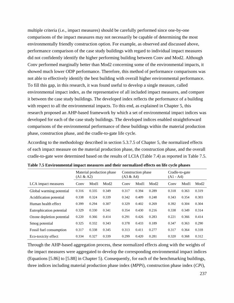
237

multiple criteria (i.e., impact measures) should be carefully performed since one-by-one

comparisons of the impact measures may not necessarily be capable of determining the most

environmentally friendly construction option. For example, as observed and discussed above,

performance comparison of the case study buildings with regard to individual impact measures

did not confidently identify the higher performing building between Conv and Mod2. Although

Conv performed marginally better than Mod2 concerning some of the environmental impacts, it

showed much lower ODP performance. Therefore, this method of performance comparisons was

not able to effectively identify the best building with overall higher environmental performance.

To fill this gap, in this research, it was found useful to develop a single measure, called

environmental impact index, as the representative of all included impact measures, and compare

it between the case study buildings. The developed index reflects the performance of a building

with respect to all the environmental impacts. To this end, as explained in Chapter 5, this

research proposed an AHP-based framework by which a set of environmental impact indices was

developed for each of the case study buildings. The developed indices enabled straightforward

comparisons of the environmental performance of these buildings within the material production

phase, construction phase, and the cradle-to-gate life cycle.

According to the methodology described in section 5.3.7.5 of Chapter 5, the normalized effects

of each impact measure on the material production phase, the construction phase, and the overall

cradle-to-gate were determined based on the results of LCIA (Table 7.4) as reported in Table 7.5.

Table 7.5 Environmental impact measures and their normalized effects on life cycle phases


(A1 & A2)

Construction phase

(A3 & A4)

Cradle-to-gate

(A1 - A4)

LCA impact measures Conv Mod1 Mod2 Conv Mod1 Mod2 Conv Mod1 Mod2

Global warming potential 0.316 0.335 0.349 0.317 0.394 0.289 0.318 0.363 0.319

Acidification potential 0.338 0.324 0.339 0.342 0.409 0.248 0.343 0.354 0.303

Human health effect 0.399 0.294 0.307 0.329 0.402 0.269 0.392 0.304 0.304

Eutrophication potential 0.329 0.330 0.341 0.354 0.430 0.216 0.338 0.349 0.314

Ozone depletion potential 0.220 0.366 0.414 0.291 0.426 0.283 0.221 0.366 0.414

Smog potential 0.325 0.332 0.343 0.378 0.433 0.189 0.347 0.363 0.290

Fossil fuel consumption 0.317 0.338 0.345 0.313 0.411 0.277 0.317 0.364 0.318

Eco-toxicity effect 0.334 0.327 0.339 0.299 0.420 0.281 0.320 0.368 0.312

Through the AHP-based aggregation process, these normalized effects along with the weights of

the impact measures were aggregated to develop the corresponding environmental impact indices

(Equations [5.86] to [5.88] in Chapter 5). Consequently, for each of the benchmarking buildings,

three indices including material production phase index (MPPi), construction phase index (CPi),

238

and cradle-to-gate index (CTGi) were developed. As discussed before, to counter the human

subjectivity in assigning weights for different impact measures, a sensitivity analysis was

conducted where three different weighting schemes were applied and the environmental impact

indices were re-developed for each building. In doing so, the aggregation process were repeated

three times for all buildings by considering the EPA Science Advisory weighting, the BEES

Stakeholder Panel weighting, and equal weighting (see Table 5.12). Table 7.6 presents the

environmental impact indices developed for the buildings based on these weighting schemes. In

addition, the CTGi values for the buildings based on different weighting schemes are shown in

graphical form in Figure 7.10.

As seen in Table 7.6 that although different values for MPPi, CPi and CTGi were obtained under

each weighting scheme, this did not change the rank order of the benchmarking buildings in any

of the material production phase, the construction phase, and the overall cradle-to-gate.

Table 7.6 Environmental impact indices for the benchmarking buildings

MPPi CPi CTGi

Weighting schenes Conv Mod1 Mod2 Conv Mod1 Mod2 Conv Mod1 Mod2

EPA Science Advisory 0.328 0.328 0.344 0.323 0.411 0.266 0.328 0.352 0.320

BEES Stakeholder Panel 0.329 0.329 0.342 0.321 0.406 0.272 0.329 0.352 0.319

Equal weighting 0.322 0.331 0.347 0.328 0.416 0.256 0.324 0.354 0.322

The results of the CTGi values showed that, in all cases of the weighting schemes, the Mod1

building was the top ranked building in terms of overall cradle-to-grate performance. This

confirmed the findings from comparisons of individual impact measures before. In addition, by

comparing the MPPi and CPi values in Table 7.6, Mod1 was again the best performing building

in both the material production phase and the construction phase.

Similar to the results of comparing individual impact measures discussed before, comparing the

impact indices of the Conv and Mod2 buildings again rejected the belief that modular

construction method is always the most environmentally friendly option. As seen in Figure 7.10,

the Conv building showed a slightly better overall performance than the Mod2 building.

However, the results of the MPPi and CPi values in Table 7.6 revealed that the Mod2 building

performed better in the material production phase, while the Conv building is better within the

construction phase. This indicated the fact that the design of Mod2 (e.g, assemblies, space

configurations) was better than Conv (and even Mod1) so that fewer materials were used in the

buildings, which required less energy in its material production phase (i.e., activity categories A1

and A2).

239

In contrast, the energy consumed in the construction phase of the Conv building resulted less

environmental impacts than that of the Mod2 building. The collected data from the participating

homebuilders showed that majority of the Mod2-builder’s employees used private car for

commuting to and from work (i.e., modular factory), while car-sharing and public transportation

were more common in the cases of the Conv and Mod1 projects. This is necessary to remind

that, the employees of a modular factory are permanent employees that commute between home

and the manufacturing center all year round. Therefore, choosing more environmentally friendly

commuting options can lead to less environmental burdens.

Figure 7.10 Cradle-to-grate index (CTGi) for different building alternatives

It is also important to mention that the total annual production of a modular factory can influence

the total off-site energy consumption. The annual energy data provided by Mod1-builder and

Mod2-builder revealed that the electricity and natural gas consumption per functional unit of

production in the former modular factory (total annual floor area production of 408,000 ft2) was

less than that of the latter modular factory (total annual floor area production of 300,000 ft2).

In addition to the above factors, the role of module transportation energy should not be

overlooked. This factor is amongst the main differences between the conventional and modular

construction methods. The final project site of a conventional building is usually within the city

in which the conventional homebuilders are also located. Similarly, the on-site work of a

modular building project, such as site preparation, foundation construction, and module

installation of modules on foundation are usually performed by local contractors within the same

city. However, the distance between the final project site of a modular building and the

0.000

0.100

0.200

0.300

0.400

0.500

Conv Mod1 Mod2

CTGi

EPA Science Advisory

BEES Stakeholder Panel

equal weighting

240

corresponding modular homebuilder can significantly vary, which influences on the energy

required for transportation of the completed modules from the factory to the project site. Both the

modular buildings in this study (Mod1 and Mod2) were located in the same city where their

corresponding modular factories were also located. Thus, the module transportation effect did

not play a significant role in the environmental performance of these buildings in the

construction phase and subsequently in the overall cradle-to-gate. However, according to both

modular builders, the project sites can be located within 300 km from the manufacturing centers.

7.4 Summary

In the first part of this chapter, the decision support framework (DSF) proposed in this research

has been validated by applying it to two case study modular buildings in the Okanagan, BC

(Mod1 and Mod2). Different components of the proposed DSF were carefully implemented.

Using the collected data, the sustainability indices of each case study building were developed at

different levels and then, they were compared to the corresponding sustainability performance

scales (SPSs). Subsequently, the underperforming areas (SPCs) were realized. By conducting a

sensitivity analysis, the indicators under each of the underperforming SPCs were ranked and the

high contributing indicators were recognized and given high priorities for improvement actions.

The results showed that both buildings performed Good and Excellent with respect to overall

sustainability (Level 1) and also with respect to environmental and economic dimensions of

sustainability (Level2). However, the buildings performed Poor or Moderate with respect to a

number of SPCs (Level 3). Altogether, Mod1 showed better life cycle environmental and

economic performances. This part of Chapter 7 showed that the implementation of the proposed

DSF was straightforward and the outcome were easy to understand and interpret.

In the second part, the performance of the Mod1 and Mod2 buildings along with one

conventional building (Conv) with respect to the GE SPC were evaluated. By conducting LCA,

the values of eight environmental impact measures for each building were calculated and

compared. In addition, a set of environmental impact indices were developed and compared,

which enabled easier and confident comparison of the environmental performance of these

buildings. From this part of the chapter, it was concluded that Mod1 is the most environmentally

responsible building. However, comparing the impact indices of the Conv and Mod2 buildings

ranked Conv higher than Mod2. This was important because it rejected the claim that modular

construction method is always the most environmentally friendly option. However, the claim can

be stated in a better way that modular construction has the potential to reduce the overall energy

consumption which can result in less environmental burdens.

241

Chapter 8 Conclusions and Recommendations

In the past few decades, the construction industry has been exposed to the process of

industrialization and experimenting different methods of construction. As a result, the off-site

construction came into practice as an alternative to conventional on-site construction. Modular

construction, as the primary method of off-site construction, has been increasingly grabbing

attention in the past few years. Modular construction was claimed to offer many advantages over

conventional construction and a building built using this method has been claimed to be a

sustainable building.

Because of the importance of sustainability, in particular sustainable construction, it is

imperative to comprehensively assess the life cycle sustainability performance of different

construction methods. This can be accomplished by analyzing and comparing the sustainability

performance of buildings constructed using on-site and off-site construction methods. In this

regard, this research proposed a novel sustainability assessment framework for performance

benchmarking of residential modular buildings. The results of this study can enhance sustainable

construction by identifying the most sustainable construction options and also by improving the

underperforming areas.

8.1 Summary and Conclusions

A summary of the specific study sections and the main conclusions are presented below.

In Chapter 3, a thorough review was presented on existing sustainability assessment methods for

buildings, potential advantages and disadvantages of modular construction, and current studies

on the life cycle performance of modular buildings. The findings showed that sustainability

assessment methods can be categories into systems, standards, and tools. The sustainability

assessment systems were realized as the most comprehensive methods because they are capable

to evaluate the sustainability of a building by choosing suitable sustainability criteria related to

different TBL dimensions of sustainability and different life cycle phases. The results of the

literature review also revealed that the main advantages of modular construction were higher

speed of construction, better productivity and workmanship, cost savings, higher safety, higher

product control and quality, and less environmental impacts. However, amongst the challenges

faced by modular construction were transportation constraints, more complicated engineering

and planning processes, need for more coordination and communication, higher initial

investment, and more importantly, people’s negative perceptions of new construction methods.

The literature review also presented that only a few studies have been quantitatively performed

242

to compare the (environmental) performance of modular buildings and conventional buildings.

This indicated the need for a comprehensive sustainability assessment framework to evaluate the

life cycle performance of modular buildings with respect to the TBL sustainability dimensions.

The findings of this chapter were used in identifying the research gap and in defining the

research concepts and the methodologies associated with the proposed sustainability assessment

framework in this research.

In Chapter 4, the TBL SPCs were compiled and the construction industry’s feedback on

applicability of the SPCs for sustainability assessment of residential modular buildings was

captured. Consequently, the SPCs were ranked within the associated sustainability dimension

categories and an importance level ranging from ‘Extremely Low’ to ‘Extremely High’ was

assigned to each SPC. Among all the 32 TBL SPCs, 26 SPCs were assigned either ‘Medium’,

‘High’, or ‘Very High’ importance criteria, which indicated that most of the SPCs are relevant

and should be selected for performance assessment of modular buildings. In addition, comparing

the results between different sustainability dimension categories revealed that the economic

criteria still play the most significant role in distinguishing modular and conventional

construction methods. Based on the results of this chapter, all SPCs with the importance level

equal or higher than ‘Medium’ including 8 environmental SPCs and 9 economic SPCs were

chosen for performance evaluation of residential modular buildings (the social dimension was

beyond the scope of this research). It should be mentioned that although some of the selected

SPCs had a level of interdependency, it was assumed that all the SPCs are independent of one

another.

Chapter 5 consisted of two parts. The first part focused on quantification of the selected SPCs. In

this regard, suitable measurable sustainability performance indicators (SPIs and sub-SPIs) under

each SPC along with their measurement methods, their weights, their least and most desirable

performance values, and corresponding ranges of data variables, were determined. The main

output of this part was establishment of a performance level function (PLF) for each indicator by

which it can be calculated using least data, then normalized, and represented based on a

dimensionless unit of performance level (PL) between 0 and 100. Representing the calculated

indicators in this way was found useful because all the indicators related to a SPC can be directly

combined regardless of their original units of measurements. In addition, the PL value of an

indicator indicates the closeness of the given building’s performance to the most desirable

performance of the indicator (PL = 100). The second part of Chapter 5 proposed a methodology

using a suitable aggregation process (TOPSIS MCDA) to develop a set of sustainability indices

(between 0 and 100) for a given modular building to evaluate its performance at different levels.

243

The outcomes were the sustainability indices for SPCs (Level 3), each of the sustainability

dimensions, i.e., environmental and economic (Level 2), and overall sustainability of the given

building (Level 1). The sustainability indices at different levels enable the decision maker (DM)

to focus on the desired level (i.e., Level 3, Level 2, or Level l) and investigate the performance of

the building at that level using the corresponding sustainability indices.

In the first part of Chapter 6, an attempt was made to establish appropriate scales by which the

developed sustainability indices of modular buildings can be compared and contrasted to their

conventional counterparts. The historical performances of conventional buildings with respect to

the indicators developed in the previous chapter were explored based on expert opinions and then

combined using the Monte Carlo simulation method to develop the performances of these

buildings with respect to the corresponding SPCs. Similarly the environmental, economic, and

overall sustainability performances of conventional buildings were developed. The outcomes of

this part of Chapter 6 were a set of sustainability performance scales (SPSs) for SPCs (Level 3),

each of the sustainability dimensions, i.e., environmental and economic (Level 2), and overall

sustainability (Level 1). The domain of each SPS ranged between 0 and 100, which was

consistent with the applicable range of the developed sustainability indices and enabled easier

evaluations. In addition, to provide effective and straightforward performance comparisons, the

domain of each SPS was divided into four evaluation categories including Poor, Fair, Good, and

Excellent performances. The sustainability performance of a given modular can be benchmarked

by comparing the developed sustainability indices at the desired level (i.e., Level 3, Level 2, or

Level 1) with the corresponding SPSs established in this chapter. In the second part of this

chapter, all the frameworks, methodologies, and deliverables of the research, were incorporated

into a single framework as an integrated decision support framework (DSF). The proposed DSF

is capable of comprehensively assessing modular buildings in terms of environmental and

economic performances. Since the developed DSF is a multi-level framework, the user (i.e., DM)

is able to evaluate the performance of the subject modular building at each of the aforementioned

levels depending on the desire and scope of the assessment study. It should be stated that, since it

was not possible to establish a SPS for the GE SPC, the performance of modular buildings with

respect to this SPC was evaluated using the review benchmarking method based on LCA

analyses.

In Chapter 7, the proposed DSF was applied on actual case study buildings for the proof-of-

concept. To this end, the life cycle sustainability performance of two case study modular

buildings in the Okanagan, BC, were benchmarked by implementing different components of the

developed DSF. Subsequently, the underperforming environmental and economic SPCs were

244

realized. The results revealed that both modular buildings performed Excellent in term of overall

sustainability (Level 1) and either Excellent or Good in terms of the sustainability dimensions

(Level 2). However, the performance of these buildings with respect to some of the SPCs (Level

3) were shown as Fair and even Low, which indicated the need for making improvement

decisions and actions to enhance the corresponding performances. By conducting a sensitivity

analysis, the indicators (sub-SPIs and SPIs) under each of these SPCs were ranked and the high

contributing indicators were recognized and given high priorities for improvement. In addition, a

cradle-to-gate LCA was conducted for the two modular buildings and also a conventional

building to examine the environmental impacts due to construction of these buildings (i.e., GE

SPC). One of the modular buildings showed better performance among the three case study

buildings followed by the conventional building that showed better performance than the second

modular building. These findings were not fully consistent with the claim reported in the

literature that construction of modular buildings is always more environmentally responsible

than construction of conventional buildings. The results of the case study analyses provided a

better insight into the sustainability performance of single-family modular buildings in the

Okanagan, BC. In addition, the case study analyses showed that the proposed DSF is a

straightforward and easy to follow framework, albeit comprehensive, that can effectively be used

to promote sustainable construction.

8.2 Originality and Contribution

This research delivers the following unique contributions to the body of knowledge:

Identifying the most applicable sustainability performance criteria for modular

buildings: Numerous criteria have been used in different studies to evaluate the

performance of conventional buildings. However, the primary focus has been on the

environmental criteria and on specific life cycle phases of these buildings. This research

developed the key performance criteria for modular buildings which covered all the TBL

sustainability dimensions (i.e., environmental, economic, and social) and also all the life

cycle phases of these buildings. In addition, the developed criteria were prioritized that

enables the assessor to pay more attention to the top priority criteria. Furthermore, these

criteria can be used in any sustainability assessment framework for modular buildings

with different methodology than developed in this research.

Presenting a novel method for calculating and combining quantitative and qualitative

criteria: This research introduced the dimensionless unit of Performance Level (PL) to

calculate and represent different qualitative and quantitative indicators and criteria. The

245

other advantage of using the PL unit is that different indicators associated with a SPC can

be combined regardless of their original units. In addition, the results of combining the

PLs of the indicators, i.e., the sustainability indices for the corresponding SPCs, will also

be dimensionless values between 0 and 100 (similarly, the indices at upper levels), which

facilitate the evaluation of a building’s performance at different levels. Furthermore, the

lower and upper bounds of each indicator. i.e., PL = 0 and PL = 100, have been set as the

least and most desirable performances of the indicator. This means that the performance

of a given building with respect to an indicator is calculated according to its benchmarks;

therefore, the calculated PL of the indicator provides a deeper insight into the

performance of the building.

Proposing a method to explore the performance benchmarks of buildings: In this

research, the historical performance of conventional buildings with respect to different

environmental and economic criteria were developed using an innovative methodology.

Since there was no database on the past performance of buildings, this research used the

limited available data to determine the performance of buildings with respect to all the

indicators and criteria using simulation methods. The outcomes were a set of

sustainability performance scales for SPCs, sustainability dimensions, and overall

sustainability that can be used as a basis to benchmark not only modular but also

conventional buildings. Moreover, the proposed methodology can be used to explore the

performance benchmarks of other products where there is limited data on the historical

performance of them.

Developing a holistic life cycle based sustainability assessment framework for modular

buildings: This research developed an integrated sustainability assessment framework as

a decision support framework (DSF) that enables modular buildings to be quantitatively

evaluated. The proposed DSF can effectively identify the underperforming environmental

and economic areas over the life cycle of a modular building and suggest relevant

corrective actions to apply on similar projects. The DSF was developed as a multi-level

assessment framework; therefore, the user can focus on one or more levels depending on

the scope and aim of the performance assessment study. Implementation of the proposed

DSF can assist decision makers including governments and developers with making

informed decisions on the selection of the most sustainable construction methods by

taking into account the regional and socio-economic circumstances. Furthermore, it can

be used to address the underperforming areas over the life cycle of a modular building,

even if the decision on the construction method has already been made. The presented

246

DSF is also a flexible such that the number and type of criteria and corresponding

indicators, their measurement methods, and their benchmarks, can be updated when more

information regarding the performance of conventional and modular buildings becomes

available. Finally yet importantly, the methodology outlined in this research to develop

the integrated sustainability assessment framework can also be adopted for assessment of

other construction practices or other products and processes.

8.3 Research Limitations

Specific data collection had been a challenge in this study. A considerable amount of the

required data was not available in the published literature due to the nature of this data, such as

the need for local data, existing buildings’ historical performance benchmarks, among others.

Therefore, this research required extensive data collection from the field. A total of six surveys

and several interviews and meetings have been conducted to collect the data from experts in both

the construction industry and academia. This process was time-consuming and stressful because:

1) The construction industry practitioners have usually a tight schedule; therefore, it was

difficult to make appointments, follow up meetings, and so forth;

2) A number of construction firms needed justifications to provide the data of their projects to

be used in the case study analyses.

3) The importance of research is not well appreciated in the construction industry; therefore,

only a limited number of the invited firms/expert have finally participated in the research.

The other difficulty of data collection was the need for relevant data of the social sustainability

performance of buildings. The research was initially designed to address all the TBL dimensions

of sustainability. However, the social dimension was eliminated due to lack of relevant data both

in the literature and in the field (e.g., suitable indicators under the selected SPCs, their

measurement methods, their least and most desirable performances, and so forth). Therefore, this

research covered enviro-economic performance evaluation of modular buildings. However, the

developed framework and corresponding methodologies are flexible enough to accommodate the

data of social performance, when it becomes available in future.

The next limitation of the research was unclear interrelationships between different SPCs. In the

cases of some SPCs, there was not a clear environmental and economic distinction. In other

words, some economic SPCs could also be considered as environmental SPCs. Even for some

SPCs within the same sustainability dimension category, there have been some overlaps.

Similarly, some indicators could belong to both an environmental SPC and an economic SPC, or

belong to two SPCs within the same sustainability dimension category.

247

Finally, there was uncertainty involved in the collected data. For example, the historical

performances of conventional buildings with respect to each indicator was determined based on

opinions of a limited number of experts (although experienced). Similarly, ranking of the SPCs

and also the weights of the indicators, that can significantly influence the outputs, were

determined based on the literature and expert opinions.

8.4 Recommendations for Future Research

For future research, following recommendations are made:

The developed SPCs and the associated indicators provide a basis to initiate the

sustainability performance assessment process of modular buildings. Consistent review

and improvement of the selected SPCs and corresponding SPIs and sub-SPIs over time is

recommended. The performance benchmarks of the indicators can also be updated in the

future.

The performance assessment of modular buildings in this research was designed based on

comparing with the performance of similar conventional buildings. More case studies on

actual modular projects are recommended to compile a database for the historical

performances of modular buildings. Such database offers the additional benefit of

comparisons a given modular building with other modular buildings.

The proposed DSF suffers from the lack of the social performance assessment of modular

buildings. In this research, suitable social SPCs were ranked and selected. However, if

sufficient resources are available, determination of suitable indicators under each selected

SPC, and establishment of corresponding PLFs and SPSs are recommended.

A detailed investigation on the interrelationships between different SPCs and between

different indicators (sub-SPIs and SPIs) is recommended. This will assist with the use of

each criterion and indicator in the most relevant position and avoidance of double

counting. Such interrelationships can be investigated using different methods that allow

consideration of the interdependence of factors, such as the analytic network process

(ANP) method.

248

References

Achal, V., Mukherjee, A., Kumari, D., Zhang, Q. 2015. Biomineralization for sustainable

construction–A review of processes and applications. Earth-Science Reviews, 148, 1-17.

ADB. 2012. Handbook for selecting performance indicators for ADB-funded projects in the

PRC. Asian Development Bank. Retrieved from www.adb.org/prc (Accessed June 5, 2012).

Ahn, Y.H., Kim, K. 2014. Sustainability in modular design and construction: A case study of 'the

stack'. International Journal of Sustainable Building Technology and Urban Development, 5(4),

250-259.

Ahn, Y.H., Kwon, H., Pearce, A.R. 2009. Sustainable education for construction students. In:

Proceedings of Associated Schools of Construction Conference, 1-10. Retrieved from

http://ascpro.ascweb.org/chair/paper/CEUE141002009.pdf (Accessed 12 March 2017).

Ahn, Y.H., Pearce, A.R., Wang, Y.H., Wang, G. 2013. Drivers and barriers of sustainable design

and construction: The perception of green building experience. International Journal of

Sustainable Building Technology and Urban Development, 4 (1), 35-45.

Aigbavboa, C. 2015. A Delphi technique approach of identifying and validating subsidised low-

income housing satisfaction indicators. In: Proceedings of 12th International OTMC Conference:

Organisation, Technology and Management in Construction, 1-10. Retrieved from

https://core.ac.uk/download/pdf/54199033.pdf (Accessed 10 March 2016).

Ajayi, S.O., Oyedele, L.O. 2018. Waste-efficient materials procurement for construction

projects: A structural equation modelling of critical success factors. Waste Management, 75, 60-

69.

Al-hammad, A., Assaf, S., Al-shihah, M. 1997. The effect of faulty design on building

maintenance. Journal of Quality in Maintenance Engineering, 3(1), 29-39.

Al-Homoud, M.S. 2005. Performance characteristics and practical applications of common

building thermal insulation materials. Building and Environment, 40(3), 353-366.

Al-Hussein, M., Manrique, J.D., Mah, D. 2009. North Ridge CO2 analysis report: comparison

between modular and on-site construction. Report, Alberta: University of Alberta, Edmonton.

Ali, A.S., Kamaruzzaman, S.N., Sulaiman, R., Cheong Peng, Y. 2010. Factors affecting housing

maintenance cost in Malaysia. Journal of Facilities Management, 8(4), 285-298.

Ali, H.H., Al Nsairat, S.F. 2009. Developing a green building assessment tool for developing

http://www.adb.org/prc

http://ascpro.ascweb.org/chair/paper/CEUE141002009.pdf

https://core.ac.uk/download/pdf/54199033.pdf

249

countries – Case of Jordan. Building and Environment, 44, 1053-1064.

Alwaer, H., Clements-Croome, D.J. 2010. Key performance indicators (KPIs) and priority

setting in using the multi-attribute approach for assessing sustainable intelligent buildings,

Building and Environment, 45(4), 799-807.

Ambler, S. 2013. Briefing: Off-site construction of a new nuclear laboratory at Dounreay,

Scotland. Proceedings of the ICE-Energy 2013, 166(2), 49-52.

Amiri, A., Caddock, P., Whitehead, M. 2013. Accounting for the greenhouse gas emissions of

construction: a UK case study. Proceedings of the ICE-Civil Engineering, 166(2), 82-88.

Annan, C. 2008. Applicability of traditional design procedures to modular steel building. PhD

thesis, University of Western Ontario, London.

Antar, A.H. 2012. Managing the Communication Challenge in Offshore IT Organizations. PhD

Thesis, Capella University, Minnesota.

APEGBC/ACEC. 2009. BC Budget guidelines for consulting engineering services. Consulting

Engineering Companies British Columbia, Engineers and Geoscientists British Columbia and

Association of Professional Engineers and Geoscientists. Retrieved from

https://www.egbc.ca/getmedia/c31c2f50-83fe-4cc2-83a6-f3d9f81c6905/APEGBC-Budget-

Guidelines-for-Consulting-Engineering-Services.pdf.aspx (Accessed June 9, 2017).

Arif, M., Egbu, C. 2010. Making a case for offsite construction in China. Engineering,

Construction and Architectural Management, 17, 536–548.

Asif, M., Muneer, T., Kelley, R. 2007. Life cycle assessment: A case study of a dwelling home

in Scotland. Building and Environment, 42(3), 1391-1394.

Athena. 2016. User manual and transparency document impact estimator for buildings, v.5.

Athena Sustainable Materials Institute. Retrieved from https://calculatelca.com/wp-

content/uploads/2017/02/IE4B_v5.2_User_Guide_December_2016.pdf (Accessed November 21,

2017).

Athena. 2018. Impact estimator for buildings. Athena Sustainable Materials Institute. Ottawa,

Canada. Retrieved from: https://calculatelca.com/software/impact-estimator/ (Accessed June 15,

2018).

Atkinson, R. 1999. Project management: Cost, time and quality, two best guesses and a

phenomenon, it's time to accept other success criteria. International Journal of Project

Management, 17(6), 337-342.

https://www.egbc.ca/getmedia/c31c2f50-83fe-4cc2-83a6-f3d9f81c6905/APEGBC-Budget-Guidelines-for-Consulting-Engineering-Services.pdf.aspx

https://www.egbc.ca/getmedia/c31c2f50-83fe-4cc2-83a6-f3d9f81c6905/APEGBC-Budget-Guidelines-for-Consulting-Engineering-Services.pdf.aspx

https://calculatelca.com/wp-content/uploads/2017/02/IE4B_v5.2_User_Guide_December_2016.pdf

https://calculatelca.com/wp-content/uploads/2017/02/IE4B_v5.2_User_Guide_December_2016.pdf

https://calculatelca.com/software/impact-estimator/

250

Aye, L., Ngo, T., Crawford, R.H., Gammampila, R., Mendis, P. 2012. Life cycle greenhouse gas

emissions and energy analysis of prefabricated reusable building modules. Energy and Buildings,

47, 159-168.

Azapagic, A., Emsley, A., Hamerton, L. 2003. Polymers: The Environment and Sustainable

Development. Wiley & Sons, San Francisco.

Bakshan, A., Srour, I., Chehab, G., El-Fadel, M. 2015. A field based methodology for estimating

waste generation rates at various stages of construction projects. Resources, Conservation and

Recycling, 100, 70-80.

Ball, S., Taleb, M.A. 2011. Benchmarking waste disposal in the Egyptian hotel industry.

Tourism and Hospitality Research, 11(1), 1-18.

Banks, J., Carson, J.S., Barry, L., Nicol, D.M. 2010. Discrete Event System Simulation. 5th

Edition, Pearson Publishing.

Bare, J., Young, D., Hopton, M., Chief, S.A.B. 2012. Tool for the Reduction and Assessment of

Chemical and other Environmental Impacts (TRACI). US Environmental Protection Agency

(EPA). Retrieved from https://www.pre-

sustainability.com/download/TRACI_2_1_User_Manual.pdf (Accessed June, 12, 2018).

Bartlett, J.E., Kotrlik, J.W., Higgins, C.C. 2001. Organizational research: Determining

appropriate sample size in survey research. Information Technology, Learning, and Performance

Journal, 19(1), 43.

BC ECCS. 2017. 2017 B.C. Best practices methodologies for quantifying greenhouse gas

emissions. BC Environment and Climate Change Strategy. Retrieved from

https://www2.gov.bc.ca/assets/gov/environment/climate-change/cng/methodology/2017-pso-

methodology.pdf (Accessed July, 30, 2018).

BC Housing. 2018. LEED for Homes v4 checklist. BC Housing’s Energy Management

department. Retrieved from https://www.bchousing.org/search#stq=leed&stp=1 (Accessed

March 10, 2018).

BC Hydro. 2018. Solar power & heating for your home. BC Hydro. Retrieved from

https://www.bchydro.com/powersmart/residential/building-and-renovating/switch-to-solar-

energy.html (Accessed 11 February, 2018).

BCBCC. 2014. A City of Kelowna interpretation of the 2014 Building Code Changes for 9.36 &

9.32. City of Kelowna (Development Services Department). Retrieved from

https://boabc.org/wp-content/uploads/2015/10/Kelowna-9.36-Guide-The-Kelowna-9.36-

https://www.pre-sustainability.com/download/TRACI_2_1_User_Manual.pdf

https://www.pre-sustainability.com/download/TRACI_2_1_User_Manual.pdf

https://www2.gov.bc.ca/assets/gov/environment/climate-change/cng/methodology/2017-pso-methodology.pdf

https://www2.gov.bc.ca/assets/gov/environment/climate-change/cng/methodology/2017-pso-methodology.pdf

https://www.bchousing.org/search#stq=leed&stp=1

https://www.bchydro.com/powersmart/residential/building-and-renovating/switch-to-solar-energy.html

https://www.bchydro.com/powersmart/residential/building-and-renovating/switch-to-solar-energy.html

https://boabc.org/wp-content/uploads/2015/10/Kelowna-9.36-Guide-The-Kelowna-9.36-Guide.pdf

251

Guide.pdf (Accessed November 5, 2016).

BCSEA. 2018. Could BC become a 100% renewable energy region? British Columbia

Sustainable Energy Association (BCSEA). Retrieved from https://www.bcsea.org/news/could-

bc-become-100-renewable-energy-region-part-1-of-4-part-series (Accessed 11 February, 2018).

Benayoun, R., Roy, B. Sussman, N. 1966. Manual de reference du programme ELECTRE, Note

de Synthese et. Formation n.25. Paris, Direction scientifique SEMA.

Berdahl, P., Bretz, S. 1997. Preliminary survey of the solar reflectance of cool roofing materials.

Energy and Buildings, 25, 149-158.

Bernardi, E., Carlucci, S., Cornaro, C., Bohne, R. 2017. An analysis of the most adopted rating

systems for assessing the environmental impact of buildings. Sustainability, 9(7), 1226.

Bettencourt, L.M., Kaur, J. 2011. Evolution and structure of sustainability science. Proceedings

of the National Academy of Sciences, 108(49), 19540-19545.

Bilal, M., Oyedele, L.O., Akinade, O.O., Ajayi, S.O., Alaka, H.A., Owolabi, H.A., Qadir, J.,

Pasha, M., Bello, S.A. 2016. Big data architecture for construction waste analytics (CWA): A

conceptual framework. Journal of Building Engineering, 6,144-156.

Blismas, N., Pasquire, C., Gibb, A. 2006. Benefit evaluation for off‐site production in

construction. Construction Management and Economics, 24(2), 121-130.

Blismas, N., Wakefield, R. 2009. Drivers, constraints and the future of offsite manufacture in

Australia. Construction Innovation, 9(1), 72-83.

Blismas, N., Wakefield, R., Bullen, P., Sher, W., Bird, R., Brotherwood, S. 2007. Offsite

manufacture in Australia. Report, Brisbane: Cooperative Research Centre for Construction

Innovation (CRC). http://eprints.qut.edu.au/26806/1/26806.pdf (Accessed March 23, 2014].

Boiral, O., Henri, J.F. 2012. Modelling the impact of ISO 14001 on environmental performance:

a comparative approach. Journal of Environmental Management, 99, 84-97.

Bossink, B.A.G., Brouwers, H.J.H. 1996. Construction waste: quantification and source

evaluation. Journal of Construction Engineering and Management (ASCE), 122(1), 55-60.

Bowen, G.A. 2009. Document analysis as a qualitative research method. Qualitative Research

Journal, 9(2), 27-40.

Bowick, M., O'Connor, J. 2017. Carbon Footprint Benchmarking of BC Multi-Unit Residential

Buildings. Athena Sustainable Materials Institute. Retrieved from http://www.athenasmi.org/wp-

content/uploads/2017/09/BC_MURB_carbon_benchmarking_final_report.pdf (Accessed July 22,

https://boabc.org/wp-content/uploads/2015/10/Kelowna-9.36-Guide-The-Kelowna-9.36-Guide.pdf

https://www.bcsea.org/news/could-bc-become-100-renewable-energy-region-part-1-of-4-part-series

https://www.bcsea.org/news/could-bc-become-100-renewable-energy-region-part-1-of-4-part-series

http://eprints.qut.edu.au/26806/1/26806.pdf

http://www.athenasmi.org/wp-content/uploads/2017/09/BC_MURB_carbon_benchmarking_final_report.pdf

http://www.athenasmi.org/wp-content/uploads/2017/09/BC_MURB_carbon_benchmarking_final_report.pdf

252

2018).

Boyd, N., Khalfan, M.M., Maqsood, T. 2013. Off-site construction of apartment buildings.

Journal of Architectural Engineering, 19(1), 51-57.

Braganca, L., Mateus, R., Koukkari, H. 2010. Building sustainability assessment, Sustainability,

2(7), 2010-2023.

BRE. 2001. Current practice and potential uses of prefabrication. Report (No: 203032), Scotland:

Building Research Establishment (BRE), Department of Trade and Industry.

BRE. 2016. BREEAM International New Construction 2016. The Building Research

Establishment (BRE Group). Retrieved from

https://www.breeam.com/BREEAMInt2016SchemeDocument/#resources/output/10_pdf/a4_pdf/

nc_pdf_printing/sd233_nc_int_2016_print.pdf (Accessed June 20, 2018).

Bribian, I.Z., Capilla, A.V., Uson, A.A. 2011. Life cycle assessment of building materials:

Comparative analysis of energy and environmental impacts and evaluation of the ecoefficiency

improvement potential. Building and Environment, 46(5), 1133-1140.

Brundtland Commission. 1987. Our Common Future: The Report of the World Commission on

Environment and Development. Oxford: Oxford University Press.

BSI. 2011. BS EN 15978: Sustainability of construction works–Assessment of environmental

performance of buildings–Calculation method. British Standards Institution, London.

Buckley, B., Ichniowski, T. 2010. Fatalities down, but rate stays flat. Engineering News-Record

(ENR), 265(6), 13.

CaGBC. 2009. LEED Canada for Homes 2009. Canada Green Building Council. Retrieved from

https://www.cagbc.org/cagbcdocs/LEED_Canada_for_Homes_2009_RS+addendum_EN.pdf

(Accessed March 23, 2014).

CaGBC. 2018. LEED: The international mark of excellence. Canada Green Building Council.

Retrieved from

https://www.cagbc.org/CAGBC/LEED/Why_LEED/CAGBC/Programs/LEED/_LEED.aspx?hke

y=5d7f0f3e-0dc3-4ede-b768-021835c8ff92 (Accessed April 3, 2018).

Cameron, P.J., Di Carlo, N.G. 2007. Piecing together modular: understanding the benefits and

limitations of modular construction methods for multifamily development. Master’s thesis,

Massachusetts Institute of Technology, Cambridge.

Camp, R.C. 1989. Benchmarking: The Search For Industry Best Practices That Lead To Superior

https://www.breeam.com/BREEAMInt2016SchemeDocument/#resources/output/10_pdf/a4_pdf/nc_pdf_printing/sd233_nc_int_2016_print.pdf

https://www.breeam.com/BREEAMInt2016SchemeDocument/#resources/output/10_pdf/a4_pdf/nc_pdf_printing/sd233_nc_int_2016_print.pdf

https://www.cagbc.org/cagbcdocs/LEED_Canada_for_Homes_2009_RS+addendum_EN.pdf

https://www.cagbc.org/CAGBC/LEED/Why_LEED/CAGBC/Programs/LEED/_LEED.aspx?hkey=5d7f0f3e-0dc3-4ede-b768-021835c8ff92

https://www.cagbc.org/CAGBC/LEED/Why_LEED/CAGBC/Programs/LEED/_LEED.aspx?hkey=5d7f0f3e-0dc3-4ede-b768-021835c8ff92

253

Performance. Quality Press, University of Michigan.

Cartwright, J.T., 2011. Zoning and designing for affordability using modular housing. Master’s

thesis, Iowa State University, Ames.

Cartz, J.P., Crosby, M. 2007. Building high-rise modular homes. The Structural Engineer,

85(19), 20-21.

Castro-Lacouture, D., Sefair, J.A., Flórez, L., Medaglia, A.L. 2009. Optimization model for the

selection of materials using a LEED-based green building rating system in Colombia. Building

and Environment, 44(6), 1162-1170.

CCC. 2016. Canada GHG by province. Climate Change Connection. Retrieved from

http://climatechangeconnection.org/emissions/ghg-emissions-canada/canada-ghg-by-province/

(Accessed May, 24, 2018).

Celine, J.L., 2009. The evolution of the use of prefabrication techniques in Hong Kong

construction industry. PhD thesis, Hong Kong Polytechnic University, Hong Kong.

Che-Ghani, N.Z., Myeda, N.E., Ali, A.S. 2016. Operations and maintenance cost for stratified

buildings: A critical review. In: MATEC Web of Conferences, 66, 00041.

Chen, Y., Okudan, G.E., Riley, D.R. 2010. Sustainable performance criteria for construction

method selection in concrete buildings, Automation in Construction, 19(2), 235-244.

Cheung, S.O. 2010. Relational contracting for construction excellence: principles, practices and

case studies. Construction Management and Economics, 28(7), 805-806.

Chiang, Y.H., Chan, E.H.W., Lok, L.K.L. 2006. Prefabrication and barriers to entry: A case

study of public housing and institutional buildings in Hong Kong. Habitat International, 30(3),

482-499.

Chiu, S.T.L. 2012. An analysis on: the potential of prefabricated construction industry. PhD

thesis, The University of British Columbia, Vancouver.

Chong, W.K., Haas, C.T., Beheiry, S.M.A., Coplen, L., Oey, M. 2009. Understanding and

interpreting baseline perceptions of sustainability in construction among civil engineers in the

United States. Journal of Management in Engineering, 25(3), 143-154.

CIWMB. 2000. Designing with vision: a technical manual for materials choices in sustainable

construction. California Integrated Waste Management Board.

CMHC. 2004. Assessing building for adaptability – energy-related environmental impact of

buildings. Canada Mortgage and Housing Corporation (CMHC), Annex 31 Project, 2-7.

http://climatechangeconnection.org/emissions/ghg-emissions-canada/canada-ghg-by-province/

254

Cochran, W.G. 1977. Sampling Techniques, third ed. Wiley & Sons, New York.

Coelho, A., de Brito, J. 2012. Influence of construction and demolition waste management on the

environmental impact of buildings. Waste Management, 32, 532-541.

Collette, Y., Siarry, P. 2003.Multiobjective Optimization: Principles and Cases Studies. Decision

Engineering, Springer, New York.

Cotgrave, A.J., Kokkarinen, N. 2011. Promoting sustainability literacy in Construction students:

Implementation and testing of a curriculum design model. Structural Survey, 29(3), 197-212.

Demirel, Y. 2014. Nonequilibrium Thermodynamics: Transport and Rate Processes in Physical,

Chemical and Biological Systems. 3rd Edition. Elsevier Science, Amsterdam.

DiGiovanni, D., Jeng, B., Wan, A. 2012. High performance modular building: cost effective

solutions for design and construction of a sustainable commercial building. In: Proceedings of

the Structures Congress, ASCE, 953-964.

DOE. 2008. Energy efficiency trends in residential and commercial buildings. Report,

Washington DC: US Department of Energy (DOE).

Douglas, J. Building Adaptation. Second ed. 2006: Routledge.

Du Plessis, C. 2002. Agenda 21 for sustainable construction in developing countries. Report

(No.: BOU E, 204), Pretoria: CSIR Publication.

Economy Watch. 2010. World construction industry. Retrieved from

http://www.economywatch.com/world-industries/construction/world.html (Accessed 12 March

2016).

Edmonds, J., Gorgolewski, M. 2000. Design for adaptability in steel. Steel-Reuse Information

Paper, No.1, Ryerson University.

Edwards, B. 2014. Rough Guide To Sustainability: A Design Primer. RIBA Publishing, London.

Egan, J. 1998. Rethinking Construction. London: Department of the Environment, Transport and

the Regions.

EIA. 2018. Renewable energy explained. U.S. Energy Information Administration (EIA).

Retrieved from http://www.eia.gov/energyexplained/?page=renewable_home (Accessed July 20,

2018).

El-Haram, M.A., Horner, M.W. 2002. Factors affecting housing maintenance cost. Journal of

Quality in maintenance Engineering, 8(2), 115-123.

http://www.economywatch.com/world-industries/construction/world.html

http://www.eia.gov/energyexplained/?page=renewable_home

255

Energy Research Group. 1999. A Green Vitruvius – Principles and Practice of Sustainable

Architectural Design. James & James (Science Publishers) Ltd, London.

Energyhub. 2019. Complete guide for solar power British Columbia 2019. Energyhub. Retrieved

from https://energyhub.org/british-columbia/ (Accessed January 17, 2019).

Environment Canada. 2018. Canadian climate normals. Environment Canada. Retrived from

http://climate.weather.gc.ca/climate_normals/index_e.html (Accessed June 2, 2018).

EPA. 1997. Guiding principles for Monte Carlo analysis. US Environmental Protection Agency

(EPA), Risk Assessment Forum, Washington, DC.

EPA. 2001. Life-cycle assessment (LCA) program. US Environmental Protection Agency (EPA).

Retrieved from

https://cfpub.epa.gov/si/si_public_record_report.cfm?Lab=NRMRL&dirEntryId=19547&simple

Search=1&searchAll=lca%252C%2520life%2520cycle%2520assessment (Accessed May, 23,

2018).

EPA. 2018a. Learn About Heat Islands. US Environmental Protection Agency (EPA). Retrieved

from https://www.epa.gov/heat-islands/learn-about-heat-islands (Accessed June 12, 2018).

EPA. 2018b. Smart Growth: Comparison of Green Building Standards. US Environmental

Protection Agency (EPA). Retrieved from https://www.epa.gov/smartgrowth/comparison-green-

building-standards (Accessed January 10, 2018).

Escobar, M.T., Moreno-jiménez, J.M. 2007. Aggregation of individual preference structures in

AHP-group decision making. Group Decision and Negotiation, 16(4), 287-301.

Esin, T., Cosgun, N. 2007. A study conducted to reduce construction waste generation in Turkey.

Building and Environment, 42(4), 1667-74.

Estaji, H. 2017. A Review of flexibility and adaptability in housing design. The New Arch:

International Journal of Contemporary Architecture, 4, 37-49.

European Commission. 2011. Roadmap to a Resource Efficient Europe. COM (2011) 571 final.

Brussels, 20.9.2011. Available online:

http://ec.europa.eu/environment/resource_efficiency/pdf/com2011 _571.pdf (accessed 21 July

2016).

Evans, R.L. 2008. Alternative energy technologies for BC. Pacific Institute for Climate

Solutions, University of Victoria.

Faludi, J., Lepech, M.D., Loisos, G. 2012. Using life cycle assessment methods to guide

https://energyhub.org/british-columbia/

http://climate.weather.gc.ca/climate_normals/index_e.html

https://cfpub.epa.gov/si/si_public_record_report.cfm?Lab=NRMRL&dirEntryId=19547&simpleSearch=1&searchAll=lca%252C%2520life%2520cycle%2520assessment

https://cfpub.epa.gov/si/si_public_record_report.cfm?Lab=NRMRL&dirEntryId=19547&simpleSearch=1&searchAll=lca%252C%2520life%2520cycle%2520assessment

https://www.epa.gov/heat-islands/learn-about-heat-islands

https://www.epa.gov/smartgrowth/comparison-green-building-standards

https://www.epa.gov/smartgrowth/comparison-green-building-standards

http://ec.europa.eu/environment/resource_efficiency/pdf/com2011

256

architectural decision-making for sustainable prefabricated modular buildings. Journal of Green

Building, 7(3), 151-170.

Feibel, B. 2003. Investment Performance Measurement, Wiley, New York.

Ferguson, G.A., Takane, Y. 1989. Statistical Analysis in Psychology and Education, 6th ed.

McGraw-Hill, New York.

Fernandez, J. 2003. Design for change: Part 1: diversified lifetimes. Arq: Architectural Research

Quarterly, 7(2), 169-182.

Ferreira, J., Pinheiro, M.D., de Brito, J. 2014. Portuguese sustainable construction assessment

tools benchmarked with BREEAM and LEED: An energy analysis. Energy and Building, 69:

451-463.

Forman, E., Peniwati, K. 1998. Aggregating individual judgements and priorities with the

analytic hierarchy process. European Journal of Operational Research, 108, 165-169.

Formoso, C.T., Soibelman, I., De Cesare, C., Isatto E.L. 2002. Material waste in building

industry: main causes and prevention. Journal of Construction Engineering and Management,

128, 316-25.

Fowler, K.M. and Rauch, E.M. 2006. Sustainable building rating systems summary. Report

(PNNL-15858), Richland: Pacific Northwest National Laboratory (PNNL).

Gardner, M. 2013. Total cost of ownership. The builders' association. Retrieved from

http://www.buildersassociation.com/docs/Education/Estimating%20Academy/Mark%20Gardner

%20Total%20Cost%20of%20Ownership.pdf (Accessed June 16, 2017).

GBI. 2014. Green Globes Canada: Design for New Construction and Major Retrofits 2014. V2.

The Green Building Initiative Canada. Retrieved from

http://www.greenglobes.com/newconstruction/Green_Globes_Design_for_New_Construction_v

2_Summary.pdf (Accessed September 17, 2014).

GBI. 2015. Green Globes for New Construction, Technical Manual. The Green Building

Initiative Canada. Retrieved from

http://www.greenglobes.com/newconstruction/Green_Globes_NC_Technical_Reference_Manual

_CANADA.pdf (Accessed March 24, 2015).

Gibb, A., Isack, F. 2003. Re-engineering through pre-assembly: client expectations and drivers.

Building Research & Information, 31(2), 146-160.

Gibb, A., Pendlebury, M. 2006. Build offsite glossary of terms. Report, London: Construction

http://www.buildersassociation.com/docs/Education/Estimating%20Academy/Mark%20Gardner%20Total%20Cost%20of%20Ownership.pdf

http://www.buildersassociation.com/docs/Education/Estimating%20Academy/Mark%20Gardner%20Total%20Cost%20of%20Ownership.pdf

http://www.greenglobes.com/newconstruction/Green_Globes_Design_for_New_Construction_v2_Summary.pdf

http://www.greenglobes.com/newconstruction/Green_Globes_Design_for_New_Construction_v2_Summary.pdf

http://www.greenglobes.com/newconstruction/Green_Globes_NC_Technical_Reference_Manual_CANADA.pdf

http://www.greenglobes.com/newconstruction/Green_Globes_NC_Technical_Reference_Manual_CANADA.pdf

257

Industry Research and Information Association (CIRIA).

Giel, B.K., Issa, R.R. 2011. Return on investment analysis of using building information

modeling in construction. Journal of Computing in Civil Engineering, 27(5), 511-521.

Giff, G.A., Crompvoets, J. 2008. Performance indicators a tool to support spatial data

infrastructure assessment, Computers. Environment and Urban Systems, 32, 365-376.

Goedkoop, M. Spriensma, R. 2001. The eco-indicator99: A damage oriented method for life

cycle impact assessment: Methodology report. Product Ecology Consultants.

Golden, B.L., Harker, P.T., Wasil, E.A. 1989. Applications of the Analytic Hierarchy Process.

Springer-Verlag, Berlin.

Goodier, C., Gibb, A. 2007. Future opportunities for offsite in the UK. Construction

Management and Economics, 25(6), 585-595.

Gosling, J., Naim, M., Sassi, P., Iosif, L., Lark, R. 2008. Flexible buildings for an adaptable and

sustainable future. In: Proceedings of 24th Annual ARCOM Conference, 1-3.

Grammenos, F., Russell, P. 1997. Building adaptability: a view from the future. In: Proceedings

of 2nd International Conference on Buildings and the Environment.

Greden, L. 2005. Flexibility in building design: a real options approach and valuation

methodology to address risk. PhD thesis, Massachusetts Institute of Technology, Cambridge.

Gustavsson, L., Joelsson, A. 2010. Life cycle primary energy analysis of residential buildings.

Energy and Buildings, 42(2), 210-220.

Haas, C.T., Fagerlund, W.R. 2002. Preliminary research on prefabrication, pre-assembly,

modularization and off-site fabrication in construction. Report, Austin: The Construction

Industry Institute, The University of Texas at Austin.

Haas, C.T., O’Connor, J.T., Tucker, R.L., Eickmann, J.A., Fagerlund, W.R. 2000. Prefabrication

and preassembly trends and effects on the construction workforce. Report, Austin: Center for

Construction Industry Studies, University of Texas.

Haider, H., Sadiq, R. Tesfamariam, S. 2015. Selecting performance indicators for small and

medium sized water utilities: Multi-criteria analysis using ELECTRE method. Urban Water

Journal, 12(4), 305-327.

Haider, H., Sadiq, R., Tesfamariam, S. 2014. Performance indicators for small and medium sized

water supply systems: a review. Environmental Reviews, 22(1), 1-40.

258

Han, Y., Skibniewski, M.J., Wang, L. 2017. A Market Equilibrium Supply Chain Model for

Supporting Self-Manufacturing or Outsourcing Decisions in Prefabricated Construction.

Sustainability, 9(11), 2069.

Hayter, S.J., Kandt, A. 2011. Renewable energy applications for existing buildings. National

Renewable Energy Laboratory, Golden. Retrieved from

https://www.nrel.gov/docs/fy11osti/52172.pdf (Accessed June 15, 2018).

Hegazy, M., Hegazy, S. 2012. The development of key financial performance indicators for UK

construction companies. Accounting, Accountability & Performance, 17(1/2), 49-77.

Heidrich, O., Kamara, J., Maltese, S., Re Cecconi, F., Dejaco, M.C. 2017. A critical review of

the developments in building adaptability. International Journal of Building Pathology and

Adaptation, 35(4), 284-303.

Hermann, H.R. 2017. Dominance and Aggression in Humans and Other Animals: The Great

Game of Life. Academic Press (Elsevier), Boston.

Holsti, O.R. 1969. Content analysis for the social sciences and humanities. Addison-Wesley,

Reading.

Horta, I.M., Camanho, A.S., Da Costa, J.M. 2009. Performance assessment of construction

companies integrating key performance indicators and data envelopment analysis. Journal of

Construction Engineering and Management, 136(5), 581-594.

Horta, I.M., Camanho, A.S., Da Costa, J.M. 2009. Performance assessment of construction

companies integrating key performance indicators and data envelopment analysis. Journal of

Construction engineering and Management, 136(5), 581-594.

Hossaini, N., Reza, B., Akhtar, S., Sadiq, R., Hewage, K. 2015. AHP based life cycle

sustainability assessment (LCSA) framework: a case study of six storey wood frame and

concrete frame buildings in Vancouver. Journal of Environmental Planning and Management,

58(7), 1217-1241.

Hunn, B.D., Conover, D.R., Jarnagin, R.E., McBride, M., Schwedler, M. 2010. 35 years of

Standard 90.1. ASHRAE Journal, 52(3), 36.

Hunt, N. 2014. Construction & site waste management strategy. Retrieved from

http://www.lboro.ac.uk/media/wwwlboroacuk/content/sustainability/downloads/6.2.9.Constructi

on%20&%20Site%20Waste%20Management%20Strategy.01.01.pdf (Accessed March 25,

2016).

https://www.nrel.gov/docs/fy11osti/52172.pdf

http://www.lboro.ac.uk/media/wwwlboroacuk/content/sustainability/downloads/6.2.9.Construction%20&%20Site%20Waste%20Management%20Strategy.01.01.pdf

http://www.lboro.ac.uk/media/wwwlboroacuk/content/sustainability/downloads/6.2.9.Construction%20&%20Site%20Waste%20Management%20Strategy.01.01.pdf

259

Idrus, A.B., Newman, J.B. 2002. Construction related factors influencing the choice of concrete

floor systems. Construction Management and Economics, 20, 13-19.

IHOBE. 2010. Green building rating systems: ¿Cómo evaluar la sostenibilidad en la edificación?

Sociedad Pública de Gestión Ambiental (IHOBE). Retrieved from

http://www.ihobe.eus/Publicaciones/Ficha.aspx?IdMenu=97801056-cd1f-4503-bafa-

f54fa80d9a44&Cod=2e2fd25e-c820-4fe5-9b29-504f39e432ee&Idioma=en-GB (Accessed May

10, 2018)

ILFI. 2014. Living Building Challenge (LBC) 3.0: A Visionary Path to a Regenerative Future

Standard. International Living Future Institute. Retrieved from https://living-future.org/wp-

content/uploads/2016/12/Living-Building-Challenge-3.0-Standard.pdf (Accessed March 20,

2014).

Industry Canada. 2011. Buildings. Industry Canada, Corporate Social Responsibility. Retrieved

from www.ic.gc.ca/eic/site/csr-rse.nsf/eng/rs00585.html (Accessed February 15, 2013).

Insulation Institute. 2018. Home insulation: Achieving Grade 1 installation. Insulation Institute.

Retrieved from http://insulationinstitute.org/wp-content/uploads/2016/10/Home_Insulation.pdf

(Accessed June 24, 2018).

ISO. 2006a. ISO 14040: Environmental management - Life cycle assessment - Principles and

framework. International Organization for Standardization, Geneva, Switzerland.

ISO. 2006b. ISO 14044: Environmental management - Life cycle assessment - Requirements and

guidelines management. International Organization for Standardization, Geneva, Switzerland.

ISO. 2008. ISO 15686-5: Buildings and Constructed Assets-Service-Life Planning-Part 5: Life-

Cycle Costing. Geneva, Switzerland: International Organization for Standardization, Geneva,

Switzerland.

Israelsson, N., Hansson, B. 2009. Factors influencing flexibility in buildings. Structural Survey,

27(2), 138-147.

Jacobs, M. 2017. What is wall cladding? Retrieved from https://www.quora.com/What-is-wall-

cladding (Accessed April 12, 2018).

Jaillon, L., Poon, C.S. 2010. Design issues of using prefabrication in Hong Kong building

construction. Construction Management and Economics, 28(10), 1025-1042.

Jameson, P.H. 2007. Is modularization right for your project?. Hydrocarbon Processing, 86(12),

67–71.

http://www.ihobe.eus/Publicaciones/Ficha.aspx?IdMenu=97801056-cd1f-4503-bafa-f54fa80d9a44&Cod=2e2fd25e-c820-4fe5-9b29-504f39e432ee&Idioma=en-GB

http://www.ihobe.eus/Publicaciones/Ficha.aspx?IdMenu=97801056-cd1f-4503-bafa-f54fa80d9a44&Cod=2e2fd25e-c820-4fe5-9b29-504f39e432ee&Idioma=en-GB

https://living-future.org/wp-content/uploads/2016/12/Living-Building-Challenge-3.0-Standard.pdf

https://living-future.org/wp-content/uploads/2016/12/Living-Building-Challenge-3.0-Standard.pdf

http://www.ic.gc.ca/eic/site/csr-rse.nsf/eng/rs00585.html

http://insulationinstitute.org/wp-content/uploads/2016/10/Home_Insulation.pdf

https://www.quora.com/What-is-wall-cladding

https://www.quora.com/What-is-wall-cladding

260

Jeng, B., DiGiovanni, D., Wan, A. 2011. High performance modular building: Inspiration from

the past, technology from the present, design for the future. In: Proceeding of the Architectural

Engineering National Conference (AEI 2011), ASCE, 343-350.

Johnson, R.A., Bhattacharyya, G.K. 1996. Statistics: Principles and Methods, third ed. Wiley,

New York.

Juwana, I., Perera, B.J.C., Muttil, N. 2010. A water sustainability index for West Java - Part 2:

refining the conceptual framework using Delphi technique. Water Science and Technology,

62(7), 1641-1652.

Kamali, M., Hewage, K. 2015a. A framework for comparative evaluation of the life cycle

sustainability of modular and conventional buildings. In: Proceeding of the 2015 Modular and

Offsite Construction (MOC15) Summit & 1st International Conference on the Industrialization of

Construction (ICIC), Edmonton, Canada, 40-48.

Kamali, M., Hewage, K. 2015b. Performance indicators for sustainability assessment of

buildings. In: Proceeding of the 5th International/11th Construction Specialty Conference

(ICSC), Vancouver, Canada, 1-11.

Kamali, M., Hewage, K. 2016. Life cycle performance of modular buildings: A critical review.

Renewable and Sustainable Energy Reviews, 62, 1171-1183.

Kamali, M., Hewage, K. 2017a. Sustainability performance assessment: a life cycle based

framework for modular buildings. In: 6th International Construction Specialty Conference

(CSCE/CRC 2017), Vancouver, Canada.

Kamali, M., Hewage, K. 2017b. Development of performance criteria for sustainability

evaluation of modular versus conventional construction methods, Journal of Cleaner Production,

142 (4), 3592-3606.

Kamali, M., Hewage, K., Milani, A.S. 2018. Life cycle sustainability performance assessment

framework for residential modular buildings: Aggregated sustainability indices. Building and

Environment, 138, 21-41.

Kandil, A., El-Rayes, K., El-Anwar, O. 2010. Optimization research: enhancing the robustness

of large-scale multiobjective optimization in construction. Journal of Construction Engineering

and Management, 136(1), 17-25.

Karami, M., Alvani, S.M., Zare, H., Kheirandish, M. 2015. Determination of critical success

factors for knowledge management implementation, using qualitative and quantitative tools.

Journal of Management Studies, 8(2), 181-201.

261

Kawecki, L.R. 2010. Environmental performance of modular fabrication: calculating the carbon

footprint of energy used in the construction of a modular home. PhD thesis, Arizona State

University, Tempe.

Keil, M., Lee, H.K., Deng, T. 2013. Understanding the most critical skills for managing IT

projects: A Delphi study of IT project managers. Information & Management, 50(7), 398-414.

Keoleian, G.A., Blanchard, S., Reppe, P. 2000. Life‐cycle energy, costs, and strategies for

improving a single‐family house. Journal of Industrial Ecology, 4(2), 135-156.

Kerzner, H. 2017. Project Management Metrics, KPIs, and Dashboards: A Guide to Measuring

and Monitoring Project Performance, third ed. John Wiley & Sons.

Kim, D. 2008. Preliminary life cycle analysis of modular and conventional housing in Benton

Harbor, Michigan. Master’s thesis, University of Michigan, Ann Arbor.

Kim, M.K., Kim, M.J. 2016. Affordable modular housing for college students emphasizing

habitability, Journal of Asian Architecture and Building Engineering, 15(1), 49-56.

Kofoworola, O.F., Gheewala, S.H. 2009. Estimation of construction waste generation and

management in Thailand. Waste Management, 29(2), 731-738.

Kohler, N., Moffatt, S. 2003. Life-cycle analysis of the built environment. Industry and

environment, 26(2-3), 17-21.

Kozlovská, M., Kaleja, P., Struková, Z. 2014. Sustainable construction technology based on

building modules. Advanced Materials Research, 1041, 231-234.

Krstić, H., Marenjak, S. 2012. Analysis of buildings operation and maintenance costs.

Građevinar, 64(4), 293-303.

Lampe, J., Platten, J. 2015. Triangular distributions and correlations, the simple math behind

triangular distributions and correlations in Monte Carlo simulations. Retrieved from

http://www.iceaaonline.com/ready/wp-content/uploads/2015/06/RI08-Presentation-Lampe-

Triangular-Distributions.pdf (Accessed on June 10, 2018).

Lawson, R.M., Ogden, R.G. 2008. “Hybrid” light steel panel and modular systems. Thin-Walled

Structures, 46(7), 720-730.

Lawson, R.M., Ogden, R.G. 2010. Sustainability and process benefits of modular construction.

In: Proceedings of the 18th CIB World Building Congress, TG57-Special Track, 38-51.

Lawson, R.M., Ogden, R.G., Bergin, R. 2012. Application of modular construction in high-rise

buildings. Journal of Architectural Engineering, 18(2), 148-154.

http://www.iceaaonline.com/ready/wp-content/uploads/2015/06/RI08-Presentation-Lampe-Triangular-Distributions.pdf

http://www.iceaaonline.com/ready/wp-content/uploads/2015/06/RI08-Presentation-Lampe-Triangular-Distributions.pdf

262

Lee, M.C. 2010. The analytic hierarchy and the network process in multicriteria decision

making: Performance evaluation and selecting key performance indicators based on ANP model,

Convergence and Hybrid Information Technologies, INTECH, Croatia.

Li, H.X., Al-Hussein, M., Lei, Z., Ajweh, Z. 2013. Risk identification and assessment of modular

construction utilizing fuzzy analytic hierarchy process (AHP) and simulation. Canadian Journal

of Civil Engineering, 40(12), 1184-1195.

Li, X.X., Li, G.L. 2013. Exploration of modular build of architectural space. Applied Mechanics

and Materials, 357, 338-344.

Li, Z., Shen, G., Ji, C., Hong, J. 2014. Stakeholder-based analysis of drivers and constraints in

the use of off-site construction. In: Proceedings of the International Conference on Construction

and Real Estate Management (ICCREM 2014), ASCE, 26-36.

Lim, Y.S., Xia, B., Skitmore, M., Gray, J., Bridge, A. 2015. Education for sustainability in

construction management curricula. International Journal of Construction Management, 15(4),

321-331.

Lin, G., Shen, G.Q., Sun, M., Kelly, J. 2011. Identification of key performance indicators for

measuring the performance of value management studies in construction. Journal of Construction

Engineering and Management, 137(9), 698-706.

Lstiburek, J.W. 2004. Understanding vapor barriers. ASHRAE Journal, 46(8), 40-50.

Lu, N. 2009. The current use of offsite construction techniques in the United States construction

industry. In: Proceedings of the Construction Research Congress, Building a Sustainable Future,

ASCE. 946-955.

Lu, N., Korman, T. 2010. Implementation of building information modeling (BIM) in modular

construction: Benefits and challenges. In: Proceedings of the Construction Research Congress,

1136-1145.

Lu, W., Chen, X., Peng, Y., Shen, L. 2015. Benchmarking construction waste management

performance using big data. Resources, Conservation and Recycling, 105, 49-58.

Lu, W.S., Tam, V.W.Y. 2013. Construction waste management policies and their effectiveness

in Hong Kong: a longitudinal review. Renewable & Sustainable Energy Reviews, 23, 214-223.

Lundin, M., Morrison, G.M. 2002. A life cycle assessment based procedure for development of

environmental sustainability indicators for urban water systems. Urban water, 4(2), 145-152.

Mah, D.E. 2011. Framework for rating the sustainability of the residential construction practice.

263

PhD thesis, University of Alberta, Edmonton.

Malin, N. 2005. Life cycle assessment for whole buildings: seeking the Holy Grail. Building

Design and Construction, 5, 6-11.

Manewa, A., Siriwardena, M., Ross, A., Madanayake, U. 2016. Adaptable buildings for

sustainable built environment. Built Environment Project and Asset Management, 6(2), 139-158.

Mansfield, J. 2009. Sustainable refurbishment: policy direction and support in the UK. Structural

Survey, 27(2), 148-161.

Mao, C., Shen, Q., Pan, W., Ye, K. 2015. Major barriers to off-site construction: The developer's

perspective in China. Journal of Management in Engineering, 31(3), 4014043.

Martinez, S., Jardon, A. 2008. Building industrialization: robotized assembly of modular

products. Assembly Automation, 28(2), 134-142.

MBI. 2012a. Improving construction efficiency and productivity with modular construction.

Report, Virginia: Modular Building Institute (MBI).

MBI. 2012b. Permanent modular construction. Report, Virginia: Modular Building Institute

(MBI).

MBI. 2014. About Modular Building Institute. Modular Building Institute (MBI). Retrieved from

http://www.modular.org/HtmlPage.aspx?name=about_mbi (Accessed September 4, 2014).

McGraw-Hill Construction. 2011. Prefabrication and modularization: increasing productivity in

the construction industry. Report, New Orleans: McGraw-Hill Construction.

McGregor, M., Washburn, H., Palermini, D. 1993. Characterization of construction site waste

(Final report). In: Presented to the METRO Solid Waste Department, Portland, Oregon.

Méda, Z.C., Lin, Y.T., Sombié, I., Maré, D., Morisky, D.E., Chen, Y.M.A. 2014. Medication-

adherence predictors among patients with tuberculosis or human immunodeficiency virus

infection in Burkina Faso. Journal of Microbiology, Immunology and Infection, 47(3), 222-232.

Merlino, K. 2011. Report on Historic Preservation and Sustainability. Summary Report,

Summary Report prepared for Washington State Department of Archeology and Historic

Preservation.

Milani, A.S., Shanian, A., El-Lahham, C. 2006. Using different ELECTRE methods in strategic

planning in the presence of human behavioral resistance. Journal of Applied Mathematics and

Decision Sciences, 2006, 1-19.

http://www.modular.org/HtmlPage.aspx?name=about_mbi

264

Misra, S.C., Mondal, A. 2011. Identification of a company’s suitability for the adoption of cloud

computing and modelling its corresponding Return on Investment. Mathematical and Computer

Modelling, 53(3-4), 504-521.

Moffatt, S., Russell, P. 2001. Assessing the adaptability of buildings. International Energy

Agency (IEA), IEA Annex, 31.

Mohamed, S., McCowan, A.K. 2001. Modelling project investment decisions under uncertainty

using possibility theory. International Journal of Project Management, 19(4), 231-241.

Monahan, J., Powell, J.C. 2011. An embodied carbon and energy analysis of modern methods of

construction in housing: a case study using a lifecycle assessment framework. Energy and

Buildings, 43(1), 179-188.

Monroe, L.K. 2008. Diverting construction waste: The consequences of construction and

demolition (C&D) debris on the environment are staggering. Buildings, 102(3), 24.

Moon, C. 2014. Three dimensions of sustainability and floating architecture. International

Journal of Sustainable Building Technology and Urban Development, 5(2), 123-127.

Moselhi, O., Deb, B. 1993. Project selection considering risk. Construction Management and

Economics, 11, 45-52.

Mun, J. 2008. Advanced Analytical Models: Over 800 Models and 300 Applications from the

Basel II Accord to Wall Street and Beyond (Vol. 419). John Wiley & Sons.

Mwasha, A., Williams, R.G., Iwaro, J. 2011. Modeling the performance of residential building

envelope: the role of sustainable energy performance indicators, Energy and Buildings, 43(9),

2108-2117.

Na, L., 2007. Investigation of the designers’ and general contractors’ perceptions of offsite

construction techniques in the United States construction industry. PhD Thesis, Clemson

University, Clemson.

NAHB. 2006. Lean construction. Report, Marlboro: National Association of Home Builders

National Association of Home Builders.

Nahmens, I., Ikuma, L.H. 2012. Effects of lean construction on sustainability of modular

homebuilding. Journal of Architectural Engineering, 18(2), 155-163.

NAIMA Canada. 2013. Building insulation: A performance comparison for today’s

environmental home builder & renovation project. North American Insulation Manufacturers

Association. Retrieved from http://www.naimacanada.ca/naima/wp-

http://www.naimacanada.ca/naima/wp-content/uploads/2016/08/NAIMA-Canada-Building-Insulation-Performance-Comparison-FINAL-12_05_13-.pdf

265

content/uploads/2016/08/NAIMA-Canada-Building-Insulation-Performance-Comparison-

FINAL-12_05_13-.pdf (Accessed December 11, 2017).

NAIMA Canada. 2018. Building insulation information. North American Insulation

Manufacturers Association. Retrieved from http://www.naimacanada.ca/for-

professionals/building-insulation/building-insulation-information/ (Accessed January 8, 2018)

Naqvi, D., Wey, E., Patel, J., Siegert, G. 2014. Modularization in the petrochemical industry. In:

Proceedings of the Structures Congress, ASCE, 1741-1751.

NEB. 2017. Canada’s renewable power landscape: Energy market analysis 2017. National

Energy Board (NEB). Retrieved from https://www.neb-

one.gc.ca/nrg/sttstc/lctrct/rprt/2017cndrnwblpwr/2017cndrnwblpwr-eng.pdf (Accessed 22 June,

2018).

NMHC. 2016. Builder’s guide to modular home set-up & completion. Report, Arlington, VA,

USA: National Modular Housing Council (NMHC). Retrieved from

http://www.modularcouncil.org/mc/lib/showtemp_detail.asp?id=69&cat=whats_hot (Accessed

Feb 1, 2016).

NRC. 2004. Heating and cooling with a heat pump. Natural Resources Canada. Retrieved from

https://www.nrcan.gc.ca/sites/oee.nrcan.gc.ca/files/pdf/publications/infosource/pub/home/heatin

g-heat-pump/booklet.pdf (Accessed April 4, 2018).

NRC. 2010. ENERGY STAR® qualified windows, doors & skylights. Natural Resources

Canada. Retrieved from http://oee.nrcan.gc.ca/residential/business/energystar/pdf/Windows-

Doors-and-Skylights-factsheet-eng.pdf (Accessed June 18, 2018).

NRC. 2014. ENERGY STAR® qualified windows, doors & skylights. Natural Resources

Canada. Retrieved from

https://www.nrcan.gc.ca/sites/www.nrcan.gc.ca/files/energy/pdf/energystar/Energy%20Star-

WDS_e(1).pdf (Accessed June 19, 2018).

NRC. 2015a. Residential Sector, British Columbia: Heating System Stock by Building Type and

Heating System Type. Natural Resources Canada (NRC). Retrieved from

http://oee.nrcan.gc.ca/corporate/statistics/neud/dpa/showTable.cfm?type=CP&sector=res&juris=

bc&rn=21&page=5 (Accessed 10 July, 2018).

NRC. 2015b. Residential Sector, Canada: Secondary Energy Use and GHG Emissions by End-

Use. Natural Resources Canada (NRC). Retrieved from




http://www.naimacanada.ca/for-professionals/building-insulation/building-insulation-information/

http://www.naimacanada.ca/for-professionals/building-insulation/building-insulation-information/

https://www.neb-one.gc.ca/nrg/sttstc/lctrct/rprt/2017cndrnwblpwr/2017cndrnwblpwr-eng.pdf

https://www.neb-one.gc.ca/nrg/sttstc/lctrct/rprt/2017cndrnwblpwr/2017cndrnwblpwr-eng.pdf

http://www.modularcouncil.org/mc/lib/showtemp_detail.asp?id=69&cat=whats_hot

https://www.nrcan.gc.ca/sites/oee.nrcan.gc.ca/files/pdf/publications/infosource/pub/home/heating-heat-pump/booklet.pdf

https://www.nrcan.gc.ca/sites/oee.nrcan.gc.ca/files/pdf/publications/infosource/pub/home/heating-heat-pump/booklet.pdf

http://oee.nrcan.gc.ca/residential/business/energystar/pdf/Windows-Doors-and-Skylights-factsheet-eng.pdf

http://oee.nrcan.gc.ca/residential/business/energystar/pdf/Windows-Doors-and-Skylights-factsheet-eng.pdf

https://www.nrcan.gc.ca/sites/www.nrcan.gc.ca/files/energy/pdf/energystar/Energy%20Star-WDS_e(1).pdf

https://www.nrcan.gc.ca/sites/www.nrcan.gc.ca/files/energy/pdf/energystar/Energy%20Star-WDS_e(1).pdf

http://oee.nrcan.gc.ca/corporate/statistics/neud/dpa/showTable.cfm?type=CP&sector=res&juris=bc&rn=21&page=5


http://oee.nrcan.gc.ca/corporate/statistics/neud/dpa/showTable.cfm?type=CP&sector=res&juris=ca&rn=2&page=0

266

ca&rn=2&page=0 (Accessed 12 July, 2018).

NRC. 2015c. Residential Sector, British Columbia: Secondary Energy Use and GHG Emissions

by End-Use. Natural Resources Canada (NRC). Retrieved from



NRC. 2015d. Residential Sector, British Columbia: Water Heating Secondary Energy Use and

GHG Emissions by Energy Source. Natural Resources Canada (NRC). Retrieved from



NRC. 2016. Rating criteria and standards-windows, doors and skylights. Natural Resources

Canada. Retrieved from https://www.nrcan.gc.ca/node/13978 (Accessed June 18, 2018).

NRC. 2017a. Air-source heat pumps. Natural Resources Canada. Retrieved from

https://www.nrcan.gc.ca/energy/publications/efficiency/heating-heat-pump/6831 (Accessed

April 4, 2018).

NRC. 2017b. Gas furnaces. Natural Resources Canada. Retrieved from

https://www.nrcan.gc.ca/energy/regulations-codes-standards/19631 (Accessed January 16,

2018).

NRC. 2017c. About renewable energy. Natural Resources Canada (NRC). Retrieved from

https://www.nrcan.gc.ca/energy/renewable-electricity/7295#what (Accessed 18 December,

2017).

NRC. 2017d. Renewable energy facts. Natural Resources Canada (NRC). Retrieved from

https://www.nrcan.gc.ca/energy/facts/renewable-energy/20069 (Accessed 22 January, 2018).

NRC. 2018a. Window, door and skylights—residential, sold in Canada—ENERGY STAR

technical specifications. Natural Resources Canada. Retrieved from

https://www.nrcan.gc.ca/energy/products/for-participants/specifications/13720 (Accessed June

18, 2018).

NRC. 2018b. Gas boilers. Natural Resources Canada. Retrieved from

https://www.nrcan.gc.ca/energy/regulations-codes-standards/products/6935 (Accessed March 2,

2018).

NRC. 2018c. Energy and greenhouse gas emissions. Natural Resources Canada (NRC).

Retrieved from https://www.nrcan.gc.ca/energy/facts/energy-ghgs/20063 (Accessed 12 January,

2018).

http://oee.nrcan.gc.ca/corporate/statistics/neud/dpa/showTable.cfm?type=CP&sector=res&juris=ca&rn=2&page=0





https://www.nrcan.gc.ca/node/13978

https://www.nrcan.gc.ca/energy/publications/efficiency/heating-heat-pump/6831

https://www.nrcan.gc.ca/energy/regulations-codes-standards/19631

https://www.nrcan.gc.ca/energy/renewable-electricity/7295#what

https://www.nrcan.gc.ca/energy/facts/renewable-energy/20069

https://www.nrcan.gc.ca/energy/products/for-participants/specifications/13720

https://www.nrcan.gc.ca/energy/regulations-codes-standards/products/6935

https://www.nrcan.gc.ca/energy/facts/energy-ghgs/20063

267

Nunnally, J.C. 1978. Psychometric Theory. McGraw Hill, New York.

O’Brien, M., Wakefield, R., Belivean, Y. 2000. Industrializing the residential construction site.

Report, Washington, DC: Department of Housing and Urban Development, Office of Policy

Development and Research.

O’Connor, J.T., O’Brien, W.J., Choi, J.O. 2016. Industrial project execution planning:

Modularization versus stick-built. Practice Periodical on Structural Design and Construction,

21(1), 4015014.

ODEQ. 2010. A life cycle approach to prioritizing methods of preventing waste from the

residential construction sector in the state of Oregon. Report, Portland: Oregon Department of

Environmental Quality (ODEQ).

Olanrewaju, A.L., Idrus, A., Khamidi, M.F. 2011. Investigating building maintenance practices

in Malaysia: a case study. Structural Survey, 29(5), 397-410.

Olson, J.S., Kellogg, W.A. 2014. Ways of Knowing in HCI. Springer, New York.

Ortiz, O., Castells, F., Sonnemann, G. 2009. Sustainability in the construction industry: a review

of recent developments based on LCA. Construction and Building Materials, 23(1), 28-39.

P´erez-Lombard, L., Ortiz, J., Pout, C. 2008. A review on buildings energy consumption

information. Energy and Buildings, 40(3), 394-398.

Palaniappan, S. 2009. Environmental performance of on-site construction processes in post-

tensioned slab foundation construction: a study of production home building in the greater

Phoenix area. PhD thesis, Arizona State University, Tempe.

Pan, W., Dainty, A.R.J., Gibb, A.G.F. 2012. Establishing and weighting decision criteria for

building system selection in housing construction, Journal of Construction Engineering and

Management, 138(11), 1239-1250.

Pan, Y., Wong, F.K.W., Hui, E.C.M. 2011. Application of industrialized housing system in

China: A Chongqing study. In: Wu DD, editor. Modeling risk management in sustainable

construction, computational risk management, Berlin: Springer-Verlag, 161-168.

Pasquire, C.L., Gibb, A.G. 2002. Considerations for assessing the benefits of standardization and

pre-assembly in construction. Journal of Financial Management of Property and Construction,

7(3), 151-161.

Paya-Marin, M.A., Lim, J., Sengupta, B. 2013. Life-cycle energy analysis of a modular/off-site

building school. American Journal of Civil Engineering and Architecture, 1(3), 59-63.

268

Peng, C.L., Scorpio, D.E., Kitbert, C.J. 1997. Strategies for successful construction and

demolition waste recycling operations. Construction Management and Economics, 15(1), 49-58.

Pérez-Lombard, L., Ortiz, J., Pout, C. 2008. A review on buildings energy consumption

information. Energy and Building, 40(3), 394-398.

Peterson, K., Torcellini, P., Grant, R., Taylor, C., Punjabi, S., Diamond, R., Colker, R., Moy, G.,

Kennett, E. 2015. A common definition for zero energy buildings. US Department of Energy,

Energy Efficiency and Renewable Energy. Retrieved from

https://www.energy.gov/sites/prod/files/2015/09/f26/A%20Common%20Definition%20for%20Z

ero%20Energy%20Buildings.pdf (Accessed June 15, 2018).

Pirdashti, M., Omidi, M., Pirdashti, H., Hassim, M. H., Teknologi, U. 2011. An AHP-Delphi

multi-criteria decision making model with application to environmental decision-making. Iranian

Journal of Chemical Engineering, 8(2), 3-17.

Pless, S.D., Torcellini, P.A. 2010. Net-zero energy buildings: A classification system based on

renewable energy supply options. Department of Energy, National Renewable Energy

Laboratory. Retrieved from https://www.nrel.gov/docs/fy10osti/44586.pdf (Accessed June 15,

2018).

Poon, C.S. 2007. Reducing construction waste. Waste Management, 27(12), 1715-1716.

Poon, C.S., Yu, A.T.W., Ng, L.H. 2001. On-site sorting of construction and demolition waste in

Hong Kong. Resources, Conservation and Recycling, 32(2), 157-172.

Poon, C.S., Yu, A.T.W., Wong, S.W., Cheung, E. 2004. Management of construction waste in

public housing projects in Hong Kong. Construction Management and Economics, 22(7), 675-

689.

Priemus, H. 2005. How to make housing sustainable? The Dutch experience. Environment and

Planning B: Planning and Design, 32(1), 5-19.

Quale, J., Eckelman, M.J., Williams, K.W., Sloditskie, G., Zimmerman, J.B. 2012. Construction

matters: comparing environmental impacts of building modular and conventional homes in the

United States. Journal of Industrial Ecology, 16(2), 243-253.

Rahman, M.M. 2013. Barriers of implementing modern methods of construction. Journal of

Management in Engineering, 30(1), 69-77.

Ramaji, I., Memari, A. 2015. Information exchange standardization for BIM application to multi-

story modular residential buildings. In: Proceeding of the 6th Biennial Professional Conference

https://www.energy.gov/sites/prod/files/2015/09/f26/A%20Common%20Definition%20for%20Zero%20Energy%20Buildings.pdf

https://www.energy.gov/sites/prod/files/2015/09/f26/A%20Common%20Definition%20for%20Zero%20Energy%20Buildings.pdf

269

(AEI 2015), ASCE, 13-24.

Ramanathan, R., Ganesh, L.S. 1994. Group preference aggregation methods employed in AHP:

an evaluation and intrinsic process for deriving members' weightages. European Journal of

Operational Research, 79, 249-265.

REAP. 2014. Residential Environmental Assessment Program 3.0. University of British

Columbia, Vancouver, Canada. Retrieved from https://sustain.ubc.ca/campus-initiatives/green-

buildings/reap (Accessed June 13, 2018).

RESNET. 2013. Mortgage industry national home energy rating system standards. Residential

Energy Services Network.

Roberts, D. 2018. Piecewise, absolute value, and step functions. Retrieved from

https://mathbitsnotebook.com/Algebra2/FunctionGraphs/FGTypePiecewise.html (Accessed

September 11, 2018).

Roche, T.D., Hegarty, S. 2006. Best Practice Guidelines on the Preparation of Waste

Management Plans for Construction and Demolition Projects.

Roeberts, D. 2018. Piecewise, absolute value, and step functions. MathBitsNotebook. Retrieved

from https://mathbitsnotebook.com/Algebra1/FunctionGraphs/FNGTypePiecewise.html

(Accessed April 22, 2018).

Rogan, A.L., Lawson, R.M., Bates-Brkljac, N. 2000. Value and benefits assessment of modular

construction. Report, Berkshire: Steel Construction Institute.

Ruuska, A. Häkkinen, T. 2014. Material efficiency of building construction. Buildings, 4(3),

266-294.

SA EPA. 2004. Photochemical smog. South Australia Environment Protection Authority (SA

EPA). Retrieved from file:///C:/Users/mokamali/Downloads/8238_info_photosmog.pdf

(Accessed June 13, 2018).

Saaty, T.L. 1980. The Analytic Hierarchy Process. McGraw-Hill, New York.

SAIC. 2006. Life-cycle assessment: principles and practice. Report No. EPA/600/R-60/0-60,

Cincinnati, OH: Scientific Applications International Corporation (SAIC), National Risk

Management Research Laboratory, Office of Research and Development, US Environmental

Protection Agency (EPA). Retrieved from https://19-659-fall-

2011.wiki.uml.edu/file/view/Life+Cycle+Assessment+Principles+and+Practice.pdf/249656154/

Life+Cycle+Assessment+Principles+and+Practice.pdf (Accessed May, 23, 2018).

https://sustain.ubc.ca/campus-initiatives/green-buildings/reap

https://sustain.ubc.ca/campus-initiatives/green-buildings/reap

https://mathbitsnotebook.com/Algebra2/FunctionGraphs/FGTypePiecewise.html

file:///C:/Users/mokamali/Downloads/8238_info_photosmog.pdf

https://19-659-fall-2011.wiki.uml.edu/file/view/Life+Cycle+Assessment+Principles+and+Practice.pdf/249656154/Life+Cycle+Assessment+Principles+and+Practice.pdf



270

Said, H., Ali, A.R., Alshehri, M. 2014. Analysis of the growth dynamics and structure of the

modular building construction industry. In: Proceedings of the Construction Research Congress,

ASCE, 1977-1986.

Sartori, I., Hestnes, A.G. 2007. Energy use in the life cycle of conventional and low-energy

buildings: a review article. Energy and Buildings, 39(3), 249-257.

Scheuer, C., Keoleian, G.A., Reppe, P. 2003. Life cycle energy and environmental performance

of a new university building: modeling challenges and design implications. Energy and

Buildings, 35(10), 1049-1064.

Schoenborn, J.M. 2012. A case study approach to identifying the constraints and barriers to

design innovation for modular construction. Master’s Thesis, Virginia Polytechnic Institute and

State University, Blacksburg.

Sev, A., 2009. How can the construction industry contribute to sustainable development? A

conceptual framework. Sustainable Development, 17(3), 161-173.

Shelbourn, M., Bouchlaghem, D., Anumba, C., Carrillo, P., Khalfan, M., Glass, J. 2006.

Managing knowledge in the context of sustainable construction. Journal of Information

Technology in Construction, 11, 57-71.

Siew, R.Y.J., Balatbat, M.C.A., Carmichael, D.G. 2013. A review of building/infrastructure

sustainability reporting tools (SRTs). Smart and Sustainable Built Environment, 2, 106-139.

Skoyles, E.R. 1976. Materials wastage e a misuse of resources. Batiment International, Building

Research and Practice, 4(4), 232-243.

Smith, R.E. 2011. Prefab Architecture: A Guide To Modular Design And Construction. John

Wiley & Sons Inc., New Jersey.

Smith, T.M., Fischlein, M., Suh, S., Huelman, P. 2006. Green building rating systems: A

comparison of the LEED and Green Globes Systems in the US. The Western Council of

Industrial Workers, Minnesota. Retrieved from

http://www.nlcpr.com/Green_Building_Rating_UofM.pdf (Accessed January 21, 2015).

Solar BC. 2008. Regulations and government policies. Why solar? Retrieved from

http://www.solarbc.ca/learn/regulations-and-government-policies (Accessed 1 June, 2018).

Stapenhurst, T. 2009. The Benchmarking Book. Routledge, first ed. Butterworth-Heinemann

(Elsevier), Oxford.

Starnes, D.S., Yates, D., Moore, D.S. 2010. The Practice of Statistics. Fourth Edition. Macmillan

http://www.nlcpr.com/Green_Building_Rating_UofM.pdf

271

Publishing.

Stewart, J. 2001. Is Delphi method a qualitative method? Medical Education, 35(10), 922-923.

Stewart, W.J. 2011. Probability, Markov Chains, Queues, and Simulation: The Mathematical

Basis of Performance Modeling. Princeton University Press.

Stitt-Gohdes, W.L. Crews, T.B. 2004. The Delphi technique: A research strategy for career and

technical education. Journal of Career and Technical Education, 20(2), 55-67.

Straube, J. 2017. Meeting and exceeding building code thermal performance requirements.

Canadian Precast/Prestressed Concrete Institute (CPCI). Retrieved from

http://www.cpci.ca/files/news_events/news/1491990595_1.pdf (Accessed December 15, 2017).

Sumer, A. 1997. Flexibility management: the ultimate strategy. Industrial Management, 39(1),

26-31.

Sushil, Connell, J., Burgess, J., 2016. Flexible Work Organizations: The Challenges of Capacity

Building in Asia, first ed. Springer, New Delhi.

Tam, V.W.Y., Tam, C.M., Zeng, S.X., Ng, W.C.Y. 2007. Towards adoption of prefabrication in

construction. Building and Environment, 42(10), 3642-3654.y

Terratek Energy. 2017. Solar in Kelowna: What you need to know. Terratek Energy. Retrieved

from http://terratek.ca/solar-in-kelowna-what-you-need-to-know/ (Accessed November 22,

2017).

Thomas, G., Thomas, M. 2008. Construction Partnering and Integrated Teamworking. John

Wiley & Sons.

Thormark, C. 2002. A low energy building in a life cycle - its embodied energy, energy need for

operation and recycling potential. Building and Environment, 37(4), 429-435.

Torcellini, P., Pless, S., Deru, M., Crawley, D. 2006. Zero energy buildings: A critical look at the

definition. Department of Energy, National Renewable Energy Laboratory. Retrieved from

https://www.nrel.gov/docs/fy06osti/39833.pdf (Accessed June 15, 2018).

Treloar, G.J., Gupta, H., Love, P.E., Nguyen, B. 2003. An analysis of factors influencing waste

minimisation and use of recycled materials for the construction of residential buildings.

Management of Environmental Quality: An International Journal, 14(1), 134-145.

Trusty, W. 2010. An Overview of Life Cycle Assessments: Part One. International Code Council

Building Safety Journal, 8(5). Retrieved from: http://www.athenasmi.org/wp-

content/uploads/2012/05/BSJ_overview_life_cycle_assessment.pdf (Accessed February 5,

http://www.cpci.ca/files/news_events/news/1491990595_1.pdf

http://terratek.ca/solar-in-kelowna-what-you-need-to-know/

https://www.nrel.gov/docs/fy06osti/39833.pdf

http://www.athenasmi.org/wp-content/uploads/2012/05/BSJ_overview_life_cycle_assessment.pdf

http://www.athenasmi.org/wp-content/uploads/2012/05/BSJ_overview_life_cycle_assessment.pdf

272

2018).

USCB. 2016 Characteristics of new housing. Report, Washington, DC: US Census Bureau

(USCB). Retrieved from http://www.census.gov/construction/chars/completed.html (Accessed

Feb 3, 2016).

USGBC. 2018. LEED v4 Homes Design and Construction. U.S. Green Building Council.

Retrieved from

https://www.usgbc.org/sites/default/files/LEED%20v4%20Homes_10.5.18_current_0.pdf

(Accessed October 9, 2018).

Valdes-Vasquez, R., Pearce, A., Clevenger, C. 2012. Teaching social sustainability in sustainable

construction and infrastructure courses: A collaborative approach. In: Construction Research

Congress 2012: Construction Challenges in a Flat World, 2129-2138.

Van Delft, A., Nijkamp, P. 1976. A multi-objective decision model for regional development,

environmental quality control and industrial land use. Papers in Regional Science, 36 (1), 35-57.

Velamati, S. 2012. Feasibility, benefits and challenges of modular construction in high rise

development in the United States: a developers’ perspective. Master’s thesis, Massachusetts

Institute of Technology, Cambridge.

Viveros Santos, I., Bulle, C., Levasseur, A., Deschênes, L. 2018. Regionalized terrestrial

ecotoxicity assessment of copper-based fungicides applied in viticulture. Sustainability, 10(7),

2522.

Walker, A. 2016. Solar water heating. National Renewable Energy Laboratory. Retrieved from

https://www.wbdg.org/resources/solar-water-heating (Accessed November 2, 2018).

Wang, J., Yuan, H., Kang, X., Lu, W. 2010. Critical success factors for on-site sorting of

construction waste: a China study. Resources, Conservation and Recycling, 54(11), 931-936.

Wang, J., Wu, H., Tam, V.W., Zuo, J. 2019. Considering life-cycle environmental impacts and

society's willingness for optimizing construction and demolition waste management fee: An

empirical study of China. Journal of Cleaner Production, 206, 1004-1014.

WCED. 1987. Our Common Future. World Commission on Environment and Development.

Oxford University Press, Oxford.

Wedley, W.C. 1990. Combining qualitative and quantitative factors—an analytic hierarchy

approach. Socio-Economic Planning Sciences, 24(1), 57-64.

Wei, Y., Wang, D.F., Liu, J.Y., Yu, C.L., Cheng, T., Zhang, D.G. 2014. Modularization

http://www.census.gov/construction/chars/completed.html

https://www.usgbc.org/sites/default/files/LEED%20v4%20Homes_10.5.18_current_0.pdf

https://www.wbdg.org/resources/solar-water-heating

273

technology development prospects. Applied Mechanics and Materials, 509, 92-95.

Wey, W.M., Wu, K.Y. 2008. Interdependent urban renewal project selection under the

consideration of resource constraints. Environment and Planning B, 35, 122-147.

Wright, J.F. 2002. Monte Carlo Risk Analysis and Due Diligence of New Business Ventures.

AMACOM.

Yeheyis, M., Hewage, K., Alam, M.S., Eskicioglu, C., Sadiq, R. 2013. An overview of

construction and demolition waste management in Canada: a lifecycle analysis approach to

sustainability. Clean Technologies and Environmental Policy, 15(1), 81-91.

Yoon, K.P., Hwang, C.L. 1995. Multiple Attribute Decision Making: An Introduction. Sage

Publications, Thousand Oaks.

Zenga, M., Javor, A., 2008. Modular Homes: The Future Has Arrived. Fideli Publishing,

Paragon.

274

Appendices

Appendix A: Evaluation of SPCs against ‘Applicability’ and ‘Measurability’

In order to identify the most appropriate SPCs for sustainability assessment of a building project,

the potential SPCs should be evaluated against suitable evaluation criteria. The study described

in this appendix, employs both ‘Applicability’ and ‘Measurability’ to evaluate and rank the

SPCs. It should be mentioned that ‘Measurability’ itself consists of ‘Data availability’ and ‘Data

accuracy’.

A.1 Criteria for evaluation of SPCs

Descriptions of the evaluation criteria are as follows:

CI – Applicability (Relevance): How important and relevant is the SPC when assessing the

sustainability of modular versus conventional buildings?

CII – Data Availability: Regardless of the given SPC whether quantitative or qualitative, is the

data available to measure it?

CIII – Data Accuracy: How accurate is the available data to measure the given SPC?

The relative importance weights of these criteria were determined through a group decision

making process using the AHP method (Saaty 1980). The participant group consisted of a

number of researchers at the University of British Columbia, Canada, who were familiar with

sustainability assessment of industrial projects. A questionnaire survey was designed to facilitate

experts’ pairwise comparisons between the evaluation criteria. The relative importance of one

criterion over the other was asked to be judged using a rating scheme ranging from 1 (Equally

important) to 9 (Extremely more important). In this research, the questionnaires were delivered

to and collected from participants separately; therefore, the AHP’s aggregating individual

priorities (AIP) aggregation method was used to deal with the outcomes of the survey (Forman

and Peniwati 1998; Ramanathan and Ganesh 1994; Escobar and Moreno-jiménez 2007).

By implementing the AHP group decision making process, the weights of applicability, data

availability, and data accuracy, were determined to be 59.65%, 20.54%, and 19.81%,

respectively. This indicates that participants believed that the applicability of a SPC is more

important than its measurability.

275

A.2 Survey implementation

The compiled environmental, economic, and social SPCs were evaluated by the construction

industry experts against the evaluation criteria to rank them according to their suitability for

assessing sustainability of modular buildings. Using the developed SPC categories, two

questionnaire surveys, called Applicability and Measurability surveys, in this study, were

designed with the help of Adobe LiveCycle Designer that provided the respondents an

interactive environment. In both surveys, the objective, advantages, confidentiality, duration,

completion guidance, contact information, and consent form were included. The surveys also

included questions on the participant’s background, such as the profession, the years of

experience, and the amount of involvement in modular construction projects.

The core section of both surveys was intended to evaluate the developed SPCs with respect to the

evaluation criteria. Through the Applicability survey and a number of informal interviews, the

applicability (relevance) of each SPC for sustainability assessment of modular buildings was

examined. In the Measurability survey, the SPCs were evaluated against data availability and

data accuracy criteria. In both surveys, the SPCs and their descriptions along with the

descriptions of the evaluation criteria were listed. The participants were asked to outline their

preferences by scoring each SPC with respect to the evaluation criterion by comparing the

sustainability of modular and conventional construction methods. In this research, ordinal scales

were chosen to capture the construction professionals’ opinions.

Primary construction practitioners, such as engineers, architects, construction managers, and

manufacturers, as well as academically affiliated experts (originally engineers/architects) were

searched as the potential participants for the first questionnaire and informal interviews. In this

connection, an attempt was made to identify those practitioners that had experience in both

modular and conventional building projects with focus on North American construction industry.

A.3 ELECTRE 1 MCDA method

The data collected through the surveys and interviews for scoring the SPCs against the

evaluation criteria was combined with the weights of the evaluation criteria using the

Elimination and Choice Translating (ELECTRE) analyses. Developed by Benayoun et al. (1966),

ELECTRE method is one of the most known MCDA outranking methods that have been

extensively employed in different decision making problems. The ELECTRE method has

different versions. In this study, the ELECTRE 1 version was employed to analyze and rank the

developed SPCs within each sustainability category. In the solution algorithm of this method,

dissimilar to the other compensatory MCDA methods, weights are not viewed as the direct

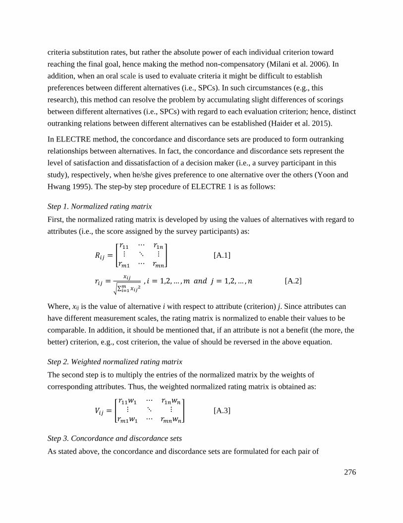
276

criteria substitution rates, but rather the absolute power of each individual criterion toward

reaching the final goal, hence making the method non-compensatory (Milani et al. 2006). In

addition, when an oral scale is used to evaluate criteria it might be difficult to establish

preferences between different alternatives (i.e., SPCs). In such circumstances (e.g., this

research), this method can resolve the problem by accumulating slight differences of scorings

between different alternatives (i.e., SPCs) with regard to each evaluation criterion; hence, distinct

outranking relations between different alternatives can be established (Haider et al. 2015).

In ELECTRE method, the concordance and discordance sets are produced to form outranking

relationships between alternatives. In fact, the concordance and discordance sets represent the

level of satisfaction and dissatisfaction of a decision maker (i.e., a survey participant in this

study), respectively, when he/she gives preference to one alternative over the others (Yoon and

Hwang 1995). The step-by step procedure of ELECTRE 1 is as follows:

Step 1. Normalized rating matrix

First, the normalized rating matrix is developed by using the values of alternatives with regard to

attributes (i.e., the score assigned by the survey participants) as:

𝑅𝑖𝑗 = [

𝑟11 ⋯ 𝑟1𝑛⋮ ⋱ ⋮𝑟𝑚1 ⋯ 𝑟𝑚𝑛

] [A.1]

𝑟𝑖𝑗 =𝑥𝑖𝑗

√∑ 𝑥𝑖𝑗2𝑚

𝑖=1

, 𝑖 = 1,2, … ,𝑚 𝑎𝑛𝑑 𝑗 = 1,2, … , 𝑛 [A.2]

Where, xij is the value of alternative i with respect to attribute (criterion) j. Since attributes can

have different measurement scales, the rating matrix is normalized to enable their values to be

comparable. In addition, it should be mentioned that, if an attribute is not a benefit (the more, the

better) criterion, e.g., cost criterion, the value of should be reversed in the above equation.

Step 2. Weighted normalized rating matrix

The second step is to multiply the entries of the normalized matrix by the weights of

corresponding attributes. Thus, the weighted normalized rating matrix is obtained as:

𝑉𝑖𝑗 = [

𝑟11𝑤1 ⋯ 𝑟1𝑛𝑤𝑛⋮ ⋱ ⋮

𝑟𝑚1𝑤1 ⋯ 𝑟𝑚𝑛𝑤𝑛] [A.3]

Step 3. Concordance and discordance sets

As stated above, the concordance and discordance sets are formulated for each pair of

277

alternatives Ap and Aq (p, q = 1, 2, …, m, and p ≠ q). The concordance set includes all attributes

for which Ap is preferred to Aq, can be expressed as:

𝐶(𝑝, 𝑞) = {𝑗|𝑣𝑝𝑗 ≥ 𝑣𝑞𝑗} [A.4]

Where vpj is the weighted normalized rating of alternative Ap with respect to the jth attribute

(Equation [A.3]). In other words, C(p, q) is the collection of attributes where Ap is better than or

equal Aq.

The discordance set, D(p, q), which is the compliment of concordance set, comprises all

attributes for which Ap is worse than Aq and can be stated as:

𝐷(𝑝, 𝑞) = {𝑗|𝑣𝑝𝑗 < 𝑣𝑞𝑗} [A.5]

Step 4. Concordance and discordance indices

The concordance index, Cpq, represents the relative power of each concordance set. In other

words, Cpq indicates the degree of confidence in the pairwise judgment of two alternatives (Ap →

Aq) and can be computed as:

𝐶𝑝𝑞 = ∑ 𝑤𝑗∗𝑗∗ [A.6]

Where j* are attributes included in the concordance set, i.e., j* ϵ C(p, q). In fact, Cpq, is the sum of

the weights of all attributes contained in Equation [A.4].

Conversely, the discordance index (Dpq), represents the relative power of each discordance set

and measures the degree of disagreement in pairwise judgment, Ap → Aq. Two main equations

have been proposed for Dpq. According to Yoon and Hwang (1995), Dpq can be calculated as:

𝐷𝑝𝑞 =(∑ |𝑣𝑝𝑗∗−𝑣𝑞𝑗∗|)𝑗∗

(∑ |𝑣𝑝𝑗−𝑣𝑞𝑗|)𝑗 [A.7]

Where j ϵ (1, 2,…, n) and j* are attributes that contained in the discordance set, i.e., j* ϵ D (p, q).

Dpq can also be obtained by the following equation (Milani et al. 2006; Collette and Siarry 2003):

𝐷𝑝𝑞 =𝑚𝑎𝑥𝑗∗ |𝑣𝑝𝑗∗−𝑣𝑞𝑗∗|

𝑚𝑎𝑥𝑗 |𝑣𝑝𝑗−𝑣𝑞𝑗| [A.8]

In this study, Equation [A.7] was used to calculate Dpq values.

Step 5. Outranking relationships

The power of the dominance relationship of alternative Ap over alternative Aq depends on how

high is the concordance index (Cpq) and how low is the discordance index (Dpq). The outranking

relationships are built by comparing the concordance and discordance indices with specified

278

limits (thresholds) for concordance and discordance. In fact, Ap outranks Aq if:

𝐶𝑝𝑞 ≥ 𝑐 [A.9]

and

𝐷𝑝𝑞 < 𝑑 [A.10]

Where 𝑐 and 𝑑 are the concordance and discordance thresholds, respectively. The more severe

the threshold values, the more difficult it is to pass the tests. The values of 𝑐 and 𝑑 can be

calculated based on the results of Cpq and Dpq, or constant values chosen by the decision

maker/analyst. For example, Yoon and Hwang (1995) defined 𝑐 and 𝑑 as the averages of Cpq and

Dpq values, respectively, while Collette and Siarry (2003) suggested 𝑐 = 0.7 and 𝑑 = 0.3.

By defining the threshold values 𝑐 and 𝑑, the outranking relationships between alternatives can

be established. However, the impact of the selected threshold values upon the ultimate ranking

can be significant and this is one of the weaknesses of the ELECTRE 1 method (Yoon and

Hwang 1995). Therefore, to avoid defining the threshold values, a complementary version of

ELECTRE 1 was introduced by Van Delft and Nijkamp (1976) by defining net concordance and

net discordance indices for each alternative. The net concordance and discordance indices

provide an effective numerical measure to sort all the alternatives from the best to the worst

(Haider et al. 2014). The complementary analysis of the ELECTRE 1 method is described below

as the last step of the calculations.

Step 6. Net outranking relationships for ranking the alternatives

As stated above, through this last step, the overall ranks of alternatives are established using the

net outranking relationships; therefore, the selection process of suitable alternatives becomes

easier. The net outranking relationships are obtained by calculating the net concordance and the

net discordance indices for each alternative. The net concordance index (Cp) estimates the degree

to which the dominance of an alternative (e.g., Ap) over all other alternatives exceeds the

dominance of other alternatives over the given alternative. Cp can be computed as: thereof

𝐶𝑝 = ∑ 𝐶𝑝𝑘𝑚𝑘=1 − ∑ 𝐶𝑘𝑝;

𝑚𝑘=1 𝑘 ≠ 𝑝 [A.11]

Similarly, the net discordance (Dp) indicates the relative feebleness of an alternative with regard

to the others and can be calculated as:

𝐷𝑝 = ∑ 𝐷𝑝𝑘𝑚𝑘=1 − ∑ 𝐷𝑘𝑝;

𝑚𝑘=1 𝑘 ≠ 𝑝 [A.12]

By calculating and checking the values of Cp and Dp for all the alternatives, the net outranking

relationships can be developed and thereof final ranking of the alternatives is established.

279

Namely, the higher Cp and lower Dp values control the final ranking order of the alternatives. In

other words, the alternative with the maximum Cp and minimum Dp values is the most preferred

alternative, and the other alternatives are ranked accordingly.

A.4 Ranking the SPC categories

As stated earlier, the data collected from the surveys along with the weights of the evaluation

criteria were analyzed to rank the SPCs. The ELECTRE 1 steps were carefully followed for each

sustainability category to separately determine the overall rank of the environmental, economic,

and social SPCs.

The overall rank order of each SPC within the environmental, economic, and social categories

are presented in Table A.1, Table A.2, and Table A.3, respectively. Each SPC was ranked within

its associated category based on its net concordance and net discordance indices (Cp and Dp). In

the cases of some SPCs such as EP, the ranking of net concordance and net discordance are

consistent (identical); therefore, finding the overall rank order of these SPCs is not difficult.

However, some discrepancies were recognized in the cases of other SPCs as their net

concordance ranks were different from their net discordance ranks (e.g., CWM and MCC);

consequently, this is a challenge to determine the final ranking of these criteria. Following the

step 6 of ELECTRE method above, this issue can be addressed by plotting the SPCs using their

net concordance vs. net discordance values, as shown in Figure A.1a. By projecting the SPCs on

the -45° line, and eventually, calculating the distance of the projected points from the origin, final

ranking of alternatives can be obtained. For those SPCs located in the fourth quadrant, higher

distances means better ranks. Contrary, in the cases of SPCs located in the second quadrant,

lower distances indicate better ranks. Hence, by calculating and comparing these distances, all

the SPCs alternatives were ranked as reflected in the last column of Table A.1.

Similarly, based on the values of Cp and Dp indices, the economic SPCs were ranked (Table A.2

and Figure A.1b). Despite the environmental SPCs, almost all the economic SPCs were

consistent in terms of their Cp and Dp rankings (except DB and IM).

In the case of the social category, for majority of the social SPCs, the net concordance and net

discordance rankings were identical. The only inconsistencies were noted in AB and ILE. The

final ranking of these two SPCs were determined by using Figure A.1c and comparing the

distance of each SPC from the origin.

280

Figure A.1 Net Concordance (Cp) and net discordance (Dp) indices for SPCs; (a) Environmental

category; (b) Economic category; (c) Social category. Reproduced from Kamali et al. (2018). Used

with permission from © Elsevier

Table A.1 Net outranking of the environmental sustainability performance criteria

SPC Cp Dp Ranking

of Cp

Ranking

of Dp

Final ranking

of SPC

Energy performance and efficiency strategies (EP) 9.807 -10.773 1 1 1

Construction waste management (CWM) 7.772 -8.178 3 2 2

Material consumption in construction (MCC) 7.807 -8.008 2 3 3

Site disruption and appropriate strategies (SD) 0.983 -3.014 4 4 4

Renewable & environmentally preferable products (REP) -0.174 -0.127 5 5 5

Greenhouse gas emissions (GE) -0.840 1.145 6 7 6

Renewable energy use (RE) -1.772 1.139 7 6 7

Regional (local) materials (RM) -6.176 6.837 9 9 8

Site selection (SS) -6.809 6.645 10 8 9

Water and wastewater efficiency strategies (WE) -5.832 7.860 8 10 10

Alternative transportation (AT) -6.994 7.876 11 11 11


281

Table A.2 Net outranking of the economic sustainability performance criteria

SPC Cp Dp Ranking

of Cp

Ranking

of Dp

Final ranking

of SPC

Design and construction time (DCT) 7.604 -7.583 1 1 1

Design and construction costs (DCC) 6.396 -6.417 2 2 2

Investment and related risks (IRR) 1.614 -3.478 4 3 3

Durability of building (DB) 2.203 -1.540 3 4 4

Integrated management (IM) 1.186 -0.736 5 5 5

Operational costs (OC) -2.587 3.333 6 6 6

Adaptability of building (AB) -3.420 3.564 7 7 7

Maintenance costs (MC) -4.995 4.875 8 8 8

End of life costs (EC) -8.000 8.000 9 9 9


Table A.3 Net outranking of the social sustainability performance criteria

SPC Cp Dp Ranking

of Cp

Ranking

of Dp

Final ranking

of SPC

Workforce health and safety (WHS) 9.386 -10.360 1 1 1

Safety and security of building (SSB) 8.418 -9.238 2 2 2

Affordability (A) 5.619 -6.038 3 3 3

Community disturbance (CD) 5.361 -5.292 4 4 4

Functionality and usability of the physical space (FU) 2.409 -3.119 5 5 5

User acceptance and satisfaction (UAS) 0.965 0.760 6 6 6

Aesthetic options and beauty of the building (ABB) -1.980 0.935 8 7 7

Influence on the local economy (ILE) -1.600 2.330 7 8 8

Neighborhood accessibility and amenities (NAA) -3.953 4.491 9 9 9

Health, comfort and well-being of occupants (HO) -6.599 7.078 10 10 10

Influence on local social development (ISD) -8.012 8.080 11 11 11

Cultural and heritage conservation (CHC) -10.002 10.372 12 12 12


As an example, the ELECTRE calculations for the economic SPC category have been included

in the following section.

A.5 Calculation example for final ranking of the economic SPCs

Based on the literature review, interviews, and screening process, 9 SPCs were selected as

potential representatives of the economic sustainability. Then, the construction experts evaluated

these SPCs against applicability, data availability, and data accuracy. Table A.4 shows the

resulting rating matrix. As stated in Section 2.1.2 of this main manuscript, the weights of the

evaluation criteria were allocated using a group decision making process and AHP method.

Accordingly, the normalized weighted rating matrix was developed using Equations [A.1], [A.2],

and [A.3] as presented in Table A.5.

282

Table A.4 The rating matrix for the economic category

SPC Applicability (CI) Data availability (CII) Data accuracy (CIII)

Design and construction time (DCT) 4.37 2.41 2.38

Design and construction costs (DCC) 4.32 2.35 2.41

Operational costs (OC) 3.80 1.88 1.88

Maintenance costs (MC) 3.73 1.82 1.94

End of life costs (EC) 3.32 1.65 1.59

Durability of building (DB) 3.93 1.94 1.94

Investment and related risks (IRR) 3.85 2.18 2.19

Adaptability of building (AB) 3.78 1.76 2.00

Integrated management (IM) 3.88 1.88 2.00


Table A.5 The normalized weighted rating matrix for the economic category

SPC Applicability (CI) Data availability (CII) Data accuracy (CIII)

Weights of the evaluation criteria (%) 59.65 20.54 19.81

Design and construction time (DCT) 0.223 0.082 0.076

Design and construction costs (DCC) 0.220 0.080 0.078

Operational costs (OC) 0.194 0.064 0.061

Maintenance costs (MC) 0.190 0.062 0.063

End of life costs (EC) 0.169 0.056 0.051

Durability of building (DB) 0.200 0.066 0.063

Investment and related risks (IRR) 0.197 0.074 0.070

Adaptability of building (AB) 0.193 0.060 0.064

Integrated management (IM) 0.198 0.064 0.064


Using the normalized weighted values of the SPCs (Table A.5), Equation [A.4], and Equation

[A.5], the concordance and discordance sets are obtained as shown in Tables A.6 and A.7.

In the next step, using Equation [A.6], Equation [A.7], and the results of concordance and

discordance sets, the concordance and discordance indices were developed for all the SPCs and

presented in Tables A.8 and A.9.

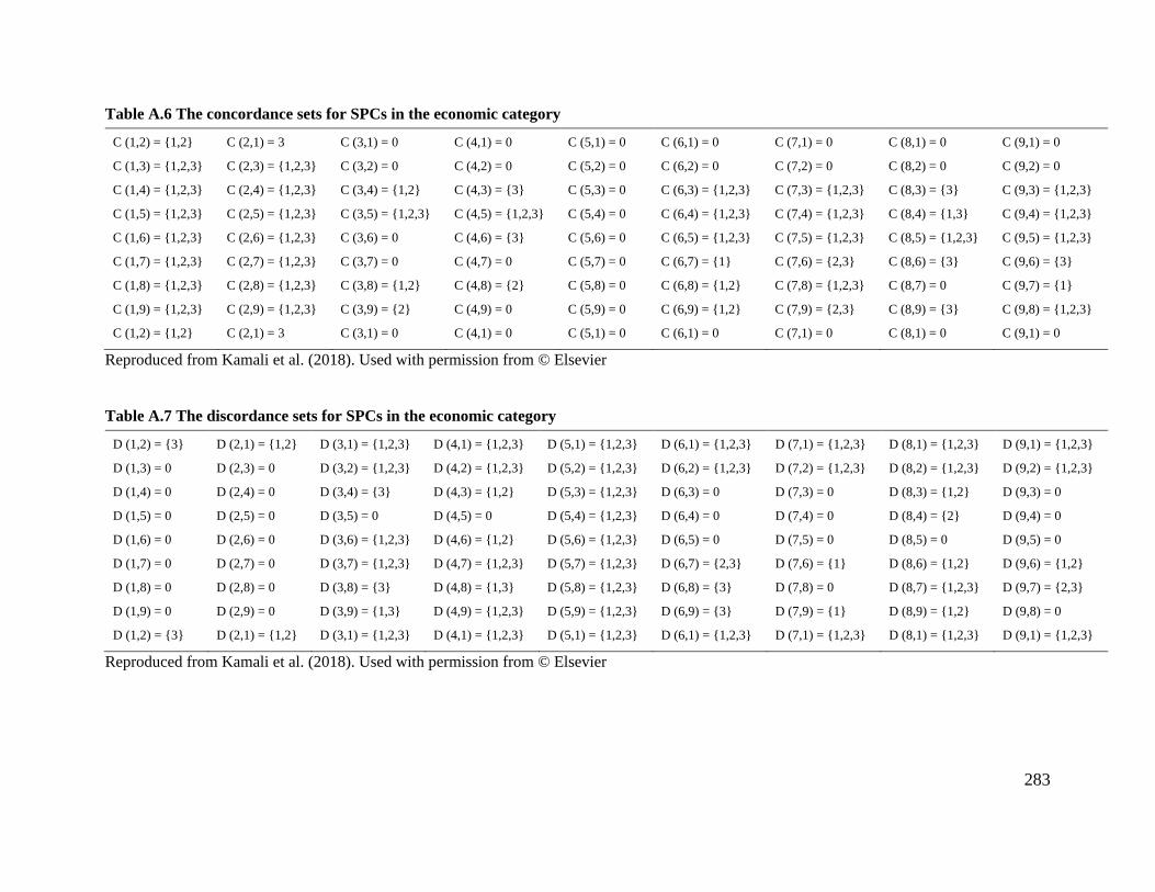
283

Table A.6 The concordance sets for SPCs in the economic category

C (1,2) = {1,2} C (2,1) = 3 C (3,1) = 0 C (4,1) = 0 C (5,1) = 0 C (6,1) = 0 C (7,1) = 0 C (8,1) = 0 C (9,1) = 0

C (1,3) = {1,2,3} C (2,3) = {1,2,3} C (3,2) = 0 C (4,2) = 0 C (5,2) = 0 C (6,2) = 0 C (7,2) = 0 C (8,2) = 0 C (9,2) = 0

C (1,4) = {1,2,3} C (2,4) = {1,2,3} C (3,4) = {1,2} C (4,3) = {3} C (5,3) = 0 C (6,3) = {1,2,3} C (7,3) = {1,2,3} C (8,3) = {3} C (9,3) = {1,2,3}

C (1,5) = {1,2,3} C (2,5) = {1,2,3} C (3,5) = {1,2,3} C (4,5) = {1,2,3} C (5,4) = 0 C (6,4) = {1,2,3} C (7,4) = {1,2,3} C (8,4) = {1,3} C (9,4) = {1,2,3}

C (1,6) = {1,2,3} C (2,6) = {1,2,3} C (3,6) = 0 C (4,6) = {3} C (5,6) = 0 C (6,5) = {1,2,3} C (7,5) = {1,2,3} C (8,5) = {1,2,3} C (9,5) = {1,2,3}

C (1,7) = {1,2,3} C (2,7) = {1,2,3} C (3,7) = 0 C (4,7) = 0 C (5,7) = 0 C (6,7) = {1} C (7,6) = {2,3} C (8,6) = {3} C (9,6) = {3}

C (1,8) = {1,2,3} C (2,8) = {1,2,3} C (3,8) = {1,2} C (4,8) = {2} C (5,8) = 0 C (6,8) = {1,2} C (7,8) = {1,2,3} C (8,7) = 0 C (9,7) = {1}

C (1,9) = {1,2,3} C (2,9) = {1,2,3} C (3,9) = {2} C (4,9) = 0 C (5,9) = 0 C (6,9) = {1,2} C (7,9) = {2,3} C (8,9) = {3} C (9,8) = {1,2,3}

C (1,2) = {1,2} C (2,1) = 3 C (3,1) = 0 C (4,1) = 0 C (5,1) = 0 C (6,1) = 0 C (7,1) = 0 C (8,1) = 0 C (9,1) = 0


Table A.7 The discordance sets for SPCs in the economic category

D (1,2) = {3} D (2,1) = {1,2} D (3,1) = {1,2,3} D (4,1) = {1,2,3} D (5,1) = {1,2,3} D (6,1) = {1,2,3} D (7,1) = {1,2,3} D (8,1) = {1,2,3} D (9,1) = {1,2,3}

D (1,3) = 0 D (2,3) = 0 D (3,2) = {1,2,3} D (4,2) = {1,2,3} D (5,2) = {1,2,3} D (6,2) = {1,2,3} D (7,2) = {1,2,3} D (8,2) = {1,2,3} D (9,2) = {1,2,3}

D (1,4) = 0 D (2,4) = 0 D (3,4) = {3} D (4,3) = {1,2} D (5,3) = {1,2,3} D (6,3) = 0 D (7,3) = 0 D (8,3) = {1,2} D (9,3) = 0

D (1,5) = 0 D (2,5) = 0 D (3,5) = 0 D (4,5) = 0 D (5,4) = {1,2,3} D (6,4) = 0 D (7,4) = 0 D (8,4) = {2} D (9,4) = 0

D (1,6) = 0 D (2,6) = 0 D (3,6) = {1,2,3} D (4,6) = {1,2} D (5,6) = {1,2,3} D (6,5) = 0 D (7,5) = 0 D (8,5) = 0 D (9,5) = 0

D (1,7) = 0 D (2,7) = 0 D (3,7) = {1,2,3} D (4,7) = {1,2,3} D (5,7) = {1,2,3} D (6,7) = {2,3} D (7,6) = {1} D (8,6) = {1,2} D (9,6) = {1,2}

D (1,8) = 0 D (2,8) = 0 D (3,8) = {3} D (4,8) = {1,3} D (5,8) = {1,2,3} D (6,8) = {3} D (7,8) = 0 D (8,7) = {1,2,3} D (9,7) = {2,3}

D (1,9) = 0 D (2,9) = 0 D (3,9) = {1,3} D (4,9) = {1,2,3} D (5,9) = {1,2,3} D (6,9) = {3} D (7,9) = {1} D (8,9) = {1,2} D (9,8) = 0

D (1,2) = {3} D (2,1) = {1,2} D (3,1) = {1,2,3} D (4,1) = {1,2,3} D (5,1) = {1,2,3} D (6,1) = {1,2,3} D (7,1) = {1,2,3} D (8,1) = {1,2,3} D (9,1) = {1,2,3}


284

Table A.8 The concordance index for SPCs in the economic category

Cpq 1 2 3 4 5 6 7 8 9

1 - 0.802 1.000 1.000 1.000 1.000 1.000 1.000 1.000

2 0.198 - 1.000 1.000 1.000 1.000 1.000 1.000 1.000

3 0.000 0.000 - 0.802 1.000 0.000 0.000 0.802 0.205

4 0.000 0.000 0.198 - 1.000 0.198 0.000 0.205 0.000

5 0.000 0.000 0.000 0.000 - 0.000 0.000 0.000 0.000

6 0.000 0.000 1.000 1.000 1.000 - 0.597 0.802 0.802

7 0.000 0.000 1.000 1.000 1.000 0.404 - 1.000 0.404

8 0.000 0.000 0.198 0.795 1.000 0.198 0.000 - 0.198

9 0.000 0.000 1.000 1.000 1.000 0.198 0.597 1.000 -


Table A.9 The discordance index for SPCs in the economic category

Dpq 1 2 3 4 5 6 7 8 9

1 - 0.208 0.000 0.000 0.000 0.000 0.000 0.000 0.000

2 0.792 - 0.000 0.000 0.000 0.000 0.000 0.000 0.000

3 1.000 1.000 - 0.248 0.000 1.000 1.000 0.418 1.000

4 1.000 1.000 0.752 - 0.000 1.000 1.000 0.685 1.000

5 1.000 1.000 1.000 1.000 - 1.000 1.000 1.000 1.000

6 1.000 1.000 0.000 0.000 0.000 - 0.811 0.123 0.296

7 1.000 1.000 0.000 0.000 0.000 0.189 - 0.000 0.072

8 1.000 1.000 0.582 0.315 0.000 0.877 1.000 - 1.000

9 1.000 1.000 0.000 0.000 0.000 0.704 0.928 0.000 -


Using the concordance and discordance indices, Equation [A.11] and Equation [A.12], the net

concordance index (Cp) and net discordance index (Dp) for all the SPCs were calculated;

consequently, the net outranking relationships were developed. The net concordance and

discordance indices and the net outranking of the economic sustainability performance criteria

have presented earlier in this appendix (Table A.2) and not repeated here.

A.6 Sensitivity analysis

In addition to the weight set assigned through the AHP-based group decision making process

(WSGDM), two additional hypothetical weight sets were applied to examine the sensitivity of the

SPC ranking results to the weights of the evaluation criteria as:

WS1: applicability (70%), data availability (15%), data accuracy (15%)

WS2: applicability (50%), data availability (25%), data accuracy (25%)

Compared to WSGDM (i.e., applicability: 59.65%, data availability: 20.54%, and data accuracy:

285

19.81%), in WS1, more weight was assigned to the applicability criterion, contrary to the case of

WS2 where the weights of data availability and data accuracy criteria were increased. Results of

repeating the ELECTRE analyses for each sustainability category using the three different

weight sets are presented in Figure A.2.

Figure A.2 Net outranking of (a) Environmental category; (b) Economic category; (c) Social

category, for different weight sets of the evaluation criteria. Reproduced from Kamali et al. (2018).

Used with permission from © Elsevier

It can be seen from the net outranking of the SPCs that changing the established weights of the

evaluation criteria (WSGDM) within at least the defined range (WS1↔WS2), does not affect the

rankings of the economic and social SPCs (FigureA.2b and Figure A.2c). In other words, all the

economic and social SPCs were assigned identical ranks using the three weight sets except CD

and A with rank orders of third and fourth for WS1 (they are fourth and third, respectively, for

both WSGDM and WS2).

In contrast, as Figure A.2a demonstrates, there are some minor discrepancies between the

environmental SPC rankings when using the different weight sets. Yet, these inconsistencies

286

cannot be significant because (1) all the SPC rankings follow the same trend, which means when

switching from a WS to another, the rank order of a SPC changed locally; and (2) there is no

change in the rank order of the top priority SPCs (i.e., EP, CWM, and MC) for all three WSs.

287

Appendix B: First Step Study

In this appendix, the results of the first step study to estimate population variances for sample

size determination of Survey A including the respondents’ scores and the standard deviations for

the environmental, economic, and social SPC categories are presented.

Table B.1 Standard deviations (σ) of scores for the environmental SPC category

Sample #

Score of SPC

SS AT SD RE EP WE RM REP CWM GE MCC

1 3 2 2 3 4 3 2 3 3 3 5

2 2 4 2 4 4 3 4 4 5 4 5

3 3 2 5 3 5 3 3 3 3 2 3

4 4 4 4 3 4 4 4 4 5 4 4

5 4 3 4 5 4 4 3 4 4 4 3

6 3 2 4 5 4 3 5 3 4 4 2

7 2 2 4 3 4 2 4 4 5 3 4

8 3 4 4 3 3 2 3 3 5 3 4

9 3 4 5 2 4 4 3 3 4 3 3

10 3 2 3 4 4 3 3 4 5 5 4

11 4 3 4 3 5 4 5 4 4 4 4

12 3 3 4 3 3 3 2 3 3 4 5

13 2 3 4 3 5 1 4 3 5 5 5

σ 0.71 0.86 0.93 0.87 0.64 0.91 0.96 0.52 0.83 0.85 0.95

Table B.2 Standard deviations (σ) of scores for the economic SPC category

Sample #

Score of SPC

DCT DCC OC MC EC DB IRR AB IM

1 5 5 3 3 3 3 4 3 3

2 5 5 4 4 3 5 5 5 5

3 4 4 4 4 3 3 3 3 3

4 4 4 4 3 3 4 4 3 4

5 4 3 4 3 3 4 4 3 5

6 5 4 4 2 5 4 4 5 5

7 5 5 3 3 3 4 4 4 4

8 5 4 3 3 5 3 4 2 4

9 4 4 3 3 2 4 2 4 3

10 5 5 5 3 3 5 4 4 4

11 4 4 4 5 5 5 4 4 3

12 5 4 1 1 3 2 4 2 3

13 5 5 3 3 3 5 4 3 5

σ 0.51 0.63 0.96 0.95 0.96 0.95 0.69 0.96 0.86

288

Table B.3 Standard deviations (σ) of scores for the social SPC category

Sample #

Score of SPC

HO ILE FU ABB WHS CD ISD CHS A SSB UAS NAA

1 5 3 3 3 5 4 2 3 4 4 4 3

2 4 4 4 4 5 4 4 4 4 5 5 4

3 4 3 3 3 3 3 3 3 4 4 3 3

4 4 4 4 4 4 4 4 4 4 4 4 4

5 3 2 3 3 4 3 2 3 5 5 3 2

6 5 5 3 5 5 5 3 1 5 5 5 3

7 3 4 2 3 4 4 3 3 3 4 3 3

8 3 4 3 4 5 4 3 3 3 4 3 3

9 4 3 4 4 5 4 4 3 3 5 4 4

10 3 3 4 4 5 5 4 1 3 5 2 5

11 5 4 4 5 4 4 3 4 5 4 4 4

12 3 3 4 2 5 4 3 3 4 3 2 3

13 5 4 4 4 5 5 3 3 4 5 4 3

σ 0.86 0.78 0.66 0.85 0.66 0.64 0.69 0.95 0.76 0.65 0.96 0.77

289

Appendix C: TOPSIS MCDA Method

In this appendix, the step-by step procedure of the TOPSIS MCDA method used in this research

has been described (adapted from Yoon and Hwang (1995)).

Step 1. Weights of SPIs

The relative importance weights of the sustainability performance indicators (SPIs) under each

sustainability performance criterion (SPC) should be determined.

Step 2. Normalized SPIs

Once the SPIs are calculated (performance score or xij), if the xij values are not already

normalized, they need to be normalized (rij). The vector normalization can be used for

normalization:

𝑟𝑖𝑗 =𝑥𝑖𝑗

√∑ 𝑥𝑖𝑗2𝑚

𝑖=1

𝑖 = 1,… ,𝑚 𝑗 = 1,… , 𝑛 [C.1]

Step 3. Weighted normalized matrix

The weighted normalized matrix should be developed. The weighted normalized performance

score of each SPI is calculated as:

𝑣𝑖𝑗 = 𝑤𝑗𝑟𝑖𝑗 [C.2]

where wj = corresponding weight of that SPI.

Step 4. Positive-Ideal and Negative-Ideal Solutions

In this step, the positive-ideal solution (PIS) and negative-ideal solution (NIS) are identified. X+

and X− are defined as the PIS and NIS, respectively, in terms of weighted performance scores as

follows:

𝑋+ = {𝑣1+, 𝑣2

+, … , 𝑣𝑗+, … , 𝑣𝑛

+} = {(𝑚𝑎𝑥𝑖𝑣𝑖𝑗|𝑗𝜖𝐽1), (𝑚𝑖𝑛𝑖𝑣𝑖𝑗|𝑗𝜖𝐽2), 𝑖 = 1,2, … ,𝑚} [C.3]

𝑋− = {𝑣1−, 𝑣2

−, … , 𝑣𝑗−, … , 𝑣𝑛

−} = {(𝑚𝑖𝑛𝑖𝑣𝑖𝑗|𝑗𝜖𝐽1), (𝑚𝑎𝑥𝑖𝑣𝑖𝑗|𝑗𝜖𝐽2), 𝑖 = 1,2, … ,𝑚} [C.4]

where J1 = set of benefit attributes; and J2 = set of cost attributes.

Step 5. Separation measures

In this step, the distance of the subject building from PIS and NIS values (i.e., separation

measures) is calculated. The distances of all the performance levels of SPIs associated with a SPC

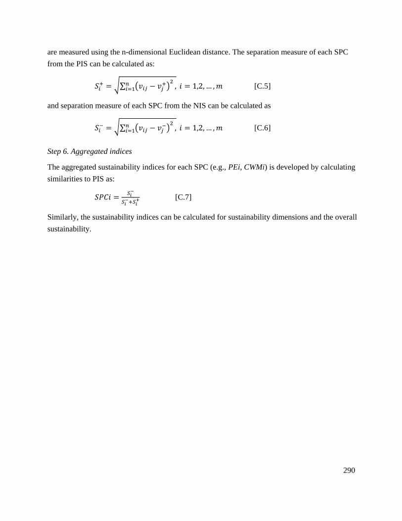
290

are measured using the n-dimensional Euclidean distance. The separation measure of each SPC

from the PIS can be calculated as:

𝑆𝑖+ = √∑ (𝑣𝑖𝑗 − 𝑣𝑗

+)2𝑛

𝑖=1 , 𝑖 = 1,2,… ,𝑚 [C.5]

and separation measure of each SPC from the NIS can be calculated as

𝑆𝑖− = √∑ (𝑣𝑖𝑗 − 𝑣𝑗

−)2𝑛

𝑖=1 , 𝑖 = 1,2,… ,𝑚 [C.6]

Step 6. Aggregated indices

The aggregated sustainability indices for each SPC (e.g., PEi, CWMi) is developed by calculating

similarities to PIS as:

𝑆𝑃𝐶𝑖 =𝑆𝑖−

𝑆𝑖−+𝑆𝑖

+ [C.7]

Similarly, the sustainability indices can be calculated for sustainability dimensions and the overall

sustainability.

291

Appendix D: Establishment of a Suitable PLF for ‘Construction waste reuse’

Although many studies mentioned that ‘reuse’ is an important CWM strategy, rare studies

provided the quantification and evaluation of the strategy in a building project. Green Globes is

one of the rating systems that addressed the reuse of buildings’ parts and components. It

classified and scored the ‘reuse’ implementation according to the reused elements and

components of an existing building in a new building project (GBI 2014; GBI 2015). However,

this classification and evaluation standards have been provided for multi-family residential

multifamily buildings (EPA 2018b). Therefore, the provided standards have been adjusted to fit

single-family buildings with the help of experts in this research. A total of three sub-SPIs have

been recognized for this SPI: ‘CWM3-1 Reuse of façades’, ‘CWM3-2 Reuse of structural

systems’, and ‘CWM3-3 Reuse of non-structural elements’.

Reuse of façades (CWM3-1)

This sub-SPI addresses the reuse the existing building’s façades at the end of its lifetime in

another building projects. The percentage of the façade from an existing building that is retained

and incorporated in the new building design is calculated as (GBI 2015):

ReFa = 100 × A/B [D.1]

Where ReFa is the percentage of the reused façade, A is the area of retained façade reused in the

new building, and B is the total area of the new building’s façade.

A building shows its least and best performances with respect to this sub-SPI when the ReFa

came to be 10% and 50%, respectively. Therefore, the PLF to calculate the performance level of

CWM3-1 is:

PLCWM3-1 = 250(𝑅𝑒𝐹𝑎) − 25 10% ≤ 𝑅𝑒𝐹𝑎 ≤ 50% [D.2]

Reuse of structural systems (CWM3-2)

Structural systems refer to the load-resisting system of a building (other than the building

envelope) that transfers loads to the foundation though interconnected structural components or

members. In some cases, the structural systems of the existing building at the end of its life can

be retained and reused in another building project. The percentage of the reused structural

components or members in a new building design can be calculated as (GBI 2015):

ReSt = 100 × A/B [D.3]

Where ReSt is the percentage of the reused structural systems, A is the volume of the reused

structural components or members in the new building, and B is the total volume of the new

292

building’s structural systems.

A building shows its least and best performances with respect to this CWM3-2 when the ReSt

reaches 10% and 60%, respectively. Therefore, the PLF to calculate the performance level of the

sub-SPI is presented as:

PLCWM3-2 = 200(𝑅𝑒𝑆𝑡) − 20 10% ≤ 𝑅𝑒𝑆𝑡 ≤ 60% [D.4]

Reuse of non-structural elements (CWM3-3)

CWM3-3 seeks the reuse of the existing non-structural elements such as interior ceilings, interior

partitions, furnishings and/or demountable walls, in a new building design.

The percentage of the reused non-structural elements in a new building design can be calculated

as (GBI 2015):

ReNSt = 100 × A/B [D.5]

Where ReNSt is the percentage of the reused structural systems, A is the area of the reused non-

structural elements in the new building, and B is the total area of the non-structural element in

the new building. Areas are calculated as the projected area of the element. For example, if an

interior partition is re-used, the area is calculated as length × height of the wall.

Similar to the case of the previous sub-SPI, the new building performs excellent with respect to

this sub-SPI by incorporating up to 60% non-structural elements from the older projects.

Subsequently, the following PLF can be used to calculate the performance level of CWM3-3:

PLCWM3-3 = 200(𝑅𝑒𝑁𝑆𝑡) − 20 10% ≤ 𝑅𝑒𝑁𝑆𝑡 ≤ 60% [D.6]

The performance level of the parent CWM3 SPI is calculated based on the performance levels of

the three associated sub-SPIs and their weights. The weights of CWM3-1, CWM3-2, and CWM3

have been determined as 0.374, 0.313, and 0.313, respectively (GBI 2015). Thus, the following

PLF was can be used to calculate CWM3 performance of the subject building:

PLCWM3 = 0.374×PLCWM3-1 + 0.313×PLCWM3-2 + 0.313×PLCWM3-3 [D.7]

293

Appendix E: Renewable Energy Sources and Net-zero Energy Buildings

Renewable energy is derived from natural processes that are replenished at an equal or faster rate

than the rate at which they are consumed (except biomass). There are various forms of renewable

energy, deriving directly or indirectly from the sun or from heat generated deep within the earth

(NRC 2017d). There are five commonly used renewable energy sources (EIA 2018):

Biomass. Biomass is organic material that comes from plants and animals. Biomass contains

stored energy from the sun. Plants absorb the sun's energy in a process called photosynthesis.

The chemical energy in plants is passed to animals and people after the plants are consumed.

The biomass source includes wood and wood waste, municipal solid waste, landfill gas and

biogas, ethanol, and biodiesel.

Hydropower. Hydropower is electricity produced from flowing water. Hydropower is the

largest renewable energy source for electricity generation in the US.

Geothermal. Geothermal energy is heat from within the earth. This heat can be recovered as

steam or as hot water, and it can be used to heat buildings or to generate electricity.

Wind. Today, wind energy is mainly used to generate electricity energy.

Solar. Solar energy systems use radiation from the sun to produce heat and electricity. There

are three basic categories of solar energy systems: solar thermal systems, solar thermal-

electric power plants, and photovoltaic systems.

Renewable energy plays an important role in reducing greenhouse gas emissions. When

renewable energy sources are used, the demand for finite fossil fuels is reduced. Unlike fossil

fuels, non-biomass renewable sources of energy (i.e., hydropower, geothermal, wind, and solar)

do not directly emit greenhouse gases (NEB 2017; EIA 2018). However, the use of renewable

energy is still limited. For example, about 11% of the total US energy consumption was supplied

by renewable energy sources in 2017 as shown in Figure E.1 (EIA 2018).

A wide range of energy-producing technologies and equipment has been developed over time to

take advantage of these natural resources. As a result, usable energy can be produced in the form

of electricity, industrial heat, thermal energy for space and water conditioning, and transportation

fuels (NRC 2017c). In the case of buildings, renewable energies can be used for space heating,

water heating, and electricity (e.g., lighting, appliances) (NRC 2017c).

The known concept of net-zero energy building (NZEB) (also known as zero-energy building

or zero net energy) is used as a benchmark building in terms of using renewable energy sources.

In a NZEB, the total amount of energy used by the building on an annual basis is roughly equal

to the amount of renewable energy created on the site or by renewable energy sources elsewhere

http://www.eia.gov/energyexplained/?page=biomass_home

http://www.eia.gov/energyexplained/?page=biomass_wood

http://www.eia.gov/energyexplained/?page=biomass_waste_to_energy

http://www.eia.gov/energyexplained/?page=biomass_biogas

http://www.eia.gov/energyexplained/?page=biomass_biogas

http://www.eia.gov/energyexplained/?page=biofuel_ethanol_home

http://www.eia.gov/energyexplained/?page=biofuel_biodiesel_home

http://www.eia.gov/energyexplained/?page=hydropower_home

http://www.eia.gov/energyexplained/?page=geothermal_home

http://www.eia.gov/energyexplained/?page=wind_home

http://www.eia.gov/energyexplained/?page=solar_home

http://www.eia.gov/energyexplained/?page=solar_thermal_collectors

http://www.eia.gov/energyexplained/?page=solar_thermal_power_plants

http://www.eia.gov/energyexplained/?page=solar_photovoltaics

294

(Pless and Torcellini 2010; Peterson et al. 2015; Torcellini et al. 2006).

Figure E.1 US energy consumption by energy source in 2017. Reproduced from EIA (2018). Used

with permission from © U.S. Energy Information Administration

The energy performance of a NZEB can be accounted for or defined in several ways. Torcellini

et al. (2006) developed the following four definitions for a NZEB, each of which has its own

measurement method and metrics:

• Net-Zero Site Energy: A site NZEB produces at least as much RE as it uses in a year, when

accounted for at the site.

• Net-Zero Source Energy: A source NZEB produces or purchases at least as much RE as it

uses in a year, when accounted for at the source.

• Net-Zero Energy Costs: In a cost NZEB, the amount of money the utility pays the building

owner for the RE the building exports to the grid is at least equal to the amount the owner pays

the utility for the energy services and energy used over the year.

• Net-Zero Emissions: A net-zero emissions building produces or purchases enough emissions-

free RE to offset emissions from all energy used in the building annually.

In addition to the above definitions, net-zero energy buildings can be hierarchically classified

(i.e., priority levels). Pless and Torcellini (2010) categorized NZEBs into four classes from the

most priority to the least priority. A building that offsets all its energy use from renewable

resources available within the footprint is on top of the classification (NZEB-A). Contrary, a

building that offsets its energy requirements through a combination of on-site renewables and

off-site purchases is placed at the lowest class (NZEB-D). Although NZEB-A class homes are

technically feasible, but not yet affordable and common for average homebuyers (NRC 2018e).

integrated life cycle sustainability performance assessment

Documents