Integrated Chassis Control and Control Allocation for All ...

 Electronics 2021, 10, 2885. https://doi.org/10.3390/electronics10222885  www.mdpi.com/journal/electronics 

Article 

Integrated Chassis Control and Control Allocation for All 

Wheel Drive Electric Cars with Rear Wheel Steering 

Pai‐Chen Chien and Chih‐Keng Chen * 

Department of Vehicle Engineering, National Taipei University of Technology, Taipei 10604, Taiwan; 

[email protected] 

*  Correspondence: [email protected] 

Abstract: This study investigates a control strategy for torque vectoring (TV) and active rear wheel 

steering  (RWS) using  feedforward  and  feedback  control  schemes  for different  circumstances. A 

comprehensive vehicle and combined slip tire model are used to determine the secondary effect and 

to generate desired yaw acceleration and side slip angle rate. A model‐based feedforward controller 

is designed to improve handling but not to track an ideal response. A feedback controller based on 

close loop observation is used to ensure its cornering stability. The fusion of two controllers is used 

to stabilize a vehicle’s lateral motion. To increase lateral performance, an optimization‐based control 

allocation distributes the wheel torques according to the remaining tire force potential. The simula‐

tion results show that a vehicle with the proposed controller exhibits more responsive lateral dy‐

namic  behavior  and  greater maximum  lateral  acceleration. The  cornering  safety  is  also demon‐

strated using a standard stability test. The driving performance and stability are improved simulta‐

neously by the proposed control strategy and the optimal control allocation scheme. 

Keywords: chassis control; torque vectoring; vehicle dynamics; secondary effect; rear wheel steer‐

ing; control allocation 

1. Introduction 

Various chassis control systems have been studied and developed to increase driving 

dynamics and safety. Growth in safety equipment and demand for space lead to an in‐

crease in modern vehicles’ weight. To improve performance and stability, many control 

systems have been implemented. Yaw motion control for safety, such as an electronic sta‐

bility program (ESP), is generally a standard equipment item. Advanced control systems, 

such as torque vectoring, rear wheel steering and active suspension become popular and 

common because these types of control systems can improve driving performance for a 

vehicle. 

Four‐wheel steering (4WS) or active rear wheel steering (RWS) was introduced in the 

1980s on commercial vehicles. Nowadays,  the  technology  is often used  in high perfor‐

mance or sports vehicles and is available as an optional extra on some passenger vehicles, 

such as Porsche 911. The advantages of RWS are reducing the turning radius at low ve‐

locity and increasing the stability at high velocity by using the additional steering angle 

at the rear axle. 

All wheel drive (AWD) has been adopted for years to improve longitudinal acceler‐

ation performance [1], but it is also possible to control a vehicle’s yaw motion by distrib‐

uting the longitudinal tire forces on each wheel. During cornering, the tire lateral force 

approaches its peak value, but it is still possible to produce longitudinal force. Direct yaw 

moment control  (DYC) or  torque vectoring  (TV) systems control a vehicle’s motion by 

intentionally distributing the wheel driving or braking torques to increase the cornering 

performance at the near‐limit status [2]. In‐wheel motor vehicles are used in sports or race 

cars to increase their efficiency and controllability. Each wheel produces either a driving 

Citation: Chien, P.‐C.; Chen, C.‐K. 

Integrated Chassis Control and   

Control Allocation for All Wheel 

Drive Electric Cars with Rear Wheel 

Steering. Electronics 2021, 10, 2885. 

https://doi.org/10.3390/ 

electronics10222885 

Academic Editor: Carlos Andrés 

García‐Vázquez 

Received: 21 October 2021 

Accepted: 20 November 2021 

Published: 22 November 2021 

Publisher’s Note: MDPI  stays  neu‐

tral  with  regard  to  jurisdictional 

claims in published maps and institu‐

tional affiliations. 

Copyright: © 2021 by the authors. Li‐

censee  MDPI,  Basel,  Switzerland. 

This article  is an open access article 

distributed under the terms and con‐

ditions of the Creative Commons At‐

tribution (CC BY) license (https://cre‐

ativecommons.org/licenses/by/4.0/). 

Electronics 2021, 10, 2885  2  of  19  

or a braking torque independently, without the physical limitations of the traditional me‐

chanical differential systems. 

Rear wheel steering and torque vectoring both produce a yaw moment around the 

vertical axis of the vehicle. Many control methods, such as sliding mode control (SMC) 

[3,4] and linear quadratic regulator (LQR), are investigated, but the approaches of differ‐

ent researches are diverse. Chen [5] used a combination of LQR, integral and feedforward 

control  to eliminate  the effect of steering  input on side slip motion. Peters  [6] used an 

open‐loop controller and a fine‐tuned reference model to achieve precise and reproduci‐

ble behavior under all circumstances, without the synthetic driving feeling from feedback 

controllers. Since TV or DYC controllers are usually model based, and vehicles’ parame‐

ters and road conditions often change significantly, there are some approaches to increas‐

ing system robustness. Kissai [7] synthesized an 𝐻   controller to enhance the control ro‐

bustness against  the uncertainties  in vehicle parameters. Warth  [8] designed a  central 

feedforward control using an extended single‐track model and the input‐output lineari‐

zation method, and made the reference generation adaptive by detecting the important 

parameters of tires. Hang [9] proposed a polytopic model to make the vehicle model adapt 

along with the vehicle velocity and road friction coefficient, and developed a gain‐sched‐

uled robust controller to improve the vehicle’s stability in extreme conditions. Feedfor‐

ward control is widely used for chassis control systems and requires tuning that takes a 

long time. The performance might be degraded by model uncertainties; by contrast it has 

the advantage of being easily tunable and of reproducible behavior, which is important 

for human drivers. Feedback control is more robust against model uncertainties; however, 

it relies on accurate estimation. 

For multi‐input systems, the most popular issue is control allocation (CA). There are 

many approaches to implement the optimal distribution. Mokhiamar [3] proposed an op‐

timum  tire  force distribution method  to optimize  the workload  for  each  tire by using 

equality constraints to eliminate variables, and ensuring the objective function is not sub‐

jected to any constraints. Chen [5] used a weighted pseudo‐inverse to approach the de‐

sired longitudinal acceleration and desired yaw moment. Kissai [10] studied the dynamics 

of actuators and used model predictive control allocation (MPCA) to predict the imminent 

saturation of actuators. Han [11] proposed “equal distribution” to minimize power losses 

and increase energy efficiency. Xiao [12] used a weighted least squares method to deter‐

mine the optimal distribution to minimize control effort. There are many approaches to 

CA for over‐actuated systems. Algebraic solvers require less computational effort; how‐

ever, numerical methods are frequently used to deal with hard constraints such as actua‐

tors’ limitations. 

This study proposes a combined control method to allow sporty driving behavior in 

normal condition and guarantees safety in severe situations. Driving feeling is crucial for 

the human driver. A reproducible linear dependency between the driver’s steering input 

and the lateral acceleration output is preferred for sporty driving sensation. To achieve 

this driving behavior, a model‐based feedforward controller with a reference generator is 

proposed to improve lateral performance instead of tracking an ideal response. This kind 

of controller should take account of the secondary effect, which is proposed in [6], to de‐

scribe the interaction between longitudinal and lateral tie forces. The secondary effect is 

more complex for independent all‐wheel drive vehicles because front and rear axles can 

both produce yaw torque. If a driver makes a mistake or road conditions deteriorate, the 

stability mode uses a feedback controller, intervenes in the vehicle’s motion to reduce its 

instability. The control allocation method maximizes the remaining friction potential in 

the tires and increases performance and safety. 

This study is structured as follows. Section 2 presents the tire and vehicle model and 

the coordinate system for this study. Section 3 details the method to calculate the second‐

ary effect and shows how the secondary effect affects the vehicle’s motion. Section 4 pre‐

sents the control and allocation algorithm in detail. Sections 4.2 and 4.3 detail the struc‐

tures of the feedforward and feedback controllers and Section 4.4 expresses the concept of 

Electronics 2021, 10, 2885  3  of  19  

the controller allocation method. Section 5 presents  the  test procedures and simulation 

results. Section 6 draws conclusions about the control system and details future opportu‐

nities. 

2. Modeling of Lateral Dynamics 

This section presents a complex  tire model, an advanced vehicle dynamics model 

with RWS  and  additional  external  yaw moment  and  a  simplified  single‐track model. 

These are the basics for the following design of controllers. 

The proposed controller uses commands from the driver, an advanced vehicle model 

with individual wheel  loads, and a semi‐empirical tire model based on the methods of 

Pacejka [13] and Burhaumudin [14] to generate the reference responses. 

2.1. Tire Model 

For this study, the secondary effect, which is caused by the interaction between lon‐

gitudinal and lateral forces on the tire, is used for the feedforward controller. Basic mod‐

els, such as linear tire models or the one used in [4], are not sufficient to present the com‐

bined slip characteristic. The semi‐empirical Magic Formula considers all of the relevant 

factors for this study. 

The following simulations use different vertical loads on the tires due to load trans‐

fer, the longitudinal slip and the side slip angle under combined slip situation. Other fac‐

tors, such as temperature and pressure, are assumed to be constant. The equations for the 

longitudinal and lateral force are: 

𝐹 𝐺 𝐷 𝑐𝑜𝑠 𝐶 𝑡𝑎𝑛 𝐵 𝜅 𝐸 𝐵 𝑡𝑎𝑛 𝐵 𝜅   (1) 

𝐹 𝐺 𝐷 𝑐𝑜𝑠 𝐶 𝑡𝑎𝑛 𝐵 𝛼 𝐸 𝐵 𝑡𝑎𝑛 𝐵 𝛼 𝑆   (2) 

The parameters that are used in Equations (1) and (2) are defined in Table 1. 

Table 1. Parameters for the magic formula. 

Parameter  Description 

𝐹  Tire force at the center of contact patch 

𝐺  Weighting function for combined slip 

𝐵  Stiffness factor 

𝐶  Shape factor 

𝐷  Peak factor 

𝐸  Curvature factor 

𝜅  Longitudinal slip ratio 

𝛼  Lateral slip angle 

𝑆   Vertical shift of lateral force 

Parameters B, C, D, E are a function of vertical load  𝐹 , G is a function of longitudinal 

or lateral slip and  𝑆   is related to the wheel camber angle, ply‐steer or conicity. This is 

assumed to be zero for this study. These calculations result in the following equations: 

𝐹 𝑓 𝛼, 𝜅,𝐹   (3) 

𝐹 𝑓 𝛼, 𝜅,𝐹   (4) 

The method to fit the tire model from experimental data is based on the CarSim tire 

tester procedure and a genetic algorithm. Using velocity, vertical load, and the road sur‐

face, the longitudinal slip ratio at different side slip angles and vertical loads are used to 

find the unknown parameters for longitudinal behavior. 

Electronics 2021, 10, 2885  4  of  19  

The blue lines in Figure 1a,b are the experimental data and the red lines represent the 

GA fitting results. The combined slip characteristic is used for this study, which is essen‐

tial for the subsequent research, as shown in Figure 1c,d. 

(a) Longitudinal Force  𝐹   (b) Lateral Force  𝐹  

(c) Combined Slip  𝐹   (𝐹   = 3800 N)  (d) Combined Slip  𝐹   (𝐹   = 3800 N) 

Figure 1. Pacejka tire model. (a) Fitting results, longitudinal force; (b) Fitting results, longitudinal force; and (c,d) Com‐

bined slip characteristic under 3800 N vertical load. 

The transient behavior of a tire is described using the linear first‐order lag element 

(PT ‐element) method [8]. The time constant is converted using the vehicle’s velocity and 

the relaxation length as: 

𝑇 𝐹 𝐹 𝐹 , 𝑇 𝑢 𝐿   (5) 

where  𝐿   is the relaxation  length, as specified  in the CarSim tire model,  𝑇   is the time 

constant and  𝐹   is the steady state tire force. The defined relaxation length is 1/3 of the distance that the tire must roll before tire force is 95% of the steady‐state value. Modeling 

the  transient tire behavior allows  the reference generator  in  the  follow‐up controller to 

account for additional dynamic effects on the driving behavior. 

2.2. Vehicle Dynamics Model 

The vehicle model for this study is defined in ISO coordinates. A definition of vehicle 

coordinates is shown in Figure 2. In the following equations, subscripts  𝑓𝑙, 𝑓𝑟, 𝑟𝑙, 𝑟𝑟  rep‐resent the four different wheels of the vehicle. 

Electronics 2021, 10, 2885  5  of  19  

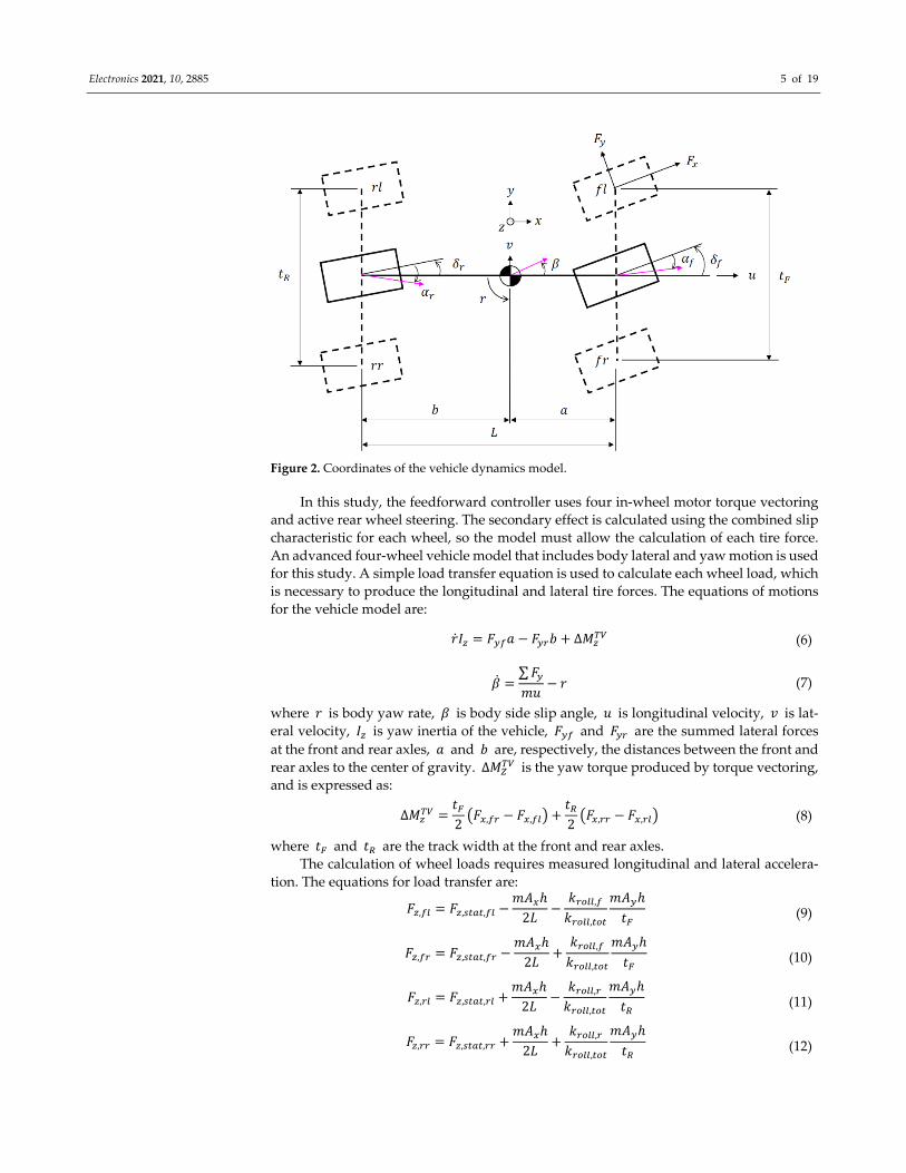
Figure 2. Coordinates of the vehicle dynamics model. 

In this study, the feedforward controller uses four in‐wheel motor torque vectoring 

and active rear wheel steering. The secondary effect is calculated using the combined slip 

characteristic for each wheel, so the model must allow the calculation of each tire force. 

An advanced four‐wheel vehicle model that includes body lateral and yaw motion is used 

for this study. A simple load transfer equation is used to calculate each wheel load, which 

is necessary to produce the longitudinal and lateral tire forces. The equations of motions 

for the vehicle model are: 

𝑟𝐼 𝐹 𝑎 𝐹 𝑏 ∆𝑀   (6) 

𝛽∑𝐹𝑚𝑢

𝑟  (7) 

where  𝑟  is body yaw rate,  𝛽  is body side slip angle,  𝑢  is longitudinal velocity,  𝑣  is lat‐eral velocity,  𝐼   is yaw inertia of the vehicle,  𝐹   and  𝐹   are the summed lateral forces 

at the front and rear axles,  𝑎  and  𝑏  are, respectively, the distances between the front and 

rear axles to the center of gravity.  ∆𝑀   is the yaw torque produced by torque vectoring, 

and is expressed as: 

∆𝑀𝑡2

𝐹 , 𝐹 ,𝑡2

𝐹 , 𝐹 ,   (8) 

where  𝑡   and  𝑡   are the track width at the front and rear axles. 

The calculation of wheel loads requires measured longitudinal and lateral accelera‐

tion. The equations for load transfer are: 

𝐹 , 𝐹 , ,𝑚𝐴 ℎ

2𝐿𝑘 ,

𝑘 ,

𝑚𝐴 ℎ𝑡

  (9) 

𝐹 , 𝐹 , ,𝑚𝐴 ℎ

2𝐿𝑘 ,

𝑘 ,

𝑚𝐴 ℎ𝑡

  (10) 

𝐹 , 𝐹 , ,𝑚𝐴 ℎ

2𝐿𝑘 ,

𝑘 ,

𝑚𝐴 ℎ𝑡

  (11) 

𝐹 , 𝐹 , ,𝑚𝐴 ℎ

2𝐿𝑘 ,

𝑘 ,

𝑚𝐴 ℎ𝑡

  (12) 

Electronics 2021, 10, 2885  6  of  19  

where  𝐹 ,   is the static load on each wheel,  𝐿  is the wheelbase of the vehicle,  ℎ  is the height of the center of gravity,  𝐴   and  𝐴   are  the  longitudinal and lateral acceleration and  𝑘   is the roll stiffness. 

2.3. Simplified Single‐Track Model 

For the feedback controller, a linearized single‐track model is used. In order to sim‐

plify calculations, this model uses the linear tire model to calculate the lateral force. The 

longitudinal velocity is assumed as a variable in the model. The equations of the bicycle 

model are: 

𝛼 𝛿𝑣 𝑎𝑟𝑢

, 𝛼 𝛿𝑣 𝑏𝑟𝑢

  (13) 

𝐹 𝐶 𝛼 , 𝐹 𝐶 𝛼   (14) 

where  𝛿  is the wheel steering angle and  𝐶   is the cornering stiffness. Equations (6), (7), (13) and (14) are used to create a 2‐DOF state based model. The 

inputs for the system are the rear wheel steering angle and the resulting yaw torque for 

the torque vectoring system. The  front steering angle  from the driver is expressed as a 

measurable disturbance for this study. 

𝐱 𝐀𝐱 𝐁𝐮 𝐆𝑤  (15) 

where   

𝐱 𝛽𝑟

, 𝐮𝛿

∆𝑀, 𝑤 𝛿    

𝐀

⎣⎢⎢⎢⎡ 𝐶 𝐶

𝑚𝑢𝑏𝐶 𝑎𝐶

𝑚𝑢1

𝑏𝐶 𝑎𝐶𝐼

𝑎 𝐶 𝑏 𝐶𝐼 𝑢 ⎦

⎥⎥⎥⎤

, 𝐁

⎣⎢⎢⎡𝐶𝑚𝑢

0

𝑏𝐶𝐼

1𝐼 ⎦⎥⎥⎤

, 𝐆

⎣⎢⎢⎡𝐶𝑚𝑢𝑎𝐶𝐼 ⎦

⎥⎥⎤   

Using this model, the understeering coefficient can be expressed as: 

𝐾𝑚𝑏𝐿𝐶

𝑚𝑎𝐿𝐶

  (16) 

3. Study of the Secondary Effect 

The secondary effect is the result of the interaction between longitudinal and lateral 

tire  forces. The  first definition of secondary effect  is given  in  [6]. The additional wheel 

torque due to the yaw torque request from the torque vectoring system results a reduction 

or an increase in the lateral force, which affects the lateral dynamics. 

To determine  the effect of  the secondary effect,  the Pacejka  tire model and an ad‐

vanced vehicle model are used. The method simulates two vehicle models under the same 

given states, such as velocity, steering wheel angle and throttle. One vehicle model uses 

an abstract input for the yaw torque request so the primary yaw torque is perfectly applied 

for  this vehicle. The other vehicle model uses asymmetric wheel  torque distribution  to 

apply the command for torque vectoring so the secondary effect affects only this vehicle. 

Using the two vehicle models, the combined slip characteristics of the tire and the 

difference  in  lateral dynamics are compared. The difference  in  the  lateral  forces shows 

how  the secondary effect affects  the vehicle’s motion. The definitions of  the secondary 

effect are shown in the following equations: 

∆𝐹 𝐹 , 𝐹 ,   (17) 

∆𝐹 𝐹 , 𝐹 ,   (18) 

Electronics 2021, 10, 2885  7  of  19  

𝑀 , ∆𝐹 𝑎 ∆𝐹 𝑏  (19) 

The subscript  𝑎𝑏𝑠  represents the model that uses an abstract input yaw torque, sub‐

script  𝑎𝑐𝑡  represents the model that uses true actuators to produce the yaw torque and 

𝑀 ,   is the secondary yaw torque due to the difference  in the lateral forces for the two 

vehicles. 

This study uses an electrical vehicle with  independent all‐wheel drive so  the yaw 

torque command is applied on the vehicle through the front and rear axles. The control 

allocation strategy and analysis of the secondary effect is more complex. 

Changes  in  the  lateral  forces during a  left  turn are shown  in Figure 3. Each circle 

represents a change in the lateral forces at the front and rear axles due to different yaw 

torque requests and torque distributions. Both the front and rear axles can produce a yaw 

torque. If using only one axle to produce yaw torque request, the stress of the tires of the 

axle might be  increased significantly. This causes a radical change  in  lateral forces and 

side  slip.  In  a  certain  situation,  such  as  certain velocity,  lateral  acceleration,  and yaw 

torque request, there will exist a best torque distribution that minimizes the changes in 

the lateral forces. 

Figure 3. Changes in the lateral force for different yaw torque requests and distributions. 

Figure 4 and Figure 5 show the step responses of yaw rate and the corresponding 

side slip angle during a  left turn at 80 km/h for the same primary yaw torque request. 

Each dashed‐line represents the different longitudinal distribution between the front and 

rear axles. Due to the different distribution of wheel torques, the deviations between ve‐

hicle models with the abstract inputs and with true‐actuator inputs are different for the 

same primary yaw torque request. This shows the influence of the secondary effect. For 

high lateral acceleration, the secondary effect becomes more significant and can cause a 

spin if the lateral force at the rear axle is saturated. 

Electronics 2021, 10, 2885  8  of  19  

(a)Yaw rate responses  (b) Side slip angle responses 

Figure 4. Secondary effects for different distributions for a left turn at 80 km/h and 30 deg steering wheel input. (a) Yaw 

rate responses; (b) Side slip angle responses. 

(a) Yaw rate responses  (b) Side slip angle responses 

Figure 5. Secondary effects for different distributions for a left turn at 80 km/h and 60 deg steering wheel input. (a) Yaw 

rate responses; (b) Side slip angle responses. 

These results show that the secondary effect, which is a result of the interaction be‐

tween longitudinal and lateral tire forces, varies significantly with the primary yaw torque 

requests and the torque distributions. This effect should not be neglected for feedforward 

control because it can cause an unexpected extra slip that leads to loss of control during 

fierce driving. On the other hand, proper distribution of torque requests can minimize the 

stresses of the tires and keep the side slip response precise. 

4. Controller Design 

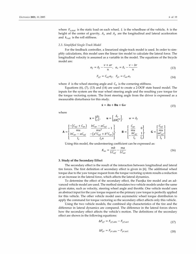
Figure 6 shows the block diagram of the overall system. The strategy uses handling 

mode to increase lateral performance and stability mode to stabilize the vehicle’s motion 

when  losing  control. The handling mode uses  a  feedforward  controller  that provides 

sporty  and  reproducible driving behavior  and prevents  a  synthetic driving  sensation, 

which is unacceptable for sports car drivers [6]. The stability mode uses a feedback con‐

troller  to stabilize  the vehicle’s motion when  the vehicle  loses control, which might be 

caused by a driver’s mistake. To make a smooth intervention of the stability mode, the 

stability  criterion adjusts  the weighting between  two  controllers according  to  the  esti‐

mated understeering coefficient, then transits to stability mode when the vehicle experi‐

ences an undesired oversteer or understeer situation. The allocation scheme distributes 

the motor’s torque to each wheel. This is an optimization problem to prevent the satura‐

tion of tire forces. 

Electronics 2021, 10, 2885  9  of  19  

Figure 6. Block diagram of the overall control system. 

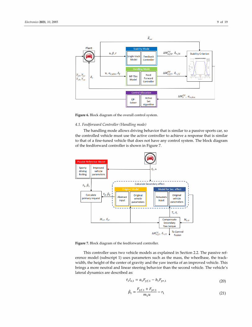
4.1. Feedforward Controller (Handling mode) 

The handling mode allows driving behavior that is similar to a passive sports car, so 

the controlled vehicle must use the active controller to achieve a response that is similar 

to that of a fine‐tuned vehicle that does not have any control system. The block diagram 

of the feedforward controller is shown in Figure 7. 

Figure 7. Block diagram of the feedforward controller. 

This controller uses two vehicle models as explained in Section 2.2. The passive ref‐

erence model (subscript 1) uses parameters such as the mass, the wheelbase, the track‐

width, the height of the center of gravity and the yaw inertia of an improved vehicle. This 

brings a more neutral and linear steering behavior than the second vehicle. The vehicle’s 

lateral dynamics are described as: 

𝑟 𝐼 , 𝑎 𝐹 , 𝑏 𝐹 ,   (20) 

𝛽𝐹 , 𝐹 ,

𝑚 𝑢𝑟   (21) 

Electronics 2021, 10, 2885  10  of  19  

The original vehicle model’s  (subscript 2) parameters are  the same as those of the 

plant vehicle, for which the active controller is actually implemented. This model is ex‐

tended using the yaw torque and the additional lateral force at the rear axle that is pro‐

duced by the torque vectoring and the rear wheel steering system. The lateral dynamics 

are described using the following equations. The responses are neither measured nor es‐

timated values so this method is similar to a state‐of‐the‐art look‐up table. 

𝑟 𝐼 , 𝑎 𝐹 , 𝑏 𝐹 , ∆𝐹 , ∆𝑀 ,   (22) 

𝛽𝐹 , 𝐹 , ∆𝐹 ,

𝑚 𝑢𝑟   (23) 

The  objective  is  to  achieve driving  behavior  that  is  comparable  to  the  improved 

model. In an ideal scenario, this demand is expressed as: 

𝑟 𝑟 , 𝛽 𝛽   (24) 

Using these equations, the required additional lateral force at the rear axle and the 

yaw torque request for torque vectoring are solved. The secondary effect is calculated us‐

ing the method in Section 3, followed by compensation for the primary yaw torque re‐

quest. The control commands are expressed as: 

∆𝐹 , 𝑢 𝑟 𝑟 𝑚 𝐹 ,𝑚𝑚

𝐹 , 𝐹 , 𝐹 ,   (25) 

𝛿 , ∆𝐹 ,

𝜕𝛼 ,

𝜕𝐹 ,  (26) 

𝑀 ,𝐼 ,

𝐼 ,𝑎 𝐹 , 𝑏 𝐹 , 𝑎 𝐹 , 𝑏 𝐹 , ∆𝐹 ,   (27) 

∆𝑀 , 𝑀 , 𝑀 ,   (28) 

4.2. Feedback Controller (Stability Mode) 

Unlike the feedforward controller, this controller does not consider driving feeling. 

It concentrates on stability. The block diagram of the feedback controller is shown in Fig‐

ure 8. 

Figure 8. Block diagram of feedback controller. 

For  this  study,  a  Linear Quadratic Regulator  (LQR), which  uses  the  single‐track 

model in Section 2.3, is designed. The objective function of the controller is expressed as 

Equation (29). The designed reference value for yaw rate is expressed in (30) with a 10 ms 

time constant [7]. The reference value of the side slip angle in this scenario is zero. 

𝐽12

𝐱 𝐱 𝐐 𝐱 𝐱 𝐮 𝐑𝐮 𝑑𝑡  (29) 

Electronics 2021, 10, 2885  11  of  19  

𝑟𝑢

𝐿 𝐾 , 𝑢𝛿 , 𝛽 0  (30) 

where Q and R are the weighting matrices for the state deviations and the input effort. 

By solving the algebraic Riccati equation, the optimal control inputs minimizing the 

objective function are provided as: 

𝐮𝛿 ,

∆𝑀 ,𝐊 𝐱 𝐱   (31) 

𝐊 𝐑 𝐁 𝐏  (32) 

𝐀 𝐏 𝐏𝐀 𝐏𝐁𝐑 𝐁 𝐏 𝐐 0  (33) 

where K is the optimal state feedback gain and P is the symmetric matrix solved from the 

algebraic Riccati equation. 

4.3. Control Integration 

The  integration  of  the  two  controllers  uses  the  current  understeering  coefficient, 

which is calculated using Equation (16) with parameters estimated from a Kalman filter. 

The  threshold  is designed to maintain neutral steering behavior using the definition  in 

[15], as expressed in Equation (34). Note that the threshold is tunable, depending on the 

limits of the design or driver preference. 

𝐿𝑢

𝐾2𝐿𝑢  (34) 

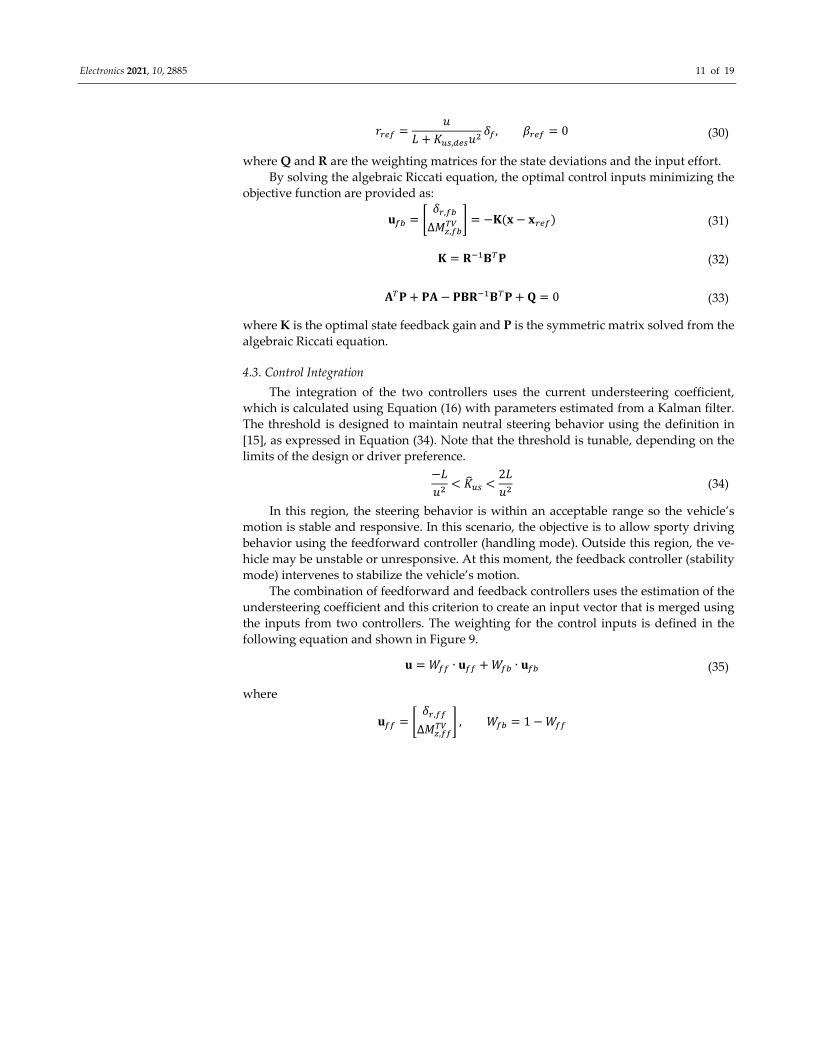
In  this region,  the steering behavior  is within an acceptable range so  the vehicle’s 

motion is stable and responsive. In this scenario, the objective is to allow sporty driving 

behavior using the feedforward controller (handling mode). Outside this region, the ve‐

hicle may be unstable or unresponsive. At this moment, the feedback controller (stability 

mode) intervenes to stabilize the vehicle’s motion. 

The combination of feedforward and feedback controllers uses the estimation of the 

understeering coefficient and this criterion to create an input vector that is merged using 

the  inputs  from  two controllers. The weighting  for  the control  inputs  is defined  in  the 

following equation and shown in Figure 9. 

𝐮 𝑊 ∙ 𝐮 𝑊 ∙ 𝐮   (35) 

where   

𝐮𝛿 ,

∆𝑀 ,, 𝑊 1 𝑊    

Electronics 2021, 10, 2885  12  of  19  

Figure 9. Weighting between the feedforward and feedback controllers. 

4.4. Control Allocation 

To properly distribute commands  from  the driver and  the high‐level controller, a 

control allocation is designed as a low‐level controller. The rear wheel steering system is 

straightforward because  there  is only one control  input: The  rear wheel steering angle 

(shown in Figure 6). The torque vectoring system is more complicated because of its multi‐

input nature. Hence, the allocation scheme in this study only contains the torque vectoring 

by the four wheel torques as inputs. 

The objective of the optimization problem is to prevent the saturation of the tires. The 

method is to award a higher penalty to the wheel for which the potential of tire force is 

lower, usually with a lower vertical load or a higher slip. The friction value for the most 

stressed tire represents the current required tire‐road friction value. The friction value is 

defined as: 

𝜇𝐹 𝐹

𝐹  (36) 

The optimization problem is solved by a QP‐solver in Matlab/Simulink. The solver 

uses an Active Set Algorithm (ASA). This method is similar to the one in [7], but for this 

study the weighted objective function is designed to increase performance. The quadratic 

objective function of the optimization problem is: 

𝑚𝑖𝑛 12𝐮 𝐖𝐮 , 𝑠𝑢𝑏𝑗𝑒𝑐𝑡 𝑡𝑜

𝐁 𝐮 𝐯 ,𝐮 𝐮 𝐮   (37) 

where 𝐁   is the control effectiveness matrix that describes the relationship between the 

command vector  𝐯   and the input vector  𝐮   and  𝐮   is the maximum limit for the 

inputs. The conversion of required  longitudinal  tire  force  to wheel  torque command  is 

multiplied by the static wheel radius  𝑟 . 

The parameters for the optimization problem are: 

𝐮

⎣⎢⎢⎡𝑇𝑇𝑇𝑇 ⎦

⎥⎥⎤

, 𝐯𝑎 ,

∆𝑀 , 𝐁1𝑟∙

1𝑚

1𝑚

1𝑚

1𝑚

𝑡2

𝑡2

𝑡2

𝑡2

𝜎𝜅

1 𝜅, 𝜎

tan𝛼1 𝜅

, 𝜎 𝜎 𝜎    

Electronics 2021, 10, 2885  13  of  19  

𝐖

⎣⎢⎢⎢⎢⎢⎢⎢⎡𝜎𝐹 ,

0 0 0

0𝜎𝐹 ,

0 0

0 0𝜎𝐹 ,

0

0 0 0𝜎𝐹 , ⎦

⎥⎥⎥⎥⎥⎥⎥⎤

The tuning term in the optimization problem is the positive definite weighting matrix 

𝐖, which is used to calculate the remaining potential for the tire force using the value of 

the vertical  load  𝐹   and the combined slip  𝜎. The remaining potential decreases as the 

vertical load decreases or the tire slip increases. Previous methods use the value in Equa‐

tion (36) as the weight but this can cause improper distribution if the tire forces decrease 

due to saturation, especially during violent maneuvers. To prevent this inverse proportion 

between tire forces and workloads, this study substitutes combined slip  𝜎  for the result‐ant tire force, which is in the numerator of the friction value. 

5. Results 

The proposed controller is tested in a CarSim and Simulink environment. To evaluate 

the vehicle’s lateral dynamics, the following procedures are simulated: 

Frequency response of steering wheel sine wave input. 

Slow ramp input of steering wheel at constant speed. 

Sine with Dwell steering with a 5A amplitude. 

Double lane change (DLC). 

The first three procedures are open‐loop tests. Maneuvering the same steering wheel 

inputs in both the passive and controlled vehicles. The DLC procedure uses the built‐in 

preview driver model with a 0.5 s preview time.   

In this study, the steering wheel sine wave input, ramp input and DLC tests are de‐

signed to examine the improvement of handling performance. Thus, in these procedures, 

we do not apply extreme severe maneuvers to make the vehicle lose control. On the con‐

trary, the objective of the Sine with Dwell test is to examine the quality of stability mode. 

The maneuver in this test will be fierce to cause an unstable situation and activate stability 

mode. 

The plant model used in this study is one of the B‐class Hatchback vehicles in CarSim. 

The improved vehicle, which is used as the reference model, has a mass and yaw inertia 

of 10% less to make the vehicle nimbler and more neutral. All procedures are tested on a 

flat road for which the road coefficient is 0.85. 

5.1. Frequency Responses 

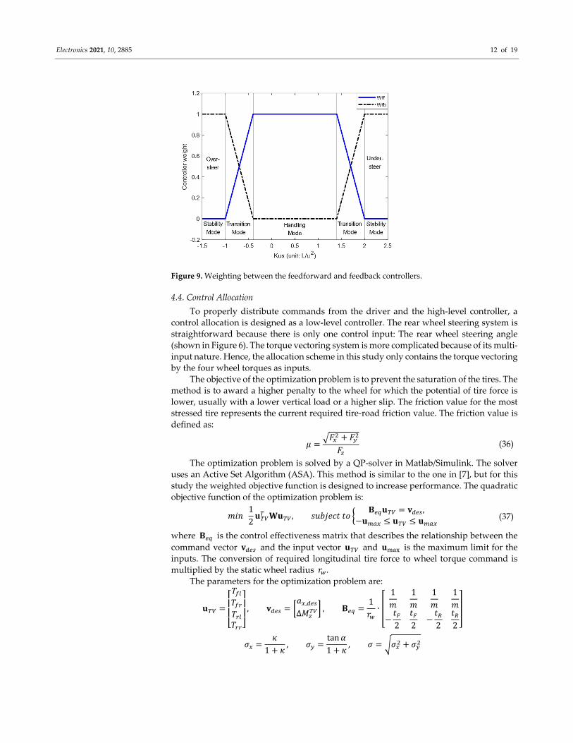
Figure 10 shows the frequency response plots for the yaw rate and side slip angle, 

from the steering wheel sine sweep maneuver. The amplitude of yaw rate increases and 

the amplitude of side slip angle decreases from low to high frequency. The increase in the 

phase margin for yaw motion represents an improvement in the vehicle’s agility, which 

is generally considered as a handling index by drivers. The bandwidths are increased for 

both systems so the responsiveness and stability are increased. 

Electronics 2021, 10, 2885  14  of  19  

(a) Yaw rate response  (b) Side slip angle response 

Figure 10. Frequency response in steering sine sweep test: (a) Yaw rate response; (b) Side slip angle response. 

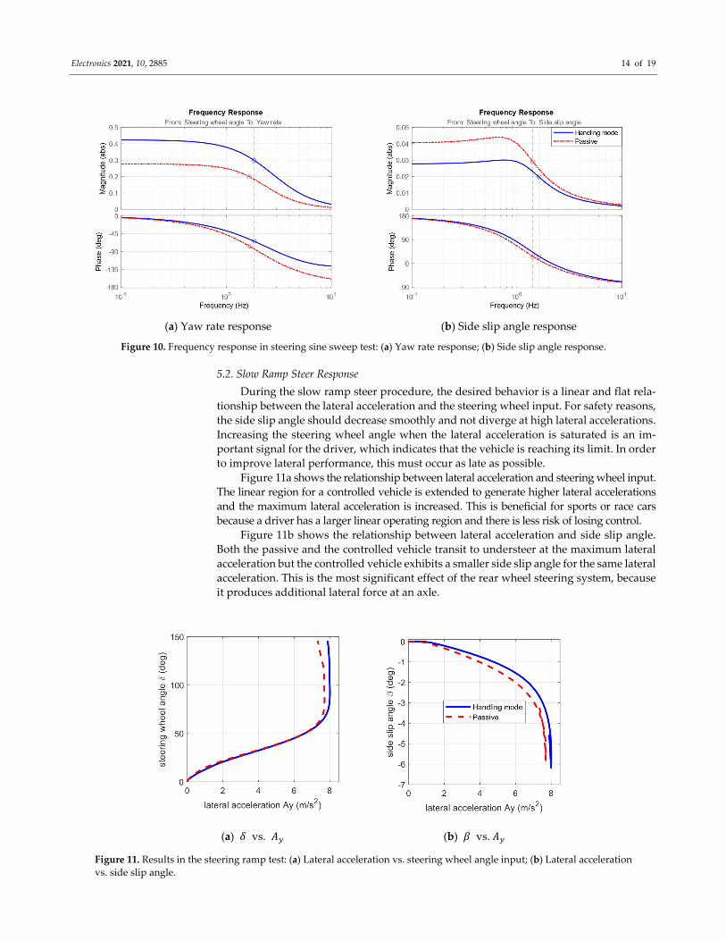
5.2. Slow Ramp Steer Response 

During the slow ramp steer procedure, the desired behavior is a linear and flat rela‐

tionship between the lateral acceleration and the steering wheel input. For safety reasons, 

the side slip angle should decrease smoothly and not diverge at high lateral accelerations. 

Increasing  the steering wheel angle when  the  lateral acceleration  is saturated  is an  im‐

portant signal for the driver, which indicates that the vehicle is reaching its limit. In order 

to improve lateral performance, this must occur as late as possible. 

Figure 11a shows the relationship between lateral acceleration and steering wheel input. 

The linear region for a controlled vehicle is extended to generate higher lateral accelerations 

and the maximum lateral acceleration is increased. This  is beneficial for sports or race cars 

because a driver has a larger linear operating region and there is less risk of losing control. 

Figure 11b shows the relationship between lateral acceleration and side slip angle. 

Both the passive and the controlled vehicle transit to understeer at the maximum lateral 

acceleration but the controlled vehicle exhibits a smaller side slip angle for the same lateral 

acceleration. This is the most significant effect of the rear wheel steering system, because 

it produces additional lateral force at an axle. 

(a)  𝛿  vs.  𝐴   (b)  𝛽  vs. 𝐴  

Figure 11. Results in the steering ramp test: (a) Lateral acceleration vs. steering wheel angle input; (b) Lateral acceleration 

vs. side slip angle. 

Electronics 2021, 10, 2885  15  of  19  

5.3. Sine with Dwell 

Sine with Dwell is a standard stability test that was formulated by the National High‐

way Traffic Safety Administration (NHTSA) [16]. The first step of this test involves ma‐

neuvering with a slow steering ramp input until the vehicle’s lateral acceleration reaches 

0.3g at 80 km/h. This defines  the unit angle amplitude A of  the steering wheel  for  the 

following tests. For this study, the stability test tests a situation that the feedforward con‐

troller (handling mode) cannot handle well due to violent maneuvering or model uncer‐

tainties. The steering amplitude of 5A is used for this test and the feedback controller (sta‐

bility mode) must intervene to stabilize its motion. The open‐loop steering command is 

shown in Figure 12 

Figure 12. Steering wheel input in the Sine with Dwell stability test. 

Figure 13 shows the yaw rate and the side slip responses in the Sine with Dwell test. 

Due  to the violent change  in direction, the amplitude of yaw motion  is  increased. This 

effect is known as a Scandinavian flick, and is usually used in rally races but is difficult to 

handle for normal drivers. All vehicles become unstable after 2 s, but the passive vehicle 

loses control completely and the side slip angle becomes significant. The vehicle that uses 

handling mode has  a  smaller  side  slip angle but does not  return  to  the zero‐dynamic 

quickly after the steering wheel angle returns to zero. Combined control with additional 

stability mode maintains a lower side slip angle and returns to the zero‐dynamic relatively 

quickly. The feedback controller produces some oscillations in the yaw motion at about 2 

to 3 s, which produces a synthetic driving feeling. This is not beneficial to handling im‐

provement scenarios. 

Electronics 2021, 10, 2885  16  of  19  

(a) Yaw rate responses  (b) Side slip angle responses 

Figure 13. Results in Sine with Dwell stability test: (a) Yaw rate responses; (b) Side slip angle responses. 

5.4. Double Lane Change 

A double lane change (DLC) is a universally acknowledged handling test. For this 

study,  the  standard  test  ISO  3888‐1  is  implemented using  the  built‐in preview driver 

model with a 0.5 s preview time. The driver model in CarSim represents an average driver 

and generates a steering action for trajectory tracking. This procedure is known as a moose 

test or elk test because a quick change in direction tests the responsiveness, stability and 

oscillation of the lateral dynamics. The track layout and vehicle’s trajectory of ISO 3888‐1 

are shown in Figure 14. The longitudinal distance and the lateral offset of the centerline 

are fixed and the width of cones in each section is varied depending on the vehicle’s width. 

Although the trajectories of both vehicles are similar, the lateral dynamic responses are 

different. This demonstrates the benefits of the proposed controller. 

The lateral distance error is not meaningful for the DLC test because drivers should 

plan the best route or racing line that allows the fastest passage in the real test. The lateral 

tracking error is affected by the driver model more than the chassis control system. There‐

fore, the DLC test should not be tested by virtual drivers only. A road test or driver  in 

loop (DIL) environment is necessary to verify its performance. 

Figure 14. Track layout and trajectories for ISO 3888‐1. 

Electronics 2021, 10, 2885  17  of  19  

Figure 15 shows the yaw rate and the side slip responses for the DLC test. For the 

target path in Figure 14, the curvatures are the same for the first two and last two corners, 

but the yaw rate response for the passive vehicle is larger for corners 2 and 4 due to the 

lack of  responsiveness. The controlled vehicle has a similar magnitude of response  for 

every corner and the side slip angle is decreased. Oscillations are also decreased when the 

controlled vehicle returns to a straight line after corners. It shows that the responsiveness 

and stability are improved simultaneously. 

(a) Yaw rate response  (b) Side slip angle response 

Figure 15. Results for ISO 3888‐1 at 80 km/h: (a) Yaw rate response; (b) Side slip angle response. 

Figure 16 shows the steering angles at the rear axle and the driver’s input. The pro‐

posed control system provides a sporty driving sensation and makes a driver pass the 

track with smoother steering wheel input. 

(a) Rear wheel steering angle  (b) Steering wheel angle 

Figure 16. Steering angle for ISO 3888‐1 at 80 km/h: (a) Rear wheel steering angle; (b) Steering wheel angle. 

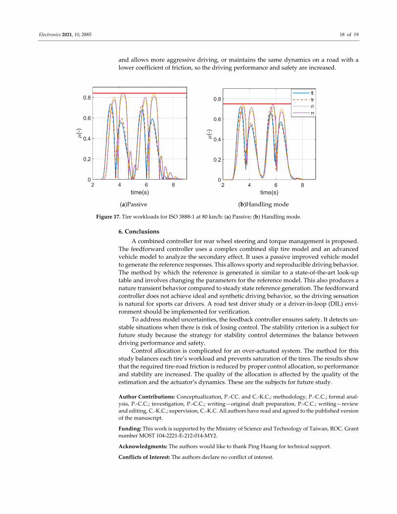
Figure 17 shows  the  tire workload  for  the passive and  the controlled vehicle. The 

used friction value at the most stressed tire represents the current required tire‐road fric‐

tion coefficient and must be as small as possible. The red horizontal lines show that the 

controlled vehicle has a significantly lower required friction value because the allocation 

method balances each tire’s workload and prevents early saturation for a single wheel. 

Retaining more capacity for tire force means that the vehicle produces greater acceleration 

Electronics 2021, 10, 2885  18  of  19  

and allows more aggressive driving, or maintains the same dynamics on a road with a 

lower coefficient of friction, so the driving performance and safety are increased. 

(a)Passive  (b)Handling mode 

Figure 17. Tire workloads for ISO 3888‐1 at 80 km/h: (a) Passive; (b) Handling mode. 

6. Conclusions 

A combined controller for rear wheel steering and torque management is proposed. 

The  feedforward controller uses a complex combined slip  tire model and an advanced 

vehicle model to analyze the secondary effect. It uses a passive improved vehicle model 

to generate the reference responses. This allows sporty and reproducible driving behavior. 

The method by which  the reference  is generated  is similar  to a state‐of‐the‐art  look‐up 

table and involves changing the parameters for the reference model. This also produces a 

nature transient behavior compared to steady state reference generation. The feedforward 

controller does not achieve ideal and synthetic driving behavior, so the driving sensation 

is natural for sports car drivers. A road test driver study or a driver‐in‐loop (DIL) envi‐

ronment should be implemented for verification. 

To address model uncertainties, the feedback controller ensures safety. It detects un‐

stable situations when there is risk of losing control. The stability criterion is a subject for 

future  study because  the  strategy  for  stability control determines  the balance between 

driving performance and safety. 

Control allocation is complicated for an over‐actuated system. The method for this 

study balances each tire’s workload and prevents saturation of the tires. The results show 

that the required tire‐road friction is reduced by proper control allocation, so performance 

and stability are increased. The quality of the allocation is affected by the quality of the 

estimation and the actuator’s dynamics. These are the subjects for future study. 

Author Contributions: Conceptualization, P.‐CC. and C.‐K.C.; methodology, P.‐C.C.; formal anal‐

ysis, P.‐C.C.;  investigation, P.‐C.C.; writing—original draft preparation, P.‐C.C.; writing—review 

and editing, C.‐K.C.; supervision, C.‐K.C. All authors have read and agreed to the published version 

of the manuscript. 

Funding: This work is supported by the Ministry of Science and Technology of Taiwan, ROC. Grant 

number MOST 104‐2221‐E‐212‐014‐MY2. 

Acknowledgments: The authors would like to thank Ping Huang for technical support. 

Conflicts of Interest: The authors declare no conflict of interest. 

Electronics 2021, 10, 2885  19  of  19  

References 

1. Piyabongkarn,  D.;  Rajamani,  R.;  Lew,  J.Y.;  Yu, H.  On  the  use  of  torque‐biasing  devices  for  vehicle  stability  control.  In 

Proceedings of the 2006 American Control Conference, Minneapolis, MN, USA, 14–16 June 2006. 

2. Shibahata, Y.; Shimada, K.; Tomari, T. Improvement of Vehicle Maneuverability by Direct Yaw Moment Control. Veh. Syst. Dyn. 

1993, 22, 465–481, https://doi.org/10.1080/00423119308969044.. 

3. Mokhiamar, O.; Abe, M. Simultaneous Optimal Distribution of Lateral and Longitudinal Tire Forces for the Model Following 

Control. J. Dyn. Syst. Meas. Control. 2004, 126, 753–763, https://doi.org/10.1115/1.1850533. 

4. Shen, H.; Tan, Y.‐S. Vehicle handling and stability control by the cooperative control of 4WS and DYC. Mod. Phys. Lett. B 2017, 

31, 1740090, https://doi.org/10.1142/s0217984917400905. 

5. Chen, B.‐C.; Kuo, C.‐C. Electronic stability control for electric vehicle with four in‐wheel motors. Int. J. Automot. Technol. 2014, 

15, 573–580, https://doi.org/10.1007/s12239‐014‐0060‐4. 

6. Peters, Y.; Stadelmayer, M. Control allocation for all wheel drive sports cars with rear wheel steering. Automot. Engine Technol. 

2019, 4, 111–123, https://doi.org/10.1007/s41104‐019‐00047‐9. 

7. Kissai, M.; Monsuez, B.; Mouton, X.; Tapus, A. Optimization‐Based Control Allocation for Driving/Braking Torque Vectoring 

in a Race Car. In Proceedings of the 2020 American Control Conference (ACC), Denvor, CO, USA, 1‐3 July 2020. 

8. Warth, G.;  Frey, M.; Gauterin,  F. Design  of  a  central  feedforward  control  of  torque  vectoring  and  rear‐wheel  steering  to 

beneficially use tyre information. Veh. Syst. Dyn. 2019, 58, 1789–1822, https://doi.org/10.1080/00423114.2019.1647345. 

9. Hang, P.; Xia, X.; Chen, X. Handling Stability Advancement With 4WS and DYC Coordinated Control: A Gain‐Scheduled 

Robust Control Approach. IEEE Trans. Veh. Technol. 2021, 70, 3164–3174, https://doi.org/10.1109/tvt.2021.3065106. 

10. Kissai, M.; Monsuez, B.; Mouton, X.; Martinez, D.; Tapus, A. Model Predictive Control Allocation of Systems with Different 

Dynamics. In Proceedings of the 2019 IEEE Intelligent Transportation Systems Conference (ITSC), Auckland, New Zealand, 27–

30 October 2019. 

11. Han, Z.; Xu, N.; Chen, H.; Huang, Y.; Zhao, B. Energy‐efficient control of electric vehicles based on linear quadratic regulator 

and phase plane analysis. Appl. Energy 2018, 213, 639–657, https://doi.org/10.1016/j.apenergy.2017.09.006. 

12. Xiao, F. Optimal torque distribution for four‐wheel‐motored electric vehicle stability enhancement. In Proceedings of the 2015 

IEEE International Transportation Electrification Conference (ITEC), Chennai, India, 27‐29 Aug 2015. 

13. Pacejka, H. Tire and Vehicle Dynamics; Elsevier: Amsterdam, The Netherlands, 2005;. pp. 165–190. 

14. Burhaumudin, M.S.; Samin, P.M.; Jamaluddin, H.; Rahman, R.A.; Sulaiman, S. Modeling and validation of magic formula tire 

model.  In  Proceedings  of  the  International  Conference  on  the  Automotive  Industry, Mechanical  and Materials  Science 

(ICAMMEʹ2012), Penang, Malaysia, 19 May 2012. 

15. Huang, Y.; Chen, Y. Estimation  and analysis of vehicle  lateral  stability  region with both  front  and  rear wheel  steering.  In 

Proceedings of  the Dynamic Systems and Control Conference, American Society of Mechanical Engineers. Tysons Corner, 

Virginia, 11‐13 Oct 2017. 

16. Proposed FMVSS No. 126 Electronic Stability Control Systems, Office of Regulatory Analysis and Evaluation, National Center for 

Statistics and Analysis, March 2007.