Numerical Differentiation and Integration INTEGRASI NUMERIS Universitas Gadjah Mada Departemen Teknik Sipil dan Lingkungan Prodi Sarjana Teknik Sipil

Welcome message from author
This document is posted to help you gain knowledge. Please leave a comment to let me know what you think about it! Share it to your friends and learn new things together.
Transcript

Numerical Differentiation and Integration
INTEGRASI NUMERIS
Universitas Gadjah Mada Departemen Teknik Sipil dan Lingkungan Prodi Sarjana Teknik Sipil

http://istiarto.staff.ugm.ac.id
Integrasi Numeris
q Acuan q Chapra, S.C., Canale R.P., 1990, Numerical Methods for Engineers, 2nd
Ed., McGraw-Hill Book Co., New York. n Chapter 15 dan 16, hlm. 459-523.
2

http://istiarto.staff.ugm.ac.id
Diferensial, Derivatif
xi xi +Δx
yi
yi +Δy
Δx
Δy
xi xi +Δx
yi
yi +Δy
xi
yi
(a) (b) (c)
( ) ( )x
xfxxfxy ii
Δ
−Δ+=
Δ
Δ ( ) ( )x
xfxxfxy ii
x Δ
−Δ+=
→Δ 0lim
dd
difference approximation
f(xi+Δx)
f(xi)
3

http://istiarto.staff.ugm.ac.id
Diferensial, Derivatif
( ) ( )x
xfxxfxy ii
Δ
−Δ+=
Δ
Δ ( ) ( )x
xfxxfxy ii
x Δ
−Δ+=
→Δ 0lim
dd
pendekatan beda (hingga) difference approximation derivatif
( )xfyxy
ʹ=ʹ=dd
derivatif = laju perubahan y terhadap x
4

http://istiarto.staff.ugm.ac.id
Diferensial
0
40
80
120
160
0 2 4 6 8 10
y
x
slope = dy/dx
0
6
12
18
24
0 2 4 6 8 10
dy/d
x
x
5.15xy =
5.05.7dd xxy=
5

http://istiarto.staff.ugm.ac.id
Integral
0
40
80
120
160
0 2 4 6 8 10
∫y d
x
x
5.05.7 xy =5.15d xxy =∫
∫=x
xy0dluas
§ “kebalikan” dari proses men-diferensial-kan adalah meng-integral-kan § integrasi ›‹ diferensiasi
0
6
12
18
24
0 2 4 6 8 10
y
x
6

http://istiarto.staff.ugm.ac.id
Fungsi
q Fungsi-fungsi yang di-diferensial-kan atau di-integral-kan dapat berupa: q fungsi kontinu sederhana: polinomial, eksponensial, trigonometri
q fungsi kontinu kompleks yang tidak memungkinkan didiferensialkan atau dintegralkan secara langsung
q fungsi yang nilai-nilainya disajikan dalam bentuk tabel [tabulasi data x vs f(x)]
7
http://istiarto.staff.ugm.ac.id
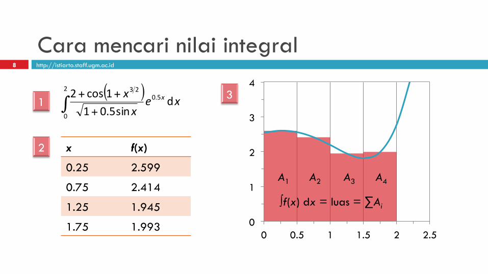
Cara mencari nilai integral
( )∫ +
++2
0
5.023
dsin5.01
1cos2 xex
x x
x f(x)
0.25 2.599
0.75 2.414
1.25 1.945
1.75 1.993 0
1
2
3
4
0 0.5 1 1.5 2 2.5
A1 A2 A3 A4
∫f(x) dx = luas = ∑Ai
8

http://istiarto.staff.ugm.ac.id
Derivatif
xuun
xy n
dd
dd 1−=
( ) ( )xfvxfu == dan
nuy =
vuy =
vuy =
xvu
xuv
xy
dd
dd
dd
+=
2dd
dd
dd
vxvu
xuv
xy −=
xx eex
xx
x
xxx
xxx
xxx
=
=
=
−=
=
dd
1lndd
sectandd
sincosdd
cossindd
2
aaax
axx
x
xxxx
xxxx
xxx
xx
a
lndd
ln1log
dd
cotcsccscdd
tansecsecdd
csccotdd 2
=
=
−=
=
−=
9

http://istiarto.staff.ugm.ac.id
Integral
( ) ( ) Cbaxa
xbax
Cxxx
aaCab
axa
nCnuvu
uvuvvu
bxbx
nn
++−=+
+=
≠>+=
−≠++
=
−=
∫
∫
∫
∫
∫∫+
cos1dsin
lnd
1,0ln
d
11
d
dd1
( ) ( )
( )
Cxaab
abbxax
Caxaexex
Caexe
Cxxxxx
Cbaxa
xbax
axax
axax
+=+
+−=
+=
+−=
++=+
−∫
∫
∫
∫
∫
12
2
tan1d
1d
d
lndln
sin1dcos
10

Metode Trapesium Metode Simpson Metode Kuadratur Gauss
Metode Integrasi Newton-Cotes 11

http://istiarto.staff.ugm.ac.id
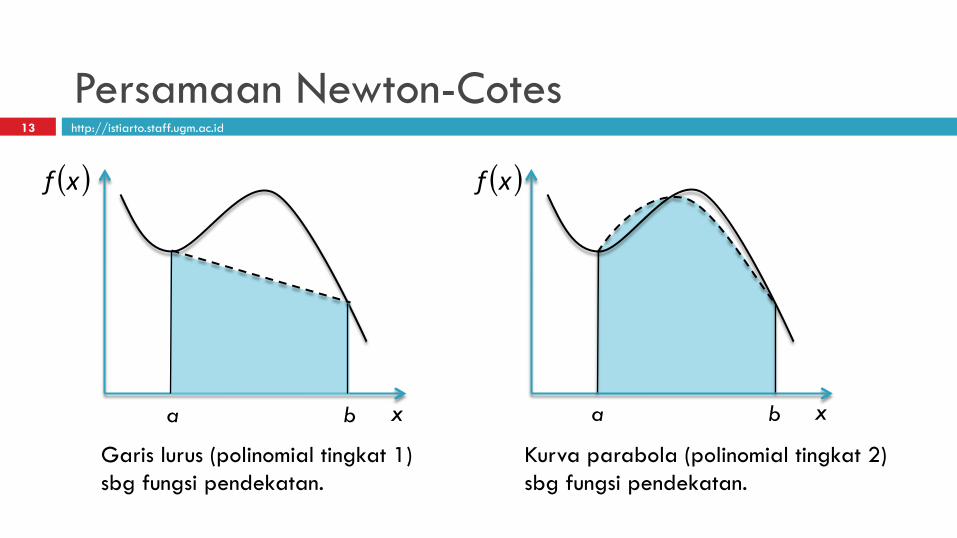
Persamaan Newton-Cotes
q Strategi q mengganti fungsi kompleks dan rumit atau tabulasi data dengan
yang mudah untuk diintegralkan
( ) ( )∫∫ ==b
a n
b
axxfxxfI dd
( ) nn
nnn xaxaxaxaaxf +++++= −−
11
2210 ...
polinomial tingkat n
12
http://istiarto.staff.ugm.ac.id
Persamaan Newton-Cotes
( )xf
x a b
( )xf
x a b
Garis lurus (polinomial tingkat 1) sbg fungsi pendekatan.
Kurva parabola (polinomial tingkat 2) sbg fungsi pendekatan.
13

http://istiarto.staff.ugm.ac.id
Persamaan Newton-Cotes
( )xf
x a b
Garis lurus (polinomial tingkat 1) sbg fungsi pendekatan.
1 2
3
Fungsi yang diintegralkan didekati dengan 3 buah garis lurus (polinomial tingkat 1). Dapat pula dipakai beberapa kurva polinomial tingkat yang lebih tinggi.
14
http://istiarto.staff.ugm.ac.id
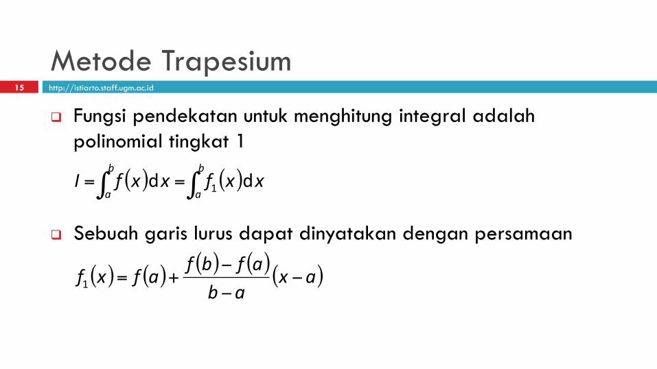
Metode Trapesium
q Fungsi pendekatan untuk menghitung integral adalah polinomial tingkat 1
q Sebuah garis lurus dapat dinyatakan dengan persamaan
( ) ( )∫∫ ==b
a
b
axxfxxfI dd 1
( ) ( ) ( ) ( )( )axabafbfafxf −
−
−+=1
15

http://istiarto.staff.ugm.ac.id
Metode Trapesium
( ) ( ) ( )( )
( ) ( ) ( )2
d
bfafab
xaxabafbfafI
b
a
+−≅
⎥⎦⎤
⎢⎣⎡ −
−
−+≅ ∫
Metode Trapesium
( )xf
x a b
error
16

http://istiarto.staff.ugm.ac.id
Metode Trapesium
( )
640533.16400180
4675
32005.122.0
d400900675200252.08.0
0
65432
8.0
0
5432
=⎟⎠⎞
⎜⎝⎛ +−+−+=
+−+−+= ∫
xxxxxx
xxxxxxI
( )( ) ( ) 232.08.0dan2.00
400900675200252.0 5432
==
+−+−+=
ffxxxxxxf
Penyelesaian eksak
Metode Trapesium
( ) 1728.02232.02.008.0 =
+−=I [error] ( )%89467733.11728.0640533.1 ≈=−=tE
17

http://istiarto.staff.ugm.ac.id
0
1
2
3
4
0 0.2 0.4 0.6 0.8
x
f(x)
Metode Trapesium
q Error atau kesalahan q bentuk trapesium untuk
menghitung nilai integral mengabaikan sejumlah besar porsi daerah di bawah kurva
q Kuantifikasi error pada Metode Trapesium
error
( )( )3121 abfEt −ξʹ́−=
ξ adalah titik di antara a dan b
18

http://istiarto.staff.ugm.ac.id
Metode Trapesium
0
1
2
3
4
0 0.2 0.4 0.6 0.8
x
f(x)
error ( )( ) 56.208.060.0
121 3 =−−−=aE
( ) 323 8000108004050400 xxxxf +−+−=ʹ́
nilai rata-rata derivatif kedua:
( )( )
6008.0
d80001080040504008.0
0
323
−=−
+−+−=ʹ́ ∫ xxxx
xf
error:
order of magnitude nilai error ini sama dengan order of magnitude nilai error terhadap nilai penyelesaian eksak dan keduanya sama tanda (sama-sama positif)
19

http://istiarto.staff.ugm.ac.id
Trapesium multi pias
q Peningkatan akurasi q selang ab dibagi menjadi sejumlah n pias dengan lebar seragam h
nabh −
=
20

http://istiarto.staff.ugm.ac.id
0
1
2
3
4
0 0.1 0.2 0.3 0.4 0.5 0.6 0.7 0.8
x
f(x)
h = 0.1
Trapesium multi pias
0
1
2
3
4
0 0.2 0.4 0.6 0.8
x
f(x)
h = 0.2
nabh −
=
21

http://istiarto.staff.ugm.ac.id
Trapesium multi pias
nabh −
=nxbxa == danJika 0
( ) ( ) ( )
( ) ( ) ( ) ( ) ( ) ( )2
...22
d...dd
12110
1
2
1
1
0
nn
x
x
x
x
x
x
xfxfhxfxfhxfxfhI
xxfxxfxxfI n
n
+++
++
+≈
+++=
−
∫∫∫−
( ) ( ) ( )⎥⎦
⎤⎢⎣
⎡+
⎭⎬⎫
⎩⎨⎧
+≈ ∑−
=n
n
ii xfxfxfhI
1
10 2
2( )
( ) ( ) ( )
!!!! "!!!! #$"#$rata-ratatinggi
1
10
lebar2
2
n
xfxfxfabI
n
n
ii +⎭⎬⎫
⎩⎨⎧
+−≈
∑−
=
22

http://istiarto.staff.ugm.ac.id
Trapesium multi pias
( ) ( )∑=
ξʹ́−
−=n
iit f
nabE
13
3
12
Error = jumlah error pada setiap pias
( ) ffn
n
ii ʹ́=ξʹ́∑
=1
1 ( ) fnabEE at ʹ́−
−=≈ 2
3
12
setiap kelipatan jumlah pias, error mengecil dengan faktor kuadrat peningkatan jumlah pias
23

http://istiarto.staff.ugm.ac.id
Trapesium multi pias ( ) 5432 400900675200252.0 xxxxxxf +−+−+=
n h I Et %Et Ea
1 0.8 0.1728 1.4677 89% 2.56
2 0.4 1.0688 0.5717 35% 0.64
4 0.2 1.4848 0.1557 9% 0.16
8 0.1 1.6008 0.0397 2% 0.04
( ) 640533.1d8.0
0== ∫ xxfI
( )∫≈8.0
0 1 dxxfI (the trapezoidal rule)
(exact solution)
0
20
40
60
80
100
1 2 4 8 n
%Et vs n
24
http://istiarto.staff.ugm.ac.id
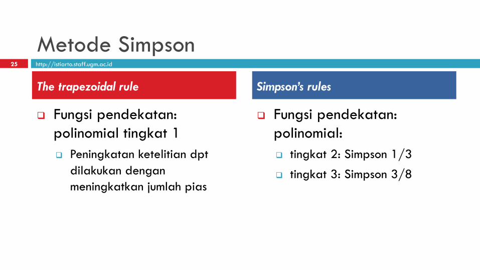
Metode Simpson
q Fungsi pendekatan: polinomial tingkat 1 q Peningkatan ketelitian dpt
dilakukan dengan meningkatkan jumlah pias
q Fungsi pendekatan: polinomial: q tingkat 2: Simpson 1/3
q tingkat 3: Simpson 3/8
The trapezoidal rule Simpson’s rules
25
http://istiarto.staff.ugm.ac.id
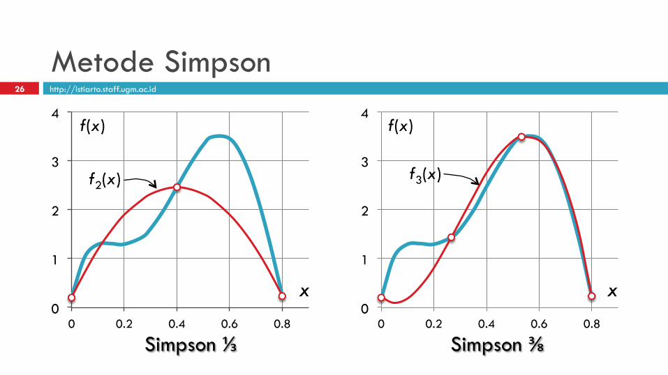
Metode Simpson
0
1
2
3
4
0 0.2 0.4 0.6 0.8
x
f(x)
f2(x)
0
1
2
3
4
0 0.2 0.4 0.6 0.8
x
f(x)
f3(x)
Simpson ⅓ Simpson ⅜
26

http://istiarto.staff.ugm.ac.id
Metode Simpson
q Polinomial tingkat 2 atau 3 q dicari dengan Metode Newton atau Lagrange (lihat materi tentang
curve fitting)
27
http://istiarto.staff.ugm.ac.id
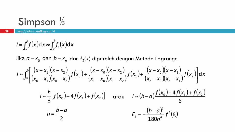
Simpson ⅓
( ) ( )∫∫ ≈=b
a
b
axxfxxfI dd 2
nxbxa == danJika 0
( )( )( )( )
( ) ( )( )( )( )
( ) ( )( )( )( )
( )∫ ⎥⎦
⎤⎢⎣
⎡
−−−−
+−−−−
+−−−−
≈b
axxf
xxxxxxxxxf
xxxxxxxxxf
xxxxxxxxI d2
1202
101
2101
200
2010
21
dan f2(x) diperoleh dengan Metode Lagrange
( ) ( ) ( )[ ]210 43
xfxfxfhI ++≈
2abh −
=
( ) ( ) ( ) ( )6
4 210 xfxfxfabI ++−≈atau
( ) ( )ξ−−= 4
4
5
180f
nabEt
28
http://istiarto.staff.ugm.ac.id
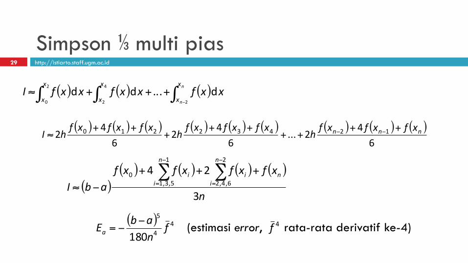
Simpson ⅓ multi pias
( ) ( ) ( )∫∫∫−
+++≈n
n
x
x
x
x
x
xxxfxxfxxfI
2
4
2
2
0
d...dd
( ) ( ) ( ) ( ) ( ) ( ) ( ) ( ) ( )6
42...
64
26
42 12432210 nnn xfxfxf
hxfxfxf
hxfxfxf
hI++
++++
+++
≈ −−
( )( ) ( ) ( ) ( )
n
xfxfxfxfabI
n
n
ii
n
ii
3
242
6,4,2
1
5,3,10 +++
−≈∑∑−
=
−
=
( ) 44
5
180f
nabEa
−−= (estimasi error, 4f rata-rata derivatif ke-4)
29

http://istiarto.staff.ugm.ac.id
Simpson ⅜
( ) ( )∫∫ ≈=b
a
b
axxfxxfI dd 3
nxbxa == danJika 0
( )( )( )( )( )( )
( ) ( )( )( )( )( )( )
( ) ( )( )( )( )( )( )
( ) ( )( )( )( )( )( )
( )∫ ⎥⎦
⎤⎢⎣
⎡
−−−−−−
+−−−−−−
+−−−−−−
+−−−−−−
≈b
axxf
xxxxxxxxxxxxxf
xxxxxxxxxxxxxf
xxxxxxxxxxxxxf
xxxxxxxxxxxxI d3
231303
2102
321202
3101
312101
3200
302010
321
dan f3(x) diperoleh dengan Metode Lagrange
( ) ( ) ( ) ( )[ ]3210 3383 xfxfxfxfhI +++≈
3abh −
=
( ) ( ) ( ) ( ) ( )!!!!! "!!!!! #$"#$
rataratatinggi
3210
lebar833
−
+++−≈
xfxfxfxfabIatau
30

http://istiarto.staff.ugm.ac.id
Simpson ⅜
( ) ( )ξ−−= 4
5
6480fabEt
Error
( )ξ−= 45
803 fhEt atau
31

http://istiarto.staff.ugm.ac.id
Simpson ⅓ dan ⅜ ( ) 5432 400900675200252.0 xxxxxxf +−+−+=
( ) 640533.1d8.0
0== ∫ xxfI (exact solution)
Metode I Et
Simpson ⅓ (n = 2) 1.367467 0.273067 (17%)
Simpson ⅜ (n = 3) 1.51917 0.121363 (7%)
Simpson ⅓ (n = 4) 1.623467 0.017067 (1%)
32

http://istiarto.staff.ugm.ac.id
Pias tak seragam: Metode Trapesium
( )543
2
400900675
200252.0
xxx
xxxf
+−
+−+=i xi f(xi) I
0 0 0.2
1 0.12 1.309729 0.090584
2 0.22 1.305241 0.130749
3 0.32 1.743393 0.152432 4 0.36 2.074903 0.076366 5 0.4 2.456 0.090618
6 0.44 2.842985 0.10598
7 0.54 3.507297 0.317514
8 0.64 3.181929 0.334461
9 0.7 2.363 0.166348
10 0.8 0.232 0.12975
1.594801
I dihitung dengan Metode Trapesium di setiap pias:
( ) ( )
( ) ( ) ( ) ( )2
...2
2112
2
011
−+++
+
++
=
nnn
xfxfhxfxfh
xfxfhI
( ) 594801.1d8.0
0=∫ xxf
33
http://istiarto.staff.ugm.ac.id
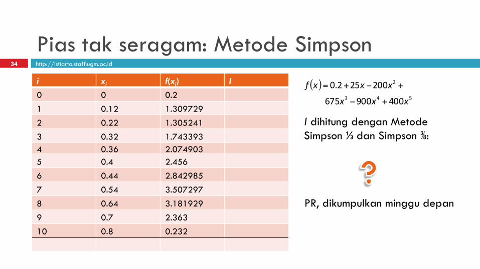
Pias tak seragam: Metode Simpson
( )543
2
400900675
200252.0
xxx
xxxf
+−
+−+=i xi f(xi) I
0 0 0.2
1 0.12 1.309729
2 0.22 1.305241
3 0.32 1.743393 4 0.36 2.074903 5 0.4 2.456
6 0.44 2.842985
7 0.54 3.507297
8 0.64 3.181929
9 0.7 2.363
10 0.8 0.232
I dihitung dengan Metode Simpson ⅓dan Simpson ⅜:
PR, dikumpulkan minggu depan
34
http://istiarto.staff.ugm.ac.id
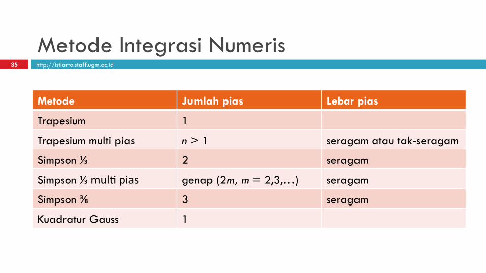
Metode Integrasi Numeris
Metode Jumlah pias Lebar pias
Trapesium 1
Trapesium multi pias n > 1 seragam atau tak-seragam
Simpson ⅓ 2 seragam
Simpson ⅓mul(pias genap (2m, m = 2,3,…) seragam
Simpson ⅜ 3 seragam
Kuadratur Gauss 1
35
http://istiarto.staff.ugm.ac.id
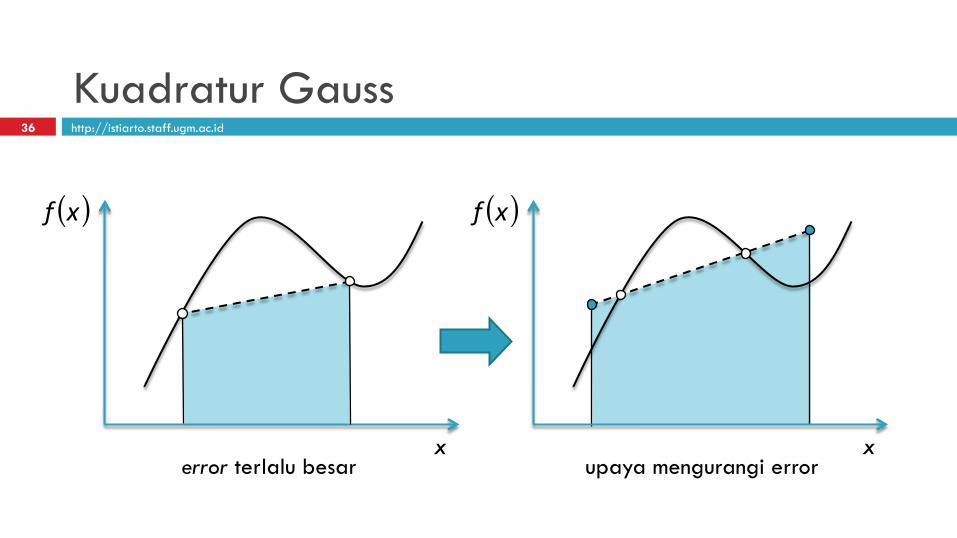
Kuadratur Gauss
( )xf
x
( )xf
x error terlalu besar upaya mengurangi error
36

http://istiarto.staff.ugm.ac.id
Kuadratur Gauss
( )xf
x
( )0xf
( )1xf
0x 1x1− 1
Kuadratur Gauss 2 Titik: Gauss-Legendre
( ) ( ) ( )1100
1
1d xfcxfcxxfI +≈= ∫−
( ) ( )
( ) ( )
( ) ( )
( ) ( ) 0d
32d
0d
2d1
1
1
31100
1
1
21100
1
11100
1
11100
==+
==+
==+
==+
∫
∫
∫
∫
−
−
−
−
xxxfcxfc
xxxfcxfc
xxxfcxfc
xxfcxfc c0 , c1, x0 , x1 : unknowns
37

http://istiarto.staff.ugm.ac.id
0
0.5
1
1.5
2
-1.5 -1 -0.5 0 0.5 1 1.5 -1.5
-1
-0.5
0
0.5
1
1.5
-1.5 -1 -0.5 0 0.5 1 1.5
Kuadratur Gauss
( )xf
x
( ) 1=xf
( ) xxf =
2d11
1=∫− x 0d
1
1=∫− xx
( )xf
x
38

http://istiarto.staff.ugm.ac.id
0
1
2
-1.5 -1 -0.5 0 0.5 1 1.5
Kuadratur Gauss
( )xf
x
( ) 2xxf = ( ) 3xxf =
32d1
1
2 =∫− xx 0d1
1
3 =∫− xx
( )xf
x
-3
-2
-1
0
1
2
3
-1.5 -1 -0.5 0 0.5 1 1.5
39

http://istiarto.staff.ugm.ac.id
Kuadratur Gauss
( ) ( )
( ) ( )
( ) ( )
( ) ( ) 0d
32d
2d
2d1
1
1
31100
1
1
21100
1
11100
1
11100
==+
==+
==+
==+
∫
∫
∫
∫
−
−
−
−
xxxfcxfc
xxxfcxfc
xxxfcxfc
xxfcxfc
( ) ( )1100 xfcxfcI +≈31
31
1
1
0
10
=
−=
==
x
x
cc
( ) ( )3131 ffI +−≈
40

http://istiarto.staff.ugm.ac.id
Kuadratur Gauss
Untuk batas integrasi dari a ke b: § diambil asumsi suatu variabel xd yang dapat dihubungkan dengan variabel asli
x dalam suatu relasi linear
dxaax 10 +=
§ jika batas bawah, x = a, berkaitan dengan xd = −1
§ jika batas atas, x = b, berkaitan dengan xd = 1
( )110 −+=⇒ aaa( )110 aab +=⇒
2dan
2 10abaaba −
=+
=
( ) ( )
( )d
d
xabx
xababx
d2
d
2−
=
−++=
dxaax 10 +=
41
http://istiarto.staff.ugm.ac.id
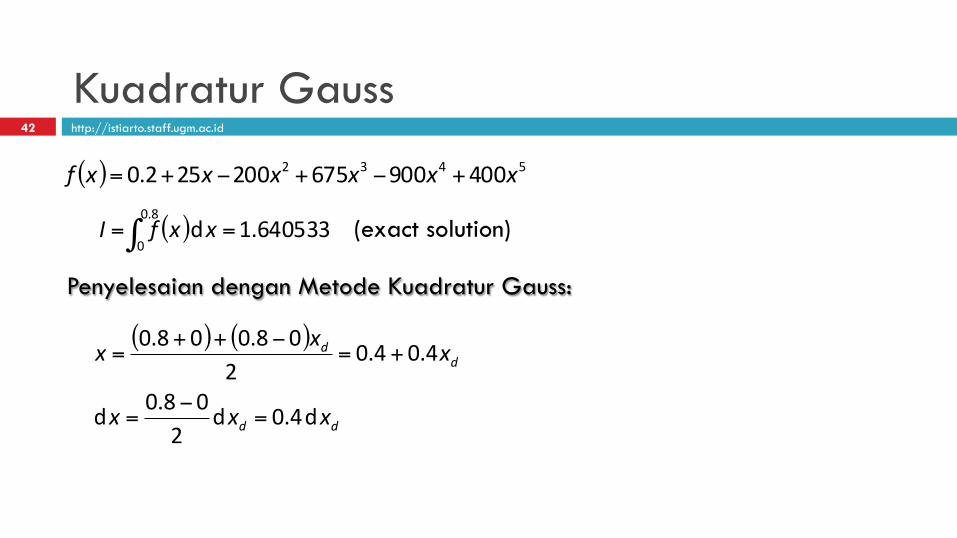
Kuadratur Gauss
( ) 5432 400900675200252.0 xxxxxxf +−+−+=
( ) 640533.1d8.0
0== ∫ xxfI (exact solution)
Penyelesaian dengan Metode Kuadratur Gauss:
( ) ( )
dd
dd
xxx
xxx
d4.0d2
08.0d
4.04.02
08.008.0
=−
=
+=−++
=
42
http://istiarto.staff.ugm.ac.id
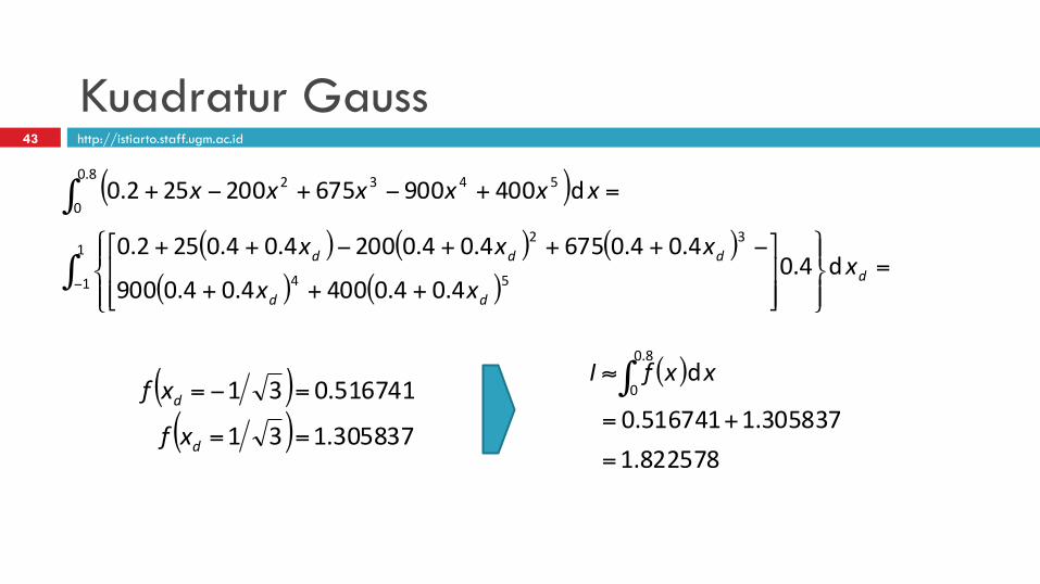
Kuadratur Gauss
( )( ) ( ) ( )
( ) ( )=
⎪⎭
⎪⎬⎫
⎪⎩
⎪⎨⎧
⎥⎥⎦
⎤
⎢⎢⎣
⎡
+++
−+++−++
=+−+−+
∫
∫
−
1
1 54
32
8.0
0
5432
d4.04.04.04004.04.0900
4.04.06754.04.02004.04.0252.0
d400900675200252.0
ddd
ddd xxx
xxx
xxxxxx
( )( ) 305837.131
516741.031
==
=−=
d
d
xf
xf( )
822578.1305837.1516741.0
d8.0
0
=
+=
≈ ∫ xxfI
43

44
Related Documents