Integral form of Yang-Mills equations and its gauge invariant conserved charges

The integral equations of Yang-Mills and its gauge invariantconserved charges

L. A. Ferreira1 and G. Luchini2

Instituto de Fısica de Sao Carlos; IFSC/USP;

Universidade de Sao Paulo - USP

Caixa Postal 369, CEP 13560-970, Sao Carlos-SP, Brazil

Abstract

Despite the fact that the integral form of the equations of classical electrody-

namics is well known, the same is not true for non-abelian gauge theories. The

aim of the present paper is threefold. First, we present the integral form of the

classical Yang-Mills equations in the presence of sources, and then use it to solve

the long standing problem of constructing conserved charges, for any field configu-

ration, which are invariant under general gauge transformations and not only under

transformations that go to a constant at spatial infinity. The construction is based

on concepts in loop spaces and on a generalization of the non-abelian Stokes theo-

rem for two-form connections. The third goal of the paper is to present the integral

form of the self dual Yangs-Mills equations, and calculate the conserved charges

associated to them. The charges are explicitly evaluated for the cases of monopoles,

dyons, instantons and merons, and we show that in many cases those charges must

be quantized. Our results are important in the understanding of global properties

of non-abelian gauge theories.

1e-mail: [email protected]: [email protected]

arX

iv:1

205.

2088

v2 [

hep-

th]

10

Oct

201

2

1 Introduction

The integral form of the equations of classical electrodynamics precedes Maxwell equations

and play a crucial role in the understanding of electromagnetic phenomena. The non-

abelian gauge theories have been originally formulated in a differential form through the

Yang-Mills equations, and its integral formulation has not been constructed. The aim

of the present paper is threefold. First we present the integral form of the classical

equations of motion of non-abelian gauge theories, which allows us to present the Yang-

Mills equations as the equality of an ordered volume integral to an ordered surface integral

on its border. Our construction was made possible by the use of a generalization of the

non-abelian Stokes theorem for two-form connections proposed some years ago in the

context of integrable field theories in dimensions higher than two [1, 2]. The volume

ordered integral present some highly non-trivial and non-linear terms, involving the field

tensor and its Hodge dual, which certainly will play an important role in the global aspects

of the Yang-Mills theory. The differential Yang-Mills equations are recovered in the limit

when the volume is taken to be infinitesimal. The second goal of the paper is to solve the

long standing problem of the construction of conserved charges that are invariant under

general gauge transformations. As it is well known, the conserved charges presented in

the Yang and Mills original paper [3], as well as in modern textbooks, are invariant under

gauge transformations where the group element, performing the transformation, goes to

a constant at spatial infinity. In the last decades several attempts were made to find

truly gauge invariant conserved charges using several techniques [4]. We show that our

integral form of Yang-Mills equations becomes a conservation law when the volume where

it is considered is a closed volume, i.e. a three dimensional sub-manifold of the four

dimensional space-time which has no border. Using appropriate boundary conditions we

obtain a closed expression for the conserved charges as the eigenvalues of an operator

obtained by a volume ordered integral, over the entire spatial sub-manifold (fixed time).

As a consequence of our integral Yang-Mills equations that operator can also be written

as an ordered surface integral on the border of the spatial sub-manifold. That fact makes

the evaluation of the charges much simpler. We then show that such charges are invariant

under general gauge transformation, independent of the parameterization of the volume,

and on the reference point used on that parameterization. The expression is valid for any

field configuration, and we evaluate it for well known solutions like monopoles, dyons,

instantons and merons.

The third goal of the paper is to construct the integral form of the self dual Yang-

Mills equations. That is obtained in a similar manner as that of the integral form of the

full Yang-Mills equations, but using instead the usual non-abelian Stokes for one-form

1

connections. We show that such integral formulation leads to gauge invariant conserved

quantities, which are invariant under reparameterization of surfaces and independent of

the reference point used in such parameterization. The novelty is that the charges are

given by the eigenvalues of surface ordered integrals of the field tensor and its Hodge dual,

and they are shown to be constant on the other two coordinates perpendicular to that

surface.

The examples of monopoles, dyons, instantons and merons discussed in the paper are

very important to shed light on the physical properties of the conserved charges. The first

point is that for those well known solutions the surface ordering becomes irrelevant in the

evaluation of the operators leading to the charges. In fact, those operators tend to lie in

the center of the gauge group, and the physical charges are identified with the eigenvalues

of the Lie algebra elements which lead to those group elements under the exponential

map. That relation between charges and elements in the center of the group leads, in

many cases, to the quantization of the physical charges. Another point is that the charges

are associated to the abelian subgroup of the gauge group. In the examples we have

worked out there are no gauge invariant conserved charges associated to the generators

lying outside the abelian subalgebra. A further point is that the charges associated to the

Wu-Yang monopole and the ’t Hooft-Polyakov monopole are identical. In addition, they

are shown to be conserved due to the equations of motion and no topological arguments

are used. The evaluation of the charges do not involve the Higgs field and seems not

to pay attention to the symmetry breaking pattern. The construction of the magnetic

charges in our paper differs from the usual techniques used in the literature involving

homotopy invariant quantities, even though it leads to the same results. But our methods

allow to evaluate charges for cases that were not really known in the literature. We show

that the merons carry a charge, conserved in the euclidean time, which is identical to the

magnetic charge of the Wu-Yang and ’t Hooft-Polyakov monopoles.

Our construction explores loop space techniques used in the study of integrable theo-

ries in any dimension [1, 2], and may be important in the understanding of the integrability

properties of Yang-Mills theory as well as of its self-dual sector. In fact, the most ap-

propriate mathematical language to phrase our results is that of generalized loop spaces.

There is a quite vast literature on integral and loop space formulations of gauge theories

[5]. Our approach differs in many aspects of those formulations even though it shares

some of the ideas and insights permeating them. We stress however that the relevant loop

space in our formulation is that of the maps from the two-sphere S2 (and not from the

circle S1) onto the space-time, in the case of the full Yang-Mills equations. For the self

dual sector however, the relevant loop space is that of the maps from the circle S1 onto

the space-time.

2

The connection between integrable field theories in any dimension and loop space

techniques by exploring the integral form of the equations of motion has been studied in

[6]. It was shown there that integrable field theories in 1 + 1 dimensions, Chern-Simons

theory in 2+1 dimensions, and Yang-Mills theory in 2+1 and 3+1 dimensions, all admit

a uniform formulation in terms of integral equations on loop spaces, leading to a general

and unique method for constructing conserved charges. The integral form of the Yang-

Mills equations in 3 + 1, discussed in this paper, already appears in [6]. In the present

paper we discuss further the physical consequences for non-abelian gauge theories of the

existence of such integral equation. In addition, we show that the self-dual sector of Yang-

Mills also admit an integral equation, and that it leads in a similar way to new conserved

quantities. The second part of the present paper is dedicated to the application of our

ideas to well known solutions of Yang-Mills theory, like Wu-Yang and ’tHooft-Polyakov

monopoles and dyons, as well as Euclidean solutions like instantons and merons. That

is a very important contribution of the paper since the conserved charges evaluated for

those solutions are new and were not explored in the literature before. We believe that

most of the physical consequences of those charges are still to be explored and perhaps

we have to consider the quantum theory to fully understand them.

The paper is organized as follows: in section 2 we present the main results of the

paper in the form of very precise statements. It is stated the integral equations for the

full Yang-Mills theory as well as for its self-dual sector. In this section we also present the

closed expressions for the conserved charges. In section 3 we give the proof for the integral

equation for the self-dual sector of the Yang-Mills theory using the ordinary non-abelian

Stokes theorem. In section 4 we give the proof for the generalized non-abelian Stokes

theorem for a two-form connection based on the results of [1, 2]. Then in section 5 we use

that theorem to prove the integral equations for the full Yang-Mills theory. In section 6

we discuss some consequences of our integral equations and give the detailed construction

of the conserved charges for the full Yang-Mills equations as well as for its self-dual sector.

In section 7 we discuss the examples of monopoles, dyons, instantons and merons, and

explicitly evaluated the conserved charges for all those solutions. Finally in appendix A

we show how to (classically) regularize the Wilson line operator in order to evaluate the

charges of the Wu-Yang monopole and dyon solutions.

2 The main statements

The integral Yang-Mills equation and its charges. Consider a Yang-Mills theory

for a gauge group G, with gauge field Aµ, in the presence of matter currents Jµ, on a four

3

dimensional space-time M . Let Ω be any tridimensional (topologically trivial) volume on

M , and ∂Ω be its border. We choose a reference point xR on ∂Ω and scan Ω with closed

surfaces, based on xR, labelled by ζ, and we scan the closed surfaces with closed loops

based on xR, labelled by τ , and parametrized by σ, as we describe below. The classical

dynamics of the gauge fields is governed by the following integral equations, on any such

volume Ω,

P2eie∫∂Ω

dτdσ[αFWµν+βFWµν ] dxµ

dσdxν

dτ = P3e∫

ΩdζdτV J V −1

(2.1)

where P2 and P3 means surface and volume ordered integration respectively, Fµν is the

Hodge dual of the field tensor, i.e.

Fµν = ∂µAν − ∂νAµ + i e [Aµ , Aν ] Fµν ≡1

2εµνρλ F

ρλ (2.2)

where e is the gauge coupling constant, α and β are free parameters, and where we have

used the notation XW ≡ W−1XW , with W being the Wilson line defined on a curve Γ,

parameterized by σ, through the equation

dW

dσ+ i eAµ

d xµ

d σW = 0 (2.3)

where xµ (µ = 0, 1, 2, 3) are the coordinates on the four dimensional space-time M . The

quantity V is defined on a surface Σ through the equation

d V

d τ− V T (A, τ) = 0 (2.4)

with

T (A, τ) ≡ ie∫ 2π

0dσW−1

[αFµν + βFµν

]Wdxµ

dσ

dxν

dτ(2.5)

and where

J ≡∫ 2π

0dσ

ieβJWµνλ

dxµ

dσ

dxν

dτ

dxλ

dζ

+ e2∫ σ

0dσ′

[ ((α− 1)FW

κρ + βFWκρ

)(σ′) ,

(αFW

µν + βFWµν

)(σ)

]

× d xκ

d σ′d xµ

d σ

(d xρ (σ′)

d τ

d xν (σ)

d ζ− d xρ (σ′)

d ζ

d xν (σ)

d τ

)(2.6)

where Jµνλ is the Hodge dual of the current, i.e. Jµ = 13!εµνρλ Jνρλ. The Yang-Mills

equations are recovered from (2.1) in the case where Ω is taken to be an infinitesimal

volume. Under appropriate boundary conditions the conserved charges are the eigenvalues

4

of the operator

QS = P2eie∫∂S

dτdσW−1 (αFµν+βFµν)W dxµ

dσdxν

dτ = P3e∫SdζdτV J V −1

(2.7)

where S is the 3-dimensional spatial sub-manifold of M . Equivalently the charges are

TrQNS .

The integral self-dual Yang-Mills equation and its charges. Consider the

self-dual sector of the Yang-Mills theory defined by the first order differential equations

Fµν = κ Fµν (2.8)

where κ are the eigenvalues of the Hodge dual operation. We shall be interested here in

the case of an Euclidean space-time where κ = ±1. We propose that the integral equation

for the self-dual sector of the Yang-Mills theory is given by

P1 e−ie∮∂Σ

dσ Aµdxµ

dσ = P2 eie∫

Σdσdτ W−1[αFµν+κ (1−α) Fµν]W dxµ

dσdxν

dτ (2.9)

where Σ is any two-dimensional surface in the space-time M , ∂Σ is its border, and α

is a free parameter. The symbols P1 and P2 mean path and surface ordered integration

respectively, and those are performed as follows. We choose a reference point xR on the

border of Σ, and scan Σ with closed loops, labelled by τ , starting and ending at xR, such

that τ = 0 corresponds to the infinitesimal loop around xR, and τ = 2π corresponds to

the border ∂Σ. Each loop is parameterize by σ, such that σ = 0 and σ = 2π correspond

to xR. The quantity W appearing on the r.h.s. of (2.9) is obtained by integrating (2.3)

on each loop from σ = 0 (i.e. xR) up to the point of the loop corresponding to σ where

the integrand[αFµν + κ (1− α) Fµν

]is evaluated. The l.h.s. of (2.9) is obtained by

integrating (2.3) along the border of Σ. On the other hand the r.h.s. of (2.9) comes from

the integration of (2.4) with the same T (A, τ) given in (2.5), but with β replaced by

κ (1− α).

The self-dual equations (2.8) are recovered from (2.9) in the limit where the surface

Σ is taken to be infinitesimal. The conserved charges associated to (2.9) are constructed

as follows: consider any two-dimensional plane D∞ in the space-time M , and let S1∞ be

its border, i.e. a circle of infinite radius on that plane. Under appropriate boundary

conditions, the eigenvalues of the operator

V (D∞) = P2 eie∫D∞

dσdτ W−1[αFµν+κ (1−α) Fµν]W dxµ

dσdxν

dτ = P1 e−ie∮S1∞dσ Aµ

dxµ

dσ (2.10)

are constants, i.e. independent of the two coordinates associated to the two axis perpen-

5

dicular to D∞ in M .

On the nature of the eigenvalues. All the quantities appearing in the formulas

above are either elements of the gauge Lie algebra (like Aµ and Fµν) or of the gauge Lie

group (like W and V ). In order to perform the calculations however we need to choose a

matrix representation of the Lie group (or equivalently of the Lie algebra) because equa-

tions like (2.3) and (2.4) involve the product of Lie algebra and Lie group quantities and

so a definite representation has to be used. However, the choice of that representation

is quite arbitrary. Note that not even the representation under which the matter fields

transform under gauge transformations is relevant. Indeed, in the case of fermions for in-

stance the current has the form Jµ ∼ ηab ψi γµRij (Ta) ψj Tb, where Ta, a = 1, 2, . . . dimG,

are the generators of the gauge group G, ηab is the inverse of the Killing form of G, and Rij

is the matrix representation under which the spinors ψi transform, i, j = 1, 2, . . . dimR.

Therefore, Jµ ≡ J bµ Tb is an element of the Lie algebra for any choice of R, and in order

to perform our calculations Jµ can be taken in any matrix representation irrespective of

R. Consequently, the conserved charges which are the eigenvalues of the operators (2.7)

and (2.10), which are in fact Lie group elements, correspond to the eigenvalues of those

operators in the chosen representation of G. That choice of representation however is

arbitrary. We face then two possibilities. The eigenvalues can be different in different

representations and then one finds an infinite spectrum of conserved charges, or then

there is only a finite number of charges and the eigenvalues of the operators (2.7) and

(2.10) are the same in large (infinite) classes of representations. As we will show in the

examples of monopoles, dyons, instantons and merons, the second possibility happens,

i.e. we find a finite number of charges, and the operators (2.7) and (2.10) evaluated on

those solutions tend to lie in the center of the gauge group. In fact, we show that the path

and surface orderings become irrelevant for those solutions and the operators (2.7) and

(2.10) are expressed as (products of) ordinary exponentials of Lie algebra elements. The

physical interpretation of the charges turn out to be associated to the eigenvalues of those

Lie algebra elements and not really to the eigenvalues of the group elements (2.7) and

(2.10). The connection between the eigenvalues of the Lie group and Lie algebra element

leads, in many cases, to the quantization of the physical charges.

3 The construction of the integral equation for the

self-dual sector

In order to prove that (2.9) does correspond to the integral form of the self dual equations

(2.8) we use the ordinary non-abelian Stokes theorem for a one-form connection Cµ given

6

by [7, 1, 2]

P1 e−∮∂Σ

dσ Cµdxµ

dσ WR = WR P2 e∫

Σdσdτ W−1HµνW

dxµ

dσdxν

dτ (3.1)

with Hµν = ∂µCν − ∂νCµ + [Cµ , Cν ], being the curvature of the connection Cµ, and

where WR is an integration constant, the value of W at xR. The meanings of the path

and surface ordered integrations are the same as that in (2.9). For a simple and concise

proof of the theorem (3.1) see section 2 of [1]. The proof of the non-abelian Stokes theorem

(3.1) does not rely on the use of a metric tensor, and so it is valid on any space-time (flat

or curved) of any dimension with any metric. The only requirements are that the surfaces

Σ are topologically trivial (no holes or handles) and that the connection is a regular

function of the space-time coordinates. Note that one can obtain (2.9) from (3.1) by the

identifications

Cµ ≡ ieAµ ; Hµν ≡ ie[αFµν + κ (1− α) Fµν

]; WR ∈ Z (G) (3.2)

where Z (G) is the centre of the gauge group G. However, the first equation above implies

that

Hµν = ie Fµν (3.3)

The compatibility between (3.2) and (3.3) is provided by (2.8). Note that the case α = 1

is trivial since it leads to an identity. Therefore, (2.9) is a direct consequence of the non-

abelian Stokes theorem (3.1) and the self dual Yang-Mills equations (2.8). The condition

that the integration constant WR has to belong to Z (G) comes from the requirement

that (2.9) has to transform covariantly under gauge transformations. The argument for

that is similar to the one used in the paragraph below (5.2), in the context of the integral

equation for the full Yang-Mills equations.

On the other hand the integral equations (2.9) imply the differential equations (2.8)

in the limit where the surface Σ is infinitesimal. Indeed, take Σ to be of rectangular

shape on the plane xµ xν , with infinitesimal sides δxµ and δxν (µ and ν fixed). We then

evaluate both sides of (2.9) by Taylor expanding the integrands around one given corner

of the rectangle and keeping things up to first non-trivial order. One can check that the

l.h.s. of (2.9) gives [1l + ie Fµν δxµ δxν ], with no sum in µ and ν. In addition, the r.h.s. of

(2.9) gives, up to first non-trivial order,[1l + ie

(αFµν + κ (1− α) Fµν

)δxµ δxν

](again

no sum in µ and ν). By equating those two quantities one obtains (2.8) for any value of

α, except α = 1, which should be excluded.

7

4 The generalized non-abelian Stokes theorem

In order to prove that (2.1) does correspond to an integral formulation of the classical

Yang-Mills dynamics, we shall start by describing the generalization of the non-abelian

Stokes theorem as formulated in [1, 2]. Consider a surface Σ scanned by a set of closed

loops with common base point xR on the border ∂Σ. The points on the loops are pa-

rameterized by σ ∈ [0, 2π] and each loop is labeled by a parameter τ such that τ = 0

corresponds to the infinitesimal loop around xR, and τ = 2π to the border ∂Σ. We then

introduce, on each point of M , a rank two antisymmetric tensor Bµν taking values on the

Lie algebra G of G, and construct a quantity V on the surface Σ through

d V

d τ− V T (B,A, τ) = 0 with T (B,A, τ) ≡

∫ 2π

0dσ W−1BµνW

dxµ

d σ

d xν

d τ(4.1)

where the σ-integration is along the loop Γ labeled by τ , and W is obtained from (2.3),

by integrating it along Γ from the reference point xR to the point labeled by σ, where Bµν

is evaluated. By integrating (2.4), from the infinitesimal loop around xR to the border of

Σ, we obtain

V = VR P2e∫ 2π

0dτ∫ 2π

0dσW−1BµνW

dxµ

dσdxν

dτ (4.2)

where P2 means surface ordering according to the parameterization of Σ as described

above, and VR is an integration constant corresponding to the value of V on an infinites-

imal surface around xR. If one changes Σ, keeping its border fixed, by making variations

δxµ perpendicular to Σ then V varies according to

δV V −1 ≡∫ 2π

0dτ

∫ 2π

0dσ V (τ)

W−1 [DλBµν +DµBνλ +DνBλµ] W

dxµ

d σ

d xν

d τδxλ

−∫ σ

0dσ′

[BWκρ (σ′)− ieFW

κρ (σ′) , BWµν (σ)

] dxκ

dσ′dxµ

dσ

×(d xρ (σ′)

d τδxν (σ)− δxρ (σ′)

d xν (σ)

d τ

)V −1 (τ) (4.3)

where Dµ∗ = ∂µ ∗+i e [Aµ , ∗ ]. For a detailed account on how to obtain (4.3) see sec. 5.3

of [1], or sec. 2.3 of [2], or then the appendix of [6]. The quantity V (τ) appearing on the

r.h.s. of (4.3) is obtained by integrating (4.1) from the infinitesimal loop around xR to the

loop labelled by τ on the scanning of Σ described above. Note that the two σ-integrations

on the second term on the r.h.s. of (4.3) are performed on the same loop labelled by τ .

Consider now the case where the surface Σ is closed, and the border of Σ is contracted

to xR. The expression (4.3) gives then the variation of V when we vary Σ keeping xR

fixed. Therefore, if one starts with an infinitesimal closed surface ΣR around xR one can

8

blows it up until it becomes Σ. One can label all those closed surfaces using a parameter

ζ ∈ [0, 2π], such that ζ = 0 corresponds to ΣR and ζ = 2π to Σ. The expression (4.3)

can be seen as a differential equation on ζ defining V on the surface Σ, i.e.

d V

d ζ−K V = 0 (4.4)

where K corresponds to the r.h.s. of (4.3) with δxµ replaced by d xµ

d ζ, i.e.

K ≡∫ 2π

0dτ

∫ 2π

0dσ V (τ)

W−1 [DλBµν +DµBνλ +DνBλµ] W

dxµ

d σ

d xν

d τδxλ

−∫ σ

0dσ′

[BWκρ (σ′)− ieFW

κρ (σ′) , BWµν (σ)

] dxκ

dσ′dxµ

dσ

×(d xρ (σ′)

d τ

d xν (σ)

d ζ− d xρ (σ′)

d ζ

d xν (σ)

d τ

)V −1 (τ) (4.5)

By integrating (4.4) from ΣR to Σ, one obtains V evaluated on Σ, which is now an

ordered volume integral, over the volume Ω inside Σ, and the ordering is determined by

the scanning of Ω by closed surfaces as described above. But this result has of course

to be the same as that obtained in (4.2), i.e. by integrating (4.1) when the surface is

closed, namely ∂Ω. Therefore, we obtain the generalized non-abelian Stokes theorem for

a two-form connection Bµν , parallel transported by a one-form connection Aµ

VR P2 e∫∂Ω

dτdσW−1BµνWdxµ

dσd xν

d τ = P3 e∫

Ωdζ K VR (4.6)

where P3 means volume ordering according to the scanning described above, and VR is

the integration constant obtained when integrating (4.1) and (4.4). It corresponds in fact

to the value of V at the reference point xR. Note that such theorem holds true on a

space-time of any dimension, and since the calculations leading to it make no mention to

a metric tensor, it is valid on flat or curved space-time. The only restrictions appear when

the topology of the space-time is non-trivial (existence of handles or holes for instance).

9

5 The construction of the integral equation for the

full Yang-Mills theory

One notes that (2.1) can be obtained from (4.6) by replacing Bµν by ie[αFµν + β Fµν

],

and using the Yang-Mills equations

DνFνµ = Jµ DνF

νµ = 0 (5.1)

to replace (DλBµν +DµBνλ +DνBλµ) in (4.5) by (−ieβJµνλ), and so K introduced in

(4.5) is now given by K =∫ 2π

0 dτ V J V −1, with J given in (2.6). Therefore, (2.1) is a

direct consequence of the Yang-Mills equations (5.1) and the Stokes theorem (4.6). Note

that VR introduced in (4.6), does not appear in (2.1) because it has to lie in the centre

Z (G) of G to keep the gauge covariance of (2.1). Indeed, consider a gauge transformation

Aµ → g Aµ g−1 +

i

e∂µg g

−1 ; Fµν → g Fµν g−1 ; Jµ → g Jµ g

−1 (5.2)

From (2.3), W → gf W g−1i , with gi and gf being the values of g at the initial and

final points respectively of the path determining W . Consequently, J defined in (2.6)

transforms as J → gR J g−1R , with gR being the value of g at xR. One also has T (A, τ)→

gR T (A, τ) g−1R , and so from (2.4) V → gR V g

−1R . Similarly, one sees that K → gRK g−1

R ,

and so (4.4) also implies that V transforms as V → gR V g−1R . Note however that if V1 is

a solution of (2.4) so is V2 = k V with k being a constant element of G. Similarly, if V3

satisfies (4.4) so does V4 = V h, with h ∈ G being constant. Under a gauge transformation

V1 → gR V1 g−1R , and V2 → gR V2 g

−1R = gR k V1 g

−1R . But k is any chosen constant group

element and it should not depend upon the gauge field, and so it should not change

under gauge transformations. In fact, the arbitrariness associated to k corresponds to the

choice of integration constants in (2.4) and (4.4). From this point of view we should have

V2 → k gR V1 g−1R . The only way to establish the compatibility is to have k gR = gR k, i.e.

k should be an element of the centre Z (G) of G. A similar analysis applies to V3 and V4.

Therefore, the transformation law V → gR V g−1R , and so the gauge covariance of (2.1), is

only valid when the integration constants in (2.4) and (4.4) are taken in Z (G). In such

case, VR cancels out of (4.6) and that is why it does not appear in (2.1). Consequently

(2.1) transforms covariantly under the gauge transformations (5.2).

The integral equation (2.1) implies the local Yang-Mills equations. In order to see

that, consider the case where Ω is an infinitesimal volume of rectangular shape with

lengths dxµ, dxν and dxλ along three chosen Cartesian axis labelled by µ, ν and λ. We

choose the reference point xR to be at a vertex of Ω. By considering only the lowest order

10

contributions, in the lengths of Ω, to the integrals in (2.1), one observes that the surface

and volume ordering become irrelevant. We have to pay attention only to the orientation

of the derivatives of the coordinates w.r.t. the parameters σ, τ and ζ, determined by

the scanning of Ω described above. In addition, the contribution of a given face of Ω

for the l.h.s. of (2.1) can be obtained by evaluating the integrand on any given point

of the face since the differences will be of higher order. Consider the two faces parallel

to the plane xµxν . The contribution to the l.h.s. of (2.1) of the face at xR is given by

−ie(αFµν +βFµν)xRdxµdxν , with the minus sign due to the orientation of the derivatives,

and the contribution of the face at xR + dxλ is ie(W−1(αFµν + βFµν)W )(xR+dxλ)dxµdxν ,

with W(xR+dxλ) ∼ 1l − ieAλ (xR) dxλ. By Taylor expanding the second term, the joint

contribution is ieDλ(αFµν + βFµν)xRdxµdxνdxλ, with no sums in the Lorentz indices.

The contributions of the other two pairs of faces are similar, and the l.h.s. of (2.1) to

lowest order is 1l + ie(Dλ[αFµν +βFµν ] + cyclic perm.)xRdxµdxνdxλ. When evaluating the

r.h.s. of (2.1) we can take the integrand at any point of Ω since the differences are of

higher order. In addition, the commutator term in J given in (2.6) is of higher order

w.r.t. the first term involving the current. Therefore, the r.h.s. of (2.1) to lowest order

is 1l + ieβJµνλdxµdxνdxλ. Equating the coefficients of α and β one gets the pair of the

(Hodge dual) Yang-Mills equations (5.1).

6 Path independency on loop space and the

conserved charges

Let us discuss some consequences of (2.1). In order to write it for a given volume Ω, we

had to choose a reference point xR on its border, and define a scanning of Ω with surfaces

and loops. If one changes the reference point and the scanning, both sides of (2.1) will

change. However, the generalized non-abelian Stokes theorem (4.6) guarantees that the

changes are such that both sides are still equal to each other. Therefore, one can say that

(2.1) transforms “covariantly” under the change of scanning and reference point. In fact

to be precise, the equation (2.1) is formulated not on Ω but on the generalized loop space

LΩ =γ : S2 → Ω | north pole→ xR ∈ ∂Ω

(6.1)

The image of a given γ is a closed surface Σ in Ω containing xR. A scanning of Ω

is a collection of surfaces Σ, parametrized by τ , such that τ = 0 corresponds to the

infinitesimal surface around xR and τ = 2π to ∂Ω. Such collection of surfaces is a path

in LΩ and each one corresponds to Ω itself. In order to perform each mapping γ we scan

11

the corresponding surface Σ with closed loops starting and ending at xR, and each loop is

parametrized by σ, in the same way as we did in the arguments leading to (4.6). Therefore,

the change of the scanning of Ω corresponds to a change of path in LΩ. In this sense, the

r.h.s. of (2.1) is a path dependent quantity in LΩ and its l.h.s. is evaluated at the end

of the path. Of course, we do not want physical quantities to depend upon the choice of

paths in LΩ, neither on the reference point. Note that if we take, in the four dimensional

space-time M , a closed tridimensional volume Ωc, then the integral Yang-Mills equation

(2.1) implies that

P3e∮

ΩcdζdτV J V −1

= 1l (6.2)

since the border ∂Ωc vanishes, and the ordered integral of the l.h.s. of (2.1) becomes

trivial. On the loop space LΩc, Ωc corresponds to a closed path starting and ending at

xR. Consider now a point γ on that closed path, corresponding to a closed surface Σ,

in such a way that Ω1 corresponds to the first part of the path and Ω2 to the second,

i.e. Ωc = Ω1 + Ω2, and Σ is the common border of Ω1 and Ω2. By the ordering of

the integration determined by (4.4) one observes that the relation (6.2) can be split as

P3e∫

Ω2dζdτV J V −1

P3e∫

Ω1dζdτV J V −1

= 1l. However, by reverting the sense of integration along

the path, one gets the inverse operator when integrating (4.4). Therefore, Ω1 and Ω−12 are

two different paths (volumes) joining the same points, namely the infinitesimal surface

around xR and the surface Σ, which correspond to their border. One then concludes that

the operator P3e∫

ΩdζdτV J V −1

is independent of the path, and so of the scanning of Ω, as

long as the end points, i.e. xR and the border ∂Ω, are kept fixed.

6.1 The conserved charges for the full Yang-Mills theory

The path independency of that operator can be used to construct conserved charges using

the ideas of [1, 2]. First of all, let us assume that the space-time is of the form S × IR,

with IR being time and S the spatial sub-manifold which we assume simply connected

and without border. An example is when S is the three dimensional sphere S3. It follows

from (6.2) that QS ≡ P3e∮S dζdτV J V

−1

= 1l. That means that QS is not only conserved

in time, but also that there can be no net charge in S. In fact, there is the possibility

of getting charge quantization conditions in such case, if for some reason at the quantum

level α and β are not free parameters. Indeed, take for instance Maxwell theory [8], where

G = U(1), and so the commutators in (2.6) drop, the surface and volume ordering are

irrelevant, and QS is unity if

∫

SdζdτdσJµνλ

dxµ

dσ

dxν

dτ

dxλ

dζ=

2πn

eβ(6.3)

12

with n integer. At the classical level, where β is a free parameter, the only acceptable

solution to (6.3) is n = 0, and so there should be no net charge is a space-time of the

form S × IR, with S being closed, i.e. with no border.

xtR

xR

C

sábado, 14 de abril de 2012

(a)

S2,(t)

xR

xtR

C

sábado, 14 de abril de 2012

(b)

xtR

xR

C

sábado, 14 de abril de 2012

(c)

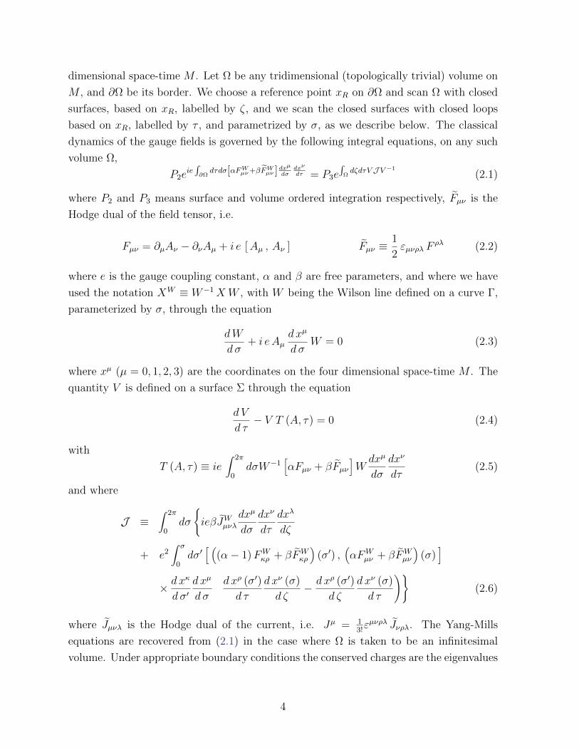
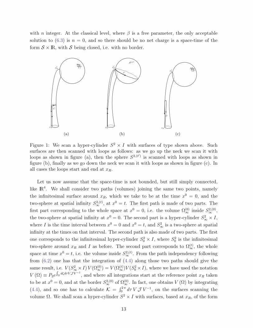
Figure 1: We scan a hyper-cylinder S2 × I with surfaces of type shown above. Suchsurfaces are then scanned with loops as follows: as we go up the neck we scan it withloops as shown in figure (a), then the sphere S2,(t′) is scanned with loops as shown infigure (b), finally as we go down the neck we scan it with loops as shown in figure (c). Inall cases the loops start and end at xR.

Let us now assume that the space-time is not bounded, but still simply connected,

like IR4. We shall consider two paths (volumes) joining the same two points, namely

the infinitesimal surface around xR, which we take to be at the time x0 = 0, and the

two-sphere at spatial infinity S2,(t)∞ , at x0 = t. The first path is made of two parts. The

first part corresponding to the whole space at x0 = 0, i.e. the volume Ω(0)∞ inside S2,(0)

∞ ,

the two-sphere at spatial infinity at x0 = 0. The second part is a hyper-cylinder S2∞ × I,

where I is the time interval between x0 = 0 and x0 = t, and S2∞ is a two-sphere at spatial

infinity at the times on that interval. The second path is also made of two parts. The first

one corresponds to the infinitesimal hyper-cylinder S20 × I, where S2

0 is the infinitesimal

two-sphere around xR and I as before. The second part corresponds to Ω(t)∞ , the whole

space at time x0 = t, i.e. the volume inside S2,(t)∞ . From the path independency following

from (6.2) one has that the integration of (4.4) along those two paths should give the

same result, i.e. V (S2∞× I)V (Ω(0)

∞ ) = V (Ω(t)∞ )V (S2

0 × I), where we have used the notation

V (Ω) ≡ P3e∫

ΩdζdτV J V −1

, and where all integrations start at the reference point xR taken

to be at x0 = 0, and at the border S2,(0)∞ of Ω(0)

∞ . In fact, one obtains V (Ω) by integrating

(4.4), and so one has to calculate K =∫ 2π

0 dτ V J V −1, on the surfaces scanning the

volume Ω. We shall scan a hyper-cylinder S2 × I with surfaces, based at xR, of the form

13

given in Figure 1, with t′ denoting a time in the interval I. Each one of such surfaces

are scanned with loops, labelled by τ , in the following way. For 0 ≤ τ ≤ 2π3

, we scan the

infinitesimal cylinder as shown in figure (1.a), then for 2π3≤ τ ≤ 4π

3we scan the sphere S2

as shown in figure (1.b), and finally for 4π3≤ τ ≤ 2π we go back to xR with loops as shown

in figure (1.c). The quantity K can then be split into the contributions coming from each

one of those surfaces as K = Ka +Kb +Kc. In the case of the infinitesimal hyper-cylinder

S20 × I, the sphere has infinitesimal radius and so it does not really contribute to Kb. We

shall assume the currents and field strength vanish at spatial infinity as

Jµ ∼1

R2+δand Fµν ∼

1

R32

+δ′

with δ, δ′ > 0, for R → ∞. Therefore the quantity J , given in (2.6), vanishes when

calculated on loops at spatial infinity. Consequently, in the case of the hyper-cylinder

S2∞ × I, the contribution to Kb coming from the sphere with infinite radius vanishes,

and we have that K calculated on the surfaces scanning S2∞ × I and S2

0 × I is the same,

and so V (S2∞ × I) = V (S2

0 × I). In fact there is more to it, since when we contract the

radius of the cylinders in Figure 1 to zero the loops in figures (1.a) and (1.c) become the

same. Therefore, the quantities J calculated on them are the same except for a minus sign

coming from the derivatives dxµ

dτ, since the loops in figure (1.a) get longer with the increase

of τ , and in figure (1.c) the opposite occurs. In addition, the quantity V inside the the

expressionK =∫ 2π

0 dτ V J V −1 is insensitive to that sign since it is obtained by integrating

(2.4) starting at xR in both cases. Therefore, it turns out that Ka + Kc = 0. The loops

scanning the sphere in figure (1.b) have legs linking the reference point xR, at x0 = 0, to

the same space point but at x0 = t′, i.e. xt′R. Therefore, when integrating (2.4) one gets

VxR = W (xt′R, xR)−1Vxt′R

W (xt′R, xR), where W (xt

′R, xR) is obtained by integrating (2.3) along

the leg linking xR to xt′R, and where we have used the notation Vx, meaning V obtained

from (2.4) with reference point x. Using the same arguments and notation one obtains

from (2.6) that, on the loops of figure (1.b), JxR = W (xt′R, xR)−1Jxt′RW (xt

′R, xR), and so

Kb,xR = W (xt′R, xR)−1Kb,xt′RW (xt

′R, xR). The quantity V (Ω(t)

∞ ) is obtained by integrating

(4.4) and by scanning the volume Ω(t)∞ with surfaces of the type shown in figure (1.b), and

where the radius of S2 varies from zero to infinity keeping the point xtR fixed. Therefore,

from the above arguments one gets that

VxR(Ω(t)∞ ) = W (xtR, xR)−1VxtR(Ω(t)

∞ )W (xtR, xR) (6.4)

One then concludes that such operator has an iso-spectral time evolution

VxtR(Ω(t)∞ ) = U(t)VxR(Ω(0)

∞ )U(t)−1 with U(t) = W (xtR, xR)V(S2

0 × I)

(6.5)

14

Therefore, its eigenvalues, or equivalently Tr(VxtR(Ω(t)∞ ))N , are constant in time. Note that

from the Yang-Mills equations (2.1) one has that such operator can be written either as

a volume or surface ordered integrals, and so we have proved (2.7).

Note that if VxtR(Ω(t)∞ ) has an iso-spectral evolution so does gcVxtR(Ω(t)

∞ ), with gc ∈ Z(G),

the center of the gauge group. That fact has to do with the freedom we have to choose

the integration constants of (2.4) and (4.4) to lie in Z(G), without spoiling the gauge

covariance of (2.1) (see discussion in the proof of (2.1) above).

Properties of the charges. First of all we point out that the conserved charges

are gauge invariant. Indeed, using the same arguments given below (5.2) for the proof of

(2.1), one has that under the gauge transformations (5.2) the operator VxtR transforms as

VxtR(Ω(t)∞ )→ gRVxtR(Ω(t)

∞ )g−1R

with gR being the group element, performing the gauge transformation, at xtR. Therefore

its eigenvalues, which are the charges, are gauge invariant. Note that the operator VxtRis the same as that given in (2.7), since the volume Ω(t)

∞ corresponds to the spatial sub-

manifold S at time equals t.

Note that when one changes the reference point from xtR to xtR, the operator VxtR(Ω(t)∞ )

changes under conjugation by W (xtR, xtR), i.e. the holonomy of the gauge field Aµ through

a path joining those two points. Therefore, similarly to (6.4) one has

VxtR(Ω(t)∞ )→ W (xtR, x

tR)−1 VxtR(Ω(t)

∞ )W (xtR, xtR)

So the conserved quantities, being the eigenvalues of VxtR(Ω(t)∞ ), are also independent of

the base points. Note in addition that the reference points xtR and xtR are on the border

of the volume Ω(t)∞ and so they lie at spatial infinity. Our boundary conditions imply that

the field strength goes to zero at infinity and so the gauge potential is asymptotically flat,

and consequently W (xtR, xtR) is independent of the choice of path joining the two reference

points.

We have seen below (6.1) that the volume Ω can be seen as a path in the loop space

LΩ. In fact, there is an infinite number of paths in LΩ representing the same physical

volume Ω, due to the infinite ways of scanning Ω with closed surfaces based at xR. We

have shown that, as a consequence of (6.2), the operator P3e∫

ΩdζdτV J V −1

is independent

of the path on loop space, as long as the end points, i.e. xR and the border ∂Ω, are

kept fixed. When we say that we have to keep the end points xR and ∂Ω fixed, we

mean that not only the physical point xR and surface ∂Ω are kept fixed but also its

scanning with loops. We do not have to worry about the scanning of xR because that is

15

trivial. A re-parameterization of the volume Ω corresponds to a change of the path in

loop space representing Ω. Therefore, the operator VxtR(Ω(t)∞ ), or equivalently the r.h.s.

of (2.7) is independent of the re-parameterization of the volume Ω(t)∞ . Consequently, the

conserved charges, which are the eigenvalues of that operator, are invariant under re-

parameterization (scanning) of the volume Ω(t)∞ that keep fixed its end points, i.e. keep

fixed the physical point xR and surface ∂Ω(t)∞ , as well as its scanning with loops.

We now have to analyze how the charges transform when we fix the physical point xR

and surface ∂Ω(t)∞ , but change the scanning of ∂Ω(t)

∞ with loops. Again we do not have to

worry about the scanning of the infinitesimal surface around xR because that is trivial.

The volume Ω(t)∞ corresponds to the spatial sub-manifold S introduced in (2.7), at time

equals t. Therefore, we have to analyze how the surface ordered integral over ∂S given in

(2.7), transforms under the change of the scanning of ∂S with loops. Remember however

that such integral is obtained by integrating (2.4) over ∂S. In (4.3) we have shown how

such kind of integral changes when the surface of integration is changed. The calculation

in (4.3) is valid not only for a change of the physical surface but also for a change of the

scanning of it with loops. In the latter case the variation δxµ (σ) of the loop is parallel

to the surface, i.e. there are no variations δxµ (σ) perpendicular to the surface. Since ∂S

is a two-dimensional surface all 3-forms on it vanish. Therefore, the first term of (4.3)

must vanish trivially when we restrict δxλ to be parallel to the surface, since d xµ

d σand d xν

d τ

are, by definition, parallel to the surface. The argument we are using here is the same as

that in the proof of Theorem 2.1 of [2] for r-flat connections in loop space. Replacing Bµν

by ie[αFµν + β Fµν

]we get that (4.1) becomes (2.4) and (2.5). Therefore, the condition

for the surface ordered integral over ∂S in (2.7), to be invariant under changes of the

scanning of ∂S with loops is

∫ 2π

0dσ

∫ σ

0dσ′

[(α− 1) FW

κρ (σ′) + β FWκρ (σ′) , α FW

µν (σ) + β FWµν (σ)

]

× dxκ

dσ′dxµ

dσ

(d xρ (σ′)

d τδxν (σ)− δxρ (σ′)

d xν (σ)

d τ

)= 0 (6.6)

where we have used the notation XW ≡ W−1XW . Such double integral in σ and σ′ is

performed over a given loop, based at xR, scanning the surface ∂S. Note however that

such surface is the border of the spatial sub-manifold S, and so it lies at spatial infinity.

Therefore, the field tensor and its Hodge dual, appearing in the integrand, are to be

evaluated at spatial infinity.

There are at least two sufficient conditions for (6.6) to hold true. The first one is that

the field tensor and its dual should fall at spatial infinity faster than 1/R2, where R is

the radius (or a measure of size) of the surface ∂S, which should be taken to infinity,

16

i.e. R → ∞. That is so, because the integrand in (6.6) is quartic in variations of the

Cartesian coordinates xµ and quadratic in the field tensor and its dual. As we will see

in section 7.2 that is exactly what happens in the case of instantons. So, the conserved

(in the Euclidean time) charges constructed as the eigenvalues of the operator (2.7) are

invariant under re-parameterization of volumes and surfaces for the instantons solutions.

The second sufficient condition is that the commutator in the integrand of (6.6) must

vanish, and so the field tensor and its dual conjugated by the holonomy W has to lie in

an abelian subalgebra. As we discuss in sections 7.1 and 7.3 that is exactly what happens

in the cases of monopoles, dyons and merons. For those solutions the field tensor at

spatial infinity has the form Fµν ∼ 1r2 G (r), where r is the radial distance, and G (r) is

a Lie algebra element depending on the unit vector r, and being covariantly constant,

i.e. DµG (r) = 0. That fact implies that W−1G (r) W is constant everywhere, and so all

components of the field tensor and its dual (conjugated by W ) lies in the direction of that

element of the Lie algebra. Therefore, the commutator in the integrand of (6.6) vanishes.

Consequently, the conserved charges constructed as the eigenvalues of the operator (2.7)

are invariant under re-parameterization of volumes and surfaces for the monopole, dyon

and meron solutions.

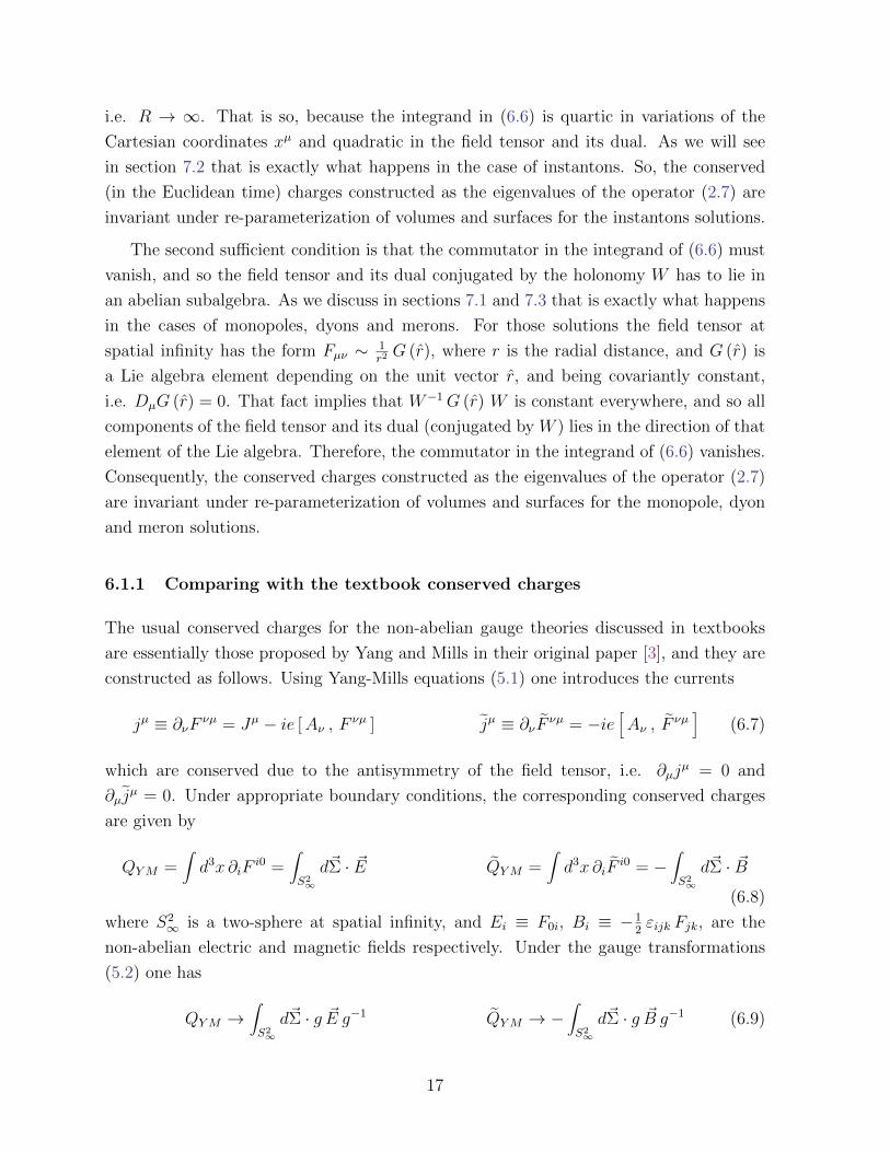
6.1.1 Comparing with the textbook conserved charges

The usual conserved charges for the non-abelian gauge theories discussed in textbooks

are essentially those proposed by Yang and Mills in their original paper [3], and they are

constructed as follows. Using Yang-Mills equations (5.1) one introduces the currents

jµ ≡ ∂νFνµ = Jµ − ie [Aν , F

νµ ] jµ ≡ ∂νFνµ = −ie

[Aν , F

νµ]

(6.7)

which are conserved due to the antisymmetry of the field tensor, i.e. ∂µjµ = 0 and

∂µjµ = 0. Under appropriate boundary conditions, the corresponding conserved charges

are given by

QYM =∫d3x ∂iF

i0 =∫

S2∞

d~Σ · ~E QYM =∫d3x ∂iF

i0 = −∫

S2∞

d~Σ · ~B(6.8)

where S2∞ is a two-sphere at spatial infinity, and Ei ≡ F0i, Bi ≡ −1

2εijk Fjk, are the

non-abelian electric and magnetic fields respectively. Under the gauge transformations

(5.2) one has

QYM →∫

S2∞

d~Σ · g ~E g−1 QYM → −∫

S2∞

d~Σ · g ~B g−1 (6.9)

17

If one restricts oneself to gauge transformations where the group element g goes to a con-

stant at spatial infinity then the charges transform covariantly, i.e. QYM → g∞QYM g−1∞ ,

and QYM → g∞ QYM g−1∞ , with g∞ being the constant group element on S2

∞. Therefore,

the eigenvalues of QYM and QYM are invariant under those restricted gauge transforma-

tion.

The conserved charges we construct in this paper, namely the eigenvalues of the op-

erator (2.7) differ in many aspects from the charges (6.8). First, we show that only

the eigenvalues of the operator (2.7) are conserved in time. The full operator has an

isospectral time evolution. Second, those eigenvalues are invariant under general gauge

transformations, and not only under restricted transformations where the group element

goes to a constant at infinity. Third, the charges obtained from (2.7) are different from

those obtained from (6.8). Indeed, as we show in the example of the monopole in section

7.1, all the charges coming from (6.8) vanish, and those obtained from (2.7) give the mag-

netic charge of the monopole, as well as its quantization. There are two aspects to stress

here. First our calculations work equally well for the Wu-Yang monopole as well as for

the ’tHooft-Polyakov monopole, and the conservation of the charge is dynamical and not

necessarily topological. Second, the magnetic charge which is conserved is associated to

the abelian subgroup only (in the case the gauge group is SO(3), to the U(1) subgroup)

and not to the full group as is the case of the charge coming from (6.8). That is also true

for the Wu-Yang monopole where the gauge symmetry is not spontaneously broken. For

those reasons, the construction of conserved charges for non-abelian gauge theories that

we propose in this paper constitute a great advance with respect to what is usually found

in the literature.

6.2 The conserved charges for the self-dual sector

The integral equation (2.9) leads to some interesting consequences which we now discuss.

Consider the case where the surface Σ is closed, i.e. it has no border. Then, ∂Σ disappears

and the l.h.s. of (2.9) is trivial and so

P2 eie∫∂Ω

dσdτ W−1[αFµν+κ (1−α) Fµν]W dxµ

dσdxν

dτ = 1l (6.10)

where we have denoted Σ = ∂Ω, i.e. the border of the volume Ω contained inside Σ. Now,

if one takes β = κ (1− α) in (2.1), one observes that the second term in the expression

(2.6) for J vanishes, when the self dual equation (2.9), or equivalently (2.8), are imposed.

18

Therefore, (6.10) and (2.1) imply that

P3 eieκ(1−α)

∫ΩdζdτdσV JWµνλ

dxµ

dσdxν

dτdxλ

dζV −1

= 1l (6.11)

Since that has to be valid on any volume Ω, one concludes that the current Jµ should

vanish. That is an expected result, and indeed the imposition of the Yang-Mills equations

(5.1) and the self duality equations (2.8) imply the vanishing of Jµ. In addition, the

first order differential equations (2.8) imply the second order equations (5.1) when the

current vanishes, since the second equation in (5.1) is just an identity, the so-called Bianchi

identity, i.e.

DλFµν +DµFνλ +DνFλµ = 0 (6.12)

In order to understand that the integral self dual Yang-Mills equation (2.9) implies the

the full integral Yang-Mills equation (2.1) we have to construct the integral version of

the Bianchi identity. One can obtain that by taking the generalized non-abelian Stokes

theorem (4.6), which is an identity, and choose Bµν = i e λFµν , with λ a free parameter,

and use (6.12) to get

P2eie λ

∫∂Ω

dτdσFWµνdxµ

dσdxν

dτ = P3e∫

ΩdζdτV CV −1

(6.13)

with

C ≡ e2 λ (λ− 1)∫ 2π

0dσ∫ σ

0dσ′

[FWκρ (σ′) , FW

µν (σ)]

× d xκ

d σ′d xµ

d σ

(d xρ (σ′)

d τ

d xν (σ)

d ζ− d xρ (σ′)

d ζ

d xν (σ)

d τ

)(6.14)

The relation (6.13) is highly non-trivial for λ 6= 0 or 1. Indeed, for λ = 1 it leads

to what one would naively expect as the integral version of the Bianchi identity, i.e.

P2eie∫∂Ω

dτdσFWµνdxµ

dσdxν

dτ = 1l. The relation (6.13) carries important information about the

flux of a non-abelian field strength Fµν through a closed surface when that is rescaled

by a factor λ, and it certainly deserves further investigation. Now, by imposing the

self duality equation (2.9), or equivalently (2.8), one observes that (2.1) becomes (6.13)

with λ = α + κβ. So, the self duality condition does turn the full integral Yang-Mills

equation (2.1) into an identity, namely (6.13), in a manner similar that (2.8) does to the

full differential Yang-Mills equation (5.1).

The other consequence of the relation (6.10) is that it leads to conservation laws, in a

manner similar to that which (6.2) does in the case of the full Yang-Mills equations. In

19

order to do that let us consider the loop space associated to a surface Σ

LΣ = γ : S1 → Σ | north pole→ xR ∈ ∂Σ (6.15)

A scanning of Σ with loops, in the way described below (2.9), corresponds to a path in

LΣ. In fact, there is an infinity of paths in LΣ corresponding to the same physical surface

Σ. The closed surface ∂Ω is a closed path in L∂Ω, and the reference point xR is now any

chosen point on ∂Ω since it has no border. Let us now take a point in that closed path

corresponding to a loop in ∂Ω. It then splits the path into two parts, or equivalently ∂Ω

into two surfaces with a common border, i.e. ∂Ω = Σ1 + Σ2. Consequently (6.10) can be

written as

P2 eie∫

Σ1dσdτ W−1[αFµν+κ (1−α) Fµν]W dxµ

dσdxν

dτ P2 eie∫

Σ2dσdτ W−1[αFµν+κ (1−α) Fµν]W dxµ

dσdxν

dτ = 1l

(6.16)

By reverting the sense of integration along the path one gets the inverse operator. But Σ1

and Σ−12 are two different paths joining the same two points in the loop space L∂Ω, namely

the infinitesimal loop around xR and the common border of Σ1 and Σ−12 . Therefore, (6.16)

implies that the operator

V (Σ) ≡ P2 eie∫

Σdσdτ W−1[αFµν+κ (1−α) Fµν]W dxµ

dσdxν

dτ (6.17)

is independent of the path, or equivalently of the surface Σ, as long as the end points

(the border of Σ and the reference point xR on it) are kept fixed. In addition, by fixing

the surface Σ and changing the path in the loop space LΣ that corresponds to it, we see

that V (Σ) is independent of the choice of the scanning. Such path independency leads

to conservation laws as we now explain.

First of all let us fix a plane in an Euclidean space-time M , and let us denote by

xµ and xν (µ and ν fixed) the Cartesian coordinates associated to the two orthogonal

axis lying on that plane. That could be done in a space time of any metric, but we are

interested in real solutions of the self dual Yang-Mills equations (2.8), and so we choose

the Euclidean metric. We shall denote by xα and xβ (α and β fixed) the two Cartesian

coordinates corresponding to the directions orthogonal to the plane xµ xν . In fact, we

shall work with a given fixed axis parameterized by t which is a linear combination of the

xα and xβ axis, i.e. we write

xα = t cosφ xβ = t sinφ −∞ < t <∞ 0 ≤ φ ≤ π (6.18)

We shall choose two surfaces Σ1 and Σ2 with the same border as shown in Figure 2. The

20

xR

D(0)∞

S1∞ × I

xR

D(t)∞

S10 × I

x(t)R

Surface Σ2 = (S10 × I) ∪ D(t)

∞Surface Σ1 = D(0)∞ ∪ (S1

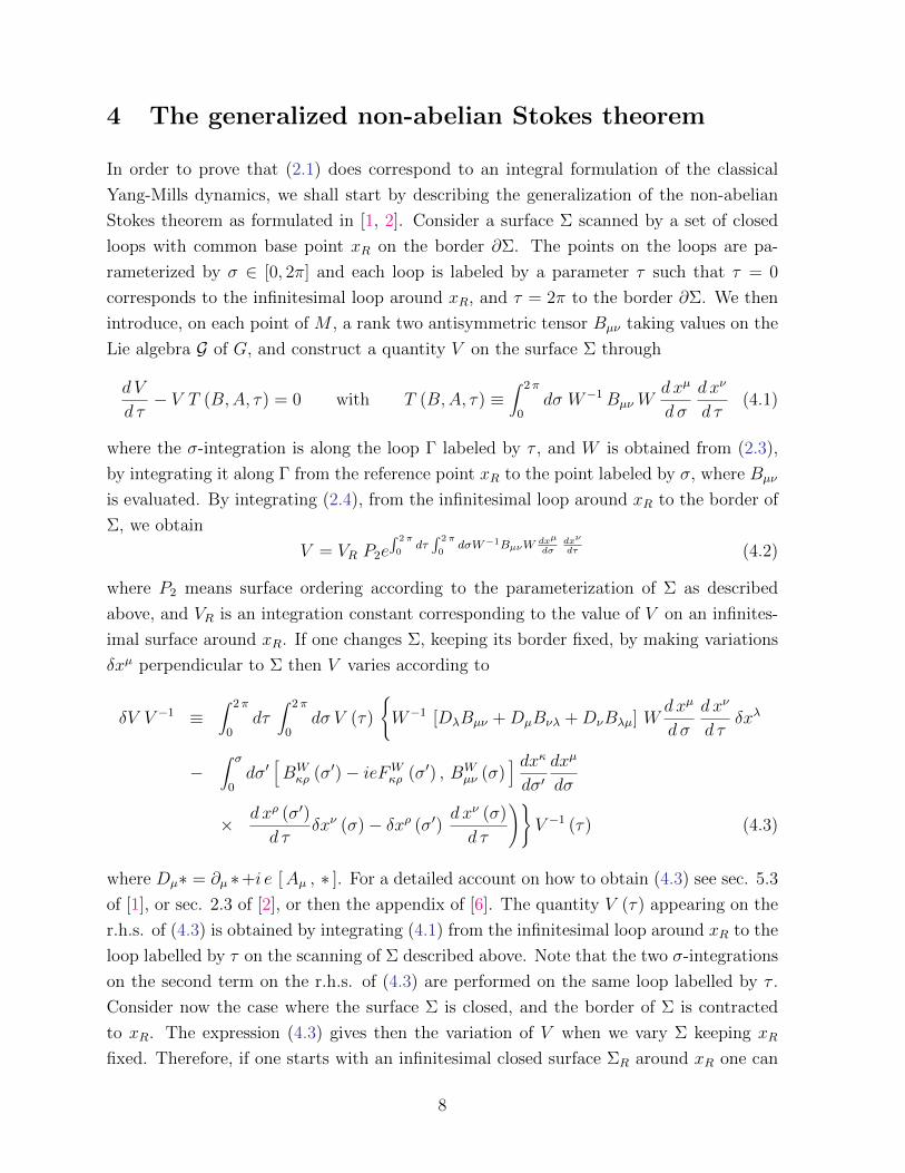
∞ × I)segunda-feira, 23 de abril de 2012

Figure 2: The surfaces Σ1 and Σ2, with the same border S1,(t)∞ , and reference point xR,

used in the construction of conserved charges.

surface Σ1 is made of two parts. The first part is a disc D(0)∞ of infinite radius on the plane

xµ xν at t = 0, i.e. it is the whole plane xµ xν at t = 0. The second part is a cylinder

S1∞ × I, where I is a segment of the t-axis going from t = 0 to t = t, and S1

∞ is a circle

of infinite radius parallel to the plane xµ xν . We choose the reference point xR to lie on

the border of D(0)∞ , i.e. on the circle S1

∞ at t = 0. The surface Σ2 is also made of two

parts. The first part is an infinitesimal cylinder S10 × I , with I as before, and S1

0 a circle

of infinitesimal radius also parallel to the plane xµ xν . We choose the infinitesimal circle

S10 such that xR lies on it at t = 0. The second part of Σ2 is a disc D(t)

∞ of infinite radius,

parallel to the plane xµ xν , and at t = t. We scan the two surfaces with loops, as shown

in Figure 2, starting and ending at the reference point xR (for a similar discussion on

how to do that see section 3.1 of [6]). Therefore, the surfaces Σ1 and Σ2 are two different

paths in the loop space L∂Ω, such that ∂Ω = Σ1 +Σ−12 , with the same end points, namely

the infinitesimal circle at xR and the circle S1∞ at t = t. Since the operator (6.17) is

independent of the surface, it follows that it is the same calculated on those two surfaces,

i.e.

V (Σ1) = V (Σ2) → V(D(0)∞

)V(S1∞ × I

)= V

(S1

0 × I)V(D(t)∞

)(6.19)

Note that in fact, V (S10 × I) = 1l since S1

0 is infinitesimal. Now if we impose the boundary

conditions

Fρσ = κ Fρσ ∼1

r2+δT (r) for r →∞ (6.20)

where δ > 0, r is the radial distance in the xµ xν plane, i.e. r2 = (xµ)2 + (xν)2 (µ and ν

fixed), and T (r) is a Lie algebra element depending only on the radial direction, i.e. r = ~rr.

Those boundary conditions imply that the integrand in (6.17) vanishes on the cylinder

S1∞ × I, and so V (S1

∞ × I) = 1l. Therefore, one gets that V(D(0)∞

)= V

(D(t)∞

). We can

21

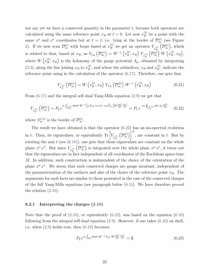
not say yet we have a conserved quantity in the parameter t, because both operators are

calculated using the same reference point xR at t = 0. Let now x(t)R be a point with the

same xµ and xν coordinates but at t = t, i.e. lying at the border of D(t)∞ (see Figure

2). If we now scan D(t)∞ with loops based at x

(t)R we get an operator V

x(t)R

(D(t)∞

), which

is related to that, based at xR, as VxR(D(t)∞

)= W−1

(x

(t)R , xR

)Vx

(t)R

(D(t)∞

)W(x

(t)R , xR

),

where W(x

(t)R , xR

)is the holonomy of the gauge potential Aµ, obtained by integrating

(2.3), along the line joining xR to x(t)R , and where the subindices, xR and x

(t)R , indicate the

reference point using in the calculation of the operator (6.17). Therefore, one gets that

Vx

(t)R

(D(t)∞

)= W

(x

(t)R , xR

)VxR

(D(0)∞

)W−1

(x

(t)R , xR

)(6.21)

From (6.17) and the integral self dual Yang-Mills equation (2.9) we get that

Vx

(t)R

(D(t)∞

)= P2 e

ie∫D(t)∞

dσdτ W−1[αFµν+κ (1−α) Fµν]W dxµ

dσdxν

dτ = P1 e−ie∮S

1,(t)∞

dσ Aµdxµ

dσ (6.22)

where S1,(t)∞ is the border of D(t)

∞ .

The result we have obtained is that the operator (6.22) has an iso-spectral evolution

in t. Then, its eigenvalues, or equivalently Tr[Vx

(t)R

(D(t)∞

)]N, are constant in t. But by

rotating the axis t (see (6.18)), one gets that those eigenvalues are constant on the whole

plane xα xβ. But since Vx

(t)R

(D(t)∞

)is integrated over the whole plane xµ xν , it turns out

that the eigenvalues are in fact independent of all coordinates of the Euclidean space-time

M . In addition, such construction is independent of the choice of the orientation of the

plane xµ xν . We stress that such conserved charges are gauge invariant, independent of

the parametrization of the surfaces and also of the choice of the reference point xR. The

arguments for such facts are similar to those presented in the case of the conserved charges

of the full Yang-Mills equations (see paragraph below (6.5)). We have therefore proved

the relation (2.10).

6.2.1 Interpreting the charges (2.10)

Note that the proof of (2.10), or equivalently (6.22), was based on the equation (6.10)

following from the integral self-dual equation (2.9). However, if one takes (6.10) on shell,

i.e. when (2.8) holds true, then (6.10) becomes

P2 eie∫∂Ω

dσdτ W−1 FµνWdxµ

dσdxν

dτ = 1l (6.23)

22

But that is just an identity following either from the usual non-abelian Stokes theorem

(3.1) by taking Cµ ≡ ieAµ, and Σ a closed surface, i.e. the border of a volume Σ = ∂Ω,

or then from the integral Bianchi identity (6.13) with λ = 1. Therefore, if the field tensor

satisfies the boundary conditions (see (6.20))

Fρσ ∼1

r2+δT (r) for r →∞ (6.24)

with δ > 0, all the arguments leading to (6.22) hold true, and we obtain an isospectral

evolution for the operator

V ′x

(t)R

(D(t)∞

)= P2 e

ie∫D(t)∞

dσdτ W−1 FµνWdxµ

dσdxν

dτ = P1 e−ie∮S

1,(t)∞

dσ Aµdxµ

dσ (6.25)

Therefore the eigenvalues of (6.25) are constant in the time t introduced in (6.18). Note

that such result applies to any field configuration satisfying (6.24) and it does not have

necessarily to be a self-dual solution of the Yang-Mills equations. In fact, it does not even

have to be a solution of the Yang-Mills theory since (6.23) follows from identities.

Note that if D(t)∞ is a spatial surface then the surface ordered integral in (6.25), namely

P2 eie∫D(t)∞

dσdτ W−1 FµνWdxµ

dσdxν

dτ , corresponds to the flux of the non-abelian magnetic field

(Bi ≡ −12εijk Fjk) through that surface. On the other hand, if D(t)

∞ has a time component

then that integral corresponds to the flux of the non-abelian electric field (Ei ≡ F0i)

through such spatial-temporal surface. Note that the conservation of those fluxes can be

intuitively understood by the fact that the border of D(t)∞ is the circle S1,(t)

∞ of infinite

radius. Therefore, if the field configuration is localized in a region at a finite distance to

the plane containing S1,(t)∞ the solid angle defined by that circle is 2π spheroradians. If

that field configuration evolves in the time t changing its distance to that plane by a finite

amount, the solid angle will remain the same, and so should the flux of the magnetic or

electric fields. Of course, that is an intuitive view, and so not precise, of the conservation

of the charge, but we will show that it stands reasonable in the examples we discuss in

section 7.

7 Examples

We now evaluate the conserved charges obtained from (2.7) and (2.10) for well known so-

lutions like monopoles, dyons, instantons and merons. For simplicity we restrict ourselves

to the case where the gauge group is SU(2), since it contains all the physically relevant

aspects of the construction.

23

7.1 Monopoles and dyons

In order to evaluate the operator (2.7) let us first work with its form as a surface ordered

integral of the field tensor and its dual, and then consider the volume ordered integral form

of it. Therefore we need the field tensor at spatial infinity only. The ’tHooft-Polyakov [9]

and Wu-Yang [10] monopoles for a gauge group SU(2) have the same behavior at infinity.

Indeed, the gauge field and field tensor at infinity are given by

Ai = −1

eεijk

rjrTk =

1

2

i

e∂ig g

−1 ; A0 = 0

Fij =1

eεijk

rkr2r · T ; F0i = 0 (7.1)

where r = ~rr, is unit vector in the radial direction, Ti are the generators of the SU(2) Lie

algebra satisfying

[Ti , Tj ] = i εijk Tk i, j, k = 1, 2, 3 (7.2)

and g is the group element g = exp (i π r · T ). In the case of the Wu-Yang monopole the

formulas (7.1) correspond to the exact solution, and not only to its behavior at infinity.

In the case of the ’tHooft-Polyakov monopole, on the other hand, (7.1) is true only in the

limit r → ∞, and we do not show the behavior of the Higgs field since it is not relevant

in the evaluation of the charges as we show below.

In order to calculate (2.7) we have to scan the two-sphere at spatial infinity with

loops starting and ending at a chosen reference point xR. The quantity W is obtained

by integrating (2.3) from xR to a given point on the loop. An important fact in such

calculation is that the quantity r · T is covariantly constant, i.e.

Di r · T = ∂i r · T + i e [Ai , r · T ] = 0 (7.3)

Therefore, using (2.3) one gets that

d

dσ

(W−1 r · T W

)= 0 (7.4)

So, W−1 r · T W is constant along any loop, and consequently constant everywhere. If we

denote by TR the value of r · T at the reference point xR, one gets from (7.1) that

W−1 FijW =1

eεijk

rkr2TR (7.5)

24

and so it belongs to the abelian subalgebra U(1) generated by TR. Therefore, the surface

ordering becomes irrelevant and the operator (2.7) becomes (since Fij = 0)

QS = ei e α

∫S2∞dσ dτ W−1 FijW

dxi

dσdxj

dτ = e−i e α

∫S2∞d~Σ· ~BR

= ei α TR

∫S2∞dσ dτ εijk

rkr2

dxi

dσdxj

dτ = ei 4π αTR (7.6)

where we have introduced the abelian magnetic field BRi ≡ −1

2εijkW

−1 FjkW = −1erir2 TR,

and have denoted dΣi = εijkdxj

dσdxk

dτdσ dτ . Using Gauss law we define the magnetic charge

as ∫

S2∞

d~Σ · ~BR = GR and so GR = −4 π

eTR (7.7)

According to our construction (see (2.7)) the eigenvalues of QS are constant in time which,

in view of (7.6), is equivalent to say that the eigenvalues of GR are constants. At the end

of section 2, where we discuss the nature of the eigenvalues of the charges, we have shown

that our construction does not fix the vector space (representation) where such eigenvalues

should be evaluated. If we choose to calculate them on a finite dimensional representation

of the gauge group SU(2) (or SO(3)), then the eigenvalues of TR are integers or half-

integers. Therefore it follows that the magnetic charges, on those representations, must

be quantized as

eigenvalues of GR =2π n

en = 0,±1,±2 . . . (7.8)

Let us now look at the evaluation of the magnetic charges as volume ordered integrals.

From (2.7), (2.6) and (7.6) one gets that

e−i e αGR = P3e∫

spacedζdτV JmonopoleV

−1

(7.9)

with

Jmonopole ≡ e2 α (α− 1)∫ 2π

0dσ∫ σ

0dσ′

[FWij (σ′) , FW

kl (σ)]

× d xi

d σ′d xk

d σ

(d xj (σ′)

d τ

d xl (σ)

d ζ− d xj (σ′)

d ζ

d xl (σ)

d τ

)(7.10)

where we have used the fact that Fij = 0, and J123 = J0 = 0, since in the Wu-Yang case

there is no current, and in the ’tHooft-Polyakov case we have a static solution with A0 = 0,

and so the time component of the Higgs field current vanishes. Note that (7.9) and (7.10)

could also have been obtained from the integral Bianchi identity (6.13). In the case of the

’tHooft-Polyakov monopole it follows that (7.5) is not true inside the monopole core and

25

we have a quite non-trivial expression for the magnetic charge as a volume integral. We

do not evaluate it in this paper and so we do not have anything to add to the result (7.8).

Note however, that even though the r.h.s. of (7.9) is integrated over the entire space, the

Higgs field does not contribute for such formula of the magnetic charge.

In the case of the Wu-Yang monopole, however, it is not that difficult to evaluate (7.10)

after performing a regularization of the Wilson line, passing through the singularity of

the gauge potential (7.1). That calculation is given in the appendix A and the result is

that Jmonopole vanishes in all loops, and so (see (A.10))

e−i e αGR = P3e∫

spacedζdτV JmonopoleV

−1

= 1l (7.11)

Such result implies that the magnetic charge for the Wu-Yang monopole is quantized as

eigenvalues of GR =2π n

eαn = 0,±1,±2 . . . (7.12)

If the parameter α is indeed arbitrary, and there is no physical condition to fix it, then

the only acceptable value for the integer n is n = 0, and so the magnetic charge of the

Wu-Yang monopole should vanish. Perhaps we have to go to the quantum theory to

settle that issue. It might happen that quantum conditions restrict the allowed values of

α. That is one of the important points of our construction to be further investigated.

Let us now consider the case of dyon solutions. For the Wu-Yang and the ’tHooft-

Polyakov case, as calculated by Julia and Zee [11], the space components of the gauge

potential and field tensor, namely Ai and Fij, i, j = 1, 2, 3, are the same as those in (7.1),

and the time components, at spatial infinity, are replaced by

A0 =M

er·T+

γ

e

r · Tr

+O(1

r2) ; F0i =

γ

e

rir2r·T+O(

1

r3) ; r →∞ (7.13)

with M and γ being parameters of the solution. In the case of the Wu-Yang dyon, i.e.

when there is no Higgs field and no symmetry breaking, the formulas (7.13), as well as

(7.1), are true everywhere and not only at spatial infinity. In other words, there are no

terms of order r−2 and r−3 in A0 and F0i respectively. Using (7.4) we have, in anology to

(7.5), that

W−1 FijW → −γ

eεijk

rkr2TR r →∞ (7.14)

So, W−1 FijW also belongs to the abelian subalgebra U(1) generated by TR, and it is

in fact proportional to W−1 FijW . Therefore, the surface ordering is not relevant in the

26

evaluation of the operator (2.7), and we get in the dyon case that

QS = e−i e

[α∫S2∞d~Σ· ~BR+β

∫S2∞d~Σ· ~ER

]= e−i e [αGR+β KR] = ei 4π [α−β γ]TR (7.15)

where we have introduced the abelian electric field ERi = W−1 F0iW = γ

erir2 TR, ~BR and

GR are the same as before, and using Gauss law we have defined the electric charge as

∫

S2∞

d~Σ · ~ER = KR and so KR =4 π γ

eTR (7.16)

According to (2.7) the eigenvalues of QS are constant in time, and so we conclude from

(7.15) that the eigenvalues of (αGR + β KR) are constants. But if we assume that the

parameters α and β are arbitrary it follows that the eigenvalues of GR and KR are inden-

pendently constant in time. We have seen that, by evaluating the eigenvalues of TR on

finite dimensional representations of the gauge group SU(2), where they are integers or

half-integers, the eigenvalues of the magnetic charge GR are quantized as in (7.8). Under

the same assumptions it follows from (7.16) that

eigenvalues of KR =2 π γ n

en = 0,±1,±2, . . . (7.17)

Again from (2.7) we can express the charges in terms of volume ordered integrals, and

from (2.7), (2.6) and (7.15) we get

e−i e [αGR+β KR] = P3e∫

spacedζdτV JdyonV

−1

(7.18)

with

Jdyon ≡∫ 2π

0dσ

ieβJWijk

dxi

dσ

dxj

dτ

dxk

dζ

+ e2∫ σ

0dσ′

[ ((α− 1)FW

ij + βFWij

)(σ′) ,

(αFW

kl + βFWkl

)(σ)

]

× d xi

d σ′d xk

d σ

(d xj (σ′)

d τ

d xl (σ)

d ζ− d xj (σ′)

d ζ

d xl (σ)

d τ

)(7.19)

In the case of the Wu-Yang dyon we have J123 = J0 = 0, since there are no sources.

However, for the Julia-Zee dyon we have that the Higgs field contributes to the current

Jµ. One can extract the magnetic and electric charges GR and KR from (7.18), by setting

β = 0 and α = 0 respectively. Then, the Higgs field contributes to the electric charge

only.

27

In the case of the Wu-Yang dyon it is possible to evaluate (7.19) after a regularization

of the Wilson line operator passing through the singularity of the gauge potential (7.1).

That calculation is shown in the appendix A and it was found that Jdyon vanishes in all

loops for the Wu-Yang dyon (see (A.10)). Therefore

e−i e [αGR+β KR] = P3e∫

spacedζdτV JdyonV

−1

= 1l (7.20)

which implies that

eigenvalues of [αGR + β KR] =2 π n

en = 0,±1,±2, . . . (7.21)

Again, if the parameters α and β are indeed arbitrary, then it follows from (7.21) that

by taking β = 0, the eigenvalues of GR should obey (7.12). On the other hand by taking

α = 0, one concludes that (7.21) implies that

eigenvalues of KR =2π n

e βn = 0,±1,±2 . . . (7.22)

Now, if (7.12) and (7.22) should hold true for arbitrary values of α and β respectively, then

the only acceptable value of the integer n in both equations is n = 0, and consequently

the electric and magnetic charges of the Wu-Yang dyon should vanish. As discussed below

(7.12), we have perhaps to consider of the quantum theory to settle that issue, since there

could be quantum conditions restricting the values of α and β.

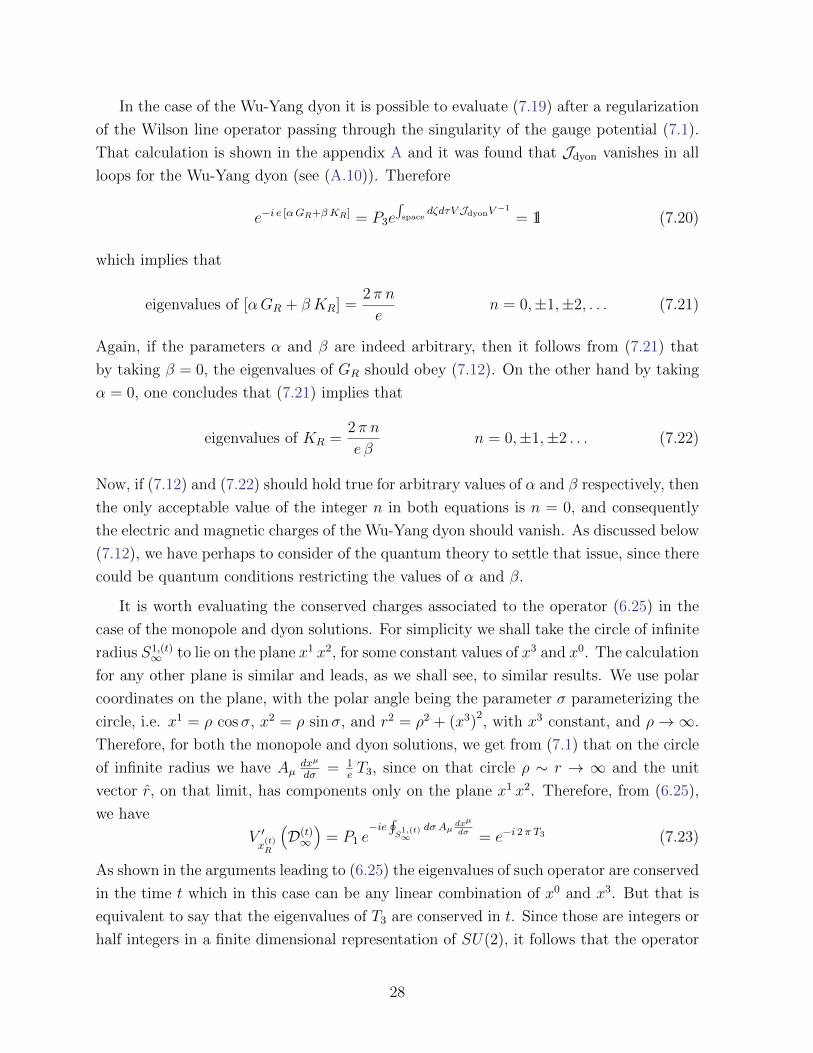
It is worth evaluating the conserved charges associated to the operator (6.25) in the

case of the monopole and dyon solutions. For simplicity we shall take the circle of infinite

radius S1,(t)∞ to lie on the plane x1 x2, for some constant values of x3 and x0. The calculation

for any other plane is similar and leads, as we shall see, to similar results. We use polar

coordinates on the plane, with the polar angle being the parameter σ parameterizing the

circle, i.e. x1 = ρ cosσ, x2 = ρ sinσ, and r2 = ρ2 + (x3)2, with x3 constant, and ρ→∞.

Therefore, for both the monopole and dyon solutions, we get from (7.1) that on the circle

of infinite radius we have Aµdxµ

dσ= 1

eT3, since on that circle ρ ∼ r → ∞ and the unit

vector r, on that limit, has components only on the plane x1 x2. Therefore, from (6.25),

we have

V ′x

(t)R

(D(t)∞

)= P1 e

−ie∮S

1,(t)∞

dσ Aµdxµ

dσ = e−i 2π T3 (7.23)

As shown in the arguments leading to (6.25) the eigenvalues of such operator are conserved

in the time t which in this case can be any linear combination of x0 and x3. But that is

equivalent to say that the eigenvalues of T3 are conserved in t. Since those are integers or

half integers in a finite dimensional representation of SU(2), it follows that the operator

28

V ′x

(t)R

(D(t)∞

)is either 1l or −1l, i.e. an element of the center of SU(2). As pointed out

below (6.25) such conserved charge can be interpreted as the non-abelian magnetic flux

through the surface D(t)∞ , which border is S1,(t)

∞ . Indeed, we see that the argument of the

exponential in (7.23) is half of the argument of the exponential in (7.6), if one takes α = 1,

and considers that TR and T3 have the same norm and so the same eigenvalues. Remember

TR is the value of r · T at the reference point xR and so Tr (TR)2 = Tr (Ti Tj) ri rj = λ,

where Tr (Ti Tj) = λ δij, and λ depends upon the representation used. Since the argument

of the exponential in (7.6) corresponds to the total flux of the magnetic field through S2∞,

we see that it is the double of the flux through D(t)∞ . Due to the spherical symmetry of the

solution that is compatible with interpretation, given below (6.25), since S2∞ corresponds

to a solid angle of 4 π spheroradians as seen from the center of the solution and D(t)∞

corresponds to only 2π spherodradians.

There are several comments that are important to make regarding the construction

of charges for monopoles and dyons. First of all the charges we constructed are different

from those given by (6.8). Indeed, from (7.1) and (7.13) we have that the magnetic and

electric fields at spatial infinity for the Wu-Yang and ’tHooft-Polyakov cases are given by

Bi → −1

e

rir2r · T ; Ei →

γ

e

rir2r · T ; r →∞ (7.24)

So, they do not lie on an abelian U(1) subalgebra like BRi and ER

i given above, and when

integrated on the two-sphere at infinity lead to the vanishing of the charges (6.8), i.e.

Qmonopole/dyonYM = Q

monopole/dyonYM = 0 (7.25)

Note that even though the evaluation of the charges (7.6) and (7.15) rely on the choice of

a reference point xR, which leads to a particular generator TR, the charges do not depend

upon that reference point. Indeed, if one changes the reference point from xR to xR, then

the operator QS changes as (see discussion below (6.5))

QS → W (xR, xR)−1QSW (xR, xR) (7.26)

where W (xR, xR) is the holonomy from the old reference point xR to the new one xR.

Therefore the charges, which are the eigenvalues of QS, do not change.

Note that since the charges are the eigenvalues of the operator (2.7), the number of

charges is equal to the rank of the gauge group G. However, since the field tensor and

its Hodge dual come multiplied by the arbitrary parameters α and β respectively, the

number of charges is in fact twice the rank of the gauge group. So, we have rank of G

29

magnetic charges and rank of G electric charges. In this sense the number of charges does

not pay attention to the pattern of symmetry breaking. Indeed, our calculations have

shown that the electric and magnetic charges are the same for the Wu-Yang case, which

is a solution of the pure Yang-Mills theory, and for the ’tHooft-Polyakov case which has

a Higgs field breaking the gauge symmetry from SO(3) down to SO(2). In fact, as we

have shown above the Higgs field does not play any role in the evaluation of the charges.

In addition the conservation of the charges is dynamical, i.e. it follows directly from

the integral form of the equations of motion (2.1). That contrasts to the conservation

of the magnetic charge of the ’tHooft-Polyakov monopole which follows from topological

(homotopy) considerations related to the mapping of the Higgs field from the spatial

infinity to the Higgs vacua. Another point relates to the quantization of the magnetic

charge, which in the case of ’tHooft-Polyakov monopole comes from the topology again,

i.e. the charge is determined by second homotopy group of the Higgs vacua. In our case,

the quantization of the charges comes from the integral equations of motion themselves

(more precisely the integral Bianchi identity (6.13)), without any reference to the Higgs

field since it works equally well for the Wu-Yang and ’tHooft-Polyakov monopoles. It is

worth pointing out that the magnetic charges of monopoles of ’tHooft-Polyakov type have

already been expressed in the literature, as surface ordered integral using the ordinary

non-abelian Stokes theorem. See for instance section 5 of Goddard and Olive’s review

paper [12]. However, that construction is totally based on the properties of the Higgs

vacua, since the fact that the Higgs field must be covariantly constant at spatial infinity

leads to an equation for it similar to (2.3) for the Wilson line W . In addition the argument

for the conservation of the magnetic charge is particular to that type of solution since it

is based on topology considerations of the solution. The generalized non-abelian Stokes

theorem (4.6), and consequently the integral Yang-Mills equations (2.1) were not known

by that time. We believe that the role played by the integral equation (2.1) in monopole

and dyon solutions deserves further study specially in the quantum theory. It might

connect to the so-called abelian projection and arguments for confinement.

7.2 Euclidean solutions

Note that the proof that the eigenvalues of the operator (2.7) are constant in the time

x0 did not really depend on the particular properties of the metric on the Minkowski

space-time. In fact, the metric tensor was only necessary to introduce the Hodge duals of

the field tensor and of the matter current. Therefore, one could evaluate those eigenvalues

for Euclidean solutions, like instantons and merons, and obtain charges conserved in the

Euclidean time x4. We will see that those charges are trivial in the case of instantons

30

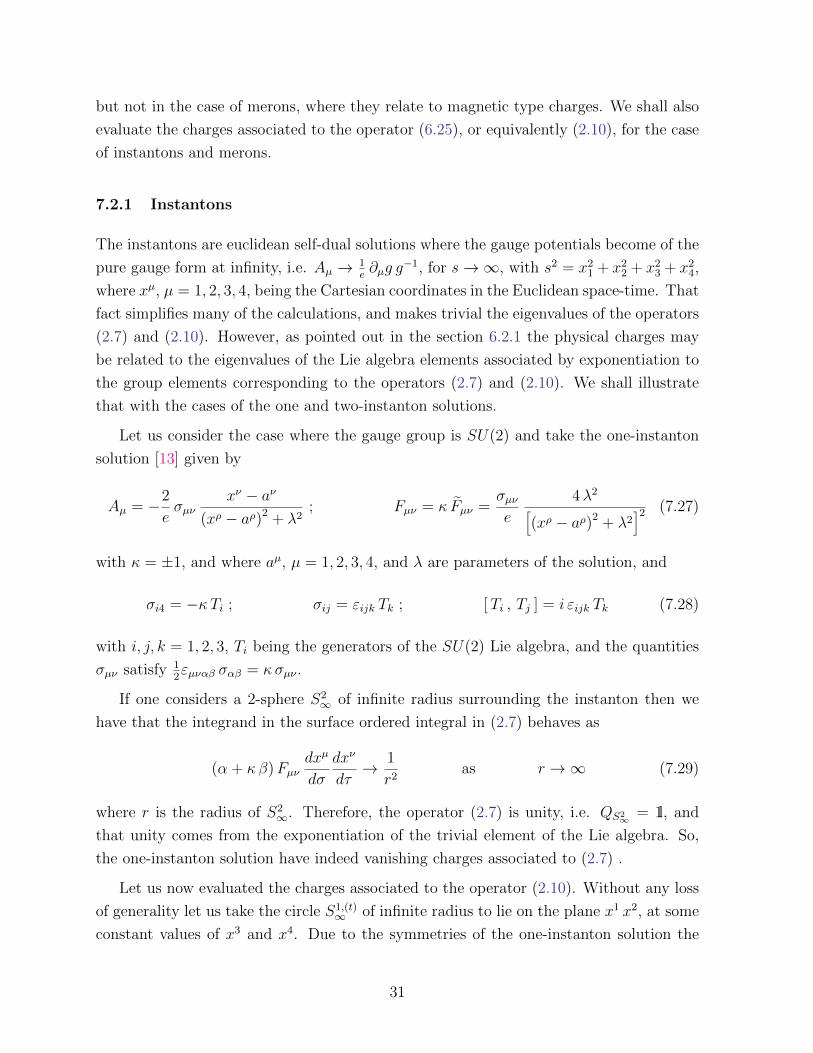
but not in the case of merons, where they relate to magnetic type charges. We shall also

evaluate the charges associated to the operator (6.25), or equivalently (2.10), for the case

of instantons and merons.

7.2.1 Instantons

The instantons are euclidean self-dual solutions where the gauge potentials become of the

pure gauge form at infinity, i.e. Aµ → 1e∂µg g

−1, for s→∞, with s2 = x21 + x2

2 + x23 + x2

4,

where xµ, µ = 1, 2, 3, 4, being the Cartesian coordinates in the Euclidean space-time. That

fact simplifies many of the calculations, and makes trivial the eigenvalues of the operators

(2.7) and (2.10). However, as pointed out in the section 6.2.1 the physical charges may

be related to the eigenvalues of the Lie algebra elements associated by exponentiation to

the group elements corresponding to the operators (2.7) and (2.10). We shall illustrate

that with the cases of the one and two-instanton solutions.

Let us consider the case where the gauge group is SU(2) and take the one-instanton

solution [13] given by

Aµ = −2

eσµν

xν − aν(xρ − aρ)2 + λ2

; Fµν = κ Fµν =σµνe

4λ2

[(xρ − aρ)2 + λ2

]2 (7.27)

with κ = ±1, and where aµ, µ = 1, 2, 3, 4, and λ are parameters of the solution, and

σi4 = −κTi ; σij = εijk Tk ; [Ti , Tj ] = i εijk Tk (7.28)

with i, j, k = 1, 2, 3, Ti being the generators of the SU(2) Lie algebra, and the quantities

σµν satisfy 12εµναβ σαβ = κσµν .

If one considers a 2-sphere S2∞ of infinite radius surrounding the instanton then we

have that the integrand in the surface ordered integral in (2.7) behaves as

(α + κβ)Fµνdxµ

dσ

dxν

dτ→ 1

r2as r →∞ (7.29)

where r is the radius of S2∞. Therefore, the operator (2.7) is unity, i.e. QS2

∞ = 1l, and

that unity comes from the exponentiation of the trivial element of the Lie algebra. So,

the one-instanton solution have indeed vanishing charges associated to (2.7) .

Let us now evaluated the charges associated to the operator (2.10). Without any loss

of generality let us take the circle S1,(t)∞ of infinite radius to lie on the plane x1 x2, at some

constant values of x3 and x4. Due to the symmetries of the one-instanton solution the

31

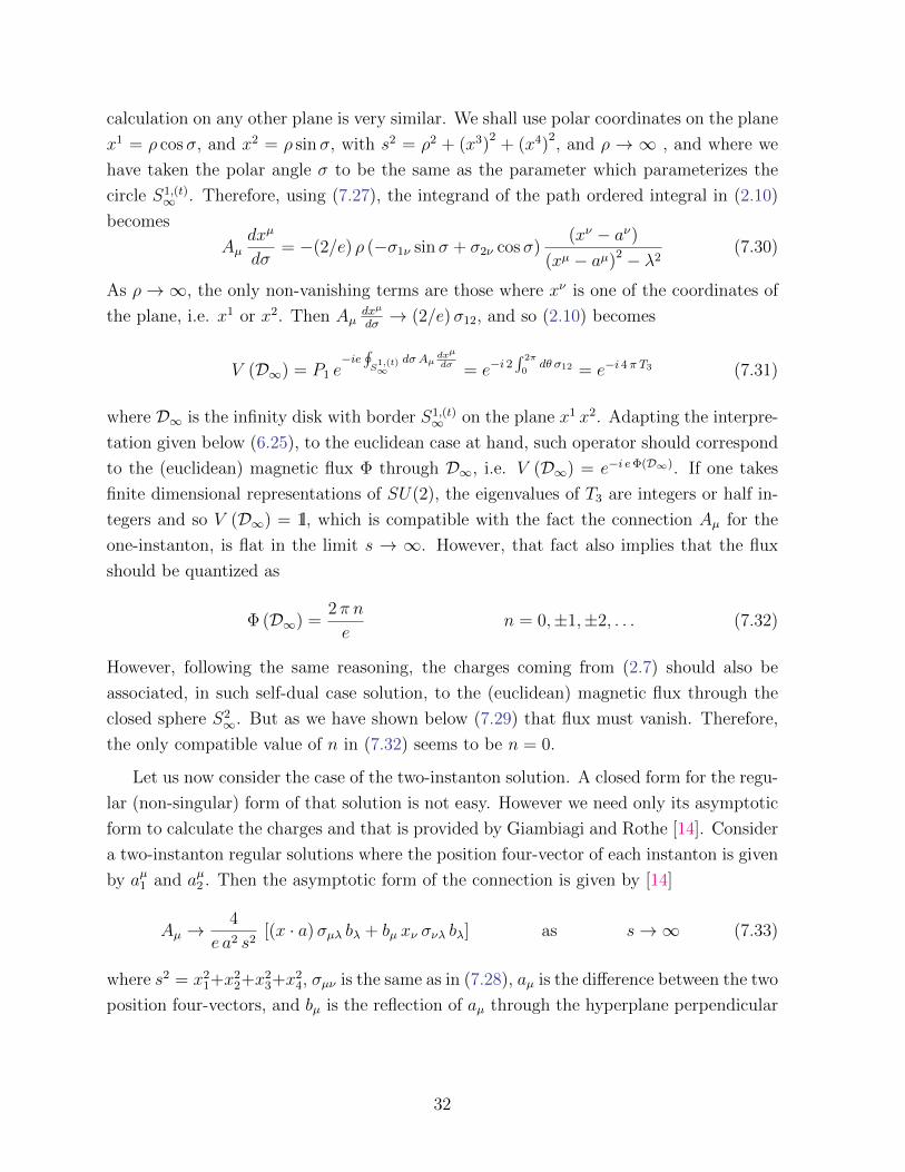
calculation on any other plane is very similar. We shall use polar coordinates on the plane

x1 = ρ cosσ, and x2 = ρ sinσ, with s2 = ρ2 + (x3)2

+ (x4)2, and ρ → ∞ , and where we

have taken the polar angle σ to be the same as the parameter which parameterizes the

circle S1,(t)∞ . Therefore, using (7.27), the integrand of the path ordered integral in (2.10)

becomes

Aµdxµ

dσ= −(2/e) ρ (−σ1ν sinσ + σ2ν cosσ)

(xν − aν)(xµ − aµ)2 − λ2

(7.30)

As ρ→∞, the only non-vanishing terms are those where xν is one of the coordinates of

the plane, i.e. x1 or x2. Then Aµdxµ

dσ→ (2/e)σ12, and so (2.10) becomes

V (D∞) = P1 e−ie∮S

1,(t)∞

dσ Aµdxµ

dσ = e−i 2∫ 2π

0dθ σ12 = e−i 4π T3 (7.31)

where D∞ is the infinity disk with border S1,(t)∞ on the plane x1 x2. Adapting the interpre-

tation given below (6.25), to the euclidean case at hand, such operator should correspond

to the (euclidean) magnetic flux Φ through D∞, i.e. V (D∞) = e−i eΦ(D∞). If one takes

finite dimensional representations of SU(2), the eigenvalues of T3 are integers or half in-

tegers and so V (D∞) = 1l, which is compatible with the fact the connection Aµ for the

one-instanton, is flat in the limit s → ∞. However, that fact also implies that the flux

should be quantized as

Φ (D∞) =2π n

en = 0,±1,±2, . . . (7.32)

However, following the same reasoning, the charges coming from (2.7) should also be

associated, in such self-dual case solution, to the (euclidean) magnetic flux through the

closed sphere S2∞. But as we have shown below (7.29) that flux must vanish. Therefore,

the only compatible value of n in (7.32) seems to be n = 0.

Let us now consider the case of the two-instanton solution. A closed form for the regu-

lar (non-singular) form of that solution is not easy. However we need only its asymptotic

form to calculate the charges and that is provided by Giambiagi and Rothe [14]. Consider

a two-instanton regular solutions where the position four-vector of each instanton is given

by aµ1 and aµ2 . Then the asymptotic form of the connection is given by [14]

Aµ →4

e a2 s2[(x · a)σµλ bλ + bµ xν σνλ bλ] as s→∞ (7.33)

where s2 = x21+x2

2+x23+x2

4, σµν is the same as in (7.28), aµ is the difference between the two

position four-vectors, and bµ is the reflection of aµ through the hyperplane perpendicular

32

to xµ, i.e.

aµ ≡ aµ1 − aµ2 bµ ≡ aµ − 2(x · a)

x2xµ (7.34)

and so b2 = a2.

The leading term of the connection given in (7.33) is flat, and it falls as 1/s as s→∞.

Therefore, the leading term of the field tensor which would fall as 1/s2 vanishes, and

therefore Fµν falls at least as 1/s3. Consequently, the integrand of the surface ordered

integral in (2.7), namely Fµνdxµ

dσdxν

dτ, falls faster than 1/s, and so it vanishes in the limit

s→∞. We then conclude that, similarly to the one-instanton case, the charges associated

to the operator (2.7) vanish when evaluated on the two-instanton solution.

We now evaluate the charges associated to the operator (2.10) for the two-instanton

solution. Given an infinite plane (disk) D∞ with border being the circle S1,(t)∞ of infinite

radius we can choose, without loss of generality, the axis x1 and x2 to lie on that plane.

We then split the vector aµ in its perpendicular and parallel parts w.r.t. to the plane,

i.e. aµ = aµ⊥ + aµ‖ , and take the axis x1 to lie along aµ‖ , and the axis x3 to lie along

aµ⊥. In addition we take polar coordinates on the plane x1 x2, such that x1 = ρ cosσ,

and x2 = ρ sinσ, with the polar angle σ being the same as the parameter in (2.10)

parametrizing S1,(t)∞ . Then the integrand of the path ordered integral in (2.10) along the

infinite circle S1,(t)∞ for the connection (7.33) becomes (ρ→∞)

Aµdxµ

dσ→ 4

e

[| a‖ |2a2

T3 +| a‖ | | a⊥ |

a2[cos (2σ) T1 + sin (2σ) T2]

](7.35)

We now perform a gauge transformation Aµ → (g2 g1) Aµ (g2 g1)−1 + ie∂µ (g2 g1) (g2 g1)−1,

with g1 = ei 2σ T3 and g2 = ei 2ϕT2 . The angle ϕ is defined as follows: since a2 =| a‖ |2 + |a⊥ |2, we parametrize it as | a‖ |=| a | cosϕ, and | a⊥ |=| a | sinϕ, with 0 ≤ ϕ ≤ π

2. So,

since the vector aµ was chosen to lie on the plane x1 x3, ϕ is the angle between aµ and

the plane x1 x2 measured along the plane x1 x3. Under such a gauge transformation one

gets that

Aµdxµ

dσ→ A′µ

dxµ

dσ=

2

eT3 (7.36)

and so

P1 e−ie∮S1∞dσ Aµ

dxµ

dσ → g1 (σ = 2π)−1 g−12 P1 e

−ie∮S1∞dσ A′µ

dxµ

dσ g2 g1 (σ = 0) (7.37)

Therefore, the operator (2.10) becomes

V (D∞) = P1 e−ie∮S1∞dσ Aµ

dxµ

dσ = e−i 4π T3 e−i 2ϕT2 e−i 4π T3 ei 2ϕT2 (7.38)

33

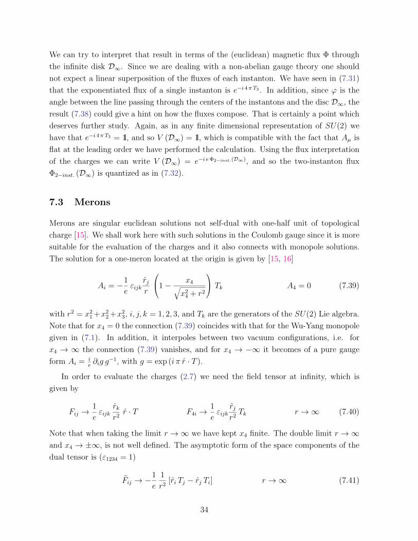
We can try to interpret that result in terms of the (euclidean) magnetic flux Φ through

the infinite disk D∞. Since we are dealing with a non-abelian gauge theory one should

not expect a linear superposition of the fluxes of each instanton. We have seen in (7.31)

that the exponentiated flux of a single instanton is e−i 4π T3 . In addition, since ϕ is the

angle between the line passing through the centers of the instantons and the disc D∞, the

result (7.38) could give a hint on how the fluxes compose. That is certainly a point which

deserves further study. Again, as in any finite dimensional representation of SU(2) we

have that e−i 4π T3 = 1l, and so V (D∞) = 1l, which is compatible with the fact that Aµ is

flat at the leading order we have performed the calculation. Using the flux interpretation

of the charges we can write V (D∞) = e−i eΦ2−inst.(D∞), and so the two-instanton flux

Φ2−inst. (D∞) is quantized as in (7.32).

7.3 Merons

Merons are singular euclidean solutions not self-dual with one-half unit of topological

charge [15]. We shall work here with such solutions in the Coulomb gauge since it is more

suitable for the evaluation of the charges and it also connects with monopole solutions.

The solution for a one-meron located at the origin is given by [15, 16]

Ai = −1

eεijk

rjr

1− x4√

x24 + r2

Tk A4 = 0 (7.39)

with r2 = x21 +x2

2 +x23, i, j, k = 1, 2, 3, and Tk are the generators of the SU(2) Lie algebra.

Note that for x4 = 0 the connection (7.39) coincides with that for the Wu-Yang monopole

given in (7.1). In addition, it interpoles between two vacuum configurations, i.e. for

x4 → ∞ the connection (7.39) vanishes, and for x4 → −∞ it becomes of a pure gauge

form Ai = ie∂ig g

−1, with g = exp (i π r · T ).

In order to evaluate the charges (2.7) we need the field tensor at infinity, which is

given by

Fij →1

eεijk

rkr2r · T F4i →

1

eεijk

rjr2Tk r →∞ (7.40)

Note that when taking the limit r →∞ we have kept x4 finite. The double limit r →∞and x4 → ±∞, is not well defined. The asymptotic form of the space components of the

dual tensor is (ε1234 = 1)

Fij → −1

e

1

r2[ri Tj − rj Ti] r →∞ (7.41)

34

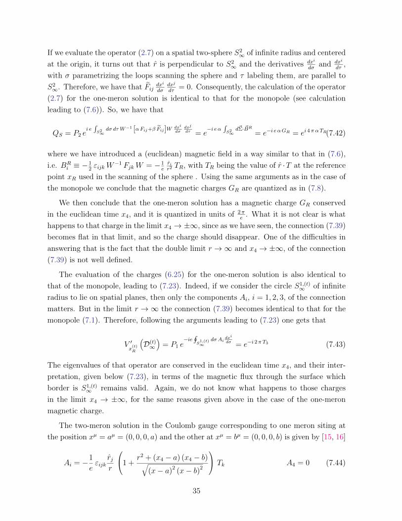
If we evaluate the operator (2.7) on a spatial two-sphere S2∞ of infinite radius and centered

at the origin, it turns out that r is perpendicular to S2∞ and the derivatives dxi

dσand dxi

dτ,

with σ parametrizing the loops scanning the sphere and τ labeling them, are parallel to

S2∞. Therefore, we have that Fij

dxi

dσdxj

dτ= 0. Consequently, the calculation of the operator

(2.7) for the one-meron solution is identical to that for the monopole (see calculation

leading to (7.6)). So, we have that

QS = P2 ei e∫S2∞dσ dτ W−1 [αFij+β Fij]W dxi

dσdxj

dτ = e−i e α

∫S2∞d~Σ· ~BR

= e−i e αGR = ei 4π αTR(7.42)

where we have introduced a (euclidean) magnetic field in a way similar to that in (7.6),

i.e. BRi ≡ −1

2εijkW

−1 FjkW = −1erir2 TR, with TR being the value of r ·T at the reference

point xR used in the scanning of the sphere . Using the same arguments as in the case of

the monopole we conclude that the magnetic charges GR are quantized as in (7.8).

We then conclude that the one-meron solution has a magnetic charge GR conserved

in the euclidean time x4, and it is quantized in units of 2πe

. What it is not clear is what

happens to that charge in the limit x4 → ±∞, since as we have seen, the connection (7.39)

becomes flat in that limit, and so the charge should disappear. One of the difficulties in

answering that is the fact that the double limit r →∞ and x4 → ±∞, of the connection

(7.39) is not well defined.

The evaluation of the charges (6.25) for the one-meron solution is also identical to

that of the monopole, leading to (7.23). Indeed, if we consider the circle S1,(t)∞ of infinite

radius to lie on spatial planes, then only the components Ai, i = 1, 2, 3, of the connection

matters. But in the limit r →∞ the connection (7.39) becomes identical to that for the

monopole (7.1). Therefore, following the arguments leading to (7.23) one gets that

V ′x

(t)R

(D(t)∞

)= P1 e

−ie∮S

1,(t)∞

dσ Aidxi

dσ = e−i 2π T3 (7.43)

The eigenvalues of that operator are conserved in the euclidean time x4, and their inter-

pretation, given below (7.23), in terms of the magnetic flux through the surface which

border is S1,(t)∞ remains valid. Again, we do not know what happens to those charges

in the limit x4 → ±∞, for the same reasons given above in the case of the one-meron

magnetic charge.

The two-meron solution in the Coulomb gauge corresponding to one meron siting at

the position xµ = aµ = (0, 0, 0, a) and the other at xµ = bµ = (0, 0, 0, b) is given by [15, 16]

Ai = −1

eεijk

rjr

1 +

r2 + (x4 − a) (x4 − b)√(x− a)2 (x− b)2

Tk A4 = 0 (7.44)

35

Expanding it in powers of 1r

one gets that

Ai =i

e∂ig g

−1 +1

e

(a− b)2

2εijk

rjr3Tk +O

(1

r5

)(7.45)

with g = exp (i π r · T ), and so the leading term is of pure gauge form, i.e. it is flat.

Therefore, we have that

Fij ∼ O(

1

r4

)F0i ∼ O

(1

r5

)(7.46)

Consequently, the integrand in (2.7), namely (αFij + βFij)dxi

dσdxj

dτ, behaves as O

(1r2

)in

the limit r →∞. Therefore, the charges associated to (2.7) vanish, i.e. QS = 1l.

Note that in the limit r → ∞ the spatial component of the connection (7.44) for

the two-meron solution is twice that of the one-meron solution (7.39). Therefore, the

evaluation of the charges associated to the operator (6.25) is very similar to that leading

to (7.43) and gives

V ′x

(t)R

(D(t)∞

)= P1 e

−ie∮S

1,(t)∞

dσ Aidxi

dσ = e−i 4π T3 = 1l (7.47)

where the last equality follows from the fact that the leading term of Ai is flat. The inter-

pretation for such conserved charges, given below (6.25), holds true, i.e. they correspond

to the magnetic flux through the surface which border is S1,(t)∞ , and such fluxes are also

quantized.

The meron-antimeron solution in the Coulomb gauge, corresponding to a meron and

an anti-meron located at xµ = −aµ and xµ = aµ respectively, with aµ = (0, 0, 0, a), is

given by [15, 16]

Ai = −1

eεijk

rjr

1− x2 − a2

√(x+ a)2 (x− a)2

Tk A4 = 0 (7.48)

Again expanding in powers of 1r

one gets

Ai = −2 a2

eεijk

rjr3Tk +O

(1

r5

)(7.49)

Then, similarly to the two-meron case one has that Fij ∼ O(

1r4

)and F0i ∼ O

(1r5

), and

so the charges coming from (2.7) are trivial, i.e. QS = 1l. In addition, since the connection

falls faster than 1r

the integrand in the operator (6.25) vanishes, i.e. P1 e−ie∮S

1,(t)∞

dσ Aidxi

dσ =

36

1l. The corresponding charges are also trivial in this case.

7.4 Summary of the charges

As we have seen in the examples above the surface and path ordering are not necessary in

the evaluation of the operators (2.7) and (2.10) (or equivalently (6.25)) which eigenvalues

are the charges. Therefore, those operators can be written as an ordinary exponential

of Lie algebra elements. The only exception is the charge for the two-instanton solution

associated to the operator (2.10) which involve a non-linear superposition of fluxes (see

eq. (7.38)). Therefore, we shall write the operator (2.7), defined on a volume inside a

two-sphere S2∞ of infinite radius, as

P2eie∫S2∞dτdσW−1 (αFµν+βFµν)W dxµ

dσdxν

dτ = e−i e [αGR+β KR] (7.50)

where GR and KR are the magnetic and electric charges defined as

GR =∫

S2∞

d~Σ · ~BR KR =∫

S2∞

d~Σ · ~ER (7.51)

with BRi ≡ −1

2εijkW

−1 FjkW and ERi = W−1 F0iW , being respectively the abelian

magnetic and electric fields.

Similarly we shall write the operators (2.10) and (6.25) on a surface D∞ with the

border being a circle S1∞ of infinite radius, as

P1 e−ie∮S1∞dσ Aµ

dxµ

dσ = e−i eΦ(D∞) (7.52)

where Φ (D∞) is interpreted as the magnetic flux through the surface D∞.

Note that the magnetic charge GR is quantized due to the integrable Bianchi identity

(6.13). The electric charge KR and the magnetic flux Φ (D∞) are quantized only if we

evaluate the operators (2.7), (2.10) and (6.25) on a finite dimensional representation of

the SU(2) gauge group, where the eigenvalues of the generator T3 (or any other element

conjugated to it) are integers or half-integers, which we shall denote by n2, with n integer.

With those definitions we summarize the spectrum of charges of the solutions discussed

above in the Table 1.

37

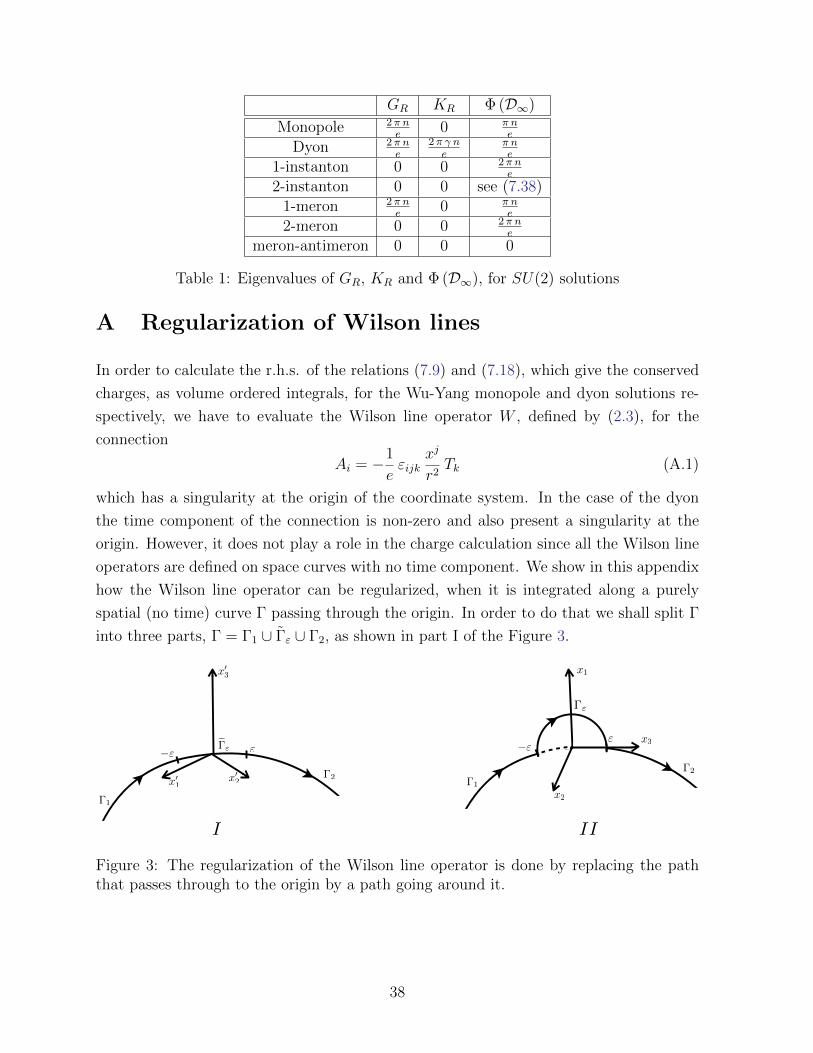
GR KR Φ (D∞)

Monopole 2π ne

0 π ne

Dyon 2π ne

2π γ ne

π ne

1-instanton 0 0 2π ne

2-instanton 0 0 see (7.38)1-meron 2π n

e0 π n

e

2-meron 0 0 2π ne

meron-antimeron 0 0 0

Table 1: Eigenvalues of GR, KR and Φ (D∞), for SU(2) solutions

A Regularization of Wilson lines

In order to calculate the r.h.s. of the relations (7.9) and (7.18), which give the conserved

charges, as volume ordered integrals, for the Wu-Yang monopole and dyon solutions re-

spectively, we have to evaluate the Wilson line operator W , defined by (2.3), for the

connection

Ai = −1

eεijk

xj

r2Tk (A.1)

which has a singularity at the origin of the coordinate system. In the case of the dyon

the time component of the connection is non-zero and also present a singularity at the

origin. However, it does not play a role in the charge calculation since all the Wilson line

operators are defined on space curves with no time component. We show in this appendix

how the Wilson line operator can be regularized, when it is integrated along a purely

spatial (no time) curve Γ passing through the origin. In order to do that we shall split Γ

into three parts, Γ = Γ1 ∪ Γε ∪ Γ2, as shown in part I of the Figure 3.

−ε ε

Γ1

Γ2

Γε

x3

x1

x2

−εε

x2

x1

x3

Γ1

Γ2

Γε

I II

Figure 3: The regularization of the Wilson line operator is done by replacing the paththat passes through to the origin by a path going around it.

38

Therefore, the solution of (2.3) can be written as

W = W (Γ2) W(Γε)W (Γ1) (A.2)

The quantities W (Γ1) and W (Γ2) do not involve the singularity and so we should not

worry about them. We have to evaluate W(Γε)

which pass through the origin. We shall

take Γε infinitesimally small in such a way that we can approximate it by an infinites-

imal straight line of length 2 ε containing the origin in its middle point. Note that the

quantity Aid xi

d σ, appearing in (2.3), is invariant under rotations, and so we can rotate the

coordinate system in such a way that the x3-axis lies parallel to Γε and in the direction

of growing σ, i.e. in the sense of integration of (2.3), as shown in part II of the Fig-

ure 3. Along such infinitesimal straight line Γε, parametrized as x3 = σ, we have that

Aid xi

d σ= −1

e1r2 [x1 T2 − x2 T1]. However, on Γε one has x1 = x2 = 0, and so for r 6= 0 such

expression vanishes. On the other hand, for r = 0 it diverges, and so, we have a quite ill

defined quantity.

In order to regularize the Wilson line we shall replace Γε by a semi-circle Γε of radius

ε, with diameter being the previous straight line, and lying on the plane x1 x3 as shown

in part II of Figure 3. We evaluate W (Γε) on such semi-circle and then take the limit

ε→ 0. The points in Γε can be parameterized as

x1 = ε sinσ x2 = 0 x3 = −ε cosσ 0 ≤ σ ≤ π (A.3)

Therefore for all such points we have r = ε, and so from (A.1) one has

Aid xi

d σ= ε (A1 cosσ + A3 sinσ) = −1

eT2 (A.4)

We note that it does not depend upon ε and σ, and lies in the direction of just one

generator of SU(2). Therefore, the problem is abelian and the path ordering is not

necessary. Then from (2.3) we have

W (Γε) = ei π T2 (A.5)

which we take as the regularized expression for W(Γε). Of course, we would obtain

different results for different choices of curves going around the origin, specially non-

planar curves. However, as we shown below, the evaluation of the r.h.s. of the relations

(7.9) and (7.18) is independent of such choices, and the regularization of those quantities

is quite unique.

39

Note that for the Wu-Yang monopole and dyon solutions one has that

Fij =1

eεijk

rkr2r · T ; Fij = −γ

eεijk

rkr2r · T (A.6)

with γ = 0 in the pure monopole case. In the evaluation of (7.10) and (7.19) we have

to deal with the conjugated quantities FWij and FW

ij , and so essentially we have to worry

about the quantity W−1 r ·T W . Our prescription is to scan the volume (the whole space)

with closed surfaces based at xR, and each of those surfaces are scanned with loops starting

and ending at xR. The origin lies on a given surface labeled by ζ0, and to just one loop,

labeled by τ0, on that surface, and corresponding to the point labeled by σ0 on that loop.

For the surfaces corresponding to ζ < ζ0 there are no problems in the integration since

everything is regular. On each loop on those surfaces one can use the relations (7.3) and

(7.4) to conclude that, along such loops, W−1 r ·T W is constant and equal to TR, i.e. the

value of r · T at the reference point xR where all loops are based.

Therefore, the commutators in (7.10) and (7.19) vanish for ζ < ζ0, since the conjugated

tensors FWij and FW

ij all lie in the direction of TR on any point of any loop scanning the

surfaces for ζ < ζ0. On the surface for ζ = ζ0 everything is fine until we reach the loop

corresponding to τ = τ0. In other words, the commutators in (7.10) and (7.19) also

vanish for ζ = ζ0 and τ < τ0. Let us consider the loop corresponding to τ = τ0. For

σ < σ0 we still have the vanishing of those commutators since the singularity has not

been touched yet. After crossing the singularity we have that the Wilson line W becomes

W2W (Γε) W1 (see (A.2)), where W1 is the result of the integration of (2.3) along Γ1, i.e.

the curve from the reference point xR up to the point marked −ε on Figure 3, along the

loop corresponding to τ = τ0, which passes through the origin. Similarly W2 is obtained

by integrating (2.3) along Γ2, i.e. the curve from the point marked ε on Figure 3, up to

some generic point beyond the origin along that same loop. In addition, W (Γε) is the

regularized expression, given in (A.5), for the integration of (2.3) along Γε.

Along the curve Γ2 the connection (A.1) is regular, and so we can use (7.3) and (7.4)

to conclude that

W−12 r · T W2 = (r · T )Γ0

2(A.7)

where (r · T )Γ02

is the value of r · T at the initial point of the curve Γ2, which is the point

marked ε on Figure 3. But since we have rotated the coordinate system such that the

x3-axis lies along Γε, we have that (r · T )Γ02

= T3. Now using (A.5), we have that

W−1 (Γε) W−12 r · T W2W (Γε) = e−i π T2 T3 e

i π T2 = −T3 = (r · T )Γend1

(A.8)

since −T3 is the value of r ·T at the final point of the curve Γ1, which is the point marked

40

−ε on Figure 3. Along the curve Γ1 the connection (A.1) is regular, and so we can use

(7.3) and (7.4) to get

W−11 W−1 (Γε) W

−12 r · T W2W (Γε) W1 = W−1

1 (r · T )Γend1

W1 = TR (A.9)

where TR is the value of (r · T ) at the reference point xR which is the initial point of Γ1.

Therefore, the field tensor and its dual, given in (A.6), lie in the direction of TR when

conjugated with W2W (Γε) W1, and so the commutators in (7.10) and (7.19) vanish when

evaluated on the loop corresponding to τ = τ0, i.e. the one passing through the singularity

of (A.1). Of course, the quantities (7.10) and (7.19) will vanish on all loops scanning the

surfaces for ζ > ζ0, since the potential (A.1) is not singular there, and the relations (7.3)

and (7.4) can be used to show that W−1 r · T W = TR, for W obtained by the integration

of (2.3) on such loops.

Consequently all the commutators in (7.10) and (7.19) vanish on any loop on the

scanning of any surface on the scanning of the volume. Since the Wu-Yang solutions have

no sources we have J123 = J0 = 0, and so Jmonopole and Jdyon also vanishes. Therefore we

conclude that the r.h.s. of (7.9) and (7.18) are equal to unity, i.e.

P3e∫

spacedζdτV JmonopoleV

−1

= 1l ; P3e∫

spacedζdτV JdyonV

−1

= 1l (A.10)

We now come to the issue of the uniqueness of the regularization procedure. We have

chosen to replace the segment Γε by the semi-cicle Γε. Let us now analyze what happens

to the quantity W−1 (Γε) (r · T )Γend1

W (Γε) = W−1 (Γε) (−T3) W (Γε), when we make

arbitrary infinitesimal variations on the semi-circle Γε keeping its end points fixed, i.e.

the points marked ε and −ε on Figure 3. We have

δ[W−1 (Γε) (−T3) W (Γε)

]=

[W−1 (Γε) (−T3) W (Γε) , W

−1 (Γε) δW (Γε)]

=[T3 , W

−1 (Γε) δW (Γε)]

(A.11)

where in the last equality we have used (A.5) and (A.8). The variation of the Wilson line

can be easily evaluated using for instances the techniques of section 2 of [1]. When the

end points of the curve Γε are kept fixed one gets

W−1(Γε)δW (Γε) =∫ π

0dσW−1FijW

dxi

dσδxj (A.12)

where Fij is the curvature, given in (A.6), of the connection (A.1), and where W in the

integrand in (A.12), is obtained by integrating (2.3) along Γε, from its initial point at

41

σ = 0 to the point σ = σ where the tensor Fij is evaluated. As long as the transformed

curve does not pass through the singularity of the connection (A.1), the relations (7.3)

and (7.4) can be used to show that W−1 r · T W = −T3, where −T3 is the value of r · Tat the initial point of Γε. Therefore, the integrand in (A.12) always lies in the direction

of T3, and so

δ[W−1 (Γε) (−T3) W (Γε)

]= 0 (A.13)

Consequently any curve Γ, with the same end points as Γε, and that can be continuously

deformed into Γε, satisfies W−1 (Γε) (−T3) W (Γε) = W−1 (Γ ) (−T3) W (Γ) = T3. That

shows that our prescription for the regularization of the Wilson line is independent of the

choice of the curve replacing the segment Γε.

Note that the special role being played by T3 is an artifact of our choice of the orien-

tation of the coordinate axis w.r.t. the curve. Note in addition that our results do not

imply that the Wilson line does not change. It is just the conjugation of T3 by the Wilson

line that remains invariant. In the cases where the variation of the curve lies on the same

plane as Γε, then the Wilson line itself is invariant. The reason is that the r.h.s. of (A.12)

measures the magnetic flux through the infinitesimal surface spanned by the variation,

and since the magnetic field is radial it is parallel to such surface, and so δW (Γε) = 0 in

such cases.

Acknowledgements: The authors are grateful to fruitful discussions with O. Alvarez,

E. Castellano, P. Klimas, M.A.C. Kneipp, R. Koberle, J. Sanchez-Guillen, N. Sawado and

W. Zakrzewski. LAF is partially supported by CNPq, and GL is supported by a CNPq

scholarship.

42

References

[1] O. Alvarez, L. A. Ferreira and J. Sanchez Guillen, A New approach to integrable

theories in any dimension, Nucl. Phys. B 529, 689 (1998) [arXiv:hep-th/9710147].

[2] O. Alvarez, L. A. Ferreira and J. Sanchez-Guillen, Integrable theories and loop spaces:

Fundamentals, applications and new developments, Int. J. Mod. Phys. A 24, 1825

(2009) [arXiv:0901.1654 [hep-th]].

[3] C. N.Yang and R. L. Mills, Physical Review 96 191-195 (1954)

[4] S. Schlieder, Some remarks on charges and their conservation in a classical SU(2)

Yang-Mills theory, Nuovo Cim. A 63, 137 (1981);

L. F. Abbott and S. Deser, Charge definition in nonabelian gauge theories, Phys.

Lett. B 116, 259 (1982);

K. P. Tod, Quasilocal charges in Yang-Mills theory, Proc. Roy. Soc. Lond. A 389,

369 (1983);

P. T. Chrusciel and W. Kondracki, Some global charges in classical Yang-Mills the-

ory, Phys. Rev. D 36, 1874 (1987);

R. Farkas and L. B. Szabados, On quasi-local charges and Newman-Penrose

type quantities in Yang-Mills theories, Class. Quant. Grav. 28, 145013 (2011)

[arXiv:1012.4662 [gr-qc]].

[5] S. Mandelstam, Quantum electrodynamics without potentials, Annals Phys. 19, 1

(1962);

C. N. Yang, Integral formalism for gauge fields, Phys. Rev. Lett. 33, 445 (1974);

T. T. Wu and C. N. Yang, ‘Concept of nonintegrable phase factors and global formu-

lation of gauge fields, Phys. Rev. D 12, 3845 (1975);

A. M. Polyakov, String representations and hidden symmetries for gauge fields, Phys.

Lett. B 82, 247 (1979);

T. Eguchi, Y. Hosotani, Integrability condition in loop space, Phys. Lett. B96, 349

(1980);

A. A. Migdal, Loop equations and 1/N expansion, Phys. Rept. 102, 199-290 (1983);

Y. .M. Makeenko, A. A. Migdal, Exact equation for the loop average in multicolor

QCD, Phys. Lett. B88, 135 (1979);

I. Y. Arefeva, Gauge theory and bags, Phys. Lett. B95, 269-272 (1980); and The in-

tegral formulation of gauge theories - strings, bags or something else, Karpacz 1980,

Proceedings, Developments In The Theory Of Fundamental Interactions*, 295-330;

R. Gambini, A. Trias, Second quantization of the free electromagnetic field as quan-

43

tum mechanics in the loop space, Phys. Rev. D22, 1380 (1980), Nucl. Phys. B278,

436 (1986);

S. G. Rajeev, Yang-Mills theory on loop space, AIP Conf. Proc. 687, 41-48 (2003),

[hep-th/0401215];

R. Loll, Loop approaches to gauge field theory, Theor. Math. Phys. 93, 1415 (1992)

[Teor. Mat. Fiz. 93, 481 (1992)].

[6] L. A. Ferreira and G. Luchini, Gauge and integrable theories in loop spaces, Nucl.

Phys. B 858, 336 (2012) [arXiv:1109.2606 [hep-th]].

[7] Ya. Aref’eva, Theor. Mat. Phys. 43 (1980) 353

N. E. Bralic, “Exact computation of loop averages in two-dimensional Yang-Mills

theory,” Phys. Rev. D 22, 3090 (1980).

[8] M. Alvarez, D. I. Olive, The Dirac quantization condition for fluxes on four manifolds,

Commun. Math. Phys. 210, 13-28 (2000). [hep-th/9906093]; Spin and Abelian elec-

tromagnetic duality on four manifolds, Commun. Math. Phys. 217, 331-356 (2001).

[hep-th/0003155]; Charges and fluxes in Maxwell theory on compact manifolds with

boundary, Commun. Math. Phys. 267, 279-305 (2006). [hep-th/0303229].

[9] G. ’t Hooft, “Magnetic monopoles in unified gauge theories,” Nucl. Phys. B 79, 276

(1974).

A. M. Polyakov, “Particle spectrum in the quantum field theory,” JETP Lett. 20,

194 (1974) [Pisma Zh. Eksp. Teor. Fiz. 20, 430 (1974)].

[10] T. T. Wu and C. -N. Yang, “Some solutions of the classical isotopic gauge field

equations,” In *Yang, C.N.: Selected Papers 1945-1980*, 400-405 also in *H. Mark

and S. Fernbach, Properties Of Matter Under Unusual Conditions*, New York 1969,

349-345.

[11] B. Julia and A. Zee, “Poles with both magnetic and electric charges in nonabelian

gauge theory,” Phys. Rev. D 11, 2227 (1975).

[12] P. Goddard, D. I. Olive, New developments in the theory of magnetic monopoles,

Rept. Prog. Phys. 41, 1357 (1978);

[13] N. S. Manton, P. Sutcliffe, Topological solitons, Cambridge, UK: Univ. Pr. (2004)

[14] J. J. Giambiagi and K. D. Rothe, “Regular n instanton fields and singular gauge

transformations,” Nucl. Phys. B 129, 111-124 (1977).

44

[15] V. de Alfaro, S. Fubini and G. Furlan, “A new classical solution of the Yang-Mills

field equations,” Phys. Lett. B 65, 163 (1976); “Properties of O(4) x O(2) symmetric

solutions of the Yang-Mills field equations,” Phys. Lett. B 72, 203 (1977); “Classical

solutions of generally invariant gauge theories,” Phys. Lett. B 73, 463 (1978).

[16] A. Actor, “Classical solutions of SU(2) Yang-Mills theories,” Rev. Mod. Phys. 51,

461 (1979).

45