Integral equation solution for the flow due to the motion of a body of arbitrary shape near a plane interface at small Reynolds number

Applied Numerical Mathematics 2 (1986) 79-94 North-Holland

79

INTEGRAL EQUATION SOLUTION FOR THE FLOW DUE TO THE MOTION OF A BODY OF ARBITRARY SHAPE NEAR A PLANE INTERFACE AT SMALL REYNOLDS NLMBER

Henry POWER and Reinaldo GARCIA lnstituto de Mechica de Fhidos, Univew’dad Central de Venezuela, Caracas, Venezuela

Guillermo MIRANDA Departamentn de Matemhticas, Facultad de Ciencias, Universidad Central de Venezuela, Caracas, Venezuela

The problem of determining the slow viscous flow due to an arbitrary motion of a particle of arbitrary shape near a plane interface is formulated exactly as a system of three linear Fredholm integral equations of the first kind, which is shown to have a unique solution. A numerical method based on these integral equations is proposed. In order to test this method valid for arbitrary particle shape, the probl-,m of arbitrary motion of a sphere is worked out and compared with the available analytical solution. This technique can be also extended to low Reynolds number flow due to the motion of a finite number of bodies of arbitrary shape near a plane interface. As an example the case of two equal sized spheres moving parallel and perpendicular to the interface is solved in the limiting case of infinite viscosity ratio.

1. Introduction

There have been a number of studies of the motion of particles in the presence of rigid plane

wall boundaries (for a good literature survey see [7, Chapter 7]), this not being the case when the particle is moving near a fluid-fluid interface, and in this last case there have been only a few studies for particles of a simple shape. The motion of a sphere perpendicular to a plane interface, where it is assumed that the fluid-fluid interface remains flat when the particle is moving, has been solved exactly by Bart [3] using the general bipolar coordinate solution of the creeping motion equations. An approximate solution for the flow due to an arbitrary motion of a sphere near a plane interface was found by Lee et al. [9] using the method of reflections, where arbitrary motion is considered to be any linear combination of translation and rotation. Lee and Lea1 [lo]

obtained exact solutions for the arbitrary motion of a sphere near a plane interface using a series expansion of eigen solutions in bipolar coordinates.

The translation of a sphere normal to.a deformable interface has been also solved by Lee and Lea1 [ll] using a system of six linear integral equations, which is the simplification of a system of nine linear integral equations for the case of axisymmetric flows. This system of integral equations comes from Green’s integral representation formulae, the boundary conditions at the surface of the sphere and the matching conditions at the interface; this leads to considering singularity distributions on the surface of the sphere and the unbounded interface. The domain of integration on the interface is truncated far from the sphere, using an asymptotic estimate which is obtained from the known solution for a flat interface. However, they do not establish uniqueness and existence of solutions for the referred system of integral equations. The integral

0168-9274/86/$3.50 0 1986, Elsevier Science Publishers B.V. (North-Holland)

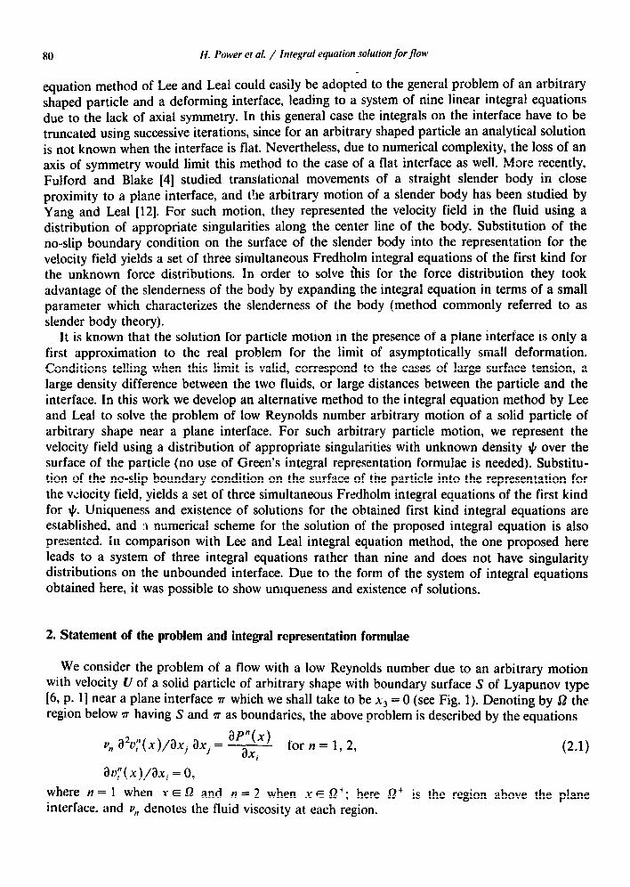
80 H. Power et al. / Integral equation solution for flow

eauation method of Lee and Lea1 could easily be adopted to the general problem of an arbitrary shaped particle and a deforming interface, leading to a System of nine linear integral equations due to the lack of axial symmetry. In this general case the integrals on the interface have to be truncated using successive iterations, since for an arbitrary shaped particle an analytical solution is not known when the interface is flat. Nevertheless, due to numerical complexity, the 10~s of an axis of symmetry would limit this method to the case of a flat interface as well. More recently, Fulford and Blake [4] studied translational movements of a straight slender body in close proximity to a plane interface, and t!ie arbitrary motion of a slender body has been studied by Yang and Lea1 [l2]. For such motion, they represented the velocity field in the fluid using a distribution of appropriate singularities along the center line of the body. Substitution of the no-slip boundary condition on the surface of the slender body into the representation for the velocity field yields a set of three simultaneous Fredholm integral equations of the first kind for the unknown force distributions. In order to solve this for the force distribution they took advantage of the slenderness of the body by expanding the integral equation in terms of a small parameter which characterizes the slenderness of the body (method commonly referred to as slender body theory).

It is known that the solution for particle motion in the presence of a plane interface is only a first approximation to the real problem for the limit of asymptotically small deformation. Conditions telling when this limit is valid, correspond to the cases of large surface tension, a large density difference between the two fluids, or large distances between the particle and the interface. In this work we develop an alternative method to the integral equation method by Lee and Lea1 to solve the problem of low Reynolds number arbitrary motion of a solid particle of arbitrary shape near a plane interface. For such arbitrary particle motion, we represent the velocity field using a distribution of appropriate singularities with unknown density 4 over the surface of the particle (no use of Green’s integral representation formulae is needed). Substitu- tion of the no-slip boundary condition on the surface of the particle into the representation for the v;iocity field, yields a set of three simultaneous Fredholm integral equations of the first kind for $. Uniqueness and existence of solutions for the obtained first kind integral equations are established, and 2 numerical scheme for the solution of the proposed integral equation is also pre3rrr.lkb rew+d. in comparison with Lee and Lea1 integral equation method, the one proposed here leads to a system of three integral equations rather than nine and does not have singularity

distributions on the unbounded interface. Due to the form of the system of integral equations obtained here, it was possible to show uniqueness and existence of solutions.

2. Statement of the problem and integral representation formulae

We consider the problem of a flow with a low Reynolds number due to an arbitrary motion with velocity U of a solid particle of arbitrary shape with boundary surface S of Lyapunov type [6, p. l] near a plane interface n which we shall take to be x3 = 0 (see Fig. 1). Denoting by a the region below ?T having S and ?T as boundaries, the above problem is described by the equations

v,, aZvl’( x)/ax, axj = W”(x) aXi

for n = 1, 2,

av;( x)/ax, = 0,

(2 1) .

where n = 1 when x~fi and n = 2 when XE 52’; here Q2+ is the region above the plane interface, and v,~ denotes the fluid viscosity at each region.

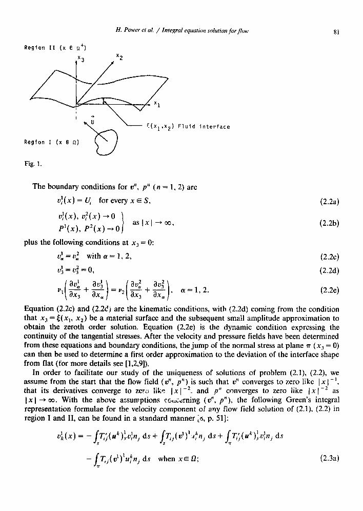
H. Power et al. / Integral equation solution /or flow

Region II (x e L?')

81

Region I (x 6 S2)

E(xl,x2) Fluid interface

Fig. 1.

The boundary conditions for on, p” (n = 1, 2) are

vi(x)= CJ foreveryxES, (2.2a)

vi’(x), of(x) + 0

P’(x), P”(x) --) 0 1 aslxl+oo, (2.2b)

plus the following conditions at x3 = 0:

v; = 0,2 witha,=l?2, (2.2c)

0; = v_: = 0, (2.2d)

(2.2e)

Equation (2.2~) and (2.2dj are the kinematic conditions, with (2.2d) coming from the condition that x3 = [( x1, x2) be a material surface and the subsequent small amplitude approximation to obtain the zeroth order solution. Equation (2.2e) is the dynamic condition expressing the continuity of the tangential stresses. After the velocity and pressure fields have been determined from these equations and boundary conditions, the jump of the normal stress at plane 7~ (x1 = 0) can then be used to determine a first order approximation to the deviation of the interface shape from flat (for more details see [1,2,9]).

In order to facilitate our study of the uniqueness of solutions of problem (2.1), (2.2), we assume from the start that the flow field (v”, p”) is such that vn converges to zero like 1 x 1 -l.

that its derivatives converge to zero like Ix I -2_ and p” converges to zero like Ix I -’ as I x 1 --) oo. With the above assumptions cc, 3 icdrning (v”, p”), the following Green’s integral representation formulae for the velocity component of any flow field solution of (2.Q (2.2) in region I and II, can be found in a standard manner id, p. 511:

vi(x) = - s T.>( U”):fv:nj ds + s 1

T.j( v’)‘~~~n, ds + s J

7@” ):.vfn, ds P

- $

Tij(v’)‘u”nj ds when XE i2; 7r

(2.3a)

M. Power rr al. / Integral equation solution for flow

and

(2.3b)

wlih

Uk = 1 I - -(&k/r i- r,r,/r3),

8Trrv

qk = - rJ(471r 3), r= Ix-yl, rk= (xk-_yk)9 is the fundamental singular solution of (2.1) known as ‘Stokeslet’ located at the point y [8, p. 491,

T,,(u”)” = al4,k al4;

-qks,, + u* z -1- K ,

i I J I

n(y) is the outward unit normal to the surface of integration, and

3 q;(u”)j: = - TJ(uk)* = - j-$r;rJrk)/r’.

Now we introduce .he potentials of single and double-layer V(x, #; S) and W(x, $; S) defined by Ladyzhenskaya [8, p. 52, eq. (14) and (IS)], where the third variable in brackets corresponds to the surface of integration, which is known to be continuous and discontinuous respectively across the density carrying surface. Formulae (2.3a, b) can now be writt.en in the form:

and

vi(x) = -&(x, Y’; s) + wk(x, v’; v)+ vk(x, Tj(V’); b!$)- Vk(X, qj(V’); vj (2.4~)

V,‘(X) = ~k(X, V2; 72) - Vk(X, ~j( V’); m).

Equation (2.4a) can be simplified to

(2.4b)

v,‘(x) = wk(x, v’; VT) + Vk(X, Tj(V’); S) - Vk(X, Tj(V’); ?T) (2 5) .

where the double-layer potential with density carrying surface S in (2.4a) drops, since any double-layer potential with rigid body motion as density vanishes identically at points exterior to the density carrying surface.

3. Uniqueness of solutions of the boundary value problem

From Green’s first identity for this problem 18, p. 51, eq. (9)] the following integral relations can be found:

In region I.

dx= J

“Tk( u’)‘vfnk ds - /Tk( v’)‘ulfi, ds; n s

aud, in region II,

T,,(02)2v;fl, ds. (3.lb)

(3.la)

Adding (3.la) and (3.1 b), using the boundary conditions at the interface given by (2.2~)

H. Power et al. / Integral equatiorl solutiort for flow 83

through (2.2e), and recalling that the normals to the plane outwardly directed from dL and G?+ are opposite vectors, it is found

Now, it is clear from formula (3.2) that the present problem does not have more than one solution. In fact, if ui satisfies a homogeneous boundary condition on S, then (3.2) implies

&$/ax, + &$/ax, = 0 for every x E L? (3.3a)

and

&$/ax, + &$/ax, = 0 for every x E O+. (3.3b)

Each of the above systems has six linearly independent solutions uf = uf = 4; with k = 1, 2 , . . . ,6, corresponding to the motion of the fluids as a rigid body in each region, where

~: = Si;;, k = 1, 2, 3, (3 4) .

J4= (0, x3, -x2), q5 = (-x3, 0, xi) and 4” = (x,, -x1, 0).

Therefore U” (and also p”) vanishes throughout G? u L?+ since such null field is the only rigid body motion compatible with a homogeneous boundary condition on S and the boundary condition for the velocity fields at the plane V.

4. Proposed form of the solution

In this section we apply the so called ‘indirect method’ to solve the problem stated in Section 2, which is based upon the linearity of the problem, representing the flow field (v”, p”) by appropriate unknown Stokeslets distributions on S together with the image system needed to satisfy the boundary conditions on the plane r.

In region I (x3 < 0) we obtain

u:(x~ It) =/u:(x~ Y)+j(v) dsy+ 1 Qij(x, Y*)Gj(Y*) dsJ.*v (4.la) s s*

P’(x, $J) = J4’(X. _Y)$j(_Y) ds, + J Hj(x, Y*)+j(_Y*) dsy*;

and, in region II (x3 > ‘b),

s* (4.lb)

u12(x9 #) = JAij(*xy Y)\C/i(Y) dsyy P2(x, ol/) = JBj(X, Y)\Clj(YJ dsJ** (4 2) . s s

I-Iere s* is an auxiliary surface mirror image of s with respect to the plane x3 = 0, y;” =yl+

YT = y2, !‘3* = -y3, and Q;j, Hj, A,j, B’ are given as follows (cf. [l]):

H'(x, y*) =

(4.3b)

84 H. Power et al. / Infegrul equation solufion for flon

26 2Y3 Y3 a2 4,(x. Y) = --11,,;h, y\ - - - -

! +e w 8 i

i + e 2 ax, ax, ( ) a

u/ -I- - u,3 ax, ( 4 ,

= =4l B/(x* Y) l+e\ ~a q’(x, y) a

-.Y’T$x_ q3 x9 .v (( )) * J

(4.4a)

(4.4b)

Here (Y = 1, 2, e = Y~/v,, and fX is the velocity component due to a Stokeslet located at y *. The unknown Stokeslet’s density \I/j( y ) = +!Q( y*) is to be determined from the following first

kind Fredholm integral equation stemming from the boundary condition for of on the body surface S:

U, = fi,‘i-v. J*)+,(Y) dS,. + / Q,j(xq y*)#j(y*) dS,.* for every x E S. s s*

(4 5) .

Contrasting with t e integral equation method by Lee and Lea1 where the unknown densities can be identified with physical quantities, in our approach the density J/i(Y) does not have a direct physical meanin,, 0 which is due to the fact that our integral equation does not come from a Green’s type integr 21 representation. On the other hand, in the present method the local stress force is computed b> applying the stress operator Tij to the flow field (u’, p’) given by (4.la) and (4,ib). and the total drag force 6 acting on the body is given by

F,= J T,,( +I, dS. .Y

In spite of the relative complexity of the expression for Ti( d), the total force reduces to the following simple expression:

c=- /I

$,<-‘) + jK,,(? , -+J (L’) ds,. ds, 9

1

(4 6) .

.\ s

where

K,,(_V. x) = -a,&+, _k+‘j,jA(x) 3 (~~,-x,)(4J-xJ)(Y~-x,)

=- -n,(x). (4 7) .

The above result stems from the fact that the multipoles corresponding to the Stokes’ equalion yield zero total force. and the same is true for the Stokeslets located outside the closed surface S. Expression (4.6) can even be further simplified to:

I;;= - J q,(x) ds,. Y

This is easily seen, recalling that jJ,,(x, y) ds?. = is,,, since

(4 8) .

It can be concluded that, in spite of the fact that the density I/J, is not equal to the local surface stress force h = q,( u’ ) n J, their corresponding surface integrals are identical and thus equal to the total force 4. This is an important characteristic of the so called ‘indirect’ boundary integral methods (where the unknown densities do not have a direct physical meaning), which seems to have gone unnoticed so far. Since we have reduced the original differential problem to the integral equation ( -:), it is natural to ask about the uniqueness and existence of solutions of such integral equation-!. The next two sections will answer these questions.

Il. Fower et al. / Integral equation solutiotl for flotit 85

5. Uniqueness of solutions of the integral equation

Since the integral equation (4.5) is linear, in order to show uniqueness it suffices to establish that it’s homogeneous form admits only the trivial solution I/.$ = 0,

$u;bv Y)+;(Y) dS,.+ / S S*

Qij(x, Y*)#Y*) dS,.* =O

where I,!$( y) = I,!$( y*). Equation (5.1) can be written in the following form:

+ / g,,(y*)L_!J( zi(x, y*))#y(y*) ds_,.* = 0 s *

for every x E s

(5 1) .

(5 2) .

where

Cjk = 8 1

witha=l,2

and g,,,( y*) Id_: is a linear differential operator such that when applied to the Stokeslet I;:( x, y*) it generates the following mui::poles:

with m = 1, 2.

Let us define the velocity field

+ / g,H(Y*)c( qx9 y*)) dS,.*. (5 3) . SW

Taking into account the way the image Qij is constructed and the uniqueness established in Section 3, it follows from equation (5.2) that V( x, J/O) vanishes for every x E 2. The same will be true for every point in ai, where Oi is the domain bounded by the surface S, since V( x, I/J’) can be extended continuously into S, because this velocity field consist of a single-layer potential with S as the density carrying surface plus a surface distribution of given singularities with S* as the density carrying surface.

On the other hand, the corresponding stress of V( x, J/O) experiences a jump as point x crosses S from ti to Gi, the stress jump comes only from the single-layer potential (the stress tensor of a single-layer potential is discontinuous [8, p. 561). Since the remaining surface distribution of V( x, 4’) is infinitely differentiable except on S*, this jump is given by

qj(v(t9 $0))~i]nj(5)=iIClp(t)+ Tj(v(S7 #"))nj(E)~

Tj(v(tv lCl"))~eJnj(S)= -Q#~(S) + Tj(v(t9 #"))njO (5 4) .

for every 5 E S. Here qj( V( 5, #O))ci, is the limiting value of the stress 7].j( V(x, 4’)) when a point x tends to a point 5 on the surface S coming from the interior of the particle;

Tjtvt5, rcl"))fe! is the limiting value of the stress when x tends to 6 coming from ti and

86 H. Power et al. / Integral equation solutiorl for floes

T,,( V( &I/?)) is the direct value of the stress at the point 5. Since V( X, \cI”) is zero outside and inside of the surface S, the corresponding limiting values of the stress as x tends to [ coming from inside or outside of S are identically zero. Therefore, (5.4) gives:

Thus #p( 5) is also identically zero by (5.5).

6. Existence results for the integral equation

In order to prove that the system of integral equations (4.5) has a continuous solution \I/j, we shall consider the following fictitious Stokes flow field in the region pi:

v,(s) = LJ,s,,. p(S)=0 fOreVery_YEQi.

corresponding to the motion of the fluid as a rigid body. Since the surface potentials used in (4.1 a) are continuous across S. have the boundary values U, on S and define flow solutions in Qi, it follows that these potentials with density +LJ solution of (4.5) can be also used to represent V, in 52,:

l<(x) = u,s,, = / u;( x, .I+),(.,~) dsy + / for x E a,.

\ .s * Q,,(x. _I~*)#,( _Y*) ds,,..

(6 1) .

Obviously, T,,( I+,( X) = 0 for every _Y E pi, and thus iaking the limiting value of this tension as x tends to a point at S we obtain

Here C&-~. Y*) = (Q,,\C/,q Qz,rC/,. Q&h The above relation can be rewritten using the operator L’,” as follo,ws: defining &,( y*. x) =

C,x K,,( _r*. A-).

- J .\ * g,,,(_r*)L:“( K,,(y*, -u))#,(_r*) d.s,.* (6.3)

where we have interchanged the operators T,,( )n,(s) and R,,~(_I’*)L~( ) in the last integral. We shall now show that the homogeneous system (6.3) has no more than six linearly

independent solutions. Suppose that JI’( x), . . . , $“I~( _Y are linearly independent solutions of (6.3) )

with k,, > 6. Then V(x. \cI’) defined by (4.la) for k = 1, 2 , . . . , k, and x E L?i are velocity fields such that T,,( V” )( i ,/I,( x) = 0 for x E S. By Green’s formula for interior flows, it follows that each VA. k = 1. 2 , . . . , /lo satt:fies the system av,“/axj + i3~"/ax, = 0, i, j = 1, 2, 3 for x E L?i, which is known to have only six linearly independent solutions, namely, rigid body motions. Thus I”, Z”.. . . . VA0 are linearly dependent, i.e., there are scalar constants C,, C,, . . . , CA,, not all

H. Power et ul. / Integral equation solution for flow 87

zero, such that Cko ,=,C,V”(X)=O~~~~.BU~C::‘~IC~~~~(X)=C::’~~C~V(X,~~)~ V(X,+)=OinOi

with + = C~(l,C,J/“. Considering now the velocity field V( x, 9) for x E Q and taking into account the continuity of the potentials used in (4.la) across S, the way the image Qii is constructed and the uniqueness established in Section 3, it follows that V(x, 9) vanishes identically everywhere, and hence + must vanish on S implying that J1’, #‘, . . . , +kfl are linearly dependent. This implies a contradiction, and therefore k, < 6.

On the other hand, it is easy to see now that (6.3) has exactly six linearly independent solutions \cI’, \c12 , . . . , +“. By virtue of Fredholm’s theorems. it is enough to verify that the adjoint hymogeneous system of integral equations (6.4) has six linearly independent solutions $‘,

JI , . . . ,J6 which are the rigid body motions defined by (3.4) restricted to S

+g,,(X)Ly’JKij(X. y*)qj(y*) dS1,.* for every XES, (6 4) . s

with ~ij(X, JJ*) = CikKkj( X, v*), and where we have used the fact that Ly*( ) = -Ly( ).

Indeed, each $m given by (3.4) is a solution of

0 = ~&Y(X) - IK,(X, Y)$~(JT) ds.,. for every x E S,

and

/ s* Kij(X, J’*)&yiy*) dS,,*

vanishes identically in the region exterior body motions as density is identically zero

Let us define the following six auxiliary pi, k= 1, 2,...,6:

to s*, since every double-layer potential with rigid in the region exterior to the density carrying surface. linearly independent Stokes’ velocity fields H”(X) in

H;(x) = fi:(X. Y)+;(Y) dsJ,+ / Qij(Xq Y*)$F(.Y*) dsy* (6 5) . s s *

where #“, k = 1, 2,. . . , 6, are the six linearly independent solutions of (6.3). For each k, the surface tension of H”( x) has a zero limiting value, and therefore H”(x) is necessarily some rigid body motion in Qi, and the same is true for any linear combination tl( x) = Ci= ,C,#( x). Since the fictitious velocity fields y(x) = UiSij is a rigid body motion, it follows that constants C,, c,,..., C6 can be chosen so that

h H,(X) = C CkH,x’(X) = UjSij for every xE Qi. (6.6)

k=l

Finally, we can now establish explicitly the existence of a continuous solution +, for the system (4.5) by simply defining +!Q( x) = &C&(x) for every x E S u S* since the limiting value of H,(X) when x tends to a point 5 E S is given by (see (6.5) and (6.6)).

q = ds,.+ J Qij(tq Y*) s *

for every 5 E S. (6.7)

88 H. Power et al. / Integral equation solution for flow

7. Numerical solution of the integral equation

In the previous section we have found the solution of integral equation (4.5) as a definite iinear combination of the six linearly independent solutions of integral equation (4.3). However, since these solutions are in general unknown, this approach is not convenient for computational purposes. One way around this difficulty is to solve integral equation (4.5) using the Youngren pnd Acrivos [13] numerical method to solve the low Reynolds number motion of a particle in an unbounded fluid, this method is based upon discretization of the surface integrals involved, which transforms the integral equations into a linear system of algebraic equations. This is accomplished by dividing S and S* into N elements Aj and AT ( j = 1, 2,. . . , #) respectively, where AT is the mirror image of Aj, all of which are small relative to S and over which the components of J, may be considered approximately constant and equal to their value at the centre of the element. Then, we can write (4.5) approximately as

j=l

fork, i=l, 2, 3 and m=l, 2 ,..., ;N, where

A!,!‘( x0”)) = ( uf( x(“‘), y ) ds,

(7 1) .

(7 2) .

@,y(,+‘)) = j- Q;,( xfn’), y) ds, A:

(7 3) .

since #li( x*(l) ) = &(x(j)). Here xtM) is the location of the center of the element A,, in the real body. The above form a linear system of $11’ equations in the $N unknowns, &(x(~)), this algebraic system can be solved numerically using suitable integration and matrix inversion technique.

In order to allow a simplification in the expression for the surface integrals, we use a cylindrical coordinate system ( R, x1, 8) with the cylindrical axis, xi, perpendicular to the plane interface. The surface of the body is described by R = s( x,, 0) and the elements Aj ( j = 1, 2 . . . ,iN) are surfaces whose boundaries are lines of constant x1 and constant 8. In this way the surface elements become rectangular in x1, 0 coordinates.

With this surface elements the numerical calculation of the surface integrals (7.2) presents no problems, except when j = m, in which case the integrals are sensitive furActions of position for small 1 P’) - y 1 and are improper at y = x(*) since the integration is carried out over the element which contains x w In this case the integration is divided into two regions: in the first .

region the integration is carried out over a small neighbourhood of xfrn) where the surface is assumed locally flat and it is approximated by the tangent plane at x0”! Then, by transforming to a local polar coordinate system lying in this tangent plane, it is possible to integrate analytically the expression (7.2). This neighbourhood is chosen such that, in terms of the local polar coordinate system, it is a planar square SC centered at x(“‘) with side of length 2~. The final expression for (7.2) in this region is given by Youngren and Acrivos as

A!;])= - $-(ln$$)(?+ 1 +iS,,‘), (7.4a)

(7.4b, c)

II. Bower et al . ,/ Integral equation solution _fiw flw 89

A:‘;” = -0.1403c

i

2 + n: + (s’J2(ni + II:)

e (ni -I- n:)(l + (s’)~) 1 ’

A’;;” = @.1403uz,n, -.

e (n; + n:)(l + (d)“) ’

A$ = -0.14036

i

2 “I- ni + Cs’)‘( ni + n:)

t I (ni + n:)(l + (s’)‘] i

(7.4d)

(7.4e)

(7.4f)

where s’ = as/&~,, n2 and n3 are the components of the inward normal to the body at the point x(~) in the x2 and x3 direction respectively. The second region is the remainder of A,,. i.e..

Am - S,, where the numerical calculation presents no problems. On the other hand, the integrals in (7.3) are proper, even when j = m, since the integration is

carried out over the image body and xl”‘) is on the real body. This ir egrations as well as all the others which are solved numerically have been calculated using Gaussian quadratures.

Finally, the obtained linear algebraic system for Jlj ( j = 1, 2.. . .&V>. which is normally completely dense, was solved using standard Gaussian elimination followed by iterative improve- ment. In general, because of the singularity in the integrand of (7.2), the diagonal terms of the resulting matrix are the largest in any row (or column) though not sufficiently large to make the matrix diagonally dominant. It is important to note that, since the matrix is a function of only the body geometry, it is only necessary to invert it once for all possible motions of the body.

After finding the local densities I/Q(x(“‘)), by solving the linear system (7.1) the total force 6 given by (4.8) can be approximated by

(7 9 .

and the force coefficient can be defined as

Ci=2E;j,/~p( IUla)’ (7 6) . In order to test the numerical method developed in this work, valid for arbitrary particle shape

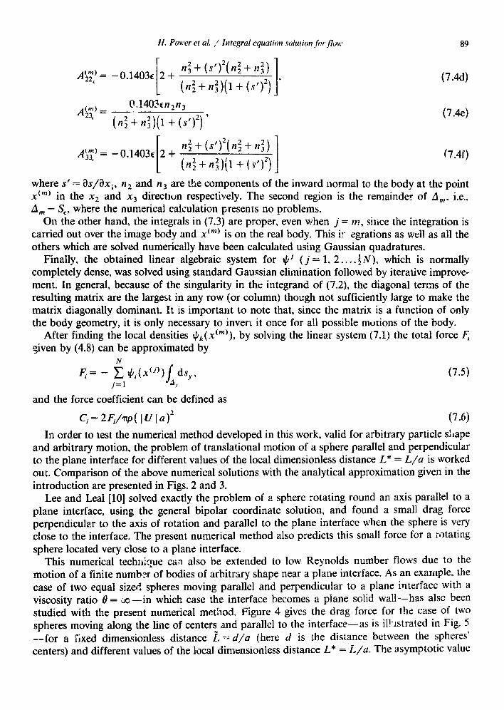
and arbitrary motion, the problem of translational motion of a sphere parallel and perpendicular to the plane interface for different values of the local dimensionless distance L,* = L/a is worked out. Comparison of the above numerical solutions with the analytical approximation given in the introduction are presented in Figs. 2 and 3.

Lee and Lea1 [lo] solved exactly the problem of a sphere rotating round an axis parallel to a plane interface, using the general bipolar coordinate solution, and found a small drag force perpendicular to the axis of rotation and parallel to the plane interface when the sphere is very close to the interface. The present numerical method also predicts this small force for a rotating sphere located very close to a plane interface.

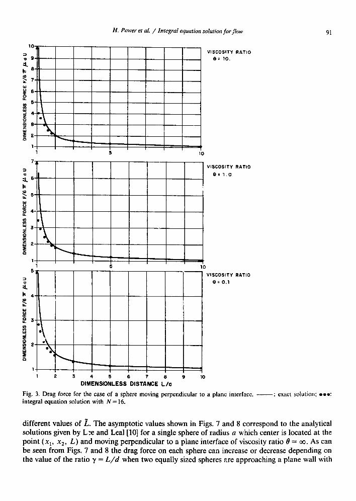
This numerical technique can also be extended to low Reynolds number flows due to the motion of a finite number of bodies of arbitrary shape near a plane interface. As an example, the case of two equal sized spheres moving parallel and perpendicular to a plane interface with a viscosity ratio 6 = ;10 - in which case the interface becomes a plane solid wall-has alsc been studied with the present numerical method. Figure 4 gives the drag force for thz case of two spheres moving along the line of centers and parallel to the interface-as is il!.lstrated in Fig. 5

-for a fixed dimensionless distance z 7~ d/a (here d is the distance between the spheres’ centers) and different values of the local dimensionless distance L* = t/a. The asymptotic value

90 H. Power et al. / Integral equation solution for flow

VISCOSITY RATIO

8 = 10.

1 2 3 4 6 6 7 6 9 10

DIMENSIONLESS DISTANCE L/a

VlSCOSlfY

e= 1.0

RATIO

vl!jCOSlfY RATIO

8 = 0.1

Fig. 2. Drag force for the case of a sphere moving perpendicular to a plane interface, : exact solution; 000: integral equation solution with N = 16.

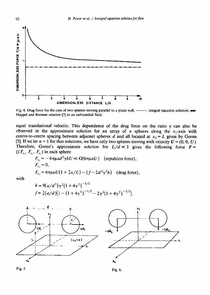
shown in Fig. 4 corresponds to the analytical solution given in 17, Chapter 61 for the case of two equal sized spheres moving along the line of centers with equal translational velocity in an unbounded fluid. Figures 7 and 8 give the drag force for the case of two spheres moving perpendicular to the line of centers and approaching the interface (see Fig. 6) for a fixed L* and

H. Power et al. / Integral equation solution for flow 91

1 2 3 4 5 8 7 8 9 10

DIMENSIONLESS DISTANCE L/a

Fig. 3. Drag force for the case of a sphere moving perpendicular to integral equation solution with N = 16.

VISCOSITY RATIO

e= 10.

VISCOSITY RATIO

8: 1.0

VISCOSITY RATIO

8 = 0.1

a plane interface, - : exact solution; 000:

different values of i,. The asymptotic values shown in Figs. 7 and 8 correspond to the analytical solutions given by L:e and Lea1 [lo] for a single sphere of radius a which center is located at the point (x,, x2, L) and moving perpendicular to a plane interface of viscosity ratio 8 = 00. As can be seen from Figs. 7 and 8 the drag force on each sphere can increase or decrease depending on the value of the ratio y = L/d when two equally sized spheres are approaching a plane wall with

H. Power et al, / Integral equation solution /or flow

01:: 6 ~‘7--7--- IO DIMENSIONLESS DiSfANCE L/a

Fig. 4. Drag force for the case of two spheres moving parallel to a piane wall. -: integral equation solution; m: Happel and Brenner solution [7] in an unbounded fluid.

equal translational velocity. This dependence of the drag force on the ratio y can also be observed in the approximate solution for an array of n spheres along the x,-axis with centre-to-centre spacing between adjacent spheres d and all located at x3 = L given by Goren [5]. If we let n = 1 for that solutions, we have only two spheres moving with velocity CI = (0, 0, U). Therefore, Goren’s approximate solution for L/d K 1 gives the following force F = {< CT,, F& &.,I in each sphere

&, = -6qmd’yhU s O(6~paU) (repulsion force),

FYz = 0.

with

FY1 = 61r~uU(l + za/L) - (f- 2d2y2h) (drag force),

h = 9( a/d3)y2(1 + 4~‘) -5’2

/ = &z/d)(l - (1 + 4~~)-“~ -- 2y2(1 + 4~~)-~‘~).

Fig. 5 Fig. 6.

H. Ponw et al. / Integrul equation solution forfioH 93

.88 , I I I I I I I I 2 3 3 11 14

I v I7 20 23 20 29 32

DIMENSIONLESS DISTANCE d/a

Fig. 7. Drag force for the case of two spheres moving perpendicular to a plane wall, - : integral equation solution:

. -. -. : Lee and Lea1 solution [lo] for single sphere.

2.2*

3

: k

s -.--,-..-.- -.--.- --.- w : 2.1-, \

,o - : I 4

i 0 iii 2

ii

ii 27 I 1 2 3 4 5 6 7 8 9 IO II 12

DIMENSIONLESS DISTANCE d/o

L=Z.

Fig. 8. Drag force for the case of two speres moving perpendicular to plane wall, -: integral equation solution;

. -. -a : Lee and Leal solution for a single sphere.

DIMENSIONLESS DISTANCE d/o

Fig, 9. Repulsion force for the case of two spheres moving perpendicular to a plane wall.

94 H. Power et al. / Integral equation solution for flow

The repulsion force given by Goren’s approximate solution is also predicted with the present numerical method. This repulsion force becomes of the order of 6TpaU when the spheres are very close to each other and to the wall as can be seen in Fig. 9.

From the comparison given here for a spherical body, we can conclude that the proposed numerical technique is a reasonable and simple one for the hydrodynamic interaction of a body of arbitrary shape with a plane interface under Stokes approximation, due to the well-known lack of sensitivity of the integral equation method upon the particular shape of the integration surface, provided such surface remains adequately smooth.

References

[I] K. Aderogba and J.R. Blake, Action of a force near the planar surface between semi-infinite immiscible liquids at very low Reynolds numbers, Bull. Austra!. Math. Sa. 1X (1978) 345.

[2] K. Aderogba and J.R. Blake, Action of a force near the planar surface between semi-infinite immiscible liquids at very low Reynolds numbers: Addendum, Bull. Austral. Math. Sot. 19 (1978) 309.

[3) E. Bart, The slow unsteady settling of a fluid sphere toward a flat fluid interface, Chew. Engng. Sci. 23 (1968) 193.

[4] G.R. Fulford and J.R. Blake, On the motion of a slender body near an interface between two immiscible liquids at very low Reynolds numbers. J. Fluid. Mech. 127 (1983) 203.

[5] S.L. Goren. Resistance and stability of a line of particles moving near a wall, J. Fluid. Mech. 132 (1983) 185. [6] N.M. Gunter, Potential Theory and Its Applications to Basic Problems of Mathematical Pll_vsics (Ungar, New York,

1967). [7] J. Happel and H. Brenner, LOW Reynolds Number H~drod~vtamics (Noordhoff. Leiden, 1973). [S] O.A. Ladyzhenskaya, The Mathematical Theory a/ Viscous Incompressil~le Flaw (Gordon and Breach, New York,

1963). [9] S.H. Lee, R.S. Chadwick and L.G. Leal, Motion of a sphere in the presence of a plane interface, Part I. An

approximate solution by generalization of the method of Lorentz. J. Fluid. Mech. 93 (1979) 705. [lo] S.H. Lee and L.G. Leal, Motion of a sphere in the presence of a plane interface, Part 2. An exact solution in

bipolar coordinates, J. Fluid. Mech. 98 (1980) 193. [ 1 l] S.H. Lee and L.G. Leal. The motion of a sphere in the presence of a deformable interface. J. Coil. und Interface

Science 87 (1) ( 1982) 89. [12] S.A. Yang and L.G. Leal, Particle motion in Stokes flow near a plane fluid-fluid interface. Part. 1. Slender body

in a quiescent fluid, J. Fluid Mech. 136 (1983) 393. [13] G.K. Youngren and A. Acrivos. Stokes flow past a particle of arbitrary shape: A numerical method of solution, J.

Fluid. Mech. 69 (1975) 377.