Available online at www.sciencedirect.com International Journal of Non-Linear Mechanics 39 (2004) 1217 – 1226 Integral convexity argument for plasticity function and monotonicity of iteration process for elasto-plastic problems Alemdar Hasanov ∗ Department of Mathematics, Applied Mathematical Sciences Research Center, University of Kocaeli, Ataturk Bulvari, 41300, Izmit, Turkey Received 15 April 2003; received in revised form 14 August 2003 Abstract The variational approach for boundary value problems related to non-linear materials is presented. The approach is based on the introduced integral convexity argument and monotone operator theory. This permits to obtain an existence and uniqueness of the solution within the range of Kachanov’s theory, under natural and general conditions. The introduced argument allows to prove monotonicity of the sequence of potentials on the sequence of iterations. As a result monotonicity of the iteration process for elastoplastic problems is obtained. Theoretical results are illustrated by computational experiments. ? 2003 Elsevier Ltd. All rights reserved. MSC: 75E10; 73C60 Keywords: Non-linear Lame equations; Integral convexity argument; Monotone iteration scheme; Convergence 1. Introduction The classical elastic and elastoplastic problems re- lated to deformations have been well studied in the literature (see, for example, [1–7]). The problem of behaviour of potentials with respect to iterations, as well as its monotonicity is, however, less well known and has received relatively little attention in the en- gineering and mathematical literature. In this paper we analyze a mathematical model for elastoplasticity which has been proposed in [3,4], obtaining general criteria not only for monotonicity of potentials, but also convergence of iteration scheme. We use the mathematical model of elastoplastic- ity (deformation theory) for homogeneous isotropic ∗ Tel.: +90-532-465-2884; fax: +90-262-321-5968. E-mail address: [email protected] (A. Hasanov). deformable materials. In this model one seeks the weak solution u ∈ 0 H 1 () to the following non-linear boundary value problem in R 3 − ij;i (u)= F (x); x ∈ ⊂ R 3 ; (1) u(x)=0; x ∈ 0 ⊂ @; (2) ij (u)n j = f i (x); x ∈ 1 ⊂ @; (3) where u(x)=(u 1 (x);u 2 (x);u 3 (x)) is the unknown dis- placement vector, F (x)=(F 1 (x);F 2 (x);F 3 (x)) and f(x)=(f 1 (x);f 2 (x);f 3 (x)) are the source and sur- face vectors, 0 ∪ 1 = ∅, 0 ∩ 1 = @, 0 = ∅ and n =(n 1 ;n 2 ;n 3 ) is the unit outward normal vector to the smooth surface 1 of the body ⊂ R 3 . Within the range of deformation theory of plastic- ity the elastoplastic properties of a material can be de- scribed by the deformation curve (Fig. 1, solid line) i =3G[1 − g(e 2 i )]e i (4) 0020-7462/$ - see front matter ? 2003 Elsevier Ltd. All rights reserved. doi:10.1016/j.ijnonlinmec.2003.08.004

Welcome message from author
This document is posted to help you gain knowledge. Please leave a comment to let me know what you think about it! Share it to your friends and learn new things together.
Transcript
Available online at www.sciencedirect.com
International Journal of Non-Linear Mechanics 39 (2004) 1217–1226
Integral convexity argument for plasticity function andmonotonicity of iteration process for elasto-plastic problems
Alemdar Hasanov∗
Department of Mathematics, Applied Mathematical Sciences Research Center, University of Kocaeli,Ataturk Bulvari, 41300, Izmit, Turkey
Received 15 April 2003; received in revised form 14 August 2003
Abstract
The variational approach for boundary value problems related to non-linear materials is presented. The approach is based onthe introduced integral convexity argument and monotone operator theory. This permits to obtain an existence and uniquenessof the solution within the range of Kachanov’s theory, under natural and general conditions. The introduced argument allowsto prove monotonicity of the sequence of potentials on the sequence of iterations. As a result monotonicity of the iterationprocess for elastoplastic problems is obtained. Theoretical results are illustrated by computational experiments.? 2003 Elsevier Ltd. All rights reserved.
MSC: 75E10; 73C60
Keywords: Non-linear Lame equations; Integral convexity argument; Monotone iteration scheme; Convergence
1. Introduction
The classical elastic and elastoplastic problems re-lated to deformations have been well studied in theliterature (see, for example, [1–7]). The problem ofbehaviour of potentials with respect to iterations, aswell as its monotonicity is, however, less well knownand has received relatively little attention in the en-gineering and mathematical literature. In this paperwe analyze a mathematical model for elastoplasticitywhich has been proposed in [3,4], obtaining generalcriteria not only for monotonicity of potentials, butalso convergence of iteration scheme.We use the mathematical model of elastoplastic-
ity (deformation theory) for homogeneous isotropic
∗ Tel.: +90-532-465-2884; fax: +90-262-321-5968.E-mail address: [email protected] (A. Hasanov).
deformable materials. In this model one seeks the
weak solution u∈ 0H 1(>) to the following non-linear
boundary value problem in R3
− ij; i(u) = F(x); x∈ ⊂ R3; (1)
u(x) = 0; x∈0 ⊂ @; (2)
ij(u)nj = fi(x); x∈1 ⊂ @; (3)
where u(x)=(u1(x); u2(x); u3(x)) is the unknown dis-placement vector, F(x) = (F1(x); F2(x); F3(x)) andf(x) = (f1(x); f2(x); f3(x)) are the source and sur-face vectors, 0 ∪1 = ∅, 0 ∩ 1 = @, 0 = ∅ andn = (n1; n2; n3) is the unit outward normal vector tothe smooth surface 1 of the body ⊂ R3.
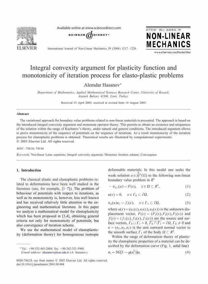
Within the range of deformation theory of plastic-ity the elastoplastic properties of a material can be de-scribed by the deformation curve (Fig. 1, solid line)
i = 3G[1− g(e2i )]ei (4)
0020-7462/$ - see front matter ? 2003 Elsevier Ltd. All rights reserved.doi:10.1016/j.ijnonlinmec.2003.08.004
1218 A. Hasanov / International Journal of Non-Linear Mechanics 39 (2004) 1217–1226
0 0.05 0.1 0.15 0.20
2
4
6
8
10
12
14
16σ iσ i,h
(e1, σ1)×
×(e0,σ0)
ei
σi
Fig. 1. The deformation curve i = i(ei) and its piecewise linearapproximation.
which satisDes the following conditions [5,6]:
(i) i ∈C1(0; e∗i ); di=dei ¿ 0; ∀ei ∈ (0; e∗i ) (mono-tonicity);
(ii) di=dei − i=ei06 0; ∀ei ∈ (0; e∗i ) (concavity);(iii) i = 3Gei, ∀ei ∈ (0; e0) (pure elastic case).
Here i = i(u) is the stress intensity, e2i (u) =(23
)eij(u)eij(u) is the deformation intensity, G =
is the modulus of rigidity and e0 ¿ 0 is the elasticitylimit of a deformable material.The relationship between the stress tensor =ij
and deviator of deformation e= eij is given as fol-lows:
ij(u) = K(u)ij + 2G(1− g(e2i (u)))eij(u);
i; j = 1; 2; 3;
or, by using the relationship eij(u) = (u)ij −(13
)(u)ij,
ij(u) =[K − 2
3 G(1− g(e2i (u)))](u)ij
+2G(1− g(e2i (u)))ij(u); i; j = 1; 2; 3:(5)
Here K = +(23
) is the modulus of volumetric
expansion and ij—Kronecker delta (the summationconvention from 1 to 3 will be employed throughout);¿ 0 and ¿ 0 are usually called the Lame coeF-cients. e2i (u) =
(23
)eij(u)eij(u) is the deformation in-
tensity, (u) = ii and ij(u) = 0:5(@ui=@xj + @uj=@xi)is the tensor of deformation.
The function g=g(e2i (u)), called the plasticity func-tion, is assumed to be piecewise diGerentiable and sat-isDes the following conditions:
06 g(e2i (u))6 g(e2i (u)) + 2g′(e2i (u))e2i (u)¡ 1;
e2i (u)¿ e20: (6)
Note that the above properties of the plasticity func-tion g= g(e2i ) follows from properties (i)–(iii) of thedeformation curve (4). Indeed, condition i(ei)¿ 0in (4) means g(e2i )¡ 1. Monotonicity condition (i)means 3G[1− g(ei)− 2e2i g
′(e2i )]¿ 0, which impliesg(e2i )+2e2i g
′(e2i )¡ 1. Further, the concavity condition(ii) implies g′(e2i )¿ 0. The case g() = 0, ∈ [0; 0],0=e20, corresponds to pure elastic deformations, whene2i 6 e0. In this case the above relationship has theform
ij(u) =[K − 2
3 G](u)ij + 2Gij(u);
i; j = 1; 2; 3: (7)
Note that the deformation theory can also be ex-tended for thermal deformations, replacing (u) by(u)− 3T , where is the coeFcient of thermal ex-pansion and T ¿ 0 is the temperature.By using the above relationship (5) we can rewrite
the non-linear Lame system (1) in the form of theplasticity operator
Au≡−(+ 2) grad div u− 2Iu
+2 div[g(e2i )e(u)] = F(x); x∈
in the terms of independent variable displacements.In Section 2 we develop monotone operator theory
for the above considered model and prove an exis-
tence of a unique solution in0H 1(). In Section 3 we
introduce the integral convexity argument which im-plies a relationship (inequality) between potential ofthe plasticity operator and its Drst Gateaux derivative.Based on this notion we prove monotonicity of the se-quence of potentials (corresponding to the sequence
of approximate solutions u(n) ∈ 0H 1()) of problems
(1)–(3) and obtain the rate of convergence. In Section4 we discuss numerical aspects of the approach givenon some examples.
A. Hasanov / International Journal of Non-Linear Mechanics 39 (2004) 1217–1226 1219
2. Monotonicity and potentialness of the plasticityoperator and solvability of problems (1)–(3)
Let us deDne a weak solution u∈ 0H 1() of prob-
lems (1)–(3).
Find u∈ 0H 1() such that∫
[+
23g(e2i (u))
](u)(v)
+2[1− g(e2i (u))]ij(u)ij(v)
dx
=∫Fi(x)vi(x) dx +
∫2
fi(x)vi(x) dx;
∀v∈ 0H 1(): (8)
Here0H 1() = v∈H 1(): v(x) = 0; x∈0 and
H 1() is the Sobolev space of vector functions v(x)=(v1(x); v2(x); v3(x)), with the norm [8]
‖v‖1 :=∫
[|v|2 + |∇v|2] dx
1=2
∀v∈ 0H 1():
We assume that F ∈H 0() and f∈H 0(@).Denote by 〈Au; v〉 the left-hand side and by l(v) =
〈F; v〉+〈f; v〉 the right-hand side of the above integralidentity, correspondingly, where A is the plasticity op-erator. Then we can rewrite (7) in the operator form
〈Au; v〉= l(v) ∀v∈ 0H 1(): (9)
Taking into account the dependence of the plasticity
function g= g(e2i (u)), on u∈ 0H 1() we introduce the
following non-linear functional:
a(u; v; w) =∫
[+
23g(e2i (u))
](v)(w)
+2[1− g(e2i (u))]ij(v)ij(w)
dx;
u; v; w∈ 0H 1(): (10)
It is easy to verify that a(u; ·; ·): 0H 1()× 0
H 1() → R1
is a symmetric bilinear form. Then
we have
〈Au; v〉= a(u; u; v); ∀u; v∈ 0H 1(): (11)
Following [9] we introduce the following.
Denition 1. The functional J (u) :0H 1() → R1 is
said to be a potential of the operator A, if
〈J ′(u); v〉= 〈Au; v〉; ∀u; v∈ 0H 1():
Here
〈J ′(u); v〉 := ddt
J (u+ tv)|t=0
is the Drst Gateaux derivative of the functional J (u)
at u∈ 0H 1() on the direction v∈ 0
H 1(). Evidently,the plasticity operator is a potential operator with thepotential
J (u) = 0:5∫
2(u) + 2ij(u)ij(u)
−3∫ e2i (u)
0g() d
dx; u∈ 0
H 1() (12)
since ∀u; v∈ 0H 1()
〈J ′(u); v〉=∫[(u)(v) + 2ij(u)ij(v)
− 2g(e2i (u))eij(u)eij(v)] dx (13)
due to e2i (u)=(23
)eij(u)eij(u). We can use the identity
eij(u)eij(v)=eij(u)ij(v) and rewrite the above integralas follows:
〈J ′(u); v〉=∫
[+
23g(e2i (u))
](u)(v)
+ 2[1− g(e2i (u))]ij(u)ij(v)
dx (14)
which shows with (9), that 〈J ′(u); v〉= a(u; u; v); ∀u;v∈ 0
H 1(). As we will see below the above form (13)of the non-linear functional a(u; u; v) is also conve-nient for the iteration process.
1220 A. Hasanov / International Journal of Non-Linear Mechanics 39 (2004) 1217–1226
By the same way we can introduce the potential
((u) = J (u)− l(u); u∈ 0H 1()
of problems (1)–(3), and show that
〈(′(u); v〉= 〈A(u); v〉 − l(v); u; v∈ 0H 1();
where J (u) and l(u) are the above deDned functionals.Consider the plasticity operator A deDned by (9)–
(10). According to [9] the operator A is said to beradially continuous, if the real-valued function
’(t) = 〈A(u+ tv); v〉; t ∈R
is continuous as a function of t ∈R, for any Dxed
u; v∈ 0H 1().
Lemma 1. If the plasticity function g()∈C[0; 1],satis6es conditions (6), then the plasticity operatorA, de6ned by (9)–(10), is radially continuous.
Proof. Let tn ⊂ R and tn → t, as n → ∞. Then for
a Dxed u; v∈ 0H 1() formula (12) implies
〈A(u+ tnv); v〉
=∫[(u+ tnv)(v) + 2ij(u+ tnv)ij(v)
− 2g(e2i (u+ tnv))eij(u+ tnv)eij(v)] dx
=〈A(u+ tv); v〉+∫[(u+ (tn − t)v)(v)
+ 2ij(u+ (tn − t)v)ij(v)] dx
+2∫[g(e2i (u+ tv))
−g(e2i (u+ tnv))]eij(u+ tv)eij(v) dx
+2∫g(e2i (u+ tnv))[eij(u+ tv)
−eij(u+ tnv)]eij(v) dx:Going to the limit tn → t on the right-hand side of theabove equality and using continuity of the function (t)=g(e2i (u+tv)) we obtain 〈A(u+tnv); v〉 → 〈A(u+tv); v〉.
Lemma 2. If conditions of Lemma 1 hold, then theplasticity operator A is strong monotone, i.e.
〈A(u)− A(v); u− v〉¿ +0‖u− v‖1;
∀u; v∈ 0H 1():
Proof. Based on the equivalence of the strong mono-tonicity of the potential operator and positivity of itspotential, let us calculate the second Gateaux deriva-tive of the functional J (u), deDned by (11)
J ′′(u; v; w) : =ddt〈J ′(u+ tw); v〉|t=0
=∫
[+
23Q(e2i (u))
](v)(w)
+ 2[1− Q(e2i (u))]ij(v)ij(w)
dx;
u; v; w∈ 0H 1();
where Q(e2i (u))= g(e2i (u))+2g′(e2i (u))e2i (u). Due to
conditions (5), 1−Q(e2i (u))¿ 0 ¿ 0. Then by ¿ 0and Korn’s inequality [6] we have
J ′′(u : v; v) = 20
∫ij(v)ij(v) dx
¿ +0‖v‖21 ∀v∈ 0H 1():
This implies the proof.
Corollary 1. Since A0=0, from strong monotonicityof the operator A follows also its coercivity.
Thus the potential operator is radially continuous,strong monotone and coercive. Then by Browder–Minty theorem [9] we have the following existence.
Theorem 1. Let g = g() be a piecewise di9eren-tiable function satisfying conditions (6). Then thenon-linear mixed problems (1)–(3) has a unique so-
lution u∈ 0H 1(), de6ned by the integral identity (7).
A. Hasanov / International Journal of Non-Linear Mechanics 39 (2004) 1217–1226 1221
3. Integral convexity and monotonicity of theiteration process
Consider now the non-linear term in (11), in theform of integral
Q(e2i (u)) =∫ e2i (u)
0g() d:
The following lemma shows convexity of the aboveintegral.
Lemma 3. Let g= g() be a piecewise di9erentiablefunction satisfying conditions (6). Then the function
Q(t) =∫ t
0g() d; t ∈ [0; 1]
is convex, i.e.
Q(t + (1− )t)6 Q(t) + (1− )Q(t)
∀∈ [0; 1] ∀t ∈ [0; 1]:
The proof is obvious, since Q′′(t) = g′(t)¿ 0.Taking into account the well-known property
Q′(t1)(t2 − t1)6Q(t2)− Q(t1)
∀t2¿ t1; t1; t2 ∈ [0; 1]
of convex functions, for the above function Q(e2i (u))we get (t1 = e2i (v); t2 = e2i (w))
g(e2i (v))(e2i (v)− e2i (w)) +
∫ e2i (w)
0g() d
−∫ e2i (v)
0g() d¿ 0 ∀v; w∈ 0
H 1()
or
g(e2i (v))(e2i (v)− e2i (w)) +
∫ e2i (w)
e2i (v)g() d
¿ 0 ∀v; w∈ 0H 1(): (15)
Next we show that the integral convexity (14) im-plies a relationship between the potential J (u) of thenon-linear operator A, deDned by (11), and its DrstGateaux derivative
〈J ′(v); v〉= 〈Av; v〉 := a(v; v; v) ∀v∈ 0H 1()
at an element v∈ 0H 1() on the same direction.
Lemma 4. Let g= g() be a piecewise di9erentiablefunction satisfying conditions (6). Then the followinginequality holds:
0:5a(v;w; w)− J (w)− [0:5a(v; v; v)− J (v)]
¿ 0 ∀v; w∈ 0H 1(): (16)
Proof. From (11) and (12) we get
0:5a(v;w; w)− 0:5a(v; v; v)− J (w) + J (v)
=∫[g(e2i (v))eij(v)eij(v)
−g(e2i (v))eij(w)eij(w)] dx
+32∫
∫ e2i (w)
e2i (v)g() d
dx
∀v; w∈ 0H 1():
Taking into account the identity e2i (v)=(23
)eij(v)eij(v)
we have
0:5a(v;w; w)− 0:5a(v; v; v) + J (w)− J (v)
=32∫
[g(e2i (v))[eij(v)eij(v)− eij(w)eij(w)]
+∫ e2i (w)
e2i (v)g() d
dx:
Using inequality (14) on the right-hand side we obtaininequality (15).
As a Drst application of the inequality above we getthe following.
Corollary 2. Let u∈ 0H 1() be the solution of the
mixed problems (1)–(3). If conditions of Lemma 4
hold, then the function u∈ 0H 1() is a solution of the
following variational problem:
J (u) + 0:5a(u; u; u)
= infv∈ 0
H 1()
J (v) + 0:5a(u; v; v):
Next we linearize the non-linear problem (7) byusing the simple iteration (or Kachanov’s) method [2].
1222 A. Hasanov / International Journal of Non-Linear Mechanics 39 (2004) 1217–1226
Find u(n) ∈ 0H 1() such that
a(u(n−1); u(n); v)=l(v) ∀v∈ 0H 1(); n= 1; 2; 3; : : : ;
(17)
where u0 ∈ 0H 1() is a given data.
Since the plasticity operator A is a strong mono-tone potential one, the iteration scheme can also beconsidered as a particular case of the abstract iterativescheme given in [2].The functional a(u(n−1); ·; ·) is a symmetric coercive
bilinear form and hence the linearized problem (16)is equivalent to the minimization problem
0:5a(u(n−1); u(n); u(n))− l(u(n))
= infv∈ 0
H 1()
0:5a(u(n−1); v; v)− l(v): (18)
Lemma 5. Let conditions of Lemma 4 hold, thenthe sequence of potentials ((u(n)) is monotonedecreasing.
Proof. For v = u(n−1) and w = u(n) inequality (15)implies:
0:5a(u(n−1); u(n); u(n))− 0:5a(u(n−1); u(n−1); u(n−1))
−J (u(n−1)) + J (u(n))¿ 0:
We can get the similar inequality from (17)
0:5a(u(n−1); u(n−1); u(n−1))− l(u(n−1))
¿ 0:5a(u(n−1); u(n); u(n)) + l(u(n)):
From these two inequalities we have
J (u(n)) + l(u(n))¿ J (u(n−1)) + l(u(n−1))
∀n= 1; 2; 3; : : : ;
hence ((u(n))¿((u(n−1)).
Let us analyze now the behaviour of the potential
(0(u(n)) = J0(u(n))− l(u(n)); u(n) ∈ 0H 1() (19)
of the linearized problem (16) on the sequence ofapproximate solutions u(n).Based on deDnition (18) of the potential for the
linearized problem (16), we can derive it in the explicitform. For this aim consider the left-hand side of (17).
By deDnition of the functional a(u; v; w),
a(u(n−1); u(n); u(n))
=∫
[+
23g(e2i (u
(n−1)))] 2(u(n))
+ 2[1− g(e2i (u(n−1)))]ij(u(n))ij(u(n))
dx:
(20)
On the other hand, in the case of pure elastic defor-mations formula (11) implies
J0(u) = 0:5∫ 2(u) + 2ij(u)ij(u) d
dx;
e2i (u)6 e20: (21)
Comparing (19) and (20), and taking into account that
(n) = + 23 g(e2i (u
(n−1)));
(n) = [1− g(e2i (u(n−1)))]; (22)
where (n) ¿ 0 and (n) ¿ 0 are known coeFcientsfrom the (n− 1)th iteration, we conclude that the bi-linear functional (19) is the potential of the linearizedoperator on nth iteration. Then, due to the deDnition(0(u(n)) = 0:5a(u(n−1); u(n); u(n))− l(u(n)), we have
(0(u(n)) = 0:5∫
(n) 2(u(n))
+ 2(n)ij(u(n))ij(u(n))dx − l(u(n));
(23)
where (n) ¿ 0 and (n) ¿ 0 are deDned by (21).On the other hand, for v=u(n) the linearized equation
(16) implies
l(u(n)) = a(u(n−1); u(n); u(n));
n= 1; 2; 3; : : : :
Hence from (22) we get the following explicit formfor the potential of the linearized problem (16):
(0(u(n)) =−0:5∫
(n) 2(u(n))
+ 2(n)ij(u(n))ij(u(n))dx: (24)
A. Hasanov / International Journal of Non-Linear Mechanics 39 (2004) 1217–1226 1223
Taking into account that the minimization problem(17) can also be formulated as follows:
(0(u(n)) = infv∈ 0
H 1()
(0(v) (25)
this result with Lemma 5 implies that the constructedsequence u(n) of approximate solutions is, not only aminimizing sequence, but also amonotone minimizingone.To prove the convergence of the sequence of po-
tentials (0(u(n)), we use Corollary 1 which impliescoercivity of the bilinear form a(u(n−1); ·; ·)a(u(n−1); u(n); u(n))¿ +0‖u(n)‖21: (26)
Conditions F ∈H 0() and f∈H 0(@) mean theboundedness |l(u(n))|6 c0‖u(n)‖1, c0 ¿ 0, of thelinear form l(u), where the constants +0 ¿ 0 andc0 ¿ 0 do not depend on the number of iterationsn= 1; 2; 3; : : :, due to conditions (6). Hence
(0(u(n))¿ [0:5+0‖u(n)‖1 − c0]‖u(n)‖1 (27)
and the sequence of potentials (0(u(n)) is boundedbelow.
Corollary 3. Let conditions (6) hold and u(n)∈0H 1() be the sequence of solutions of the linearizedproblem (16). Then the sequence of potentials(0(u(n)), de6ned by (22), is a monotone conver-gent sequence.
Now we can apply the convergence theorem forabstract monotone potential operators given in ([1,Theorem 1]), to the considered problem and prove thefollowing.
Theorem 2. Let u(x); u(n)(x)∈ 0H 1() be solutions of
the non-linear problem (7) and the linearized prob-lem (16), respectively. If conditions (6) hold, thenu(n)(x) → u(x) as n → 0, in the norm of H 1(), andfor the rate of convergence the following estimateholds:
‖u− u(n)‖16√2+1
+0√+0
((u(n))−((u(n+1))
1=2;
+0; +1 ¿ 0: (28)
Proof. The proof of the convergence can be obtainedby reproducing Theorem 1 [1]. We estimate the rateof convergence over the sequence of potentials.Evidently the coercive symmetric bilinear form
a(u(n−1); ·; ·) is bounded:|a(u(n−1); v; w)|6 +1‖v‖‖w‖;
∀v; w∈ 0H 1(); +1 ¿ 0:
Then applying Lemma 2 and Theorem 1 from [1] weget
‖u(n) − u(n−1)‖1
6
√2+0
((u(n−1))−((u(n))
1=2; +0 ¿ 0
(29)
and
‖u− u(n−1)‖16 +1+0‖u(n) − u(n−1)‖1: (30)
These two inequalities imply estimate (27).
Theorem 2 asserts that the iteration process given by(16) converges at all. Moreover, estimate (27) showsthe rate of convergence depends on the rate of mono-tonicity of the sequence of potentials J (u(n)).
4. Numerical results
The computational experiment here for thenon-linear elastoplastic problem is based on the Dniteelement (FE) discretization with the Lagrange type oftriangle elements. The ultimate veriDcation of the er-ror estimate (27) (also (28)–(29)), as well as all iter-ation processes, would be to consider the dependenceof number of iterations not only on the accuracy
p =
∑(ij) [u
(n)i; j − u(n−1)
i; j ]21=2
∑ij [u
(n−1)i; j ]2
1=2 (31)
given, but also on the plasticity function g= g() anddiGerent levels of plastic deformations of the mate-rial, during the deformation process. For this reason anaxisymmetric problem of indentation of an isotropichomogeneous deformable sample under a rigid spher-ical indentor is considered. The uniaxial indentation
1224 A. Hasanov / International Journal of Non-Linear Mechanics 39 (2004) 1217–1226
y
x
α
Γ1 Γσ
Γ0
Γu
Ω
P
y = (x)
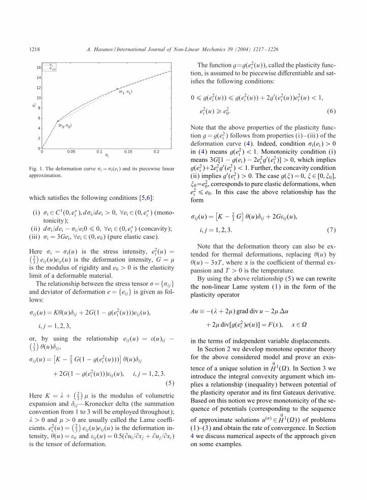
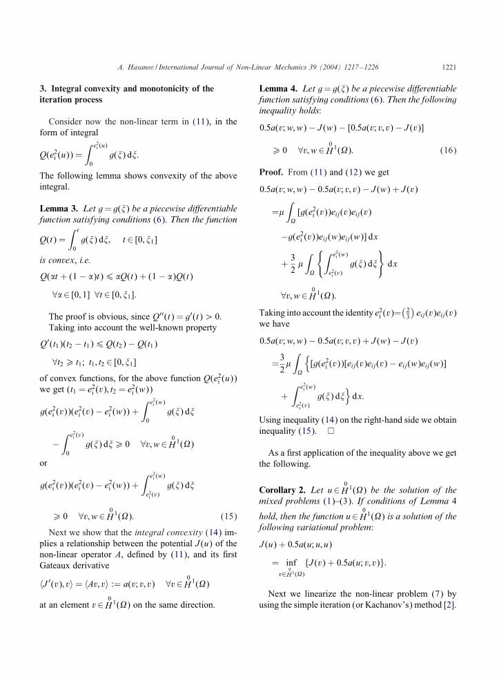
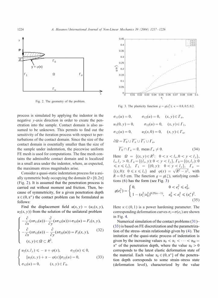
Fig. 2. The geometry of the problem.
process is simulated by applying the indentor in thenegative y-axis direction in order to create the pen-etration into the sample. Contact domain is also as-sumed to be unknown. This permits to Dnd out thesensitivity of the iteration process with respect to per-turbations of the contact domain. Since the size of thecontact domain is essentially smaller than the size ofthe sample under indentation, the piecewise uniformFE mesh is used for computations. The Dne mesh con-tains the admissible contact domain and is localizedin a small area under the indentor, where, as expected,the maximum stress magnitudes arise.Consider a quasi-static indentation process for a axi-
ally symmetric body occupying the domain×[0; 20](Fig. 2). It is assumed that the penetration process iscarried out without moment and friction. Then, be-cause of symmetricity, for a given penetration depth∈ (0; ∗) the contact problem can be formulated asfollows:Find the displacement Deld u(x; y) = (u1(x; y);
u2(x; y)) from the solution of the unilateral problem
− @@x
(x11(u))− @@y
(x12(u))+33(u) = F1(x; y);
− @@x
(x12(u))− @@y
(x22(u)) = F2(x; y);
(x; y)∈ ⊂ R2:
(32)
u2(x; ly)6− + ’(x); 22(u)6 0;
[u2(x; y) + − ’(x)]22(u) = 0;
12(u) = 0; (x; y)∈0:
(33)
0 0.01 0.02 0.03 0.04 0.05 0.06 0.07 0.08 0.09 0.10
0.05
0.1
0.15
0.2
0.25
0.3
0.35
0.4
0.45κ=0.2κ=0.5κ=0.8
g (e
i2 )
ei
Fig. 3. The plasticity function g = g(e2i ); 1 = 0:8; 0:5; 0:2.
11(u) = 0; 12(u) = 0; (x; y)∈;
u1(0; y) = 0; 12(u) = 0; (x; y)∈1;
12(u) = 0; u2(x; 0) = 0; (x; y)∈u;
@ = 0 ∪ ∪ 1 ∪ u;
0 ∩ u = ∅; measu = 0: (34)
Here = (x; y)∈R2: 0¡x¡lx; 0¡y¡ly,lx; ly ¿ 0, =(lx; y): 0¡y¡ly; 0=(x; ly): 06 x6 lx, 1 = (0; y): 0¡y¡ly, u =(x; 0): 06 x6 lx and ’(x) =
√R2 − x2, with
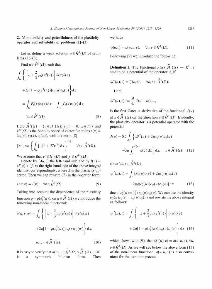
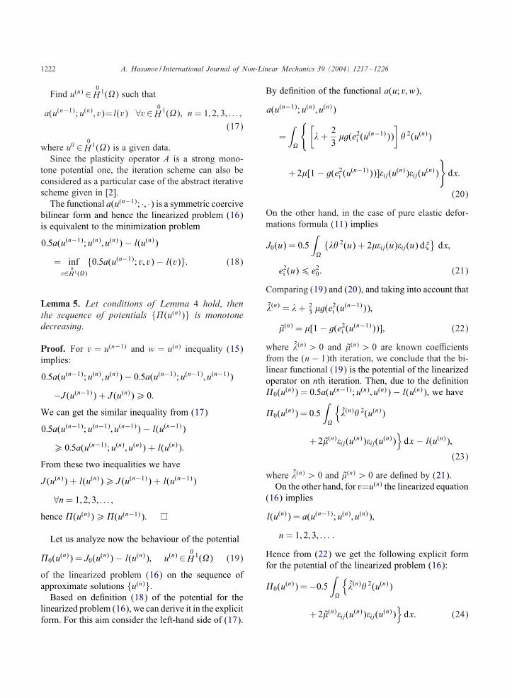
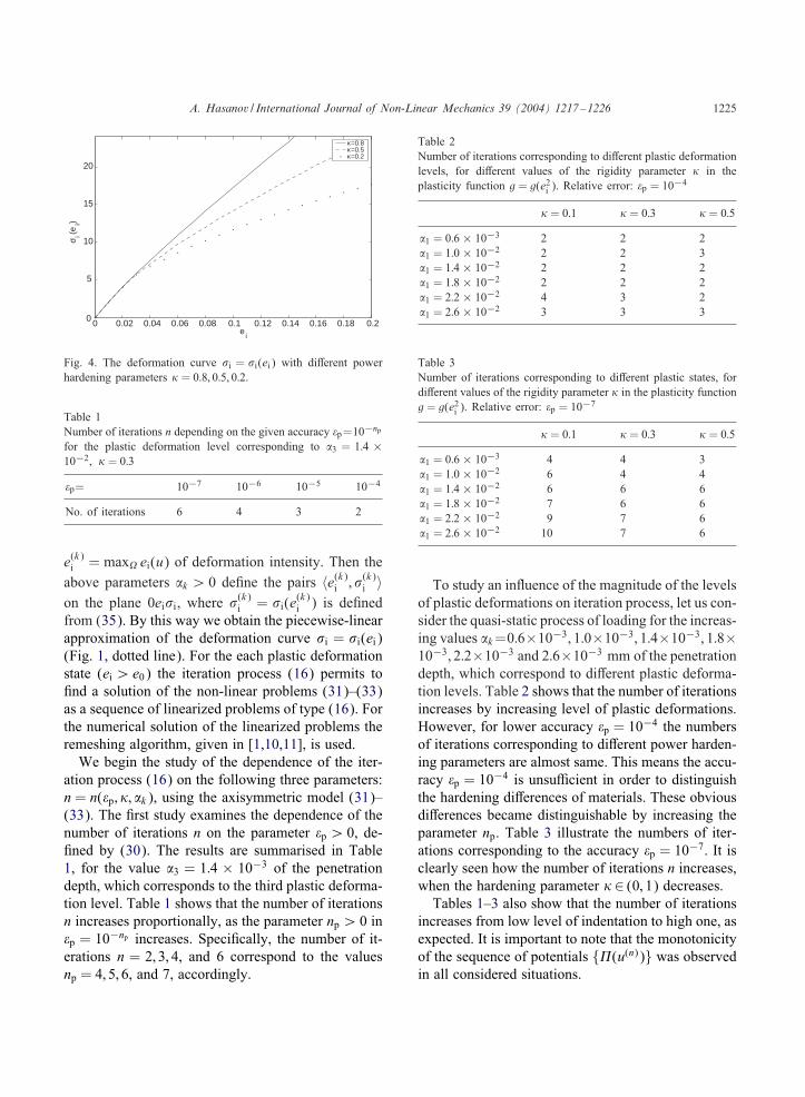
R = 0:5 cm. The function g = g(), satisfying condi-tions (6) has the form (see Fig. 3)
g(e2i ) =
0; 0¡e2i 6 e20;
1− (e2i =e20)
0:25(1−1); e20 ¡e2i 6 (e∗i )2:(35)
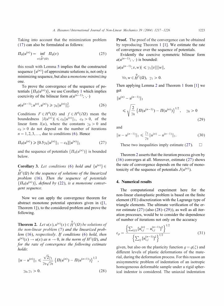
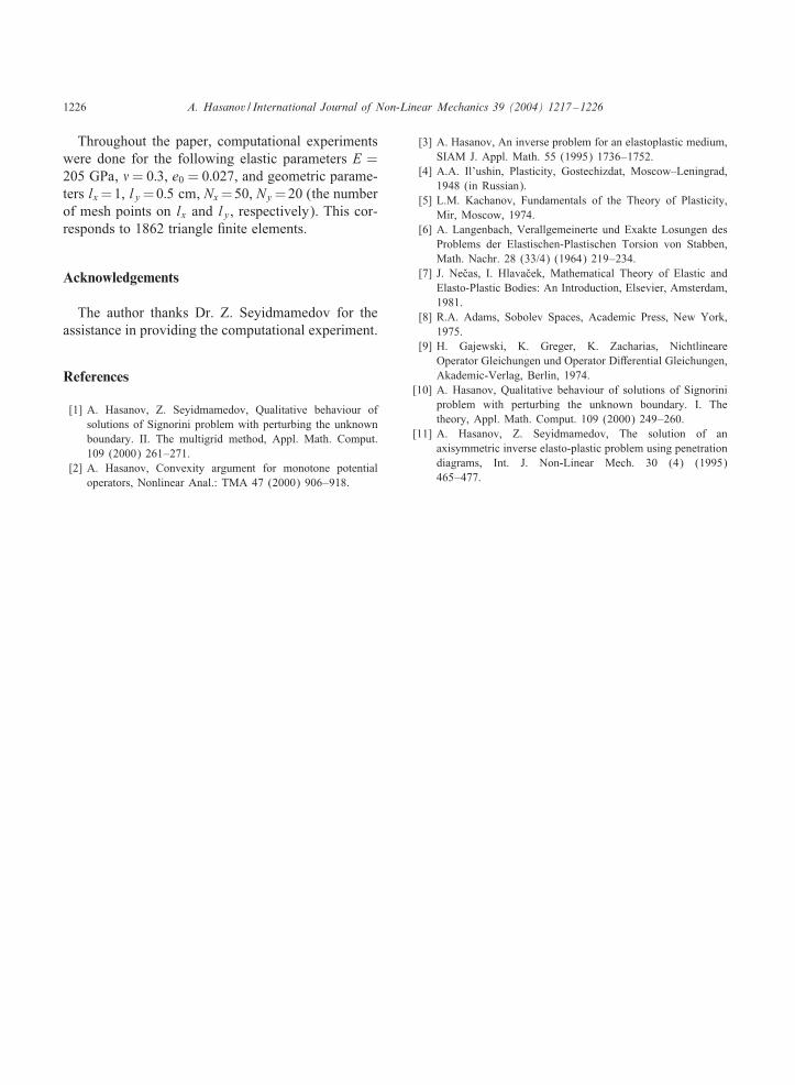
Here 1∈ (0; 1) is a power hardening parameter. Thecorresponding deformation curves i=(ei) are shownin Fig. 4.Numerical simulation of the contact problems (31)–
(33) is based on FE discretization and the parametriza-tion of the stress–strain relationship given by (4). Theimitation of the quasi-static process of indentation isgiven by the increasing values 0 ¡1 ¡ · · ·¡M =∗ of the penetration depth, where the value 0 ¿ 0corresponds to the latest elastic deformation state ofthe material. Each value k ∈ (0; ∗] of the penetra-tion depth corresponds to some strain–stress state(deformation level), characterized by the value
A. Hasanov / International Journal of Non-Linear Mechanics 39 (2004) 1217–1226 1225
0 0.02 0.04 0.06 0.08 0.1 0.12 0.14 0.16 0.18 0.20
5
10
15
20
κ=0.8κ=0.5κ=0.2
ei
σ i(ei)
Fig. 4. The deformation curve i = i(ei) with diGerent powerhardening parameters 1 = 0:8; 0:5; 0:2.
Table 1Number of iterations n depending on the given accuracy p=10−np
for the plastic deformation level corresponding to 3 = 1:4 ×10⁻²; 1 = 0:3
p= 10−7 10−6 10−5 10−4
No. of iterations 6 4 3 2
e(k)i = max ei(u) of deformation intensity. Then theabove parameters k ¿ 0 deDne the pairs 〈e(k)i ; (k)
i 〉on the plane 0eii, where (k)
i = i(e(k)i ) is deDned
from (35). By this way we obtain the piecewise-linearapproximation of the deformation curve i = i(ei)(Fig. 1, dotted line). For the each plastic deformationstate (ei ¿e0) the iteration process (16) permits toDnd a solution of the non-linear problems (31)–(33)as a sequence of linearized problems of type (16). Forthe numerical solution of the linearized problems theremeshing algorithm, given in [1,10,11], is used.We begin the study of the dependence of the iter-
ation process (16) on the following three parameters:n = n(p; 1; k), using the axisymmetric model (31)–(33). The Drst study examines the dependence of thenumber of iterations n on the parameter p ¿ 0, de-Dned by (30). The results are summarised in Table1, for the value 3 = 1:4 × 10⁻³ of the penetrationdepth, which corresponds to the third plastic deforma-tion level. Table 1 shows that the number of iterationsn increases proportionally, as the parameter np ¿ 0 inp = 10−np increases. SpeciDcally, the number of it-erations n = 2; 3; 4, and 6 correspond to the valuesnp = 4; 5; 6, and 7, accordingly.
Table 2Number of iterations corresponding to diGerent plastic deformationlevels, for diGerent values of the rigidity parameter 1 in theplasticity function g = g(e2i ). Relative error: p = 10−4
1 = 0:1 1 = 0:3 1 = 0:5
1 = 0:6× 10⁻³ 2 2 21 = 1:0× 10−2 2 2 31 = 1:4× 10⁻² 2 2 21 = 1:8× 10⁻² 2 2 21 = 2:2× 10⁻² 4 3 21 = 2:6× 10⁻² 3 3 3
Table 3Number of iterations corresponding to diGerent plastic states, fordiGerent values of the rigidity parameter 1 in the plasticity functiong = g(e2i ). Relative error: p = 10−7
1 = 0:1 1 = 0:3 1 = 0:5
1 = 0:6× 10⁻³ 4 4 31 = 1:0× 10−2 6 4 41 = 1:4× 10⁻² 6 6 61 = 1:8× 10⁻² 7 6 61 = 2:2× 10⁻² 9 7 61 = 2:6× 10⁻² 10 7 6
To study an inPuence of the magnitude of the levelsof plastic deformations on iteration process, let us con-sider the quasi-static process of loading for the increas-ing values k=0:6×10⁻³; 1:0×10−3; 1:4×10⁻³; 1:8×10⁻³; 2:2×10⁻³ and 2:6×10⁻³ mm of the penetrationdepth, which correspond to diGerent plastic deforma-tion levels. Table 2 shows that the number of iterationsincreases by increasing level of plastic deformations.However, for lower accuracy p = 10−4 the numbersof iterations corresponding to diGerent power harden-ing parameters are almost same. This means the accu-racy p = 10−4 is unsuFcient in order to distinguishthe hardening diGerences of materials. These obviousdiGerences became distinguishable by increasing theparameter np. Table 3 illustrate the numbers of iter-ations corresponding to the accuracy p = 10−7. It isclearly seen how the number of iterations n increases,when the hardening parameter 1∈ (0; 1) decreases.
Tables 1–3 also show that the number of iterationsincreases from low level of indentation to high one, asexpected. It is important to note that the monotonicityof the sequence of potentials ((u(n)) was observedin all considered situations.
1226 A. Hasanov / International Journal of Non-Linear Mechanics 39 (2004) 1217–1226
Throughout the paper, computational experimentswere done for the following elastic parameters E =205 GPa, 4= 0:3, e0 = 0:027, and geometric parame-ters lx =1, ly =0:5 cm, Nx =50, Ny =20 (the numberof mesh points on lx and ly, respectively). This cor-responds to 1862 triangle Dnite elements.
Acknowledgements
The author thanks Dr. Z. Seyidmamedov for theassistance in providing the computational experiment.
References
[1] A. Hasanov, Z. Seyidmamedov, Qualitative behaviour ofsolutions of Signorini problem with perturbing the unknownboundary. II. The multigrid method, Appl. Math. Comput.109 (2000) 261–271.
[2] A. Hasanov, Convexity argument for monotone potentialoperators, Nonlinear Anal.: TMA 47 (2000) 906–918.
[3] A. Hasanov, An inverse problem for an elastoplastic medium,SIAM J. Appl. Math. 55 (1995) 1736–1752.
[4] A.A. Il’ushin, Plasticity, Gostechizdat, Moscow–Leningrad,1948 (in Russian).
[5] L.M. Kachanov, Fundamentals of the Theory of Plasticity,Mir, Moscow, 1974.
[6] A. Langenbach, Verallgemeinerte und Exakte Losungen desProblems der Elastischen-Plastischen Torsion von Stabben,Math. Nachr. 28 (33/4) (1964) 219–234.
[7] J. NeUcas, I. HlavaUcek, Mathematical Theory of Elastic andElasto-Plastic Bodies: An Introduction, Elsevier, Amsterdam,1981.
[8] R.A. Adams, Sobolev Spaces, Academic Press, New York,1975.
[9] H. Gajewski, K. Greger, K. Zacharias, NichtlineareOperator Gleichungen und Operator DiGerential Gleichungen,Akademic-Verlag, Berlin, 1974.
[10] A. Hasanov, Qualitative behaviour of solutions of Signoriniproblem with perturbing the unknown boundary. I. Thetheory, Appl. Math. Comput. 109 (2000) 249–260.
[11] A. Hasanov, Z. Seyidmamedov, The solution of anaxisymmetric inverse elasto-plastic problem using penetrationdiagrams, Int. J. Non-Linear Mech. 30 (4) (1995)465–477.
Related Documents