INSTRUCTOR'S SOLUTIONS MANUAL NUMERICAL ... - Test Bank

INSTRUCTOR’S SOLUTIONS MANUAL

NUMERICAL ANALYSIS THIRD EDITION

Timothy Sauer George Mason University

The author and publisher of this book have used their best efforts in preparing this book. These efforts include the development, research, and testing of the theories and programs to determine their effectiveness. The author and publisher make no warranty of any kind, expressed or implied, with regard to these programs or the documentation contained in this book. The author and publisher shall not be liable in any event for incidental or consequential damages in connection with, or arising out of, the furnishing, performance, or use of these programs. Reproduced by Pearson from electronic files supplied by the author. Copyright © 2018, 2012 by Pearson Education, Inc. Publishing as Pearson, 501 Boylston Street, Boston, MA 02116. All rights reserved. No part of this publication may be reproduced, stored in a retrieval system, or transmitted, in any form or by any means, electronic, mechanical, photocopying, recording, or otherwise, without the prior written permission of the publisher. Printed in the United States of America.

1 17

ISBN-13: 978-0-13-469732-1 ISBN-10: 0-13-469732-4

© 2018, 2012 Pearson Education, Inc.

iii

Table of Contents

Chapter 0: Fundamentals

0.1 Evaluating a Polynomial 1 0.2 Binary Numbers 2 0.3 Floating Point Representation of Real Numbers 8 0.4 Loss of Significance 13 0.5 Review of Calculus 15

Chapter 1: Solving Equations

1.1 The Bisection Method 17 1.2 Fixed-Point Iteration 19 1.3 Limits of Accuracy 24 1.4 Newton’s Method 25 1.5 Root-Finding without Derivatives 28

Chapter 2: Systems of Equations

2.1 Gaussian Elimination 31 2.2 The LU Factorization 32 2.3 Sources of Error 35 2.4 The PA=LU Factorization 40 2.5 Iterative Methods 45 2.6 Methods for Symmetric Positive-Definite Matrices 49 2.7 Nonlinear Systems of Equations 57

Chapter 3: Interpolation

3.1 Data and Interpolating Functions 63 3.2 Interpolation Error 67 3.3 Chebyshev Interpolation 71 3.4 Cubic Splines 75 3.5 Bézier Curves 85

Chapter 4: Least Squares

4.1 Least Squares and the Normal Equations 91 4.2 A Survey of Models 98 4.3 QR Factorization 105 4.4 GMRES Method 115 4.5 Nonlinear Least Squares 121

© 2018, 2012 Pearson Education, Inc. iv

Chapter 5: Numerical Differentiation and Integration

5.1 Numerical Differentiation 127 5.2 Newton-Cotes Formulas for Numerical Integration 136 5.3 Romberg Integration 146 5.4 Adaptive Quadrature 150 5.5 Gaussian Quadrature 155

Chapter 6: Ordinary Differential Equations

6.1 Initial Value Problems 159 6.2 Analysis of IVP Solvers 168 6.3 Systems of Ordinary Differential Equations 176 6.4 Runge-Kutta Methods and Applications 182 6.5 Variable Step-Size Methods 192 6.6 Implicit Methods and Stiff Equations 193 6.7 Multistep Methods 195

Chapter 7: Boundary Value Problems

7.1 Shooting Method 207 7.2 Finite Difference Methods 211 7.3 Collocation and the Finite Element Method 220

Chapter 8: Partial Differential Equations

8.1 Parabolic Equations 225 8.2 Hyperbolic Equations 228 8.3 Elliptic Equations 230 8.4 Nonlinear Partial Differential Equations 237

Chapter 9: Random Numbers and Applications

9.1 Random Numbers 239 9.2 Monte Carlo Simulation 242 9.3 Discrete and Continuous Brownian Motion 243 9.4 Stochastic Differential Equations 245

Chapter 10: Trigonometric Interpolation and the FFT

10.1 The Fourier Transform 253 10.2 Trigonometric Interpolation 256 10.3 The FFT and Signal Processing 265

© 2018, 2012 Pearson Education, Inc.

v

Chapter 11: Compression

11.1 The Discrete Cosine Transform 271 11.2 Two-Dimensional DCT and Image Compression 276 11.3 Huffman Coding 280 11.4 Modified DCT and Audio Compression 284

Chapter 12: Eigenvalues and Singular Values

12.1 Power Iteration Methods 293 12.2 QR Algorithm 297 12.3 Singular Value Decomposition 301 12.4 Applications of the SVD 305

Chapter 13: Optimization

13.1 Unconstrained Optimization without Derivatives 307 13.2 Unconstrained Optimization with Derivatives 309

© 2018, 2012 Pearson Education, Inc. vi

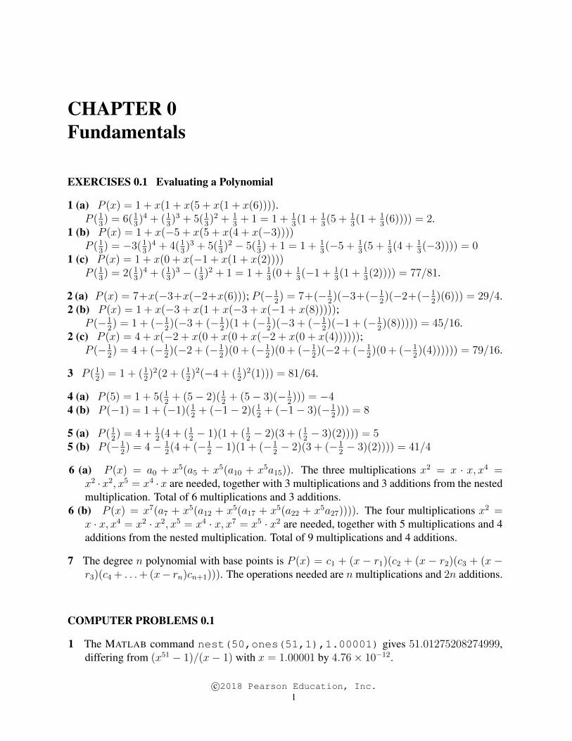
CHAPTER 0Fundamentals

EXERCISES 0.1 Evaluating a Polynomial

1 (a) P (x) = 1 + x(1 + x(5 + x(1 + x(6)))).P (1

3) = 6(1

3)4 + (1

3)3 + 5(1

3)2 + 1

3+ 1 = 1 + 1

3(1 + 1

3(5 + 1

3(1 + 1

3(6)))) = 2.

1 (b) P (x) = 1 + x(−5 + x(5 + x(4 + x(−3))))P (1

3) = −3(1

3)4 + 4(1

3)3 + 5(1

3)2 − 5(1

3) + 1 = 1 + 1

3(−5 + 1

3(5 + 1

3(4 + 1

3(−3)))) = 0

1 (c) P (x) = 1 + x(0 + x(−1 + x(1 + x(2))))P (1

3) = 2(1

3)4 + (1

3)3 − (1

3)2 + 1 = 1 + 1

3(0 + 1

3(−1 + 1

3(1 + 1

3(2)))) = 77/81.

2 (a) P (x) = 7+x(−3+x(−2+x(6))); P (−12) = 7+(−1

2)(−3+(−1

2)(−2+(−1

2)(6))) = 29/4.

2 (b) P (x) = 1 + x(−3 + x(1 + x(−3 + x(−1 + x(8)))));P (−1

2) = 1 + (−1

2)(−3 + (−1

2)(1 + (−1

2)(−3 + (−1

2)(−1 + (−1

2)(8))))) = 45/16.

2 (c) P (x) = 4 + x(−2 + x(0 + x(0 + x(−2 + x(0 + x(4))))));P (−1

2) = 4 + (−1

2)(−2 + (−1

2)(0 + (−1

2)(0 + (−1

2)(−2 + (−1

2)(0 + (−1

2)(4)))))) = 79/16.

3 P (12) = 1 + (1

2)2(2 + (1

2)2(−4 + (1

2)2(1))) = 81/64.

4 (a) P (5) = 1 + 5(12+ (5− 2)(1

2+ (5− 3)(−1

2))) = −4

4 (b) P (−1) = 1 + (−1)(12+ (−1− 2)(1

2+ (−1− 3)(−1

2))) = 8

5 (a) P (12) = 4 + 1

2(4 + (1

2− 1)(1 + (1

2− 2)(3 + (1

2− 3)(2)))) = 5

5 (b) P (−12) = 4− 1

2(4 + (−1

2− 1)(1 + (−1

2− 2)(3 + (−1

2− 3)(2)))) = 41/4

6 (a) P (x) = a0 + x5(a5 + x5(a10 + x5a15)). The three multiplications x2 = x · x, x4 =x2 ·x2, x5 = x4 ·x are needed, together with 3 multiplications and 3 additions from the nestedmultiplication. Total of 6 multiplications and 3 additions.

6 (b) P (x) = x7(a7 + x5(a12 + x5(a17 + x5(a22 + x5a27)))). The four multiplications x2 =x · x, x4 = x2 · x2, x5 = x4 · x, x7 = x5 · x2 are needed, together with 5 multiplications and 4additions from the nested multiplication. Total of 9 multiplications and 4 additions.

7 The degree n polynomial with base points is P (x) = c1 + (x − r1)(c2 + (x − r2)(c3 + (x −r3)(c4 + . . .+ (x− rn)cn+1))). The operations needed are n multiplications and 2n additions.

COMPUTER PROBLEMS 0.1

1 The MATLAB command nest(50,ones(51,1),1.00001) gives 51.01275208274999,differing from (x51 − 1)/(x− 1) with x = 1.00001 by 4.76× 10−12.

c©2018 Pearson Education, Inc.1

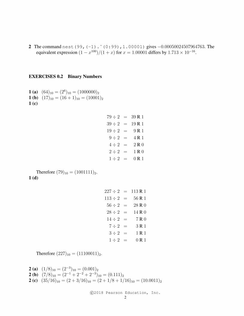
2 The command nest(99,(-1).ˆ(0:99),1.00001) gives−0.00050024507964763. Theequivalent expression (1− x100)/(1 + x) for x = 1.00001 differs by 1.713× 10−16.

EXERCISES 0.2 Binary Numbers

1 (a) (64)10 = (26)10 = (1000000)21 (b) (17)10 = (16 + 1)10 = (10001)21 (c)

79÷ 2 = 39 R 1

39÷ 2 = 19 R 1

19÷ 2 = 9 R 1

9÷ 2 = 4 R 1

4÷ 2 = 2 R 0

2÷ 2 = 1 R 0

1÷ 2 = 0 R 1

Therefore (79)10 = (1001111)2.1 (d)

227÷ 2 = 113 R 1

113÷ 2 = 56 R 1

56÷ 2 = 28 R 0

28÷ 2 = 14 R 0

14÷ 2 = 7 R 0

7÷ 2 = 3 R 1

3÷ 2 = 1 R 1

1÷ 2 = 0 R 1

Therefore (227)10 = (11100011)2.

2 (a) (1/8)10 = (2−3)10 = (0.001)22 (b) (7/8)10 = (2−1 + 2−2 + 2−3)10 = (0.111)22 (c) (35/16)10 = (2 + 3/16)10 = (2 + 1/8 + 1/16)10 = (10.0011)2


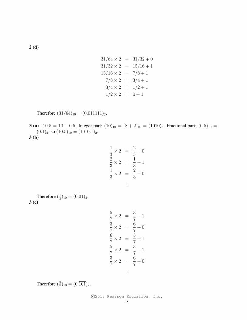
2 (d)

31/64× 2 = 31/32 + 0

31/32× 2 = 15/16 + 1

15/16× 2 = 7/8 + 1

7/8× 2 = 3/4 + 1

3/4× 2 = 1/2 + 1

1/2× 2 = 0 + 1

Therefore (31/64)10 = (0.011111)2.

3 (a) 10.5 = 10 + 0.5. Integer part: (10)10 = (8 + 2)10 = (1010)2. Fractional part: (0.5)10 =(0.1)2, so (10.5)10 = (1010.1)2.

3 (b)

1

3× 2 =

2

3+ 0

2

3× 2 =

1

3+ 1

1

3× 2 =

2

3+ 0

...

Therefore (13)10 = (0.01)2.

3 (c)

5

7× 2 =

3

7+ 1

3

7× 2 =

6

7+ 0

6

7× 2 =

5

7+ 1

5

7× 2 =

3

7+ 1

3

7× 2 =

6

7+ 0

...

Therefore (57)10 = (0.101)2.


3 (d) (12.8)10 = (12)10 + (0.8)10; (12)10 = (1100)2.

0.8× 2 = 0.6 + 1

0.6× 2 = 0.2 + 1

0.2× 2 = 0.4 + 0

0.4× 2 = 0.8 + 0

0.8× 2 = 0.6 + 1...

Therefore (12.8)10 = (1100.1100)2.3 (e) (55.4)10 = (55)10 + (0.4)10; (55)10 = (32 + 16 + 4 + 2 + 1)10 = (110111)2.

0.4× 2 = 0.8 + 0

0.8× 2 = 0.6 + 1

0.6× 2 = 0.2 + 1

0.2× 2 = 0.4 + 0

0.4× 2 = 0.8 + 0...

Therefore (55.4)10 = (110111.0110)2.3 (f)

0.1× 2 = 0.2 + 0

0.2× 2 = 0.4 + 0

0.4× 2 = 0.8 + 0

0.8× 2 = 0.6 + 1

0.6× 2 = 0.2 + 1

0.2× 2 = 0.4 + 0...

Therefore (0.1)10 = (0.00011)2.

4 (a) 11.25 = 11 + 0.25. Integer part: (11)10 = (8 + 2 + 1)10 = (1011)2. Fractional part:(0.25)10 = (0.01)2, so (10.25)10 = (1011.01)2.


4 (b)

2

3× 2 =

1

3+ 1

1

3× 2 =

2

3+ 0

2

3× 2 =

1

3+ 1

...

Therefore (23)10 = (0.10)2.

4 (c)

3

5× 2 =

1

5+ 1

1

5× 2 =

2

5+ 0

2

5× 2 =

4

5+ 0

4

5× 2 =

3

5+ 1

3

5× 2 =

1

5+ 1

...

Therefore (35)10 = (0.1001)2.

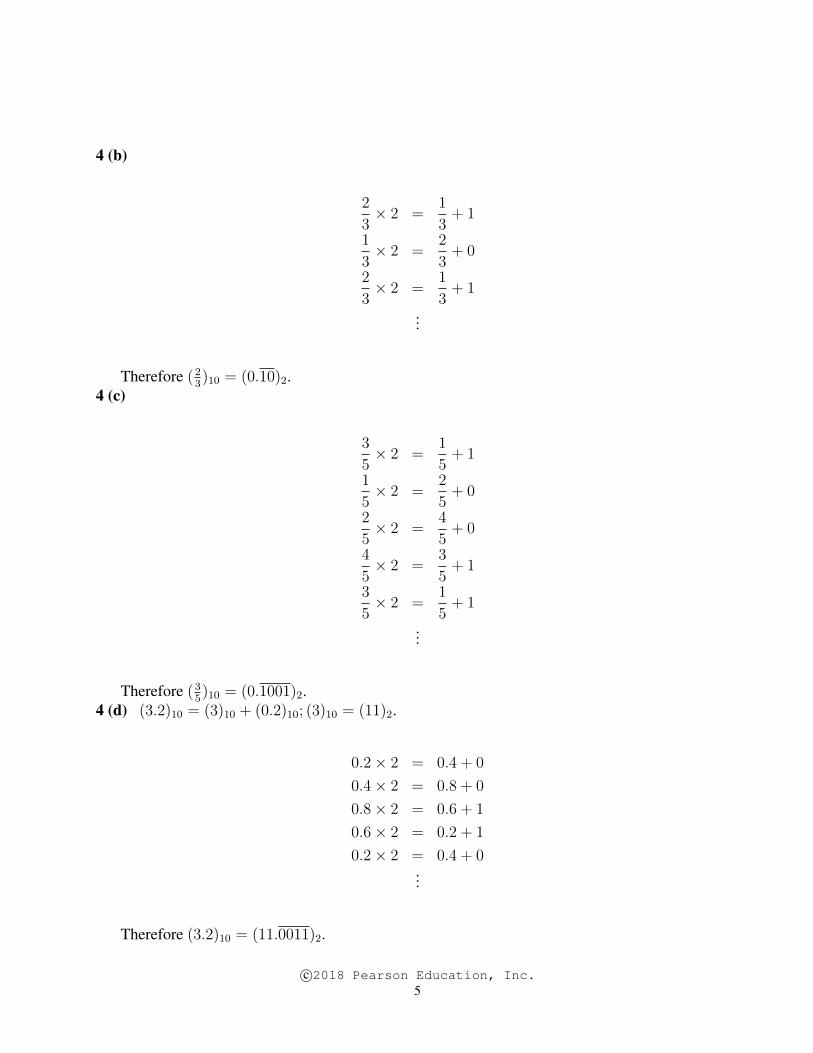
4 (d) (3.2)10 = (3)10 + (0.2)10; (3)10 = (11)2.

0.2× 2 = 0.4 + 0

0.4× 2 = 0.8 + 0

0.8× 2 = 0.6 + 1

0.6× 2 = 0.2 + 1

0.2× 2 = 0.4 + 0...

Therefore (3.2)10 = (11.0011)2.


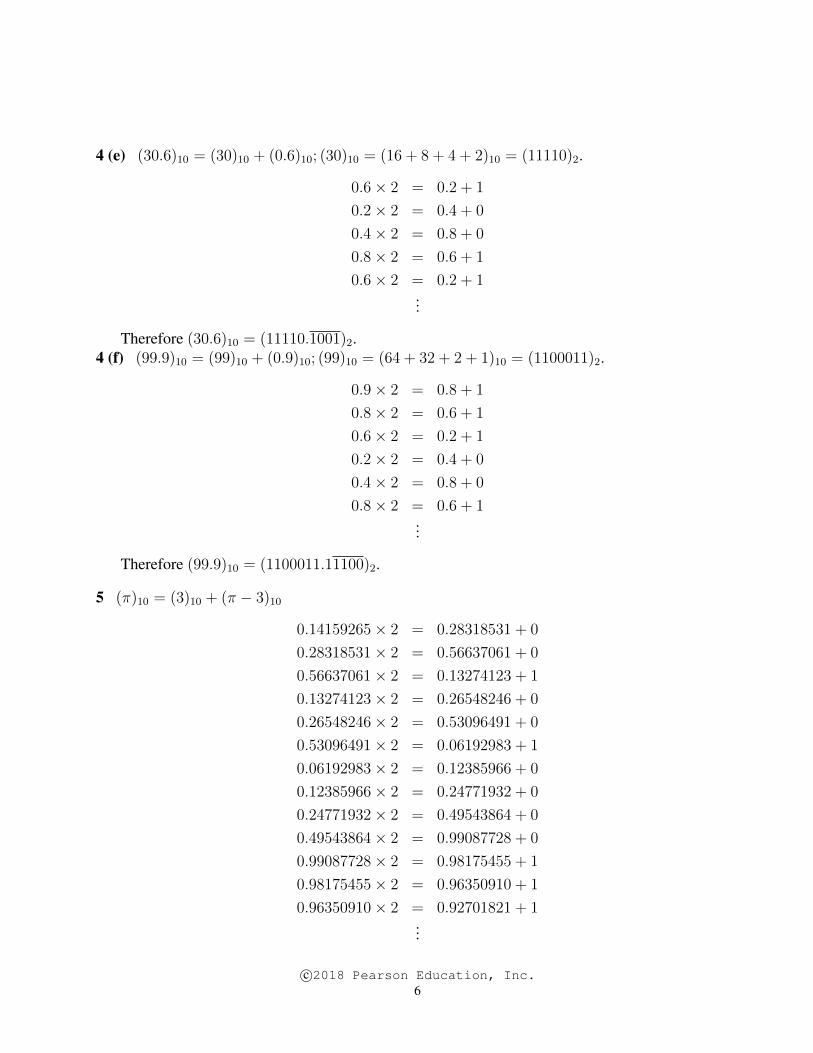
4 (e) (30.6)10 = (30)10 + (0.6)10; (30)10 = (16 + 8 + 4 + 2)10 = (11110)2.

0.6× 2 = 0.2 + 1

0.2× 2 = 0.4 + 0

0.4× 2 = 0.8 + 0

0.8× 2 = 0.6 + 1

0.6× 2 = 0.2 + 1...

Therefore (30.6)10 = (11110.1001)2.4 (f) (99.9)10 = (99)10 + (0.9)10; (99)10 = (64 + 32 + 2 + 1)10 = (1100011)2.

0.9× 2 = 0.8 + 1

0.8× 2 = 0.6 + 1

0.6× 2 = 0.2 + 1

0.2× 2 = 0.4 + 0

0.4× 2 = 0.8 + 0

0.8× 2 = 0.6 + 1...

Therefore (99.9)10 = (1100011.11100)2.

5 (π)10 = (3)10 + (π − 3)10

0.14159265× 2 = 0.28318531 + 0

0.28318531× 2 = 0.56637061 + 0

0.56637061× 2 = 0.13274123 + 1

0.13274123× 2 = 0.26548246 + 0

0.26548246× 2 = 0.53096491 + 0

0.53096491× 2 = 0.06192983 + 1

0.06192983× 2 = 0.12385966 + 0

0.12385966× 2 = 0.24771932 + 0

0.24771932× 2 = 0.49543864 + 0

0.49543864× 2 = 0.99087728 + 0

0.99087728× 2 = 0.98175455 + 1

0.98175455× 2 = 0.96350910 + 1

0.96350910× 2 = 0.92701821 + 1...


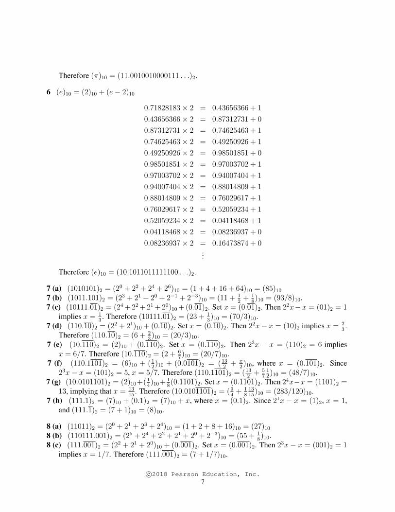
Therefore (π)10 = (11.0010010000111 . . .)2.

6 (e)10 = (2)10 + (e− 2)10

0.71828183× 2 = 0.43656366 + 1

0.43656366× 2 = 0.87312731 + 0

0.87312731× 2 = 0.74625463 + 1

0.74625463× 2 = 0.49250926 + 1

0.49250926× 2 = 0.98501851 + 0

0.98501851× 2 = 0.97003702 + 1

0.97003702× 2 = 0.94007404 + 1

0.94007404× 2 = 0.88014809 + 1

0.88014809× 2 = 0.76029617 + 1

0.76029617× 2 = 0.52059234 + 1

0.52059234× 2 = 0.04118468 + 1

0.04118468× 2 = 0.08236937 + 0

0.08236937× 2 = 0.16473874 + 0...

Therefore (e)10 = (10.1011011111100 . . .)2.

7 (a) (1010101)2 = (20 + 22 + 24 + 26)10 = (1 + 4 + 16 + 64)10 = (85)107 (b) (1011.101)2 = (23 + 21 + 20 + 2−1 + 2−3)10 = (11 + 1

2+ 1

8)10 = (93/8)10.

7 (c) (10111.01)2 = (24+22+21+20)10+(0.01)2. Set x = (0.01)2. Then 22x−x = (01)2 = 1implies x = 1

3. Therefore (10111.01)2 = (23 + 1

3)10 = (70/3)10.

7 (d) (110.10)2 = (22 + 21)10 + (0.10)2. Set x = (0.10)2. Then 22x− x = (10)2 implies x = 23.

Therefore (110.10)2 = (6 + 23)10 = (20/3)10.

7 (e) (10.110)2 = (2)10 + (0.110)2. Set x = (0.110)2. Then 23x − x = (110)2 = 6 impliesx = 6/7. Therefore (10.110)2 = (2 + 6

7)10 = (20/7)10.

7 (f) (110.1101)2 = (6)10 + (12)10 + (0.0101)2 = (13

2+ x

2)10, where x = (0.101)2. Since

23x− x = (101)2 = 5, x = 5/7. Therefore (110.1101)2 = (132+ 5

712)10 = (48/7)10.

7 (g) (10.0101101)2 = (2)10+(14)10+

18(0.1101)2. Set x = (0.1101)2. Then 24x−x = (1101)2 =

13, implying that x = 1315

. Therefore (10.0101101)2 = (94+ 1

81315)10 = (283/120)10.

7 (h) (111.1)2 = (7)10 + (0.1)2 = (7)10 + x, where x = (0.1)2. Since 21x − x = (1)2, x = 1,and (111.1)2 = (7 + 1)10 = (8)10.

8 (a) (11011)2 = (20 + 21 + 23 + 24)10 = (1 + 2 + 8 + 16)10 = (27)108 (b) (110111.001)2 = (25 + 24 + 22 + 21 + 20 + 2−3)10 = (55 + 1

8)10.

8 (c) (111.001)2 = (22 + 21 + 20)10 + (0.001)2. Set x = (0.001)2. Then 23x− x = (001)2 = 1implies x = 1/7. Therefore (111.001)2 = (7 + 1/7)10.


8 (d) (1010.01)2 = (23+21)10+(0.01)2. Set x = (0.01)2. Then 22x−x = (01)2 implies x = 13.

Therefore (1010.01)2 = (10 + 13)10 = (10 + 1/3)10.

8 (e) (10111.10101)2 = (10111.10)2 = (24 + 22 + 21 + 20)10 + (0.10)2. Set x = (0.10)2. Then22x− x = (10)2 = 2 implies x = 2/3. Therefore (10111.10101)2 = (23 + 2

3)10.

8 (f) (1111.010001)2 = (15)10 + (1/4)10 +18(0.001)2 = (15 + 1/4 + x

8)10, where x = (0.001)2.

Since 23x − x = (001)2 = 5, x = 1/7. Therefore (1111.010001)2 = (15 + 1/4 + 1817)10 =

(15 + 15/56)10.

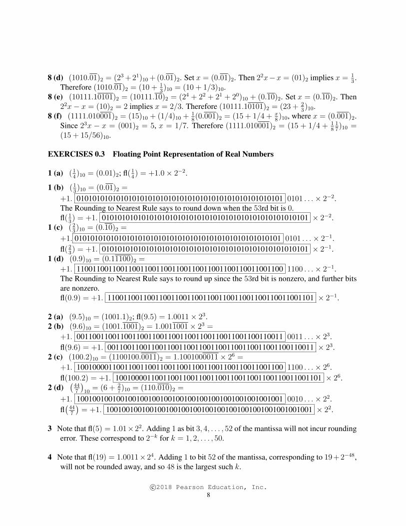
EXERCISES 0.3 Floating Point Representation of Real Numbers

1 (a) (14)10 = (0.01)2; fl(1

4) = +1.0× 2−2.

1 (b) (13)10 = (0.01)2 =

+1. 0101010101010101010101010101010101010101010101010101 0101 . . .× 2−2.The Rounding to Nearest Rule says to round down when the 53rd bit is 0.fl(1

3) = +1. 0101010101010101010101010101010101010101010101010101 × 2−2.

1 (c) (23)10 = (0.10)2 =

+1. 0101010101010101010101010101010101010101010101010101 0101 . . .× 2−1.fl(2

3) = +1. 0101010101010101010101010101010101010101010101010101 × 2−1.

1 (d) (0.9)10 = (0.11100)2 =

+1. 1100110011001100110011001100110011001100110011001100 1100 . . .× 2−1.The Rounding to Nearest Rule says to round up since the 53rd bit is nonzero, and further bitsare nonzero.fl(0.9) = +1. 1100110011001100110011001100110011001100110011001101 × 2−1.

2 (a) (9.5)10 = (1001.1)2; fl(9.5) = 1.0011× 23.2 (b) (9.6)10 = (1001.1001)2 = 1.0011001× 23 =

+1. 0011001100110011001100110011001100110011001100110011 0011 . . .× 23.fl(9.6) = +1. 0011001100110011001100110011001100110011001100110011 × 23.

2 (c) (100.2)10 = (1100100.0011)2 = 1.1001000011× 26 =

+1. 1001000011001100110011001100110011001100110011001100 1100 . . .× 26.fl(100.2) = +1. 1001000011001100110011001100110011001100110011001101 × 26.

2 (d)(447

)10

= (6 + 27)10 = (110.010)2 =

+1. 1001001001001001001001001001001001001001001001001001 0010 . . .× 22.fl(447

)= +1. 1001001001001001001001001001001001001001001001001001 × 22.

3 Note that fl(5) = 1.01×22. Adding 1 as bit 3, 4, . . . , 52 of the mantissa will not incur roundingerror. These correspond to 2−k for k = 1, 2, . . . , 50.

4 Note that fl(19) = 1.0011×24. Adding 1 to bit 52 of the mantissa, corresponding to 19+2−48,will not be rounded away, and so 48 is the largest such k.


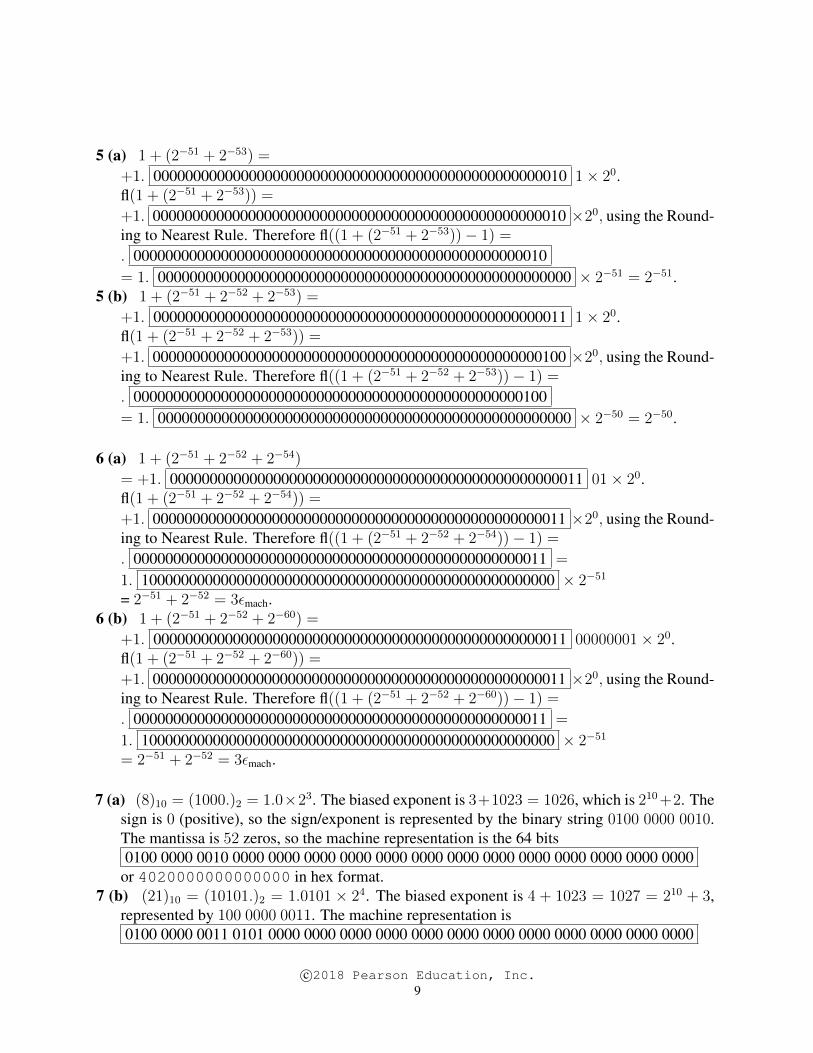
5 (a) 1 + (2−51 + 2−53) =

+1. 0000000000000000000000000000000000000000000000000010 1× 20.fl(1 + (2−51 + 2−53)) =

+1. 0000000000000000000000000000000000000000000000000010 ×20, using the Round-ing to Nearest Rule. Therefore fl((1 + (2−51 + 2−53))− 1) =

. 0000000000000000000000000000000000000000000000000010= 1. 0000000000000000000000000000000000000000000000000000 × 2−51 = 2−51.

5 (b) 1 + (2−51 + 2−52 + 2−53) =

+1. 0000000000000000000000000000000000000000000000000011 1× 20.fl(1 + (2−51 + 2−52 + 2−53)) =

+1. 0000000000000000000000000000000000000000000000000100 ×20, using the Round-ing to Nearest Rule. Therefore fl((1 + (2−51 + 2−52 + 2−53))− 1) =

. 0000000000000000000000000000000000000000000000000100= 1. 0000000000000000000000000000000000000000000000000000 × 2−50 = 2−50.

6 (a) 1 + (2−51 + 2−52 + 2−54)

= +1. 0000000000000000000000000000000000000000000000000011 01× 20.fl(1 + (2−51 + 2−52 + 2−54)) =


. 0000000000000000000000000000000000000000000000000011 =

1. 1000000000000000000000000000000000000000000000000000 × 2−51

= 2−51 + 2−52 = 3εmach.6 (b) 1 + (2−51 + 2−52 + 2−60) =

+1. 0000000000000000000000000000000000000000000000000011 00000001× 20.fl(1 + (2−51 + 2−52 + 2−60)) =


. 0000000000000000000000000000000000000000000000000011 =

1. 1000000000000000000000000000000000000000000000000000 × 2−51

= 2−51 + 2−52 = 3εmach.

7 (a) (8)10 = (1000.)2 = 1.0×23. The biased exponent is 3+1023 = 1026, which is 210+2. Thesign is 0 (positive), so the sign/exponent is represented by the binary string 0100 0000 0010.The mantissa is 52 zeros, so the machine representation is the 64 bits0100 0000 0010 0000 0000 0000 0000 0000 0000 0000 0000 0000 0000 0000 0000 0000

or 4020000000000000 in hex format.7 (b) (21)10 = (10101.)2 = 1.0101 × 24. The biased exponent is 4 + 1023 = 1027 = 210 + 3,

represented by 100 0000 0011. The machine representation is0100 0000 0011 0101 0000 0000 0000 0000 0000 0000 0000 0000 0000 0000 0000 0000


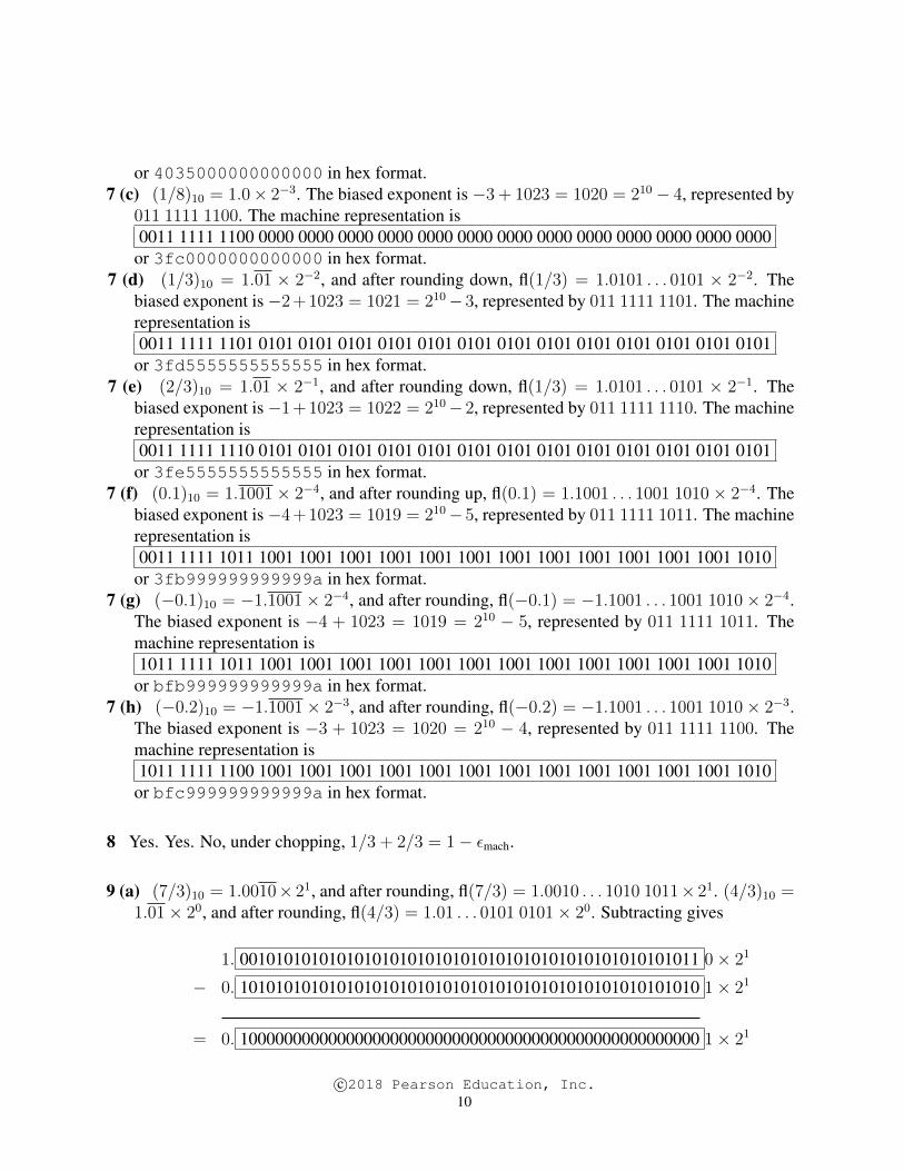
or 4035000000000000 in hex format.7 (c) (1/8)10 = 1.0× 2−3. The biased exponent is −3 + 1023 = 1020 = 210 − 4, represented by

011 1111 1100. The machine representation is0011 1111 1100 0000 0000 0000 0000 0000 0000 0000 0000 0000 0000 0000 0000 0000

or 3fc0000000000000 in hex format.7 (d) (1/3)10 = 1.01 × 2−2, and after rounding down, fl(1/3) = 1.0101 . . . 0101 × 2−2. The

biased exponent is−2+1023 = 1021 = 210−3, represented by 011 1111 1101. The machinerepresentation is0011 1111 1101 0101 0101 0101 0101 0101 0101 0101 0101 0101 0101 0101 0101 0101

or 3fd5555555555555 in hex format.7 (e) (2/3)10 = 1.01 × 2−1, and after rounding down, fl(1/3) = 1.0101 . . . 0101 × 2−1. The


or 3fe5555555555555 in hex format.7 (f) (0.1)10 = 1.1001× 2−4, and after rounding up, fl(0.1) = 1.1001 . . . 1001 1010× 2−4. The


or 3fb999999999999a in hex format.7 (g) (−0.1)10 = −1.1001× 2−4, and after rounding, fl(−0.1) = −1.1001 . . . 1001 1010× 2−4.

The biased exponent is −4 + 1023 = 1019 = 210 − 5, represented by 011 1111 1011. Themachine representation is1011 1111 1011 1001 1001 1001 1001 1001 1001 1001 1001 1001 1001 1001 1001 1010

or bfb999999999999a in hex format.7 (h) (−0.2)10 = −1.1001× 2−3, and after rounding, fl(−0.2) = −1.1001 . . . 1001 1010× 2−3.

The biased exponent is −3 + 1023 = 1020 = 210 − 4, represented by 011 1111 1100. Themachine representation is1011 1111 1100 1001 1001 1001 1001 1001 1001 1001 1001 1001 1001 1001 1001 1010

or bfc999999999999a in hex format.

8 Yes. Yes. No, under chopping, 1/3 + 2/3 = 1− εmach.

9 (a) (7/3)10 = 1.0010× 21, and after rounding, fl(7/3) = 1.0010 . . . 1010 1011× 21. (4/3)10 =1.01× 20, and after rounding, fl(4/3) = 1.01 . . . 0101 0101× 20. Subtracting gives

1. 0010101010101010101010101010101010101010101010101011 0× 21

− 0. 1010101010101010101010101010101010101010101010101010 1× 21

= 0. 1000000000000000000000000000000000000000000000000000 1× 21


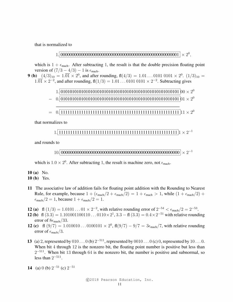
that is normalized to

1. 0000000000000000000000000000000000000000000000000001 × 20,

which is 1 + εmach. After subtracting 1, the result is that the double precision floating pointversion of (7/3− 4/3)− 1 is εmach.

9 (b) (4/3)10 = 1.01 × 20, and after rounding, fl(4/3) = 1.01 . . . 0101 0101 × 20. (1/3)10 =1.01× 2−2, and after rounding, fl(1/3) = 1.01 . . . 0101 0101× 2−2. Subtracting gives

1. 0101010101010101010101010101010101010101010101010101 00× 20

− 0. 0101010101010101010101010101010101010101010101010101 01× 20

= 0. 1111111111111111111111111111111111111111111111111111 11× 20

that normalizes to

1. 1111111111111111111111111111111111111111111111111111 1× 2−1

and rounds to

10. 0000000000000000000000000000000000000000000000000000 × 2−1

which is 1.0× 20. After subtracting 1, the result is machine zero, not εmach.

10 (a) No.10 (b) Yes.

11 The associative law of addition fails for floating point addition with the Rounding to NearestRule, for example, because 1 + (εmach/2 + εmach/2) = 1 + εmach > 1, while (1 + εmach/2) +εmach/2 = 1, because 1 + εmach/2 = 1.

12 (a) fl (1/3) = 1.0101 . . . 01× 2−2, with relative rounding error of 2−54 < εmach/2 = 2−53.12 (b) fl (3.3) = 1.101001100110 . . . 0110×21, 3.3− fl (3.3) = 0.4×2−51 with relative rounding

error of 8εmach/33.12 (c) fl (9/7) = 1.010010 . . . 0100101 × 20, fl(9/7) − 9/7 = 3εmach/7, with relative rounding

error of εmach/3.

13 (a) 2, represented by 010 . . . 0 (b) 2−511, represented by 0010 . . . 0 (c) 0, represented by 10 . . . 0.When bit 4 through 12 is the nonzero bit, the floating point number is positive but less than2−511. When bit 13 through 64 is the nonzero bit, the number is positive and subnormal, soless than 2−511.

14 (a) 0 (b) 2−51 (c) 2−51


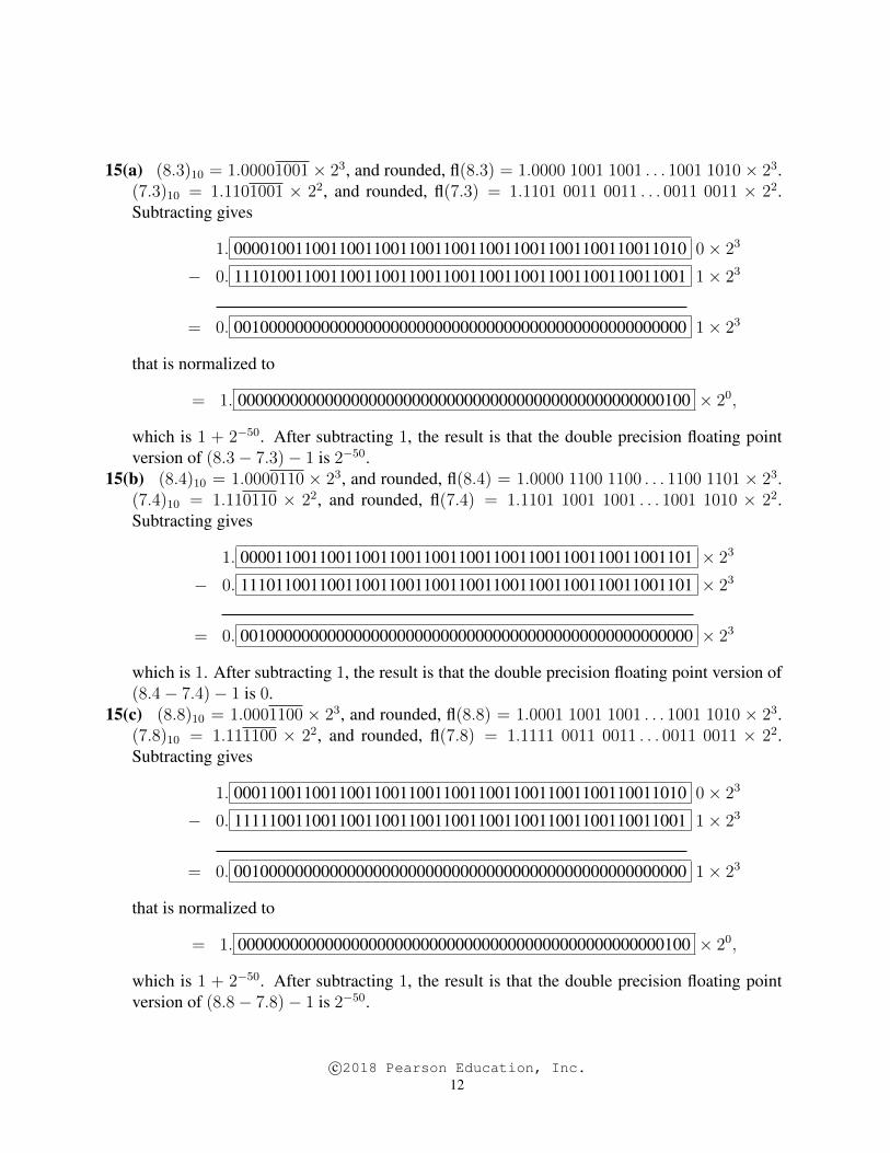
15(a) (8.3)10 = 1.00001001× 23, and rounded, fl(8.3) = 1.0000 1001 1001 . . . 1001 1010× 23.(7.3)10 = 1.1101001 × 22, and rounded, fl(7.3) = 1.1101 0011 0011 . . . 0011 0011 × 22.Subtracting gives

1. 0000100110011001100110011001100110011001100110011010 0× 23

− 0. 1110100110011001100110011001100110011001100110011001 1× 23

= 0. 0010000000000000000000000000000000000000000000000000 1× 23


= 1. 0000000000000000000000000000000000000000000000000100 × 20,

which is 1 + 2−50. After subtracting 1, the result is that the double precision floating pointversion of (8.3− 7.3)− 1 is 2−50.

15(b) (8.4)10 = 1.0000110 × 23, and rounded, fl(8.4) = 1.0000 1100 1100 . . . 1100 1101 × 23.(7.4)10 = 1.110110 × 22, and rounded, fl(7.4) = 1.1101 1001 1001 . . . 1001 1010 × 22.Subtracting gives

1. 0000110011001100110011001100110011001100110011001101 × 23

− 0. 1110110011001100110011001100110011001100110011001101 × 23

= 0. 0010000000000000000000000000000000000000000000000000 × 23

which is 1. After subtracting 1, the result is that the double precision floating point version of(8.4− 7.4)− 1 is 0.

15(c) (8.8)10 = 1.0001100 × 23, and rounded, fl(8.8) = 1.0001 1001 1001 . . . 1001 1010 × 23.(7.8)10 = 1.111100 × 22, and rounded, fl(7.8) = 1.1111 0011 0011 . . . 0011 0011 × 22.Subtracting gives

1. 0001100110011001100110011001100110011001100110011010 0× 23

− 0. 1111100110011001100110011001100110011001100110011001 1× 23

= 0. 0010000000000000000000000000000000000000000000000000 1× 23


= 1. 0000000000000000000000000000000000000000000000000100 × 20,

which is 1 + 2−50. After subtracting 1, the result is that the double precision floating pointversion of (8.8− 7.8)− 1 is 2−50.


16 (a) fl (11/4) = 1.011× 21, with rounding error of 0.16 (b) fl (2.7) = 1.010110011001 . . . 100110010 × 21, fl (2.7) − 2.7 = 4εmach/5 with relative

rounding error of 8εmach/2716 (c) fl (10/3) = 1.1010 . . . 1011× 21, fl(10/3)− 10/3 = 2εmach/3, with relative rounding error

of εmach/5.

EXERCISES 0.4 Loss of Significance

1 (a) For x near 2πn for integer n, secx ≈ 1, and the numerator exhibits subtraction of nearlyequal numbers. An algebraically equivalent expression avoids the difficulty:

1− 1/ cosx

tan2 x=

cosx− 1

cosx tan2 x

=cosx− 1

secx sin2 x· cosx+ 1

cosx+ 1

=cos2−1

secx sin2 x(cosx+ 1)

= − 1

1 + sec x

1 (b) For x near 0, the numerator subtracts nearly equal numbers. Simplifying to

1− (1− x)3

x=

1− (1− 3x+ 3x2 − x3

x= 3− 3x+ x2

eliminates the loss of significance.1 (c) For x near 0, there is subtraction of nearly equal numbers. Using common denominators

eliminates the problem:

1

1 + x− 1

1− x=

1− x− (1 + x)

(1 + x)(1− x)=

2x

x2 − 1

2 −3.000; 7.579× 10−14

3 Since b is positive, the roots should be calculated as in (0.13):

x1 = −b+√b2 + 4× 10−12

2

x2 =2× 10−12

b+√b2 + 4× 10−12

4 8.5

5 −0.125



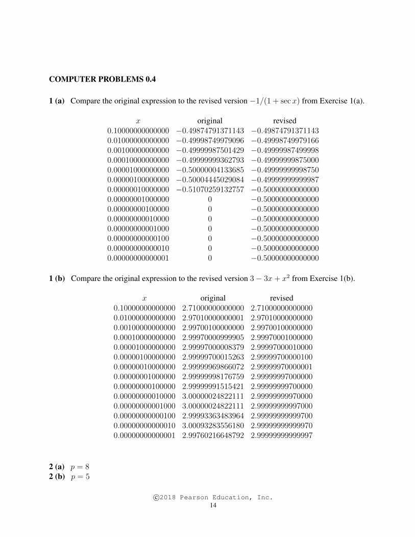
1 (a) Compare the original expression to the revised version −1/(1 + sec x) from Exercise 1(a).

x original revised0.10000000000000 −0.49874791371143 −0.498747913711430.01000000000000 −0.49998749979096 −0.499987499791660.00100000000000 −0.49999987501429 −0.499999874999980.00010000000000 −0.49999999362793 −0.499999998750000.00001000000000 −0.50000004133685 −0.499999999987500.00000100000000 −0.50004445029084 −0.499999999999870.00000010000000 −0.51070259132757 −0.500000000000000.00000001000000 0 −0.500000000000000.00000000100000 0 −0.500000000000000.00000000010000 0 −0.500000000000000.00000000001000 0 −0.500000000000000.00000000000100 0 −0.500000000000000.00000000000010 0 −0.500000000000000.00000000000001 0 −0.50000000000000

1 (b) Compare the original expression to the revised version 3− 3x+ x2 from Exercise 1(b).

x original revised0.10000000000000 2.71000000000000 2.710000000000000.01000000000000 2.97010000000001 2.970100000000000.00100000000000 2.99700100000000 2.997001000000000.00010000000000 2.99970000999905 2.999700010000000.00001000000000 2.99997000008379 2.999970000100000.00000100000000 2.99999700015263 2.999997000001000.00000010000000 2.99999969866072 2.999999700000010.00000001000000 2.99999998176759 2.999999970000000.00000000100000 2.99999991515421 2.999999997000000.00000000010000 3.00000024822111 2.999999999700000.00000000001000 3.00000024822111 2.999999999970000.00000000000100 2.99993363483964 2.999999999997000.00000000000010 3.00093283556180 2.999999999999700.00000000000001 2.99760216648792 2.99999999999997

2 (a) p = 82 (b) p = 5


3 Since a is large and negative, the expression represents subtraction of nearly equal numbers.Multiply numerator and denominator by the conjugate:

a+√a2 + b2 =

(a+√a2 + b2)(a−

√a2 + b2)

a−√a2 + b2

=−b2

a−√a2 + b2

≈ 6.1272× 10−13.

4 2.7500× 10−8

5 Set x = 3344556600 and y = 1.2222222. The difference between the lengths of the hypotenuseand the longer leg is√

x2 + y2 − x = (√x2 + y2 − x)

√x2 + y2 + x√x2 + y2 + x

=y2√

x2 + y2 + x

where we have rewritten the expression to eliminate the subtraction of nearly equal numbers.Although calculating the leftmost expression in double precision yields no correct significantdigits, the rightmost expression gives the correct answer 2.23322× 10−10.

EXERCISES 0.5 Review of Calculus

1 (a) Since f(0)f(1) = (1)(−2) < 0, there exists c between 0 and 1 such that f(c) = 0 by theIntermediate Value Theorem.

1 (b) Since f(0)f(1) = (1)(−9) < 0, f(c) = 0 for some c between 0 and 1 as in (a).1 (c) Since f(0)f(1/2) = (1)(−1/2) < 0, f(c) = 0 for some c between 0 and 1/2 by the

Intermediate Value Theorem, thus 0 ≤ c ≤ 1.

2 (a) c = ln(e− 1)2 (b) c = 1/22 (c) c =

√2− 1

3 (a) According to the Mean Value Theorem for Integrals, there exists c between 0 and 1 satisfy-

ing f(c) =

∫ 1

0x · x dx∫ 1

0x dx

=1/3

1/2=

2

3. Since f(x) = x, choose c = 2/3.

3 (b) According to the Mean Value Theorem for Integrals, there exists c between 0 and 1 satisfy-ing

f(c) =

∫ 1

0x3 dx∫ 1

0x dx

=1/4

1/2=

1

2.

Since f(x) = x2, this implies c2 = 1/2, or c = 1/√2.

3 (c) According to the Mean Value Theorem for Integrals, there exists c between 0 and 1 satisfy-

ing f(c) =

∫ 1

0xex dx∫ 1

0ex dx

=1

e− 1. Since f(x) = x, choose c =

1

e− 1.


4 (a) P (x) = 1 + x2

4 (b) P (x) = 1− 252x2

4 (c) P (x) = 1− x+ x2

5 (a) The derivatives evaluated at x = 0 are f(0) = 1, f ′(0) = 0, f ′′(0) = 2, f ′′′(0) =0, f (iv)(0) = 12, and f (v)(0) = 0. Then the degree 5 Taylor polynomial is P (x) = 1+x2+ 1

2x4.

5 (b) The derivatives evaluated at x = 0 are f(0) = 1, f ′(0) = 0, f ′′(0) = −4, f ′′′(0) =0, f (iv)(0) = 16, and f (v)(0) = 0. The degree 5 Taylor polynomial is P (x) = 1− 2x2 + 2

3x4.

5 (c) The derivatives at x = 0 are f(0) = 0, f ′(0) = 1, f ′′(0) = −1, f ′′′(0) = 2, f (iv)(0) = −6,and f (v)(0) = 24. The degree 5 Taylor polynomial is P (x) = x− 1

2x2 + 1

3x3 − 1

4x4 + 1

5x5.

5 (d) The derivatives at x = 0 are f(0) = 0, f ′(0) = 0, f ′′(0) = 2, f ′′′(0) = 0, f (iv)(0) = −8,and f (v)(0) = 0. The degree 5 Taylor polynomial is P (x) = x2 − 1

3x4.

6 (a) P (x) = 1− 2(x− 1) + 3(x− 1)2 − 4(x− 1)3 + 5(x− 1)4

6 (b) P (0.9) = 1.2345, P (1.1) = 0.82656 (c) error bound = 0.000125 for x = 0.9, 0.00006 for x = 1.16 (d) actual error ≈ 0.0000679 at x = 0.9, 0.0000537 at x = 1.1

7 (a) The derivatives at x = 1 are f(1) = 0, f ′(1) = 1, f ′′(1) = −1, f ′′′(1) = 2, and f (iv)(1) =−6. The degree 4 Taylor polynomial is P (x) = x− 1− 1

2(x− 1)2 + 1

3(x− 1)3 − 1

4(x− 1)4.

7 (b) f(0.9) can be approximated by P (0.9) = −0.1053583. Likewise, f(1.1) ≈ P (1.1) =0.0953083.

7 (c) The remainder term is (x− 1)5/(5c5), where c lies between x and 1. At x = 0.9, the erroris (0.1)5/(5c5) ≤ (0.1)5/(5(0.9)5) ≈ 0.000003387, where the upper bound results from eval-uating c at the worst case c = 0.9. At x = 1.1, the error is (0.1)5/(5c5) ≤ (0.1)5/(5(1.0)5) ≈0.000002. On the basis of the remainder, we predict smaller error at x = 1.1.

7 (d) The error at x = 0.9 is |f(0.9) − P (0.9)| = 0.00000218, and the error at x = 1.1 is|f(1.1)− P (1.1)| = 0.00000185.

8 (a) P (x) = 1− x2/2 + x4/248 (b) 0.000326

9 The degree one Taylor polynomial is P (x) = 1 + 12x, with Taylor remainder E = x2/(8(1 +

c)3/2) for c between x and 0. Setting x = 0.02, E ≤ (0.02)2/(8(1)3/2) = 0.00005. The actualvalues are

√1.02 ≈ 1.0099505 and 1 + 1

2(0.02) = 1.01, which is a difference of 0.0000495,

slightly less than the upper bound E.


CHAPTER 1Solving Equations

EXERCISES 1.1 The Bisection Method

1 (a) Check that f(x) = x3−9 satisfies f(2) = −1 and f(3) = 27−9 = 18. By the IntermediateValue Theorem, f(2)f(3) < 0 implies the existence of a root between x = 2 and x = 3.

1 (b) Define f(x) = 3x3 + x2 − x− 5. Check that f(1) = −2 and f(2) = 21, so there is a rootin [1, 2].

1 (c) Define f(x) = cos2 x− x+ 6. Check that f(6) > 0 and f(7) < 0. There is a root in [6, 7].

2 (a) [0, 1]2 (b) [−1, 0]2 (c) [1, 2]

3 (a) Start with f(x) = x3 + 9 on [2, 3], where f(2) < 0 and f(3) > 0. The first step isto evaluate f(5

2) = 53

8> 0, which implies the new interval is [2, 5

2]. The second step is to

evaluate f(94) = 729

64− 9 > 0, giving the interval [2, 9

4]. The best estimate is the midpoint

xc = 178

.3 (b) Start with f(x) = 3x3+x2−x−5 on [1, 2], where f(1) > 0 and f(2) < 0. Since f(3

2) > 0,

the second interval is [1, 32]. Since f(5

4) > 0, the third interval is [1, 5

4]. The best estimate is

the endpoint xc = 98.

3 (c) Start with f(x) = cos2 x+ 6−x on [6, 7], where f(6) > 0 and f(7) < 0. Since f(6.5) > 0,the second interval is [6.5, 7]. Since f(6.75) > 0, the third interval is [6.75, 7]. The bestestimate is the midpoint xc = 6.875.

4 (a) 0.8754 (b) −0.8754 (c) 1.625

5 (a) Setting f(x) = x4 − x3 − 10, check that f(2) = −2 and f(3) = 44, so there is a root in[2, 3].

5 (b) According to (1.1), the error after n steps is less than (3−2)/2n+1. Ensuring that the error isless than 10−10 requires

(12

)n+1< 10−10, or 2n+1 > 1010, which yields n > 10/ log10(2)−1 ≈

32.2. Therefore 33 steps are required.

6 Bisection Method converges to 0, but 0 is not a root.



1 (a) There is a root in [2, 3] (see Exercise 1.1.1). In MATLAB , use the textbook’s Program 1.1,bisect.m. Six correct decimal places corresponds to error tolerances 5 × 10−7, accordingto Def. 1.3. The calling sequence

>> f=@(x) xˆ3-9;>> xc=bisect(f,2,3,5e-7)

returns the approximate root 2.080083.1 (b) Similar to (a), on interval [1, 2]. The command

>> xc=bisect(@(x) 3*xˆ3+xˆ2-x-5,1,2,5e-7)

returns the approximate root 1.169726.1 (c) Similar to (a), on interval [6, 7]. The command

>> xc=bisect(@(x) cos(x)ˆ2+6-x,6,7,5e-7)

returns the approximate root 6.776092.

2 (a) 0.754877672 (b) −0.970898922 (c) 1.59214294

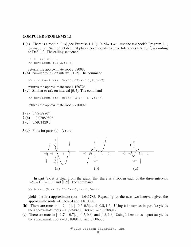
3 (a) Plots for parts (a) - (c) are:

−2 −1 1 2

−4−3−2−1

1234

(a)

−2 −1 1 2

−2−1

12

(b)

−2 −1 1 2

−2−1

12

(c)

In part (a), it is clear from the graph that there is a root in each of the three intervals[−2,−1], [−1, 0], and [1, 2]. The command

>> bisect(@(x) 2*xˆ3-6*x-1,-2,-1,5e-7)

yields the first approximate root −1.641783. Repeating for the next two intervals gives theapproximate roots −0.168254 and 1.810038.

(b) There are roots in [−2,−1], [−0.5, 0.5], and [0.5, 1.5]. Using bisect as in part (a) yieldsthe approximate roots −1.023482, 0.163823, and 0.788942.

(c) There are roots in [−1.7,−0.7], [−0.7, 0.3], and [0.3, 1.3]. Using bisect as in part (a) yieldsthe approximate roots −0.818094, 0, and 0.506308.


4 (a) [1, 2], 27 steps, 1.414213564 (b) [1, 2], 27 steps, 1.732050814 (c) [2, 3], 27 steps, 2.23606798

5 (a) There is a root in the interval [1, 2]. Eight decimal place accuracy implies an error toleranceof 5× 10−9. The command

>> bisect(@(x) xˆ3-2,1,2,5e-9)

yields the approximate cube root 1.25992105 in 27 steps.5 (b) There is a root in the interval [1, 2]. Using bisect as in (a) gives the approximate cube

root 1.44224957 in 27 steps.5 (c) There is a root in the interval [1, 2]. Using bisect as in (a) gives the approximate cube

root 1.70997595 in 27 steps.

6 0.785398

7 Trial and error, or a plot of f(x) = det(A) − 1000, shows that f(−18)f(−17) < 0 andf(9)f(10) < 0. Applying bisect to f(x) yields the roots −17.188498 and 9.708299. Thebackward errors of the roots are |f(−17.188498)| = 0.0018 and |f(9.708299)| = 0.00014.

8 2.948011

9 The desired height is the root of the function f(H) = πH2(1− 13H)− 1. Using

>> bisect(@(H) pi*Hˆ2*(1-H/3)-1,0,1,0.001)

gives the solution 636 mm.

EXERCISES 1.2 Fixed-Point Iteration

1 (a)3

x= x⇒ x2 = 3⇒ x = ±

√3

1 (b) x2 − 2x+ 2 = x⇒ x2 − 3x+ 2 = 0⇒ x = 1, 2

1 (c) x2 − 4x+ 2 = x⇒ x2 − 5x+ 2 = 0⇒ x =5±√

17

2

2 (a) −1, 22 (b) 22 (c) −1, 0, 1

3 (a) Check by substitution. For example,13 + 1− 6

6(1)− 10= 1.

3 (b) Check by substitution.


4 (a) Check by substitution.4 (b) Check by substitution.

5 (a) No, g(√

3) 6=√

3.

5 (b) Yes, g(√

3) =2√

3

3+

1√3

=√

3.

5 (c) No, g(√

3) 6=√

3.

5 (d) Yes, g(√

3) = 1 +2√

3 + 1=√

3.

6 (a) Yes.6 (b) Yes.6 (c) No.6 (d) Yes.

7 (a) g′(x) = 23(2x − 1)−

23 , and |g′(1)| = 2

3< 1. Theorem 1.6 implies that FPI is locally

convergent to r = 1.7 (b) g′(x) = 3

2x2, and |g′(1)| = 3

2> 1; FPI diverges from r = 1.

7 (c) g′(x) = cos x+ 1, and |g′(0)| = 2 > 1; FPI diverges from r = 0.

8 (a) locally convergent8 (b) locally convergent8 (c) divergent

9 (a) Solve 12x2 + 1

2x = x to find the fixed points r = 0, 1. The derivative g′(x) = x + 1

2.

By Theorem 1.6, |g′(0)| = 12< 1 implies that FPI converges to r = 0, and |g′(1)| = 3

2> 1

implies that FPI diverges from r = 1.9 (b) Solve x2 − 1

4x + 3

8= x to find the fixed points r = 1

2, 34. The derivative g′(x) = 2x − 1

4.

|g′(12)| = 3

4< 1 implies that FPI is locally convergent to r = 1

2. |g′(3

4)| = 5

4> 1 implies that

FPI diverges from r = 34.

10 (a) FPI diverges from 3/2, while 1 is locally convergent10 (b) FPI diverges from 1, while −1/2 is locally convergent

11 (a) There is a variety of answers, obtained by rearranging the equation x3 − x + ex = 0 toisolate x. For example, x = x3 + ex, x = 3

√x− ex, x = ln(x− x3).

11 (b) As in (a), rearrange 3x−2+9x3 = x2 to isolate x. For example, x =3

x3+9x2, x =

1

9− 1

3x4,

x =x5 − 9x6

3.

12 (a) Faster than Bisection Method12 (b) FPI diverges from the fixed point 1.2


13 (a) Solving the fixed point equationx = g(x) = 0.39− x2 yields the fixed points r = 0.3 and−1.3.

13 (b) g′(x) = −2x so |g′(0.3)| = 0.6 and |g′(−1.3)| = 2.6. By Theorem 1.6, Fixed PointIteration is locally convergent to r = 0.3.

13 (c) Convergence by FPI is at the rate ei+1 ≈ 0.6ei, which is slower than the Bisection Method.

14 All converge to√

2, from fastest to slowest: (A), (B), (C).

15 Check that√

5 is a fixed point for each iteration. Then calculate convergence rates for the

three iterations. (A) g′(x) =4

5− 1

x2, g′(√

5) =4

5− 1√

52 =

3

5.

(B) g′(x) =1

2+

5

2

(− 1

x2

), g′(√

5) =1

2− 1

2= 0.

(C) g′(x) = − 4

(x+ 1)2, g′(√

5) = − 4

(√

5 + 1)2≈ −0.382.

From fastest to slowest: (B), (C), (A).

16 All converge to 41/3, from fastest to slowest: (C), (B), (A).

17 Solving x2 =1− x

2for x results in the two separate equations g1(x) =

√1− x

2and

g2(x) = −√

1− x2

. First notice that g1(x) returns only positive numbers, and g2(x) only

negative. Therefore −1 cannot be a fixed point of g1(x), and 12

cannot be a fixed point of

g2(x). Check that g1(12) = 12

and g′1(x) = − 1

2√

2− 2x. |g′1(12)| = 1

2< 1 confirms that FPI

with g1(x) is locally convergent to r = 12. Likewise, g2(−1) = −1, g′2(x) =

1

2√

2− 2xand

|g′2(−1)| = 14

implies that FPI with g2(x) is locally convergent to r = −1.

18 For a positive number A, consider applying Fixed Point Iteration to g(x) = (x + A/x)/2.Note that g′(

√A) = 0, so FPI is locally convergent to

√A by Theorem 1.6. A simple sketch

of y = g(x) shows that FPI converges to√A for all positive initial guesses.

19 Define g(x) = (x+A/x2)/2. Since |g′( 3√A)| = 1

2< 1, FPI is locally convergent to the cube

root 3√A.

20 w = 2/3

21 (a) Substitute roots and check.21 (b) g′(x) = −5 + 15x − 15

2x2. FPI diverges from all three roots, because |g′(1 −

√3/5)| =

|g′(1 +√

3/5)| = 2 and |g′(1)| = 2.5.


22 Initial guesses 0, 1 and 2 all lead to r = 1. Neaby initial guesses cause FPI to move awayfrom the divergent fixed point 1 and oscillate chaotically.

23 The slopes of g at r1 and r3 imply that the graph of y = g(x) must pass through the line y = xat x = r2 from below the line to above the line. Therefore g′(r2) must belong to the interval(1,∞).

24 g′(1) = 1

25 Let x belong to [a, b]. By the Mean Value Theorem, |g(x0)− r| ≤ B|x0− r| < |x0− r|. Sincer belongs to [a, b], x1 = g(x0) does also, and by extension, so does x2, x3, etc. Similarly,|x1 − r| ≤ B|x0 − r| extends to |xi − r| ≤ Bi|x0 − r|, which converges to zero as i→∞.

26 If x1 = g(x1) and x2 = g(x2) are both fixed points, then by the Mean Value Theorem, thereexists c between x1 and x2 for which x2−x1 = g(x2)−g(x1) = g′(c)(x2−x1), which impliesg′(c) = 1, a contradiction.

27 (a) Solving x− x3 = x yields x3 = 0, or x = 0.27 (b) Assume 0 < x0 < 1. Then x30 < x0, and so 0 < x1 = x0 − x30 < x0 < 1. The same

argument implies by induction that x0 > x1 > x2 > ... > 0.27 (c) The limit L = lim

i→∞xi exists because the xi form a bounded monotonic sequence. Since

g(x) is continuous, g(L) = g( limi→∞

xi) = limi→∞

g(xi) = limi→∞

xi+1 = L, so L is a fixed point,and by (a), L = 0.

28 (a) x = x+ x3 implies x = 028 (b) If 0 < xi, then xi+1 = xi + x3i = xi(1 + x2i ) > xi.28 (c) g′(0) = 1, but the xi move away from r = 0.

29 (a) Set g(x) =x3 + (c+ 1)x− 2

c. Then g′(x) =

3x2 + (c+ 1)

c, and |g′(1)| = |4 + c

c| < 1

for c < −2. By Theorem 1.6, FPI is locally convergent to r = 1 if c < −2.29 (b) g′(1) = 0 if c = −4.

30 By Taylor’s Theorem, g(xi) = g(r) + g′(r)(xi− r) + g′′(c)(x− r)2/2, where c is between xiand r. Thus ei+1 = |r− xi+1| = |g′′(c)|(r− xi)2/2 = |g′′(c)|e2i /2. In the limit, c converges tor.

31 By factoring or the quadratic formula, the roots of the equation are −54

and 14. Set g(x) =

516− x2. Using the cobweb diagram of g(x), it is clear that initial guesses in (−5

4, 54) converge

to r2 = 14, and initial guesses in (−∞,−5

4)∪ (5

4,∞) diverge to−∞ under FPI. Initial guesses

−54

and 54

limit on −54.

32 The open interval (−4/3, 4/3) of initial guesses converge to the fixed point 1/3; the two initialguesses −4/3, 4/3 lead to −4/3.


33 (a) Choose a = 0 and |b| < 1, c arbitrary. Since a = 0, r = 0 is a fixed point, andg′(x) = b+ 2cx implies |g′(0)| = |b| < 1, so FPI is locally convergent to 0 by Theorem 1.6.

33 (b) Choose a = 0 and |b| > 1 to make initial guesses move away from the fixed point 0.


1 (a) Define g(x) = (2x+ 2)13 , for example. Using the fpi code, the command

>> x=fpi(@(x) (2*x+2)ˆ(1/3),1/2,20)

yields the solution 1.76929235 to 8 correct decimal places.1 (b) Define g(x) = ln(7 − x). Using fpi as in part (a) returns the solution 1.67282170 to 8

correct decimal places.1 (c) Define g(x) = ln(4− sinx). Using fpi as in part (a) returns the solution 1.12998050 to 8

correct decimal places.

2 (a) 0.754877672 (b) −0.970898922 (c) 1.59214294

3 (a) Iterate g(x) = (x + 3/x)/2 with starting guess 1. After 4 steps of FPI, the results is1.73205081 to 8 correct places.

3 (b) Iterate g(x) = (x + 5/x)/2 with starting guess 1. After 5 steps of FPI, the results is2.23606798 to 8 correct places.

4 (a) 1.259921054 (b) 1.442249574 (c) 1.70997595

5 Iterating g(x) = cos2 x with initial guess x0 = 1 results in 0.641714 to six correct places after350 steps. Checking |g′(0.641714)| ≈ 0.96 verifies that FPI is locally convergent by Theorem1.6.

6 (a) −1.641784,−0.168254, 1.8100386 (b) −1.023482, 0.163822, 0.7889416 (c) −0.818094, 0, 0.506308.

7 (a) Almost all numbers between 0 and 1.7 (b) Almost all numbers between 1 and 2.7 (c) Any number greater than 3 or less than −1 will work.


EXERCISES 1.3 Limits of Accuracy

1 (a) The forward error is |r − xc| = |0.75 − 0.74| = 0.01. The backward error is |f(xc)| =|4(0.74)− 3| = 0.04.

1 (b) FE = |r − xc| = 0.01 as in (a). BE = |f(0.74)| = (0.04)2 = 0.0016.1 (c) FE = |r − xc| = 0.01 as in (a). BE = |f(0.74)| = (0.04)3 = 0.000064.1 (d) FE = |r − xc| = 0.01 as in (a). BE = |f(0.74)| = (0.04)

13 = 0.342.

2 (a) FE = 0.00003, BE = 10−4

2 (b) FE = 0.00003, BE = 10−8

2 (c) FE = 0.00003, BE = 10−12

2 (d) FE = 0.00003, BE = 0.0464

3 (a) Check derivatives: f(0) = f ′(0) = 0, f ′′(0) = cos 0 = 1. The multiplicity of the root r = 0is 2.

3 (b) The forward error is |r − xc| = |0 − 0.0001| = 0.0001. The backward error is |f(xc)| =|1− cos 0.0001| ≈ 5× 10−9.

4 (a) 44 (b) FE = 10−2, BE = 10−8

5 The root of f(x) = ax − b is r = b/a. If xc is an approximate root, the forward error isFE = |b/a−xc|while the backward error isBE = |f(xc)| = |axc−b| = |a|| ba−xc| = |a|FE.Therefore the backward error is a factor of |a| larger than the forward error.

6 (a) 16 (b) Let ε be the backward error. By the Sensitivity Formula, the forward error ∆r is ε/f ′(A1/n) =

ε/(nA(n−1)/n).

7 (a) W ′(x) = (x− 2) · · · (x− 20) + (x− 1)(x− 3) · · · (x− 20) + . . .+ (x− 1) · · · (x− 19),so W ′(16) = (16− 1)(16− 2) · · · (16− 15)(16− 17)(16− 18)(16− 19)(16− 20) = 15!4!

7 (b) For a general integer j between 1 and 20,W ′(j) = (j − 1)(j − 2) · · · (1)(−1)(−2) · · · (j − 20) = (−1)j(j − 1)!(20− j)!

8 (a) Predicted root a+ ∆r = a− εa8 (b) Actual root a/(1 + ε) = a− εa+ ε2a− ε3a+ . . .


1 (a) Check the derivatives of f(x) = sinx − x to see that f(0) = f ′(0) = f ′′(0) = 0 andf ′′′(0) = − cos 0 = −1, giving multiplicity 3.

1 (b) fzero returns xc = −2.0735 × 10−8. The forward error is 2.0735 × 10−8 and MATLAB


reports the backward error to be |f(xc)| = 0. This means the true backward error is likely lessthan machine epsilon.

2 (a) m = 92 (b) xc = FE = 0.0014, BE = 0

3 (a) The MATLAB command

>> xc=fzero(@(x) 2*x*cos(x)-2*x+sin(xˆ3),[-0.1,0.2])

returns xc = 0.00016881. The forward error is |xc − r| = 0.00016881 and the backward erroris reported by MATLAB as |f(xc)| = 0.

3 (b) The bisection method with starting interval [−0.1, 0.2] stops after 13 steps, giving xc =−0.00006103. Neither method can determine the root r = 0 to more than about 3 correctdecimal places.

4 (a) r + ∆r = 3− 2.7ε4 (b) Predicted root = 3− 0.0027 = 2.9973, actual root = 2.9973029

5 To use (1.21), set f(x) = (x− 1)(x− 2)(x− 3)(x− 4), ε = −10−6 and g(x) = x6. Then nearthe root r = 4, ∆r ≈ −εg(r)/f ′(r) = 46/6 ≈ 0.00068267. According to (1.22), the errormagnification factor is |g(r)|/|rf ′(r)| = 46/24 ≈ 170.7. fzero returns the approximate root4.00068251, close to the guess 4.00068267 given by (1.21).

6 Actual root xc = 14.856, predicted root = r + ∆r = 15− 0.14 = 14.86

EXERCISES 1.4 Newton’s Method

1 (a) x1 = x0−(x30+x0−2)/(3x20+1) = 0−(−2)/(1) = 2; x2 = 2−(23+2−2)/(3(22)+1) =18/13.

1 (b) x1 = x0 − (x40 − x20 + x0 − 1)/(4x30 − 2x0 + 1) = 1; x2 = 1.1 (c) x1 = x0 − (x20 − x0 − 1)/(2x0 − 1) = −1; x2 = −2

3.

2 (a) x1 = 0.8, x2 = 0.7568182 (b) x1 = −0.2, x2 = 0.1808562 (c) x1 = x2 = 2

3 (a) According to Theorem 1.11, f ′(−1) = 8 implies that convergence to r = −1 is quadratic,with ei+1 ≈ |f ′′(−1)/(2f ′(−1))|e2i = | − 40/(2)(8)|e2i = 2.5e2i ; f ′(0) = −1 implies conver-gence to r = 0 is quadratic, ei+1 ≈ 2e2i ; f ′(1) = f ′′(1) = 0 and f ′′′(1) = 12 implies thatconvergence to r = 1 is linear, ei+1 ≈ 2

3ei.

3 (b) f ′(−12) = −27/4 implies that convergence to r = −1

2is quadratic, with error relationship

ei+1 ≈ |27/2(−274

)|e2i = 2e2i ; f ′(1) = f ′′(1) = 0 and f ′′′(1) = 18 implies that convergence tor = 1 is linear, ei+1 ≈ 2

3ei.


4 (a) r = −1/2, ei+1 = 1.6e2i ; r = 3/4, ei+1 = 12ei

4 (b) r = −1, ei+1 = 12ei; r = 3, ei+1 = 1

2e2i

5 Convergence to r = 0 is quadratic since f ′(0) = −1 6= 0, so Newton’s Method convergesfaster than the Bisection Method. Convergence to r = 1

2is linear since f ′(1

2) = f ′′(1

2) = 0

and f ′′′(12) = 24, with ei+1 ≈ 2

3ei. Since S = 2

3> 1

2, Newton’s Method will converge to

r = 12

slower than the Bisection Method.

6 Many possible answers; for example, f(x) = xe−x with initial guess greater than 1.

7 Computing derivatives, f ′(2) = f ′′(2) = 0 and f ′′′(2) = 6 implies that r = 2 is a tripleroot. Therefore Newton’s Method does not converge quadratically, but converges linearly andei+1/ei → 2

3according to Theorem 1.12.

8 x1 = x0 − (ax0 + b)/a = −b/a

9 Since f ′(x) = 2x, Newton’s Method is

xi+1 = xi −x2i − A

2xi=xi2

+A

2xi=xi + A/xi

2.

10 xi+1 = (2xi + A/x2i )/3

11 The nth root of A is the real root of f(x) = xn − A = 0. Newton’s Method applied to theequation is

xi+1 = xi −xni − Anxn−1i

=n− 1

nxi +

A

nxn−1i

=(n− 1)xi + A/xn−1i

n.

Since f ′(A1n ) = nA

n−1n , Theorem 1.11 implies that Newton’s Method converges quadratically

as long as A 6= 0.

12 x50 = 250

13 (a) Newton’s Method converges quadratically to r = 2 since f ′(2) = 8 6= 0, and e5 ≈f ′′(2)/(2f ′(2))e24 = 3

4(10−6)

2= 0.75× 10−12.

13 (b) Since f ′(0) = −4 and f ′′(0) = 0, Theorem 1.11 implies that limi→∞

ei+1/e2i = 0, and no

useful estimate of e5 follows. Essentially, convergence is faster than quadratic. Reverting to

the definition of Newton’s Method, xi+1 = xi −x3i − 4xi3x2i − 4

=2x3i

3x2i − 4, and because r = 0,

ei+1 =

∣∣∣∣ 2e3i3e2i − 4

∣∣∣∣. Substituting e4 = 10−6 yields e5 =

∣∣∣∣ 2× 10−18

3× 10−12 − 4

∣∣∣∣ ≈ 0.5× 10−18.



1 (a) Newton’s Method is xi+1 = xi − (x3i − 2xi − 2)/(3x2i − 2). Setting x0 = 1 yieldsx7 = 1.76929235 to eight decimal places.

1 (b) Applying Newton’s Method with x0 = 1 yields x5 = 1.67282170 to eight places.1 (c) Applying Newton’s Method with x0 = 1 yields x3 = 1.12998050 to eight places.

2 (a) 0.754877672 (b) −0.970898922 (c) 1.59214294

3 (a) Newton’s Method converges linearly to xc = −0.6666648. Subtracting xc from xi showserror ratios |xi+1 − xc|/|xi − xc| ≈ 2

3, implying a multiplicity 3 root. Applying Modified

Newton’s Method with m = 3 and x0 = 0.5 converges to xc = −23.

3 (b) Newton’s Method converges linearly to xc = 0.166666669. The error ratios |xi+1−xc|/|xi−xc| ≈ 1

2, implying a multiplicity 2 root. Applying Modified Newton’s Method withm = 2 and

x0 = 1 converges quadratically to 0.166666667 ≈ 16. In fact, one checks by direct substitution

that the root is r = 16.

4 (a) r = 1,m = 34 (b) r = 2,m = 2

5 The volume of the silo is 400 = 10πr2 + 23πr3. Solving for r by Newton’s Method yields

3.2362 meters.

6 r = 2.0201 cm

7 Newton’s Method converges quadratically to −1.197624 and 1.530134, and converges linearlyto the root 0. The error ratio is |xi+1 − 0|/|xi − 0| ≈ 3

4, implying that r = 0 is a multiplicity 4

root. This can be confirmed by evaluating the first four derivatives.

8 0.841069, quadratic convergence; π/3 ≈ 1.047198, linear convergence, m = 3; 2.300524,quadratic convergence

9 Newton’s Method converges quadratically to 0.8571428571 with quadratic error ratio M =

limi→∞

ei+1/e2i ≈ 2.4, and converges linearly to the root 2 with error ratio S = lim

i→∞ei+1/ei ≈

2

3.

10 −1.381298, quadratic convergence; −2/3, linear convergence, m = 2; 0.205183, quadraticconvergence; 1/2, quadratic convergence; 1.176116, quadratic convergence

11 Solving the ideal gas law for an initial approximation gives V0 = nRT/P = 1.75. ApplyingNewton’s Method to the non-ideal gas Van der Waal’s equation with initial guess V0 = 1.75converges to V = 1.701.


12 initial guess V0 = 2.87, solution V = 2.66 L

13 (a) The equation is equivalent to 1− 3/(4x) = 0, and has the root r = 34.

13 (b) Newton’s Method applied to f(x) = (1− 3/(4x))13 does not converge.

13 (c) f(x) is not differentiable at 0.

14 (a) Assume that h(c) = c, g(c) 6= c, and f ′′(c) = 0. First note that

g′(x) = 1− f ′(x)f ′(x)− f(x)f ′′(x)

f ′(x)2=f(x)f ′′(x)

f ′(x)2,

implying that g′(c) = 0, and therefore that h′(c) = g′(g(c))g′(c) = 0. By Theorem 1.6, thefixed point iteration h is locally convergent to c.

14 (b) Define f(x) = 4x4 − 6x2 − 11/4; then f ′(x) = 16x3 − 12x. Set c = 1/2. Then

g(1/2) =1

2− f(1/2)

f ′(1/2)=

1

2− −4

−4= −1

2

and likewise g(−1/2) = 1/2. Now we can verify that h(1/2) = g(g(1/2)) = g(−1/2) = 1/2,that g(1/2) 6= 1/2, and that f ′′(1/2) = 48(1/2)2 − 12 = 0, as required.

15 0.6355

16 (a) 0.578 and 1.67016 (b) 0.644 and 1.767

17 (a) 0.866% per year17 (b) 0.576% per year

18 (a) 0.02098

EXERCISES 1.5 Root-Finding without Derivatives

1 (a) Applying the Secant Method with x0 = 1 and x1 = 2 yields x2 = x1−(x1 − x0)f(x1)

f(x1)− f(x0)=

8

5and x3 ≈ 1.742268.

1 (b) Using the Secant Method formula with x0 = 1 and x1 = 2 as in (a) returns x2 ≈ 1.578707and x3 ≈ 1.660160.

1 (c) The Secant Method yields x2 ≈ 1.092907 and x3 ≈ 1.119357.

2 (a) x2 = 8/5, x3 = 1.7422682 (b) x2 = 1.578707, x3 = 1.660162 (c) x2 = 1.092907, x3 = 1.119357


3 (a) Applying IQI with x0 = 1, x1 = 2 and x2 = 0 yields x3 = −15

and x4 ≈ −0.11996018from formula (1.37).

3 (b) Applying the IQI formula gives x3 ≈ 1.75771279 and x4 ≈ 1.66253117.3 (c) Applying IQI as in (a) and (b) yields x3 ≈ 1.13948155 and x4 ≈ 1.12927246.

4 10.25 m

5 Setting A = f(a), B = f(b), C = f(c), and y = 0 in (1.35) gives

P (0) =af(b)f(c)

(f(a)− f(b))(f(a)− f(c))+

bf(a)f(c)

(f(b)− f(a))(f(b)− f(c))

+cf(a)f(b)

(f(c)− f(a))(f(c)− f(b))

=af(b)−f(c)

f(a)+ bf(c)−f(a)

f(b)+ cf(a)−f(b)

f(c)

(1− f(b)f(a)

)(f(a)f(c)− 1)(1− f(c)

f(b))

=as(1− qs) + bqs(r − q) + c(q − 1)

(q − 1)(r − 1)(s− 1)

= c+as(1− r) + br(r − q)− c(r2 − qr − rs+ s)

(q − 1)(r − 1)(s− 1)

= c− (c− b)r(r − q) + (c− a)s(1− r)(q − 1)(r − 1)(s− 1)

.

7 (a) (A) is the Bisection Method, which cuts uncertainty in half on each step.(B) Check that f(21/4) = 0 and f ′(21/4) = (4)23/4 6= 0. Therefore the Secant Methodconverges superlinearly.

(C) 21/4 is a fixed point because g(21/4) =21/4

2+

1

23/4=

21/4 + 21/4

2= 21/4.

Note that g′(x) =1

2− 3

x4⇒ g′(21/4) =

1

2− 3

(21/4)4=

1

2− 3

2= −1.

(D) 21/4 is a fixed point because g(21/4) =21/4

3+

1

(3)23/4=

2 + 1

(3)23/4= 21/4.

Note that g′(x) =1

3− 3

3x4⇒ g′(21/4) =

1

3− 1

(21/4)4=

1

3− 1

2= −1/6.

Fastest to slowest: (B), (D), (A); (C) does not converge to 21/4.7 (b) Newton’s Method will converge faster than the four above choices.


1 (a) Applying the Secant Method formula shows convergence to the root 1.769292351 (b) 1.672821701 (c) 1.12998050.


2 (a) 1.769292352 (b) 1.672821702 (c) 1.12998050

3 (a) Applying formula (1.37) for Inverse Quadratic Interpolation shows convergence to 1.76929235.3 (b) Similar to part (a). Converges to 1.672821703 (c) Similar to part (a). Converges to 1.129998050.

4 −1.381298, superlinear; −2/3, linear; 0.205183, superlinear; 1/2, superlinear; 1.176116,superlinear

5 The MATLAB command

>> fzero(@(x) 1/x,[-2,1])

converges to zero, although there is no root there.

6 fzero fails in both cases because the functions never cross zero


INSTRUCTOR'S SOLUTIONS MANUAL NUMERICAL ... - Test Bank

Documents