Institutionen för systemteknik Department of Electrical Engineering Examensarbete Reliability calculations for complex systems Examensarbete utfört i Reglerteknik vid Tekniska högskolan vid Linköpings universitet av Malte Lenz och Johan Rhodin LiTH-ISY-EX--11/4441--SE Linköping 2011 Department of Electrical Engineering Linköpings tekniska högskola Linköpings universitet Linköpings universitet SE-581 83 Linköping, Sweden 581 83 Linköping

Welcome message from author
This document is posted to help you gain knowledge. Please leave a comment to let me know what you think about it! Share it to your friends and learn new things together.
Transcript

Institutionen för systemteknikDepartment of Electrical Engineering
Examensarbete
Reliability calculations for complex systems
Examensarbete utfört i Reglerteknikvid Tekniska högskolan vid Linköpings universitet
av
Malte Lenz och Johan Rhodin
LiTH-ISY-EX--11/4441--SE
Linköping 2011
Department of Electrical Engineering Linköpings tekniska högskolaLinköpings universitet Linköpings universitetSE-581 83 Linköping, Sweden 581 83 Linköping


Reliability calculations for complex systems
Examensarbete utfört i Reglerteknikvid Tekniska högskolan i Linköping
av
Malte Lenz och Johan Rhodin
LiTH-ISY-EX--11/4441--SE
Handledare: André Carvalho Bittencourtisy, Linköpings universitet
Examinator: Torkel Gladisy, Linköpings universitet
Linköping, 8 June, 2011


Avdelning, InstitutionDivision, Department
Division of Automatic ControlDepartment of Electrical EngineeringLinköping UniversitySE–581 83 LinköpingSweden
DatumDate
2011-06-08
SpråkLanguage
� Svenska/Swedish
� Engelska/English
�
�
RapporttypReport category
� Licentiatavhandling
� Examensarbete
� C-uppsats
� D-uppsats
� Övrig rapport
�
�
URL för elektronisk versionhttp://www.control.isy.liu.se
http://www.ep.liu.se
ISBN
—
ISRN
LiTH-ISY-EX--11/4441--SE
Serietitel och serienummerTitle of series, numbering
ISSN
—
TitelTitle
Tillförlitlighetsberäkningar för komplexa system
Reliability calculations for complex systems
FörfattareAuthor
Malte Lenz och Johan Rhodin
SammanfattningAbstract
Functionality for efficient computation of properties of system lifetimes was developed,based on the Mathematica framework. The model of these systems consists of a system struc-ture and the component’s independent lifetime distributions. The components are assumedto be non-repairable. In this work a very general implementation was created, allowing alarge number of lifetime distributions from Mathematica for all the component distributions.All system structures with a monotone increasing structure function can be used. Special ef-fort has been made to compute fast results when using the exponential distribution for com-ponent distributions. Standby systems have also been modeled in similar generality. Bothwarm and cold standby components are supported. During development, a large collectionof examples were also used to test functionality and efficiency. A number of these examplesare presented. The implementation was evaluated on large real world system examples, andwas found to be efficient. New results are presented for standby systems, especially for thecase of mixed warm and cold standby components.
NyckelordKeywords reliability, Mathematica, statistics, distributions, standby


Abstract
Functionality for efficient computation of properties of system lifetimes was de-veloped, based on the Mathematica framework. The model of these systems con-sists of a system structure and the component’s independent lifetime distribu-tions. The components are assumed to be non-repairable. In this work a verygeneral implementation was created, allowing a large number of lifetime distri-butions from Mathematica for all the component distributions. All system struc-tures with a monotone increasing structure function can be used. Special efforthas been made to compute fast results when using the exponential distributionfor component distributions. Standby systems have also been modeled in simi-lar generality. Both warm and cold standby components are supported. Duringdevelopment, a large collection of examples were also used to test functionalityand efficiency. A number of these examples are presented. The implementationwas evaluated on large real world system examples, and was found to be efficient.New results are presented for standby systems, especially for the case of mixedwarm and cold standby components.
Sammanfattning
Funktionalitet för effektiv beräkning av systems livstidsegenskaper har utveck-lats, baserat på Mathematicas ramverk. Modellerna för dessa system består aven systemstruktur och komponenternas oberoende livstidsdistributioner. Kom-ponenterna antas vara icke reparerbara. En mycket generell implementation somhanterar ett stort antal distributioner från Mathematica som komponenters distri-butioner har utvecklats. Alla systemstrukturer med en monotont växande struk-turfunktion kan användas. Särskild hänsyn har tagits för att uppnå effektiva ut-räkningar när exponentialdistributionen används för komponenter. Standbysy-stem har också modellerats med motsvarande generalitet. Både varma och kallastandbykomponenter stöds. Under utvecklingen har ett stort antal exempel an-vänts för utvärdering av korrekthet och effektivitet. Ett antal av dessa exempelpresenteras. Implementationen har även utvärderats på stora verklighetsbasera-de system, och konstaterats vara effektiv. Nya resultat presenteras för standby-system, speciellt för fallet med blandade varma och kalla standbykomponenter.
v


Acknowledgments
We would like to thank Roger Germundsson and Wolfram Research for the oppor-tunity to do our thesis project at the Wolfram Research headquarters in Cham-paign, Illinois. Special thanks to Oleksandr Pavlyk for all his support. Withouthis help, ideas and pointers this project would not have gotten as far as it has.Also, the whole statistics team at Wolfram Research deserves many thanks forbuilding an excellent framework on which we rely, as well as answering all ourquestions.
We would also like to thank Henrik Tidefelt for his aid in everything betweenMathematica, LATEX and restaurants in Champaign.
At Linköping University we would like to thank André Bittencourt and TorkelGlad at the Department of Electrical Engineering, ISY.
Champaign, Illinois, March 2011Malte Lenz and Johan Rhodin
vii


Contents
Notation xiii
1 Introduction 11.1 Purpose and goal . . . . . . . . . . . . . . . . . . . . . . . . . . . . 21.2 Outline of the thesis . . . . . . . . . . . . . . . . . . . . . . . . . . . 2
2 Theoretical background 32.1 Reliability measures . . . . . . . . . . . . . . . . . . . . . . . . . . . 3
2.1.1 Distribution functions . . . . . . . . . . . . . . . . . . . . . 42.1.2 Lifetime distributions . . . . . . . . . . . . . . . . . . . . . . 62.1.3 Properties of the lifetime distribution . . . . . . . . . . . . 9
2.2 Boolean logic . . . . . . . . . . . . . . . . . . . . . . . . . . . . . . . 102.3 Systems of components . . . . . . . . . . . . . . . . . . . . . . . . . 11
2.3.1 Series system . . . . . . . . . . . . . . . . . . . . . . . . . . . 122.3.2 Parallel system . . . . . . . . . . . . . . . . . . . . . . . . . . 122.3.3 Mixed system . . . . . . . . . . . . . . . . . . . . . . . . . . 132.3.4 Structure function to survival function . . . . . . . . . . . . 132.3.5 Standby systems . . . . . . . . . . . . . . . . . . . . . . . . . 13
2.4 Graph theory . . . . . . . . . . . . . . . . . . . . . . . . . . . . . . . 152.4.1 Adjacency matrix . . . . . . . . . . . . . . . . . . . . . . . . 162.4.2 Path and cut vectors . . . . . . . . . . . . . . . . . . . . . . . 172.4.3 Minimal cut set . . . . . . . . . . . . . . . . . . . . . . . . . 17
2.5 Importance measures . . . . . . . . . . . . . . . . . . . . . . . . . . 182.5.1 Structural importance . . . . . . . . . . . . . . . . . . . . . 182.5.2 Birnbaum importance . . . . . . . . . . . . . . . . . . . . . 192.5.3 Risk Achievement Worth and Risk Reduction Worth . . . . 202.5.4 Improvement potential . . . . . . . . . . . . . . . . . . . . . 212.5.5 Barlow-Proschan importance . . . . . . . . . . . . . . . . . 212.5.6 Criticality importance . . . . . . . . . . . . . . . . . . . . . 222.5.7 Fussell-Vesely importance . . . . . . . . . . . . . . . . . . . 22
2.6 Special functions . . . . . . . . . . . . . . . . . . . . . . . . . . . . 23
ix

x CONTENTS
3 Structure function 253.1 Check if a boolean function is increasing . . . . . . . . . . . . . . . 253.2 Converting a boolean expression . . . . . . . . . . . . . . . . . . . . 263.3 Structure function to survival function . . . . . . . . . . . . . . . . 27
3.3.1 Expanding to remove exponents . . . . . . . . . . . . . . . . 27
4 Reliability distribution 334.1 Properties for some basic systems . . . . . . . . . . . . . . . . . . . 33
4.1.1 Serial system . . . . . . . . . . . . . . . . . . . . . . . . . . . 344.1.2 Parallel system . . . . . . . . . . . . . . . . . . . . . . . . . . 354.1.3 2 out of 3 system . . . . . . . . . . . . . . . . . . . . . . . . 364.1.4 Simple mixed system . . . . . . . . . . . . . . . . . . . . . . 374.1.5 Bridge system . . . . . . . . . . . . . . . . . . . . . . . . . . 38
4.2 Parallelization . . . . . . . . . . . . . . . . . . . . . . . . . . . . . . 394.2.1 Parallelization on system level . . . . . . . . . . . . . . . . . 404.2.2 Parallelization on component level . . . . . . . . . . . . . . 404.2.3 Comparison . . . . . . . . . . . . . . . . . . . . . . . . . . . 41
4.3 Properties for real world systems . . . . . . . . . . . . . . . . . . . 424.3.1 Cockpit information system . . . . . . . . . . . . . . . . . . 424.3.2 Airplane . . . . . . . . . . . . . . . . . . . . . . . . . . . . . 434.3.3 Electrical diesel generator system . . . . . . . . . . . . . . . 45
5 Optimizations 475.1 Simplification of distributions . . . . . . . . . . . . . . . . . . . . . 475.2 Special cases of properties . . . . . . . . . . . . . . . . . . . . . . . 48
5.2.1 Exponentially distributed components . . . . . . . . . . . . 485.2.2 Hazard function . . . . . . . . . . . . . . . . . . . . . . . . . 50
6 Importance measures 536.1 Properties for a bridge system . . . . . . . . . . . . . . . . . . . . . 53
6.1.1 Structural importance . . . . . . . . . . . . . . . . . . . . . 536.1.2 Birnbaum importance . . . . . . . . . . . . . . . . . . . . . 546.1.3 Risk Achievement Worth . . . . . . . . . . . . . . . . . . . . 556.1.4 Risk Reduction Worth . . . . . . . . . . . . . . . . . . . . . 556.1.5 Improvement potential . . . . . . . . . . . . . . . . . . . . . 566.1.6 Barlow-Proschan importance . . . . . . . . . . . . . . . . . 576.1.7 Criticality importance . . . . . . . . . . . . . . . . . . . . . 586.1.8 Fussell-Vesely importance . . . . . . . . . . . . . . . . . . . 58
6.2 Comparison on a simple system . . . . . . . . . . . . . . . . . . . . 59
7 rbdmodeling 637.1 Boolean expression to rbd . . . . . . . . . . . . . . . . . . . . . . . 637.2 rbd to boolean expression . . . . . . . . . . . . . . . . . . . . . . . 65
7.2.1 Breadth-first traversal . . . . . . . . . . . . . . . . . . . . . 65
CONTENTS xi
8 Standby systems 698.1 Cold standby . . . . . . . . . . . . . . . . . . . . . . . . . . . . . . . 69
8.1.1 Cold standby with perfect switching . . . . . . . . . . . . . 698.1.2 Cold standby with imperfect switching . . . . . . . . . . . . 72
8.2 Warm standby . . . . . . . . . . . . . . . . . . . . . . . . . . . . . . 758.2.1 Warm standby with perfect switching . . . . . . . . . . . . 758.2.2 Warm standby with imperfect switching . . . . . . . . . . . 778.2.3 Mixed standby . . . . . . . . . . . . . . . . . . . . . . . . . . 80
8.3 Applications . . . . . . . . . . . . . . . . . . . . . . . . . . . . . . . 82
9 Conclusions and future work 879.1 Conclusions . . . . . . . . . . . . . . . . . . . . . . . . . . . . . . . 879.2 Future work . . . . . . . . . . . . . . . . . . . . . . . . . . . . . . . 88
9.2.1 Graph editor . . . . . . . . . . . . . . . . . . . . . . . . . . . 889.2.2 Special system structures . . . . . . . . . . . . . . . . . . . . 889.2.3 Repairable systems . . . . . . . . . . . . . . . . . . . . . . . 889.2.4 Censored data . . . . . . . . . . . . . . . . . . . . . . . . . . 889.2.5 Dependent lifetime distributions . . . . . . . . . . . . . . . 889.2.6 Accelerated life . . . . . . . . . . . . . . . . . . . . . . . . . 899.2.7 Real world reliability data verification . . . . . . . . . . . . 89
A Computable properties 91
B Airplane cockpit system 93B.1 System presentation . . . . . . . . . . . . . . . . . . . . . . . . . . . 93
B.1.1 rbd . . . . . . . . . . . . . . . . . . . . . . . . . . . . . . . . 93B.1.2 Structure function . . . . . . . . . . . . . . . . . . . . . . . . 93B.1.3 Basic events . . . . . . . . . . . . . . . . . . . . . . . . . . . 93
C Electrical diesel generator system 97C.1 System presentation . . . . . . . . . . . . . . . . . . . . . . . . . . . 97
C.1.1 Structure function . . . . . . . . . . . . . . . . . . . . . . . . 98C.1.2 Basic events . . . . . . . . . . . . . . . . . . . . . . . . . . . 98
Bibliography 103
Index 105


Notation
Abbreviations
Abbreviation Meaning
cdf Cumulative Distribution Functionccdf Complementary Cumulative Distribution Functioncnf Conjunctive Normal Formdnf Disjunctive Normal Formpdf Probability Density Functionmgf Moment Generating Functionmttf Mean Time To Failureraw Risk Achievement Worthrbd Reliability Block Diagramrrw Risk Reduction Worth
Probability and Statistics
Notation Meaning
T ∼ L T is distributed according to lifetime distribution LP(A) Probability of the event A
P(A|B) Conditional probability of event A given event BE(T ) or 〈T 〉 Expectation of T
µ′n The n’th moment around 0 (see definition 2.18)µ Mean (see definition 2.19)µn n’th central moment (see definition 2.20)σ2 Variance (see definition 2.21)σ Standard deviation (see definition 2.22)β2 Kurtosis (see definition 2.24)γ1 Skewness (see definition 2.23)
MT (s) Moment-generating function (see definition 2.25)ϕT (s) Characteristic function (see definition 2.27)
xiii

xiv Notation
Reliability
Notation Meaning
Φ(~x) Structure function for the component states ~x (see def-inition 2.32)
Importance measures
Notation Meaning
Iφ(i) Structural importance of component i (see defini-tion 2.46)
I(i)B (t) Birnbaum importance of component i at time t (see
definition 2.48)
I(i)IP (t) Improvement potential of component i at time t (see
definition 2.52)IB−P (i) Barlow-Proschan importance of component i (see defi-
nition 2.53)
I(i)raw(t) Risk Achievement Worth of component i at time t (see
definition 2.50)
I(i)rrw(t) Risk Reduction Worth of component i at time t (see
definition 2.51)
I(i)CR−F(t) Criticality importance (failure oriented) of component
i at time t (see definition 2.55)
I(i)CR−S (t) Criticality importance (success oriented) of compo-
nent i at time t (see definition 2.56)
I(i)F−V (t) Fussell-Vesely measure of component i at time t (see
definition 2.57)
Boolean operators
Notation Meaning
a ∧ b Conjunction of a and b, “a and b”a ∨ b Disjunction of a and b, “a or b”¬a Negation of a, “not a”a∨b Negation of a disjunction of a and b, ¬(a ∨ b)a∧b Negation of a conjunction of a and b, ¬(a ∧ b)a⇒ b If a is true, b must be true, ¬a ∨ b
majority True if more than half of the arguments are true (seedefinition 2.31)

Notation xv
Graph theory
Notation Meaning
vi Vertex in a graphvi → vk Edge from vertex vi to vertex vk in a graph
Special functions
Notation Meaning
Γ (a, z) Incomplete gamma function (see definition 2.58)min(t) The minimum of tmax(t) The maximum of t


1Introduction
“It is scientific only to say what is more likely and what less likely,and not to be proving all the time the possible and impossible.”
Richard P. Feynman
Reliability engineering deals with the construction and study of reliable systems.This is used in a wide range of applications such as semiconductor design andproduction, aerospace, nuclear engineering and space flight.
By studying the configurations and the lifetimes of components in complex sys-tems, one can draw conclusions regarding the optimal design for reliability. Byusing importance measures, it is possible to draw conclusions about which com-ponents are the most important to improve to achieve better reliability of thewhole system.
The first examples of reliability calculations and estimates can be found in theinvestigations of John Graunt in 1662. Graunt studied the probability of survivalfor humans to different ages [Graunt, 1662, p. 75]. From this first step it took along time before the field of reliability emerged and became frequently used. Itwas not before the end of the second world war that the field of reliability engi-neering expanded rapidly due to mass manufacturing, statistical quality controland computational resources at hand [Saleh and Marais, 2006, p. 251].
Modern day reliability measures and methods depend heavily on the contribu-tions of W. Weibull and Z.W. Birnbaum. Birnbaum developed the first impor-tance measure, which can be used to rank components in a system according tohow important they are. Weibull developed the distribution that now bears hisname and is a standard tool in reliability applications. Richard E. Barlow andFrank Proschan are frequently credited as the founders of the reliability field inits form today, and their book Mathematical Theory of Reliability [Barlow andProschan, 1965] is one of the standard texts in the field.
1

2 1 Introduction
1.1 Purpose and goal
This thesis uses the software Mathematica from Wolfram Research for its imple-mentation. This is an application that supports a wide array of mathematicalcomputation. The high level language used in Mathematica also lends itself verywell to quickly implementing efficient new algorithms and functionality. In ver-sion 8 of Mathematica, an extensive new framework for probability and statisticswas created. This framework makes it easy to create new distributions, and cal-culate properties for them.
The purpose of this thesis is to implement functionality in Mathematica for thebasics in the field of reliability, and to then explore how Mathematicas mathemat-ics framework can be used to extend the amount of computations possible. Tothis end, we look at modeling non-repairable systems, standby systems, and howto determine the importance of components in a system. From these models, thegoal is to be able to efficiently compute properties, both symbolically and numer-ically. A part of the goal is to introduce this functionality in a future release ofMathematica.
1.2 Outline of the thesis
The thesis is structured as follows:
• Chapter 2 presents the theoretical background necessary to understand re-liability calculations from the areas of statistics, graph theory and booleanlogic.
• Chapter 3 shows how to represent the structure of a system and how to mapit to the survival function.
• Chapter 4 describes the reliability distribution and shows some importantproperties for different system configurations.
• Chapter 5 shows some special cases of distributions and distribution prop-erties for which optimizations can be done.
• Chapter 6 shows results for importance measures.
• Chapter 7 presents prototypes for converting back and forth between relia-bility block diagrams and boolean structure functions.
• Chapter 8 covers standby systems and how to calculate their reliability.
• Chapter 9 discusses conclusions and future work.
• Appendix A presents a list of lifetime properties we can calculate.
• Appendix B defines the system of an airplane cockpit.
• Appendix C presents the diesel generator system of a nuclear power plant.

2Theoretical background
“Each problem that I solved became a rule which servedafterwards to solve other problems.”
Rene Descartes
In this chapter we will present the theoretical background of the parts of relia-bility engineering that are interesting in the scope of the thesis. Readers familiarwith probability and statistics might want to read sections 2.3 and 2.5, and thenfocus on the later chapters.
2.1 Reliability measures
We define some basic terminology that is used in the description of reliabilitysystems.
2.1 Definition (Working and Failed). A component or system is working whenit is performing its intended function. A component or system is failed when itis not performing as intended.
2.2 Definition (State). The state of a component is defined as a boolean vari-able x(t), where
x(t) = 1 (or true) (2.1)
if the component is working at time t, and
x(t) = 0 (or false) (2.2)
if the component is failed at t.
With this definition we can define the time to failure T .
3

4 2 Theoretical background
2.3 Definition (Time To Failure). The time to failure T of a component is de-fined as
T = Min(t) where x(t) = 0 (2.3)
assuming that the component is not repairable.
Time to failure T can be any of a large number of units. One example would be aunit of time, such as the number of hours a component is used. Another exampleis a unit of distance, such as how far a car is driven.
2.4 Definition (Lifetime distribution). The lifetime distribution L is definedas the probability distribution of the time to failure T .
2.1.1 Distribution functions
Based on the previous definitions, there are a few different functions describingthe probability of times to failure. These are presented in the following defi-nitions. Throughout the scope of this thesis we assume all distributions to becontinuous and univariate.
2.5 Definition (Cumulative Density Function, cdf). The cdf F(t) describesthe probability that a specific component fails before the time t:
F(t) = P (T ≤ t) (2.4)
where T ∼ L (T is distributed according to lifetime distribution L).
The following conditions are fulfilled by all cumulative density functions:
All components fail eventually:
limt→∞
F(t) = 1 (2.5)
A failed component never starts working again:
F(t) is nondecreasing(2.6)
Components always work at t ≤ 0:
F(t) = 0, t ≤ 0(2.7)
2.6 Definition (Probability Density Function, pdf). The pdf f (t) describesthe probability that a specific component fails at the time t:
f (t)∆t ≈ P (t < T ≤ t + ∆t) (2.8)
for small values of ∆t, where T ∼ L.
2.1 Reliability measures 5
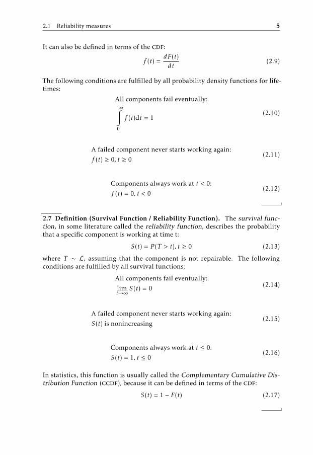
It can also be defined in terms of the cdf:
f (t) =dF(t)dt
(2.9)
The following conditions are fulfilled by all probability density functions for life-times:
All components fail eventually:∞∫
0
f (t)dt = 1(2.10)
A failed component never starts working again:
f (t) ≥ 0, t ≥ 0(2.11)
Components always work at t < 0:
f (t) = 0, t < 0(2.12)
2.7 Definition (Survival Function / Reliability Function). The survival func-tion, in some literature called the reliability function, describes the probabilitythat a specific component is working at time t:
S(t) = P (T > t), t ≥ 0 (2.13)
where T ∼ L, assuming that the component is not repairable. The followingconditions are fulfilled by all survival functions:
All components fail eventually:
limt→∞
S(t) = 0 (2.14)
A failed component never starts working again:
S(t) is nonincreasing(2.15)
Components always work at t ≤ 0:
S(t) = 1, t ≤ 0(2.16)
In statistics, this function is usually called the Complementary Cumulative Dis-tribution Function (ccdf), because it can be defined in terms of the cdf:
S(t) = 1 − F(t) (2.17)

6 2 Theoretical background
2.8 Definition (Hazard Function). The Hazard Function describes the failurerate at time t, given it is still working at that time:
h(t) = lim∆t→0
P (t ≤ T < t + ∆t|T ≥ t)∆t
=f (t)S(t)
, t ≥ 0 (2.18)
where T ∼ L.
Once one of these functions is known, all the others can be calculated as needed,as can be seen for example in Leemis [2009, Table 3.1, p. 62]. As an example, theconversions from the survival function to the other functions are given here.
h(t) =−S ′(t)S(t)
(2.19)
F(t) = 1 − S(t) (2.20)
f (t) = −S ′(t) (2.21)
2.1.2 Lifetime distributions
There are a few distributions that are most often used as lifetime distributions. Intheory any distribution where the pdf is 0 for t ≤ 0 can be used. This requirementcomes from the assumption that a system does not fail before time t = 0. Herewe present the distributions used in this thesis.
Exponential distribution
The exponential distribution is the most commonly used lifetime distribution. Itis defined as follows:
2.9 Definition (Exponential distribution). The exponential distribution canbe defined by its pdf:
f (t) ={e−tλ t > 00 otherwise
(2.22)
where λ is called the failure rate of the component and λ > 0.
The exponential distribution has the important memoryless property:
P (T ≥ t) = P (T ≥ t + s | T ≥ s), t ≥ 0; s ≥ 0 (2.23)
which means that a used component that has survived to time t is as good as anew component. The exponential distribution is the only distribution with thisproperty [Leemis, 2009, pp. 325-326]. The exponential distribution has a hazardfunction h(t) that is a constant λ for t > 0, and 0 otherwise. It is sometimes calledthe Epstein distribution [Saunders, 2010, p. 14].

2.1 Reliability measures 7
Weibull distribution
A very commonly used distribution is the Weibull distribution, named after theSwedish mathematician Waloddi Weibull who used the distribution for a largenumber of applications, for example the strength of Indian cotton or Bofors steel[Weibull, 1951, p. 293].
2.10 Definition (Weibull distribution). The Weibull distribution can be de-fined by its survival function:
S(t) =
e−( t−µβ
)αt > µ
1 otherwise(2.24)
where α is called the shape parameter, β the scale parameter, and µ the locationparameter.
For this distribution to make sense as a lifetime distribution, µ must be non-negative.
Erlang distribution
The Erlang distribution was developed by the Danish mathematician Agner KrarupErlang for modeling of telephone systems. This distribution comes up in relationto standby systems, as we show in section 8.1.1.
2.11 Definition (Erlang distribution). We define the Erlang distribution by itsprobability density function:
f (t) =
λk tk−1e−tλ
(k−1)! t > 01 otherwise
(2.25)
where k is called the shape parameter and λ the rate parameter.
Pareto distribution
The Pareto distribution takes two parameters.
2.12 Definition (Pareto distribution). The Pareto distribution is most readilydefined by its survival function:
S(t) ={ (
tk
)−αt > k
1 otherwise(2.26)
where k is the minimum value parameter and α the shape parameter.
Frechet distribution
The Frechet distribution, as used in this thesis, takes two parameters.
2.13 Definition (Frechet distribution). The Frechet distribution can be defined

8 2 Theoretical background
by its cdf:
F(t) ={e−(t/β)−α t > 01 otherwise
(2.27)
where α is the shape parameter and β the scale parameter.
Lognormal distribution
The lognormal distribution is based on the normal distribution.
2.14 Definition (Normal distribution). The normal distribution can be definedby its pdf:
f (t) =e− (t−µ)2
2σ2
√2πσ
(2.28)
where µ is the mean and σ the standard deviation.
2.15 Definition (Lognormal distribution). If X is a normally distributed ran-dom variable, the variable
Y = eX (2.29)
will be distributed according to a lognormal distribution.
Hypoexponential distribution
A distribution that comes up in standby systems is the hypoexponential distribu-tion. We show this in section 8.1.1
2.16 Definition (Hypoexponential distribution). The hypoexponential distri-bution is most readily defined relative to the exponential distribution. If Xi are kindependently exponentially distributed random variables with failure rates λi ,then the random variable X
X =k∑i=1
Xi (2.30)
will be hypoexponentially distributed.
Order distribution
The order distribution is a derived distribution, in the sense that it relates to a“parent” distribution.
2.17 Definition (Order distribution). The order distribution is the distribu-tion of the k’th smallest element in a sorted list of n samples from the parentdistribution.
The order distribution comes up in reliability as a natural representation of somespecial systems.

2.1 Reliability measures 9
2.1.3 Properties of the lifetime distribution
Lifetimes can be characterized by expectations, such as the mean time to failure(mttf), or probabilities, such as the probability of the system working until atime t, or the probability of the system working until a time t2, given it works attime t1.
2.18 Definition (Moment). The n’th moment of a lifetime distribution L withpdf f (t) is defined as
µ′n = 〈T n〉 =
∞∫−∞
tnf (t)dt (2.31)
if the integral converges, where T ∼ L.
Mean is a moment deemed important enough to deserve it’s own name.
2.19 Definition (Mean). The mean µ of a lifetime distribution L is defined asthe first moment of L:
µ = µ′1 (2.32)
Another family of properties of a lifetime distribution are the central moments.
2.20 Definition (Central moment). The n’th central moment of a lifetime dis-tribution L with pdf f (t) is defined as
µn = 〈(T − µ)n〉 =
∞∫−∞
(t − µ)nf (t)dt (2.33)
where T ∼ L, if the integral converges.
With the central moments, a few more named properties can be defined.
2.21 Definition (Variance). The variance σ2 of a lifetime distribution L is de-fined as the second central moment of L:
σ2 = µ2 (2.34)
2.22 Definition (Standard Deviation). The standard deviation σ of a lifetimedistribution L is defined as the square root of the variance of L:
σ =√σ2 (2.35)

10 2 Theoretical background
2.23 Definition (Skewness). The skewness γ1 of a lifetime distribution L isdefined as a function of central moments:
γ1 =µ3
µ3/22
(2.36)
2.24 Definition (Kurtosis). The kurtosis β2 of a lifetime distribution L is de-fined as a function of central moments:
β2 =µ4
µ22
(2.37)
A sequence of moments can also be represented as a function, that can be used togenerate these moments. These are defined as follows.
2.25 Definition (Moment-generating function). The moment-generating func-tion is defined as:
MT (s) = E(esT ) (2.38)
if this expectation exists.
2.26 Definition (Central moment-generating function). The central moment-generating function is defined as:
CMT (s) = MT (s)e−tµ (2.39)
2.27 Definition (Characteristic function). The characteristic function is definedas:
ϕT (s) = E(eisT ) (2.40)
if this expectation exists.
2.2 Boolean logic
Boolean logic is used in reliability to define how the reliability of a system de-pends on the underlying components. Boolean functions can be represented indifferent but logically equivalent ways. Two presentations are cnf and dnf.
2.28 Definition (Conjunctive Normal Form, CNF). A boolean expression is inConjunctive Normal Form when it is a conjunction (∧) of disjunctions (∨), asfollows:
(x1 ∨ x2 ∨ . . . ) ∧ (xn ∨ xn+1 ∨ . . . ) ∧ . . . (2.41)
where xn is a literal or a negation of a literal.

2.3 Systems of components 11
2.29 Definition (Disjunctive normal form, DNF). A boolean expression is inDisjunctive Normal Form when it is a disjunction (∨) of conjunctions (∧), as fol-lows:
(x1 ∧ x2 ∧ . . . ) ∨ (xn ∧ xn+1 ∧ . . . ) ∨ . . . (2.42)
where xn is a literal or a negation of a literal.
A requirement on the boolean functions used for reliability systems is that theyare monotone increasing.
2.30 Definition (Monotone increasing boolean function). A monotone increas-ing boolean function is a function such that f (x1, ..., xn) ≤ f (y1, ..., yn),∀x, y wherexi ≤ yi ,∀i and xi , yi ∈ {0, 1}.
An alternative definition is that in a monotone increasing boolean function, theminimal dnf and cnf forms contain no negations [Biere and Gomes, 2006, p.228].
This is also sometimes called a positive unate boolean function.
majority is a boolean function sometimes used in reliability.
2.31 Definition (majority). Majority(e1, e2, ...en) = true if the majority of theboolean variables ek are true. If exactly half of the ek are true, majority givesfalse.
2.3 Systems of components
The previous definitions describe single components. Now we expand the scopeand look at systems of components. For this we need a few more definitions. Wecan define a structure function φ(~x).
2.32 Definition (Structure function). We define the structure function of a sys-tem with the component states given as the vector ~x as follows:
φ(~x) = 1 (2.43)
if the system works with the component states ~x, and
φ(~x) = 0 (2.44)
if the system does not work with the component states ~x.
The structure function is a boolean expression, where the states of the compo-nents are represented by the state as per definition 2.2.
The system structures most commonly found in literature are the series systemand the parallel system. These are presented below.

12 2 Theoretical background
Start x y End
Figure 2.1: A serial system with two components.
2.3.1 Series system
The series system is the system where all components are needed for the system tofunction. The rbd (see section 2.4) of a simple serial system with two componentsis shown in figure 2.1. The time to failure T then is the time to failure for the firstcomponent that fails. With the structure function we can express this as follows:
φ(~x) = min{x1, x2, . . . , xn} =n∏i=1
xi (2.45)
or equivalently:
φ(~x) = x1 ∧ x2 ∧ · · · ∧ xn (2.46)
2.3.2 Parallel system
Start
x
y
End
Figure 2.2: A parallel system with two components.
The parallel system is the system where only one of the components is needed forthe system to work. A simple parallel system with two components is shown infigure 2.2. The time to failure T then is the time to failure for the last componentto fail. With the structure function we can express this as follows:
φ(~x) = max{x1, x2, . . . , xn} = 1 −n∏i=1
(1 − xi) (2.47)

2.3 Systems of components 13
or equivalently:
φ(~x) = x1 ∨ x2 ∨ · · · ∨ xn (2.48)
2.3.3 Mixed system
It can be shown that any system with an increasing structure function and noirrelevant components can be seen as a series of parallel arrangement, or equiv-alently, as a parallel arrangement of a series, see Leemis [2009, pp. 27-29]. Inthis way, more complex systems can be modeled. For such a general system, wedefine the reliability distribution.
2.33 Definition (Reliability distribution). The reliability distribution of a sys-tem is defined as the lifetime distribution of that system.
2.3.4 Structure function to survival function
Once we have the structure function, the survival function can be calculated byreplacing the state variables of the components in the structure function withtheir survival functions. For the series system this gives
Sserial(t) = S1(t) · S2(t) · · · Sn(t) (2.49)
and for the parallel system
Sparallel(t) = 1 − (1 − S1(t)) · (1 − S2(t)) · · · (1 − Sn(t)) (2.50)
as seen in for example Leemis [2009, pp. 18-19].
2.3.5 Standby systems
For some real world systems, a few more advanced concepts in the system modelmay be considered for modeling. For example, in a critical system, standby com-ponents are often used, which will be switched on and used when the originalcomponent fails. Systems using this concept are called standby systems.
There are three different categories of standby components, hot standby, warmstandby and cold standby [Kuo and Zuo, 2002, p. 129]. Hot standby componentsare always switched on, and have the same failure distribution as normal compo-nents. Cold standby components are switched off until they are needed, andtherefore cannot fail before that time. Warm standby systems have some proba-bility of failing while waiting to be used. This probability is normally lower thanthe failure probability of the active component.
A further complication in the real world is that the component responsible for theswitching itself can fail. This can be modeled with imperfect switching, either asa component with a lifetime distribution, or as a probability of failure on eachswitch.

14 2 Theoretical background
Cold standby
The cold standby system with perfect switching fails when the last componentfails, and the system lifetime is equal to the sum of the component lifetimes,as we assume that switching takes no time, and no components fail until theyare switched on. The survival function can be found intuitively. The survivalfunction describes the probability that a system works until time t.
2.34 Example: Two component cold standby, perfect switchingWe consider a standby system with one component in standby, as shown in fig-
Start
x1
Switch Endx2
Figure 2.3: A standby system with two components.
ure 2.3. Also assume the that the switch always works as intended. This systemworks until time t in either of the following scenarios:
• component 1 survives until time t
• component 1 fails at time x < t, and component 2 survives longer than t − x
As these two scenarios are independent, the survival function follows:
Scold_standby_2(t) = S1(t) +
t∫0
f1(x)S2(t − x)dx (2.51)
The general case for n components can be found in a similar way as in exam-ple 2.34.

2.4 Graph theory 15
2.35 Definition (Survival Function, cold standby system). The survival func-tion of a cold standby system with n components, where we assume perfectswitching, is defined as [Kuo and Zuo, 2002, Equation 4.133, p. 131]:
Scold_standby_n(t) = S1(t) +
t∫0
f1(x1)S2(t − x1)dx1+
+
t∫0
f1(x1)
t−x1∫0
f2(x2)S3(t − x1 − x2)dx2dx1 + · · ·
+
t∫0
f1(x1)
t−x1∫0
f2(x2) · · ·
· · ·t−x1−x2−···−xn−2∫
0
fn−1(xn−1)Sn(t − x1 − · · · − xn−1)dxn−1 · · ·dx2dx1
(2.52)
Warm standby
The warm standby case considers the possibility of failure of the componentswhile they are in standby and waiting to go into operation. This possibility offailure is modeled by a lifetime distribution for the standby mode, in addition tothe lifetime distribution while the component is operational. There is very littleinformation on how to exactly compute warm standby systems in the literature.This is probably because this would be extremely tedious to do by hand, as thecomplexity grows rapidly with the number of standby components. Results fortwo components can be found, for example in Kuo and Zuo [2002, Equation 4.138p. 138]. The result is reproduced here for convenience:
Swarm_standby_2(t) = S1(t) +
t∫0
f1(x)S2sb(x)S2op(t − x)dx (2.53)
where S2sb(t) is the survival function for component 2 in standby mode, andS2op(t) the survival function for component 2 while it is operating.
2.4 Graph theory
An alternative way to define a structure function is through a reliability blockdiagram (rbd). This is essentially a graph, defining a system structure. If a pathcan be found from the left (or the start vertex) to the right (the end vertex), thesystem works, and if no path can be found the system has failed. Each componentcan be represented by a vertex, usually presented in the form of a rectangularblock. A failed vertex is represented by removing that vertex and all connectingedges from the rbd.
16 2 Theoretical background
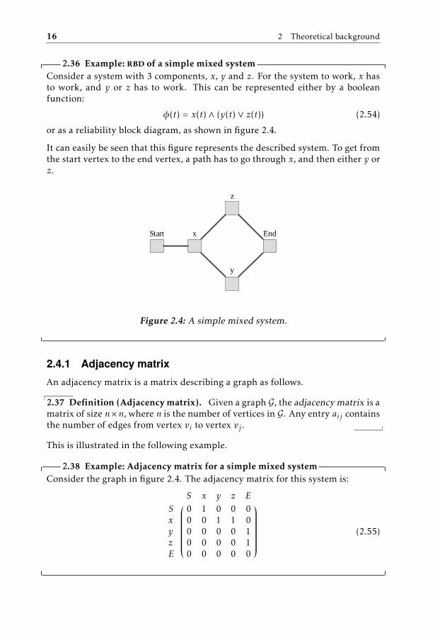
2.36 Example: rbd of a simple mixed systemConsider a system with 3 components, x, y and z. For the system to work, x hasto work, and y or z has to work. This can be represented either by a booleanfunction:
φ(t) = x(t) ∧ (y(t) ∨ z(t)) (2.54)
or as a reliability block diagram, as shown in figure 2.4.
It can easily be seen that this figure represents the described system. To get fromthe start vertex to the end vertex, a path has to go through x, and then either y orz.
Start x
y
z
End
Figure 2.4: A simple mixed system.
2.4.1 Adjacency matrix
An adjacency matrix is a matrix describing a graph as follows.
2.37 Definition (Adjacency matrix). Given a graph G, the adjacency matrix is amatrix of size n×n, where n is the number of vertices in G. Any entry aij containsthe number of edges from vertex vi to vertex vj .
This is illustrated in the following example.
2.38 Example: Adjacency matrix for a simple mixed systemConsider the graph in figure 2.4. The adjacency matrix for this system is:
S x y z E
S 0 1 0 0 0x 0 0 1 1 0y 0 0 0 0 1z 0 0 0 0 1E 0 0 0 0 0
(2.55)

2.4 Graph theory 17
2.4.2 Path and cut vectors
The structure of the system can also be described with path vectors or cut vectors.
2.39 Definition (Path vector). A path vector is a vector ~x for which the follow-ing property holds:
φ(~x) = 1 (2.56)
Equivalently, a path vector is a vector of component states ~x for which the systemworks.
A subset of the path vectors are the minimal path vectors.
2.40 Definition (Minimal path vector). The set of minimal path vectors are thepath vectors for which the system will stop working if any working componentin the vector fails.
2.41 Example: Minimal path vectors of a simple mixed systemConsider the system in figure 2.4. The set of path vectors are {1, 1, 0}, {1, 0, 1} and{1, 1, 1}. Of these, the last one is not minimal.
States for which the system does not work are defined by cut vectors.
2.42 Definition (Cut vector). A cut vector is a vector ~x for which the followingproperty holds:
φ(~x) = 0 (2.57)
Equivalently, a cut vector is a vector of component states ~x for which the systemdoes not work.
As with path vectors, a subset of cut vectors, the minimal cut vectors, can bedefined.
2.43 Definition (Minimal cut vector). The set of minimal cut vectors are thecut vectors for which the system would work if any of the failed components wasrepaired.
2.44 Example: Minimal cut vectors of a simple mixed systemConsider the system in figure 2.4. The set of minimal cut vectors are {0, 1, 1} and{1, 0, 0}.
2.4.3 Minimal cut set
For each minimal cut vector there is a minimal cut set which contains the failedcomponents in that cut vector.

18 2 Theoretical background
2.45 Example: Minimal cut sets of a simple mixed systemConsider the system in figure 2.4. The minimal cut sets of this system are {y, z}and {x}.
2.5 Importance measures
When designing and analyzing a system, it is of interest to know the importanceof the different components in a system and how they contribute to the overallreliability of the system. There are several measures for this, depending on howmuch information is available, and what measure of importance is of interest.The simplest case is structural importance. If more advanced analysis is desired,there are many importance measures that account for the lifetime distributions.
2.5.1 Structural importance
The simplest measure of how important a component is for the reliability of asystem is the structural importance. It only takes into account the structure ofthe system, and not the lifetime distributions of the components. As such, it isrelatively easy to calculate, and can for example be used in the design phase orwhen the lifetime distributions are not known. It is also an alternative when themore advanced measures would be too time consuming to compute or difficult touse.
2.46 Definition (Structural importance). When φ(si , ~x) is the structure func-tion where component i is in state s, the structural importance of a component iin a system with n components is defined as
Iφ(i) =1
2n−1
∑{~x|xi=1}
[φ(1i , ~x) − φ(0i , ~x)] (2.58)
for i = 1, 2, . . . , n.
The result can be seen as a measure of how much the system would suffer fromthe component going from a working state (φ(1i , ~x)) to a failed state (φ(0i , ~x)).
2.47 Example: Structural importance for a mixed systemCalculate the structural importance for the mixed system shown in figure 2.5.
For component x the state vectors are (1,0,0), (1,0,1), (1,1,0) and (1,1,1). For thesefour vectors the three last ones corresponds to a working system and hence thestructural importance is 1
4 [(0 − 0) + (1 − 0) + (1 − 0) + (1 − 0)] = 34
For component y the summation over the state vectors yield: 14 [(0 − 0) + (0 − 0) +
(1 − 0) + (1 − 1)] = 14 . Similarly component z has the same structural importance
as component y.
We can now see that component x has higher structural importance than y and z.

2.5 Importance measures 19
Start x
y
z
End
Figure 2.5: A simple mixed system.
2.5.2 Birnbaum importance
The Birnbaum importance (sometimes also called reliability importance) is some-what more advanced than the structural importance. It does take into accountthe lifetime distributions of components. It does however ignore the lifetime dis-tribution of the component studied. The original version of this measure wasfirst introduced in Birnbaum [1968, pp. 9 - 11]. However, this definition onlyused a fixed probability for each component, ignoring the time component. Alater adaptation can be found in Natvig and Gåsemyr [2009, p. 605], which ispresented here:
2.48 Definition (Birnbaum importance). If S(xi , t) is the survival function forthe system at time t given that the component i has state xi , and Si(t) is the
survival function for component i, the Birnbaum importance I (i)B of a component
i in a system at time t is defined as
I(i)B (t) =
∂S(t)∂Si(t)
(2.59)
or equivalently
I(i)B (t) = S(1i , t) − S(0i , t) (2.60)
for i = 1, 2, . . . , n.
For a component with a high Birnbaum importance, a small change in reliabilitywill give a large increase in system reliability. This can be used to decide whichcomponent to focus improvement efforts on in the design of a system.
2.49 Example: Birnbaum importance for a mixed systemConsider the same system as in example 2.47, but this time with exponentiallifetime distributions for all components. Let the failure rate be 1 for all compo-nents.
For component x the Birnbaum importance will be, according to equation 2.60,

20 2 Theoretical background
S(1x, t) − S(0x, t). The system doesn’t work with component x in a failed stateS(0x, t) = 0, and S(1x, t) corresponds to a parallel system of two exponential dis-tributions. The parallel system can be calculated with equation 2.47:
S(1x, t) = 1 − (1 − S1(t)) (1 − S2(t))S1(t)=S2(t)=e−t
= 2e−t − e−2t (2.61)
For component y the working state corresponds to a system with just one com-ponent and survival function S(0y , t) = e−t and the failed state corresponds to aserial system of components x and z with survival function S(t) = e−2t . Equation2.60 now gives the Birnbaum importance as
I(y)B (t) = S(1y , t) − S(0y , t) = e−t − e−2t (2.62)
The Birnbaum importance plotted as a function of time can be seen in figure 2.6.
1 2 3 4 5t
0.2
0.4
0.6
0.8
1.0
I B H t L
yx
Figure 2.6: The Birnbaum importance for component x and y over time.
2.5.3 Risk Achievement Worth and Risk Reduction Worth
In nuclear power stations, the two related measures Risk Achievement Worth(raw) and Risk Reduction Worth (rrw) are often used [Rausand and Høyland,2004, pp. 190 - 191].
2.50 Definition (Risk Achievement Worth, raw). The importance I (i)raw of a
component i is defined as
I(i)raw(t) =
1 − S(0i , t)1 − S(t)
(2.63)
for i = 1, 2, . . . , n.
The rawmeasure represents how much the component is worth for the reliabilityof the system. Components with high raw values are the ones that will impactthe system the most if their reliability would go down.

2.5 Importance measures 21
2.51 Definition (Risk Reduction Worth, rrw). The importance I (i)rrw of a com-
ponent i is defined as
I(i)rrw(t) =
1 − S(t)1 − S(1i , t)
(2.64)
for i = 1, 2, . . . , n.
The rrw represents with what ratio the system reliability would be improved byreplacing the component with a perfect one.
2.5.4 Improvement potential
The improvement potential I (i)IP of a component i also describes how much the
system reliability would be increased by replacing i with a perfect component.
2.52 Definition (Improvement potential).
I(i)IP (t) = S(1i , t) − S(t) (2.65)
for i = 1, 2, . . . , n.
It can also be defined in terms of I (i)B (t) as
I(i)IP (t) = I
(i)B (t) · (1 − Si(t)) (2.66)
This is related to rrw and is sometimes called the rrw calculated as a difference[Modarres et al., 2010, p. 309].
2.5.5 Barlow-Proschan importance
This measure is a weighted version of the Birnbaum importance, where the weightis the pdf fi(t) of the component i being investigated. The measure can be seenas the probability that the component i fails at the time the system fails.
2.53 Definition (Barlow-Proschan importance).
I(i)B−P =
∞∫0
I(i)B (t)fi(t)dt =
∞∫0
[S(1i , t) − S(0i , t)]fi(t)dt (2.67)
for i = 1, 2, . . . , n.
2.54 Example: Barlow-Proschan importanceCalculate the Barlow-Proschan importance for component x in figure 2.5 when
all components have exponential lifetime distributions with failure rate 1.
When component x is working the survival function will be S(1x, t) = −e−2t +2e−t
22 2 Theoretical background
and when component x is failed the survival function is zero. Equation 2.67 gives:
I(x)B−P =
∞∫0
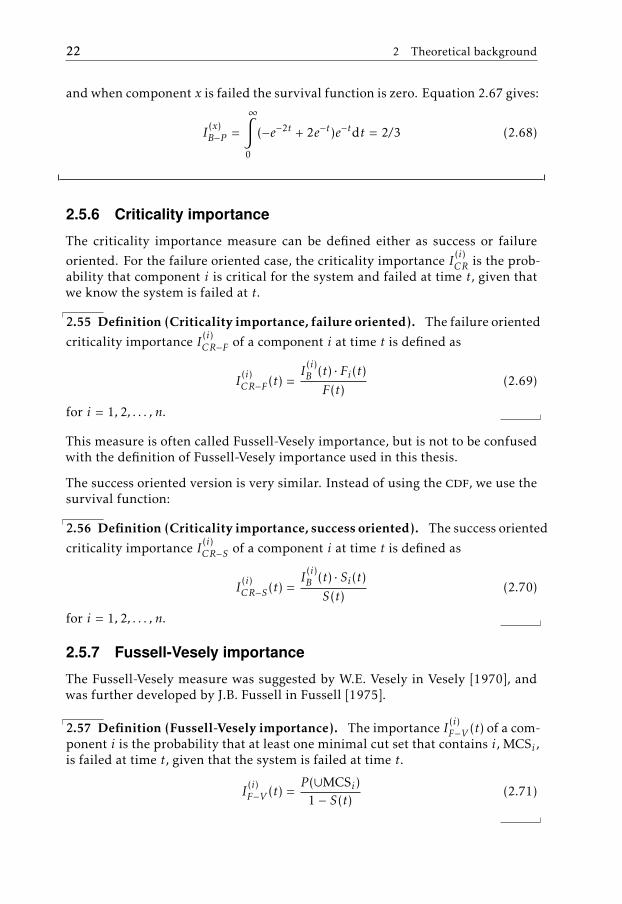
(−e−2t + 2e−t)e−tdt = 2/3 (2.68)
2.5.6 Criticality importance
The criticality importance measure can be defined either as success or failure
oriented. For the failure oriented case, the criticality importance I (i)CR is the prob-
ability that component i is critical for the system and failed at time t, given thatwe know the system is failed at t.
2.55 Definition (Criticality importance, failure oriented). The failure oriented
criticality importance I (i)CR−F of a component i at time t is defined as
I(i)CR−F(t) =
I(i)B (t) · Fi(t)F(t)
(2.69)
for i = 1, 2, . . . , n.
This measure is often called Fussell-Vesely importance, but is not to be confusedwith the definition of Fussell-Vesely importance used in this thesis.
The success oriented version is very similar. Instead of using the cdf, we use thesurvival function:
2.56 Definition (Criticality importance, success oriented). The success oriented
criticality importance I (i)CR−S of a component i at time t is defined as
I(i)CR−S (t) =
I(i)B (t) · Si(t)S(t)
(2.70)
for i = 1, 2, . . . , n.
2.5.7 Fussell-Vesely importance
The Fussell-Vesely measure was suggested by W.E. Vesely in Vesely [1970], andwas further developed by J.B. Fussell in Fussell [1975].
2.57 Definition (Fussell-Vesely importance). The importance I (i)F−V (t) of a com-
ponent i is the probability that at least one minimal cut set that contains i, MCSi ,is failed at time t, given that the system is failed at time t.
I(i)F−V (t) =
P (∪MCSi)1 − S(t)
(2.71)

2.6 Special functions 23
An interpretation of what the Fussell-Vesely importance means is the fraction ofthe system risk that is associated with the component i.
2.6 Special functions
To be able to represent certain expressions in a concise way, we define the Incom-plete Gamma function.
2.58 Definition (Incomplete Gamma function Γ ). The incomplete Gamma func-tion Γ (a, z) is defined, for positive a and z, as:
Γ (a, z) =
∞∫z
ta−1e−t dt (2.72)


3Structure function
“By a model is meant a mathematical construct which, with theaddition of certain verbal interpretations, describes observed
phenomena. The justification of such a mathematical construct issolely and precisely that it is expected to work.”
John Von Neumann
Given the structure function in a boolean form, we need to do certain conversionsand changes on it to get a form which can be efficiently used in computation. Inthis chapter, we present these operations.
3.1 Check if a boolean function is increasing
We first want to validate that the function given does indeed represent a validsystem. The requirement is that the function is increasing. According to the def-inition 2.30, a monotone increasing boolean function is equivalent to a booleanfunction which does not contain ¬ in the cnf or dnf form. To check if a booleanexpression is monotone increasing is then a matter of converting the expressionto conjunctive normal form (cnf) and check if the result contains any ¬. Thiscan easily be done with the builtin function BooleanConvert. However, this doesmore work than we actually need, and is therefore slower than necessary. Thealternative approach is to structurally take the expression in question apart on∧ and ∨ recursively, and only convert to cnf for the subparts of the expressionsactually containing other expressions, such as ∨, ∧ and ¬. A speed comparisonfor the systems defined in appendices B and C is shown in table 3.1.
25

26 3 Structure function
System BooleanConvert Our implementation
Airplane cockpit 0.13 0.47Diesel generator 2780 1.36
Table 3.1: Computation time in milliseconds for checking if a function ismonotone increasing, averaged over 1000 runs.
3.2 Converting a boolean expression
To make computation easy and to be able to use simple replacement rules forthe conversion of the structure function to a survival function, the boolean ex-pression for the structure function should be in a form only containing ∧ and∨. A simple solution which was used in our first approach, was to just use thebuiltin Mathematica function BooleanConvert for converting to conjunctive nor-mal form. However, this results in a very large expression for many systems, as it,again, does more work than needed. The only thing we need is to do the followingconversions:
a⇒ b → ¬a ∨ b (3.1)
a∨b → ¬a ∧ ¬b (3.2)
a∧b → ¬a ∨ ¬b (3.3)
We also need to convert the majority function to the appropriate combination of∧ and ∨.
An efficient way to do these conversions is to use Mathematicas pattern matching[Wolfram Research, 2011] to look for the functions we need to convert, and thenonly convert these subfunctions. This is somewhat slower than running Boolean-Convert on an expression with a large number of the unwanted functions, butgives a smaller final representation. The reason this is slower than the builtinfunction is most likely that the builtin function is more optimized. On an expres-sion with only a few of the unwanted functions, our implementation is found tobe faster, and also returns a much smaller expression, which is beneficial for fur-ther calculation and memory use. This second type of expression is the one thatoccurs most in real world systems.
Table 3.2 shows the computation time for BooleanConvert and our implementa-tion for the systems given in appendices B and C.
System BooleanConvert Our implementation
Airplane cockpit 0.13 1.65Diesel generator 2793 4.97
Table 3.2: Computation time in milliseconds for converting a boolean func-tion, averaged over 1000 runs.

3.3 Structure function to survival function 27
3.3 Structure function to survival function
The survival function of a system can be calculated with S(t) = E(Φ(~x)) [Leemis,2009, p. 32]. The first step of this calculation is to represent the structure func-tion in its polynomial form using the following relations:
xi ∧ xj → xi · xj (3.4)
xi ∨ xj → 1 − (1 − xi) · (1 − xj ) (3.5)
An intuitive way to explain these rules is to see the complex system as consistingof a combination of the special cases of serial and parallel systems.
We then need to take the expectation of this expression. All states are Bernoullivariables, which gives that E(Xn) = E(X) †. This means we can find the survivalfunction of the system, S(t), by expanding the expression, replacing all exponentswith 1, and then replace each variable with the corresponding survival function,as the survival function at the time t is the probability of a component workingat time t, which is the expectation of the state variable at time t.
3.3.1 Expanding to remove exponents
To be able to replace the states above with the survival functions for the com-ponents, all exponents have to be removed from the expression we get from thereplacement procedure. To do this, we started out by using the builtin Mathemat-ica function Expand, which expands the whole expression as much as possible.Given a large system, such as the system describing the information system in anairplane cockpit (see appendix B), this quickly results in large memory consump-tion. An alternative solution was devised, where instead of expanding everything,we only expand on the variables that actually need expanding, i.e. the ones thathave an exponent higher than 1. This was checked with the builtin function Ex-ponent. This gives a much smaller expression that takes less memory to handle,and thus enables the implementation to handle much larger systems. It also givesa speedup in computation time, as less computations are needed to expand theexpression.
Later on an even larger example was tried, namely a system of diesel generatorsin a nuclear power plant (see appendix C). This system took a relatively longtime to calculate properties for, and almost all the time was spent in expanding.To speed up the calculations even more, another solution to give an increase inexecution speed was investigated and implemented.
As most of the time is spent in expanding the expression, we naturally want toexpand as little as possible. The only time we need to expand, is if there are ex-
†Proof: The mgf for a Bernoulli distribution is q + pet and since E (Xn) = M(n)X (0) = dnMX (t)
dtn
∣∣∣∣t=0
we have E (Xn) = E (X) for Bernoulli random variables.

28 3 Structure function
ponents that are not 1 in the polynomial. That only occurs if a variable in theboolean expression occurs multiple times. A natural approach to take then is toget rid of as many duplications as possible in the boolean expressions, by apply-ing different boolean algebra transformation rules. This gives a remarkable in-crease in computation speed for many systems. A problem with this approach isthat there are systems for which there is no way to represent the boolean functionwithout duplicating variables. Therefore, this is only a partial solution, and afterapplying the transformation, checks for exponents must still be done. However,these checks are inexpensive compared to expanding, so a substantial decrease incomputation time is still achieved.
The simplifications used, with boolean functions g1 and g2, are:
g1(e1, b)∧b ∧ g2(e2, b)→ g1(e1, 1) ∧ b ∧ g2(e2, 1)
g1(e1, b)∨b ∨ g2(e2, b)→ g1(e1, 0) ∨ b ∨ g2(e2, 0)
d1 ∨ (a1∧b ∧ a2) ∨ d2 ∨ (c1 ∧ b ∧ c2) ∨ d3 →d1 ∨ d2 ∨ d3 ∨ (b ∧ ((a1 ∧ a2) ∨ (c1 ∧ c2)))
d1 ∧ (a1∨b ∨ a2) ∧ d2 ∧ (c1 ∨ b ∨ c2) ∧ d3 →d1 ∧ d2 ∧ d3 ∧ (b ∨ ((a1 ∨ a2) ∧ (c1 ∨ c2)))
(3.6)
The first two rules do pure simplifications, while the other two factor out expres-sions or variables. All variables with an index may or may not be present. Someexamples where the rules are used are found in example 3.1. The rules are ap-plied recursively to each subexpression.
3.1 Example: Boolean simplificationsA few boolean expressions are simplified according to the rules in equation 3.6.The first rule is used:
(x ∨ y) ∧ y = y (3.7)
The second rule works similarly:
(x ∧ y) ∨ z ∨ y = z ∨ y (3.8)
The third rule:
(x ∧ y) ∨ (x ∧ v) = x ∧ (y ∨ v) (3.9)
Applying the last rule in a similar manner:
(x ∨ y) ∧ (x ∨ v) = x ∨ (y ∧ v) (3.10)

3.3 Structure function to survival function 29
Finding the highest exponent of a polynomial
To find the highest exponent of our polynomial, we first used the Mathemat-ica builtin function Exponent. We found, however, that a simplistic approachwhich recursively calculates the exponent of a certain variable in a polynomialperformed better. The calls to Exponent were replaced with this new function,giving an increase in performance. This new function simply splits the expres-sion recursively on multiplication and addition. On a multiplication, it returnsthe sum of the exponents, and on a plus the maximum of the exponents. If anexpression does not contain the variable, it returns 0. Once a single symbol isreached, it returns 1 if the symbol is the variable we want the exponent for. Aspeed comparison is shown in table 3.3.
System Exponent Our implementation
Airplane cockpit 74.3 18.7Diesel generator 191.2 190.8
Table 3.3: Computation time in milliseconds for finding exponents of allvariables, averaged over 100 runs.
Expanding and exponent removal
An effective way of expanding and removing all exponents that we finally used isbased on the Shannon expansion, presented in his masters thesis [Shannon, 1938,p. 34]. The approach is to recursively apply the Shannon expansion to the partsof the expression that contain the given variable. The order of variables on whichto expand first is chosen so that the one with the lowest exponent gets expandedfirst. This gives the result that we work with a smaller expression as long aspossible.
The Shannon expansion on variable x of the function f works on the followingprinciple:
f (x) = x (f (1) − f (0)) + f (0) (3.11)
We show our implementation in an example:
3.2 Example: Shannon expansionLet us start with the polynomial for the system that works when two out of threecomponents work:
1 − (1 − xy)(1 − xz)(1 − yz) (3.12)
We want to expand on the variables that have a degree higher than 1, and removethese exponents. The degrees are 2 for all variables. In this example we willillustrate the principle by expanding on x. Let the expanding function have the

30 3 Structure function
name SExp. First we split SExp over the minus:
SExp(1 − (1 − xy)(1 − xz)(1 − yz)) =
= SExp(1) − SExp((1 − xy)(1 − xz)(1 − yz))(3.13)
1 does not contain x, so we can remove the expansion around it:
= 1 − SExp((1 − xy)(1 − xz)(1 − yz)) (3.14)
To expand on x, we take the polynomial from the input, and apply equation 3.11.We first compute f (1) and f (0):
f (1) = (1 − 1y)(1 − 1z)(1 − yz) = (1 − y)(1 − z)(1 − yz)f (0) = (1 − 0y)(1 − 0z)(1 − yz) = (1 − yz)
(3.15)
We can now expand (from equation 3.14):
=1 − x(f (1) − f (0)) + f (0) =
= x((1 − y)(1 − z)(1 − yz) − (1 − yz)) + (1 − yz)(3.16)
We now have an expression with degree 1 in x. The same procedure can be usedfor y and z. This allows us to use the replacement procedure in equations 3.4 and3.4.
Table 3.4 shows the time required to remove all exponents from the diesel genera-tor systems in appendix C. The cockpit system example also used in the previousspeed comparisons is not shown, as both solutions are instantaneous. This is be-cause there are no exponents to remove. The times given are after applying thesimplification rules in 3.6. In both cases, expanding is only done on the variablesthat require it, and with the variable with the lowest exponent first. We can seethat our final implementation is significantly faster than the simple approach ofexpanding with Expand and then removing exponents.
System Expand and Replace Our implementation
Diesel generator 15.140 0.44
Table 3.4: Computation time in seconds for removing all exponents.
3.3 Example: Boolean expression to survival functionIn this example we will go from a boolean expression to a survival function, us-ing the same steps as the final implementation in Mathematica. We start out bydefining our boolean expression.
(¬x∨¬y) ∧ (z ∨ x) (3.17)
The first thing we do is check that the expression is indeed a monotone increasingboolean function. The algorithm for this is the one presented in section 3.1. Let us

3.3 Structure function to survival function 31
call the recursive function IncrQ for the purpose of this example. The followingchain of calls will be the result.
IncrQ((¬x∨¬y
)∧ (z ∨ x)
)=
= IncrQ(¬x∨¬y
)∧ IncrQ (z ∨ x) =
= IncrQ(BooleanConvert
(¬x∨¬y
))∧ IncrQ (z) ∧ IncrQ (x) =
= IncrQ (x ∧ y) ∧ true ∧ true =
= IncrQ (x) ∧ IncrQ (y) = true
(3.18)
This result shows that the given function is monotone increasing. We continue byconverting the expression to one with only ∧ and ∨, as discussed in section 3.2.Let us call the function for this Conv. The following is the result on running thefunction on our expression.
Conv((¬x∨¬y
)∧ (z ∨ x)
)=
= Conv(¬x∨¬y
)∧ Conv (z ∨ x) =
= BooleanConvert(¬x∨¬y
)∧ (z ∨ x) =
= (x ∧ y) ∧ (z ∨ x)
(3.19)
We now have a function consisting only of our three variables, x, y and z, aswell as ∧ and ∨. The next step is to reduce our function as much as possible byapplying the rules in equation 3.6. We can apply the first rule.
(x∧y) ∧ (z ∨ x) =
= x ∧ y ∧ (z ∨ x) =
= x ∧ y ∧ (z ∨ 1) =
= x ∧ y ∧ 1 = x ∧ y
(3.20)
As we can see, the function was in fact not dependent on z, making it an irrele-vant component that does not impact reliability of the system. We now do thereplacement procedure given in equations 3.4 and 3.4.
x ∧ y → x · y (3.21)
We check to see that there are no exponents in the result, which is trivial in thiscase. Finally, we replace each variable with that components survival function,arriving at the systems survival function.
Ssys(t) = Sx(t) · Sy(t) (3.22)


4Reliability distribution
“The theory of probabilities is basically justcommon sense reduced to calculus.”
Pierre-Simon Laplace
When the survival function is known, a large number of properties follow fromfairly straightforward definitions. A complete list of properties and functionsthat can now be calculated for the system distribution are presented in table A.1.
Since our implementation is integrated into the Mathematica framework, we canuse the very large number of distributions already included in Mathematica ascomponent distributions. This includes parametric distributions, non-parametricdistributions and derived distributions. Parametric distributions are distribu-tions defined by parameters, such as the exponential distribution or the Weibulldistribution. Non-parametric distributions are distributions constructed directlyfrom data. This can be done by smoothing the data, or using a histogram of thedata as a pdf. Under derived distributions, we find distributions defined as afunction of a random variable, a truncated version of another distribution, or theorder distribution presented in definition 2.17. A distribution can also be definedby simply giving a formula for the pdf or the survival function.
This thorough framework of distributions allows flexible modeling, either viaparametric distributions, or directly from data collected during testing of compo-nents.
4.1 Properties for some basic systems
The standard example systems in the literature are the parallel, serial and k-out-of-n systems. The most commonly used distribution for the lifetime distributionsis the exponential distribution, because of its simplicity in calculation. Since the
33

34 4 Reliability distribution
exponential distribution is so common, we present the mean time to failure, thesurvival function, the pdf as well as random number generation for these stan-dard systems where all components follow the exponential lifetime distribution.For random number generation it is assumed that λ equals 1.
We present the mean time to failure, the survival function, the PDF as well asrandom number generation,
4.1.1 Serial system
Start x y End
Figure 4.1: A serial system with two components.
The serial system is the least reliable configuration, given a set of components andtheir lifetime distributions. It requires all components to work, which means thatthe system will survive until the first component fails. The rbd for such a systemwith two components is shown in figure 4.1.
With our implementation, properties for this system can be readily calculated.Assume that the components lifetimes are exponentially distributed with param-eters λx and λy .
The mttf of this system is found to be:
µserial(t) =1
λx + λy(4.1)
The survival function can also easily be found, and is shown in figure 4.2 and
0.0 0.5 1.0 1.5 2.0 2.5t
0.2
0.4
0.6
0.8
1.0SH t L
0.5 1.0 1.5 2.0 2.5 3.0t
0.5
1.0
1.5
2.0
f H t L
Figure 4.2: Survival function (left) and PDF with random numbers (right)for a serial system.

4.1 Properties for some basic systems 35
below:
Sserial(t) ={e−t(λx+λy) t ≥ 01 otherwise
(4.2)
From this formula we can easily see that the result is another exponential distri-bution. This is used in the implementation for efficiency in computation. Suchrelations are discussed further in chapter 5.
4.1.2 Parallel system
Start
x
y
End
Figure 4.3: A parallel system with two components.
The parallel system is the most reliable configuration, given a set of componentsand their lifetime distributions. It requires only one component to work, whichmeans the system will survive as long as the longest surviving component. Therbd for such a system with two components is shown in figure 4.3.
We again assume that the components lifetimes are exponentially distributedwith parameters λx and λy . The mttf for this parallel system is:
µparallel(t) =1λx
+1λy− 1λx + λy
(4.3)
The survival function can also easily be found, and is shown in figure 4.4 andbelow:
Sparallel(t) ={
1 −(1 − e−tλx
) (1 − e−tλy
)t ≥ 0
1 otherwise(4.4)

36 4 Reliability distribution
0 1 2 3 4 5 6 7t
0.2
0.4
0.6
0.8
1.0SH t L
1 2 3 4 5 6 7t
0.1
0.2
0.3
0.4
0.5
f H t L
Figure 4.4: Survival function (left) and PDF with random numbers (right)for a parallel system.
4.1.3 2 out of 3 system
The 2 out of 3 system is the system where any two of the three components needto work for the system to work. The rbd for such a system is shown in figure 4.5.For this system, we make the assumption that the components lifetimes are expo-
Start x
x
y
y
z
z
End
Figure 4.5: A two-out-of-three system.
nentially distributed with parameters λx, λy and λz . The mttf for this system isthen:
µ2oo3(t) =1
λx + λy− 2λx + λy + λz
+1
λx + λz+
1λy + λz
(4.5)
The survival function can also easily be found, and is shown in figure 4.6 andbelow:
S2oo3(t) =
e−t(λx+λy) − e−tλz((
2e−tλx − 1)e−tλy − e−tλx
)t ≥ 0
1 otherwise(4.6)

4.1 Properties for some basic systems 37
0.0 0.5 1.0 1.5 2.0 2.5 3.0t
0.2
0.4
0.6
0.8
1.0SH t L
0.5 1.0 1.5 2.0 2.5 3.0 3.5t
0.2
0.4
0.6
0.8
1.0
f H t L
Figure 4.6: Survival function (left) and PDF with random numbers (right)for a two-out-of-three system.
4.1.4 Simple mixed system
Another simple mixed system is the one shown in figure 4.7. In this system, thecomponents x, and either y or z have to work for the system to work. Again, we
Start x
y
z
End
Figure 4.7: rbd for a simple mixed system.
make the assumption that the components lifetimes are exponentially distributedwith parameters λx, λy and λz . The mttf for this system is then:
µsms(t) =1
λx + λy+
1λx + λz
− 1λx + λy + λz
(4.7)
The survival function can easily be found, and is shown in figure 4.8 and below:
Ssms(t) ={e−tλx
(1 −
(1 − e−tλy
) (1 − e−tλz
))t ≥ 0
1 otherwise(4.8)

38 4 Reliability distribution
0.0 0.5 1.0 1.5 2.0 2.5 3.0t
0.2
0.4
0.6
0.8
1.0SH t L
0.5 1.0 1.5 2.0 2.5 3.0t
0.2
0.4
0.6
0.8
1.0
1.2
f H t L
Figure 4.8: Survival function (left) and PDF with random numbers (right)for a simple mixed system.
4.1.5 Bridge system
A somewhat more advanced system often studied is the bridge system, shownin figure 4.9. Again, we make the assumption that the components lifetimes are
Start
x
y
z
v
w
End
Figure 4.9: rbd for a bridge system.
exponentially distributed with parameters λx, λy , λz , λv and λw. The mttf forthis system is:
µbridge(t) =1
λv + λw− 1λv + λw + λx + λy
+
+2
λv + λw + λx + λy + λz− 1λv + λw + λx + λz
−
− 1λv + λw + λy + λz
− 1λv + λx + λy + λz
+1
λv + λy + λz−
− 1λw + λx + λy + λz
+1
λw + λx + λz+
1λx + λy
(4.9)

4.2 Parallelization 39
0.0 0.5 1.0 1.5 2.0 2.5 3.0t
0.2
0.4
0.6
0.8
1.0SH t L
0.5 1.0 1.5 2.0 2.5 3.0t
0.2
0.4
0.6
0.8
1.0
f H t L
Figure 4.10: Survival function (left) and PDF with random numbers (right)for a bridge system.
The survival function can also be found, and is shown in figure 4.10 and below:
Sbridge(t) =
e−tλy((e−tλx − 1
) (1 − e−tλv−tλz
)+ 1
)−
− e−tλw (−e−tλv + e−tλy (e−tλv +(1 − e−tλv
) (1 − e−tλx
)+
+ e−tλz (−(1 − e−tλv )(1 − e−tλx ) − e−tλx + 1)−− e−tλz (e−tλv + (1 − e−tλv )(1 − e−tλx ) − 1) + e−tλx − 1)+
+ e−tλz (e−tλv + (1 − e−tλv )(1 − e−tλx ) − 1))
t ≥ 0
1 otherwise(4.10)
4.2 Parallelization
An interesting property to analyze is if it is more beneficial to parallelize on a sys-tem level, or on the component level. A structural analysis was done by Leemis[2009, p. 23]. Here we will present an example with specific lifetime distribu-tions. To this end, the system in figure 4.7 is studied. We assume all componentsto be exponentially distributed, with the failure rate λ.
For the original system, we have the survival function:
Sorig(t) ={
1 t < 0e−3λt
(2eλt − 1
)otherwise
(4.11)
and the mttf:
µorig(t) =20
30λ(4.12)

40 4 Reliability distribution
Start
x1
y1
z1x2
y2
z2
End
Figure 4.11: rbd with system level parallelism.
4.2.1 Parallelization on system level
In figure 4.11 we see the system when parallelized on a system level. The survivalfunction of this system is found to be:
Ssys(t) =
1 t < 0
1 − e−6λt(−2eλt + e3λt + 1
)2otherwise
(4.13)
and the mttf:
µsys(t) =29
30λ(4.14)
4.2.2 Parallelization on component level
In figure 4.12 we see the system when parallelized on a component level. Thesurvival function of this system is found to be:
Scomp(t) =
1 t < 0(1 −
(1 − eλ(−t)
)2) (
1 −(1 − eλ(−t)
)4)
otherwise(4.15)
and the mttf:
µcomp(t) =34
30λ(4.16)

4.2 Parallelization 41
Start
x1
y1
z1x2
y2
z2
End
Figure 4.12: rbd with component level parallelism.
4.2.3 Comparison
As can be seen in figure 4.13 of the survival function of the two systems, it isclear that a parallelization on the component level is always better than on thesystem level, at any time t. The mttf of the systems also shows that on average,a parallelization on the component level is most beneficial for this example. Itis also clear that both parallelization on the component level and on the systemlevel is better than the original system in this case.
0 1 2 3 4t
0.2
0.4
0.6
0.8
1.0SH t L
System
Component
Original
Figure 4.13: Survival function of component and system level paralleliza-tion.

42 4 Reliability distribution
4.3 Properties for real world systems
Our implementation also allows for the fast computation of properties for sys-tems with many components, such as the ones presented in appendix B and ap-pendix C. Some results for such systems are presented in the sections below.
4.3.1 Cockpit information system
With our implementation, we can calculate many properties of the cockpit infor-mation system (thoroughly defined in appendix B), as listed in appendix A. Someinteresting properties are presented here.
Mean
The mttf of the system is found to be approximately 159.487 hours. The exactanswer is easily computed, but consists of a fraction of two numbers with around2000 digits each, so it is not presented here. This result means that if no main-tenance is done on the airplane, the cockpit information system will be able toprovide enough information to the pilots on average for around 160 hours.
Survival function, hazard function, PDF and CDF
0 100 200 300 400 500 600 700t
0.2
0.4
0.6
0.8
1.0SHt L
0 100 200 300 400 500 600 700t
0.2
0.4
0.6
0.8
1.0
F Ht L
0 100 200 300 400 500 600 700t
0.001
0.002
0.003
0.004
0.005
0.006
fHt L
0 100 200 300 400 500 600 700t
0.001
0.002
0.003
0.004
0.005
0.006
hHt L
Figure 4.14: Survival function (top left), cdf (top right), pdf (bottom left)and hazard function (bottom right) of cockpit information system.
The symbolic representation of the survival function of the system is rather long,and is shown as a plot in figure 4.14. From the plot we can see that the probability

4.3 Properties for real world systems 43
of survival drops fairly rapidly for small t.
From the hazard function in figure 4.14 we can see that the lifetime distributionfor the system is similar to an exponential distribution, with an almost constanthazard rate.
Comparison of results
The original study Pettit and Turnbull [2001, Appendix A] focuses on a six hourlong flight, as such a flight is a reasonable time span for a trip inside the UnitedStates.
The report gives the probability of completing such a six hour flight with func-tioning cockpit information system as 0.976. This probability can be computed inseveral ways, the most straight-forward one probably being the survival functionat t = 6. Our model gives this probability as 0.965. We assume that the reporthas used approximate methods, giving a slightly different result.
4.3.2 Airplane
In the same paper by Pettit and Turnbull that contains the system definition forthe information system of the airplane cockpit [Pettit and Turnbull, 2001], wealso find failure rates for other parts of airplanes. We use this to model an air-plane. A single engine has the structure shown in figure 4.15. The airplane needs
Start motor fuel cooling propeller End
Figure 4.15: System structure for an airplane engine.
both wings, one engine out of two on each wing, and the control system to func-tion. The control system is shown in figure 4.16, with the mapping to componentnames in table 4.1. Based on these subsystems, we can model the whole sys-
Start 5 6 7 8 9 10 11 12 End
Figure 4.16: System structure for airplane controls.
tem structure, which is shown in figure 4.17. All components have lifetimes dis-tributed with a Weibull distribution. The parameters are presented in table 4.1.The hazard function displays a so called “bathtub shape”, a typical shape foundin reliability. The high hazard rate in the beginning of the lifetime is called theburn-in phase, and the increasing hazard rate in the end corresponds to wearout.

44 4 Reliability distribution
Start
engine1
engine2
engine3
engine4
control wing1 wing2 End
Figure 4.17: System structure for airplane.
Nr Component α β
1 motor 1.58 48302 fuel 1.44 51303 cooling 1.60 41904 propeller 1.63 37405 directional 1.85 4729.026 longitudinal 1.57 4718.227 lateral 2.25 5843.588 flaps 0.95 39569 trim 0.73 2672.110 hydraulics 1.14 3977.3911 landing gear 0.92 2895.6212 steering 1.65 3994.7813 wing 1.79 4250
Table 4.1: Weibull parameters for airplane.
We can calculate properties for the lifetime of this system. Interesting ones couldagain be the mean time to failure, and the probability of the airplane surviving asix hour flight.
µ ≈ 506.447 (4.17)
P (t ≥ 6) ≈ 0.982331 ≈ 98.2% (4.18)
Let us also compute the probability of the airplane surviving a six hour flightgiven that it has already survived 100 flight hours.
P (t ≥ 106 | t > 100) ≈ 0.989977 ≈ 99.0% (4.19)
It seems there is a burn-in period in the beginning of the lifetime of the airplane.This can also be seen in the hazard function in figure 4.18.

4.3 Properties for real world systems 45
0 200 400 600 800 1000t
0.2
0.4
0.6
0.8
1.0SH t L
0 200 400 600 800 1000t
0.2
0.4
0.6
0.8
F H t L
0 200 400 600 800 1000t
0.0005
0.0010
0.0015
0.0020
f H t L
0 200 400 600 800 1000t
0.0005
0.0010
0.0015
0.0020
0.0025
0.0030
h H t L
Figure 4.18: Survival function (top left), cdf (top right), pdf (bottom left)and hazard function (bottom right) of airplane.
4.3.3 Electrical diesel generator system
Some interesting properties of an electrical diesel generator system for a nuclearpower plant (defined in appendix C) are the mean and the different distribu-tion functions. The mttf of the electrical diesel generator system is found tobe 10.8157 years. The distribution functions are presented in figure 4.19. Thissystem is somewhat close to an exponential distribution as well, as the hazardfunction is almost constant. For small t however, we can see that this is not thecase.
Comparison of results
In the thesis with the system definition [Dulik, 1996, Appendix A], the wholesystem is found to have approximately an exponential lifetime distribution, withfailure rate λ = 0.097 per year. This is similar to our exact result, as can be seenin figure 4.20.
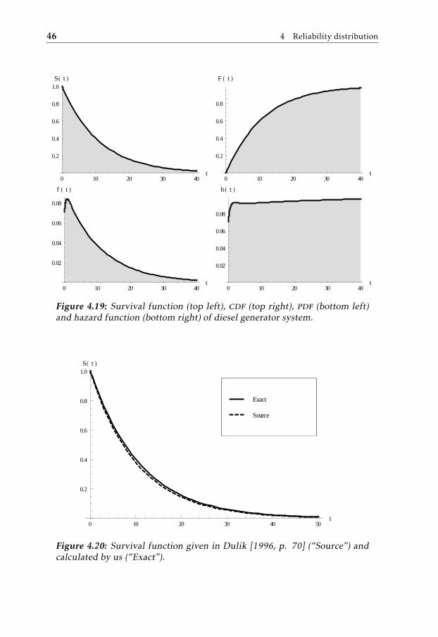
46 4 Reliability distribution
0 10 20 30 40t
0.2
0.4
0.6
0.8
1.0SH t L
0 10 20 30 40t
0.2
0.4
0.6
0.8
F H t L
0 10 20 30 40t
0.02
0.04
0.06
0.08
f H t L
0 10 20 30 40t
0.02
0.04
0.06
0.08
h H t L
Figure 4.19: Survival function (top left), cdf (top right), pdf (bottom left)and hazard function (bottom right) of diesel generator system.
0 10 20 30 40 50t
0.2
0.4
0.6
0.8
1.0SH t L
Source
Exact
Figure 4.20: Survival function given in Dulik [1996, p. 70] (“Source”) andcalculated by us (“Exact”).

5Optimizations
“Everything should be made as simple as possible, but not simpler.”
Albert Einstein
For efficient computation of properties for the reliability distribution, we can insome cases do better than the general case. These special cases where simplifica-tions can be done are presented in this chapter.
5.1 Simplification of distributions
For some systems the reliability distribution reduces to a known distribution. Forexample, the series of exponential distributions.
5.1 Example: Series system with exponential distributionsConsider a system with n components in series, with hazard functions hk(t) = λk ,where k = 1, . . . , n. This means the lifetime distributions are exponential, withthe survival functions Sk(t) = e−λk t .
Using equation 2.49 we get
S(t) = S1(t) ∗ · · · ∗ Sn(t) = e−λ1t ∗ · · · ∗ e−λnt = e−(λ1+···+λn) (5.1)
From this we can easily identify that this is a system with an exponential lifetimedistribution, with the parameter
λ =n∑i=1
λi (5.2)
which has the advantage that we can use known properties of the exponentialdistribution for further calculations on our system.
47
48 5 Optimizations
Similar to example 5.1, there are other configurations of systems that reduce toknown distributions. Some of the relations are presented here:
• A series system of i identical components with lifetime distribution D, isidentical to an order distribution where k = 1 and n = i.
• A parallel system of i identical components with lifetime distribution D, isidentical to an order distribution where k = i and n = i.
• A series system of i components that have lifetime distributions accordingto Weibull distributions with identical α and β = β1, . . . , βi , is identical to a
Weibull distribution with the same α and β =(∑i
j=11βαj
)− 1α
.
• A series system of i components that have lifetime distributions accordingto Pareto distribution with identical k and α = α1, . . . , αi , is identical to aPareto distribution with the same k and α =
∑ij=1 αj .
• A series system of i components that have lifetime distributions accordingto exponential distribution with λ = λ1, . . . , λi , is identical to an exponen-tial distribution with λ =
∑ij=1 λj .
• A parallel system of i identical components with lifetime distributions ac-cording to a Frechet distribution with parameters α and βc, is identical to aFrechet distribution with the same α and β = βcn
1/α
In the cases where we can find a known distribution, we use this known distribu-tion internally for all calculations. This is to take full advantage of any optimiza-tions and known properties in the built in implementations.
5.2 Special cases of properties
For some properties of the reliability distribution, there exist properties that en-able optimizations. These optimizations are of interest if they can be done forsuch systems that are often used in computations. An example is the case whereall the component distributions are exponentially distributed.
5.2.1 Exponentially distributed components
Since exponential distributions are used to a large extent in the reliability fieldit is justifiable to look for all possible simplifications that can be done to suchsystems. When a system contains only exponential distributions, a number ofoptimizations can be made, and these are presented in this chapter.
Moments around zero
The moments can be calculated from the survival function, which will only con-sist of a sum of exponentials, S(t) =
∑i cie
di t . We can rewrite the definition of the

5.2 Special cases of properties 49
moments around zero as follows:
µ′k =⟨tk
⟩=
∞∫0
tkf (t)dt =
=
∞∫0
tk∑i
−diciedi tdt =∑i
−dici
∞∫0
tkedi tdt =
=∑i
−dicik!
(−di)1+k=
∑i
cik!
(−di)k
(5.3)
This has a striking similarity with the survival function, namely that it is a sumof a function multiplied by coefficients ci . This allows us to simply replace thefunctions in the survival function, using a replacement rule:
edi t → k!(−di)k
(5.4)
A special case of this is of course the first moment where k = 1, the mean, givenby the replacement:
edi t → 1−di
(5.5)
Central moments
The central moments can also be calculated from the survival function. A sim-ilar approach to the moments above is used. Using the definition for centralmoments:
µk =⟨(t − µ)k
⟩=
k∑n=0
(kn
)(−µ)k−n〈tn〉 =
=k∑n=0
(kn
)(−µ)k−n
∞∫0
tnf (t)dt =
=k∑n=0
(kn
)(−µ)k−n
∞∫0
tn∑i
−diciedi tdt =
=k∑n=0
(kn
)(−µ)k−n
∑i
−dicin!
(−di)1+n =
=∑i
ci
k∑n=0
k!(k − n)!
(−µ)k−n1
(−di)n=
=∑i
ci(−1)kediµd−ki Γ (1 + k, diµ)
(5.6)

50 5 Optimizations
We identify the replacement rule to use in the survival function:
edi t → (−1)kediµd−ki Γ (1 + k, diµ) (5.7)
Moment-generating function
Given the survival function, the moment-generating function again can be com-puted efficiently for the case with only exponential distributions. With the defi-nition we find:
MT (s) =
∞∫0
estf (t)dt =
∞∫0
est∑i
−diciedi tdt =
=∑i
−dici
∞∫0
e(s+di )tdt =∑i
dici1
s + di
(5.8)
And we can identify the replacement rule:
edi → di /(di + s) (5.9)
Characteristic function
Similar to the mgf, there is an easy way to compute the characteristic functionwhen all distributions are exponentials. We rewrite the definition:
ϕT (s) =
∞∫0
eistf (t)dt =
∞∫0
eist∑j
−djcjedj tdt =
=∑j
−djcj
∞∫0
et(is+dj)dt =∑j
djcj1
dj + is
(5.10)
We identify the replacement rule and use it on the survival function:
edj → dj /(dj + is) (5.11)
Other properties
Based on the properties calculated above, the variance, standard deviation, kur-tosis, skewness and the central moment-generating function can be efficientlycalculated according to their definitions.
5.2.2 Hazard function
The calculation of the hazard function h(t) can be partly simplified by using thefact that the hazard function for a series of components is just the sum of thehazard functions for the components. We can then break out the part of a systemthat is serial. For this part, we separately compute the hazard function by adding

5.2 Special cases of properties 51
the hazard functions for the components. Then we add this result to the hazardfunction for the non-serial part, which is computed in the standard way. Weillustrate this in an example:
5.2 Example: Efficient hazard function computationConsider the system in figure 5.1. The components x1 and x2 are in series. We
want to compute the hazard function for this system. Let us assume that each
Start x1 x2
x3
x4
End
Figure 5.1: A system with a serial part.
component is exponentially distributed with failure rates of λ1, λ2, λ3 and λ4 forx1, x2, x3 and x4, respectively.
We first calculate the hazard function of the serial part, which is just the sum ofthe hazard functions of x1 and x2:
hseries(t) = λ1 + λ2 (5.12)
The remaining part is now a simple parallel connection between x3 and x4. Forthis we compute the hazard function as usual, via the survival function. Thesurvival function for this part is:
Sparallel(t) =1 −(1 − Sx3
(t)) (
1 − Sx4(t)
)=
={
1 −(1 − e−tλ3
) (1 − e−tλ4
)t > 0
1 otherwise
(5.13)
Using equation 2.19 we get:
hparallel(t) =
λ3(eλ4t−1)+λ4(eλ3t−1)eλ3t+eλ4t−1
t > 01 otherwise
(5.14)
The hazard function for the whole system is then obtained by adding the serial

52 5 Optimizations
and parallel parts, as they are connected in series:
h(t) =
λ3(eλ4t−1)+λ4(eλ3t−1)eλ3t+eλ4t−1
+ λ1 + λ2 t > 01 otherwise
(5.15)
This approach is more efficient, as it reduces the expression for which we need tocompute a survival function which is then derived.

6Importance measures
“When you can measure what you are speaking about, and express itin numbers, you know something about it; when you cannot express
it in numbers, your knowledge is of a meagre and unsatisfactorykind; it may be the beginning of knowledge, but you have scarcely, in
your thoughts, advanced to the stage of science.”
Lord Kelvin
With our implementation we are able to calculate all the importance measuresdefined in section 2.5. These measures are used to find out which componentsin a system are important. Depending on what is meant with “important”, andwhat the goal is, different importance measures are used.
6.1 Properties for a bridge system
We calculate the importance measures for a bridge system with five components,as seen in figure 6.1. We let all components have an exponential lifetime distri-bution with failure rate λ unless otherwise noted. In plots, λ is assumed to be 1.
6.1.1 Structural importance
The structural importance results for the components in the bridge system areillustrated in figure 6.2. This measure illustrates how much worse the systemreliability would be if the component would fail. It only takes into account thestructure of the system itself, not the lifetime distributions of the components.
53

54 6 Importance measures
Start
x
y
z
v
w
End
Figure 6.1: A bridge system with 5 components.
x y z v w
0.05
0.10
0.15
0.20
0.25
0.30
0.35
IΦ
Figure 6.2: Structural importance for components in a bridge system.
6.1.2 Birnbaum importance
All components except the z-component have the same importance. We can seehow the components behave with respect to time in figure 6.3, showing both thefour components with the same importance and the z component. The symbolicrepresentation of the Birnbaum importance for the system can be seen in table 6.1.
1 2 3 4t
0.05
0.10
0.15
0.20
0.25
0.30
0.35
I B H t L
z
x , y , v , w
Figure 6.3: The Birnbaum importance for components in a bridge system.
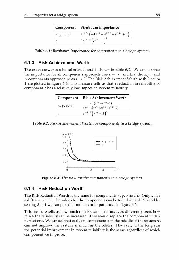
6.1 Properties for a bridge system 55
Component Birnbaum importance
x, y, v, w e−4λt(−4eλt + e2λt + e3λt + 2
)z 2e−4λt
(eλt − 1
)2
Table 6.1: Birnbaum importance for components in a bridge system.
6.1.3 Risk Achievement Worth
The exact answer can be calculated, and is shown in table 6.2. We can see thatthe importance for all components approach 1 as t → ∞, and that the x,y,v andw components approach∞ as t → 0. The Risk Achievement Worth with λ set to1 are plotted in figure 6.4. This measure tells us that a reduction in reliability ofcomponent z has a relatively low impact on system reliability.
Component Risk Achievement Worth
x, y, v, weλt(e2λt+e3λt−1)
(eλt−1)(eλt+2e2λt+e3λt−2)
z e−4λt(eλt − 1
)2
Table 6.2: Risk Achievement Worth for components in a bridge system.
0 1 2 3 4t
1.0
1.5
2.0
2.5
3.0I RAW H t L
z
x , y , v , w
Figure 6.4: The raw for the components in a bridge system.
6.1.4 Risk Reduction Worth
The Risk Reduction Worth is the same for components x, y, v and w. Only z hasa different value. The values for the components can be found in table 6.3 and bysetting λ to 1 we can plot the component importances in figure 6.5.
This measure tells us how much the risk can be reduced, or, differently seen, howmuch the reliability can be increased, if we would replace the component with aperfect one. We can see that early on, component z in the middle of the structure,can not improve the system as much as the others. However, in the long runthe potential improvement in system reliability is the same, regardless of whichcomponent we improve.

56 6 Importance measures
Component Risk Reduction Worth
x, y, v, w 2 cosh(t) − 4 sinh2(t)2 sinh(t)+1
z −e−2t+cosh(t)+1sinh(t)+1
Table 6.3: rrw for components in a bridge system.
1 2 3 4t
0.5
1.0
1.5
2.0
I RRW H t L
z
x , y , v , w
Figure 6.5: The rrw for the components in a bridge system.
6.1.5 Improvement potential
The improvement potential is related to rrw and describes the how much thesystem reliability, expressed in terms of the survival function, would increase ifthe component were to be replaced with a perfect component. We can see theresults for our bridge system in table 6.4, and plotted in figure 6.6.
1 2 3 4t
0.05
0.10
0.15
0.20
I IP H t L
z
x , y , v , w
Figure 6.6: Improvement potential for the components in a bridge system.
Comparing with figure 6.5 we can see that this measure agrees with the rrw,although the curves are slightly shifted and scaled.
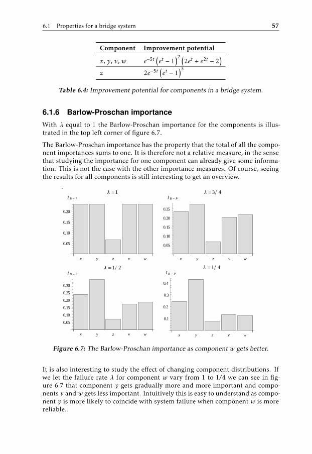
6.1 Properties for a bridge system 57
Component Improvement potential
x, y, v, w e−5t(et − 1
)2 (2et + e2t − 2
)z 2e−5t
(et − 1
)3
Table 6.4: Improvement potential for components in a bridge system.
6.1.6 Barlow-Proschan importance
With λ equal to 1 the Barlow-Proschan importance for the components is illus-trated in the top left corner of figure 6.7.
The Barlow-Proschan importance has the property that the total of all the compo-nent importances sums to one. It is therefore not a relative measure, in the sensethat studying the importance for one component can already give some informa-tion. This is not the case with the other importance measures. Of course, seeingthe results for all components is still interesting to get an overview.
x y z v w
0.05
0.10
0.15
0.20
I B - P
Λ = 1
x y z v w
0.05
0.10
0.15
0.20
0.25
I B - P
Λ = 3 � 4
x y z v w
0.05
0.10
0.15
0.20
0.25
0.30
I B - P
Λ = 1 � 2
x y z v w
0.1
0.2
0.3
0.4
I B - P
Λ = 1 � 4
Figure 6.7: The Barlow-Proschan importance as component w gets better.
It is also interesting to study the effect of changing component distributions. Ifwe let the failure rate λ for component w vary from 1 to 1/4 we can see in fig-ure 6.7 that component y gets gradually more and more important and compo-nents v and w gets less important. Intuitively this is easy to understand as compo-nent y is more likely to coincide with system failure when component w is morereliable.

58 6 Importance measures
6.1.7 Criticality importance
The criticality importance can be defined either by failure or success, as describedin definitions 2.55 and 2.56. The exact results are shown in table 6.5, and thenumerical plots in figure 6.8. As can be seen, the central component z is the least
Component Failure oriented Success oriented
x, y, v, w 2et+e2t−2et+2e2t+e3t−2
−4et+e2t+e3t+2−5et+2e2t+2e3t+2
z2(et−1)
et+2e2t+e3t−22(et−1)2
−5et+2e2t+2e3t+2
Table 6.5: Criticality importance for components in a bridge system.
1 2 3 4t
0.1
0.2
0.3
0.4
0.5
I CR - F H t L
z
x , y , v , w
1 2 3 4t
0.1
0.2
0.3
0.4
0.5
I CR - S H t L
z
x , y , v , w
Figure 6.8: Failure (left) and success oriented (right) criticality importancefor components in a bridge system.
important according to this measure, regardless if the success or failure orientedversion is used.
6.1.8 Fussell-Vesely importance
The Fussell-Vesely importance for the components are shown in table 6.6 andplotted in figure 6.9. This last importance measure is a probability of the compo-
Component Fussell-Vesely importance
x, y, v, wet(et+e2t−1)et+2e2t+e3t−2
z −3et+e2t+e3t+1et+2e2t+e3t−2
Table 6.6: The Fussell-Vesely importance for components in a bridge system.
nent having contributed to system failure, by being part of a failed minimal cutset when we know the system is failed. In this case, we can see that the compo-nent in the center, z, has a smaller probability of being in such a cut set of failure.This is not surprising, as the cut sets that contain the component z all contain

6.2 Comparison on a simple system 59
1 2 3 4t
0.2
0.4
0.6
0.8
1.0
I F - V H t L
z
x , y , v , w
Figure 6.9: Fussell-Vesely importance for components in a bridge system.
three components. These cut sets therefore have smaller risk of being the cut setcausing the system to fail, than the two cut sets containing only two components.
In this often studied case of the bridge system, all measures do agree on thatthe component z is not as important as the other components. For an engineerdesigning this system, that should give a clear indication that trying to improvethe reliability of the other components would be more worthwhile. In anotherscenario, the system may be part of a mission critical system, such as for examplea nuclear power plant, or an emergency communications network. Here it wouldmake sense to monitor the other components more closely, and replace or repairthem at first sign of failure.
6.2 Comparison on a simple system
In the previous section all importance measures agreed on the ranking of compo-nents. In this section we will show that this is not always the case. We considera simple system with three components, one in series with two in parallel, de-picted in figure 6.10. Let the components have exponential lifetime distributions,where the failure rates for x, y and z are 1/2, 1 and 10, respectively. We plot
Start x
y
z
End
Figure 6.10: rbd of a simple system.

60 6 Importance measures
the importance measures in figure 6.11. It can be immediately seen that the dif-ferent measure do not always agree. It is also true that the ranking for a singlemeasure changes depending on what time point we look at. The example alsoillustrates that the importance measures can be both a great help to understanda system that is complicated, but also pose a danger if used carelessly. Becausethe measures tell different things about the system and do not always agree, it isimportant to be aware of the meaning of the measure used.

6.2 Comparison on a simple system 61
x y z
0.1
0.2
0.3
0.4
0.5
0.6
0.7
I Φ
x y z
0.1
0.2
0.3
0.4
0.5
I B - P
0.2 0.4 0.6 0.8 1.0
0.2
0.4
0.6
0.8
1.0
I B
z
y
x
0.2 0.4 0.6 0.8 1.0
0.050.100.150.200.250.300.35
I IP
z
y
x
0.2 0.4 0.6 0.8 1.0
2
3
4
5
6
I RAW
z
y
x
0.2 0.4 0.6 0.8 1.0
1.5
2.0
2.5
3.0
3.5
4.0
I RRW
z
y
x
0.2 0.4 0.6 0.8 1.0
0.2
0.4
0.6
0.8
1.0
I CR - F
z
y
x
0.2 0.4 0.6 0.8 1.0
0.2
0.4
0.6
0.8
1.0
I CR - S
z
y
x
0.2 0.4 0.6 0.8 1.0
0.2
0.4
0.6
0.8
1.0
I F - V
z
y
x
Figure 6.11: All importance measures for a simple mixed system.


7RBD modeling
“The cheapest, fastest, and most reliable componentsare those that aren’t there.”
Gordon Bell
To enable manageable input of larger systems, a graph of the rbd should be pos-sible to use instead of a boolean expression. It is also useful to see a graphicalrepresentation of an entered boolean expression, to check for correctness, and tobetter understand the system structure. To this end we have implemented proto-types for converters from a boolean expression of a structure function to a rbdand vice versa.
7.1 Boolean expression to RBD
We approach this conversion in a structural way. We analyze the given expression,taking the “top”, outermost function, and apply the function recursively on thesubexpressions. Then we return the appropriate list of vertices and edges forgraph construction.
7.1 Example: Boolean to graph conversionConsider the structure function with the boolean representation x ∧ (y ∨ z). Thereliability block diagram of this is found by recursively going through the expres-sion as presented below. The function takes three arguments, an expression, astart vertex vs, and an end vertex ve.
1. Function is called with arguments {x ∧ (y ∨ z), vs, ve}
2. Divide into two branches, one for x, and one for (y ∨ z). The splitting func-tion is ∧, which is a serial connection. We create a mock vertex vj to jointhe two subexpressions with.
63

64 7 rbdmodeling
(a) Function is called with arguments {x, vs, vj }, and returns the vertices{vx, vs, vj } and edges {vs → vx, vx → vj }:
v s v x v j
(b) Function is called with arguments {y∨z, vj , ve}. Divide into two branches,one for y and one for z. The splitting function is ∨, so the start andend vertices for both calls will be the given ones.
i. Function is called with arguments {y, vj , ve}, and returns the ver-tices {vy , vj , ve} and edges {vj → vy , vy → ve}:
v j v y v e
ii. Function is called with arguments {z, vj , ve}, and returns the ver-tices {vz , vj , ve} and edges {vj → vz , vz → ve}:
v j v z v e
Combine the two returned results into vertices {vz , vy , vj , ve} and edges{vj → vy , vy → ve vj → vz , vz → ve}:
v j
v z
v y
v e
Combine the two results into vertices {vx, vy , vz , vj , ve} and edges {vs →vx, vx → vj , vj → vy , vy → ve, vj → vz , vz → ve}:

7.2 rbd to boolean expression 65
v s v jv x
v z
v y
v e
3. Finally short circuit the mock vertex vj to arrive at our final result in fig-ure 7.1.
v s v x
v z
v y
v e
Figure 7.1: rbd of simple mixed system.
This direction of conversion is interesting for the case where one has a largeboolean structure function. In that case, a reliability block diagram of the func-tion may give a cleaner more visual overview of the system and its configuration.
7.2 RBD to boolean expression
The prototype for converting graphs in rbd form to a boolean structure functionis based on a breadth first traversal.
7.2.1 Breadth-first traversal
First, a copy of the whole graph is created for storing the intermediate results.Then the graph is traversed breadth first. Each traversal through the graph keepsa list of previously visited vertices. On visiting a new vertex, this list is saved tothe vertex properties as a new possible path to get there from the start vertex. Ifa subset of the path is already stored at the vertex, this means that a shorter wayto get there has already been found. In that case, that branch of the traversal isstopped. Once all traversals have arrived at the end vertex, the set of paths foundat the end vertex, is a set of possible paths there. These sets of vertices are all

66 7 rbdmodeling
path vectors, as defined in definition 2.39. It is not guaranteed that these are theminimal path vectors. It is however guaranteed that all the minimal path vectorscan be found in this set of path vectors, although reduction may be necessary.The algorithm is illustrated in an example.
7.2 Example: Graph to boolean conversionLet us consider the rbd we created in example 7.1. We create a new copy of thegraph. We show the list of paths stored in each vertex in this table, which ofcourse starts out empty:vs vx vy vz ve{} {} {} {} {}
1. Now we start from the start vertex vs, and visit vx. This is the first vertexwe visit, so the path there is nonexistent. We add vx to our list of visitedvertices. We branch into two paths, in items 2 and 3 below.
v s v x
v z :8 <
v y :8 <
v e :8 <
2. Visiting vertex vy , we add our previously traveled path {vx} to the path listof vy . We also add vy to our list of visited vertices. It now contains {vx, vy}.
v s v x
v z :8 <
v y :8 8 v x < <
v e :8 <
vs vx vy vz ve{} {} {{vx}} {} {}
3. Visiting vertex vz , we add our previously traveled path {vx} to the path listof vz . We also add vy to our list of visited vertices. It now contains {vx, vz}.

7.2 rbd to boolean expression 67
v s v x
v z :8 8 v x < <
v y :8 8 v x < <
v e :8 <
vs vx vy vz ve{} {} {{vx}} {{vx}} {}
4. Continuing the path from point 2, we now visit the end vertex ve. There weadd our list of visited vertices:
v s v x
v z :8 8 v x < <
v y :8 8 v x < <
v e :8 8 v x , v y < <
vs vx vy vz ve{} {} {{vx}} {{vx}} {{vx, vy}}
5. Continuing the path from point 3, we now visit the end vertex ve. There weadd our list of visited vertices:
v s v x
v z :8 8 v x < <
v y :8 8 v x < <
v e :8 8 v x , v y < , 8 v x , v z < <

68 7 rbdmodeling
vs vx vy vz ve{} {} {{vx}} {{vx}} {{vx, vy}, {vx, vz}}
At the end vertex we now have a set of path vectors. To get from the start vertexto the end vertex, we can take any of these path vectors. This corresponds to an∨ operation. To follow a path, all vertices on it have to be functioning. This cor-responds to an ∧ operation. From this we can get the boolean structure function:
(vx ∧ vy) ∨ (vx ∧ vz) (7.1)
This is not the minimal representation of the given rbd. To achieve a smallerexpression, boolean conversions according to the rules in equation 3.6 can beapplied. The result for this simple case is then of course:
vx ∧ (vy ∨ vz) (7.2)

8Standby systems
“Nature laughs at the difficulties of integration.”
Pierre-Simon de Laplace
Standby systems are used for modeling the case where components are in a non-operating mode until the operating component fails. At that point these compo-nents take the operating components place.
The standby system is modeled as one standby component with a special standbydistribution for the lifetime. This standby distribution is dependent on the life-time distributions of the components it contains, but this is completely transpar-ent in the modeling of the rest of the system. On the system level, the wholestandby subsystem looks just like any other component with a lifetime distribu-tion.
There are a few different models with varying tractability which can be used.The ones of interest defined in the literature are the cold standby and the warmstandby. Both of these cases have two subcases with perfect and imperfect switch-ing to the standby components. We also study the more general case where bothwarm and cold components are allowed.
8.1 Cold standby
This is the simplest case of standby, where the components in standby do not failuntil switched on.
8.1.1 Cold standby with perfect switching
If we assume that the switching between components always works, the lifetimeof the system is the sum of the component lifetimes. As seen in definition 2.35,
69

70 8 Standby systems
the survival function is straightforward to define, but quickly becomes hard tocalculate. For the special case where all the components are exponentially dis-tributed, a much simpler expression can be derived.
8.1 Example: Cold standby with exponentially distributed componentsConsider a cold standby system with two components x1 and x2, with exponentiallifetime distributions with failure rates λ1 and λ2.
The survival function for this system can be found by definition:
Scold_standby_2(t) =S1(t) +
t∫0
f1(x)S2(t − x)dx =
=e−tλ1 +
t∫0
λ1e−xλ1e−(t−x)λ2dx
=λ1e
−tλ2
λ1 − λ2+λ2e
−tλ1 )λ2 − λ1
(8.1)
If expanded to the case with three components, where the third component x3has failure rate λ3:
Scold_standby_3(t) =S1(t) +
t∫0
f1(x1)S2(t − x1)dx1+
+
t∫0
f1(x1)
t−x1∫0
f2(x2)S3(t − x1 − x2)dx2dx1
=e−tλ1 +
t∫0
λ1e−x1λ1e−(t−x1)λ2dx1+
+
t∫0
λ1e−x1λ1
t−x1∫0
λ2e−x2λ2e−(t−x1−x2)λ3dx2dx1
=λ1λ2e
−tλ3
(λ1 − λ3) (λ2 − λ3)+
+λ3λ2e
−tλ1
(λ2 − λ1) (λ3 − λ1)+
+λ1λ3e
−tλ2
(λ1 − λ2) (λ3 − λ2)
(8.2)

8.1 Cold standby 71
The example can be extended to a general formula for n components:
Scold_standby_n(t) =n∑j=1
e−tλj∏i,j
λiλi − λj
(8.3)
This is the survival function of a hypoexponential distribution, as defined in def-inition 2.16.
As was the case for the reliability distribution, once the survival function isknown, other properties can be calculated with definitions. The mean also has aclosed form for the case where all components have exponential lifetime distribu-tions with failure rate λi :
µcold_standby_n =1∑ni=1 λi
(8.4)
After we found the above closed cases, a hypoexponential distribution was imple-mented in Mathematica, allowing us to fall back on that distribution for compu-tation of such systems.
For the case where all components in a cold standby system with perfect switch-ing have identical exponential lifetime distributions, the lifetime distribution ofthe system is an Erlang distribution. For a system with n components with failurerate λ, the shape parameter is n and the rate parameter is λ.
It can be interesting to see how two available components should be used for thehighest reliability.
8.2 Example: Comparison - Cold standby and parallelAssume we have two identical components available. We want to find out whichis better for reliability: a parallel configuration, or a cold standby configuration.A graph of the standby configuration is shown in figure 8.1. We assume that theswitch never fails. Let us assume that the components lifetimes are distributed
Start
x1
Switch Endx2
Figure 8.1: A standby system with one component (x2) in standby.
according to an Erlang distribution (see definition 2.11) with shape parameter 2

72 8 Standby systems
and rate parameter 4.
With the implementation of the equations above, the following two results arefound for the survival functions:
Sparallel(t) ={e−8t
(−4t + 2e4t − 1
)(4t + 1) t > 0
1 otherwise(8.5)
Sstandby(t) ={
13 e−4t
(4t
(8t2 + 6t + 3
)+ 3
)t > 0
1 otherwise(8.6)
As can be seen in figure 8.2, it is better to use a standby configuration than aparallel one.
0.0 0.5 1.0 1.5 2.0 2.5 3.0t
0.2
0.4
0.6
0.8
1.0SH t L
StandbyParallel
Figure 8.2: Survival functions for the parallel and standby configurations.
8.1.2 Cold standby with imperfect switching
This case can be modeled either with a probability of success for the switching tosucceed, or by seeing the switch as a component with a lifetime distribution ofits own.
Switch with probability of success
In this case, a principal component has several components in standby, waitingto replace the principal component when it fails. The components in standbycannot fail while they are in standby. However, on failure of an operating compo-nent, the switch to the next component succeeds only with a probability p. If theswitch does not succeed, the system is seen as failed.
8.3 Example: Cold standby with probability modeled switchConsider a cold standby system with two components x1 and x2, with exponen-tial lifetime distributions with failure rates λ1 and λ2. On the failure of the com-ponent x1, component x2 is used with probability p, representing the switch be-tween them.

8.1 Cold standby 73
The survival function for this system can be found as follows:
Scold_standby_2_p(t) =S1(t) + p
t∫0
f1(x)S2(t − x)dx =
=e−tλ1 + p
t∫0
λ1e−xλ1e−(t−x)λ2dx
=e−tλ1 −λ1p
(e−tλ1 − e−tλ2
)λ1 − λ2
(8.7)
The probability of two switchings in a row succeeding is p2. If we expand to thecase with three components, where the third component x3 has failure rate λ3,this gives:
Scold_standby_3_p(t) =S1(t) + p
t∫0
f1(x1)S2(t − x1)dx1+
+ p2
t∫0
f1(x1)
t−x1∫0
f2(x2)S3(t − x1 − x2)dx2dx1
=e−tλ1 + p
t∫0
λ1e−x1λ1e−(t−x1)λ2dx1+
+ p2
t∫0
λ1e−x1λ1
t−x1∫0
λ2e−x2λ2e−(t−x1−x2)λ3dx2dx1
=e−tλ1−
−λ1p
(e−tλ1 − e−tλ2
)λ1 − λ2
+λ1λ2p
2(e−tλ1−e−tλ2λ1−λ2
− e−tλ1−e−tλ3λ1−λ3
)λ2 − λ3
(8.8)
Let us study how much worse a standby system becomes by having a non-perfectswitch.
8.4 Example: Perfect and imperfect switchingAssume we have two components, x1 and x2. Let x1 be the first component, andx2 a component in standby to x1. Also let x1 have an exponential lifetime distri-bution with failure rate 1, and x2 a Weibull distribution with shape parameter 2and scale parameter 4. Finally, assume the switch works with a probability p.

74 8 Standby systems
The exact symbolic result is long and therefore not presented here. The result isinstead shown as a plot in figure 8.3. As expected, the perfect system is the best,and it gets worse with a lower probability of success for the switch.
0 2 4 6 8 10 12t
0.2
0.4
0.6
0.8
1.0SH t L
p = 0.4
p = 0.6
p = 0.8Perfect
Figure 8.3: Survival functions for the case with perfect standby, and for afew values of switch success probability.
Switch with a lifetime distribution
Another model of the switching between components, is to see the switch as acomponent in itself, with its own lifetime distribution. In the same way as inexample 2.34, the survival function can be found by enumerating all cases andcalculating their probability. With SS (t) as the survival function for the switch,the result for n components follows:
Scold_standby_n_d(t) = S1(t) +
t∫0
f1(x1)SS (x1)S2(t − x1)dx1+
+
t∫0
f1(x1)
t−x1∫0
f2(x2)SS (x1 + x2)S3(t − x1 − x2)dx2dx1 + · · ·
+
t∫0
f1(x1)
t−x1∫0
f2(x2) · · ·
· · ·t−x1−x2−···−xn−2∫
0
fn−1(xn−1)SS
n−1∑i=1
xi
Snt − n−1∑
i=1
xi
dxn−1 · · ·dx2dx1
(8.9)

8.2 Warm standby 75
8.2 Warm standby
In the case of warm standby, the components can fail while in standby. These fail-ures are modeled by a lifetime distribution while in standby, and another whileoperating.
8.2.1 Warm standby with perfect switching
Let us first look at the case where the switching between components alwaysworks. The following example illustrates the model:
8.5 Example: Warm standby with perfect switchingConsider a standby system with one component x2 in standby to a component x1.The system is illustrated in figure 8.4. We assume that the switch always works.
Start
x1
Switch Endx2
Figure 8.4: A standby system with one component (x2) in standby.
Let the lifetime of x1 be distributed exponentially with a failure rate λ. Finally,let component x2 have failure rate λs while in standby, and λ while operating.
We can now calculate the survival function by enumerating the possible caseswhere the system survives until time t:
• The first component survives until time t
• The first component survives until time x, the second component surviveswhile in standby until time x, and the second component survives in opera-tion for t − x
These cases are independent, and therefore we can add the probability for themto get the survival function at time t. In an equation this gives:
Swarm_standby_2(t) =Sx1(t) +
t∫0
fx1(x)Sx2s(x)Sx2o(t − x)dx =
=
e−t(λ+λs )((λ+λs)etλs−λ)λs
t > 01 otherwise
(8.10)

76 8 Standby systems
We can compare this to the same system with cold standby to see how much thereliability suffers from the component failing in standby. This is done for λ = 2and λs = 1 in figure 8.5.
0 1 2 3 4t
0.2
0.4
0.6
0.8
1.0SH t L
ColdWarm
Figure 8.5: Survival functions for warm and cold standby.
Expanding the reasoning from the example to the case with n components istricky to write in a closed form. This is because the number of cases increaserapidly, as we need to consider cases where standby components fail before theyare switched into operation. In interest of brevity, only the case for n = 3 is givenhere:
Swarm_standby_3(t) = S1(t) +
t∫0
f1(x1)S2,s(x1)S2,o(t − x1)dx1+
+
t∫0
f1(x1)S2,s(x1)
t−x1∫0
f2,o(x2)S3,s(x1 + x2)S3,o(t − x1 − x2)dx2dx1+
+
t∫0
f1(x1)F2,s(x1)S3,s(x1)S3,o(t − x1)dx1
(8.11)
The first three terms follow from the reasoning in the example. The last term isthe case where the second component fails in standby before the first, so only thefirst and third components are used. These extra terms are the ones which growquickly in number as n gets larger.
We have developed closed forms for two cases of warm standby with perfectswitching. For the first case, we assume that all distributions have an exponen-tial lifetime distribution, with the same failure rate λ both in standby and whileoperating. In this case, the survival function for n components becomes:
S(t) = 1 − e(−ntλ)(etλ − 1)n (8.12)
For the more general case where all n components have failure rate λs in standby

8.2 Warm standby 77
and λ while operating, the following is the survival function:
S(t) = e−tλ +n∑i=2
e−t((i−1)λs+λ)(etλs − 1)i−1 ∏i−2k=0 λ + kλs
(i − 1)!λi−1s
(8.13)
We have also found a closed form for the moment of this case. The kth momentis:
µ′k =
∏nq=1 (λ + qλs)
λns n!
n∑m=0
((nm
)(−1)m
k!λ(λ + mλs)k+1
)(8.14)
A special case of this is of course the mean:
µ = µ′1 =
∏nq=1 (λ + qλs)
λns n!
n∑m=0
((nm
)(−1)m
λ
(λ + mλs)2
)(8.15)
These special cases allow for very fast computation of the given properties.
8.2.2 Warm standby with imperfect switching
As we did for the cold standby case, we can study warm standby where the switch-ing between the components can fail. Again, the switch can be modeled with aprobability of success on each switch, or as a component with a lifetime distribu-tion.
Switch with probability of success
In this case, as for the version of cold standby, each switch to a new componenthas a probability of success p. The general case again becomes large, so the casewhere n = 3 is presented:
Swarm_standby_3_p(t) = S1(t) + p
t∫0
f1(x1)S2,s(x1)S2,o(t − x1)dx1+
+p2
t∫0
f1(x1)S2,s(x1)
t−x1∫0
f2,o(x2)S3,s(x1 + x2)S3,o(t − x1 − x2)dx2dx1+
+p2
t∫0
f1(x1)F2,s(x1)S3,s(x1)S3,o(t − x1)dx1
(8.16)
Switch with a lifetime distribution
With the same approach as previously, where we enumerate all possible cases,we can calculate a result for the general case with n components. However, thisresult is even larger than the case with perfect switching. Therefore we again

78 8 Standby systems
only show the case where n = 3. With the switch survival function SS (t) we get:
Swarm_standby_3_d(t) = S1(t) +
t∫0
f1(x1)S2,s(x1)SS (x1)S2,o(t − x1)dx1+
+
t∫0
f1(x1)S2,s(x1)
t−x1∫0
f2,o(x2)S3,s(x1 + x2)SS (x1 + x2)S3,o(t − x1 − x2)dx2dx1+
+
t∫0
f1(x1)F2,s(x1)S3,s(x1)SS (x1)S3,o(t − x1)dx1
(8.17)
Now we can compute properties for all the basic cases. It is interesting to com-pare the four systems in an example.
8.6 Example: Comparison - Warm and cold, perfect and imperfect switchingConsider a standby system with two components x2 and x3 in standby to a compo-nent x1. The system is illustrated in figure 8.6. We want to compare the following
Start
x1
Switch
Endx2
x3
Figure 8.6: A standby system with two components in standby.
four cases:
• Cold standby, perfect switching (CP)
• Cold standby, imperfect switching with a lifetime distribution (CI)
• Warm standby, perfect switching (WP)
• Warm standby, imperfect switching with a lifetime distribution (WI)
Let the component xi have an exponential lifetime distribution with a failure rateof 1. Similarly, let x2 and x3 have operating failure rates of 2 and 3 respectively.Let their failure rates while in standby be 1/2 and 1/3 where applicable. Finally,let the switch have a constant failure rate of 1/5 in the cases with imperfect switch-ing. We can then find the survival functions as previously shown. The survival

8.2 Warm standby 79
functions are illustrated in figure 8.7. As we can see, the cold standby is better
0 1 2 3 4 5t
0.2
0.4
0.6
0.8
1.0SH t L
WI
WP
CI
CP
Figure 8.7: Survival functions for warm and cold standby, with perfect andimperfect switching.
than warm standby, and perfect switches are better than imperfect switches. Thisis intuitively correct, as cold standby is a special case of warm standby, where thefailure rate in standby is 0. In this example, it is also true that the cold standby
0 1 2 3 4 5t
0.2
0.4
0.6
0.8
1.0SH t L
WI
WP
CI
CP
Figure 8.8: Survival functions for warm and cold standby, with low reliabil-ity switch and perfect switching.
system with imperfect switching is better than the warm standby system withperfect switching. This is however not true in general. For example, if the switchhad a very short lifetime, the cold standby case with imperfect switching wouldbe worse than the warm standby case. This is shown in figure 8.8, where theswitch has been given a failure rate of 5.

80 8 Standby systems
Another interesting property shown in figure 8.8 is that both cases with imperfectswitching are almost identical. This is because if the switch fails fast, the wholesystem lifetime will be equal to the lifetime of component x1.
8.2.3 Mixed standby
A natural generalization of the previously presented warm and cold standby mod-els, is to allow mixing of components that can fail while in standby, with compo-nents that do not fail while in standby. As is to be expected, this results in ratherlarge expressions of integrals, which do not lend themselves well to be presentedin printed form. Our software implementation in Mathematica can handle arbi-trary mixtures and sizes of this most general case. We limit ourselves to presenta small example to show the principle.
8.7 Example: Mixed standby with three componentsConsider a standby system with a principal component x1, one warm componentx2, and a cold component x3. The system is illustrated in figure 8.9. Let the
Start
x1
Switch
Endx2
x3
Figure 8.9: A standby system with two components in standby.
switch succeed with probability p each time it is invoked. We can find the sur-vival function by adding together the probability for all the possible cases wherethe system survives until time t. The cases are:
1. x1 survives until time t
2. x1 survives until time s1, x2 survives until s1 in standby, the switch succeeds,and x2 then survives for time t − s1
3. x1 survives until time s1, x2 survives until s1 in standby, the switch succeeds,x2 survives for time s2, the switch succeeds again, and x3 survives for timet − s1 − s2
4. x1 survives until time s1, the second component has failed in standby befores1, the switch to x2 succeeds, the switch to x3 succeeds, and x3 survives fort − s1

8.2 Warm standby 81
The probability for each case follows:
1. S1(t)
2. p∫ t
0 f1(s1)S2s(s1)S2(t − s1)
3. p2∫ t
0 f1(s1)S2s(s1)∫ t−s1
0 f2(s2)S3(t − s1 − s2)
4. p2∫ t
0 f1(s1)F2s(s1)S3(t − s1)
For a specific numeric case, let the component xi have exponential lifetime distri-butions with failure rates of 1, 1 and 3 for x1, x2 and x3 respectively. Also let x2have a failure rate of 2/3 while in standby. Finally, assume that the switch works95 percent of the time. The survival function then is:
Smixed(t) =
e−3t(−10089e4t/3+11446e2t+1843)3200 t > 0
1 otherwise(8.18)
An interesting example is to compare this to the survival function when the sec-ond and third component switch places. This would mean that when x1 fails, thecold component takes its place first, and then the warm component. The survivalfunction is found by the same reasoning as above:
Smixed_2(t) =
e−11t/3(−3040e2t/3−12996e2t+19187e8t/3+3249)6400 t > 0
1 otherwise(8.19)
0 1 2 3 4t
0.2
0.4
0.6
0.8
1.0SH t L
cold first
warm first
Figure 8.10: Comparison between order of components in mixed standby.
As can be seen in figure 8.10, the system with the warm standby first is morereliable. This is intuitively correct, as it has less time to fail while in standby.
With the implementation in Mathematica we can calculate all the properties wecan for the reliability distribution, as shown in table A.1.

82 8 Standby systems
8.3 Applications
The standby model presented in the sections can be directly applied to real lifeapplications.
8.8 Example: Power supply standby modelConsider a power supply system that has two components. The primary powercomes from a normal power network. In addition to that, a battery is keptcharged and is used if necessary. All lifetime distributions follows the exponen-tial distribution.
Start
Net
Switch EndBattery
Figure 8.11: Power supply standby system.
Let us assume that the switch always succeeds. Also assume that the power fromthe net is highly reliable with a failure rate with parameter 1/400 days, and thatthe battery has a failure rate of 1/50 days. The survival function is shown infigure 8.12.
0 200 400 600 800 1000t
0.2
0.4
0.6
0.8
1.0SH t L
Figure 8.12: Survival function for power supply standby system.

8.3 Applications 83
Start
Net
Switch
EndBattery
Generator
Figure 8.13: Power supply standby system with generator.
We now contemplate if we want to buy a diesel generator to improve the relia-bility. The generator we are thinking about buying has a failure rate of 1/150days. The new system is shown in figure 8.13, and both survival functions infigure 8.14. We can see that the reliability is much higher for the system with thegenerator.
0 200 400 600 800 1000t
0.2
0.4
0.6
0.8
1.0SH t L
Generator
No generator
Figure 8.14: Survival function for power supply standby with generator.
We can also model mixes of standby systems and general systems. We show thisin an example that studies the reliability of a computer server.

84 8 Standby systems
8.9 Example: Computer serverIn this example we model a computer server. Such a server requires a powersupply, hard drives, a network card, and a network router to fulfill it’s intendedfunction. The power supply is backed by a battery and a diesel generator. Letus assume the distributions from example 8.8. The power subsystem is shown infigure 8.13.
The hard drives are arranged in a RAID, which requires 2 out of 3 of them towork. Their respective lifetimes are modeled by a lognormal distribution withparameters 4 and 1.
The network card has a second card in standby, both distributed according tothe Weibull distribution with the shape parameter 1 and scale parameter 3. Thissubsystem is shown in figure 8.15.
Start
net1
Switch Endnet2
Figure 8.15: Network subsystem.
Two routers are connected in parallel, both with exponentially distributed life-times with failure rate 1/4.
Start power hdd1
hdd1
hdd2
hdd2
hdd3
hdd3
network
router1
router2
End
Figure 8.16: rbd for a computer server.
The complete system is shown in figure 8.16. The plot of the survival function isshown in figure 8.17.
We also find the mean time to failure (given in months):
µ ≈ 3.70535 (8.20)

8.3 Applications 85
0 2 4 6 8 10t
0.2
0.4
0.6
0.8
1.0SH t L
Figure 8.17: Survival function for a computer server.
We finally compare with a version where all redundancy has been removed. Bothsurvival functions are shown in figure 8.18.
0 2 4 6 8 10t
0.2
0.4
0.6
0.8
1.0SH t L
No redundancy
Redundancy
Figure 8.18: Survival function comparison for computer servers.
We can see from the survival function plot that the reliability is considerablyworse in a consumer grade computer with no redundancy. The mean time tofailure is lower as well:
µconsumer ≈ 1.70406 (8.21)


9Conclusions and future work
“We can only see a short distance ahead, but we can see plenty therethat needs to be done.”
Alan Turing
The purpose of this thesis was to implement functionality covering the basics inthe reliability field, and to then study how Mathematica can be used as a frame-work to extend the area of possible computation. In this chapter we discuss ourresults and present suggestions for future work in the field.
9.1 Conclusions
We implemented very general functionality for computing properties for systemsthat are studied in reliability. This includes both the complex systems of compo-nents where the structure is defined by a boolean function, and standby wherethe components are put into operation one after the other. With this implemen-tation, we can compute a vast majority of these kind of textbook examples in anefficient way. However our implementation is not limited to such small systemsas are presented in textbooks. It is also not limited to the exponential distributionthat is most often used both in textbooks and in real world reliability computa-tions.
For the standby system case, we have developed a general implementation thatcan handle both cold standby components, warm standby components, and anymix thereof. To our knowledge, no results from mixing cold and warm standbycomponents have previously been published.
Another area which we have covered is importance measures for complex systemsof components. Here we have implemented a wide selection of measures that areused in the reliability field.
87

88 9 Conclusions and future work
Finally, we have developed prototypes for converting reliability block diagramsto boolean expressions and vice versa. This is useful to give an overview of largesystems, and to enable graphical input to the previously mentioned functionality.
9.2 Future work
Although we have covered a fair part of the basics in the reliability field, thereare many areas for further explorations and extensions. Here we present someinteresting areas for possible continuations in development and research.
9.2.1 Graph editor
To make input of large complex systems more convenient, a possible future ap-proach is to allow an rbd object to be used as an input. Theoretically, this objectcould then contain the full model of the system, including the component distri-bution. For this, a number of things would need to be done. For example, wewould need a way to convert back and forth between the boolean structure func-tion and the rbd model efficiently, such as the prototypes in chapter 7. The userwould also need a user friendly way to input and edit this rbd model, so somekind of editor would be useful.
9.2.2 Special system structures
There are a family of previously studied systems, such as the consecutive-k-out-of-n systems, for which special closed form results exist. Incorporating these intoour design would improve computation speed and ease of modeling for thesespecific systems [Hwang, 1982][Antonopoulou and Papastavridis, 1987], as wellas give opportunity to extend previously presented closed form results. It wouldalso make calculating importance measures faster [Kuo et al., 1990].
9.2.3 Repairable systems
A whole branch of systems that can be modeled are repairable systems. Thesetake into account that a component that breaks, can be repaired and replaced.This can happen either while the system is offline, or while it is running, de-pending on the system. To model this, different type of stochastic processes areprimarily used [Barlow and Proschan, 1965, p. 119].
9.2.4 Censored data
To model the component distributions, it would be useful to use censored dataobtained from for example testing or customer reports of failures.
9.2.5 Dependent lifetime distributions
Component lifetimes may be dependent on each other. An intuitive example ofthis would be the cables on a bridge. When one breaks, the load on the othercables is increased, which may impact their lifetime [Bedford and Cooke, 2001,pp. 140 - 152].

9.2 Future work 89
9.2.6 Accelerated life
To get an estimate of component lifetimes, manufacturers often do acceleratedtesting. In practice, this often means that the component is put into an envi-ronment or handled in such a way as to simulate a normal lifetime in a shortertime span [Tobias and Trindade, 1994, p. 166]. The results from this testing canthen be modeled in different ways to arrive at an estimate for the lifetime duringnormal operating conditions.
9.2.7 Real world reliability data verification
We have found a few real world data sources with system definitions, but themajority of such data is kept secret by the companies that go to the trouble ofcreating it. If more data were to be found, it would be interesting to see how ourimplementation copes with it. What would be especially interesting would belarge real world systems.


AComputable properties
Distribution properties
cdf Log likelihoodCentral moment generating function MeanCentral moment MedianCharacteristic function mgfCumulant generating function Probability (including conditional)Cumulant Quantile plotExpectation QuantileFactorial moment generating function Quartile deviationFactorial moment Quartile skewnessHazard function QuartilesInterquartile range Random variablesInverse cdf SkewnessInverse survival function Standard deviationKurtosis Survival functionLikelihood Variance
Table A.1: Distribution properties that can be calculated.
91


BAirplane cockpit system
In this chapter we present the structure and the related lifetime distributions forthe information system in an airplane cockpit. It was first presented in a reportfrom NASA [Pettit and Turnbull, 2001, Appendix A].
B.1 System presentation
B.1.1 RBD
A reliability block diagram of the system is shown in figure B.1. A translation ofnumbers to event names is given in table B.1.
B.1.2 Structure function
The boolean expression for the structure function of the system follows:
(30 ∨ (9 ∧ 26 ∧ 31 ∧ 13)) ∧ 8 ∧ 22 ∧ 10 ∧ 6 ∧ 25 ∧ 17 ∧ 14 ∧ 7 ∧ 32∧((33 ∧ 35 ∧ 34) ∨ (1 ∧ 3 ∧ 2)) ∧ 24 ∧ 18 ∧ 15 ∧ 16 ∧ 21 ∧ 20 ∧ 12 ∧ 11 ∧ 28 ∧ 29
(B.1)
B.1.3 Basic events
The basic events of the system are given in table B.1. The event numbers are theones given in the rbd in figure B.1. The event names given are shortened versionsof the names given in the original source. The third column is the parameter forthe exponential lifetime distribution of the event, where the measure of time isin hours.
Event number Event name λ
1 ADF Antenna 1/40002 ADF Display 1/199003 ADF Receiver 1/4200
93

94 B Airplane cockpit system
Event number Event name λ4 Airspeed Indicator 1 1/181005 Airspeed Indicator 2 1/25006 Alternator 1/76007 Altimeter 1/55008 Ammeter Vacuum Pressure 1/215009 Attitude Indicator 1/250010 Clock 1/1760011 Comm Antenna 1/120012 Comm Radio 1/90013 Directional Gyro 1/340014 Fuel Quantity Indicator 1/1650015 GS Antenna 1/90016 ILS Display 1/1000017 Left Fuel Quantity Transduce 1/5140018 LOC Antenna 1/90019 Magnetic Comp 1/1990020 Marker Beacon Antenna 1/1480021 Marker Beacon Receiver 1/530022 Oil Temp Pressure Gauge 1/620023 Pilot System 1/7360024 Receiver 1/1000025 Right Fuel Quantity Transduce 1/5140026 Suction Gauge 1/2150027 Tachometer 1/840028 Transponder 1/170029 Transponder Antenna 1/950030 Turn Coordinator 1/210031 Vacuum Pump 1/400032 Vertical Speed Indicator 1/14500033 VOR Antenna 1/960034 VOR Display 1/1000035 VOR Receiver 1/900
Table B.1: Event numbers, names and lifetime distributions for cockpit in-formation system.

B.1 System presentation 95
30 926
3113
822
106
2517
147
3233
3534
13
224
1815
1621
2012
1128
29s
e
Figure B.1: rbd representation of cockpit information system.


CElectrical diesel generator system
This is the system description for the diesel generator system for a nuclear powerplant. It was first presented by Dulik in his Masters Thesis [Dulik, 1996, Ap-pendix A]. This chapter serves to present the system configuration and the life-time distributions for the components. Results from computations on this systemcan be found in section 4.3.1.
C.1 System presentation
As the system is large, the fault tree or the reliability block diagram would takea lot of space to present. We therefore only show the boolean structure function.The fault tree is available in the original source [Dulik, 1996, Appendix A].
97

98 C Electrical diesel generator system
C.1.1 Structure function
The boolean expression for the system follows:
((e5 ∧ e88) ∨ (e85 ∧ e87 ∧ e84 ∧ e81 ∧ e80 ∧ e83)) ∧ e82 ∧ e86 ∧ e16 ∧ e29∧e14 ∧ e66 ∧ e18 ∧ e26 ∧ (e109 ∨ ((e104 ∨ (e106 ∧ e107 ∧ e100 ∧ e90 ∧ e97 ∧ e102∧e92 ∧ e108 ∧ e16 ∧ e29 ∧ e14 ∧ e66 ∧ e18 ∧ e26 ∧ e72 ∧ e77 ∧ e4 ∧ ((e74∧e79) ∨ (e1 ∧ e2 ∧ e3)) ∧ e76 ∧ e111 ∧ e96)) ∧ ((e106 ∧ e107 ∧ e100 ∧ e90 ∧ e97∧e102 ∧ e92 ∧ e108 ∧ e94) ∨ e5 ∨ (e99 ∧ e89 ∧ e98 ∧ e91 ∧ e101 ∧ e105 ∧ e104))))∧(e110 ∨ ((e107 ∨ (e103 ∧ e104 ∧ e99 ∧ e89 ∧ e98 ∧ e91 ∧ e101 ∧ e105 ∧ e16 ∧ e29∧e14 ∧ e66 ∧ e18 ∧ e26 ∧ e72 ∧ e77 ∧ e4 ∧ ((e74 ∧ e79) ∨ (e1 ∧ e2 ∧ e3))∧e76 ∧ e111 ∧ e95)) ∧ (e5 ∨ (e103 ∧ e104 ∧ e99 ∧ e89 ∧ e98 ∧ e91 ∧ e101 ∧ e105∧e93) ∨ (e100 ∧ e90 ∧ e97 ∧ e102 ∧ e92 ∧ e108 ∧ e107)))) ∧ ((e120 ∧ e113 ∧ e112 ∧ e116∧e118 ∧ e115 ∧ e114 ∧ e117 ∧ e16 ∧ e29 ∧ e14 ∧ e66 ∧ e18 ∧ e26 ∧ e72 ∧ e77∧e4 ∧ ((e74 ∧ e79) ∨ (e1 ∧ e2 ∧ e3)) ∧ e76) ∨ e5) ∧ e119 ∧ e27 ∧ e10 ∧ (e109∨(e6 ∧ e11 ∧ e8) ∨ (e106 ∧ e107 ∧ e100 ∧ e90 ∧ e97 ∧ e102 ∧ e92 ∧ e108 ∧ e72∧e77 ∧ e4 ∧ ((e74 ∧ e79) ∨ (e1 ∧ e2 ∧ e3)) ∧ e76 ∧ e16 ∧ e29 ∧ e14 ∧ e66∧e18 ∧ e26 ∧ ((e111 ∧ e96) ∨ e121))) ∧ (e110 ∨ (e7 ∧ e12 ∧ e9) ∨ (e103 ∧ e104 ∧ e99∧e89 ∧ e98 ∧ e91 ∧ e101 ∧ e105 ∧ e72 ∧ e77 ∧ e4 ∧ ((e74 ∧ e79) ∨ (e1 ∧ e2∧e3)) ∧ e76 ∧ e16 ∧ e29 ∧ e14 ∧ e66 ∧ e18 ∧ e26 ∧ ((e111 ∧ e95) ∨ e121))) ∧ e25∧e17 ∧ e73 ∧ e78 ∧ e74 ∧ e79 ∧ e76 ∧ e74 ∧ e79 ∧ e72 ∧ e77 ∧ e76 ∧ ((e56∧e55 ∧ e53 ∧ e19) ∨ (e58 ∧ e57 ∧ e54 ∧ e20)) ∧ e70 ∧ e71 ∧ e28 ∧ e15 ∧ e26∧e14 ∧ e66 ∧ e18 ∧ e27 ∧ e64 ∧ e65 ∧ e67 ∧ e46 ∧ e45 ∧ e36 ∧ e22 ∧ e47∧e49 ∧ e48 ∧ e37 ∧ e23 ∧ e50 ∧ e28 ∧ e15 ∧ e26 ∧ e14 ∧ e66 ∧ e18 ∧ e27∧e42 ∧ e40 ∧ e41 ∧ e43 ∧ e21 ∧ e61 ∧ e33 ∧ ((e59 ∧ e32) ∨ (e63 ∧ e35)) ∧ e38∧e69 ∧ e68 ∧ e39 ∧ e13 ∧ e62 ∧ e34 ∧ e31 ∧ e24 ∧ e60 ∧ e30 ∧ e51 ∧ e74∧e79 ∧ e75 ∧ e76 ∧ e52
(C.1)
C.1.2 Basic events
Table C.1 shows the distribution parameter of the different events. The givenevent number corresponds to the event numbers specified in the original source.The measure of time for the system is years, and the lifetime distributions areexponential.
Event number λ
e1 7/1000000e2 19/12500000e3 19/12500000

C.1 System presentation 99
Event number λe4 1/5000000e5 1e6 53/625000000e7 53/625000000e8 7/50000000e9 7/50000000e10 1/31250e11 53/625000000e12 1/31250e13 1/500e14 19/12500000e15 19/12500000e16 19/12500000e17 79/500000e18 19/12500000e19 169/500000e20 169/500000e21 19/12500000e22 169/500000e23 169/500000e24 169/500000e25 79/500000e26 1/5000000e27 1/5000000e28 1/5000000e29 1/5000000e30 1/5000000e31 27/200000e32 27/200000e33 27/200000e34 27/200000e35 27/200000e36 27/200000e37 27/200000e38 11/1000e39 41/2500e40 1/250e41 1/250e42 1/250e43 1/250e45 789/100000000e46 121/250000e47 283/500000

100 C Electrical diesel generator system
Event number λe48 789/100000000e49 121/250000e50 283/500000e51 1/2000000e52 1/50000e53 1/100000e54 1/100000e55 1/40000e56 1/500e57 1/40000e58 1/500e59 1/10000e60 1/10000e61 1/10000e62 1/10000e63 1/10000e64 1/10000000e65 1/10000000e66 3/2500000e67 1/5000e68 1/500e69 41/2500e70 1/40000e71 1/500e72 19/12500000e73 19/12500000e74 19/12500000e75 19/12500000e76 1/5000000e77 1/5000000e78 1/5000000e79 1/2000e80 169/500000e81 1/500e82 789/100000000e83 121/250000e84 1/5000e85 1/500e86 789/100000000e87 121/250000e88 1e89 169/500000e90 169/500000

C.1 System presentation 101
Event number λe91 169/500000e92 169/500000e93 27/200000e94 27/200000e95 27/200000e96 27/200000e97 1/5000e98 1/5000e99 1/5000e100 1/5000e101 1/250e102 1/250e103 11/1000e104 1/31250e105 3/1250e106 9/10000e107 1/31250e108 3/1250e109 1e110 1e111 1/5000e112 1/5000e113 1/5000e114 1/5000e115 1/5000e116 1/250e117 1/250e118 3/1250e119 1/31250e120 3/1250e121 1
Table C.1: Event numbers and lifetime distributions for nuclear power plantdiesel generator system.

102 C Electrical diesel generator system

Bibliography
Ira Antonopoulou and Stavros Papastavridis. Fast recursive algorithm to evaluatethe reliability of a circular consecutive-k-out-of-n:f system. IEEE Transactionson reliability, R-36(1):83,84, 1987. Cited on page 88.
Richard E. Barlow and Frank Proschan. Mathematical Theory of Reliability. JohnWiley & Sons, Inc., first edition, 1965. Cited on pages 1 and 88.
Tim Bedford and Roger Cooke. Probabilistic Risk Analysis - Foundations andMethods. Cambridge University Press, first edition, 2001. Cited on page 88.
Armin Biere and Carla P. Gomes. Theory and Applications of Satisfiability Test-ing - SAT 2006. Springer, first edition, 2006. Cited on page 11.
Z.W. Birnbaum. On the importance of different components in a multicomponentsystem. Laboratory of Statistical Research, University of Washington, pages 1–24, 1968. Cited on page 19.
Jeffrey D. Dulik. Use of performance-monitoring to improve reliability of emer-gency diesel generators. Department of Nuclear Engineering, MassachusettsInstitute of Technology, 1996. Cited on pages 45, 46, and 97.
J.B. Fussell. How to hand-calculate system reliability and safety characteristics.IEEE Transactions on Reliability, R-24(3):169–174, 1975. Cited on page 22.
John Graunt. Natural and Political Observations Made upon the Bills of Mortality.Dicas, at the Sign of the Bell in St. Paul’s Church-yard, first edition, 1662. URLhttp://www.edstephan.org/Graunt/bills.html. Cited on page 1.
Frank Hwang. Fast solutions for consecutive-k-out-of-n: F system. IEEE Transac-tions on reliability, R-31(5):447–448, 1982. Cited on page 88.
Way Kuo and Ming J. Zuo. Optimal Reliability Modeling, Principles and Appli-cations. John Wiley & Sons, Inc, first edition, 2002. Cited on pages 13 and 15.
Way Kuo, Weixing Zhang, and Mingjian Zuo. A consecutive-k-out-of-n:g system:The mirror image of a consecutive-k-out-of-n:f system. IEEE Transactions onreliability, 39(2), 1990. Cited on page 88.
103

104 Bibliography
Lawrence M. Leemis. Reliability, Probabilistic Models and Statistical Methods.second edition, 2009. Cited on pages 6, 13, 27, and 39.
Mohammad Modarres, Mark Kaminskiy, and Vasiliy Krivtsov. Reliability Engi-neering and Risk Analysis, A Practical Guide. CRC Press, second edition, 2010.Cited on page 21.
Bent Natvig and Jørund Gåsemyr. New results on the barlow-proschan andnatvig measures of component importance in nonrepairable and repairablesystems. Methodology and Computing in Applied Probability, 11(4):603–620,2009. Cited on page 19.
Duane Pettit and Andrew Turnbull. General aviation aircraft reliability study.NASA, CR-2001-210647, 2001. Cited on pages 43 and 93.
Marvin Rausand and Arnljot Høyland. System Reliability Theory, Models, Statis-tical Methods, and Applications. John Wiley & Sons, Inc, second edition, 2004.Cited on page 20.
J.H. Saleh and K. Marais. Highlights from the early (and pre-) history of reliabilityengineering. Reliability Engineering & System safety, 91(1), 2006. Cited onpage 1.
Sam C. Saunders. Reliability, Life Testing, and Prediction of Service Lives.Springer, first edition, 2010. Cited on page 6.
Claude Elwood Shannon. A symbolic analysis of relay and switching circuits.Transactions, American Institute of Electrical Engineers, 57:713–723, 1938.Cited on page 29.
Paul A. Tobias and David C. Trindade. Applied Reliability. Chapman &Hall/CRC, second edition, 1994. Cited on page 89.
W.E. Vesely. A time-dependent methodology for fault tree evaluation. NuclearEngineering and Design, 13(2):337–360, 1970. Cited on page 22.
Waloddi Weibull. A statistical distribution function of wide applicability. ASMEJournal of Applied Mechanics, 1951. Cited on page 7.
Wolfram Research. Introduction to Patterns. http://reference.wolfram.com/mathematica/tutorial/Introduction-Patterns.html, 2011.[Online; accessed 2011-03-15]. Cited on page 26.

Index
2-out-of-3 system, 36
accelerated life, 89adjacency matrix
definition, 16airplane, 43airplane cockpit, 27, 42, 93
Barlow-Proschan importance, 57definition, 21
Bernoulli variable, 27Birnbaum importance, 54
definition, 19boolean simplification, 28, 68breadth-first traversal, 65bridge system, 38, 53
ccdfabbreviation, xiii
cdf, 42abbreviation, xiiidefinition, 4
censoring, 88central moment, 49
definition, 9central moment-generating function, 50
definition, 10characteristic function, 50
definition, 10cnf, 25, 26
abbreviation, xiiidefinition, 10
cockpit, 27, 42, 93cold standby, 13, 14, 69
imperfect switching, 72perfect switching, 69
criticality importance, 58definition, 22
cumulative density functiondefinition, 4
cut vectordefinition, 17minimal
definition, 17
dependent distribution, 88derived distribution, 33dnf, 25
abbreviation, xiii
Erlang distribution, 71definition, 7
exponential distribution, 33, 47, 48, 70,71, 75, 87, 93, 98
definition, 6
failure rate, 6Frechet distribution, 48
definition, 7Fussell-Vesely importance, 58
definition, 22
gamma functiondefinition, 23
graph editor, 88
hazard function, 42, 47, 50definition, 5
105

106 Index
hot standby, 13hypoexponential distribution, 71
definition, 8
imperfect switching, 69, 72, 77importance measures, 18, 53, 87improvement potential, 56
definition, 21incomplete gamma function
definition, 23increasing boolean function, 25
definition, 11
k-out-of-n system, 33, 36kurtosis, 50
definition, 10
lifetime distributiondefinition, 4
lognormal distributiondefinition, 8
majority, 26definition, 11
Mathematica, iii, v, vii, 2, 26, 27, 29, 33,71, 80, 81, 87
mean, 42definition, 9standby, 71, 77
mgfabbreviation, xiii
minimal cut vectordefinition, 17
minimal path vector, 66definition, 17
mixed standby, 80, 87mixed system, 13moment, 48
definition, 9standby, 77
moment-generating function, 50definition, 10
monotone increasing boolean function,25
definition, 11mttf, 9
abbreviation, xiii
non-parametric distribution, 33normal distribution
definition, 8nuclear power plant, 27, 45, 97
optimization, 47order distribution, 48
definition, 8
parallel system, 12, 27, 33, 35, 48parallelization, 39
component level, 40system level, 40
parametric distribution, 33Pareto distribution, 48
definition, 7path vector, 66
definition, 17minimal
definition, 17pdf, 42
abbreviation, xiiidefinition, 4
perfect switching, 69, 75positive unate boolean function, 25
definition, 11probability density function
definition, 4
rawabbreviation, xiii
rbd, 15, 63, 88, 93abbreviation, xiii
reliability block diagram, 15reliability distribution, 33, 47
definition, 13reliability function
definition, 5repairable system, 88Risk Achievement Worth, 55
definition, 20Risk Reduction Worth, 55
definition, 20rrw
abbreviation, xiii
serial system, 33, 34

Index 107
series system, 12, 27, 47, 48, 50skewness, 50
definition, 10standard deviation, 50
definition, 9standby, 13, 69, 87
cold, 13, 14, 69hot, 13mixed, 80, 87warm, 13, 15, 75
standby distribution, 69state, 18
definition, 3structural importance, 53
definition, 18structure function, 13, 25, 27, 63
definition, 11survival function, 13, 27, 33, 42
definition, 5standby, 77
switchingimperfect, 69, 72, 77perfect, 69, 75
time to failure, 3, 12
variance, 50definition, 9
warm standby, 13, 15, 69, 75imperfect switching, 77perfect switching, 75
Weibull distribution, 48definition, 7

108 Index

Upphovsrätt
Detta dokument hålls tillgängligt på Internet — eller dess framtida ersättare —under 25 år från publiceringsdatum under förutsättning att inga extraordinäraomständigheter uppstår.
Tillgång till dokumentet innebär tillstånd för var och en att läsa, ladda ner,skriva ut enstaka kopior för enskilt bruk och att använda det oförändrat för icke-kommersiell forskning och för undervisning. Överföring av upphovsrätten viden senare tidpunkt kan inte upphäva detta tillstånd. All annan användning avdokumentet kräver upphovsmannens medgivande. För att garantera äktheten,säkerheten och tillgängligheten finns det lösningar av teknisk och administrativart.
Upphovsmannens ideella rätt innefattar rätt att bli nämnd som upphovsmani den omfattning som god sed kräver vid användning av dokumentet på ovanbeskrivna sätt samt skydd mot att dokumentet ändras eller presenteras i sådanform eller i sådant sammanhang som är kränkande för upphovsmannens litteräraeller konstnärliga anseende eller egenart.
För ytterligare information om Linköping University Electronic Press se förla-gets hemsida http://www.ep.liu.se/
Copyright
The publishers will keep this document online on the Internet — or its possi-ble replacement — for a period of 25 years from the date of publication barringexceptional circumstances.
The online availability of the document implies a permanent permission foranyone to read, to download, to print out single copies for his/her own use andto use it unchanged for any non-commercial research and educational purpose.Subsequent transfers of copyright cannot revoke this permission. All other usesof the document are conditional on the consent of the copyright owner. Thepublisher has taken technical and administrative measures to assure authenticity,security and accessibility.
According to intellectual property law the author has the right to be men-tioned when his/her work is accessed as described above and to be protectedagainst infringement.
For additional information about the Linköping University Electronic Pressand its procedures for publication and for assurance of document integrity, pleaserefer to its www home page: http://www.ep.liu.se/
© Malte Lenz och Johan Rhodin
Related Documents