A DOMINATION ALGORITHM FOR {0, 1}-INSTANCES OF THE TRAVELLING SALESMAN PROBLEM DANIELA KÜHN, DERYK OSTHUS AND VIRESH PATEL Abstract. We present an approximation algorithm for {0, 1}-instances of the travelling salesman problem which performs well with respect to com- binatorial dominance. More precisely, we give a polynomial-time algorithm which has domination ratio 1 - n -1/29 . In other words, given a {0, 1}-edge- weighting of the complete graph Kn on n vertices, our algorithm outputs a Hamilton cycle H * of Kn with the following property: the proportion of Hamilton cycles of Kn whose weight is smaller than that of H * is at most n -1/29 . Our analysis is based on a martingale approach. Previously, the best result in this direction was a polynomial-time algorithm with domina- tion ratio 1/2 - o(1) for arbitrary edge-weights. We also prove a hardness result showing that, if the Exponential Time Hypothesis holds, there exists a constant C such that n -1/29 cannot be replaced by exp(-(log n) C ) in the result above. 1. Introduction Many important combinatorial optimization problems are known to be NP- hard, and this has led to a vast body of research in approximation algorithms. One well-known way to measure the performance of an approximation algorithm is to consider its approximation ratio, i.e. the cost ratio of the approximate solution to an optimal solution in the worst case. Another is to consider the proportion of all feasible solutions that are worse than the approximate solution in the worst case. The two measures should be viewed as complementary as there are examples of approximation algorithms that perform well with respect to one measure but badly with respect to the other. It is the latter measure, called combinatorial dominance, that we consider in this paper. In general, the domination ratio of an approximation algorithm A for an optimization problem P is the largest r = r(n) such that for each instance I of P of size n, A outputs a solution that is not worse than an r proportion of all feasible solutions. The study of this approximation measure was initiated by Glover and Punnen in [11], where they analysed the domination ratio of various heuristics for the travelling salesman problem. 1.1. Travelling salesman problem. Let us begin by formally defining the travelling salesman problem. Let K n =(V n ,E n ) be the complete graph on n D. Kühn, D. Osthus and V. Patel were supported by the EPSRC, grant no. EP/J008087/1. D. Kühn was also supported by the ERC, grant no. 258345. D. Osthus was also supported by the ERC, grant no. 306349. 1

Welcome message from author
This document is posted to help you gain knowledge. Please leave a comment to let me know what you think about it! Share it to your friends and learn new things together.
Transcript

A DOMINATION ALGORITHM FOR 0, 1-INSTANCES OFTHE TRAVELLING SALESMAN PROBLEM
DANIELA KÜHN, DERYK OSTHUS AND VIRESH PATEL
Abstract. We present an approximation algorithm for 0, 1-instances ofthe travelling salesman problem which performs well with respect to com-binatorial dominance. More precisely, we give a polynomial-time algorithmwhich has domination ratio 1− n−1/29. In other words, given a 0, 1-edge-weighting of the complete graph Kn on n vertices, our algorithm outputsa Hamilton cycle H∗ of Kn with the following property: the proportion ofHamilton cycles of Kn whose weight is smaller than that of H∗ is at mostn−1/29. Our analysis is based on a martingale approach. Previously, thebest result in this direction was a polynomial-time algorithm with domina-tion ratio 1/2 − o(1) for arbitrary edge-weights. We also prove a hardnessresult showing that, if the Exponential Time Hypothesis holds, there existsa constant C such that n−1/29 cannot be replaced by exp(−(logn)C) in theresult above.
1. Introduction
Many important combinatorial optimization problems are known to be NP-hard, and this has led to a vast body of research in approximation algorithms.One well-known way to measure the performance of an approximation algorithmis to consider its approximation ratio, i.e. the cost ratio of the approximatesolution to an optimal solution in the worst case. Another is to consider theproportion of all feasible solutions that are worse than the approximate solutionin the worst case. The two measures should be viewed as complementary asthere are examples of approximation algorithms that perform well with respectto one measure but badly with respect to the other. It is the latter measure,called combinatorial dominance, that we consider in this paper.
In general, the domination ratio of an approximation algorithm A for anoptimization problem P is the largest r = r(n) such that for each instance Iof P of size n, A outputs a solution that is not worse than an r proportion ofall feasible solutions. The study of this approximation measure was initiated byGlover and Punnen in [11], where they analysed the domination ratio of variousheuristics for the travelling salesman problem.
1.1. Travelling salesman problem. Let us begin by formally defining thetravelling salesman problem. Let Kn = (Vn, En) be the complete graph on n
D. Kühn, D. Osthus and V. Patel were supported by the EPSRC, grant no. EP/J008087/1.D. Kühn was also supported by the ERC, grant no. 258345. D. Osthus was also supported bythe ERC, grant no. 306349.
1

2 DANIELA KÜHN, DERYK OSTHUS AND VIRESH PATEL
vertices and let Hn be the set of all (n − 1)!/2 Hamilton cycles of Kn. For anedge weighting w of Kn (i.e. a function w : En → R) and a subgraph G = (V,E)of Kn, we define
w(G) :=∑e∈E
w(e).
The travelling salesman problem (TSP) is the following algorithmic problem:given an instance (n,w) of TSP, where n is a positive integer and w is an edgeweighting of Kn, determine a Hamilton cycle H∗ of Kn which satisfies
w(H∗) = minH∈Hn
w(H).
The asymmetric travelling salesman problem (ATSP) is a directed version ofTSP, in which one considers Hamilton cycles in complete directed graphs andin which the weights of the two oppositely directed edges between two verticesare allowed to be different from each other.
1.2. TSP and approximation ratio. We now give some brief background onTSP and approximation ratio. It is well known that TSP is NP-hard [10], andindeed, NP-hard to approximate to within a constant factor [28]. On the otherhand, Christofides [4] gave a 3/2-approximation algorithm for metric-TSP, thatis, TSP in which the edge-weights of Kn satisfy the triangle inequality. However,even for 1, 2-TSP, Papadimitriou and Vempala [23] showed there is no 220
219 -approximation algorithm unless P = NP . Here 1, 2-TSP is the special caseof TSP where all edge-weights are either 1 or 2, and this is in fact a specialcase of metric TSP. Arora [2] and Mitchell [21] independently gave a PTAS forEuclidean-TSP, a special case of metric-TSP in which the edge-weights of Kn
arise as the distances between vertices that have been embedded in Euclideanspace of fixed dimension.
1.3. TSP and combinatorial dominance. A TSP algorithm is an algorithmwhich, given any instance (n,w) of TSP, outputs some Hamilton cycle of Kn.For r ∈ [0, 1] and (n,w) a fixed instance of TSP, we say that a TSP algorithm Ahas domination ratio at least r for (n,w) if, given (n,w) as input, the algorithmA outputs a Hamilton cycle H∗ of Kn satisfying
|H ∈ Hn : w(H∗) ≤ w(H)||Hn|
≥ r.
The domination ratio of a TSP algorithm is the maximum r such that thealgorithm has domination ratio at least r for all instances (n,w) of TSP. (Thus,the aim is to have a domination ratio close to one.) We often refer to a TSPalgorithm as a TSP-domination algorithm to indicate our intention to evaluateits performance in terms of the domination ratio.
The notion of combinatorial dominance (although slightly different to above)was first introduced by Glover and Punnen [11]. They gave various polynomial-time TSP-domination algorithms and showed that their algorithms have domi-nation ratio Ω(cn/n!) for some constant c > 1. Glover and Punnen [11] believed
A DOMINATION ALGORITHM FOR 0, 1-INSTANCES OF TSP 3
that, unless P = NP , there cannot be a polynomial-time TSP-domination al-gorithm with domination ratio at least 1/p(n) for any polynomial p. This wasdisproved by Gutin and Yeo [15], who gave a polynomial-time ATSP-dominationalgorithm with domination ratio at least 1/(n− 1). It was later found that thishad already been established in the early 1970’s [26, 27]. Alon, Gutin, andKrivelevich [1] asked whether one can achieve a domination ratio Ω(1). Kühnand Osthus [19] resolved this question by proving an algorithmic Hamilton de-composition result which, together with a result by Gutin and Yeo [14], givesa polynomial-time ATSP-domination algorithm with domination ratio at least1/2− o(1).
It is worth noting (see [16]) that some simple, well-known TSP heuristics givethe worst possible domination ratio, that is, for certain instances of TSP, theseheuristics produce the unique worst (i.e. most expensive) Hamilton cycle. Inparticular this is the case for the greedy algorithm, in which one recursivelyadds the cheapest edge maintaining a disjoint union of paths (until the end),and the nearest neighbour algorithm, in which one builds (and finally closes)a path by recursively adding the cheapest neighbour of the current end-vertex.Other algorithms have been shown to have small domination ratio [25], e.g.Christofides’ algorithm [4] has domination ratio at most bn/2c!/12(n − 1)! =exp(−Ω(n)), even for instances of TSP satisfying the triangle inequality.
Our main result gives an algorithm with domination ratio of 1− o(1) for theTSP problem restricted to 0, 1-instances, i.e. for instances where all the edge-weights lie in 0, 1. Note that this clearly implies the same result whenever theweights may take two possible values; in particular it implies the same result for1, 2-instances. The latter is the more usual formulation, but for our algorithmwe find it more natural to work with weights in 0, 1 rather than in 1, 2.Theorem 1.1. There exists an O(n5)-time TSP-domination algorithm whichhas domination ratio at least 1 − 6n−1/28 for every 0, 1-instance (n,w) ofTSP.
In fact we have a TSP-domination algorithm which, for most 0, 1-instancesof TSP, has domination ratio that is exponentially close to 1.
Theorem 1.2. Fix η ∈ (0, 1/2). There exists an O(n5)-time TSP-dominationalgorithm which has domination ratio at least 1 − O(exp(−η4n/104)) for every0, 1-instance (n,w) of TSP satisfying w(Kn) = d
(n2
)for some d ∈ [η, 1− η].
We use a combination of algorithmic and probabilistic techniques as well assome ideas from extremal combinatorics to establish the results above. On thehardness side, assuming the Exponential Time Hypothesis (discussed in Sec-tion 6), we show that there is no TSP-domination algorithm for 0, 1-instancesthat substantially improves the domination ratio in Theorem 1.1 and, in partic-ular, there is no TSP-domination algorithm that achieves the domination ratioof Theorem 1.2 for general 0, 1-instances of TSP. We can prove weaker boundsassuming P 6= NP .
Theorem 1.3.

4 DANIELA KÜHN, DERYK OSTHUS AND VIRESH PATEL
(a) Fix ε ∈ (0, 12). If P 6= NP , then there is no polynomial-time TSP-domination algorithm which, for all 0, 1-instances (n,w) of TSP, hasdomination ratio at least 1− exp(−nε).
(b) There exists a constant C > 0 such that if the Exponential Time Hypoth-esis holds, then there is no polynomial-time TSP-domination algorithmwhich, for all 0, 1-instances (n,w) of TSP, has domination ratio atleast 1− exp(−(log n)C).
Previously, Gutin, Koller and Yeo [12] proved a version of Theorem 1.3(a) forgeneral instances of TSP, and we use some of the ideas from their reduction inour proof.
1.4. Combinatorial dominance and other algorithmic problems. Alon,Gutin and Krivelevich [1] gave algorithms with large domination ratios for sev-eral optimization problems. For example, they gave a (1 − o(1))-dominationalgorithm for the minimum partition problem and an Ω(1)-domination algo-rithm for the max-cut problem. Berend, Skiena and Twitto [3] introduced anotion of combinatorial dominance for constrained problems, where not all per-mutations, subsets or partitions form feasible solutions. They analysed variousalgorithms for the maximum clique problem, the minimum subset cover andthe maximum subset sum problem with respect to their notion of combinatorialdominance. See e.g. [13, 18] for further results on domination analysis appliedto other optimization problems.
1.5. Organisation of the paper. In the next section, we introduce some basicterminology and notation that we use throughout the paper. In Section 3, wepresent an algorithm, which we call Algorithm A, that will turn out to have alarge domination ratio for ‘most’ 0, 1-instances of TSP. We define it as a ran-domized algorithm and describe how it can be derandomized using the methodof conditional expectations of Erdős and Selfridge. In Section 4, we develop theprobabilistic tools needed to evaluate the domination ratio of Algorithm A. Inparticular, our approach is based on a martingale associated with a random TSPtour. We begin Section 5 by evaluating the domination ratio of Algorithm Aand proving Theorem 1.2. We also present and evaluate two other algorithms,Algorithm B and Algorithm C, which have large domination ratios for 0, 1-instances of TSP where Algorithm A does not work well (roughly speaking, thisis the case when almost all weights are 0 or almost all weights are 1). The anal-ysis of Algorithms B and C is based on a result from extremal combinatorics.We conclude Section 5 by proving Theorem 1.1. Section 6 is devoted to theproof of Theorem 1.3. We end with concluding remarks and an open problemin Section 7.
2. Preliminaries
We use standard graph theory notation. Let G = (V,E) be a graph. Wesometimes write V (G) and E(G) for the vertex and edge set of G and we writee(G) for number of edges of G.

A DOMINATION ALGORITHM FOR 0, 1-INSTANCES OF TSP 5
We write H ⊆ G to mean that H is a subgraph of G. For U ⊆ V , we writeG[U ] for the graph induced by G on U , EG(U) for the set of edges in G[U ], andeG(U) for the number of edges in G[U ]. Similarly for A,B ⊆ V not necessarilydisjoint, we write G[A,B] for the graph given by G[A,B] := (A∪B,EG(A,B)),where
EG(A,B) := ab ∈ E : a ∈ A, b ∈ B.Define eG(A,B) := |EG(A,B)|. For v ∈ V , we write degG(v) for the numberof neighbours of v in G. A set D ⊆ V is called a vertex cover if V \ D is anindependent set in G, i.e. if EG(V \D) = ∅.
For any set A, we write A(2) for the set of all unordered pairs in A. Thus ifA is a set of vertices, then A(2) is the set of all edges between the vertices of A.
Recall that we write Kn = (Vn, En) for the complete graph on n vertices,where Vn and En is the vertex and edge set respectively of Kn. A functionw : En → R is called a weighting of Kn. For E ⊆ En, and more generally, for asubgraph G = (V,E) of Kn, we define
w(G) = w(E) :=∑e∈E
w(e) and w[G] = w[E] :=∑e∈E|w(e)|.
Recall that we write Hn for the set of all (n − 1)!/2 Hamilton cycles of Kn.We write Hn for the set of all (n − 1)! directed Hamilton cycles of Kn. For neven, we define Mn to be the set of all perfect matchings of Kn. An optimalmatching of Kn is any set of bn/2c independent edges in Kn; thus an optimalmatching is a perfect matching if n is even and is a matching spanning all butone vertex of Kn if n is odd. At certain points throughout the course of thepaper, we shall distinguish between the cases when n is odd and even. The casewhen n is odd requires a little extra care, but the reader loses very little byfocusing on the case when n is even.
We have already defined the domination ratio of a TSP-domination algorithm,but we give here an equivalent reformulation which we shall use henceforth. Notethat, for r ∈ [0, 1] and (n,w) a fixed instance of TSP, a TSP algorithm A hasdomination ratio at least r for (n,w) if and only if, given (n,w) as input, thealgorithm A outputs a Hamilton cycle H∗ of Kn satisfying
P(w(H) < w(H∗)) ≤ 1− r,where H is a uniformly random Hamilton cycle from Hn.
Note that for the TSP problem, if λ > 0, then two instances (n,w) and (n, λw)are completely equivalent, and so by suitably scaling w, we can and shall alwaysassume that w : En → [−1, 1].
While the TSP problem is known to be NP-hard, the corresponding problemfor optimal matchings is polynomial-time solvable [5].
Theorem 2.1. There exists an O(n4)-time algorithm which, given (n,w) asinput (where n ≥ 2 and w is a weighting of Kn), outputs an optimal matchingM∗ of Kn, such that
w(M∗) = minM∈Mn
w(M).

6 DANIELA KÜHN, DERYK OSTHUS AND VIRESH PATEL
We call this algorithm the minimum weight optimal matching algorithm.
3. An algorithm
We now informally describe a simple polynomial-time algorithm that turnsout to give a domination ratio close to one for many instances of TSP. Givenan instance (n,w) of TSP, we apply the minimum weight optimal matchingalgorithm to find an optimal matching M∗ of Kn of minimum weight. We thenextend M∗ to a Hamilton cycle H∗ of Kn using a randomized approach. Thislast step can be transformed into a deterministic polynomial-time algorithmusing the method of conditional expectations of Erdős and Selfridge [8, 9, 22].
Note that in this section and the next, we allow our weightings to take valuesin the interval [−1, 1]. This does not make the analysis more difficult than inthe 0, 1-case.
Lemma 3.1. There exists an O(n5)-time algorithm which, given an instance(n,w) of TSP (with n ≥ 3) and any optimal matching M of Kn as input,outputs a Hamilton cycle H of Kn satisfying
(1) w(H) ≤(
1− 1
n− 2
)w(M) +
1
n− 2w(Kn) + ρ(n),
where ρ(n) = 1 if n is odd and ρ(n) = 0 if n is even.
Proof. Assume first that n ≥ 4 is even. For G ⊆ Kn, we write HG for auniformly random Hamilton cycle from Hn that contains all edges of G. Wehave
E(w(HM )) =∑e∈En
P(e ∈ HM )w(e) =∑
e∈E(M)
w(e) +∑
e∈En\E(M)
1
n− 2w(e)
= w(M) +1
n− 2(w(Kn)− w(M))
=
(1− 1
n− 2
)w(M) +
1
n− 2w(Kn).
Let H be a Hamilton cycle of Kn such that w(H) ≤ E(w(HM )); thus H satisfies(1). It remains for us to show that we can find such a Hamilton cycle in O(n5)-time. The following claim provides a subroutine that we shall iteratively applyto obtain the desired algorithm.
By a non-trivial path, we mean a path with at least two vertices. If G =(Vn, E) ⊆ Kn is the union of vertex-disjoint non-trivial paths, let J(E) denotethose edges of Kn that join the end-vertices of two distinct paths of G together.
Claim. Let w be a weighting of Kn and let G = (Vn, E) be a union of i ≥ 2vertex-disjoint non-trivial paths. Then in O(n4)-time, we can find e∗ ∈ J(E)such that
E(w(HG∪e∗)) ≤ E(w(HG)).
Furthermore G ∪ e∗ is the union of i− 1 vertex-disjoint non-trivial paths.

A DOMINATION ALGORITHM FOR 0, 1-INSTANCES OF TSP 7
First note that we can determine J(E) in O(n2)-time and that for each e ∈ J(E),G ∪ e is the disjoint union of i − 1 non-trivial paths. Furthermore, for eache ∈ J(E), we can compute E(w(HG∪e)) in O(n2)-time. Indeed, assuming firstthat i > 2, note that P(e′ ∈ HG∪e) = 1
2(i−2) for all e′ ∈ J(E ∪ e) sinceJ(E∪e) is regular of degree 2(i−2) and each edge at a given vertex is equallylikely to be in HG∪e. Now we have
E(w(HG∪e)) = w(G ∪ e) +∑
e′∈J(E∪e)
P(e′ ∈ HG∪e)w(e′)
= w(G ∪ e) +1
2(i− 2)
∑e′∈J(E∪e)
w(e′),
so we see that computing E(w(HG∪e)) takes O(n2)-time. (For i = 2, we haveE(w(HG∪e)) = w(G ∪ e) + w(e′), where e′ is the unique edge that closes theHamilton path G ∪ e into a Hamilton cycle.) Since
E(w(HG)) =1
|J(E)|∑
e∈J(E)
E(w(HG∪e)),
there exists some e∗ ∈ J(E) such that E(w(HG∪e∗)) ≤ (w(HG)). By computingE(w(HG∪e)) for each e ∈ J(E), we can determine e∗ in O(n4)-time. This provesthe claim.
We now iteratively apply the subroutine from the claim n/2 − 1 times. Thuslet A0 := M , and let G0 := (Vn, A0), and for each i = 1, . . . , n/2 − 1, letGi := (Vn, Ai) be obtained from Gi−1 := (Vn, Ai−1) by setting Ai := Ai−1∪ei,where ei is obtained by applying the subroutine of the claim to Gi−1.
By induction, it is clear that Gi is the disjoint union of n/2− i ≥ 2 non-trivialpaths for i = 0, . . . , n/2− 2, and so the claim can be applied at each stage. Byinduction it is also clear for all i = 1, . . . , n/2 − 1, that E(HGi) ≤ E(HM ). LetH be the Hamilton cycle obtained by closing the Hamilton path Gn/2−1. Thenwe have
w(H) = E(w(HGn/2−1)) ≤ E(HM ),
as required.The running time of the algorithm is dominated by the O(n) applications of
the subroutine from the claim each taking O(n4)-time, giving a running time ofO(n5).
Now consider the case when n ≥ 3 is odd. Let (n,w) be an instance of TSPwith n ≥ 3 odd and M an optimal matching of Kn = (Vn, En). We introducea weighting w′ of Kn+1 ⊇ Kn defined as follows. Let v be the unmatchedvertex of Kn in M and let v′ be the unique vertex in Kn+1 but not in Kn. Setw′(e) := w(e) for all e ∈ En, set w(v′x) := w(vx) for all x ∈ Vn \ v, and setw(vv′) := 0. Let M ′ be the perfect matching of Kn+1 given by M ′ := M ∪vv′.We apply the algorithm for n even to (n+ 1, w′) and M ′ to produce a Hamilton

8 DANIELA KÜHN, DERYK OSTHUS AND VIRESH PATEL
cycle H ′ satisfying
w′(H ′) ≤(
1− 1
n− 1
)w′(M ′) +
1
n− 1w′(Kn+1)
≤(
1− 1
n− 1
)w(M) +
1
n− 1w(Kn) + 1
≤(
1− 1
n− 2
)w(M) +
1
n− 2w(Kn) + 1,
where the second inequality follows from the fact that w(M) = w′(M ′) andw′(Kn+1) ≤ w(Kn) + n − 1. Now contracting the edge vv′ in H ′ to give aHamilton cycle H ofKn, and noting that w′(H ′) = w(H), the result immediatelyfollows.
We end the section by formally describing the steps of our main algorithm,which we call Algorithm A.
1. Using the minimum weight optimal matching algorithm (Theorem 2.1),find a minimum weight optimal matching M∗ of Kn. (O(n4) time)
2. Apply the algorithm of Lemma 3.1 to extend M∗ to a Hamilton cycleH∗ satisfying w(H∗) ≤ (1− 1
n−2)w(M∗) + 1n−2w(Kn) + ρ(n).
(Recall that ρ(n) = 1 if n is odd and ρ(n) = 0 otherwise.) So Algorithm A hasrunning time O(n5). In the next few sections, we evaluate the performance ofthis algorithm for certain instances of TSP.
4. Martingale estimates
Our next task is to find for each instance (n,w) of TSP and each r ∈ [0, 1], anon-trivial threshold t(w, r) satisfying
P(w(H) < t(w, r)) ≤ r,
where H is a uniformly random Hamilton cycle from Hn. We achieve this usingmartingale concentration inequalities, for which we now introduce the necessarysetup, following McDiarmid [20].
Let (Ω,F ,P) be a finite probability space with (Ω, ∅) = F0 ⊆ F1 ⊆ · · · ⊆ Fn =F a filtration of F . A martingale is a sequence of finite real-valued randomvariables X0, X1, . . . , Xn such that Xi is Fi-measurable and E(Xi | Fi−1) =Xi−1 for all i = 1, . . . , n. Note that for any real-valued F-measurable randomvariable X, the sequence of random variables given by Xi := E(X | Fi) is amartingale. The difference sequence Y1, . . . , Yn of a martingale X0, X1, . . . , Xn
is the sequence of random variables given by Yi := Xi −Xi−1. The predictablequadratic variation of a martingale is defined to be the random variableW givenby
W :=n∑
i=1
E(Y 2i | Fi−1).

A DOMINATION ALGORITHM FOR 0, 1-INSTANCES OF TSP 9
We shall use the following variant of Freedman’s inequality; see e.g. Theo-rem 3.15 in the survey [20] of McDiarmid.
Theorem 4.1. Let X0, X1, . . . , Xn be a martingale with difference sequenceY1, . . . , Yn and predictable quadratic variation W . If there exist constants Rand σ2 such that |Yi| ≤ R for all i and W ≤ σ2, then
P(|Xn −X0| ≥ t) ≤ 2 exp
(− t2/2
σ2 +Rt/3
).
In our setting, we work with the probability space (Hn,F ,P), where P isthe uniform distribution on Hn (and so F is the power set of Hn). Given aninstance (n,w) of TSP, we aim to study the random variable X : Hn → R givenby X(H) := w(H) (here H is directed but we interpret w(H) in the obvious wayto mean the sum of the weights of the undirected edges of H). Thus X = w(H),where H is a uniformly random Hamilton cycle of Hn.
We define a filtration F0 ⊆ · · · ⊆ Fn−1 = F , where Fk is given by fixing thefirst k vertices of Hamilton cycles. Let us define this more formally. We start byfixing a distinguished vertex v0 of Kn that represents the start of our Hamiltoncycle (we will say more later on how v0 should be chosen). Define seq(Vn, k)to be the set of sequences (v1, . . . , vk) of length k where v1, . . . , vk are distinctvertices from Vn \ v0. For s = (v1, . . . , vk) ∈ seq(Vn, k), define Hn(s) to bethe set of Hamilton cycles whose first k vertices after v0 are v1, . . . , vk in thatorder. Then Fk is the σ-field generated by Hn(s) : s ∈ seq(Vn, k), and it isclear that F0 ⊆ · · · ⊆ Fn−1 = F is a filtration of F .
Thus we obtain a martingale X0, . . . , Xn−1 by setting Xi := E(X | Fi). Wecall this the Hamilton martingale for (n,w). Note that Xn−2 = Xn−1 = X (thisis because knowing the order of the first n− 1 vertices of an n-vertex Hamiltoncycle determines it completely).
Let us return to the question of how the distinguished vertex v0 should bechosen. Given our instance (n,w) of TSP, by simple averaging we can and shallchoose v0 to be a vertex such that
(2)∑
v∈Vn\v0
|w(v0v)| ≤ 2w[Kn]
n.
We require such a choice of v0 in order to effectively bound the difference se-quence and predictable quadratic variation of Hamilton martingales in the fol-lowing lemma.
Lemma 4.2. Let (n,w) be an instance of TSP and assume that w[Kn] = d(n2
)for some d ∈ [0, 1]. Let X0, X1, . . . , Xn−1 be the Hamilton martingale for (n,w),let Y1, . . . , Yn−1 be its difference sequence and let W be its predictable quadraticvariation. Then we have the following uniform bounds |Yi| ≤ 6 for all i andW ≤ 60(
√dn+ 1).
Before we prove the lemma, we prove a few basic properties of w.

10 DANIELA KÜHN, DERYK OSTHUS AND VIRESH PATEL
Proposition 4.3. Suppose (n,w) is an instance of TSP with w[Kn] = d(n2
)for
some d ∈ [0, 1]. For every A ⊆ Vn with |A| = r, we have w[A(2)] ≤ dr(r2
), where
dr := min1, d(n2
)/(r2
). Furthermore
n−1∑r=2
dr ≤ 2√dn+ 1.
Proof. For (n,w) and A as in the statement of the proposition, we clearlyhave that w[A(2)] ≤ min
(r2
), w[Kn] = dr
(r2
). Furthermore, we have
n−1∑r=2
dr ≤d√dne+1∑r=2
1 +
n−1∑r=d√dne+1
d
(n
2
)/
(r
2
)
= d√dne+ dn(n− 1)
n−1∑r=d√dne+1
(1
r − 1− 1
r
)
≤ d√dne+
dn(n− 1)
d√dne
≤ 2√dn+ 1.
Given an instance (n,w) of TSP and a Hamilton cycle H ∈ H whose verticesare ordered v0, v1, . . . , vn−1, we write
w+H(vi) :=
∑i+1≤j≤n−1
|w(vivj)|.
Proposition 4.4. Suppose (n,w) is an instance of TSP with w[Kn] = d(n2
)for
some d ∈ [0, 1] and let H ∈ Hn. Then
n−2∑i=1
w+H(vi−1)
n− i≤√dn+ 2.
Proof. Let (n,w) and H be as in the statement of the proposition and letv0, v1, . . . , vn−1 be the ordering of vertices given by H. Let e1, e2, . . . , e(n2) bethe lexicographic ordering on the edges of Kn induced by the vertex ordering ofH. If ei = vjvk with j < k, then set λi := 1/(n− j − 1). Thus
n−2∑i=1
w+H(vi−1)
n− i≤
n−1∑i=1
w+H(vi−1)
n− i=
(n2)∑i=1
λi|w(ei)|.
Note that the λi form an increasing sequence and so∑λi|w(ei)| is maximised
(subject to the constraints that w(e) ∈ [−1, 1] for all e and w[Kn] = d(n2
)) by
maximising the weights of edges at the end of the lexicographic order. Thereforewe obtain an overestimate of
∑λi|w(ei)| by assigning a weight of 1 to the last
A DOMINATION ALGORITHM FOR 0, 1-INSTANCES OF TSP 11(r2
)edges (and 0 to all other edges), where r is chosen such that
(r2
)≥ d
(n2
).
The last inequality is satisfied by taking r := d√dne+ 1, and so
n−2∑i=1
w+H(vi−1)
n− i≤
n−1∑i=1
w+H(vi−1)
n− i≤
n−1∑i=n−r
n− in− i
= r = d√dne+ 1.
Before proving Lemma 4.2 we introduce some further notation. For any H ∈Hn, define si(H) = (v1, . . . , vi) ∈ seq(Vn, i), where v1, . . . , vi are the first ivertices (after v0) of H, in that order.
If Z is a random variable on (Hn,F ,P), then as usual, we write Z(H) for thevalue of Z at H ∈ Hn. For s = (v1, . . . , vk) ∈ seq(Vn, k), we write E(Z | s) =E(Z | v1, . . . , vk) to mean the expected value of Z given that the first k vertices(after v0) of our uniformly random Hamilton cycle from Hn are v1, . . . , vk inthat order. Thus we have E(Z | Fi)(H) = E(Z | si(H)) for all H ∈ Hn and inparticular, we have Xi(H) = E(X | si(H)).
Finally, for any s = (v1, . . . , vi) ∈ seq(Vn, i), write V (s) := v0, v1, . . . , viand V (s) := Vn \ V (s).
Proof of Lemma 4.2. Fix a Hamilton cycle H ∈ Hn and let v0, v1, . . . , vn−1be the order of vertices in H. Let sk = sk(H) = (v1, . . . , vk). Also, let H be auniformly random Hamilton cycle from Hn.
We have for each k = 0, . . . , n− 2 that
Xk(H) = E(X | sk) =∑e∈En
P(e ∈ H | sk(H) = sk)w(e)
=1
n− k − 1
∑v∈V (sk)
w(vkv) +1
n− k − 1
∑v∈V (sk)
w(v0v)
+2
n− k − 1
∑e∈V (sk)(2)
w(e) +
k∑i=1
w(vi−1vi).
Using the above, and after cancellation and collecting terms, we obtain, for eachk = 1, . . . , n− 2
Yk(H) = Xk(H)−Xk−1(H) = A1 +A2 −A3 −A4 −A5 +A6,
where Ai = Ai(H) is given by
A1 :=
(1
n− k − 1− 1
n− k
) ∑v∈V (sk−1)
w(v0v), A4 :=1
n− k − 1
∑v∈V (sk)
w(vkv),
A2 := 2
(1
n− k − 1− 1
n− k
) ∑e∈V (sk−1)(2)
w(e), A5 :=1
n− k∑
v∈V (sk−1)
w(vk−1v),
A3 :=1
n− k − 1w(v0vk), A6 := w(vk−1vk).
12 DANIELA KÜHN, DERYK OSTHUS AND VIRESH PATEL
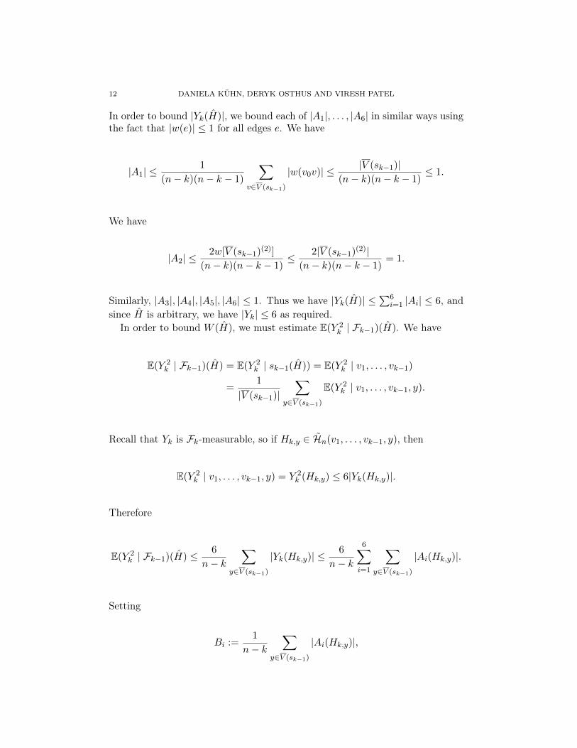
In order to bound |Yk(H)|, we bound each of |A1|, . . . , |A6| in similar ways usingthe fact that |w(e)| ≤ 1 for all edges e. We have
|A1| ≤1
(n− k)(n− k − 1)
∑v∈V (sk−1)
|w(v0v)| ≤ |V (sk−1)|(n− k)(n− k − 1)
≤ 1.
We have
|A2| ≤2w[V (sk−1)
(2)]
(n− k)(n− k − 1)≤ 2|V (sk−1)
(2)|(n− k)(n− k − 1)
= 1.
Similarly, |A3|, |A4|, |A5|, |A6| ≤ 1. Thus we have |Yk(H)| ≤∑6
i=1 |Ai| ≤ 6, andsince H is arbitrary, we have |Yk| ≤ 6 as required.
In order to bound W (H), we must estimate E(Y 2k | Fk−1)(H). We have
E(Y 2k | Fk−1)(H) = E(Y 2
k | sk−1(H)) = E(Y 2k | v1, . . . , vk−1)
=1
|V (sk−1)|
∑y∈V (sk−1)
E(Y 2k | v1, . . . , vk−1, y).
Recall that Yk is Fk-measurable, so if Hk,y ∈ Hn(v1, . . . , vk−1, y), then
E(Y 2k | v1, . . . , vk−1, y) = Y 2
k (Hk,y) ≤ 6|Yk(Hk,y)|.
Therefore
E(Y 2k | Fk−1)(H) ≤ 6
n− k∑
y∈V (sk−1)
|Yk(Hk,y)| ≤ 6
n− k
6∑i=1
∑y∈V (sk−1)
|Ai(Hk,y)|.
Setting
Bi :=1
n− k∑
y∈V (sk−1)
|Ai(Hk,y)|,
A DOMINATION ALGORITHM FOR 0, 1-INSTANCES OF TSP 13
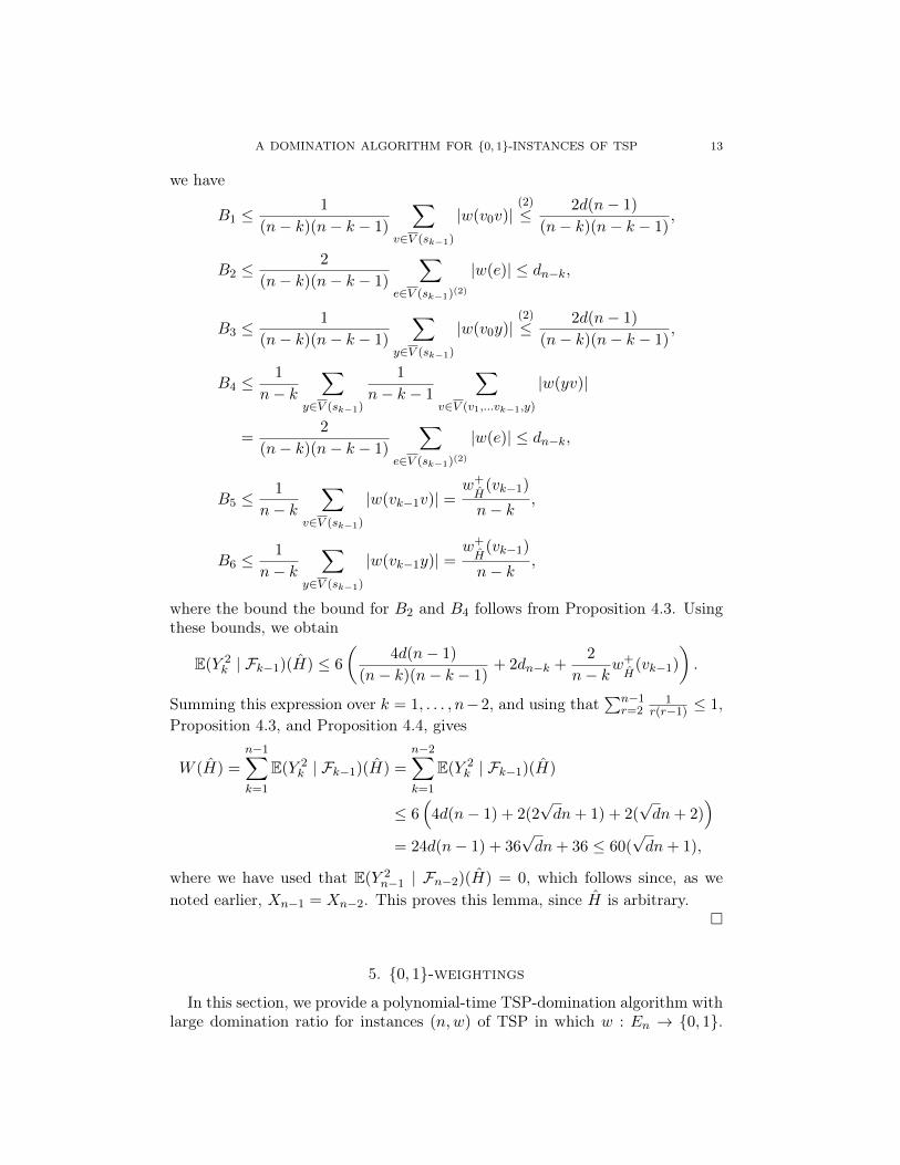
we have
B1 ≤1
(n− k)(n− k − 1)
∑v∈V (sk−1)
|w(v0v)|(2)
≤ 2d(n− 1)
(n− k)(n− k − 1),
B2 ≤2
(n− k)(n− k − 1)
∑e∈V (sk−1)(2)
|w(e)| ≤ dn−k,
B3 ≤1
(n− k)(n− k − 1)
∑y∈V (sk−1)
|w(v0y)|(2)
≤ 2d(n− 1)
(n− k)(n− k − 1),
B4 ≤1
n− k∑
y∈V (sk−1)
1
n− k − 1
∑v∈V (v1,...vk−1,y)
|w(yv)|
=2
(n− k)(n− k − 1)
∑e∈V (sk−1)(2)
|w(e)| ≤ dn−k,
B5 ≤1
n− k∑
v∈V (sk−1)
|w(vk−1v)| =w+
H(vk−1)
n− k,
B6 ≤1
n− k∑
y∈V (sk−1)
|w(vk−1y)| =w+
H(vk−1)
n− k,
where the bound the bound for B2 and B4 follows from Proposition 4.3. Usingthese bounds, we obtain
E(Y 2k | Fk−1)(H) ≤ 6
(4d(n− 1)
(n− k)(n− k − 1)+ 2dn−k +
2
n− kw+
H(vk−1)
).
Summing this expression over k = 1, . . . , n−2, and using that∑n−1
r=21
r(r−1) ≤ 1,Proposition 4.3, and Proposition 4.4, gives
W (H) =n−1∑k=1
E(Y 2k | Fk−1)(H) =
n−2∑k=1
E(Y 2k | Fk−1)(H)
≤ 6(
4d(n− 1) + 2(2√dn+ 1) + 2(
√dn+ 2)
)= 24d(n− 1) + 36
√dn+ 36 ≤ 60(
√dn+ 1),
where we have used that E(Y 2n−1 | Fn−2)(H) = 0, which follows since, as we
noted earlier, Xn−1 = Xn−2. This proves this lemma, since H is arbitrary.
5. 0, 1-weightings
In this section, we provide a polynomial-time TSP-domination algorithm withlarge domination ratio for instances (n,w) of TSP in which w : En → 0, 1.

14 DANIELA KÜHN, DERYK OSTHUS AND VIRESH PATEL
We call such instances 0, 1-instances of TSP. In fact our algorithm consists ofthree separate algorithms, each adapted for different types of 0, 1-instances.
We begin with the following classical result of Erdős and Gallai [7] on thenumber of edges needed in a graph to guarantee a matching of a given size.
Theorem 5.1. Let n, s be positive integers. Then the minimum number of edgesin an n-vertex graph that forces a matching with s edges is
max
(2s− 1
2
),
(n
2
)−(n− s+ 1
2
)+ 1.
We recast the above result into a statement about 0, 1-instances of TSPand the existence of optimal matchings of Kn with small weight.
Proposition 5.2. Let (n,w) be a 0, 1-instance of TSP with n ≥ 1 andw(Kn) = d
(n2
)for some d ∈ [0, 1] satisfying n−1 ≤ d ≤ 1 − 4n−1. Then there
exists a optimal matching M∗ of Kn such that w(M∗) ≤ f(n, d), where
f(n, d) :=
12dn−
18dn+ 1 if d ≤ 9
25 ;12dn−
18(1− d)2n+ 1 if d ≥ 9
25 .
We remark that for a random perfect matching M of Kn (where n is even),we have E(w(M)) = 1
2dn. Thus it is instructive to compare the expressions inthe statement of Proposition 5.2 with 1
2dn. We note in particular that when d isbounded away from 0 and 1, we can find a perfect matching whose weight is sig-nificantly smaller than that of an average perfect matching, but as d approaches0 or 1, all perfect matchings tend to have roughly the same weight.
Proof. Let G be the n-vertex subgraph of Kn whose edges are the edges ofKn of weight zero; thus e(G) = (1− d)
(n2
).
If s = 12
√1− dn then it is easy to check that (1 − d)
(n2
)≥(2s−12
)+ 1, and
if s = (1 −√d)n then it is easy to check that (1 − d)
(n2
)≥(n2
)−(n−s+1
2
)+ 1.
Thus Theorem 5.1 implies that G has a matching of size at least
g(n, d) :=
⌊min
1
2
√1− dn, (1−
√d)n
⌋.
Note that if M is any matching of G with s edges, then we can extend Marbitrarily to an optimal matching M ′ of Kn such that w(M ′) ≤ (n/2) − s.Thus there is an optimal matching M∗ of Kn with
w(M∗) ≤ n/2− g(n, d) ≤ 1 + max
1
2(1−
√1− d)n,
(√d− 1
2
)n
.
It is easy to compute that the maximum above is given by its first term ifd ∈ [0, 9/25] and the second when d ∈ [9/25, 1]. Now using that
√1− d ≥ 1− 3
4d
for d ∈ [0, 9/25] and that√d ≤ 1
2 + 12d−
18(1− d)2 for d ∈ [0, 1], the proposition
easily follows. (The latter inequality can be checked by substituting 1−x for d,squaring both sides, and rearranging.)

A DOMINATION ALGORITHM FOR 0, 1-INSTANCES OF TSP 15
Next we combine the various results we have gathered so far to prove Theo-rem 1.2 by showing that Algorithm A (see end of Section 3) has a dominationratio exponentially close to 1 for 0, 1-instances of TSP with fixed density, i.e.density that is independent of n. In fact, we will not make use of Theorem 1.2in order to prove Theorem 1.1: instead we will make use of a similar and slightlymore technical result in which d may depend on n.
Proof of Theorem 1.2. Given an instance (n,w) as in the statement of thetheorem, Proposition 5.2 implies that there exists an optimal matching M∗ ofKn satisfying w(M∗) ≤ 1
2dn −18η
2n + O(1). Thus Algorithm A, which hasrunning time O(n5) outputs a Hamilton cycle H∗ satisfying
w(H∗) ≤(
1− 1
n− 2
)(1
2dn− 1
8η2n+O(1)
)+
1
n− 2d
(n
2
)+ ρ(n)
= dn− 1
8η2n+O(1).
Set t := dn− w(H∗) ≥ 18η
2n+O(1). Let X0, X1, . . . , Xn−1 be the Hamiltonmartingale for (n,w), so that Xn−1 = w(H) where H is a uniformly randomHamilton cycle from Hn and X0 = E(w(H)) = dn. From Theorem 4.1 andLemma 4.2, we have
P(w(H) ≤ w(H∗)) ≤ P(Xn−1 ≤ X0 − t) ≤ 2 exp
(− t2/2
σ2 +Rt/3
)≤ O(exp(−η4n/104)),
where R = 6 and σ2 = 60(√dn+ 1) ≤ 60n+O(1).
We remark that, although we used Theorem 4.1 (the variant of Freedman’sinequality) in the proof above, Azuma’s inequality, which is much simpler toapply, gives the same bounds. However, Azuma’s inequality is not strong enoughto derive our main result, and in particular, it is not strong enough to deriveTheorem 5.4.
Our next goal is to give a result similar to Theorem 1.2 in which the densityof our 0, 1-instance of TSP can depend on n. We begin with the followingdefinition.
Definition 5.3. For d ∈ [0, 1], ε > 0 and an integer n > max6, exp(ε−1), wecall a 0, 1-instance (n,w) of TSP an (n, d, ε)-regular instance if
(i) w(Kn) = d(n2
);
(ii) there exists an optimal matching M∗ of Kn such that either w(M∗) ≤12dn−mε(n, d) or w(M∗) ≤ 1
2dn−mε(n, 1− d), where
mε(n, d) := 40(ε+ ε1/2) log n+ 40ε1/2d1/4√n log n.
Note that w(Kn) = w[Kn] for 0, 1-instances of TSP.
Theorem 5.4. If (n,w) is an (n, d, ε)-regular instance of TSP, then Algo-rithm A has domination ratio at least 1− 2n−ε for (n,w).

16 DANIELA KÜHN, DERYK OSTHUS AND VIRESH PATEL
Proof. Suppose (n,w) is an (n, d, ε)-regular instance of TSP and set m :=mε(n, d). Assume first that there exists an optimal matching M∗ of Kn withw(M∗) ≤ dn/2−m. Then Algorithm A outputs a Hamilton cycle H∗ with
w(H∗) ≤(
1− 1
n− 2
)(dn/2−m) +
1
n− 2d
(n
2
)+ ρ(n)
= dn−(
1− 1
n− 2
)m+ ρ(n)
≤ dn−m/2,
where the last inequality follows because n > 6 and m > 4 (which followsbecause n > exp(ε−1)). Set t := m/2.
Let X0, X1, . . . , Xn−1 be the Hamilton martingale for (n,w), so that Xn−1 =
w(H) where H is a uniformly random Hamilton cycle from Hn and X0 =E(w(H)) = dn. From Theorem 4.1 and Lemma 4.2, we have
P(w(H) ≤ w(H∗)) ≤ P(Xn−1 ≤ X0 − t) ≤ 2 exp
(− t2/2
σ2 +Rt/3
),
where R = 6 and σ2 = 60(√dn+ 1). We have that
t2/2
σ2 +Rt/3≥ min
t2/2
2σ2,t2/2
2Rt/3
= min
t2
4σ2,t
8
.
Noting that
t2 =1
4(40(ε+ ε1/2) log n+ 40ε1/2d1/4
√n log n)2 ≥ 400ε log n(
√dn+ 1),
we have t2/4σ2 ≥ ε log n. Also t/8 ≥ ε log n, and so we have
P(w(H) ≤ w(H∗)) ≤ 2 exp(−ε log n) = 2n−ε,
as required.Now set m := mε(n, 1 − d) and assume there is an optimal matching M∗ of
Kn with w(M∗) ≤ dn/2−m. As before Algorithm A outputs a Hamilton cycleH∗ with w(H∗) ≤ dn−m/2. Again set t := m/2.
This time let X0, X1, . . . , Xn−1 be the Hamilton martingale for w := 1 − w.From Theorem 4.1 and Lemma 4.2, we have
P(w(H) ≤ w(H∗)) = P(w(H) ≥ w(H∗)) ≤ P(Xn−1 ≥ X0 + t)
≤ 2 exp
(− t2/2
σ2 +Rt/3
),
where R = 6 and σ2 = 60(√
1− dn+ 1) (since w(Kn) = (1− d)(n2
)). Following
the same argument as before with d replaced by 1− d, we obtain
P(w(H) ≤ w(H∗)) ≤ 2n−ε,
as required.

A DOMINATION ALGORITHM FOR 0, 1-INSTANCES OF TSP 17
Corollary 5.5. For every ε > 0 there exists n0 ∈ N such that for all n > n0,the following holds. Define fε(n) := 104(1 + 2ε)n−2/3 log n and gε(n) := 104(1 +
ε)n−2/7 log n. Iffε(n) ≤ d ≤ 1− gε(n),
and (n,w) is a 0, 1-instance of TSP with w(Kn) = d(n2
)then (n,w) is an
(n, d, ε)-regular instance. In particular Algorithm A has domination ratio atleast 1− 2n−ε for (n,w).
Proof. First assume fε(n) ≤ d ≤ 925 . From Definition 5.3, it is sufficient
to exhibit an optimal matching M∗ of Kn for which w(M∗) ≤ 12dn −mε(n, d).
By Proposition 5.2 (note that d satisfies the condition of Proposition 5.2), thereexists an optimal matchingM∗ of Kn such that w(M∗) ≤ 1
2dn−116dn−
116dn+1.
Thus we see that w(M∗) ≤ 12dn−mε(n, d) if
1
16dn ≥ 40(ε+ ε
12 ) log n+ 1 and
1
16dn ≥ 40ε
12d
14
√n log n.
One can check that both inequalities hold if d ≥ fε(n).Now assume that 9
25 ≤ d ≤ 1 − gε(n). From Definition 5.3, it is sufficient toexhibit an optimal matching M∗ of Kn for which w(M∗) ≤ 1
2dn−mε(n, 1− d).Set d := 1 − d and note gε(n) ≤ d ≤ 16
25 . By Proposition 5.2, there exists anoptimal matching M∗ of Kn such that w(M∗) ≤ 1
2dn−18d
2n+ 1. Thus we see
that w(M∗) ≤ 12dn−mε(n, d) if
1
16d2n ≥ 40(ε+ ε
12 ) log n+ 1 and
1
16d2n ≥ 40ε
12d
14√n log n.
One can check that both inequalities hold if d ≥ gε(n).
We have seen in the previous corollary and theorem that Algorithm A hasa large domination ratio for 0, 1-instances of TSP when d is bounded awayfrom 0 and 1, or when there exists an optimal matching of Kn whose weightis significantly smaller than the average weight of an optimal matching. The-orem 5.10 and Theorem 5.13 give polynomial-time TSP-domination algorithmsfor all remaining 0, 1-instances. Before we can prove these, we require somepreliminary results.
Our first lemma is a structural stability result. Suppose G ⊆ Kn is a graphwith d
(n2
)edges, and let w be a weighting of Kn such that w(e) = 1 if e ∈ E(G)
and w(e) = 0 otherwise. Then for a random optimal matchingM ofKn, we haveE(w(M)) = dn/2 if n is even and E(w(M)) = d(n− 1)/2 if n is odd; this showsthat G has a matching of size at least d(n− 1)/2. We cannot improve much onthis if d is close to zero: consider the graph H with a small set A ⊆ V (H) suchthat E(H) consists of all edges incident to A. The next lemma says that anygraph whose largest matching is only slightly larger than dn/2 must be similarto the graph H described above.

18 DANIELA KÜHN, DERYK OSTHUS AND VIRESH PATEL
Lemma 5.6. Fix an integer s ≥ 2 and let G be an n-vertex graph with e(G) =d(n2
)for some d ∈ (0, (4s)−1]. If the largest matching of G has at most 1
2dn+ redges for some positive integer r < n/(8s), then G has a vertex cover D with
|D| ≤ 1
2d(n+ 2) + sd2(n+ 1) + (7s+ 2)r.
LetS := v ∈ D : degG(v) ≤ s|D|.
Then |S| ≤ 2sd2(n+ 1) + (14s+ 4)r + 3d. Furthermore, D and S can be foundin O(n4)-time.
Proof. Let M∗ be any matching of G of maximum size and set m := e(M∗);hence 1
2d(n − 1) ≤ m ≤ 12dn + r (the lower bound follows from the remarks
before the statement of the lemma). Let U be the set of vertices of G incidentto edges of M∗; thus d(n − 1) ≤ |U | = 2m ≤ dn + 2r and U is a vertex cover(by the maximality of M∗). Let
A := u ∈ U : degG(u) ≤ 2sm ⊆ U.We bound the size of A as follows. We have
d
(n
2
)= e(G) ≤
∑u∈U
degG(u) ≤ |A|2sm+ |U \A|n = 2mn− |A|(n− 2sm)
≤ (dn+ 2r)n− |A|(n− sdn− 2sr).
Rearranging gives
|A| ≤ (1− sd− 2sr/n)−1(
1
2dn+
1
2d+ 2r
)≤ (1 + 2sd+ 4sr/n)
(1
2dn+
1
2d+ 2r
);
the last inequality follows by noting that (1− x)−1 ≤ 1 + 2x for x ≤ 12 and that
sd+ 2sr/n ≤ 12 (by our choices of s, r, d). Expanding the expression above, and
using that r ≤ n/(8s) gives
|A| ≤ 1
2dn+ sd2n+ 6sdr +
1
2d+ sd2 + 2r +
2sdr + 8sr2
n
≤ 1
2d(n+ 2) + sd2(n+ 1) + (6sd+ 2)r +
8sr2
n
≤ 1
2d(n+ 2) + sd2(n+ 1) + (7s+ 2)r.
Let B := U \A.Claim 1. No edge of M∗ lies in B.Indeed suppose e = xy is an edge ofM∗ with x, y ∈ B. Then degG(x),degG(y) >2sm ≥ |U |+ 2 (since s ≥ 2). Hence there exist distinct x′, y′ ∈ V \ U such thatxx′, yy′ ∈ E(G). Replacing e with the two edges xx′, yy′ in M∗ gives a largermatching, contradicting the choice of M∗. This proves the claim.

A DOMINATION ALGORITHM FOR 0, 1-INSTANCES OF TSP 19
Let C := u ∈ A : uv ∈ E(M∗), v ∈ B. By Claim 1, we have |B| = |C| andB,C are disjoint.
Claim 2. There are no edges of G between C and V \U , i.e. EG(C, V \U) = ∅.Indeed suppose e = xy ∈ E(G) with x ∈ C and y ∈ V \ U . By definitionof C, there exists z ∈ B such that xz ∈ E(M∗). By the definition of B,degG(z) > 2sm ≥ |U | + 2, and so we can find z′ ∈ V \ U distinct from y suchthat zz′ ∈ E(G). Then we can replace xz with the two edges xy, zz′ in M∗ toobtain a larger matching, contradicting the choice ofM∗. This proves the claim.
Claim 3. C is an independent set.Indeed, suppose e = xy ∈ E(G) with x, y ∈ C. By definition of C, there existx′, y′ ∈ B such that xx′, yy′ ∈ E(M∗). By definition of B, degG(x′),degG(y′) >2sm ≥ |U |+ 2, and so there exist distinct x′′, y′′ ∈ V \ U such that x′x′′, y′y′′ ∈E(G). Now replace xx′, yy′ with xy, x′x′′, y′y′′ inM∗ to obtain a larger matching,contradicting the choice of M∗. This proves the claim.
Set D := U \ C. First we check that D is a vertex cover; indeed note thatV \D = (V \ U) ∪C. But EG(V \ U), EG(V \ U,C), and EG(C) are all emptyusing respectively the fact that U is a vertex cover, Claim 2, and Claim 3. Also,we have
|D| = |U | − |C| = |U | − |B| = |U \B| = |A|
≤ 1
2d(n+ 2) + sd2(n+ 1) + (7s+ 2)r.
Finally, let
S := v ∈ D : degG(v) ≤ s|D| ⊆ v ∈ D : degG(v) ≤ s|U | = A ∩D.
So, we have
|S| ≤ |A ∩D| = |A|+ |D| − |A ∪D| = |A|+ |D| − |U |
≤ 2
(1
2d(n+ 2) + sd2(n+ 1) + (7s+ 2)r
)− d(n− 1)
= 2sd2(n+ 1) + (14s+ 4)r + 3d.
Note that M∗ can be found in O(n4)-time by suitably adapting the minimumweight optimal matching algorithm (Theorem 2.1). From this, A, B, C, D, andS can all be constructed in O(n2)-time, as required.
Next we give a polynomial-time algorithm for finding a maximum doublematching in a bipartite graph: it is a simple consequence of the minimum weightoptimal matching algorithm from Theorem 2.1. Given a bipartite graph G =(V,E) with vertex classes A and B, a double matching of G from A to B is asubgraphM = (V,E′) of G in which degM (v) ≤ 2 for all v ∈ A and degM (v) ≤ 1for all v ∈ B.

20 DANIELA KÜHN, DERYK OSTHUS AND VIRESH PATEL
Theorem 5.7. There exists an O(n4)-time algorithm which, given an n-vertexbipartite graph G with vertex classes A and B as input, outputs a double matchingM∗ of G from A to B with
e(M∗) = maxM
e(M),
where the maximum is over all double matchings of G from A to B. We call thisalgorithm the maximum double matching algorithm.
Proof. Recall that the minimum weight optimal matching algorithm of The-orem 2.1 immediately gives an O(n4)-time algorithm for finding a maximummatching in a graph.
Given G, define a new bipartite graph G′ by creating a copy a′ of each vertexa ∈ A so that a′ and a have the same neighbourhood. Note that every matchingM ′ of G′ corresponds to a double matching M of G by identifying each a ∈ Awith its copy a′ and retaining all the edges of M ′; hence e(M) = e(M ′).
Therefore finding a double matching in G from A to B of maximum size isequivalent to finding a matching of G′ of maximum size, and we can use theminimum weight optimal matching algorithm of Theorem 2.1 to find such amatching.
Next we prove a lemma that says that for a small subset S of vertices of Kn,almost all Hamilton cycles avoid S ‘as much as possible’.
Lemma 5.8. Fix ε ∈ (0, 1/2) and n ≥ 4. Let S ⊆ Vn be a subset of the verticesof the n-vertex complete graph Kn = (Vn, En) with |S| ≤ n
12−ε. Let H ∈ Hn be
a uniformly random Hamilton cycle of Kn. Let E := E1 ∩ E2, where E1 is theevent that H uses no edge of S and E2 is the event that eH(v, S) ≤ 1 for allv ∈ Vn \ S. Then
P(E) ≥ 1− 6n−2ε.
Proof. For each e ∈ En, we have P(e ∈ E(H)) = 2/(n− 1), and so
P(E1) = P(|E(H) ∩ S(2)| ≥ 1) ≤ E(|E(H) ∩ S(2)|)(3)
=
(|S|2
)2
n− 1≤ 1
2n1−2ε
2
n− 1≤ 2n−2ε.
Let R be the random variable counting the number of vertices v ∈ Vn \ S suchthat eH(v, S) = 2. We have
P(E2) ≤ E(R) = |Vn \ S|P(eH(v, S) = 2)(4)
= |Vn \ S||S|(|S| − 1)
(n− 1)(n− 2)≤ n2−2ε
(n− 2)2≤ 4n−2ε.
The lemma follows immediately from (3) and (4).

A DOMINATION ALGORITHM FOR 0, 1-INSTANCES OF TSP 21
We are now ready to present a polynomial-time TSP-domination algorithmwhich has a large domination ratio for 0, 1-instances of TSP in which w(Kn) =d(n2
)with d close to 1 and in which all optimal matchings have weight close to
dn/2. Let us first formalise this in a definition.
Definition 5.9. For n ≥ 4 a positive integer, r > 0, d ∈ [0, 1], and ε ∈ (0, 1/2)we call a 0, 1-instance (n,w) of TSP an (n, d, r, ε)-dense instance if
(i) w(Kn) = d(n2
)with 1− d ≤ 1/12;
(ii) w(M) ≥ 12dn− r for all optimal matchings M of Kn; and
(iii) 6d2(n+ 1) + 46r + 3d ≤ n
12−ε, where d := 1− d.
Theorem 5.10. There exists an O(n4)-time TSP-domination algorithm whichhas domination ratio at least 1− 6n−2ε for all (n, d, r, ε)-dense instances (n,w)of TSP. We call this Algorithm B.
Proof. We begin by describing Algorithm B in steps with the running timeof each step in brackets. We then explain each step. Let (n,w) be a (n, d, r, ε)-dense instance of TSP and let G = (Vn, E) ⊆ Kn be the graph in which we havee ∈ E if and only if w(e) = 0. We set V := Vn in order to reduce notationalclutter.
1. Construct G and note that e(G) = d(n2
), where d := 1−d. (O(n2) time)
2. Using the algorithm of Lemma 5.6 (with s = 3), find a vertex cover Dfor G such that |D| ≤ 1
2d(n+ 2) + 3d2(n+ 1) + 23r. (O(n4) time)
3. Construct the bipartite graph G′ := G[D,V \D]. (O(n2) time)4. Apply the maximum double matching algorithm (Theorem 5.7) to G′ to
obtain a double matching M∗ of G′ from D to V \D of maximum size.(O(n4)-time).
5. Extend M∗ arbitrarily to a Hamilton cycle H∗ of Kn (i.e. choose H∗ tobe any Hamilton cycle of Kn that includes all the edges of M∗). (O(n)time)
Altogether, the running time of the algorithm is O(n4). Note that in Step 2,the conditions of Lemma 5.6 are satisfied by (n, d, r, ε)-dense instances of TSP.Also the algorithm of Lemma 5.6 gives us the set
S = v ∈ D : degG(v) ≤ 3|D|,
where |S| ≤ 6d2(n+1)+46r+3d ≤ n
12−ε, which we shall require in the analysis
of Algorithm B.Next we show that this algorithm has domination ratio at least 1 − 6n−2ε
for (n,w) by showing that for a uniformly random Hamilton cycle H ∈ Hn, wehave P(w(H) < w(H∗)) ≤ 6n−2ε. Since |S| ≤ n
12−ε, we can apply Lemma 5.8
to conclude thatP(E) ≥ 1− 6n−2ε,
where E := E1 ∩ E2 with E1 being the event that H uses no edge of S and E2being the event that eH(v, S) ≤ 1 for all v ∈ V \ S. We show that if H is any

22 DANIELA KÜHN, DERYK OSTHUS AND VIRESH PATEL
Hamilton cycle in E ⊆ Hn then w(H∗) ≤ w(H), i.e.
(5) P(w(H) < w(H∗) | E) = 0.
Assuming (5), we can prove the theorem since
P(w(H) < w(H∗)) = P(w(H) < w(H∗) | E)P(E) + P(w(H) < w(H∗) | E)P(E)
≤ 0 + P(E) ≤ 6n−2ε,
as required.In order to verify (5), it is sufficient to show that |E(H∗)∩E(G)| ≥ |E(H)∩
E(G)| for all H ∈ E .
Claim. L := E(M∗) ∩ EG(S, V \ D) is a maximum-sized double matching ofG[S, V \D] from S to V \D.Suppose, for a contradiction, that there is some double matching L′ ofG[S, V \D]from S to V \D with more edges than L. Then since every vertex of D \ S hasdegree at least 3|D| in G, we can greedily extend L′ to a double matching M∗∗of G[D,V \D] such that in M∗∗, every vertex of D \ S has degree 2. Hence
e(M∗∗) = e(L′) + 2|D \ S| > e(L) + 2|D \ S| ≥ e(M∗),
contradicting the maximality of M∗. This proves the claim.
Now for H ∈ E ⊆ Hn, we have that E(H) ∩EG(S, V \D) is a double matchingof G[S, V \D] from S to V \D. Hence by the claim and the definition of H∗
(6) |E(H)∩EG(S, V \D)| ≤ |E(M∗)∩EG(S, V \D)| ≤ |E(H∗)∩EG(S, V \D)|.
Writing DS := D \ S, we have that
E(H) ∩ E(G) = [E(H) ∩ EG(DS , V )] ∪ [E(H) ∩ EG(V \DS)]
= [E(H) ∩ EG(DS , V )] ∪ [E(H) ∩ EG(S, V \D)].
Now we see that
|E(H) ∩ E(G)| ≤ 2|DS |+ |E(H) ∩ EG(S, V \D)|.
Also note that eH∗(v, V \ D) = eM∗(v, V \ D) = 2 for all v ∈ DS since M∗ ismaximal and vertices in DS have degree at least 3|D| in G. Hence
|E(H∗) ∩ E(G)| ≥ 2|DS |+ |E(H∗) ∩ EG(S, V \D)|.
But now (6) implies |E(H∗) ∩ E(G)| ≥ |E(H) ∩ E(G)|, as required.
Finally we provide a TSP-domination algorithm that has a large domina-tion ratio for sparse 0, 1-instances of TSP. Before we do this, we require onesubroutine for our algorithm.
Lemma 5.11. There exists an O(n3)-time algorithm which, given an n-vertexgraph G with δ(G) ≥ n/2 + 3
2k and k independent edges e1, . . . , ek, outputs aHamilton cycle H∗ of G such that e1, . . . , ek ∈ E(H∗).

A DOMINATION ALGORITHM FOR 0, 1-INSTANCES OF TSP 23
The proof of this lemma is a simple adaptation of the proof of Dirac’s theorem,but we provide the details for completeness. A threshold of n/2+k/2 was provedby Pósa [24], but it is not clear whether the proof is algorithmic.
Proof. Let ei = xiyi, and set S := x1, . . . , xk, y1, . . . , yk so that |S| = 2k.By the degree condition of G, every pair of vertices have at least 3k commonneighbours and so G is 3k-connected. In particular, we can pick distinct verticesz1, . . . , zk−1 ∈ V (G)\S such that zi is a common neighbour of yi and xi+1. HenceP := x1y1z1x2y2z2 · · · zk−1xkyk is a path of G containing all the edges e1, . . . , ek.This can be found in O(nk) time.
We say any path or cycle Q is good if it contains all the edges e1, . . . , ek; inparticular P is good. We show that if Q is a good path or cycle with |V (Q)| < nor e(Q) < n, then we can extend Q to a good path or cycle Q′ such that either|V (Q′)| > |V (Q)| or e(Q′) > e(Q).
If Q is a good cycle with |V (Q)| < n, then since G is 3k-connected, there issome vertex c ∈ V (G) \ V (Q) that is adjacent to some b ∈ V (Q). Let a and a′be the two neighbours of b on Q. Since e1, . . . , ek are independent edges, eitherab or a′b, say ab, is not amongst e1, . . . , ek. Thus we can extend Q to the goodpath Q′ := aQbc, and we see |V (Q′)| = |V (Q)|+ 1. This takes O(n2) time.
Now suppose Q is a good path with end-vertices a and b, i.e. Q = aQb, andone of the end-vertices, say b, has a neighbour c in V (G)\V (Q). Then we canextend Q to a good path Q′ := aQbc, and |V (Q′)| > |V (Q)|. Checking whetherwe are in this case and obtaining Q′ takes O(n) time.
Finally suppose Q is a good path with end-vertices a and b, but where aand b have all their neighbours on Q. Since a and b have at least n/2 + 3
2kneighbours, there are at least 3k edges xx+ ∈ E(Q), where Q = aQxx+Qband ax+, xb ∈ E(G). Thus there are at least 2k such edges that are not oneof e1, . . . , ek; let xx+ be such an edge. Then Q′ := ax+QbxQa is a cycle withe(Q′) > e(Q). Checking whether we are in this case and obtaining Q′ takesO(n) time.
Thus extending P at most 2n times as described above gives us a Hamiltoncycle, and the running time of the algorithm is dominated by O(n3).
Definition 5.12. For 0 < ε < 1/2, we call a 0, 1-instance (n,w) of TSP a(n, d, ε)-sparse instance if w(Kn) = d
(n2
)with d ≤ 1
4n− 1
2−ε.
Theorem 5.13. Fix 0 < ε < 1/2. There exists an O(n4)-time TSP-dominationalgorithm which has domination ratio at least 1− 6n−2ε for any (n, d, ε)-sparseinstance of TSP with n ≥ 225. We call this Algorithm C.
Proof. Assume n ≥ 225 and let (n,w) be an (n, d, ε)-sparse instance of TSPso that w(Kn) = d
(n2
)with d ≤ 1
4n− 1
2−ε. Let G = (Vn, E) be the graph where
e ∈ E if and only if w(e) = 0. We write G for the complement of G. Let
S := v ∈ Vn : degG(v) ≤ 2n/3,
and let S := V \ S.

24 DANIELA KÜHN, DERYK OSTHUS AND VIRESH PATEL
Claim. We have |S| ≤ n12−ε.
In G, we have that S = v ∈ Vn : degG(v) ≥ (n/3)− 1. Then1
2|S|(n
3− 1)≤ e(G) = d
(n
2
)≤ 1
4n−
12−ε(n
2
)≤ 1
8n
32−ε,
which implies the required bounds.
We note for later that
(7) δ(G[S]) ≥ 2
3n− |S| ≥ 2
3n− n
12−ε ≥ 1
2n+
3
2n
12−ε ≥ 1
2n+
3
2|S|.
where the penultimate inequality follows since n ≥ 225.We now describe the steps of our algorithm with the run time of each step in
brackets; we then elaborate on each step below.1. Construct G. (O(n2) time)2. Obtain the set S ⊆ Vn as defined above. (O(n2) time)3. Construct G′ := G[S, S]. (O(n2) time)4. Apply the maximum double matching algorithm (Theorem 5.7) to G′
to obtain a double matching M∗ of G′ from S to S of maximum size.(O(n4) time)
5. Arbitrarily extend M∗ to a maximum double matching M∗∗ of Kn[S, S]from S to S, i.e. degM∗∗(v) = 2 for all v ∈ S, degM∗∗(v) ≤ 1 for allv ∈ S, and E(M∗) ⊆ E(M∗∗). (O(n2) time)
6. For each v ∈ S, determine its two neighbours xv, yv ∈ S in M∗∗, and letev := xvyv ∈ S
(2). (O(n) time)7. Apply the algorithm of Lemma 5.11 to obtain a Hamilton cycle H∗ ofG[S] ∪ ev : v ∈ S that includes all edges ev : v ∈ S. (O(n3) time)
8. Replace each edge ev = xvyv in H∗ by the two edges vxv, vyv ∈ E(M∗∗)to obtain a Hamilton cycle H∗∗ of Kn. (O(n) time)
Note that the edges ev determined in Step 6 are independent because M∗∗is a double matching. This together with (7) means that we can indeed applythe algorithm of Lemma 5.11 in Step 7. Altogether, the algorithm takes O(n4)time.
Finally, let us verify that the algorithm above gives a domination ratio of atleast 1−6n−2ε by showing that for a uniformly random Hamilton cycle H ∈ Hn,we have P(w(H) < w(H∗∗)) ≤ 6n−2ε. As in the proof of Theorem 5.10, it sufficesto show
(8) P(w(H) < w(H∗∗) | E) = 0,
where E := E1 ∩ E2 with E1 being the event that H uses no edge of S and E2being the event that eH(v, S) ≤ 1 for all v ∈ Vn \ S.
In order to verify (8), it suffices to show that |E(H∗∗)∩E(G)| ≥ |E(H)∩E(G)|for all H ∈ E ⊆ Hn. Assuming H ∈ E , note that E(H) ∩ EG(S, S) is a doublematching of G[S, S] from S to S; hence by the definition of M∗ and H∗∗, wehave
|E(H) ∩ EG(S, S)| ≤ |E(M∗)| = |E(H∗∗) ∩ EG(S, S)|.
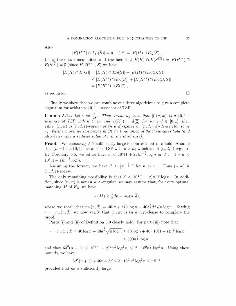
A DOMINATION ALGORITHM FOR 0, 1-INSTANCES OF TSP 25
Also|E(H∗∗) ∩ EG(S)| = n− 2|S| = |E(H) ∩ EG(S)|.
Using these two inequalities and the fact that E(H) ∩ E(S(2)) = E(H∗∗) ∩E(S(2)) = ∅ (since H,H∗∗ ∈ E) we have
|E(H) ∩ E(G)| = |E(H) ∩ EG(S)|+ |E(H) ∩ EG(S, S)|≤ |E(H∗∗) ∩ EG(S)|+ |E(H∗∗) ∩ EG(S, S)|= |E(H∗∗) ∩ E(G)|,
as required.
Finally we show that we can combine our three algorithms to give a completealgorithm for arbitrary 0, 1-instances of TSP.
Lemma 5.14. Let ε := 128 . There exists n0 such that if (n,w) is a 0, 1-
instance of TSP with n > n0 and w(Kn) = d(n2
)for some d ∈ [0, 1], then
either (n,w) is (n, d, ε)-regular or (n, d, ε)-sparse or (n, d, r, ε)-dense (for somer). Furthermore, we can decide in O(n4) time which of the three cases hold (andalso determine a suitable value of r in the third case).
Proof. We choose n0 ∈ N sufficiently large for our estimates to hold. Assumethat (n,w) is a 0, 1-instance of TSP with n > n0 which is not (n, d, ε)-regular.By Corollary 5.5, we either have d < 104(1 + 2ε)n−
23 log n or d := 1 − d <
104(1 + ε)n−27 log n.
Assuming the former, we have d ≤ 14n− 1
2−ε for n > n0. Thus (n,w) is
(n, d, ε)-sparse.The only remaining possibility is that d < 104(1 + ε)n−
27 log n. In addi-
tion, since (n,w) is not (n, d, ε)-regular, we may assume that, for every optimalmatching M of Kn, we have
w(M) ≥ 1
2dn−mε(n, d),
where we recall that mε(n, d) = 40(ε + ε12 ) log n + 40ε
12d
14√n log n. Setting
r := mε(n, d), we now verify that (n,w) is (n, d, r, ε)-dense to complete theproof.
Parts (i) and (ii) of Definition 5.9 clearly hold. For part (iii) note that
r = mε(n, d) ≤ 40 log n+ 40d14√n log n ≤ 40 log n+ 40 · 10(1 + ε)n
37 log n
≤ 500n37 log n,
and that 6d2(n + 1) ≤ 109(1 + ε)2n
37 log2 n ≤ 2 · 109n
37 log2 n. Using these
bounds, we have
6d2(n+ 1) + 46r + 3d ≤ 3 · 109n
37 log2 n ≤ n
12−ε,
provided that n0 is sufficiently large.
26 DANIELA KÜHN, DERYK OSTHUS AND VIRESH PATEL
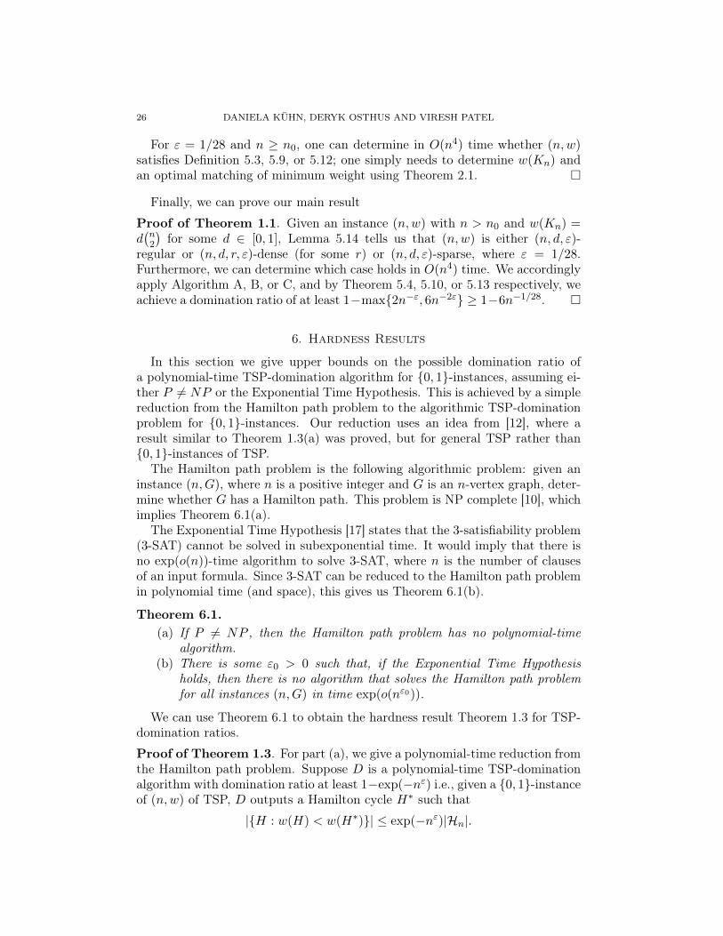
For ε = 1/28 and n ≥ n0, one can determine in O(n4) time whether (n,w)satisfies Definition 5.3, 5.9, or 5.12; one simply needs to determine w(Kn) andan optimal matching of minimum weight using Theorem 2.1.
Finally, we can prove our main result
Proof of Theorem 1.1. Given an instance (n,w) with n > n0 and w(Kn) =d(n2
)for some d ∈ [0, 1], Lemma 5.14 tells us that (n,w) is either (n, d, ε)-
regular or (n, d, r, ε)-dense (for some r) or (n, d, ε)-sparse, where ε = 1/28.Furthermore, we can determine which case holds in O(n4) time. We accordinglyapply Algorithm A, B, or C, and by Theorem 5.4, 5.10, or 5.13 respectively, weachieve a domination ratio of at least 1−max2n−ε, 6n−2ε ≥ 1−6n−1/28.
6. Hardness Results
In this section we give upper bounds on the possible domination ratio ofa polynomial-time TSP-domination algorithm for 0, 1-instances, assuming ei-ther P 6= NP or the Exponential Time Hypothesis. This is achieved by a simplereduction from the Hamilton path problem to the algorithmic TSP-dominationproblem for 0, 1-instances. Our reduction uses an idea from [12], where aresult similar to Theorem 1.3(a) was proved, but for general TSP rather than0, 1-instances of TSP.
The Hamilton path problem is the following algorithmic problem: given aninstance (n,G), where n is a positive integer and G is an n-vertex graph, deter-mine whether G has a Hamilton path. This problem is NP complete [10], whichimplies Theorem 6.1(a).
The Exponential Time Hypothesis [17] states that the 3-satisfiability problem(3-SAT) cannot be solved in subexponential time. It would imply that there isno exp(o(n))-time algorithm to solve 3-SAT, where n is the number of clausesof an input formula. Since 3-SAT can be reduced to the Hamilton path problemin polynomial time (and space), this gives us Theorem 6.1(b).
Theorem 6.1.(a) If P 6= NP , then the Hamilton path problem has no polynomial-time
algorithm.(b) There is some ε0 > 0 such that, if the Exponential Time Hypothesis
holds, then there is no algorithm that solves the Hamilton path problemfor all instances (n,G) in time exp(o(nε0)).
We can use Theorem 6.1 to obtain the hardness result Theorem 1.3 for TSP-domination ratios.
Proof of Theorem 1.3. For part (a), we give a polynomial-time reduction fromthe Hamilton path problem. Suppose D is a polynomial-time TSP-dominationalgorithm with domination ratio at least 1−exp(−nε) i.e., given a 0, 1-instanceof (n,w) of TSP, D outputs a Hamilton cycle H∗ such that
|H : w(H) < w(H∗)| ≤ exp(−nε)|Hn|.
A DOMINATION ALGORITHM FOR 0, 1-INSTANCES OF TSP 27
We show that we can use D to determine whether any graph G has a Hamil-ton path in time polynomial in |V (G)|, contradicting Theorem 6.1(a). AssumeG is an n-vertex graph and let G be its complement. Choose n′ such thatbn′ε/ log n′c = n; thus n′ is bounded above by a polynomial in n. Consider then′-vertex graph G′ = (V ′, E′) obtained from G by first partitioning V ′ into twosets S, S with |S| = n and |S| = n′ − n, and setting G′[S] to be isomorphic toG, setting G′[S] to be empty, and setting G′[S, S] to be the complete bipartitegraph between S and S. We define an instance (n′, w) of TSP where the edgeweighting w of Kn′ ⊇ G′ = (V ′, E′) is given by w(e) = 1 for each e ∈ E′ andw(e) = 0 for e 6∈ E′.
Applying D to (n′, w), we obtain a Hamilton cycle H∗ of Kn′ in time polyno-mial in n′ (which is therefore polynomial in n). We claim that G has a Hamiltonpath if and only if w(H∗) = 2, and this proves Theorem 1.3(a).
To see the claim, first assume that w(H∗) = 2. Note that for any H ∈ Hn′ ,we have w(H[S, S]) ≥ 2, and if we have equality, then H[S] is a Hamilton pathof Kn′ [S] (and H[S] is a Hamilton path of Kn′ [S]). Since w(H∗) = 2, we havew(H[S, S]) = 2 and w(H∗[S]) = 0. Thus H∗[S] is a Hamilton path of Kn′ [S]and every edge of H∗[S] is an edge of G. Hence G has a Hamilton path.
To see the claim in the other direction, suppose G has a Hamilton path Pand consider the set HP of all Hamilton cycles H of Kn′ such that H[S] = P .Note that w(H) = 2 for all H ∈ HP and that
|HP | = (n′ − n)! = 2[(n′ − 1) · · · (n′ − n+ 1)]−1|Hn′ |(9)
≥ 2(n′)−n|Hn′ | = 2 exp(−n log n′)|Hn′ |> exp(−n′ε)|Hn′ |;
the last inequality follows by our choice of n′. Since D has domination ratioat least 1 − exp(−n′ε) for (n′, w), D must output a Hamilton cycle H∗ withw(H∗) = 2. This proves the claim and completes the proof of (a).
The proof of (b) follows almost exactly the same argument as above. SetC := 2ε−10 + 2, where ε0 is as in the statement of Theorem 6.1(b), and setβ(n) := exp(−(log n)C).
Suppose D is an O(nk)-time algorithm (for some k ∈ N) which, given a0, 1-instance of (n,w) of TSP, outputs a Hamilton cycle H∗ such that
|H : w(H) < w(H∗)| ≤ β(n)|Hn|.
We show that we can use D to determine whether any n-vertex graph G hasa Hamilton path in time exp(o(nε0)), contradicting Theorem 6.1(b). We setn′ := dexp(nε0/2/k)e and apply D to the n′-vertex graph G′ constructed in thesame way as in part (a). The algorithm takes time O(n′k) = exp(o(nε0)) andthe proof of the claim proceeds in the same say as in part (a), except that (9)is replaced by |HP | > β(n′)|Hn′ |.

28 DANIELA KÜHN, DERYK OSTHUS AND VIRESH PATEL
7. Concluding remarks and an open problem
In view of Theorem 1.1, it is natural to ask whether there exists a poly-nomial-time TSP-domination algorithm with domination ratio 1− o(1) for gen-eral instances of TSP. Below we discuss some of the challenges which this wouldinvolve.
Note that the average weight of a perfect matching in a weighted completegraph Kn is w(Kn)/(n − 1). For instances (n,w) of TSP for which thereexists a perfect matching M∗ of Kn with w(M∗) ‘significantly’ smaller thanw(Kn)/(n − 1), our techniques immediately imply that Algorithm A gives alarge domination ratio. We call these typical instances. However instances ofTSP where all perfect matchings have approximately the same weight (aftersome suitable normalisation) need to be treated separately, and we call thesespecial instances. For weights in 0, 1, there are essentially two different typesof special instances: either most edges have weight 0 or most edges have weight1. Even then, some additional ideas were needed to treat the special instances.If we allow weights in [−1, 1], there are many different types of special instancesand the challenge is to find a way to treat all of these cases simultaneously. As anexample of a special instance, consider a weighting of Kn where we take S ⊆ Vnwith |S| close to n/2 and set w(e) := 1 if e ∈ S(2), w(e) := −1 if e ∈ S(2), andw(e) := 0 if e ∈ E(S, S). Then any perfect matching has weight close to zero.
References
[1] N. Alon, G. Gutin and M. Krivelevich, Algorithms with large domination ratio, J. Algo-rithms 50 (2004), 118–131.
[2] S. Arora, Polynomial time approximation schemes for Euclidean traveling salesman andother geometric problems, J. ACM 45 (1998), 753–782.
[3] D. Berend, S. Skiena, Y. Twitto, Combinatorial dominance guarantees for problems withinfeasible solutions, ACM Transactions on Algorithms 5 (2008), article 8.
[4] N. Christofides, Worst-case analysis of a new heuristic for the traveling salesman problem,Technical Report 388, GSIA, Carnegie-Mellon University, 1976.
[5] J. Edmonds, Maximum matching and a polyhedron with 0, 1-vertices, Journal of Researchof the National Bureau of Standards 69B (1965), 125–130.
[6] P. Erdős, A problem on independent r-tuples, Ann. Univ. Sci. Budapest. Eőtvős Sect.Math. 8 (1965), 93–95.
[7] P. Erdős, T. Gallai, On maximal paths and circuits of graphs, Acta Math. Acad. Sci.Hung. 10 (1959), 337–356.
[8] P. Erdős and J.L. Selfridge, On a combinatorial game, Journal of Combinatorial Theory,Series A 14 (1973), 289–301.
[9] P. Erdős and J. Spencer, The Probabilistic Method (2nd edition), Wiley-Interscience 2000.[10] M.R. Garey and D.S. Johnson, Computers and Intractability: A Guide to the Theory of
NP-completeness, Freeman 1979.[11] F. Glover and A.P. Punnen, The traveling salesman problem: new solvable cases and
linkages with the development of approximation algorithms, Journal of the OperationalResearch Society 8 (1997), 502–510.
[12] G. Gutin, A. Koller and A. Yeo, Note on upper bounds for TSP domination number, JAlgorithmic Oper. Res. 1 (2006), 52–54.
[13] G. Gutin, A. Vainshtein and A. Yeo, Domination analysis of combinatorial optimizationproblems. Discrete Applied Mathematics 129 (2003), 513–520.

A DOMINATION ALGORITHM FOR 0, 1-INSTANCES OF TSP 29
[14] G. Gutin and A. Yeo, TSP tour domination and Hamilton cycle decompositions of regulardigraphs, Oper. Res. Letters 28 (2001), 107–111.
[15] G. Gutin and A. Yeo, Polynomial approximation algorithms for the TSP and QAP witha factorial domination number, Discrete Applied Mathematics 119 (2002), 107–116.
[16] G. Gutin, A. Yeo and A. Zverovich, Traveling salesman should not be greedy: dominationanalysis of greedy-type heuristics for the TSP, Discrete Applied Mathematics 117 (2002),81–86.
[17] R. Impagliazzo and R. Paturi, On the complexity of k-sat, J. Comput. Syst. Sci. 62(2001), 367–375.
[18] A.E. Koller and S.D. Noble, Domination analysis of greedy heuristics for the frequencyassignment problem, Discrete Mathematics 275 (2004), 331–338.
[19] D. Kühn and D. Osthus, Hamilton decompositions of regular expanders: a proof of Kelly’sconjecture for large tournaments, Advances in Mathematics 237 (2013), 62–146.
[20] C. McDiarmid, Concentration, Probabilistic methods for algorithmic discrete mathematics,195–248, Algorithms, Combin., 16, Springer, Berlin, 1998.
[21] J. Mitchell, Guillotine subdivisions approximate polygonal subdivisions: A simplepolynomial-time approximation scheme for geometric TSP, k-MST, and related problems,SIAM J. Comput. 28 (1999), 1298–1309.
[22] R. Motwani and P. Raghavan, Randomized Algorithms, Cambridge University Press, 1995.[23] C. H. Papadimitriou and S. Vempala, On the approximability of the traveling salesman
problem, Combinatorica 26 (2006), 101–120[24] L. Pósa, On the circuits of finite graphs, Publ. Math. Inst. Hungar. Acad. Scien. 9 (1963),
355–361.[25] A.P. Punnen, F. Margot and S.N. Kabadi, TSP heuristics: domination analysis and
complexity, Algorithmica 35 (2003), 111–127.[26] V.I. Rublineckii, Estimates of the accuracy of procedures in the traveling salesman prob-
lem, Numerical Mathematics and Computer Technology 4 (1973), 18–23. (in Russian)[27] V.I. Sarvanov, On the minimization of a linear form on a set of all n-elements cycles,
Vestsi Akad. Navuk BSSR, Ser. Fiz.-Mat. Navuk 4 (1976), 17–21. (in Russian)[28] S. Sahni and T. Gonzalez, P-complete approximation problems, J. Assoc. Comput. Mach.
23 (1976), 555–565.
Daniela Kühn, Deryk Osthus, Viresh PatelSchool of MathematicsUniversity of BirminghamEdgbastonBirminghamB15 2TTUKE-mail addresses:d.kuhn, [email protected], [email protected]
Related Documents