Instance-based learning algorithms - Welcome to the …sci2s.ugr.es/keel/pdf/algorithm/articulo/aha1991.pdf · Instance-based learning algorithms suffer from several problems that

Machine Learning, 6, 37-66 (1991) © 1991 Kluwer Academic Publishers, Boston. Manufactured in The Netherlands.

Instance-Based Learning Algorithms DAVID W. AHA ([email protected]) DENNIS KIBLER ([email protected]) MARC K. ALBERT ([email protected]) Department of Information and Computer Science, University of California, lrvine, CA 92717

Editor: J.R. Quinian

Abstract. Storing and using specific instances improves the performance of several supervised learning algorithms. These include algorithms that learn decision trees, classification rules, and distributed networks. However, no investigation has analyzed algorithms that use only specific instances to solve incremental learning tasks. In this paper, we describe a framework and methodology, called instance-based learning, that generates classification predictions using only specific instances. Instance-based learning algorithms do not maintain a set of abstractions derived from specific instances. This approach extends the nearest neighbor algorithm, which has large storage requirements. We describe how storage requirements can be significantly reduced with, at most, minor sacrifices in learning rate and classification accuracy. While the storage-reducing algorithm performs well on several real- world databases, its performance degrades rapidly with the level of attribute noise in training instances. Therefore, we extended it with a significance test to distinguish noisy instances. This extended algorithm's performance degrades gracefully with increasing noise levels and compares favorably with a noise-tolerant decision tree algorithm.

Keywords. Supervised concept learning, instance-based concept descriptions, incremental learning, learning theory, noise, similarity

1. Introduct ion

Several different representations have been used to describe concepts for supervised learning tasks. These include decision trees (Quinlan, 1986), connectionist networks (Rumelhart, McClelland, & The PDP Research Group, 1987), and rules (Michalski, Mozetic, Hong, & Lavra~, 1986; Clark & Niblett, 1989). Numerous empirical studies have reported that these algorithms record excellent performances (e.g., high classification accuracies) in a large and varied set of applications.

Algorithms that employ these representations were improved by either storing and using specific instances or by supporting partial matching techniques. For example, Utgoff (1989) showed how the updating costs of incremental decision tree algorithms can be significantly decreased by saving specific instances. Similarly, Volper and Hampson (1987) showed that the perceptron's learning rate can be significantly increased in some applications by using specific instance detectors. Finally, Michalski et al. (1986) extended AQI1 (Michalski & Larson, 1978) to employ partial matching strategies to support the description ofprobabilistic concepts as defined in Smith and Medin (1981). The topic of this article is instance-based learning algorithms, which use specific instances rather than pre-compiled abstractions during prediction tasks. These algorithms can also describe probabilistic concepts because they use similarity functions to yield graded matches between instances.

38 D.w. AHA, D. KIBLER, AND M.K. ALBERT

Furthermore, domain-specific systems that use instance-based learning algorithms have performed extremely well in industrial applications. One example is ALFA (Jabbour, Riveros, Landsbergen, & Meyer, 1987), a load forecasting assistant used by the Niagara Mohawk Power Company of central New York State to estimate power load. ALFA uses an instance-based learning algorithm to generate an initial prediction for power load, which is then modified according to a rule-based domain theory. ALFA achieves the same accuracy as experts but requires only two minutes to make load predictions (experts require two hours). Another example is Clark's (1989) system for geologic prospect appraisal, which is being used by Enterprise Oil to generate predictions of oil reservoir thickness and porosity at a prospect site based on prospecting information gathered from nearby sites.

Using specific instances in supervised learning algorithms decreases the costs incurred when updating concept descriptions, increases learning rates, allows for the representation of probabilistic concept descriptions, and focuses theory-based reasoning in real-world applications. However, no investigation has analyzed algorithms that use only specific instances to solve incremental, supervised learning tasks.

In this article, we describe a methodology for instance-based learning (IBL) algorithms, provide a geometric analysis to describe their generality and underlying intuition, address two problems with this approach, and summarize convincing empirical evidence which suggests that IBL algorithms perform well in applications to artificial and real-world domains.

1.1. History and related work

IBL algorithms are derived from the nearest neighbor pattern classifier (Cover & Hart, 1967). They are highly similar to edited nearest neighbor algorithms (Hart, 1968; Gates, 1972; Dasarathy, 1980), which also save and use only selected instances to generate classification predictions. While several researchers demonstrated that edited nearest neighbor algorithms can reduce storage requirements with, at most, small losses in classification accuracy, they were unable to predict the expected savings in storage requirements. We present an analysis in Section 2.5 that answers this question: the expected storage requirements are polynomial in the size of the target concept's boundary in the instance space.

Edited nearest neighbor algorithms are nonincremental and their primary goal is to maintain perfect consistency with the initial training set. Although they summarize data, they do not attempt to maximize classification accuracy on novel instances. This ignores real- world problems such as noise. Therefore, edited nearest neighbor algorithms are brittle. IBL algorithms are instead incremental and their goals include maximizing classification accuracy on subsequently presented instances. We address how IBL algorithms tolerate noise in Section 4. Further discussions on how IBL algorithms can solve real-world problems can be found in Aha (1989b).

The design of IBL algorithms was also inspired by exemplar-based models of categorization (Smith &Medin, 1981). 1 Exemplar-based models are one of three proposed models of categorization in the psychological literature (the others are the classical and probabilistic models). Several researchers have defended the exemplar-based model as psychologically plausible (Medin& Schaffer, 1978; Brooks, 1978; Hintzman, 1986; Nosofsky, 1986). How- ever, computationally efficient exemplar-based process models of incremental learning have

INSTANCE-BASED LEARNING ALGORITHMS 39

not been published in this literature. Moreover, there is no discussion of real-world issues such as storage reduction and noise.

More recently, case-based reasoning (CBR) systems have been introduced to solve diagnosis and other problems (Bareiss, Porter, & Wier, 1987; Koton, 1988; Stanfill & Waltz, 1986; Rissland, Kolodner, & Waltz, 1989). Like IBL algorithms, these systems use previously processed cases to focus problem-solving activity on new cases. However, CBR systems also modify cases and use parts of cases during problem solving. Case-based reasoning systems address several issues simultaneously, the most frequent of which concerns the indexing and retrieval of cases in memory. Instance-based learning is a carefully focused case-based learning approach that contributes evaluated algorithms for selecting good cases for classification, reducing storage requirements, tolerating noise, and learning attribute relevances (Kibler & Aha, 1988; Aha, 1989a). This focus allowed us to provide precise analyses of the capabilities of IBL algorithms. Similar analyses are absent in the case-based reasoning literature due to the simultaneous concern with numerous issues. We believe that, without a clear understanding of the capabilities and limitations of instance-based learning algorithms, it is difficult (if not impossible) to characterize the capabilities and limitations of more elaborate case-based reasoning systems.

1.2. Outline of this article

Instance-based learning algorithms suffer from several problems that must be solved before they can be successfully applied to real-world learning tasks. For example, Breiman, Fried- man, Olshen, and Stone (1984) described several problems confronting derivatives of the nearest neighbor algorithm:

I. they are computationally expensive classifiers since they save all training instances, 2. they are intolerant of attribute noise, 3. they are intolerant of irrelevant attributes, 4. they are sensitive to the choice of the algorithm's similarity function, 5. there is no natural way to work with nominal-valued attributes or missing attributes, and 6. they provide little usable information regarding the structure of the data.

This article focuses on reducing storage requirements (Section 3) and tolerating noisy instances (Section 4), the first two problems listed above. Section 5.1 includes references to research efforts that address the latter four problems.

Section 2 introduces IBL algorithms and describes an analysis that is used to motivate the need for the more elaborate algorithms described in Sections 3 and 4. We conclude in Section 5 with a discussion of the limitations and advantages of applying IBL algorithms in supervised learning tasks and prioritize those research issues which require further investigation.

2. Instance-based learning

In this section we present an overview of the incremental learning task, describe a framework for instance-based learning algorithms, detail the simplest IBL algorithm (IB1), and provide an analysis for what classes of concepts it can learn.

40 D.W. AHA, D. KIBLER, AND M.K. ALBERT

2.1. Learning task

The task studied in this article is supervised learning or learning from examples. More specifically, we focus on the incremental, empirical variant of this task in which the only input is a sequence of instances.

Each instance is assumed to be represented by a set of attribute-value pairs. All instances are assumed to be described by the same set of n attributes, although this restriction is not required by the paradigm itself (Aha, 1989c) and missing attribute values are tolerated (see Section 2.4). This set of attributes defines an n-dimensional instance space. Exactly one of these attributes corresponds to the category attribute; the other attributes are predictor attributes. A category is the set of all instances in an instance space that have the same value for their category attribute. In this article, we assume that there is exactly one category attribute and that categories are disjoint. However, IBL algorithms can learn multiple, possibly overlapping concept descriptions simultaneously (Aha, 1989a). Also, we will focus on using predictor attributes defined over a set of totally-ordered values to predict values for a category attribute defined over a set of symbolic (unordered) values. We discuss the issue of predicting numeric values with IBL algorithms in Kibler, Aha, and Albert (1989). Stanfill and Waltz (1986) present a promising similarity function for symbolic-valued predictor attributes.

2.2. Methodology and framework

The primary output of IBL algorithms is a concept description (or concept). This is a function that maps instances to categories: given an instance drawn from the instance space, it yields a classification, which is the predicted value for this instance's category attribute. 2

An instance-based concept description includes a set of stored instances and, possibly, some information concerning their past performances during classification (e.g., their number of correct and incorrect classification predictions). This set of instances can change after each training instance is processed. However, IBL algorithms do not construct extensional concept descriptions. Instead, concept descriptions are determined by how the IBL algorithm's selected similarity and classification functions use the current set of saved instances. These functions are two of the three components in the following framework that describes all IBL algorithms:

1. Similarity Function: This computes the similarity between a training instance i and the instances in the concept description. Similarities are numeric-valued.

2. Classification Function: This receives the similarity function's results and the classification performance records of the instances in the concept description. It yields a classification for i.

3. Concept Description Updater: This maintains records on classification performance and decides which instances to include in the concept description. Inputs include i, the similarity results, the classification results, and a current concept description. It yields the modified concept description.


The similarity and classification functions determine how the set of saved instances in the concept description are used to predict values for the category attribute. Therefore, IBL concept descriptions not only contain a set of instances, but also include these two functions.

IBL algorithms assume that similar instances have similar classifications. This leads to their local bias for classifying novel instances according to their most similar neighbor's classification. IBL algorithms also assume that, without prior knowledge, attributes will have equal relevance for classification decisions (i.e., by having equal weight in the similarity function). This bias is achieved by normalizing each attribute's range of possible values)

IBL algorithms differ from most other supervised learning methods: they don't construct explicit abstractions such as decision trees or rules. Most learning algorithms derive generalizations from instances when they are presented and use simple matching procedures to classify subsequently presented instances. This incorporates the purpose of the generalizations at presentation time. IBL algorithms perform comparatively little work at presentation time since they do not store explicit generalizations. However, their work load is higher when presented with subsequent instances for classification, at which time they compute the similarities of their saved instances with the newly presented instance. This obviates the need for IBL algorithms to store rigid generalizations in concept descriptions, which can require large updating costs to account for prediction errors.

2.3. Performance dimensions

We will use the following five dimensions to measure the performance of supervised learning algorithms:

1. Generality: This is the class of concepts which are describable by the representation and learnable by the algorithm. We will show that IBL algorithms can pac-learn (Valiant, 1984) any concept whose boundary is a union of a finite number of closed hyper-curves of finite size.

2. Accuracy: This is the concept descriptions' classification accuracy. 3. Learning Rate: This is the speed at which classification accuracy increases during training.

It is a more useful indicator of the performance of the learning algorithm than is accuracy for finite-sized training sets.

4. Incorporation Costs: These are incurred while updating the concept descriptions with a single training instance. They include classification costs.

5. Storage Requirement: This is the size of the concept description which, for IBL algorithms, is defined as the number of saved instances used for classification decisions.

Reducing storage requirements is the topic of Section 3.

2.4. The IB1 algorithm

The IB1 algorithm, described in Table 1, is the simplest instance-based learning algorithm. The similarity function used here (and in the algorithms we present in Sections 3 and 4) is


Similarity(x, y ) = - i, Yi) ,

where the instances are described by n attributes. We define f ( x i , Yi) -=- (Xi -- Yi) 2 for numeric-valued attributes a n d f ( x i , Yi) = (xi 5~ Yi) for Boolean and symbolic-valued attributes. 4 Missing attribute values are assumed to be maximally different from the value present. If they are both missing, then f ( x i , Yi) yields 1. IBI is identical to the nearest neighbor algorithm except that it normalizes its attributes' ranges, processes instances incrementally, and has a simple policy for tolerating missing values.

It is instructive to see an example of how IBl's concept description changes over time. This requires understanding how the similarity and classification functions of IB1 yield an extensional concept description from the set of saved instances. Since the nearest neighbor classification function simply assigns classifications according to the nearest neighbor policy, we can determine which instances in the instance space will be classified by each of the stored instances.

As an example, consider an instance space defined by two numeric dimensions where 100 training instances are randomly selected from a uniform distribution and the target concept consists of four disjuncts. Figure 1 shows both IBl's approximation of the target concept and the set of instances saved at three different moments during training. The predicted boundaries for the target concept, delineated using solid lines in Figure 1, form a Voronoi diagram (Shamos & Hoey, 1975) which completely describes the classification predictions of the IB1 algorithm. Each predicted boundary of the target concept lies halfway between a pair of adjacent positive and negative instances. All instances on the same side of a boundary as a positive instance are predicted to be positive (i.e., members of the target concept). All other instances are predicted to be negative (i.e., nonmembers). These pic- tures indicate that IBl's approximation of the target concept description improves as training continues. In this example, the extension of IBl's concept description is similar to the description learned by Quinlan's (1987) C4 decision tree algorithm (Figure 2). We believe that simple rule-based, decision tree, instance-based, and connectionist learning algorithms will converge to nearly the same description for a large class of concepts when given sufficient numbers of instances.

Table 1. The IB1 algorithm (CD = Concept

Description).

CD*- -O for each x ~ Training Set do

1. for each y ~ CD do Sim[y] "-- Similarity(x, y)

2. Ymax *-- some y ~ CD with maximal Sire[y] 3. if class(x) = class(Ymax)

then classification ~ correct else classification ~ incorrect

4. CD "-- CD t.J {x}


(Af ter 5 Ins tances

- - [ ~ - ~ S S ' '

r--n (~'Q

(After 25 Instances)

- - k L l s"~l". " " J

...., r - - - , _ \ ~ , ' N > - - " I


Figure 1. The extension of IBl's concept description, denoted by the solid lines, improves with training. Dashed lines delineate the four disjuncts of the target concept. Positive (+) and negative ( - ) instances are shown where possible.

(Af ter 25 Instances) (After 100 Instances) i ] . -

] h ~ . ~ s

I • I I I s. I I


t . -_d"

[-2-1

Figure 2. C4's extension eventually converges to an approximation similar to IBl's on this same training set, although C4's significance testing slows its learning rate.

We will present empirical results that summarize applications of the IB1 algorithm in Section 3, where we contrast them with results obtained using the IB2 (storage reducing) algorithm.

2.5. Analysis of the IB1 algorithm

In this section we will examine the dimension of generality to determine which assumptions guarantee the correctness of the IB1 algorithm. The significant contributions of our analysis are that (1) we prove that the IB1 algorithm is applicable to a large class of concepts and (2) we prove that the upper bound on the number of instances that it requires to pac-learn a concept is polynomial in the size of the concept's boundary.

IB1 will clearly fail in some cases. For example, if the given attributes are logically inadequate for describing the target concept, then IB1 will be unable to learn it (e.g., the concept of even numbers given positive and negative instances whose only attribute is their integer value).

Cover and Hart (1967) demonstrated that, under very general statistical assumptions, the nearest neighborhood decision policy has a misclassification rate of at most twice the optimal Bayes (or maximum likelihood) decision policy. 5 This result is weakened since it


requires an unbounded number of samples. While we make a statistical assumption on the distributions of training sets, we make geometric assumptions concerning the target concept. Rosenblatt (1962) demonstrated that if a concept is an arbitrary hyper-half-plane (i.e., the set of points on one side of a hyper-plane), then the perceptron learning algorithm is guaranteed to converge. We make a more general geometric assumption. We show that the nearest neighbor algorithm converges if the boundary of the concept is the union of a finite number of closed hyper-curves of finite size. (We will call these nice boundaries for the remainder of this article.) We suspect this is the same requirement C4 (Quinlan, 1987), PLS (Rendell, 1988), and back-propagation (Rumelhart et al., 1987) need to ensure that target concepts are learnable. Although they may have certain restrictions concerning the shape of their concept descriptions (e.g., a concept description formed by a decision tree that uses only single-attribute splits must consist of a union of hyper-rectangles), any concept description formed by an IBL algorithm can be closely approximated by a concept description generated by these algorithms.

2.5.1. Coverage lemma

We introduced the coverage lemma in Kibler, Aha, and Albert (1989). This lemma estab- lished the sample sizes that IBL algorithms require to perform well. We then proved that IBL algorithms are applicable to a large class of continuously-valued functions, namely those with a bounded derivative in a n-dimensional space. In this paper, we are concerned with the learning of subspaces of an instance space (concepts) rather than numeric-valued functions. We will extend the coverage lemma here and use it to support our theorems in Section 2.5.2.

We start by introducing some necessary definitions.

Dermition. The c-ball about a point x in ~n is the set of points within distance c of x: {y E ~]distance(x, y) < c}. (Note that the size of an c-ball in 2-dimensional space is approximately c2.)

Definition. Let X be a subset of ~n with a fixed probability distribution. A subset S of X is an <c, "g)-net for X if, for all x in X, except for a set with probability less than 3', there exists an s in S such that Is - xl < c. Figure 3 displays an example (c, ~/>-net for the unit interval domain, where e is set to 0.1.

We now prove that a sufficiently large random sample from the unit square will probably be an (c, 3,>-net.

I - - - - I r ' - - - I - - I ~ I | I I

0 0.2 0 .4 0 .6 0 .8 1

Figure 3. An example (e,),)-net for the unit interval where e = 0.1 and ), = 0. The training instances are marked by the black circles. Every point along the interval is within 0.1 of some training instance.

I N S T A N C E - B A S E D L E A R N I N G A L G O R I T H M S 45

l_emma 1. Let e, 6, and ! /bef ixedposi t ive numbers less than 1. A random sample S containing N > ( [',/2/eq 2/3/) × In( [',/2/cq 2/6) instances from [0 - 1, 0 - 1], drawn according to any fixed probability distribution, will form an (e, 2/)-net with confidence greater than 1 - 6.

Proof. We prove this lemma by partitioning the unit square into k z equal-area sub-squares, each with diagonal length less than e (such that all pairs of instances in the sub-square are within distance e of each other). The idea of the proof is to ensure that, with high confidence, at least one of the N sample instances lies in each sub-square of sufficient probability.

Let k = [-,,/2/e 7 . (We assume, without loss of generality, that [-',/2/e~ > ",/r2/e.) Let S~ be the set of sub-squares with probability greater than or equal to 3//k z. Let SE be the set of remaining sub-squares. The probability that arbitrary instance i ~ [0 - 1, 0 - 1] will not lie in some selected sub-square in $1 is at most 1 - ~//k z. The probability that none of the N sample instances will lie in a selected sub-square in $1 is at most (1 - 3//k2) N. The probability that any sub-square in S~ is excluded by all N sample instances is at most k 2 × (1 - 3//k2) N. Since (1 - 3//k2) N < e -uv/k', then k 2 × (1 - 3//k2) N < k 2 × e -N'#k2.

We ensure that this probability is small by forcing it to be less than 6. This yields N > I P'/2/~l 2/3/) x in( [q2/e 12/6).

Consequently, with confidence greater than 1 - 6, each sub-square in S~ contains some sample instance of S. Also, the total probability of all the sub-squares in $2 is less than (3//k 2) x k 2 = 3/. Since each instance of [0 - 1, 0 - 1] is in some sub-square of S~, except for a set of probability less than 3/, then, with confidence greater than 1 - 6, an arbitrary instance of [0 - 1, 0 - 1] is within e of some instance of S (except for a set of small probability). •

This proof generalizes to any bounded region in 9~ n (i.e., it guarantees that by pick- ing enough random samples, we can ensure that we will probably get a good coverage of any domain). However, the number of samples required in 9~ n is bounded above by ([Vn/eTn/3/) × In([',/~n/eTn/6). Thus, the number of instances required increases exponentially with the dimensionality of the instance space.

2.5.2. Convergence theorems for the IB1 algorithm

In this section we introduce convergence theorems for the IB1 algorithm. These theorems employ a geometric perspective in which concepts are viewed as sub-spaces of the instance space. We need a few more definitions for the analysis. Figure 4 illustrates these definitions.

Definition. For any e > 0, let the e-core of a set C be all those points of C such that the e-ball about them is contained in C.

Definition. The e-neighborhood of C is defined as the set of points that are within ¢ of some point of C.

Definition. The set of points C ' is an (e, "/)-approximation of C if, ignoring some set with probability less than 3/, it contains the e-core of C and is contained in the e-neighborhood of C.


of C~: an e-approximation of C

~k~ ~ ~ ~ Boundary of C's e-core

o ,

~ ~ ~ j P~- Boundary of C's e-neighborhood

Figure 4. Exemplifying some terms we use for analyzing learnability. This instance space has two numeric-valued attributes.

Note that, if the e-neighborhood of a finite set of points contains the entire space, then that set is an (e, 0)-net for this space.

We will now establish that the IB1 algorithm, which saves every instance, nearly always converges to an approximately correct definition of the target concept. "Nearly always" means with probability greater than 1 - 6, where 6 is an arbitrarily small positive number. "Approximately correct" means that the generated concept is an (e, 3")-approximation of the target concept, where e and 3" are arbitrarily small positive numbers.

The proof for Theorem 1 shows how close IBl's derived concept description approximates the target concept. In particular, we conclude that the IB1 algorithm converges (nearly always) to a set which, except for a set of probability less than 3', lies between the e-core and the e-neighborhood of the concept. We will establish the theorem for any finite region bounded by a closed curve in the unit square [0 - 1, 0 - 1]. Its proof can be generalized to Euclid- ean space of arbitrary dimension.

Theo rem 1. Let C be any f inite region bounded by a closed curve in [0 - 1, 0 - 1]. Given

1 > e, 6, 3" > O, then the IB1 algorithm converges to C' where

(e-core(C) - G) c_ (C' - G) c (e-neighborhood(C) - G)

with confidence 1-6, where G is a set with probabil i ty less than 3".

Proof . Let e, 6, and 3' be arbitrary positive numbers less than 1. The coverage lemma tells us that, if N > (F~/-2/e72/~/) × In(F,,/2/e72/6), then any N randomly-selected samples will form an (e, 3,)-net (with confidence 1 - 6) for C.

By definition, C ' is the set of points that the IB1 algorithm predicts will belong to C. More precisely, C ' is the set of points whose nearest sample instance is positive.

We need to prove two inclusions. Let G be the set of points in [0 - 1, 0 - 1] that are not within e of one of the N sample

points.


First we show that, excluding the points in G, the c-core of C is contained in C ' (and thus in C ' - G). L e t p be an arbitrary point in the e-core of C not in G and let s be its nearest sample point. Since the distance between s andp is less than e andp is in the c-core, s is also in C. Thus, s correctly predicts that p is a member of C. Equivalently, this shows that p is a member of C'. Consequently, (e-core (C) - G) c_ (C' - G).

The second inclusion states that C ' - G is contained in the c-neighborhood of C. We prove this using a contrapositive argument. More specifically, we show that, i fp is outside the e-neighborhood of C, thenp is outside of C ' - G. Le tp be outside the c-neighborhood of C and let s be its nearest neighbor. I f p is not in G, then s is within e of p, so s is outside of C. In this case, we have that s correctly predicts that p is not a member of C. Since no point outside the c-neighborhood of C, excluding points in G, is predicted by C ' to be a member of C, then (C ' - G) c (c-neighborhood(C) - G). •

Pictorially, this proof guarantees that, given a confidence, if a sufficient number of training instances are available (polynomially bounded), then the approximation C ' of C is contained in the c-neighborhood of C and contains the c-core of C, ignoring a set of probability less than 3'. Thus, the only cases in which C ' could falsely classify p are either (1) when p fi e-neighborhood of C and p ~ e-core of C or (2) when p ~ G.

Notice that Theorem 1 does not say what the probability is of the set on which C ' and C differ. To do so, we must put some constraints on both the length of the boundary of C and the probability of regions of a given area. First, let us define learnability. Assume in what follows that C is a class of concepts in [0 - 1, 0 - 1] such that each C E C has a nice boundary.

Definition. A class of concepts C is polynomially learnable from examples with respect to a class of probability distributions P iff there exists an algorithm A and a polynomial r such that for any 0 < e, 6 < 1, and any C E C, if more than r(1/e, 1/6) examples are chosen according to any fixed probability distributionp fi P, then, with confidence at least 1 - 6, A will output a hypothesis for C that is also a member of C which differs from C on a set of probability less than e.

Theorem 2. Let C be the class of all concepts in [0 - 1, 0 - 1] that consist of a finite set of regions bounded by closed curves of total length less than L. Let P be the class of probability distributions representable by probability density functions bounded from above by B. Then C is polynomially learnable from examples with respect to P using IB1.

Proof. In Theorem 1, if the length of the boundary of C is less than L, then the total area between the c-core and the e-neighborhood of C is less than 2eL. So c~ -- 2eLB is an upper bound on the probability of that area. Now the total error made by C ' in Theorem 1 is less than c~ + y. If we fix 3' = c~ = e/2 and set e = d4LB, then the theorem follows by substituting these expressions for 3' and e back into the inequality derived in Lemma 1.

Note that this proof shows that the number of instances required by IB1 is also polynomial in L and B.


Blumer, Ehrenfeucht, Haussler, and Warmuth (1986) proved that a concept class C is learnable with respect to the class of all probability distributions iff C has finite VC dimension. Theorem 2 may appear to conflict with this result since we prove that a certain class of concepts C is learnable even though it does not have finite VC dimension. IB1 is able to learn e because we restrict the class of allowable probability distributions.

2.6. Consequences of the theorems

These proofs allow us to conclude several qualitatively important statements.

1. If the e-core is empty, then C' could be any subset of the e-neighborhood of C. (C's e-core is empty when all elements of C are within e of C's boundary, as could occur when C's shape is extremely thin and e is chosen to be too large.) The IBL approximation of C will be poor in this case.

2. As the length of the boundary of a target concept increases, the expected number of instances required to learn (closely approximate) it will also increase.

3. Except for a set of size less than % the set of false positives is contained in the outer ribbon (the e-neighborhood of C excluding C) and the set of false negatives is contained in the inner ribbon.

4. 1BI cannot distinguish a target concept from anything containing the e-core and contained in its e-neighborhood. Consequently, small perturbations in the shape of a concept are not captured by this approach.

5. No assumptions about the convexity of the target concept, its connectedness (number of components or disjuncts), nor the relative positions of the various components of the target concepts need be made.

6. This proof generalizes to Euclidean space of arbitrary dimension.

The primary conclusion of these proofs is that C is learnable by the IB1 algorithm if both the e-core and e-neighborhood of C are good approximations of C.

3. Reducing storage requirements

The instances between the e-neighborhood and e-core of C are the only ones needed to produce an accurate approximation of the concept boundary. The other instances do not distinguish where the concept boundary lies. Therefore, a great reduction in storage requirements is gained by saving only informative instances. Unfortunately, this set is not known without complete knowledge of the concept boundary. However, it is approximated by the set of IBl's misclassified instances. This is the basis of the IB2 algorithm, which is the topic of this section.

3.1. Description of the IB2 algorithm

The IB2 algorithm, described in Table 2, is identical to IB1 except that it saves only misclassified instances. Figure 5 summarizes its behavior on the training set given previously


Table 2. The IB2 algorithm (CD = Concept Description).

CD*--O for each x E Training Set do

1. for each y E CD do Sim[y] ' - Similarity(x, y)

2. Ymax '-- some y E CD with maximal Sire[y] 3. if class(x) = class(Ymax)

then classification , - correct else

3.1 classification *- incorrect 3.2 CD ,--- CD U { x }

A f t e r 5 I n s t a n c e s

C_, L - - d ~a~. I

A f t e r 25 I n s t a n c e s A f t e r 100 I n s t a n c e s

g r " : - C ~, ~.

I

% /

Figure 5. IB2's concept description also improves with training.

to IB1 (see Figure 1). IB2's approximation after 100 training instances is almost as good as IBl's approximation. The intuition in IB2's design is that the vast majority of misclassified instances are near-boundary instances that are located in the e-neighborhood and outside the e-core of the target concept (for some reasonably small e). This can be seen more clearly in Figure 6, which shows which instances were saved by IB2 when it was applied to a simpler,

- (Negat ive Instance) + (Posi t ive Instance)

+

+

4-

Saved I n s t a n c e s ' A c c u r a c y on S u b s e q u e n t T r a i n i n g I n s t a n c e s

100%

0 % ~ > - ~ 0 M a x

D i s t a n c e f r o m C o n c e p t B o u n d a r y

Figure 6 Most of IB2's saved instances are close to the concept's boundary (denoted by the jagged solid line in the middle of the instance space shown on the left). Also, their classification accuracy on subsequent training instances increases exponentially with distance from the concept boundary. (The training set consisted of 250 randomly selected instances drawn uniformly over this two-dimensional numeric-valued instance space.)


two-dimensional artificial domain that contained no noisy instances. This figure displays (1) the set of saved instances, (2) their distance from the concept boundary, and (3) their (nearest-neighbor) classification accuracy on subsequent instances in the training set. Most of the saved instances are close to the concept boundary. 6

3.2. IB2 ' s behavior on a s imple domain

IB2's storage requirements can be significantly smaller than IBl's in those applications where the instances vary greatly in their distance from the concept boundary. This can be seen in the summary of IB2's behavior in this artificial domain, as shown in Figure 7. This reduction in storage requirements is most dramatic when none of the training instances are noisy. However, IB2 is more sensitive to the noise level in the training set than is IB1, where we define the noise level to be the probability that each attribute value (except the class attribute) of each instance is replaced with a randomly-selected value from the attribute's domain (according to the attribute's distribution)? IB2's classification accuracy decreases more quickly than does IBl's as the level of noise increases. This occurs because noisy instances are, naturally, almost always misclassified. Since IB2 saves only a small percentage of the non-noisy training instances, its saved noisy instances are more often used to generate classification decisions.

To further understand this behavior, it is instructive to see which instances are saved by IB2 when the training set contains noise. Figure 8 summarizes IB2's behavior when the training set was corrupted at the 10% noise level. In this case, 20 of IB2's 76 saved instances (26.3%) were noisy. This is not an unusual result; Figure 7 shows than an average of 28.3% of IB2's saved instances (at this noise level) were noisy. The scatter graph in Figure 8 shows that the noisy instances (black boxes) are easily distinguished from non- noisy instances (white boxes). The noisy instances invariably had poor classification accuracies on subsequent training instances, especially when they were located far from the

% Average Accuracy % Storage Requirements 100 100 : : •

90-

80 ~ ~ 60- 50-

70 40- 30 - ~ .

60 ~ 20- D I0 -~_

50 O- , 0 10 20 30 40 50 0 10

The X Axis is the Percent Noise Level i IB1 :

% Noise in Concept Description

. . . . - 60

50 .6.

40 -~ ~ O "

.......... .[] 30 .~.:~ /

20

10

I I i 0 I I I I

20 30 40 50 0 10 20 30 40 50 in the Training Set

= IB2 .........

Figure 7. IB2 reduces storage requirements but is sensitive to noise. (These results are averaged over 50 trials.)


- (Negat ive Ins tance) + (Posit ive Ins tance)

Saved Ins tances ' Accuracy on Subsequent Training Instances

100%

0% 0 Max

Distance f rom Concept Bounda ry

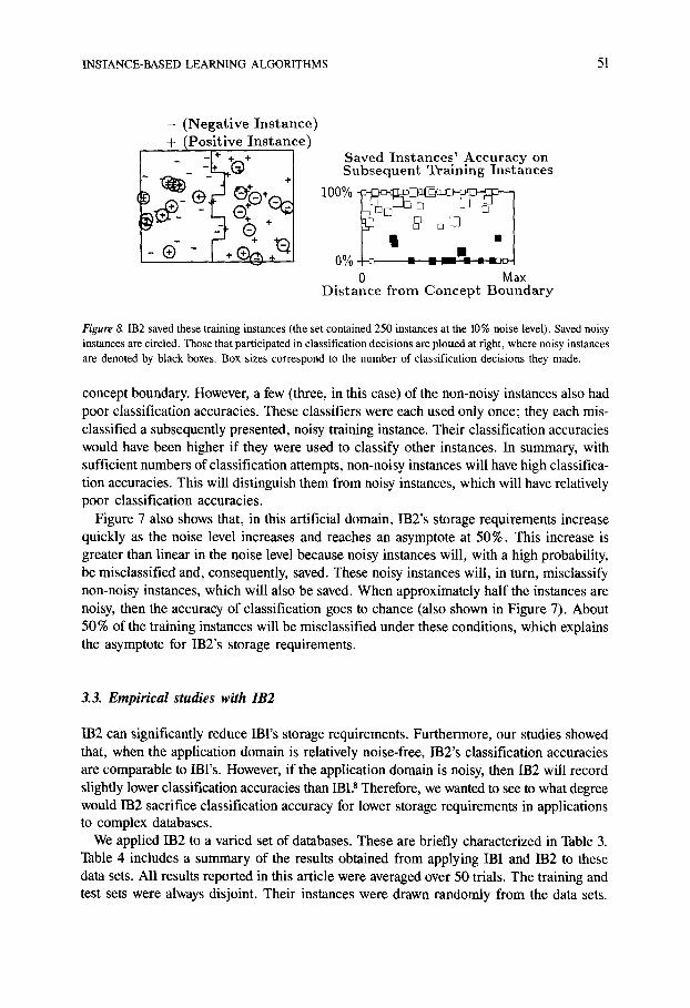
Figure & IB2 saved these training instances (the set contained 250 instances at the 10% noise level), Saved noisy instances are circled. Those that participated in classification decisions are plotted at right, where noisy instances are denoted by black boxes. Box sizes correspond to the number of classification decisions they made.

concept boundary. However, a few (three, in this case) of the non-noisy instances also had poor classification accuracies. These classifiers were each used only once; they each misclassified a subsequently presented, noisy training instance. Their classification accuracies would have been higher if they were used to classify other instances. In summary, with sufficient numbers of classification attempts, non-noisy instances will have high classification accuracies. This will distinguish them from noisy instances, which will have relatively poor classification accuracies.

Figure 7 also shows that, in this artificial domain, IB2's storage requirements increase quickly as the noise level increases and reaches an asymptote at 50%. This increase is greater than linear in the noise level because noisy instances will, with a high probability, be misclassified and, consequently, saved. These noisy instances will, in turn, misclassify non-noisy instances, which will also be saved. When approximately half the instances are noisy, then the accuracy of classification goes to chance (also shown in Figure 7). About 50 % of the training instances will be misclassified under these conditions, which explains the asymptote for IB2's storage requirements.

3.3. Empirical studies with IB2

IB2 can significantly reduce IBl's storage requirements. Furthermore, our studies showed that, when the application domain is relatively noise-free, IB2's classification accuracies are comparable to IBl's. However, if the application domain is noisy, then IB2 will record slightly lower classification accuracies than IB1. s Therefore, we wanted to see to what degree would IB2 sacrifice classification accuracy for lower storage requirements in applications to complex databases.

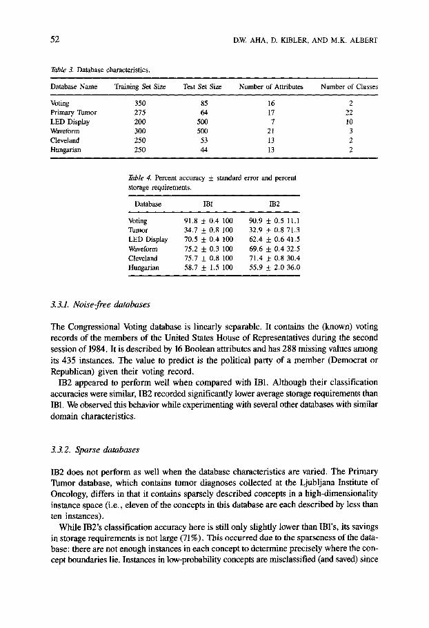
We applied IB2 to a varied set of databases. These are briefly characterized in Table 3. Table 4 includes a summary of the results obtained from applying IB1 and IB2 to these data sets. All results reported in this article were averaged over 50 trials. The training and test sets were always disjoint. Their instances were drawn randomly from the data sets.

52 D.W. AHA, D. K1BLER, AND M.K. ALBERT

Table 3. Database characteristics.

Database Name Training Set Size Test Set Size Number of Attributes Number of Classes

Voting 350 85 16 2 Primary Tumor 275 64 17 22 LED Display 200 500 7 10 Wave form 300 500 21 3 Cleveland 250 53 13 2 Hungarian 250 44 13 2

Table 4. Percent accuracy + standard error and percent storage requirements.

Database IB1 IB2

Voting 91.8 + 0.4 100 90.9 ± 0.5 11.1 Tumor 34.7 + 0.8 100 32.9 ± 0.8 71.3 LED Display 70.5 + 0.4 100 62.4 ± 0.6 41.5 Waveform 75.2 ± 0.3 100 69.6 + 0.4 32.5 Cleveland 75.7 + 0.8 100 71.4 ± 0.8 30.4 Hungarian 58.7 ± 1.5 100 55.9 ± 2.0 36.0

3.3.1. Noise-free databases

The Congressional Voting database is l inearly separable. It contains the (known) voting records of the members of the United States House of Representatives during the second session of 1984. It is described by 16 Boolean attributes and has 288 missing values among

its 435 instances. The value to predict is the political party of a member (Democrat or Republican) given their voting record.

IB2 appeared to perform well when compared with IB1. Although their classification accuracies were similar, IB2 recorded significantly lower average storage requirements than IB1. We observed this behavior while experimenting with several other databases with similar

domain characteristics.

3.3.2. Sparse databases

IB2 does not perform as well when the database characteristics are varied. The Pr imary Tumor database, which contains tumor diagnoses collected at the Ljubljana Institute of Oncology, differs in that it contains sparsely described concepts in a high-dimensionality instance space (i.e., eleven of the concepts in this database are each described by less than

ten instances). While IB2's classification accuracy here is still only slightly lower than IBl's, its savings

in storage requirements is not large (71%). This occurred due to the sparseness of the database: there are not enough instances in each concept to determine precisely where the concept boundaries lie. Instances in low-probability concepts are misclassified (and saved) since


there are few instances in their concept to classify them correctly. These instances, in turn, misclassified instances in other concepts because even the higher-frequency concepts are represented with too few instances to distinguish their concept's interior from its boundary. IB2 recorded high storage requirements because most instances appeared to be near-boundary instances.

3. 3. 3. Noisy artificial domains

Noise is another factor that rapidly degrades IB2's performance. The LED Display and Waveform domains (Breiman et al., 1984) are artificial domains with a known, large amount of noise (the Bayes optimal classification rate for these domains is 74 % and 86 %, respectively). This allowed us to compare our algorithm's classification accuracy with a known optimal accuracy when instances were noisy. Both databases provide useful data points since the one database's attributes are Boolean and the other's are continuously-valued. The value to predict in the LED Display domain, whose Boolean attribute values are each negated with a probability of 10%, is the digit represented by the instance, which is described by the settings (on or off) of seven LEDs. The Waveform domain has three classes, each of which is described by a linear combination of two waves (each wave is represented by 21 numeric attribute values). Its instances are each corrupted through the addition of a noise factor (with mean zero and variance one).

IB2's classification accuracy was substantially lower than IBl's for both domains. This occurred because IB2 misclassified and, subsequently, saved most of the noisy instances. Saved noisy instances will then be used, without discretion, to misclassify subsequently presented instances. This motivates the need for IB3, the noise-tolerant extension of IB2 described in Section 4.

3.3.4. Learning concepts with imperfect attributes

IB2's loss of classification accuracy also occurs in applications with real-world databases when the target concepts are not well-defined, such as is the case in medical diagnosis. The Cleveland and Hungarian databases (Detrano, 1988) contain heart disease diagnoses collected from the Cleveland Clinic Foundation and the Hungarian Institute of Cardiology, respectively. Diagnoses are described by 13 numeric-valued attributes (e.g., age, fasting blood sugar level). The objective here is to determine whether a patient has heart disease.

Again, IB2 significantly reduced storage requirements for both databases but also sacrificed classification accuracy. This occurred because the descriptive attributes do not completely describe the target concept. This results with a large number of exceptional instances. These instances act like noisy instances since they are poor classifiers of similar instances. Therefore, IB2 performs somewhat poorly in these applications due to the same reasons it performs poorly when instances are subject to noise.

In summary, IB2 significantly reduced storage requirements in each of the application domains. However, it also sacrificed classification accuracy, especially when the domains were noisy or had many exceptional instances. Section 4 describes an extension to IB2 that addresses this problem.


4. T o l e r a t i n g n o i s y i n s t a n c e s

Although IB2 is sensitive to the amount of noise present in the training set, it still drastically

reduced IBl's storage requirements in several applications (e.g., it required fewer than 12 % of the Congressional Voting database's instances to make relatively accurate predictions). We suspected that some simple noise-tolerant extension of IB2 could reduce its noise sensitivity. This section describes IB3, a noise-tolerant extension of IB2 that employs a simple selective utilization filter (Markovitch & Scott, 1989) to determine which of the saved in-

stances should be used to make classification decisions.

4.1. D e s c r i p t i o n o f t he I B 3 a l g o r i t h m

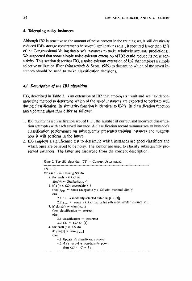
IB3, described in Table 5, is an extension of IB2 that employs a "wait and see" evidence- gathering method to determine which of the saved instances are expected to perform well during classification. Its similarity function is identical to IB2's. Its classification function and updating algorithm differ as follows:

1. IB3 maintains a classification record (i.e., the number of correct and incorrect classification attempts) with each saved instance. A classification record summarizes an instance's classification performance on subsequently presented training instances and suggests how it will perform in the future.

2. IB3 employs a significance test to determine which instances are good classifiers and

which ones are believed to be noisy. The former are used to classify subsequently presented instances. The latter are discarded from the concept description.

Table 5. The IB3 algorithm (CD = Concept Description).

CD, - -O for each x in Training Set do

1. for each y E CD do Sire[y] '-- Similarity(x, y)

2. if 3{y E CDI acceptable(y)} then Ymax ¢ - - some acceptable y E Cd with maximal Sim[y] else

2.1 i ~ a randomly-selected value in [1,1CDI] 2.2 Yrnax ~ some y E CD that is the i-th most similar instance to x

3. if class(x) ~ class(Ymax) then classification ,-- correct else

3.1 classification *-- incorrect 3.2 CD "- CD t_) {x}

4. for each y in CD do if Sim[y] >_ Sim[Ymax] then

4.1 Update y's classification record 4.2 if y's record is significantly poor

then CD ~ C - {y}


For each training instance t, classification records are updated for all saved instances that are at least as similar as t's most similar acceptable neighbor. If none of the saved instances are (yet) acceptable, we use a policy that closely simulates the behavior of the algorithm when at least one instance is acceptable. If none are acceptable, a random number r is generated from the range [1, n], where n is the number of saved instances, and the r most similar saved instances' classification records are updated. If at least one instance is acceptable, then the set of saved instances whose records are updated consist of those that are in the hyper-sphere, centered on the current training instance t, with radius equal to the normalized distance between t and its nearest acceptable neighbor. The policy for updating classification records when no instances are acceptable is essentially identical, except that the radius of the hyper-sphere is some random value at least as large as the distance between t and its nearest neighbor and no larger than the distance between t and its farthest neighbor.

IB3 accepts an instance if its classification accuracy is significantly greater than its class's observed frequency and removes the instance from the concept description if its accuracy is significantly less. We used a confidence intervals of proportions test to determine whether an instance is acceptable, mediocre, or noisy. Confidence intervals are constructed around both the instance's current classification accuracy (i.e., its percentage of correct classification attempts) and its class's current observed relative frequency (i.e., the percentage of processed training instances that are members of this class).9 If the accuracy interval's lower endpoint is greater than the class frequency interval's higher endpoint, then the instance is accepted. Similarly, instances are dropped when their accuracy interval's higher endpoint is less than their class frequency interval's lower endpoint. Finally, if the two intervals overlap, then a decision on whether to accept or discard the instance is postponed until after further training.

This test assumes that the number of successes (i.e., classification accuracies or class frequencies) are binomially distributed. While this assumption may not be correct, several IBL algorithms that employ this significance test have performed well in many applications (Aha & Kibler, 1989).

We designed the confidence test to make it difficult for an instance to be accepted. A high (z represents 90%) confidence is used for acceptance. However, we selected a lower (z represents 75 %) confidence level for dropping since we would like to drop those instances with even moderately poor classification accuracies. These are the only two parameters required by IB3.1°

The advantage gained by comparing a saved instance's accuracy with its class's observed relative frequency requires further explanation. IB3 normalizes the acceptance of an instance with respect to concept frequency distributions to decrease its sensitivity to skewed distributions. Instances in concepts with high observed relative frequencies are expected to have relatively high classification accuracies since a relatively high percentage of its possible classification attempts will be for instances in its class. Similarly, instances in concepts with low observed relative frequencies are expected to have relatively low classification accuracies. By comparing an instance's accuracy against its class's frequency, IB3 can more easily tolerate skewed concept distributions.

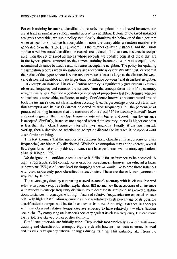
Confidence intervals are initially wide. They shrink monotonically in width with more training and classification attempts. Figure 9 details how an instance's accuracy interval and its class's frequency interval changes during training. This instance, taken from the


Ins tance ' s Accuracy 100%

Concept ' s Observed Frequency

80%

60%

2O%

O% 0 50 100 150 200 250 50 100 150 200 250

N u m b e r Of Training Ins tances

Figure 9. Confidence intervals shrink in width over time. This is an example of an accepted (good) instance in the LED display domain. The middle curve in each graph is the actual value (i.e., instance accuracy, class frequency). The other two curves denote the respective confidence interval's upper and lower bounds.

LED Display domain, was accepted since its classification accuracy, which reached 46 %, is significantly better than its class's observed relative frequency, which reached 12 %. Both intervals are initially large in width and gradually shrink. The frequency interval is smaller in size because it is computed over the entire set of observed training instances (250 total), whereas the accuracy interval is instead computed only over this instance's classification attempts (i.e., 53). The accuracy interval's upper endpoint and the concept frequency interval's lower endpoint are closer to the actual values than are the other two endpoints. This is because IB3 uses a looser bound (75 % confidence level) for determining which instances to drop than the bound used to determine which instances to accept (90% confidence interval).

This figure shows that this instance was not accepted until after 120 instances were processed. At that point, the accuracy interval's lower bound first became higher than the frequency interval's upper bound. The instance's accuracy remained significantly higher than its class's frequency for the duration of training.

4.2. IB3's behavior on a simple domain

IB3 assumes that the classification records of noisy instances will distinguish them from non-noisy instances. Noisy instances will have poor classification accuracies because their nearby neighbors in the instance space will invariably have other classifications. This assumption is exemplified in Figure 10, which summarizes IB3's performance on the same data set given to IB2 to produce Figure 8. There are several striking differences between these two figures. First, IB3 used z e r o noisy instances for classification whereas IB2 used 20. This provides our first piece of evidence that IB3's selective utilization filter works in noisy domains. Second, IB3 used only 25 instances for classific~ttion whereas IB2 used 76. Third, the instances chosen by IB3 to use for classification all recorded relatively high classification accuracies. This is another consequence of IB3's noise-tolerant filter. Next, several


- (Negat ive Ins tance) + (Posit ive Ins tance)

-- L q" + - ] %÷

- ], . : • _ r -I-

Saved Ins tances ' Accuracy on Subsequent Training Instances

100%0% l ' ~

0 Max Distance f rom Concept B o u n d a r y

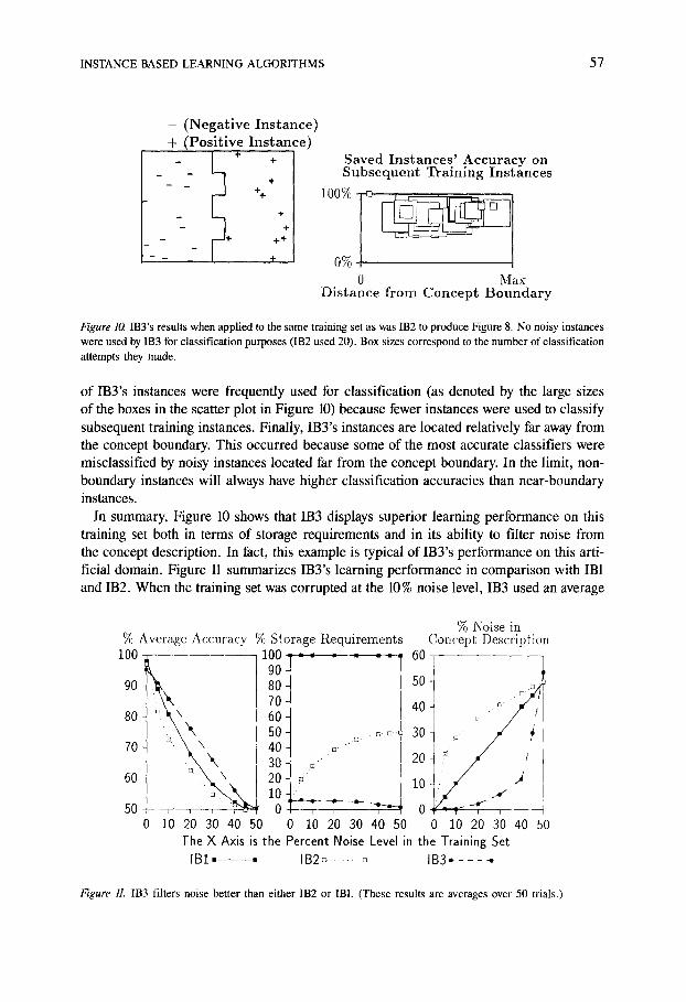
Figure 10. IB3's results when applied to the same training set as was IB2 to produce Figure 8. No noisy instances were used by IB3 for classification purposes (IB2 used 20). Box sizes correspond to the number of classification attempts they made.

of IB3's instances were frequently used for classification (as denoted by the large sizes of the boxes in the scatter plot in Figure 10) because fewer instances were used to classify subsequent training instances. Finally, IB3's instances are located relatively far away from the concept boundary. This occurred because some of the most accurate classifiers were misclassified by noisy instances located far from the concept boundary. In the limit, non- boundary instances will always have higher classification accuracies than near-boundary instances.

In summary, Figure 10 shows that IB3 displays superior learning performance on this training set both in terms of storage requirements and in its ability to filter noise from the concept description. In fact, this example is typical of IB3's performance on this artificial domain. Figure 11 summarizes IB3's learning performance in comparison with IB1 and IB2. When the training set was corrupted at the 10% noise level, IB3 used an average

% Average Accuracy % Storage Requirements 100 100 . . . . . . •

90 ~ - - - 90 80 4

8O

70

60

50

60 q

N 40

20 ?

i0 20 30 40 50 0 10 20 30 40 50

% Noise in Concept Description

60

50-

40- ~ / i 3o- / / /

20- y J j / 10 -:/

o : ~ - - ~ , - , - - - 0 10 20 30 40 50

The X Axis is the Percent Noise Level in the Training Set IB1 -------- IB2 ... . . . . . . . IB3 . . . . .

Figure 11. IB3 filters noise better than either IB2 or IB1. (These results are averages over 50 trials.)


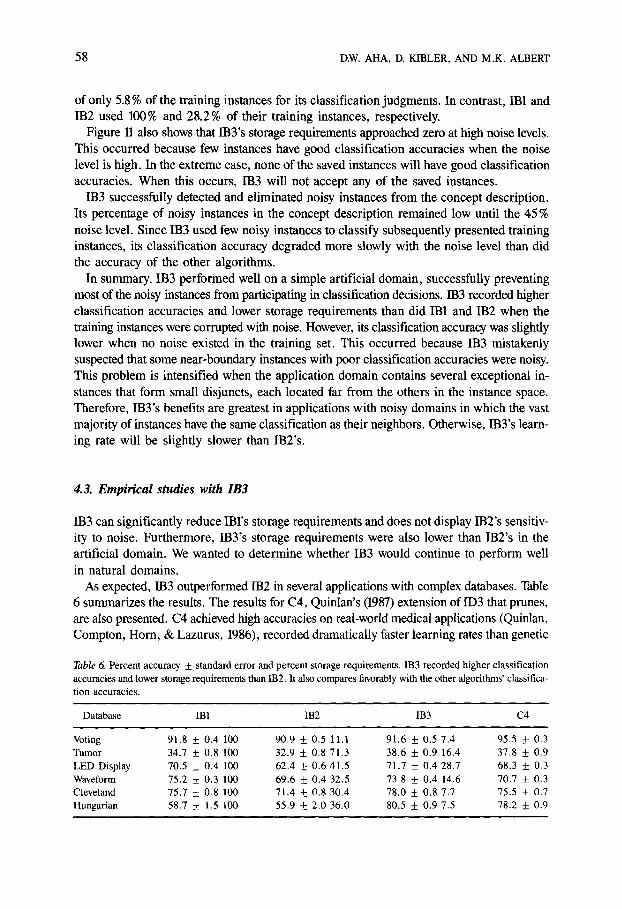
of only 5.8 % of the training instances for its classification judgments. In contrast, IB1 and IB2 used 100% and 28.2% of their training instances, respectively.

Figure 11 also shows that IB3's storage requirements approached zero at high noise levels. This occurred because few instances have good classification accuracies when the noise level is high. In the extreme case, none of the saved instances will have good classification accuracies. When this occurs, IB3 will not accept any of the saved instances.

IB3 successfully detected and eliminated noisy instances from the concept description. Its percentage of noisy instances in the concept description remained low until the 45 % noise level. Since IB3 used few noisy instances to classify subsequently presented training instances, its classification accuracy degraded more slowly with the noise level than did the accuracy of the other algorithms.

In summary, IB3 performed well on a simple artificial domain, successfully preventing most of the noisy instances from participating in classification decisions. IB3 recorded higher classification accuracies and lower storage requirements than did IB1 and IB2 when the training instances were corrupted with noise. However, its classification accuracy was slightly lower when no noise existed in the training set. This occurred because IB3 mistakenly suspected that some near-boundary instances with poor classification accuracies were noisy. This problem is intensified when the application domain contains several exceptional instances that form small disjuncts, each located far from the others in the instance space. Therefore, IB3's benefits are greatest in applications with noisy domains in which the vast majority of instances have the same classification as their neighbors. Otherwise, IB3's learning rate will be slightly slower than IB2's.

4.3. Empirical studies with IB3

IB3 can significantly reduce IBl's storage requirements and does not display IB2's sensitivity to noise. Furthermore, IB3's storage requirements were also lower than IB2's in the artificial domain. We wanted to determine whether IB3 would continue to perform well in natural domains.

As expected, IB3 outperformed IB2 in several applications with complex databases. Table 6 summarizes the results. The results for C4, Quinlan's (1987) extension oflD3 that prunes, are also presented. C4 achieved high accuracies on real-world medical applications (Quinlan, Compton, Horn, & Lazurus, 1986), recorded dramatically faster learning rates than genetic

Table 6 Percent accuracy ± standard error and percent storage requirements. IB3 recorded higher classification accuracies and lower storage requirements than IB2. It also compares favorably with the other algorithms' classification accuracies.

Database IB1 IB2 IB3 C4

Voting 91.8 + 0.4 100 90.9 +_ 0.5 11.1 91.6 + 0.5 7.4 95.5 ___ 0.3 Tumor 34.7 + 0.8 100 32.9 _+ 0.8 71.3 38.6 ___ 0.9 16.4 37.8 + 0.9 LED Display 70.5 _.+ 0.4 100 62.4 _.+ 0.6 41.5 71.7 + 0.4 28.7 68.3 + 0.3 Waveform 75.2 + 0.3 100 69.6 ± 0.4 32.5 73.8 +_ 0.4 14.6 70.7 + 0.3 Cleveland 75.7 + 0.8 100 71.4 ± 0.8 30.4 78.0 ± 0.8 7.7 75.5 ± 0.7 Hungarian 58.7 + 1.5 100 55.9 ± 2.0 36.0 80.5 ± 0.9 7.5 78.2 ___ 0.9


algorithms on multiplexor learning tasks (Quinlan, 1988), and has generally performed well on a large and varied set of learning tasks that are similar to the ones we have chosen for our experiments (Quinlan, 1987). Furthermore, C4 is highly similar to a set of decision tree algorithms that have performed well in a large number of research experiments and industrial applications (Breiman et al., 1984; Michie, Muggleton, Riese, & Zubrick, 1984; Cestnik, Konenenko, & Bratko, 1987). Therefore, we chose to compare C4's results with the results from our own algorithms to determine whether they form comparatively accurate concept descriptions in these experiments.

4.3.1. Noise-free databases

IB3's performance improvement over IB2 is not substantial in the application involving the Congressional Voting database. This was predicted since they performed equally well under similar conditions, as described in Section 4.2 (i.e., when applied to the 2-dimensional artificial domain at the 0% noise level).

C4's higher classification accuracy is due to the nature of the target concept's description, whose boundaries are orthogonal to the attribute dimensions. The learning bias of decision tree algorithms (i.e., that concepts can be easily described using hyper-rectangular parti- tions of the instance space) is appropriate for this application.

4. 3. 2. Sparse databases

IB3 recorded substantial improvements upon IB2's classification performance in the Primary Tumor database. IB2's classification accuracy was low because it used saved instances from low-frequency concepts to classify instances in other concepts and the database does not contain sufficient numbers of instances to well-describe its concepts' boundaries. Although IB3 also initially saves these same instances, it instead requires that they demonstrate good classification behavior before it uses them in subsequent classification decisions. IB3 therefore rarely uses instances from sparsely described, low-frequency concepts to misclassify instances from high-frequency concepts. IB3 also tends to use instances further from the actual concept boundaries than does IB2 for classification decisions. This means that it is better able to define the interior ("core") of the high-frequency concepts, which leads to better classification behavior on these concepts and in the entire database. (Unfortunately, this example also displays one of IB3's weaknesses: it is unable to distinguish noise from disjuncts described by few instances.)

4. 3. 3. Noisy artificial domains

IB3's superior learning performance is evident in the applications to the noisy LED Display and Waveform domains. It recorded higher classification accuracies and substantially lower storage requirements than IB2 in these domains.


The concepts in these databases do not as easily admit to C4's learning bias: their descriptions are more easily expressed using IBL's piecewise-linear approximations, which are not restricted to being orthogonal to the given attribute dimensions. Subsequently, C4's learning rate is decreased to the point at which it does not record higher classification accuracies than IB3 here.

4.3.4. Learning concepts with imperfect attributes

IB3's advantages are far more pronounced in the applications to the heart disease databases. IB3's results are most striking for the Hungarian database, where both IBl's and IB2's performances degraded due to the large amounts of noise in this database.

C4's test of statistical significance also helped it achieve a relatively high accuracy. How- ever, IB3's more relaxed learning bias again allowed it to perform favorably in comparison.

In summary, IB3 demonstrated significant improvement over IB2 in these applications. It consistently reduced IB2's storage requirements and improved upon IB2's classification accuracy. IB3 compared favorably with IB1 in measurements of classification accuracy. IB3's relatively weak learning bias for piecewise-linear approximations of concept descriptions often allowed it to achieve slightly faster learning rates than C4 in these applications.

4.4. Generality of the noise-tolerant extension

Although we focused on extending the nearest neighbor classification algorithm in this article, we also learned that this same noise-tolerant extension can improve similar classification algorithms (Aha & Kibler, 1989).

For example, we showed that a similar noise-tolerant extension of Bradshaw's (1987) Dis- junctive Spanning algorithm increased its classification accuracy and lowered its storage requirements in applications involving this same set of databases. The Disjunctive Spanning algorithm is identical to IB2 except that, whereas IB2 discards correctly classified instances, it instead averages them with the correctly classifying (stored) instance. All instances are initially assigned weights of one. When two instances are averaged, their weights are summed. Instances are relocated in the instance space through this averaging process. Reloca- tion is radical when the weights are small and gradually becomes highly conservative. If the first few averagings are across disjuncts or if the concept is not convex in shape, then the averaged "instance" may not be located in the concept (Bradshaw, 1987). This makes instance-averaging algorithms difficult to analyze, even when the concepts are convex in shape (Kibler & Aha, 1989). Since the disjunctive spanning algorithm and its noise-tolerant extension have not proven to be empirically superior to IB2 and IB3, we believe that the latter algorithms are safer--they never construct incorrectly classified "instances."

Our noise-tolerant extension can also be used with k-nearest neighbor algorithms, which classify an instance according to a majority vote of its k most similar instances. However, noise-tolerant extensions of these algorithms explore a risky tradeoff in which slightly increased classification accuracies are gained at the expense of reduced learning rates (Aha & Kibler, 1989). The noise-tolerant k-nearest neighbor algorithm performed poorly when


"-x - J

/

J <

\ \

\ \

\

(

v

Figure 12. An example where the 1-nn algorithm outperforms a k-nn algorithm. If any of the ten instances shown here is removed, then the removed instance will be classified correctly by the nearest neighbor algorithm, but misclassified by the k-nearest neighbor algorithm (where k is 3).

applied to small (insufficiently sized) training sets. This occurred because k > 1 acceptable instances are required to make classification judgments. Few of the saved instances are acceptable during the early training stages. Therefore, some of them are relatively dissimilar to the instance being classified. This reduced the learning rate. Figure 12 shows a simple and dramatic example of this behavior. IB3, the noise-tolerant 1-nearest neighbor algorithm, is more robust than any other k-nearest neighbor algorithm since it has a faster learning rate.

5. Discussion and summary

In this section, we survey existing limitations with IB3, outline possible solutions, and point out some of the benefits gained from using instance-based representation for concepts during supervised learning tasks.

5.1. Limitations

IB3's learning performance is highly sensitive to the number of irrelevant attributes used to describe instances. Its storage requirements increase exponentially and its learning rate decreases exponentially with increasing dimensionality. IB3 is, therefore, a poor learning algorithm to apply in applications involving multiple irrelevant attributes (this is also true of its predecessors, IB1 and IB2). However, extensions of IB3 exist that alleviate this problem by learning relative attribute relevances that are used to adjust the similarity function (Aha, 1989a). These extensions locate irrelevant attributes which, once ignored, effectively reduces the dimensionality of the instance space.

IB3 assumes that concepts are disjoint and that they jointly exhaust the instance space. It is unable to represent overlapping concepts and assumes that every instance is a member of exactly one concept. Fortunately, this problem can be solved by learning a separate concept description for each concept (Aha, 1989a).


We have studied how the instance-based approach can use continuously-valued attributes to predict the values of either unordered or totally-ordered (Kibler, Aha, & Albert, 1989) attributes. While we have not yet experimented with sophisticated definitions for defining similarity for symbolic-valued attributes, variants of Stanfill and Waltz's (1986) similarity algorithm may prove useful for this task. We have also not addressed the learning of rela- tional and structured concepts.

We left out the comprehensibility performance measure from the list in Section 2.1. This measure indicates the ability for humans (often experts in the domain) to verify and use the concept descriptions generated by the learning program. While some researchers argue that a distributed instance-based representation does not summarize conceptual structure (e.g., Breiman et al., 1984), evidence exists that experts in some domains reason by appeal- ing to the similarity of new and old instances (Brooks, 1989; Clark, 1989). Nonetheless, the algorithms described in this paper do not form concise abstractions from instances to describe concepts. (Salzberg (1988) presents an IBL algorithm that constructs and uses abstractions for classification decisions.)

We have not yet developed IBL algorithms that construct nor induce higher-order attributes. Therefore, the current algorithms are restricted to selective induction (Dietterich & Michalski, 1983) and will record relatively slow learning rates when higher-order attributes provide significantly better descriptions of the target concept (e.g., by reducing the disjunctiveness of the target concept (Rendell, 1988) or by reducing the size of its boundary). We plan to investigate methods for constructive induction in the near future.

Storage reduction techniques are only one approach for reducing classification costs. Several incremental learning algorithms (e.g., Fisher, 1989; Utgoff, 1989) build data structures which can be used to reduce the number of attribute references required to generate classification predictions. Organizational hierarchies can also be constructed to index instances for IBL algorithms.

5.2. Advantages

Instance-based algorithms also have several advantages. One benefit of this approach is its simplicity, which allowed us to use a rigorous analysis to guide our intuition and research goals. Our analysis of IB1 led to the development of the storage reduction algorithm. Our expectations and validation that IB2 is sensitive to noise led us to develop IB3. Researchers studying pattern recognition (Gates, 1972), psychological concept formation (Hintzman, 1986), and machine learning (Bradshaw, 1987) have all benefited from the simplicity of the instance-based approach.

The IBL paradigm supports relatively robust learning algorithms. They can tolerate noise and irrelevant attributes and can represent both probabilistic and overlapping concepts (Aha, 1989b). Barsalou (1983) pointed out that exemplar-based models can also be used to solve ad-hoc categorization tasks, in which the learning algorithm is asked to classify instances for concepts it was not explicitly learning (i.e., "things sold at a garage sale").

IBL algorithms have a relatively relaxed concept bias. They incrementally learn piecewise- linear approximations of concepts. In contrast, algorithms that learn decision trees or rules approximate concepts with hyper-rectangular representations. Instance-based algorithms


can record faster learning rates than these other algorithms when their bias is not satisfied by target concepts in the application domain. This occurs when the target concept's boundary is not parallel to the attribute dimensions. Although multi-attribute splitting techniques for decision tree algorithms can lessen this sensitivity, these techniques are expensive. IBL algorithms naturally exploit inter-attribute relationships.

Finally, IBL algorithms have relatively low updating costs. If the updating algorithm decides to update a concept description, then it simply saves the current training instance. However, IBL updating costs include classification costs, which require O([N[ × IA]) attribute examinations, where N is the set of instances saved (from a training set of size 1I[) in the current concept description and A is the set of attributes used to describe the instances. In contrast, C4 (Quinlan, 1987) requires O(1I[ × [A[ 2) attribute examinations to incorporate a new training instance, during which time it creates a new decision tree. Several researchers have shown how to decrease these costs significantly (Schlimmer & Fisher, 1986; Utgoff, 1989; Van de Velde, 1989). Parallel processing methods and/or indexing strategies can similarly be used to reduce the training costs for the IBL approach. For example, with IN[ processors, only O([AI log [A[) time is required to compute similarities and yield a classification. Gates (1972) showed that classification costs can also be further reduced by discarding saved instances that no longer provide concept boundary information.

5.3. Summary and future directions

In this article, we described robust extensions of the nearest neighbor pattern classifier, analyzed their capabilities, and described their empirical behavior in incremental, supervised learning applications. Our analysis showed that IBL algorithms can learn any concept describable as a finite union of closed hypercurves of finite size in the instance space whose instances are selected from any fixed and bounded continuous distribution. We then showed that these algorithm's storage requirements can be sharply reduced with small sacrifices in classification accuracy. Finally, we demonstrated that this storage-reducing algorithm can be improved by using a selective utilization filter on the saved instances. This improved the algorithm's ability to tolerate noisy instances.

Most of the limitations confronting the instance-based learning paradigm are currently being investigated (e.g., deriving concise abstractions, learning data structures for indexing, similarity definitions for nominal-valued attributes). However, we recognize that its restriction to selective induction is problematic, and we plan to investigate methods for constructive induction. We also plan to evaluate the utility of IBL algorithms as empirical components in a combined analytic/empirical framework.

Acknowledgments

We would like to thank our editor, Ross Quinlan, and our anonymous reviewers. Their insightful suggestions resulted in a substantially improved article. We would also like to thank Jeff Schlimmer (Carnegie Mellon) for providing the Congressional Voting database, M. Zwitter and M. Sokli~ (Institute of Oncology, Ljubljana, Yugoslavia) for the primary


t u m o r da t abase , R o b e r t D e t r a n o (V.A. Cen te r , L o n g B e a c h , C A) fo r t he C l e v e l a n d da t abase ,

a n d A n d r a s J a n o s i ( H u n g a r i a n Ins t i tu te o f Card io logy , B u d a p e s t ) for the H u n g a r i a n da tabase .

T h e s e d a t a b a s e s a r e a v a i l a b l e f r o m the U.C. I . r e p o s i t o r y o f m a c h i n e l e a r n i n g d a t a b a s e s

a n d d o m a i n t h e o r i e s . S p e c i a l t h a n k s to C a r o l i n e E h r l i c h a n d h e r a s s i s t a n t s for c a r e f u l l y

p r o o f r e a d i n g o u r f i na l d ra f t .

No~s

1. IBL algorithms are exemplar-based models with learning/process components. Many descriptions of exemplar- based models do not include these components (e.g., Medin& Schaffer, 1978; Nosofsky, 1986), However, while each input to an exemplar-based model is either a specific instance (e.g,, "Charlie," a pet snake) or a set of instances (e.g., "snakes"), our current IBL algorithms are designed to input only specific instances.

2. We describe how IBL algorithms can yield a graded estimate of an instance's membership in each category in Aha (1989a).

3. Our algorithms normalize an attribute's values by scaling them according to the highest and lowest values yet presented for this attribute. Renormalization is required whenever a new highest and lowest value is presented.

4. One of the databases that we will use (Primary Tumor) contains one symbolic-valued attribute. All the other attributes used to describe instances in the databases we use in our experiments range over Boolean or numeric values.

5. If a probabilistic model is appropriate for classification and all joint density functions are known, then the optimal Bayes decision policy is that process which minimizes the probability of misclassification.

6. Hart (1968) also reported this phenomenon for his Condensed Nearest Neighbor algorithm, which differs from IB2 in that (1) it does not normalize attribute values and (2) it iterates through the training data.

7. For this two-dimensional instance space, the probability that a training instance will be misclassified by all- attribute noise is (52.3 × N)%, where N is the noise level. This is almost identical to the probability that class noise will result with a misclassification, which is (50.0 × N)%. An empirical study of either type of noise will yield highly similar results. Therefore, we have chosen to focus on only one of these types of noise. For other instance spaces, the probability of misclassifications in the training set can differ greatly, depending on whether all-attribute or class noise is used to corrupt the instances. In such cases, the type of noise with a higher probability of misclassification will result with accelerated degradations of our algorithms, but will not alter their relative behaviors.

8. Actually, this is a matter of learning rate rather than asymptotic classification accuracy. IB2 will have a slower learning rate in noisy domains, but its asymptotic classification accuracy is always the same as IBl's.

9. We used Equation 5.5-4 on page 296 in Hogg and Tanis (1983). 10. We performed a post-hoc sensitivity analysis of these parameters in applications with the LED Display domain.

IB3's performance degrades quickly when the confidence level for acceptance is too high (e.g., 95%), independent of the other parameter's setting. Settings below 80% for the acceptance parameter begin to show slight degradations in performance. Higher settings for the dropping parameter increase storage requirements without affecting classification accuracy.

References

Aha, D.W. (1989a). Incremental, instance-based learning of independent and graded concept descriptions. Proceed- ings of the Sixth International Workshop on Machine Learning (pp. 387-391). Ithaca, NY: Morgan Kaufmann.

Aha, D.W. (1989b). Incremental learning of independent, overlapping, and graded concepts with an instance- based process framework (Technical Report 89-10). Irvine, CA: University of California, Irvine, Department of Information and Computer Science.

Aha, D.W. (1989c). Tolerating noise, irrelevant attributes, and novel attributes in instance-based learning algorithms. Proceedings of the IJCAI-1989 Workshop on Symbolic Problem Solving in Noisy, Novel, and Uncertain Task Environments. Detroit, MI: Computing Research Laboratory, New Mexico State University.


Aha, D.W., & Kibler, D. (1989). Noise-tolerant instance-based learning algorithms. Proceedings of the Eleventh International Joint Conference on Artificial Intelligence (pp. 794-799). Detroit, MI: Morgan Kaufmann.

Bareiss, E.R., Porter, B., & Wier, C.C. (1987). PROTOS: An exemplar-based learning apprentice. Proceedings of the Fourth International Workshop on Machine Learning (pp. 12-23). Irvine, CA: Morgan Kaufmann.

Barsalou, L.W. (1983). Ad hoc categories. Memory and Cognition, 11, 211-227. Blumer, A., Ehrenfeucht, A., Haussler, D., & Warmuth, M. (1986). Classifying learnable geometric concepts

with the Vapnik-Chervonenkis dimension. Proceedings of the Eighteenth Annual Association for Computing Machinery Symposium on Theory of Computing (pp. 273-282). Berkeley, CA: Association for Computing Machinery.

Breiman, L., Friedman, J.H., Olshen, R.A., & Stone, C.J. (1984). Classification and regression trees. Belmont, CA: Wadsworth International Group.

Bradshaw, G. (1987). Learning about speech sounds: The NEXUS project. Proceedings of the Fourth International Workshop on Machine Learning (pp. 1-11). Irvine, CA: Morgan Kaufmann.

Brooks, L. (1978). Nonanalytic concept formation and memory for instances. In E. Rosch & B.B. Lloyd (Eds.), Cognition and categorization. Hillsdale, NJ: Lawrence Erlbaum Associates.

Brooks, L. (1989). Concept formation and particularizing learning. In S. Hanson & R. Davis (Eds.), Information, language, & cognition: Vancouver studies in cognitive science (Vol. 1). Vancouver, B.C.: UBC Press.

Cestnik, B., Kononenko, I., & Bratko, I. (1987). ASSISTANT-86: A knowledge-elicitation tool for sophisticated users. In 1. Bratko & N. Lavrac (Eds.), Progress in machine learning. Bled, Yugoslavia: Sigma Press.

Clark, P.E. (1989). Exemplar-based reasoning in geologicalprospect appraisal (Technical Report 89-034). Glasgow, Scotland: Turing Institute.

Clark, EE., & Niblett, T. (1989). The CN2 induction algorithm. Machine Learning, 3, 261-284. Cover, T.M., & Hart, P.E. (1967). Nearest neighbor pattern classification. Institute of Electrical and Electronics

Engineers Transactions on Information Theory, 13, 21-27. Dasarathy, B.V. (1980). Nosing around the neighborhood: A new system structure and classification rule for recogni-

tion in partially exposed environments. Pattern Analysis and Machine Intelligence, 2, 67-71. Detrano, R., M.D. (1988), International application of a new probability algorithm for the diagnosis of coronary

artery disease. Unpublished manuscript. Dietterich, T.G., & Michalski, R.S. (1983). A comparative review of selected methods for learning from examples.

In R.S. Michalski, J.G. Carbonell, & T.M. Mitchell (Eds.), Machine learning: An artificial intelligence approach. San Mateo, CA: Morgan Kaufmann.

Fisher, D.E (1989). Noise-tolerant concept clustering. Proceedings of the Eleventh International Conference on Artificial Intelligence (pp. 825-830). Detroit, MI: Morgan Kaufmann.

Gates, G.W. (1972). The reduced nearest neighbor rule. IEEE Transactions on Information Theory, 431-433. Hart, P.E. (1968). The condensed nearest neighbor rule. Institute of Electrical and Electronics Engineers and

Transactions on Information Theory, 14, 515-516. Hintzman, D.L. (1986). "Schema abstraction" in a multiple-trace memory model. Psychological Review, 93, 411-428. Hogg, R.V., & Tanis, E.A. (1983). Probability and statistical inference. New York, NY: Macmillan. Jabbour, K., Riveros, J.F.V., Landsbergen, D., & Meyer, W. (1987). ALFA: Automated load forecasting assistant.

Proceedings of the 1987 IEEE Power Engineering Society Summer Meeting. San Francisco, CA. Kibler, D., & Aha, D.W. (1988). Case-based classification. Proceedings of the Case-Based Reasoning Workshop

at AAA1 1988 (pp. 62-67). Unpublished manuscript. Kibler, D., & Aha, D.W. (1989). Comparing instance-saving with instance-averaging learning algorithms. In D.P.

Benjamin (Ed.), Change of representation and inductive bias. Norwell, MA: Kluwer Academic Publishers. Kibler, D., Aha, D.W., & Albert, M. (1989). Instance-based prediction of real-valued attributes. Computational

Intelligence, 5, 51-57. Koton, E (1988). Reasoning about evidence in causal explanations. Proceedings of the Seventh National Confer-

ence on Artificial Intelligence (pp. 256-261). St. Paul, MN: Morgan Kaufmann. Markovitch, S., & Scott, P.D. (1989). Information filters and their implementation in the SYLLOG system. Pro-

ceedings of the Sixth International Workshop on Machine Learning (pp. 404-407). Ithaca, NY: Molgan Kaufinann. Medin, D.L., & Schaffer, M.M. (1978). Context theory of classification learning. Psychological Review, 85, 207-238. Michalski, R.S., & Larson, J.B. (1978). Selection of mast representative training examples and incremental generation

of VLI hypotheses: The underlying methodology and the description of programs ESEL and AQll (Technical Report 867). Urbana, IL: University of Illinois, Department of Computer Science.


Michalski, R.S., Mozetic, I., Hong, J., & Lavrafi, N. (1986). The multi-purpose incremental learning system AQ15 and its testing application to three medical domains. Proceedings of the Fifth National Conference on Artificial Intelligence (pp. 1041-1045). Philadelphia, PA: Morgan Kaufmann.

Michie, D., Muggleton, S., Riese, C., & Zubrick, S. (1984). Rulemaster: A second-generation knowledge- engineering facility. 1984 Conference on Artificial Intelligence and Applications.

Nosofsky, R.M. (1986). Attention, similarity, and the identification-categorization relationship. Journal of Experi- mental Psychology: General, 15, 39-57.

Quinlan, J.R. (1986). Induction of decision trees. Machine Learning, 1, 81-106. Quinlan, J.R. (1987). Generating production rules from decision trees. Proceedings of the Tenth International

Joint Conference on Artificial Intelligence (pp. 304-307). Milan, Italy: Morgan Kanfmann. Quinlan, J.R. (1988). An empirical comparison of genetic and decision-tree classifiers. Proceedings of the Fifth

International Conference on Machine Learning (pp. 135-141). Ann Arbor, MI: Morgan Kaufmann. Quinlan, J.R., Compton, EJ., Horn, K.A., & Lazurus, L. (1986). Inductive knowledge acquisition: A case study.

Proceedings of the Second Australian Conference on Applications of Expert Systems. Sydney, Australia. Rendell, L. (1988). Learning hard concepts. Proceedings of the Third European Working Session on Learning

(pp. 177-200). Glasgow, Scotland: Pitman Publishing. Rissland, E.L., Kolodner, J., & Waltz, D. (1989). Case-based reasoning from DARPA: Machine learning pro-

gram plan. Proceedings of the Case-Based Reasoning Workshop (pp. 1-13). Pensecola Beach, FL: Morgan Kaufmann.

Rosenblatt, E (1962). Principles of neurodynamics. New York, NY: Spartan. Rumelhart, D.E., McClelland, J.L., & The PDP Research Group (Eds.) (1987). Parallel distributed processing:

Explorations in the microstructure of cognition (Vol. 1). Cambridge, MA: MIT Press. Shamos, M.I., & Hoey, D. (1975). Closest point problems. Proceedings of the Sixteenth Annual Institute of Elec-

trical and Electronic Engineers Symposium on the Foundations of Computer Science (pp. 151-162. IEEE Com- puter Society.

Salzberg, S. (1988). Exemplar-based learning: Theory and implementation (Technical Report TR-10-88). Cambridge, MA: Harvard University, Center for Research in Computing Technology.

Schlimmer, J.C., & Fisher, D. (1986). A case study of incremental concept induction. Proceedings of the Fifth National Conference on Artificial Intelligence (pp. 496-501). Philadelphia, PA: Morgan Kaufmann.

Smith, E.E., & Medin, D.L. (1981). Categories and concepts. Cambridge, MA: Harvard University Press. Stanfill, C., & Waltz, D. (1986). Toward memory-based reasoning. Communications of the ACM, 29, 1213-1228. Utgoff, EE. (1989). Incremental induction of decision trees. Machine Learning, 4, 161-186. Valiant, L.G. 0984). A theory of the learnable. Communications of the Association for Computing Machinery,

27, 1134-1142. Van de Velde, W. (1989). IDL, or taming the multiplexer. Proceedings of the Fourth European Working Session

on Learning (pp. 211-225). Montpellier, France: Morgan Kaufmann. Volper, D.J., & Hampson, S.E. (1987). Learning and using specific instances. Biological Cybernetics, 57, 57-71.

Instance-based learning algorithms - Welcome to the …sci2s.ugr.es/keel/pdf/algorithm/articulo/aha1991.pdf · Instance-based learning algorithms suffer from several problems that

Documents