INSTABILITY AND STABILITY PROPERTIES OF TRAVELING …

INSTABILITY AND STABILITY PROPERTIES OF TRAVELING

WAVES FOR THE DOUBLE DISPERSION EQUATION

H. A. ERBAY, S. ERBAY, AND A. ERKIP

Abstract. In this article we are concerned with the instability and stability

properties of traveling wave solutions of the double dispersion equation utt −uxx + auxxxx − buxxtt = −(|u|p−1u)xx for p > 1, a > b > 0. The main

characteristic of this equation is the existence of two sources of dispersion,

characterized by the terms uxxxx and uxxtt. We obtain an explicit conditionin terms of a, b and p on wave velocities ensuring that traveling wave solutions

of the double dispersion equation are strongly unstable by blow up. In the

special case of the Boussinesq equation (b = 0), our condition reduces tothe one given in the literature. For the double dispersion equation, we also

investigate orbital stability of traveling waves by considering the convexity of

a scalar function. We provide analytical as well as numerical results on thevariation of the stability region of wave velocities with a, b and p and then

state explicitly the conditions under which the traveling waves are orbitallystable.

1. Introduction

The present paper is concerned with the instability and stability properties oftraveling wave solutions for the double dispersion equation

(1.1) utt − uxx + auxxxx − buxxtt = −(|u|p−1u)xx,

where a, b are positive real constants with a > b, and p > 1. In particular we provethat traveling wave solutions are unstable by blow-up if the wave velocities of thetraveling waves are less than a critical wave velocity. We also state explicitly a setof conditions on a, b and p for which the traveling waves are orbitally stable.

The double dispersion equation (1.1) was derived as a mathematical model of thepropagation of dispersive waves in a wide variety of situations, see for instance [1, 2]and the references therein. Well posedness (and related properties) of the Cauchyproblem for the double dispersion equation have been studied in the literature byseveral authors [3, 4, 5]. It is interesting to note that (1.1) is a special case of thegeneral class of nonlinear nonlocal wave equations

(1.2) utt − Luxx = B(g(u))xx,

with pseudo-differential operators L and B, studied in [6, 7, 8]. Indeed, for the case

(1.3) L = (I − aD2x)(I − bD2

x)−1, B = (I − bD2x)−1, g(u) = −|u|p−1u,

where I is the identity operator and Dx denotes the partial derivative with respec-tive to x, (1.2) reduces to (1.1). The well-posedness of the Cauchy problem for the

Date: December 15, 2015.2010 Mathematics Subject Classification. 74J35, 76B25, 35L70, 35Q51.Key words and phrases. Double dispersion equation, Boussinesq equation, Solitary waves,

Instability by blow-up, Orbital stability.1

2 H. A. ERBAY, S. ERBAY, AND A. ERKIP

general class (1.2) was studied in [6] and then the parameter dependent thresholdsfor global existence versus blow-up were established in [7] for power nonlineari-ties. In a recent study [8] on (1.2), again for power nonlinearities, the existenceof traveling wave solutions u = φc(x − ct), where c ∈ R is the wave velocity, hasbeen established and orbital stability of the traveling waves has been studied. Theorbital stability is based on the convexity of a certain function d(c) related to con-served quantities. Furthermore, it has been shown that when L = I, (1.2) becomesa special case of the Klein-Gordon-type equations and d(c) can be computed ex-plicitly. In [8] the sharp threshold of instability/stability of traveling waves for thisregularized Klein-Gordon equation has been established. In other words, for L = I,it has been shown that traveling wave solutions of (1.2) are orbitally stable for

(1.4)p− 1

p+ 3< c2 < 1

and are unstable by blow-up for

(1.5) c2 <p− 1

p+ 3.

It remains an open question, however, whether a sharp threshold of instability/stabilitycan be obtained for the double dispersion equation (1.1) which is another specialcase of (1.2).

For some limiting cases of (1.1), the above question was fully answered in theliterature. For the special case a = 1, b = 0; (1.1) becomes the (generalized)Boussinesq equation [9]

(1.6) utt − uxx + uxxxx = −(|u|p−1u)xx

which has received much attention in the literature. It was established in [10] thatsolitary wave solutions of (1.6) are orbitally stable if

(1.7)p− 1

4< c2 < 1 and 1 < p < 5.

In [11], it was proved that solitary waves for (1.6) are orbitally unstable if

(1.8) c2 <p− 1

4and 1 < p < 5,

or

(1.9) c2 < 1 and p ≥ 5.

On the other hand, in [12] it was shown that traveling wave solutions of (1.6) arestrongly unstable by blow-up for

(1.10) c2 <p− 1

2(p+ 1).

In the limiting case a = b; (1.1) reduces to

(1.11) utt − uxx = −(1− bD2x)−1(|u|p−1u)xx,

which is a special case of the regularized Klein-Gordon equation studied in [8] andtherefore the results given by (1.4) and (1.5) are also valid for this special case. Forthe special case a = 0, b = 1; (1.1) reduces to the improved Boussinesq equation[13]

(1.12) utt − uxx − uxxtt = −(|u|p−1u)xx,

THE DOUBLE DISPERSION EQUATION 3

which has no traveling wave solution due to the minus sign on the right hand side.For the sake of completeness, we point out that, in [14], a sufficient condition fororbital stability of solitary waves was given for a more general version of (1.1):

(1.13) (1 + γ |Dx|ν)utt − (a0 + a1 |Dx|ν)uxx = −(|u|p−1 u

)xx,

where ν ≥ 1, γ > 0, a0 and a1 are real constants.The aim of the present study is to investigate instability/stability properties of

traveling wave solutions for (1.1) when a > b > 0. Our main result is that for allwave velocities c with c2 < c20 where

(1.14) c20 =

(p− 1

p+ 1

)[1 +

(1− b(p+ 3)(p− 1)

a(p+ 1)2

)1/2]−1

,

traveling wave solutions of (1.1) are unstable by blow-up. It is important to notethat our condition c2 < c20 for instability by blow-up matches the known results inthe two limiting cases a = 1, b = 0 and a = b. That is, as it is expected, it reduces to(1.10) when a = 1, b = 0 and to (1.5) when a = b. For the other result of this work,we investigate both analytically and numerically orbital stability of traveling wavesby applying the convexity criterion to (1.1). We then identify conditions (see (4.8)-(4.10)) on wave velocity and the parameters a, b and p for which traveling wavesolutions of (1.1) are orbitally stable. Recalling that we restrict the discussion tothe case a > b > 0, one may ask whether similar conclusions are still true if a < b.We emphasize that for a < b, (1.1) has traveling wave solutions with c2 < a/b butwe cannot make a conclusion about instability by blow-up in this case. The crucialfact is that for a < b the dispersive term uxxtt in (1.1) dominates and thus (1.1)behaves much like (1.12). It seems that our restriction a > b is more structuralthan a technical one.

The structure of the paper is as follows. In Section 2 we first review somepreviously known results, including the local existence theorem and the conservedquantities, for (1.1) and then discuss the Pohozaev identities and the invariant sets.In Section 3, we prove instability by blow-up of traveling waves with c2 < c20 for(1.1). In Section 4, we announce orbital stability conditions for traveling wavesolutions of (1.1).

Throughout this paper, we use the standard notation for function spaces. Thesymbol u represents the Fourier transform of u, defined by u(ξ) =

∫R u(x)e−iξxdx.

The Lp (1 ≤ p < ∞) norm of u on R is denoted by ‖u‖Lp . The inner product ofu and v in L2 is represented by 〈u, v〉. The L2 Sobolev space of order s on R isdenoted by Hs = Hs(R) with the norm ‖u‖2Hs =

∫R(1 + ξ2)s|u(ξ)|2dξ. The symbol

R in∫R will be mostly suppressed to simplify exposition.

2. Pohozaev Identities and Invariant Sets

2.1. Preliminaries: Local Existence and Conserved Quantities. We nowlist some preliminary results for (1.1) (or equivalently, for (1.2) with (1.3)). Localexistence of the Cauchy problem for (1.1) has been established in [3]. The localexistence result given in [6] for (1.2) will also apply. For our purposes it is sufficientto consider solutions in H1 and therefore we restrict our remarks concerning (1.1) tothis case. The local existence result in [3] implies that for initial data in H1×L2, theCauchy problem for (1.1) has a unique solution u ∈ C([0, T ), H1) ∩ C1([0, T ), L2)


for some T > 0. As in [7], we now introduce new variables (u,w), where u = vxand w = vt for a suitable function v. Then we consider the following equivalentinitial-value problem:

ut = wx, x ∈ R, t > 0(2.1)

wt = (1− bD2x)−1

[(1− aD2

x)ux − (|u|p−1u)x], x ∈ R, t > 0(2.2)

u(x, 0) = u0(x), w(x, 0) = w0(x), x ∈ R(2.3)

for which the local existence theorem in [7] is rephrased as follows.

Theorem 2.1. For initial data U0 = (u0, w0) ∈ H1 ×H1, there exists some T >0 so that the Cauchy problem (2.1)-(2.3) is locally well-posed with solution U =(u,w) ∈ C([0, T ), H1 ×H1).

The energy and momentum functionals given in [7] turn out to be

E(U) = E(u,w) =1

2

∫(w2 + bw2

x)dx+1

2

∫(u2 + au2x)dx− 1

p+ 1

∫|u|p+1dx,(2.4)

M(U) = M(u,w) =

∫(uw + buxwx)dx(2.5)

for (2.1)-(2.2). The energy and momentum are conserved quantities of (2.1)-(2.2),namely for a solution U(t) of (2.1)-(2.2) both E(U(t)) and M(U(t)) are independentof t [7]. We note that H1 ×H1 is the natural energy and momentum space.

2.2. Pohozaev Identities and Invariant Sets.Traveling wave solutions u(x, t) = φc(x − ct) of (1.1) satisfy the differential

equation

(2.6) (a− bc2)φ′′c − (1− c2)φc + |φc|p−1φc = 0

where we have assumed that φc and all its derivatives decay at infinity. For a−bc2 >0 and 1− c2 > 0, (2.6) has a unique solution up to translation, namely

(2.7) φc(x) =

[1

2(p+ 1)(1− c2)

] 1p−1

sech2

p−1

[1

2(p− 1)(

1− c2

a− bc2)

12x

].

As we assume that a > b, the above two conditions given for the wave velocityreduce to c2 < min {1, a/b} = 1. We note that this is exactly the bound obtainedin [8], which is due to the fact that the symbol l(ξ) of the operator L in (1.3)satisfies

1 ≤ l(ξ) =1 + aξ2

1 + bξ2≤ a

b

for a > b.We make extensive use of the following two Pohozaev identities.

Lemma 2.2. Traveling wave solutions of (2.6) satisfy the Pohozaev identities

(1− c2)‖φc‖2L2 + (a− bc2) ‖φ′c‖2L2 − ‖φc‖p+1

Lp+1 = 0(2.8)

(1− c2)

2‖φc‖2L2 −

(a− bc2)

2‖φ′c‖2L2 −

1

p+ 1‖φc‖p+1

Lp+1 = 0.(2.9)

Proof. The first identity is obtained multiplying (2.6) by φc and then integratingthe resulting equation over R. To obtain the second one we multiply (2.6) by xφ′cand again integrate. �


To simplify the notation, from now on we will fix c with c2 < 1 and let

A = 1− c2, B = a− bc2.

For u ∈ H1 we define two functionals, P1 and P2, as follows:

P1(u) = A ‖u‖2L2 +B ‖ux‖2L2 − ‖u‖p+1Lp+1 ,(2.10)

P2(u) =A

2‖u‖2L2 −

B

2‖ux‖2L2 −

1

p+ 1‖u‖p+1

Lp+1 .(2.11)

From Lemma 2.2 we have P1(φc) = 0 and P2(φc) = 0. Moreover, we note thatP1(u) coincides with the functional 2Ic(u) − Q(u) of [8] (and with 2Iγ(u) − Q(u)of [7]). As in [7] and [8], using (2.4) and (2.5) we get the following identity:

(2.12) E(u,w) + cM(u,w) =1

2‖w + cu‖2L2 +

b

2‖wx + cux‖2L2 + V (u),

where V (u) is defined as

(2.13) V (u) =A

2‖u‖2L2 +

B

2‖ux‖2L2 −

1

p+ 1‖u‖p+1

Lp+1 .

In what follows, for the traveling wave solution u(x, t) = φc(x − ct), the corre-sponding solution of (2.1)-(2.2) will be denoted by U(x, t) = Φc(x − ct) in whichΦc(x) = (φc(x),−cφc(x)). From (2.12) and (2.13) it follows that

(2.14) E(Φc) + cM(Φc) = V (φc).

We now rephrase Lemma 4.1 of [7] and Lemma 4.2 of [8] together as follows:

Lemma 2.3. d(c) = inf{V (u) : u ∈ H1, u 6= 0, P1(u) = 0

}is attained at the trav-

elling wave φc. Moreover

inf{E(U) + cM(U) : U = (u,w) ∈ H1 ×H1, u 6= 0, P1(u) = 0

}= d(c).

For α ∈ R, we now define a functional, Kα(u), as follows:

Kα(u) = αP1(u) + P2(u)

=A

2(2α+ 1) ‖u‖2L2 +

B

2(2α− 1) ‖ux‖2L2 − (α+

1

p+ 1) ‖u‖p+1

Lp+1 .(2.15)

Note that Kα(φc) = 0 for all α. Consider the family of minimization problems

dα(c) = inf{V (u) : u ∈ H1, u 6= 0, Kα(u) = 0

}.

Following the scaling idea in [15], we prove:

Lemma 2.4. For every α > 12 we have dα(c) = d(c).

Proof. Since Kα(φc) = 0 we have dα(c) ≤ V (φc) = d(c). For the converse, we takesome u 6= 0 with Kα(u) = 0. If P1(u) = 0, then by Lemma 2.3 we have V (u) ≥ d(c).We now turn to the case P1(u) 6= 0. For λ > 0 we let uλ(x, t) = λαu

(xλ , t).

Substituting uλ into (2.10) yields

P1(uλ) = Aλ2α+1 ‖u‖2L2 +Bλ2α−1 ‖ux‖2L2 − λα(p+1)+1 ‖u‖p+1LP+1

= λ2α−1(Aλ2 ‖u‖2L2 +B ‖ux‖2L2 − λα(p−1)+2 ‖u‖p+1

LP+1

),


from which it follows that P1(uλ) is positive for small λ but negative for large λ.Hence there is some λ0 for which P1(uλ0) = 0. Thus, by Lemma 2.3, we haveV (uλ0) ≥ d(c). On the other hand, computation of V (u) at uλ gives

V (uλ) =A

2λ2α+1 ‖u‖2L2 +

B

2λ2α−1 ‖ux‖2L2 −

1

p+ 1λα(p+1)+1 ‖u‖p+1

LP+1 .

Differentiating this we get

dV (uλ)

dλ=

A

2(2α+ 1)λ2α ‖u‖2L2 +

B

2(2α− 1)λ2α−2 ‖ux‖2L2

−α(p+ 1) + 1

p+ 1λα(p+1) ‖u‖p+1

LP+1

= λ2α−2g(λ)

with

g(λ) =A

2(2α+ 1)λ2 ‖u‖2L2 +

B

2(2α− 1) ‖ux‖2L2 −

α(p+ 1) + 1

p+ 1λα(p−1)+2 ‖u‖p+1

LP+1 .

It is easy to se that g′(λ) changes sign from positive to negative exactly once on(0,∞). We observe that when 2α − 1 > 0, the function g(λ) is positive for smallλ but negative for large λ. Hence we conclude that g(λ) changes its sign exactlyonce on (0,∞). The same conclusion holds for d

dλV (uλ). This in turn shows thatV (uλ) attains its global maximum at exactly one point in (0,∞). Moreover

dV (uλ)

dλ|λ=1 =

A

2(2α+ 1) ‖u‖2L2 +

B

2(2α− 1) ‖ux‖2L2 −

α(p+ 1) + 1

p+ 1‖u‖p+1

LP+1

= Kα(u) = 0,

so that the maximum is attained at λ = 1. This means V (u) ≥ V (uλ0) ≥ d(c). Sowe have dα(c) ≥ d(c). This completes the proof. �

We now let

Σα ={U ∈ H1 ×H1 : E(U) + cM(U) < d(c), Kα(u) < 0

}.

Lemma 2.5. Let α > 12 . Then Σα is invariant under the flow defined by the

Cauchy problem (2.1)-(2.3).

Proof. Suppose U0 ∈ Σα and let U(t) be the solution of (2.1)-(2.3) with initialvalue U0. Since E and M are conserved quantities, then E(U(t))+cM(U(t)) < d(c).

Assume that U(t) does not stay in Σα. Then there is some t1 for which Kα(u(t1)) =0. Thus, by Lemma 2.4, we get E(U0) + cM(U0) = E(U(t1)) + cM(U(t1)) ≥V (u(t1)) ≥ d(c) implying that U0 is not in Σα, which is a contradiction. �

3. Instability of Traveling Waves

We first compute d(c) and some related quantities. It follows from (2.13) andLemma 2.3 that

d(c) = V (φc)

=A

2‖φc‖2L2 +

B

2‖φ′c‖

2L2 −

1

p+ 1‖φc‖p+1

Lp+1 .(3.1)


Using the Pohozaev identities, (2.8) and (2.9), in this equation yields

(3.2) d(c) = A

(p− 1

p+ 3

)‖φc‖2L2 .

We observe from (2.7) that φc and φ0 are related through the scaling:

φc(x) = A1

p−1φ0(a12A

12B−

12x),

so that

‖φc‖2L2 = a−12A

5−p2p−2B

12 ‖φ0‖2L2 .

Substituting this into (3.2) we obtain

(3.3) d(c) = a−12 (1− c2)

p+32(p−1) (a− bc2)

12 d(0),

where

d(0) =p− 1

p+ 3‖φ0‖2L2 > 0.

Our main result is the following theorem showing that traveling waves withc2 < c20 are unstable by blow-up in a finite time.

Theorem 3.1. Suppose c2 < c20 where c20 is given by (1.14), and φc is a travelingwave solution of (1.1) with velocity c. Let Φc = (φc,−cφc) be the correspondingsolution of (2.1)-(2.2). There exists initial data U0 arbitrarily close to Φc in H1×H1

such that the H1×H1 norm of the solution U(t) = (u(t), w(t)) of (2.1)-(2.3) blowsup in finite time.

Proof. We consider the solution Φc = (φc,−cφc) of (2.1)-(2.2), corresponding tothe traveling wave solution φc. For λ > 1, we let

h(λ) = E(λΦc) + cM(λΦc) = V (λφc)

=1

2

(A ‖φc‖2L2 +B ‖φ′c‖

2L2

)λ2 − 1

p+ 1‖φc‖p+1

Lp+1 λp+1,

where we have used (2.13) and (2.14). The function h(λ) has a local maximum at

λmax =

(A ‖φc‖2L2 +B ‖φ′c‖

2L2

‖φc‖p+1Lp+1

) 1p−1

.

The Pohozaev identity (2.8) implies that λmax = 1. Then, for λ > 1 (λ near 1) wehave

(3.4) E(λΦc) + cM(λΦc) < V (φc) = d(c).

As λp+1 > λ2, using (2.15) we get

Kα(λφc) = λ2A

2(2α+ 1) ‖φc‖2L2 + λ2

B

2(2α− 1) ‖φ′c‖

2L2 − λp+1(α+

1

p+ 1) ‖φc‖p+1

Lp+1

< λ2Kα(φc) = 0.

The above two results imply that λΦc ∈ Σα. We now choose a function v0 suchthat

v0(ξ) =

{1iξλφc(ξ) for |ξ| ≥ h > 0,

0 for |ξ| < h

and set U0 = ((v0)x,−c(v0)x). We note that ‖U0 − Φc‖H1×H1 can be made arbi-trarily small by choosing λ− 1 and h sufficiently small. Thus, by continuity of the


functionals, we get that U0 ∈ Σα. By Lemma 2.5 it follows that the solution of (2.1)-

(2.3) with initial value U0 stays in Σα as long as it exists: U(t) = (u(t), w(t)) ∈ Σα.Also, using (2.5), (2.8), (2.9) and d(c) = V (φc) we obtain

−2cM(Φc) = −2cM(φc,−cφc) = 2c2(‖φc‖2L2 + b ‖φ′c‖2L2)

= 2c2[1 +

b(p− 1)(1− c2)

(p+ 3)(a− bc2)

]‖φc‖2L2

=2c2

1− c2

[1 +

b(p− 1)(1− c2)

(p+ 3)(a− bc2)

](p+ 3

p− 1

)d(c).

Consequently, for λ > 1, we have

−2cM(λΦc) > −2cM(Φc) =2c2

1− c2

[1 +

b(p− 1)(1− c2)

(p+ 3)(a− bc2)

](p+ 3

p− 1

)d(c).

Again, by continuity, this leads to the following estimate that will be used later:

(3.5) −2cM(U0) >2c2

1− c2

[1 +

b(p− 1)(1− c2)

(p+ 3)(a− bc2)

](p+ 3

p− 1

)d(c).

We now define

H(t) =1

2

(‖v(t)‖2L2 + b ‖u(t)‖2L2

),

where v is defined as

v(t) = v0 +

∫ t

0

w(τ)dτ.

Note that, due to (2.1), u = vx and w = vt. We will now show that H(t) blowsup in finite time. As in [7], this will ensures that the solution U(t) will blow upin H1 ×H1 in finite time. To this end we employ Levine’s Lemma [16] and startby estimating H ′′(t). For convenience we suppress the dependencies on t from nowon. Since vt = w and ut = wx, using (2.2) we get

H ′ = 〈v, w〉+ b〈u,wx〉,(3.6)

H ′′ = ‖w‖2L2 + b ‖wx‖2L2 − ‖u‖2L2 − a ‖ux‖2L2 + ‖u‖p+1Lp+1 .(3.7)

From the energy conservation we have

E(U) =1

2

(‖w‖2L2 + b ‖wx‖2L2 + ‖u‖2L2 + a ‖ux‖2L2

)− 1

p+ 1‖u‖p+1

Lp+1 = E(U0).

Eliminating ‖u‖p+1Lp+1 in (3.7) we get

H ′′(t) =p+ 3

2

(‖w + cu‖2L2 + b‖wx + cux‖2L2

)− 2cM(U0)

−(p+ 1)[E(U0) + cM(U0)] + Jc(u),(3.8)

where

(3.9)Jc(u) =p− 1

2

{[1− c2

(p+ 3

p− 1

)]‖u‖2L2 +

[a− bc2

(p+ 3

p− 1

)]‖ux‖2L2

}.

To control Jc(u) we first claim that there are constants α > 12 and C > 0 such that

Jc(u) = C

[V (u)− 1

α(p+ 1) + 1Kα(u)

].


Note that the coefficient of Kα(u) is chosen so that the term ‖u‖p+1Lp+1 disappears.

We then have

V (u)− 1

α(p+ 1) + 1Kα(u)

=(1− c2)

2

(α(p− 1)

α(p+ 1) + 1

)‖u‖2L2 +

a− bc2

2

(α(p− 1) + 2

α(p+ 1) + 1

)‖ux‖2L2

=1

C

{p− 1

2

[1− c2

(p+ 3

p− 1

)]‖u‖2L2

+(a− bc2)

2(1− c2)α

[1− c2

(p+ 3

p− 1

)][α(p− 1) + 2]‖ux‖2L2

}(3.10)

where we set

(3.11) C =[α(p+ 1) + 1]

(1− c2)α

[1− c2

(p+ 3

p− 1

)].

The coefficient of ‖ux‖2L2 inside curly brackets in (3.10) is the same with that of(3.9), if we choose α as follows:

(3.12) α =(a− bc2)

2c2(a− b)

[1− c2

(p+ 3

p− 1

)].

Hence, combining (3.11) and (3.12) gives

(3.13) C =(a− bc2)

[1− c2

(p+3p−1

)](p+ 1) + 2c2(a− b)

(1− c2)(a− bc2).

To ensure α > 12 we must have

(a− bc2)

[1− c2

(p+ 3

p− 1

)]> c2(a− b).

This can be simplified as follows

(3.14) k(c2) = b(p+ 3)c4 − 2a(p+ 1)c2 + a(p− 1) > 0.

Since k(0) > 0 and k(1) < 0, the function k(c2) has only one zero on the interval(0, 1). Then, (3.14) is satisfied if c2 < c20 with

c20 =a

b

(p+ 1

p+ 3

)[1−

(1− b(p+ 3)(p− 1)

a(p+ 1)2

)1/2]

=

(p− 1

p+ 1

)[1 +

(1− b(p+ 3)(p− 1)

a(p+ 1)2

)1/2]−1

.

Finally, it follows from (3.13) that C > 0 since

c20 ≤p− 1

p+ 3.

We next claim that Jc(u) ≥ Cd(c). Since u ∈ Σα, we have Kα(u) < 0. We can thenfind 0 < γ < 1 so that Kα(γu) = 0. By Lemma 2.3, this implies that V (γu) ≥ d(c).But then

Jc(u) > γ2Jc(u) = Jc(γu) = C

[V (γu)− 1

α(p+ 1) + 1Kα(γu)

]= CV (γu) ≥ Cd(c)(3.15)


which proves our claim. We are now in the position of putting all the above calcu-lations together to estimate H ′′. Writing E(U0) + cM(U0) = d(c)− δ with δ > 0 in(3.8) and using (3.5), (3.15), we get

H ′′ ≥ p+ 3

2

(‖w + cu‖2L2 + b‖wx + cux‖2L2

)− (p+ 1)d(c) + (p+ 1)δ

+2c2

1− c2

[1 +

b(p− 1)(1− c2)

(p+ 3)(a− bc2)

](p+ 3

p− 1

)d(c) + Cd(c)

=p+ 3

2

(‖w + cu‖2L2 + b‖wx + cux‖2L2

)+ (p+ 1)δ + σd(c)

where

σ = −(p+ 1) +2c2

1− c2

[1 +

b(p− 1)(1− c2)

(p+ 3)(a− bc2)

](p+ 3

p− 1

)

+(a− bc2)

[1− c2

(p+3p−1

)](p+ 1) + 2c2(a− b)

(1− c2)(a− bc2).

A direct calculation shows that σ is zero to yield

H ′′ ≥ p+ 3

2

(‖w + cu‖2L2 + b‖wx + cux‖2L2

)+ (p+ 1)δ.

So, H ′′ (t) > (p+ 1) δ which in turn implies that H ′ (t0) > 0 for some t0 > 0. Sinceu = vx we have 〈v, u〉 = 〈u, ux〉 = 0. Then from (3.6)

H ′ = 〈v, w + cu〉+ b〈u,wx + cux〉.

Thus

(H ′)2 ≤(‖v‖2L2 + b‖u‖2L2

) (‖w + cu‖2L2 + b‖wx + cux‖2L2

).

Finally, we have

HH ′′ − p+ 3

4(H ′)

2 ≥ (p+ 1)Hδ ≥ 0.

By Levine’s Lemma [16] this shows thatH(t) blows up in finite time. This completesthe proof. �

4. Stability Regions for Traveling Waves

In this section we investigate both analytically and numerically the dependenceof stability regions of traveling wave solutions of the double dispersion equation onthe parameters a, b and p. To be precise, by the stability region we mean the set ofwave velocities c for which the traveling wave solutions of (1.1) are orbitally stable.Recall that a traveling wave φc is said to be orbitally stable if any solution U(t) withinitial data sufficiently close to the traveling wave stays close, at any later time, tosome translate of φc. It is a well-known phenomena in nonlinear wave theory thatorbital stability occurs for all values of c for which a scalar function d(c) is convex[17, 18, 19]. For the general class given by (1.2), this was proved explicitly in [8].To apply the convexity criterion to the double dispersion equation, we first rewritethe function d(c) given in (3.3) as

(4.1) d(c) = d(0)(1− c2)p+3

2(p−1) (1− µc2)12 , µ =

b

a.


As 0 ≤ b < a, we will consider 0 ≤ µ < 1. A direct computation of d′′(c) gives

(4.2)d′′(c) = d(0)(p− 1)−2(1− c2)7−3p

2(p−1) (1− µc2)−3/2(Pc6 −Qc4 +Rc2 − S)

with

P = 2(p+ 3)(p+ 1)µ2,

Q = 3(p+ 3)(p− 1)µ2 + (3p2 + 10p+ 19)µ,

R = 2((3p+ 5)(p− 1)µ+ 2(p+ 3)),

S = (p− 1)2µ+ (p− 1)(p+ 3).

Hence the sign of d′′(c) is determined by the sign of the polynomial

(4.3) G(z, p, µ) = Pz3 −Qz2 +Rz − S.Recalling that traveling waves exist for c2 < 1, we see that the stability regions arethe set of all wave velocities c for which c2 < 1 and G(c2, p, µ) > 0. So the problemreduces to the problem of finding real roots of G(z, p, µ) on the interval (0, 1). Theremainder of this section focuses on analyzing how the parameters p and µ affectthe locations of the roots and, consequently, the stability regions. We first restrictour attention to the exploration of locations and number of the roots in (0, 1) andthen focus on formulating explicit stability conditions in terms of c in the last partof this section.

First we observe that the coefficients P , Q, R and S are all positive, so all realroots of G(z, p, µ) must be positive and G(0, p, µ) < 0. As P , Q, R, S are continuousin the parameters p and µ, the three (possibly complex) roots z(p, µ) of the cubicpolynomial G(z, p, µ) depend continuously on p and µ for p > 1 and µ > 0.

It will be useful to consider what happens at z = 1. Computation gives

(4.4) G(1, p, µ) = (µ− 1)2(p+ 3)(5− p).Hence, for µ < 1, G(1, p, µ) > 0 when p < 5 but G(1, p, µ) < 0 when p > 5. SinceG(0, p, µ) < 0, the number of distinct roots of G(z, p, µ) in the interval (0, 1) mustbe (i) one or three when p < 5 and (ii) zero or two when p > 5.

Equation (4.4) shows that when p = 5 we have the root z1(5, µ) = 1. This willallow us to determine completely the case p = 5. Factoring G(z, 5, µ), we get

(4.5) G(z, 5, µ) = 16(z − 1)(6µ2z2 − 9µz + µ+ 2),

which yields the other two distinct roots

(4.6) z±(5, µ) =1

12µ(9±

√33− 24µ).

We now try to locate the roots z±(5, µ) of G(z, 5, µ) in (0, 1). Since 0 ≤ µ < 1, theroots z±(5, µ) are real and, in consequence, there are three real roots. First notethat µ < 1 implies z+(5, µ) ≥ 1

µ > 1. On the other hand, an easy computation

shows that z−(5, µ) < 1 if and only if 13 < µ < 1. Summing up, we have: G(z, 5, µ)

has one root z−(5, µ) in (0, 1) for 13 < µ < 1 but no root in (0, 1) for 0 ≤ µ ≤ 1

3 .Next we want to use continuity of the roots with respect to the parameters to

understand what happens when p is near 5 and µ is fixed. We first decrease pslightly from 5. Recall that G(z, p, µ) must have exactly one root or three roots in(0, 1) for p < 5. Since z+(5, µ) > 1 for µ < 1, we cannot have the case of threeroots. Therefore, for p slightly smaller than 5 and 0 ≤ µ < 1, G(z, p, µ) will haveexactly one root in (0, 1). To determine what happens when p increases slightly


from 5, we have to consider two cases: µ < 13 and µ > 1

3 . When µ < 13 , G(z, 5, µ)

has two roots z−(5, µ) and z+(5, µ) in (1,∞). For p sufficiently close to 5, none ofthese two roots can move into (0, 1). Recalling that for p > 5, G(z, p, µ) must havezero or two roots in (0, 1), and noting that we have just eliminated the possibility oftwo roots when p is slightly greater than 5 and µ < 1

3 , we conclude that G(z, p, µ)

has no root in (0, 1). Finally, consider the case µ > 13 with p slightly larger than 5.

Since z−(5, µ) < z1(5, µ) = 1, the only possibility is that the root z1(5, µ) moves tothe left, yielding exactly two roots in (0, 1) for G(z, p, µ).

0 1

−5

0

5

10

p = 2

z

G(z

,p,µ

)

0 1

−20

−10

0

5

p = 4

z

G(z

,p,µ

)

Figure 1. Variation of the function G(z, p, µ) with z on the in-terval [0, 1] for (a) p = 2, (b) p = 4 and for µ = 0.1, 0.3, 0.5, 0.7, 0.9(from top to bottom at the right end-point).

Summing up what we know about the total number of roots on the interval(0, 1), we have:

• For any 0 ≤ µ < 1, G(z, p, µ) has only one root in (0, 1) when p < 5 and pnear 5.• For µ < 1

3 , G(z, p, µ) has no root in (0, 1) when p > 5 and p near 5.

• For µ > 13 , G(z, p, µ) has two roots in (0, 1) when p > 5 and p near 5.

For general values of p and µ we now provide numerical evidence to suggest thatexactly the same behavior is observed for other parameter values. In Figures 1 and2 we present the graph of G(z, p, µ) as a function of z on [0, 1] for p = 2, 4 and


0 1

−40

−20

0

p = 6

z

G(z

,p,µ

)

0 1

−100

−50

0

p = 8

z

G(z

,p,µ

)

Figure 2. Variation of the function G(z, p, µ) with z on the in-terval [0, 1] for (a) p = 6, (b) p = 8 and for µ = 0.1, 0.3, 0.5, 0.7, 0.9(from bottom to top at the right end-point).

p = 6, 8, respectively. In each figure, the curves correspond to the following fivecases: µ = 0.1, 0.3, 0.5, 0.7, 0.9. The curves are identified from (4.4) by observingthat G(1, p, µ) is decreasing in µ for p < 5 but increasing in µ for p > 5. That is, atthe right end-point, the curves correspond to µ = 0.1, 0.3, 0.5, 0.7, 0.9 from top tobottom for p < 5 but from bottom to top for p > 5, respectively. We see from thefigures that the itemized conclusions of the previous paragraph about the numberof roots of G(z, p, µ) for p near 5 are exactly valid for all values of p and µ with acritical value µp replacing the value 1/3. Motivated by this fact, we will make thefollowing claim about the number of roots of G(z, p, µ) in (0, 1):

• For p < 5 and 0 ≤ µ < 1, G(z, p, µ) has only one root z1(p, µ) in (0, 1).• For p > 5 there is a critical value µp ∈ (0, 1) so that G(z, p, µ) has no root

in (0, 1) for 0 ≤ µ < µp but it has two roots z1(p, µ), z2(p, µ) in (0, 1) forµp < µ < 1.

We note that the above claim contains the case of the Boussinesq equation (µ = 0),where G(z, p, 0) has exactly one root z1(p, 0) = p−1

4 . This root is in (0, 1) if andonly if p < 5. Another limiting case where µ = 1 was analysed in [8]. In this case


we have

(4.7) G(z, p, 1) = 2(p+ 1)(p+ 3)

(z − p− 1

p+ 3

)(z − 1)2,

which implies that G(z, p, 1) has only one root z = p−1p+3 in (0, 1). Note that this

can be considered as a limiting case of the claim above with z2(p, 1) = 1.

0 11

5

10

G(z,p,µ)= 0

z

p

Figure 3. Variation of p with z on the interval [0, 1] whenG(z, p, µ) = 0 for µ = 0.1, 0.3, 0.5, 0.7, 0.9 (from bottom to top).

The information collected for the locations of the roots of G(z, p, µ) allows us todetermine the stability regions as follows:

• If G(z, p, µ) has no root in (0, 1), then the stability region is empty.• If G(z, p, µ) has one root z1(p, µ) in (0, 1), then the stability region is the

set of wave velocities satisfying z1(p, µ) < c2 < 1.• If G(z, p, µ) has two roots z1(p, µ) < z2(p, µ) in (0, 1), then the stability

region is the set of wave velocities satisfying z1(p, µ) < c2 < z2(p, µ).

To illustrate the roots of G(z, p, µ) and the corresponding stability regions, wehave also graphed the set G(z, p, µ) = 0 in the zp−plane for certain fixed values ofµ in Fig. 3. The curves are ordered from bottom to top: the bottom one is theset G(z, p, 0) = 0, and the curves move up as µ increases. The curves show thelocation of the real roots of G(z, p, µ) for the corresponding values of µ. Namely,a point (z∗, p∗) on the curve corresponds to the root z∗ of G(z, p∗, µ). Conformingwith our conjecture about the roots, the graph indicates that: (i) when p < 5there is exactly one root z1(p, µ) in (0, 1) which decreases as µ increases; (ii) whenp > 5, there is some µp such that for µ < µp there is no root in (0, 1) whereasfor µ > µp there are two roots z1(p, µ) < z2(p, µ) in (0, 1). Moreover, z1(p, µ) isdecreasing in µ, while z2(p, µ) increases and approaches 1 as µ approaches 1. Fora fixed µ0, the orbital stability interval is obtained by intersecting the line p = p0


0 11

5

z

p

G(z,p,µ)=0

p=pµ

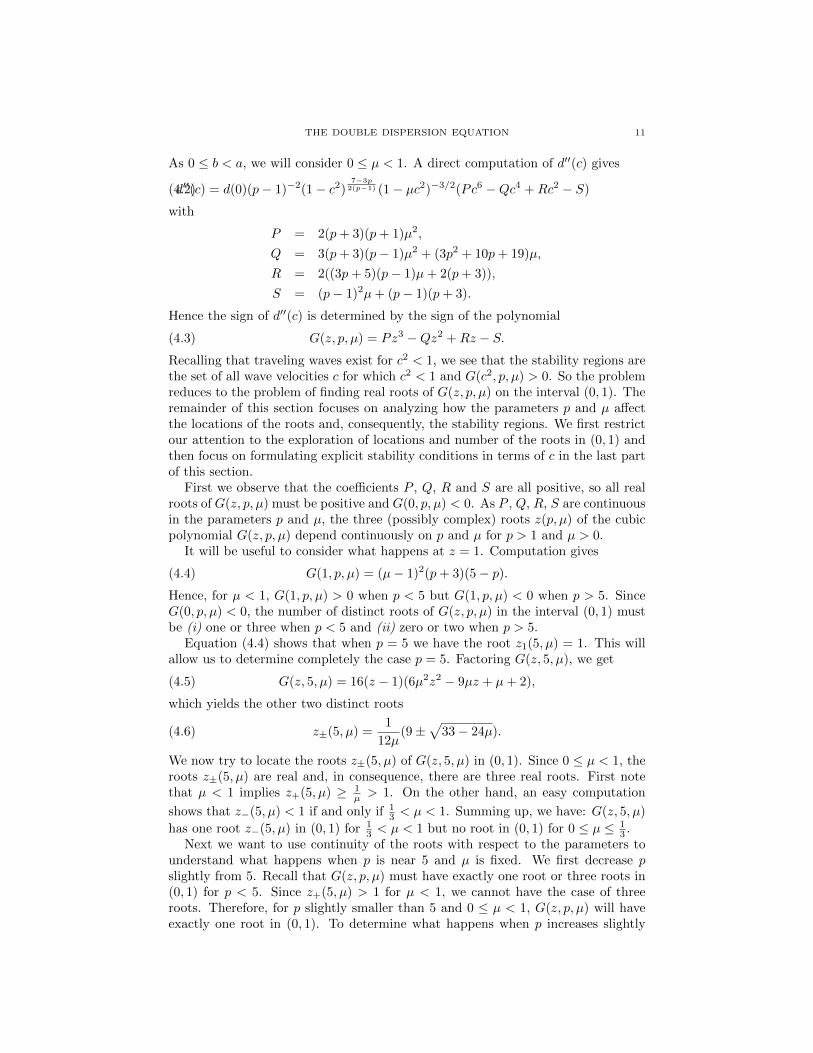
Figure 4. Schematic diagram of the stability region (shaded re-gion) for a fixed µ.

with the set G(z, p, µ0) = 0, this set in turn is either empty or an interval for c2

of the form (z1(p0, µ0), 1) or (z1(p0, µ0), z2(p0, µ0)). Fig. 3 also indicates that thecritical value µp increases with p. This means that we can as well fix µ and vary p.Then there is a critical value p = pµ so that when p ≥ pµ the stability regions areempty. To illustrate this, in Fig. 4 we take a single curve G(z, p, µ) = 0 with fixedµ and several horizontal lines corresponding to different values of p. We observetransitions between different types of stability regions as p varies for a fixed µ. Fig.4 also gives the critical value pµ. The shaded region in Fig. 4, that is, the areabetween the curve G(z, p, µ) = 0 and the line p = 1, corresponds to the stabilityregions of the problem for varying p.

To conclude, our analysis in this section leads to the following observation: Trav-eling wave solutions of the double dispersion equation (1.1) are orbitally stable ineach of the following three cases;

(A) p < 5 and z1(p, µ) < c2 < 1,(4.8)

(B) p = 5,1

3< µ < 1 and

1

12µ(9−

√33− 24µ) < c2 < 1,(4.9)

(C) p > 5, µp < µ < 1 and z1(p, µ) < c2 < z2(p, µ) < 1.(4.10)

Moreover, for a fixed p, as µ increases, the stability interval gets larger. Also, forp > 5, the critical value µp increases as p increases.


References

[1] A.M. Samsonov, Strain Solitons in Solids and How to Constuct Them, Chapman and Hall,Boca Raton, 2001.

[2] A.V. Porubov, Amplification of Nonlinear Strain Waves in Solids, World Scientific, Singapore,

2003.[3] S. Wang, G. Chen, Cauchy problem of the generalized double dispersion equation, Nonlinear

Anal. 64 (2006) 159–173.

[4] L. Yacheng, X. Runzhang, Potential well method for Cauchy problem of generalized doubledispersion equations, J. Math. Anal. Appl. 338 (2008) 1169–1187.

[5] N. Kutev, N. Kolkovska, M. Dimova, Global existence to generalized Boussinesq equationwith combined power-type nonlinearities, J. Math. Anal. Appl. 410 (2014) 427–444.

[6] C. Babaoglu, H.A. Erbay, A. Erkip, Global existence and blow-up of solutions for a general

class of doubly dispersive nonlocal nonlinear wave equations, Nonlinear Anal. 77 (2013) 82–93.[7] H.A. Erbay, S. Erbay, A. Erkip, Thresholds for global existence and blow-up in a general class

of doubly dispersive nonlocal nonlinear wave equations, Nonlinear Anal. 95 (2014) 313–322.

[8] H.A. Erbay, S. Erbay, A. Erkip, Existence and stability of traveling waves for a class ofnonlocal nonlinear equations, J. Math. Anal. Appl. 425 (2015) 307–336.

[9] J. Boussinesq, Theorie des ondes et des remous qui se propagent le long d’un canal rectangu-

laire horizontal, en communiquant au liquide contenu dans ce canal des vitesses sensiblementpareilles de la surface au fond, J. Math. Pures Appl. 17 (1872) 55–108.

[10] J.L. Bona, R. Sachs, Global existence of smooth solutions and stability of solitary waves for

a generalized Boussinesq equation, Comm. Math. Phys. 118 (1988) 15–29.[11] Y. Liu, Instability of solitary waves for generalized Boussinesq equations, J. Dynam. Differ-

ential Equations 5 (1993) 537–558.[12] Y. Liu, M. Ohta, G. Todorova, Strong instability of solitary waves for nonlinear Klein Gordon

equations and generalized Boussinesq equations, Ann. Inst. H. Poincare Anal. Non Lineaire

24 (2007) 539–548.[13] L.A. Ostrovskii, A.M. Sutin, Nonlinear elastic waves in rods, J. App. Math. Mech. 41 (1977)

543–549.

[14] J. Stubbe, Existence and stability of solitary waves of Boussinesq-type equations, Port. Math.46 (1989) 501–516.

[15] S. Le Coz, A note on Berestycki-Cazenave’s classical instability result for nonlinear

Schrodinger equations, Advanced Nonlinear Studies 8 (2008) 455–464.[16] H.A. Levine, Instability and nonexistence of global solutions to nonlinear wave equations of

the form Putt = −Au + f(u), Trans. Amer. Math. Soc. 192 (1974) 1–21.

[17] M. Grillakis, J. Shatah, W. Strauss, Stability theory of solitary waves in the presence ofsymmetry. I., J. Funct. Anal. 74 (1987) 160-197.

[18] P.E. Souganidis, W.A. Strauss, Instability of a class of dispersive solitary waves, Proc. Roy.

Soc. Edinburgh Sect. A 114 (1990) 195–212.[19] A. Esfahani, S. Levandosky, Stability of solitary waves for the generalized higher-order Boussi-

nesq equation, J. Dynam. Differential Equations 24 (2012) 39–425

Department of Natural and Mathematical Sciences, Faculty of Engineering, OzyeginUniversity, Cekmekoy 34794, Istanbul, Turkey

E-mail address: [email protected]

Department of Natural and Mathematical Sciences, Faculty of Engineering, Ozyegin

University, Cekmekoy 34794, Istanbul, Turkey

E-mail address: [email protected]

Faculty of Engineering and Natural Sciences, Sabanci University, Tuzla 34956, Is-

tanbul, TurkeyE-mail address: [email protected]

INSTABILITY AND STABILITY PROPERTIES OF TRAVELING …

Documents