I NSTABILITY AND R ECEPTIVITY OF B OUNDARY L AYERS ON C ONCAVE S URFACES AND S WEPT W INGS A THESIS PRESENTED FOR THE DEGREE OF DOCTOR OF P HILOSOPHY OF I MPERIAL COLLEGE LONDON AND THE DIPLOMA OF I MPERIAL COLLEGE BY D IFEI Z HAO DEPARTMENT OF MATHEMATICS I MPERIAL COLLEGE 180 QUEEN’ S GATE,LONDON SW7 2BZ S EPTEMBER 2011

Welcome message from author
This document is posted to help you gain knowledge. Please leave a comment to let me know what you think about it! Share it to your friends and learn new things together.
Transcript
INSTABILITY AND RECEPTIVITY OF BOUNDARY
LAYERS ON CONCAVE SURFACES AND SWEPT
WINGS
A THESIS PRESENTED FOR THE DEGREE OF
DOCTOR OFPHILOSOPHY OFIMPERIAL COLLEGE LONDON
AND THE
DIPLOMA OF IMPERIAL COLLEGE
BY
DIFEI ZHAO
DEPARTMENT OFMATHEMATICS
IMPERIAL COLLEGE
180 QUEEN’ S GATE, LONDON SW7 2BZ
SEPTEMBER2011

2
I certify that this thesis, and the research to which it refers, are the product of my own work,
and that any ideas or quotations from the work of other people, published or otherwise, are
fully acknowledged in accordance with the standard referencing practices of the discipline.
Signed:

3
Copyright
Copyright in text of this thesis rests with the Author. Copies (by any process) either in full,
or of extracts, may be madeonly in accordance with instructions given by the Author and
lodged in the doctorate thesis archive of the college central library. Details may be obtained
from the Librarian. This page must form part of any such copies made. Further copies (by
any process) of copies made in accordance with such instructions may not be made without
the permission (in writing) of the Author.
The ownership of any intellectual property rights which may be described in this thesis
is vested in Imperial College, subject to any prior agreement to the contrary, and may not
be made available for use by third parties without the written permission of the University,
which will prescribe the terms and conditions of any such agreement. Further information
on the conditions under which disclosures and exploitation may take place is available from
the Imperial College registry.
4
TO MY PARENTS
5
Abstract
This thesis studies the instability and receptivity of boundary layers over a concave wall
and a swept Joukowski airfoil. The main interest is in excitation of relevant instability
waves by free-stream vortical disturbances and in their subsequent linear development.
We first consider excitation of Gortler vortices in a Blasius boundary layer over a con-
cave wall. Attention is focused on disturbances with long streamwise wavelengths, to
which the boundary layer is most receptive. The appropriate initial-boundary-value prob-
lem describing both the receptivity process and the subsequent development of the induced
perturbation is formulated for the generic case where the Gortler numberGΛ (based on
the spanwise wavelengthΛ of the disturbance) is of order one. The impact of free-stream
disturbances on the boundary layer is accounted for by the far-field boundary condition and
the initial condition near the leading edge, both of which turn out to be the same as those
given by Leib, Wundrow and Goldstein (J. Fluid Mech. vol. 380, 1999, p.169) for the flat-
plate boundary layer.
Numerical solutions of the initial-value problem show that for a sufficiently smallGΛ,
the induced perturbation exhibits essentially the same characteristics as streaks occuring
in the flat plate case: the streamwise velocity undergoes considerable amplification and
then decays. However, whenGΛ exceeds a critical value, the induced perturbation exhibits
(quasi-)exponential growth. Comparison with local parallel and non-parallel instability
theories reveal that the perturbation acquires the modal shape of Gortler vortices rather
quickly, but its growth rate differs appreciably from that predicted by local instability theo-
ries before the convergence at large downstream distances. Nevertheless, the overall agree-
ment is close enough to indicate that Gortler vortices have been excited by free-stream
disturbances. The amplitude of excited Gortler vortices is found to decrease with the fre-
6
quency. Steady vortices, generated by steady components of free-stream disturbances, tend
to be dominant. Detailed quantitative comparisons with experiments were performed. It
is found that the eigenvalue approach predicts the modal shape adequately, but only the
initial-value approach can accurately predict the evolution of the amplitude as well as the
modal shape.
An asymptotic analysis is performed on the assumption ofGΛ � 1 to map out distinct
regimes through which a disturbance of a fixed spanwise wavelength evolves. The centrifu-
gal force enters the play to influence the generation of the pressure whenx∗ ∼ ΛRΛG−2/3Λ ,
whereRΛ denotes the Reynolds number based onΛ. The induced pressure leads to full
coupling of the momentum equations whenx∗ ∼ ΛRΛG−2/5Λ . This is the crucial regime
linking the pre-modal and modal phases of the perturbation because the governing equa-
tions admit a countable set of growing asymptotic eigensolutions, which develop into fully
fledged Gortler vortices of inviscid nature whenx∗ ∼ ΛRΛ. From this position onwards,
local eigenvalue formulations are mathematically justified. The generated Gortler vortices
continue to amplify and enter the so-called most unstable regime whenx∗ ∼ ΛRΛGΛ, and
ultimately approach the right-branch regime whenx∗ ∼ ΛRΛG2Λ.
We then extend our study to the receptivity of a three-dimensional boundary layer over
a swept wing to free-stream vortical disturbances. The base flow is taken to be the bound-
ary layer over a swept Joukowski airfoil. In contrast to the two-dimensional boundary
layer, external disturbances with comparable streamwise and spanwise wavelengths are rel-
evant to receptivity. The appropriate initial-boundary-value problem consists of linearised
boundary-layer equations supplemented by the initial condition at the leading edge and
the boundary condition in the far field, which are derived by applying the rapid distortion
theory, and matching the resultant inviscid solution with the boundary-layer solution. It is
found that the linearised boundary-layer equations support spatially growing eigenmodes
despite the absence of a pressure gradient. The modes may be first excited by free-stream
disturbances, and eventually evolve into fully fledged crossflow vortices.
7
Acknowledgements
I would like to thank my supervisor, Prof. Xuesong Wu, for his guidance over the last four
years. Without him, this work would not have been possible. I would also like to thank
my PhD student friends for helpful discussions. Special thanks are given to my parents for
their unconditional support and love.
Difei Zhao
8
Table of contents
Abstract 5
1 Introduction 141.1 Laminar-turbulent transition and hydrodynamic instability. . . . . . . . . 141.2 General approach to hydrodynamic instability. . . . . . . . . . . . . . . . 151.3 Important instability mechanisms. . . . . . . . . . . . . . . . . . . . . . . 171.4 Transition routes and receptivity. . . . . . . . . . . . . . . . . . . . . . . 20
2 Gortler Vortices 232.1 Introduction. . . . . . . . . . . . . . . . . . . . . . . . . . . . . . . . . . 232.2 Formulation and scaling. . . . . . . . . . . . . . . . . . . . . . . . . . . 292.3 The base flow. . . . . . . . . . . . . . . . . . . . . . . . . . . . . . . . . 312.4 Perturbation equations. . . . . . . . . . . . . . . . . . . . . . . . . . . . 31
2.4.1 The upstream and far-field boundary conditions. . . . . . . . . . . 342.5 Eigensolution formulation:GΛ = O(1) . . . . . . . . . . . . . . . . . . . 38
2.5.1 Non-parallel eigenvalue problem. . . . . . . . . . . . . . . . . . . 382.5.2 Parallel-flow approximation. . . . . . . . . . . . . . . . . . . . . 39
2.6 Asymptotic analysis forGΛ � O(1) . . . . . . . . . . . . . . . . . . . . . 402.6.1 Pre-modal stage I:x = O(G−2/3Λ ) . . . . . . . . . . . . . . . . . . 402.6.2 Pre-modal stage II:x = O(G−2/5Λ ) . . . . . . . . . . . . . . . . . . 412.6.3 Inviscid regime:x = O(1) . . . . . . . . . . . . . . . . . . . . . . 472.6.4 Most unstable regime:x = O(GΛ) . . . . . . . . . . . . . . . . . . 50
2.7 Numerical methods. . . . . . . . . . . . . . . . . . . . . . . . . . . . . . 522.7.1 Numerical method for the initial-boundary-value problem. . . . . 522.7.2 Numerical method for solving the local eigenvalue problem. . . . 542.7.3 Validation. . . . . . . . . . . . . . . . . . . . . . . . . . . . . . . 54
2.8 Results and comparisons with experiments. . . . . . . . . . . . . . . . . . 552.8.1 Steady Gortler vortices. . . . . . . . . . . . . . . . . . . . . . . . 552.8.2 Unsteady Gortler vortices . . . . . . . . . . . . . . . . . . . . . . 71
2.9 Summary and discussions. . . . . . . . . . . . . . . . . . . . . . . . . . . 77
3 Crossflow Vortices 793.1 Introduction. . . . . . . . . . . . . . . . . . . . . . . . . . . . . . . . . . 793.2 Formulation and scalings. . . . . . . . . . . . . . . . . . . . . . . . . . . 863.3 The base flow. . . . . . . . . . . . . . . . . . . . . . . . . . . . . . . . . 88

9
3.3.1 The inviscid external flow. . . . . . . . . . . . . . . . . . . . . . 883.3.2 The boundary layer flow. . . . . . . . . . . . . . . . . . . . . . . 97
3.4 Perturbation equations. . . . . . . . . . . . . . . . . . . . . . . . . . . . 1053.4.1 General governing equations. . . . . . . . . . . . . . . . . . . . . 1073.4.2 The linear inviscid solution. . . . . . . . . . . . . . . . . . . . . . 1103.4.3 The linearised boundary layer equations. . . . . . . . . . . . . . . 116
3.5 Eigenvalue formulation. . . . . . . . . . . . . . . . . . . . . . . . . . . . 1243.5.1 Non-parallel boundary-layer eigenvalue formulation. . . . . . . . 1243.5.2 Parallel boundary-layer eigenvalue formulation. . . . . . . . . . . 1253.5.3 Non-parallel Navier-Stokes eigenvalue formulation. . . . . . . . . 125
3.6 Numerical results. . . . . . . . . . . . . . . . . . . . . . . . . . . . . . . 1313.6.1 Validation of the eigenvalue solver. . . . . . . . . . . . . . . . . . 1313.6.2 Initial-value and eigenvalue solutions. . . . . . . . . . . . . . . . 1353.6.3 The intermediate regime. . . . . . . . . . . . . . . . . . . . . . . 139
3.7 Summary and discussion. . . . . . . . . . . . . . . . . . . . . . . . . . . 142
4 Further discussions and future work 1444.1 Summary of conclusions and further discussions. . . . . . . . . . . . . . . 1444.2 Topics for future study. . . . . . . . . . . . . . . . . . . . . . . . . . . . 146
A Approximation for S − θ relation for π − θ = O(b/a) 148
B Evaluation of drift function 151
References 164
10
List of Figures
2.1 Influence of FST on the occurrence of Gortler vortices (Kottke 1988). Left:adjusting the distance of the grid to the leading edge with fixed mesh size.Right: adjusting the mesh size with fixed distance. . . . . . . . . . . . . . 27
2.2 Schematic illustration of the physical problem and the asymptotic flowstructure. Also shown are the main stages: pre-modal, inviscid and the‘most unstable’ regimes, through which the induced perturbation evolveswhenGΛ � 1 (Courtesy of Dr. P. Ricco).. . . . . . . . . . . . . . . . . . 32
2.3 Matching of different regimes. Dashed lines: asymptotic eigen mode; solidlines: inviscid modes; dotted lines: the large-x limit of inviscid modes, i.e.(2.6.41) with n = 2, 3. . . . . . . . . . . . . . . . . . . . . . . . . . . . . 49
2.4 |u| at η = 1.64 calculated from different values ofκ ≤ 1.0 with κ2 = −κusing equations (2.4.9)–(2.4.12). . . . . . . . . . . . . . . . . . . . . . . . 55
2.5 Profiles of the streamwise and spanwise velocities of the perturbation at theindicated values ofx for κ = 1.0, κ2 = −1.0. . . . . . . . . . . . . . . . . 56
2.6 Profiles of|u|/|u|max at indicatedx for κ = 1.0, κ2 = −1.0. . . . . . . . . 562.7 |u|max and ln|u|max calculated for different values of Gortler numberGΛ
with k1 = 0.0, k2 = −1.0 andk3 = 1.0. . . . . . . . . . . . . . . . . . . . 572.8 Comparison of the growth rates as predicted by nonparallel eigenvalue ap-
proach (σ, dashed line) and by initial-value approach (1ududx
at η = 1.64,solid line) for k1 = 0.0, k2 = −1.0, k3 = 1.0 and different values ofGΛ asindicated in the plot. . . . . . . . . . . . . . . . . . . . . . . . . . . . . . 57
2.9 Comparison of streamwise and spanwise perturbation velocity profiles pre-dicted by nonparallel eigenvalue and initial-value approaches. Top row:x = 1.0; bottom row: x = 4.0. The parameters arek1 = 0.0, k2 = −1.0,k3 = 1.0 and Gortler numberGΛ = 20.0 . . . . . . . . . . . . . . . . . . . 58
2.10 Comparison of the streamwise and spanwise velocity profiles (atx = 1.0)predicted by the nonparallel eigenvalue and initial-value approaches. Theparameters arek1 = 0.0, k2 = −1.0, k3 = 1.0 and Gortler numberGΛ =200.0 (top), and 100.0 (bottom).. . . . . . . . . . . . . . . . . . . . . . . 59
2.11 Downstream development of normalised streamwise and spanwise veloc-ities at indicated values ofx, with k1 = 0.0, k2 = −1.0, k3 = 1.0 andGortler numberGΛ= 100.0 . . . . . . . . . . . . . . . . . . . . . . . . . . 59
LIST OF FIGURES 11
2.12 Growth rates predicted by different parallel and nonparallel theories as wellas by initial-value calculation, whenk1 = 0.0 andGΛ=89.5 (correspondingtoGb ≈ 15 in the paper of Boiko et al.(2007, 2010) ) . . . . . . . . . . . . 61
2.13 Normalised streamwise and spanwise velocity profiles predicted by differ-ent parallel and nonparallel theories atx = 0.6241494 (top) andx = 8.0(bottom) forGΛ=89.5, which corresponds toΛb = 149 in Boiko et al.(2010). 63
2.14 Normalised streamwise and spanwise velocity profiles of the second modepredicted by parallel and nonparallel theories atx = 0.6241494 (top) andx = 8.0 (bottom), forGΛ=89.5, which corresponds toΛb = 149 in Boikoet al.(2010). . . . . . . . . . . . . . . . . . . . . . . . . . . . . . . . . . . 64
2.15 Comparison of the downstream development of the maximum streamwisevelocity predicted by the initial-value approach with the experiment data ofTani (1962). The parameters areGΛ = 1765.0, k1 = 0.0, k2 = −1.0 andk3 = 1.0. . . . . . . . . . . . . . . . . . . . . . . . . . . . . . . . . . . . 68
2.16 Comparison of the growth rate predicted by the initial-value approach andby the nonparallel eigenvalue theory. The parameters areGΛ = 1765.0,k1 = 0.0, k2 = −1.0 andk3 = 1.0. . . . . . . . . . . . . . . . . . . . . . . 68
2.17 Comparison of normalised streamwise velocity obtained from the initial-value and eigenvalue calculations with the experiment data of Tani(1962).The parameters areGΛ = 1765.0, k1 = 0.0, k2 = −1.0 andk3 = 1.0 atx = 0.03906 (top left), x = 0.065 (top right),x = 0.1172 (bottom left) andx = 0.1562 (bottom right). . . . . . . . . . . . . . . . . . . . . . . . . . . 69
2.18 Comparison of downstream development of the maximum streamwise ve-locity predicted by initial-value approach with experiment data of Finnisand Brown(1997) for U∞ = 10m/s (left) andU∞ = 7.5m/s (right). Theparameters areGΛ = 2192 (left), GΛ = 1222 (right), k1 = 0.0, k2 = −1.0andk3 = 1.0. . . . . . . . . . . . . . . . . . . . . . . . . . . . . . . . . . 70
2.19 Comparison of the growth rate predicted by initial-value approach, nonpar-allel eigenvalue theory, inviscid approach and the experiment data of Fin-nis and Brown(1997). The parameters areGΛ = 2192 (left), GΛ = 1222(right), k1 = 0.0, k2 = −1.0 andk3 = 1.0. . . . . . . . . . . . . . . . . . . 70
2.20 ln|u|max v.s. x for different frequencies withGΛ = 89.5. The frequenciesin the plot (top to bottom ) correspond to 0, 5.67, 8.0, 12.0, 20.0 and 40.0in Boiko et al.(2007, 2010) . . . . . . . . . . . . . . . . . . . . . . . . . 71
2.21 Growth rates predicted by local instability theories and comparison withthe initial-value prediction. The parameters are taken to bek1 = 3.33604,GΛ=89.5 (corresponding toΛb = 149 andF = 5.67 in Boiko et al.(2007,2010)). . . . . . . . . . . . . . . . . . . . . . . . . . . . . . . . . . . . . . 72
2.22 Comparison of the streamwise and spanwise velocity profiles predictedby the initial-value approach with the eigenfuctions of different paralleland non-parallel theories atx = 0.624, 4.0 and8.0. The parameters areGΛ=89.5 andk1 = 3.336 (corresponding toΛb = 149 andF = 5.67 inBoiko et al.(2007, 2010) . . . . . . . . . . . . . . . . . . . . . . . . . . . 73
LIST OF FIGURES 12
2.23 Comparison of the streamwise velocity profiles predicted by the initial-value, parallel and non-parallel theories with the measurements of Boikoet al.(2010) atx = 0.378 (left), 0.749 (right) for k1 = 3.336 andGΛ = 89.5(Λb = 149, F = 5.67). . . . . . . . . . . . . . . . . . . . . . . . . . . . . 74
2.24 Development of unsteady Gortler vortices and comparison with the experi-ment of Boiko et al.(2010). The parameters areGΛ = 89.5 andk1 = 3.336( Λb = 149 andF = 5.67). . . . . . . . . . . . . . . . . . . . . . . . . . . 74
2.25 Growth rates (a) and phase speeds (b) of unsteady Gortler vortices pre-dicted for different frequencies and comparison with the experimental dataat x = 0.62. The parameters areGΛ = 89.5 andΛb = 149. . . . . . . . . . 75
3.1 Joukowski transformationζ(z) = z + c2/z from the exterior of the circleto the exterior of the airfoil.. . . . . . . . . . . . . . . . . . . . . . . . . . 90
3.2 Geometry of Joukowski airfoil for different ratios ofb/a. . . . . . . . . . . 913.3 Characteristic length scales of symmetric Joukowski airfoil forb/a = 0.035. 923.4 Comparison of the asymptotic approximations with the exact solution (the-
ory) for ue (b/a = 0.035). . . . . . . . . . . . . . . . . . . . . . . . . . . 953.5 The relation betweenue andS, and comparison of the asymptotic approx-
imation with the exact numerical solution(b/a = 0.035). . . . . . . . . . . 973.6 The distribution of the slip velocity along the airfoil surface for different
values ofb/a. . . . . . . . . . . . . . . . . . . . . . . . . . . . . . . . . . 983.7 Solution to Falkner-Skan equation for different values ofm. . . . . . . . . 1023.8 Velocity profiles for different ratios ofb/a atS = 0.05. . . . . . . . . . . . 1023.9 Velocity profiles for different ratios ofb/a atS = 0.99. . . . . . . . . . . . 1033.10 Velocity profiles of Falkner-Skan-Cooke boundary layer withm = 1. . . . . 1063.11 Chordwise and spanwise velocity profiles at different downstream locations
with b/a = 0.035. . . . . . . . . . . . . . . . . . . . . . . . . . . . . . . . 1063.12 Velocity profiles at the stagnation point. The parameters used areω = 0.12,
k3 = 1.0, Λ = 0.05, andb/a = 0.1. . . . . . . . . . . . . . . . . . . . . . . 1213.13 The distribution ofR1 = δ/δs andR1/R0 along the airfoil forb/a = 0.1. . 1303.14 The growth rate and chordwise wavenumber of crossflow vortices at dif-
ferent chordwise locations. Parameter values:ω = 0.1071, RΛ = 1428.57andΛ/a = 2.9× 10⁻⁴. . . . . . . . . . . . . . . . . . . . . . . . . . . . . 134
3.15 Non-parallel eigenvalue calculation for different frequencies atx = 35with Λ/a = 0.005, k3 = 1.0, andb/a = 0.1. . . . . . . . . . . . . . . . . . 135
3.16 The growth rates(Re(σ)) and chordwise wavenumber(Im(σ)) of the non-parallel eigenmodes for different spanwise wavelengths forω = 0.12, k3 =1.0, andb/a = 0.1. . . . . . . . . . . . . . . . . . . . . . . . . . . . . . . 138
3.17 Non-parallel eigenvalue and comparison with the theoretical result . Pa-rameter values:ω = 0.12, Λ/a = 0.001, k3 = 1.0, andb/a = 0.1. . . . . . 138
3.18 Comparison between non-parallel and parallel eigenvalue calculations withthe theoretical result forω = 0.12, Λ/a = 0.001, k3 = 1.0, andb/a = 0.1. 139
3.19 The local growth rate predicted by the initial-value calculation for FST andcomparison with the non-parallel eigenvalues. Parameter values:ω = 0.12,Λ/a = 0.001, k3 = 1.0, andb/a = 0.1. . . . . . . . . . . . . . . . . . . . 140
LIST OF FIGURES 13
3.20 The local growth rate predicted by the initial-value calculation for suctionand comparison with the non-parallel eigenvalues. Parameter values:ω =0.12, Λ/a = 0.001, k3 = 1.0, andb/a = 0.1. . . . . . . . . . . . . . . . . 140
A.1 Comparison of thes − θ relation obtained by numerical integration withthe asymptotic approximation (A.0.5) (b/a = 0.035). . . . . . . . . . . . . 150
B.1 Drift function forb/a = 0.1, andΛ/a = 0.001. . . . . . . . . . . . . . . . 155
14
Chapter 1
Introduction
1.1 Laminar-turbulent transition and hydrodynamic instability
Flow motions exhibit different degree of spatial and temporal complexity. Laminar flows
refer to those which display relatively simple variations in both space and time, whereas
turbulent flows refer to those which display no discernable spatial pattern or temporal re-
peatability at all; the flow field appears chaotic and random. When the controlling param-
eters vary, a laminar flow may change to a turbulent state, usually through a sequence of
increasingly more complex intermediate states. Transition to turbulence may take place in
physical space, from one part of the flow field to another, rather than with respect to change
of an overall controlling parameter.
A simple example is the so-called thermal convection, a horizontal layer of quiescent
fluid being heated from below. When the temperature difference is small enough, the fluid
remains motionless and the heat exchange between the top and bottom is through conduc-
tion, which is a very inefficient process. When the temperature difference is raised beyond
a critical value, the resulting buoyancy may cause the fluid particles near the bottom to
overcome the viscous resistance and move upwards. A pattern of steady convection cells
is formed. When the temperature difference is increased further, the cells may become un-
steady and be eventually replaced by an apparently turbulent state. The non-dimensional
parameter controlling the process is the so-called Rayleigh number, which measures the
ratio of the buoyancy to the viscous resistance. Another example is the flow through a cir-
cular pipe, which was first studied byReynolds(1883) in his well-known experiment. By
visualising the flow via injected dye, he observed that at relatively low speeds, the flow is

Chapter 1. Introduction 15
steady and all fluid particles move parallel to each other along the axial direction. How-
ever, when the speed exceeds a critical value, the flow becomes time dependent and three-
dimensional, i.e. a state of turbulence prevails. Crucially, Reynolds established that the
transition was determined by the dimensionless parameterUD/ν, which was later referred
to as the Reynolds number, whereD is the diameter of the pipe, andν is the kinematic
viscosity of the fluid. The work of Reynolds has been credited as the first to discover and
systematically document two flow states: laminar and turbulent, and it marked the begin-
ning of turbulence research.
Transition also takes place in the flow around an airfoil. In this case, a Reynolds number
Re based on the airfoil length can be defined. However, unlike the flows mentioned above,
the parameter Re does not dictate the entire flow field provided that Re is sufficiently large.
No matter how large Re is, the flow near the leading edge of the airfoil is laminar, but
is turbulent further downstream. There is an extended region in between where transition
takes place.
Transition between from one state to another, especially transition to turbulence, is
not only of fundamental importance in science, but also of great practical relevance to
engineering and technology. For instance, transition in thermal convection is closely related
to heat transfer and mixing, while transition in the pipe flow and in the flow around an
airfoil is closely related to drag that the fluid exerts on the surfaces. At supersonic speeds,
transition in the flow around the airfoil affects the aerodynamic heating.
1.2 General approach to hydrodynamic instability
Hydrodynamic stability is concerned with when and how a laminar flow loses its stability,
and how it evolves subsequently. The eventual transition to turbulence is of particular
interest. The topic has been regarded as one of the central problems in fluid mechanics.
Research activities in this area in the past few decades were driven by modern technology
needs, especially those in aeronautical and astronautical engineering.
The field of hydrodynamic instability has attracted many of great physicists, includ-
ing Lord Kelvin, Lord Rayleigh, Sommerfeld and Heisenberg, whose work laid down the
theoretical foundation.
The flow whose stability is of concern is referred to as the base flow. It is characterized
by a velocity fieldU(x, t), and other quantities, such as pressureP (x, t) and temperature
1.2 General approach to hydrodynamic instability 16
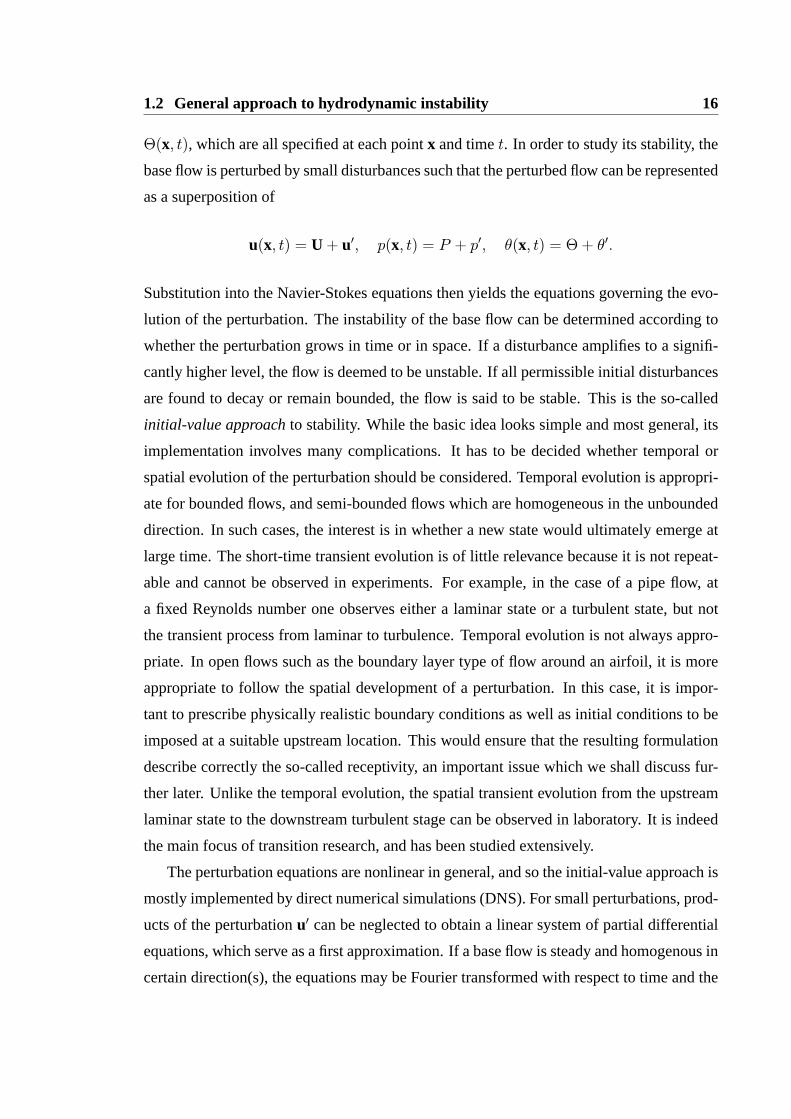
Θ(x, t), which are all specified at each pointx and timet. In order to study its stability, the
base flow is perturbed by small disturbances such that the perturbed flow can be represented
as a superposition of
u(x, t) = U+ u′, p(x, t) = P + p′, θ(x, t) = Θ + θ′.
Substitution into the Navier-Stokes equations then yields the equations governing the evo-
lution of the perturbation. The instability of the base flow can be determined according to
whether the perturbation grows in time or in space. If a disturbance amplifies to a signifi-
cantly higher level, the flow is deemed to be unstable. If all permissible initial disturbances
are found to decay or remain bounded, the flow is said to be stable. This is the so-called
initial-value approachto stability. While the basic idea looks simple and most general, its
implementation involves many complications. It has to be decided whether temporal or
spatial evolution of the perturbation should be considered. Temporal evolution is appropri-
ate for bounded flows, and semi-bounded flows which are homogeneous in the unbounded
direction. In such cases, the interest is in whether a new state would ultimately emerge at
large time. The short-time transient evolution is of little relevance because it is not repeat-
able and cannot be observed in experiments. For example, in the case of a pipe flow, at
a fixed Reynolds number one observes either a laminar state or a turbulent state, but not
the transient process from laminar to turbulence. Temporal evolution is not always appro-
priate. In open flows such as the boundary layer type of flow around an airfoil, it is more
appropriate to follow the spatial development of a perturbation. In this case, it is impor-
tant to prescribe physically realistic boundary conditions as well as initial conditions to be
imposed at a suitable upstream location. This would ensure that the resulting formulation
describe correctly the so-called receptivity, an important issue which we shall discuss fur-
ther later. Unlike the temporal evolution, the spatial transient evolution from the upstream
laminar state to the downstream turbulent stage can be observed in laboratory. It is indeed
the main focus of transition research, and has been studied extensively.
The perturbation equations are nonlinear in general, and so the initial-value approach is
mostly implemented by direct numerical simulations (DNS). For small perturbations, prod-
ucts of the perturbationu′ can be neglected to obtain a linear system of partial differential
equations, which serve as a first approximation. If a base flow is steady and homogenous in
certain direction(s), the equations may be Fourier transformed with respect to time and the

Chapter 1. Introduction 17
homogenous direction(s). This leads to normal mode analysis, in which each perturbation
quantity is written into independent components or modes, which vary with timet and ho-
mogenous direction(s),x say, likeei(αx−ωt), whereα andω may be complex numbers. The
formulation is referred to as being temporal ifα is assumed to be real andω = ωr + iωi
complex, or spatial ifω is taken to be real andα = αr + iαi complex (Gaster 1962).
The equations and the homogeneous boundary conditions form an eigenvalue problem to
determine the complex frequencyω for a given wavenumberα in the temporal instability
formulation, or the complex wavenumberα for a given real frequencyω in the spatial in-
stability formulation. Ifωi > 0 (αi < 0) for anyα (ω), then the perturbation will grow with
time (in the homogenous direction), and the flow is said to be unstable. Ifωi < 0 (αi > 0)
for all α (ω), then the perturbation will decay exponentially with time (in space), and the
flow is said to be asymptotically stable or stable; ifωi = 0 or αi = 0, the mode neither
grows nor decays, and is referred to as a neutral mode. The flow is said to be neutrally sta-
ble if all modes decay except neutral modes (Drazin and Reid 1981). The conditionωi = 0,
orαi = 0, defines in the parameter space a neutral curve or surface. The mathematical pro-
cedure described above forms the so-calledeigenvalue approach, which was pioneered by
Lord Rayleigh(1880) and LordKelvin (1880), and has now become the standard tool for
predicting instability.
1.3 Important instability mechanisms
While the theoretical approaches described in the previous section are general, they have
not been able to give a criterion for the onset of instability in an arbitrarily base flow. In-
stability has therefore been studied for relatively simply flows which include, in addition
to the quiescent state, plane Poiseuille flow and boundary layer type of flows. Several
important fundamental physical mechanisms of instability have been identified. These in-
clude thermal instability induced by the buoyancy effect; inertial instability induced purely
by the background shear or by the combined effect of viscosity and shear, which are usu-
ally referred to as Rayleigh and Tollmien-Schlichting (T-S) instabilities respectively; cen-
trifugal instability induced by the centrifugal force. The first of these mechanisms is well
understood. In this section, we shall summarise the main results concerning inertial and
centrifugal instabilities, which are directly relevant to the investigation in this thesis.
The simplest flow in which inertial or shear instability can arise is a uni-directional

1.3 Important instability mechanisms 18
parallel flow with a velocity profileUB(y). The variation of the velocity is with respect
to the transverse variabley, which is normalised by a characteristic length scaleδ∗. The
relevant parameter is the Reynolds numberU0δ∗/ν, whereU0 is a typical velocity. Lord
Rayleigh(1880) first studied the stability of such a base flow bounded by two parallel
planes. With the Reynolds number being taken to be infinite, i.e. the viscous effects being
neglected, he showed that if instability is to occur, the basic velocity profile must have an
inflectional pointyc interior to the flow, that is
U ′′B(yc) = 0. (1.3.1)
This result is commonly called Rayleigh’s inflection-point theorem, which states that (1.3.1)
is a necessary condition for inviscid instability. A stronger form of the Rayleigh’s inflection-
point theorem was proved by Fjørtoft. He showed that the necessary condition for instabil-
ity is
U′′
B(yc) = 0, and U′′
B[UB − UB(yc)] < 0, (1.3.2)
somewhere interior to the flow. Later,Tollmien (1935) showed that for bounded flows
with symmetric profiles, and unbounded flows with monotonic velocity profile, condition
(1.3.2) is both necessary and sufficient for instability (Drazin and Reid 1981). For a general
unbounded flow, however, the condition (1.3.1) is not sufficient to guarantee the occurrence
of instability. The instability is of inviscid nature and is customary referred to as Rayleigh
instability, and the associated waves are called Rayleigh waves/modes, the phase speeds
of which are bounded by the maximum and minimum of the base velocity. The temporal
(spatial) growth rate has an order of magnitude ofU0/δ∗ (1/δ∗). Due to large growth rates,
the instability can lead to rapid breakdown to turbulence (Reed et al. 1996).
According to Rayleigh’s theorem, velocity profiles without an inflection point ought
to be stable, at least when Reynolds number is sufficiently high. However, instability and
transition do occur in many flows with non-inflectional velocity profiles (e.g. the plane
Poiseuille flow and Blasius boundary layer). This prompted the formulation of viscous
instability theory. For parallel shear flows, the normal-mode analysis led to the eigenvalue
problem governed by the Orr-Sommerfield (O-S) equation. Applying this theory to the
plane Poiseuille flow,Heisenberg(1924) showed that provided the Reynolds number is
sufficiently large, viscosity may cause instability despite that it dissipates energy. The
eigenvalue problem was later solved by highly accurate numerical method, and the critical

Chapter 1. Introduction 19
Reynolds number for linear instability was found to be 5772.2 (Orszag 1971).
Viscous instability theory formulated for exactly parallel flows has been frequently
adapted to boundary layers, where the base flow consists of a transverse componentVB
and the streamwise component varies with the streamwise coordinate. The normal-mode
analysis is, strictly speaking, not applicable. A remedy is making the local parallel-flow
approximation, first suggested by Prandtl. In this approximation, the streamwise varia-
tion andVB are ignored, and the streamwise profile is frozen at each location allowing a
normal-mode solution to be sought. This approach was first taken byTollmien (1929) and
Schlichting(1933) for the Blasius boundary layer. They demonstrated boundary layer is
unstable, which was later confirmed by experiments (Schubauer and Skramstad 1947). The
viscous shear instability then became known as Tollmien-Schlichting instability. Refined
analysis of the O-S equation was carried out byLin (1945, 1955), and the equation was
solved numerically by numerous researchers to map out the neutral curve, which consists
of lower and upper branches. The predicted characteristics of the instability are broadly in
agreement with experiments.
The non-parallel-flow effects have been investigated following two different approaches.
The first is the composite approximation, in which the O-S equation serves as the first ap-
proximation. The non-parallel-flow corrections, associated withVB and the streamwise
variations of the base flow and the eigenfunction, were taken into account atO(R−1)
(Gaster 1974). Comparison with experimental data suggests that this approach gives more
accurate prediction, especially at moderated Reynolds numbers (Saric and Nayfeh 1975).
The alternative approach is the systematic high-Reynolds-number asymptotic expansion.
At leading order, the instability near the lower branch is governed by the well-known triple-
deck structure (Lin 1945), and the wavelength is of orderR1/4 times the boundary layer
thickness, much longer than what was implicitly assumed in the composite approximation.
As a result, non-parallelism appears as anO(R−3/4) correction to the growth rate (Smith
1979). The accuracy of this approach is unfortunately rather poor at moderate Reynolds
number. However, it provides the precise asymptotic estimate of the characteristic length
scale of the instability, an insight crucial for understanding receptivity.
Centrifugal instability is best illustrated in the flow between two concentric rotating
cylinders, known as the Taylor-Couette problem. Detailed theoretical and experimental
studies were carried out byTaylor (1923). The instability leads to the formation of toroidal
vortices, an periodic array of doughnut-shaped cells, along the axial direction. A simi-

1.4 Transition routes and receptivity 20
lar mechanism operates in a boundary layer over a concave wall. The imbalance between
the centrifugal force and the pressure gradient in the wall-normal direction leads to for-
mation of longitudinal counter rotating vortices, which are now called Gortler vortices, as
Gortler (1940) was the first to investigate them theoretically. Realising the analogy with
Taylor-Couette flow, Gortler considered temporal instability and formulated an eigenvalue
problem. However, it was realized later that Gortler instability differs considerably from
Taylor instability in many aspects. A detailed introduction will be given in chapter 2 of this
thesis.
The base flow for the aforementioned instabilities is two dimensional. In practical
applications, of which the boundary layer over a swept wing is a typical example, the base
flow is three-dimensional, and the characteristics of stability will be affected substantially
by the additional velocity component in the crossflow direction. A multitude of instabilities
may operate in different regions of the flow, including (temporal) viscous instability along
the attachment line, and crossflow instability in the region of favourable pressure gradient
(i.e. near the leading edge), streamwise T-S type instability in the adverse pressure region
and Gortler instability in the concave section of the wing (Reed and Saric 1989, Saric
et al. 2003). The occurrence of crossflow instability is often attributed to the fact that
the crossflow velocity is zero at the wall and at the outer edge of the boundary layer so
that an inflectional point must exist in the profile, and inviscid instability may be possible
and instability modes must propagate in the direction nearly coinciding with the crossflow
direction. In this sense, crossflow instability is in essence a Rayleigh instability. This
simple interpretation holds in the majority of the flow region where the wavelength of
instability modes is comparable with the local boundary layer thickness. However, near
the leading edge, crossflow instability has a viscous origin. We will give, in chapter 3,
a detailed introduction to crossflow instability and the issues related to receptivity and
transition.
1.4 Transition routes and receptivity
Transition of a laminar flow to turbulence is caused by the intrinsic instability, but it is also
influenced by external disturbances. This is the case especially for open flows. The infor-
mation of instability alone is not sufficient for predicting transition. Depending on the level
of external disturbances, transition may take different routes. In order to be specific, we
Chapter 1. Introduction 21
consider two-dimensional boundary-layer transition as an example. When the free-stream
turbulence level is low, the growth of T-S waves is instrumental and ensuing transition is
referred to as natural transition. When the free-stream turbulence level is high, transition
occurs without apparently involving T-S waves. Transition of this kind is referred to as
bypass transition (Morkovin 1969).
The natural transition is a complicated process consisting of five different stages: recep-
tivity where external disturbances excite intrinsic instability (i.e. T-S) waves; linear growth
where T-S waves amplify exponentially as predicted by linear stability theory, nonlinear
saturation, secondary instability leading to eventual breakdown to turbulence. It has been
observed in experiments that the final transition location varies significantly with the level
of free-stream disturbances and surface roughness. This has been attributed to different
initial amplitudes of T-S waves that are excited through the receptivity. Clearly, transition
cannot be predicted without accounting for receptivity.
Receptivity is concerned with how the boundary layer responds to external disturbances
and how the instability waves develop from the response. This means that mathematically
receptivity must be described by an initial-boundary-value problem (Reshotko 1976). In
order to formulate such a problem, it is necessary to consider first physical nature of the
disturbances present in the ambient environment. In the case of boundary layer, unsteady
external disturbances consist of vortical and acoustical disturbances in the free stream. The
former represents vorticity fluctuation being advected by the uniform background flow so
that there is no associated pressure fluctuation at leading order, while the latter is an irro-
tational motion representing pressure waves propagating through the fluid with the speed
of sound. Steady disturbances come from surface roughness, which may be isolated or
distributed. None of these disturbances alone could excite T-S waves because the time
and length scales of each of these disturbances cannot be the same simultaneously as the
corresponding intrinsic characteristic scales of the instability. As was pointed out byGold-
stein(1983), crucial to receptivity is the scale conversion, which tunes the external scales
to match the intrinsic scales. Several scale conversion mechanisms have been identified
(Goldstein and Hultgren 1989).
The first is the the so-called ‘leading-edge adjustment’ mechanism, discovered first by
Goldstein(1983). He demonstrated that while T-S waves are governed by the O-S equation
or triple-deck theory, this eigenvalue formulation becomes invalid near the leading edge,
where non-parallelism is a leading-order effect so that the perturbation must be governed by

1.4 Transition routes and receptivity 22
linearised boundary layer equations. These equations admit the so-called Lam-Rott asymp-
totic modes. Acoustic disturbances, appearing as the inhomogeneous boundary condition
of the boundary layer equations, excite Lam-Rott modes, among which the most rapidly
decaying one undergoes wavelength shortening and eventually evolves into a T-S wave.
The second scale-conversion mechanism was identified byRuban(1984) andGoldstein
(1985). It involves interaction of an acoustic wave with a local roughness. The frequency
of the acoustic wave and the length scale of the roughness are chosen to be comparable
to the frequency and wavelength of an amplifying T-S mode respectively. The acoustic
wave interacts with the local mean-flow induced by the roughness to generate an unsteady
forcing, which has time and length scales matching the intrinsic scales. A T-S wave is
generated as a result. A similar mechanism has been described byDuck et al.(1996) for
receptivity to vortical disturbances.Wu (2001a,b) later formulated receptivity theory for
distributed roughness, and also extended the theory ofDuck et al.(1996) to second order.
Detailed quantitative comparison was made with experimental data, and a good agreement
was found.
In summary, the seminal work ofGoldstein(1983, 1985) and Ruban(1984) marks
a breakthrough in our understanding of receptivity. The receptivity process in the two-
dimensional flat-plate boundary layer has been thoroughly understood at least in incom-
pressible flows. The key idea and existing mathematical formalisms can be generalised, in
a rather straightforward manner, to many other flows including certain forms of crossflow
receptivity.
In this thesis, we shall tackle two of remaining receptivity problems for which the
solutions are far from being obvious or straightforward. One is concerned with generation
of steady and unsteady Gortler vortices by free-stream vortical disturbances, while the other
is excitation of non-stationary crossflow vortices in three-dimensional boundary layers by
free-stream vortical disturbances. Both problems require a detailed examination of the
instability properties of the underlying base flows in the leading-edge region. These two
problems will be investigated in chapter 2 and chapter 3 respectively. In chapter 4, we give
an overall summary and highlight a few topics for future study.

23
Chapter 2
Gortler Vortices
2.1 Introduction
Gortler instability is an important type of centrifugal instability. It occurs in a boundary
layer over a concave wall due to the imbalance between the centrifugal force and the nor-
mal pressure gradient. The instability leads to formation of counter-rotating vortices with
axes parallel to the free stream. Usually the vortex pattern appears more-or-less periodic
in the spanwise direction with a discernible wavelengthλz. While the underlying physi-
cal mechanism is essentially the same as that of Taylor instability in a flow between two
concentric rotating cylinders, the mathematical theory for Gortler instability is more com-
plex because of the non-parallelism associated with the streamwise growth of the boundary
layer. As the instability occurs in an open domain, it is also crucially affected by ambi-
ent perturbations, making an accurate prediction a considerable challenge. The problem
of Gortler instability and the resulting transition to turbulence has been a subject of ac-
tive research for several decades. Comprehensive reviews have been given byHall (1990),
Floryan(1991) andSaric(1994).
The problem was first studied by Gortler in 1940 (Gortler 1940). In his original for-
mulation, two assumptions were made: (a) the boundary-layer thickness is much smaller
than the radius of curvature; (b) the base flow is nearly parallel to the wall with its depen-
dence on the streamwise coordinate and the transverse velocity both being neglected. The
second assumption is referred to as the quasi-parallel approximation, which allows us to
seek normal-mode solution for the perturbation so that the instability can be treated as an

2.1 Introduction 24
eigenvalue problem. The relevant parameter controlling the instability is
Gθ = (U∞θ/ν)√θ/r∗0,
whereU∞ is the free-stream velocity,θ is the momentum thickness of the boundary layer,
ν is the kinematic viscosity, andr∗0 is the radius of curvature. This parameter was later
referred to as the Gortler number in recognition of Gortler’s pioneering work.
Gortler (1940) formulated and solved a temporal instability problem, in which the per-
turbation was assumed to amplify with time. Improvements to Gortler’s work were made
over several decades since.Smith(1955) formulated a spatial instability problem, in which
vortices grow with the streamwise position. The normal velocity and the variation of the
streamwise velocity of the base flow were retained. However, Smith neglected the stream-
wise derivative of the normal velocity as result of assuming that all three velocity com-
ponents of the perturbation have the same order of magnitude. This assumption was er-
roneous as was first recognised byFloryan and Saric(1982, 1984), who pointed out that
the streamwise velocity of the perturbation has magnitude greater than that of the normal
and spanwise velocities by factor ofO(Rθ), whereRθ = U∞θ/ν is the Reynolds number
based onθ. With this correct scaling, the streamwise derivative of the normal velocity of
the base flow appears at leading-order and must be retained in the stability equations. In
all eigenvalue formulations, for a given wavenumberk = (2π/λz)θ, a Gortler numberGθ
may be found such that the mode is neutral, i.e. a unique neutral curve in the(k,Gθ) plane
may be identified. The neutral curve indicates that vortices of a given wavelength begin to
amplify at some distance downstream but decay near the leading edge.
In conjunction with theoretical studies, many experiments have been conducted. Early
investigations include hot-wire measurements (Tani 1962, Tani and Sakagami 1962, Tani
and Aihara 1969) and visualization of the vortex pattern (Wortmann 1969, Bippes and
Gortler 1972). The result ofTani (1962) supports the theoretical assumption that the span-
wise wavelength of Gortler vortices remains constant as they evolve downstream. The
measurements were compared with the theoretical prediction ofSmith(1955), and a rela-
tively good agreement was obtained for the normalised streamwise velocity profile, but the
agreement for growth rates was unsatisfactory. A relatively recent experimental study fo-
cusing on the linear regime of vortices was that ofFinnis and Brown(1997). They carried
out detailed measurements of the velocity profile and amplitude of steady Gortler vortices
Chapter 2. Gortler Vortices 25
at different streamwise locations. The measured streamwise growth rate was found to be
nearly a constant. A comparison with the local eigenvalue approach indicated that the
eigenvalue approach over-predicted the growth rate considerably.
Hall (1982) andHall (1983) pointed out that the normal-mode approach amounts to
an ad-hoctreatment that cannot be justified mathematically for a weak curvature corre-
sponding toGθ = O(1). This is because vortices grow weakly in the streamwise direction
over the same length scale as that of the underlying boundary layer, which means that
the dependence of the coefficients in the perturbation equations cannot be treated as being
parametric, and seeking a normal-mode solution is therefore inappropriate. Instead, one
has to formulate the Gortler instability as an initial-value problem. The eigenvalue ap-
proach may be justified only when the Gortler numberGθ is asymptotically large, in which
case distinguished regimes that may arise at a fixed downstream location have been identi-
fied for different spanwise wavelengthλz, relative to the local boundary-layer thicknessδ.
In asymptotic analyses of Gortler instability, one usually uses, followingHall (1982) and
Hall (1983), the Gortler numberGH = (2L/r∗0)(U∞L/ν)12 , which is related toGθ via the
relationGθ = 0.6643/2√2
G12H , i.e.GH ∝ G2θ, whereL is the distance to the leading edge. In
order to provide an asymptotic characterisation of the neutral curve obtained by the eigen-
value approach,Hall (1982) first considered the regime pertaining to the right branch of the
neutral curve. He showed that the ratio of the spanwise wavelength to the boundary-layer
thicknessδ is ofO(G−1/2θ ), i.e. λz/δ = O(G−1/2θ ). The typical growth rate, normalised by
L , is ofO(Gθ). Neutral modes with a zero growth rate fall into this regime. The eigen-
function concentrates in a thin viscous layer located in the main bulk of the boundary layer.
Two further regimes emerge asλz/δ is increased. Whenλz/δ = O(G−2/5θ ), the growth
rate raises toO(G6/5θ ), and this is referred to as the most unstable regime (Timoshin 1990,
Denier et al. 1991). The eigenfunction is confined in a thin viscous sub-layer adjacent
to the wall. The inviscid regime operates whenλz/δ = O(1). Gortler vortices spreads
across the main boundary layer and have a growth rate ofO(Gθ). In all these regimes,
the nonparallel-flow effect appears as a high-order correction, which can be accounted for
either by a formal asymptotic expansion or by a successive approximation (Bottaro and
Luchini 1999) ; the latter assumesGθ � 1 but is not strictly asymptotic because viscous
terms are retained at leading order despite being of smaller magnitude.
ForGθ = O(1), the growth rate of Gortler vortices is dependent on the upstream con-
dition and as well as on ambient disturbances. A unique growth rate is thus not tenable and
2.1 Introduction 26
neither is a unique neutral curve. This conclusion was made byHall (1983), who solved
the initial-value problem by applying a marching procedure, starting from a more or less
arbitrarily imposed initial condition.Day et al.(1990) compared eigenvalue (normal mode)
and marching (initial-value) solutions with the initial (upstream) disturbance being taken
to be either a local eigenmode or its distorted form. It was found that solutions starting
from different initial conditions evolve differently, but eventually approach the local eigen
solution sufficiently downstream. The total accumulated growth is different albeit by a
moderate amount.
The asymptotic analyses mentioned earlier imply that if vortices are initiated suffi-
ciently near the leading edge, they must necessarily evolve through a regime in which
λz/δ = O(1) or larger, andGθ = O(1) so that the initial-value problem is the only correct
formulation. Specifying relevant initial conditions is therefore vital if the entire evolution
of Gortler vortices is to be described. Such a condition can only be provided by investigat-
ing how Gortler vortices are generated by external disturbances present in the environment.
This is the so-called receptivity process, i.e. the process by which external disturbances
enter the boundary layer to initiate unstable waves.
One important source of external disturbances is surface roughness, and the process by
which Gortler vortices are generated was analysed byDenier et al.(1991) andBassom and
Hall (1994). An array of surface roughness element with a spanwise wavelength smaller
than the local boundary-layer thickness was found to be extremely inefficient in exciting
Gortler vortices as the coupling coefficient (the ratio of the amplitude of the vortices to
that of the roughness) turned out to be exponentially small. For surface roughness with
a wavelength comparable to the boundary-layer thickness, the coupling coefficient was of
order one. However, for a streamwise isolated roughness the vortices decay first before
the eventual growth at large distances. Interestingly, vortices generated by a streamwise
distributed roughness amplify from outset. Further details can be found in the review by
Bassom and Seddougui(1995).
Another important type of external disturbances is free-stream turbulence (FST), which
usually consists of acoustic, vortical and entropy modes (Kovasznay 1953). Evidence of its
effect on Gorter vortices was indicated in the experiments ofBippes and Gortler(1972) and
Swearingen and Blackwelder(1987), where it was found that the preferred wavelength, the
pattern and onset locations as well as the amplitude of vortices all depend rather sensitively
on the characteristics of FST. Employing grid-generated turbulence,Kottke (1988) investi-

Chapter 2. Gortler Vortices 27
Figure 2.1: Influence of FST on the occurrence of Gortler vortices (Kottke 1988). Left:adjusting the distance of the grid to the leading edge with fixed mesh size. Right: adjustingthe mesh size with fixed distance.
gated in detail how FST influences the occurrence and characteristics of Gortler vorticies.
By adjusting the mesh size and/or the distance of the grid to the leading edge, he could
alter the intensity and length scale of FST impinging on the boundary layer. When the dis-
tance is too large and hence FST intensity is almost diminished due to dissipation, Gortler
vortices do not arise in the boundary layer. Clear vortex patterns are observed if the grid is
relatively close to the leading edge (see figure2.1 left), and the wavelength increases with
the mesh size (see figure2.1 right). These results provide the most convincing evidence
that FST may excite Gortler vortices. This receptivity problem is of particular importance
to turbo-machinery, where the oncoming flow is characterised by high turbulence intensity
Tu (about 1–10 %). Since blade surfaces are curved, Gortler instability operates to affect
transition (Volino and Simon 1995). Steady Gortler vortices were observed at moderateTu
of about1% (Kim et al. 1992). At high Tu (8%), it was speculated that unsteady Gortler
vortices may be present (Schultz and Volino 2003). Hot-wire measurements indicate that
significant low-frequency fluctuations, reminiscent of unsteady streaks or vortices, reside
in the boundary layer (Volino and Simon 2000).
Despite its importance, the initiation of Gortler vortices by free-stream disturbances has
received very little theoretical attention.Hall (1990) considered the receptivity to a steady
disturbance in the form of a spanwise-varying streamwise velocity superimposed on the on-
coming flow. In this case, vortices in the boundary layer are driven by the streamwise slip
velocity. This mechanism may be inefficient because vortices excited experience consider-
able decay before the eventual amplification.Schrader et al.(2011) attempted to simulate
numerically the excitation of Gortler vortices by free-stream vortical disturbances and the
subsequent transition process. In their work, which was published after ours, the free-

2.1 Introduction 28
stream vortical disturbances were represented by continuous spectra of Orr-Sommerfeld
and Squire equations. These equations were solved numerically, and the eigenfunctions
obtained were imposed at the inlet of the computation domain. This is the only place
where the external forcing acts on the boundary layer since a zero-disturbance condition is
imposed on the upper calculation domain. Numerical results indicate that unstable modes
are generated. However, the inlet condition is chosen for computational convenience rather
than for having any physical significance. Further more, eigenfunctions of continuous spec-
tra, which are based on the local parallel-flow approximation, cannot describe the entrain-
ment of the most relevant long-wavelength disturbances because the latter have the same
length scale as that of the base flow and are influenced by non-parallelism at leading or-
der. Therefore, we believe that the receptivity process is not properly accounted for in the
numerical simulations ofSchrader et al.(2011).
The aim of this chapter is to provide a mathematical formulation which describes both
the excitation of Gortler vortices by FST and their linear development. The relevant com-
ponents in FST are long-wavelength steady or unsteady vortical disturbances. The effect of
such disturbances on the pre-transitional flat-plate boundary layer was investigated byLeib
et al. (1999) (referred to hereinafter as LWG). They showed that the boundary-layer sig-
nature is governed by the linearised unsteady boundary-region equations (LUBR), i.e. the
linearised Navier-Stokes (N-S) equations with the viscous diffusion and pressure gradient
in the streamwise direction being neglected, and derived appropriate initial and boundary
conditions, which account for the action of the free-stream disturbance. Numerical so-
lutions show that the boundary layer acts as a filter, allowing low-frequency fluctuations
to penetrate into the shear layer and amplify downstream to form streamwise elongated
streaks, while blocking high-frequency components. The problem formulated by LWG
for a flat-plate boundary layer will be extended to a boundary layer over a concave wall,
where the centrifugal force induces Gortler instability. The LUBR equations are modified
by taking the centrifugal force into consideration.
The rest of this chapter is organized as follows. In§2.2–§2.4, we formulate the problem
of Gortler instability and receptivity for the generic case corresponding toGΛ = O(1).
The initial and boundary conditions, derived by LWG for the flat-plate case, are found
to be applicable. In order to characterise the nature of the perturbation excited by FST,
and to assess the validity and accuracy ofad-hoceigenvalue approaches, the parallel and
non-parallel instability equations are presented in§2.5 forGΛ = O(1). The limiting case

Chapter 2. Gortler Vortices 29
GΛ � 1 is considered in§2.6, where an asymptotic analysis of the initiation and sub-
sequent development of Gortler vortices was performed to map out the regimes, through
which vortices with a fixed spanwise wavelength evolve. In§2.7, we describe the numeri-
cal methods used to solve the initial-value and eigenvalue problems. Numerical solutions
and extensive comparisons with experimental data are presented in§2.8. A summary and
concluding remarks are given in§2.9.
2.2 Formulation and scaling
We consider a boundary-layer flow over a concave wall with a local radius of curvature
r∗0, which varies slowly. The oncoming flow is assumed to be uniform with a speedU∞,
on which FST is superimposed. The FST has a characteristic spanwise length scaleΛ. In
order to include the curvature effect, we describe the fluid motion in a curvilinear system
(x∗, y∗, z∗) with its origin at the leading edge, wherex∗ measures the streamwise distance
to the leading edge along the wall,y∗ is the distance normal to the wall, andz∗ the spanwise
coordinate normal to bothx∗ andy∗. Let
(x, y, z) = (x∗, y∗, z∗)/Λ, r0 =r∗0Λ, t =
U∞t∗
Λ,
wheret∗ is the dimensional time. The Reynolds number is defined as
RΛ =U∞Λ
ν, (2.2.1)
with ν being the kinematic viscosity.
The current research interest lies in FST with long streamwise wavelengths2π/k∗1 �
Λ, wherek∗1 is the dimensional streamwise wavenumber. They are either steady or have
low frequencies ofO(R−1Λ U∞/Λ). In the special case of a flat plate, FST are known to
penetrate into the boundary layer to generate streamwise elongated streaks (LWG). The
latter attain their maximum amplitude atx∗ ∼ 2π/k∗1 (and decay further downstream).
The local boundary-layer thickness becomes comparable withΛ when streaks are fully
developed if2π/k∗1 = O(ΛRΛ); this is the distinguished scaling because the spanwise
elliptic effect must be considered. In the case of a curved plate with a suitable curvature,
streaks are expected to take on the character of Gortler vortices whenx∗ ∼ 2π/k∗1 ∼
ΛRΛ. The above consideration suggests the introduction of the slow streamwise and time
2.2 Formulation and scaling 30
variables
x =x
RΛ, τ =
t
RΛ. (2.2.2)
Let the dimensional velocity and pressure fields,(u∗, v∗, w∗) andp∗, be written as
(u∗, v∗, w∗)/U∞ = (u,R−1Λ v,R
−1Λ w), and
p∗
ρU2∞=
p
R2Λ. (2.2.3)
Substitution of (2.2.2)–(2.2.3), and the Lame coefficients (Tobak 1971)
h1 =r0 − yr0
, h2 = 1, h3 = 1,
into the Navier-Stokes equations written in the body-fitted coordinates yields the leading
order equations (Hall 1988)
∂u
∂x+∂v
∂y+∂w
∂z= 0,
∂u
∂τ+ u
∂u
∂x+ v
∂u
∂y+ w
∂u
∂z=∂2u
∂y2+∂2u
∂z2,
∂v
∂τ+ u
∂v
∂x+ v
∂v
∂y+ w
∂v
∂z+GΛu
2 = −∂p
∂y+∂2v
∂y2+∂2v
∂z2,
∂w
∂τ+ u
∂w
∂x+ v
∂w
∂y+ w
∂w
∂z= −
∂p
∂z+∂2w
∂y2+∂2w
∂z2.
(2.2.4)
The essential influence of the wall curvature is contained in the termGΛu2 , where
GΛ =R2Λr0
(2.2.5)
is called Gortler number, which is the ratio of the centrifugal force to the viscous force in
the boundary layer. Use ofGΛ is convenient and natural since our interest is in tracing the
development of vortices of a fixed wavelength. The relation betweenGΛ andGθ is
GΛ =R2Λr0=(U∞Λν)2
r∗0/Λ=(U∞ν
)2Λ3
r∗0=(U∞θ
ν
√θ
r∗0
)2(Λθ
)3= G2θ
(Λθ
)3. (2.2.6)
We assume thatGΛ = O(1), which is the most generic scaling. The resulting equations
(2.2.4) are most general. They are the Navier-Stokes equations with the streamwise dif-

Chapter 2. Gortler Vortices 31
fusion and pressure gradient being neglected. FollowingKemp (1951), Davis and Rubin
(1980) and LWG, we refer to (2.2.4) as the boundary-region equations. Equations (2.2.4)
are valid for perturbations of any kind provided their streamwise length scale and frequen-
cies are ofO(ΛRΛ) andO(R−1Λ U∞/Λ) respectively.
2.3 The base flow
In this study, the base flow is taken to be the Blasius boundary layer, for which velocity
components have the similarity solution,
U = F ′(η), V = (1
2x)12 (ηF ′ − F ), (2.3.1)
where a prime denotes the differentiation with respect to the similarity variable
η = y(1
2x)12 .
The Blasuis functionF is determined by (Schlichting 1955)
F ′′′ + FF ′′ = 0,
subject to the boundary conditionsF (0) = 0, F ′(0) = 0. As η → ∞, F ′ → 1, F →
η − β with β ≈ 1.217.
2.4 Perturbation equations
As in LWG, we assume that FST is statistically stationary and homogenous, and consists
of small-amplitude convected vortical disturbances. In general, FST can be treated as a
superposition of harmonic disturbances, but due to linearity, it suffices to consider a single
component
u− ı = εu∞ei(k∙x−k1t) = εu∞ei(k∙x−k1τ), (2.4.1)
whereı is the unit vector in the streamwise direction,ε� 1 is a measure of the turbulence
intensity,u∞ = {u∞1 , u∞2 , u
∞3 } is the scaled velocity perturbation,k = {k1, k2, k3} is the
non-dimensional wavenumber vector, andk1 = k1RΛ = O(1).
For the flat-plate case, LWG showed that the flow domain can be divided into four

2.4 Perturbation equations 32
x
y
z
Λ
u = ı+ εu∞ei(k∙x−k1 τ)
Λ
Λ
Λ
ΛRΛ
ΛRΛ
Free-stream disturbance
Gortler vortex profile
O(εRΛ)
I
II
III
IV
ΛRΛG-2/5Λ
ΛRΛGΛ
Streak
Pre-modal
Inviscid
Most unstable
Figure 2.2: Schematic illustration of the physical problem and the asymptotic flow struc-ture. Also shown are the main stages: pre-modal, inviscid and the ‘most unstable’ regimes,through which the induced perturbation evolves whenGΛ � 1 (Courtesy of Dr. P. Ricco).
asymptotic regions. The asymptotic structure holds for a concave wall and is illustrated in
figure2.2. Over theO(Λ) distance to the leading edge is an inviscid region (I), which has
O(Λ) dimensions in the wall-normal and spanwise directions. The disturbance is treated as
a small perturbation to the oncoming uniform flow. An analysis of the perturbation gives
the stream- and spanwise slip velocities
u1(0) = u∞1 +
ik1
γu∞2 , u3(0) = u
∞3 +
ik3
γu∞2 , (2.4.2)
whereγ =√k21 + k
23. The slip velocities are reduced to zero across region (II), the viscous
boundary layer beneath the inviscid region. The perturbation is governed by the quasi-
steady boundary-layer equations. Both the streamwise and spanwise components of the
free-stream fluctuation are the leading-order forcing acting on the boundary layer to gen-
erate anO(ε) response. However, as in LWG, the response to the streamwise slip velocity
remains bounded, and only the streamwise velocity driven by the spanwise slip velocity has
amplitude in proportional tox and develops into larger amplitude streaks and eventually to
Gortler vortices further downstream.
Chapter 2. Gortler Vortices 33
As the boundary-layer thickness grows withx, it becomes comparable to the spanwise
length scale whenx = O(RΛ) or x = O(1), at which point the spanwise derivative in
the viscous terms becomes of the same order as the normal derivative. The perturbation is
governed by the so-called boundary-region equations for the flat-plate case. In the case of
a curved wall, the centrifugal force appears in the wall-normal momentum equation so that
Gortler vortices emerge in this region (III). In order to provide the appropriate boundary
condition in the far field, it is necessary to consider the outer region (IV).
In region III, the perturbed flow can be written as
(u, v, w, p) =(U(x, y), V (x, y), 0,−1
2
)
+εRΛ
(u(x, y, z, τ), v(x, y, z, τ), w(x, y, z, τ), p(x, y, z, τ)
), (2.4.3)
whereu, v, w and p are all ofO(1). Obviously the disturbance is fully nonlinear if the
turbulent Reynolds numberrt ≡ εRΛ = O(1), but linear ifrt � 1, which is assumed to be
the case in the present thesis. Inserting (2.4.3) into (2.2.4), and linearising, one obtains the
leading-order perturbation equations (Hall 1983),
ux + vy + wz = 0, (2.4.4)
uτ + uxU + uUx + V uy + vUy = uyy + uzz, (2.4.5)
vτ + Uvx + uVx + V vy + vVy + 2GΛuU = −py + vyy + vzz, (2.4.6)
wτ + wxU + V wy = −pz + wyy + wzz. (2.4.7)
The essential influence of the wall curvature is contained in the term2GΛuU .
The slip velocities (2.4.2) suggest that it would be convenient to decompose the boundary-
region solution for the perturbation as (Gulyaev et al. 1989, LWG)
(u, v, w, p) =[R−1Λ u1(0)
(u(0), (2x)
12 v(0), 0, p(0)
)
+ik3u3(0)(u, (2x)
12 v, w/(ik3), p
)]ei(k3z−k1τ), (2.4.8)
where{u(0), v(0), 0, p(0)} is the two-dimensional part driven directly by the streamwise slip
velocity u1(0), and{u, v, w, p} is the three-dimensional part driven by the spanwise slip
velocityu3(0). We only need to focus on the latter, which will evolve into dominant Gortler
2.4 Perturbation equations 34
vortices; the much smaller two-dimensional part is of no concern to us. Substituting (2.3.1)
and (2.4.8) into (2.4.4)–(2.4.7) and rewriting the equations in terms ofη, we obtain
∂u
∂x−
η
2x
∂u
∂η+∂v
∂η+ w = 0, (2.4.9)
− ik1u+ F′∂u
∂x−
F
2x
∂u
∂η−ηF ′′
2xu+ F ′′v =
1
2x
∂2u
∂η2− k23u, (2.4.10)
−ik1v + F′ ∂v
∂x−F
2x
∂v
∂η−1
(2x)2[η(ηF ′)′ − F ]u+
(ηF ′)′
2xv + 2GΛF
′u(1
2x)12
= −1
2x
∂p
∂η+1
2x
∂2v
∂η2− k23 v, (2.4.11)
− ik1w + F′∂w
∂x−F
2x
∂w
∂η= k23 p+
1
2x
∂2w
∂η2− k23w. (2.4.12)
2.4.1 The upstream and far-field boundary conditions
The linearised boundary-region equations (2.4.9)–(2.4.12) must be solved subject to proper
far-field and upstream boundary conditions. The former may be derived by considering the
flow in region IV, which is above region III. The large–η asymptotic solution of (2.4.9)–
(2.4.12) that matches the solution in region III then provides the correct boundary condi-
tion. Using the large-η form of the Blasius solution in (2.4.9)–(2.4.12), and rewriting these
equations in terms ofy(0), we have
∂u
∂x−
β
(2x)1/2∂u
∂y(0)+ (2x)1/2
∂v
∂y(0)+ w = 0, (2.4.13)
− ik1u+∂u
∂x=
∂2u
∂y(0)2 − k
23u, (2.4.14)
− ik1v +∂v
∂x+1
2xv −
β
(2x)2u+2GΛu
(2x)12
= −1
(2x)1/2∂p
∂y(0)+
∂2v
∂y(0)2 − k
23 v, (2.4.15)
− ik1w +∂w
∂x= k23 p+
∂2w
∂y(0)2 − k
23w, (2.4.16)
wherey(0) = (2x)1/2(η − β). Note that the streamwise velocity of the perturbation within
the boundary layer is ofO(εRΛu) (see (2.4.3)), while the perturbation in the free-stream
only has anO(ε) streamwise velocity. The matching requirement is satisfied only ifu = 0
for η � 1.
Chapter 2. Gortler Vortices 35
Elimination of v andw among (2.4.14)–(2.4.16) yields the equation forp, i.e.
∂2p
∂y(0)2 − k
23 p = 0.
The solution is
p = g(x)e−|k3|y(0)
.
At the moment, the functiong(x) is as yet unknown, but its behaviour asx → 0 can be
determined by matching with the solution in region (I).
The solution forp is inserted into (2.4.16) to find w. The particular solution forced by
p is found as
wp = k23eik1x−|k3|y(0)
x∫
0
g(x)e−ik1xdx.
Guided by the solutions in the outer region (IV) and the upstream region (I), we seek
complementary solution of the form
wcp = h1(x)eik1x+ik2y(0) + h2(y
(0))eik1x,
where the first term represents the incident wave while the second is the reflected wave.
Substitution into (2.4.16) yields the equations forh1(x) andh2(y(0)),
∂h1
∂x= −(k22 + k
23)h1,
∂2h2
∂y(0)2 − k
23h2 = 0,
from which one finds
h1 = Ae−(k22+k
23)x, h2 = Be
−|k3|y(0) .
The constantsA andB may be determined by matching.
As x→ 0, matching with the solution in region (I) requires
(u∞3 +ik3
γu∞2 )(Ae
ik2y(0)
+Be−|k3|y(0)
)→ u∞3 eik2y +
ik3
γu∞2 e
−γy.
It is deduced that
A =k2
k2 − i|k3|, and B = −
i|k3|k2 − i|k3|
,

2.4 Perturbation equations 36
where we have used the fact thaty(0) → y asx→ 0, andγ ≈ |k3| sincek1 � 1.
Therefore, the general solution forw can be written as
w =eik1x
k2 − i|k3|
{
k2eik2y
(0)−(k22+k23)x − i|k3|e
−|k3|y(0)}
+ k23eik1x−|k3|y(0)
x∫
0
g(x)e−ik1xdx.
Similarly, insertingw into (2.4.13), and solving the resulting equation, we obtain
v =ieik1x
(k2 − i|k3|)(2x)1/2
{
eik2y(0)−(k22+k
23)x − e−|k3|y
(0)
}
+k3e
ik1x−|k3|y(0)
(2x)1/2
x∫
0
g(x)e−ik1xdx.
In conclusion, the solution to (2.4.13)–(2.4.16) that matches the outer solution turns out
to be the same as that derived by LWG for the flat-plate case, namely
u→ 0, (2.4.17)
v →ieik1x
(k2 − i|k3|)(2x)1/2
{
eik2y(0)−(k22+k
23)x − e−|k3|y
(0)
}
+k3e
ik1x−|k3|y(0)
(2x)1/2
x∫
0
g(x)e−ik1xdx,
(2.4.18)
w →eik1x
k2 − i|k3|
{
k2eik2y
(0)−(k22+k23)x − ik3e
−|k3|y(0)}
+ k23eik1x−|k3|y(0)
x∫
0
g(x)e−ik1xdx,
(2.4.19)
p→ g(x)e−|k3|y(0)
, (2.4.20)
Elimination of the functiong(x) from (2.4.18)–(2.4.20) leads to mixed boundary conditions
on the transverse velocity components and the pressure,
u→ 0,
∂v
∂η+ |k3|(2x)
1/2v → −ei(x+k2(2x)1/2η)−(k22+k
23)x,
∂w
∂η+ |k3|(2x)
1/2w → ik2√2xei(x+k2(2x)
1/2η)−(k22+k23)x,
∂p
∂η+ |k3|(2x)
1/2p→ 0.
(2.4.21)

Chapter 2. Gortler Vortices 37
As in LWG, the upstream condition may be derived by first considering the small-x
solution of the boundary-region equations. The solution takes the form of a power series
{u, v, w, p} =∞∑
n=0
(2x)n/2{
2xUn(η), Vn(η),Wn(η), (2x)− 12Pn(η)
}
. (2.4.22)
Substituting (2.4.22) into (2.4.9)–(2.4.12), and collecting like powers ofx, one obtains a
system of ordinary differential equations for the terms in the series (2.4.22). Sinceu tends
to zero whilev andw do not, the centrifugal force vanishes in the limitx→ 0. As a result,
the equations for(Un, Vn,Wn) (n = 0, 1) are the same as those given in LWG.
The upstream condition must be specified over the entire regiony = η(2x)12 = O(1), in
order to account for the increased boundary-layer thickness in region III (LWG). The uni-
formly valid condition may be constructed by forming a composite solution from (2.4.17)-
(2.4.20) and (2.4.22),
u→ 2xU0 + (2x)32U1, (2.4.23)
v → V0 + (2x)12V1 +
ieik1x
(k2 − i|k3|)(2x)12
{
eik2(2x)12 η−(k23+k
22)x − e−|k3|(2x)
12 η
}
−
(3β
4−1
2g1|k3|(2x)
12
)
e−|k3|(2x)12 η − vc, (2.4.24)
w → W0 + (2x)12W1 +
eik1x
(k2 − i|k3|)
{
k2eik2(2x)
12−(k23+k
22)x − i|k3|e
−|k3|(2x)12 η
}
−3β|k3|4(2x)
12 e−|k3|(2x)
12 η − wc, (2.4.25)
whereη = η − β, and the common parts,vc andwc, are given as
vc = −η +β
4+ (2x)
12
{
−i
2(k2 + i|k3|)η
2 + β(ik2 −1
4|k3|)η + c1
}
,
wc = 1 + (2x)12
[
i(k2 + i|k3|)η − β(ik2 −1
4|k3|)
]
.
The normal and spanwise velocities of the initial condition (2.4.24)–(2.4.25), do not how-
ever vanish at the wall. They take non-zero values ofO(x). Though the error at the wall
is comparable with that of the upstream condition fory = O(1), it is preferable to have an
initial condition satisfying the no-slip boundary condition exactly. This can be constructed
by observing that the error was introduced by expanding the outer solution into a Taylor
2.5 Eigensolution formulation:GΛ = O(1) 38
series for bothη � 1 and x � 1 when matching it with the inner solution, and can be
prevented if the expansion with respect tox is avoided. The resulting initial condition may
then be written as (Wu et al. 2011)
v → V0 + (2x)12V1 +
ie−ik2(2x)12 β−(k23+k
22)x
(k2−i|k3|)(2x)12
[eik2(2x)
12 η − e−|k3|(2x)
12 η]
+e−|k3|(2x)12 η(β
4+√2xc1)− vc, (2.4.26)
w →W0 + (2x)12W1 +
k2e−ik2(2x)
12 β−(k23+k
22)x
(k2−i|k3|)
[eik2(2x)
12 η − e−|k3|(2x)
12 η]
+e−|k3|(2x)12 η{1− β
[i(k2 + i|k3|) + 3
4|k3|]√2x}− wc. (2.4.27)
2.5 Eigensolution formulation:GΛ = O(1)
2.5.1 Non-parallel eigenvalue problem
The initial boundary-value problem formulated in§2.3-§2.4 describes both the receptivity
to FST and the evolution of the disturbance excited. As will be shown later, numerical
solutions indicate that the disturbance exhibits exponentially growth that is characteristic
of spatially growing eigenmodes. This prompts us to formulate a local eigenvalue problem
for Gortler vortices. As usual, we seek a normal-mode solution
(u, v, w, p) =[u(η), v(η), w(η), p(η)
]exp{
∫ xσ(x)dx}, (2.5.1)
whereσ is in general a complex quantity dependent onx, with its real part representing the
local growth rate. Substituting (2.5.1) into (2.4.9)–(2.4.12), and neglecting the streamwise
variation of the eigenfunction, we obtain a set of ODEs. Upon introducing
f =du
dη, g =
dw
dη,
the resulting ODEs can be written as a first-order system,
du
dη= f , (2.5.2)
dv
dη= −σu− w +
η
2xf , (2.5.3)
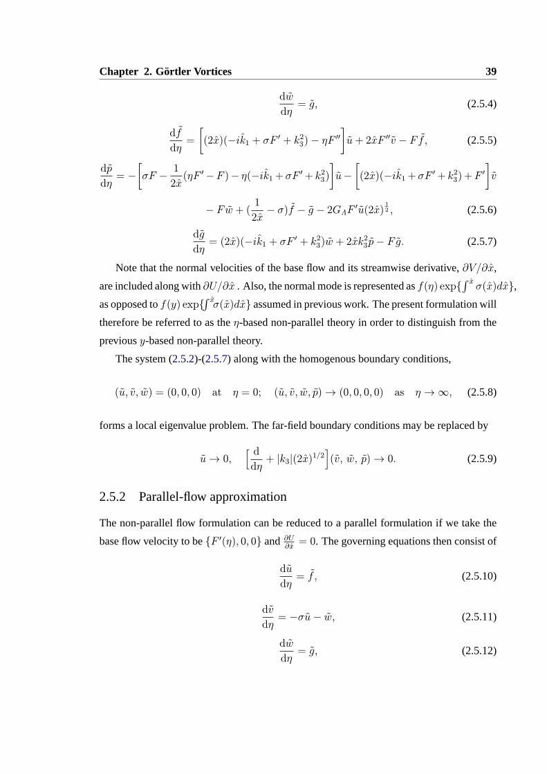
Chapter 2. Gortler Vortices 39
dw
dη= g, (2.5.4)
df
dη=
[
(2x)(−ik1 + σF′ + k23)− ηF
′′
]
u+ 2xF ′′v − F f, (2.5.5)
dp
dη= −
[
σF −1
2x(ηF ′−F )− η(−ik1+ σF
′+ k23)
]
u−
[
(2x)(−ik1+ σF′+ k23)+F
′
]
v
− Fw + (1
2x− σ)f − g − 2GΛF
′u(2x)12 , (2.5.6)
dg
dη= (2x)(−ik1 + σF
′ + k23)w + 2xk23 p− F g. (2.5.7)
Note that the normal velocities of the base flow and its streamwise derivative,∂V/∂x,
are included along with∂U/∂x . Also, the normal mode is represented asf(η) exp{∫ xσ(x)dx},
as opposed tof(y) exp{∫ xσ(x)dx} assumed in previous work. The present formulation will
therefore be referred to as theη-based non-parallel theory in order to distinguish from the
previousy-based non-parallel theory.
The system (2.5.2)-(2.5.7) along with the homogenous boundary conditions,
(u, v, w) = (0, 0, 0) at η = 0; (u, v, w, p)→ (0, 0, 0, 0) as η →∞, (2.5.8)
forms a local eigenvalue problem. The far-field boundary conditions may be replaced by
u→ 0,[ ddη+ |k3|(2x)
1/2](v, w, p)→ 0. (2.5.9)
2.5.2 Parallel-flow approximation
The non-parallel flow formulation can be reduced to a parallel formulation if we take the
base flow velocity to be{F ′(η), 0, 0} and∂U∂x= 0. The governing equations then consist of
du
dη= f , (2.5.10)
dv
dη= −σu− w, (2.5.11)
dw
dη= g, (2.5.12)
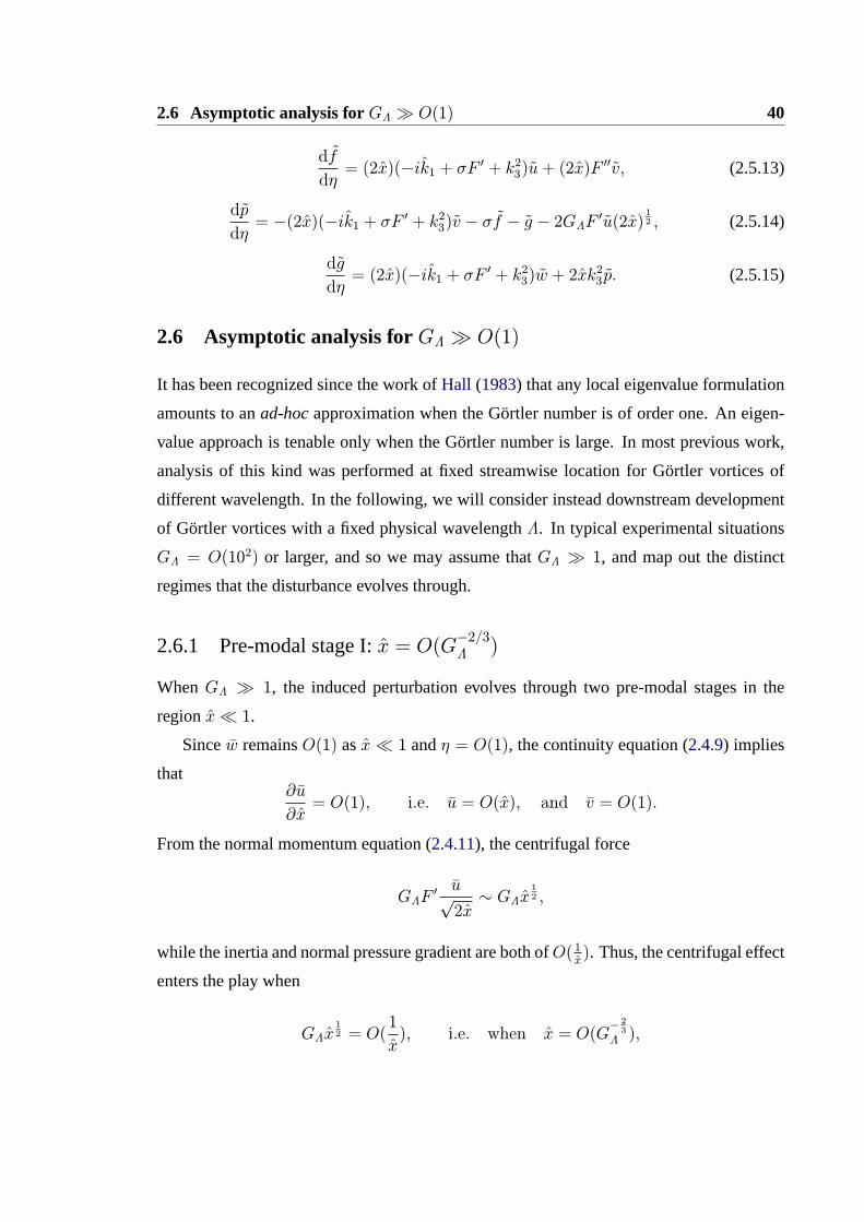
2.6 Asymptotic analysis forGΛ � O(1) 40
df
dη= (2x)(−ik1 + σF
′ + k23)u+ (2x)F′′v, (2.5.13)
dp
dη= −(2x)(−ik1 + σF
′ + k23)v − σf − g − 2GΛF′u(2x)
12 , (2.5.14)
dg
dη= (2x)(−ik1 + σF
′ + k23)w + 2xk23 p. (2.5.15)
2.6 Asymptotic analysis forGΛ � O(1)
It has been recognized since the work ofHall (1983) that any local eigenvalue formulation
amounts to anad-hocapproximation when the Gortler number is of order one. An eigen-
value approach is tenable only when the Gortler number is large. In most previous work,
analysis of this kind was performed at fixed streamwise location for Gortler vortices of
different wavelength. In the following, we will consider instead downstream development
of Gortler vortices with a fixed physical wavelengthΛ. In typical experimental situations
GΛ = O(102) or larger, and so we may assume thatGΛ � 1, and map out the distinct
regimes that the disturbance evolves through.
2.6.1 Pre-modal stage I:x = O(G−2/3Λ )
WhenGΛ � 1, the induced perturbation evolves through two pre-modal stages in the
regionx� 1.
Sincew remainsO(1) asx� 1 andη = O(1), the continuity equation (2.4.9) implies
that∂u
∂x= O(1), i.e. u = O(x), and v = O(1).
From the normal momentum equation (2.4.11), the centrifugal force
GΛF′ u√2x∼ GΛx
12 ,
while the inertia and normal pressure gradient are both ofO( 1x). Thus, the centrifugal effect
enters the play when
GΛx12 = O(
1
x), i.e. when x = O(G
− 23Λ ),

Chapter 2. Gortler Vortices 41
but is negligible whenx� G− 23Λ .
The scaling deduced above suggests the introduction of
x† = G23Λx, u† = G
23Λu. (2.6.1)
It follows that∂
∂x= O(G
23Λ
∂
∂x†). (2.6.2)
Substitution of (2.6.1) and (2.6.2) into (2.4.9)–(2.4.12) yields
∂u†
∂x†−
η
2x†∂u†
∂η+∂v
∂η+ w = 0
F ′∂u†
∂x†−
F
2x†∂u†
∂η−ηF ′′
2x†u† + F ′′v =
1
2x†∂2u†
∂η2
F ′∂w
∂x†−
F
2x†∂w
∂η=1
2x†∂2w
∂η2
, (2.6.3)
and1
2x†∂2v
∂η2+ F ′
∂v
∂x†−
F
2x†∂v
∂η+ 2F ′u†(
1
2x†)12 =
1
2x†∂p
∂η. (2.6.4)
We call this regime, which operates in the region overO(G− 23Λ RΛΛ) distances to the
leading edge, the pre-modal stage I. The induced velocity field is governed by the quasi-
steady boundary-layer equations (2.6.3), and the pressure can be solved passively from the
transverse momentum equation (2.6.4). Non-parallelism is at leading order, and the veloc-
ity response to FST remains identical to the flat-plate case. This regime is distinguished
only in the sense that the centrifugal force influences the pressure distribution across the
boundary layer, as is indicated by (2.6.4).
2.6.2 Pre-modal stage II:x = O(G−2/5Λ )
Sinceu ∼ x, the balance in the normal momentum equation suggests thatp = O(GΛx32 )
for η = O(1). The induced pressure affects the spanwise momentum equation (2.4.12)
when
F ′∂w
∂x= O(GΛx
32 ), i.e. when x = O(G
− 25Λ ),

2.6 Asymptotic analysis forGΛ � O(1) 42
and the perturbation enters a new regime. The scaling argument above suggests that we
introduce
x = G25Λx, (2.6.5)
and write the solution forη = O(1) as
u = G− 25Λ
(u+O(G
−1/5Λ )
), p = G
25Λ
(p+O(G
−1/5Λ )
). (2.6.6)
Inserting these into (2.4.9)–(2.4.12), we obtain
∂u
∂x−
η
2x
∂u
∂η+∂v
∂η+ w = 0, (2.6.7)
F ′∂u
∂x−F
2x
∂u
∂η−ηF ′′
2xu+ F ′′v =
1
2x
∂2u
∂η2, (2.6.8)
∂p
∂η= −2
√2xF ′u, (2.6.9)
F ′∂w
∂x−F
2x
∂w
∂η= k23 p+
1
2x
∂2w
∂η2. (2.6.10)
Since the non-parallel-flow effect appears at leading order, the regime is termed as pre-
modal stage II. It is distinguished in that the pressure is fully coupled with the velocity
field. As a result, Gortler instability starts to operate. We demonstrate this by showing that
asx� 1, the system (2.6.7)-(2.6.10) admits asymptotic eigen solutions of the form
(u, v, w, p) = xγ{(x−α+1UE(η), VE(η),WE(η), x
−α+ 32PE(η)
)+ . . .
}eσ(x),(2.6.11)
whereσ(x) expands as
σ = σ0xα + . . . , (2.6.12)
with σ0, α, andγ being constants to be found. Inserting (2.6.11) with (2.6.12) into (2.6.10)
yields at leading order,xγ+α−1ασ0F′WE = k23x
γ−α+ 32PE, from which it may be deduced
that
α = 5/4, (2.6.13)
ασ0F′WE = k
23PE.
Chapter 2. Gortler Vortices 43
Substituting (2.6.11) into (2.6.7)–(2.6.9), we obtain at leading order
ασ0UE + VE,η +WE = 0, ασ0F′UE + F
′′VE = 0, PE,η = −2√2F ′UE.
Elimination ofUE,WE, andPE leads to the equation forVE,
∂2VE
∂η2−
[F ′′′
F ′−2√2k23F
′′
(ασ0)2F ′
]
VE = 0. (2.6.14)
SinceF ′ = F ′′′ = 0 butF ′′ 6= 0 atη = 0, η = 0 is a regular singular point of the equation.
The local solution can be constructed as a Frobenus series
VE = a(η +12η2) + b
[1− η2 + . . .+ (η + 1
2η2) ln η
].
We takeb = 0 so that the no-penetration condition,
VE(0) = 0, (2.6.15)
is satisfied. Without losing generality, we seta = 1, which amounts to normalising the
eigenfunction such that
VE,η(0) = 1. (2.6.16)
On the other hand, asη →∞, ∂2VE/∂η2 → 0 (see (2.6.14)). In order to keepVE bounded,
the boundary condition imposed is
VE,η → 0 as η →∞. (2.6.17)
With the normalisation (2.6.16), it follows thatUE → −1/(ασ0) asη → 0. The slip
velocity is reduced to zero across a viscous sublayer, the width of which isη ∼ x−5/12, as
can be deduced by balancing the convection and diffusion in the momentum equations. We
thus introduce the local transverse coordinate
ζ = (2λασ0)1/3x5/12η.

2.6 Asymptotic analysis forGΛ � O(1) 44
For ζ = O(1), the viscous solution expands as
(u, v, w, p) = xγ{(x−
14us(ζ), x
− 512 (2λασ0)
−1/3vs, ws, (2λασ0)−1/3x−
16ps
)+ . . .
}eσ(x),
(2.6.18)
whereus, vs, ws andps functions ofζ. Their governing equations, obtained by inserting
(2.6.18) into (2.6.7)–(2.6.9), are
ασ0us + vs,ζ + ws = 0, ασ0(ζus − us,ζζ) + vs = 0, ασ0(ζws − ws,ζζ) = k23ps,
andps,ζ = 0. Elimination ofus andws among these equations gives
(d2
dζ2− ζ)vs,ζζ = 0, (2.6.19)
for vs, while the boundary conditions,us(0) = vs(0) = 0, and the matching requirement
correspond to
vs,ζζζ(0) = k23ps/ασ0, vs,ζ(0) = 0; vs,ζ → 1 as ζ →∞.
The solution is
vs = c0
∫ ζ
0
(ζ − ζ)Ai(ζ)dζ , with c0 = 1/
∫ ∞
0
Ai(ζ)dζ = 3, (2.6.20)
whereAi denotes the Airy function. The solution to the pressure is
ps =ασ0
k23c0Ai
′(0). (2.6.21)
It follows that asζ →∞,
vs → ζ − c0
∫ ∞
0
ζAi(ζ)dζ ≡ ζ + v∞.
The transpiration velocity,v∞, induces a correction ofO(x−5/12) in the core of the
boundary layer; see (2.6.18). It may be further deduced that the expansions (2.6.11)-
(2.6.12) should proceed as
σ = σ0x5/4 + σ1x
5/6 + σ2x5/12, (2.6.22)
Chapter 2. Gortler Vortices 45
(u, v, w, p)=xγ{(x−1/4UE(η), VE(η),WE(η), x
1/4PE(η))
+3∑
n=1
x−5n12
(x−1/4U
(n)E (η), V
(n)E (η),W
(n)E (η), x
1/4P(n)E (η)
)}
eσ(x) .
(2.6.23)
The lowest-order correction satisfies a system of inhomogeneous equations,
ασ0U(1)E + V
(1)E,η +W
(1)E =−
56σ1UE,
ασ0F′U(1)E + F
′′V(1)E =−5
6σ1F
′UE,
P(1)E,η + 2
√2F ′U
(1)E =0,
ασ0F′W(1)E − k
23P(1)E =−
56σ1F
′WE.
(2.6.24)
These equations can be reduced to
∂2V(1)E
∂η2−
[F ′′′
F ′−2√2k23F
′′
(ασ0)2F ′
]
V(1)E =
10√2k23σ1
3(ασ0)3F ′′VE/F
′. (2.6.25)
The boundary conditions are
V(1)E = (2λασ0)
−1/3v∞ at η = 0; V(1)E,η → 0 as η →∞.
Imposing the solvability condition on (2.6.25), we find that
10√2k23σ1
3(ασ0)3
∫ ∞
0
F ′′V 2E/F′dη = (2λασ0)
−1/3v∞, (2.6.26)
which determinesσ1. The higher-order corrections,σ2 andγ, can be obtained by consider-
ing V (2)E andV (3)E respectively.
It can be deduced thatUE, WE andPE all decay exponentially asη → ∞, but VE
tends to a constant, indicating that the scaling (2.6.6) and the system (2.6.7)-(2.6.10) are
not uniformly valid for allη. An outer layer must be introduced, where the inertia in the
normal momentum equation, negligible whenη = O(1) (see (2.6.9)), comes into play. A
scaling argument suggests that the width of this layer corresponds toη ∼ G1/5Λ /√2x, and
2.6 Asymptotic analysis forGΛ � O(1) 46
hence we introduce
yo = G−1/5Λ
√2x η.
Foryo = O(1), the solution expands as
(u, v, w, p) = (G−3/5Λ uo, vo, G
−1/5Λ wo, G
1/5Λ po). (2.6.27)
It follows from the streamwise momentum equation (2.4.10) that ∂uo/∂yo = 0, and so
uo = 0 in order to satisfies the boundary layer condition at the infinity. Substitution of
(2.6.27) into (2.4.9) and (2.4.11)-(2.4.12) shows that
√2x∂vo
∂yo+ wo = 0,
∂vo
∂x+vo
2x= −
1√2x
∂po
∂yo,
∂wo
∂x= k23 po. (2.6.28)
The solution is found as
po = g′o(x) e
−|k3|yo , wo = k23go(x) e
−|k3|yo , v0 =|k3|√2xgo(x) e
−|k3|yo .
The functiongo is found by matching with the main-deck solution as
go(x) = xγ+ 1
2
(VE,∞ +O(x
−5/12))eσ(x), (2.6.29)
whereVE,∞ = limη→∞
VE(η), which is determined once the eigenvalue problem, defined by
(2.6.14) with (2.6.15) and (2.6.17), is solved.
The asymptotic eigenvalue problem, (2.6.14) with (2.6.15)–(2.6.17), is solved by a
shooting method. A countable set of asymptotic eigen modes exist, and for the first four
we find thatσ0 = 0.8209, 0.5143, 0.3781 and 0.2996 while the viscous correctionσ1 =
−1.6614, -1.8047, -1.8122, -1.6729. The role of the asymptotic eigen modes in the recep-
tivity of Gortler instability is analogous to that of the first Lam-Rott mode in the Tollmien-
Schlichting instability (Goldstein 1983): they represent the earliest intrinsic characteristic
motion that develops from the forced motion, and then evolves into fully fledged local
eigen modes, i.e. Gortler vortices in the present case. On the other hand, unlike the damped
Lam-Rott mode, the present eigen modes are unstable. Consequently, Gortler vortices are
much more receptive to FST than Tollmien-Schlichting waves.
Chapter 2. Gortler Vortices 47
2.6.3 Inviscid regime:x = O(1)
In the region wherex = O(G2/5Λ ), i.e. x = O(1), the outer region merges with the main
layer, and the spanwise wavelength becomes comparable with the local boundary-layer
thickness, so thatGθ = O(GΛ). As was suggested by (2.6.22)–(2.6.23), the solution now
takes the WKBJ form
(u, v, w, p)=[(G− 12Λ u0(x, η), v0(x, η), w0(x, η), G
12Λp0(x, η)
)
+G− 16Λ
(G− 12Λ u1(x, η), v1(x, η), w1(x, η), G
12Λp1(x, η)
)+ . . .
]E,
(2.6.30)
where we have put
E = exp{G12Λ
∫ xσ(x)dx
}(2.6.31)
with σ being expanded as
σ = σ0 +G− 16Λ σ1 + . . . . (2.6.32)
As will be shown later, theO(G− 16Λ ) correction is contributed by the viscous effect near the
wall. Substituting (2.6.30) and (2.6.32) into (2.4.9)-(2.4.12), we obtain
σ0u0 +∂v0
∂η+ w0 = 0,
σ0F′u0 + F
′′v0 = 0, σ0F′v0 +
2F ′√2xu0 = −
1
2x
∂p0
∂η, σ0F
′w0 = k23p0.
(2.6.33)
These equations can be reduce to the equation forv0,
∂2v0
∂η2−
[F ′′′
F ′+ 2xk23 −
2√2xk23F
′′
σ20F′
]
v0 = 0, (2.6.34)
subject to the boundary conditions:
v0 = 0 at η = 0; v0 → 0 as η →∞. (2.6.35)
The eigenvalue problem (2.6.34)-(2.6.35) corresponds to the inviscid limit of Gortler
formulation. The eigenfunction is normalised such that
v0,η(0) = 1. (2.6.36)
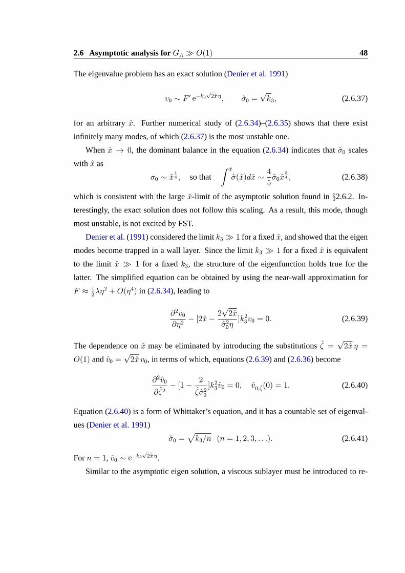
2.6 Asymptotic analysis forGΛ � O(1) 48
The eigenvalue problem has an exact solution (Denier et al. 1991)
v0 ∼ F ′ e−k3√2x η, σ0 =
√k3, (2.6.37)
for an arbitraryx. Further numerical study of (2.6.34)–(2.6.35) shows that there exist
infinitely many modes, of which (2.6.37) is the most unstable one.
When x → 0, the dominant balance in the equation (2.6.34) indicates thatσ0 scales
with x as
σ0 ∼ x14 , so that
∫ xσ(x)dx ∼
4
5σ0x
54 , (2.6.38)
which is consistent with the largex-limit of the asymptotic solution found in§2.6.2. In-
terestingly, the exact solution does not follow this scaling. As a result, this mode, though
most unstable, is not excited by FST.
Denier et al.(1991) considered the limitk3 � 1 for a fixedx, and showed that the eigen
modes become trapped in a wall layer. Since the limitk3 � 1 for a fixedx is equivalent
to the limit x � 1 for a fixedk3, the structure of the eigenfunction holds true for the
latter. The simplified equation can be obtained by using the near-wall approximation for
F ≈ 12λη2 +O(η4) in (2.6.34), leading to
∂2v0
∂η2− [2x−
2√2x
σ20η]k23v0 = 0. (2.6.39)
The dependence onx may be eliminated by introducing the substitutionsζ =√2x η =
O(1) andv0 =√2x v0, in terms of which, equations (2.6.39) and (2.6.36) become
∂2v0
∂ζ2− [1−
2
ζ σ20]k23 v0 = 0, v0,ζ(0) = 1. (2.6.40)
Equation (2.6.40) is a form of Whittaker’s equation, and it has a countable set of eigenval-
ues (Denier et al. 1991)
σ0 =√k3/n (n = 1, 2, 3, . . .). (2.6.41)
Forn = 1, v0 ∼ e−k3√2x η.
Similar to the asymptotic eigen solution, a viscous sublayer must be introduced to re-

Chapter 2. Gortler Vortices 49
0 0.5 1 1.5 2 2.5 30
0.1
0.2
0.3
0.4
0.5
0.6
0.7
0.8
Mode 1
Mode 2
x
σ
Figure 2.3: Matching of different regimes. Dashed lines: asymptotic eigen mode; solidlines: inviscid modes; dotted lines: the large-x limit of inviscid modes, i.e. (2.6.41) withn = 2, 3.
duce the slip velocity to zero. The normal velocity may be written as
v = G−1/6Λ (2λσ0x)
−1/3vs(ζ), ζ = G1/6Λ (2λσ0x)
1/3η,
with vs satisfying the equation (2.6.19) and has the solution (2.6.20). The viscous effect
induces a transpiration velocity, which in turn forces anO(G−1/6Λ ) correction in the main
layer; see (2.6.30). The equation forv1 is
∂2v1
∂η2−
[F ′′′
F ′+ 2xk23 −
2√2xk23F
′′
σ20F′
]
v1 =4√2xk23σ1σ30
F ′′v0
F ′, (2.6.42)
subject to the boundary condition
v1(0) = (2λσ0x)−1/3v∞, v1,η → 0 as η →∞.
From the solvability condition on (2.6.42), it follows that
(2λσ0x)−1/3v∞ =
4√2xk23σ1σ30
∫ ∞
0
F ′′v20F ′dη →
2√2k23σ1σ30
x−1/2∫ ∞
0
v20
ζdζ as x→∞.
Note thatσ1 ∼ x1/6 asx→∞, use of which in (2.6.32) suggests that the viscous correction
to the growth rate becomes leading order whenx = O(GΛ).
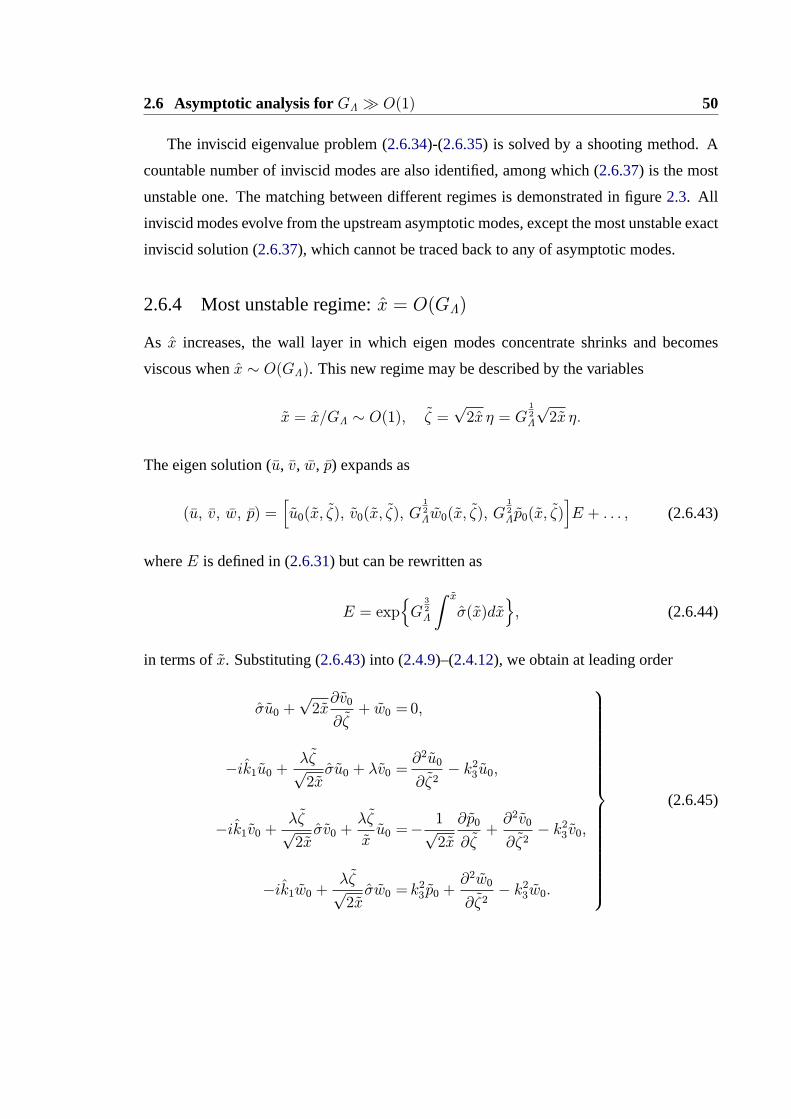
2.6 Asymptotic analysis forGΛ � O(1) 50
The inviscid eigenvalue problem (2.6.34)-(2.6.35) is solved by a shooting method. A
countable number of inviscid modes are also identified, among which (2.6.37) is the most
unstable one. The matching between different regimes is demonstrated in figure2.3. All
inviscid modes evolve from the upstream asymptotic modes, except the most unstable exact
inviscid solution (2.6.37), which cannot be traced back to any of asymptotic modes.
2.6.4 Most unstable regime:x = O(GΛ)
As x increases, the wall layer in which eigen modes concentrate shrinks and becomes
viscous whenx ∼ O(GΛ). This new regime may be described by the variables
x = x/GΛ ∼ O(1), ζ =√2x η = G
12Λ
√2x η.
The eigen solution (u, v, w, p) expands as
(u, v, w, p) =[u0(x, ζ), v0(x, ζ), G
12Λw0(x, ζ), G
12Λp0(x, ζ)
]E + . . . , (2.6.43)
whereE is defined in (2.6.31) but can be rewritten as
E = exp{G32Λ
∫ xσ(x)dx
}, (2.6.44)
in terms ofx. Substituting (2.6.43) into (2.4.9)–(2.4.12), we obtain at leading order
σu0 +√2x∂v0
∂ζ+ w0 =0,
−ik1u0 +λζ√2xσu0 + λv0 =
∂2u0
∂ζ2− k23u0,
−ik1v0 +λζ√2xσv0 +
λζ
xu0 =−
1√2x
∂p0
∂ζ+∂2v0
∂ζ2− k23 v0,
−ik1w0 +λζ√2xσw0 = k
23 p0 +
∂2w0
∂ζ2− k23w0.
(2.6.45)
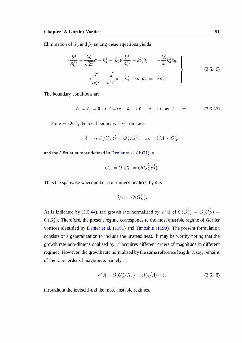
Chapter 2. Gortler Vortices 51
Elimination ofw0 andp0 among these equations yields
(∂2
∂ζ2−
λζ√2xσ − k23 + ik1)(
∂2
∂ζ2− k23)v0 = −
λζ
xk23u0,
(∂2
∂ζ2−
λζ√2xσ − k23 + ik1)u0 = λv0.
(2.6.46)
The boundary conditions are
u0 = v0 = 0 at ζ = 0; u0 → 0, v0 → 0 as ζ →∞. (2.6.47)
For x = O(1), the local boundary-layer thickness
δ = (νx∗/U∞)12 = G
12ΛΛx
12 , i.e. δ/Λ ∼ G
12Λ,
and the Gortler number defined inDenier et al.(1991) is
GH = O(G2θ) = O(G
52Λx
32 ).
Thus the spanwise wavenumber non-dimensionalised byδ is
δ/Λ = O(G15H).
As is indicated by (2.6.44), the growth rate normalised byx∗ is of O(G32Λ) = O(G
35H) =
O(G65θ ). Therefore, the present regime corresponds to the most unstable regime of Gortler
vortices identified byDenier et al.(1991) andTimoshin(1990). The present formulation
consists of a generalization to include the unsteadiness. It may be worthy noting that the
growth rate non-dimensionalised byx∗ acquires different orders of magnitude in different
regimes. However, the growth rate normalised by the same reference length,Λ say, remains
of the same order of magnitude, namely
σ∗Λ = O(G12Λ/RΛ) = O(
√Λ/r∗0 ), (2.6.48)
throughout the inviscid and the most unstable regimes.
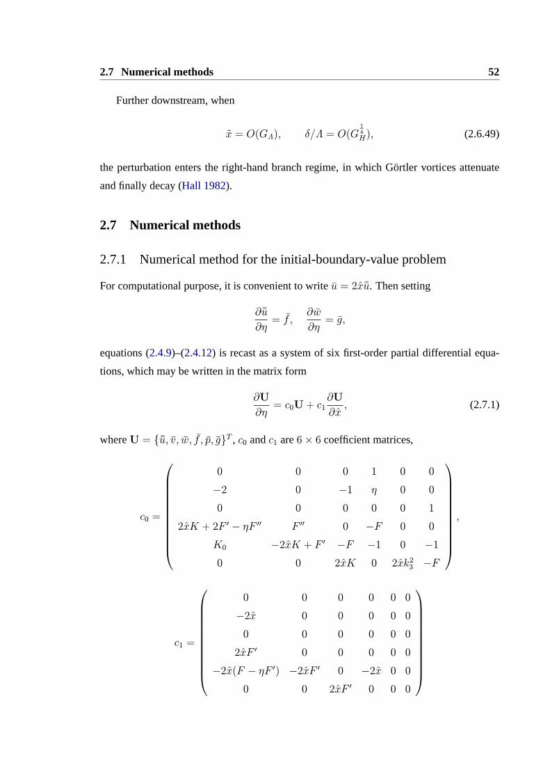
2.7 Numerical methods 52
Further downstream, when
x = O(GΛ), δ/Λ = O(G14H), (2.6.49)
the perturbation enters the right-hand branch regime, in which Gortler vortices attenuate
and finally decay (Hall 1982).
2.7 Numerical methods
2.7.1 Numerical method for the initial-boundary-value problem
For computational purpose, it is convenient to writeu = 2xˉu. Then setting
∂ ˉu
∂η= f ,
∂w
∂η= g,
equations (2.4.9)–(2.4.12) is recast as a system of six first-order partial differential equa-
tions, which may be written in the matrix form
∂U
∂η= c0U+ c1
∂U
∂x, (2.7.1)
whereU = {ˉu, v, w, f , p, g}T , c0 andc1 are6× 6 coefficient matrices,
c0 =
0 0 0 1 0 0
−2 0 −1 η 0 0
0 0 0 0 0 1
2xK + 2F ′ − ηF ′′ F ′′ 0 −F 0 0
K0 −2xK + F ′ −F −1 0 −1
0 0 2xK 0 2xk23 −F
,
c1 =
0 0 0 0 0 0
−2x 0 0 0 0 0
0 0 0 0 0 0
2xF ′ 0 0 0 0 0
−2x(F − ηF ′) −2xF ′ 0 −2x 0 0
0 0 2xF ′ 0 0 0

Chapter 2. Gortler Vortices 53
with K0 = −3(F − ηF ′) + (2x)ηK − 2GF ′(2x)3/2, andK = −ik1 + k23.
We apply the second-order central difference scheme in the normal direction, i.e.
Uj+1 −Uj =h
2(U′j+1 +U
′j) +O(h
3), (2.7.2)
whereh = ηj+1 − ηj, and a prime indicates differentiation with respect toη. By using
(2.7.2), equation (2.7.1) can be rewritten as
[
I −h
2cj+10
]
Uj+1 +
[
− I −h
2cj0
]
Uj =h
2
(
cj+11∂Uj+1∂x
+ cj1∂Uj∂x
)
, (2.7.3)
whereI is the6× 6 identity matrix.
A second order accurate backward differencing scheme is used in the streamwise direc-
tion to approximate∂Un+1/∂x,
∂Un+1
∂x= γUn+1 + fn+1d +O((Δx)2), (2.7.4)
whereΔx = xn+1 − xn, and
fn+1d = −(α0Un + α1U
n−1).
If we chooseγ = 32Δx
, α0 = 2Δx
, α1 = − 12Δx
, then discretization is of second-order
accuracy. For convenience, we rewrite the discretized equations in the following form,
[I −
h
2cj+1
]Uj+1 +
[−I −
h
2cj
]Uj =
h
2(gj+1 + gj), (2.7.5)
wherecj+1 = cj+10 + γcj+11 is evaluated atxn+1,U stands forUn+1 andgj = c
j1fn+1d .
In order to march downstream, the values ofU at the first two steps are specified by
using the composite solution (2.4.26)-(2.4.27) or (2.4.23)–(2.4.25). Alternatively, the com-
posite solution is used to evaluateU0, while U1 is calculated by dividing the stepΔx
into ten sub-steps and using a first-order difference scheme (Euler’s Method) for∂U/∂x,
i.e. by choosingγ = 10.1Δx
, α0 = 10.1Δx
andα1 = 0. Values ofU at subsequent mesh
points can be calculated using the second-order scheme. Typically, the marching starts from
x = 0.003, and the step sizeΔx = 10−3. The numerical solution overlaps (2.4.26)-(2.4.27)
for 0.003 < x ≤ 0.005, indicating that the choice of the starting point is appropriate.
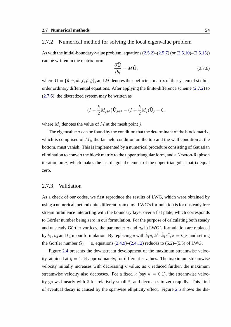
2.7 Numerical methods 54
2.7.2 Numerical method for solving the local eigenvalue problem
As with the initial-boundary-value problem, equations (2.5.2)–(2.5.7) (or (2.5.10)–(2.5.15))
can be written in the matrix form∂U
∂η=MU, (2.7.6)
whereU = {u, v, w, f , p, g}, andM denotes the coefficient matrix of the system of six first
order ordinary differential equations. After applying the finite-difference scheme (2.7.2) to
(2.7.6), the discretized system may be written as
(I −h
2Mj+1)Uj+1 − (I +
h
2Mj)Uj = 0,
whereMj denotes the value ofM at the mesh pointj.
The eigenvalueσ can be found by the condition that the determinant of the block matrix,
which is comprised ofMj, the far-field condition on the top and the wall condition at the
bottom, must vanish. This is implemented by a numerical procedure consisting of Gaussian
elimination to convert the block matrix to the upper triangular form, and a Newton-Raphson
iteration onσ, which makes the last diagonal element of the upper triangular matrix equal
zero.
2.7.3 Validation
As a check of our codes, we first reproduce the results of LWG, which were obtained by
using a numerical method quite different from ours. LWG’s formulation is for unsteady free
stream turbulence interacting with the boundary layer over a flat plate, which corresponds
to Gortler number being zero in our formulation. For the purpose of calculating both steady
and unsteady Gortler vortices, the parameterκ andκ2 in LWG’s formulation are replaced
by k1, k2 andk3 in our formulation. By replacinguwith k1u, k23=k1κ2, x = k1x, and setting
the Gortler numberGΛ = 0, equations (2.4.9)–(2.4.12) reduces to (5.2)–(5.5) of LWG.
Figure2.4 presents the downstream development of the maximum streamwise veloc-
ity, attained atη = 1.64 approximately, for differentκ values. The maximum streamwise
velocity initially increases with decreasingκ value; asκ reduced further, the maximum
streamwise velocity also decreases. For a fixedκ (sayκ = 0.1), the streamwise veloc-
ity grows linearly withx for relatively smallx, and decreases to zero rapidly. This kind
of eventual decay is caused by the spanwise ellipticity effect. Figure2.5 shows the dis-

Chapter 2. Gortler Vortices 55
0 1 2 3 4 5 6 7 80
0.05
0.1
0.15
0.2
0.25
0.3
0.35
x
1
|u| 1.64
1
κ = 0.01
1
κ = 0.025
1
κ = 0.05
1
κ = 0.1
1
κ = 1.0
1
Figure 2.4:|u| atη = 1.64 calculated from different values ofκ ≤ 1.0 with κ2 = −κ usingequations (2.4.9)–(2.4.12).
tributions of the streamwise and spanwise velocities at different downstream locations. It
is known that the profile of the streamwise velocity given by LUBL is valid for relatively
small x. However, the shape of the profile does not change significantly whenx becomes
relatively large as indicated in figure2.6
Figures2.4–2.6 are in exact agreement with the results as shown in Figures 3-4 and
Figures 6-7 of LWG, thereby giving us the confidence in our own codes.
2.8 Results and comparisons with experiments
Since the majority of experiments were conducted on a curved plate with a constant cur-
vature, our calculations will be carried out for this special case, even though the nu-
merical method is applicable to a curved wall with a varying curvature. With the non-
dimensionalisation adopted, the spanwwise wavenumberk3 = 1. We setk2 = −1, which
serves as a representative case.
2.8.1 Steady Gortler vortices
In this section, we present results on the response of the boundary layer over a curved plate
with a constant curvature to steady free-stream disturbances (k1 = 0.0). The particular in-
terest is in the generation of steady Gortler vortices. For the purpose of observing the effect
of curvature on the boundary-layer response to free-stream disturbances, the downstream
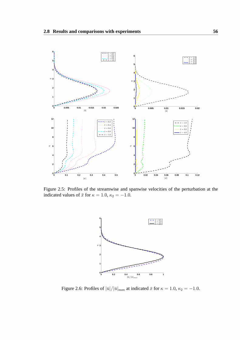
2.8 Results and comparisons with experiments 56
0 0.005 0.01 0.015 0.02 0.0250
1
2
3
4
5
6
|u|
1
η
1
x = 0.2
1
x = 0.4
1
x = 0.6
1
x = 0.8
1
x = 1.0
1
0 0.005 0.01 0.015 0.020
1
2
3
4
5
6
|u|
1
η
1
x = 1.0
1
x = 2.0
1
x = 3.0
1
x = 4.0
1
0 0.1 0.2 0.3 0.4 0.50
2
4
6
8
10
12
|w|
1
η
1
x = 0.2
1
x = 0.4
1
x = 0.6
1
x = 0.8
1
x = 1.0
1
0 0.02 0.04 0.06 0.08 0.1 0.120
2
4
6
8
10
12
|w|
1
η
1
x = 1.0
1
x = 2.0
1
x = 3.0
1
x = 4.0
1
Figure 2.5: Profiles of the streamwise and spanwise velocities of the perturbation at theindicated values ofx for κ = 1.0, κ2 = −1.0.
0 0.2 0.4 0.6 0.8 10
1
2
3
4
5
6
|u|/|u|max
1
η
1
x = 0.5
1
x = 1.0
1
x = 2.0
1
Figure 2.6: Profiles of|u|/|u|max at indicatedx for κ = 1.0, κ2 = −1.0.
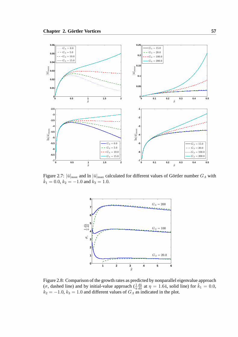
Chapter 2. Gortler Vortices 57
0 0.5 1 1.5 20
0.01
0.02
0.03
0.04
0.05
0.06
x
1
|u| max
1
GΛ = 0.0
1
GΛ = 5.0
1
GΛ = 10.0
1
GΛ = 15.0
1
0 0.1 0.2 0.3 0.4 0.50
0.05
0.1
0.15
0.2
0.25
x
1
|u| max
1
GΛ = 15.0
1
GΛ = 20.0
1
GΛ = 100.0
1
GΛ = 200.0
1
0 0.5 1 1.5 2-7
-6.5
-6
-5.5
-5
-4.5
-4
-3.5
-3
-2.5
ln|u| max
1
x
1
GΛ = 0.0
1
GΛ = 5.0
1
GΛ = 10.0
1
GΛ = 15.0
1
0 0.1 0.2 0.3 0.4 0.5-7
-6
-5
-4
-3
-2
-1
x
1
ln|u| max
1
GΛ = 15.0
1
GΛ = 20.0
1
GΛ = 100.0
1
GΛ = 200.0
1
Figure 2.7:|u|max and ln|u|max calculated for different values of Gortler numberGΛ withk1 = 0.0, k2 = −1.0 andk3 = 1.0.
1 2 3 4 5 60
1
2
3
4
5
6
7
8
x
1
σ,
1 ududx
1
GΛ = 200
1
GΛ = 100
1
GΛ = 20.0
1
Figure 2.8: Comparison of the growth rates as predicted by nonparallel eigenvalue approach(σ, dashed line) and by initial-value approach (1
ududx
at η = 1.64, solid line) for k1 = 0.0,k2 = −1.0, k3 = 1.0 and different values ofGΛ as indicated in the plot.
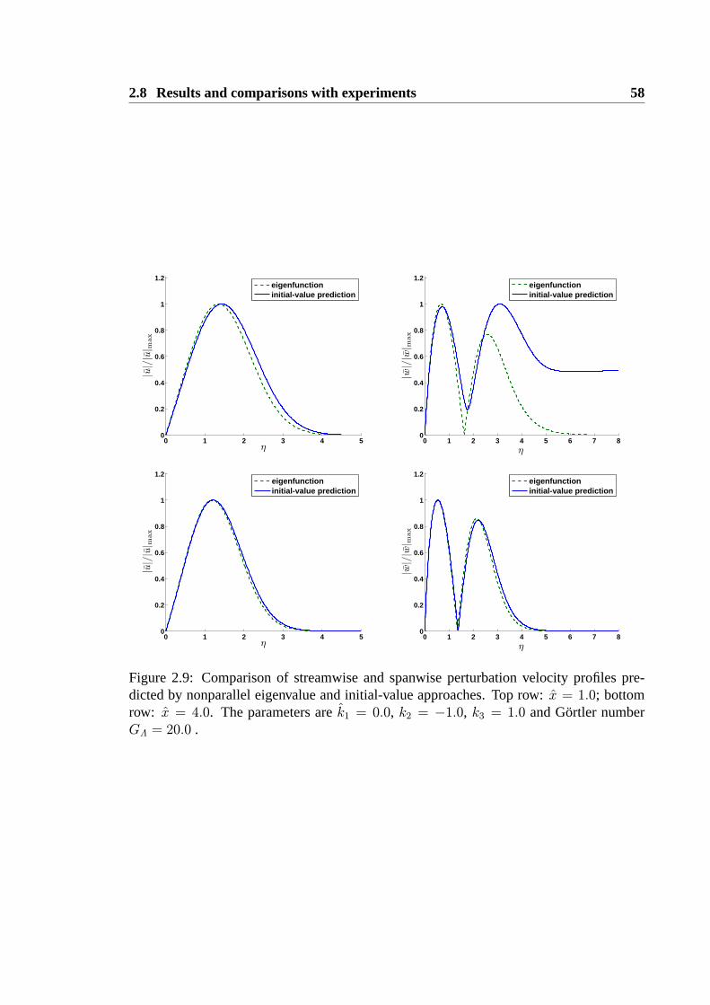
2.8 Results and comparisons with experiments 58
0 1 2 3 4 50
0.2
0.4
0.6
0.8
1
1.2
η
1
|u|/|u| max
1
eigenfunctioninitial-value prediction
0 1 2 3 4 5 6 7 80
0.2
0.4
0.6
0.8
1
1.2
η
1
|w|/|w| max
1
eigenfunctioninitial-value prediction
0 1 2 3 4 50
0.2
0.4
0.6
0.8
1
1.2
η
1
|u|/|u| max
1
eigenfunctioninitial-value prediction
0 1 2 3 4 5 6 7 80
0.2
0.4
0.6
0.8
1
1.2
η
1
|w|/|w| max
1
eigenfunctioninitial-value prediction
Figure 2.9: Comparison of streamwise and spanwise perturbation velocity profiles pre-dicted by nonparallel eigenvalue and initial-value approaches. Top row:x = 1.0; bottomrow: x = 4.0. The parameters arek1 = 0.0, k2 = −1.0, k3 = 1.0 and Gortler numberGΛ = 20.0 .
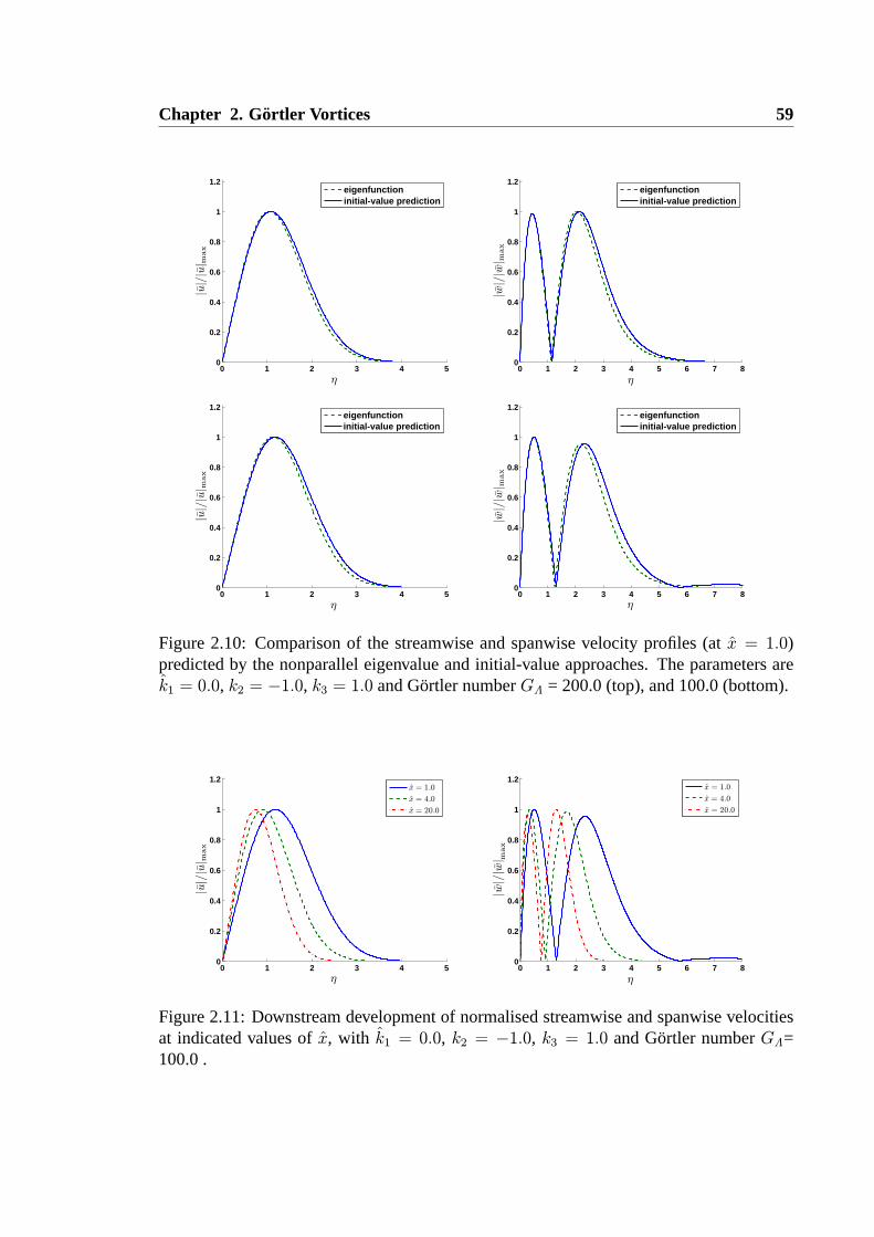
Chapter 2. Gortler Vortices 59
0 1 2 3 4 50
0.2
0.4
0.6
0.8
1
1.2
η
1
|u|/|u| max
1
eigenfunctioninitial-value prediction
0 1 2 3 4 5 6 7 80
0.2
0.4
0.6
0.8
1
1.2
η
1
|w|/|w| max
1
eigenfunctioninitial-value prediction
0 1 2 3 4 50
0.2
0.4
0.6
0.8
1
1.2
η
1
|u|/|u| max
1
eigenfunctioninitial-value prediction
0 1 2 3 4 5 6 7 80
0.2
0.4
0.6
0.8
1
1.2
η
1
|w|/|w| max
1
eigenfunctioninitial-value prediction
Figure 2.10: Comparison of the streamwise and spanwise velocity profiles (atx = 1.0)predicted by the nonparallel eigenvalue and initial-value approaches. The parameters arek1 = 0.0, k2 = −1.0, k3 = 1.0 and Gortler numberGΛ = 200.0 (top), and 100.0 (bottom).
0 1 2 3 4 50
0.2
0.4
0.6
0.8
1
1.2
η
1
|u|/|u| max
1
x = 1.0
1
x = 4.0
1
x = 20.0
1
0 1 2 3 4 5 6 7 80
0.2
0.4
0.6
0.8
1
1.2
η
1
|w|/|w| max
1
x = 1.0
1
x = 4.0
1
x = 20.0
1
Figure 2.11: Downstream development of normalised streamwise and spanwise velocitiesat indicated values ofx, with k1 = 0.0, k2 = −1.0, k3 = 1.0 and Gortler numberGΛ=100.0 .
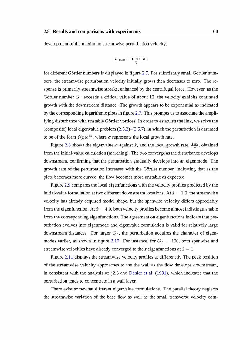
2.8 Results and comparisons with experiments 60
development of the maximum streamwise perturbation velocity,
|u|max = maxη|u|,
for different Gortler numbers is displayed in figure2.7. For sufficiently small Gortler num-
bers, the streamwise perturbation velocity initially grows then decreases to zero. The re-
sponse is primarily streamwise streaks, enhanced by the centrifugal force. However, as the
Gortler numberGΛ exceeds a critical value of about 12, the velocity exhibits continued
growth with the downstream distance. The growth appears to be exponential as indicated
by the corresponding logarithmic plots in figure2.7. This prompts us to associate the ampli-
fying disturbance with unstable Gortler vortices. In order to establish the link, we solve the
(composite) local eigenvalue problem (2.5.2)–(2.5.7), in which the perturbation is assumed
to be of the formf(η)eσx, whereσ represents the local growth rate.
Figure2.8 shows the eigenvalueσ againstx, and the local growth rate,1ududx
, obtained
from the initial-value calculation (marching). The two converge as the disturbance develops
downstream, confirming that the perturbation gradually develops into an eigenmode. The
growth rate of the perturbation increases with the Gortler number, indicating that as the
plate becomes more curved, the flow becomes more unstable as expected.
Figure2.9compares the local eigenfunctions with the velocity profiles predicted by the
initial-value formulation at two different downstream locations. Atx = 1.0, the streamwise
velocity has already acquired modal shape, but the spanwise velocity differs appreciably
from the eigenfunction. Atx = 4.0, both velocity profiles become almost indistinguishable
from the corresponding eigenfunctions. The agreement on eigenfunctions indicate that per-
turbation evolves into eigenmode and eigenvalue formulation is valid for relatively large
downstream distances. For largerGΛ, the perturbation acquires the character of eigen-
modes earlier, as shown in figure2.10. For instance, forGΛ = 100, both spanwise and
streamwise velocities have already converged to their eigenfunctions atx = 1.
Figure2.11displays the streamwise velocity profiles at differentx. The peak position
of the streamwise velocity approaches to the the wall as the flow develops downstream,
in consistent with the analysis of§2.6 andDenier et al.(1991), which indicates that the
perturbation tends to concentrate in a wall layer.
There exist somewhat different eigenvalue formulations. The parallel theory neglects
the streamwise variation of the base flow as well as the small transverse velocity com-

Chapter 2. Gortler Vortices 61
0 2 4 6 8 10-1
0
1
2
3
4
5
x
1
σ,
1 ududx
1
initial-value
1
parallel (full Blasius)
1
nonparallel (η-based)
1
nonparallel (y-based)
1
parallel (U = λη)
1
2nd mode
1st mode
Figure 2.12: Growth rates predicted by different parallel and nonparallel theories as wellas by initial-value calculation, whenk1 = 0.0 andGΛ=89.5 (corresponding toGb ≈ 15 inthe paper ofBoiko et al.(2007, 2010) )
ponent, that is, the base flow is taken to be{F ′(η), 0, 0}. For the so-called most un-
stable modes, which concentrate in the viscous sub-layer, the profile can be simplified to
{λη, 0, 0}, whereλ refers to the wall shear (Denier et al. 1991). In the non-parallel flow
formulation, both the streamwise variation of the base flow and the transverse velocity are
included, i.e. the base flow is taken to be{F ′(η), 1RΛ( 12x)12 (ηF ′ − F ), 0}. The perturbation
may be assumed to be of the formf(y) exp{∫ x
σdx} or f(η) exp{∫ x
σdx}, leading to the
η-based andy-based non-parallel formulations respectively. None of these formulations
are strictly justifiable for finite Gortler numbers, and so their relative merit can only be
assessed by comparing with the initial-value calculation results.
Figure2.12displays the growth rates predicted by different local eigenvalue theories
and the initial-value formulation where we chooseGΛ = 89.5 corresponding to one of
the experimental condition ofBoiko et al. (2010). For x ≥ 0.3, they all give qualita-
tively similar results, but there still exists appreciable quantitative difference. Theη-based
non-parallel theory appears to match with the initial-value prediction best. Somewhat sur-
prisingly, the parallel theory, employing either the full Blasius solution or its approximation
U = λη, gives a more accurate result than they-based non-parallel theory does. As ex-
pected, the difference between different formulations diminishes asx increases. The local
eigenvalue problems admit multiple modes. The growth rates of the second mode calcu-
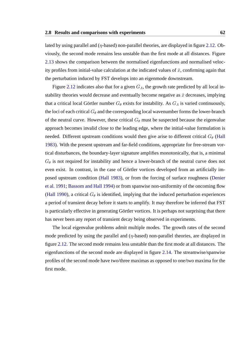
2.8 Results and comparisons with experiments 62
lated by using parallel and (η-based) non-parallel theories, are displayed in figure2.12. Ob-
viously, the second mode remains less unstable than the first mode at all distances. Figure
2.13shows the comparison between the normalised eigenfunctions and normalised veloc-
ity profiles from initial-value calculation at the indicated values ofx, confirming again that
the perturbation induced by FST develops into an eigenmode downstream.
Figure2.12indicates also that for a givenGΛ, the growth rate predicted by all local in-
stability theories would decrease and eventually become negative asx decreases, implying
that a critical local Gortler numberGθ exists for instability. AsGΛ is varied continuously,
the loci of each criticalGθ and the corresponding local wavenumber forms the lower-branch
of the neutral curve. However, these criticalGθ must be suspected because the eigenvalue
approach becomes invalid close to the leading edge, where the initial-value formulation is
needed. Different upstream conditions would then give arise to different criticalGθ (Hall
1983). With the present upstream and far-field conditions, appropriate for free-stream vor-
tical disturbances, the boundary-layer signature amplifies monotonically, that is, a minimal
Gθ is not required for instability and hence a lower-branch of the neutral curve does not
even exist. In contrast, in the case of Gortler vortices developed from an artificially im-
posed upstream condition (Hall 1983), or from the forcing of surface roughness (Denier
et al. 1991; Bassom and Hall 1994) or from spanwise non-uniformity of the oncoming flow
(Hall 1990), a criticalGθ is identified, implying that the induced perturbation experiences
a period of transient decay before it starts to amplify. It may therefore be inferred that FST
is particularly effective in generating Gortler vortices. It is perhaps not surprising that there
has never been any report of transient decay being observed in experiments.
The local eigenvalue problems admit multiple modes. The growth rates of the second
mode predicted by using the parallel and (η-based) non-parallel theories, are displayed in
figure2.12. The second mode remains less unstable than the first mode at all distances. The
eigenfunctions of the second mode are displayed in figure2.14. The streamwise/spanwise
profiles of the second mode have two/three maximas as opposed to one/two maxima for the
first mode.
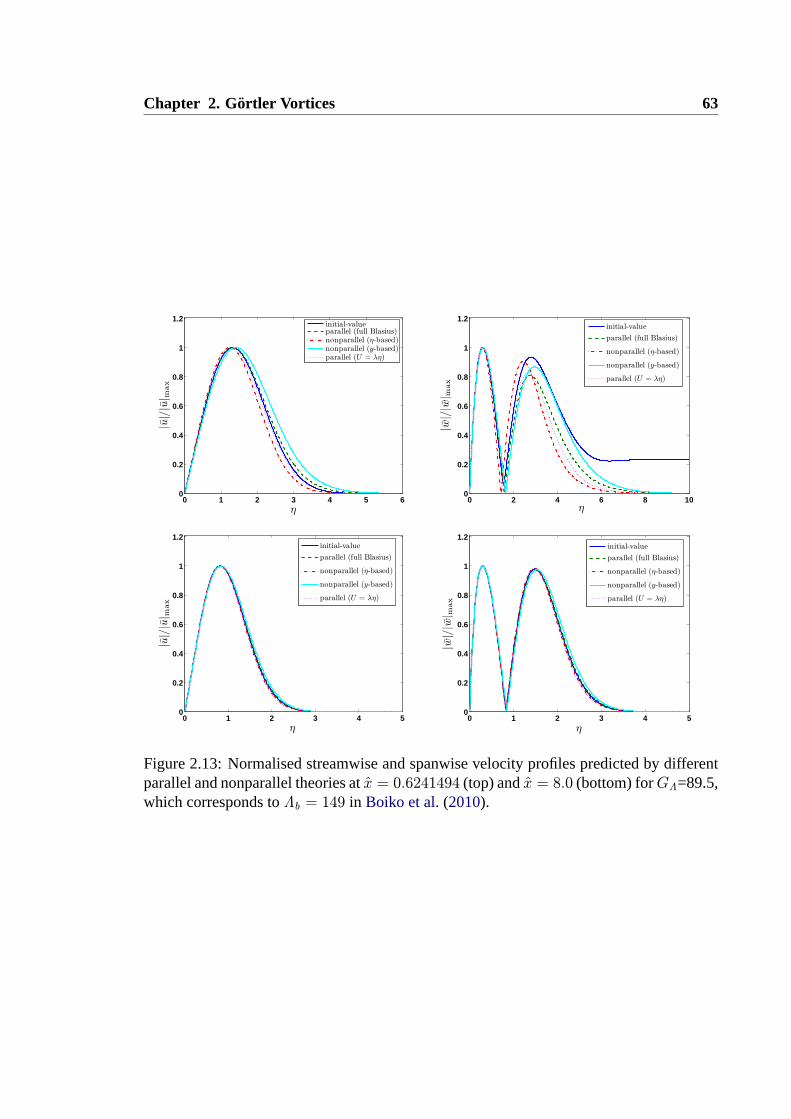
Chapter 2. Gortler Vortices 63
0 1 2 3 4 5 60
0.2
0.4
0.6
0.8
1
1.2
η
1
|u|/|u| max
1
initial-value
1
parallel (full Blasius)
1
nonparallel (η-based)
1
nonparallel (y-based)
1
parallel (U = λη)
1
0 2 4 6 8 100
0.2
0.4
0.6
0.8
1
1.2
η
1
|w|/|w| max
1
initial-value
1
parallel (full Blasius)
1
nonparallel (η-based)
1
nonparallel (y-based)
1
parallel (U = λη)
1
0 1 2 3 4 50
0.2
0.4
0.6
0.8
1
1.2
η
1
|u|/|u| max
1
initial-value
1
parallel (full Blasius)
1
nonparallel (η-based)
1
nonparallel (y-based)
1
parallel (U = λη)
1
0 1 2 3 4 50
0.2
0.4
0.6
0.8
1
1.2
η
1
|w|/|w| max
1
initial-value
1
parallel (full Blasius)
1
nonparallel (η-based)
1
nonparallel (y-based)
1
parallel (U = λη)
1
Figure 2.13: Normalised streamwise and spanwise velocity profiles predicted by differentparallel and nonparallel theories atx = 0.6241494 (top) andx = 8.0 (bottom) forGΛ=89.5,which corresponds toΛb = 149 in Boiko et al.(2010).

2.8 Results and comparisons with experiments 64
0 2 4 6 8 100
0.2
0.4
0.6
0.8
1
1.2
η
1
|u|/|u| max
1
parallelnonparallel
0 2 4 6 8 100
0.2
0.4
0.6
0.8
1
1.2
η
1
|w|/|w| max
1
parallelnonparallel
0 1 2 3 4 50
0.2
0.4
0.6
0.8
1
1.2
η
1
|u|/|u| max
1
parallelnonparallel
0 1 2 3 4 50
0.2
0.4
0.6
0.8
1
1.2
η
1
|w|/|w| max
1
parallelnonparallel
Figure 2.14: Normalised streamwise and spanwise velocity profiles of the second modepredicted by parallel and nonparallel theories atx = 0.6241494 (top) andx = 8.0 (bottom),for GΛ=89.5, which corresponds toΛb = 149 in Boiko et al.(2010).

Chapter 2. Gortler Vortices 65
Detailed measurements of Gortler vortices were conducted byTani (1962) on two
concave-wall models, which have radii of curvature of 5 and 10 metres respectively. The
streamwise gradient of the free-stream velocity was eliminated within the accuracy of
measurements so that the base flow corresponds to a Blasius boundary layer. Station-
ary vortices were observed whose spanwise wavelengthΛ remains fixed as the pertur-
bation evolves downstream. When the radius of curvature is 10 meters, and the free
stream velocityU∞ = 11m/s, a spanwise wavelengthλz = 2.1cm was observed. The
streamwise velocity of the vortices was measured at locations betweenx∗ = 30cm and
x∗ = 120cm. No vortex generator was employed, and it was most likely that vortices
were excited by free-stream disturbances, which were later found to be a dominant source
of Gortler vortices in addition to wall roughnesses (Swearingen and Blackwelder 1987,
Kottke 1988, Crane and Sabzvari 1982). It is therefore appropriate to compare our theo-
retical results with the experiment data ofTani (1962). For that purpose, we need to figure
out the corresponding Gortler numberGΛ and the downstream locationsx in our formula-
tion. We first calculate the Reynolds number pertaining to the experiment ofTani (1962),
RΛ = U∞Λ/ν = U∞λz/(2πν) = 2.298 × 10³, where we takeν = 1.6 × 10⁻⁵m2/s, the
kinematic viscosity coefficient of dry air at the pressure of one atmosphere at 30◦C (Batch-
elor 1967). The Gortler number isGΛ = R2Λ/r0 = R2Λλz/(2πr
∗0) = 1765. The dimensional
downstream distancex∗ is related to the dimensionless distancex via the relation
x = x∗/(ΛRΛ) = 2πx∗/(RΛλz). (2.8.1)
The measurement locations atx∗ = 30cm, 50cm, 90cm and120cm thus correspond tox =
0.03906, 0.065, 0.1172 and 0.1562 respectively.
The data in figure 5 ofTani (1962) is converted toln(|u|max/|u|30), and is compared
in figure2.15with the theoretical prediction by the initial-value approach, where|u|30 de-
notes the maximum value ofu at x∗ = 30cm. A good agreement is noted. This indicates
that the initial-value approach describes the development of Gortler vortices very well even
at small distances to the leading edge. To the best of our knowledge, this is the first time
that a quantitatively accurate prediction of the amplitude development of steady Gortler
vortices is made. Crucial to the present success is the inclusion in our formulation of the
relevant receptivity process. In figure2.16, we compare the amplification rate given by the
initial-value calculation with the non-parallel viscous and parallel inviscid eigen solutions.
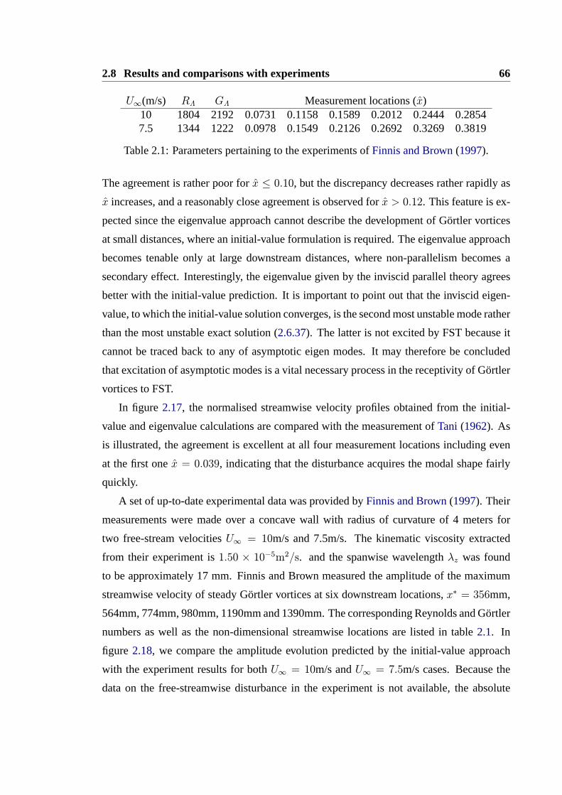
2.8 Results and comparisons with experiments 66
U∞(m/s) RΛ GΛ Measurement locations (x)10 1804 2192 0.0731 0.1158 0.1589 0.2012 0.2444 0.28547.5 1344 1222 0.0978 0.1549 0.2126 0.2692 0.3269 0.3819
Table 2.1: Parameters pertaining to the experiments ofFinnis and Brown(1997).
The agreement is rather poor forx ≤ 0.10, but the discrepancy decreases rather rapidly as
x increases, and a reasonably close agreement is observed forx > 0.12. This feature is ex-
pected since the eigenvalue approach cannot describe the development of Gortler vortices
at small distances, where an initial-value formulation is required. The eigenvalue approach
becomes tenable only at large downstream distances, where non-parallelism becomes a
secondary effect. Interestingly, the eigenvalue given by the inviscid parallel theory agrees
better with the initial-value prediction. It is important to point out that the inviscid eigen-
value, to which the initial-value solution converges, is the second most unstable mode rather
than the most unstable exact solution (2.6.37). The latter is not excited by FST because it
cannot be traced back to any of asymptotic eigen modes. It may therefore be concluded
that excitation of asymptotic modes is a vital necessary process in the receptivity of Gortler
vortices to FST.
In figure 2.17, the normalised streamwise velocity profiles obtained from the initial-
value and eigenvalue calculations are compared with the measurement ofTani (1962). As
is illustrated, the agreement is excellent at all four measurement locations including even
at the first onex = 0.039, indicating that the disturbance acquires the modal shape fairly
quickly.
A set of up-to-date experimental data was provided byFinnis and Brown(1997). Their
measurements were made over a concave wall with radius of curvature of 4 meters for
two free-stream velocitiesU∞ = 10m/s and 7.5m/s. The kinematic viscosity extracted
from their experiment is1.50 × 10−5m2/s. and the spanwise wavelengthλz was found
to be approximately 17 mm. Finnis and Brown measured the amplitude of the maximum
streamwise velocity of steady Gortler vortices at six downstream locations,x∗ = 356mm,
564mm, 774mm, 980mm, 1190mm and 1390mm. The corresponding Reynolds and Gortler
numbers as well as the non-dimensional streamwise locations are listed in table2.1. In
figure 2.18, we compare the amplitude evolution predicted by the initial-value approach
with the experiment results for bothU∞ = 10m/s andU∞ = 7.5m/s cases. Because the
data on the free-streamwise disturbance in the experiment is not available, the absolute
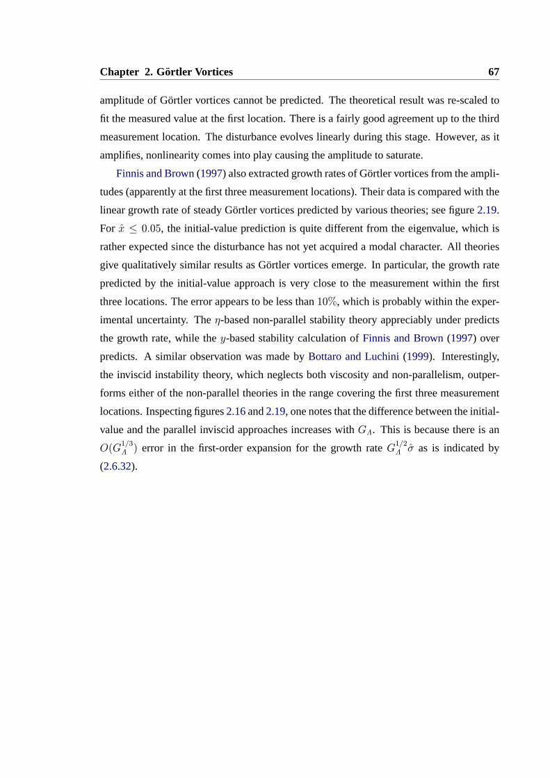
Chapter 2. Gortler Vortices 67
amplitude of Gortler vortices cannot be predicted. The theoretical result was re-scaled to
fit the measured value at the first location. There is a fairly good agreement up to the third
measurement location. The disturbance evolves linearly during this stage. However, as it
amplifies, nonlinearity comes into play causing the amplitude to saturate.
Finnis and Brown(1997) also extracted growth rates of Gortler vortices from the ampli-
tudes (apparently at the first three measurement locations). Their data is compared with the
linear growth rate of steady Gortler vortices predicted by various theories; see figure2.19.
For x ≤ 0.05, the initial-value prediction is quite different from the eigenvalue, which is
rather expected since the disturbance has not yet acquired a modal character. All theories
give qualitatively similar results as Gortler vortices emerge. In particular, the growth rate
predicted by the initial-value approach is very close to the measurement within the first
three locations. The error appears to be less than10%, which is probably within the exper-
imental uncertainty. Theη-based non-parallel stability theory appreciably under predicts
the growth rate, while they-based stability calculation ofFinnis and Brown(1997) over
predicts. A similar observation was made byBottaro and Luchini(1999). Interestingly,
the inviscid instability theory, which neglects both viscosity and non-parallelism, outper-
forms either of the non-parallel theories in the range covering the first three measurement
locations. Inspecting figures2.16and2.19, one notes that the difference between the initial-
value and the parallel inviscid approaches increases withGΛ. This is because there is an
O(G1/3Λ ) error in the first-order expansion for the growth rateG1/2Λ σ as is indicated by
(2.6.32).
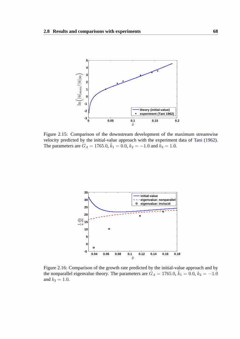
2.8 Results and comparisons with experiments 68
0 0.05 0.1 0.15 0.2-3
-2
-1
0
1
2
3
4
5
x
1
ln(|u| max/|u| 30
)
1
theory (initial-value)experiment (Tani 1962)
Figure 2.15: Comparison of the downstream development of the maximum streamwisevelocity predicted by the initial-value approach with the experiment data ofTani (1962).The parameters areGΛ = 1765.0, k1 = 0.0, k2 = −1.0 andk3 = 1.0.
0.04 0.06 0.08 0.1 0.12 0.14 0.16 0.18-5
0
5
10
15
20
25
30
35
x
1
1 ududx
1
initial-valueeigenvalue: nonparalleleigenvalue: inviscid
Figure 2.16: Comparison of the growth rate predicted by the initial-value approach and bythe nonparallel eigenvalue theory. The parameters areGΛ = 1765.0, k1 = 0.0, k2 = −1.0andk3 = 1.0.

Chapter 2. Gortler Vortices 69
0 1 2 3 4 5 60
0.2
0.4
0.6
0.8
1
1.2
η
1
|u|/|u| max
1
initial-value predictioneigenfunctionexperiment (Tani 1962)
0 1 2 3 4 5 60
0.2
0.4
0.6
0.8
1
1.2
η
1
|u|/|u| max
1
initial-value predictioneigenfunctionexperiment (Tani 1962)
0 1 2 3 4 5 60
0.2
0.4
0.6
0.8
1
1.2
η
1
|u|/|u| max
1
initial-value predictioneigenfunctionexperiment (Tani 1962)
0 1 2 3 4 5 60
0.2
0.4
0.6
0.8
1
1.2
η
1
|u|/|u| max
1
initial-value predictioneigenfunctionexperiment (Tani 1962)
Figure 2.17: Comparison of normalised streamwise velocity obtained from the initial-valueand eigenvalue calculations with the experiment data ofTani (1962). The parameters areGΛ = 1765.0, k1 = 0.0, k2 = −1.0 andk3 = 1.0 at x = 0.03906 (top left), x = 0.065 (topright), x = 0.1172 (bottom left) andx = 0.1562 (bottom right).
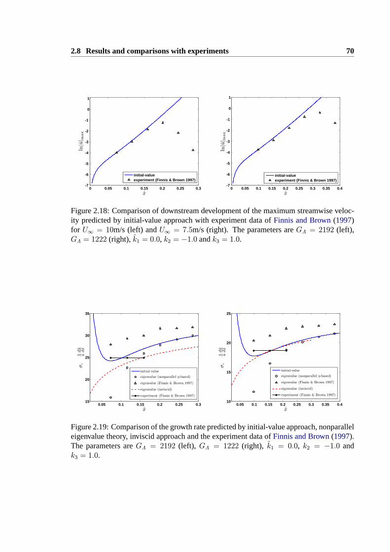
2.8 Results and comparisons with experiments 70
0 0.05 0.1 0.15 0.2 0.25 0.3-7
-6
-5
-4
-3
-2
-1
0
1
x
1
ln|u| max
1
initial-valueexperiment (Finnis & Brown 1997)
0 0.05 0.1 0.15 0.2 0.25 0.3 0.35 0.4-7
-6
-5
-4
-3
-2
-1
0
1
x
1
ln|u| max
1
initial-valueexperiment (Finnis & Brown 1997)
Figure 2.18: Comparison of downstream development of the maximum streamwise veloc-ity predicted by initial-value approach with experiment data ofFinnis and Brown(1997)for U∞ = 10m/s (left) andU∞ = 7.5m/s (right). The parameters areGΛ = 2192 (left),GΛ = 1222 (right), k1 = 0.0, k2 = −1.0 andk3 = 1.0.
0.05 0.1 0.15 0.2 0.25 0.315
20
25
30
35
x
1
σ,
1 ududx
1
initial-value
1
eigenvalue (nonparallel η-based)
1
eigenvalue (Finnis & Brown 1997)
1
eigenvalue (inviscid)
1
experiment (Finnis & Brown 1997)
1
0.05 0.1 0.15 0.2 0.25 0.3 0.35 0.410
15
20
25
x
1
σ,
1 ududx
1
initial-value
1
eigenvalue (nonparallel η-based)
1
eigenvalue (Finnis & Brown 1997)
1
eigenvalue (inviscid)
1
experiment (Finnis & Brown 1997)
1
Figure 2.19: Comparison of the growth rate predicted by initial-value approach, nonparalleleigenvalue theory, inviscid approach and the experiment data ofFinnis and Brown(1997).The parameters areGΛ = 2192 (left), GΛ = 1222 (right), k1 = 0.0, k2 = −1.0 andk3 = 1.0.

Chapter 2. Gortler Vortices 71
0 1 2 3 4 5-15
-10
-5
0
5
10
15
x
1
ln|u| max
1
k1 = 0.0
1
k1 = 3.336
1
k1 = 4.707
1
k1 = 7.060
1
k1 = 11.787
1
k1 = 23.535
1
Figure 2.20: ln|u|max v.s. x for different frequencies withGΛ = 89.5. The frequenciesin the plot (top to bottom ) correspond to 0, 5.67, 8.0, 12.0, 20.0 and 40.0 inBoiko et al.(2007, 2010)
2.8.2 Unsteady Gortler vortices
In this section, we present results on the response of the boundary layer over a curved plate
to unsteady free-stream disturbances (k1 6= 0). The particular interest is in the generation
of unsteady Gortler vortices. The parameters to be used in the calculation are chosen to
correspond to those in the two recent papers ofBoiko et al.(2007, 2010), who have carried
out theoretical and experimental investigations of unsteady Gortler vortices. They define
the Gortler number and the dimensionless spanwise wavelength by
Gb =U∞δ
∗
ν
√δ∗
r∗0, Λb =
U∞λz
ν
√λz
r∗0, (2.8.2)
whereδ∗ is the boundary-layer displacement thickness, andr∗0 the radius of the wall curva-
ture.Gb andΛb are related toGΛ andRΛ via
GΛ = Λ2b/(2π)
3, RΛ = Λb(r∗0/λz)
12/(2π). (2.8.3)
Using the definition for the boundary-layer displacement thickness,
δ∗ = Λ
∫ ∞
0
(1− U)dy = Λ√2x
∫ ∞
0
(1− F ′)dη = Λβ√2x, (2.8.4)
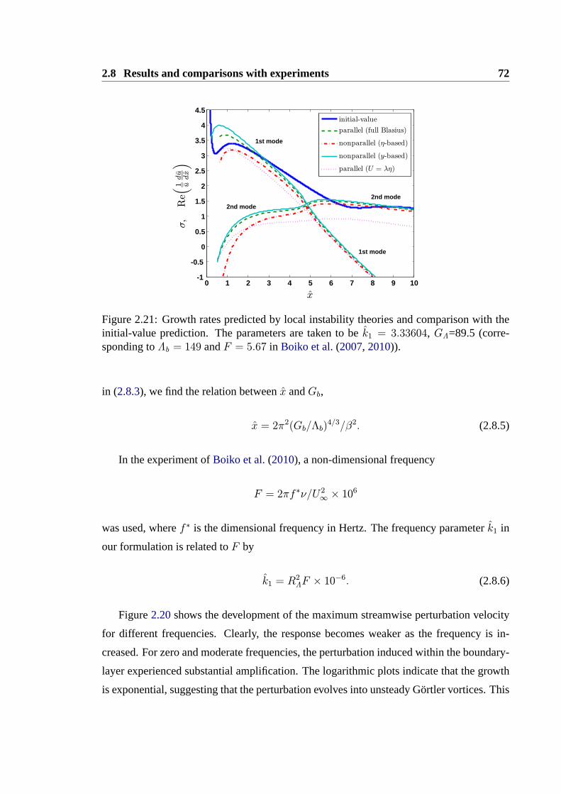
2.8 Results and comparisons with experiments 72
0 1 2 3 4 5 6 7 8 9 10-1
-0.5
0
0.5
1
1.5
2
2.5
3
3.5
4
4.5
x
1
σ,Re(1 ududx
)
1
initial-value
1
parallel (full Blasius)
1
nonparallel (η-based)
1
nonparallel (y-based)
1
parallel (U = λη)
1
2nd mode
1st mode
2nd mode
1st mode
Figure 2.21: Growth rates predicted by local instability theories and comparison with theinitial-value prediction. The parameters are taken to bek1 = 3.33604, GΛ=89.5 (corre-sponding toΛb = 149 andF = 5.67 in Boiko et al.(2007, 2010)).
in (2.8.3), we find the relation betweenx andGb,
x = 2π2(Gb/Λb)4/3/β2. (2.8.5)
In the experiment ofBoiko et al.(2010), a non-dimensional frequency
F = 2πf ∗ν/U 2∞ × 106
was used, wheref ∗ is the dimensional frequency in Hertz. The frequency parameterk1 in
our formulation is related toF by
k1 = R2ΛF × 10
−6. (2.8.6)
Figure2.20shows the development of the maximum streamwise perturbation velocity
for different frequencies. Clearly, the response becomes weaker as the frequency is in-
creased. For zero and moderate frequencies, the perturbation induced within the boundary-
layer experienced substantial amplification. The logarithmic plots indicate that the growth
is exponential, suggesting that the perturbation evolves into unsteady Gortler vortices. This

Chapter 2. Gortler Vortices 73
0 1 2 3 4 5 60
0.2
0.4
0.6
0.8
1
1.2
η
1
|u|/|u| max
1
initial-value
1
parallel (full Blasius)
1
nonparallel (η-based)
1
nonparallel (y-based)
1
parallel (U = λη)
1
0 2 4 6 8 100
0.2
0.4
0.6
0.8
1
1.2
η
1
|w|/|w| max
1
initial-value
1
parallel (full Blasius)
1
nonparallel (η-based)
1
nonparallel (y-based)
1
parallel (U = λη)
1
0 1 2 3 4 5 60
0.2
0.4
0.6
0.8
1
1.2
η
1
|u|/|u| max
1
initial-value
1
parallel (full Blasius)
1
nonparallel (η-based)
1
nonparallel (y-based)
1
parallel (U = λη)
1
0 1 2 3 4 50
0.2
0.4
0.6
0.8
1
1.2
η
1
|w|/|w| max
1
initial-value
1
parallel (full Blasius)
1
nonparallel (η-based)
1
nonparallel (y-based)
1
parallel (U = λη)
1
Figure 2.22: Comparison of the streamwise and spanwise velocity profiles predicted by theinitial-value approach with the eigenfuctions of different parallel and non-parallel theoriesat x = 0.624, 4.0 and8.0. The parameters areGΛ=89.5 andk1 = 3.336 (corresponding toΛb = 149 andF = 5.67 in Boiko et al.(2007, 2010)
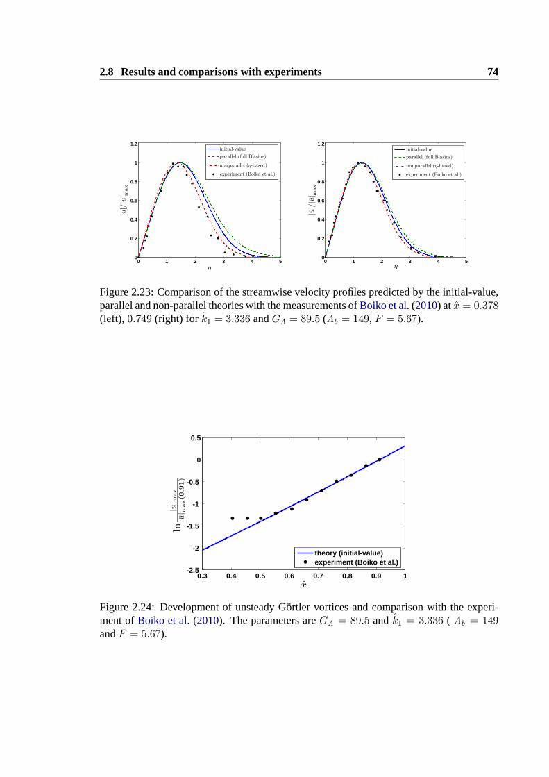
2.8 Results and comparisons with experiments 74
0 1 2 3 4 50
0.2
0.4
0.6
0.8
1
1.2
η
1
|u|/|u| max
1
initial-value
1
parallel (full Blasius)
1
nonparallel (η-based)
1
experiment (Boiko et al.)
1
0 1 2 3 4 50
0.2
0.4
0.6
0.8
1
1.2
η
1
|u|/|u| max
1
initial-value
1
parallel (full Blasius)
1
nonparallel (η-based)
1
experiment (Boiko et al.)
1
Figure 2.23: Comparison of the streamwise velocity profiles predicted by the initial-value,parallel and non-parallel theories with the measurements ofBoiko et al.(2010) atx = 0.378(left), 0.749 (right) for k1 = 3.336 andGΛ = 89.5 (Λb = 149, F = 5.67).
0.3 0.4 0.5 0.6 0.7 0.8 0.9 1-2.5
-2
-1.5
-1
-0.5
0
0.5
x
1
ln|u| max
|u| max(0.91)
1
theory (initial-value)experiment (Boiko et al.)
Figure 2.24: Development of unsteady Gortler vortices and comparison with the experi-ment ofBoiko et al.(2010). The parameters areGΛ = 89.5 andk1 = 3.336 ( Λb = 149andF = 5.67).
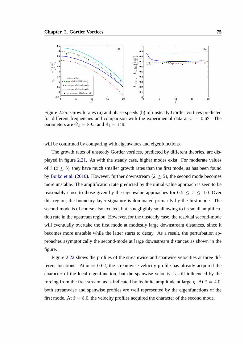
Chapter 2. Gortler Vortices 75
0 5 10 15 20-0.5
0
0.5
1
1.5
2
2.5
3
3.5
4
4.5
f
1
σr,Re(1 ududx
)
1
initial-value
1
parallel (full Blasius)
1
nonparallel (η-based)
1
nonparallel (y-based)
1
experiment (Boiko et al.)
1
(a)
0 5 10 15 200
0.1
0.2
0.3
0.4
0.5
0.6
0.7
0.8
0.9
1
f
1
k1/σr,k1/Im(1 ududx
)
1
(b)
Figure 2.25: Growth rates (a) and phase speeds (b) of unsteady Gortler vortices predictedfor different frequencies and comparison with the experimental data atx = 0.62. Theparameters areGΛ = 89.5 andΛb = 149.
will be confirmed by comparing with eigenvalues and eigenfunctions.
The growth rates of unsteady Gortler vortices, predicted by different theories, are dis-
played in figure2.21. As with the steady case, higher modes exist. For moderate values
of x (x ≤ 5), they have much smaller growth rates than the first mode, as has been found
by Boiko et al.(2010). However, further downstream(x ≥ 5), the second mode becomes
more unstable. The amplification rate predicted by the initial-value approach is seen to be
reasonably close to those given by the eigenvalue approaches for0.5 ≤ x ≤ 4.0. Over
this region, the boundary-layer signature is dominated primarily by the first mode. The
second-mode is of course also excited, but is negligibly small owing to its small amplifica-
tion rate in the upstream region. However, for the unsteady case, the residual second-mode
will eventually overtake the first mode at modestly large downstream distances, since it
becomes more unstable while the latter starts to decay. As a result, the perturbation ap-
proaches asymptotically the second-mode at large downstream distances as shown in the
figure.
Figure2.22shows the profiles of the streamwise and spanwise velocities at three dif-
ferent locations. Atx = 0.62, the streamwise velocity profile has already acquired the
character of the local eigenfunction, but the spanwise velocity is still influenced by the
forcing from the free-stream, as is indicated by its finite amplitude at largeη. At x = 4.0,
both streamwise and spanwise profiles are well represented by the eigenfunctions of the
first mode. Atx = 8.0, the velocity profiles acquired the character of the second mode.

2.8 Results and comparisons with experiments 76
We now focus on the disturbance withF = 5.67 or k1 = 3.336, for whichBoiko et al.
(2010) measured the streamwise velocity profiles at locations corresponding tox = 0.378,
0.526 and 0.749 as well as the amplitude development. We calculated the streamwise ve-
locity profiles at these locations using the parallel and non-parallel (η-based) instability
theories. The results are compared with the experimental data in figure2.23. The agree-
ment is fairly good even for quite small downstream distancex = 0.378 and improves
as x increases. It is hardly possible to tell which theory is the best. The close agree-
ment indicates that the modal shape of the streamwise velocity is only slightly affected by
non-parallelism. Figure2.24presents the evolution of the amplitude of unsteady Gortler
vortices. The theoretical prediction by the initial-value approach is compared with the ex-
perimental data. The agreement is good when the perturbation has acquired the character
of Gortler vortice, which is signaled by the exponential growth. The initial phase of the de-
velopment is however not captured by the theory. This is because in the experiment Gortler
vortices are excited by spanwise periodic blowing/suction imposed on the wall rather than
by a free-stream convected gust assumed by the theory. The discrepancy highlights once
again the importance of including the receptivity process in the formulation if the entire
evolution of the boundary-layer signature is to be predicted.
Finally, we computed the instability characteristics of unstable Gortler vortices for a
range of frequencies, and the results are shown and compared with the experiment in figure
2.25for x = 0.62, where the perturbation just enters the phase of modal development as
figure 2.24 implies. The growth rate decreases with the frequency with steady vortices
being the most unstable. The predictions by the initial-value approach and the parallel
instability theory are in reasonable agreement with the experiment data with an error less
than10% (figure2.25a). Theη- andy-based nonparallel theories are both are less accurate
with an error of about15%, and they under- and over-predict the growth rate respectively.
The predictions by different approaches for the phase speed exhibit closer agreement (figure
2.25b). Overall, the phase speed is less sensitive to the non-parallel-flow effect.
Our theoretical results suggest that unsteady Gortler vortices can be excited by FST.
Surprisingly, only a few laboratory observations of such vortices have been reported. These
include the laser-Doppler measurements carried out byWinoto and Crane(1980) andCrane
and Sabzvari(1982), which revealed that vortices may undergo slow, small-amplitude span-
wise meandering, and the hot-wire measurements ofVolino and Simon(2000), which de-
tected a significant level of low-frequency fluctuations.Floryan(1991) mentioned a similar
Chapter 2. Gortler Vortices 77
finding by Ito in 1991 (unpublished). In typical experimental settings, vortices oscillate
in the frequency band below 10Hz, and hence are distinctively different from the sec-
ondary instability of Gortler vortices, whose characteristic frequency is about two orders
of magnitude higher. However, such low-frequency fluctuations are not readily detected by
usual surface visualisation techniques (Schultz and Volino 2003). We hope that the present
theoretical work would stimulate further investigations of the possible unsteady nature of
Gortler vortices.
2.9 Summary and discussions
It is well known that Gortler instability should, in the generic regime where the spanwise
wavelength is comparable with the local boundary-layer thickness, be formulated as an
initial-value as opposed to an eigenvalue problem (Hall 1983). This implies that specifi-
cation of appropriate initial and boundary conditions is of fundamental importance. Those
conditions could only be provided by studying the receptivity of the boundary layer to rel-
evant external disturbances. In this chapter, we considered the receptivity to steady and
unsteady vortical disturbances in the free stream, which experiments show to be a key
agent exciting Gortler vortices. The present work relies heavily on that of LWG, which is
concerned with generation of streaks in a flat-plate boundary layer by FST. As in LWG,
attention is focussed on components with a long streamwise wavelength because they are
entrained into the boundary layer most effectively. The initial-boundary-value problem de-
scribing both the excitation and subsequent evolution of Gortler vortices consists of the lin-
earised boundary-region equations (but including the centrifugal force), and the upstream
and far-field boundary conditions, which turn out to be the same as those given by LWG.
The initial-value problem was solved numerically for different values of the Gortler
numberGΛ. For a sufficiently smallGΛ, the induced boundary-layer signature exhibits
essentially the same characteristics as streaks occurring in the flat-plate case: the stream-
wise velocity amplifies and then decays. WhenGΛ exceeds a critical value, the induced
perturbation undergoes (quasi-)exponential growth. By comparing with the predictions by
ad-hoclocal parallel and non-parallel instability theories, it is found that the perturbation
evolves to acquire the modal shape of Gortler vortices rather quickly, but its growth rate
differs appreciably from that given by the local eigenvalue approach. Nevertheless, the
overall agreement with, and the eventual convergence to, the eigenvalue at large distances
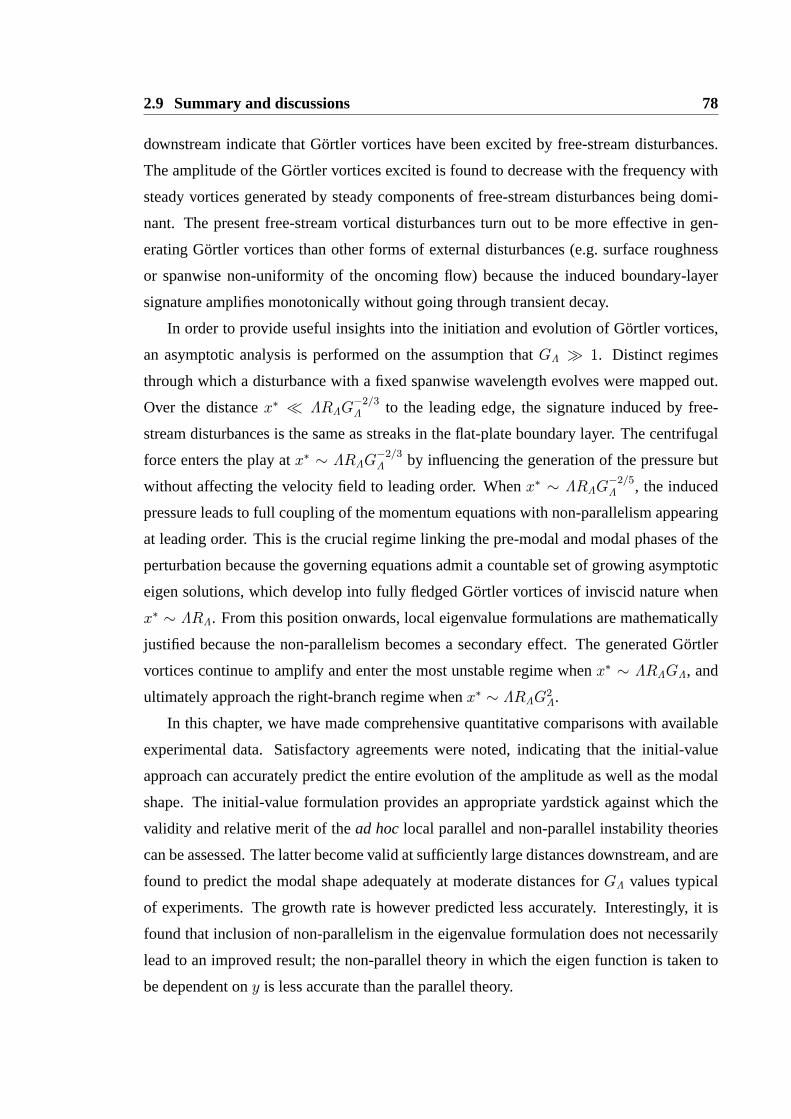
2.9 Summary and discussions 78
downstream indicate that Gortler vortices have been excited by free-stream disturbances.
The amplitude of the Gortler vortices excited is found to decrease with the frequency with
steady vortices generated by steady components of free-stream disturbances being domi-
nant. The present free-stream vortical disturbances turn out to be more effective in gen-
erating Gortler vortices than other forms of external disturbances (e.g. surface roughness
or spanwise non-uniformity of the oncoming flow) because the induced boundary-layer
signature amplifies monotonically without going through transient decay.
In order to provide useful insights into the initiation and evolution of Gortler vortices,
an asymptotic analysis is performed on the assumption thatGΛ � 1. Distinct regimes
through which a disturbance with a fixed spanwise wavelength evolves were mapped out.
Over the distancex∗ � ΛRΛG−2/3Λ to the leading edge, the signature induced by free-
stream disturbances is the same as streaks in the flat-plate boundary layer. The centrifugal
force enters the play atx∗ ∼ ΛRΛG−2/3Λ by influencing the generation of the pressure but
without affecting the velocity field to leading order. Whenx∗ ∼ ΛRΛG−2/5Λ , the induced
pressure leads to full coupling of the momentum equations with non-parallelism appearing
at leading order. This is the crucial regime linking the pre-modal and modal phases of the
perturbation because the governing equations admit a countable set of growing asymptotic
eigen solutions, which develop into fully fledged Gortler vortices of inviscid nature when
x∗ ∼ ΛRΛ. From this position onwards, local eigenvalue formulations are mathematically
justified because the non-parallelism becomes a secondary effect. The generated Gortler
vortices continue to amplify and enter the most unstable regime whenx∗ ∼ ΛRΛGΛ, and
ultimately approach the right-branch regime whenx∗ ∼ ΛRΛG2Λ.
In this chapter, we have made comprehensive quantitative comparisons with available
experimental data. Satisfactory agreements were noted, indicating that the initial-value
approach can accurately predict the entire evolution of the amplitude as well as the modal
shape. The initial-value formulation provides an appropriate yardstick against which the
validity and relative merit of thead hoclocal parallel and non-parallel instability theories
can be assessed. The latter become valid at sufficiently large distances downstream, and are
found to predict the modal shape adequately at moderate distances forGΛ values typical
of experiments. The growth rate is however predicted less accurately. Interestingly, it is
found that inclusion of non-parallelism in the eigenvalue formulation does not necessarily
lead to an improved result; the non-parallel theory in which the eigen function is taken to
be dependent ony is less accurate than the parallel theory.
79
Chapter 3
Crossflow Vortices
3.1 Introduction
In this chapter, we consider instability and receptivity of three-dimensional boundary lay-
ers, which exist on swept surfaces or rotating disks. The inviscid streamline at the edge
of the boundary layer is usually curved due to the combined effects of the sweep and the
chordwise pressure gradient, or in the case of a rotating disk, due to the imposed circum-
ferential motion. Crossflow appears in boundary layers on swept surfaces or rotating disks
due to the imbalance between the centripetal force and the pressure gradient in the so-called
crossflow direction, i.e. the direction perpendicular to the inviscid streamline (Saric et al.
2003). In the inviscid region, the centripetal force is balanced with the pressure gradi-
ent so that the crossflow velocity is zero. Inside the boundary layer, the pressure remains
unchanged, however the centripetal force decreases approaching the wall. Due to the im-
balance between the two forces, a crossflow must be formed. At the wall, the crossflow
velocity is also zero due to the no-slip boundary condition. Therefore, between the wall
and the far field, an inflectional point will exist in the crossflow profile. According to the
inflection point theorem in linear inviscid stability theory of parallel flows, established first
by Rayleigh(1880) and extended later byTollmien (1935), instability may occur in the
presence of a crossflow (Gregory et al. 1955). The instability leads to the formation of
crossflow vortices. Similar to Gortler vortices, the crossflow vortex pattern also appears
more-or-less periodic in the spanwise direction with a discernable wavelength, which is,
for fully developed vortices, of the same order of magnitude as the local boundary layer
thickness. But, unlike Gortler vortices which are counter rotating, crossflow vortices all ro-
3.1 Introduction 80
tate in the same direction with the axes being nearly parallel to the free streamline. While
the instability mechanism sustaining the vortices is well understood qualitatively at least
over the majority of the flow field, a quantitative prediction of crossflow instability is quite
a challenge because of three-dimensional nature of the base flow and the non-parallelism
associated with the streamwise growth of the boundary layer. The latter effect is particu-
larly significant in the region close to the leading edge, where the wavelength of the vortices
may be much longer than the local boundary layer thickness. The research on crossflow
instability and the resulting transition to turbulence has continued for decades, and com-
prehensive reviews have been given byReed and Saric(1989), Reed et al.(1996), Bippes
(1999), Saric et al.(2003), Theofilis (2003), andTheofilis (2011). In the following, only
major historic developments and key results will be summarised.
The stability study of crossflow instability and transition has focused on two proto-
types of flows: the boundary layer flow on the surface of a rotating disk, and boundary
layer flow on a swept wing. The theoretical and experimental work carried out byGre-
gory et al.(1955) on the flow over a rotating disk signified a first important step towards
the understanding of crossflow instability and ensuing transition. Using the china-clay
evaporation technique, Gregory and Walker first observed clear crossflow vortices patten
in an annular region, beyond the outer boundary of which the flow becomes turbulent. A
convincing theoretical explanation was given in the same paper by Stuart. He derived the
governing equations for the perturbation, which consisted, in their most general form, of six
first-order equations. However, after neglecting the Coriolis and viscous forces, which is
justified when the Reynolds number is large, they reduce to the Rayleigh equation with an
effective profileUeff , representing the velocity in the wavenumber vector direction. This
profile would have an inflection point and thus support unstable modes if the wavenumber
vector is aligned approximately with the crossflow direction. Since this pioneering work,
rotating disk has become a favorite model and been extensively studied. This is because
firstly the base flow is an exact solution of the N-S equations that can be easily computed,
and secondly in laboratory the flow can be set up much more easily than the boundary layer
over a swept wing. For the rotating disk case, the pressure gradient is absent, the boundary
layer thickness is independent of the radius, and the flow does not involve a sweep angle.
For the swept wing flow, the base flow is in general non-parallel, the pressure gradient is
present, the boundary layer thickness depends on the downstream locations, and the sweep
angle needs to be taken into account; the stability and transition of a swept wing flow is
Chapter 3. Crossflow Vortices 81
thus more challenging.
Detailed experiments have been carried out on swept-wing boundary layers and other
flows which closely resemble them. It is found that crossflow instability typically operates
in the region where a favorable pressure gradient is present and the flow is still subcritical
for T-S instability. The transition route has been identified. Similar to transition initiated by
T-S waves in two-dimensional boundary layers, it consists of several stages including: re-
ceptivity, (i.e. excitation of cross-flow vortices), linear growth, nonlinear development and
final breakdown through secondary instability (see e.g.Bippes 1999; Saric et al. 2003).
Linear stability analysis has been performed, and an important finding is that both sta-
tionary and unsteady (travelling-wave) vortices are possible with the latter having larger
growth rates. Theoretical predictions have broadly been confirmed by experiments (e.g.
Nitschke-Kowsky and Bippes 1988; Bippes et al. 1991), but quantitative differences re-
main. Notwithstanding this unsatisfactory aspect of the theory, linear stability analysis has
been used to correlate the transition location with the accumulated growth, measured by
the so-called N-factor (Malik and Orszag 1980, Mack 1984, Arnal 1986, Arnal 1994). This
so-calledeN -method, which worked rather successfully for transition in two-dimensional
boundary layers, turned out to be rather unreliable for crossflow transition. The failure may
be attributed to the facts that crossflow vortices are extremely sensitive to the presence of
external disturbances, and undergo nonlinear saturation at a fairly low amplitude, which
imply that theN factor is not the most decisive factor determining the actually strength of
the vortices. Clearly, transition cannot be predicted without accounting for receptivity and
nonlinearity.
In the last two decades or so, the method based on parabolised stability equations (PSE)
emerged as a popular tool for studying nonlinear instability (Herbert 1997). In this ap-
proach, the disturbance is assumed to be nearly sinusoidal in the spanwise direction so that
a local wavenumber can be defined in a heuristic manner, and this property is then used to
deal with the pressure gradient and diffusion in the chordwise direction, thereby allowing
the original elliptic equations to be parabolized. This approach was promptly adapted to
predict nonlinear evolution of crossflow vortices by numerous researchers.Malik et al.
(1994) (referred to as MLC hereafter) formulated the nonlinear parabolized stability equa-
tions (PSE) for a relatively simple model incompressible three-dimensional boundary layer,
a swept Hiemenz flow. Since receptivity is not part of their study, the governing equations
satisfy homogenous boundary conditions. In order to initiate marching, they solved the

3.1 Introduction 82
local eigenvalue problem, and used the linear eigenmode as the initial condition. The am-
plification of stationary vortices is inhibited by nonlinearity when their amplitude reaches
just about4%. As vortices saturate, they roll up to form half-mushroom shaped structures,
and inflectional points appear on the velocity profile, leading to secondary instability. MLC
also studied nonlinear interaction between stationary and non-stationary modes. Station-
ary vortices were found to dominate most of the downstream development when its initial
amplitude is ten times larger than that of the non-stationary mode. However, the non-
stationary mode eventually acquires the same order of magnitude as the stationary one in
the far downstream. When the initial amplitude of the stationary and non-stationary modes
are of the same order of magnitude, the non-stationary mode dominates the downstream
development. This trend of development is in agreement with the observation in experi-
ment (Muller 1990). As a side product, the linear stability analysis shows that non-parallel
flow effects destabilize crossflow disturbances, but the impact of non-parallelism depends
on the value ofR = W ∗f δs/ν, whereW ∗
f denotes the free-stream velocity in the spanwise
direction,δs denotes the (constant) boundary layer thickness, andν is the kinematic viscos-
ity. Their parametric study indicates that non-parallel flow effects play a more destabilizing
role at lower values ofR.
In a subsequent paper,Malik et al. (1999) applied PSE approach to model the vortices
pertaining to the experiments conducted on the45◦ NLF(2)-0415 Airfoil in the Arizona
State University (ASU) wind tunnel. The amplitude development of stationary vortices was
predicted quite accurately by PSE. Secondary instability analysis of saturated vortices was
performed, and the characteristics of growing modes are in agreement with experiments.
Malik et al. (1999) suggested that transition could be correlated with the N-factor of the
secondary mode rather than of the primary instability.Haynes and Reed(2000) carried out
PSE analysis of the same experiments, with the aim of resolving discrepancy between the
growth rate predicted by linear stability theory and measurements. They found that for the
case of strong favourable pressure gradient, nonlinearity is the cause of the difference, but
for weak pressure gradients, the curvature and non-parallel-flow effects are more impor-
tant. Secondary instability of nonlinear travelling-wave vortices have been investigated by
Wassermann and Kloker(2003) andBonfigli and Kloker(2007) using DNS.
It has increasingly been recognised that receptivity is of crucial importance for tran-
sition. Experiments indicate that the size of the growth rate is not sufficient to determine
which mode is the dominant disturbance; the occurrence of the latter depends also the

Chapter 3. Crossflow Vortices 83
level of external disturbances. When the free-stream turbulence level is sufficiently low
(typically below 0.15%), steady vortices dominate and cause transition (Muller and Bippes
1989, Deyhle and Bippes 1996) despite that they have smaller growth rates than travelling-
wave modes. This was due to the extreme sensitivity to surface roughness, and further
experimental studies showed that micron-sized roughness elements could generate steady
vortices of considerable magnitude thereby influencing the transition process (Radeztsky
et al. 1999). However, in presence of relatively high free-stream turbulence, travelling-
wave vortices appear and become dominant (Nitschke-Kowsky and Bippes 1988; Bippes
et al. 1991). Much of our current understanding of the role of environmental disturbances
in transition process comes from the experimental work ofDeyhle and Bippes(1996).
They investigated the effect of different types of external disturbances on the excitation of
crossflow vorticity including surface roughness, acoustic and vortical fluctuations in the
free stream, or a combination of these. Their work confirmed the importance of rough-
ness in exciting steady vortices, which are dominant distances in the boundary layer when
the turbulence level is below a certain level. But as the turbulence intensity is increased
from Tu = 0.15% to Tu = 0.27%, the dominant mode changes from stationary to non-
stationary. Interestingly, increasing the roughness height or the acoustic intensity had no
appreciable impact. This is a clear indication that unsteady vortices are generated by free-
stream turbulence alone without involving roughness. Free-stream acoustic fluctuations are
found to have little influence.
Receptivity of three-dimensional boundary layers have been studied theoretically. The
physical ideas are similar to those for two-dimensional boundary layers (e.g.Ruban 1984;
Goldstein 1985), but mathematically finite-Reynolds-number formulations are adopted in-
stead of an asymptotic approach.Crouch(1993) andChoudhari(1994) both considered
excitation of stationary vortices by surface roughness which is periodic along the spanwise
direction but localised in the chordwise direction. Since the time scale is absent, the mech-
anism is relatively straightforward: the scale matching only requires the spanwise wave-
length of the roughness array to be comparable with that of steady modes. The boundary
layer response is governed by an inhomogeneous boundary value problem, which can be
solved by taking Fourier transform with respect the streamwise variable. The response has
a continuous streamwise spectrum, from which a vortex mode would emerge.Choudhari
(1994) also considered the generation of travelling-wave vortices by a free-stream acoustic
wave interacting with roughness, but this mechanism turned out to be inefficient, consistent
3.1 Introduction 84
with experimental observations. Both of these authors used in their calculations a simple
model base flow, the Falkner-Skan-Cooke profile.Ng and Crouch(1999) went a step fur-
ther and considered receptivity of the boundary layer over the NLF(2)-0415 with45◦ sweep
angle, which was used in numerous experiments at ASU. A good agreement was found be-
tween their theoretical prediction and the measurement made at ASU for roughness height
up to twice the local boundary-layer displacement thickness, beyond which nonlinear ef-
fects become appreciable.
In all the work mentioned, curvature and nonparallel-flow effects are neglected.Bertolotti
(1997) attempted to include the latter effect by a Taylor expansion of the mean flow about
the roughness site. In order to account fully the curvature and non-parallelism,Collis and
Lele (1999) carried out a DNS of crossflow vortices induced by surface roughness on a
swept airfoil with a parabolic leading edge. Their numerical results indicate that recep-
tivity is enhanced on a convex curvature. Comparing the non-parallel flow and parallel
flow predictions, they concluded that parallel flow receptivity theory over predicts the re-
ceptivity considerably, contrary to the earlier conclusion ofNg and Crouch(1999) that the
combined effects of non-parallelism and curvature were insignificant.
There have been very few theoretical studies of excitation of crossflow vortices by
free-stream vortical disturbances.Ustinov(2001) considered the receptivity of swept wing
boundary layer with a blunt leading edge to steady free-stream turbulence. The highlight of
his work lies in applying the rapid distortion theory to obtain the inviscid solution, and using
the method of matched asymptotic expansion to derive the initial and boundary conditions
for the equations governing the induced perturbation within the boundary layer. However,
the analysis assumed that the induced disturbance is periodic along the direction perpendic-
ular to the direction of propagation rather than along the spanwise direction as it should be.
The formulation is therefore not entirely correct. Recently,Schrader et al.(2009) attempted
to use DNS to study the generation of non-stationary vortices by free-stream turbulence.
The based flow was taken to be a Falkner-Skan-Cooke profile, which represents a swept
wedge, while free-stream vortical disturbances were represented by continuous spectra of
the O-S and Squire equations. These equations were solved with the resulting eigenfunc-
tions being imposed at the inlet of the computation domain. This is the sole site where
the external forcing acts on the boundary layer since a Neumann boundary condition is
specified at the top of the computation domain. Numerical results indicate that unstable
modes are generated, which the authors claim to describe the receptivity. However, we
Chapter 3. Crossflow Vortices 85
think that neither the numerical set-up nor the result has much relevance to receptivity, for
the following reasons. Firstly, the representation of free-stream disturbance is nonphysical.
Crossflow instability occurs only when a pressure gradient is present, which means that
the inviscid flow outide the boundary layer must be non-uniform. Oncoming disturbances
are thus strained (distorted) when they propagate through the inviscid region. Clearly, con-
tinuous spectra, which take no account of this process and are completely local, cannot
represent the true disturbance acting on the outer edge of the boundary layer. Secondly, the
location of the inlet is chosen purely for computational convenience rather than for having
any physical significance, which implies that the site at which the external disturbance en-
ters the boundary layer is artificial and arbitrary. The DNS result indicates that the coupling
coefficient depends on the location of the inlet, and keeps increasing as the inlet is moved
upstream. This is a clear warning that vortices are actually generated near the leading edge,
but as the authors concede, their numerical approach fails there. In summary, we believe
that the claim of the paper is rather misleading and indeed trivialises the very issue of re-
ceptivity. Obviously, a similar simulation could be done for the familiar Blasius boundary
layer, but then few would accept that as describing receptivity of T-S waves.
The aim of the present study is to provide a mathematical formulation which describes
the excitation of crossflow vortices by small-amplitude free-stream vortical disturbances
and their subsequent linear development. To fix the idea, we consider the base flow due
to a uniform flow past a swept airfoil. The Reynolds number is assumed to be large so
that the entire flow consists of an inviscid region, and a viscous boundary layer adjacent to
the surface. The airfoil has a finite thickness causing a non-uniform ambient inviscid flow
and a non-zero chordwise pressure gradient. The vortical disturbance in the oncoming flow
is simply advected by the background mean velocity, but gets distorted by the strain field
when approaching the airfoil. Our main interest is in analysing the boundary layer response
to the disturbance in the inviscid region and identifying modes that can be excited.
The rest of this chapter is organized as follows. In§3.2, we formulate the problem
mathematically and specify relevant scalings. In§3.3, the base flow field is calculated. Us-
ing the conformal mapping method, we first obtain the inviscid flow around a Joukowski
airfoil at zero angle of attack. The slip velocity provides the far-field boundary condi-
tion for the base flow within the boundary layer. Then, the boundary-layer equations are
solved numerically using Keller’s box scheme. In§3.4, we formulate the initial-boundary-
value problem for the unsteady perturbation. The solution in the inviscid region is derived

3.2 Formulation and scalings 86
by applying the generalised rapid distortion theory, and the solution provides the far-field
boundary condition for the unsteady boundary-layer equations governing the perturbation
within the boundary layer. In order to determine the nature of the induced disturbance, the
parallel and non-parallel eigenvalue problems are presented in§3.5. We show that the lin-
ear boundary-layer equations support a growing eigen mode, which will develop into fully
fledge non-stationary vortices further downstream. The initial-boundary-value and eigen-
value problems are solved using numerical methods similar to those for Gortler vortices.
Numerical solutions are presented in§3.6. A summary and concluding remarks are given
in §3.7.
3.2 Formulation and scalings
We consider the response of a three-dimensional boundary layer over a swept Joukowski
airfoil to free-stream turbulence. The oncoming mean flow is assumed to be uniform with a
speedU∞/ cosφ∞, whereU∞ is the free-stream velocity in the chordwise direction, andφ∞
is the sweep angle. Free-stream turbulence is chosen to be stationary with a characteristic
spanwise length scaleΛ. The flow is described by the normalised orthogonal Cartesian
coordinates
(xo, yo, z) = (x∗o, y
∗o , z
∗)/Λ, (3.2.1)
and the normalised time
t = U∞t∗/Λ, (3.2.2)
wherex∗o is along the chordwise direction,y∗o is along the chord-normal direction, andz∗
the spanwise direction;t∗ is the dimensional time.
The oncoming mean flow, normalised by the chordwise free-stream velocityU∞, can
be written as
Uf = (Uf , Vf ,Wf ) = (1, 0, −tanφ∞), (3.2.3)
where the suffixf indicates the far field. As in LWG, we assume that FST is statistically
stationary and homogenous, which allows us to represent it in the form of Fourier series.
However, due to linearity, it suffices to consider a single Fourier component
u∞ = u∞exp
[i(k ∙ x− ωt)
], (3.2.4)

Chapter 3. Crossflow Vortices 87
wherek = (k1, k2, k3) is the non-dimensional wavenumber vector,ω is the non-dimensional
frequency and
u∞ = (u∞1 , u∞2 , u
∞3 )
are the normalised amplitudes of the FST in chordwise, normal and spanwise directions
respectively. The normalised perturbed flow fieldv in the upstream can be written as
v = Uf + εu∞exp
[i(k ∙ x− ωt)
],
whereε � 1 is a measure of turbulence intensity. Substituting the perturbed flow into the
momentum equations, after linearisation, we obtain the governing equation for the distur-
bance∂u∞∂t+ Uf
∂u∞∂xo
+Wf∂u∞∂z= 0. (3.2.5)
Substitution of the mean flow (3.2.3) and perturbation (3.2.4) into (3.2.5) yields
ω = k1 − k3tanφ∞.
Therefore, the perturbation can be written as
u∞ = u∞exp
{i[k ∙ x− (k1 − k3tanφ∞)t
]}.
Unlike streaks in a flat plate boundary layer (LWG) or Gortler vortices in the boundary
layer over a concave wall, wherek1 = ω � O(1), we assume hereω, k1 = O(1).
The flow domain can be divided into four asymptotic regions. OverO(Λ) distances
from the attachment line is an inviscid region, which hasO(Λ) dimensions in both the
wall-normal and spanwise directions. The disturbance is treated as a small perturbation on
a distorted mean flow. Beneath the inviscid region is a viscous boundary layer, where the
perturbation is governed by the unsteady boundary layer equations. When the local bound-
ary layer thicknessδ grows to the same order of magnitude as the spanwise length scale
Λ, a new region emerges, which will be referred to loosely as boundary region. However,
the perturbation is not governed by the boundary region equations, but by linearised Eu-
ler equations or slightly more generally the Navier-Stokes equations with the streamwise
diffusion terms being neglected. There is also an outer region describing the continued
evolution of the oncoming disturbance, which is however of little relevance to issue ad-

3.3 The base flow 88
dressed in this thesis. We shall therefore concentrate on the first three regions, especially
the inviscid and the boundary layer regions.
3.3 The base flow
In this study, the base flow is taken to be the boundary layer over a swept Joukowski airfoil.
In order to provide the appropriate far-field boundary condition, the external inviscid slip
velocity u∗e needs to be known. We apply the method of conformal mapping to obtain the
value ofu∗e, and then solve the boundary layer equations numerically. The boundary layer
over the airfoil will be described by the body-oriented coordinates(s∗, y∗), wheres∗ and
y∗ denote the distances alongside and perpendicular to the airfoil surface respectively. We
let
S = s∗/L, and y = y∗/δs,
whereL is the chord length of the airfoil, and its value will be given in§3.3.1;δs denotes
a characteristic boundary layer thickness at a particular streamwise location, and its value
will be given when we consider the perturbation equations in§3.4.
3.3.1 The inviscid external flow
Complex potential and conformal mapping
For a two-dimensional irrotational flow, the velocity field can be described by
(u∗, v∗) =( ∂φ∂x∗o
,∂φ
∂y∗o
), (3.3.1)
where the scalar functionφ(x∗, y∗) is called the potential function. The velocity field can
also be written as
(u∗, v∗) =( ∂ψ∂y∗o
,−∂ψ
∂x∗o
), (3.3.2)
where the scalar functionψ(x∗o, y∗o) is called the stream function. From (3.3.1) and (3.3.2)
follow the relations betweenφ(x∗o, y∗o) andψ(x∗o, y
∗o)
∂φ
∂x∗o=∂ψ
∂y∗o,
∂φ
∂y∗o= −
∂ψ
∂x∗o. (3.3.3)

Chapter 3. Crossflow Vortices 89
The above relations are called Cauchy-Riemann conditions, which are both necessary and
sufficient conditions forφ + iψ to be an analytic function of the complex argumentz =
x∗o + iy∗o , if the four partial derivatives in (3.3.3) are continuous. We may introduce a
complex potential
w(z) = φ+ iψ, (3.3.4)
which is related to the velocity field by
dw
dz=
∂φ
∂x∗o+ i
∂ψ
∂x∗o= u∗ − iv∗. (3.3.5)
For a two-dimensional irrotational flow past a circular cylinder with its centre at(0, 0), the
complex potential can be written as
w(z) = U∞
(ze−iα +
a2rzeiα)−iΓ
2πlogz, (3.3.6)
wherear is the radius of the circle,α is the attack angle of the oncoming flow,U∞ is the
free-stream velocity, andΓ is the circulation around the cylinder. As is well known, the
irrotational flow field past a circle can be mapped onto the one past a symmetric Joukowski
airfoil by Joukowski transformation
ζ(z) = z +c2
z, (3.3.7)
whereζ = ξ∗ + iη∗ is the complex variable for the airfoil,z = x∗c + iy∗c is the complex
variable for the circle, andc is a constant. The centre of the circle is at(−b, 0) with a radius
ar = a + b. Upon introducing the polar coordinates(r, θ) in the z plane, the circle and
Joukowski airfoil can be parameterised byθ, i.e.
z = x∗c + iy∗c = −b+ (a+ b)e
iθ, (3.3.8)
and
ζ = ξ∗ + iη∗ = −b+ (a+ b)eiθ +a2
−b+ (a+ b)eiθ. (3.3.9)
It follows that
ξ∗(θ) = −b+ (a+ b) cos θ +a2[−b+ (a+ b) cos θ]
b2 − 2b(a+ b) cos θ + (a+ b)2, (3.3.10)

3.3 The base flow 90
-2 -1.5 -1 -0.5 0 0.5 1 1.5 2-1.5
-1
-0.5
0
0.5
1
1.5
x∗c
1
y∗ c
1
(−b, 0)
1
(a, 0)
1
-3 -2 -1 0 1 2 3-0.5
-0.4
-0.3
-0.2
-0.1
0
0.1
0.2
0.3
0.4
0.5
ξ∗
1
η∗
1
(−b, 0)
1
(2a, 0)
1
Figure 3.1: Joukowski transformationζ(z) = z + c2/z from the exterior of the circle tothe exterior of the airfoil.
and
η∗(θ) = (a+ b) sin θ[1−
a2
b2 − 2b(a+ b) cos θ + (a+ b)2
]. (3.3.11)
Note that the trailing and leading edges correspond toθ = 0, π respectively. From (3.3.10),
we can obtain the chord length
L = ξ∗(0)− ξ∗(π) = 3a+ 2b+a2
a+ 2b. (3.3.12)
Figure3.1 shows the geometry of Joukowski airfoil through the conformal mapping
(3.3.7), and figure3.2shows the geometry of Joukowski airfoil for different ratios ofb/a.
As is illustrated, an airfoil shape appears for relatively smallb/a, and so we assume that
b/a� 1.
Using (3.3.10) and (3.3.11), we may calculate the curvature of the airfoil , which is
defined as
K =|η∗′′ξ∗′ − η∗′ξ∗′′|
[(ξ∗′)2 + (η∗′)2]32
, (3.3.13)
where a prime denotes differentiation with respect toθ, with
dξ∗
dθ= −(a+ b) sin θ +
a2(a+ b)[b2 − (a+ b)2] sin θ[b2 − 2b(a+ b) cos θ + (a+ b)2
]2 ,

Chapter 3. Crossflow Vortices 91
-2 -1 0 1 2-1
-0.8
-0.6
-0.4
-0.2
0
0.2
0.4
0.6
0.8
1
ξ∗
1
η∗
1
b/a=0.035
1
b/a=0.07
1
b/a=0.1
1
Figure 3.2: Geometry of Joukowski airfoil for different ratios ofb/a.
dη∗
dθ= (a+ b) cos θ +
a2(a+ b)[2b(a+ b)− b2 cos θ − (a+ b)2 cos θ][b2 − 2b(a+ b) cos θ + (a+ b)2
]2 ,
d2ξ∗
dθ2= a2(a+ b)[b2 − (a+ b)2]
[b2 + (a+ b)2] cos θ − 2b(a+ b)− 2b(a+ b) sin2 θ[b2 − 2b(a+ b) cos θ + (a+ b)2
]3
−(a+ b) cos θ,
d2η∗
dθ2= a2(a+ b)
[b2 + (a+ b)2
][b2 + 2b(a+ b) cos θ + (a+ b)2
]− 8b2(a+ b)2
[b2 − 2b(a+ b) cos θ + (a+ b)2
]3 sin θ
−(a+ b) sin θ.
Substituting the derivatives into (3.3.13) , and taking the leading-order approximation, we
obtain the leading-order approximation for the curvature,
K =a3(a+ 2b)
16b2(a+ b)3= O(
a
16b2), (3.3.14)
indicating that the radius of curvature is ofO(16b2/a). Figure3.3shows the relevant char-

3.3 The base flow 92
-2.5 -2 -1.5 -1 -0.5 0 0.5 1 1.5 2 2.5-0.25
-0.2
-0.15
-0.1
-0.05
0
0.05
0.1
0.15
0.2
0.25
ξ∗
1
η∗
1
midchord thickness
1
thickest point
1
L ≈ 4a
1
ε = 2b√1+ 2ba
≈ 2b
1
1.30ε
1
R ≈ 4ε2
1
8b2
a
1
region
1
fast accelerating
1
Figure 3.3: Characteristic length scales of symmetric Joukowski airfoil forb/a = 0.035.
acteristic length scales of a symmetric Joukowski airfoil.
When the circle is centred at(−b, 0), the complex potential (3.3.6) becomes
w(z) = U∞
[(z + b)e−iα +
(a+ b)2
z + beiα]−iΓ
2πlog(z + b). (3.3.15)
Since the complex potentials for the flows past the circle and airfoil have the same value at
the corresponding points of the two planes,
dW
dζ=dw/dz
dζ/dz=
{
U∞
[e−iα −
(a+ bz + b
)2eiα]−
iΓ
2π(z + b)
}/{
1−a2
z2
}
= u∗et − iv∗et,
(3.3.16)
whereW (ζ) is the complex potential around the airfoil,u∗et andv∗et are the velocity com-
ponents in the chordwise and normal directions respectively. Note that the velocity given
by equation (3.3.16) becomes singular atz = ±a in general. The singular pointz = −a is
inside the airfoil, and hence no special treatment for this singular point is needed. However,
the singular pointz = a locates at the trailing edge of the airfoil. The singularity at the
trailing edge must be removed by assigning the appropriate value toΓ. This is the so-called
Kutta-Joukowski condition. Application of this means the value ofΓ must be chosen such
that the numerator of (3.3.16) tends to zero asz → a, that is
Γ = −4πU∞(a+ b)sinα. (3.3.17)
Chapter 3. Crossflow Vortices 93
Substituting (3.3.17) into (3.3.16), the flow field of the airfoil becomes singularity free
(Acheson 1990). Equation (3.3.17) indicates that there is no circulation (Γ = 0) when the
angle of attackα is zero, which is the case we consider in this thesis.
The slip velocity
For the special caseΓ = 0, if we substitute (3.3.8) into (3.3.16), the non-dimensional
chordwise and normal components of the slip velocity can be written as
uet = 1− cos2θ +(1 + p)2
q2 + 2qcosθ + 1
[qcosθ + cos2θ + qcos2θ + cos3θ
], (3.3.18)
vet = sin2θ −(1 + p)2
q2 + 2qcosθ + 1
[qsinθ + sin2θ + qsin2θ + sin3θ
], (3.3.19)
where
uet = u∗et/U∞, vet = v
∗et/U∞, (3.3.20)
p =−bb+ a
= O(b/a), q =−b+ ab+ a
= O(1).
The total slip velocityu∗e ≡√u∗et2 + v∗et
2 is normalised by the chordwise free-stream ve-
locity U∞, i.e.
ue =u∗eU∞=√u2et + v
2et. (3.3.21)
Using (3.3.18) and (3.3.19), we find
ue =2sinθ(p2 + 2pcosθ + 1)
√2(1− cosθ)(q2 + 2qcosθ + 1)
, (3.3.22)
which is the same as given inTurkyilmazoglu et al.(1999).
We now seek asymptotic approximation toue asθ → π, i.e. near the leading edge,
which will be used to approximate other values within the boundary layer. Substitution of
the Taylor expansions ofsin θ andcos θ aboutθ = π,
sin θ = π − θ +O[(π − θ)3], and cos θ = −1 +O[(π − θ)2], (3.3.23)
into (3.3.22) yields
ue =(π − θ)(p− 1)2
|q − 1|+O[(π − θ)2]. (3.3.24)
3.3 The base flow 94
Equation (3.3.24) will be referred to as the first-order approximation toue, where|q− 1| =
O(b/a), andp− 1 = O(1). Since the first term in (3.3.24) should be much larger than the
second term, this first-order approximation is valid for(π − θ)� b/a.
The slip velocity given by(3.3.22) may also be written as
ue = 2 cosθ
2
p2 + 2p cos θ + 1√q2 + 2q cos θ + 1
. (3.3.25)
Expandingcos θ andcos(θ/2) as Taylor series aboutθ = π up to second order,
cos θ = −1+(θ − π)2
2+O[(π−θ)4], and cos
θ
2= −(θ − π)2+(θ − π)3
48+O[(π−θ)5].
(3.3.26)
and inserting them into (3.3.25), we obtain
ue =(p− 1)2(π − θ)
√(q − 1)2 + q(π − θ)2
{1 +O[(π − θ)2]
}. (3.3.27)
The two terms within the square root of equation (3.3.27) are of the same order of mag-
nitude forπ − θ = O(b/a). Equation (3.3.27) will be referred to as the second-order
approximation toue, valid forπ− θ = O(b/a). When(π− θ)� b/a, Taylor expansion of
the denominator of (3.3.27) can be performed to obtain
ue =(p− 1)2(π − θ)|q − 1|
+[ p
|q − 1|−q(p− 1)2
2|q − 1|3
](π − θ)3 +O[(π − θ)5].
On the other hand, whenb/a � π − θ � 1, from equation (3.3.25), and retaining the
O[(π − θ)2] terms, the slip velocity can be written as
ue =(p− 1)2 + [p− (p− 1)2/48](π − θ)2
√
q +(q−1π−θ
)2+O[(π − θ)3]. (3.3.28)
A further Taylor expansion of the denominator for(q − 1)/(π − θ)� 1 gives the second-
order approximation for (3.3.28),
ue =1√q(p− 1)2 +
p− (p− 1)2/48√q
(π − θ)2 −p− 12q√q
(q − 1)2
(π − θ)2+O[(π − θ)3]. (3.3.29)
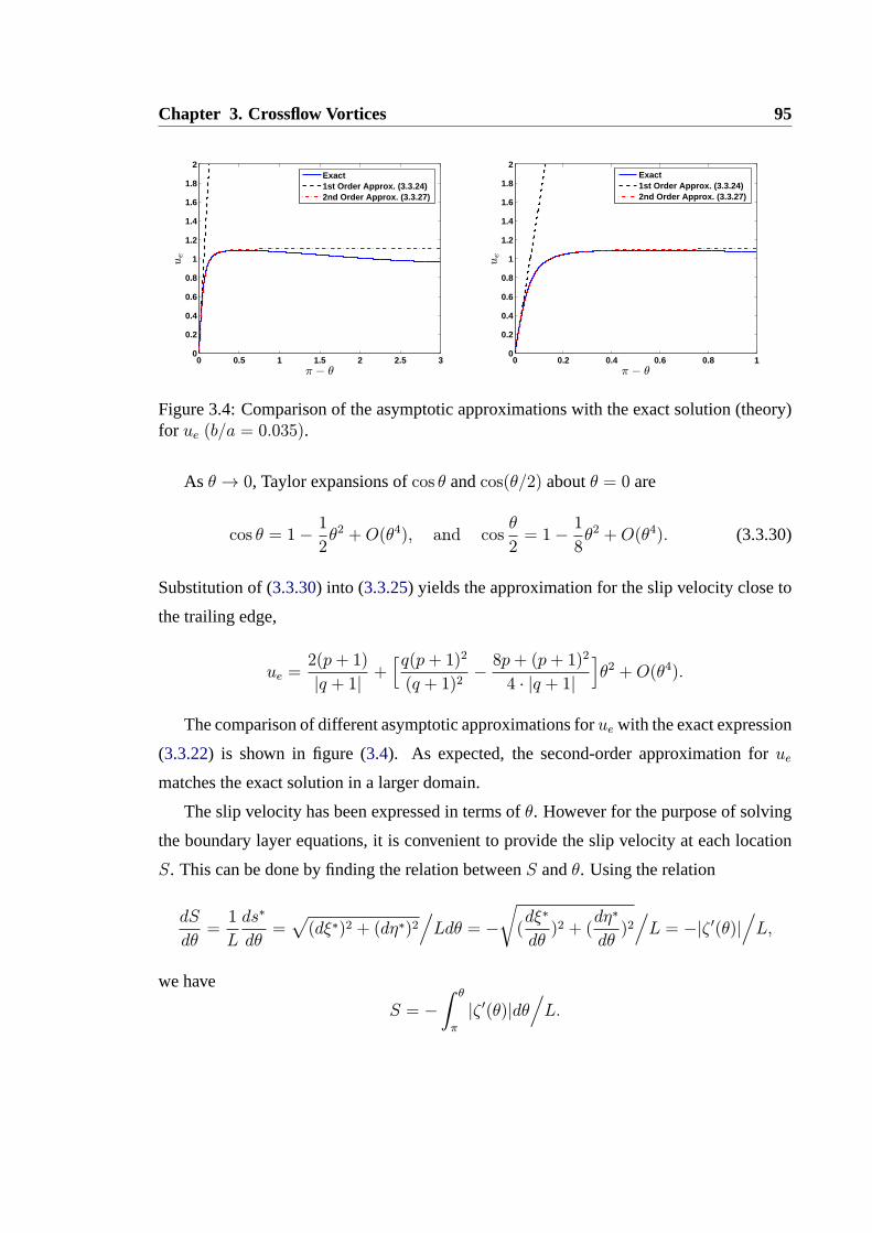
Chapter 3. Crossflow Vortices 95
0 0.5 1 1.5 2 2.5 30
0.2
0.4
0.6
0.8
1
1.2
1.4
1.6
1.8
2
π − θ
1
ue
1
Exact1st Order Approx. (3.3.24)2nd Order Approx. (3.3.27)
0 0.2 0.4 0.6 0.8 10
0.2
0.4
0.6
0.8
1
1.2
1.4
1.6
1.8
2
π − θ
1
ue
1
Exact1st Order Approx. (3.3.24)2nd Order Approx. (3.3.27)
Figure 3.4: Comparison of the asymptotic approximations with the exact solution (theory)for ue (b/a = 0.035).
As θ → 0, Taylor expansions ofcos θ andcos(θ/2) aboutθ = 0 are
cos θ = 1−1
2θ2 +O(θ4), and cos
θ
2= 1−
1
8θ2 +O(θ4). (3.3.30)
Substitution of (3.3.30) into (3.3.25) yields the approximation for the slip velocity close to
the trailing edge,
ue =2(p+ 1)
|q + 1|+[q(p+ 1)2
(q + 1)2−8p+ (p+ 1)2
4 ∙ |q + 1|
]θ2 +O(θ4).
The comparison of different asymptotic approximations forue with the exact expression
(3.3.22) is shown in figure (3.4). As expected, the second-order approximation forue
matches the exact solution in a larger domain.
The slip velocity has been expressed in terms ofθ. However for the purpose of solving
the boundary layer equations, it is convenient to provide the slip velocity at each location
S. This can be done by finding the relation betweenS andθ. Using the relation
dS
dθ=1
L
ds∗
dθ=√(dξ∗)2 + (dη∗)2
/Ldθ = −
√
(dξ∗
dθ)2 + (
dη∗
dθ)2/L = −|ζ ′(θ)|
/L,
we have
S = −∫ θ
π
|ζ ′(θ)|dθ/L.

3.3 The base flow 96
From equation (3.3.9) it follows that
|ζ ′(θ)| =∣∣∣i(a+ b)eiθ −
ia2(a+ b)eiθ
[−b+ (a+ b)eiθ]2
∣∣∣ = (a+ b)
∣∣∣∣∣[−b+ (a+ b)eiθ]2 − a2
[−b+ (a+ b)eiθ]2
∣∣∣∣∣,
and therefore
S = −(a+ b
L
)∫ θ
π
∣∣∣∣∣[−b+ (a+ b)eiθ]2 − a2
[−b+ (a+ b)eiθ]2
∣∣∣∣∣dθ, (3.3.31)
and the total length is
Stotal = −(a+ b
L
)∫ 0
π
∣∣∣∣∣[−b+ (a+ b)eiθ]2 − a2
[−b+ (a+ b)eiθ]2
∣∣∣∣∣dθ.
Whenθ → π, the first-order approximation forS can be found from (3.3.31) as
S =(a+ b
L
)[(a+ 2b)2 − a2
(a+ 2b)2
](π − θ) +O[(π − θ)2], (3.3.32)
Combination of (3.3.24) and (3.3.32) gives an explicit relation betweenue andS,
ue =S ∙ L2(a+ b)
∙[(a+ 2b)2
2b(a+ b)
]2+O(S2). (3.3.33)
Since [(a+ 2b)2
2b(a+ b)
]2= O(a2/b2), and L = O(a),
the validity of (3.3.33) is restricted toS � O(b2/a2). A second-order approximation valid
up to S = O(b2/a2) can be derived by expressingS in terms ofπ − θ, accurate up to
π − θ = O(b/a). This requires us to expand the integrand in (3.3.31) to the second order.
The detailed derivation is given in the appendix A1.
For a general0 < θ < π, the relation betweenue andS has to be determined numeri-
cally. We let
F (θ, S) = S +(a+ b
L
)∫ θ
π
∣∣∣∣∣[−b+ (a+ b)eiθ]2 − a2
[−b+ (a+ b)eiθ]2
∣∣∣∣∣dθ.
The relation betweenS andθ is determined byF (θ, S) = 0. For each given value ofS, the

Chapter 3. Crossflow Vortices 97
0 0.1 0.2 0.3 0.4 0.50
0.5
1
1.5
S
1
ue
1
Exact1st Order Approx. (3.3.33)2nd Order Approx.
0 0.02 0.04 0.06 0.08 0.10
0.5
1
1.5
S
1
ue
1
Exact1st Order Approx. (3.3.33)2nd Order Approx.
Figure 3.5: The relation betweenue andS, and comparison of the asymptotic approxima-tion with the exact numerical solution(b/a = 0.035).
corresponding value ofθ can be calculated using the Newton-Raphson iteration
θi+1 = θi −F (θi, S)
F ′(θi, S),
where the integral term in functionF (θ) is evaluated by using Simpson’s Rule. When the
value ofθ is known, the value ofue will be known from (3.3.22). Therefore, a relation
betweenue andS is built.
Figures3.5 and3.6 show the slip velocity as a function ofS. As is indicated, the slip
velocity undergoes a rapid linear increase close to the leading edge, and then decreases
slowly asS becomes larger. From figure3.5, we note that the second-order approximation
fits the numerical result in a larger domain, which is due to the fact that this approximation
is valid up toS = O(b2/a2).
3.3.2 The boundary layer flow
The steady two-dimensional boundary layer equations can be written as
∂u∗B∂s∗+∂v∗B∂y∗= 0, (3.3.34)
u∗B∂u∗B∂s∗+ v∗B
∂u∗B∂y∗= −1
ρ
∂p∗
∂s∗+μ
ρ
∂2u∗B∂y∗2
, (3.3.35)
whereu∗B, andv∗B are the dimensional velocities ins∗ andy∗ directions respectively, and
p∗ is the dimensional pressure.

3.3 The base flow 98
0 0.2 0.4 0.6 0.8 10
0.5
1
1.5
S
1
ue
1
b/a = 0.035
1
b/a = 0.024
1
b/a = 0.012
1
b/a = 0.0
1
0 0.05 0.1 0.15 0.20
0.5
1
1.5
S
1
ue
1
b/a = 0.035
1
b/a = 0.024
1
b/a = 0.012
1
b/a = 0.0
1
0.5 0.6 0.7 0.8 0.9 1 1.10.95
0.96
0.97
0.98
0.99
1
1.01
1.02
1.03
1.04
1.05
S
1
ue
1
b/a = 0.035
1
b/a = 0.024
1
b/a = 0.012
1
b/a = 0.0
1
Figure 3.6: The distribution of the slip velocity along the airfoil surface for different valuesof b/a.

Chapter 3. Crossflow Vortices 99
The Falkner-Skan transformation is introduced by
η =( u∗eνs∗
)1/2y∗, (3.3.36)
whereu∗e = ue(S)U∞, andν = μ/ρ is the kinematic viscosity. A dimensionless stream
functionf(S, η) is introduced by
ψ(s∗, y∗) = (u∗eνs∗)1/2f(S, η).
Then the streamwise and normal velocities can be written as
u∗B =∂ψ
∂y∗= (
u∗eνs∗)1/2
∂ψ
∂η= uef
′U∞, (3.3.37)
and
v∗B = −∂ψ
∂s∗= −
(∂ψ
∂s∗
∣∣∣∣η
+∂ψ
∂η
∂η
∂s∗
)
= −∂[(u∗eνs
∗)1/2f ]
∂s∗
∣∣∣∣η
− (u∗eνs∗)1/2f ′
∂η
∂s∗, (3.3.38)
where a prime denotes differentiation with respect toη. Substituting (3.3.37), (3.3.38) and
dp∗
ds∗= −ρu∗e
du∗eds∗
which comes from Bernoulli’s principle, into (3.3.34) and (3.3.35), we obtain the trans-
formed momentum equation for two-dimensional laminar flow (Cebeci and Bradshaw 1977)
f ′′′ +m+ 1
2ff ′′ +m[1− (f ′)2] = s∗
(f ′∂f ′
∂s∗− f ′′
∂f
∂s∗
)= S
(f ′∂f ′
∂S− f ′′
∂f
∂S
), (3.3.39)
wherem is a dimensionless pressure gradient parameter defined by
m =s∗
u∗e
du∗eds∗=S
ue
due
dS.
Excluding suction or blowing at the wall, the boundary conditions for (3.3.39) are
f ′ = 0 and f(S, 0) = 0 at η = 0; (3.3.40)
f ′ → 1 as η →∞. (3.3.41)
3.3 The base flow 100
Near the leading edge (S → 0), the slip velocityue ∼ S as is indicated by (3.3.33), and
som = 1, and the functionf is independent of the coordinateS. Equation (3.3.39) then
reduces to the Falkner-Skan equation,
f ′′′ +m+ 1
2ff ′′ +m[1− (f ′)2] = 0, (3.3.42)
which describes the boundary-layer flow in the vicinity of the stagnation point.
The solution to the Falkner-Skan equation (3.3.42) serves as the initial condition for
solving (3.3.39). We apply Keller’s shooting method to solve (3.3.42) (Cebeci and Brad-
shaw 1977; Cebeci and Cousteix 2005). According to this method, we need first to recast
equation (3.3.42) into a system of three first-order ordinary differential equations,
f ′ = u, (3.3.43)
u′ = h0, (3.3.44)
h′0 = −m+ 1
2fh0 −m(1− u
2), (3.3.45)
with the boundary conditions
f(0) = 0, u(0) = 0; (3.3.46)
u→ 1 as η →∞. (3.3.47)
In order to start the numerical integration of (3.3.43)–(3.3.45), the value ofh0(0) is needed.
Let an initial guess forh0(0) be denoted byg, i.e.
h0(0) = g, (3.3.48)
and the solution of Falkner-Skan equation be denoted by[f(η, g), u(η, g), h0(η, g)
]. Then
the value ofg can be determined by matching with the upper boundary condition, which is
imposed by using the Newton-Raphson iteration,
gi+1 = gi −H(gi)
H ′(gi), (3.3.49)

Chapter 3. Crossflow Vortices 101
where
H(g) = u(η∞, g)− 1,
a prime denotes differentiation with respect tog, andη∞ is a large positive number suitably
chosen. In order to determine
H ′(g) =∂u(η∞, g)
∂g,
we differentiate (3.3.43)–(3.3.45) with respect tog to obtain the so-called variational equa-
tions (Cebeci and Bradshaw 1977; Cebeci and Cousteix 2005)
F ′ = U, (3.3.50)
U ′ = H0, (3.3.51)
H ′0 = −m+ 1
2(fH0 + h0F ) + 2muU, (3.3.52)
where a prime denotes differentiation with respect toη, andF , U andH0 are defined by
F (η, g) =∂f
∂g, U(η, g) =
∂u
∂g, H0(η, g) =
∂h0
∂g.
The initial conditions (atη = 0) are
F (0) = 0, U(0) = 0, H0(0) =∂g
∂g= 1. (3.3.53)
For a givengi, the Falkner-Skan equation (3.3.43)–(3.3.45) subject to the boundary con-
dition (3.3.46) and (3.3.48) is solved using a fourth-order Runge-Kutta method to obtain
u(η∞, g) andH(g). The variational equations (3.3.50)–(3.3.52) subject to the conditions
(3.3.53) is integrated using the Runge-Kutta method to calculateU(η∞, g) = H ′(g). The
next approximation toh0(0), gi+1, can be computed from (3.3.49). This procedure is re-
peated until convergence is achieved, i.e. when
|gi+1 − gi| < ε,
whereε is a tolerance parameter, chosen to be10−6 in our calculation (Cebeci and Brad-
shaw 1977; Cebeci and Cousteix 2005).
Figure3.7displays the profiles of the base flow velocity in theS direction for different
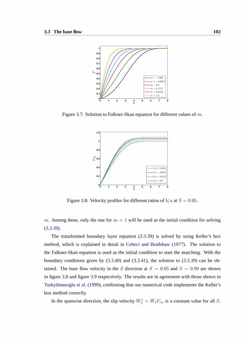
3.3 The base flow 102
0 1 2 3 4 5 6 7 80
0.1
0.2
0.3
0.4
0.5
0.6
0.7
0.8
0.9
1
η
1
f′
1
m = −0.091
1
m = −0.0654
1
m = 0.0
1
m = 0.1111
1
m = 0.3333
1
m = 1.0
1
Figure 3.7: Solution to Falkner-Skan equation for different values ofm.
0 1 2 3 4 5 6 7 80
0.2
0.4
0.6
0.8
1
1.2
η
1
UB
1
b/a = 0.035
1
b/a = 0.024
1
b/a = 0.012
1
b/a = 0.0
1
Figure 3.8: Velocity profiles for different ratios ofb/a atS = 0.05.
m. Among these, only the one form = 1 will be used as the initial condition for solving
(3.3.39).
The transformed boundary layer equation (3.3.39) is solved by using Keller’s box
method, which is explained in detail inCebeci and Bradshaw(1977). The solution to
the Falkner-Skan equation is used as the initial condition to start the marching. With the
boundary conditions given by (3.3.40) and (3.3.41), the solution to (3.3.39) can be ob-
tained. The base flow velocity in theS direction atS = 0.05 andS = 0.99 are shown
in figure3.8and figure3.9 respectively. The results are in agreement with those shown in
Turkyilmazoglu et al.(1999), confirming that our numerical code implements the Keller’s
box method correctly.
In the spanwise direction, the slip velocityW ∗f = WfU∞ is a constant value for allS.
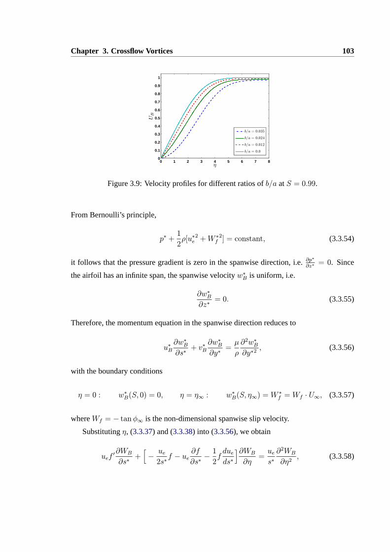
Chapter 3. Crossflow Vortices 103
0 1 2 3 4 5 6 7 80
0.1
0.2
0.3
0.4
0.5
0.6
0.7
0.8
0.9
1
η
1
UB
1
b/a = 0.035
1
b/a = 0.024
1
b/a = 0.012
1
b/a = 0.0
1
Figure 3.9: Velocity profiles for different ratios ofb/a atS = 0.99.
From Bernoulli’s principle,
p∗ +1
2ρ[u∗e
2 +W ∗f2] = constant, (3.3.54)
it follows that the pressure gradient is zero in the spanwise direction, i.e.∂p∗
∂z∗= 0. Since
the airfoil has an infinite span, the spanwise velocityw∗B is uniform, i.e.
∂w∗B∂z∗
= 0. (3.3.55)
Therefore, the momentum equation in the spanwise direction reduces to
u∗B∂w∗B∂s∗+ v∗B
∂w∗B∂y∗
=μ
ρ
∂2w∗B∂y∗2
, (3.3.56)
with the boundary conditions
η = 0 : w∗B(S, 0) = 0, η = η∞ : w∗B(S, η∞) = W∗f = Wf ∙ U∞, (3.3.57)
whereWf = − tanφ∞ is the non-dimensional spanwise slip velocity.
Substitutingη, (3.3.37) and (3.3.38) into (3.3.56), we obtain
uef′∂WB
∂s∗+[−
ue
2s∗f − ue
∂f
∂s∗−1
2fdue
ds∗
]∂WB∂η=ue
s∗∂2WB
∂η2, (3.3.58)

3.3 The base flow 104
where
WB =w∗BU∞
. (3.3.59)
After a rearrangement of (3.3.58), we have
∂2WB
∂η2+[12f + S
∂f
∂S+1
2fS
ue
due
dS
]∂WB∂η= Sf ′
∂WB
∂S. (3.3.60)
After solving the transformed streamwise momentum equation,f , f ′ and ∂f∂S
are already
known. Equation (3.3.60) can be solved by using Keller’s box method once the proper
initial condition is provided. The latter can be derived by noting that asS → 0, equation
(3.3.60) reduces to∂2WB
∂η2+1
2f(1 +m)
∂WB
∂η= 0. (3.3.61)
Equation (3.3.61) combined with (3.3.42) are called the Falkner-Skan-Cooke equations.
The initial condition for (3.3.60) is obtained by solving (3.3.61). In order to solve (3.3.61),
it is convenient to introduce a dimensionless functionh(S, η) through the relation
WB = Wfh(S, η). (3.3.62)
In terms ofh, we can write (3.3.61) as
∂2h
∂η2+1
2f(1 +m)
∂h
∂η= 0, (3.3.63)
with the boundary conditions:
η = 0 : h(0) = 0, η = η∞ : h(η∞) = 1. (3.3.64)
Keller’s shooting method (Cebeci and Bradshaw 1977; Cebeci and Cousteix 2005) is ap-
plied to solve (3.3.63). In order to implement this method, we first recast the equation into
two first-order ODEs,
h′ = d, (3.3.65)
d′ = −γ1d, (3.3.66)
where
γ1 =1
2(1 +m)f.
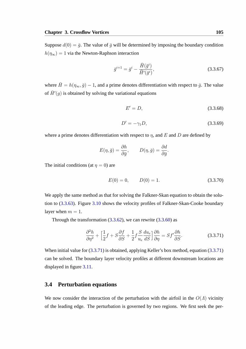
Chapter 3. Crossflow Vortices 105
Supposed(0) = g. The value ofg will be determined by imposing the boundary condition
h(η∞) = 1 via the Newton-Raphson interaction
gi+1 = gi −H(gi)
H ′(gi), (3.3.67)
whereH = h(η∞, g)− 1, and a prime denotes differentiation with respect tog. The value
of H ′(g) is obtained by solving the variational equations
E ′ = D, (3.3.68)
D′ = −γ1D, (3.3.69)
where a prime denotes differentiation with respect toη, andE andD are defined by
E(η, g) =∂h
∂g, D(η, g) =
∂d
∂g.
The initial conditions (atη = 0) are
E(0) = 0, D(0) = 1. (3.3.70)
We apply the same method as that for solving the Falkner-Skan equation to obtain the solu-
tion to (3.3.63). Figure3.10shows the velocity profiles of Falkner-Skan-Cooke boundary
layer whenm = 1.
Through the transformation (3.3.62), we can rewrite (3.3.60) as
∂2h
∂η2+[12f + S
∂f
∂S+1
2fS
ue
due
dS
]∂h∂η= Sf ′
∂h
∂S. (3.3.71)
When initial value for (3.3.71) is obtained, applying Keller’s box method, equation (3.3.71)
can be solved. The boundary layer velocity profiles at different downstream locations are
displayed in figure3.11.
3.4 Perturbation equations
We now consider the interaction of the perturbation with the airfoil in theO(Λ) vicinity
of the leading edge. The perturbation is governed by two regions. We first seek the per-
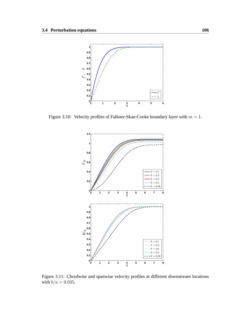
3.4 Perturbation equations 106
0 1 2 3 4 5 60
0.1
0.2
0.3
0.4
0.5
0.6
0.7
0.8
0.9
1
η
1
f′ ,h
1
f ′
1
h
1
Figure 3.10: Velocity profiles of Falkner-Skan-Cooke boundary layer withm = 1.
0 1 2 3 4 5 6 7 80
0.2
0.4
0.6
0.8
1
1.2
η
1
UB
1
S = 0.1
1
S = 0.2
1
S = 0.3
1
S = 0.5
1
S = 0.99
1
0 1 2 3 4 5 6 7 80
0.1
0.2
0.3
0.4
0.5
0.6
0.7
0.8
0.9
1
η
1
WB
1
S = 0.1
1
S = 0.2
1
S = 0.3
1
S = 0.5
1
S = 0.99
1
Figure 3.11: Chordwise and spanwise velocity profiles at different downstream locationswith b/a = 0.035.

Chapter 3. Crossflow Vortices 107
turbation solution in the inviscid region, which will be treated as the far-field condition
for unsteady boundary layer equations which govern the perturbation within the boundary
layer. In order to provide the initial condition, the solution for the perturbation at the stag-
nation point is constructed. With both the initial and boundary conditions specified, we
solve the initial-boundary-value problem to calculate the amplitude and the growth rate of
the perturbation.
3.4.1 General governing equations
In the inviscid region, the normalised coordinates and timet are given in (3.2.1) and (3.2.2)
respectively. The velocity field is normalised by the free-stream velocity in the chordwise
directionU∞, and the pressurep∗ is normalised byρU2∞ , i.e.
(u, v, w) = (u∗, v∗, w∗)/U∞, (3.4.1)
and
p = p∗/ρU2∞. (3.4.2)
The governing equations in this region are the continuity equation and Euler’s equations,
which can, in the vector form, be written as
∇ ∙ v = 0, (3.4.3)
andDv
Dt= −∇p, (3.4.4)
wherev = (u, v, w) is the velocity vector,
∇ =∂
∂xoı+
∂
∂yoj +
∂
∂zz,
D
Dt=
∂
∂t+ v ∙ ∇
with ı, j , z being the unit vectors inxo, yo, andz directions respectively.
In the viscous region, the body-oriented coordinates(s∗, y∗, z∗) are applied, wheres∗
andy∗ measure the distance along and normal to the airfoil surface respectively, andz∗

3.4 Perturbation equations 108
measures the distance in the spanwise direction. The local boundary layer thickness is
δ =(νs∗
u∗e
) 12=( νSLU∞ue
) 12. (3.4.5)
Close to the stagnation point, the slip velocityue(S) is approximated by (3.3.33), i.e.
ue = C ∙ S, (3.4.6)
where
C =L
2(a+ b)∙[(a+ 2b)2
2b(a+ b)
]2= O(a2/2b2). (3.4.7)
Use of (3.4.6) in (3.4.5) gives the stagnation point boundary layer thickness
δs =( νL
U∞C
) 12. (3.4.8)
We introduce the normal coordinate, made dimensionless by the stagnation point bound-
ary layer thicknessδs ,
y =y∗
δs. (3.4.9)
The coordinatess∗ andz∗ are normalised by the characteristic spanwise wavelengthΛ, so
that
x =s∗
Λ, z =
z∗
Λ. (3.4.10)
In the calculation of the entire viscous base flow velocity field over the airfoil, we used
variablesS andη, which are normalised byL andδ respectively. The relations between the
set of non-dimensional variables,(S, η) and(x, y), are
S =s∗
L=s∗
Λ∙Λ
L= x ∙
Λ
L, (3.4.11)
η =
√u∗eνs∗
y∗ =
√U∞ue
νSLyδs =
√U∞ue
νSL∙ y
√νL
U∞C= y
√ue
CS. (3.4.12)
We define the Reynolds numbers based on the spanwise wavelength and on the boundary
layer thicknessδs:
RΛ =U∞Λ
ν, Rδs =
U∞δs
ν=(U∞LνC
) 12.
The velocities in thex andz directions are normalised by the chordwise free-stream
Chapter 3. Crossflow Vortices 109
velocityU∞, and the normal velocity is normalised byR−1δs U∞ due to its small magnitude,
i.e.
(u, v, w) = (u∗, Rδsv∗, w∗)/U∞. (3.4.13)
The normalised time and pressure are given in (3.2.2) and (3.4.2) respectively. After intro-
ducing the non-dimensional quantities, the continuity equation
∂u∗
∂x∗+∂v∗
∂y∗+∂w∗
∂z∗= 0
can be written as∂u
∂x+R20 ∙
∂v
∂y+∂w
∂z= 0, (3.4.14)
where
R20 ≡Λ
δsRδs= Λ ∙
(U∞CνL
) 12∙( νC
U∞L
) 12=ΛC
L=Λ(a+ 2b)4
8b2(a+ b)3, i.e. R0 =
√ΛC
L.
If Λ is chosen to be ofO(b2/a), thenR0 = O(1).
For the momentum equation in thex direction
∂u∗
∂t∗+ u∗
∂u∗
∂x∗+ v∗
∂u∗
∂y∗+ w∗
∂u∗
∂z∗= −1
ρ
∂p∗
∂x∗+ ν(∂2u∗
∂x∗2+∂2u∗
∂y∗2+∂2u∗
∂z∗2
),
the non-dimensional form is
U2∞Λ
∂u
∂t+U2∞Λu∂u
∂x+
U2∞δsRδs
v∂u
∂y+U2∞Λw∂u
∂z= −
U2∞Λ
∂p
∂x+ν(U∞Λ2
∂2u
∂x2+U∞
δs2
∂2u
∂y2+U∞
Λ2∂2u
∂z2
),
i.e.
∂u
∂t+ u
∂u
∂x+R20v
∂u
∂y+ w
∂u
∂z= −
∂p
∂x+1
RΛ
∂2u
∂x2+R20
∂2u
∂y2+1
RΛ
∂2u
∂z2. (3.4.15)
Similarly, the non-dimensionalised normal and spanwise momentum equations are
∂v
∂t+ u
∂v
∂x+R20v
∂v
∂y+ w
∂v
∂z= −RΛ
∂p
∂y+1
RΛ
∂2v
∂x2+R20
∂2v
∂y2+1
RΛ
∂2v
∂z2, (3.4.16)
3.4 Perturbation equations 110
and
∂w
∂t+ u
∂w
∂x+R20v
∂w
∂y+ w
∂w
∂z= −
∂p
∂z+1
RΛ
∂2w
∂x2+R20
∂2w
∂y2+1
RΛ
∂2w
∂z2. (3.4.17)
3.4.2 The linear inviscid solution
As a vortical disturbance approaches the airfoil, it is strained (distorted) by the non-uniform
inviscid mean flow, which is created by the presence of the airfoil. The inviscid solution
in this region may be obtained by applying the generalised rapid distortion theory (RDT)
(Hunt 1973, Goldstein 1978).
Let U = (Ux, Uy, Uz) be the mean flow in the chordwise, normal, and spanwise di-
rections respectively. The mean flow velocitiesUx = uet andUy = vet are obtained from
conformal mapping. In the spanwise direction, the mean flow velocityUz = − tanφ∞
remains constant. The perturbed flow flow field can be written as
v = U+ εu(x, t), p = P0(x) + εp′(x, t), (3.4.18)
where the vectorx = (xo, yo, z), consisting of the Cartesian coordinates along the chord-
wise(xo), normal(yo) and spanwise(z) directions respectively, andu(x, t) andp′(x, t) de-
note the perturbation velocity and pressure respectively. Substituting the perturbed velocity
and pressure (3.4.18) into (3.4.3)–(3.4.4), and neglecting the products of the perturbation,
we obtain the linearised governing equations
∇ ∙ u = 0, (3.4.19)
∂u
∂t+U ∙ ∇u+ u ∙ ∇U = −∇p′. (3.4.20)
The solution to (3.4.19)–(3.4.20) is composed of two parts, one is the complementary so-
lution u(H), which is obtained by solving the homogenous part of (3.4.20); the other part
is the particular integral, which represents an irrotational fluctuation. Upon introducing a
potential functionφ(x, t), the particular solution can be expressed asup = ∇φ. Therefore,
the general solution to (3.4.19)–(3.4.20) can be written as
u = u(H) +∇φ. (3.4.21)

Chapter 3. Crossflow Vortices 111
Goldstein(1978) first obtained the solution to (3.4.19)–(3.4.20) in the form of (3.4.21) in-
cluding a general solution form foru(H). But in his work, the sweep angle is considered
to be zero, and so his solution is not directly applicable to the present problem. We follow
the derivation steps ofGoldstein(1978), and extend the inviscid solution to the case of a
nonzero sweep angle.
Consider the homogeneous part of equation (3.4.20),
∂u
∂t+U ∙ ∇u+ u ∙ ∇U = 0. (3.4.22)
The original three-dimensional problem can be reduced to a two-dimensional one by intro-
ducing the substitution
u = u ∙ exp[i(k3z + k3 tanφ∞t)
], (3.4.23)
whereu =[u(xo, yo, t), v(xo, yo, t), w(xo, yo, t)
]. Substitution of (3.4.23) into (3.4.22)
yields the governing equations for the two-dimensional problem. In the chordwise direc-
tion, (3.4.22) can be rewritten as
∂u
∂t+ Ux
∂u
∂xo+ Uy
∂u
∂yo+ u
∂Ux
∂xo+ v
∂Ux
∂yo= 0, (3.4.24)
in the normal direction,
∂v
∂t+ Ux
∂v
∂xo+ Uy
∂v
∂yo+ u
∂Uy
∂xo+ v
∂Uy
∂yo= 0, (3.4.25)
and in the spanwise direction,
∂w
∂t+ Ux
∂w
∂xo+ Uy
∂w
∂yo= 0. (3.4.26)
The general solution to (3.4.24)-(3.4.25) can be constructed following the standard pro-
cedure. First, consider the equation
dx
Ux=dy
Uy. (3.4.27)

3.4 Perturbation equations 112
This equation has an integralY (xo, yo) with the property that
y → Y as x0 → −∞.
For the present two-dimensional problem,Y is the stream function, i.e.Y = ψ(xo, yo).
This integral defines the trajectoryyo = yo(xo, Y ), which corresponds to the streamline
starting from the point(−∞, Y ). Each streamline is identified byY . Next, we define the
Darwin-Lighthill drift function
Δ(xo, yo) = xo +
∫ xo
−∞
[ 1
Ux(x′, yo(x′, Y ))− 1]dx′, (3.4.28)
where the integration is carried out along a streamline, along whichY remains constant.
The second term in the integral corresponds to the time difference for a fluid particle to
travel from far upstreamxo → −∞ to certain downstream locationxo in the presence and
absence of the obstacle. Note that asxo → −∞, the chordwise slip velocity tends to the
upstream mean flow, i.e.Ux → 1. It follows thatΔ→ xo in this limit. Introduce the vector
X′ = (Δ, Y ).
It can be shown thatX′ has the property that
D′
Dt
(X′ − ıt
)= 0, (3.4.29)
whereD′
Dt=
∂
∂t+U ∙ ∇′ =
∂
∂t+ Ux
∂
∂xo+ Uy
∂
∂yo
is the convective derivative, andı is the unit vector in the chordwise direction. The verifi-
cation of (3.4.29) is given as follows. Differentiation using the chain rule shows that
∂Δ
∂xo=∂Δ
∂xo+∂Δ
∂Y∙∂Y
∂xo=1
Ux+ Cr ∙
∂Y
∂xo,
∂Δ
∂yo= Cr ∙
∂Y
∂yo,
where
Cr =∂Δ
∂Y= −
∫ xo
−∞
1
U2x∙∂Ux
∂yo∙∂yo
∂Ydx′,

Chapter 3. Crossflow Vortices 113
It follows that
( ∂∂t+ Ux
∂
∂xo+ Uy
∂
∂yo
)(Δ− t) = Cr ∙
{Ux
∂Y
∂xo+ Uy
∂Y
∂yo
}.
Now differentiationyo = yo(xo, Y ) with respect toxo andyo gives
∂yo
∂Y∙∂Y
∂xo+dyo
dxo= 0,
∂yo
∂Y∙∂Y
∂yo= 1,
and from which it follows
∂Y
∂xo= −
dyo
dxo
/∂yo∂Y= −
Uy
Ux
/∂yo∂Y
,∂yo
∂Y= 1/(∂Y
∂yo),
and
Ux∂Y
∂xo+ Uy
∂Y
∂yo= −Uy
∂Y
∂yo+ Uy
∂Y
∂yo= 0.
Therefore equation (3.4.29) is satisfied for the component in the chordwise direction.
For the component the normal direction,Y , the equation (3.4.29) reads
( ∂∂t+ Ux
∂
∂xo+ Uy
∂
∂yo
)Y = Ux
∂Y
∂xo+ Uy
∂Y
∂yo= 0.
Therefore, the relation (3.4.29) is proved to be satisfied. As was stated inGoldstein(1978),
equation (3.4.29) means that for an observer travelling at the same speed with the mean
flow, the components of the vectorX′ − ıt remain constant.
As was shown byGoldstein(1978), the solution to (3.4.24)–(3.4.25) can be constructed
as
u(H)i = A
(X′ − ıt
)∙∂X′
∂xi, for i = 1, 2, (3.4.30)
whereA is an arbitrary vector function of its argumentX′− ıt with ı denoting a unit vector
in thexo direction. That (3.4.30) satisfies (3.4.24)–(3.4.25) can be verified as follows. Since
the relation (3.4.29) implies that
D′ADt= 0,
3.4 Perturbation equations 114
D′u(H)j
Dt=[D′AiDt
]∙∂X ′i∂xj+Ai ∙
[D′
Dt
(∂X ′i∂xj
)]= Ai ∙
D′
Dt
(∂X ′i∂xj
),
and
D′u(H)j
Dt+ u
(H)k ∙
∂Uj
∂xk= Ai ∙
D′
Dt
(∂X ′i∂xj
)+(Ai ∙
∂X ′i∂xk
)∙∂Uj
∂xk
= Ai ∙[ ∂∂t
(∂X ′i∂xj
)+ Uk
∂
∂xk
(∂X ′i∂xj
)]+(Ai ∙
∂X ′i∂xk
)∙∂Uj
∂xk
= Ai ∙[ ∂∂t
(∂X ′i∂xj
)+
∂
∂xj
(Uk∂X ′i∂xk
)]−Ai ∙
∂X ′i∂xk
(∂Uk∂xj−∂Uj
∂xk
).
Since the mean flow is irrotational,
∂Uj
∂xk−∂Uk
∂xj= 0,
and
D′u(H)j
Dt+ u
(H)k ∙
∂Uj
∂xk= Ai ∙
∂
∂xj
[∂X ′i∂t+ Uk
∂X ′i∂xk
]= Ai ∙
∂
∂xj
(D′X ′iDt
).
Since
D′Xi
Dt=
1 if i = 1,
0 if i = 2,
we obtainD′u
(H)j
Dt+ u
(H)k ∙
∂Uj
∂xk= 0. (3.4.31)
If we put u(H)0 = (u(H)1 , u
(H)2 ), then (3.4.31) can be written into vector form as
D′u(H)0
Dt+ u
(H)0 ∙ ∇U = 0.
The arbitrary functionA(X′ − ıt
)can be determined by matching the complementary
solutionu(H) with the imposed free-stream turbulenceu∞. This requires that asxo → −∞,
Aj(X′ − ıt
)exp
[i(k3z + k3 tanφ∞t)
]→ u∞j exp
[i(k ∙ x− ωt)
], for j = 1, 2,
(3.4.32)

Chapter 3. Crossflow Vortices 115
where we use the fact that
X′ → (xo, yo). (3.4.33)
From (3.4.32) it follows that we must take the arbitrary functionA to be
Aj(X′ − ıt
)= u∞j exp
[i(k′ ∙X′ − k1t)
], for j = 1, 2,
wherek′ = (k1, k2) is the wavenumber vector.
The solution to (3.4.26) can be written as
w(H) = u(H)3 = B
(X′ − ıt
), (3.4.34)
whereB is an arbitrary function. Matching with the spanwise velocity component of the
imposed disturbance requires that asxo → −∞,
B(X′ − ıt
)exp
[i(k3z + k3 tanφ∞t)
]→ u∞3 exp
[i(k ∙ x− ωt)
](3.4.35)
from whichB is fixed so that
u(H)3 = u∞3 ∙ exp
[i(k′ ∙X′ − k1t)
]. (3.4.36)
We now consider the particular integral of the linearised Euler’s equation,
up = ∇φ.
From Bernoulli’s principle it follows that the pressure is
p′ = −(∂
∂t+U ∙ ∇)φ. (3.4.37)
In order to determineφ, we substitute (3.4.21) into the continuity equation (3.4.19) to obtain
∇2φ = −∇ ∙ u(H). (3.4.38)
In the far field upstream, i.e.xo → −∞, andu(H) → u∞. Sinceu∞ satisfies the solenoidal
condition, i.e.∇ ∙ u∞ = 0, equation (3.4.38) reduces to Laplace’s equation. The boundary
3.4 Perturbation equations 116
conditions for (3.4.38) can be written as
φ→ 0 as xo → −∞, (3.4.39)
φ→ 0 as yo →∞, (3.4.40)
n ∙ ∇φ→ −n ∙ u(H) asyo approaches the airfoil surface,xo > 0, (3.4.41)
wheren is the unit vector in the normal direction. The condition (3.4.41) follows from the
requirement that the normal component ofu vanishes at the surface of the airfoil. The equa-
tion (3.4.38) and the boundary conditions (3.4.39)–(3.4.41) form a mixed boundary value
problem, which may be solved numerically or analytically by the Wiener-Hopf technique.
In the present thesis, we will omit the potential functionφ and the associated pressure gra-
dients in our later analysis, and consider the boundary-layer response to the slip velocity of
inviscid the complementary solution only.
The inviscid solution can be written explicitly as
ux =∂φ
∂xo+ u∞1 exp
{i[k ∙X− (k1 − k3tanφ∞)t
]}∙∂Δ
∂xo
+u∞2 ∙ exp{i[k ∙X− (k1 − k3tanφ∞)t
]} ∂Y∂xo
,
uy =∂φ
∂yo+ u∞1 exp
{i[k ∙X− (k1 − k3tanφ∞)t
]}∙∂Δ
∂yo
+u∞2 ∙ exp{i[k ∙X− (k1 − k3tanφ∞)t
]}∂Y∂yo
,
uz =∂φ
∂z+ u∞3 exp
{i[k ∙X− (k1 − k3tanφ∞)t
]}, (3.4.42)
where
k = (k1, k2, k3), and X = (Δ, Y, z).
3.4.3 The linearised boundary layer equations
In the present analysis, we assume that
R20 �1
RΛ,
Chapter 3. Crossflow Vortices 117
which implies that
Λ�( νL
U∞C
) 12= δs. (3.4.43)
If only O(1) terms are retained, equations (3.4.15) and (3.4.17) reduce to
∂u
∂t+ u
∂u
∂x+R20v
∂u
∂y+ w
∂u
∂z= −
∂p
∂x+R20
∂2u
∂y2. (3.4.44)
∂w
∂t+ u
∂w
∂x+R20v
∂w
∂y+ w
∂w
∂z= −
∂p
∂z+R20
∂2w
∂y2, (3.4.45)
while equation (3.4.16) simplifies to
∂p
∂y= 0,
which indicates that the pressure is given by the inviscid solution. The governing equations
for the perturbation are the linearised boundary layer equations. The pressure gradients in
(3.4.44)–(3.4.45) will be known from (3.4.37) when the solution to the potential functionφ
is known. Unfortunately, solving the mixed boundary-value problem consisting of (3.4.38)
and (3.4.39)–(3.4.41), either numerically or analytically by the Wiener-Hopf technique, is
a challenging task. This has to be left to a future study. In the present thesis, we will
omit the potential functionφ and the associated pressure gradients in our later analysis, and
consider only the boundary-layer response to the slip velocity of the inviscid complemen-
tary solution, i.e. the solution to the homogenous equation (3.4.22). In this case, equations
(3.4.44)–(3.4.45) reduces to
∂u
∂t+ u
∂u
∂x+R20v
∂u
∂y+ w
∂u
∂z= R20
∂2u
∂y2, (3.4.46)
and∂w
∂t+ u
∂w
∂x+R20v
∂w
∂y+ w
∂w
∂z= R20
∂2w
∂y2. (3.4.47)
Equations (3.4.46)–(3.4.47) combined with the continuity equation (3.4.14) form the gov-
erning equations for the perturbed flow field in the boundary layer forx∗ = Λ = O(b2/a).
In the following, we consider first the perturbation in the stagnation region, and its
further development downstream.
3.4 Perturbation equations 118
Perturbation in the region of the stagnation point
In the vicinity of the stagnation pointx � 1, the slip velocityue(S) = CS, and the base
flow velocity in thex direction can be written as
US = ue(S)f′ = CSf ′ = C
Λ
L∙ x ∙ f ′ = R20f
′x, (3.4.48)
wheref = f(η)is governed by (3.3.42). From (3.3.38) and the non-dimensionalisation
(3.4.13), the base flow in they direction is found as
VS =v∗B
R−1δs U∞= −Rδs
( ν
U∞L
) 12
{∂
∂S
[(ue(S) ∙ S
) 12∙ f]+(ue(S) ∙ S
) 12∙ f ′ ∙
∂η
∂S
}
= −1√C
{∂
∂S
[(ue(S) ∙ S
) 12∙ f]+(ue(S) ∙ S
) 12∙ f ′ ∙
∂η
∂S
}
. (3.4.49)
Near the stagnation point, the local boundary layer thickness is the (constant) stagnation
point boundary layer thickness, i.e.δ(S) = δs, andη = y so that
∂η
∂S=∂y
∂S= 0. (3.4.50)
Substitution of (3.4.50) and (3.4.6) into (3.4.49) gives the non-dimensional base flow ve-
locity in they direction
VS = −f. (3.4.51)
The base flow at the stagnation point is thus given by
(US, VS,WS) = (R20f′x,−f,−h tanφ∞), (3.4.52)
whereh, a function ofη only, is governed by (3.3.63). This type of base flow is referred
to as swept Hiemenz flow in the literature. The velocityUS(x, η) grows linearly with the
coordinatex, while the normal and spanwise velocities,VS(η) andWS(η), are homogenous
in thex direction.
In order to deduce the appropriate form of the boundary-layer perturbation, we consider
the inviscid slip velocity. As in LWG and the Gortler problem consider in the previous
chapter, we focus on the spanwise velocity. With the contribution fromφ being neglected,

Chapter 3. Crossflow Vortices 119
it follows from (3.4.42) that
u(H)3 → u∞3 exp
{i[k1Δ− (k1 − k3tanφ∞)t
]}as yo → 0. (3.4.53)
Close to the stagnation point, the slip velocity componentUx is also approximated by
Ux → CS = R20x. (3.4.54)
Substitution of (3.4.54) into (3.4.28) shows that the drift function
Δ→1
R20log x as x→ 0+,
use of which in (3.4.53) yields
u(H)3 → u∞3 exp
{i[k1 log x/R
20 − (k1 − k3tanφ∞)t
]}as yo → 0. (3.4.55)
The perturbed flow within the boundary layer can be written as
(u, v, w) =[US(x, y), VS(y),WS(y)
]
+ε[xu(y, z, t), v(y, z, t), w(y, z, t)
]exp
(ik1 log x/R
20
), (3.4.56)
whereε � 1 is a measure of the amplitude of the disturbance. The exponential factor
appears due to the matching with (3.4.55), and the extrax factor in the velocity component
in thex direction arises due to the form ofUS and the constrain of the equations.
Substituting (3.4.56) into the non-dimensional boundary layer equations (3.4.14), (3.4.46)
and (3.4.47), we obtain after linearisation the leading order perturbation equations
u+ik1
R20u+R20
∂v
∂y+∂w
∂z= 0, (3.4.57)
∂u
∂t+R20f
′u(2 +
ik1
R20
)+R20
(v ∙R20f
′′ − f∂u
∂y
)− tanφ∞h
∂u
∂z= R20
∂2u
∂y2, (3.4.58)
∂w
∂t+ ik1f
′w −R20(tanφ∞v
∂h
∂y+ f
∂w
∂y
)− tanφ∞h
∂w
∂z= R20
∂2w
∂y2. (3.4.59)
3.4 Perturbation equations 120
The solution for(u, v, w) takes the form
(u, v, w) =(u, v,
1
k3w)exp
{i(k3z − ωt)
},
where(u, v, w) is the scaled velocity,ω = k1 − k3 tanφ∞ is the frequency. Substitution
into (3.4.57)–(3.4.59) yields
u+ik1
R20u+R20
∂v
∂y+ iw = 0, (3.4.60)
(−iω − ik3 tanφ∞h)u+R20f′u(2 +
ik1
R20
)+R20
(vR20f
′′ − f∂u
∂y
)= R20
∂2u
∂y2, (3.4.61)
(−iω − ik3 tanφ∞h)w + ik1f′w −R20
(k3 tanφ∞v
∂h
∂y+ f
∂w
∂y
)= R20
∂2w
∂y2. (3.4.62)
For computational purpose, we rewrite (3.4.60)–(3.4.62) into a first-order system,
∂u
∂y= f , (3.4.63)
∂v
∂y= −
1
R20
[(1 +
ik1
R20)u+ iw
], (3.4.64)
∂w
∂y= g, (3.4.65)
∂f
∂y=1
R20
[− iω − ik3 tanφ∞h+R
20f′(2 +
ik1
R20)]u+ v ∙R20f
′′ − ff , (3.4.66)
∂g
∂y=1
R20(−iω − ik3 tanφ∞h+ ik1f
′)w − k3 tanφ∞h′v − fg. (3.4.67)
The above equations satisfy the no-slip boundary condition at the wall, and the matching
condition with the spanwise velocity of the inviscid solution (3.4.55), i.e.
y = 0 : u = v = w = 0; y →∞ : u→ 0, and w → 1, (3.4.68)
where we have takenu∞3 = 1 without losing generality. A solution to (3.4.63)–(3.4.67) is
shown in figure3.12.
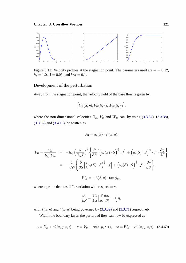
Chapter 3. Crossflow Vortices 121
0 1 2 3 4 5 6 7 80
0.005
0.01
0.015
0.02
0.025
0.03
0.035
0.04
η
1
|u|
1
0 1 2 3 4 5 6 7 80
1
2
3
4
5
6
7
8
η
1
|v|
1
0 1 2 3 4 5 6 7 80
0.1
0.2
0.3
0.4
0.5
0.6
0.7
0.8
0.9
1
η
1
|w|
1
Figure 3.12: Velocity profiles at the stagnation point. The parameters used areω = 0.12,k3 = 1.0, Λ = 0.05, andb/a = 0.1.
Development of the perturbation
Away from the stagnation point, the velocity field of the base flow is given by
[UB(S, η), VB(S, η),WB(S, η)
],
where the non-dimensional velocitiesUB, VB andWB can, by using (3.3.37), (3.3.38),
(3.3.62) and (3.4.13), be written as
UB = ue(S) ∙ f′(S, η),
VB =v∗B
R−1δs U∞= −Rδs
( ν
U∞L
) 12
{∂
∂S
[(ue(S) ∙ S
) 12∙ f]+(ue(S) ∙ S
) 12∙ f ′ ∙
∂η
∂S
}
= −1√C
{∂
∂S
[(ue(S) ∙ S
) 12∙ f]+(ue(S) ∙ S
) 12∙ f ′ ∙
∂η
∂S
}
,
WB = −h(S, η) ∙ tanφ∞,
where a prime denotes differentiation with respect toη,
∂η
∂S=1
2
1
S
[ Sue
due
dS− 1]η,
with f(S, η) andh(S, η) being governed by (3.3.39) and (3.3.71) respectively.
Within the boundary layer, the perturbed flow can now be expressed as
u = UB + εu(x, y, z, t), v = VB + εv(x, y, z, t), w = WB + εw(x, y, z, t). (3.4.69)

3.4 Perturbation equations 122
The perturbed flow is substituted into the non-dimensional boundary layer equations (3.4.14),
(3.4.46), and (3.4.47). After linearisation, we obtain the leading-order perturbation equa-
tions∂u
∂x+R20
∂v
∂y+∂w
∂z= 0, (3.4.70)
∂u
∂t+ UB
∂u
∂x+ u
∂UB
∂x+R20
(VB
∂u
∂y+ v
∂UB
∂y
)+WB
∂u
∂z= R20
∂2u
∂y2, (3.4.71)
∂w
∂t+ UB
∂w
∂x+ u
∂WB
∂x+R20
(VB
∂w
∂y+ v
∂WB
∂y
)+WB
∂w
∂z= R20
∂2w
∂y2. (3.4.72)
The solution for (u, v, w) takes the form
(u, v, w) =[u(x, η), v(x, η),
1
k3w(x, η)
]exp
{i(k3z − ωt)
},
substitution of which into (3.4.70)–(3.4.72) yields
∂u
∂x+R20
∂v
∂y+ iw = 0, (3.4.73)
− iωu+ UB∂u
∂x+ u
∂UB
∂x+R20
(VB
∂u
∂y+ v
∂UB
∂y
)+ ik3WBu = R
20
∂2u
∂y2, (3.4.74)
− iωw+UB∂w
∂x+ k3u
∂WB
∂x+R20
(VB
∂w
∂y+ k3v
∂WB
∂y
)+ ik3WBw = R
20
∂2w
∂y2. (3.4.75)
For computational purpose, we rewrite (3.4.73)–(3.4.75) into a first-order system,
∂u
∂y= f , (3.4.76)
∂v
∂y= −
1
R20
(∂u∂x+ iw
), (3.4.77)
∂w
∂y= g, (3.4.78)
∂f
∂y=1
R20
(− iω + UB
∂
∂x+ ik3WB
)u+
u
R20
∂UB
∂x+ v
∂UB
∂y+ VB f , (3.4.79)
∂g
∂y= u
k3
R20
∂WB
∂x+ k3v
∂WB
∂y+1
R20
(− iω + UB
∂
∂x+ ik3WB
)w + VB g. (3.4.80)
Since the base flow is evaluated on theη grid, we need to re-write (3.4.76)–(3.4.80) in terms
Chapter 3. Crossflow Vortices 123
of η, in order to input the corresponding base flow at each mesh point. Noting that
∂
∂x→
∂
∂x+
∂
∂η
∂η
∂x,
∂
∂y→
δs
δ
∂
∂η,
we convert (3.4.76)–(3.4.80) into the following system,
∂u
∂η= R1f , (3.4.81)
∂v
∂η= −
R1
R20
∂u
∂x− i
R1
R20w −
R21R20
∂η
∂xf , (3.4.82)
∂w
∂η= R1g, (3.4.83)
∂f
∂η=R1
R20
(−iω+UB
∂
∂x+ik3WB+
Λ
L
∂UB
∂S+∂UB
∂η
∂η
∂x
)u+v
∂UB
∂η+(R21R20
∂η
∂xUB+R1VB
)f ,
(3.4.84)
∂g
∂η=
k3R1
R20
(ΛL
∂WB
∂S+∂WB
∂η
∂η
∂x
)u+ k3v
∂WB
∂η+R1
R20
(− iω + UB
∂
∂x+ ik3WB
)w
+(R21R20
∂η
∂xUB +R1VB
)g, (3.4.85)
where
R1 =δ
δs=
√CS
ue, and
∂η
∂x=1
2
Λ
L
1
S
[ S
ue(S)
due
dS− 1]η.
The values of∂UB
∂S,
∂UB
∂η,
∂WB
∂Sand
∂WB
∂η
are evaluated from solving the steady boundary layer equations.
The boundary conditions for (3.4.81)–(3.4.85) are
u = v = w = 0 at η = 0; u→ 0, w → exp (ik1Δ) as η →∞. (3.4.86)
Note that the boundary condition at infinity comes from matching with the spanwise slip
velocity. The drift functionΔ needs to be evaluated numerically, and the detailed evaluation
procedure is given in the appendix A2.

3.5 Eigenvalue formulation 124
The initial condition for (3.4.81)–(3.4.85) is
(u, v, w)→ (xu, v, w) as x→ 0 (3.4.87)
with (u, v, w) being obtained from solving (3.4.63)–(3.4.67) subject to the boundary condi-
tion (3.4.68). The initial-boundary-value problem consisting of equations (3.4.81)–(3.4.85)
and (3.4.86)–(3.4.87) describes the receptivity and evolution of the excited perturbation.
3.5 Eigenvalue formulation
3.5.1 Non-parallel boundary-layer eigenvalue formulation
In order to see whether the perturbation evolves into a spatially growing eigenmode, we
formulate a local eigenvalue problem for crossflow vortices. As usual, we seek a normal-
mode solution
(u, v, w) =[uc(η), vc(η), wc(η)
]exp{
∫ xσ(x)dx},
whereσ is in general a complex number dependent onx with its real part representing the
local growth rate. Substitution of the above expression into (3.4.81)–(3.4.85), we obtain a
set of ordinary differential equations
ducdη= R1fc, (3.5.1)
dvcdη= −
R1
R20σuc − i
R1
R20wc −
R21R20
∂η
∂xfc, (3.5.2)
dwcdη= R1gc, (3.5.3)
dfcdη=R1
R20
(−iω+σUB+ik3WB+
Λ
L
∂UB
∂S+∂UB
∂η
∂η
∂x
)uc+vc
∂UB
∂η+(R21R20
∂η
∂xUB+R1VB
)fc,
(3.5.4)
dgcdη
= uck3R1
R20
(ΛL
∂WB
∂S+∂WB
∂η
∂η
∂x
)+ k3vc
∂WB
∂η+R1
R20
(− iω + σUB + ik3WB
)wc
+(R21R20
∂η
∂xUB +R1VB
)gc. (3.5.5)
Chapter 3. Crossflow Vortices 125
The system (3.5.1)–(3.5.5) along with the homogenous boundary conditions,
(uc, vc, wc) = (0, 0, 0) at η = 0;
(uc, wc)→ (0, 0) as η →∞,
forms the non-parallel eigenvalue formulation. Since the pressure perturbation is absent,
the ensuring eigen solution will be referred to as the ‘boundary layer mode’.
3.5.2 Parallel boundary-layer eigenvalue formulation
If the nonparallel flow terms∂UB∂x
, ∂WB∂x
, VB, and∂η∂x
are neglected, equations (3.5.1)–(3.5.5)
simplify toducdη= R1fc, (3.5.6)
dvcdη= −
R1
R20(σuc + iwc), (3.5.7)
dwcdη= R1gc, (3.5.8)
dfcdη=R1
R20
(− iω + σUB + ik3WB
)uc + vc
∂UB
∂η, (3.5.9)
dgcdη= k3vc
∂WB
∂η+R1
R20
(− iω + σUB + ik3WB
)wc, (3.5.10)
with the boundary conditions
(uc, vc, wc) = (0, 0, 0) at η = 0;
(uc, wc) = (0, 0) as η →∞.
The above system will be referred to as parallel boundary layer eigenvalue problem.
3.5.3 Non-parallel Navier-Stokes eigenvalue formulation
In the previous non-parallel eigenvalue formulation, the pressure gradient terms are ne-
glected, which is justified forx = O(1). However, the pressure fluctuation induced by
the displacement will eventually become anO(1) effect whenx = O(RΛ). The usual
Navier-Stokes eigenvalue problem will have to be considered.

3.5 Eigenvalue formulation 126
Insertingp = PB + εp along with (3.4.69) into the normalised Navier-Stokes equations
(3.4.14)–(3.4.17), we obtain the linearised perturbation equations
∂u
∂x+R20
∂v
∂y+∂w
∂z= 0, (3.5.11)
∂u
∂t+UB
∂u
∂x+u
∂UB
∂x+R20
(VB
∂u
∂y+v
∂UB
∂y
)+WB
∂u
∂z= −
∂p
∂x+R20
∂2u
∂y2+1
RΛ
∂2u
∂z2, (3.5.12)
∂v
∂t+ UB
∂v
∂x+ u
∂VB
∂x+R20
(VB
∂v
∂y+ v
∂VB
∂y
)+WB
∂v
∂z= −RΛ
∂p
∂y+R20
∂2v
∂y2+1
RΛ
∂2v
∂z2,
(3.5.13)∂w
∂t+UB
∂w
∂x+ u
∂WB
∂x+R20
(VB
∂w
∂y+ v
∂WB
∂y
)+WB
∂w
∂z= −
∂p
∂z+R20
∂2w
∂y2+1
RΛ
∂2w
∂z2,
(3.5.14)
wherep is the perturbation pressure. Note that we have neglected the streamwise diffusion
terms because they remain of a higher-order effect in the entire region of interest, over
which the equations (3.5.11)–(3.5.14) serve as an composite approximation in the sense that
they contain the upstream and downstream regimes in the appropriate asymptotic limits.
The solution foru, v, w, andp may be sought of the form
(u, v, w, p) =[u(x, η), v(x, η),
1
k3w(x, η), p(x, η)
]exp
{i(k3z − ωt)
}.
Substitution into (3.5.11)–(3.5.14) yields
∂u
∂x+R20
∂v
∂y+ iw = 0, (3.5.15)
− iωu+ UB∂u
∂x+ u
∂UB
∂x+R20
(VB
∂u
∂y+ v
∂UB
∂y
)+ ik3WBu = −
∂p
∂x+R20
∂2u
∂y2−k23RΛ
u,
(3.5.16)
− iωv +UB∂v
∂x+ u
∂VB
∂x+R20
(VB
∂v
∂y+ v
∂VB
∂y
)+ ik3WB v = −RΛ
∂p
∂y+R20
∂2v
∂y2−k23RΛ
v,
(3.5.17)
−iωw+UB∂w
∂x+k3u
∂WB
∂x+R20
(VB
∂w
∂y+k3v
∂WB
∂y
)+ik3WBw = −ik
23 p+R
20
∂2w
∂y2−k23RΛ
w.
(3.5.18)
Since the base flow is evaluated onη grid, equations (3.5.15)–(3.5.18) are re-written in
terms ofη,∂u
∂x+∂u
∂η
∂η
∂x+R20R1
∂v
∂η+ iw = 0, (3.5.19)

Chapter 3. Crossflow Vortices 127
−iωu+ UB(∂u∂x+∂u
∂η
∂η
∂x
)+ u(∂UB∂x+∂UB
∂η
∂η
∂x
)+R20
(VBR1
∂u
∂η+
v
R1
∂UB
∂η
)
+ik3WBu = −(∂p∂x+∂p
∂η
∂η
∂x
)+R20R21
∂2u
∂η2−k23RΛ
u, (3.5.20)
−iωv + UB(∂v∂x+∂v
∂η
∂η
∂x
)+ u(∂VB∂x+∂VB
∂η
∂η
∂x
)+R20
(VBR1
∂v
∂η+
v
R1
∂VB
∂η
)
+ik3WB v = −RΛ
R1
∂p
∂η+R20R21
∂2v
∂η2−k23RΛ
v, (3.5.21)
−iωw + UB(∂w∂x+∂w
∂η
∂η
∂x
)+ k3u
(∂WB∂x+∂WB
∂η
∂η
∂x
)+R20
(VBR1
∂w
∂η+k3v
R1
∂WB
∂η
)
+ik3WBw = −ik23 p+
R20R21
∂2w
∂η2−k23RΛ
w. (3.5.22)
For the linearised Navier-Stokes eigenmode formulation, the ratiob/a, spanwise wave-
lengthΛ/a, Reynolds numberRΛ, and the frequencyω are the four independent parame-
ters.
We seek normal-mode solution
(u, v, w, p) =[uc(η), vc(η), wc(η), pc(η)
]exp{
∫ xσdx},
whereσ is in general a complex number dependent onx with its real part representing the
local growth rate. We let
ducdη= R1fc, and
dwcdη= R1gc. (3.5.23)
From the continuity equation (3.5.19), we have
dvcdη= −
R1
R20σuc − i
R1
R20wc −
R21R20
∂η
∂xfc. (3.5.24)
3.5 Eigenvalue formulation 128
Eliminating dpdη
through the operation,(3.5.20)× RΛR1− (3.5.21)× ∂η
∂x, we find
dfcdη
=1
A1
{
− iωRΛ
R1+[RΛR1
UB +R1
R20
(∂η∂x
)2+∂η
∂xVB
]σ +
RΛ
R1
(∂UB∂x+∂UB
∂η
∂η
∂x
)
−∂η
∂x
(∂VB∂x+∂VB
∂η
∂η
∂x
)+ ik3WB
RΛ
R1+k23R1
}
uc
+1
A1
[iω∂η
∂x− σUB
∂η
∂x+RΛ
R20R21
∂UB
∂η−R20R1
∂η
∂x
∂VB
∂η− ik3WB
∂η
∂x−k23RΛ
∂η
∂x
]vc
+i
A1
[VB
∂η
∂x+ UB
R1
R20
(∂η∂x
)2]wc +
RΛ
A1R1σpc −
i
A1
∂η
∂xgc
+1
A1
{
RΛUB∂η
∂x+ UB
R21R20
(∂η∂x
)3+RΛR
20
R1VB +R1VB
(∂η∂x
)2
−∂η
∂x
[σ +
∂
∂η
(∂η∂x
)]}
fc, (3.5.25)
where
A1 =RΛR
20
R21+(∂η∂x
)2, and
∂
∂η
(∂η∂x
)=1
2
Λ
L
1
S
[ S
ue(S)
due
dS− 1].
Elimination dfcdη
through manipulation,(3.5.20)× ∂η∂x+ (3.5.21)× R20
R1, we obtain
dpcdη
= −1
A1
{
− iω∂η
∂x−R20R1VBσ +
∂UB
∂x
∂η
∂x+∂UB
∂η
(∂η∂x
)2+R20R1
∂VB
∂x
+R20R1
∂VB
∂η
∂η
∂x+ ik3WB
∂η
∂x+k23RΛ
∂η
∂x
}
uc
−R20A1R1
[− iω + σUB +
∂UB
∂η
∂η
∂x+R20R1
∂VB
∂η+ ik3WB +
k23RΛ
]vc
+i
A1
(UB
∂η
∂x+ VB
R20R1
)wc −
1
A1
R20R1
[σ +
∂
∂η
(∂η∂x
)]fc −
σ
A1
∂η
∂xpc
− iR20A1R1
gc. (3.5.26)

Chapter 3. Crossflow Vortices 129
The spanwise momentum equation (3.5.22) may be written as
dgcdη
= uck3R1
R20
(ΛL
∂WB
∂S+∂WB
∂η
∂η
∂x
)+ k3vc
∂WB
∂η+ik23R1
R20pc +
(R21R20
∂η
∂xUB +R1VB
)gc
+R1
R20
(− iω + σUB + ik3WB +
k23RΛ
)wc (3.5.27)
In conclusion, the classical non-parallel eigenvalue formulation consists of (3.5.23)–(3.5.27),
and the boundary conditions
(uc, vc, wc) = (0, 0, 0) at η = 0;
(uc, vc, wc, pc) = (0, 0, 0) as η →∞.
The above linearised Navier-Stokes eigenvalue problem is more general than the boundary-
layer eigenvalue problem. Let us now discuss the relationship between them and the re-
spective region of validity in the context of the present problem. In the downstream region,
whereS = O(1) andue = O(1), we know from (3.4.7) thatC = O(a2/b2), and so
R1 =δ
δs=
√CS
ue= O(
a
b).
The local boundary layer thickness
δ =
√νs∗
u∗e∼
√νL
U∞=Λ√RΛ
√L
Λ= O(Λ),
if we take the Reynolds number
RΛ = O(a2
b2).
Thus
A1 =RΛR
20
R21+(∂η∂x
)2= O(1),
implying anO(1) pressure variation across the boundary layer so that the instability is
governed by the Navier-Stokes eigenvalue problem. A closer inspection of the asymptotic
scalings suggests that the viscous terms are all of higher-order effects, that is, the eigen
modes are actually governed by the Rayleigh equation with the effective profile
Ueff = UB +ik3
σWB.
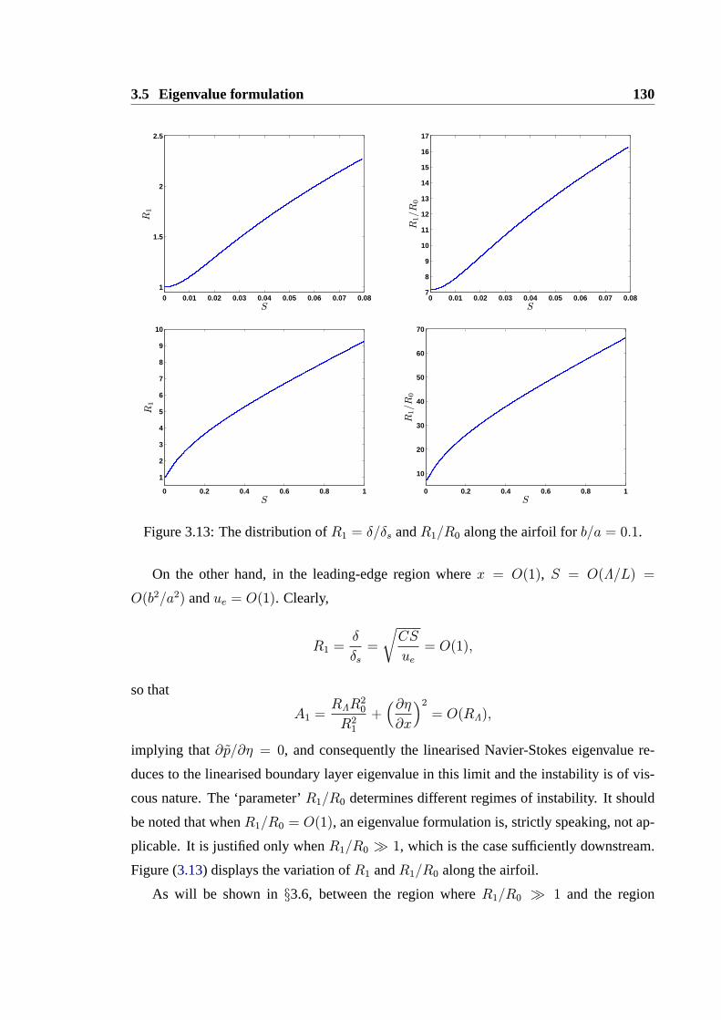
3.5 Eigenvalue formulation 130
0 0.01 0.02 0.03 0.04 0.05 0.06 0.07 0.08
1
1.5
2
2.5
S
1
R1
1
0 0.01 0.02 0.03 0.04 0.05 0.06 0.07 0.087
8
9
10
11
12
13
14
15
16
17
S
1
R1/R0
1
0 0.2 0.4 0.6 0.8 1
1
2
3
4
5
6
7
8
9
10
S
1
R1
1
0 0.2 0.4 0.6 0.8 1
10
20
30
40
50
60
70
S
1
R1/R0
1
Figure 3.13: The distribution ofR1 = δ/δs andR1/R0 along the airfoil forb/a = 0.1.
On the other hand, in the leading-edge region wherex = O(1), S = O(Λ/L) =
O(b2/a2) andue = O(1). Clearly,
R1 =δ
δs=
√CS
ue= O(1),
so that
A1 =RΛR
20
R21+(∂η∂x
)2= O(RΛ),
implying that∂p/∂η = 0, and consequently the linearised Navier-Stokes eigenvalue re-
duces to the linearised boundary layer eigenvalue in this limit and the instability is of vis-
cous nature. The ‘parameter’R1/R0 determines different regimes of instability. It should
be noted that whenR1/R0 = O(1), an eigenvalue formulation is, strictly speaking, not ap-
plicable. It is justified only whenR1/R0 � 1, which is the case sufficiently downstream.
Figure (3.13) displays the variation ofR1 andR1/R0 along the airfoil.
As will be shown in§3.6, between the region whereR1/R0 � 1 and the region

Chapter 3. Crossflow Vortices 131
whereR1/R0 = O(RΛ), there exists an intermediate regime corresponding toR1/R0 =
O(RΛ)1/5. In this region, the viscosity effect and the pressure perturbation are both impor-
tant.
3.6 Numerical results
The initial-boundary-value and eigenvalue problems are solved numerically using the same
numerical algorithms as in the case of Gortler vortices. However, extra terms appear due to
the presence of the crossflow. Further validation of the code is needed. This is performed
by comparing the growth rates obtained by solving the linearised Navier-Stokes eigenvalue
problem (3.5.23)–(3.5.27) for the swept Hiemenz flow with the result presented in MLC.
3.6.1 Validation of the eigenvalue solver
MLC studied spatial crossflow instability using the swept Hiemenz flow as the base flow.
The growth rates shown in their paper can be used as a reference for us to check our codes.
Since the variables used in MLC are defined differently from ours, we need first to find the
relations between the two sets of variables. The subscriptM will be used to denote the
variables in MLC.
The slip velocity in MLC’s is given by
U∞M = CM ∙ s∗ = CM ∙
s∗
Λ∙ Λ = CM ∙ x ∙ Λ, (3.6.1)
while in ours
u∗e = C ∙ S ∙ U∞ = C ∙Λ
L∙ x ∙ U∞. (3.6.2)
Equality of the two,U∞M = u∗e, implies that
CM =C
L∙ U∞. (3.6.3)
In MLC, the reference length scale used for non-dimensionalisation is defined as
l =( ν
CM
) 12. (3.6.4)
3.6 Numerical results 132
Substitution of (3.6.3) into (3.6.4) yields
l =( νL
CU∞
) 12= δs, (3.6.5)
whereδs refers to the stagnation point boundary layer thickness in our formulation. The
Reynolds number defined in MLC is
RM =U∞M l
ν=CM ∙ s∗ ∙ l
ν=s∗ ∙ ll2=s∗
l=xΛ
l. (3.6.6)
Substituting (3.6.5) into (3.6.6), we find
RM = x ∙ Λ ∙(U∞CνL
) 12= x ∙
(U∞Λν∙ΛC
L
) 12= x(RΛR
20)12 . (3.6.7)
The normalised spanwise wavenumber in our formulation and MLC’s are
k3 = k∗3Λ, and β = k∗3l (3.6.8)
respectively. It follows that
β =k3
Λl =
k3
Λ
( νL
CU∞
) 12=( ν
ΛU∞∙L
ΛC
) 12= k3(RΛR
20)− 12 . (3.6.9)
In our formulationk3 = 1, which means
β = (RΛR20)− 12 . (3.6.10)
From the normalisation of the velocity in thex direction, we know
US =u∗
U∞=
u∗
W∞M∙W∞MU∞
= UM tanφ∞, (3.6.11)
whereUS = R20f′x, andUM = xMf
′M/R = Rf ′M/R respectively. Iftanφ∞ = 1, then the
base flows are identical,
US = UM , i.e. R20f′x =
R
Rf ′M =
x(RΛR20)12
Rf ′M . (3.6.12)

Chapter 3. Crossflow Vortices 133
Sincef ′ = f ′M , the relation (3.6.12) implies that
R20 =(R20RΛ)
12
R. (3.6.13)
Combining (3.6.10) and (3.6.13), we get
R20 =1
βR, RΛ =
R
β, (3.6.14)
and
Λ/a =L
aC∙R20 =
L
aC∙1
βR. (3.6.15)
Substitution of (3.6.14) into (3.6.7) shows
RM = x/β. (3.6.16)
The growth rate is normalised byl in MLC, i.e.
σM = σ∗l, (3.6.17)
while in our formualtion, the growth rate is normalised byΛ, i.e.
σ = σ∗Λ. (3.6.18)
From (3.6.17) and (3.6.18), we have
σ =σM
l∙ Λ = σM ∙
( νL
CU∞
)− 12Λ = σM ∙
( ν
ΛU∞∙L
ΛC
)− 12= σM(RΛR
20)12 = σM/β.
(3.6.19)
The frequencyω in our formulation is
ω = 2πf ∗ ∙Λ
U∞, i.e. f ∗ =
ω
2π∙U∞
Λ, (3.6.20)
wheref ∗ denotes the dimensional frequency. The frequency in MLC’s formulation is
FM =2πνf ∗
W 2∞M
, i.e. f ∗ =FM
2πν∙W 2
∞M , (3.6.21)

3.6 Numerical results 134
100 200 300 400 500 600 700 800 900 1000-0.01
-0.005
0
0.005
0.01
0.015
0.02
0.025
0.03
0.035
0.04
RM
1
GrowthRateRe(σM)
1
NumericalTheory
0 200 400 600 800 1000-1.4
-1.2
-1
-0.8
-0.6
-0.4
-0.2
0
RM
1
Im(σM)
1
NumericalTheory
Figure 3.14: The growth rate and chordwise wavenumber of crossflow vortices at differentchordwise locations. Parameter values:ω = 0.1071,RΛ = 1428.57 andΛ/a = 2.9×10⁻⁴.
whereW∞M is the oncoming free-stream velocity in the spanwise direction. From (3.6.20)
and (3.6.21), it follows
ω
2π∙U∞
Λ=FM
2πν∙W 2
∞M , i.e. ω = FM ∙RΛ ∙W 2∞M
U2∞(3.6.22)
From the definition
R =W∞M l
ν,
we have
W∞M =R ∙ νl. (3.6.23)
Substitution of (3.6.23) and (3.6.5) into (3.6.22) leads to
ω = FM ∙R20 ∙ R
2 = FM R/β. (3.6.24)
From figure 5 in MLC, we can extract the value ofσM = iα = −αi + iαr. The value
of αi can be read directly from the figure. From the relation
tan(θ + ψ) =β
αr, (3.6.25)
whereθ is the local sweep angle in MLC defined asθ = arctan(R/R), andψ is the
orientation angle, which can be read from the figure directly, the value ofαr can be ob-
tained. When frequencyF = 0.75 × 10⁻⁴ andβ ≈ 0.35, we have−αi = 0.032, and
αr = −0.36289472. Using (3.6.16) and (3.6.19), we find the corresponding location
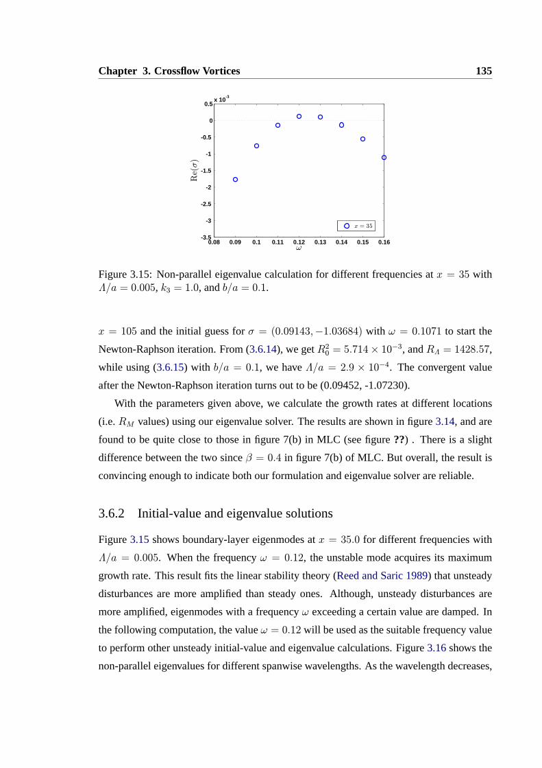
Chapter 3. Crossflow Vortices 135
0.08 0.09 0.1 0.11 0.12 0.13 0.14 0.15 0.16-3.5
-3
-2.5
-2
-1.5
-1
-0.5
0
0.5x 10
-3
ω
1
Re(σ)
1
x = 35
1
Figure 3.15: Non-parallel eigenvalue calculation for different frequencies atx = 35 withΛ/a = 0.005, k3 = 1.0, andb/a = 0.1.
x = 105 and the initial guess forσ = (0.09143,−1.03684) with ω = 0.1071 to start the
Newton-Raphson iteration. From (3.6.14), we getR20 = 5.714× 10⁻³, andRΛ = 1428.57,
while using (3.6.15) with b/a = 0.1, we haveΛ/a = 2.9 × 10⁻⁴. The convergent value
after the Newton-Raphson iteration turns out to be (0.09452, -1.07230).
With the parameters given above, we calculate the growth rates at different locations
(i.e.RM values) using our eigenvalue solver. The results are shown in figure3.14, and are
found to be quite close to those in figure 7(b) in MLC (see figure??) . There is a slight
difference between the two sinceβ = 0.4 in figure 7(b) of MLC. But overall, the result is
convincing enough to indicate both our formulation and eigenvalue solver are reliable.
3.6.2 Initial-value and eigenvalue solutions
Figure3.15shows boundary-layer eigenmodes atx = 35.0 for different frequencies with
Λ/a = 0.005. When the frequencyω = 0.12, the unstable mode acquires its maximum
growth rate. This result fits the linear stability theory (Reed and Saric 1989) that unsteady
disturbances are more amplified than steady ones. Although, unsteady disturbances are
more amplified, eigenmodes with a frequencyω exceeding a certain value are damped. In
the following computation, the valueω = 0.12 will be used as the suitable frequency value
to perform other unsteady initial-value and eigenvalue calculations. Figure3.16shows the
non-parallel eigenvalues for different spanwise wavelengths. As the wavelength decreases,
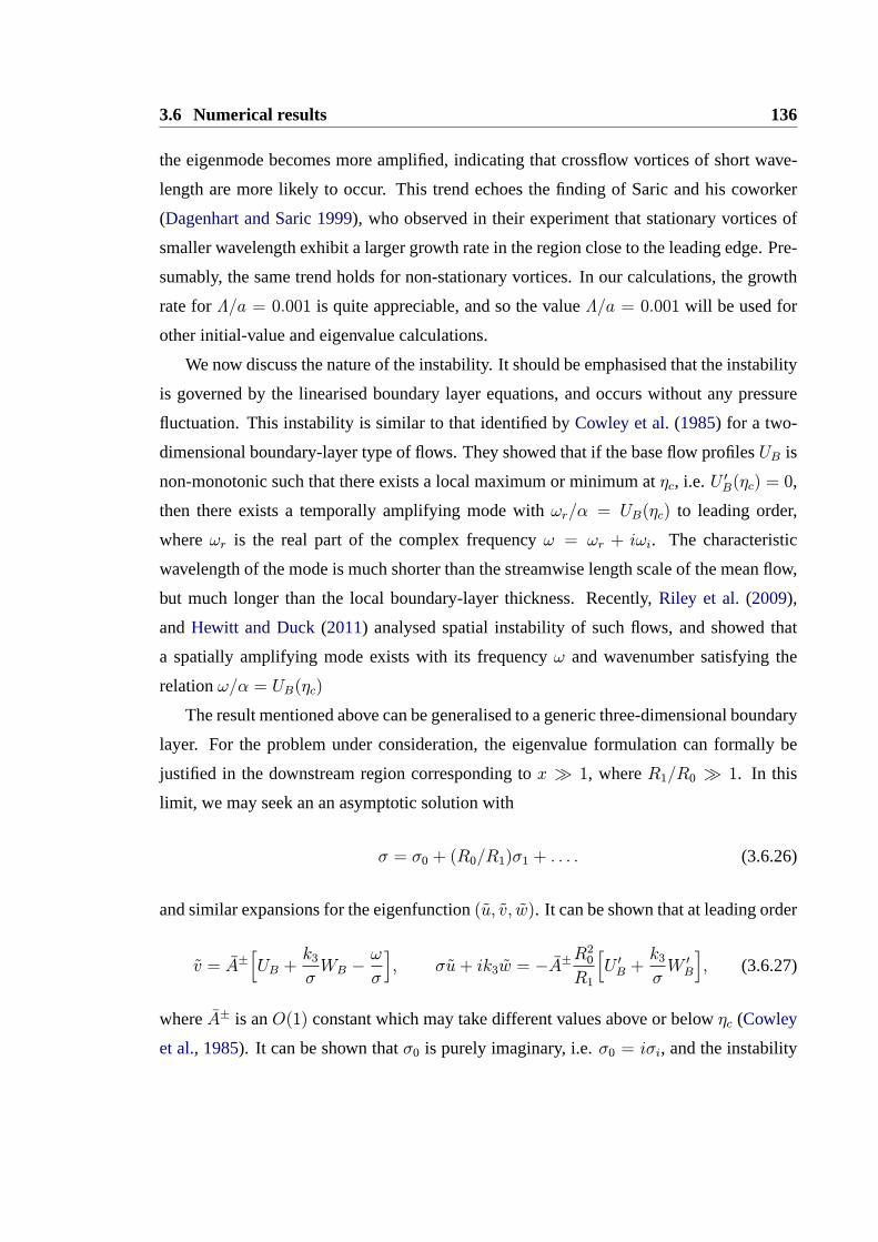
3.6 Numerical results 136
the eigenmode becomes more amplified, indicating that crossflow vortices of short wave-
length are more likely to occur. This trend echoes the finding of Saric and his coworker
(Dagenhart and Saric 1999), who observed in their experiment that stationary vortices of
smaller wavelength exhibit a larger growth rate in the region close to the leading edge. Pre-
sumably, the same trend holds for non-stationary vortices. In our calculations, the growth
rate forΛ/a = 0.001 is quite appreciable, and so the valueΛ/a = 0.001 will be used for
other initial-value and eigenvalue calculations.
We now discuss the nature of the instability. It should be emphasised that the instability
is governed by the linearised boundary layer equations, and occurs without any pressure
fluctuation. This instability is similar to that identified byCowley et al.(1985) for a two-
dimensional boundary-layer type of flows. They showed that if the base flow profilesUB is
non-monotonic such that there exists a local maximum or minimum atηc, i.e.U ′B(ηc) = 0,
then there exists a temporally amplifying mode withωr/α = UB(ηc) to leading order,
whereωr is the real part of the complex frequencyω = ωr + iωi. The characteristic
wavelength of the mode is much shorter than the streamwise length scale of the mean flow,
but much longer than the local boundary-layer thickness. Recently,Riley et al. (2009),
andHewitt and Duck(2011) analysed spatial instability of such flows, and showed that
a spatially amplifying mode exists with its frequencyω and wavenumber satisfying the
relationω/α = UB(ηc)
The result mentioned above can be generalised to a generic three-dimensional boundary
layer. For the problem under consideration, the eigenvalue formulation can formally be
justified in the downstream region corresponding tox � 1, whereR1/R0 � 1. In this
limit, we may seek an an asymptotic solution with
σ = σ0 + (R0/R1)σ1 + . . . . (3.6.26)
and similar expansions for the eigenfunction(u, v, w). It can be shown that at leading order
v = A±[UB +
k3
σWB −
ω
σ
], σu+ ik3w = −A
±R20
R1
[U ′B +
k3
σW ′B
], (3.6.27)
whereA± is anO(1) constant which may take different values above or belowηc (Cowley
et al., 1985). It can be shown thatσ0 is purely imaginary, i.e.σ0 = iσi, and the instability

Chapter 3. Crossflow Vortices 137
is equivalent to that for a two-dimensional flow with an effective profile
Ueff = UB +k3
σiWB.
The skewed profile has a maximum atηc, U ′eff = 0, i.e.
σi∂UB(ηc)
∂η+ k3
∂WB(ηc)
∂η= 0. (3.6.28)
The frequencyω andσi satisfy the relation
ω
σi= UB +
k3
σiWB,
i.e.
ω = σiUB(ηc) + k3WB(ηc). (3.6.29)
From (3.6.28) and (3.6.29) it follows
−ω
k3+ [
WB(ηc)
UB(ηc)−W ′B(ηc)
U ′B(ηc)]UB(ηc) = 0. (3.6.30)
The relations (3.6.28) and (3.6.30) allow us to determineσi. At a given downstream loca-
tion, the values of the base flowUB, WB, and their derivativesU ′B, andW ′B are all known.
We are able to find the location ofη which satisfies the relation (3.6.30). When the value of
ηc is known, the imaginary part of the eigenvalue, i.e.σi will be obtained from (3.6.28). An
analysis of the viscous critical layer, which has a width ofO[(R0/R1)1/2], gives the value
of
σ1 = −(−iσiU ′′eff )
1/2
√2UB(ηc)
,
and so the real part ofσ
σr =(σiU
′′eff )
1/2
2UB(ηc)R0/R1. (3.6.31)
In figure3.17, the value ofσ computed by solving the non-parallel eigenvalue problem
is compared with the theoretical result. As illustrated in figure3.17, for σi the numeri-
cal result matches with the theoretical prediction quite well. The theoretical value forσr
is about twice the numerical value. The discrepancy arises becauseR0/R1 is not large
enough, merely0.2. But the general trend is consistent. The overall agreement reassures

3.6 Numerical results 138
20 25 30 35 40 45 50-0.04
-0.03
-0.02
-0.01
0
0.01
0.02
0.03
x
1
Re(σ)
1
Λ/a = 0.005
1
Λ/a = 0.0025
1
Λ/a = 0.002
1
Λ/a = 0.0015
1
Λ/a = 0.00125
1
Λ/a = 0.001
1
20 25 30 35 40 45 500.8
1
1.2
1.4
1.6
1.8
2
x
1
Im(σ)
1
Λ/a = 0.005
1
Λ/a = 0.0025
1
Λ/a = 0.002
1
Λ/a = 0.0015
1
Λ/a = 0.00125
1
Λ/a = 0.001
1
Figure 3.16: The growth rates(Re(σ)) and chordwise wavenumber(Im(σ)) of the non-parallel eigenmodes for different spanwise wavelengths forω = 0.12, k3 = 1.0, andb/a =0.1.
0 50 100 150 200-0.01
-0.005
0
0.005
0.01
0.015
0.02
0.025
0.03
0.035
0.04
x
1
Re(σ)
1
NumericalTheory
20 40 60 80 100 120 140 160 180 2000.5
1
1.5
2
2.5
3
3.5
4
x
1
Im(σ)
1
NumericalTheory
Figure 3.17: Non-parallel eigenvalue and comparison with the theoretical result . Parametervalues:ω = 0.12, Λ/a = 0.001, k3 = 1.0, andb/a = 0.1.
us that the numerical results are reliable. We also apply the theory to the swept Hiemenz
flow. The result is shown in figure3.14, and a reasonable agreement is obtained.
Both non-parallel and parallel eigenvalues calculations are carried out, and the results
are compared with the theoretical results in figure3.18. Figure3.18 indicates that non-
parallel flow effects destabilize the flow. In the upstream region wherex = O(1), there is
significant difference. But the eigenvalue formulation in this region isad hoc, and the result
should probably be rejected. In the downstream region where the character of the asymp-
totic mode is established, the difference between parallel and non-parallel predictions is
rather small.
We solved the initial-boundary-value problem (3.4.81)–(3.4.85) with (3.4.86)–(3.4.87)

Chapter 3. Crossflow Vortices 139
20 40 60 80 100 120 140 160 180 200-0.16
-0.14
-0.12
-0.1
-0.08
-0.06
-0.04
-0.02
0
0.02
0.04
x
1
Re(σ)
1
nonparallelparalleltheory
20 40 60 80 100 120 140 160 180 2000.5
1
1.5
2
2.5
3
3.5
4
x
1
Im(σ)
1
nonparallelparalleltheory
Figure 3.18: Comparison between non-parallel and parallel eigenvalue calculations withthe theoretical result forω = 0.12, Λ/a = 0.001, k3 = 1.0, andb/a = 0.1.
pertaining to the free-stream turbulence. The local growth rate,1ududx
, is computed and
shown in figure3.19. We note that1ududx
remains positive, indicating that the induced dis-
turbance amplifies monotonically. We also compared1ududx
with the eigenvalueσ. The two
solutions converge asx increases, suggesting that the perturbation gradually develops into
an eigen mode.
We performed the calculation of boundary layer receptivity to suction imposed on the
surface. For this case, the initial condition is taken to beu = v = w = 0. The boundary
conditions are
η = 0 : u = w = 0, v = xe−x; η = η∞ : u = v = w = 0.
The local growth rates obtained are compared with the non-parallel eigenvalues in figure
3.20. The result shows that the induced perturbation eventually develops into an eigen-
mode, i.e. crossflow vortices are excited by suction. As can be seen from the figure, the
form of the initial disturbance affects the response in the region relatively close to the lead-
ing edge, but the induced motion acquire the same behaviour at large distances.
3.6.3 The intermediate regime
In this subsection, we analyse the development of boundary-layer modes farther down-
stream, and show that the mode will enter an intermediate regime where the induced pres-
sure will eventually balance the inertia and viscous effects.
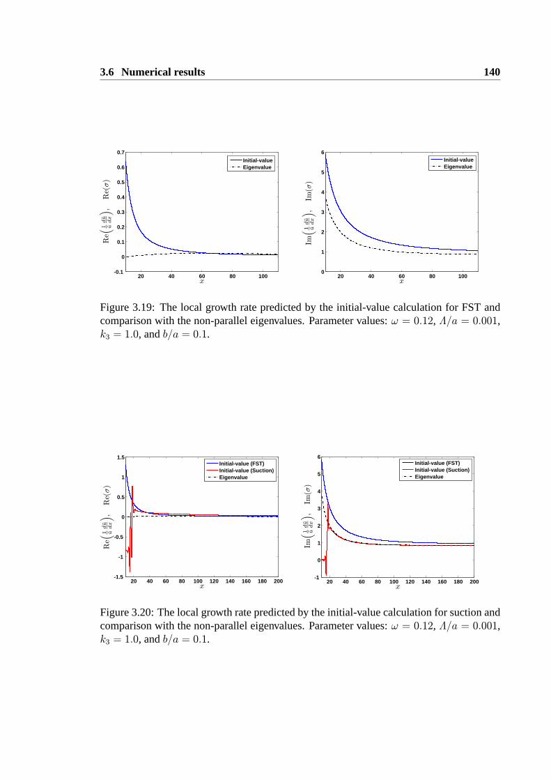
3.6 Numerical results 140
20 40 60 80 100-0.1
0
0.1
0.2
0.3
0.4
0.5
0.6
0.7
x
1
Re(1 ududx
),Re(σ)
1
Initial-valueEigenvalue
20 40 60 80 1000
1
2
3
4
5
6
x
1
Im(1 ududx
),Im(σ)
1
Initial-valueEigenvalue
Figure 3.19: The local growth rate predicted by the initial-value calculation for FST andcomparison with the non-parallel eigenvalues. Parameter values:ω = 0.12, Λ/a = 0.001,k3 = 1.0, andb/a = 0.1.
20 40 60 80 100 120 140 160 180 200-1.5
-1
-0.5
0
0.5
1
1.5
x
1
Re(1 ududx
),Re(σ)
1
Initial-value (FST)Initial-value (Suction)Eigenvalue
20 40 60 80 100 120 140 160 180 200-1
0
1
2
3
4
5
6
x
1
Im(1 ududx
),Im(σ)
1
Initial-value (FST)Initial-value (Suction)Eigenvalue
Figure 3.20: The local growth rate predicted by the initial-value calculation for suction andcomparison with the non-parallel eigenvalues. Parameter values:ω = 0.12, Λ/a = 0.001,k3 = 1.0, andb/a = 0.1.

Chapter 3. Crossflow Vortices 141
In order to estimate the induced pressure, we note that the first equation in (3.6.27)
shows that asη →∞,
v → A±[1 +
k3
σtanφ∞ −
ω
σ
]= O(1).
Sincev does not vanish at the edge of the boundary layer, an outer layer has to be intro-
duced, where a pressure is induced byv. The pressure is governed by the Laplace equation
(in they − z plane)
∇2p =[(R21/R
20)∂
2/∂η2 − k23/RΛ]p = 0.
The balance of the two terms indicates that the width of the outer layer corresponds to
η = O[R0R1
√RΛ
]. (3.6.32)
The balance between the inertial term and the pressure gradient in the normal momentum
equation (3.5.21) implies thatRΛ
R1
∂p
∂η= O(1).
By using (3.6.32) in the above relation, the induced pressure is estimated as
p = O[(R1/RΛ)
R0
R1
√RΛ
]= O(R0/
√RΛ). (3.6.33)
Now we consider the dominant balance in the critical layer corresponding toη − ηc =
O[(R0/R1)1/2]. The streamwise and spanwise momentum equations (3.5.20) and (3.5.22)
can be combined to show that
iσiUeff (σu+ ik3w)−R20R21
∂2
∂η2(σu+ ik3w) = (−σ
2 + k23)p+ . . . ,
where higher-order terms are omitted. SinceUeff = O(R0/R1), and
σu+ ik3u = O[(R20/R1)(R0/R1)
1/2] = O(R5/20 /R
3/21 )
as can be inferred from the second equation of (3.6.27), the pressure will be comparable
3.7 Summary and discussion 142
with the inertia if(R0/R1)R5/20 /R
3/21 ∼ R0/
√RΛ, i.e. if
R1 ∼ R0R15Λ, (3.6.34)
which signifies the region where the pressure gradient comes into play. The viscous effect
remains at leading order, and thus this intermediate regime links the upstream viscous
boundary-layer mode and the downstream inviscid Rayleigh mode.
3.7 Summary and discussion
Transition initiated by crossflow instability on a swept wing is of great practical importance
for aeronautic technology. Although, the problem has been studied for several decades,
there are still quite a lot of unsolved issues. One of these is the receptivity to external
disturbances. Much of the previous work considered excitation of steady vortices by sur-
face roughness, or of unsteady vortices by free-stream disturbance interacting with surface
roughness elements. In the present study, we consider a possible new and more effective re-
ceptivity mechanism: excitation of crossflow vortices by free-stream vortical disturbances
directly without any involvement of surface roughness. In the present work, we have as-
sumed that the intensity of free-stream turbulence is sufficient low so that the excitation
and the subsequent growth of crossflow vortices remains linear. An initial-boundary-value
problem describing the excitation and evolution of crossflow vortices was derived. The
initial-boundary-value problem was solved numerically for appropriate values of relevant
parameters. The result showed the induced perturbation amplifies downstream.
In order to identify the character of the induced motion, we formulated the ‘boundary-
layer eigenvalue problem’. An interesting growing mode was found to exist despite that the
pressure gradient is absent. The instability is associated with the existence of a maximum
of the skewed mean-flow profile, and is essentially a generalisation to the three-dimensional
flows of the instability identified byCowley et al.(1985) for two-dimensional flows. The
solution of the initial-boundary-value problem was found to converge to this mode down-
stream, indicating that the latter was excited by FST alone without interacting with surface
roughness. The boundary-layer mode develops into a usual N-S (or more precisely inviscid
Rayleigh) mode further downstream. This new receptivity mechanism is much more effec-
tive as it does not need a quadratic interaction between the unsteady vortical disturbance

Chapter 3. Crossflow Vortices 143
and steady mean-flow distortion caused by roughness elements.
The response to the spanwise slip velocity was found to be monotonically increasing,
but it should be pointed out that the contribution from both the unsteady pressure gradients
and from the potential part of the fluctuation are ignored. Further work is needed in order
to obtain the complete response.

144
Chapter 4
Further discussions and future work
4.1 Summary of conclusions and further discussions
In this thesis, we have studied receptivity of boundary layers on a concave wall and a
swept wing to oncoming free-stream turbulence. The underlying instabilities are Gortler
and crossflow instabilities respectively, which lead to formation of Gortler and crossflow
vortices. The FST was represented by small-amplitude vortical disturbances. In each case,
an initial-boundary-value problem was formulated and then solved numerically. Numerical
solutions showed that both types of vortices can be excited by FST directly without the
need of surface roughness. The specific conclusions for each problem are already drawn
in chapter 2 and 3 respectively. Rather than repeating them here, we now give a brief
summary of the main findings and insights, and discuss the main common features as well
as differences of the two problems.
Crucial to both receptivity problems is the proper specification of disturbances in the
free stream. For the Gortler problem, the instability has a long streamwise length scale, and
so the relevant free-stream disturbances must have long streamwise wavelengths and low
frequencies. Since the inviscid mean flow is uniform, these disturbances are not strained
near the leading edge, but sufficient downstream they are affected by the displacement
produced by the viscous motion in the boundary layer. This effect can be accounted for by a
suitable shift of the transverse coordinate. The long-wavelength disturbances are entrained
into the boundary layer over an extended region. For the crossflow problem, the instability
in the majority of the flow field has streamwise and spanwise length scales comparable with
the local boundary thicknessδ∗, and it is receptive to disturbances having wavelengths

Chapter 4. Further discussions and future work 145
comparable with a typicalδ∗. Because a pressure gradient is present (due to the finite
thickness of the airfoil), the inviscid mean flow is non-uniform so that the disturbances
are strained as they propagate through this region. The generalised rapid distortion theory
has to be applied to account for this process in order to obtain the slip velocity. Because
of their relatively short streamwise wavelength, the disturbances entrain into the boundary
layer near the leading edge.
The initial-boundary-value problem for the Gortler instability can describe the receptiv-
ity and the entirely linear development. The concept of eigenvalue is redundant, and indeed
is not even tenable unless the Gortler numberGΛ � 1. However, in typical experiments
and practical applications,GΛ turns out to be a large number ofO(102) at least, for which
initial-value solutions approach the local eigenfunction rather quickly, but the growth rate
is not accurately predicted by the eigenvalue until very large distances downstream. Useful
insights into the instability and receptivity has been gained from the asymptotic analysis
assumingGΛ � 1. An important finding is the growing asymptotic modes, which link
the pre-modal phase to the modal stage of the disturbance development. Because of these
modes, the induced vortices amplify monotonically without exhibiting transient decay.
For crossflow vortices, receptivity and instability have to be considered in two dis-
tinct (but asymptotically overlapping) regions. Near the leading edge, the boundary layer
response to free-stream disturbances is described by an inhomogeneous initial-boundary-
value problem, consisting of the linearised boundary layer equations. We show that these
equations support a growing asymptotic mode despite that no pressure fluctuation is present.
This mode has a viscous origin, and exists because the effective velocity profile in the direc-
tion of propagation has a maximum. In the downstream limit of this region, the asymptotic
mode develops out of the overall response, and evolves into usual inviscid crossflow vor-
tices.
In each problem, the respective asymptotic modes, identified for the first time, are in-
strumental to receptivity. They play a similar role as the well-known Lam-Rott modes for
T-S receptivity. The importance of the present asymptotic modes is arguably more signifi-
cant because they are all amplifying. This implies that the lower branches of the respective
neutral curves do not exist, and that Gortler and crossflow vortices are extremely receptive
to free-stream vortical disturbances.
Finally, it should be pointed out that while a local eigenvalue problem can be readily
formulated at any streamwise location, it is important to determine where it is applicable
4.2 Topics for future study 146
and where it is not. For both problems, there always exist regions close to the leading edge
where the eigenvalue approach cannot be justified, and may give incorrect predictions such
as a superficial lower branch of the neutral curve.
4.2 Topics for future study
The work undertaken in the thesis points to several topics for future study. In the Gortler
problem, we have assumed that FST intensity is sufficiently low that the excitation and
the subsequent growth of Gortler vortices remain linear. Further more, it was assumed
that the free-stream disturbance consists of a single Fourier mode and is periodic in the
spanwise direction. In reality, the disturbance may have a continuous spectrum, and the
resulting Gortler vortices may not exhibit a strictly periodic patten (e.g.Finnis and Brown
1997). The calculation can be generalized to such more general cases, for which one could
compute the root-mean-square of the induced boundary-layer signature and then compare
it with experimental data (e.g.Volino and Simon 2000).
When FST is high, the excitation and evolution of unsteady Gortler vortices are gov-
erned by the nonlinear boundary-region equations. Unsteady vortices of sufficient ampli-
tude may undergo secondary instability to cause transition to turbulence as it occurs in the
case of steady Gortler vortices (Saric 1994). The secondary instability of steady Gortler
vortices, developed from an arbitrarily imposed upstream perturbation or from roughness,
has been studied by a number of researchers (e.g.Hall and Horseman 1991, Li and Malik
1995). However, nonlinear unsteady vortices generated by strong FST and their secondary
instability have not yet been studied. Both problems are of particular practical importance
to turbo-machinery, where the pre-transitional flow over the blade features streaks or vor-
tices due to the combined effects of high turbulence intensityTu and the centrifugal force,
and the onset location of transition is strongly dependent on bothTu and the surface curva-
ture (Schultz and Volino 2003). With this application in sight, a future task is to solve the
nonlinear boundary-region equations, which govern nonlinear excitation and evolution of
unsteady Gortler vortices, and perform related secondary instability analysis. Investigation
along this line may allow us to correlate, on a physical basis, the transition location with
Tu and the geometry feature of blades.
In the Gortler problem studied in the present thesis, the pressure gradient of the mean
flow is absent. However, in applications such as turbo-machinery, a pressure gradient is

Chapter 4. Further discussions and future work 147
usually present because of the geometry of the blade. This means that the inviscid mean
flow must be non-uniform and the ensuing distortion of the turbulence will complicate the
receptivity analysis. This is another topic for further research.
In the crossflow problem, we have shown that the response to the spanwise slip ve-
locity is monotonically increasing. However, as has been pointed out in chapter 3, the
contribution from the unsteady pressure and the potential part of the fluctuation have been
neglected. These have to be taken into account by solving the mixed boundary-value prob-
lem (formulated in chapter 3) so that the complete response can be predicted.
In many application, the airfoil may be both concave and swept. This means that Gortler
and crossflow instability mechanisms operate simultaneously. The receptivity in this more
complicated setting is of interest.Bassom and Hall(1991) showed that a small amount of
crossflow may produce anO(1) effect on Gortler instability. In this weak sweep limit, a
receptivity theory may be formulated by combining the analyses in chapters 2 and 3.
Finally, the receptivity result may be used to improve some of current transition pre-
diction methods. A popular method for correlating transition location is theeN -method.
Typically, theN factor is calculated by integrating the local growth rate from the first neu-
tral point, which is, in the case of crossflow instability, very close to the leading edge. But
the present study indicates that near the leading edge, eigenvalue approach is not applicable,
and the predicted growth rate and the neutral point are both suspected. This observation
may explain why theeN -method does not work well. A simple remedy would be to ex-
clude a suitable region near the leading edge in the calculation ofN , but an improved and
physics-based method is to use the receptivity analysis to provide the correct initial am-
plitude, and then use theeN and/or PSE to account for the subsequent development. The
transition location may be decided by an amplitude criterion: transition occurs once the
amplitude reaches a certain threshold. If the nonlinear PSE is used, the location where sat-
urated crossflow vortices become unstable to high-frequency perturbations may be taken as
an approximation for the transition location.
148
Appendix A
Approximation for S − θ relation for
π − θ = O(b/a)
We first expand the term within the modulus of (3.3.31) at θ = π to second order:
1−a2
[−b+ (a+ b)eiθ]2= I − iI ′ϕ+
1
2I ′′ϕ2, (A.0.1)
where we have putϕ = π − θ,
I = 1−a2
(a+ 2b)2=4b(a+ b)
(a+ 2b)2, I ′ =
2a2(a+ b)
(a+ 2b)3, I ′′ =
2a2(a+ b)(2a+ b)
(a+ 2b)4.
It follows that
∣∣∣∣∣1−
a2
[−b+ (a+ b)eiθ]2
∣∣∣∣∣=
√[I +1
2I ′′ϕ2
]2+[I ′ϕ]2
=
√
I2 +1
4[I ′′ϕ2]2 + II ′′ϕ2 + [I ′ϕ]2. (A.0.2)
Fora = O(1) andb/a� 1,
I = 1−a2
(a+ 2b)2=4b(a+ b)
(a+ 2b)2= O(b/a), I ′ = O(1) and I ′′ = O(1).
Sinceϕ = O(b/a), we may neglect terms which are smaller thanO(b2/a2) within the
Appendix A. Approximation for S − θ relation for π − θ = O(b/a) 149
square root of (A.0.2), so that
∣∣∣∣∣1−
a2
[−b+ (a+ b)eiθ]2
∣∣∣∣∣=√I2 + [I ′ ∙ ϕ]2 = I
√
1 +(I ′
Iϕ)2.
Use of this approximation in (3.3.31) gives ,
S(θ) = −(a+ b
L
)∫ θ
π
∣∣∣∣∣1−
a2
[−b+ (a+ b)eiθ]2
∣∣∣∣∣dθ
=(a+ b
L
)I
∫ ϕ
0
√
1 +(I ′
Iϕ)2dϕ. (A.0.3)
By performing integration by parts, we find that
∫ ϕ
0
√
1 +(I ′
Iϕ)2dϕ =
1
2
(√
1 +(I ′
Iϕ)2∙ ϕ+
∫ ϕ
0
1√
1 +(I′
Iϕ)2dϕ)
=1
2
{√
1 +(I ′
Iϕ)2∙ ϕ+
I
I ′ln[I ′
Iϕ+
√
1 +(I ′
Iϕ)2]}
.
(A.0.4)
Substituting the integration values of (A.0.4) into (A.0.3) yields
S =1
2
(a+ bL
)I2
I ′
{√
1 +(I ′
Iϕ)2∙(I ′
Iϕ)+ ln
[I ′
Iϕ+
√
1 +(I ′
Iϕ)2]}
. (A.0.5)
Equations (A.0.5) and (3.3.27) give theue ∼ S relation valid forS = O(b2/a2).

Appendix A. Approximation for S − θ relation for π − θ = O(b/a) 150
0 0.5 1 1.5 2 2.5 30
0.2
0.4
0.6
0.8
1
1.2
1.4
1.6
1.8
2
π − θ
1
S
1
Numerical1st Order Approx. (3.3.32)2nd Order Approx. (A.0.5)
0 0.2 0.4 0.6 0.8 10
0.05
0.1
0.15
0.2
0.25
π − θ
1
S
1
Numerical1st Order Approx. (3.3.32)2nd Order Approx. (A.0.5)
Figure A.1: Comparison of thes − θ relation obtained by numerical integration with theasymptotic approximation (A.0.5) (b/a = 0.035).
151
Appendix B
Evaluation of drift function
We re-write the drift function (3.4.28) as
Δ =1
Λ
[ξ∗ +
∫ ξ∗
−∞
( 1Uξ− 1)dξ∗], (B.0.1)
whereUξ is the inviscid velocity in theξ∗ direction, and the form ofξ∗ is given in (3.3.10).
As the streamline approaches the surface of the airfoil,Uξ is the slip velocity component in
theξ∗ direction, i.e.Uξ = uet. From equation (3.3.18), we have
Uξ = 1− cos2θ +(1 + p)2
q2 + 2qcosθ + 1
[qcosθ + cos2θ + qcos2θ + cos3θ
]≡ G(θ), (B.0.2)
whereθ is the polar angle parameterising the circle on thez∗-plane;ξ∗ is related toθ via
equation (3.3.10). The expression (B.0.2) is valid when0 ≤ θ ≤ π, i.e. −(a + 2b) −
[a2/(a+ 2b)] ≤ ξ∗ ≤ 2a.
The inviscid velocity in theη∗ direction is zero along the streamlineη∗ = 0 upstream
of the airfoil, i.e.vet = 0. Corresponding toη∗ = 0, y∗c = 0 in thez∗-plane. From equation
(3.3.16), we obtain the inviscid velocity upstream of the airfoil
Uξ =[1−
( a+ bx∗c + b
)2]/[1−
a2
x∗c2
], (B.0.3)
which is valid whenξ∗ < −(a+2b)− [a2/(a+2b)]. The validity limits forUξ can in terms
Appendix B. Evaluation of drift function 152
of x∗c , be written as
Uξ =
[1−
( a+ bx∗c + b
)2]/[1−
a2
x∗c2
]x∗c < −(a+ 2b),
G(θ) x∗c ≥ −(a+ 2b),
wherex∗c = −(a+ 2b) corresponds to the forward stagnation point on the circle.
Upstream of the airfoil, it follows from Joukowski transformation (3.3.7) that
ξ∗ = x∗c +a2
x∗c, dξ∗ = (1−
a2
x∗c2)dx∗c . (B.0.4)
Along the airfoil, we can writedξ∗ as
dξ∗ =dξ∗
dθ∙ dθ, (B.0.5)
wheredξ∗
dθ= −(a+ b) sin θ +
a2(a+ b)[b2 − (a+ b)2] sin θ[b2 − 2b(a+ b) cos θ + (a+ b)2
]2 .
Substituting (B.0.2), (B.0.3), and (B.0.4) into (B.0.1), we write the drift function as
Δ =[(x∗c +
a2
x∗c)/Λ]+ Δ1 + Δ2 +Δ1 +Δ2, (B.0.6)
where
Δ1 =1
Λ
∫ −(a+2b)+δ
−∞
{[(1−
a2
x∗c2)/(1−
( a+ bx∗c + b
)2)]− 1
}[1−
a2
x∗c2
]dx∗c , (B.0.7)
Δ2 =1
Λ
∫ θ
π−δ
[ 1G(θ)
− 1]ξ∗′(θ)dθ, (B.0.8)
Δ1 =1
Λ
∫ −(a+2b)
−(a+2b)+δ
{[(1−
a2
x∗c2)/(1−
( a+ bx∗c + b
)2)]− 1
}[1−
a2
x∗c2
]dx∗c , (B.0.9)
Appendix B. Evaluation of drift function 153
Δ2 =1
Λ
∫ π−δ
π
[ 1G(θ)
− 1]ξ∗′(θ)dθ, (B.0.10)
where a prime denotes differentiation with respect toθ, δ andδ are small positive constants
introduced to deal with the singularity at the leading edge, andG(θ) is defined in (B.0.2).
The first two integral terms in the drift function will be evaluated numerically using
Simpson’s rule. The last two integral terms in the drift function are singular atθ = π, and
x∗c = −(a+ 2b) respectively. They will be interpreted as Hadamard’s principal values, and
evaluated accordingly.
By using the software of Mathematica, we can evaluate the indefinite integral
∫ (1−
a2
x∗c
)∙[ 1− a2
x∗c2
1− ( a+bx∗c+b)2− 1]dx∗c
=b
3x∗c3(a+ 2b)4
{
a(a+ 2b)[6ab2(b− 3x)x− 12b3x2 + a4(b+ 3x)
+a2b(4b2 + 15bx− 15x2) + 2a3(2b2 + 6bx− 3x2)]
+24bx∗c3(a+ b)3 ln |x∗c | − 24(a+ b)
3bx∗c3 ln |a+ 2b+ x∗c |
}
, (B.0.11)
which is used to calculate the finite part ofΔ1.
Δ1 =1
Λ
∫ −(a+2b)
−(a+2b)+δ
(1−
a2
x∗c
)∙[ 1− a2
x∗c2
1− ( a+bx∗c+b)2− 1]dx∗c →
8b2(a+ b)3
Λ(a+ 2b)4ln |δ|. (B.0.12)
As θ → π, cos θ, cos 2θ, andcos 3θ can be expanded as
cos θ = −1 +1
2(θ − π)2 +O[(θ − π)4], (B.0.13)
cos 2θ = 1− 2(θ − π)2 +O[(θ − π)4], (B.0.14)
cos 3θ = −1 +9
2(θ − π)2 +O[(θ − π)4]. (B.0.15)
Substitution of (B.0.13), (B.0.14) and (B.0.15) into (B.0.2) gives
Uξ = 2(θ − π)2 +(1 + p)2
(q − 1)2 + q(θ − π)2
(−3
2q +5
2
)(θ − π)2 +O[(θ − π)4].
(B.0.16)
Appendix B. Evaluation of drift function 154
The leading-order term of equation (B.0.16) is
Uξ →[2 +
(1 + pq − 1
)2(52−3
2q)](θ − π)2. (B.0.17)
As θ → π, the leading order approximation fordξ∗/dθ is
dξ∗
dθ≈ (a+ b)
[1 +
a3
(a+ 2b)3
](θ − π). (B.0.18)
If we substitute (B.0.17) and (B.0.18) into the fourth integral in (B.0.6), we get the leading-
order approximation for the above integral,
Δ2 →(a+ b)
Λ
[1 +
a3
(a+ 2b)3
] ∫ π−δ
π
{1
[2 +
(1+pq−1
)2(52− 32q)](θ − π)2
− 1
}
(θ − π)dθ
=(a+ b)
Λ
[1 +
a3
(a+ 2b)3
]{
1[2 +
(1+pq−1
)2(52− 32q)]
∫ π−δ
π
1
θ − πdθ −
1
2δ2
}
.
(B.0.19)
The integral∫ π−δ
π
1
θ − πdθ
is singular, but we take its finite part in the sense of Hadamard, and so
∫ π−δ
π
1
θ − πdθ = ln |δ|.
Therefore equation (B.0.19) can be written as
Δ2 →a+ b
Λ
[1 +
a3
(a+ 2b)3
]{
1[2 +
(1+pq−1
)2(52− 32q)] ln |δ| −
1
2δ2
}
→8b2(a+ b)3
Λ(a+ 2b)4ln |δ|. (B.0.20)
Substitution of (B.0.20) and (B.0.12) into (B.0.6), finally gives
Δ =[(x∗c +
a2
x∗c)/Λ]+ Δ1 + Δ2 +
8b2(a+ b)3
Λ(a+ 2b)4ln |δ|+
8b2(a+ b)3
Λ(a+ 2b)4ln |δ|. (B.0.21)
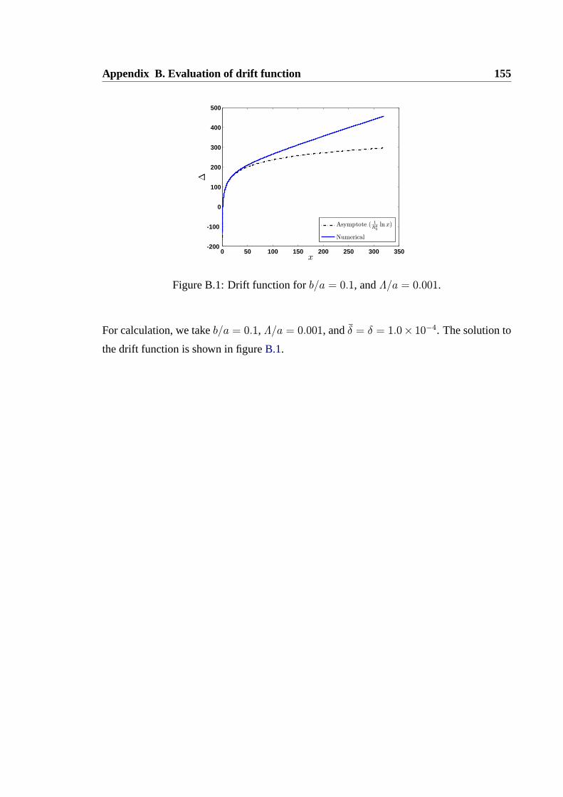
Appendix B. Evaluation of drift function 155
0 50 100 150 200 250 300 350-200
-100
0
100
200
300
400
500
x
1
Δ
1
Asymptote ( 1R20ln x)
1
Numerical
1
Figure B.1: Drift function forb/a = 0.1, andΛ/a = 0.001.
For calculation, we takeb/a = 0.1, Λ/a = 0.001, andδ = δ = 1.0× 10⁻⁴. The solution to
the drift function is shown in figureB.1.

156
References
D. J. Acheson.Elementary Fluid Dynamics. Oxford University Press, 1990.
D. Arnal. Three-dimensional boundary layers: Laminar-turbulent transition. AGARD Rep.
741, Von Karman Inst., Rhode-St.-Genese, Belg., 1986. Special course on calculation of
three-dimensional boundary layers with separation.
D Arnal. Predictions based on linear theory.Progress in transition modelling. AGARD
Rep. No.709, 1994.
A. P. Bassom and P. Hall. Vortex instabilities in three-dimensional layers: the relationship
between Gortler vortices and crossflow vortices.J. Fluid Mech., 232:647–680, 1991.
A. P. Bassom and P. Hall. The receptivity problem forO(1) wavelength Gortler vortices.
Proc. R. Soc. Lond. A, 446:499–516, 1994.
A. P. Bassom and S. O. Seddougui. Receptivity mechanisms for Gortler vortex modes.
Theor. Comput. Fluid Dyn., 7:317–339, 1995.
G. K. Batchelor.An Introduction to Fluid Mechanics. Cambridge University Press, 1967.
F. P. Bertolotti. Response of the Blasius boundary layer to free stream vorticity.Phys.
Fluids, 9:2286–2299, 1997.
H. Bippes. Basic experiments on transition in three-dimensional boundary layers domi-
nated by crossflow instability.Prog. Aerosp. Sci., 35:363–412, 1999.
H. Bippes and H. Gortler. Dreidimensionale storungen in der grenzschicht an einer
konkaven wand.Acta Mech., 14:251–267, 1972.
REFERENCES 157
H. Bippes, B. Muller, and M. Wagner. Measurements and stability calculations of the
disturbance growth in an unstable three-dimensional boundary layer.Phys. Fluids, 3:
2371–2377, 1991.
A. V. Boiko, Y. S. Kachanov, and D. A. Mischenko. Quasi-steady and unsteady Gortler vor-
tices on a concave wall: experiment and theory. In J. M. L. M. Palma and A. Silva Lopes,
editors,Advances in Turbulence XI: Proc. 11th Euromech Euro. Turbulence Conf., Porto,
pages 173–175. Springer, 2007.
A. V. Boiko, Y. S. Kachanov, and D. A. Mischenko. Steady and unsteady Gortler boundary-
layer instability on concave wall.Euro. J. Mech. B/Fluids, 29:61–83, 2010.
G. Bonfigli and M. Kloker. Secondary instability of crossflow vortices: validation of the
stability theory by direct numerical simulation.J. Fluid Mech., 583:229–272, 2007.
A. Bottaro and P. Luchini. Gortler vortices: are they amenable to local eigenvalue analysis?
Euro. J. Mech. B/Fluids, 18:47–65, 1999.
T. Cebeci and P. Bradshaw.Momentum Transfer in Boundary Layers. McGraw-Hill, 1977.
T. Cebeci and J. Cousteix.Modeling and Computation of Boundary-Layer Flows (2nd
Edition). Horizons Publishing Inc., 2005.
M. Choudhari. Roughness-induced generation of crossflow boundary vortices in three-
dimensional boundary layers.Theor. Comput. Fluid Dyn., 6:1–30, 1994.
S. S. Collis and S. K. Lele. Receptivity to surface roughness near a swept leading edge.J.
Fluid Mech., 380:141–168, 1999.
S. J. Cowley, L. M. Hocking, and O. R. Tutty. The stability of solutions of classical un-
steady boundary layer equation.Phys. Fluids, 28(2):441–443, 1985.
R. I. Crane and J. Sabzvari. Laser-doppler measurements of Gortler vortices in laminar and
low-reynolds number turbulent boundary layers. InProc. Int. Symp.Applications of Lase
Doppler Anemometry to Fluid Mechanics, Lisbon, 1982.
J. D. Crouch. Receptivity of three-dimensional boundary layers.AIAA Pap.No. 93-0074,
1993.
REFERENCES 158
J. R. Dagenhart and W. S. Saric. Crossflow stability and transition experiments in swept
wing flow. TP 209344, NASA, 1999.
R. T. Davis and S. G. Rubin. Non-Navier-Stokes viscous flow computations.Comput.
Fluids, 8:101–131, 1980.
H. P. Day, T. Herbert, and W. S. Saric. Comparing local and marching analyses of Gortler
instability. AIAA J., 28(6):1010–1015, 1990.
J. P. Denier, P. Hall, and S. O. Seddougui. On the receptivity problem for Gortler vortices:
vortex motions induced by wall roughness.Phil. Trans. R. Soc. Lond. A, 335:51–85,
1991.
H. Deyhle and H. Bippes. Disturbance growth in an unstable three-dimensional boundary
layer and its dependence on environmental conditions.J. Fluid Mech., 316:73–113,
1996.
P. G. Drazin and W. H. Reid.Hydrodynamic Stability. Cambridge University Press, 1981.
P. W. Duck, A. I. Ruban, and C. N. Zhikharev. The generation of Tollmien-Schlichting
waves by freestream turbulence.J. Fluid Mech., 312:341–371, 1996.
M. V. Finnis and A. Brown. The linear growth of Gortler vortices.J. Heat Fluid Flow, 18:
389–399, 1997.
J. M. Floryan. On the Gortler instability of boundary layers.Prog. Aerospace Sci., 28:
235–271, 1991.
J. M. Floryan and W. S. Saric. Stability of Gortler vortices in boundary layers.AIAA J., 20
(3):316–323, 1982.
J. M. Floryan and W. S. Saric. Wavelength selection of Gortler vortices.AIAA J., 22(11):
1529–1538, 1984.
M. Gaster. A note on the relation between temporally-increasing and spatially-increasing
disturbances in hydrodynamic stability.J. Fluid Mech., 14:222–224, 1962.
M. Gaster. On the effects of boundary-layer growth on flow stability.J. Fluid Mech., 66:
465–480, 1974.

REFERENCES 159
M. E. Goldstein. Unsteady vortical and entropic distortions of potential flows round arbi-
trary obstacles.J. Fluid Mech., 89:433–468, 1978.
M. E. Goldstein. The evolution of Tollmien-Schlichting waves near a leading edge.J.
Fluid Mech., 127:59–81, 1983.
M. E. Goldstein. Scattering of acoustic waves into Tollmien-Schlichting waves by small
streamwise variations in surface geometry.J. Fluid Mech., 154:509–529, 1985.
M. E. Goldstein and L. S. Hultgren. Boundary-layer receptivity to long-wave free-stream
disturbances.Annu. Rev. Fluid Mech., 21:137–166, 1989.
H. Gortler. Uber eine dreidimensionale instabilitat laminarer grenzschichten an konkaven
wanden.des. d. wiss. gottingen, nachr.1(2); translated as ‘on the three-dimensional in-
stability of laminar boundary layers on concave walls’. TM 1375(1954), NACA, 1940.
N. Gregory, J. T. Stuart, and W. S. Walker. On the stability of three-dimensional boundary
layers with application to the flow due to a rotating disk.Philos. Trans. Roy. Soc. Lond.
Ser. A, 248:155–199, 1955.
A. N. Gulyaev, V. E. Kozlov, V. R. Kuzenetsov, B. I. Mineev, and A. N. Sekundov. Interac-
tion of a laminar boundary layer with external turbulence.Izv. Akad. Nauk. SSSR Mekh.
Zhid. i Gaza, 24(5):700–710, 1989.
P. Hall. Taylor–Gortler vortices in fully developed or boundary-layer flows: linear theory.
J. Fluid Mech., 124:475–494, 1982.
P. Hall. The linear development of Gortler vortices in growing boundary layers.J. Fluid
Mech., 130:41–58, 1983.
P. Hall. The nonlinear development of Gortler vortices in growing boundary layers.J.
Fluid Mech., 193:243–266, 1988.
P. Hall. Gortler vortices in growing boundary layers: The leading edge receptivity problem,
linear growth and the nonlinear breakdown stage.Mathematika, 37:151–189, 1990.
P. Hall and N. J. Horseman. The linear inviscid secondary instability of longitudinal vortex
structures in boundary layers.J. Fluid Mech., 232:357–375, 1991.
REFERENCES 160
T. S. Haynes and H. L. Reed. Simulation of swept-wing vortices using nonlinear parabo-
lized stability equations.J. Fluid Mech., 405:325–349, 2000.
W. Heisenberg.Uber Stabilitat und Turbulenz von Flussigkeitsstromen.Ann. Phys., Lpz.
(4)74,577–627. (translated as ‘On stability and turbulence of fluid flows ’,Tech. Memor.
Nat. Adv. Comm. Aero, Wash., No. 1291(1951)). 1924.
T. Herbert. Parabolized stability equations.Annu. Rev. Fluid Mech., 29:245–283, 1997.
R. E. Hewitt and P. W. Duck. Pulsatile jets.J. Fluid Mech., 670:240–259, 2011.
J. C. R. Hunt. A theory of turbulent flow round two-dimensional bluff bodies.J. Fluid
Mech., 61:625–706, 1973.
Lord Kelvin. On a disturbing infinity in lord rayleigh’s solution for waves in a plane vortex
stratum.Nature, 23:45–46, 1880.
N. Kemp. The laminar three-dimensional boundary layer and a study of the flow past a side
edge. Macs thesis, Cornell University, 1951.
J. Kim, T. W. Simon, and S. G. Russ. Free-stream turbulence and concave curvature effects
on heated transitional boundary layers.ASME J. Heat Transfer, 114:338–347, 1992.
V. Kottke. On the instability of laminar boundary layers along concave walls towards
Gortler vortices. InPropagation in Nonequilibrium Systems, pages 390–398, Berlin,
1988. Springer.
L. S. G. Kovasznay. Turbulence in supersonic flow.J. Aero. Sci., 20:657–682, 1953.
S. J. Leib, D. W. Wundrow, and M. E. Goldstein. Effect of free-stream turbulence and other
vortical disturbances on a laminar boundary layer.J. Fluid Mech., 380:169–203, 1999.
F. Li and M. R. Malik. Fundamental and subharmonic secondary instabilities of Gortler
vortices.J. Fluid Mech., 297:77–100, 1995.
C. C. Lin. On the stability of two-dimensional parallel flows.Quart. Appl. Math., 3:
117–142,218–234,277–301, 1945.
C. C. Lin. The theory of Hydrodynamic Stability. Cambridge University Press, 1955.
REFERENCES 161
L. M. Mack. Boundary-layer linear stability theory.Spec. Course Stab. Transit. Laminar
Flows, AGARD Rep. 709, pages 3.1–81, 1984.
M. R. Malik, F. Li, and C.-L. Chang. Crossflow disturbances in three-dimensional bound-
ary layers: nonlinear development, wave interaction and secondary instability.J. Fluid
Mech., 268:1–36, 1994.
M. R. Malik, F. Li, and C. L. Chang. Secondary instability of crossflow vortices and swept-
wing boundary layer transition.J. Fluid Mech., 399:85–115, 1999.
M. R. Malik and S. A. Orszag. Comparison of methods for prediction of transition by
stability analysis.AIAA J., 18:1485–1489, 1980.
M. V. Morkovin. On the many faces of transition. InViscous Drag Reduction, pages 1–31.
1969.
B. Muller. Experimentelle Untersuchung der Querstromungsinstabilitat im linearen und
nichtlinearen Bereich des Transitionsgebietes. Dissertation zum dr.-ing., Universitat
Fridericiana zu Karlsruhe, 1990.
B. Muller and H. Bippes. Experimental study of instability modes in a three-dimensional
boundary layer.Fluid Dyn. Three-Dimens Turbul. Shear Flows Transit., AGARD CP
438, pages 13.1–15, 1989.
L. L. Ng and J. D. Crouch. Roughness-induced receptivity to crossflow vortices on a swept
wing. Phys. Fluids, 11(2):432–438, 1999.
P. Nitschke-Kowsky and H. Bippes. Instability and transition of a three-dimensional bound-
ary layer on a swept flat plate.Phys. Fluids, 31:786–795, 1988.
S. A. Orszag. Accurate solution of the Orr-Sommerfeld stability equation.J. Fluid Mech.,
50:689–703, 1971.
R. H. Jr Radeztsky, Reibert M. S., and W. S. Saric. Effect of isolated micron-sized rough-
ness on transition in swept wing flows.AIAA J., 37:1371–1377, 1999.
Lord Rayleigh. On the stability, or instability, of certain fluid motions.Proc. Lond. Math.
Soc., 11:57–70, 1880.

REFERENCES 162
H. L. Reed and W. S. Saric. Stability of three-dimensional boundary layers.Annu. Rev.
Fluid Mech., 21:235–284, 1989.
H. L. Reed, W. S. Saric, and D. Arnal. Linear stability theory applied to boundary layers.
Annu. Rev. Fluid Mech., 28:389–428, 1996.
E. Reshotko. Boundary-layer stability and transition.Annu. Rev. Fluid Mech., 8:311–349,
1976.
O. Reynolds. An experimental investigation of the circumstances which determine whether
the motion of water shall be direct or sinuous, and of the low of resistance in parallel
channels.Phil. Trans. Roy. Soc., 174:935–982, 1883.
N. Riley, M. Sanchez-sanz, and E. J. Watson. A planar pulsating jet.J. Fluid Mech., 638:
161–172, 2009.
A. I. Ruban. On the generation of Tollmien-Schlichting waves by sound.Izv. Akad. Nauk
SSSR, Mech. Zhidk. & Gaza., 5:44–52, 1984.
W. S. Saric. Gortler vortices.Annu. Rev. Fluid Mech., 26:379–409, 1994.
W. S. Saric and A. H. Nayfeh. Non-parallel stability of boundary layer flows.Phys. Fluids,
18(8):945–950, 1975.
W. S. Saric, H. L. Reed, and E. B. White. Stability and transition of three-dimensional
boundary layers.Annu. Rev. Fluid Mech., 35:413–440, 2003.
H. Schlichting. Zur Entstehung der Turbulenz bei der Plattenstromung. Nachr. Ges. Wiss
Gottingen, Math.-phys. Kl., pages 181–208, 1933.
H. Schlichting.Boundary Layer Theory. McGraw-Hill, 1955.
L. U. Schrader, L. Brandt, and D. S. Henningson. Receptivity mechanisms in three-
dimensional boundary-layer flows.J. Fluid Mech., 618:209–241, 2009.
L. U. Schrader, L. Brandt, and T. A. Zaki. Receptivity, instability and breakdown of Gortler
flow. J. Fluid Mech., 682:362–396, 2011.
G. B. Schubauer and H. Skramstad. Laminar boundary-layer oscillations and transition on
a flat plate.J. Res. Nat. Bur. Stand., 38:251–292, 1947.

REFERENCES 163
M. P. Schultz and R. J. Volino. Effects of concave curvature on boundary layer transition
under high freestream turbulence conditions.ASME J. Turbomach., 125:18–27, 2003.
A. M. O. Smith. On the growth of Taylor-Gortler vortices along highly concave walls.
Quart. J. Math., 13(3):233–262, 1955.
F. T. Smith. On the nonparallel flow stability of the Blasuis boundary layer.Proc. Roy. Soc.
A, 366:91–109, 1979.
J. D. Swearingen and R. F. Blackwelder. The growth and breakdown of streamwise vortices
in the presence of a wall.J. Fluid Mech., 182:255–290, 1987.
I. Tani. Production of longitudinal vortices in the boundary layer along a concave wall.J.
Geophys. Res., 67(8):3075–3080, 1962.
I. Tani and Y. Aihara. Gortler vortices and boundary-layer transition.ZAMP, 20:609–618,
1969.
I. Tani and J. Sakagami. Boundary-layer instability at subsonic speeds. InProc. Intl.
Council Aerosp. Sci., 3rd Cong., pages 391–403, Washington: Spartan, 1962.
G. I. Taylor. Stability of a viscous liquid contained between two rotating cylinders.Phil.
Tran. Roy. Soc. A, 223:289–343, 1923.
V. Theofilis. Advances in global linear instability analysis of nonparallel and three-
dimensional flows.Prog. Aerosp. Sci., 39:249–315, 2003.
V. Theofilis. Global linear instability.Annu. Rev. Fluid Mech., 43:319–352, 2011.
S. N. Timoshin. Asymptotic analysis of a spatially unstable Gortler vortex spectrum.Izv.
Akad. Nauk. SSSR Mekh. Zhid. i Gaza, 25(1):25–33, 1990.
M. Tobak. On local Gortler instability.ZAMP, 22:130–143, 1971.
W. Tollmien.Uber die Entstehung der Turbulenz.Nachr. Ges. W.iss Gottingen, Math.-phys.
Kl.,21–44. (translated as ‘The production of turbulence’,Tech. Memor. Nat. Adv. Comm.
Aero, Wash., No. 609(1931)). 1929.

REFERENCES 164
W. Tollmien. Ein allgemeines Kriterium Instabilitat laminarer Geschwindigkeitsverteilun-
gen. Nachr. Wiss. Fachgruppe, Gottingen, Math.-Phys. Kl.1, 79–114. (Translated as
‘General instability criterion of laminar velocity distributions’Tech. Memor. Nat. Adv.
Comm. Aero., Wash.No. 792 (1936)). 1935.
M. Turkyilmazoglu, J.S.B. Gajjar, and A.I. Ruban. The absolute instability of thin wakes
in an incompressible compressible fluid.Theoret. Comput. Fluid Dynamics, 13:91–114,
1999.
M. V. Ustinov. Receptivity of the swept wing boundary layer to a steady flow inhomogene-
ity. Fluid Dynamics, 36(3):437–447, 2001.
R. J. Volino and T. W. Simon. Bypass transition in boundary layers including curvature and
favourable pressure gradient effects.ASME J. Turbomach., 117:166–174, 1995.
R. J. Volino and T. W. Simon. Spectral measurements in transitional boundary layers on
a concave wall under high and low free-stream turbulence conditions.ASME J. Turbo-
mach., 122:450–457, 2000.
P. Wassermann and M. Kloker. Transition mechanisms induced by travelling crossflow
vortices in a three-dimensional boundary layer.J. Fluid Mech., 483:67–89, 2003.
S. H. Winoto and R. I. Crane. Vortex structure in laminar boundary layers on a concave
wall. Int. J. Heat Fluid Flow, 2:221–231, 1980.
F. X. Wortmann. Visualizaton of transition.J. Fluid Mech., 38:473–480, 1969.
X. Wu. On local boundary-layer receptivity to vortical disturbances in the free stream.J
Fluid Mech., 449:373–393, 2001a.
X. Wu. Receptivity of boundary layers with distributed roughness to acoustic and vortical
disturbances: a second order asymptotic theory and comparison with experiments.J.
Fluid Mech., 431:91–133, 2001b.
X. Wu, D. Zhao, and J. Luo. Excitation of steady and unsteady Gortler vortices by free-
stream vortical disturbances.J. Fluid Mech., 682:66–100, 2011.
Related Documents