Instabilities of flow in a collapsed tube

J . Fluid Mech. (1990), vol. 220, pp . 623-659 Printed in Great Britain

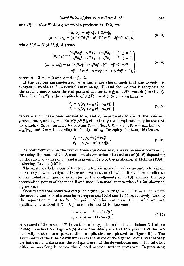
623

Instabilities of flow in a collapsed tube

By 0. E. JENSEN Department of Applied Mathematics and Theoretical Physics, University of Cambridge,

Silver Street, Cambridge CB3 9EW, UK

(Received 13 December 1989)

In a previous paper (Jensen & Pedley 1989) a model was analysed describing the effects of longitudinal wall tension and energy loss through flow separation on the existence and nature of steady flow in a finite length of externally pressurized, elastic-walled tube. The stability of these steady flows to small time-dependent perturbations is now determined. A linear analysis shows that the tube may be unstable to at least three different modes of oscillation, with frequencies in distinct bands, depending on the governing parameters ; neutral stability curves for each mode are calculated. The motion of the separation point a t a constriction in the tube appears to play an important role in the mechanism of these oscillations. A weakly nonlinear analysis is used to examine the instabilities in a neighbourhood of their neutral curves and to investigate mode interactions. The existence of multiple independent oscillations indicates that very complex dynamical behaviour may occur.

1. Introduction The self-excited oscillations which occur in externally pressurized collapsible tubes

are of interest both physiologically, for example as a possible source of the noises heard when a cuff is inflated around the upper arm during sphygmomanometry - the so-called ‘ Korotkoff sounds ’ - and fluid dynamically, where many questions concerning the nature of three-dimensional, unsteady, separating flows must be answered. These oscillations involve the interaction of a high-Reynolds-number internal flow and the elastic tube walls: in the case of airways in the lung they typically take the form of small-amplitude, high-frequency wall flutter causing wheezing ; for tubes in which the fluid inertia is much greater than the wall inertia (such as blood vessels), they may involve larger, lower-frequency variations of pressures, flow rates and the tube cross-sectional area. In many experiments designed to mimic physiological systems (Conrad 1969; Brower & Scholten 1975; Bonis & Ribreau 1978; Bertram, Raymond & Pedley 1990a,b), in which a segment of collapsible tube is mounted between two rigid tubes and is enclosed in a pressurized chamber (see figure l ) , a remarkable variety of unsteady behaviour has been observed even using steady controlling parameters. Bertram et al. (1990a, b ) describe features typical of a complex dynamical system : many oscillations were highly nonlinear ; often the transitions between different oscillatory regimes displayed hysteresis ; unsteady behaviour could be extremely sensitive to small variations in the governing parameters ; and the behaviour frequently appeared to be chaotic, although it was not possible to confirm this conclusively from Bertram’s data. It is therefore desirable to provide a relatively simple mathematical description of this experiment, with a view to obtaining an improved understanding of the mechanism

624 0. E. Jensen

P, P1 P¶

A h A t

x i 0 x = A

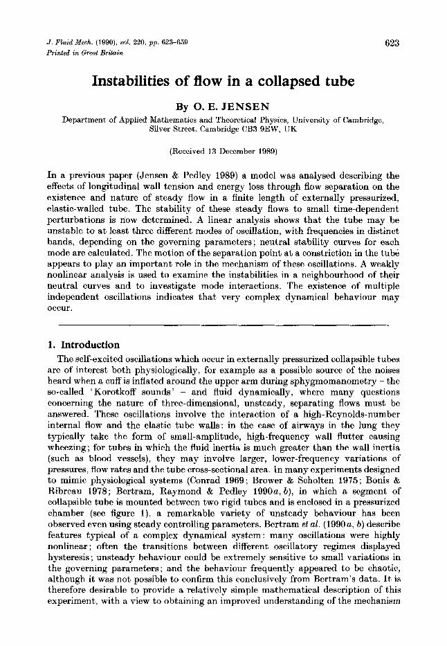
FIGURE 1. The conventional experimental apparatus : an elastic tube of non-dimensional length A and cross-sectional area a(s, t ) is mounted between two rigid tubes and is enclosed in a pressurized chamber. The externally controlled parameters are the chamber pressure p,, the upstream reservoir pressure pr and the resistances T, , 7, and inertances A,, A, of the upstream and downstream rigid tubes; the system is open to the atmosphere downstream.

of a t least some of the oscillations, and also to develop a picture of the detailed bifurcation structure of the system.

The model that will be used in this paper is based upon that devised by Cancelli & Pedley (1985, hereinafter referred to as I), which is a one-dimensional description of the flow in a finite length of collapsible tube in which the tube elasticity is described by a simple ‘tube law ’, relating the non-dimensional tube cross-sectional area a(x,t) (see figure 1) to the transmural pressure (the internal pressure p(x,t) minus the external chamber pressure p e ) , coupled with a description of longitudinal tension (see below). The important features of such a model were described in I , but are summarized again here. (i) It takes account of the energy loss associated with a gradually broadening jet which is formed (at high Reynolds numbers) downstream of a constriction in the tube: such losses were found to be necessary to predict self- excited oscillations in the ‘lumped-parameter ’ models such as that of Bertram & Pedley (1982). (ii) It describes the influence of the upstream and downstream rigid tubes (see figure 1 ) : experimentally these have been shown to have a very significant effect on unsteady behaviour (Conrad 1969; Bertram et al. 1990a); again this was predicted by the lumped-prtrameter models. (iii) Since it is a one-dimensional model (which the lumped-parameter models are not), it describes elastic wave propagation. The importance of this effect was demonstrated by experiments such as those by Brower & Scholten (1975), who found that instability occurred as soon as the flow ‘choked ’ ; they associated the loss of steady flow with the flow speed u(x, t) at some point along the tube exceeding the speed c(x, t ) of small-amplitude pressure waves in the tube wall.

A fundamental feature of the model in I is the description of constant longitudinal wall tension, which makes pressure waves propagate dispersively. Jensen & Pedley (1989, hereinafter referred to as 11) showed that the presence of tension in steady flows in which there is no energy loss allows choking, with the disappearance of steady solutions, not precisely when u > c but rather a t some flow rate which also depends on the degree of longitudinal tension and on the tube length. It was also shown in I1 that the introduction of a model of energy loss through flow separation has a profound effect on the nature of steady solutions : choking no longer occurs, and a steady flow exists for all flow rates. Using the steady solutions predicted by this model, the relation between the pressure drop down the tube and the flow rate was calculated, and qualitatively this compared well with experiment.

The success of the model used in I1 in describing steady, separated flows suggests that i t will also describe a number of the important characteristics of unsteady flows. (Of course with a one-dimensional model it will not be possible to describe wall

Instabilities of flow in a collapsed tube 625

flutter, for example.) Therefore the effect of introducing infinitesimally small, time- dependent perturbations to the solutions calculated in I1 will be considered, to determine the linear stability of these steady flows. It will be found that the tube is unstable to a number of different modes of oscillation, depending on the tube geometry and the governing parameters. A weakly nonlinear analysis will be used to describe first how small-amplitude oscillations develop as a single parameter is varied and a steady solution becomes unstable, and secondly how two independent modes of oscillation interact with one another at particular points in a two-dimensional parameter space.

This largely mathematical approach is complementary to the numerical study in I, as it allows a much broader range of parameter space to be examined. The calculations in this paper and those in I also differ in another important respect : the location of the separation point. Self-excited oscillations will be shown to arise if it is assumed, for example, that separation always occurs where the tube area is minimum. In I, on the other hand, it was possible to obtain large-scale (and presumably experimentally significant) oscillations only if the separation point was assumed to move hysteretically in response to a changing adverse pressure gradient just beyond the constriction. A mechanism (first proposed in I) will be described that demonstrates how motion of the separation point influences unsteady behaviour, while showing that hysteresis is not an essential part of this process.

There have been other numerical studies analysing different models of unsteady flow in collapsible tubes. Following the approach of I, but including variation of longitudinal tension with time, Matsuzaki & Matsumoto (1989) found complicated unsteady solutions of the governing equations. However, the analysis presented here suggests that this additional factor is not a prerequisite for complex behaviour. Walsh, Sullivan & Hansen (1988) used a Lagrangian formulation of the mechanics of an elastic membrane, and included the effects of wall inertia, to describe flow in a one-dimensional model of the trachea. Although they ignored all dissipative effects, they were able to obtain flutter-like oscillations; these appear to arise through a coupling between transverse and longitudinal strain.

With the exception of other flutter studies, few authors have performed linear stability calculations. In I, a finite-difference scheme was used to determine the stability of some steady solutions, but the findings were dependent on the type of differencing used. This difficulty will be avoided by the use of a shooting technique. Reyn (1988) considered the stability of an idealized steady flow (a uniform cylindrical elastic tube mounted in the conventional apparatus), but he neglected to incorporate any energy loss or longitudinal wall-tension in his model. Thus he could examine only subcritical flow (u < c ) , finding that it is linearly stable whenever there is non-zero damping in the rigid parts of the system. The conclusions of this study will be much more general in that it is not restricted to an artificial steady flow or to a small range of flow rates.

The model and the steady flows it predicts are briefly reviewed in $2, and the linear stability analysis of these steady solutions is presented in $3. The weakly nonlinear analysis in $4 is extended in $5 to examine mode interactions at codimension-2 bifurcation points in parameter space. It is demonstrated in the final section ($6) that the linear and weakly nonlinear theories describe many of the significant features of the experiments of Bertram et al. (1990a, b) with reasonable qualitative accuracy. In Appendix A, an explanation is offered of the large regions of unattainable parameter space observed by Bertram et al. (1990 b ) in terms of a static bifurcation of the steady solutions. A more complete description of fully nonlinear and perhaps chaotic

626 0. E . Jensen

behaviour (such as the interaction of three independent oscillations) must await further numerical investigations.

2. An outline of the model and its steady solutions The elastic properties of the tube are described using a ‘tube law’, which relates

the transmural pressure to the tube’s non-dimensional cross-sectional area a(x, t ) . In the absence of longitudinal tension, a good approximation for a uniform tube (Shapiro 1977) is

1-a-t if a < 1 k(a-1) if a > 1;

p - p , = P(a) = I

pressure has been non-dimensionalized with the wall bending stiffness K,. The tube has an unstressed circular cross-section when a = 1 ; for positive transmural pressure i t maintains a circular shape but has very low compliance (k is some large constant, which is taken in these calculations to equal 45, the value corresponding to the experiments of Bertram et al. 1990a, b) . As the transmural pressure decreases below zero the cross-section changes from a circular to an elliptical shape ; then the opposite walls come into contact so that when p - p , is very low only two very narrow channels remain open.

Longitudinal tension in the tube wall is related to the transmural pressure through the longitudinal wall curvature. Assuming first that the tube may be represented by a pair of parallel flat membranes (McClurken et al. 1981), and secondly that a varies slowly with the longitudinal coordinate x (see 11), the effects of constant longitudinal wall tension are approximated by modifying (2.1) as

p-po, = 9(a)- iaxz . (2 .2 )

By incorporating the dimensional tension T into a lengthscale = (Do T/K,)i, where Do is the diameter of the tube, the non-dimensional tension has been set equal to 1. This means that the parameter A, which is proportional to the dimensional tube length, is also proportional to T-4.

Following the non-dimensionalization scheme of 11, the mass and momentum conservation equations for unsteady one-dimensional flow in a collapsible tube are

at + (ua), = 0, (2.3)

Ut+XuUz = -pz . (2.4) (Time is scaled by z/co, where co is the wave speed (K,/p)i and p is the fluid density.) u(x,t) is the axial velocity averaged over the cross-section. The effect of frictional forces is assumed to be negligible: this is a reasonable assumption except when the tube is severely collapsed along much of its length. The only dissipation in the collapsible segment is represented by the factor x in the inertia term of (2.4), which was introduced in I to describe the energy loss that occurs in the region downstream of a constriction in the tube in which there is a gradually broadening, turbulent jet. For a steady high-Reynolds-number flow it is reasonable to assume (as in 11) that the jet separates a t a point x = X which is coincident with X, , the point of minimum area; this is, of course, also Xu, the point of maximum velocity and X,, the point of minimum pressure. Then it is assumed that

x = 1 when O<x<X, O < x < 1 when X<x<A. (2 .5)

InstabiEities of $ow in a collapsed tube 627

0 0.2 0.4 0.6 0.8 1 .O

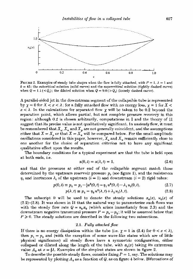
FIGURE 2. Examples of steady tube shapes when the flow is fully attached, with P = 1, h = 1 and k = 45 : the subcritical solution (solid curve) and the supercritical solution (tightly dashed curve) when Q = 1.1 ( < Q , ) ; the dilated solution when Q = 9.0 (> Q b ) (loosely dashed curve).

X

A parallel-sided jet in the downstream segment of the collapsible tube is represented by x = 0 for X < x < A ; for a fully attached flow with no energy loss, x = 1 for X < x < A. In the calculations for separated flow x will be taken to be 0.2 beyond the separation point, which allows partial, but not complete pressure recovery in this region: although 0.2 is chosen arbitrarily, computations in I and the theory of I1 suggest that its precise value is not qualitatively significant. In unsteady flow, it must be remembered that X,, Xu and X, are not generally coincident, and the assumptions either that X = X, or that X = Xu will be compared below. For the small-amplitude oscillations considered in this paper, however, X , and Xu remain sufficiently close to one another for the choice of separation criterion not to have any significant qualitative effect upon the results.

The boundary conditions for a typical experiment are that the tube is held open at both ends, i.e.

and that the pressures at either end of the collapsible segment match those determined by the upstream reservoir pressure p , (see figure l) , and the resistances qt and inertances A, of the upstream (i = 1) and downstream (i = 2) rigid tubes:

a(0,t) = a(A,t) = 1, (2.6)

p(O,t) = P, = p , - ~ U 2 ( 0 , ~ ) - q l U 2 ( 0 , t ) - - l ~ , ( 0 , t ) ,

p(A, t ) = p , = q,u2(A, t )+Azu, (A , t ) . (2.7)

(2.8)

The subscript 0 will be used to denote the steady solutions a,(x), uo(x) of (2.2)-(2.8). It was shown in I1 that the natural way to parameterize such flows was with the steady flow rate Q = uoao (which arises immediately from 2.3) and the downstream negative transmural pressure P = p , -p , ; it will be assumed below that P 2 0. The steady solutions are described in the following two subsections.

2.1. Ful ly attached flow

If there is no energy dissipation within the tube (i.e. x = 1 in (2.4) for 0 < x < A ) , then p , = p , and (with the exception of some wave-like states which are of little physical significance) all steady flows have a symmetric configuration, either collapsed or dilated along the length of the tube, with ao(x) taking its extremum value A , at x = ;A. Examples of the simplest states are shown in figure 2.

To describe the possible steady flows, consider fixing P = 1, say. The solutions may be represented by plotting A , as a function of Q , as on figure 4 below. Bifurcations of

628 0. E . Jensen

x = Yo

0 0.2 0.4 0.6 0.8 1 .0

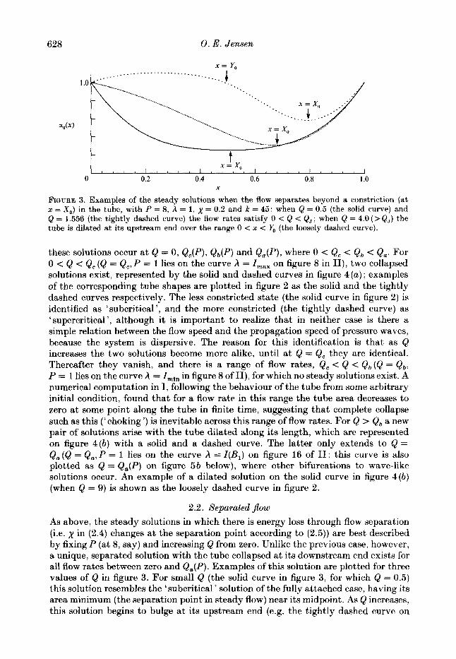
FIGURE 3. Examples of the steady solutions when the flow separates beyond a constriction (at 2 = X,) in the tube, with P = 8, A = 1, x = 0.2 and k = 45: when Q = 0.5 (the solid curve) and Q = 1.556 (the tightly dashed curve) the flow rates satisfy 0 < Q < QJ; when Q = 4.0 [ > Q,) the tube is dilated a t its upstream end over the range 0 < z < & (the loosely dashed curve).

X

these solutions occur at Q = 0, Q,(P), Q,(P) and Q,(P), where 0 < Q, < Q, < Q,. For 0 < Q < Q, (Q = Q,, P = 1 lies on the curve h = I,,, on figure 8 in 11), two collapsed solutions exist, represented by the solid and dashed curves in figure 4 (a) ; examples of the corresponding tube shapes are plotted in figure 2 as the solid and the tightly dashed curves respectively. The less constricted state (the solid curve in figure 2 ) is identified as ‘subcritical’, and the more constricted (the tightly dashed curve) as ‘supercritical’, although it is important to realize that in neither case is there a simple relation between the flow speed and the propagation speed of pressure waves, because the system is dispersive. The reason for this identification is that as Q increases the two solutions become more alike, until a t Q = Q, they are identical. Thereafter they vanish, and there is a range of flow rates, Q, < Q < Q,(Q = Q,, P = 1 lies on the curve h = Imin in figure 8 of II), for which no steady solutions exist. A numerical computation in I, following the behaviour of the tube from some arbitrary initial condition, found that for a flow rate in this range the tube area decreases to zero a t some point along the tube in finite time, suggesting that complete collapse such as this (‘ choking ’) is inevitable across this range of flow rates. For Q > Q, a new pair of solutions arise with the tube dilated along its length, which are represented on figure 4(b) with a solid and a dashed curve. The latter only extends to Q = Q, (Q = Q,,P = 1 lies on the curve h = I @ , ) on figure 16 of 11; this curve is also plotted as Q = Q,(P) on figure 5 b below), where other bifurcations to wave-like solutions occur. An example of a dilated solution on the solid curve in figure 4 ( b ) (when Q = 9) is shown as the loosely dashed curve in figure 2.

2.2. Separated flow

As above, the steady solutions in which there is energy loss through flow separation (i.e. x in (2.4) changes a t the separation point according to (2.5)) are best described by fixing P (at 8, say) and increasing Q from zero. Unlike the previous case, however, a unique, separated solution with the tube collapsed a t its downstream end exists for all flow rates between zero and &,(P). Examples of this solution are plotted for three values of Q in figure 3. For small Q (the solid curve in figure 3, for which Q = 0.5) this solution resembles the ‘ subcritical ’ solution of the fully attached case, having its area minimum (the separation point in steady flow) near its midpoint. As Q increases, this solution begins to bulge at its upstream end (e.g. the tightly dashed curve on

Instabilities of $ow in a collapsed tube 629

figure 3) and the separation point X, moves downstream. When Q = Q,(P), where 0 < Q,(P) < &,(P) (& = QJ, P = 8 lies on the curve A = I @ , ) on figure 16 of 11; the curve Q = Q,(P) is also plotted on figure 5 b below), this bulge has grown such that a,,(O) = 0; for Q > Qj the tube is dilated for 0 < x < Y,, say, and collapsed for y0 < x < A. An example of such a state is plotted as the loosely dashed curve in figure 3, for which Q = 4. The ‘jump point’ Y , (shown on figure 3, so-called because the gradient of the tube law (2.1) is discontinuous across it) moves downstream as the flow rate rises, and approaches x = A as Q --f Q,. For larger flow rates the tube can switch to a fully dilated state (by jumping onto the solid solution branch in figure 4b) in which there is no energy loss. Note that the jump in the gradient of the tube law (2.1) and in x (2.5) cause discontinuities in the third and fourth derivatives of ao(x) (and uo(x)) at Y, and X , respectively.

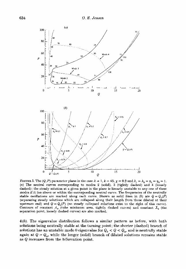
A more global description of these steady, separated solutions is provided by figure 5(b) below. This is a map of the (Q,P)-plane in the case A = 1, k = 45 and x = 0.2, showing contours of the tube minimum area A , (the tightly dashed curves), of the position of the separation point X , (the loosely dashed curves) and two solid curves, Q = &,(P) (along which Y , = 0) and Q = Qa(P) (Y , = A) . This figure will be considered further in $3.5.

3. Linear stability theory 3.1. Formulation

In this section the stability of the steady solutions ao(x), uo(x) of (2.2)-(2.8) to small time-dependent perturbations will be analysed. The tube area and fluid velocity may be written as

a(x, t ) = ao(x) +a’($, t ) , ufz, t ) = uo(x) + u’(x, t ) .

(3.1)

(3.2)

Substituting these expressions into (2.2)-(2.4), eliminating the pressure and removing the time-independent terms which govern the steady solution leads to

a; + (u’a, + u, a’), = - (u’a’),, (3.3)

(3.4) U;+X(U,U’)~+ (a’9’(ao))z-&~zz = -$~(~’2)Z-(+‘29’’(a0)+&’39’”(a,)+. . .),,

with boundary conditions (from (2.6)-(2.8))

a’(0, t ) = 0,

a’(A, t ) = 0,

-~a;,(o,t)+(++~l)2u,(0)u’(0, t)+A,uI(O,t) = - (++?&P(O, t ) ,

-$&(A, t ) - 2 y 2 u,(A) u’(A, t ) -A2 u,’(A, t ) = q2 d 2 ( A , t ) . (3.7)

(3.8)

All the nonlinear terms have been taken to the right-hand sides of (3.3)-(3.8) ; they will be neglected in the remainder of $3.

Recall that, if all energy losses are ignored, x = 1 in (3.4) along the length of the tube. However, if the flow is assumed to separate, then because of the two discontinuities inherent in the model - the jump in x (2.5) and in the gradient of the tube law (2.1) - two internal .boundary points must be considered explicitly: the separation point X ( t ) , which is assumed to be either the point of minimum area X,(t) or the point of maximum velocity X,(t), so that either

a z ( X , t ) = 0 or u,(X, t ) = 0; (3.9a, b )

630 0. E . Jensen

and, if it exists, the jump point Y(t) at the downstream end of a bulge in the tube where

a(Y,t) = 1. (3.10)

Equations ( 3 . 9 ~ or b) and (3.10) can be used to calculate the perturbation of each point about its steady position (X, or Y,,) as a(z, t ) varies according to (3.1). A t each point continuity of area, velocity and pressure must be ensured. So at the separation point, for example, the first-order terms in the expansion of conditions such as [a(z, t)];! = 0 are derived, which requires expansion first of a about its steady value using (3.1), and then expansion ofX about X,. Using either ( 3 . 9 ~ ) or (3.9 b) , it is easily shown that

[u’, a’, a:, a:,]2t = 0. (3.11)

Accordingly the predictions of linear theory are independent of the choice of the position of the separation point. The steady-state area has a discontinuous fourth derivative at X, (see 11), and correspondingly the lowest discontinuous derivative of a’ is the third, representing a jump in the perturbation pressure gradient. A similar argument must be followed at the jump point, where consideration of the velocity and area imply that

[u’, a’, a:12+, (3.12)

while to ensure that the pressure (2.2) is continuous, one must take

[a’9’(a0)-~a~,]2+ = 0. (3.13)

Unfortunately when a,,(0) = 0 (i.e. Q = QJ(P) ) , the tube law in (3.4) cannot be used consistently within linear theory, since perturbations Y in the position of the jump point are an order of magnitude greater than those in the tube area (and also depend explicitly upon the sign of a,(O,t)). The following calculations are invalid in this exceptional case.

When linearized, the perturbation equations (3.3) and (3.4) admit solutions with separable space- and time-dependence, so solutions for which u’ and a’ are both proportional to e(r+i‘o)t can be sought. The stability of a steady solution is determined by the corresponding eigenvalues (7, w ) . These have to be determined numerically, as the coefficients in the governing linearized equations (3.3) and (3.4) depend on z.

3.2. Numerical method The governing equations may be reformulated as a set of ordinary differential equations with four independent variables u‘, a‘, a: and a:,, which are written as Re (Z,(x) e(r+iw)t), i = 1 , 2 , 3 , 4 respectively, where Re denotes real part. Then the linearized versions of (3.3) and (3.4) become

2, = - (a,, Z, + (7 + iw + u,,) Z, + u, Z,)/a,,

2, = z,, 2, = z,,


and the linearized boundary conditions (3.5)-(3.8) may be rewritten as

BU(7, w ) z(0) = 0,

BD(7, w ) Z(A) = 0,

(3.15)

(3.16)

where Z = (Zl, Z,, Z,, Z4)T and

(3.17)

(3.18)

Equation (3.11) tells us that 2 is continuous across the separation point; the discontinuity in 2, a t the jump point given by (3.13) must also be considered.

A shooting technique is used to solve this linear, boundary-value eigenproblem. The solution of (3.14)-(3.18) may be expressed as

z = AIZ(1)+A,Z(2) (3.19)

(A, and A , are complex), a combination of two linearly independent solutions 2(3), j = 1,2 , which both satisfy the upstream boundary conditions (3.15). For fixed Q, P and A (which define a steady state), (3.14) is integrated downstream for some ( 7 , w ) to find each of these solutions, and then the complex 2 x 2 matrix

D(7, w ) = (B, Z ( l ) ( A ) , B, Z2)(A))

is calculated. Now from (3.19) and (3.20),

B, Z(A) = B, (A , 2‘’’ ( A ) + A 2 ( 2 ) ( A ) ) ,

= DA,

(3.20)

(3.21)

(3.22)

where A = (A1,A,JT. Therefore (7, w ) are eigenvalues of (3.14)-(3.18) provided that the downstream boundary conditions (3.16) are satisfied, i.e. if, and only if, for non- trivial A

d ( 7 , w ) = det (0) = 0. (3.23)

Therefore, by seeking the zeros of d over the complex plane, either by locating the intersections of the loci of Re (d ) = 0 and Im (d ) = 0, or by locating the minima of Id(, the eigenvalues corresponding to a given steady solution may be determined. An eigensolution is then computed by using as initial values Z(0) = Z(l)(O) + A,Z(”(O), where a is an eigenvector satisfying D a = 0; a may be arbitrarily normalized since the problem is homogeneous.

A shooting method was chosen in order to avoid the inconsistencies between different finite-difference schemes experienced in I. Nevertheless, shooting has its own difficulties, which arise in calculating d ( 7 , w ) . For example, when shooting using values of 7 and w which do not coincide with an eigenvalue (as is generally the case), the components of 2 grow very rapidly as x increases, and small errors are therefore quickly magnified. This occurs increasingly for larger values of A , 7 and w. Inaccuracies accumulate further when d is evaluated using (3.23), as this involves calculating the relatively small difference of two large numbers. (Modifications of the method, such as parallel shooting across small subsections of [0, A ] , fail to alleviate

632 0. E . Jensen

this problem.) Although d is generally well behaved across most of parameter space, there are situations in which it is impossible to calculate eigenvalues with an integration scheme of given tolerance and order. (In these calculations a fourth-order Runge-Kutta scheme from the NAG numerical library was used with a relative error tolerance of lo’+.) For example, when Q is near zero and P is large, so that the tube is substantially collapsed over most of its length, the coefficients in (3.14) become very large (e.g. s’(01,) = 500 if 01, = 0.098). If A = 1 , for example, the method breaks down a t small flow rates (Q < 0.5) once P > 25.

The large number of parameters in the problem prohibit a very extensive examination of parameter space. In all that follows a restricted but hopefully representative domain will be considered : ql = q2 = A, = A, = 1 , k = 45, x = 0.2 and A = 1 .

3.3. The distribution of eigenvalues

Since (3.14)-(3.18) is a one-dimensional boundary-value problem over a finite domain, it has an infinite number of discrete eigenvalues; each associated eigensolution has a wavelength which is determined by the length of the tube. The eigenvalues arise either as complex-conjugate pairs or as pairs of real roots, and so the eigenmode corresponding to the j t h pair is labelled by its frequency w j , j = 0, I , 2 , etc. Thuso, = 0, and in general oi + Oforj >, 1 . The numerical constraints described above prevent examination of any modes higher than the fifth, but this is not too severe a restriction : first, the low modes give an indication of how the higher modes behave ; secondly, the model is based upon a long-wavelength approximation, so it cannot be expected to describe the shorter-wavelength perturbations accurately,

Let us begin the description of the distribution of eigenvalues in the complex plane with a simple case: Q = 0 and P positive. With these parameter values, the steady equations have a solution in which tube is collapsed symmetrically (such as the solid curve in figure 2 ) , the tube law and longitudinal wall tension together determining its shape. (This solution lies on the branch of subcritical solutions, i.e. on the solid curve on figure 4 ( u ) ; the supercritical solution a t Q = 0 has zero minimum area (see the dashed curve in figure 4u), and so infinitely negative internal pressure a t its midpoint, which is obviously unphysical.) With no flow through it, the elastic tube behaves like a stretched string : all modes are neutrally stable standing waves. With P = 1, the eigenvalues 7 j & i w j , j = 0 , 1 , 2 , . . . , all have zero real part, with o, = 0, o1 = 3.72, w2 = 17.63, w3 = 43.97, up = 83.28, etc. The dispersive influence of longitudinal wall tension is responsible for the irregular distribution of eigenvalues along the imaginary axis. The j t h oscillatory mode has j half-wavelengths of area perturbation over the length of the tube, with each half-wavelength in antiphase with its neighbour. I n what follows, the paths of these eigenvalues in the complex plane will be traced as the flow rate is increased, considering first fully attached flow (53.4) and then separated flow (83.5).

3.4. Fully attached $ow Consider holding P = 1 and increasing Q from zero. The steady solutions that exist in this case are represented on the bifurcation diagrams in figure 4, in which extremum area is plotted against flow rate. Recall from 52.1 that for 0 < Q < Q J P ) two distinct collapsed solutions exist, represented in figure 4 ( a ) . As Q grows from zero each eigenvalue corresponding to the subcritical solution moves leftwards from the imaginary axis. The (real) mode 0 eigenvalue moves from the origin down the negative real axis, reverses direction and returns to the origin as Q + Q , ; the remaining eigenvalues do not leave the left-hand half-plane. Thus the subcritical


0

1.5 -

1.4 -

1.3 -

A" 1

1.2 -

0.5 1 .o 1.5 Q

FIGURE 4. Bifurcation diagrams representing typical steady solutions when the flow is fully attached, obtained by plotting extremum tube area A , against flow rate Q for fixed values of downstream pressure ( P = 1) and tube length ( A = 1): (a) two branches representing collapsed solutions, the solid curve corresponding to the subcritical solution and the dashed to the supercritical solution (cf. the solid and tightly dashed curves in figure 2); ( b ) two branches of solutions with the tube dilated along its length, calculated with k = 45; the solution with Q = 9 is plotted on figure 2.

collapsed solution (represented by the solid curve in figure 4a) is neutrally stable when Q = 0 and Q = Q,, and stable otherwise. On the other hand, the supercritical collapsed solution (the dashed curve in figure 4a) is unstable for 0 < Q < Q,, as a positive real eigenvalue which originates from infinity moves in towards the origin of the complex plane as Q increases from zero ; it also reaches the origin as Q --f Q,. The stable subcritical solution meets the unstable supercritical solution at the turning point (Q = Q,) in the bifurcation diagram in figure 4 ( a ) ; this is a saddle-node bifurcation. For Q, < Q < Qb no steady solutions exist, and then at Q = Qb another saddle-node bifurcation occurs as two dilated solutions appear, as shown in figure

634

I00

80

0. E . Jensen

60

P

40

20

I00

80

60

P

40

20

I 5 10 15 20 Q Q = Q d P )

FIQURE 5 . The (&,P)-parameter plane in the case A = 1, k = 45, x = 0.2 and A, = A, = v1 = 7, = 1. (a) The neutral curves corresponding to modes 2 (solid), 3 (tightly dashed) and 4 (loosely dashed) ; the steady solution at a given point in the plane is linearly unstable to any one of these modes if it lies above or within the corresponding neutral curve. The frequencies of the neutrally stable oscillations are marked along each curve. Shown as solid lines in (a) are Q = Q,(P) (separating steady solutions which are collapsed along their length from those dilated at their upstream end) and Q = &,(P) (no steady collapsed solutions exist to the right of this curve). Contours of constant A , (tube minimum area, tightly dashed curves) and constant X , (the separation point, loosely dashed curves) are also marked.

4 ( b ) . The eigenvalue distribution follows a similar pattern as before, with both solutions being neutrally stable at the turning point ; the shorter (dashed) branch of solutions has an unstable mode 0 eigenvalue for Qb < Q < Qa, and is neutrally stable again a t Q = Q,, while the longer (solid) branch of dilated solutions remains stable as Q increases from the bifurcation point.


3.5. Separated $ow As was described in $2.2, when there is energy loss in the tube through flow separation, then for fixed downstream transmural pressure P > 0 a unique steady solution exists for 0 < Q < Q,(P). Once again the eigenvalues can be followed in the complex (~,w)-plane as the flow rate is increased from zero for a fixed value of P . When Q = 0 all the eigenvalues lie on the imaginary axis (see §3.3), and for small Q these all move into the left-hand half-plane. A real eigenvalue (e.g. 7,) cannot become positive for larger Q, as a divergent bifurcation would imply the existence of a second, steady solution of the governing equations, which is known not to exist. If P is small (less than about 6.2 for the values of A , x, etc., considered here), then for 0 < Q < Q,(P) all the eigenvalues with an imaginary part remain in the left-hand half-plane also. Thus the steady solution remains stable for these values of Q and P . If P is slightly larger, on the other hand (between about 6.2 and 12.4), then as Q increases from zero the mode-2 eigenvalue moves first from T = 0 into T < 0, and then reverses direction and enters the right-hand half-plane. As it crosses the imaginary axis (i.e. as r2 passes through 0) , the steady state undergoes a Hopf bifurcation and becomes unstable to a mode-2 oscillation with frequency w2. As Q increases further, the mode-2 eigenvalue returns again to T < 0, and the steady state regains stability. The boundary of the region of ( Q , P)-parameter space for which the steady state is linearly unstable to a mode-2 oscillation (i.e. the locus T~ = 0) has been calculated for P < 100, and is plotted as the solid line in figure 5(a ) .

For larger values of P, the eigenvalues corresponding to the third- and fourth- order modes may also cross the imaginary axis for certain ranges of flow rate, making the tube unstable to these higher-mode oscillations as well. The neutral stability curves of these modes, the loci r j = 0,j = 3,4 have also been plotted on figure 5 (a) . It is clear from figure 5 (a ) that the steady solutions are linearly stable for small Q or small P . Notice that there are regions of parameter space in which as many as three modes are unstable simultaneously. (Mode-5 instabilities were also identified for large Q and P, but since w5 is so large accurate calculation of r5 = 0 was not possible.) On figure 5 (a ) the (dimensionless) frequency of the neutrally stable oscillations is indicated a t points along each neutral curve. Each mode oscillates in a distinct frequency band: modes 2, 3, and 4 have frequencies in the range 10-25, 25-60 and 50-110 respectively.

The shape of the neutral curves is clearly influenced by the behaviour of the steady solutions across (Q, P)-space, which is represented in figure 5(b). The two solid lines in this figure are Q = Qj(P) and Q = Q,(P). At points between these curves the tube has a jump point Y,, somewhere along its length. Notice that the discontinuity in the tube law manifests itself as discontinuities in the gradient of a neutral curve where it intersects Q = QJ(P) ; this is apparent as a bulge along the lower left portion of r2 = 0. The ‘kinks’ in r3 = 0 and rP = 0 as each curve crosses Q = Qj(P) arise from a combination of this discontinuity with the strong nonlinearity of the steady solution, which is responsible for a similar kink (with Q < QJ(P)) in the contour A , = 0.1 in figure 5 ( b ) .

3.6. The nature of the oscillations The tightly dashed curve in figure 3 shows the steady tube shape ao(x) when P = 8 and Q = 1.556, a situation in which the tube is neutrally stable to a mode-2 oscillation. Notice that a,(.) shows a definite asymmetry; this is reflected in the shape of the amplitudes of the perturbation area, velocity and pressure, which are plotted as functions of x in figure 6. Notice also the discontinuous perturbation

21 FLM 220

636 0. E . Jensen

0.2

la’l

0.1

0

2

I 4

1

0

I I . I . I I I I I I I I I I I I I I . J I I I I I I .o

X o.6 t O 3 0 0.2 0.4

x = x, FIQURE 6. The amplitudes of (a) the area, ( b ) the velocity and (c) the pressure of the marginally stable mode-2 eigensolution of frequency o = 9.74, which exists when P = 8, &, = 1.556, and all other parameters as in figure 5. The corresponding steady state is shown as the tightly dashed curve in figure 3.

pressure gradient across the separation point X,. The two-humped shape of this mode-2 oscillation is obvious. Whereas the neutrally stable mode-2 oscillation which exists when Q = 0 is symmetric, with the two halves of the tube vibrating exactly out of phase, in this case the phase of the eigensolution increases slightly along each half of the tube, implying that the crests of the perturbations will move upstream.

The form of the oscillation may be visualized more clearly if the size of the infinitesimal perturbation is exaggerated and is superimposed upon the steady state ; their sum is plotted as a function of space and time in figure 7. The oscillating path of the separation point, taken here to be the point of minimum area, is indicated by a wavy curve (which should of course be almost exactly straight). This figure is presented to demonstrate the mechanism of self-excited oscillations proposed in 5 5.2 of I : as the separation point moves downstream, an increasing proportion of the flow along’ the tube becomes attached, and this results in a wave of high pressure propagating downstream and a low-pressure wave moving upstream ; the former is reflected at the junction with the downstream rigid tube, forcing the area in the downstream half of the collapsible tube to increase ; this causes the constriction to diminish and the separation point to move upstream. The reverse process then


FIGURE 7. The area perturbation in figure 6 is artificially amplified and superimposed upon the steady state, and then plotted as a function of space and time over two periods; the position of the moving separation point X,(t) is marked with a solid line.

begins, with a low-pressure wave moving downstream, ultimately causing the separation point to move downstream once more.

This mechanism provides a possible explanation of the absence of any unstable mode- 1 oscillations. Since these are disturbances with only a single half-wavelength along the length of the tube, the pressure and area gradients across the separation point will generally be smaller than with higher modes. Longitudinal motion ofX will thus be smaller, and hence mode-1 perturbations will not be capable of drawing sufficient energy from the flow to become unstable.

4. Weakly nonlinear analysis It was shown in $3.5 that if the flow in the tube separates, then for suitable

parameter values a Hopf bifurcation occurs as either the flow rate Q, or the downstream transmural pressure P , is varied through some point (Qo, Po) on a neutral curve corresponding to mode j, j = 2,3,4. In this section the nonlinear terms of (3.3)-(3.8) will be used to determine whether such a bifurcation is sub- or supercritical.

Consider a vector in the (Q , P)-plane which passes through (Qo, Po) ; for the moment its direction is assumed to be arbitrary. To determine the nature of the mode-j oscillation a t points a small distance p-po along this vector from (Qo,P0), the following expansions are made in powers of a small quantity E (a measure of the amplitude of the perturbation) of the conventional Stuart-Watson type :

p = p, + e2p2 + W3), (4.1) qY(q t ) = s ( ~ ( x ) A ( T ) eiwjot + c.c.)

+ ~ ~ ( # ~ ~ ( ~ ) A ~ ( T ) e ~ ~ ~ r o ~ + c . c . +#,,(x)IA(T)I2) + ~ ~ ( # ~ ~ ( z ) A ~ ( T ) e ~ ~ ' + o ~ + # ~ ~ ( x ) d(T)eiW~ot+c.c.)+O(s4), (4.2)

where #' = ( a ' , ~ ' ) ~ (see (3.1) and (3.2)) and the functions q$ z (a,,uJT, i = 1,22,20, etc., are to be calculated. An overbar will be used to denote complex conjugate (c.c.). oio is the frequency of the linear mode-j oscillation at (Qo, Po). A(T) is an 0(1) complex function of a slow time T = s2t, its real and imaginary parts represent slow temporal variations in the amplitude and phase of the perturbation; d ( T ) depends on A and

21-2

638 0. E . Jensen

(AI2A. #1 is the neutrally stable fundamental eigensolution (calculated in §3), #,, represents a distortion to the mean flow generated by quadratic nonlinearities, #22

and & are harmonics of the fundamental perturbation, and #31 is a distortion of this fundamental.

In varying Q or P near the bifurcation point according to (4.1), the steady solution changes from ao(x;po) = E,(x) (a tilde will denote that a quantity is to be evaluated at p = po) to

(4.3)

(4.4) aa, aP

where

etc. For completeness a steady, separated solution will be considered in which the tube is dilated a t its upstream end and collapsed downstream (e.g. the loosely dashed curve in figure 3), so that it has a jump point % and a separation point 2, (see $2.2) ; it is an elementary matter to apply this discussion to the simpler case.

Substituting (4.1)-(4.3) into the nonlinear equations for time-dependent perturbations to steady flow (3.3)-(3.8), a succession of boundary-value problems are recovered at increasing orders in e. These will be complicated by the jump conditions : the steadx-state area dio(x) has discontinuities in its third and fourth x-derivatives at

and X , respectively, and these have an increasing influence on the lower derivatives of the perturbations at higher orders in e. In addition, the O ( 2 ) and O(e3) perturbations depend on whether the separation point is chosen to be the point of minimum area or of maximum velocity. Results will be presented for each case. The details of the jump conditions are given in Appendix B.

At O(E) , two sets of equations are obtained, one the complex conjugate of the other, each equivalent to the original linear stability problem that was the subject of $3. This system of equations may be represented succinctly as

o ? . o , p ( 4 = - (x; Po),

(4.5) 1 (L-iwjol)#l = 0,

J+l = S#l = 0, B o G q o ) 41 = BA(iW,O) 41 = 0,

where I is the identity matrix. The linear differential operator L (from (3.3) and (3.4)) is written as

L = ( - az(.ii,* ) - % ( 9 ’ @ 0 ) * ) +a axsz

and the boundary condition operators (from (3.5)-(3.8)) are

(4.7)

J and S (in 4.5) refer to the jump conditions at x = 8 and x = z,, which were shown in (3.11)-(3.13) to be respectively

Instabilities of j b w in a collapsed tube 639

At second order in E , three boundary-value problems emerge. First, taking all the terms proportional to A2 e2i@’fot gives

(4.10)

Note how the quadratic forcing terms on the right-hand sides of (4.10) match the right-hand sides of (3.3)-(3.8). The corresponding nonlinear jump perturbations, J422 and S#,,, are given in Appendix B. The second set of equations, those terms proportional to A2e-2i@’jot, is simply the complex conjugate of those above. The third set consists of real functions, which arise from taking all terms proportional to IAI2 :

0 Bo(o) 420 = (- (1 + 2r1) U l ( O ) a1(0)

(4.1 1)

J+,, and S&, are given in Appendix B. Now from the linear stability calculations it is known that in general the homogeneous problem

(L-iD I)# = 0 , Bo(ii2) 4 = 0 , BA(iD) 4 = 0 , J4 = S4 = 0 (4.12)

has a non-trivial solution only when D = q0. (The exceptional case, when two modes become unstable simultaneously, will be examined in $ 5 . ) Thus each of the inhomogeneous boundary-value problems (4.10) and (4.1 I) has a unique solution. These can be calculated with a shooting method similar to that described in $3.2 : $22

and 420 are expressed as the sum of an arbitrary inhomogeneous solution (satisfying the inhomogeneous upstream boundary and jump conditions) and a suitable linear combination of Zl and Z2 (see 3.19), chosen such that the sum satisfies the inhomogeneous downstream boundary conditions.

At 0(c3) two further boundary value problems are obtained. Only one of these need be considered, however. Taking all terms proportional to ei@jot, one finds

(4.13)

The components of F are determined from the nonlinear terms in (3.3) and (3.4) :

640 0. E . Jensen

the inhomogeneous contributions to the boundary conditions (from (3.5)-(3.8)) are

(4.15) 1 GI = - [(I + 271) ((% u20 + G 2 =

u 2 2 ) A I A 1 2 +ul s 0 , p p 2 A ) +’l u1 ATlz-O,

u20+a1 u 2 2 ) A 1 A 1 2 + u 1 ‘ 0 , p p 2 A ) +’2 u1 AT1z-A ;

J#31 d and S$,, d are given in Appendix B. To ensure that the forcing terms in (4.14) and (4.15) give rise to an O(1)

eigensolution, so that the expansion (4.2) remains uniformly asymptotic for T = O ( i ) , these inhomogeneous terms must satisfy a solvability condition. This is obtained by calculating the eigensolution #of the adjoint operator Lt; the details of this procedure are described in Appendix C. Using the inner product ( . ) defined by (C l), the adjoint eigensolution is defined so that the boundary and jump condition terms vanish in

(4.16)

where R($t, 4,) is a quadratic function related to L (see C 5). Now (4.13) will have a bounded solution provided #t is also adjoint to #31, i.e. provided (4.16) is satisfied with all the inhomogeneous terms in (4.13) substituted :

(#, F) = d ( [ R ] ; - [R];;’- [R]5+). (4.17)

This equation may be shown to reduce to an equation for the complex amplitude

HoAT = -H1p2A-H2IAl2A (4.18)

(recall that p , is the independent bifurcation parameter given in (4.1)), where the coefficients Ha, H , and H , are derived from boundary conditions and integrals involving the first-order eigensolution, its adjoint and the solutions of the second- order boundary -value problems. Expressions for these coefficients are presented in Appendix D ; note that substantial contributions arise from the jump and separation points. Using (D 1) and (D 2),

t f - Po+ (bt , L4J = <L+#t> 41) + [RI;:- [RI& [Ripob-'

YO-

A ( T ) ,

Ha = flO(ift? 411, H , = H1(4+, $1 ; p ) (4.19)

and a2 = HM+’t , 91,42)> (4.20)

where the product terms in (D 3) are given by

(4.21)

There is a substantial amount of algebra and computation required in the evaluation of these coefficients. While there is no simple way to confirm the accuracy of the calculated values of H , (short of numerical solution of (2.3) and (2.4)), there is fortunately a simple check on the accuracy of Ha and H , since the linear term in (4.18) is related to quantities that can be calculated independently using the results of $3, as the following heuristic argument shows. In the expansion (4.2) the time- dependent part of the mode-j linear eigensolution e(Tj+i”’j) has effectively been replaced by A(T) eiojot. If one writes A(!?’) = r(T) eie(T)t, then r(T) x eTjt and B(T) x (u,-q0) t . Now since from (4.1) p = p o + ~ * p 2 , 7&) and q(p) may be expanded as

I {Ul, v,) = u, %a + a1 v22, [u,, w,, wl] = (u, w, @I+ u1 g, w, +a, w1 2 0 1 ) .

(4.22)


where the subscript 0 denotes evaluation a t p = pa, so that

and so from (4.18) at leading order

(4.23)

(4.24)

Since the choice of the direction of the vector parameterized by p is arbitrary, it may be chosen to be tangent to the neutral curve at (Qo,Po). The eigenvalue r,+io, corresponding to parameter values along this vector follows a path which is tangential to the imaginary axis, i.e. dr,/dp vanishes when p = pa, and from (4.24) the real part of H J H , vanishes there also. This and similar checks have been confirmed.

Suppose now that p is normal to the neutral curve, passing into the (Q , P)-domain in which mode j is unstable, so that dr,/dp > 0. Then defining p = -Re (HJH, ) pz, the real part of (4.18) may be written

?: = ~ ~ - 1 ~ 3 , (4.25)

a standard normal form equation for a Hopf bifurcation, where 1 (the Landau constant) is the real part of H2/Ho. If 1 > 0 then the bifurcation is supercritical, and as p increases the steady solution becomes unstable to a stable mode-j oscillation of non-zero amplitude. Otherwise, if 1 < 0 then the linearly stable steady solution in the neighbourhood of the neutral point coexists with an unstable nonlinear oscillation, and the bifurcation is sub-critical.

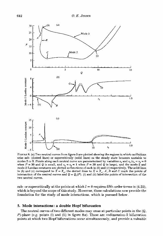
The Landau constant in (4.25) has been calculated along the neutral curves of modes 2 and 3 for P < 30; it is not possible to calculate 1 either for larger values of P or for those modes with higher frequencies, because of the limited accuracy of the numerical solutions of the linear stability problem. The sign of 1 (calculated assuming X = X,) is indicated in figure 8(a ) , where the mode-2 and -3 neutral curves have been plotted with solid lines if 1 is positive and dotted lines if 1 is negative ; the variation of I along each neutral curve is shown in more detail by the solid lines in figures 8 (6) and 8 ( c ) for modes 2 and 3 respectively. The dotted curves in these two graphs show the corresponding values of 1 calculated assuming that the separation point is the point of maximum velocity Xu. Clearly the predictions of the weakly nonlinear theory are not strongly dependent on the assumed position of the separation point. Of far greater significance is the form of the model tube law (2.1). Recall that the linear stability calculations are not valid at those points where the neutral curves intersect Q = Q,(P) (marked as A , B and C on figure 8), and across such points the neutral curves have discontinuities in gradient and curvature. Similarly, I has jumps in gradient and curvature, although over a much more rapid scale. This behaviour is an artefact of the tube law, and I is therefore unlikely to be physically meaningful in neighbourhoods of these points.

Elsewhere, however, both modes arise predominantly through supercritical Hopf bifurcations, although each has a region of subcritical behaviour near the point (ii) on figure 8 ( a ) where the two neutral curves intersect. Where the bifurcation is supercritical the neutral curve bounds a domain of parameter space in which the steady state is stable to linear and weakly nonlinear perturbations. Where it is subcritical, hysteresis between the stable steady state and a stable nonlinear oscillation can in general be anticipated. To determine whether oscillations develop

642 0. E . Jensen

30

25

20

15

10

P

5

0 5 10 15 Q

FIGURE 8. (a) Two neutral curves from figure 5 are plotted showing the regions in which oscillations arise sub- (dotted lines) or supercritically (solid lines) as the steady state becomes unstable to modes 2 or 3. Points along each neutral curve are parameterized by variables sz and s8 (sz = .s3 = 0 when P = 30 and Q is small, and s2 = s8 = 1 when P = 30 and Q is large), and the mode-2 and mode-3 Landau constants are plotted as functions of each in (a) and ( c ) respectively. The solid lines in ( b ) and (c) correspond to X = X,, the dotted lines to X = X , . A , B and C mark the points of intersection of the neutral curves and Q = Q,(P). ( i ) and (ii) label the points of intersection of the two neutral curves.

sub- or supercritically a t the points at which 1 = 0 requires fifth-order terms in (4.25), which is beyond the scope of this study. However, these calculations now provide the foundation for the study of mode interactions, which is pursued below.

5. Mode interactions: a double Hopf bifurcation The neutral curves of two different modes may cross at particular points in the (&,

P)-plane (e.g. points (i) and (ii) in figure 8a). These are codimension-2 bifurcation points at which two Hopf bifurcations occur simultaneously, and provide a valuable


opportunity for analytical treatment of the local dynamics. Of course only a small number of such points can be examined, and the results will be dependent on the parameter values chosen. It is hoped, however, they will provide a good flavour of more global dynamical behaviour.

Let (Qo, Po) be a point a t which modes 2 and 3, say, become unstable. Two non- parallel vectors in (Q,P)-space may be chosen which both pass through this bifurcation point, and let p-po and v-uo be the distance along each from (Qo, Po). Then expansions similar to (4.1) and (4 .2 ) can be made:

AE(T) #it)(x) e2iW2t+Ai(T) #!$(x) e2iwat + C.C.

+ IA2(T) 12#%(x) i- IA3(T) 12#%(x) + A , A , #r) ei(w*+wa)t +A2A- 3 2 @(-) ei(wz--w,)t + C.C.

+ 2

+ ~ ~ ( ~ , ( T ) # ~ ~ ) ( s ) e ~ ~ a ~ + 5 ; 4 , ( T ) # ~ ~ ) ( x ) eiwat+c.c. and additional terms)

+ o(E4). (5.3) As before #' = ( a ' , ~ ' ) ~ and w 2 , w 3 are the frequencies of the two modes a t the bifurcation point. The analysis that follows requires that the two frequencies are not strongly resonant, i.e. that they satisfy

mw,+nw3 =!= 0 for m , n = 0 , 1 , 2 , 3 . (5.4) As each frequency is the root of some highly nonlinear equation, (5.4) is almost invariably satisfied, especially to within the bounds of numerical error. (However, with many independent parameters in this problem apart from Q and P, a resonant bifurcation can undoubtedly be obtained.) A,,j = 2,3, are complex functions of a slow time T = e2t, and d,(T) depends on A,, IA2I2A, and IA3I2A,. In varying the parameters around the bifurcation point the steady solution is also perturbed, as in (4.3) :

a O ( x ; ~ , v) = + ~ 2 ( ~ 2 ~ 0 , r ( ~ ) + ~ 2 ~ 0 , v ( ~ ) ) + 0 ( ~ 3 ) . (5.5) These expansions are substituted into the nonlinear equations (3.3)-(3.8) governing

perturbations to steady flow, and a sequence of linear equations is recovered at increasing powers of B , following the pattern of $4. The equations for the eigensolutions #I,), #${), #,j = 2 , 3 , follow immediately from (4.5), (4 .10) and (4.11) respectively, and the adjoint eigensolutions # j ) t , j = 1 , 2 , are calculated as before using Appendix C. However, a t second order in 8, provided the non-resonance conditions (5.4) are satisfied, two additional inhomogeneous boundary-value problems arise : the terms proportional to A2A3ei("'zfWa) give

644 0. E. Jensen

and those proportional to A2A3 ei(wz-wa)t give

In each case the discontinuities in the eigensolutions at To and may be determined using Appendix B, and (5.6) and (5.7) are solved in the usual way.

At O(e3), taking terms proportional to eiujt,j = 2,3, two boundary-value problems are obtained for #$fat,. These are of the form (4.13) but with inhomogeneous terms (labelled by j = 2,3) given by

(5.9) I (5.10) i {ul, up} = u:”v‘,;) + 4” v22 ( 5 ) 3

[u,, v23 = { uv)vit) + u13)vi-) + G \ ~ ) v ~ ) if j = 2 4 3 + g + u ( 2 ) 4 - ) + +2) (+) if j = 3.

1 v2 u1 v2

Jump conditions are again obtained from Appendix B. It is from this set of equations that a pair of coupled amplitude equations can be

derived. Following the same procedure as in $4, the adjoint eigensolutions are combined with the inhomogeneous equations for #d,, j = 2,3, to obtain two solvability conditions. These reduce to

Hpkl,, = -(Hi? p2 +Hi”? U2)A2-HpIA,12A2 -H$2’IA312A2, Hi3’A3, = -(Hi:)p2 +Hit) V ~ ) A , - H ~ ) J A ~ ~ ~ A ~ - H ( , ~ ) J A ~ J ~ A ,

(cf. (4.18)), where the coefficients may be expressed in terms of the functions given in Appendix D. Thus for j = 2,3,

(5.12)

645

(5.13)

(5.14)

ur)wg) +u$3’w‘-’ +d3) (+) if j = 2 4 3 ) , 4 ) + u ( 2 ) ~ - ) +&2) (+) if j = 3,

1 1 1 wl”),

2 1 % 1 2 1 21-2

u1 v1 w1 [u,, wl, wl] = (upJy’w\w + (3)+W (k) +fpwywy

+ u $ W w i 3 ) ~ i W + uiW.@)w(f) + a(Ww(W

where k = 3 if j = 2 and k = 2 if j = 3. If the vectors parameterized by p and v are chosen such that the p-vector is

tangential to the mode-3 neutral curve at ( Q 0 , Po) and the v-vector is tangential to the mode-2 curve, then the real parts of the terms HI: and HE) vanish (see (4.24)). Therefore if r,(T) is the amplitude of A,(T), j = 2,3, (5.11) simplifies to

(5.15)

where p and v have been rescaled to ,ii, and ,ii3 respectively to absorb the non-zero growth rates, and aZ2 = -Re (Hi2)/H$2)) , etc. Finally each amplitude may be rescaled to simplify (5.15) further, by setting F2 = ~,/la,,l~, F3 = ~ ~ / l a ~ ~ l ~ , b = aZ3/la3,l, c = a3 , /~a22~ and d = f 1 according to the sign of a33. Dropping the bars, this leaves

i, = r,(p, + T i + bri), i3 = r3(p3 + cri + dr i ) .

(5.16)

(The coefficient of ri in the first of these equations may always be made positive by reversing the sense of T . ) A complete classification of solutions of (5.16) depending on the relative values of b, c and d is given in $7.5 of Guckenheimer & Holmes (1986), following Takens (1974).

The unsteady behaviour of the tube in the vicinity of a codimension-2 bifurcation point may now be analysed. There are two instances in which it has been possible to obtain reliable numerical estimates of the coefficients in (5.16), namely the two intersection points of the mode-2 and mode-3 neutral curves with P < 30, shown in figure 8 (a).

Consider first the point marked (i) on figure 8(a), with &, = 9.60, Po = 12.55, where the mode-2 and -3 oscillations have frequencies 10.18 and 39.55 respectively. Taking the separation point to be the point of minimum area (the results are not qualitatively altered if X = Xu), one finds that (5.16) becomes

i2 = y2(p2 - T; - 5.02~3, t3 = r3(p3-o. i iT;-r;) .

(5.17)

A reversal of the sense of T shows this to be type Ia in the Guckenheimer & Holmes (1986) classification. Figure 9 ( b ) shows the steady state at this point, and the two neutrally stable area perturbation amplitudes are plotted in figure 9(c). The asymmetry of the tube clearly influences the shape of the eigensolutions, so that they are both much alike across the collapsed neck at the downstream end of the tube but differ in wavelength across the dilated section further upstream. Representing

646 0. E . Jensen

Q

0.81 ' " " " " ' " " " ' ' " ' " ' ~ 0 0.2 0.4 0.6 0.8 1 .o

X

0.2

0.1

0 1 .o 0.2 0.4 0.6 0.8 X

FIGURE 9. The double Hopf bifurcation point a t Q = 9.60, P = 12.55: the mode-2 and mode-3 interactions in a neighbourhood of the point of intersection of the two neutral curves are shown schematically in (a ) ; r2 and r3 are the slowly varying amplitudes of the mode-2 and mode-3 perturbations. The steady state at the bifurcation point is shown in ( b ) , and the two perturbation area amplitudes are plotted in ( c ) .

solutions of (5.17) as trajectories in the ( r2 , r,)-plane, the structure of the phase space in the neighbourhood of (Q0,P,) is shown schematically in figure 9(a). The origin corresponds to the steady solution, and a non-trivial fixed point on the rp (r,)-axis corresponds to a mode 2(3) oscillation with frequency w 2 ( w 3 ) . Such points arise through pitchfork bifurcations in ( r2 , r,)-space, which are equivalent to the original

Instabilities of f i w in a collapsed tube 647

P -

1.3 1.4 1.5 I .6 Q

0 0.2 0.4 0.6 0.8 1 .o X

(4 r

0 0.2 0.4 0.6 0.8 1 .o X

FIQURE 10. The double Hopf bifurcation point at Q = 1.48, P = 28.16 (cf. figure 9).

Hopf bifurcations in the phase space S of solutions of the governing equations (2.2)-(2.8). Since both the mode-2 and the mode-3 oscillations arise supercritically, the fixed points on each axis are stable. Additional supercritical pitchfork bifurcations in (r2, r,)-space (corresponding to Hopf bifurcations of the periodic orbits in S ) occur across the two lines p3 = pJb , where b = 5.02, and p, = cp2, where c = 0.11 (see figure 9a) , as a further fixed point with non-zero r2 and r3 appears and then vanishes. This fixed point represents stable quasi-periodic motion with two incommensurate frequencies, i.e. trajectories in S cover the surface of a 2-torus. Such

648 0. E . Jensen

behaviour should be observable within a wedge of (Q, P)-parameter space adjacent to the codimension-2 point ; the two pitchfork lines in figure 9 (a) are the tangents of this wedge at the bifurcation point.

The other codimension-2 bifurcation to be examined has Qo = 1.48 and Po = 28.16, and is point (ii) on figure 8(a) . The calculated values of the coefficients in (5.16) are b = -9.82, c = 14.55 and d = 1, making this a type 111 bifurcation in the Guckenheimer & Holmes (1986) classification. Again the steady state and the two area eigensolutions are shown in figure I0 ( b ) and (c ) . The two frequencies in this case (21.06 and 31.22) are much closer in magnitude than in the previous example, and correspondingly the two eigensolutions bear a closer resemblance to one another. (Note that they are not far from a strong $resonance, but not so close for this analysis to be invalid.) From the bifurcation diagram in figure 10 (a ) it is clear that the mode- 2 and mode-3 Hopf bifurcations are subcritical, and in this instance there is a wide domain of parameter space near (Qo,Po) in which unstable quasi-periodic motion is predicted. Thus, unfortunately, this third-order theory predicts none of the behaviour that will be observed in practice in the neighbourhood of this bifurcation point, as nothing can be said about the large-amplitude mode-2 and mode-3 oscillations that can be expected to exist for neighbouring parameter values.

6. Discussion 6.1. Fully attached flow

It was shown in $3.4 that when there is no energy loss in the collapsible tube, a steady, linearly stable, solution with the tube collapsed along its length exists provided the flow rate Q is sufficiently small. As Q increases beyond a critical value Q,, which depends on the downstream transmural pressure P, the longitudinal wall tension and the tube length A, this steady solution vanishes and choking is inevitable. For larger flow rates a steady, linearly stable dilated configuration exists. It is not possible to associate the loss of steady behaviour with the flow speed a t some point in the tube exceeding the local wave speed, as was suggested by the experiments of Brower & Scholten (1975), because the dispersive effect of longitudinal wall tension means that there is no unique wave speed.

This analysis is consistent with the numerical computations reported in $4.1 of I. With either a very small flow rate or large longitudinal tension, ensuring that Q < Q, in each case, a collapsed solution corresponding to a stable, ‘subcritical ’ state was obtained as the final steady state of an initial-value problem. Complete collapse of the tube at some point along its length occurred at a larger flow rate (with Q, < Q < Qb). It thus appears essential to include dissipation within the tube for oscillatory behaviour to occur.

6.2. Separated $ow In $3.5 it was demonstrated that for a particular set of parameter values ( A , k, x, T ~ , etc.) the steady, separated solutions which exist across (Q, P)-space are linearly unstable to a t least three different modes of oscillation. Each mode consists of small perturbations of area, velocity and pressure with an integral number of half- wavelengths along the length of the tube, and each has a frequency in a distinct range. The domains of parameter space in which each mode is linearly unstable are bounded by neutral curves: a set of such curves is shown in figure 5(a). The higher- mode instabilities (with shorter wavelengths and higher frequencies) arise a t larger values of Q and P , when the tube has an increasingly narrow collapsed neck at its


downstream end and is dilated upstream ; an example of such a state is shown in figure 9 (b) . The narrowness of the neck may be estimated from figure 5 ( b ) , where the position of the separation point X , is shown as a function of Q and P. Roughly speaking, as the ‘aspect ratio ’ of the tube increases (the ratio A to A-X,) the number of unstable modes increases, just as occurs with Rayleigh-BBnard convection experiments in a box of fixed height and increasing length. This ‘aspect ratio’ increases with A for fixed Q and P (see 11), which is consistent with the observation of Bertram et al. (1990a) that the number of unstable modes increases with increasing tube length over a given ( Q , P)-range.

At any point in parameter space only a finite number of modes will be involved in the fully nonlinear, unsteady behaviour of the tube, and the dynamics may then be represented by a vector field on a low-dimensional centre manifold. The dimension of this manifold increases with the ‘ aspect ratio ’ of the tube. At points where just one mode becomes unstable (in the neighbourhood of a neutral curve) amplitude equations were derived which approximate the motion in a two-dimensional phase plane containing a stable or unstable limit cycle ($4). At the intersection points of two neutral curves, where two modes become unstable simultaneously, the motion on a four-dimensional centre manifold was represented with a set of coupled amplitude equations ($5) . In one instance it was possible to predict the existence of stable, quasi-periodic motion on a 2-torus.

There are domains of parameter space in which three modes are simultaneously unstable. One might expect that in such cases, provided the oscillations are not strongly resonant, an essentially quasi-periodic motion would result, with the frequency spectrum having a small number of distinct contributions at different frequencies. In fact such three-frequency behaviour has only rarely been observed in experiments on nonlinear physical systems (Swinney 1983). Instead, what generally occurs is that as soon as a third mode becomes unstable, the frequency spectrum develops a broad-band structure, indicating chaotic motion ; Swinney gives references of experiments in which this transition to chaos has been observed. (Such a transition sequence was first proposed by Ruelle & Takens (1971), and it draws upon a theorem of Newhouse, Ruelle & Takens (1978) which says that a 3-torus, satisfying certain technical conditions, is not structurally stable and can be perturbed to a strange attractor.) Therefore, on the basis of previous experimental observations, the tentative postulation can be made that chaotic behaviour can be expected across at least some parts those regions of parameter space in which there is competition between three unstable modes.

6.3. Comparison with experiment Unfortunately, quantitative comparison between the present theory and experiment is not yet possible. Of all the currently available studies, only Bertram et al. (1990a) recorded all the relevant parameters, and even these results do not allow direct comparison : first, constraints on the numerical method (see $3.2) did not allow the use of dimensionless tube lengths A as large as the data demand; secondly, it was shown in $5.3 of I1 that the model for steady flow (based on an approximation that the tube walls behave like thin membranes) does not describe Bertram’s experiments with thick-walled tubes with quantitative accuracy. In addition, there are a number of regions of parameter space in which the model must be regarded as primarily qualitative : at small flow rates (when the tube is collapsed along most of its length), and also in the neighbourhood of Q = Q, (when it is nearing a completely dilated state), the pressure drop down the tube is significantly underestimated because of the

650 0. E . Jensen

I '2 / + - 1

4.69 4.62: 4.52: 4.39 C t

+ LU * + - 3.?8 3.53.. 3.46

228 2.71 2.96 UN C 2.70 3.14 3.06 3.- .26

4 i i + t 0 0 0 0 4 + 0 0 0

, 0 ; 100 200

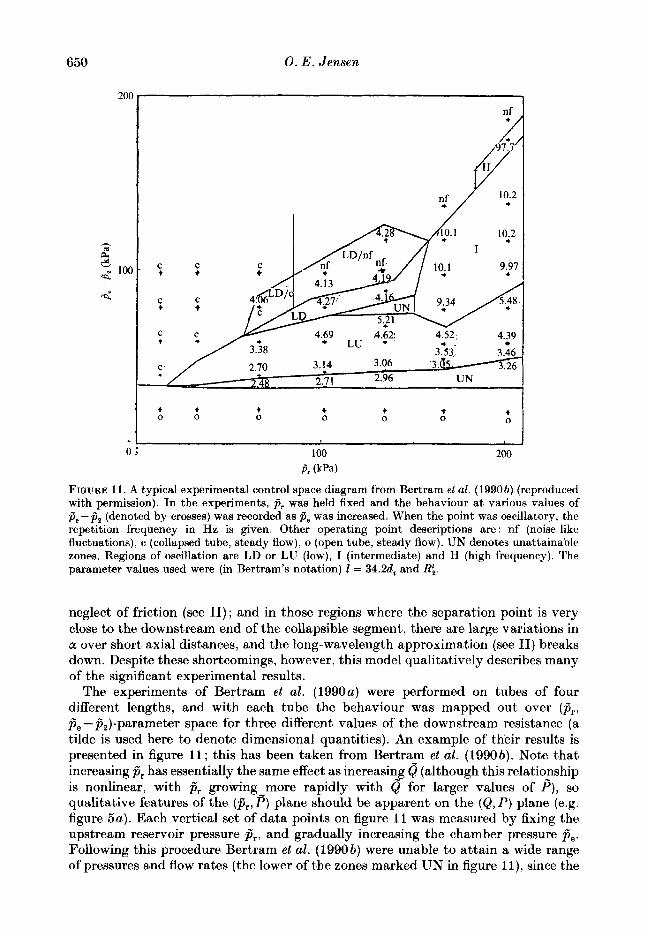
A (kP4 FIGURE 11. A typical experimental control space diagram from Bertram et al. (19906) (reproduced with permission). In the experiments, 3, was held fixed and the behaviour at various values of j3e-@2 (denoted by crosses) was recorded as j3, was increased. When the point was oscillatory, the repetition frequency in Hz is given. Other operating point descriptions are : nf (noise-like fluctuations), e (collapsed tube, steady flow), o (open tube, steady flow). UN denotes unattainable zones. Regions of oscillation are LD or LU (low), I (intermediate) and H (high frequency). The parameter values used were (in Bertram's notation) 2 = 34.2d3, and Rh.

neglect of friction (see 11); and in those regions where the separation point is very close to the downstream end of the collapsible segment, there are large variations in a over short axial distances, and the long-wavelength approximation (see 11) breaks down. Despite these shortcomings, however, this model qualitatively describes many of the significant experimental results.

The experiments of Bertram et al. (1990~) were performed on tubes of four different lengths, and with each tube the behaviour was mapped out over (p , , 9, -&)-parameter space for three different values of the downstream resistance (a tilde is used here to denote dimensional quantities). An example of their results is presented in figure 1 1 ; this has been taken from Bertram et al. (1990b). Note that increasing 9, has essentially the same effect as increasin3 6 (although this relationship is nonlinear, with @, growing more rapidly with Q for larger values of p ) , so qualitative features of the (@,, P ) plane should be apparent on the (&, P ) plane (e.g. figure 5a). Each vertical set of data points on figure 11 was measured by fixing the upstream reservoir pressure pr, and gradually increasing the chamber pressure P e . Following this procedure Bertram et al. (1990b) were unable to attain a wide range of pressures and flow rates (the lower of the zones marked UN in figure l l ) , since the

Instabilities of flow in a collapsed tube 65 1

system would jump from an open state (denoted o in figure 11) along the bottom of such regions (with P x 30 kPa, where the thick-walled tube is on the point of collapse) to one with smaller 9, larger P and the tube collapsed. A qualitative description of this behaviour using the model for steady flow is provided in Appendix A ; it is a static bifurcation phenomenon, a form of cusp catastrophe. No such phenomenon occurs for the parameter values used in figure 5(a ) .

The tube is stable and collapsed (operating points marked c in figure 11) a t small flow rates with P > 30 kPa. The width of the stable zone increases with P in figure 11, but is roughly constant for P > 10 in figure 5 ( a ) : to some extent this difference can be accounted for by the nonlinear relationship between Q and 9,. A variety of different oscillations with increasing frequency arise for increasing values of 9, and P , most of which fall into one of three well-defined frequency ranges: low (3-6 Hz, denoted by LU or LD in figure l l) , intermediate (9-12 Hz, denoted by I) or high (50-100 Hz, denoted by H). The three classes of oscillation can be identified with the distinct modes predicted by the model ; the relative sizes of the frequencies compare favourably with those shown on figure 5(a ) . But, just as in 11, accurate comparison of parameter values is not possible: with a bending stiffness K p = 11.1 kPa, an internal tube diameter Do = 13.3 mm and a longitudinal tension per unit perimeter T = 74.2 Nm-’, Bertram’s parameters give a velocity scale co = 3.33 ms-l, a lengthscale L” = 9.4 mm and so a timescale of 2.8 x lop3 s, making his observed frequencies orders of magnitude smaller than those predicted by the model. The scaling appropriate for thin-walled tubes is obviously not suitable for these experiments.

The resistance of the downstream rigid tube damps the oscillations by taking energy from pressure waves as they are reflected a t x = A. Experimentally, the regions of parameter space in which steady, collapsed flows exist decrease in size as y2 is decreased. Correspondingly, calculations with yz = 0.1, and all other parameters as used in figure 5(a ) , show that decreasing the downstream resistance causes the tube to become unstable to a given mode of oscillation for lower values of Q and P : the neutral curves are shifted mostly towards the Q-axis in the (&, P)-plane. In the process they suffer large but not qualitatively significant deformations, except that the two branches of 72 = 0 form a closed loop at large P.

The low-frequency oscillations recorded by Bertram et al. (1990a, 6 ) fall into two classes, each of them highly nonlinear, large-amplitude oscillations : during an LU oscillation the tube remains open for the majority of the period and suddenly collapses and opens again ; during the LD oscillation it remains closed throughout most of the cycle. The former have elsewhere been referred to as ‘milking ’ oscillations (Bertram 1982), and involve substantial longitudinal motion of the narrowest point of the tube, and thus considerable motion of the separation point. It was demonstrated in this study that small-amplitude oscillations arise if it is assumed that the separation point is coincident either with the point of greatest constriction in the tube, or with the point a t which the flow first experiences an axial deceleration, and that the resulting behaviour is only very slightly different in the two cases. These rather ad hoc assumptions, made for ease of analysis, may well have to be reconsidered in the fully nonlinear regime. Future studies should in particular assess the importance of hysteresis in the motion of the separation point, the condition found in I to be necessary for the prediction of large-amplitude oscillations.

In addition to the oscillations with well-defined frequencies, Bertram et al. (1990a, b ) recorded a variety of other oscillations. Some of the ‘irregular ’ oscillations (not shown in figure 11) with a broad-band frequency spectrum may well be chaotic,

652 0. E. Jensen

and it remains to be determined if this behaviour ever arises (say) through the thpee- frequency route to chaos referred to above. ‘Noisy’ oscillations of very high frequency (marked nf in figure 11) occurred at moderate flow rates and high I‘, in ranges of parameter space in which the tube was substantially collapsed a t its downstream end and flow velocities were therefore high. Bertram et al. (1990b) suggested that these oscillations are due to turbulent fluctuations within the tube, and if this is so i t is not surprising that they cannot be predicted with this simple one- dimensional model. Combinations of all the above types of oscillation were widespread : either two modes with incommensurate frequencies gave rise to quasi- periodic motion (an example of which was predicted in 95); or else their interaction would be strongly resonant, like the ‘ two-out-of-three ’ oscillation described by Bertram el al. (1990a). Finally, the regions marked LD/c and LD/nf in figure 11 are regions of hysteresis, indicating that low-frequency oscillations arise subcritically nearby; this is consistent with the predictions of the model (figure 8a) , since mode-2 oscillations develop subcritically in a comparable region of parameter space.

The author is grateful to acknowledge the support of an SERC Research Studentship, a bursary from Smith Associates Limited, and the generous hospitality during the course of this work of: Professor R. M. Nerem, School of Mechanical Engineering, Georgia Institute of Technology ; Professor J. 0. Kessler, Department of Physics, University of Arizona; and Professor R. D. Kamm, Department of Mechanical Engineering, Massachusetts Institute of Technology. He also wishes to thank Professor T. J. Pedley for his excellent comments and guidance.

Appendix A. Hysteresis of the steady solutions The procedure followed by Bertram et al. (1990a, b) in their experiments was to

hold the upstream reservoir pressure p , fixed (see figure l), and then slowly to increase the external chamber pressure p,. For small p,, p , is sufficiently large for the flow rate to be large and the tube to be completely dilated. Increasing p , causes the downstream end of the tube to collapse, resulting in increased resistance to the flow and a reduction in Q . Bertram et al. (1990a, b ) found that this transition from a dilated to a collapsed state was not always continuous: for the range of parameter space that was explored, for small p , the change might be smooth, while for larger pr a substantial reduction in flow rate would occur as the tube abruptly collapsed, causing a large increase in pe-p,. Subsequent reduction in p , would result in a hysteretic return to an open state. Thus quite sizeable regions of parameter space were ‘unattainable’ by this procedure; an example is shown as the lower of the regions marked UN in figure 11. (Note that the lower boundary of this zone is the value of p,-pz a t which the ‘open to collapsed’ jump occurred with p , increasing, whereas the upper boundary is the critical value of p,-p, at which the tube re- opened with p , decreasing.) Although it was frequently found that the tube would oscillate as soon as it had collapsed, it is confirmed here that this is a static bifurcation of the steady solutions, as Bertram et al. (1990a) proposed. This argument is analogous to the mechanism of ‘ catastrophic collapse ’ predicted by the lumped-parameter model of Pedley (1980).

For fixed p,, I),, T,I~ and qz there are two expressions for the pressure drop down the tube, one equal to the pressure difference imposed by the external parts of the apparatus

Pi-Pz = p r - + ~ 2 ) Q2 (A 1 )

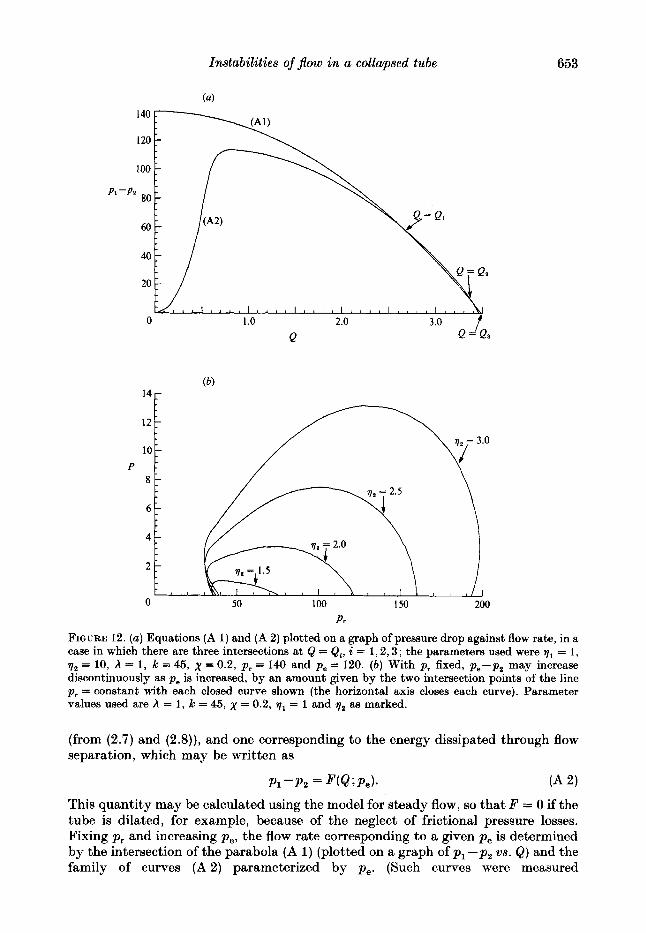
Instabilities of j b w in a collapsed tube

(a)

653

Q Q =‘e3

0 50 100 150 200 P I

FIGURE 12. (a) Equations (A 1) and (A 2) plotted on a graph of pressure drop against flow rate, in a case in which there are three intersections at Q = Q,, i = 1,2,3; the parameters used were y1 = 1, ya = 10, A = 1, k = 45, x = 0.2, p , = 140 and p , = 120. (b) With p , fixed, p , - p , may increase discontinuously aa p , is increased, by an amount given by the two intersection points of the line p , = constant with each closed curve shown (the horizontal axis closes each curve). Parameter values used are A = 1, k = 45, x = 0.2, T~ = 1 and q2 as marked.

(from (2.7) and (2.8)), and one corresponding to the energy dissipated through flow separation, which may be written as

~ 1 - 1 7 2 = F(Q;Pe)* (A 2)

This quantity may be calculated using the model for steady flow, so that F = 0 if the tube is dilated, for example, because of the neglect of frictional pressure losses. Fixing p , and increasing p, , the flow rate corresponding to a given p e is determined by the intersection of the parabola (A 1) (plotted on a graph of p 1 - p , us. &) and the family of curves ( A 2 ) parameterized by p, . (Such curves were measured

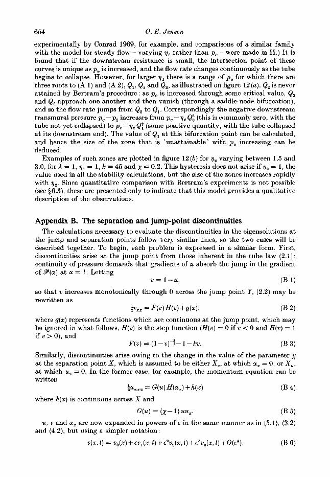
654 0. E . Jensen

experimentally by Conrad 1969, for example, and comparisons of a similar family with the model for steady flow - varying v 2 rather than p, - were made in 11.) It is found that if the downstream resistance is small, the intersection point of these curves is unique asp, is increased, and the flow rate changes continuously as the tube begins to collapse. However, for larger yz there is a range of p , for which there are three roots to (A 1 ) and (A 2), Q1, Qz and Q,, as illustrated on figure 12 (a). Q2 is never attained by Bertram’s procedure : as p , is increased through some critical value, Q, and Q2 approach one another and then vanish (through a saddle-node bifurcation), and so the flow rate jumps from Q3 to Q1. Correspondingly the negative downstream transmural pressure p,-p, increases from p , - T ~ Q: (this is commonly zero, with the tube not yet collapsed) to p , - va Q: (some positive quantity, with the tube collapsed a t its downstream end). The value of Q1 a t this bifurcation point can be calculated, and hence the size of the zone that is ‘unattainable’ with p, increasing can be deduced.

Exa,mples of such zones are plotted in figure 12 ( b ) for v2 varying between 1.5 and 3.0, for h = 1, q1 = 1, k = 45 and x = 0.2. This hysteresis does not arise if q2 = 1, the value used in all the stability calculations, but the size of the zones increases rapidly with 7,. Since quantitative comparison with Bertram’s experiments is not possible (see §6.3), these are presented only to indicate that this model provides a qualitative description of the observations.

Appendix B. The separation and jump-point discontinuities The calculations necessary to evaluate the discontinuities in the eigensolutions at

the jump and separation points follow very similar lines, so the two cases will be described together. To begin, each problem is expressed in a similar form. First, discontinuities arise a t the jump point from those inherent in the tube law (2.1); continuity of pressure demands that gradients of a absorb the jump in the gradient of 9 ( a ) at a = 1. Letting

so that rewritten as

0 = 1-a, (B 1)

increases monotonically through 0 across the jump point Y , (2.2) may be

+%, = mJ) fW-4 +g(z), (B 2)

where g(x) represents functions which are continuous at the jump point, which may be ignored in what follows, H(v) is the step function ( H ( v ) = 0 if v < 0 and H(v) = 1 if v > 0), and

Similarly, discontinuities arise owing to the change in the value of the parameter x at the separation point X , which is assumed to be either X,, a t which a, = 0, or Xu, a t which ux = 0. In the former case, for example, the momentum equation can be written

(B 3) F(v ) = ( l - - v ) - t - l - k v .

;ax,, = G(u) W a x ) + 4x1

G(u) = ( x - 1 ) UU,.

(B 4)

(B 5)

where h(x) is continuous across X and

u, and a, are now expanded in powers of 8 in the same manner as in (3.1), (3.2) and (4.2), but using a simpler notation :

v(2, t ) = vo(x) + €V1(X, t ) + € 2 V Z ( X , t ) +e3v3(x, t ) + 0(€4). (B 6)


Thus v2(x, t ) represents A2w2,(x) etiWt+ ( A ( 2 ~ 2 , ( x ) +X2~22(x) e-liot, etc. P, G, and H may be expanded according to (B 6), so that for example

F(v ) = F(v,) +€?IIF1(VO) + € 2 ( V 2 F ’ ( V O ) ++?J;F(v,))

+e3(v3B”(v0) +v1v2F”(vo) +hV:P’”(v,)) +0(e4). (B 7)

Equations (B 2) and (B 4) are both expanded using expressions such as (B 7) to obtain equations for vixz and a,xxx, i = 0 , 3 at increasing powers of 8. Each of these is of the form

biz2 = fo(4 H(v0) + f l ( X ) @o) +f2(x) #(?I,) + f 3 ( 4 6”(vo) (B 8)

for some fi(z),j = 0 , 3 where S(v) = H’(v) is the delta function. Now it may easily be shown by integration by parts that

&4xx13: =fo(Y,),

and likewise with aix and X, replacing v, and Y, respectively, so (B 9) can be used to determine the discontinuities in the derivatives of a,, i = 1,3, at the jump and separation points. The details of the algebra are omitted, and only the results that are relevant to the analyses in 9$4 and 5 are presented. For brevity’s sake time- dependence will remain suppressed, so that J h represents J#22 or Jd20 etc. The complete time-dependent expansions in particular cases are readily established from the context in $94 and 5. However, the terms that arise at third order that contribute to the growth-rate term in the amplitude equation (4.18) will be introduced; these result from second-order perturbations of the steady state proportional to p2, and are obtained simply by replacing v2 by V ~ + , U ~ I ~ ~ , ~ , for example.

At the jump point, (3.13) is recovered at first order:

A t second order, the only non-zero contributions to J#, are

Fo+ [a&- = ( 3 - 2 4 7 ,

p + 15a: 0 4 2

[ 9 ’ ( & o ) a 2 - ~ a 2 x z ] ~ - = --.

a3 and all its derivatives are discontinuous at E, so in J#, we have

P + 105 a: = ya,(a2 + p2 Go, p ) - __ -

0 8 6 [8 ’ ( E o ) a3 - J

656 0. E. Jensen

One further quantity must be calculated at this order, the jump in u3 at 8. This is obtained from the O ( E ~ ) contribution to the mass conservation relation (3.3) :

iwa3+ (~oa3+gou3)x = - ~ ~ ~ a 2 + ~ 2 ~ l ~ x - ~ , ~ ~ o , , ~ l + ~ o , , ~ ~ ~ x ~ (B 13)

(B 14) Integration across gives

as required.

contribution to S#2 is

Po+ zi0[a31:+ + ii0[U3lPo- = 0

Assuming that the separation point is the point of minimum area, the only

There are two non-zero terms in s#,:

If the separation point is the point of maximum velocity, S#, and S#3 are obtained by replacing every a on the right-hand sides of (B 15) and (B 16) with u.

Appendix C. The adjoint eigensolution At a point (Q0, Po) of marginal stability, the linearized equations governing small-

amplitude perturbations #l = (a1, uJT are given by (4.5)-(4.9). This system of equations is not self-adjoint, and it is necessary to calculate the adjoint eigensolution explicitly. The inner product (-) is defined by

=w, (C 2)

where overbar denotes complex conjugate. Using (C 1) and integrating the first equation in (4.5) by parts gives

(C 3) at,+ (P, l-4) = (W, #) + [RI;: - [R12’- tRl,o- 3

where the adjoint differential operator is

and R(#,+l) is a quadratic function which may be written as

R = - ~ ( . i i o a l + ~ o u l ) - ~ t ( ~ ~ ( ~ O ) a l - ~ a l x x + ~ z i o u l ) - ~ ~ a l x + ~ ~ x a l . (C 5 )

We must choose boundary conditions and jump conditions for the adjoint eigenproblem,

(C 6) Bb#+ = Bf #t = 0, Jt4t = St#? = 0,


such that the terms in (C 3) involving R vanish. To determine the adjoint boundary conditions, one writes

LR1; = @O, b B i , 5-d +B,,dBf\, 5 4 1 9 (C 7 ) i - l , 4

where B, = (Bol,Bo2)T from (4.7) etc., and then choosing B,, = zcl(0), Bo4 = -+zl,(0), B,, = -u,(h) and BA4 = -$l,(A) it is easily shown that

(C 9)

Bi4 = -Qoc?(A) -9 ’ (Eo) at(h)+$L,(h).. 1 together with Bi, = d ( O ) ,

Bi4 = Qo &(O) +s’(bo) tZt(0) -$L,(O),

Iq, = -at@),

To determine whether $ has any discontinuities at the separation point (C 5 ) is rewritten as

R = - al[tZoZt+ 9 ’ ( G 0 ) E’-~zL,. -ul[E0 Zt++tZo a’] -a,,[$L] + al,,[$t]. (C 10)

Since al, and al,, are continuous across xo, and @ must be chosen to be continuous there also. Further, by integrating both equations in (C4) across the separation point, so that for example

(C 11) do(X,) [zt];;: + tZ,(X0) [@]& a + - - 0,

it is clear that the first two square-bracketed quantities in (C 10) vanish, and hence &+ and @, are discontinuous across the separation point with

Similarly, using (C 5 ) it is easily shown that [R]Y“+ vanishes provided c?, at, $, are continuous across the jump point.

now satisfies

and Lt@ = io+, $. It is straightforward to calculate # using the method described in 53.2.

and

With this choice of boundary conditions and jump conditions, the adjoint solution

YO-

w, L4) = (Lvt, +), (C 13)

Appendix D. Coefficients in the amplitude equation These are the expressions used in (4.19) and (5.12) :

Hn($, 91) = [ (dal + d t u 1 ) dx+A1 dull0 +h,dtu,J,; (D 1) 0

Hl($t,#l;,u) = [c?(Egu,+@a,),dx+ at(x(~u1),+(9’’(d,,)E~al),)dz l + (1 + 27J atu, %lo + 2T2 atu, qj,

The shorthand [u3] = [u, u, u] , [u2, w] = [u, u, w] etc. has been used in (U 3). The products {u, v} and [u, v, w] are given in the appropriate parts of the text: (4.21) or (5.13) and (5.14). Equation (D 3) holds under the assumption thatX = X,; ifX = X,, every a in a term evaluated at z,, should be replaced by a u.

R E F E R E N C E S

BERTRAM, C. I). 1982 Two modes of instahility in a thick-walled collapsible tube conveying a flow. J . Biomech. 15, 223-224.

BERTRAM, C. I). & PEDLEY, T. J. 1982 A mathematical model of unsteady collapsible tube behaviour. J . Biomech. 15, 39-50.

BERTRAM, C. D., RAYMOND, C. J . & PEDLEY, T. J . 1990a Mapping of instabilities during flow through collapsed tubes of differing length. J . Fluids Structures 4, 125-153.

BERTRAM, C. D., RAYMOND, C. J. & PEDLEY, T. J. 1990b Applications of nonlinear dynamics concepts to the analysis of self-excited oscillations of a collapsible tube conveying a flow. J . Fluids SZructures (submitted).

BONIS, M. & RIBREAU, C. 1978 Etude de quelques propri6t6s de 1’8coulement dans une conduite collabable. La Houille Blanche 314, 165-173.

BROWER, R. W. & SCHOLTEN, C. 1975 Experimental evidence on the mechanism for the instability of flow in collapsible vessels. Med. Biol. Engng 13, 83S845.


CANCELLI, C. & PEDLEY, T. J. 1985 A separated-flow model for collapsible-tube oscillations.

CONRAD, W. A. 1969 Pressure-flow relationships in collapsible tubes. IEEE Trans. Bio-med.

GUCKENHEIMER, J. & HOLMES, P. 1986 Nonlinear Oscillations, Dynamical Systems and Bifurcations

JENSEN, 0. E. & PEDLEY, T. J. 1989 The existence of steady flow in a collapsed tube. J . Fluid

MATSUZAKI, Y. & MATSUMOTO, T. 1989 Flow in a two-dimensional collapsible channel with rigid

MCCLURKEN, M. E., KECECIOQLU, I., KAMM, R. D. & SHAPIRO, A. H. 1981 Steady, supercritical

NEWHOUSE, S. E., RUELLE, D. & TAKENS, F. 1978 Occurrence of strange axiom A attractors near

PEDLEY, T. J. 1980 The Fluid Mechanics of Large Blood Vessels. Cambridge University Press. REYN, J. W. 1988 Stability of the flow through a collapsible tube mounted in a rigid hydraulic

RUELLE, D. & TAKENS, F. 1971 On the nature of turbulence. Commun. Math. Phys. 20, 167-192;

J . Fluid Mech. 157, 375404 (referred to herein as I).

Enqng, BME 16, 284-295.

of Vector Fields. Springer.

Mech. 206, 33S374 (referred to herein as 11).

inlet and outlet. Trans. ASME K : J . Biomech. Engng 111, 18CL184.

flow in collapsible tubes. Part 2. Theoretical studies. J . Fluid Mech. 109, 391415.

quasiperiodic flows on P , m 2 3. Commun. Math. Phys. 64, 35-40.

circuit (abstract). Phys. Med. Biol. 33 (suppl. l ) , 260.

23, 343-344. SHAPIRO, A. H. 1977 Steady flow in collapsible tubes. Trans. ASME K: J . Biomech. Engng 99,

12fH47. SWINNEY, H. L. 1983 Observations of order and chaos in nonlinear systems. Physicu 7D, 3-15. TAKENS, F. 1974 Singularities of vector fields. Publ. Math. IHES 43, 47-100. WALSH, C., SULLIVAN, P. A. & HANSEN, J. S. 1988 Numerical simulation of flow in the trachea,

incorporating a membrane wall model (abstract). Phys. Med. Biol. 33 (suppl. l) , 263.

Instabilities of flow in a collapsed tube

Documents