Instabilities of a steady, barotropic, wind-driven circulation

Journal of Marine Research, 55, 885-9 13, 1997

Instabilities of a steady, barotropic, wind-driven circulation

by S. P. Meachaml and P. S. Berloff 1,2

ABSTRACT We explore the stability characteristics of a single, barotropic, wind-driven gyre as a function of

the strength of the wind forcing and the size and shape of the basin. We find steady solutions for the barotropic flow in a basin driven by a steady wind stress over a range of values of the Reynolds number and the strength of the wind stress. For those solutions that are close to the stability boundary, we examine the form of the most unstable normal mode. We find that for sufficiently weak forcing, the form of the first instability seen is an instability of the western boundary current. However, for larger values of the forcing, the first instability to set in, as the Reynolds number is reduced, is centered on a standing meander that forms on the continuation of the boundary current after it has left the boundary. Both types of instability are oscillatory. There are several different modes of standing meander instability each associated with Rossby wave-like disturbances in the eastern half of the basin. Each of these modes is most unstable when its frequency is close to a resonance with a basin mode with similar spatial scales.

1. Introduction

Despite the fact that steady, wind-driven circulations in an enclosed basin have been examined fairly frequently over the past few decades, their stability properties are not very well understood. One reason for this is the relatively complicated nature of equilibrium circulations on a P-plane. There is no prospect of calculating the normal modes of these circulations analytically. However, several numerical approaches are available for calculating normal modes. In this paper we use perhaps the simplest such numerical method, based on an evolution model of the flow, and look at the stability of barotropic circulation patterns in a basin on a mid-latitude P-plane. Our main results are that there are two dominant forms of instability in the single gyre problems that we consider-one dominat- ing when the wind forcing is weak and the other when the wind forcing is strong-and that the stability threshold of the basin (as measured in terms of Reynolds number) is strongly influenced by resonances between the localized, oscillatory normal modes that constitute the instability and the normal modes of the quiescent basin.

Before discussing some of the background, let us first specify the particular problem that we will examine. We will consider a single homogeneous layer of fluid driven by a steady

1. Department of Oceanography, Florida State University, Tallahassee, Florida, 32306-3048, U.S.A. 2. Present address: IGPP, University of California, 405 Hilgard Avenue, Los Angeles, California, 90095,

U.S.A. 885

886 Journal of Marine Research 15% 5

wind stress with a uniform curl. The fluid is enclosed by a rectangular basin of uniform depth on a mid-latitude P-plane. We look at barotropic solutions, in which the horizontal flow is taken to be vertically uniform. Friction is included as a Fickian diffusion of relative vorticity in the horizontal with a uniform diffusion coefficient. No attempt is made to make the horizontal diffusion of vorticity sensitive to the local large-scale shear nor is any bottom friction included. At the lateral boundaries we require zero normal and tangential velocities.

Modeling wind-driven barotropicJlow in a basin. Steady solutions of the problem outlined above are strongly asymmetric. This asymmetry is a result of the combined effects of nonlinearity and the gradient of the planetary vorticity. The consequence is a flow in which different regions of the flow have different local instability properties. Normal modes, which are the focus of this paper, are global solutions of the perturbed flow problem. We therefore anticipate that there will be several classes of normal mode instabilities differentiated by the location of the region associated with the dominant transfer of energy from the unstable steady flow to the growing normal mode. There are at least five recognizable regions of a typical steady single gyre circulation: the western boundary current, the “Moore wave” (described further below), one or more inertial recirculations, the Sverdrup interior flow, and a relatively weak zonal boundary current (along the northern boundary in the cyclonic circulation discussed here). Some examples may be seen in Figure 1; more may be found in Meacham and Berloff (1997). For the range of parameters considered in this work, we find that the western boundary current and the “Moore wave” are significant sites of instability. In a companion study of baroclinic flows, Berloff and Meacham (1997), other regions are also found to contribute to instabilities of the general circulation.

In large ocean basins, a dominant feature of the upper ocean circulation is a strong, narrow western boundary current. Steady linear models of the wind-driven circulation, developed by Stommel(1948) and Munk (1950), were able to produce such a feature in the form of a frictional boundary layer. This layer allows the excess potential vorticity picked up by the fluid parcels as they move through the Sverdrup interior to be removed at the side or lower boundary so that the parcels can return to the interior of the circulation and repeat their progress around the basin. On a P-plane, linear frictional homogeneous models of flows in rectangular basins with edges parallel to the geographical coordinate axes and driven by a uniform wind stress curl yield streamlines that are symmetric about the mid-latitude line of the basin and consist of a single dominant cell, the center (i.e. the pressure extremum) of which lies to the west of the center of the basin. The flow along the western boundary is stronger than that along the eastern boundary, with the boundary layer character of the western boundary current increasing as friction is reduced. A second type of model of fundamental importance to circulation problems is the inertial circulation model of Fofonoff (1954). In this, forcing and dissipation are omitted while nonlinearity is retained. An infinite family of free (i.e. unforced) stationary solutions are possible, the

19971 Meacham & BerlofS: Wind-driven circulation instabilities

-

Figure 1. Streamfunctions of marginally stable steady solutions of (2) in a square basin for (a) 6, = 0.0226, (b) 6, = 0.0308, (c) 6, = 0.0382. The contour interval (CI) is approximately 10% of the range of streamfunction values.

simplest of which is a single cell that is symmetric about the mid-longitude line of the basin and which has a center that is displaced toward the northern or southern edge of the basin depending on whether the cell is anticyclonic or cyclonic. Perturbing the linear viscous models with weak nonlinearity results in a meridional displacement of the center of the cell (Munk et al., 1950) while perturbing the nonlinear model with friction moves the center of the basin-wide vortex westward. Thus, in a figurative sense, the linear viscous models and the free nonlinear model of barotropic flow in a rectangular basin appear to lie at the ends of a continuum. (When lateral diffusion of vorticity is included, the inertial limit is sensitive to the boundary conditions specified. Theoretically, when lateral viscosity is included, a generalization of an argument by Stewart (1984) shows that only super-slip boundary conditions are consistent with a predominantly inertial interior. Numerically, when the Reynolds number is sufficiently high, a predominantly inertial solution can still be realized, as shown by Ierley and Sheremet (1995). An extended discussion of these points may be found in Pedlosky (1996).) The circulation in a real ocean is, of course, both unsteady and unsteadily forced, and is affected by both stratification and topography.

888 Journal of Marine Research [55,5

However, if one were to smooth the forcing and construct a steady, flat-bottomed, barotropic model, that included both frictional and inertial effects, then the parameters of the model would put it somewhere in the middle of this continuum.

Following further work on the nature of nonlinear boundary layers by Charney (1955) and Morgan (1956) Moore (1963) proposed an elegant, steady barotropic model that included both frictional and inertial effects. In this model, the northern and southern boundaries are not rigid but are assumed to coincide with latitude lines along which the wind stress curl goes to zero and free slip boundary conditions are applied there. An asymptotic analysis yields a standing, spatially decaying Rossby wave in the region where the western boundary current leaves the western boundary and the flow returns to the interior of the domain. When the flow is strongly nonlinear, not all of the excess vorticity, picked up as fluid parcels move through the interior Sverdrup flow, can be removed as the parcels transit the western boundary current. Pedlosky (1987) suggests that the dynamical role of this standing Rossby wave is to provide the returning fluid parcels greater opportunity to diffuse their excess potential vorticity to the boundary of the domain so that they can re-enter the interior circulation with potential vorticities appropriate to a (statistically) steady circulation. Il’in and Kamenkovich (1964) showed that while a decaying Rossby wave can exist next to a free zonal boundary for a wide range of flow intensities, when the zonal boundary is rigid, formally a decaying Rossby wave can only exist when the how is sufficiently weak. (See Ierley, 1987, for a detailed discussion.) However, this analysis is based on a Taylor expansion about the zonal boundary and so is local to the boundary. Numerical simulations can exhibit a steady current with large meanders along a zonal boundary even when the boundary is rigid; the “Moore wave.” We shall see, below, that this can be a significant source of instability.

In the presence of a rigid zonal boundary, the need to dissipate more potential vorticity than a simple inertio-viscous boundary layer can handle leads to the formation of a recirculation gyre in the southwest comer of a cyclonic circulation (northwest for an anticyclonic circulation). This enhances the transport in the southern (northern) part of the western boundary layer and augments the destruction of excess potential vorticity there (Ierley, 1987; Cessi et al., 1990). In the work we consider here, such a recirculation gyre will be a prominent feature.

Bryan (1963) made a numerical study of a barotropic circulation subject to slightly different boundary conditions than those used here. In it, he established the following general sequence, since confirmed by numerous other models. (1) At low Reynolds numbers, the flow in the basin is weak, almost linear and steady. Streamlines are roughly symmetric about the mid-latitude line of the basin. The meridional flow is intensified toward the western boundary. (2) As the Reynolds number is increased, the asymptotic solution obtained by integrating from a resting ocean remains steady but is increasingly nonlinear in the western part of the basin where a prominent western boundary current forms. The interior of the basin has a Sverdrup-like flow. The north-south symmetry is lost and a nonlinear recirculating gyre begins to appear in the northwest comer of the basin.

19971 Meacham & Berlofl Wind-driven circulation instabilities 889

(Bryan’s model is forced with an anticyclonic wind-stress.) (3) Eventually a critical Reynolds number, Recr is reached at which the asymptotic state ceases to be steady. The unsteady solution contains Rossby-wave-like features propagating westward from the eastern boundary.

Our goal in this paper is to understand a little more about the primary instability, as a result of which, the asymptotic state changes from a steady state to a time-dependent solution.

Ierley and Young (1991) (IY) considered the linear stability properties of the Munk model of a frictional western boundary current. That work examined the Munk layer in a meridional channel or on a half plane, removing the effects of northern and southern basin boundaries. The normal modes are therefore sinusoidal in y (the meridional direction). IY found that the boundary current was unstable when the Reynolds number, Re, was greater than a critical value, Re,. When Re = Re,, the wavelength, h,, of the marginal wave was 19.26 ?I~, where &., is the Munk boundary layer scale. Even when & is relatively small, e.g. 20 km, A, is quite large, (e.g. 400 km). This makes it likely that in a basin of relatively small meridional extent, e.g. O(lOO0 km), the onset of this type of instability may be strongly affected by the presence of zonal boundaries. IY went further and examined the linear stability of boundary layer solutions in which the Munk dynamics were supple- mented by the advection of relative vorticity. Nonlinearity had the effect of increasing the critical Reynolds number Re,.

The problem considered in this paper is driven with a uniform wind stress curl and so the curl does not vanish at the zonal boundaries. In a number of other studies, e.g. Bryan (1963), Veronis (1966), and Ierley and Sheremet (1995), a sinusoidal wind stress curl is used. When the wind stress curl is nonzero at the zonal boundaries of the basin, the Sverdrup flow does not vanish there. One expects a more intense zonal boundary current along such a boundary when the Sverdrup flow is toward the wall (the northern boundary in this paper). Numerical calculations verify this and also show the nature of the difference. For example, in a square basin with no-slip boundary conditions, at a Reynolds number just below that at which the steady circulation solution becomes unstable to time-dependent instabilities, both types of wind stress curl produce a zonal boundary current. The width of this boundary current in the case of the uniform wind stress curl is roughly half as wide as in the case of the sinusoidal wind stress curl.

An alternative approach to examining the linear modes of a single-gyre circulation is currently being used by Sheremet and Ierley (pers. comm.). In this, the steady state solutions are found by an iterative technique and the eigenvalue problem for the normal modes is cast as a very large matrix eigenvalue problem. One advantage of this approach is that it provides information about more modes than just the most unstable. A disadvantage is the limitation placed on spatial resolution by the size of the matrix that can be handled with present computers. To date, the results of our two approaches appear consistent.

A potential complication is the possibility that multiple steady solutions may exist for the same forcing. This is known to occur in double-gyre models (e.g. Cessi and Ierley,


1995; Jiang et al., 1995) and in some types of single gyre models (Ierley and Sheremet, 1995). Over the parameter ranges considered here, no additional stationary solutions branched off from the primary steady solution before the latter lost stability to time-dependent perturbations.

2. Model

We consider a potential vorticity/streamfunction formulation of the barotropic circulation problem:

CI,V~+ + J($, V2+) + f3+x = uV4+ + curl (7/poH) (1)

Here, + is the barotropic streamfunction, r is the wind stress, pa, the uniform ocean density, H is the uniform depth of the model ocean, l3 is the meridional gradient of the planetary vorticity, and v is the eddy viscosity. (We have treated the wind stress as a body force distributed throughout the depth of the fluid.)

Letting Lx and LY be the zonal and meridional dimensions of the basin, we limit our attention to a steady, purely zonal, wind-stress of the form r = rdL,(x - Lx/ 2), which has a uniform, cyclonic curl. We nondimensionalize as follows. We first introduce the Munk boundary layer width, 1 = (~lp)i’~, and then scale lengths with 1, time with @l)-i, and streamfunction with 1313. Eq. (1) becomes

&V2$ + J(+, V2$) + +x = V4$ + E,

with domain 0 < x < Lx/l, 0 < y < L,ll, where

(2)

One can define a Reynolds number, Re, a dimensionless Munk layer scale, SM, and a dimensionless inertial boundary layer scale, 6, by

70 Re=->

POPVH 6, = [rd(poP2L; H)]1’2.

Thus E = (S,/S,,,,)2, Re = S$&, and E = SW Re. One more dimensionless parameter relevant to the problem is the basin aspect ratio

+

x

Together with the no-slip boundary conditions adopted here, and in some cases the choice of initial conditions, the specification of only three of the dimensionless parameters is sufficient to determine the flow field. We will use S,, which can be thought of as an indication of the strength of the forcing, Re, which, although it depends on ro, is best

19971 Meacham & Berloff: Wind-driven circulation instabilities 891

considered as an indication of the degree of friction in the problem, and y, representing the basin geometry.

3. Methods

In the work reported here, we only consider four values of y, y = 0.25,0.5, 1 and 2. For each value of y, we look in the small 6, part of the (a,, Re) parameter plane (i.e. a basin that is from thirteen to sixty-seven times wider than the inertial boundary layer thickness), and attempt to trace the marginal curve, M(6,, Re) = 0 across which the steady circulation present at small Re first becomes unstable. In using Re as a parameter, we follow Ierley and Young (199 1). The oscillatory instabilities described below are shear instabilities and, as in classical fluid dynamics, the Reynolds number is a natural control parameter. It expresses, amongst other things, the ratio between the timescale associated with the relative vorticity of the flow in the western boundary layer and in the recirculation regions, and the diffusive time scale. On the (6,, Re) plane, the marginal curve for the square basin has a horizontal trend allowing one to see more clearly the influence of resonance with basin modes. (See Section 4.) A reader more comfortable with the (S,, 8,) parameter space may transform between the two spaces using the relation Re = S$3~.

We are interested in several aspects of the marginal modes as we move along the curve M = 0 and as we vary the basin aspect ratio, y. We would like to identify the spatial structure of the marginal modes and in particular any sudden transition in this structure. It is of interest to try and identify the mechanisms responsible for the primary instabilities along the marginal curve.

We take a relatively crude approach to this problem. We integrate a numerical model of (2) for times on the order of the equivalent of 5000 days in dimensional time (roughly 300 in nondimensional units, when a1 = 0.05 and Re = 60 for y = 0.5, 1 .O and 2.0) in order to determine the asymptotic behavior of the system for particular sets of the parameters Re, SI, and y. We then find the marginal curve by bracketing. The time scale of 5000 days is long compared to the viscous damping time of disturbances with length scales of 0( 100 km) but shorter than the viscous damping time for disturbance with length scales of 0( 1000 km). It is much longer than the periods of the basin modes discussed later in the text and of the marginal modes shown later in Figure 3.

At a number of parameter values, a variety of initial conditions were used in order to search for multiple stable equilibria. These initial conditions included a resting ocean, stationary solutions obtained for other values of Re and &, and very energetic flows obtained as snapshots from time dependent solutions. However over the parameter range examined we found no multiple stable stationary states. Examples of multiple solutions in which one solution is a stationary state and others were time-dependent were found and are described in Meacham and Berloff (1997). For fixed y, the stationary solutions form a sheet over the 6,, Re plane. Once points were found on the sheet of steady solutions, regions between were filled out by repeatedly moving small distances in parameter space and initializing with the preceding steady state. Unstable steady states on the continuation of

892 Journal of Marine Research

the sheet of stationary equilibria across the curve of marginal stability were found with an

iterative technique described in Meacham and Berloff (1997). To examine an unstable normal mode near the marginal curve, we use a linearized

version of the full numerical model,

&V2+’ + J(+‘, V2q) + J(?, V2+‘)+ $; = v41Jc’

where *(x, y) represents the steady basic state and +‘(x, y, t) is the perturbation to that state. Below, U = k A VT and u’ = k A V+‘.

An unstable steady state close to the marginal curve is used as the basic state in the linear model and this model is usually initialized with a perturbation obtained from one of the small amplitude limit cycles seen on the unstable side of the marginal curve. The initial condition is constructed by subtracting the basic state from a snapshot of the streamfunction on the limit cycle and then resealing the residual to a very small (“almost linear”) amplitude. Since the bifurcation across the marginal curve is usually of the Hopf type, near the marginal curve, the unstable mode has an 0( 1) frequency, w,, and therefore a definite period, together with a weak growth rate. Our procedure for finding this unstable mode is to

integrate the linear model for several periods, rescale the resulting perturbation streamfunction so that its amplitude is the same as it was initially, reinitialize the linear model with the resealed perturbation streamfunction and iterate. Providing that there is an eigenmode with a largest growth rate, the iterates converge to this eigenmode. We find that the convergence is generally rapid except in the vicinity of codimension 2 bifurcation points where more iterations had to be used.

Formally, the numerical model may be written as

q, = E(q)

where q is the vector of vorticity values at the points of the model grid and E is the nonlinear operator that gives the rate of change of q once q and the boundary conditions are specified. Given a basic state go, the linear model for q’ is

d = UqoNl’

where L = VqE is a real matrix linear operator. Integration over a fixed interval T corresponds to the operation

q’(T) = Mq’(O)

where M = eL(so)T is a real matrix, of dimension N + 1 say. Let X0, X1 . . . , hN be the (complex) eigenvalues of L ranked in order of descending real part (with degenerate eigenvalues treated in the obvious way). Let eo, . . . , eN, be the associated eigenvectors. A general initial condition will have the form qh = 2: o,e, with nonzero constants (Y,. It is extremely unlikely that one would choose a random initial condition with 01~ = 0. Iterate


the procedure of integrating over a fixed interval T and define q; = Mkq& Then

q; = EanekhnTen. 0

If there is an eigenvalue with largest real part, then

sL - a0e kAoT [eo + o(e-[k(Xo-Xl)Tl)(yle,]

while if there is a pair of complex eigenvalues with largest real part, as at a Hopf bifurcation,

s; - e~~~~~~o~~l[,oe~~~~~“O~~leo + a,eMOdTle, + ~(~-[fid~o-Wl)]

These iterations rapidly converge to the dominant eigenvector near a stationary bifurcation or to the dominant pair of eigenvectors near a Hopf bifurcation. The numerical procedure used adds one more step, that of renormalizing each iterate q;, in order to prevent the numerical values of the iterates from becoming too large.

The numerical model of (2) is discretized on a grid with square cells. The resolution is equivalent to a grid spacing of 8 km in both horizontal directions. The models used were: 257 X 65 for y = 0.25, 129 X 65 for y = 0.5, 129 X 129 for y = 1.0, and 129 X 257 for y = 2.0. The advection operator is handled using a scheme due to Fromm (1964); in Arakawa’s notation, it is (l/2) (J ++ + J+x) (Arakawa, 1966). An explicit time-stepping scheme is used for all terms in (2) (a second-order Runge-Kutta scheme). The Poisson problem is solved using Hackney’s FACR method (Hackney, 1970). We have examined the behavior of this scheme at resolutions of 16 km, 8 km, 4 km, 2 km. At the Reynolds numbers used here, all give phenomenologically similar results. The sequences for the location of the stability threshold and the frequencies associated with the linear instabilities, obtained as the mesh size is reduced, are convergent. A quantitative example of the difference in frequencies that can be expected may be obtained from a comparison of two limit cycle solutions obtained on the unstable side of the marginal curve. These were obtained at Re = 100, S1 = 0.03412. With 8 km resolution the nondimensional period was 2.099 while with 4 km resolution it was 2.083, a difference of less than 1%.

4. Results

In Figure 2, we show the marginal curves for the four values of y. As we cross the marginal curve, in most places, the steady solution undergoes a Hopf bifurcation. In Figure 3, we show the period, 21r/o,, of the marginal modes along the marginal curves. Note that in the case of the square basin, y = 1, we see several abrupt changes in period along the marginal curve.

894

2

Journal of Marine Research [55,5

MARGINAL CURVES FOR GAMMA = 0.25. 0.5. 1 .O. 2.0

90

80

70

60

50

40

30

0.02 0.03 0.04 0.05 0.06 0.07 0.08 s-1

Figure 2. Marginal curves for basins with aspect ratios y = 0.25,0.5, 1 and 2. The unstable side of each curve is the larger Re side.

a. Square basin. We begin our discussion by looking at what happens in a square basin. In Figures 2 and 3, we can see that a transition occurs near s1 = 0.022. There is a sharp bend in the marginal curve shown in Figure 2 and a sudden jump in the period of the marginal mode, from approximately 1.54 on the small g1 side of the transition to approximately 2.96 on the large 6, side. This should not be confused with a period doubling. To within + l%, this transition occurs at E = 1, i.e. where 6[ = a,,+ Snapshots of the horizontal structure of the streamfunction associated with the marginal mode on either side of the transition (Fig. 4), at 6, = 0.0219 and I?$ = 0.0226, show a marked contrast. Figure 4a shows the marginal mode on the weaker forcing (small 6,) side of the transition. Here, the disturbance takes the form of relatively short waves concentrated in the western boundary current and has the character of the model western boundary current instability noted by IY. On the strong forcing side of the transition, i.e. on the large S1 side, Figure 4b, the spatial structure of the marginal mode streamfunction is quite different. There is very little signal in the western boundary layer. In contrast, the marginal mode streamfunction is largest in the vicinity of the recirculation gyre in the southwest corner of the basin. We will call this type of mode an interior mode.

5

4.5

4

3.5

3

2.5

2

1.5

Meacham & Berloff: Wind-driven circulation instabilities 895

MARGINAL CURVES FOR GAMMA = 0.25, 0.5, 1 .O, 2.0

\

c

I I t I I 1

y-2.0 - y1.0 - yo.5 -

FO.25 -

0.02 0.03 0.04 0.05 0.06 0.07 0.08 61 -

Figure 3. The period of the marginal modes as a function of the position along the marginal curves shown in Figure 2. Points on the marginal curve are identified by their S1 coordinate.

The sense of there being different marginal modes on the two sides of s1 = 0.022 is reinforced by the details of the barotropic energy conversion term. An energy balance equation may be constructed either directly from (1) or from the primitive equations from which (1) is derived. We will adopt the second route since this seems physically more transparent. The primitive equations may be written

v,+uv,+vv,+fu= -p~+vv2v+L Pd

u, + vr = 0.

where U, v are the horizontal velocities and p is the pressure. For disturbances close to a steady equilibrium, we decompose the fields:

u = wx> Y> + u’(x, y, 0, p=P+p’

where E andp represent the steady, but spatially varying, equilibrium (the basic state) while U’ and p’ denote small time-dependent perturbations from this. Substituting this decompo-


STREAMFUNCTION, CI= .20

I E

,_---. : : : ,A :-..’

@I 0 0 ; -. # ‘L’

Figure 4. Snapshots of the streamfunction at different times during the period of near-marginal normal modes of the square basin. The time interval between each snapshot is 116th period. (a) 6, = 0.0219, (b) 6, = 0.0226.

Meacham & Berlofl Wind-driven circulation instabilities


Figure 4. (Continued)

sition into the primitive equations yields equations for the perturbations:

u; + ii.Vu’ + u’.Vii - fk A u’ = -VP’ + vV2u’

V.u’ = 0.

Taking the dot product of the momentum equation with u’, we obtain an energy equation

&K + V.M = F


PRODUCTION, CI= .20

I C

II552 5

I B

Figure 5. Snapshots of the barotropic energy transfer term, AT, for the modes and times shown in Figure 4. (a) 6, = 0.0219, (b) 6, = 0.0226.

where

I D

&ii au; au; F = -~:“;a, - y--z

.I J J

M = ii% lull2 + p’u’ - vVK


PRODUCTION, CI= -60

t

I

and

I A

I E


1 B

I D

F represents exchanges of energy between the perturbation and the mean flow (the first term) and dissipation of perturbation energy. M summarizes processes that transport energy from place to place in the perturbation field. F and A4 are not unique.


When applied to one of the normal modes near the marginal curve, the exchange term,

A = -,.,.25 I I T L J axj

dominates the dissipative term,

au; dLl[ DE -,,--7 axj axj

almost everywhere. All of the terms are almost periodic with a frequency twice that of the bifurcating mode. (M, K, F, AT, and D are all quadratic in the perturbation.) In terms of the streamfunction, the barotropic energy conversion term may be written as

A, = V+‘V+‘:VU.

This is plotted in Figure 5 for the modes shown in Figure 4. It is apparent that the frequency of AT is twice that of the normal mode itself, as it should be if we have correctly obtained the normal mode. In Figure 5a, we see that on the weak forcing side, there is a dominant region of energy conversion from the mean flow to the normal mode on the seaward side of the western boundary current. For the nondimensional values of the model parameters that we used, at its maximum intensity, the width of this region is only about 2.4 S1 and its length is about 6 &. In Figure 5b, the dominant part of the energy conversion term is located in the large meander just to the east of the recirculation gyre. There is a conversion maximum at the northern tip of this meander and, for part of the period of the normal mode, there is a ribbon of positive energy conversion south of this along the western side of the meander where it abuts the recirculation gyre. Figure 5 shows the spatio-temporal behavior of AT. The conversion term is predominantly positive for both modes and the area integral is positive. (A marginal mode requires a positive integrated AT to balance the energy dissipated by friction.)

Figures 4b and 5b suggest that the primary instability encountered on the stronger forcing side of a1 = 0.022 is neither a boundary current instability nor an instability of the recirculation gyre. There is very little energy conversion inside the recirculation gyre. Another possible explanation might be the destabilization of one of the normal modes of the basin. Figure 4b does not really support this: there are no stationary nodal lines as one might expect to see in a basin mode (other than the gravest mode), even one distorted by the mean flow, and the streamfunction perturbation is at a maximum in the vicinity of the dominant meander in the southwest. In Figure 4b, there is a train of Rossby waves stretching from the dominant southwestern meander to the northeast comer of the domain. Using zonal and meridional wavenumbers estimated from Figure 4b, the group velocity of a free Rossby wave with this structure would be eastward so it seems simplest to interpret this train of Rossby waves as being emitted from the vicinity of the southwestern meander and considering the site of the instability to be this meander. However, the normal modes of

Meacham & Berlofi Wind-driven circulation instabilities 901

MARGINAL CURVE FOR GAMMA = 1 .O

0.02 0.03 0.04 0.05 0.06 0.07 0.08 s-1

Figure 6. The period of marginal modes along the y = 1 marginal curve. Unlike Figure 2, time is scaled by (@,L,)-‘. Superimposed are the frequencies of the (m, n) = (2, 1) and (3, 1) basin modes.

the quiescent basin do play a more important role at other values of the forcing as we shall see below.

Discussions of the free normal modes of a basin are given by Longuet-Higgins (1964), Buchwald (1972) and Pedlosky (1987). For the barotropic basin, these have the form

IJJ = A(sin (mw) sin (nny) cos (pmnx + o,,t) + C,,,, cos (m,,t + $,)I

where A is an amplitude, undetermined by the linear theory, C,, and (bmn are constants which depend on the choice of m and n, and m and n are positive integers. The term C,,,, cos (w,,t + $,,) does not affect the velocity field but does contribute to the temporal variation of the effective sea-surface height needed to provide the barotropic pressure field. pm,, and o,, are given by

P PL 1 Pm = - * 2W,, omn = G (m2 + a2)1’2

In Figure 2, we see that there are two more “kinks” in the marginal curve for y = 1. On the larger 6, side of the transition to the meander instability, we see three minima in Re. In


STREAMFUNCTION. CI= .60

[55,5

I ,.---.*

: : B --._ : --.a

I--.. ‘.

: ,. ‘,

0 : : s,

‘; : : ‘,,I :

Q

/-. : 1 ,--. , ,*;*;.L-:: : : ‘\_. ,’

0 $$@$J$$,,

/:s’,* ,‘,‘/,/ i .‘,’ : y,,y, ‘. I.,‘-:.-..’ -....--

D

Figure 7. Snapshots of streamfunction at several times during the periods of two near marginal interior modes for y = 1. (a) 6, = 0.026, (b) 6, = 0.038.

Figure 6, we plot the period of the marginal mode versus 6, for the y = 1 basin but this time we nondimensionalize the period using (p6,LJ1 rather than (pZ)-r. We superimpose the frequencies of the basin modes (m, n) = (2, 1) and (3, 1) (which are the same as the frequencies of the (1, 2) and (1, 3) modes). Below S1 = 0.022, the primary instability is of the western boundary current type. For larger values of S1, the instability is of the interior

19971 Meacham & Berlofl Wind-driven circulation instabilities 903


I I 1 r I

;~, g

: , ‘.,.‘,’ ‘. ‘.J. * : I- : ‘,

,.-- .-‘ : ; : :’ -. : t.! ‘\ ‘, :: : ., ,, : : : : :

‘-_.....- .:

AID

: \ .--‘,,; \_*--. _,.- -._ . .


type. Above 6, = 0.022, the dimensionless period of the marginal mode varies smoothly along three arcs corresponding to three different interior modes with jumps in period separating the arcs. The period of the (3, 1) basin mode crosses the first arc near S1 = 0.026 while the period of the (2, 1) mode crosses the second arc near 6, = 0.04.

Comparing Figure 6 with Figure 2, we see that there is a maximum in the curve of Re, at the point where the marginal mode changes from the boundary current instability to an


interior mode (approximately S1 = 0.022). Beyond that there are minima in Re,, i.e. stability minima, at roughly 6, = 0.026 and S1 = 0.04. These lie close to the values of S1 at which the period of the marginal mode is approximately equal to one of the basin mode frequencies (see Fig. 6), the (3, 1) mode in the case of S1 = 0.026 and the (2, 1) mode in the case of 6, = 0.04. A resonance with the (1, 1) mode is not seen. Additional maxima in Re, are located at 6, = 0.031 and 6, = 0.050. The sharpness of the peak in the Re, curve at 6, =

0.03 1 is suggestive of a second switchover between different modes, though this time both are of interior type. For example, for fixed S1 between 0.022 and 0.03 1, one particular interior mode is the most unstable in the sense that it is the first mode to go unstable as the Reynolds number is increased; at S1 = 0.031, the critical Re curve for a second interior mode crosses that of the first and this second mode is the most unstable mode for S1 between 0.03 1 and 0.05; at 6, = 0.05, the critical Re curve for a third interior mode crosses that of the second mode. In Figure 6, we see that the marginal frequency appears to jump near 6, = 0.031 and S1 = 0.05 which is consistent with the idea of a switchover between different interior modes. We can look for further support of this idea by comparing the spatial structure of the eigenfunctions at 6, = 0.026 and S1 = 0.038 (Fig. 7). We see that the wavelength of the Rossby wave tail in the eastern half of the basin is less for 6, = 0.026 than for 6, = 0.038. Schematically, the situation appears to correspond to that sketched in Figure 8. The circulation possesses a set of discrete modes of instability, each with a distinct marginal curve on the (S,, Re) plane. These curves overlap and the dominant instability is determined by the value of SP

The segment of the y = 1 global marginal curve in Figure 2 that corresponds to western boundary current instability suggests that the marginal curve for that instability asymptotes quickly to high Re past 6, = 0.022 and probably approaches a stability cut-off. The physical reason for this cut-off can be readily deduced. Looking at Figure 4a and 5a, we see that, at the point on the marginal curve where we switch from the western boundary current instability to the meander instability, there appears to be only one wavelength of the boundary current instability visible. This strongly suggests that the limited meridional extent of the basin determines whether the western boundary current instability is seen. (For a fixed aspect ratio, decreasing S1 increases the dimensional meridional extent of the western boundary current.) To test this, we consider two basins with different aspect ratios,

one with y = 2, a basin with a meridional extent that is twice its zonal width, and one with y = 0.5.

6. Rectangular basins. For the tall basin, y = 2, we find that all along the part of the marginal curve that we have examined (see Fig. 2) the instability encountered at the marginal curve is the western boundary current instability. The streamfunction and energy conversion terms for this are plotted in Figure 9 for the case of the marginal mode at S1 = 0.034. The tall basin is nearer to the channel situation investigated by Ierley and Young (1991) and we see almost two “wavelengths” of the instability in the streamfunction


\ western boundary current mode

Figure 8. Sketch showing how the global marginal curve is built up of the overlapping marginal curves for different modes.

picture. Over the range of S1 that we examined, we did not see any evidence, along the marginal curve, of the second type of instability seen for the square basin.

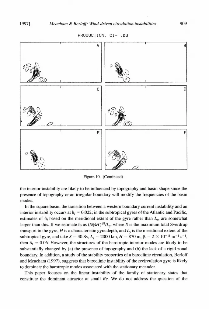
In the case of the basin with a meridional extent of only half the zonal width (y = 0.5) we saw the opposite effect; along the marginal curve, we saw no example of the western boundary current instability at any of the s1 values that we examined. Instead the instability encountered at the marginal curve appeared to be an interior instability associated with the south-western meander. Again, from the shape of the marginal curve in Figure 2, it appears that there are multiple interior modes. Pictures of the streamfunction of the marginal mode and the energy conversion term are shown in Figure 10, for the case 6, = 0.0153, and in Figure 11, for 6, = 0.0539.

5. Discussion

From the results above, we conclude that the steady circulation patterns that exist as solutions of the barotropic circulation problem with no-slip boundary conditions can give way to time-dependent solutions via at least two different types of linear instability. The first of these seems to match previous descriptions of shear instability of the western boundary current (c.f. IY). The second (the interior instability) is associated with the flow near a zonal boundary of fluid from the western boundary current as it rejoins the interior circulation. This latter part of the flow contains several structural units including a predominantly inertial recirculation gyre in the southwestern comer and a strong meander of the southern boundary current just to the east of the recirculation gyre. The second instability involves a strong cyclic exchange of energy between the perturbation and the basic steady flow in the vicinity of this meander.


Figure 9. Snapshots of the streamfunction and energy conversion term at different times during the period of a near-marginal normal mode of the y = 2 basin at 6, = 0.034. The snapshots are separated by l/4 period. (a) Streamfunction, (b) Energy conversion.

PRODUCTION,

I A

. I ‘\ ‘2

I

I C

I . : ‘8 \ t

:

I

CI= .I0



STREAMFUNCTION. CI= .I0

t C

I D

E I F

Figure 10. Snapshots of the streamfunction and energy conversion term at different times during the period of a near-marginal normal mode of the y = 0.5 basin at 6, = 0.0153. (a) Streamfunction, (b) Energy conversion.

There appear to be several different modes of interior instability. From the structure of the eddy energy conversion term, these are driven by a local instability of the stationary meander just to the east of the main recirculation gyre. Each is associated with a train of Rossby waves with predominantly eastward energy propagation in the eastern half of the basin. The modes differ mainly in the zonal scale of these Rossby waves. The dimensional period of a mode with a shorter scale is longer than that of a mode with a longer scale (the periods of two modes can be easily compared where their marginal curves cross)-the same sort of dependence as is exhibited by short Rossby waves. For the square basin, only three interior modes ever become more unstable than the western boundary current instability. Two of these are most unstable when their period is close to that of an eigenmode of the resting basin. This suggests that the instability of the standing meander forces a damped resonant response from the basin modes. It also suggests that the instability is not wholly local-the eastern boundary is playing a role in determining the marginal value of Re for a given 6,. From this we conclude that the stability thresholds of

19971 Meacham & BerlofS: Wind-driven circulation instabilities

PRODUCTION, CI= .03


the interior instability are likely to be influenced by topography and basin shape since the presence of topography or an irregular boundary will modify the frequencies of the basin modes.

In the square basin, the transition between a western boundary current instability and an interior instability occurs at 6, = 0.022; in the subtropical gyres of the Atlantic and Pacific, estimates of 6, based on the meridional extent of the gyre rather than Lx, are somewhat larger than this. If we estimate 6, as (S/PH)1’3/Ly, where S is the maximum total Sverdrup transport in the gyre, His a characteristic gyre depth, and Ly is the meridional extent of the subtropical gyre, and take S = 30 Sv, Ly = 2000 km, H = 870 m, p = 2 X lo-” m-l s-i, then 6, = 0.06. However, the structures of the barotropic interior modes are likely to be substantially changed by (a) the presence of topography and (b) the lack of a rigid zonal boundary. In addition, a study of the stability properties of a baroclinic circulation, Berloff and Meacham (1997) suggests that baroclinic instability of the recirculation gyre is likely to dominate the barotropic modes associated with the stationary meander.

This paper focuses on the linear instability of the family of stationary states that constitute the dominant attractor at small Re. We do not address the question of the



Figure 11. Snapshots of the streamfunction and energy conversion term at different times during the period of a near-marginal normal mode of the y = 0.5 basin at s1 = 0.0539. (a) Streamfunction, (b) Energy conversion.

existence of multiple stationary states in the presence of no-slip boundary conditions. However, we note that we found no evidence of stationary bifurcations such as a saddle-node bifurcation over the ranges of Re and s1 that we examined. Consequently, we found only a single branch of steady solutions. The parameter range that we have examined includes values of 6, and SW at which, in a model with free-slip boundary conditions, Ierley and Sheremet (1995) found multiple stationary states. This should be contrasted with the multiple stationary equilibria found in double gyre problems with both free-slip and no-slip boundary conditions (Cessi and Ierley, 1995; Jiang et al., 1995, Speich et al., 1995 and Meacham, 1997). In the quasi-geostrophic double-gyre problem driven by an antisymmetric wind stress, the stationary bifurcation structure is very similar, whether free-slip (Cessi and Ierley, 1995) or no-slip (Meacham, 1997) boundary conditions are used. That the boundary conditions should play an apparently stronger role in the single gyre problem seems unsurprising. In the antisymmetric double gyre problem there are two types of stationary bifurcations, symmetry-breaking pitchfork bifurcations and saddle node bifurca-

Meacham & Berloff: Wind-driven circulation instabilities

PRODUCTION, CI= .22

911


tions of the antisymmetric solutions (Cessi and Ierley, 1995). The latter are more relevant for the single gyre problem. Near these bifurcations, the higher energy antisymmetric states feature strong gyres against the mid-latitude line of the basin. The flows are much weaker near the rigid basin walls. These solutions are relatively insensitive to a change from free-slip to no-slip boundary conditions. Counterparts of these relatively inertial solutions exist in the anticyclonically forced single gyre problem when the northern boundary is free-slip (Ierley and Sheremet, 1995). When all the boundaries are no-slip, a large gyre against a boundary would require a strong shear layer next to the boundary in order to satisfy the no-slip condition, and hence a region near the boundary of strong vorticity of a sign opposite the predominant vorticity of the gyre itself. Such a structure would not be a small perturbation to the solution of the free-slip problem. It would seem possible that multiple strongly inertial solutions might exist when the a1 is much larger than ?iM, so that the frictional boundary layer is small compared to the inertial jet around the gyre, however Pedlosky (1996) makes a case that strongly inertial solutions of the singe gyre problem should not exist in a no-slip basin. In any event, such a solution would likely be very unstable, given the strong shear in the frictional boundary layer and so could not be a


“global attractor” of the sort found in inertial runaway problems (Ierley and Sheremet, 1995).

Given the arguments of the preceding paragraph about the influence of the boundary conditions on strongly inertial solutions, these no-slip results have only limited application to double-gyre problems. It should be recalled that in a “large” basin, in which the length of the western boundary current is larger than two or three times the critical wavelength predicted by Ierley and Young (1991), the western boundary current instability predomi- nates. This is likely to remain true in a double gyre model. A good example of a basin that is “small” in this sense and has a predominantly single gyre wind forcing is provided by the Black Sea.

Acknowledgments. The authors gratefully acknowledge the support of the National Science Foundation under contract number OCE-9301318.

REFERENCES Arakawa, A. 1966. Computational design for long-term numerical integration of the equations of

fluid motion: two-dimensional compressible flow. Part I. J. Comp. Phys., 1, 119-143. Berloff, P. S. and S. P Meacham. 1997. On the stability of equivalent barotropic and baroclinic

models of the wind-driven circulation. J. Mar Res., (submitted). Bryan, K. 1963. A numerical investigation of a nonlinear model of a wind-driven ocean. J. Atmos.

Sci., 20, 594-606. Buchwald, V. 1972. Long period divergent planetary waves. Geophys. Fluid Dyn., 5, 359-367. Cessi, P., R. V. Condie and W. R. Young. 1990. Dissipative dynamics of a western boundary current.

J. Mar. Res., 48, 677-700. Cessi, P. and G. Ierley. 1995. Symmetry-breaking multiple equilibria in quasi-geostrophic wind-

driven flows. J. Phys. Oceanogr., 25, 1196-1205. Charney, J. G. 1955. The Gulf Stream as an inertial boundary layer. Proc. Nat. Acad. Sci., 41,

73 l-740. Fofonoff, N. 1954. Steady flow in a frictionless homogeneous ocean. J. Mar. Res., 13, 254-262. Fromm, J. 1964. The time-dependent flow of an incompressible viscous fluid. Meth. Comp. Phys., 3,

345-382. Hackney, R. 1970. The potential calculation and some applications. Methods in Comput. Phys., 9,

136-211. Ierley, G. R. 1987. On the onset of general circulation in barotropic general circulation models. J.

Phys. Oceanogr., 17, 23662374. Ierley, G. R. and V. Sheremet. 1995. Multiple solutions and advection-dominated flows in the

wind-driven circulation. Part I: Slip. J. Mar. Res., 53, 703-737. Ierley, G. R. and W. R. Young. 1991. Viscous instabilities in the western boundary layer. J. Phys.

Oceanogr., 21, 1323-1332. Bin, A. M. and V. V. Kamenkovich. 1964. The structure of the boundary layer in the two-

dimensional theory of oceanic currents. Oceanology, 4, 756769. Jiang, S., F. Jin and M. Ghil. 1995. Multiple equilibria, periodic, and aperiodic solutions in a

wind-driven, double-gyre, shallow-water model. J. Phys. Oceanogr., 25, 764-786. Longuet-Higgins, M. S. 1964. Planetary waves on a rotating sphere. Proc. Roy. Sot. Lond., A 279,

446-473. Meacham, S. P. 1997. Low frequency variability in the wind-driven circulation. J. Phys. Oceanogr.,

(submitted).


Meacham, S. P. and P S. Berloff. 1997. Barotropic, wind-driven circulation in a small basin. J. Mar. Res., 55, 523-563.

Moore, D. 1963. Rossby waves in ocean circulation. Deep-Sea Res., IO, 735-748. Morgan, G. W. 1956. On the wind-driven ocean circulation. Tellus, 8, 301-320. Munk, W. H. 1950. On the wind-driven ocean circulation. J. Meteorol., 7, 79-93. Munk, W. H., G. W. Groves and G. F. Carrier. 1950. Note on the dynamics of the Gulf Stream. J. Mar.

Res., 9, 218-238. Pedlosky, J. 1987. Geophysical Fluid Dynamics. 2nd ed., Springer-Verlag, New York 710 pp. -1996. Ocean Circulation Theory. Springer-Verlag, New York, 453 pp. Speich, S., H. Dijkstra and M. Ghil. 1995. Successive bifurcations in a shallow-water model applied

to the wind-driven ocean circulation. Nonlin. Proc. Geophys., 2, 241-268. Stewart, R. W. 1984. The influence of friction on inertial models of oceanic circulation, in, Studies on

Oceanography, K. Yoshida. ed., Tokyo Univ., 3-9. Stommel, H. 1948. The westward intensification of wind-driven oceanic currents. Trans. Am.

Geophys. Union, 29, 202-206. Veronis, G. 1966. Wind-driven ocean circulation. Part 2. Deep-Sea Res., 13, 31-55.

Received: 14 January, 1997; revised: 19 June, 1997.

Instabilities of a steady, barotropic, wind-driven circulation

Documents