August 1998 NASA/CR-1998-208698 Input Shaping to Reduce Solar Array Structural Vibrations Michael J. Doherty and Robert H. Tolson Joint Institute for Advancement of Flight Sciences The George Washington University Langley Research Center, Hampton, Virginia

Welcome message from author
This document is posted to help you gain knowledge. Please leave a comment to let me know what you think about it! Share it to your friends and learn new things together.
Transcript

August 1998
NASA/CR-1998-208698
Input Shaping to Reduce Solar ArrayStructural Vibrations
Michael J. Doherty and Robert H. TolsonJoint Institute for Advancement of Flight SciencesThe George Washington UniversityLangley Research Center, Hampton, Virginia

The NASA STI Program Office ... in Profile
Since its founding, NASA has been dedicatedto the advancement of aeronautics and spacescience. The NASA Scientific and TechnicalInformation (STI) Program Office plays a keypart in helping NASA maintain thisimportant role.
The NASA STI Program Office is operated byLangley Research Center, the lead center forNASAÕs scientific and technical information.The NASA STI Program Office providesaccess to the NASA STI Database, thelargest collection of aeronautical and spacescience STI in the world. The Program Officeis also NASAÕs institutional mechanism fordisseminating the results of its research anddevelopment activities. These results arepublished by NASA in the NASA STI ReportSeries, which includes the following reporttypes: · TECHNICAL PUBLICATION. Reports of
completed research or a major significantphase of research that present the resultsof NASA programs and include extensivedata or theoretical analysis. Includescompilations of significant scientific andtechnical data and information deemedto be of continuing reference value. NASAcounter-part of peer reviewed formalprofessional papers, but having lessstringent limitations on manuscriptlength and extent of graphicpresentations.
· TECHNICAL MEMORANDUM.
Scientific and technical findings that arepreliminary or of specialized interest,e.g., quick release reports, workingpapers, and bibliographies that containminimal annotation. Does not containextensive analysis.
· CONTRACTOR REPORT. Scientific and
technical findings by NASA-sponsoredcontractors and grantees.
· CONFERENCE PUBLICATION.
Collected papers from scientific andtechnical conferences, symposia,seminars, or other meetings sponsored orco-sponsored by NASA.
· SPECIAL PUBLICATION. Scientific,
technical, or historical information fromNASA programs, projects, and missions,often concerned with subjects havingsubstantial public interest.
· TECHNICAL TRANSLATION. English-
language translations of foreign scientificand technical material pertinent toNASAÕs mission.
Specialized services that help round out theSTI Program OfficeÕs diverse offerings includecreating custom thesauri, building customizeddatabases, organizing and publishingresearch results ... even providing videos.
For more information about the NASA STIProgram Office, see the following:
· Access the NASA STI Program HomePage at http://www.sti.nasa.gov
· E-mail your question via the Internet to
[email protected] · Fax your question to the NASA Access
Help Desk at (301) 621-0134 · Phone the NASA Access Help Desk at
(301) 621-0390 · Write to:
NASA Access Help Desk NASA Center for AeroSpace Information 7121 Standard Drive Hanover, MD 21076-1320

National Aeronautics andSpace Administration
Langley Research Center Prepared for Langley Research CenterHampton, Virginia 23681-2199 under Cooperative Agreement NCC1-104
August 1998
NASA/CR-1998-208698
Input Shaping to Reduce Solar ArrayStructural Vibrations
Michael J. Doherty and Robert H. TolsonJoint Institute for Advancement of Flight SciencesThe George Washington UniversityLangley Research Center, Hampton, Virginia

Available from the following:
NASA Center for AeroSpace Information (CASI) National Technical Information Service (NTIS)7121 Standard Drive 5285 Port Royal RoadHanover, MD 21076-1320 Springfield, VA 22161-2171(301) 621-0390 (703) 487-4650

iii
Abstract
Structural vibrations induced by actuators can be minimized through the effective use
of feedforward input shaping. Actuator commands are convolved with an input shaping
function to yield an equivalent shaped set of actuator commands. The shaped commands
are designed to achieve the desired maneuver and minimize the residual structural
vibrations.
Input shaping was extended for stepper motor actuators through this research. An
input-shaping technique based on pole-zero cancellation was used to modify the Solar
Array Drive Assembly (SADA) stepper motor commands for the NASA/TRW Lewis
satellite. A series of impulses were calculated as the ideal SADA output for vibration
control and were then discretized for use by the SADA actuator. Simulated actuator
torques were used to calculate the linear structural response and resulted in residual
vibrations that were below the magnitude of baseline cases.
The effectiveness of input shaping is limited by the accuracy of the modal
identification of the structural system. Controller robustness to identification errors was
improved by incorporating additional zeros in the input shaping transfer function. The
additional shaper zeros did not require any increased performance from the actuator or
controller, and the resulting feedforward controller reduced residual vibrations to the level
of the exactly modeled input shaper despite the identification errors.

iv
Table of Contents
ABSTRACT ____________________________________________________________ iii
TABLE OF CONTENTS ___________________________________________________ iv
LIST OF FIGURES _______________________________________________________ vi
L IST OF TABLES_________________________________________________________ x
NOMENCLATURE _______________________________________________________ xi
1 INTRODUCTION ______________________________________________________ 1
1.1 POLE-ZERO CANCELLATION THEORY 2
1.2 EXAMPLE OF STRUCTURAL VIBRATION CONTROL : THE LEWIS SPACECRAFT 2
1.3 OVERVIEW OF RESULTS 3
2 POLE-ZERO CANCELLATION VIBRATION CONTROL THEORY ________________ 6
2.1 DISCRETE TIME SYSTEM DESCRIPTION 6
2.2 ROBUSTNESS AND M ULTIPLE -M ODE CONSIDERATIONS 8
2.3 TIME DOMAIN IMPLEMENTATION 11
2.4 EXTENSION OF POLE-ZERO CANCELLATION FOR STEPPER M OTORS 12
2.5 SELECTION AND IMPLEMENTATION OF VIBRATION CONTROL SEQUENCES 13
3 EXAMPLE OF STRUCTURAL VIBRATION CONTROL ________________________ 17
3.1 OVERVIEW OF LEWIS SPACECRAFT 17
3.2 LEWIS SPACECRAFT DYNAMIC M ODEL 29
3.3 DETERMINATION OF TARGET M ODES 33

v
4 SIMULATIONS AND RESULTS__________________________________________ 42
4.1 JITTER ANALYSIS M ETHOD 42
4.2 BASELINE SIMULATIONS AND JITTER ANALYSIS RESULTS 46
4.3 SHAPED INPUT SIMULATIONS AND RESULTS 57
4.4 SUMMARY OF RESULTS 79
5 CONCLUSIONS______________________________________________________ 82
5.1 CURRENT RESULTS 82
5.2 RECOMMENDATIONS FOR FUTURE RESEARCH 83
REFERENCES __________________________________________________________ 86
APPENDIX A: STEPPER M OTOR DESCRIPTION _______________________________ 88
APPENDIX B: M ODAL FREQUENCIES OF LEWIS FINITE ELEMENT M ODEL ________ 95
APPENDIX C: COMPARISON OF JITTER ANALYSIS RESULTS____________________ 97

vi
List of Figures
FIGURE 2.1: SYSTEM BLOCK DIAGRAM 6
FIGURE 2.2: EXAMPLE SYSTEM POLES IN THE Z-PLANE 9
FIGURE 2.3: EXAMPLE SYSTEM POLES AND SHAPER ZEROS IN THE Z-PLANE 10
FIGURE 2.4: EXAMPLE IMPULSE AMPLITUDES 12
FIGURE 2.5: EXAMPLE IMPULSE AMPLITUDES AND STEP SEQUENCE APPROXIMATIONS 13
FIGURE 2.6: EXAMPLE TIME –ADJUSTED STEP SEQUENCE APPROXIMATIONS 13
FIGURE 3.1: LEWIS SPACECRAFT 17
FIGURE 3.2: LEWIS SPACECRAFT ORBITAL OPERATIONS 18
FIGURE 3.3: SPACECRAFT DIMENSIONS (INCHES) 21
FIGURE 3.4: PAYLOAD INSTRUMENT MODULE PLAN VIEW 22
FIGURE 3.5: SOLAR ARRAY WING ISOMETRIC VIEW 24
FIGURE 3.6: TYPE 2 STEPPER MOTOR CUT-AWAY VIEW 25
FIGURE 3.7: TYPE 2 STEPPER MOTOR EXTERNAL VIEW 26
FIGURE 3.8: FOUR-DOF STEPPER MOTOR MODEL DIAGRAM 31
FIGURE 3.9: MOTOR STEPPING OPERATION PARAMETERS 32
FIGURE 3.10: SADA #1 Y-ROTATION (INPUT) – HSI X-ROTATION (OUTPUT) FRF 36
FIGURE 3.11: SADA #1 Y-ROTATION – HSI X-ROTATION RANKED MODES (1) 37
FIGURE 3.12: SADA #1 Y-ROTATION – HSI X-ROTATION RANKED MODES (2) 38
FIGURE 3.13: PAYLOAD INSTRUMENT X-ROTATION FRF MAGNITUDES 39
FIGURE 3.14: PAYLOAD INSTRUMENT Y-ROTATION FRF MAGNITUDES 41
FIGURE 4.1: JITTER ANALYSIS EXAMPLE (1) 44
FIGURE 4.2: JITTER ANALYSIS EXAMPLE (2) 44

vii
FIGURE 4.3: SINGLE STEP TORQUE TIME PROFILE 48
FIGURE 4.4: CSRS TORQUE TIME PROFILE, 3.16 PPS 48
FIGURE 4.5: HSI X-ROTATION RESPONSE TO CSRS TORQUE INPUT 49
FIGURE 4.6: HSI Y-ROTATION RESPONSE TO CSRS TORQUE INPUT 50
FIGURE 4.7: MATS TORQUE TIME PROFILE, 200 PPS 52
FIGURE 4.8: HSI X-ROTATION RESPONSE TO MATS TORQUE INPUT 53
FIGURE 4.9: HSI Y-ROTATION RESPONSE TO MATS TORQUE INPUT 54
FIGURE 4.10: HSI X-ROTATION BASELINE JITTER LEVELS 55
FIGURE 4.11: LEISA X-ROTATION BASELINE JITTER LEVELS 55
FIGURE 4.12: HSI Y-ROTATION BASELINE JITTER LEVELS 56
FIGURE 4.13: LEISA Y-ROTATION BASELINE JITTER LEVELS 56
FIGURE 4.14: SYSTEM POLES IN THE Z-PLANE (T=1.14 SECONDS) 61
FIGURE 4.15: SADA TORQUE TIME PROFILE FOR VCS #1 62
FIGURE 4.16: HSI X-ROTATION RESPONSE TO VCS #1 63
FIGURE 4.17: HSI Y-ROTATION RESPONSE TO VCS #1 64
FIGURE 4.18: HSI X-ROTATION JITTER ANALYSIS RESULTS (3.5-SECOND WINDOW) 67
FIGURE 4.19: LEISA X-ROTATION JITTER ANALYSIS RESULTS (3.5-SECOND WINDOW) 68
FIGURE 4.20: HSI Y-ROTATION JITTER ANALYSIS RESULTS (3.5-SECOND WINDOW) 69
FIGURE 4.21: LEISA Y-ROTATION JITTER ANALYSIS RESULTS (3.5-SECOND WINDOW) 70
FIGURE 4.22: SYSTEM POLES AND VCS #2 ZEROS IN THE Z-PLANE (T=1.035 SECONDS) 73
FIGURE 4.23: HSI X-ROTATION JITTER ANALYSIS RESULTS (3.5-SECOND WINDOW) 74
FIGURE 4.24: LEISA X-ROTATION JITTER ANALYSIS RESULTS (3.5-SECOND WINDOW) 75
FIGURE 4.25: HSI Y-ROTATION JITTER ANALYSIS RESULTS (3.5-SECOND WINDOW) 76
FIGURE 4.26: LEISA Y-ROTATION JITTER ANALYSIS RESULTS (3.5-SECOND WINDOW) 77

viii
FIGURE A.1: DETENT AND STATE #1 TORQUES VS. ROTOR ELECTRICAL ANGLE 90
FIGURE A.2: COMPOSITE TORQUE VS. ROTOR ELECTRICAL ANGLE 91
FIGURE A.3: DETENT, STATES #1, #2, AND #3 TORQUES VS. ROTOR ELECTRICAL ANGLE 93
FIGURE C.1: HSI X-ROTATION JITTER LEVELS (0.05 SECOND WINDOW) 98
FIGURE C.2: LEISA X-ROTATION JITTER LEVELS (0.05 SECOND WINDOW) 99
FIGURE C.3: HSI X-ROTATION JITTER LEVELS (0.1 SECOND WINDOW) 100
FIGURE C.4: LEISA X-ROTATION JITTER LEVELS (0.1 SECOND WINDOW) 101
FIGURE C.5: HSI X-ROTATION JITTER LEVELS (0.2 SECOND WINDOW) 102
FIGURE C.6: LEISA X-ROTATION JITTER LEVELS (0.2 SECOND WINDOW) 103
FIGURE C.7: HSI X-ROTATION JITTER LEVELS (0.5 SECOND WINDOW) 104
FIGURE C.8: LEISA X-ROTATION JITTER LEVELS (0.5 SECOND WINDOW) 105
FIGURE C.9: HSI X-ROTATION JITTER LEVELS (1 SECOND WINDOW) 106
FIGURE C.10: LEISA X-ROTATION JITTER LEVELS (1 SECOND WINDOW) 107
FIGURE C.11: HSI X-ROTATION JITTER LEVELS (3.5 SECOND WINDOW) 108
FIGURE C.12: LEISA X-ROTATION JITTER LEVELS (3.5 SECOND WINDOW) 109
FIGURE C.13: HSI Y-ROTATION JITTER LEVELS (0.05 SECOND WINDOW) 110
FIGURE C.14: LEISA Y-ROTATION JITTER LEVELS (0.05 SECOND WINDOW) 111
FIGURE C.15: HSI Y-ROTATION JITTER LEVELS (0.1 SECOND WINDOW) 112
FIGURE C.16: LEISA Y-ROTATION JITTER LEVELS (0.1 SECOND WINDOW) 113
FIGURE C.17: HSI Y-ROTATION JITTER LEVELS (0.2 SECOND WINDOW) 114
FIGURE C.18: LEISA Y-ROTATION JITTER LEVELS (0.2 SECOND WINDOW) 115
FIGURE C.19: HSI Y-ROTATION JITTER LEVELS (0.5 SECOND WINDOW) 116
FIGURE C.20: LEISA Y-ROTATION JITTER LEVELS (0.5 SECOND WINDOW) 117
FIGURE C.21: HSI Y-ROTATION JITTER LEVELS (1 SECOND WINDOW) 118

ix
FIGURE C.22: LEISA Y-ROTATION JITTER LEVELS (1 SECOND WINDOW) 119
FIGURE C.23: HSI Y-ROTATION JITTER LEVELS (3.5 SECOND WINDOW) 120
FIGURE C.24: LEISA Y-ROTATION JITTER LEVELS (3.5 SECOND WINDOW) 121

x
List of Tables
TABLE 3.1: PAYLOAD INSTRUMENT MISSION REQUIREMENTS 19
TABLE 3.2: LEWIS SPACECRAFT PHYSICAL QUANTITIES 20
TABLE 3.3: TYPE 2 STEPPER MOTOR SPECIFICATIONS 23
TABLE 3.4: STEPPER MOTOR MODEL MECHANICAL SPECIFICATIONS 31
TABLE 3.5: STEPPER MOTOR MODEL ELECTRICAL SPECIFICATIONS 32
TABLE 3.6: RANKED MODES FOR PAYLOAD INSTRUMENT X-ROTATIONS 39
TABLE 3.7: RANKED MODES FOR PAYLOAD INSTRUMENT Y-ROTATIONS 40
TABLE 4.1: EFFECT OF JITTER WINDOWS ON MODAL CONTRIBUTIONS 45
TABLE 4.2: CSRS JITTER ANALYSIS RESULTS 51
TABLE 4.3: VIBRATION CONTROL SEQUENCE #1 DATA 60
TABLE 4.4: VIBRATION CONTROL SEQUENCE #2 DATA 72
TABLE 4.5: VIBRATION CONTROL SEQUENCE #3 DATA 80

xi
Nomenclature
busiiI spacecraft bus moment of inertia about ith Cartesian axisSAiiI solar array moment of inertia about ith Cartesian axis
motormaxω maximum SADA step rate
busstepθ∆ spacecraft bus step angleSAstepθ∆ solar array step anglebussimθ∆ spacecraft bus inertial rotation over the course of a simulationSAsimθ∆ solar array inertial rotation over the course of a simulation
cssim
/θ∆ combined spacecraft bus and solar array inertial rotation during asimulation
SAtrackingω solar array inertial angular rate for solar trackingmotortrackingω SADA step rate for solar tracking
cstracking
/ω combined spacecraft bus and solar array inertial angular rate for solartracking
nω undamped natural frequency
dω damped natural frequency
eθ SADA rotor electrical angle at equilibrium for an arbitrary electrical statesumroundingE summation of impulse amplitude to step sequence rounding errorsmaxroundingE maximum of impulse amplitude to step sequence rounding errorssumvariationE summation of impulse amplitude variation errorsmaxvariationE maximum of impulse amplitude variation errors
ζ damping ratioθ angular displacementω angular velocityω frequency domain variable∆θr SADA rotor step angle∆θSA SADA output shaft step angleδ(t) Dirac delta functionωbus spacecraft bus inertial angular rateθe SADA rotor electrical angleφir i th FEM node, rth modeshape coefficientθm SADA rotor mechanical angleωnr natural frequency of rth modeζr damping ratio of rth modeωSA solar array inertial angular rateACS Attitude Control System

xii
C damping coefficientCe SADA motor torque function electrical constantCm SADA motor torque function mechanical constantCSRS Constant Step Rate SequenceFEM Finite Element MethodFRF Frequency Response FunctionGR harmonic drive ratio (gear reduction)H(s) continuous time domain transfer function HH(z) discrete time domain transfer function HHij(ω) frequency response functionHSI Hyper Spectral ImagerIr SADA rotor moment of inertiaj imaginary quantity 1−J moment of inertia coefficientK stiffness coefficientLEISA Linear Etalon Imaging Spectral ArrayMATS Minimum Actuation Time Sequencemr rth modal massn current motor electrical statesNASA National Aeronautics and Space Administrationnmax total number of motor electrical statesNrev steps per SADA output shaft revolutionpi ith system polePPS Pulses Per Seconds Laplace continuous time domain variableSADA Solar Array Drive AssemblySSTI Small Spacecraft Technology InitiativeT discrete time sampling periodt timeTdetent torque developed on the SADA rotor by the motor permanent magnetsTFext torque due to external coulomb frictionTFext torque due to internal coulomb frictionTorbit orbital periodTpowered torque developed on the SADA rotor by the motor electromagnetsTrotor total torque developed on the SADA rotorUCB Ultraviolet Cosmic Background SpectrometerVCS Vibration Controlling SequenceX x-direction displacement or rotationY y-direction displacement or rotationZ z-direction displacement or rotationz discrete time domain variablezi ith system zero

1
1 Introduction
Structural vibrations must be minimized if continued improvements in the
performance of many types of equipment are to be realized. Many different approaches
can be utilized in any combination to reduce unacceptable vibrations:
• Additional hardware can be installed to mechanically isolate or dissipate the
vibration.
• Sensors and control equipment can be installed to enable a classic feedback
control technique to actively respond to and cancel the vibration.
• Operational parameters can be modified to avoid scheduling vibration sensitive
tasks while the vibration is present.
All of the above vibration mitigation methods either reduce the possible range of
equipment operation or increase the production cost and complexity. When vibrations are
induced by actuators within the equipment in the course of performing a desired
maneuver, altering or shaping the actuator input to avoid initially exciting vibrations
would be the simplest solution. The new actuator commands must acceptably perform the
desired equipment motion. This input shaping technique could potentially solve vibration
problems without any additional cost or complexity and allow vibration sensitive tasks to
be accomplished at any time. Additional mechanical hardware or feedback control
techniques could still be used to augment input shaping.

2
1.1 Pole-Zero Cancellation Theory
Many different input shaping methods using time domain and frequency domain
approaches have been developed. Singer [11] derived an impulse sequence method for
vibration control in the continuous time domain, which was later extended to include the
suppression of multiple modes of vibration [6, 9]. It has been shown by several researchers
[7, 12] that working with input shaping techniques in the Laplace s-plane or discrete time
z-plane rather than in the continuous time domain results in improved mathematical
simplicity, especially when a system has multiple undesirable modes of vibration.
Tuttle and Seering [15] have developed a controller design formulation based on the
input-shaping technique of Singer, but use pole-zero cancellation in the discrete time
domain as suggested by Smith [14]. In this research, the zero-placement technique is used
to develop an input shaping algorithm that satisfies structural vibration requirements while
operating within actuator capabilities. Controller design incorporating the dynamics of a
stepper motor actuator is the primary extension of Tuttle and Seering’s work by the
current research. Other recent research [2] has examined the use of stepper motor
actuators using different vibration control methods.
1.2 Example of Structural Vibration Control: The Lewis Spacecraft
The Lewis spacecraft is a small solar powered Earth-orbiting satellite. Therefore, the
satellite must be able to track the sun to maximize the power production from the solar
array panels. During normal operation, this tracking is accomplished entirely by rotating
the solar arrays relative to the rest of the spacecraft body. This is accomplished by a pair

3
of stepper motor actuators, one for each of two solar array wings extending from the main
body.
Several instruments are onboard the Lewis spacecraft that have strict pointing
requirements to satisfy the designed data gathering capability. Any proposed control
algorithm for the solar array drive assembly (SADA) actuators must satisfy both of these
basic mission requirements as a minimum capability. This problem in structural vibration
control is used as an example of the pole-zero cancellation technique.
1.3 Overview of Results
Two different solar tracking methods for the Lewis SADA were initially investigated
as baseline cases. The first method was the Constant Step Rate Sequence (CSRS) which
tracks the sun most accurately by maintaining a constant step rate that corresponds to one
full rotation of the solar array per orbit. This repetitive input results in an average of
approximately 19 and 54 µradians of rotational jitter about the Y-axis (or Y-rotation jitter)
for the HSI and LEISA instruments respectively during a 3.5 second period of time,
known as a jitter window. These instruments have maximum allowable jitter limits of 10
and 30 µradians respectively, and so the CSRS as simulated was unacceptable. The 3.5
second jitter window allows all identified structural modes (listed in Appendix B) to
complete at least one cycle within the window and therefore fully contribute to the
measured jitter of the linear simulation. The jitter analysis results using the 3.5 second
window only are presented in this section as a summary of the effects of the various
SADA control methods investigated.

4
A second baseline tracking method was the Minimum Actuation Time Sequence
(MATS) which makes use of the ±5° maximum “tracking error” allowed and achieves a
new solar array orientation in one large rotational slew. From an initial orientation of -5°,
the solar arrays would be rotated through the ideal sun orientation of 0° to the opposite
maximum of +5° at one time. Approximately 160 seconds later another 10° rotation of the
solar arrays would be required. The rotations are done at the maximum angular rate of the
actuator to minimize the disturbance time. Structural damping does reduce the vibrational
motion during the quiescent period, but the simulated jitter about the Y-axis during a 3.5
second window was an average of approximately 297 µradians for both instruments and
never reduced to an acceptable level during the 160 second simulation.
The first Vibration Control Sequence (VCS #1) uses the z-plane pole-zero
cancellation method of Tuttle and Seering [15] to “shape” the SADA output and cancel
the dynamics of eight target structural modes. This sequence achieves acceptable levels of
jitter about the Y-axis for the HSI instrument for approximately 65% of the 160 second
simulation time. The corresponding LEISA jitter results are within the instrument
requirements for approximately 84% of the simulation time. The use of VCS #1 to
command the SADA actuator would therefore allow the full capability of the HSI and
LEISA instruments to be realized for the majority of the time. This would require
coordination between the SADA and payload instrument operations, but conservation of
angular momentum calculations indicate that even a single step of the SADA actuator
would cause unacceptable rigid body motion of the spacecraft bus and therefore this
coordination is unavoidable.

5
VCS #2 introduces the issue of controller robustness by incorporating a 10% error in
the target natural frequencies, and is presented as a typical system identification error. This
SADA command sequence has Y-rotation jitter levels that are about midway between both
the VCS #1 and MATS jitter levels and actually has better performance than VCS #1 for
jitter about the X-axis. However, the VCS #2 jitter about the Y-axis is above the jitter
limits during the entire simulation for the HSI instrument and approximately 90% of the
simulation for the LEISA.
A final vibration controlling sequence, VCS #3, illustrates the proposed method of
increasing the input shaping robustness to system identification errors. The same errors in
the target frequencies used for VCS #2 are used for this sequence, but now the number of
shaper zeros is tripled. Increasing the number of zeros increases the bandwidth of the
vibration reduction of the input shaper. The results from this final simulation closely match
the performance of VCS #1, and actually allow greater than 67% and 87% of the
simulation time to be available for the HSI and LEISA operations respectively. The large
improvement in shaper performance in the presence of system identification errors is
achieved at no additional actuator or computational requirements.

6
2 Pole-Zero Cancellation Vibration Control Theory
The residual vibration control design method of Tuttle and Seering [15] is presented.
This formulation is based on pole-zero cancellation and the design is accomplished in the
discrete time domain. The resulting input shaping function consists of impulse sequences
occurring at discrete time intervals. Robustness and multiple mode vibration issues can be
handled in a direct geometric manner using z-plane shaper design as discussed in Section
2.1. The input shaping impulse sequence is in general convolved with arbitrary actuator
commands and the subsequent continuous time input then used to drive the actuator.
2.1 Discrete Time System Description
Denoting the discrete time domain system input as U(z), the shaper transfer function
as H(z), and the plant transfer function as G(z), the open loop transfer function description
of the system shown in Figure 2.1 is
Y z
U zG z H z
( )
( )( ) ( )= ⋅ (2.1
where Y(z) is the system output.
FIGURE 2.1: SYSTEM BLOCK DIAGRAM
The general form of G(z) with k zeros and l poles is
H G YU

7
( )( )( )( ) ( )( )( )( )( )( ) ( )( )G z
z z z z z z z z z z z z
z p z p z p z p z p z p
k k
l l
( )* * *
* * *=
− − − − − −− − − − − −
1 1 2 2
1 1 2 2
�
�
(2.2
where zi, zi*, pi and pi* are the ith complex conjugate pairs of the plant zeros and poles
respectively. The resonant modes are indicated by the poles in G(z). The input to G(z) that
will not excite particular modes will have matching zeros to cancel the corresponding
resonant poles. Following the development of Tuttle and Seering [15], for m undesirable
modes of vibration in G(z), there are 2m complex poles which must be canceled, e.g. p1 ,
p1* , ... , pm , pm* . The shaper H(z) must take the initial form
( )( )( )( ) ( )( )H z z p z p z p z p z p z pm m( ) * * *= − − − − − −1 1 2 2 � (2.3
The ith damped mode of the system is defined by the complex conjugate pair of poles
p
p
e e
e ei
i
T j T
T j T
i ni di
i ni di*
=
−
− −
ζ ω ω
ζ ω ω (2.4
where T is the discrete time sampling period, ωni and ωdi are the undamped and damped
natural frequencies of the ith mode, and ζi is the damping ratio of the ith mode with the
standard relationship
ω ω ζdi ni i= −1 2(2.5
The sampling period T is the time intervals at which the discrete time transfer function
is defined. It is separate from the sampling period of a digital controller or other hardware
in the system and represents the zero-order hold in the transformation of the continuous
time physical system into the discrete time representation.

8
H(z) must be causal or nonanticipatory, i.e., the output at time t does not depend on
the input applied after time t, but only on the input applied before and at time t. Therefore
the past affects the future but not conversely and this condition applies to all real systems.
The causality condition translates to the z-plane as a requirement that the order of the
numerator of H(z) is less than or equal to the order of the denominator.
The numerator contains all the desired input shaping dynamics. Therefore, placing all
the denominator poles at z=0 eliminates any denominator dynamics that might unduly
affect the input U(z). With these additional requirements, H(z) now has the more general
form
( )( )( )( ) ( )( )H z C
z p z p z p z p z p z p
zm m
m( )* * *
=− − − − − −1 1 2 2 �
(2.6
where C is a constant gain used to change the overall amplitude of the shaper transfer
function output.
2.2 Robustness and Multiple-Mode Considerations
Equation 2.6 is a minimally robust version of U(z), i.e. only one shaper zero per
system pole. Increasing the number of zeros placed at a particular pole has been shown to
improve shaper robustness [12, 15] to variations or inaccuracies in the system parameters
defining that mode. The most general form of H(z) therefore is
( ) ( ) ( ) ( ) ( ) ( )H z C
z p z p z p z p z p z p
z
n n n n
m
n
m
n
n n n
m m
m( )
* * *
( )=− − − − − −
+ + +1 1 2 2
2
1 1 2 2
1 2
�
�
(2.7
where each zero pi is repeated ni times, resulting in nith order robustness.

9
In addition, a z-plane plot of the shaper zeros and system poles can show in a simple
geometric way the relative effectiveness of each shaper zero on multiple system poles.
Consider the pole -zero plot of Figure 2.2, which shows the location on the z-plane of four
poles by their complex conjugate roots.
FIGURE 2.2: EXAMPLE SYSTEM POLES IN THE Z-PLANE
Undesirable system poles that are near one another in the z-plane could be targeted by
a lesser number of well-placed shaper zeros [15]. In this manner, an initial shaper transfer
function can be very quickly designed and respond to robustness concerns while
incorporating a minimum number of shaper zeros. Reducing the number of shaper zeros
reduces the time lag produced by convolving the input with the shaper transfer function.

10
To cancel the four poles in Figure 2.2, four shaper zeros with the same complex roots
would be required. Alternatively, three zeros could be employed with one zero being
midway between the two closely located poles in the second and third quadrant of the unit
circle as shown in Figure 2.3. The plant dynamics represented by those two poles would
not be completely canceled but may be reduced to acceptable levels while the additional
dynamics and time delay introduced by the shaper are decreased.
FIGURE 2.3: EXAMPLE SYSTEM POLES AND SHAPER ZEROS IN THE Z-PLANE

11
2.3 Time Domain Implementation
Expanding the terms of Equation 2.7 yields
H z Cz a z a z a
z
n n n n n nn n n n n n
n n n
m m
m m
m( )
( ) ( )( ) ( )
( )=+ ++ + + + + + −
+ + + − + + ++ + +
21
2 12 1 2
2
1 2 1 2
1 2 1 2
1 2
� �
� �
�
�
(2.8
and mapping the z-plane poles and zeros to the s-plane by the relation
z esT= (2.9
yields the equivalent continuous time transfer function
( )H s C
e a e a e a
e
n n n sT n n n sTn n n
sTn n n
n n n sT
m m
m m
m( )
( ) ( )( ) ( )
( )=+ ++ + + + + + −
+ + + − + + ++ + +
21
2 12 1 2
2
1 2 1 2
1 2 1 2
1 2
��
� �
�
�
(2.10
Transforming Equation 2.10 to the time domain can be accomplished by dividing the
numerator by the denominator and taking the inverse Laplace transform, which results in
( ) ( ) ( ) ( ) ( )( )[ ]TnnntaTtaTtatCtH mnnn m+++−++−+−+= +++ ��
� 21221 22)(21
δδδδ (2.11
Equation 2.11 represents a series of impulses of varying magnitudes that are evenly spaced
in time by T, the discrete time sampling period. The constant C can be used to scale the
amplitudes a such that the sum of all the impulse amplitudes is unity or any arbitrary value.
As T is varied for any given set of shaper zeros, the dimensionless impulse amplitudes
will change according to the relations above. In this manner, an infinite set of impulse
amplitudes and corresponding time spacing between them can be found with the same
theoretical vibration canceling effect. In practice, the minimum time spacing and maximum
impulse magnitude are limited by the actuator capability. The maximum time spacing is
generally limited by the desired system performance since increasing T causes an increased

12
time delay when convolving the input shaping impulse sequence with an arbitrary input
[15].
2.4 Extension of Pole-Zero Cancellation for Stepper Motors
The input shaping transfer function as developed by Singer, et al [9, 10] is intended
for convolution with an arbitrary input. For simplicity, assume the arbitrary input is a
constant torque. The convolution of the impulse sequences with a constant torque results
in a series of impulsive torques that are related to the constant torque value by the impulse
amplitudes a. Figure 2.4 shows a representative set of impulse amplitudes with T=3
seconds.
FIGURE 2.4: EXAMPLE IMPULSE AMPLITUDES
A stepper motor actuator cannot produce a specified torque, it can only increment the
output shaft forward or reverse at a specified step rate. Since a true impulse is impossible
to produce, it is proposed that a variable number of actuator steps at a high step rate could
have a similar effect on the structure as a variable magnitude “impulse” torque. Each
impulse torque is transformed into a sequence of actuator steps and assuming a maximum

13
step rate is used for all sequences, larger impulse amplitudes result in longer step
sequences, as shown in Figure 2.5.
FIGURE 2.5: EXAMPLE IMPULSE AMPLITUDES AND STEP SEQUENCE APPROXIMATIONS
Finally, the step sequences are shifted in time so that each sequence is centered about
the original impulse time as shown in Figure 2.6.
FIGURE 2.6: EXAMPLE TIME –ADJUSTED STEP SEQUENCE APPROXIMATIONS
2.5 Selection and Implementation of Vibration Control Sequences
There are an infinite number of input shaping transfer functions that can be developed.
However, actuator and application-specific constraints will most likely not allow most of
these possible transfer functions and favor some of the remaining over others. To aid in

14
the selection of transfer functions, several guidelines in the form of error calculations are
presented.
2.5.1 Error Calculations
The step sequences produced by the procedure of Section 2.4 do not in general
consist of integer numbers of steps and must be rounded to integer values for
implementation by a stepper motor. The total error produced by rounding the amplitudes
is defined as
( )E E a round aroundingsum
roundingi
i
N
i ii
N
= = −=
+
=
+
∑ ∑1
2 1
1
2 1
(2.12
and was one criteria used in the ranking of the many possible input shaper solutions. The
maximum rounding error
( )irounding
maxrounding EE max= (2.13
within each solution was also calculated. Ranking the solutions in order of increasing error
was developed as an aid in selecting a solution for a simulation run. Concern about the
disparity between the mathematically ideal impulse amplitude and the resulting rounded
number of stepper motor steps assumes the structure is sensitive to the exact number of
steps.
Conversely, if the structure is insensitive to the exact number of steps, then the step
sequences will all have a similar effect on the structure. It would therefore be desirable
that the vibration control solution require the same force or torque on the structure at each
sampling time T. This translates to having all the impulse amplitudes as close in value as
possible. The variation between the normalized impulse amplitudes and an ideal amplitude

15
(which is constant for all 2N+1 impulses) was a second criteria used to rank the solutions
and is defined as
∑∑+
=
+
= +−==
12
1
12
1 12
1N
ii
N
i
ivariation
sumvariation
NaEE (2.14
The maximum variation error
( )ivariation
maxvariation EE max= (2.15
can also be calculated for each solution.
2.5.2 Other Considerations
The values for T must be compatible with the actuator and problem specifications to
generate useful sets of impulse sequences. The actuator is capable of a maximum stepping
rate and therefore a minimum time between steps can be calculated. Therefore, T should
be incremented by this minimum interval throughout a specified range. The range for T
was chosen based on the number of zeros (and therefore the number of step sequences)
that were to be implemented by the input shaper transfer function.
In general, smaller values of T and larger values for N were desirable for several
reasons. Placing N zeros in the shaper transfer function results in 2N+1 impulses in the
time domain. As the number of impulses in the solution increases, the number of steps
contained within each step sequence generally decreases, and therefore less time is
required for that sequence. Smaller step sequences should have more of an impulsive
nature in their effect on the structure and can be placed closer together, i.e., the sampling
period T can be smaller. As T decreases, all 2N+1 step sequences can be completed in less

16
time and there is more time in the simulation for structural damping to quiet residual
vibrations that could have a significant effect.

17
3 Example Of Structural Vibration Control
3.1 Overview Of Lewis Spacecraft
The National Aeronautics and Space Agency (NASA) Small Spacecraft Technology
Initiative (SSTI) is intended to demonstrate the viability of new technologies for use in
space. The first pair of these next generation satellites are appropriately named Lewis and
Clark. These satellites feature modular construction and make extensive use of off-the-
shelf hardware. The current SSTI program has formed partnerships between NASA and
two aerospace corporations: TRW is the corporate partner for the Lewis (shown in Figure
3.1) and CTA is the partner for the Clark spacecraft.
FIGURE 3.1: LEWIS SPACECRAFT

18
3.1.1 Lewis Orbital Operations
The Lewis spacecraft [13] will be inserted into a sun-synchronous orbit with a mean
altitude of 283 nautical miles and 97.1° inclination. The orbital period will be
approximately 95 minutes and for approximately 63% of the orbit, Lewis will be in
sunlight. Some of the major operations over the course of a single orbit are illustrated in
Figure 3.2.
While the satellite is in sunlight, there are two primary instruments which will observe
Earth: the Hyper Spectral Imager (HSI) and Linear Etalon Imaging Spectral Array
(LEISA). During the orbital eclipse, the Ultraviolet Cosmic Background Spectrometer
(UCB) will operate to avoid interference from the sun.
The two solar array wings are required to track the sun and maximize power
generation during the sunlit period. The Solar Array Drive Assembly (SADA) of the
FIGURE 3.2: LEWIS SPACECRAFT ORBITAL OPERATIONS

19
Lewis spacecraft can rotate the solar array wings 360° continuously about the Y-axis and
is required to track the sun to within ±5°. For a given orientation of the other two
spacecraft axes with respect to the sun, this specification will assure at least 99.6% of the
maximum solar radiation is available for electrical power generation. The SADA utilizes a
rotary stepper motor which is capable of up to 200 steps or pulses per second (PPS). The
stepper motor actuator imparts impulsive-like torques into the Lewis structure.
The HSI and LEISA instruments have relatively high resolution capabilities and
consequently are sensitive to small amplitude vibrations. The requirements for the UCB
instrument are not critical and it is not necessary for the solar arrays to track the sun
during the 35 minute eclipse. Consequently, this research is limited to the operations and
requirements during the approximately 60 minutes per orbit when the SADA could
potentially incur structural vibrations that reduce the HSI or LEISA data quality. The
range of time these two instruments may require to complete gathering data for an image
and the maximum allowable vibratory motion or jitter of the instrument boresight is given
in Table 3.1.
TABLE 3.1: PAYLOAD INSTRUMENT MISSION REQUIREMENTS
HSI LEISA
Minimum Data Acquisition Period 3 sec 20 secMaximum Data Acquisition Period 30 sec 50 secMaximum Allowable Boresight Jitter 10 µradians, < 250Hz
2 µradians, > 1500Hz30 µ radians

20
3.1.2 Physical Description
Table 3.2 summarizes the dimensions, masses, idealized geometry, and the
corresponding moments of inertia of the spacecraft bus and the solar array wings.
TABLE 3.2: LEWIS SPACECRAFT PHYSICAL QUANTITIES
Basic Shape& Dimensions (in)
Weight(lbf)
Ixx
(lbf-in-s2)Iyy
(lbf-in-s2)Izz
(lbf-in-s2)Spacecraft Bus Cylinder: 70 x 28 (radius) 797.2 25.16 38.78 38.78Solar Array Flat Plate: 59 x 138 x 1 26.4 3.989 0.6167 3.373
3.1.3 Description Of Payload Instruments Module And Mission Requirements
The payload instruments are attached to the upper payload platform as shown in
Figures 3.4. These items consist of the Hyper Spectral Imager (HSI), Linear Etalon
Imaging Spectral Array (LEISA), Ultraviolet Cosmic Background Spectrograph (UCB),
and both the Wide and Narrow Field of View Star Tracker Assemblies. For each
instrument, there are six possible jitter quantities: a displacement and a rotation
corresponding to each of the three orthogonal Cartesian coordinates. Displacements have
a negligible effect on the pointing accuracy of instruments in orbit due to the large
distances between the instrument and subject. Therefore, only the three rotations are of
possible concern.
The HSI has a line-of-sight that is fixed relative to the spacecraft and parallel to the Z
axis. The line-of-sight of the LEISA can change within the instrument field-of-regard, but
the field-of-regard is centered about a vector that is parallel to the HSI line-of-sight.
Rotation about the line-of-sight is a secondary concern and so the two important motions
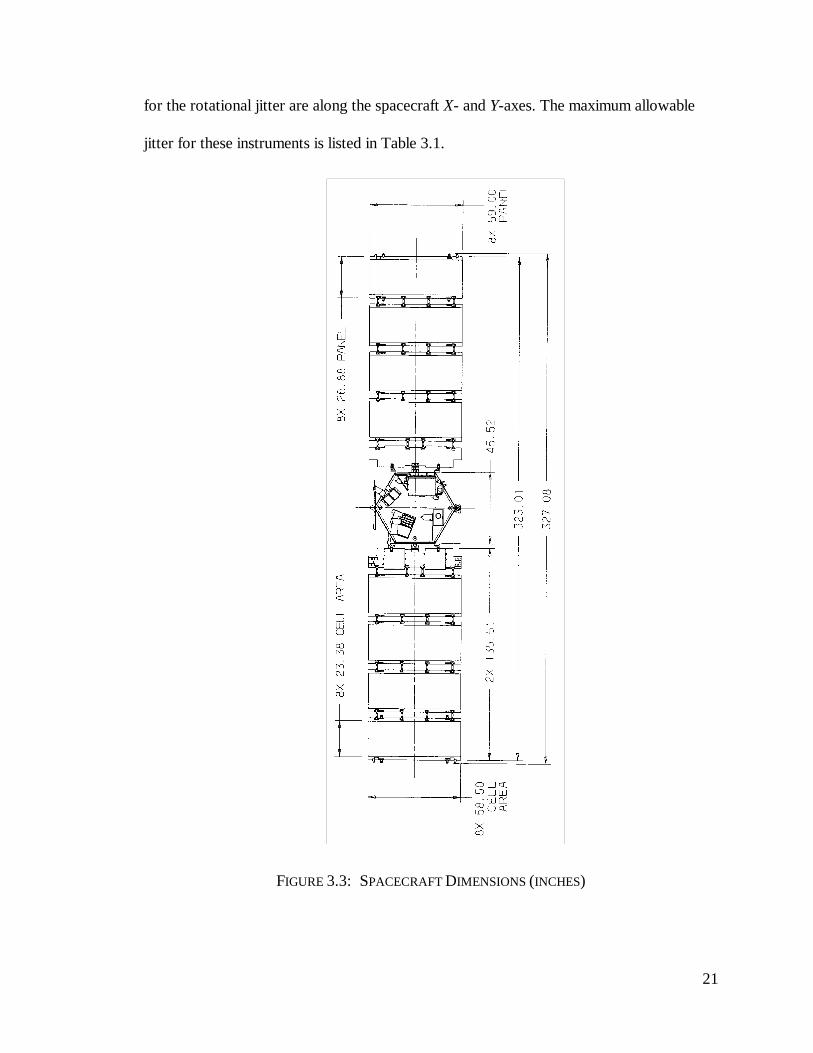
21
for the rotational jitter are along the spacecraft X- and Y-axes. The maximum allowable
jitter for these instruments is listed in Table 3.1.
FIGURE 3.3: SPACECRAFT DIMENSIONS (INCHES)

22
FIGURE 3.4: PAYLOAD INSTRUMENT MODULE PLAN VIEW

23
3.1.4 Description Of Solar Array Drive Assembly And Mission Requirements
Each of the two Solar Array Drive Assemblies (SADA) for Lewis use a single
Schaeffer Magnetics Type 2 Rotary Incremental Actuator and associated drive electronics.
The SADA’s have the functional requirement of pointing the solar arrays at the sun within
±5° about the Y axis. Each solar array wing interfaces with the main spacecraft bus via 52
sliprings and the actuator output shaft. This arrangement provides continuous 360°
rotational freedom of motion. The actuator output shaft is aligned with the spacecraft Y-
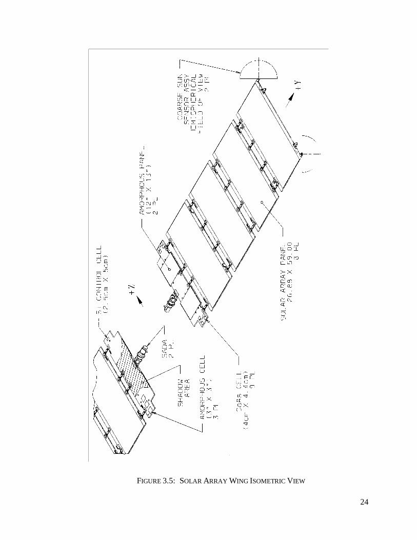
axis. A more detailed view of the solar array wings is shown in Figure 3.5. The
specifications for the Schaeffer Magnetics stepper motor are shown in Table 3.3.
TABLE 3.3: TYPE 2 STEPPER MOTOR SPECIFICATIONS
Output shaft step angle, ∆θSA 0.02°Steps per revolution, Nrev 18,000Harmonic drive ratio, GR 100Rotor step angle, ∆θr 2.0°Output step rate, motor
maxω 450 steps/sec; 9.0°/sec
Holding torquesPowered: 150 in-lbfDetent: 50 in-lbf
Torsional stiffness 6,000 in-lbf/radTotal assembly weight 2.0 lbfRotor moment of inertia, Ir 8.3 x 10⁻⁵ lbf-in-s2
24
FIGURE 3.5: SOLAR ARRAY WING ISOMETRIC VIEW

25
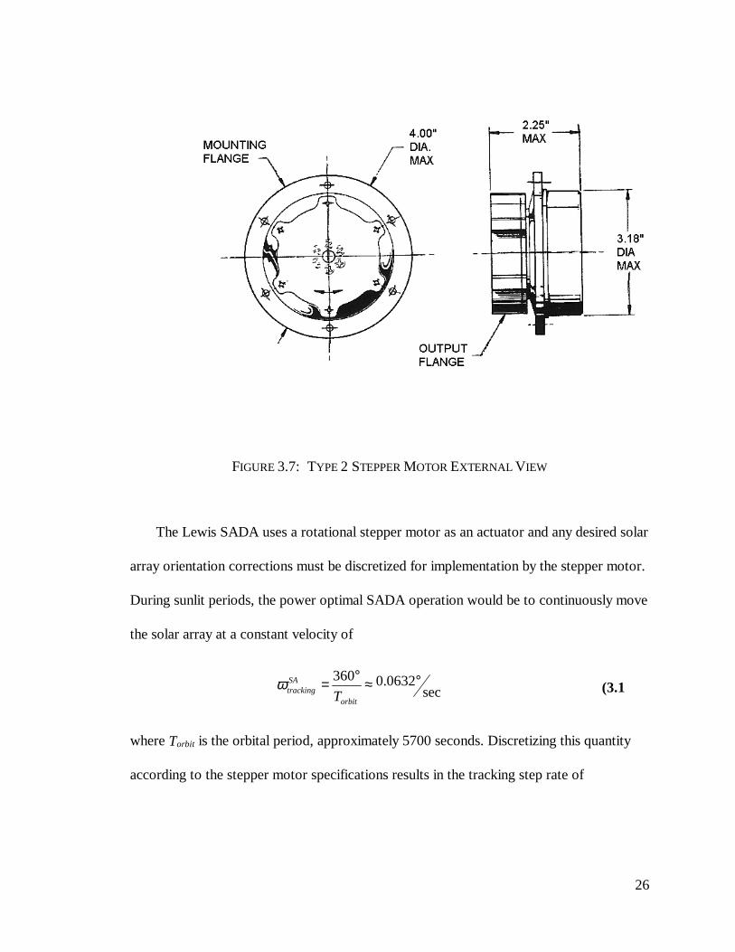
Figures 3.6 and 3.7 illustrate the basic physical dimensions and the main internal
components of the Type 2 actuator. During SADA operation, the stator electromagnets
develop torque on the rotor. The rotor then transfers this torque and resulting angular
motion through the harmonic drive, a gear reduction device. The harmonic drive transfers
the amplified SADA torque to the motor output flange and end load. The end loads for the
Lewis spacecraft SADA’s are the solar array panels.
FIGURE 3.6: TYPE 2 STEPPER MOTOR CUT-AWAY VIEW
26
FIGURE 3.7: TYPE 2 STEPPER MOTOR EXTERNAL VIEW
The Lewis SADA uses a rotational stepper motor as an actuator and any desired solar
array orientation corrections must be discretized for implementation by the stepper motor.
During sunlit periods, the power optimal SADA operation would be to continuously move
the solar array at a constant velocity of
sec0632.0360 °≈°=
orbit
SAtracking
Tω (3.1
where Torbit is the orbital period, approximately 5700 seconds. Discretizing this quantity
according to the stepper motor specifications results in the tracking step rate of

27
sec
step16.3≈
∆=
SAstep
SAtrackingmotor
tracking θω
ω (3.2
This quantity is about 0.7% of motormaxω , the maximum step rate of the actuator listed in
Table 3.3. Experimental investigations by Miller [LaRC, private communication] have
shown step rates up to 100 Hz to be dynamically discrete operations for unloaded
Schaeffer Magnetics Type 1 actuators in the laboratory. However, the Type 2 actuator
employed on Lewis is a larger stepper motor and will have a significantly different
environment and an end load. The motor dynamics are further discussed in Section 3.2.
All simulations for this research were conducted for 10° of SADA rotation over a
total time of 160 seconds. These parameters were chosen based on two requirements.
First, the normal to the solar array panels is allowed to vary up to 5° about the Y axes
from the sun vector, resulting in at most a 0.4% decrease from the maximum possible
incident solar radiation. This allows a maximum rotational motion at one time of 10°, if
the solar arrays begin with a 5° bias. Second, this amount of rotation for the solar arrays is
required over an interval of time dictated by the orbital period and is
seconds3.15810 ≈°SAtrackingω (3.3
which was then rounded up to 160 seconds.
3.1.5 Angular Momentum Calculations
A single finite element model (FEM) was used to simulate the spacecraft structure.
This model had a fixed orientation of the solar arrays relative to the spacecraft bus and did
not allow the rotation of the solar array panels to be simulated. Therefore, the simulated

28
SADA torque acts as an external torque on the FEM at the nodes corresponding to the
SADA’s and is not represented by equal and opposite internal torques. The angular
momentum of the system is not conserved since the SADA output acts as an external
torque. To provide a basic check on the simulation results the following calculations are
performed.
By rotating both solar arrays at the solar tracking velocity, the simulated SADA
torque should increase the angular momentum of the system by the quantity
secinlbf1036.12 3 ⋅⋅×= −SAtracking
SAyyI ω (3.4
Dividing this angular momentum increase by the combined inertia of the spacecraft bus
and the solar arrays yields the average angular velocity of the spacecraft expected from the
CSRS simulation as
sec
radians104.3 5/ −×=cs
trackingω (3.5
A simulated 10° rotation of the solar array panels will maintain this average velocity for
158.3 seconds and cause a total spacecraft rotation of
radians104.5 3/ −×=∆ cssimulationθ (3.6
This quantity is then used as a basic check on the various stepper motor command
sequences. Since each sequence should simulate a 10° solar array rotation, the total
spacecraft rotation should approximately equal cssimulation
/θ∆ .

29
3.2 Lewis Spacecraft Dynamic Model
Several different analytical tools were used to complete this research. A model of the
Lewis spacecraft structural dynamics was a core element, and it was fundamental to
producing the final results simulating the jitter experienced by the payload instruments. A
separate dynamic model of the Schaeffer Magnetics Type 2 actuator employed within the
Solar Array Drive Assembly (SADA) was used to develop the torque time profiles of the
SADA operations. These two components were then incorporated into one computer
based simulation through the use of the PLATSIM [4] analysis package.
3.2.1 Structural Model
A NASTRAN finite element model was used to develop a modal model of the
spacecraft structural dynamics. The finite element model (FEM) eigensolution identified
the flexible body modes and the corresponding lowest 163 natural frequencies are listed in
Appendix B. The modal damping ratio was modeled as 0.2% for all modes. The mass-
normalized modeshapes at the nodes corresponding to the HSI and LEISA instruments
and the two SADA’s were available to the author. The modeshape information was not
included for space considerations.
3.2.2 PLATSIM Linear Analysis Software
PLATSIM [4] is a NASA Langley Research Center developed software package that
incorporates the spacecraft modal model, ACS description, and the disturbance models
into one dynamic simulation. Various disturbance scenarios can be constructed and used
as input to the modal model. During a time domain simulation, these scenarios are input to
the modal model at the specific node(s) associated with the disturbance source. The

30
response of specific nodes can be selected and their response tracked during the
simulation. Displacement, rate, or acceleration data can be chosen as the output for each
node and jitter analysis can be conducted.
3.2.3 Stepper Motor Model
Farley modified a dynamic model of a Schaeffer Magnetics Type 1 actuator [3] to
represent a Type 2 actuator for the author [private communication]. Additional data for
the Lewis spacecraft application was determined [13] and used to create various torque
time profiles of the motor output flange.
The four degree of freedom (DOF) electromechanical dynamic model developed by
Farley is shown in Figure 3.8. The inertia, damping, and stiffness characteristics of the
spacecraft, motor rotor, harmonic drive gear reduction, end load and their connecting
elements are included. The coulomb friction acting on the harmonic drive gear reduction
inside the stepper motor (TFint) and acting on the output flange (TFext) are also included.
The data used in the motor simulation to describe the model is listed in Tables 3.4 and 3.5
The static, back EMF, and transient currents in the stepper motor electrical system
can be calculated from the motor model. These currents superpose within the
electromagnets to develop torque on the rotor. The model requires the permanent magnet
or detent torque maximum amplitude, motor electrical constant, resistance of each phase
separately, series resistance of all 3 phases, inductance of each phase, and applied voltage.
The motor was treated as having a constant voltage source and the limiting current (the
largest current that can be drawn by the motor) was therefore defined.

31
FIGURE 3.8: FOUR-DOF STEPPER MOTOR MODEL DIAGRAM
TABLE 3.4: STEPPER MOTOR MODEL MECHANICAL SPECIFICATIONS
Motor Rotor Inertia, J1 9.38×10⁻⁶ Kg-m2
Spacecraft Inertia, J2 4.38 Kg-m2
Output Flange Inertia, J3 0.03 Kg-m2
Load / Solar Array Inertia, J4 0.0697 Kg-m2
Harmonic Drive Torsional Stiffness, K23 677.9 N-M/radLoad Torsional Stiffness, K34 50 N-M/radRotor Viscous Damping, C12 0.0 N-m/rad-secHarmonic Drive Damping Ratio, C23 0.1Flexible Load Damping Ratio, C34 0.02External Coulomb Friction, TFext 0.268 N-mInternal Coulomb Friction, TFint 0.117 N-m (Rotor Break-away Friction)
0.003 radians (Dahl Friction Factor)Gear Reduction Ratio, GR 100:1Output Step Size 2 degrees

32
TABLE 3.5: STEPPER MOTOR MODEL ELECTRICAL SPECIFICATIONS
Applied Voltage 12 voltsCurrent Limit 0.5 ampsPhase Inductance 0.003 HenrysSeries Resistance (all phases) 0.35 OhmsPhase Resistance 12 OhmsMotor Constant 0.169477 N-m/AmpDetent Torque 0.056492 N-mMaximum Pulse Width 0.035 secondsMinimum Dead Time Between Pulses 0.0005 seconds
Different types of stepping sequences can be simulated within the model: a constant
step rate, or a linear ramping or staircase ramping of the step rate. Only a constant 200
steps or pulses per second (PPS) step rate was used for this research, but it is common
practice to ramp up the motor step rate in various ways to more smoothly accelerate the
load. These other methods would be of possible interest in further studies of vibration
control using stepper motors. For all step rate options, the motor model requires
information about the maximum pulse width and minimum dead time or spacing between
pulses, as illustrated in Figure 3.9 and listed in Table 3.5.
FIGURE 3.9: MOTOR STEPPING OPERATION PARAMETERS

33
3.3 Determination of Target Modes
The NASTRAN analysis of the finite element model of Lewis returned a mass-
normalized eigenvalue solution and the 163 lowest frequency flexible-body modes were
then identified. A frequency response function analysis was used to determine the modes
that had the strongest coupling between the two SADA input nodes and the two payload
instrument output nodes.
3.3.1 Finite Element Analysis Results
Modeshapes are ratios of motions between all of the nodes within a finite element
model and only the relative magnitude of a particular value is important. Most of the low
frequency modes involve relatively large motions of the solar arrays compared to the
deflection of the rest of the structure, and this is not surprising due to their large size and
flexibility. The modeshape values, however, do not directly indicate the quantitative
relationship between SADA input and the resulting payload instrument motion.
The natural frequencies identified range from 0.3 Hz to 149.5 Hz with 13 modes
having a resonant frequency below 10 Hz. The damping ratio for all modes was modeled
as 0.2% and lower frequency modes would dissipate energy more slowly than high
frequency modes. Therefore, the low frequency modes would affect the jitter at the
payload instruments more than higher frequency modes during a quiescent period without
SADA input.
The stepper motor input is simulated at 200 PPS and would be expected to excite
high frequency modes. High frequency modes would therefore possibly affect the jitter at
the payload instruments more than lower frequency modes during active periods with

34
SADA input. Selecting the target modes for pole-zero cancellation will require a more
objective FRF analysis.
3.3.2 Frequency Response Function
The frequency response function (FRF) quantitatively defines the relationship between
a pair of input and output locations within a structure over a range of frequencies. The
coordinate direction of each location must be defined as well. For example, an input could
be at one of the SADA nodes with a torque in the Y direction, and an output could be the
rotation about the X-axis of the HSI node.
For a modal, two degree of freedom system, the FRF reduces to
( ) ( )Hm
jij
ir jr
r
nr r nrr
N
ω
φ φ
ω ω ζ ω ω=
− +=∑ 2 2
1 2(3.7
where there are N modes to be included. The rth mode has a natural frequency ωnr ,
damping ratio ζr , modal mass mr , and corresponding modeshape coefficients φir and φjr
(for input node i and output node j). Hij(ω) is a complex number and typically is shown on
a magnitude and phase plot. To evaluate the importance of each mode to the input-output
relationship, only the magnitude information is of concern.
Normally, the response for all the N modes is summed as shown in Equation 3.7. The
modes can be ranked in contribution to the magnitude of the input-output relationship by
calculating the frequency response function for each mode at its natural frequency. This
results in the purely imaginary quantity

35
( )Hm
jij n
ir jr
r
r nr
ω
φ φ
ζ ω=
2 2(3.8
Each mode therefore contributes a specific magnitude response at the output location
to a unit input. These 163 different values are then sorted and used to identify the most
important modes in causing the output response. Both Equations 3.7 and 3.8 were used
for a total of eight different input output pairs: both SADA’s as inputs and the HSI X-
rotation, LEISA X-rotation, HSI Y-rotation, and LEISA Y-rotation as outputs.
3.3.3 Modal Input-Output Analysis
The two different SADA nodes were denoted as SADA #1 and SADA #2 for clarity.
All simulations operated both solar array drives in tandem, using the same vibration
control solution to determine the step sequences. Therefore the SADA’s are handled
separately only during the FRF analysis. The FRF analysis was performed for all eight
input-output pairs: two SADA’s with torque about the Y-axis as inputs and the HSI and
LEISA rotations about the X- and Y-axes as outputs.
Figure 3.10 shows the FRF for the input-output pair SADA #1 (Y-rotation) - HSI (X-
rotation). The lower frequencies have the largest magnitude response, but there is a broad
band of increased coupling from about 65 to 130 Hz. Specifically, the two highest peaks
occur under 5 Hz and there are other sizable responses at about 65 Hz, 85 Hz, and 115
Hz.

36
FIGURE 3.10: SADA #1 Y-ROTATION (INPUT) – HSI X-ROTATION (OUTPUT) FRF

37
Use of Equation 3.8 ranked each mode in its importance with respect to this input-
output pair. A semilog plot of the ranked modes is shown in Figure 3.11. The two highest
decades of the plot contain 10 modes, with the other 153 modes decreasing to eight orders
of magnitude less.
1.E-14
1.E-131.E-12
1.E-111.E-101.E-09
1.E-081.E-07
1.E-061.E-05
1.E-04
1 19 37 55 73 91 109 127 145 163
Modal Rank
FR
F M
agn
itude
FIGURE 3.11: SADA #1 Y-ROTATION – HSI X-ROTATION RANKED MODES (1)
The ten highest magnitude modes are plotted linearly in Figure 3.12. This plot clearly
shows the importance of each mode in the magnitude of the output response to a unit
input. The contribution from mode #4 is approximately six times that of the next two,
modes #3 and #8. Appendix C contains the FRF analysis plots for the remaining seven
input-output pairs.

38
SADA 1 (Y-rotation) - HSI (X-rotation) Modal FRF Amplitudes
0.E+00
1.E-05
2.E-05
3.E-05
4.E-05
5.E-05
6.E-05
7.E-05
4 3 8 7 2 79 118 53 132 137
Mode
Mod
al F
RF
Am
plitu
de
FIGURE 3.12: SADA #1 Y-ROTATION – HSI X-ROTATION RANKED MODES (2)
3.3.4 Selection of Target Modes
Table 3.6 and Figure 3.13 summarize the results of half of the FRF analysis by
presenting the ten modes that provide the strongest input-output correlation in order of
payload instrument X-rotation magnitude. The three largest contributors to both the HSI
and LEISA X-rotations for both SADA inputs are modes #3, #4, and #8 although the
modes are varied in ranking between the two SADA’s. The other modes common to the
four input-output pairs are #2 and #7. Of the remaining modes, #11 is ranked fourth for
SADA #2 and the other modes are of decreasing importance. Therefore modes #2, #3, #4,
#7, and #8 and possibly #11 would be recommended as target modes for input shaping to
reduce payload instrument X-rotation.

39
TABLE 3.6: RANKED MODES FOR PAYLOAD INSTRUMENT X-ROTATIONS
SADA #1 Input Mode Number
HSI Output 4 3 8 7 2 79 118 53 132 137
LEISA Output 4 3 8 7 2 118 53 137 117 109
SADA #2 Input
HSI Output 3 8 4 11 7 2 68 69 53 118
LEISA Output 3 8 4 11 7 2 118 119 53 82
0.E+00
1.E-05
2.E-05
3.E-05
4.E-05
5.E-05
6.E-05
7.E-05
1 2 3 4 5 6 7 8 9 10
Mode Rank
Mod
al F
RF
Am
plitu
de
SADA #1 - HSI
SADA #1 - LEISA
SADA #2 - HSI
SADA #2 - LEISA
FIGURE 3.13: PAYLOAD INSTRUMENT X-ROTATION FRF MAGNITUDES
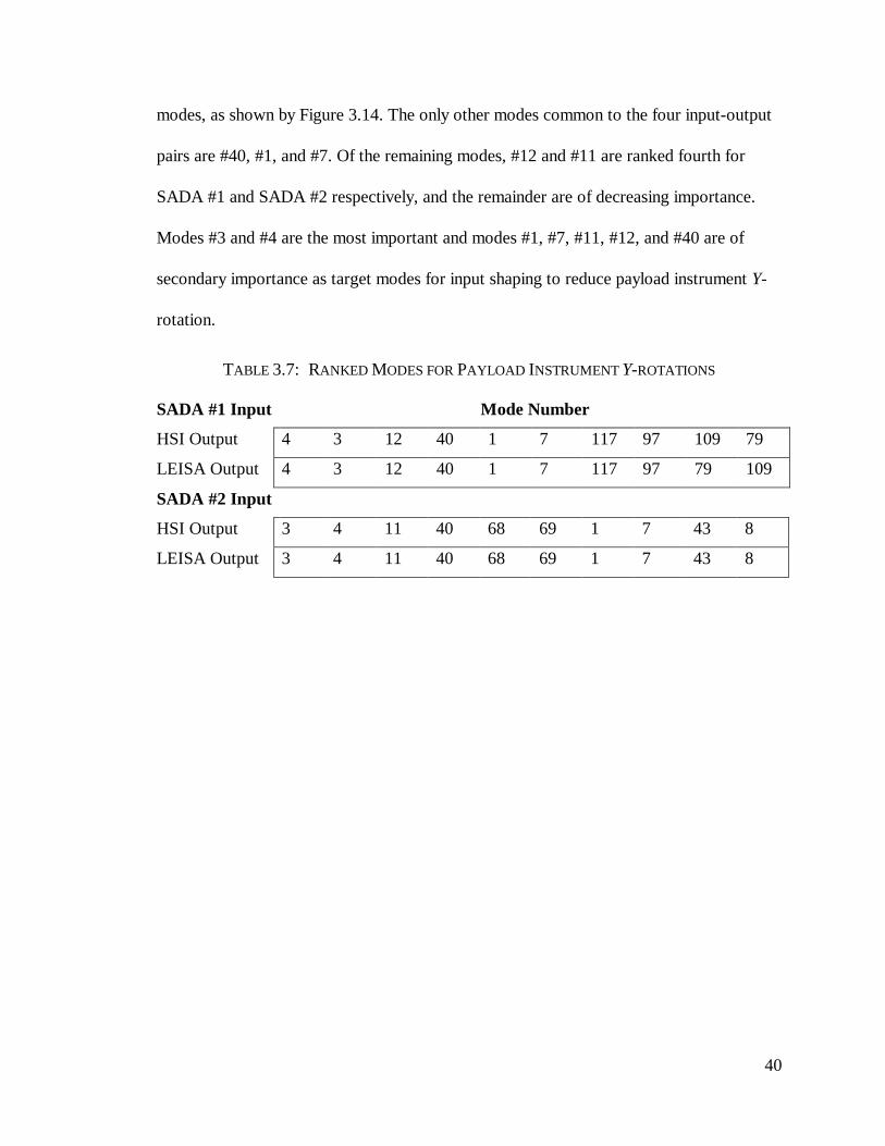
Table 3.7 summarizes the results of the second half of the FRF analysis by listing the
10 modes that provide the strongest input-output correlation in order of payload
instrument Y-rotation magnitude. The two largest contributors to both the HSI and LEISA
X-rotations for both SADA inputs are modes #3 and #4. The magnitude of the input-
output correlation for both of these modes is much greater than for any of the other
40
modes, as shown by Figure 3.14. The only other modes common to the four input-output
pairs are #40, #1, and #7. Of the remaining modes, #12 and #11 are ranked fourth for
SADA #1 and SADA #2 respectively, and the remainder are of decreasing importance.
Modes #3 and #4 are the most important and modes #1, #7, #11, #12, and #40 are of
secondary importance as target modes for input shaping to reduce payload instrument Y-
rotation.
TABLE 3.7: RANKED MODES FOR PAYLOAD INSTRUMENT Y-ROTATIONS
SADA #1 Input Mode Number
HSI Output 4 3 12 40 1 7 117 97 109 79
LEISA Output 4 3 12 40 1 7 117 97 79 109
SADA #2 Input
HSI Output 3 4 11 40 68 69 1 7 43 8
LEISA Output 3 4 11 40 68 69 1 7 43 8

41
0.0E+00
5.0E-04
1.0E-03
1.5E-03
2.0E-03
2.5E-03
3.0E-03
3.5E-03
1 2 3 4 5 6 7 8 9 10
Mode Rank
Mod
al F
RF
Am
plitu
de
SADA #1 - HSI
SADA #1 - LEISA
SADA #2 - HSI
SADA #2 - LEISA
FIGURE 3.14: PAYLOAD INSTRUMENT Y-ROTATION FRF MAGNITUDES

42
4 Simulations And Results
The analysis technique used to evaluate the structural vibrations due to the SADA
torque inputs is presented and then the structural responses and calculated vibration levels
for the two baseline simulations are discussed. The application to the Lewis spacecraft of
the pole-zero cancellation technique is introduced and the results from three vibration
control simulations are included. These examples illustrate the vibration control effects of
pole-zero cancellation and a method for increasing shaper robustness to errors in system
identification.
4.1 Jitter Analysis Method
Motion of the solar array panels must be accomplished without exciting structural
modes beyond acceptable jitter for the various payloads onboard. Jitter is usually defined
as the absolute value of the peak-to-peak change in the displacement or rotation of a
particular point on the spacecraft during a period of time called a jitter window. As an
example, a jitter requirement might be “10 µradians / 1 sec” which means a maximum of
10 µradians of rotation is allowable over any one second period of time.
When the period of a sinusoidal or other periodic vibration is less than the jitter
window, the vibration will complete at least one full cycle during the jitter window. The
resulting jitter would then equal the peak-to-peak amplitude of the vibration. When the
jitter window is less time than the vibration period, the jitter also depends on the phase of
the vibration in the jitter window as well as the vibration amplitude. Therefore, careful

43
selection of jitter windows can restrict the contributions of vibrations below the jitter
cutoff frequency, which is defined here as the reciprocal of the jitter window.
The total time the jitter is of concern can be much longer than the jitter window. The
largest jitter value that occurs during the total time of interest is known as the maximum
jitter. Continuing the previous example, let the 10 µradians / 1 sec jitter requirement be
prescribed for total time of interest of 3 seconds. In Figure 4.1, two different sinusoidal
vibrations are shown and a one second long jitter window is specified. Since the 3 Hz
vibration completes several cycles during the jitter window, it has a jitter that is equal to
the peak-to-peak amplitude (2.5 µradians in this example) and is constant for the total
time of interest. The displacement due to the 0.5 Hz vibration during the jitter window
indicated is 2 µradians. However, the lower frequency vibration has a longer period than
the jitter window (i.e., the vibration frequency is below the jitter cutoff frequency), and
therefore the maximum displacement within the jitter window also depends on the phase
of the vibration.

44
-2.5
-2
-1.5
-1
-0.5
0
0.5
1
1.5
2
2.5
0 0.5 1 1.5 2 2.5 3
Time, seconds
Rot
atio
n, u
radi
ans
JitterWindo3 Hz
vibration
0.5 Hz vibration
FIGURE 4.1: JITTER ANALYSIS EXAMPLE (1)
-2.5
-2
-1.5
-1
-0.5
0
0.5
1
1.5
2
2.5
0 0.5 1 1.5 2 2.5 3
Time, seconds
Rot
atio
n, u
radi
ans
JitterWindo
3 Hz vibration
0.5 Hz vibration
FIGURE 4.2: JITTER ANALYSIS EXAMPLE (2)

45
For a one second jitter window from 1.5 to 2.5 seconds the displacement for the 0.5
Hz vibration would double to 4 µradians as shown in Figure 4.2. If the jitter window is
“slid” in this manner along the total time of interest the maximum jitter for all possible
jitter windows can be found. More computationally efficient means of calculating jitter [5]
were used for this research but the result is the same. Since 4 µradians is the maximum
jitter value, these example vibrations would satisfy the 10 µradians / 1 second jitter
requirement for the entire time shown. Only the maximum rotation over all possible jitter
windows is of interest, and so the term jitter alone will be used to refer to the maximum
jitter. Jitter analysis of this nature will be used to determine the effectiveness of the
vibration reduction.
4.1.1 Selection of Jitter Windows and Analysis Start Time
Use of different length jitter windows can better reveal the vibration due to a
particular frequency range of modes. The shorter length windows will not allow lower
frequency vibrations to complete a full cycle within the window and therefore the
measured jitter due to lower frequency modes will be diminished. Table 4.1 details the
jitter windows used and the corresponding cutoff frequency, and lists the modes that are
above the cutoff frequency and therefore able to contribute fully within that jitter window.
The modal frequencies as determined by the FEM eigensolution are listed in Appendix B.
TABLE 4.1: EFFECT OF JITTER WINDOWS ON MODAL CONTRIBUTIONS
Jitter Window, seconds 0.05 0.1 0.2 0.5 1.0 3.5
Cutoff Frequency, Hz 20 10 5 2 1 0.286
Fully Included Modes 23-163 15-163 10-163 8-163 3-163 1-163
46
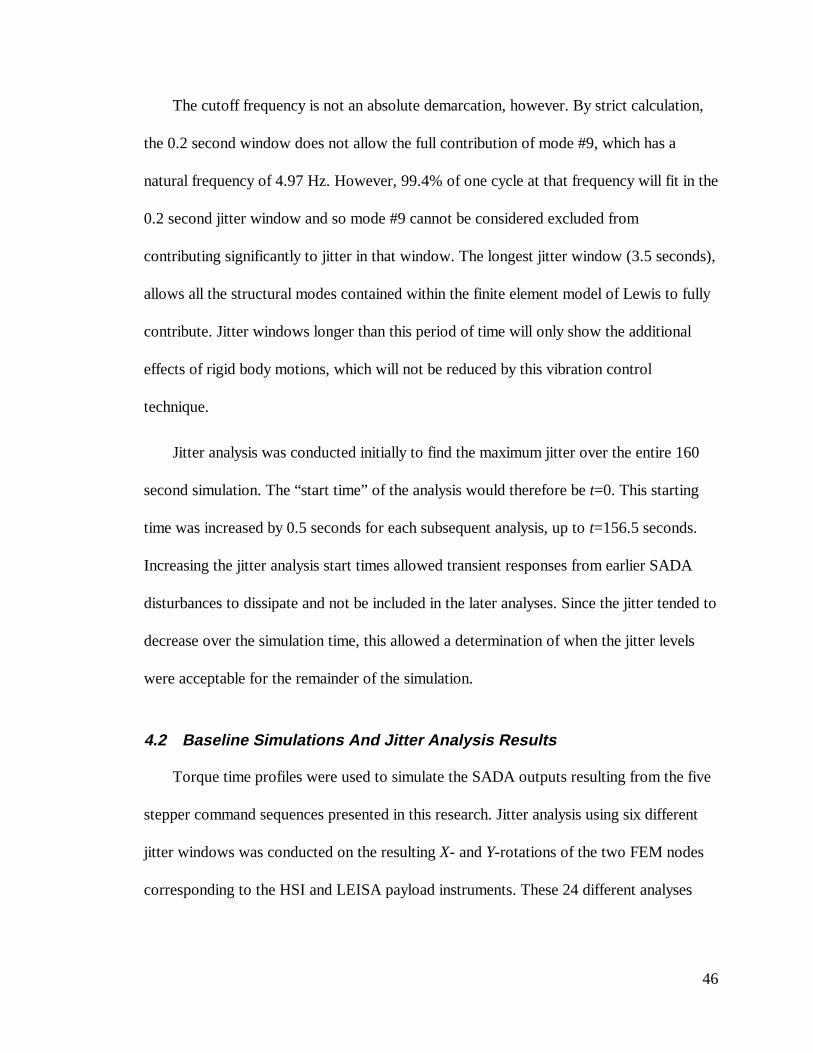
The cutoff frequency is not an absolute demarcation, however. By strict calculation,
the 0.2 second window does not allow the full contribution of mode #9, which has a
natural frequency of 4.97 Hz. However, 99.4% of one cycle at that frequency will fit in the
0.2 second jitter window and so mode #9 cannot be considered excluded from
contributing significantly to jitter in that window. The longest jitter window (3.5 seconds),
allows all the structural modes contained within the finite element model of Lewis to fully
contribute. Jitter windows longer than this period of time will only show the additional
effects of rigid body motions, which will not be reduced by this vibration control
technique.
Jitter analysis was conducted initially to find the maximum jitter over the entire 160
second simulation. The “start time” of the analysis would therefore be t=0. This starting
time was increased by 0.5 seconds for each subsequent analysis, up to t=156.5 seconds.
Increasing the jitter analysis start times allowed transient responses from earlier SADA
disturbances to dissipate and not be included in the later analyses. Since the jitter tended to
decrease over the simulation time, this allowed a determination of when the jitter levels
were acceptable for the remainder of the simulation.
4.2 Baseline Simulations And Jitter Analysis Results
Torque time profiles were used to simulate the SADA outputs resulting from the five
stepper command sequences presented in this research. Jitter analysis using six different
jitter windows was conducted on the resulting X- and Y-rotations of the two FEM nodes
corresponding to the HSI and LEISA payload instruments. These 24 different analyses

47
were conducted over the course of the simulation and used to determine the relative
effectiveness of the vibration control method in comparison to baseline results.
4.2.1 Constant Step Rate Simulation
The torque variation of a single step of the SADA rotary actuator is shown in Figure
4.3. The duration of a single step is about 1/40th of a second from beginning to end and
therefore up to about a 40 Hz step rate would be expected to consist of entirely discrete
operations. This is a reasonable result given that a smaller rotary stepper motor with
lighter end-loading conditions was found by Jim Miller of NASA Langley Research Center
[private communication] to have discrete steps up to 100 Hz. Cascading these steps at the
prescribed step rate of approximately 3.16 steps or pulses per second (PPS) results in the
Constant Step Rate Sequence (CSRS) torque input, a portion of which is shown in Figure
4.4. This plot illustrates the short time length and impulsive nature of the individual steps.

48
-5
-4
-3
-2
-1
0
1
2
3
0 0.005 0.01 0.015 0.02
Time, seconds
Tor
que
, in-
lbf
FIGURE 4.3: SINGLE STEP TORQUE TIME PROFILE
0 0.2 0.4 0.6 0.8 1 1.2 1.4 1.6 1.8 2−2
−1.5
−1
−0.5
0
0.5
1
Time, sec
Torq
ue, i
n−lb
f
FIGURE 4.4: CSRS TORQUE TIME PROFILE, 3.16 PPS

49
The X- and Y-rotations of the HSI instrument are shown in Figures 4.5 and 4.6. These
figures show the total response (combined rigid and flexible body terms) and the flexible
body response alone. The rigid body Y-rotation of the HSI instrument was approximately
5,350 µradians, close to the quantity predicted by Equation 3.6. The rigid body X- and Z-
rotations are approximately -102 and –13.5 µradians respectively, and this indicates that
the simulated spacecraft structure transfers some energy between the coordinate directions
via non-zero off-diagonal terms in the inertia matrix.
0 20 40 60 80 100 120 140 160−12
−10
−8
−6
−4
−2
0
2x 10
−5 csrs HSI X−Rotation Response
Rot
atio
n, m
icro
radi
ans
0 20 40 60 80 100 120 140 160−5
0
5x 10
−6 csrs HSI X−Rotation Flexible−Body Response
Time, seconds
Rot
atio
n, m
icro
radi
ans
FIGURE 4.5: HSI X-ROTATION RESPONSE TO CSRS TORQUE INPUT

50
0 20 40 60 80 100 120 140 160−1
0
1
2
3
4
5
6x 10
−3 csrs HSI Y−Rotation Response
Rot
atio
n, m
icro
radi
ans
0 20 40 60 80 100 120 140 160−1.5
−1
−0.5
0
0.5
1
1.5x 10
−5 csrs HSI Y−Rotation Flexible−Body Response
Time, seconds
Rot
atio
n, m
icro
radi
ans
FIGURE 4.6: HSI Y-ROTATION RESPONSE TO CSRS TORQUE INPUT
For both instruments, the jitter response to the CSRS torque input are nearly constant
values for all analysis start times. Within the simulation, the HSI and LEISA nodes achieve
a steady state response almost immediately to the repetitive CSRS torque input. Table 4.2
summarizes the average jitter levels for the six jitter windows used.
The Y-rotation jitter levels are clearly not acceptable and have significant input from
the higher frequency modes (i.e., the jitter levels only increase slightly as the jitter window
is lengthened from 0.05 seconds to 3.5 seconds). The X-rotation is much less, and is due

51
to the structural transfer of rotational energy since the input torque is acting about the Y-
axis only.
TABLE 4.2: CSRS JITTER ANALYSIS RESULTS
JitterWindows
in seconds
HSIX-rotation
LEISAX-rotation
HSIY-rotation
LEISAY-rotation
Jitter, µradians 7.20 5.91 16.96 51.950.05
% of Jitter Limit 72.0% 19.7% 169.6% 173.2%Jitter, µradians 7.20 5.91 16.99 51.95
0.1% of Jitter Limit 72.0% 19.7% 169.9% 173.2%Jitter, µradians 7.20 5.91 17.56 51.95
0.2% of Jitter Limit 72.0% 19.7% 175.6% 173.2%Jitter, µradians 7.79 5.97 18.87 54.31
0.5% of Jitter Limit 77.9% 19.9% 188.7% 181.0%Jitter, µradians 7.79 5.99 19.01 54.32
1% of Jitter Limit 77.9% 20.0% 190.1% 181.1%Jitter, µradians 7.80 6.00 19.07 54.43
3.5% of Jitter Limit 78.0% 20.0% 190.7% 181.4%
4.2.2 Minimum Actuation Time Simulation
A single actuator sequence consisting of 500 consecutive steps at the maximum rate
of 200 pulses per second (PPS) was simulated. The first 0.5 seconds of the 200 PPS
torque output is shown in Figure 4.7. This achieves the required 10° of rotation in a
minimum time of 2.5 seconds and would allow a maximum amount of time for structural
damping to dissipate the vibrational energy. The stepper motor torque output at high step
rates loses its distinct step characteristics. The response of the HSI to the MATS torque
input is shown in Figures 4.8 and 4.9.

52
0 0.05 0.1 0.15 0.2 0.25 0.3 0.35 0.4 0.45 0.5−3
−2
−1
0
1
2
3
Time, sec
Torq
ue, i
n−lb
f
FIGURE 4.7: MATS TORQUE TIME PROFILE, 200 PPS

53
0 20 40 60 80 100 120 140 160−15
−10
−5
0
5x 10
−5 mats HSI X−Rotation Response
Rot
atio
n, m
icro
radi
ans
0 20 40 60 80 100 120 140 160−4
−2
0
2
4x 10
−5 mats HSI X−Rotation Flexible−Body Response
Time, seconds
Rot
atio
n, m
icro
radi
ans
FIGURE 4.8: HSI X-ROTATION RESPONSE TO MATS TORQUE INPUT
The rigid body Y-rotation for the spacecraft is approximately 5,350 µradians, agreeing
with the response from the CSRS input. After the SADA input is complete at t=2.5
seconds, the spacecraft structure was allowed to settle until t=160 seconds. The HSI Y-
rotation response during the settling period consists of a superposition of decaying
sinusoids from the simulated structural modes. Jitter analysis was conducted as stated
previously over the entire simulation time.

54
0 20 40 60 80 100 120 140 160−1
0
1
2
3
4
5
6x 10
−3 mats HSI Y−Rotation Response
Rot
atio
n, m
icro
radi
ans
0 20 40 60 80 100 120 140 160−4
−2
0
2
4
6
8
10x 10
−4 mats HSI Y−Rotation Flexible−Body Response
Time, seconds
Rot
atio
n, m
icro
radi
ans
FIGURE 4.9: HSI Y-ROTATION RESPONSE TO MATS TORQUE INPUT
The jitter analysis results for both the CSRS and MATS simulations are summarized
in Figures 4.10 through 4.13, and show the jitter values as percentages of the instrument
jitter limits. Jitter analyses of the MATS simulation response with a start time of t=0 had
the largest values. The jitter levels steadily decreased as the analysis start time progressed
and the last jitter analyses, with a start time of t=156.5 seconds, had the minimum value.

55
1%
10%
100%
1000%
JItter Windows, seconds
Per
cent
of J
itter
Lim
it
CSRS 71.95% 71.95% 71.95% 77.93% 77.93% 77.96%
MATS Maximum 377.3% 453.1% 487.4% 548.3% 548.3% 599.8%
MATS Mean 22.4% 34.7% 46.1% 67.0% 67.5% 69.3%
MATS Minimum 1.3% 2.6% 4.9% 7.2% 7.2% 7.6%
0.05 0.1 0.2 0.5 1 3.5
FIGURE 4.10: HSI X-ROTATION BASELINE JITTER LEVELS
0.1%
1.0%
10.0%
100.0%
1000.0%
JItter Windows, seconds
Per
cent
of J
itter
Lim
it
CSRS 19.70% 19.70% 19.70% 19.90% 19.97% 20.00%
MATS Maximum 130.9% 150.8% 151.4% 154.5% 163.1% 175.4%
MATS Mean 7.3% 11.3% 15.2% 22.2% 22.4% 23.0%
MATS Minimum 0.4% 0.9% 1.6% 2.4% 2.4% 2.5%
0.05 0.1 0.2 0.5 1 3.5
FIGURE 4.11: LEISA X-ROTATION BASELINE JITTER LEVELS

56
10%
100%
1000%
10000%
100000%
JItter Windows, seconds
Per
cent
of J
itter
Lim
it
CSRS 169.60 169.90 175.60 188.70 190.10 190.70
MATS Maximum 1666.0 2895.0 4717.0 8941.0 9139.0 13224.0
MATS Mean 485.7% 973.5% 1815.9 2909.1 2909.7 2971.0
MATS Minimum 68.7% 139.5% 261.3% 373.5% 373.5% 373.5%
0.05 0.1 0.2 0.5 1 3.5
FIGURE 4.12: HSI Y-ROTATION BASELINE JITTER LEVELS
10%
100%
1000%
10000%
JItter Windows, seconds
Per
cent
of J
itter
Lim
it
CSRS 173.18%173.18%173.18%181.04%181.06%181.42%
MATS Maximum 1237.0%1425.7%1998.7%3287.7%3421.7%4581.0%
MATS Mean 171.6% 331.3% 610.7% 974.8% 975.6% 994.5%
MATS Minimum 22.9% 46.5% 87.0% 124.4% 124.4% 124.4%
0.05 0.1 0.2 0.5 1 3.5
FIGURE 4.13: LEISA Y-ROTATION BASELINE JITTER LEVELS
Examination of the MATS simulation response reveals that the average and minimum
X-rotations are below the desired jitter limits, but the corresponding Y-rotations generally
exceed the limits. The HSI minimum Y-rotation jitter values are above the instrument jitter

57
limit for the 5 longer jitter windows, with only the 0.05 second window having an
acceptable minimum jitter value (68.7% of the jitter limit, see Figure 4.12). Structural
damping (modeled as 0.2% for all modes) decreased the minimum LEISA Y-rotation jitter
for the 0.5, 1.0 and 3.5 second windows to 124.4% of the instrument jitter limit (see
Figure 4.13). These results illustrate that with a lightly damped system the structural
modes can cause sustained vibratory motion that could reduce the data quality from the
payload instruments and a more advanced command sequence could be employed to
directly address this concern.
4.3 Shaped Input Simulations and Results
The implementation of the z-plane pole-zero cancellation theory for the Lewis
spacecraft SADA is presented. To aid in the selection of input shaper solutions, additional
calculations using four different criteria are performed. These calculations rank the many
possible sets of stepper motor sequences produced by the vibration control theory. The
proposed solutions were then transformed into equivalent SADA torque time profiles and
the Lewis spacecraft response was simulated using the model introduced in Section 3.
Jitter analysis was then performed to evaluate the performance of each sequence in
reducing vibration. The results from three of these simulations are presented in Sections
4.3.
The target modes were selected as discussed in Section 3.3. The corresponding target
poles were calculated from the modal information according to Equation 2.4 and the
discrete time transfer function was constructed. This transfer function was transformed to
the Laplace s-domain and the numerator coefficients were extracted. These coefficients

58
are the impulse amplitudes of Equation 2.11, and solutions with any negative impulses
were removed. This is not essential, but removing solutions with negative impulses
ensured that the SADA would always move the solar arrays in the desired direction. Other
researchers have investigated the use of negative impulses to shorten the time interval T
between impulses [8] but this was not investigated for the Lewis spacecraft. The impulse
amplitudes of the remaining solutions were normalized to sum to one. The four ranking
criteria of Equations 2.12 through 2.15 were calculated and based on these rankings, one
or more solutions were selected and used with the PLATSIM Lewis simulation.
The stepper sequence(s) defined by a given input shaper solution was then used to
construct an SADA torque time profile. This torque profile contained the desired number
of steps in each sequence and had each sequence spaced in time at a center-to-center
distance equal to T as shown in Figure 2.6. The simulated SADA torque was applied to
the SADA nodes within an open-loop simulation (to remove any effects from the Lewis
spacecraft ACS) and the resulting jitter levels of the HSI and LEISA payload instruments
examined to evaluate the vibration reduction.
The results for all eight input-output pairs must be considered in the selection of
target modes for the input shaper, since the one shaper is to attempt to reduce the four
output vibrations. The X-rotations from the constant step rate and single sequence
simulations were below the jitter limits for all jitter windows, and so it was desired to
maintain that performance. At the same time, the simulated Y-rotations were up to 1.5
times the jitter limits and so that performance had to be improved. Comparison of the FRF
analysis plots show that a torque input about the Y-axis by either of the SADA’s has a

59
much greater impact on the Y-rotation of the payload instruments than on the X-rotation
of that node. Therefore, the controllability of the Y-rotations by the SADA torque is
greater.
4.3.1 Vibration Control Sequence #1
Table 4.3 shows the information that fully describes Vibration Control Sequence #1
(VCS #1) as implemented for the Lewis spacecraft. The Target Modes are the modes
selected using the FRF analysis of Section 3.3. The Target Robustness is the total number
of zeros that are placed over the corresponding system poles by the shaper transfer
function. The Impulse Amplitudes listed are the normalized values, and the Step Time is
the time at which each step sequence begins, adjusted as explained in Section 2.4. The
system poles corresponding to the eight target modes are plotted in the z-plane in Figure
4.14, and the shaper zeros are placed exactly over the system poles in this command
sequence. The first 30 seconds of the SADA torque for VCS #1 is shown in Figure 4.15,
with the torque being zero from t=30 to t=160 seconds.

60
TABLE 4.3: VIBRATION CONTROL SEQUENCE #1 DATA
Target Modes #2 #3 #4 #7 #8 #11 #12 #40Target Robustness 1 2 2 1 2 1 1 1Total # Impulses 23Sampling Time, T 1.14 secondsStep Rate 200 PPSImpulse # Impulse Amplitudes # Steps Impulse Time, seconds Step Time, seconds
1 0.023073 12 0 02 0.03148 16 1.14 1.1253 0.036154 18 2.28 2.2554 0.08806 44 3.42 3.3255 0.051758 26 4.56 4.5056 0.040324 20 5.7 5.6557 0.094088 47 6.84 6.72258 0.012803 6 7.98 7.969 0.047849 24 9.12 9.0510 0.113721 57 10.26 10.102511 0.037566 19 11.4 11.332512 0.09349 47 12.54 12.397513 0.100759 50 13.68 13.52514 0.022169 11 14.82 14.757515 0.050666 25 15.96 15.857516 0.036388 18 17.1 17.0117 0.008973 4 18.24 18.1818 0.032492 16 19.38 19.28519 0.029042 15 20.52 20.422520 0.019262 10 21.66 21.5721 0.017665 9 22.8 22.707522 0.009763 5 23.94 23.852523 0.002455 1 25.08 24.9975
Totals 1.00 500

61
FIGURE 4.14: SYSTEM POLES IN THE Z-PLANE (T=1.14 SECONDS)

62
0 5 10 15 20 25
−8
−6
−4
−2
0
2
4
6
8
Time, seconds
Tor
que,
in−
lbf
FIGURE 4.15: SADA TORQUE TIME PROFILE FOR VCS #1
The HSI X- and Y-rotations resulting from the VCS #1 input torque are depicted in
Figures 4.16 and 4.17. The LEISA response was nearly identical within the scale of the
graph. The total rigid body Y-rotation of the spacecraft agrees quite closely with the
prediction of Equation 3.6 and is approximately 5,350 µradians.

63
0 20 40 60 80 100 120 140 160−15
−10
−5
0
5x 10
−5 vcs1 HSI X−Rotation Response
Rot
atio
n, m
icro
radi
ans
0 20 40 60 80 100 120 140 160−4
−2
0
2
4x 10
−5 vcs1 HSI X−Rotation Flexible−Body Response
Time, seconds
Rot
atio
n, m
icro
radi
ans
FIGURE 4.16: HSI X-ROTATION RESPONSE TO VCS #1

64
0 20 40 60 80 100 120 140 160−1
0
1
2
3
4
5
6x 10
−3 vcs1 HSI Y−Rotation Response
Rot
atio
n, m
icro
radi
ans
0 20 40 60 80 100 120 140 160−3
−2
−1
0
1
2
3x 10
−4 vcs1 HSI Y−Rotation Flexible−Body Response
Time, seconds
Rot
atio
n, m
icro
radi
ans
FIGURE 4.17: HSI Y-ROTATION RESPONSE TO VCS #1
Jitter analysis of the HSI and LEISA responses was then performed. The jitter values
for a 3.5-second window are shown in Figures 4.18 through 4.21. These plots are
representative of the performance of the VCS #1 step commands in comparison to the
CSRS and MATS step commands introduced in Section 3. The X-rotation jitter is plotted
on a linear scale, while the Y-rotation jitter is plotted on a semi-log scale to display the
larger variation in the jitter results. The staircase nature of the plots is an effect of the jitter
analysis method since the maximum jitter quantity from the given analysis start time until

65
the end of the simulation is displayed. A solid gray line at the 100% level on all four plots
marks the jitter limit.
For all three simulations, the jitter levels are fairly constant while the SADA torque is
non-zero. Referring to the 3.5-second jitter window results shown in Figures 4.18 and
4.19, the VCS #1 simulation X-rotation jitter begins (at t=0 seconds) with values that are
greater than the MATS simulation values. For both the MATS and VCS #1 simulations,
the jitter levels drop very quickly once the SADA input torque ceases. For the MATS
simulation, this event occurs at t=2.5 seconds, but doesn’t occur for the VCS #1
simulation until approximately t=25 seconds. The payload instrument jitter requirements
are therefore not satisfied in X-rotation by the VCS #1 simulation until t=50 seconds for
the HSI and t=33 seconds for the LEISA.
However, the input shaper was primarily designed to reduce the problematic Y-
rotation jitter levels (and the X-rotations of the payload instruments are not very
controllable by the torque about the Y-axis produced by the SADA, as revealed by the
FRF analysis of Section 3). The Y-rotation jitter analysis results are shown for the 3.5-
second window in Figures 4.20 and 4.21. For the VCS #1 simulation, the Y-rotation jitter
levels are approximately constant when the SADA torque is non-zero and then drop off
very sharply. The large decrease in Y-rotation jitter levels immediately following the end of
the SADA input during the VCS #1 simulation is due to the shaping of the SADA input.
The HSI and LEISA instruments have acceptable Y-rotation jitter levels by t=56 and 26
seconds, respectively. In contrast, the MATS simulation jitter levels decrease at a much
smaller rate due to structural damping only and never achieve acceptable jitter levels. The

66
CSRS simulation jitter levels are approximately constant at 190.7% and 181.4% of the
jitter requirements for the HSI and LEISA respectively. In general, the VCS #1 step
sequence causes both the X-rotation and Y-rotation jitter levels to be within the payload
instrument requirements shortly after the SADA step commands are completed.
Since angular momentum is conserved in the physical system, the rigid body rotation
about the Y-axis of the spacecraft bus from even a single step of the SADA is of a
significant quantity (10.3 µradians, which corresponds to approximately 103% and 33% of
the HSI and LEISA jitter requirements respectively). Therefore, any action by the SADA
would preclude the optimal operation of the payload instruments. The VCS #1 step
commands cause a minority of the simulation time to be spent at the higher jitter levels and
allow more time for a vibration sensitive operation to be performed.
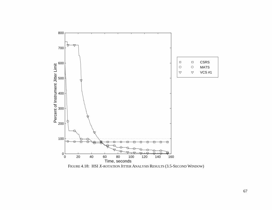
67
0 20 40 60 80 100 120 140 1600
100
200
300
400
500
600
700
800
Time, seconds
Per
cent
of I
nstr
umen
t Jitt
er L
imit CSRS
MATS
VCS #1
FIGURE 4.18: HSI X-ROTATION JITTER ANALYSIS RESULTS (3.5-SECOND WINDOW)

68
0 20 40 60 80 100 120 140 1600
50
100
150
200
250
Time, seconds
Per
cent
of I
nstr
umen
t Jitt
er L
imit CSRS
MATS
VCS #1
FIGURE 4.19: LEISA X-ROTATION JITTER ANALYSIS RESULTS (3.5-SECOND WINDOW)

69
0 20 40 60 80 100 120 140 16010
1
102
103
104
105
Time, seconds
Per
cent
of I
nstr
umen
t Jitt
er L
imit CSRS
MATS
VCS #1
FIGURE 4.20: HSI Y-ROTATION JITTER ANALYSIS RESULTS (3.5-SECOND WINDOW)

70
0 20 40 60 80 100 120 140 16010
0
101
102
103
104
Time, seconds
Per
cent
of I
nstr
umen
t Jitt
er L
imit CSRS
MATS
VCS #1
FIGURE 4.21: LEISA Y-ROTATION JITTER ANALYSIS RESULTS (3.5-SECOND WINDOW)

71
4.3.2 Vibration Control Sequence #2
The VCS #1 simulation had perfect identification of the system poles, allowing the
shaper zeros to be collocated with the target poles for maximum effectiveness in vibration
reduction. However, significant errors in the identification of even moderately complex
structures are possible and a robust control system must be able to operate well despite
these inaccuracies. The technique of using additional shaper zeros to compensate for
errors in the identification of the system poles is presented in this section.
Table 4.4 shows the data for a second vibration reducing solution as implemented for
the Lewis spacecraft. The final step sequence of VCS #2 rounded down to zero when
discretized for the SADA actuator and was removed from the command sequence. This
discretization caused the impulse amplitudes to sum to slightly less than one. VCS #2 has
the same target modes as VCS #1, but the natural frequencies of the target modes have
been intentionally made erroneous for this case. Specifically, the frequencies of the zeros
placed by the pole-zero cancellation algorithm have been made 10% higher than the poles
of the modeled system. Having an inconsistent value for the modal natural frequencies
between the input shaping algorithm and the physical system (represented by a finite
element model in this research) explores the robustness of the pole-zero cancellation
method. The system poles and VCS #2 shaper zeros are plotted in the z-plane in Figure
4.22 and this graph illustrates the large inaccuracies introduced by the 10% error in natural
frequency.

72
TABLE 4.4: VIBRATION CONTROL SEQUENCE #2 DATA
Target Modes #2 #3 #4 #7 #8 #11 #12 #40Target Robustness 1 2 2 1 2 1 1 1Total # Impulses 22Sampling Time, T 1.035 secondsStep Rate 200 PPSImpulse # Impulse Amplitudes # Steps Impulse Time, seconds Step Time, seconds
1 0.008644 4 0 02 0.016913 8 1.035 1.0253 0.024012 12 2.07 2.054 0.048988 24 3.105 3.0555 0.051361 26 4.14 4.0856 0.052878 26 5.175 5.127 0.077811 39 6.21 6.12258 0.061522 31 7.245 7.17759 0.068918 34 8.28 8.20510 0.094138 47 9.315 9.207511 0.071606 36 10.35 10.2712 0.081233 41 11.385 11.292513 0.083637 42 12.42 12.32514 0.052490 26 13.455 13.415 0.052883 26 14.49 14.43516 0.044653 22 15.525 15.4817 0.027901 14 16.56 16.53518 0.028963 14 17.595 17.5719 0.022739 11 18.63 18.612520 0.013575 7 19.665 19.657521 0.009587 5 20.7 20.697522 0.004635 2 21.735 21.74
Totals 0.999 500
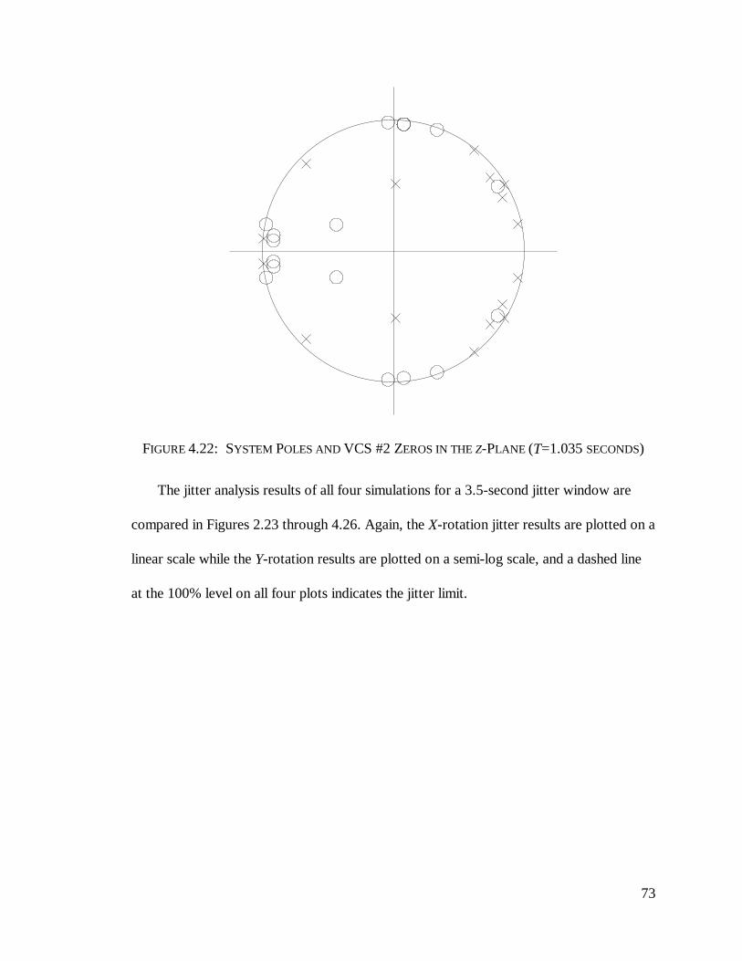
73
FIGURE 4.22: SYSTEM POLES AND VCS #2 ZEROS IN THE Z-PLANE (T=1.035 SECONDS)
The jitter analysis results of all four simulations for a 3.5-second jitter window are
compared in Figures 2.23 through 4.26. Again, the X-rotation jitter results are plotted on a
linear scale while the Y-rotation results are plotted on a semi-log scale, and a dashed line
at the 100% level on all four plots indicates the jitter limit.

74
0 20 40 60 80 100 120 140 1600
100
200
300
400
500
600
700
800
Time, seconds
Per
cent
of I
nstr
umen
t Jitt
er L
imit CSRS
MATS
VCS #1
VCS #2
FIGURE 4.23: HSI X-ROTATION JITTER ANALYSIS RESULTS (3.5-SECOND WINDOW)

75
0 20 40 60 80 100 120 140 1600
50
100
150
200
250
Time, seconds
Per
cent
of I
nstr
umen
t Jitt
er L
imit CSRS
MATS
VCS #1
VCS #2
FIGURE 4.24: LEISA X-ROTATION JITTER ANALYSIS RESULTS (3.5-SECOND WINDOW)

76
0 20 40 60 80 100 120 140 16010
1
102
103
104
105
Time, seconds
Per
cent
of I
nstr
umen
t Jitt
er L
imit CSRS
MATS
VCS #1
VCS #2
FIGURE 4.25: HSI Y-ROTATION JITTER ANALYSIS RESULTS (3.5-SECOND WINDOW)

77
0 20 40 60 80 100 120 140 16010
0
101
102
103
104
Time, seconds
Per
cent
of I
nstr
umen
t Jitt
er L
imit CSRS
MATS
VCS #1
VCS #2
FIGURE 4.26: LEISA Y-ROTATION JITTER ANALYSIS RESULTS (3.5-SECOND WINDOW)

78
As might be expected, the vibration control performance for the Y-rotation of VCS #2
is less satisfactory than that of VCS #1. The 10% error in natural frequency for the target
modes caused the 3.5-second window Y-Rotation jitter levels for VCS #2 (see Figures
4.25 and 4.26) to never achieve acceptable levels. Conversely, the X-rotation jitter results
for VCS #2 are actually improved over the VCS #1 results. This is primarily due to the
shorter time interval between the step sequences (T=1.14 seconds for VCS #1 and
T=1.035 seconds for VCS #2) since the reduction in X-rotation jitter levels is caused by
structural damping. In general, errors in identification of the natural frequencies or
damping ratios of the target modes will cause less than ideal input shaper performance. To
incorporate insensitivity to these possible errors, additional zeros can be placed on some
or all of the target modes [15]. This technique is explored in the following section.
4.3.3 Vibration Control Sequence #3
It has been shown that the deleterious effects on vibration reduction caused by errors
in either damping ratio or natural frequency can be mitigated by the placement of
additional shaper zeros [15]. To illustrate this technique, the same target modes and
erroneous natural frequencies used for VCS #2 were used for the final case, VCS #3, but
three times as many zeros were placed. The 22 additional zeros for VCS #3 were located
on the same points on the z-plane as the original 11 zeros for VCS #2, resulting in third
order pole-zero cancellation.
Placing 33 input shaper zeros results in 67 impulse amplitudes but many impulse
amplitudes rounded down to zero steps when discretized for the SADA actuator. Since
these 21 null sequences occurred either before and after but not during the set of 46 non-

79
zero sequences, all the null sequences were ignored. The data describing this third
vibration control sequence is given in Table 4.5. The total number of actuator steps was
500 but the sum of the impulse amplitudes is slightly less than one. If the discretization
caused the total number of steps to be some value other than 500, the next SADA
command sequence should then be performed at the appropriate time according to the
solar tracking requirement, i.e., some time other than t=160 seconds.
4.4 Summary Of Results
The value of T and the total number of non-zero “impulses” are substantially different
between the VCS #1 and VCS #3 command sequences, but these parameters combine to
cause both to complete the solar array 10° rotation at similar times in the simulation
(approximately T=25 seconds for VCS #1 and T=19.35 seconds for VCS #3). The
command sequences consist of sets of actuator steps that vary from 1 to 57 steps for VCS
#1 and from 1 to 23 steps for VCS #3. Therefore, these two command sequences are very
comparable in the length of the actuation time and the SADA performance required which
implies that in this application the “cost” of the additional robustness is negligible.
The complete set of graphs comparing the jitter analysis results for the CSRS, MATS,
VCS #1, VCS #2, and VCS #3 simulations are given in Appendix C. Increasing the input
shaper robustness allowed very similar vibration reduction performance to be achieved by
VCS #3 in comparison to VCS #1, even though the VCS #3 target natural

80
TABLE 4.5: VIBRATION CONTROL SEQUENCE #3 DATA
Target Modes #2 #3 #4 #7 #8 #11 #12 #40Target Robustness 3 6 6 3 6 3 3 3Total # Impulses 46Sampling Time, T 0.43 secondsStep Rate 200 PPSImpulse # Impulse Amplitudes # Steps Impulse Time, seconds Step Time, seconds1 0.001188 1 0.00 0.00002 0.001784 1 0.43 0.43003 0.002598 1 0.86 0.86004 0.003612 2 1.29 1.28755 0.004805 2 1.72 1.71756 0.006211 3 2.15 2.14507 0.007927 4 2.58 2.57258 0.010022 5 3.01 3.00009 0.012460 6 3.44 3.427510 0.015108 8 3.87 3.852511 0.017854 9 4.30 4.280012 0.020717 10 4.73 4.707513 0.023798 12 5.16 5.132514 0.027116 14 5.59 5.557515 0.030493 15 6.02 5.985016 0.033650 17 6.45 6.410017 0.036421 18 6.88 6.837518 0.038864 19 7.31 7.265019 0.041113 21 7.74 7.690020 0.043152 22 8.17 8.117521 0.044744 22 8.60 8.547522 0.045628 23 9.03 8.975023 0.045750 23 9.46 9.405024 0.045296 23 9.89 9.835025 0.044482 22 10.32 10.267526 0.043333 22 10.75 10.6975
27 0.041693 21 11.18 11.130028 0.039446 20 11.61 11.562529 0.036697 18 12.04 11.997530 0.033718 17 12.47 12.430031 0.030727 15 12.90 12.865032 0.027753 14 13.33 13.297533 0.024711 12 13.76 13.732534 0.021586 11 14.19 14.165035 0.018504 9 14.62 14.600036 0.015648 8 15.05 15.032537 0.013114 7 15.48 15.465038 0.010871 5 15.91 15.900039 0.008847 4 16.34 16.332540 0.007019 4 16.77 16.762541 0.005432 3 17.20 17.195042 0.004132 2 17.63 17.627543 0.003108 2 18.06 18.057544 0.002302 1 18.49 18.490045 0.001655 1 18.92 18.920046 0.001139 1 19.35 19.3500Totals 0.996228 500

81
frequencies were 10% higher than the modeled system. For several windows the jitter
decreased below the jitter limit at an earlier time for VCS #3 than for VCS #1, primarily
due to the earlier completion of the solar array rotation by VCS #3. These results indicate
that in this application, an increase in the number of shaper zeros can improve the
feedforward robustness of the system with very little or no decrease in other aspects of
system performance.
For rotation about the X-axis, the VCS simulations in general have less time with
acceptable jitter levels than either the CSRS or MATS simulations. These results are
presented in Figures C.1 through C.12. One notable exception is the 3.5 second window
analysis of the CSRS simulation for the HSI instrument shown in Figure C.11.
Figures C.13 through C.24 show the marked improvement for rotation about the Y-
axis in the VCS #1 and #3 simulations in comparison to the CSRS and MATS baseline
cases. The CSRS and MATS simulations have limited to zero time during the simulation
when acceptable jitter levels were achieved. The system identification error explored in the
VCS #2 simulation shows up as significantly worse mission performance but the use of
additional shaper zeros counteracts this deficiency very well. These results show that the
VCS step commands are an effective means to control structural vibrations and therefore
improve mission performance when the system identification is reasonably accurate and
robustness techniques are employed.

82
5 Conclusions
The structural vibration response of a well-understood system can be reduced
considerably through the use of input shaping techniques. Reduction of structural vibration
can often allow the system to perform required tasks more quickly, using less actuator
power, reducing system wear, and possibly allowing the addition of new tasks that were
not possible before.
5.1 Current Results
As is the case for many techniques in structural dynamics, the vibration reduction
performance of pole-zero cancellation methods is dependent on the accuracy of the system
identification. In the Lewis spacecraft vibration problem, the system identification for VCS
#1 was perfect insofar as the results presented were generated through the use of a
simulation that used the same system description as that used to generate the input shaper.
Therefore the results could be viewed as exceptional in comparison to the results that
would be obtained in practice with a poorly understood physical system. This is a known
limitation of the pole-zero cancellation approach.
However, identifying a physical system through empirical techniques is becoming
common and can yield accurate descriptions of complex systems relatively quickly. The
results presented here and through experimentation [15] have shown that the robustness of
an input shaper transfer function can be increased through the placement of additional
zeros as discussed in this paper. In the current research, it was found that this increase in

83
controller robustness could be accomplished without any increase in computational
complexity or actuator requirements.
5.2 Recommendations for Future Research
Several areas were recognized as topics that warrant additional investigation and are
presented briefly below. The use of alternative actuators is a basic consideration, as is a
deeper understanding of the effects of changing system parameters to multiple mode
robustness. Beyond those topics, adaptation of the input shaper (perhaps automatically) to
changes in the system should be considered. This is particularly appropriate as digital
computing power increases in capability and much more involved control schemes can be
implemented.
5.2.1 Further Study of Actuator Dynamics
A stepper motor actuator was simulated as the system input device for the shaped
commands. This is not the most desirable actuator for the pole-zero cancellation technique
implemented, but it was shown that the technique is still very effective with this actuator.
Use of alternative stepping methods to a constant step rate and other actuator techniques
specific to stepper motors might allow further improvement on the results obtained.
5.2.2 Further Study of Multiple-Mode Robustness
A more extensive study of the relationship between the structural modes, system
identification accuracy, controller robustness, and input shaper performance could be
useful since the effective use of the robustness afforded by additional shaper zeros depends
upon the application. In the case of a rotating solar array presented here, the system modal

84
parameters would change as the orientation of the solar arrays relative to the spacecraft
bus progressed.
Extending the input shaper algorithm to account for the current relative orientation
(and therefore the expected change in system parameters) before calculating the command
sequence would be one method of handling this variation in system parameters. A simpler
method might be to “frame” the range of possible values of natural frequency and damping
ratio for the target modes with multiple zeros. This second technique could produce
acceptable system performance with a single command sequence for all relative
orientations, or both techniques could be combined to produce a limited number of
command sequences to cover the range of possible system parameters.
5.2.3 Automatic Selection of Target Modes
Study of the effectiveness of the frequency response function or other methods in
identifying the modes of concern in the presence of the many variables could also be topics
for further research. There are, in general, many feasible input shaper transfer functions for
a particular application and a study of a method to automate the selection of the most
desirable input shaping solution would be a first step to an adaptive extension of pole-zero
cancellation.
5.2.4 Extension to Adaptive Feedforward Vibration Control
The pole-zero cancellation method presented in this paper is computationally simple
to implement and could be incorporated into an on-board computing system or embedded
controller. With the addition of feedback, the on-board computer could be programmed to
automatically adapt the input shaper to any variations in the system parameters or

85
environment, or changes to the mission requirements, whether these variations were
expected or not. This would be an extension of existing research into input shaping for
varying system parameters [1]. Better performance of mechanical systems can be obtained
with fewer feedback components through the use of a feedforward input shaping
algorithm [12]. The entirely software-based simulation and jitter analysis tools presented
in this research would facilitate rapid experimentation with proposed adaptive feedforward
algorithms and allow researchers to pursue the most promising methods.

86
References
[1] Book, W.J. and Magee, D.P., “Application of Input Shaping to a System with
Varying Parameters”, Proceedings of the 1992 Japan-USA Symposium on
Flexible Automation, San Francisco, CA, July 1992, pp. 519-526
[2] Bouton, C.E. and McConnell, K.G., “Noise and Vibration Control with Robust
Vibration Suppression”, Sound and Vibration, June 1997, pp. 24-26
[3] Farley, R., "Modeling of a Rotational Stepper Motor with a Flexible Load",
Proceedings of the 29th Aerospace Mechanisms Symposium, NASA Conference
Publication #3293, League City, TX, May 1995, pp. 280-282
[4] Giesy, D.P., Kenny, S. and Maghami, P., "PLATSIM: A Simulation and Analysis
Package for Large-Order Flexible Systems (Version 2.0)," NASA TM-4790,
1997
[5] Giesy, D.P., "Efficient Calculation of Jitter/Stability Metric," Journal of
Spacecraft and Rockets, Vol. 34, No. 4, July-August 1997, pp. 549-557
[6] Hyde, J.M. and Seering, W.P., “Using Input Command Pre-Shaping to Suppress
Multiple Mode Vibration”, Proceedings of the 1991 IEEE International
Conference on Robotics and Automation, Sacramento, CA, April 1991, pp.
2604-2609
[7] Murphy, B.R. and Watanabe, I., “Digital Shaping Filters for Reducing Machine
Vibration”, IEEE Transactions on Robotics and Automation, April 1992, Vol. 8,
No. 2, pp. 285-289
[8] Rappole, B.W., Singer, N.C., and Seering, W.P., “Input Shaping with Negative
Sequences for Reducing Vibrations in Flexible Structures”, Proceedings of the
1993 American Control Conference, San Francisco, CA, June 1993, Vol. 3, pp.
2695-2699

87
[9] Rappole, B.W., Singer, N.C., and Seering, W.P., “Multiple-Mode Input Shaping
Sequences for Reducing Residual Vibrations”, Machine Elements and Machine
Dynamics (ASME), 1994, Vol. 71, pp. 11-16
[10] Singer, N.C. and Seering, W.P., “Preshaping Command Inputs to Reduce System
Vibration”, ASME Journal of Dynamic Systems, Measurements, and Control,
March 1990, Vol. 112, pp. 76-81
[11] Singer, N.C., “Residual Vibration Reduction in Computer Controlled Machines”,
Ph.D. Dissertation, Massachusetts Institute of Technology, February 1989
[12] Singh, T. and Vadali, S.R., “Robust Time-Delay Control”, ASME Journal of
Dynamic Systems, Measurement, and Control, 1993, Vol. 115, pp. 303-306
[13] Small Satellite Technology Initiative: Lewis Spacecraft Program, System Critical
Design Audit, NASA and TRW, January 1995
[14] Smith, O.J.M., Feedback Control Systems, 1958, New York, McGraw-Hill Book
Company, Inc., pp. 331-345
[15] Tuttle, T.D. and Seering, W.P., “A Zero-Placement Technique for Designing
Shaped Inputs to Suppress Multiple-Mode Vibration”, Proceedings of the 1994
American Control Conference, Baltimore, MD, June 1994, Vol. 3, pp. 2533-
2537

88
Appendix A: Stepper Motor Description
The basic operation of a three-phase stepper motor is presented in this section. The
relationship between the rotor position and the motor output torque is shown, and the
specific motor parameters for the SADA actuator on Lewis are calculated.
A.1 Torque Function
Referring to the stepper motor parameters of Table 2.2, the stepper motor torque
function is
[ ]T T C n T Cmotor powered e e detent m e= +
+cos sinθπ
θ3
(A.1
where Tpowered and Tdetent are the maximum torques the electromagnets and permanent
magnets of the motor can respectively develop on the rotor, θe is the current rotor
electrical angle (from 0 to 2π radians), Cm and Ce are constant motor parameters, and n is
the state count. The three-phase stepper motors manufactured by Schaeffer Magnetics
have a total of 6 different electrical states. Therefore n is an integer value that repeats
from 1 to 6, forming one electrical cycle of the motor. One electrical cycle can be thought
of as a rotation through 360 electrical degrees denoted as o360e from here on. Cm is a
motor constant equal to the number of mechanical steps per revolution of the motor rotor
CN
Rmrev= = =
18 000
100180
,(A.2

89
where Nrev is the total number of steps per revolution of the output shaft and R is the gear
reduction of the motor harmonic drive. Ce is a second motor constant that defines the
number of electrical cycles per revolution of the motor rotor
CC
nem= = =
max
180
630 (A.3
where nmax equals 6 and is the total number of different states in one electrical cycle. The
rotor electrical angle, θe , is related to the rotor mechanical angle, θm ,by
max
o360n
e
e
m
m θθ
θ =∆ (A.4
where mθ∆ equals 2° and is the incremental change in the rotor mechanical angle caused
by progression through one electrical state. Substituting in specific motor values results in
me θθ 30= (A.5
In summary, one complete electrical cycle of the stepper motor consists of
progressive motion through 6 electrical states (i.e., rotation through o360e ) that results in a
12° rotation of the motor rotor. With a 100:1 gear reduction through the harmonic drive,
a corresponding 0.12° rotation of the output shaft will occur.
A.2 Detent and Powered Motor Torques
The torque developed on the rotor at any time depends on which, if any, motor
electrical state is powered, the position or phase of the rotor relative to the motor
windings, and the maximum amplitude of the powered and detent holding torques. Figure
A.1 shows the torques on the rotor for a complete electrical cycle, if only state #1 is

90
powered. The two torques are the detent or unpowered torque, produced by permanent
magnets and the state 1 torque, produced by the state 1 electromagnets.
-200
-150
-100
-50
0
50
100
150
200
0 60 120 180 240 300 360
Electrical Angle, deg
Tor
que,
in-lb
f
Primary Equilibrium Point
Detent torque
State 1 torque
FIGURE A.1: DETENT AND STATE #1 TORQUES VS. ROTOR ELECTRICAL ANGLE

91
-250
-200
-150
-100
-50
0
50
100
150
200
250
0 60 120 180 240 300 360
Electrical Angle, deg
Tor
que,
in-lb
f
PrimaryEquilibrium Point
Secondary Equilibrium Point
FIGURE A.2: COMPOSITE TORQUE VS. ROTOR ELECTRICAL ANGLE
Figure A.2 shows the composite torque of these two sources. For nearly o180e in both
directions from the equilibrium point, the composite torque of the detent permanent
magnets and the state 1 electromagnets are restoring forces to the equilibrium point at
o150e . Note that there is a narrow secondary equilibrium region centered at o330e . The
width of this secondary equilibrium region is dependent on the motor parameters, and is
defined by the solution to the transcendental relation
[ ][ ]
−=
T
T
C
C
powered
detent
m e
e e
sin
cos
θθ
(A.6
For the motor configuration of interest the two solutions to Equation 5.6 between o0e and
o360e are

92
[ ][ ]− =3180
30
sin
cos
θθ
e
e
≈∴o
o
3.348
7.311
e
eeθ
(A.7
Therefore, for approximately o7.161 e on either side of the desired equilibrium point,
the composite motor torque will be a restoring force. If the load inertia were to cause the
rotor to fall out of phase with the equilibrium point by up to o7.161 e in either direction, it
will eventually settle to the correct position. This statement assumes that the same
electrical state is maintained during this settling time and for this reason the Schaeffer
Motor Driver incorporates a “Last Pulse Detector” which ensures that the last of a series
of pulses stays on for as long as 100 milliseconds [private communication]. The rotor
could fall out of phase with the equilibrium position by up to 5.39° (using Equation A.5 to
convert electrical to mechanical degrees) and still recover to the correct location.
A.3 Stepping Operation of a Three Phase Motor
During operation in a single direction, the stepper motor drive electronics power the
six electrical states consecutively. For clarity, the powered torques from only the first
three states are shown in Figure A.3. The rotor will stabilize at each of the equilibrium
points (marked as 1,2, and 3) corresponding to the current state. Once the rotor has
achieved the desired rotation, the electrical power can be removed from the motor
windings and the permanent magnet detent torque can be used to maintain the rotor
position.

93
-200
-150
-100
-50
0
50
100
150
200
0 60 120 180 240 300 360
Electrical Angle, deg
Tor
que,
in-lb
f
1
3
2
Detent Torques
FIGURE A.3: DETENT, STATES #1, #2, AND #3 TORQUES VS. ROTOR ELECTRICAL ANGLE
The detent torque does not require electrical power but is generally much less than
the composite torque and sufficiently large disturbances will cause the rotor to slip to a
different equilibrium position. However, powering the electrical state again would cause
the rotor to achieve its previous position, if the rotor position was within the range
specified by Equation A.6. Stepper motors are inherently underdamped, and therefore the
choice of actuator should take into consideration the expected overshoot. This overshoot
must be examined to see that it is acceptable from a system performance standpoint and
also that it does not cause the rotor to slip and come to rest at a different equilibrium point
than the one desired.

94
A.4 Motor-Load Dynamics
Using the simple rigid body physical model developed in Section 3, standard gear
reduction principles yield the moment of inertia of the solar array wing reflected through
the harmonic drive to the rotor as
I RotorI
R.yy
SA yySA
@ = ≈ × − −−2
5617 10 lbf in s2 (A.8
The reflected load inertia is only slightly less than the rotor inertia (IR≈8.3x10⁻⁵ lbf-in-s2)
and warrants the more sophisticated modeling of the coupled stepper motor and output
shaft load dynamics in Section 3.2.3.

95
Appendix B: Modal Frequencies of Lewis Finite Element Model
Mode Number Modal Frequency (Hz)1 0.297901
2 0.4681513 1.049531
4 1.103733
5 1.677571
6 1.725550
7 1.9649688 4.4692719 4.97326910 5.03493311 5.69719612 5.72715913 9.51433014 9.58912215 11.7492516 11.7838617 17.0615118 17.2653819 19.0960520 19.1550521 19.3933622 19.7539523 23.8678324 24.1503025 26.4396026 26.4819827 31.2219728 31.4123529 34.5286830 34.8900931 40.8514332 40.8688733 41.3638334 41.6447535 42.5263136 47.9823537 48.5840238 48.8058239 49.7283840 51.4439741 51.7452342 52.5727343 53.0879944 53.19312
Mode Number Modal Frequency (Hz)45 54.5456146 54.5549647 57.8986648 58.3965949 60.7112150 61.1728751 64.1989852 64.7162453 65.1863254 66.0091055 66.1010756 66.2085757 66.3353558 66.4443659 69.4502560 69.6086461 70.5989762 71.4818863 73.3968364 74.3390665 74.8791966 75.3163867 75.9945168 76.8390869 76.9475270 79.7938171 79.9436472 81.6165373 82.4384674 82.5807675 83.1601176 84.2170877 85.1097578 85.4536879 85.5126880 87.1465181 87.2502882 87.6869983 89.0059284 89.4497785 89.4720786 89.6661987 89.9620188 90.8583689 91.08218

96
Mode Number Modal Frequency (Hz)90 91.2705591 91.4257892 92.1212793 92.7444194 92.9329195 94.1701796 94.5620797 95.1754498 95.8882399 97.16349
100 98.18956101 98.31394102 98.41007103 98.78435104 99.69010105 101.8710106 102.3199107 102.4502108 104.5725109 106.0651110 106.3290111 107.3103112 107.6709113 108.1076114 108.1819115 109.7548116 110.1198117 113.3281118 114.6113119 114.9526120 115.4971121 116.0151122 116.9398123 117.1381124 119.3052125 119.3512
Mode Number Modal Frequency (Hz)126 119.4839127 120.8883128 121.5600129 121.8896130 122.0094131 122.6839132 123.0976133 124.0886134 125.1805135 125.4099136 126.0566137 127.9412138 129.4753139 129.9970140 130.5938141 130.6799142 130.8793143 131.6988144 132.3342145 134.0331146 134.5332147 134.7790148 135.3067149 135.7669150 135.9420151 136.2022152 137.5837153 137.8179154 138.9227155 139.1206156 139.6903157 140.6596158 140.8990159 142.4252160 144.1907161 146.4973162 149.1704163 149.5050

97
Appendix C: Comparison Of Jitter Analysis Results

98
0 20 40 60 80 100 120 140 1600
50
100
150
200
250
300
350
400
450
500
Time, seconds
Per
cent
of I
nstr
umen
t Jitt
er L
imit CSRS
MATS
VCS #1
VCS #2
VCS #3
FIGURE C.1: HSI X-ROTATION JITTER LEVELS (0.05 SECOND WINDOW)

99
0 20 40 60 80 100 120 140 1600
50
100
150
200
250
300
350
400
450
500
Time, seconds
Per
cent
of I
nstr
umen
t Jitt
er L
imit CSRS
MATS
VCS #1
VCS #2
VCS #3
FIGURE C.2: LEISA X-ROTATION JITTER LEVELS (0.05 SECOND WINDOW)

100
0 20 40 60 80 100 120 140 1600
100
200
300
400
500
600
700
800
Time, seconds
Per
cent
of I
nstr
umen
t Jitt
er L
imit CSRS
MATS
VCS #1
VCS #2
VCS #3
FIGURE C.3: HSI X-ROTATION JITTER LEVELS (0.1 SECOND WINDOW)

101
0 20 40 60 80 100 120 140 1600
50
100
150
200
250
Time, seconds
Per
cent
of I
nstr
umen
t Jitt
er L
imit CSRS
MATS
VCS #1
VCS #2
VCS #3
FIGURE C.4: LEISA X-ROTATION JITTER LEVELS (0.1 SECOND WINDOW)
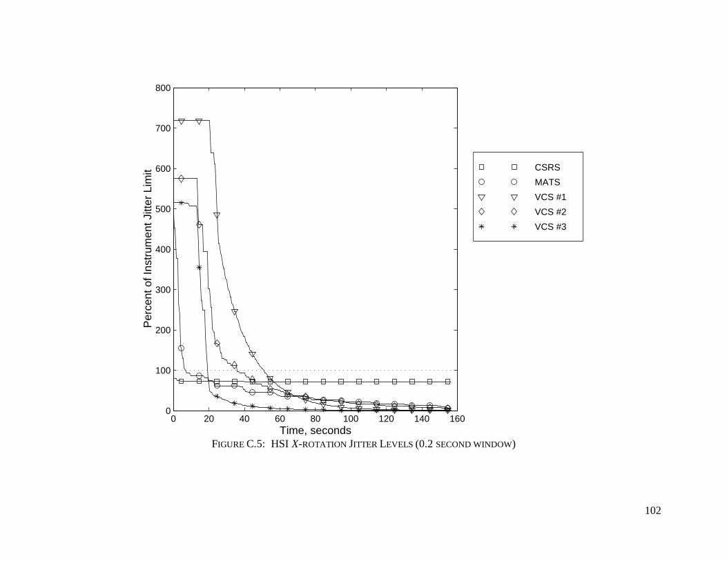
102
0 20 40 60 80 100 120 140 1600
100
200
300
400
500
600
700
800
Time, seconds
Per
cent
of I
nstr
umen
t Jitt
er L
imit CSRS
MATS
VCS #1
VCS #2
VCS #3
FIGURE C.5: HSI X-ROTATION JITTER LEVELS (0.2 SECOND WINDOW)

103
0 20 40 60 80 100 120 140 1600
50
100
150
200
250
Time, seconds
Per
cent
of I
nstr
umen
t Jitt
er L
imit CSRS
MATS
VCS #1
VCS #2
VCS #3
FIGURE C.6: LEISA X-ROTATION JITTER LEVELS (0.2 SECOND WINDOW)

104
0 20 40 60 80 100 120 140 1600
100
200
300
400
500
600
700
800
Time, seconds
Per
cent
of I
nstr
umen
t Jitt
er L
imit CSRS
MATS
VCS #1
VCS #2
VCS #3
FIGURE C.7: HSI X-ROTATION JITTER LEVELS (0.5 SECOND WINDOW)

105
0 20 40 60 80 100 120 140 1600
50
100
150
200
250
Time, seconds
Per
cent
of I
nstr
umen
t Jitt
er L
imit CSRS
MATS
VCS #1
VCS #2
VCS #3
FIGURE C.8: LEISA X-ROTATION JITTER LEVELS (0.5 SECOND WINDOW)

106
0 20 40 60 80 100 120 140 1600
100
200
300
400
500
600
700
800
Time, seconds
Per
cent
of I
nstr
umen
t Jitt
er L
imit CSRS
MATS
VCS #1
VCS #2
VCS #3
FIGURE C.9: HSI X-ROTATION JITTER LEVELS (1 SECOND WINDOW)

107
0 20 40 60 80 100 120 140 1600
50
100
150
200
250
Time, seconds
Per
cent
of I
nstr
umen
t Jitt
er L
imit CSRS
MATS
VCS #1
VCS #2
VCS #3
FIGURE C.10: LEISA X-ROTATION JITTER LEVELS (1 SECOND WINDOW)

108
0 20 40 60 80 100 120 140 1600
100
200
300
400
500
600
700
800
Time, seconds
Per
cent
of I
nstr
umen
t Jitt
er L
imit CSRS
MATS
VCS #1
VCS #2
VCS #3
FIGURE C.11: HSI X-ROTATION JITTER LEVELS (3.5 SECOND WINDOW)

109
0 20 40 60 80 100 120 140 1600
50
100
150
200
250
Time, seconds
Per
cent
of I
nstr
umen
t Jitt
er L
imit CSRS
MATS
VCS #1
VCS #2
VCS #3
FIGURE C.12: LEISA X-ROTATION JITTER LEVELS (3.5 SECOND WINDOW)

110
0 20 40 60 80 100 120 140 16010
0
101
102
103
104
Time, seconds
Per
cent
of I
nstr
umen
t Jitt
er L
imit CSRS
MATS
VCS #1
VCS #2
VCS #3
FIGURE C.13: HSI Y-ROTATION JITTER LEVELS (0.05 SECOND WINDOW)

111
0 20 40 60 80 100 120 140 16010
0
101
102
103
104
Time, seconds
Per
cent
of I
nstr
umen
t Jitt
er L
imit CSRS
MATS
VCS #1
VCS #2
VCS #3
FIGURE C.14: LEISA Y-ROTATION JITTER LEVELS (0.05 SECOND WINDOW)

112
0 20 40 60 80 100 120 140 16010
0
101
102
103
104
Time, seconds
Per
cent
of I
nstr
umen
t Jitt
er L
imit CSRS
MATS
VCS #1
VCS #2
VCS #3
FIGURE C.15: HSI Y-ROTATION JITTER LEVELS (0.1 SECOND WINDOW)

113
0 20 40 60 80 100 120 140 16010
0
101
102
103
104
Time, seconds
Per
cent
of I
nstr
umen
t Jitt
er L
imit CSRS
MATS
VCS #1
VCS #2
VCS #3
FIGURE C.16: LEISA Y-ROTATION JITTER LEVELS (0.1 SECOND WINDOW)

114
0 20 40 60 80 100 120 140 16010
1
102
103
104
Time, seconds
Per
cent
of I
nstr
umen
t Jitt
er L
imit CSRS
MATS
VCS #1
VCS #2
VCS #3
FIGURE C.17: HSI Y-ROTATION JITTER LEVELS (0.2 SECOND WINDOW)

115
0 20 40 60 80 100 120 140 16010
0
101
102
103
104
Time, seconds
Per
cent
of I
nstr
umen
t Jitt
er L
imit CSRS
MATS
VCS #1
VCS #2
VCS #3
FIGURE C.18: LEISA Y-ROTATION JITTER LEVELS (0.2 SECOND WINDOW)

116
0 20 40 60 80 100 120 140 16010
1
102
103
104
Time, seconds
Per
cent
of I
nstr
umen
t Jitt
er L
imit CSRS
MATS
VCS #1
VCS #2
VCS #3
FIGURE C.19: HSI Y-ROTATION JITTER LEVELS (0.5 SECOND WINDOW)

117
0 20 40 60 80 100 120 140 16010
0
101
102
103
104
Time, seconds
Per
cent
of I
nstr
umen
t Jitt
er L
imit CSRS
MATS
VCS #1
VCS #2
VCS #3
FIGURE C.20: LEISA Y-ROTATION JITTER LEVELS (0.5 SECOND WINDOW)

118
0 20 40 60 80 100 120 140 16010
1
102
103
104
Time, seconds
Per
cent
of I
nstr
umen
t Jitt
er L
imit CSRS
MATS
VCS #1
VCS #2
VCS #3
FIGURE C.21: HSI Y-ROTATION JITTER LEVELS (1 SECOND WINDOW)
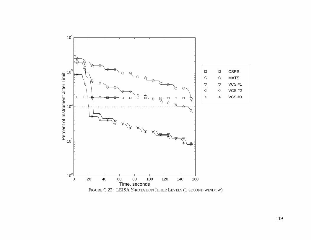
119
0 20 40 60 80 100 120 140 16010
0
101
102
103
104
Time, seconds
Per
cent
of I
nstr
umen
t Jitt
er L
imit CSRS
MATS
VCS #1
VCS #2
VCS #3
FIGURE C.22: LEISA Y-ROTATION JITTER LEVELS (1 SECOND WINDOW)

120
0 20 40 60 80 100 120 140 16010
1
102
103
104
105
Time, seconds
Per
cent
of I
nstr
umen
t Jitt
er L
imit CSRS
MATS
VCS #1
VCS #2
VCS #3
FIGURE C.23: HSI Y-ROTATION JITTER LEVELS (3.5 SECOND WINDOW)

121
0 20 40 60 80 100 120 140 16010
0
101
102
103
104
Time, seconds
Per
cent
of I
nstr
umen
t Jitt
er L
imit CSRS
MATS
VCS #1
VCS #2
VCS #3
FIGURE C.24: LEISA Y-ROTATION JITTER LEVELS (3.5 SECOND WINDOW)

REPORT DOCUMENTATION PAGE Form ApprovedOMB No. 0704-0188
Public reporting burden for this collection of information is estimated to average 1 hour per response, including the time for reviewing instructions, searching existing data sources,gathering and maintaining the data needed, and completing and reviewing the collection of information. Send comments regarding this burden estimate or any other aspect of thiscollection of information, including suggestions for reducing this burden, to Washington Headquarters Services, Directorate for Information Operations and Reports, 1215 JeffersonDavis Highway, Suite 1204, Arlington, VA 22202-4302, and to the Office of Management and Budget, Paperwork Reduction Project (0704-0188), Washington, DC 20503.
1. AGENCY USE ONLY (Leave blank) 2. REPORT DATE
August 19983. REPORT TYPE AND DATES COVERED
Contractor Report4. TITLE AND SUBTITLE
Input Shaping to Reduce Solar Array Structural Vibrations5. FUNDING NUMBERS
NCC1-104
6. AUTHOR(S)
Michael J. Doherty and Robert H. Tolson632-10-14-28
7. PERFORMING ORGANIZATION NAME(S) AND ADDRESS(ES)
The George Washington University Joint Institute for Advancement of Flight Sciences NASA Langley Research Center Hampton, VA 23681-2199
8. PERFORMING ORGANIZATIONREPORT NUMBER
9. SPONSORING/MONITORING AGENCY NAME(S) AND ADDRESS(ES)
National Aeronautics and Space AdministrationLangley Research CenterHampton, VA 23681-2199
10. SPONSORING/MONITORINGAGENCY REPORT NUMBER
NASA/CR-1998-208698
11. SUPPLEMENTARY NOTES
The information presented in this report was submitted to the School of Engineering and Applied Science of TheGeorge Washington University in partial fulfillment of the requirements for the Degree of Master of Science,April 1998. Langley Technical Monitor: Kenny B. Elliott.
12a. DISTRIBUTION/AVAILABILITY STATEMENT
Unclassified-UnlimitedSubject Category 18 Distribution: StandardAvailability: NASA CASI (301) 621-0390
12b. DISTRIBUTION CODE
13. ABSTRACT (Maximum 200 words)
Structural vibrations induced by actuators can be minimized using input shaping. Input shaping is a feedforward methodin which actuator commands are convolved with shaping functions to yield a shaped set of commands. These commandsare designed to perform the maneuver while minimizing the residual structural vibration. In this report, input shapingis extended to stepper motor actuators. As a demonstration, an input-shaping technique based on pole-zero cancellationwas used to modify the Solar Array Drive Assembly (SADA) actuator commands for the Lewis satellite. A series ofimpulses were calculated as the ideal SADA output for vibration control. These impulses were then discretized for use bythe SADA stepper motor actuator and simulated actuator outputs were used to calculate the structural response. Theeffectiveness of input shaping is limited by the accuracy of the knowledge of the modal frequencies. Assuming perfectknowledge resulted in significant vibration reduction. Errors of 10% in the modal frequencies caused notably higherlevels of vibration. Controller robustness was improved by incorporating additional zeros in the shaping function.The additional zeros did not require increased performance from the actuator. Despite the identification errors, theresulting feedforward controller reduced residual vibrations to the level of the exactly modeled input shaper and wellbelow the baseline cases. These results could be easily applied to many other vibration-sensitive applicationsinvolving stepper motor actuators.
14. SUBJECT TERMS
Jitter; Control; Input shaping; s/c vibration; Precision pointing15. NUMBER OF PAGES
136
16. PRICE CODE
A0717. SECURITY CLASSIFICATION
OF REPORT
Unclassified
18. SECURITY CLASSIFICATIONOF THIS PAGE
Unclassified
19. SECURITY CLASSIFICATION OF ABSTRACT
Unclassified
20. LIMITATION OF ABSTRACT
NSN 7540-01-280-5500 Standard Form 298 (Rev. 2-89)Prescribed by ANSI Std. Z-39-18298-102
Related Documents