Input-output linearization with delay cancellation for nonlinear delay systems: the problem of the internal stability

International Journal of Robust and Nonlinear Control

SPECIAL ISSUE on DELAY SYSTEMS

Preprint

Input-Output Linearization with Delay Cancellation

for Nonlinear Delay Systems:

the Problem of the Internal Stability

A. Germani, C. Manes, P. Pepe

Dipartimento di Ingegneria ElettricaUniversitµa degli Studi dell'Aquila

Monteluco di Roio 67040 L'Aquila - ITALYFax. ++39 { 0862 434403

e-mail: [email protected]

Abstract

This paper investigates the issue of the internal stability of nonlinear delay systems con-

trolled with a feedback law that performs exact input-output linearization and delay cancela-

tion. In previous works the authors showed that, di®erently from the case of systems without

state delays, when the relative degree is equal to the number of state variables and the output

is forced to be identically zero, delay systems still possess a non trivial internal state dynam-

ics. Not only: in the same conditions delay systems are also characterized by a non trivial

input dynamics. Obviously, both internal state and input dynamics should give bounded

trajectories, otherwise the exact input-output linearization and delay cancelation technique

cannot be applied. This paper studies the relationships between the internal state and input

dynamics of a controlled nonlinear delay system. An interesting result is that a suitable

stability assumption on the internal state dynamics ensures that, when the output is asymp-

totically driven to zero, both the state and control variables asymptotically decay to zero.

Keywords: Nonlinear Systems, Delay Systems, Output Regulation,

In¯nite Dimensional Systems, Delay Cancelation.

This work is supported by ASI (Italian Aerospace Agency).

1

1. Introduction

Some control problems for nonlinear systems can be solved through a preliminary com-

pensation of nonlinearities, so that virtually all control techniques developed for linear

systems can be applied to the linearized system (see e.g. [9]). In the same way, when

dealing with delay systems, a feasible approach to control problems is the preliminary

compensation of all delays, followed by the application of control techniques developed for

systems without delays. Nonlinear systems with state and input delays can be object of

various kinds of compensation of nonlinearities and delays: the linearization can be exact

or approximated, the delay can be partially compensated through prediction or, in some

cases, can be exactly canceled. The approach of preliminary delay compensation through

prediction is pursued in [8, 11, 14]. After delay compensation, classical tools of di®erential

geometry can be applied for the analysis of nonlinear systems and for control synthesis.

A di®erent approach is followed in [4, 6, 15, 16, 18, 19], where preliminary delay compen-

sation is avoided and suitable extensions of di®erential geometry have been developed for

dealing with delay systems. The papers [15, 16] were concerned mainly with the problem

of disturbance decoupling, while papers [4, 6, 18, 19] developed the extension to delay sys-

tems of the classical technique of input-output (I/O) linearization [9]. In these works exact

I/O linearization was obtained together with exact delay cancelation by means of a state

feedback. After exact I/O linearization and delay cancelation the problem of driving the

output exponentially to zero becomes an easy task. However, output stabilization is not

su±cient to achieve state stabilization, because the control law that achieves an identically

zero output may create an unobservable dynamics, denoted zero-dynamics. As in the case

of systems without delays, the stability of the zero-dynamics is a necessary condition for

the practical use of the control law that linearizes the I/O map and removes the delay. It

is well known that systems without state delay do have non trivial zero dynamics if and

only if the relative degree is smaller than the number of state variables. This situation

is investigated in [19] for the case of delay systems, and it is shown that, under suitable

assumptions, the local asymptotic stability of the zero-dynamics implies the local asymp-

totic stability of the origin of the controlled delay systems. In [6] it has been shown that,

di®erently from the case of systems without state delays, nonlinear delay systems with

relative degree equal to the number of state variables (full relative degree) may have, in

general, a non trivial zero-dynamics. For such systems a su±cient stability criterion of

the state zero-dynamics is discussed in [6]. The existence of the state internal dynamics in

the case of full relative degree is due to intrinsic in¯nite dimensionality of delay systems.

A necessary and su±cient condition which characterizes delay systems that do not admit

state internal dynamics is reported in [3].

This paper points out that in addition to the internal state dynamics, the output

stabilizing control law through I/O linearization and delay cancelation induces also an

internal dynamics of the control variable (input dynamics). This means that the true

zero-dynamics for nonlinear delay systems is composed of both the internal state and

input dynamics, and both the state and input trajectories must be uniformly bounded,

2

otherwise the technique of exact input-output linearization with delay cancelation cannot

be applied. The remarkable result obtained in this work is that the stability of the input

dynamics is not an additional assumption, but is implied by a suitable stability property

of the internal state dynamics. Such property will be proved with reference to the class

of nonlinear systems with delay only in the state. Similar results are proved in [13] with

reference to the class of linear systems with delays both in the state and in the input; in

this case an additional stability condition is also needed.

2. Problem Statement and Preliminaries

This paper considers delay systems described by the following equations

_x(t) = f(x(t); x(t¡¢)) + g(x(t); x(t¡¢))u(t); t ¸ 0; (2.1)

y(t) = h(x(t)); (2.2)

where ¢ > 0, x(t) 2 IRn, u(t) 2 IR and y(t) 2 IR, the vector functions f and g are C1with respect to both arguments, and h is a C1 scalar function. The model description is

completed by the knowledge of the function x(¿), ¿ 2 [¡¢; 0], in a suitable function space,which represents the initial state in the classical in¯nite dimensional description of delay

systems. It is assumed that system (2.1), (2.2) is such that

f(0; 0) = 0; g(0; 0)6= 0; h(0) = 0: (2.3)

These positions imply that the state x(¿) = 0, ¿ 2 [¡¢; 0], is an equilibrium point. In the

following some notations are introduced in order to simplify the writing of mathematical

expressions. Throughout the paper the symbol 0a£b denotes the zero matrix in IRa£b,while Ia denotes the identity matrix in IR

a£a. The symbols ABp£q; BBp£q; C

Bp£q will denote

the block-Brunowsky triplet de¯ned as

ABp;q =

2666640q£q Iq ¢ ¢ ¢ 0q£q0q£q 0q£q ¢ ¢ ¢ 0q£q...

... ¢ ¢ ¢ ...0q£q 0q£q ¢ ¢ ¢ Iq0q£q 0q£q ¢ ¢ ¢ 0q£q

377775 2 IRpq£pq BBp;q =

26640q£q0q£q...Iq

3775 2 IRpq£q;CBp;q = [ Iq 0q£q ¢ ¢ ¢ 0q£q ] 2 IRq£pq;

(2.4)

The symbol Xi;j , with i; j integer numbers, will denote a vector in IR(ji¡jj+1)n, composedof subvectors Âk 2 IRn as follows

if i · j : Xi;j =

2664ÂiÂi+1...Âj

3775 if j < i : Xi;j =

2664ÂiÂi¡1...Âj

3775 : (2:5)

3

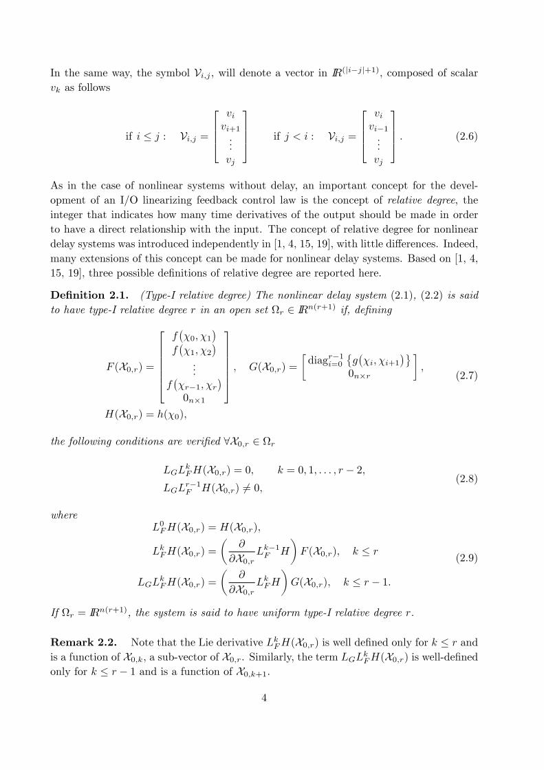
In the same way, the symbol Vi;j , will denote a vector in IR(ji¡jj+1), composed of scalarvk as follows

if i · j : Vi;j =

2664vivi+1...vj

3775 if j < i : Vi;j =

2664vivi¡1...vj

3775 : (2:6)

As in the case of nonlinear systems without delay, an important concept for the devel-

opment of an I/O linearizing feedback control law is the concept of relative degree, the

integer that indicates how many time derivatives of the output should be made in order

to have a direct relationship with the input. The concept of relative degree for nonlinear

delay systems was introduced independently in [1, 4, 15, 19], with little di®erences. Indeed,

many extensions of this concept can be made for nonlinear delay systems. Based on [1, 4,

15, 19], three possible de¯nitions of relative degree are reported here.

De¯nition 2.1. (Type-I relative degree) The nonlinear delay system (2.1), (2.2) is said

to have type-I relative degree r in an open set −r 2 IRn(r+1) if, de¯ning

F (X0;r) =

2666664f¡Â0; Â1

¢f¡Â1; Â2

¢...

f¡Âr¡1; Âr

¢0n£1

3777775 ; G(X0;r) =·diagr¡1i=0

©g¡Âi; Âi+1

¢ª0n£r

¸;

H(X0;r) = h(Â0);

(2.7)

the following conditions are veri¯ed 8X0;r 2 −r

LGLkFH(X0;r) = 0; k = 0; 1; : : : ; r ¡ 2;

LGLr¡1F H(X0;r)6= 0;

(2.8)

whereL0FH(X0;r) = H(X0;r);

LkFH(X0;r) =µ

@

@X0;rLk¡1F H

¶F (X0;r); k · r

LGLkFH(X0;r) =

µ@

@X0;rLkFH

¶G(X0;r); k · r ¡ 1:

(2.9)

If −r = IRn(r+1), the system is said to have uniform type-I relative degree r.

Remark 2.2. Note that the Lie derivative LkFH(X0;r) is well de¯ned only for k · r andis a function of X0;k, a sub-vector of X0;r. Similarly, the term LGLkFH(X0;r) is well-de¯nedonly for k · r ¡ 1 and is a function of X0;k+1.

4

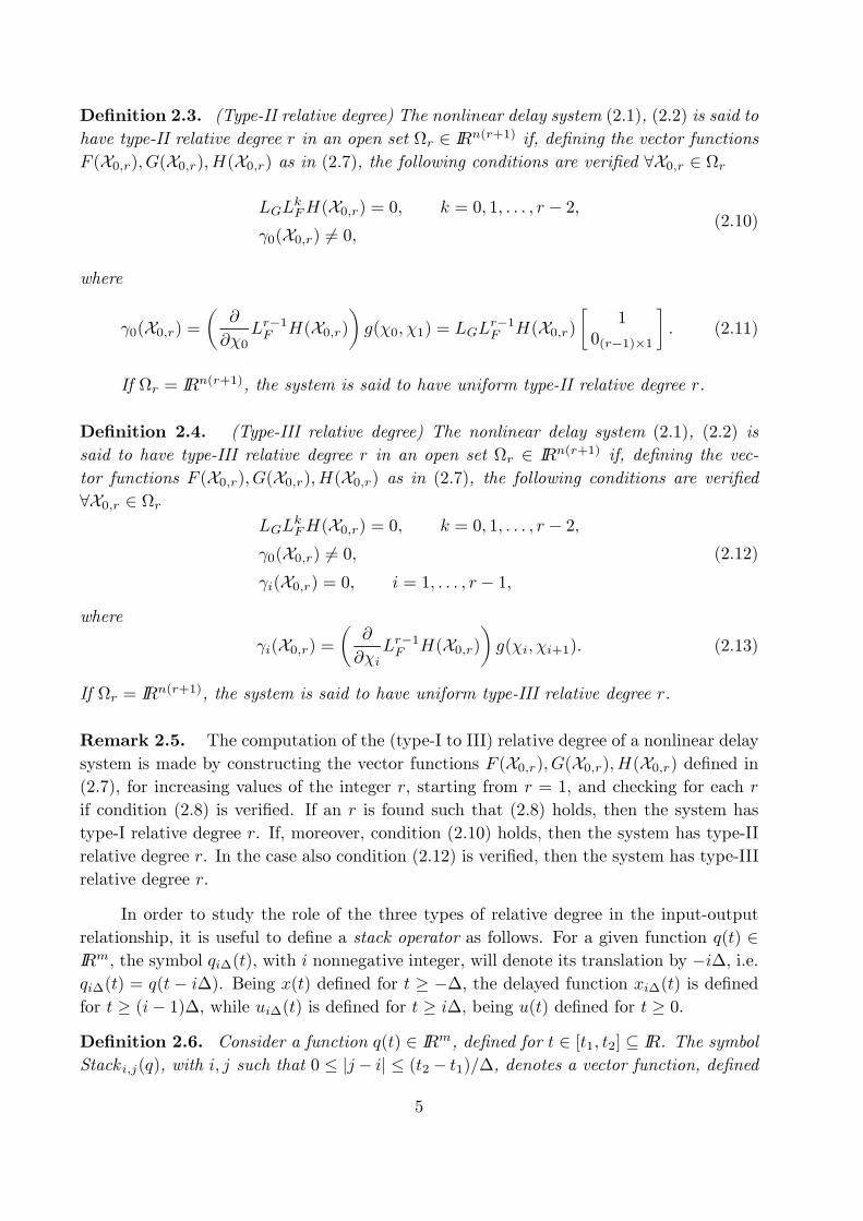
De¯nition 2.3. (Type-II relative degree) The nonlinear delay system (2.1), (2.2) is said to

have type-II relative degree r in an open set −r 2 IRn(r+1) if, de¯ning the vector functionsF (X0;r); G(X0;r);H(X0;r) as in (2.7), the following conditions are veri¯ed 8X0;r 2 −r

LGLkFH(X0;r) = 0; k = 0; 1; : : : ; r ¡ 2;

°0(X0;r)6= 0;(2.10)

where

°0(X0;r) =µ@

@Â0Lr¡1F H(X0;r)

¶g(Â0; Â1) = LGL

r¡1F H(X0;r)

·1

0(r¡1)£1

¸: (2.11)

If −r = IRn(r+1), the system is said to have uniform type-II relative degree r.

De¯nition 2.4. (Type-III relative degree) The nonlinear delay system (2.1), (2.2) is

said to have type-III relative degree r in an open set −r 2 IRn(r+1) if, de¯ning the vec-tor functions F (X0;r); G(X0;r);H(X0;r) as in (2.7), the following conditions are veri¯ed8X0;r 2 −r

LGLkFH(X0;r) = 0; k = 0; 1; : : : ; r ¡ 2;

°0(X0;r)6= 0;°i(X0;r) = 0; i = 1; : : : ; r ¡ 1;

(2.12)

where

°i(X0;r) =µ@

@ÂiLr¡1F H(X0;r)

¶g(Âi; Âi+1): (2.13)

If −r = IRn(r+1), the system is said to have uniform type-III relative degree r.

Remark 2.5. The computation of the (type-I to III) relative degree of a nonlinear delay

system is made by constructing the vector functions F (X0;r); G(X0;r); H(X0;r) de¯ned in(2.7), for increasing values of the integer r, starting from r = 1, and checking for each r

if condition (2.8) is veri¯ed. If an r is found such that (2.8) holds, then the system has

type-I relative degree r. If, moreover, condition (2.10) holds, then the system has type-II

relative degree r. In the case also condition (2.12) is veri¯ed, then the system has type-III

relative degree r.

In order to study the role of the three types of relative degree in the input-output

relationship, it is useful to de¯ne a stack operator as follows. For a given function q(t) 2IRm, the symbol qi¢(t), with i nonnegative integer, will denote its translation by ¡i¢, i.e.qi¢(t) = q(t¡ i¢). Being x(t) de¯ned for t ¸ ¡¢, the delayed function xi¢(t) is de¯nedfor t ¸ (i¡ 1)¢, while ui¢(t) is de¯ned for t ¸ i¢, being u(t) de¯ned for t ¸ 0.De¯nition 2.6. Consider a function q(t) 2 IRm, de¯ned for t 2 [t1; t2] µ IR. The symbolStack i;j(q), with i; j such that 0 · jj ¡ ij · (t2¡ t1)=¢, denotes a vector function, de¯ned

5

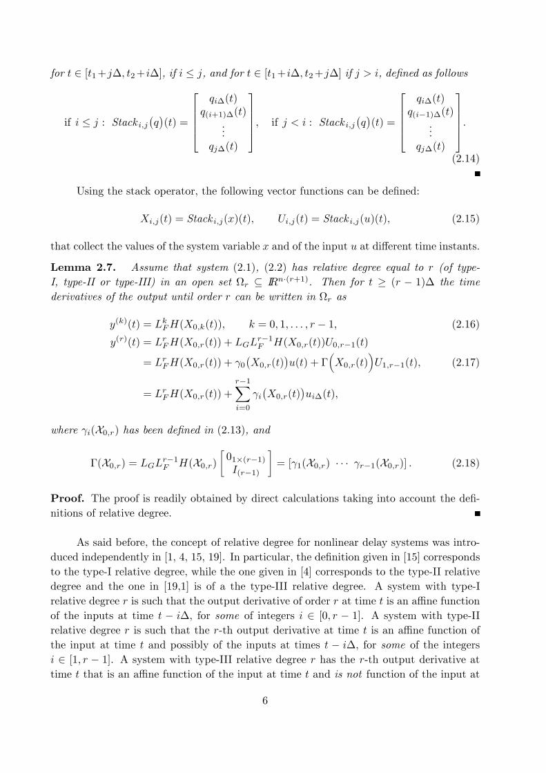
for t 2 [t1+j¢; t2+i¢], if i · j, and for t 2 [t1+i¢; t2+j¢] if j > i, de¯ned as follows

if i · j : Stack i;j¡q¢(t) =

26664qi¢(t)

q(i+1)¢(t)...

qj¢(t)

37775; if j < i : Stack i;j¡q¢(t) =

26664qi¢(t)

q(i¡1)¢(t)...

qj¢(t)

37775:(2.14)

Using the stack operator, the following vector functions can be de¯ned:

Xi;j(t) = Stack i;j(x)(t); Ui;j(t) = Stack i;j(u)(t); (2.15)

that collect the values of the system variable x and of the input u at di®erent time instants.

Lemma 2.7. Assume that system (2.1), (2.2) has relative degree equal to r (of type-

I, type-II or type-III) in an open set −r µ IRn¢(r+1). Then for t ¸ (r ¡ 1)¢ the time

derivatives of the output until order r can be written in −r as

y(k)(t) = LkFH(X0;k(t)); k = 0; 1; : : : ; r ¡ 1; (2.16)

y(r)(t) = LrFH(X0;r(t)) + LGLr¡1F H(X0;r(t))U0;r¡1(t)

= LrFH(X0;r(t)) + °0¡X0;r(t)

¢u(t) + ¡

³X0;r(t)

´U1;r¡1(t); (2.17)

= LrFH(X0;r(t)) +r¡1Xi=0

°i¡X0;r(t)

¢ui¢(t);

where °i(X0;r) has been de¯ned in (2.13), and

¡(X0;r) = LGLr¡1F H(X0;r)·01£(r¡1)I(r¡1)

¸= [°1(X0;r) ¢ ¢ ¢ °r¡1(X0;r)] : (2:18)

Proof. The proof is readily obtained by direct calculations taking into account the de¯-

nitions of relative degree.

As said before, the concept of relative degree for nonlinear delay systems was intro-

duced independently in [1, 4, 15, 19]. In particular, the de¯nition given in [15] corresponds

to the type-I relative degree, while the one given in [4] corresponds to the type-II relative

degree and the one in [19,1] is of a the type-III relative degree. A system with type-I

relative degree r is such that the output derivative of order r at time t is an a±ne function

of the inputs at time t ¡ i¢, for some of integers i 2 [0; r ¡ 1]. A system with type-II

relative degree r is such that the r-th output derivative at time t is an a±ne function of

the input at time t and possibly of the inputs at times t ¡ i¢, for some of the integersi 2 [1; r ¡ 1]. A system with type-III relative degree r has the r-th output derivative at

time t that is an a±ne function of the input at time t and is not function of the input at

6

times t¡ i¢, for all integers i 2 [1; r ¡ 1]. In [7] an observation delay relative degree wasde¯ned, that is a type-I relative degree. For a nonlinear delay system the assumption to

have a type-III relative degree is rather strong. In this paper, following the approach of

[4], we will consider systems with type-II relative degree.

It is well-known that for nonlinear systems without delay when the relative degree

is equal to the dimension of the state space n, the existence of a state feedback that

achieves exact linearization of the input-output map implies the existence of the solution

of the problem of exact linearization of the system through a static state feedback and a

nonlinear change of coordinates (see [9]). The new coordinates are the output derivatives

up to order n ¡ 1. The stabilization of the system is obtained assigning the eigenvalues

to the system in the linear form. If the relative degree r is strictly less than n, only

a subsystem of dimension r can be linearized and stabilized through linearization and

stabilization of the input-output map. r eigenvalues can be assigned in this case. The

linearizing feedback induces an unobservable dynamics, the so-called zero-dynamics, that is

una®ected by the assigned eigenvalues. The control via exact linearization can be pursued

only if the zero-dynamics is stable. On the other hand, systems with full relative degree

do not have zero-dynamics, and therefore the exact linearization approach can be always

pursued. Unfortunately, this is not the case for nonlinear delay systems. Also when the

relative degree is equal to the dimension n of the system variable x, exact linearization of

the input-output map does not imply exact linearization of the system.

The control law that linearizes the input-output map with delay-cancelation is de-

scribed in the following proposition, whose simple proof can be found in [4, 6, 19]

Proposition 2.8. Assume that the nonlinear delay system (2.1), (2.2) has type-II relative

degree n in an open set −n. Moreover, assume that the initial state x0 2 C([¡¢; 0]; IRn)and the initial choice of the input u in the time interval [0; (n ¡ 1)¢) are such to guar-antee the existence and uniqueness of a continuous solution x(t) on [0; (n¡ 1)¢] and thatX0;n((n¡1)¢) 2 −n. Then, de¯ning a new input function v(t), the feedback control law

u(t) =v(t)¡ LnFH(X0;n(t))¡ ¡

¡X0;n(t)

¢U1;n¡1(t)

°0(X0;n(t)); t ¸ (n¡ 1)¢; (2.19)

is such that the input-output map becomes

y(n)(t) = v(t); t ¸ (n¡ 1)¢; (2.20)

provided that, with the chosen v(t), X0;n(t) exists unique continuous and remains in −n.

The output derivatives up to order n ¡ 1 can be written by de¯ning the followingmap © : IRn

2 7! IRn

z =

2664L0FH(Â0)L1FH(X0;1)

...Ln¡1F H(X0;n¡1)

3775 = ©¡X0;n¡1¢: (2.21)

7

After the substitution of X0;k with X0;k(t) in (2.21), that is giving to Âi the value x(t¡i¢),the map © gives a vector z(t) that collects the output derivatives up to order n¡ 1:

z(t) =

264 y(t)...

y(n¡1)(t)

375 = ©¡X0;n¡1(t)¢; t ¸ (n¡ 1)¢: (2.22)

After feedback (2.19) the input-output dynamics can be put in the form

_z(t) = ABn;1z(t) +BBn;1v(t);

y(t) = CBn;1z(t);t ¸ (n¡ 1)¢; (2.23)

where (ABn;1; BBn;1; C

Bn;1) is a Brunowsky triplet, as de¯ned in (2.4). Applying a linear

feedback law of the formv(t) = ¡kTz(t)

= ¡kT©¡X0;n¡1(t)¢ (2.24)

the output dynamics is governed by the autonomous linear system

_z(t) = (ABn;1 ¡BBn;1kT)z(t);y(t) = CBn;1z(t);

t ¸ (n¡ 1)¢: (2.25)

If k assigns all the eigenvalues of matrix ABn;1¡BBn;1kT in the open left half complex plane(i.e. k is Hurwitz) the output is exponentially stabilized, i.e. there exist positive °; ¯ such

that

kz(t)k · °e¡¯¡t¡(n¡1)¢

¢kz¡(n¡ 1)¢¢k; t ¸ (n¡ 1)¢: (2.26)

The feedback law that achieves exponential output stabilization, after linearization and

delay cancelation of the input-output map (as long as X0;n(t) 2 −n), is obtained replacingthe variable v in (2.19) with the expression (2.24), obtaining

u(t) =¡kTz(t)¡ LnFH(X0;n(t))¡ ¡

¡X0;n(t)

¢U1;n¡1(t)

°0(X0;n(t)); t ¸ (n¡ 1)¢: (2.27)

This equation describes the dynamics of the control variable u(t) for t ¸ (n ¡ 1)¢ in

closed loop. If the type-III relative degree is assumed, as in [18], it is °(X0;n) 6= 0 and

¡(X0;n) ´ 0 and it is evident that if z(t) and x(t) asymptotically go to zero, then also u(t)asymptotically goes to zero. This is the reason why in [19] the issue of the boundedness of

the control variable is not addressed. If the less-restrictive assumption of type-II relative

degree is made, the equation (2.27) is a continuous-time algebraic delay equation, where

the value of the control variable u at time t depends on n¡ 1 previous values of the samevariable and on old and present values of the state. Equation (2.27) can be put in the

form

u(t) = ¡ 1

°0(X0;n(t))kTz(t)¡p0(X0;n(t))¡

n¡1Xj=1

pj(X0;n(t))u(t¡j¢); t ¸ (n¡1)¢; (2.28)

8

where pj : −n ! IR, j = 0; 1; : : : ; n¡ 1 are de¯ned as

p0(X0;n) = LnFH(X0;n)°0(X0;n) ;

pj(X0;n) = °j(X0;n)°0(X0;n) ; j = 1; : : : ; n¡ 1:

(2:29)

Note that the vector of output derivatives behaves as an input for the input dynamics .

For this reason throughout the paper the dynamics described by equation (2.28) will be

also denoted as the output-driven input dynamics.

In the following it is shown that the internal dynamics of the system variable x(t) is

governed by the map z = ©(X0;n¡1) de¯ned in (2.21). In [7] this map is called observabilitymap of system (2.1)-(2.2), because suitable assumptions on this map allow the construction

of an observer for nonlinear time delay systems. The observability map can be seen as

a square map from Â0 to z, in which the sub-vector X1;n¡1 2 IRn(n¡1) is considered asa vector of parameters. To stress this point of view, in the following the map © will be

rewritten as follows

z = ©(Â0;X1;n¡1): (2.30)

For systems with type-II and type-III relative degree in a set −n, it is

det

µ@©(Â0;X1;n¡1)

@Â0

¶6= 0; 8X0;n¡1 2 −n: (2:31)

The proof can be found in [19] (Lemma 1). This implies that the map © is locally invertible

with respect to the ¯rst component Â0 (local partial invertibility).

From here on we suppose that the following assumption holds for the observability

map © (Global partial invertibility):

H1) System (2.1), (2.2) has uniform type-II relative degree equal to n (the dimension of

the system variable x) and there exists the inverse ©¡1 of the function (2.30) w.r.t.the ¯rst component Â0 for all z 2 IRn and X1;n¡1 2 IRn(n¡1), that is

Â0 = ©¡1(z;X1;n¡1); 8z 2 IRn; X1;n¡1 2 IRn(n¡1): (2.32)

In the paper [7] assumption H1 is a necessary condition for the construction of an

asymptotic observer for a delay system.

The state dynamics of the system variable x(t) for t ¸ (n ¡ 1)¢ is governed by

the following continuous-time algebraic delay equation forced by the vector z(t) of output

derivatives

x(t) = ©¡1¡z(t); X1;n¡1(t)

¢: (2.33)

z(t) acts as an input in equation (2.33), and therefore such dynamics will be denoted

throughout this paper as the output-driven state dynamics. The stability of this dynamics

has been studied in the papers [6, 20], where su±cient conditions on the map © are

9

provided that ensure convergence of x(t) to zero when the output, together with its n¡ 1derivatives, is driven to zero by the control law (2.27). The output dynamics (2.25), the

state dynamics (2.33) and the input dynamics (2.28) of the closed loop-system, form a

triangular system of di®erential-algebraic equations, well de¯ned for t ¸ (n¡ 1)¢:

_z(t) = (ABn;1 ¡BBn;1kT)z(t); (2.34a)

x(t) = ©¡1¡z(t); X1;n¡1(t)

¢; (2.34b)

u(t) = ¡ kTz(t)

°0(X0;n(t))¡ p0(X0;n(t))¡ pT(X0;n(t))Un¡1;1(t); (2.34c)

where

pT(X0;n¡1) =£pn¡1(X0;n) ¢ ¢ ¢ p1(X0;n)

¤: (2.35)

The output dynamics (2.34a) is autonomous and can be made stable by a suitable choice of

the gain vector k. Obviously, the stability of the state dynamics and of the input dynamics

is a necessary condition for the overall stability of the controlled delay system.

Now consider an (open-loop) input function u(t), t 2 [0; (n¡ 1)¢] such to bring z(t)to zero at time t = (n¡ 1)¢, and then apply the feedback law (2.27), that keeps z(t) = 0for t ¸ (n¡ 1)¢. The equations (2.33) and (2.28) become, for t ¸ (n¡ 1)¢,

x(t) = ©¡1¡0; X1;n¡1(t)

¢; (2.36a)

u(t) = ¡p0(X0;n(t))¡ pT(X0;n(t))Un¡1;1(t); (2.36b)

Equation (2.36) is a continuous-time algebraic delay equation that describes the system

zero-dynamics, that is the internal state and input dynamics when the output is identically

zero. Note that the dynamics of x(t), given by (2.36a), is only a part of the zero-dynamics

and is completely characterized by the partial inverse map ©¡1, and in the following will bedenoted the state zero-dynamics. We will refer to eq. (2.36b) as the input zero-dynamics,

and we will say that the system zero-dynamics is composed of the state and input zero-

dynamics. Here follows a simple example of delay system with full uniform Type-II relative

degree with unstable zero-dynamics.

Example. Consider the following nonlinear delay systems

_x1(t) = x2(t) + ¾x2(t¡¢);_x2(t) =

¡1 + x21(t)

¢u(t);

y(t) = x1(t);

(2.37)

where ¾ 2 IR is a parameter. Instead to test the conditions given in the de¯nitions 2.1-

2.4 for r = 1; 2 : : :, the relative degree can be computed by repeatedly di®erentiating the

output with respect to time. The output and its ¯rst derivative are

y(t) = x1(t);

_y(t) = x2(t) + ¾x2(t¡¢):(2.38)

10

Since they do not depend on the input u(t), the relative degree must be greater than one.

The second order derivative is

Äy(t) =¡1 + x21(t)

¢u(t) + ¾

¡1 + x21(t¡¢)

¢u(t¡¢); (2:39)

and depends on both u(t) and u(t ¡ ¢). Since the coe±cient of u(t) is never zero, thesystem has uniform type-II relative degree r = 2. Equation (2.38) is the map ©(X0;1(t))

de¯ned in (2.22) that gives the output derivatives. The coe±cient °0(X0;2) de¯ned in (2.9)is¡1 + Â20;1

¢. The output stabilizing control law (2.27) is

u(t) =

µ¡¾¡1 + x21(t¡¢)¢u(t¡¢)¡ kT · x1(t)

x2(t)¡ 2x2(t¡¢)¸¶

1¡1 + x21(t)

¢ : (2.40)

This control law, with k such that AB2;1 ¡ BB2;1kT is stable, is such to drive y(t) and _y(t)exponentially to zero. The equations (2.36) of the zero-dynamics are the following

x1(t) = 0;

x2(t) = ¡¾x2(t¡¢);

u(t) = ¡¾ 1 + x21(t¡¢)

1 + x21(t)u(t¡¢);

t ¸ ¢: (2:41)

Considering that x1(t) = 0, the third equation becomes u(t) = ¡¾u(t¡¢). It follows thatthe zero-dynamics for system (2.37) is stable for j¾j · 1 and unstable for j¾j > 1. In thelatter case, the closed-loop system is unstable.

This example shows that it is not su±cient to have relative degree equal to the

dimension of the system vector x to stabilize a nonlinear delay system by means of expo-

nential output stabilization, after exact input-output linearization with delay cancelation.

In general there exists a zero-dynamics that may be unstable. In the case of systems with

type-III relative degree the input u(t) is a continuous function of only X0;n(t), and is not

a function of the past values u(t ¡ i¢), so that the stability of the state zero-dynamicstrivially implies the stability of the zero-dynamics.

3. The Case of Linear Delay Systems

This section shows the application of the exact input-output linearization with delay can-

celation to the case of linear delay systems. Obviously, in the linear case the interest of the

approach is in the delay cancelation. Moreover, this section presents some results on the

stability of the zero-dynamics that will be needed later in the paper to prove more general

results for nonlinear systems.

Consider a linear delay system of the form

_x(t) = A0x(t) +A1x(t¡¢) +Bu(t);y(t) = Cx(t)

(3.1)

11

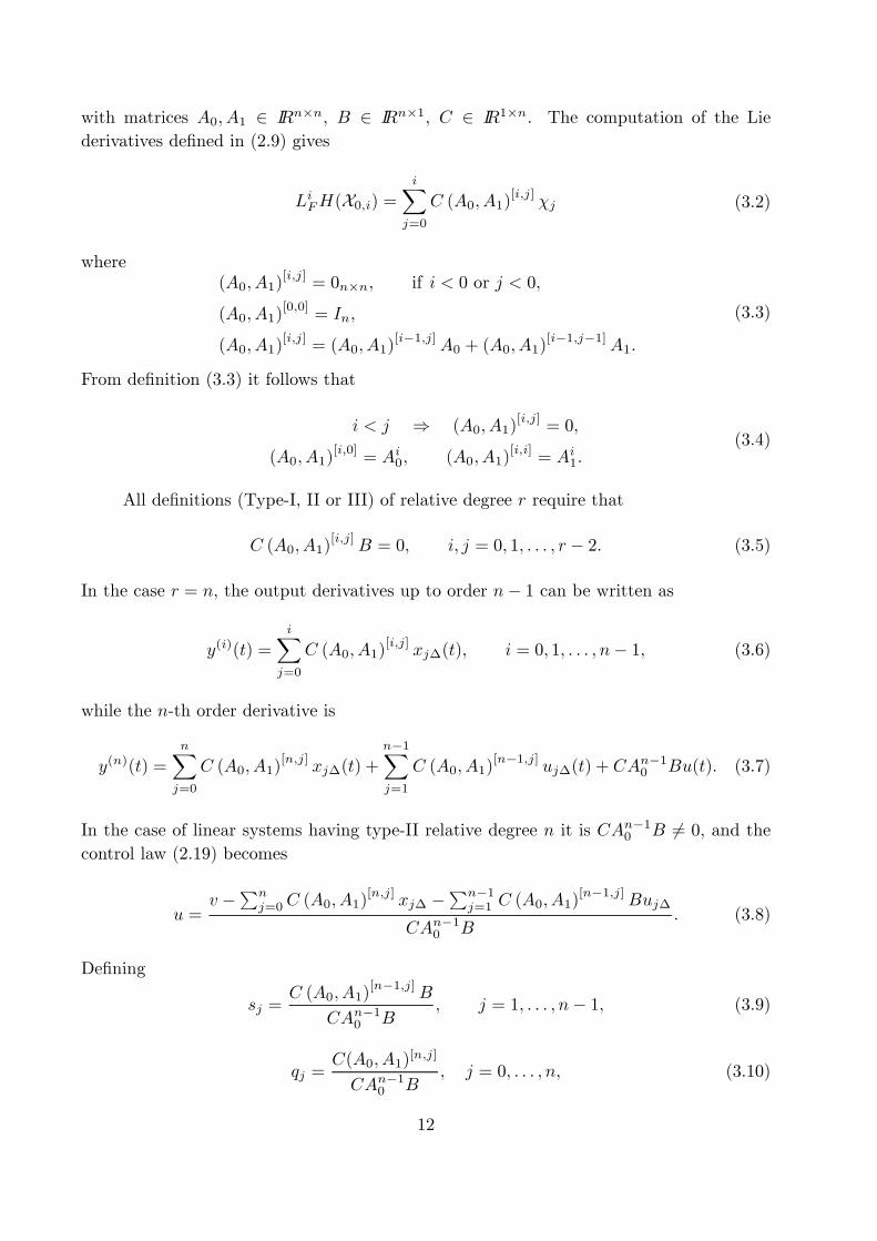
with matrices A0; A1 2 IRn£n, B 2 IRn£1, C 2 IR1£n. The computation of the Lie

derivatives de¯ned in (2.9) gives

LiFH(X0;i) =iX

j=0

C (A0; A1)[i;j]

Âj (3.2)

where(A0; A1)

[i;j]= 0n£n; if i < 0 or j < 0;

(A0; A1)[0;0]

= In;

(A0; A1)[i;j]

= (A0; A1)[i¡1;j]

A0 + (A0; A1)[i¡1;j¡1]

A1:

(3:3)

From de¯nition (3.3) it follows that

i < j ) (A0; A1)[i;j]

= 0;

(A0; A1)[i;0]

= Ai0; (A0; A1)[i;i]

= Ai1:(3:4)

All de¯nitions (Type-I, II or III) of relative degree r require that

C (A0; A1)[i;j]

B = 0; i; j = 0; 1; : : : ; r ¡ 2: (3:5)

In the case r = n, the output derivatives up to order n¡ 1 can be written as

y(i)(t) =iX

j=0

C (A0; A1)[i;j]

xj¢(t); i = 0; 1; : : : ; n¡ 1; (3:6)

while the n-th order derivative is

y(n)(t) =nXj=0

C (A0; A1)[n;j]

xj¢(t) +n¡1Xj=1

C (A0; A1)[n¡1;j]

uj¢(t) + CAn¡10 Bu(t): (3:7)

In the case of linear systems having type-II relative degree n it is CAn¡10 B 6= 0, and thecontrol law (2.19) becomes

u =v ¡Pn

j=0C (A0; A1)[n;j]

xj¢ ¡Pn¡1j=1 C (A0; A1)

[n¡1;j]Buj¢

CAn¡10 B: (3.8)

De¯ning

sj =C (A0; A1)

[n¡1;j]B

CAn¡10 B; j = 1; : : : ; n¡ 1; (3.9)

qj =C(A0; A1)

[n;j]

CAn¡10 B; j = 0; : : : ; n; (3.10)

12

the control law (3.8) is written as

u(t) = ¡ v(t)

CAn¡10 B¡

nXj=0

qjxj¢(t)¡n¡1Xj=1

sjuj¢(t): (3.11)

In the case of linear systems the relative degree (of any type) is always uniform, and

the transformation of the I/O map in a chain of n integrators, i.e. y(n)(t) = v(t), is global.

The map © de¯ned in (2.21) is as follows

z =n¡1Xj=0

QjÂj ; (3.12)

where the n£ n matrix Q0 is the observability matrix of the pair (A0; C), i.e.

Q0 =

2664CCA0...

CAn¡10

3775 (3.13)

and the n £ n matrices Qj ; j = 1; 2; : : : ; n ¡ 1, can be computed using (3.2), and are asfollows

fQjg(i;:) = 0;fQjg(i;:) = C(A0; A1)[i¡1;j];

for i = 1; : : : ; j;

for i = j + 1; : : : ; n:(3.14)

where fQjg(i;:) denotes the i-th row of matrix Qj .Exponential convergence of the output y(t) to zero is obtained with the feedback law

(3.11) with v given by (2.24), so that the control law (2.28), de¯ned for t ¸ (n ¡ 1)¢,results to be

u(t) = ¡ kTz(t)

CAn¡10 B¡ qTXn;0(t)¡ sTUn¡1;1(t); (3.15)

where

qT = [ qn qn¡1 ¢ ¢ ¢ q0 ] ; (3.16)

sT = [ sn¡1 sn¡2 ¢ ¢ ¢ s1 ] : (3.17)

with qj and sj de¯ned in (3.10) and (3.9), respectively. With this control law, the vector of

output derivatives z(t) exponentially goes to zero, i.e. satis¯es (2.26) for suitable positive °

and ¯. The partial invertibility property of the map © with respect to the Â0 (assumption

H1) is equivalent to observability of the pair (A0; C). The inverse map ©¡1 de¯ned in

(2.32) is

Â0 = Q¡10 z ¡

n¡1Xj=1

Q¡10 QjÂj ; (3:18)

13

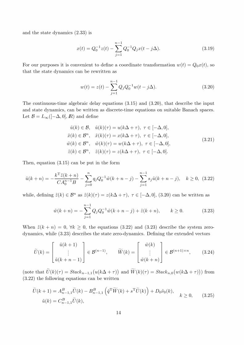
and the state dynamics (2.33) is

x(t) = Q¡10 z(t)¡n¡1Xj=1

Q¡10 Qjx(t¡ j¢): (3.19)

For our purposes it is convenient to de¯ne a coordinate transformation w(t) = Q0x(t), so

that the state dynamics can be rewritten as

w(t) = z(t)¡n¡1Xj=1

QjQ¡10 w(t¡ j¢): (3.20)

The continuous-time algebraic delay equations (3.15) and (3.20), that describe the input

and state dynamics, can be written as discrete-time equations on suitable Banach spaces.

Let B = L1([¡¢; 0]; IR) and de¯ne

~u(k) 2 B; ~u(k)(¿) = u(k¢+ ¿); ¿ 2 [¡¢; 0];~x(k) 2 Bn; ~x(k)(¿) = x(k¢+ ¿); ¿ 2 [¡¢; 0];~w(k) 2 Bn; ~w(k)(¿) = w(k¢+ ¿); ¿ 2 [¡¢; 0];~z(k) 2 Bn; ~z(k)(¿) = z(k¢+ ¿); ¿ 2 [¡¢; 0]:

(3.21)

Then, equation (3.15) can be put in the form

~u(k + n) = ¡kT~z(k + n)

CAn¡10 B¡

nXj=0

qjQ¡10 ~w(k + n¡ j)¡

n¡1Xj=1

sj ~u(k + n¡ j); k ¸ 0; (3.22)

while, de¯ning ~z(k) 2 Bn as ~z(k)(¿) = z(k¢+ ¿); ¿ 2 [¡¢; 0], (3.20) can be written as

~w(k + n) = ¡n¡1Xj=1

QjQ¡10 ~w(k + n¡ j) + ~z(k + n); k ¸ 0: (3.23)

When ~z(k + n) = 0, 8k ¸ 0, the equations (3.22) and (3.23) describe the system zero-

dynamics, while (3.23) describes the state zero-dynamics. De¯ning the extended vectors

eU(k) =264 ~u(k + 1)

...~u(k + n¡ 1)

375 2 B(n¡1); fW (k) =264 ~w(k)

...~w(k + n)

375 2 B(n+1)£n; (3.24)

(note that eU(k)(¿) = Stackn¡1;1¡u(k¢+ ¿)¢ and fW (k)(¿) = Stackn;0¡w(k¢+ ¿)¢) from(3.22) the following equations can be written

eU(k + 1) = ABn¡1;1 eU(k)¡BBn¡1;1 ³~qTfW (k) + sT eU(k)´+D0~º0(k);~u(k) = CBn¡1;1 eU(k); k ¸ 0; (3.25)

14

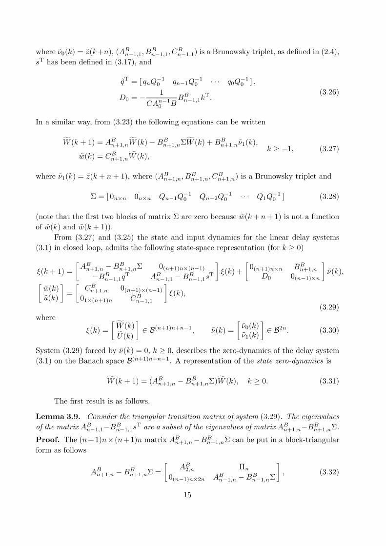
where ~º0(k) = ~z(k+n), (ABn¡1;1; B

Bn¡1;1; C

Bn¡1;1) is a Brunowsky triplet, as de¯ned in (2.4),

sT has been de¯ned in (3.17), and

~qT = [ qnQ¡10 qn¡1Q¡10 ¢ ¢ ¢ q0Q

¡10 ] ;

D0 = ¡ 1

CAn¡10 BBBn¡1;1k

T:(3:26)

In a similar way, from (3.23) the following equations can be written

fW (k + 1) = ABn+1;nfW (k)¡BBn+1;n§fW (k) +BBn+1;n~º1(k);~w(k) = CBn+1;nfW (k); k ¸ ¡1; (3.27)

where ~º1(k) = ~z(k + n+ 1), where (ABn+1;n; B

Bn+1;n; C

Bn+1;n) is a Brunowsky triplet and

§ = [ 0n£n 0n£n Qn¡1Q¡10 Qn¡2Q¡10 ¢ ¢ ¢ Q1Q¡10 ] (3.28)

(note that the ¯rst two blocks of matrix § are zero because ~w(k+ n+1) is not a function

of ~w(k) and ~w(k + 1)).

From (3.27) and (3.25) the state and input dynamics for the linear delay systems

(3.1) in closed loop, admits the following state-space representation (for k ¸ 0)

»(k + 1) =

·ABn+1;n ¡BBn+1;n§ 0(n+1)n£(n¡1)

¡BBn¡1;1qT ABn¡1;1 ¡BBn¡1;1sT¸»(k) +

·0(n+1)n£n BBn+1;n

D0 0(n¡1)£n

¸~º(k);·

~w(k)~u(k)

¸=

·CBn+1;n 0(n+1)£(n¡1)01£(n+1)n CBn¡1;1

¸»(k);

(3.29)

where

»(k) =

·fW (k)eU(k)¸2 B(n+1)n+n¡1; ~º(k) =

·~º0(k)~º1(k)

¸2 B2n: (3.30)

System (3.29) forced by ~º(k) = 0, k ¸ 0, describes the zero-dynamics of the delay system(3.1) on the Banach space B(n+1)n+n¡1. A representation of the state zero-dynamics is

fW (k + 1) = (ABn+1;n ¡BBn+1;n§)fW (k); k ¸ 0: (3.31)

The ¯rst result is as follows.

Lemma 3.9. Consider the triangular transition matrix of system (3.29). The eigenvalues

of the matrix ABn¡1;1¡BBn¡1;1sT are a subset of the eigenvalues of matrix ABn+1;n¡BBn+1;n§.Proof. The (n+1)n£ (n+1)n matrix ABn+1;n¡BBn+1;n§ can be put in a block-triangularform as follows

ABn+1;n ¡BBn+1;n§ =·

AB2;n ¦n0(n¡1)n£2n ABn¡1;n ¡BBn¡1;n ¹§

¸; (3.32)

15

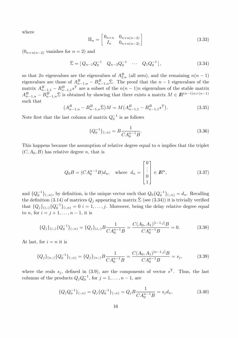
where

¦n =

·0n£n 0n£n(n¡2)In 0n£n(n¡2)

¸(3:33)

(0n£n(n¡2) vanishes for n = 2) and

¹§ = [Qn¡1Q¡10 Qn¡2Q¡10 ¢ ¢ ¢ Q1Q¡10 ] ; (3.34)

so that 2n eigenvalues are the eigenvalues of AB2;n (all zero), and the remaining n(n ¡ 1)eigenvalues are those of ABn¡1;n ¡ BBn¡1;n ¹§. The proof that the n ¡ 1 eigenvalues of thematrix ABn¡1;1 ¡ BBn¡1;1sT are a subset of the n(n ¡ 1)n eigenvalues of the stable matrixABn¡1;n ¡BBn¡1;n ¹§ is obtained by showing that there exists a matrix M 2 IR(n¡1)n£(n¡1)such that ¡

ABn¡1;n ¡BBn¡1;n ¹§¢M =M

¡ABn¡1;1 ¡BBn¡1;1sT

¢: (3.35)

Note ¯rst that the last column of matrix Q¡10 is as follows

fQ¡10 g(:;n) = B 1

CAn¡10 B: (3:36)

This happens because the assumption of relative degree equal to n implies that the triplet

(C;A0; B) has relative degree n, that is

Q0B = (CAn¡10 B)dn; where dn =

26640...01

3775 2 IRn; (3:37)

and fQ¡10 g(:;n), by de¯nition, is the unique vector such that Q0fQ¡10 g(:;n) = dn. Recallingthe de¯nition (3.14) of matrices Qj appearing in matrix ¹§ (see (3.34)) it is trivially veri¯ed

that fQjg(i;:)fQ¡10 g(:;n) = 0 i = 1; : : : ; j. Moreover, being the delay relative degree equalto n, for i = j + 1; : : : ; n¡ 1, it is

fQjg(i;:)fQ¡10 g(:;n) = fQjg(i;:)B 1

CAn¡10 B=C(A0; A1)

[i¡1;j]BCAn¡10 B

= 0: (3:38)

At last, for i = n it is

fQjg(n;:)fQ¡10 g(:;n) = fQjg(n;:)B 1

CAn¡10 B=C(A0; A1)

[n¡1;j]BCAn¡10 B

= sj ; (3:39)

where the reals sj , de¯ned in (3.9), are the components of vector sT. Thus, the last

columns of the products QjQ¡10 , for j = 1; : : : ; n¡ 1, are

fQjQ¡10 g(:;n) = QjfQ¡10 g(:;n) = QjB 1

CAn¡10 B= sjdn; (3:40)

16

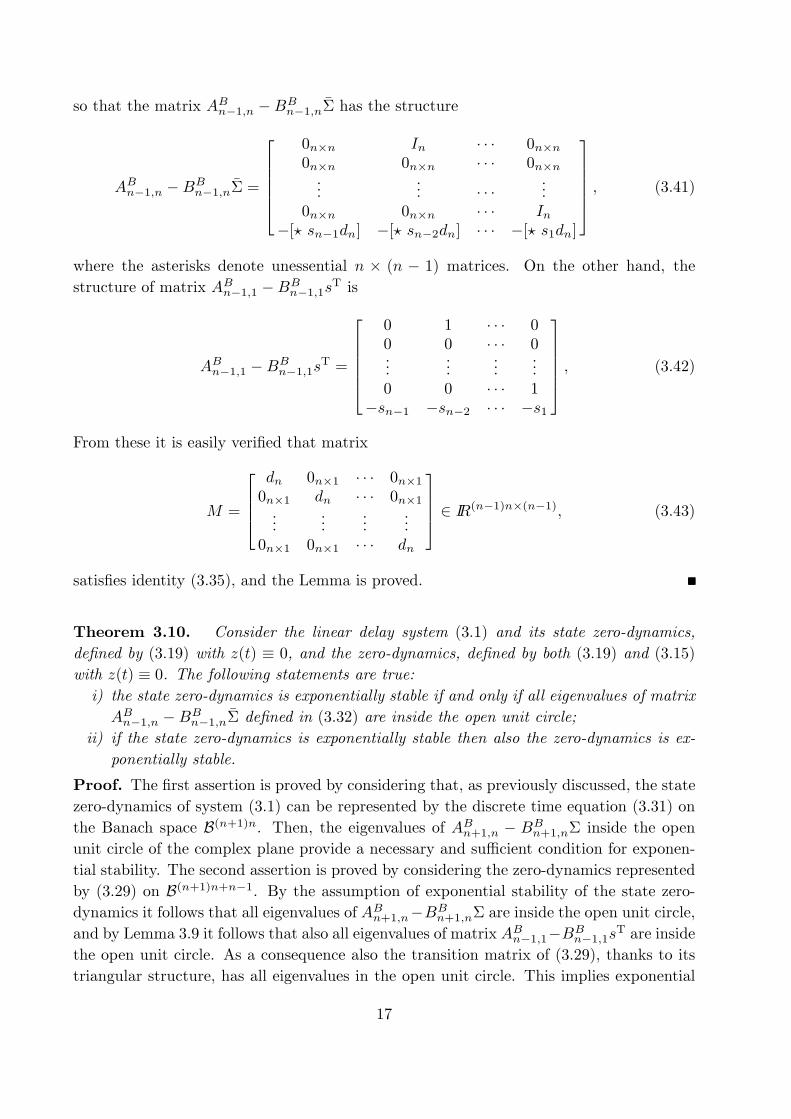
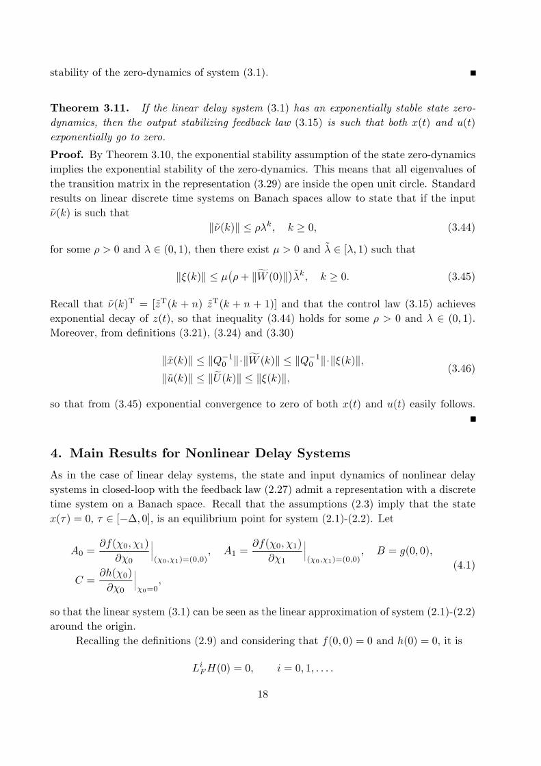
so that the matrix ABn¡1;n ¡BBn¡1;n ¹§ has the structure

ABn¡1;n ¡BBn¡1;n ¹§ =

2666640n£n In ¢ ¢ ¢ 0n£n0n£n 0n£n ¢ ¢ ¢ 0n£n...

... ¢ ¢ ¢ ...0n£n 0n£n ¢ ¢ ¢ In

¡[? sn¡1dn] ¡[? sn¡2dn] ¢ ¢ ¢ ¡[? s1dn]

377775 ; (3:41)

where the asterisks denote unessential n £ (n ¡ 1) matrices. On the other hand, the

structure of matrix ABn¡1;1 ¡BBn¡1;1sT is

ABn¡1;1 ¡BBn¡1;1sT =

2666640 1 ¢ ¢ ¢ 00 0 ¢ ¢ ¢ 0...

......

...0 0 ¢ ¢ ¢ 1

¡sn¡1 ¡sn¡2 ¢ ¢ ¢ ¡s1

377775 ; (3:42)

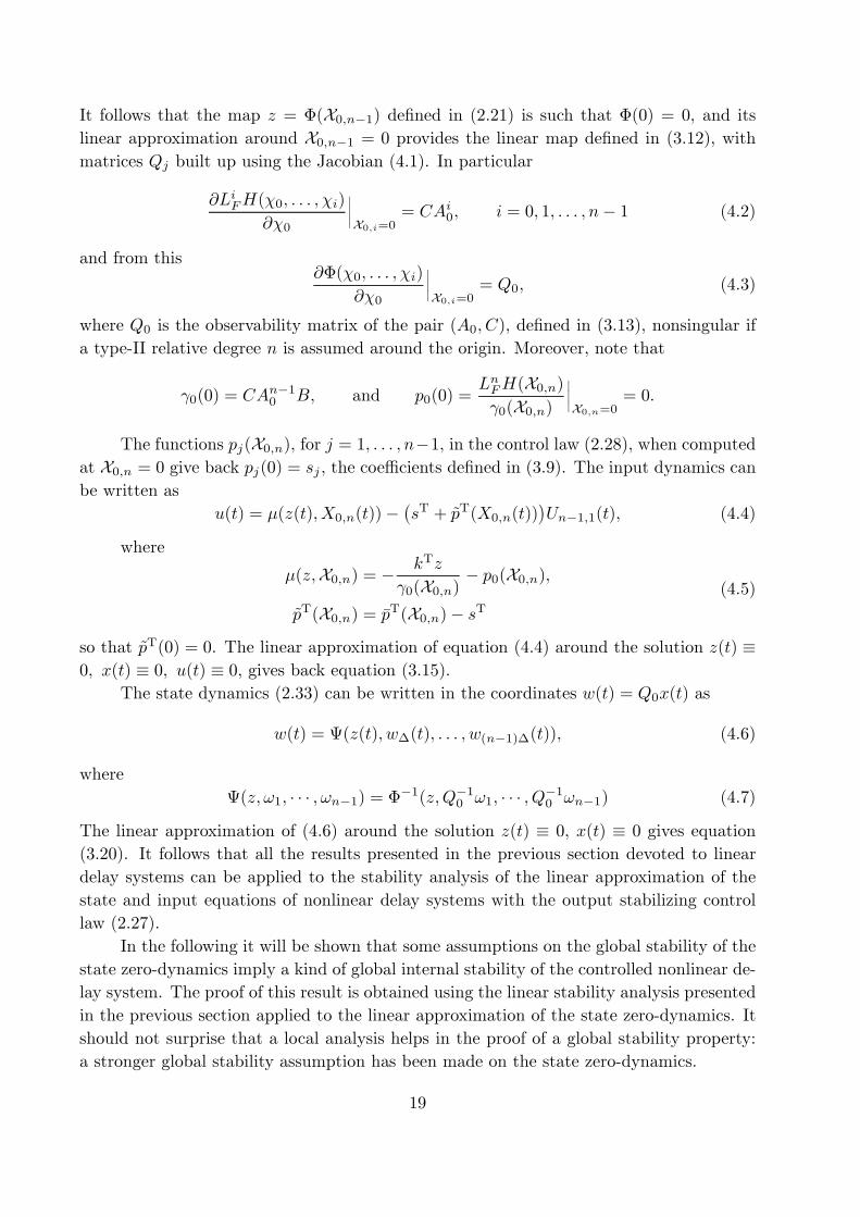
From these it is easily veri¯ed that matrix

M =

2664dn 0n£1 ¢ ¢ ¢ 0n£10n£1 dn ¢ ¢ ¢ 0n£1...

......

...0n£1 0n£1 ¢ ¢ ¢ dn

3775 2 IR(n¡1)n£(n¡1); (3:43)

satis¯es identity (3.35), and the Lemma is proved.

Theorem 3.10. Consider the linear delay system (3.1) and its state zero-dynamics,

de¯ned by (3.19) with z(t) ´ 0, and the zero-dynamics, de¯ned by both (3.19) and (3.15)with z(t) ´ 0. The following statements are true:i) the state zero-dynamics is exponentially stable if and only if all eigenvalues of matrix

ABn¡1;n ¡BBn¡1;n ¹§ de¯ned in (3.32) are inside the open unit circle;ii) if the state zero-dynamics is exponentially stable then also the zero-dynamics is ex-

ponentially stable.

Proof. The ¯rst assertion is proved by considering that, as previously discussed, the state

zero-dynamics of system (3.1) can be represented by the discrete time equation (3.31) on

the Banach space B(n+1)n. Then, the eigenvalues of ABn+1;n ¡ BBn+1;n§ inside the open

unit circle of the complex plane provide a necessary and su±cient condition for exponen-

tial stability. The second assertion is proved by considering the zero-dynamics represented

by (3.29) on B(n+1)n+n¡1. By the assumption of exponential stability of the state zero-dynamics it follows that all eigenvalues of ABn+1;n¡BBn+1;n§ are inside the open unit circle,and by Lemma 3.9 it follows that also all eigenvalues of matrix ABn¡1;1¡BBn¡1;1sT are insidethe open unit circle. As a consequence also the transition matrix of (3.29), thanks to its

triangular structure, has all eigenvalues in the open unit circle. This implies exponential

17

stability of the zero-dynamics of system (3.1).

Theorem 3.11. If the linear delay system (3.1) has an exponentially stable state zero-

dynamics, then the output stabilizing feedback law (3.15) is such that both x(t) and u(t)

exponentially go to zero.

Proof. By Theorem 3.10, the exponential stability assumption of the state zero-dynamics

implies the exponential stability of the zero-dynamics. This means that all eigenvalues of

the transition matrix in the representation (3.29) are inside the open unit circle. Standard

results on linear discrete time systems on Banach spaces allow to state that if the input

~º(k) is such that

k~º(k)k · ½¸k; k ¸ 0; (3.44)

for some ½ > 0 and ¸ 2 (0; 1), then there exist ¹ > 0 and ~̧ 2 [¸; 1) such that

k»(k)k · ¹¡½+ kfW (0)k¢~̧k; k ¸ 0: (3.45)

Recall that ~º(k)T = [~zT(k + n) ~zT(k + n + 1)] and that the control law (3.15) achieves

exponential decay of z(t), so that inequality (3.44) holds for some ½ > 0 and ¸ 2 (0; 1).Moreover, from de¯nitions (3.21), (3.24) and (3.30)

k~x(k)k · kQ¡10 k¢kfW (k)k · kQ¡10 k¢k»(k)k;k~u(k)k · keU(k)k · k»(k)k; (3:46)

so that from (3.45) exponential convergence to zero of both x(t) and u(t) easily follows.

4. Main Results for Nonlinear Delay Systems

As in the case of linear delay systems, the state and input dynamics of nonlinear delay

systems in closed-loop with the feedback law (2.27) admit a representation with a discrete

time system on a Banach space. Recall that the assumptions (2.3) imply that the state

x(¿) = 0, ¿ 2 [¡¢; 0], is an equilibrium point for system (2.1)-(2.2). Let

A0 =@f(Â0; Â1)

@Â0

¯̄̄(Â0;Â1)=(0;0)

; A1 =@f(Â0; Â1)

@Â1

¯̄̄(Â0;Â1)=(0;0)

; B = g(0; 0);

C =@h(Â0)

@Â0

¯̄̄Â0=0

;

(4.1)

so that the linear system (3.1) can be seen as the linear approximation of system (2.1)-(2.2)

around the origin.

Recalling the de¯nitions (2.9) and considering that f(0; 0) = 0 and h(0) = 0, it is

LiFH(0) = 0; i = 0; 1; : : : :

18

It follows that the map z = ©(X0;n¡1) de¯ned in (2.21) is such that ©(0) = 0, and its

linear approximation around X0;n¡1 = 0 provides the linear map de¯ned in (3.12), with

matrices Qj built up using the Jacobian (4.1). In particular

@LiFH(Â0; : : : ; Âi)

@Â0

¯̄̄X0;i=0

= CAi0; i = 0; 1; : : : ; n¡ 1 (4:2)

and from this@©(Â0; : : : ; Âi)

@Â0

¯̄̄X0;i=0

= Q0; (4:3)

where Q0 is the observability matrix of the pair (A0; C), de¯ned in (3.13), nonsingular if

a type-II relative degree n is assumed around the origin. Moreover, note that

°0(0) = CAn¡10 B; and p0(0) =

LnFH(X0;n)°0(X0;n)

¯̄̄X0;n=0

= 0:

The functions pj(X0;n), for j = 1; : : : ; n¡1, in the control law (2.28), when computedat X0;n = 0 give back pj(0) = sj , the coe±cients de¯ned in (3.9). The input dynamics canbe written as

u(t) = ¹(z(t);X0;n(t))¡¡sT + ~pT(X0;n(t))

¢Un¡1;1(t); (4.4)

where

¹(z;X0;n) = ¡ kTz

°0(X0;n) ¡ p0(X0;n);

~pT(X0;n) = ¹pT(X0;n)¡ sT(4.5)

so that ~pT(0) = 0. The linear approximation of equation (4.4) around the solution z(t) ´0; x(t) ´ 0; u(t) ´ 0, gives back equation (3.15).

The state dynamics (2.33) can be written in the coordinates w(t) = Q0x(t) as

w(t) = ª(z(t); w¢(t); : : : ; w(n¡1)¢(t)); (4.6)

where

ª(z; !1; ¢ ¢ ¢ ; !n¡1) = ©¡1(z;Q¡10 !1; ¢ ¢ ¢ ; Q¡10 !n¡1) (4.7)

The linear approximation of (4.6) around the solution z(t) ´ 0, x(t) ´ 0 gives equation

(3.20). It follows that all the results presented in the previous section devoted to linear

delay systems can be applied to the stability analysis of the linear approximation of the

state and input equations of nonlinear delay systems with the output stabilizing control

law (2.27).

In the following it will be shown that some assumptions on the global stability of the

state zero-dynamics imply a kind of global internal stability of the controlled nonlinear de-

lay system. The proof of this result is obtained using the linear stability analysis presented

in the previous section applied to the linear approximation of the state zero-dynamics. It

should not surprise that a local analysis helps in the proof of a global stability property:

a stronger global stability assumption has been made on the state zero-dynamics.

19

A ¯rst useful lemma is the following.

Lemma 4.12. Consider a nonlinear delay system (2.1)-(2.2) with uniform type-II relative

degree and globally partially invertible observability map (assumption H1). Assume that the

equilibrium x(t) ´ 0 of the state zero-dynamics (2.36a) is exponentially stable. Then, thelinear approximation of the zero dynamics (2.36) around x(t) ´ 0; u(t) ´ 0 is exponentiallystable.

Proof. From the previous discussion, equation (3.29), with ~º(k) ´ 0 is a representation ofthe linear approximation of the zero-dynamics (2.36) around x(t) ´ 0; u(t) ´ 0. Moreover,the assumption of exponential stability of the nonlinear state zero-dynamics implies ex-

ponential stability of the linear approximation of the state zero-dynamics. From assertion

(ii) of Theorem 3.10 the linear approximation of the zero dynamics is exponentially stable.

Di®erently from the case of linear systems, it is not obvious if the exponential stability

of the nonlinear state zero-dynamics (2.36a) implies that if z(t) asymptotically goes to

zero, then also x(t) asymptotically goes to zero. As a consequence, this kind of input-state

stability for the output-driven state dynamics (2.33) is a property that must be explicitely

assumed, together with the exponential stability of the state zero-dynamics.

De¯nition 4.13. The output-driven state dynamics (2.33) is said to be globally input-

state asymptotically (exponentially) stable if for all z(t) that asymptotically (exponentially)

go to zero and for all initial states, x(t) asymptotically (exponentially) goes to zero.

Remark 4.14. If the output-driven state dynamics (2.33) is globally Input-State

exponentially stable, then the state zero-dynamics is exponentially stable and the transition

matrix of the linear approximation (3.27) has all eigenvalues inside the unit circle. On

the other hand, if the linear approximation is exponentially stable, then the state zero-

dynamics is locally exponentially stable, and the output-driven state dynamics (2.33) is

locally Input-State exponentially stable.

As done for the output-driven input dynamics of linear delay systems with control

law (3.15) also the (output-driven) input dynamics of nonlinear delay systems can be

written on the Banach space B(n¡1) exploiting the same de¯nitions given in (3.21) and(3.24), but in this case the transition operator cannot be represented simply by a matrix

in IR(n¡1)£(n¡1). Regarding X0;n(t) as a time-varying parameter, equation (4.4) can bewritten as a time-varying system on the Banach Space B(n¡1) as follows

eU(k + 1) = ¡A+ S(k)¢eU(k)¡BBn¡1;1~¹(k); (4.8)

where A and S(k) are operators from Bn¡1 to B, de¯ned as

[AeU ](¿) = ¡ABn¡1;1 ¡BBn¡1;1sT¢[eU(k)](¿)[S(k)eU(k)](¿) = ~pT

¡X0;n((k + n)¢ + ¿)

¢[eU(k)](¿) ; ¿ 2 [¡¢; 0]; (4:9)

20

and the sequence ~¹(k) 2 B is de¯ned as

[~¹(k)](¿) = ¹³z((k + n)¢ + ¿);X1;n((k + n)¢ + ¿)

´; ¿ 2 [¡¢; 0]; (4:10)

where ~pT(X0;n) and ¹(z;X1;n) have been de¯ned in (4.5).The following theorem is the main result on the internal stability of nonlinear delay

systems controlled with the output-stabilizing law (2.27).

Theorem 4.15. Consider the control law (2.27), with k Hurwitz, applied to a non-

linear delay system (2.1)-(2.2) with uniform type-II relative degree and globally partially

invertible observability map (assumption H1). Assume that the state zero-dynamics is glob-

ally exponentially stable and that the output-driven state dynamics is globally input-state

asymptotically stable (de¯nition 4.13). Then, both the system variable x(t) and the input

variable u(t) asymptotically go to zero.

Proof. Thanks to the control law (2.27), with k Hurwitz, the vector z(t) exponentially

goes to zero. By the assumption of global Input-State asymptotic stability of the output-

driven state dynamics, also x(t) asymptotically goes to zero. The assumption of global

exponential stability of the state zero-dynamics implies that the linear approximation of

the state zero-dynamics on the Banach space B(n+1)n is exponentially stable, and thereforethat all eigenvalues of matrix ABn+1;n¡BBn+1;n§ are inside the open unit circle of the com-plex plane. Thanks to Lemma 3.9, also the eigenvalues of matrix ABn¡1;1¡BBn¡1;1sT, thatgoverns the linear approximation of the input dynamics (4.8) on Bn¡1, are inside the openunit circle. Now, note that the representation (4.8) is of the same type of the one described

by eq. (A.1) in the Appendix. Since z(t), x(t), and therefore X0;n(t), asymptotically go to

zero, recalling that, from (4.5), ~pT(0) = 0 and ¹(0; 0) = 0, the sequence k~¹(k)k and kS(k)kare bounded by sequences convergent to zero. Since the matrix ABn¡1;1¡BBn¡1;1sT has alleigenvalues inside the open unit circle, thanks to Lemma A.1, proved in the Appendix, it

follows that the sequence keU(k)k asymptotically tends to zero. This trivially implies thatu(t) asymptotically goes to zero, and the proof is complete.

Remark 4.16. The local exponential stability of the state zero dynamics, and hence the

local input-state exponential stability of the output-driven state dynamics, can be tested

by evaluating the eigenvalues of matrix ABn¡1;n¡BBn¡1;n ¹§. Global stability properties aremuch harder to investigate.

5. An Example

Consider the following delay system of the type (2.1), (2.2)

_x1(t) =x2(t)

1 + x21(t¡¢)+ ¾x2(t¡¢);

_x2(t) = x1(t)x2(t¡¢) + u(t);y(t) = x1(t)

(5.1)

21

where ¾ is a constant parameter. According to the de¯nition 2.3 it is not di±cult to

show that this system has uniform Type-II relative degree r = n = 2. Here follows the

expression of °0(X0;2), as de¯ned in (2.11),

°0(X0;2) = 1

1 + Â21;16= 0; 8X0;2 2 IR6: (5:2)

The substitution X0;2 = X0;2(t) in the previous equation yields

°0(X0;2(t)) =1

1 + x21(t¡¢): (5:3)

Following the de¯nition (2.21) the map z = ©(X0;2) can be easily constructed and canbe shown to be globally partially invertible, i.e. Â0 = ©¡1(z;X1;2) exists 8z 2 IR2 and8X1;2 2 IR4. After the substitutions of X0;2 with X0;2(t) and of X1;2 with X1;2(t), themaps © and ©¡1, for the given example, are as follows

z(t) = ©¡X0;2(t)

¢=

24 x1(t)x2(t)

1 + x21(t¡¢)+ ¾x2(t¡¢)

35 ; (5:4)

x(t) = ©¡1¡z(t);X1;2(t)

¢=

·z1(t)¡

z2(t)¡ ¾x2(t¡¢)¢¡1 + x21(t¡¢)

¢ ¸ : (5.5)

The control law (2.27) has the following expression

u(t) = ®¡z(t); x(t); x(t¡¢); x(t¡ 2¢)¢+ ¯¡x(t); x(t¡¢)¢u(t¡¢) (5.6)

with

® =¡1 + x21(t¡¢)

¢h¡kTz(t)¡ ¾x1(t¡¢)x2(t¡ 2¢) (5.7)

+x2(t)x1(t¡¢)¡1 + x21(t¡¢)

¢2³ x2(t¡¢)1 + x21(t¡ 2¢)

+ ¾x2(t¡ 2¢)´i;

¯ =¡ ¾¡1 + x21(t¡¢)¢: (5.8)

The gain vector kT = [k1 k2] is such to assign stable eigenvalues to the matrix

AB2;1 ¡BB2;1kT =·0 1¡k1 ¡k2

¸: (5.9)

The equation (5.5), when z(t) ´ 0, for t ¸ ¢, de¯nes the state-zero-dynamics of the system,and together with (5.6) de¯ne the system zero-dynamics (see eqn.'s (2.36)). According to

the results of Theorem 4.15, the convergence of the system variables (state and input)

to zero is guaranteed if the state-zero-dynamics is globally exponentially stable and if

the dynamics given by (5.5) is globally input-state asymptotically stable. Thanks to the

22

continuity of the map ©¡1, and suitably exploiting the ¯rst scalar equation (x1(t) = z1(t),for t ¸ ¢), it is not di±cult to prove that the null element of L1([¡¢;¢]; IR2) is a globallyexponentially stable equilibrium point of the state-zero-dynamics if and only if j¾j < 1.

Under the same condition on ¾ it can be shown that if z(t) asymptotically converges to

zero then also x(t) asymptotically decays to zero. Thanks to Theorem 4.15 it follows that

if j¾j < 1 then the feedback law (5.6), with stabilizing gain k, is such to asymptotically

drive to zero both the state and the input of system (5.1). All computer simulations have

shown that all system variables asymptotically go to zero when j¾j < 1.The results of two numerical simulations are presented below, in which two di®erent

values of the parameter ¾ are used. The delay ¢ used in the simulations is ¢ = 0:1. In

both simulations the initial state for the system has been chosen as

x(¿) =

·1¡1¸; ¿ 2 [¡0:1; 0]: (5:10)

The gain matrix kT in (5.6) used is kT = [20 9] (assigns eigenvalues ¸1 = ¡4 and ¸2 = ¡5to matrix (5.9)). The control law (5.6) is applied starting at time t = 0:1.

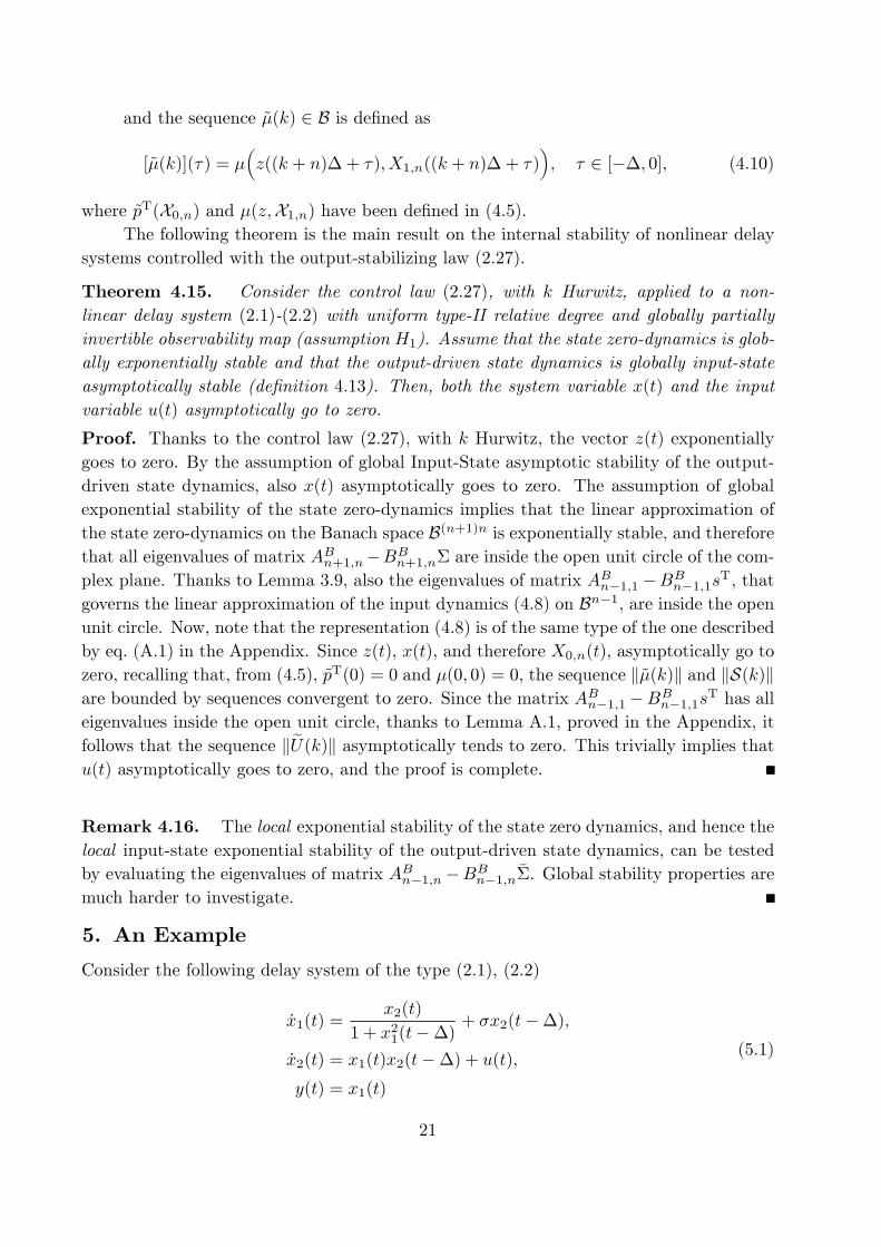
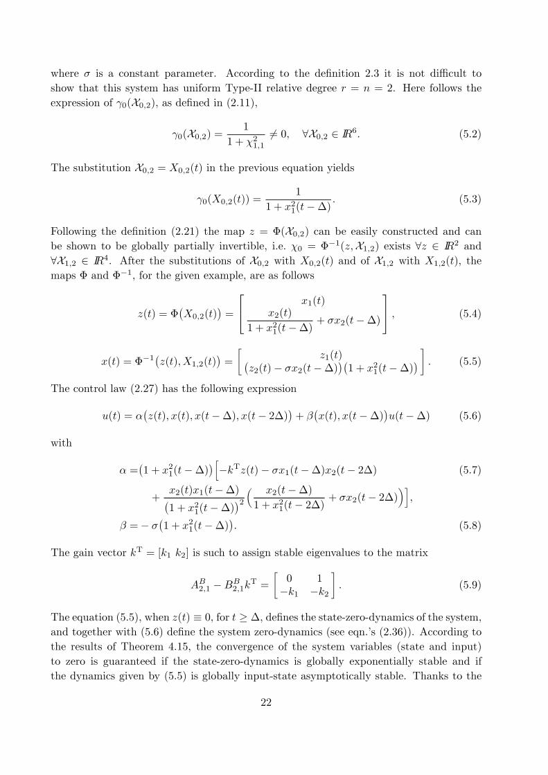
Figures 1 and 2 report simulation results when ¾ = 0:5. Figure 1 shows the state

evolution of the controlled system. Note that the ¯rst state component, the system output,

asymptotically goes to zero with a typical two modes exponential decay. Also the second

system variable asymptotically goes to zero, together with the input, depicted in Figure 2.

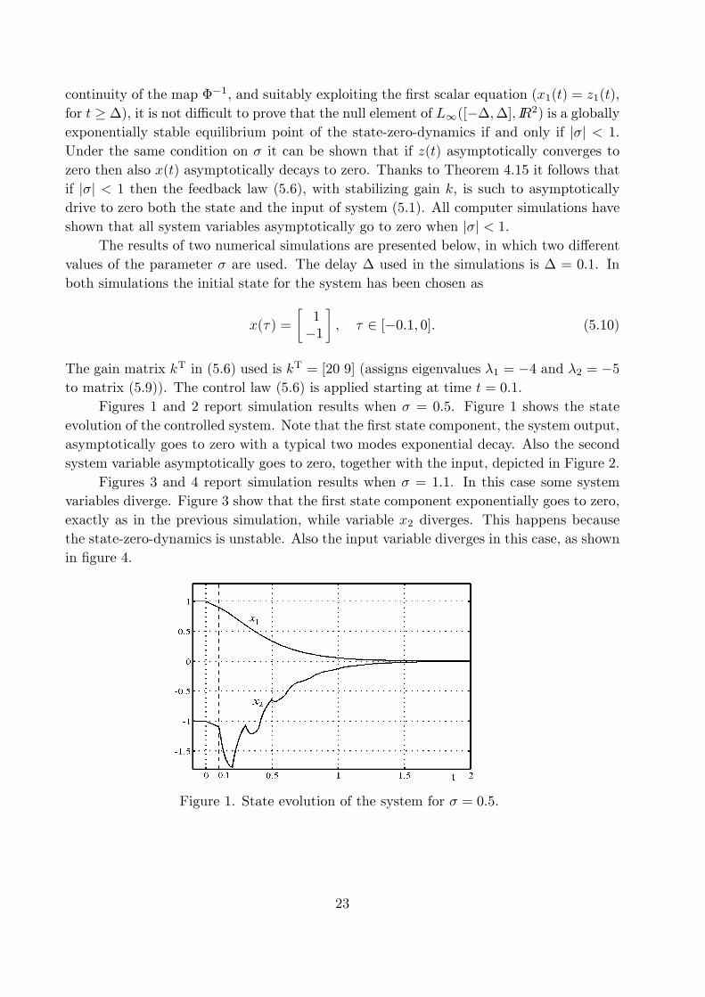
Figures 3 and 4 report simulation results when ¾ = 1:1. In this case some system

variables diverge. Figure 3 show that the ¯rst state component exponentially goes to zero,

exactly as in the previous simulation, while variable x2 diverges. This happens because

the state-zero-dynamics is unstable. Also the input variable diverges in this case, as shown

in ¯gure 4.

Figure 1. State evolution of the system for ¾ = 0:5.

23

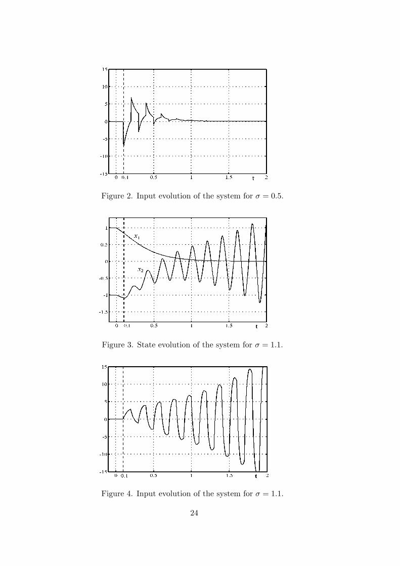
Figure 2. Input evolution of the system for ¾ = 0:5.

Figure 3. State evolution of the system for ¾ = 1:1.

Figure 4. Input evolution of the system for ¾ = 1:1.

24

6. Concluding Remarks

The technique of exact I/O linearization, originally developed for nonlinear systems with-

out state delay, has been recently applied to nonlinear delay systems by means of a suitable

extension of the tools of the standard di®erential geometry [4, 6, 15, 16, 18, 19]. Simul-

taneous I/O linearization and delay cancelation can be obtained for systems that have a

relative degree and have stable zero-dynamics (internal state and input dynamics when the

output is forced to be zero). In this paper we pointed out that, di®erently from the case of

systems without delay, for delay systems the full relative degree property does not imply

the absence of the zero-dynamics. The stability of the state zero-dynamics in the case of

full relative degree delay systems has been studied for the ¯rst time in [6]. In [19] the

authors discussed the issue of stability of what in this paper is called state zero-dynamics

(eq. (2.36a)) in the case of non-full relative degree, while the issue of stability of the total

zero-dynamics (eq.'s (2.36a) and (2.36b)) was not investigated because the authors con-

sidered a class of systems (those with type-III relative degree) that do not have input

zero-dynamics. This paper explicitely consider delay systems with full relative degree and

with non trivial state and input zero-dynamics. The main result presented here is that

a suitable stability assumption on the state zero-dynamics, a necessary assumption for

the applicability of the technique of exact I/O linearization with delay cancelation, in the

case of full relative degree implies the stability of the input zero-dynamics. This implies

the closed-loop stability of the nonlinear delay system, with the output zeroing controller.

Future work will involve the study of the internal state and input dynamics in the case of

not full relative degree.

25

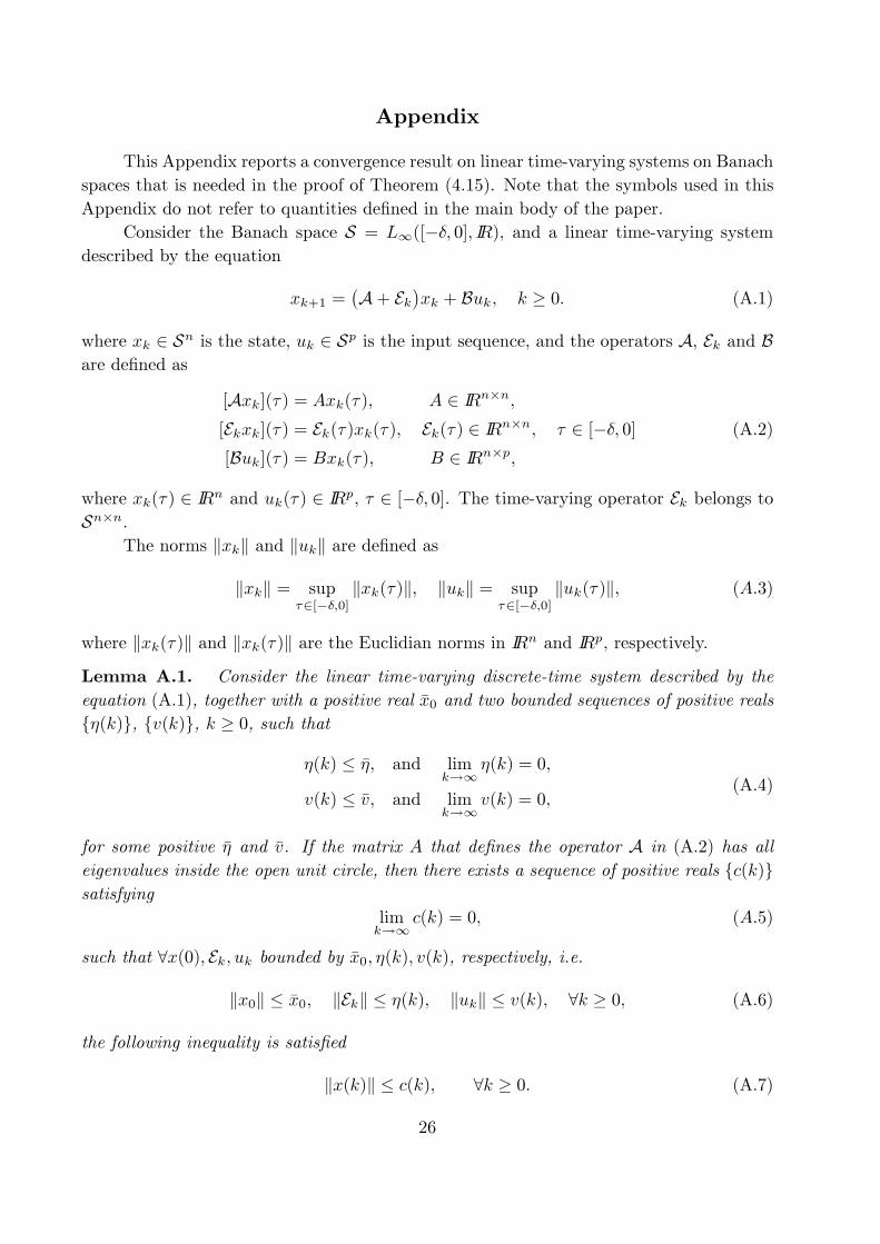
Appendix

This Appendix reports a convergence result on linear time-varying systems on Banach

spaces that is needed in the proof of Theorem (4.15). Note that the symbols used in this

Appendix do not refer to quantities de¯ned in the main body of the paper.

Consider the Banach space S = L1([¡±; 0]; IR), and a linear time-varying systemdescribed by the equation

xk+1 =¡A+ Ek¢xk + Buk; k ¸ 0: (A.1)

where xk 2 Sn is the state, uk 2 Sp is the input sequence, and the operators A, Ek and Bare de¯ned as

[Axk](¿) = Axk(¿); A 2 IRn£n;[Ekxk](¿) = Ek(¿)xk(¿); Ek(¿) 2 IRn£n; ¿ 2 [¡±; 0][Buk](¿) = Bxk(¿); B 2 IRn£p;

(A.2)

where xk(¿) 2 IRn and uk(¿) 2 IRp, ¿ 2 [¡±; 0]. The time-varying operator Ek belongs toSn£n.

The norms kxkk and kukk are de¯ned as

kxkk = sup¿2[¡±;0]

kxk(¿)k; kukk = sup¿2[¡±;0]

kuk(¿)k; (A:3)

where kxk(¿)k and kxk(¿)k are the Euclidian norms in IRn and IRp, respectively.Lemma A.1. Consider the linear time-varying discrete-time system described by the

equation (A.1), together with a positive real ¹x0 and two bounded sequences of positive reals

f´(k)g, fv(k)g, k ¸ 0, such that

´(k) · ¹́; and limk!1

´(k) = 0;

v(k) · ¹v; and limk!1

v(k) = 0;(A.4)

for some positive ¹́ and ¹v. If the matrix A that de¯nes the operator A in (A.2) has all

eigenvalues inside the open unit circle, then there exists a sequence of positive reals fc(k)gsatisfying

limk!1

c(k) = 0; (A:5)

such that 8x(0); Ek; uk bounded by ¹x0; ´(k); v(k), respectively, i.e.

kx0k · ¹x0; kEkk · ´(k); kukk · v(k); 8k ¸ 0; (A.6)

the following inequality is satis¯ed

kx(k)k · c(k); 8k ¸ 0: (A.7)

26

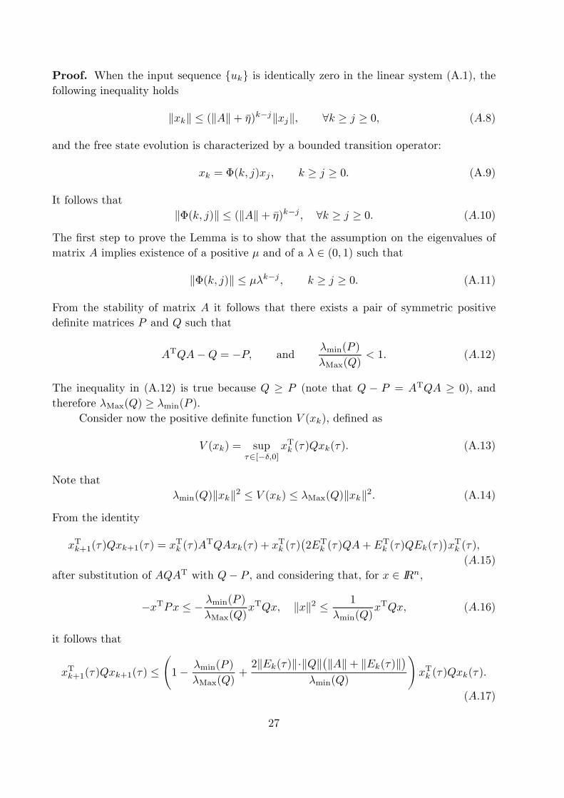
Proof. When the input sequence fukg is identically zero in the linear system (A.1), the

following inequality holds

kxkk · (kAk+ ¹́)k¡jkxjk; 8k ¸ j ¸ 0; (A:8)

and the free state evolution is characterized by a bounded transition operator:

xk = ©(k; j)xj ; k ¸ j ¸ 0: (A.9)

It follows that

k©(k; j)k · (kAk+ ¹́)k¡j ; 8k ¸ j ¸ 0: (A:10)

The ¯rst step to prove the Lemma is to show that the assumption on the eigenvalues of

matrix A implies existence of a positive ¹ and of a ¸ 2 (0; 1) such that

k©(k; j)k · ¹¸k¡j ; k ¸ j ¸ 0: (A.11)

From the stability of matrix A it follows that there exists a pair of symmetric positive

de¯nite matrices P and Q such that

ATQA¡Q = ¡P; and¸min(P )

¸Max(Q)< 1: (A:12)

The inequality in (A.12) is true because Q ¸ P (note that Q ¡ P = ATQA ¸ 0), and

therefore ¸Max(Q) ¸ ¸min(P ).Consider now the positive de¯nite function V (xk), de¯ned as

V (xk) = sup¿2[¡±;0]

xTk (¿)Qxk(¿): (A.13)

Note that

¸min(Q)kxkk2 · V (xk) · ¸Max(Q)kxkk2: (A.14)

From the identity

xTk+1(¿)Qxk+1(¿) = xTk (¿)A

TQAxk(¿) + xTk (¿)

¡2ETk (¿)QA+E

Tk (¿)QEk(¿)

¢xTk (¿);

(A:15)

after substitution of AQAT with Q¡ P , and considering that, for x 2 IRn,

¡xTPx · ¡ ¸min(P )¸Max(Q)

xTQx; kxk2 · 1

¸min(Q)xTQx; (A:16)

it follows that

xTk+1(¿)Qxk+1(¿) ·Ã1¡ ¸min(P )

¸Max(Q)+2kEk(¿)k¢kQk

¡kAk+ kEk(¿)k¢¸min(Q)

!xTk (¿)Qxk(¿):

(A:17)

27

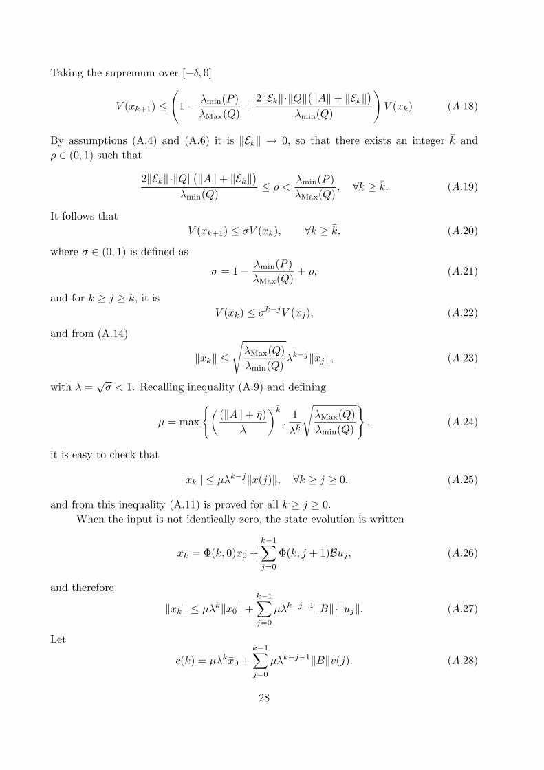
Taking the supremum over [¡±; 0]

V (xk+1) ·Ã1¡ ¸min(P )

¸Max(Q)+2kEkk¢kQk

¡kAk+ kEkk¢¸min(Q)

!V (xk) (A:18)

By assumptions (A.4) and (A.6) it is kEkk ! 0, so that there exists an integer ¹k and

½ 2 (0; 1) such that2kEkk¢kQk

¡kAk+ kEkk¢¸min(Q)

· ½ < ¸min(P )

¸Max(Q); 8k ¸ ¹k: (A:19)

It follows that

V (xk+1) · ¾V (xk); 8k ¸ ¹k; (A:20)

where ¾ 2 (0; 1) is de¯ned as¾ = 1¡ ¸min(P )

¸Max(Q)+ ½; (A:21)

and for k ¸ j ¸ ¹k, it isV (xk) · ¾k¡jV

¡xj); (A:22)

and from (A.14)

kxkk ·s¸Max(Q)

¸min(Q)¸k¡jkxjk; (A:23)

with ¸ =p¾ < 1. Recalling inequality (A.9) and de¯ning

¹ = max

(µ(kAk+ ¹́)

¸

¶¹k;1

¸¹k

s¸Max(Q)

¸min(Q)

); (A:24)

it is easy to check that

kxkk · ¹¸k¡jkx(j)k; 8k ¸ j ¸ 0: (A:25)

and from this inequality (A.11) is proved for all k ¸ j ¸ 0.When the input is not identically zero, the state evolution is written

xk = ©(k; 0)x0 +k¡1Xj=0

©(k; j + 1)Buj ; (A:26)

and therefore

kxkk · ¹¸kkx0k+k¡1Xj=0

¹¸k¡j¡1kBk¢kujk: (A:27)

Let

c(k) = ¹¸k¹x0 +k¡1Xj=0

¹¸k¡j¡1kBkv(j): (A:28)

28

By construction c(k) is such that (A.7) holds. It remains to prove that c(k) asymptotically

goes to zero, that is, for any " > 0 there exists a k" such that 8k ¸ k" it is c(k) < ". Tothis aim, rewrite c(k) setting k ¡ j ¡ 1 = i

c(k) = ¹¸k¹x0 +k¡1Xi=0

¹¸ikBkv(k ¡ i¡ 1): (A:29)

and split the summations as follows

c(k) = ¹¸k¹x0 +

º"Xi=0

¹¸ikBkv(k ¡ i¡ 1)

+k¡1X

i=º"+1

¹¸ikBkv(k ¡ i¡ 1);(A.30)

The ¯rst term in the expression (A.30) tends to zero (recall that ¸ =p¾ 2 (0; 1)), therefore

there exists k1;" such that 8k ¸ k1;" it is ¹¸k¹x0 · "=3. As for the third term in (A.30) it

isk¡1X

i=º"+1

¹¸ikBkv(k ¡ i¡ 1) ·1X

i=º"+1

¹¸ikBk¹v = ¹kBk¹v¸1¡ ¸ ¸º" : (A:31)

Since ¸ 2 (0; 1), it is easy to choose º" such that

¹kBk¹v¸1¡ ¸ ¸º" : · "

3: (A:32)

As for the second term in (A.30), de¯ning

¹w(k) = supi2[0;º"]

v(k ¡ i¡ 1): (A:33)

it isº"Xi=0

¹¸ikBk¹u(k ¡ i¡ 1) · ¡º" + 1¢¹kBk ¹w(k): (A:34)

Now, by assumption (A.4), ¹w(k) goes to zero and therefore there exists k2;" such that

º"Xi=0

¹¸ikBkv(k ¡ i¡ 1) · "

3; 8k ¸ k2;": (A:35)

As a result, denoting k" = maxfk1;"; k2;"g we have that

c(k) · "; 8k ¸ k"; (A:36)

and this concludes the proof.

29

References

[1] C. Antoniades and P. D. Christo¯des, Robust Control of Nonlinear Time-Delay Systems,Int. J. Appl. Math. and Comp. Sci., 1999, Vol. 9, No. 4, pp. 811-837.

[2] L. Dugard, E. I. Verriest, (Eds), Stability and Control of Time-delay Systems, Springer,1998.

[3] A. Germani, C. Manes, On the Existence of the Linearizing State-Feedback for Nonlin-ear Delay Systems, proc. of 40th IEEE Conf. on Decision and Control, pp. 4628{4629,Orlando, Florida, 2001.

[4] A. Germani, C. Manes and P. Pepe, Linearization of Input-Output Mapping for NonlinearDelay Systems via Static State Feedback, IMACS CESA Multiconference on Computa-tional Engineering in Systems Applications, Vol. 1, pp. 599{602, Lille, France, 1996.

[5] A. Germani, C. Manes and P. Pepe, A State Observer for Nonlinear Delay Systems, proc. of37th IEEE Conference on Decision and Control, Tampa, Florida, 1998.

[6] A. Germani, C. Manes and P. Pepe, Local Asymptotic Stability for Nonlinear State Feed-back Delay Systems, Kybernetika, Vol. 36, 2000.

[7] A. Germani, C. Manes and P. Pepe, An Asymptotic Observer for a Class of NonlinearDelay Systems, Kybernetika,, Vol.37, n. 4, pp. 459-478, 2001

[8] H.P. Huang, G.B. Wang, \Deadtime Compensation for Nonlinear Processes With Distur-bances," International Journal of Systems Science, Vol. 23, pp. 1761{1776, 1992.

[9] A. Isidori, Nonlinear Control Systems, 3rd edition, Springer-Verlag, Berlin, 1995.[10] B. Jakubczyk, W. Respondek, On Linearization of Control Systems, Bull. Acad. Polonaise

Sci. Ser. Sci. Math. 28,1980, pp. 517{522.[11] C. Kravaris and R.A. Wright, \Deadtime Compensation for Nonlinear Chemical Pro-

cesses," AIChE Journal, Vol. 35, pp. 1535{1542, 1989.[12] B. Lehman, J. Bentsman, S. V. Lunel and E. I. Verriest, Vibrational Control of Nonlinear

Time Lag Systems with Bounded Delay: Averaging Theory, Stabilizability, and TransientBehavior, IEEE Trans. Automat. Contr., No. 5, 1994, pp. 898{912.

[13] A. G. Loukianov, B. Castillo-Toledo, J. Escoto Hern¶andez, V. I. Utkin, "DecompositionFeedback Stabilization of Systems with Delay", 15th IFAC Triennal World Congress,Barcelona, Spain, 2002.

[14] E.S. Meadows and J.B. Rawlings, \Model Predictive Control". In Nonlinear ProcessControl, chapter 5, M.A. Henson and D.E. Seborg, eds., Prentice Hall, 1997.

[15] C. H. Moog, R. Castro, M. Velasco, The Disturbance Decoupling Problem for Non-linear Systems with Multiple Time-Delays: Static State Feedback Solutions, proc. ofIMACS CESA Multiconference on Computational Engineering in Systems Applications,Lille, France, 1996.

[16] C.H. Moog, R. Castro-Linares, M. Velasco-Villa, L.A.Marquez-Martinez, The DisturbanceDecoupling Problem for Time Delay Nonlinear Systems, IEEE Transactions on AutomaticControl, Vol. 45, No. 2, pp. 305-309, 2000.

[17] S.-I. Niculescu, Delay E®ects on Stability, a Robust Control Approach, Lecture Notes inControl and Information Sciences, Springer, 2001

[18] T. Oguchi and A. Watanabe, \Input-Output Linearization of Non-linear Systems WithTime Delays in State Variables", International Journal of Systems Science, Vol. 29, 573{578, 1998.

[19] T. Oguchi, A. Watanabe and T. Nakamizo, \Input-Output Linearization of Retarded Non-linear Systems by Using an Extension of Lie Derivative", Int. J. Control, Vol. 75, No. 8,582{590, 2002.

[20] P. Pepe, Stability of Time Varying Nonlinear Di®erence Equations with Continuous Time,3rd Workshop on Time-Delay Systems, Santa Fe, New Mexico, 2001

30