Input Harmonic and Input Harmonic and Input Harmonic and Input Harmonic and Mixing Behavioural Mixing Behavioural Mixing Behavioural Mixing Behavioural Model Analysis Model Analysis Model Analysis Model Analysis ____________________________________________________________________ A thesis submitted to Cardiff University in candidature for the degree of: Doctor of Philosophy By James J. W. Bell, BEng. Division of Electronic Engineering School of Engineering Cardiff University United Kingdom

Welcome message from author
This document is posted to help you gain knowledge. Please leave a comment to let me know what you think about it! Share it to your friends and learn new things together.
Transcript

Input Harmonic and Input Harmonic and Input Harmonic and Input Harmonic and
Mixing Behavioural Mixing Behavioural Mixing Behavioural Mixing Behavioural
Model Analysis Model Analysis Model Analysis Model Analysis
____________________________________________________________________
A thesis submitted to Cardiff University in candidature for the degree
of:
Doctor of Philosophy
By
James J. W. Bell, BEng.
Division of Electronic Engineering
School of Engineering
Cardiff University
United Kingdom

DDDDECLARATIONECLARATIONECLARATIONECLARATION
II
DECLARATION
This work has not been submitted in substance for any other degree
or award at this or any other university or place of learning, nor is
being submitted concurrently in candidature for any degree or other
award.
Signed…………………………....(candidate) Date ………………........
STATEMENT 1
This thesis is being submitted in partial fulfillment of the
requirements for the degree of PHD.
Signed…………………………....(candidate) Date ………………........
STATEMENT 2
This thesis is the result of my own independent work/investigation,
except where otherwise stated.
Other sources are acknowledged by explicit references. The views
expressed are my own.
Signed…………………………....(candidate) Date ………………........
STATEMENT 3
I hereby give consent for my thesis, if accepted, to be available for
photocopying and for inter-library loan, and for the title and
summary to be made available to outside organizations.
Signed…………………………....(candidate) Date ………………........

AAAABSTRACTBSTRACTBSTRACTBSTRACT
III
AbstractAbstractAbstractAbstract
This thesis details the necessary evolutions to Cardiff University's HF
measurement system and current CAD model implementation to
allow for input second harmonic and mixing models to be measured,
generated, and simulated. A coherent carrier distribution system was
built to allow four Agilent PSGs to be trigger linked, thus enabling for
the first time three harmonic active source- and load-pull
measurements at X-band. Outdated CAD implementations of the
Cardiff Model were made dynamic with the use of ADS' AEL. The
move to a program controlled schematic population for the model
allows for any type of model to be generated and input into ADS for
simulation. The investigations into isolated input second harmonic
models have yielded an optimal formulation augmentation that
describes a quadratic magnitude and phase dependency.
Furthermore, augmentations to the model formulation have to
comprise of a model coefficient and its complex conjugate in order to
maintain real port DC components. Any additional terms that
describe higher than a cubic phase dependency are not
recommended as average model accuracy plateaus, at 0.89%, from

AAAABSTRACTBSTRACTBSTRACTBSTRACT
IV
the quartic terms onwards. Further model investigations into input
and output harmonic mixing of coefficients has been detailed and
shows that model coefficient mixing achieves better model accuracy,
however, coefficient filtering is suggested to minimize model file sizes.
Finally, exercising the modelling process from measurement to
design, a generated source- and load-pull mixing model was used to
simulate an extrinsic input second harmonic short circuit, an
intrinsic input second harmonic short circuit, and input second
harmonic impedance that half-rectified the input voltage waveform
with Class-B output impedances. The tests were set up to see the
impact of input second harmonic tuning on drain efficiency.
Efficiencies of 77.31%, 78.72%, and 73.35% were observed for the
respective cases, which are approximately a 10% efficiency
improvement from measurements with no input second harmonic
tuning. These results indicate that to obtain performances at X-band
close to theory or comparable to performance at lower frequencies
input waveform engineering is required.

AcknowledgementsAcknowledgementsAcknowledgementsAcknowledgements
V
AcknowledgementsAcknowledgementsAcknowledgementsAcknowledgements
would like to give my warmest thanks to my supervisor Professor
Paul Tasker. He suffered my short-sightedness and floundering as
a first year and through the years was a consistent source of
intelligent conversation and an idea hub for inspiration. This man is
a true force of nature in academia and it is my hope to, one day,
emulate some of his drive and enthusiasm for the frontier of this
science.
I am of course incredibly thankful for the financial support from all of
my sponsors. The Engineering and Physical Sciences Research
Council (EPSRC) and Selex Galileo being the main contributors.
Selex must also be thanked for the industrial support that they
provided and without their help I would not have had a consistent
source of devices and information. In this regard Mesuro must also
be acknowledged, as they have provided a commercial proving ground
I

AcknowledgementsAcknowledgementsAcknowledgementsAcknowledgements
VI
for my implementation of the Cardiff Model and its surrounding
concepts.
Thanks must also be extended to the Cardiff Centre for High
Frequency Engineering group as a whole. My time at Cardiff
University has only got better the longer I have been there and the
years spent as a doctoral candidate were some of the most
challenging and most fun. A big thank you to all in the trenches with
me and I am sure bright things await all of you. Special mention
needs to go to Dr. Randeep Saini and Dr. Simon Woodington, as their
help, encouragement and insight into my challenge was
tremendously helpful and I'm sure I owe them a pint or two.
Finally, I would like to acknowledge my wife and family. Who have
provided perspective and reasoning for the problems that I have had
and for their encouragement that spurred my tenacity.

List of PublicationsList of PublicationsList of PublicationsList of Publications
VII
ListListListList of Publicationsof Publicationsof Publicationsof Publications
J. J. Bell et al. "Behavioral Model Analysis using Simultaneous Active
Fundamental Load-Pull and Harmonic Source-Pull Measurements at
X-Band," IEEE MTT-S International. Pg 1-4. 5th Jun 2011.
DOI: 10.1109/MWSYM.2011.5972803
J. J. W. Bell et al. "X-Band Behavioral Model Analysis using an Active
Harmonic Source-Pull and Load-Pull Measurement System," Asia-
Pacific Microwave Conference Proceedings. Pg 1430-1433. 5th Dec
2011.
R. S. Saini, J. W. Bell et al. "High Speed Non-Linear Device
Characterization and Uniformity Investigations at X-Band
Frequencies Exploiting Behavioral Models," 77th ARFTG Microwave
Measurement Conference. Pg 1-4. 10th Jun 2011.
DOI: 10.1109/ARFTG77.2011.6034552

List of PublicationsList of PublicationsList of PublicationsList of Publications
VIII
R. S. Saini, J. J. Bell et al. "Interpolation and Extrapolation
Capabilities of Non-Linear Behavioral Models," 78th ARFTG Microwave
Measurement Symposium. Pg 1-4. 1st Dec 2011.
DOI: 10.1109/ARFTG78.2011.6183865
V. Carrubba, J. J. Bell et al. "Inverse Class-FJ: Experimental
Validation of a New PA Voltage Waveform Family," Asia-Pacific
Microwave Conference Proceedings. Pg. 1254-1257. 5th Dec 2011.
OTHER CONTRIBUTIONS
J. R. Powell, M. J. Uren, T. Martin, A. McLachlan, P. J. Tasker, J. J.
Bell, et al. "GaAs X-Band High Efficiency (65%) Broadband (30%)
Amplifier MMIC Based on the Class B to Class J Continuum," IEEE
MTT-S International. Pg 1. 5th Jun 2011.
DOI: 10.1109/MWSYM.2011.5973350

TTTTABLE OF ABLE OF ABLE OF ABLE OF CCCCONTENTSONTENTSONTENTSONTENTS
IX
Table of Table of Table of Table of ContentsContentsContentsContents
ABSTRACT.....................................................................III
ACKNOWLEDGEMENTS.......................................................V
LIST OF PUBLICATIONS AND ASSOCIATED WORKS..................VII
TABLE OF CONTENTS.......................................................IX
LIST OF ABBREVIATIONS ................................................XIII
CHAPTER I - INTRODUCTION..............................................15
1.1 MODELLING BRANCHES.....................................................16
1.2 MEASUREMENT STRATEGIES..............................................19
1.3 COMPUTER AIDED DESIGN.................................................21
1.4 THESIS OBJECTIVE..........................................................21
1.5 CHAPTER SUMMARY.........................................................22
1.6 REFERENCES..................................................................24
CHAPTER II - LITERATURE REVIEW ....................................26
2.1 S-PARAMETER MODELLING................................................27
2.1.1 S-Parameter Theory....................................................27
2.1.2 Measurement of S-Parameters.....................................29
2.1.3 S-Parameter Discussion..............................................31

TTTTABLE OF ABLE OF ABLE OF ABLE OF CCCCONTENTSONTENTSONTENTSONTENTS
X
2.2 VOLTERRA INPUT OUTPUT MAP MODELLING..........................32
2.2.1 VIOMAP Theory...........................................................33
2.2.2 Measurements of VIOMAPs.........................................35
2.2.1 VIOMAP Discussion....................................................37
2.3 HOT S-PARAMETER MODELLING..........................................37
2.3.1 Hot S-Parameter Theory..............................................38
2.3.2 Measurement of Hot S-Parameters..............................42
2.3.3 Hot S-Parameter Discussion........................................44
2.4 X-PARAMETER MODELLING................................................45
2.4.1 X-Parameter Theory....................................................45
2.4.2 Measurement of X-Parameters....................................49
2.4.3 X-Parameter Discussion..............................................53
2.5 THE CARDIFF MODEL.......................................................54
2.5.1 The Cardiff DWLUT Model Theory...............................55
2.5.2 Measurement of the DWLUTs......................................57
2.5.3 DWLUT Discussion.....................................................59
2.5.4 The Cardiff Behavioural Model Theory.........................60
2.5.5 Measurement of the Cardiff Behavioural Model...........66
2.5.6 Extraction of the Cardiff Behavioural Model................68
2.5.7 The Cardiff Model Discussion......................................70
2.6 REFERENCES..................................................................71
CHAPTER III - MEASUREMENT SYSTEM DEVELOPMENT...........77
3.1 INTRODUCTION................................................................77
3.2 COHERENT CARRIER DISTRIBUTION SYSTEM..........................80
3.3 COHERENT CARRIER DISTRIBUTION TESTING........................82
TTTTABLE OF ABLE OF ABLE OF ABLE OF CCCCONTENTSONTENTSONTENTSONTENTS
XI
3.4 SUMMARY......................................................................83
3.6 REFERENCES..................................................................89
CHAPTER IV - CAD IMPLEMENTATION IMPROVEMENT.............91
4.1 INTRODUCTION................................................................92
4.2 CREATING A DYNAMIC MODEL SOLUTION...............................94
4.2.1 AEL in ADS.................................................................95
4.2.2 The Cardiff Model File.................................................96
4.2.3 Designing the AEL Script............................................98
4.2.4 Testing the AEL Script..............................................103
4.3 SUMMARY....................................................................105
4.4 REFERENCES................................................................106
CHAPTER V - SOURCE- AND LOAD-PULL BEHAVIOURAL MODEL
ANALYSIS ...................................................................108
5.1 INTRODUCTION..............................................................109
5.2 MEASUREMENT OF SOURCE- AND LOAD-PULL MODELS...........109
5.2.1 Measurement Sequence............................................111
5.3 ANALYSIS OF THE INPUT SECOND HARMONIC MODEL.............113
5.3.1 Augmenting Model Formulations...............................113
5.3.2 Isolation of the Input Second Harmonic.....................117
5.3.3 Input Second Harmonic Mixing Model.......................123
5.3.4 Higher Harmonic Mixing...........................................129
5.4 OVER DETERMINATION OF HARMONIC AND DC DATA.............134
5.5 HF AMPLIFIER DESIGN AND MEASUREMENT IMPLICATIONS.....137
5.6 SUMMARY....................................................................142

TTTTABLE OF ABLE OF ABLE OF ABLE OF CCCCONTENTSONTENTSONTENTSONTENTS
XII
5.7 REFERENCES................................................................146
CHAPTER VI - CONCLUSIONS AND FUTURE WORK.................148
6.1 CONCLUSIONS...............................................................149
6.2 FUTURE WORK..............................................................151
6.3 REFERENCES................................................................153

List of AbbreviationsList of AbbreviationsList of AbbreviationsList of Abbreviations
XIII
List of AbbreviationsList of AbbreviationsList of AbbreviationsList of Abbreviations
1) CAD - Computer Aided Design.
2) IP - Intellectual Property.
3) LUT - Look-Up Table.
4) VNA - Vector Network Analyser.
5) IC - Integrated Circuit.
6) EMT - Electromechanical Tuners.
7) ETS - Electronic Tuners.
8) RF - Radio Frequency.
9) ADS - Agilent's Advanced Design System simulation software.
10) DRC - Design Rule Check.
11) PDK - Product Design Kit.
12) EM - Electromagnetic.
13) VIOMAP - Volterra Input Output MAP.
14) HF - High Frequency.
15) PHD - Poly-Harmonic Distortion.
16) HP - Hewlett Packard.
17) NA - Network Analyser.
18) UHF - Ultra High Frequency.
List of AbbreviationsList of AbbreviationsList of AbbreviationsList of Abbreviations
XIV
19) PA - Power Amplifier.
20) DUT - Device Under Test.
21) HB - Harmonic Balance.
22) DWLUT - Direct Wave Look-Up Table.
23) FDD - Frequency Domain Device.
24) MTA - Microwave Transition Analyzer.
25) ESG - Agilent's E-type Signal Generator.
26) LMS - Least Mean Squared.
27) PSG - Agilent's P-type Signal Generator.
28) HCC - High frequency signal generator carrier option.
29) SMA - A type of coaxial connector.
30) PLL - Phase Locked Loop
31) DAC - Data Access Component.
32) AEL - Application Enhancement Language.
33) GaAs - Gallium Arsenide.
34) pHEMT - pseudomorphic High Electron Mobility Transistor.
35) MMIC - Monolithic Microwave Integrated Circuit.

15
Chapter IChapter IChapter IChapter I
IntroductionIntroductionIntroductionIntroduction
ransistors today are designed, based on their application, to
efficiently utilise the complex physical mechanisms between the
different semi-conductive and conductive regions of the device to the
advantage of the user. A satisfactory device geometry producing good
electrical behaviour is, however, not converged upon on the first pass
and successful processes can often be modified many times in the
search for better operation or a new application. This ever changing
device process scenario necessitates the usage of modelling to quickly
gain an insight as to whether the process is good or not. There are,
as a consequence of the many applications for transistors, different
modelling processes that require varying measurement system
configurations to obtain the data necessary for model calculation or
extraction. This chapter will introduce the different modelling
branches and discuss their usage before looking at the different
measurement strategies associated with device modelling. Computer
Aided Design (CAD) and its role in the measurement-to-design cycle
will then be outlined followed by a section detailing the thesis
T

Chapter I Chapter I Chapter I Chapter I ---- IntroductionIntroductionIntroductionIntroduction
16
objective. Finally a brief chapter summary will follow for the reader's
convenience.
1.1 MODELLING BRANCHES
There are two main umbrella terms that describe all transistor
modelling efforts over the past fifty to sixty years; they are small-
signal modelling and large-signal modelling.
Small-signal models are linear by virtue of the excitation signals
being small in comparison to the nonlinearity of the device. They can
be used to characterise the gain, stability, bandwidth, and noise of a
device and therefore are a good tool for quickly assessing
performance during device process iterations. When compared to
large-signal models, they have an advantage in the fact that they are
directly calculated, rather than iteratively extracted. Moreover,
because small-signal models are inherently linear, simpler
mathematics is directly applicable to them. S-parameters are the
direct quantities that are measured for the models; however, these
can be transformed into many other parameters.
Large-signal models can be further separated into three main
branches: physical models, behavioural models, and table-based
17
models. Physical models, unsurprisingly, are models that are based
on the physics of the device. The modelling process builds up a
formulaic structure that closely approximates the physical
phenomena exhibited by the transistor. However, as transistors over
the years have become more complex, theses models take increasing
lengths of time to create, hence tend to be utilised on existing devices
with unchanging geometry. The most common physics-based models
that are currently generated are compact models [1]. However,
although compact models analytically approximate the device physics
in the I-Q domain they often can become behavioural in nature if
applied to specific device responses.
At the basic level, behavioural models attempt to just accurately fit a
measured response and are not coupled to any physical
interpretation. For example, a mathematical function just required to
describe load-pull type measurements. The mathematical function
arrived at from the data fitting procedure is key to the success of a
behavioural model as its flexibility to application, interpolation
accuracy, and ability to extrapolate need to be robust. However,
current behavioural models are pushed too far when asked to
extrapolate and hence produce erroneous simulation results. In
contrast to physical models, behavioural models have no
fundamental physics basis; as such they protect Intellectual Property
(IP) since the modelling equation reveals nothing about the geometry
Chapter I Chapter I Chapter I Chapter I ---- IntroductionIntroductionIntroductionIntroduction
18
of a device. The device's behaviour in certain areas of the Smith
Chart can be measured relatively quickly; therefore, behavioural
modelling can be used to give detailed information on whether the
device process is achieving its goals related to its application. This
would be the next step after using small-signal modelling to choose
appropriated process iterations for further performance optimization.
Current behavioural models trying the establish usage in industry
are Agilent's X-parameter model [2] and Cardiff University's Cardiff
Model [3].
Table-based models are a type of Look-UP Table (LUT) model that
consist of large numbers of device measurements stored in a compact
format and indexed against the independent variables or operating
conditions, i.e. bias, frequency, and input drive power. Model
accuracy with this approach relies on the density of measurement
points over the myriad measurement variables combined with the
computer simulators ability to interpolate between measurement
points. Therefore, if a simulator has no interpolation capabilities
then an infinite number of measurement points are needed. The
nature of these types of models also means that extrapolation is not
possible; hence this functionality is, again, purely reliant on the
capabilities of the CAD software. Table-based models can be used
much like behavioural models are used in the process testing and
design procedures; however, their tendency to rely on the CAD

19
software for help pushes the focus back to behavioural models for a
solution. An example of this modelling technique can be seen in [4].
1.2 MEASUREMENT STRATEGIES
The modelling procedure being used is critical in deciding what
measurements need to be performed in order to be able to extract a
model. The modelling branches fall into two main types: small-
signal, and large-signal. These branches clearly indicate the type of
measurements that are being performed.
Small-signal measurements can be performed with Vector Network
Analysers (VNAs), which will natively perform the measurements over
the frequency bandwidth of the measurement apparatus. Depending
on whether the device is fixture mounted or an Integrated Circuit (IC),
the measurement system will be set up with either conecterized
cables or with probes with bias-Ts for the application of DC. For S-
parameters, small-signal measurements are usually performed as a
function of bias in order to get performance at different operating
conditions.
Large-signal measurements performed for model generation are
typically load-pull measurements. Load-pull systems can be realised
with impedances created passively, actively, or by using a hybrid
combination of active and passive techniques. Passive load
Chapter I Chapter I Chapter I Chapter I ---- IntroductionIntroductionIntroductionIntroduction
20
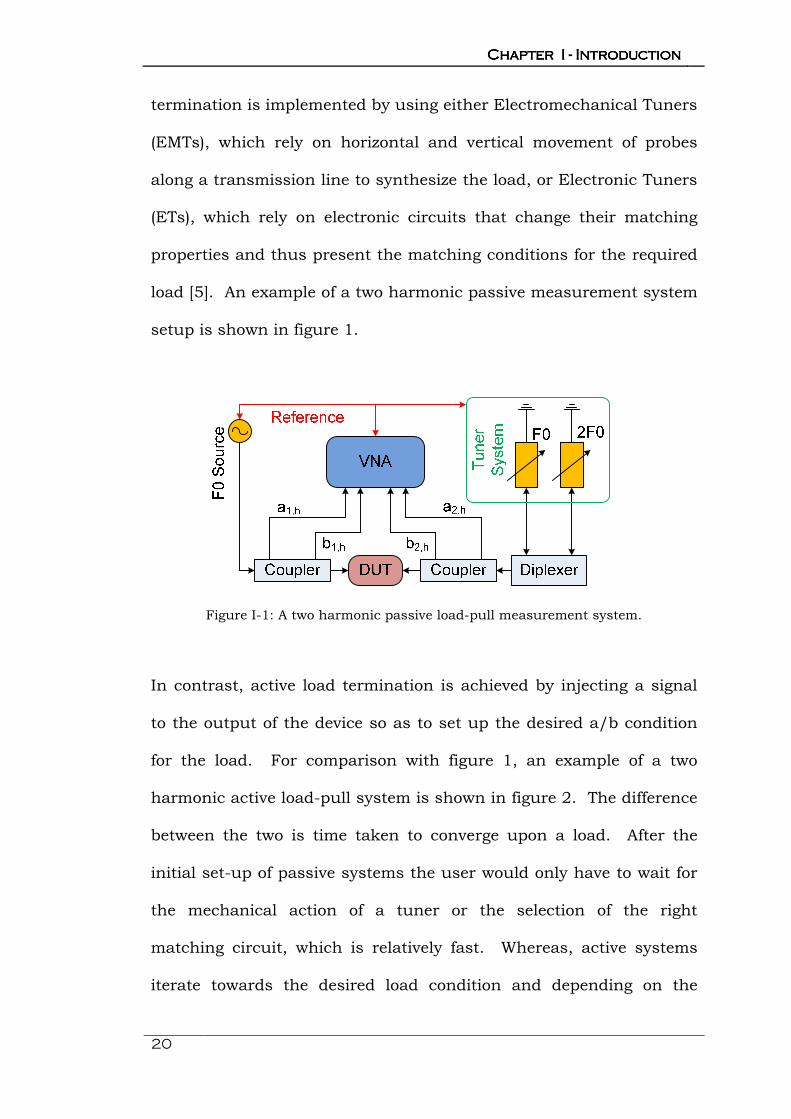
termination is implemented by using either Electromechanical Tuners
(EMTs), which rely on horizontal and vertical movement of probes
along a transmission line to synthesize the load, or Electronic Tuners
(ETs), which rely on electronic circuits that change their matching
properties and thus present the matching conditions for the required
load [5]. An example of a two harmonic passive measurement system
setup is shown in figure 1.
Figure I-1: A two harmonic passive load-pull measurement system.
In contrast, active load termination is achieved by injecting a signal
to the output of the device so as to set up the desired a/b condition
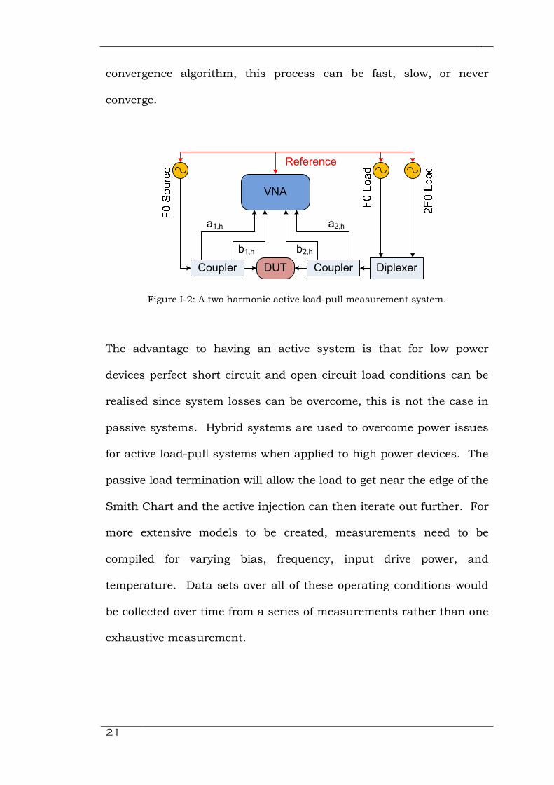
for the load. For comparison with figure 1, an example of a two
harmonic active load-pull system is shown in figure 2. The difference
between the two is time taken to converge upon a load. After the
initial set-up of passive systems the user would only have to wait for
the mechanical action of a tuner or the selection of the right
matching circuit, which is relatively fast. Whereas, active systems
iterate towards the desired load condition and depending on the
21
convergence algorithm, this process can be fast, slow, or never
converge.
DUT Diplexer
VNA
CouplerCoupler
a1,h a2,h
b1,h b2,h
Reference
Figure I-2: A two harmonic active load-pull measurement system.
The advantage to having an active system is that for low power
devices perfect short circuit and open circuit load conditions can be
realised since system losses can be overcome, this is not the case in
passive systems. Hybrid systems are used to overcome power issues
for active load-pull systems when applied to high power devices. The
passive load termination will allow the load to get near the edge of the
Smith Chart and the active injection can then iterate out further. For
more extensive models to be created, measurements need to be
compiled for varying bias, frequency, input drive power, and
temperature. Data sets over all of these operating conditions would
be collected over time from a series of measurements rather than one
exhaustive measurement.

Chapter I Chapter I Chapter I Chapter I ---- IntroductionIntroductionIntroductionIntroduction
22
1.3 COMPUTER AIDED DESIGN
CAD certainly has its place in the circuit design area of Radio
Frequency (RF) and microwave engineering. Increasing complexity of
the circuitry used to enable wireless communication over the years
necessitated the development of early circuit simulators. The first
available circuit simulator being the SPICE (Simulation Program with
Integrated Circuit Emphasis) package developed at the University of
California, Berkeley [6]. Since the seventies, the program has been
modified and transferred to a new programming language, however,
currently there are two more prolific microwave circuit simulators;
Agilent's Advanced Design System (ADS) [7] and AWR's Microwave
Office [8]. ADS and Microwave Office are competing simulation
platforms that offer linear and nonlinear circuit simulation Design
Rule Checking (DRC) and can import Process Design Kits (PDKs) from
foundries. They also offer Electromagnetic (EM) analysis, which can
be used to bolster results from circuit simulation for on wafer
amplifiers.
1.4 THESIS OBJECTIVE
The objective of this thesis is to develop the framework for input and
output harmonic behavioural modelling and provide the necessary
modifications to existing measurement systems and CAD
implementation solutions to enable an X-band measurement-to-CAD
cycle. The limits, applicability, and implications of input/output
23
mixing models should be analysed and discussed. The thesis should
also look to overcome exhaustive measurements by effectively
covering device impedance spaces of interest, for Class-B to Class-J
amplifiers, with source- and load-pull points therefore reducing the
time needed for the measurement of the input and output
behavioural models.
1.5 CHAPTER SUMMARY
This thesis details the analysis of input second harmonic behavioural
models in isolation and the mixing necessary for input and output
models up to the second harmonic. The measurement system and
CAD implementation improvements necessary for the measurement
and analysis of the models have been included. The following is a
chapter-by-chapter summary of the contents.
Chapter II presents a literature review of the behavioural modelling
techniques that have been employed in the past and present.
Specifically mentioned and discussed are: S-parameters, Volterra
Input Output MAP (VIOMP), hot S-parameters, X-parameters, and the
Cardiff Model.
Chapter III outlines the creation of a bespoke coherent carrier
distribution system; a necessary addition to the current High
Frequency (HF) measurement system in order to perform source- and
load-pull measurements.

Chapter I Chapter I Chapter I Chapter I ---- IntroductionIntroductionIntroductionIntroduction
24
Chapter IV details the improvements made to the CAD
implementation of the Cardiff Model. It shows how the
implementation was moved from a static power series equation
concerning two output harmonics to a dynamic CAD solution able to
manage any model measured over three harmonics on the input and
output.
Chapter V contains the analysis of the input second harmonic
models. The correct process for augmenting model formulations is
highlighted before isolating an input second harmonic source-pull
sweep and ascertaining its optimal coefficients in line with the
augmentation process. Input and output mixing models are then
examined for both input second harmonic and output fundamental
measurement source- and load-pull sweeps, and input and output
second harmonic source- and load-pull sweeps. Due to the large
number for coefficients that can arise from mixing models, the
methods for truncating model coefficients are discussed and
advantages highlighted. Finally, the design and measurement
implications resulting from performing input second harmonic
source-pull sweeps are discussed.
Chapter VI concludes the thesis work before offering interesting
suggestions for future efforts in this vein of transistor behavioural
modelling.

25
1.6 REFERENCES
[1] J. B. King and T. J. Brazil, "Equivalent Circuit GaN HEMT Model
Accounting for Gate-Lag and Drain-Lag Transient Effects," IEEE
Topical Conference on Power Amplifiers for Wireless and Radio
Applications (PAWR). Pg 93-96. Jan. 2012.
[2] J. Verspecht and D. E. Root, "Polyharmonic Distortion Modelling,"
IEEE Microwave Magazine, Volume 7. No. 3. Pg 44-57. Jun 2006.
[3] P. J. Tasker and J. Benedikt, "Waveform Inspired Models and the
Harmonic Balance Emulator," IEEE Microwave Magazine. Pg 38-42.
Apr 2011.
[4] H. Qi, J Benedikt and P. J. Tasker, "A Novel Approach for Effective
Import of Nonlinear Device Characteristics into CAD for Large
Signal Power Amplifier Design," IEEE MTT-S International
Microwave Symposium Digest. Pg 477-480. 2006.
[5] F. M. Ghannouchi and M. S. Hashmi, "Load-Pull Techniques with
Applications to Power Amplifier Design," Springer Series in
Advanced Microelectronics 32. Pg. 29-30. 2013. ISBN: 978-94-
007-4460-8
[6] L. W. Nagel and D. O. Paderson, "SPICE (Simulation Program with
Integrated Circuit Emphasis)," Memorandum No. ERL-M382,
University of California, Berkeley, Apr. 1973.
[7] Agilent Technologies, "Advanced Design System ADS Home page,"
Downloaded from: http://www.home.agilent.com/en/pc-1297113
/advanced-design-system-ads?nid=-34346.0&cc=GB&lc=eng

Chapter I Chapter I Chapter I Chapter I ---- IntroductionIntroductionIntroductionIntroduction
26
[8] AWR a National Instruments Company, "Microwave Office Home
page," Downloaded from: http://www.awrcorp.com/products/
microwave-office
Chapter II Chapter II Chapter II Chapter II ---- Literature ReviewLiterature ReviewLiterature ReviewLiterature Review
27
Chapter IIChapter IIChapter IIChapter II
Literature ReviewLiterature ReviewLiterature ReviewLiterature Review
athematical modelling of any system is a useful and long
term way to reduce the cost of, and perhaps eliminate,
experimental prototyping. Diminishing the need for prototyping is
attractive for small and large business alike, as employee time can be
better spent designing with simulators, and the costing for prototype
evolutions becomes unnecessary. It is therefore understandable that
there has been a push in the modelling area, to make models more
accurate, robust and integrate seamlessly with various CAD
packages. In the RF and Microwave industries there have been many
types of modelling that have been used, in the case of behavioural
models, a short list would surely contain the following approaches: S-
Parameters, Poly-Harmonic Distortion (PHD) modelling, X-Parameters
and S-Functions, and more recently, the Cardiff Model. This chapter
will address the aforementioned modelling approaches and assay
their qualities. Where appropriate, the paradigms mentioned above
M
28
will be dealt with together. This is because there is significant
overlap of theory, as early concepts spawned the later solutions.
2.1 S-PARAMETER MODELLING
S-parameters initially developed because of ambiguities arising from
the concept of impedance when applied to microwave circuits [1].
This occurred when the wavelength of the operating signal became
comparable to the size of the circuit components; hence
inconsistencies in scalar voltage and current could be seen in
sections of circuitry. This gave rise to the use of transmission line
theory applied to microwave circuits, hence the travelling a-b waves
and scattering coefficients, or S-parameters, were used.
2.1.1 S-Parameter Theory
Although S-parameters have been seen to be mentioned as far back
as the 1920’s it was not until the late 60’s that they were popularized.
This, in part, was due to Hewlett Packard (HP) releasing their
HP8410A Network Analyser (NA) which applied the S-parameter
theory from [2] in their Hewlett-Packard journal [3]. The theory in [2]
defines the scattering waves as follows:

Chapter II Chapter II Chapter II Chapter II ---- Literature ReviewLiterature ReviewLiterature ReviewLiterature Review
29
Where 'i' indicates the port index, (*) indicates the conjugate, and
Re(Zi) indicates the real component of the complex impedance Zi. The
ratio of the two scattering waves is then defined as the following:
Where subscripts 'ib' and 'ia' denote the respective 'b' and 'a' port
indices. This is for one port analysis and does not take into account
harmonic effects, however one must note that this work treats the
scattering a-b waves as being in the frequency domain, hence they
can have both port and harmonic indices when applied to non-linear
systems (e.g. ap,h). Extending these fundamentals in relation to a two
port network, the equation below can be written:
Equation 4 is an important result as it allows for two port
measurement analyses, whilst also being the backbone of early linear
and non-linear device modelling [4-5]. The work performed in [4]
(II-1 & 2) �� = ��+����2|��(��)| �� =
��−��∗��2|��(��)|
(II-3) ����� = ����
(II-4) ������ = ���� ������ ���� × ������

30
highlights the use of bias dependent small-signal S-parameters in
calculating equivalent circuit component values for a F.E.T device.
Whereas [5] extends the design techniques for use with small-signal
S-parameters to large-signal S-parameters and successfully utilizes
them in the design of a Class-C Ultra High Frequency (UHF) Power
Amplifier (PA). In the case of [5] it has to be noted that the selectivity
of the device's package parasitic network meant that the observed
waveforms were nearly sinusoidal in Class-C operation, hence had
negligible harmonic components, and could be considered reasonably
linear. Normally, the small conduction angle of Class-C amplifiers
results in an over-half-rectified output voltage waveform, which has
considerable harmonics. Although this is a specific case where large-
signal S-parameters have been used in amplifier design the methods
do not exactly translate to other amplifier modes. The two practices,
previously mentioned, were commonplace in amplifier and mixer
design and the use of the small-signal linear parameters in describing
systems in the seventies and eighties was abundant.
2.1.2 Measurement of S-Parameters
This will be discussed whilst only considering two port active devices,
as these are the types of systems that resemble transistors operated
as amplifiers or oscillators. These concepts can easily be extended to
multi-port systems, in fact many current VNAs provide for multi-port
S-parameter measurements.

Chapter II Chapter II Chapter II Chapter II ---- Literature ReviewLiterature ReviewLiterature ReviewLiterature Review
31
The forward and reverse VNA measurement scenarios are shown in
figures 1 and 2. The forward measurement should be performed with
matched source and load impedances to ensure there is no reflection
a2 from the terminated port 2. Using this measurement S11 and S21
can be computed using the following formulas:
Figure II-1: A 2-port forward VNA measurement on a DUT.
The reverse measurement should also be performed with matched
source and load impedances, this time, to ensure that there is no
reflection a1 from the terminated port 1. This measurement enables
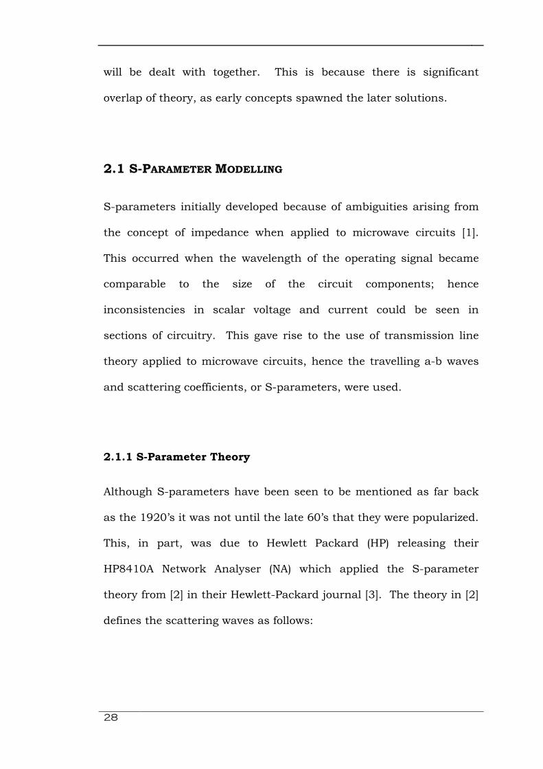
S22 and S12 to be computed by the use of the following:
��� = ������� !" ��� = ������� !" (II-5 & 6)
32
Figure II-2: A 2-port reverse VNA measurement on a DUT.
Usual S-parameter measurements are small-signal, bias dependent
and swept over frequency. Since the measurements alone get the
required quantities for the aforementioned quotients there is no need
for a further extraction process.
2.1.3 S-Parameter Discussion
The S-parameter modelling approach certainly has its advantages
with respect to linear systems and in some specific ways can be used
with non-linear devices. However, S-parameters are formulaically
linear and despite certain modifications and extrapolations there is
��� = �������#!" ���,% = �������#!" (II-7 & 8)

Chapter II Chapter II Chapter II Chapter II ---- Literature ReviewLiterature ReviewLiterature ReviewLiterature Review
33
no getting away from this fact. Harrop and Claasen [4] show the
usefulness of S-parameters when attempting to extract an equivalent
circuit model, however there were still some non-linear components
left un-described and the effort made by Leighton et al. [5], with large
signal S-parameters showed their selectivity to applications, hence
their significant limitations as a non-linear modelling solution. With
that said, the modelling community sought to rectify behavioural
modelling issues in the nineties by introducing the Hot S-parameter,
PHD and X-parameter concepts, but before addressing these
solutions the VIOMAP concept needs to be introduced [6-9].
2.2 VOLTERRA INPUT OUTPUT MAP MODELLING (VIOMAP)
The VIOMAP provides an extension to S-parameters for use with
weakly nonlinear RF and microwave devices, as seen in [6]. It deals
with nonlinearities in terms of signal harmonic mixing in relation to
the chosen, or observed, degree of system nonlinearity. Previous
work has shown that VIOMAPs can be measured like S-parameters,
are able to predict the behaviour of cascaded systems [6], can be
used to enhance prediction of spectral regrowth and predistortion [7],
can be used to reduce conventional load-pull time and predict gain
contours over the whole Smith Chart [8], and by substituting
VIOMAPs for orthogonal polynomials the concept can be applied to
stronger device nonlinearities [9].

34
2.2.1 VIOMAP Theory
[6-9] consider the Device Under Test (DUT) from a black-box
perspective where the system responses bp,h are a product of its
inputs ap,h and the systems transfer function H, as displayed in figure
3. The 'a' and 'b' quantities have subscripts denoting port and
harmonic index respectively.
Figure II-3: A two-port device and system representation. H represents the
system's transfer function and subscripts h represents harmonic index.
The system transfer function 'H', termed VIOMAP kernel in [6], is
defined as: Hn,ji1,i2...in(f1,f2,...,fn) related to a fundamental frequency f0,
where j is the input port, 'i' is the output port and 'n' is the nth degree
of system nonlinearity. Here 'H' has the argument of frequency.
Hence the output is a summation of all relevant products of 'H' and
'a' with respect to harmonic frequency. Although the VIOMAP
transfer function 'H' is a lot like the S-matrix in equation 4 it is not
DUT
(H)
a1,h
b2,h b1,h
a2,h

Chapter II Chapter II Chapter II Chapter II ---- Literature ReviewLiterature ReviewLiterature ReviewLiterature Review
35
limited to two terms. Verbeyst an Bossche [6] make the observation
that when a system is linear the first order VIOMAP kernel is the
same as S-parameters, notwithstanding the difference in notation.
The VIOMAP solutions all use Volterra theory; however, none of the
papers detail the inner workings of the models and the generation of
the polynomials. The underlying time-domain Volterra theory will
now be covered. Starting with the Volterra series of Nth degree:
If Hn(t1,...,tn) = anδ(t1)δ(t2)...δ(tn), the power series would be obtained:
The VIOMAP solution is obtained when the chosen order of
polynomial N is large enough that the polynomial approximates the
nonlinear system. The difference between the above equations and
the ones that would be employed in [6-9] is that they operate in the
time domain and the measured travelling waves have arguments of
frequency. The formulation examples in [6-9] clearly show the
&(') = ��((') + ��((')� +⋯+�*((')*
…((' − ,-).,�….,-
&(') = / 0 1(,�, … , ,-)((' − ,�)2
32
*
-!�…
(II-9)
(II-10)

36
Volterra series summation of signal component powers, mirroring the
process in equation 10.
2.2.2 Measurement of VIOMAPs
The measurement scenarios in [6-9] detail different measurement
equipment configurations; this is due to measurement being tailored
to the specific modelling application and the apparent lack of
equipment. The measurement solution in [8] represents a load-pull
system, which is the same as approaches that will be presented later
on in this chapter, so it shall be used as an example of the type of
measurement setup necessary for VIOMAP measurement. The
determination of a two port device's VIOMAP requires measurements
that exercise the device the desired impedances, e.g. load-pull.
Fundamental output load-pull behaviour is being explored in [8],
hence a measurement system is required that can stimulate a DUT at
both input and output ports simultaneously at the fundamental
frequency. In their case a single source is used to achieve phase
coherence, however, the same can be achieved with active load-pull
measurement systems that use two phase coherent sources.
The measurement system in Figure 4 [8] is based around the
HP8510B Network Analyzer [10] and a HP8515A [11] S-parameter
test set. The measurement sequence for load-pull was not rigorous.

Chapter II Chapter II Chapter II Chapter II ---- Literature ReviewLiterature ReviewLiterature ReviewLiterature Review
37
The model was calculated from a set of 100 impedance points
acquired over a range of powers from -7dBm to 8dBm. Each time the
power level was changed the variable attenuator and line stretcher,
governing the position of the load impedance, were set randomly a
few times.
Figure II-4: The block diagram of the measurement setup for fundamental load-pull
and VIOMAP determination [8].
A VIOMAP was extracted from the measurements that required a 5th
order polynomial to describe the distortion of the output fundamental
tone as a function of the separate input powers at port 1 and port 2.
Another 3rd order polynomial was also required to describe the

38
distortion of the output fundamental tone as a function of a
combination of the input powers at ports 1 and 2 [6]. The model
comprised of 10 coefficients and was sufficient to model the load-pull
measurement data, with modelled and measured power plots differing
within 0.2dB.
2.2.4 VIOMAP Discussion
The VIOMAP solutions proved promising. However, they were not
widely accepted in the RF and microwave design community as a
valid solution to the modelling problem. This is possibly because,
although theoretically sound, there were issues with the
understanding of the selection of the VIOMAP polynomials, as this
was not intricately detailed. Also, the practicalities of the advanced
extraction procedures are questionable. Furthermore, despite the
sound theory [12], there were problems with the overly complicated
computation necessary for the orthogonal polynomial approach [9],
which was necessary for characterization of devices operated in their
strongly non-linear regions. The approach, however, does have a lot
of similarities with the Hot S-parameter, X-parameter, and Cardiff
Model approaches, notwithstanding the fact that these approaches
are formulaically simpler and this may explain why they are perhaps
more favourable to the measurement-design scenarios of today.

Chapter II Chapter II Chapter II Chapter II ---- Literature ReviewLiterature ReviewLiterature ReviewLiterature Review
39
2.3 HOT S-PARAMETER MODELLING
Hot S-parameters, also known as large-signal S-parameters, allow for
a black-box frequency domain behavioural model that protects
intellectual property. The technique is derived from S-parameters;
however, the S-parameter type measurements are performed when
the device is being actively stimulated.
2.3.1 Hot S-Parameter Theory
The work in [13] quite nicely surveys the hot S-parameter works of
the time. It shows how hot S-parameters were applied to predicting
stability and distortion. The two applications use a variant of the S-
parameter matrix equation in section 1:
The difference in the above equation is that the scattering wave
quantities 'a' and 'b' have the argument of frequency. The frequency
subscript 's/c' is meant to deal with the stability and distortion
variants of equation 11, which have exactly the same formulation.
The equation only containing subscript 's' is used for stability
calculations, as this is the frequency at which the hot S-parameter
4��567/9:��567/9:; = �ℎ='��� ℎ='���ℎ='��� ℎ='���� 4��567/9:��567/9:; (II-11)

40
stability measurements are being performed. In [14] the argument of
frequency (fS) is swept from 300MHz to F0/2, where F0 is the
fundamental frequency that a11 is set to. This changes equation 11
to that of a conversion matrix [14]:
In equation 12 the [S] matrix contains the hot small signal S-
parameters and relates the [a] and [b] matrices at the frequencies
(KF0 ± fS) at each of the swept perturbation frequencies fS, where K is
the harmonic multiplier. If it is assumed, for a system with fixed
drive and bias levels, that there are known constant terminations at
the F0 and (KF0 ± fS) frequencies it is possible to concentrate on the
input and output probing waves at the swept frequencies fS and the
equation reduces again to that shown in equation 11. Stability
assessments are undertaken in the same way as with S-parameters
>????????@��∗(AB" − 67)⋮��(67)⋮��(AB" + 67)��∗(AB" − 67)⋮��(67)⋮��(AB" − 67)D
EEEEEEEEF
= G�H
>????????@��∗(AB" − 67)⋮��(67)⋮��(AB" + 67)��∗(AB" − 67)⋮��(67)⋮��(AB" − 67)D
EEEEEEEEF
(II-12)
Chapter II Chapter II Chapter II Chapter II ---- Literature ReviewLiterature ReviewLiterature ReviewLiterature Review
41
and are centred around the calculation of the relevant 'hot' stability
parameter(s).
The subscript 'c', in equation 11, applies when it is concerning the
prediction of system distortion characteristics. In this variant, the
energy of the system is only expected in the fundamental frequency
and harmonic signal components, therefore the interaction between
the a-b scattering waves can be viewed in the limited frequency set
defined by k.fC, where k is a positive integer that reflects the
harmonic number. This can be done because there are a few
assumptions that are taken into account: the application is for
narrowband use, hence the input signal is thought of as a one-tone
carrier that can be modulated by a frequency less than the carrier
frequency; the DUT is being operated at near matched conditions,
consequently, signal energy is expected at the fundamental and
harmonic frequencies only.
The different subscripts for frequency in equation 9 naturally
highlight, in view of a priori assumptions, differences in the
equation's relation to a1. The incident a1(fS) is linear and the incident
a1(fC) is non-linear, however, both variations of equation 9 are linear
with respect to a2. The work in [15] shows, for hotS22, that equation
11 is really a basic functional description of a device's nonlinearity. It

42
details, through the use of “smiley faces”, the impact of hot S-
parameters, extended hotS22 and quadratic hotS22. The importance
of the work concerns the phase relationship between a1 and a2 or 'P',
as it is termed in [15], because this is the term that provides the
necessary deformation to the “smiley face” and results in better
agreement between measurements and model.
In equation 13 the ah and bh matrices are functions of harmonic
frequency fC and the hot S-parameters are the same as before. The
'T' matrix consists of model coefficients that relate to the conjugate of
the output perturbation a2(fC), hence why they are output only 'T'
terms. As such, equation 13 is the extended hot S-parameter
equation from [13], where the exponential part equates to the
constant 'P' in [15], the phase difference between a1 and a2. The
addition of the 'T' terms and their association with a2 is because at
higher degrees of nonlinearity the phase difference between a11 and a2
becomes important to the accuracy of the model. The interpretation
of the 'T' terms, suggested in [13], is usually problematic but can be
looked at in terms of stability hot S-parameters. If equation 11 is
considered and the probing measurement frequency fS is allowed to
���(69)��(69)� = �ℎ='��� ℎ='���ℎ='��� ℎ='���� ���(69)��(69)�
+ �I��I��� �J�K5�#(LM):N=OP(��(69))(II-13)
Chapter II Chapter II Chapter II Chapter II ---- Literature ReviewLiterature ReviewLiterature ReviewLiterature Review
43
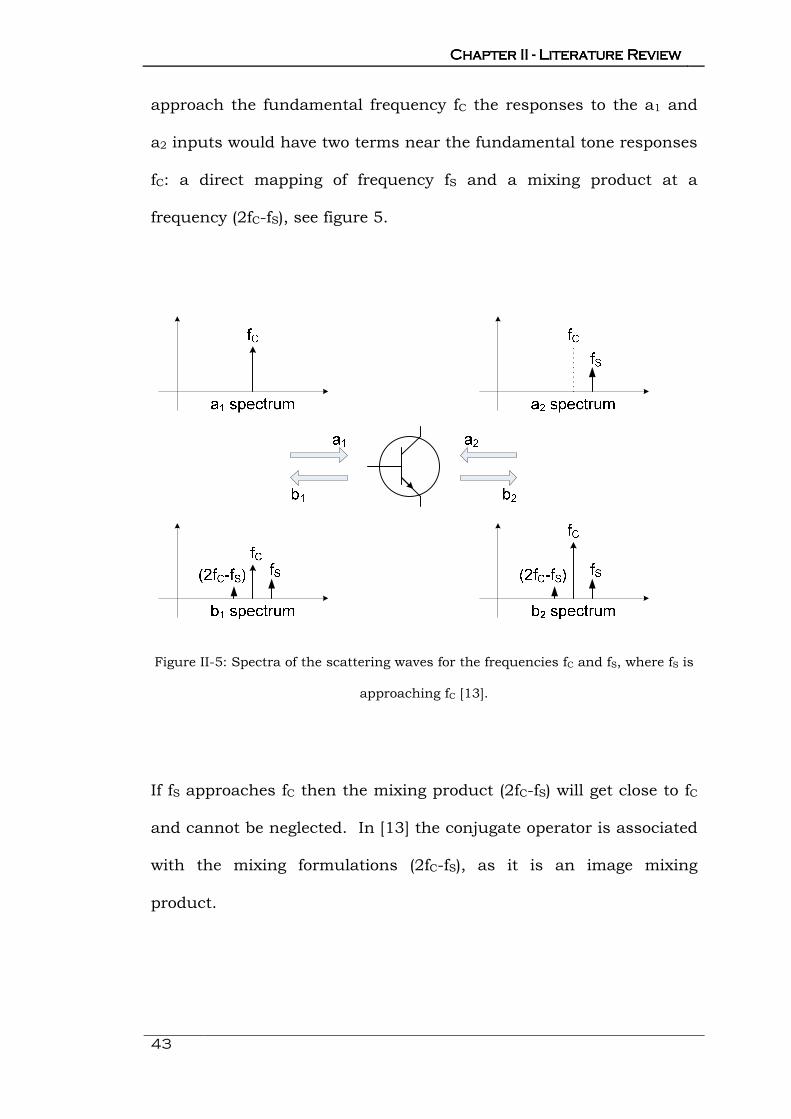
approach the fundamental frequency fC the responses to the a1 and
a2 inputs would have two terms near the fundamental tone responses
fC: a direct mapping of frequency fS and a mixing product at a
frequency (2fC-fS), see figure 5.
Figure II-5: Spectra of the scattering waves for the frequencies fC and fS, where fS is
approaching fC [13].
If fS approaches fC then the mixing product (2fC-fS) will get close to fC
and cannot be neglected. In [13] the conjugate operator is associated
with the mixing formulations (2fC-fS), as it is an image mixing
product.
44
2.3.2 Measurement of Hot S-Parameters
The measurement of these parameters depends on the application. If
the hot S-parameters are being used for stability measurements there
is one scenario and if they are being used for non-linear
characterisation there is another scenario. The difference mainly
relies on the necessary assumptions. For stability measurements the
probe frequency 'f' can be swept as shown in [14] and is usually
much lower than the drive frequency F0 and since stability is being
investigated at the lower frequency the mixing products (KF0 ± f) are
not considered. For predicting a device's distortion characteristics,
the assumptions allow for the probe frequency to be at the
fundamental or a harmonic frequency (F0 or k.F0).
Figure 6 shows a block diagram of a measurement system setup that
would be required to extract hot S-parameters. It shows that, for a
correctly biased device, an input drive is applied to the DUT at a
frequency F0 the output tuner would then converge on a suitable load
(e.g. near the device's optimum power point) before the second
source, at a lower frequency 'f', switches between sending its probing
S-parameter measurement tones in the forward and reverse
directions. The forward measurement obtains hotS11 and hotS21 and
the reverse measurement obtains hotS12 and hotS22. The extraction
of the stability hot S-parameters is the same as the one necessary for

Chapter II Chapter II Chapter II Chapter II ---- Literature ReviewLiterature ReviewLiterature ReviewLiterature Review
45
S-parameters, hence the appropriate travelling wave quotients are
used.
Figure II-6: Measurement system block diagram [14].
2.3.3 Hot S-Parameter Discussion
There are various types of hot S-parameter and the application is the
main driver behind what type is used. The measurement procedure
is, understandably, different in comparison to the standard S-
parameter or the VIOMAP approaches. With regards to
measurements, the user must be aware of the necessary assumptions
that accompany the type of hot S-parameter before deciding upon the
setup. In general, the measurement setups are more complicated

46
than the other modelling approaches; hence, they require more
equipment and can cost more. The formulaic structure and
augmentations to it can be seen in the X-parameter and Cardiff
model solutions that follow, so it was definitely a step in the right
direction. It was the growth in popularity of X-parameters that
probably saw diminishing usage of hot S-parameters, as the
measurement setup was easier (with Agilent's PNA-X) and the model
structure was rigid, as there were three terms that needed to be
extracted for the model.
2.4 X-PARAMETER MODELLING
This school of thought will be treated alone, rather than with the S-
function paradigm, as there are great similarities between the two in
the model measurement, extraction, and only small differences in
model formulation. In practice though, X-parameters, having been
backed by Agilent Technologies, are more widespread and used more
often in the RF and Microwave industry. It is by virtue of this that X-
parameters will be the paradigm analysed and discussed in this
section.
Chapter II Chapter II Chapter II Chapter II ---- Literature ReviewLiterature ReviewLiterature ReviewLiterature Review
47
2.4.1 X-Parameter Theory
X-parameters are a superset of S-parameters and the modelling
process, like the hot S-parameter approach, is a frequency domain
black-box behavioural modelling concept. X-parameters are based on
the Poly-Harmonic Distortion work in [16-17], where, for the case
where a system is stimulated by an A1,1 and all the generated
harmonics are small in comparison to that A1,1, the harmonic
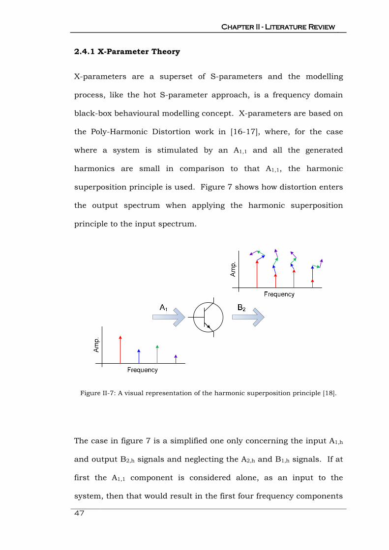
superposition principle is used. Figure 7 shows how distortion enters
the output spectrum when applying the harmonic superposition
principle to the input spectrum.
Figure II-7: A visual representation of the harmonic superposition principle [18].
The case in figure 7 is a simplified one only concerning the input A1,h
and output B2,h signals and neglecting the A2,h and B1,h signals. If at
first the A1,1 component is considered alone, as an input to the
system, then that would result in the first four frequency components
48
of B2,h. Then the second A1,h component can be considered and this
would result in the first summation/deviation to the output B2,h
spectrum. It follows then that the third and fourth A1,h components
(A1,3 and A1,4 respectively) result in the third and fourth
summations/deviations to the output B2,h spectrum. As stated in
[17] "the harmonic superposition principle holds when the overall
deviation of the output spectrum B2 is the superposition of all
individual deviations." It should be noted that the experimental
verification of the principle in [19] holds true for the practical
amplifier modes. The harmonic superposition principle utilised in the
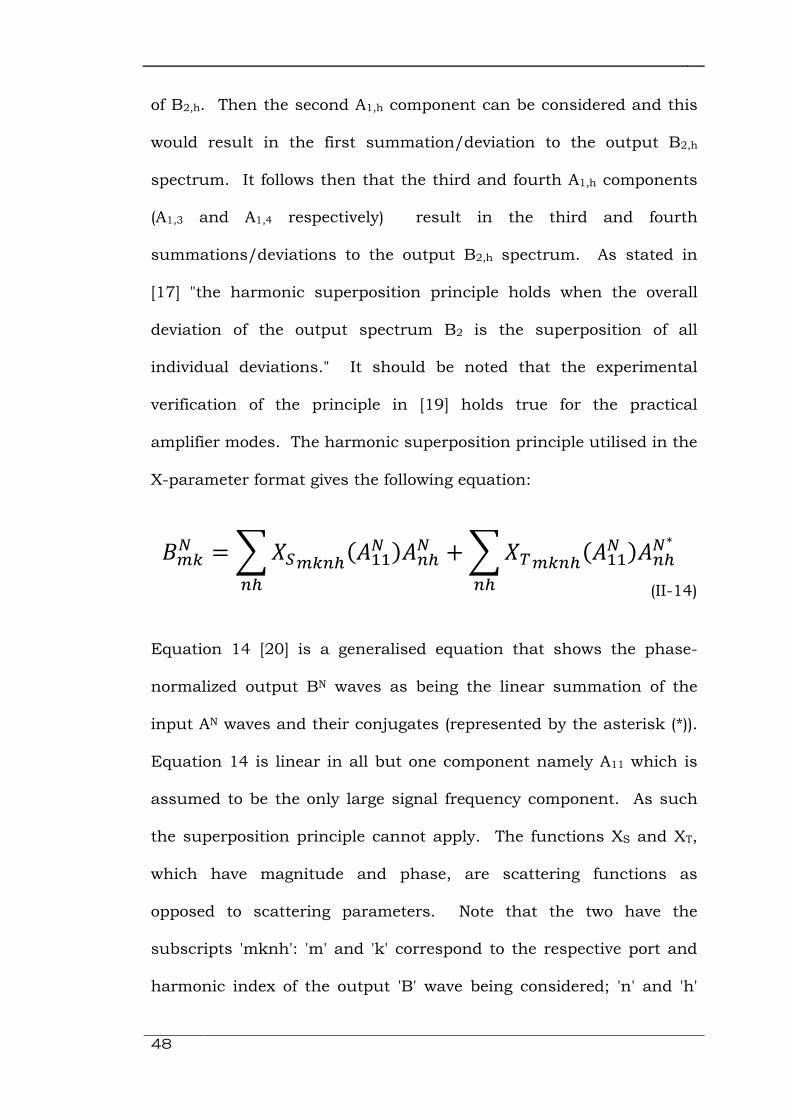
X-parameter format gives the following equation:
Equation 14 [20] is a generalised equation that shows the phase-
normalized output BN waves as being the linear summation of the
input AN waves and their conjugates (represented by the asterisk (*)).
Equation 14 is linear in all but one component namely A11 which is
assumed to be the only large signal frequency component. As such
the superposition principle cannot apply. The functions XS and XT,
which have magnitude and phase, are scattering functions as
opposed to scattering parameters. Note that the two have the
subscripts 'mknh': 'm' and 'k' correspond to the respective port and
harmonic index of the output 'B' wave being considered; 'n' and 'h'
QRS* =/TURS-%(V��* )V-%* +/TWRS-%(V��* )V-%*∗
-%-%
(II-14)

Chapter II Chapter II Chapter II Chapter II ---- Literature ReviewLiterature ReviewLiterature ReviewLiterature Review
49
correspond to the respective port and harmonic index of the input 'A'
wave being considered. By virtue of this notation, the scattering
functions allow for multi-harmonic interactions to be characterised.
For example the effects of the input second harmonic A12 on the
output B21 component can be characterised as well as any manor of
relevant combinations, as long as the system is stimulated with the
correct Aph signals. A more practical case, concerning more familiar
scattering quantities, would be to observe the changes in B21 (output
fundamental component) as a function of A11 (input fundamental
drive) and A21 (output reflected fundamental). In this case the
general equation 14 becomes more specific:
Equation 15 provides a case that would be needed by most amplifier
designers, because it concerns the output of a system, B21, in
response to an input A11 and A21 (i.e. fundamental load-pull). Note
that the product XS2111A11 is often termed XF21. It is a distinct
element because it is the term that deals with the large-signal A11
that is outside the harmonic superposition principle. It should be
clear that to be able to do any analysis on B21 at least three
quantities must be known:
Q�� = TU����(|V��|) + TU����(|V��|)V��+ TW����(|V��|)X�N=OP(V��)
(II-15)

50
This requires that at least three measurements be made so as to have
sufficient data to extract the three quantities.
2.4.2 Measurement of X-Parameters
There are two ways of obtaining X-parameter models. The first, that
will be discussed, is the 'on-frequency' method. The second is the
'off-frequency' method. The principles in both techniques are the
same.
The 'On-Frequency' Method:
Figure II-8: Simple diagram of the parameter extraction procedure [17].
1.TU����(|V��|)V��//T[��(|V��|)V��
2.TU����(|V��|)V��
3.TW����(|V��|)X�N=OP(V��)
Chapter II Chapter II Chapter II Chapter II ---- Literature ReviewLiterature ReviewLiterature ReviewLiterature Review
51
To extract the necessary parameters in equation 14 the basic set of
three measurements that need to be performed are shown in figure 8.
Firstly, an A11 signal is applied and kept constant for the rest of the
measurement (shown as the square in figure 8). This initial condition
allows for the extraction of the XS2111(|A11|)A11 term. The next step is
to perform two independent orthogonal perturbations of the term A21.
This is done by applying an A21 signal with θ° phase then applying an
A21 with a (θ±90)° phase (represented by the star and triangle
respectively in figure 8). These last two measurements allow for the
extraction of the XS2121(|A11|) and XT2121(|A11|)P2 terms. A typical
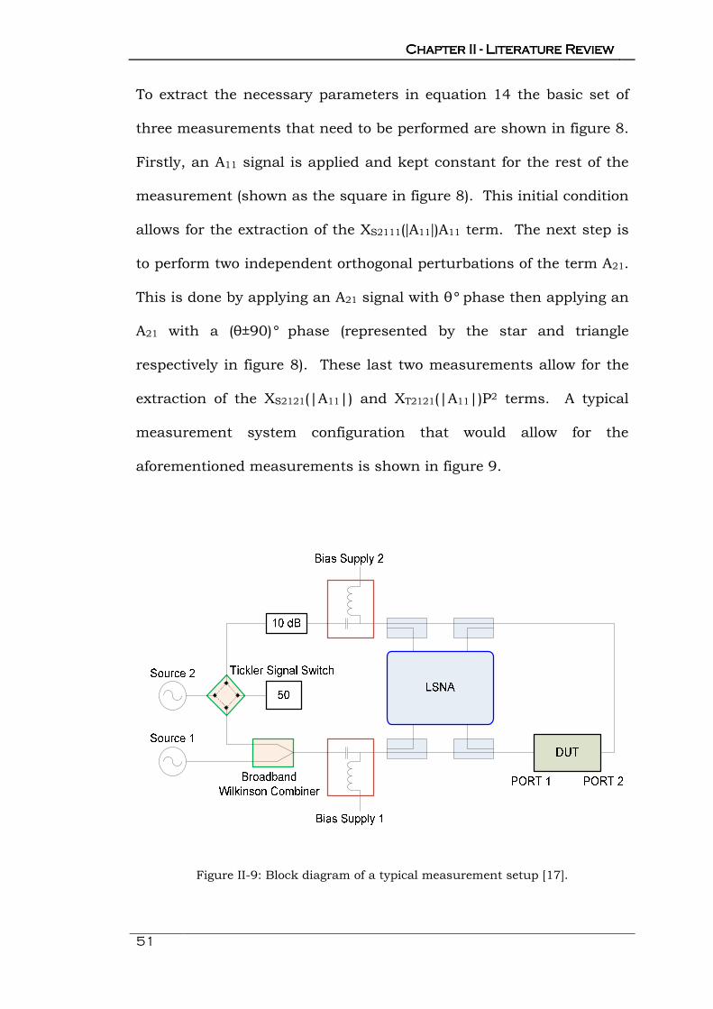
measurement system configuration that would allow for the
aforementioned measurements is shown in figure 9.
Figure II-9: Block diagram of a typical measurement setup [17].

52
In figure 9, source 1 is used for the generation of the large-signal A11
and source 2, combined with a switch, is used for the generation of
the small-signal Aph orthogonal tones, termed 'tickler signals' in [17].
An interesting point with the set of measurements is that, although
the minimum number of measurements is three, if a multitude of
measurements are performed the redundancy gained presents
opportunities in terms of system characterisation and, from this
redundancy, data can be collected on noise and model errors [17].
The drawback of the above scenario is that the measurements are
based around matched impedances. Therefore, the ability to
characterize the whole Smith Chart is entirely reliant on the
extrapolation capabilities of the localized model measured in a
50Ohm environment. This would put unnecessary strain on the
extrapolation capabilities of a model that is best used for
interpolation. Moreover, because deviating from a match can cause
large variations in a21, it would not be small when compared to a11;
hence, the harmonic superposition principle would not hold. This
violation of the harmonic superposition principle should provide
erroneous responses. The work in [19] recognises that most high
power devices have optimal performances far from 50Ohm.
Furthermore, it is asserted that the acquisition of X-parameters over
a large area of the Smith Chart is a necessity for the model to remain
Chapter II Chapter II Chapter II Chapter II ---- Literature ReviewLiterature ReviewLiterature ReviewLiterature Review
53
valid over the range of impedances it would meet in design
applications.
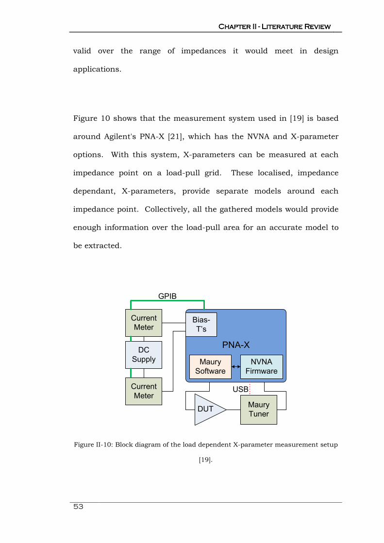
Figure 10 shows that the measurement system used in [19] is based
around Agilent's PNA-X [21], which has the NVNA and X-parameter
options. With this system, X-parameters can be measured at each
impedance point on a load-pull grid. These localised, impedance
dependant, X-parameters, provide separate models around each
impedance point. Collectively, all the gathered models would provide
enough information over the load-pull area for an accurate model to
be extracted.
DUTMaury
Tuner
PNA-X
Maury
Software
NVNA
Firmware
USB
Current
Meter
DC
Supply
Bias-
T’s
Current
Meter
GPIB
Figure II-10: Block diagram of the load dependent X-parameter measurement setup
[19].
54
The 'Off-Frequency' Method:
This method is in principle the same as the 'on frequency' method.
However, the generation of the orthogonal 'tickler signals' is achieved
differently. They are generated by injecting a perturbation at a
frequency offset to the fundamental A11 drive frequency. This can be
compared to the measurements performed to obtain hot S-
parameters. There is an issue of increased hardware and
complication of measurement approach needed to perform the off-
frequency measurement, which is why some might prefer the on-
frequency method.
2.4.3 X-Parameters Discussion
X-parameters are currently the most prolific behavioural modelling
parameters being used. By virtue of their development being 'in-
house' at Agilent, their operation and form are composed with ADS's
Harmonic Balance (HB) simulator in mind. When this is coupled
with Agilent's hardware, PNA-X, the user has a complete
measurement to simulation-design path. Perhaps at first this is
attractive for industry. However, there will always be pitfalls when
you try and make a whole industry buy your measurement solution if
they want to measure X-parameters.

Chapter II Chapter II Chapter II Chapter II ---- Literature ReviewLiterature ReviewLiterature ReviewLiterature Review
55
The model itself has been shown to characterize load-pull data [19],
incorporate long-term memory effects [22], and be used predict
broad-band responses [23]. In terms of equation complexity,
however, it is limited to three parameters XF, XS, and XT; solutions to
which are converged upon with linear regression techniques. These
equate to the Sph and Tph terms in equation 13 in section 2.3.1 about
hot S-parameters. The issue with having a rigid formulaic structure
is that it is inflexible when presented with increasing degrees of
nonlinearity. The observed gains in model accuracy with the hot S-
parameter approach when quadratic terms were added are not
available to the rigid X-parameter structure. It is supposed that this
can be solved by increasing the density of measurement points, to
take the strain off the X-parameter formulation by having load points
situated inside the interpolation region of a local X-parameter model.
Although, this solution is flawed, due to the fact that more measured
impedance points means more impedance-dependent X-parameters
yielding a larger X-parameter data file. Admittedly, ADS handles
large X-parameter data files well. However, current trends in
measurement and design have been focusing on output fundamental
and second harmonic load terminations. When the measurement
and design community want models over more power, bias, and
frequency levels accompanied with more harmonic data, the file sizes
would become too great for most desk-top PC's to cope with any type
of simulation. This file size problem is inherent for all potential
modelling solutions. However, behavioural model formulations allow

56
for efficient measurement data compression and X-parameters only
go part of the way.
2.5 THE CARDIFF MODEL
Over the past several years, the Cardiff Model has undergone a
metamorphosis. It began as a Direct Wave Look-Up Table (DWLUT)
approach ("truth look-up model" [24]) and changed to a polynomial
based behavioural model. The DWLUT was created to allow for quick
access to measurement data in CAD. However, the accepted pitfalls
of the DWLUT approach were overcome with an equation based
descriptive behavioural model approach. Both approaches are
detailed by Qi in [24]. This section will look at the two approaches
separately, beginning with the DWLUT approach.
2.5.1 The Cardiff DWLUT Model Theory
The Cardiff DWLT model is table based and utilises admittance, as a
function of the operating conditions, to relate a device's extrinsic
measured port currents and voltages. Below is a simplistic block
diagram from the systems perspective.

Chapter II Chapter II Chapter II Chapter II ---- Literature ReviewLiterature ReviewLiterature ReviewLiterature Review
57
Figure II-10: DWLUT system.
In figure 10 the port currents I1(ω) and I2(ω) are treated as the
responses of the system caused by the application of the voltages
V1(ω) and V2(ω). An and Bn are the systems port 1 and port 2 transfer
functions, respectively. The different port currents and voltages at
specific load impedances ZLOAD are related by equations containing An
and Bn [25]:
Where VIN is the input voltage signal, 'n' is the harmonic number, f0 is
the fundamental frequency, and A0 and B0 are the DC components.
The current and voltage spectra are functions of the many operating
��(]) = Q" ∙ _(]) +/Q- ∙ �̀*- ∙ _(] − 2a ∙ O ∙ 6")R
-!�
��(]) = V" ∙ _(]) +/V- ∙ �̀*- ∙ _(] − 2a ∙ O ∙ 6")R
-!�
(II-16)
(II-17)
58
conditions, hence so too are An and Bn. With the former being
considered the following are obtained:
Equations 18 and 19 [25] are thus using the input and output port
admittances to relate the currents and voltages at those ports. The
above equations equate An and Bn to functions with the arguments of
input drive voltage, load reflection coefficient, and the input and
output bias conditions. This modelling process makes use of the port
current and voltages because the resulting An and Bn models fit the
measurement data irrespective of whether the scattering a-b waves or
the currents and voltages are used. The advantage to using the I-V
waves becomes apparent when the model data is transported to CAD,
namely Agilent's ADS [26]. Here the implementation uses a
Frequency Defined Device (FDD) as the 'go-between' for the DWLUT
and the simulation circuit. Since this component directly computes
with current and voltage, the initial decision to work with them
makes the CAD implementation easier.
Q- = ��(O6")�̀*- (O6") = B�(|�̀*|, bcdef , �fg`* , �fgdhW)
V- = ��(O6")�̀*- (O6") = B�(|�̀*|, bcdef , �fg`* , �fgdhW)
(II-18)
(II-19)

Chapter II Chapter II Chapter II Chapter II ---- Literature ReviewLiterature ReviewLiterature ReviewLiterature Review
59
2.5.2 Measurement of the DWLUTs
Reference [24] concentrates on fundamental load-pull measurements
over a range of swept power levels. Figure 11 shows the
measurement system, developed by Benedikt et al [27] at Cardiff
University, which was used to perform the measurements.
In figure 11, the use of switches 'A' and 'B' are to overcome the
problem of a two channel Microwave Transition Analyser (MTA) [28]
needing to behave like a four channel instrument in order to perform
the measurements. In this configuration, channel 1 would measure
the incident travelling waves, a1 and a2, and channel two would
measure the reflected travelling waves, b1 and b2. In relation to the
figure: switch 'A' handles a1 and a2 and switch 'B' handles b1 and b2.
The problem with this is that there can be a loss of synchronisation
between the travelling waves. A systematic switching strategy and a
phase handover measurement solves the synchronisation problem
and allows for the travelling waves to be correctly measured.
Figure 11 shows that active load-pull is used to present the desired
impedance environment to the DUT. Unlike passive load-pull, active
load-pull utilises convergence algorithms to iteratively converge upon
the desired reflection coefficient. Once the error tolerance between
desired load and actual load is small enough the system will measure

60
and store the travelling waves. Providing that the load-pull grid is
sufficiently dense, travelling waves for each load-pull point on the
grid can be collected, without raising concerns of poor interpolation
within the CAD environment. The data table can be expanded when
uniform load-pull measurements are done at varying power levels.
Figure II-11: Block diagram of the Cardiff waveform measurement system [27].
The extraction of the parameters is virtually nonexistent, since the
travelling waves are used to compute the currents and voltages which
are then substituted in the ratios of equations 15 and 16 to obtain
the relative An and Bn admittance quantities. This process halves the
amount of data contained when compared with the measurement file,
as one value of admittance is stored to represent an I-V pairing.

Chapter II Chapter II Chapter II Chapter II ---- Literature ReviewLiterature ReviewLiterature ReviewLiterature Review
61
2.5.3 DWLUT Discussion
The main aim of the DWLT approach was to enable the import of
load-pull measurement data into the CAD environment for
simulation. From this perspective it was very successful. It fails as
an overall modelling solution because it does not generate a
relationship between a device's inputs and outputs. The approach
handles one measurement at a time as a look-up parameter,
therefore does not compress the measurement data much, and does
not aim to describe the system response as a whole. It also does not
have any native interpolation or extrapolation capabilities and for this
it relies on CAD and its mathematical ability to compute unknown
quantities within-grid data points (interpolation) and beyond-grid
data points (extrapolation). It is shown in [25] that CAD has the
ability to accurately interpolate between measurement points,
providing that the data points are not too sparsely situated.
Extrapolation is not as good. The fundamental extrapolation holds
under a 1% error when a data point is chosen just outside the
measurement grid. However, when the load is pushed further away
from the measurement grid larger discrepancies in the DC
components are generally observed and harmonic errors quickly
exceed 10% [25].

62
2.5.4 The Cardiff Behavioural Model Theory
The earliest work in this area was performed by Qi [24]. The DWLUT
model had proved useful as a tool for observing load-pull data in the
CAD environment, however, the DWLUT approach does not yield a
relationship between the input and output characteristics.
In [24] there is analysis of the PHD model [16-17], mentioned earlier.
As a model formulation the PHD model is good, but it relies on the
harmonic superposition principle. In examples where a device is
terminated with a 50Ohm impedance, the harmonic superposition
principle holds. However, in [25] the models are necessary for
characterizing load-pull data from high power devices. Since
optimum power, gain, and efficiency impedance points are usually
located far from 50Ohm and involve large variation in a2 the
harmonic superposition principle does not hold.
The work in [24] links the DWLUT work with its provision of the
necessary extension to the poly-harmonic distortion work, in [16], no
longer limited by the superposition principle to allow for large
variations in a2. The polynomial formulation deals with the travelling
waves as opposed to the port currents and voltages considered in the
DWLT approach. It treats the responses, b waves, as functions of a1
and a2:

Chapter II Chapter II Chapter II Chapter II ---- Literature ReviewLiterature ReviewLiterature ReviewLiterature Review
63
The functions, f( ) and g( ), are then distributed between their
arguments to present the assumption that if bp is a function of both
a1 and a2, then bp is also a function of a1 multiplied by a function of
a2:
The paper then approximates the functions to 3rd order polynomials
and reformulates them so that they resemble the PHD formulations
in [16]. The difference between the equations in [24] and the PHD
equations is that they are a function of both a1 and a2.
The components P and Q in the above equations represent the phase
vectors e-jω(a1) and e-jω(a2) respectively. This approach only concerns
the fundamental output impedance behaviour and was the first step
in the Cardiff behavioural modelling formulation.
A noted point for extraction in [24] was that high-power PAs normally
have low values for their maximum power impedance points. This
�� = ����� + I����∗i� + ����� + I����∗X� �� = ����� + I����∗i� + ����� + I����∗X�
�� = 6�(��)6�(��)�� = j�(��)j�(��)
�� = 6(��, ��)�� = j(��, ��)
(II-20 & 21)
(II-22 & 23)
(II-24)
(II-25)
64
finding results in large values of a2, which would normally require a
high order polynomial for the purpose of a2 modelling. To be able to
reduce observed strong nonlinearities, impedance renormalization
was used on the I-V data in its conversion to a-b-data:
Equations 26 and 27 demonstrate a pseudo-wave based
renormalization and the resulting renormalized impedance will be
complex.
The work by Qi was extended by Woodington in his doctoral thesis
and papers [30-32] and Cardiff's measurement and modelling efforts
were summarized by Tasker in [33]. The predominant goals of the
works [30-32] were to extend the harmonic complexity of Qi's
behavioural model platform and define the coefficient structure that
output harmonic models frequently exhibited. There was slight
modification, in [31], of equations 24 and 25:
�kl-mnR = � − �mop�2 . ��(�mop)q�mopq
�kl-mnR = � + �mop�2 . ��(�mop)q�mopq
(II-27)
(II-26)

Chapter II Chapter II Chapter II Chapter II ---- Literature ReviewLiterature ReviewLiterature ReviewLiterature Review
65
These equations introduce the relative phase vectors P/Q and Q/P, or
displayed in exponential form: P/Q = e-jω(a1-a2) and Q/P = e-jω(a2-a1).
The work highlighted that each 'S' and 'T' coefficient now had a
unique phase vector and if load-pull measurements were performed
on loci of constant |a1| and |a2| with swept relative phase then the
extraction of the 'S' and 'T' coefficients could be extracted
independently by integrating the respective measured b-waves after
multiplying them by the correlated phase operators. For example:
This work also uses impedance normalization, like [24], to improve
model accuracy. However, it should be noted that the
renormalization in [24] was for a high-power device, whereas in [31]
���|��| = 1O/��. 1 Xr ,I��|��| = 1
O/��. X i�r
�� = ���|��|X + I��|��|i. iX + ���|��|i+ I��|��|X. Xi
�� = ���|��|X + I��|��|i. iX + ���|��|i+ I��|��|X. Xi
(II-28)
(II-29)
(II-30 & 31)
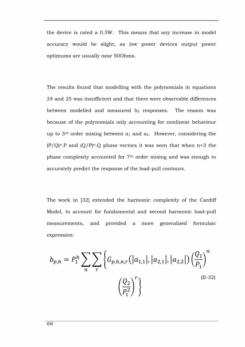
66
the device is rated a 0.5W. This means that any increase in model
accuracy would be slight, as low power devices output power
optimums are usually near 50Ohms.
The results found that modelling with the polynomials in equations
24 and 25 was insufficient and that there were observable differences
between modelled and measured b2 responses. The reason was
because of the polynomials only accounting for nonlinear behaviour
up to 3rd order mixing between a1 and a2. However, considering the
(P/Q)n.P and (Q/P)n.Q phase vectors it was seen that when n=3 the
phase complexity accounted for 7th order mixing and was enough to
accurately predict the response of the load-pull contours.
The work in [32] extended the harmonic complexity of the Cardiff
Model, to account for fundamental and second harmonic load-pull
measurements, and provided a more generalized formulaic
expression:
�o,% = X�%//sto,%,-,n5q��,�q, q��,�q, q��,�q: ui�X�v- �
n-
�wi�X��xny
(II-32)

Chapter II Chapter II Chapter II Chapter II ---- Literature ReviewLiterature ReviewLiterature ReviewLiterature Review
67
In equation 32, subscripts 'p' and 'h' are the familiar port and
harmonic indices. The 'n' and 'r' scripts denote the model order or
complexity. The 'G' term denotes the extractable coefficient. It is
shown to be a function of the magnitudes of the driving signals for
the system; however, it is also a function of other fundamental
operation parameters, namely bias and frequency.
Tasker better defines the model mixing order in [33], where a
generalised model equation is formulated to encompass any number
of harmonics in the load-pull measurements:
This equation represents the functional expression of 'G' in equation
32 as the parameter 'K'; the meaning is the same however.
2.5.5 Measurement of the Cardiff Behavioural Model
The work by Woodington et al [31] and [32] draws reference to the
measurement system developed by Tasker [34]. This system was
expanded in order to perform two harmonic load-pull CW
�-,% = X�%. / …… / A-,%,R#,…,Rz
R#!{(|#{�)/�
R#!3(|#{�)/�
Rz!{(|z{�)/�
Rz!3(|z{�)/�
. ui�X�vR# ……winX�nx
Rz
(II-33)
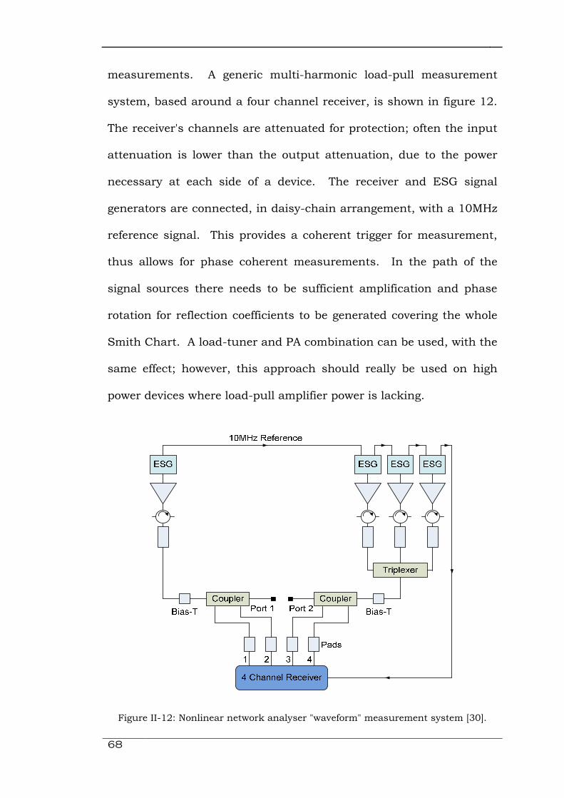
68
measurements. A generic multi-harmonic load-pull measurement
system, based around a four channel receiver, is shown in figure 12.
The receiver's channels are attenuated for protection; often the input
attenuation is lower than the output attenuation, due to the power
necessary at each side of a device. The receiver and ESG signal
generators are connected, in daisy-chain arrangement, with a 10MHz
reference signal. This provides a coherent trigger for measurement,
thus allows for phase coherent measurements. In the path of the
signal sources there needs to be sufficient amplification and phase
rotation for reflection coefficients to be generated covering the whole
Smith Chart. A load-tuner and PA combination can be used, with the
same effect; however, this approach should really be used on high
power devices where load-pull amplifier power is lacking.
Figure II-12: Nonlinear network analyser "waveform" measurement system [30].

Chapter II Chapter II Chapter II Chapter II ---- Literature ReviewLiterature ReviewLiterature ReviewLiterature Review
69
The measurements required for model extraction are, simply, load-
pull measurements. The works [30-32] utilise impedance points
located on concentric circles, as they provide a clear base for
observational analysis of distortion on the load-pull grid. In [30] and
[32] the analysis of fundamental models and second harmonic mixing
models requires two harmonic load-pull to be performed. Taking [32]
as the example, a circle of fundamental impedance points, and
another circle of second harmonic impedance points were imported
into load-pull software, developed by Saini [35]. The software took all
the points and iterated round the circles, measuring once per
iteration, to produce a fundamental impedance circle of second
harmonic impedance circles. The normalized travelling-wave
measurement data for the aforementioned nested load-pull
measurement scenario are shown in figure 13. Figure 13 shows how
the b2,h waves respond to the nested injections of a2,h. The a2,1 and
a2,2 traces show fuzzy dots, this is a result of performing nested load-
pull because when a2,2 is varied for a specific a2,1 that a2,1 point is
affected slightly when iterating through points of a2,2 and vice-versa.
Measurements do not simply provide the operator with a model. An
extraction procedure is necessary to converge on a best fit model and
so the collected data can be used inside CAD via a representative
polynomial.
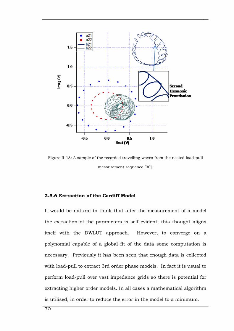
70
Figure II-13: A sample of the recorded travelling-waves from the nested load-pull
measurement sequence [30].
2.5.6 Extraction of the Cardiff Model
It would be natural to think that after the measurement of a model
the extraction of the parameters is self evident; this thought aligns
itself with the DWLUT approach. However, to converge on a
polynomial capable of a global fit of the data some computation is
necessary. Previously it has been seen that enough data is collected
with load-pull to extract 3rd order phase models. In fact it is usual to
perform load-pull over vast impedance grids so there is potential for
extracting higher order models. In all cases a mathematical algorithm
is utilised, in order to reduce the error in the model to a minimum.

Chapter II Chapter II Chapter II Chapter II ---- Literature ReviewLiterature ReviewLiterature ReviewLiterature Review
71
Equations 34 to 36 show the derivation of the Least Mean Squares
(LMS) algorithm that is tailored to suit this type of modelling. It is a
type of adaptive equation used to change the coefficient weighting, in
this case R, of an equation to produce the least mean squares of an
error. By using this algorithm a model of best fit can be converged
upon giving the best global accuracy for the provided data.
Once the coefficients are computed the [B] matrix can be calculated
from the [A] and [R] matrices and it can be compared to the measured
[B] to give a model error of B. The factors that drive this error are
model complexity and measurement quantity. These two are not
mutually exclusive, in that the measurement quantity directly affects
the maximum complexity. If there are more coefficients than
measurement data points the LMS algorithm will not converge due to
their being more unknown quantities than known quantities.
GQH = GVH. G�H
GVH}. GQH = GVH}GVH. G�H
G�H = (GVH}GVH)3�. GVH}. GQH
(II-34, 35 & 36)
72
2.5.7 The Cardiff Model Discussion
Although the Cardiff model initially began as a way to quickly
transport measurement data into CAD for observation it grew into a
usable behavioural modelling solution that efficiently compressed
measurement data. The work in [24] shows a specific case of the
model being applied to a high power device and raises the importance
of impedance renormalization. Woodington extended the scope of the
model and introduced more generalized model formulations in [30-
32]. The investigations into output fundamental and second
harmonic models showed that mixing of the harmonic model
coefficients was needed to describe the device's harmonic
interactions. The change in application and device process saw that
the fundamental coefficient space needed to be increased to account
for 7th order mixing. The necessity and effectiveness of the
renormalization can be questioned, as the works by Woodington et al
are based on relatively low power devices when compared to the
devices Qi et al were using.
Unlike X-parameters, the Cardiff model approach does not need to
perform specific X-parameter-type measurements and simple load-
pull is sufficient. The model formulation is flexible to allow for future
changes to normal device processes and device design. This can be
seen as similar to that of hot S-parameters, except the measurement
procedure is simpler. The flexible formulation essentially means that
Chapter II Chapter II Chapter II Chapter II ---- Literature ReviewLiterature ReviewLiterature ReviewLiterature Review
73
X-parameters can be a subset of the Cardiff model coefficients or if
there are three model coefficients, the Cardiff model equates to X-
parameters. The relative ease of measurement and flexible nature of
the model is promising. However, current CAD implementations are
not as flexible as the model formulations and would need improving if
the Cardiff model could be mentioned alongside X-parameters.
Moreover, the harmonic scope of the measurement system does not
cater for the control of more than three sources, which limits model
analysis of input harmonics, and higher harmonics.
2.6 REFERENCES
[1] E. W. Mathews, “The Use of Scattering Matrices in Microwave
Circuits,” IRE Transactions – Microwave Theory and Techniques.
Pg 21-26, Apr. 1955.
[2] K. Kurokawa, “Power Waves and the Scattering Matrix,” IEEE
Transactions on Microwave Theory and Techniques. Pg 194-202,
Mar. 1965.
[3] “HEWLETT-PACKARD JOURNAL,” Technical Information from the
Laboritories of the Hewlett-Packard Company, Volume 18,
Number 6. Pg 13-24, Feb. 1967.
[4] P. Harrop and T. A. Claasen "Modelling of an F.E.T Mixer,"
Electronics Letters, Vol. 14, No. 12. Pg 369-370. Jun. 1978.
[5] W. H. Leighton, R. J. Chaffin, J. G. Webb "RF Amplifier Design
with Large-Signal S-Parameters," IEEE Transactions on Microwave
74
Theory and Techniques, Volume 21, No. 12. Pg 809-814. Dec.
1973.
[6] F. Verbeyst and M. V. Bossche, "VIOMAP, the S-Parameter
Equivalent for Weakly Nonlinear RF and Microwave Devices," IEEE
Transactions on Microwave Theory and Techniques, Volume 42,
No. 12. Pg 2531-2535. Dec 1994.
[7] F. Verbeyst and M. V. Bossche, "VIOMAP, 16QAM and Spectral
Regrowth: Enhanced Prediction and Predistortion based on Two-
Tone Black-Box Model Extraction," 45th ARFTG Conference
Digest-Spring, Volume 27. Pg 19-28. May 1995.
[8] F. Verbeyst and M. V. Bossche, "The Volterra Input-Output Map of
a High-Frequency Amplifier as a Practical Alternative to Load-Pull
Measurements," IEEE Transactions on Instrumentation and
Measurement, Volume 44, No. 3. Pg 662-665. Jun 1995.
[9] F. Verbeyst and M. V. Bossche, "Using Orthogonal Polynomials as
Alternative for VIOMAP to Model Hardly Nonlinear Devices," 47th
ARFTG Conference Digest-Spring, Volume 29. Pg 112-120. Jun
1996.
[10] Hewlett Packard, "Microwave Network Analyzers, 45 MHz to 100
GHz," Downloaded from: www.mrtestequipment.com/getfile.php?s
= Agilent...Data...
[11] Hewlett Packard, "Network Analyzers Test Sets 8510 Series,"
Downloaded from: http://www.equipland.com/objects/catalog/
product/ extras/33812_HP_8516a.pdf.
Chapter II Chapter II Chapter II Chapter II ---- Literature ReviewLiterature ReviewLiterature ReviewLiterature Review
75
[12] G. E. Forsythe," Generation and Use of Orthogonal Polynomials
for Data-fitting with a Digital Computer," Journal of the Society of
Industrial and Applied Mathematics, Volume 5, No. 2. Pg 74-88.
June 1957.
[13] J. Verspecht, D. Barataud, J-P. Teyssier and J-M Nébus, "Hot
S-Parameter Techniques: 6 = 4 + 2," 66th ARFTG Conference. Dec
2005.
[14] T. Gasseling et al. "Hot Small-Signal S-Parameter
Measurements of Power Transistors Operating Under Large-Signal
Conditions in a Load-Pull Environment for the Study of Nonlinear
Parametric Interactions," IEEE Transactions on Microwave Theory
and Techniques. Volume 52, No. 3. Pg 805-812. Mar 2004.
[15] J. Verspecht, "Everything you've always wanted to know about
Hot-S22 (but we're afraid to ask)," IMS workshop: Introducing New
Concepts in the Nonlinear Network Design. 2002.
[16] J. Verspecht, “Black Box Modelling of Power Transistors in the
Frequency Domain,” Presented at the 4th workshop on INMMC.
1996.
[17] J. Verspecht and D. E. Root, "Polyharmonic Distortion
Modelling," IEEE Microwave Magazine, Volume 7. No. 3. Pg 44-57.
Jun 2006.
[18] J. Verspecht, "Large Signal Network Analysis - 'Going Beyond S-
Parameters'," 62nd ARFTG Conference Short course Notes. Dec
2003.
76
[19] G. Simpson, J. Horn, D. Gunyan and D. Root, "Load-pull +
NVNA = Enhanced X-Parameters for PA Designs with High
Mismatch and Technology-Independent Large-Signal Device
Models," 72nd ARFTG Microwave Measurement Symposium. Pg
88-91. Dec 2008.
[20] J. Wood, D. E. Root et al. "Fundamentals of Nonlinear
Behavioral Modeling for RF and Microwave Design," Chapter 5.
Artech House Inc 2005. ISBN: 1-58053-775-8.
[21] Agilent Technologies, "Agilent 2-Port and 4-Port PNA-X Network
Analyzer," Downloaded from: http://cp.literature.agilent.com/
litweb/pdf/N5242-90007.pdf. Sept 29, 2011.
[22] J. Verspecht et al, "Extension of X-parameters to Include Long-
Term Dynamic Memory Effects," IEEE MTT-S International
Microwave Symposium Digest. Pg. 741-744. Jun. 2009.
[23] D. E. Root et al, "Broad-Band Poly-Harmonic Distortion (PHD)
Behavioral Models from Fast Automated Simulations and Large-
Signal Vectorial Network Measurements," IEEE Transactions on
Microwave Theory and Techniques, Vol. 53, No. 11. Pg. 3656-
3664. Nov. 2005.
[24] H. Qi, "Nonlinear Data Utilization: Direct Data Look-Up to
Behavioural Modelling," Doctoral Thesis, Cardiff University. Feb
2008.
[25] H. Qi, J Benedikt and P. J. Tasker, "A Novel Approach for
Effective Import of Nonlinear Device Characteristics into CAD for

Chapter II Chapter II Chapter II Chapter II ---- Literature ReviewLiterature ReviewLiterature ReviewLiterature Review
77
Large Signal Power Amplifier Design," IEEE MTT-S International
Microwave Symposium Digest. Pg 477-480. 2006.
[26] Agilent Technologies, "Advanced Design System ADS Home
page," Downloaded from:
http://www.home.agilent.com/en/pc1297113/ advanced-design-
system-ads?nid=-34346.0&cc=GB&lc=eng.
[27] J. Benedikt, R. Gaddi, P. J. Tasker and M. Goss, "High-Power
Time-Domain Measurement System with Active Harmonic Load-Pull
for High-Efficiency Base-Station Amplifier Design," IEEE
Transactions on Microwave Theory and Techniques. Volume 48,
No. 12. Pg 2617-2624. Dec 2000.
[28] Agilent Technologies, "HP 71500A Microwave Transition
Analyzer," Downloaded from: http://cp.literature.agilent.com/
litweb/pdf/5091-0791E.pdf
[29] H. Qi, J. Benedikt and P. J. Tasker, "Novel Nonlinear Model for
Rapid Waveform-based Extraction Enabling Accurate High Power
PA Design," IEEE MTT-S International Microwave Symposium
Digest. Pg 2019-2022. 2007.
[30] S. Woodington, "Behavioural Model Analysis of Active Harmonic
Load-Pull Measurements," Doctoral thesis submitted to Cardiff
University. 2012.
[31] S. Woodington et al, "A Novel Measurement based Method
Enabling Rapid Extraction of a RF Waveform Look-Up Table
Based Behavioural Model," IEEE MTT-S International. Pg 1453-
1456. Jun 2008.

78
[32] S. Woodington et al, "Behavioural Model Analysis of Active
Harmonic Load-Pull Measurements," IEEE MTT-S International. Pg
1688-1691. May 2010.
[33] P. J. Tasker and J. Benedikt, "Waveform Inspired Models and
the Harmonic Balance Emulator," IEEE Microwave Magazine. Pg
38-42. Apr 2011.
[34] P. J. Tasker, "Practical Waveform Engineering," IEEE Microwave
Magazine. Volume 10, No. 7. Pg 65-67. Dec 2009.
[35] R. S. Saini, "Intelligence Driven Load-pull Measurement
Strategies," A Doctoral Thesis submitted to Cardiff University.
2013.

Chapter III Chapter III Chapter III Chapter III ---- Measurement System DevelopmentMeasurement System DevelopmentMeasurement System DevelopmentMeasurement System Development
79
Chapter IIIChapter IIIChapter IIIChapter III
Measurement System Measurement System Measurement System Measurement System
DevelopmentDevelopmentDevelopmentDevelopment
he HF measurement systems at Cardiff University have been
under constant improvement over the past decade. The
challenges of research often call for new improvements of hardware
and new procedures or autonomy in software. It was shown in
chapter II that the platform for the measurement systems used for
modelling was based on the work by Benedikt et al [1]. In order for
further model explorations to be conducted, where a device is
stimulated by more than the output fundamental and second
harmonic signals, the measurement system needs to be updated.
3.1 INTRODUCTION
The measurement system used by Woodington and Saini provided the
basis for model investigations concerning the output fundamental
and second harmonic frequency dimensions. In order to further
analyse harmonic relations in the model formulation, the addition of
T

80
one or more signal source was necessary. The previous measurement
system did not permit the addition of any more sources because it
lacked adequate number of coherent carrier distribution ports. Also
the set-up did not permit source locking at all frequencies thus only
specific frequencies were previously chosen for operation and it was
impossible to perform X-band load-pull measurements.
Figure III-1: Two harmonic load-pull measurement system block diagram.
The measurement system in figure 1 is based around the Tektronix
DSA8200 sampling oscilloscope [2] for travelling wave measurement
and the Agilent Z5623AK07 [3] distribution amplifier, for the
distribution of the coherent carrier. The PSGs are from Agilent's
E8267D [4] range and have the HCC option, which is important for
the coherent carrier set-up as its 3.2-10GHz range allows for a larger

Chapter III Chapter III Chapter III Chapter III ---- Measurement System DevelopmentMeasurement System DevelopmentMeasurement System DevelopmentMeasurement System Development
81
band of stable phase coherence necessary for X-band measurement.
The 10MHz references of the PSGs are not suitable for X-band
measurements, as at the desired operation frequency of 9GHz the
PSGs will drift over time in relation to one another and hence the
phases will not be locked.
The importance of having a coherent carrier is that measurements
require traceable phase relationships between stimulating signals, if
there is no coherent phase relationship the measurement of models
becomes impossible. To take the example of the phase vectors Q and
P in [5], if there was no common carrier between signal sources then
there is no reference for phase and hence the Q/P phase vectors
would vary from measurement to measurement for a single load-pull
point. Consequently, and importantly, it is crucial for model
extraction that there be phase coherence between all sources. Figure
2 shows the master-slave structure of the signal sources and the
coherent carrier. This configuration allows all sources the use of the
master source's local oscillator; also its coupling with the oscilloscope
provides a consistent trigger from signal master to measurement. In
this case the attenuated coupled port is connected to the
oscilloscope, as it can still be triggered despite 6dB attenuation.

82
Figure III-2: The Master-slave source configuration.
For the addition of an extra source, to the measurement setup, the
Agilent Z5623AK07 needs to be replaced with a carrier distribution
system capable of handling more sources.
3.2 COHERENT CARRIER DISTRIBUTION DESIGN
The fundamental area of developing the coherent carrier distribution
system is ensuring the master source has the same power and fidelity
of its phase locked loop (PLL) signal, whilst also delivering the right
power to the slave signal generators, as it does when operating alone.
The power level of the reference signal to the PLL is important in
terms of device safety; as if the signal is too large the PSG can be
damaged. The fidelity of the signal is also important as poor signal
quality and stability will result in phase jitter that does not allow the
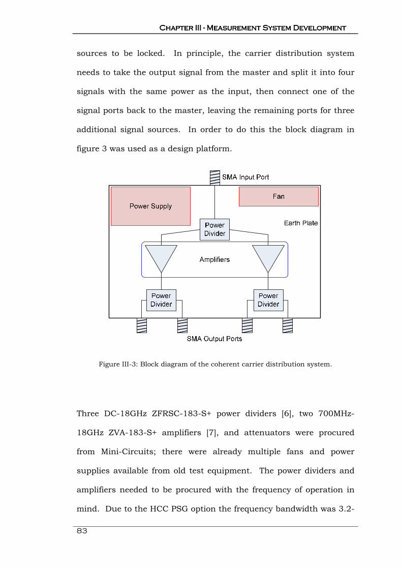
Chapter III Chapter III Chapter III Chapter III ---- Measurement System DevelopmentMeasurement System DevelopmentMeasurement System DevelopmentMeasurement System Development
83
sources to be locked. In principle, the carrier distribution system
needs to take the output signal from the master and split it into four
signals with the same power as the input, then connect one of the
signal ports back to the master, leaving the remaining ports for three
additional signal sources. In order to do this the block diagram in
figure 3 was used as a design platform.
Figure III-3: Block diagram of the coherent carrier distribution system.
Three DC-18GHz ZFRSC-183-S+ power dividers [6], two 700MHz-
18GHz ZVA-183-S+ amplifiers [7], and attenuators were procured
from Mini-Circuits; there were already multiple fans and power
supplies available from old test equipment. The power dividers and
amplifiers needed to be procured with the frequency of operation in
mind. Due to the HCC PSG option the frequency bandwidth was 3.2-
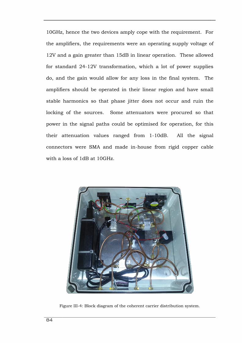
84
10GHz, hence the two devices amply cope with the requirement. For
the amplifiers, the requirements were an operating supply voltage of
12V and a gain greater than 15dB in linear operation. These allowed
for standard 24-12V transformation, which a lot of power supplies
do, and the gain would allow for any loss in the final system. The
amplifiers should be operated in their linear region and have small
stable harmonics so that phase jitter does not occur and ruin the
locking of the sources. Some attenuators were procured so that
power in the signal paths could be optimised for operation, for this
their attenuation values ranged from 1-10dB. All the signal
connectors were SMA and made in-house from rigid copper cable
with a loss of 1dB at 10GHz.
Figure III-4: Block diagram of the coherent carrier distribution system.

Chapter III Chapter III Chapter III Chapter III ---- Measurement System DevelopmentMeasurement System DevelopmentMeasurement System DevelopmentMeasurement System Development
85
Figure 4 shows the completed build of the distribution system. The
SMA copper cables had to be bent in that fashion to fit inside the box
with its lid on. The bending of the cables resulted in them having
more loss than the 1dB measured result at 10GHz.
3.3 COHERENT CARRIER DISTRIBUTION TESTING
The carrier distribution system was tested in three ways. Firstly, it
was connected to a PSG and the power was individually measured at
two of the output ports in order to test the two amplifiers. This
experiment was repeated three times at 3.2GHz, 6GHz, and then
9GHz to observe any differences or irregularities in the gain plots.
Secondly, a quick check was performed with a spectrum analyser to
make sure the outputs were not distorted by large unstable
harmonics. Thirdly, the carrier distribution system was integrated
into the full measurement system with all PSGs connected so that
any adjustments to signal power, discrepancies between PSGs etc,
could be solved. This test was to validate whether all the PSGs could
be locked, hence consisted of an instrument display check and any
“UNLOCK” notification would constitute failure. Further to this test
two PSGs, operating at 9GHz and 18GHz, were combined through a
90degree hybrid coupler and measured directly with the scope. A
waveform capture at time zero and one approximately 4 hours later
were performed to observe any discrepancy in the phase relationship
between the fundamental and second harmonic signal.
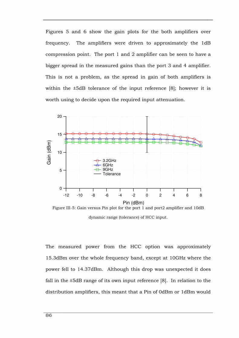
86
Figures 5 and 6 show the gain plots for the both amplifiers over
frequency. The amplifiers were driven to approximately the 1dB
compression point. The port 1 and 2 amplifier can be seen to have a
bigger spread in the measured gains than the port 3 and 4 amplifier.
This is not a problem, as the spread in gain of both amplifiers is
within the ±5dB tolerance of the input reference [8]; however it is
worth using to decide upon the required input attenuation.
Figure III-5: Gain versus Pin plot for the port 1 and port2 amplifier and 10dB
dynamic range (tolerance) of HCC input.
The measured power from the HCC option was approximately
15.3dBm over the whole frequency band, except at 10GHz where the
power fell to 14.37dBm. Although this drop was unexpected it does
fall in the ±5dB range of its own input reference [8]. In relation to the
distribution amplifiers, this meant that a Pin of 0dBm or 1dBm would
20
15
10
5
0
Ga
in (
dB
m)
-12 -10 -8 -6 -4 -2 0 2 4 6 8
Pin (dBm)
3.2GHz 6GHz 9GHz Tolerance

Chapter III Chapter III Chapter III Chapter III ---- Measurement System DevelopmentMeasurement System DevelopmentMeasurement System DevelopmentMeasurement System Development
87
have sufficed if there was no loss in the signal path after the
amplifier.
Figure III-6: Gain versus Pin plot for the port 3 and 4 amplifier and 10dB dynamic
range (tolerance) of HCC input.
The distribution system was driven at 0dBm and 1dBm into a
spectrum analyser for both amplifiers. In this test port 1 and port 4
were used so as to exercise both PAs. The harmonic content in both
cases was below 20dBc of the fundamental output power.
Figure 7 shows a ±2dBm variation in the outputs of the distribution
system until 9GHz. At 9GHz and 10GHz there is a drop in power
with the lowest point being 10.68dBm. This, however, was not
sufficient to cause any of the PSGs to become unlocked in the test
condition. When measurements were performed it was noticed that
20
15
10
5
0
Ga
in (
dB
m)
-12 -10 -8 -6 -4 -2 0 2 4 6 8
Pin (dBm)
3.2GHz 6GHz 9GHz Tolerance

88
the PSG connected to port 4 became unlocked for some but not all of
the measurement points. This discovery resulted in a reduction of
the input attenuation of 1dB which resulted in consistent, stable
carrier locking.
Figure III-7: Pout variation over frequency for the four ports of the distribution box.
Figure III-8: A 9GHz and 18GHz combined signal captured at time = 0 (red trace)
and 4 hours later (blue dashed trace).
16
14
12
10
8
6
4
Po
ut
(dB
m)
109876543
Frequency (GHz)
Port 1 Port 2 Port 3 Port 4
-0.15
-0.10
-0.05
0.00
0.05
0.10
Am
plit
ude (
V)
200x10-12150100500
Time (ps)
Chapter III Chapter III Chapter III Chapter III ---- Measurement System DevelopmentMeasurement System DevelopmentMeasurement System DevelopmentMeasurement System Development
89
Figure 8 shows the good alignment of the two traces take over a 4
hour period. The 9GHz and 18GHz signals have stayed locked in
their phase relationship proving the carrier distribution system works
over time.
3.4 SUMMARY
In order to be able to perform more complex load-pull device
measurements additional signal sources needed to be added to the
system. The most cost effective way of adding a signal source, was to
make, in-house, a coherent carrier distribution system which could
link four sources. Using a simple design platform the system was
made from Mini-Circuits power dividers and amplifiers. Necessary
padding was applied at the input due to the amplification of the Mini-
Circuits amplifiers.
The carrier distribution system was tested with varying input power
at 3.2GHz, 6GHz, and 9GHz to check that the amplifiers were
performing correctly over the PSG's HCC option frequency bandwidth
and input dynamic range. Furthermore, the system was tested with
a spectrum analyser and the harmonic components were found to be
lower than 20dBc for both PAs. The carrier distribution system was
implemented in the measurement systems and test measurements
were performed to observe whether the 'unlock' warning on any of the

90
PSGs appeared. The PSG connected to port 4 was noticed to become
unlocked for some measurements not all. This finding resulted in a
2dB attenuation reduction and yielded reliable source locking. One
further practical test was performed by combining two signals from
the PSGs, one at 9GHz and one at 18GHz, and observing the change
in the waveform over a 4 hour period. The test showed good
alignment of the start and end waveforms hence device
measurements over time would not suffer phase drift between
harmonics. The inclusion of the coherent carrier system in the HF
measurement system allowed for the first time harmonic load-pull to
be performed at X-band.
The drawback of a hardware project like this is that they tend to be
short term solutions and in this case future hurdles are obvious,
since the coherent carrier distribution system only links a maximum
of four signal sources. However, if one extrapolates upon the inner
workings of figure 3, the addition of more and more sources will soon
become costly, as more power dividers and amplifiers will be needed
to expand the signal divide-and-amplify 'tree'. For future
measurement system iterations it is suggested that signal source and
measurement hybrid solutions be considered, Agilent's four-channel
PNA [9] is a good example of what to aim for. However, addition of
more sources would still be sought after although seven is an
estimated maximum necessary for decades of research. Seven
Chapter III Chapter III Chapter III Chapter III ---- Measurement System DevelopmentMeasurement System DevelopmentMeasurement System DevelopmentMeasurement System Development
91
sources would allow for three input and four output injections, or any
other input/output configuration.
3.5 REFERENCES
[1] P. J. Tasker and J. Benedikt, "Waveform Inspired Models and the
Harmonic Balance Emulator," IEEE Microwave Magazine. Pg 38-
42. Apr 2011.
[2] Tektronix "Digital Serial Analyzer Sampling Oscilloscope DSA8200
Data Sheet," Downloaded from: http://www.tek.com/sites
/tek.com/files/media/media/resources/85W_17654_20.pdf
[3] Agilent Technologies "Z5623A Option K07 User's and Service
Guide," Downloaded from: http://www.home.agilent.com/upload/
cmc_upload/All/Z5623AK07Usersguide.pdf
[4] Agilent Technologies "Agilent E8267D PSG Vector Signal Generator
Configuration Guide," Downloaded from: http://www.cnam.umd.
edu/anlage/Microwave%20Measurements%20for%20Personal%2
0Web%20Site/5989-1326EN.pdf
[5] S. Woodington et al, "A Novel Measurement based Method
Enabling Rapid Extraction of a RF Waveform Look-Up Table
Based Behavioural Model," IEEE MTT-S International. Pg 1453-
1456. Jun 2008.
[6] Mini-Circuits "Coaxial power Splitter/Combiner ZFRSC-183+,"
Downloaded from: http://217.34.103.131/pdfs/ZFRSC-183+.pdf

92
[7] Mini-Circuits "Super Ultra Wideband Amplifier ZVA-183+,"
Downloaded from: http://217.34.103.131/pdfs/ZVA-183+.pdf
[8] Agilent Technologies "Agilent E8267D PSG Vector Signal Generator
Data Sheet," Downloaded from: http://www.keysight.com/en/pd-
680840-pn-E8267D/rear-panel-connections-for-multi-source-
phase-coherency-special-option?cc=GB&lc=eng
[9] Agilent Technologies "N5242A PNA-X Network Analyzer,"
Downloaded from: http://www.home.agilent.com/en/pd-867173-
pn-N5242A/pna-x-microwave-network-analyzer?&cc=GB&lc=eng

Chapter IV Chapter IV Chapter IV Chapter IV ---- CAD Implementation ImprovementCAD Implementation ImprovementCAD Implementation ImprovementCAD Implementation Improvement
93
Chapter Chapter Chapter Chapter IVIVIVIV
CAD Implementation CAD Implementation CAD Implementation CAD Implementation
ImprovementImprovementImprovementImprovement
he investigations by Woodington et al [1-3] were predominately
concerned with analysis of the model structure and accuracy
with respect to fundamental only and fundamental and second
harmonic load-pull measurements. There was some effort to
implement a usable CAD implementation; however, the end result
had a rigid formulaic structure in Agilent ADS that would only
simulate with a particular file containing a specific number of
coefficients. This chapter will detail the process of implementing a
dynamic model solution within the CAD environment that was
necessary to prevent future model-simulator integration problems
arising from the myriad models that can be generated with a flexible
model extraction procedure.
T

94
4.1 INTRODUCTION
The Cardiff Model has been developed, over the years, to be as flexible
as possible. The relevant contrast to this being Agilent's, X-
parameter, approach that uses a fixed formulaic structure. Chapter
II mentioned that the synergy between X-parameter data files and
Agilent's ADS harmonic balance simulator was good. The Cardiff
model has yet to reach the usability or the speed of simulation
exhibited by Agilent's X-parameter solution.
Figure 1 shows the core of a current iteration of the ADS
implementation of the Cardiff model. It utilises a four port Frequency
Domain Device (FDD) to extract and compute the port incident and
reflected travelling waves. The FDD has four ports because it needs
to perform operations on the DC current and AC voltage and ADS
does not support single ports that can do operations on both
quantities simultaneously.
Figure IV-1: FDD core of the model schematic.
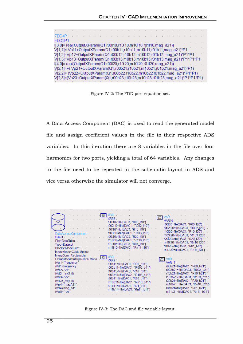
Chapter IV Chapter IV Chapter IV Chapter IV ---- CAD Implementation ImprovementCAD Implementation ImprovementCAD Implementation ImprovementCAD Implementation Improvement
95
Figure IV-2: The FDD port equation set.
A Data Access Component (DAC) is used to read the generated model
file and assign coefficient values in the file to their respective ADS
variables. In this iteration there are 8 variables in the file over four
harmonics for two ports, yielding a total of 64 variables. Any changes
to the file need to be repeated in the schematic layout in ADS and
vice versa otherwise the simulator will not converge.
Figure IV-3: The DAC and file variable layout.

96
The equations highlighted in figure 2 reconstruct the harmonic
waveform components from the model coefficients and the
renormalized FDD port values. The equation sets that are used, as
well as the file's coefficient composition, are rigid and hence do not
permit any other model type or complexity.
The rigid CAD implementation poses significant problems for anyone
wishing to increase model complexity and if three harmonics are used
to create a model the equations would get cumbersome to implement
by hand. The solution to these problems was native to the model
generation software; however, there was no obvious way to implement
the IGOR Pro [4] code in Agilent's ADS. This chapter will now
demonstrate the process of creating a dynamic CAD implementation
of the Cardiff Model within ADS.
4.2 CREATING A DYNAMIC CAD MODEL SOLUTION
Fundamentally, the only thing wrong with the old solution was that
developing ADS templates for the many instances of different model
implementations was impractical and could be prone to error. The
solution is to perform the long-hand power series summation
calculation using matrix formations, this way there would be a
specific number of variables in the CAD schematic window, but they
Chapter IV Chapter IV Chapter IV Chapter IV ---- CAD Implementation ImprovementCAD Implementation ImprovementCAD Implementation ImprovementCAD Implementation Improvement
97
could be changed more easily than rewriting the long-hand
equations.
4.2.1 AEL in ADS
AEL is ADS' Application Extension Language (AEL). Agilent describe
it as a general purpose programming language modelled on C.
Similar to C, AEL has sets of native functions to handle file I/O,
database queries, mathematics, lists, and string manipulation. The
way AEL is integrated with ADS means that it has different
functionality in the various windows you can access. The model
implementation will only occur in the schematic window; hence the
function set specific to this window will be the one that can be used.
By virtue of AEL being a tool used to add extra functionality and
aesthetics to the core ADS program AEL procedures cannot be called
and run whilst the simulator is performing calculations see figure 3.
This flow diagram seems sound to begin with, however for an AEL
script to interact with an ADS simulation in this way ADS' flow
diagram would have to be structured differently. As it is, when the
user hits 'run simulation' all the data in the schematic hierarchy gets
written to a Netlist that the simulator uses in its operations before
stopping and creating a data set for the data display window to use.
Therefore, the AEL script cannot be used to do parallel work during
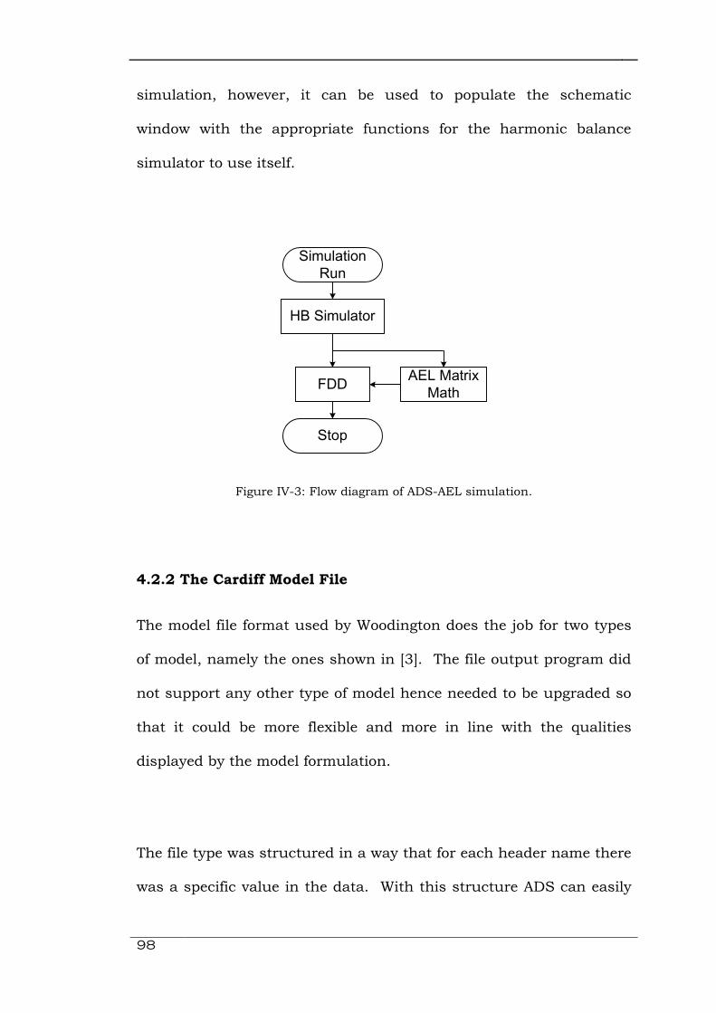
98
simulation, however, it can be used to populate the schematic
window with the appropriate functions for the harmonic balance
simulator to use itself.
Simulation
Run
HB Simulator
AEL Matrix
MathFDD
Stop
Figure IV-3: Flow diagram of ADS-AEL simulation.
4.2.2 The Cardiff Model File
The model file format used by Woodington does the job for two types
of model, namely the ones shown in [3]. The file output program did
not support any other type of model hence needed to be upgraded so
that it could be more flexible and more in line with the qualities
displayed by the model formulation.
The file type was structured in a way that for each header name there
was a specific value in the data. With this structure ADS can easily
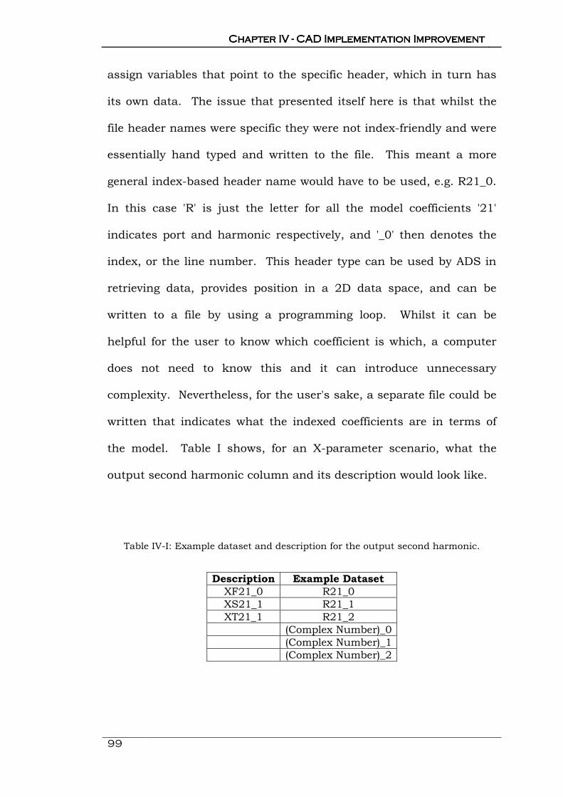
Chapter IV Chapter IV Chapter IV Chapter IV ---- CAD Implementation ImprovementCAD Implementation ImprovementCAD Implementation ImprovementCAD Implementation Improvement
99
assign variables that point to the specific header, which in turn has
its own data. The issue that presented itself here is that whilst the
file header names were specific they were not index-friendly and were
essentially hand typed and written to the file. This meant a more
general index-based header name would have to be used, e.g. R21_0.
In this case 'R' is just the letter for all the model coefficients '21'
indicates port and harmonic respectively, and '_0' then denotes the
index, or the line number. This header type can be used by ADS in
retrieving data, provides position in a 2D data space, and can be
written to a file by using a programming loop. Whilst it can be
helpful for the user to know which coefficient is which, a computer
does not need to know this and it can introduce unnecessary
complexity. Nevertheless, for the user's sake, a separate file could be
written that indicates what the indexed coefficients are in terms of
the model. Table I shows, for an X-parameter scenario, what the
output second harmonic column and its description would look like.
Table IV-I: Example dataset and description for the output second harmonic.
Description Example Dataset
XF21_0 R21_0
XS21_1 R21_1
XT21_1 R21_2
(Complex Number)_0
(Complex Number)_1
(Complex Number)_2

100
It is not assumed that this is the final and best iteration of the model
file; rather, it is a step in the right direction. It is clear that as more
complex models are made more coefficients will be created. With the
header to data ratio being 1:1, that means for a single data block half
of the file size is allocated just for headers; this is without
consideration of the data block headers. This is not ideal but it
provides a solution to file interactions with the schematic window in
ADS.
4.2.3 Designing the AEL Script
Knowing that AEL could be used to populate the schematic window
was useful; however, it did not immediately present a solution to the
problem of a dynamic model implementation. AEL has functions to
operate on lists and arrays, which can both be multidimensional.
However, mathematical operations, akin to matrix algebra, can only
be performed on arrays and via heuristic testing it was found that the
schematic window did not support arrays, hence matrix algebra could
not be performed in the schematic window. The solution to this,
given the way AEL can be applied to ADS, is to use AEL to populate
the model schematic window with long-hand formulas and functions
that can execute the matrix calculations, albeit in a long winded way.
The AEL script can now be thought of as a by product of a schematic
design for the model. Therefore, after having decided on the
functions and variables that will be necessary for operation, ADS'

Chapter IV Chapter IV Chapter IV Chapter IV ---- CAD Implementation ImprovementCAD Implementation ImprovementCAD Implementation ImprovementCAD Implementation Improvement
101
command line window can be used to find the code necessary to draw
schematic objects onto the window.
Figure IV-4: V-I to a-b translation equations and equations for phase normalisation.
Figure 5 shows the equations for extracting the scattering wave
components from the ports of the FDD and the required
renormalization to bring the phase of a1,1 to zero. It should be noted
that the 1x10-18 is in the translation equations to eliminate the
occurrence of zeros in future calculations, hence eliminate the
computation of NaNs (Not a Number) when division or indices are
being applied. It is not then taken out of future equations as its
value introduces an error far less than measurement error.
Figure IV-5: A-element calculations.
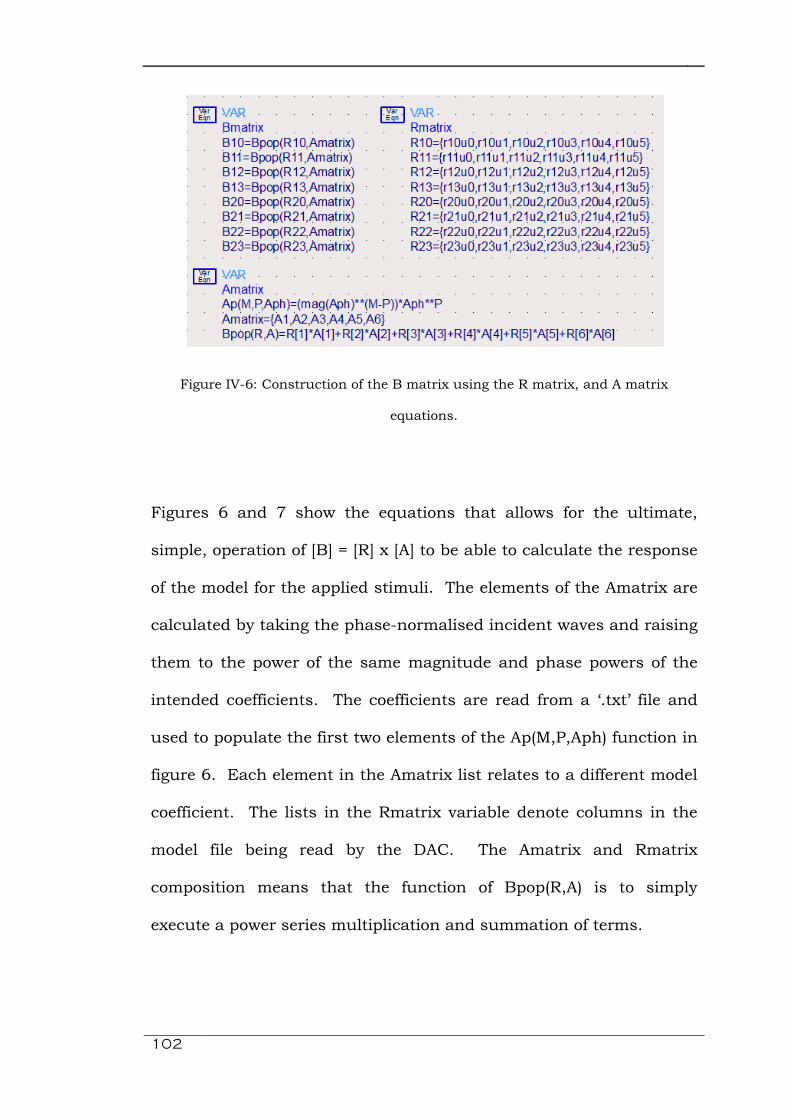
102
Figure IV-6: Construction of the B matrix using the R matrix, and A matrix
equations.
Figures 6 and 7 show the equations that allows for the ultimate,
simple, operation of [B] = [R] x [A] to be able to calculate the response
of the model for the applied stimuli. The elements of the Amatrix are
calculated by taking the phase-normalised incident waves and raising
them to the power of the same magnitude and phase powers of the
intended coefficients. The coefficients are read from a ‘.txt’ file and
used to populate the first two elements of the Ap(M,P,Aph) function in
figure 6. Each element in the Amatrix list relates to a different model
coefficient. The lists in the Rmatrix variable denote columns in the
model file being read by the DAC. The Amatrix and Rmatrix
composition means that the function of Bpop(R,A) is to simply
execute a power series multiplication and summation of terms.
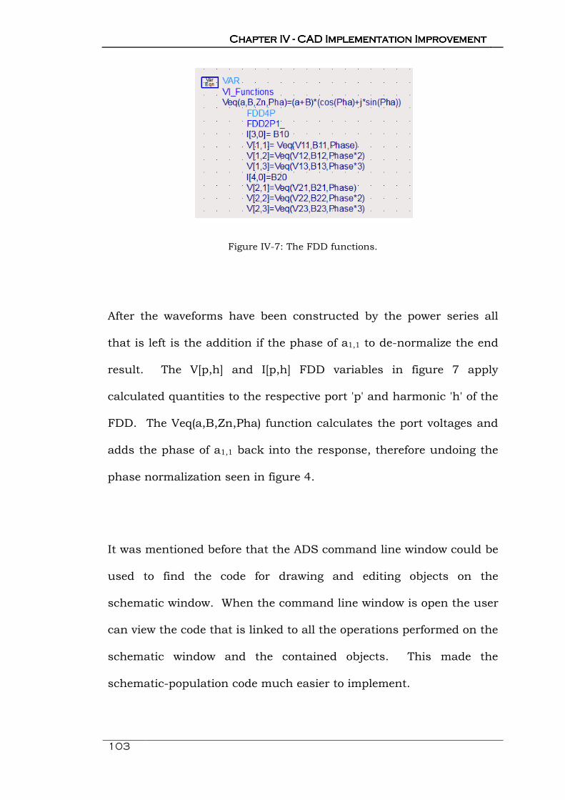
Chapter IV Chapter IV Chapter IV Chapter IV ---- CAD Implementation ImprovementCAD Implementation ImprovementCAD Implementation ImprovementCAD Implementation Improvement
103
Figure IV-7: The FDD functions.
After the waveforms have been constructed by the power series all
that is left is the addition if the phase of a1,1 to de-normalize the end
result. The V[p,h] and I[p,h] FDD variables in figure 7 apply
calculated quantities to the respective port 'p' and harmonic 'h' of the
FDD. The Veq(a,B,Zn,Pha) function calculates the port voltages and
adds the phase of a1,1 back into the response, therefore undoing the
phase normalization seen in figure 4.
It was mentioned before that the ADS command line window could be
used to find the code for drawing and editing objects on the
schematic window. When the command line window is open the user
can view the code that is linked to all the operations performed on the
schematic window and the contained objects. This made the
schematic-population code much easier to implement.

104
Figure IV-8: The command line window displaying code that sets schematic
variables
Figure IV-9: Data access file variable layout.
The utilization of the command line window enabled planning when it
came to the layout of the data access variables. In principle there is
not a problem with combining each variable in the VAR blocks, in

Chapter IV Chapter IV Chapter IV Chapter IV ---- CAD Implementation ImprovementCAD Implementation ImprovementCAD Implementation ImprovementCAD Implementation Improvement
105
figure 9, so that the harmonic access variables are grouped.
However, the function used to write the VARs to the schematic
window is inherently a long string and each access variable that is
added would make it longer and more unusable. This issue is a
sticking point as the programming environment allows for string
variables but not if the string variable represents a function, or part
of a function, that writes to the schematic window. A solution,
presented in figure 9, would be to loop the schematic write process
and only write one variable to each VAR.
4.2.4 Testing the AEL Script
The testing procedure was laborious since ADS is not a programming
environment, rather a simulator, hence a text based program was
used to write the code, and with that semantics checks had to be left
until run-time. Nevertheless, functions were written for loading the
coefficient, model, and impedance files into arrays, as well as a
function to operate on the data and write it to the schematic window.
Each function was run via a load command in the command line
window (load("testAEL.ael")). The AEL debugger was used by calling
it in the AEL script at the end; this allowed the programme to be
stepped through which made pinpointing any errors easier.

106
Apart from debugging functions within the code, crude comparison
was made between an X-parameter simulation and a Cardiff Model
simulation for the same model complexity. Although simulation
within the modelled area was achieved by both approaches there was
a difference in simulation time. The harmonic balance simulator,
once operating, seemed to iterate through the calculations in both
cases at the same rate. The time discrepancy can therefore be
attributed to a loading time necessary for the simulator to retrieve the
data in the model file via the DAC component into a Netlist prepared
for simulation. The loading time is rather obvious, as the X-
parameter simulation would begin in less than two seconds, whereas
the Cardiff Model simulation would begin at about ten seconds. By
virtue of the delay being attributed to a file load, the associated
loading time is directly proportional to the model file size; meaning
that very large model files would have very long loading times before
the simulator could perform any calculations. A solution to this, in
the future, would be to directly write the Netlist of the model
schematic, thus simultaneously performing the time consuming file
load ahead of run-time and once only. The most annoying trait of the
simulations is the cumulative waste of time that builds up over a
period of simulator use. However, the Netlist solution would be the
next organic progression because without a schematic of a working
dynamic solution, one cannot be certain of the form of the Netlist.
The model implementation was also tested with a model file that had
215 coefficients; this was to see if there would be any issue in
Chapter IV Chapter IV Chapter IV Chapter IV ---- CAD Implementation ImprovementCAD Implementation ImprovementCAD Implementation ImprovementCAD Implementation Improvement
107
computer memory for writing the ADS schematic window. The
resulting issue was not memory related; rather, it was related to the
Bpop(R,A) power series function. The string that needed to be
populated to the schematic somewhere in either the AEL program or
when it is written to the schematic window caused ADS to
unexpectedly close down with no error. Since the Bpop(R,A) function
only performed multiplication and summation operations it was split
up into multiple functions with 50 or less summations, which solved
the crash problem.
4.3 SUMMARY
This chapter has detailed the process and rationale behind the
development of the Cardiff model implementation. The conversion to
a dynamic solution presented challenges both inside and outside the
CAD environment. The root problems lie in the model file structure
and the formulaic representation of the model in ADS; however, the
two were not entirely separate entities. The model file was changed
so that index-based headers were used, which allowed for easier file
writing in IGOR Pro, and file reading in AEL. The AEL program was
initially designed in a top-down way so that the schematic window’s
functions could be tested and so an appropriate layout could be
obtained via the command line window. After the basics had been
finalised the intricacies of the implementation were examined and
improvements were made in the way the program handles the long
108
power series summation string. In terms of simulation, the model
solution is slower than the X-parameter model block that has been
optimised for ADS. The difference in speed is due to the different file
processes the two methods go through. Since the X-parameter
blocks have the data pre–loaded into memory it can operate on the
data almost immediately. However, for the Cardiff model, the data
has to be read into the schematic each time a simulation is run,
which results in a loading time, proportional to the size of the model
file, before ADS can do any operations on the data. This model
implementation consequently has shown a disadvantage of using
DACs. A possible solution to this, which could be implemented in the
future, is to compile a Netlist for the model schematic using AEL.
This way all the data would be contained in the Netlist and the
process would not necessitate additional loading of data.
4.4 REFERENCES
[1] S. Woodington et al, "A Novel Measurement based Method
Enabling Rapid Extraction of a RF Waveform Look-Up Table Based
Behavioural Model," IEEE MTT-S International. Pg 1453-1456.
Jun 2008.
[2] S. Woodington et al, "Behavioural Model Analysis of Active
Harmonic Load-Pull Measurements," IEEE MTT-S International. Pg
1688-1691. May 2010.

Chapter IV Chapter IV Chapter IV Chapter IV ---- CAD Implementation ImprovementCAD Implementation ImprovementCAD Implementation ImprovementCAD Implementation Improvement
109
[3] S. Woodington, "Behavioural Model Analysis of Active Harmonic
Load-Pull Measurements," Doctoral thesis submitted to Cardiff
University. 2012.
[4] WaveMetrics "IGOR Pro Product page," Downloaded from:
http://www.wavemetrics.com/products/igorpro/igorpro.htm

Chapter V Chapter V Chapter V Chapter V ---- SourceSourceSourceSource---- and Loadand Loadand Loadand Load----Pull Behavioural Model AnalysisPull Behavioural Model AnalysisPull Behavioural Model AnalysisPull Behavioural Model Analysis
110
Chapter Chapter Chapter Chapter VVVV
SourceSourceSourceSource---- and Loadand Loadand Loadand Load----Pull Pull Pull Pull
Behavioural Model Behavioural Model Behavioural Model Behavioural Model
AnalysisAnalysisAnalysisAnalysis
ecently, it has been common to generate models for output
fundamental load-pull data only. Sometimes, the procedure is
stretched to include output second harmonic load-pull for
applications such as amplifiers operating in the Class-B to Class-J
continuum. These are modes of amplifier that have and optimum
fundamental impedance and short circuit second harmonic
impedance. The work in this chapter goes even further by
investigating the required model necessary to describe input second
harmonic variations and then its relationship with the output
fundamental and second harmonic models. In addition, coefficient
truncation is investigated with the aim of potentially reducing model
file sizes for model types describing multi-harmonic interactions.
Furthermore, the models are used in ADS for the analysis of input
R

111
second harmonic shorting and other cases that have an impact on
future HF measurements and design.
5.1 INTRODUCTION
In chapters III and IV it was shown how the measurement system
was augmented to accommodate second harmonic source-pull along
with fundamental and second harmonic load-pull, as well as detailing
the improvements to the CAD implementation. In this chapter, a
Gallium-Arsenide (GaAs) pseudomorphic High Electron Mobility
Transistor (pHEMT), operated at a frequency of 9GHz, will be used to
demonstrate model relationships between the input second harmonic
and output harmonic load-pull data sets.
5.2 MEASUREMENT OF SOURCE- AND LOAD-PULL MODELS
The investigations performed by Woodington et al in [1-3] utilised
measurement points on concentric circles to extract the relative
phase relationship between the stimulating signals. Taking a
fundamental only load-pull power sweep case as an example, the
coefficients that would be extracted can be seen as a function of the
varying operating conditions.

Chapter V Chapter V Chapter V Chapter V ---- SourceSourceSourceSource---- and Loadand Loadand Loadand Load----Pull Behavioural Model AnalysisPull Behavioural Model AnalysisPull Behavioural Model AnalysisPull Behavioural Model Analysis
112
Where Rp,h are the model coefficients that are a function of the phase
normalised the measurement parameters, having subscripts 'p' and
'h' denoting port and harmonic index respectively. P1 is the phase of
a1,1 and Q1 is the phase of a2,1.
In equation 1 the bias and frequency are left out because they would
be constant for the entire sweep. If the arguments of G, in equation
1, are broken down into measurement iterations the equation can be
simplified to:
Where equation 2 now represents static |a1,1| and |a2,1|, and the
final argument left is the relative phase response of the system for a
given drive power and output fundamental power. Now, if it is
supposed that the iterations of phase Q1 coincide with iterations with
output fundamental power. The |a2,1| argument now becomes part
of equation 2:
�o,% = X�%. to,% ui�X�v
�o,% = X�%. to,% uq��,�q, q��,�q, i�X�v (V-1)
(V-2)
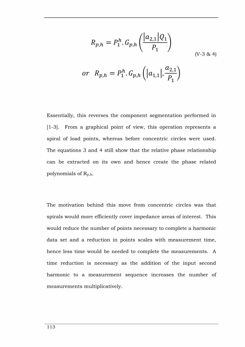
113
Essentially, this reverses the component segmentation performed in
[1-3]. From a graphical point of view, this operation represents a
spiral of load points, whereas before concentric circles were used.
The equations 3 and 4 still show that the relative phase relationship
can be extracted on its own and hence create the phase related
polynomials of Rp,h.
The motivation behind this move from concentric circles was that
spirals would more efficiently cover impedance areas of interest. This
would reduce the number of points necessary to complete a harmonic
data set and a reduction in points scales with measurement time,
hence less time would be needed to complete the measurements. A
time reduction is necessary as the addition of the input second
harmonic to a measurement sequence increases the number of
measurements multiplicatively.
�o,% = X�%. to,% wq��,�qi�X� x
=~�o,% = X�%. to,% uq��,�q, ��,�X� v (V-3 & 4)
Chapter V Chapter V Chapter V Chapter V ---- SourceSourceSourceSource---- and Loadand Loadand Loadand Load----Pull Behavioural Model AnalysisPull Behavioural Model AnalysisPull Behavioural Model AnalysisPull Behavioural Model Analysis
114
5.2.1 Measurement Sequence
The measurement software used at Cardiff University, developed by
Saini [4], could cope with single harmonic grids well. The
functionality for two harmonic load-pull was also sound when using
Newton-Raphson impedance convergence, which is a way of
iteratively computing a better approximation to the roots of a
function. The issue presenting this work was that there was no
inbuilt utility for spiral ap,h grids. As a result, a supplementary piece
of software was written that would create a measurement procedure
data table that would be executed by the measurement software. It
contained all the injected a-wave quantities for the whole sweep as
well as the fundamental operating conditions: bias and frequency.
The file could be loaded into the Cardiff measurement software and
run like a normal grid, except the grid was unable to be viewed. This
disconnect between the two programs lead to the authors adherence
to a specific methodology in order to converge upon the correct
measurement test. The measurements were prioritised so that more
a-wave grids were performed at the higher harmonics on the input
and output when compared to a2,1. Moreover, in the case where just
a1,2 and a2,2 were perturbed, the device was more sensitive to
movement of a1,2 therefore the measurement was designed so that it
was in the outer iterative loop in figure 1. When the focus is on a1,2
and a2,2 this is sensible, although there are many other measurement
scenarios where this is not the case.

115
Figure IV-
Figure 1 describes the nested
input and output second
until 'e', which is the number of points in the a
'm' is iterated once and 'n' resets to zero before iterating to 'e' again.
This whole process is repeated until m=f, as this is where a
the a1,2 spiral have been measured. The number of measurements
form this process is therefore 'e' multiplied by 'f'.
can be replaced by any combination of input and output harmonic
perturbations to obtain variants of the sam
scenario.
-1: A flow diagram of the measurement methodology.
describes the nested a-injection measurement sequence for
output second harmonic perturbations. For
until 'e', which is the number of points in the a2,2 grid. From there,
'm' is iterated once and 'n' resets to zero before iterating to 'e' again.
This whole process is repeated until m=f, as this is where a
spiral have been measured. The number of measurements
form this process is therefore 'e' multiplied by 'f'. The a
can be replaced by any combination of input and output harmonic
perturbations to obtain variants of the same nested measurement
1: A flow diagram of the measurement methodology.
measurement sequence for
harmonic perturbations. For a2,2 'n' iterates
grid. From there,
'm' is iterated once and 'n' resets to zero before iterating to 'e' again.
This whole process is repeated until m=f, as this is where all points in
spiral have been measured. The number of measurements
The a-injections
can be replaced by any combination of input and output harmonic
e nested measurement

Chapter V Chapter V Chapter V Chapter V ---- SourceSourceSourceSource---- and Loadand Loadand Loadand Load----Pull Behavioural Model AnalysisPull Behavioural Model AnalysisPull Behavioural Model AnalysisPull Behavioural Model Analysis
116
5.3 ANALYSIS OF THE INPUT SECOND HARMONIC MODEL
Previous work has shown the development of the Cardiff model
formulation, different to the X-parameter approach, so that more
accurate behavioural representations can be achieved when
measuring performance at high mismatched states. This
predominantly involves the introduction of a coefficient that accounts
for quadratic variation of magnitude. The introduction of the input
second harmonic in to the model needs to be investigated
progressively. At first, in terms of model expansion, the Input second
harmonic will be looked at on its own. However before this, the
expansion of the model formulation will be looked at.
5.3.1 Augmenting Model Formulations
The work in [1-3] shows, in detail, the significance of the terms in the
model formulation past the three terms at the beginning, which are
the X-parameter terms. Most importantly is the introduction of the
XF2 term that accounted for an observed centre shift of the data.
However, the addition of more coefficients in the model, although
increasing model accuracy, can have consequences.
The problem lies in the DC components of the model. Since DC is
important, especially if one is to calculate efficiency from modelled
117
data, it is important that errors are prevented. The fundamental
component of a GaAs pHEMT has been modelled in two ways in order
to exemplify correct model augmentations. Figures 2(a) and 2(b)
represent the model coefficients with phase exponents (n) in the
output fundamental plane. These 'dot-graphs' are useful to see the
coefficient complexity and coefficient importance over many harmonic
dimensions. They show two cases for the output fundamental
coefficient distribution; here the size of the dot represents the
coefficient's significance in the model. When modelling strong
nonlinearities, one might require the addition of more coefficients to
get the accuracy of fit to an acceptable level. Asymmetry of the
coefficients in the phase domain, however, is to be avoided. An
asymmetric model formulation can be defined as a model formulation
whose maximum phase exponent is not equal to the absolute
maximum conjugate phase exponent. The input and output ports DC
are displayed in figures 3 (a), (b), (c), and (d).

Chapter V Chapter V Chapter V Chapter V ---- SourceSourceSourceSource---- and Loadand Loadand Loadand Load----Pull Behavioural Model AnalysisPull Behavioural Model AnalysisPull Behavioural Model AnalysisPull Behavioural Model Analysis
118
Figure IV-2(a): Symmetric-in-phase coefficient distribution.
Figure IV-2(b): Asymmetric-in-phase coefficient distribution.
It can be seen that a symmetry-in-phase coefficient distribution
results in a DC model with conjugate pairs that, in a power series,
have imaginary components that cancel leaving a real DC component.
0.00
Input S
econd H
arm
onic
(r)
-2 -1 0 1 2
Output Fundamental (n)
0.00
Input S
econd H
arm
onic
(r)
3210-1-2
Output Fundamental (n)
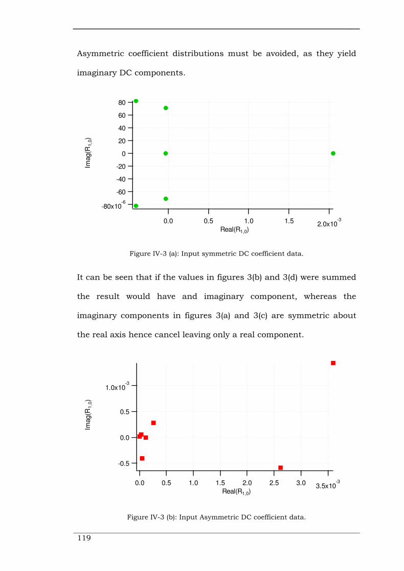
119
Asymmetric coefficient distributions must be avoided, as they yield
imaginary DC components.
Figure IV-3 (a): Input symmetric DC coefficient data.
It can be seen that if the values in figures 3(b) and 3(d) were summed
the result would have and imaginary component, whereas the
imaginary components in figures 3(a) and 3(c) are symmetric about
the real axis hence cancel leaving only a real component.
Figure IV-3 (b): Input Asymmetric DC coefficient data.
-80x10-6
-60
-40
-20
0
20
40
60
80
Imag(R
1,0
)
2.0x10-31.51.00.50.0
Real(R1,0)
1.0x10⁻³
0.5
0.0
-0.5
Imag(R
1,0
)
3.5x10-33.02.52.01.51.00.50.0
Real(R1,0)

Chapter V Chapter V Chapter V Chapter V ---- SourceSourceSourceSource---- and Loadand Loadand Loadand Load----Pull Behavioural Model AnalysisPull Behavioural Model AnalysisPull Behavioural Model AnalysisPull Behavioural Model Analysis
120
Figure IV-3 (c): Output symmetric DC coefficient data.
Figure IV-3 (d): Output Asymmetric DC coefficient data.
The same is true for the output cases and hence a phase coefficient
and its conjugate should always be added to the model formulation if
increased accuracy is required.
-6x10⁻³
-4
-2
0
2
4
6
Imag(R
1,0
)
0.100.080.060.040.020.00
Real(R1,0)
-10x10-3
-8
-6
-4
-2
0
2
4
Imag(R
1,0
)
0.100.080.060.040.020.00
Real(R1,0)
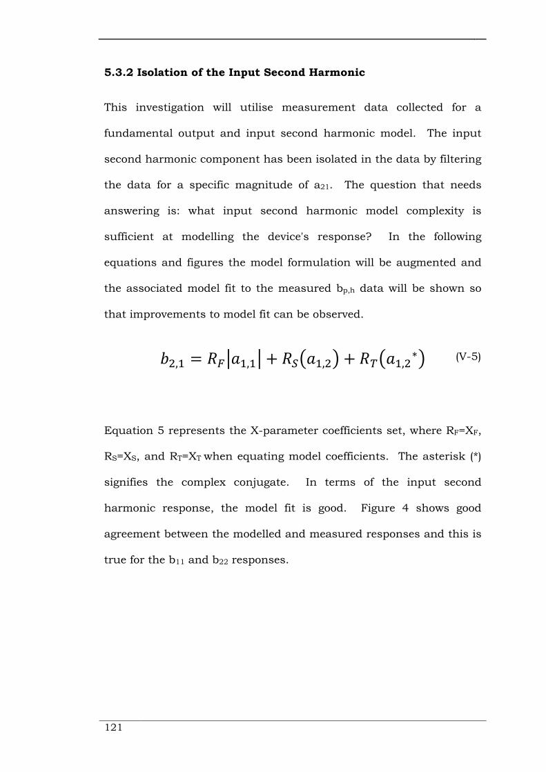
121
5.3.2 Isolation of the Input Second Harmonic
This investigation will utilise measurement data collected for a
fundamental output and input second harmonic model. The input
second harmonic component has been isolated in the data by filtering
the data for a specific magnitude of a21. The question that needs
answering is: what input second harmonic model complexity is
sufficient at modelling the device's response? In the following
equations and figures the model formulation will be augmented and
the associated model fit to the measured bp,h data will be shown so
that improvements to model fit can be observed.
Equation 5 represents the X-parameter coefficients set, where RF=XF,
RS=XS, and RT=XT when equating model coefficients. The asterisk (*)
signifies the complex conjugate. In terms of the input second
harmonic response, the model fit is good. Figure 4 shows good
agreement between the modelled and measured responses and this is
true for the b11 and b22 responses.
��,� = �[q��,�q + �U5��,�: + �W5��,�∗: (V-5)

Chapter V Chapter V Chapter V Chapter V ---- SourceSourceSourceSource---- and Loadand Loadand Loadand Load----Pull Behavioural Model AnalysisPull Behavioural Model AnalysisPull Behavioural Model AnalysisPull Behavioural Model Analysis
122
Figure IV-4: Measured versus modelled b12 responses from a set of harmonic
source- and load-pull measurements.
The b21 response, on the next page, does not present a good fit. In
Figure 5, the modelled response can be seen as elliptical and hence
typical of the type of nonlinearities expected to be modelled by an X-
parameter coefficient set. Augmentations to the model formulation
should result in the shape of the b21 measured data being better
described by the model.
-1.5
-1.0
-0.5
0.0
0.5
1.0
Imag (
V)
2.01.51.00.50.0-0.5
Real (V) Measured values of b12 Modelled values of b12
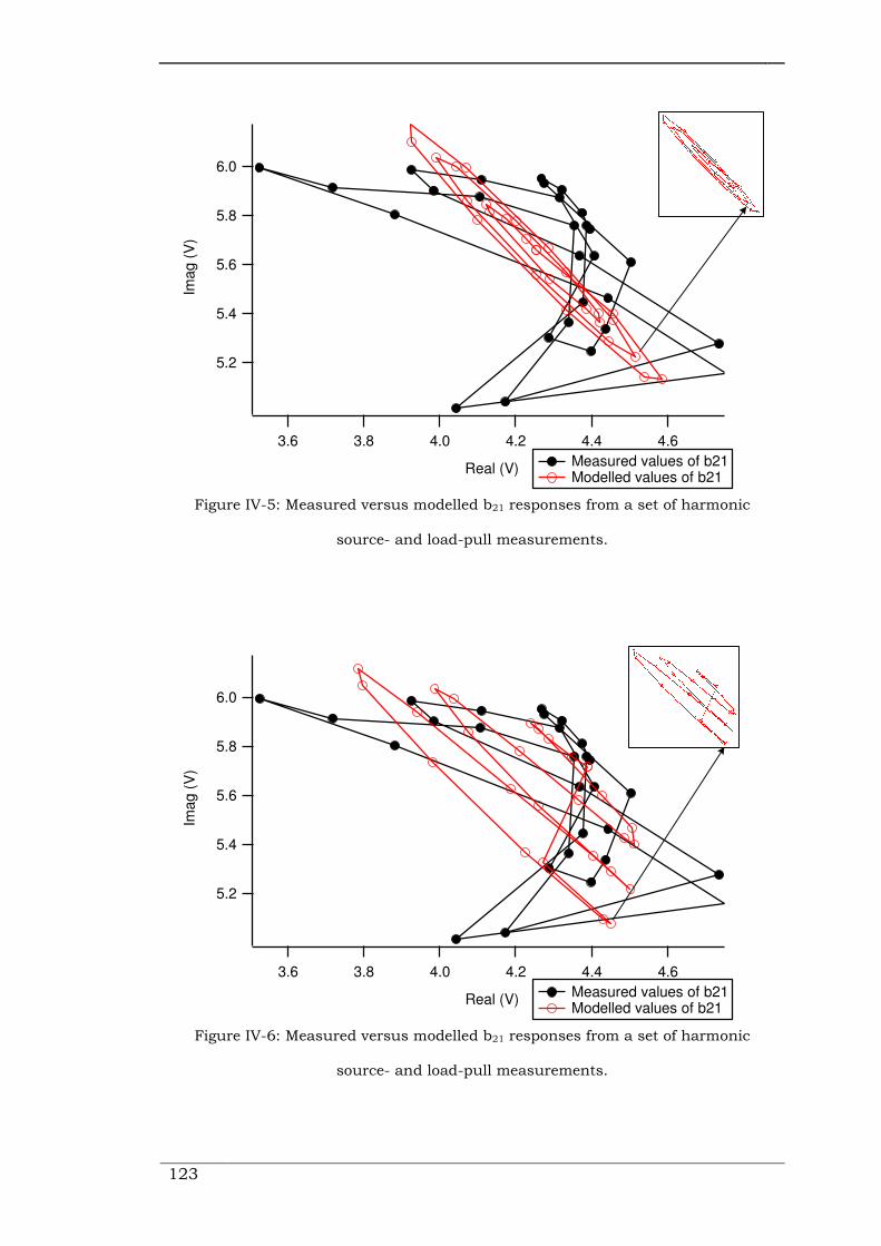
123
6.0
5.8
5.6
5.4
5.2
Imag (
V)
4.64.44.24.03.83.6
Real (V) Measured values of b21 Modelled values of b21
Figure IV-5: Measured versus modelled b21 responses from a set of harmonic
source- and load-pull measurements.
6.0
5.8
5.6
5.4
5.2
Imag (
V)
4.64.44.24.03.83.6
Real (V) Measured values of b21 Modelled values of b21
Figure IV-6: Measured versus modelled b21 responses from a set of harmonic
source- and load-pull measurements.
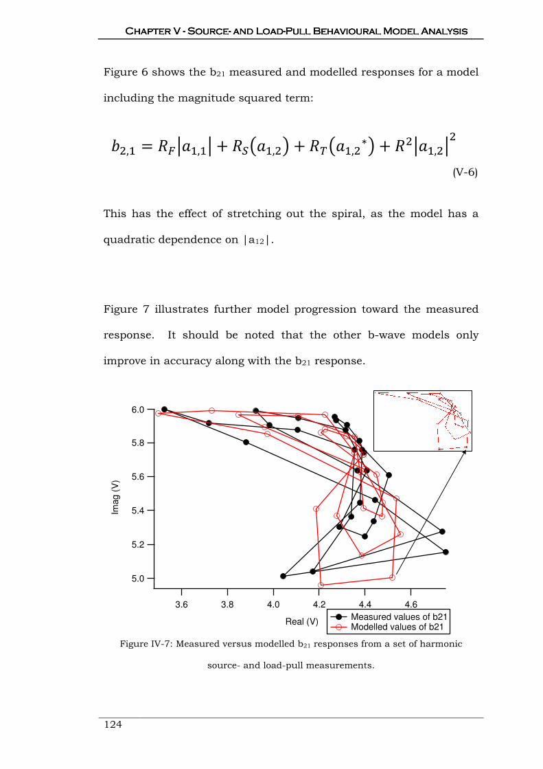
Chapter V Chapter V Chapter V Chapter V ---- SourceSourceSourceSource---- and Loadand Loadand Loadand Load----Pull Behavioural Model AnalysisPull Behavioural Model AnalysisPull Behavioural Model AnalysisPull Behavioural Model Analysis
124
Figure 6 shows the b21 measured and modelled responses for a model
including the magnitude squared term:
This has the effect of stretching out the spiral, as the model has a
quadratic dependence on |a12|.
Figure 7 illustrates further model progression toward the measured
response. It should be noted that the other b-wave models only
improve in accuracy along with the b21 response.
6.0
5.8
5.6
5.4
5.2
5.0
Imag (
V)
4.64.44.24.03.83.6
Real (V) Measured values of b21 Modelled values of b21
Figure IV-7: Measured versus modelled b21 responses from a set of harmonic
source- and load-pull measurements.
��,� = �[q��,�q + �U5��,�: + �W5��,�∗: + ��q��,�q� (V-6)
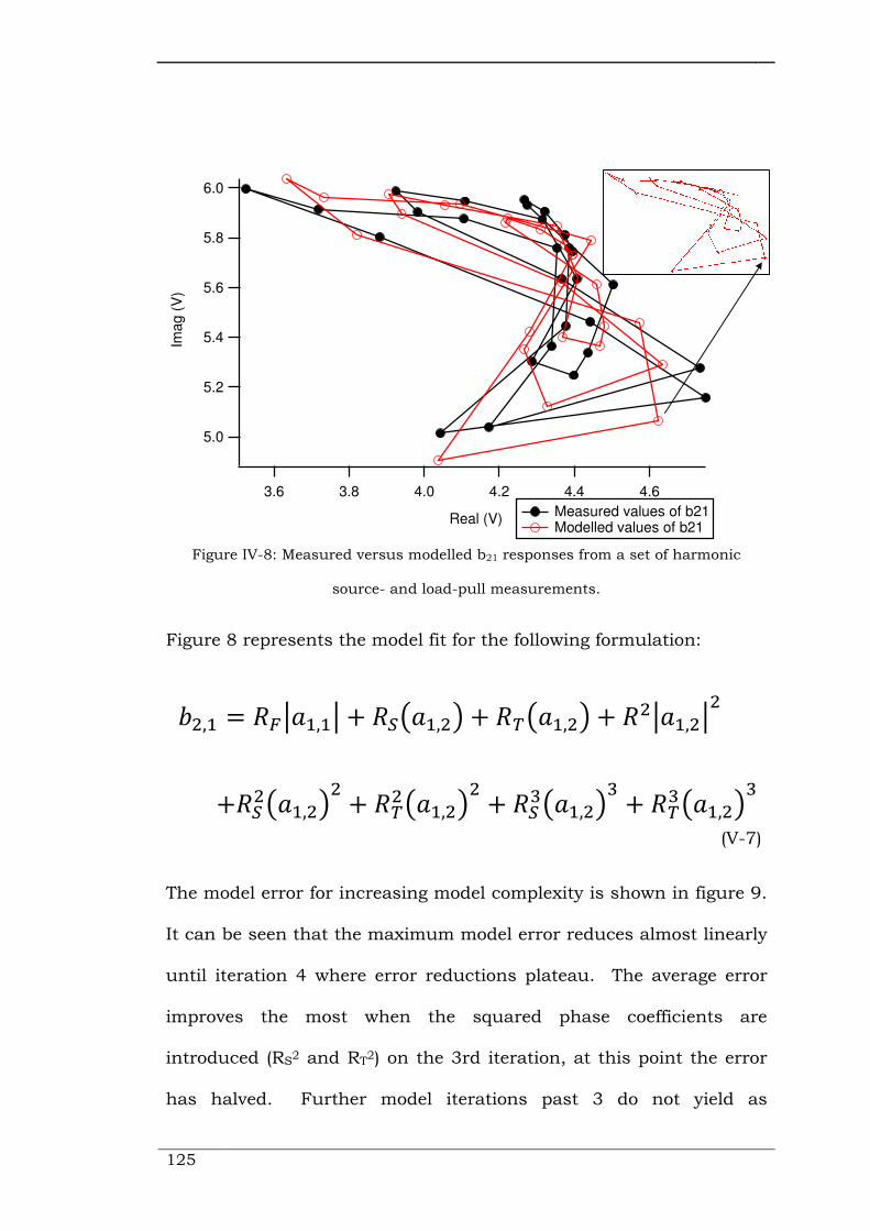
125
6.0
5.8
5.6
5.4
5.2
5.0
Imag (
V)
4.64.44.24.03.83.6
Real (V) Measured values of b21 Modelled values of b21
Figure IV-8: Measured versus modelled b21 responses from a set of harmonic
source- and load-pull measurements.
Figure 8 represents the model fit for the following formulation:
The model error for increasing model complexity is shown in figure 9.
It can be seen that the maximum model error reduces almost linearly
until iteration 4 where error reductions plateau. The average error
improves the most when the squared phase coefficients are
introduced (RS2 and RT
2) on the 3rd iteration, at this point the error
has halved. Further model iterations past 3 do not yield as
��,� = �[q��,�q + �U5��,�: + �W5��,�: + ��q��,�q�
+�U�5��,�:� + �W�5��,�:� + �U�5��,�:� + �W�5��,�:� (V-7)
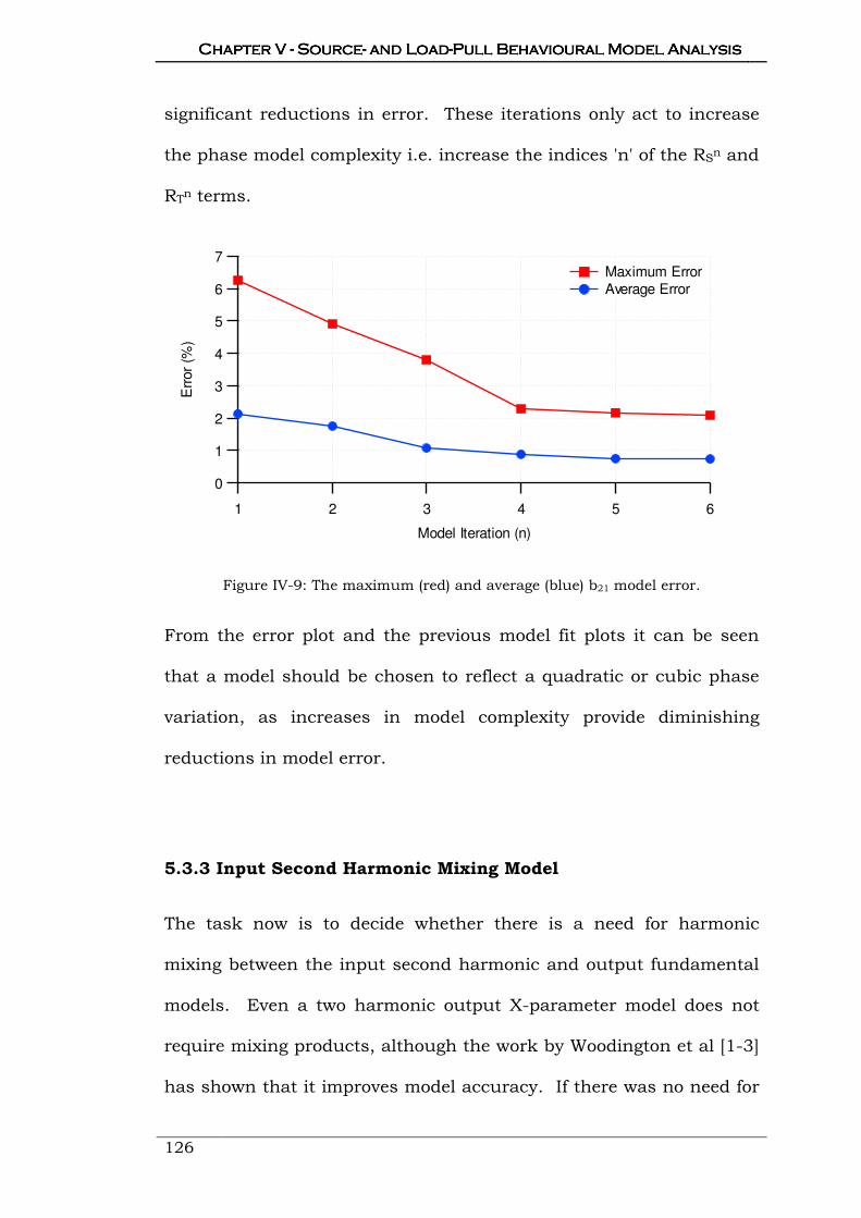
Chapter V Chapter V Chapter V Chapter V ---- SourceSourceSourceSource---- and Loadand Loadand Loadand Load----Pull Behavioural Model AnalysisPull Behavioural Model AnalysisPull Behavioural Model AnalysisPull Behavioural Model Analysis
126
significant reductions in error. These iterations only act to increase
the phase model complexity i.e. increase the indices 'n' of the RSn and
RTn terms.
Figure IV-9: The maximum (red) and average (blue) b21 model error.
From the error plot and the previous model fit plots it can be seen
that a model should be chosen to reflect a quadratic or cubic phase
variation, as increases in model complexity provide diminishing
reductions in model error.
5.3.3 Input Second Harmonic Mixing Model
The task now is to decide whether there is a need for harmonic
mixing between the input second harmonic and output fundamental
models. Even a two harmonic output X-parameter model does not
require mixing products, although the work by Woodington et al [1-3]
has shown that it improves model accuracy. If there was no need for
7
6
5
4
3
2
1
0
Err
or
(%)
654321
Model Iteration (n)
Maximum Error
Average Error

127
mixing it would improve the compactness of the model and hint that
further harmonic additions might also constitute coefficient addition.
The output fundamental model has been investigated in previous
work; therefore it suffices for this work to state that an output
fundamental that is quadratic in magnitude and phase was found to
model the fundamental b21 response correctly, to a confidence of
99.60% at the highest b12 power level.
Figure IV-10: The output fundamental and input second harmonic coefficient
space.
Figure 10 shows the coefficient distribution if the separate models for
the output fundamental and input second harmonic are added
together. With this distribution no mixing is taken into account,
-2
-1
0
1
2
Input S
econd
Harm
on
ic (
r)
-2 -1 0 1 2
Output Fundamental (n)

Chapter V Chapter V Chapter V Chapter V ---- SourceSourceSourceSource---- and Loadand Loadand Loadand Load----Pull Behavioural Model AnalysisPull Behavioural Model AnalysisPull Behavioural Model AnalysisPull Behavioural Model Analysis
128
therefore its ability to model the data can be analysed. There are
actually 11 coefficients in the figure. Two are not visible as they
stack at the (0,0) location. These terms are the ones concerning the
quadratic variation with the magnitudes of a12 and a21, therefore have
no phase component and can only reside at the (0,0) location.
Measured output F0 Load
Modeled output F0 Load
Measured output 2F0 Load
Modeled output 2F0 Load
Figure IV-11: The output fundamental (red) and second harmonic (blue) load space.
Figure 11 shows the measured output fundamental and second
harmonic loads overlaid with the modelled loads. This figure shows
fair agreement of the fundamental loads at low mismatches; however
this becomes worse for larger mismatched conditions.
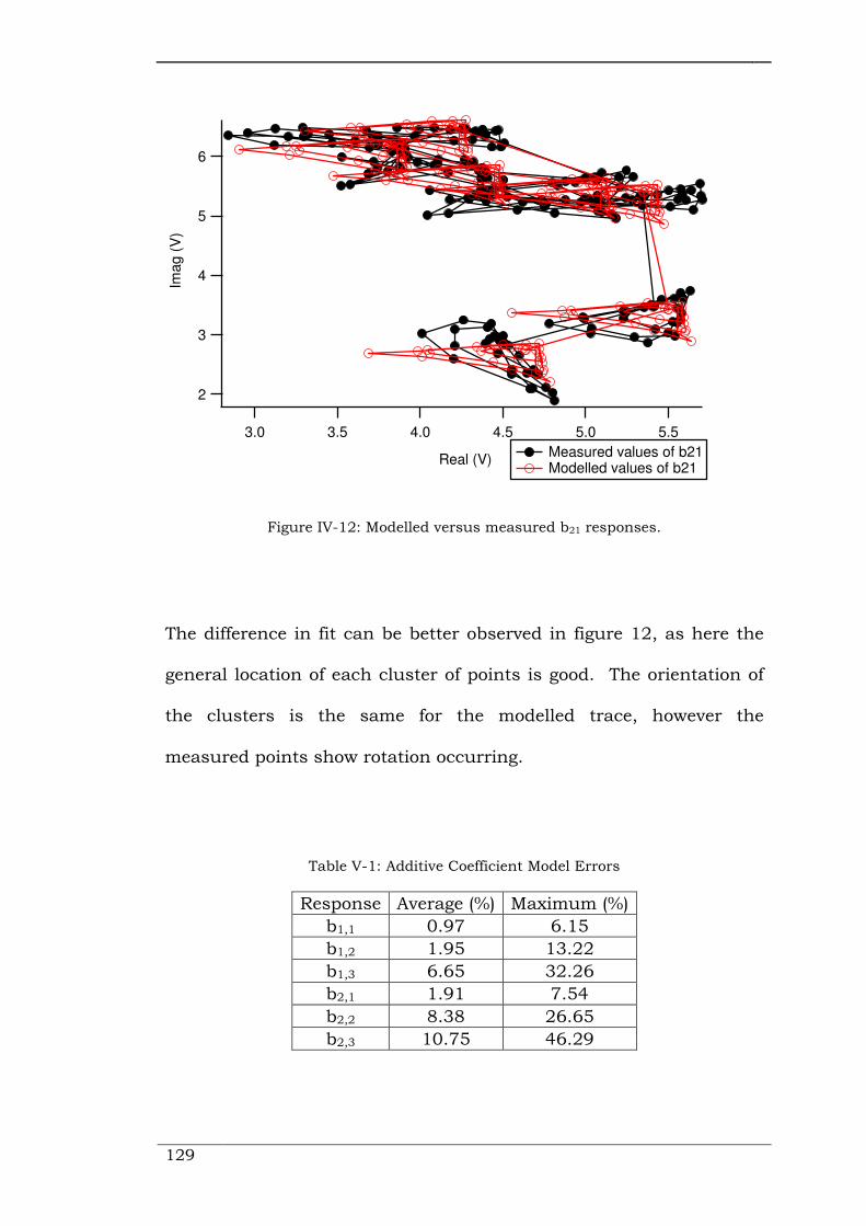
129
Figure IV-12: Modelled versus measured b21 responses.
The difference in fit can be better observed in figure 12, as here the
general location of each cluster of points is good. The orientation of
the clusters is the same for the modelled trace, however the
measured points show rotation occurring.
Table V-1: Additive Coefficient Model Errors
Response Average (%) Maximum (%)
b1,1 0.97 6.15
b1,2 1.95 13.22
b1,3 6.65 32.26
b2,1 1.91 7.54
b2,2 8.38 26.65
b2,3 10.75 46.29
6
5
4
3
2
Imag (
V)
5.55.04.54.03.53.0
Real (V) Measured values of b21 Modelled values of b21
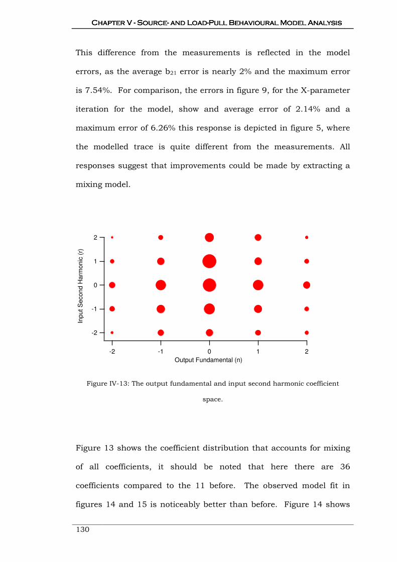
Chapter V Chapter V Chapter V Chapter V ---- SourceSourceSourceSource---- and Loadand Loadand Loadand Load----Pull Behavioural Model AnalysisPull Behavioural Model AnalysisPull Behavioural Model AnalysisPull Behavioural Model Analysis
130
This difference from the measurements is reflected in the model
errors, as the average b21 error is nearly 2% and the maximum error
is 7.54%. For comparison, the errors in figure 9, for the X-parameter
iteration for the model, show and average error of 2.14% and a
maximum error of 6.26% this response is depicted in figure 5, where
the modelled trace is quite different from the measurements. All
responses suggest that improvements could be made by extracting a
mixing model.
Figure IV-13: The output fundamental and input second harmonic coefficient
space.
Figure 13 shows the coefficient distribution that accounts for mixing
of all coefficients, it should be noted that here there are 36
coefficients compared to the 11 before. The observed model fit in
figures 14 and 15 is noticeably better than before. Figure 14 shows
-2
-1
0
1
2
Input S
econd H
arm
onic
(r)
-2 -1 0 1 2
Output Fundamental (n)

131
improved impedance comparison and figure 15 shows that now the
rotation of the point clusters has been described by the model.
When comparing figures 12 and 15 it should be clear that correct
point cluster orientation was what was going to arise from mixing the
coefficient sets. Since both the shapes of the individual b1,2 and b2,1
responses had been modelled by their respective model coefficients;
the missing element was orientation or rotation.
Measured output F0 Load
Modeled output F0 Load
Measured output 2F0 Load
Modeled output 2F0 Load
Figure IV-14: The output fundamental and second harmonic load space.

Chapter V Chapter V Chapter V Chapter V ---- SourceSourceSourceSource---- and Loadand Loadand Loadand Load----Pull Behavioural Model AnalysisPull Behavioural Model AnalysisPull Behavioural Model AnalysisPull Behavioural Model Analysis
132
Figure IV-15: Modelled versus measured b21 responses.
Table V-2: Mixing Coefficient Model Errors
Response Average (%) Maximum (%)
b1,1 0.26 1.03
b1,2 0.55 2.12
b1,3 1.76 7.27
b2,1 0.59 4.48
b2,2 2.43 16.38
b2,3 2.43 11.65
Table 2 shows good improvements in all of the harmonic responses,
particularly the reduction of all the maximum errors from table 1.
However, although the model fit is good the downside to modelling
like this is the number of coefficients needed. Gains in model
accuracy are achieved when going from the coefficient distribution
shown in figure 10, of 11 coefficients, to the one in figure 13, with 36
6
5
4
3
2
Imag (
V)
5.55.04.54.03.53.0
Real (V) Measured values of b21 Modelled values of b21

133
coefficients. Therefore, these accuracy gains are not wholly bolstered
by the increase in model complexity, as ultimately an increase in
model complexity produces an increase in model file size. If the
desired model is to cover sets of bias, frequency, and power data an
increase in model complexity will be multiplied by the amount of
measurements in the bias, frequency, and power data when it comes
to the file size. When viewed from this perspective it can be seen that
the application to which the model is being used is also key in
determining the complexity of the model. Therefore, it is not
recommended that full mixing of coefficients be performed for models
measured over many harmonics for multiple operation levels. In
these cases mixing truncation can be performed on high order mixing
terms to reduce the overall amount of coefficients needed whilst
preserving model accuracy.
5.3.4 Higher Harmonic Mixing
There are observable matches between measured and modelled data
sets in the above case when mixing was taken into account.
However, it is hoped that higher harmonic mixing products can be
ignored since this would result in a more compact model file for three
or more harmonic models. To investigate higher harmonic model
interactions extensive measurements were performed with fixed bias,
frequency, drive power, and a21; perturbations were made with a12
and a21.

Chapter V Chapter V Chapter V Chapter V ---- SourceSourceSourceSource---- and Loadand Loadand Loadand Load----Pull Behavioural Model AnalysisPull Behavioural Model AnalysisPull Behavioural Model AnalysisPull Behavioural Model Analysis
134
Figure IV-16: The a2,2 stimulus points at 18GHz in the complex plane.
Both a12 and a21 spirals were offset towards a short circuit as this is
where best efficiency can be achieved, hence is the most important
impedance area. Figure 16 shows the a2,2 spiral and is representative
of all the perturbation grids in this chapter. A spiral similar to figure
16 was also use for the a1,2 perturbations.
By isolating the a1,2 and a2,1 signals and creating models for them
separately, it was found that both could be modelled by a coefficient
distribution that was quadratic in phase. The mixed coefficient
distribution is shown in figure 17.
0.15
0.10
0.05
0.00
-0.05
-0.10
Ima
g (
V)
0.150.100.050.00-0.05-0.10
Real (V)
Centre of spiral
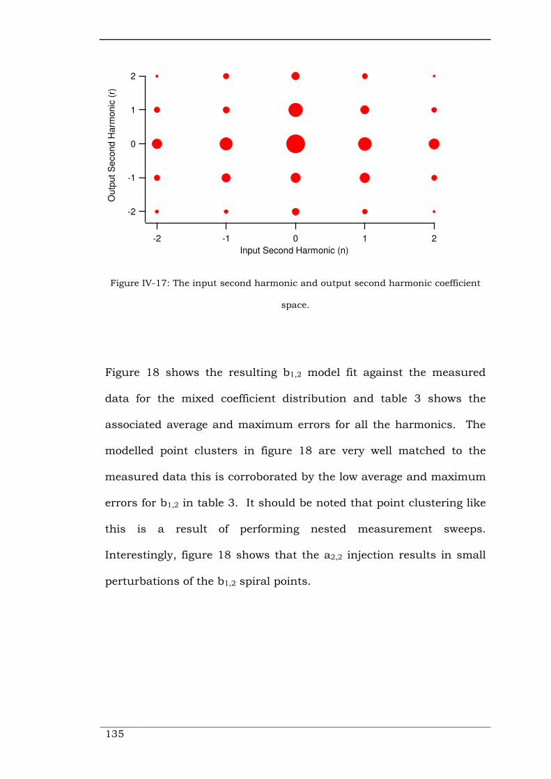
135
Figure IV-17: The input second harmonic and output second harmonic coefficient
space.
Figure 18 shows the resulting b1,2 model fit against the measured
data for the mixed coefficient distribution and table 3 shows the
associated average and maximum errors for all the harmonics. The
modelled point clusters in figure 18 are very well matched to the
measured data this is corroborated by the low average and maximum
errors for b1,2 in table 3. It should be noted that point clustering like
this is a result of performing nested measurement sweeps.
Interestingly, figure 18 shows that the a2,2 injection results in small
perturbations of the b1,2 spiral points.
-2
-1
0
1
2
Outp
ut S
econd
Harm
onic
(r)
-2 -1 0 1 2
Input Second Harmonic (n)

Chapter V Chapter V Chapter V Chapter V ---- SourceSourceSourceSource---- and Loadand Loadand Loadand Load----Pull Behavioural Model AnalysisPull Behavioural Model AnalysisPull Behavioural Model AnalysisPull Behavioural Model Analysis
136
Figure IV-18: The b1,2 modelled versus measured responses.
TABLE V-3: Mixing Model Errors
Response Average (%) Maximum (%)
b1,1 0.56 2.26
b1,2 0.68 2.77
b1,3 2.45 8.71
b2,1 0.31 1.08
b2,2 2.60 10.41
b2,3 2.01 8.84
Figure 19 shows the b1,2 fit for the additive coefficient distribution. It
is obvious here that the two harmonics cannot just be treated
separately, therefore the mixing rationale holds. The large average
and maximum errors are not satisfactory and so modelling with an
additive coefficient distribution resulted in a skewed model fit.
2
1
0
-1
-2
Imag (
V)
210-1
Real (V) Measured values of b12 Modelled values of b12

137
Figure IV-19: The b1,2 modelled versus measured responses.
TABLE V-4: Additive Model Errors
Response Average (%) Maximum (%)
b1,1 84.84 94.07
b1,2 27.24 42.68
b1,3 15.73 38.17
b2,1 84.81 90.54
b2,2 37.73 108.00
b2,3 76.16 105.59
Table 4 shows the errors for the harmonics and, as expected, all
other harmonics corroborate the bad model fit that is displayed in
figure 19.
2
1
0
-1
-2
Imag (
V)
3210-1
Real (V) Measured values of b12 Modelled values of b12
Chapter V Chapter V Chapter V Chapter V ---- SourceSourceSourceSource---- and Loadand Loadand Loadand Load----Pull Behavioural Model AnalysisPull Behavioural Model AnalysisPull Behavioural Model AnalysisPull Behavioural Model Analysis
138
If the model interactions between the output fundamental and input
second harmonic, and the input second harmonic and output second
harmonic are compared, it can be seen that the output second
harmonic is more sensitive to variations of the input second
harmonic. It is suggested that this relationship will also extend to
higher harmonics, where ultimately there is probably little interaction
with the input and output nth harmonics and the fundamental but
large interaction between the input and output nth harmonics. In
terms of coefficient distributions this would suggest that the
fundamental and nth harmonic interactions would be characterised
by additive coefficient distributions and nth harmonic interactions
would need mixing coefficient distributions for them to be modelled
accurately.
5.4 OVER DETERMINATION OF HARMONIC AND DC DATA
The models created up to this point have treated all the harmonics
the same. Therefore, if a mixing model, between the fundamental
output and input second harmonics, required 36 coefficients to
correctly describe the mixing and nonlinearities then those
coefficients were used to model DC as well. The issue here is that the
unrelated harmonics, in terms of mixing, may not need such
complexities in order to be modelled correctly. The reduction in total
coefficients will also reduce the model file size, which is a nice by-
product.

139
There are two ways to re-determine the separate harmonic model
coefficients. The first would be to simply truncate the existing
determination of the model by replacing the least important
coefficient results by zero. The second would be to truncate the
coefficients before their calculation and then recalculate the specific,
changed, harmonic models according to the new coefficients.
To compare the two methods, using isolated measurement data from
the previous section, an input second harmonic spiral of data points
will be modelled; firstly, by the truncation method, and then by the
recalculation method. The model errors can then be compared
against each other and the errors of a six coefficient model. The level
to which the DC and third harmonic components will be truncated
represents the maximum recommended truncation. The DC
components (b1,0 and b2,0) will be modelled by only one coefficient and
the third harmonic components will be modelled by the X-parameter
coefficient set. The measurement data being used is for an output
fundamental and input second harmonic model; the input second
harmonic response has been isolated for the test. This means that
truncations and recalculations should be performed on the DC and
third harmonic components, as these have weakest correlation to the
measurements that were performed.
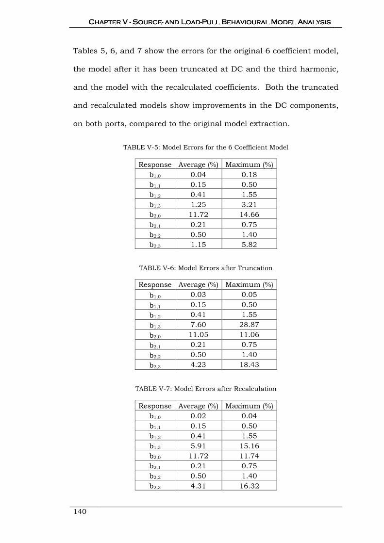
Chapter V Chapter V Chapter V Chapter V ---- SourceSourceSourceSource---- and Loadand Loadand Loadand Load----Pull Behavioural Model AnalysisPull Behavioural Model AnalysisPull Behavioural Model AnalysisPull Behavioural Model Analysis
140
Tables 5, 6, and 7 show the errors for the original 6 coefficient model,
the model after it has been truncated at DC and the third harmonic,
and the model with the recalculated coefficients. Both the truncated
and recalculated models show improvements in the DC components,
on both ports, compared to the original model extraction.
TABLE V-5: Model Errors for the 6 Coefficient Model
Response Average (%) Maximum (%)
b1,0 0.04 0.18
b1,1 0.15 0.50
b1,2 0.41 1.55
b1,3 1.25 3.21
b2,0 11.72 14.66
b2,1 0.21 0.75
b2,2 0.50 1.40
b2,3 1.15 5.82
TABLE V-6: Model Errors after Truncation
Response Average (%) Maximum (%)
b1,0 0.03 0.05
b1,1 0.15 0.50
b1,2 0.41 1.55
b1,3 7.60 28.87
b2,0 11.05 11.06
b2,1 0.21 0.75
b2,2 0.50 1.40
b2,3 4.23 18.43
TABLE V-7: Model Errors after Recalculation
Response Average (%) Maximum (%)
b1,0 0.02 0.04
b1,1 0.15 0.50
b1,2 0.41 1.55
b1,3 5.91 15.16
b2,0 11.72 11.74
b2,1 0.21 0.75
b2,2 0.50 1.40
b2,3 4.31 16.32

141
The b1,3 and b2,3 errors are clearly worse after truncation and
recalculation, however, the average errors are both under 10% and
since there was no effort to control the third harmonic this error
would not constitute to huge differences between modelled and
measured I-V waveforms. Large maximum errors in the uncontrolled
harmonics usually arise from trying to model noise not very well,
therefore, differences in these values constitutes a difference in the
model's ability to model the smallest ap,h in the dataset. The
difference between the truncated and recalculated average errors,
although small, shows that the over determined model does a good
job of modelling the RF, RS, and RT components for DC and the third
harmonic respectively. However, if it is necessary to preserve
accuracy then the recalculation method is suggested.
The same principles can be applied to mixing models with the
potential of producing less error in the uncontrolled model responses.
This is by virtue of the little importance higher order terms have in
the power series, unless harmonics interactions are strong, therefore
removing them would do little to model errors.
5.5 HF AMPLIFIER DESIGN AND MEASUREMENT IMPLICATIONS
The source- and load-pull measurements thus produced an
improved model implementation within CAD, that allow for detailed
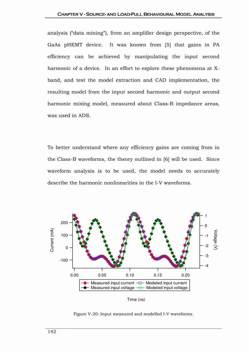
Chapter V Chapter V Chapter V Chapter V ---- SourceSourceSourceSource---- and Loadand Loadand Loadand Load----Pull Behavioural Model AnalysisPull Behavioural Model AnalysisPull Behavioural Model AnalysisPull Behavioural Model Analysis
142
analysis (“data mining”), from an amplifier design perspective, of the
GaAs pHEMT device. It was known from [5] that gains in PA
efficiency can be achieved by manipulating the input second
harmonic of a device. In an effort to explore these phenomena at X-
band, and test the model extraction and CAD implementation, the
resulting model from the input second harmonic and output second
harmonic mixing model, measured about Class-B impedance areas,
was used in ADS.
To better understand where any efficiency gains are coming from in
the Class-B waveforms, the theory outlined in [6] will be used. Since
waveform analysis is to be used, the model needs to accurately
describe the harmonic nonlinearities in the I-V waveforms.
Figure V-20: Input measured and modelled I-V waveforms.
-4
-3
-2
-1
0
1
Vo
ltag
e (V
)
0.200.150.100.050.00
Time (ns)
200
100
0
-100
Cu
rre
nt (m
A)
Measured input current Modeled input current Measured input voltage Modeled input voltage

143
Figure V-21: Output measured and modelled I-V waveforms.
Figures 20 and 21 show a single input and output current and
voltage waveform instance of the measurement results with the
modelled waveforms overlaid. In both traces the modelled waveforms
are almost exact replicas of the measurements, which were the case
for all instances of measured waveforms, thus validating the models
capability of replicating measured waveforms.
The measurements alone were not positioned well enough to analyse
certain conditions that arise when manipulating the input second
harmonic about its short circuit point. The conditions in question
were an extrinsic input second harmonic short circuit, an intrinsic
input second harmonic short circuit, and input second harmonic
impedance that would half rectify the input voltage at the intrinsic
14
12
10
8
6
4
2
0
Volta
ge (V
)
0.200.150.100.050.00
Time (ns)
200
150
100
50
0
Curr
en
t (m
A)
Measured output current Modeled output current Measured output voltage Modeled output voltage
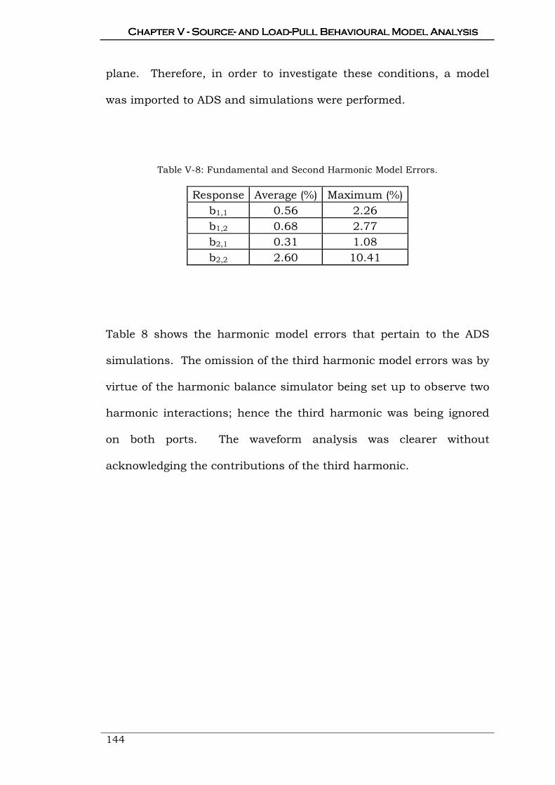
Chapter V Chapter V Chapter V Chapter V ---- SourceSourceSourceSource---- and Loadand Loadand Loadand Load----Pull Behavioural Model AnalysisPull Behavioural Model AnalysisPull Behavioural Model AnalysisPull Behavioural Model Analysis
144
plane. Therefore, in order to investigate these conditions, a model
was imported to ADS and simulations were performed.
Table V-8: Fundamental and Second Harmonic Model Errors.
Response Average (%) Maximum (%)
b1,1 0.56 2.26
b1,2 0.68 2.77
b2,1 0.31 1.08
b2,2 2.60 10.41
Table 8 shows the harmonic model errors that pertain to the ADS
simulations. The omission of the third harmonic model errors was by
virtue of the harmonic balance simulator being set up to observe two
harmonic interactions; hence the third harmonic was being ignored
on both ports. The waveform analysis was clearer without
acknowledging the contributions of the third harmonic.

145
Curre
nt (A
)
Time (psec)
Voltag
e (
V)
Intrinsic Short Voltage Intrinsic Short Current Extrinsic Short Voltage Extrinsic Short Current Half Rec. Voltage Half Rec. Current
Figure V-22: The simulated de-embedded input I-V waveforms.
Time (psec)
Cu
rren
t (A) V
oltag
e (
V)
Intrinsic Short Voltage Intrinsic Short Current Extrinsic Short Voltage Extrinsic Short Current Half Rec. Voltage Half Rec. Current
Figure V-23: The simulated de-embedded output I-V waveforms.
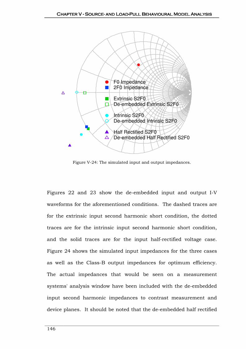
Chapter V Chapter V Chapter V Chapter V ---- SourceSourceSourceSource---- and Loadand Loadand Loadand Load----Pull Behavioural Model AnalysisPull Behavioural Model AnalysisPull Behavioural Model AnalysisPull Behavioural Model Analysis
146
F0 Impedance 2F0 Impedance
Extrinsic S2F0 De-embedded Extrinsic S2F0
Intrinsic S2F0 De-embedded Intrinsic S2F0
Half Rectified S2F0 De-embedded Half Rectified S2F0
Figure V-24: The simulated input and output impedances.
Figures 22 and 23 show the de-embedded input and output I-V
waveforms for the aforementioned conditions. The dashed traces are
for the extrinsic input second harmonic short condition, the dotted
traces are for the intrinsic input second harmonic short condition,
and the solid traces are for the input half-rectified voltage case.
Figure 24 shows the simulated input impedances for the three cases
as well as the Class-B output impedances for optimum efficiency.
The actual impedances that would be seen on a measurement
systems' analysis window have been included with the de-embedded
input second harmonic impedances to contrast measurement and
device planes. It should be noted that the de-embedded half rectified

147
input second harmonic reflection coefficient was -1.23-j0.009 to
achieve the desired input voltage waveform shape.
The three conditions' respective drain efficiencies are 77.31%,
78.72%, and 73.35%. This shows that of the three conditions, the
intrinsic short circuit is the best for drain efficiency and that device
robustness improvements can be made, by half rectifying the input
voltage waveform and reducing the voltage swing, without
compromising too much in efficiency. The output power range for the
three cases was 25dBm ±0.5dBm.
The intrinsic output waveforms look very similar to ideal Class-B
output waveforms. The other cases' variations away from the ideal
are reflected in the loss in drain efficiency. It should be noted that
theses waveforms cannot be obtained under normal load-pull
conditions, with the input second harmonic at 50Ohms, therefore one
would not be able to observe efficiencies from devices measured at X-
band that are in accord with the theoretical predictions without
source-pull. Implementing an input second harmonic short circuit
via a stub on a test MMIC (Monolithic Microwave Integrated Circuit)
structure would be a way to aid measurement, for future output
investigations, and would enable three harmonic load-pull by
releasing a source. In the future it would be good to perform

Chapter V Chapter V Chapter V Chapter V ---- SourceSourceSourceSource---- and Loadand Loadand Loadand Load----Pull Behavioural Model AnalysisPull Behavioural Model AnalysisPull Behavioural Model AnalysisPull Behavioural Model Analysis
148
investigations into the breakdown of ideal Class-B waveforms as the
operation frequency is increased and how to combat it with input
second harmonic impedance tuning.
5.6 SUMMARY
This chapter has detailed the rationale behind conducted model
measurements, the model extraction, and model filtering or
truncation. The measurement of the models needed to be addressed
since fundamental analysis about the created model’s relationships
to the model order had been performed in earlier work. This allowed
for magnitude and phase variance in the measurements of the model.
The corollary of this is that spirals, instead of offset circles, could be
used. This measurement approach reduces the total number of
measurements needed to cover an impedance area of interest for a
particular harmonic. The measurement reductions, i.e. time
reductions, for model sweeps over many harmonics are
multiplicative, which is favourable for the generation of model for
more complex data.
In order for there to be proper analysis of the input second harmonic
models, there was an issue concerning model formula augmentations
that had not previously been addressed that needed to be
investigated. In previous work, asymmetric coefficient distributions
149
were allowed when gains to mode accuracy were sufficient. However,
no comparison of what happened at DC, with symmetric and
asymmetric coefficient distributions, was performed. The data clearly
shows that, at both the input and output ports, asymmetric model
coefficient distributions lead to non-cancelling imaginary components
at DC, whereas the imaginary components at DC produced by
symmetric coefficient distributions were complex conjugates and
therefore cancelled.
The characterization of the input second harmonic model from
measurement data obtained from a GaAs pHEMT was performed, at
first, with it in isolation and then model mixing phenomena were
assayed. The comparison of the input second harmonic model's
minimum and maximum errors showed that a plateau in error
reductions at around the 3rd or 4th model formula expansion. These
constituted models, describing the response of the input second
harmonic, with a quadratic dependency in magnitude and a
quadratic (3rd expansion) or cubic (4th expansion) dependency in
phase. Due to the gains in average model error being more important
than gains in maximum model error, and having a tendency toward
models with reduced complexity, the input second harmonic model
was created with a quadratic phase dependency.
Chapter V Chapter V Chapter V Chapter V ---- SourceSourceSourceSource---- and Loadand Loadand Loadand Load----Pull Behavioural Model AnalysisPull Behavioural Model AnalysisPull Behavioural Model AnalysisPull Behavioural Model Analysis
150
Input second harmonic and output harmonic mixing was, at first,
hoped to be negligible. The results from testing a model with additive
harmonic coefficients, for the input second and output fundamental,
did not reflect this initial hope. The shape of the b2,1 response in
figure 12, in terms of the output fundamental model, was good. The
point clusters in the response, defined by the input second harmonic
model, were good too. However, they were misaligned and did not
exhibit similar rotation to the measured b2,1 response. A full mixing
model was created and the model fit was observably better, however,
the gains in model complexity were not bolstered by the reductions in
model error. As such, it would be acceptable to perform some
filtering on the fully mixed model, keeping a symmetric coefficient
distribution, as a compromised solution preserving model accuracy
without overly increasing model complexity.
The investigations into model mixing phenomena between the input
and output second harmonic components yielded a similar result as
above. The additive coefficient model manifested a shift in the b1,2
trace that was clearly rectified by the introduction of a fully mixed
model. In this case, the average model errors for the b1,2 and b2,2
responses were improved by over a factor of ten. There was a clearly
indicated sensitivity between harmonic components at the same
frequency, whereas fundamental sensitivities were comparably less.

151
The over determination of harmonic and DC data occurs every time a
model is created. This is because, until now, there has been no
truncation applied to the model. The truncation method was divided
into two: first, unnecessary coefficients could be replaced by zeros;
second, the harmonic models could be recalculated at the desired
model order then the removed coefficients could be padded with zeros
after calculation. Comparison between original, truncated, and
recalculated model errors showed that the DC component errors
improved for both truncations however the third harmonic
component errors worsened. The increase in third harmonic errors
was not necessarily a significant issue due to the third harmonic, in
this case being very small, hence exhibiting minimal effects on the I-V
responses. However, behavioural models for amplifier modes that
clearly utilize the third harmonic would not have this truncation
performed. The effects of the truncations would be less for mixing
model cases due to coefficients, representing high orders of non-
linearity, and mixing at uncontrolled harmonic components, having
ever decreasing effects on the I-V responses.
The position, on the Smith Chart, of the model measurements
allowed for more than just model analysis to be performed.
Simulation of three input second harmonic impedance cases, with
optimum Class-B output load impedances, was undertaken to
investigate improvements of drain efficiency, and to exercise the

Chapter V Chapter V Chapter V Chapter V ---- SourceSourceSourceSource---- and Loadand Loadand Loadand Load----Pull Behavioural Model AnalysisPull Behavioural Model AnalysisPull Behavioural Model AnalysisPull Behavioural Model Analysis
152
dynamic CAD implementation. To be able to analyse the I-V
waveforms, it was found that removing the third harmonic
component unveiled waveforms close to theory. The comparison of
the drain efficiencies showed that and intrinsic short circuit produced
the best drain efficiency, 78.72%, and that only small reductions in
efficiency would occur if the input voltage waveform was half-rectified
to improve device robustness. The measurement implications, of
measuring in a 50Ohm system rather than shorting the input second
harmonic, were made apparent, as it would be impossible to recreate
waveforms observed at lower frequencies. The results obtained
represent state of the art X-band performance comparable with device
performance at lower frequencies and are only obtainable through
input waveform engineering. Therefore future measurements would
require a shorted input second harmonic component either by
source-pull or by the fabrication of an appropriate MMIC test
structure.
5.7 REFERENCES
[1] S. Woodington et al, "A Novel Measurement based Method
Enabling Rapid Extraction of a RF Waveform Look-Up Table Based
Behavioural Model," IEEE MTT-S International. Pg 1453-1456.
Jun 2008.
153
[2] S. Woodington et al, "Behavioural Model Analysis of Active
Harmonic Load-Pull Measurements," IEEE MTT-S International. Pg
1688-1691. May 2010.
[3] S. Woodington, "Behavioural Model Analysis of Active Harmonic
Load-Pull Measurements," Doctoral thesis submitted to Cardiff
University. 2012.
[4] R. S. Saini, "Intelligence Driven Load-pull Measurement Strategies,"
A Doctoral Thesis submitted to Cardiff University. 2013.
[5] P. Colantonio, F. Giannini, E. Limiti and V. Teppati, "An Approach
to Harmonic Load- and Source-Pull Measurements at X-Band," IEEE
Transactions on Microwave Theory and Techniques, Vol. 52, No 1,
Jan. 2004.
[6] S. Cripps, "RF Power Amplifiers for Wireless Communications,"
Norwood, MA: Artech House, 1999.

Chapter VI Chapter VI Chapter VI Chapter VI ---- Conclusions and Future WorkConclusions and Future WorkConclusions and Future WorkConclusions and Future Work
154
Chapter Chapter Chapter Chapter VIVIVIVI
Conclusions and Future Conclusions and Future Conclusions and Future Conclusions and Future
WorkWorkWorkWork
he work presented in this thesis has covered the processes
involved in a measurement-to-CAD modelling cycle, whilst also
providing key analysis of input and output harmonic model
interactions. Although the past and present modelling techniques,
from S-parameters to the Cardiff Model, are unquestionably linked,
the Cardiff Model has its place at the forefront of current behavioural
modelling trends. This thesis has realised behavioural models that
consider the interactions between the input and output harmonics,
and outlined the necessary framework in order to develop and
augment said models. The development of the measurement system
and improvements to past model implementations have been
included to show the necessary steps for the measurement and
simulation of input and output harmonic models. Without a
developed measurement platform and dynamic model implementation
T

155
in CAD, measurement and analysis of the mixing models would not
have been possible.
6.1 CONCLUSIONS
The investigations into input second harmonic modelling and the
model's interactions with output harmonic models have conveyed its
limits and have shown that the modelling process is application
specific. Each chapter has had its conclusions raised and here they
will be highlighted.
Chapter III details the design of a coherent carrier system. In the
testing phase it was observed that upon measurement of some points
in a multi-harmonic grid, the PSG attached to port 4 of the system
became unlocked. This was, in part, due to the variation of the
internal workings of the HCC options across the PSGs, and variation
in the carrier distribution system's cable attenuation, but mainly due
to a non-ideal input power to one of the system PAs. The problem
was rectified by reducing the attenuation at the input of the system
by 1dB. The coherent carrier distribution system overcame the
frequency selectivity of the previous implementation and allowed for
the first time harmonic load-pull measurements to be performed at X-
band. Although the coherent carrier distribution system was fit for
purpose future measurement system augmentations would not be

Chapter VI Chapter VI Chapter VI Chapter VI ---- Conclusions and Future WorkConclusions and Future WorkConclusions and Future WorkConclusions and Future Work
156
accommodated. This setback promotes VNA measurement solutions
where four port (source) analysers are standard.
Chapter IV outlines the procedure taken to improve the CAD
implementation of the Cardiff Model. Although the fundamental
components in ADS, the FDD and DAC component, have not changed
the formulaic and function structure has been transformed a lot. The
implementation now uses the simple matrix equation [B] = [R] x [A] to
calculate the system response for any type of model or harmonic
complexity. To be able to use such a simple formula, the schematic
needs to be populated by an AEL script run from the command line
window within ADS. This implementation has significantly improved
the model implementation's usability, whilst also overcoming the
challenges of dealing with different model complexities.
Chapter V addresses augmentations to the model formulation, from
which it is clear that additions to the formulation must consist of a
model parameter and it's conjugate. Furthermore the chapter clearly
highlights saturation of model accuracy for the addition of
parameters that imply higher than cubic phase dependency.
Therefore a model with cubic phase dependency is considered the
most complex model that would be necessary for an isolated
measurement harmonic. The analysis of mixing models has shown
157
that they are beneficial for input second harmonic mixing with both
the output fundamental and output second harmonic. However,
despite the gains in model accuracy, filtering of the coefficient
distributions would be necessary for more complex measurement
scenarios, for example: the measurement of the Class-F amplifier
mode. The filtering would be necessary to reduce mode file size,
which ultimately will help the simulator. Since high order mixing
terms have diminished effects on model accuracy their removal would
result in a slight decrease in model accuracy. Finally, through
simulation of impedance conditions about a short circuit, it is
concluded that to be able to measure device performance, at X-band,
in accord with theory and comparable to performance measured at
lower frequencies the input second harmonic must be presented with
a short circuit. This can be achieved by engineering the input
waveform through the design of MMIC test topologies or by
performing source-pull.
6.2 FUTURE WORK
The framework for the Cardiff Model has certainly been established
for the input and output stimuli. However, there is still much that
can be done to bolster previous efforts as well as the developments
contained in this thesis. Currently the magnitude of a1,1 is an
independent variable therefore if variations in the model coefficients,
up until Rp,h(ap,h*)3, are observed against variations of |a1,1|
Chapter VI Chapter VI Chapter VI Chapter VI ---- Conclusions and Future WorkConclusions and Future WorkConclusions and Future WorkConclusions and Future Work
158
mathematical relationships could be defined and hence |a1,1| could be
absorbed in the coefficient block leaving just bias and frequency as
the independent variables.
The scalability of the model has been investigated in [1], however,
that is for device size only. It would be beneficial if the model was
scalable over frequency, as models could be extrapolated for
measurement scenarios at frequencies not possible with standard
industry network analyser systems. The scaling could be realised by
contiguous circuitry, to perform the scaling within CAD, or it could be
done formulaically.
The CAD implementation demonstrated in this thesis is by no means
a final iteration. The approach that has been developed has given an
indication to the sort of Netlist file that needs to be written for ADS to
use at simulation run-time. The next iteration would only produce a
Netlist based on the model file that follows the template of what ADS
produces. This would significantly reduce the initial loading time
before each simulation of the Cardiff Model, by virtue of there being
only one load of a file, the Netlist.
The termination of the input second harmonic impedance into a short
circuit showed that efficiency close to theory and results obtained at
159
lower frequencies, for a Class-B amplifier, could be obtained. This
suggests that designing MMIC test structures that short circuit the
input second harmonic would allow measurement of device
performance representative of theory. The recovery of the waveforms
and efficiency, by applying and intrinsic short circuit to the device
over frequency, can be investigated to better demonstrate the need for
MMIC test structures when measuring at X-band.
6.3 REFERENCES
[1] M. Koh et al, "X-band MMIC Scalable Large Signal Model based on
Unit Cell Behavioral Data Model and Passive Embedding Network,"
Selected for presentation at IMS 2013.
Related Documents