Innovative approaches for short-term vehicular volume ...

Innovative approaches for short-term

vehicular volume prediction in

Intelligent Transportation System

by

Yanjie Tao

Thesis submitted to the University of Ottawa

in partial Fulfillment of the requirements for the

M.A.Sc. degree in

Electrical and Computer Engineering

School of Electrical Engineering and Computer Science

Faculty of Engineering

University of Ottawa

c© Yanjie Tao, Ottawa, Canada, 2020

Abstract

Accurate and timely short-term traffic flow predictions can provide useful traffic volume

information beforehand and help people make better route decisions, which plays a vital

role in the Intelligent Transport System (ITS). Currently, mainly two problems are focused

in this field. The first one is the spatiotemporal relations mining problem. With the road

networking in ITS, the capture of spatiotemporal correlations is significant for conducting

an accurate traffic flow prediction. However, most of the previous studies rely on the

information collected from the single road point, which lost many useful road information.

The second one is the model adaptability problem. In fact, simple road contexts such as

suburban highways are preferred by previous researches due to simplex and easily captured

features. However, with the progress of ITS, a great prediction model is supposed to fit

into more complex road conditions. Therefore, how to make the designed models fit into

more complicated prediction environments is necessary and critical.

Currently, mainly two sorts of approaches, statistic-based and machine learning (ML)-

based are used for short-term traffic flow predictions, but both of them face challenges

mentioned above. Statistic-based models generally have better model interpretability, but

delicate interpretative formulas conversely limit the model structure flexibility. As for

the ML-based models, although they have a more flexible model structure and stronger

non-linear pattern capture ability, the high training cost is a remarkable drawback. In

this thesis, these two categories of models are both optimized to achieve a more accurate

prediction. Based on the Vector Autoregressive Moving Average model (VARMA), an

innovative Delay-based Spatiotemporal ARIMA (DSTARMA) is proposed to improve the

spatiotemporal features mining ability of statistic-based models. This model focus on the

travel delay problem, which is represented by a weighting matrix to help describe the real

spatiotemporal correlations. As for the improvement of the ML-based category, an inno-

vative Selected Stacked Gated Recurrent Units model (SSGRU) is proposed, particularly

which includes a linear regression data pre-processing system to analyzes spatiotemporal

relations. Further, for enhancing the model adaptability, an optimized model Multivariable

Delay-based GRU (MDGRU), based on SSGRU is designed. This model extends the pre-

diction scenario to a more complex traffic condition with a more compact model structure,

and also the travel delay is considered into the prediction process. The prediction results

show it outperforms many other similar models.

ii

Acknowledgements

It is my honor to have research experience in PARADISE Lab under the guidance of my

supervisor Prof. Azzedine Boukerche. He funds my research and brings me into an edge-

cutting field, and gives me a general view of Intelligent Traffic System (ITS), which greatly

inspires my further research. I am so impressed with every conversation between us, since

from which I learned a lot, not only how to complete beautiful academic projects but also

things about life.

Besides, I would like to express my gratitude to Dr. Peng Sun, who gave me much

useful advice and help me overcome many difficulties when I was trapped in some technical

problems. He always shows his exceptional patience and preciseness while gives me many

helpful revise advise.

Finally, I also would like to appreciate my mother Tao Ronghong who supports my life

and study. It is she that gives me love, confidence as well as encouragement to finish my

thesis.

iii

Publications Related to This Thesis

Yanjie Tao, Peng Sun, and Azzedine Boukerche, “A Delay-Based Deep Learning Ap-

proach for Urban Traffic Volume Prediction”, IEEE ICC, 2020.

Yanjie Tao, Peng Sun, and Azzedine Boukerche, “A Novel Travel-Delay Aware Short-

Term Vehicular Traffic Flow Prediction Scheme for VANET”, IEEE Wireless Communica-

tions and Networking Conference (WCNC’19) – Track 4: Emerging Technologies, Archi-

tectures and Services, 2019.

Yanjie Tao, Peng Sun and Azzedine Boukerche.“A Hybrid Stacked Traffic Volume Pre-

diction Approach for a Sparse Road Network.” In procedings of 2019 IEEE Symposium on

Computers and Communications (ISCC).

Peng Sun, Azzedine Boukerche and Yanjie Tao.“Theoretical Analysis of the Area Cov-

erage in a UAV-based Wireless Sensor Network.” 2017 13th International Conference on

Distributed Computing in Sensor Systems (DCOSS) (2017): 117-120.

iv

Table of Contents

List of Tables ix

List of Figures x

1 Introduction 1

1.1 Motivation and Objectives . . . . . . . . . . . . . . . . . . . . . . . . . . . 2

1.2 Contribution . . . . . . . . . . . . . . . . . . . . . . . . . . . . . . . . . . . 2

1.3 Outline . . . . . . . . . . . . . . . . . . . . . . . . . . . . . . . . . . . . . . 3

Nomenclature 1

2 Related Work 4

2.1 Preliminary concepts of traffic flow prediction . . . . . . . . . . . . . . . . 4

2.1.1 Model Selection . . . . . . . . . . . . . . . . . . . . . . . . . . . . . 4

2.1.1.1 In-sample and out-of-sample . . . . . . . . . . . . . . . . . 5

2.1.2 Model Training . . . . . . . . . . . . . . . . . . . . . . . . . . . . . 5

2.1.2.1 On-line and off-line training . . . . . . . . . . . . . . . . 6

2.1.2.2 Real-time data and historical data . . . . . . . . . . . . . 6

2.1.2.3 Overfitting and distribution drift . . . . . . . . . . . . . . 6

2.1.3 Result Evaluation . . . . . . . . . . . . . . . . . . . . . . . . . . . . 7

2.1.3.1 Computation time . . . . . . . . . . . . . . . . . . . . . . 7

2.1.3.2 Accuracy . . . . . . . . . . . . . . . . . . . . . . . . . . . 7

v

2.2 Statistic-based model . . . . . . . . . . . . . . . . . . . . . . . . . . . . . . 8

2.2.1 ARIMA . . . . . . . . . . . . . . . . . . . . . . . . . . . . . . . . . 9

2.2.2 ARIMA derivatives for traffic flow prediction . . . . . . . . . . . . . 12

2.2.2.1 SARIMA . . . . . . . . . . . . . . . . . . . . . . . . . . . 12

2.2.2.2 VARIMA . . . . . . . . . . . . . . . . . . . . . . . . . . . 13

2.2.3 Exponential Smoothing . . . . . . . . . . . . . . . . . . . . . . . . . 15

2.3 Machine learning-based prediction approaches . . . . . . . . . . . . . . . . 18

2.3.1 Supervised learning-based approaches . . . . . . . . . . . . . . . . . 19

2.3.1.1 K-NN algorithm . . . . . . . . . . . . . . . . . . . . . . . 19

2.3.1.2 Linear regression algorithm . . . . . . . . . . . . . . . . . 22

2.3.1.3 Support vector machine (SVM) . . . . . . . . . . . . . . . 24

2.3.1.4 Recurrent neural network (RNN) . . . . . . . . . . . . . . 26

2.3.2 Unsupervised learning-based methods . . . . . . . . . . . . . . . . . 35

2.4 Other prediction algorithms . . . . . . . . . . . . . . . . . . . . . . . . . . 37

2.4.1 Kalman Filter-based methods . . . . . . . . . . . . . . . . . . . . . 37

2.4.2 Hidden Markov Machine (HMM) . . . . . . . . . . . . . . . . . . . 39

2.5 Conclusion . . . . . . . . . . . . . . . . . . . . . . . . . . . . . . . . . . . . 42

3 DSTARMA: A travel-delay aware short-term vehicular traffic flow pre-

diction scheme for VANET 43

3.1 Problem statement . . . . . . . . . . . . . . . . . . . . . . . . . . . . . . . 43

3.2 Proposed method . . . . . . . . . . . . . . . . . . . . . . . . . . . . . . . . 44

3.2.1 VARMA/ STARMA . . . . . . . . . . . . . . . . . . . . . . . . . . 45

3.2.2 DSTARMA . . . . . . . . . . . . . . . . . . . . . . . . . . . . . . . 46

3.3 Verification . . . . . . . . . . . . . . . . . . . . . . . . . . . . . . . . . . . 48

3.3.1 Dataset . . . . . . . . . . . . . . . . . . . . . . . . . . . . . . . . . 48

3.3.2 Performance evaluation . . . . . . . . . . . . . . . . . . . . . . . . . 49

3.4 Conclusion . . . . . . . . . . . . . . . . . . . . . . . . . . . . . . . . . . . . 51

vi

4 SSGRU: A Hybrid Traffic Volume Prediction Approach for a Sparse Road

Network 53

4.1 Problem statement . . . . . . . . . . . . . . . . . . . . . . . . . . . . . . . 53

4.2 Proposed method . . . . . . . . . . . . . . . . . . . . . . . . . . . . . . . . 54

4.2.1 Linear Resgression Weigt Selection System . . . . . . . . . . . . . . 56

4.2.2 Stacked GRU . . . . . . . . . . . . . . . . . . . . . . . . . . . . . . 56

4.3 Verification . . . . . . . . . . . . . . . . . . . . . . . . . . . . . . . . . . . 58

4.3.1 Dataset . . . . . . . . . . . . . . . . . . . . . . . . . . . . . . . . . 58

4.3.2 Performance evaluation . . . . . . . . . . . . . . . . . . . . . . . . . 59

4.4 Conclusion . . . . . . . . . . . . . . . . . . . . . . . . . . . . . . . . . . . . 59

5 A Delay-Based Deep Learning Approach for Traffic Volume Prediction

on a Road Network 64

5.1 Problem statement . . . . . . . . . . . . . . . . . . . . . . . . . . . . . . . 64

5.1.1 Suburban scenario . . . . . . . . . . . . . . . . . . . . . . . . . . . 65

5.1.2 Urban scenario . . . . . . . . . . . . . . . . . . . . . . . . . . . . . 66

5.2 Proposed method . . . . . . . . . . . . . . . . . . . . . . . . . . . . . . . . 67

5.2.1 Delay-based Weight . . . . . . . . . . . . . . . . . . . . . . . . . . . 67

5.2.2 Delay-based GRU . . . . . . . . . . . . . . . . . . . . . . . . . . . . 69

5.2.3 MDGRU . . . . . . . . . . . . . . . . . . . . . . . . . . . . . . . . . 70

5.3 Verification . . . . . . . . . . . . . . . . . . . . . . . . . . . . . . . . . . . 71

5.3.1 Suburban scenario . . . . . . . . . . . . . . . . . . . . . . . . . . . 71

5.3.1.1 Dataset . . . . . . . . . . . . . . . . . . . . . . . . . . . . 71

5.3.1.2 Results for Suburban context . . . . . . . . . . . . . . . . 71

5.3.2 Urban scenario . . . . . . . . . . . . . . . . . . . . . . . . . . . . . 74

5.3.2.1 Dataset . . . . . . . . . . . . . . . . . . . . . . . . . . . . 74

5.3.2.2 Results for Urban context . . . . . . . . . . . . . . . . . . 75

5.4 Conclusion . . . . . . . . . . . . . . . . . . . . . . . . . . . . . . . . . . . . 75

vii

6 Conclusion and Future Work 78

References 80

viii

List of Tables

2.1 Features of statistical-based models . . . . . . . . . . . . . . . . . . . . . . 9

2.2 Comparision of some existing statistial prediction models . . . . . . . . . . 17

2.3 Features of supervised ML-based models . . . . . . . . . . . . . . . . . . . 19

2.4 Comparison of recent works in K-NN . . . . . . . . . . . . . . . . . . . . . 21

2.5 Comparison of recent works in SVM . . . . . . . . . . . . . . . . . . . . . . 27

2.6 Comparison of recent works in RNN . . . . . . . . . . . . . . . . . . . . . 29

2.7 Comparison of recent works in Machine Learning category . . . . . . . . . 34

3.1 Location of probers under study . . . . . . . . . . . . . . . . . . . . . . . . 49

3.2 Prediction Accuracy of DSTARMA . . . . . . . . . . . . . . . . . . . . . . 51

5.1 Comparision of GRU, LSTM and MDGRU . . . . . . . . . . . . . . . . . . 68

5.2 Prediction Accuracy of Suburban road network . . . . . . . . . . . . . . . 72

5.3 Location of probers under Urban area . . . . . . . . . . . . . . . . . . . . . 74

5.4 Prediction Accuracy of Urban road network . . . . . . . . . . . . . . . . . 77

ix

List of Figures

2.1 General procedure of short-term traffic flow prediction . . . . . . . . . . . 5

2.2 ARIMA model . . . . . . . . . . . . . . . . . . . . . . . . . . . . . . . . . 10

2.3 Machine learning for traffic flow prediction . . . . . . . . . . . . . . . . . . 19

2.4 K-NN algorithm . . . . . . . . . . . . . . . . . . . . . . . . . . . . . . . . . 20

2.5 Simple linear regression algorithm . . . . . . . . . . . . . . . . . . . . . . . 23

2.6 An illustration of SVM . . . . . . . . . . . . . . . . . . . . . . . . . . . . . 25

2.7 RNN structure . . . . . . . . . . . . . . . . . . . . . . . . . . . . . . . . . 28

2.8 An illustration of LSTM . . . . . . . . . . . . . . . . . . . . . . . . . . . . 29

2.9 An illustration of GRU . . . . . . . . . . . . . . . . . . . . . . . . . . . . . 32

2.10 Working process of Kalman filter with ARIMA . . . . . . . . . . . . . . . . 38

2.11 HMM model . . . . . . . . . . . . . . . . . . . . . . . . . . . . . . . . . . . 41

3.1 An example of a three-level road network . . . . . . . . . . . . . . . . . . . 44

3.2 Road Network Structure . . . . . . . . . . . . . . . . . . . . . . . . . . . . 46

3.3 Comparison of Three models for L7, L6, L5 . . . . . . . . . . . . . . . . . 50

4.1 Weight assignment for a road network . . . . . . . . . . . . . . . . . . . . . 54

4.2 SSGRU model structure . . . . . . . . . . . . . . . . . . . . . . . . . . . . 55

4.3 Internal structure of GRU . . . . . . . . . . . . . . . . . . . . . . . . . . . 58

4.4 Comparison of Three models for L7, L6, L5 . . . . . . . . . . . . . . . . . 60

4.5 RMSE and r2 for LSTM, GRU and SSGRU . . . . . . . . . . . . . . . . . 61

x

4.6 RMSE and r2 for SEGRU, SGRU and SSGRU . . . . . . . . . . . . . . . . 62

5.1 Three-layer tree shape unit . . . . . . . . . . . . . . . . . . . . . . . . . . . 65

5.2 Decomposition of two types of road structure . . . . . . . . . . . . . . . . . 66

5.3 Two types of GRU structures . . . . . . . . . . . . . . . . . . . . . . . . . 69

5.4 MDGRU structure . . . . . . . . . . . . . . . . . . . . . . . . . . . . . . . 70

5.5 Comparison of three models for L7, L6, L5 under Suburban context . . . . 73

5.6 Urban Road Network Structure . . . . . . . . . . . . . . . . . . . . . . . . 74

5.7 Comparison of three models for L7, L6, L5 under Urban context . . . . . . 76

xi

Chapter 1

Introduction

As an essential part of the Intelligent Transportation System (ITS) [1], traffic flow predic-

tion has attracted much attention. With the development of ITS, the higher requirements

for reliable and timely road information are needed [2] [3] [4]. However, the high mobility

of the vehicles results in more diverse and volatile traffic environments [5] [6], which is a

difficulty to achieve highly reliable and accurate traffic flow predictions.

Based on the mentioned difficulty, there are mainly two sorts of approaches can be

used to do short-term traffic flow predictions, the statistic-based models and ML-based

models. In fact, statistic-based models such as Autoregressive Integrated Moving Average

(ARIMA) and Seasonal ARIMA model (SARIMA) [7] are widely used in earlier ages.

Generally, they have better model interpretability, but the rigid model structure is their

main drawback. Recent years, with stronger feature mining ability, especially for non-linear

parts, ML-based models are given more focuses.

Although many efforts have been made to improve the traffic flow prediction accuracy

and reliability in previous researches [8] [9] [9], there are still some problems that have not

been solved, which can significantly influence the prediction results. In this chapter, based

on the current traffic flow prediction challenges and background, research motivations, and

objectives are illustrated. Also, some contributions derived from this research will be listed,

following by a brief introduction for overall arrangement in the end.

1

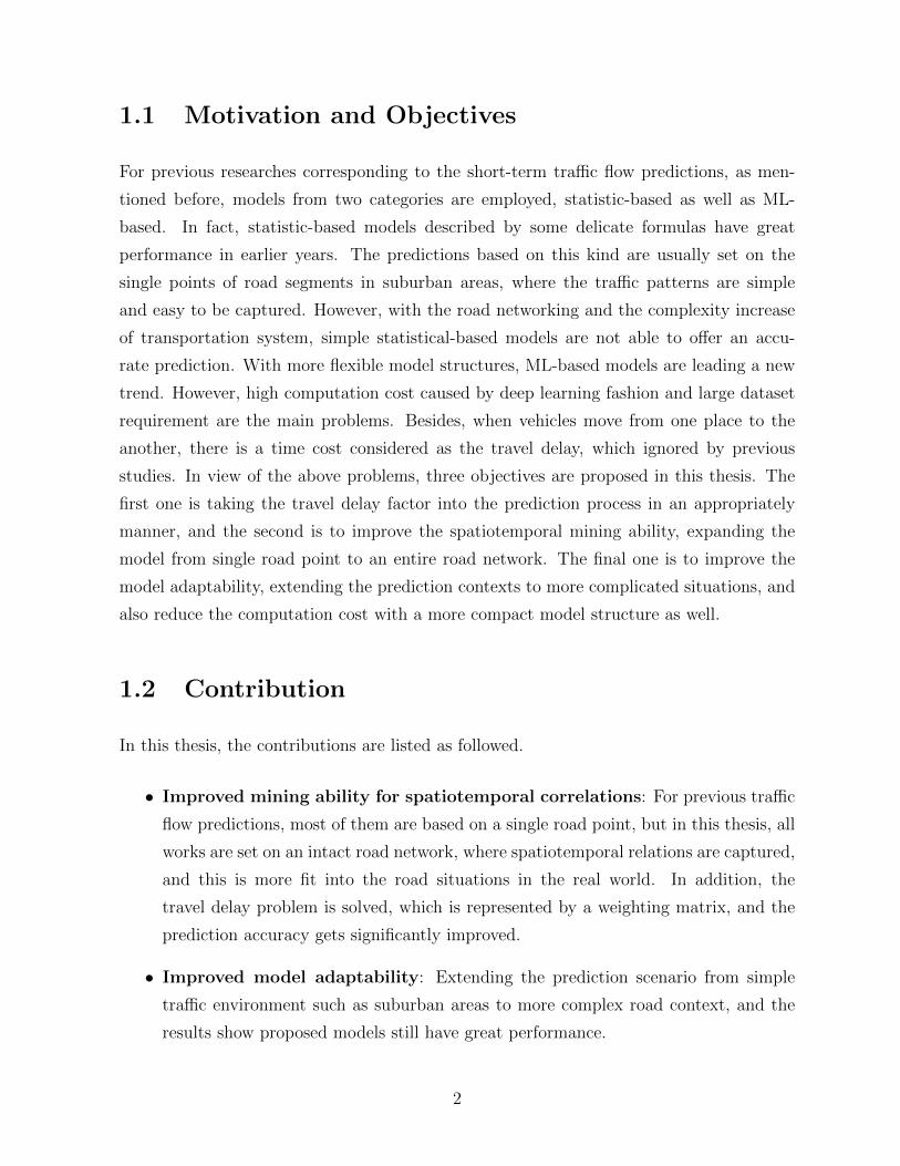
1.1 Motivation and Objectives

For previous researches corresponding to the short-term traffic flow predictions, as men-

tioned before, models from two categories are employed, statistic-based as well as ML-

based. In fact, statistic-based models described by some delicate formulas have great

performance in earlier years. The predictions based on this kind are usually set on the

single points of road segments in suburban areas, where the traffic patterns are simple

and easy to be captured. However, with the road networking and the complexity increase

of transportation system, simple statistical-based models are not able to offer an accu-

rate prediction. With more flexible model structures, ML-based models are leading a new

trend. However, high computation cost caused by deep learning fashion and large dataset

requirement are the main problems. Besides, when vehicles move from one place to the

another, there is a time cost considered as the travel delay, which ignored by previous

studies. In view of the above problems, three objectives are proposed in this thesis. The

first one is taking the travel delay factor into the prediction process in an appropriately

manner, and the second is to improve the spatiotemporal mining ability, expanding the

model from single road point to an entire road network. The final one is to improve the

model adaptability, extending the prediction contexts to more complicated situations, and

also reduce the computation cost with a more compact model structure as well.

1.2 Contribution

In this thesis, the contributions are listed as followed.

• Improved mining ability for spatiotemporal correlations: For previous traffic

flow predictions, most of them are based on a single road point, but in this thesis, all

works are set on an intact road network, where spatiotemporal relations are captured,

and this is more fit into the road situations in the real world. In addition, the

travel delay problem is solved, which is represented by a weighting matrix, and the

prediction accuracy gets significantly improved.

• Improved model adaptability: Extending the prediction scenario from simple

traffic environment such as suburban areas to more complex road context, and the

results show proposed models still have great performance.

2

1.3 Outline

The remainder of this thesis is organized as followed. Chapter 2 will give a general review of

previous works with regard to the short-term traffic flow prediction, and following Chapter 3

will propose a delay-based statistical model, DSTARMA. This model is aimed at solving the

travel delay problem in road networks. Besides the usage of statistic-based model, SSGRU

model that belongs to ML-based kind is also came up with in Chapter 4. Specially, by

adding a data-preprocessing system and in a stacked structure, SSGRU outperforms many

other similar models. Considering the spatiotemporal relations in a road network as well

as the travel delay, model MDGRU in Chapter 5 is more compact and cost-saving, and

also it extends the prediction environment from an only suburban area to the urban by a

separation method. Finally, future works and conclusion are discussed in Chapter 6.

3

Chapter 2

Related Work

For providing a full-scale understanding of short-term predictions, related literature will be

reviewed and summarized in this chapter. Statistical methods, including Autoregressive

(AR) family and Exponential Smoothing (ES) family as well as some basic concepts will

be illustrated at the very beginning. Then, ML-based approaches are focused, in which

Recurrent Neural Network (RNN), Support Vector Machine (SVM), etc., are explicitly

discussed. In addition, some other helpful methods, e.g., Hidden Markov Machine (HMM)

and Kalman Filter, are described in detail. Through analyzing several supportive cases,

the general framework of short-term prediction for recent years is obtained.

2.1 Preliminary concepts of traffic flow prediction

The entire short-term traffic flow prediction procedure will be introduced in this section

to help later introduction. For each step, some significant concepts are illustrated in detail

since they are easily misunderstanding and promiscuous. As shown in Fig. 2.1, there

are mainly four steps to design and evaluate a traffic flow prediction model, i.e., model

selection, model training, prediction, and result evaluation.

2.1.1 Model Selection

Model selection is the start of design a short-term traffic flow prediction (see Fig. 2.1),

which has a great impact on the subsequential steps. A good model leads to a good output

4

Figure 2.1: General procedure of short-term traffic flow prediction

and results in a great performance but with less cost. In-sample and out-of-sample [10, 11]

are two commonly seen selection mechanisms in traffic flow prediction process.

2.1.1.1 In-sample and out-of-sample

The most remarkable diverse between statistic-based and ML-based approaches are the

model building fashion. To be more precise, most statistical models are in-sample model

selection, which means the same dataset is used in both model building and fitting stage.

In-sample ways make the user model building firstly to determine parameters in the model.

For instance, in the Autoregressive Integrated Moving Average (ARIMA) process, critical

parameters p,d,q are determined by using the autocorrelation function (ACF) and the par-

tial autocorrelation function (PACF) pictures from the very beginning. Further, relying

on the adopted criterion, (e.g., Bayesian information criterion (BIC), Akaike informa-

tion (AIC),) the optimal values are selected for the control parameters of the prediction

model [12]. On the other hand, based on a given rule, out-of-sample divides the single

dataset into two parts to implement the training and validation of the prediction model,

respectively. Typically, ML-based approaches often rely on the out-of-sample.

2.1.2 Model Training

After the determination of the prediction model, the training begins. In this period, how

to choose a suitable training fashion and the dataset are also big challenges. On-line and

Off-line training are the two popular options for the training stage, and also whether using

real-time or historical data source also needs to be considered. In fact, the training process

is not easy, which needs to face some difficulties such as overfitting and distribution drift.

5

2.1.2.1 On-line and off-line training

The correlation of On-line and Off-line seems like the relationship between In-sample and

Out-of-sample. On-line training means that the training process begins as the data comes

in. Conversely, Off-line training is based on a static dataset. To be more precise, for On-line

training the algorithm updates parameters after learning from one training instance. In

contrast, in off-line training, the parameters are updated when all data has been learned.

As mentioned in [13], these two training strategy are both widely used in many classic

machine learning models, such as Convolutional Neural Network (CNN), and Support

Vector Regression (SVM), etc. While, For reinforcement learning-based method, online

training is more common.

2.1.2.2 Real-time data and historical data

The historical data is the data gathered from a specified period in the past. The advantage

of historical data is that it can tell the past trend and help to analyze mistakes, but it

may take more time and effort to make decisions. In the contrary, the real-time data is

considered as a more-recent data [14], which can be strictly guaranteed to be time-sensitive

by minimizing or even eliminating delays between data acquisition and data processing. For

example, in [15], real-time traffic data is defined as data collected within 40 minutes, and

the historical data is defined as the daily data. Particularly, in real-time data predictions,

there is no need for the historical data analysis, and the acquisition of prediction results is

more dependent on the intrinsic relationship between the recently acquired data.

2.1.2.3 Overfitting and distribution drift

Overfitting is the situation that focuses on the details overly, and hence over fit some quirks

and random noise, which results in a complicated model. Generally, overfitting usually

happens in regression data analysis stage, especially machine learning process [16]. To get

rid of this, a proper learning rate to update weights is significant. Another unexpected case

is the distribution drift, which is more found in statistical-based prediction models [17]. In

fact, there is no need to use big data while applying a statistical-based model to predict

since too many data can cause the covariate drift phenomenon and lead to lousy predict

result [17].

6

2.1.3 Result Evaluation

After the completion of the model building, the model evaluation begins, which can level

the quality of prediction models. Some criteria are introduced in this part from different

perspectives, such as computation time as well as prediction accuracy.

2.1.3.1 Computation time

Computation time is a significant indicator, as a good prediction in transportation system

requires that it is fast and timely. Generally, computation time in short-term traffic flow

prediction is the lenghth of the whole prediction process, from model selection to prediction

stage. Generally, pure statistical models have lower computation complexity than multi-

layer machine learning based models. Hence, for the simple road structure, it is better to

use statistical approaches, and for the more complex and more extensive dataset, which is

more suitable to use machine learning based systems.

2.1.3.2 Accuracy

The accuracy of prediction can be influenced by many factors, including the prediction

methods, experimental conditions, the reliability of data source, etc. Therefore, it is nec-

essary to give a general standard to level the prediction quality. This indicator is the most

critical one, which shows the quality of a prediction model directly. There are mainly four

figures are adopted by previous studies [18, 19, 20].

• Mean squared error (MSE)

MSE shows the average squared difference between the observations and predictions.

And it works based on the equation as follows.

MSE =1

n

n∑t=1

(Xt − Xt

)2, (2.1)

in which, Xt is the observation value, Xt is the estimated value.

• Mean absolute percentage error (MAPE)

MAPE is another basic index to evaluate the accuracy of an estimator. Different

from the MSE, it is widely used in both statistics-based and machine learning based

7

models, which is defined as follows.

MAPE =100%

n

n∑t=1

∣∣∣∣∣Xt − Xt

Xt

∣∣∣∣∣ . (2.2)

• R-square (R2)

Typically, this metric is usually used to measure the consistency between the re-

gression lines obtained by a given algorithm and the given dataset, i.e., the distance

between the regression line and data points, which is derived as,

R2 = 1− SSresSStot

= 1−

∑t

(Xt − Xt

)2∑

t

(Xt − X

)2 , (2.3)

where, the R2 is a value between 0 ∼ 1, in particular, the closer to 1, the higher the

prediction accuracy is. Conversely, the closer to 0, the lower the accuracy is.

• Root mean square error (RMSE)

RMSE evaluate the performance of a prediction model from another perspective, i.e.,

it draws the standard deviation of the prediction errors (residuals), which is defined

by,

RMSE =

√(Xt −Xt

)2. (2.4)

In addition to the criteria mentioned above for measuring timeliness and accuracy, other

principles that used to evaluate the quality of a model are broad. For example, reliability

is one of the significant aspects that widely considered by most researchers nowadays.

Basically, the error evaluation criteria are supposed to be easily adapted in real situations

and should be selected according to the actual needs of the method design. After giving

the general idea of the whole prediction procedure, models commonly used in traffic flow

prediction will be introduced explicitly in the following sections.

2.2 Statistic-based model

With benefits of comparatively lower computation complexity, good model analytical abil-

ity, and more well-rounded implementation experience [21], statistic-based models are

8

widely adopted for implementing short-term traffic flow prediction. There are many differ-

ent models in this category, from the simplest Autoregressive (AR) [22], Moving Average

(MA) [23] to more complex models, AutoRegressive Integrated Moving Average model

(ARIMA) [24], Seasonal ARIMA (SARIMA) [25] and Vector ARIMA (VARIMA), etc.

Besides, Exponential Smoothing series are also included.

For this sort of models, their features are listed and compared in Tab. 2.1, which gives

a better view for them. In the rest part of this section, some of the existing prediction

approaches designed based on these statistical models will be reviewed.

Table 2.1: Features of statistical-based models

Model Interpretability SeasonalityStationarydataset

Abilityfor non-lineardataset

Multivariate

EffectforLong-termdataset

EffectforShort-termdataset

ARMA(AR/MA)

Simple N Y N N Medium Good

ARIMA Simple N N N N Medium GoodSARIMA Medium Y N N N Good GoodVARIMA Medium N N N Y Medium GoodES (SES,DES)

Simple N N N N Bad Good

2.2.1 ARIMA

ARIMA model is a classic and fundamental model widely used in prediction fields, such

as stock forecasting [26], weather prediction [27], etc. In transportation system, ARIMA

is also widely used, for its simplicity and easily understood nature. It not only singly

combines the AR model [28] with MA indicator [29], but also handles data to be stationary

before prediction, where p is the number of time lags of autoregressive and q is the moving

average term. As for the d, it represents the number of differential times that makes the

sequence stable. The essence of the ARIMA model is to perform AR and MA calculations

simultaneously by ensuring that the time series is stationary. The corresponding prediction

result is derived as,

yt = µ+ φ1 ∗ yt−1 + · · ·+ φp ∗ yt−p + θ ∗ ct−1 + · · ·+ θ ∗ ct−q, (2.5)

9

where, φ and θ are the related polynomials of AR and MA, and yt is the predicted value.

Moreover, p, q are the time lag for AR and MA process, respectively. A general structure

of the ARIMA model is shown in Fig. 2.2.

Figure 2.2: ARIMA model

ARIMA model exploits the data feature by conducting four-stage procedures, i.e., data

acquisition, model fitting, validation, and prediction. And, there are some exclusive models

designed based on ARIMA. For instance, random walk model, first-order autoregressive

model, differenced first-order autoregressive model are the frequently used simple models

that are derived from the ARIMA model but with different p, d, q values. Typically, for

ARIMA-based short-term traffic flow prediction methods, historical dataset is preferred,

since the offline parameter selection procedure is essential for implementing ARIMA.

As a classic time series analysis model, the advantages and disadvantages of ARIMA

are also apparent. First, the model is straightforward, requiring only endogenous variables

without resorting to other exogenous variables. On the other hand, as for is shortcomings,

it requires that the time-series data be stable or differentiated to be stable. Also, it

essentially captures linear relationship, but cannot capture the nonlinear relationship.

ARIMA shows its high adaptability and feasibility to be an essential method that widely

used in early traffic flow prediction field. However, because ARIMA lacks the ability to

extract the inherent nonlinear characteristics of vehicular traffic flow information, solely

used ARIMA may not derive the sufficiently accurate prediction results. Therefore, when

using ARIMA in practice, some data preprocessing methods are usually used to remove

the trend in the data, such as, wavelet analysis, Kalman filter, even some other more

complicated algorithms.

In [30], a prediction system was proposed based on the wavelet analysis. In this system,

through a wavelet analysis system, the original time series V (k) was firstly decomposed

into two sequence, i.e., the N -level approximate coefficients V N (k) and j-level interference

10

factor W j (k). Further, an image reconstruction system is employed to reconstruct these

decomposed signals, to enable ARIMA conducting a 5-min traffic flow prediction. In this

study, only db2, db4, and db5 wavelet were compared, and 4-level decomposition was used.

The highlight of this hybrid approach is that nonlinear parts of time series are decomposed

firstly by wavelet analysis into different signals that carry details of traffic condition, and

then the ARIMA models properly tuned by ACF and PACF analysis handle this series

of signals. Different from the conventional ARIMA, it introduces the wavelet analysis-

based data preprocessing stage, which greatly improves the prediction accuracy. As for its

shortcoming, the decomposition reduces the error rate remarkably, but the time cost also

increases.

For better solving the volatile traffic problem in prediction, the authors in [31] built

different ARIMA models with appropriate parameters to fit into different pattern states

within a day, namely switching ARIMA through introducing a variable duration concept.

This model has stronger ability to overcome the challenge of volatile road situations. Also,

the authors defined the traffic flow waveform by two pairs of patterns (M=4), i.e., ascending

and descending patterns, bottom and peak patterns. Better than previous simple switching

ARIMA, it built a duration state transition probability p = (St+1 = j | St = i), in which

St is under the state li to smooth the link between two different state ARIMA models

and further improved the prediction accuracy as well. For this study, model switching is

its main advantage. However, there are still some disadvantages. The most obvious one

is that high time cost for model selecting. Precisely, it needs more time to do pattern

analysis, and if encounter diverse traffic situation that includes more complicated traffic

states, this cost will be dramatically increased. Also, considering of this problem and the

similarities in traffic flow pattern in the specified period within a day, for simple traffic

context, time division first and then modeling is a good choice but for a complex road

network, the benefit of this approach maybe dramatically falling. Similar work can be

seen in [32], where Dong et al. used a time-oriented dataset, in which, data is dealt with

separately on the basis of different periods.

The combination is becoming a new trend in short-term traffic flow prediction in recent

years, enhancing the model adaptability of conventional ARIMA model. A model named

ARIMA-GARCH is introduced in [33], which combines the ARIMA with the Generalized

autoregressive conditional heteroscedasticity (GARCH) analysis. In this hybrid model,

ARIMA is for analyzing the linear part of input traffic flow data, and GARCH is for

the nonlinear part. For the nonlinear part in series, GARCH captured the sequential

11

dependence based on the observations, and it depicted the conditional variance of prediction

error εt. Moreover, GARCH (1,1) was used in this study. The benefit of using GARCH

is that it only needs several lags to estimate the randomness instead of all lags, which

greatly improves efficiency. A similar hybrid model was proposed in [34], combing an

initial classifier, Kohonen self-organizing map, and ARIMA model to make short-term

traffic flow prediction.

To sum up, ARIMA is a simple model, which has good performance under simple traffic

scenarios, and when using this model, a stable and linear dataset is required.

2.2.2 ARIMA derivatives for traffic flow prediction

To better fit the complex traffic system in the real world, many prediction algorithms

derived from ARIMA have been introduced. Here, I discuss two most widely used models,

i.e., SARIMA and VARIMA.

2.2.2.1 SARIMA

SARIMA is a model evolved from the ARIMA, which adds more attention to the periodicity

and seasonality of data source to enable a better prediction result. Apart from the three

parameters represented in the ARIMA model, there are another three new parameters,

P , D, and Q. These three parameters are added to SARIMA as the factors to revealing

the seasonality, indicated as SARIMA (p, d, q) × (P,D,Q)s. To give a better view of its

nature, Eq. (2.6) is used for describing and showing the inner relationship of this model,

ψ (B)φ(BS)

(1−B)d(1−BS

)DXt = ω (B)W

(BS)ηt. (2.6)

As showing in equation above, the capital letters decouple the seasonal part according

to this expression, and each parameters meaning listed as follows: B is the back-shift (lag),

the same as the one in ARIMA model; ψ (B) and φ(BS)

are the polynomials from AR

and seasonal AR individually. Difference frequency and seasonal difference frequency are

represented as d and D. As for the MA processing, ω (B) and W are adapted to be related

coefficient.

To enhance the accuracy of the 15-min traffic flow prediction, the SARIMA + GARCH

method was proposed by Guo et al. [35]. More precisely, by adopting the specific SARIMA(1,0,1)

12

(0,1,1) plus GARCH(1,1) structure, the short-term vibrations within input traffic flow data

is eliminated to a certain extent, which in turn improve the ability of the model facing the

traffic volatility. Moreover, this model made a seasonal exponential smoothing operator

and two state-space models. And then the introduced Adaptive Kalman recursion solved

these two state-space models. Apart from the combination of GARCH, another highlight of

this one is the replacement from the Ljung-Box test to Adaptive Kalman filter. Compared

with the ARIMA-GARCH structure, this one is more powerful and stable.

Further, for better illustrating the spatial relationships, a hybrid improved SARIMA

(ISARIMA) model was proposed by [36]. In this model, A sliding-window function S4

was added in a simple SARIMA to update the training set. The proposed ISARIMA is

mainly responsible for the prediction task. Different from previous studies, this one is

based on the road network, which means it needs to consider the spatial correlations. The

high correlated road with aim road was selected by the genetic algorithm (GA) to form

a matrix to feed into prediction process. The experimental results showed this model is

time-saving and accurate. Another similar work can be found in [37]. Compared with

ARIMA, SARIMA is able to deal with more complex flow data and usually achieve higher

accuracy.

Generally, SARIMA has better performance than ARIMA, due to its ability to handle

seasonality in dataset. While, since SARIMA is still not separated from ARIMA in essence,

it still can only deal with the stable and linear data.

2.2.2.2 VARIMA

Arising from the needs of multivariate forecasting, the VARIMA model is proposed. As

an advanced model deriving from ARIMA, the nature of VARIMA is also the statistical

process, which can be defined as follows,

A (L)Xt = M (L) ηt, (2.7)

where Xt and L denote the aim feature at time t and the lag operator, respectively. In

particular, polynomial A and M are both metrics.

The traffic flow data has two intrinsic features, i.e., spatial-correlation and temporal-

correlation. However, in most of ARIMA- and SARIMA-based models, the spatial-correlation

of traffic flow data is ignored due to the dimension of these models is only one. Therefore,

13

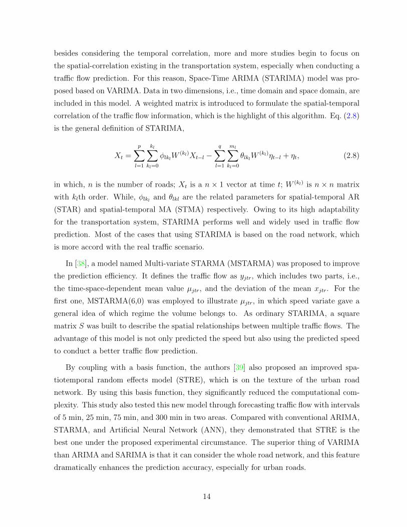
besides considering the temporal correlation, more and more studies begin to focus on

the spatial-correlation existing in the transportation system, especially when conducting a

traffic flow prediction. For this reason, Space-Time ARIMA (STARIMA) model was pro-

posed based on VARIMA. Data in two dimensions, i.e., time domain and space domain, are

included in this model. A weighted matrix is introduced to formulate the spatial-temporal

correlation of the traffic flow information, which is the highlight of this algorithm. Eq. (2.8)

is the general definition of STARIMA,

Xt =

p∑l=1

kl∑kl=0

φlklW(kl)Xt−l −

q∑l=1

ml∑kl=0

θlklW(kl)ηt−l + ηt, (2.8)

in which, n is the number of roads; Xt is a n × 1 vector at time t; W (kl) is n × n matrix

with klth order. While, φlkl and θlkl are the related parameters for spatial-temporal AR

(STAR) and spatial-temporal MA (STMA) respectively. Owing to its high adaptability

for the transportation system, STARIMA performs well and widely used in traffic flow

prediction. Most of the cases that using STARIMA is based on the road network, which

is more accord with the real traffic scenario.

In [38], a model named Multi-variate STARMA (MSTARMA) was proposed to improve

the prediction efficiency. It defines the traffic flow as yjtr, which includes two parts, i.e.,

the time-space-dependent mean value µjtr, and the deviation of the mean xjtr. For the

first one, MSTARMA(6,0) was employed to illustrate µjtr, in which speed variate gave a

general idea of which regime the volume belongs to. As ordinary STARIMA, a square

matrix S was built to describe the spatial relationships between multiple traffic flows. The

advantage of this model is not only predicted the speed but also using the predicted speed

to conduct a better traffic flow prediction.

By coupling with a basis function, the authors [39] also proposed an improved spa-

tiotemporal random effects model (STRE), which is on the texture of the urban road

network. By using this basis function, they significantly reduced the computational com-

plexity. This study also tested this new model through forecasting traffic flow with intervals

of 5 min, 25 min, 75 min, and 300 min in two areas. Compared with conventional ARIMA,

STARMA, and Artificial Neural Network (ANN), they demonstrated that STRE is the

best one under the proposed experimental circumstance. The superior thing of VARIMA

than ARIMA and SARIMA is that it can consider the whole road network, and this feature

dramatically enhances the prediction accuracy, especially for urban roads.

14

Similar work can also be found in [40], Pavlyuk et al. conducted a 5-min traffic flow pre-

diction by using STARIMA and other models such as ARIMA, VARIMA, etc. The derived

prediction results also showed the superior of STARIMA. In addition to the short-term

traffic flow prediction, this algorithm is also pretty helpful to solve some transportation

issues. For instance, a study regarding how to solve the missing counting problem in bi-

cycle traffic system was introduced in [41], in which STARIMA was adopted to address

this issue. By utilizing data from nearby road segments, the missing accounting number

is estimated. The spatial relationship plays an essential role in this case and dramatically

improves the estimation accuracy as well.

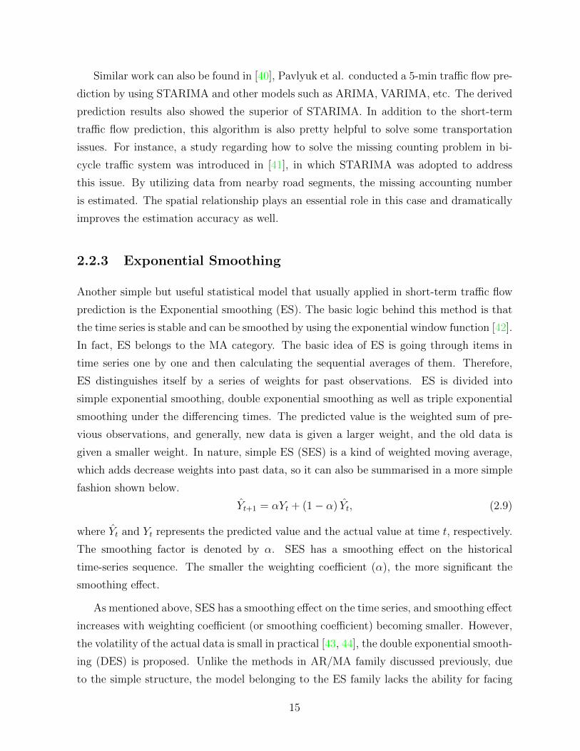
2.2.3 Exponential Smoothing

Another simple but useful statistical model that usually applied in short-term traffic flow

prediction is the Exponential smoothing (ES). The basic logic behind this method is that

the time series is stable and can be smoothed by using the exponential window function [42].

In fact, ES belongs to the MA category. The basic idea of ES is going through items in

time series one by one and then calculating the sequential averages of them. Therefore,

ES distinguishes itself by a series of weights for past observations. ES is divided into

simple exponential smoothing, double exponential smoothing as well as triple exponential

smoothing under the differencing times. The predicted value is the weighted sum of pre-

vious observations, and generally, new data is given a larger weight, and the old data is

given a smaller weight. In nature, simple ES (SES) is a kind of weighted moving average,

which adds decrease weights into past data, so it can also be summarised in a more simple

fashion shown below.

Yt+1 = αYt + (1− α) Yt, (2.9)

where Yt and Yt represents the predicted value and the actual value at time t, respectively.

The smoothing factor is denoted by α. SES has a smoothing effect on the historical

time-series sequence. The smaller the weighting coefficient (α), the more significant the

smoothing effect.

As mentioned above, SES has a smoothing effect on the time series, and smoothing effect

increases with weighting coefficient (or smoothing coefficient) becoming smaller. However,

the volatility of the actual data is small in practical [43, 44], the double exponential smooth-

ing (DES) is proposed. Unlike the methods in AR/MA family discussed previously, due

to the simple structure, the model belonging to the ES family lacks the ability for facing

15

the traffic flow violations. Alternatively, the ES family is comparatively fundamental and

easy understanding, so it is a unique algorithm to help do traffic flow prediction. Another

advantage of ES is the great adaptability, which means that predictive models can adjust

automatically with changes in traffic flow data patterns. In practice, only one parameter α

needs to be selected for prediction, and that is simple and easy to implement. Combining

with other methods to improve the prediction reliability is a new trend for this family.

In [45], simple ES was combined with a neural network (NN) structure, and also a

Taguchi Method was adopted in this innovative model. In detail, simple ES was used

to filter the noises in the raw dataset at first, and then these preprocessed data were

imported into the Taguchi system and after that a extreme learning was used on them to

do a prediction. The mechanism of Taguchi system is to use an orthogonal array to realize

the effects of variates, which can greatly reduces the computation cost compared with the

traditional trial-and-error method.

Briefly, based on the traffic flow information in a given road network, the proposed

method can prune the input network according to the effect of the traffic flow of each

road segment within the road network on the change of traffic volume of the target section,

and only retain the valid road segments (i.e., high-impact roads). Relying on the simplified

road network, the system further determines the hyper-parameter for the NN. Through this

procedure, unnecessary traffic data are removed, which further facilitates pattern mining

and to make a more accurate short-term traffic flow prediction.

For avoiding the overfitting problem, the approach presented in [46] enrolled a sim-

ple ES. Precisely, the simple ES was used to eliminate the lumpy characteristics of raw

data, which relies on the irregular variation on raw dataset. Also, smoothing constant

α controlled the filtering speed, for which the larger the α is, the faster the change of

filtered traffic flow data θ′ (l) is. To further improve the prediction accuracy, through min-

imizing the mean absolute relative error eMARE, Levenberg-Marquardt algorithm replaced

Back-Propagation (BP) method to train NN, which had better performance. They com-

pared their approach with other parallel models such as Bayesian NN, Exponential LSTM,

etc. The derived results showed this EXP-LM model had best performance among them.

Similar work, in which ES is used to be preprocess tool,can be also found in [47].

However, the lack of identification ability for the turning point of data and lower accu-

racy for long-term traffic flow prediction is the primary shortages of the ES-based method.

Therefore, this sort of method more is more suitably used in the single road of suburban

areas.

16

Table 2.2: Comparision of some existing statistial prediction models

Category ModelPredictionperiod

Roadstruc-ture

Predictionarea

Combinationor SingleUse

Highlight

ARIMA

ARIMA-GARCH[33](2011)

3, 5, 10,15-min

Singleroad

Suburbanhighway

Combination

Generalizedautoregressiveconditionalheteroscedastic-ity (GARCH)analysis

WARIMA[30](2010)

5-minSingleroad

Suburban(railway)

CombinationWavelet analy-sis for non-linearnoises

ARIMA[32](2009)

5, 10-minSingleroad

Urban SingleMulti-perioddata training

SARIMA

ISARIMA[36](2018)

15-minRoad net-work

Suburbanhighway

Combination

Consideration ofspatio-temporalrelationship &Genetic algo-rithm (GA)optimization

SARIMA[37](2016)

15-minSingleroad

Suburbanhighway

Sinlge

Comparisionwith most ofcurent popularmodels

SARIMA+GARCH[35](2014)

15-minSingleroad

Suburban &Urban high-way

CombinationAdaptiveKalman fil-ter and GARCH

VARIMA

VARIMA[40](2017)

5-minSingleroad

Urban Single

Consideration ofspatio-temporalrelationship inurban area

STRE[39](2016)

5-minRoad net-work

Urban Combination

Reduced com-putationalcomplexity by abasis function

MSTARMA[38](2011)

5-min∼1h(5-mininterval)

Road net-work

Urban high-way

CombinationReal-time pre-diction

ES

E-ELM[45](2019)

1h∼3h(15-mininterval)

Road net-work

Suburbanhighway

CombinationIntroduction ofTaguchi method

EXP-LM [46](2012)

1-minSingleroad

Suburbanhighway

CombinationCombinationwith NN

EXP-NN [47](2011)

1-minSingleroad

Suburbanhighway

Combination

ES as a datapre-process tool,combined withNN

17

Here, I summarize the characteristics of some recent researches designed based on the

aforementioned statistical models in Tab. 2.2.

To sum up, statistic-based models generally have good model interpretability, which

means they can be described more clearly and explicitly by some delicate formulas. How-

ever, rigid and straightforward model structure leads to bad model adaptability, which is a

big challenge for design a practical traffic flow prediction method, especially under complex

traffic conditions. Also, how to properly capture the spatiotemporal correlations in road

networks is another challenge for this sort of models, which is widely ignored by previous

studies.

2.3 Machine learning-based prediction approaches

As mentioned previously, ML-based models, that have a deep connection with various

fields, such as pattern recognition, statistical learning, data mining, computer vision, speech

recognition, and natural language processing, etc., have caught considerable attention in

recent years. Multi-disciplined nature makes these methods have better adaptability for

different contexts. Accordingly, how to design a practical ML-based approach for sup-

porting the Intelligent Transportation System (ITS) [48] [49] has become a hot research

topic [50]. Recent years, as a supportive component of ITS, ML-based models are widely

adopted as the popular short-term traffic flow prediction methods due to their high accu-

racy and strong non-linear capture ability for big data [51]. In general, machine learning

goes to three types, supervised learning, unsupervised learning, and reinforced learning.

In fact, supervised learning is more widely used than another two categories in short-term

traffic flow prediction owing to the learning mechanism. Accordingly, in this section, I

will focus on prediction models designed relying on supervised learning, and introduce the

related algorithms in detail based on the core principles of these prediction methods, i.e.,

classification-based method, regression models, and recurrent neural network. While, for

the unsupervised learning as well as reinforced learning, I will give some simple introduc-

tion only. Moreover, a general taxonomy of the ML-based prediction method is shown in

Fig. 2.3.

18

Figure 2.3: Machine learning for traffic flow prediction

2.3.1 Supervised learning-based approaches

Supervised learning separates the dataset into two sets, one for training and one for val-

idation. Classification and regression are two typical categories in this learning fashion.

For the classification category, the K-nearest neighbors algorithm (KNN) [52] and decision

tree classification [53] are the most commonly seen algorithms. It is worth to pint out that

when applying recurrent neural network (RNN) to the field of traffic forecasting, I usually

classify it as supervised learning, in which, long-short term memory (LSTM) and the gated

recurrent unit (GRU) are two most widely adopted models. Therefore, this part will begin

from the K-NN algorithm, and then linear regression as well as Support vector machine

(SVM), and RNN is illustrated at the end. Here, in Tab. 2.3, I summarize some features

of these supervised ML-based prediction models.

Table 2.3: Features of supervised ML-based models

Model InterpretabilityAbility fornon-lineardataset

Abilityfor non-normalizeddataset

Memoryrequire-ment

Effectfor Long-termdataset

Effect forShort-termdataset

K-NN Simple Y Y Large Medium GoodLinear re-gression

Simple N Y Large Medium Good

SVM Medium Y N Large Bad GoodLSTM Complex Y Y Large Good GoodGRU Medium Y Y Large Good Good

2.3.1.1 K-NN algorithm

K-NN algorithm is one of the most straightforward classifications, which is a simple but

high efficient model that can be easily applied in short-term traffic flow prediction. In

short, the essence of K-NN is that, based on the classification result derived by learning

19

the training dataset, the K-NN model classifies the newly sampled data and put them into

fitted categories. It is also a non-parametric, lazy learning algorithm which mainly contains

five steps. First, it determines the value of K (i.e., the number of nearest neighbours), and

then calculates the distance between the query-instance and all training samples. After

that, these distances are sorted to determine the nearest neighbours. By gathering the

category Y of nearest neighbours, the aim feature is finally assigned to the group which

owes the closest distance with the aim.

Figure 2.4: K-NN algorithm

For instance, Fig. 2.4 shows the K-NN algorithm for k = 4, where there are three

groups, labeled as ω1, ω2 and ω3 respectively. It can be found that there are three out

of four points belong to the blue group, only one belongs to the black group, so it can

conclude that the unknown point Xµ belongs to the blue group. The aim feature Xµ is

classified into group ω1 based on the corresponding Euclidean distance d between itself and

a labeled feature Xh = {xh,t−1, xh,t−2, · · · , xh,t−n}, which is given by,

d =

√(xt−1 − xh,t−1)2 + · · ·+ (xt−n − xh,t−n)2. (2.10)

K-NN is adopted by many researchers in short-term traffic flow prediction field since it

can be easily adapted into the real traffic situation, especially when the flow data is noisy

and large.

In [57], it adopted a dataset recorded in 5-min interval to make a short-term traffic

flow prediction. Different from the previous data preprocessing, it made a data selection

standard to first roughly clean the input dataset by removing the unnecessary data. For

example, it only kept the volume between 0 and mc×CAP×T/60. After the preprocessing,

the standardized data were imported into K-NN system to do prediction, and this process

20

Table 2.4: Comparison of recent works in K-NN

ModelDistancemetric

Number ofk

Method for datapre-processing

Method for spatialcorrelation

Improvement

[54](2016)

Euclideandistance

k = 4 N

Divide roadnetworks intoupstream, down-stream to con-struct KNN

Multi-step pre-diction

[55](2015)

NormalizedEuclideandistances

k = 5, 10 N NSequential-search strategy

[56](2014)

Euclideandistance

k = 10Single-factoranalysis of vari-ance (ANOVA)

N

Improved modelability for spe-cial event con-text

was based on the distance qi between the actual data and k nearest neighbors. In this

work, k ∈ [5, 30]. To further improve the prediction accuracy, K-NN was weighted by

parameter ai, which is the highlight of this method. After calculating the MAD and

MAPE, the derived results showed that this weighted K-NN had better performance than

non-weighted K-NN, with the accuracy higher up to over 90%.

In [56], a basic K-NN was used to do the 1-hour traffic flow prediction under some

typical circumstances. For reducing the bad influence originated from the special events on

prediction results, the authors used a NN to do a prediction analysis, in which Twitter and

traffic features were both fed into the prediction system, and extracted by four components.

Then the optimal features were determined to further build a model. In this work, the

adopted dataset is large, which is aggregated from the different social media platforms. If

using statistical methods such as ARIMA, SARIMA, it will be a great challenge and need

to consume large memory requirement. Conversely, for K-NN, it can fast category these

data and accurately capture their patterns.

Another example that put K-NN into data preprocess can be found in [58], in which

traffic flow prediction is to do pattern recognition. Precisely, through digging and identi-

fying different traffic flow patterns of the raw dataset, the authors optimized the original

K-NN algorithm. They conducted a series experiments with prediction horizon varying

from 30-min to one-hour to evaluate their new enhanced K-NN model, and demonstrated

its great ability for traffic prediction.

To conclusion, K-NN is a suitable method for short-term traffic flow prediction, which

has a good model interpretability and lower computation cost. When using this mehtod

21

to do a short-term traffic flow prediction, raw historical traffic flow with time can be used

directly. From the Tab. 2.3, I can find that K-NN has the ability to handle both the non-

linear and non-normalized datasets, which means it can be directly used without any data

pre-processing stages. This feature is important since for most of the traffic system the flow

patterns usually non-linear and statistical-based models cannot handle them directly. On

the other hand, there are still some shortages of the conventional K-NN-based approach.

The computation for the distance that determines the final lable needs to comsume large

memory space, especially when the historical dataset is large, and may hence have higher

requirement for the memory space. For example, when calculating the distance, K-NN

cannot figure out which method is the best under the existing circumstance, i.e., whether

to use all attributes or only specific attributes to do the classification. This shortcoming

reduces the prediction accuracy to some extent. Therefore, to overcome this shortage,

many optimized K-NN approaches are designed. For example, there is a sequential re-

search of K-NN popping out, which is worth to give some briefly introduce. In [55], the

proposed work used a method of disaggregating the cluster to reduce the computational

complexity, thereby improving the accuracy and efficiency of the prediction. In the past

traffic flow prediction, there are usually two feature vectors, one to reflect the speed and

the other to indicate the acceleration. These two feature vectors are considered together

when clustering. However, in the normalization process, it brings a difficulty to predictor

due to their different units. In this model, the authors separated the two feature vectors

for clustering, which dramatically simplifies the problem of cumbersome normalization. By

splitting the complex non-uniform variables into two sets of sequences, the K-NN processing

is performed separately. Accordingly, in the normalization process, the inconvenient unit

unification can be avoided. Consequently, the computational complexity of the proposed

work is reduced. Meanwhile, the prediction accuracy is also improved to some extent.

2.3.1.2 Linear regression algorithm

Linear regression algorithm is a type of regression method, which belongs to the supervised

learning. In essence, the purpose of regression is to predict continuous value. There

are several standard algorithms included in the regression algorithm, i.e., simple linear

regression, polynomial regression, decision tree regression, etc. As the simplest one, simple

linear regression is more commonly used in short-term traffic flow prediction. There are

two compelling reasons why linear regression is more accessible in short-term traffic flow

prediction field: the first one is its simplicity, and the second one is that it can reduce the

22

risk of over-fitting by regularization.

The main objective of Linear Regression is to find the most fitted line to describe the

characteristics of the input dataset. Typically, linear regression process is done by using

the well-known least squares method.

Figure 2.5: Simple linear regression algorithm

As shown in Fig. 2.5, the points are the training data, and the line is the predicted line

fitting training data. The following formula can represent this fitted line,

Y = aX + b (2.11)

Accordingly, training and building a linear regression model can be considered a process

of seeking appropriate coefficients a, b, finally to find the best fit line Y . Apparently, if

variables in the dataset have a linear relationship, they fit well. Moreover, the regression

algorithm expects to use a hyperplane to fit the non-linear data.

In [59], a local linear regression model was proposed. Different from non-parametric

models used before, this one has a higher minimum efficiency, and greater ability to deal

with the distributed dataset. In this study, traffic flow data was described as a multivariate

covariate Xi, and by using a cross-validation approach to determine the the dimension d of

the covariate vector and the bandwidth h, the useful data were selected to build a regression

model mh,i, and finally the predicted value y was obtained. Moreover, both single-step and

multi-step predictions are adopted in this research.

To sum up, linear regression algorithm has two distinct disadvantages. First, it has poor

performance when variables are non-linear. In fact, real traffic flows are high oscillatory,

expecially in suburban areas, which means that most of the flow sources are the non-

23

linear, and linear regression alogorithm is not able to used directly on raw dataset. The

computation cost will increase due to the employment of extra stationary process. Besides,

it is not flexible enough to capture more complex patterns due to its machanism. The single

fitted straight line can only cover fundamental features but usually ignores some critical

details that are not on the line, so the more complex traffic conditions, the more details

are lost, leading worse results accordingly. But the fact is that with the development of

ITS, the flow patterns are becoming more and more complicated, but the standard input

data for this method is non-linear and simple, so it is difficult for this algorithm to fit

into modern traffic systems. However, instead of using as a core model, linear regression

methods are often used in conjunction with other algorithms to support a short-term traffic

flow prediction, which is also its new trend in future works. Generally, there are pretty

limited simple case studies learned in early researchers, even though linear regression have

some unique advatages, such as its high efficiency for simple structural road.

2.3.1.3 Support vector machine (SVM)

Another classic ML model widely used for traffic flow prediction is the support vector

machine (SVM), which also can be extended to the nonlinear classification problem by

using a technique called kernel function. Briefly, this function essentially calculates the

distance between two observation data, hence called support vectors [60]. SVM aims to

find the decision boundary, which can maximize the border using the sample interval.

Therefore, SVM is also known as a large space classifier, an enhancement of the logistic

regression algorithm. The most significant advantage of SVM is the use of nonlinear kernel

function, which is introduced to figure out the model nonlinear decision boundary. In a

simple context, the nonlinear problem can be effectively transformed into a linear problem,

as shown in Fig. 2.6(a). In this picture, the straight line separating sample A and sample B

is a normal SVM that makes two divided samples A and B become linearly separable. From

the Fig. 2.6(b), three steps are included in SVM: the first step is to find an optimal decision

plane for two linearly separable classes, and then make the minimum distances between

each class and optimal decision plane are maximized to minimize the decision error. In the

last step, only the data points that lie in the boundary of the optimal decision plane are

chosen as support vectors.

As an outstanding short-term traffic flow prediction method, SVM can model nonlinear

decision boundaries and has many alternative forms of kernel functions, which is superior to

24

(a) Mechnism of SVM (b) Details of SVM

Figure 2.6: An illustration of SVM

simple linear regression. However, it also faces considerable over-fitting robustness, which

is especially prominent in high-dimensional space. Moreover, since it is vital to choose

the correct kernel, SVM is challenging to tune and cannot be extended to more massive

datasets, and as a result, it is a memory-intensive algorithm. This feature makes SVM

more suitable for short-term traffic flow prediction rather than the long-term. Besides,

SVM is a unique algorithm that not only can maintain computational efficiency but also

get outstanding classification results. Considering all the characteristics of SVM, it is

suitable for short-term traffic flow prediction.

In [61], the authors proposed an improved SVM-based method, namely ISVR, to im-

prove the model capability with the increase of traffic structural complexity, which is based

on the least square support vector machine. The ISVR was completed when matrix A−1l

can be obtained from the A−1l+k without any repeatly calculation, in which the matrix Al

and Al+k were both the kernel correlation matrix of learning set S. Different from previous

cases, this study aimes for a road network, in which input data were in matrices fashion

fed into ISVR model. Besides, this hybrid model combines with the incremental learning

strategy to dynamically update the forecasts to achieve a higher pattern mining ability for

this road structure. Compared with BPNN regarding six error indicators, such as MAPE,

RMSER, this model showed its stronger prediction ability.

Another innovative hybrid model can found in [62], in which, according to the incor-

poration of ARIMA and SVM, the noise of raw dataset is eliminated and further fast the

prediction speed with higher accuracy. More precisely, the time series was treated as a

signal sequence St, containing the white noises. After Wavelet analysis, this time series

25

was regarded as a nonlinear sequence yt that contains two part, linear autocorrelation Lt

as well as nonlinear autocorrelation Nt. ARIMA was firstly used to predict yt , and the

SVM was used to predict the error εt, and final prediction result was the combination of

these two forecasting values. The benefit of using wavelet analysis and hybrid model shows

in the reduced EMAPE and increased r2. The minimal sequential optimization was also

introduced by [63], which was combined with the SVM algorithm to improve the prediction

accuracy for short-term traffic flow. In this study, SVM was employed to make a 10-min

traffic flow prediction under the urban intersection circumstance, and their experiment

results proved the SVM is a reliable approach in short-term traffic flow prediction field.

In Tab. 2.5, I summarize the features of the SVM-based traffic flow prediction methods

discussed above. To conclusion, for the SVM model, it has great effect on the predictions for

short-term traffic flow, and compared with Linear regression, it is more suitable in volatile

traffic environmnets. Although it performes well in short-term traffic flow predictions, there

are two distinct shortcomings of this algorithm, and the first one is intensive memory. To

be more precise, the training fashion for SVM is memory-intensive, and prediction nature

is the linear combination of all support vectors. Therefore, if the number of support vectors

are large, a big store space is recquired, and this is a big challenge for some low-memory

devices. Another challenge for SVM is the kernel selection, as the function of kernel is

to take data as input and transform it into the required form, and therefore, different

kernel leads to different SVM effect. Among most of the kernels, the RBF kernel and

Gaussian kernel are the most popular two, because they can be used when there is no

prior knowledge about the data, and have higher prediction accuracy than others proved

by many previous studies, which is more fit in the supervised learning process in traffic

flow predictions. Conversely, inappropriate kernels will reduce the prediction accuracy and

load more computation cost as well. In addition the multi-kernel SVM is also brought

forward to overcome the strong stochastic and non-linear characteristics in city ITS.

2.3.1.4 Recurrent neural network (RNN)

Most used machine learning models nowadays can be supervised or unsupervised fashion,

which depends on the specific requirements. However, in traffic flow prediction, most

of the researches related to RNN are supervised [68], so it is included in this part. In

the traditional neural network model, from the input layer to the hidden layer and then

to the output layer, the layers are fully connected, and the nodes between each layer

26

Table 2.5: Comparison of recent works in SVM

ModelKernel func-tion

Method for select-ing control parame-ters

Method for ob-taining spatial-temporal correla-tions

Improvement

[64] (2018)

RBF +polyno-mial kernelfunction

Chaotic Cloud Par-ticle Swarm Opti-mization

Analysing the pe-riodicy and changetendency of nearbypoints in the samePoint of Interest(POI) to capturespatial correlations,and these data aregathered throughroadside units(RSU).

Decomposing the roadnetwork into severalPOIs, to obtain thespatial-temporal corre-lations and also byintroducing the real-time information tofurther enhance themodel adaptability, es-pecially in rush hour.

[65] (2018) RBF kernelPredeterminate pa-rameters: C = 100,γ = 0.01, ε = 0.1

N

Combined withARIMA model, SVMis used for residu-als prediction, andARIMA is for thelinear part prediction.

[62] (2009)Mercer ker-nel function

Determined by Lib-svm package [66]

N

Employing WaveletDenoising firstly toreduce the noisein raw dataset forprediction accuracyimprovement.

[61] (2007) Gauss kernelImplemented basedon LS-SVM algo-rithm [67]

N

Using the real-timedata to update the pre-diction function, whichis more fit in volatiletraffic conditions.

[63] (2005) Gauss kernel

Based on Sequen-tial Minimal Op-timization (SMO),Predeterminate pa-rameters: C = 5,σ2 = 0.5, ε = 0.05

N

By introducing SMO,the prediction accu-racy and speed are in-creased.

27

are disconnected. Due to this connection feature, the global neural network is weak for

many problems, especially time-series problems. However, the traffic flow patterns change

with time, so traditional neural network with the global connection structure such as a

convolutional neural network (CNN), is unsuitable for short-term traffic flow prediction

problem. For better solving the time-series-based problems, RNN was proposed. The core

principle of RNN is using classifiers repeatedly, and precisely, only one classifier is used to

summarize the state, and other classifiers receive training for the corresponding time and

then pass the state, which avoids the need for a large number of historical classifiers, and

is more effective for time-series problems.

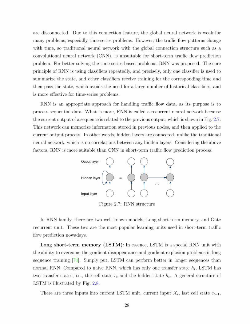
RNN is an appropriate approach for handling traffic flow data, as its purpose is to

process sequential data. What is more, RNN is called a recurrent neural network because

the current output of a sequence is related to the previous output, which is shown in Fig. 2.7.

This network can memorize information stored in previous nodes, and then applied to the

current output process. In other words, hidden layers are connected, unlike the traditional

neural network, which is no correlations between any hidden layers. Considering the above

factors, RNN is more suitable than CNN in short-term traffic flow prediction process.

Figure 2.7: RNN structure

In RNN family, there are two well-known models, Long short-term memory, and Gate

recurrent unit. These two are the most popular learning units used in short-term traffic

flow prediction nowadays.

Long short-term memory (LSTM): In essence, LSTM is a special RNN unit with

the ability to overcome the gradient disappearance and gradient explosion problems in long

sequence training [74]. Simply put, LSTM can perform better in longer sequences than

normal RNN. Compared to naive RNN, which has only one transfer state ht, LSTM has

two transfer states, i.e., the cell state ct and the hidden state ht. A general structure of

LSTM is illustrated by Fig. 2.8.

There are three inputs into current LSTM unit, current input Xt, last cell state ct−1,

28

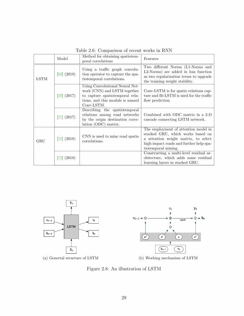
Table 2.6: Comparison of recent works in RNN

ModelMethod for obtaining spatiotem-poral correlations

Features

LSTM[69] (2018)

Using a traffic graph convolu-tion operator to capture the spa-tiotemporal correlations.

Two different Norms (L1-Norms andL2-Norms) are added in loss functionas two regularization terms to upgradethe training weight stability.

[70] (2017)

Using Convolutional Neural Net-work (CNN) and LSTM togetherto capture spatiotemporal rela-tions, and this module is namedConv-LSTM.

Conv-LSTM is for spatio relations cap-ture and Bi-LSTM is used for the trafficflow prediction.

[71] (2017)

Describing the spatiotemporalrelations among road networksby the origin destination corre-lation (ODC) matrix.

Combined with ODC matrix in a 2-Dcascade connecting LSTM network.

GRU[72] (2018)

CNN is used to mine road spatiocorrelations.

The employment of attention model instacked GRU, which works based ona attention weight matrix, to selecthigh-impact roads and further help spa-tiotemporal mining.

[73] (2018)Constructing a multi-level residual ar-chitecture, which adds some residuallearning layers in stacked GRU.

(a) Genertal structure of LSTM (b) Working mechanism of LSTM

Figure 2.8: An illustration of LSTM

29

and last hidden state ht−1. The first step of LSTM is to use the LSTM’s current input

Xt and the ht−1 stitching passed from the previous state to get four states z, zi, zo and

zf . While, zf , zi, zo are multiplied by the splicing vector and then converted to a value

between 0 and 1 by a sigmoid activation function as a gating state. Moreover, z is the result

of converting the result to a value between -1 and 1 through a tanh activation function.

Having these states, the mechanism of LSTM can be introduced in detail.

There are mainly three states in LSTM, the forget stage, selected memory stage as well

as output stage. The forget stage, which is mainly to forget the input from the previous

node selectively. Simply put, it only keeps the necessary information and deletes secondary

information/the redundancy. The corresponding functionality is achieved by,

zf = σ(xtU

f + ht−1Wf), (2.12)

in which, xt is the current input; ht−1 is the last node’s hidden state; U f works as a bridge

for the connection of inputs and current hidden layer. By the link generated by W f , the last

hidden layer and the current hidden layer is connected. The main aim of selective memory

stage is to electively memorize the inputs. It records more significant information and

keeps less about not very important parts. The corresponding process can be formulated

by Eq. (2.13) and Eq. (2.14), respectively.

z = tanh (xtUc + ht−1W

c) , (2.13)

zi = σ(xtU

i + ht−1Wi). (2.14)

Particularly, superscript c represents the current cell state, and zi is regarded as selected

gating signal. As for the output stage, this phase will determine which outputs will be

treated as current states and mainly controlled by zo, which is given by,

zo = σ (xtUo + ht−1W

o) . (2.15)

Controlling the state of transmission through gated state, remembering that it takes a

long time to remember, forgetting unimportant information; unlike ordinary RNNs, there

is only one way to superimpose memory. It is especially useful for many tasks that require

long-term memory.

Accordingly, in recent years, many LSTM-based prediction models have been proposed

for addressing traffic flow predicting. For example, a 15-min interval traffic flow prediction

30

was conducted by [75]. In this study, they proved the superiority of simple LSTM, through

comparing it with other similar methods such as SAE, SVM, and FFNN, etc. Currently,

there two new trends for LSTM in short-term traffic flow prediction. The first one is

the combination model structure, and the other is the concern about Spatial-temporal

relationship.

In [69], a physical network topology, TCG-LSTM model was built to capture the spatial

correlations within the traffic flow information. By introducing a localized spectral graph

convolution, which works according to a N × N adjacency matrix A. A link counting

function d (vi, vj) further defined the spatial correlations by using the adjacency matrix.

Creative thing of this model is that the input is the graph convolution features, which is a

vector. This structure greatly interpreted the spatial relationship by convolution weights.

Based on LSTM, this model showed a great performance on both suburban and urban road

networks.

Similarly, for better decribing the road spatial correlations, the authors in [70] intro-

duced a hybrid model, in which the traffic flow data was represented by a one-dimension

vector. Conv-LSTM and Bi-LSTM were both used to learning the traffic patterns. For the

Conv-LSTM, it aimed for the spatial relationship features. While, Bi-LSTM was for the pe-

riodicity feature mining. Combining these two types of LSTM together, a 30-second traffic

flow prediction was conducted for both suburban and urban roads. The derived MSE value

significantly decreased compared with the many other approaches, such as pure LSTM,

ARIMA, SAE, etc. Particularly, it also replaced the Conv-LSTM with CNN-LSTM, but

the performance was not become better, which further showed that the combination of

Conv and LSTM was the optimal in this context.

Moreover, based on the conventional LSTM, a deep learning LSTM was proposed

by [71], in which two-dimensional LSTM was built for digging the spatial-temporal re-

lationships of the traffic flow. They validated their model by comparing it with other

commonly seen models. For further digging out the spatial correlation, two variables, traf-

fic speed and occupancy were both adopted by [76], and the authors also adopted K-NN

to help improve the prediction accuracy.

Gate Recurrent Unit (GRU): Similar to LSTM, GRU is also considered a upgraded

RNN-based method that is proposed for dealing with the gradient-missing problem in

the training for long-term sequences. Compared to LSTM, the use of GRU can achieve

comparable results, and it is easier to train in comparison, which can greatly improve

training efficiency, so short-term traffic flow predictions are more inclined to use GRU in

31

recent years. Different from the multi-gate framework in LSTM, GRU has less control

gates, which can be seen in Fig. 2.9, and that is why it has a lower computational cost

than LSTM in general. Only two control gates in GRU, the reset gate r and update gate

z (see Fig. 2.9(b)). These two gates can be calculated by Eq. (2.16) and Eq. (2.17),

rt = σ (xtUz + ht−1W

z) , (2.16)

zt = σ (xtUr + ht−1W

r) , (2.17)

where σ denotes the sigmoid function. xt is the current input, and ht−1 is the state passing

from the last node. Similar to the LSTM, here, the W , U are also the weight matrices

acting as the critical link between the last hidden layer and current hidden layer, and the

connection of inputs and current hidden layer, respectively.

(a) Genertal structure of GRU (b) Working mechanism of GRU

Figure 2.9: An illustration of GRU

After getting the gating signal, GRU firstly use the reset gate to get the reseted data.

And this process is described in following equation.

ht−1′ = ht−1 � r, (2.18)

where � is the Hadamard Product, and that is to say, the corresponding elements in the

operation matrix are multiplied, so the two multiplication matrices are required to be

homo-typed. And then, the memory task is achieved by combining these processed data

and current input xt, which is,

h′ = tanh(xtU

h + (rt � ht−1)W h). (2.19)

32

Notably, in this formula, the effect of function tanh is to range the data between -1 and

1. Similar to the selected memory phase in LSTM, h′ mainly contains the data of current

input xt.

The last but not least stage is the update memory phase. At this stage, it has two

functions, i.e., forgetting and remembering, implemented at the same time. It uses the

previously acquired update gate zt to figure out ht, which is given by,

ht = zt � ht−1 + (1− zt)� h′. (2.20)

Particularly, the gate signal zt ranges from 0 to 1. The closer the gating signal is to 1, the

more data is remembered; the closer to 0, the more data is forgotten. The smartest thing

of GRU is that it greatly reduces the number of control gates, using the same gate z to

finish the memory and forgetting purposes, which is described in Fig. 2.9(b).

Compared with LSTM, the GRU has fewer gates inside, and accordingly, the parameters

are less than LSTM, and even better thing is that it can also achieve the same function

as LSTM. By considering the computing power and time cost of the hardware, GRU is a

better option than LSTM for implementing short-term traffic flow prediction. Accordingly,

there are many studies based on GRU in recent years.

In [77], authors conducted a 5-min traffic flow prediction by using the naive GRU, LSTM

as well as ARIMA. In this paper, the traffic flow is predicted in 5-min interval relying on

the traffic flow information recorded within the last 30-min. The derived prediction results

showed that the deep-learning approach such as LSTM and GRU are better than the

general statistical methods like ARIMA. Moreover, GRU even a little better than LSTM

with reduced 5% MAE value.

For further enhancing the adaptability of prediction models, the combination GRU

with other methods are commonly seen in recent years. For example, a hybrid GRU-based

method was proposed by [72], in which three convolution layers were applied to extract

spatial correlations and a stacked structure with two layers of GRU was adopted to dig out

the temporal patterns. Compared with conventional GRU or CNN models, this proposed

model owns a higher ability to handle the spatial-temporal relationships existing in the

transportation system, and this sort of link has a significant influence in the forecasting

process.

Similar work can be also found in [?], where an innovative model named STGCN came

up with. Different from the previous one, the authors creatively put the spatial correlations

33

Table 2.7: Comparison of recent works in Machine Learning category

Category ModelPredictionperiod

Roadstructure

Predictionarea

Combinationor Single Use

Highlight

K-NN[54] (2016) 5-min

Road net-work

Urban Single

Consideration ofSpatial-temporal re-lationship in urbanarea

[55] (2015) 5-minSingleroad

Suburbanhighway

SingleSeparation of two fea-ture vectors for cluster-ing

[56] (2014) 1-hSingleroad

Urban Single Social media dataset

Linear re-gression

[59] (2003) 5-minSingleroad

Suburbanfreeway

Single

As one type of lo-cal weighted regressionmodels, it can used innon-linear time-seriesprediction under cer-tain mixing conditions

SVM

ISVR [64](2018)

5-minRoad net-work

Suburban Singlemulti-kernel use tohandle the temporal-spatial correlations

[65] (2018) 5-minSingleroad

Urbanroad

CombinationCombined withARIMA to improvemodel adaptability

ARIMA+SVM [62](2009)

1hSingleroad

Suburbanhighway

Combination

Wavelet transform isemployed to eliminatethe noise of originaltraffic data as well asthe combination withARIMA

LSTM

TGC-LSTM [69](2018)

5-minRoad net-work

Suburban& Urban

Combination

Spatial-temporal rela-tionships are consid-ered; Consideration ofboth urban and subur-ban areas

[71] (2017) 5-minRoad net-work

Urban Single

Consideration ofspatial-temporal cor-relations in urbanarea

[76] (2017) 5-minSingleroad

Suburban(high-way)

Single

Take advantage of traf-fic speed/occupancy aswell as spatial relation-ships to help prediction

Conv+Bi-LSTM [70](2017)

5-minSingleroad

SuburbanandUrban

Combination

Conv-LSTM forspatial-temporalrelationships,Bi-LSTMfor prediction

GRU

DNN-BTF[72] (2018)

5-minSingleroad

Suburbanhighway

CombinationGRU is used to minetemporal correlations

HMDLF[78] (2018)

15-minSingleroad

Suburbanhighway

Combination

Innovative CNN-GRU-Attention modules forspatial-temporal corre-lation features learning

34

on a graph, according to that, building the model. In their structure, GRU was adopted for

extracting temporal features, and Graph CNN was for the spatial patterns mining. Other

hybrid frameworks designed based on GRU can be found in [79, 80, 69, 78].

To sum up, RNNs that contain LSTM and GRU as basic units generally outperform

many other traditional models such as ARIMA, K-NN, CNN etc., owing to their recurrent

mechanism, which gives the neural network stronger memory ability for time sequences.

When I predict the traffic volume, the input is a historical volumes vector covers a specific

time period. If using previous ML-based algorithms, for example, CNN, some critical

information may get lost with the learning process, which lowers down the final accuracy.

Moreover, LSTM and GRU can further deal with the greadiant vanishing problem in RNN,

and particularly, with less control gates and nearly same prediction ability, GRU is given

more attention in recent years. As for the disadvantages of LSTM and GRU, the bad model

interpretability is the main concern, and apart from that, some deep learning structure

may over mining the details so that reduce the prediction accuracy while computation cost

significantly soars up.

In conclusion, the supervised learning approaches (e.g., K-NN, SVM, Linear regression,

etc.) are adopted by many researchers in last several years. They have significant contri-

butions to the traffic flow prediction field. Due to road networking and highly non-linear

nature of traffic flow, conventional statistics-based algorithms are not able to extract these

complicated flow features. As for the machine learning approach, such as CNN, KNN,

etc., is weak when it encounters the time-series problems. So, designing the RNN-based

method, e.g., LSTM and GRU, etc., is a new trend to make short-term traffic flow predic-

tion nowadays by exploiting its great memory for sequential data over time. In addition,

combining multiple algorithms into one hybrid model is also a trend in traffic prediction.

Generally, the commonly seen building fashion in most of the hybrid models is combing two

sub-modules, i.e., one for capture the temporal correlation within the traffic information,

and the other one is for the spatial part. For better illustration, the comparison of some

existing supervised learning series methods are summarized in Tab. 2.7.

2.3.2 Unsupervised learning-based methods

Another machine learning category is unsupervised learning, which has no corresponding

output for input. Having many commons with K-NN algorithm, the clustering algorithm

is one of widespread unsupervised learning in traffic flow prediction field.

35

Based on the derived distances between samples (similar to Eq. (2.10)), the clustering

algorithm is able to make those samples into the most proper groups. Different from the

training data containing labels, the trained model can predict the label of other unknown

data, the unsupervised algorithm represented by the clustering algorithm is not labeled,

and the purpose of the algorithm through training infers the label of these data. Also,

different from classification, classification is to classify a thing into a specified category.

Ideally, a classifier will learn from the training set to have the ability to classify unknown

data.

Many researchers have used the clustering algorithm in short-term traffic flow predic-

tions for a long time. For instance, the authors in [81] designed a model to support the In-

telligent vehicle-highway systems, where the dynamic clustering algorithm was introduced.

They tested their model under the 15-min traffic interval, and the result showed that this

model had better performance than general neural networks. An improved clustering al-

gorithm was included in a hybrid short-term traffic flow prediction model in [82]. Instead

of putting all task together, like the traditional clustering way in traffic flow predictions,

the authors used a weight clustering approach to find correlated tasks. To better identify

the traffic patterns in short-term traffic flow, the approach introduced in [83] employed

a clustering algorithm to group similar traffic behaviors. In [84], subtractive clustering

algorithm was adopted to help traffic flow prediction. In this method, subtractive cluster-

ing was enrolled into a data-driven NN model, for improving the accuracy of traffic flow

predictions in high volatile situations. After compared with some of the similar models

such as BP, FNN, and sub-FNN, etc., the authors showed the superiority of their model.

Other publications related to the clustering algorithm in short-term traffic flow predictions

also can be found in [85, 86, 87].

Apart from the prevalent clustering algorithm, there are many other unsupervised

learning algorithms, for example, Dimension reduction algorithm [88], Recommended al-

gorithm [89], and so on. However, these are not very commonly considered by researchers

when they prepare to forecast short-term traffic volumes. In this chapter, just some basic

concepts of these two are introduced to give a new view of future work. For the Dimension

reduction model, which is to reduce the data from high dimension to low dimension. By

reducing the dimensionality, redundant information can be removed, and therefore reduc-

ing the data from high dimension to low dimension, which not only benefits the expression

but also accelerates the calculation. For the second one, the recommended algorithm is a

very straightforward and standard algorithm used in the business world for a long time.

36

In short, the main feature of the recommendation algorithm is that it can automatically

recommend to the user what they are most interested in and help to make better decisions

efficiently. There are two main types of recommendation algorithms; one is recommenda-

tion based on the content of items; the other is recommendation based on user similarity.

These two are also potential good methods for short-term prediction but is less focused

nowadays.

To sum up, ML-based models are more used in recent years due to their better model

flexibility, higher model adaptability and stronger non-linear features mining ability. Al-

though they have many advantages, some challenges still obstruct future researches and

reduce model accuracy.

2.4 Other prediction algorithms

Apart from the statistic-based models and ML-based approaches discussed above, there

are some other helpful algorithms, such as Kalman filter and Hidden Markov chain that

benefit the short-term traffic flow prediction. These methods are helpful but few mentioned

in past studies, so it is vital to put them together to introduce in this section.

2.4.1 Kalman Filter-based methods

Kalman filter is a linear system using the state equation, input, and output through the

system observation data, which is also a system state optimal estimation algorithm [90].

Because the observed data includes the influence coming from the noise and interference in

the system, and hence, the optimal estimation can also be regarded as the filtering process.

Also, since it is convenient to update and process the real-time data collected in different

fields and easy to be implemented, Kalman filter is the most widely used filtering method,

and has been widely applied in many fields, such as communication, navigation, guidance,

and control [91], etc. In recent years, Kalman filter combines other basic forecasting

methods, which has been a new trend in short-term traffic flow prediction. For a system

37

X (t), the simplest Kalman filter process is described as below.

X (t | t− 1) = AX (t− 1 | t− 1) +BU (t) , (2.21)

P (t | t− 1) = AP (t− 1 | t− 1)A′ +Q, (2.22)

Y (t) = X (t | t− 1) +Kg (t) (Z (t)−HX (t | t− 1)) , (2.23)

where X (t | t− 1) is the result of the previous state prediction, X (t− 1 | t− 1) is the

optimal result of the previous state. As for U (t), it is the control quantity of the current

state, and if there is no control Quantity, it can be 0. In addition, P (t | t− 1) is a

covariance corresponding to X (t | t− 1), P (t− 1 | t− 1) is a covariance corresponding to

X (t− 1 | t− 1) , and A′ represents the transposed matrix of A , and Q is the covariance

of the system process. Kg (t) is the Kalman gain, and Z (t) is the measurement at time t.

Considered as a meaningful method, Kalman filter is used in many time series analysis

to track past values, filter current values, and estimate future values [92, 93]. Accordingly,

in traffic flow prediction field, there is a new trend for Kalman filter, that is to mix the

Kalman filter with time series analysis approaches such as ARMA, ARIMA, etc. This sort

of combination is effective and efficient, so it has caught lots of attention and is worthy of

some introduction.

When combining the Kalman filter algorithm with the ARIMA model, the Kalman filter

algorithm recursively updates the information of the state variables (predictors) as a new

data point. In other words, the correction function improves the prediction accuracy of the

ARIMA model to a certain extent. For Kalman filter part, it can be described by a state

space model, in which state is related to the measurement, to remove the measurement

error from the data, and Fig. 2.10 shows this process.

Figure 2.10: Working process of Kalman filter with ARIMA

Generally, the fitting results obtained by the ARIMA+Kalman filter algorithm are

38

smoother, which shows that the noise filtering effect is better after the Kalman filter

adjustment. Therefore, the Kalman filter considered an effective method had been applied

for facilitating the traffic flow prediction.

In [94], data preprocessing mechanism was used to reduce the corruption of local noises.

In this model, traffic flow data was firstly denoised by using the discrete wavelet decom-

position analysis, and maximum three-level decomposition was conducted based on the

function f (t), which was linearly composed of two parts, scaling ϕj,k (t) as well as wavelet

Ψj,k (t). Traffic flow was treated as k-th time interval signal vol (k), processed by the

Kalman filter model. Especially, the transition matrix Fk,k−1 used in Kalman filter model

was regarded as a smooth process, so the it was simplified as an identity matrix with n×ndimension, which reduced the computational cost and improve the efficiency. Finally, the

derived MAPE and RMSE values also demonstrated the superior of this model.

Two Kalman filter-based models are given by [95], where the proposed models achieved

a better trade-off between accuracy and computation cost in a short-term interval. For

the first one, the average historical flow was used as an evaluation tool for current flow

noises. However, the excessive dependence on historical data is its distinct shortage. The

pseudo-observations was introduced for reducing the computation burden, which was able

to catch some simple noises in traffic flow. When combined with an Adaptive Kalman

filter, where Kalman filter was used to obtain the mean and variance and also the noises

estimation. Although easy on-line implementation is its big advantage, the lack of the

comparison with other models under different road context is its main shortcoming.

Another work, a new Kalman filter-based scheme, i.e., KFT [96], broke through from

the preceding limitations including large dataset, reliable backup from the software, etc.

By making less input convert to PCUs, they predicted the one-day traffic flow values and

acquired a higher prediction accuracy. The Kalman filter is more than that, but due to its

comparatively complex mathematical background, it is not easy to be creatively included

in a model, which is also its weakness.

2.4.2 Hidden Markov Machine (HMM)

Hidden Markov Machine is based on the Markov chain, which is another supportive method

used by many researchers to implement short-term traffic flow prediction. As for the

Markov chain, supposing there is a process that consists of a sequence of states, this state

sequence is called the state space. Furthermore, supposing the state at a precise moment is

39

a function of its state at the previous moment, and that is to say, it shows that this sequence

has Markov character. Generally speaking, the state at that moment is only related to

the state of its previous moment, and then the sequence has Markov property [97, 98].

Accordingly, only the current state is considered to predict the next state.

Markov process is aiming for the continuous-time scenario while Markov chain is related

to the discrete state. The benefit to category these two classes is that it can easily use

the matrix (one-step transfer probability matrix) to portray the transfer state (transition

diagram). Accordingly, I can translate the problem abstracted from the random process

into a linear algebra problem. The state transition matrix is a crucial factor in the Markov

chain. It expresses the change of state when it is transferred from m to m + n. The

transition probability can be expressed as the following equation,

Pi,j (m,m+ n) = P {Xm+n = aj | Xm = ai} , (2.24)

where, Xt represents the state at time t. The transition state matrix is a set of transition

probabilities that can be expressed as,

∝∑j=1

Pi,j (m,m+ n) = 1, i = 1, 2, · · · . (2.25)

The above equation shows a state transition matrix of n steps, where n is a given value, and

the number of rows and columns are denoted by i and j, respectively. Also, in this matrix,

the sum of each individual row is 1. Moreover, Pi,j represents the transfer probability of

the n-step transfer probability matrix from ai to aj. There is a special case where the value

of Pi,j (m,m+ n) is only related to n, and I have,

Pi,j (m,m+ n) = Pi,j (n) . (2.26)

Accordingly, I can consider Pi,j (n) as a time-independent constant. Meanwhile, the chain

is deemed as homogeneous. Markov chain is also regarded as a Markov process that can

be merged into many prediction structures.

As defined in [99], HMM is a special statistical model used to describe the Markov

process of implicit unknown states. In fact, for the HMM, it is fairly easy to simulate

the probability of transition between all implicit states and the output probability of all

implicit states to all visible states in advance. However, when applying the HMM model,

40

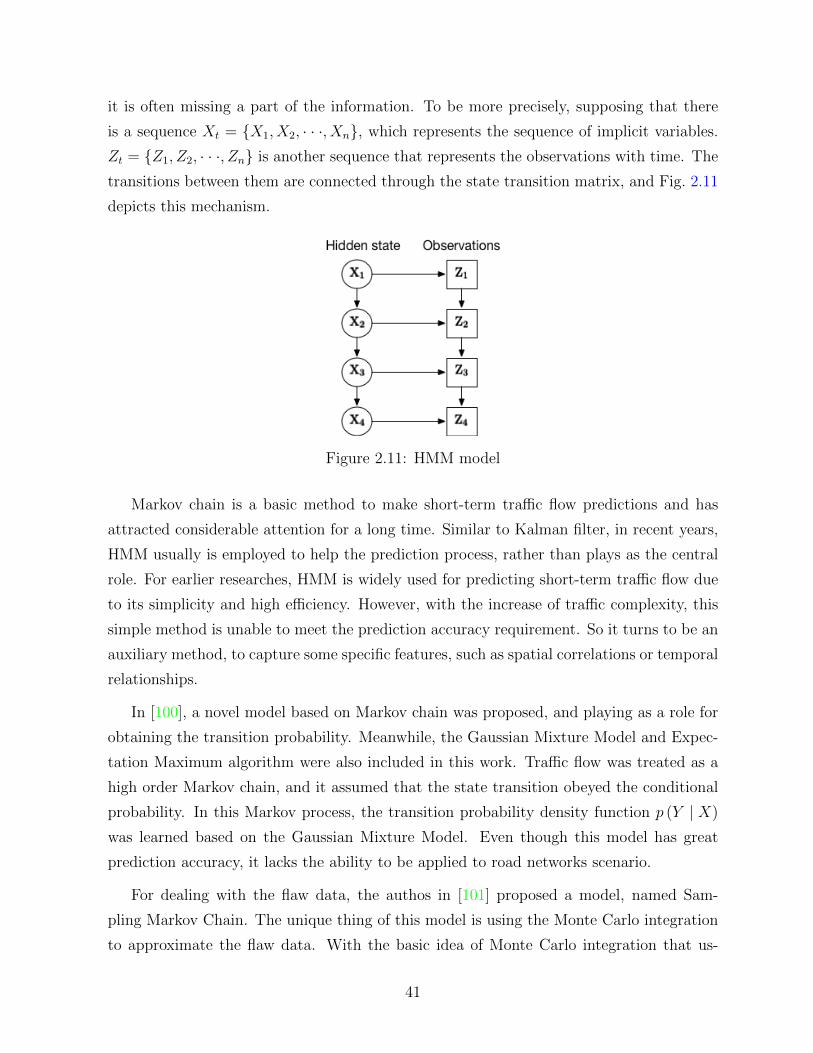
it is often missing a part of the information. To be more precisely, supposing that there

is a sequence Xt = {X1, X2, · · ·, Xn}, which represents the sequence of implicit variables.

Zt = {Z1, Z2, · · ·, Zn} is another sequence that represents the observations with time. The

transitions between them are connected through the state transition matrix, and Fig. 2.11

depicts this mechanism.

Figure 2.11: HMM model

Markov chain is a basic method to make short-term traffic flow predictions and has

attracted considerable attention for a long time. Similar to Kalman filter, in recent years,

HMM usually is employed to help the prediction process, rather than plays as the central

role. For earlier researches, HMM is widely used for predicting short-term traffic flow due

to its simplicity and high efficiency. However, with the increase of traffic complexity, this

simple method is unable to meet the prediction accuracy requirement. So it turns to be an

auxiliary method, to capture some specific features, such as spatial correlations or temporal

relationships.

In [100], a novel model based on Markov chain was proposed, and playing as a role for

obtaining the transition probability. Meanwhile, the Gaussian Mixture Model and Expec-

tation Maximum algorithm were also included in this work. Traffic flow was treated as a

high order Markov chain, and it assumed that the state transition obeyed the conditional

probability. In this Markov process, the transition probability density function p (Y | X)

was learned based on the Gaussian Mixture Model. Even though this model has great

prediction accuracy, it lacks the ability to be applied to road networks scenario.

For dealing with the flaw data, the authos in [101] proposed a model, named Sam-

pling Markov Chain. The unique thing of this model is using the Monte Carlo integration

to approximate the flaw data. With the basic idea of Monte Carlo integration that us-

41

ing random numbers to numerical integration, the prediction Y converted into the form

E (Y | Xti) = 1/n∑n

i=1E (Y | Xti), which greatly overcome the missing data problem. For

better proving the high performance of this model, the authors compared it with two simi-

lar models, Historical Average Markov Chain method and Joint Distribution Recalculating

method.

Apart from the flow prediction, HMM also can be found in traffic state prediction.

In [102], HMM was employed to make a short-term freeway traffic state and speed predic-

tion, in which the traffic states are upgraded from one dimension to a higher dimension.

Different from the previous studies using traffic volume to implement prediction, this work

is by using the speed information to conduct a peak-hour traffic state prediction. Notably,

the time series was imported into two-dimensional space to facilitate the HMM process.

To summarize, HMM is a simple and easily understood approach that suitable for

short-term traffic flow prediction. However, for better dealing with the more and more

complicated road structure and volatile transportation system, combining HMM with other

prediction methods is becoming a new trend today.

2.5 Conclusion

This chapter gives a general review of the researches on the short-term traffic flow predic-

tion field. Beginning from some fundamental concepts in the forecasting process, such as

on-sample/out-of-sample, on-line/off-line, etc., which gives a basic idea of what it is the

prediction. And then, two main prediction categories are introduced, i.e., the statistical

models and machine learning-based ones. For the class of statistical models, it consists of

different models such as AR/MA family (e.g., ARMA, ARIMA, SARIMA, and VARIMA,

etc.) and ES series. For the machine learning category, both supervised methods and

unsupervised learning methods are introduced. In supervised learning subclass, several

popular algorithms are given, including K-NN, Linear regression, SVM, and RNN, etc.

Notably, RNN including LSTM, GRU as a significant approach is adopted by more and

more researchers nowadays in short-term traffic flow prediction area. Based on the previous

works and also considering of the advantages as well disadvantages of them, some studies

are conducted at the following chapters.

42

Chapter 3

DSTARMA: A travel-delay aware

short-term vehicular traffic flow

prediction scheme for VANET

In this chapter, an innovative hybrid prediction method, Delay-based Spatial-Temporal

Autoregressive Moving Average model (DSTARMA) is proposed to enhance the patterns

mining ability of statistic-based models. In fact, the high mobility of the vehicles makes

the topology of Vehicular ad-hoc network (VANET) unstable [103] [104], and real-time

road information is generally limited [105] [106] [107]. Considering these shortcomings,

it is helpful to use the accurate traffic prediction to assist the topology control in the

VANET [108] [109]. Particularly, this model also focuses on dealing with the travel delay

problem in short-term traffic flow prediction, and by handling it in the form of spatial-

temporal weighted matrices to help capture non-linear features in spatiotemporal relations.

In addition, this method has been accpted and published in [110].

3.1 Problem statement

As we all know, the traffic volume generated by different roads may be able to interact with

each other, which means the traffic volume at one road may be influenced by its nearby

road segments directly or indirectly in the same certain area. For better illustrating the

spatial correlations of these road segments, Seven probers located in different connected

road segments were chosen, namely Location n (n = 1, 2, 3...7). So there are seven locations

43

in my tree-type road network shown in Fig. 3.1. In this road structure, It assumes that the

traffic flow is one-way from top to bottom, and location 1 (L1), location 2 (L2), location

3 (L3) and location 4 (L4) are the level I, and location 5 (L5) as well as location 6 (L6)

are the level II, following the location 7 (L7), the level III. It also assumes the traffic flow

from a higher level has an effect on itself as well as the traffic volume at a lower level. For

example, the impact of their own in level I is called the zeroth-order impact. Similarly,

the influence from level I to level II is called first-order impact, and to level III is called

second-order impact. So, these locations can be divided to k th order, k = 0, 1, 2..., on the

impact degree basis. In the traditional equal weight STARMA model (EW-STARMA),

the influence weight of locations at the same level is average. For example, the impact on

L5 is shared evenly by L1 and L2. Likely to L5, for L7, six locations can have an impact

on it, so each location contributes 1/6 influence to L7. However, this allocation approach

is too simple to capture the spatial-temporal characteristics entirely. In other words, the

travel time of vehicles from one location to another location, namely travel delay, is ignored

by this EW-STARMA model. So, how to properly take advantage of this travel delay for

improving the accuracy of short-term traffic flow prediction is my goal in this chapter.

Figure 3.1: An example of a three-level road network

3.2 Proposed method

In consideration of the hypothesis stated before that the spatial-temporal relationship can

make an impact on prediction result, DSTARMA is illustrated specifically in this section

in a progressive manner. From the very beginning, some very fundamental theories and

formulas will be explained briefly, such as VARMA and STARMA. After having a basic

view of these models, my DSTARMA will be introduced precisely.

44

3.2.1 VARMA/ STARMA

Different from ARMA and ARIMA, the nature of VARMA is a multivariate process [111],

in which, multivariate data and their patterns can be identified, and the mutual impact

of them is shown at the same time. Especially, variables exist in the form of matrices

in VARMA model. Similar to the ARMA and ARIMA, VARMA can be defined by a

statistical formula, shown as follows.

A (L)Xt = M (L) ηt (3.1)

In this equation, Xt is the aim variable at time t that needs to be predicted, and L is the

lag operator like the function of B in ARMA [28].

A (z) = A0 + A1z + A2z2 + · · ·+ Apz

p (3.2)

M (z) = M0 + M1z + M2z2 + · · ·+ Mqz

q (3.3)

In two above equations, coefficients A0,A1, · · · ,Ap and M0,M1, · · · ,Mq are both matrices

with order n× n.

STARMA is derived from VARMA, and it distinguishes itself with weighted matrices.

There are mainly two variables in STARMA, space and time. By using a weighted matrix

to emphasize the spatial relationship is the main advantage of this model. The general

definition is expressed as follows.

Xt =

p∑l=1

kl∑kl=0

φlklW(kl)Xt−l −

q∑l=1

ml∑kl=0

θlklW(kl)ηt−l + ηt (3.4)

in which, n is the number of locations, and Xt is a n × 1 vector at time t. W(kl) is the

klth order n × n matrix. φlkl , θlkl are parameters terms of spatial-temporal AR (STAR)

and spatial-temporal MA (STMA) respectively, and ηt−l is a n × 1 vector at time t − l.According to the second stage of Box-Jenkins models, modeling is split into three stages,

model identification, parameter estimation and model checking [112]. As for parameter

estimation process, different from ordinary STARMA, using Yule-Walker equation and

Maximum Likelihood [113] as estimators to get φ and θ, in this study, Kalman fliter is

adopted to be estimator due to its high efficiency and accuracy.

45

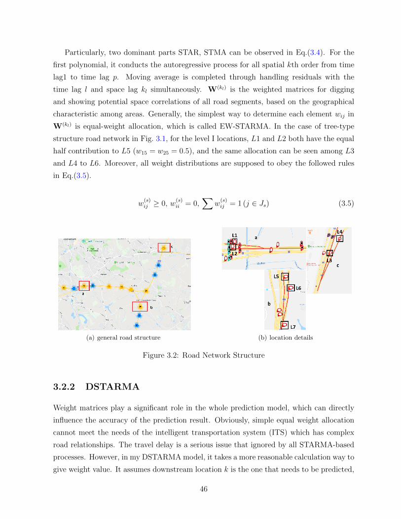
Particularly, two dominant parts STAR, STMA can be observed in Eq.(3.4). For the

first polynomial, it conducts the autoregressive process for all spatial kth order from time

lag1 to time lag p. Moving average is completed through handling residuals with the

time lag l and space lag kl simultaneously. W(kl) is the weighted matrices for digging

and showing potential space correlations of all road segments, based on the geographical

characteristic among areas. Generally, the simplest way to determine each element wij in

W(kl) is equal-weight allocation, which is called EW-STARMA. In the case of tree-type

structure road network in Fig. 3.1, for the level I locations, L1 and L2 both have the equal

half contribution to L5 (w15 = w25 = 0.5), and the same allocation can be seen among L3

and L4 to L6. Moreover, all weight distributions are supposed to obey the followed rules

in Eq.(3.5).

w(s)ij ≥ 0, w

(s)ii = 0,

∑w

(s)ij = 1 (j ∈ Js) (3.5)

(a) general road structure (b) location details

Figure 3.2: Road Network Structure

3.2.2 DSTARMA

Weight matrices play a significant role in the whole prediction model, which can directly

influence the accuracy of the prediction result. Obviously, simple equal weight allocation

cannot meet the needs of the intelligent transportation system (ITS) which has complex

road relationships. The travel delay is a serious issue that ignored by all STARMA-based

processes. However, in my DSTARMA model, it takes a more reasonable calculation way to

give weight value. It assumes downstream location k is the one that needs to be predicted,

46

and there are only two locations (Li, Lj) with directly connected, like the relationship of

L1, L2 and L5 in Fig. 3.1. The distance between i, k and j, k are dik, djk respectively, and

the travel delay is calculated with formulas in Eq.(3.6).

τik =dikνik

, τjk =djkνjk

(3.6)

and the final weight of Li to Lk at time t is defined in Eq.(3.7).

wik =Vi (t− τik)Vk (t)

=Vi (t− τik)

Vi (t− τik) + Vj (t− τjk)(3.7)

In Eq.(3.7), Vi (t) represents the traffic volume generated by upstream loation Li at

time t. This equation describes a fact that traffic flow data acquired at the moment t for

downstream location Lk is the sum of traffic volumes for upper stream location Li and Lj

at the time (t− τik) and (t− τjk). The travel delay τik,τjk in Eq.(3.6) are the time that

vehicles travel from Li to Lk, Lj to Lk. In this way, travel delay becomes a factor in spatial

weighted matrices when evaluating spatial relationship. Taking Fig. 3.1 for example, when

kl = 0, the weighted matrix for spatial lag 0 is an Identity matrix W(0) = I7×7, and for

spatial lag kl = 1 :

W(1) =

0 0 0 0 w15 0 0

0 0 0 0 w25 0 0

0 0 0 0 0 w36 0

0 0 0 0 0 w46 0

0 0 0 0 0 0 w57

0 0 0 0 0 0 w67

0 0 0 0 0 0 0

(3.8)

for spatial lag kl = 2 :

W(2) =

0 0 0 0 0 0 w17

0 0 0 0 0 0 w27

0 0 0 0 0 0 w37

0 0 0 0 0 0 w47

0 0 0 0 0 0 0

0 0 0 0 0 0 0

0 0 0 0 0 0 0

(3.9)

47

3.3 Verification

In this section, a case study is implemented by using my new model. As for the effect

evaluation, mean squared error (MSE), mean absolute percentage error (MAPE) and the

square of the sample correlation coefficient R-square (R2) are applied [114]. The formulas

are defined by following equations.

MSE =1

n

n∑t=1

(Xt − Xt

)2(3.10)

MAPE =100%

n

n∑t=1

∣∣∣∣∣Xt − Xt

Xt

∣∣∣∣∣ (3.11)

R2 = 1− SSresSStot

= 1−

∑t

(Xt − Xt

)2∑

t

(Xt − X

)2 (3.12)

3.3.1 Dataset

In this study, the England Highway traffic flow data at a 15-min interval were chosen,

which covers the period of all Wednesdays in May 2015 for seven different roads [115].

The location of seven probers is circled in Fig. 3.2, and the related information is listed

in Tab. 3.1. Since the travel delay is calculated based on the distance between the two

locations, the too-small distance leads to an insignificant travel delay, which does not meet

the experimental requirements, so followed seven locations were chosen as the experimental

path. Also, because the available and experimentally required data sets are very limited,

this experiment only adopted these seven locations as the predicted roads.

In addition, in my DSTARMA model, travel delay τ is short at the second level, which

is almost a real-time value but used dataset is 15-min interval statistic value, so that

practical traffic volume Vi (t− τik) cannot get directly.

For solving this problem, the Vl (t) l ∈ (i, j) was calculated as follows,

Vl (t) = Vl (t− τlk) =Vl (t) · (15− τlk)

15+Vl (t− 15) · τlk

15(3.13)

48

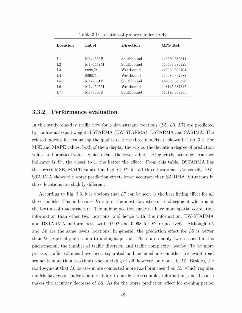
Table 3.1: Location of probers under study

Location Label Direction GPS Ref.

L1 M1/4556B Southbound 443630;389314

L2 M1/4557M Southbound 443593;389329

L3 8898/2 Westbound 449965;392404

L4 8898/1 Westbound 449989;392388

L5 M1/4551B Southbound 444092;389326

L6 M1/4505M Westbound 448145;387845

L7 M1/4500B Southbound 448120;387365

3.3.2 Performance evaluation

In this study, one-day traffic flow for 3 downstream locations (L5, L6, L7) are predicted

by traditional equal weighted STARMA (EW-STARMA), DSTARMA and SARIMA. The

related indexes for evaluating the quality of these three models are shown in Tab. 3.2. For

MSE and MAPE values, both of them display the errors, the deviation degree of prediction

values and practical values, which means the lower value, the higher the accuracy. Another

indicator is R2, the closer to 1, the better the effect. From this table, DSTARMA has

the lowest MSE, MAPE values but highest R2 for all three locations. Conversely, EW-

STARMA shows the worst prediction effect, lower accuracy than SARIMA. Situations in

three locations are slightly different.

According to Fig. 3.3, it is obvious that L7 can be seen as the best fitting effect for all

three models. This is because L7 sits in the most downstream road segment which is at

the bottom of road structure. The unique position makes it have more spatial correlation

information than other two locations, and hence with this information, EW-STARMA

and DSTARMA perform best, with 0.992 and 0.998 for R2 respectively. Although L5

and L6 are the same levels locations, in general, the prediction effect for L5 is better

than L6, especially afternoon to midnight period. There are mainly two reasons for this

phenomenon, the number of traffic diversion and traffic complexity nearby. To be more

precise, traffic volumes have been separated and included into another irrelevant road

segments more than two times when arriving at L6, however, only once in L5. Besides, the

road segment that L6 locates in are connected more road branches than L5, which requires

models have good understanding ability to tackle these complex information, and this also

makes the accuracy decrease of L6. As for the worse prediction effect for evening period

49

(a) one-day traffic flow prediction for L5

(b) one-day traffic flow prediction for L6

(c) one-day traffic flow prediction for L7

Figure 3.3: Comparison of Three models for L7, L6, L5

50

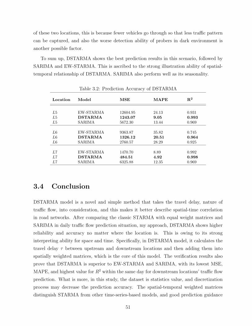
of these two locations, this is because fewer vehicles go through so that less traffic pattern

can be captured, and also the worse detection ability of probers in dark environment is

another possible factor.

To sum up, DSTARMA shows the best prediction results in this scenario, followed by

SARIMA and EW-STARMA. This is ascribed to the strong illustration ability of spatial-

temporal relationship of DSTARMA. SARIMA also perform well as its seasonality.

Table 3.2: Prediction Accuracy of DSTARMA

Location Model MSE MAPE R2

L5 EW-STARMA 12604.95 24.13 0.931L5 DSTARMA 1243.07 9.05 0.993L5 SARIMA 5672.30 13.44 0.969

L6 EW-STARMA 9363.87 35.82 0.745L6 DSTARMA 1326.12 20.51 0.964L6 SARIMA 2760.57 28.29 0.925

L7 EW-STARMA 1470.70 8.89 0.992L7 DSTARMA 484.51 4.92 0.998L7 SARIMA 6325.88 12.35 0.969

3.4 Conclusion

DSTARMA model is a novel and simple method that takes the travel delay, nature of

traffic flow, into consideration, and this makes it better describe spatial-time correlation

in road networks. After comparing the classic STARMA with equal weight matrices and

SARIMA in daily traffic flow prediction situation, my approach, DSTARMA shows higher

reliability and accuracy no matter where the location is. This is owing to its strong

interpreting ability for space and time. Specifically, in DSTARMA model, it calculates the

travel delay τ between upstream and downstream locations and then adding them into

spatially weighted matrices, which is the core of this model. The verification results also

prove that DSTARMA is superior to EW-STARMA and SARIMA, with its lowest MSE,

MAPE, and highest value for R2 within the same day for downstream locations’ traffic flow

prediction. What is more, in this study, the dataset is statistics value, and discretization

process may decrease the prediction accuracy. The spatial-temporal weighted matrices

distinguish STARMA from other time-series-based models, and good prediction guidance

51

can have the great impact on whatever data dissemination or vehicular routing scheduling

in VANET, so how to improve the matrices facilitating modeling is still a big challenge for

future research. In addition, a more diversified road network structure can be incorporated

in the future work. For example, it can select a more complex urban road network structure

rather than freeway roads, to apply in my new model, because rich data sets facilitate the

promotion of this model in multiple scenarios to increase its practical value.

52

Chapter 4

SSGRU: A Hybrid Traffic Volume

Prediction Approach for a Sparse

Road Network

This chapter focuses on the optimization of ML-based models. In previous studies, some

machine learning (ML)-based models were proposed to predict the traffic volume at a single

road segment/position, and these models performed not bad. However, when applied in a

more complicated road network, they show low efficiency or need to pay higher computing

costs. To solve this problem and further improve the model feature mining ability for

ML-based models, an innovative selected stacked gated recurrent units model (SSGRU) is

proposed. In addition, this method has been accepted and published in [116].

4.1 Problem statement

Different from the predictions based on the single road, an intact road network traffic vol-

ume prediction usually requires the higher mining ability for spatial-temporal information.

Considering of this, it assumes that there is a tree-shape road network within n road seg-

ments, and for each road, one detector is selected to count the number of vehicles, namely

Ln (n = 1, 2, 3, ...7), the same as the road structure shown in Fig. 3.1 of Chapter 3. The

traffic flow is the single direction from top to bottom, and the traffic volumes have an

impact on each other to a various extent. Traffic flow in the suburbs area is less on-ramp

and off-ramp [117], and also the impact from too far level traffic flow on the target location

53

is very limited or even negligible, so three-layer tree-shaped road network structure was

adopted to simulate the real road convergence, which is widely seen situation in real suburb

highway.

Figure 4.1: Weight assignment for a road network

Similar to the weights set in the last chapter, a set of weights wab, a, b ∈ (1, 2, 3, 4, 5, 6, 7)

are still used to describe these influential degrees among road segments, shown in Fig. 4.1.

Subscript a and b represent any two locations in this road framework. For example, weight

vector for Location1 (L1) is in the form of w1 = {w11, w21, ..., w71}, in which wa1, a ∈(2, 3, 4, 5, 6, 7), is the impact factor from La to L1. Through employing different wab, it can

be easier to catch correlations of all roads. Most of the previous traffic flow predictions only

consider a certain road segment. However, roads are interconnected, and traffic information

is fluent in real life. Prediction only with the temporal relationship is not able to meet

the needs of the more and more complicated transportation system nowadays. So how to

expand the prediction view from a single road to a road network and improve the accuracy

with a comparatively simple model at the same time is the goal of this chapter.

4.2 Proposed method

In consideration of the hypothesis stated above, a selected stacked GRU model is introduced

since GRU has a good ability to handle the time series in a highly efficient way. Also, a

stacked structure generates a deep learning procedure to gain a better training effect. There

are mainly two parts of this model, and the general structure is shown in Fig. 4.2. A road

network including multiple roads is firstly processed by Linear Regression Weight Selected

System, obtaining useful roads in this stage.

As for the second stage, stacked GRU learning system, does the model building, fore-

casting as well as results output. Additionally, traffic flow data selected by the previous

54

stage are split into training and testing groups. Multiple features (i.e., n features) are

simultaneously transported with aim feature into GRUs in layer 1. Manipulated by three

GRUs respectively, they get into layer 2, where input dimension change from n + 1 fea-

tures to only three features for each GRU in layer 2. Through a fully connected dense

layer, the shape of predictions is adjusted to one time series vector and ready to output.

Particularly, only five GRUs are used in this model, because traffic flow vibrations in the

same area show some similarities and hence a small number of learning units are enough to

dig their patterns. What is more, different from many other neural networks such as the

convolutional neural network (CNN) [118], which can stack over one hundred layers, RNN,

regards only two layers as deep learning network. Because each layer of RNN has a depth

in the time dimension, even if the number of RNN layers is small, the overall network size

will be pretty significant. Considering the above factors, two-layer and a total of five GRUs

are included in this model.

Figure 4.2: SSGRU model structure

55

4.2.1 Linear Resgression Weigt Selection System

This selection system is responsible for spatial correlation study, selecting high-impact

roads. In this period, every roads are given a weight related to the aim road by fitting into

a linear regression model. For example, given an aim road x0, it assumes all n roads in the

same area have impacts on it, so their relationship can be described by,

x0 = ω1x1 + ω2x2 + · · ·+ ωnxn, (4.1)

in which, x0, x1 · · · xn and ω1, ω2 · · · ωn are both 1× t vectors, and t is the time length.

Since it is linear regression, the linear function in Eq.(4.1) must be able to fit the data

optimally, that is, it must minimize the variance of the data to the fitted line. To represent

this variance, a cost function is defined to represent this amount as follows,

J (ω) =1

2t

t∑i=1

(hω(x(i))− x(i)0

)2, (4.2)

where, x(i) ∈ (x1, x2, · · ·, xn). To find a best parameter ω to minimize the cost function,

the gradient decent approach is employed based on the following equation,

ωj = ωj − α1

t

t∑i=1

(hω(x(i))− x(i)0

)x(i)j , (4.3)

where α is the learning rate and hω is the coefficient related to current ω. Finally, for each

road, this system will output a suitable weight ωj, with regards to the aim road x0. For

reduce input size, the weights that lower than 0.5 is drop, as this kind weights has limited

even converse impact on aim feature.

4.2.2 Stacked GRU

The principle of stacked GRU is similar with the simple GRU, and its internal structure

is shown in Fig. 4.3. As one kind of Recurrent Neural Network (RNN) unit, like LSTM,

it is also proposed to solve problems such as gradients in long-term memory and back

propagation [119] but with fewer control gates. In my case, the number of current input

xt is n, showing in red dash circle in Fig. 4.2. The hidden state ht−1 is passed by the

previous node owing the same size with xt. This hidden state contains information about

56

the previous node. Combined with xt and ht−1, GRU will get the output of the current

hidden node yt and the hidden state passed to the next node ht. Two gate states r and z

are calculated from the very beginning by using the formula shown below,

rt = σ(W (r)xt + U (r)ht−1

), (4.4)

zt = σ(W (z)xt + U (z)ht−1

), (4.5)

in which, W (r), W (z) and U (r), U (z) are weight matrices, and once one h is generated, a

ω is produced and added in the matrix. rt is the state of reset gate at time t, and zt is

the state of update gate at time t. These two gates decide how much to discard previous

information and what new information to add and pass to the future. The function σ

converts the data to a value in the range of 0 ∼ 1 to act as a gate signal. Reset gate will

store the relevant information from the past in h′ in Eq.(4.6),

h′ = tanh(Wxt + rt � Uht−1

), (4.6)

where � is the Hadamard Product, and ⊕ stands for matrix addition.

In this step, h′ contains current input data xt, scaling the data to a range of -1 to 1 by

a tanh activation function, to achieve memory purpose. Last but not least procedure of

GRU is to figure out current hidden state ht by Eq.(4.7) and output yt is the combination

of ht and xt. When this step is done, the model finish the memory update process, and

particularly, the closer the gating signal of z is to 1, the more data represents ”memory”;

the closer to 0, the more ”forgotten”.

ht = zt � ht−1 +(1− zt

)� h′ (4.7)

The first part of this equation is to forget some useless information in the ht−1, similar to

the forget gate in LSTM [120]. The second part indicates the selective ”memory” of h′,

which contains current node information. After the first layer GRU finishes their task and

each GRU output a prediction sequence, these sequence will be continue input into next

layer GRU. Stacked GRU is the upgrade version of GRU, which has a much stronger ability

of individual pattern learning, digging into details through layer by layer. For example,

after disposing of three GRUs in layer 1, three first-learned results are thrown into all

GRUs in the second layer as the Fig. 4.2 shows.

57

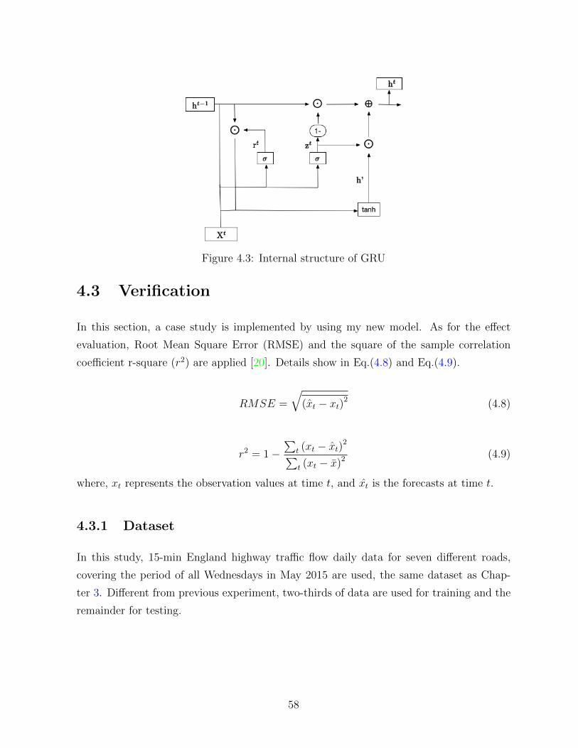
Figure 4.3: Internal structure of GRU

4.3 Verification

In this section, a case study is implemented by using my new model. As for the effect

evaluation, Root Mean Square Error (RMSE) and the square of the sample correlation

coefficient r-square (r2) are applied [20]. Details show in Eq.(4.8) and Eq.(4.9).

RMSE =

√(xt − xt)2 (4.8)

r2 = 1−∑

t (xt − xt)2∑t (xt − x)2

(4.9)

where, xt represents the observation values at time t, and xt is the forecasts at time t.

4.3.1 Dataset

In this study, 15-min England highway traffic flow daily data for seven different roads,

covering the period of all Wednesdays in May 2015 are used, the same dataset as Chap-

ter 3. Different from previous experiment, two-thirds of data are used for training and the

remainder for testing.

58

4.3.2 Performance evaluation

In this study, one-day traffic flow prediction for all seven locations is conducted at an

interval of 15-min. To better describe the high performance of my model, the validation

work not only tested my new model, but also compared it with other models, such as

LSTM, GRU, Stacked GRU (SGRU) and Selected GRU (SEGRU).

The predicted traffic flow for three downstream locations are shown in Fig. 4.4, from

which we can see that my method is to perform better in details forecasting. Moreover,

according to Fig. 4.5, we can see that RMSE values for all locations of my SSGRU model are

the smallest. Notably, the decline for L5 is the most dramatic, to almost half amount of the

other two methods. This is may because there are more connected fork roads connected

with this road, and the linear regression selection system is more helpful to filter the

useful roads to make the subsequent learning more effective. As for the L6 and L7, the

performance of these two roads are pretty similar, and both with nearly 10% reduction

since the road condition in these two roads are similar. In contrast to RMSE, the index of

r2 shows a slight increase in three locations, become closer to 1, which fully demonstrates

that my algorithm performs are the best among three models, and my approach makes the

prediction accuracy improved obviously.

To further prove the advancement of my model, SSGRU was compared with two other

similar models. The first one is the GRU with road selection (SEGRU), the second one is

the stacked GRU without road selection (SGRU), and the results can be seen in Fig. 4.6.

Although the r2 values of these three models are very close, the RMSE is quite different, in

which my model SSGRU always maintains the lowest RMSE. This set of comparisons also

illustrates that the combination of data pre-processing and stacking structure can make

the prediction effect the best.

4.4 Conclusion

SSGRU is an innovative model, which is good to be fit into a road network, in a simple

and easy to understanding manner. The data preprocessing system leaves out low impact

roads, which not only reduces the cost of subsequent computational but also improves the

prediction accuracy. Besides, the low computational cost and ease of understanding are

also advantages of this pre-processing system. Stacked two layers of GRUs give the deep

learning ability to data, better digging out the pattern details. In fact, due to the less

59

(a) one-day traffic flow prediction for L5

(b) one-day traffic flow prediction for L6

(c) one-day traffic flow prediction for L7

Figure 4.4: Comparison of Three models for L7, L6, L5

60

(a) RMSE

(b) r2

Figure 4.5: RMSE and r2 for LSTM, GRU and SSGRU

61

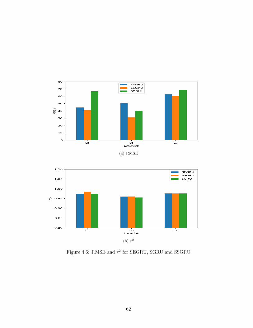
(a) RMSE

(b) r2

Figure 4.6: RMSE and r2 for SEGRU, SGRU and SSGRU

62

number of gating controls in GRU, the computational complexity is significantly reduced

compared with LSTM but with a much better result in my study. In general, this new

model is simple, high efficiency and low computational complexity, and last but not least, it

conducts prediction from a network perspective instead of an individual one, which is more

practical in real life. In fact, with the development of ITS, reliable traffic flow predictions

for the urban areas become significant because this information can greatly facilitate traffic

management. However, the more complicated urban road features make it is difficult to

achieve, so in the next chapter, an innovative approach will be proposed to solve this

problem.

63

Chapter 5

A Delay-Based Deep Learning

Approach for Traffic Volume

Prediction on a Road Network

Based on the DSTARMA and SSGRU introduced before, a delay-based deep learning

framework (MDGRU) will be proposed to improve the accuracy of the short-term traffic

flow prediction, in which travel delay is handled in the form of a weighted matrix enrolled

into a multivariate input stacked Recurrent Neural Network (RNN). Multivariate input

makes this approach has a stronger mining ability for spatial relationships capture, and

the stacked structure leads to a more accurate pattern learning process. Moreover, urban

and suburban road networks are both tested in this chapter, and the results show that my

approach is accurate and reliable.

5.1 Problem statement

Most of the previous studies related to the short-term traffic flow predictions are based

on the single road, in which spatial correlations are lost. Therefore, how to improve the

accuracy and efficiency of the volume predictions under a specific road network structure

is my main task in this chapter. In particular, for better model adpatability, my study is

based on two environments, suburban and urban areas.

64

5.1.1 Suburban scenario

Traffic patterns in suburban areas are comparatively simple and usually set as a funda-

mental road context in many traffic flow prediction researches. In this paper, to better

describe the spatial information, we adopt a tree structure to modeling the real traffic

shape shown in Fig. 5.1, since the on-ramp and off-ramp situations are less seen in subur-

ban highways [117] and too long-distance locations barely affect the aim feature. Also, we

assume the traffic flow is single direction only, from top to bottom. For this road structure,

7 locations are set, where the L7 is the aim feature, and for each location, it has a corre-

sponding weight to describe the spatial correlations. In fact, there are two level influences

have an impact on the aim feature: the first level is coming from the L1, L2, L3, and L4,

and L5, L6 generates the second-level effect. To better depicting the spatial relationships

among different road segments, a set of weights wab are employed, and it represents the

influence of the La to Lb.

Figure 5.1: Three-layer tree shape unit

When vehicles move from any two neighboring locations, from La to Lb, the time cost

is produced, and this time cost is named the travel delay τab. With the different distance

and speed, travel delay varies. In previous studies, travel delay is neglected, and they more

focus on the single road prediction instead of the whole road network. So, how to consider

these two issues and further improve the forecasting accuracy and efficiency is my goal in

this chapter.

65

5.1.2 Urban scenario

For the suburban road network, the traffic condition is comparatively simple and easy to

describe, so a tree-shape structure is a good model to depict the suburban road networks.

However, for the urban road network, the road shapes are more complex, so how to fit

this given tree-shaped structure into the urban road network is my primary task, which is

accordingly convenient to urban routing and data transmission [121] [2].

In fact, typical urban road structures with m road segments can be decomposed into

several binary tree shape units. For example, the T road (m = 3) and the crossroad (m = 4)

can be separated into one and two binary tree units respectively, shown in Fig. 5.2. Further,

if expanding the road shape to the star type, the number of binary tree unit N can be

calculated based on the equation below.

N =

{m−12

m ∈ odd,m2

m ∈ even,(5.1)

in which, m ≥ 3. For the special case that m = 1 or m = 2, which is not a road network

anymore, and was not in my discussion range.

(a) T-shape Road (b) Cross Road

Figure 5.2: Decomposition of two types of road structure

When in network decomposition, some road segments may be shared by several divided

tree units. For example, the crossroad shown in Fig. 5.2, is divided into two binary tree

units, and obviously, two middle road segments and four locations are shared. As for the

66

weights of shared locations, the influence is allocated equally. To be more precise, in this

case, a crossroad is separated as tree shape structure, which is the same as the situation in

Fig. 3.1. However, Lb, Lc equally share the same location volume, in which Vb = Ve = 1/2V1

and Ve = Vf = 1/2V2. Generally, if there are the number of a shared locations, and the

volume recorded by the prober at this area is Vp, so for each shared location, the volume

Vsl can be calculated as follows.

Vsl =1

aVp (5.2)

This section illustrates the problem that needs to be resolved, and in the following

section, my innovative approaches will be given in a step by step manner.

5.2 Proposed method

My method is based on a deep learning framework, and delay-based GRU is the basic unit

in this model, which is used to complete different tasks at different layers. Compared to

the shallow learning fashion, deep learning can obtain more patterns and dig out more

in-depth information, and this advantage can significantly improve prediction accuracy.

Original GRU structure contains two gates, reset gate and update gate respectively. Fewer

gates than LSTM makes GRU more efficient in the prediction process but still with the high

prediction accuracy. Different from the basic gates in traditional GRU based structures,

my MDGRU consists of the two delay-based gates within the three-layer learning structure.

What is more, the details for these three RNN units are listed in the Tab. 5.1. As for my

two improved gates, they are able to handle the travel delay according to the delay-based

weights. So before stepping into the specific MDGRU structures, the concept of delay-based

weights, as well as the delay-based GRU, are illustrated, to give a better understanding of

MDGRU.

5.2.1 Delay-based Weight

In the previous spatial weights calculation, most of them are worked out in an even fashion.

For example, for L5 in Fig. 3.1 there are two directly linked locations L1 and L2 respec-

tively, and contribution weight of each location is average assigned. So the influential from

L1 to L5 (w15) is equal to the L2 to the L5 (w25), are both 0.5. However, this calculation

approach is too naive to fit into the real traffic conditions. In fact, when vehicles move

67

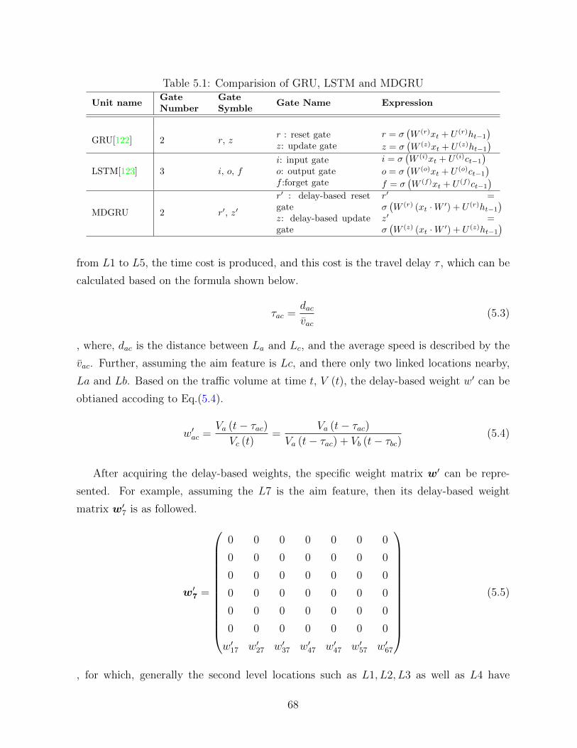
Table 5.1: Comparision of GRU, LSTM and MDGRU

Unit nameGateNumber

GateSymble

Gate Name Expression

GRU[122] 2 r, zr : reset gatez: update gate

r = σ(W (r)xt + U (r)ht−1

)z = σ

(W (z)xt + U (z)ht−1

)LSTM[123] 3 i, o, f

i: input gateo: output gatef :forget gate

i = σ(W (i)xt + U (i)ct−1

)o = σ

(W (o)xt + U (o)ct−1

)f = σ

(W (f)xt + U (f)ct−1

)MDGRU 2 r′, z′

r′ : delay-based resetgatez: delay-based updategate

r′ =σ(W (r) (xt ·W ′) + U (r)ht−1

)z′ =σ(W (z) (xt ·W ′) + U (z)ht−1

)from L1 to L5, the time cost is produced, and this cost is the travel delay τ , which can be

calculated based on the formula shown below.

τac =dacvac

(5.3)

, where, dac is the distance between La and Lc, and the average speed is described by the

vac. Further, assuming the aim feature is Lc, and there only two linked locations nearby,

La and Lb. Based on the traffic volume at time t, V (t), the delay-based weight w′ can be

obtianed accoding to Eq.(5.4).

w′ac =Va (t− τac)Vc (t)

=Va (t− τac)

Va (t− τac) + Vb (t− τbc)(5.4)

After acquiring the delay-based weights, the specific weight matrix w′ can be repre-

sented. For example, assuming the L7 is the aim feature, then its delay-based weight

matrix w′7 is as followed.

w′7 =

0 0 0 0 0 0 0

0 0 0 0 0 0 0

0 0 0 0 0 0 0

0 0 0 0 0 0 0

0 0 0 0 0 0 0

0 0 0 0 0 0 0

w′17 w′27 w′37 w′47 w′47 w′57 w′67

(5.5)

, for which, generally the second level locations such as L1, L2, L3 as well as L4 have

68

limited influences on L7, due to the off-ramp or on-ramp situations commonly seen in

middle locations L5, L6. So for further reducing the computation burden, the directly

linked features are considered only. And for the whole road network the delay-based

matrices is W ′ = [w′a,w′b, · · ·,w′n], which is comprised of the delay-based weight matrix of

all locations.

5.2.2 Delay-based GRU

Different from the ordinary GRU shown in Fig. 5.3, which only contains two gates, r and

z. A delay-based GRU introduces the delay-based weight matrix in its control gates, which

is based on the followed equations.

(a) Simple GRU structure (b) Delay-based GRU structure

Figure 5.3: Two types of GRU structures

r′t = σ(W (r) (xt ·W ′) + U (r)ht−1

)(5.6)

z′t = σ(W (z) (xt ·W ′) + U (z)ht−1

)(5.7)

ht = z′t � ht−1 + (1− z′t)� h′ (5.8)

, in which the σ is a function that transforms data between 0 to 1, and � is the Hadamard

Product. Moreover, W (r), W (z) and U (r), U (z) are the original weights related to the two

control gates.

69

5.2.3 MDGRU

To tackle the travel delay in a more sensible and efficient way, Multivariate Delay-based

GRU (MDGRU) is given. By adding a delay based weight in each GRU, and canceling

the data preprocessing system used by many previous GRU-based researches, MDGRU is

coming out. MDGRU model choose the deep learning as its core prediction structure, and

the structure is shown in Fig. 5.4. There are three layers included in this structure, in

which the first layer is hired to handle the spatial relationships, and the second layer is to

temporal patterns mining. The last layers are for reshape and output final result.

Figure 5.4: MDGRU structure

Compared with the most deep learning models, MDGRU is more compact, which gets

rid of the data-preprocessing system and disposes of the raw data directly. The dimension

of the dataset is gradually reduced, where precisely, the n × t input matrice is fed, and

after the first layer disposal, the dimension is down to 3 × t. And then the 2 × t matrice

produced by Layer 2 is reshaped by the dense layer, and finally, a 1 × t prediction vector

is prepared for output.

For this optimized system that is based on the trial-and-error method, the traffic flow of

an intact road network can be efficiently used to make a short-term traffic flow prediction.

By replacing the GRU to the delay-based GRU as its main prediction unit, and based

on a deep learning structure, MDGRU has ability to not only prediction the whole road

network, but also solve the travel delay problem.

70

5.3 Verification

To further test my innovative methods, in this section, a case study is implemented. My

proposed methods, MDGRU is used to predict short-term traffic flow, and two kinds of

road conditions are covered as well, urban and suburban road networks in a step-by-step

fasion. What is more, some error evaluation figures such as mean absolute error (MAE),

the square of the sample correlation coefficient r-square (r2) and Root Mean Square Error

(RMSE) shown in Eq.(5.9)-Eq.(5.11) are employed to judge the model performance at the

end.

MAE =

∑ni=1 |yt − xt|

n(5.9)

RMSE =

√(yt − xt)2 (5.10)

r2 = 1−∑

t (xt − yt)2∑t (xt − xt)2

(5.11)

5.3.1 Suburban scenario

5.3.1.1 Dataset

The used suburban data source is based on the England highway system, and 15-min

interval traffic flow is adopted, and they cover all Wednesdays in May 2015 for seven

different roads respectively, the same dataset used in Chapter.3.

In addition, since the real travel delay τ is pretty short at the second level, which is

almost a real-time value, so the Va (t− τac) can not be obtained directly for the raw dataset.

For getting over this problem, the practical traffic volume can be calculated based on the

equation below.

Va (t− τac) =Va (t) · (15− τac)

15+Va (t− 15) · τac

15(5.12)

5.3.1.2 Results for Suburban context

In this study, one-day traffic flow with the 15-min interval of three downstream locations

L5, L6, L7 are predicted. For further proving the superiority of my method, two popular

71

and widely used machine learning models, GRU and LSTM are compared under the same

situations.

Table 5.2: Prediction Accuracy of Suburban road network

Location Model MAE RMSE r2

L5 GRU 49.145 66.169 0.975

L5 MDGRU 38.128 51.689 0.986

L5 LSTM 48.819 66.377 0.975

L6 GRU 31.683 43.714 0.946

L6 MDGRU 28.986 40.019 0.964

L6 LSTM 33.701 48.742 0.951

L7 GRU 49.781 69.480 0.972

L7 MDGRU 44.140 59.857 0.990

L7 LSTM 49.791 69.161 0.974

As for the suburban context, the prediction results are shown in Tab. 5.2, and Fig. 5.5,

from which it can be found that MDGRU has the highest prediction accuracy for all

locations. With nearly 20% decrease of MAE and RMSE in L5, MDGRU shows its stronger

forecasting ability than the other two methods. Particularly, the r2 for L7 rises up to

0.990, which is pretty close to the 1.0, while GRU and LSTM only reach to 0.972 and

0.974 individually. For the L6, MDGRU still has the best prediction accuracy, 28.986 for

MAE and 40.019 for RMSE, both lower than values generated by fundamental GRU and

LSTM. In addition, for L6, it has slightly worse accuracy than L5 and L7, and the reason

for this is that there are more road segments connected with L6, so the on-ramp and off-

ramp probability are higher than other two locations. From the results shown in Fig. 5.5,

it can be found that my MDGRU model has the best performance along all day, especially

at the afternoon to midnight period. The reason for this phenominon is that the traffic

volume at that time is large, accordingly the patterns are comparatively hard to capture.

So, the accuracy of three models at this time period are all decrease with varing degrees.

Particularly, the most slight deviation is happend in my MDGRU model, which means

my model has the more powerful prediction ability than the others. When compared the

general prediction results of three downstream locations, the best fiiting effect is the L6,

since L6 has the least connected road segments nearby and off-ramp (on-ramp) situations.

72

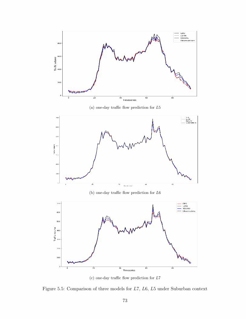
(a) one-day traffic flow prediction for L5

(b) one-day traffic flow prediction for L6

(c) one-day traffic flow prediction for L7

Figure 5.5: Comparison of three models for L7, L6, L5 under Suburban context

73

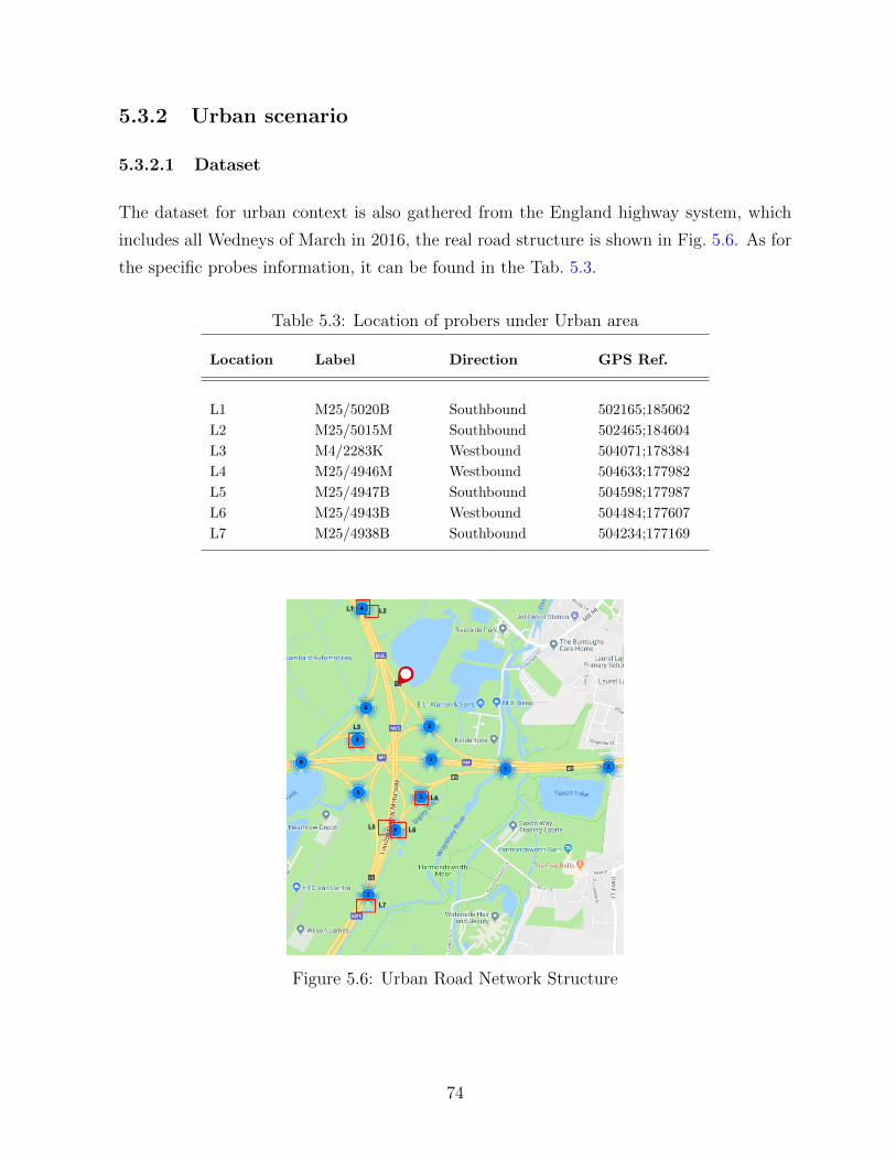
5.3.2 Urban scenario

5.3.2.1 Dataset

The dataset for urban context is also gathered from the England highway system, which

includes all Wedneys of March in 2016, the real road structure is shown in Fig. 5.6. As for

the specific probes information, it can be found in the Tab. 5.3.

Table 5.3: Location of probers under Urban area

Location Label Direction GPS Ref.

L1 M25/5020B Southbound 502165;185062

L2 M25/5015M Southbound 502465;184604

L3 M4/2283K Westbound 504071;178384

L4 M25/4946M Westbound 504633;177982

L5 M25/4947B Southbound 504598;177987

L6 M25/4943B Westbound 504484;177607

L7 M25/4938B Southbound 504234;177169

Figure 5.6: Urban Road Network Structure

74

5.3.2.2 Results for Urban context

Three methods under the urban road network are also compared, and the result is shown

in Tab. 5.4. Compared with the suburban context, the urban road network is more com-

plicated and volatile. However, for the urban context, MDGRU has a bigger improvement

than under suburban road condition. With almost 35% and 15% decrease of MAE and

RMSE for L6 and the other two locations, MDGRU shows its stronger adaptability for

unstable conditions. Besides, even though in complex road conditions, the r2 values pro-

duced by MDGRU for three locations are all beyond 0.97, which proves the outstanding

stability of my new method.

The prediction curves for urban area in Fig. 5.7 further illustrates the stronger pre-

diction ability of MDGRU. For all three locations, L5, L6 and L7, MDGRU shows the

best fitting effect. The prediction accuracy for these three models on urban context all

fall down, due the more complexity prediction enviroments carring more noises and use-

ful information. Even though, compared to GRU and LSTM, my model shows its high

reliability, has the slightest deteriorate for all error values amongß three locations.

To sum up, the results for both suburban and urban road networks, MDGRU has high

accuracy and stable performance, and the improvement for the latter is more obvious.

Despite the accuracy for the urban roads are lower than the roads located in suburban

area, the r2 values are all higher than 0.96 by using the MDGRU model; as for another

error evaluation standards, MAE and RMSE, the values generated by MDGRU are all

greatly lower than the values derived from GRU and LSTM.

5.4 Conclusion

In this chapter, based on the basic GRU, a deep learning model is come up with, namely

MDGRU, to solve the travel delay problem in road networks. In my model, the three-layer

structure is adopted with a diminishing dimension, for which the first layer is used to mine

the spatial correlations and the second layer is responsible for the traffic patterns learning

with time. Particularly, my model is an optimized GRU model, which contains mult-task

delay-based GRUs. Delay-based weights participate in the prediction process, used to takle

the travel delay problem, and they are fed into simple GRU to form the delay-based GRU.

Simply, the travel delay is treated as the form of delay-based weight matrice to be fed

into the simple GRU, and also the advantage of this proposed model is that it can handle

75

(a) one-day traffic flow prediction for L5

(b) one-day traffic flow prediction for L6

(c) one-day traffic flow prediction for L7

Figure 5.7: Comparison of three models for L7, L6, L5 under Urban context

76

Table 5.4: Prediction Accuracy of Urban road network

Location Model MAE RMSE r2

L5 GRU 58.329 79.612 0.962

L5 MDGRU 52.013 74.216 0.971

L5 LSTM 57.837 79.205 0.963

L6 GRU 80.282 108.916 0.974

L6 MDGRU 53.179 73.198 0.977

L6 LSTM 80.298 107.842 0.974

L7 GRU 80.354 107.575 0.964

L7 MDGRU 69.258 90.282 0.974

L7 LSTM 80.252 108.469 0.972

the whole road network dataset just one time and no need to do any pre-processing data

works. Compared with previous short-term traffic flow prediction studies, MDGRU model

has a more simple structure but higher efficiency.

For better illustrating the great adaptability and stability for most of the road networks,

two kinds of road contexts are employed, roads in suburban and urban areas. Different

from the simplicity of suburban road shape, in the urban area, the shapes of which are

more complex. The introduce of binary tree unit is greatly deal with this problem through

the road network decomposition. Generally, most of the commonly seen road shapes can

be separated into several binary tree units, and the final impact is the sum of influence

from these units. Through a 15-min traffic flow prediction by using three test models,

GRU, LSTM, and MDGRU, respectively, the superiority of my MDGRU is shown. To be

more specific, the three error evaluation figures MAE, RMSE and r2 of MDGRU are all

the lowest among three models for both two road conditions.

This method not only figures out the travel delay problem in most of the road networks

but simplify the deep learning inner structure. By using this method, the prediction

accuracy is obviously improved, and the computation cost is reduced at the same time.

Particularly, for making approach more general, it is extended to urban road networks, and

the experiment shows its great adaptability. In my study, due to the limitation of a valid

dataset, the experiment only based on the three-week traffic flow data, so for the future

work, the data source can be more abundant. Also, bi-direction traffic flow is a potential

problem that may affect prediction accuracy, which is deserved to discuss.

77

Chapter 6

Conclusion and Future Work

In this thesis, three models are proposed to improve the spatiotemporal feature mining abil-

ity and adaptability for both statistical-based and ML-based models. In the first model,

based on the statistics model (VARIMA) and considers travel delay, DSTARIMA dra-

matically improves the classic statistic-based models feature capture ability, especially for

non-linear patterns. The results show it has higher prediction accuracy than other classic

statistic-based models. To further enhance the adaptability of ML-based models, SSGRU

is designed, in which a data preprocessing system is introduced, and the whole training

process is under a deep learning structure. As for the final scheme, MDGRU, which is

inspired by the SSGRU and DSTARIMA. Notably, this model considers the travel delay,

and moreover, it extends the prediction scenario to a more complicated road environment,

which makes this model have better adaptability and more practical in the real world.

Although the proposed three models enhance the model feature mining ability and

adaptability to some extent, there are still many potential works for the future. The first

one is to reduce the model complexity in a proper way. To be more precise, model complex-

ity generally can be judged from two aspects, the structure complexity, and computation

complexity. Ordinarily, with the increase of model structure complexity, the computation

complexity will rise accordingly. In fact, the hybrid models are leading a new trend, but

in some models, improperly combination of too many algorithms gives much burden on

prediction procedure and causes a low prediction efficiency and accuracy. The second one

is finding a more reliable data source and properly fixing the flaw dataset. The limitation

of the valid data source is another problem needed to be solved, for which data missing as

well as error are main concerns [124]. Currently, they are many data sources used in traf-

fic flow predictions, such as Highways England [115], Caltrans Performance Measurement

78

System (PeMs) [125], Maryland 511 (MD) [126], etc. However, the traffic flow interval of

these data sources is generally based on the 15-min, which also is a limitation for shorter

interval studies. Besides, how to adapt these three models into hybrid city road networks

that involve highways and paths is also a potential work in the future.

To sum up, in this thesis both statistic-based and ML-based models are improved

within two aspects, the model mining ability, and adaptability. Besides, some fundamental

concepts and potential future works about the short-term traffic flow predictions are also

briefly illustrated at the very beginning and at the end respectively.

79

References

[1] Maram Bani Younes and Azzedine Boukerche. A performance evaluation of an effi-

cient traffic congestion detection protocol (ecode) for intelligent transportation sys-

tems. Ad Hoc Networks, 24:317–336, 2015.

[2] Hengheng Xie, Azzedine Boukerche, and Antonio AF Loureiro. A multipath video

streaming solution for vehicular networks with link disjoint and node-disjoint. IEEE

Transactions on Parallel and Distributed Systems, 26(12):3223–3235, 2014.

[3] Azzedine Boukerche, Jan M Correa, Alba Cristina Magalhaes Melo, and Ricardo P

Jacobi. A hardware accelerator for the fast retrieval of dialign biological sequence

alignments in linear space. IEEE Transactions on Computers, 59(6):808–821, 2010.

[4] Azzedine Boukerche, Richard WN Pazzi, and Jing Feng. An end-to-end virtual en-

vironment streaming technique for thin mobile devices over heterogeneous networks.

Computer Communications, 31(11):2716–2725, 2008.

[5] Abdelhamid Mammeri, Azzedine Boukerche, and Zongzhi Tang. A real-time lane

marking localization, tracking and communication system. Computer Communica-

tions, 73:132–143, 2016.

[6] Abdelhamid Mammeri, Azzedine Boukerche, and Guangqian Lu. Lane detection and

tracking system based on the mser algorithm, hough transform and kalman filter. In

Proceedings of the 17th ACM international conference on Modeling, analysis and

simulation of wireless and mobile systems, pages 259–266, 2014.

[7] Cesar Hernandez, Diego Giral, and Fredy Martinez. Radioelectric spectrum predic-

tion based in arima and sarima time series models. International Journal of Applied

Engineering Research, 13(22):15688–15695, 2018.

80

[8] Azzedine Boukerche, Horacio ABF Oliveira, Eduardo F Nakamura, and Antonio AF

Loureiro. Localization systems for wireless sensor networks. IEEE wireless Commu-

nications, 14(6):6–12, 2007.

[9] A Boukerch, Li Xu, and Khalil El-Khatib. Trust-based security for wireless ad hoc

and sensor networks. Computer Communications, 30(11-12):2413–2427, 2007.

[10] Hirotugu Akaike. A new look at the statistical model identification. In Selected

Papers of Hirotugu Akaike, pages 215–222. Springer, 1974.

[11] Chris Chatfield. The analysis of time series: an introduction. Chapman and

Hall/CRC, 2016.

[12] William D Penny. Comparing dynamic causal models using aic, bic and free energy.

Neuroimage, 59(1):319–330, 2012.

[13] Paul B Wigley, Patrick J Everitt, Anton van den Hengel, JW Bastian, Mahasen A

Sooriyabandara, Gordon D McDonald, Kyle S Hardman, CD Quinlivan, P Manju,

Carlos CN Kuhn, et al. Fast machine-learning online optimization of ultra-cold-atom

experiments. Scientific reports, 6:25890:1–6, 2016.

[14] Dean Croushore. Frontiers of real-time data analysis. Journal of economic literature,

49(1):72–100, 2011.

[15] Nicholas G. Polson and Vadim O. Sokolov. Deep learning for short-term traffic flow

prediction. Transportation Research Part C: Emerging Technologies, 79(Supplement

C):1–17, 2017.

[16] Douglas M Hawkins. The problem of overfitting. Journal of chemical information

and computer sciences, 44(1):1–12, 2004.

[17] Harry Fisch, Grace Hyun, Robert Golden, Terry W Hensle, Carl A Olsson, and

Gary L Liberson. The influence of paternal age on down syndrome. The Journal of

urology, 169(6):2275–2278, 2003.

[18] Erich L Lehmann and George Casella. Theory of point estimation. Springer Science

& Business Media, 2006.

[19] Arnaud De Myttenaere, Boris Golden, Benedicte Le Grand, and Fabrice Rossi. Mean

absolute percentage error for regression models. Neurocomputing, 192:38–48, 2016.

81

[20] Tianfeng Chai and Roland R Draxler. Root mean square error (rmse) or mean ab-

solute error (mae)?–arguments against avoiding rmse in the literature. Geoscientific

model development, 7(3):1247–1250, 2014.

[21] Salvador Garcıa, Alberto Fernandez, Julian Luengo, and Francisco Herrera. A study

of statistical techniques and performance measures for genetics-based machine learn-

ing: accuracy and interpretability. Soft Computing, 13(10):959, 2009.

[22] Hirotugu Akaike. Autoregressive model fitting for control. In Selected Papers of

Hirotugu Akaike, pages 153–170. Springer, 1998.

[23] James Durbin. Efficient estimation of parameters in moving-average models.

Biometrika, 46(3/4):306–316, 1959.

[24] Wen-chuan Wang, Kwok-wing Chau, Dong-mei Xu, and Xiao-Yun Chen. Improv-

ing forecasting accuracy of annual runoff time series using arima based on eemd

decomposition. Water Resources Management, 29(8):2655–2675, 2015.

[25] Mohammad Valipour. Long-term runoff study using sarima and arima models in the

united states. Meteorological Applications, 22(3):592–598, 2015.

[26] Ping-Feng Pai and Chih-Sheng Lin. A hybrid arima and support vector machines

model in stock price forecasting. Omega, 33(6):497–505, 2005.

[27] Osamah Basheer Shukur and Muhammad Hisyam Lee. Daily wind speed forecasting

through hybrid kf-ann model based on arima. Renewable Energy, 76:637–647, 2015.

[28] Marco Lippi, Matteo Bertini, and Paolo Frasconi. Short-term traffic flow forecasting:

An experimental comparison of time-series analysis and supervised learning. IEEE

Transactions on Intelligent Transportation Systems, 14(2):871–882, 2013.

[29] Sangsoo Lee and Daniel B Fambro. Application of subset autoregressive integrated

moving average model for short-term freeway traffic volume forecasting. Transporta-

tion Research Record, 1678(1):179–188, 1999.

[30] Ni Lihua, Chen Xiaorong, and Huang Qian. Arima model for traffic flow prediction

based on wavelet analysis. In The 2nd International Conference on Information

Science and Engineering, pages 1028–1031. IEEE, 2010.

82

[31] Guoqiang Yu and Changshui Zhang. Switching arima model based forecasting for

traffic flow. In 2004 International Conference on Acoustics, Speech, and Signal Pro-

cessing, volume 2, pages 429–432. IEEE, 2004.

[32] Honghui Dong, Limin Jia, Xiaoliang Sun, Chenxi Li, and Yong Qin. Road traffic

flow prediction with a time-oriented arima model. In 2009 Fifth International Joint

Conference on INC, IMS and IDC, pages 1649–1652. IEEE, 2009.

[33] Chenyi Chen, Jianming Hu, Qiang Meng, and Yi Zhang. Short-time traffic flow

prediction with arima-garch model. In 2011 IEEE Intelligent Vehicles Symposium

(IV), pages 607–612. IEEE, 2011.

[34] Mascha Van Der Voort, Mark Dougherty, and Susan Watson. Combining kohonen

maps with arima time series models to forecast traffic flow. Transportation Research

Part C: Emerging Technologies, 4(5):307–318, 1996.

[35] Jianhua Guo, Wei Huang, and Billy M Williams. Adaptive kalman filter approach

for stochastic short-term traffic flow rate prediction and uncertainty quantification.

Transportation Research Part C: Emerging Technologies, 43:50–64, 2014.

[36] Xianglong Luo, Liyao Niu, and Shengrui Zhang. An algorithm for traffic flow pre-

diction based on improved sarima and ga. KSCE Journal of Civil Engineering,

22(10):4107–4115, 2018.

[37] Fan Zhang, Robson E De Grande, and Azzedine Boukerche. Accuracy analysis of

short-term traffic flow prediction models for vehicular clouds. In Proceedings of the

13th ACM Symposium on Performance Evaluation of Wireless Ad Hoc, Sensor, &

Ubiquitous Networks, pages 19–26. ACM, 2016.

[38] Wanli Min and Laura Wynter. Real-time road traffic prediction with spatio-temporal

correlations. Transportation Research Part C: Emerging Technologies, 19(4):606–616,

2011.

[39] Yao-Jan Wu, Feng Chen, Chang-Tien Lu, and Shu Yang. Urban traffic flow prediction

using a spatio-temporal random effects model. Journal of Intelligent Transportation

Systems, 20(3):282–293, 2016.

[40] Dmitry Pavlyuk. Short-term traffic forecasting using multivariate autoregressive

models. Procedia Engineering, 178:57–66, 2017.

83

[41] Mohamed El Esawey. Estimation of daily bicycle traffic volumes using spatiotem-

poral relationships. Journal of Transportation Engineering, Part A: Systems,

143(11):04017056:1–11, 2017.

[42] Everette S Gardner Jr. Exponential smoothing: The state of the art—part ii. Inter-

national journal of forecasting, 22(4):637–666, 2006.

[43] M Xie, GY Hong, and C Wohlin. A study of the exponential smoothing technique

in software reliability growth prediction. Quality and reliability engineering interna-

tional, 13(6):347–353, 1997.

[44] Ahmad Nazim and Asyraf Afthanorhan. A comparison between single exponential

smoothing (ses), double exponential smoothing (des), holt’s (brown) and adaptive

response rate exponential smoothing (arres) techniques in forecasting malaysia pop-

ulation. Global Journal of Mathematical Analysis, 2(4):276–280, 2014.

[45] Hao-Fan Yang, Tharam S Dillon, Elizabeth Chang, and Yi-Ping Phoebe Chen. Op-

timized configuration of exponential smoothing and extreme learning machine for

traffic flow forecasting. IEEE Transactions on Industrial Informatics, 15(1):23–34,

2019.

[46] Kit Yan Chan, Tharam S Dillon, Jaipal Singh, and Elizabeth Chang. Neural-

network-based models for short-term traffic flow forecasting using a hybrid expo-

nential smoothing and levenberg–marquardt algorithm. IEEE Transactions on In-

telligent Transportation Systems, 13(2):644–654, 2012.

[47] Kit Yan Chan, TS Dillon, J Singh, and Elizabeth Chang. Traffic flow forecasting neu-

ral networks based on exponential smoothing method. In 2011 6th IEEE Conference

on Industrial Electronics and Applications, pages 376–381. IEEE, 2011.

[48] Kaouther Abrougui, Azzedine Boukerche, and Richard Werner Nelem Pazzi. De-

sign and evaluation of context-aware and location-based service discovery protocols

for vehicular networks. IEEE Transactions on Intelligent Transportation Systems,

12(3):717–735, 2011.

[49] Azzedine Boukerche, Ioannis Chatzigiannakis, and Sotiris Nikoletseas. A new energy

efficient and fault-tolerant protocol for data propagation in smart dust networks using

varying transmission range. Computer communications, 29(4):477–489, 2006.

84

[50] Aleksander S ladkowski and Wies law Pamu la. Intelligent transportation systems-

problems and perspectives, volume 303. Springer, 2016.

[51] Omar Y Al-Jarrah, Paul D Yoo, Sami Muhaidat, George K Karagiannidis, and Kamal

Taha. Efficient machine learning for big data: A review. Big Data Research, 2(3):87–

93, 2015.

[52] Kevin Beyer, Jonathan Goldstein, Raghu Ramakrishnan, and Uri Shaft. When is

“nearest neighbor” meaningful? In International conference on database theory,

pages 217–235. Springer, 1999.

[53] Mark A Friedl and Carla E Brodley. Decision tree classification of land cover from

remotely sensed data. Remote sensing of environment, 61(3):399–409, 1997.

[54] Bin Yu, Xiaolin Song, Feng Guan, Zhiming Yang, and Baozhen Yao. k-nearest neigh-

bor model for multiple-time-step prediction of short-term traffic condition. Journal

of Transportation Engineering, 142(6):04016018:1–10, 2016.

[55] Simon Oh, Young-Ji Byon, and Hwasoo Yeo. Improvement of search strategy with

k-nearest neighbors approach for traffic state prediction. IEEE Transactions on

Intelligent Transportation Systems, 17(4):1146–1156, 2015.

[56] Ming Ni. Using social media to predict traffic flow under special event conditions.

Master’s thesis, University at Buffalo, 2013.

[57] Lun Zhang, Qiuchen Liu, Wenchen Yang, Nai Wei, and Decun Dong. An improved

k-nearest neighbor model for short-term traffic flow prediction. Procedia-Social and

Behavioral Sciences, 96:653–662, 2013.

[58] Filmon G Habtemichael and Mecit Cetin. Short-term traffic flow rate forecasting

based on identifying similar traffic patterns. Transportation research Part C: emerg-

ing technologies, 66:61–78, 2016.

[59] Hongyu Sun, Henry X Liu, Heng Xiao, Rachel R He, and Bin Ran. Short term traffic

forecasting using the local linear regression model. In 82nd Annual Meeting of the

Transportation Research Board, 2003.

[60] Marti A. Hearst, Susan T Dumais, Edgar Osuna, John Platt, and Bernhard

Scholkopf. Support vector machines. IEEE Intelligent Systems and their applica-

tions, 13(4):18–28, 1998.

85

[61] Haowei Su, Ling Zhang, and Shu Yu. Short-term traffic flow prediction based on

incremental support vector regression. In Third International Conference on Natural

Computation, volume 1, pages 640–645. IEEE, 2007.

[62] Manchun TAN, Yingjun LI, and Jianmin XU. A hybrid arima and svm model for

traffic flow prediction based on wavelet denoising. Journal of Highway and Trans-

portation Research and Development, 7:126–133, 2009.

[63] QH Xu and Rui Yang. Traffic flow prediction using support vector machine

based method. Journal of Highway and Transportation Research and Development,

22(12):131–134, 2005.

[64] Xinxin Feng, Xianyao Ling, Haifeng Zheng, Zhonghui Chen, and Yiwen Xu. Adaptive

multi-kernel svm with spatial–temporal correlation for short-term traffic flow predic-

tion. IEEE Transactions on Intelligent Transportation Systems, 20(6):2001–2013,

2018.

[65] Zengxiao Chi and Lin Shi. Short-term traffic flow forecasting using arima-svm al-

gorithm and r. In 2018 5th International Conference on Information Science and

Control Engineering, pages 517–522. IEEE, 2018.

[66] Chih-Chung Chang and Chih-Jen Lin. Libsvm: A library for support vector ma-

chines. ACM Trans. Intell. Syst. Technol., 2(3):27:1–27, 2011.

[67] Zhifeng Hao, Shu Yu, Xiaowei Yang, Feng Zhao, Rong Hu, and Yanchun Liang.

Online ls-svm learning for classification problems based on incremental chunk. In

International Symposium on Neural Networks, pages 558–564. Springer, 2004.

[68] Andrej Karpathy, Justin Johnson, and Li Fei-Fei. Visualizing and understanding

recurrent networks. [Online]. Available: https://arxiv.org/abs/1506.02078, Jun

2015. Accessed on: Sept., 2019.

[69] Zhiyong Cui, Kristian Henrickson, Ruimin Ke, and Yinhai Wang. Traffic graph

convolutional recurrent neural network: A deep learning framework for network-

scale traffic learning and forecasting. [Online]. Available: https://arxiv.org/abs/

1802.07007, Nov. 2018. Accessed on: Sept., 2019.

[70] Yipeng Liu, Haifeng Zheng, Xinxin Feng, and Zhonghui Chen. Short-term traffic

flow prediction with conv-lstm. In 2017 9th International Conference on Wireless

Communications and Signal Processing, pages 1–6. IEEE, 2017.

86

[71] Zheng Zhao, Weihai Chen, Xingming Wu, Peter CY Chen, and Jingmeng Liu. Lstm

network: a deep learning approach for short-term traffic forecast. IET Intelligent

Transport Systems, 11(2):68–75, 2017.

[72] Yuankai Wu, Huachun Tan, Lingqiao Qin, Bin Ran, and Zhuxi Jiang. A hybrid deep

learning based traffic flow prediction method and its understanding. Transportation

Research Part C: Emerging Technologies, 90:166–180, 2018.

[73] Bo Zhao and Xinran Zhang. A parallel-res gru architecture and its application to

road network traffic flow forecasting. In Proceedings of 2018 International Conference

on Big Data Technologies, pages 79–83. ACM, 2018.

[74] Razvan Pascanu, Tomas Mikolov, and Yoshua Bengio. On the difficulty of training

recurrent neural networks. In International conference on machine learning, pages

1310–1318, 2013.

[75] Yongxue Tian and Li Pan. Predicting short-term traffic flow by long short-term

memory recurrent neural network. In 2015 IEEE international conference on smart

city/SocialCom/SustainCom (SmartCity), pages 153–158. IEEE, 2015.

[76] Danqing Kang, Yisheng Lv, and Yuan-yuan Chen. Short-term traffic flow prediction

with lstm recurrent neural network. In 2017 IEEE 20th International Conference on

Intelligent Transportation Systems (ITSC), pages 1–6. IEEE, 2017.

[77] Rui Fu, Zuo Zhang, and Li Li. Using lstm and gru neural network methods for

traffic flow prediction. In 2016 31st Youth Academic Annual Conference of Chinese

Association of Automation (YAC), pages 324–328. IEEE, 2016.

[78] Shengdong Du, Tianrui Li, Xun Gong, and Shi-Jinn Horng. A hybrid method for

traffic flow forecasting using multimodal deep learning. [Online]. Available: https:

//arxiv.org/abs/1803.02099, Mar. 2019. Accessed on: Sept., 2019.

[79] aguang Li, Rose Yu, Cyrus Shahabi, and Yan Liu. Diffusion convolutional recurrent

neural network: Data-driven traffic forecasting. [Online]. Available: https://arxiv.

org/abs/1707.01926, Feb. 2018. Accessed on: Sept., 2019.

[80] Huaxiu Yao, Xianfeng Tang, Hua Wei, Guanjie Zheng, Yanwei Yu, and Zhen-

hui Li. Modeling spatial-temporal dynamics for traffic prediction. arXiv preprint

arXiv:1803.01254, 2018.

87

[81] Brian L Smith and Michael J Demetsky. Short-term traffic flow prediction models-a

comparison of neural network and nonparametric regression approaches. In Proceed-

ings of IEEE International Conference on Systems, Man and Cybernetics, volume 2,

pages 1706–1709. IEEE, 1994.

[82] Wenhao Huang, Guojie Song, Haikun Hong, and Kunqing Xie. Deep architecture for

traffic flow prediction: deep belief networks with multitask learning. IEEE Transac-

tions on Intelligent Transportation Systems, 15(5):2191–2201, 2014.

[83] Eleni I Vlahogianni, Matthew G Karlaftis, and John C Golias. Temporal evolution

of short-term urban traffic flow: a nonlinear dynamics approach. Computer-Aided

Civil and Infrastructure Engineering, 23(7):536–548, 2008.

[84] Ming-bao Pang and Xin-ping Zhao. Traffic flow prediction of chaos time series by

using subtractive clustering for fuzzy neural network modeling. In 2008 Second Inter-

national Symposium on Intelligent Information Technology Application, pages 23–27.

IEEE, 2008.

[85] Alessandro Attanasi, Lorenzo Meschini, Marco Pezzulla, Gaetano Fusco, Guido Gen-

tile, and Natalia Isaenko. A hybrid method for real-time short-term predictions of

traffic flows in urban areas. In 2017 5th IEEE International Conference on Models

and Technologies for Intelligent Transportation Systems (MT-ITS), pages 878–883.

IEEE, 2017.

[86] Danping Wang, Kunyuan Hu, Maowei He, and Hanning Chen. Cooperative dif-

ferential evolution with dynamical population for short-term traffic flow prediction

problem. International Journal of Performability Engineering, 14(4):785–794, 2018.

[87] Dongjie Zhu, Haiwen Du, Yundong Sun, and Ning Cao. Research on path planning

model based on short-term traffic flow prediction in intelligent transportation system.

Sensors, 18(12):4275:1–15, 2018.

[88] Yisheng Lv, Yanjie Duan, Wenwen Kang, Zhengxi Li, and Fei-Yue Wang. Traffic

flow prediction with big data: a deep learning approach. IEEE Transactions on

Intelligent Transportation Systems, 16(2):865–873, 2015.

[89] Junwei Ge, Chun Yang, and Yiqiu Fang. Recommended algorithm of latent factor

model fused with user clustering. In 2018 3rd International Conference on Automa-

tion, Mechanical Control and Computational Engineering, 2018.

88

[90] Andrew C Harvey. Forecasting, structural time series models and the Kalman filter.

Cambridge university press, 1990.

[91] Mohinder S Grewal. Kalman filtering. Springer, 2011.

[92] Hui Liu, Hong-qi Tian, and Yan-fei Li. Comparison of two new arima-ann and arima-

kalman hybrid methods for wind speed prediction. Applied Energy, 98:415–424, 2012.

[93] SR Stein and John Evans. The application of kalman filters and arima models to the

study of time prediction errors of clocks for use in the defense communication system

(dcs). In 44th Annual Symposium on Frequency Control, pages 630–635. IEEE, 1990.

[94] Yuanchang Xie, Yunlong Zhang, and Zhirui Ye. Short-term traffic volume forecasting

using kalman filter with discrete wavelet decomposition. Computer-Aided Civil and

Infrastructure Engineering, 22(5):326–334, 2007.

[95] Luis Leon Ojeda, Alain Y Kibangou, and Carlos Canudas De Wit. Adaptive kalman

filtering for multi-step ahead traffic flow prediction. In 2013 American Control Con-

ference, pages 4724–4729. IEEE, 2013.

[96] Selvaraj Vasantha Kumar. Traffic flow prediction using kalman filtering technique.

Procedia Engineering, 187:582–587, 2017.

[97] Samuel Karlin. A first course in stochastic processes. Academic press, 2014.

[98] Gareth O Roberts. Markov chain concepts related to sampling algorithms. Markov

chain Monte Carlo in practice, 57, 1996.

[99] Sean R. Eddy. Profile hidden markov models. Bioinformatics (Oxford, England),

14(9):755–763, 1998.

[100] Guoqiang Yu, Jianming Hu, Changshui Zhang, Like Zhuang, and Jingyan Song.

Short-term traffic flow forecasting based on markov chain model. In IEEE IV2003

Intelligent Vehicles Symposium. Proceedings (Cat. No. 03TH8683), pages 208–212.

IEEE, 2003.

[101] Shiliang Sun, Guoqiang Yu, and Changshui Zhang. Short-term traffic flow forecasting

using sampling markov chain method with incomplete data. In IEEE Intelligent

Vehicles Symposium, 2004, pages 437–441. IEEE, 2004.

89

[102] Yan Qi and Sherif Ishak. A hidden markov model for short term prediction of traffic

conditions on freeways. Transportation Research Part C: Emerging Technologies,

43:95–111, 2014.

[103] Cristiano Rezende, Abdelhamid Mammeri, Azzedine Boukerche, and Antonio AF

Loureiro. A reliable synchronous transport protocol for wireless image sensor net-

works. Ad Hoc Networks, 17:1–17, 2014.

[104] Azzedine Boukerche, Horacio ABF Oliveira, Eduardo F Nakamura, and Antonio AF

Loureiro. Secure localization algorithms for wireless sensor networks. IEEE Com-

munications Magazine, 46(4):96–101, 2008.

[105] Felipe Boeira, Mikael Asplund, and Marinho P. Barcellos. Vouch: A secure proof-of-

location scheme for vanets. In Proceedings of the 21st ACM International Conference

on Modeling, Analysis and Simulation of Wireless and Mobile Systems, MSWiM

2018, pages 241–248, 2018.

[106] Sergio Correia, Azzedine Boukerche, and Rodolfo I Meneguette. An architecture for

hierarchical software-defined vehicular networks. IEEE Communications Magazine,

55(7):80–86, 2017.

[107] Osama Abumansoor and Azzedine Boukerche. A secure cooperative approach for

nonline-of-sight location verification in vanet. IEEE Transactions on Vehicular Tech-

nology, 61(1):275–285, 2011.

[108] Xu Han, Daxin Tian, Xuting Duan, Zhengguo Sheng, Yunpeng Wang, and Victor

C. M. Leung. Optimized anonymity updating in VANET based on information and

privacy joint metrics. In Proceedings of the 8th ACM Symposium on Design and

Analysis of Intelligent Vehicular Networks and Applications, MSWIM 2018, pages

63–69, 2018.

[109] Rene Oliveira, Carlos Montez, Azzedine Boukerche, and Michelle S Wangham. Re-

liable data dissemination protocol for vanet traffic safety applications. Ad Hoc Net-

works, 63:30–44, 2017.

[110] Yanjie Tao, Peng Sun, and Azzedine Boukerche. A novel travel-delay aware short-

term vehicular traffic flow prediction scheme for vanet. In Proceedings of IEEE

Wireless Communications and Networking Conference (WCNC), 2018.

90

[111] Helmut Lutkepohl. Forecasting with varma models. Handbook of economic forecast-

ing, 1:287–325, 2006.

[112] Richard McCleary, Richard A Hay, Erroll E Meidinger, and David McDowall. Applied

time series analysis for the social sciences. Sage Publications Beverly Hills, CA, 1980.

[113] Jyoti Prakash Singh, Paramartha Dutta, and Amlan Chakrabarti. Time Series Anal-

ysis, pages 9–13. Springer Singapore, Singapore, 2018.

[114] Subrata Bhowmik, Abhishek Paul, Rajsekhar Panua, Subrata Kumar Ghosh, and

Durbadal Debroy. Performance-exhaust emission prediction of diesosenol fueled diesel

engine: An ann coupled morsm based optimization. Energy, 153:212–222, 2018.

[115] Highways-England. Highways england network journey time and

traffic flow data. [Online].Available:https://data.gov.uk/dataset/

highways-england-network-journey-time-and-traffic-flow-data, 2016.

Accessed on: Sept., 2019.

[116] Yanjie Tao, Peng Sun, and Azzedine Boukerche. A hybrid stacked traffic volume

prediction approach for a sparse road network. In Proceedings of IEEE Symposium

on Computers and Communications (ISCC), 2019.

[117] Lei Zhang. Do freeway traffic management strategies exacerbate urban sprawl? the

case of ramp metering. Transportation Research Record, 2174(1):99–109, 2010.

[118] Miroslav Malik, Sharath Adavanne, Konstantinos Drossos, Tuomas Virtanen, Dasa

Ticha, and Roman Jarina. Stacked convolutional and recurrent neural networks

for music emotion recognition. [Online]. Available: https://arxiv.org/abs/1706.

02292, Jun 2017. Accessed on: Sept., 2019.

[119] Hasim Sak, Andrew Senior, and Francoise Beaufays. Long short-term memory re-

current neural network architectures for large scale acoustic modeling. In Fifteenth

annual conference of the international speech communication association, 2014.

[120] Ming Tan, Cicero dos Santos, Bing Xiang, and Bowen Zhou. Lstm-based deep

learning models for non-factoid answer selection. [Online]. Available: https:

//arxiv.org/abs/1511.04108, March 2016. Accessed on: Sept., 2019.

91

[121] Renfei Wang, Cristiano Rezende, Heitor S Ramos, Richard W Pazzi, Azzedine Bouk-

erche, and Antonio AF Loureiro. Liaithon: A location-aware multipath video stream-

ing scheme for urban vehicular networks. In 2012 IEEE Symposium on Computers

and Communications (ISCC), pages 000436–000441. IEEE, 2012.

[122] Junyoung Chung, Caglar Gulcehre, KyungHyun Cho, and Yoshua Bengio. Empirical

evaluation of gated recurrent neural networks on sequence modeling. arXiv preprint

arXiv:1412.3555, 2014.

[123] Klaus Greff, Rupesh K Srivastava, Jan Koutnık, Bas R Steunebrink, and Jurgen

Schmidhuber. Lstm: A search space odyssey. IEEE transactions on neural networks

and learning systems, 28(10):2222–2232, 2016.

[124] Azzedine Boukerche and Samer Samarah. An efficient data extraction mechanism for

mining association rules from wireless sensor networks. In 2007 IEEE International

Conference on Communications, pages 3936–3941. IEEE, 2007.

[125] pems.dot.ca.gov. Pems data source - caltrans - state of california. [On-

line].Available:http://pems.dot.ca.gov, 2016. Accessed on: Sept., 2019.

[126] Maryland.gov. Maryland 511 traffic. [Online].Available:https://www.maryland.

gov/Pages/default.aspx, 2019. Accessed on: Sept., 2019.

92