Innovation, Market Share, and Market Value Bronwyn H. Hall 1 Katrin Vopel 2 June 1997 1 University of California at Berkeley, Oxford University, and the National Bureau of Economic Re- search. The …rst draft of this paper was written during a visit to Nu¢eld College, and their hospitality is gratefully acknowledged. 2 Diplom-candidat, University of Mannheim, and visiting researcher, University of California at Berke- ley, August 1995-February 1996.

Welcome message from author
This document is posted to help you gain knowledge. Please leave a comment to let me know what you think about it! Share it to your friends and learn new things together.
Transcript

Innovation, Market Share, and Market Value
Bronwyn H. Hall1 Katrin Vopel2
June 1997
1University of California at Berkeley, Oxford University, and the National Bureau of Economic Re-search. The …rst draft of this paper was written during a visit to Nu¢eld College, and their hospitalityis gratefully acknowledged.
2Diplom-candidat, University of Mannheim, and visiting researcher, University of California at Berke-ley, August 1995-February 1996.

Abstract
Recently, Blundell, Gri¢th, and Van Reenen (1995) have argued that the fact that the stockmarket valuation of innovative output is higher when a …rm has large market share impliesthat the ”strategic preemption” e¤ect is more important than the Schumpeterian e¤ect inexplaining the importance of large …rms in innovation. Using a newly constructed dataset onapproximately 1000 US manufacturing …rms from 1987 to 1991 for which we have a measure ofmarket share, we document the fact that the market value of innovative activity as measuredby R&D expenditures is higher for …rms with a higher market share in their industry in theUnited States as well. However, the relationship is highly nonlinear and may also depend on…rm size. We explore the implications of our …ndings for models of competition in innovation(June 1997).
1 Introduction
Since the in‡uential articles of Nelson (1958) and Arrow (1962), who argued that individual…rms are unable to fully appropriate the output of their innovative activity, many appliedeconomists have focused their attention on measuring the extent to which this possibility ac-tually results in market failure in the production of innovations. A variety of approaches havebeen used to investigate the appropriability or lack of appropriability of R&D and other invest-ments in innovation. For example, an important goal of surveys by Mans…eld (1967) a group of(former) Yale economists (Klevorick, Levin, Nelson, and Winter 1988, 1989), and the successorsurvey by Cohen, Levin, and ?(1995?) was to obtain information on the perceived imitationcosts and appropriability conditions in a variety of industries. Other approaches seek to mea-sure the gap between the private and social returns to R&D at an industry or economy-widelevel in order to evaluate the magnitude of the externality problem (see Griliches 1992 and Hall1996 for surveys of this type of evidence). The conclusion of both surveys and the econometricliterature is that appropriability is neither perfect nor is it absent. There are clearly privatereturns to R&D that accrue to the individuals and …rms that perform it, and there are alsosubstantial costs of imitation to the follower of an innovating …rm. Although imitation costscan be fairly high (up to 50-70 percent of the original innovation cost), which mitigates againstinappropriability, they are nowhere near 100 percent in most cases, implying that in some casesan imitator has higher returns available than an innovator for any given innovation.
Besides the obvious but frequently imperfect strategies of patenting innovations or usingtrade secret protection, one way modern industrial …rms raise the imitation costs of their rivalsis by developing special skills in a particular type of innovation.
Other things equal, one expects low appropriability or appropriability di¢culties in settingswhere there exist a number of competing …rms whose competence level is such that they mighteasily imitate any promising new idea discovered by one of their number and where patents,trade secrets, and lead times do not confer complete protection on innovating …rms. Obviously,other things are not equal: …rms in high appropriability industries will invest to the point wheretheir net returns match those of …rms in low appropriability industries, so that a comparisonof marginal returns will not reveal the di¤erence. However, we still expect that average returnswill be somewhat higher for …rms facing better appropriability conditions.
Appropriability of the output of innovative activity and the creation of rents from innovativeactivity are not the same thing, but they will be correlated, especially in the presence ofuncertainty. In a completely certain world, we expect that …rms will undertake investmentsin innovation to the point where the marginal return to such investment equals the cost ofcapital. Appropriability conditions enter this calculus to the extent that they a¤ect the numberof investment projects that satisfy the cuto¤ criterion, and thus, in principle, the average returnfrom these investments. Introducing uncertainty tends to make the returns to innovation skewto the right (especially in view of limited liability), which will introduce correlation betweenrents and appropriability conditions in practice.
1

This paper represents another look at the pro…tability-innovation-market structure nexusthat has been widely studied at the industry level in the past. Using the market value of a…rm as an indicator of pro…tability and returns to R&D investment, we ask whether the price(value) applied by the market to that investment varies in any systematic way with the sizeor market dominance of the …rm undertaking the investment. Again, the average-marginaldistinction is useful: although marginal rates of return should be equalized across industriesand …rms (assuming similar risk portfolios), average returns ought to be higher if the …rm facesa larger market over which to sell the results of its R&D, or if it operates in an industry witha large number of potentially pro…table projects.
Recently, Blundell, Gri¢th, and Van Reenen (1995) have argued that the fact that thestock market valuation of innovative output is higher when a …rm has a large market shareimplies that the ”strategic preemption” e¤ect is more important than the Schumpetericane¤ect in explaining the importance of large …rms in innovation. Our aim in exploring the roleof appropriability and market share in explaining the returns to R&D is intended to shed lighton this issue also. First we document the precise form of the relationship in United States,as opposed to United Kingdom, data. Next we explore it in more detail: how does it varyacross industries? How is it related to …rm size and industry-level concentration, and to theappropriability indicators of Klevorick et al? Finally, we o¤er some thoughts on making thedistinction between the strategic preemption and ”deep pockets” explanations for the …ndingthat larger size and larger market share lead to a higher valuation for R&D.
Our work is also related to the large literature that relates market structure, pro…tability,and innovation at the industry level (see Cohen and Levin (1984) for a survey of this literature).Because we focus on the …rm as the unit of observation rather than the industry, we will beable to shed a di¤erent sort of light on the well-documented relationship between concentration,industry pro…ts, and R&D performance. From the results presented here, it appears that thisrelationship is driven by the larger …rms in an industry, without much spillover to the smaller…rms. This presents an interesting avenue of exploration for future work.
2 The Value Equation and the Pricing of R&D Assets
The value of a …rm’s assets in the market place is the price at which the claims to the cash‡ows from those assets trade. Tobin’s Q, the ratio of the market value of the assets to theirbook value, is commonly used as a shorthand summary of the market price of the assets.In a cross-sectional equilibrium, we expect the price of the …rm’s assets (properly measured)to be approximately unity, because deviations from unity suggest either that investment beundertaken to expand the asset base (Q is above one, and the cost of investment is lower thanthe return to that investment) or to shrink the asset base (the same argument in reverse). As iswell-known, departures from equilibrium are endemic in the data, and arise for a whole rangeof reasons, such as large adjustment costs (both up and down), tax considerations, and …xed
2

costs.This paper considers yet another departure of market from book value, that due to the
rents created by R&D investments. Under the assumption that past R&D investments createintangible assets that yield pro…ts into the future, and that these pro…ts are capitalized by thestock market into the price of the …rm’s stock, it is possible to use the stock price to quantifythe returns to these innovative investments. Previous work that has applied this methodologyto R&D investment includes Griliches (1981), Cockburn and Griliches (1988), Ja¤e (1986), andHall (1988, 1993a,b). Most of these authors have found sizable premia for R&D investment,corresponding to a capitalization rate of approximately 4 or 5, but see Hall (1993a,b) forevidence that these premia have varied considerably over time and across industry.
The theoretical underpinnings of such an exercise are derived from a dynamic optimizingprogram for a …rm undertaking investments in ordinary capital and innovation. Using themethods of Hayashi and Inoue (1991) for …rms with more than one type of capital and anadditively separable capital aggregator, it is possible to show that the market value of such a…rm can be written as follows:1
V (Ait;Kit) = pItAit +Et
1Xs=1
¯s¡t[¦Á ¡ ¸(cI ; cR)]Ai;t+s (1)
+pRt Kit +Et
1Xs=1
¯s¡t[¦Á ¡ ¸(cI ; cR)]°Ki;t+s
¦Á is the average marginal product of the capital aggregate ©; ¸ is a shadow cost of capitalfor the capital aggregate (a function of the two capital costs cI and cR), and the p’s are the priceof investment in plant and equipment (I) and research and development (R). Our measuresof capital are in current prices, and thus already include the prices; that is, they are equal topItAit (tangible assets) and p
Rt Kit (intangible assets). Equation 1says that the market value of
a …rm with capital A and R&D capital K is the sum of four terms, two that are simply thecurrent book value of the capital and two that describe the rents to be earned in the future bya …rm with this capital. Market equilibrium (Tobin’s Q equal to unity) implies that these latterterms are zero in expectation; that is, that the average marginal product of future investments¦Á will be on average equal to its cost ¸:
In fact, cross-sectional estimates of Tobin’s Q based on manufacturing data have deviatedfrom unity for extended periods of time: during the …rst two-thirds of the 1980s, for example,they were well below one (although there was still a premium for R&D capital), while duringthe 1990s, they have moved well above one. Much of this shift has been associated with the
1The capital aggregator in this case is ©(Ait;Kit) = Ait + °Kit, where ° is a premium or discount for theR&D stock Kit (the relative marginal product of K vs A). ° may also re‡ect the fact that Kit is mismeasuredin some way (using the wrong depreciation rate, etc.). See Appendix A of Hall (1993b) for details.
3
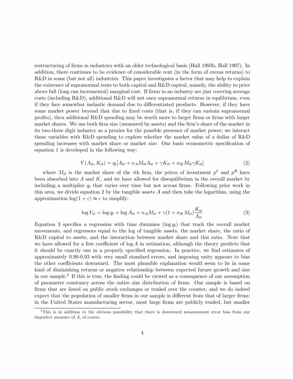
restructuring of …rms in industries with an older technological basis (Hall 1993b, Hall 1997). Inaddition, there continues to be evidence of considerable rent (in the form of excess returns) toR&D in some (but not all) industries. This paper investigates a factor that may help to explainthe existence of supranormal rents to both capital and R&D capital, namely, the ability to priceabove full (long run incremental) marginal cost. If …rms in an industry are just covering averagecosts (including R&D), additional R&D will not earn supranormal returns in equlibrium, evenif they face somewhat inelastic demand due to di¤erentiated products. However, if they havesome market power beyond that due to …xed costs (that is, if they can sustain supranormalpro…ts), then additional R&D spending may be worth more to larger …rms or …rms with largermarket shares. We use both …rm size (measured by assets) and the …rm’s share of the market inits two-three digit industry as a proxies for the possible presence of market power; we interactthese variables with R&D spending to explore whether the market value of a dollar of R&Dspending increases with market share or market size. Our basic econometric speci…cation ofequation 1 is developed in the following way:
V (Ait;Kit) = qt[Ait + ®AMitAit + °Kit + ®KMit°Kit] (2)
where Mit is the market share of the ith …rm, the prices of investment pI and pR havebeen absorbed into A and K, and we have allowed for disequilibrium in the overall market byincluding a multiplier qt that varies over time but not across …rms. Following prior work inthis area, we divide equation 2 by the tangible assets A and then take the logarithm, using theapproximation log(1 + ") t " to simplify:
logVit = log qt + logAit + ®AMit + °(1 + ®KMit)KitAit
(3)
Equation 3 speci…es a regression with time dummies (log qt) that track the overall marketmovements, and regressors equal to the log of tangible assets, the market share, the ratio ofR&D capital to assets, and the interaction between market share and this ratio. Note thatwe have allowed for a free coe¢cient of logA in estimation, although the theory predicts thatit should be exactly one in a properly speci…ed regression. In practice, we …nd estimates ofapproximately 0.90-0.93 with very small standard errors, and imposing unity appears to biasthe other coe¢cients downward. The most plausible explanation would seem to lie in somekind of diminishing returns or negative relationship between expected future growth and sizein our sample.2 If this is true, the …nding could be viewed as a consequence of our assumptionof parameter constancy across the entire size distribution of …rms. Our sample is based on…rms that are listed on public stock exchanges or traded over the counter, and we do indeedexpect that the population of smaller …rms in our sample is di¤erent from that of larger …rms:in the United States manufacturing sector, most large …rms are publicly traded, but smaller
2This is in addition to the obvious possibility that there is downward measurement error bias from ourimperfect measure of A, of course.
4

…rms tend to be those that expect to grow and want access to public capital markets. We willexplore this di¤erence later in the paper.
3 Data and Market De…nition
Our data come from several sources: Standard and Poor’s Compustat Annual Industrial, OTC,and Research data …les (…rm-level data, approximately 3000 …rms for 1959-1991, unbalanced):Standard and Poor’s Compustat Business Segment …le (business segment-level data for approx-imately 500 …rms, 1987-1992); 1982 and 1987 Census of Manufactures and 1988-1991 AnnualSurvey of Manufacturing (4-digit industry-level data, 1982, 1987-1991); and the Yale surveydataset AMAZ (131-IDS-level data, merged to the Census of Manufactures and ASM for 1977and 1982). We combined data from all these sources and created an unbalanced panel of …rmswith data from 1982 to 1991 (including data on their primary industry at the 131-…rm level) inthe manner described below.
The central problem in conducting an investigation into the e¤ects of industry conditions onthe performance of individual large manufacturing …rms is the matching of …rms to industries.In general, assigning these …rms to a single 4-digit SIC industry is impossible because these …rmsare usually engaged in more than one such industry in a signi…cant way. Like so many otherstudies, ours struggles with this problem and ultimately …nds a less than complete satisfactory,but workable, solution.. We begin with the 131-sector manufacturing industry breakdownoriginally created by Scherer for the analysis of the Federal Trade Commission data in theseventies. This classi…cation system was also used in a somewhat modi…ed form by the Yalesurvey (Levin et al 1987) to analyze their results. It has the advantage that it has a somewhattechnological basis (SIC industries are aggregated when they are based on similar technologiesand tend to be found in the same …rms (e.g., all dairy products, all plastic products except…lms and sheets, and so forth). A second advantage is that using this system will enable us tomatch our data to the Yale survey data (or to an updated version of that survey) if we wish toobtain measures of appropriability and technological opportunity.
We have modi…ed the IDS classi…cation to conform to the 1987 4-digit industrial classi…-cation of the Census of Manufactures, combined some industries, and created a few new ones(especially in the computing and electronics areas). In all cases our focus was on creatingindustries that would plausibly contain …rms that could compete on the technological side,which means that we tended to focus on supply side substitution when aggregating, althoughwithout completely ignoring the markets that the …rms face (e.g., refrigerating and heatingequipment, IDS 119 and 126, is separated by the ultimate consumer of the product). We alsoadded …rms and industries from outside manufacturing if they were particularly likely to beintegrated into manufacturing and to perform signi…cant amounts of R&D. This a¤ected thepetroleum industry, where we included …rms in SICs 1311 and 1389, and the communicationequipment industry, where we added …rms in SICs 4810, 4811, and 4813. A complete list of
5

industries and the 4-digit classes they contain, together with their aggregation to the 2-digitlevel, is shown in Table 1 of the appendix.3
After creating the industry classi…cation (called IDS), which is at the lowest level of aggre-gation that allows …rms to be assigned more or less uniquely to a single industry, we assignedthe …rms from Compustat using their primary 4-digit SIC code. For very large …rms on whichwe also had business segment data (approximately 500), we actually used their sales in a par-ticular business segment when computing their market share, and weighted up their marketshares in di¤erent industries to obtain a single market share for the market value regression(which is at the …rm level). Market shares were de…ned as the ratio of …rm (or segment) salesto the total value of shipments in the IDS industry classi…cation, aggregated from the 1987Census of Manufacturing …gures at the 4-digit level, Obviously, this will produce numbers thatare not internally consistent, given the slightly inaccurate procedure of assigning whole …rmsto industries, but we believe that this is preferable to using a denominator that is based onaggregation of the Compustat sales …gures. In fact, our examination of a few key industriessuggests that the market share numbers are generally not that far o¤. We have deleted the fewobservations for which they are completely implausible.
Figure 1 shows the frequency distribution of our market share variable; as expected, thedistribution is highly skewed, with only about 300 of the observations (approximately 60 ofthe …rms) having market shares greater than 10 percent. Figure ?? plots the average marketshare at the two-digit level versus the 1987 Her…ndahl index for that industry (constructed asa shipments-weighted average of the Her…ndahl at the lower level of aggregation). It is clearfrom this …gure that the two measure slightly di¤erent quantities: it is possible for an industryto be concentrated (high Her…ndahl) and still have a large number of very small …rms (lowaverage market share), as in the case of the aircraft and parts industry (17). In this case, it isprobably that the assumption of a homogeneous industry is problematical. On the other hand,and industry can be only moderately concentrated, but contain …rms that have fairly highaverage market shares (food & tobacco, petroleum, and primary metal products). Con…rmingthe extreme skewness of the market share distribution, Table 1 shows that the average marketshare in these data is 4.3 percent, while the median is 0.9 percent. One quarter of the …rmshave market shares above 3.9 percent.
The rest of the data we use is more straightforward to construct, and is described morecompletely in Hall (1990). The sample is United States R&D-performing manufacturing …rmstraded on the New York Stock Exchange, the American Stock Exchange, or Over-the-Counterduring the 1987 to 1991 period, with up to 5 years of history (back to 1982). For this paperwe use the market value of corporate assets (equity, debt, preferred stock, and other liabilities)and the in‡ation-adjusted book value of tangible assets (plant and equipment, inventories, andother assets) to construct a measure of Tobin’s Q. In addition, we use the sales (revenue), the
3We welcome suggestions for improvement of this classi…cation system, which is by no means perfect at thepresent time.
6

0.0 0.1 0.2 0.3 0.4 0.5 0.6 0.7 0.8
5
10
15
20
25
30
Weighted Market Share
Num
ber of observations
Figure 1: Histogram of weighted market share
7

Aver
age
Mar
ket S
hare
2-digit Manufacturing1987 Herfindahl
0 500 1000 1500
0
.05
.1
.15
Figure 2: Market share versus Her…ndahl
capital expenditures, the ‡ow of R&D spending, and an R&D stock measure constructed fromthe …rm’s history of R&D spending using the perpetual inventory method with a depreciationrate of 15 percent. Summary statistics for all our variables are shown in Table 1. We trimmedTobin’s Q, the R&D-assets ratio, the investment-assets ratio, and the market share variable foroutliers (the minima and maxima after trimming are also shown in Table 1).
4 Empirical Evidence
In Table 1, the median Tobin’s Q is well above unity, which is to be expected since all of these…rms are R&D-doers and therefore can be expected to have sizable intangible assets that are notcaptured by this measure. The average ratio of current R&D to tangible assets is approximately
8

10 percent, and the distribution is fairly skewed. Innovative activity, as proxied by the R&Dstock, is a major piece of the explanation for the fact that Tobin’s Q is well above one for these…rms. Evidence of this fact is that a simple correction to Tobin’s Q (adding the R&D capitalto the assets in the denominator) yielded the results in the row labeled ”Corrected Tobin’sQ”: The median premium on the assets of the …rms is now 15 percent rather than 52 percent,and the dispersion has also been reduced considerably (the interquartile ranges). Although ourmeasure of the R&D stock is a very rough approximation to the intangible ”knowledge” capitalthat the market presumably values, it is clearly related to something that generates returns forthe …rm.
An issue that confronts anyone working with panel data is the possible presence of unob-servables in the relationship being estimated that are correlated with the variables of interest.In our case, this would correspond to left-out variables in the market value equation that arecorrelated with either the market share or R&D intensity. The well-known method of di¤er-encing to correct estimates for bias from permanent unobservable di¤erences across …rms isvery unattractive in our case for two reasons. First, both of the right hand side variables ofinterest (R&D and market share) are rather stable over time, and di¤erencing them reduces thevariability associated with their ”true” values considerably (see Griliches and Hausman 1986for discussion of the errors in variables problem in panel data).
Second, and more importantly, we do not believe that ”correlated e¤ects” bias is likely to beof great importance in estimating the relationship in equation 3; most of the reasons why thereexist ”permanent” di¤erences across …rms in the market value relationship can be attributedto R&D and/or market share, and we would like to measure these e¤ects rather than simplydi¤erencing them away. For example, …rms within the same industry may di¤er permanentlyfrom each other to the extent that they serve a niche market or produce higher quality products.If this fact generates higher market value and simultaneously higher R&D, we want to associatethis e¤ect with the R&D spending; it would be incorrect to di¤erence in order to remove thiscorrelation.4 For this reason, we emphasize results in this paper that are based on ordinaryleast squares estimates of the relationship in equation 3, although we have pursued a varietyof experiments that use initial conditions for some of the right hand side variables as partialcontrols for a ”…xed e¤ect.” In contrast to Blundell et al (1996), we found these variables tobe statistically insigni…cant or of small economic consequence, in general, and including themhad no e¤ect on the other coe¢cient estimates.
Table 2 presents the basic regression. We use both the current ‡ow of R&D (columns 1, 3, 5,and 6) and the beginning-of-year stock of R&D (columns 2 and 4) as indicators of the innovativeactivity of the …rm. Market share by itself is clearly positively associated with market value;
4We can think of one case where a third variable might cause ”spurious” correlation between R&D and marketvalue: we know that R&D intensive …rms have lower levels of debt, and if our measure of market value includesa measure of the market value of debt that is biased on average, this will induce a correlation between marketvalue of debt that is not of interest. Although this could be true, it is unlikely to be anywhere nearly as large asthe direct relation between R&D and market value, and we expect the bias from this source to be small.
9

the e¤ect is small but signi…cant in percentage terms. An increase in market share equal to itsstandard deviation (9 percent) is associated with an increase in market value of approximately5 percent. Regressions not shown con…rm that this result is essentially orthogonal to the R&De¤ects; when market share is omitted, the R&D coe¢cient in the …rst column rises to 1.50with the same standard error. In columns 3 and 4 of this table, we include the interactionbetween market share and R&D; using either the ‡ow or stock of R&D, the market valuepremium associated with larger market share is not a¤ected by the R&D intensity of the …rm.Column 5 provides evidence that these results are largely una¤ected by the inclusion of 212-digit industry dummies (the industries are given in the Appendix); that is, they are primarilydue to the characteristics of individual …rms rather than to the industries in which they arelocated.
As we have already emphasized, the market share variable is extremely skewed, and it isunlikely that it enters in the simple linear way indicated in equation 3. One piece of evidenceon this question is the last column of Table 2, which presents results for the approximately 40percent of our sample that had data on sales in individual lines of business. These are larger…rms (median assets approximately 400 million dollars vs. 143 million dollars for the wholesample), and we also expect that the market share variable is better measured for this sample(and slightly larger, with a median of about two percent). The results for this sample are indeedquite di¤erent, with essentially no raw market share e¤ect, but a sizable market share-R&Dinteraction. At the median market share for these …rms of two percent, the R&D coe¢cient ishigher by 0.3 than the base value of 1.95 for …rms with negligible market shares. At a largemarket share of 10 percent, the R&D coe¢cient increases by about 1.5 which translates into amarket value premium of about 5 percent at the median R&D to assets ratio for these …rms,which is 0.33.
Table 3 takes a di¤erent approach to measuring these valuation e¤ects. Recognizing thatour market share is both measured with considerable error and likely to enter the relationshipin a nonlinear way, we explore the results of estimation using categorical variables for tiny(MS<1%), small (1%<MS<4%), medium (4%<MS<8%), and large (MS>8%) market shares.The …rst two columns indicate that the relationship between market value and market share ismonotonic, but probably not linear; there is some hint that e¤ects are larger for larger marketshares (see Klette and Griliches 1997 for a quality ladder model that predicts a monotonicnonlinear relationship of this kind). The next two columns show that there is an interactionbetween large market share and high R&D intensities, but mainly for …rms with a large stockof past R&D expenditures and a very large market share. Such …rms are worth 24 percent moreon average, and have a much higher premium than others on their stock of R&D (although theoverall R&D stock coe¢cient is still substantially lower than would be predicted by a modelwhere such investment was valued at parity with ordinary investment).
The …nal two columns in Table 3 present the results of an investigation into whether themarket share e¤ects are simply due to …rm size. The results are fairly clear-cut: market shareitself is a better predictor of market value than size (once we control for the obvious linear
10
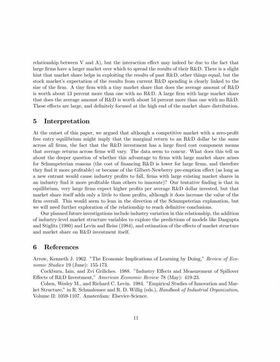
relationship between V and A), but the interaction e¤ect may indeed be due to the fact thatlarge …rms have a larger market over which to spread the results of their R&D. There is a slighthint that market share helps in exploiting the results of past R&D, other things equal, but thestock market’s expectation of the results from current R&D spending is clearly linked to thesize of the …rm. A tiny …rm with a tiny market share that does the average amount of R&Dis worth about 13 percent more than one with no R&D. A large …rm with large market sharethat does the average amount of R&D is worth about 54 percent more than one with no R&D.These e¤ects are large, and de…nitely focused at the high end of the market share distribution.
5 Interpretation
At the outset of this paper, we argued that although a competitive market with a zero-pro…tfree entry equilibrium might imply that the marginal return to an R&D dollar be the sameacross all …rms, the fact that the R&D investment has a large …xed cost component meansthat average returns across …rms will vary. The data seem to concur. What does this tell usabout the deeper question of whether this advantage to …rms with large market share arisesfor Schumpeterian reasons (the cost of …nancing R&D is lower for large …rms, and thereforethey …nd it more pro…table) or because of the Gilbert-Newberry pre-emption e¤ect (as long asa new entrant would cause industry pro…ts to fall, …rms with large existing market shares inan industry …nd it more pro…table than others to innovate)? Our tentative …nding is that inequilibrium, very large …rms expect higher pro…ts per average R&D dollar invested, but thatmarket share itself adds only a little to these pro…ts, although it does increase the value of the…rm overall. This would seem to lean in the direction of the Schumpeterian explanation, butwe will need further exploration of the relationship to reach de…nitive conclusions.
Our planned future investigations include industry variation in this relationship, the additionof industry-level market structure variables to explore the predictions of models like Dasguptaand Stiglitz (1980) and Levin and Reiss (1984), and estimation of the e¤ects of market structureand market share on R&D investment itself.
6 References
Arrow, Kenneth J. 1962. ”The Economic Implications of Learning by Doing,” Review of Eco-nomic Studies 19 (June): 155-173.
Cockburn, Iain, and Zvi Griliches. 1988. ”Industry E¤ects and Measurement of SpilloverE¤ects of R&D Investment,” American Economic Review 78 (May): 419-23.
Cohen, Wesley M., and Richard C. Levin. 1984. ”Empirical Studies of Innovation and Mar-ket Structure,” in R. Schmalensee and R. D. Willig (eds.), Handbook of Industrial Organization,Volume II: 1059-1107. Amsterdam: Elsevier-Science.
11
Blundell, Richard, Rachel Gri¢th, and John van Reenen. 1995. ”Market Dominance,Market Value, and Innovation in a Panel of British Manufacturing Firms,” London: Institutefor Fiscal Studies Working Paper No. 95-????.
Dasgupta, Partha, and Joseph Stiglitz. 1980. ”Industrial Structure and the Nature ofInnovative Activity,” Economic Journal 90 (June): 266-93.
Economic Classi…cation Policy Committee. 993. Issues Paper No. 1, ”Conceptual Issues,”Federal Register (March 31): 16991-17000.
Executive O¢ce of the President, O¢ce of Management and Budget. 1987. StandardIndustrial Classi…cation Manual 1987, Spring…eld, Virginia: Technical Information Service.
Gilbert, Richard J., and David M. G. Newberry. 1982. ”Preemptive Patenting and thePersistence of Monopoly,” American Economic Review 72 (No. 3): 514-526.
Griliches, Zvi, Bronwyn H. Hall, and Ariel Pakes. 1991. ”R&D, Patents, and Market ValueRevisited: Is There a Second (Technological Opportunity) Factor?,” Economics of Innovationand New Technology 1: 183-202.
Griliches, Zvi. 1994. ”Productivity, R&D, and the Data Constraint,” American EconomicReview 84 (No. 1): 1-23.
Griliches, Zvi. 1992. ”The Search for R&D Spillovers,” Scandinavian Journal of Economics94: 529-548.
Griliches, Zvi, and Jerry A. Hausman. 1986. ”Errors in Variables in Panel Data,” Journalof Econometrics ????.
Hall, Bronwyn H. 1996. ”The Private and Social Returns to R&D:What HaveWe Learned?,”in Smith, Bruce L. R., and Claude Bar…eld (eds.), Technology, R&D, and the Economy,Wash-ington, DC: The Brookings Institution and the American Enterprise Institute.
_________. 1993a. ”The Stock Market Valuation of R&D Investment During the1980s,” American Economic Review 83 (May): 259-264.
_________. 1993b. ”New Evidence on the Impacts of R&D,” Brookings Papers onEconomic Activity (Microeconomics): 289-343.
_________. 1990. ”The Manufacturing Sector Master File: 1959-1987,” Cambridge,Mass.: National Bureau of Economic Research Working Paper No. 3366.
Hayashi, Fumio. 1982. ”Tobin’s Marginal q and Average q: A Neoclassical Interpretation,”Econometrica 50 (No. 1): 213-224.
Hayashi, Fumio, and Tonru Inoue. 1991. ”The Relation between Firm Growth and qwith Multiple Capital Goods: Theory and Evidence from Panel Data on Japanese Firms,”Econometrica 59 (No. 3): 731-753.
Ja¤e, Adam B. 1986. ”Technological Opportunity and Spillovers of R&D: Evidence fromFirms’ Patents, Pro…ts, and Market Value,” American Economic Review 76 (No. 5): 984-1001.
Lee, T., and L. L. Wilde. 1980. ”Market Structure and Innovation: A Reformulation,”Quarterly Journal of Economics 94: 429-436.
Levin, Richard C., Alvin Klevorick, Richard R. Nelson, and Sidney G. Winter. 1987. ”Ap-propriating the Returns to Industrial R&D,” Brookings Papers on Economic Activity 3: 785-
12

832.Levin, Richard C., and Peter C. Reiss. 1984. ”Tests of a Schumpeterian Model of R&D and
Market Structure,” in Griliches, Zvi (ed.), R&D, Patents, and Productivity, Chicago: Universityof Chicago Press.
Levin, Richard C. 1988. ”Appropriability, R&D Spending, and Technological Performance,”American Economic Review 86 (May): 424-428.
Loury, Glenn. 1979. ”Adjustment Costs and the Theory of Supply,” Quarterly Journal ofPolitical Economy 93: 395-410.
Lucas, Robert E. 1967. ”Adjustment Costs and the Theory of Supply,” Journal of PoliticalEconomy 75 (No. 4): 321-343.
Mans…eld, Edwin. 1987. ” ?????,”.Martin, Stephen. 1988. Industrial Economic Analysis and Public Policy, New York:
MacMillan and Co.Mohnen, Pierre. 1994. ”The Econometric Approach to R&D Externalities,” Montreal:
Universit·e du Quebec a Montreal Working Paper No. 9408.Nelson, Richard R. 1959. ”The Simple Economics of Basic Research,” Journal of Political
Economy 67: 297-306.Nelson, Richard R., and Sidney G. Winter. 1982. An Evolutionary Theory of Economic
Change. Cambridge, Mass: ??????.Restoy, Fernando, and Michael Rockinger. 1994. ”On Stock Market Returns and Returns
on Investment,” The Journal of Finance XLIX (June): 543-565.Romer, David. 1996. Advanced Macroeconomics. New York: McGraw-Hill Co.Romer, Paul. 1990. ”Endogenous Technological Change,” Journal of Political Economy 96
(October): S71-S102.Reinganum, Jennifer F. 1983. ”Uncertain Innovation and the Persistence of Monopoly,”
American Economic Review 73: 61-66._________. 1989. ”The Timing of Innovation: Research, Development, and Di¤usion,”
in The Handbook of Industrial Organization, New York: Elsevier Science Publishers, Vol. I:175-204.
Salinger, Michael. 1984. ”Tobin’s q, Unionization, and the Concentration-Pro…t Relation-ship,” Rand Journal of Economics 15 (Summer): 159-170.
Solow, Robert M. 1956. ”A Contribution to the Theory of Economic Growth,” QuarterlyJournal of Economics 70 (February): 65-94.
Tobin, James. 1969. ”A General Equilibrium Approach to Monetary Theory,” Journal ofMoney, Credit, and Banking 1 (February): 15-29.
Wildasin, David E. 1984. ”The q Theory of Investment with Many Capital Goods,” Amer-ican Economic Review 74 (No. 1): 203-210.
13

StandardVariable Mean Median deviation 1Q 3Q Minimum Maximum
Market value ($M)** 236.75 176.27 1.99 52.56 903.93 0.83 201,592
Tangible assets ($M)** 144.60 103.75 2.04 33.46 572.78 0.46 97,149
Sales ($M)** 266.40 200.34 1.93 64.72 1017.39 1.75 124,991Tobin's q**(mkt value to assets ratio) 1.64 1.52 0.62 1.08 2.37 0.18 9.91Tobin's q corrected**(mkt value to assets+R&D) 1.19 1.48 0.63 0.81 1.75 0.08 8.59
Investment-assets ratio(%) 11.10% 9.29% 8.11% 5.81% 14.10% 0.10% 94.16%
R&D-assets ratio(%) 9.38% 5.35% 11.14% 2.18% 12.44% 0.07% 94.65%
R&D stock-assets ratio(%) 42.90% 26.94% 48.00% 12.19% 56.48% 0.61% 423.70%
Weighted market shares (%) 4.34% 0.93% 9.28% 0.25% 3.86% 0.01% 97.09%
4-Firm concentration ratio (%)* 37.01% 33.72% 15.46% 28.17% 48.70% 9.00% 88.84%
Herfindahl index* 675.1 506.8 497.2 391.4 911.7 45.0 2600.4
*These variables for 887 observations in 1987 only.**The geometric mean and s.d. of the log are shown for these variables.
Table 1Descriptive Statistics
3932 Observations on 887 Firms (1987-1991)
IQ Range

Flow Stock Flow Stock Flow FlowIndependent variable with ind dums segment firms
Log assets 0.939 (0.006) 0.922 (0.006) 0.938 (0.006) 0.923 (0.006) 0.927 (0.006) 0.959 (0.008)
R&D-assets ratio 1.49 (0.10) 0.14 (0.03) 1.52 (0.13) 0.11 (0.03) 1.53 (0.11) 1.95 (0.36)
Market share 0.51 (0.11) 0.68 (0.11) 0.60 (0.13) 0.49 (0.16) 0.53 (0.13) -.26 (0.21)Market share*R&D-assets ratio -.90 (0.85) 0.51 (0.34) 0.05 (0.91) 14.9 (4.1)
Standard error 0.576 0.594 0.576 0.594 0.529 0.501R-squared 0.917 0.911 0.917 0.911 0.93 0.947
LM (heteroskedasticity) 47.9 (.000) 46.6 (.000) 46.8 (.000) 46.6 (.000) 78.9 (.000) 8.8 (.003)Durbin-Watson 0.846 (.000) 0.844 (.000) 0.845 (.000) 0.846 (.000) 0.898 (.000) 0.796 (.000)Ramsey's RESET 12.4 (.000) 9.0 (.003) 11.2 (.001) 12.3 (.000) 11.5 (.001) 1.2 (.277)
All equations include a full set of year dummies.Standard errors in parentheses are heteroskedastic-consistent estimates.Segment firms are firms where data on sales by business segment was used in constructing the market share variable.21 industry dummies at the 2/3 digit level were included in the regression in column (5) (see Appendix A for details).Diagnostic tests for heteroskedasticity, serial correlation, and nonlinearity are shown with p-values in parentheses.
R&D Measure
Table 2Market Value Regressions: 1987-1991
3932 observations (1558 with segment data)Dependent Variable: Log of Market Value

Flow Stock Flow Stock Flow FlowIndependent variable with ind dums segment firms
Log assets 0.914 (0.007) 0.892 (0.007) 0.913 (0.007) 0.894 (0.007) 0.896 (0.013) 0.891 (0.013)
R&D-assets ratio 1.43 (0.10) 0.11 (0.03) 1.55 (0.13) 0.11 (0.03) 1.42 (0.15) 0.11 (0.34)
0.01<MS<0.04 (952 obs.) 0.09 (0.03) 0.11 (0.03) 0.15 (0.03) 0.14 (0.03) 0.19 (0.03) 0.17 (0.04)0.04<MS<0.08 (400 obs.) 0.20 (0.04) 0.25 (0.04) 0.23 (0.04) 0.23 (0.04) 0.28 (0.04) 0.26 (0.05)0.08<MS<1.0 (555 obs.) 0.28 (0.04) 0.35 (0.04) 0.27 (0.04) 0.23 (0.05) 0.33 (0.05) 0.26 (0.05)
30M<assets<100M (1038 obs.) -0.06 (0.04) -0.01 (0.04)100M<assets<500M (950 obs.) -0.07 (0.05) -0.05 (0.05)500M<assets (1040 obs.) -0.07 (0.07) -0.02 (0.08)
Small MS * (R/A) -0.63 (0.23) -0.09 (0.05) -1.08 (0.23) -0.19 (0.06)Medium MS * (R/A) -0.28 (0.33) 0.03 (0.08) -1.07 (0.30) -0.12 (0.11)Large MS * (R/A) 0.18 (0.28) 0.32 (0.09) -0.48 (0.32) 0.20 (0.11) Small size * (R/A) -0.06 (0.26) -0.13 (0.06)Medium size * (R/A) 0.90 (0.25) 0.13 (0.07)Large size * (R/A) 1.85 (0.33) 0.28 (0.10)
Standard error 0.573 0.591 0.573 0.590 0.568 0.587R-squared 0.918 0.912 0.918 0.913 0.919 0.914
LM (heteroskedasticity) 42.9 (.000) 52.2 (.000) 51.7 (.000) 57.3 (.000) 57.2 (.000) 58.7 (.003)Durbin-Watson 0.857 (.000) 0.857 (.000) 0.860 (.000) 0.862 (.000) 0.869 (.000) 0.867 (.000)Ramsey's RESET 16.1 (.000) 14.8 (.000) 17.9 (.000) 22.5 (.000) 16.9 (.000) 21.8 (.000)
All equations include a full set of year dummies.Standard errors in parentheses are heteroskedastic-consistent estimates.The omitted categories are tiny market share (less then 1 percent) and tiny size (assets less than 30 million dollars).
R&D Measure
Table 3Market Value Regressions: 1987-1991
3932 observations (887 Firms)Dependent Variable: Log of Market Value

Table A1Industry Codes: IND-IDS-SIC Correspondence
Chandler IND IDS Old (S-L) IDS, SIC Description SIC Codes (1987)Segment Industry (Quasi 2-digit) IDS
4 Low-tech 01 Food & tobacco 1 1 Meat products 2010 2011 2013 2015 201601 Food & tobacco 4 3,4 Dairy products 2020 2021 2022 2023 2024 202601 Food & tobacco 6 5,6 Canned & frozen foods 2030-2032 3037 2038 2053 3091 309201 Food & tobacco 7 7 Processed fruits & vegetables 2033 2034 2035 2068 209601 Food & tobacco 8 8 Breakfast cereals 204301 Food & tobacco 10 10 Animal feed 2047 204801 Food & tobacco 11 11 Grain mill products 2040 2041 2044 204501 Food & tobacco 12 12 Wet corn milling 204601 Food & tobacco 13 13 Bakery products 2050 2051 205201 Food & tobacco 14 14,15,16 Sugar chocolate & cocoa prods. 2060-206701 Food & tobacco 18 18 Fats & oils 207x01 Food & tobacco 19 19 Malt & malt beverages, alcoholic bev. 2082 2083 2084 208501 Food & tobacco 21 21 Soft drinks & flavourings 2080 2086 208701 Food & tobacco 22 22 Miscellaneous preproduced food 2090 2095 2098 209901 Food & tobacco 23 23 Tobacco products 21xx
4 Low-tech 02 Textiles, apparel & footwear 24 -- Textile mill products 22xx excl. 2270 227302 Textiles, apparel & footwear 27 -- Rugs 2270 227302 Textiles, apparel & footwear 34 -- Apparel 23xx 396502 Textiles, apparel & footwear 62 -- Footwear, rubber & leather 3021 314x02 Textiles, apparel & footwear 163 -- Leather & leather products 310x-313x 315x 316x 317x 319x 3961
4 Low-tech 03 Lumber & wood products 25 25 Logging & sawmills 241x 242x03 Lumber & wood products 26 26 Millwork, veneer & plywood 243x 2450 2451 245203 Lumber & wood products 33 -- Wood products 244x 249x
4 Low-tech 04 Furniture 28 -- Household furniture 251x04 Furniture 29 29 Office furniture 252x04 Furniture 30 30 Shelving, lockers, office & store fixtures 253x 254x 259x
4 Low-tech 05 Paper & paper products 31 31 Pulp, paper & paperboard mills 261x 262x 263x05 Paper & paper products 32 32, 35, 36 Industrial paper & paper products 2600 264x 265x 266x05 Paper & paper products 39 -- Converted paper - household use 267x
4 Low-tech 06 Printing & publishing 37 37 Commercial printing 275x 279606 Printing & publishing 38 -- Printing & publishing 27xx excl. 275x 2796
2 Stable tech 07 Chemical products 40 39, 40, 41 Industrial inorganic chemicals 281x (Long horizon) 07 Chemical products 42 42, 43, 44 Plastic materials & resins 282x
07 Chemical products 48 48 Paints & allied products 285x07 Chemical products 49 49 Industrial organic chemicals 286x07 Chemical products 50 50, 51 Fertilizer 287x07 Chemical products 52 52 Explosives & misc. chemicals 289x
2 Stable tech 08 Petroleum refining & prods 51 -- Asphalt, roofing & misc coal/oil prods 2950 2951 2952 2990 2992 2999 (Long horizon) 08 Petroleum refining & prods 53 53 Petroleum & refining 291x 1311 13893 Stable tech 09 Plastics & rubber prods 54 54 Tires & innertubes 301x (Short horizon) 09 Plastics & rubber prods 55 55 Plastic products 307x 3080 3084-3089
09 Plastics & rubber prods 56 -- Unsupported plastics, films &sheets 3081 3082 308309 Plastics & rubber prods 164 -- Packing & sealing dev. & fab. rubber nec 3050 3051 3052 3053 3060 3061 3069
3 Stable tech 10 Stone, clay & glass 57 57 Glass & glass products 321x 322x 323x (Short horizon) 10 Stone, clay & glass 58 58 Cement 324x
10 Stone, clay & glass 59 59 Structural clay products 325x10 Stone, clay & glass 60 60 Pottery & related products 326x10 Stone, clay & glass 61 61, 62 Concrete, gypsum & related prods 327x10 Stone, clay & glass 63 63, 64, 65 Abrasive asbestos & mineral wool prods 329x
2 Stable tech 11 Primary metal products 66 66 Steelworks, rolling & finishing mills 331x (Long horizon) 11 Primary metal products 67 67 Iron & steel foundries 332x
11 Primary metal products 70 -- Primary metal products 339x11 Primary metal products 71 71 Prim aluminum smltg, reg, roll, &draw 3334 3353 3354 3355

11 Primary metal products 72 68,69,70,72 Primary smeltg & refing (non-ferrous) 3330 3331 3332 3333 333911 Primary metal products 73 73 Secondary smeltg & refing (non-fer.) 334x11 Primary metal products 74 74 Rolling, drawing, & extruding of nonferr. 3350 3351 335611 Primary metal products 75 75 Drawing & insulating of nonfer. wires 335711 Primary metal products 76 76 Nonferrous metal casting 336x
3 Stable tech 12 Fabricated metal products 77 77 Metal cans & containers 3411 3412 (Short horizon) 12 Fabricated metal products 78 78, 79 Cutlery & hand tools 342x
12 Fabricated metal products 80 80 Heating equipment & plumbing fix. 3430 3431 3432 3433 3437 346712 Fabricated metal products 81 81, 82, 83 Fabricated structural metal 344x12 Fabricated metal products 84 84 Screw machine products, bolts, nuts 345x12 Fabricated metal products 85 85 Metal forgings, plating & coating 346x 347x12 Fabricated metal products 86 -- Wire springs & misc. metal prods. 3495-349912 Fabricated metal products 89 89 Ordnance & accessories 348x12 Fabricated metal products 90 90 Valves & pipe fittings 3490 3491 3492 3493 3494
2 Stable tech 13 Machinery & engines 91 91, 92 Turbines, generators, & combustion eng. 351x (Long horizon) 13 Machinery & engines 93 93 Lawn, garden & farm mach. & equip. 3523 3524
13 Machinery & engines 95 95, 96 Const. & mining mach. & equip. 3530 3531 353213 Machinery & engines 97 97 Oilfield machinery 3533 353413 Machinery & engines 99 99 Conveyors, ind. trucks&cranes, monorails 3535 3536 353713 Machinery & engines 102 102, 103 Mach. tools, metalworking eq. & acc. 354x excl. 354813 Machinery & engines 104 104 Special industrial machinery 3550 355913 Machinery & engines 105 105 Food prods & packaging machinery 3556 356513 Machinery & engines 106 106 Textile machinery 355213 Machinery & engines 108 108 Wood & paper industry machinery 3553 355413 Machinery & engines 109 109 Printing trades machinery & equip. 355513 Machinery & engines 110 110 Pumps & pumping equip. 3561 3586 359413 Machinery & engines 111 111 Ball & roller bearings 356213 Machinery & engines 112 112, 113 Compressors, exhaust., & ventilation fans 3563 3564 363413 Machinery & engines 113 -- General industrial machinery 3560 3568 3569 359x13 Machinery & engines 114 114 Ind. high drives, changers & gears 356613 Machinery & engines 115 115 Industrial process furnace ovens 3567 355813 Machinery & engines 118 118 Scales & balances excl. laboratory 359613 Machinery & engines 123 -- General office machines 3579
1 High-tech 14 Computers & comp. equip. 116 116 Electronic computing equipment 3570-3573 3575 3576 357714 Computers & comp. equip. 117 -- Calculating machines excl. comp. 3578
1 High-tech 15 Electrical machinery 119 119 Refrigerating & heating equip. (comml) 3580-3582 3585 3589 359615 Electrical machinery 120 120 Power distribution & transformers 361215 Electrical machinery 121 121 Switchgear & switchboard apparatus 361315 Electrical machinery 122 122 Motors, generators & industrial controls 3600 3620 3621 3622 362515 Electrical machinery 124 -- Electronic & electric coils & connectors 3524 367715 Electrical machinery 126 126 Household refrigerators & freezers 3630 3631 3632 3633 3635 363915 Electrical machinery 128 128 Lighting fixtures & equipment 3640 3641 36425 3646 3647 364815 Electrical machinery 134 134 Primary & storage batteries 3691 3692 3693 15 Electrical machinery 135 135 Engine elctrical equipment & misc 3694 369915 Electrical machinery 137 -- Electronic & electric connections 3643 3644 3678
1 High-tech 16 Electronic inst. & comm. eq. 125 -- Electronic signaling & alarm systems 366916 Electronic inst. & comm. eq. 127 -- Radio & TV broadcasting sets 366316 Electronic inst. & comm. eq. 129 129 Radio & TV receiving sets 365116 Electronic inst. & comm. eq. 130 130 Records, magnetic, &optical recording 3652 3690 369516 Electronic inst. & comm. eq. 131 -- Communication equipment 3661 3662 3669 4810 4812 481316 Electronic inst. & comm. eq. 132 132 Electron tubes 367116 Electronic inst. & comm. eq. 133 133 Semiconductors & printed circuit boards 3672 3674 3675 367616 Electronic inst. & comm. eq. 138 -- Electronic components, computer acc. 3670 367916 Electronic inst. & comm. eq. 147 147 Engineering scientific instruments 381x16 Electronic inst. & comm. eq. 148 148 Measuring & controlling devices 382x
1 High-tech 17 Transportation equipment 141 141, 142 Aircraft parts & engines 3720 3721 3724 372817 Transportation equipment 143 143 Ship & boat building & repairing 373x 379517 Transportation equipment 144 144 Railroad equipment 374x17 Transportation equipment 145 145 Complete guided missiles, aerospace 376x
2 Stable tech 18 Motor vehicles 136 136 Motor vehicles 3711 3713 3715 3799

(Long horizon) 18 Motor vehicles 140 -- Motor homes 3716 379218 Motor vehicles 146 -- Motorcycles & bicycles 3751 3790
1 High-tech 19 Optical & medical instruments 149 149 Optical instruments & lenses 382719 Optical & medical instruments 150 150 Dental equipment & supplies 384319 Optical & medical instruments 151 151 Surg. & med. inst., appliances, & supplies 3840 3841 384219 Optical & medical instruments 152 -- X-ray apparatus 384419 Optical & medical instruments 153 153 Photographic equipment & supplies 386119 Optical & medical instruments 154 - Electromedical apparatus 3845
1 High-tech 20 Pharmaceuticals 45 45 Pharmaceuticals 283x20 Pharmaceuticals 155 -- Opthalmic goods 3851
4 Low-tech 21 Misc. manufacturing 156 -- Musical instruments 393121 Misc. manufacturing 157 157 Sporting & athletic goods 394921 Misc. manufacturing 158 158 Dolls, games & toys 3942 394421 Misc. manufacturing 159 159 Pens, pencils, & other office & artists mat. 395x21 Misc. manufacturing 160 -- Misc. manufacturing industries 399x21 Misc. manufacturing 162 -- Jewelry & watches 3873 3910 3911 3914 3915 396x
3 Stable tech 22 Soap & toiletries 46 46 Perfumes & toilet prods. 2844 (Short horizon) 22 Soap & toiletries 47 47 Soaps & cleaning products 2840-28433 Stable tech (SH) 23 Auto parts 139 139 Motor vehicle parts & accessories 3714
Chandler segment: 4 industry segments from Al Chandler (Business History Review, Summer 1994). IND: Corresponds roughly to the old ARDSIC (Bound et al) but with soap and auto parts broken out for Chandler's segments.IDS: Hall-Vopel industries, based on the old Scherer-Levin classification (used in Levin-Reiss and Yale survey stuff).IDS (old) : correspondence to Scherer-LevinSIC: 4-digit sic, using 1987 codes, but roughly corresponding to those in use by Compustat, although not all will be populated.
Related Documents