Initiation Of Excitation Waves

Initiation Of Excitation Waves

Thesis submitted in accordance with the requirements of the

University of Liverpool for the degree of Doctor in Philosophy

by

Ibrahim Idris

March 2008

Abstract

The thesis considers analytical approaches to the problem of initiation of excitation

waves. An excitation wave is a threshold phenomenon. If the initial perturbation is

below the threshold, it decays; if it is large enough, it triggers propagation of a wave,

and then the parameters of the generated wave do not depend on the details of the

initial conditions.

The problem of initiation of excitation waves is by necessity nonlinear, non-stationary

and spatially extended with at least one spatial dimension. These factors make the

problem very complicated. There are no known exact analytical, or even good asymp-

totic solutions to this kind of problem in any model, and the practical studies rely on

numerical simulations.

In this thesis, we develop approaches to this problem based on some asymptotic

ideas, but applied in the situation where the “small parameters” of those methods are

not very small. Although results obtained by such methods are not very accurate, they

still can be useful if they give qualitatively correct answers in a compact analytical

form; such answers can give analytical insights which are impossible or very difficult to

gain from numerical simulations.

We develop the approaches using, as examples, two simplified models describing

fast stages of excitation process:

• Zeldovich-Frank-Kamenetskii (ZFK) equation, which is the fast (activator) sub-

system of the FitzHugh-Nagumo (FHN) “base model” of excitable media, and

• Biktashev (2002) [8] front model, which is a caricature simplification of the fast

subsystem of a typical detailed ionic model of cardiac excitation waves.

For these models, we consider two different approaches:

• Galerkin-style approximation, where the solution is sought for in a pre-determined

analytical form (“ansatz”) depending on a few parameters, and then the evolution

equation for these parameters are obtained by minimizing the norm of a residual

of the partial differential equation (PDE) system,

• linearization of the threshold hyper-surface in the functional space, described via

linearization of the PDE system on an appropriately chosen solution on that

surface (a “critical solution”).

i

Publications and Presentations

Some of the materials in Chapter 2 and most of the materials in Chapter 3 are based

on the following publications:

1. I. Idris, R. D. Simitev and V. N. Biktashev. “Using novel simplified models

of excitation for analytic description of initiation propagation and blockage of

excitation waves”. In IEEE Computers in Cardiology, volume 33, pages 213 -

217, Valencia, Spain, 2006.

2. I. Idris and V. N. Biktashev. “Critical fronts in initiation of excitation waves”.

Phys. Rev. E., 76(2): 021906-1 - 021906-6, 2007.

The following presentations have been given based on some of the materials in this

thesis:

1. “Modelling initiation of propagation in excitable media”, I. Idris, Annual Applied

Maths. PhD symposium, University of Liverpool, May 23rd, 2006.

2. “Initiation and Block Excitation Waves: Some Analytical Insights”, V. N. Bikta-

shev and the Liverpool Cardiology group, Cardiac Dynamics miniprogram, Kavli

Institute of Theoretical Physics, University of California in Santa Barbara, Cali-

fornia, USA, July 17th, 2006.

3. “Simplified Models for Initiation and Block of Excitation Waves”, V. N. Bikta-

shev, I. Idris and R. D. Simitev, Computers in Cardiology, Valencia, Spain, Sept.

19th, 2006.

4. “Modelling excitation waves in heart muscle”, V. N. Biktashev, the Liverpool

Maths. Cardiology group, Liverpool Biocomplexity workshop, Liverpool, Nov.

16th, 2006.

5. “Asymptotic approaches to cardiac excitation models”, V. N. Biktashev, I. V.

Biktasheva, I. Idris, R. D. Simitev and R. Suckley, “Complex nonlinear processes

in chemistry and biology”, Institute of Theoretical Physics at Berlin University

of Technology, Berlin, Germany. Feb. 2nd, 2007.

ii

6. “Asymptotic approaches to cardiac excitation models”, V. N. Biktashev, I. V.

Biktasheva, I. Idris, R. D. Simitev and R. Suckley, Applied Mathematics seminar,

University of Leicester, Feb. 22nd, 2007.

7. “Liverpool mathematical cardiology group: work in progress”, V. N. Biktashev, I.

V. Biktasheva, I. Idris, A. J. Foulkes, S. W. Morgan, B. N. Vasiev and G. V. Bor-

dyugov, BIOSIM: Engineering Virtual Cardiac Tissues, Manchester University,

March 16th, 2007.

8. “Non-standard asymptotics and analytical approaches to excitation waves in

heart”, V. N. Biktashev and the Liverpool Mathematical Cardiology Group,

workshop, “Nonlinear dynamics in excitable media”, Ghent, Belgium, April 16th,

2007.

9. “Critical fronts in initiation of excitation waves”, I. Idris and V. N. Biktashev,

The 49th BAMC, Bristol, April 17th-19th, 2007.

10. “Critical fronts and initiation of waves in ionic models of excitation”, V. N. Bik-

tashev and I. Idris, ESF Exploratory Workshop on European Heart Modelling

and Supporting Technology, Oxford University, May 17th, 2007.

11. “Critical fronts in initiation of excitation waves”, I. Idris and V. N. Biktashev,

Annual Applied Maths. PhD symposium, University of Liverpool, May 22nd,

2007.

12. “Asymptotics of cardiac excitability equations”, V. N. Biktashev, I. V. Bikta-

sheva, I. Idris, R. D. Simitev and R. Suckley, Oxford Maths. Biology and Ecology

seminar, Oxford university, Feb. 1st, 2008.

13. “Initiation of excitation waves”, V. N. Biktashev and I. Idris, Liverpool Applied

Maths. seminar, April 9th, 2008.

iii

Contents

Abstract i

Publications and Presentations ii

Contents iv

List of Tables vii

List of Figures viii

Declaration x

Acknowledgment xi

Dedication xii

1 Introduction 1

1.1 Overview . . . . . . . . . . . . . . . . . . . . . . . . . . . . . . . . . . . 1

1.2 Background . . . . . . . . . . . . . . . . . . . . . . . . . . . . . . . . . . 2

1.3 Problem statement . . . . . . . . . . . . . . . . . . . . . . . . . . . . . . 5

2 Literature Review 7

2.1 Mathematical definitions and concepts . . . . . . . . . . . . . . . . . . . 7

2.2 Hodgkin-Huxley (HH) model . . . . . . . . . . . . . . . . . . . . . . . . 9

2.2.1 Definitions and description of some technical terms . . . . . . . . 9

2.2.2 Equations . . . . . . . . . . . . . . . . . . . . . . . . . . . . . . . 11

2.2.3 Action potentials (AP): Solutions and structure . . . . . . . . . . 13

2.3 FitzHugh-Nagumo (FHN) model . . . . . . . . . . . . . . . . . . . . . . 15

2.3.1 Bonhoeffer-van der Pol (BVP) Model . . . . . . . . . . . . . . . 15

2.3.2 FitzHugh-Nagumo (FHN) equations . . . . . . . . . . . . . . . . 17

2.3.3 Zeldovich-Frank-Kamenetskii (ZFK) equation . . . . . . . . . . . 18

2.4 Biktashev 2002 model (a front model) . . . . . . . . . . . . . . . . . . . 18

2.4.1 Traveling fronts solutions . . . . . . . . . . . . . . . . . . . . . . 20

2.5 Approximations to initiation problem for the ZFK equation . . . . . . . 21

iv

2.5.1 The critical nucleus . . . . . . . . . . . . . . . . . . . . . . . . . 21

2.5.2 Variational approaches . . . . . . . . . . . . . . . . . . . . . . . . 22

2.6 Summary . . . . . . . . . . . . . . . . . . . . . . . . . . . . . . . . . . . 27

3 Numerical study of two nonlinear models 31

3.1 Introduction . . . . . . . . . . . . . . . . . . . . . . . . . . . . . . . . . . 31

3.2 Numerical Methods . . . . . . . . . . . . . . . . . . . . . . . . . . . . . . 31

3.2.1 Finite difference approximation schemes . . . . . . . . . . . . . . 31

3.2.2 Fitting methods . . . . . . . . . . . . . . . . . . . . . . . . . . . 34

3.3 Initiation problem for the ZFK equation . . . . . . . . . . . . . . . . . . 34

3.3.1 The critical nucleus . . . . . . . . . . . . . . . . . . . . . . . . . 34

3.3.2 Numerical critical nuclei . . . . . . . . . . . . . . . . . . . . . . . 36

3.4 Initiation problem for the FHN system . . . . . . . . . . . . . . . . . . . 39

3.4.1 The critical pulse . . . . . . . . . . . . . . . . . . . . . . . . . . . 39

3.5 Initiation problem for the front model . . . . . . . . . . . . . . . . . . . 40

3.5.1 The critical front . . . . . . . . . . . . . . . . . . . . . . . . . . . 40

3.5.2 Numerical Results for the front model . . . . . . . . . . . . . . . 42

3.5.3 Detailed cardiac excitation model . . . . . . . . . . . . . . . . . . 46

3.6 Summary . . . . . . . . . . . . . . . . . . . . . . . . . . . . . . . . . . . 48

4 Analysis of variational approximations to initiation problems 50

4.1 ZFK equation . . . . . . . . . . . . . . . . . . . . . . . . . . . . . . . . . 50

4.1.1 Piece-wise smooth ansatzes . . . . . . . . . . . . . . . . . . . . . 50

4.2 Front equations . . . . . . . . . . . . . . . . . . . . . . . . . . . . . . . . 52

4.2.1 Piece-wise smooth ansatzes . . . . . . . . . . . . . . . . . . . . . 52

4.2.2 Smooth ansatzes . . . . . . . . . . . . . . . . . . . . . . . . . . . 58

4.3 Summary . . . . . . . . . . . . . . . . . . . . . . . . . . . . . . . . . . . 65

5 Linear perturbation theory for the ZFK and the front equations 67

5.1 Introduction . . . . . . . . . . . . . . . . . . . . . . . . . . . . . . . . . . 67

5.2 Analytical initiation criterion for the ZFK equation . . . . . . . . . . . . 68

5.2.1 Solution to the eigenvalue problem . . . . . . . . . . . . . . . . . 69

5.2.2 Analytical critical (threshold) curve for the ZFK equation . . . . 72

5.2.3 Generalized threshold criterion for the ZFK equation . . . . . . . 75

5.2.4 The value for δ in the generalized criterion . . . . . . . . . . . . 75

5.3 Analytical initiation criterion for the front model . . . . . . . . . . . . . 80

5.3.1 Introduction . . . . . . . . . . . . . . . . . . . . . . . . . . . . . 80

5.3.2 Eigenvalue problem to the Hinch (2004) model . . . . . . . . . . 81

5.3.3 Eigenvalue problem to the Biktashev (2002) model . . . . . . . . 85

5.3.4 Projection onto the unstable mode . . . . . . . . . . . . . . . . . 90

v

5.3.5 Method 1: threshold minimization . . . . . . . . . . . . . . . . . 93

5.3.6 Method 2: initial condition minimization . . . . . . . . . . . . . 96

5.4 Summary . . . . . . . . . . . . . . . . . . . . . . . . . . . . . . . . . . . 100

6 Conclusions 105

6.1 Results . . . . . . . . . . . . . . . . . . . . . . . . . . . . . . . . . . . . . 105

6.2 Further Directions . . . . . . . . . . . . . . . . . . . . . . . . . . . . . . 106

A Derivation of the variational approximation of the front equations 108

A.1 Integrands for the ODE system . . . . . . . . . . . . . . . . . . . . . . . 108

A.2 Alternative representation of the integrands . . . . . . . . . . . . . . . . 109

A.3 The ODE system . . . . . . . . . . . . . . . . . . . . . . . . . . . . . . . 110

B Integrals for the variational approximation of the front equations 112

B.1 Derivation of the integrals . . . . . . . . . . . . . . . . . . . . . . . . . . 112

B.2 Values of the integrals . . . . . . . . . . . . . . . . . . . . . . . . . . . . 114

C Linear approximations of the front equations 118

C.1 Correspondence between Biktashev (2002) and Hinch (2004) models . . 118

C.1.1 Linearized equations . . . . . . . . . . . . . . . . . . . . . . . . . 120

C.2 Linearization of Hinch (2004) equations . . . . . . . . . . . . . . . . . . 121

C.2.1 Eigenvalue problem . . . . . . . . . . . . . . . . . . . . . . . . . 122

C.2.2 Characteristic equation . . . . . . . . . . . . . . . . . . . . . . . 123

C.3 Linearization of the Biktashev (2002) equations . . . . . . . . . . . . . . 127

C.3.1 Eigenvalue problem . . . . . . . . . . . . . . . . . . . . . . . . . 129

C.3.2 Characteristic equation . . . . . . . . . . . . . . . . . . . . . . . 133

C.3.3 Adjoint eigenvalue problem . . . . . . . . . . . . . . . . . . . . . 139

C.3.4 Characteristic equation for the adjoint problem . . . . . . . . . . 142

Bibliography 155

vi

List of Tables

2.1 Glossary of notations for Chapter 2 . . . . . . . . . . . . . . . . . . . . . 28

3.1 Parameters used for the numerical simulations . . . . . . . . . . . . . . 33




B.1 Functions value in specified intervals . . . . . . . . . . . . . . . . . . . . 113

vii

List of Figures

1.1 The pictures for the match head chemistry . . . . . . . . . . . . . . . . . 3

2.1 The numerical solutions to the Hodgkin-Huxley (HH) model [44] . . . . 14

2.2 The numerical solutions to the FitzHugh-Nagumo (FHN) model [33] . . 16

2.3 A propagating pulse profile for the FHN system . . . . . . . . . . . . . . 18

2.4 A propagating front profile for the ZFK equation . . . . . . . . . . . . . 18

2.5 A propagating front profile for the simplied cardiac front equations . . . 21

2.6 The phase portrait from the variational approx. for the ZFK equation . 24

3.1 Initiation failure/success for the ZFK equation . . . . . . . . . . . . . . 35

3.2 Analytical and numerical critical nuclei for the ZFK equation . . . . . . 36

3.3 Excitation threshold curves for ZFK equation . . . . . . . . . . . . . . . 38

3.4 Critical pulse solution to FHN model (ε = 0.02) as universal transient . 40

3.5 Critical pulse solution to FHN model (ε = 0.0094) as universal transient 41

3.6 Numerical threshold curves for the front model (a) . . . . . . . . . . . . 43

3.7 Numerical threshold curves for the front model (b) . . . . . . . . . . . . 43

3.8 Evolution of the near-threshold initial conditions toward the critical front 44

3.9 Transient “critical fronts” from bigger excitation width (xstim = 1.5) . . 45

3.10 Transient “critical fronts” from smaller excitation width (xstim = 0.3) . . 46

3.11 Critical fronts in CRN model . . . . . . . . . . . . . . . . . . . . . . . . 47

4.1 The sketch of the piece-wise smooth ansatz to the ZFK equation . . . . 51

4.2 Phase portrait from the piece-wise smooth ansatzes approx. for ZFK . . 52

4.3 Sketches of the piecewise smooth ansatzes and the exact front solutions 54

4.4 Phase portrait from the front ODEs . . . . . . . . . . . . . . . . . . . . 58

4.5 The current (INa) profile plot for the front equations . . . . . . . . . . . 59

4.6 The sketches of the smooth ansatzes and profile to the front equations . 61

4.7 The 3D-phase portrait of the projected system for the front model . . . 63

4.8 Approximation of the critical curve from the surface fit for front model . 64

5.1 The sketch of a stable manifold for the ZFK equation . . . . . . . . . . 68

5.2 The interlacing zeros of the eigenfunctions for the ZFK equation . . . . 72

5.3 The analytical threshold curve for the ZFK equation . . . . . . . . . . . 74

viii

5.4 The sketch of a center-stable manifold for the ZFK equation . . . . . . . 76

5.5 The plot of the unstable eigenmode and the critical nucleus . . . . . . . 78

5.6 The plot of the minimum ustim and the zeros of D2(δ) . . . . . . . . . . 80

5.7 The sketch of a center-stable manifold for the front equations . . . . . . 81

5.8 Plot of the eigenvalue equation for the Hinch (2004) front model [43] . . 84

5.9 Plot of the characteristic function for Biktashev (2002) front model [8] . 88

5.10 Plot of the adjoint characteristic function for the front model [8] . . . . 90

5.11 Plot of the unstable adjoint eigenmodes for Biktashev (2002) model [8] . 93

5.12 The plot of the threshold curves for Biktashev (2002) front: Method 1 . 95

5.13 The plot of the η- function . . . . . . . . . . . . . . . . . . . . . . . . . . 100

5.14 The plot of the threshold curves for Biktashev (2002) front: Method 2 . 100

ix

Declaration

No part of the work referred to in this thesis have been submitted in support of an

application for another degree or qualification of this or any other institution of learning.

However, some part of the materials contained herein have been previously published.

x

Acknowledgment

I wish to express my deep and sincere gratitude and appreciation to my supervisor Prof.

V. N. Biktashev for the sustained guidance and motivation throughout the course of

my study here in University of Liverpool, U. K. This work would not have been possible

without his extraordinary degree of understanding, patience and support. I will forever

remain grateful to him for introducing and leading me into the world of programming

(C, Perl, Unix, Maple, Gnuplot, LATEX, Far).

I acknowledge all the support accorded me by my sponsor, Bayero University, Kano.

I cannot thank you enough for offering me this rare and privileged opportunity. In par-

ticular, my special appreciation goes to Prof. M. Y. Bello for all his support and

encouragement. I must express my deep appreciation to The John D. and Catherine T.

MacArthur Foundation for the grant. I also have to acknowledge some partial support

that I received from EPSRC and for that I am indeed very grateful.

I have to thank Dr Irina for all her words of advice and encouragement especially

her unique, interesting and helpful ways of explaining difficult concepts. I can never

forget the consultations I enjoyed from Dr Radostin, Dr Grigory and Dr Bakhti. They

have been very helpful and accommodating personalities and so they will always be

remembered. To Andy and Stuart I very much appreciated and enjoyed their friendly

and very accommodating company. It is interesting having such wonderful pals.

Special thanks must go to all the staff members of the department for their friendli-

ness and for providing a conducive atmosphere for learning and research. In particular,

I am very grateful to my second supervisor, Prof. Bowers for all his advice and guidance.

Many special thanks and appreciation go to Prof. Movchan (Sasha) whose Modules I

quite enjoyed and immensely benefited from. I must also acknowledge all the support

received from Prof. Giblin, especially for the software (Micrografx Designer) that I

used for some of the sketches in this thesis. I appreciated the informal discussions I

had with Dr Andre in the course of this work.

The indirect support that I enjoyed from Prof. Starmer via his web page in the early

stages of my research work and later through his Scholarpedia articles, have played a

significant role in the direction of this work. I am also grateful for the nice pictures on

the match head chemistry he sent to me.

Finally, I wish to thank my family, friends and colleagues for all their support,

messages of good will and prayers.

xi

Dedication

This work is dedicated to my mum Hajara Muhammad Tabi (of blessed memory) and

my dad Idris Ibrahim. This great achievement culminated several years of your efforts

and support and is as well a testimony to your much cherished foresight.

xii

Chapter 1

Introduction

1.1 Overview

In this work, we seek to study systems of partial differential equations (PDEs) that

describe the electrical behaviour in nerve cells and cardiac tissues. In general, it is not

always easy to obtain explicit analytical solutions to problems that involve PDEs. We

will resort to numerical or qualitative techniques as appropriate where analytical ones

are not possible or where they are going to be extremely difficult to obtain. Even where

analytical solutions are found we will use numerical simulations to validate them.

In this chapter, we present an overview of the whole work, then give a brief exposition

on excitable media and follow it up with some definitions and descriptions of some

concepts and terminologies to be used throughout the entire work. We will end the

chapter by stating the main objective of our work.

Chapter two is where we review the literature which starts with the continuation

of the description of some concepts and terminologies. We then present, by way of

exposition, some works, procedures which are used to tackle the problems we seek

to address. Here, we analyse the excitability properties of the celebrated Hodgkin-

Huxley (HH) model [44] and that of its descendants, the FitzHugh-Nagumo (FHN)

system [33, 67, 74] and the simplified front model due to Biktashev [8]. The chapter is

then closed with a review of some analytical approaches used to describe initiation of

propagation waves: the projected dynamics to class of Gaussian ansatz by Neu and his

co-workers [68] and the Biot-Mornev procedure [64] which is a variational method of

computation of non-stationary processes of heat and diffusion mass transfer in regions

of complex shape.

The major aspect of our work starts in chapter three where we formulate, solve and

analyse the initiation problem for the three types of equations that we consider. That

is, the Zeldovich-Frank-Kamenetskii (ZFK) equation, FHN system and the simplified

1

cardiac front model. We present and discuss some important numerical results which

are crucial to initiation of propagation waves in excitable media.

In chapter four some variational approximation procedures are used to solve and

analyse initiation problem in the ZFK equation and the front equations, and some

numerical as well as qualitative results are then presented.

Chapter five is where we present the ignition criteria for both the ZFK equation and

the front equations by deriving explicit analytical expressions for the threshold curves

which then serve as the analytical initiation criteria for the two types of equations.

Finally, in chapter six we draw conclusions for our work and outline directions for

future studies.

1.2 Background

Historically, in its original sense, excitability (i.e., the magnitude of perturbation re-

quired to initiate a propagating wave [48, 90]) refers to the property of living organisms

(or of their constituent cells) to respond strongly to the action of a relatively weak ex-

ternal stimulus [103, 90, 92, 102]. A typical example of excitability is the formation

of spike of transmembrane potential (action potential) by a cardiac cell, induced by a

short depolarizing (becoming less negative) electrical perturbation (disturbance) of a

resting state. Normally, the shape of the generated action potential does not depend

on the perturbation strength provided that the perturbation exceeds a certain thresh-

old value (all-or-nothing principle as is generally known in the literature). After the

generation of this strong response, the system returns to its initial resting state. A

subsequent excitation can be generated after the passage of a suitable length of time,

called the refractory period. For another explanation of the concept of excitability, see

[93, 18].

An excitable medium, by definition is a dynamical system distributed continuously

in space, each elementary segment of which possesses the property of excitability [103,

94, 60, 59, 27]. The neighbouring segments of an excitable medium interact with each

other via diffusion-like local transport processes. It is possible for excitation to be

passed from one segment to another by means of local coupling. Thus, an excitable

medium is able to support propagation of undamped solitary excitation waves, as well

as wave trains.

Many cells such as neurons and muscle cells make use of the membrane potential as

a signal, and thus, the operation of the nervous system and the contraction of a muscle

2

(just two of the numerous examples that abound) are dependent on the formation and

propagation of electrical signals. The division of all cell types into two broad classes,

excitable and non-excitable, aids in the understanding and the analysis of electrical

signaling in cells.

Many cells maintain a stable equilibrium potential; for some, if a current is applied

to the cell for a short time period, the potential returns directly to its equilibrium

value after the removal of the applied current. The cells with this behavior are called

non-excitable. For example, the epithelial cells that line the wall of the gut and the

photoreceptor (a photosensitive cell) found in the retina of vertebrate eyes. Meanwhile,

there are cells for which, if the applied current is strong enough, the membrane potential

undergoes a large excursion, called an action potential, before eventually returning to

rest. Such type of cells are called excitable. Examples for excitable cells include cardiac

cells, smooth and skeletal muscle cells, secretory cells and most neurons [49]. Excitable

media, in other words, are active (nonlinear) media as compared to passive (linear)

media (for example, electromagnetic waves in a vacuum or sound waves [85]).

There are many examples of excitability that occur in nature and an example of one of

the simplest of such excitable systems is a household match. The chemical components

of the match head are stable to small fluctuations in temperature, but a sufficiently

large temperature change due to the friction between the head and an abrasive surface,

triggers the abrupt oxidation of these chemicals with a dramatic release of heat and

light. In other words, the amount of pressure exerted during the striking of the match

head against a rough surface plays a significant role, where a gentle pressure results in

little friction and therefore occasionally the small spark generated is self-extinguished.

In contrast, greater pressure causes more friction which produces a propagating flame

as a result [49, 87].

(a) (b) (c)

Figure 1.1: The match head chemistry, c©: [87] (a) Preparing to strike the match headagainst the abrasive surface (b) Ignition after the strike (c) Stable propagating flame.

The most prominent examples of excitable media [61, 4, 37, 14, 102] are propa-

gation of electrical excitation in various biological tissues, including nerve fibre and

myocardium, concentration waves in the bromate-malonic acid reagent (the Belousov-

Zhabotinsky reaction), propagating waves during the aggregation of social amoeba

3

(Dictyostelium), plankton’s population explosion as described in [93], waves of spread-

ing depression in the retina of the eye, concentrations waves in yeast extract during

glycosis, calcium waves within frog eggs and the Mexican wave (or La Ola) [31].

The fuse of a dynamite is an example of one-dimensional continuous version of an

excitable medium, while a field of dry grass is its two-dimensional counterpart. These

two spatially extended systems admit the possibility of (excitation) wave propagation.

The field of dry grass has an additional property that both the match head and the

dynamite fuse fail to have, the recovery property. Though not very rapid by physio-

logical standards, after a few months, a burnt-over field of grass still has the chance of

regrowing enough fuel for another fire to spread across it [49].

Excitation waves play key roles in living organisms and they are observed in chem-

ical and physical systems, e.g. nerves, heart muscle, catalytic redox reactions, large

aspect lasers and star formation in galaxies [52]. Understanding conditions of success-

ful initiation is particularly important for excitation waves in the heart where they

trigger coordinated contraction of the muscle and where failure of initiation can cause

or contribute to serious or fatal medical conditions, or render inefficient the work of

pacemakers or defibrillators [101].

The ability of a stimulus to initiate a wave depends on its spatial extent. Rushton

[81, 71], considering an early mathematical model of nerve excitation, introduced the

concept of the “liminal length”, the minimal spatial extent of the stimulus necessary

to initiate an excitation wave. A more modern and detailed concept is that of the

“critical curve” in the stimulus strength-spatial extent plane. A stimulus generates an

excitation wave if its parameters are above this curve; otherwise the wave is either not

created or collapses after a while. For a stimulus of nonzero time duration, the concept

of a critical “strength-duration” curve is relevant [71].

Mathematically, after the stimulus has finished, the problem is in any case reduced

to classification of initial conditions that will or will not lead to a propagating wave

solution. The key question is the nature of the boundary between the two classes. A

detailed analysis of this boundary has been done for simplified models of excitable media

such as the FHN system and its variations. This has led to the concept of a critical

nucleus, briefly reviewed below. Numerical simulations of the cardiac excitation models

reveal significant qualitative differences in the way initiation occurs in such models,

compared to the FHN-style systems [89]. In order to understand these differences, we

analyse a recently proposed simplified model of cardiac excitation in this work, and

demonstrate that for this model the concept of critical nucleus should be replaced with

a new concept of critical front.

4

1.3 Problem statement

The mathematical models of excitable systems, specifically the detailed ionic models of

propagation of excitation in the heart, are complicated and so are to a larger extent not

analytically tractable. Therefore, they are mostly studied numerically and more often

than not, these purely numerical studies provide limited insights into the mechanisms

of the phenomena under investigation. In general, the parameter dependence of the

models are sometimes not entirely known reliably. Therefore, simplified caricature-type

models become subjects of intense studies. In particular, the study of front propaga-

tion is one of the fundamental problems in nonlinear dynamics. Our knowledge and

understanding of the experimental and numerical studies of these nonlinear excitable

systems are enhanced and deepened by analytical approaches which as a result help to

reveal some qualitative properties of the underlying PDEs formed.

The central theme of this thesis is therefore the exploration and exposition of the

nature of the critical solutions in some simplified models of excitable media. These

models are namely, the ZFK equation which is a fast subsystem of the FHN equations

and the Biktashev (2002) [8] model, a fast subsystem of the detailed ionic cardiac

tissue models. We are not aware of any analytical approach pertaining to initiation

of excitation wave propagation regarding the derivation of expression for the threshold

curves in a compact form for the ZFK equation and most especially that of the front

equations (Biktashev (2002) model). Therefore, one of the main goals of this work

is to develop some analytical approaches to solve the nonlinear initiation problem for

the two subsystems by deriving in a compact form, the analytical expression of their

numerically obtained critical curves. This then serves as analytical ignition criteria for

these subsystems in particular, and hopefully for excitable systems in general.

Initiation of excitation waves is a threshold phenomenon [19, 28] and therefore, these

problems are about classification of initial conditions that will or will not lead to a

traveling-wave solution (i.e., excitation wave). Basically, the key question is about

the nature of the boundary between these two classes (i.e., excitation and decay).

Mathematically, this can be formulated as follows: Given

∂u

∂t= f(u) + D

∂2u

∂X2, (X, t) ∈ [0,+∞) × [0,+∞),

u(X, 0) = Ur + Ustim H(X,Xstim),

where Ur is the resting state, H describes the shape of the initial perturbation, say

H(X,Xstim) = cΘ(Xstim − X), Xstim and Ustim are the width and amplitude of that

perturbation respectively; c is a constant vector, u ∈ Rn is an n-dimensional vector

of dynamic variables, D a diagonal diffusion coefficients matrix and f(u) a vector of

5

nonlinear functions that specify the local dynamics. A typical picture observed in

numerical simulations is that if initial conditions satisfy Ustim < U∗stim(Xstim), X ∈

[0,∞) then u(X, t) decays as t → ∞, and if Ustim > U∗stim(Xstim), X ∈ [0,∞) then

u(X, t) approaches a stable propagating front solution as t→ ∞. Hence, the goal is to

find such U∗stim(Xstim).

6

Chapter 2

Literature Review

2.1 Mathematical definitions and concepts

In this section we present definitions and description of some mathematical concepts

used in the study.

Mathematical models

The description of the dynamical processes in excitable media are represented in many

applications in the generic form [103]

∂Ei

∂t= ∇(Di ∇Ei) + Fi(∇Ei, E) + Ii(r, t), (2.1)

where Ei are the field variables of the active medium, E determines the state of the

system, Fi are nonlinear functions of E and perhaps ∇Ei, Di are diffusion coefficients,

Ii are external actions varying in space (r) and time (t) used for initiation of excitation

waves. The system in (2.1) is a generic form of nonlinear reaction-diffusion equations

which are used widely to describe various phenomena in neurobiology, electrophysiology,

biophysics, chemical physics, population genetics, mathematical ecology and in other

areas [21, 103].

Reaction-diffusion systems [78, 69] are mathematical equations which describe how

the concentration of one or more substances distributed in space changes under the

influences of two processes: (1) local (chemical) reactions in which substances are

transformed into each other and, (2) diffusion that causes the substances to spread

out in space. Originally, as the name suggests, reaction diffusion systems are natu-

rally applied in chemistry. However, later these equations have been used to describe

dynamical processes of non-chemical nature. Example of such processes are found in

biology, physics, geology, ecology.

The solutions of reaction-diffusion equations exhibit a broad range of behaviours,

for example, formation of traveling waves and wave-like phenomena and other self-

7

organized patterns like spiral waves and stripes, and intricate structures as solitons.

The simplest type of reaction-diffusion equation is the one which is concern with the

concentration of a single substance in one spatial dimension which is of the form

∂u

∂t= D

∂2u

∂x2+ f(u), (2.2)

and is also referred to as the KPP (Kolmogorov-Petrovsky-Piscounov) equation; f(u)

is the reaction part which takes on various forms. If the reaction part vanishes, then

the equation represent a pure diffusion process which is known as the heat equation.

The choice of f(u) in (2.2) gives the following well known equations which were named

after their founders [97, 69]:

• f(u) = u(1−u): Fishers’s equation [20], originally used to describe the spreading

of biological populations;

• f(u) = u(1−u2): Newell-Whitehead-Segel equation, to describe Rayleigh-Benard

convection;

• f(u) = u(1 − u)(u− α), 0 < α < 1: the general Zeldovich equation that arises in

combustion theory, and its particular degenerate case f(u) = u2 − u3.

In contrast, the basic features of self-sustained dynamics in excitable media can be

describe by the relatively simple two-component activator-inhibitor (or propagator-

controller) system

∂u

∂t= ∇2u+ f(u, v),

∂v

∂t= σ∇2v + ε g(u, v), (2.3)

where u(r, t) and v(r, t) describe the state of the system, f(u, v) and g(u, v) specify

the local dynamics, σ determines the ratio between two diffusion constants and ε is

the ratio of the reaction rates. For parameter ε ≪ 1, the reaction-diffusion system

exhibit relaxational dynamics with interval of fast and slow motions. The system is

referred to as the Brusselator, FitzHugh-Nagumo [33, 28], Rinzel-Keller, [80], Barkley

[5] depending on the nature of the nonlinear functions f, g.

The space-clamped version of (2.3) reduces to

du

dt= f(u, v),

dv

dt= ε g(u, v), (2.4)

which is known as FitzHugh-Nagumo equations (also often called Bonhoeffer Van der

Pol (oscillator) equations).

8

Classifications of the reaction-diffusion systems

Based on the nature of nullclines which emanate as a result of the type of nonlinearity

of the functions f, g, [26, 41, 65, 66], the systems (2.2, 2.3, 2.4) can roughly be classified

into three groups (i) monostable (ii) bistable and (iii) oscillatory.

The monostable systems have only one stable fixed point (stationary state or resting

state). A small (subthreshold) perturbation of the stationary state returns immediately

to it, while a sufficiently large (superthreshold) perturbation induces a long excursion

in the phase space and eventually the system relaxes again to its rest state.

For the bistable system, it nullclines intersect at three fixed points, two of which

are stable, sometimes referred to as rest and excited states and the one remaining is

unstable (saddle point). Meanwhile, in the oscillatory system there is one unstable

fixed point and a stable limit cycle.

2.2 Hodgkin-Huxley (HH) model

In 1952, Alan Hodgkin and Andrew Huxley in their Noble Prize winning work devel-

oped a model from the popularly known cable equation which describes the electrical

behaviour and properties of the surface membrane of a giant squid axon [44, 84, 72].

Later this system of equations became a prototype of a large family of mathematical

models quantitatively describing electrophysiology of various living cells and tissues.

These cells and tissues are specialized electric circuits that carry vital signals from one

part of either animals or human system to another. Therefore, an understanding of

the structures of the equations in this model is indispensable as it serves as the spring

board from which many researches in the field of biophysical sciences take off.

Before giving a brief description of this model there is the need for an acquaintance

with some terminologies as found in the literature.

2.2.1 Definitions and description of some technical terms

Membrane potential Also called transmembrane potential difference or transmem-

brane potential or transmembrane potential gradient is the electrical potential

difference across a plasma membrane. In physical terms it is described as the

voltage drop or the difference in voltage between one face of a bilayer and its

immediate opposite face.

Resting membrane potential In biological cells that are electrically at rest, the

cytosol (the internal fluid of the cell) posses a uniform electrical potential or

voltage compared to the extracellular solution. This voltage is the resting cell

potential, also called the resting potential. In other words, the constant potential

9

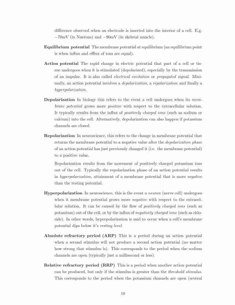
difference observed when an electrode is inserted into the interior of a cell. E.g.

−70mV (in Nuerons) and −90mV (in skeletal muscle).

Equilibrium potential The membrane potential at equilibrium (an equilibrium point

is when influx and efflux of ions are equal).

Action potential The rapid change in electric potential that part of a cell or tis-

sue undergoes when it is stimulated (depolarized), especially by the transmission

of an impulse. It is also called electrical excitation or propagated signal. Mini-

mally, an action potential involves a depolarization, a repolarization and finally a

hyperpolarization.

Depolarization In biology this refers to the event a cell undergoes when its mem-

brane potential grows more positive with respect to the extracellular solution.

It typically results from the influx of positively charged ions (such as sodium or

calcium) into the cell. Alternatively, depolarization can also happen if potassium

channels are closed.

Repolarization In neuroscience, this refers to the change in membrane potential that

returns the membrane potential to a negative value after the depolarization phase

of an action potential has just previously changed it (i.e. the membrane potential)

to a positive value.

Repolarization results from the movement of positively charged potassium ions

out of the cell. Typically the repolarization phase of an action potential results

in hyperpolarization, attainment of a membrane potential that is more negative

than the resting potential.

Hyperpolarization In neuroscience, this is the event a neuron (nerve cell) undergoes

when it membrane potential grows more negative with respect to the extracel-

lular solution. It can be caused by the flow of positively charged ions (such as

potassium) out of the cell, or by the influx of negatively charged ions (such as chlo-

ride). In other words, hyperpolarization is said to occur when a cell’s membrane

potential dips below it’s resting level.

Absolute refractory period (ARP) This is a period during an action potential

when a second stimulus will not produce a second action potential (no matter

how strong that stimulus is). This corresponds to the period when the sodium

channels are open (typically just a millisecond or less).

Relative refractory period (RRP) This is a period when another action potential

can be produced, but only if the stimulus is greater than the threshold stimulus.

This corresponds to the period when the potassium channels are open (several

10

milliseconds). In this case nerve cell membrane becomes progressively more ‘sen-

sitive’ (easier to stimulate) as the relative refractory period proceeds. Therefore

it takes a very strong stimulus to cause an action potential at the beginning of the

relative refractory period, but only a slightly above threshold stimulus to cause

an action potential near the end of the relative refractory period.

Threshold(stimulus/potential) The minimum stimulus needed to achieve an action

potential is called threshold stimulus and the resultant potential change is called

the threshold potential. Thus, if the membrane potential reaches the threshold

potential (generally 5 − 15 mV less negative than the resting potential), the

voltage-regulated sodium channels all open and sodium ions rapidly diffuse inward

and depolarization occurs.

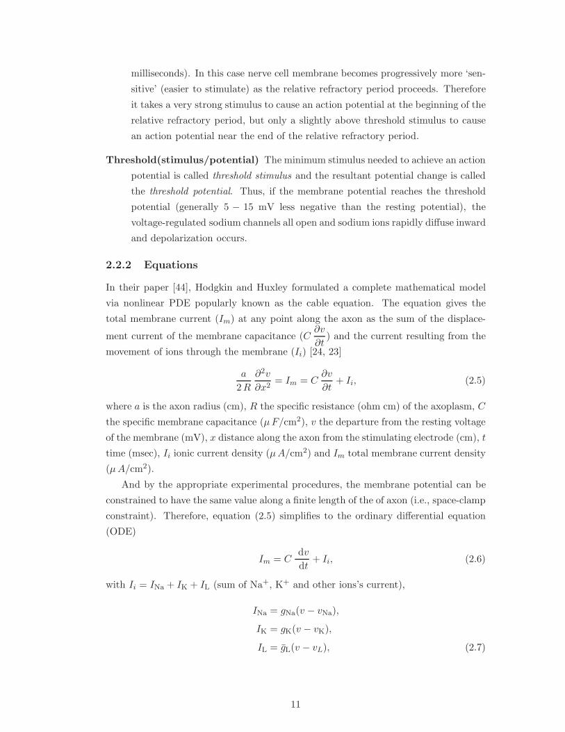
2.2.2 Equations

In their paper [44], Hodgkin and Huxley formulated a complete mathematical model

via nonlinear PDE popularly known as the cable equation. The equation gives the

total membrane current (Im) at any point along the axon as the sum of the displace-

ment current of the membrane capacitance (C∂v

∂t) and the current resulting from the

movement of ions through the membrane (Ii) [24, 23]

a

2R

∂2v

∂x2= Im = C

∂v

∂t+ Ii, (2.5)

where a is the axon radius (cm), R the specific resistance (ohm cm) of the axoplasm, C

the specific membrane capacitance (µF/cm2), v the departure from the resting voltage

of the membrane (mV), x distance along the axon from the stimulating electrode (cm), t

time (msec), Ii ionic current density (µA/cm2) and Im total membrane current density

(µA/cm2).

And by the appropriate experimental procedures, the membrane potential can be

constrained to have the same value along a finite length of the of axon (i.e., space-clamp

constraint). Therefore, equation (2.5) simplifies to the ordinary differential equation

(ODE)

Im = Cdv

dt+ Ii, (2.6)

with Ii = INa + IK + IL (sum of Na+, K+ and other ions’s current),

INa = gNa(v − vNa),

IK = gK(v − vK),

IL = gL(v − vL), (2.7)

11

vNa, vK, vL, the equilibrium potential for sodium, potassium and leakage current re-

spectively and where

gNa = gNam3 h,

gK = gK n4. (2.8)

Note that gNa, gK, gL are respectively the conductivities for Na+, K+, and other ions

species and correspondingly gNa, gK (constants) are the maximum attainable values for

gNa, gK.

The dimensionless variables m, h, n, which varies from 0 to 1, are voltage-sensitive

gate proteins (otherwise known as the gating variables). Specifically, m, h (for activa-

tion and inactivation of Na+ gate) and n (for activation of K+ gate) describe all the

smoothly varying voltage and time dependence of the kinectics. These gating variables

obey the ODEs

dm

dt= αm(v)(1 −m) − βm(v)m,

dh

dt= αh(v)(1 − h) − βh(v)h,

dn

dt= αn(v)(1 − n) − βn(v)n, (2.9)

where αj(v), βj(v), j = h, m, n are gate’s closing and opening rates in ms−1. Hodgkin

and Huxley empirically determined expressions for the gate rates as

αm(v) =0.1(v + 25)

exp [(v + 25)/10] − 1, βm(v) = 4.0 exp (v/18),

αh(v) = 0.07 exp (v/20), βh(v) =1

exp [(v + 30)/10] + 1,

αn(v) =0.01(v + 10)

exp[(v + 10)/10] − 1, βn(v) = 0.125 exp(v/80). (2.10)

The values of other constants appearing in the equations are gNa = 120, gK = 36, gL =

0.3 (m.mho/cm2); vNa = −115, vK = 12, vL = −10.5989 (mv). Hence, the Hodgkin-

Huxley model consist of four coupled ordinary differential equations (ODEs), and thus,

from (2.6) and (2.9) we obtain

dv

dt= − 1

C

(gNam

3 h (v − vNa) + gK n4 (v − vK) + gL (v − vL)

),

dm

dt= αm(v)(1 −m) − βm(v)m,

dh

dt= αh(v)(1 − h) − βh(v)h,

dn

dt= αn(v)(1 − n) − βn(v)n. (2.11)

12

2.2.3 Action potentials (AP): Solutions and structure

By ‘membrane’ action potential is meant one in which the membrane potential is uni-

form, at each instant, over the whole of the length of fibre under consideration. There

is no current along the axis cylinder and the net membrane current must therefore

always be zero, except during the stimulus. If the stimulus is a short shock at t = 0,

the form of the action potential should be given by solving equation (2.11) with the

initial conditions that v = v0 and m, n and h take on their resting steady state values

n0 = 0.3177, m0 = 0.0530, h0 = 0.5961, to four places of decimals.

The process by which an action potential signal is propagated can be understood

when we look closely at the events happening in the immediate vicinity of the membrane

[85, 30]. A certain threshold voltage is required to start the process: the potential

difference must be raised to about −30 to −20 (mV) at some site on the membrane.

Experimentally this can be achieved by a stimulating electrode that pierces a single

neuron. Biologically this happens at the axon hillock in response to an integrated

appraisal of excitatory inputs impinging on the soma. Consequently, when the threshold

voltage is reached the following sequence of events occur:

• Sodium channels open, letting to the influx of Na+ ions into the cell interior. This

causes the membrane potential to depolarize further; that is, the inside becomes

more positive with respect to the outside, the reverse of resting-state polarization.

• After a slight delay, the potassium channels open, letting to the eflux of K+

ions to the cell exterior. This in essence restores the original polarization of

the membrane, and further causes an overshoot of the negative rest potential

(hyperpolarization).

• The sodium channels then close in response to a decrease in the potential differ-

ence.

• Adjacent to a site that has experienced these events the potential difference ex-

ceeds the threshold level necessary to set in motion the first event. The process

repeats, leading to a spatial conduction of spike-like signal. The action poten-

tial can thus be transported down the length of the axon without attenuation or

change in shape, mathematically, this makes it a traveling wave.

The system (2.11) and equations (2.10) are used to draw the graphs in Fig. 2.1. The

red solid curve in the left top panel of Fig. 2.1 describes the complete stages of an

action potential (i.e., electrical excitability) process: depolarization, repolarization and

hyperpolarization.

Also shown in Fig. 2.1 are: The absolute refractory period (ARP) which is the period

during which a second stimulus will not trigger a second action potential (however,

13

-20

0

20

40

60

80

100

120

0 2 4 6 8 10

t

active

ARP

depo

lari

zatio

n

repolarization

hyperpolarization

RRP

rest

ing

pote

ntia

l

-v

0 2 4 6 8 10

t

v0=90

v0=15 v0=7

v0=6

superthres

hold

subthreshold

-0.25

-0.15

-0.05

0.05

0.15

0.25

0.35

-150 -100 -50 0

u

activ

e

No Man’s Landre

lativ

ere

frac

tory

absoluterefractory

rest. point

regenerative

w

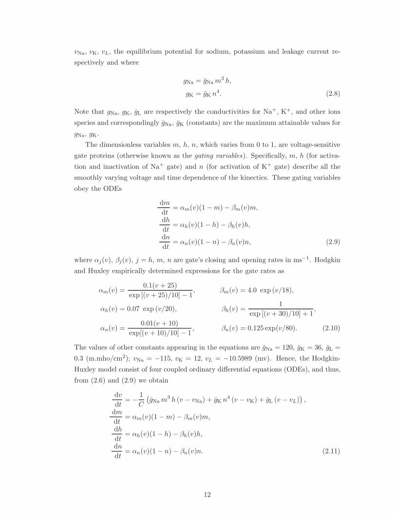
Figure 2.1: Numerical solution of system (2.11) [44, 63] for initial depolarization v0 = 15 mVshowing the complete stages of an action potential process: depolarization, repolarization andhyperpolarization.

strong the second stimulus might be). This corresponds to the period when the sodium

channels are open (typically some millisecond or less);

The relative refractory period (RRP) which is the period when another action po-

tential is possible if the stimulus is greater than the threshold stimulus. This corre-

sponds to the period when the potassium channels are open (several milliseconds). In

other words, the nerve cell membrane becomes progressively more ‘sensitive’ (easier to

stimulate) as the relative refractory period proceeds. Therefore, it takes a very strong

stimulus to produce an action potential at the beginning of the relative refractory pe-

riod, but only a slightly above threshold stimulus to cause an action potential near the

end of the relative refractory period.

In the top right panel of Fig. 2.1 are solutions of (2.11) for initial depolarizations, v0,

14

of 90, 15, 7 and 6 (mV) illustrating excitability around the threshold and equilibrium.

The HH model has only one equilibrium (resting point), therefore if a small shock

(subthreshold) is applied to the resting state, then this shock cause small perturbation

which is below the critical level (threshold) of the system, and it decays immediately

back to the resting state (no excitation). However, if the shock exceeds the critical level

of the system due to a large shock (superthreshold), then this cause excitation to occur

and the cells are depolarized, meaning the membrane potential is moved away from its

resting state for quite a while before eventually returning to the rest state. In other

words, above threshold initial voltages lead to a rapid response with large changes in

the state of the system.

In the bottom panel is the reduced 2-dimensional (u, w) phase portrait of the 4-

dimensional (v, m, n, h) space of the HH model with u = v − 36m and w = (n −h)/2 [33]. The regions marked on the trajectories (red solid curves) correspond to the

physiological responses which are known as: regenerative, active, absolute refractory,

and relative refractory phases. It also shows the only one equilibrium (resting point)

of the HH system from which small, below threshold (subthreshold) stimulus do not

lead to excitation, but rather a gradual return to it; while larger, above-threshold

(superthreshold) stimulus result in a large excursion through the phase space before

finally returning to it (the equilibrium). Such superthreshold trajectories are the phase-

space representation of an action potential. The region marked ’no man’s land’, a non-

physiological term is a region where rare trajectories could be obtained and so chosen

to represent a state the nerve seldom reached in physiological experiments.

2.3 FitzHugh-Nagumo (FHN) model

2.3.1 Bonhoeffer-van der Pol (BVP) Model

Richard FitzHugh was the first investigator to apply mathematical analysis (phase

plane analysis) to study the qualitative properties of HH system of equations. In his

paper [33], FitzHugh suggested that a modified version of the Van der Pol system of

equations which he called the Bonhoeffer-van der Pol (BVP) model [33, 39, 36, 74], has

similar qualitative properties to the HH system. He suggested that the four-dimensional

projection of HH space portrait to a two-dimensional subspace gives a phase portrait,

(see Sec. 2.2), where the trajectories look similar to that of FitzHugh phase portrait.

The BVP model is given by

x = c (y + x− x3/3 + z)

y = − (x− a+ by)/c (2.12)

where a and b are constants and satisfy the conditions 1−2b/3 < a < 1, 0 < b < 1, b <

c2 and x represents the excitability of the system (membrane potential,v), y represents

15

-2-1.5

-1-0.5

0 0.5

1 1.5

2

0 5 10 15 20

t

x0=1.2

x0=0.6

x0=0.2

subthreshold

superthreshold-x

-1.5

-1

-0.5

0

0.5

1

1.5

-2 -1 0 1 2 3

x

yrest.pt. p

rela

tive

refr

acto

ry

absolute

refractory

no man’s landactiv

e

regenerative

x• =0

y• =0

• ••

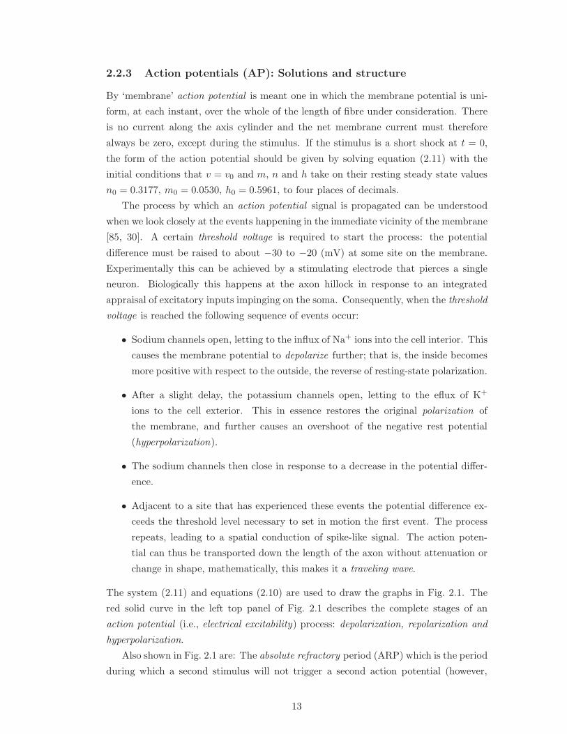
Figure 2.2: Solutions of equations (2.12) [33] having an equilibrium (x0, y0) = (1.20,−0.625)with parameters a = 0.7, b = 0.8, c = 3.0 and z = 0 for stimuli 1.20, 0.6, 0.2. It shows thecomplete stages of an action potential process: depolarization, repolarization and hyperpolar-ization.

combined forces that tend to return the axonal membrane resting state, z represents

the stimulus intensity which corresponds to the external current I(t) in HH equations.

Action potentials and physiological states of BVP Model

In Fig. 2.2 the curves fairly resemble those of the HH model in Fig. 2.1 with small shock

(subthreshold) of 0.2, and 0.6, 1.20 as superthreshold respectively. This illustrates the

same excitability phenomenon of the HH model in that the small shock fails to excite as

the action potential it elicits immediately goes back to the resting point of the system.

The resting point (P) the only one as is the case with HH system is stable , therefore

if a phase point displaced initially a short distance from the resting point will return

toward its spontaneously. If a stimulus consisting of an instantaneous shock is applied

to the system, the phase point jumps horizontally along the dotted line for a distance

∆x proportional to the amplitude of the shock- to the left for a cathodal (-z) shock or

to the right for an anodal one (+z) (see [33] for detailed explanations).

After a sufficiently large cathodal shock, the phase point travels along a path to

the left through the regenerative zone, upward through the active, to the right through

the absolute refractory, downward to the relatively refractory and finally back to P.

This clockwise circuit represents a complete action potential (electrical excitability).

If the shock is too small, no impulse (AP) results; instead, the phase point returns

more directly to P through the small clockwise- circuits (representing subthresholds)

as shown in the diagram Fig. 2.2.

The no-man’s land (non-physiological term) is a region where rare trajectories could

be obtained and is chosen to represent state the nerve seldom reached in physiological

experiments. The horizontal distance of a point from the separatrix is proportional to

16

the threshold (magnitude of instantaneous z pulse). It should be noted that since ex-

citation is the result of the phase point being displaced horizontally across the threshold

separatrix, it follows that the system will be absolutely refractory when the phase point

is above the separatrix, where such crossing is impossible. In the relative refractory

zone, the phase point lies to the right of the separatrix and can be displaced across it,

but the threshold stimulus required is greater than for the resting point [33].

In Fig. 2.2 we can see that we have a stable singular point (equilibrium point) with a

trajectory that spirals toward its. FitzHugh used the BVP system of equations because

it has qualitative properties similar to that of HH system. Thus, it can be argued

that the pair (v,m) corresponds to x and they represent excitability. The pair (h, n)

corresponds to y and represent recovery. As suggested by FitzHugh [33], the phase

portraits of both HH and BVP look similar and hence exhibit the same excitability

phenomenon.

2.3.2 FitzHugh-Nagumo (FHN) equations

The FHN model [33, 67] which is a generic model for excitable media and its numerous

variants have served well as simple yet qualitatively reasonable models of the compli-

cated processes of excitation and propagation in nerve fibre, heart muscle and other

biological spatially-extended excitable systems. Among the variants, this is one of the

format as used by Winfree [96]

∂u

∂t=

1

εf(u, v) +D

∂2u

∂x2,

∂v

∂t= εg(u, v) + δD

∂2v

∂x2, (2.13)

where x, t ∈ R are measured respectively in “space units” and “time units”, f(u, v) =

u − u3/3 − v, g(u, v) = u + β − γv. The propagation variable u represents an electric

potential, the recovery variable v represents ion channels (as those channels in HH

model), D is the coefficient of diffusion in “space units/time unit” and δ the diffusion

rate (it is usual in electrophysiological applications to take δ = 0). Often for the sake

of simplicity D = 1, δ = 0 and the system reduced to

∂u

∂t=

1

εf(u, v) +

∂2u

∂x2,

∂v

∂t= εg(u, v). (2.14)

The generic FHN system has been represented by various formats as discussed in [96,

28]. The form we are going to use in this work is the one due to Neu, Pressig and

Krassowska [68] but with the notational change v = u, y = v, µ = θ

∂u

∂t=∂2u

∂x2+ f(u) − v,

∂v

∂t= ε(αu− v), (2.15)

17

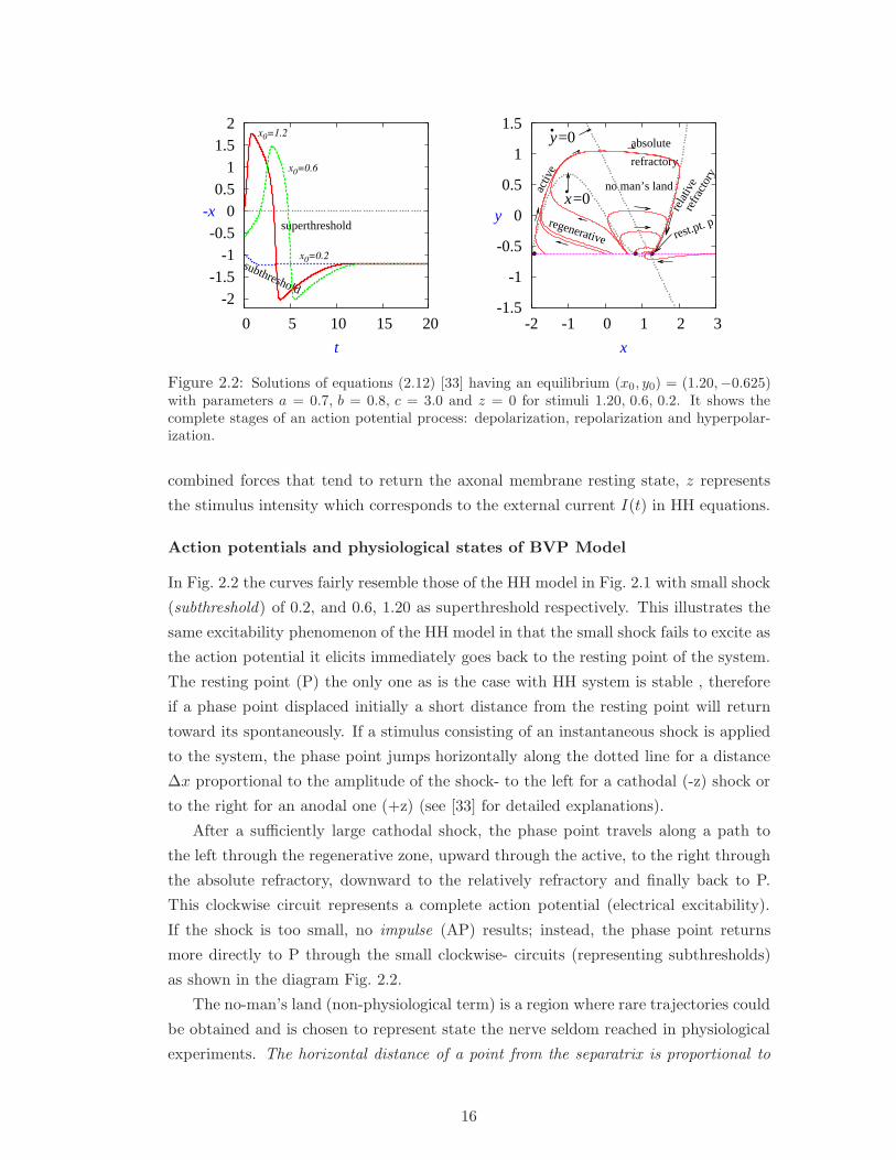
where f(u) = u(u − θ)(1 − u), a cubic polynomial with the state variables, u and v

representing respectively the transmembrane potential and inactivation variable; ε a

small parameter, α a constant and θ corresponds to the threshold state of the system

and must satisfy 0 < θ < 1/2 in order for the FHN system to give rise to a propagating

wave [56, 57] as shown in Fig. 2.3

u,v

x

uv

Figure 2.3: A propagating pulse profile solution to the FHN system (2.15).

2.3.3 Zeldovich-Frank-Kamenetskii (ZFK) equation

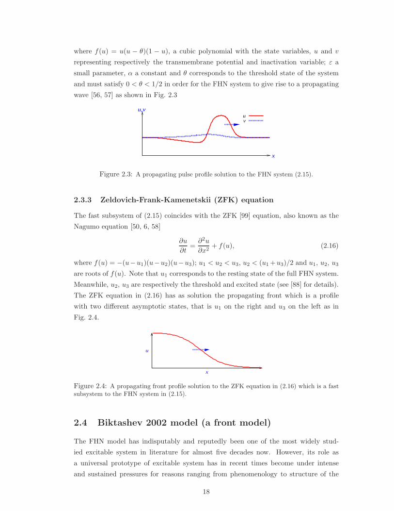
The fast subsystem of (2.15) coincides with the ZFK [99] equation, also known as the

Nagumo equation [50, 6, 58]

∂u

∂t=∂2u

∂x2+ f(u), (2.16)

where f(u) = −(u−u1)(u−u2)(u−u3); u1 < u2 < u3, u2 < (u1 +u3)/2 and u1, u2, u3

are roots of f(u). Note that u1 corresponds to the resting state of the full FHN system.

Meanwhile, u2, u3 are respectively the threshold and excited state (see [88] for details).

The ZFK equation in (2.16) has as solution the propagating front which is a profile

with two different asymptotic states, that is u1 on the right and u3 on the left as in

Fig. 2.4.

u

x

Figure 2.4: A propagating front profile solution to the ZFK equation in (2.16) which is a fastsubsystem to the FHN system in (2.15).

2.4 Biktashev 2002 model (a front model)

The FHN model has indisputably and reputedly been one of the most widely stud-

ied excitable system in literature for almost five decades now. However, its role as

a universal prototype of excitable system has in recent times become under intense

and sustained pressures for reasons ranging from phenomenology to structure of the

18

model(s) it ought to caricature. As a results many alternative simplified models had

been suggested [1, 32, 29, 7, 42, 8].

Here, we are presenting the simplified cardiac front model due to Biktashev [8],

the main subject of our study. It is one of the direct descendants of the biophysically

detailed models. The two-variable cardiac excitation front model which we shall be

referring to as the front model is a simplified model based on the celebrated HH model

[44], the more recent ionic models such as the Noble-1962 [70] and Courtmenche et

al (CRN-1998) [25, 86] models. The human atrial tissue model (CRN-1998) is a ho-

mogenous and isotropic one-dimensional medium which satisfies the reaction-diffusion

system (RDS)

∂u

∂T= D · ∂

2u

∂X2+ F(u), (2.17)

where F(u) is a vector defined according to the atrial single-cell realistic CRN-1998

model, u = (E,m, h, j, . . . , )T ∈ R21 is a vector of all dynamic variables of the model

and D = diag (D, 0, 0, . . . , ) is the tensor of diffusion in which only the coefficients of

the voltage E is nonzero. Thus, the simplified description focuses on the excitation and

propagation of impulses while ignoring the effects due to the geometry, anisotropy and

heterogeneity of a real atrium [86].

After some non-standard asymptotic analysis [8, 9, 46] based on the smallness of

certain quantities in the equations in (2.17), formalized with an explicit parameter ǫ it

is re-written as

∂E

∂T= −C−1

M

(1

ǫINa(E,m, h, j) +

∑ ′

I(E, · · · ))

+D∂2E

∂X2,

∂m

∂T=

(m(E; ǫ) −m)

ǫ τm(E), m(E; ǫ) =

{

m(E), ǫ = 1,

Θ(E − Em), ǫ = 0,

∂h

∂T=

(h(E; ǫ) − h

)

ǫ τh(E), h(E; ǫ) =

{

h(E), ǫ = 1,

Θ(Eh − E), ǫ = 0,

∂y

∂T=

(y(E; ǫ) − y)

ǫ τy(E), y = ua, w, oa, d,

∂U

∂T= W(E, · · · ), (2.18)

where Θ() is the Heaviside function. The dynamic variables E, m, h, ua, w, oa and

d as defined in [25] are considered as “fast” variables and change significantly during

the upstroke of a typical action potential (AP). U = (j, oi, · · · , Nai,Ki, · · · )T is the

vector of all other slower variables and W is the vector of the corresponding right-hand

sides. The sum∑ ′

I(E, · · · ), is for all other currents except the fast sodium current

INa = INam3 h j, which is only large during the upstroke of the AP and not that

large otherwise (the m or h gates are almost closed outside the upstroke since their

quasistationary values m(E), h(E) are small there).

19

Thus, in the limit ǫ → 0, functions m(E) and h(E) have to be considered as zero

in certain overlapping intervals E ∈ (−∞, Em], E ∈ [Eh,∞) and Eh ≤ Em. Hence,

the representations m(E; 0) = Θ(E−Em) and h(E; 0) = Θ(Eh −E). Therefore, (2.18)

in the limit ǫ → 0, in the fast time t = T/ǫ, and with x = (ǫD)−1/2 X gives a closed

system of three equations

∂E

∂t= −INam

3 h j/CM +D∂2E

∂x2,

∂m

∂t= (Θ(E − Em) −m) /τm(E),

∂h

∂t= (Θ(Eh − E) − h) /τh(E). (2.19)

Simplifying (2.19) further by replacing τh(E) and INa(E) with constants and assuming

additionally the limit of small τm(E) so that m always remains close to its quasi-

stationary value Θ(E − Em).

Hence, after suitable rescaling (so that Em = 1, Eh = 0) (2.19) reduced to the system

of two PDEs (2.20) that models the excitation fronts in cardiac tissue. It describes very

well the propagation block phenomenon, a feature typical of realistic excitation models

that the FHN failed to adequately capture [8, 9, 10]

∂E

∂t=∂2E

∂x2+ F (E,h),

∂h

∂t= G(E,h)/τ, (2.20)

with

F (E,h) = Θ(E − 1)h,

G(E,h) = Θ(−E) − h, (2.21)

where E corresponds to the transmembrane potential, h is the probability density of

the Na+ channel gates being open and τ is a dimensionless parameter.

2.4.1 Traveling fronts solutions

The solutions to (2.20) are in the form of traveling front propagating rightward with

speed c > 0, z = x− c t and satisfying the system of ODEs

−cE′ = E′′ + Θ(E − 1)h,

−c h′ =1

τ(Θ(−E) − h), (2.22)

where (′) =d

dzand with auxiliary conditions given by

E(+∞) = −α < 0, E(−∞) = ω > 1,

h(+∞) = 1, h(−∞) = 0. (2.23)

20

The phase of the front solution is chosen so that the internal boundary conditions

E(0) = 0 and E(−∆) = 1 at z = 0, −∆ are satisfied with the requirements that

E(z) ∈ C1 and h(z) ∈ C0. The ODE problem along with its auxilliary conditions has

a family of propagating front solutions that depends on one parameter, the pre-front

voltage α which is fixed.

E(z) =

ω − τ2 c2

1 + τc2ez/τc, z ≤ −∆,

−α+ α e−c z, z ≥ −∆,

h(z) =

ez/τc, z ≤ 0,

1, z ≥ 0,

(2.24)

where z = x− c t, ω = 1 + τc2(α+ 1), ∆ =1

cln(

α+ 1

α) and c is an implicit function of

τ and α as given by the following transcendental function,

τ c2 ln((1 + α)(1 + τ c2)

τ

)

+ ln(α+ 1

α

)

= 0. (2.25)

For a fixed α, there is a τ∗(α) such that for τ > τ∗ ≈ 7.6740, equation (2.25) has

two solutions for c: c = c±(α, τ), c+(higher) > c−(lower) [8]. There is numerical and

analytical evidence that solutions (2.24) with c = c+ are stable and those with c = c−

are unstable with one positive eigenvalue [8, 43].

E

x

Eh

Figure 2.5: A typical propagating front profile for the unstable front solution to the ODEsystem (2.22) for the simplified cardiac equations in (2.20).

2.5 Approximations to initiation problem for the ZFKequation

2.5.1 The critical nucleus

There exist a well developed theory of initiation of propagating waves in the FitzHugh-

Nagumo equations [34, 35, 68], in the singular limit when the activator (excitation)

variable is much faster than the inhibitor (recovery) variable. The key role in this

theory is played by the so called critical nucleus, ucr(x), which is an unstable, non-

trivial stationary solution of

∂u

∂t=∂2u

∂x2+ f(u), (2.26)

21

such that ucr(±∞) = u1 where f(u) = −(u−u1)(u−u2)(u−u3) with u1 corresponding to

the resting state (see Sec. 2.3.3). The critical nucleus plays a key role in understanding

the initiation processes for the FHN systems, such solution is unique as found in [68]

for quadratic nonlinearity (i.e., when the limit of small θ is considered for the cubical

f(u) in (2.16)) as

ucr(x) =3θ

2sech2(

√θ

2x). (2.27)

However, for the cubical nonlinearity f(u) as in (2.16) we have reproduced the solution

as found by Flores in [34] though in a slightly different form

u∗cr(x) = 3 θ√

2[

(1 + θ)√

2 + cosh(x√θ)√

2 − 5θ + θ2]−1

. (2.28)

Its linearization spectrum has exactly one unstable eigenvalue, while all other eigenval-

ues are stable. So the center-stable manifold of this stationary solution has codimension

one, and divides the phase space of (2.16) into two open sets. One of these sets cor-

responds to initial conditions leading to successful initiation, and the other to decay

[58, 34, 62, 35, 68].

2.5.2 Variational approaches

One of the analytical approaches to the description of initiation of propagation as

employed in [68] was the use of projected dynamics (a Galerkin-style approximation)

to the class of Gaussian ansatz. Neu and co-workers derived this approximation after

transforming the ZFK equation to gradient form. In general not every equation can be

written in that form, so we have tried more generic approaches, for instance, we present

some new results of approximations done on the ZFK equation for both smooth and

piece-wise smooth ansatzes by minimizing the L2-norm of the residual of the equation

on one hand and on the other by using a modified Biot-Mornev procedure [64].

Variational approximation of initiation problem by Neu et al

An analytical approach to the description of initiation of propagation as used by Neu

and co-workers, [68] is the used of projected dynamics (a Galerkin-style approximation)

to the class of Gaussian ansatz

u(x, t) = a(t) exp(−k(t)x)2, (2.29)

with varying amplitude a(t) and inverse width k(t). After rewriting the ZFK equation

in terms of variational derivative they obtained ODE system in the limit of small θ. Not

every equation can be written that form, so we tried a more generic approach, where we

minimize the equation of the residuals using L2-norm. To find the residue functional,

22

we express our approximate solution u(x, t) in terms of the unknown parameters a(t)

and k(t) by letting

u(x, t) ≡ V (x, a(t), k(t)) (2.30)

and the residue functional is then

R =

∫ ∞

0

(∂u

∂t− ∂2u

∂x2− f(u)

)2

dx. (2.31)

Now minimizing (2.31) w.r.t a, k by using calculus we have the ODE system as obtained

by Neu and co-workers [68] in terms of a, k

a = −a(2k2 + 1 − c1a),

k = −k(2k2 − c2a), (2.32)

where

c1 =7√

6

18, c2 =

7√

6

9. (2.33)

We have approximated the stable separatrices (the center-stable manifold) of the critical

nucleus with its eigenvector by using the transformation

a = 1.4697 + 1.2866 s

k = 0.4472 + s, (2.34)

where s ∈ R is a parameter, (1.4697, 0.4472) is the critical nucleus and (1.2866, 1)T its

corresponding eigenvector.

With the knowledge that x−1stim ∝ k and ustim ∝ a, we obtain a relationship between

the threshold curve and the center-stable manifold (the separatrix of our Galerkian

ODE) as

xstim =B

k, ustim = Aa. (2.35)

Now using the ansatz

V = a e−(kx)2 ≈ ustimΘ(xstim − x), (2.36)

where Θ is a Heaviside function and the values of the parameters A = 0.7506376700

and B = 0.9899390828 numerically determined. The result shown in Fig. 2.6(b) is our

contribution and therefore, not found in [68].

23

0

0.2

0.4

0.6

0.8

1

0 1 2 3 4 5

a

k

R• T•

C•

a• = 0

k• = 0

0

0.5

1

1.5

2

2.5

3

0 0.5 1 1.5 2 2.5 3

ustim

xstim

Gal. approxPDE

(a) (b)

Figure 2.6: (a) The phase-portrait of the Galerkin ODE system reproduced from [68]. Theeigenvector (dashed - green line) of the center-stable manifold (solid - red line) of the criticalnucleus serving as the approximation of the center-stable manifold of the critical nucleus. Theunstable manifold is the dotted - gray curve. (b) The threshold curves in the ustim - xstim

plane, the result of our approximation (dotted - blue line) compared with that (solid - blackline) obtained from simulations with the PDE system in [68].

The Biot-Mornev variational approximation

Mornev [64], devised a modified version of the Biot’s variational method of computation

of non-stationary processes of heat and diffusion mass transfer in regions of complex

shape. The modification were necessary because Biot procedure according to Mornev

[64] had some setbacks. One of the setbacks was the non invocation of any variational

principle since no minimization functional that would yield the analytical relations

obtained had been specified. There was also the usage of variables that had no physical

meaning [13] which made it difficult for physical intuition to be used to construct a

priori classes of functions via which approximate solutions could be sought for. In

addition, the method was not applicable to the integration of diffusion or heat matter

generation by chemical reaction. In fact, the method as suggested by Mornev did not

even allow for the integration of the simplest reaction-diffusion with nonlinear reaction

part of the form

ϕt = div (D∇ϕ) + f(ϕ), (2.37)

where f(ϕ) = − dΠ

dϕ, is a nonlinear function generated by the potential Π(ϕ),

div (D∇ϕ) = ∇ • (D∇ϕ) = D∇2ϕ.1 Therefore, Mornev suggested some modifica-

tions of the Biot method to take care of the outlined disadvantages by developing a

direct method of integration of reaction-diffusion equations of type (2.37) and their

generalization based on the minimum dissipation principle.

1For convenience and brevity we retain the original notations for the partial derivatives as used in[64].

24

The generalized versions of the the reaction-diffusion of type (2.37) given in contin-

uous (2.38) format is

ϕt = v,

γ v = −δGδϕ

= div∂g

∂(∇ϕ)− ∂g

∂ϕ, (2.38)

where ϕ is an unknown function with arguments x, t; γ = γ(ϕ,∇(ϕ), x) is a specified

function and G = G[ϕ] ≡∫

W

g(ϕ,∇(ϕ), x, t) dτ is the energy functional, and dτ is the

volume element of the physical space. The integration is performed via the spatial

region W which can be finite or infinite. Equation (2.38) is supplemented with the

boundary conditions

n∂g

∂(∇ϕ)|∂W = 0, (2.39)

where n is the outer normal to the ∂W . The dynamic principle of minimum dissipation

for mechanical system suggested that the actual vector v = ϕ, as defined by the right-

hand side of (2.38) and realized along the paths of the actual motion ϕ(x, t) obtained by

the integration of system (2.38) at boundary conditions (2.39), provided a stationarity

for the local dissipative potential (2.40)

σ = Γ +dG

dt, (2.40)

in which the functional (2.41) is substituted for G

G = G[ϕ] =

∫

W

g dτ ≡ 1

2

∫

W

D|∇ϕ|2 dτ +

∫

W

Π(ϕ) dτ, (2.41)

and the dissipation functional

Γ = Γ[ϕ, v] ≡ (1/2)

∫

W

γ(ϕ,∇(ϕ), x) v2 dτ, (2.42)

for Γ. Therefore, the second equation in (2.38) is represented in the form of variational

condition as

δv σ|t,ϕ ≡ δv

(

Γ[ϕ, v] +dG[ϕ]

dt

)

|t,ϕ,

= δvΓ[ϕ, v]|t,ϕ + δv

(dG[ϕ]

dt

)

|t,ϕ = 0. (2.43)

Mornev method considered some a priori specified family of of functions (“ansatz”),

ϕ(x, t,q) that satisfy conditions (2.39) at any time t, and where q ≡ {qα}nα=1 is a set

of parameters which Biot termed as Lagrange variables. The main idea of the method

is that the unknown solutions ϕ(x, t) to (2.38) are approximated by the functions

ϕ(x, t,q(t)) which at any time belong to a specified family, with functions qα(t) found by

integration of the ordinary differential equations derived from the variational condition

(2.43).

25

The geometrical interpretations of the stated points in the previous paragraph as

explained by Mornev are: The evolution of a physical system described by equations

(2.38) occurs in an infinite-dimensional states space (ϕ-space) whose points are the

functions ϕ(x) which obey the boundary conditions (2.39).

The right-hand side of the the second/third equation in (2.38) specify in the ϕ-space,

a time dependent vector field that provides the stationarity to the potential σ. Integra-

tion of this field with some initial conditions ϕ(x, t0) = ϕ0(x) recovers in the ϕ-space

the actual path, ϕ(x, t) (i.e., solution) of the system passing through the point ϕ0(x) at

t = t0. Therefore, introducing an a priori (“ansatz”) family of functions ϕ(x, t,q) that

imaged the infinite-dimensional space into n-dimensional space of Lagrange functions

constructed from qα (q-space). Thus, the states of the system and its evolution is now

approximated by the points of the q-space and by the paths in it. Finding the actual

path q(t), necessitated the construction of the actual vector field in the q-space that

would approximate the original field in (2.38) and then integrating the corresponding

system of ordinary differential equations.

Construction of the vector field in the q-space

Mornev considered the velocity vector in (2.38) to be such that

ϕt =∂ϕ

∂t+∂ϕ

∂qq =

∂ϕ

∂t+∂ϕ

∂qu ≡ v(x, t,q,u), (2.44)

where q ≡ {qα}nα=1 = u ≡ {uα}n

α=1; thus, the velocity vector is expressed in terms of

the velocity vector u in the q-space. Then it is very clear from (2.44),

∂ϕ

∂q=∂v

∂u=∂ϕt

∂q,

δv =∂ϕ

∂qδu =

∂v

∂uδu =

∂ϕt

∂qδu. (2.45)

Using (2.42) and (2.43), expressions for Γ become

Γ[ϕ, v] ≡ 1

2

∫

W

γ v2 dτ =1

2

∫

W

γ ϕ2t dτ ≡ Γ[ϕ, ϕ2

t ], (2.46)

and δvΓ

δv Γ[ϕ, v] ≡ 1

2

∫

W

γ v δv dτ =1

2

∫

W

γ v∂v

∂uδu dτ,

=

∫

W

γ ϕt∂ϕt

∂qδu dτ =

∂

∂qα

1

2

∫

W

γ ϕ2t dτ

δuα =∂

∂qα(Γ[ϕ, ϕt]) δu

α,

(2.47)

26

are obtained in terms of ϕ. And for dG[ϕ]dt in (2.43),

dG[ϕ]

dt=∂G[ϕ]

∂t+∂G[ϕ]

∂qαqα =

∂G[ϕ]

∂t+∂G[ϕ]

∂qαuα, (2.48)

and since δv

(∂G[ϕ]

∂t

)

= 0,

δv

(dG[ϕ]

dt

)

=∂G[ϕ]

∂qαδuα. (2.49)

Thus, substituting (2.48) and (2.49) in (2.43) and due to the arbitrariness of δuα, the

system of ordinary differential equations were obtained

∂

∂qα(Γ[ϕ, ϕt]) δu

α = −∂G[ϕ]

∂qα, (α = 1, 2, · · · , n). (2.50)

Hence, the required vector field is determined by the right-hand sides of the resultant

equations obtain when (2.50) is resolved with respect to qα. Note that ODE system

(2.50) is now a finite-dimensional approximation of the initial partial differential equa-

tions (PDEs) (2.38).

2.6 Summary

• We have reviewed models of excitable media of two classes: generic ones, including

FitzHugh-Nagumo (FHN) system and fast subsystem known as Zeldovich-Frank-

Kamenetskii (ZFK) equation, and biologically specific “ionic” models, such as the

Hodgkin-Huxley model one of its descendants, including the simplified model of

cardiac front due to Biktashev [8, 9].

• We have also reviewed existing analytical approaches to approximate description

of excitation waves, such as Galerkin style (variational) approaches of Neu et al.

and Mornev’s modification of the Biot’s variational method. Both approaches

have been applied to the generic models (FHN and ZFK) but not to the ionic

models.

• We note that in the analytical treatment of the initiation problem in the ZFK

equation, the central role belongs to the concept of the critical nucleus, which is an

unstable stationary and spatially inhomogeneous solution whose stable manifold

is the threshold surface in the functional space, separating the initial conditions

leading to successful initiation from those leading to decay.

27

Table 2.1: Glossary of notations for Chapter 2

Notation Explanation(s): bf=before, af=after Place introduced

α pre-frontal voltage af (2.2)

ω post-frontal voltage (2.23)

αj(v), βj(v),

j = m, h, n Na+; K+ opening/closing gate rates (2.9)

ε; ǫ ratio of the reaction rates (2.3); (2.18)

σ ratio between diffusion constants (2.3)

σ minimization functional [64] (2.40)

Γ a component of σ [64] (2.40)

γ a specified function (2.38)

Π the potential in the Biot-Mornev formal-ism

af (2.37)

Θ Heaviside step function (2.18)

δ diffusion rate (2.13)

δ variational derivative (2.38)

ϕ path of actual motion [64] (2.37)

ϕ path of motion in the q-space [64] af (2.43)

θ threshold parameter bf (2.15)

τ parameter (2.20)

∆ constant af (2.23)

τm, τh, τn Na+, K+ time scales (2.19)

dτ volume element of the physical space [64] af (2.38)

a axon radius (2.5)

A, B constants (2.35)

c : c−, c+ speed: lower, higher af (2.21), af (2.25)

C, CM specific membrane capacitance bf (2.5), (2.18)

Di, D diffusion coefficient (2.1)

D tensor of diffusion (2.17)

continued on the next page ⇒

28

⇒ continued from the previous page


Eh, Em constants (2.18)

Ei field variable (2.1)

E state of the system (2.1)

E Voltage (2.18)

Fi, f, g nonlinear function (2.1), (2.2), (2.3)

F, G nonlinear function (2.20)

F nonlinear vector (2.17)

G energy functional [64] (2.38)

g energy density [64] (2.38)

Ii external actions (2.1)

Im total membrane current density bf (2.5)

INa, IK, IL Na+, K+, other ions’ current af (2.6)

gNa, gK, gL Na+, K+, other ions’ conductance (2.7)

¯gNa, gK Na+, K+ max. conductance (2.7), (2.8)

vNa, vK, vL Na+, K+, other ions’ equilibrium poten-tial

(2.7)

m, h, n Na+, K+ gates variables (2.8)

m, h Na+, K+ gate variables’ quasi-stationaryvalues

(2.18)

n outer normal to ∂W [64] (2.39)

q : q vector of Lagrange variables: its velocity[64]

af (2.43): (2.44)

r space coordinate (2.1)

R specific resistance (2.5)

R residue functional (2.31)

s parameter (2.34)

u, v dynamic variable (2.2, 2.3)

ucr critical nucleus for the quadratic nonlin-earity

bf (2.26)


29



u∗cr critical nucleus for the cubic nonlinearity (2.28)

u1, u2, u3 roots of f(u) af (2.16)

v : v, u velocity, velocity in q−space [64] (2.38): (2.44)

V : a, k Galerkin ansatz : its parameters (2.30): (2.29)

u; U, W vector of dynamic variables (2.17); (2.18)

W : ∂W spatial region: its boundary [64] af (2.38): (2.39)

xstim, ustim stimulus: width, amplitude bf (2.35)

30

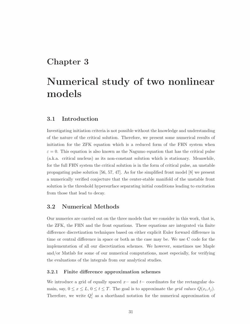
Chapter 3

Numerical study of two nonlinearmodels

3.1 Introduction

Investigating initiation criteria is not possible without the knowledge and understanding

of the nature of the critical solution. Therefore, we present some numerical results of

initiation for the ZFK equation which is a reduced form of the FHN system when

ε = 0. This equation is also known as the Nagumo equation that has the critical pulse

(a.k.a. critical nucleus) as its non-constant solution which is stationary. Meanwhile,

for the full FHN system the critical solution is in the form of critical pulse, an unstable

propagating pulse solution [56, 57, 47]. As for the simplified front model [8] we present

a numerically verified conjecture that the center-stable manifold of the unstable front

solution is the threshold hypersurface separating initial conditions leading to excitation

from those that lead to decay.

3.2 Numerical Methods

Our numerics are carried out on the three models that we consider in this work, that is,

the ZFK, the FHN and the front equations. These equations are integrated via finite

difference discretization techniques based on either explicit Euler forward difference in

time or central difference in space or both as the case may be. We use C code for the

implementation of all our discretization schemes. We however, sometimes use Maple

and/or Matlab for some of our numerical computations, most especially, for verifying

the evaluations of the integrals from our analytical studies.

3.2.1 Finite difference approximation schemes

We introduce a grid of equally spaced x− and t− coordinates for the rectangular do-

main, say, 0 ≤ x ≤ L, 0 ≤ t ≤ T . The goal is to approximate the grid values Q(xi, tj).

Therefore, we write Qji as a shorthand notation for the numerical approximation of

31

Q(xi, tj) with the grid points xi, tj chosen as

xi = x0 + i∆x,

tj = t0 + j∆t, (3.1)

where ∆x, ∆t are the spatial and time grid sizes, otherwise known as the discretization

steps and i = 0, 1, . . . , N , j = 0, 1, . . . ,M for N, M > 0, the pre-determined numbers

of grid points.

We therefore, discretize our PDEs by replacing the time derivative with the explicit

Euler forward difference approximation (a forward difference approximation for first

order PDE with respect to time t)

∂Qji

∂t≈Q

j+1i −Qj

i

∆t, Q = u, v, E, h,

(3.2)

and the spatial derivative with the explicit central difference approximation of the

second order PDE with respect to x

∂2Qji

∂x2≈Qj

i−1 − 2Qji +Qj

i+1

(∆x)2, Q = u, E. (3.3)

The discretization schemes in (3.2)-(3.3) give the following discretization formulas:

FHN (ZFK) discretization formulas

The formulas for FHN equations are

uj+1i = uj

i + ∆t f(uji , v

ji ) +

∆t

(∆x)2(uj

i−1 − 2uji + uj

i+1),

vj+1i = vj

i + ∆t ε g(uji , v

ji ), (3.4)

where

f(uji , v

ji ) = uj

i (uji − θ)(1 − uj

i ) − vji (3.5)

g(uji , v

ji ) = αuj

i − vji . (3.6)

Meanwhile, for its initial conditions

u0i = u0 + ustim Θ(xstim − xi),

v0i = v0, (3.7)

and boundary conditions

u01 = u0

0,

u0N = u0

N−1,

uj+11 = uj+1

0 ,

uj+1N = uj+1

N−1, (3.8)

32

for i = 1, . . . , N − 1, j = 0, 1, . . . ,M − 1.

Front discretization formulas

The formulas for the front equations are

Ej+1i = Ej

i + ∆t F (Eji , h

ji ) +

∆t

(∆x)2(Ej

i−1 − 2Eji + Ej

i+1),

hj+1i = hj

i + ∆t1

τG(Ej

i , hji ), (3.9)

where

F (Eji , h

ji ) = Θ(Ej

i − 1)hji ,

G(Eji , h

ji ) = Θ(−Ej

i ) − hji . (3.10)

While that of its initial conditions

E0i = −α+ Estim Θ(xstim − xi),

h0i = 1, ∀xi, (3.11)

and boundary conditions

E01 = E0

0 ,

E0N = E0

N−1,

Ej+11 = Ej+1

0 ,

Ej+1N = Ej+1

N−1, (3.12)

for i = 1, . . . , N−1, j = 0, 1, . . . ,M−1. Table (3.1) gives a summary of the parameters

that we used for our numerics according to figures

Table 3.1: Parameters used for the numerical simulations

Figure Parameter values

Fig. 3.1(a, b) ε = 0, θ = 0.13, ∆x = 0.15, ∆t = 0.01, L = 120, xstim = 2.10

Fig. 3.1(c) α = 0.37, θ = 0.13, ε = 0(ZFK), ε = 0.02(FHN), ∆x =0.15, ∆t = 0.01, L = 120

Fig. 3.2 α = 0.37, θ = 0.13, ε = 0, ∆x = 0.15, ∆t = 0.01, L = 15

Fig. 3.3(a, b) α = 0.37, θ = 0.13, ε = 0, ∆x = 0.15, ∆t = 0.01, L = 15

Fig. 3.4 α = 0.37, θ = 0.13, ε = 0.02, ∆x = 0.15, ∆t = 0.01,

L = 120, xstim = 2.10(a, b), xstim = 10.05(c, d)


33


Figure Parameter values

Fig. 3.5 α = 0.37, θ = 0.13, ε = 0.0094, ∆x = 0.15, ∆t = 0.01,

L = 60, xstim = 2.10(a, b), xstim = 10.05(c, d)

Fig. 3.6(a) α = 1, 0.75, τ = 8, ∆x = 0.075, ∆t = 0.0025, L = 450

Fig. 3.6(b) α = 1, 0.5, τ = 9, ∆x = 0.075, ∆t = 0.0025, L = 450

Fig. 3.7(a) α = 1, 1.5, τ = 10, ∆x = 0.075, 0.15, ∆t = 0.0025, 0.01, L = 450

Fig. 3.7(b) α = 0.5, 1, 0.75, 1.5, τ = 8, 9, 10, ∆x = 0.075, ∆t = 0.0025, L =450

Fig. 3.8 α = 1, τ = 8.2, ∆x = 0.075, ∆t = 0.0025, L = 50,

xstim = 0.3(top panel), xstim = 1.5(bottom panel)

Fig. 3.9 α = 1, τ = 8.2, ∆x = 0.075, ∆t = 0.0025, L = 450, xstim = 1.5

Fig. 3.10 α = 1, τ = 8.2, ∆x = 0.075, ∆t = 0.0025, L = 450, xstim = 0.3

Fig. 3.11 ∆x = 0.2, ∆t = 0.01, L = 40, xstim = 2

Fig. 4.2 ∆t = 0.0025, T = 250, α = 0.37

3.2.2 Fitting methods

We have used an implementation of the nonlinear least-squares (NLLS) Marquardt-

Levenberg algorithm in Gnuplot for the linear fit in Fig. 3.3(b) and for the nolinear fit

in Fig. 4.8(a).

3.3 Initiation problem for the ZFK equation

3.3.1 The critical nucleus

As pointed out earlier in Chapter 2 the theoretical concept of initiation of excitation

waves started with the initiation problem for the ZFK equation, which is the reduced

form of the FHN system when ε→ 0, v = 0

∂u

∂t=∂2u

∂x2+ f(u), (x, t) ∈ [0,+∞) × [0,+∞), (3.13)

where f(u) = u (u− θ) (1 − u).

The initiation problem consists of (3.13), the boundary and initial conditions

∂u

∂x(0, t) = 0, t ∈ [0,+∞),

u(x, 0) = ustimΘ(xstim − x), x ∈ [0,+∞), (3.14)

where Θ is a Heaviside step function, ustim and xstim are respectively the threshold

potential (excitation amplitude) and width of the excited region.

Fig. 3.1 (a,b) shows two typical results for the ZFK initiation process: a successful

initiation, leading to generation of a propagating front, and an unsuccessful initiation,

34

0

50

100

150

200

250

0 10 20

(a)

init.

0 10 20(b)

init.

0

1

2

3

4

0 1 2 3(c)

ZFKFHN

t+ 100u ustim

xx xstim

Figure 3.1: Initiation of excitation in ZFK equation. (a,b) Fast subsystem (3.13, 3.14)“ZFK” of “FHN” (2.15): for parameters values: α = 0.37, θ = 0.13, ε = 0. Stimulationparameters: xstim = 2.10 for both, subthreshold ustim = 0.3304831 for (a) and superthresholdustim = 0.3304833 for (b). Bold black lines: initial conditions. (c) The corresponding criticalcurves, separating initiation initial conditions from decay initial conditions.

leading to decay of excitation in the whole half-fibre into the resting state. The ZFK

problem has a critical pulse as its non-constant solution which is stationary. Moreover,

if a continuous one-parametric family of initial conditions contains some that initiate

a wave and some that lead to decay, there is always at least one that does neither, but

gives a solution that approaches the critical nucleus. This critical nucleus is the same

for all such families, that is, it does not depend on the shape of the initial distribution

u(x, 0), as long as its amplitude is at the threshold corresponding to that shape. Initial

conditions very close to the threshold generate solutions which approach the critical

nucleus and then depart from it, either toward propagation or toward decay. This

transient stationary state can be seen in Fig. 3.1(a,b) where the initial conditions are

selected very close to the threshold.

The theoretical understanding of excitability stems from FitzHugh’s simplified model

of a nerve membrane [33]. One of his key concepts is “quasi-threshold”, which gets

precise in the limit of large time scale separation between the processes of excitation

and recovery. Then the fast subsystem has unstable “threshold” equilibria; initial

conditions below such an equilibrium lead to decay, and those above it to propagation

(excitation).

In a spatially extended FHN system [33, 67, 71, 28, 27] the ability of a stimulus

to initiate a wave depends on its spatial extent, the aspect summarized by Ruston’s

concept of “liminal length” [81, 71, 15]. A more generic concept is that of the “critical

curve” in the stimulus-spatial extent plane (see Fig. 3.1(c)). A stimulus initiates a wave

if its parameters are above this curve or decays if below.

Mathematically, the problem is about classification of initial conditions that will or

will not lead to a traveling (excitation) wave solution. The key question is the nature

35

of the boundary between the two classes. A detailed analysis of which has been done

for the FitzHugh-Nagumo system and its variations.

In particular, if initial condition u(x, 0) < ucr(x), x ∈ [0,∞) then u(x, t) decays as

t→ ∞, and if u(x, 0) > ucr(x), x ∈ [0,∞) then u(x, t) approaches a stable propagating

front solution. The center-stable manifold of the “critical nucleus” is the threshold

surface separating initiation initial conditions and decay initial conditions. Roughly,

this is a spatially extended analogue of a threshold equilibrium in the point system;

critical nucleus is also a stationary but unstable solution, and its small perturbation

lead to either initiation of excitation wave, for perturbations in one direction, or to

decay, for perturbations in the opposite direction.

3.3.2 Numerical critical nuclei

The values of the parameters used for the numerics are θ = 0.13, ε = 0 and α = 0.37.

The spatial distributions of the potential u are constructed based on a one-dimensional

fibre model of length L = 15 and a predetermined value of time t given by T = 200

with no flux boundary conditions. The evolution of u is computed from (3.13) with

the initial conditions u0(x) as given by (3.14). The PDE for u was solved using the

method of forward differences in time and central differences in space with a time step

∆t = 0.01 and the fibre discretized with ∆x = 0.15.

0

0.05

0.1

0.15

0.2

0.25

0 2 4 6 8 10 12 14 16

x

u

ustim=0.3304888ustim=0.3304890ustim=0.1434738ustim=0.1434740

u*cr(x)ucr(x)

Figure 3.2: Plot of solutions (2.27, 2.28), the analytical critical nucleus ucr(x) due to Neu [68]shown as the black solid curve and u∗cr(x) represented by the black-dashed curve, the analyticalcritical nucleus for cubic nonlinearity compared with the four extracted numerical nuclei (shownin other colors).

Four numerical critical nuclei (shown in Fig. 3.2) were extracted by means of the

minimal distance D(t) between two consecutive voltage profiles in L2 norm. The min-

36

imal distance is an indicator for the slowest voltage profile u(x, t) which approximates

the critical nucleus. The computation of the minimal distance between consecutive

voltage profiles is achieved using the following discretization formula

D(t) =∑

x

|u(x, t+ dt) − u(x, t)|2, (3.15)

where the right-hand side of (3.15) is equivalent to (3.16) as given in terms of continuous

functions

limdt→0dx→0

∫ ∞

0|∂u(x, t)

∂tdt|2 dx = (dt)2

∫ ∞

0|∂u(x, t)

∂t|2 dx. (3.16)

The computation is done by fixing xstim, the excitation width, as the excitation am-

plitude ustim is varied (see (3.14)). Two values, xstim = 2.10, 10.05 which respectively

represent subthreshold and superthreshold u0(x). In each case both the lower and up-

per bounds for ustim are determined. The lower and upper bounds for the excitation

amplitude ustim that correspond to xstim = 2.10 are respectively, 0.3304888, 0.3304890

and that of xstim = 10.05 are 0.1434738, 0.1434740.

The original values for the excitation amplitude had four digits which were later

extended to seven significant digits in order to improve the accuracy of the numerics.

Such a high precision is needed as the solution we are looking for is unstable, in that

the slightest change in initial conditions brings with it a significant change in the

solution. When initial condition chosen is very close to the excitation threshold, we see

a solution (with bell-shape) developing toward the critical nucleus and which after some

time interval either decays to zero or propagates (i.e. excites). This critical nucleus

corresponds to the saddle point which has a codimension-1 stable manifold and 1D-

unstable manifold. The stable manifold of the saddle point acts as a separatrix that

separates its two basins of attraction. In other words, the separatrix divides the phase

plane into two regions, one of decay and the other of excitation (i.e. a region with no

excitation and excitation respectively).

Initial pulses below the separatrix decay to zero with larger time and those pulses

above the separatrix give rise to propagating wavefronts. The former are initial condi-

tions that fail to start propagation while the latter are those that succeed in starting

propagation.

In [34], it has been established that the Nagumo equation (3.13) has three relevant

stationary solutions: 0, 1, and a standing wave u(x). The constant states are stable,

while the standing wave is a saddle of index 1 (i.e having a codimension 1 stable man-

ifold) and thus corresponds to our critical nucleus. The stable manifold is sometimes

called a nucleation manifold or ignition manifold [2, 3].

37

Excitation threshold curve for ZFK equation

The excitation threshold curve is a plot of the stimulus strength (excitation amplitude)

and the width of excited region. It is the curve that separates the region when the

wave just propagates (i.e. excites) and when it just diffuses (i.e. no propagation).

0

0.5

1

1.5

2

2.5

0 0.5 1 1.5 2 2.5 3

xstim

ustim

0

0.5

1

1.5

2

2.5

3

3.5

0 0.5 1 1.5 2 2.5

ustim

1/xstim

(a) (b)

Figure 3.3: (a) The excitation amplitude ustim as a function of the length of the excitedregion xstim plotted using errorbars with 10−7 precision. (b) The excitation threshold curve(the separatrix of the critical nucleus) confirming that ustim ∝ k as k → ∞ [68], wherek = 1/xstim; that is, as xstim → 0 the separatrix can be fitted with a straight line.

Fig. 3.3 suggests that corresponding to certain excitation amplitude (chosen as ini-

tial conditions) a length of excited region is required in order to initiate propagation.

This has confirmed the prediction by Neu and his co-workers [68] that for a specific

pulse width, the separatrix determines the minimum amplitude necessary to start prop-

agation and that infinitely broad pulses require amplitude equal to the membrane ex-

citation threshold. In addition, as the width of the pulses decreases, the requirement

on the amplitude grows.

Now plotting the inverse of the length of the excited region 1/xstim which is given by

k in [68] against the excitation amplitude ustim, we obtain the excitation threshold curve

as in Fig. 3.3 (b) where we see that despite the fact that rectangular initial conditions

are used instead of the Gaussian one, yet we observe the same qualitative property as

predicted in [68]: In the limit of very narrow pulses (very small excitation width), the

pulse width and the amplitude are related by a linear relationship corresponding to a

constant charge developed by the pulse (i.e ustim ∝ k as k → ∞, where k = 1/xstim).

In other words, in the limit of a very large k the separatrix as represented in the

2D-manifold of initial conditions looks like a straight line.

38

3.4 Initiation problem for the FHN system

3.4.1 The critical pulse

We consider the problem of initiation of propagating waves in a one-dimensional ex-

citable fibre by considering the FHN system in the form

∂u

∂t=∂2u

∂x2+ f(u) − v,

∂v

∂t= ε (αu − v), (3.17)

where (x, t) ∈ [0,∞) × [0,∞) with no-flux boundary conditions

∂u

∂x(0, t) = 0, t ∈ [0, ∞), (3.18)

and a rectangular initial perturbation of width xstim and amplitude ustim,

u(x, 0) = ustimΘ (xstim − x),

v(x, 0) = 0, x ∈ [0, ∞), (3.19)

where f(u) = u (u − θ) (1 − u), ε > 0, α > 0, θ ∈ (0, 1/2) and Θ a Heaviside step

function.

For small ε > 0, system (3.17) does not have nontrivial stationary solutions, but has

an unstable propagating pulse solution ucr(x−ct), vcr(x−ct) such that ucr(x) → ucr(x),

vcr(x) → 0 and c = O(ε1/2

)as ε ց 0. This solution also has a single unstable

eigenvalue [34, 35, 98, 2, 53, 3], and so its center-stable manifold is the threshold

hypersurface (see [62] for a different treatment) dividing the phase space into the decay

domain and the initiation domain. So, here we have a critical pulse solution, which

is essentially a slowly traveling variant of the critical nucleus. Any solution with the

initial condition at the threshold hypersurface asymptotically approaches this critical

pulse (suitably shifted), and any solution starting close to the threshold approaches

this critical pulse as a transient. This is illustrated in Fig. 3.4.

For much smaller value of the parameter ε, the results are shown in Fig. 3.5. With

this understanding, the excitation condition in terms of (xstim, ustim) reduces to com-

puting the intersection of the two-parametric manifold described by (3.19) with the

codimension 1 stable (center-stable) manifold of the critical nucleus (critical pulse).

This gives the curve on the (xstim, ustim) plane separating initial conditions leading to

excitation propagation from those leading to decay. This can be done numerically or,

with appropriate simplifications, analytically. An example of dealing with this problem

in the ZFK equation, using Galerkin style approximations can be found in [68] (see

also Sec. 2.5.2 and figure Fig. 2.6(b)). We present some further approaches below, in

Sec. 4.1 and Sec. 5.2.

39

0

100

200

300

400

500

0 40 80 120

x

t+100u

(a)

init.

0 40 80 120

x(b)

init.

0

100

200

300

400

500

0 40 80 120

x(c)

init.

0 40 80 120

x(d)

init.

Figure 3.4: The critical pulse is a universal transient for any near-threshold initial condi-tion. The solutions to (3.17) for slightly sub-threshold (a,c) and slightly super-threshold (b,d)amplitudes, for smaller stimulus width xstim = 2.10 in (a,b) and larger xstim = 10.05 in (c,d).Parameter values: ε = 0.02, α = 0.37, ∆t = 0.01, ∆x = 0.15, L = 120. Bold black lines:initial conditions. In all cases we see a slow, low-amplitude unstable propagating pulse whichsubsequently either decays or evolves into a fast, high-amplitude stable propagating pulse [45].

3.5 Initiation problem for the front model

3.5.1 The critical front

Now consider the simplified model of INa-driven excitation fronts in typical cardiac

excitation models [8]

∂E

∂t=∂2E

∂x2+ F (E,h),

∂h

∂t= (1/τ)G(E,h), (x, t) ∈ (−∞,+∞) × [0,+∞), (3.20)

where

F (E,h) = Θ(E − 1)h,

G(E,h) = Θ(−E) − h, (3.21)

40

0

50

100

150

200

250

0 20 40 60

x

t+100u

(a)

init.

0 50

100 150 200 250 300 350

0 20 40 60

x(b)

init.

0

50

100

150

200

250

0 20 40 60

x(c)

init.

0 50

100 150 200 250 300 350

0 20 40 60

x(d)

init.

Figure 3.5: The critical pulse solutions to the FHN system (3.17) for parameter val-ues: ε = 0.0094, α = 0.37, ∆t = 0.01, ∆x = 0.15. Top panels: xstim = 2.10 (a)ustim = 0.380723412971864, (b) ustim = 0.380723412971866. Bottom panels: xstim = 10.05(c) ustim = 0.168543917244412, (d) ustim = 0.168543917244414. (a) & (c) for slightly-belowthreshold initial conditions (b) & (d) for slightly-above threshold initial conditions [45].

and Θ is a Heaviside function with boundary condition

∂E

∂x(0, t) = 0, t ∈ [0,+∞), (3.22)

and initial conditions

E(x, 0) = −α+ EstimΘ(xstim − x),

h(x, 0) = 1, x ∈ (−∞,+∞). (3.23)

System (3.20) does not have nontrivial bounded stationary solutions: if∂E

∂t=∂h

∂t= 0

then any bounded solution has the form E = a, h = Θ(−a) for some a = const. So,

there are no critical nuclei in this system. Nevertheless, system (3.20) is known to

develop stable propagating wave solutions from some initial conditions but not from

others, and there should therefore be a threshold, i.e. a boundary in the phase space

of (3.20, 3.23) between initial conditions leading to initiation and those leading to

41

decay. Hence the question, what happens when the initial conditions are exactly at the

threshold? We answer this question shortly. Meanwhile, we note that system (3.20)

has a family of propagating front solutions

E(z) =

ω − τ2c2

1 + τc2exp

( z

τc

)

, (z ≤ −∆),

−α+ α exp(−cz), (z ≥ −∆),

h(z) =

exp( z

τc

)

, (z ≤ 0),

1, (z ≥ 0),(3.24)

where z = x− ct, ω = 1 + τc2(1 + α), ∆ =1

cln

(1 + α

α

)

.

3.5.2 Numerical Results for the front model

Our numerics were carried out via the finite differencing method using forward differ-

ences in time and central difference in space implemented using a C code. The time step

and space steps for the numerical integration were ∆t = 0.0025,∆x = 0.075 but only

used ∆t = 0.01,∆x = 0.15 once to check our discretization steps. In the simulations

the model parameters were τ, α and the admissible values for the pair chosen so that

propagation would be possible.

Threshold curves for the front model

The threshold curve that determines the parameter region for Estim, xstim, the paramet-

ric set of initial conditions, is the curve which sets conditions for the success or failure

of propagation in the simplified cardiac front model. In our case we obtain threshold

curves for different admissible pairs of the numerical parameters τ, α where the front

model is simulated with the following pairs. The threshold curves for τ = 8, α = 1, 0.75;

τ = 9, α = 1, 0.5; and τ = 10, α = 1, 1.5 are respectively given in Fig. 3.6 and Fig. 3.7.

The solid black curves are for α = 1 while the dashed blue are for other values of α.

Note also that the asymptotic threshold value for the voltage, Easym is α+ 1 which is

represented by the dashed cyan line as shown in Fig. 3.7(b).

The threshold curves in Fig. 3.7 are calculated with the same values of parameters

as used in Fig. 3.6 but only with different spatial and time steps, ∆t = 0.01,∆x = 0.15

and different τ . The lack of any conspicuous error suggest that our discretization steps

in space and time are not crude.

From the plot given in Fig. 3.7(b) we can easily deduce that the dependence of the

asymptotic threshold (rheobase), Easym on the pre-frontal voltage α is linear and is

given by the relation Easym = α+ 1 which is represented by the red solid line.

42

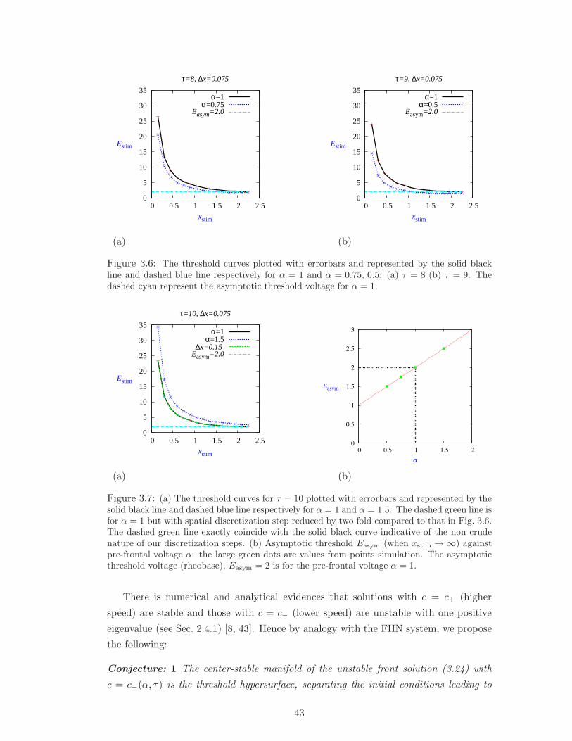
0

5

10

15

20

25

30

35

0 0.5 1 1.5 2 2.5

Estim

xstim

τ=8, ∆x=0.075

α=1α=0.75

Easym=2.0

0

5

10

15

20

25

30

35

0 0.5 1 1.5 2 2.5

Estim

xstim

τ=9, ∆x=0.075

α=1α=0.5

Easym=2.0

(a) (b)

Figure 3.6: The threshold curves plotted with errorbars and represented by the solid blackline and dashed blue line respectively for α = 1 and α = 0.75, 0.5: (a) τ = 8 (b) τ = 9. Thedashed cyan represent the asymptotic threshold voltage for α = 1.

0

5

10

15

20

25

30

35

0 0.5 1 1.5 2 2.5

Estim

xstim

τ=10, ∆x=0.075

α=1α=1.5

∆x=0.15 Easym=2.0

0

0.5

1

1.5

2

2.5

3

0 0.5 1 1.5 2

Easym

α

(a) (b)

Figure 3.7: (a) The threshold curves for τ = 10 plotted with errorbars and represented by thesolid black line and dashed blue line respectively for α = 1 and α = 1.5. The dashed green line isfor α = 1 but with spatial discretization step reduced by two fold compared to that in Fig. 3.6.The dashed green line exactly coincide with the solid black curve indicative of the non crudenature of our discretization steps. (b) Asymptotic threshold Easym (when xstim → ∞) againstpre-frontal voltage α: the large green dots are values from points simulation. The asymptoticthreshold voltage (rheobase), Easym = 2 is for the pre-frontal voltage α = 1.

There is numerical and analytical evidences that solutions with c = c+ (higher

speed) are stable and those with c = c− (lower speed) are unstable with one positive

eigenvalue (see Sec. 2.4.1) [8, 43]. Hence by analogy with the FHN system, we propose

the following:

Conjecture: 1 The center-stable manifold of the unstable front solution (3.24) with

c = c−(α, τ) is the threshold hypersurface, separating the initial conditions leading to

43

initiation from the initial conditions leading to decay.

An “experimentally testable” consequence of this conjecture is that for any initial

conditions exactly at the threshold, the solution will approaches the unstable front as

t → +∞. For any initial condition near to the threshold, the solution comes close to

the unstable front and stays in its vicinity for a long time: if the positive eigenvalue

is λ and the initial condition is δ-close to the threshold, the transient front should be

observed for the time ∝ λ−1| ln δ|. This transient front solution does not depend on the

initial condition, as long as the initial condition is at the threshold.

-2

0

2

4

6

8

10

12

E

t ∈ [0, 0.125]

init.

-1-0.5

0 0.5

1 1.5

2 2.5

3

0 0.5 1 1.5 2 2.5 3

x

E

init.

-1

0

1

2

3

4

5

6

t ∈ [0, 1.25]

init.

-1-0.5

0 0.5

1 1.5

2 2.5

3

0 1 2 3 4 5

x

init.

-1-0.5

0 0.5

1 1.5

2 2.5

3t ∈ [0, 12.5]

init.

-1-0.5

0 0.5

1 1.5

2 2.5

3

0 2 4 6 8 10 12

x

init.

Figure 3.8: Evolution of two different near-threshold initial conditions toward the critical frontsolution in system (3.20). Initial stimuli: xstim = 0.3, Estim = 12.716330706144868 (upper row)and xstim = 1.5, Estim = 2.619968799545055 (lower row). Other parameters: τ = 8.2, α = 1,∆x = 0.075, ∆t = 0.0025, L = 50 [45].

We have tested these predictions by numerical simulation of (3.20, 3.22, 3.23). The

results are shown in Fig. 3.8 and Fig. 3.9. Fig. 3.8 illustrates two solutions starting from

initial conditions with different xstim. In both cases, Estim values have been chosen close

to the respective threshold with high precision. In both cases, the solutions evolve in

the long run toward the same propagating front. Fig. 3.9 presents an analysis of a pair

of solutions, one with slightly overthreshold and the other with slightly underthreshold

initial conditions. To separate the evolution of the front shape from its movement, we

employ the idea of symmetry group decomposition with explicit representation of the

orbit manifold (see e.g. [11]). Practically, we define the front point xf = xf (t) via

E(xf (t), t) = E∗, (3.25)

44

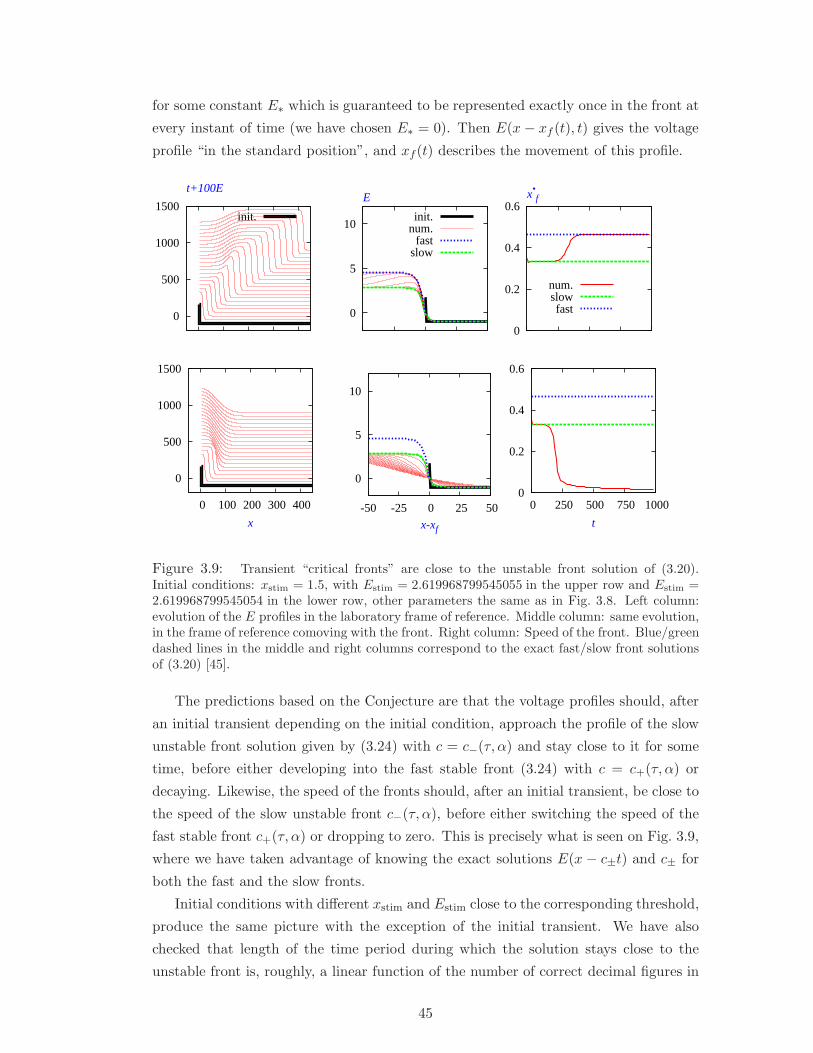
for some constant E∗ which is guaranteed to be represented exactly once in the front at

every instant of time (we have chosen E∗ = 0). Then E(x− xf (t), t) gives the voltage

profile “in the standard position”, and xf (t) describes the movement of this profile.

0

500

1000

1500

t+100E

init.

0

500

1000

1500

0 100 200 300 400

x

0

5

10

E

init.num.

fastslow

0

5

10

-50 -25 0 25 50

x-xf

0

0.2

0.4

0.6

x•f

num.slowfast

0

0.2

0.4

0.6

0 250 500 750 1000

t

Figure 3.9: Transient “critical fronts” are close to the unstable front solution of (3.20).Initial conditions: xstim = 1.5, with Estim = 2.619968799545055 in the upper row and Estim =2.619968799545054 in the lower row, other parameters the same as in Fig. 3.8. Left column:evolution of the E profiles in the laboratory frame of reference. Middle column: same evolution,in the frame of reference comoving with the front. Right column: Speed of the front. Blue/greendashed lines in the middle and right columns correspond to the exact fast/slow front solutionsof (3.20) [45].

The predictions based on the Conjecture are that the voltage profiles should, after

an initial transient depending on the initial condition, approach the profile of the slow

unstable front solution given by (3.24) with c = c−(τ, α) and stay close to it for some

time, before either developing into the fast stable front (3.24) with c = c+(τ, α) or

decaying. Likewise, the speed of the fronts should, after an initial transient, be close to

the speed of the slow unstable front c−(τ, α), before either switching the speed of the

fast stable front c+(τ, α) or dropping to zero. This is precisely what is seen on Fig. 3.9,

where we have taken advantage of knowing the exact solutions E(x − c±t) and c± for

both the fast and the slow fronts.

Initial conditions with different xstim and Estim close to the corresponding threshold,

produce the same picture with the exception of the initial transient. We have also

checked that length of the time period during which the solution stays close to the

unstable front is, roughly, a linear function of the number of correct decimal figures in

45

Estim, as it should be according to the Conjecture.

0

500

1000

1500

t+100E

init.

0

500

1000

1500

0 100 200 300 400

x

0

5

10

E

init.num.

fastslow

0

5

10

-50 -25 0 25 50

x-xf

0

0.2

0.4

0.6

x•f

num.slowfast

0

0.2

0.4

0.6

0 250 500 750 1000

t

Figure 3.10: Transient “critical fronts” are close to the unstable front solution of (3.20).Initial conditions: xstim = 0.3, with Estim = 12.716330706144868 in the upper row and Estim =12.716330706144867 in the lower row, other parameters the same as in Fig. 3.8. Left column:evolution of the E profiles in the laboratory frame of reference. Middle column: same evolution,in the frame of reference comoving with the front. Right column: Speed of the front. Blue/greendashed lines in the middle and right columns correspond to the exact fast/slow front solutionsof (3.20) [45].

3.5.3 Detailed cardiac excitation model

The simplified front model (3.20, 3.21) has many peculiar qualitative features which

stemmed from the nonstandard asymptotic embedding leading to it. Quantitatively,

however, it is very far from any realistic ionic model of cardiac excitation. Hence, the

newly described phenomena of critical front could be an artifact which might have been

brought about by the simplifications.

To eliminate this possibility, we have tested the relevance of the critical concept in a

full ionic model of cardiac excitation. We have chosen the model of human atrial tissue

due to Courtmanche, Ramirez and Nattel (CRN) [25], which is less stiff than most

stereotypical ventricular or Purkinje fibre model. It is well formulated in mathematical

sense and is also popular among cardiac modelers. The model operates with 21 dynamic

variables including the transmembrane voltage V . We have used the default parameters

as described in [25] and supplemented the equation for V in the system of equations

46

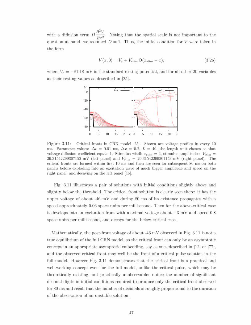
with a diffusion term D∂2V

∂x2. Noting that the spatial scale is not important to the

question at hand, we assumed D = 1. Thus, the initial condition for V were taken in

the form

V (x, 0) = Vr + Vstim Θ(xstim − x), (3.26)

where Vr = −81.18 mV is the standard resting potential, and for all other 20 variables

at their resting values as described in [25].

0

-20

-40

-60

-80

20 15 10 5 0

init.

20 15 10 5 0

init.V

x x

Figure 3.11: Critical fronts in CRN model [25]. Shown are voltage profiles in every 10ms. Parameter values: ∆t = 0.01 ms, ∆x = 0.2, L = 40, the length unit chosen so thatvoltage diffusion coefficient equals 1. Stimulus witdh xstim = 2, stimulus amplitudes: Vstim =29.31542299307152 mV (left panel) and Vstim = 29.31542299307153 mV (right panel). Thecritical fronts are formed within first 10 ms and then are seen for subsequent 80 ms on bothpanels before exploding into an excitation wave of much bigger amplitude and speed on theright panel, and decaying on the left panel [45].

Fig. 3.11 illustrates a pair of solutions with initial conditions slightly above and

slightly below the threshold. The critical front solution is clearly seen there: it has the

upper voltage of about -46 mV and during 80 ms of its existence propagates with a

speed approximately 0.06 space units per millisecond. Then for the above-critical case

it develops into an excitation front with maximal voltage about +3 mV and speed 0.8

space units per millisecond, and decays for the below-critical case.

Mathematically, the post-front voltage of about -46 mV observed in Fig. 3.11 is not a

true equilibrium of the full CRN model, so the critical front can only be an asymptotic

concept in an appropriate asymptotic embedding, say as ones described in [12] or [77],

and the observed critical front may well be the front of a critical pulse solution in the

full model. However Fig. 3.11 demonstrates that the critical front is a practical and

well-working concept even for the full model, unlike the critical pulse, which may be

theoretically existing, but practically unobservable: notice the number of significant

decimal digits in initial conditions required to produce only the critical front observed

for 80 ms and recall that the number of decimals is roughly proportional to the duration

of the observation of an unstable solution.

47

3.6 Summary

• We have developed a numerical procedure for identifying critical nucleus in an

excitable model by means of finding the minimal value of the L2-norm of the

time derivative of a solution with near-threshold initial conditions. This has

been tested on the ZFK equation for which the critical nucleus solution is known

exactly.

• Our numerical critical curves confirm the prediction from the approximate ana-

lytical theory by Neu et al. [68] about inverse proportionality of critical stimulus

amplitude to its width.

• We presented numerical evidence that the role of the “critical nucleus” as for

ZFK equation is being played by its slowly moving variant, the “critical pulse”

for FHN system, which is consistent with the theoretical results by Flores [35, 57].

The critical pulse is an unstable propagating pulse whose center-stable manifold

is the threshold hypersurface dividing the phase space into excitation and decay

regions. We showed that any solution with initial conditions at the threshold

approach this “critical pulse” asymptotically as a transient. In other words, the

critical pulse plays the role of an attractor on the critical manifold. This is found

to be the case even with different nonzero values for the small parameter solution.

• In the case of the simplified front model, we have observed through numerics

that the relationship between the asymptotic voltage (rheobase), Easym and the

pre-frontal voltage α is found to be Easym = α + 1, which means that at very

large stimulus width, the stimulus amplitude should be such that it opens the

m-gates (see Sec. 2.4). This revelation will among other things assist us to check

the analytical ignition criteria that we seek to find.

• We have demonstrated that neither critical nucleus nor critical pulse concepts are

applicable to the front model. We have conjectured that the role of the critical

solution is played by the unstable front solutions which were known to exist in

this model. We have confirmed this “critical front” conjecture by numerical simu-

lation. That is, we presented numerical evidence that the center-stable manifold

of the unstable front solution in the simplified cardiac model is the threshold

hypersurface that separate excitation initial conditions from decay initial condi-

tions. This is found to be always true no matter the nature of the initial stimulus

we consider provided it is chosen at the threshold.

48



α constant Fig. 3.1

α pre-frontal voltage (3.23)


ε ratio of the reaction rates Sec. 3.1

δ distance between the initial condition andthe threshold surface

af(Con. 1)

λ positive eigenvalue of the unstable front af(Con. 1)


θ threshold parameter af (3.13)

τ parameter (3.20)

D L2-distance between consecutive voltageprofiles

(3.15)

a constant af (3.23)

c : c−, c+ speed:lower, higher af(3.25):bf(Con. 1)

D diffusion coefficient bf (3.26)

E∗ constant (3.25)

E, h dynamic variable: Voltage, gate variable (3.20)

Easym rheobase Sec. 3.5.2

Estim stimulus amplitude (3.23)

f nonlinear function (3.13)


INa Na+ current bf (3.20)

ucr critical nucleus for the quadratic nonlin-earity

Sec. 3.3.1

u∗cr critical nucleus for the cubic nonlinearity Fig. 3.2

ucr, vcr critical pulse af (3.19)

V transmembrane voltage [25] bf/in (3.26)

Vr resting potential [25] bf/in (3.26)

u, v dynamic variable (3.13, 3.17)

xstim, ustim stimulus: width, amplitude (3.14)

xf front position (3.25)

49

Chapter 4

Analysis of variationalapproximations to initiationproblems

4.1 ZFK equation

4.1.1 Piece-wise smooth ansatzes

In Sec. 2.5.2, we have reproduced results by Neu et al. [68] on a variational approxima-

tion to the initiation problem for the ZFK equation, using the method of minimization

of the residual, which is close to that used by Neu et al. themselves but we did not

require the equations to be written in the gradient form.

In this section, we apply the variational method of Biot-Mornev [64], which we

briefly described (also see Sec. 2.5.2). An advantage of this method is that it requires

from the ansatz to have only one spatial derivative and not necessarily the second, even

though reaction-diffusion equation contains second spatial derivative.

We consider the functional σ as a function of u and∂u

∂tas given by the formulation

σ = Γ +dG

dt= σ[u,

∂u

∂t], (4.1)

where

Γ =1

2

∫ +∞

−∞

(∂u

∂t− f(u)

)2dx = Γ[u,

∂u

∂t], (4.2)

and

G =1

2

∫ +∞

−∞

(∂u

∂x

)2dx = G[u]. (4.3)

It can be easily verified that the variational equation (with u fixed)

δσ

δ(∂u

∂t)

= 0, (4.4)

50

is equivalent to the PDE for u,

∂u

∂t= f(u) +

∂2u

∂x2, x ∈ [0,+∞). (4.5)

We consider (4.5) and the boundary condition∂

∂xu(0, t) = 0, by applying the procedure

to the piece-wise smooth ansatz

u =

a, 0 ≤ x ≤ xa,

a(x0 − x)

x0 − xa, xa ≤ x ≤ x0,

0, otherwise,

(4.6)

with the cubic nonlinearity f(u) = u(u− θ)(1− u) and where a ≡ a(t), xa ≡ xa(t) and

x0 ≡ x0(t) are the dynamic variables. The sketch of the ansatz is as shown in Fig. 4.1.

a

u

xxa x000

Figure 4.1: The sketch of the piece-wise smooth ansatz given in (4.6).

We use (4.6) and its temporal derivative∂u

∂t(derived via formulation (4.7))

∂u

∂t=∑

q

∂u

∂qq, q = a, xa, x0, (4.7)

(q =

dq

dt

)in (4.2, 4.3) to minimize the resultant functional σ given in (4.1) with respect

to q. Then by considering xa = x0/2 due to translational invariant we obtain the ODE

system

a = −a(468a2 − (1 + θ)475a+ 480θ + 1920k2

)/480,

k = −k(36a2 − (1 + θ)25a+ 480k2

)/240, (4.8)

where k = 1/x0.

51

The phase portrait of the ODE system (4.8) is presented in Fig. 4.2. The equilibria

of the ODE system are depicted with the thick blue dot, the null-clines by the dotted-

blue and dotted-magenta lines. The saddle-point equilibrium with both a and k nonzero

corresponds to the critical nucleus. Its stable separatrix is shown by the solid red line

and its unstable separatrix is shown by the dashed black line. The stable separatrix

serves as the boundary between excitation and decay. Initial conditions to the left of

it correspond to decaying solutions, and initial conditions to the right of it give rise to

excitation, i.e. propagating waves. The phase portrait is qualitatively similar to that

obtained by Neu et al. in [68]. However, one major difference is that we have successful

initiation represented by solutions with a→ 1, which corresponds to propagating waves,

as opposed to those in [68] which have a→ ∞, blow up in finite time. This is because

we have used the full cubic kinetics in the ZFK equation whereas Neu et al. used

its quadratic approximation, which corresponds to the limit of very high values of the

upper zero of the cubic.

0

0.05

0.1

0.15

0.2

0.25

0 0.2 0.4 0.6 0.8 1 1.2

a

• • •

•k

Figure 4.2: The equilibria of the ODE system are depicted with the thick blue dot, the null-clines by the dotted-blue and -magenta lines. The center-stable manifolds (solid - red lines) ofthe critical nucleus (i.e., point of intersection of the stable and unstable manifolds) serving asthe boundary between excitation and decay. The unstable manifolds are the dotted - gray lines.Initial perturbations to the left of the stable manifolds decays to zero, and those to the rightgive rise to excitation. The phase portrait is qualitatively similar to that obtained by Neu andhis co-workers [68] shown in Fig. 2.6 of Chapter 2

.

4.2 Front equations

4.2.1 Piece-wise smooth ansatzes

In this section, we consider a variational description of the rightward propagating front

solution for the Biktashev model (2.20)-(2.21) [8] written in the form of piece-wise linear

functions. Instead of using Biot-Mornev technique, we use the method of minimization

52

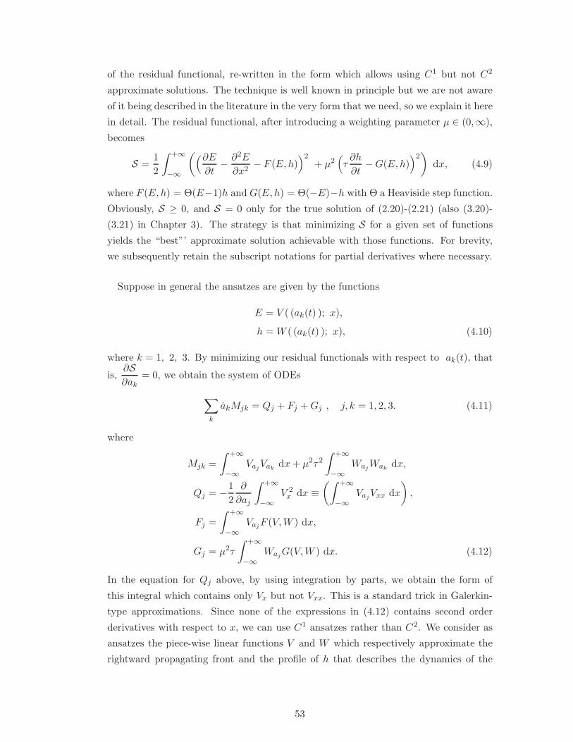
of the residual functional, re-written in the form which allows using C1 but not C2

approximate solutions. The technique is well known in principle but we are not aware

of it being described in the literature in the very form that we need, so we explain it here

in detail. The residual functional, after introducing a weighting parameter µ ∈ (0,∞),

becomes

S =1

2

∫ +∞

−∞

((∂E

∂t− ∂2E

∂x2− F (E,h)

)2+ µ2

(

τ∂h

∂t−G(E,h)

)2)

dx, (4.9)

where F (E,h) = Θ(E−1)h and G(E,h) = Θ(−E)−h with Θ a Heaviside step function.

Obviously, S ≥ 0, and S = 0 only for the true solution of (2.20)-(2.21) (also (3.20)-

(3.21) in Chapter 3). The strategy is that minimizing S for a given set of functions

yields the “best”’ approximate solution achievable with those functions. For brevity,

we subsequently retain the subscript notations for partial derivatives where necessary.

Suppose in general the ansatzes are given by the functions

E = V ( (ak(t) ); x),

h = W ( (ak(t) ); x), (4.10)

where k = 1, 2, 3. By minimizing our residual functionals with respect to ak(t), that

is,∂S∂ak

= 0, we obtain the system of ODEs

∑

k

akMjk = Qj + Fj +Gj , j, k = 1, 2, 3. (4.11)

where

Mjk =

∫ +∞

−∞Vaj

Vakdx+ µ2τ2

∫ +∞

−∞Waj

Wakdx,

Qj = −1

2

∂

∂aj

∫ +∞

−∞V 2

x dx ≡(∫ +∞

−∞Vaj

Vxx dx

)

,

Fj =

∫ +∞

−∞Vaj

F (V,W ) dx,

Gj = µ2τ

∫ +∞

−∞Waj

G(V,W ) dx. (4.12)

In the equation for Qj above, by using integration by parts, we obtain the form of

this integral which contains only Vx but not Vxx. This is a standard trick in Galerkin-

type approximations. Since none of the expressions in (4.12) contains second order

derivatives with respect to x, we can use C1 ansatzes rather than C2. We consider as

ansatzes the piece-wise linear functions V and W which respectively approximate the

rightward propagating front and the profile of h that describes the dynamics of the

53

gating variable

V =

V (x, t), x < xω

−α− α+ ω

xα − xω(x− xα), xω ≤ x < xα

−α, xα ≤ x,

W =

0, x < xωα+ ω

ω(xα − xω)(x− xω), xω ≤ x < x0

1, x0 ≤ x.

(4.13)

Here, a1(t) = ω(t), a2(t) = x0(t) and a3(t) = x1(t). The sketch of the ansatzes, the

red solid (V ) and the blue dashed (W ) lines are shown in Fig. 4.3(a).

VV

W

Wω

1

0

−αxω x1 x0 xa x 4 8 12

100

200

1

0

0

0

EE

h

h

x

(a) (b)

Figure 4.3: (a) The sketch of the piece-wise smooth ansatzes for the front model given in (4.13)and (b) the plot of a propagating front profile. The red solid (E) curve and blue-dashed (h)respectively correspond to solid red line (V ) and dashed blue line (W ) in (a).

We take the function V (x, t) for x < xω(t) as the exact solution of the diffusion

equation Vt = Vxx with an appropriate initial condition and the boundary condition

V (xω(t), t) = ω(t). This exact solution can be written explicitly but it is complicated

and we do not need it, so we omit it. Also W = 0 in the interval, (−∞, xω). Thus, the

terms,

∫ xω

−∞

(∂E

∂t− ∂2E

∂x2− F (E,h)

)2dx, µ2

∫ xω

−∞

(

τ∂h

∂t−G(E,h)

)2dx, (4.14)

contribute nothing to the residuals S. Consequently, we consider our integrals in the

interval [xω(t),∞).

From our knowledge of the internal boundary conditions E(x1) = 1 and E(x0) = 0,

we derive the relationships between xω, xα and our dynamic variables ω, x1 and x0

(whichever is suitable) as

x0 =αxω + ωxα

α+ ω, x1 =

(1 + α)xω + (ω − 1)xα

α+ ω, (4.15)

xω = −(ω − 1)x0 + ωx1, xα = (1 + α)x0 − αx1. (4.16)

54

Also, to simplify the computations of the integrals Mjk, Qj, Fj and Gj and their inte-

grands, we take advantage of the equivalence relationships Θ(V − 1) ≡ Θ(x1 − x) and

Θ(−V ) ≡ Θ(x− x0)

F (V,W ) = Θ(V − 1)W = Θ(x1 − x)W,

G(V,W ) = Θ(−V ) −W = Θ(x− x0) −W. (4.17)

For the computation of the integrands in (4.12) and subsequently the values of the

integrals see Sec. A.1 in Appendix A.

The second order ODE system resulting from the approximation as derived in Ap-

pendix A is

dω

dt= −

(

τ µ2ω6 + (4α τ µ2 − τ2 µ2)ω5 + (6α2 τ µ2 + τ3 µ4 − 4α τ2 µ2)ω4

+ (3 τ2 µ2 − τ4 µ4 + 4α3 τ µ2 − 9α2 τ2 µ2)ω3

− (6α3 τ2 µ2 − 3α2τ3 µ4 − 2 τ2 µ2 + 12α2 τ2 µ2 + τ α4 µ2 + 12α τ2 µ2)ω2

+ (12α3 τ2 µ2 + 3α2τ2 µ2 − 8α τ2 µ2 + 3 τ4 µ4 − 2α3 τ3 µ4 − 2α3 τ3 µ4)ω

− 6α2 τ2 µ2 − 6α3τ2 µ2 − 2 τ4 µ4)

/(

2 τ2 µ2(

ω5 + 4αω4 + (6α 2 + τ2 µ2)ω3

+ 4α3 ω2 + α4 ω − α3 τ2 µ2))

−(

3ω6 + 12αω5 + (9 τ2 µ2 + 18α2)ω4 + (27α τ2 µ2 + 12α3)ω3

+ (3α4 + 39α2 τ2µ2 + 6 τ4 µ4)ω2 + (3α τ4 µ4 + 21α3 τ2 µ2)ω)

/(

2 τ2 µ2 q2

(

ω5 + 4αω4 + (6α 2 + τ2 µ2)ω3 + 4α3 ω2 + α4 ω + α3 τ2 µ2))

= f(ω, q),

dq

dt= q

(

2ω5 + (−4α + 3 τ µ2 − 12)ω4 + (−τ2 µ2 − 6α2 + 18)ω3

+ (−3α2 τ µ2 + 12α2 − 8 + 12α)ω2 + (−6α2 − 8α+ 3 τ2 µ2)ω − 2 τ2 µ2)

/(

2ω (ω + α)(

ω4 + 3αω3 + (3α2 + τ2 µ2)ω2 + (α3 − α τ2 µ2)ω + α2 τ2 µ2))

+(

15ω4 + 36αω3 + (21α2 + 6 τ2 µ2)ω2 + 3α τ2 µ2 ω)

/(

2ω (ω + α) q(


= g(ω, q). (4.18)

Choice of parameter value for µ

In the above consideration, µ is an arbitrary positive constant, therefore, we need to

choose a value for it. Let us choose it so that some parameters of propagating fronts in

the approximation correspond to those in the exact solution. A steady front solution

corresponds to an equilibrium of (4.18) given by

f(ω, q) = 0, g(ω, q) = 0. (4.19)

55

The quest for suitable choice of parameter value for µ is simplified if we can reduce

the 2D system (4.19) into a single equation. Therefore, resolving each of the equations

with respect to q

q = fω(ω;µ, τ, α), q = gω(ω;µ, τ, α), (4.20)

we obtain a single equation with G = 0, where G is a function in terms of ω:

G(ω;µ, τ, α) = fω(ω;µ, τ, α) − gω(ω;µ, τ, α) = 0. (4.21)

The equation (4.21) can be written explicitly as

G =

√

G0

G1−√τ µ

√

G2

G3= 0, (4.22)

where

G0(ω) = ω5 + 4αω4 +(6α2 + 3 τ2µ2

)ω3 +

(9µ2τ2α+ 4α3

)ω2

+(2µ4τ4 + α4 + 13α2µ2τ2

)ω + 7α3τ2µ2 + µ4τ4α,

G1(ω) = −ω6 − (4α− τ)ω5 +(4 τ α− 6α2 − τ2µ2

)ω4

−(3 τ − 9α2τ − µ2τ3 + 4α3

)ω3

+(3α2µ2τ2 + 2 τ − α4 + 6α3τ − 12α2τ − 12 τ α

)ω2

+(2α3τ2µ2 − 3α2τ − 12α3τ + 8 τ α− 3µ2τ3

)ω + 6α2τ + 2µ2τ3 + 6α3τ,

G2(ω) = 5ω3 + 12αω2 +(7α2 + 2 τ2µ2

)ω + µ2τ2α,

G3(ω) = −2ω5 +(12 + 4α− 3µ2τ

)ω4 −

(18 − 6α2 − τ2µ2

)ω3

+(8 − 12α− 12α2 + 3α2µ2τ

)ω2 +

(8α+ 6α2 − 3 τ2µ2

)ω + 2 τ2µ2. (4.23)

We choose µ using the following consideration: For the ODE system (4.18) to be a

qualitatively adequate approximation of the original PDE system, it should have a

saddle-point equilibrium corresponding to the unstable front solution of the original

system. Ideally, we would like this ODE system to have equilibria corresponding to the

stable and unstable front solutions. Hence, we choose µ to ensure the existence of such

equilibria. Moreover, we can choose µ to ensure not only existence of two equilibria,

but also their qualitative characteristics, say the value of ω of an equilibrium in (4.18)

which corresponds to the post-front voltage of the stable front or the unstable front.

It is clear that by varying only one parameter µ we can only arrange an exact value of

only one characteristic.

From numerics, for τ = 8.2 and α = 1.0, we find that c− = 0.3318742892 (unstable

front speed) and c+ = 0.4650981666 (stable front speed) [8, 9]. Therefore, using ω =

1 + τ c2(1 + α), the corresponding values for ω are then ω− = 2.8063049181 and ω+ =

4.547587396 respectively.

56

If we demand that ω− (ω+) is a root of equation (4.22), this then becomes an equation

for µ. For τ = 8.2, α = 1.0 and ω− = 2.8063049181 (ω+ = 4.547587396), corresponding

to our unstable (stable) front solution we have from (4.22) an equation in terms of µ

as

G =

√

c0 + c1 µ2 + c2 µ

4

c3 + c4 µ2−

√τ µ

√

c5 + c6 µ2

c7 − c8 µ2= 0, (4.24)

where for ω−

c0 = 589.0459329, c1 = 12147.71067, c2 = 29897.04797, c3 = 1799.883593,

c4 = 6442.102195, c5 = 224.6514311, c6 = 444.6318854, c7 = 292.3125140,

c8 = 277.547141. (4.25)

We have found solutions to the equation (4.24) numerically, and there is only one

positive real root for µ. Thus, for ω− = 2.8063049181 the root is µ− = 0.3235887618.

Similarly for ω+ = 4.547587396 the only positive real root is µ+ = 0.3115506093.

Having determined µ and ω, we now need to ensure that the corresponding value of

q represents a feasible equilibrium, that is, it is positive. To check this, we substitute the

values τ = 8.2, α = 1.0, ω− = 2.8063049181 (ω+ = 4.547587396) into the two equations

in (4.20) and find q− = 2.945066761 (q+ = 3.148342385) and which are positive in each

case.

Equilibrium for the ODE system

Substituting τ = 8.2, α = 1.0, µ− = 0.3235887618 in (4.18), we obtain an ODE

system in terms of ω, q with three real equilibria (w∗, q∗): (0.2187904350, 0.8244415445)

represented by the magenta solid box, (2.806304866, 2.945066780) by the black solid

diamond and (3.798043236, 2.878740670) by the red solid circle symbols, as shown

in Fig. 4.4(a). And the corresponding eigenvalues λ1, λ2 from the Jacobian matrix

of the ODE system are found to be -17.240, 0.116; -0.014, -0.625; and 0.007, -0.107

respectively. Thus, we have two saddle points, represented by the magenta solid box and

red solid circle, meanwhile the stable equilibrium is represented by the small black solid

diamond. This is not good enough as we need to have two stable equilibria with a saddle

point in between them to exemplify excitability. Similarly for µ+ = 0.3115506095,

the corresponding equilibria are: (0.2286427356, 0.8563359843) which is a saddle and

represented by the magenta solid box, (2.054948934, 3.637802532) a node by the black

solid diamond and (4.547587392,3.148342384) a saddle point represented by the red

solid circle symbols, as shown in Fig. 4.4(b).

Therefore, our analysis did not yield the desired result, perhaps the ansatz for the

h variable does not exhibit the vital dissipation property as its slope remains constant

in the interval [xω, x0] where it ideally supposed to be changing. The reason for the

57

w0 2 4 6 8 10

q

0

10

20

30

w0 2 4 6 8 10

q

0

10

20

30

(a) (b)

Figure 4.4: The Phase portrait from the approximation to the front using the piece-wise smoothansatz corresponding to µ− = 0.3235887617 for (a) and µ+ = 0.3115506093 for (b) respectively.The blue and green lines are the null-clines, the magenta solid box and red solid circle representthe saddle points meanwhile the black solid diamond represent the stable equilibrium.

unexpected result is due to the absence of dissipation property in our chosen ansatz. To

illustrate this, we plot the current profiles INa ≡ F (E,h) = Θ(E−1)h (see (2.20, 2.21))

together with their corresponding front profiles as shown in the top panel of Fig. 4.5.

Meanwhile, in the bottom panel we emulate these profiles by estimating the parameters

in our piecewise linear ansatz to correspond to the ones from our real numerics in the

top panel. The INa profile in (d) can be seen to be a correct caricature of that in (b)

and so its corresponding ansatz can be used in approximating successful propagation.

However, in (c), we see a considerable INa profile as opposed to very small INa profile

in (a). Thus, the two are very different. Therefore the ansatz is not good enough for

approximating unsuccessful propagation. The results, as shown in the bottom panel of

Fig. 4.5, (c) and (d), where we have non-changing INa profile for both successful and

unsuccessful initiations, illustrate the absence of dissipation for this case.

4.2.2 Smooth ansatzes

We have seen that 2-parametric ansatzes are not flexible enough to represent the es-

sential features (front dissipation) for our ignition procedure. Hence, we want to try

3-parametric ansatzes. In this section, we try smooth ansatzes akin to the ones used

by Neu et al for the ZFK equation [68].

Galerkin residue functional to the front model

We consider the simplified ionic model (2.20)-(2.21) (also (3.20)-(3.21) in Chapter 3)

We build a finite dimensional approximation to this front model in the following way.

58

-2-1 0 1 2 3

0 5 10 15 20 25 0

0.2

0.4

0.6

DecayE,h

EhINa

INa

-2-1 0 1 2 3

10 15 20 25 30 0

0.2

0.4

0.6

ExcitationE,h

EhINa

INa

(a) (b)

-2-1 0 1 2 3

0 5 10 15 20 25 0

0.2

0.4

0.6

DecayE,h

VWINa

INa

-2-1 0 1 2 3

0 5 10 15 20 25 30 0

0.2

0.4

0.6

ExcitationE,h

VWINa

INa

(c) (d)

Figure 4.5: The plots of the current profile INa in (d) can be viewed as a correct caricatureof that in (b), so the ansatz is in this case suitable for approximating successful propagation.However, in (c) the INa profile is very different from that in (a), the ansatz in (c) showsconsiderable INa, whereas the accurate numerical profile in (a) shows only very small INa.Thus, the ansatz is in this case not good for approximating failure (unsuccessful propagation).

We seek for approximations to E(x, t) and h(x, t) in the form of ansatzes V , W

E ≈ V(x, a(t), b(t), x1(t)

),

h ≈W(x, a(t), b(t), x1(t)

), (4.26)

where the time dynamics is via the dynamics of three parameters a, b and x1. Parame-

ters a(t) and x1(t) correspond to a(t), 1/k(t), the amplitude and width of the Gaussian

ansatz as in [68] (see also Sec. 2.5.2) and b(t) is the new parameter introduced to

describe the dynamics of gate h.

We substitute these approximations into (2.20) (also (3.20)) and minimize the resid-

ual, that is, a norm of the discrepancy between the left and right hand sides of the

equations. We do the minimization locally in time, i.e. we vary (a, b, x1) at given

(fixed) values of (a, b, x1) at every t. For the x-dependence, we choose the L2 norm,

with an equal weight for both equations, so the minimization function is

59

S =

∫ +∞

−∞

((

Vt − Vxx − F (V,W ))2

+(

Wt −1

τG(V,W )

)2)

dx. (4.27)

As all time dependence is via the parameters (a, b, x1), the minimization function

becomes

S =

∫ +∞

−∞

(

aVa + bVb + x1Vx1− Vxx − F (V,W )

)2dx,

+

∫ +∞

−∞

(

aWa + bWb + x1Wx1− 1

τG(V,W )

)2

dx. (4.28)

Using our ansatzes V, W , the functions in (3.21) become

F (V,W ) = Θ(V − 1)W,

G(V,W ) = Θ(−V ) −W. (4.29)

Now, by minimizing (4.28) with respect to a, b, x1 (using∂S∂a

= 0,∂S∂b

= 0,∂S∂x1

= 0),

we obtain the integral system in terms of the unknown parameters a, b and x1

a

∫ ∞

0V 2

a dx+W 2a ) dx+ b

∫ ∞

0(VaVb +WaWb) dx+ x1

∫ ∞

0(VaVx1

+WaWx1) dx

=

∫ ∞

0Va(Vxx + F (V,W )) dx+

∫ ∞

0

1

τWaG(V,W ) dx, (4.30)

a

∫ ∞

0(VaVb +WaWb) dx+ b

∫ ∞

0(V 2

b +W 2b ) dx+ x1

∫ ∞

0(VbVx1

+WbWx1) dx

=

∫ ∞

0Vb(Vxx + F (V,W )) dx+

∫ ∞

0

1

τWbG(V,W ) dx, (4.31)

a

∫ ∞

0(VaVx1

+WaWx1) dx+ b

∫ ∞

0(VbVx1

+WbWx1) dx+ x1

∫ ∞

0(V 2

x1+W 2

x1) dx

=

∫ ∞

0Vx1

(Vxx + F (V,W )) dx+

∫ ∞

0

1

τWx1

G(V,W ) dx. (4.32)

The nature of the front model profiles as observed through numerics informed our

decision to now choose the ansatzes for both the front and recovery variable as (see

60

Fig. 4.6)

V =

−α+ a− a− 1 − α

1 − cosh(x1

p)

(

1 − cosh(x

p)

)

, x < x1,

−α+ (1 + α) exp

−ctanh(

x1

2p)(x− x1)

, x > x1,

W =

1 − b+b

x02x2 , x < x0,

1 , x > x0,

(4.33)

where

x0 = x1 −1

cln(

α

1 + α) tanh(

x1

2p),

p =a− 1 − α

c (1 + α). (4.34)

The sketch of the ansatzes (V, W ) presented in Fig. 4.6(a) are shown respectively as

the solid red and dashed blue lines and that of the front model profiles (E, h) are also

shown respectively as the solid red and dashed blue lines as in Fig. 4.6(b).

VV

W

W

111 − b

0

0

0

x1 x0

−α

−α+ a

x 4 8 12

100

200h

hE

E

1

0

0

0

x

(a) (b)

Figure 4.6: The sketch of (a) the smooth ansatzes (4.33) to the front model and that of its(b) profile which serves as the motivation that informed our choice of the ansatzes. The redsolid (V ) and blue dashed (W ) lines in (a) respectively correspond to the red solid (E) andblue dashed (h) profiles to the front model in (b).

For computational convenience, we transform the ansatzes V and W in (4.33) using

x =σ

β1ln(η), x1 =

σ

β1ln(ξ), x0 =

σ

β1ln(ξ) − β

ξ − 1

ξ + 1and after some simplifications to

61

the form

V =

1 + σ − σ ξ

(ξ − 1)2(η − 1)2

η, η < ξ,

−α+ (1 + α) ξk1σ η−k1σ , η > ξ,

W =

1 − b+b (ξ + 1)2σ2

(

σ(ξ + 1) ln(ξ) − ββ1(ξ − 1))2 ln(η)2 , η < η0,

1 , η > η0,

(4.35)

with

k1 =ξ + 1

(1 + α)(ξ − 1), σ = a− 1 − α, ξ = e

β1x1

σ ,

β =1

cln(

α

1 + α), β1 = c(1 + α), x0 =

σ

β1ln(ξ) − β

ξ − 1

ξ + 1,

η0 = ξ e−ββ1

σ(ξ − 1

ξ + 1)

, η = e

β1x

σ . (4.36)

Galerkin ODE system for the front model

The evaluation of the integrals in (4.30, 4.31, 4.32) and resolving these equations with

respect to a, b and x1 give explicit but rather complicated equations of motion in the

form

a = Fa(a, b, x1), b = Fb(a, b, x1), x1 = Fx1(a, b, x1). (4.37)

The details of the calculations and description of the functions Fa(a, b, x1), Fb(a, b, x1)

and Fx1(a, b, x1) are given in Appendix B.

The 3D-phase portrait for the front model

We present the 3D - phase portrait of the ODE system (4.37) in stereo-pairs, as shown

in Fig. 4.7. For visualization purposes, x1 and a − (1 + α) are in logarithmic scale.

The two panels show the same 3D picture from slightly different angles so that the 3D

image can be appreciated.

The trajectories are selected numerically by considering initial conditions to the initial

value problem for the ODE system in (4.37) to be very close to the excitation threshold.

The black and red bold lines result from the choice of initial conditions very close to the

threshold. These two collections of lines are chosen such that they all lie on the critical

surface. The bold blue and green trajectories, however, result when initial conditions

are chosen slightly above and below threshold respectively.

62

The bold lines are the trajectories in the 3D space, and the thin lines are their

projections onto the coordinate walls. The blue, green and brown lines represent su-

perthreshold, subthreshold and near-critical trajectories respectively. The brown lines

which are formed as a result of the superposition of the black (the slightly subthreshold)

and the red (the slightly superthreshold) trajectories represent the critical, or threshold

surface between excitation (i.e., initiation) and decay and its structure consists of ini-

tial segments that depend on initial conditions, all meeting at a set of common points

(i.e., “highway”) which corresponds to the unstable propagating front solution. These

illustrate the idea that the critical surface is the center-stable manifold of the unstable

propagating front solution.

0.01 0.1

1 10

0 0.4

0.8 1.2

1.6

0.001

0.01

0.1

1

10

100

ln (a-1-α) b

ln (x1)

0.01 0.1

1 10

0 0.4

0.8

1.2 1.6

0.001

0.01

0.1

1

10

100

ln (a-1-α) b

ln (x1)

Figure 4.7: The 3D-phase portrait of the projected system (4.37). The bold lines are the tra-jectories in the 3D space, and the thin lines are their projections onto the coordinate walls. Theblue, green and brown lines represent superthreshold, subthreshold and near-critical trajecto-ries respectively. The brown lines represent the critical, or threshold surface between excitation(i.e., initiation) and decay and its structure consists of initial segments that depend on initialconditions, all meeting at a “highway” which corresponds to the unstable propagating frontsolution.

The critical surface fit for the front model

In order to derive the expression for the critical curve to the front model we fit a surface

of the form z = f(b, y) to the critical surface obtained through numerical simulations

of the Galerkin approximation (4.37). The critical surface is taken to be represented

by the near-critical trajectories (brown lines in Fig. 4.7). The fitting surface is chosen

in the form of a cubic polynomial

f(b, y) = c1 b3 + c2 y

3 + c3 b2 y + c4 b y

2 + c5 b y + c6 b2 + c7 y

2 + c8 b+ c9 y + c10,(4.38)

63

where z = ln(x1), y = ln(a− 1−α) and cj , j = 1, 2, · · · , 10 are the fitting parameters.

The cj ’s are found to be

c1 = 0.43158, c2 = −0.0136067, c3 = −0.0558982, c4 = 0.0178415,

c5 = −0.192341, c6 = 0.18523, c7 = −0.0852002, c8 = 0.59912,

c9 = 0.0402983, c10 = −0.22668. (4.39)

The coordinates a, x1 correspond respectively to the amplitude and width of the ansatz

in our Galerkin approximation, while b describes the dynamics of the h-gate. The

logarithmic scales as used for a, x1 are purposely for visualizations.

The blue solid curves in Fig. 4.8(a) represent the fitting surface (4.38), while the red

solid lines represent the trajectories we presume lie on the critical surface (that is, the

threshold surface). The results from our fit are used to obtain the red solid line that is

being compared with the numerical critical curve (black line) in Fig. 4.8(b). The red

solid line in Fig. 4.8(b) is the plot of a against x1 derived from the relation

z = f(0, y) ≡ ln(x1) = c2 y3 + c7 y

2 + c9 y + c10. (4.40)

It is evident from Fig. 4.8(b) that the approximation is not good enough. The fol-

0

0.2

0.4

0.6

0.8

1

-4 -3 -2 -1 0 1 2 3 4

-1.5

-1

-0.5

0

0.5

1

1.5

ln (a-1-α)

ln (x1)

cubic fit

b 0

5

10

15

20

25

0 0.5 1 1.5

xstim

Estim

numerical

"cubic fit"

(a) (b)

Figure 4.8: (a) The fitting of the critical surface (red-solid lines) with a cubic functional(blue-dashed lines). (b) The numerical critical curve for the simplified front model (black-solidline) compared with the approximated analytical critical curve (red-solid line).

lowing might be the possible reasons for the discrepancy in the approximation: the

actual initial conditions are different from the ansatz profiles and the errors from the

Galerkin approximation itself. Therefore, linear approximation in functional space (the

eigenfunction expansion approach) is to be employed as we did for the ZFK equation

(see Chapter 5).

64

4.3 Summary

• We have applied a modified version of Biot-Mornev approximation procedure to

the ZFK equation, using a piece-wise linear ansatz. This has led to a phase

portrait similar to that in [68]. However, we did not employ the quadratic ap-

proximation of the cubic nonlinearity in the ZFK equation, so our phase portrait

is more realistic: trajectories representing successful initiation approach a finite

equilibrium, (a, k) → (a∗, 0), a∗ ≈ 1, rather than blow up (a→ ∞) in finite time

as in [68].

• We have applied the minimization of the residuals method with a two-parametric

piece-wise linear ansatz to the front model. This has led to a phase portrait

qualitatively different from the expected: no stable equilibrium representing the

successful initiation and no saddle point corresponding to the critical front. The

conclusion is that a two-parametric approximation is insufficient as it gives no

possibility to account for decrease in the h gate distribution which is responsible

for the propagation block.

• We have applied the minimization of the residuals method with a three-parametric

ansatz which is smooth for the voltage. This has led to a three-dimensional phase

portrait that is qualitatively correct, with an unstable trajectory representing the

critical front, and its stable manifold as the critical surface. We have obtained

an analytical fit of this critical surface. Intersection of this fit with the manifold

of initial conditions produced an approximation of the critical curve, which is

comparable with the exact curve, but the approximation is not very good.



α pre-frontal voltage (4.13)


σ minimization functional (4.1)

Γ component of σ (4.1)

µ weighting variable bf (4.9)

Θ Heaviside step function af (4.9)


65



θ threshold parameter af (4.6)

G function of ω bf (4.21)

S residue functional (4.9)

τ dimensionless paramter (4.9)

η independent variable bf (4.35)

σ, β, β1, ξ, η0 auxiliary variable (combination of param-eters)

bf (4.35),(4.35)

a, xa, x0 dynamic variables (4.6)

a, b, x1, k Galerkin parameters (4.26), af(4.26)

x0, k1 auxiliary variable (combination of param-eters)

bf (4.35),(4.35)

ci, i = 1, 2, · · · , 8 constant (4.24)

c : c−, c+ speed: lower, higher bf (4.24)

C1 space of continuously real valued functions af (4.9)

C2 space of functions whose second derivativeexists & are continuous

af (4.9)

E dynamic variable: voltage (4.9)

f nonlinear function (4.2)


G energy functional (4.1)

f, g right hand side of the Galerkin ODEs (4.18)

Fa, Fb, Fx1right hand side of the Galerkin ODEs (4.37)

h dynamic variable: Na+ gate variable (4.9)

Mjk, Qj , Fj , Gj

j, k = 1, 2, 3 Galerkin integral (4.12)

k, q indexing paramter (4.7), (4.10)

u dynamic variable: voltage (4.1)

V, W Galerkin ansatz (4.10)

66

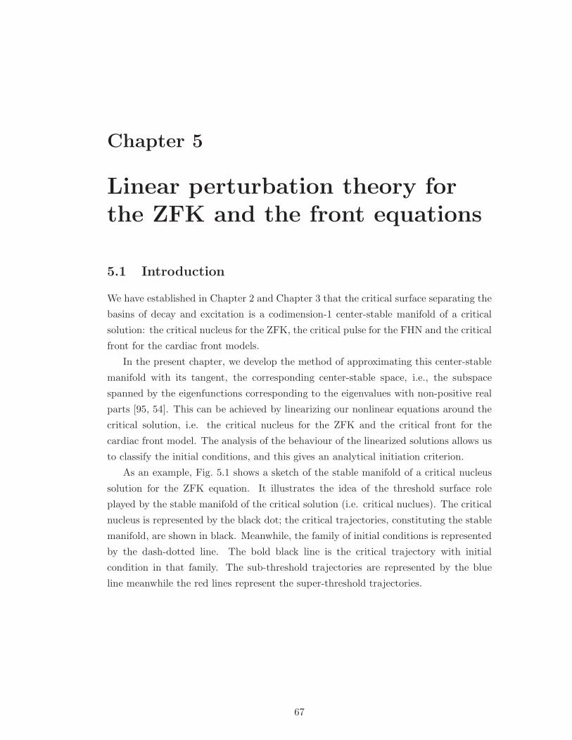
Chapter 5

Linear perturbation theory forthe ZFK and the front equations

5.1 Introduction

We have established in Chapter 2 and Chapter 3 that the critical surface separating the

basins of decay and excitation is a codimension-1 center-stable manifold of a critical

solution: the critical nucleus for the ZFK, the critical pulse for the FHN and the critical

front for the cardiac front models.

In the present chapter, we develop the method of approximating this center-stable

manifold with its tangent, the corresponding center-stable space, i.e., the subspace

spanned by the eigenfunctions corresponding to the eigenvalues with non-positive real

parts [95, 54]. This can be achieved by linearizing our nonlinear equations around the

critical solution, i.e. the critical nucleus for the ZFK and the critical front for the

cardiac front model. The analysis of the behaviour of the linearized solutions allows us

to classify the initial conditions, and this gives an analytical initiation criterion.

As an example, Fig. 5.1 shows a sketch of the stable manifold of a critical nucleus

solution for the ZFK equation. It illustrates the idea of the threshold surface role

played by the stable manifold of the critical solution (i.e. critical nuclues). The critical

nucleus is represented by the black dot; the critical trajectories, constituting the stable

manifold, are shown in black. Meanwhile, the family of initial conditions is represented

by the dash-dotted line. The bold black line is the critical trajectory with initial

condition in that family. The sub-threshold trajectories are represented by the blue

line meanwhile the red lines represent the super-threshold trajectories.

67

u0

ustim

Figure 5.1: The sketch of a stable manifold of the critical solution for the ZFK equation.The critical nucleus is represented by the black dot; the critical trajectories, constituting thestable manifold, are shown in black. The family of initial conditions is represented by the dash-dotted line. The bold black line is the critical trajectory with initial condition in that family.The sub-threshold trajectories are represented by the blue line, while the red lines representsuper-threshold trajectories. Note that the point where the initial condition intersect the stablemanifold is shown as the empty circle.

5.2 Analytical initiation criterion for the ZFK equation

Recall the initiation problem for the ZFK equation (3.13, 3.14) in Sec. 3.3

∂u

∂t=∂2u

∂x2+ f(u), x, t ≥ 0

∂u(0, t)

∂x= 0, t ≥ 0

u(x, 0) = ustimΘ(xstim − x), x ≥ 0. (5.1)

Let us consider an even extension of problem (5.1),

∂u

∂t=∂2u

∂x2+ f(u), x ∈ (−∞,∞),

u(−x, 0) = u(x, 0) = ustimΘ(xstim − x), x ≥ 0,

or, equivalently, u(x, 0) = ustimΘ(xstim − x)Θ(xstim + x). (5.2)

It is easy to see that if u(x, t) satisfies (5.2), then its restriction to x ≥ 0 satisfies (5.1),

since the initial condition in (5.2) is even and the equation is equivariant with respect

to inversion x → −x; therefore its solution remains even for all t > 0 and as such

satisfies the boundary condition of (5.1).

To obtain an analytical criterion of initiation, we linearize the first equation in (5.2)

68

about the critical nucleus solution, ucr(x) its steady state solution. Using

u(x, t) = ucr(x) + w(x, t), (5.3)

where w(x, t) is a perturbation such that |w| ≪ 1, this leads to the linearized problem

∂w

∂t=∂2w

∂x2+ q(x)w, (5.4)

where q(x) =∂f(ucr)

∂u. The substitution

w(x, t) = eλtϕ(x), (5.5)

now leads to a self-adjoint (Sturm-Liouville) eigenvalue problem

d2ϕ(x)

dx2+ (q(x) − λ)ϕ(x) = 0. (5.6)

Hence all eigenvalues λ ∈ R. In linear operator format, (5.6) is written as

Lϕ = 0, (5.7)

where L ≡ d2

dx2+ q(x) − λ.

Flores in [34] proved using Sturm’s Theorem that (5.6) has exactly one solution

with positive λ.

Here, we look for solutions of the eigenvalue equation (5.6) with bounded ϕ(x) and

λ > 0, analytical if possible. Thus, our eigenvalue problem becomes for λ > 0

d2ϕ(x)

dx2+ (q(x) − λ)ϕ(x) = 0,

ϕ(±∞) = 0 ( or in general |ϕ| < Const). (5.8)

5.2.1 Solution to the eigenvalue problem

To solve (5.8), we suppose ϕ(x) = ψ(z) where z ≡ z(x) is to be chosen, and knowing

the critical nucleus solution of the ZFK equation, using approximate f(u) = u (u− θ),

is of the form

ucr(x) =3θ

2sech2(kx), (5.9)

where k =

√θ

2, we choose z = tanh(kx). Then q(x) = θ

(3sech2(kx) − 1

)is trans-

formed to

q(z) = θ(3(1 − z2) − 1

). (5.10)

69

The problem given by (5.8) can now be re-written in terms of the variable z as

d

dz

(

(1 − z2)dψ

dz

)

+

12 −

4(1 +λ

θ)

(1 − z2)

ψ = 0,

ψ(±1) = 0. (5.11)

Problem (5.8) is a Sturm-Liouville problem for a (time independent) Schrodinger equa-

tion [83]. The properties of eigenfunctions of this problem are well known [40, 16, 22,

73, 17]. The spectrum consists of a number of discrete real and simple eigenvalues and

a continuous spectrum. If the eigenvalues λn are numbered in decreasing order,

λ1 > λ2 > λ3 > · · · λn > · · · , (5.12)

then eigenfunction φn(x) has exactly (n− 1) zeros in the interval x ∈ (−∞,∞); corre-

spondingly, ψn(z) has exactly (n − 1) zeros in z ∈ (−1, 1). We are however, after an

unstable eigenfunction corresponding to a positive eigenvalue.

It is easy to show that∂

∂xucr(x) is a solution to (5.6) at λ = 0, therefore it is the

same as the eigenfunction which corresponds to the zero eigenvalue. Thus, knowing∂

∂xucr(x) from (5.9) and using the transformation z = tanh(k x), the zero eigenfunction

is then

ducr(x)

dx= −3

2θ3/2sech2(k x) tanh(k x),

≡ C z (1 − z2), (5.13)

where C = −3

2is a multiplicative constant. It is obvious in (5.13) that our zero

eigenfunction, C z (1− z2) has only one zero in the interval (-1, 1). Hence, we conclude

that, according to Sturm-Liouville theory, λ2 = 0 and ψ2(z) ∝ z(1− z2), and therefore

there is a λ1 > 0, exactly one positive eigenvalue, which corresponds to a ψ1(z) which

has no zeros in (−1, 1). Therefore, the unstable eigenvalue we are after corresponds to

this one and only one positive eigenvalue.

Equation (5.11) is a special case of the differential equation

d

dz

(

(1 − z2)dW

dz

)

+

(

ν(ν + 1) − µ2

(1 − z2)

)

W = 0, (5.14)

which has as its solutions the so-called Associated Legendre Functions [75, 38] in

which ν and µ are arbitrary complex constants. The linearly independent functions

70

that are the associated Legendre functions are given by

Pµν (z) =

1

Γ(1 − µ)

(z + 1

z − 1

)µ/2

F

(

−ν, ν + 1; 1 − µ;1 − z

2

)

,

Qµν (z) =

eµπi Γ(ν + µ+ 1)Γ(1/2)

2ν+1Γ(ν + 32)

(z2 − 1)µ/2 z−ν−µ−1

× F

(ν + µ+ 2

2,ν + µ+ 1

2; ν +

3

2;

1

z2

)

, (5.15)

where F is a hypergeometric function which by definition is of the form

F (α, β; γ; z) = 1 +α · βγ · 1 z +

α(α + 1)β(β + 1)

γ(γ + 1) · 1 · 2 z2

+α(α+ 1)(α + 2)β(β + 1)(β + 2)

γ(γ + 1)(γ + 2) · 1 · 2 · 3 z3 + · · · . (5.16)

The hypergeometric series terminates if α or β is a negative integer or zero as it is

obvious from the definition. The functions Pµν (z) and Qµ

ν (z) are referred to as the asso-

ciated Legendre P and Legendre Q respectively (see, for example [38]). Therefore,

the general solution is

ψ(z) = C1 Pµν (z) + C2 Q

µν (z), (5.17)

where C1 and C2 are undetermined constants. Comparing (5.11) and (5.14), we have

ν = 3 and µ = ±2√

λ+θ√θ

. It happens that the solution we are after and which satisfies

our boundary conditions is

P2√

λ+θ√θ

3 (z) =

(z − 1)(

√θ + λ√θ

)

F (−3, 4;

√θ + 2

√θ + λ√θ

;1

2− z

2)

(z + 1)(

√θ + λ√θ

)

Γ(

√θ + 2

√θ + λ√θ

)

.

(5.18)

Using (5.16), solution (5.18) simplifies to

ψ(z) =

(z − 1

z + 1

)√

θ+λ√θ

(

15θ3

2 z3 + 30θ√θ + λ z2 + (24λ

√θ + 15θ

3

2 )z + 8λ√θ + λ

)

Γ(√

θ+2√

θ+λ√θ

)(√θ +

√θ + λ)(

√θ + 2

√θ + λ)(3

√θ + 2

√θ + λ)

.

(5.19)

The values of the eigenvalue λ which make our boundary conditions ψ(±1) = 0 to be

satisfied are the solutions to the equation

8λ√θ + λ+ 30θ

3

2 + 24λ√θ + 30θ

√θ + λ = 0, (5.20)

71

and are found to be λ1 =5θ

4, λ2 = 0, λ3 =

−3θ

4. From (5.19), it follows that the

corresponding eigenfunction to the eigenvalue λ2 = 0 is

ψ2(z) = −z(1 − z2)

8, (5.21)

which is equivalent to our deduced zero eigenfunction in (5.13) and therefore confirms

that our solution is correct.

We are interested in the positive eigenvalue λ which corresponds to the unstable

eigenfunction that we are looking for. Thus, substituting λ1 =5θ

4in (5.19) reduces it

to

ψ1(z) =1

48(1 − z2)(3/2). (5.22)

From Sturm-Liouville’s theory, λ1 =5θ

4is the only positive eigenvalue and ψ1(z) does

not change sign. The plots of ψ1 and ψ2 are shown in Fig. 5.2.

-0.2

-0.15

-0.1

-0.05

0

0.05

0.1

0.15

0.2

-1 -0.5 0 0.5 1

ψ1, ψ2

ψ1ψ2

z

Figure 5.2: The plot of the unstable eigenmode ψ1 (green curve) for the ZFK equation and thezero eigenmode ψ2 (red curve) showing the only zero of ψ2 in the interval (−1, 1) confirmingthat λ1 is the only positive eigenvalue.

Finally, rewriting the unstable eigenfunction in terms of the original variable x, we

obtain after simplifications and neglecting of multiplicative constant

ϕ(x) = sech3(k x), (5.23)

where k =

√θ

2.

5.2.2 Analytical critical (threshold) curve for the ZFK equation

A general solution to (5.4) satisfying appropriate conditions at x → ±∞ can be de-

scribed by

w(x, t) =∑

j

aj ϕj(x) eλjt =∑

j

wj(x, t), (5.24)

72

where ϕj(x), j = 1, . . . are the eigenfunctions, λj are the corresponding eigenvalues and

aj are constants depending on initial conditions, and summation includes integration

for the continuous part of the spectrum. That is,

∑

j

aj ϕj(x) eλjt =N∑

j=1

aj ϕj(x) eλjt +

∫ −θ

−∞a(λ)ϕλ(x) eλt dλ. (5.25)

Recall that λj ≤ 0 for j ≥ 2. Therefore, as t → ∞, we have wj → 0 for any j > 2

and w2 → a2 ϕ2(x). As to w1(x), it exponentially grows unless a1 = 0: w1(x, t) → −∞if a1 < 0 (decay: below the critical surface) and w1(x, t) → ∞ if a1 > 0 (excitation:

above the critical surface). If a1 = 0, then the solution is on the critical surface. Note

that a2 ϕ2(x) accounts for a shift of the perturbation by the distance a2.

The coefficients aj are determined from initial conditions, as aj are the projections

of initial conditions onto the eigenfunctions (see for example [22]). Initially, that is, at

t = 0

w0(x) = u0(x) − ucr(x) =∑

j

aj ϕj(x), (5.26)

where w0(x) = w(x, 0), u0(x) = u(x, 0). Now if we take the scalar product of both

sides of (5.26) by ϕk, and since the operator L in (5.7) is self-adjoint [55], then the

eigenfunctions can be normalized so that

〈ϕj , ϕk〉 ≡∫ +∞

−∞ϕj ϕk dx = δjk =

{

1 j = k

0 j 6= k(5.27)

(δjk, the Kronecker delta symbol), we have

aj = 〈w0(x), ϕj(x)〉 = 〈u0(x) − ucr(x), ϕj〉. (5.28)

Thus, to obtain the expression for our critical surface (and by implication our critical

curve) we consider the unstable eigenmode ϕ1. For any family of initial perturbations

rewritten as

w0(x) = u0(x) − ucr(x) =∑

j

aj ϕj(x), (5.29)

we compute a1 = 〈w0(x), ϕ1〉. If a1 > 0, then the initial condition leads to initiation;

and if a1 < 0, it leads to decay and if a1 = 0, it is on the critical surface (i.e. the

center-stable manifold). Therefore, our ignition criterion then becomes

a1 =

∫ +∞

0

(u0(x) − ucr(x)

)ϕ1 dx = 0,

=

∫ xstim

0ustim ϕ1(x) dx−

∫ +∞

0ucr(x)ϕ1(x) dx = 0, (5.30)

73

after substituting in it u0(x) = ustimΘ(xstim − x). Now by using

ucr(x) ≈3θ

2sech2

(

x√θ

2

)

, ϕ1(x) ≈ sech3

(

x√θ

2

)

, (5.31)

we obtain after resolving in terms of ustim, the explicit expression for the threshold

(critical) curve

ustim =9θ

8

(

2

πtanh

(

xstim

√θ

2

)

sech

(

xstim

√θ

2

)

+4

πarctan

(

exp(xstim

√θ

2)

)

− 1

)−1

.

(5.32)

The plot of our analytical critical curve is compared with other numerical critical curves

as shown in the Fig. 5.3. It shows the graphs of the analytical threshold curve for

the quadratic nonlinearity (red-solid) compared with the numerical ones for the ZFK

(blue-dashed: cubic nonlinearity; light green-cross: quadratic nonlinearity) and the

FHN (black-solid) equations. The value of θ for both quadratic and cubic nonlinearity

is 0.13 in both numerical and analytic computations. From the plot, one can see some

agreement between the analytical threshold curve for the quadratic nonlinearity and

the numerical for the ZFK (with cubic nonlinearity). The vital question of how far

0

1

2

3

4

0 1 2 3

ustim

xstim

ZFK[cubic]

ZFK[quad]

FHN

anal. (quad.)

Figure 5.3: The plot of the analytical threshold curves for the quadratic nonlinearity (red-

solid) versus the numerical ones for the ZFK (blue-dashed: cubic, light green - cross: quadratic

) and the FHN (black-solid) equations. The value of θ for both quadratic and cubic nonlinearity

is 0.13 in both numerical and analytic computations.

the critical nucleus should be from initial perturbations is to be addressed in the next

section.

74

5.2.3 Generalized threshold criterion for the ZFK equation

The above consideration has avoided one delicate issue. Equation (5.2) has not just

one unstable spatially nonuniform solution (critical nucleus) ucr(x) but a whole one-

parametric family of such solutions ucr(x− δ), obtained by shifts by arbitrary distance

δ from the original critical nucleus ucr(x). It is easy to show that ϕ2(x) =∂

∂xucr(x)

and that a small shift in ucr(x) is equivalent to adding/subtracting a bit of ϕ2(x) to

ucr(x) for some small δ. This is derived via Taylor expansion as

ucr(x− δ) = ucr(x) − δ∂

∂xucr(x) = ucr(x) − δ ϕ2(x). (5.33)

When the additional constraint of u(−x, t) = u(x, t) is imposed, only ucr(x) is ad-

missible. However, if we want to generalize the method for arbitrary, not necessarily

even initial conditions, then this constraint has to be lifted. We thus have infinitely

many critical nuclei which could be used to linearize our equation, and correspondingly,

infinitely many initiation criteria which have the form

a1(δ) =

∫ +∞

−∞

(u0(x) − ucr(x− δ)

)ϕ1(x− δ) dx = 0, (5.34)

for arbitrary δ. The question then arises, which of these infinitely many criteria to

prefer that gives a more accurate result? In the light of the foregoing reasons, we have

a center-stable manifold instead of a stable manifold as illustrated by the sketch in

Fig. 5.4

5.2.4 The value for δ in the generalized criterion

There is the important question of the value of δ to be used in the formulation (5.34).

We have considered two approaches on how to determine the appropriate value of δ

that should be used for our threshold criterion. One approach is through minimization

of ustim, that is, we choose δ such that ustim is minimum. The second is minimization of

the amplitude of the initial perturbation where we exploit the linearization requirement

that the perturbation w0 should be small.

First, we consider the minimization of ustim by taking a general initial condition of

the form

u0 = ustimH(x), (5.35)

where H(x) is some function of x. Equation (5.34) can then be written as

a1(δ) ≡ ustimD1(xstim, δ) −N1 = 0, (5.36)

75

u0

ustim

δ

Figure 5.4: The sketch of a center-stable manifold of the critical solution for the ZFK equation.The line δ is a 1-parametric family of equilibria corresponding to translations of the “standard”critical solution (i.e. critical nucleus). Otherwise, notations are the same as in Fig. 5.1.

where

D1(xstim, δ) =

∫ +∞

−∞H(x)ϕ1(x− δ) dx,

N1 =

∫ +∞

−∞ucr(x− δ)ϕ1(x− δ) dx. (5.37)

Thus, from (5.36)

ustim =N1

D1(xstim, δ), (5.38)

and therefore to minimize ustim, we maximize D1(xstim, δ) with respect to δ using∂D1

∂δ= 0 which then leads to

∫ +∞

−∞H(x)ϕ

′

1(x− δ) dx = 0. (5.39)

Now integrating (5.39) by parts, we obtain

∫ +∞

−∞H

′(x)ϕ1(x− δ) dx = 0, (5.40)

which then becomes the equation for determining δ such that ustim in (5.38) is minimum.

Hence, our threshold criterion is then given by (5.38) after substituting the δ value we

get from (5.40).

76

For the second approach, we recall from equation (5.26) that

w0(x) = u0(x) − ucr(x− δ) =∑

j

aj ϕj(x− δ). (5.41)

This is an initial condition for the linearized equation. Linearization assumes that

perturbation is small, therefore our linearized approximation is the more accurate the

smaller is the solution, that is, the smaller is the initial condition. We choose δ so as

to minimize a norm ∆ of the initial condition. That is, we choose an L2 norm

∆(δ) =

∫ +∞

−∞w2

0 dx =

∫ +∞

−∞

(

u0(x) − ucr(x− δ))2

dx. (5.42)

Now minimizing (5.42) with respect to δ using∂∆(δ)

∂δ= 0 we have

a2(δ) =

∫ +∞

−∞

(u0(x) − ucr(x− δ)

)ϕ2(x− δ) dx = 0, (5.43)

since by chain rule∂

∂δucr(x− δ) = − ∂

∂xucr(x− δ) and ϕ2(x− δ) =

∂

∂xucr(x− δ).

Hence, using the initial condition u0 = ustimH(x), as in the first approach, equation

(5.43) then reduces to

a2(δ) ≡ ustimD2(xstim, δ) −N2 = 0, (5.44)

where

D2(xstim, δ) =

∫ +∞

−∞H(x)ϕ2(x− δ) dx,

N2 =

∫ +∞

−∞ucr(x− δ)ϕ2(x− δ) dx. (5.45)

Considering N2 from (5.45), integrating the right hand side by parts and also since

ϕ2(x− δ) =∂

∂xucr(x− δ), we have

N2 =

∫ +∞

−∞ucr(x− δ)ϕ2(x− δ) dx,

=

∫ +∞

−∞ucr(x− δ)

∂

∂xucr(x− δ) dx,

= 0, (5.46)

but as ustim 6= 0, it then implies from (5.44) that D2 = 0.

Now, since ϕ2(x− δ) =∂

∂xucr(x− δ), and using integration by parts, D2 can con-

veniently be written as

D2(xstim, δ) =

∫ +∞

−∞H

′(x)ucr(x− δ) dx = 0. (5.47)

The value of δ is computed from this equation and the threshold criterion is then

obtained after substituting this δ in (5.38).

77

Symmetric initial condition

For symmetric initial condition u0 = ustimH(x), where

H(x) = Θ(x+ xstim) − Θ(x− xstim), (5.48)

we have

H′(x) = δ(x+ xstim) − δ(x − xstim). (5.49)

Substituting (5.49) in (5.40) we get

ϕ1(xstim − δ) − ϕ1(−xstim − δ) = 0, (5.50)

from which δ is to be determined. In this case, because of the even nature of the

function ϕ1(x) (see Fig. 5.5), the only possibility is δ = 0. This means that the only

possible real δ such that ustim is minimum is δ = 0.

In the alternative, substituting (5.49) in (5.47) we get

ucr(xstim − δ) − ucr(−xstim − δ) = 0, (5.51)

whose zero also gives the value of δ to be used in (5.38) for the threshold criterion.

Here again, due to the even nature of the ucr(x) (see Fig. 5.5), the only value of δ such

that ustim is minimum is δ = 0.

φ1ucr

φ1, ucr

1

x00

Figure 5.5: The plot of the unstable eigenmode φ1(x) (blue-dashed curve) and the criticalnucleus ucr(x) (red-solid curve) for ZFK equation (5.1).

Asymmetric initial condition

For an asymmetric initial condition in a form of a 2-step function u0 = ustimH(x)

where

H(x) = Θ(xstim + x)Θ(−x) + 2Θ(xstim − x)Θ(x), (5.52)

78

and then

H′(x) =

(

2Θ(xstim − x) − Θ(x+ xstim))

δ(x) + Θ(−x) δ(x + xstim)

− 2Θ(x) δ(x − xstim). (5.53)

Therefore, substituting (5.53) in (5.40) we get

2ϕ1(xstim − δ) − ϕ1(−δ) − ϕ1(−xstim − δ) = 0, (5.54)

from which we determine the value of δ that can be used to achieve the minimum ustim

in (5.38). We can also use (5.47) from the second method to find the value of such δ

from

2ucr(xstim − δ) − ucr(−δ) − ucr(−xstim − δ) = 0. (5.55)

We observe that the value of δ such that ustim is minimum is close to the zero of

(5.55). In other words, the zero of D2(δ) = 0 is very close to the minimum of ustim from

(5.38). We have tested this observation numerically where we fixed xstim at the values

0.3, 0.6, 0.9 and θ at 0.13 in both (5.38, 5.55) while plotting against δ the resultant

ustim in (5.38) and the resultant function of δ from (5.55). The results shown in Fig. 5.6

where in all the three cases (a), (b) and (c), the minimum of ustim coincides exactly,

with the accuracy allowed by the graph, with the zero of D2(δ) = 0, thus confirming

our observation.

For the ZFK equation in (5.1) with quadratic nonlinearity, f(u) = u (u− θ) we find

ucr(x− δ) =3θ

2sech2

(

(x− δ)√θ

2

)

, (5.56)

ϕ2(x− δ) =−3

2θ3/2sech2

(

(x− δ)√θ

2

)

tanh

(

(x− δ)√θ

2

)

, (5.57)

ϕ1(x− δ) = sech3

(

(x− δ)√θ

2

)

. (5.58)

By fixing xstim at the values 0.3, 0.6, 0.9 and θ at 0.13 we obtain the results shown in

Fig. 5.6 where in all the three cases (a), (b) and (c), the minimum of ustim very closely

coincides with the zero of a2(δ) = 0, thus again confirming our observation.

The two different approaches give the same result based on our tested observations.

We explain this coincidence in this way. To determine optimal δ, one of the approaches

uses equation (5.40), and the other uses equation (5.47). These two equations have

very similar form, the difference is that, what is ucr in one equation, is φ1 in the other.

However, as Fig. 5.5 shows, these two functions are rather close to each other, hence it

is not surprising that the two equations give close results.

Clearly, this explanation depends on the details of this particular problem, so we do

not expect this to be the case with other types of equations like the cardiac equations.

79

0

0.002

0.004

0.006

0.008

0.01

0 0.02 0.04 0.06 0.08 0.1

δ

xstim = 0.30

50 (ustim (δ) - uminstim )

10 a2 (δ)

0

0.005

0.01

0.015

0.02

0 0.05 0.1 0.15 0.2

δ

xstim = 0.60


10 a2 (δ)

0

0.005

0.01

0.015

0.02

0.025

0.03

0 0.05 0.1 0.15 0.2 0.25 0.3

δ

xstim = 0.90


10 a2 (δ)

(a) (b) (c)

Figure 5.6: The plots of the minimum of ustim and zeros of D2(δ) = 0 for fixed values(a) 0.3 (b) 0.6 and (c) 0.9 of xstim and θ = 0.13 for the quadratic nonlinearity f(u) =u(u− θ). In all the three cases the minimum of ustim exactly coincides with the zero ofD2(δ) = 0, thus confirming our prediction.

5.3 Analytical initiation criterion for the front model

5.3.1 Introduction

The simplified front model does not have “critical nucleus” or “critical pulse” solution.

Instead, the role of the threshold is played by a “critical front”, which is the unstable

front solution with speed c−(α, τ) as explained in Chapter 2. Also we provide numerical

evidence in Chapter 3 that the center-stable manifold of the unstable front solution is

the threshold hypersurface separating initial conditions leading to excitation from initial

conditions leading to decay.

We try to find the expression for the “critical curve” for a 2-parametric family of

initial conditions with parameters xstim, Estim as the intersection of the codimension-1

unstable critical hypersurface, which is the centre-stable manifold of the critical front

solution, with the 2-dimensional manifold of initial conditions. To do this analytically,

as in the previous section for the ZFK equation, we approximate the center-stable man-

ifold by a center-stable space which is a subspace spanned by eigenfunction correspond-

ing to eigenvalues with nonpositive real parts (see [95, 54, 51]). This approximation

is possible if we linearize our nonlinear system around the exact critical front solution

which plays the same role as the critical nucleus solution in the ZFK equation. The

sketch of the center-stable manifold of a non-stationary solution is shown in Fig. 5.7.

When we consider the problem in a frame of reference comoving with the critical front

then our critical front becomes a stationary solution (i.e. an equilibrium solution).

Thus, we are dealing with a center-stable manifold of an equilibrium as in Fig. 5.4.

80

u0

vstim

Figure 5.7: The sketch of a center-stable manifold of the critical solution for the front equations.Instead of the line of equilibria as in Fig. 5.4, we have a trajectory (bold black line) correspondingto the critical front. Otherwise, notations are the same as in in Fig. 5.4.

5.3.2 Eigenvalue problem to the Hinch (2004) model

Linearization of the system (2.20)-(2.21) is not straightforward, as the right-hand sides

of it include Heaviside step functions and are discontinuous, thus linearization includes

Dirac delta function and therefore is singular. A rigorous justification of this ap-

proach can be made by regularization, by considering our problem as a limit of a

one-parametric, say depending on parameter ε, family of regular problems in which

the step functions are replaced with smooth steps of width ε, and delta functions are

replaced, correspondingly, by bell-shaped functions of width ε. Examples of using sin-

gular linearized equations for stability analysis with discontinuous right-hand sides are

known in literature (see, for example, [79, 100]).

Another way to investigate stability of solutions in such equations is the free-boundary

method, which considers, alongside with perturbations of the solutions, also pertur-

bations of the matching points between the domains where the right-hand sides are

continuous, thus avoiding any singularities in the linearized equations. This method

has been used by Hinch [43] for a system similar to (2.20), (2.21) (see Appendix C for a

detailed analysis establishing the equivalence of these two models with an appropriate

choice of parameters).

However, for the purpose of developing an analytical initiation criterion, we need

eigenfunctions of the adjoint linearized problem. We are not aware of any extensions

of the free-boundary method to the adjoint problems. So we use linearization with the

singular right-hand sides. We, first of all, find the eigenvalues and the eigenfunctions to

81

the linearized problem and compare the results with [43]. We accept this comparison

as a justification of our method in lieu of the regularization proof, since this method

has already been successfully used in literature for similar problems. Then we use the

same method to find the eigenfunctions of the adjoint linearized problem which is used

for the initiation criterion.

Linearization of the Hinch’s equations

In a laboratory reference frame with (x, T ) as coordinates, the front model [43] can be

written in the form

∂v

∂T=∂2v

∂x2+ F (v, h),

∂h

∂T= G(v, h), (5.59)

where F (v, h) = gΘ(v)h, G(v, h) = Θ(−v− ∆)− h and Θ is a Heaviside step function.

Meanwhile, in a moving frame of reference, the solutions to (5.59) for a right-ward

moving front are of the form v(T − x/c, T ), h(T − x/c, T ). Introducing the coordinates

ξ = T − x/c, t = T with c > 0, we look for functions v(ξ, t), h(ξ, t) which satisfy (5.59)

to give

∂v

∂t=

1

c2∂2v

∂ξ2− ∂v

∂ξ+ F (v, h),

∂h

∂t= −∂h

∂ξ+ G(v, h). (5.60)

Traveling wave solutions of (5.59) correspond to stationary solutions of (5.60), (see, for

example, [82]). Suppose (v0(ξ), h0(ξ)) is a stationary solution of (5.60), then

1

c2d2v0

dξ2− dv0

dξ+ F (v0, h0) = 0,

dh0

dξ− G(v0, h0) = 0. (5.61)

The linearized version of (5.60) about(

v0(ξ), h0(ξ))

is obtained by neglecting higher

order terms as

∂v1

∂t=

1

c2∂2v1

∂ξ2− ∂v1

∂ξ+ g δ(v0) h0 v1 + gΘ(v0) h1,

∂h1

∂t= −∂h1

∂ξ− δ(v0 + ∆) v1 − h1. (5.62)

82

Let the linearized equations (5.62) support solutions of the form v1(ξ, t) = eλ t φ(ξ) and

h1(ξ, t) = eλ t ψ(ξ). This leads to the (temporal) eigenvalue problem

λ φ =1

c2d2φ

dξ2− dφ

dξ+ g δ(v0) h0 φ+ gΘ(v0) ψ,

λ ψ = − dψ

dξ− δ(v0 + ∆) φ− ψ, (5.63)

where φ(ξ) and ψ(ξ) are eigenfunctions. The eigenvalue equation (5.63) is then casted

into a three first-order ODEs by lettingdφ

dξ= η and Ξ = (φ, η, ψ)T, thus, obtaining

a linear system in R3

Ξ′= A Ξ, (5.64)

where prime (′) denotesd

dξ,

A =

0 1 0

c2(

λ− g δ(v0) h0

)

c2 −c2 gΘ(v0)

−δ(v0 + ∆) 0 −(1 + λ)

, (5.65)

v0(ξ) =

−1 + eβ ξ, ξ ≤ 0,

β g H0

1 + β(1 − e−ξ), ξ ≥ 0,

h0(ξ) =

1, ξ ≤ ξ1,

H0e− ξ, ξ ≥ ξ1,

(5.66)

and

ξ1 = −δ/β, H0 = e−δ/β , g = (1 + β) e δ/β . (5.67)

The general solution to (5.64) is (see Appendix C for details)

φa

ηa

ψa

= a2

1

ν2

0

e ν2 ξ,

φb

ηb

ψb

= b1

0

0

1

e−ν1 ξ + b2

1

ν2

0

eν2 ξ + b3

1

˜ν2

0

e˜ν2 ξ,

φc

ηc

ψc

= c1

1

−ν1

−νs

e−ν1 ξ + c3

1

˜ν2

0

e˜ν2 ξ, (5.68)

83

where

ν1 = 1 + λ, ν2 =β +

√

β2 + 4 λ β

2, ˜ν2 =

β −√

β2 + 4 λ β

2. (5.69)

The arbitrary constants a2, b1, b2, b3, c1 and c3 are to be determined from matching

conditions of the solutions in the three intervals, which give the system of equations

b2 (g H0 − ν2) + b3 (g H0 − ˜ν2) − c1 ν1 + c3 ˜ν2 = 0,

b2 + b3 − c1 − c3 = 0,

b1 β g + c1

(

(1 + λ)2 + β)

= 0,

a2 e ν2 ξ1 + b1 β e (β−ν1) ξ1 = 0,

a2 e ν2 ξ1 − b2 e ν2 ξ1 − b3 e˜ν2 ξ1 = 0,

a2 ν2 e ν2 ξ1 − b2 ν2 e ν2 ξ1 − b3 ˜ν2 e˜ν2 ξ1 = 0. (5.70)

The solvability condition of this system leads to the characteristic equation

fe(λ, β, δ) = β (σ − µ− 1) − 1 +(1 + β)(β µ+ 1 + λ)

(1 + λ)2 + βe−δ

(

λ/β+σ−1

)

= 0. (5.71)

The characteristic equation (5.71) is exactly the same as that obtained in [43] when

εk1= 0 which is the case of interest to us in this work. For selected parameter values,

which correspond to other numerical illustrations in this thesis, the graph of the function

fe against λ is shown in Fig. 5.8. This also confirms the existence of only one positive

eigenvalue as reported in [8, 43].

-0.04

-0.02

0

0.02

0.04

0.06

0.08

0.1

-0.04-0.02 0 0.02 0.04 0.06 0.08 0.1

λ

fe

Figure 5.8: The plot of the characteristic function from (5.71) for the front in Hinch’s model[43] for parameter values εk1 = 0, c = 0.3318742892, τ = 8.2, α = 1.0.

84

5.3.3 Eigenvalue problem to the Biktashev (2002) model

Linearization of the front equations

Let us consider the front model in laboratory frame of reference (x, T ) (see (C.69) in

Appendix C)

∂E

∂T=∂2E

∂x2+ F (E,h),

∂h

∂T= G(E,h)/τ, (5.72)

where F (E,h) = Θ(E− 1)h, G(E,h) = Θ(−E)−h and Θ is a Heaviside step function.

In a comoving frame of reference, (ξ, t), the solutions to (5.72) for a right-ward

moving front can be represented in the form E(ξ, t), h(ξ, t). Using the transformations

ξ = x− c T , t = T , with c > 0, (5.72) becomes

∂E

∂t=∂2E

∂ξ2+ c

∂E

∂ξ+ F (E,h),

∂h

∂t= c

∂h

∂ξ+G(E,h)/τ. (5.73)

The traveling waves of (5.72) correspond to the stationary solution of (5.73). Suppose

we take the exact unstable front solution as stationary to (5.73) and designate it by

U0 =

(

v0(ξ)

h0(ξ)

)

,

v0(ξ) =

ω − τ2 c2

1 + τ c2e ξ/τc, ξ ≤ −∆,

−α+ α e−c ξ, ξ ≥ −∆,

h0(ξ) =

e ξ/τc, ξ ≤ 0,

1, ξ ≥ 0,(5.74)

where

ξ = x− c t, ω = 1 + τ c2 (1 + α),∆ =1

cln(

1 + α

α). (5.75)

Therefore, we linearize (5.73) around (v0(ξ), h0(ξ)) using

E = v0(ξ) + ε v1(ξ, t),

h = h0(ξ) + ε h1(ξ, t). (5.76)

Now using Taylor expansion, Θ(−v0) ≡ Θ(ξ), Θ(v0−1) ≡ Θ(−ξ−∆) and the fact that

δ(u) =dΘ(u)

du, then by chain rule δ(−v0) = δ(v0) =

1

v′

0

δ(ξ), δ(v0 − 1) =−1

v′

0

δ(ξ + ∆).

85

Thus, we obtain (see Sec. C.3 in Appendix C)

∂v1∂t

=∂2v1∂ξ2

+ c∂v1∂ξ

− 1

v′

0

δ(ξ + ∆)h0 v1 + Θ(−ξ − ∆)h1,

∂h1

∂t= c

∂h1

∂ξ+( 1

v′

0

δ(ξ) v1 − h1

)

/τ. (5.77)

Let the linearized equation (5.77) support solutions of the form U1 =

(

v1(ξ, t)

h1(ξ, t)

)

where v1(ξ, t) = eλ t φ(ξ) and h1(ξ, t) = eλ t ψ(ξ). This leads to a (temporal) eigenvalue

problem with λ, ϕ as eigenpairs

L V = λ V , (5.78)

where

L ≡ Dd2

dξ2+ C

d

dξ+ F , V =

(

φ

ψ

)

, D =

(

1 0

0 0

)

,

C =

(

c 0

0 c

)

, F =

−1

v′

0

δ(ξ + ∆)h0 Θ(−ξ − ∆)

1

τ v′

0

δ(ξ) −1/τ

. (5.79)

We now cast (5.78) into a three ODE system

dφ

dξ= η,

dη

dξ=(

λ+1

v′

0

δ(ξ + ∆)h0

)

φ− c η − Θ(−ξ − ∆)ψ,

dψ

dξ= − 1

τ c v′

0

δ(ξ)φ +(1 + λ τ)

τ cψ, (5.80)

which can be written in matrix form as

Ξ′= AΞ, (5.81)

where

A =

0 1 0

λ+1

v′

0

δ(ξ + ∆)h0 −c −Θ(−ξ − ∆)

−1

τ c v′

0

δ(ξ) 01 + λ τ

τ c

. (5.82)

86

The general solution to (5.81) is therefore,

φa

ηa

ψa

= a1

1

ν1

−νq

eν1 ξ + a3

1

−ν2

0

e−ν2 ξ,

φb

ηb

ψb

= b1

0

0

1

eν1 ξ + b2

1

−ν2

0

e−ν2 ξ + b3

1

−ν2

0

e−ν2 ξ,

φc

ηc

ψc

= c2

1

−ν2

0

e−ν2 ξ, (5.83)

where

ν1 =1 + λ τ

τ c, ν2 =

c+√c2 + 4λ

2, ν2 =

c−√c2 + 4λ

2. (5.84)

The arbitrary constants a1, a3, b1, b2, b3, and c2 are to be determined from matching

conditions of the solutions in the three intervals, which gives a system of six equations

a1 α c ν1 e−ν1∆ − a3 α cν2 eν2∆ + b2 eν2∆(

α c ν2 − e−ν∆)

,

+b3 eν2∆(

α c ν2 − e−ν∆)

= 0,

a1 e−ν1 ∆ + a3 e ν2 ∆ − b2 e ν2 ∆ − b3 e ν2 ∆ = 0,

a1 νq + b1 = 0,

b1 α τ c2 + c2 = 0,

b2 + b3 − c2 = 0,

b2 ν2 + b3 ν2 − c2 ν2 = 0. (5.85)

The solvability condition for this system gives a characteristic equation

fe(λ; c, α, τ) = α c (ν2 − ν2) e ν ∆ − 1 +τ c (ν1 + ν2)

(1 + λ τ)2 + τ c2e−(ν1+ν2−ν)∆ = 0, (5.86)

where

ν =1 + τ c2

τ c, ν1 =

1 + λ τ

τ c,

ν2 =c+

√c2 + 4λ

2, ν2 =

c−√c2 + 4λ

2,

∆ =1

cln

(1 + α

α

)

. (5.87)

It is easy to check using (C.147, C.148) that the characteristic equations (5.71, 5.86)

are equivalent. This further confirm the validity of our linearization procedure. For

selected parameter values, which correspond to other numerical illustrations in this

thesis, the graph of the function fe against λ is shown in Fig. 5.9.

87

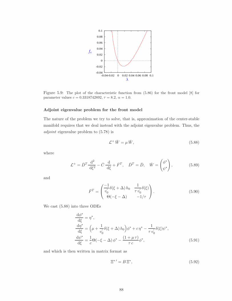
-0.04

-0.02

0

0.02

0.04

0.06

0.08

0.1

-0.04-0.02 0 0.02 0.04 0.06 0.08 0.1

λ

fe

Figure 5.9: The plot of the characteristic function from (5.86) for the front model [8] forparameter values c = 0.3318742892, τ = 8.2, α = 1.0.

Adjoint eigenvalue problem for the front model

The nature of the problem we try to solve, that is, approximation of the center-stable

manifold requires that we deal instead with the adjoint eigenvalue problem. Thus, the

adjoint eigenvalue problem to (5.78) is

L+ W = µ W , (5.88)

where

L+ = DT d2

dξ2− C

d

dξ+ F T , DT = D, W =

(

φ∗

ψ∗

)

, (5.89)

and

F T =

−1

v′

0

δ(ξ + ∆)h01

τ v′

0

δ(ξ)

Θ(−ξ − ∆) −1/τ

. (5.90)

We cast (5.88) into three ODEs

dφ∗

dξ= η∗,

dη∗

dξ=(

µ+1

v′

0

δ(ξ + ∆)h0

)

φ∗ + c η∗ − 1

τ v′

0

δ(ξ)ψ∗,

dψ∗

dξ=

1

cΘ(−ξ − ∆)φ∗ − (1 + µ τ)

τ cφ∗, (5.91)

and which is then written in matrix format as

Ξ∗ ′ = B Ξ∗, (5.92)

88

where Ξ∗ = (φ∗, η∗, ψ∗)T , η∗ = φ∗ ′ and

B =

0 1 0

µ+1

v′

0

δ(ξ + ∆)h0 c−1

τ c v′

0

δ(ξ)

1

cΘ(−ξ − ∆) 0 −(1 + µ τ)

τ c

. (5.93)

The general solution to the eigenvalue problem (5.92) (see Sec. C.3 in Appendix C)

is

φ∗(ξ) =

φ∗a(ξ) = a∗2 e γ2 ξ, ξ < −∆,

φ∗b(ξ) = b∗2 e γ2 ξ + b∗3 e γ2 ξ, −∆ ≤ ξ < 0,

φ∗c(ξ) = c∗3 e γ2 ξ, ξ ≥ 0,

ψ∗(ξ) =

ψ∗a(ξ) = a∗2 γ3 e γ2 ξ, ξ < −∆,

ψ∗b (ξ) = b∗1 e−γ1 ξ, −∆ ≤ ξ < 0,

ψ∗c (ξ) = c∗1 e−γ1 ξ, ξ ≥ 0,

(5.94)

η∗(ξ) =

η∗a(ξ) = a∗2 γ2 e γ2 ξ, ξ < −∆,

η∗b (ξ) = b∗2 γ2 e γ2 ξ + b∗3 γ2 e γ2 ξ, −∆ ≤ ξ < 0,

η∗c (ξ) = c∗3 γ2 e γ2 ξ, ξ ≥ 0,

where

γ1 =1 + µ τ

τ c, γ2 =

c+√

c2 + 4µ

2,

γ2 =c−

√

c2 + 4µ

2, γ3 =

1

c (γ1 + γ2),

γ =1 + τ c2

τ c, ∆ =

1

cln(

1 + α

α). (5.95)

The arbitrary constants a∗2, b∗1, b

∗2, b

∗3, c

∗1, c

∗3 are to be determined from the matching

conditions which give a system of six equations for six unknowns

a∗2 α c γ2 e−γ2∆ − b∗2 e−γ2∆(α c γ2 + e−γ∆

)− b∗3 e−γ2∆

(α c γ2 + e−γ∆

)= 0,

a∗2 e−γ2 ∆ − b∗2 e−γ2 ∆ − b∗3 e−γ2 ∆ = 0,

a∗2 γ3 e−γ2 ∆ − b∗1 e γ1 ∆ = 0,

b∗2 α τ c γ2 + b∗3 α τ c γ2 + c∗1 − c∗3 α τ c γ2 = 0,

b∗2 + b∗3 − c∗3 = 0,

b∗1 − c∗1 = 0. (5.96)

System (5.96) has nontrivial solutions only if the determinant of its coefficient matrix is

zero which consequently leads to the following characteristic equation (see Appendix C)

f∗e = α c (γ2 − γ2) eγ∆ − 1 +τ c (γ1 + γ2)

(1 + µ τ)2 + τ c2e−(γ1+γ2−γ)∆ = 0. (5.97)

89

We note that this characteristic equation (5.97) is exactly equivalent to (5.86), the

characteristic equation of the direct problem with γ ≡ ν, λ ≡ µ.

For the same selected parameter values which correspond to numerical illustrations

in this work, the Fig. 5.10 shows the graph of f∗e as a function of µ.

-0.04

-0.02

0

0.02

0.04

0.06

0.08

0.1

-0.04-0.02 0 0.02 0.04 0.06 0.08 0.1

µ

f∗e

Figure 5.10: The plot of the adjoint characteristic function from (5.97) for the front model in[8] for parameter values c = 0.3318742892, τ = 8.2, α = 1.0.

5.3.4 Analytical threshold curve for the front: Projection onto theunstable mode

Now we use the adjoint eigenfunctions to obtain analytical ignition criteria, using the

same two methods as we developed for the ZFK equation in sections Sec. 5.2.

We illustrate the method for particular values of parameters, as used in Fig. 5.8,

Fig. 5.9 and Fig. 5.10. For c = 0.3318742892, α = 1.0, τ = 8.2, the linearized equation

at the unstable front and its adjoint have one positive eigenvalue λ = 0.03990255031

which guarantees that the center-stable manifold is a codimension-1 hypersurface in

the functional space, which separates the decay and ignition initial conditions, as we

have shown in Sec. 4.2.2.

To derive the ignition criterion, we consider, as in ZFK equation, linearization at

the unstable front solution. We look for a solution in the form

U = U0 +

∞∑

k=1

akVk(ξ) eλkt, (5.98)

where U =

(

E(ξ, t)

h(ξ, t)

)

is the solution to (5.73) of Sec. 5.3.3, U0 =

(

v0(ξ)

h0(ξ)

)

is a sta-

tionary solution to the nonlinear system (5.73) (see (5.74) in Sec. 5.3.3) and the second

term on the right hand side of (5.98) represents the solution to the linearized problem

(5.78). Specifically, Vk =

(

φk(ξ)

ψk(ξ)

)

and λk are eigenpairs to the linearized problem.

90

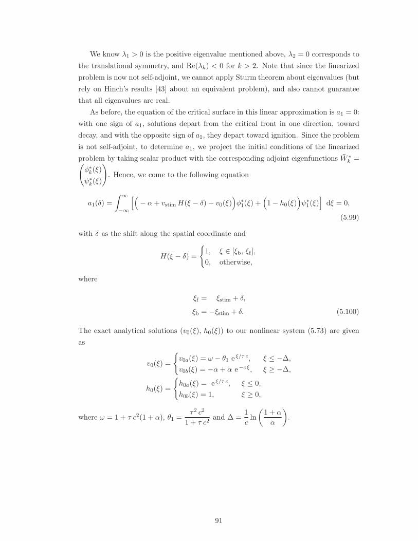
We know λ1 > 0 is the positive eigenvalue mentioned above, λ2 = 0 corresponds to

the translational symmetry, and Re(λk) < 0 for k > 2. Note that since the linearized

problem is now not self-adjoint, we cannot apply Sturm theorem about eigenvalues (but

rely on Hinch’s results [43] about an equivalent problem), and also cannot guarantee

that all eigenvalues are real.

As before, the equation of the critical surface in this linear approximation is a1 = 0:

with one sign of a1, solutions depart from the critical front in one direction, toward

decay, and with the opposite sign of a1, they depart toward ignition. Since the problem

is not self-adjoint, to determine a1, we project the initial conditions of the linearized

problem by taking scalar product with the corresponding adjoint eigenfunctions W ∗k =

(

φ∗k(ξ)

ψ∗k(ξ)

)

. Hence, we come to the following equation

a1(δ) =

∫ ∞

−∞

[(

− α+ vstimH(ξ − δ) − v0(ξ))

φ∗1(ξ) +(

1 − h0(ξ))

ψ∗1(ξ)

]

dξ = 0,

(5.99)

with δ as the shift along the spatial coordinate and

H(ξ − δ) =

{

1, ξ ∈ [ξb, ξf ],

0, otherwise,

where

ξf = ξstim + δ,

ξb = −ξstim + δ. (5.100)

The exact analytical solutions (v0(ξ), h0(ξ)) to our nonlinear system (5.73) are given

as

v0(ξ) =

{

v0a(ξ) = ω − θ1 e ξ/τ c, ξ ≤ −∆,

v0b(ξ) = −α+ α e−c ξ, ξ ≥ −∆,

h0(ξ) =

{

h0a(ξ) = e ξ/τ c, ξ ≤ 0,

h0b(ξ) = 1, ξ ≥ 0,

where ω = 1 + τ c2(1 + α), θ1 =τ2 c2

1 + τ c2and ∆ =

1

cln

(1 + α

α

)

.

91

The unstable eigenmodes, φ∗1, ψ∗1 which correspond to the positive eigenvalue are 1

φ∗1(ξ) =

φ∗a(ξ) = a∗12 e γ2 ξ, ξ < −∆,

φ∗b(ξ) = b∗12 e γ2 ξ + b∗13 e γ2 ξ, −∆ ≤ ξ < 0,

φ∗c(ξ) = c∗13 e γ2 ξ, ξ ≥ 0,

ψ∗1(ξ) =

ψ∗a(ξ) = a∗12 γ3 e γ2 ξ, ξ < −∆,

ψ∗b (ξ) = b∗11 e−γ1 ξ, −∆ ≤ ξ < 0,

ψ∗c (ξ) = c∗11 e−γ1 ξ, ξ ≥ 0,

where

γ1 =1 + µ τ

τ c, γ2 =

c+√

c2 + 4µ

2,

γ2 =c−

√

c2 + 4µ

2, γ3 =

1

c (γ1 + γ2). (5.101)

The formulation in (5.99) can be compactly expressed in the form

D1(ξstim, δ) vstim +N1 = 0, (5.102)

where

D1 =

∫ ξf

ξb

φ∗1 dξ,

N1 =

∫ ∞

−∞

(

(−α− v0)φ∗1 + (1 − h0)ψ

∗1

)

dξ. (5.103)

Due to the nature of the unstable eigenmode as shown in Fig. 5.11 the integrals in

(5.103) now become

D1 =

∫ −∆

ξb

φ∗a(ξ) dξ +

∫ ξf

−∆φ∗b(ξ) dξ,

N1 =

∫ −∆

−∞

(

(−α− v0a)φ∗a(ξ) + (1 − h0a)ψ

∗a(ξ)

)

dξ

+

∫ 0

−∆

(

(−α− v0b)φ∗b (ξ) + (1 − h0a)ψ

∗b (ξ)

)

dξ

+

∫ ∞

0(−α− v0b)φ

∗c(ξ) dξ. (5.104)

Therefore,

D1 =a∗12γ2

( e−γ2 ∆ − e γ2 ξb) +b∗12γ2

( e γ2 ξf − e−γ2 ∆) +b∗13γ2

( e γ2 ξf − e−γ2 ∆), (5.105)

1Note that we use a∗1j , b∗1j , c∗1j , j = 1, 2, 3 in place of a∗

j , b∗j , c∗j , j = 1, 2, 3 if the eigenvalue forunstable eigenmode applies. Meanwhile, we use a∗

2j , b∗2j , c∗2j , j = 1, 2, 3 whenever the zero eigenvaluethat corresponds to zero eigenmode applies.

92

-1

0

1

2

3

−∆ 0v 0,h

0,φ

∗ ,ψ∗

φ∗ψ∗v0h0

ξ

Figure 5.11: The plot of the unstable eigenmode for the front obtained from Biktashev’s model[8] for parameter values c = 0.3318742892, τ = 8.2, α = 1.0. The red solid line, the magenta,blue and green dashed lines are respectively for v, h, φ∗, ψ∗.

and

N1 =a∗12

θ1 − γ3

γ2 +1

τc

e−(γ2+

1

τc)∆

+γ3 − α− ω

γ2e−γ2 ∆

+b∗11

1

γ1 −1

τc

(1 − e(γ1−

1

τc)∆

) − 1

γ1(1 − e γ1 ∆)

− b∗12 α

γ2 − c

(

1 − e−(γ2−c)∆)

− b∗13 α

γ2 − c

(

1 − e−(γ2−c)∆)

+c∗13 α

γ2 − c. (5.106)

Hence,

vstim = − N1

D1(ξstim, δ). (5.107)

5.3.5 Analytical threshold curve for the front: threshold minimizationmethod (Method 1)

As with the ZFK equation, we explore two methods for choosing the arbitrary constant

δ in (5.107): minimization of the threshold and minimization of the norm of the initial

condition.

The minimum value of vstim is attained if D1 is at maximum, therefore, maximizing

D1 with respect to δ, we get

b∗12 e γ2(ξstim+δ) + b∗13 e γ2(ξstim+δ) − a∗12 e−γ2(ξstim−δ) = 0, (5.108)

and correspondingly the expression for δ at this minimum vstim is

δ = δ∗ = − 1

Dln

(−b∗12

b∗13

)

− ξstim − 1

D

(

1 − a∗12b∗

12

e− 2 γ2 ξstim

)

, (5.109)

where D =√

c2 + 4µ.

93

We now use the known values of our parameters c = 0.3318742892, α = 1.0, τ = 8.2

for the unstable front solution and µ = 0.03990255031 found from the adjoint character-

istic equation (5.97), to determine the arbitrary constants a∗12, b∗11, b

∗12, b

∗13, c

∗11, c

∗13 in

system (5.96). For these parameter values, ω = 2.806304918, θ1 = 3.891359376. There-

fore, by arbitrarily choosing a∗12 = 1 we find b∗11 = 0.4897404175, b∗12 = −0.3464951502,

b∗13 = 0.4550928743, c∗11 = 0.4897404175 and c∗13 = 0.1085977241. Consequently,

(5.106) evaluates to N1 = −0.8630528410 and thus,

δ∗(ξstim) = 0.5249242192 − ξstim − 1.925389830 ln(

1 + 2.886043281 e−0.8512496304 ξstim)

.

(5.110)

We then substitute δ = δ∗ in (5.107) to obtain

vstim(ξstim) =−k0 (1 + k2 e−k8 ξstim)k3

k5 + k1 e−k8 ξstim + k4 (1 + k2 e−k8 ξstim)k3

(

k6 (1 + k2 e−k8 ξstim)k7 − 1)

,

(5.111)

where

k0 = 0.03443800972, k1 = 0.1172206492, k2 = 2.886043281,

k3 = 0.8194936906, k4 = 0.2874873522, k5 = 0.04061638645,

k6 = 0.6414100599, k7 = 0.1805063093, k8 = 0.8512496304. (5.112)

Alternatively, we can find the maximum of D1 by analysing equation (5.103). We

observe that D1 =

∫ ξf

ξb

φ∗1(ξ) dξ and therefore

∂D1

∂δ= φ∗1(ξf)

∂ξf∂δ

− φ∗1(ξb)∂ξb∂δ

,

= φ∗1(ξf) − φ∗1(ξb), (5.113)

and thus the maximum of D1 is achieved when φ∗1(ξb) = φ∗1(ξf). Hence a graphical

method of solution: we need to find two points on the graph of φ∗1(x) (see Fig. 5.11)

which have the same ordinate φ∗∗ and whose abscissas are at the distance 2ξstim from

each other. As evident from Fig. 5.11, graph of φ∗1(x) is unimodal so the solution to

such a problem is unique, and ξf > −∆ and ξb < −∆, and for smaller values of ξstim,

we have ξf < 0. Therefore,

φ∗a(ξb) = φ∗∗ = φ∗b(ξf), (5.114)

which leads to

ξb(ξf) =1

γ2ln(b∗12 e γ2 ξf + b∗13 e γ2 ξf

a∗12

)

. (5.115)

94

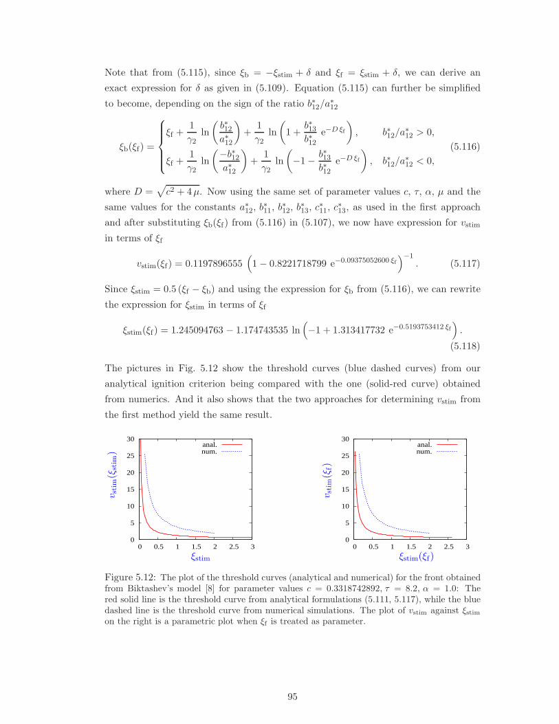
Note that from (5.115), since ξb = −ξstim + δ and ξf = ξstim + δ, we can derive an

exact expression for δ as given in (5.109). Equation (5.115) can further be simplified

to become, depending on the sign of the ratio b∗12/a∗12

ξb(ξf) =

ξf +1

γ2ln

(b∗12a∗12

)

+1

γ2ln

(

1 +b∗13b∗12

e−D ξf

)

, b∗12/a∗12 > 0,

ξf +1

γ2ln

(−b∗12a∗12

)

+1

γ2ln

(

−1 − b∗13b∗12

e−D ξf

)

, b∗12/a∗12 < 0,

(5.116)

where D =√

c2 + 4µ. Now using the same set of parameter values c, τ, α, µ and the

same values for the constants a∗12, b∗11, b

∗12, b

∗13, c

∗11, c

∗13, as used in the first approach

and after substituting ξb(ξf) from (5.116) in (5.107), we now have expression for vstim

in terms of ξf

vstim(ξf) = 0.1197896555(

1 − 0.8221718799 e−0.09375052600 ξf)−1

. (5.117)

Since ξstim = 0.5 (ξf − ξb) and using the expression for ξb from (5.116), we can rewrite

the expression for ξstim in terms of ξf

ξstim(ξf) = 1.245094763 − 1.174743535 ln(

−1 + 1.313417732 e−0.5193753412 ξf)

.

(5.118)

The pictures in Fig. 5.12 show the threshold curves (blue dashed curves) from our

analytical ignition criterion being compared with the one (solid-red curve) obtained

from numerics. And it also shows that the two approaches for determining vstim from

the first method yield the same result.

0

5

10

15

20

25

30

0 0.5 1 1.5 2 2.5 3

anal.num.

v stim

(ξst

im)

ξstim

0

5

10

15

20

25

30

0 0.5 1 1.5 2 2.5 3

anal.num.

v stim

(ξf)

ξstim(ξf)

Figure 5.12: The plot of the threshold curves (analytical and numerical) for the front obtainedfrom Biktashev’s model [8] for parameter values c = 0.3318742892, τ = 8.2, α = 1.0: Thered solid line is the threshold curve from analytical formulations (5.111, 5.117), while the bluedashed line is the threshold curve from numerical simulations. The plot of vstim against ξstimon the right is a parametric plot when ξf is treated as parameter.

95

5.3.6 Analytical threshold curve for the front: initial condition mini-mization method (Method 2)

The threshold criteria are given by

a1(δ) =

∫ ∞

−∞

[(


φ∗1(ξ) +(

1 − h0(ξ))

ψ∗1(ξ)

]

dξ = 0,

a2(δ) =

∫ ∞

−∞

[(


φ∗2(ξ) +(

1 − h0(ξ))

ψ∗2(ξ)

]

dξ = 0,

(5.119)

where the first is the projection onto the positive eigenmodes and the second can be

derived from the condition of minimum of the L2 norm of the initial condition for

the linearized problem as in ZFK equation. Note that the second equation can be

considered as corresponding to projection onto the zero eigenmodes in a similar fashion

to the first equation. Here, H is given by

H(ξ − δ) =

{

1, ξ ∈ [ξb, ξf ],

0, Otherwise,(5.120)

where

ξf = ξstim + δ,

ξb = −ξstim + δ. (5.121)

The exact analytical solutions to the nonlinear system are

v0(ξ) =

v0a(ξ) = ω − θ1 e

ξ

τ c , ξ ≤ −∆,

+v0b(ξ) = −α+ α e−c ξ, ξ ≥ −∆,

h0(ξ) =

h0a(ξ) = e

ξ

τ c , ξ ≤ 0,

h0b(ξ) = 1, ξ ≥ 0,

(5.122)

where ω = 1 + τ c2(1 + α), θ1 =τ2 c2

1 + τ c2and ∆ =

1

cln

(1 + α

α

)

.

Meanwhile, φ∗1, ψ∗1 , the unstable eigenmodes corresponding to the positive eigenvalue

are

φ∗1(ξ) =

φ∗1a(ξ) = a∗12 e γ2 ξ, ξ < −∆,

φ∗1b(ξ) = b∗12 e γ2 ξ + b∗13 e γ2 ξ, −∆ ≤ ξ < 0,

φ∗1c(ξ) = c∗13 e γ2 ξ, ξ ≥ 0,

ψ∗1(ξ) =

ψ∗1a(ξ) = a∗12 γ3 e γ2 ξ, ξ < −∆,

ψ∗1b(ξ) = b∗11 e−γ1 ξ, −∆ ≤ ξ < 0,

ψ∗1c(ξ) = c∗11 e−γ1 ξ, ξ ≥ 0,

(5.123)

96

where

γ1 =1 + µ τ

τ c, γ2 =

c+√

c2 + 4µ

2,

γ2 =c−

√

c2 + 4µ

2, γ3 =

1

c (γ1 + γ2). (5.124)

The eigenmodes φ∗2, ψ∗2 correspond to zero eigenvalue

φ∗2(ξ) =

φ∗2a(ξ) = a∗22 e c ξ, ξ < −∆,

φ∗2b(ξ) = b∗22 e c ξ + b∗23, −∆ ≤ ξ < 0,

φ∗2c(ξ) = c∗23, ξ ≥ 0,

ψ∗2(ξ) =

ψ∗2a(ξ) = a∗22

τ

1 + τ c2e c ξ, ξ < −∆,

ψ∗2b(ξ) = b∗21 e

−ξ

τ c , −∆ ≤ ξ < 0,

ψ∗2c(ξ) = c∗21 e

−ξ

τ c , ξ ≥ 0.

(5.125)

The equations in (5.119) can be rewritten as

vstimD1(ξ, δ) = N1,

vstimD2(ξ, δ) = N2, (5.126)

where

D1 =

∫ ∞

−∞H(ξ − δ)φ∗1(ξ) dξ,

D2 =

∫ ∞

−∞H(ξ − δ)φ∗2(ξ) dξ,

N1 =

∫ ∞

−∞

(

α+ v0(ξ))

φ∗1(ξ) dξ −∫ ∞

−∞

(

1 − h0(ξ))

ψ∗1(ξ) dξ,

N2 =

∫ ∞

−∞

(

α+ v0(ξ))

φ∗2(ξ) dξ −∫ ∞

−∞

(

1 − h0(ξ))

ψ∗2(ξ) dξ. (5.127)

From (5.126, 5.127) we have

∫ ∞

−∞H(ξ − δ)Φ(ξ) dξ = 0, (5.128)

where

Φ(ξ) = N1 φ∗2(ξ) −N2 φ

∗1(ξ). (5.129)

Let us look for η(x) such that Φ(x) = [η(x)]′, that is,

η(x) =

∫ x

−∞

(

N1 φ∗2(ξ) −N2 φ

∗1(ξ)

)

dξ. (5.130)

97

Then we can apply here the same graphical method of solution as we applied in our

first method in the previous subsection, with function η(x) in place of φ∗1(x).

For x < −∆,

ηL(x) = N1 a∗22

∫ x

−∞e c ξ dξ −N2 a

∗12

∫ x

−∞e γ2 ξ dξ,

=N1 a

∗22

ce c x − N2 a

∗12

γ2e γ2 x, (5.131)

and for x > −∆ and x ≤ 0,

ηR1(x) =

∫ −∆

−∞

(

N1 φ∗2(ξ) −N2 φ

∗1(ξ)

)

dξ +

∫ x

−∆

(

N1 φ∗2(ξ) −N2 φ

∗1(ξ)

)

dξ,

= N1 a∗22

∫ −∆

−∞e c ξ dξ −N2 a

∗12

∫ −∆

−∞e γ2 ξ dξ

+N1

∫ x

−∆

(

b∗22 e c ξ + b∗23

)

dξ −N2

∫ x

−∆

(

b∗12 e γ2 ξ + b∗13 e γ2 ξ)

dξ,

=N1 a

∗22

ce− c ∆ − N2 a

∗12

γ2e− γ2 ∆ +

N1 b∗22

ce c x − N1 b

∗22

ce− c ∆ +N1 b

∗23 (x+ ∆)

− N2 b∗12

γ2e γ2 x +

N2 b∗12

γ2e− γ2 ∆ − N2 b

∗13

γ2e γ2 x +

N2 b∗13

γ2e− γ2 ∆. (5.132)

We note that ηL(−∆) =∫ −∆−∞

(

N1 φ∗2(ξ) −N2 φ

∗1(ξ)

)

dξ.

Thus,

ηL(x) =N1 a

∗22

ce c x − N2 a

∗12

γ2e γ2 x, (5.133)

and

ηR1(x) =

N1 b∗22

ce c x − N2 b

∗12

γ2e γ2 x − N2 b

∗13

γ2e γ2 x +N1 b

∗23 (x+ ∆)

+N1

c(a∗22 − b∗22) e− c ∆ +

N2

γ2(b∗12 − a∗12) e−γ2 ∆ +

N2 b∗13

γ2e− γ2 ∆. (5.134)

For x ≥ 0,

ηR2(x) = ηR1

(0) +

∫ x

0

(

N1 φ∗2(ξ) −N2 φ

∗1(ξ)

)

dξ,

= ηR1(0) +N1 c

∗23

∫ x

0dξ −N2 c

∗23

∫ x

0e γ2 ξ dξ,

= ηR1(0) +

ηR2a(x)

︷︸︸︷

N1 c∗23 x− N2 c

∗13

γ2

(

e γ2 x − 1)

. (5.135)

where

ηR1(0) =

N1 b∗22

c− N2 b

∗12

γ2− N2 b

∗13

γ2+N1 b

∗23 ∆ +

N1

c(a∗22 − b∗22) e− c ∆

+N2

γ2(b∗12 − a∗12) e−γ2 ∆ +

N2 b∗13

γ2e− γ2 ∆. (5.136)

We also note that ηR1(0) =

∫ 0−∞

(

N1 φ∗2(ξ) −N2 φ

∗1(ξ)

)

dξ.

98

Thus, ηR2(x) = ηR1

(0) + ηR2a(x) and hence, our η(x) function is written as

η(x) =

ηL(x), x < −∆,

ηR1(x), − ∆ ≤ x < 0,

ηR2(x), x ≥ 0.

(5.137)

The values of our parameters for the unstable front solution are c = 0.3318742892,

τ = 8.2, α = 1.0 (for this value, ∆ = 2.088583549) and µ = 0.03990255031 is found to

be the only positive zero of the characteristic function from (5.97). For an arbitrary

chosen value of one of the arbitrary constants, a∗12 = 1, we find from system (5.96)2 the values of the other constants to be b∗11 = 0.4897404175, b∗12 = −0.3464951502,

b∗13 = 0.4550928743, c∗11 = 0.4897404175 and c∗13 = 0.1085977241.

Similarly for µ = 0 the eigenvalue corresponding to the zero eigenmode of the

adjoint and for arbitrarily chosen value a∗22 = 1, we find from system (5.96) the

other constants, b∗21 = 1.0, b∗22 = −1.107232771, b∗23 = 1.053616385, c∗21 = 1.0 and

c∗23 = −0.05361638563.

And for these values, the integrals in (5.127) evaluate to N1 = 0.863052923, N2 =

−0.970438513,

D1 = 1.158369225 e−0.0937505260 ξb − 1.158369225 e−0.0937505260 ξf , (5.138)

and the η functions in (5.137) then become

ηL(x) = 2.600541684 e0.3318742892 x + 2.280032739 e0.4256248152 x,

ηR1(x) = 11.63093169 − 2.879404976 e0.3318742892 x + 0.9093267008x

− 0.7900202861 e0.4256248152 x − 4.710796526 e−0.0937505260 x,

ηR2(x) = 4.374836009 − 0.04627377834x − 1.124126108 e−0.0937505260 x. (5.139)

The plot of the η(x) function (see Fig. 5.13) shows that it has a unique maximum in

the interval x > 0. Applying the same reasoning as in our first method, we need to find

two points ξb and ξf such that ξf − ξb = 2 ξstim and η(ξb) = η(ξf). Hence ξb and ξf are

at different sides of the maximum of η(x), and close to it, if δ is small.

The maximum of ηR2(x) is found to be located at x = 8.779341309 and has value

ηmax = 3.474998428. We consider

ηR2(x) = 4.374836009 − 0.04627377834x − 1.124126108 e−0.0937505260 x = ηs, (5.140)

2Note that we use a∗1j , b∗1j , c∗1j , j = 1, 2, 3 in place of a∗

j , b∗j , c∗j , j = 1, 2, 3 for unstable eigenvalueand a∗

2j , b∗2j , c∗2j , j = 1, 2, 3 for the zero eigenvalue.

99

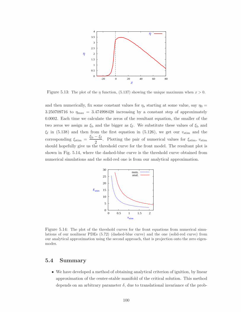
0

0.5

1

1.5

2

2.5

3

3.5

4

-20 0 20 40 60 80

η

η

x

Figure 5.13: The plot of the η function, (5.137) showing the unique maximum when x > 0.

and then numerically, fix some constant values for ηs starting at some value, say η0 =

3.250709716 to ηmax = 3.474998428 increasing by a constant step of approximately

0.0002. Each time we calculate the zeros of the resultant equation, the smaller of the

two zeros we assign as ξb and the bigger as ξf . We substitute these values of ξb and

ξf in (5.138) and then from the first equation in (5.126), we get our vstim and the

corresponding ξstim =ξb − ξf

2. Plotting the pair of numerical values for ξstim, vstim

should hopefully give us the threshold curve for the front model. The resultant plot is

shown in Fig. 5.14, where the dashed-blue curve is the threshold curve obtained from

numerical simulations and the solid-red one is from our analytical approximation.

0

5

10

15

20

25

30

0 0.5 1 1.5 2

Estim

xstim

num.anal.

Figure 5.14: The plot of the threshold curves for the front equations from numerical simu-lations of our nonlinear PDEs (5.72) (dashed-blue curve) and the one (solid-red curve) fromour analytical approximation using the second approach, that is projection onto the zero eigen-modes.

5.4 Summary

• We have developed a method of obtaining analytical criterion of ignition, by linear

approximation of the center-stable manifold of the critical solution. This method

depends on an arbitrary parameter δ, due to translational invariance of the prob-

100

lem. This arbitrary parameter is to be determined from further considerations,

independent of the linear approximation.

• We have proposed two methods of determining parameter δ. Method 1 is about

finding minimal ustim at the given stimulus profile, and therefore provides a lower

estimate of the threshold of all possible δ. Method 2 is about finding minimal L2

norm of the initial condition for the linearized problem.

• We have applied the two methods for the ZFK equation. Both methods gave

very close results, which agree very well with critical curve obtained by direct

numerical simulations.

• We have applied the two methods for the front model. They gave qualitatively

correct shape of the critical curve and correct order of magnitude of the quantities.

Method 1 gave a noticeable underestimation of the threshold stimulus amplitude,

whereas Method 2 gave a noticeable overestimation of this amplitude.

We conclude that a good approximation for the critical curve in the front model

can be obtained for an appropriately chosen method of determining δ. This

method remains a question for further study.

101



α constant (5.16)

α, ω voltage: pre-frontal, post-frontal (5.74)

β constant (5.16),(5.66)

ξ1 constant parameter (5.66)

∆ norm (5.42)

∆ constant af(5.59)

εk1parameter af(5.71)

ε parameter Sec. 5.3.2

δ parameter (Hinch’s equations) bf(5.67)

δ distance bf(5.33)

τ parameter Fig. 5.8

θ threshold parameter bf(5.9)

θ1 constant af(5.100)

ηmax constant bf(5.140)

ηs constant (5.140)

Γ Gamma function (5.15)

λ temporal eigenvalue (Hinch’s problem) af(5.62)

λ1, λ2, λ3 eigenvalue: unstable, translation, stable(ZFK problem)

(5.12)

λ temporal eigenvalue (direct front prob-lem)

(5.5)

µ parameter (Hinch’s equation) (5.71)

µ temporal eigenvalue (adjoint to the directfront problem)

bf(5.88)

ν1, ν2, ˜ν2 spatial eigenvalue (Hinch’s problem) (5.68)

ν1, ν2, ν2 spatial eigenvalue (direct front problem) (5.83)

γ1, γ2, γ2 spatial eigenvalue (adjoint to the directfront problem)

(5.94)


102



µ, ν complex constant (5.14)

φ eigenfunction (ZFK) (5.5)

ϕ, ψ, η eigenfunction (direct front problem) bf(5.78),(5.80)

ϕ∗, ψ∗, η∗ eigenfunction (adjoint to the direct frontproblem)

(5.89),(5.91)

ψ1, ψ2; eigenfunction (ZFK): unstable, transla-tion

(5.22), (5.21);

φ1, φ2 bf(5.29), af(5.25)

φj, φk the j’th, k’th eigenfunction (ZFK) (5.24),(5.25),bf(5.27)

φ∗1, ψ∗1 unstable eigenfunction for the adjoint

front problem(5.99)

φ∗2, ψ∗2 translation (zero) eigenfunction for the ad-

joint front problem(5.119)

Φ, η function (5.128), af(5.129)

ηL, ηR1, ηR2

function (5.131), (5.132),(5.135)

ξstim : ξb, ξf stimulus width: back, front (5.100), bf(5.100)


Ξ, Ξ, Ξ∗ vector of eigenfunctions bf(5.64),(5.81),(5.92)

A, A, B coefficients matrix (5.64),(5.81),(5.92)

a1(δ) projection onto the unstable eigenfunction (5.34)

a2(δ) projection onto the translational eigen-function

(5.43)

c : c− speed in the front equations: lower bf(5.73),Sec. 5.3.1

c speed in Hinch’s model [43] bf(5.60)

C constant (5.13)

C matrix (5.79)

D, D diffusion: coefficient, matrix (5.109), (5.79)

D parameter dependent on c, µ (5.109)

D1, N1, D2, N2 integral (5.36), (5.126)


103



E, h dynamic variables: voltage, gate (5.72)

F hypergeometric function (5.15)

f ; F, G nonlinear function (5.1), (5.72)

F , G nonlinear function (5.59)

F matrix (5.79)

fe, fe, f∗e characteristics function (5.71),(5.86),(5.97)

H function (5.35), (5.119)

g, H0 parameter in Hinch’s equations af (5.59), (5.66)

k parameter (5.9)

q functions of x or z (5.4),(5.10)

Pµν , Q

µν Legendre P, Legendre Q (5.15)

ucr critical nucleus for quadratic nolinearity bf(5.3)

u dynamic variable: voltage (5.1)

v0, h0 exact solution (stationary) to the front bf (5.74)

v1, h1 perturbation for the front equations bf (5.76)

v, h dynamic variable: voltage, gate (5.59)

v0, h0 stationary solution bf (5.61)

v1, h1 perturbation for the Hinch equations (5.62)

w perturbation (5.3)

W dynamic variable (5.14)

U , U0 solution: nonlinear, unstable af (5.73), af(5.77),(5.98)

V , W vector of eigenfunctions (5.78), (5.88)

vstim stimulus amplitude Fig. 5.7

xstim, ustim stimulus: width, amplitude (5.1)

104

Chapter 6

Conclusions

6.1 Results

In this thesis, the following results have been obtained:

• We have developed a numerical procedure for identifying critical nucleus and

validated for the ZFK equation for which the critical nucleus solution is known

exactly.

• Our numerical critical curves confirm the prediction from the approximate ana-

lytical theory by Neu et al. about inverse proportionality of the critical stimulus

amplitude to its width.

• We presented numerical evidence that the role of the “critical nucleus” as for the

ZFK equation is being played by its slowly moving variant, the “critical pulse”

for the FHN system, which is consistent with the theoretical results by Flores. In

the case of the simplified front model, we have observed through numerics that

the relationship between the asymptotic voltage (rheobase) Easym and the pre-

frontal voltage α is found to be Easym = α + 1, which means that at very large

stimulus width, the stimulus amplitude should be such that it opens the m-gates.

This revelation will among other things assist in checking the analytical ignition

criteria that we seek to find.

• We have established the role of unstable fronts as critical solutions in the cardiac

front models, whose center-stable manifolds serve as threshold hyper-surfaces in

the functional space between decay and ignition initial conditions.

• We have extended the variational description by Neu et al. of ignition in the ZFK

equation, by using two-parametric piecewise linear ansatzes and avoiding blow-up

solutions.

• We have developed a variational description of ignition in the front model using

2-parametric piece-wise linear ansatz, and established that a 2-parametric ap-

105

proximation is insufficient to describe the front dissipation mechanism essential

for ignition failure in this model.

• We have developed a variational description of ignition in the front model using 3-

parametric piece-wise smooth ansatz. This leads to a qualitatively correct critical

curve approximation.

• We have developed a method of obtaining analytical criterion of ignition, by linear

approximation of the center-stable manifold of the critical solution. This method

depends on an arbitrary parameter δ, due to translational invariance of the prob-

lem. This arbitrary parameter is to be determined from further considerations,

independent of the linear approximation.

• We have proposed two methods of determining parameter δ, one based on mini-

mization of the threshold amplitude and the other based on minimization of the

perturbation initial condition.

• We have applied the two linearized methods for the ZFK equation. Both methods

gave very close results, which agree very well quantitatively with critical curve

obtained by direct numerical simulations.

• We have applied the two methods for the front model. They gave qualitatively

correct shape of the critical curve and correct order of magnitude of the quan-

tities, with one of the method giving an overestimation and the other giving an

underestimation of the threshold amplitude.

6.2 Further Directions

• Sequel to the unexpected result from our piece-wise linear variational approxima-

tion to the front model, we will revisit the problem adopting now a new approach

by considering t(x) rather than x(t) description of the front motion, which hope-

fully will produce the unstable front solution.

• A good approximation for the critical curve in the front model can be obtained

for an appropriately chosen method of determining the parameter δ. This method

remains a question for further study.

• The propagation of excitation in cardiac muscle for example, generally have been

treated as though it occurred in a continuous structure (medium). However, new

evidences are emerging that suggest propagation in cardiac muscle often displays a

discontinuous nature, “ectopic nexus” as it is popularly referred to (see [76]). We

will therefore extend our initiation criterion to other applications and phenomena

such as the ectopic nexus where initiation thresholds are crucial.

106

• We will consider other different initiation protocols, for example, initiation by

current, where currents are used as stimulus, popularly used in physiology and

experiment (see [88, 91]).

• It will also be interesting and quite challenging as well to try and explore how

our initiation criteria are going to be molded appropriately so as to investigate

initiation processes in models of higher dimensions, for example, 2D and 3D.

107

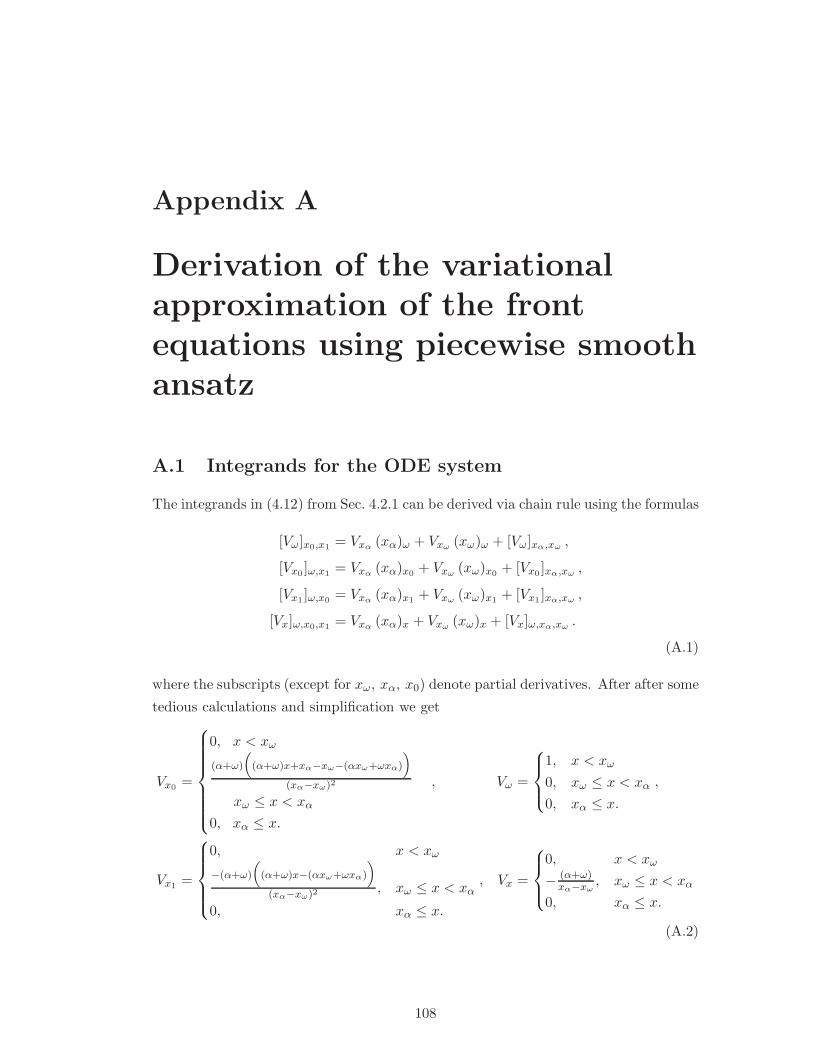
Appendix A

Derivation of the variationalapproximation of the frontequations using piecewise smoothansatz

A.1 Integrands for the ODE system

The integrands in (4.12) from Sec. 4.2.1 can be derived via chain rule using the formulas

[Vω]x0,x1= Vxα (xα)ω + Vxω (xω)ω + [Vω]xα,xω ,

[Vx0]ω,x1

= Vxα (xα)x0+ Vxω (xω)x0

+ [Vx0]xα,xω ,

[Vx1]ω,x0

= Vxα (xα)x1+ Vxω (xω)x1

+ [Vx1]xα,xω ,

[Vx]ω,x0,x1= Vxα (xα)x + Vxω (xω)x + [Vx]ω,xα,xω .

(A.1)

where the subscripts (except for xω, xα, x0) denote partial derivatives. After after some

tedious calculations and simplification we get

Vx0=

0, x < xω

(α+ω)

(

(α+ω)x+xα−xω−(αxω+ωxα)

)

(xα−xω)2

xω ≤ x < xα

0, xα ≤ x.

, Vω =

1, x < xω

0, xω ≤ x < xα

0, xα ≤ x.

,

Vx1=

0, x < xω

−(α+ω)

(

(α+ω)x−(αxω+ωxα)

)

(xα−xω)2 , xω ≤ x < xα

0, xα ≤ x.

, Vx =

0, x < xω

− (α+ω)xα−xω

, xω ≤ x < xα

0, xα ≤ x.

(A.2)

108

Similarly, the integrands in terms of W are obtained using the chain rule formulas in

(A.1)

Wω =

0, x < xω

− (α+ω)x−(αxω+ωxα)ω2(xα−xω)

, xω ≤ x < x0

0, x0 ≤ x.

,

Wx0=

0, x < xω

−(α+ω)

(

(α+ω)x+xα−xω−(αxω+ωxα)

)

ω(xα−xω)2,

xω ≤ x < x0

0, x0 ≤ x.

Wx1=

0, x < xω

−(α+ω)

(

(α+ω)x−(αxω+ωxα)

)

ω(xα−xω)2, xω ≤ x < x0

0, x0 ≤ x.

(A.3)

A.2 Alternative representation of the integrands

Alternatively, we could express the integrands (4.12) directly in terms the dynamic

variables (ω, x0, x1). Therefore, using the same formulas (A.1) we get

V =

V (x, t), x < xω

− x−x0

x0−x1, xω ≤ x < xα

−α, xα ≤ x.

(A.4)

Vω =

1, x < xω

0, xω ≤ x < xα

0, xα ≤ x.

, Vx0=

0, x < xω

x−x1

(x0−x1)2, xω ≤ x < xα

0, xα ≤ x.

Vx1=

0, x < xω

− x−x0

(x0−x1)2, xω ≤ x < xα

0, xα ≤ x.

, Vx =

0, x < xω

− 1x0−x1

, xω ≤ x < xα

0, xα ≤ x.

(A.5)

W =

0, x < xω

1 + x−x0

ω(x0−x1), xω ≤ x < x0

1, x0 ≤ x.

(A.6)

Wω =

0, x < xω

− x−x0

ω2(x0−x1), xω ≤ x < x0

0, x0 ≤ x.

, Wx0=

0, x < xω

− x−x1

ω(x0−x1)2, xω ≤ x < x0

0, x0 ≤ x.

Wx1=

0, x < xω

x−x0

ω(x0−x1)2, xω ≤ x < x0

0, x0 ≤ x.

(A.7)

109

A.3 The ODE system

Substituting the integrands (A.2, A.3) in (4.12) and from (4.11) we have

Mωω Mωx0Mωx1

Mx0ω Mx0x0Mx0x1

Mx1ω Mx1x0Mx1x1

ω

x0

x1

=

Qω + Fω +Gω

Qx0+ Fx0

+Gx0

Qx1+ Fx1

+Gx1

(A.8)

where (after some tedious computations)

Mωω =(x0 − x1)µ

2τ2

3ω, Mωx0

=(2ω − 3)µ2τ2

6ω, Mωx1

= −µ2τ2

3,

Mx0x0=ω4 − 3ω3 + (µ2τ2 + 3)ω2 − (3µ2τ2 − α3 − 3α2 − 3α)ω + 3µ2τ2

3ω(x0 − x1),

Mx0x1=

2ω3 − 3ω2 + 2µ2τ2ω + 2α3 + 3α2 − 3µ2τ2

−6(x0 − x1), Mx0ω = Mωx0

,

Mx1x1=ω3 + µ2τ2ω + α3

3(x0 − x1), Mx1x0

= Mx0x1, Mx1ω = Mωx1

(A.9)

Qω =−1

2(x0 − x1), Qx0

=α+ ω

2(x0 − x1)2, Qx1

= − α+ ω

2(x0 − x1)2,

Fω = 0, Fx0= −(ω − 1)3

6ω, Fx1

=(ω + 2)(ω − 1)2

6ω,

Gω = −(x0 − x1)µ2τ

6, Gx0

= −(ω − 3)µ2τ

6, Gx1

=ωµ2τ

6. (A.10)

Thus, we obtained the following system

τ2 µ2(2ω − 3)(x0 − x1) x0 − 2 τ2 µ2 ω (x0 − x1) x1 + 2 τ2 µ2(x0 − x1)2 ω

+(

τ µ2 (x0 − x1)2 + 3

)

ω = 0,

2 (x0 − x1)(

ω4 − 3ω3 + (3 + τ2 µ2)ω2 + (α3 + 3α2 + 3α − 3 τ2 µ2)ω + 3 τ2 µ2)

x0

− (x0 − x1)(

2ω4 − 3ω3 + 2 τ2 µ2 ω2 + (2α3 + 3α2 + 3α− 3 τ2 µ2)ω)

x1

+ (x0 − x1)2 τ2 µ2 (2ω − 3) ω + (x0 − x1)

2 ω3 −(

(x0 − x1)2(3 − τ µ2) + 3

)

ω2

− 3(

(1 + τ2 µ2)(x0 − x1)2 − α

)

ω − (x0 − x1)2 = 0,

(x0 − x1)(

− 2ω4 + 3ω3 − 2 τ2 µ2 ω2 − (2α3 + 3α2 − 3 τ2 µ2)ω)

x0

+ (x0 − x1)(

2ω4 + 2 τ2 µ2 ω2 + 2α3 ω)

x1 − 2 τ2 µ2 (x0 − x1)2 ω ω

− (x0 − x1)2 ω3 −

(

τ µ2 (x0 − x1)2 − 3

)

ω2 + 3(

(x0 − x1)2 + α

)

ω − 2 (x0 − x1)2 = 0.

(A.11)

We solve (A.11) for ω, x0, x1 to obtain the third order ODE system and because of

translation invariance we use x0 = x1+q to get the second order ODE system involving

110

only ω, q

dω

dt= −

(

τ µ2ω6 + (4α τ µ2 − τ2 µ2)ω5 + (6α2 τ µ2 + τ3 µ4 − 4α τ2 µ2)ω4

+ (3 τ2 µ2 − τ4 µ4 + 4α3 τ µ2 − 9α2 τ2 µ2)ω3

− (6α3 τ2 µ2 − 3α2τ3 µ4 − 2 τ2 µ2 + 12α2 τ2 µ2 + τ α4 µ2 + 12α τ2 µ2)ω2

+ (12α3 τ2 µ2 + 3α2τ2 µ2 − 8α τ2 µ2 + 3 τ4 µ4 − 2α3 τ3 µ4 − 2α3 τ3 µ4)ω

− 6α2 τ2 µ2 − 6α3τ2 µ2 − 2 τ4 µ4)

/(

2 τ2 µ2(

ω5 + 4αω4 + (6α 2 + τ2 µ2)ω3

+ 4α3 ω2 + α4 ω − α3 τ2 µ2))

−(

3ω6 + 12αω5 + (9 τ2 µ2 + 18α2)ω4 + (27α τ2 µ2 + 12α3)ω3

+ (3α4 + 39α2 τ2µ2 + 6 τ4 µ4)ω2 + (3α τ4 µ4 + 21α3 τ2 µ2)ω)

/(

2 τ2 µ2 q2

(

ω5 + 4αω4 + (6α 2 + τ2 µ2)ω3 + 4α3 ω2 + α4 ω + α3 τ2 µ2))

= f(ω, q),

dq

dt= q

(

2ω5 + (−4α+ 3 τ µ2 − 12)ω4 + (−τ2 µ2 − 6α2 + 18)ω3

+ (−3α2 τ µ2 + 12α2 − 8 + 12α)ω2 + (−6α2 − 8α+ 3 τ2 µ2)ω − 2 τ2 µ2)

/(

2ω (ω + α)(


+(

15ω4 + 36αω3 + (21α2 + 6 τ2 µ2)ω2 + 3α τ2 µ2 ω)

/(

2ω (ω + α) q(


= g(ω, q).

(A.12)

111

Appendix B

Integrals for the variationalapproximation of the frontequations using smooth ansatz

B.1 Derivation of the integrals

The integrals in (4.30, 4.31, 4.32) in Chapter 4 can respectively be further split so as

to facilitate their computations

a

(∫ x1

0V 2

a dx+

∫ ∞

x1

V 2a dx+

∫ x0

0W 2

a dx+

∫ ∞

x0

W 2a dx

)

+ b

(∫ x1

0VaVb dx+

∫ ∞

x1

VaVb dx+

∫ x0

0WaWb dx+

∫ ∞

x0

WaWb dx

)

+ x1

(∫ x1

0VaVx1

dx+

∫ ∞

x1

VaVx1dx+

∫ x0

0WaWx1

dx+

∫ ∞

x0

WaWx1dx

)

=

∫ x1

0Va(Vxx + f(V,W )) dx+

∫ ∞

x1

Va(Vxx + f(V,W )) dx

+

∫ x0

0

1

τWa g(V,W ) dx+

∫ ∞

x0

1

τWa g(V,W ) dx, (B.1)

a

(∫ x1

0VaVb dx+

∫ ∞

x1

VaVb dx+

∫ x0

0WaWb dx+

∫ ∞

x0

WaWb dx

)

+ b

(∫ x1

0V 2

b dx+

∫ ∞

x1

V 2b dx+

∫ x0

0W 2

b dx+

∫ ∞

x0

W 2b dx

)

+ x1

(∫ x1

0VbVx1

dx+

∫ ∞

x1

VbVx1dx+

∫ x0

0WbWx1

dx+

∫ ∞

x0

WbWx1dx

)

=

∫ x1

0Vb(Vxx + f(V,W )) dx+

∫ ∞

x1

Vb(Vxx + f(V,W )) dx

+

∫ x0

0

1

τWb g(V,W ) dx+

∫ ∞

x0

1

τWb g(V,W ) dx, (B.2)

112

a

(∫ x1

0VaVx1

dx+

∫ ∞

x1

VaVx1dx+

∫ x0

0WaWx1

dx+

∫ ∞

x0

WaWx1dx

)

+ b

(∫ x1

0VbVx1

dx+

∫ ∞

x1

VbVx1dx+

∫ x0

0WbWx1

dx+

∫ ∞

x0

WbWx1dx

)

+ x1

(∫ x1

0V 2

x1dx+

∫ ∞

x1

V 2x1

dx+

∫ x0

0W 2

x1dx+

∫ ∞

x0

W 2x1

dx

)

=

∫ x1

0Vx1

(Vxx + f(V,W )) dx+

∫ ∞

x1

Vx1(Vxx + f(V,W )) dx

+

∫ x0

0

1

τWx1

g(V,W ) dx+

∫ ∞

x0

1

τWx1

g(V,W ) dx. (B.3)

The definitions in (B.4, B.5) and the Table (B.1) are used to help simplify and trim

down the integrals in (B.1, B.2, B.3). Let f(V,W ) and g(V,W ) be define by

f(V,W ) = fV · fW , g(V,W ) = gV − gW , (B.4)

where

fV = Θ(V − 1), fW = W,

gV = Θ(−V ), gW = W, (B.5)

and let the table of the functional values of f(V,W ) and g(V,W ) in the specified

intervals be:

Table B.1: Functions value in specified intervals

Interval Functional value

[0, x1] fV = 1, fW = W, gV = 0, gW = W

[x1, x0] fV = 0, fW = W, gV = 0, gW = W

[x0,∞) fV = 0, fW = 1, gV = 1, gW = 1

Thus, the integrals in (B.1, B.2, B.3) simplify to

a

(∫ x1

0V 2

a dx+

∫ ∞

x1

V 2a dx+

∫ x0

0W 2

a dx

)

+ b

∫ x0

0WaWb dx

+ x1

(∫ x1

0VaVx1

dx+

∫ ∞

x1

VaVx1+

∫ x0

0WaWx1

dx

)

=

∫ x1

0Va(Vxx +W ) dx+

∫ ∞

x1

VaVxx dx+

∫ x0

0

1

τWa(−W ) dx, (B.6)

a

∫ x0

0WaWb dx+ b

∫ x0

0W 2

b dx+ x1

∫ x0

0WbWx1

dx =

∫ x0

0

1

τWb (−W ) dx, (B.7)

113

a

(∫ x1

0VaVx1

dx+

∫ ∞

x1

VaVx1dx+

∫ x0

0WaWx1

dx

)

+ b

∫ x0

0WbWx1

dx

+ x1

(∫ x1

0V 2

x1dx+

∫ ∞

x1

V 2x1

dx+

∫ x0

0W 2

x1dx

)

=

∫ x1

0Vx1

(Vxx +W ) dx+

∫ ∞

x1

Vx1Vxx dx+

∫ x0

0

1

τWx1

(−W ) dx. (B.8)

B.2 Values of the integrals

Let denote the values of integrals in (B.6) by I11 , · · · , I1

10, those in (B.7), by I21 , · · · , I2

4

and those in (B.8) by I31 , · · · , I3

10 respectively. Using (4.35), (4.36) from Chapter 4 and

letting φ = ξ−1 = e−β1x1

σ , we obtain the values to the integrals in (B.6, B.7, B.8) as

follows:

I11 = 8σ(2φ4 + 5φ3 + 2φ2)ln(ξ)3/(3β1(1 − φ)6)

+ 2σ(−2φ5 + φ4 − φ2 + 2φ)ln(ξ)2/(β1(1 − φ)6)

+ σ(φ6 − 11φ5 + 10φ4 + 10φ2 − 11φ+ 1)ln(ξ)/(β1(1 − φ)6)

+ 11σ(φ6 − 2φ5 + φ4 − φ2 + 2φ− 1)/(4β1(1 − φ)6), (B.9)

I12 = (φ2(1 + α)3ln(ξ)2)/(β1σ

2(1 − φ2)(1 + φ)2), (B.10)

I13 = 16b2β2β1ln(ξ)2φ2)/((5σ2(1 + φ)3)(σ(1 + φ)ln(ξ) − ββ1(1 − φ)), (B.11)

I14 = (8bβln(ξ)φ)/(15σ(1 + φ)2), (B.12)

I15 = σ(1 + φ)(1 − 2ln(ξ)φ− φ2)/((1 − φ)3)

− σ(1 + φ)((ln(ξ) + 1) + φ(ln(ξ) − 1))(1 − 8φ+ 12ln(ξ)φ2 + 8φ3 − φ4)/(2(1 − φ)6)

+ σ(1 + φ)(2ln(ξ)(1 − 4φ− 4φ3 + φ4) − (1 − 8φ+ 8φ3 − φ4))/(4(1 − φ)5)), (B.13)

I16 = (−(1 + α)3ln(ξ)φ2)/(σ2(1 + φ)2(1 − φ2)) − ((1 + α)2ln(ξ)φ)/(2σ(1 − φ2)),(B.14)

I17 = (8b2ββ1(σ(1 + φ)2 − 2ββ1φ)ln(ξ)φ)/(5σ2(1 + φ)3(σ(1 + φ)ln(ξ) − ββ1(1 − φ))),

(B.15)

114

I18 = σ(1 − b)ln(ξ)/β1 − β1(1 + φ)/(1 − φ) − σ(1 − b)((ln(ξ) + 1)

+ (ln(ξ) − 1)φ)(1 − 2ln(ξ)φ− φ2)/(β1(1 − φ)3)

+ β1((ln(ξ) + 1) + (ln(ξ) − 1)φ)(1 − 4φ+ 4ln(ξ)φ2 + 4φ3 − φ4)/(2(1 − φ)5)

+ bσ3(1 + φ)2ln(ξ)3/(3β1(σ(1 + φ)ln(ξ) − ββ1(1 − φ))2)

+ σ(1 − b)((ln(ξ) − 1) + (ln(ξ) + 1)φ2)/(β1(1 − φ)2)

− β1((2ln(ξ) − 1) + (2ln(ξ) + 1)φ4)/(4(1 − φ)4)

+ bσ3(1 + φ)2((ln(ξ) + 1) + (ln(ξ) − 1)φ)(2ln(ξ)3φ− 3ln(ξ)2(1 − φ2) + 6ln(ξ)(1 + φ2)

− 6(1 − φ2))/(3β1(1 − φ)3(σ(1 + φ)ln(ξ) − ββ1(1 − φ))2)

+ bσ3(1 + φ)2(ln(ξ)3(1 + φ2) − 3ln(ξ)2(1 − φ2) + 6ln(ξ)(1 + φ2)

− 6(1 − φ2))/(β1(1 − φ)2(σ(1 + φ)ln(ξ) − ββ1(1 − φ))2), (B.16)

I19 = (−(1 + α)β1ln(ξ)φ)/(2σ(1 − φ)2), (B.17)

I110 = (−4b(2b− 5)βln(ξ)φ)/(15στ(1 + φ)2), (B.18)

I21 = (8bβln(ξ)φ)/(15σ(1 + φ)2), (B.19)

I22 = 8(σ(1 + φ)ln(ξ) − ββ1(1 − φ))/(15β1(1 + φ)), (B.20)

I23 = 4b(σ(1 + φ)2 − 2ββ1φ)/(15σ(1 + φ)2), (B.21)

I24 = −2(4b− 5)(σ(1 + φ)ln(ξ) − ββ1(1 − φ))/(15τβ1(1 + φ)), (B.22)

I31 = σ(1 + φ)(1 − 2ln(ξ)φ− φ2)/((1 − φ)3)

− σ(1 + φ)((ln(ξ) + 1) + φ(ln(ξ) − 1))(1 − 8φ+ 12ln(ξ)φ2 + 8φ3 − φ4)/(2(1 − φ)6)

+ σ(1 + φ)(2ln(ξ)(1 − 4φ− 4φ3 + φ4) − (1 − 8φ+ 8φ3 − φ4))/(4(1 − φ)5), (B.23)

I32 = (−(1 + α)3ln(ξ)φ2)/(σ2(1 + φ)2(1 − φ2)) − ((1 + α)2ln(ξ)φ)/(2σ(1 − φ2)), (B.24)

I33 = (8b2ββ1(σ(1 + φ)2 − 2ββ1φ)ln(ξ)φ)/(5σ2(1 + φ)3(σ(1 + φ)ln(ξ) − ββ1(1 − φ))),

(B.25)

I34 = 4b(σ(1 + φ)2 − 2ββ1φ)/(15σ(1 + φ)2), (B.26)

I35 = σβ1(1 + φ)2(1 − 8φ+ 12ln(ξ)φ2 + 8φ3 − φ4)/(2(1 − φ)6), (B.27)

115

I36 = (1 + α)β1(1 + φ)/(2(1 − φ)) + ((1 + α)2β1φ)/(σ(1 − φ2))

+ ((1 + α)3β1φ2)/(σ2(1 + φ)2(1 − φ2)), (B.28)

I37 = 4b2β1(σ(1 + φ)2 − 2ββ1φ)2/(5σ2(1 + φ)3(σ(1 + φ)ln(ξ) − ββ1(1 − φ))),

(B.29)

I38 = (σ(1 − b)(1 + φ)(1 − 2ln(ξ)φ− φ2))/((1 − φ)3)

− (β21(1 + φ)(1 − 4φ+ 4ln(ξ)φ2 + 4φ3 − φ4))/(2(1 − φ)5)

− (bσ3(1 + φ)3(2ln(ξ)3φ− 3ln(ξ)2(1 − φ2) + 6ln(ξ)(1 + φ2) − 6(1 − φ2)))

/ (3(1 − φ)3(σ(1 + φ)ln(ξ) − ββ1(1 − φ))2), (B.30)

I39 = ((1 + α)β2

1φ)/(2σ(1 − φ)2) + (β21(1 + φ)2)/(2(1 − φ)2), (B.31)

I310 = (−2b(2b− 5)(σ(1 + φ)2 − 2ββ1φ))/(15τσ(1 + φ)2). (B.32)

Thus, from integrals (B.6, B.7, B.8) and equations (B.9) to (B.32)

a11 a12 a13

a21 a22 a23

a31 a32 a33

a

b

x1

=

b1

b2

b3

, (B.33)

where

a11 = I11 + I1

2 + I13 ,

a12 = I14 ,

a13 = I15 + I1

6 + I17 ,

a21 = I21 ,

a22 = I22 ,

a23 = I23 ,

a31 = I31 + I3

2 + I33 , (B.34)

a32 = I34 ,

a33 = I35 + I3

6 + I37 ,

b1 = I18 + I1

9 + I110,

b2 = I24 ,

b3 = I38 + I3

9 + I310.

116

Let

∆ =

∣∣∣∣∣∣∣∣

a11 a12 a13

a21 a22 a23

a31 a32 a33

∣∣∣∣∣∣∣∣

,

∆1 =

∣∣∣∣∣∣∣∣

b1 a12 a13

b2 a22 a23

b3 a32 a33

∣∣∣∣∣∣∣∣

,

∆2 =

∣∣∣∣∣∣∣∣

a11 b1 a13

a21 b2 a23

a31 b3 a33

∣∣∣∣∣∣∣∣

,

∆3 =

∣∣∣∣∣∣∣∣

a11 a12 b1

a21 a22 b2

a31 a32 b3

∣∣∣∣∣∣∣∣

. (B.35)

Now using Cramer’s method we obtain the ODE system

a =∆1

∆≡ Fa(a, b, x1),

b =∆2

∆≡ Fb(a, b, x1),

x1 =∆3

∆≡ Fx1

(a, b, x1). (B.36)

117

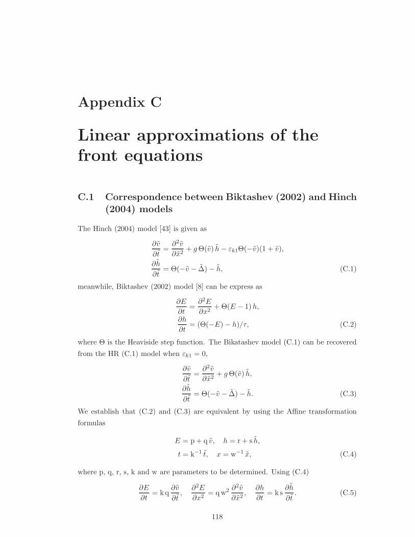
Appendix C

Linear approximations of thefront equations

C.1 Correspondence between Biktashev (2002) and Hinch(2004) models

The Hinch (2004) model [43] is given as

∂v

∂t=∂2v

∂x2+ gΘ(v) h− εk1Θ(−v)(1 + v),

∂h

∂t= Θ(−v − ∆) − h, (C.1)

meanwhile, Biktashev (2002) model [8] can be express as

∂E

∂t=∂2E

∂x2+ Θ(E − 1)h,

∂h

∂t= (Θ(−E) − h)/τ, (C.2)

where Θ is the Heaviside step function. The Bikatashev model (C.1) can be recovered

from the HR (C.1) model when εk1 = 0,

∂v

∂t=∂2v

∂x2+ gΘ(v) h,

∂h

∂t= Θ(−v − ∆) − h. (C.3)

We establish that (C.2) and (C.3) are equivalent by using the Affine transformation

formulas

E = p + q v, h = r + s h,

t = k−1 t, x = w−1 x, (C.4)

where p, q, r, s, k and w are parameters to be determined. Using (C.4)

∂E

∂t= kq

∂v

∂t,

∂2E

∂x2= qw2 ∂

2v

∂x2,

∂h

∂t= k s

∂h

∂t. (C.5)

118

Substituting (C.4) and (C.5) in (C.2) we obtain

∂v

∂t= (w2/k)

∂2v

∂x2+ (1/(k q))Θ(p − 1 + q v) h,

∂h

∂t= (1/(k s τ))

(

Θ(−p − q v) − (r + s h))

. (C.6)

Now by comparing (C.3) and (C.6) and since Θ(CE) ≡ Θ(E) for some scalar C, we

get

w2/k = 1, r = 0, s/(k q) = g, p = 1,

τk s = 1, s = 1, p/q = ∆, (C.7)

from which we have

p = 1, q = τ/g (≡ 1/∆), r = 0, s = 1,

k = 1/τ (i.e., k = τ−1), w2 = 1/τ (i.e., w = τ−1/2), (C.8)

and from (C.8), g = τ ∆. Hence,

E = 1 + (1/∆) v, h = h,

t = τ t, x = τ1/2 x. (C.9)

And from the boundary conditions, E(−∞) = −α [8] and v(−∞) = −1 [43]

∆ = 1/(1 + α). (C.10)

The speeds are related via c = x/t, c = x/t and which lead from (C.9) to

c = c τ1/2, β = c2 = τ c2. (C.11)

Here, we check our transformation formulas using

∂

∂t= τ−1 ∂

∂t,

∂

∂x= τ−1/2 ∂

∂x, (C.12)

and thus,

∂E

∂t=

1

τ ∆

∂v

∂t=

1

g

∂v

∂t,

∂h

∂t=

1

τ

∂h

∂t,

∂2E

∂x2=

1

τ ∆

∂2v

∂x2=

1

g

∂2v

∂x2. (C.13)

But since Θ(v/∆) = Θ(v), Θ(

−(v + ∆)/∆)

= Θ(−(v + ∆)) and (C.13) we have

∂v

∂t=∂2v

∂x2+ gΘ(v) h,

∂h

∂t= Θ(−v − ∆) − h, (C.14)

which is exactly the same as (C.3).

119

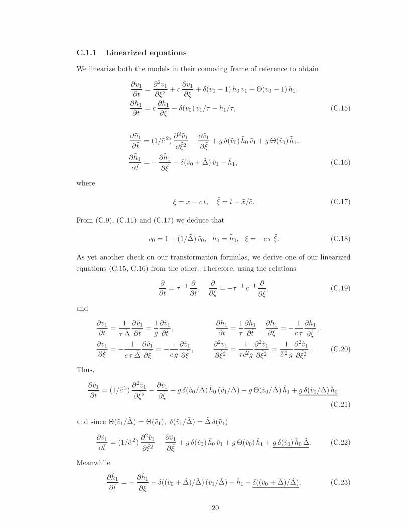
C.1.1 Linearized equations

We linearize both the models in their comoving frame of reference to obtain

∂v1∂t

=∂2v1∂ξ2

+ c∂v1∂ξ

+ δ(v0 − 1)h0 v1 + Θ(v0 − 1)h1,

∂h1

∂t= c

∂h1

∂ξ− δ(v0) v1/τ − h1/τ, (C.15)

∂v1

∂t= (1/c 2)

∂2v1

∂ξ2− ∂v1

∂ξ+ g δ(v0) h0 v1 + gΘ(v0) h1,

∂h1

∂t= − ∂h1

∂ξ− δ(v0 + ∆) v1 − h1, (C.16)

where

ξ = x− c t, ξ = t− x/c. (C.17)

From (C.9), (C.11) and (C.17) we deduce that

v0 = 1 + (1/∆) v0, h0 = h0, ξ = −c τ ξ. (C.18)

As yet another check on our transformation formulas, we derive one of our linearized

equations (C.15, C.16) from the other. Therefore, using the relations

∂

∂t= τ−1 ∂

∂t,

∂

∂ξ= −τ−1 c−1 ∂

∂ξ, (C.19)

and

∂v1∂t

=1

τ ∆

∂v1

∂t=

1

g

∂v1

∂t,

∂h1

∂t=

1

τ

∂h1

∂t,∂h1

∂ξ= − 1

c τ

∂h1

∂ξ,

∂v1∂ξ

= − 1

c τ ∆

∂v1

∂ξ= − 1

c g

∂v1

∂ξ,

∂2v1

∂ξ2=

1

τc2g

∂2v1

∂ξ2=

1

c 2 g

∂2v1

∂ξ2. (C.20)

Thus,

∂v1

∂t= (1/c 2)

∂2v1

∂ξ2− ∂v1

∂ξ+ g δ(v0/∆) h0 (v1/∆) + gΘ(v0/∆) h1 + g δ(v0/∆) h0,

(C.21)

and since Θ(v1/∆) = Θ(v1), δ(v1/∆) = ∆ δ(v1)

∂v1

∂t= (1/c 2)

∂2v1

∂ξ2− ∂v1

∂ξ+ g δ(v0) h0 v1 + gΘ(v0) h1 + g δ(v0) h0 ∆. (C.22)

Meanwhile

∂h1

∂t= − ∂h1

∂ξ− δ((v0 + ∆)/∆) (v1/∆) − h1 − δ((v0 + ∆)/∆), (C.23)

120

reduces to

∂h1

∂t= − ∂h1

∂ξ− δ(v0 + ∆) v1 − h1 − δ(v0 + ∆) ∆. (C.24)

Hence,

∂v1

∂t= (1/c 2)

∂2v1

∂ξ2− ∂v1

∂ξ+ g δ(v0) h0 v1 + gΘ(v0) h1 + g δ(v0) h0 ∆,

∂h1

∂t= − ∂h1

∂ξ− δ(v0 + ∆) v1 − h1 − δ(v0 + ∆) ∆. (C.25)

NB: System (C.16) and (C.25) are equivalent only when the underlined extra terms in

(C.25) become zero.

C.2 Linearization of Hinch (2004) equations

In a laboratory reference frame with (x, T ) as coordinates, the front model ( [43]), can

be written in the form

∂v

∂T=∂2v

∂x2+ F (v, h),

∂h

∂T= G(v, h), (C.26)

where F (v, h) = gΘ(v)h, G(v, h) = Θ(−v− ∆)− h and Θ is a Heaviside step function.

In a moving frame of reference, the solutions to (C.26) for a right-ward moving front

are of the form v(T − x/c, T ), h(T − x/c, T ). Introducing the coordinates ξ = T − x/c,

t = T with c > 0, we look for functions v(ξ, t), h(ξ, t) which satisfy (C.26) to give

∂v

∂t=

1

c2∂2v

∂ξ2− ∂v

∂ξ+ F (v, h),

∂h

∂t= −∂h

∂ξ+ G(v, h). (C.27)

NB: Traveling waves of (C.26) corresponds to stationary solutions of (C.27). Suppose

v0(ξ), h0(ξ), is a stationary solution of (C.27), then

1

c2d2v0

dξ2− dv0

dξ+ F (v0, h0) = 0,

dh0

dξ− G(v0, h0) = 0. (C.28)

The linearized version of (C.27) about(

v0(ξ), h0(ξ))

is neglecting higher order

terms)

∂v1

∂t=

1

c2∂2v1

∂ξ2− ∂v1

∂ξ+ g δ(v0) h0 v1 + gΘ(v0) h1,

∂h1

∂t= −∂h1

∂ξ− δ(v0 + ∆) v1 − h1. (C.29)

121

C.2.1 Eigenvalue problem

Let the linearized eqtn (C.29) support solutions of the form h1(ξ, t) = eλ t φ(ξ) and

h1(ξ, t) = eλ t ψ(ξ). This lead to the (temporal eigenvalue) problem

λ φ =1

c2d2φ

dξ2− dφ

dξ+ g δ(v0) h0 φ+ gΘ(v0) ψ,

λ ψ = − dψ

dξ− δ(v0 + ∆) φ− ψ, (C.30)

where φ(ξ) and ψ(ξ) are some eigenfunctions. The eigenvalue eqtn (C.30) is then casted

into a three first-order (ODE) equations by lettingdφ

dξ= η and Ξ = (φ, η, ψ)T. Thus,

we obtain a linear system in C3

Ξ′= A Ξ, (C.31)

where (′) =d

dξ,

A =

0 1 0

c2(

λ− g δ(v0) h0

)

c2 −c2 gΘ(v0)

−δ(v0 + ∆) 0 −(1 + λ)

, (C.32)

v0(ξ) =

−1 + eβ ξ, ξ ≤ 0,

β g H0

1 + β(1 − e−ξ), ξ ≥ 0,

h0(ξ) =

1, ξ ≤ ξ1,

H0e− ξ, ξ ≥ ξ1,

(C.33)

and

ξ1 = −δ/β, H0 = e−δ/β , g = (1 + β) e δ/β . (C.34)

Solution to the linearized equations We have three intervals (cases i = a, b, c)

to consider. For case i = a, ξ ∈ (−∞, ξ1), therefore in this interval, Θ(v0) = 0, δ(v0) =

0, δ(v0 + ∆) = δ(ξ − ξ1) = 0, h0 = 1. Thus, the solution is

φa

ηa

ψa

= a1 ~va1 e−ν1 ξ + a2 ~v

a2 e−ν2 ξ + a3 ~v

a3 e

˜ν2 ξ,

= a1

0

0

1

e−ν1 ξ + a2

1

ν2

0

eν2 ξ + a3

1

˜ν2

0

e˜ν2 ξ, (C.35)

122

where

ν1 = 1 + λ, ν2 =β +

√

β2 + 4 λ β

2, ˜ν2 =

β −√

β2 + 4 λ β

2. (C.36)

For case i = b, ξ ∈ (ξ1, ξ0), therefore in this interval, Θ(v0) = 0, δ(v0) = 0, δ(v0 + ∆) =

δ(ξ − ξ1) = 0, h0 = H0e−ξ. Thus, the solution is

φb

ηb

ψb

= b1 ~vb1 e−ν1 ξ + b2 ~v

b2 e−ν2 ξ + b3 ~v

b3 e

˜ν2 ξ,

= b1

0

0

1

e−ν1 ξ + b2

1

ν2

0

eν2 ξ + b3

1

˜ν2

0

e˜ν2 ξ, (C.37)

and lastly, for case i = c, ξ ∈ (ξ0,∞), therefore in this interval, Θ(v0) = 1, δ(v0) =

0, δ(v0 + ∆) = δ(ξ − ξ1) = 0, h0 = H0e−ξ. Thus, the solution is

φc

ηc

ψc

= c1 ~vc1 e−ν1 ξ + c2 ~v

c2 e−ν2 ξ + c3 ~v

c3 e

˜ν2 ξ,

= c1

1

−ν1

−νs

e−ν1 ξ + c2

1

ν2

0

eν2 ξ + c3

1

˜ν2

0

e˜ν2 ξ, (C.38)

where

νs =(1 + λ)2 + β

β g. (C.39)

C.2.2 Characteristic equation

Now to determine the characteristic equation for Hinch (2004) equations we consider

the conditions at the boundaries:

Boundary conditions at ±∞: With λ ≥ 0 : ν1 > 0, ν2 > 0, ˜ν2 < 0, for the case

i = a

limξ→−∞

φa

ηa

ψa

, (C.40)

123

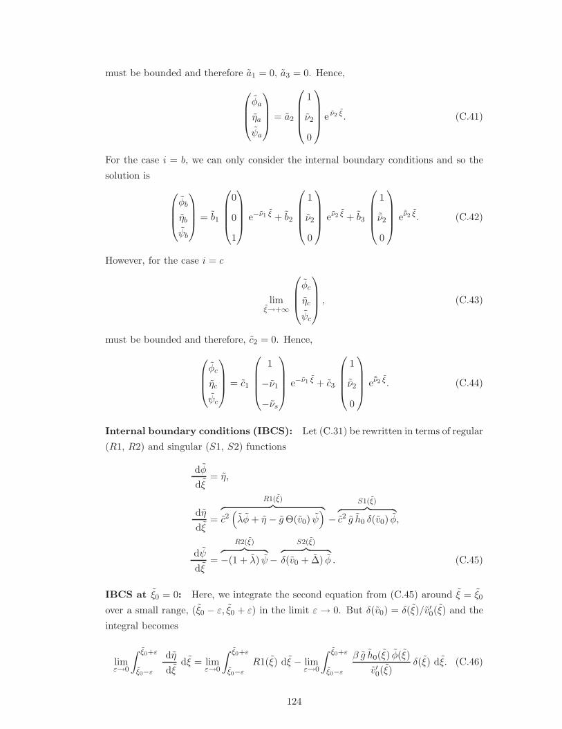
must be bounded and therefore a1 = 0, a3 = 0. Hence,

φa

ηa

ψa

= a2

1

ν2

0

e ν2 ξ. (C.41)

For the case i = b, we can only consider the internal boundary conditions and so the

solution is

φb

ηb

ψb

= b1

0

0

1

e−ν1 ξ + b2

1

ν2

0

eν2 ξ + b3

1

˜ν2

0

e˜ν2 ξ. (C.42)

However, for the case i = c

limξ→+∞

φc

ηc

ψc

, (C.43)

must be bounded and therefore, c2 = 0. Hence,

φc

ηc

ψc

= c1

1

−ν1

−νs

e−ν1 ξ + c3

1

˜ν2

0

e˜ν2 ξ. (C.44)

Internal boundary conditions (IBCS): Let (C.31) be rewritten in terms of regular

(R1, R2) and singular (S1, S2) functions

dφ

dξ= η,

dη

dξ=

R1(ξ)︷︸︸︷

c2(

λφ+ η − gΘ(v0) ψ)

−

S1(ξ)︷︸︸︷

c2 g h0 δ(v0) φ,

dψ

dξ=

R2(ξ)︷︸︸︷

−(1 + λ) ψ−

S2(ξ)︷︸︸︷

δ(v0 + ∆) φ . (C.45)

IBCS at ξ0 = 0: Here, we integrate the second equation from (C.45) around ξ = ξ0

over a small range, (ξ0 − ε, ξ0 + ε) in the limit ε → 0. But δ(v0) = δ(ξ)/v′0(ξ) and the

integral becomes

limε→0

∫ ξ0+ε

ξ0−ε

dη

dξdξ = lim

ε→0

∫ ξ0+ε

ξ0−εR1(ξ) dξ − lim

ε→0

∫ ξ0+ε

ξ0−ε

β g h0(ξ) φ(ξ)

v′0(ξ)δ(ξ) dξ. (C.46)

124

Its solution is

limε→0

[ηc(ξ0 + ε) − ηb(ξ0 − ε)

]≤ lim

ε→0M1 ε− lim

ε→0

β g h0(ξ0) φ(ξ0)

v′0(ξ0), (C.47)

for some bounded function M1. Hence,

ηc(ξ0) − ηb(ξ0) = −β g h0(ξ0) φ(ξ0)

v′0(ξ0). (C.48)

But from (C.37) and (C.38),

ηc(ξ0) − ηb(ξ0) = −b2 ν2 − b3 ˜ν2 − c1 ν1 + c3 ˜ν2, (C.49)

while from (C.33), (C.42),

h0(ξ0) = H0 e− ξ0 = H0,

v′

0(ξ0) = β e β ξ0 = β,

φ(ξ0) = φb(ξ0) = b2 e ν2 ξ0 + b3 e˜ν2 ξ0 = b2 + b3. (C.50)

Hence,

b2 (g H0 − ν2) + b3 (g H0 − ˜ν2) − c1 ν1 + c3 ˜ν2 = 0. (C.51)

The IBCS at ξ = ξ0 = 0 for regular functions are derived using the continuity

conditions

limξ→ξ0−

φb = limξ→ξ0+

φc,

limξ→ξ0−

ψb = limξ→ξ0+

ψc, (C.52)

which respectively give

b2 + b3 − c1 − c3 = 0, (C.53)

b1 β g + c1

(

(1 + λ)2 + β)

= 0. (C.54)

IBCS at ξ = ξ1: Here we integrate the third equation from (C.45) around ξ = ξ1

over a small range, (ξ1 − ε, ξ1 + ε) in the limit ε→ 0. But, δ(v0 + ∆) = δ(ξ − ξ1)/v′0(ξ)

and the integral becomes

limε→0

∫ ξ1+ε

ξ1−ε

dψ

dξdξ = lim

ε→0

∫ ξ1+ε

ξ1−εR2(ξ) dξ − lim

ε→0

∫ ξ1+ε

ξ1−ε

φ(ξ)

v′0(ξ)δ(ξ − ξ1) dξ. (C.55)

Its solution is

limε→0

[ψb(ξ + ε) − ψa(ξ − ε)

]≤ lim

ε→0M2 ε− lim

ε→0

φ(ξ1)

v′0(ξ1), (C.56)

125

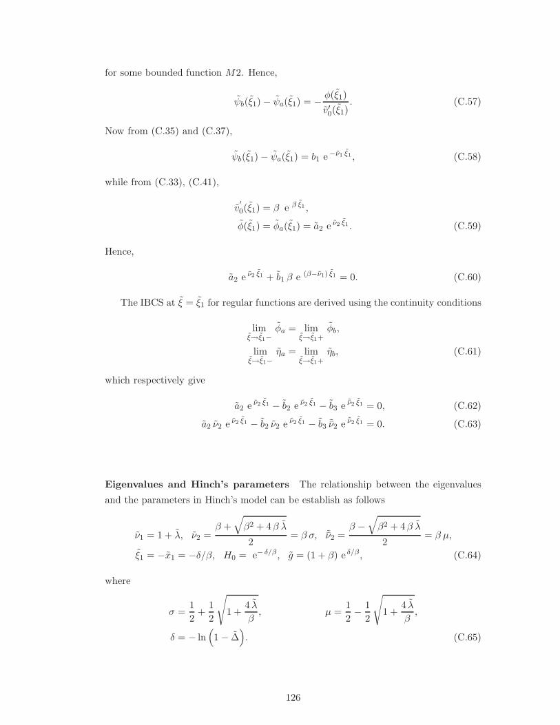
for some bounded function M2. Hence,

ψb(ξ1) − ψa(ξ1) = − φ(ξ1)

v′0(ξ1). (C.57)

Now from (C.35) and (C.37),

ψb(ξ1) − ψa(ξ1) = b1 e−ν1 ξ1 , (C.58)

while from (C.33), (C.41),

v′

0(ξ1) = β e β ξ1 ,

φ(ξ1) = φa(ξ1) = a2 e ν2 ξ1 . (C.59)

Hence,

a2 e ν2 ξ1 + b1 β e (β−ν1) ξ1 = 0. (C.60)

The IBCS at ξ = ξ1 for regular functions are derived using the continuity conditions

limξ→ξ1−

φa = limξ→ξ1+

φb,

limξ→ξ1−

ηa = limξ→ξ1+

ηb, (C.61)


a2 e ν2 ξ1 − b2 e ν2 ξ1 − b3 e˜ν2 ξ1 = 0, (C.62)

a2 ν2 e ν2 ξ1 − b2 ν2 e ν2 ξ1 − b3 ˜ν2 e˜ν2 ξ1 = 0. (C.63)

Eigenvalues and Hinch’s parameters The relationship between the eigenvalues

and the parameters in Hinch’s model can be establish as follows

ν1 = 1 + λ, ν2 =β +

√

β2 + 4β λ

2= β σ, ˜ν2 =

β −√

β2 + 4β λ

2= β µ,

ξ1 = −x1 = −δ/β, H0 = e− δ/β , g = (1 + β) e δ/β , (C.64)

where

σ =1

2+

1

2

√

1 +4 λ

β, µ =

1

2− 1

2

√

1 +4 λ

β,

δ = − ln(

1 − ∆)

. (C.65)

126

Therefore, from (C.51), (C.54), (C.60), (C.63), and (C.64) we have a system of six equa-

tions in terms of the undetermined arbitrary constants

b2 (g H0 − ν2) + b3 (g H0 − ˜ν2) − c1 ν1 + c3 ˜ν2 = 0,

b2 + b3 − c1 − c3 = 0,

b1 β g + c1

(

(1 + λ)2 + β)

= 0,

a2 e ν2 ξ1 + b1 β e (β−ν1) ξ1 = 0,

a2 e ν2 ξ1 − b2 e ν2 ξ1 − b3 e˜ν2 ξ1 = 0,

a2 ν2 e ν2 ξ1 − b2 ν2 e ν2 ξ1 − b3 ˜ν2 e˜ν2 ξ1 = 0. (C.66)

System (C.66), has non-trivial solutions only if the determinant of the coefficient

matrix is zero.∣∣∣∣∣∣∣∣∣∣∣∣∣∣∣∣∣∣∣∣∣

0 0 1 + β − β σ 1 + β − β µ −(1 + λ) β µ

0 0 1 1 −1 −1

0 β (1 + β) eδ/β 0 0 (1 + λ)2 + β 0

e−δ σ β e− δ

β (β−1−λ)0 0 0 0

e−δ σ 0 − e−δ σ − e−δ µ 0 0

β σ e−δ σ 0 −β σ e−δ σ −β µ e−δ µ 0 0

∣∣∣∣∣∣∣∣∣∣∣∣∣∣∣∣∣∣∣∣∣

= 0. (C.67)

This lead to a characteristic equation

fe(λ, β, δ) = β (σ − µ− 1) − 1 +(1 + β)(β µ+ 1 + λ)

(1 + λ)2 + βe−δ

(

λ/β+σ−1

)

= 0. (C.68)

C.3 Linearization of the Biktashev (2002) equations

In a laboratory reference frame with (x, T ) as coordinates, the front model [8], is

written in the form

∂E

∂T=∂2E

∂x2+ F (E,h),

∂h

∂T= G(E,h)/τ, (C.69)

where F (E,h) = Θ(E− 1)h, G(E,h) = Θ(−E)−h and Θ is a Heaviside step function.

In a moving frame of reference, the solutions to (C.69) for a right-ward moving front

are of the form E(x − c T, T ), h(x − c T, T ). Introducing the coordinates ξ = x − c T ,

t = T , and with c > 0, we look for functions E(ξ, t), h(ξ, t) that satisfy (C.69) thereby

getting

∂E

∂t=∂2E

∂ξ2+ c

∂E

∂ξ+ F (E,h),

∂h

∂t= c

∂h

∂ξ+G(E,h)/τ. (C.70)

127

NB: Traveling waves of (C.69) corresponds to stationary solutions of (C.70). Suppose

v0(ξ), h0(ξ), is a stationary solution of (C.70), then

d2v0dξ2

+ cdv0dξ

+ F (v0, h0) = 0,

cdh0

dξ+G(v0, h0)/τ = 0. (C.71)

Now linearizing (C.70) about(

v0(ξ), h0(ξ))

using

E = v0(ξ) + ε v1(ξ, t),

h = h0(ξ) + ε h1(ξ, t), (C.72)

where ε≪ 1, |v1(ξ, t)| ≪ 1 and |h1(ξ, t)| ≪ 1. Thus, (C.70) becomes

ε∂v1∂t

=d2v0dξ2

+ cdv0dξ

+ ε∂2v1∂ξ2

+ ε c∂v1∂ξ

+ F (v0 + ε v1, h0 + ε h1),

ε∂h1

∂t= c

dh0

dξ+ ε c

∂h1

∂ξ+G(v0 + ε v1, h0 + ε h1)/τ. (C.73)

Using Taylor expansion we express F (v0 + ε v1, h0 + ε h1) and G(v0 + ε v1, h0 + ε h1) as

F (v0 + ε v1, h0 + ε h1) = F (v0, h0) + ε∂F

∂v(v0, h0) v1 + ε

∂F

∂h(v0, h0)h1 +O(ε2),

G(v0 + ε v1, h0 + ε h1) = G(v0, h0) + ε∂G

∂v(v0, h0) v1 + ε

∂G

∂h(v0, h0)h1 +O(ε2).

(C.74)

Since Θ(−v0) ≡ Θ(ξ), Θ(v0 − 1) ≡ Θ(−ξ − ∆) and using the fact that δ(u) =dΘ(u)

du

and from chain rule δ(−v0) = δ(v0) =1

v′

0

δ(ξ), δ(v0 − 1) =−1

v′

0

δ(ξ + ∆),

F (v0, h0) = Θ(−ξ − ∆)h0, G(v0, h0) = Θ(ξ) − h0,

∂F

∂v(v0, h0) =

−1

v′

0

δ(ξ + ∆)h0,∂G

∂v(v0, h0) =

1

v′

0

δ(ξ),

∂F

∂h(v0, h0) = Θ(−ξ − ∆),

∂G

∂h(v0, h0) = −1.

(C.75)

Equation (C.70) then reduce to (neglecting higher order terms)

∂v1∂t

= c∂v1∂ξ

+∂2v1∂ξ2

− 1

v′

0

δ(ξ + ∆)h0 v1 + Θ(−ξ − ∆)h1,

∂h1

∂t= c

∂h1

∂ξ+( 1

v′

0

δ(ξ) v1 − h1

)

/τ. (C.76)

128

C.3.1 Eigenvalue problem

Let the linearized eqtn (C.76) support solutions of the form v1(ξ, t) = eλ t φ(ξ) and

h1(ξ, t) = eλ t ψ(ξ). This lead to the (temporal eigenvalue) problem

λφ =d2φ

dξ2+ c

dφ

dξ− 1

v′

0

δ(ξ + ∆)h0 φ+ Θ(−ξ − ∆)ψ,

λψ = cdψ

dξ+( 1

v′

0

δ(ξ)φ − ψ)

/τ, (C.77)

where φ(ξ) and ψ(ξ) are some eigenfunctions. The eigenvalue problem (C.77) of the

linearized equations (C.76) can be express in a compact form as

L V = λ V , (C.78)

where

L = Dd2

dξ2+ C

d

dξ+ F , V =

(

φ

ψ

)

, D =

(

1 0

0 0

)

,

C =

(

c 0

0 c

)

, F =

−1

v′

0

δ(ξ + ∆)h0 Θ(−ξ − ∆)

1

τ v′

0

δ(ξ) −1/τ

. (C.79)

Equation (C.78) is then converted into a three first-order (ODE) equations by lettingdφ

dξ= η and Ξ = (φ, η, ψ)T. Thus, we obtain a linear system in C

3

Ξ′= AΞ, (C.80)

where (′) =d

dξand

A =

0 1 0

λ+1

v′

0

δ(ξ + ∆)h0 −c −Θ(−ξ − ∆)

−1

τ c v′

0

δ(ξ) 01 + λ τ

τ c

, (C.81)

v0(ξ) =

ω − τ2 c2

1 + τ c2e ξ/τc, ξ ≤ −∆,

−α+ α e−c ξ, ξ ≥ −∆,

h0(ξ) =

e ξ/τc, ξ ≤ 0,

1, ξ ≥ 0,(C.82)

where

ξ = x− c t, ω = 1 + τ c2 (1 + α), ∆ =1

cln(

1 + α

α). (C.83)

129

We have three intervals (cases i = a, b, c) to consider. For case i = a, ξ ∈ (−∞,−∆)

so therefore in this interval, Θ(−ξ−∆) = 1, δ(ξ+∆) = δ(ξ) = 0 and h0 = e ξ/τc. Thus,

the matrix A in (C.81) becomes

Aa =

0 1 0

λ −c −1

0 0 ν1

, (C.84)

and whose characteristic equation (i.e., |µa I −Aa|=0) gives the spatial eigenvalues

µa1 = ν1 =

1 + λ τ

τ c,

µa2,3 = −ν2, −ν2, (C.85)

(C.86)

where

ν2 =c+

√c2 + 4λ

2, (C.87)

ν2 =c−

√c2 + 4λ

2. (C.88)

Eigenvectors for case i = a:

The eigenvector corresponding to µa1 = ν1 =

1 + λ τ

τ cis derived as follow

ν1 −1 0

−λ ν1 + c 1

0 0 0

va11

va21

va31

=

0

0

0

. (C.89)

From (C.89) and for some parameter k

va11 = k, va

21 = k ν1, va31 = k

(

λ− ν1(ν1 + c))

. (C.90)

Thus, the eigenvector is

~va1 =

va11

va21

va31

= k

1

ν1

−(ν21 + c ν1 − λ)

. (C.91)

Hence, taking k = 1,

~va1 =

1

ν1

−νq

, (C.92)

130

where νq = (ν21 + c ν1 − λ) =

(1 + λ τ)2 + τ c2

τ2 c2. For µa

2 = −ν2

−ν2 −1 0

−λ −ν2 + c 1

0 0 −ν2 − ν1

va12

va22

va32

=

0

0

0

, (C.93)

From (C.93) and for some parameter k

va12 = k, va

22 = −ν2 k, va32 = 0

(

since ν1 + ν2 6= 0)

. (C.94)

Thus, the eigenvector is

~va2 =

va12

va22

va32

= k

1

−ν2

0

, (C.95)

hence, taking k = 1,

~va2 =

1

−ν2

0

. (C.96)

Similarly, for µa3 = −ν2, the eigenvector is

~va3 =

1

−ν2

0

. (C.97)

For case i = b, ξ ∈ (−∆, 0), and in this region, Θ(−ξ−∆) = 0, δ(ξ+∆) = δ(ξ) = 0,

h0 = e ξ/τc. Therefore, the matrix A in (C.81) then becomes

Ab =

0 1 0

λ −c 0

0 0 ν1

, (C.98)

from which we get the spatial eigenvalues

µb1 = ν1 =

1 + λ τ

τ c,

µb2,3 = −ν2, −ν2. (C.99)

Eigenvectors for case i = b:

131

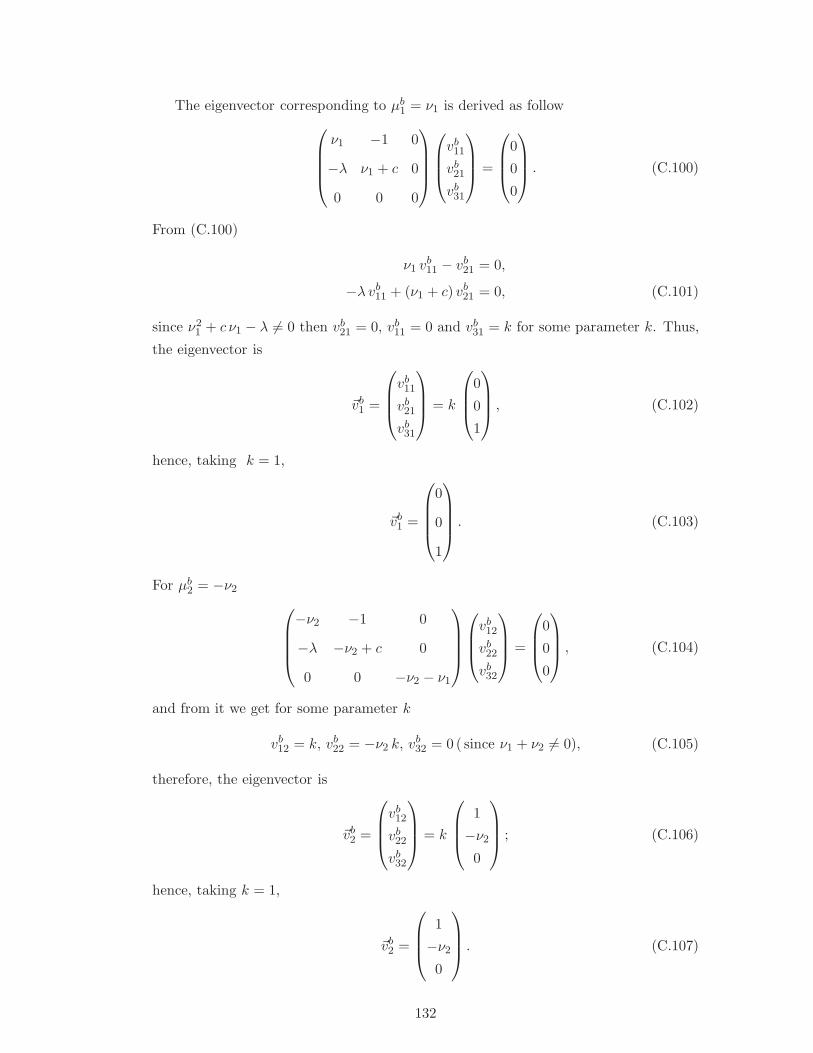
The eigenvector corresponding to µb1 = ν1 is derived as follow

ν1 −1 0

−λ ν1 + c 0

0 0 0

vb11

vb21

vb31

=

0

0

0

. (C.100)

From (C.100)

ν1 vb11 − vb

21 = 0,

−λ vb11 + (ν1 + c) vb

21 = 0, (C.101)

since ν21 + c ν1 − λ 6= 0 then vb

21 = 0, vb11 = 0 and vb

31 = k for some parameter k. Thus,

the eigenvector is

~vb1 =

vb11

vb21

vb31

= k

0

0

1

, (C.102)


~vb1 =

0

0

1

. (C.103)

For µb2 = −ν2

−ν2 −1 0

−λ −ν2 + c 0

0 0 −ν2 − ν1

vb12

vb22

vb32

=

0

0

0

, (C.104)

and from it we get for some parameter k

vb12 = k, vb

22 = −ν2 k, vb32 = 0 ( since ν1 + ν2 6= 0), (C.105)

therefore, the eigenvector is

~vb2 =

vb12

vb22

vb32

= k

1

−ν2

0

; (C.106)


~vb2 =

1

−ν2

0

. (C.107)

132

Similarly, for µb3 = −ν2, the eigenvector will then be

~vb3 =

1

−ν2

0

. (C.108)

And lastly for the case i = c, ξ ∈ (0,+∞), then Θ(−ξ − ∆) = 0, δ(ξ + ∆) = δ(ξ) = 0

and h0 = 1. Thus, the matrix A in (C.81) then becomes

Ac =

0 1 0

λ −c 0

0 0 ν1

, (C.109)

from which we get the same set of spatial eigenvalues as with the case i = b

µc1 = ν1,

µc2,3 = −ν2, −ν2, (C.110)

and so we will have the same corresponding eigenvectors

~vc1 =

0

0

1

, ~vc

2 =

1

−ν2

0

, ~vc

3 =

1

−ν2

0

. (C.111)

C.3.2 Characteristic equation

To determine the characteristic equation we rewrite the solutions to (C.80) by consider-

ing each of the three regions. Each of the solutions are written as a linear combination

of the product of its corresponding eigenvectors and the exponential of its eigenvalues.

That is,

φi

ηi

ψi

=∑

j

ij ~vij eµi

j ξ, (C.112)

and is such that Ai ~v ij = µi

j ~vij, where Ai = Ai(λ), µi

j = µij(λ) for i = a, b, c and

j = 1, 2, 3.

NB: Note that ~va2 = ~vb

2 = ~vc2, ~v

a3 = ~vb

3 = ~vc3, ~v

b1 = ~vc

1. The solutions for the three

cases can be written explicitly as

φa

ηa

ψa

= a1 ~va1 eν1 ξ + a2 ~v

a2 e−ν2 ξ + a3 ~v

a3 e−ν2 ξ, (C.113)

133

φb

ηb

ψb

= b1 ~vb1 eν1 ξ + b2 ~v

b2 e−ν2 ξ + b3 ~v

b3 e−ν2 ξ, (C.114)

φc

ηc

ψc

= c1 ~vc1 eν1 ξ + c2 ~v

c2 e−ν2 ξ + c3 ~v

c3 e−ν2 ξ, (C.115)

where ν1 =1 + λ τ

τ c, ν2 =

c+√c2 + 4λ

2, ν2 =

c−√c2 + 4λ

2.

And ~va1 , ~v

a2 , ~v

a3 ; ~vb

1, ~vb2, ~v

b3; ~v

c1, ~v

c2, ~v

c3 as given in equations (C.92) - (C.96), (C.103) -

(C.108) and (C.111)

~v a1 =

va11

va21

va31

=

1

ν1

−νq

, ~v b

1 =

vb11

vb21

vb31

= ~v c1 =

vc11

vc21

vc31

=

0

0

1

,

~v a2 =

va12

va22

va32

= ~v b2 =

vb12

vb22

vb32

= ~v c2 =

vc12

vc22

vc32

=

1

−ν2

0

,

~v a3 =

va13

va23

va33

= ~v b3 =

vb13

vb23

vb33

= ~v c3 =

vc13

vc23

vc33

=

1

−ν2

0

. (C.116)

Determination of the constants (ij): To determine the constants ij : i = a, b, c; j =

1, 2, 3, the solutions (C.113), (C.114) and (C.115) has to satisfy both the boundaries

at ±∞ (i.e., ξ → ±∞) and at the internal boundaries ξ = −∆ and ξ = 0.

Boundary conditions at ±∞: With λ ≥ 0 : ν1 > 0, ν2 > 0, ν2 < 0:

For the case i = a

limξ→−∞

φa

ηa

ψa

, (C.117)

must be bounded and therefore a2 = 0. Thus,

φa

ηa

ψa

= a1

1

ν1

−νq

eν1 ξ + a3

1

−ν2

0

e−ν2 ξ. (C.118)

134

For the case i = b, we can only consider the internal boundary conditions and so the

solution (for the time being) is

φb

ηb

ψb

= b1

0

0

1

eν1 ξ + b2

1

−ν2

0

e−ν2 ξ + b3

1

−ν2

0

e−ν2 ξ. (C.119)

However, for the case i = c

limξ→+∞

φc

ηc

ψc

(C.120)

must be bounded and so therefore c1 = 0, c3 = 0. Thus

φc

ηc

ψc

= c2

1

−ν2

0

e−ν2 ξ. (C.121)

Internal boundary conditions (IBCS): Let (C.80) be rewritten in terms of regular

(R1, R2) and singular (S1, S2) functions

dφ

dξ= η,

dη

dξ=

R1(ξ)︷︸︸︷

λφ− c η − Θ(−ξ − ∆)ψ +

S1(ξ)︷︸︸︷

1

v′

0

δ(ξ + ∆)h0 φ,

dψ

dξ=

R2(ξ)︷︸︸︷

ν1 ψ −

S2(ξ)︷︸︸︷

1

τc v′

0

δ(ξ)φ . (C.122)

IBCS at ξ = −∆: The trick here is to integrate the second equation from (C.122)

around ξ = −∆ over a small range, (−∆ − ε,−∆ + ε) and consider limit ε→ 0,

limε→0

∫ −∆+ε

−∆−ε

dη

dξdξ = lim

ε→0

∫ −∆+ε

−∆−εR1(ξ) dξ + lim

ε→0

∫ −∆+ε

−∆−ε

h0(ξ)φ(ξ)

v′0(ξ)δ(ξ + ∆) dξ.

(C.123)

Its solution is

limε→0

[ηb(−∆ + ε) − ηa(−∆ − ε)

]≤ lim

ε→0M ε+ lim

ε→0

h0(−∆)φ(−∆)

v′0(−∆), (C.124)

hence,

ηb(−∆) − ηa(−∆) =h0(−∆)φ(−∆)

v′0(−∆), (C.125)

135

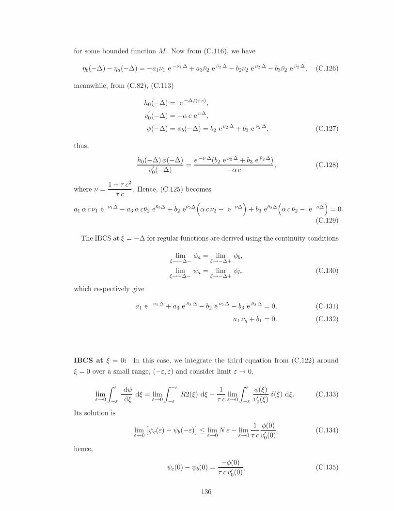
for some bounded function M . Now from (C.116), we have

ηb(−∆) − ηa(−∆) = −a1ν1 e−ν1 ∆ + a3ν2 e ν2 ∆ − b2ν2 e ν2 ∆ − b3ν2 e ν2 ∆, (C.126)

meanwhile, from (C.82), (C.113)

h0(−∆) = e−∆/(τ c),

v′

0(−∆) = −α c e c ∆,

φ(−∆) = φb(−∆) = b2 e ν2 ∆ + b3 e ν2 ∆, (C.127)

thus,

h0(−∆)φ(−∆)

v′0(−∆)=e−ν ∆(b2 e ν2 ∆ + b3 e ν2 ∆)

−α c , (C.128)

where ν =1 + τ c2

τ c. Hence, (C.125) becomes


α c ν2 − e−ν∆)

+ b3 eν2∆(

α c ν2 − e−ν∆)

= 0.

(C.129)

The IBCS at ξ = −∆ for regular functions are derived using the continuity conditions

limξ→−∆−

φa = limξ→−∆+

φb,

limξ→−∆−

ψa = limξ→−∆+

ψb, (C.130)


a1 e−ν1 ∆ + a3 e ν2 ∆ − b2 e ν2 ∆ − b3 e ν2 ∆ = 0, (C.131)

a1 νq + b1 = 0. (C.132)

IBCS at ξ = 0: In this case, we integrate the third equation from (C.122) around

ξ = 0 over a small range, (−ε, ε) and consider limit ε→ 0,

limε→0

∫ ε

−ε

dψ

dξdξ = lim

ε→0

∫ −ε

−εR2(ξ) dξ − 1

τ climε→0

∫ ε

−ε

φ(ξ)

v′0(ξ)δ(ξ) dξ. (C.133)

Its solution is

limε→0

[ψc(ε) − ψb(−ε)

]≤ lim

ε→0N ε− lim

ε→0

1

τ c

φ(0)

v′0(0), (C.134)

hence,

ψc(0) − ψb(0) =−φ(0)

τ c v′0(0), (C.135)

136

for some bounded function N . Now from (C.116), we have

ψc(0) − ψb(0) = 0 − b1 = −b1, (C.136)

and meanwhile from (C.82), (C.115)

v′

0(0) = −α c,φ(0) = φc(0) = c2; (C.137)

thus,

φ(0)

τ c v′0(0)=

c2α τ c2

, (C.138)

hence, (C.135) becomes

b1 α τ c2 + c2 = 0. (C.139)

The IBCS at ξ = 0 for regular functions are also derived using the continuity condi-

tions

limξ→0−

φb = limξ→0+

φc,

limξ→0−

ηb = limξ→0+

ηc, (C.140)

which respectively yield

b2 + b3 − c2 = 0, (C.141)

b2 ν2 + b3 ν2 − c2 ν2 = 0. (C.142)

Thus, we have a system of six equations in terms of the undetermined arbitrary con-

stants


α c ν2 − e−ν∆)

+b3 eν2∆(

α c ν2 − e−ν∆)

= 0,

a1 e−ν1 ∆ + a3 e ν2 ∆ − b2 e ν2 ∆ − b3 e ν2 ∆ = 0,

a1 νq + b1 = 0,

b1 α τ c2 + c2 = 0,

b2 + b3 − c2 = 0,

b2 ν2 + b3 ν2 − c2 ν2 = 0. (C.143)

The system in (C.143) with a1, a3, b1, b2, b3, and, c2 to be determined can be written in

matrix form having a six-by-six coefficient matrix. The system has nontrivial solutions

137

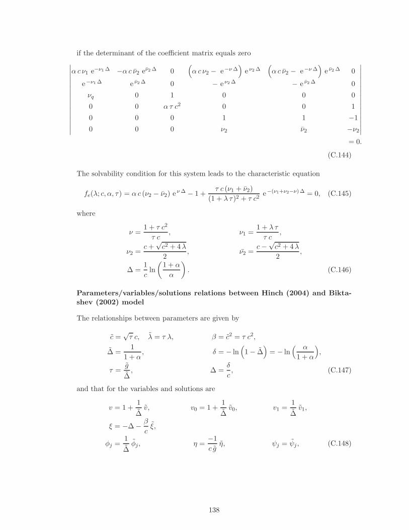
if the determinant of the coefficient matrix equals zero

∣∣∣∣∣∣∣∣∣∣∣∣∣∣∣∣

α c ν1 e−ν1 ∆ −α c ν2 eν2 ∆ 0(

α c ν2 − e−ν ∆)

e ν2 ∆(

α c ν2 − e−ν ∆)

e ν2 ∆ 0

e−ν1 ∆ e ν2 ∆ 0 − e ν2 ∆ − e ν2 ∆ 0

νq 0 1 0 0 0

0 0 α τ c2 0 0 1

0 0 0 1 1 −1

0 0 0 ν2 ν2 −ν2

∣∣∣∣∣∣∣∣∣∣∣∣∣∣∣∣

= 0.

(C.144)

The solvability condition for this system leads to the characteristic equation

fe(λ; c, α, τ) = α c (ν2 − ν2) e ν ∆ − 1 +τ c (ν1 + ν2)

(1 + λ τ)2 + τ c2e−(ν1+ν2−ν)∆ = 0, (C.145)

where

ν =1 + τ c2

τ c, ν1 =

1 + λ τ

τ c,

ν2 =c+

√c2 + 4λ

2, ν2 =

c−√c2 + 4λ

2,

∆ =1

cln

(1 + α

α

)

. (C.146)

Parameters/variables/solutions relations between Hinch (2004) and Bikta-shev (2002) model

The relationships between parameters are given by

c =√τ c, λ = τ λ, β = c2 = τ c2,

∆ =1

1 + α, δ = − ln

(

1 − ∆)

= − ln( α

1 + α

)

,

τ =g

∆, ∆ =

δ

c, (C.147)

and that for the variables and solutions are

v = 1 +1

∆v, v0 = 1 +

1

∆v0, v1 =

1

∆v1,

ξ = −∆ − β

cξ,

φj =1

∆φj, η =

−1

c gη, ψj = ψj , (C.148)

138

for j = a, b, c. Meanwhile, for the yet to be determined constants and eigenvalues the

relationships are

a1 =1

∆e

δβ (1+λ)

c1, a2 = 0 {c2 = 0}, a3 =1

∆e−δ µ c3,

b1 = eδβ (1+λ)

b1, b2 =1

∆e−δ σ b2, b3 =

1

∆e−δ µ b3,

c1 = 0 {a1 = 0}, c2 =1

∆e−δ σ a2, c3 = 0 {a3 = 0};

ν1 =c

βν1 =

c

β(1 + λ), ν2 =

c

βν2 = c σ, ν2 =

c

β˜ν2 = c µ. (C.149)

C.3.3 Adjoint eigenvalue problem

We can construct the adjoint eigenvalue problem to the front model from the eigenvalue

problem (C.79) Thus, the adjoint eigenvalue problem is

L+ W = µ W , (C.150)

where

L+ = DT d2

dξ2− C

d

dξ+ F T , DT = D, W =

(

φ∗

ψ∗

)

, (C.151)

and

F T =

−1

v′

0

δ(ξ + ∆)h01

τ v′

0

δ(ξ)

Θ(−ξ − ∆) −1/τ

. (C.152)

Now when casted into a three ODE equations, (C.150) becomes

dφ∗

dξ= η∗,

dη∗

dξ=(

µ+1

v′

0

δ(ξ + ∆)h0

)

φ∗ + c η∗ − 1

τ v′

0

δ(ξ)ψ∗,

dψ∗

dξ=

1

cΘ(−ξ − ∆)φ∗ − (1 + µ τ)

τ cφ∗, (C.153)

which is then written in matrix format as

Ξ∗′ = B Ξ∗, (C.154)

where (′) =d

dξand

B =

0 1 0

µ+1

v′

0

δ(ξ + ∆)h0 c−1

τ c v′

0

δ(ξ)

1

cΘ(−ξ − ∆) 0 −(1 + µ τ)

τ c

. (C.155)

139

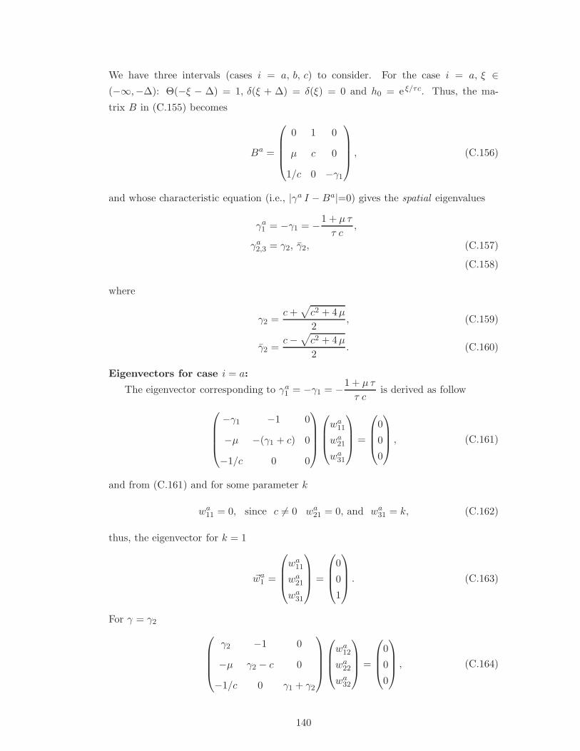
We have three intervals (cases i = a, b, c) to consider. For the case i = a, ξ ∈(−∞,−∆): Θ(−ξ − ∆) = 1, δ(ξ + ∆) = δ(ξ) = 0 and h0 = e ξ/τc. Thus, the ma-

trix B in (C.155) becomes

Ba =

0 1 0

µ c 0

1/c 0 −γ1

, (C.156)

and whose characteristic equation (i.e., |γa I −Ba|=0) gives the spatial eigenvalues

γa1 = −γ1 = −1 + µ τ

τ c,

γa2,3 = γ2, γ2, (C.157)

(C.158)

where

γ2 =c+

√

c2 + 4µ

2, (C.159)

γ2 =c−

√

c2 + 4µ

2. (C.160)

Eigenvectors for case i = a:

The eigenvector corresponding to γa1 = −γ1 = −1 + µ τ

τ cis derived as follow

−γ1 −1 0

−µ −(γ1 + c) 0

−1/c 0 0

wa11

wa21

wa31

=

0

0

0

, (C.161)

and from (C.161) and for some parameter k

wa11 = 0, since c 6= 0 wa

21 = 0, and wa31 = k, (C.162)

thus, the eigenvector for k = 1

~wa1 =

wa11

wa21

wa31

=

0

0

1

. (C.163)

For γ = γ2

γ2 −1 0

−µ γ2 − c 0

−1/c 0 γ1 + γ2

wa12

wa22

wa32

=

0

0

0

, (C.164)

140

and we get from (C.164) for some parameter k

wa12 = k, wa

22 = γ2 k, ( since γ2(γ2 − c) − µ = 0) , wa32 =

k

c (γ1 + γ2). (C.165)

Hence, the eigenvector is (for k = 1)

~wa2 =

wa12

wa22

wa32

=

1

γ2

γ3

, (C.166)

where γ3 =1

c (γ1 + γ2).

Similarly, for γ = γ2, the eigenvector will then be

~wa3 =

wa13

wa23

wa33

=

1

γ2

γ3

, (C.167)

where γ3 =1

c (γ1 + γ2).

For case i = b, ξ ∈ (−∆, 0), and in this region, Θ(−ξ−∆) = 0, δ(ξ + ∆) = δ(ξ) = 0,

h0 = e ξ/τc. Therefore, the matrix B in (C.155) then becomes

Bb =

0 1 0

µ c 0

0 0 −γ1

, (C.168)

from which we get the spatial eigenvalues,γb1 = −γ1, γ

b2,3 = γ2, γ2.

Eigenvectors for case i = b:

The eigenvector corresponding to γb1 = −γ1 is derived as follow

−γ1 −1 0

−µ −(γ1 + c) 0

0 0 0

wb11

wb21

wb31

=

0

0

0

, (C.169)

which yields

−γ1wb11 − wb

21 = 0,

−µwb11 − (γ1 + c)wb

21 = 0, (C.170)

since γ21 + c γ1 −µ 6= 0 then wb

21 = 0, wb11 = 0 and wb

31 = k for some parameterk. Thus,

the eigenvector is, for k = 1

~wb1 =

wb11

wb21

wb31

=

0

0

1

. (C.171)

141

For γb2 = γ2

γ2 −1 0

−µ γ2 − c 0

0 0 γ1 + γ2

wb12

wb22

wb32

=

0

0

0

, (C.172)

and then from (C.172) for some parameter k

wb12 = k, wb

22 = γ2 k ( since γ22 − cγ2 − µ = 0), wb

32 = 0 ( γ1 + γ2 6= 0). (C.173)

Therefore, the eigenvector for k = 1 is

~wb2 =

wb12

wb22

wb32

=

1

γ2

0

. (C.174)

Similarly, for γb3 = γ2, the eigenvector will then be

~wb3 =

1

γ2

0

. (C.175)

For region (i.e. case i = c) three, the matrix is exactly the same as that one in (C.168),

that is case i = b, and so has the eigenvectors

~wc1 =

wc11

wc21

wc31

=

0

0

1

, ~wc

2 =

wc12

wc22

wc32

=

1

γ2

0

, ~wc

2 =

wc13

wc23

wc33

=

1

γ2

0

. (C.176)

C.3.4 Characteristic equation for the adjoint problem

To determine the characteristic equation, we rewrite the solutions to (C.154) taking

into account each of the three regions. The solutions are written as

φ∗i

η∗i

ψ∗i

=∑

j

ij ~wij e γi

j ξ, (C.177)

and is such that Bi ~w ij = γi

j ~wij, where Bi = Bi(µ), γi

j = γij(µ) for i = a, b, c and

j = 1, 2, 3.

NB: The solutions for the three cases can be written explicitly as

φ∗a

η∗a

ψ∗a

= a∗1 ~wa1 e−γ1 ξ + a∗2 ~w

a2 eγ2 ξ + a∗3 ~w

a3 eγ2 ξ, (C.178)

142

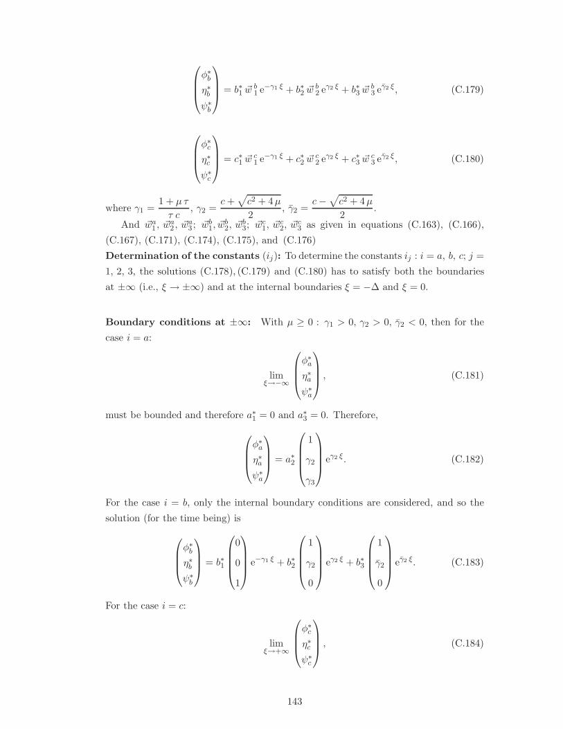
φ∗bη∗bψ∗

b

= b∗1 ~wb1 e−γ1 ξ + b∗2 ~w

b2 eγ2 ξ + b∗3 ~w

b3 eγ2 ξ, (C.179)

φ∗c

η∗c

ψ∗c

= c∗1 ~wc1 e−γ1 ξ + c∗2 ~w

c2 eγ2 ξ + c∗3 ~w

c3 eγ2 ξ, (C.180)

where γ1 =1 + µ τ

τ c, γ2 =

c+√

c2 + 4µ

2, γ2 =

c−√

c2 + 4µ

2.

And ~wa1 , ~w

a2 , ~w

a3 ; ~wb

1, ~wb2, ~w

b3; ~wc

1, ~wc2, ~w

c3 as given in equations (C.163), (C.166),

(C.167), (C.171), (C.174), (C.175), and (C.176)

Determination of the constants (ij): To determine the constants ij : i = a, b, c; j =

1, 2, 3, the solutions (C.178), (C.179) and (C.180) has to satisfy both the boundaries

at ±∞ (i.e., ξ → ±∞) and at the internal boundaries ξ = −∆ and ξ = 0.

Boundary conditions at ±∞: With µ ≥ 0 : γ1 > 0, γ2 > 0, γ2 < 0, then for the

case i = a:

limξ→−∞

φ∗a

η∗a

ψ∗a

, (C.181)

must be bounded and therefore a∗1 = 0 and a∗3 = 0. Therefore,

φ∗a

η∗a

ψ∗a

= a∗2

1

γ2

γ3

eγ2 ξ. (C.182)

For the case i = b, only the internal boundary conditions are considered, and so the

solution (for the time being) is

φ∗bη∗bψ∗

b

= b∗1

0

0

1

e−γ1 ξ + b∗2

1

γ2

0

eγ2 ξ + b∗3

1

γ2

0

eγ2 ξ. (C.183)

For the case i = c:

limξ→+∞

φ∗c

η∗c

ψ∗c

, (C.184)

143

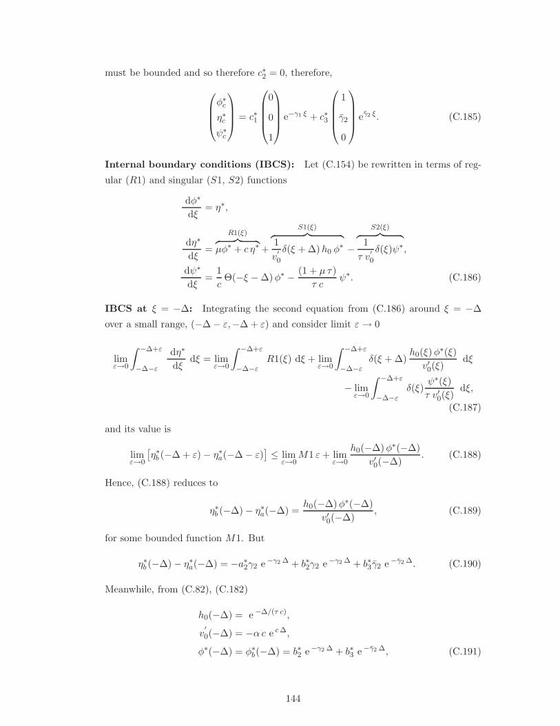
must be bounded and so therefore c∗2 = 0, therefore,

φ∗c

η∗c

ψ∗c

= c∗1

0

0

1

e−γ1 ξ + c∗3

1

γ2

0

eγ2 ξ. (C.185)

Internal boundary conditions (IBCS): Let (C.154) be rewritten in terms of reg-

ular (R1) and singular (S1, S2) functions

dφ∗

dξ= η∗,

dη∗

dξ=

R1(ξ)︷︸︸︷

µφ∗ + c η∗ +

S1(ξ)︷︸︸︷

1

v′

0

δ(ξ + ∆)h0 φ∗ −

S2(ξ)︷︸︸︷

1

τ v′

0

δ(ξ)ψ∗,

dψ∗

dξ=

1

cΘ(−ξ − ∆)φ∗ − (1 + µ τ)

τ cψ∗. (C.186)

IBCS at ξ = −∆: Integrating the second equation from (C.186) around ξ = −∆

over a small range, (−∆ − ε,−∆ + ε) and consider limit ε→ 0

limε→0

∫ −∆+ε

−∆−ε

dη∗

dξdξ = lim

ε→0

∫ −∆+ε

−∆−εR1(ξ) dξ + lim

ε→0

∫ −∆+ε

−∆−εδ(ξ + ∆)

h0(ξ)φ∗(ξ)

v′0(ξ)dξ

− limε→0

∫ −∆+ε

−∆−εδ(ξ)

ψ∗(ξ)

τ v′0(ξ)dξ,

(C.187)

and its value is

limε→0

[η∗b (−∆ + ε) − η∗a(−∆ − ε)

]≤ lim

ε→0M1 ε+ lim

ε→0

h0(−∆)φ∗(−∆)

v′0(−∆). (C.188)

Hence, (C.188) reduces to

η∗b (−∆) − η∗a(−∆) =h0(−∆)φ∗(−∆)

v′0(−∆), (C.189)

for some bounded function M1. But

η∗b (−∆) − η∗a(−∆) = −a∗2γ2 e−γ2 ∆ + b∗2γ2 e−γ2 ∆ + b∗3γ2 e−γ2 ∆. (C.190)

Meanwhile, from (C.82), (C.182)

h0(−∆) = e−∆/(τ c),

v′

0(−∆) = −α c e c ∆,

φ∗(−∆) = φ∗b(−∆) = b∗2 e−γ2 ∆ + b∗3 e−γ2 ∆, (C.191)

144

thus,

h0(−∆)φ∗(−∆)

v′0(−∆)=e−γ ∆(b∗2 e−γ2 ∆ + b∗3 e−γ2 ∆)

−α c , (C.192)

where γ =1 + τ c2

τ c. Hence, (C.189) becomes

a∗2 α c γ2 e−γ2∆ − b∗2 e−γ2∆(

α c γ2 + e−γ∆)

− b∗3 e−γ2∆(

α c γ2 + e−γ∆)

= 0. (C.193)

The IBCS at ξ = −∆ for regular functions are derived using the continuity conditions

limξ→−∆−

φ∗a = limξ→−∆+

φ∗b ,

limξ→−∆−

ψ∗a = lim

ξ→−∆+ψ∗

b , (C.194)


a∗2 e−γ2 ∆ − b∗2 e−γ2 ∆ − b∗3 e−γ2 ∆ = 0, (C.195)

and

a∗2 γ3 e−γ2 ∆ − b∗1 e γ1 ∆ = 0, (C.196)

where γ3 =1

c (γ1 + γ2).

IBCS at ξ = 0: In this case, we integrate the second from (C.186) around ξ = 0 over

a small range, (−ε, ε) and consider limit ε→ 0.

limε→0

∫ ε

−ε

dη∗

dξdξ = lim

ε→0

∫ ε

−εR1(ξ) dξ + lim

ε→0

∫ ε

−εδ(ξ + ∆)

h0(ξ)φ∗(ξ)

v′0(ξ)dξ

− limε→0

∫ ε

−εδ(ξ)

ψ∗(ξ)

τ v′0(ξ)dξ, (C.197)

which evaluates to

limε→0

[η∗c (ε) − η∗b (−ε)

]≤ lim

ε→0M2 ε− lim

ε→0

ψ∗(ξ)

τ v′0(ξ), (C.198)

thus,

η∗c (0) − η∗b (0) = − ψ∗(0)

τ v′0(0), (C.199)

for some bounded function M2. Now from (C.185), we have

η∗c (0) − η∗b (0) = −b∗2 γ2 − b∗3 γ2 + c∗3 γ2, (C.200)

and from (C.82), (C.185)

v′

0(0) = −α c,ψ∗(0) = ψ∗

c (0) = c∗1. (C.201)

Hence, (C.189) becomes

b∗2 α τ c γ2 + b∗3α τ c γ2 + c∗1 − c∗3α τ c γ2 = 0. (C.202)

145

The IBCS at ξ = 0 for regular functions are also derived using the continuity condi-

tions

limξ→0−

φ∗b = limξ→0+

φ∗c ,

limξ→0−

ψ∗b = lim

ξ→0+ψ∗

c , (C.203)

which respectively yield

b∗2 + b∗3 − c∗3 = 0, (C.204)

b∗1 − c∗1 = 0. (C.205)

Thus, we have a system of six equations in terms of the undetermined arbitrary con-

stants

a∗2 α c γ2 e−γ2∆ − b∗2 e−γ2∆(α c γ2 + e−γ∆

)− b∗3 e−γ2∆

(α c γ2 + e−γ∆

)= 0,

a∗2 e−γ2 ∆ − b∗2 e−γ2 ∆ − b∗3 e−γ2 ∆ = 0,

a∗2 γ3 e−γ2 ∆ − b∗1 e γ1 ∆ = 0,

b∗2 α τ c γ2 + b∗3 α τ c γ2 + c∗1 − c∗3 α τ c γ2 = 0,

b∗2 + b∗3 − c∗3 = 0,

b∗1 − c∗1 = 0. (C.206)

The system in (C.206) can be written in matrix form with a six-by-six coefficient matrix

whose determinant is given as∣∣∣∣∣∣∣∣∣∣∣∣∣∣∣∣∣∣∣∣∣

α c γ2 e−γ2∆ 0 −(α c γ2 + e−γ∆) e−γ2 ∆ −(α c γ2 + e−γ∆) e−γ2 ∆ 0 0

e−γ2∆ 0 − e−γ2∆ e−γ2∆ 0 0

γ3 e−γ2∆ − eγ1∆ 0 0 0 0

0 0 α τ cγ2 α τ c γ2 1 −α τ c γ2

0 0 1 1 0 −1

0 1 0 0 −1 0

∣∣∣∣∣∣∣∣∣∣∣∣∣∣∣∣∣∣∣∣∣

= 0.

(C.207)

System (C.206), has non-trivial solutions only if the determinant of the coefficient

matrix is zero. This lead to a characteristic equation(

f∗e (µ; c, α, τ))

f∗e = α c (γ2 − γ2) eγ∆ − 1 +1

τ c (γ1 + γ2)e−(γ1+γ2−γ)∆ = 0. (C.208)

146

NB: Note that1

τ c (γ1 + γ2)≡ τ c(γ1 + γ2)

(1 + µ τ)2 + τ c2. Hence,

f∗e = α c (γ2 − γ2) eγ∆ − 1 +τ c (γ1 + γ2)

(1 + µ τ)2 + τ c2e−(γ1+γ2−γ)∆ = 0, (C.209)

where

γ =1 + τ c2

τ c, γ1 =

1 + µ τ

τ c,

γ2 =c+

√

c2 + 4µ

2, γ2 =

c−√

c2 + 4µ

2,

∆ =1

cln

(1 + α

α

)

. (C.210)

147

Bibliography

[1] R. R. Aliev and A. V. Panfilov. A simple two-variable model of cardiac excitation.

Chaos, Solitons and Fractals, 7(3):293–301, 1996.

[2] M. Argentina and P. Coullet. Colliding waves in a model excitable medium:

Preservation, annihilation, and bifurcation. Phys. Rev. Lett., 79(15):2803–2806,

1997.

[3] M. Argentina, P. Coullet, and V. Krinsky. Head-on-collisions of waves in an ex-

citable FitzHugh-Nagumo system: a transition from wave annihilation to classical

wave behavior. J. Theor. Biol., 205:47–52, 2000.

[4] O. V. Aslanidi and O. A. Mornev. Soliton-like regimes and excitation pulse

reflection (Echo) in homogeneous cardiac purkinje fibres: Results of numerical

simulations. J. Biol. Phys., 25:149–164, 1999.

[5] D. Barkley. A model for fast computer simulation of waves in excitable media.

Physica D., 49:61–70, 1991.

[6] R. D. Benguria and M. C. Depassier. Speed of fronts of the reaction-diffusion

equation. Phys. Rev. Lett, 77(6):1171–1173, 1996.

[7] O. Bernus, R. Wilders, C. W. Zemlin, H. Verschelde, and A. V. Panfilov. A

computationally efficient electrophysiological model of human ventricular cells.

Am. J. Physiol. Heart. Circ Physiol., 282(6):H2296–H2308, 2002.

[8] V. N. Biktashev. Dissipation of the excitation wavefronts. Phys. Rev. Lett.,

89(16):168102–1 – 168102–4, 2002.

[9] V. N. Biktashev. A simplified model of propagation and dissipation of excitation

fronts. Int. J. of Birfucation and Chaos, 13(12):3605–3619, 2003.

[10] V. N. Biktashev and I. V. Biktasheva. Dissipation of Excitation Fronts as a

Mechanism of Conduction Block in Re-entrant Waves,, volume 3504 of Lecture

Notes in Computer Science, pages 283–292. Springer Berlin/Heidelberg, 2005.

[11] V. N. Biktashev and A. V. Holden. Deterministic Brownian motion in the hy-

permeander of spiral waves. Physica D., 116(3–4):342–354, 1998.

148

[12] I. V. Biktasheva, R. D. Simitev, R. S. Suckley, and V. N. Biktashev. Asymptotic

properties of mathematical models of excitability. Phil. Trans. Roy. Soc. A.,

364(1842):1283–1298, 2006.

[13] M. A. Biot. Variational principles in heat transfer. Oxford University Press,

1970.

[14] G. Bordyugov. Dynamics and Stability of Pulses and Pulse Trains in Excitable

Media. PhD thesis, Technical University Berlin, Germany, 2006.

[15] T. Bountis, C. F. Starmer, and A. Bezerianos. Stationary pulses and wave front

formation in an excitable medium. Progr. Theor. Phys. Suppl., 139:12–33, 2000.

[16] W. E. Boyce and R. C. Diprima. Elementary differential equations and boundary

value problems. John Wiley & Sons, Inc., eigth edition, 2005.

[17] M. Braun. Differential equations and their applications. Springer-Verlag New

York, Inc., fourth edition, 1993.

[18] J. Brindley, V. N. Biktashev, and M. A. Tsyganov. Invasion waves in populations

with excitable dynamics. Biol. Invasions., 7:807816, 2005.

[19] N. F. Britton. Threshold phenomena and solitary traveling waves in a class of

reaction-diffusion systems. SIAM J. Appl. Math., 42(1):188–217, 1982.

[20] N. F. Britton. Essential Mathematical Biology. Springer Verlag London, first

edition, 2003.

[21] K. J. Brown and A. A. Lacey. Reaction-Diffusion Equations. Oxford Science

Publications, 1990.

[22] G. Cain and G. H. Meyer. Separation of Variables for Partial Differential Equa-

tions: An Eigenfunction Approach. Chapman & Hall/CRC, 2006.

[23] R. G. Casten, H. Cohen, and P. A. Lagerstrom. Perturbation analysis of an

approximation to the Hodgkin-Huxley theory. Quart. Appl. Math., 32(4):365–

402, 1975.

[24] J. W. Cooley and F. A. Dodge Jr. Digital computer solutions for excitation and

propagation of the nerve impulse. Biophys. J., 6:583–599, 1966.

[25] M. Courtemanche, R. Ramirez, and S. Nattel. Ionic mechanisms underlying

human atrial action potential properties: Insights from a mathematical model.

Am. J. Physiol. Heart. Circ Physiol, 275:H301–H321, 1998.

[26] M. C. Cross and P. C. Hohenberg. Pattern formation outside of equilibrium. Rev.

Mod. Phys., 65:852–1086, 1993.

149

[27] P. C. Dauby, Th. Desaive, H. Croisier, and Ph. Kolh. Standing waves in FitzHugh-

Nagumo model of cardiac electrical activity. Phys. Rev. E., 73:021908 [1–5], 2006.

[28] J. D. Dockery. Existence of standing pulse solutions for an excitable activator-

inhibitory system. J. Dynam. Diff. Eqtns., 4(2):231–257, 1992.

[29] G. Duckett and D. Barkley. Modelling the dynamics of cardiac action potential.

Phys. Rev. Lett., 85(4):884–887, 2000.

[30] L. Edelstein-Keshet. Mathematical models in biology. SIAM, 2005.

[31] I. Farkas, D. Helbing, and T. Vicsek. Social behaviour: Mexican waves in an

excitable media. Nature, 419:131–132, 2002.

[32] F. Fenton and A. Karma. Vortex dynamics in three-dimensional continuous

myocardium with fiber rotation: Filament instability and fibrillation. Chaos,

8(1):20–47, 1998.

[33] R. A. FitzHugh. Impulses and physiological states in theoritical models of nerve

membrane. Biophys. J., 1:445–466, 1961.

[34] G. Flores. The stable manifold of the standing wave of the Nagumo equation. J.

Differential Equations, 80:306–314, 1989.

[35] G. Flores. Stability analysis for the slow traveling pulse of the FitzHugh-Nagumo

system. SIAM J. Math. Anal., 22(2):392–399, 1991.

[36] C. J. A. Game. BVP models: An adjustment to express a mechanism of inacti-

vation. Biol. Cybern, 44:223–229, 1982.

[37] G. A. Gottwald and L. Kramer. On propagation failure in one- and two-

dimensional excitabe media. Chaos., 14(3):855–863, 2004.

[38] I. S. Gradshteyn and I. M. Rhyzhik. Tables of integrals, series, and products.

Academic Press, sixth edition, 2000.

[39] M. W. Green and B. D. Sleeman. On FitzHugh’s nerve axon equations. J. Math.

Biol., 1:153–163, 1974.

[40] R. Habermann. Elementary applied partial differential equations with Fourier

series and boundary value problems. Prentice-Hall, Inc., second edition, 1987.

[41] A. Hagberg and E. Meron. Pattern formation in non-gradient reaction-diffusion

systems: the effects of bifurcations. Nonlin., 7:805–835, 1994.

[42] R. Hinch. An analytical study of the physiology and pathology of the propagation

of cardiac action potentials. Progr. Biophys. Mol. Biol., 78:45–81, 2002.

150

[43] R. Hinch. Stability of cardiac waves. Bulletin of Math. Biol., 66:1887–1908, 2004.

[44] A. L. Hodgkin and A. F. Huxley. A quantitative description of membrane current

and its application to conduction and excitation in nerve. J. Physiol., 117:500–

544, 1952.

[45] I. Idris and V. N. Biktashev. Critical fronts in initiation of excitation waves.

Phys. Rev. E., 76(2):021906–1 – 021906–6, 2007.

[46] I. Idris, R. D. Simitev, and V. N. Biktashev. Using novel simplified models

of excitation for analytic description of initiation propagation and blockage of

excitation waves. In IEEE Computers in Cardiology, volume 33, pages 213–217,

Valencia, Spain, 2006.

[47] C. K. R. T. Jones. Stability of the travelling wave solution of the FitzHugh-

Nagumo system. Trans. Amer. Math. Soc., 286(2):431–469, 1984.

[48] H. R. Karfunkel and F. F. Seelig. Excitable chemical reaction systems I. Definition

of excitability and simulation of model systems. J. Math. Biol., 2:123–132, 1975.

[49] J. P. Keener and J. Sneyd. Mathematical Physiology. Springer-Verlag, 1998.

[50] B. I. Khaikin and A. G. Merzhanov. Theory of thermal propagation of a chemical

reaction front. Fizika Goreniya I Vzryva, 2:36–46, 1966.

[51] B. Krauskopf, H. M. Osinga, E. J. Doedel, M. E. Henderson, J. Guckenheimer,

A. Vladimirsky, M. Dellnitz, and O. Junge. A survey of methods for computing

(un)stable manifolds of vector fields. Int. J. Birfuc. and Chaos, 15:763–791, 2005.

[52] V. Krinsky and H. Swinney (eds). Waves and patterns in biological and chemical

excitable media. North-Holland, Amsterdam, 1991.

[53] M. Krupa, B. Sandstede, and P. Szmolyan. Fast and slow waves in the FitzHugh-

Nagumo equation. J. Diff. Eqtns., 133:49–97, 1997.

[54] Y. A. Kuznetsov. Elements of applied birfucation theory, volume 112 of Applied

Mathematical Sciences. Springer-Verlag New York, Inc, 1995.

[55] B. M. Levitan and I. S. Sargsjan. Introduction to spectral theory: Selfadjoint

ordinary differential operators, volume 39 of Translations of Mathematical mono-

graphs. American Mathematical Society, 1975.

[56] K. Maginu. Stability of periodic travelling wave solutions of a nerve conduction

equation. J. Math. Biol., 6:49–57, 1978.

[57] K. Maginu. Existence and stability of periodic travelling wave solutions to

Nagumo’s nerve equation. J. Math. Biol., 10:133–153, 1980.

151

[58] H. P. McKean. Nagumo’s equation. Adv. Appl. Math., 4:209–223, 1970.

[59] E. Meron. Pattern formation in excitable media. Phys. Reports, 218(1):1–66,

1992.

[60] E. Meron and P. Pelce. Model of spiral wave formation in excitable media. Phys.

Rev. Lett., 60(18):1880–1883, 1988.

[61] A. S. Mikhailov and V. I. Krinsky. Rotating spiral waves in excitable media: The

analytical results. Physica D., 9:346–371, 1983.

[62] V. Moll and S. I. Rosencrans. Calculation of the threshold surface for nerve

equations. SIAM J. Appl. Math., 50(5):14191441, 1990.

[63] M. R. Monica and C. K. R. T. Jones. Stability of neuron pulses composed of

concatenated unstable kinks. Phys. Rev. E., 63:011904[1–4], 2000.

[64] O. A. Mornev. Modification of the Biot method on the basis of the principle

of minimum dissipation (with an application to the problem of propagation of

nonlinear concentration waves in an autocatalytic medium). Russian Journal of

Physical Chemistry, 72:112–118, 1998.

[65] J. D. Murray. Mathematical Biology I: An Introduction, volume 1. Springer-

Verlag, third edition, 2002.

[66] J. D. Murray. Mathematical Biology II: Spatial Models and Biomedical Applica-

tions, volume 2. Springer Verlag Berlin/Heidelberg, third edition, 2003.

[67] J. Nagumo, S. Arimoto, and S. Yoshizawa. An active pulse transmission line

simulating nerve axon. Proc. IRE, 50:2061–2070, 1962.

[68] J. C. Neu, R. S. Pressig, and W. Krassowska. Initiation of propagation in a

one-dimensional excitable medium. Physica D., 102:285–299, 1997.

[69] G. Nicolis and A. De Wit. Reaction-diffusion systems.

http://www.scholarpedia.org/article/Reaction-diffusion_systems.

[70] D. Noble. A modification of the Hodgkin-Huxley equations applicable to Purkinje

fibre action potential and pace-maker potentials. J. Physiol., 160:317–352, 1962.

[71] D. Noble. The relations of Rushton’s ‘liminal length’ for exciation to the resting

and active conductances of excitable cells. J. Physiol., 226(2):573–591, 1972.

[72] D. Noble. From the Hodgkin-Huxley axon to the virtual heart. J. Physiol.,

580(1):15–22, 2007.

152

http://www.scholarpedia.org/article/Reaction-diffusion_systems

[73] L. Perko. Differential equations and dynamical systrems. Number 7 in Text in

applied Mathematics. Springer-Verlag New York, Inc., 1991.

[74] P. E. Phillipson and P. Schuster. A comparative study of the Hodgkin-Huxley

and FitzHugh-Nagumo models of neuron pulse propagation. Int. J. of Birf. and

Chaos, 15(12):3851–3866, 2005.

[75] Y. Pinchover and J. Rubinstein. An introduction to partial differential equations.

Cambridge University Press, first edition, 2005.

[76] A. Pumir, A. Aruntunyan, V. Krinsky, and N. Sarvazyn. Genesis of ectopic waves:

Role of coupling, automaticity, and heterogeneity. Biophys. J., 89(4):2332–2349,

2005.

[77] D. Smitev Radostin and V. N. Biktashev. Conductions for propagation and block

of excitation in an asymptotic model of atrial tissue. Biophys. J., 90:2258–2269,

2006.

[78] RDEwiki. Reaction-diffusion system.

http://en.wikipedia.org/wiki/Reaction-diffusion_equation.

[79] J. Rinzel. Spatial stability of travelling wave solutions of a nerve conduction

equation. Biophys. J., 15:975–988, 1975.

[80] J. Rinzel and J. B. Keller. Traveling waves solutions of a nerve conduction equa-

tion. Biophys. J., 13:1313–1337, 1973.

[81] W. A. H. Rushton. Initiation of the propagated disturbance. Proc. R. Soc. B,

124:210–243, 1937.

[82] B. Sandstede. Stability of traveling waves, volume 2, pages 983–1055. North-

Holland, Amsterdam, 2002.

[83] L. I. Schiff. Quantum Mechanics. International series in pure and applied Physics.

McGraw-Hill Book company, Inc, 2nd edition, 1955.

[84] A. C. Scott. The electrophysics of a nerve fiber. Rev. Modern Phys., 47(2):487–

535, 1975.

[85] V. Y. Sidorov, R. R. Aliev, M. C. Woods, F. Baudenbacher, P. Baudenbacher,

and J. P. Wikswo. Spatiotemporal dynamics of damped propagation in excitable

cardiac tissue. Phys. Rev. Lett., 91(20):208104 [1–4], 2003.

[86] R. Simitev and V. N. Biktashev. An Analytically Solvable Asymptotic Model of

Atrial Excitability, in ”Mathematical Modeling of Biological Systems”, volume 2,

chapter 5, pages 289–302. Birkhauster Boston, 2008.

153

http://en.wikipedia.org/wiki/Reaction-diffusion_equation

[87] C. F. Starmer. Initiation of excitation waves.

http://www.scholarpedia.org/article/Initiation_of_excitation_waves.

[88] C. F. Starmer, V. N. Biktashev, D. N. Romashko, M. R. Stephanov, O. N.

Makarova, and V. I. Krinsky. Vulnerability in excitable medium: Analytical and

numerical studies of initiating unidirectional propagation. Biophys. J., 65:1775–

1787, 1993.

[89] C. F. Starmer, T. J. Colastky, and A. O. Grant. What happens when cardiac

Na channels lose their function? 1-numerical studies of the vulnerable period in

tissue expressing mutant channels. Cardi-vasc. Res., 57:82–91, 2003.

[90] J. M. Starobin and C. F. Starmer. Boundary-layer analysis of waves propagating

in an excitable medium: Medium conditions for wave-front-obstacle separation.

Phys. Rev. E., 54(1):430–437, 1996.

[91] J. M. Starobin, Y. I. Zilberter, and C. F. Starmer. Vulnerability in one-

dimensional excitable media. Physica D., 70:321–341, 1994.

[92] J. F. Stein and C. J. Stoodley. Neuroscience: An introduction. John Wiley &

Sons Ltd, 2006.

[93] J. E. Trustcott and J. Brindley. Ocean plankton populations as excitable media.

Bull. Maths. Bios., 56(5):981–998, 1994.

[94] J. J. Tyson and J. P. Keener. Singular perturbation theory of traveling waves in

excitable media (a review). Physica D., 32:327–361, 1988.

[95] S. Wiggins. Introduction to applied nonlinear dynamical systems and chaos, vol-

ume 2 of Texts in applied Mathematics. Springer-Verlag New York, Inc., 1990.

[96] A. T. Winfree. Varieties of spirals wave behaviour: An experimentalist’s approach

to the theory of excitable media. Chaos, 1(3):303–334, 1991.

[97] J. Xian. Front propagation in heterogenous media. SIAM REV., 42(2):161–230,

2000.

[98] E. Yanagida and K. Maginu. Stability of double-pulse solutions in nerve axon

equations. SIAM J. Appl. Math., 49(4):1158–1173, 1989.

[99] Y.B. Zel’dovich and D. A. Frank-Kamenetskii. On the theory of of uniform flame

propagation. Doklady AN SSSR, 19:693–697, 1938.

[100] E. P. Zemskov, V. S. Zykov, K. Kassner, and S. C. Muller. Stability of travelling

fronts in a piecewise-linear reaction-diffusion system. Nonlin., 13(6):2063–2076,

2000.

154

http://www.scholarpedia.org/article/Initiation_of_excitation_waves

[101] D. P. Zipes and J. Jalife. Cardiac electrophysiology: From cell to bedside. W B

Saunders Co, 2000.

[102] V. S. Zykov. Excitable media.

http://www.scholarpedia.org/article/Excitable_media.

[103] V. S. Zykov and A. T. Winfree. Simulation of wave processes in excitable media.

Manchester University Press and New York, 1992.

155

http://www.scholarpedia.org/article/Excitable_media

Initiation Of Excitation Waves

Documents