Initial value problems for ordinary differential equations Xiaojing Ye, Math & Stat, Georgia State University Spring 2019 Numerical Analysis II – Xiaojing Ye, Math & Stat, Georgia State University 1

Welcome message from author
This document is posted to help you gain knowledge. Please leave a comment to let me know what you think about it! Share it to your friends and learn new things together.
Transcript

Initial value problems for ordinary differentialequations
Xiaojing Ye, Math & Stat, Georgia State University
Spring 2019
Numerical Analysis II – Xiaojing Ye, Math & Stat, Georgia State University 1

IVP of ODE
We study numerical solution for initial value problem (IVP) ofordinary differential equations (ODE).
I A basic IVP:
dydt
= f (t , y), for a ≤ t ≤ b
with initial value y(a) = α.
RemarkI f is given and called the defining function of IVP.I α is given and called the initial value.I y(t) is called the solution of the IVP if
I y(a) = α;I y ′(t) = f (t , y(t)) for all t ∈ [a,b].
Numerical Analysis II – Xiaojing Ye, Math & Stat, Georgia State University 2
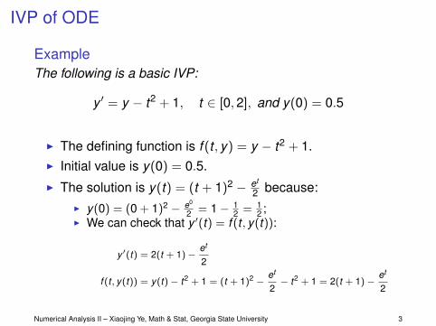
IVP of ODE
ExampleThe following is a basic IVP:
y ′ = y − t2 + 1, t ∈ [0,2], and y(0) = 0.5
I The defining function is f (t , y) = y − t2 + 1.I Initial value is y(0) = 0.5.I The solution is y(t) = (t + 1)2 − et
2 because:I y(0) = (0 + 1)2 − e0
2 = 1− 12 = 1
2 ;I We can check that y ′(t) = f (t , y(t)):
y ′(t) = 2(t + 1)−et
2
f (t , y(t)) = y(t)− t2 + 1 = (t + 1)2 −et
2− t2 + 1 = 2(t + 1)−
et
2
Numerical Analysis II – Xiaojing Ye, Math & Stat, Georgia State University 3
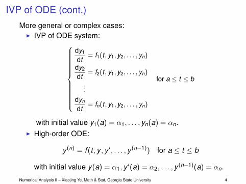
IVP of ODE (cont.)More general or complex cases:
I IVP of ODE system:
dy1
dt= f1(t , y1, y2, . . . , yn)
dy2
dt= f2(t , y1, y2, . . . , yn)
...dyn
dt= fn(t , y1, y2, . . . , yn)
for a ≤ t ≤ b
with initial value y1(a) = α1, . . . , yn(a) = αn.I High-order ODE:
y (n) = f (t , y , y ′, . . . , y (n−1)) for a ≤ t ≤ b
with initial value y(a) = α1, y ′(a) = α2, . . . , y (n−1)(a) = αn.
Numerical Analysis II – Xiaojing Ye, Math & Stat, Georgia State University 4

Why numerical solutions for IVP?
I ODEs have extensive applications in real-world: science,engineering, economics, finance, public health, etc.
I Analytic solution? Not with almost all ODEs.I Fast improvement of computers.
Numerical Analysis II – Xiaojing Ye, Math & Stat, Georgia State University 5

Some basics about IVP
Definition (Lipschitz functions)A function f (t , y) defined on D = {(t , y) : t ∈ R+, y ∈ R} iscalled Lipschitz with respect to y if there exists a constantL > 0
|f (t , y1)− f (t , y2)| ≤ L|y1 − y2|
for all t ∈ R+, and y1, y2 ∈ R.
RemarkWe also call f is Lipschitz with respect to y with constant L, orsimply f is L-Lipschitz with respect to y.
Numerical Analysis II – Xiaojing Ye, Math & Stat, Georgia State University 6
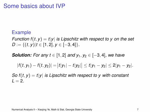
Some basics about IVP
ExampleFunction f (t , y) = t |y | is Lipschitz with respect to y on the setD := {(t , y)|t ∈ [1,2], y ∈ [−3,4]}.
Solution: For any t ∈ [1,2] and y1, y2 ∈ [−3,4], we have
|f (t , y1)− f (t , y2)| =∣∣t |y1| − t |y2|
∣∣ ≤ t |y1 − y2| ≤ 2|y1 − y2|.
So f (t , y) = t |y | is Lipschitz with respect to y with constantL = 2.
Numerical Analysis II – Xiaojing Ye, Math & Stat, Georgia State University 7

Some basics about IVP
Definition (Convex sets)A set D ∈ R2 is convex if whenever (t1, y1), (t2, y2) ∈ D there is(1− λ)(t1, y1) + λ(t2, y2) ∈ D for all λ ∈ [0,1].
5.1 The Elementary Theory of Initial-Value Problems 261
Definition 5.1 A function f (t, y) is said to satisfy a Lipschitz condition in the variable y on a set D ⊂ R2
if a constant L > 0 exists with
|f (t, y1)− f (t, y2, )| ≤ L| y1 − y2|,
whenever (t, y1) and (t, y2) are in D. The constant L is called a Lipschitz constant for f .
Example 1 Show that f (t, y) = t| y| satisfies a Lipschitz condition on the interval D = {(t, y) | 1 ≤t ≤ 2 and − 3 ≤ y ≤ 4}.Solution For each pair of points (t, y1) and (t, y2) in D we have
|f (t, y1)− f (t, y2)| = |t| y1|− t| y2∥ = |t|∥ y1|− | y2∥ ≤ 2| y1 − y2|.
Thus f satisfies a Lipschitz condition on D in the variable y with Lipschitz constant 2. Thesmallest value possible for the Lipschitz constant for this problem is L = 2, because, forexample,
|f (2, 1)− f (2, 0)| = |2 − 0| = 2|1− 0|.
Definition 5.2 A set D ⊂ R2 is said to be convex if whenever (t1, y1) and (t2, y2) belong to D, then((1− λ)t1 + λt2, (1− λ)y1 + λy2) also belongs to D for every λ in [0, 1].
In geometric terms, Definition 5.2 states that a set is convex provided that whenevertwo points belong to the set, the entire straight-line segment between the points also belongsto the set. (See Figure 5.1.) The sets we consider in this chapter are generally of the formD = {(t, y) | a ≤ t ≤ b and −∞ < y <∞} for some constants a and b. It is easy to verify(see Exercise 7) that these sets are convex.
Figure 5.1
(t1, y1)
(t1, y1)(t 2, y2)(t2, y2)
Convex Not convex
Theorem 5.3 Suppose f (t, y) is defined on a convex set D ⊂ R2. If a constant L > 0 exists with!!!!∂f
∂y(t, y)
!!!! ≤ L, for all (t, y) ∈ D, (5.1)
then f satisfies a Lipschitz condition on D in the variable y with Lipschitz constant L.
The proof of Theorem 5.3 is discussed in Exercise 6; it is similar to the proof of thecorresponding result for functions of one variable discussed in Exercise 27 of Section 1.1.
Rudolf Lipschitz (1832–1903)worked in many branches ofmathematics, including numbertheory, Fourier series, differentialequations, analytical mechanics,and potential theory. He is bestknown for this generalization ofthe work of Augustin-LouisCauchy (1789–1857) andGuiseppe Peano (1856–1932).
As the next theorem will show, it is often of significant interest to determine whetherthe function involved in an initial-value problem satisfies a Lipschitz condition in its second
Copyright 2010 Cengage Learning. All Rights Reserved. May not be copied, scanned, or duplicated, in whole or in part. Due to electronic rights, some third party content may be suppressed from the eBook and/or eChapter(s).Editorial review has deemed that any suppressed content does not materially affect the overall learning experience. Cengage Learning reserves the right to remove additional content at any time if subsequent rights restrictions require it.
Numerical Analysis II – Xiaojing Ye, Math & Stat, Georgia State University 8
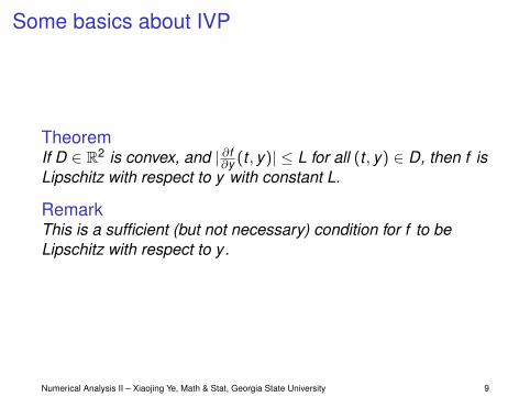
Some basics about IVP
TheoremIf D ∈ R2 is convex, and | ∂f
∂y (t , y)| ≤ L for all (t , y) ∈ D, then f isLipschitz with respect to y with constant L.
RemarkThis is a sufficient (but not necessary) condition for f to beLipschitz with respect to y.
Numerical Analysis II – Xiaojing Ye, Math & Stat, Georgia State University 9

Some basics about IVP
Proof.For any (t , y1), (t , y2) ∈ D, define function g by
g(λ) = f (t , (1− λ)y1 + λy2)
for λ ∈ [0,1] (need convexity of D!). Then we have
g′(λ) = ∂y f (t , (1− λ)y1 + λy2) · (y2 − y1)
So |g′(λ)| ≤ L|y2 − y1|. Then we have
|g(1)− g(0)| =∣∣∣∫ 1
0g′(λ) dλ
∣∣∣ ≤ L|y2 − y1|∣∣∣∫ 1
0dλ∣∣∣ = L|y2 − y1|
Note that g(0) = f (t , y1) and g(1) = f (t , y2). This completes theproof.
Numerical Analysis II – Xiaojing Ye, Math & Stat, Georgia State University 10
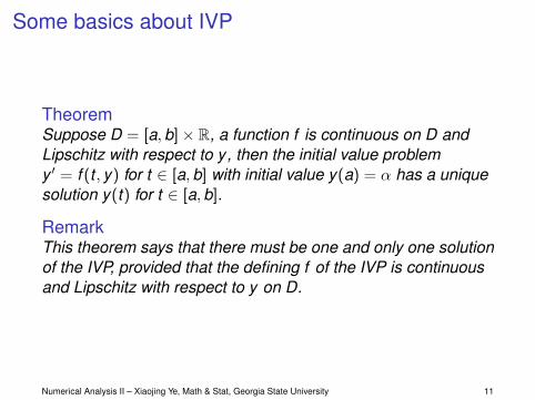
Some basics about IVP
TheoremSuppose D = [a,b]× R, a function f is continuous on D andLipschitz with respect to y, then the initial value problemy ′ = f (t , y) for t ∈ [a,b] with initial value y(a) = α has a uniquesolution y(t) for t ∈ [a,b].
RemarkThis theorem says that there must be one and only one solutionof the IVP, provided that the defining f of the IVP is continuousand Lipschitz with respect to y on D.
Numerical Analysis II – Xiaojing Ye, Math & Stat, Georgia State University 11
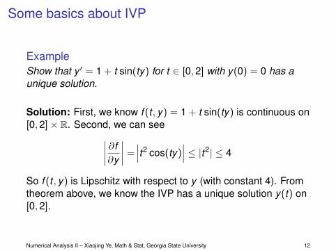
Some basics about IVP
ExampleShow that y ′ = 1 + t sin(ty) for t ∈ [0,2] with y(0) = 0 has aunique solution.
Solution: First, we know f (t , y) = 1 + t sin(ty) is continuous on[0,2]× R. Second, we can see∣∣∣∣ ∂f
∂y
∣∣∣∣ =∣∣∣t2 cos(ty)
∣∣∣ ≤ |t2| ≤ 4
So f (t , y) is Lipschitz with respect to y (with constant 4). Fromtheorem above, we know the IVP has a unique solution y(t) on[0,2].
Numerical Analysis II – Xiaojing Ye, Math & Stat, Georgia State University 12
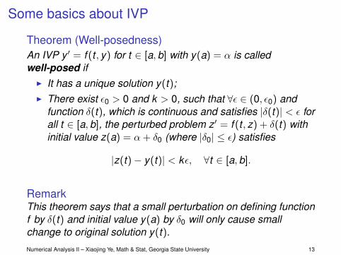
Some basics about IVP
Theorem (Well-posedness)An IVP y ′ = f (t , y) for t ∈ [a,b] with y(a) = α is calledwell-posed if
I It has a unique solution y(t);I There exist ε0 > 0 and k > 0, such that ∀ε ∈ (0, ε0) and
function δ(t), which is continuous and satisfies |δ(t)| < ε forall t ∈ [a,b], the perturbed problem z ′ = f (t , z) + δ(t) withinitial value z(a) = α + δ0 (where |δ0| ≤ ε) satisfies
|z(t)− y(t)| < kε, ∀t ∈ [a,b].
RemarkThis theorem says that a small perturbation on defining functionf by δ(t) and initial value y(a) by δ0 will only cause smallchange to original solution y(t).Numerical Analysis II – Xiaojing Ye, Math & Stat, Georgia State University 13

Some basics about IVP
TheoremLet D = [a,b]× R. If f is continuous on D and Lipschitz withrespect to y, then the IVP is well-posed.
RemarkAgain, a sufficient but not necessary condition forwell-posedness of IVP.
Numerical Analysis II – Xiaojing Ye, Math & Stat, Georgia State University 14

Euler’s method
Given an IVP y ′ = f (t , y) for t ∈ [a,b] and y(a) = α, we want tocompute y(t) on mesh points {t0, t1, . . . , tN} on [a,b].
To this end, we partition [a,b] into N equal segments: seth = b−a
N , and define ti = a + ih for i = 0,1, . . . ,N. Here h iscalled the step size.
268 C H A P T E R 5 Initial-Value Problems for Ordinary Differential Equations
The graph of the function highlighting y(ti) is shown in Figure 5.2. One step in Euler’smethod appears in Figure 5.3, and a series of steps appears in Figure 5.4.
Figure 5.2
t
y
y(tN) ! y(b) y" ! f (t, y),y(a) ! α
y(t2)
y(t1)y(t0) ! α
t0 ! a t1 t2 tN ! b. . .
. . .
Figure 5.3
w1
Slope y"(a) ! f (a, α)
y
t
y" ! f (t, y),y(a) ! α
α
t0 ! a t1 t2 tN ! b. . .
Figure 5.4
w1
y
t
α
t 0 ! a t1 t2 tN ! b
y(b)
w2
wN
y" ! f (t, y),y(a) ! α
. . .
Example 1 Euler’s method was used in the first illustration with h = 0.5 to approximate the solutionto the initial-value problem
y′ = y − t2 + 1, 0 ≤ t ≤ 2, y(0) = 0.5.
Use Algorithm 5.1 with N = 10 to determine approximations, and compare these with theexact values given by y(t) = (t + 1)2 − 0.5et .
Solution With N = 10 we have h = 0.2, ti = 0.2i, w0 = 0.5, and
wi+1 = wi + h(wi − t2i + 1) = wi + 0.2[wi − 0.04i2 + 1] = 1.2wi − 0.008i2 + 0.2,
for i = 0, 1, . . . , 9. So
w1 = 1.2(0.5)− 0.008(0)2 + 0.2 = 0.8; w2 = 1.2(0.8)− 0.008(1)2 + 0.2 = 1.152;
and so on. Table 5.1 shows the comparison between the approximate values at ti and theactual values.
Copyright 2010 Cengage Learning. All Rights Reserved. May not be copied, scanned, or duplicated, in whole or in part. Due to electronic rights, some third party content may be suppressed from the eBook and/or eChapter(s).Editorial review has deemed that any suppressed content does not materially affect the overall learning experience. Cengage Learning reserves the right to remove additional content at any time if subsequent rights restrictions require it.
Numerical Analysis II – Xiaojing Ye, Math & Stat, Georgia State University 15
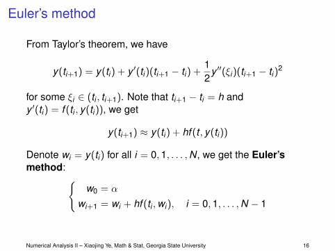
Euler’s method
From Taylor’s theorem, we have
y(ti+1) = y(ti) + y ′(ti)(ti+1 − ti) +12
y ′′(ξi)(ti+1 − ti)2
for some ξi ∈ (ti , ti+1). Note that ti+1 − ti = h andy ′(ti) = f (ti , y(ti)), we get
y(ti+1) ≈ y(ti) + hf (t , y(ti))
Denote wi = y(ti) for all i = 0,1, . . . ,N, we get the Euler’smethod:{
w0 = α
wi+1 = wi + hf (ti ,wi), i = 0,1, . . . ,N − 1
Numerical Analysis II – Xiaojing Ye, Math & Stat, Georgia State University 16

Euler’s method
268 C H A P T E R 5 Initial-Value Problems for Ordinary Differential Equations
The graph of the function highlighting y(ti) is shown in Figure 5.2. One step in Euler’smethod appears in Figure 5.3, and a series of steps appears in Figure 5.4.
Figure 5.2
t
y
y(tN) ! y(b) y" ! f (t, y),y(a) ! α
y(t2)
y(t1)y(t0) ! α
t0 ! a t1 t2 tN ! b. . .
. . .
Figure 5.3
w1
Slope y"(a) ! f (a, α)
y
t
y" ! f (t, y),y(a) ! α
α
t0 ! a t1 t2 tN ! b. . .
Figure 5.4
w1
y
t
α
t 0 ! a t1 t2 tN ! b
y(b)
w2
wN
y" ! f (t, y),y(a) ! α
. . .
Example 1 Euler’s method was used in the first illustration with h = 0.5 to approximate the solutionto the initial-value problem
y′ = y − t2 + 1, 0 ≤ t ≤ 2, y(0) = 0.5.
Use Algorithm 5.1 with N = 10 to determine approximations, and compare these with theexact values given by y(t) = (t + 1)2 − 0.5et .
Solution With N = 10 we have h = 0.2, ti = 0.2i, w0 = 0.5, and
wi+1 = wi + h(wi − t2i + 1) = wi + 0.2[wi − 0.04i2 + 1] = 1.2wi − 0.008i2 + 0.2,
for i = 0, 1, . . . , 9. So
w1 = 1.2(0.5)− 0.008(0)2 + 0.2 = 0.8; w2 = 1.2(0.8)− 0.008(1)2 + 0.2 = 1.152;
and so on. Table 5.1 shows the comparison between the approximate values at ti and theactual values.
Copyright 2010 Cengage Learning. All Rights Reserved. May not be copied, scanned, or duplicated, in whole or in part. Due to electronic rights, some third party content may be suppressed from the eBook and/or eChapter(s).Editorial review has deemed that any suppressed content does not materially affect the overall learning experience. Cengage Learning reserves the right to remove additional content at any time if subsequent rights restrictions require it.
Numerical Analysis II – Xiaojing Ye, Math & Stat, Georgia State University 17
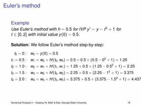
Euler’s method
ExampleUse Euler’s method with h = 0.5 for IVP y ′ = y − t2 + 1 fort ∈ [0,2] with initial value y(0) = 0.5.
Solution: We follow Euler’s method step-by-step:
t0 = 0 : w0 = y(0) = 0.5
t1 = 0.5 : w1 = w0 + hf (t0,w0) = 0.5 + 0.5× (0.5− 02 + 1) = 1.25
t2 = 1.0 : w2 = w1 + hf (t1,w1) = 1.25 + 0.5× (1.25− 0.52 + 1) = 2.25
t3 = 1.5 : w3 = w2 + hf (t2,w2) = 2.25 + 0.5× (2.25− 12 + 1) = 3.375
t4 = 2.0 : w4 = w3 + hf (t3,w3) = 3.375 + 0.5× (3.375− 1.52 + 1) = 4.4375
Numerical Analysis II – Xiaojing Ye, Math & Stat, Georgia State University 18
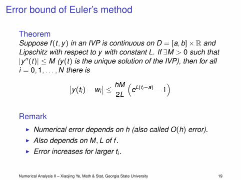
Error bound of Euler’s method
TheoremSuppose f (t , y) in an IVP is continuous on D = [a,b]× R andLipschitz with respect to y with constant L. If ∃M > 0 such that|y ′′(t)| ≤ M (y(t) is the unique solution of the IVP), then for alli = 0,1, . . . ,N there is∣∣y(ti)− wi
∣∣ ≤ hM2L
(eL(ti−a) − 1
)
RemarkI Numerical error depends on h (also called O(h) error).I Also depends on M,L of f .I Error increases for larger ti .
Numerical Analysis II – Xiaojing Ye, Math & Stat, Georgia State University 19
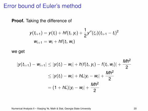
Error bound of Euler’s method
Proof. Taking the difference of
y(ti+1) = y(ti) + hf (ti , yi) +12
y ′′(ξi)(ti+1 − ti)2
wi+1 = wi + hf (ti ,wi)
we get
|y(ti+1)− wi+1| ≤ |y(ti)− wi |+ h|f (ti , yi)− f (ti ,wi)|+Mh2
2
≤ |y(ti)− wi |+ hL|yi − wi |+Mh2
2
= (1 + hL)|yi − wi |+Mh2
2
Numerical Analysis II – Xiaojing Ye, Math & Stat, Georgia State University 20
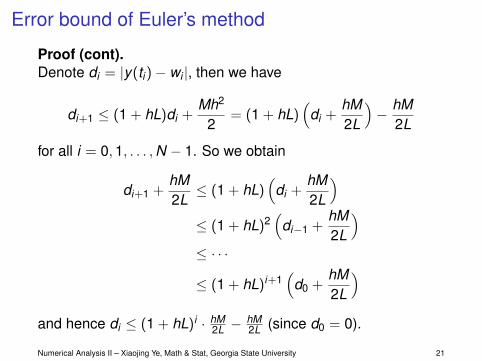
Error bound of Euler’s method
Proof (cont).Denote di = |y(ti)− wi |, then we have
di+1 ≤ (1 + hL)di +Mh2
2= (1 + hL)
(di +
hM2L
)− hM
2L
for all i = 0,1, . . . ,N − 1. So we obtain
di+1 +hM2L≤ (1 + hL)
(di +
hM2L
)≤ (1 + hL)2
(di−1 +
hM2L
)≤ · · ·
≤ (1 + hL)i+1(
d0 +hM2L
)and hence di ≤ (1 + hL)i · hM
2L −hM2L (since d0 = 0).
Numerical Analysis II – Xiaojing Ye, Math & Stat, Georgia State University 21
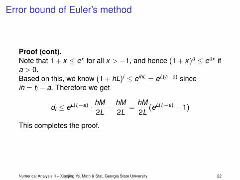
Error bound of Euler’s method
Proof (cont).Note that 1 + x ≤ ex for all x > −1, and hence (1 + x)a ≤ eax ifa > 0.Based on this, we know (1 + hL)i ≤ eihL = eL(ti−a) sinceih = ti − a. Therefore we get
di ≤ eL(ti−a) · hM2L− hM
2L=
hM2L
(eL(ti−a) − 1)
This completes the proof.
Numerical Analysis II – Xiaojing Ye, Math & Stat, Georgia State University 22

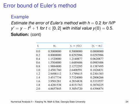
Error bound of Euler’s method
ExampleEstimate the error of Euler’s method with h = 0.2 for IVPy ′ = y − t2 + 1 for t ∈ [0,2] with initial value y(0) = 0.5.
Solution: We first note that ∂f∂y = 1, so f is Lipschitz with
respect to y with constant L = 1. The IVP has solutiony(t) = (t − 1)2 − et
2 so |y ′′(t)| = |et
2 − 2| ≤ e2
2 − 2 =: M. Bytheorem above, the error of Euler’s method is
∣∣y(ti)− wi∣∣ ≤ hM
2L
(eL(ti−a) − 1
)=
0.2(0.5e2 − 2)
2
(eti − 1
)
Numerical Analysis II – Xiaojing Ye, Math & Stat, Georgia State University 23
Error bound of Euler’s method
ExampleEstimate the error of Euler’s method with h = 0.2 for IVPy ′ = y − t2 + 1 for t ∈ [0,2] with initial value y(0) = 0.5.Solution: (cont) 5.2 Euler’s Method 269
Table 5.1 ti wi yi = y(ti) |yi − wi|0.0 0.5000000 0.5000000 0.00000000.2 0.8000000 0.8292986 0.02929860.4 1.1520000 1.2140877 0.06208770.6 1.5504000 1.6489406 0.09854060.8 1.9884800 2.1272295 0.13874951.0 2.4581760 2.6408591 0.18268311.2 2.9498112 3.1799415 0.23013031.4 3.4517734 3.7324000 0.28062661.6 3.9501281 4.2834838 0.33335571.8 4.4281538 4.8151763 0.38702252.0 4.8657845 5.3054720 0.4396874
Note that the error grows slightly as the value of t increases. This controlled errorgrowth is a consequence of the stability of Euler’s method, which implies that the error isexpected to grow in no worse than a linear manner.
Maple has implemented Euler’s method as an option with the command Initial-ValueProblem within the NumericalAnalysis subpackage of the Student package. To useit for the problem in Example 1 first load the package and the differential equation.
with(Student[NumericalAnalysis]): deq := diff(y(t), t) = y(t)− t2 + 1
Then issue the command
C := InitialValueProblem(deq, y(0) = 0.5, t = 2, method = euler, numsteps = 10,output = information, digits = 8)
Maple produces⎡
⎢⎢⎣
1 . . 12× 1 . . 4 ArrayData Type: anythingStorage: rectangularOrder: Fortran_order
⎤
⎥⎥⎦
Double clicking on the output brings up a table that gives the values of ti, actual solutionvalues y(ti), the Euler approximations wi, and the absolute errors | y(ti)− wi|. These agreewith the values in Table 5.1.
To print the Maple table we can issue the commands
for k from 1 to 12 doprint(C[k, 1], C[k, 2], C[k, 3], C[k, 4])end do
The options within the InitialValueProblem command are the specification of the first orderdifferential equation to be solved, the initial condition, the final value of the independentvariable, the choice of method, the number of steps used to determine that h = (2 − 0)/
(numsteps), the specification of form of the output, and the number of digits of roundingto be used in the computations. Other output options can specify a particular value of t ora plot of the solution.
Error Bounds for Euler’s Method
Although Euler’s method is not accurate enough to warrant its use in practice, it is sufficientlyelementary to analyze the error that is produced from its application. The error analysis for
Copyright 2010 Cengage Learning. All Rights Reserved. May not be copied, scanned, or duplicated, in whole or in part. Due to electronic rights, some third party content may be suppressed from the eBook and/or eChapter(s).Editorial review has deemed that any suppressed content does not materially affect the overall learning experience. Cengage Learning reserves the right to remove additional content at any time if subsequent rights restrictions require it.
Numerical Analysis II – Xiaojing Ye, Math & Stat, Georgia State University 24
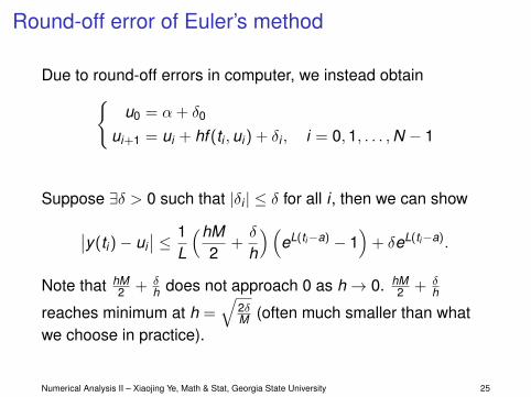
Round-off error of Euler’s method
Due to round-off errors in computer, we instead obtain{u0 = α + δ0
ui+1 = ui + hf (ti ,ui) + δi , i = 0,1, . . . ,N − 1
Suppose ∃δ > 0 such that |δi | ≤ δ for all i , then we can show
∣∣y(ti)− ui∣∣ ≤ 1
L
(hM2
+δ
h
)(eL(ti−a) − 1
)+ δeL(ti−a).
Note that hM2 + δ
h does not approach 0 as h→ 0. hM2 + δ
h
reaches minimum at h =√
2δM (often much smaller than what
we choose in practice).
Numerical Analysis II – Xiaojing Ye, Math & Stat, Georgia State University 25
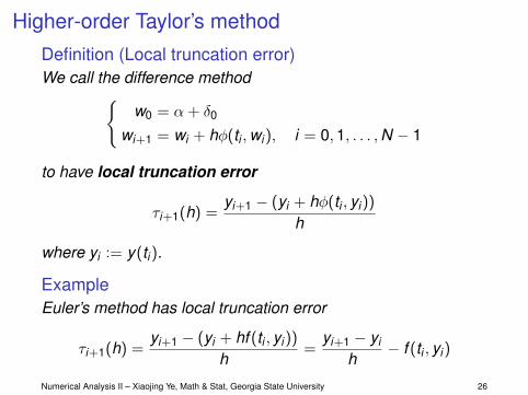
Higher-order Taylor’s methodDefinition (Local truncation error)We call the difference method{
w0 = α + δ0
wi+1 = wi + hφ(ti ,wi), i = 0,1, . . . ,N − 1
to have local truncation error
τi+1(h) =yi+1 − (yi + hφ(ti , yi))
h
where yi := y(ti).
ExampleEuler’s method has local truncation error
τi+1(h) =yi+1 − (yi + hf (ti , yi))
h=
yi+1 − yi
h− f (ti , yi)
Numerical Analysis II – Xiaojing Ye, Math & Stat, Georgia State University 26
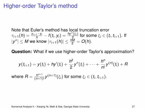
Higher-order Taylor’s method
Note that Euler’s method has local truncation errorτi+1(h) =
yi+1−yih − f (ti , yi) = hy ′′(ξi )
2 for some ξi ∈ (ti , ti+1). If|y ′′| ≤ M we know |τi+1(h)| ≤ hM
2 = O(h).
Question: What if we use higher-order Taylor’s approximation?
y(ti+1) = y(ti) + hy ′(ti) +h2
2y ′′(ti) + · · ·+ hn
n!y (n)(ti) + R
where R = hn+1
(n+1)!y(n+1)(ξi) for some ξi ∈ (ti , ti+1).
Numerical Analysis II – Xiaojing Ye, Math & Stat, Georgia State University 27
Higher-order Taylor’s method
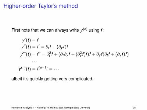
First note that we can always write y (n) using f :
y ′(t) = fy ′′(t) = f ′ = ∂t f + (∂y f )f
y ′′′(t) = f ′′ = ∂2t f + (∂t∂y f + (∂2
y f )f )f + ∂y f (∂t f + (∂y f )f )
· · ·y (n)(t) = f (n−1) = · · ·
albeit it’s quickly getting very complicated.
Numerical Analysis II – Xiaojing Ye, Math & Stat, Georgia State University 28
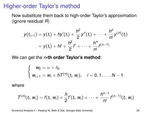
Higher-order Taylor’s methodNow substitute them back to high-order Taylor’s approximation(ignore residual R)
y(ti+1) = y(ti) + hy ′(ti) +h2
2y ′′(ti) + · · ·+ hn
n!y (n)(ti)
= y(ti) + hf +h2
2f ′ + · · ·+ hn
n!f (n−1)
We can get the n-th order Taylor’s method:{w0 = α + δ0
wi+1 = wi + hT (n)(ti ,wi), i = 0,1, . . . ,N − 1
where
T (n)(ti ,wi) = f (ti ,wi) +h2
f ′(ti ,wi) + · · ·+ hn−1
n!f (n−1)(ti ,wi)
Numerical Analysis II – Xiaojing Ye, Math & Stat, Georgia State University 29
Higher-order Taylor’s method
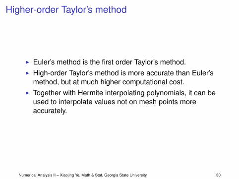
I Euler’s method is the first order Taylor’s method.I High-order Taylor’s method is more accurate than Euler’s
method, but at much higher computational cost.I Together with Hermite interpolating polynomials, it can be
used to interpolate values not on mesh points moreaccurately.
Numerical Analysis II – Xiaojing Ye, Math & Stat, Georgia State University 30
Higher-order Taylor’s method
TheoremIf y(t) ∈ Cn+1[a,b], then the n-th order Taylor method has localtruncation error O(hn).
Numerical Analysis II – Xiaojing Ye, Math & Stat, Georgia State University 31
Runge-Kutta (RK) method
Runge-Kutta (RK) method attains high-order local truncationerror without expensive evaluations of derivatives of f .
Numerical Analysis II – Xiaojing Ye, Math & Stat, Georgia State University 32
Runge-Kutta (RK) method
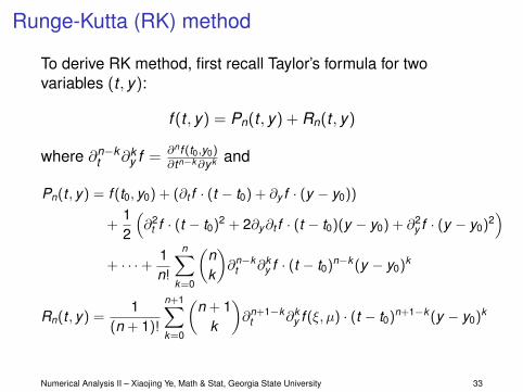
To derive RK method, first recall Taylor’s formula for twovariables (t , y):
f (t , y) = Pn(t , y) + Rn(t , y)
where ∂n−kt ∂k
y f = ∂nf (t0,y0)∂tn−k∂yk and
Pn(t , y) = f (t0, y0) + (∂t f · (t − t0) + ∂y f · (y − y0))
+12
(∂2
t f · (t − t0)2 + 2∂y∂t f · (t − t0)(y − y0) + ∂2y f · (y − y0)2
)+ · · ·+ 1
n!
n∑k=0
(nk
)∂n−k
t ∂ky f · (t − t0)n−k (y − y0)k
Rn(t , y) =1
(n + 1)!
n+1∑k=0
(n + 1
k
)∂n+1−k
t ∂ky f (ξ, µ) · (t − t0)n+1−k (y − y0)k
Numerical Analysis II – Xiaojing Ye, Math & Stat, Georgia State University 33
Runge-Kutta (RK) method
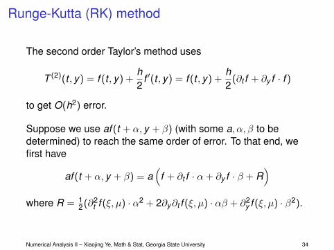
The second order Taylor’s method uses
T (2)(t , y) = f (t , y) +h2
f ′(t , y) = f (t , y) +h2
(∂t f + ∂y f · f )
to get O(h2) error.
Suppose we use af (t + α, y + β) (with some a, α, β to bedetermined) to reach the same order of error. To that end, wefirst have
af (t + α, y + β) = a(
f + ∂t f · α + ∂y f · β + R)
where R = 12(∂2
t f (ξ, µ) · α2 + 2∂y∂t f (ξ, µ) · αβ + ∂2y f (ξ, µ) · β2).
Numerical Analysis II – Xiaojing Ye, Math & Stat, Georgia State University 34

Runge-Kutta (RK) method
Suppose we try to match the terms of these two formulas(ignore R):
T (2)(t , y) = f +h2∂t f +
hf2∂y f
af (t + α, y + β) = af + aα∂t f + aβ∂y f
then we have
a = 1, α =h2, β =
h2
f (t , y)
So instead of T (2)(t , y), we use
af (t + α, y + β) = f(
t +h2, y +
h2
f (t , y))
Numerical Analysis II – Xiaojing Ye, Math & Stat, Georgia State University 35
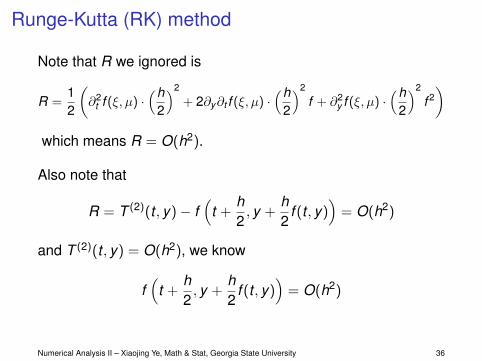
Runge-Kutta (RK) method
Note that R we ignored is
R =12
(∂2
t f (ξ, µ) ·(h
2
)2
+ 2∂y∂t f (ξ, µ) ·(h
2
)2
f + ∂2y f (ξ, µ) ·
(h2
)2
f 2)
which means R = O(h2).
Also note that
R = T (2)(t , y)− f(
t +h2, y +
h2
f (t , y))
= O(h2)
and T (2)(t , y) = O(h2), we know
f(
t +h2, y +
h2
f (t , y))
= O(h2)
Numerical Analysis II – Xiaojing Ye, Math & Stat, Georgia State University 36
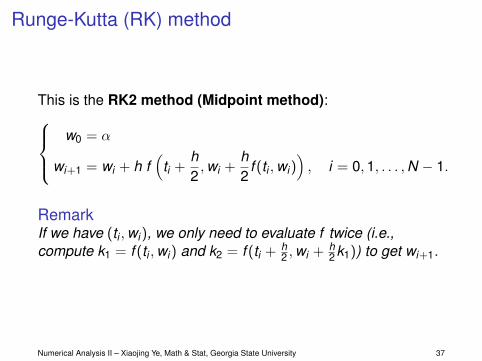
Runge-Kutta (RK) method
This is the RK2 method (Midpoint method):w0 = α
wi+1 = wi + h f(
ti +h2,wi +
h2
f (ti ,wi)), i = 0,1, . . . ,N − 1.
RemarkIf we have (ti ,wi), we only need to evaluate f twice (i.e.,compute k1 = f (ti ,wi) and k2 = f (ti + h
2 ,wi + h2k1)) to get wi+1.
Numerical Analysis II – Xiaojing Ye, Math & Stat, Georgia State University 37
Runge-Kutta (RK) method
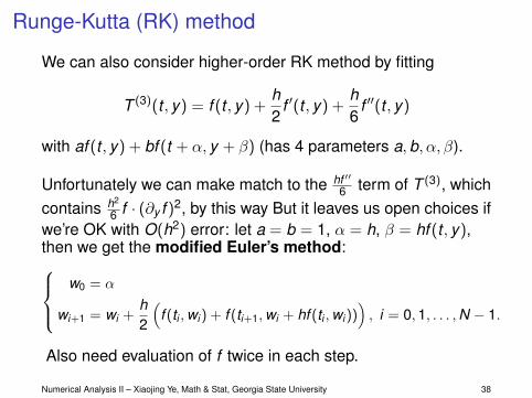
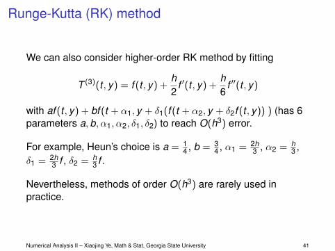
We can also consider higher-order RK method by fitting
T (3)(t , y) = f (t , y) +h2
f ′(t , y) +h6
f ′′(t , y)
with af (t , y) + bf (t + α, y + β) (has 4 parameters a,b, α, β).
Unfortunately we can make match to the hf ′′6 term of T (3), which
contains h2
6 f · (∂y f )2, by this way But it leaves us open choices ifwe’re OK with O(h2) error: let a = b = 1, α = h, β = hf (t , y),then we get the modified Euler’s method:
w0 = α
wi+1 = wi +h2
(f (ti ,wi ) + f (ti+1,wi + hf (ti ,wi ))
), i = 0,1, . . . ,N − 1.
Also need evaluation of f twice in each step.
Numerical Analysis II – Xiaojing Ye, Math & Stat, Georgia State University 38
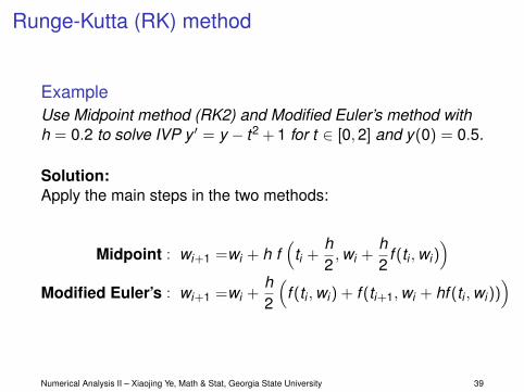
Runge-Kutta (RK) method
ExampleUse Midpoint method (RK2) and Modified Euler’s method withh = 0.2 to solve IVP y ′ = y − t2 + 1 for t ∈ [0,2] and y(0) = 0.5.
Solution:Apply the main steps in the two methods:
Midpoint : wi+1 =wi + h f(
ti +h2,wi +
h2
f (ti ,wi))
Modified Euler’s : wi+1 =wi +h2
(f (ti ,wi) + f (ti+1,wi + hf (ti ,wi))
)
Numerical Analysis II – Xiaojing Ye, Math & Stat, Georgia State University 39

Runge-Kutta (RK) method
ExampleUse Midpoint method (RK2) and Modified Euler’s method withh = 0.2 to solve IVP y ′ = y − t2 + 1 for t ∈ [0,2] and y(0) = 0.5.Solution: (cont)
5.4 Runge-Kutta Methods 287
and
Midpoint method: w2 = 1.22(0.828)− 0.0088(0.2)2 − 0.008(0.2) + 0.218
= 1.21136;
Modified Euler method: w2 = 1.22(0.826)− 0.0088(0.2)2 − 0.008(0.2) + 0.216
= 1.20692,
Table 5.6 lists all the results of the calculations. For this problem, the Midpoint methodis superior to the Modified Euler method.
Table 5.6 Midpoint Modified Eulerti y(ti) Method Error Method Error
0.0 0.5000000 0.5000000 0 0.5000000 00.2 0.8292986 0.8280000 0.0012986 0.8260000 0.00329860.4 1.2140877 1.2113600 0.0027277 1.2069200 0.00716770.6 1.6489406 1.6446592 0.0042814 1.6372424 0.01169820.8 2.1272295 2.1212842 0.0059453 2.1102357 0.01699381.0 2.6408591 2.6331668 0.0076923 2.6176876 0.02317151.2 3.1799415 3.1704634 0.0094781 3.1495789 0.03036271.4 3.7324000 3.7211654 0.0112346 3.6936862 0.03871381.6 4.2834838 4.2706218 0.0128620 4.2350972 0.04838661.8 4.8151763 4.8009586 0.0142177 4.7556185 0.05955772.0 5.3054720 5.2903695 0.0151025 5.2330546 0.0724173
Runge-Kutta methods are also options within the Maple command InitialValueProblem.The form and output for Runge-Kutta methods are the same as available under the Euler’sand Taylor’s methods, as discussed in Sections 5.1 and 5.2.
Higher-Order Runge-Kutta Methods
The term T (3)(t, y) can be approximated with error O(h3) by an expression of the form
f (t + α1, y + δ1f (t + α2, y + δ2f (t, y))),
involving four parameters, the algebra involved in the determination of α1, δ1,α2, and δ2 isquite involved. The most common O(h3) is Heun’s method, given by
w0 = α
wi+1 = wi + h4
!f (ti, wi) + 3f
!ti + 2h
3 , wi + 2h3 f
!ti + h
3 , wi + h3f (ti, wi)
""",
for i = 0, 1, . . . , N − 1.
Karl Heun (1859–1929) was aprofessor at the TechnicalUniversity of Karlsruhe. Heintroduced this technique in apaper published in 1900. [Heu]
Illustration Applying Heun’s method with N = 10, h = 0.2, ti = 0.2i, and w0 = 0.5 to approximatethe solution to our usual example,
y′ = y − t2 + 1, 0 ≤ t ≤ 2, y(0) = 0.5.
Copyright 2010 Cengage Learning. All Rights Reserved. May not be copied, scanned, or duplicated, in whole or in part. Due to electronic rights, some third party content may be suppressed from the eBook and/or eChapter(s).Editorial review has deemed that any suppressed content does not materially affect the overall learning experience. Cengage Learning reserves the right to remove additional content at any time if subsequent rights restrictions require it.
Midpoint (RK2) method is better than modified Euler’s method.Numerical Analysis II – Xiaojing Ye, Math & Stat, Georgia State University 40
Runge-Kutta (RK) method
We can also consider higher-order RK method by fitting
T (3)(t , y) = f (t , y) +h2
f ′(t , y) +h6
f ′′(t , y)
with af (t , y) + bf (t + α1, y + δ1(f (t + α2, y + δ2f (t , y)) ) (has 6parameters a,b, α1, α2, δ1, δ2) to reach O(h3) error.
For example, Heun’s choice is a = 14 , b = 3
4 , α1 = 2h3 , α2 = h
3 ,δ1 = 2h
3 f , δ2 = h3 f .
Nevertheless, methods of order O(h3) are rarely used inpractice.
Numerical Analysis II – Xiaojing Ye, Math & Stat, Georgia State University 41
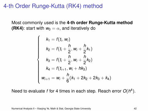
4-th Order Runge-Kutta (RK4) method
Most commonly used is the 4-th order Runge-Kutta method(RK4): start with w0 = α, and iteratively do
k1 = f (ti ,wi)
k2 = f (ti +h2,wi +
h2
k1)
k3 = f (ti +h2,wi +
h2
k2)
k4 = f (ti+1,wi + hk3)
wi+1 = wi +h6
(k1 + 2k2 + 2k3 + k4)
Need to evaluate f for 4 times in each step. Reach error O(h4).
Numerical Analysis II – Xiaojing Ye, Math & Stat, Georgia State University 42

4-th Order Runge-Kutta (RK4) method
ExampleUse RK4 (with h = 0.2) to solve IVP y ′ = y − t2 + 1 for t ∈ [0,2]and y(0) = 0.5.Solution: With h = 0.2, we have N = 10 and ti = 0.2i fori = 0,1, . . . ,10. First set w0 = 0.5, then the first iteration is
k1 = f (t0,w0) = f (0,0.5) = 0.5− 02 + 1 = 1.5
k2 = f (t0 +h2,w0 +
h2
k1) = f (0.1,0.5 + 0.1× 1.5) = 1.64
k3 = f (t0 +h2,w0 +
h2
k2) = f (0.1,0.5 + 0.1× 1.64) = 1.654
k4 = f (t1,w0 + hk3) = f (0.2,0.5 + 0.2× 1.654) = 1.7908
w1 = w0 +h6
(k1 + 2k2 + 2k3 + k4) = 0.8292933
So w1 is our RK4 approximation of y(t1) = y(0.2).Numerical Analysis II – Xiaojing Ye, Math & Stat, Georgia State University 43
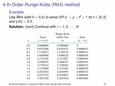
4-th Order Runge-Kutta (RK4) method
ExampleUse RK4 (with h = 0.2) to solve IVP y ′ = y − t2 + 1 for t ∈ [0,2]and y(0) = 0.5.Solution: (cont) Continue with i = 1,2, · · · ,9:
5.4 Runge-Kutta Methods 289
Step 1 Set h = (b− a)/N ;t = a;w = α;
OUTPUT (t, w).
Step 2 For i = 1, 2, . . . , N do Steps 3–5.
Step 3 Set K1 = hf (t, w);K2 = hf (t + h/2, w + K1/2);K3 = hf (t + h/2, w + K2/2);K4 = hf (t + h, w + K3).
Step 4 Set w = w + (K1 + 2K2 + 2K3 + K4)/6; (Compute wi.)t = a + ih. (Compute ti.)
Step 5 OUTPUT (t, w).
Step 6 STOP.
Example 3 Use the Runge-Kutta method of order four with h = 0.2, N = 10, and ti = 0.2i to obtainapproximations to the solution of the initial-value problem
y′ = y − t2 + 1, 0 ≤ t ≤ 2, y(0) = 0.5.
Solution The approximation to y(0.2) is obtained by
w0 = 0.5
k1 = 0.2f (0, 0.5) = 0.2(1.5) = 0.3
k2 = 0.2f (0.1, 0.65) = 0.328
k3 = 0.2f (0.1, 0.664) = 0.3308
k4 = 0.2f (0.2, 0.8308) = 0.35816
w1 = 0.5 + 16(0.3 + 2(0.328) + 2(0.3308) + 0.35816) = 0.8292933.
The remaining results and their errors are listed in Table 5.8.
Table 5.8 Runge-KuttaExact Order Four Error
ti yi = y(ti) wi |yi − wi|0.0 0.5000000 0.5000000 00.2 0.8292986 0.8292933 0.00000530.4 1.2140877 1.2140762 0.00001140.6 1.6489406 1.6489220 0.00001860.8 2.1272295 2.1272027 0.00002691.0 2.6408591 2.6408227 0.00003641.2 3.1799415 3.1798942 0.00004741.4 3.7324000 3.7323401 0.00005991.6 4.2834838 4.2834095 0.00007431.8 4.8151763 4.8150857 0.00009062.0 5.3054720 5.3053630 0.0001089
Copyright 2010 Cengage Learning. All Rights Reserved. May not be copied, scanned, or duplicated, in whole or in part. Due to electronic rights, some third party content may be suppressed from the eBook and/or eChapter(s).Editorial review has deemed that any suppressed content does not materially affect the overall learning experience. Cengage Learning reserves the right to remove additional content at any time if subsequent rights restrictions require it.
Numerical Analysis II – Xiaojing Ye, Math & Stat, Georgia State University 44
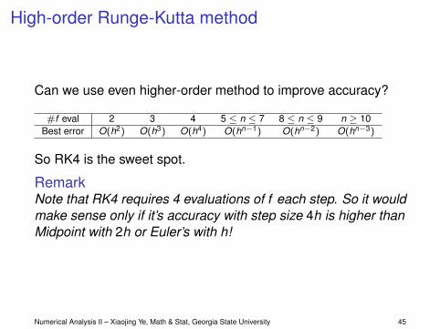
High-order Runge-Kutta method
Can we use even higher-order method to improve accuracy?
#f eval 2 3 4 5 ≤ n ≤ 7 8 ≤ n ≤ 9 n ≥ 10Best error O(h2) O(h3) O(h4) O(hn−1) O(hn−2) O(hn−3)
So RK4 is the sweet spot.
RemarkNote that RK4 requires 4 evaluations of f each step. So it wouldmake sense only if it’s accuracy with step size 4h is higher thanMidpoint with 2h or Euler’s with h!
Numerical Analysis II – Xiaojing Ye, Math & Stat, Georgia State University 45

High-order Runge-Kutta method
ExampleUse RK4 (with h = 0.1), Midpoint (with h = 0.05), and Euler’smethod (with h = 0.025) to solve IVP y ′ = y − t2 + 1 fort ∈ [0,0.5] and y(0) = 0.5.Solution:
5.4 Runge-Kutta Methods 291
Table 5.10 Modified Runge-KuttaEuler Euler Order Four
ti Exact h = 0.025 h = 0.05 h = 0.1
0.0 0.5000000 0.5000000 0.5000000 0.50000000.1 0.6574145 0.6554982 0.6573085 0.65741440.2 0.8292986 0.8253385 0.8290778 0.82929830.3 1.0150706 1.0089334 1.0147254 1.01507010.4 1.2140877 1.2056345 1.2136079 1.21408690.5 1.4256394 1.4147264 1.4250141 1.4256384
E X E R C I S E S E T 5.4
1. Use the Modified Euler method to approximate the solutions to each of the following initial-valueproblems, and compare the results to the actual values.a. y′ = te3t − 2y, 0 ≤ t ≤ 1, y(0) = 0, with h = 0.5; actual solution y(t) = 1
5 te3t − 125 e3t +
125 e−2t .
b. y′ = 1 + (t − y)2, 2 ≤ t ≤ 3, y(2) = 1, with h = 0.5; actual solution y(t) = t + 11−t .
c. y′ = 1 + y/t, 1 ≤ t ≤ 2, y(1) = 2, with h = 0.25; actual solution y(t) = t ln t + 2t.d. y′ = cos 2t + sin 3t, 0 ≤ t ≤ 1, y(0) = 1, with h = 0.25; actual solution y(t) =
12 sin 2t − 1
3 cos 3t + 43 .
2. Use the Modified Euler method to approximate the solutions to each of the following initial-valueproblems, and compare the results to the actual values.a. y′ = et−y, 0 ≤ t ≤ 1, y(0) = 1, with h = 0.5; actual solution y(t) = ln(et + e− 1).
b. y′ = 1 + t1 + y
, 1 ≤ t ≤ 2, y(1) = 2, with h = 0.5; actual solution y(t) =√
t2 + 2t + 6− 1.
c. y′ = −y + ty1/2, 2 ≤ t ≤ 3, y(2) = 2, with h = 0.25; actual solution y(t) =!t − 2 +
√2ee−t/2
"2.
d. y′ = t−2(sin 2t − 2ty), 1 ≤ t ≤ 2, y(1) = 2, with h = 0.25; actual solution y(t) =12 t−2(4 + cos 2 − cos 2t).
3. Use the Modified Euler method to approximate the solutions to each of the following initial-valueproblems, and compare the results to the actual values.
a. y′ = y/t − (y/t)2, 1 ≤ t ≤ 2, y(1) = 1, with h = 0.1; actual solution y(t) = t/(1 + ln t).
b. y′ = 1 + y/t + (y/t)2, 1 ≤ t ≤ 3, y(1) = 0, with h = 0.2; actual solution y(t) = t tan(ln t).
c. y′ = −(y + 1)(y + 3), 0 ≤ t ≤ 2, y(0) = −2, with h = 0.2; actual solution y(t) =−3 + 2(1 + e−2t)−1.
d. y′ = −5y+5t2 +2t, 0 ≤ t ≤ 1, y(0) = 13 , with h = 0.1; actual solution y(t) = t2 + 1
3 e−5t .
4. Use the Modified Euler method to approximate the solutions to each of the following initial-valueproblems, and compare the results to the actual values.
a. y′ = 2 − 2tyt2 + 1
, 0 ≤ t ≤ 1, y(0) = 1, with h = 0.1; actual solution y(t) = 2t + 1t2 + 1
.
b. y′ = y2
1 + t, 1 ≤ t ≤ 2, y(1) = −(ln 2)−1, with h = 0.1; actual solution y(t) = −1
ln(t + 1).
c. y′ = (y2 + y)/t, 1 ≤ t ≤ 3, y(1) = −2, with h = 0.2; actual solution y(t) = 2t1− 2t
.
d. y′ = −ty + 4t/y, 0 ≤ t ≤ 1, y(0) = 1, with h = 0.1; actual solution y(t) =#
4− 3e−t2 .
Copyright 2010 Cengage Learning. All Rights Reserved. May not be copied, scanned, or duplicated, in whole or in part. Due to electronic rights, some third party content may be suppressed from the eBook and/or eChapter(s).Editorial review has deemed that any suppressed content does not materially affect the overall learning experience. Cengage Learning reserves the right to remove additional content at any time if subsequent rights restrictions require it.
RK4 is better with same computation cost!
Numerical Analysis II – Xiaojing Ye, Math & Stat, Georgia State University 46

Error control
Can we control the error of Runge-Kutta method by usingvariable step sizes?
Let’s compare two difference methods with errors O(hn) andO(hn+1) (say, RK4 and RK5) for fixed step size h, which haveschemes below:
wi+1 = wi + hφ(ti ,wi ,h) O(hn)
w̃i+1 = w̃i + hφ̃(ti , w̃i ,h) O(hn+1)
Suppose wi ≈ w̃i ≈ y(ti) =: yi . Then for any given ε > 0, wewant to see how small h should be for the O(hn) method so thatits error |τi+1(h)| ≤ ε?
Numerical Analysis II – Xiaojing Ye, Math & Stat, Georgia State University 47

Error control
We recall that the local truncation errors of these two methodsare:
τi+1(h) =yi+1 − yi
h− φ(ti , yi ,h) ≈ O(hn)
τ̃i+1(h) =yi+1 − yi
h− φ̃(ti , yi ,h) ≈ O(hn+1)
Given that wi ≈ w̃i ≈ yi and O(hn+1)� O(hn) for small h, wesee
τi+1(h) ≈ τi+1(h)− τ̃i+1(h) = φ̃(ti , yi ,h)− φ(ti , yi ,h)
≈ φ̃(ti , w̃i ,h)− φ(ti ,wi ,h) =w̃i+1 − w̃i
h− wi+1 − wi
h
≈ w̃i+1 − wi+1
h≈ Khn
for some K > 0 independent of h, since τi+1(h) ≈ O(hn).Numerical Analysis II – Xiaojing Ye, Math & Stat, Georgia State University 48
Error control
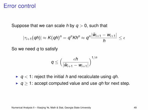
Suppose that we can scale h by q > 0, such that
|τi+1(qh)| ≈ K (qh)n = qnKhn ≈ qn |w̃i+1 − wi+1|h
≤ ε
So we need q to satisfy
q ≤( εh|w̃i+1 − wi+1|
)1/n
I q < 1: reject the initial h and recalculate using qh.I q ≥ 1: accept computed value and use qh for next step.
Numerical Analysis II – Xiaojing Ye, Math & Stat, Georgia State University 49
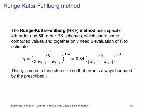
Runge-Kutta-Fehlberg method
The Runge-Kutta-Fehlberg (RKF) method uses specific4th-order and 5th-order RK schemes, which share somecomputed values and together only need 6 evaluation of f , toestimate
q =( εh
2|w̃i+1 − wi+1|
)1/4= 0.84
( εh|w̃i+1 − wi+1|
)1/4
This q is used to tune step size so that error is always boundedby the prescribed ε.
Numerical Analysis II – Xiaojing Ye, Math & Stat, Georgia State University 50

Multistep method
DefinitionLet m > 1 be an integer, then an m-step multistep method isgiven by the form of
wi+1 = am−1wi + am−2wi−1 + · · ·+ a0wi−m+1
+ h[bmf (ti+1,wi+1) + bm−1f (ti ,wi ) + · · ·+ b0f (ti−m+1,wi−m+1)
]for i = m − 1,m, . . . ,N − 1.
Here a0, . . . ,am−1, b0, . . . ,bm are constants. Alsow0 = α,w1 = α1, . . . ,wm−1 = αm−1 need to be given.
I bm = 0: Explicit m-step method.I bm 6= 0: Implicit m-step method.
Numerical Analysis II – Xiaojing Ye, Math & Stat, Georgia State University 51

Multistep method
DefinitionThe local truncation error of the m-step multistep methodabove is defined by
τi+1(h) =yi+1 − (am−1yi + · · ·+ a0yi−m+1)
h−[bmf (ti+1, yi+1) + bm−1f (ti , yi ) + · · ·+ b0f (ti−m+1, yi−m+1)
]where yi := y(ti).
Numerical Analysis II – Xiaojing Ye, Math & Stat, Georgia State University 52
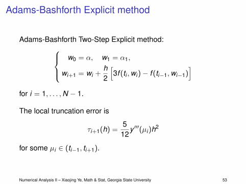
Adams-Bashforth Explicit method
Adams-Bashforth Two-Step Explicit method:w0 = α, w1 = α1,
wi+1 = wi +h2
[3f (ti ,wi)− f (ti−1,wi−1)
]for i = 1, . . . ,N − 1.
The local truncation error is
τi+1(h) =5
12y ′′′(µi)h2
for some µi ∈ (ti−1, ti+1).
Numerical Analysis II – Xiaojing Ye, Math & Stat, Georgia State University 53

Adams-Bashforth Explicit method
Adams-Bashforth Three-Step Explicit method:w0 = α, w1 = α1, w2 = α2,
wi+1 = wi +h12
[23f (ti ,wi)− 16f (ti−1,wi−1) + 5f (ti−2,wi−2)
]for i = 2, . . . ,N − 1.
The local truncation error is
τi+1(h) =38
y (4)(µi)h3
for some µi ∈ (ti−2, ti+1).
Numerical Analysis II – Xiaojing Ye, Math & Stat, Georgia State University 54
Adams-Bashforth Explicit method
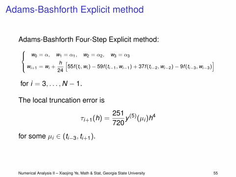
Adams-Bashforth Four-Step Explicit method:w0 = α, w1 = α1, w2 = α2, w3 = α3
wi+1 = wi +h24
[55f (ti ,wi )− 59f (ti−1,wi−1) + 37f (ti−2,wi−2)− 9f (ti−3,wi−3)
]for i = 3, . . . ,N − 1.
The local truncation error is
τi+1(h) =251720
y (5)(µi)h4
for some µi ∈ (ti−3, ti+1).
Numerical Analysis II – Xiaojing Ye, Math & Stat, Georgia State University 55

Adams-Bashforth Explicit method
Adams-Bashforth Five-Step Explicit method:w0 = α, w1 = α1, w2 = α2, w3 = α3, w4 = α4
wi+1 = wi +h
720[1901f (ti ,wi )− 2774f (ti−1,wi−1) + 2616f (ti−2,wi−2)
− 1274f (ti−3,wi−3) + 251f (ti−4,wi−4)]
for i = 4, . . . ,N − 1.
The local truncation error is
τi+1(h) =95
288y (6)(µi)h5
for some µi ∈ (ti−4, ti+1).
Numerical Analysis II – Xiaojing Ye, Math & Stat, Georgia State University 56

Adams-Moulton Implicit method
Adams-Moulton Two-Step Implicit method:w0 = α, w1 = α1,
wi+1 = wi +h12
[5f (ti+1,wi+1) + 8f (ti ,wi)− f (ti−1,wi−1)]
for i = 1, . . . ,N − 1.
The local truncation error is
τi+1(h) = − 124
y (4)(µi)h3
for some µi ∈ (ti−1, ti+1).
Numerical Analysis II – Xiaojing Ye, Math & Stat, Georgia State University 57
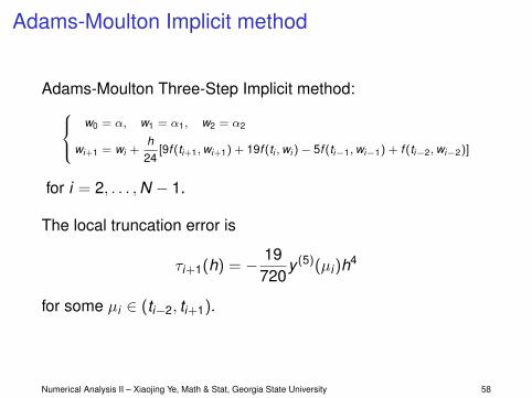
Adams-Moulton Implicit method
Adams-Moulton Three-Step Implicit method:w0 = α, w1 = α1, w2 = α2
wi+1 = wi +h24
[9f (ti+1,wi+1) + 19f (ti ,wi )− 5f (ti−1,wi−1) + f (ti−2,wi−2)]
for i = 2, . . . ,N − 1.
The local truncation error is
τi+1(h) = − 19720
y (5)(µi)h4
for some µi ∈ (ti−2, ti+1).
Numerical Analysis II – Xiaojing Ye, Math & Stat, Georgia State University 58
Adams-Moulton Implicit method
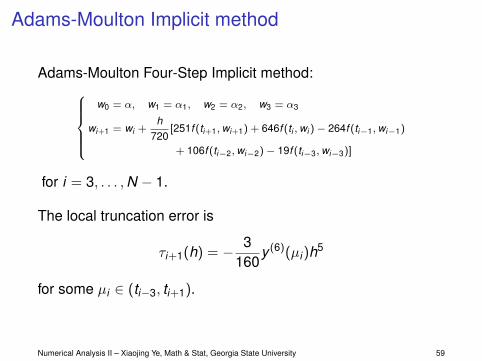
Adams-Moulton Four-Step Implicit method:w0 = α, w1 = α1, w2 = α2, w3 = α3
wi+1 = wi +h
720[251f (ti+1,wi+1) + 646f (ti ,wi )− 264f (ti−1,wi−1)
+ 106f (ti−2,wi−2)− 19f (ti−3,wi−3)]
for i = 3, . . . ,N − 1.
The local truncation error is
τi+1(h) = − 3160
y (6)(µi)h5
for some µi ∈ (ti−3, ti+1).
Numerical Analysis II – Xiaojing Ye, Math & Stat, Georgia State University 59

Steps to develop multistep methods
I Construct interpolating polynomial P(t) (e.g., Newton’sbackward difference method) using previously computed(ti−m+1,wi−m+1), . . . , (ti ,wi).
I Approximate y(ti+1) based on
y(ti+1) = y(ti ) +
∫ ti+1
tiy ′(t) dt = y(ti ) +
∫ ti+1
tif (t , y(t)) dt
≈ y(ti ) +
∫ ti+1
tif (t ,P(t)) dt
and construct difference method:
wi+1 = wi + hφ(ti , . . . , ti−m+1,wi , . . . ,wi−m+1)
Numerical Analysis II – Xiaojing Ye, Math & Stat, Georgia State University 60
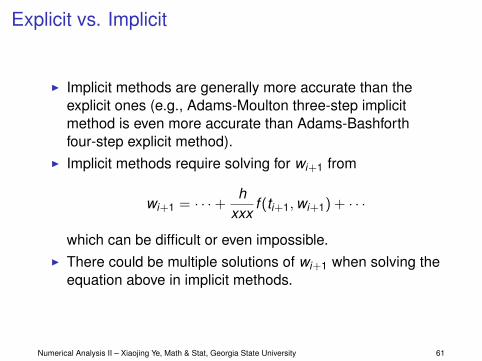
Explicit vs. Implicit
I Implicit methods are generally more accurate than theexplicit ones (e.g., Adams-Moulton three-step implicitmethod is even more accurate than Adams-Bashforthfour-step explicit method).
I Implicit methods require solving for wi+1 from
wi+1 = · · ·+ hxxx
f (ti+1,wi+1) + · · ·
which can be difficult or even impossible.I There could be multiple solutions of wi+1 when solving the
equation above in implicit methods.
Numerical Analysis II – Xiaojing Ye, Math & Stat, Georgia State University 61
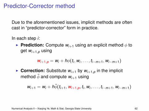
Predictor-Corrector method
Due to the aforementioned issues, implicit methods are oftencast in “predictor-corrector” form in practice.
In each step i :I Prediction: Compute wi+1 using an explicit method φ to
get wi+1,p using
wi+1,p = wi + hφ(ti ,wi , . . . , ti−m+1,wi−m+1)
I Correction: Substitute wi+1 by wi+1,p in the implicitmethod φ̃ and compute wi+1 using
wi+1 = wi + hφ̃(ti+1,wi+1,p, ti ,wi , . . . , ti−m+1,wi−m+1)
Numerical Analysis II – Xiaojing Ye, Math & Stat, Georgia State University 62
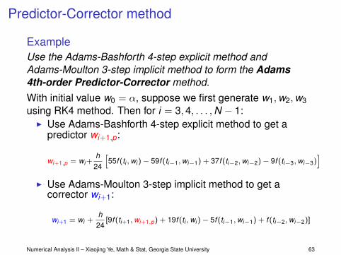
Predictor-Corrector method
ExampleUse the Adams-Bashforth 4-step explicit method andAdams-Moulton 3-step implicit method to form the Adams4th-order Predictor-Corrector method.With initial value w0 = α, suppose we first generate w1,w2,w3using RK4 method. Then for i = 3,4, . . . ,N − 1:
I Use Adams-Bashforth 4-step explicit method to get apredictor wi+1,p:
wi+1,p = wi +h24
[55f (ti ,wi )− 59f (ti−1,wi−1) + 37f (ti−2,wi−2)− 9f (ti−3,wi−3)
]I Use Adams-Moulton 3-step implicit method to get a
corrector wi+1:
wi+1 = wi +h24
[9f (ti+1,wi+1,p) + 19f (ti ,wi )− 5f (ti−1,wi−1) + f (ti−2,wi−2)]
Numerical Analysis II – Xiaojing Ye, Math & Stat, Georgia State University 63

Predictor-Corrector method
ExampleUse Adams Predictor-Corrector Method with h = 0.2 to solveIVP y ′ = y − t2 + 1 for t ∈ [0,2] and y(0) = 0.5.
5.6 Multistep Methods 313
= 2.1272056 + 0.0083333(9(2.6409314) + 19(2.4872056) − 5(2.2889220)
+ (2.0540762))
= 2.6408286.
In Example 1 we found that using the explicit Adams-Bashforth method alone producedresults that were inferior to those of Runge-Kutta. However, these approximations to y(0.8)
and y(1.0) are accurate to within
|2.1272295 − 2.1272056| = 2.39× 10− 5 and |2.6408286 − 2.6408591| = 3.05× 10− 5.
respectively, compared to those of Runge-Kutta, which were accurate, respectively, to within
|2.1272027 − 2.1272892| = 2.69× 10− 5 and |2.6408227 − 2.6408591| = 3.64× 10− 5.
The remaining predictor-corrector approximations were generated using Algorithm 5.4 andare shown in Table 5.14.
Table 5.14 Errorti yi = y(ti) wi |yi − wi|
0.0 0.5000000 0.5000000 00.2 0.8292986 0.8292933 0.00000530.4 1.2140877 1.2140762 0.00001140.6 1.6489406 1.6489220 0.00001860.8 2.1272295 2.1272056 0.00002391.0 2.6408591 2.6408286 0.00003051.2 3.1799415 3.1799026 0.00003891.4 3.7324000 3.7323505 0.00004951.6 4.2834838 4.2834208 0.00006301.8 4.8151763 4.8150964 0.00007992.0 5.3054720 5.3053707 0.0001013
Adams Fourth Order Predictor-Corrector method is implemented in Maple for theexample problem with
C := InitialValueProblem(deq, y(0) = 0.5, t = 2, method = adamsbashforthmoulton,submethod = step4, numsteps = 10, output = information, digits = 8)
and generates the same values as in Table 5.14.Other multistep methods can be derived using integration of interpolating polynomials
over intervals of the form [tj, ti+1], for j ≤ i − 1, to obtain an approximation to y(ti+1). Whenan interpolating polynomial is integrated over [ti− 3, ti+1], the result is the explicit Milne’smethod:
wi+1 = wi− 3 + 4h3
[2f (ti, wi) − f (ti− 1, wi− 1) + 2f (ti− 2, wi− 2)],
which has local truncation error 1445 h4y(5)(ξi), for some ξi ∈ (ti− 3, ti+1).
Edward Arthur Milne(1896–1950) worked in ballisticresearch during World War I, andthen for the Solar PhysicsObservatory at Cambridge. In1929 he was appointed theW. W. Rouse Ball chair atWadham College in Oxford.
Milne’s method is occasionally used as a predictor for the implicit Simpson’s method,
wi+1 = wi− 1 + h3[f (ti+1, wi+1) + 4f (ti, wi) + f (ti− 1, wi− 1)],
which has local truncation error − (h4/90)y(5)(ξi), for some ξi ∈ (ti− 1, ti+1), and is obtainedby integrating an interpolating polynomial over [ti− 1, ti+1].
Simpson’s name is associatedwith this technique because it isbased on Simpson’s rule forintegration.
Copyright 2010 Cengage Learning. All Rights Reserved. May not be copied, scanned, or duplicated, in whole or in part. Due to electronic rights, some third party content may be suppressed from the eBook and/or eChapter(s).Editorial review has deemed that any suppressed content does not materially affect the overall learning experience. Cengage Learning reserves the right to remove additional content at any time if subsequent rights restrictions require it.
Numerical Analysis II – Xiaojing Ye, Math & Stat, Georgia State University 64
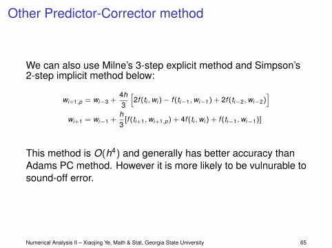
Other Predictor-Corrector method
We can also use Milne’s 3-step explicit method and Simpson’s2-step implicit method below:
wi+1,p = wi−3 +4h3
[2f (ti ,wi )− f (ti−1,wi−1) + 2f (ti−2,wi−2)
]wi+1 = wi−1 +
h3
[f (ti+1,wi+1,p) + 4f (ti ,wi ) + f (ti−1,wi−1)]
This method is O(h4) and generally has better accuracy thanAdams PC method. However it is more likely to be vulnurable tosound-off error.
Numerical Analysis II – Xiaojing Ye, Math & Stat, Georgia State University 65
Predictor-Corrector method
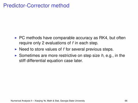
I PC methods have comparable accuracy as RK4, but oftenrequire only 2 evaluations of f in each step.
I Need to store values of f for several previous steps.I Sometimes are more restrictive on step size h, e.g., in the
stiff differential equation case later.
Numerical Analysis II – Xiaojing Ye, Math & Stat, Georgia State University 66
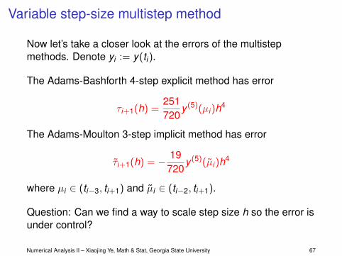
Variable step-size multistep method
Now let’s take a closer look at the errors of the multistepmethods. Denote yi := y(ti).
The Adams-Bashforth 4-step explicit method has error
τi+1(h) =251720
y (5)(µi)h4
The Adams-Moulton 3-step implicit method has error
τ̃i+1(h) = − 19720
y (5)(µ̃i)h4
where µi ∈ (ti−3, ti+1) and µ̃i ∈ (ti−2, ti+1).
Question: Can we find a way to scale step size h so the error isunder control?
Numerical Analysis II – Xiaojing Ye, Math & Stat, Georgia State University 67
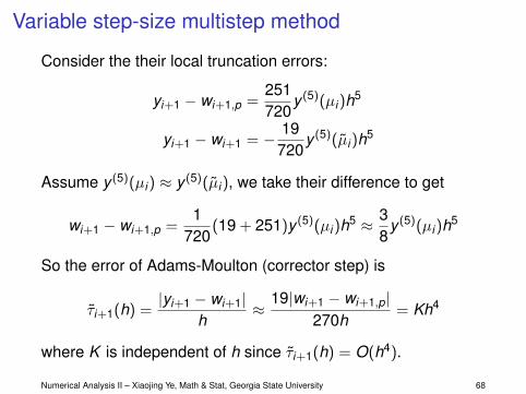
Variable step-size multistep method
Consider the their local truncation errors:
yi+1 − wi+1,p =251720
y (5)(µi)h5
yi+1 − wi+1 = − 19720
y (5)(µ̃i)h5
Assume y (5)(µi) ≈ y (5)(µ̃i), we take their difference to get
wi+1 − wi+1,p =1
720(19 + 251)y (5)(µi)h5 ≈ 3
8y (5)(µi)h5
So the error of Adams-Moulton (corrector step) is
τ̃i+1(h) =|yi+1 − wi+1|
h≈
19|wi+1 − wi+1,p|270h
= Kh4
where K is independent of h since τ̃i+1(h) = O(h4).
Numerical Analysis II – Xiaojing Ye, Math & Stat, Georgia State University 68

Variable step-size multistep method
If we want to keep error under a prescribed ε, then we need tofind q > 0 such that with step size qh, there is
τ̃i+1(qh) =|y(ti + qh)− wi+1|
qh≈
19q4|wi+1 − wi+1,p|270h
< ε
This implies that
q <( 270hε
19|wi+1 − wi+1,p|
)1/4≈ 2
( hε|wi+1 − wi+1,p|
)1/4
To be conservative, we may replace 2 by 1.5 above.
In practice, we tune q (as less as possible) such that theestimated error is between (ε/10, ε)
Numerical Analysis II – Xiaojing Ye, Math & Stat, Georgia State University 69

System of differential equations
The IVP for a system of ODE has form
du1
dt= f1(t ,u1,u2, . . . ,um)
du2
dt= f2(t ,u1,u2, . . . ,um)
...dum
dt= fm(t ,u1,u2, . . . ,um)
for a ≤ t ≤ b
with initial value u1(a) = α1, . . . ,um(a) = αm.
DefinitionA set of functions u1(t), . . . ,um(t) is a solution of the IVPabove if they satisfy both the system of ODEs and the initialvalues.
Numerical Analysis II – Xiaojing Ye, Math & Stat, Georgia State University 70

System of differential equations
In this case, we will solve for u1(t), . . . ,um(t) which areinterdependent according to the ODE system.
330 C H A P T E R 5 Initial-Value Problems for Ordinary Differential Equations
Let an integer N > 0 be chosen and set h= (b − a)/N . Partition the interval [a, b] intoN subintervals with the mesh points
tj = a + jh, for each j = 0, 1, . . . , N .
Use the notation wij, for each j = 0, 1, . . . , N and i = 1, 2, . . . , m, to denote an approx-imation to ui(tj). That is, wij approximates the ith solution ui(t) of (5.45) at the jth meshpoint tj. For the initial conditions, set (see Figure 5.6)
w1,0 = α1, w2,0 = α2, . . . , wm,0 = αm. (5.48)
Figure 5.6
y
t
w11w12w13
y
t
w23w22
w21
a ! t0 t1 t2 t3 a ! t0 t1 t2 t3
u1(a) ! α1
u2(a) ! α2
u2(t)
u1(t)
y
t
wm3wm2
wm1
a ! t0 t1 t2 t3
um(t)
um(a) ! αm
Suppose that the values w1, j, w2, j, . . . , wm, j have been computed. We obtain w1, j+1,w2, j+1, . . . , wm, j+1 by first calculating
k1,i = hfi(tj, w1, j, w2, j, . . . , wm, j), for each i = 1, 2, . . . , m; (5.49)
k2,i = hfi
!tj + h
2, w1, j + 1
2k1,1, w2, j + 1
2k1,2, . . . , wm, j + 1
2k1,m
", (5.50)
for each i = 1, 2, . . . , m;
k3,i = hfi
!tj + h
2, w1, j + 1
2k2,1, w2, j + 1
2k2,2, . . . , wm, j + 1
2k2,m
", (5.51)
for each i = 1, 2, . . . , m;
k4,i = hfi(tj + h, w1, j + k3,1, w2, j + k3,2, . . . , wm, j + k3,m), (5.52)
for each i = 1, 2, . . . , m; and then
wi, j+1 = wi, j + 16(k1,i + 2k2,i + 2k3,i + k4,i), (5.53)
for each i = 1, 2, . . . , m. Note that all the values k1,1, k1,2, . . . , k1,m must be computed beforeany of the terms of the form k2,i can be determined. In general, each kl,1, kl,2, . . . , kl,m must becomputed before any of the expressions kl+1,i. Algorithm 5.7 implements the Runge-Kuttafourth-order method for systems of initial-value problems.
Copyright 2010 Cengage Learning. All Rights Reserved. May not be copied, scanned, or duplicated, in whole or in part. Due to electronic rights, some third party content may be suppressed from the eBook and/or eChapter(s).Editorial review has deemed that any suppressed content does not materially affect the overall learning experience. Cengage Learning reserves the right to remove additional content at any time if subsequent rights restrictions require it.
Numerical Analysis II – Xiaojing Ye, Math & Stat, Georgia State University 71
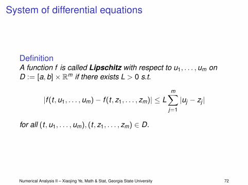
System of differential equations
DefinitionA function f is called Lipschitz with respect to u1, . . . ,um onD := [a,b]× Rm if there exists L > 0 s.t.
|f (t ,u1, . . . ,um)− f (t , z1, . . . , zm)| ≤ Lm∑
j=1
|uj − zj |
for all (t ,u1, . . . ,um), (t , z1, . . . , zm) ∈ D.
Numerical Analysis II – Xiaojing Ye, Math & Stat, Georgia State University 72

System of differential equations
TheoremIf f ∈ C1(D) and | ∂f
∂uj| ≤ L for all j , then f is Lipschitz with
respect to u = (u1, . . . ,um) on D.
Proof.Note that D is convex. For any(t ,u1, . . . ,um), (t , z1, . . . , zm) ∈ D, define
g(λ) = f (t , (1− λ)u1 + λz1, . . . , (1− λ)um + λzm)
for all λ ∈ [0,1]. Then from |g(1)− g(0)| ≤∫ 1
0 |g′(λ)|dλ and the
definition of g, the conclusion follows.
Numerical Analysis II – Xiaojing Ye, Math & Stat, Georgia State University 73
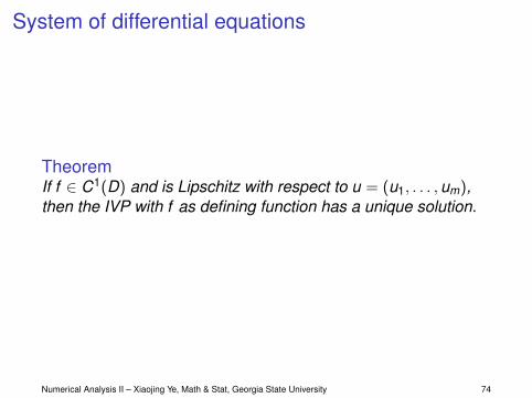
System of differential equations
TheoremIf f ∈ C1(D) and is Lipschitz with respect to u = (u1, . . . ,um),then the IVP with f as defining function has a unique solution.
Numerical Analysis II – Xiaojing Ye, Math & Stat, Georgia State University 74
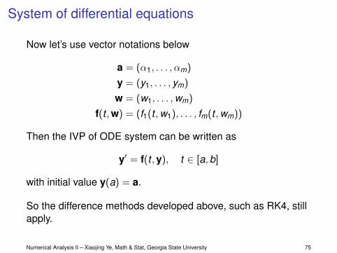
System of differential equations
Now let’s use vector notations below
a = (α1, . . . , αm)
y = (y1, . . . , ym)
w = (w1, . . . ,wm)
f(t ,w) = (f1(t ,w1), . . . , fm(t ,wm))
Then the IVP of ODE system can be written as
y′ = f(t ,y), t ∈ [a,b]
with initial value y(a) = a.
So the difference methods developed above, such as RK4, stillapply.
Numerical Analysis II – Xiaojing Ye, Math & Stat, Georgia State University 75
System of differential equations
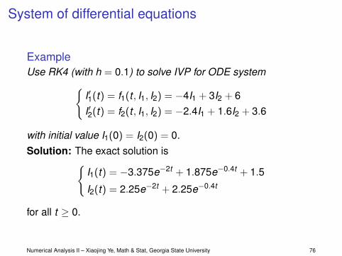
ExampleUse RK4 (with h = 0.1) to solve IVP for ODE system{
I′1(t) = f1(t , I1, I2) = −4I1 + 3I2 + 6I′2(t) = f2(t , I1, I2) = −2.4I1 + 1.6I2 + 3.6
with initial value I1(0) = I2(0) = 0.Solution: The exact solution is{
I1(t) = −3.375e−2t + 1.875e−0.4t + 1.5
I2(t) = 2.25e−2t + 2.25e−0.4t
for all t ≥ 0.
Numerical Analysis II – Xiaojing Ye, Math & Stat, Georgia State University 76
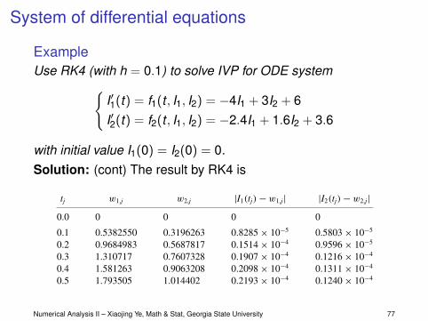
System of differential equations
ExampleUse RK4 (with h = 0.1) to solve IVP for ODE system{
I′1(t) = f1(t , I1, I2) = −4I1 + 3I2 + 6I′2(t) = f2(t , I1, I2) = −2.4I1 + 1.6I2 + 3.6
with initial value I1(0) = I2(0) = 0.Solution: (cont) The result by RK4 is
5.9 Higher-Order Equations and Systems of Differential Equations 333
As a consequence,
I1(0.1) ≈ w1,1 = w1,0 + 16(k1,1 + 2k2,1 + 2k3,1 + k4,1)
= 0 + 16
(0.6 + 2(0.534) + 2(0.54072) + 0.4800912) = 0.5382552
and
I2(0.1) ≈ w2,1 = w2,0 + 16(k1,2 + 2k2,2 + 2k3,2 + k4,2) = 0.3196263.
The remaining entries in Table 5.19 are generated in a similar manner. !
Table 5.19 tj w1,j w2,j |I1(tj) − w1,j| |I2(tj) − w2,j|0.0 0 0 0 0
0.1 0.5382550 0.3196263 0.8285× 10− 5 0.5803× 10− 5
0.2 0.9684983 0.5687817 0.1514× 10− 4 0.9596× 10− 5
0.3 1.310717 0.7607328 0.1907× 10− 4 0.1216× 10− 4
0.4 1.581263 0.9063208 0.2098× 10− 4 0.1311× 10− 4
0.5 1.793505 1.014402 0.2193× 10− 4 0.1240× 10− 4
Recall that Maple reserves theletter D to representdifferentiation.
Maple’s NumericalAnalysis package does not currently approximate the solution tosystems of initial value problems, but systems of first-order differential equations can bysolved using dsolve. The system in the Illustration is defined with
sys 2 := D(u1)(t) = − 4u1(t) + 3u2(t) + 6, D(u2)(t) = − 2.4u1(t) + 1.6u2(t) + 3.6
and the initial conditions with
init 2 := u1(0) = 0, u2(0) = 0
The system is solved with the command
sol 2 := dsolve({sys 2, init 2}, {u1(t), u2(t)})and Maple responds with
!u1(t) = − 27
8e− 2t + 15
8e−
52 t + 3
2, u2(t) = − 9
4e− 2t + 9
4e−
52 t"
To isolate the individual functions we use
r1 := rhs(sol 2[1]); r2 := rhs(sol 2[2])producing
− 278
e− 2t+158
e−52 t + 3
2
− 94
e− 2t+94
e−52 t
and to determine the value of the functions at t = 0.5 we use
evalf (subs(t = 0.5, r1)); evalf (subs(t = 0.5, r2))
Copyright 2010 Cengage Learning. All Rights Reserved. May not be copied, scanned, or duplicated, in whole or in part. Due to electronic rights, some third party content may be suppressed from the eBook and/or eChapter(s).Editorial review has deemed that any suppressed content does not materially affect the overall learning experience. Cengage Learning reserves the right to remove additional content at any time if subsequent rights restrictions require it.
Numerical Analysis II – Xiaojing Ye, Math & Stat, Georgia State University 77
High-order ordinary differential equations
A general IVP for mth-order ODE is
y (m) = f (t , y , y ′, . . . , y (m−1)), t ∈ [a,b]
with initial value y(a) = α1, y ′(a) = α2, . . . , y (m−1)(a) = αm.
DefinitionA function y(t) is a solution of IVP for the mth-order ODEabove if y(t) satisfies the differential equation for t ∈ [a,b] andall initial value conditions at t = a.
Numerical Analysis II – Xiaojing Ye, Math & Stat, Georgia State University 78

High-order ordinary differential equations
We can define a set of functions u1, . . . ,um s.t.
u1(t) = y(t), u2(t) = y ′(t), . . . , um(t) = y (m−1)(t)
Then we can convert the mth-order ODE to a system offirst-order ODEs:
u′1 = u2
u′2 = u3
...u′m = f (t ,u1,u2, . . . ,um)
for a ≤ t ≤ b
with initial values u1(a) = α1, . . . ,um(a) = αm.
Numerical Analysis II – Xiaojing Ye, Math & Stat, Georgia State University 79
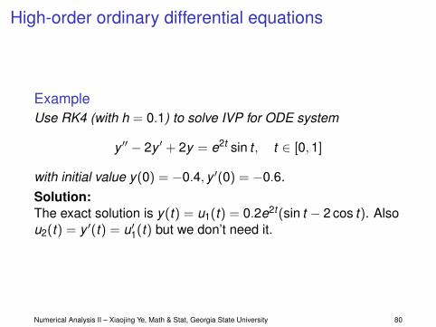
High-order ordinary differential equations
ExampleUse RK4 (with h = 0.1) to solve IVP for ODE system
y ′′ − 2y ′ + 2y = e2t sin t , t ∈ [0,1]
with initial value y(0) = −0.4, y ′(0) = −0.6.Solution:The exact solution is y(t) = u1(t) = 0.2e2t (sin t − 2 cos t). Alsou2(t) = y ′(t) = u′1(t) but we don’t need it.
Numerical Analysis II – Xiaojing Ye, Math & Stat, Georgia State University 80
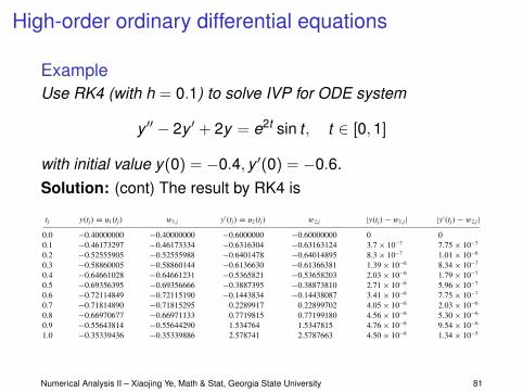
High-order ordinary differential equations
ExampleUse RK4 (with h = 0.1) to solve IVP for ODE system
y ′′ − 2y ′ + 2y = e2t sin t , t ∈ [0,1]
with initial value y(0) = −0.4, y ′(0) = −0.6.Solution: (cont) The result by RK4 is336 C H A P T E R 5 Initial-Value Problems for Ordinary Differential Equations
Table 5.20
tj y(tj) = u1(tj) w1,j y′(tj) = u2(tj) w2,j |y(tj) − w1,j| |y′(tj) − w2,j|0.0 − 0.40000000 − 0.40000000 − 0.6000000 − 0.60000000 0 00.1 − 0.46173297 − 0.46173334 − 0.6316304 − 0.63163124 3.7× 10− 7 7.75× 10− 7
0.2 − 0.52555905 − 0.52555988 − 0.6401478 − 0.64014895 8.3× 10− 7 1.01× 10− 6
0.3 − 0.58860005 − 0.58860144 − 0.6136630 − 0.61366381 1.39× 10− 6 8.34× 10− 7
0.4 − 0.64661028 − 0.64661231 − 0.5365821 − 0.53658203 2.03× 10− 6 1.79× 10− 7
0.5 − 0.69356395 − 0.69356666 − 0.3887395 − 0.38873810 2.71× 10− 6 5.96× 10− 7
0.6 − 0.72114849 − 0.72115190 − 0.1443834 − 0.14438087 3.41× 10− 6 7.75× 10− 7
0.7 − 0.71814890 − 0.71815295 0.2289917 0.22899702 4.05× 10− 6 2.03× 10− 6
0.8 − 0.66970677 − 0.66971133 0.7719815 0.77199180 4.56× 10− 6 5.30× 10− 6
0.9 − 0.55643814 − 0.55644290 1.534764 1.5347815 4.76× 10− 6 9.54× 10− 6
1.0 − 0.35339436 − 0.35339886 2.578741 2.5787663 4.50× 10− 6 1.34× 10− 5
In Maple the nth derivative y(n)(t)is specified by (D@@n)(y)(t).
We can also use dsolve from Maple on higher-order equations. To define the differentialequation in Example 1, use
def 2 := (D@@2)(y)(t) − 2D(y)(t) + 2y(t) = e2t sin(t)
and to specify the initial conditions use
init 2 := y(0) = − 0.4, D(y)(0) = − 0.6
The solution is obtained with the command
sol 2 := dsolve({def 2, init 2}, y(t))
to obtain
y(t) = 15
e2t(sin(t) − 2 cos(t))
We isolate the solution in function form using
g := rhs(sol 2)
To obtain y(1.0) = g(1.0), enter
evalf (subs(t = 1.0, g))
which gives − 0.3533943574.Runge-Kutta-Fehlberg is also available for higher-order equations via the dsolve com-
mand with the numeric option. It is employed in the same manner as illustrated for systemsof equations.
The other one-step methods can be extended to systems in a similar way. When errorcontrol methods like the Runge-Kutta-Fehlberg method are extended, each component ofthe numerical solution (w1j, w2j, . . . , wmj) must be examined for accuracy. If any of thecomponents fail to be sufficiently accurate, the entire numerical solution (w1j, w2j, . . . , wmj)
must be recomputed.The multistep methods and predictor-corrector techniques can also be extended to
systems. Again, if error control is used, each component must be accurate. The extensionof the extrapolation technique to systems can also be done, but the notation becomes quiteinvolved. If this topic is of interest, see [HNW1].
Convergence theorems and error estimates for systems are similar to those consideredin Section 5.10 for the single equations, except that the bounds are given in terms of vectornorms, a topic considered in Chapter 7. (A good reference for these theorems is [Ge1],pp. 45–72.)
Copyright 2010 Cengage Learning. All Rights Reserved. May not be copied, scanned, or duplicated, in whole or in part. Due to electronic rights, some third party content may be suppressed from the eBook and/or eChapter(s).Editorial review has deemed that any suppressed content does not materially affect the overall learning experience. Cengage Learning reserves the right to remove additional content at any time if subsequent rights restrictions require it.
Numerical Analysis II – Xiaojing Ye, Math & Stat, Georgia State University 81
A brief summary
The difference methods we developed above, e.g., Euler’s,midpoints, RK4, multistep explicit/implicit, predictor-correctormethods, are
I based on step-by-step derivation and easy to understand;I widely used in many practical problems;I fundamental to more advanced and complex techniques.
Numerical Analysis II – Xiaojing Ye, Math & Stat, Georgia State University 82

Stability of difference methods
Definition (Consistency)A difference method is called consistent if
limh→0
(max
1≤i≤Nτi(h)
)= 0
where τi(h) is the local truncation error of the method.
RemarkSince local truncation error τi(h) is defined assuming previouswi = yi , it does not take error accumulation into account. So theconsistency definition above only considers how goodφ(t ,wi ,h) in the difference method is.
Numerical Analysis II – Xiaojing Ye, Math & Stat, Georgia State University 83

Stability of difference methods
For any step size h > 0, the difference methodwi+1 = wi + hφ(ti ,wi ,h) can generate a sequence of wi whichdepend on h. We call them {wi(h)}i . Note that wi graduallyaccumulate errors as i = 1,2, . . . ,N.
Definition (Convergent)A difference method is called convergent if
limh→0
(max
1≤i≤N|yi − wi(h)|
)= 0
Numerical Analysis II – Xiaojing Ye, Math & Stat, Georgia State University 84
Stability of difference methods
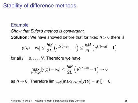
ExampleShow that Euler’s method is convergent.Solution: We have showed before that for fixed h > 0 there is∣∣y(ti)− wi
∣∣ ≤ hM2L
(eL(ti−a) − 1
)≤ hM
2L
(eL(b−a) − 1
)for all i = 0, . . . ,N. Therefore we have
max1≤i≤N
∣∣y(ti)− wi∣∣ ≤ hM
2L
(eL(b−a) − 1
)→ 0
as h→ 0. Therefore limh→0(max1≤i≤N∣∣y(ti)− wi
∣∣) = 0.
Numerical Analysis II – Xiaojing Ye, Math & Stat, Georgia State University 85

Stability of difference method
DefinitionA numerical method is called stable if its results depend on theinitial data continuously.
Numerical Analysis II – Xiaojing Ye, Math & Stat, Georgia State University 86
Stability of difference methods
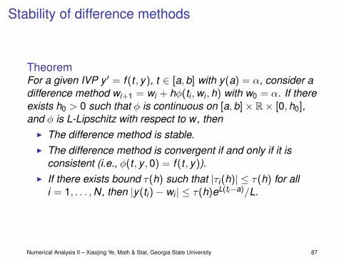
TheoremFor a given IVP y ′ = f (t , y), t ∈ [a,b] with y(a) = α, consider adifference method wi+1 = wi + hφ(ti ,wi ,h) with w0 = α. If thereexists h0 > 0 such that φ is continuous on [a,b]× R× [0,h0],and φ is L-Lipschitz with respect to w, then
I The difference method is stable.I The difference method is convergent if and only if it is
consistent (i.e., φ(t , y ,0) = f (t , y)).I If there exists bound τ(h) such that |τi(h)| ≤ τ(h) for all
i = 1, . . . ,N, then |y(ti)− wi | ≤ τ(h)eL(ti−a)/L.
Numerical Analysis II – Xiaojing Ye, Math & Stat, Georgia State University 87

Stability of difference methods
Proof.Let h be fixed, then wi(α) generated by the difference methodare functions of α. For any two values α, α̂, there is
|wi+1(α)− wi+1(α̂)| = |(wi (α)− hφ(ti ,wi (α)))− (wi (α̂)− hφ(ti ,wi (α̂)))|≤ |wi (α)− wi (α̂)|+ h|φ(ti ,wi (α))− φ(ti ,wi (α̂))|≤ |wi (α)− wi (α̂)|+ hL|wi (α)− wi (α̂)|= (1 + hL)|wi (α)− wi (α̂)|≤ · · ·
≤ (1 + hL)i+1|w0(α)− w0(α̂)|
= (1 + hL)i+1|α− α̂|
≤ (1 + hL)N |α− α̂|
Therefore wi(α) is Lipschitz with respect to α (with constant atmost (1 + hL)N ), and hence is continuous with respect to α.We omit the proofs for the other two assertions here.
Numerical Analysis II – Xiaojing Ye, Math & Stat, Georgia State University 88
Stability of difference method
ExampleUse the result of Theorem above to show that the ModifiedEuler’s method is stable.Solution:Recall the Modified Euler’s method is given by
wi+1 = wi +h2
(f (ti ,wi) + f (ti+1,wi + hf (ti ,wi))
)So we have φ(t ,w ,h) = 1
2(f (t ,w) + f (t + h,w + hf (t ,w))).Now we want to show φ is continuous in (t ,w ,h), and Lipschitzwith respect to w .
Numerical Analysis II – Xiaojing Ye, Math & Stat, Georgia State University 89

Stability of difference method
Solution: (cont) It is obvious that φ is continuous in (t ,w ,h)since f (t ,w) is continuous. Fix t and h. For any w , w̄ ∈ R, thereis
|φ(t ,w , h)− φ(t , w̄ , h)| =12|f (t ,w)− f (t , w̄)|
+12|f (t + h,w + hf (t ,w))− f (t + h, w̄ + hf (t , w̄))|
≤L2|w − w̄ |+
L2|(w + hf (t ,w))− (w̄ + hf (t , w̄))|
≤ L|w − w̄ |+Lh2|f (t ,w)− f (t , w̄)|
≤ L|w − w̄ |+L2h2|w − w̄ |
= (L +L2h2
)|w − w̄ |
So φ is Lipschitz with respect to w . By first part of Theoremabove, the Modified Euler’s method is stable.
Numerical Analysis II – Xiaojing Ye, Math & Stat, Georgia State University 90

Stability of multistep difference method
DefinitionSuppose a multistep difference method given by
wi+1 = am−1wi + am−2wi−1 + · · ·+ a0wi−m+1 + hF (ti ,h,wi+1, . . . ,wi−m+1)
Then we call the following the characteristic polynomial ofthe method:
λm − (am−1λm−1 + · · ·+ a1λ+ a0)
DefinitionA difference method is said to satisfy the root condition if allthe m roots λ1, . . . , λm of its characteristic polynomial havemagnitudes ≤ 1, and all of those which have magnitude =1 aresingle roots.
Numerical Analysis II – Xiaojing Ye, Math & Stat, Georgia State University 91

Stability of multistep difference method
DefinitionI A difference method that satisfies root condition is called
strongly stable if the only root with magnitude 1 is λ = 1.I A difference method that satisfies root condition is called
weakly stable if there are multiple roots with magnitude 1.I A difference method that does not satisfy root condition is
called unstable.
Numerical Analysis II – Xiaojing Ye, Math & Stat, Georgia State University 92
Stability of multistep difference method
TheoremI A difference method is stable if and only if it satisfies the
root condition.I If a difference method is consistent, then it is stable if and
only if it is covergent.
Numerical Analysis II – Xiaojing Ye, Math & Stat, Georgia State University 93

Stability of multistep difference method
ExampleShow that the Adams-Bashforth 4-step explicit method isstrongly stable.Solution: Recall that the method is given by
wi+1 = wi +h24
[55f (ti ,wi )− 59f (ti−1,wi−1) + 37f (ti−2,wi−2)− 9f (ti−3,wi−3)
]
So the characteristic polynomial is simply λ4 − λ3 = λ3(λ− 1),which only has one root λ = 1 with magnitude 1. So themethod is strongly stable.
Numerical Analysis II – Xiaojing Ye, Math & Stat, Georgia State University 94
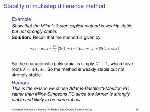
Stability of multistep difference method
ExampleShow that the Milne’s 3-step explicit method is weakly stablebut not strongly stable.Solution: Recall that the method is given by
wi+1 = wi−3 +4h3
[2f (ti ,wi )− f (ti−1,wi−1) + 2f (ti−2,wi−2)
]
So the characteristic polynomial is simply λ4 − 1, which haveroots λ = ±1,±i. So the method is weakly stable but notstrongly stable.
RemarkThis is the reason we chose Adams-Bashforth-Moulton PCrather than Milne-Simpsons PC since the former is stronglystable and likely to be more robust.
Numerical Analysis II – Xiaojing Ye, Math & Stat, Georgia State University 95
Stiff differential equations
Stiff differential equations have e−ct terms (c > 0 large) in theirsolutions. These terms→ 0 quickly, but their derivatives (ofform cne−ct ) do not, especially at small t .
Recall that difference methods have errors proportional to thederivatives, and hence they may be inaccurate for stiff ODEs.
Numerical Analysis II – Xiaojing Ye, Math & Stat, Georgia State University 96
Stiff differential equations
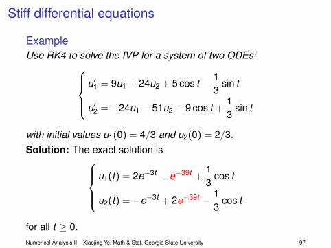
ExampleUse RK4 to solve the IVP for a system of two ODEs:
u′1 = 9u1 + 24u2 + 5 cos t − 13
sin t
u′2 = −24u1 − 51u2 − 9 cos t +13
sin t
with initial values u1(0) = 4/3 and u2(0) = 2/3.Solution: The exact solution is
u1(t) = 2e−3t − e−39t +13
cos t
u2(t) = −e−3t + 2e−39t − 13
cos t
for all t ≥ 0.Numerical Analysis II – Xiaojing Ye, Math & Stat, Georgia State University 97
Stiff differential equations
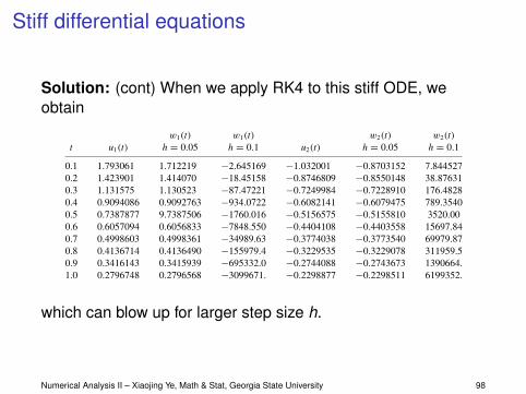
Solution: (cont) When we apply RK4 to this stiff ODE, weobtain
5.11 Stiff Differential Equations 349
has the unique solution
u1(t) = 2e− 3t − e− 39t + 13
cos t, u2(t) = − e− 3t + 2e− 39t − 13
cos t.
The transient term e− 39t in the solution causes this system to be stiff. Applying Algorithm5.7, the Runge-Kutta Fourth-Order Method for Systems, gives results listed in Table 5.22.When h = 0.05, stability results and the approximations are accurate. Increasing the stepsize to h= 0.1, however, leads to the disastrous results shown in the table. !
Table 5.22 w1(t) w1(t) w2(t) w2(t)t u1(t) h= 0.05 h= 0.1 u2(t) h= 0.05 h= 0.1
0.1 1.793061 1.712219 − 2.645169 − 1.032001 − 0.8703152 7.8445270.2 1.423901 1.414070 − 18.45158 − 0.8746809 − 0.8550148 38.876310.3 1.131575 1.130523 − 87.47221 − 0.7249984 − 0.7228910 176.48280.4 0.9094086 0.9092763 − 934.0722 − 0.6082141 − 0.6079475 789.35400.5 0.7387877 9.7387506 − 1760.016 − 0.5156575 − 0.5155810 3520.000.6 0.6057094 0.6056833 − 7848.550 − 0.4404108 − 0.4403558 15697.840.7 0.4998603 0.4998361 − 34989.63 − 0.3774038 − 0.3773540 69979.870.8 0.4136714 0.4136490 − 155979.4 − 0.3229535 − 0.3229078 311959.50.9 0.3416143 0.3415939 − 695332.0 − 0.2744088 − 0.2743673 1390664.1.0 0.2796748 0.2796568 − 3099671. − 0.2298877 − 0.2298511 6199352.
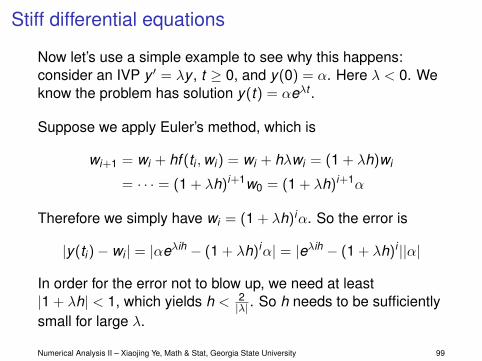
Although stiffness is usually associated with systems of differential equations, theapproximation characteristics of a particular numerical method applied to a stiff system canbe predicted by examining the error produced when the method is applied to a simple testequation,
y′ = λy, y(0) = α, where λ < 0. (5.64)
The solution to this equation is y(t) = αeλt , which contains the transient solution eλt . Thesteady-state solution is zero, so the approximation characteristics of a method are easy todetermine. (A more complete discussion of the round-off error associated with stiff systemsrequires examining the test equation when λ is a complex number with negative real part;see [Ge1], p. 222.)
First consider Euler’s method applied to the test equation. Letting h= (b − a)/N andtj = jh, for j = 0, 1, 2, . . . , N , Eq. (5.8) on page 266 implies that
w0 = α, and wj+1 = wj + h(λwj) = (1 + hλ)wj,
so
wj+1 = (1 + hλ)j+1w0 = (1 + hλ)j+1α, for j = 0, 1, . . . , N − 1. (5.65)
Since the exact solution is y(t) = αeλt , the absolute error is
| y(tj) − wj| =!!ejhλ − (1 + hλ) j
!! |α| =!!(ehλ) j − (1 + hλ) j
!! |α|,
and the accuracy is determined by how well the term 1+hλ approximates ehλ. When λ < 0,the exact solution (ehλ) j decays to zero as j increases, but by Eq.(5.65), the approximation
Copyright 2010 Cengage Learning. All Rights Reserved. May not be copied, scanned, or duplicated, in whole or in part. Due to electronic rights, some third party content may be suppressed from the eBook and/or eChapter(s).Editorial review has deemed that any suppressed content does not materially affect the overall learning experience. Cengage Learning reserves the right to remove additional content at any time if subsequent rights restrictions require it.
which can blow up for larger step size h.
Numerical Analysis II – Xiaojing Ye, Math & Stat, Georgia State University 98
Stiff differential equations
Now let’s use a simple example to see why this happens:consider an IVP y ′ = λy , t ≥ 0, and y(0) = α. Here λ < 0. Weknow the problem has solution y(t) = αeλt .
Suppose we apply Euler’s method, which is
wi+1 = wi + hf (ti ,wi) = wi + hλwi = (1 + λh)wi
= · · · = (1 + λh)i+1w0 = (1 + λh)i+1α
Therefore we simply have wi = (1 + λh)iα. So the error is
|y(ti)− wi | = |αeλih − (1 + λh)iα| = |eλih − (1 + λh)i ||α|
In order for the error not to blow up, we need at least|1 + λh| < 1, which yields h < 2
|λ| . So h needs to be sufficientlysmall for large λ.
Numerical Analysis II – Xiaojing Ye, Math & Stat, Georgia State University 99
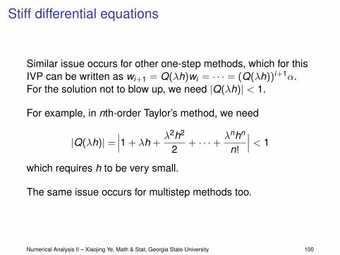
Stiff differential equations
Similar issue occurs for other one-step methods, which for thisIVP can be written as wi+1 = Q(λh)wi = · · · = (Q(λh))i+1α.For the solution not to blow up, we need |Q(λh)| < 1.
For example, in nth-order Taylor’s method, we need
|Q(λh)| =∣∣∣1 + λh +
λ2h2
2+ · · ·+ λnhn
n!
∣∣∣ < 1
which requires h to be very small.
The same issue occurs for multistep methods too.
Numerical Analysis II – Xiaojing Ye, Math & Stat, Georgia State University 100
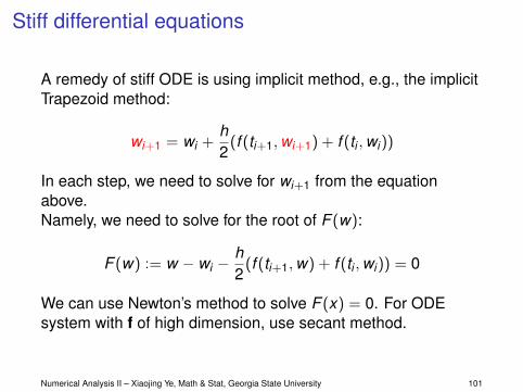
Stiff differential equations
A remedy of stiff ODE is using implicit method, e.g., the implicitTrapezoid method:
wi+1 = wi +h2
(f (ti+1,wi+1) + f (ti ,wi))
In each step, we need to solve for wi+1 from the equationabove.Namely, we need to solve for the root of F (w):
F (w) := w − wi −h2
(f (ti+1,w) + f (ti ,wi)) = 0
We can use Newton’s method to solve F (x) = 0. For ODEsystem with f of high dimension, use secant method.
Numerical Analysis II – Xiaojing Ye, Math & Stat, Georgia State University 101
Related Documents