American Economic Review 2015, 105(1): 35–66 http://dx.doi.org/10.1257/aer.20110572 35 Infrastructure Quality and the Subsidy Trap † By Shaun McRae * Electricity and water are often subsidized in developing countries to increase their affordability for low-income households. Ideally, such subsidies would create sufficient demand in poor neighborhoods to encourage private investment in their infrastructure. Instead, many regions receiving large subsidies have precarious distribution net- works supplying users who never pay. Using a structural model of household electricity demand in Colombia, I predict the change in consumption and profits from upgrading low-quality electricity con- nections. I show that the existing subsidies, which provide greater transfers to areas with unreliable supply, deter investment to mod- ernize infrastructure. Finally, I analyze alternative programs with stronger investment incentives. (JEL H23, H54, L94, L98, O12, O13) Electricity and water are often subsidized in developing countries to increase their affordability for low-income households. Ideally, such subsidies would create suffi- cient demand in poor neighborhoods to encourage private investment in their infra- structure. Instead, many regions receiving large subsidies have precarious distribution networks supplying users who never pay. The persistence of this phenomenon is a puzzle. There are no technological obstacles to providing modern connections, and infrastructure upgrades could potentially benefit both households (through higher quality service) and firms (through lower costs and higher payment rates). In this paper I provide an empirical explanation for this puzzle based on data from the elec- tricity sector in Colombia: the subsidies discourage investment in infrastructure and trap households and firms in a nonpaying, low-quality equilibrium. * Department of Economics, University of Michigan, 611 Tappan Avenue, Ann Arbor, MI 48109 (e-mail: sdm- [email protected]). I thank Frank Wolak for his advice and encouragement, as well as Dan Ackerberg, Timothy Bresnahan, Ryan Kellogg, Ryan Lampe, Jonathan Levin, Romans Pancs, Peter Reiss and seminar participants at Clemson University, Consortium on Financial Systems and Poverty IO/Development workshop, Indiana University (School of Public and Environmental Affairs), International Food Policy Research Institute, Latin American and Caribbean Economic Association annual meeting, Michigan Development Day, Michigan State University, Motu Economic and Public Policy Research, Resources for the Future, Stanford University, University of California Berkeley Energy Camp, University of Michigan, University of North Carolina, and Washington University (Olin Business School), for their many helpful comments and suggestions. Special thanks to the Superintendencia de Servicios Públicos for compiling the billing and outage data used in this study. Financial support for this work was provided by the Martin Lee Johnson Stanford Graduate Fellowship and the Kapnick Fellowship Program at the Stanford Institute for Economic Policy Research. The author declares that he has no relevant or material financial interests that relate to the research described in this paper. † Go to http://dx.doi.org/10.1257/aer.20110572 to visit the article page for additional materials and author disclosure statement(s).

Welcome message from author
This document is posted to help you gain knowledge. Please leave a comment to let me know what you think about it! Share it to your friends and learn new things together.
Transcript
American Economic Review 2015, 105(1): 35–66 http://dx.doi.org/10.1257/aer.20110572
35
Infrastructure Quality and the Subsidy Trap †
By Shaun McRae *
Electricity and water are often subsidized in developing countries to increase their affordability for low-income households. Ideally, such subsidies would create sufficient demand in poor neighborhoods to encourage private investment in their infrastructure. Instead, many regions receiving large subsidies have precarious distribution net-works supplying users who never pay. Using a structural model of household electricity demand in Colombia, I predict the change in consumption and profits from upgrading low-quality electricity con-nections. I show that the existing subsidies, which provide greater transfers to areas with unreliable supply, deter investment to mod-ernize infrastructure. Finally, I analyze alternative programs with stronger investment incentives. (JEL H23, H54, L94, L98, O12, O13)
Electricity and water are often subsidized in developing countries to increase their affordability for low-income households. Ideally, such subsidies would create suffi-cient demand in poor neighborhoods to encourage private investment in their infra-structure. Instead, many regions receiving large subsidies have precarious distribution networks supplying users who never pay. The persistence of this phenomenon is a puzzle. There are no technological obstacles to providing modern connections, and infrastructure upgrades could potentially benefit both households (through higher quality service) and firms (through lower costs and higher payment rates). In this paper I provide an empirical explanation for this puzzle based on data from the elec-tricity sector in Colombia: the subsidies discourage investment in infrastructure and trap households and firms in a nonpaying, low-quality equilibrium.
* Department of Economics, University of Michigan, 611 Tappan Avenue, Ann Arbor, MI 48109 (e-mail: [email protected]). I thank Frank Wolak for his advice and encouragement, as well as Dan Ackerberg, Timothy Bresnahan, Ryan Kellogg, Ryan Lampe, Jonathan Levin, Romans Pancs, Peter Reiss and seminar participants at Clemson University, Consortium on Financial Systems and Poverty IO/Development workshop, Indiana University (School of Public and Environmental Affairs), International Food Policy Research Institute, Latin American and Caribbean Economic Association annual meeting, Michigan Development Day, Michigan State University, Motu Economic and Public Policy Research, Resources for the Future, Stanford University, University of California Berkeley Energy Camp, University of Michigan, University of North Carolina, and Washington University (Olin Business School), for their many helpful comments and suggestions. Special thanks to the Superintendencia de Servicios Públicos for compiling the billing and outage data used in this study. Financial support for this work was provided by the Martin Lee Johnson Stanford Graduate Fellowship and the Kapnick Fellowship Program at the Stanford Institute for Economic Policy Research. The author declares that he has no relevant or material financial interests that relate to the research described in this paper.
† Go to http://dx.doi.org/10.1257/aer.20110572 to visit the article page for additional materials and author disclosure statement(s).

36 THE AMERICAN ECONOMIC REVIEW JANuARy 2015
Latin American countries exhibit vast differences across households in the quality of infrastructure services.1 While middle- and upper-income households in major cities enjoy similar levels of service to those in developed countries, households in informal settlements on the outskirts of cities suffer from dangerous and unre-liable infrastructure. Electricity supply to informal settlements may be nothing more than a bare wire strung up by residents and attached to the nearest power line. Nevertheless, households see an important advantage of this type of connection: although the quality is low, payment for the service cannot be enforced. Attempts to improve this situation have focused on infrastructure upgrades that are funded through higher payment rates by households. Many such efforts have been met with widespread and sometimes violent resistance.2
Inadequate infrastructure such as found in informal settlements has been recognized as a major barrier to economic advancement for affected households. A growing lit-erature examines the social and economic impact of improvements in physical infra-structure in developing countries.3 Dinkelman (2011) shows that a rural electrification program in South Africa led to an increase in female employment, plausibly as the result of labor-saving technology used for home production activities.4 Lipscomb, Mobarak, and Barham (2013) use exogenous variation in electrification in Brazil between 1960 and 2000, and show that access to electricity had large positive effects on education and labor force outcomes. Rud (2012) uses irrigation groundwater availability in India as an instrument for investment in electricity infrastructure, finding that moving a state from the twenty-fifth to the seventy-fifth percentile of the distribution of electrification would increase manufacturing output by nearly 25 percent.
The contribution of this paper is to characterize the persistence of low-quality infrastructure as a dysfunctional outcome involving households, utility firms, and government. Households with informal connections receive low-quality service for
1 This paper is focused exclusively on electricity distribution infrastructure. Firms build the electricity network, then buy electricity from the wholesale market which they sell to consumers at a regulated price. There are no constraints on the supply of wholesale electricity. This is a reasonable assumption for Latin America, where countries that have undertaken wholesale market reforms normally have sufficient generation capacity to meet electricity demand. By contrast, many countries in Africa and Asia face supply constraints in electricity generation—which affect both rich and poor households—as well as the problem of low-quality distribution infrastructure in poor neighborhoods.
2 The best-known example of such resistance is the “water war” in Cochabamba, Bolivia, in 2000. The Cochabamba water utility, SEMAPA, was privatized in 1999. The new owners, a consortium of firms known as Aguas del Tunari, agreed to finance the expansion of the distribution network and a large project to increase the water supply. This investment was to be funded by an increase in water rates for most users. The rate increase led to large protests that spread to other parts of Bolivia and ultimately, in April 2000, the cancellation of the Aguas del Tunari contract and a return to public ownership. However, nine years later Oscar Olivera, the leader of the protests, said that SEMAPA is “equally bad, or worse, than in 2000.” Current problems include the increased rationing of supplies due to a reduction in the available water sources, the lack of expansion of service to the southern part of the city, under-investment in major pipelines, and a large financial deficit due in part to nonenforcement of bill payment (Gisela Alcócer Caero, “Cochabamba ganó la guerra y perdió el agua,” Los Tiempos, April 5, 2009).
3 Apart from electricity, researchers have studied the effects of many other types of infrastructure investment, including irrigation dams (Duflo and Pande 2007), piped water connections (Devoto et al. 2012), protected water sources (Kremer et al. 2011), public water taps (Meeks 2012), mobile phones (Jensen 2007), railroads (Donaldson forthcoming; Banerjee, Duflo, and Qian 2012), urban street paving (Gonzalez-Navarro and Quintana-Domeque 2012), and interstate highways (Duranton and Turner 2012).
4 Many researchers have analyzed the effect of electrical appliances on household decision-making. For devel-oped countries, Greenwood, Seshadri, and Vandenbroucke (2005) suggest that labor-saving appliances created the baby boom by reducing the cost of having children, although Bailey and Collins (2011) do not find empirical sup-port for this claim. For developing countries, television has been shown to increase female autonomy and reduce fertility, possibly through the example of small urban families shown on television dramas (Jensen and Oster 2009; La Ferrara, Chong, and Duryea 2012), while also reducing participation in social activities (Olken 2009).
37Mcrae: Infrastructure QualIty and the subsIdy trapVOl. 105 nO. 1
which they do not pay. Utility firms tolerate nonpayment because they receive finan-cial support from the government covering the cost of service. The government pro-vides these payments to retain the political support of the poor households and avoid civil unrest should the firm disconnect areas with many nonpaying users.
However, the financial transfers by the government to utilities have a dramatic effect on investment incentives. Because the government cannot observe the con-sumption of households with informal connections, firms may receive fiscal trans-fers greater than the cost of providing service. The resulting high profits from low-quality service mean that the incremental profit from improving service is lower than the capital cost, even if such an upgrade means that payment by households can subsequently be enforced. Although the finding that subsidies create distortions is not unexpected, the particular mechanism described in this paper is novel. A subsidy program for short-term consumption instead displaces long-term investment. Based on the results in the literature about the long-term benefits of infrastructure invest-ment, the potential welfare costs of this distortion are very large.
In this paper I use detailed household and firm data from Colombia to demonstrate the incentive effects of one such transfer program. This requires an analysis of how an upgrade affects the consumption of households with informal connections. There are three major changes for households from the provision of a modernized connection. First, installation of a meter means that the household is billed for its true usage, so it faces a nonzero marginal price for consumption. Second, a connection built to a high technical standard will improve the reliability and quality of the household’s utility supply. Finally, an individual connection to the distribution network enables the firm to disconnect for nonpayment and makes it much more likely that the household will pay.
These changes as the result of an upgrade induce two opposing effects on electric-ity consumption: an increase in marginal price due to metering reduces the quantity demanded, and an increase in reliability rotates out the household’s demand. To characterize these effects, I estimate a model of household electricity demand using data for a large sample of metered households in Colombia. I rely on data from metered households because consumption patterns of unmetered households are unobservable. Nevertheless, there are many households in my sample with similar demographic characteristics to unmetered households. I use a dataset that combines household electricity billing data, household characteristics including appliance holdings and demographics, and data on the number and length of electricity out-ages. The model accounts for the nonlinearity in the price schedules due to electric-ity subsidies, and allows for price, income, and reliability effects that differ across households depending on their appliance holdings.
I then use the model estimates to predict the consumption of unmetered house-holds from 100 counties in Colombia with the least reliable electricity supply. I observe the characteristics of households and the typical number and duration of outages from each county. Based on these inputs, I predict the electricity consump-tion of each household using the estimates of preferences. I then predict the con-sumption of each household after a hypothetical upgrade of the distribution network that reduces the number and length of outages and increases the household’s mar-ginal price to the regulated price schedule.
The predicted consumption of households before and after an upgrade is combined with cost and regulatory data for each firm to estimate the change in the firm’s profit as
38 THE AMERICAN ECONOMIC REVIEW JANuARy 2015
a result of the upgrade. I show that for all but one of the counties in the sample, it would be more profitable for the firm not to upgrade its network, and instead maintain existing low-quality service to informal settlements. This is true even though payment rates are assumed to increase from 0 to 100 percent as a result of the upgrade. Household elec-tricity consumption is lower after the upgrade, because the increase in consumption as a result of the improved quality is more than offset by the reduction in consumption from the higher marginal price. The upgrade also results in the firm losing large sub-sidy payments from the government. The capital cost of the upgrade and the reduction in subsidies more than offset the increase in revenue from user payments, resulting in the upgrade being unprofitable for most counties. Variation across counties in the prof-itability of an upgrade is the result of differences in household characteristics (in par-ticular, appliance ownership rates), differences in electricity prices and subsidy levels across regions, and differences in the existing level of network reliability.
Finally, I analyze alternative subsidy programs that may provide stronger incen-tives for electricity suppliers to invest in network modernization. I compute the opti-mal combination of several different policies under various political constraints that the government might face in changing the existing program. For example, if there are no constraints on reducing the existing value of firms, then all counties could be upgraded at a total cost to the government 34 percent less than the current program. Alternatively, if firms cannot be made worse off, then all counties could be upgraded at a total cost to the government 23 percent less than the existing program.
The major result of this paper is that government policies to maintain service for nonpaying, unmetered households may perpetuate the existence of low- quality connections by creating a disincentive for firms to invest. The prerequisites for this result—quantity-based subsidies, low-quality infrastructure, unmetered and non-paying users—are common in the infrastructure sectors of most developing coun-tries. The particular problem in Colombia arises from two features of the subsidy program that are otherwise regarded as very successful: the targeting of subsidies to poor households, and the provision of an external funding mechanism for the sub-sidies.5 Larger transfers from the government to firms supplying households with low-quality service reduce the incentive for these firms to undertake investments that potentially result in the loss of these transfers. This problem is not unique to the electricity sector in Colombia. Similar incentive problems have arisen in other countries with subsidy programs for informal settlements.6,7
5 In terms of the allocation of government resources across households, the Colombian utility subsidy program is one of the most successful of any developing country at targeting subsidies to poor households. Komives et al. (2005) review the targeting performance of water and electricity subsidy schemes in many developing countries. They show that the Colombian scheme outperforms quantity-based subsidies in other countries that do not use any form of administrative selection of subsidy recipients. These other schemes are almost always regressive: both because many poor households do not have an electricity connection, and those with a connection use less electric-ity than rich households.
6 The Blackout Reduction Program (PRA) was a subsidy program in the Dominican Republic in which the gov-ernment paid 75 percent of the cost of electricity used in informal settlements. Krishnaswamy and Stuggins (2007) describe how this created incentives for firms to expand the number of households included in the program. By the end of 2004, it covered one-third of the electricity customers in the country. The PRA was originally intended to be a two-year program with a cost of US$30 million per year—however, in 2004 the cost was US$226 million. The program was canceled in July 2009.
7 Singh et al. (1993) describe a “low-level equilibrium trap” for water supply in rural Kerala, India, in which the water authority provides an unreliable free service funded by the central government. They use contingent valuation to analyze the willingness-to-pay for upgraded service. Olmstead (2004) uses data for colonias in Texas
39Mcrae: Infrastructure QualIty and the subsIdy trapVOl. 105 nO. 1
This paper complements the previous literature that focuses on the effects of infrastructure on economic development. The results from this literature suggest that the long-term benefits of improved infrastructure are complex and far-reaching, and could not reasonably be captured by standard welfare calculations. Therefore, in this paper I do not attempt to calculate the welfare benefits from provision of more reliable electricity. Instead, I assume that the goal of government policy for informal settlements is (or arguably should be) the provision of a metered connection built to a high technical standard for all households. The major contribution of this paper is to show how regulatory design—in particular, the pricing and subsidy policy—plays an essential role in determining whether this goal is achieved.
The remainder of the paper is organized as follows. The next section provides brief background information on the Colombian electricity market and subsidy programs. Section II describes the model of household demand for electricity, the data that will be used to estimate this model, the econometric methodology, and the results of the demand estimation. Section III uses the demand estimates, along with firm-level cost and regulatory data, to show how the current subsidy program discourages firms from upgrading the informal connections to their networks, and how alternative policies would increase the number of upgraded counties. Section IV concludes.
I. Institutional Setting
In Colombia, 34 firms provide combined distribution and retail services to resi-dential and small commercial users, with each of the distributors being a monop-oly in its geographical service area.8 The Energy and Gas Regulatory Commission (CREG) sets a regulated base price for each firm f and period t , P ft . This regu-lated price applies to residential and small commercial users (with demand less than 2 MW). The price has components corresponding to the four segments of the electricity industry. Transmission, distribution, and retailing charges are determined by the regulator, and in most cases these are revised once every five years.9 The generation charge is calculated based on the average price of wholesale electricity purchases—both spot and contract—over the previous 12 months.10
For the firm, the marginal cost of supplying a unit of electricity, c ft , is the whole-sale cost of electricity, which comprises the wholesale generation price and trans-mission charges. The firm must buy more electricity than the end user consumes because of the physical losses in the distribution network. The regulator sets a target rate for these line losses and, in the calculation of P ft , wholesale costs are scaled up by this target amount.11 Other costs for the distribution and retail firm—capital, maintenance, billing, customer service, administration—are fixed and do not vary
border counties to show that, in the absence of universal service requirements, regulation of water rates can deter investment to provide service to poor communities.
8 In the electricity supply industry, the distribution segment is the provision of the physical infrastructure (such as transformers and power lines) for local delivery of electricity to end users. The retail segment is the metering and billing of end users, and the settlement of electricity purchases in the wholesale market.
9 This paper considers the firm’s decision to upgrade a small part of its network. I assume throughout that the effect of the firm’s decision on its overall profit is sufficiently small that the firm does not consider potential feed-back from the upgrade to future values of the regulated price P ft .
10 CREG (1997), Resolution 31, Appendix 1. 11 The true level of line losses in the distribution network is unobserved. If all electricity users are metered, then
line losses can be determined as the difference between the metered consumption and the injections into the network

40 THE AMERICAN ECONOMIC REVIEW JANuARy 2015
with usage. Nevertheless, all of these costs are recovered through the per-unit price P ft because there are no fixed monthly charges.
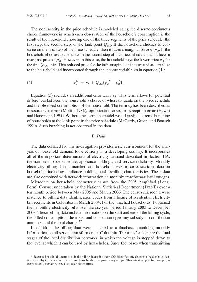
Colombia has a targeted program of quantity-based subsidies that mean most users do not pay the base price P ft . There is a universal geographical classification of all neighborhoods into six socioeconomic strata (estratos).12 Households classi-fied in Strata 1, 2, and 3 receive a subsidy of approximately 50 percent, 40 percent, and 15 percent, respectively, for the first Q sub units of consumption, and then pay P ft for all additional units.13,14 Households in Strata 5 and 6 (less than 5 percent of all households) and commercial users pay 120 percent of P ft for their entire con-sumption, with the additional 20 percent being used as a contribution to the subsidy program.15 Only households in Strata 4 pay P ft for their entire consumption.
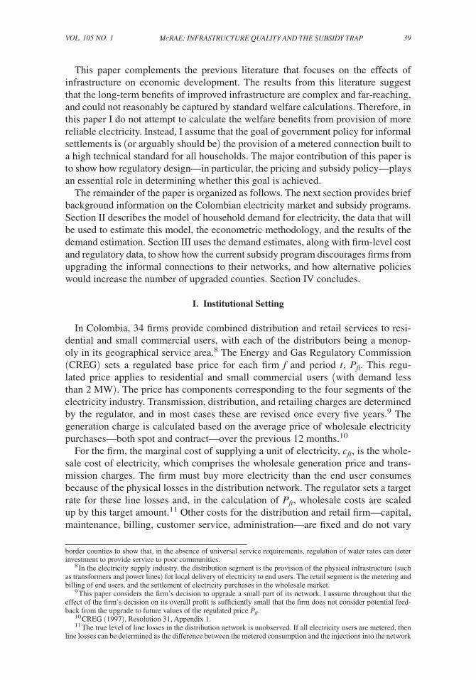
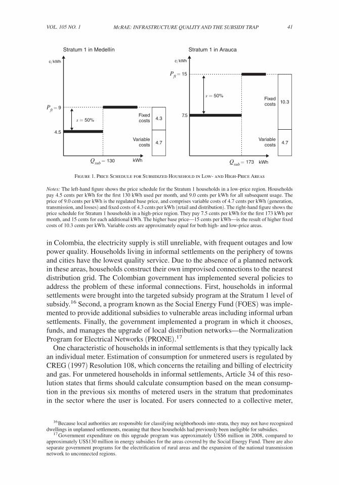
Figure 1 shows the Stratum 1 price schedule, in a region with a low base price (Medellín) and a region with a high base price (Arauca). The maximum amount of the subsidy is more than twice as large in Arauca as in Medellín ($12.98 versus $5.85), for two reasons. First, the subsidy is calculated as a fraction (50 percent) of P ft , and P ft is 6 cents/kWh higher in Arauca than in Medellín. Second, the subsidized quantity Q sub is 173 kWh in Arauca compared to 130 kWh in Medellín. Because the variable costs are similar in both regions, the subsidy covers 138 percent of variable costs in Arauca but only 62 percent of variable costs in Medellín, for a household consuming 200 kWh per month. That is, in areas with a high base price such as Arauca, the Stratum 1 subsidy is sufficient to cover variable costs and contribute to fixed costs and profit, even if the household does not pay their bill.
The Ministry of Mines and Energy operates a redistribution fund to rebalance the contributions and subsidies across different retailers. At a national level, total subsidies exceeded total contributions by 46 percent in 2008. The central government makes up this difference through a contribution to the redistribution fund. Every quarter, firms report the total amount billed to customers in each category, as well as the total subsi-dies and contributions by category. Based on the difference between reported subsidies and contributions, the firm either pays or receives a transfer to or from the government.
The quality of electricity service in most metropolitan areas in Colombia is com-parable to that in developed countries. However, for a minority of poor households
from the high voltage transmission network. However, if some users are unmetered, it is impossible to distinguish their unmetered consumption from the physical line losses.
12 This classification is the responsibility of local government authorities. The criteria are based on external characteristics of the dwellings and the overall quality of the urban environment, and do not depend on household characteristics such as income. For example, a house in Stratum 1 might be an unfinished wooden shack in an area without paved roads, or situated close to a refuse dump. A dwelling in Stratum 6 might be a luxury apartment or a mansion in a gated neighborhood. Because it is the dwelling that is classified, and not the residents of the dwelling, a rich family could move to a house in a poor neighborhood and receive subsidized public utilities and other government benefits that are linked to the stratification program. There is considerable policy debate within Colombia on how to improve the targeting of the public utility subsidy program (Meléndez, Casas, and Medina 2004; Departamento Nacional de Planeación 2008). A separate issue is the linking of subsidies to the geographical location of the dwelling. Medina and Morales (2007) provide evidence for Bogotá that most of these subsidy ben-efits are capitalized into housing prices.
13 There are small differences in these subsidy levels across retailers. Law 1117 of 2006 increased the maximum subsidies for Strata 1 and 2 to 60 percent and 50 percent, respectively, with subsidies allowed to increase up to these levels to ensure that electricity prices for low-consumption users rise by no more than inflation.
14 Before August 2004, the size of the subsidized block ( Q sub ) was 200 kWh/month for all subsidized users. This was reduced over three years to 130 kWh/month for users in highland regions (1,000 meters or more above sea level) and 173 kWh/month for users in lowland regions. For users with informal connections, Q sub is larger: 184 kWh/month and 138 kWh/month in lowland and highland regions, respectively.
15 Since 2012, industrial users have been exempt from the requirement to pay this contribution (Law 1430 of 2010).
41Mcrae: Infrastructure QualIty and the subsIdy trapVOl. 105 nO. 1
in Colombia, the electricity supply is still unreliable, with frequent outages and low power quality. Households living in informal settlements on the periphery of towns and cities have the lowest quality service. Due to the absence of a planned network in these areas, households construct their own improvised connections to the nearest distribution grid. The Colombian government has implemented several policies to address the problem of these informal connections. First, households in informal settlements were brought into the targeted subsidy program at the Stratum 1 level of subsidy.16 Second, a program known as the Social Energy Fund (FOES) was imple-mented to provide additional subsidies to vulnerable areas including informal urban settlements. Finally, the government implemented a program in which it chooses, funds, and manages the upgrade of local distribution networks—the Normalization Program for Electrical Networks (PRONE).17
One characteristic of households in informal settlements is that they typically lack an individual meter. Estimation of consumption for unmetered users is regulated by CREG (1997) Resolution 108, which concerns the retailing and billing of electricity and gas. For unmetered households in informal settlements, Article 34 of this reso-lution states that firms should calculate consumption based on the mean consump-tion in the previous six months of metered users in the stratum that predominates in the sector where the user is located. For users connected to a collective meter,
16 Because local authorities are responsible for classifying neighborhoods into strata, they may not have recognized dwellings in unplanned settlements, meaning that these households had previously been ineligible for subsidies.
17 Government expenditure on this upgrade program was approximately US$6 million in 2008, compared to approximately US$130 million in energy subsidies for the areas covered by the Social Energy Fund. There are also separate government programs for the electrification of rural areas and the expansion of the national transmission network to unconnected regions.
c/kWhc/kWh
Qsub = 130 Qsub = 173
Pft = 9
Pft = 15
s = 50%
s = 50%
4.5
7.5
kWh kWh
Stratum 1 in Medellín Stratum 1 in Arauca
4.3Fixedcosts
4.7Variable
costs
10.3Fixedcosts
4.7Variable
costs
Figure 1. Price Schedule for Subsidized Household in Low- and High-Price Areas
Notes: The left-hand figure shows the price schedule for the Stratum 1 households in a low-price region. Households pay 4.5 cents per kWh for the first 130 kWh used per month, and 9.0 cents per kWh for all subsequent usage. The price of 9.0 cents per kWh is the regulated base price, and comprises variable costs of 4.7 cents per kWh (generation, transmission, and losses) and fixed costs of 4.3 cents per kWh (retail and distribution). The right-hand figure shows the price schedule for Stratum 1 households in a high-price region. They pay 7.5 cents per kWh for the first 173 kWh per month, and 15 cents for each additional kWh. The higher base price—15 cents per kWh—is the result of higher fixed costs of 10.3 cents per kWh. Variable costs are approximately equal for both high- and low-price areas.
42 THE AMERICAN ECONOMIC REVIEW JANuARy 2015
Article 33 states that individual users should be billed for total metered consumption divided by the number of users.18 The regulations provide flexibility for firms to set the parameters and choose the methodology for estimating the consumption of unmetered households.19 Although bill payment rates for households in informal settlements are very low, the methodology for estimating unmetered consumption is still very important, because the estimated consumption determines the amount of subsidy reimbursement from the government.
II. Household Demand for Electricity
In this section I describe the model of household demand for electricity, the data-set constructed to estimate the model, the econometric methodology used for the estimation, and the estimation results. The demand model builds on that of Reiss and White (2005), with the addition of supply outages. This model incorporates the nonlinearity in the price schedule described in Section I, the heterogeneity across households in characteristics and appliance holdings, and the effect of reliability on electricity demand. All of these components are used for the empirical application in Section III, in which I use the model estimates to simulate electricity consumption before and after a hypothetical network upgrade.
A. Model
People do not consume electricity directly. Instead, the demand for electricity is derived from the demand for the services provided by each of the devices in the home that consume electricity. For example, a television consumes approxi-mately 0.2 kWh of electricity per hour. The household decides how many hours of television to watch, recognizing the price of their viewing hours which includes the television’s consumption of electricity. A similar decision is made by the household for each of the appliances in the home. The total electricity consumption is the sum of the device-level consumption across all appliances.
The electricity consumption of appliance i in household j during a month t with no supply interruptions, q ijt ∗ , is given by equation (1).
(1) q ijt ∗ ( p jt , y jt , · ) = α i + γ i y jt + β i p jt + δ i ′ z jt + η ijt .
Variable y jt is the income of household j in month t , and coefficient γ i measures the effect of income on the electricity consumption of appliance i .20 p jt = p jt ( q jt ) is the
18 This will include the average distribution losses between the meter and the dwellings. 19 For example, an additional provision states that when consumption cannot be determined as a result of
unauthorized behavior by the customer, the firm can calculate consumption from the maximum capacity of the connection, multiplied by a utilization factor established by the firm (Article 54). There is substantial variation across electricity retailers in these parameters: the utilization factor applied varies from 10 percent to 30 percent. Furthermore, there may be ambiguity in the classification of unmetered households. A household in an informal settlement with an unauthorized connection to the distribution network could be covered by Articles 34 or 54. It is possible that firms estimate consumption using several different methodologies and then choose the approach that gives the highest consumption estimate. The utility serving Bogotá, Codensa, explicitly states in its customer con-tract that it uses the maximum from six different methods to estimate the quantity of any unauthorized consumption.
20 As shown below in equation (4), income y jt will be adjusted to account for the nonlinearity of the price schedule.
43Mcrae: Infrastructure QualIty and the subsIdy trapVOl. 105 nO. 1
marginal price of electricity consumption faced by household j during month t . This price is a function of the total household electricity consumption in that period, q jt , due to the possible nonlinearity in the price schedule.21 Coefficient β i captures the appli-ance-level response to changes in this marginal price.22 The vector z jt is a vector of household characteristics for household j in month t . The coefficient vector δ i measures the effect of these characteristics on appliance-level demand. Finally, η ijt is an appliance, household, and month specific error term that reflects unobservable household charac-teristics that affect the electricity consumption of appliance i of household j in month t .
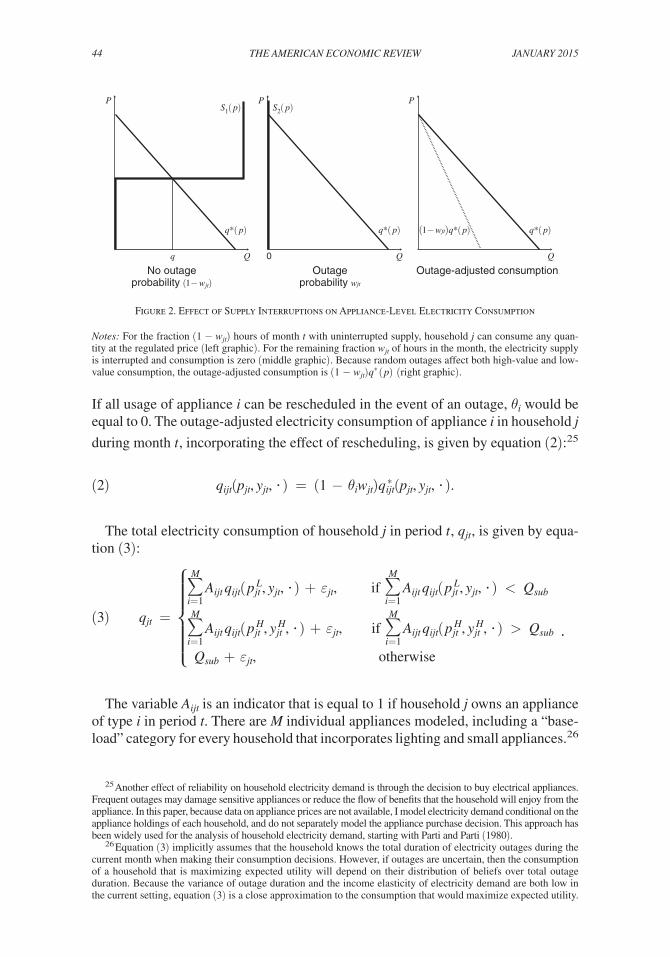
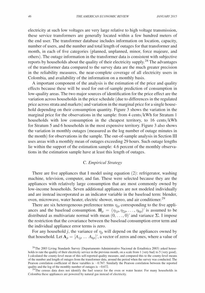
In practice, the household may face unpredictable interruptions to electricity supply during the period. Figure 2 illustrates the effect of these interruptions on the appliance-level consumption of electricity. The line q ∗ (p) represents the appli-ance-level demand without interruptions from equation (1), with quantity normal-ized to an hourly average. For a fraction (1 − w jt ) of hours in month t , supply to household j is uninterrupted and represented by S 1 (p) : at any regulated price, the household can consume electricity up to the capacity of its connection. For the remaining fraction w jt of hours in month t , supply to household j is observed to be interrupted ( S 2 (p) ) and electricity consumption is zero. If outages occur randomly, so that both high-value and low-value consumption of electricity is interrupted, then the outage-adjusted appliance-level consumption is (1 − w jt ) q ∗ (p) .23
The above discussion assumes that electricity consumption by the appliance is constant for all hours of the month. However, most activities that use electricity take place at irregular intervals. Depending on the particular appliance, it may be possible to reschedule an activity that would have occurred during a supply interruption.24 This would reduce the overall effect of supply reliability on monthly electricity con-sumption for the appliance. For example, television watching or meal preparation may be difficult or impossible to reschedule, so a power outage during these activi-ties may have a large impact on their electricity usage. Conversely, thermal storage appliances such as refrigerators or air conditioners might run longer after a power outage in order to restore the set temperature, so the overall effect of outages on their electricity usage may be small.
The extent to which it is possible to reschedule usage of an appliance i in the event of an outage is captured by the term θ i , a scale factor on the outage frequency w jt .
21 The inclusion of price in the demand equation presupposes that the household pays for their consumption of electricity. However, particularly in a developing country, a significant minority of households do not pay for their billed consumption. In this paper, I do not model the household’s decision to pay or not to pay their electricity bill, and instead treat this as exogenously determined by the quality of the household’s infrastructure. Households without an individual meter have a marginal price of zero, regardless of whether or not they pay their bill, because even if they pay, the amount that they pay will not depend on the amount that they consume. Households with an individual connection and meter are assumed to pay their bill in order to avoid disconnection.
22 There are two reasons for using the linear specification for demand instead of a log-log or log-linear model. First, price enters linearly in order to allow for a price of zero, which is required for the empirical application. Second, quantity is linear because the total consumption is modeled as the sum of the individual appliance-level consumption.
23 This model of outages corresponds to the intermittent supply framework, one of three theoretical frame-works that Klytchnikova and Lokshin (2010) describe for analyzing infrastructure outages. An alternative approach would be to assume efficient rationing of electricity in which the supply restriction affects the units with the lowest willingness-to-pay (Davis and Kilian 2011). This would be the case if outages were scheduled to occur at the times when usage is least valuable. However, when outages are random, both high-value and low-value consumption will be affected, causing the whole demand curve to rotate.
24 Munasinghe (1980) distinguishes the use of electricity for production activities in the household, which can be rescheduled, from the use of electricity for leisure activities, which cannot be rescheduled. As a result the principal cost of power outages for residential users is the loss of leisure.
44 THE AMERICAN ECONOMIC REVIEW JANuARy 2015
If all usage of appliance i can be rescheduled in the event of an outage, θ i would be equal to 0. The outage-adjusted electricity consumption of appliance i in household j
during month t , incorporating the effect of rescheduling, is given by equation (2):25
(2) q ijt ( p jt , y jt , · ) = (1 − θ i w jt ) q ijt ∗ ( p jt , y jt , · ) .
The total electricity consumption of household j in period t , q jt , is given by equa-tion (3):
(3) q jt =
⎧
⎪ ⎨
⎪
⎩
∑ i=1
M
A ijt q ijt ( p jt L , y jt , · ) + ε jt , if ∑ i=1
M
A ijt q ijt ( p jt L , y jt , · ) < Q sub
∑ i=1
M
A ijt q ijt ( p jt H , y jt H , · ) + ε jt , if ∑ i=1
M
A ijt q ijt ( p jt H , y jt H , · ) > Q sub .
Q sub + ε jt , otherwise
The variable A ijt is an indicator that is equal to 1 if household j owns an appliance of type i in period t . There are M individual appliances modeled, including a “base-load” category for every household that incorporates lighting and small appliances.26
25 Another effect of reliability on household electricity demand is through the decision to buy electrical appliances. Frequent outages may damage sensitive appliances or reduce the flow of benefits that the household will enjoy from the appliance. In this paper, because data on appliance prices are not available, I model electricity demand conditional on the appliance holdings of each household, and do not separately model the appliance purchase decision. This approach has been widely used for the analysis of household electricity demand, starting with Parti and Parti (1980).
26 Equation (3) implicitly assumes that the household knows the total duration of electricity outages during the current month when making their consumption decisions. However, if outages are uncertain, then the consumption of a household that is maximizing expected utility will depend on their distribution of beliefs over total outage duration. Because the variance of outage duration and the income elasticity of electricity demand are both low in the current setting, equation (3) is a close approximation to the consumption that would maximize expected utility.
S1( p) S2( p)
q*( p) q*( p) q*( p)( 1 − wjt)q*( p)
0q
No outageprobability ( 1 − wjt)
Outageprobability wjt
Outage-adjusted consumption
P P P
Q Q Q
Figure 2. Effect of Supply Interruptions on Appliance-Level Electricity Consumption
Notes: For the fraction (1 − wjt) hours of month t with uninterrupted supply, household j can consume any quan-tity at the regulated price (left graphic). For the remaining fraction wjt of hours in the month, the electricity supply is interrupted and consumption is zero (middle graphic). Because random outages affect both high-value and low-value consumption, the outage-adjusted consumption is (1 − wjt) q * (p) (right graphic).
45Mcrae: Infrastructure QualIty and the subsIdy trapVOl. 105 nO. 1
The nonlinearity in the price schedule is modeled using the discrete-continuous choice framework in which each observation of the household’s consumption is the result of the household choosing one of the three segments of the price schedule: the first step, the second step, or the kink point Q sub . If the household chooses to con-sume on the first step of the price schedule, then it faces a marginal price of p jt L . If the household chooses to consume on the second step of the price schedule, then it faces a marginal price of p jt H . However, in this case, the household pays the lower price p jt L for the first Q sub units. This reduced price for the inframarginal units is treated as a transfer to the household and incorporated through the income variable, as in equation (4):
(4) y jt H = y jt + Q sub ( p jt H − p jt L ) .
Equation (3) includes an additional error term, ε jt . This term allows for potential differences between the household’s choice of where to locate on the price schedule and the observed consumption of the household. The term ε jt has been described as measurement error (Moffitt 1986), optimization error, or perception error (Hewitt and Hanemann 1995). Without this term, the model would predict extreme bunching of households at the kink point in the price schedule (MaCurdy, Green, and Paarsch 1990). Such bunching is not observed in the data.
B. Data
The data collated for this investigation provides a rich environment for the anal-ysis of household demand for electricity in a developing country. It incorporates all of the important determinants of electricity demand described in Section IIA: the nonlinear price schedule, appliance holdings, and service reliability. Monthly electricity billing data is matched at a household level to cross-sectional data on households including appliance holdings and dwelling characteristics. These data are also combined with network information on monthly transformer-level outages.
Microdata on household characteristics are from the 2005 Amplified (Long-Form) Census, undertaken by the National Statistical Department (DANE) over a ten month period between May 2005 and March 2006. The census microdata were matched to billing data identification codes from a listing of residential electricity bill recipients in Colombia in March 2004. For the matched households, I obtained their monthly electricity bills over the six-year period January 2003 to December 2008. These billing data include information on the start and end of the billing cycle, the billed consumption, the meter and connection type, any subsidy or contribution amounts, and the total charge.27
In addition, the billing data were matched to a database containing monthly information on all service transformers in Colombia. The transformers are the final stages of the local distribution networks, in which the voltage is stepped down to the level at which it can be used by households. Since the losses when transmitting
27 Because households are tracked in the billing data using their 2004 identifier, any change in the database iden-tifiers used by the firm would cause those households to drop out of my sample. This might happen, for example, as the result of a merger between two distribution firms.
46 THE AMERICAN ECONOMIC REVIEW JANuARy 2015
electricity at such low voltages are very large relative to high voltage transmission, these service transformers are generally located within a few hundred meters of the end user. The transformer database includes information on location, capacity, number of users, and the number and total length of outages for that transformer and month, in each of five categories (planned, unplanned, minor, force majeure, and others). The outage information in the transformer data is consistent with subjective reports by households about the quality of their electricity supply.28 The advantages of the transformer data compared to the survey data are the much greater precision in the reliability measures, the near-complete coverage of all electricity users in Colombia, and availability of the information on a monthly basis.
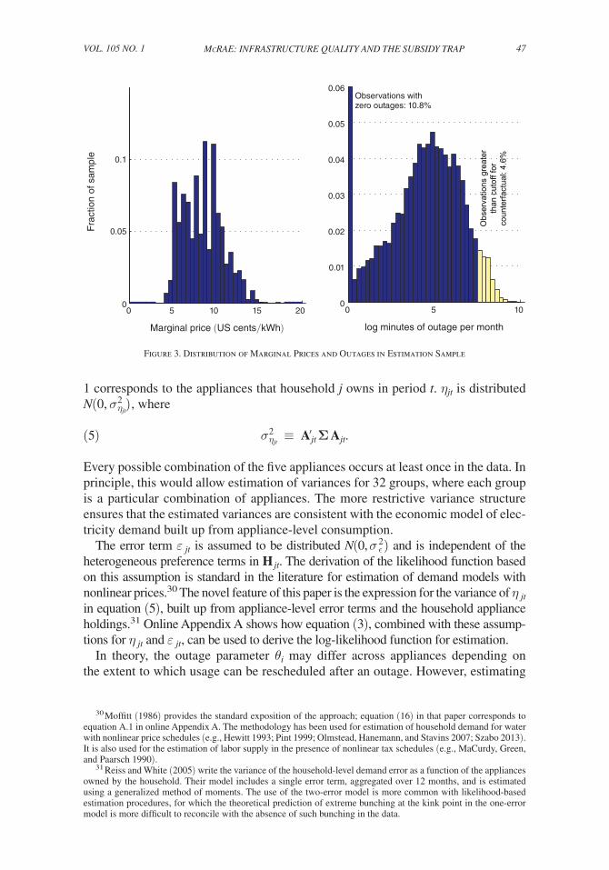
A important component of the analysis is the estimation of the price and quality effects because these will be used for out-of-sample prediction of consumption in low-quality areas. The two major sources of identification for the price effect are the variation across households in the price schedule (due to differences in the regulated price across strata and markets) and variation in the marginal price for a single house-hold depending on their consumption quantity. Figure 3 shows the variation in the marginal price for the observations in the sample: from 4 cents/kWh for Stratum 1 households with low consumption in the cheapest territory, to 16 cents/kWh for Stratum 5 and 6 households in the most expensive territory. Figure 3 also shows the variation in monthly outages (measured as the log number of outage minutes in the month) for observations in the sample. The out-of-sample analysis in Section III uses areas with a monthly mean of outages exceeding 29 hours. Such outage lengths lie within the support of the estimation sample: 4.6 percent of the monthly observa-tions in the estimation sample have at least this length of outages.
C. Empirical Strategy
There are five appliances that I model using equation (2): refrigerator, washing machine, television, computer, and fan. These were selected because they are the appliances with relatively large consumption that are most commonly owned by low-income households. Seven additional appliances are not modeled individually and are instead incorporated as an indicator variable in the baseload term: blender, oven, microwave, water heater, electric shower, stereo, and air conditioner.29
There are six heterogeneous preference terms η ijt corresponding to the five appli-ances and the baseload consumption. H jt = ( η 1jt , η 2jt , … , η 6jt ) ′ is assumed to be distributed as multivariate normal with mean (0, … , 0) ′ and variance Σ . I impose the restriction that the covariance between the baseload consumption error term and the individual appliance error terms is zero.
For any household j , the variance of η jt will depend on the appliances owned by that household. Let A jt = [ A 1jt … A 6jt ]′ , a vector of zeros and ones, where a value of
28 The 2003 Living Standards Survey (Departamento Administrativo Nacional de Estadística 2003) asked house-holds to rate the quality of their electricity service in the previous month, on a scale from 1 (very bad) to 5 (very good). I calculated the county-level mean of this self-reported quality measure, and compared this to the county-level means of the number and length of outages from the transformer data, around the period when the survey was conducted. The Pearson correlation coefficient of these variables is −0.767. Similarly the Pearson correlation between the reported quality and the log of the monthly number of outages is −0.672.
29 The census data does not identify the fuel source for the oven or water heater. For many households in Colombia these appliances are powered by natural gas instead of electricity.
47McRAE: INFRASTRUCTURE QUALITY AND THE SUBSIDY TRAPVOL. 105 NO. 1
1 corresponds to the appliances that household j owns in period t . η jt is distributed N(0, σ η jt
2 ) , where
(5) σ η jt 2 ≡ A jt ′ Σ A jt .
Every possible combination of the five appliances occurs at least once in the data. In principle, this would allow estimation of variances for 32 groups, where each group is a particular combination of appliances. The more restrictive variance structure ensures that the estimated variances are consistent with the economic model of elec-tricity demand built up from appliance-level consumption.
The error term ε jt is assumed to be distributed N(0, σ ϵ 2 ) and is independent of the heterogeneous preference terms in H jt . The derivation of the likelihood function based on this assumption is standard in the literature for estimation of demand models with nonlinear prices.30 The novel feature of this paper is the expression for the variance of η jt in equation (5), built up from appliance-level error terms and the household appliance holdings.31 Online Appendix A shows how equation (3), combined with these assump-tions for η jt and ε jt , can be used to derive the log-likelihood function for estimation.
In theory, the outage parameter θ i may differ across appliances depending on the extent to which usage can be rescheduled after an outage. However, estimating
30 Moffitt (1986) provides the standard exposition of the approach; equation (16) in that paper corresponds to equation A.1 in online Appendix A. The methodology has been used for estimation of household demand for water with nonlinear price schedules (e.g., Hewitt 1993; Pint 1999; Olmstead, Hanemann, and Stavins 2007; Szabo 2013). It is also used for the estimation of labor supply in the presence of nonlinear tax schedules (e.g., MaCurdy, Green, and Paarsch 1990).
31 Reiss and White (2005) write the variance of the household-level demand error as a function of the appliances owned by the household. Their model includes a single error term, aggregated over 12 months, and is estimated using a generalized method of moments. The use of the two-error model is more common with likelihood-based estimation procedures, for which the theoretical prediction of extreme bunching at the kink point in the one-error model is more difficult to reconcile with the absence of such bunching in the data.
0 5 100
0.01
0.02
0.03
0.04
0.05
0.06
log minutes of outage per month
0 5 10 15 200
0.05
0.1
Marginal price (US cents/kWh)
Fra
ctio
n of
sam
ple
Observations withzero outages: 10.8%
Obs
erva
tions
gre
ater
than
cut
off f
orco
unte
rfact
ual:
4.6%
Figure 3. Distribution of Marginal Prices and Outages in Estimation Sample
48 THE AMERICAN ECONOMIC REVIEW JANUARY 2015
separate θ i for each appliance is not empirically tractable. In the main specification, I restrict θ i to be the same for all appliances.32 I also impose restrictions on pref-erences to ensure that exactly one of the cases in equation (3) holds. These corre-spond to several thousand linear restrictions on γ i and β i , one for each combination of household characteristics in the data, to ensure that the income effect from the inframarginal transfer is smaller than the substitution effect from the higher price.33
The vector of household characteristics z jt includes the number of household members and the number of rooms (both also interacted with price and income), an indicator variable for whether the dwelling is an apartment, the mean daily tempera-ture at the household’s location during each billing cycle, and linear and quadratic terms in the historical number and length of outages before the sample period. The historical outage terms capture the possible long-term effects of service reliability on electricity consumption that do not operate through contemporaneous supply outages. These might include the effect of outages on the quality of the household’s capital stock or on electricity consumption behavior. Table 1 provides additional information on all variables that are used in estimation.
I estimate the model using a balanced panel of household billing data for the six months before and six months after each household’s census interview. Consumption and outages were normalized to a standard billing cycle length of 30 days. I dropped observations for households with a small business in their home, households with a consumption greater than 1,000 kWh in any of the 12 months, households with a bill-ing cycle shorter than 25 days or longer then 36 days in any of the 12 months, house-holds with observations based on estimated rather than metered usage in any of the 12 months, and households who paid a fine of more than $20 at any time in the entire billing data. After dropping these observations, I estimated a linear regression model of annual electricity consumption of the household on appliance holdings, household characteristics, and regional dummies. I calculated the residuals from these estimates and dropped those observations with residuals in the top 1 or bottom 1 percentiles.34 The total sample size after this procedure is 869,304 observations from 72,442 households.
D. Results
In this section, I describe the estimation results for the structural model of house-hold demand presented above, and interpret the preference parameters in terms of the price and income elasticities of demand, the relationship between outages and elec-tricity demand, and appliance-level consumption. The summary results presented
32 I estimate two alternative specifications to test the sensitivity of the results to this assumption. In the first, I fix θ i for the individual appliances to be zero and estimate θ i only for the baseload consumption. In the second, I allow θ i to be different between the baseload consumption and the individual appliances. As shown in Table 7, both specifications give very similar results.
33 I also estimate a parsimonious specification in which price only has an effect on baseload consumption (that is, without heterogeneous price effects). As shown in Table 7, this implies greater price sensitivity for Stratum 1 households and, consequently, a larger change in consumption for the counterfactual described in Section III.
34 These correspond to observations of electricity consumption that are not consistent with the economic model used for this study, possibly as a result of incomplete information on the electricity demand at the address. For example, suppose there is one family living at the address, but the second floor of their dwelling is rented out as a dental surgery. If there is a single electricity bill for the family and the business, but the matched census data only includes information for the family, then the demographic and appliance information of that family will not be consistent with the electricity consumption at the address. The middle block of Table 7 shows the sensitivity of the estimation and counterfactual results to changes in the assumptions for sample construction.
49Mcrae: Infrastructure QualIty and the subsIdy trapVOl. 105 nO. 1
in this section are only for descriptive purposes. The analysis of firm incentives in Section III is built up from household-level preferences and characteristics rather than the aggregate summary statistics.
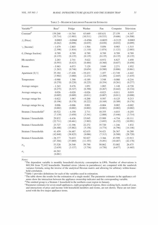
Table 2 shows the parameter estimates from the maximum likelihood estimation. The dependent variable is the monthly electricity consumption for a household in kWh. All results in the table are from a single estimation procedure: each column represents the interaction effects for the individual appliances that the household owns. Small appliance, cooking fuel, month-of-year, and eight region indicator vari-ables, as well as additional price and income interaction terms, are included in the regression but their coefficients are not reported.
Table 2 reports the estimated value of σ ϵ (44.3 kWh/month) and the appliance-level σ η i . For any particular household, their value of σ η jt is given by
Table 1—Description of Variables Used in Analysis
Variable name Description
Consumption Monthly metered electricity consumption, normalized to a standard billing cycle length by multiplying by 30/n where n is the number of days in the billing cycle.
Electricity price Price schedule for metered households has three components: low price p jt L , high price p jt H , and subsidized quantity Q sub . The high price is calculated by dividing the billed amount before subsidies by consumption. The subsidized quantity is based on the table in Resolution 355 of 2004 by the Unidad de Planeación Minero-Energética; the exact cutoff between high and low altitude areas is determined for each firm by examining discon-tinuities in the implied subsidies. The subsidy percentage (and therefore the low price) is determined by dividing the subsidy amount in pesos by the minimum of consumption quantity and subsidized quantity.
Income Monthly household expenditure in millions of Colombian pesos (1 million Colombian pesos = 422 United States dollars). Calculated as the midpoint of one of nine bins for a census question on the required level of monthly income for the household to adequately cover its basic expenses.
Outage hours Reported total number of hours of outages for a month at the transformer serving the household, allocated pro rata to observations using the number of days in the month in each billing cycle.
Appliance variables For each of 12 appliances, this is an indicator variable equal to 1 if the household reports ownership of that appliance.
Household members Total number of people in the household.
Rooms Total number of rooms in the dwelling, excluding kitchen, bathroom, and garage.
Apartment Indicator variable equal to 1 if the dwelling is an apartment.
Temperature Mean temperature in degrees Celsius for the household’s billing cycle. This is calculated using daily mean temperature observations at 42 weather stations in Colombia, obtained from Instituto de Hidrología, Meteorología y Estudios Ambientales (IDEAM). The in-terpolated daily mean temperature for each household is the mean from the 42 weather stations, weighted by the inverse square of the distance between the household and each weather station, after adjusting all temperatures for the difference in altitude (using a temperature-altitude gradient of 5.54 degrees Celsius per 1000 meters).
Average outages Mean number of supply interruptions per month at the transformer serving the household, for the 12 months before the first month in the estimation sample.
Average outage hours Mean number of hours of outages per month at the transformer serving the household, for the 12 months before the first month in the estimation sample.
Cooking fuel Three indicator variables for the household’s primary cooking fuel: electricity, piped nat-ural gas, or propane gas cylinders. The excluded group is the use of alternative cooking fuels such as wood or charcoal.

50 THE AMERICAN ECONOMIC REVIEW JANuARy 2015
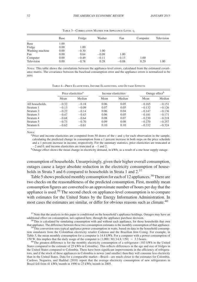
equation (5) and depends on the household’s appliance holdings and the estimated covariance matrix Σ . Table 3 reports the estimated correlation matrix for the η i .
Table 4 shows the mean and median price and income elasticities of demand, for the whole sample and by stratum. The mean price elasticity is −0.32, with price elasticities closer to zero for households in the lower strata.35 These elasticities are comparable to results from previous research on electricity demand. Reiss and White (2005) estimate a mean price elasticity of −0.39 for their sample of Californian households, compared to the mean in this paper of −0.32. For Colombia, Maddock, Castaño, and Vella (1992) apply the discrete-continuous choice method to data for Medellín, Colombia in 1986. They estimate price elasticities of −0.17 for Strata 1 and 2, −0.51 for Strata 3 and 4, and −0.79 for Strata 5 and 6. These are close to the mean elasticities from Table 4 of −0.18, −0.58, and −0.68 for these same groups. Medina and Morales (2008) also estimate the demand for electricity in Colombia using the discrete-continuous choice approach applied to household survey data from 2003. They obtain a mean price elasticity of −0.45.36
By comparison, the mean income elasticity of 0.06 in Table 4 is much lower than the previous results for Colombia. Maddock, Castaño, and Vella (1992) estimate a mean income elasticity of 0.30, and Medina and Morales (2008) estimate a mean income elasticity of 0.31. However, these results are not directly comparable. The important difference between this paper and the earlier studies is that I model elec-tricity demand at the appliance level, and the income elasticities of demand are conditional on the appliance holdings of the household. The difference in the esti-mates demonstrates that a large part of the effect of income on electricity demand is through the appliance purchase decision. The income elasticity result for this paper is closer to that of Reiss and White (2005), who condition on appliance holdings and obtain a zero income elasticity.
The final two columns in Table 4 summarize the effect of one additional outage hour on the monthly electricity consumption of households. Overall, one additional outage hour will reduce monthly electricity consumption by a mean of 0.165 kWh. This corresponds to approximately 70 percent of the hourly mean electricity
35 The method for calculating these elasticities is based on Olmstead, Hanemann, and Stavins (2007). First, for each observation in the sample, I draw values of ϵ jt and η jt from the estimated distribution of these unobservable terms. I use the draws of ϵ jt and η jt , combined with the observable variables and their estimated coefficients, to predict consumption using equation (3). Next, I increase the price at all steps on the price schedules by 1 percent, and predict consumption again using the same draws of ϵ jt and η jt but with the higher price. Finally, for each obser-vation, I compute the price elasticity using the following formula, where q ̂ jt is the predicted consumption value:
ϵ jt = q ̂ jt (1.01 P jt , · ) − q ̂ jt ( P jt , · ) ___________________
0.01 1 _______ q ̂ jt ( P jt , · )
.
The income elasticity is calculated in a similar way, increasing income by 1 percent instead of price. For the compu-tation of Table 4, I truncated the distribution of the price elasticities at −2 and 0, and the income elasticities at −1 and 2.
36 Although the pattern of the price elasticity results is similar, there are several differences between the current paper and the previous Colombian studies. I allow for considerable heterogeneity across households in their behavioral responses, which depend, for example, on the household’s income and appliance holdings. My data includes metered household consumption over several years; in comparison, Maddock, Castaño, and Vella (1992) use the average con-sumption over three months (which may be problematic in the context of nonlinear prices), and Medina and Morales (2008) impute household consumption for a single month from reported expenditure on electricity and the regulated price schedules. For unmetered households, consumption imputed from expenditure data may be different to actual consumption. Finally, I use detailed information on the number and length of outages for each household and month, which allows me to estimate the effect of service reliability on demand. This richer specification is particularly import-ant for the application in this paper to firm investment and the incentive effect of the subsidy program.
51Mcrae: Infrastructure QualIty and the subsIdy trapVOl. 105 nO. 1
Table 2—Maximum Likelihood Parameter Estimates
Variablea,b Basec Fridge Washer Fan Computer Television
Constantd 139.268 −14.764 63.669 −105.631 27.159 4.147(35.714) (13.903) (10.511) (10.533) (9.606) (14.508)
β i (Price) 0.0003 −0.0960 −0.4586 −0.0055 −0.2125 0.0003(0.262) (0.098) (0.035) (0.030) (0.032) (0.099)
γ i (Income) −1.679 −2.803 −1.504 5.056 0.903 −1.515(2.398) (1.816) (1.110) (1.074) (1.121) (2.003)
θ i (Outage fraction) 0.789 0.789 0.789 0.789 0.789 0.789(0.135) (0.135) (0.135) (0.135) (0.135) (0.135)
Hh members 2.283 2.741 5.622 −0.972 6.827 1.650(0.593) (0.423) (0.484) (0.360) (0.657) (0.458)
Rooms −5.983 6.073 7.129 3.049 2.271 1.952(1.263) (0.746) (0.654) (0.580) (0.806) (0.861)
Apartment (0/1) 35.184 −17.428 −19.433 1.457 −13.749 −4.442(3.902) (3.060) (2.231) (2.289) (2.445) (3.435)
Temperature −0.988 1.366 −0.189 3.548 −0.080 −0.216(0.270) (0.228) (0.225) (0.354) (0.261) (0.277)
Average outages −1.243 0.476 1.051 1.083 1.148 −0.720(0.275) (0.327) (0.390) (0.267) (0.442) (0.334)
Average outages sq 0.026 −0.020 −0.026 −0.023 −0.011 0.019(0.005) (0.009) (0.011) (0.007) (0.011) (0.008)
Average outage hrs −0.822 1.063 −0.200 0.587 −0.125 0.213(0.196) (0.178) (0.222) (0.169) (0.309) (0.176)
Average outage hrs sq 0.006 −0.006 0.001 −0.004 0.002 −0.002(0.002) (0.002) (0.002) (0.001) (0.002) (0.002)
Stratum 2 householdse 10.522 −4.350 2.711 10.355 −4.033 −0.255(7.139) (3.650) (3.341) (2.088) (5.446) (3.714)
Stratum 3 households 29.832 −6.436 15.045 15.989 −4.754 −10.111(22.711) (10.461) (3.903) (3.693) (6.152) (10.991)
Stratum 4 households 23.727 −12.396 22.272 35.720 −1.246 1.832(26.488) (15.882) (5.156) (4.774) (6.796) (14.146)
Stratum 5 households 41.459 −54.487 62.635 34.421 26.367 16.280(42.848) (38.825) (8.086) (7.313) (8.508) (28.720)
Stratum 6 households −28.377 74.633 92.827 −3.366 43.599 −23.913(47.304) (37.069) (11.193) (9.491) (10.487) (42.178)
σ η i 53.528 24.548 59.790 50.062 53.002 26.475(2.639) (3.137) (3.736) (4.750) (6.677) (4.465)
σ ϵ 44.263(6.061)
Notes:a The dependent variable is monthly household electricity consumption in kWh. Number of observations is 869,304 from 72,442 households. Standard errors (shown in parentheses) are computed with the sandwich variance formula, using the inverse of the analytical Hessian matrix and allowing for arbitrary within-house-hold correlation.
b Table 1 provides definitions for each of the variables used in estimation.c The table shows the results for the estimation of a single model. The parameter estimates in the appliance col-umns show the interaction between the appliance ownership indicator and the corresponding variable.
d The omitted group is a Stratum 1 household in the northern coast region in January.e Parameter estimates for seven small appliances, eight geographical regions, three cooking fuels, month-of-year, and interactions of price and income with household members and rooms, are not shown. These are not inter-acted with the five major appliance terms.
52 THE AMERICAN ECONOMIC REVIEW JANuARy 2015
consumption of households. Unsurprisingly, given their higher overall consumption, outages cause a larger absolute reduction in the electricity consumption of house-holds in Strata 5 and 6 compared to households in Strata 1 and 2.37
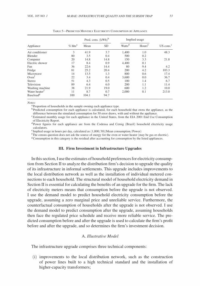
Table 5 shows predicted monthly consumption for each of 12 appliances.38 There are two checks on the reasonableness of the predicted consumption. First, monthly mean consumption figures are converted to an approximate number of hours per day that the appliance is used.39 The second check on appliance-level consumption is to compare with estimates for the United States by the Energy Information Administration. In most cases the estimates are similar, or differ for obvious reasons such as climate.40
37 Note that the analysis in this paper is conditional on the household’s appliance holdings. Outages may have an additional effect on consumption, not captured here, through the appliance purchase decision.
38 This is calculated by simulating consumption with and without each appliance, for those households that own that appliance. The difference between these two consumption estimates is the monthly consumption of that appliance.
39 This conversion uses typical appliance power consumption in watts, based on data in the household consump-tion simulators from the Colombian electricity retailer Codensa and the Brazilian firm Cemig. For example, in Table 5, the mean monthly consumption for a computer is 14.8 kWh. For a computer with a power consumption of 150 W, this implies that the daily usage of the computer is (1,000 / 30)(14.8 / 150) = 3.3 hours.
40 The greatest difference is for the monthly electricity consumption of a refrigerator (103 kWh in the United States compared to the estimate of 25 kWh in Colombia). This reflects differences in the age and size of fridges in the United States compared to Colombia. There have been significant improvements in the efficiency of refrigera-tors, and if the stock of these appliances in Colombia is newer (and smaller) then they will consume less electricity than in the United States. Data for a comparable market—Brazil—are much closer to the estimates for Colombia. Cardoso, Nogueira, and Haddad (2010) report that the average electricity consumption of new refrigerators in Brazil fell from 41 kWh/month in 1990 to 23 kWh/month in 2005.
Table 3 —Correlation Matrix for Appliance-Level η i
Base Fridge Washer Fan Computer Television
Base 1.00Fridge 0.00 1.00Washing machine 0.00 −0.30 1.00Fan 0.00 0.64 −0.09 1.00Computer 0.00 −0.49 −0.11 −0.13 1.00Television 0.00 −0.78 0.28 −0.08 0.29 1.00
Notes: This table shows the correlations between the appliance-level errors, calculated from the estimated covari-ance matrix. The covariance between the baseload consumption error and the appliance errors is normalized to be zero.
Table 4—Price Elasticities, Income Elasticities, and Outage Effects
Price elasticitiesa Income elasticities Outage effectb
Mean Median Mean Median Mean Median
All households −0.32 −0.18 0.06 0.05 −0.165 −0.151Stratum 1 −0.13 −0.09 0.07 0.05 −0.132 −0.126Stratum 2 −0.22 −0.14 0.06 0.04 −0.147 −0.136Stratum 3 −0.47 −0.43 0.06 0.05 −0.181 −0.171Stratum 4 −0.68 −0.64 0.08 0.07 −0.230 −0.218Stratum 5 −0.73 −0.70 0.09 0.08 −0.270 −0.257Stratum 6 −0.62 −0.61 0.10 0.10 −0.332 −0.324
Notes:a Price and income elasticities are computed from 50 draws of the ϵ and η for each observation in the sample, calculating the predicted change in consumption from a 1 percent increase in both steps on the price schedule and a 1 percent increase in income, respectively. For the summary statistics, price elasticities are truncated at −2 and 0, and income elasticities are truncated at −1 and 2.
b Outage effect shows the mean change in electricity demand, in kWh, as a result of a one hour supply outage.
53Mcrae: Infrastructure QualIty and the subsIdy trapVOl. 105 nO. 1
III. Firm Investment in Infrastructure Upgrades
In this section, I use the estimates of household preferences for electricity consump-tion from Section II to analyze the distribution firm’s decision to upgrade the quality of its infrastructure in informal settlements. This upgrade includes improvements to the local distribution network as well as the installation of individual metered con-nections to each household. The structural model of household electricity demand in Section II is essential for calculating the benefits of an upgrade for the firm. The lack of electricity meters means that consumption before the upgrade is not observed. I use the demand model to predict household electricity consumption before the upgrade, assuming a zero marginal price and unreliable service. Furthermore, the counterfactual consumption of households after the upgrade is not observed. I use the demand model to predict consumption after the upgrade, assuming households then face the regulated price schedule and receive more reliable service. The pre-dicted consumption before and after the upgrade is used to calculate the firm’s profit before and after the upgrade, and so determines the firm’s investment decision.
A. Illustrative Model
The infrastructure upgrade comprises three technical components:
(i) improvements to the local distribution network, such as the construction of power lines built to a high technical standard and the installation of higher-capacity transformers;
Table 5—Predicted Monthly Electricity Consumption by Appliance
Pred. cons. (kWh)b Implied usage
Appliance % hhsa Mean SD Wattsd Hourse US cons.c
Air conditioner 3 41.9 3.7 1,400 1.0 48.3Blender 80 3.5 0.4 500 0.2Computer 20 14.8 14.8 150 3.3 21.8Electric shower 17 8.4 0.9 4,400 0.1Fan 36 22.6 14.4 80 9.4 4.2Fridge 81 25.2 20.4 200 4.2 103.3Microwave 14 13.5 1.3 800 0.6 17.4Ovenf 22 3.4 0.4 3,600 0.0 36.7Stereo 51 4.3 0.5 100 1.4 6.7Television 89 6.4 6.0 200 1.1 11.4Washing machine 38 21.9 19.0 600 1.2 10.0Water heater f 11 8.7 0.7 2,000 0.1 213.0Baseloadg 100 104.1 94.7
Notes:a Proportion of households in the sample owning each appliance type.b Predicted consumption for each appliance is calculated, for each household that owns the appliance, as the
difference between the simulated consumption for 50 error draws, with and without the appliance.c Estimated monthly usage for each appliance in the United States, from the EIA 2001 End Use Consumption of Electricity Report.
d Power figures for each appliance are from the Codensa and Cemig (Brazil) household electricity usage calculators.
e Implied usage in hours per day, calculated as (1,000/30)(Mean consumption / Power) f The census question does not ask the source of energy for the oven or water heater (may be gas or electric).g Consumption in this category is the residual after accounting for consumption by the listed appliances.
54 THE AMERICAN ECONOMIC REVIEW JANuARy 2015
(ii) the installation of an individual connection from the distribution network to each customer’s dwelling; and
(iii) the installation of a meter at the entry point to the customer’s dwelling.41
For the customer, an important effect of the upgrade is that the marginal price of electricity increases from zero to a positive price on the regulated price schedule. Before the upgrade, the electricity usage of an individual household is not measured, so an additional unit of consumption has no effect on the amount that the household pays. This is true even if the household receives a bill based on estimated usage and regardless of whether they pay the bill or not. As long as there is no connection between actual consumption and the amount the household pays, the marginal price of additional consumption for the household is zero, and the household will con-sume at a price of zero on their demand curve.
The major benefit to customers of the upgrade is the reduction in the frequency and duration of electricity outages. These outages are stochastic events caused by the fail-ure of poorly maintained and overloaded equipment, as well as environmental factors such as trees, animals, storms, and lightning (Pabla 2005). Both the improvements to the distribution network and the installation of individual connections reduce the probability of outages. The individual connections enable the firm to control the num-ber of users and their total demand on each branch of its distribution network, reduc-ing the probability that customer load exceeds the capacity of the network equipment.
The individual connections also facilitate the collection of payment from each household. Before the upgrade, it may be difficult to disconnect nonpaying house-holds who receive electricity through unauthorized connections to their neighbors or the network. The installation of meters may also affect payment enforcement. If prepaid meters are installed, then all electricity is paid for before it is used. Even without prepaid meters, customers with low usage may be more willing to pay for their consumption if it is correctly measured.42
The three components of the upgrade have several effects on the firm’s profitabil-ity. The interaction of these effects determines whether investment in the upgrade is worthwhile for the firm. First, the upgrade will change the consumption of electricity. From equation (2), it will rotate outward the outage-adjusted demand for electric-ity (due to the improved reliability) but also cause a shift back along the demand curve (due to the increase in the marginal price from zero to some positive level). The relative size of these two opposing effects will differ for each firm and household,
41 The combination of these three components is defined as “normalization” of informal settlements for the government program PRONE, described in Section I (Decree 3735 of 2003, Article 3). In addition to physical investment by utility firms, normalization also requires formal recognition of the settlement by municipal authori-ties. Feler and Henderson (2011) describe strategic withholding of formalized water service by local authorities in Brazil in order to limit in-migration. In this analysis I focus solely on the profit incentive of utility firms.
42 I assume throughout this paper that the upgrade is a bundle with three components: network improvements, individual connections to households, and customer-level metering. An alternative is to analyze these investments as separate decisions by the firm. However, there are technical, legal, and economic reasons why this separation is impractical. The installation of meters without an individual connection is meaningless if there is no demarcation of the “entry point” to the dwelling. Provision of a meter may also be regarded as formal recognition of the house-hold’s connection, making the firm legally liable for any damages caused by dangerous and unreliable cables that it did not install. Conversely, upgrading the network without installing individual meters increases electricity demand, but profitability would be lower because there is no change in the firm’s revenue.
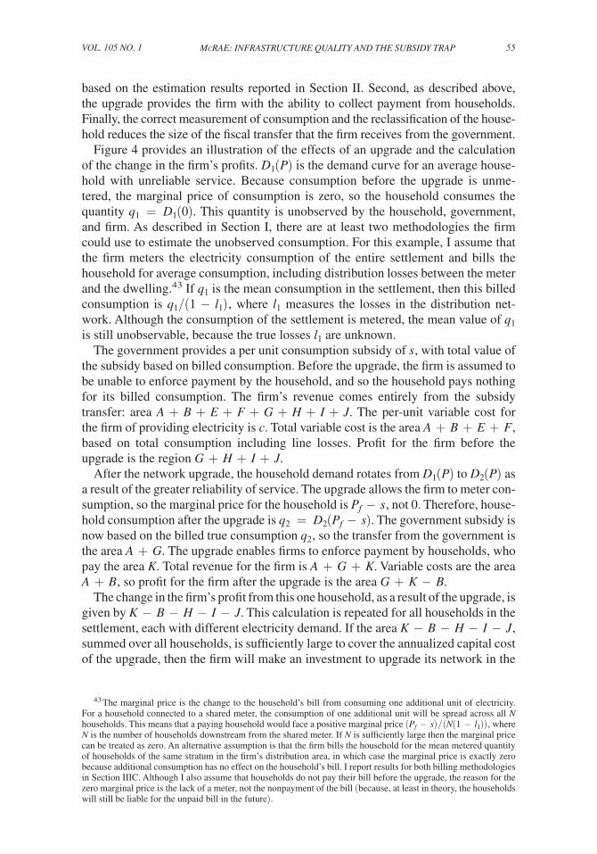
55Mcrae: Infrastructure QualIty and the subsIdy trapVOl. 105 nO. 1
based on the estimation results reported in Section II. Second, as described above, the upgrade provides the firm with the ability to collect payment from households. Finally, the correct measurement of consumption and the reclassification of the house-hold reduces the size of the fiscal transfer that the firm receives from the government.
Figure 4 provides an illustration of the effects of an upgrade and the calculation of the change in the firm’s profits. D 1 (P) is the demand curve for an average house-hold with unreliable service. Because consumption before the upgrade is unme-tered, the marginal price of consumption is zero, so the household consumes the quantity q 1 = D 1 (0) . This quantity is unobserved by the household, government, and firm. As described in Section I, there are at least two methodologies the firm could use to estimate the unobserved consumption. For this example, I assume that the firm meters the electricity consumption of the entire settlement and bills the household for average consumption, including distribution losses between the meter and the dwelling.43 If q 1 is the mean consumption in the settlement, then this billed consumption is q 1 /(1 − l 1 ) , where l 1 measures the losses in the distribution net-work. Although the consumption of the settlement is metered, the mean value of q 1 is still unobservable, because the true losses l 1 are unknown.
The government provides a per unit consumption subsidy of s , with total value of the subsidy based on billed consumption. Before the upgrade, the firm is assumed to be unable to enforce payment by the household, and so the household pays nothing for its billed consumption. The firm’s revenue comes entirely from the subsidy transfer: area A + B + E + F + G + H + I + J . The per-unit variable cost for the firm of providing electricity is c . Total variable cost is the area A + B + E + F , based on total consumption including line losses. Profit for the firm before the upgrade is the region G + H + I + J .
After the network upgrade, the household demand rotates from D 1 (P) to D 2 (P) as a result of the greater reliability of service. The upgrade allows the firm to meter con-sumption, so the marginal price for the household is P f − s , not 0. Therefore, house-hold consumption after the upgrade is q 2 = D 2 ( P f − s) . The government subsidy is now based on the billed true consumption q 2 , so the transfer from the government is the area A + G . The upgrade enables firms to enforce payment by households, who pay the area K . Total revenue for the firm is A + G + K . Variable costs are the area A + B , so profit for the firm after the upgrade is the area G + K − B .
The change in the firm’s profit from this one household, as a result of the upgrade, is given by K − B − H − I − J . This calculation is repeated for all households in the settlement, each with different electricity demand. If the area K − B − H − I − J , summed over all households, is sufficiently large to cover the annualized capital cost of the upgrade, then the firm will make an investment to upgrade its network in the
43 The marginal price is the change to the household’s bill from consuming one additional unit of electricity. For a household connected to a shared meter, the consumption of one additional unit will be spread across all N households. This means that a paying household would face a positive marginal price ( P f − s) / (N(1 − l 1 )) , where N is the number of households downstream from the shared meter. If N is sufficiently large then the marginal price can be treated as zero. An alternative assumption is that the firm bills the household for the mean metered quantity of households of the same stratum in the firm’s distribution area, in which case the marginal price is exactly zero because additional consumption has no effect on the household’s bill. I report results for both billing methodologies in Section IIIC. Although I also assume that households do not pay their bill before the upgrade, the reason for the zero marginal price is the lack of a meter, not the nonpayment of the bill (because, at least in theory, the households will still be liable for the unpaid bill in the future).
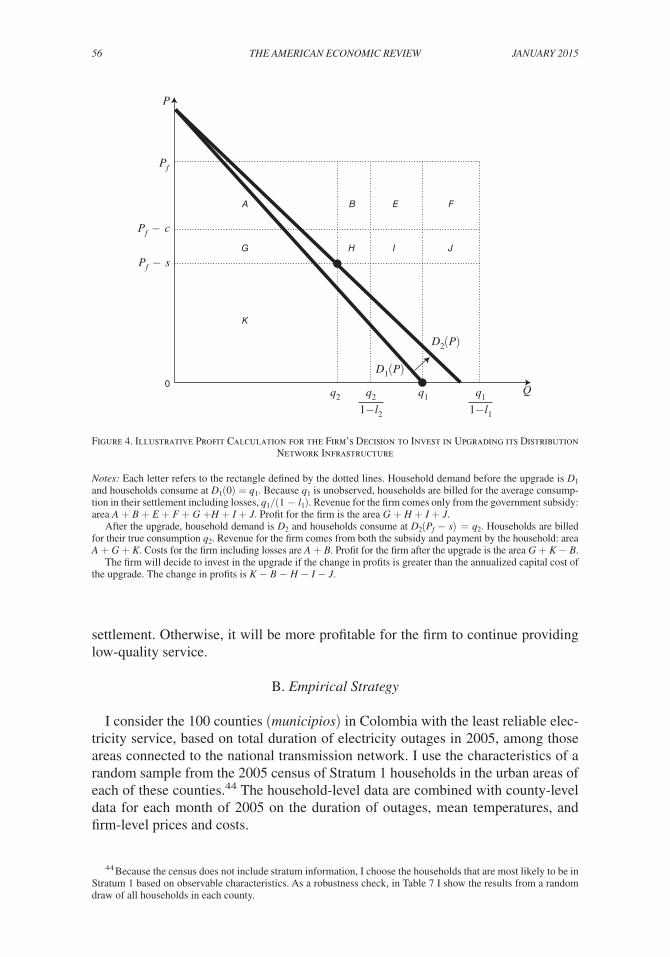
56 THE AMERICAN ECONOMIC REVIEW JANuARy 2015
settlement. Otherwise, it will be more profitable for the firm to continue providing low-quality service.
B. Empirical Strategy
I consider the 100 counties (municipios) in Colombia with the least reliable elec-tricity service, based on total duration of electricity outages in 2005, among those areas connected to the national transmission network. I use the characteristics of a random sample from the 2005 census of Stratum 1 households in the urban areas of each of these counties.44 The household-level data are combined with county-level data for each month of 2005 on the duration of outages, mean temperatures, and firm-level prices and costs.
44 Because the census does not include stratum information, I choose the households that are most likely to be in Stratum 1 based on observable characteristics. As a robustness check, in Table 7 I show the results from a random draw of all households in each county.
A B E F
G H I
q2 q1
Pf − s
Pf − c
1−l2
q2
1−l1
q1Q
D2(P)
D1(P)
P
Pf
0
J
K
Figure 4. Illustrative Profit Calculation for the Firm’s Decision to Invest in Upgrading its Distribution Network Infrastructure
Notes: Each letter refers to the rectangle defined by the dotted lines. Household demand before the upgrade is D1 and households consume at D1(0) = q1. Because q1 is unobserved, households are billed for the average consump-tion in their settlement including losses, q1/(1 − l1). Revenue for the firm comes only from the government subsidy: area A + B + E + F + G +H + I + J. Profit for the firm is the area G + H + I + J.
After the upgrade, household demand is D2 and households consume at D2(Pf − s) = q2. Households are billed for their true consumption q2. Revenue for the firm comes from both the subsidy and payment by the household: area A + G + K. Costs for the firm including losses are A + B. Profit for the firm after the upgrade is the area G + K − B.
The firm will decide to invest in the upgrade if the change in profits is greater than the annualized capital cost of the upgrade. The change in profits is K − B − H − I − J.
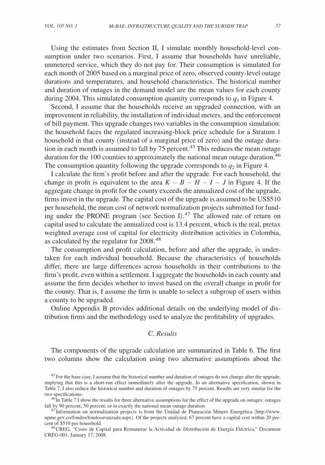
57Mcrae: Infrastructure QualIty and the subsIdy trapVOl. 105 nO. 1
Using the estimates from Section II, I simulate monthly household-level con-sumption under two scenarios. First, I assume that households have unreliable, unmetered service, which they do not pay for. Their consumption is simulated for each month of 2005 based on a marginal price of zero, observed county-level outage durations and temperatures, and household characteristics. The historical number and duration of outages in the demand model are the mean values for each county during 2004. This simulated consumption quantity corresponds to q 1 in Figure 4.
Second, I assume that the households receive an upgraded connection, with an improvement in reliability, the installation of individual meters, and the enforcement of bill payment. This upgrade changes two variables in the consumption simulation: the household faces the regulated increasing-block price schedule for a Stratum 1 household in that county (instead of a marginal price of zero) and the outage dura-tion in each month is assumed to fall by 75 percent.45 This reduces the mean outage duration for the 100 counties to approximately the national mean outage duration.46 The consumption quantity following the upgrade corresponds to q 2 in Figure 4.
I calculate the firm’s profit before and after the upgrade. For each household, the change in profit is equivalent to the area K − B − H − I − J in Figure 4. If the aggregate change in profit for the county exceeds the annualized cost of the upgrade, firms invest in the upgrade. The capital cost of the upgrade is assumed to be US$510 per household, the mean cost of network normalization projects submitted for fund-ing under the PRONE program (see Section I).47 The allowed rate of return on capital used to calculate the annualized cost is 13.4 percent, which is the real, pretax weighted average cost of capital for electricity distribution activities in Colombia, as calculated by the regulator for 2008.48
The consumption and profit calculation, before and after the upgrade, is under-taken for each individual household. Because the characteristics of households differ, there are large differences across households in their contributions to the firm’s profit, even within a settlement. I aggregate the households in each county and assume the firm decides whether to invest based on the overall change in profit for the county. That is, I assume the firm is unable to select a subgroup of users within a county to be upgraded.
Online Appendix B provides additional details on the underlying model of dis-tribution firms and the methodology used to analyze the profitability of upgrades.
C. Results
The components of the upgrade calculation are summarized in Table 6. The first two columns show the calculation using two alternative assumptions about the
45 For the base case, I assume that the historical number and duration of outages do not change after the upgrade, implying that this is a short-run effect immediately after the upgrade. In an alternative specification, shown in Table 7, I also reduce the historical number and duration of outages by 75 percent. Results are very similar for the two specifications.
46 In Table 7 I show the results for three alternative assumptions for the effect of the upgrade on outages: outages fall by 90 percent, 50 percent, or to exactly the national mean outage duration.
47 Information on normalization projects is from the Unidad de Planeación Minero Energética (http://www.upme.gov.co/fondos/fondosavanzada.aspx). Of the projects analyzed, 67 percent have a capital cost within 20 per-cent of $510 per household.
48 CREG, “Costo de Capital para Remunerar la Actividad de Distribución de Energía Eléctrica,” Document CREG-001, January 17, 2008.
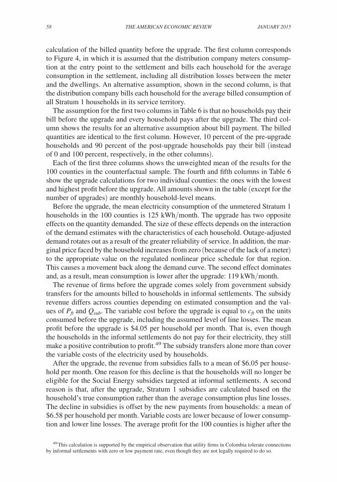
58 THE AMERICAN ECONOMIC REVIEW JANuARy 2015
calculation of the billed quantity before the upgrade. The first column corresponds to Figure 4, in which it is assumed that the distribution company meters consump-tion at the entry point to the settlement and bills each household for the average consumption in the settlement, including all distribution losses between the meter and the dwellings. An alternative assumption, shown in the second column, is that the distribution company bills each household for the average billed consumption of all Stratum 1 households in its service territory.
The assumption for the first two columns in Table 6 is that no households pay their bill before the upgrade and every household pays after the upgrade. The third col-umn shows the results for an alternative assumption about bill payment. The billed quantities are identical to the first column. However, 10 percent of the pre-upgrade households and 90 percent of the post-upgrade households pay their bill (instead of 0 and 100 percent, respectively, in the other columns).
Each of the first three columns shows the unweighted mean of the results for the 100 counties in the counterfactual sample. The fourth and fifth columns in Table 6 show the upgrade calculations for two individual counties: the ones with the lowest and highest profit before the upgrade. All amounts shown in the table (except for the number of upgrades) are monthly household-level means.
Before the upgrade, the mean electricity consumption of the unmetered Stratum 1 households in the 100 counties is 125 kWh/month. The upgrade has two opposite effects on the quantity demanded. The size of these effects depends on the interaction of the demand estimates with the characteristics of each household. Outage-adjusted demand rotates out as a result of the greater reliability of service. In addition, the mar-ginal price faced by the household increases from zero (because of the lack of a meter) to the appropriate value on the regulated nonlinear price schedule for that region. This causes a movement back along the demand curve. The second effect dominates and, as a result, mean consumption is lower after the upgrade: 119 kWh/month.
The revenue of firms before the upgrade comes solely from government subsidy transfers for the amounts billed to households in informal settlements. The subsidy revenue differs across counties depending on estimated consumption and the val-ues of P ft and Q sub . The variable cost before the upgrade is equal to c ft on the units consumed before the upgrade, including the assumed level of line losses. The mean profit before the upgrade is $4.05 per household per month. That is, even though the households in the informal settlements do not pay for their electricity, they still make a positive contribution to profit.49 The subsidy transfers alone more than cover the variable costs of the electricity used by households.
After the upgrade, the revenue from subsidies falls to a mean of $6.05 per house-hold per month. One reason for this decline is that the households will no longer be eligible for the Social Energy subsidies targeted at informal settlements. A second reason is that, after the upgrade, Stratum 1 subsidies are calculated based on the household’s true consumption rather than the average consumption plus line losses. The decline in subsidies is offset by the new payments from households: a mean of $6.58 per household per month. Variable costs are lower because of lower consump-tion and lower line losses. The average profit for the 100 counties is higher after the
49 This calculation is supported by the empirical observation that utility firms in Colombia tolerate connections by informal settlements with zero or low payment rate, even though they are not legally required to do so.
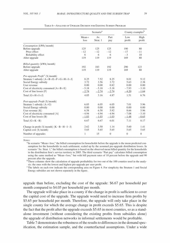
59Mcrae: Infrastructure QualIty and the subsIdy trapVOl. 105 nO. 1
upgrade than before, excluding the cost of the upgrade: $6.67 per household per month compared to $4.05 per household per month.
The upgrade will take place in a county if the change in profit is sufficient to cover the capital cost of the upgrade. The upgrade would need to increase firm profits by $5.65 per household per month. Therefore, the upgrade will only take place in the single county for which the average change in profit exceeds $5.65. This is despite the fact that the profit after the upgrade exceeds $5.65 in most counties, so as a stand-alone investment (without considering the existing profits from subsidies alone) the upgrade of distribution networks in informal settlements would be profitable.
Table 7 demonstrates the robustness of the results to differences in the demand spec-ification, the estimation sample, and the counterfactual assumptions. Under a wide
Table 6—Analysis of Upgrade Decision for Existing Subsidy Program
Scenarioa County examplesb
Mean+ Av. Part Low Highloss Strat. 1 pay profit profit
Consumption (kWh/month)Before upgrade 125 125 125 190 80 Price effect −12 −12 −12 −17 −11 Reliability effect 6 6 6 −3 10After upgrade 119 119 119 169 80
Billed quantity (kWh/month)Before upgrade 192 183 192 290 123After upgrade 119 119 119 169 80
Pre-upgrade Profit c ($/month)Stratum 1 subsidy (A+B+E+F+G+H+I+J) 8.25 7.52 8.25 8.01 9.12Social Energy subsidy 3.72 3.56 3.72 5.63 2.38User revenue 0.00 0.00 0.82 0.00 0.00Cost of electricity consumed (A+B+E) −5.18 −5.18 −5.18 −7.93 −3.10Cost of line losses (F) −2.74 −2.74 −2.74 −4.20 −1.64
Total (G+H+I+J) 4.05 3.16 4.87 1.51 6.76
Post-upgrade Profit ($/month)Stratum 1 subsidy (A+G) 6.05 6.05 6.05 7.01 5.96Social Energy subsidy 0.00 0.00 0.00 0.00 0.00User revenue (K) 6.58 6.58 5.92 8.66 5.96Cost of electricity consumed (A) −4.94 −4.94 −4.94 −7.08 −3.10Cost of line losses (B) −1.03 −1.03 −1.03 −1.48 −0.65
Total (G+K−B) 6.67 6.67 6.01 7.11 8.17
Change in profit ($/month) (K−B−H−I−J) 2.62 3.50 1.14 5.60 1.41Capital cost ($/month) 5.65 5.65 5.65 5.65 5.65
Number of upgrades 1 15 0 0 0
Notes:a In scenario “Mean+loss,” the billed consumption for households before the upgrade is the mean predicted con-sumption for the households in each settlement, scaled up by the assumed pre-upgrade distribution losses. In scenario “Av. Strat. 1,” the billed consumption is based on the observed mean billed quantity for the households in the distribution firm’s service territory in 2005. The third scenario “Part pay” calculates billed consumption using the same method as “Mean+loss,” but with bill payment rates of 10 percent before the upgrade and 90 percent after the upgrade.
b These columns show the calculation of upgrade profitability for two out of the 100 counties used in the analy-sis: the ones with the lowest and highest pre-upgrade per user profit.
c The labels on each row indicate the corresponding area on Figure 4. For simplicity the Stratum 1 and Social Energy subsidies are not shown separately in the figure.
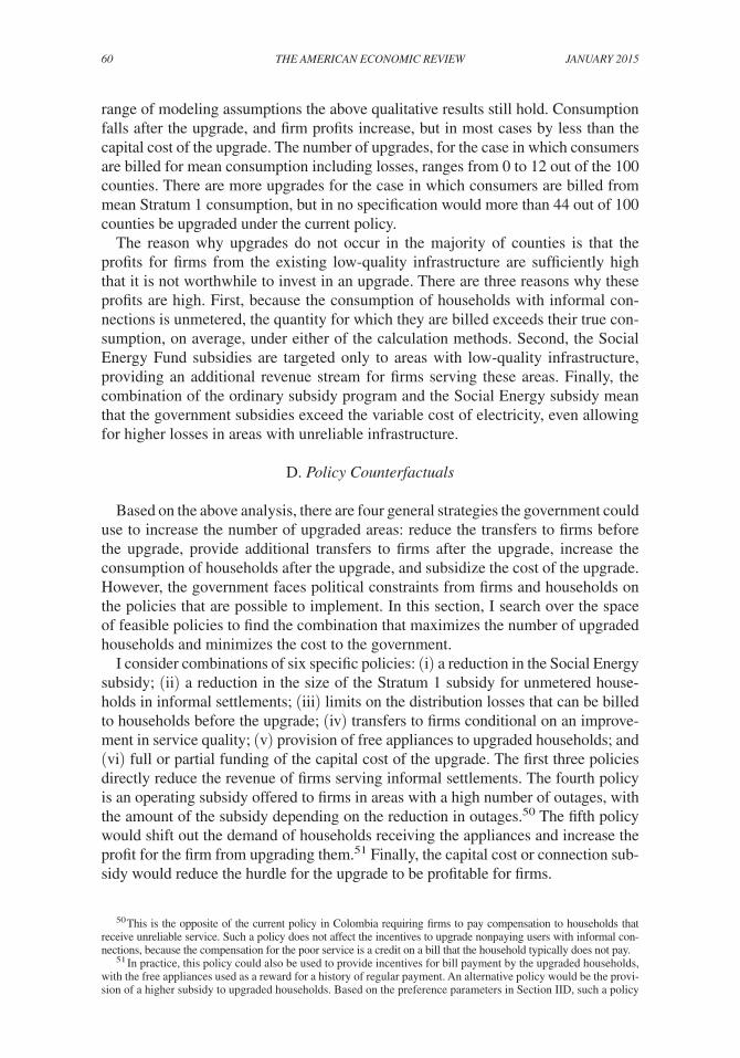
60 THE AMERICAN ECONOMIC REVIEW JANuARy 2015
range of modeling assumptions the above qualitative results still hold. Consumption falls after the upgrade, and firm profits increase, but in most cases by less than the capital cost of the upgrade. The number of upgrades, for the case in which consumers are billed for mean consumption including losses, ranges from 0 to 12 out of the 100 counties. There are more upgrades for the case in which consumers are billed from mean Stratum 1 consumption, but in no specification would more than 44 out of 100 counties be upgraded under the current policy.
The reason why upgrades do not occur in the majority of counties is that the profits for firms from the existing low-quality infrastructure are sufficiently high that it is not worthwhile to invest in an upgrade. There are three reasons why these profits are high. First, because the consumption of households with informal con-nections is unmetered, the quantity for which they are billed exceeds their true con-sumption, on average, under either of the calculation methods. Second, the Social Energy Fund subsidies are targeted only to areas with low-quality infrastructure, providing an additional revenue stream for firms serving these areas. Finally, the combination of the ordinary subsidy program and the Social Energy subsidy mean that the government subsidies exceed the variable cost of electricity, even allowing for higher losses in areas with unreliable infrastructure.
D. Policy Counterfactuals
Based on the above analysis, there are four general strategies the government could use to increase the number of upgraded areas: reduce the transfers to firms before the upgrade, provide additional transfers to firms after the upgrade, increase the consumption of households after the upgrade, and subsidize the cost of the upgrade. However, the government faces political constraints from firms and households on the policies that are possible to implement. In this section, I search over the space of feasible policies to find the combination that maximizes the number of upgraded households and minimizes the cost to the government.
I consider combinations of six specific policies: (i) a reduction in the Social Energy subsidy; (ii) a reduction in the size of the Stratum 1 subsidy for unmetered house-holds in informal settlements; (iii) limits on the distribution losses that can be billed to households before the upgrade; (iv) transfers to firms conditional on an improve-ment in service quality; (v) provision of free appliances to upgraded households; and (vi) full or partial funding of the capital cost of the upgrade. The first three policies directly reduce the revenue of firms serving informal settlements. The fourth policy is an operating subsidy offered to firms in areas with a high number of outages, with the amount of the subsidy depending on the reduction in outages.50 The fifth policy would shift out the demand of households receiving the appliances and increase the profit for the firm from upgrading them.51 Finally, the capital cost or connection sub-sidy would reduce the hurdle for the upgrade to be profitable for firms.
50 This is the opposite of the current policy in Colombia requiring firms to pay compensation to households that receive unreliable service. Such a policy does not affect the incentives to upgrade nonpaying users with informal con-nections, because the compensation for the poor service is a credit on a bill that the household typically does not pay.
51 In practice, this policy could also be used to provide incentives for bill payment by the upgraded households, with the free appliances used as a reward for a history of regular payment. An alternative policy would be the provi-sion of a higher subsidy to upgraded households. Based on the preference parameters in Section IID, such a policy
61Mcrae: Infrastructure QualIty and the subsIdy trapVOl. 105 nO. 1
I search over approximately 47.8 million combinations of different levels of these six policies.52 However, there may be political constraints on combinations of policies that can be implemented. Table 8 shows the current subsidy program
would have a relatively small effect on the consumption of households after the upgrade. This makes it an expensive way for the government to provide additional revenue to firms.
52 The specific combinations that I calculate are: 21 levels of the Stratum 1 subsidy, from 0 percent to 50 percent; 21 levels of the Social Energy subsidy, from 0 cents/kWh to 2 cents/kWh; 21 levels of the proportion of losses billed before the upgrade, from 0 percent to 100 percent, 41 levels of the capital subsidy, from 0 percent to 100 per-cent; 21 levels of the quality subsidy, from 0 cents/kWh to 1 cent/kWh for each percentage point reduction in out-ages; and the provision of 5 types of appliance (none, refrigerator, fan, computer, washing machine, and television).
Table 7—Robustness Checks and Alternative Specifications
Price elasticitya
Outage
effectb
Mean+loss scenarioc Av. Strat. 1
Overall Strat. 1 Pre q Post q Δ Prof. No. upg. No. upg.
Base case −0.32 −0.13 −0.165 125.3 119.5 2.62 1 15
Demand model d
Base outage effect only −0.32 −0.13 −0.182 125.5 119.4 2.61 1 15Diff. appliance outage effect −0.32 −0.13 −0.125 125.5 119.6 2.63 1 15Base price effect only −0.36 −0.33 −0.189 150.8 117.0 2.60 4 34Region × appliance terms −0.34 −0.14 −0.182 131.8 120.7 2.90 2 18Minor appliance interactions −0.31 −0.13 −0.165 124.4 118.9 2.57 1 13
Estimation sample e
Trim 2 percent −0.23 −0.07 −0.138 119.5 117.8 2.50 0 9+ Include home businesses −0.25 −0.10 −0.114 125.7 121.8 2.77 1 15Trim 0.25 percent −0.45 −0.22 −0.179 134.2 119.1 2.69 2 23Strata 1–3 households only −0.26 −0.12 −0.134 126.3 119.0 2.66 1 14Drop bills not households −0.28 −0.10 −0.138 121.4 118.4 2.53 1 11
Counterfactual assumptions f
Pre-upg. losses +50 percent 125.3 119.5 2.45 0 10Use all hhs in counterfactual 150.0 132.6 3.62 12 44Change historical outages 125.3 117.6 2.45 2 15Post-upg. outages at mean 125.3 119.5 2.58 1 11Post-upg. outages −90 percent 125.3 122.7 2.82 1 18Post-upg. outages −50 percent 125.3 115.3 2.36 1 13
Notes:a Price elasticities from Table 4, for all households and Stratum 1 households.b Mean change in monthly consumption (in kWh) due to one additional hour of outage, from Table 4.c Mean pre-upgrade and post-upgrade monthly consumption in kWh, mean change in profit, and number of upgrades for Mean + loss scenario in Table 6. For Av. Strat. 1 scenario, only number of upgrades from col-umn 2 in Table 6 is shown.
d Base outage effect restricts θi for non-baseload appliances to be zero. Diff. appliance outage effect allows θi to differ between baseload and non-baseload appliances. Base price effect restricts βi for nonbaseload appliances to be zero. Region × appliance includes region interactions for each appliance. Minor appliance includes inter-actions for small appliances with hh members, rooms, apartment, and temperature.
e Results for dropping households in top and bottom 2 or 0.25 percent of residuals, including households with home businesses (also dropping top and bottom 2 percent), dropping monthly observations instead of house-holds (see Section IIC), and estimating the model only for households in Strata 1 to 3.
f Pre-upgrade losses 50 percent higher than post-upgrade (instead of 100 percent in base case). Use all households does not select likely Stratum 1 households (see online Appendix). Change historical outages changes the histori-cal average number and length of outages in counterfactual. Post-upgrade outages set at national mean, 90 percent lower than pre-upgrade, and 50 percent lower than pre-upgrade (instead of 75 percent lower in base case).
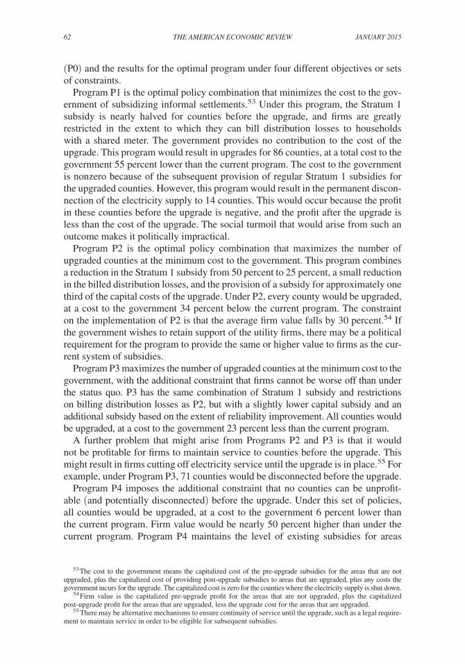
62 THE AMERICAN ECONOMIC REVIEW JANuARy 2015
(P0) and the results for the optimal program under four different objectives or sets of constraints.
Program P1 is the optimal policy combination that minimizes the cost to the gov-ernment of subsidizing informal settlements.53 Under this program, the Stratum 1 subsidy is nearly halved for counties before the upgrade, and firms are greatly restricted in the extent to which they can bill distribution losses to households with a shared meter. The government provides no contribution to the cost of the upgrade. This program would result in upgrades for 86 counties, at a total cost to the government 55 percent lower than the current program. The cost to the government is nonzero because of the subsequent provision of regular Stratum 1 subsidies for the upgraded counties. However, this program would result in the permanent discon-nection of the electricity supply to 14 counties. This would occur because the profit in these counties before the upgrade is negative, and the profit after the upgrade is less than the cost of the upgrade. The social turmoil that would arise from such an outcome makes it politically impractical.
Program P2 is the optimal policy combination that maximizes the number of upgraded counties at the minimum cost to the government. This program combines a reduction in the Stratum 1 subsidy from 50 percent to 25 percent, a small reduction in the billed distribution losses, and the provision of a subsidy for approximately one third of the capital costs of the upgrade. Under P2, every county would be upgraded, at a cost to the government 34 percent below the current program. The constraint on the implementation of P2 is that the average firm value falls by 30 percent.54 If the government wishes to retain support of the utility firms, there may be a political requirement for the program to provide the same or higher value to firms as the cur-rent system of subsidies.
Program P3 maximizes the number of upgraded counties at the minimum cost to the government, with the additional constraint that firms cannot be worse off than under the status quo. P3 has the same combination of Stratum 1 subsidy and restrictions on billing distribution losses as P2, but with a slightly lower capital subsidy and an additional subsidy based on the extent of reliability improvement. All counties would be upgraded, at a cost to the government 23 percent less than the current program.
A further problem that might arise from Programs P2 and P3 is that it would not be profitable for firms to maintain service to counties before the upgrade. This might result in firms cutting off electricity service until the upgrade is in place.55 For example, under Program P3, 71 counties would be disconnected before the upgrade.
Program P4 imposes the additional constraint that no counties can be unprofit-able (and potentially disconnected) before the upgrade. Under this set of policies, all counties would be upgraded, at a cost to the government 6 percent lower than the current program. Firm value would be nearly 50 percent higher than under the current program. Program P4 maintains the level of existing subsidies for areas
53 The cost to the government means the capitalized cost of the pre-upgrade subsidies for the areas that are not upgraded, plus the capitalized cost of providing post-upgrade subsidies to areas that are upgraded, plus any costs the government incurs for the upgrade. The capitalized cost is zero for the counties where the electricity supply is shut down.
54 Firm value is the capitalized pre-upgrade profit for the areas that are not upgraded, plus the capitalized post-upgrade profit for the areas that are upgraded, less the upgrade cost for the areas that are upgraded.
55 There may be alternative mechanisms to ensure continuity of service until the upgrade, such as a legal require-ment to maintain service in order to be eligible for subsequent subsidies.
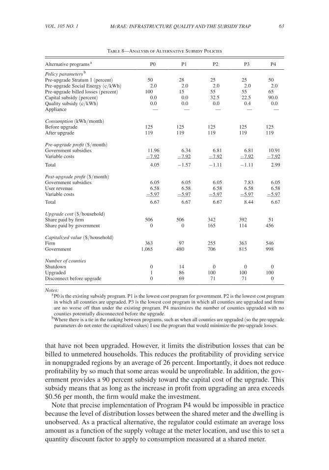
63Mcrae: Infrastructure QualIty and the subsIdy trapVOl. 105 nO. 1
that have not been upgraded. However, it limits the distribution losses that can be billed to unmetered households. This reduces the profitability of providing service in nonupgraded regions by an average of 26 percent. Importantly, it does not reduce profitability by so much that some areas would be unprofitable. In addition, the gov-ernment provides a 90 percent subsidy toward the capital cost of the upgrade. This subsidy means that as long as the increase in profit from upgrading an area exceeds $0.56 per month, the firm would make the investment.
Note that precise implementation of Program P4 would be impossible in practice because the level of distribution losses between the shared meter and the dwelling is unobserved. As a practical alternative, the regulator could estimate an average loss amount as a function of the supply voltage at the meter location, and use this to set a quantity discount factor to apply to consumption measured at a shared meter.
Table 8—Analysis of Alternative Subsidy Policies
Alternative programs a P0 P1 P2 P3 P4
Policy parameters b
Pre-upgrade Stratum 1 (percent) 50 28 25 25 50Pre-upgrade Social Energy (c/kWh) 2.0 2.0 2.0 2.0 2.0Pre-upgrade billed losses (percent) 100 15 55 55 65Capital subsidy (percent) 0.0 0.0 32.5 22.5 90.0Quality subsidy (c/kWh) 0.0 0.0 0.0 0.4 0.0Appliance — — — — —
Consumption (kWh/month)Before upgrade 125 125 125 125 125After upgrade 119 119 119 119 119
Pre-upgrade profit ($/month)Government subsidies 11.96 6.34 6.81 6.81 10.91Variable costs −7.92 −7.92 −7.92 −7.92 −7.92
Total 4.05 −1.57 −1.11 −1.11 2.99
Post-upgrade profit ($/month)Government subsidies 6.05 6.05 6.05 7.83 6.05User revenue 6.58 6.58 6.58 6.58 6.58Variable costs −5.97 −5.97 −5.97 −5.97 −5.97
Total 6.67 6.67 6.67 8.44 6.67
Upgrade cost ($/household)Share paid by firm 506 506 342 392 51Share paid by government 0 0 165 114 456
Capitalized value ($/household)Firm 363 97 255 363 546Government 1,065 480 706 815 998
Number of countiesShutdown 0 14 0 0 0Upgraded 1 86 100 100 100Disconnect before upgrade 0 69 71 71 0
Notes: a P0 is the existing subsidy program. P1 is the lowest cost program for government. P2 is the lowest cost program in which all counties are upgraded. P3 is the lowest cost program in which all counties are upgraded and firms are no worse off than under the existing program. P4 maximizes the number of counties upgraded with no counties potentially disconnected before the upgrade.
b Where there is a tie in the ranking between programs, such as when all counties are upgraded (so the pre-upgrade parameters do not enter the capitalized values) I use the program that would minimize the pre-upgrade losses.
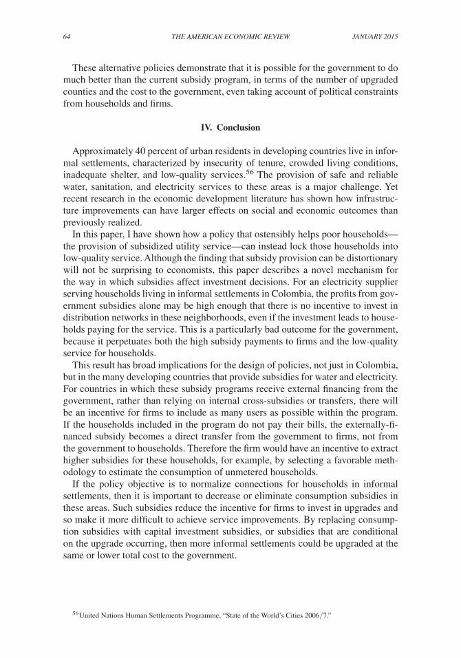
64 THE AMERICAN ECONOMIC REVIEW JANuARy 2015
These alternative policies demonstrate that it is possible for the government to do much better than the current subsidy program, in terms of the number of upgraded counties and the cost to the government, even taking account of political constraints from households and firms.
IV. Conclusion
Approximately 40 percent of urban residents in developing countries live in infor-mal settlements, characterized by insecurity of tenure, crowded living conditions, inadequate shelter, and low-quality services.56 The provision of safe and reliable water, sanitation, and electricity services to these areas is a major challenge. Yet recent research in the economic development literature has shown how infrastruc-ture improvements can have larger effects on social and economic outcomes than previously realized.
In this paper, I have shown how a policy that ostensibly helps poor households—the provision of subsidized utility service—can instead lock those households into low-quality service. Although the finding that subsidy provision can be distortionary will not be surprising to economists, this paper describes a novel mechanism for the way in which subsidies affect investment decisions. For an electricity supplier serving households living in informal settlements in Colombia, the profits from gov-ernment subsidies alone may be high enough that there is no incentive to invest in distribution networks in these neighborhoods, even if the investment leads to house-holds paying for the service. This is a particularly bad outcome for the government, because it perpetuates both the high subsidy payments to firms and the low-quality service for households.
This result has broad implications for the design of policies, not just in Colombia, but in the many developing countries that provide subsidies for water and electricity. For countries in which these subsidy programs receive external financing from the government, rather than relying on internal cross-subsidies or transfers, there will be an incentive for firms to include as many users as possible within the program. If the households included in the program do not pay their bills, the externally-fi-nanced subsidy becomes a direct transfer from the government to firms, not from the government to households. Therefore the firm would have an incentive to extract higher subsidies for these households, for example, by selecting a favorable meth-odology to estimate the consumption of unmetered households.
If the policy objective is to normalize connections for households in informal settlements, then it is important to decrease or eliminate consumption subsidies in these areas. Such subsidies reduce the incentive for firms to invest in upgrades and so make it more difficult to achieve service improvements. By replacing consump-tion subsidies with capital investment subsidies, or subsidies that are conditional on the upgrade occurring, then more informal settlements could be upgraded at the same or lower total cost to the government.
56 United Nations Human Settlements Programme, “State of the World’s Cities 2006/7.”

65Mcrae: Infrastructure QualIty and the subsIdy trapVOl. 105 nO. 1
REFERENCES
Bailey, Martha J., and William J. Collins. 2011. “Did Improvements in Household Technology Cause the Baby Boom? Evidence from Electrification, Appliance Diffusion, and the Amish.” American Economic Journal: Macroeconomics 3 (2): 189–217.
Banerjee, Abhijit, Esther Duflo, and Nancy Qian. 2012. “On the Road: Access to Transportation Infra-structure and Economic Growth in China.” National Bureau of Economic Research Working Paper 17897.
Cardoso, Rafael Balbino, Luiz Augusto Horta Nogueira, and Jamil Haddad. 2010. “Economic Feasi-bility for Acquisition of Efficient Refrigerators in Brazil.” Applied Energy 87 (1): 28–37.
Comisión de Regulación de Energía y Gas. 1997. “Resolución No. 108.” July 3, 1997.Comisión de Regulación de Energía y Gas. 1997. “Resolución No. 31.” April 4, 1997.Congreso de la República de Colombia. 2006. “Ley 1117 de 2006.” Diario Oficial No. 46494. Decem-
ber 27, 2006.Congreso de la República de Colombia. 2010. “Ley 1430 de 2010.” Diario Oficial No. 47937. Decem-
ber 29, 2010.Davis, Lucas W., and Lutz Kilian. 2011. “The Allocative Cost of Price Ceilings in the U.S. Residential
Market for Natural Gas.” Journal of Political Economy 119 (2): 212–41.Departamento Administrativo Nacional de Estadística. 2003. “Encuesta de Calidad de Vida: Dataset.”
http://formularios.dane.gov.co/Anda_4_1/index.php/catalog/186.Departamento Nacional de Planeación. 2008. Evaluación de la Estratificación socioeconómica.
Bogotá D.C., Colombia: Departamento Nacional de Planeación.Devoto, Florencia, Esther Duflo, Pascaline Dupas, William Parienté, and Vincent Pons. 2012. “Hap-
piness on Tap: Piped Water Adoption in Urban Morocco.” American Economic Journal: Economic Policy 4 (4): 68–99.
Dinkelman, Taryn. 2011. “The Effects of Rural Electrification on Employment: New Evidence from South Africa.” American Economic Review 101 (7): 3078–108.
Donaldson, Dave. Forthcoming. “Railroads of the Raj: Estimating the Impact of Transportation Infra-structure.” American Economic Review.
Duflo, Esther, and Rohini Pande. 2007. “Dams.” Quarterly Journal of Economics 122 (2): 601–46.Duranton, Gilles, and Matthew A. Turner. 2012. “Urban Growth and Transportation.” Review of Eco-
nomic Studies 79 (4): 1407–40.Feler, Leo, and J. Vernon Henderson. 2011. “Exclusionary Policies in Urban Development: Under-ser-
vicing Migrant Households in Brazilian Cities.” Journal of Urban Economics 69 (3): 253–72.Gonzalez-Navarro, Marco, and Climent Quintana-Domeque. 2012. “Paving Streets for the Poor:
Experimental Analysis of Infrastructure Effects.” http://individual.utoronto.ca/marcog/attachment/pavement_paper_2012.pdf (accessed April 12, 2013).
Greenwood, Jeremy, Ananth Seshadri, and Guillaume Vandenbroucke. 2005. “The Baby Boom and Baby Bust.” American Economic Review 95 (1): 183–207.
Hewitt, Julie A. 1993. “Watering Households: The Two-Error Discrete-Continuous Choice Model of Residential Water Demand.” PhD diss. University of California, Berkeley.
Hewitt, Julie A., and W. Michael Hanemann. 1995. “A Discrete/Continuous Choice Approach to Res-idential Water Demand under Block Rate Pricing.” Land Economics 71 (2): 173–92.
Jensen, Robert. 2007. “The Digital Provide: Information (Technology), Market Performance, and Wel-fare in the South Indian Fisheries Sector.” Quarterly Journal of Economics 122 (3): 879–924.
Jensen, Robert, and Emily Oster. 2009. “The Power of TV: Cable Television and Women’s Status in India.” Quarterly Journal of Economics 124 (3): 1057–94.
Klytchnikova, Irina, and Michael Lokshin. 2010. “Measuring Welfare Gains from Better Quality Infrastructure.” Journal of Infrastructure Development 1 (2): 87–109.
Komives, Kristin, Vivien Foster, Jonathan Halpern, and Quentin Wodon. 2005. Water, Electricity, and the Poor: Who Benefits from Utility Subsidies? Washington, DC: World Bank.
Kremer, Michael, Jessica Leino, Edward Miguel, and Alix Peterson Zwane. 2011. “Spring Cleaning: Rural Water Impacts, Valuation, and Property Rights Institutions.” Quarterly Journal of Economics 126 (1): 145–205.
Krishnaswamy, Venkataraman, and Gary Stuggins. 2007. “Closing the Electricity Supply-Demand Gap.” World Bank Energy and Mining Sector Board Discussion Paper 20.
La Ferrara, Eliana, Alberto Chong, and Suzanne Duryea. 2012. “Soap Operas and Fertility: Evidence from Brazil.” American Economic Journal: Applied Economics 4 (4): 1–31.
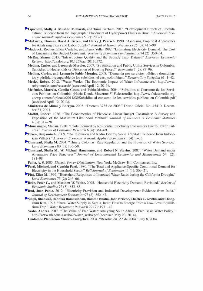
66 THE AMERICAN ECONOMIC REVIEW JANuARy 2015
Lipscomb, Molly, A. Mushfiq Mobarak, and Tania Barham. 2013. “Development Effects of Electrifi-cation: Evidence from the Topographic Placement of Hydropower Plants in Brazil.” American Eco-nomic Journal: Applied Economics 5 (2): 200–31.
MaCurdy, Thomas, David A. Green, and Harry J. Paarsch. 1990. “Assessing Empirical Approaches for Analyzing Taxes and Labor Supply.” Journal of Human Resources 25 (3): 415–90.
Maddock, Rodney, Elkin Castaño, and Frank Vella. 1992. “Estimating Electricity Demand: The Cost of Linearising the Budget Constraint.” Review of Economics and Statistics 74 (2): 350–54.
McRae, Shaun. 2015. “Infrastructure Quality and the Subsidy Trap: Dataset.” American Economic Review. http://dx.doi.org/10.1257/aer.20110572.
Medina, Carlos, and Leonardo Morales. 2007. “Stratification and Public Utility Services in Colombia: Subsidies to Households or Distortion of Housing Prices?” Economía 7 (2): 87–96.
Medina, Carlos, and Leonardo Fabio Morales. 2008. “Demanda por servicios públicos domiciliar-ios y pérdida irrecuperable de los subsidios: el caso colombiano.” Desarrollo y Sociedad 61: 1–42.
Meeks, Robyn. 2012. “Water Works: The Economic Impact of Water Infrastructure.” http://www.robynmeeks.com/research/ (accessed April 12, 2013).
Meléndez, Marcela, Camila Casas, and Pablo Medina. 2004. “Subsidios al Consumo de los Servi-cios Públicos en Colombia ¿Hacia Donde Movernos?” Fedesarrollo. http://www.fedesarrollo.org.co/wp-content/uploads/2011/08/Subsidios-al-consumo-de-los-servicios-publicos-en-Colombia.pdf (accessed April 12, 2013).
Ministerio de Minas y Energía. 2003. “Decreto 3735 de 2003.” Diario Oficial No. 45410. Decem-ber 23, 2003.
Moffitt, Robert. 1986. “The Econometrics of Piecewise-Linear Budget Constraints: A Survey and Exposition of the Maximum Likelihood Method.” Journal of Business & Economic Statistics 4 (3): 317–28.
Munasinghe, Mohan. 1980. “Costs Incurred by Residential Electricity Consumers Due to Power Fail-ures.” Journal of Consumer Research 6 (4): 361–69.
Olken, Benjamin A. 2009. “Do Television and Radio Destroy Social Capital? Evidence from Indone-sian Villages.” American Economic Journal: Applied Economics 1 (4): 1–33.
Olmstead, Sheila M. 2004. “Thirsty Colonias: Rate Regulation and the Provision of Water Service.” Land Economics 80 (1): 136–50.
Olmstead, Sheila M., W. Michael Hanemann, and Robert N. Stavins. 2007. “Water Demand under Alternative Price Structures.” Journal of Environmental Economics and Management 54 (2): 181–98.
Pabla, A. S. 2005. Electric Power Distribution. New York: McGraw-Hill Companies, Inc.Parti, Michael, and Cynthia Parti. 1980. “The Total and Appliance-Specific Conditional Demand for
Electricity in the Household Sector.” Bell Journal of Economics 11 (1): 309–21.Pint, Ellen M. 1999. “Household Responses to Increased Water Rates during the California Drought.”
Land Economics 75 (2): 246–66.Reiss, Peter C., and Matthew W. White. 2005. “Household Electricity Demand, Revisited.” Review of
Economic Studies 72 (3): 853–83.Rud, Juan Pablo. 2012. “Electricity Provision and Industrial Development: Evidence from India.”
Journal of Development Economics 97 (2): 352–67.Singh, Bhanwar, Radhika Ramasubban, Ramesh Bhatia, John Briscoe, Charles C. Griffin, and Chong-
chun Kim. 1993. “Rural Water Supply in Kerala, India: How to Emerge From a Low-Level Equilib-rium Trap.” Water Resources Research 29 (7): 1931–42.
Szabo, Andrea. 2013. “The Value of Free Water: Analyzing South Africa’s Free Basic Water Policy.” http://www.uh.edu/~aszabo2/water_szabo.pdf (accessed May 23, 2014).
Unidad de Planeación Minero-Energética. 2004. “Resolución 355 de 2004.” July 8, 2004.

This article has been cited by:
1. B. Kelsey Jack, Grant Smith. 2015. Pay as You Go: Prepaid Metering and Electricity Expenditures inSouth Africa. American Economic Review 105:5, 237-241. [Abstract] [View PDF article] [PDF withlinks]
2. Michael Greenstone, B. Kelsey Jack. 2015. Envirodevonomics: A Research Agenda for an EmergingField. Journal of Economic Literature 53:1, 5-42. [Abstract] [View PDF article] [PDF with links]
Related Documents