Informed search algorithms - web.pdx.eduweb.pdx.edu/~arhodes/ai8.pdf · Memory Bounded Heuristic Search: Recursive BFS • RBFS changes its mind very often in practice. This is because

A.I.: Informed Search Algorithms

Chapter III: Part Deux

Outline

• Best-first search

• Greedy best-first search

• A* search

• Heuristics

Overview• Informed Search: uses problem-specific knowledge.

• General approach: best-first search; an instance of TREE-SEARCH (or GRAPH-SEARCH) – where a search strategy is defined by picking the order of node expansion.

• With best-first, node is selected for expansion based on evaluation function f(n).

• Evaluation function is a cost estimate; expand lowest cost node first (same as uniform-cost search but we replace g with f).

Overview (cont’d) • The choice of f determines the search strategy (one can show

that best-first tree search includes DFS as a special case).

• Often, for best-first algorithms, f is defined in terms of a heuristic function, h(n).

h(n) = estimated cost of the cheapest path from the state at node n to a goal state. (for goal state: h(n)=0)

• Heuristic functions are the most common form in which additional knowledge of the problem is passed to the search algorithm.

Overview (cont’d) • Best-First Search algorithms constitute a large family of

algorithms, with different evaluation functions.

– Each has a heuristic function h(n)

• Example: in route planning the estimate of the cost of the cheapest path might be the straight line distance between two cities.

Recall:

• g(n) = cost from the initial state to the current state n.

• h(n) = estimated cost of the cheapest path from node n to a goal node.

• f(n) = evaluation function to select a node for expansion (usually the lowest cost node).

Best-First Search

• Idea: use an evaluation function f(n) for each node

– f(n) provides an estimate for the total cost.

Expand the node n with smallest f(n).

• Implementation:

Order the nodes in the frontier increasing order of cost.

• Special cases:

– Greedy best-first search

– A* search

Greedy best-first search• Evaluation function f(n) = h(n) (heuristic), the estimate of cost

from n to goal.

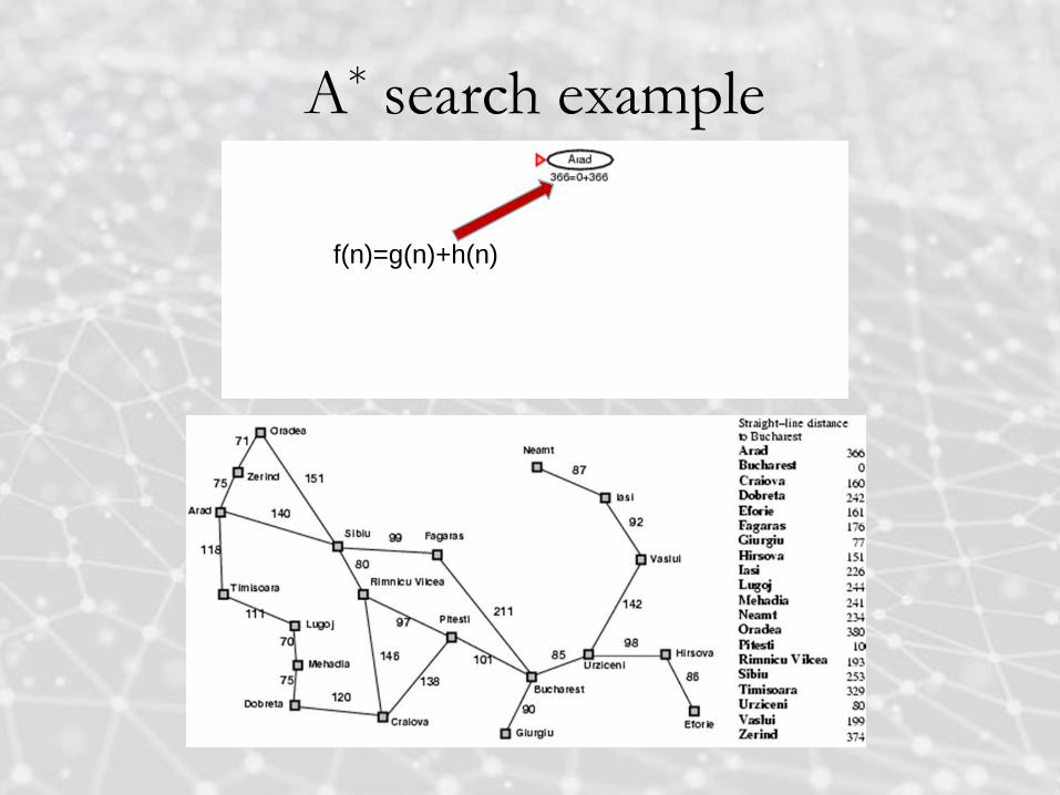
• We use the straight-line distance heuristic: hSLD(n) = straight-line distance from n to Bucharest.

• Note that the heuristic values cannot be computed from the problem description itself !

• In addition, we require extrinsic knowledge to understand that hSLD is correlated with the actual road distances, making it a useful heuristic.

• Greedy best-first search expands the node that appears to be closest to goal.

Romania with step costs in km

Greedy best-first search example

Greedy best-first search example

Greedy best-first search example

Greedy best-first search example

Greedy best-first search

• GBFS is incomplete!

• Why?

• Graph-Search version is, however, complete in finite spaces.

Properties of greedy best-first search

• Complete? No – can get stuck in loops, e.g., Iasi Neamt Iasi Neamt

• Time? O(bm), (in worst case) but a good heuristic can give dramatic improvement (m is max depth of search space).

• Space? O(bm) -- keeps all nodes in memory.

• Optimal? No (not guaranteed to render lowest cost solution).

A* Search• Most widely-known form of best-first search.

• It evaluates nodes by combining g(n), the cost to reach the node, and h(n), the cost to get from the node to the goal:

f(n) = g(n) + h(n) (estimated cost of cheapest solution through n).

• A reasonable strategy: try node with the lowest g(n) + h(n) value!

• Provided heuristic meets some basic conditions, A* is both complete and optimal.

A* search example

f(n)=g(n)+h(n)

A* search example

A* search example

A* search example

A* search example

A* search example

Admissible heuristics• A heuristic h(n) is admissible if for every node n,

h(n) ≤ h*(n), where h*(n) is the true cost to reach the goal

state from n.

• An admissible heuristic never overestimates the cost to

reach the goal, i.e., it is optimistic.

• Example: hSLD(n) (never overestimates the actual road

distance)

• Theorem: If h(n) is admissible, A* using TREE-

SEARCH is optimal.

Optimality of A* (proof)• Suppose some suboptimal goal G2 has been generated and is in

the frontier. Let n be an unexpanded node in the frontier such that

n is on a shortest path to an optimal goal G.

• f(G2) = g(G2) since h(G2) = 0

• g(G2) > g(G) since G2 is suboptimal

• f(G) = g(G) since h(G) = 0

• f(G2) > f(G) from above

Optimality of A* (proof)• Suppose some suboptimal goal G2 has been generated and is in

the fringe. Let n be an unexpanded node in the fringe such that n

is on a shortest path to an optimal goal G.

• f(G2) > f(G) (from above)

• h(n) ≤ h*(n) (since h is admissible)

-> g(n) + h(n) ≤ g(n) + h*(n)

• f(n) ≤ g(n) + h*(n) < f(G) < f(G2)

Hence f(G2) > f(n), and A* will never select G2 for expansion.

Consistent Heuristics• A heuristic is consistent (or monotonic) if for every node n,

every successor n' of n generated by any action a:

h(n) ≤ c(n,a,n') + h(n')

• If h is consistent, we have:

f(n') = g(n') + h(n')

= g(n) + c(n,a,n') + h(n')

≥ g(n) + h(n)

= f(n)

i.e., f(n) is non-decreasing along any path.

Theorem: If h(n) is consistent, A* using GRAPH-SEARCH is optimal.

Optimality of A*

• A* expands nodes in order of increasing f value.

• Gradually adds "f-contours" of nodes.

• Contour i has all nodes with f=fi, where fi < fi+1.

• That is to say, nodes inside a given contour have f-costs less

than or equal to contour value.

Properties of A*

• Complete: Yes (unless there are infinitely many nodes with

f ≤ f(G) ).

• Time: Exponential.

• Space: Keeps all nodes in memory, so also exponential.

• Optimal: Yes (provided h admissible or consistent).

• Optimally Efficient: Yes (no algorithm with the

same heuristic is guaranteed to expand fewer nodes).

• NB: Every consistent heuristic is also admissible (Pearl).

Q: What about the converse?

Admissible HeuristicsE.g., for the 8-puzzle:

• h1(n) = number of misplaced tiles

• h2(n) = total Manhattan distance (i.e. 1-norm)

(i.e., no. of squares from desired location of each tile)

Q: Why are these admissible heuristics?

• h1(S) = ?

• h2(S) = ?

Admissible HeuristicsE.g., for the 8-puzzle:

• h1(n) = number of misplaced tiles

• h2(n) = total Manhattan distance

(i.e., no. of squares from desired location of each tile)

• h1(S) = ? 8

• h2(S) = ? 3+1+2+2+2+3+3+2 = 18

Dominance• If h2(n) ≥ h1(n) for all n (both admissible), then h2 dominates

h1 .

• Essentially, domination translates directly into efficiency: “h2 is better for search.

• A* using h2 will never expand more nodes than A* using h1.

• Typical search costs (average number of nodes expanded):

d=12 IDS = 3,644,035 nodes

A*(h1) = 227 nodes A*(h2) = 73 nodes

d=24 IDS = too many nodesA*(h1) = 39,135 nodes A*(h2) = 1,641 nodes

(IDS=iterative deepening search)

Memory Bounded Heuristic Search:

Recursive BFS (best-first)

• How can we solve the memory problem for A* search?

• Idea: Try something like depth-first search, but let’s not forget

everything about the branches we have partially explored.

• We remember the best f-value we have found so far in the branch we are

deleting.

Memory Bounded Heuristic Search:

Recursive BFS

• RBFS changes its mind very

often in practice. This is because

f=g+h become more accurate

(less optimistic) as we approach

the goal. Hence, higher level nodes

have smaller f-values and

will be explored first.

• Problem: We should keep

• in memory whatever we can.

Best alternative

over frontier nodes,

which are not children:

i.e. do I want to back up?

Simple Memory-Bounded A*

• This is like A*, but when memory is full we delete the worst

node (largest f-value).

• Like RBFS, we remember the best descendent in the branch

we delete.

• If there is a tie (equal f-values) we delete the oldest nodes first.

• Simple-MBA* finds the optimal reachable solution given the

memory constraint (reachable means path from root to goal

fits in memory).

• Can also use iterative deepening with A* (IDA*).

• Time can still be exponential.

Relaxed Problems• A problem with fewer restrictions on the actions is called

a relaxed problem.

• The cost of an optimal solution to a relaxed problem is an admissible heuristic for the original problem. (why?)

• If the rules of the 8-puzzle are relaxed so that a tile can move anywhere, then h1(n) gives the shortest solution.

• If the rules are relaxed so that a tile can move to any adjacent square, then h2(n) gives the shortest solution.

Summary • Informed search methods may have access to a heuristic

function h(n) that estimates the cost of a solution from n.

• The generic best-first search algorithm selects a node for expansion according to an evaluation function.

• Greedy best-first search expands nodes with minimal h(n). It is not optimal, but is often efficient.

• A* search expands nodes with minimal f(n)=g(n)+h(n).

• A* s complete and optimal, provided that h(n) is admissible (for TREE-SEARCH) or consistent (for GRAPH-SEARCH).

• The space complexity of A* is still prohibitive.

• The performance of heuristic search algorithms depends on the quality of the h(n) function.

• One can sometimes construct good heuristics by relaxing the problem definition.