INFORMATION TO USERScollectionscanada.gc.ca/obj/s4/f2/dsk1/tape11/PQDD... · Randa, Christine. Chris, Stéphane, François, Robert, Mohson, Slava, both Andrews, Etienne, Rob, Graham,

INFORMATION TO USERS

This manuscript has b m mproduced from the rnicdilm master. UMI films

the text dimctly fmm th8 original or copy submitted. Thus, some lhesis and

dissertation copies are in tyy#mlter face, white othen may be from any type d

cornputer printer.

The qurlity of this reproduction ir &pendent upon th. qwlity of t h

copy submitted. Broken or indistinct print, aokred or poor quality illustrations

and photographs, print biedthrough, substandard rnargins, and impcoper

alignment can adversely affect nprodudion.

In the unlikely event that the author diâ not send UMI a cornplete manusuipt

and there are missing pages, thsre will be notrd. Also, if unauthoiized

copyright material had to be removed, a note will indicate the deletion.

OversUe materials (e.g., maps, dm*ngs, charts) are mproduced by

sectiming the original, beginning at the upper M-hand corner and ccmtinuing

from left to rigM in equsl sections with small overlaps.

Photographs included in the original manuscript have b e n reproduœd

xerographically in this copy. Highet quality 6' x 9 black and nihite

photographie prints an, availabk for rny photographs or llustratims appearing

in this copy for an additional diorge. Cmtaa UMI dimdy to order.

Bell & HaveIl Infomaüon and Leaming 300 North Zeeô Road, Ann Amr, MI 48106-1346 USA

800-521 -0600

Study of Stress-lnduced

Morphological Insta bilities

Judith Müller Centre b r the Physics of Materials

Department of Physics, HcGill University

Montréal, Québec

A Thesis submitted to the

Faculty of Graduate Studies and Research

in partial fulfillment of the requirements for the degree of

Doctor of Philosophy

@ Judith Müller, 1998

National Library Bibliothèque nationale du Canada

Acquisitions and Acquisitions et Bibliographie Services services bibliographiques 395 Wdlington Street 395, rue Wellington Ottawa ûN K1A ON4 ûttawa ON K1A ON4 Canede Caneda

The author has granted a non- L'auteur a accordé une Licence non exclusive licence allowing the exclusive permettant à la National Library of Canada to Bibliothèque nationale du Canada de reproduce, loan, distribute or sel reproduire, prêter, distribuer ou copies of this thesis in microform, vendre des copies de cette thèse sous paper or electronic formats. la forme de rnicrofiche/fih, de

reproduction sur papier ou sur format électronique.

The author retains ownership of the L'auteur conserve la propriété du copyright in this thesis. Neither the droit d'auteur qui protège cette thèse. thesis nor substantid extracts f5om it Ni la thèse ni des extraits substantiels may be printed or otherwise de celle-ci ne doivent être imprimés reproduced without the author's ou autrement reproduits sans son permission. autorisation.

Many individuals were involved in the accomplishment of my thesis. At first, 1 would like to thank Prof. blartin Grant for his continuous encouragement, guidance and

support. Furthermore. 1 would like to thank Karim. CVorking with him was always fun and

very relaued. His non-cornpetitive and friendly approach provided a very productive

atmosphere. I am also very grateful to Blikko Jr., his curiosity and tough questions

helped clarifying many confusions. He was also so kind to edit my thesis, as were

Andrew Rutetiberg arid Andrew Hare whoni I would like to thank as well. I would

also like to thank Celeste Sagui and Ken Elder for fruitful work related discussions.

I owe special thanks to Juan Gallego, who was always there to help with cornputer

related problems. 1 am also very grateful to Prof. llartin Zuckermann who led me to the initial stage of my research at 'vlcGill. In addition. 1 would like to thank Prof.

Hong Guo for his good teaching and his inspiring enthusiüsni for physics. I gratefully acknowledge al1 the administrative help that wirs kindly offercd by

Diane, Paula, Cindy-.hm, and Linda. For financial support, I would like to thank

Prof. Martin Grant, Prof. Martin Zuckermann, the CPM, and McGill. 1 was very fortunate to have met a lot of very riice and interesting people during my

stay at McGill. I would like to thank especially Eugenia, Geoff, Sybille, and Morten

for al1 the coffees ancl talks we had. When 1 arrived at bIcGill. I was very lucky

to move into room 421 and to enjoy the Company OF the "old gang" with Eugenia.

Martin, Geoff, Pascal, Benoit. Karirn, Oleh. and 'vIikko. After many of them had Mt. a "new gang" with Mkko Jr., Tiago, André, Jeremy, Mark, and Christian emerged

who are great office mates. 1 would also like to thank Éric, Bertrand, Nick, 'uiri, Joel.

Randa, Christine. Chris, Stéphane, François, Robert, Mohson, Slava, both Andrews,

Etienne, Rob, Graham, and many others who provided a very pleasant and supportive

at mosphere.

1 am very grateful to rny dearest friends Eugenia, Marie, Sanda and Jeannette for

their caring, open ears, encouragement and contemplation about life. 1 would also like to tliank my parents, sisters and brother for their unconditional support and love.

Finally, 1 wish to thank Martin for al1 his love and his belief in me which kept me going and helped me to finish my thesis.

Nous proposons un model pour étudier un méchanisme de relaxation des contraintes à une interface libre d'un solide sous contraintes non-hydrostatique, cornmunement

observé dans la croissance de films minces. 'Tous utilisons une approche Ginzburg-

Landau. Cette instabilité évoluante dans le temps. connue sous le nom d'instabilité

de Grinfeld, est d'une grande importance technologique. Elle peut être associGe au

mode de croissance par epitaxy d'ilôts sur couche sans dislocation, un procédé essentiel

utilisé dans l'indus trie de semi-conducteurs,

Dans notre model, le champ élastique est couplé à un paramètre d'ordre de telle fiqon que le solide puisse supporter les forces de cisaillement tandis que le liquide ne

le puisse pas. Ainsi, le paramétre d'ordre est défini clairement dans le contexte de la

transition entre les phases liquide et solide.

Nous montrons que. dans les limites appropriées, notre mode! est réduit à l'équation d'interface droite, ce qui est la formulation traditionelle du problème. Le traitement

des non-linéarités est inhérent à notre description. Il évite les déficiences numériques

des approches précédentes et permet des études numériques en deux et trois dimensions.

Pour tester notre rnodel, nous faisons une analyse numérique de la stabilité linéaire

et obtenons urie relation de dispersion qui est en accord avec les résultats analytiques.

Nous étudions le régime non-linéaire en mesurant la transformé de Fourier de la fonction de corrélation de crète à crète. Lorsque la contrainte est levée, nous observons

que les structures interfaciale correspondant à différents nombres d'onde deviennent

plus grossières. Nous nous attendons à ce que nos résultats sur les phénomènes

transitoires de diminution des fréquences spatiales soient mesurables par microscopie

ou par la diffraction de rayons X.

We propose a model based on a Ginzburg-Landau approach to study a strain re-

lief mechanism at a free interface of a non-hpdrostatically stressed solid, commonly

observed in thin-film growth. The evolving instability, known as the Grinfeld instability. is of high technological importance. It can be associated with the dislocation-free island-on-layer growth mode in epitwy which is an essential process used in the semi-

conductor industry. In Our model, the elastic field is coupled to a scalar order parameter in such a

way that the solid supports shear whereas the liquid phase does not. Thus, the order

parameter has a transparent meaning in the context of liquid-solid phase transitions.

We show that our niodel reduces in the appropriate limits to the sharp-interface

equation. which is the traditional formulation of the problem. Inherent in our descrip-

t ion is the proper treatrnent of non-Iinearit ies whicfi avoids the numerical deficiencies of previous approaches and allows numerical studies in two and threc dimensions.

To test Our model, we perform a nuinerical linear stability analysis and obtain

a dispersion relation which agrees with analytical results. We study the non-linear

regirne by rneasuring the Fourier transform of the height- height correlat ion function.

We observe t hat , as st rain is relieved, interfacial stnictures. corresponding to different wave nurnbers, coarsen. Furtherrnore, we find that the structure factor shows scale

invariance. CVe expect that our result on transieiit coarsenirig phenomena can be measured through niicroscopy or s-ray diffraction.

vii

1 INTRODUCTION 1 1.1 Field Theoretical Models . . . . . . . . . . . . . . . . . . . . . . . . . 6

. . . . . . . . . . . . . . . . . . . . . . . . . . . . . 1.2 Overview of t hesis 9

2 MULLINS-SEKERKA INSTABILITY 11 2.1 Basic Mode1 of Solidification . . . . . . . . . . . . . . . . . . . . . . . 11

2.2 Linear Stability r\nalysis . . . . . . . . . . . . . . . . . . . . . . . . . 13 2.3 Examples . . . . . . . . . . . . . . . . . . . . . . . . . . . . . . . . . . 16

3 PHASE-FIELD MODEL 21 33 . . . . . . . . . . . . . . . . . . . . . . . . . . . . . . . . . . . . . 3.1 XIoclel

3.9 Sharp Interface Limit . . . . . . . . . . . . . . . . . . . . . . . . . . . 25 3.3 Dendritic Growth . . . . . . . . . . . . . . . . . . . . . . . . . . . . . 28

3.4 Criticism . . . . . . . . . . . . . . . . . . . . . . . . . . . . . . . . . . 30

4 COARSENING 31 4.1 Linear Theory . . . . . . . . . . . . . . . . . . . . . . . . . . . . . . . 31

4.2 ?ion-linear Theory: Early Stage . . . . . . . . . . . . . . . . . . . . . 33 4.3 Xon-linear Theory: Late Stage . . . . . . . . . . . . . . . . . . . . . . 35

5 GRINFELD INSTABILITY 39 5.1 Basic quantities and concepts of elasticity . . . . . . . . . . . . . . . 40

5 . 2 Stress relief mechanism . . . . . . . . . . . . . . . . . . . . . . . . . . 41 5.3 Experimental Evidence . . . . . . . . . . . . . . . . . . . . . . . . . . 44

5.4 Traditional Approach . . . . . . . . . . . . . . . . . . . . . . . . . . . 48

6 ~ ~ O D E L OF SURFACE INSTABILITIES INDUCED BY STRESS 57 6.1 Sharp Interface Limit . . . . . . . . . . . . . . . . . . . . . . . . . . . 61

6.2 Xumerical Implementation . . . . . . . . . . . . . . . . . . . . . . . . 67 6.3 Numerical Simulation . . . . . . . . . . . . . . . . . . . . . . . . . . . 68

6.4 Numerical Linear S tability Analysis . . . . . . . . . . . . . . . . . . . 69 6.5 Non-linear Effects . . . . . . . . . . . . . . . . . . . . . . . . . . . . . 71 6.6 Three dimensional Growth . . . . . . . . . . . . . . . . . . . . . . . . 78

... Vl l l

APPENDICES 87 h.1 Sharp-interface limit . . . . . . . . . . . . . . . . . . . . . . . . . . . 87

A.2 Solution of elastic equations . . . . . . . . . . . . . . . . . . . . . . . 94

1.1 Sketch of double-well potential . . . . . . . . . . . . . . . . . . . . . . 6

2.1 Sketch of the solid-liquid interface . . . . . . . . . . . . . . . . . . . . 12

. . . . . . . . . . . 2.2 Schemntic illustration of Mullins-Sekerka instability 13

3.3 Dispersion relation for Mullins-Sekerka instability . . . . . . . . . . . . 16

2 . 4 STM of dendrites . . . . . . . . . . . . . . . . . . . . . . . . . . . . . . 1'7

2.5 Sectionofphasediagraniofdilutealloys . . . . . . . . . . . . . . . . . 18

2.6 Sketch of set-up for directional solidification . . . . . . . . . . . . . . . 18

2.7 Dispersion relation for directional solidification . . . . . . . . . . . . . 19

3.1 Double well structure of the free energy density . . . . . . . . . . . . . 23 3.2 Equilibrium interfacial profile . . . . . . . . . . . . . . . . . . . . . . . 24 3.3 Growth of a dendrite in an undercooled melt for 6-fold anisotropy . . . 29

5.1 Sketch of Grinfeld instability . . . . . . . . . . . . . . . . . . . . . . . 43 5.2 Growth modes in ep i t a~y . . . . . . . . . . . . . . . . . . . . . . . . . 46

5.3 STM image of 8 mono-layers Ge on Si(100) . . . . . . . . . . . . . . . 47

5.4 TEM rnicrograpli of Ge on Si(100) . . . . . . . . . . . . . . . . . . . . 48

5.5 Sketch of Grinfeld instabilit y. . . . . . . . . . . . . . . . . . . . . . . 50

5.6 Dispersion relations for Grinfeld instability . . . . . . . . . . . . . . . . 53

6.1 Sketchofthree-wellpotential . . . . . . . . . . . . . . . . . . . . . . 58 6.2 Time evolution of the phase field and the therniodynamic driving force . 70 6.3 Growth of Fourier mode in Fourier and real space . . . . . . . . . . . . 71 6.4 Dispersion relation obtained from numerical linear stability analyses . 72

6.5 Interfacial profile with fit . . . . . . . . . . . . . . . . . . . . . . . . . 73

6.6 Curvature versus height dependence of interfacial profile . . . . . . . . 71 6.7 Coarsening in two dimension . . . . . . . . . . . . . . . . . . . . . . . 75 6.8 Structure factor of interfacial profile during coarsening . . . . . . . . . 76

6.9 Scaling of peak height of structure factor with time . . . . . . . . . . . 77 6.10 Scaling of width of structure factor with time . . . . . . . . . . . . . . 77 6.1 1 Scaling of structure factor . . . . . . . . . . . . . . . . . . . . . . . . . 79 6.12 Fit of tails of structure factor . . . . . . . . . . . . . . . . . . . . . . . 79

List of Figures xi

6.13 Coarsening in three dimension . . . . . . . . . . . . . . . . . . . . . . 81 6.14 Side view of coarsening in three dimensions . . . . . . . . . . . . . . . 82

. . . . . A.1 Sketch of local coordinate system at the liquid-solid interface 96

Study of Stress-lnduced

Morphological Insta bilities

It has long been realixed that mechanical and optical properties, as well as electronic

performances of rnany materials, are strongly influençed by their micro-structure.

This micro-structure includes features such as the atornic and crystallographic ar-

rangements. the nature and density of defects, as well as the degree of chernical

hornogeneity. Understanding the basic meclianisms responsible for micro-structural

changes is therefore of technological and scientific interest. It is. and has been, an

active field of research, which comprises different disciplines, such as chernistry, met-

allurgy, crystal growth, rnaterial science and physics.

Traditional studies have been focused primarily on syrnmetries of atomic arrange-

ments. surface anisotropies. and. more generally, on those near-equilibrium properties

which are dominated by atomic and crystallographic effects. However, the formation

of comples solidification patterns is intrinsically a non-equilibriurn phenornena, ancl

hence has a dynarnical origin. The reason is that diffusion coefficients in solids are

very sniall: at room teniperature they are typically of order IO-" - 10-'~m*/s, im-

plying that only crystals of sniall dimensions, i.e., in the micron range, can evolve on

run-of-the-mil1 time scales of no more than the order of a few hours to their equilib-

rium shape. which minimizes the thermodynamic potential. A typical example is a

dendrite, which is a tree-like or snowfiake-like micro-structure. Its characteristics are

quasi-periodic branches, which. as they grow, emit secondary branches. Another ex-

ample is directional solidification' in which a dilute alloy is pulled at a given velocity

in an externally imposed temperature gradient. If the pulling velocity ,u exceeds a

threshold velocity II,, cellular structures emerge. The threshold velocity depends on

the thermal gradient and the impurity concentration, and is typically v, 2 lpmls .

As a consequence, the solid alloy becomes inhomogeneous and periodic patterns per-

pendiciilar to the growth front appear whose typical scales are in the 50 - lOOprn

range.

For practical reasons, metallurgists would like to be able to predict how dynamical

growth conditions influence the structure of the growing solids. Then one would know

what kind of growth method and condition should be chosen to either avoid as much

as possible deformations of the solidification front, which results in inhomogeneity,

or to control conditions to grow structure with desired properties. Hence, one must

understand the underlying mechanisms for the growth of these self-organized struc-

tures. Also, geologists and geophysicists are interested iri these issues, although from

a slightly different perspective. They are less interested in controlling the growth

process, since this is impractical in geophysics. However, they may be able to obtain,

at l e s t qualitatively, information from some rock structures about the conditions

. which prevailed w hen t hey grew.

More recently, solidification has become a subject of interest for condensed mat-

ter physicists and statistical physicists due to its non-equilibriuni character. Growth

O front morphologies are a subclass of the general problem of pattern formation in dis-

sipative systems. Other well studied examplesl are found, in hydrodyriamics such as

Rayleigh-Bériard convection, in chemistry with the Belousov-Z habot insky reactions

as prototypes, in laser physics, and so on. These examples have the common char-

acteristics that their final state is a non-equilibrium one, and the evolving pattern is

a consequence of their non-equilibrium boundary conditions. However, the systems

we shall study evolve towards thermodynamic equilibrium, implying that a well de-

fined free energy functional exists, which provides the driving force for the dynarnical

evolution. A central question in pattern formation is to understand how patterns

emerge from a structureless environment and what determines the selection, if any,

of the observed structures. One would like to find a general selection principle for

out-of-equilibrium systems which would play the same role as the free-energy min-

imization principle for systems in equilibrium. Xlthough no general scheme for the

behavior of out-of-equilibrium processes has been identified, some phenomena appear

to be "generic", while some are controlled by rnicroscopic properties of the system

under study. Generally growth patterns evolve on long length scales, typically, in the

10 - 100pm range, and long time scales, implying a 'Lmesoscopic"or continuum de-

scription. On this scale, which is large enough that the details of atomic organization

and motion do not appear explicitly, it is sufficient to describe solidification siniply

as a first-order transit ion.

The basic model of solidification is a phenomenological, minimal model which is

based on the release of latent heat at the transition. The moving solid-liquid interface

cari therrfore be viewed as a source (or sink) of heat which, once produced, diffuses

to the adjacent phase. If transport did not take place, heat would accumulate close

to the front aiid the temperature would rise so that the liquid would become locally

stable again and the solidification process would stop. Thus, there is a dynaniical

balance between production aiid transport of heat. This is responsible for the growth

modes for given external conditions. This basic model of solidification usually gives

rise to a morphological instability, the Mullznu-Sekerka instability, which drives a

pat tern-forming process and characteristically produces dendrites.

Many features of the solidification process are generic to first-order transitions

and hence are also O bserved in micro-structures. chermodynamically metastable states

which evolve with tirne. The cirivirig force for their temporal evolution usually consists

of one or more of the following:

A reduction in the bulk-chernical free energy.

a A decrease of the total interfacial energy between different phases or bet~veen

different orientation domains or grains of the same phase.

Relaxation of elastic-strain energy generated by the lattice misrnatch between

different phases or different orientation domains.

External fields such as applied stress, electrical, temperat ure, and magnetic

fields.

Asam and Tiller [72] predicted a different morphological instability which is in-

duced by stress. Like the Mullins-Sekerka instability, it is a long wavelength insta-

bility. Experirnentally it was obsewed for the first time by Torii and Balibar [92].

It is also associated with the dislocation-free island-on-layer growth, a growth mode

which is encountered in epitaxy. The instability is technologically relevant, since the

stability of strained epitâuial films is of fundamental importance to the Fabrication of

modern electrooic devices. Although much researchl has been dedicated to the study

of this stress-induced morphological instability in the last decade, it is much less well

understood than the Mullins-Sekerka instability. Little is known about the non-linear

regime. An analytical treatment is intricate since the elastic fields are tensorial quan-

tities wliich are of loiig rauge. X aysteiiiatic iiuriiericai study htrs been impossible

due to nurnerical instabilities which are encountered at very early times? Hence,

basic questions, such as whether the instability eventually settles to a steady state or

coarsens indefinitely have not been answered yet. We will propose ariother rnodel to

study this stress-induced iristsbility, or Grinfeld instability as it is often referred to,

which is based on a Ginzburg-Landau approach. Such an approach has presiously

been used very successfully to study dendrit ic growt h and other manifestations of the

hlullins-Sekerka inst ability.

Different methods have been ernployed to study the basic rnodel of solidification

and the dynarnics of phase transformations. They are either based on a kinetic in-

terface equation with appropriate boundary conditions, or on a Ginzburg-Landau

approach, which is a field theoretical description. Both torrnulations have their mer-

its and drawbacks. The interface formulation, being the conventional method for

the treatment of phase changes, is often the most convenient Form for analytical

calculations. In t his Formalism, a multi-phase andfor multi-domain heterogeneous

micro-structure is characterized solely by the geometry of sharp interfacial boundaries

bctween structural domains of different orientations. These boundaries are mathe-

matical interfaces of zero thickriess. The phases and domains are assumed to have

fixed composition and structure. The dynamical evolution of a micro-structure is

then obtained by solving a set of differential equations in each phase andfor dornain

with boundary conditions specified at the interfaces that are moving with tirne. How-

ever, for complicated micro-structures, such as a rnovzng-boundary or bec-boundary

lNozières [93]; Spencer, Voorhees and Davis [93]; Spencer, Davis and Voorhees [93]; Spencer and Meiron (941; Kassner and Misbah (941.

2Spencer, Davis and Voorhee. [93]; Spencer and hleiron [94].

problem, it is impossible to solve analytically and very difficult to solve numerically.

bloreover, different processes (e.g. phase transformations, grain growth, and Ost-

wald ripening) have usually been treated separately using different physical models.

The field theoretical description, referred to as a phase-field or diffuse-interface model,

overcomes the numerical difficulties and hence is a convenient method to model solidi-

fication processes and micro-struct ural evolution. The basic idea behind this approach

is to replace the dynamics of the boundary by an equation of motion for a phase-field

wiiicii is coristaiit in the buik pliases but changes snioothiy bu^ quickly across a thiii

interfacial region. Th-us, the explicit interfacial motion is described by, for exam-

ple. two coupled partial differential equationst one for the temperature and the other

for the phase-field. The phase-field model is closely related to model C introduced

by Halperin, Hohenberg and M a [74I in their study of non-equilibrium phenomena.

We will briefly review model C together with two other dynaniical models, narnely

rnodel A and model B, that are often encountered in the study of critical phenomena.

They also describe dynamical properties near a first-order transitions such as nucle-

ation. spinodal decomposition, late stage growth and coarsening. -4 typical situation

is a rapid quench from a one-phase, thermal equilibrium state to a two-phase, non-

equilibrium state within a coexistence curve. Once initiated by spatial fluctuations.

such a quenched system gradually evolves From this non-equilibrium state through

a sequence of highly inhomogeneous States, which are far-from-equilibrium, to an

equilibrium thermodyniirnic state which consists of two coesisting phases.

One might criticize the phenomenological Ievel of description, and wonder i l a rni-

croscopic description derived froni first principles combined with a numerical simula-

tion method is not a more rigorous approach. However, the pattern and instabilities

we are interested in evolve on time and length scales which are not accessible by

molecular dynarnics methods. State-of-the-art molecular dynamics simulations allow

systems sizes of up to log particles, which translates to 500 .hgstrorn for three di-

mensions and up to 0.5 prn for twvo dimensions. The time scale they rnay achieve

is IO-' S. Furthermore, we expect details at the rnicroscopic level to be irrelevant,

and hence it does not seem promising that such a rnicroscopic approach will help

understand the underlying physical mechanism.

Figure 1.1: Çkrtrh of doiihl-WPII potential: f($) = - f $2 >?+ :@'. On the IeR, whrre, r < O and nnly one stable minimum exists at qh Z 0. the system is diiordered. On the right, where r > O and two stable minima exist at Q 2 f fi, the system is ordered.

1.1 Field Theoretical Nhdels

The field theoretical description of non-equilibriurn dynamics is a semi-phenomenologicd

approach in which one focuses attention on a small set of serni-macroscopic variables,

whose dynamical evolution is slow compared to the remaining rnicroscopic degrees

of freedom. Using either phenomenological arguments, or forma1 projection-operator

techniques, dynamical equations of motion for the slow variables are obtained in which

the rernvining niicroscopic fast variables enter only in the forni of randorn forces. Cen-

tral to this approach is the coarse-grained Ginzburg-Landau free energy functional 3

of the order parameter 4:

where lQ is a positive constant and the function f (4 ) is

cvhere ,u is a positive constant. If T > O, f (@) has a double well structure with two de-

generate stable minima which correspond to the two phases coexisting at equilibrium.

For r < O only one stable minimum exists. Hence, r is a control parameter determin-

ing whether the systern is disordered (4 2 O) or in an ordered phase ( 4 2 f fi). Figure 1.1 shows a sketch of the two cases.

Mode1 A, in Hohenberg and Halperin [77] notation, describes the dynamics of

a non-conserved order parameter 4, which reflects the degree of local order in the

1.1 Field Theore tical Models 7

system. Its equation of motion is given by:

where r is a mobility, and ( is thermal noise. By replacing 7 by equation (1.1) we

obtain

which describes relaxational dynamics driven by a thermodynamic force a/ /& and

a noise term <(T, t ) . The noise is assumed to be Gaussian and white, generated by

the fast microscopic variables. Its mean < ((r', t ) >= O! and its correlation function

c ~ ( 7 , t )c ( r ' , t l ) >= D s ( ~ - ~ p ( t - t l ) , (1 5 )

where D is a constant, which is related to the ternperature T and the strength of the

dissipation via the fluctuation-dissipation relation:

where kB is the Boltzmann constant. Typically mode1 .A is used to describe the

dynamics of binas. alloys undergoing order-disorder transitions as well as niagnetic

phase transitions. Equation (1.4) without the noise term is known as the Allen-Cahn

equation. Contrary to the dpnamics of crit ical phenornena, where thermal fluctuations

are essent ial to unders tand the basic physics of second order phase transit ions, thermal

noise often pl-s a minor role in pattern forming systems. since the length and energy

scales of interest are normally very large.

If the order parameter is çonserved, its dynamics is more constrained. .% typicai ex-

ample is the phase separation of a binary alloy, after a quench from a high temperature

homogeneous phase to a two phase system at lower temperature. The concentration

of one alloy component is the order parameter 4. The continuity equation A .

d# -- dt

- -v A., t ) ,

describes the conservation of material. The diffusion current AF, t ) is given by:

where is a kinetic coefficient. The functional derivative on the right hand side of

the equation describes a lacal chernical potetitial. The free energy functionnl is agaio

given by equation (1.1). Upon substituting equation (1.1) in equation (1.8) we obtain

a dynsmical equation of motion for the conserved order parameter:

This equation was studied by Cahn and Hilliard [58] and is called the Cahn-Hilliard

equation. Cook [;O] realized tliat ta acliieve the correct statistical descriphi of the

alloy dynamics a noise term had to be added:

This equation is known as Cahn-Hilliard-Cook equation. or, within the classification

scheme of Hohenberg and Halperin [77], as mode1 B. ((< t ) is a Gaussian white noise

with zero mean and the correlation function:

< ((7. t ) c ( i , t ' ) >= - W ~ ~ T V ' B ( ~ ' - f') S(t - t ' ) . (1.11)

Mode1 C describes the dynamics of a systern with two coupled dynamical variables,

ü non-conserved order pararneter # and a conserved variable c:

and ac(< t ) --

at - rv2 [g - I:c%] + cC( i . t ) ,

wliere <,(Z t ) and <,(T, t ) are Gaussian white noise with zero mean and the correlation

funct ions:

< e#(T, t)C(?', t ') >= 2rakBT6(T- P)6(t - t ' ) , (1.14)

and

< cc(< t)cC(?, t') >= -21',kB~V26(.F- ?)6(t - t ' ) . (1.15)

The variable c and q5 are coupled through a term in the free energy which has to be

motivated in much the same way as the other ternis of the free energy. A typical

example is:

1.2 Overview of thesis In the following three chapters we introduce and review the main concepts and no-

tions which are going to be used to study and analyze the stress-induced morpho-

logical instability in chapter 6, the main subject of original research in this thesis.

This instability was first predicted by Açaro and Tiller [72]. However, since its redis-

covery by Grinfeld [86], it is often called the Grinfeld instability. We will follow this

nomenclature.

In chapter 2 the klullins-Sekerka instability is summarized. An understanding of

the physical mechanism underlying the bhllins-Sekerka instability will be helpful in

uriderstandirig the Grinfeld instability. Further, concepts and methods being success-

fully employed in the study of the Mullins-Sekerka instability, such as linear stability

analysis, can be used to investigate the Grinfeld instability. We will also give some

typical esarnples of where the Llullins-Sekerka instability is encountered.

Chapter 3 outlines and discusses the phase-field mode1 in the context of dendritic

growtli, tvhere it has been studied intensively. We show hom the phase-field mode1 is

relateci to the sharp-interface equations.

Chapter 4 introduces the structure factor as a convenient memure to study coars-

ening, a late stage phenornena characteristic of first-order transitions. During t his

stage the dynamics of a phase-ordering or phase separating system is highly non-

linear and mainly driven by interfacial energy. The concept of dynamical scaling and

its application is also presented.

In chapter 5 we explain the basic mechanisni of the Grinfeld instability and pro-

vide experimental evidence. Traditional approaches and formulations of the Grinfeld

instability and their results are summarized.

In chapter 6 we propose a new model for the Grinfeld instability which is based

on a Ginzburg-Landau approachl. The model is first rnotivated and discussed. An

asymptotic expansion is performed whicli shows that in the sharpinterface limit , the

sharpint erface equat ion of the traditional approach are recovered. The mode1 is t hen

analyzed numerically in two and three dimensions. The thesis ends with a conclusion

in chapter 7.

MÜLler and Grant [98].

The 'Vlullins-Sekerka instability is a thermally induced morphological instability which

can be observed during the solidification of a pure substance from its undercooled

melt . Since i t is the simplest model which comprises an interfacial (morphological)

instability which drives a pattern-forming process, it is a prototype of pattern forming

systems. I t has has been intensively studied in the last three decades. Good intro-

ductions and review articles have been written by Langer1. XIullins and Sekerka [63]

were the first to perform linear stability analyses which characterized the instability

and pointed out the underlying kinetic nature of the process.

2.1 Basic Model of Solidification

The basic model of solidification describes the propagation of a solid into an under-

cooled liquid. During this process. latent heat is generated at the solidification front.

This heat must diffuse away before Further soiidification can take place. Hence, the

rate limiting process is the propagation of heat, which is described by the following

diffusion equation:

T T where u = cp- denotes the dimensionless temperature field. Th* is the mei-

ting temperature, L is the latent heat of melting, cp is the specific heaat at constant

pressure, and D is the thermal diffusion coefficient, which in the simplest limit. the

symmetric model, is the same in the iiquid and solid phases. To complete the spec-

ificat ion of the model, the following boundary conditions at the solidification front

'Langer (801; Langer [87]; Langer [89]; Langer [92].

LIQUID n

SOLlD

Figure 2.1: Sketch of the solid-liquid interface.

have to be introduced:

U n = D [(VU) - (VU)'] Z ,

which implies that the normal velocity component v, is determined by the condition

of conservation of heat. Here, fi is the unit normal pointing from the solid (s) towards

the liquid (1) as shown in figure 2.1. The temperature at the interface is determined

by :

= - d O ~ = - P(U,), (2.3)

which is the dynnmical Gibbs-Thornson condition. The first terni on the right hand

side describes the Gibbs-Thomson condition which assumes local mechanical equilib-

rium at the interface. It accounts for the change in temperature due to a surface char-

acterized by the curvaturc K,, being defined positive for a convcx solid. do = * is the capillary length, which is proportional to the surface tension y and typically

of the order of a few ?ingstrom. The second term corrects for the departure from

local equilibrium associated with the motion of the interface. Often a linear law is

assumed, @(un) = &un. ,JO = O would describe the iimit of pure diffusion control.

which is the case of rough interfaces, in which the attachment of molecules of the li-

quid ont0 the solid-liquid interface can be assumed as quasi-instantaneous, i. e., much

faster (- 10%) than the time the interface requires to grow by one atomic layer

(typically the velocity of the interface is of the order of lOpm/s, which implies a time

of the order of 10%). The above equations, supplemented by initial conditions and

boundary conditions far from the solidification front, constitute a closed matheniat-

ical model of moving-boundary or free-boundary type. It is known as the modified

Stefan model which has been studied extensively by mathematicians.

Figure 2.2 illustrates schematically why the solidification model develops a mor-

phological instability. Comparing a planar solidification front with a deformed in-

2.2 Linear Stability Andysis 13

SOLID I I I i LIQUID 1 I I I

SOLID / ,' I I LIQUID :

Figure 2.2: Schematic illustration of >lullins-Sekerka instability. The solid line marks the solid-Iiquid interface, w hereas the dashed lines mark isothernis.

terface shows ttiat a forward bulge steepens the thermal gradient ahead in the fluid,

iniplying that heat can diffuse away more rapidly in front of the bulge. Hence. the

bulge grows h t e r and faster. This instability is cornpensated by the stabilizitig effect

of surface tension. which tries to minimize the surface area. -4 way to quantita-

tively characterize the instability is via a dispersion relation which is obtained from

a systematic lincar stability analysis.

2.2 Linear Stability Analysis

Linear stability analysis cletermiries whether a small perturbation of wavelength X

of the steady-state planar interface will grow iri time, in which case the interface is

unstable: or whether it will decay, in which case it will be stable. First, the planar

stead-state solution has to be determined. In the reference frame moving in the z

direction wit h the interfacial velocity u, the steady-state diffusion equation bas the

following form:

where 1 = y is the diffusion length. Its solution for the boundary conditions (2.2)

and (2.3) is given by:

1 exp(-$) - 1 for i > 0 (liquid) u ( d = ' ( O for z < O (solid) :

where the flat interface has been placed at z = O. Note that the steady-state solution

exists for any positive u, but requires a unit undercooling a t infinity; that is, ,ri + -1

as 2 -+ -00. This irnplies that the latent heat released at the solidification front is

equal to the heat necessary to bring the temperature of the liquid from Tm to Tnr

However, if the undercooling a t infinity is smaller than unity, only a fraction of the

latent heat is absorbed by the solid, and hence heat builds up in front of the interface

and no planar steady-state solut ion erists.

The linear stability analysis cari be perforrned in cornplete generality'. However,

here the "quasi-stationary approximation", a valid approsimation in most situations

of interest, is usecl. In that case it is assumed that the relaxation of the diffusion field

is much faster than the motion of the interface. Hence. the problem can be solved

approximately by first solving the time-independent diffusion equation (2.4), subject

to the thermodynamic boundary condition (2.3) on the quasi-stationary interface

<(s, t ) , and then inserting this result irito the continuity condition (3.3) to find an

explicit expression For de/&. The solidification front is given by:

where 6 (7) = O describes the planar steady-state solidification front and 7 the posi-

tion in the plane perpendicular to ü. SC(7, t ) describes a small amplitude sinusoidal

perturbation:

{ ( E t ) = i ( k ) exp(ik P + u k t ) . (2.6)

where t is a two-dimensional wave vector perpendicular to ü. and wk is the aniplifica-

tion rate whose sign determines stability. The corresponding solution of the diffusion

equation (2.4) u1 and us For the liquicl and solid, respectively, yields:

2c ~ ' ( 5 . r. t) = exp(--) - 1 + du'(^, 2 , t ) ,

I (2.7)

and

uS(P, z, t ) = 6us(Z, z, t ) ,

where the perturbations are expressed in Fourier components:

LCaroli, Carcli and Rda [92].

2.2 Linear Stability Analysis 15

and

~ ( 5 , t, t ) = û3(k) exp(& z + QZ + ut) , (2.10)

where q and 4 are the positive solutions of the stationary diffusion equation (2.4):

and

The amplitudes û' and ûy are small, of order (, and can therefore be obtained korn

liiiearizing the Gibbs-Thomson condition (3.3) with ,d = 0:

Linearizing the heat conservation condition ( 2 . 9 ) yields:

By expressing ûL and Gy by ( using equation (2.13): E , ûi and ûy can be eliminated in

equation (2.14, which reduces to:

Assuming that kl » 1, which implies that the diffusion length 1 is much larger than

the wavelength of perturbation X = 3 / q , equation (2.15) reduces to the dispersion

relation:

wk 2 k ,V [l - do 1 k2] , (2.16)

which is shown in figure 2.3. The interface is unstabie for w > O. which is truc

For sufficiently long wavelength perturbations. Perturbations with wavelengths for

which w < O are stabilized. The term k3, which is stabilizing, has the capillary

length do as a prefactor. Hence, diffusion destabilizes the planar solidifica~ion front

whereas capillarity acts as stabilizing agent. The wavelength A, = 2 7 r a at which

w vanishes is called the neutml or critical stabilzty point. It sets the length scale

for the problem. The diffusion length 1 is usually macroscopic, while A, is of the

order of microns, so that !/A, B 1. This is just the condition that vas needed in

Figure 2.3: Dispersion relation for Mullins-Sekerka in~tabi1ity.k~

l

i is the critical wave number. Per- turbations with k < k, are unstable, whereas perturbations with

O k > k, are stabiiized by surface /

te tension.

order to justify the *'quasi-stationary approximation". Anot her way of motivating

the approximation is by realizing that the dominant instabilities have growth rates

of order dmUx - k,v. The relaxation rates for çorresponding perturbations of the

diffusion field are 5 D k:. Thus, the ratio ~ J ~ ~ ~ ~ / u , ~ ~ is of order k,l > 1. as required.

There are different manifestations of the Mullins-Sekerka instsbilitg. The rnost stud-

ied one is the dendrite. It evolves from an initially Latureless seed, which is immersed

in an undercooled melt. Bulges then start to develop in crystallographically preferred

directions. The bulges grow into needle-shaped arrns whose tips move outward at

constant speed. These primary arms are unstable against side-branching. The side-

branches, in turn, are unstable against further side-branching, so that each outward

growing tip leaves behind itself a complicated dendritic structure. See figure 2.4 as

an example. Neglecting the surface tension y altogether in the probleni, Ivantsov

[47] found a continuous family of needle-like steady states for a fixed undercooling

il. However, these solutions k e d only the product of the tip radius and the growth

speed, and not their values individually, as required by experiments. Including the

effect of surface tension evcluded Ivantsov's needle-like solutions. Instead, the exis-

tence of a steady state solution required a non-vanishing anisotropy in the surface

tension, which then provided a discrete set of solutions for the problem. h selection

mechanism proposed that the selected dendrite is the one for which a stable solution

exists. This hypothesis has been supported by numerical simulations and is known

Figure 2.4: drites in a weld David, Vitek [94].

STM of den- single-crystal DebRoy and

as "solvability tlieory" . A good explanatory rnonograph is given by Porneau and Ben

Amar [El.

The Mullins-Sekerka instability is not limited to the diffusion of heat but has

an analog in alloys, where the diffusion of chemical species controls the motion of

the solidification front. Since thermal diffusion is always much faster than chemical

diffusion1, we assume it to be instantaneous. This implies that the solidification

of alloys is effectively isothermal. To see the analogy between the thermal and the

chemical cases, consider a typical phase diagram of a biiiary alloy, a portion of which is

illustrated schematically in figure 2.5. Here, c denotes the concentration of the solute,

and To is the local teniperature which is assumed to be constant over a large region

of the sample. In a two-phase equilibrium, the solute concentration in the liquid is

appreciably greater than in the solid. Thus an advancing solidification front rejects

solute molecules in much the same way as, in the pure thermal case, it releases latent

heat. Hence? the diffusion of the excess solute away froni the interface determines how

fast the interface can rnove. The analogy to the thermal case becornes even clearer

if we write down the equation of motion in terms of chemical potentials of the solute

relative to that of the solvent:

and

lTypical difhsion constant of a solute are D .- 10-~m*/5 whereas the thermal diausion constants range fiom 10-~on~/s for metals to 10-~crn~/s for organic materials.

hot contut I liquid

Figure 2.5: Section of phase diagram of dilute alloys.

Figure 2.6: Sketch of set-up for directional solidification. A s a - ple is pulled at a constant velocity o through a fixed temperature gradient established by hot and

L

x cold contacts, which are at temperatures above and below the liquidus and solidus line, rcspec- ti vely.

where f i mesures the difference of the chèrnical potential from its equilibriuni value

and c is the concentration. The diffusion equation then yields:

with Dc being the chemical diffusion constant. The latent heat is replaced by the

miscibility gap Ac shown in figure 2.5. The boundary conditions are then given by

equation (2.2) and equation (2.3).

The 1 s t example of a Mullins-Sekerka-like instability presented here, is in direc-

tionul solidification. a well known technique in metalliirgy to purify solids or prepare

materials with specific properties. .As above, chemical diffusion is the dominant kinetic

effect. However, in addition, a temperature gradient G is imposed which controls the

orientation and velocity of the solidification front. The basic features of the system

are shown in figure 2.6. -4 sample is pulled at a constant velocity v through a fixed

temperature gradient estabiished by hot and cold contacts, which are at temperatures

above and below the liquidus and solidus line, respectively. Hence, the problern is

Figure 2.7: Dispersion relation for directional solidification.

described by the diffusion eqiiation for the solute or impurity concentration. and the

modified boundary conditions incorporating the imposed thermal gradient. A linear

stability analysis for the modified problem yields the following dispersion relation':

which is shown in figure 2.7. Three different length scaies are involved: the diffusion

length 1 = ?DIU, the thermal length lT = AT/G. and the chernical capillary length do.

The velocity c and G are two control parameters which control the cornplex behavior

of the instability. Keeping G fixed and varying u. one observes that. for small pulling

velocities, the Rat interface is stable for a11 wavelength. This implies that the thermal

gradient is stabilizing. -4s the piilling velocity is increased beyond u,, the velocity

at which the planar front becomes unstable. a finite band of unstable wavelength

appears w hich event ually evolves to a characteristic celhlar tern2. Increasing the

velocity furt her causes a dendritic pattern to appear.

'The partition coefficient K, which is the ratio between the Liquidus and solidus slope, was set to 1. 'Weeks, van Saarloos and Grant [91].

The basic model of solidification belongs to the class of moving or free boundary

type pro blems. These pro blems are in herent ly non-linear since they include curva-

ture contributions and thus are difficult to solve analy tically. Even numerically, t hey

turn out to be çhallenging problems sinçe they involve explicit tracking of the phase

boundaries. The phase-field approach, which is rooted in continuum models of phase

transitions, avoids t liese problems by replacing the equation of motion of the macro-

scopically sharp phase boundaries by an equation of motion for a phase-field. which

is definite in the whole dornain. The phase variable, or order parameter. is constant

in the bulk phases and changes smootlily but rapidly across the phase boundary. ini-

plying a diffuse phase boundary. Hence. the problem of simulating the advance of a

sharp boundary is converted to solving a system of partial differential equations that

governs the evolution of the phase and diffusion field. Langer introduced the phase-

field model to describe the solidification of a pure melt. by reinterpreting "model

C" of Halperin, Hohenberg and Ma [74] which was introduced in chapter 1.1. F i d

was the first who called the mode1 the phase-field "approach", and implemented it

numerically. r\lso, Collins and Levine [85] have proposed independently phase-field

equations and analyzed one-dimensional steady-states. Since then, the original model

has been rnodified and reformulated to address issues of thermodynamic consistency?

It has also been extended to model the solidification of binary3 and eutectic alloys' as

well as to polymorphous crystallization5. It has been also employed to study elastic

L F h [82]; Fk [83]. ?Wang et ai. [93]. Wheeler, Boettinger and McFadden [92].

'Elder et ai. [94]. =Morin et ai. [95].

effects in phase separating solidsl. However, most of the numerical work haç been fo-

cused on the simulation of deridritic growth2 ivhich provides a non- trivial test case for

the phase-field method. One drawback of the phase-field approach is that, in order to

O btain quantitative results, the simulations have to be independent of computational

parameters. This implies tliat the interfacial region has to be resolved sufficiently

and fixes the grid size, which then constrains the length scale being siniulated. Due

to this constra.int, it is only recently that three-dimensional simulations have been

perfuriiird. Oiie way of circuiiiveiitiiig tliis cuustraiiit is Ly applyiiig adaptive grid

m e t h o d h n d using the fact that only the interfacial region changes during time.

The other approach is based on a reinterpretation of the "sharpinterface limit" by

Karma and Rappel4 and will be discussed in chapter 3.2 and appendix A.1.

The basic equation of the phase-field mode1 is given by:

- where l? is the kinetic coefficient and .F is a Ginzburg-Landau frce energy functional:

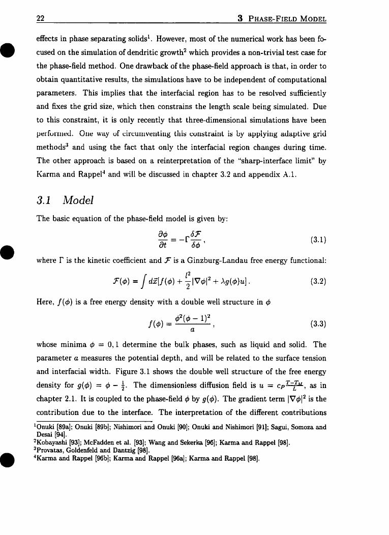
Here, f (4) is a free energy density with a double well structure in #

whose minima 4 = 0,1 determine the bulk phases, such as liquid and solid. The

parameter a measures the potential depth, and will be related to the surface tension

and interfacial width. Figure 3.1 shows the double well structure of the free energy

density for g ( 4 ) = 4 - - T T The dimensionless diffusion field is u = cp- , as in 2 '

chapter 2.1. It is coupled to the phase-field # by g(4). The gradient term IV$12 is the

contri bution due to the interface. The interpretation of the different contributions

l Onuki [aga]; Onuki [89b]; Nishimori and Onuki [go]; Onuki and Nishimoi-î [91]; Sagui, Somoza and Desai [94].

?Kobayashi [93]; Mdadden et al. [93]; Wang and Sekerka [96]; Karma and Rappel [98]. Provatas, Goldenfeld and Dantzig [98j.

'Kama and Rappel [96b]; K-a and Rappel [96a]; Karma and Rappel (981.

--A--- - ----- - .A-

-01 0 0 0 1 I O i I Q I 0 0 O L i O t~ QS a o OS t a I S

Figure 3.1: Double well structure of the free energy density f(#) coupled to g(+) u = (@ - 1 /?)IL.

will becorne more transparent by considering a one-dimensional system at equilibrium

for ,u = O. The equation of motion (3.1) reduces to:

where the s script I d enot es a derivative. The solution is given by the hpperbolic

tangent, which describes the diffuse interfacial region between the two bulk pliases:

Figure 3.2 shows the interfacial profile. The interfacial width, being the range in

which 4 changes from 0.05 to 0.95, can be deduced from equation (3.6) to be

The surface tension, which is defined as the additional free energy per unit area

generated by an interface between the two bulk phases in eqriilibriuni, is given by:

Using equation (3.5) and the fact that f (4 , O) = O in the bulk phases, we obtain:

Hence, parameter 1, togetber with parameter a, determines the surface tension y as

Figure 3.2: Equilibrium interfacial profile.

well as the interfacial t hickness ,W.

The term X g(4)u in equation (3.2) causes a bulk free energy difference between

the two phases, and thus provides a thermodynamic driving force. Depending on

the sign of u, one or the other phase is favored (see figure 3.1). To describe the full

problem of solidification the heat diffusion equation has to be added:

The first part is the diffusion equation as described in chapter 2.1. The second term

on the right side represcritr the interfacial source term with A .- 4' - 4' being related

to the release of latent heat. Substituting equation (3.2) in equation (3.1) results in:

for which different choices of g(4) have been proposed. In order to keep 4 fixed in

the bulk phases, meaning that the latent heat is only released at the inteïhce, g(#)

has to fulfill the following condition:

This can be fulfilled by choosing:

where n is a positive integer. For n = 1, the mode1 proposed by Kobayashi (931 is

recovered. This wili be discussed in chapter 3.3. Models for n = 2 have also been

st udied l .

Wang et ai. 1931; Urnantsev and Roitburd [88].

3.2 Shaxp Interface Limit 25

3.2 Sharp Interface Limit

The connection between the sharp interface formulation of the problem and the phase-

field model is established via the sharp interface limit. In the sharp interface limit the

phase-field model, consisting of a system of two non-linear coupled equations of motion

for the temperature (3.10) and the order parameter (3.11), reduces to the basic model

of solidification (equations (2.1) - (2.3)). The sharp interface limit is obtained by an

asymptotic multiple-scale analysis, also often referred to as matching asymp totics.

Caginalp and Fife (881 and Caginalp [89] showed that the different sliarp interface

models can al1 uise as particular scaling lirnits of the phase-field equations. The

resiilts are surnmarized in table 3.1. To obtain these limits. the phase-field equations

have to be rescaied:

and, 1

f = - D a=-

Lu r 12

where w is a mesoscopic length scale sucli as the diffusion length ln. Omitting the

primes we obtain:

and

We are left with three parameters É, a and A, whose scaling behavior determines

the different results of the sharp interface limit. E is a srnall expansion parameter,

a is related to a rnicroscopic relaxation time, and X is a dimensionless pararneter

that controls the strength of the coupling between the phase and diffusion fields.

Two physical parameters are involved: do, the capillary length. and 13, the kinetic

coefficient.

Caginalp [89] fixed one parameter by requiring that the surface tension y, being a

physical parameter, be independent of the scaling. Dividing equation (3.16) by h we

obtain:

where f = e2/X. The surface tension in the phase-field model was determined by

equation (3.9) to be proportional to the ratio «fi. Hence, the requiremnt of con-

stant surface tension implies: c - = const. , fi

which reduces the number of free parameters to two. With this assumption, the first

three scaling limits in table 3.1 can be derived (Caginalp [89]). In order to use the

phase-field approach for the study of dendritic growth, and other problems involving

the Mullins-Sekerka instability, the convergence of the phase-field approach has to be

studied. This was done by Wheeler, Murray and Schaefer [93], as well as by Wang

and Sekerka [96], who observed that the Iattice spacing Ax had to be chosen very

small cornparcid to the scale of the dendritic pattern. This permits convergence to

a reliable quantitative solution of the sharp interface equations. It turns out that

only the regime of a dirnensionless undercooling of the order of one, in which the

interfacial undercooling <Li is dominated by interfacial kinetics, is computational on a

quantitative level. This constraint is a consequence of the scaling ansatz that 5 -r O,

which implies that the temperature is not allowed to change across the interfacial

thickness. However, the magnitude of a variation of u across the interface scales

as du 5 &ID, since u varies locally on a scale - D1.v in the direction normal

to the interface, where v is the local normal velocity of the interface. Therefore,

neglecting this variation is equivalent to assuming that du < Bu, which yields, using

equat ion (3.19), the constraint : t3 r- d o > - . 13

Since Ax .Y <, the çonstraint implies a very small grid spacing and restricts the system

sizes which can be simulated.

However, considering the phase-field equation as a mathematical tool to solve the

sharp interface limit, one has only to demand that, in the sharp interface limit, the

sharp interface equations have to be recovered. Dropping the constraint (3. El), we are

left with three model parameters and two physical parameters. Karma and Rappel1

realized that using another scaling approach, A can be used as a free parameter, which

can be chosen for computational convenience. In their scaling limit, the interfacial

IKarrna and Rappel [96b]; Karma and Rappel [96a]; Karma and Rappel [98].

3.2 Shwp Interface Limit 27

thickness is small cornpared to the mesoscale of the diffusion field, but it remains finite.

They refer to it as the "thin-interface limit" , since its limit includes corrections for

variation of the temperature field across the interface:

where I , J, and F are integration constants which depend on the precise form

of y (4) and f (4). SIiey are deterniiiied in appeiidix A. 1. Tlie tliiii-i~iterlace liiiiit

is closely related to a limit derived by Caginalp and Fife [88], as will be shown in

appendix -4.1. This allows the constraint on do (3.20) to be lifted, which greatly

enhances corn pu tat ional efficiency, and rnakes t hree-dimensional simulations possible

wit hout adapt ive grid rnethods. However, at very low undercoolings adapt ive grid

methods have to be employed l .

Stefan mode1

classical

modified

alternative

modified A

alternative

modified B

-- --

scaling limit

c + o A, a - fixed

sharp interface limit

- = 0vzu a t

v = D(Vus - Vu') fi

Ui = do^ + ,OU

Table 3.1: Scaling relations between phase-field equation and sharp interface equations.

'Provatas, Goldenfeld and Dantzig [98].

3.3 Dendritic Growth Dendritic growth is the problem for which the phase-field appruach was created. Here

it was first introduced, here different questions of interpretation and thermodynamical

consistency were discussed, as well as its numerical appeal and limitations. Since

some analytical results are available, it is a good system to study al1 the questions

mentioned above. We will present the phase-field model of Kobayashi [93], which

was the first model which reproduced qualitatively distinct features characteristic of

dendritic growth, such as tertiary side arms and the coarsening of side arms away

from the tip. Since then, rnany contributions have been concerned with changing

the mode1 to obtain quantitative results. As the free energy functional, Kobayashi

with an anisotropy in c = t q (8 ) which will result in an anisotropy in the surface

tension. The energy density is:

1 A#, ,u) = i&(# - II* - d4)44 7 (3.23)

where u = (T - T.CI)/(T,t! - Tm) and Irn(u)l < 112, so that together with the choice

the minima of the free energy stay at 4 = O and t$ = 1 as discussed in chapter 3.1.

One possible choice for rn is m(u) = a/aarctan(-yu) with a < 1. To study the

effect of the anisotropy in c we consider a planar interface. For the isothermal case

the solution is:

implying that the width of the interface is proportional to € ( O ) . The surface energy

as defined in equation (3.9) yields:

which motivates the choice of anisotropy. The dynamics of the order parameter is

given by:

3.3 Dendri'tic Growth 29

Figure 3.3: Growth of a dendrite in an undercooled melt for 6-foid anisotropy in two dimensions. From left to right the number of times steps are: Nt = 500, Nt = 1500 and Nt = 4000.

and the equation of diffusion of heat is

wit h

denoting the dimensionless undercooling, which is an important control parameter.

The last term in equation (3.27) describes a noise with strength a which acts only at

the interface to stimulate side branching. y is a random number uniformly distributed

in the interval [-1, $1. .An example of a dendritic growth simulation is shown in

figure 3.3 for the parameters: q~ = t + dcos(6 O ) where b = 0.04, F = 0.01, r = 0.003,

a = 0.9, y = 10, a = 0.01, A = 0.6, a mesh size of 0.03 and system size iV, = iVY =

300. We start with a small solid disk at the center of the system. At the beginning

of the simulations, the system is at the undercooling temperature u = -1. Because

of the boundary conditions used, the whole liquid will transform to a crystal for 4

greater than 1. If A is less that 1, a fraction A of the whole region will solidify and

the system will lose al1 its supercooling.

3.4 Criticism

The basic mode1 of solidification is a minimal rnodel. It only considers the thermal

aspect of the phase transition, namely, the release of latent heat at the solidification

front and its diffusion into the solid and liquid phase. Due to non-linearities, which

corne into play via the curvature r;, and the normal vector fi, the mathematical

problem is non-trivial and many interesting, complex patterns evolve, as c m be seen

in dendritic growth. Nevertheless, it is a crude simplification, which does not include

Row in the liquid pliase, nor does it include elastic effects in the solid phase. Indeed,

the main distinction between a solid and a liquid is the sliear modulus. Solids support

shear. implying that their shear rnodulus is finite, whereas the shear modulus of a

iiquid is zero, implying that they do not support shear. One rnight expect that the

basic model of solidification should capture this main distinction. However, it does

not. The same criticism applies to the phase-field model. Here, although rooted in

the continuum description of phase transition, indicatiiig that tlie phase 4 is an order

parameter, 6 does not have any physical content. It is merely a label to distinguish

O the solid from the liquid phase.

Below. we will propose a solidification model in which the order parameter is

proportional to the shear modulus. Hence, it captures the main difference between

tlie solid and liquid phase. That is, the shear modulus of the liquid phase will vaiiish,

whereas the shear modulus of the solid will be finite. Thus, the phase-field obtains a

physical meaning in the context of liquid-solid phase transition.

Apart from the morphological instability discussed in the last two chapters, the first-

order phase transition shows other interesting dynamical properties which involve

such phenomena as nucleation, spinodal decomposition, late stage growth, and coars-

ening. In the classical theory of first-order phase transitions, one distinguishes be-

tween two different types of instabilities which characterize the early stages of phase

separation. The first is an instability against finite amplitude perturbations in which

localized (droplet-like) fluctuations lead to the initial decay of a metastable state. The

rate of birth of such droplets is described by homogeneous nucleation theory. The

second is an instability against infinitesinial amplitude perturbations, non-localized

(long wavelength) fluctuations which lead to the initial decay of an unstable state.

This latter instability is termed spinodal decomposition. It should be noted that this

sharp distinction between met astable and unstable states, put forward by the classical

theory of first-order phase transitions, is not supported by modern field theoretical

approaches. We now review the long wavelength instability observed in systems un-

dergoing spinodal decomposition, and in the late-stage growth and coarsening regime

as it is needed for the further discussion in chapter 6. We follow here the reviews by

Gunton, San Miguel and Sahni [83] and Bray [94].

4.1 Linear Theory

The starting point for the analysis of the early stages of spinodd decomposition is

the Cahn-Hillard equation (1.9), or mode1 B without noise:

Cahn linearized this non-linear equation about the averaged concentration to ob-

tain: am(F, t )

dt (4.2)

w heïe

m(F) = $(F) - do .

The Fourier transform of equation (4.2) yields:

where m(k) is the Fourier transform of m(7) and

Thus, iriside the spinodal regime, where 02//&$ < O , w ( k ) is negative for k < kc, where

c = - 12 1 - a;;

Hence. long wavelengths grow erponentially

The quantity of experirnental interest is the structure function ~ ( k , t ) =< l2 >. which is proportional to the small angle, diffuse scattering intensity. Linear theory

t herefore predicts

~ ( k , t ) = s(& O ) e-2"ck)t . (4.8)

This implies an exponential growth in the scattering intensity for k < kc, with a peak

at a tirnôindependent wave number km = k , / f i . The behavior predicted by the

linear theory, equation (4.8), is usually not observed in Monte-Carlo studies nor in

experimental studies of alloys and fluids. However, Binder [84] studied the effect of

a long-range force on the dynamics of first order phase transitions and found that

the time regime in which the linear theory of spinodd decomposition holds increases

logarithmically with the range of interaction. This prediction can be confirmed by

numerically simulation of the Cahn-Hillard-Cook equation. See, for example, Laradji,

4.2 Non-linear Theory: Eariy Stage 33

Grant and Zuckermann [go] and references therein. They studied the effect of long-

range interactions on the dynamics on first order transitions in two dimensional Ising

models via Monte-Carlo simulations with Glauber1 (spin-flip) and Kawasaki2 (spin-

exchange) dynamics. They observed in both cases an agreement with the linear theory

at early times.

4.2 Non-linear Theory: Early Stage

Although the linear theory predicts correctly the long wavelength instability, it is

clear frorn its prediction of exponential growth of the fluctuations that it will be

wlid at rnost at very early times. However, it cannot account for non-linear effects

such as coarsening, which stabilizes the system before it finally reaches its two-phase

equilibriurn. Many attempts have been made to incorporate non-linear effects into a

theory of spinodal decomposition. The starting point is the dynamical equation of

the correlation Function of model B. üsing equation (1.2) we obtain:

which is forrnally exact. However, < Q(7, t ) 447, t ) > is coupled to < d3(F', t ) #(& t ) > iniplying that equation (4.9) is the first of a hierarchy of coupled equations of mo-

tion. This is a common problem in many-body physics, however with the difference

here that one is dealing with two-phase phenomena, far-frorn equilibrium. Hence, the

standard techniques, such as factorizing the non-linear term by a single peaked Gaus-

siari approximation. are difficult to justify. However, coarsening does result frorn the

Gaussian approximation done by Langer. The Fourier transform of equation (4.9) is

The first higher order structure factor in the Gaussian approximation is given by:

'king mode1 with Glauber dynamics is a rnicroscopic formulation of model A. 'Ising model with Kawasaki dynamics is a rnicroscopic formulation of model B.

wit h 1 < s 2 ( t ) >= - 1 d k ~ ( k , t ) .

P*I3 Hence, the equation of motion for the structure factor is given by:

with

As a consequence, the characteristic wave number kc now decreases with timq since

< s2( t ) > is a positive, increasing function of tirne. The most important result of this

approximation, however, is a qualitative explanation of coarsening.

Langer, Bar-on and Miller [75] suggested a physical approximation which is based

on the assumption that the spatial dependence of the higher-order correlation func-

tions is the same as that of the two-point correlation function S(7, t ) . This leads

< s"( t ) > Sn(" t ) = < s 2 ( t ) , s(r, t ) . (4.15)

O This approximation seems reasonable for large length scales, but is less accurate for

short length scales. Its biggest drawback lies in the fact that it is an uncontrolled

approximation. 'Jsing this approximation in the dynamical equation of the structure

factor with

~ ( k , t ) can be obtained numerically. For a critical quench, the theory is in qualitative

agreement with Monte Car10 and experimental studies. It shows a "crossing of the

tails" of the structure factor for different times which bas been observed in numerical

and experimental studies of phase separation.

Grant et al. [851 have developed a systematic perturbation theory for the early

stages of spinodal decomposition for a system with long range interaction in which

the small parameter of the theory is proportional to the inverse of the range of the

force. The first order perturbative correction acts to substantially slow down the

evolution predicted by the linear theory and shifts the effective critical wave number

with time to srnall wave nurnbers which implies coarsening. The "crossing of tails"

4.3 Non-1inea.r Theory: Late Stage 35

of the structure factor is also O bserved. However , perturbation calculations were

performed to order c2, in which the probability distribution function corresponded to

a time-dependent Gaussian form, not to a bimodal one.

4.3 Non-linear Theory: Late Stage

Whereas the early stage is characterized by the formation of interfaces, separating

regions of space where the systern approaches one of the final coexisting states, the

late stages are dorrii~iated by the riiotiori of chese interfaces as the system acts to

minimize its surface free energy. During this time, the size of the domains grow,

while the total amount of interface decreases.

Much of the theoretical framework for understariding the dynamics of phase s e p

aration has arisen from of the pioneering work of Lifshitz and Slyosov, and Wagner,

hereafter called LSW-theory. I t describes the asymptotic ( t -t m) growth of droplets

of a rninority phase of small volume fraction in a slightly supersaturated phase of a

soiid solution. They calculated analytically the asymptotic behavior of the droplet

distribution function, f (R, t ) , where R denotes the radius of a given droplet of the

minority phase. In particular. the. showed that the average droplet size obeys the

growth law:

They also derived

showed dynamical

where

and,

jj Pd p . (4 .17 )

an expression for the droplet distribution function f (R, t) which

scaling namely,

R f(R? t ) = t a d f 5 ) y (4.18)

The physical mechanism behind the coarsening process is that larger droplets grow at

the expense of smaller droplets by evaporation-condensation. Particles of the minority

phase diffuse through the majority phase from smaller droplets that are dissolving,

to larger droplets that are growing. This late stage growth is called Ostwald ripening

and is characteristic for the dynamics of systems with conserved order parameters.

A. Scaling approach to late-stage coarsening

Yuch progress in understanding the late stage growth regime is based on a dynamical

scaling hypothesisi which states that , a t late tirnes, there exists a single characteristic

length scale L( t ) such that the domain structure is (in a statistical sense) independent

of time when lengths are scaled by L ( t ) . Hence, the evolution of the system in the

late stage regime is self-similar. The hypothesis is supported by many experirnental

studies of, for example, binary alloys, binary fluids, and polymer blends. It is also

supported by the LSW-thcory, as acll as by numericol aork.

.An important quantity to characterize the domain structure is the equal time pair

correlat ion function:

C(7, t ) =< #(% + ?, t ) @(Z, t ) > , (-4.21)

and its Fourier transform, the equal time structure factor:

where the angular brackets indicate an average over initial condition. Experirnentally.

the evolution of the structure factor can be rnonitored using srnall angle scattering of

X-rqs or neutrons, whereas the evolution of the correlation function can be obtained

by microscop. The existence of a. single characteristic length scale, implies that the

pair correlation function and the structure factor have, after some transient time to,

the following scaling form:

with

Hence, the Fourier transform sat isfies

with

where d is the spatial dimension, and g(y) is the Fourier transform of /(x). It should

be noted t bat, various choices for the definition of this lengt h exists. For example, one

'It should be noted that scaling has not been proven, except in some simple rnodels and the LSW- t heory.

4.3 Non-linear Theory: La te Stage 37

could define L(t ) as p;l, the first moment of S(q, t ) , as well as qil, the peak position

of S(q, t ) . Man] attempts have been made to predict the scaling forms f (x) and g ( y )

as well as the dynarnical behavior of L( t ) . The determination of the growtli law for

L( t ) has been done by examining interface dynarnics of phase-ordering systems. The

determination of the scaling forms f (x) and g ( y ) turns out to be very challenging. .4

number of approximate scaling functions for non-conserved fields have been proposed.

None of them seem to be completely satisfactory. For conserved fields the theory is

even less well understood.

B. Interface Dynamics

The interface dynarnics approach has been used to analyze late stage phenomena

and to obtain growth laws for L ( t ) . Depending on whether the order parameter is

conserved or not, the growth meclianisms are qui te different . The interfacial mot ion

for the different cases can be studied using the field theoretical description discussed

in chapter 1.1. An order-disorder transition, in which the order parameter is not

conserved, can be described by the Allen-Cahn equation (1.4) or mode1 .-\ without

noise. .As sliown in appendix A.1' the interface dynamics yields:

where v is the velocity of the interface (normal to itself) and K, is the curvature.

Hence, the growtli of a non-conserved field during coarsening proceeds through an

independent motion of the interface driven by curvature forces. From this Allen-

Cahn result we obtain an equation for a characteristic s a l e L( t ) :

which yields the growth law:

In the presence of a conservation law the motion of the interface is slower, and

a coupling between the bulk phases and the interface exists. Numerical studies and

'There. the more cornplex case is discussed. However, if one sets the temperature u to zero, mode1

A is obtained.

analytical investigations1 have shown that in the symmetrical as well as highly asym-

metric quenches the late stage grows is described by:

L ( t ) - t1i3 ,

which generalizes the result by the LSW-t heory.

'Bray [94].

Elastic effects can strongly influence the morphology of materials and consequently

influence material properties. Their effect on phase transformation has been studied

intensively by rnetallurgists (Khachaturyan [83]). The micro-structure of even simple

binary alloys involves an intricate system of domains of distinct compositions, sep-

arated by phase and grain boundaries. Includecl are defects such as impurities and

vacancies. as well as dislocations. Each of these components influences the elastic

state of the solid. Work by Cahn and Larchél has been dedicated to the study of

the thermodynamics of multi-phase solids under stress. A good introduction to the

thermodynamics of inhornogeneous solids, in the presence of stress, has been given by

Nozières [92]. More recently. the influence of elast ici ty on phase-separating alloys has

been studied2. Elast icity always provides a positive energy contribut ion. Thiis, solids

try to release their elastic energy in the process of energy rninirnization. There are

different ways for solids to release that elastic energ- One is by plastic deformation.

which involves dislocations, the other is by elastic deformation, which is commonly

seen in thin-film grorth. A non-hydrostatically, Le. uni-auially, strained solid, which

is in contact with its own melt or vapor, can release its elastic energy by a morpho-

logical instability a t the interface. This strain release mechanism was first predicted

by Asaro and Tiller [72]. They performed a linear stability analysis, and obtained a

dispersion relation which showed a long-wavelength instability. The instability was

driven by elastic stress, and stabilized by surface tension at short wavelengths. As

background for our investigation, we now int roduce the basic quantities and concepts

of elasticity3 which are needed for the study of the Grinfeld instability. Since the

LLarché and Cahn [78); Larché and Cahn [85]; Cahn [89]. 'Sagui, Somoza and Desai [94]; Onuki [89b]; Léonard and Desai [97]. 3Landau and Lifshitz [83].

39

Grinfeld instability is a long length scale effect, a continuum description is appropri-

ate.

5.1 Basic quantities and concepts of elasticity

In contrast to liquids, solids sustain shear, which implies that solids respond to an

external force with a deformation. The external force can either act on the whole

volume, such as

is characterized

in the case of gravity, or on tlie surface of the solid. The deformation

by a strain:

with ui being the displacements of the atoms from a reference state, which can be a

stress-free or pre-stressed state.

The most fundamental condition of elasticity is the mechanical equilibn'urn con-

dition. which states that, at equilibrium, al1 forces per unit volume in the solid, f i t

vanish: -

where oij is the stress tensor and f: are external body forces. A summation convention

over repeated indices is implicit. Solving this system of partial differential equations

for appropriate boundary conditions, which are either given in terms of externally

applied surface forces F,, or in terms of displacernents. determines tlie stress state of

the solid.

The deformation of the solid is then determined using Hooke's law, which describes

the linear relationship between the stress oij and the strain uij:

where h&l is a tensor of rank four, whose components are elastic constants. In the

case of an isotropie solid, Kijkl reduces to a tensor with oniy two components, so that

Hooke's law can be written as:

5.2 Stress relief mechanism 41

where n is the bulk rnodulus, which accounts for volume changes, p is the shear

modulus, which accounts for shape changes without volume changes, and d is the

dimension of space. Hooke's law can also be expressed in the following forrn:

where E is the

choice of these

Young's modulus, and v is the Poisson ratio. The

coefficients is based on considering homogeneous

rclation bctwccn both sets of cocfficicnts is givcn by:

and

motivation for the

deformation, The

Depending on the particular problem, one or the other formulation is more appropri-

ate.

Often it is more convenient to express the mechanical equilibrium condition (5.2)

in terms of displacements. This can be achieved using Hooke's law:

which is known as the Lamé equation. As will be seen in appendix h.2, equation (5.8)

can be solved in a straightforward way t'or two-dimensional systems. In many cases

an elastic problem can be posed by assuming that the displacement field in the y-

dimension vanishes, and that the displacement fields in the remaining two directions

do not dependent on y. This implies that u, = u, = ul, = 0, and reduces the

three-dimensional problem to a two-dimensional one. It is called the plane strain

case.

5.2 Stress relief mechanism

To understand the physical mechanism for the stress-driven morphological instabil-

ity, we consider an uni-axially and uniformly stressed semi-infinite solid as shown

in figure 5.1. If the surface is Bat, the solid will be strained unifomly. Then the

elastic energy density, being proportional to the product of strain and stress, will

also be uniform and always positive, since the applied stress and the resultant strain

always have the same sign. If, however, the surface is perturbed, the applied stress

results in a non-uniform stress distribution throughout the solid. Independent of

the sign of the applied stress, stress relavation occurs a t the peakç which are less

constrained, whereas a high stress concentration is observed in the valleys which are

more constrained. The resulting stress gradient along the surface drives a mass flow

from the valleys to the peaks. Thus, valleys will grow deeper and increase the stress

gradient even more. This positive feedback will sustain the mass flow and drive the

instability. However, the instability is balanced by the surface tension which tries to

rninimize the surface area. The cornpetition between the destabilizing effect due to

the stress relief mechanism, and the stabilizing effect due to surface tension, is char-

acterized by a dispersion relation which can be obtained by a linear stability analysis.

Like the Mullins-Sekerka instability, where during solidification the temperature can

overcome the surface free energy and destabilize a planar solidification front at long

wavelengths, a stress in a solid is capable of destabilizing an othenvise flat surface üt

long wavelengths. Before continuing with a quantitative approach, we would like to

rniphiÿize that the buekling of the surface is due to the Bet that surface corrugation

reduces the stored elastic energy. It should not be confused with the bending of a

solid when one applies a longitutional stress to a thin rod.

Nozières [92] explains the above-described stress relief mechanism in more quanti-

tative terms. Consider a two dimensional, uni-auially stressed solid where

and = zz -Pi . (5.11)

The solid is in contact with its liquid phase at a planar interface along r = O and

pressure pi. Figure 5.1 shows a sketch of the set-up. The two phases have equal

enthalpies per unit m a s , so 9 f + ~ l - = -

7

P P where f is the free energy per unit volume and p the mass density. We assume now

that the solid grows locally, so that the interface gets displaced by an amount h(z) =

5.2 Stress relief mecbanism 43

't 1 P b Figure 5.1: Sketch of Grinfeld instability.A stress a0 is applied

+ to the edges of a semi-infinite, x isotropic solid which is in free

contact with its own melt or va- d por at pressure p.

C-

ha cos qx. If we ignore capillarity, the total enthalpy is unchanged as long as the

grocvt h occurs at constant stress 0,. However, the mechanical matching conditions

at the interface are violated. To first order, a shear component appears:

where ni and t j are components of the normal and tangential vector on the interface.

To maintain mechanical equilibriurn, ail extra tangential force has to be applied to

the interface in order to cornpensate for the bulk stress:

(0) dFt = a,, d s , (5.14)

where ds is an infinitesinial surface element. If not, the solid relaxes elastically,

thereby lowering its enthalpy. The change in elastic enthalpy due to an infinitesimal

deformation is r

Using the fact that pi = -0::) ! we expand the stress as:

where Auij is the additional stress due to relaxation. Hence, the change in elastic

enthalpy for a finite deformation is:

where Aoij can be calculated. as poirited out above and see appendlu A.2. Using

Hooke's law, the strains uij are known as well and one obtains:

This is only the elastic contribution to the free enthalpy, which is destabilizing. How-

ever, the contribution due to capillarity wül stabilize the interface a t large q.

44 5 GRINFELD INSTABILITY

5.3 Ex~erimental Evidence . -

There are d'iffereot experirnental systems in which the Grinfeld instability haî been

O bserved and s t udied.

The first quantitative experiment on the equilibrium shape of crystals under non-

hydrostatic stress were performed by Torii and Balibar [92] in 1992 using solid "He in

contact wit h its own melt. "He is often used to study theories of crystd growth, sincc

one can O btain large single crystals, free of grain boundaries and defects. Since it also

grows and melts rapidly, experiments can be performed in a reasonable amount of

time. However, it has the drawback of being difficult to cool without leaks. Torii and

Balibar [92] grew a very pure "He crystal in a g l a s box, in which from one side the

crystal could be strained via a piezoelectric ceramic. This allowed a straining up to

b,, = f 3.2 IO-". The strain was measured using a Fab -Pe ro t interferorneter as was

the height of the interface. Due to the slight difference in the refractive index between

solid and liquid helium, l n = 0.0034, melting or growth, i.e., displacernent of the

interface, produces a phase shift und, hence. a fringe pattern. They first observrd

macroscopic meltiiig. At a critical strain of bu, = Ii . IO-=, grooves appeared with

a critical wavelength of 8mm. Since the onset of the instability w u sudden, and the

disappearance For decreasing strain showed strong hysteresis, the instability was of

first order. The shape of the grooves was independent of the sign of the applied strain,

Le., cusps were always pointing towards the solid. Further, it was observed that the

corrugations vanished with time, irnplying that other relaxation rnechanisms were

present which showed a clear temperature dependence. The typical relaxation time

varied from tenths of seconds a t 1.2K to an hour at O.9K. Additional experiments

on "He liquid-solid interfaces were also performed by Bowley [92].

Polymer crystal

Another interesting quantitative study of the Grinfeld instability was performed by

Berréhar et al. 1921. Their experimental systern is a single-crystal film of polymerized

polydiacetylene, gl-üit ii in epitaxy with a monomer substrate. The polymerization is

initiated by low-energy electrons and induces a uniaxial stress in the polymerized film,

5.3 Experimen tal Evidence 45

which is generated by the difference in the chain parameter between the monomer

and the polyrner. The polymer chains gow along the binary axis 6. The relative

lattice mismatch in the chain direction varies continuously with the polymer content.

Polymer content as well as the film thickness can be controlled by the electron dose

and electron energy, respectively. The thicknesses of the film studied ranged [rom 50

to 500nm. The surface profile was analyzed with an AFM (atomic force microscope).

For films up to l5Onrn the surface was covered with a wavy parallel wrinkle pattern

p~rpendiriilar to the rhain rlirwt,ion h. The surface height variations w r e typically

h m and the spacing X in the range of 150 - 350n.m. The pattern was independent

of the film thickness and the polymer content S for .Y > 10%. For films thicker

than 200n.m, the whole sample surface showed rather regular patterns of long parallel

crackso again perpendicular to the chain direction b, with hirly regular spacings in

the range of a few Pm. The cracks were straight and ran straight tlirough steps,

implying that they were not prefereritially initiated by surface defects. For the crack

depth, a lower limit of lOOnm could be obtained, comparable to the filni thickness.

By comparing the spacing of the wrinkles with the predicted wavelength derived

from the linear stability analysis of the Grinfeld instability, and the time scale of

the appearance of the wrinkle pattern which was consistent with surface diffusion, it

was argued that the wrinkle pattern is due to the Grinfeld instability, and that the

cracking was a secondary instability initiated by the Grinfeld instability, which dso

determines the crack spacing.

Dislocation-free Stranski-Krastanov growth

The Grinfeld instability is also associated with the dislocation-free Stranski-Krastanov

growt h, which describes the island-on-layer growt h mode in epitauy. Typicall- one

distinguishes t hree growth modes in epitâuy:

0 Frank-van der Menve growth (layer-by-layer growth) :

O S transki-Krastanov growth (island-on-layer gowt h) ,

O Volmer- Weber growth (island-growt h) .

Figure 5.2: Different growth modes in epitaxy. Rom left to right: Rank-van der Merwe growth (layer-by-Layer growth) , Stransky-Krastanov growth (island-on-layer growth) , Volmer- Weber growth (idand growth).

Which growth mode will be adopted in a given system will depend on the interfacial

free energy terms and on the lattice mismatch. In lattice matched systems, only the

first two growth modes ran orciir. Whether t . h ~ film wets the substrate (layer-by-layer

grow th) or does not (island-on-layer growth) depends then only on three energies: the

interfacial energies Y,,, the film surface energy y1 and the substrate surface energy y,.

If -jfr + "/I < ̂ (J island growth occurs. Otherwise layer-by-laver growth happens. By

adding a surfactant, yf, + yf can be changed, and island growth can be suppressed.

If film and substrate have different lattice constants, a coherently growing film will

be strained. As the film thickness increases, so does the elastic energy stored within

the film. At some thickness, it beconies energetically favorable to relieve this misfit

strain. This happens eit her elastically by the dislocation-free Stranski-Krastanov

mode or plastically by the formation of dislocations, or both.

For a long tirne it was assumed that dislocations provided the only stress relief

mechanism. However, in 1990, Eaglesham and Cerullo (90) showed that the islands

formed in Stranski-Krastanov growt h of Ge on Si(100) are initially dislocat ion-free.

Since then, many more systerns have been found which show dislocation-free Stranski-

Krastanov growthl. Two examples are shown in figure 5.3 and figure 5.4. In both

cases Ge is grown coherently on Si and shows an undulating surface structure. In

figure 5.3, the surfactant Sb was present. It should be noted that there is some ev-

idence that the dislocation-free Stranski-Krastanov mode is only a transient stage

towards the plastic relaxation. It has been realized that surface morphology plays

an important role in the dislocation nucleation process. As we will see in chapter 6,

inhomogeneities in the surface morphology irnply regions of high stress concentrations

which may provide enough energy to nucleate dislocations. Traditional theories of

stress relaxation via dislocations are based on the above mentioned energy balance

'LeGoues, Copel and Tromp [go]; Guha, Madhukar and Rajkumar [go]; Tersoff and LeGoues [94]; Okada, Westherly and MeComb (971.

5.3 Experimental Evidence 47

Figure 5.3: STbI image of 8 mono-layers Ge on Si(100) deposited at 7 OO°C wit h Sb as a surfactant (Horn von Hoegen [97]).

between elastic energy and surface free energy. They do not include the nucleation

process. The earliest treatment was the continuum theory of Frank and van der Slerwe

for an array of non-interacting dislocation a t the film-substrate interface. Matthews

and Blakeslee [ i d ] assumed pre-existing dislocations in the substrate, which were as-

surned to move into the film once the mean stress caused by the misfit exceeded the

dislocation line tension. However, these approaches do not consider the mechanism

y which the dislocations nucleate. Dong et al. [98] performed a two-dimensional

molecular dynamics simulation in which they studied the temporal evolution of the

surface morphology and the mechanisms for misfit dislocation nucleation and stress

relaxation. Their results show t hat the critical t hickness depends sensit ively on the

film morphology. Tersoff and LeGoues [94] indicated, by calculating the nucleation

rate of dislocations, that strain-induced surface "roughening" is the dominant mech-

anism for the introduction of dislocations in strained layers at high misfit. It is there-

fore important to study the pre-dislocation morphological changes, t hough ultimately

dislocations must be included for complete understanding.

Figure 5.4: TEM micrograph of a section of Ge g o w n on Si(1001. The 8 mono-layers of Ge on Si are pseudomorphic, i.e. have the sarne lattice-spacing (LeGoues, Copel and Tromp [go]).

5.4 Traditional Approach

The Grinfeld instability has been studied t heoretically quite intensively in the last

decade. There have been basically two approaches. The first uses a variational prin-

ciple, in which the the analysis of the second variation determines whether the systern

under consideration is stable or unstable. Grinfeldl used this approach to study vari-

ous configurations. However, these thermodynamic energy minimization calculat ions

are static and do not pennit a description of the evolution of the instability, nor can

they describe the morphology and stability of a growing film. The other approach

being used by Asaro and Tiller [72], Srolovitz (891, Spencer, Voorhees and Davis [91],

Spencer, Voorhees and Davis (931, Spencer. Davis and Voorhees [93], Spencer and

Meiron [94], Grilhé [93], Yang and Srolovitz [93] and Kassner and Misbah [94] is

based on a dynamical continuum model, in which rnass transport mechanisms, such

as condensation-evaporation or surface diffusion, are driven by the chemical potential

or the gradient of the chemical potential which comprises surface free energy as well

as elastic energy. We will present here the second approach, which is at the same t h e

the sharginterface formulation of the problem. It can be related to our phase-field

formulation, as will be seen later.

It has been seen in the experimental set-ups described above that the solid can

be strained uni-auially in different ways. In the experiment by Torii and Balibar

[92] a He4 crystal was strained by applying an extemal force at the edges of the

sample. In the case of epitaxial strained films, the film is attached coherently to the

'Grinfeld [82]; Gnnfeld [86]; Grinfeld 1891.

substrate. The difference between the lattice constant of the film a, and the substrate

a, generated a lattice mismatch e = and strained the film. If the lattice constant

of the film is greater than that of the substrate, e > 0, the film is compressed in the

horizontal directions in order to match with the substrate.

To be more precise, let us consider the set-up shown in figure 5.5. -4 stress or, = 00 is

applied to the vertiral sides of a semi-infinit,~, isotropie solid which is in free contact

with its own melt or vapor in ;-direction, constrained in x-direction and infinite in y-

direct ion. Initially the surface lies along r = O. In addition, the system is assumed to

be isothermal and the pressure of the vapor or melt is assumed to be small cornpared

to stress in the solid. The solid responds to the applied stress through a deformation.

which can easily be determined if the surface of the solid is Bat. Since the solid is

constrained in the z-direction, it is convenient to use a reference frame for which

u, = O in the stressed state. Hooke's law is then given by:

where e is the strain of the reference frame. Due to that choice:

Since the surface is flat, the boundary condition (5.24) reads:

u; however will be uniformly strained due to Poisson relaxation:

This can be seen by replacing equation (5.20) and equation (5.21) in Hooke's law

(5.19). Hence,

stress field will

the mechanical

the stressed state is uniform. However, if the surface is not flat, the

not be uniform. To determine the stress state then, one has to solve

equilibrium condition (5.2) :

Figure 5.5: Sketch of Grinfeld instability. A stress a0 is applied to the edges of a semi-infinite, isotropic solid which is in free contact with its own melt or vapor.

wit h the appropriate boundary condition at the surface:

on the surface r = h ( 4 , where nj is the normal vector to the surface pointing towards

the liquid or vapor. The ot her boundary conditions a t z -t -oo are:

and,

With equation (5.23) and boundary conditions ( L N ) , (5.45) and ( 5 . 2 6 ) , the stress

state of the solid for a given configuration of the free surface r = h ( x ) is defined. The

equation is solved in appendix A.2. Knowing the stress state at the surface of the

film, the chemical potential dong the surface can be calculated:

where po is the chemical potential for the Bat interface, y is the surface tension, SI is

an atomic volume, and rc, the curvature:

Since a,,., = a., = O are zero along the surface due to the niechanical equilibrium

condition (XM), the only non-zero stress contribution at the interface is Ott:

Essent ial for the development of the instability is mass transport, through which

the solid can reach its equilibrium state. There are mainly two mass transport mech-

anisms: evaporation-condensation, or melting-freezing, and surface diffusion. In the

case of evaporation-condensation the mass transport occurs through an attachment-

detachment process at the front. We assume that the system is above the roughening

transition, without facets, so that the attachment kinetics are fast. This implies that

the growth velocity of the surface W. (normal to itself) is proportional to the difference

in the chemical potential between the solid and liquid:

un = -r (p' - /L') (5.30)

where r is a kinetic coefficient. Since we assumed that the plan= solid is in equilib-

riurn with the liquid phase, and

small, we obtain

Hence, equation (5.30) yields:

or in terms of the surface profile

ah rn

further assumed that the liquid pressure pl is very

II the transport mechanism is surface diffusion, the total amount of material is con-

served : 7

un = -Vs.Is (5.34)

where V, is the Laplace-Beltrani operator, which ensures that diffusion occurs only

dong the surface, and T' is the material current at the surface which is proportional

to the gradient in the chemical potential of the solid:

7 3s = -DV~/L' , (5.35)

where D = D,R iS/keT, Ds is the surface diffusivity, 6 is the number of atoms per

unit area, and kBT is the thermal energy. The equation of motion for the interface

becomes:

un = D vfPs, (5.36)

and in terms of the surface profile h(x) :

52 5 GRINFELD INSTABILITY

B. Linear Stability Analyses

Linear stability analyris characterizes the instability To do so, we study the dynarnics

of a small amplitude sinusoidal surface profile,

h ( x ) = ho sin qx , (5.38)

which implies that the stress field in the film is no longer uniform. To calculate

the equation of motion of the interface, the stress state at the interface has to be

knorvn. This can bc achicred by solving the mechanical equilibriurn condition witli

the boundary conditions (5.24) and (5.25). The algebra is done in appendix A.2. The

stress in the infinitely thick solid is given by

and

This shows that the perturbation of the uniform stress field due to the sinusoidal

surface profile decays exponentially into the film (z < O ) with a decay length pro-

@ partional to the wavelength of the surface profile. At the surface only the tangentid

stress component au is non-zero. To lowest order in qho it is given by:

The first terni is a zeroth-order contribution which accoirnts for the fact that stress

increases the chemical potential, and rnelts even a planar front. This term should be

subtracted froni the chemical potential in equation (5.39). The second term is the

first order term which shows that the stress in the peaks is the lowest, whereas in the

valleys it is the highest.

Replacing equation (5.42) in the linearized equation of motion for the surface, in the

case of evaporation-condensat ion, results in

and in the case of surface diffusion,

Figure 5.6: Dispclrsion relations for Grinf~ld instahility for emporation-condenstion on the left and for surface diffusion on the right. q, is the critical wave number. Perturbations with q < qc are unstable, whereas perturbations with q > q, are stabilized by surface tension.

These linearized equations c m be solved by:

h(t) = ho exp (ut) , (5.45)

where w describes the normal-mode growth rate, which is determined by a dispersion

relation. In the case of evaporation-condensation. or melting-heezing, we obtain

and in the case of surface diffusion,

Figure 5.6 shows the dispersion relation for both cases. In both cases, modes q > q,

are stable. whereas modes q < q, are linearly unstable to small perturbations of the

surface. The neutral or critical wave nurnber is in both cases given by:

As can be seen From the sign in both equations, the elastic field destabilizes the surface

at long wavelength, whereas surface tension stabilizes short wavelength perturbations.

Therefore, the stress-induced morphological instability is also a long-wavelength in-

stability. Note that the dispersion relation passes through the ongin, meaning that

the Rat interface is marginally stable to linear order.

C. Summarv of other Results

-

Spencer, Voorhees and Davis [93] extended the linear stability analyses to a three-

dimensional epitaxially st rained film with surface diffusion. They included the sub-

strate as well as an external flux. For the static film they observed that the neutral

wave nurnber p, was a function of the film thickness, do, and the stiffness ratio = 5, and py being the shear modulus of the film and substrate, respectively. e = 1 r e p

resents the case where film and substrate have the same shear moduli, and hence

are not distinguishable elastically. In t his case, the system is equivalent to the semi-

infinite solid discussed above. For e > 1 the substrate is softer than the film. The

neutral wave nurnber q, starts off larger than for a semi-infinite solid. decreases with

increasing film thickness, and finally approaches the semi-infini te neut r d wave rium-

ber curve. For O < g < 1, the substrate is stiffer than the Film, and reduces the range

of unstable modes compared to the semi-infinite solid. With increasing film thickness,

the critical wave number increases and finally also approaches the semi-infinite solid

curve. For a rigid substrate with g = 0. the stabilizing effect of the substrate is so

prunounced that the instability is cornpletely suppressed for film thicknesses less than

a critical value. The effect of a constant deposition of particles on the film results in

a growth rate change with time. since the growth rate depends on the film thickness

as discussed above. Thus, there is no simple way of rneasuring the stability. However,

since both the perturbation and the film are growing, the growth of the perturbation

is only observable if the perturbation growth is faster than the rate at which the film v thickens. The cornpetition is quantified by a relative growth rate R = d(d) - =.

Since the growth rate w is extremely sensitive to temperature, due to the temperature

dependence of the surface diffusivity, low temperatures can suppress the instability.

By erploiting the long-wave nature of the instability Spencer, Davis and Voorhees

(931 derived a non-linear evolution equation for the film surface of an epitaxially

strained film on a rigid substrate (Q = O), in the absence of particle deposition. -4s

discussed above, linear stability analysis shows that for a rigid substrate there is a

critical thickness d, below which the film is stable, and that with increasing film

thickness the range of unstable wave numbers extends from zero. Hence, in the vicin-

ity of this critical thickness the unstable wave numbers are near zero. Introdueing

the film thickness d as the characteristic length scale, they assume that the length

scale in the lateral directions X is much larger, so that (Y = d/X CC 1 is a small

parameter. Hence, the displacement fields as well as the Lamé equation (5.8) can

be expanded in a, and solved to lowest order. They obtain a non-linear evolution

equation for the surface and examine its two-dimensional steady states. They find

sub-critical spatially periodic finite-amplitude rounded-cusp steady solutions, as well

as near-critical spatially periodic small-amplitude steady state solutions. However,

t hc stability analysis they performed shosed that al1 these solutions are unstable.

The absence of stable two-dimensional steady states leaves the eventual fate of the

evolution of the instability unresolved. To gain insight into whether additional steady

solution branches exist, or a type of coarsening occurs, they studied the time depen-

dent behavior of their long-wave evolution equation. However, the equation breaks

down before any of these issues are resolved.

By calculating the chernical potential of an uni-auially stressed, semi-infinite solid,

and incorporating higher-order terms iri the interfacial height h, Nozières [93] deter-

mined the instability to be first order (sub-criticnl). He also showed that the interface

flattens on the liquid side and develops grooves on the solid side. He also found that

gravity acts as a stabilizi~ig influence.

Spencer and Meiron [94] studied numerically the non-linear evolution of the stress-

driven morphological instability on the surface of a two-dimensional semi-infinite

solid as a function of amplitude and wave number. They found that the solution

branch of the steady states terminates with a cusp singularity which is numerically

not accessible. At small amplitudes, the steady state solution had a sinusoidal shape,

whereas a t larger amplitudes the peaks were broader and the valleys sharper. They

also studied the time dependent evolution of different small sinusoidal perturbation

which also evolved to cusp singularities.

Another numerical study was performed by Yang and Srolovitz [93]. They used

boundary integral equation rnethods to solve the elastic equations, and integrated the

sharp interface equation for the case of surface diffusion. They obserwd deep crack-

like grooves appearing, in which the growth rate for the gooves rapidly accelerated,

and the time dependence of the groove depth became faster than exponential. They

argued their observations were related to fracture. -

D. Discussion

Experirnents as well as simulations indicate that the Grinfeld instability might be

transient and will ul timately lead eit her to fracture and/or to dislocation nucleation.

By that stage the sharpinterface approach must have broken down since the problem

con no longer be descnbed by considering surface tension and linear elastic strain

only. However, nuinerirai simulationsL encounter numerical instabilities already at

much earlier tirnes. Also three-dimensional simulations have proven impractically

large using the sharp-interface equations.

The phase-field approach on the other hand is very robust against numerical insta-

bilities. Also. since non-linearities are inherent in the description numerical simula-

tions in two and three dimensions can easily be perfornied. Furthermore, the phase-

field approach can easily be extended by coupling additional fields to the phase-field.

Hençc the nucleation of dislocations can be included by coupling a dislocation density

field to the phase-field. Thus the formulation of the Grinfeld instability based on a

Ginzburg-Landau approach is the first step towards a eornplete description of stress

relaxation rnechanisms in evolving structures.

6 MODEL OF SURFACE INSTABILITIES INDUCED BY STRESS

We propose a new model to describe the Grinfeld instability which is based on a

Ginzburg-Landau approach'. .As discussed in chapter 3, the phase-field approach

is a convenient way to simulate free-boundary or moving-boundary type problems.

Since it has been employed successfully to study the Mullins-Sekerka instability, it

seems also an appropriate formulation to study the Grinfeld instability. In the con-

text of elasticity, it was first introduced by Nishimori2 to analyze elastic effects in

phase-separating alloys by coupling the elastic field to model B. In that scheme, the

elastic strain is a subsidiary tensor which can be eliminated by assuming mechanical

eyuilibrium. Thus it yielded a closed descriptiori for the equation of motion of the

concentration. Sagui, Somoza and Desai [94] applied this formalism to model C, cou-

pling the elastic field to both the concentration and the order parameter, in order to

study the effect of an elastic field on an order-disorder transition. The approach has

also been used by Aguenaou. Müller and Grant 1981 to study quasiciendritic growth

due to elastic fields.

We modify that approach by coupling the elastic field to a non-conserved scalar

order parameter field q5(fl which determines whether one is in a hard solid phase

which supports shear, or in a soft disordered phase, hereafter called the liquid phase,

which does not. The position of the interface coincides with the rapid variation of this

field. Coupled to the order parameter is the elastic strain u, which is a subsidiary

tensor. The coarse-gained Ginzburg-Landau free energy is:

where uij is the strain and ui is the displacement field.

'Müller and Grant [98]. 'Onuki [89a]; Onuki [89b]; Onuki and Nishimori [91]; Nishimori and Onuki [SOI.

57

Figure 6.2: Sketch of thrw-well potential, 3 = O is the liquid and 3 = f 1 is the solid phase. There is no difference between the two solid phases. On the left solid and liquid are at coexistence, on the right the solid is meta-stabte and will eventually melt.

The dimensionless bulk free energy density f (9, uij) is given by:

cvhere the first part describes a three-well potential with C#I = O being the liquid and

cp = *l the solid phase, ensuring that the liquid-solid phase transition is first order.

The potential depths a together with the parameter 1 fixes the interfacial thickness.

The second terrn shifts the energy, so that, for constant elastic coefficients, solid and

liquicl are at coexistence. The coupling constant is related to the externally applied

stress. The trace of the strain tensor is V 4, and f e i ($ ,u i j ) is the isotropie elastic

free energy for a d-dimensional systemL :

where rc is the bulk modulus and p the shear modulus which is # dependent:

The convenient choice

guarantees that both bulk phases keep their equilibrium values at 4 = O (liquid) and

# = f 1 (solid). By construction, the shear modulus in the soft liquid phase is zero,

whereas it stays non-zero and constant in the hard solid phase. Since the solid phase

'Landau and Lihhitz [83].

supports shear, whereas the liquid phase does not, our phase-field order parameter

has a transparent meaning in the context of liquid-solid transition.

Since elastic forces propagate with the speed of sound, it is reasonable to suppose

that the elastic field relaxes much faster than 4. Thus, the elastic field can be solved

in terms of the order parameter using the condition of mechanical equilibrium:

The stress

Note, that

tensor ai, is then given by:

aF O ~ J = - au, = (ag(4) +nVeC)& +2/-liq(4)

the first term on the right hand side corresponds to a pre-strained refer-

ence frame and is proportional to the erternally opplied stress. The solution of the

mechanical equilibrium condition. to first order in the shear modulus, is:

and

where

vZG(7, ?) = 6(rf ?)

and

Equation (6.8) justifies the coupling terni in equation (6.2), since in the absence of

external strain, that is -4, = 0, the solid will be stressed whereas the liquid is stress-

free. For a Bat surface, i.e., q5 = #(z) being a function of z only, the solution of

equation (6.8) in two dimension is:

Hence, the solid will be uni-auially strained, as discussed in chapter 5.4, with r)o

) deterrnining the çtrength. The stress c m be determined using Hooke's law (6.7):

Hence O,, determines the stress which is externally applied.

The elastic field can now be expressed in terms of the order parameter. Substituting

the sttrain from eqiiaiinn (6.8) anri equation (6.9) in equation (6.3) leaveç the total

free energy to first order in p as function of 4 only:

The long-range character of the elustic field appears now in the non-local Green's

functiori in 4. One çhould also note that qo enters quadratically in the free energy,

irnplying that compressive as well as tensile stresses contribute equally to the energy

Assuming that the dynairiics of 4 is relaxational. the equation of motion is given by:

84 - = -y- = at

(6. L 7) a

where the index Q nieans differentiation by 4. is the mobility and

Rescaling lengt h and time scales:

and,

where w is a characteristic length scale such as the wavelength of the perturbation,

rescales the parameters to:

and,

6.1 Sharp Interface Limit 61

Omitting the primes we obtain as equation of motion:

with three parameters (?, É, c) , giving the mobility, capillarity, and shear strength,

respec tively.

6.1 Sharp Interface Limit

It has been argued in chapter 3 that the sharp interface equations and the phase-

field formulation are equivalent if, in the sharp- or thin-interface limit, the phase-field

equations converge to the sharpinterface equations. To obtain the sharp-interface

lirnit, we will not integrate out the strain field, but instead we will keep the mechanical

equilibrium condition explicitly. We obtain a system of coupled partial differential

equations:

and

To obtain a dirnensionless equation, we rescale space as in equation (6.19) and time

as:

and obtain as parameter:

This yields a dimensionless equation for 4:

To perform the fonnal multiple-expansion we rescaie the phase-field equation as:

D É = ~ ~ ~ (6.30)

and, f 4 = c2f+ , (6.32)

with c being fixed in the limit e -t O as discussed by Caginalp 1891. The phase-field

equation (6.29) vields:

Here we follow a formal expansion, as worked out in the appendix -4.1 for the

!dullins-Sekerka instability. The idea of the multiple-scale expansion, or matched

asyniptotics as it is often called, is to divide the total space into an outer region

given by the bulk phases, and an inner region which contains the diffuse interface. In

) the inner region we define a local orthogonal set of curvilinear coordinates (r, s ) tlirt

moves with the instantaneous velocity of the interface. Here, r measures the length

along the normal direction, and s measures the arc length along the interface, defined

by @ = 112. Furtherrnore, we rescale the inner variable r to r = 4 and expand the

outer solution in powers of e:

and,

(0) (1) 2 (2) oij = oij(x, 9' t , e ) = Oij (x) t ) + ccij (x, 9 , t ) + € Oij (x, 9, t ) + (6.35)

For the inner solution, we obtain:

$(z, y, t , E) = @(z, S, t , e) = @ ( O ) ( Z , S , t ) + S , t ) + * o . - , (6.36)

and,

D (0 1 (1) oij(x, y, t , 6) 3 Cij(z, S, t , t) = Cij (2, S, t ) + e x i j (2, S, t ) + . (6.37)

6.1 Sliarp Interface Limi t 63

Ou ter Solution

Replacing the outer expansion in the equation of motion of 4, we obtain to zeroth

order in e:

fqdd'O') = 0 , (6.38)

which determines the bulk phases to be 4(') = f 1,O. The mechanical equilibrium

condition, to zeroth order, results in:

which is the known mechanical equilibrium condition for the liquid:

where p = pl is the liquid pressure, which is constant in the liquid phase. For the

solid phase ive have:

Since

is the stress tensor, equation (6.41) is the mechanical equilibrium condition (5.2).

Inner Solution

Rewriting the equrtion of motion for @ in terms of 2, and the erpanded quantities,

yields:

where u = T. Note, that n is the compressibiiity and n, is the curvature. Hence, 0(1)

is gîven by:

&(@'O)) - = O , (6.44)

64 6 MODEL OF SURFACE INSTABILITIES INDUCED BY STRESS

which determines @(O).

To Brst order in L \ve have:

-4s explained in appendix -4.1, this implies a solvability condition:

The strain however will be determined, giving the ioner mechanical equilibriurn con-

dition to leading order. To do so, we use

where ni is the normal vector and ti is the tangential vector to the interface. Replacing

t3/axj in the mechanical equilibrium condition (6.26) and keeping only the zeroth

order terms yields:

Integrat ing equation (6.49) over the interfacial region yields:

where the matching conditions determine to be the bulk values 4 = & l , O and

g(0) = O and g(f 1) = 9,. The above equation is simply the boundary condition at

the interface:

6.1 Sharp Interface Limi t 65

where pi = tcV 4 is the pressure in the liquid, which was assumed to be negligible,

and Oij is the stress:

as defined by equation (6.7). To deterrnine the stress state at the interface we multiply

equation (6.51) by the normal ni and tangential vector ti:

and,

Hence. Ott is riot determined by the mechaiiical equilibrium condition (6.26). The

mechanical eqiiilibriuni condition in the inner region is given by equation (6.49) and

Using the rnatching condition for CM and 2:) determines the constant ai = O and,

hence

and,

The strain terms in equation (6.47) can be expresse(

and,

1 in terms O f the stress:

which, replaced in the solvability condition (6.47), yields:

where we have introduced:

D POO

Replacing eqiiation (6.57) and equation

obtain:

(6.58) in the solvability condition (6.61), we

To obtaiii the liriearized equation, we use the linearized expression For Ct t in terms of

the e'tternally applied stress O,, as is given by equation (5.42):

Substituting the esternally applied stress O,, by equation (6.15) we obtain:

Rewriting this results. we obtain the dirnensionless sharp-interface equation (5.30):

where we have replaced I by its value equation (6.62) and the curvature K, by its

Fourier representation. Hence, we recover the sharp-interface equation (5.43) for the

case of evaporation-condensation with:

determined by the elastic parameters and

6.2 Numericd Implemen tation 67

6.2 Numerical Implementation

To study our model, numerical simulations on a discrete square and simple cubic

lattice with lattice constants Ax = h y = Az were performed in two and three di-

mensions. We will discuss the implementation for the two-dimensional case. However,

it is straightforward to generalize it to three dimensions. Euler's method was used to

integrate equation (6.24) in time. The Green's function was solved in Fourier space,

where we used the isotropic forni of the Laplacian:

and,

The discretized forms of qx and q, are

and,

where i and j are the index for row and column, respectively, and L, = N,Ax and

L, = L V , ~ give the systern size.

The point 4 = O has to be treated carefully. Since only the quotients q:/g' and

q:/q2 appear in the equation of motion (6.24), and we also know that for the flat

interface u;, = Fg(4) and u,, = u,; = 0, the quotients are determined to be:

and,

Periodic boundary conditions were employed in al1 directions. Thus, the solid was in

contact with its liquid phase a t the bottom and a t the top. It was ensured that the

solid was sufficiently thick that the interfaces at the top and bottom acted indepen-

dently. Determining the appropriate mesh size and time step requires a compromise

between numerical efficiency, which is enhanced by big mesh sizes and time steps,

and accuracy, which demands the srnallest possible time step and rnesh size. The von

Neumann stability analysis, being a linear stability analysis of the discretized equa-

tion of motion, puts an upper bound on the time step At for a given mesh size Ax.

For bigger time steps, the code is numerically unstable. The discretized, linearized

forrn of equation (6.21) is

@(il j; t + At) = [ A x h t

27rj k~ 2 r j + i2 (3 - cos- cos - - cos - - cos - ?y, NZ !VZ

where we have used that q, = 27r/L, and pz = %/L,. A numerical instability will

occur if the term in curly hrackets is greater than -1. Thus, to ensure numerical

stability the following inequality has to be fulfilled:

At &ri 27rj %rz l - - [ ' i r ~ r + i ~ ( 3 - c a s - cos - - cos - - cos -

AXA: iVx :Vz % ) ] Nz > - 1 . (6.78)

where AI = was used as in al1 simulations being presented. Ax was chosen in

such a way that the surface was resolved by at least 8 points. In any case, it was

always tested that a decrease in mesh size and time step did not change our results.

For al1 simulations presented here. the mesh size Ax = 0.01 or 0.005. the time step

At = 0.1 or 0.05, , = 1.0, and c = 0.01. The parameter set, (:Vxl Ng, iV,, ho, c) will

be specified below, where ho gives the initiai amplitude of the surface. Length scales

wiIl be measured in units of Ax.

6.3 Numerical Simulation

A typical time evolution of the Grinfeld instability is s h o w in figure 6.2. We prepare

the system initially with a small undulation at the upper interface, and let it evolve in

tirne. We observe that the valleys start to grow deeper and deeper. At the same time,

we observe that the elastic field relaxes in the hills, whereas it increases in the valleys.

Note that it seems that, in the liquid, the thermodynarnic driving force h(4) close

to the valleys has a finite value. However, h(4) represents only the strain field due

6.4 Numericd Linear Sta bility Anaiysis 69

to the geometry of the boundary. It still has to be multiplied by the shear modulus

to contribute to the free energy as well as the driving force. The shear modulus is

zero in the liquid phase. Thus, h(4) in the liquid phase does not contribute to the

equation of motion of the phase field (6.24).

6.4 Numerical Linear Sta bili ty Analysis

To analyze the Grinfeld instability and test our model, we perform a numerical linear

stability analysis in two dimensions. To do sol we prepare the system initially with

u. small amplitude sinusoidal surface profile h(x, t = 0) = hocos(qz), where q is the

wavenumber, and monitor its subsequent evolution. Figure 6.3 shows the time evo-

lution of the amplitude of one Fourier mode as well as the evolution of the interfacial

profile in real space. Initially the Fourier niode grows independently and exponen-

tially obeying exp(w(q) t ) . Later it follows a slower growth regime, which can be seen

in figure 6.3. By fitting an exponential through the initial regime, w was determined

for different Fourier modes q. The obtained dispersion relation is shown in figure 6.4.

It is consistent with

where

and,

Perturbations with wavenumber larger than a critical wavenumber q, are stabilized

by surface tension, whereas wave numbers smaller than the critical wavenumber are

unstable. Thus, we recover the long wavelength instability discussed in chapter 5.4.

The flat interface however is stable. This result agrees with the linear stability analy-

sis1 which was performed in chapter 5.4 for the case where evaporation-condensation

is the material transport mechanism, which is appropriate for our model.

In the sharpinterface limit the coefficients A and B are related to the model parame-

ter via the linearized dimensionless sharpinterface equation (6.67). The prefactor in

l Srolovitz [Bg].


Figure 6.2: Time evolution of the phase field (on the left) and the thermodynarnic àriving force (on the right). The pictures shown correspond to t = 1, t = 50, and t = 100 from top to bottom.

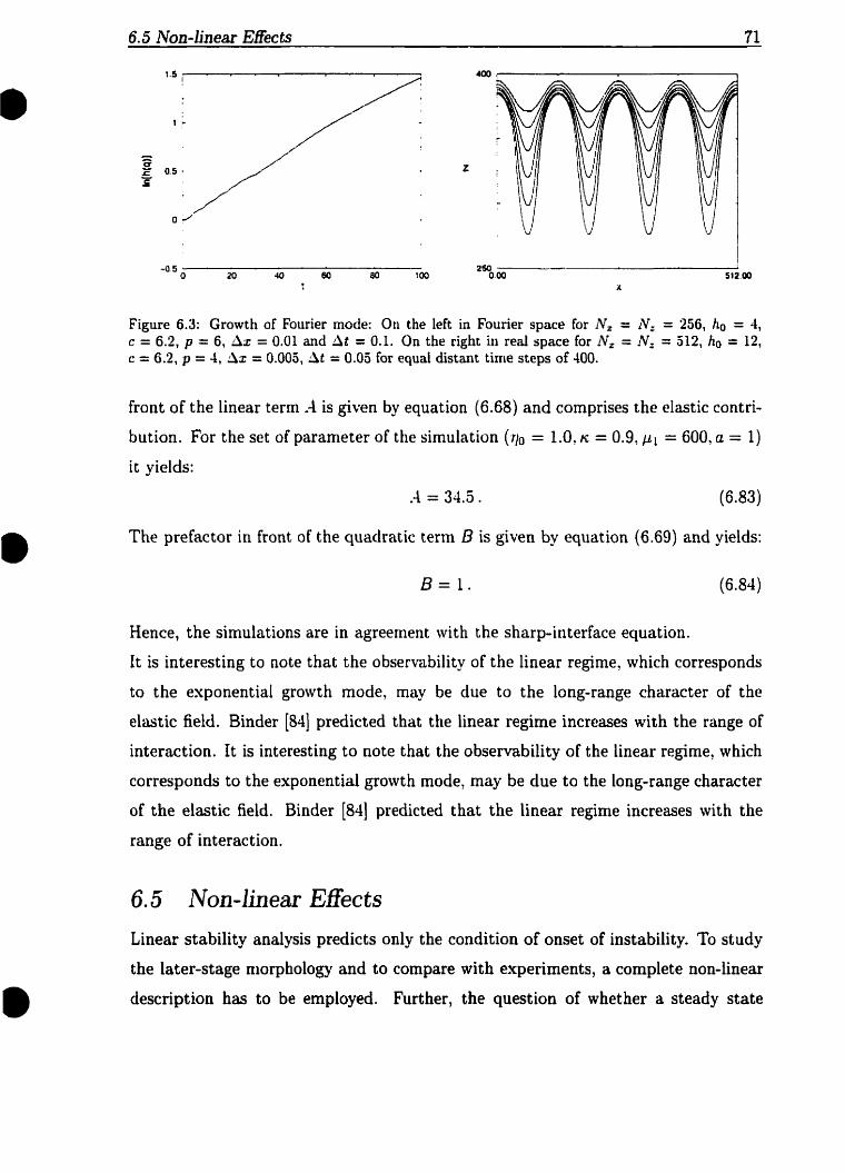
Figure 6.3: Growth of Fourier mode: On the Ieft in Fourier space for N, = N, = 256, ho = 4, c = 6.2, p = 6, AL = 0.01 and At = 0.1. On the right iii red space for N, = NZ = 512, ho = 12, c = 6.2, p = 4, Ax = 0.003, At = 0.05 for qua1 distant tirrie steps of 400.

front of the linear term -4 is given by equation (6.68) and comprises the elastic contri-

bution. For the set of parameter of the simulation (rio = 1.0, K = 0.9, pl = 600, a = 1)

it yields:

-4 = 34.5. (6.83)

The prefactor in front of the quadratic term B is given by equation (6.69) and yields:

Hence, the simulations are in agreement with the sharp-interface equation.

It is interesting to note that the observability of the linear regime, which corresponds

to the exponential growth mode, rnay be due to the long-range character of the

elastic field. Binder [84] predicted that the linear regime increases with the range of

interaction. It is interesting to note that the observability of the linear regime, which

corresponds to the exponential growth mode, may be due to the long-range character

of the elastic field. Binder 1841 predicted that the linear regime increases with the

range of interaction.

Linear stability analysis predicts only the condition of onset of instability. To study

the later-stage niorphology and to compare with experiments, a cornplete non-linear

description has to be employed. Further, the question of whether a steady state


Figure 6.4: Dispersion relation obtained from numericd linear stabili ty andyses for different p and :Vz = !V: = 256. ho = 4, and c = 6.2. The iriset shows a linear fit through the data which are plotted as w / q vs. q.

rxists or asyrnptotie coarsening occurs has ta be resolved. Neither Spencer, Davis

and Voorhees (931 with their long-wave approach, nor Spencer and Meiron [94],

could resolve that issue. Numerical instabilities and singulari ties limited t heir study,

as grooves formed. CVe did not eiicounter numerical instabilities, and hence could

study the groove formation. An advantage of the phase-field description is that non-

linearities are taken into account implicitly so that the non-linear regime does not

provide any addit ional numerical pro blems.

A. ln terfacial Profile

A typical set of interfacial configurations is shown in figure 6.2 and figure 6.3. The

nonlinear effect gives rise to a clear asymrnetry between peaks and valleys, wherein

deep grooves appear in the valleys. This behavior has been observed experimentally,

as well as in previous theoretical studiesl. It is interesting to note that in the early

'Nozièrea [s2]; Spencer, Davis and Voorhee.~ [93]; Spencer and Meiron [94]; Yang and Srolovîtz [93].

Figure 6.5: Section of interfacial profile smoothed hy a Iow frequency pass to filter out high frequencies due to discretization of space.

stages of the instability ive can fit the interfacial profile witli a simple function

where the curvature K, given by equatioii (5.28) is a low-order polynomial function of

the height h(x) of the interface. The order of the polynornial is increasing with time.

To estimate these dependences, the interfacial profile was smoothed by a low frequency

p a s to filter out high frequencies due to discretization of space. A typical profile with

a fit is sliown in figure 6.5. From this fit the curvature was calculated. Figure 6.6

shows the curvature versus the height at different times, together with higher order

polynominal fits. The above described relationship between the curvature and the

height variable can be understood by considering the sharp-interface equation (5.32):

As we have discussed before, and worked out in appendis A.2. ott is a function of the

interfacial profile h(x). Hence, ut, can be erpressed in terms of a polynomial in the

amplitude of h:

For very early tirnes we showed that both the velocity (5.43), and the stress (5.42), are

linear in h. As time progresses, the amplitude of h grows and non-linear terms become

relevant, and must be considered in equation (6.86), which then yields equation (6.85).


Figure 6.6: Curvature versus high dependence of interfacial profile at different tinie steps. The data are represented by rnarkers. Through the different data sets a polynominai was fitted. The order of the polynominal increased with tirne. At t = 100 the polynorninal was of j th d e r , at t = 200 of 6th order, at t = 300 of sth order and at t = 400 of foth order.

B. Coarsening and Scaling

Esperimentally. random fluctuations in the interface will give rise to the cornpetitive

growth of different structures corresponding to different wave numbers. To study this,

we prepared the systern with an interfacial profile consisting of a superposition of p

linearly unstable modes? P

h ( x ) = ho C cos(qix + 4,) i= 1

with q* < qc and # being a uniformly distributed random variable in the interval

[O, 'Zr]. -4 typical realization is shown in figure 6.7.

We averaged 100 mns over 500 time steps of a two-dimensional system with 100 un-

stable modes, where (N', !$, &, c, ho) = (1024, 512, 0, 12.3, 0.34). Figure 6.8 shows

the Fourier transform of the equal- t ime height-height correlation funct ion, which we

shall cal1 the structure factor S(q, t), in different regimes. Note that the structure

factor vanishes for q + O due to elasticity, not a conservation law. For very early

times, in which the linear regime is valid, the structure factor can be derived from

the dispersion relation by a Cahn-Hilliard-type theory. Figure 6.8 shows the data

Figure 6.7: Time evolution of the phase field in two dimension in the case of coarsening. The pictures shown correspond to t = 0.3, t = 5.0, t = 15.0 and t = 30.0 from left to right and top to bottom. The parameters were Nz = N: = 256, c = 12.3 and ho = 0.4 .

Figure 6.8: Structure factor of interfacial profile at equal tirne intervals. Solid lines show the structure factor derived from a linear Cahn-Hilliard-type theory, whidi only describes the data for early times.

together with the results of a linear theory. There is a strong sirnilarity between this

behavior and early-stage spinodal decomposition in long-range force systemsL. For

later times, when the non-linear effects corne into play, the linear theory no longer

describes the data. It is evident that the system coarsens. The location of the peak

of the structure factor q,,(t) moves to smaller wave numbers, as the peak height

increases and sharpens. The peak height follows

where a = 3, as can be seen in figure 6.9. This indicates that the interfacial length

increases linearly with time for any unstable wavenumber, as expected from the linear

analysis. As discussed in chapter 4.3, if a system displays dynamical scaling the

structure factor scales as (4.25), which explains the exponent a = 3, one for each

height variable and one for the dimension. As shown in figure 6.10, the peak width

sharpens with time as

Ap - t-, (6.90)

6.5 Non-Jiaear Effec ts 77

Figure 6.9: grows with

Scaling of peak beight of structure factor with time. As seen in the inset the peak height time as S(q,,,, t ) - ta with a sz 3.

Figure 6.10: Scaiiig of width of structure factor with tirne. As seen in the inset the peak width sharpens with tirne as A, - t3 with 7 = 0.5.

where y = 0.5. This dependence is due to competitive ordering between different wave

numbers, analogous to phase ordering systems with non-conserved order parameters,

as discussed in chapter 4.3. Note however that the interfacial Iength increases linearly

with time, while the peak width indicates a slower coarsening length - t Il2. This is

quite different from mode1 A or B where only one characteristic length is observed.

Even more interesting is figure 6.11, which shows that within the accuracy of our

stud- the structure factor shows scale invariance:

where q* is the scaled wave number q* = (q - qm,)/9,

Fittirig Sa to

s* - (q*)*

for small q' gives 6 -- 1 - 2 and,

for large q' gives U, - 5 - 6 as is seen in figure 6.12. C V e do not yet understand

the origins of these exponents. CVe expect that our results on transient coarsening

phenornena can be observed through microscopy or by x-ray diffraction (Sinha et al.

1881 1.

6.6 Three dimensional Growth

Since the elastic equations are much easier to solve in two dimensions, or in the plane

strain case for which the elastic equations reduce to effectively two dimensions, almost

al1 studies have been performed for these cases. Only Spencer, Voorhees and Davis

[931 have performed a linear stability analysis for the full three-dimensional problem.

Al1 nonlinear approaches as well as al1 numerical studies had been limited to two

dimensions. There has been speculation as to whether the third dimension will have

an effect on the stress relief mechanism.

To study this, we simulated a system with N, = N, = Nr = 128, with z be-

ing the direction normal to the surface. Starting with a srnall amplitude sinusoidd

perturbation in z, trenches with sharp deep grooves form, while a small amplitude

Figure 6.11: Scaling of structure factor. The structure factor shows scaling: S(q, t)/S(q,,,, t ) = S'(q9 ), where the scaled wave number q' = ( q - qmol)/Av.

Figure 6.12: Fit of taiis of structure factor. The rescaled structure factor is fitted to S' 2 (q')6 and srnail q, which gives 6 = 1.4 and to S' rz ( l /q)o which gives 4 = 5.9. The inset is a magnification of the taü region and its fit.

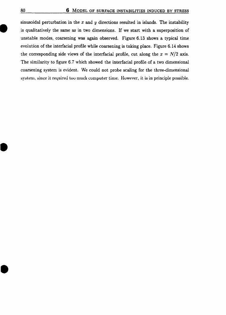
sinusoidal perturbation in the x and y directions resulted in islands. The instability

is qualitatively the sarne as in two dimensions. If we start with a superposition of

unstable modes, coarsening was again observed. Figure 6.13 shows a typical time

evolution of the interfacial profile while coarsening is taking place. Figure 6.14 shows

the corresponding side views of the interfacial profile, cut dong the x = N / 2 axis.

The similarity to figure 6.7 which showed the interfacial profile of a two dimensional

coarsening system is evident. We could not probe scaling for the three-dimensional

systeiii, àiiicr it required t w iiiucli coruputer tiriie. Huwever, it is iri principle possible.

6.6 T h e e dimensionai Growth 81

Figure 6.13: Tirne evolution of the surface profile of the phase field in three dimension. The pictures shown correspond to t = 4.5, t = 7.5, t = 10.5 and t = 15.0 from lefi to right and top to bottom with the parameters N, = N, = IV= = 128, ha = 1.0, and c = 18.5. Figure 6.14 shows the corresponding side view.


Figure 6.14: Side view of coarsening in three dimensions. The pictures shown correspond to t = 4.5, t = 7.5, t = 10.5 and t = 15.0 from left to right and top to bottom with the parameters N, = = Nz = 128, ho = 1.0, and c = 18.5. Figure 6.13 shows the corresponding top view.

We have proposed a new mode1 based on a Ginzburg-Landau approach to study a

stress-induced morphological instability, commonly known as the Gnnfeld instabil-

ity. The instability hm been observed experimentally and is often associated with

the dislocatiori-free Stranski-Krastanov growt h in epitarcy. Due to the technological

relevance of epitavial grown films in the semiconductor industry, understanding the

instabili ty is of fundamental importance.

In our approach, the elastic field is coupled to an order parameter in such a way

tliat the solid supports shear, whereas the liquid phase does not. Hence, the order

parameter obtains a transparent meaning in the context of liquid-solid phase transi-

tions.

\Ne have shown that our model reduces in the appropriate limit to the sharp-

interface equation which have been used traditionally to study the instability How-

ever, numerical studies using the sharp-interface equations had been limited to two

dimensions and were constrained by numerical instabilities appearing at very early

times. Hence, a systematic study of the non-linear regime was not possible. Impor-

tant questions, such as whether the system rnoves towards a steady state or coarsens

had not been answered yet.

In our description, the proper treatment of non-linearities is inherent. We also did

not encounter any numerical instabilities, and could perform numerical simulations in

two and three dimensions. To test our model, we first performed a numerical stability

analysis and found that the growth of the amplitude of the Fourier modes was initially

independent and exponent ial, obeying exp (w ( q ) t ) , followed by a slower growth. The

fitted dispersion relation w(q) is consistent with w = Ag - Bq2 and agrees with the

linear stability analysis carried out by Srolovitz [89].

We also observed that in the early stages of the instability, the interfaciai profile

could be fit ted with a simple funct ion n, = zi ai ( t ) hi, where the eurvature K, is a low-

order polynomial function of the height h(x) of the interface. This observation could

be explained by analyzing different contributions to the sharpinterface equation.

CVe st udied the non-linear regime, which is characterized by competit ive growt h

of different structures corresponding to different wave numbers by measuring the

Fourier transforrn of the eqüal-time height-height correlation function. For early

times we observed a strong similanty between its behavior and early-stage spinodal

decomposition in Long-range systems. For later times coarsening was evident: The

location of the peak of the structure factor q,,(t) moves to smaller wave numbers,

as the height increased and sharpened. The peak height followed S(q,,) - t a , where

a = 3, while the peak width sharpened with time as A, 5 t-?, where y 2: 0.5. The

former dependence was due to the interface length increasing linearly with time. The

latter dependence was due to cornpetitive ordering between different wave nurnbers,

analogous to phase ordering. Within the accuracy of our study, we found that the

structure factor showved scale invariance: S(q. t)/S(q,,,, t) = S*(qB)? with the scaled

wavenumberq8=(q-q,,)/~.FittingtoS*-(qa)sandS*-(~/q8)',forsmrll

and large q' respectively, gave b .- 1 - 2, and - 5 - 6. We expect that these results

can be observed through microscopy or by x-ray diffraction.

In our three-dimensional study we observed the same qualitative behavior as was

observed in two dimensions. Starting with a small amplitude sinusoidal perturbation

in one direction, trenches with sharp deep grooves form, while a small amplitude sinu-

soidal perturbation in two directions resulted in islands. S tarting with a superposition

of unstable modes, coarsening was again observed.

One advantage of cJur mode1 is that it can be easily extended. Anisotropic ef-

fects can be studied by including anisotropy through the surface tension, the elastic

coefficients, or the eutemal stress. The effect of phase separation, or of impurities,

can be analyzed by coupling an additional field to the phase-field. Also, instead of

evaporation-condensation, surface diffusion can be chosen as the material transport

mechanism. In addition, the influence of a constant flux can be studied. Furthermore,

as h a been discussed in the thesis, the stress field oear the groove can becorne so

high that dislocations might be nucleated. To study this, one can extend our mode1

by coupling the phase-field to a dislocation density field. This latter extension is

curreatly under iiivestigation.

A. 1 Sharp-interface limit Thc starting point is thc rcscalcd, gcncralizcd phase ficld equations from chapter 3.2:

and,

For

(A. 1)

(A. 3)

ive recover equation (3.16) and equation (3.17). Depending on the scaling of the

parameters, four different sharp interface limits can be obtained, which describe dif-

ferent physical systems wit h distinct stability characteristics. We will show, for one

particular scaling, how the sharp or thin interface interface limit is obtained using

the method of matched asgnzptotic expansions. We will show that the scaling Karma

and Rappel' have recently proposed, is equivalent to the scaling Caginalp and Fife

[88] worked out previously. With this scaling ansatz, much larger systems can be

simulated, including three-dimensional systems. An asymptotic analysis for e << 1

will be carried out for a layered solution of the system (A.1) and (-44, under the

assumption that a is of the order unity.

The interfacial curve is defined as the set of points at which #(x, y, t ) = 1/2. -4

local orthogonal coordinate (r , s ) system near the surface is introduced by:

at the interface and

lVrl=1, and v 2 r = n ,

IKarma and Rappel p6bj; K m a and Rappel [%a]; Karma a d Rappel

87

with n being the curvature. Hence, r rneasures the distance dong the normal, and s

is the arclengt h.

The idea behind the matched asymptotic expansion is to divide the systern into

two subregions:

1. An inner region in the vicinity of the interface, where the gradient of the order

parameter is large and

2. the ovter region in the bulk phases where the order parameter is approxirnati~cly

constant.

A. Outer expansion

CVe forrnally expand the variables in their original coordiiiates in powers of É,

and,

The leading order of the phase field equations ( A l ) and (A.9) gives respectively,

and,

The leading order solutions are given by $(O) = 1 and $(O) = O in the solid and the

liquid, respectively. For the temperature, we find the usual diffusion equation

(A. 10)

and,

B. Imer expansion

Here, we use the local curvilinear coordinate system defined above. It implies that

the Laplacian and the time derivative take the following form:

v 2 u = u, + v2r u, + I V S ~ * Z L ~ , + v2s u s , (A.13)

and,

,ut = ut + rt u,. + ~t us . (A. 14)

WC also introducc the scalcd coordinate : = r / ~ and write

u(z , y , t , 6) = U ( z , s, t , c) (A. 15)

= L~(~)(Z, s, t) + (2, S. t ) + .- .- .- , (A.16)

and,

Xow. the equations (Al) and (A.?) can be written in the following form:

and,

(A. 20)

Therefore the equations of 9 and Lr to zeroth order in e are:

and,

ulq) = o .

and, 1

1. Ma t d i n g conditions

Matching conditions provide the far-field boundary condition for the inner solution'.

The outer solution is written as a function of the inner variables, and the resulting

expressions are expanded in É. We drop the s variable, since the matching conditions

are with respect to only the coordinate orthogonal to the interface layer. Near the

layer, we formally equate the two expansions

where 2 = (x-r (t, c))/e is the scaled coordinate. The right hand side of equation (A.25)

can be expanded in a Taylor series in É

w here

hlatching is accomplished by letting É -t O and r + f oo provided that d i l + 0.

With this constraint, the remainder term in equation (A.27) is of lower order than

an? of the preceding terms.

The two first matching conditions are

2. Leading order sol u tion

The leading order solutions for Lr takes the form

with the rnatching condition:

Caginaip and Fife [88].

A. 1 Sharp-in terface limit 91

This implies that :

a = 0 ,

and the leading order solution for @ takes the form:

with the rnatching condition:

an(* m) = @(ri) = 0 and 1.

For further convenience, we define:

and,

h ( 4 ) = /,(@O1) + S b g , ( @ ' O ) ) . so that equation (-4.34 yields:

3. First-order solu tion

The first-order inner equation for U has the form

Integrating once yields: 1

where do) = 4, and Cl is a integration constant.

The matching condition implies:

Choosing p ( 4 ) = 4 results in:

Integrating once more:

O v(o) u ( ~ ) = -P(z) + C1z + C2,

2

wit h

and C2 being another integration constant, so

Using the matching condition:

results in:

The first order inner equation For <P takes the form:

w here,

The Fredholm alternative states that the linear inhomogeneous equation (A.48) is

only solvable, if the r.h.s is orthogonal to the nul1 space of the adjoint operator Lt.

Because L is self adjoint. Lt@ = O is solved by 0' = < P I ) , which is the Goldstone

mode. This can easily be seen by differentiating equation (A.38). We are left with

the following solvability condition:

and,

Replacing u( ' ) by equation (A.45) and defining:

A. 1 Sharp-in t erface I h i t 93

we obtain:

In the case that f (O) is an odd function of 8: ie., J(-9) = - f (a), 9' will be an

even in r . Then, if g(@) is even function of z, the integral:

Rewriting equation (X.53) determines C2 to be:

w here

and,

Hence, di) at the interface is given by:

where,

This is the generalized Gibbs-Thomson condition in which the kinetic coefficient ;3 is

given by:

A.2 Solution of elastic equations

Many probierns relnted to elastieity ieduce to solving partial differential equations

with fixed boundary values. In the case of the Grinfeld instability, we are dealing

with a semi-infinite, içotropic, uni-axially stressed solid which is in contact with its

own melt or vapor. The interface between the solid and the liquid is free. Since

the elastic equations (5.2) are linear, it is useful to decompose the free interface into

Fourier modes:

h(x) = ho sin qx . (A.61)

The condition of mechanical equilibrium provides us? in two-dimensions, with two

partial di Kerential equations:

A general solution for the stresses are given by:

and,

Since the stress tensor is symmetric. O,, = O,,, an additional constraint is imposed

on \II and Q z :

a,lk.,(x, 2 ) = &%P,(x, 2) , (A.68)

which is solved by:

and,

Hence, the stress field can be derived from only one scalar field X, which is called the

Airy stress func tion:

and,

(-4.71)

(A. 72)

(A. 73)

A.2 Solution of elastic equations 95

Since the free interface has a sinusoidal profile, the following Ansatz for x is justified:

Hence, the stress fields have a functional dependence as follows:

and,

ozZ (x, 2) = O" ( z ) exp(iqx) ,

oz: (x, z) = -i q (Dl(-) exp( iqx) ,

0:: (x, Z) = - q 2 @ ( - ) exp( iqx)

(A. 75)

(A. 76)

(A. 77)

where the prime means differentiation with respect to r. Now, only a(-) has to be

determined, which is a function of z only. To do so, we take the divergence of the

Lamé equation (5.8) and obtain:

V ? ( V * Z ) = O . (A. 78)

Lsing Hooke's law (E), w obtain an expression for the stress field:

v2air = 0 . (A. 79)

Replacing oii by equation (A.75) and equation (h.77) results in an ordinary differen-

tial equation of fourth order for ??(z):

Its solution is given by:

where al , bl . a2 and b2 are constants which have to be determined by the boundary

conditions. Since the stress field should vanish at (x, r + -00) , it follows that a* = O

and b2 = 0.

Hence, ~ ( x , z) is then:

no t2 X(W) = 2 + (al + blz ) sin(qx) eq' ,

Figure -4.1: Sketch of local coordinate systern at the liquid-solid interface.

where we have used only the sine part.

Now, the stress field can be determined:

o~,(x, Z) = 00 + q [2 b + q(a + b T)] sin(qx) eq' , (-1.83)

(x, 2) = - [q2 ( a + b 2 ) + b q] cos(qx) eq' , (-4.84)

and, O,&, 2) = -(12 [a + b 21 sin(qx) eq' , (-4.85)

where we have dropped the index 1 . Xow we must determine the two constants a and

6 from the boundary conditions (5.24), (5.15) and (5.26):

and,

First, we have to express the stress tensor in the local coordinate system of the

interface, which is given by the normal 5 and tangential t of the interface:

and!

where 0 is the angle b etwe en the normal n' and the z-ais as shown in figure A. 1.

Since the stress field is a tensor of rank two, it is transformed as:

sin0 cos8 sin8 - cos 8 4A.90)

A .2 Solution of elas tic equa tions 97

Hence a,,, O,,, and ott are:

O,, = oz, sin2 0 + 20,, sin 0 cos B + CL, cos2 0 , (-1.91)

O,( = (oLZ - oZ2) sin 0 cos 8 + a,, (sin2 6 - coso2 8 ) , (X.92)

and, ott = a,, coi2 0 - 20,, sin 0 cos 8 + oz= sin2 B . (A. 93)

In addition, we have:

Hence:

siri 19 = ho q cos(q2) COS 8.

Inserting equation (-4.95) in equation (A.91) and equation (.A.%?), and using the

boundary conditions (A.86) and (2\.87), we cari eliminate O,;, and are left with:

At the interface. 2 = ho sin(qz), oz, and a,, are given by:

Considering only terms up to order q':

O,, = 00 + [9 b + 2 6 ha$ sin(gx) + a gZ + 6 ho q2 ~ i n ( ~ x ) ] sin(qx) , (-4.99)

and, oz: = - b q - b ho q2 sin(qz) - aq2 - b ho q2 sin(qx) . (A. 100)

Substituting equat ion (A.99) and equation (A. 100) in equation (.\.96), and consider-

ing terms only up to second order in q, we obtain:

oohoq - b q + 4 b hoq2 sin(qx) + a q2 sin(qx) + o ( ~ ~ ) = O. (A. 101)

Hence,

and,

(A. 102)

(A. 103)

Since we are only interested in contributions up to linear order in ho:

a = 0. (-4.104)

The stress fields a,,, a,, and oz= are now completely determined:

and,

a,, (z, z) = a0 [1 - q ho (2 + qr) sin(qx) eq'] , (-4. 105)

a&, 2) = ooq ho [l + q Z] C O S ( ~ X ) eqL , (A. 106)

0:- (x, 2 j = qq2 hg L sin(qx) eV' . (.4.107)

we can substitute equation (A. los), eqiiation (..\.lQ6), alid equation (A. 107) for the

stress fields. Keeping only terms up to first order in heq, we obtain:

att ( x . 2) = ou [l - hoq (2 + (12) sin(qx) eq'] + O((hoq)') , (A. 109)

a and at the interface:

(A. 110)

AGUENAOU. K . , MÜLLER, J . , AND GRANT, M. [98]. Quaidendritic gowth due to elastic fields. Phil. Mag. B, 78, 103 (1998).

ASARO, R. J. AND TILLER, W. A. [72]. Interface morphology development during stress corrosion cracking: Part i. via surface diffusion. Metall. Tram., 3, 1789 (1972).

BERRÉHAR, J., CAROLI, C. , LAPERSONNE-MEYER, C., AND SCHOTT, M. [92]. Surface patterns on single-crystal films under uniaxial stress: Experimental evidence for the grinfeld instability. Phys. Reu. B, 46, 13487 (1992).

BINDER, K. (8-11. Nucleation barriers, spinodsls, and the Ginzburg criterion. Phys. Rev. A ? 29, 341 (1984).

BOWLEY, R. M. [92]. Instabilities of the liquid solid interface. J. Lou Ternp. Phys., 89, 401 (1992).

BRAY, A. J. (941. Theory of phase-ordering kinetics. Advances of Phpics, 43, 357 (199.1).

CAGINALP, G . [89]. Stefan and Hele-Shaw type models as asymptotic limits of the phase-field equations. Phgs. Rev. A, 39, 5887 (1989).

CAGINALP, G. AND FIFE, P. C. (881. Dynamics of layered interfaces arising from phase boundaries. S I A M J. A p p l . Math., 48, 506 (1988).

CAHN, J . W. [89]. Interfacial free energy and interfacial stress: the case of an interna1 interface in a solid. Acta Metall., 37, 773 (1989).

CAHN, J. W. AND HILLIARD, J . E. [58]. Free energy of a nonuniform system. 1. interfacial free energy. J. Chem. Phys., 28, 258 (1958).

CAROLI, B., CAROLI, C., AND ROULET, B. [92]. Instabilities of planar solidification fronts. In Godrèche, C., editor, Solids Far from Equilibrium, page 155. Cam- bridge University Press, Cambridge.

COLLINS, J . B . AND LEVINE? H. [85]. Diffuse interface mode1 of diffusion-lirnited crystal growth. Phys. Rev. B, 31, 6119 (1985).

COOK, H. E. [70]. Brownian motion in spinodal decomposition. Acta Metall., 18, 297 (1970).

CROSS, M. C. AND HOHENBERG, P. C. [93]. Pattern formation outside of equilibrium. Rev. Mod. Phys., 65, 851 (1993).

DAVID, S. A., DEBROY, T., AND VITEK, J. M. [94]. Phenomenological modeling of fusion welding processes. MRS Bull., WC, 29 (1994).

100 References

DONG, L., SCHNITKER, J. , SMITH, R. W., AND SROLOVITZ, D. J. [98]. SESS &Xa t ion and misfit dislocation nucleation in the growth of misfitting films: A molecular dynamics simulation study. J. Appi. Phys., 83, 217 (1998).

EAGLESHAM, D. J. AND CERULLO, M. [go]. Dislocation-free Stranski-Krastanow growth of Ge on Si(100). Phys. Rev. Lett., 64, 1943 (1990).

ELDER, K. R.: DROLET, F., KOSTERLITZ, J. M., AND GRANT, M. (941. Stochastic eutectic growth. Phys. Rev. Lett., 72, 677 (1994).

FIX, G. J. [82]. Numerical simulation of free bouridary problems using phase field methods. In Whiteman, J. R., editor, The Mathematics of Finite Elernents and rippliccltiorrs II.; page 265. Xcadeitiic Press, London.

Frx. G. J. [83]. Phase field models for free boundary problems. In Fasano, A. and Primicerio, hl., editors, Free Boundary Problerns: Theory und Application, volume 2, page 580. Pitman, London.

GRANT, M. , SAN ~ I I G U E L . M., VINALS, J., AND GUNTON, J. D. [as]. Theoty for the early stages of phase separation: The long-range-force limit. Phys. Reu. B, 31, 3027 (1985).

GRILHÉ, J. [93]. Study of rougliness formation induced by homogeneous stress a t the free surface of solids. Acta metall. mater., 41, 909 (1993).

G RINFELD, M. A. [82]. Stability of heterogeneous equilibrium in systems containing solid elastic phases. DoMady Akademii Nuuk SSSR, 265, 836 (1982).

GRINFELD. M. A. [8û]. Instability a l the separation boundary betiveen a non- hydrostaticaily stressed elastic body and a melt. Sov. Phys. Dokl., 31, 831 (1986).

GRINFELD, M. A. [89]. Energy release upon first-order phase transitions in solids. Sov. Phys. Dokl., 34. 1050 (1989).

GUHA, S., MADHUKAR, A., AND RAJKUMAR, K. C. [90]. Onset of incoherency and defect introduction in the initial stages of molecular beam epitavial growth of highly strained in,gal-,as on gaas(100). Appl. Phys. Lett., 57, 21 10 (1990).

G UNTON, J. D., SAN MIGUEL, M., AND SAHNI, P. S. 1831. The dynamics of first-order pliase transitions. In Domb, C. and Green, M. S., editors, Phase Transitions and Critical Phenornena, volume 8. page 267. -4cademic Press, London.

HALPERIN, B. i., HOHENBERG, P. C., AND MA, S. [74]. Renormalization-group methods for critical dynamics: 1. recursion relations and effects of energy conservation. Phys. Rev. B, 10, 139 (1974).

HOHENBERG, P. C. AND HALPERIN, B. 1. [Ti]. Theory of dynamic critical phenornena. Rev. Mod. Phys., 49, 435 (1977).

HORN VON HOEGEN, M. [97]. Surfactant mediated heteroepitaxy: Interplay of diffusion, strain relief and surface morphology. In Tringides, M. C., editor, Surface Diffusion, Atomic and Collective Processes, NATO ASI Series, page 309. Plenum Press, New York and London.

Referen ces 101

IVANTSOV, G . P. [47]. Temperature field around a spheroidal, cylindrical and acicular crystal growing in a supercooled melt. Dok. Akad. Nauk. SSSR, 58, 567 (1947).

KARMA, A. AND RAPPEL, W.-J. [96a]. Numerical simulation of three-dimensional dendritic growth. Phys. Rev. Lett., 77, 4050 (1996).

KARMA, A . AND RAPPEL, W .-J. [96b]. Phase-field method for computationally efficient modeling of solidification with arbitrary interface kinetics. Phys. Rev. E, 53, R3017 (1996).

KARMA, A. AND RAPPEL, W.- J . [98]. Quantitative phase-field modeling of dendritic growth in two and three dimensions. Phys. Rev. E, 57, 4323 (1998).

KASSNER, K. AND MISBAH, C. (941. Non-linear evolution of a uniavially stressed solid: A route to fracture? Europhys. Lett., 28, 245 (1994).

KHACHATURYAN, A. G. [83]. Theory O/ Structural Transformation in Solids. John W e y St Sons, Yew York. 1983.

KOBAYASHI, R. [93]. Modeling and numerical simulations of dendrit ic crystal growth. Phpica D, 63, 410 (ENI).

LANDAU, L. AND LIFSHITZ, E. [83]. Elastzritiitstheorie. .\kademie-Verlag, Berlin, fifth edition, 1983.

LANGER, J. S. [80]. Instabilities and pattern formation in crystal growth. Rev. Mod. Phys., 52, 1 (1980).

LANGER. J . S. [S?]. Lectures in the theory of pattern formation. In Souletie! J., Vanriimenus, J., and Stora, R., editors, Les Houches, Session XLVI, 1986 - le hasard et fa matière/Chance and Matter, page 629. Elsevier Science Publishers, Amsterdam.

LANGER, J . S. [89]. Dendrites, viscous fingers, and the theory of pattern formation. Science, 243, 1150 (1989).

LANGER, J . S. [92]. A n introduction to the kinetics of first-order phase transition. In Godrèche, C., editor, Solids Far from Equilibrium, page 297. Cambridge Univer- sity Press, Cambridge.

LANGER, J . S., BAR-ON, M., AND MILLER, H. D. [75]. New computational method in the theory of spinodal decomposition. Phys. Rev. A, 11, 1417 (1973).

LARADJI, M., GRANT, M., AND ZUCKERMANN. M. J. [go]. Dynamics of first-order transitions in two-dimensional systems wit h long-range interaction. Phys. Rev. B, 41, 1646 (1990).

LARCHÉ, F. C. AND CAHN, J. W. [78]. Thermodynamical equilibrium of multiphase solids under stress. Acta Metail., 26, 1579 (1978).

LARCHE, F. C. AND CAHN, J. W. [85]. The interactions of composition and stress in crystalline solids. Acta Metall., 33, 331 (1985).

L~Gows, F. K., COPEL, M., AND TROMP, R. M. [go]. Microstructure and strain relief of Ge films grown layer by layer on Si(001). Phys. Rev. B, 42, 11690 (1990).

102 References

LÉONARD, F. AND DESAI, R. [97]. Elastic effects and phase segregation during the

O growth of thin alloy layers by molecular-beam epitaxy. Phys. Reu. B, 56, 4955 (1997).

MATTHEWS, J . W. AND BLAKESLEE, A. E. [71]. Defects in epitaxial multilayers. Journal of Crystal Growth, 27, 118 (1974).

MCFADDEN, G. B., WHEELER, A. A . , BRAUN, R. J. , COFUELL, S. R., AND SEKERKA, R. F. [93]. Phase-field models for anisotropic interfaces. Phys. Rev. El 48, 2016 (1993).

MORIN. B . , ELDER, K. R., SUTTON, M., AND GRANT, M. [%]. Mode1 of the kinetics of polymorphous crystallixation. Phys. Reu. Lett., 75, 2156 (1995).

MÜLLER, J . AND GRANT, M. 1981. Mode1 of surface instabilities induced by stress. submitted to Phys. Rev. Lett., (1998).

MULLINS, W . W. AND SEKERKA, R. F. [63]. ~orphological stability of particle growing by diffusion or heat Bow. J. of A p p l . Phys., 34, 323 (1963).

NISHIMOR~, H. AND ONUKI, A. [go]. Pattern formation in phase separating alioys with cubic symmetry. Phys. Rev. B, 42, 980 (1990).

NOZIERES, P . [92]. Shape and growth of crystals. In Godrèche, C., editor, Solids F<Lr lrom Equilzbriurn, page 1. Cambridge University Press, Cambridge.

NOZIERES, P. [93]. Amplitude expansion for the Grinfeld instability due to uniaxial stress at a solid surface. J. Phys. 1 France, 3, 681 (1993).

OKADA. T., WEATHERLY, G. C.' AND MCCOMB, D. W. (971. Growth of strained ingaas layers on inp substrates. J. Appl. Phys.. 81, 2185 (1997).

ONUKI. A. [aga]. Ginzburg-Landau approach to elastic effects in the phase separation of solids. J. Phgs. Soc. Jpn., 58. 3065 (1989).

ONUKI, A. [89b]. Long-range interactions through elastic fields in phase separating solids. J. Phys. Soc. Jpn.. 58, 3069 (1989).

ONUKI, A. AND NISHIMORI, H. 1911. .\nomalously slow domain growth due to a modulus inhomogeneity in phase separating alloys. Phys. Rev. B, 43, 13649 (1991).

POMEAU, Y. AND BEN AMAR, M. [92]. Dendritic grolvth and related topics. In Godrèche, C., editor, Solids Far from EquzlzbBum, page 365. Cambridge Univer- sity Press, Cambridge.

PROVATAS, N., GOLDENFELD, N., AND DANTZIG, J . [98]. Efficient computation of dendri tic microstructures using adaptive mesh refinement . Ph ys. Rev. Lett., 80, 3308 (1998).

SAGUI, C., SOMOZA, A. M., AND DESAI, R. C. [94]. Spinodal decomposition in an order-disorder phase transition with elastic fields. Phys. Rev. E, 50,3865 (1994).

SINHA, S. K., SIROTA, E. B., GAROFP, S. , AND STANLEY, H. B. [88]. ?(-ray and neutron scattering from rough surfaces. Phys. Rev. B, 38, 2297 (1988).

Referen ces 103

SPENCER, B. J., DAVIS, S. H., AND VOORHEES, P. W. [93]. Morphological instability in epit axially st rained dislocation-free soiid films: Nonlinear st ability t heory. Phys. Rev. B, 47, 9760 (1993).

SPENCER, B. J. AND MEIRON, D. 1. [94]. Nonlinear evolution of the stress-driven rnorphological instability in a two-dimensional semi-infinite solid. Acta metall. muter., 42, 3629 (1994).

SPENCER, B. J . , VOORHEES, P. W . , AND DAVIS, S. H. [gl]. Morphological instability in epi tavially strained dislocation-free solid films. Phys. Rev. Lett. , 67, 3696 (1991).

SPENCER, B. J., VOONIEES, P. W., AND DAVIS, S . H . (931. Ylorphological instability in epitaxially st rained dislocat ion-free solid films: Linear stability theory. J . Appl. Phys., 73, 4955 (1993).

SROLOVITZ, D. J. (891. On the stability of surfaces of stressed solids. Acta Metall., 37, 621 (1989).

TERSOFF, J . AND LEGOUES, F. K . [94]. Cornpeting relaxation mechanism in strained layers. Phys. Rev. Lett. , 7 2 , 3570 (1994).

TORII, R. H . AND BALIBAR, S. [92]. Heliun crystals under stress: The Grinfeld instability. J . Lou, Temp. Phys., 89, 391 (1992).

UUANTSEV, A. R. AND ROITBURD, A . [88]. Nonisothernial relaxation in a nonlocal medium. Sou. Phys. Solid State, 30, 651 (1988).

WANG, S.-L. AND SEKERKA, R. F. [96]. Cornputation of the dendritic operating state at large supercoolings by the phase field model. Phys. Rev. El 53, 3760 (1996).

WANG, S.-L., SEKERKA, R. F., WHEELER, A . A. , MURRAY, B. T., COFUELL, S. R., BRAUN, R. J ., AND MCFADDEN, G . B. [93]. Thermodynamically-consistent phase- field models for solidification. Physica D, 69, 189 (1993).

WEEKS, J., VAN SAARLOOS, W., AND GRANT, M. 1911. Stability and shapes of cellular profiles in directional solidification: Expansion and matching methods. J. of Crystal Growth, 112, 244 (1991).

WHEELER, A. A. , BOETTINGER, W. J . , AND MCFADDEN, G. B. [92]. Phase-field mode! for isothermal phase transitions in binary alloys. Phys. Rev. A, 45, 7124 (1992).

WHEELER, A. A., MURRAY, B. T., AND SCHAEFER, R. J . [%Il. Computation of dendrites using a phase field model. Ph ysica 0, 66, 243 (1993).

YANG, W. H. AND SROLOVITZ, D. J . [93]. Cracklike surface instabilities in stressed solids. Phys. Rev. Lett., 71, 1593 (1993).

INFORMATION TO USERScollectionscanada.gc.ca/obj/s4/f2/dsk1/tape11/PQDD... · Randa, Christine. Chris, Stéphane, François, Robert, Mohson, Slava, both Andrews, Etienne, Rob, Graham,

Documents