Raymond W. Yeung Information Theory and Network Coding SPIN Springer’s internal project number, if known November 16, 2007 Springer

Welcome message from author
This document is posted to help you gain knowledge. Please leave a comment to let me know what you think about it! Share it to your friends and learn new things together.
Transcript

Raymond W. Yeung
Information Theory andNetwork CodingSPIN Springer’s internal project number, if known
November 16, 2007
Springer


To my parents and my family


Contents
1 The Science of Information . . . . . . . . . . . . . . . . . . . . . . . . . . . . . . . . 1
Part I Components of Information Theory
2 Information Measures . . . . . . . . . . . . . . . . . . . . . . . . . . . . . . . . . . . . . 72.1 Independence and Markov Chains . . . . . . . . . . . . . . . . . . . . . . . . . 72.2 Shannon’s Information Measures . . . . . . . . . . . . . . . . . . . . . . . . . . 122.3 Continuity of Shannon’s Information Measures for Fixed
Finite Alphabets . . . . . . . . . . . . . . . . . . . . . . . . . . . . . . . . . . . . . . . . 182.4 Chain Rules . . . . . . . . . . . . . . . . . . . . . . . . . . . . . . . . . . . . . . . . . . . . 202.5 Informational Divergence . . . . . . . . . . . . . . . . . . . . . . . . . . . . . . . . . 222.6 The Basic Inequalities . . . . . . . . . . . . . . . . . . . . . . . . . . . . . . . . . . . 262.7 Some Useful Information Inequalities . . . . . . . . . . . . . . . . . . . . . . . 282.8 Fano’s Inequality . . . . . . . . . . . . . . . . . . . . . . . . . . . . . . . . . . . . . . . . 312.9 Maximum Entropy Distributions . . . . . . . . . . . . . . . . . . . . . . . . . . 352.10 Entropy Rate of Stationary Source . . . . . . . . . . . . . . . . . . . . . . . . . 37Appendix 2.A: Approximation of Random Variables with
Countably Infinite Alphabets by Truncation . . . . . . . . . . . . . . . . 40Problems . . . . . . . . . . . . . . . . . . . . . . . . . . . . . . . . . . . . . . . . . . . . . . . . . . . 42Historical Notes . . . . . . . . . . . . . . . . . . . . . . . . . . . . . . . . . . . . . . . . . . . . . 46
3 The I-Measure . . . . . . . . . . . . . . . . . . . . . . . . . . . . . . . . . . . . . . . . . . . . 493.1 Preliminaries . . . . . . . . . . . . . . . . . . . . . . . . . . . . . . . . . . . . . . . . . . . . 503.2 The I-Measure for Two Random Variables . . . . . . . . . . . . . . . . . . 513.3 Construction of the I-Measure µ* . . . . . . . . . . . . . . . . . . . . . . . . . 533.4 µ* Can be Negative . . . . . . . . . . . . . . . . . . . . . . . . . . . . . . . . . . . . . 573.5 Information Diagrams . . . . . . . . . . . . . . . . . . . . . . . . . . . . . . . . . . . 593.6 Examples of Applications . . . . . . . . . . . . . . . . . . . . . . . . . . . . . . . . . 66Appendix 3.A: A Variation of the Inclusion-Exclusion Formula . . . . . 73Problems . . . . . . . . . . . . . . . . . . . . . . . . . . . . . . . . . . . . . . . . . . . . . . . . . . . 75

VIII Contents
Historical Notes . . . . . . . . . . . . . . . . . . . . . . . . . . . . . . . . . . . . . . . . . . . . . 77
4 Zero-Error Data Compression . . . . . . . . . . . . . . . . . . . . . . . . . . . . . 794.1 The Entropy Bound . . . . . . . . . . . . . . . . . . . . . . . . . . . . . . . . . . . . . 804.2 Prefix Codes . . . . . . . . . . . . . . . . . . . . . . . . . . . . . . . . . . . . . . . . . . . . 83
4.2.1 Definition and Existence . . . . . . . . . . . . . . . . . . . . . . . . . . . 834.2.2 Huffman Codes . . . . . . . . . . . . . . . . . . . . . . . . . . . . . . . . . . . 86
4.3 Redundancy of Prefix Codes . . . . . . . . . . . . . . . . . . . . . . . . . . . . . . 91Problems . . . . . . . . . . . . . . . . . . . . . . . . . . . . . . . . . . . . . . . . . . . . . . . . . . . 95Historical Notes . . . . . . . . . . . . . . . . . . . . . . . . . . . . . . . . . . . . . . . . . . . . . 97
5 Weak Typicality . . . . . . . . . . . . . . . . . . . . . . . . . . . . . . . . . . . . . . . . . . . 995.1 The Weak AEP . . . . . . . . . . . . . . . . . . . . . . . . . . . . . . . . . . . . . . . . . 995.2 The Source Coding Theorem . . . . . . . . . . . . . . . . . . . . . . . . . . . . . . 1025.3 Efficient Source Coding . . . . . . . . . . . . . . . . . . . . . . . . . . . . . . . . . . 1045.4 The Shannon-McMillan-Breiman Theorem . . . . . . . . . . . . . . . . . . 105Problems . . . . . . . . . . . . . . . . . . . . . . . . . . . . . . . . . . . . . . . . . . . . . . . . . . . 108Historical Notes . . . . . . . . . . . . . . . . . . . . . . . . . . . . . . . . . . . . . . . . . . . . . 110
6 Strong Typicality . . . . . . . . . . . . . . . . . . . . . . . . . . . . . . . . . . . . . . . . . . 1116.1 Strong AEP . . . . . . . . . . . . . . . . . . . . . . . . . . . . . . . . . . . . . . . . . . . . 1116.2 Strong Typicality Versus Weak Typicality . . . . . . . . . . . . . . . . . . 1196.3 Joint Typicality . . . . . . . . . . . . . . . . . . . . . . . . . . . . . . . . . . . . . . . . . 1206.4 An Interpretation of the Basic Inequalities . . . . . . . . . . . . . . . . . . 129Problems . . . . . . . . . . . . . . . . . . . . . . . . . . . . . . . . . . . . . . . . . . . . . . . . . . . 129Historical Notes . . . . . . . . . . . . . . . . . . . . . . . . . . . . . . . . . . . . . . . . . . . . . 132
7 Discrete Memoryless Channels . . . . . . . . . . . . . . . . . . . . . . . . . . . . 1337.1 Definition and Capacity . . . . . . . . . . . . . . . . . . . . . . . . . . . . . . . . . . 1367.2 The Channel Coding Theorem . . . . . . . . . . . . . . . . . . . . . . . . . . . . 1457.3 The Converse . . . . . . . . . . . . . . . . . . . . . . . . . . . . . . . . . . . . . . . . . . . 1477.4 Achievability . . . . . . . . . . . . . . . . . . . . . . . . . . . . . . . . . . . . . . . . . . . . 1537.5 A Discussion . . . . . . . . . . . . . . . . . . . . . . . . . . . . . . . . . . . . . . . . . . . . 1607.6 Feedback Capacity . . . . . . . . . . . . . . . . . . . . . . . . . . . . . . . . . . . . . . . 1637.7 Separation of Source and Channel Coding . . . . . . . . . . . . . . . . . . 168Problems . . . . . . . . . . . . . . . . . . . . . . . . . . . . . . . . . . . . . . . . . . . . . . . . . . . 172Historical Notes . . . . . . . . . . . . . . . . . . . . . . . . . . . . . . . . . . . . . . . . . . . . . 176
8 Rate-Distortion Theory . . . . . . . . . . . . . . . . . . . . . . . . . . . . . . . . . . . . 1798.1 Single-Letter Distortion Measures . . . . . . . . . . . . . . . . . . . . . . . . . 1808.2 The Rate-Distortion Function R(D) . . . . . . . . . . . . . . . . . . . . . . . 1838.3 The Rate-Distortion Theorem . . . . . . . . . . . . . . . . . . . . . . . . . . . . . 1888.4 The Converse . . . . . . . . . . . . . . . . . . . . . . . . . . . . . . . . . . . . . . . . . . . 1968.5 Achievability of RI(D) . . . . . . . . . . . . . . . . . . . . . . . . . . . . . . . . . . . 198Problems . . . . . . . . . . . . . . . . . . . . . . . . . . . . . . . . . . . . . . . . . . . . . . . . . . . 203

Contents IX
Historical Notes . . . . . . . . . . . . . . . . . . . . . . . . . . . . . . . . . . . . . . . . . . . . . 205
9 The Blahut-Arimoto Algorithms . . . . . . . . . . . . . . . . . . . . . . . . . . . 2079.1 Alternating Optimization . . . . . . . . . . . . . . . . . . . . . . . . . . . . . . . . . 2089.2 The Algorithms . . . . . . . . . . . . . . . . . . . . . . . . . . . . . . . . . . . . . . . . . 210
9.2.1 Channel Capacity . . . . . . . . . . . . . . . . . . . . . . . . . . . . . . . . . 2109.2.2 The Rate-Distortion Function . . . . . . . . . . . . . . . . . . . . . . . 215
9.3 Convergence . . . . . . . . . . . . . . . . . . . . . . . . . . . . . . . . . . . . . . . . . . . . 2189.3.1 A Sufficient Condition . . . . . . . . . . . . . . . . . . . . . . . . . . . . . 2189.3.2 Convergence to the Channel Capacity . . . . . . . . . . . . . . . . 222
Problems . . . . . . . . . . . . . . . . . . . . . . . . . . . . . . . . . . . . . . . . . . . . . . . . . . . 223Historical Notes . . . . . . . . . . . . . . . . . . . . . . . . . . . . . . . . . . . . . . . . . . . . . 223
10 Differential Entropy . . . . . . . . . . . . . . . . . . . . . . . . . . . . . . . . . . . . . . . 22510.1 Preliminaries . . . . . . . . . . . . . . . . . . . . . . . . . . . . . . . . . . . . . . . . . . . . 22710.2 Definition . . . . . . . . . . . . . . . . . . . . . . . . . . . . . . . . . . . . . . . . . . . . . . 23010.3 Joint and Conditional Differential Entropy . . . . . . . . . . . . . . . . . . 23410.4 The AEP for Continuous Random Variables . . . . . . . . . . . . . . . . 24210.5 Informational Divergence . . . . . . . . . . . . . . . . . . . . . . . . . . . . . . . . . 24510.6 Maximum Differential Entropy Distributions . . . . . . . . . . . . . . . . 246Problems . . . . . . . . . . . . . . . . . . . . . . . . . . . . . . . . . . . . . . . . . . . . . . . . . . . 249Historical Notes . . . . . . . . . . . . . . . . . . . . . . . . . . . . . . . . . . . . . . . . . . . . . 250
11 Continuous-Valued Channels . . . . . . . . . . . . . . . . . . . . . . . . . . . . . . 25111.1 Discrete-Time Channels . . . . . . . . . . . . . . . . . . . . . . . . . . . . . . . . . . 25111.2 The Channel Coding Theorem . . . . . . . . . . . . . . . . . . . . . . . . . . . . 25411.3 Proof of the Channel Coding Theorem . . . . . . . . . . . . . . . . . . . . . 256
11.3.1 The Converse . . . . . . . . . . . . . . . . . . . . . . . . . . . . . . . . . . . . . 25611.3.2 Achievability . . . . . . . . . . . . . . . . . . . . . . . . . . . . . . . . . . . . . . 259
11.4 Memoryless Gaussian Channels . . . . . . . . . . . . . . . . . . . . . . . . . . . 26411.5 Parallel Gaussian Channels . . . . . . . . . . . . . . . . . . . . . . . . . . . . . . . 26611.6 Correlated Gaussian Channels . . . . . . . . . . . . . . . . . . . . . . . . . . . . 27111.7 The Bandlimited White Gaussian Channel . . . . . . . . . . . . . . . . . . 27311.8 The Bandlimited Colored Gaussian Channel . . . . . . . . . . . . . . . . 28111.9 Zero-Mean Gaussian Noise is the Worst Additive Noise . . . . . . . 283Problems . . . . . . . . . . . . . . . . . . . . . . . . . . . . . . . . . . . . . . . . . . . . . . . . . . . 287Historical Notes . . . . . . . . . . . . . . . . . . . . . . . . . . . . . . . . . . . . . . . . . . . . . 289
12 Markov Structures . . . . . . . . . . . . . . . . . . . . . . . . . . . . . . . . . . . . . . . . . 29112.1 Conditional Mutual Independence . . . . . . . . . . . . . . . . . . . . . . . . . 29212.2 Full Conditional Mutual Independence . . . . . . . . . . . . . . . . . . . . . 30112.3 Markov Random Field . . . . . . . . . . . . . . . . . . . . . . . . . . . . . . . . . . . 30612.4 Markov Chain . . . . . . . . . . . . . . . . . . . . . . . . . . . . . . . . . . . . . . . . . . 309Problems . . . . . . . . . . . . . . . . . . . . . . . . . . . . . . . . . . . . . . . . . . . . . . . . . . . 311Historical Notes . . . . . . . . . . . . . . . . . . . . . . . . . . . . . . . . . . . . . . . . . . . . . 312

X Contents
13 Information Inequalities . . . . . . . . . . . . . . . . . . . . . . . . . . . . . . . . . . . 31313.1 The Region Γ ∗n . . . . . . . . . . . . . . . . . . . . . . . . . . . . . . . . . . . . . . . . . . 31513.2 Information Expressions in Canonical Form . . . . . . . . . . . . . . . . . 31613.3 A Geometrical Framework . . . . . . . . . . . . . . . . . . . . . . . . . . . . . . . 319
13.3.1 Unconstrained Inequalities . . . . . . . . . . . . . . . . . . . . . . . . . . 31913.3.2 Constrained Inequalities . . . . . . . . . . . . . . . . . . . . . . . . . . . . 32013.3.3 Constrained Identities . . . . . . . . . . . . . . . . . . . . . . . . . . . . . . 321
13.4 Equivalence of Constrained Inequalities . . . . . . . . . . . . . . . . . . . . 32213.5 The Implication Problem of Conditional Independence . . . . . . . 326Problems . . . . . . . . . . . . . . . . . . . . . . . . . . . . . . . . . . . . . . . . . . . . . . . . . . . 327Historical Notes . . . . . . . . . . . . . . . . . . . . . . . . . . . . . . . . . . . . . . . . . . . . . 327
14 Shannon-Type Inequalities . . . . . . . . . . . . . . . . . . . . . . . . . . . . . . . . . 32914.1 The Elemental Inequalities . . . . . . . . . . . . . . . . . . . . . . . . . . . . . . . 32914.2 A Linear Programming Approach . . . . . . . . . . . . . . . . . . . . . . . . . . 331
14.2.1 Unconstrained Inequalities . . . . . . . . . . . . . . . . . . . . . . . . . . 33314.2.2 Constrained Inequalities and Identities . . . . . . . . . . . . . . . 334
14.3 A Duality . . . . . . . . . . . . . . . . . . . . . . . . . . . . . . . . . . . . . . . . . . . . . . 33514.4 Machine Proving – ITIP . . . . . . . . . . . . . . . . . . . . . . . . . . . . . . . . . 33714.5 Tackling the Implication Problem. . . . . . . . . . . . . . . . . . . . . . . . . . 34114.6 Minimality of the Elemental Inequalities . . . . . . . . . . . . . . . . . . . . 343Appendix 14.A: The Basic Inequalities and the Polymatroidal
Axioms . . . . . . . . . . . . . . . . . . . . . . . . . . . . . . . . . . . . . . . . . . . . . . . . 346Problems . . . . . . . . . . . . . . . . . . . . . . . . . . . . . . . . . . . . . . . . . . . . . . . . . . . 347Historical Notes . . . . . . . . . . . . . . . . . . . . . . . . . . . . . . . . . . . . . . . . . . . . . 349
15 Beyond Shannon-Type Inequalities . . . . . . . . . . . . . . . . . . . . . . . . 35115.1 Characterizations of Γ ∗2, Γ ∗3, and Γ ∗n . . . . . . . . . . . . . . . . . . . . . . 35115.2 A Non-Shannon-Type Unconstrained Inequality . . . . . . . . . . . . . 35915.3 A Non-Shannon-Type Constrained Inequality . . . . . . . . . . . . . . . 36415.4 Applications . . . . . . . . . . . . . . . . . . . . . . . . . . . . . . . . . . . . . . . . . . . . 371Problems . . . . . . . . . . . . . . . . . . . . . . . . . . . . . . . . . . . . . . . . . . . . . . . . . . . 373Historical Notes . . . . . . . . . . . . . . . . . . . . . . . . . . . . . . . . . . . . . . . . . . . . . 374
16 Entropy and Groups . . . . . . . . . . . . . . . . . . . . . . . . . . . . . . . . . . . . . . . 37716.1 Group Preliminaries . . . . . . . . . . . . . . . . . . . . . . . . . . . . . . . . . . . . . 37816.2 Group-Characterizable Entropy Functions . . . . . . . . . . . . . . . . . . 38316.3 A Group Characterization of Γ ∗n . . . . . . . . . . . . . . . . . . . . . . . . . . 38816.4 Information Inequalities and Group Inequalities . . . . . . . . . . . . . 391Problems . . . . . . . . . . . . . . . . . . . . . . . . . . . . . . . . . . . . . . . . . . . . . . . . . . . 395Historical Notes . . . . . . . . . . . . . . . . . . . . . . . . . . . . . . . . . . . . . . . . . . . . . 397
Part II Fundamentals of Network Coding

Contents XI
17 Introduction . . . . . . . . . . . . . . . . . . . . . . . . . . . . . . . . . . . . . . . . . . . . . . . 40117.1 The Butterfly Network . . . . . . . . . . . . . . . . . . . . . . . . . . . . . . . . . . . 40217.2 Wireless and Satellite Communications . . . . . . . . . . . . . . . . . . . . . 40517.3 Source Separation . . . . . . . . . . . . . . . . . . . . . . . . . . . . . . . . . . . . . . . 407Problems . . . . . . . . . . . . . . . . . . . . . . . . . . . . . . . . . . . . . . . . . . . . . . . . . . . 408Historical Notes . . . . . . . . . . . . . . . . . . . . . . . . . . . . . . . . . . . . . . . . . . . . . 410
18 The Max-Flow Bound . . . . . . . . . . . . . . . . . . . . . . . . . . . . . . . . . . . . . 41318.1 Point-to-Point Communication Networks . . . . . . . . . . . . . . . . . . . 41318.2 Examples Achieving the Max-Flow Bound . . . . . . . . . . . . . . . . . . 41618.3 A Class of Network Codes . . . . . . . . . . . . . . . . . . . . . . . . . . . . . . . . 41918.4 Proof of the Max-Flow Bound . . . . . . . . . . . . . . . . . . . . . . . . . . . . . 421Problems . . . . . . . . . . . . . . . . . . . . . . . . . . . . . . . . . . . . . . . . . . . . . . . . . . . 423Historical Notes . . . . . . . . . . . . . . . . . . . . . . . . . . . . . . . . . . . . . . . . . . . . . 425
19 Single-Source Linear Network Coding: Acyclic Networks . . 42719.1 Acyclic Networks . . . . . . . . . . . . . . . . . . . . . . . . . . . . . . . . . . . . . . . . 42819.2 Linear Network Codes . . . . . . . . . . . . . . . . . . . . . . . . . . . . . . . . . . . 42919.3 Desirable Properties of a Linear Network Code . . . . . . . . . . . . . . 43419.4 Existence and Construction . . . . . . . . . . . . . . . . . . . . . . . . . . . . . . . 44119.5 Generic Network Codes . . . . . . . . . . . . . . . . . . . . . . . . . . . . . . . . . . 45219.6 Static Network Codes . . . . . . . . . . . . . . . . . . . . . . . . . . . . . . . . . . . . 46019.7 Random Network Coding: A Case Study . . . . . . . . . . . . . . . . . . . 466
19.7.1 How the System Works . . . . . . . . . . . . . . . . . . . . . . . . . . . . 46619.7.2 Model and Analysis . . . . . . . . . . . . . . . . . . . . . . . . . . . . . . . . 467
Problems . . . . . . . . . . . . . . . . . . . . . . . . . . . . . . . . . . . . . . . . . . . . . . . . . . . 470Historical Notes . . . . . . . . . . . . . . . . . . . . . . . . . . . . . . . . . . . . . . . . . . . . . 473
20 Single-Source Linear Network Coding: Cyclic Networks . . . . 47520.1 Delay-Free Cyclic Networks . . . . . . . . . . . . . . . . . . . . . . . . . . . . . . . 47520.2 Convolutional Network Codes . . . . . . . . . . . . . . . . . . . . . . . . . . . . . 47820.3 Decoding of Convolutional Network Codes . . . . . . . . . . . . . . . . . . 489Problems . . . . . . . . . . . . . . . . . . . . . . . . . . . . . . . . . . . . . . . . . . . . . . . . . . . 493Historical Notes . . . . . . . . . . . . . . . . . . . . . . . . . . . . . . . . . . . . . . . . . . . . . 493
21 Multi-Source Network Coding . . . . . . . . . . . . . . . . . . . . . . . . . . . . . 49521.1 The Max-Flow Bounds . . . . . . . . . . . . . . . . . . . . . . . . . . . . . . . . . . . 49521.2 Examples of Application . . . . . . . . . . . . . . . . . . . . . . . . . . . . . . . . . 498
21.2.1 Multilevel Diversity Coding . . . . . . . . . . . . . . . . . . . . . . . . . 49821.2.2 Satellite Communication Network . . . . . . . . . . . . . . . . . . . 500
21.3 A Network Code for Acyclic Networks . . . . . . . . . . . . . . . . . . . . . 50021.4 The Achievable Information Rate Region . . . . . . . . . . . . . . . . . . . 50221.5 Explicit Inner and Outer Bounds . . . . . . . . . . . . . . . . . . . . . . . . . . 50521.6 The Converse . . . . . . . . . . . . . . . . . . . . . . . . . . . . . . . . . . . . . . . . . . . 50621.7 Achievability . . . . . . . . . . . . . . . . . . . . . . . . . . . . . . . . . . . . . . . . . . . . 511

XII Contents
21.7.1 Random Code Construction . . . . . . . . . . . . . . . . . . . . . . . . 51421.7.2 Performance Analysis . . . . . . . . . . . . . . . . . . . . . . . . . . . . . . 517
Problems . . . . . . . . . . . . . . . . . . . . . . . . . . . . . . . . . . . . . . . . . . . . . . . . . . . 525Historical Notes . . . . . . . . . . . . . . . . . . . . . . . . . . . . . . . . . . . . . . . . . . . . . 528
References . . . . . . . . . . . . . . . . . . . . . . . . . . . . . . . . . . . . . . . . . . . . . . . . . . . . . 529
Index . . . . . . . . . . . . . . . . . . . . . . . . . . . . . . . . . . . . . . . . . . . . . . . . . . . . . . . . . . 547

1
The Science of Information
In a communication system, we try to convey information from one point toanother, very often in a noisy environment. Consider the following scenario. Asecretary needs to send facsimiles regularly and she wants to convey as muchinformation as possible on each page. She has a choice of the font size, whichmeans that more characters can be squeezed onto a page if a smaller font sizeis used. In principle, she can squeeze as many characters as desired on a pageby using a small enough font size. However, there are two factors in the systemwhich may cause errors. First, the fax machine has a finite resolution. Second,the characters transmitted may be received incorrectly due to noise in thetelephone line. Therefore, if the font size is too small, the characters may notbe recognizable on the facsimile. On the other hand, although some characterson the facsimile may not be recognizable, the recipient can still figure out thewords from the context provided that the number of such characters is notexcessive. In other words, it is not necessary to choose a font size such thatall the characters on the facsimile are recognizable almost surely. Then we aremotivated to ask: What is the maximum amount of meaningful informationwhich can be conveyed on one page of facsimile?
This question may not have a definite answer because it is not very wellposed. In particular, we do not have a precise measure of meaningful informa-tion. Nevertheless, this question is an illustration of the kind of fundamentalquestions we can ask about a communication system.
Information, which is not a physical entity but an abstract concept, is hardto quantify in general. This is especially the case if human factors are involvedwhen the information is utilized. For example, when we play Beethoven’s vio-lin concerto from a compact disc, we receive the musical information from theloudspeakers. We enjoy this information because it arouses certain kinds ofemotion within ourselves. While we receive the same information every timewe play the same piece of music, the kinds of emotions aroused may be dif-ferent from time to time because they depend on our mood at that particularmoment. In other words, we can derive utility from the same information ev-ery time in a different way. For this reason, it is extremely difficult to devise

2 1 The Science of Information
a measure which can quantify the amount of information contained in a pieceof music.
In 1948, Bell Telephone Laboratories scientist Claude E. Shannon (1916-2001) published a paper entitled “The Mathematical Theory of Communi-cation” [292] which laid the foundation of an important field now known asinformation theory. In his paper, the model of a point-to-point communicationsystem depicted in Figure 1.1 is considered. In this model, a message is gener-
TRANSMITTER
SIGNAL RECEIVED SIGNAL MESSAGE MESSAGE
NOISE SOURCE
INFORMATION SOURCE DESTINATION RECEIVER
Fig. 1.1. Schematic diagram for a general point-to-point communication system.
ated by the information source. The message is converted by the transmitterinto a signal which is suitable for transmission. In the course of transmis-sion, the signal may be contaminated by a noise source, so that the receivedsignal may be different from the transmitted signal. Based on the receivedsignal, the receiver then makes an estimate of the message and deliver it tothe destination.
In this abstract model of a point-to-point communication system, one isonly concerned about whether the message generated by the source can bedelivered correctly to the receiver without worrying about how the messageis actually used by the receiver. In a way, Shannon’s model does not cover allthe aspects of a communication system. However, in order to develop a preciseand useful theory of information, the scope of the theory has to be restricted.
In [292], Shannon introduced two fundamental concepts about ‘informa-tion’ from the communication point of view. First, information is uncertainty.More specifically, if a piece of information we are interested in is deterministic,then it has no value at all because it is already known with no uncertainty.From this point of view, for example, the continuous transmission of a stillpicture on a television broadcast channel is superfluous. Consequently, aninformation source is naturally modeled as a random variable or a randomprocess, and probability is employed to develop the theory of information.Second, information to be transmitted is digital. This means that the infor-mation source should first be converted into a stream of 0’s and 1’s called bits,and the remaining task is to deliver these bits to the receiver correctly with no

1 The Science of Information 3
reference to their actual meaning. This is the foundation of all modern digitalcommunication systems. In fact, this work of Shannon appears to contain thefirst published use of the term bit, which stands for binary digit.
In the same work, Shannon also proved two important theorems. The firsttheorem, called the source coding theorem, introduces entropy as the funda-mental measure of information which characterizes the minimum rate of asource code representing an information source essentially free of error. Thesource coding theorem is the theoretical basis for lossless data compression1.The second theorem, called the channel coding theorem, concerns communica-tion through a noisy channel. It was shown that associated with every noisychannel is a parameter, called the capacity, which is strictly positive exceptfor very special channels, such that information can be communicated reliablythrough the channel as long as the information rate is less than the capacity.These two theorems, which give fundamental limits in point-to-point commu-nication, are the two most important results in information theory.
In science, we study the laws of Nature which must be obeyed by any phys-ical systems. These laws are used by engineers to design systems to achievespecific goals. Therefore, science is the foundation of engineering. Withoutscience, engineering can only be done by trial and error.
In information theory, we study the fundamental limits in communica-tion regardless of the technologies involved in the actual implementation ofthe communication systems. These fundamental limits are not only used asguidelines by communication engineers, but they also give insights into whatoptimal coding schemes are like. Information theory is therefore the scienceof information.
Since Shannon published his original paper in 1948, information theoryhas been developed into a major research field in both communication theoryand applied probability. After more than half a century’s research, it is quiteimpossible for a book on the subject to cover all the major topics with con-siderable depth. This book is a modern treatment of information theory fordiscrete random variables, which is the foundation of the theory at large. Thebook consists of two parts. The first part, namely Chapter 1 to Chapter 13,is a thorough discussion of the basic topics in information theory, includingfundamental results, tools, and algorithms. The second part, namely Chapter14 to Chapter 16, is a selection of advanced topics which demonstrate the useof the tools developed in the first part of the book. The topics discussed inthis part of the book also represent new research directions in the field.
An undergraduate level course on probability is the only prerequisite forthis book. For a non-technical introduction to information theory, we refer thereader to Encyclopedia Britannica [47]. In fact, we strongly recommend thereader to first read this excellent introduction before starting this book. Forbiographies of Claude Shannon, a legend of the 20th Century who had made
1 A data compression scheme is lossless if the data can be recovered with an arbi-trarily small probability of error.

4 1 The Science of Information
fundamental contribution to the Information Age, we refer the readers to [53]and [308]. The latter is also a complete collection of Shannon’s papers.
Unlike most branches of applied mathematics in which physical systems arestudied, abstract systems of communication are studied in information theory.In reading this book, it is not unusual for a beginner to be able to understandall the steps in a proof but has no idea what the proof is leading to. The bestway to learn information theory is to study the materials first and come backat a later time. Many results in information theory are rather subtle, to theextent that an expert in the subject may from time to time realize that his/herunderstanding of certain basic results has been inadequate or even incorrect.While a novice should expect to raise his/her level of understanding of thesubject by reading this book, he/she should not be discouraged to find afterfinishing the book that there are actually more things yet to be understood.In fact, this is exactly the challenge and the beauty of information theory.

Part I
Components of Information Theory


2
Information Measures
Shannon’s information measures refer to entropy, conditional entropy, mutualinformation, and conditional mutual information. They are the most impor-tant measures of information in information theory. In this chapter, we in-troduce these measures and establish some basic properties they possess. Thephysical meanings of these measures will be discussed in depth in subsequentchapters. We then introduce the informational divergence which measuresthe “distance” between two probability distributions and prove some usefulinequalities in information theory. The chapter ends with a section on theentropy rate of a stationary information source.
2.1 Independence and Markov Chains
We begin our discussion in this chapter by reviewing two basic notions in prob-ability: independence of random variables and Markov chain. All the randomvariables in this book are discrete unless otherwise specified.
Let X be a random variable taking values in an alphabet X . The probabil-ity distribution for X is denoted as pX(x), x ∈ X, with pX(x) = PrX = x.When there is no ambiguity, pX(x) will be abbreviated as p(x), and p(x)will be abbreviated as p(x). The support of X, denoted by SX , is the set ofall x ∈ X such that p(x) > 0. If SX = X , we say that p is strictly positive.Otherwise, we say that p is not strictly positive, or p contains zero probabilitymasses. All the above notations naturally extend to two or more random vari-ables. As we will see, probability distributions with zero probability massesare very delicate in general, and they need to be handled with great care.
Definition 2.1. Two random variables X and Y are independent, denoted byX ⊥ Y , if
p(x, y) = p(x)p(y) (2.1)
for all x and y (i.e., for all (x, y) ∈ X × Y).
8 2 Information Measures
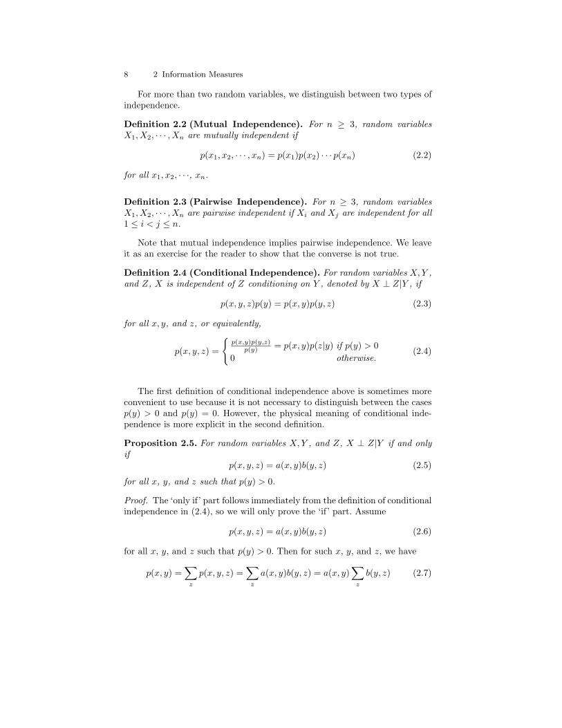
For more than two random variables, we distinguish between two types ofindependence.
Definition 2.2 (Mutual Independence). For n ≥ 3, random variablesX1, X2, · · · , Xn are mutually independent if
p(x1, x2, · · · , xn) = p(x1)p(x2) · · · p(xn) (2.2)
for all x1, x2, · · ·, xn.
Definition 2.3 (Pairwise Independence). For n ≥ 3, random variablesX1, X2, · · · , Xn are pairwise independent if Xi and Xj are independent for all1 ≤ i < j ≤ n.
Note that mutual independence implies pairwise independence. We leaveit as an exercise for the reader to show that the converse is not true.
Definition 2.4 (Conditional Independence). For random variables X,Y ,and Z, X is independent of Z conditioning on Y , denoted by X ⊥ Z|Y , if
p(x, y, z)p(y) = p(x, y)p(y, z) (2.3)
for all x, y, and z, or equivalently,
p(x, y, z) =
p(x,y)p(y,z)
p(y) = p(x, y)p(z|y) if p(y) > 00 otherwise.
(2.4)
The first definition of conditional independence above is sometimes moreconvenient to use because it is not necessary to distinguish between the casesp(y) > 0 and p(y) = 0. However, the physical meaning of conditional inde-pendence is more explicit in the second definition.
Proposition 2.5. For random variables X,Y , and Z, X ⊥ Z|Y if and onlyif
p(x, y, z) = a(x, y)b(y, z) (2.5)
for all x, y, and z such that p(y) > 0.
Proof. The ‘only if’ part follows immediately from the definition of conditionalindependence in (2.4), so we will only prove the ‘if’ part. Assume
p(x, y, z) = a(x, y)b(y, z) (2.6)
for all x, y, and z such that p(y) > 0. Then for such x, y, and z, we have
p(x, y) =∑z
p(x, y, z) =∑z
a(x, y)b(y, z) = a(x, y)∑z
b(y, z) (2.7)

2.1 Independence and Markov Chains 9
and
p(y, z) =∑x
p(x, y, z) =∑x
a(x, y)b(y, z) = b(y, z)∑x
a(x, y). (2.8)
Furthermore,
p(y) =∑z
p(y, z) =
(∑x
a(x, y)
)(∑z
b(y, z)
). (2.9)
Therefore,
p(x, y)p(y, z)p(y)
=
(a(x, y)
∑z
b(y, z)
)(b(y, z)
∑x
a(x, y)
)(∑
x
a(x, y)
)(∑z
b(y, z)
) (2.10)
= a(x, y)b(y, z) (2.11)= p(x, y, z). (2.12)
For x, y, and z such that p(y) = 0, since
0 ≤ p(x, y, z) ≤ p(y) = 0, (2.13)
we havep(x, y, z) = 0. (2.14)
Hence, X ⊥ Z|Y . The proof is accomplished. ut
Definition 2.6 (Markov Chain). For random variables X1, X2, · · · , Xn,where n ≥ 3, X1 → X2 → · · · → Xn forms a Markov chain if
p(x1, x2, · · · , xn)p(x2)p(x3) · · · p(xn−1)= p(x1, x2)p(x2, x3) · · · p(xn−1, xn) (2.15)
for all x1, x2, · · ·, xn, or equivalently,
p(x1, x2, · · · , xn) =p(x1, x2)p(x3|x2) · · · p(xn|xn−1) if p(x2), p(x3), · · · , p(xn−1) > 00 otherwise. (2.16)
We note that X ⊥ Z|Y is equivalent to the Markov chain X → Y → Z.
Proposition 2.7. X1 → X2 → · · · → Xn forms a Markov chain if and onlyif Xn → Xn−1 → · · · → X1 forms a Markov chain.

10 2 Information Measures
Proof. This follows directly from the symmetry in the definition of a Markovchain in (2.15). ut
In the following, we state two basic properties of a Markov chain. Theproofs are left as an exercise.
Proposition 2.8. X1 → X2 → · · · → Xn forms a Markov chain if and onlyif
X1 → X2 → X3
(X1, X2)→ X3 → X4
...(X1, X2, · · · , Xn−2)→ Xn−1 → Xn
(2.17)
form Markov chains.
Proposition 2.9. X1 → X2 → · · · → Xn forms a Markov chain if and onlyif
p(x1, x2, · · · , xn) = f1(x1, x2)f2(x2, x3) · · · fn−1(xn−1, xn) (2.18)
for all x1, x2, · · ·, xn such that p(x2), p(x3), · · · , p(xn−1) > 0.
Note that Proposition 2.9 is a generalization of Proposition 2.5. FromProposition 2.9, one can prove the following important property of a Markovchain. Again, the details are left as an exercise.
Proposition 2.10 (Markov subchains). Let Nn = 1, 2, · · · , n and letX1 → X2 → · · · → Xn form a Markov chain. For any subset α of Nn, denote(Xi, i ∈ α) by Xα. Then for any disjoint subsets α1, α2, · · · , αm of Nn suchthat
k1 < k2 < · · · < km (2.19)
for all kj ∈ αj, j = 1, 2, · · · ,m,
Xα1 → Xα2 → · · · → Xαm (2.20)
forms a Markov chain. That is, a subchain of X1 → X2 → · · · → Xn is alsoa Markov chain.
Example 2.11. Let X1 → X2 → · · · → X10 form a Markov chain andα1 = 1, 2, α2 = 4, α3 = 6, 8, and α4 = 10 be subsets of N10. ThenProposition 2.10 says that
(X1, X2)→ X4 → (X6, X8)→ X10 (2.21)
also forms a Markov chain.

2.1 Independence and Markov Chains 11
We have been very careful in handling probability distributions with zeroprobability masses. In the rest of the section, we show that such distributionsare very delicate in general. We first prove the following property of a strictlypositive probability distribution involving four random variables1.
Proposition 2.12. Let X1, X2, X3, and X4 be random variables such thatp(x1, x2, x3, x4) is strictly positive. Then
X1 ⊥ X4|(X2, X3)X1 ⊥ X3|(X2, X4)
⇒ X1 ⊥ (X3, X4)|X2. (2.22)
Proof. If X1 ⊥ X4|(X2, X3), we have
p(x1, x2, x3, x4) =p(x1, x2, x3)p(x2, x3, x4)
p(x2, x3). (2.23)
On the other hand, if X1 ⊥ X3|(X2, X4), we have
p(x1, x2, x3, x4) =p(x1, x2, x4)p(x2, x3, x4)
p(x2, x4). (2.24)
Equating (2.23) and (2.24), we have
p(x1, x2, x3) =p(x2, x3)p(x1, x2, x4)
p(x2, x4). (2.25)
Then
p(x1, x2) =∑x3
p(x1, x2, x3) (2.26)
=∑x3
p(x2, x3)p(x1, x2, x4)p(x2, x4)
(2.27)
=p(x2)p(x1, x2, x4)
p(x2, x4), (2.28)
orp(x1, x2, x4)p(x2, x4)
=p(x1, x2)p(x2)
. (2.29)
Hence from (2.24),
p(x1, x2, x3, x4) =p(x1, x2, x4)p(x2, x3, x4)
p(x2, x4)=p(x1, x2)p(x2, x3, x4)
p(x2)(2.30)
for all x1, x2, x3, and x4, i.e., X1 ⊥ (X3, X4)|X2. ut1 Proposition 2.12 is called the intersection axiom in Bayesian networks. See [259].

12 2 Information Measures
If p(x1, x2, x3, x4) = 0 for some x1, x2, x3, and x4, i.e., p is not strictlypositive, the arguments in the above proof are not valid. In fact, the propo-sition may not hold in this case. For instance, let X1 = Y , X2 = Z, andX3 = X4 = (Y,Z), where Y and Z are independent random variables. ThenX1 ⊥ X4|(X2, X3), X1 ⊥ X3|(X2, X4), but X1 6⊥ (X3, X4)|X2. Note thatfor this construction, p is not strictly positive because p(x1, x2, x3, x4) = 0 ifx3 6= (x1, x2) or x4 6= (x1, x2).
The above example is somewhat counter-intuitive because it appears thatProposition 2.12 should hold for all probability distributions via a continuityargument. Specifically, such an argument goes like this. For any distributionp, let pk be a sequence of strictly positive distributions such that pk → pand pk satisfies (2.23) and (2.24) for all k, i.e.,
pk(x1, x2, x3, x4)pk(x2, x3) = pk(x1, x2, x3)pk(x2, x3, x4) (2.31)
and
pk(x1, x2, x3, x4)pk(x2, x4) = pk(x1, x2, x4)pk(x2, x3, x4). (2.32)
Then by the proposition, pk also satisfies (2.30), i.e.,
pk(x1, x2, x3, x4)pk(x2) = pk(x1, x2)pk(x2, x3, x4). (2.33)
Letting k →∞, we have
p(x1, x2, x3, x4)p(x2) = p(x1, x2)p(x2, x3, x4) (2.34)
for all x1, x2, x3, and x4, i.e., X1 ⊥ (X3, X4)|X2. Such an argument wouldbe valid if there always exists a sequence pk as prescribed. However, theexistence of the distribution p(x1, x2, x3, x4) constructed immediately afterProposition 2.12 simply says that it is not always possible to find such asequence pk.
Therefore, probability distributions which are not strictly positive can bevery delicate. For strictly positive distributions, we see from Proposition 2.5that their conditional independence structures are closely related to the fac-torization problem of such distributions, which has been investigated by Chan[57].
2.2 Shannon’s Information Measures
We begin this section by introducing the entropy of a random variable. Aswe will see shortly, all Shannon’s information measures can be expressed aslinear combinations of entropies.
Definition 2.13. The entropy H(X) of a random variable X is defined as
H(X) = −∑x
p(x) log p(x). (2.35)

2.2 Shannon’s Information Measures 13
In all definitions of information measures, we adopt the convention thatsummation is taken over the corresponding support. Such a convention isnecessary because p(x) log p(x) in (2.35) is undefined if p(x) = 0.
The base of the logarithm in (2.35) can be chosen to be any convenientreal number great than 1. We write H(X) as Hα(X) when the base of thelogarithm is α. When the base of the logarithm is 2, the unit for entropy isthe bit. When the base of the logarithm is e, the unit for entropy is the nat.When the base of the logarithm is an integer D ≥ 2, the unit for entropy isthe D-it (D-ary digit). In the context of source coding, the base is usuallytaken to be the size of the code alphabet. This will be discussed in Chapter 4.
In computer science a bit means an entity which can take the value 0 or 1.In information theory the entropy of a random variable is measured in bits.The reader should distinguish these two meanings of a bit from each othercarefully.
Let g(X) be any function of a random variable X. We will denote theexpectation of g(X) by Eg(X), i.e.,
Eg(X) =∑x
p(x)g(x), (2.36)
where the summation is over SX . Then the definition of the entropy of arandom variable X can be written as
H(X) = −E log p(X). (2.37)
Expressions of Shannon’s information measures in terms of expectations willbe useful in subsequent discussions.
The entropy H(X) of a random variable X is a functional of the prob-ability distribution p(x) which measures the average amount of informationcontained in X, or equivalently, the average amount of uncertainty removedupon revealing the outcome of X. Note that H(X) depends only on p(x), noton the actual values in X . Occasionally, we also denote H(X) by H(p).
For 0 ≤ γ ≤ 1, define
hb(γ) = −γ log γ − (1− γ) log(1− γ) (2.38)
with the convention 0 log 0 = 0, so that hb(0) = hb(1) = 0. With this conven-tion, hb(γ) is continuous at γ = 0 and γ = 1. hb is called the binary entropyfunction. For a binary random variable X with distribution γ, 1− γ,
H(X) = hb(γ). (2.39)
Figure 2.1 shows the graph hb(γ) versus γ in the base 2. Note that hb(γ)achieves the maximum value 1 when γ = 1
2 .The definition of the joint entropy of two random variables is similar to
the definition of the entropy of a single random variable. Extension of thisdefinition to more than two random variables is straightforward.

14 2 Information Measures
γ
γ
Fig. 2.1. hb(q) versus q in the base 2.
Definition 2.14. The joint entropy H(X,Y ) of a pair of random variablesX and Y is defined as
H(X,Y ) = −∑x,y
p(x, y) log p(x, y) = −E log p(X,Y ). (2.40)
For two random variables, we define in the following the conditional en-tropy of one random variable when the other random variable is given.
Definition 2.15. For random variables X and Y , the conditional entropy ofY given X is defined as
H(Y |X) = −∑x,y
p(x, y) log p(y|x) = −E log p(Y |X). (2.41)
From (2.41), we can write
H(Y |X) =∑x
p(x)
[−∑y
p(y|x) log p(y|x)
]. (2.42)
The inner sum is the entropy of Y conditioning on a fixed x ∈ SX . Thus weare motivated to express H(Y |X) as
H(Y |X) =∑x
p(x)H(Y |X = x), (2.43)
whereH(Y |X = x) = −
∑y
p(y|x) log p(y|x). (2.44)
Observe that the right hand sides of (2.35) and (2.44) have exactly the sameform. Similarly, for H(Y |X,Z), we write

2.2 Shannon’s Information Measures 15
H(Y |X,Z) =∑z
p(z)H(Y |X,Z = z), (2.45)
whereH(Y |X,Z = z) = −
∑x,y
p(x, y|z) log p(y|x, z). (2.46)
Proposition 2.16.
H(X,Y ) = H(X) +H(Y |X) (2.47)
andH(X,Y ) = H(Y ) +H(X|Y ). (2.48)
Proof. Consider
H(X,Y ) = −E log p(X,Y ) (2.49)= −E log[p(X)p(Y |X)] (2.50)= −E log p(X)− E log p(Y |X) (2.51)= H(X) +H(Y |X). (2.52)
Note that (2.50) is justified because the summation of the expectation is overSXY , and we have used the linearity of expectation2 to obtain (2.51). Thisproves (2.47), and (2.48) follows by symmetry. ut
This proposition has the following interpretation. Consider revealing theoutcome of a pair of random variables X and Y in two steps: first the outcomeof X and then the outcome of Y . Then the proposition says that the totalamount of uncertainty removed upon revealing both X and Y is equal to thesum of the uncertainty removed upon revealing X (uncertainty removed in thefirst step) and the uncertainty removed upon revealing Y once X is known(uncertainty removed in the second step).
Definition 2.17. For random variables X and Y , the mutual informationbetween X and Y is defined as
I(X;Y ) =∑x,y
p(x, y) logp(x, y)p(x)p(y)
= E logp(X,Y )p(X)p(Y )
. (2.53)
Remark I(X;Y ) is symmetrical in X and Y .
Proposition 2.18. The mutual information between a random variable Xand itself is equal to the entropy of X, i.e., I(X;X) = H(X).2 See Problem 6 at the end of the chapter.

16 2 Information Measures
Proof. This can be seen by considering
I(X;X) = E logp(X)p(X)2
(2.54)
= −E log p(X) (2.55)= H(X). (2.56)
The proposition is proved. ut
Remark The entropy of X is sometimes called the self-information of X.
Proposition 2.19.
I(X;Y ) = H(X)−H(X|Y ), (2.57)I(X;Y ) = H(Y )−H(Y |X), (2.58)
andI(X;Y ) = H(X) +H(Y )−H(X,Y ), (2.59)
provided that all the entropies and conditional entropies are finite (see Exam-ple 2.46 in Section 2.8).
The proof of this proposition is left as an exercise.
From (2.57), we can interpret I(X;Y ) as the reduction in uncertaintyabout X when Y is given, or equivalently, the amount of information aboutX provided by Y . Since I(X;Y ) is symmetrical in X and Y , from (2.58), wecan as well interpret I(X;Y ) as the amount of information about Y providedby X.
The relations between the (joint) entropies, conditional entropies, and mu-tual information for two random variables X and Y are given in Propositions2.16 and 2.19. These relations can be summarized by the diagram in Figure 2.2which is a variation of the Venn diagram3. One can check that all the rela-tions between Shannon’s information measures for X and Y which are shownin Figure 2.2 are consistent with the relations given in Propositions 2.16 and2.19. This one-to-one correspondence between Shannon’s information mea-sures and set theory is not just a coincidence for two random variables. Wewill discuss this in depth when we introduce the I-Measure in Chapter 3.
Analogous to entropy, there is a conditional version of mutual informationcalled conditional mutual information.
3 The rectangle representing the universal set in a usual Venn diagram is missingin Figure 2.2.
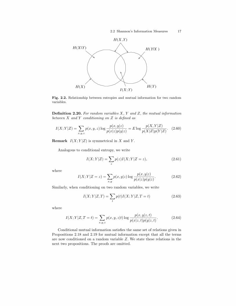
2.2 Shannon’s Information Measures 17
H ( X , Y )
H ( X | Y ) H ( Y|X )
H ( Y ) I ( X ; Y )
H ( X )
Fig. 2.2. Relationship between entropies and mutual information for two randomvariables.
Definition 2.20. For random variables X, Y and Z, the mutual informationbetween X and Y conditioning on Z is defined as
I(X;Y |Z) =∑x,y,z
p(x, y, z) logp(x, y|z)
p(x|z)p(y|z)= E log
p(X,Y |Z)p(X|Z)p(Y |Z)
. (2.60)
Remark I(X;Y |Z) is symmetrical in X and Y .
Analogous to conditional entropy, we write
I(X;Y |Z) =∑z
p(z)I(X;Y |Z = z), (2.61)
where
I(X;Y |Z = z) =∑x,y
p(x, y|z) logp(x, y|z)
p(x|z)p(y|z). (2.62)
Similarly, when conditioning on two random variables, we write
I(X;Y |Z, T ) =∑t
p(t)I(X;Y |Z, T = t) (2.63)
where
I(X;Y |Z, T = t) =∑x,y,z
p(x, y, z|t) logp(x, y|z, t)
p(x|z, t)p(y|z, t). (2.64)
Conditional mutual information satisfies the same set of relations given inPropositions 2.18 and 2.19 for mutual information except that all the termsare now conditioned on a random variable Z. We state these relations in thenext two propositions. The proofs are omitted.

18 2 Information Measures
Proposition 2.21. The mutual information between a random variable Xand itself conditioning on a random variable Z is equal to the conditionalentropy of X given Z, i.e., I(X;X|Z) = H(X|Z).
Proposition 2.22.
I(X;Y |Z) = H(X|Z)−H(X|Y,Z), (2.65)I(X;Y |Z) = H(Y |Z)−H(Y |X,Z), (2.66)
andI(X;Y |Z) = H(X|Z) +H(Y |Z)−H(X,Y |Z), (2.67)
provided that all the conditional entropies are finite.
To conclude this section, we show that all Shannon’s information measuresare special cases of conditional mutual information. Let Φ be a degenerate ran-dom variable, i.e., Φ takes a constant value with probability 1. Consider themutual information I(X;Y |Z). When X = Y and Z = Φ, I(X;Y |Z) becomesthe entropy H(X). When X = Y , I(X;Y |Z) becomes the conditional entropyH(X|Z). When Z = Φ, I(X;Y |Z) becomes the mutual information I(X;Y ).Thus all Shannon’s information measures are special cases of conditional mu-tual information.
2.3 Continuity of Shannon’s Information Measures forFixed Finite Alphabets
In this section, we prove that for fixed finite alphabets, all Shannon’s infor-mation measures are continuous functionals of the joint distribution of therandom variables involved. To formulate the notion of continuity, we firstintroduce the variational distance4 as a distance measure between two prob-ability distributions on a common alphabet.
Definition 2.23. Let p and q be two probability distributions on a commonalphabet X . The variational distance between p and q is defined as
V (p, q) =∑x∈X|p(x)− q(x)|. (2.68)
According to (2.35), the entropy of a distribution p on an alphabet X isdefined as
H(p) = −∑x∈Sp
p(x) log p(x) (2.69)
where Sp denotes the support of p and Sp ⊂ X . Let PX be the set of all distri-butions on X . In order for H(p) to be continuous with respect to convergencein variational distance at p ∈ PX , for any ε > 0, there exists δ > 0 such that4 Also referred to as the L1 distance in mathematics.

2.3 Continuity of Shannon’s Information Measures for Fixed Finite Alphabets 19
|H(p)−H(q)| < ε (2.70)
for all q ∈ PX satisfyingV (p, q) < δ, (2.71)
or equivalently, for all p ∈ PX ,
limp′→p
H(p′) = H
(limp′→p
p′)
= H(p), (2.72)
where the convergence p′ → p is in variational distance.Since a log a→ 0 as a→ 0, we define a function l : [0,∞)→ < by
l(a) =a log a if a > 00 if a = 0, (2.73)
i.e., l(a) is a continuous extension of a log a. Then (2.69) can be rewritten as
H(p) = −∑x∈X
l(p(x)), (2.74)
where the summation above is over all x in X instead of Sp. Upon defining afunction lx : PX → < for all x ∈ X by
lx(p) = l(p(x)), (2.75)
(2.74) becomesH(p) = −
∑x∈X
lx(p). (2.76)
Evidently, lx(p) is continuous in p (with respect to convergence in variationaldistance). Since the summation in (2.76) involves a finite number of terms,we conclude that H(p) is a continuous functional of p.
We now proceed to prove the continuity of conditional mutual informationwhich covers all cases of Shannon’s information measures. Consider I(X;Y |Z)and let pXY Z be the joint distribution of X, Y , and Z, where the alphabetsX , Y, and Z are assumed to be finite. From (2.47) and (2.67), we obtain
I(X;Y |Z) = H(X,Z) +H(Y, Z)−H(X,Y, Z)−H(Z). (2.77)
Note that each term on the right hand side above is the unconditional entropyof the corresponding marginal distribution. Then (2.77) can be rewritten as
IX;Y |Z(pXY Z) = H(pXZ) +H(pY Z)−H(pXY Z)−H(pZ), (2.78)
where we have used IX;Y |Z(pXY Z) to denote I(X;Y |Z). It follows that

20 2 Information Measures
limp′XYZ
→pXYZIX;Y |Z(p′XY Z)
= limp′XYZ
→pXYZ[H(p′XZ) +H(p′Y Z)−H(p′XY Z)−H(p′Z)] (2.79)
= limp′XYZ
→pXYZH(p′XZ) + lim
p′XYZ
→pXYZH(p′Y Z)
− limp′XYZ
→pXYZH(p′XY Z)− lim
p′XYZ
→pXYZH(p′Z). (2.80)
It can readily be proved, for example, that
limp′XYZ
→pXYZp′XZ = pXZ , (2.81)
so that
limp′XYZ
→pXYZH(p′XZ) = H
(lim
p′XYZ
→pXYZp′XZ
)= H(pXZ) (2.82)
by the continuity of H(·) when the alphabets involved are fixed and finite.The details are left as an exercise. Hence, we conclude that
limp′XYZ
→pXYZIX;Y |Z(p′XY Z)
= H(pXZ) +H(pY Z)−H(pXY Z)−H(pZ) (2.83)= IX;Y |Z(pXY Z), (2.84)
i.e., IX;Y |Z(pXY Z) is a continuous functional of pXY Z .We have completed the proof of the continuity of all Shannon’s informa-
tion measures with respect to convergence in variational distance for fixedfinite alphabets. However, this result is rather restrictive and need to be ap-plied with caution. It is because fixed finite alphabets are assumed for therandom variables involved, and whether continuity holds depends criticallyon the distance measure used. In fact, Shannon’s information measures areeverywhere discontinuous with respect to convergence in a number of com-monly used distance measures if the alphabets are not fixed. We refer thereaders to Problems 27 to 29 for a discussion.
2.4 Chain Rules
In this section, we present a collection of information identities known as thechain rules which are often used in information theory.
Proposition 2.24 (Chain Rule for Entropy).
H(X1, X2, · · · , Xn) =n∑i=1
H(Xi|X1, · · · , Xi−1). (2.85)

2.4 Chain Rules 21
Proof. The chain rule for n = 2 has been proved in Proposition 2.16. Weprove the chain rule by induction on n. Assume (2.85) is true for n = m,where m ≥ 2. Then
H(X1, · · · , Xm, Xm+1)= H(X1, · · · , Xm) +H(Xm+1|X1, · · · , Xm) (2.86)
=m∑i=1
H(Xi|X1, · · · , Xi−1) +H(Xm+1|X1, · · · , Xm) (2.87)
=m+1∑i=1
H(Xi|X1, · · · , Xi−1), (2.88)
where in (2.86) we have used (2.47) by letting X = (X1, · · · , Xm) and Y =Xm+1, and in (2.87) we have used (2.85) for n = m. This proves the chainrule for entropy. ut
The chain rule for entropy has the following conditional version.
Proposition 2.25 (Chain Rule for Conditional Entropy).
H(X1, X2, · · · , Xn|Y ) =n∑i=1
H(Xi|X1, · · · , Xi−1, Y ). (2.89)
Proof. This can be proved by considering
H(X1, X2, · · · , Xn|Y )= H(X1, X2, · · · , Xn, Y )−H(Y ) (2.90)= H((X1, Y ), X2, · · · , Xn)−H(Y ) (2.91)
= H(X1, Y ) +n∑i=2
H(Xi|X1, · · · , Xi−1, Y )−H(Y ) (2.92)
= H(X1|Y ) +n∑i=2
H(Xi|X1, · · · , Xi−1, Y ) (2.93)
=n∑i=1
H(Xi|X1, · · · , Xi−1, Y ), (2.94)
where (2.90) and (2.93) follow from Proposition 2.16, while (2.92) follows fromProposition 2.24. ut
Proposition 2.26 (Chain Rule for Mutual Information).
I(X1, X2, · · · , Xn;Y ) =n∑i=1
I(Xi;Y |X1, · · · , Xi−1). (2.95)

22 2 Information Measures
Proof. Consider
I(X1, X2, · · · , Xn;Y )= H(X1, X2, · · · , Xn)−H(X1, X2, · · · , Xn|Y ) (2.96)
=n∑i=1
[H(Xi|X1, · · · , Xi−1)−H(Xi|X1, · · · , Xi−1, Y )] (2.97)
=n∑i=1
I(Xi;Y |X1, · · · , Xi−1), (2.98)
where in (2.97), we have invoked both Propositions 2.24 and 2.25. The chainrule for mutual information is proved. ut
Proposition 2.27 (Chain Rule for Conditional Mutual Information).For random variables X1, X2, · · · , Xn, Y , and Z,
I(X1, X2, · · · , Xn;Y |Z) =n∑i=1
I(Xi;Y |X1, · · · , Xi−1, Z). (2.99)
Proof. This is the conditional version of the chain rule for mutual information.The proof is similar to that for Proposition 2.25. The details are omitted. ut
2.5 Informational Divergence
Let p and q be two probability distributions on a common alphabet X . Wevery often want to measure how much p is different from q, and vice versa. Inorder to be useful, this measure must satisfy the requirements that it is alwaysnonnegative and it takes the zero value if and only if p = q. We denote thesupport of p and q by Sp and Sq, respectively. The informational divergencedefined below serves this purpose.
Definition 2.28. The informational divergence between two probability dis-tributions p and q on a common alphabet X is defined as
D(p‖q) =∑x
p(x) logp(x)q(x)
= Ep logp(X)q(X)
, (2.100)
where Ep denotes expectation with respect to p.
In the above definition, in addition to the convention that the summationis taken over Sp, we further adopt the convention c log c
0 = ∞ for c > 0.With this convention, if D(p‖q) < ∞, then p(x) = 0 whenever q(x) = 0, i.e.,Sp ⊂ Sq.

2.5 Informational Divergence 23
In the literature, the informational divergence is also referred to as relativeentropy or the Kullback-Leibler distance. We note that D(p‖q) is not symmet-rical in p and q, so it is not a true metric or “distance.” Moreover, D(·‖·) doesnot satisfy the triangular inequality (see Problem 13).
In the rest of the book, the informational divergence will be referred to asdivergence for brevity. Before we prove that divergence is always nonnegative,we first establish the following simple but important inequality called thefundamental inequality in information theory.
Lemma 2.29 (Fundamental Inequality). For any a > 0,
ln a ≤ a− 1 (2.101)
with equality if and only if a = 1.
Proof. Let f(a) = ln a − a + 1. Then f ′(a) = 1/a − 1 and f ′′(a) = −1/a2.Since f(1) = 0, f ′(1) = 0, and f ′′(1) = −1 < 0, we see that f(a) attainsits maximum value 0 when a = 1. This proves (2.101). It is also clear thatequality holds in (2.101) if and only if a = 1. Figure 2.3 is an illustration ofthe fundamental inequality. ut
!0.5 0 0.5 1 1.5 2 2.5 3!1.5
!1
!0.5
0
0.5
1
1.5
1 a
!1 a
ln a
Fig. 2.3. The fundamental inequality ln a ≤ a− 1.
Corollary 2.30. For any a > 0,
ln a ≥ 1− 1a
(2.102)
with equality if and only if a = 1.
Proof. This can be proved by replacing a by 1/a in (2.101). ut
We can see from Figure 2.3 that the fundamental inequality results fromthe convexity of the logarithmic function. In fact, many important results in

24 2 Information Measures
information theory are also direct or indirect consequences of the convexityof the logarithmic function!
Theorem 2.31 (Divergence Inequality). For any two probability distribu-tions p and q on a common alphabet X ,
D(p‖q) ≥ 0 (2.103)
with equality if and only if p = q.
Proof. If q(x) = 0 for some x ∈ Sp, then D(p‖q) = ∞ and the theorem istrivially true. Therefore, we assume that q(x) > 0 for all x ∈ Sp. Consider
D(p‖q) = (log e)∑x∈Sp
p(x) lnp(x)q(x)
(2.104)
≥ (log e)∑x∈Sp
p(x)(
1− q(x)p(x)
)(2.105)
= (log e)
∑x∈Sp
p(x)−∑x∈Sp
q(x)
(2.106)
≥ 0, (2.107)
where (2.105) results from an application of (2.102), and (2.107) follows from∑x∈Sp
q(x) ≤ 1 =∑x∈Sp
p(x). (2.108)
This proves (2.103).For equality to hold in (2.103), equality must hold in (2.105) for all x ∈ Sp
and also in (2.107). For the former, we see from Lemma 2.29 that this is thecase if and only if
p(x) = q(x) for all x ∈ Sp, (2.109)
which implies ∑x∈Sp
q(x) =∑x∈Sp
p(x) = 1, (2.110)
i.e., (2.107) holds with equality. Thus (2.109) is a necessary and sufficientcondition for equality to hold in (2.103).
It is immediate that p = q implies (2.109), so it remains to prove theconverse. Since
∑x q(x) = 1 and q(x) ≥ 0 for all x, p(x) = q(x) for all x ∈ Sp
implies q(x) = 0 for all x 6∈ Sp, and therefore p = q. The theorem is proved.ut
We now prove a very useful consequence of the divergence inequality calledthe log-sum inequality.

2.5 Informational Divergence 25
Theorem 2.32 (Log-Sum Inequality). For positive numbers a1, a2, · · · andnonnegative numbers b1, b2, · · · such that
∑i ai <∞ and 0 <
∑i bi <∞,
∑i
ai logaibi≥
(∑i
ai
)log∑i ai∑i bi
(2.111)
with the convention that log ai0 = ∞. Moreover, equality holds if and only if
aibi
= constant for all i.
The log-sum inequality can easily be understood by writing it out for thecase when there are two terms in each of the summations:
a1 loga1
b1+ a2 log
a2
b2≥ (a1 + a2) log
a1 + a2
b1 + b2. (2.112)
Proof of Theorem 2.32. Let a′i = ai/∑j aj and b′i = bi/
∑j bj . Then a′i and
b′i are probability distributions. Using the divergence inequality, we have
0 ≤∑i
a′i loga′ib′i
(2.113)
=∑i
ai∑j aj
logai/∑j aj
bi/∑j bj
(2.114)
=1∑j aj
[∑i
ai logaibi−
(∑i
ai
)log
∑j aj∑j bj
], (2.115)
which implies (2.111). Equality holds if and only if a′i = b′i for all i, or aibi
=constant for all i. The theorem is proved. ut
One can also prove the divergence inequality by using the log-sum in-equality (see Problem 19), so the two inequalities are in fact equivalent. Thelog-sum inequality also finds application in proving the next theorem whichgives a lower bound on the divergence between two probability distributionson a common alphabet in terms of the variational distance between them. Wewill see further applications of the log-sum inequality when we discuss theconvergence of some iterative algorithms in Chapter 9.
Theorem 2.33 (Pinsker’s Inequality).
D(p‖q) ≥ 12 ln 2
V 2(p, q). (2.116)
Both divergence and the variational distance can be used as measures ofthe difference between two probability distributions defined on the same al-phabet. Pinsker’s inequality has the important implication that for two prob-ability distributions p and q defined on the same alphabet, if D(p‖q) is small,

26 2 Information Measures
then so is V (p, q). Furthermore, for a sequence of probability distributionsqk, as k → ∞, if D(p‖qk) → 0, then V (p, qk) → 0. In other words, conver-gence in divergence5 is a stronger notion of convergence than convergence invariational distance.
The proof of Pinsker’s inequality as well as its consequence discussed aboveis left as an exercise (see Problems 22 and 23).
2.6 The Basic Inequalities
In this section, we prove that all Shannon’s information measures, namelyentropy, conditional entropy, mutual information, and conditional mutual in-formation are always nonnegative. By this, we mean that these quantities arenonnegative for all joint distributions for the random variables involved.
Theorem 2.34. For random variables X, Y , and Z,
I(X;Y |Z) ≥ 0, (2.117)
with equality if and only if X and Y are independent when conditioning onZ.
Proof. Observe that
I(X;Y |Z)
=∑x,y,z
p(x, y, z) logp(x, y|z)
p(x|z)p(y|z)(2.118)
=∑z
p(z)∑x,y
p(x, y|z) logp(x, y|z)
p(x|z)p(y|z)(2.119)
=∑z
p(z)D(pXY |z‖pX|zpY |z), (2.120)
where we have used pXY |z to denote p(x, y|z), (x, y) ∈ X × Y, etc. Sincefor a fixed z, both pXY |z and pX|zpY |z are joint probability distributions onX × Y, we have
D(pXY |z‖pX|zpY |z) ≥ 0. (2.121)
Therefore, we conclude that I(X;Y |Z) ≥ 0. Finally, we see from Theorem 2.31that I(X;Y |Z) = 0 if and only if for all z ∈ Sz,
p(x, y|z) = p(x|z)p(y|z), (2.122)
5 In Harremoes [141], a sequence of probability distributions qk converges to aprobability distribution p if D(qk‖p) → 0 as k → ∞, which is different fromour discussion here. Nevertheless, as k → 0, it holds that if D(qk‖p) → 0, thenV (p, qk)→ 0.

2.6 The Basic Inequalities 27
orp(x, y, z) = p(x, z)p(y|z) (2.123)
for all x and y. Therefore, X and Y are independent conditioning on Z. Theproof is accomplished. ut
As we have seen in Section 2.2 that all Shannon’s information measuresare special cases of conditional mutual information, we already have provedthat all Shannon’s information measures are always nonnegative. The nonneg-ativity of all Shannon’s information measures are called the basic inequalities.
For entropy and conditional entropy, we offer the following more directproof for their nonnegativity. Consider the entropy H(X) of a random variableX. For all x ∈ SX , since 0 < p(x) ≤ 1, log p(x) ≤ 0. It then follows from thedefinition in (2.35) that H(X) ≥ 0. For the conditional entropy H(Y |X) ofrandom variable Y given random variable X, since H(Y |X = x) ≥ 0 for eachx ∈ SX , we see from (2.43) that H(Y |X) ≥ 0.
Proposition 2.35. H(X) = 0 if and only if X is deterministic.
Proof. If X is deterministic, i.e., there exists x∗ ∈ X such that p(x∗) = 1and p(x) = 0 for all x 6= x∗, then H(X) = −p(x∗) log p(x∗) = 0. On theother hand, if X is not deterministic, i.e., there exists x∗ ∈ X such that0 < p(x∗) < 1, then H(X) ≥ −p(x∗) log p(x∗) > 0. Therefore, we concludethat H(X) = 0 if and only if X is deterministic. ut
Proposition 2.36. H(Y |X) = 0 if and only if Y is a function of X.
Proof. From (2.43), we see that H(Y |X) = 0 if and only if H(Y |X = x) = 0for each x ∈ SX . Then from the last proposition, this happens if and only ifY is deterministic for each given x. In other words, Y is a function of X. ut
Proposition 2.37. I(X;Y ) = 0 if and only if X and Y are independent.
Proof. This is a special case of Theorem 2.34 with Z being a degeneraterandom variable. ut
One can regard (conditional) mutual information as a measure of (con-ditional) dependency between two random variables. When the (conditional)mutual information is exactly equal to 0, the two random variables are (con-ditionally) independent.
We refer to inequalities involving Shannon’s information measures only(possibly with constant terms) as information inequalities. The basic inequal-ities are important examples of information inequalities. Likewise, we refer toidentities involving Shannon’s information measures only as information iden-tities. From the information identities (2.47), (2.57), and (2.65), we see thatall Shannon’s information measures can be expressed as linear combinationsof entropies provided that the latter are all finite. Specifically,

28 2 Information Measures
H(Y |X) = H(X,Y )−H(X), (2.124)I(X;Y ) = H(X) +H(Y )−H(X,Y ), (2.125)
and
I(X;Y |Z) = H(X,Z) +H(Y,Z)−H(X,Y, Z)−H(Z). (2.126)
Therefore, an information inequality is an inequality which involves only en-tropies.
As we will see later in the book, information inequalities form the mostimportant set of tools for proving converse coding theorems in informationtheory. Except for a few so-called non-Shannon-type inequalities, all knowninformation inequalities are implied by the basic inequalities. Information in-equalities will be studied systematically in Chapters 13, 14, and 15. In thenext section, we will prove some consequences of the basic inequalities whichare often used in information theory.
2.7 Some Useful Information Inequalities
In this section, we prove some useful consequences of the basic inequalitiesintroduced in the last section. Note that the conditional versions of theseinequalities can be proved by techniques similar to those used in the proof ofProposition 2.25.
Theorem 2.38 (Conditioning Does Not Increase Entropy).
H(Y |X) ≤ H(Y ) (2.127)
with equality if and only if X and Y are independent.
Proof. This can be proved by considering
H(Y |X) = H(Y )− I(X;Y ) ≤ H(Y ), (2.128)
where the inequality follows because I(X;Y ) is always nonnegative. The in-equality is tight if and only if I(X;Y ) = 0, which is equivalent by Proposi-tion 2.37 to X and Y being independent. ut
Similarly, it can be shown that H(Y |X,Z) ≤ H(Y |Z), which is the con-ditional version of the above proposition. These results have the followinginterpretation. Suppose Y is a random variable we are interested in, and Xand Z are side-information about Y . Then our uncertainty about Y cannot beincreased on the average upon receiving side-information X. Once we knowX, our uncertainty about Y again cannot be increased on the average uponfurther receiving side-information Z.
Remark Unlike entropy, the mutual information between two random vari-ables can be increased by conditioning on a third random variable. We referthe reader to Section 3.4 for a discussion.

2.7 Some Useful Information Inequalities 29
Theorem 2.39 (Independence Bound for Entropy).
H(X1, X2, · · · , Xn) ≤n∑i=1
H(Xi) (2.129)
with equality if and only if Xi, i = 1, 2, · · · , n, are mutually independent.
Proof. By the chain rule for entropy,
H(X1, X2, · · · , Xn) =n∑i=1
H(Xi|X1, · · · , Xi−1) (2.130)
≤n∑i=1
H(Xi), (2.131)
where the inequality follows because we have proved in the last theorem thatconditioning does not increase entropy. The inequality is tight if and only ifit is tight for each i, i.e.,
H(Xi|X1, · · · , Xi−1) = H(Xi) (2.132)
for 1 ≤ i ≤ n. From the last theorem, this is equivalent to Xi being indepen-dent of X1, X2, · · · , Xi−1 for each i. Then
p(x1, x2, · · · , xn)= p(x1, x2, · · · , xn−1)p(xn) (2.133)= p(p(x1, x2, · · · , xn−2)p(xn−1)p(xn) (2.134)
...= p(x1)p(x2) · · · p(xn) (2.135)
for all x1, x2, · · · , xn, i.e., X1, X2, · · · , Xn are mutually independent.Alternatively, we can prove the theorem by considering
n∑i=1
H(Xi)−H(X1, X2, · · · , Xn)
= −n∑i=1
E log p(Xi) + E log p(X1, X2, · · · , Xn) (2.136)
= −E log[p(X1)p(X2) · · · p(Xn)] + E log p(X1, X2, · · · , Xn) (2.137)
= E logp(X1, X2, · · · , Xn)
p(X1)p(X2) · · · p(Xn)(2.138)
= D(pX1X2···Xn‖pX1pX2 · · · pXn) (2.139)≥ 0, (2.140)
where equality holds if and only if

30 2 Information Measures
p(x1, x2, · · · , xn) = p(x1)p(x2) · · · p(xn) (2.141)
for all x1, x2, · · · , xn, i.e., X1, X2, · · · , Xn are mutually independent. ut
Theorem 2.40.I(X;Y,Z) ≥ I(X;Y ), (2.142)
with equality if and only if X → Y → Z forms a Markov chain.
Proof. By the chain rule for mutual information, we have
I(X;Y, Z) = I(X;Y ) + I(X;Z|Y ) ≥ I(X;Y ). (2.143)
The above inequality is tight if and only if I(X;Z|Y ) = 0, or X → Y → Zforms a Markov chain. The theorem is proved. ut
Lemma 2.41. If X → Y → Z forms a Markov chain, then
I(X;Z) ≤ I(X;Y ) (2.144)
andI(X;Z) ≤ I(Y ;Z). (2.145)
Before proving this inequality we discuss its meaning. Suppose X is arandom variable we are interested in, and Y is an observation of X. If weinfer X via Y , our uncertainty about X on the average is H(X|Y ). Nowsuppose we process Y (either deterministically or probabilistically) to obtaina random variable Z. If we infer X via Z, our uncertainty about X on theaverage is H(X|Z). Since X → Y → Z forms a Markov chain, from (2.144),we have
H(X|Z) = H(X)− I(X;Z) (2.146)≥ H(X)− I(X;Y ) (2.147)= H(X|Y ), (2.148)
i.e., further processing of Y can only increase our uncertainty about X on theaverage.
Proof of Lemma 2.41. Assume X → Y → Z, i.e., X ⊥ Z|Y . By Theorem 2.34,we have
I(X;Z|Y ) = 0. (2.149)
Then
I(X;Z) = I(X;Y, Z)− I(X;Y |Z) (2.150)≤ I(X;Y, Z) (2.151)= I(X;Y ) + I(X;Z|Y ) (2.152)= I(X;Y ). (2.153)

2.8 Fano’s Inequality 31
In (2.150) and (2.152), we have used the chain rule for mutual information.The inequality in (2.151) follows because I(X;Y |Z) is always nonnegative,and (2.153) follows from (2.149). This proves (2.144).
Since X → Y → Z is equivalent to Z → Y → X, we also have proved(2.145). This completes the proof of the lemma. ut
From Lemma 2.41, we can prove the more general data processing theorem.
Theorem 2.42 (Data Processing Theorem). If U → X → Y → V formsa Markov chain, then
I(U ;V ) ≤ I(X;Y ). (2.154)
Proof. Assume U → X → Y → V . Then by Proposition 2.10, we have U →X → Y and U → Y → V . From the first Markov chain and Lemma 2.41, wehave
I(U ;Y ) ≤ I(X;Y ). (2.155)
From the second Markov chain and Lemma 2.41, we have
I(U ;V ) ≤ I(U ;Y ). (2.156)
Combining (2.155) and (2.156), we obtain (2.154), proving the theorem. ut
2.8 Fano’s Inequality
In the last section, we have proved a few information inequalities involvingonly Shannon’s information measures. In this section, we first prove an upperbound on the entropy of a random variable in terms of the size of the alpha-bet. This inequality is then used in the proof of Fano’s inequality, which isextremely useful in proving converse coding theorems in information theory.
Theorem 2.43. For any random variable X,
H(X) ≤ log |X |, (2.157)
where |X | denotes the size of the alphabet X . This upper bound is tight if andonly if X distributes uniformly on X .
Proof. Let u be the uniform distribution on X , i.e., u(x) = |X |−1 for allx ∈ X . Then
log |X | −H(X)
= −∑x∈SX
p(x) log |X |−1 +∑x∈SX
p(x) log p(x) (2.158)

32 2 Information Measures
= −∑x∈SX
p(x) log u(x) +∑x∈SX
p(x) log p(x) (2.159)
=∑x∈SX
p(x) logp(x)u(x)
(2.160)
= D(p‖u) (2.161)≥ 0, (2.162)
proving (2.157). This upper bound is tight if and if only D(p‖u) = 0, whichfrom Theorem 2.31 is equivalent to p(x) = u(x) for all x ∈ X , completing theproof. ut
Corollary 2.44. The entropy of a random variable may take any nonnegativereal value.
Proof. Consider a random variable X and let |X | be fixed. We see from thelast theorem that H(X) = log |X | is achieved when X distributes uniformlyon X . On the other hand, H(X) = 0 is achieved when X is deterministic. Forany value 0 < a < log |X |, by the intermediate value theorem of continuousfunctions, there exists a distribution for X such that H(X) = a. Then wesee that H(X) can take any positive value by letting |X | be sufficiently large.This accomplishes the proof. ut
Remark Let |X | = D, or the random variable X is a D-ary symbol. Whenthe base of the logarithm is D, (2.157) becomes
HD(X) ≤ 1. (2.163)
Recall that the unit of entropy is the D-it when the logarithm is in the baseD. This inequality says that a D-ary symbol can carry at most 1 D-it ofinformation. This maximum is achieved when X has a uniform distribution.We already have seen the binary case when we discuss the binary entropyfunction hb(p) in Section 2.2.
We see from Theorem 2.43 that the entropy of a random variable is finite aslong as it has a finite alphabet. However, if a random variable has a countablealphabet6, its entropy may or may not be finite. This will be shown in thenext two examples.
Example 2.45. Let X be a random variable such that
PrX = i = 2−i, (2.164)
i = 1, 2, · · · . Then
H2(X) =∞∑i=1
i2−i = 2, (2.165)
which is finite.6 An alphabet is countable means that it may be countably infinite.

2.8 Fano’s Inequality 33
For a random variable X with a countable alphabet and finite entropy, weshow in Appendix 2.10 that the entropy of X can be approximated by theentropy of a truncation of the distribution of X.
Example 2.46. Let Y be a random variable which takes values in the subsetof pairs of integers
(i, j) : 1 ≤ i <∞ and 1 ≤ j ≤ 22i
2i
(2.166)
such thatPrY = (i, j) = 2−2i (2.167)
for all i and j. First, we check that
∞∑i=1
22i/2i∑j=1
PrY = (i, j) =∞∑i=1
2−2i
(22i
2i
)= 1. (2.168)
Then
H2(Y ) = −∞∑i=1
22i/2i∑j=1
2−2i log2 2−2i =∞∑i=1
1, (2.169)
which does not converge.
Let X be a random variable and X be an estimate of X which takes valuein the same alphabet X . Let the probability of error Pe be
Pe = PrX 6= X. (2.170)
If Pe = 0, i.e., X = X with probability 1, then H(X|X) = 0 by Proposi-tion 2.36. Intuitively, if Pe is small, i.e., X = X with probability close to1, then H(X|X) should be close to 0. Fano’s inequality makes this intuitionprecise.
Theorem 2.47 (Fano’s Inequality). Let X and X be random variablestaking values in the same alphabet X . Then
H(X|X) ≤ hb(Pe) + Pe log(|X | − 1), (2.171)
where hb is the binary entropy function.
Proof. Define a random variable
Y =
0 if X = X
1 if X 6= X.(2.172)
The random variable Y is an indicator of the error event X 6= X, withPrY = 1 = Pe and H(Y ) = hb(Pe). Since Y is a function X and X,

34 2 Information Measures
H(Y |X, X) = 0. (2.173)
Then
H(X|X)= H(X|X) +H(Y |X, X) (2.174)= H(X,Y |X) (2.175)= H(Y |X) +H(X|X, Y ) (2.176)≤ H(Y ) +H(X|X, Y ) (2.177)
= H(Y ) +∑x∈X
[PrX = x, Y = 0H(X|X = x, Y = 0)
+PrX = x, Y = 1H(X|X = x, Y = 1)]. (2.178)
In the above, (2.174) follows from (2.173), (2.177) follows because conditioningdoes not increase entropy, and (2.178) follows from an application of (2.43).Now X must take the value x if X = x and Y = 0. In other words, X isconditionally deterministic given X = x and Y = 0. Therefore, by Proposi-tion 2.35,
H(X|X = x, Y = 0) = 0. (2.179)
If X = x and Y = 1, then X must take a value in the set x ∈ X : x 6= xwhich contains |X | − 1 elements. From the last theorem, we have
H(X|X = x, Y = 1) ≤ log(|X | − 1), (2.180)
where this upper bound does not depend on x. Hence,
H(X|X)
≤ hb(Pe) +
(∑x∈X
PrX = x, Y = 1
)log(|X | − 1) (2.181)
= hb(Pe) + PrY = 1 log(|X | − 1) (2.182)= hb(Pe) + Pe log(|X | − 1), (2.183)
which completes the proof. ut
Very often, we only need the following simplified version when we applyFano’s inequality. The proof is omitted.
Corollary 2.48. H(X|X) < 1 + Pe log |X |.
Fano’s inequality has the following implication. If the alphabet X is finite,as Pe → 0, the upper bound in (2.171) tends to 0, which implies H(X|X) alsotends to 0. However, this is not necessarily the case if X is countable, whichis shown in the next example.

2.9 Maximum Entropy Distributions 35
Example 2.49. Let X take the value 0 with probability 1. Let Z be an inde-pendent binary random variable taking values in 0, 1. Define the randomvariable X by
X =
0 if Z = 0Y if Z = 1, (2.184)
where Y is the random variable in Example 2.46 whose entropy is infinity. Let
Pe = PrX 6= X = PrZ = 1. (2.185)
Then
H(X|X) (2.186)= H(X) (2.187)≥ H(X|Z) (2.188)= PrZ = 0H(X|Z = 0) + PrZ = 1H(X|Z = 1) (2.189)= (1− Pe) · 0 + Pe ·H(Y ) (2.190)=∞ (2.191)
for any Pe > 0. Therefore, H(X|X) does not tend to 0 as Pe → 0.
2.9 Maximum Entropy Distributions
In Theorem 2.43, we have proved that for any random variable X,
H(X) ≤ log |X |, (2.192)
with equality when X is distributed uniformly over its support. In this section,we revisit this result in the context that X is a real random variable.
To simplify our discussion, all the logarithms are in the base e. Consider thefollowing problem: Maximize H(p) over all probability distribution p definedon a countable subset S (possibly infinite) of the set of real numbers, subjectto ∑
x∈Sp
p(x)ri(x) = ai for 1 ≤ i ≤ m. (2.193)
The following theorem provides a solution to this problem.
Theorem 2.50. Letp∗(x) = e−λ0−
∑m
i=1λiri(x) (2.194)
for all x ∈ S, where λ0, λ1, · · · , λm are chosen such that the constraints in(2.193) are satisfied. Then p∗ maximizes H(p) over all probability distribu-tion p on S, subject to the constraints in (2.193).

36 2 Information Measures
Proof. For any p satisfying the constraints in (2.193), consider
H(p∗)−H(p)
= −∑x∈S
p∗(x) ln p∗(x) +∑x∈Sp
p(x) ln p(x) (2.195)
= −∑x∈S
p∗(x)
(−λ0 −
∑i
λiri(x)
)+∑x∈Sp
p(x) ln p(x) (2.196)
= λ0
(∑x∈S
p∗(x)
)+∑i
λi
(∑x∈S
p∗(x)ri(x)
)+∑x∈Sp
p(x) ln p(x) (2.197)
= λ0 · 1 +∑i
λiai +∑x∈Sp
p(x) ln p(x) (2.198)
= λ0
∑x∈Sp
p(x)
+∑i
λi
∑x∈Sp
p(x)ri(x)
+∑x∈Sp
p(x) ln p(x) (2.199)
= −∑x∈Sp
p(x)
(−λ0 −
∑i
λiri(x)
)+∑x∈Sp
p(x) ln p(x) (2.200)
= −∑x∈Sp
p(x) ln p∗(x) +∑x∈Sp
p(x) ln p(x) (2.201)
=∑x∈Sp
p(x) lnp(x)p∗(x)
(2.202)
= D(p‖p∗) (2.203)≥ 0. (2.204)
In the above, (2.200) is obtained from (2.196) by replacing p∗(x) by p(x) andx ∈ S by x ∈ Sp in the first summation, while the intermediate steps (2.197)to (2.199) are justified by noting that both p∗ and p satisfy the constraintsin (2.193). The last step is an application of the divergence inequality (Theo-rem 2.31). The proof is accomplished. ut
Remark For all x ∈ S, p∗(x) > 0, so that Sp = S.
The following corollary of Theorem 2.50 is rather subtle.
Corollary 2.51. Let p∗ be a probability distribution defined on S with
p∗(x) = e−λ0−∑m
i=1λiri(x) (2.205)
for all x ∈ S. Then p∗ maximizes H(p) over all probability distribution pdefined on S, subject to the constraints∑
x∈Sp
p(x)ri(x) =∑x∈S
p∗(x)ri(x) for 1 ≤ i ≤ m. (2.206)

2.10 Entropy Rate of Stationary Source 37
Example 2.52. Let S be finite and let the set of constraints in (2.193) beempty. Then
p∗(x) = e−λ0 , (2.207)
a constant that does not depend on x. Therefore, p∗ is simply the uniformdistribution over S, i.e., p∗(x) = |S|−1 for all x ∈ S.
Example 2.53. Let S = 0, 1, 2, · · ·, and let the set of constraints in (2.193)be ∑
x
p(x)x = a, (2.208)
where a ≥ 0, i.e., the mean of the distribution p is fixed at some nonnegativevalue a. We now determine p∗ using the prescription in Theorem 2.50. Let
qi = e−λi (2.209)
for i = 0, 1. Thenp∗(x) = q0q
x1 . (2.210)
Evidently, p∗ is a geometric distribution, so that
q0 = 1− q1. (2.211)
Finally, we invoke the constraint (2.193) on p to obtain q1 = (a + 1)−1. Thedetails are omitted.
2.10 Entropy Rate of Stationary Source
In the previous sections, we have discussed various properties of the entropy ofa finite collection of random variables. In this section, we discuss the entropyrate entropy rate of a discrete-time information source.
A discrete-time information source Xk, k ≥ 1 is an infinite collection ofrandom variables indexed by the set of positive integers. Since the index setis ordered, it is natural to regard the indices as time indices. We will refer tothe random variables Xk as letters.
We assume that H(Xk) <∞ for all k. Then for any finite subset A of theindex set k : k ≥ 1, we have
H(Xk, k ∈ A) ≤∑k∈A
H(Xk) <∞. (2.212)
However, it is not meaningful to discuss H(Xk, k ≥ 1) because the jointentropy of an infinite collection of letters is infinite except in special cases.On the other hand, since the indices are ordered, we can naturally define theentropy rate of an information source, which gives the average entropy perletter of the source.

38 2 Information Measures
Definition 2.54. The entropy rate of an information source Xk is definedby
HX = limn→∞
1nH(X1, X2, · · · , Xn) (2.213)
when the limit exists.
We show in the next two examples that the entropy rate of a source mayor may not exist.
Example 2.55. Let Xk be an i.i.d. source with generic random variable X.Then
limn→∞
1nH(X1, X2, · · · , Xn) = lim
n→∞
nH(X)n
(2.214)
= limn→∞
H(X) (2.215)
= H(X), (2.216)
i.e., the entropy rate of an i.i.d. source is the entropy of any of its single letters.
Example 2.56. Let Xk be a source such that Xk are mutually independentand H(Xk) = k for k ≥ 1. Then
1nH(X1, X2, · · · , Xn) =
1n
n∑k=1
k (2.217)
=1n
n(n+ 1)2
(2.218)
=12
(n+ 1), (2.219)
which does not converge as n→∞ although H(Xk) <∞ for all k. Therefore,the entropy rate of Xk does not exist.
Toward characterizing the asymptotic behavior of Xk, it is natural toconsider the limit
H ′X = limn→∞
H(Xn|X1, X2, · · · , Xn−1) (2.220)
if it exists. The quantity H(Xn|X1, X2, · · · , Xn−1) is interpreted as the con-ditional entropy of the next letter given that we know all the past history ofthe source, and H ′X is the limit of this quantity after the source has been runfor an indefinite amount of time.
Definition 2.57. An information source Xk is stationary if
X1, X2, · · · , Xm (2.221)
andX1+l, X2+l, · · · , Xm+l (2.222)
have the same joint distribution for any m, l ≥ 1.

2.10 Entropy Rate of Stationary Source 39
In the rest of the section, we will show that stationarity is a sufficientcondition for the existence of the entropy rate of an information source.
Lemma 2.58. Let Xk be a stationary source. Then H ′X exists.
Proof. Since H(Xn|X1, X2, · · · , Xn−1) is lower bounded by zero for all n, itsuffices to prove that H(Xn|X1, X2, · · · , Xn−1) is non-increasing in n to con-clude that the limit H ′X exists. Toward this end, for n ≥ 2, consider
H(Xn|X1, X2, · · · , Xn−1)≤ H(Xn|X2, X3, · · · , Xn−1) (2.223)= H(Xn−1|X1, X2, · · · , Xn−2), (2.224)
where the last step is justified by the stationarity of Xk. The lemma isproved. ut
Lemma 2.59 (Cesaro Mean). Let ak and bk be real numbers. If an → a asn→∞ and bn = 1
n
∑nk=1 ak, then bn → a as n→∞.
Proof. The idea of the lemma is the following. If an → a as n→∞, then theaverage of the first n terms in ak, namely bn, also tends to a as n→∞.
The lemma is formally proved as follows. Since an → a as n → ∞, forevery ε > 0, there exists N(ε) such that |an − a| < ε for all n > N(ε). Forn > N(ε), consider
|bn − a| =
∣∣∣∣∣ 1nn∑i=1
ai − a
∣∣∣∣∣ (2.225)
=
∣∣∣∣∣ 1nn∑i=1
(ai − a)
∣∣∣∣∣ (2.226)
≤ 1n
n∑i=1
|ai − a| (2.227)
=1n
N(ε)∑i=1
|ai − a|+n∑
i=N(ε)+1
|ai − a|
(2.228)
<1n
N(ε)∑i=1
|ai − a|+(n−N(ε))ε
n(2.229)
<1n
N(ε)∑i=1
|ai − a|+ ε. (2.230)
The first term tends to 0 as n → ∞. Therefore, for any ε > 0, by taking nto be sufficiently large, we can make |bn − a| < 2ε. Hence bn → a as n→∞,proving the lemma. ut

40 2 Information Measures
We now prove that H ′X is an alternative definition/interpretation of theentropy rate of Xk when Xk is stationary.
Theorem 2.60. For a stationary source Xk, the entropy rate HX exists,and it is equal to H ′X .
Proof. Since we have proved in Lemma 2.58 that H ′X always exists for astationary source Xk, in order to prove the theorem, we only have to provethat HX = H ′X . By the chain rule for entropy,
1nH(X1, X2, · · · , Xn) =
1n
n∑k=1
H(Xk|X1, X2, · · · , Xk−1). (2.231)
Sincelimk→∞
H(Xk|X1, X2, · · · , Xk−1) = H ′X (2.232)
from (2.220), it follows from Lemma 2.59 that
HX = limn→∞
1nH(X1, X2, · · · , Xn) = H ′X . (2.233)
The theorem is proved. ut
In this theorem, we have proved that the entropy rate of a random sourceXk exists under the fairly general assumption that Xk is stationary. How-ever, the entropy rate of a stationary source Xk may not carry any physicalmeaning unless Xk is also ergodic. This will be explained when we discussthe Shannon-McMillan-Breiman Theorem in Section 5.4.
Appendix 2.A: Approximation of Random Variableswith Countably Infinite Alphabets by Truncation
Let X be a random variable with a countable alphabet X such that H(X) <∞. Without loss of generality, X is taken to be the set of positive integers.Define a random variable X(m) which takes values in
Nm = 1, 2, · · · ,m (2.234)
such that
PrX(m) = k =PrX = k
PrX ∈ Nm(2.235)
for all k ∈ Nm, i.e., the distribution of X(m) is the truncation of the distri-bution of X up to m.
It is intuitively correct that H(X(m)) → H(X) as m → ∞, which weformally prove in this appendix. For every m ≥ 1, define the binary randomvariable

Appendix 2.A: Approximation of Random Variables by Truncation 41
B(m) =
1 if X ≤ m0 if X > m. (2.236)
Consider
H(X) = −m∑k=1
PrX = k log PrX = k
−∞∑
k=m+1
PrX = k log PrX = k. (2.237)
As m→∞,
−m∑k=1
PrX = k log PrX = k → H(X). (2.238)
Since H(X) <∞,
−∞∑
k=m+1
PrX = k log PrX = k → 0 (2.239)
as k →∞. Now consider
H(X)= H(X|B(m)) + I(X;B(m)) (2.240)= H(X|B(m) = 1)PrB(m) = 1+H(X|B(m) = 0)×PrB(m) = 0+ I(X;B(m)) (2.241)
= H(X(m))PrB(m) = 1+H(X|B(m) = 0)×PrB(m) = 0+ I(X;B(m)). (2.242)
As m → ∞, H(B(m)) → 0 since PrB(m) = 1 → 1. This impliesI(X;B(m))→ 0 because
I(X;B(m)) ≤ H(B(m)). (2.243)
In (2.242), we further consider
H(X|B(m) = 0)PrB(m) = 0
= −∞∑
k=m+1
PrX = k logPrX = k
PrB(m) = 0(2.244)
= −∞∑
k=m+1
PrX = k(log PrX = k
− log PrB(m) = 0) (2.245)
= −∞∑
k=m+1
(PrX = k log PrX = k)

42 2 Information Measures
+
( ∞∑k=m+1
PrX = k
)log PrB(m) = 0 (2.246)
= −∞∑
k=m+1
PrX = k log PrX = k
+PrB(m) = 0 log PrB(m) = 0. (2.247)
As m → ∞, the summation above tends to 0 by (2.239). Since PrB(m) =0 → 0, PrB(m) = 0 log PrB(m) = 0 → 0. Therefore,
H(X|B(m) = 0)PrB(m) = 0 → 0, (2.248)
and we see from (2.242) that H(X(m))→ H(X) as m→∞.
Problems
1. Let X and Y be random variables with alphabets X = Y = 1, 2, 3, 4, 5and joint distribution p(x, y) given by
125
1 1 1 1 12 1 2 0 02 0 1 1 10 3 0 2 00 0 1 1 3
.Calculate H(X), H(Y ), H(X|Y ), H(Y |X), and I(X;Y ).
2. Consider any probability distribution p(x, y, z) and let
q(x, y, z) =p(x)p(y)p(z|x, y) if p(x, y) > 00 otherwise.
a) Show that q(x, y, z) is in general not a probability distribution.b) By ignoring the fact that q(x, y, z) may not be a probability distribu-
tion, application of the divergence inequality D(p‖q) ≥ 0 would yieldthe inequality
H(X) +H(Y ) +H(Z|X,Y ) ≥ H(X,Y, Z),
which indeed is valid for all jointly distributed random variables X,Y ,and Z. Explain.
3. Prove Propositions 2.8, 2.9, 2.10, 2.19, 2.21, and 2.22.4. Give an example which shows that pairwise independence does not imply
mutual independence.5. Verify that p(x, y, z) as defined in Definition 2.4 is a probability distribu-
tion. You should exclude all the zero probability masses from the summa-tion carefully.

Problems 43
6. Linearity of expectation It is well-known that expectation is linear, i.e.,E[f(X) + g(Y )] = Ef(X) + Eg(Y ), where the summation in an expec-tation is taken over the corresponding alphabet. However, we adopt ininformation theory the convention that the summation in an expectationis taken over the corresponding support. Justify carefully the linearity ofexpectation under this convention.
7. The identity I(X;Y ) = H(X)−H(X|Y ) is invalid if H(X|Y ) (and henceH(X)) is equal to infinity. Give an example such that I(X;Y ) has a finitevalue but both H(X) and H(Y |X) are equal to infinity.
8. Let p′XY and pXY be defined on X × Y, where X and Y are fixed finitealphabets. Prove that
limp′XY→pXY
p′x = pX ,
where the limit is taken with respect to the variational distance.9. Let Cα =
∑∞n=2
1n(logn)α .
a) Prove that
Cα
<∞ if α > 1=∞ if 0 ≤ α ≤ 1.
Thenpα(n) = [Cαn(log n)α]−1, n = 2, 3, · · ·
is a probability distribution for α > 1.b) Prove that
H(pα)<∞ if α > 2=∞ if 1 < α ≤ 2.
10. Prove that H(p) is concave in p, i.e., for 0 ≤ λ ≤ 1 and λ = 1− λ,
λH(p1) + λH(p2) ≤ H(λp1 + λp2).
11. Let (X,Y ) ∼ p(x, y) = p(x)p(y|x).a) Prove that for fixed p(x), I(X;Y ) is a convex functional of p(y|x).b) Prove that for fixed p(y|x), I(X;Y ) is a concave functional of p(x).
12. Do I(X;Y ) = 0 and I(X;Y |Z) = 0 imply each other? If so, give a proof.If not, give a counterexample.
13. Give an example for whichD(·‖·) does not satisfy the triangular inequality.14. Let X be a function of Y . Prove that H(X) ≤ H(Y ). Interpret this result.15. Prove that for any n ≥ 2,
H(X1, X2, · · · , Xn) ≥∑i 6=j
H(Xi|Xj).
Give the necessary and sufficient condition for equality to hold and con-struct a nontrivial example that satisfies this condition.

44 2 Information Measures
16. Prove that for any n ≥ 2,
H(X1, X2, · · · , Xn) ≥n∑i=1
H(Xi|Xj , j 6= i).
17. Prove that
12
[H(X1, X2) +H(X2, X3) +H(X1, X3)] ≥ H(X1, X2, X3).
Hint: Sum the identities
H(X1, X2, X3) = H(Xj , j 6= i) +H(Xi|Xj , j 6= i)
for i = 1, 2, 3 and apply the result in Problem 16.18. Let Nn = 1, 2, · · · , n and denote H(Xi, i ∈ α) by H(Xα) for any subset
α of Nn. For 1 ≤ k ≤ n, let
Hk =1(n−1k−1
) ∑α:|α|=k
H(Xα).
Prove thatH1 ≥ H2 ≥ · · · ≥ Hn.
This sequence of inequalities, due to Han [134], is a generalization of theindependence bound for entropy (Theorem 2.39). See Problem 5 in Chap-ter 21 for an application of these inequalities.
19. Prove the divergence inequality by using the log-sum inequality.20. Prove that D(p‖q) is convex in the pair (p, q), i.e., if (p1, q1) and (p2, q2)
are two pairs of probability distributions on a common alphabet, then
D(λp1 + λp2‖λq1 + λq2) ≤ λD(p1‖q1) + λD(p2‖q2)
for all 0 ≤ λ ≤ 1, where λ = 1− λ.21. Let pXY and qXY be two probability distributions on X × Y. Prove that
D(pXY ‖qXY ) ≥ D(pX‖qX).22. Pinsker’s inequality Let V (p, q) denotes the variational distance between
two probability distributions p and q on a common alphabet X . We willdetermine the largest c which satisfies
D(p‖q) ≥ cd2(p, q).
a) Let A = x : p(x) ≥ q(x), p = p(A), 1 − p(A), and q = q(A), 1 −q(A). Show that D(p‖q) ≥ D(p‖q) and V (p, q) = V (p, q).
b) Show that toward determining the largest value of c, we only have toconsider the case when X is binary.

Problems 45
c) By virtue of b), it suffices to determine the largest c such that
p logp
q+ (1− p) log
1− p1− q
− 4c(p− q)2 ≥ 0
for all 0 ≤ p, q ≤ 1, with the convention that 0 log 0b = 0 for b ≥ 0
and a log a0 = ∞ for a > 0. By observing that equality in the above
holds if p = q and considering the derivative of the left hand side withrespect to q, show that the largest value of c is equal to (2 ln 2)−1.
23. Let p and qk, k ≥ 1 be probability distributions on a common alphabet.Show that if qk converges to p in divergence, then it also converges to pin variational distance.
24. Find a necessary and sufficient condition for Fano’s inequality to be tight.25. Determine the probability distribution defined on 0, 1, · · · , n that max-
imizes the entropy subject to the constraint that the mean is equal to m,where 0 ≤ m ≤ n.
26. Show that for a stationary source Xk, 1nH(X1, X2, · · · , Xn) is non-
increasing in n.27. For real numbers α > 1 and β > 0 and an integer n ≥ α, define the
probability distribution
D(α,β)n =
1−(
logαlog n
)β,
1n
(logαlog n
)β, · · · , 1
n
(logαlog n
)β,︸ ︷︷ ︸
n
0, 0, · · ·
.
Let ν = 1, 0, 0, . . . be the deterministic distribution.a) Show that limn→∞D
(ν||D(α,β)
n
)= 0.
b) Determine limn→∞H(D(α,β)n
).
28. Discontinuity of entropy with respect to convergence in divergence Let Pbe the set of all probability distributions on a countable alphabet. A func-tion f : P → < is continuous with respect to convergence in divergenceat P ∈ P if for any ε > 0, there exists δ > 0 such that |f(Q)− f(P )| < εfor all Q ∈ P satisfying D(P‖Q) < δ; otherwise, f is discontinuous at P .a) Let H : P → < be the entropy function. Show that H is discontinu-
ous at the deterministic distribution ν = 1, 0, 0, · · · , . Hint: Use theresults in Problem 27.
b) Show that H is discontinuous at P = p0, p1, p2, · · · for all P suchthat H(P ) <∞. Hint: Consider the probability distribution
Qn =p0 −
p0√log n
, p1 +p0
n√
log n, p2 +
p0
n√
log n, · · · ,
pn +p0
n√
log n, pn+1, pn+2, . . .
for large n.

46 2 Information Measures
29. Discontinuity of entropy with respect to convergence in variational dis-tance Refer to Problem 28. The continuity of a function f : P → < withrespect to convergence in variational distance can be defined similarly.a) Show that if a function f is continuous with respect to convergence
in variational distance, then it is also continuous with respect to con-vergence in divergence. Hint: Use Pinsker’s inequality.
b) Repeat b) in Problem 28 with continuity defined with respect to con-vergence in variational distance.
30. Continuity of the entropy function for a fixed finite alphabet Refer toProblems 28 and 29. Suppose the domain of H is confined to P ′, the setof all probability distributions on a fixed finite alphabet. Show that H iscontinuous with respect to convergence in divergence.
31. Let p = p1, p2, · · · , pn and q = q1, q2, · · · , qn be two sets of real num-bers such that pi ≥ pi′ and qi ≥ qi′ for all i < i′. We say that p is majorizedby q if
∑mi=1 pi ≤
∑mj=1 qj for all m = 1, 2, . . . , n, where equality holds
when m = n. A function f : <n → < is Schur-concave if f(p) ≥ f(q)whenever p is majorized by q. Now let p and q be probability distribu-tions. We will show in the following steps that H(·) is Schur-concave.a) Show that for p 6= q, there exist 1 ≤ j < k ≤ n which satisfy the
following:i) j is the largest index i such that pi < qiii) k is the smallest index i such that i > j and pi > qi
iii) pi = qi for all j < i < k.b) Consider the distribution q∗ = q∗1 , q∗2 , · · · , q∗n defined by q∗i = qi for
i 6= j, k and
(q∗j , q∗k) =
(pj , qk + (qj − pj)) if pk − qk ≥ qj − pj(qj − (pk − qk), pk) if pk − qk < qj − pj .
Note that either q∗j = pj or q∗k = pk. Show thati) q∗i ≥ q∗i′ for all i ≤ i′ii)∑mi=1 pi ≤
∑mi=1 q
∗i for all m = 1, 2, · · · , n
iii) H(q∗) ≥ H(q).c) Prove that H(p) ≥ H(q) by induction on the Hamming distance
between p and q, i.e., the number of places where p and q differ.In general, if a concave function f is symmetric, i.e. f(p) = f(p′) wherep′ is a permutation of p, then f is Schur-concave. We refer the readerto [222] for the theory of majorization. (Hardy, Littlewood, and Polya[140].)
Historical Notes
The concept of entropy has its root in thermodynamics. Shannon [292] was thefirst to use entropy as a measure of information. Informational divergence was

Historical Notes 47
introduced by Kullback and Leibler [194], and it has been studied extensivelyby Csiszar [73] and Amari [14].
The materials in this chapter can be found in most textbooks in informa-tion theory. The main concepts and results are due to Shannon [292]. Pinsker’sinequality is due to Pinsker [264]. Fano’s inequality has its origin in the con-verse proof of the channel coding theorem (to be discussed in Chapter 7) byFano [95]. Generalizations of Fano’s inequality which apply to random vari-ables with countable alphabets have been obtained by Han and Verdu [139]and by Ho [148] (see also [151]). Maximum entropy, a concept in statisticalmechanics, was expounded in Jaynes [167].


3
The I-Measure
In Chapter 2, we have shown the relationship between Shannon’s informationmeasures for two random variables by the diagram in Figure 2.2. For con-venience, Figure 2.2 is reproduced in Figure 3.1 with the random variablesX and Y replaced by X1 and X2, respectively. This diagram suggests that
X 1 X 2 H ( ) ,
X 1 X 2 H ( ) X 1 X 2 H ( )
X 2 X 1 I ( ) ; X 1 H ( )
2 X H ( )
Fig. 3.1. Relationship between entropies and mutual information for two randomvariables.
Shannon’s information measures for any n ≥ 2 random variables may have aset-theoretic structure.
In this chapter, we develop a theory which establishes a one-to-one cor-respondence between Shannon’s information measures and set theory in fullgenerality. With this correspondence, manipulations of Shannon’s informa-tion measures can be viewed as set operations, thus allowing the rich suite oftools in set theory to be used in information theory. Moreover, the structureof Shannon’s information measures can easily be visualized by means of aninformation diagram if four or fewer random variables are involved. The use

50 3 The I-Measure
of information diagrams simplifies many difficult proofs in information theoryproblems. More importantly, these results, which may be difficult to discoverin the first place, can easily be obtained by inspection of an information dia-gram.
The main concepts to be used in this chapter are from measure theory.However, it is not necessary for the reader to know measure theory to readthis chapter.
3.1 Preliminaries
In this section, we introduce a few basic concepts in measure theory which willbe used subsequently. These concepts will be illustrated by simple examples.
Definition 3.1. The field Fn generated by sets X1, X2, · · · , Xn is the collec-tion of sets which can be obtained by any sequence of usual set operations(union, intersection, complement, and difference) on X1, X2, · · · , Xn.
Definition 3.2. The atoms of Fn are sets of the form ∩ni=1Yi, where Yi iseither Xi or Xc
i , the complement of Xi.
There are 2n atoms and 22n sets in Fn. Evidently, all the atoms in Fn aredisjoint, and each set in Fn can be expressed uniquely as the union of a subsetof the atoms of Fn1. We assume that the sets X1, X2, · · · , Xn intersect witheach other generically, i.e., all the atoms of Fn are nonempty unless otherwisespecified.
Example 3.3. The sets X1 and X2 generate the field F2. The atoms of F2 are
X1 ∩ X2, Xc1 ∩ X2, X1 ∩ Xc
2 , Xc1 ∩ Xc
2 , (3.1)
which are represented by the four distinct regions in the Venn diagram inFigure 3.2. The field F2 consists of the unions of subsets of the atoms in (3.1).There are a total of 16 sets in F2, which are precisely all the sets which canbe obtained from X1 and X2 by the usual set operations.
Definition 3.4. A real function µ defined on Fn is called a signed measure ifit is set-additive, i.e., for disjoint A and B in Fn,
µ(A ∪B) = µ(A) + µ(B). (3.2)
For a signed measure µ, we have
µ(∅) = 0, (3.3)
1 We adopt the convention that the union of the empty subset of the atoms of Fnis the empty set.

3.2 The I-Measure for Two Random Variables 51
X 1 X 2
Fig. 3.2. The Venn diagram for X1 and X2.
which can be seen as follows. For any A in Fn,
µ(A) = µ(A ∪ ∅) = µ(A) + µ(∅) (3.4)
by set-additivity because A and ∅ are disjoint, which implies (3.3).A signed measure µ on Fn is completely specified by its values on the
atoms of Fn. The values of µ on the other sets in Fn can be obtained viaset-additivity.
Example 3.5. A signed measure µ on F2 is completely specified by the values
µ(X1 ∩ X2), µ(Xc1 ∩ X2), µ(X1 ∩ Xc
2), µ(Xc1 ∩ Xc
2). (3.5)
The value of µ on X1, for example, can be obtained as
µ(X1) = µ((X1 ∩ X2) ∪ (X1 ∩ Xc2)) (3.6)
= µ(X1 ∩ X2) + µ(X1 ∩ Xc2). (3.7)
3.2 The I-Measure for Two Random Variables
To fix ideas, we first formulate in this section the one-to-one correspondencebetween Shannon’s information measures and set theory for two random vari-ables. For random variables X1 and X2, let X1 and X2 be sets correspondingto X1 and X2, respectively. The sets X1 and X2 generates the field F2 whoseatoms are listed in (3.1). In our formulation, we set the universal set Ω toX1 ∪ X2 for reasons which will become clear later. With this choice of Ω, theVenn diagram for X1 and X2 is represented by the diagram in Figure 3.3. Forsimplicity, the sets X1 and X2 are respectively labeled by X1 and X2 in thediagram. We call this the information diagram for the random variables X1
and X2. In this diagram, the universal set, which is the union of X1 and X2,is not shown explicitly just as in a usual Venn diagram. Note that with our

52 3 The I-Measure
X 1 X 2
Fig. 3.3. The generic information diagram for X1 and X2.
choice of the universal set, the atom Xc1 ∩ Xc
2 degenerates to the empty set,because
Xc1 ∩ Xc
2 = (X1 ∪ X2)c = Ωc = ∅. (3.8)
Thus this atom is not shown in the information diagram in Figure 3.3.For random variables X1 and X2, the Shannon’s information measures are
H(X1), H(X2), H(X1|X2), H(X2|X1), H(X1, X2), I(X1;X2). (3.9)
Writing A ∩Bc as A−B, we now define a signed measure2 µ∗ by
µ∗(X1 − X2) = H(X1|X2) (3.10)µ∗(X2 − X1) = H(X2|X1), (3.11)
andµ∗(X1 ∩ X2) = I(X1;X2). (3.12)
These are the values of µ∗ on the nonempty atoms of F2 (i.e., atoms of F2
other than Xc1 ∩Xc
2). The values of µ∗ on the other sets in F2 can be obtainedvia set-additivity. In particular, the relations
µ∗(X1 ∪ X2) = H(X1, X2) (3.13)µ∗(X1) = H(X1), (3.14)
andµ∗(X2) = H(X2) (3.15)
can readily be verified. For example, (3.13) is seen to be true by considering
µ∗(X1 ∪ X2)= µ∗(X1 − X2) + µ∗(X2 − X1) + µ∗(X1 ∩ X2) (3.16)= H(X1|X2) +H(X2|X1) + I(X1;X2) (3.17)= H(X1, X2). (3.18)
2 It happens that µ∗ defined here for n = 2 assumes only nonnegative values, butwe will see in Section 3.4 that µ∗ can assume negative values for n ≥ 3.

3.3 Construction of the I-Measure µ* 53
The right hand sides of (3.10) to (3.15) are the six Shannon’s informationmeasures for X1 and X2 in (3.9). Now observe that (3.10) to (3.15) are con-sistent with how the Shannon’s information measures on the right hand sideare identified in Figure 3.1, with the left circle and the right circle represent-ing the sets X1 and X2, respectively. Specifically, in each of these equations,the left hand side and the right hand side correspond to each other via thefollowing substitution of symbols:
H/I ↔ µ∗
,↔ ∪;↔ ∩| ↔ −.
(3.19)
Note that we make no distinction between the symbols H and I in this sub-stitution. Thus, for two random variables X1 and X2, Shannon’s informationmeasures can be regarded formally as a signed measure on F2. We will referto µ∗ as the I-Measure for the random variables X1 and X2
3.Upon realizing that Shannon’s information measures can be viewed as a
signed measure, we can apply the rich family of operations in set theory toinformation theory. This explains why Figure 3.1 or Figure 3.3 representsthe relationships among all Shannon’s information measures for two randomvariables correctly. As an example, consider the following set identity whichis readily identified in Figure 3.3:
µ∗(X1 ∪ X2) = µ∗(X1) + µ∗(X2)− µ∗(X1 ∩ X2) (3.20)
This identity is a special case of the inclusion-exclusion formula in set theory.By means of the substitution of symbols in (3.19), we immediately obtain theinformation identity
H(X1, X2) = H(X1) +H(X2)− I(X1;X2). (3.21)
We end this section with a remark. The value of µ∗ on the atom Xc1 ∩ Xc
2
has no apparent information-theoretic meaning. In our formulation, we set theuniversal set Ω to X1∪X2 so that the atom Xc
1∩Xc2 degenerates to the empty
set. Then µ∗(Xc1 ∩ Xc
2) naturally vanishes because µ∗ is a measure, so that µ∗
is completely specified by all Shannon’s information measures involving therandom variables X1 and X2.
3.3 Construction of the I-Measure µ*
We have constructed the I-Measure for two random variables in the last sec-tion. We now construct the I-Measure for any n ≥ 2 random variables.3 The reader should not confuse µ∗ with the probability measure defining the ran-
dom variables X1 and X2. The former, however, is determined by the latter.

54 3 The I-Measure
Consider n random variables X1, X2, · · · , Xn. For any random variable X,let X be a set corresponding to X. Let
Nn = 1, 2, · · · , n. (3.22)
Define the universal set Ω to be the union of the sets X1, X2, · · · , Xn, i.e.,
Ω =⋃i∈Nn
Xi. (3.23)
We use Fn to denote the field generated by X1, X2, · · · , Xn. The set
A0 =⋂i∈Nn
Xci (3.24)
is called the empty atom of Fn because
⋂i∈Nn
Xci =
( ⋃i∈Nn
Xi
)c= Ωc = ∅. (3.25)
All the atoms of Fn other than A0 are called nonempty atoms.Let A be the set of all nonempty atoms of Fn. Then |A|, the cardinality
of A, is equal to 2n − 1. A signed measure µ on Fn is completely specified bythe values of µ on the nonempty atoms of Fn.
To simplify notation, we will use XG to denote (Xi, i ∈ G) and XG todenote ∪i∈GXi for any nonempty subset G of Nn.
Theorem 3.6. Let
B =XG : G is a nonempty subset of Nn
. (3.26)
Then a signed measure µ on Fn is completely specified by µ(B), B ∈ B,which can be any set of real numbers.
Proof. The number of elements in B is equal to the number of nonemptysubsets of Nn, which is 2n − 1. Thus |A| = |B| = 2n − 1. Let k = 2n − 1.Let u be a column k-vector of µ(A), A ∈ A, and h be a column k-vector ofµ(B), B ∈ B. Since all the sets in B can expressed uniquely as the union ofsome nonempty atoms in A, by the set-additivity of µ, for each B ∈ B, µ(B)can be expressed uniquely as the sum of some components of u. Thus
h = Cnu, (3.27)
where Cn is a unique k × k matrix. On the other hand, it can be shown(see Appendix 3.6) that for each A ∈ A, µ(A) can be expressed as a linearcombination of µ(B), B ∈ B by applications, if necessary, of the following twoidentities:

3.3 Construction of the I-Measure µ* 55
µ(A ∩B − C) = µ(A− C) + µ(B − C)− µ(A ∪B − C) (3.28)µ(A−B) = µ(A ∪B)− µ(B). (3.29)
However, the existence of the said expression does not imply its uniqueness.Nevertheless, we can write
u = Dnh (3.30)
for some k × k matrix Dn. Upon substituting (3.27) into (3.30), we obtain
u = (DnCn)u, (3.31)
which implies that Dn is the inverse of Cn as (3.31) holds regardless of thechoice of µ. Since Cn is unique, so is Dn. Therefore, µ(A), A ∈ A are uniquelydetermined once µ(B), B ∈ B are specified. Hence, a signed measure µ on Fn iscompletely specified by µ(B), B ∈ B, which can be any set of real numbers.The theorem is proved. ut
We now prove the following two lemmas which are related by the substi-tution of symbols in (3.19).
Lemma 3.7.
µ(A ∩B − C) = µ(A ∪ C) + µ(B ∪ C)− µ(A ∪B ∪ C)− µ(C). (3.32)
Proof. From (3.28) and (3.29), we have
µ(A ∩B − C)= µ(A− C) + µ(B − C)− µ(A ∪B − C) (3.33)= (µ(A ∪ C)− µ(C)) + (µ(B ∪ C)− µ(C))−(µ(A ∪B ∪ C)− µ(C)) (3.34)
= µ(A ∪ C) + µ(B ∪ C)− µ(A ∪B ∪ C)− µ(C). (3.35)
The lemma is proved. ut
Lemma 3.8.
I(X;Y |Z) = H(X,Z) +H(Y, Z)−H(X,Y, Z)−H(Z). (3.36)
Proof. Consider
I(X;Y |Z)= H(X|Z)−H(X|Y,Z) (3.37)= H(X,Z)−H(Z)− (H(X,Y, Z)−H(Y, Z)) (3.38)= H(X,Z) +H(Y,Z)−H(X,Y, Z)−H(Z). (3.39)

56 3 The I-Measure
The lemma is proved. ut
We now construct the I-Measure µ∗ on Fn using Theorem 3.6 by defining
µ∗(XG) = H(XG) (3.40)
for all nonempty subsets G of Nn. In order for µ∗ to be meaningful, it has tobe consistent with all Shannon’s information measures (via the substitution ofsymbols in (3.19)). In that case, the following must hold for all (not necessarilydisjoint) subsets G,G′, G′′ of Nn where G and G′ are nonempty:
µ∗(XG ∩ XG′ − XG′′) = I(XG;XG′ |XG′′). (3.41)
When G′′ = ∅, (3.41) becomes
µ∗(XG ∩ XG′) = I(XG;XG′). (3.42)
When G = G′, (3.41) becomes
µ∗(XG − XG′′) = H(XG|XG′′). (3.43)
When G = G′ and G′′ = ∅, (3.41) becomes
µ∗(XG) = H(XG). (3.44)
Thus (3.41) covers all the four cases of Shannon’s information measures, andit is the necessary and sufficient condition for µ∗ to be consistent with allShannon’s information measures.
Theorem 3.9. µ∗ is the unique signed measure on Fn which is consistentwith all Shannon’s information measures.
Proof. Consider
µ∗(XG ∩ XG′ − XG′′)= µ∗(XG∪G′′) + µ∗(XG′∪G′′)− µ∗(XG∪G′∪G′′)− µ∗(XG′′) (3.45)= H(XG∪G′′) +H(XG′∪G′′)−H(XG∪G′∪G′′)−H(XG′′) (3.46)= I(XG;XG′ |XG′′), (3.47)
where (3.45) and (3.47) follow from Lemmas 3.7 and 3.8, respectively, and(3.46) follows from (3.40), the definition of µ∗. Thus we have proved (3.41),i.e., µ∗ is consistent with all Shannon’s information measures.
In order that µ∗ is consistent with all Shannon’s information measures, forall nonempty subsets G of Nn, µ∗ has to satisfy (3.44), which in fact is thedefinition of µ∗ in (3.40). Therefore, µ∗ is the unique signed measure on Fnwhich is consistent with all Shannon’s information measures. ut

3.4 µ* Can be Negative 57
3.4 µ* Can be Negative
In the previous sections, we have been cautious in referring to the I-Measureµ∗ as a signed measure instead of a measure4. In this section, we show thatµ∗ in fact can take negative values for n ≥ 3.
For n = 2, the three nonempty atoms of F2 are
X1 ∩ X2, X1 − X2, X2 − X1. (3.48)
The values of µ∗ on these atoms are respectively
I(X1;X2), H(X1|X2), H(X2|X1). (3.49)
These quantities are Shannon’s information measures and hence nonnegativeby the basic inequalities. Therefore, µ∗ is always nonnegative for n = 2.
For n = 3, the seven nonempty atoms of F3 are
Xi − Xj,k, Xi ∩ Xj − Xk, X1 ∩ X2 ∩ X3, (3.50)
where 1 ≤ i < j < k ≤ 3. The values of µ∗ on the first two types of atoms are
µ∗(Xi − Xj,k) = H(Xi|Xj , Xk) (3.51)
andµ∗(Xi ∩ Xj − Xk) = I(Xi;Xj |Xk), (3.52)
respectively, which are Shannon’s information measures and therefore non-negative. However, µ∗(X1 ∩ X2 ∩ X3) does not correspond to a Shannon’sinformation measure. In the next example, we show that µ∗(X1 ∩ X2 ∩ X3)can actually be negative.
Example 3.10. In this example, all entropies are in the base 2. Let X1 and X2
be independent binary random variables with
PrXi = 0 = PrXi = 1 = 0.5, (3.53)
i = 1, 2. LetX3 = (X1 +X2) mod 2. (3.54)
It is easy to check that X3 has the same marginal distribution as X1 and X2.Thus,
H(Xi) = 1 (3.55)
for i = 1, 2, 3. Moreover, X1, X2, and X3 are pairwise independent. Therefore,
H(Xi, Xj) = 2 (3.56)
and4 A measure can assume only nonnegative values.

58 3 The I-Measure
I(Xi;Xj) = 0 (3.57)
for 1 ≤ i < j ≤ 3. We further see from (3.54) that each random variableis a function of the other two random variables. Then by the chain rule forentropy, we have
H(X1, X2, X3) = H(X1, X2) +H(X3|X1, X2) (3.58)= 2 + 0 (3.59)= 2. (3.60)
Now for 1 ≤ i < j < k ≤ 3,
I(Xi;Xj |Xk)= H(Xi, Xk) +H(Xj , Xk)−H(X1, X2, X3)−H(Xk) (3.61)= 2 + 2− 2− 1 (3.62)= 1, (3.63)
where we have invoked Lemma 3.8. It then follows that
µ∗(X1 ∩ X2 ∩ X3) = µ∗(X1 ∩ X2)− µ∗(X1 ∩ X2 − X3) (3.64)= I(X1;X2)− I(X1;X2|X3) (3.65)= 0− 1 (3.66)= −1. (3.67)
Thus µ∗ takes a negative value on the atom X1 ∩ X2 ∩ X3.
Motivated by the substitution of symbols in (3.19) for Shannon’s informa-tion measures, we will write µ∗(X1 ∩ X2 ∩ X3) as I(X1;X2;X3). In general,we will write
µ∗(XG1 ∩ XG2 ∩ · · · ∩ XGm − XF ) (3.68)
asI(XG1 ;XG2 ; · · · ;XGm |XF ) (3.69)
and refer to it as the mutual information between XG1 , XG2 , · · · , XGm condi-tioning on XF . Then (3.64) in the above example can be written as
I(X1;X2;X3) = I(X1;X2)− I(X1;X2|X3). (3.70)
For this example, I(X1;X2;X3) < 0, which implies
I(X1;X2|X3) > I(X1;X2). (3.71)
Therefore, unlike entropy, the mutual information between two random vari-ables can be increased by conditioning on a third random variable. Also, wenote in (3.70) that although the expression on the right hand side is not sym-bolically symmetrical in X1, X2, and X3, we see from the left hand side thatit is in fact symmetrical in X1, X2, and X3.

3.5 Information Diagrams 59
3.5 Information Diagrams
We have established in Section 3.3 a one-to-one correspondence between Shan-non’s information measures and set theory. Therefore, it is valid to use aninformation diagram, which is a variation of a Venn diagram, to represent therelationship between Shannon’s information measures.
For simplicity, a set Xi will be labeled by Xi in an information diagram.We have seen the generic information diagram for n = 2 in Figure 3.3. Ageneric information diagram for n = 3 is shown in Figure 3.4. The information-
X 1
X 1 X 2 H ( )
X 1 H ( )
X 2
X 3
X 1 I ( ) ; X 3
; ; X 1 I ( ) X 3 X 2
; X 1 I X 3 X 2 ( )
, X 3 X 2 X 1 H ( )
Fig. 3.4. The generic information diagram for X1, X2, and X3.
theoretic labeling of the values of µ∗ on some of the sets in F3 is shownin the diagram. As an example, the information diagram for the I-Measurefor random variables X1, X2, and X3 discussed in Example 3.10 is shown inFigure 3.5.
0
0 0
1 1
1
1
X 1
X 2
X 3
Fig. 3.5. The information diagram for X1, X2, and X3 in Example 3.10.
For n ≥ 4, it is not possible to display an information diagram perfectlyin two dimensions. In general, an information diagram for n random variables

60 3 The I-Measure
needs n− 1 dimensions to be displayed perfectly. Nevertheless, for n = 4, aninformation diagram can be displayed in two dimensions almost perfectly asshown in Figure 3.6. This information diagram is correct in that the regionrepresenting the set X4 splits each atom in Figure 3.4 into two atoms. However,the adjacency of certain atoms are not displayed correctly. For example, theset X1 ∩ X2 ∩ Xc
4 , which consists of the atoms X1 ∩ X2 ∩ X3 ∩ Xc4 and X1 ∩
X2∩Xc3∩Xc
4 , is not represented by a connected region because the two atomsare not adjacent to each other.
When µ∗ takes the value zero on an atom A of Fn, we do not need todisplay the atom A in an information diagram because the atom A doesnot contribute to µ∗(B) for any set B containing the atom A. As we willsee shortly, this can happen if certain Markov constraints are imposed onthe random variables involved, and the information diagram can be simplifiedaccordingly. In a generic information diagram (i.e., when there is no constrainton the random variables), however, all the atoms have to be displayed, as isimplied by the next theorem.
Theorem 3.11. If there is no constraint on X1, X2, · · · , Xn, then µ∗ can takeany set of nonnegative values on the nonempty atoms of Fn.
Proof. We will prove the theorem by constructing a µ∗ which can take anyset of nonnegative values on the nonempty atoms of Fn. Recall that A is theset of all nonempty atoms of Fn. Let YA, A ∈ A be mutually independentrandom variables. Now define the random variables Xi, i = 1, 2, · · · , n by
Xi = (YA : A ∈ A and A ⊂ Xi). (3.72)
We determine the I-Measure µ∗ for X1, X2, · · · , Xn so defined as follows. SinceYA are mutually independent, for any nonempty subsets G of Nn, we have
H(XG) =∑
A∈A:A⊂XG
H(YA). (3.73)
X 1
X 2
X 3
X 4
Fig. 3.6. The generic information diagram for X1, X2, X3, and X4.

3.5 Information Diagrams 61
On the other hand,
H(XG) = µ∗(XG) =∑
A∈A:A⊂XG
µ∗(A). (3.74)
Equating the right hand sides of (3.73) and (3.74), we have∑A∈A:A⊂XG
H(YA) =∑
A∈A:A⊂XG
µ∗(A). (3.75)
Evidently, we can make the above equality hold for all nonempty subsets Gof Nn by taking
µ∗(A) = H(YA) (3.76)
for all A ∈ A. By the uniqueness of µ∗, this is also the only possibility for µ∗.Since H(YA) can take any nonnegative value by Corollary 2.44, µ∗ can takeany set of nonnegative values on the nonempty atoms of Fn. The theorem isproved. ut
In the rest of this section, we explore the structure of Shannon’s informa-tion measures when X1 → X2 → · · · → Xn forms a Markov chain. To startwith, we consider n = 3, i.e., X1 → X2 → X3 forms a Markov chain. Since
µ∗(X1 ∩ Xc2 ∩ X3) = I(X1;X3|X2) = 0, (3.77)
the atom X1∩Xc2∩X3 does not have to be displayed in an information diagram.
As such, in constructing the information diagram, the regions representingthe random variables X1, X2, and X3 should overlap with each other suchthat the region corresponding to the atom X1 ∩ Xc
2 ∩ X3 is empty, while theregions corresponding to all other nonempty atoms are nonempty. Figure 3.7shows such a construction, in which each random variable is represented bya mountain5. From Figure 3.7, we see that X1 ∩ X2 ∩ X3, as the only atom
X 3 X 1 X 2
Fig. 3.7. The information diagram for the Markov chain X1 → X2 → X3.
5 This form of an information diagram for a Markov chain first appeared in Kawa-bata [176].

62 3 The I-Measure
on which µ∗ may take a negative value, now becomes identical to the atomX1 ∩ X3. Therefore, we have
I(X1;X2;X3) = µ∗(X1 ∩ X2 ∩ X3) (3.78)= µ∗(X1 ∩ X3) (3.79)= I(X1;X3) (3.80)≥ 0. (3.81)
Hence, we conclude that when X1 → X2 → X3 forms a Markov chain, µ∗ isalways nonnegative.
Next, we consider n = 4, i.e., X1 → X2 → X3 → X4 forms a Markovchain. With reference to Figure 3.6, we first show that under this Markovconstraint, µ∗ always vanishes on certain nonempty atoms:
1. The Markov chain X1 → X2 → X3 implies
I(X1;X3;X4|X2) + I(X1;X3|X2, X4) = I(X1;X3|X2) = 0. (3.82)
2. The Markov chain X1 → X2 → X4 implies
I(X1;X3;X4|X2) + I(X1;X4|X2, X3) = I(X1;X4|X2) = 0. (3.83)
3. The Markov chain X1 → X3 → X4 implies
I(X1;X2;X4|X3) + I(X1;X4|X2, X3) = I(X1;X4|X3) = 0. (3.84)
4. The Markov chain X2 → X3 → X4 implies
I(X1;X2;X4|X3) + I(X2;X4|X1, X3) = I(X2;X4|X3) = 0. (3.85)
5. The Markov chain (X1, X2)→ X3 → X4 implies
I(X1;X2;X4|X3) + I(X1;X4|X2, X3) + I(X2;X4|X1, X3)= I(X1, X2;X4|X3) (3.86)= 0. (3.87)
Now (3.82) and (3.83) imply
I(X1;X4|X2, X3) = I(X1;X3|X2, X4), (3.88)
(3.84) and (3.88) imply
I(X1;X2;X4|X3) = −I(X1;X3|X2, X4), (3.89)
and (3.85) and (3.89) imply
I(X2;X4|X1, X3) = I(X1;X3|X2, X4). (3.90)

3.5 Information Diagrams 63
The terms on the left hand sides of (3.88), (3.89), and (3.90) are the threeterms on the left hand side of (3.87). Then we substitute (3.88), (3.89), and(3.90) in (3.87) to obtain
µ∗(X1 ∩ Xc2 ∩ X3 ∩ Xc
4) = I(X1;X3|X2, X4) = 0. (3.91)
From (3.82), (3.88), (3.89), and (3.90), (3.91) implies
µ∗(X1 ∩ Xc2 ∩ X3 ∩ X4) = I(X1;X3;X4|X2) = 0 (3.92)
µ∗(X1 ∩ Xc2 ∩ Xc
3 ∩ X4) = I(X1;X4|X2, X3) = 0 (3.93)µ∗(X1 ∩ X2 ∩ Xc
3 ∩ X4) = I(X1;X2;X4|X3) = 0 (3.94)µ∗(Xc
1 ∩ X2 ∩ Xc3 ∩ X4) = I(X2;X4|X1, X3) = 0. (3.95)
From (3.91) to (3.95), we see that µ∗ always vanishes on the atoms
X1 ∩ Xc2 ∩ X3 ∩ Xc
4
X1 ∩ Xc2 ∩ X3 ∩ X4
X1 ∩ Xc2 ∩ Xc
3 ∩ X4
X1 ∩ X2 ∩ Xc3 ∩ X4
Xc1 ∩ X2 ∩ Xc
3 ∩ X4
(3.96)
of F4, which we mark by an asterisk in the information diagram in Figure 3.8.In fact, the reader can gain a lot of insight by letting I(X1;X3|X2, X4) = a ≥ 0
*
*
* * * X 3 X 1
X 4
X 2
Fig. 3.8. The atoms of F4 on which µ∗ vanishes when X1 → X2 → X3 → X4 formsa Markov chain.
in (3.82) and tracing the subsequent steps leading to the above conclusion inthe information diagram in Figure 3.6.
It is not necessary to display the five atoms in (3.96) in an informationdiagram because µ∗ always vanishes on these atoms. Therefore, in constructing

64 3 The I-Measure
X 1 X 4 X 3 X 2
Fig. 3.9. The information diagram for the Markov chain X1 → X2 → X3 → X4.
the information diagram, the regions representing the random variables shouldoverlap with each other such that the regions corresponding to these fivenonempty atoms are empty, while the regions corresponding to the other tennonempty atoms, namely
X1 ∩ Xc2 ∩ Xc
3 ∩ Xc4
X1 ∩ X2 ∩ Xc3 ∩ Xc
4
X1 ∩ X2 ∩ X3 ∩ Xc4
X1 ∩ X2 ∩ X3 ∩ X4
Xc1 ∩ X2 ∩ Xc
3 ∩ Xc4
Xc1 ∩ X2 ∩ X3 ∩ Xc
4
Xc1 ∩ X2 ∩ X3 ∩ X4
Xc1 ∩ Xc
2 ∩ X3 ∩ Xc4
Xc1 ∩ Xc
2 ∩ X3 ∩ X4
Xc1 ∩ Xc
2 ∩ Xc3 ∩ X4,
(3.97)
are nonempty. Figure 3.9 shows such a construction. The reader should com-pare the information diagrams in Figures 3.7 and 3.9 and observe that thelatter is an extension of the former.

3.5 Information Diagrams 65
From Figure 3.9, we see that the values of µ∗ on the ten nonempty atomsin (3.97) are equivalent to
H(X1|X2, X3, X4)I(X1;X2|X3, X4)I(X1;X3|X4)I(X1;X4)H(X2|X1, X3, X4)I(X2;X3|X1;X4)I(X2;X4|X1)H(X3|X1, X2, X4)I(X3;X4|X1, X2)H(X4|X1, X2, X3),
(3.98)
respectively6. Since these are all Shannon’s information measures and thusnonnegative, we conclude that µ∗ is always nonnegative.
WhenX1 → X2 → · · · → Xn forms a Markov chain, for n = 3, there is onlyone nonempty atom, namely X1∩Xc
2 ∩X3, on which µ∗ always vanishes. Thisatom can be determined directly from the Markov constraint I(X1;X3|X2) =0. For n = 4, the five nonempty atoms on which µ∗ always vanishes arelisted in (3.96). The determination of these atoms, as we have seen, is notstraightforward. We have also shown that for n = 3 and n = 4, µ∗ is alwaysnonnegative.
We will extend this theme in Chapter 12 to finite Markov random fieldswith Markov chains being a special case. For a Markov chain, the informationdiagram can always be displayed in two dimensions as in Figure 3.10, and µ∗
is always nonnegative. These will be explained in Chapter 12.
... X 1 X 2 X n -1 X n
Fig. 3.10. The information diagram for the Markov chain X1 → X2 → · · · → Xn.
6 A formal proof will be given in Theorem 12.30.

66 3 The I-Measure
3.6 Examples of Applications
In this section, we give a few examples of applications of information diagrams.These examples show how information diagrams can help solving informationtheory problems.
The use of an information diagram is highly intuitive. To obtain an infor-mation identity from an information diagram is WYSIWYG7. However, howto obtain an information inequality from an information diagram needs someexplanation.
Very often, we use a Venn diagram to represent a measure µ which takesnonnegative values. If we see in the Venn diagram two sets A and B suchthat A is a subset of B, then we can immediately conclude that µ(A) ≤ µ(B)because
µ(B)− µ(A) = µ(B −A) ≥ 0. (3.99)
However, an I-Measure µ∗ can take negative values. Therefore, when we seein an information diagram that A is a subset of B, we cannot conclude fromthis fact alone that µ∗(A) ≤ µ∗(B) unless we know from the setup of theproblem that µ∗ is nonnegative. (For example, µ∗ is nonnegative if the randomvariables involved form a Markov chain.) Instead, information inequalitiescan be obtained from an information diagram in conjunction with the basicinequalities. The following examples will illustrate how it works.
Example 3.12 (Concavity of Entropy). Let X1 ∼ p1(x) and X2 ∼ p2(x). Let
X ∼ p(x) = λp1(x) + λp2(x), (3.100)
where 0 ≤ λ ≤ 1 and λ = 1− λ. We will show that
H(X) ≥ λH(X1) + λH(X2). (3.101)
Consider the system in Figure 3.11 in which the position of the switch isdetermined by a random variable Z with
X
Z = 1
Z = 2
X 1
X 2
Fig. 3.11. The schematic diagram for Example 3.12.
7 What you see is what you get.

3.6 Examples of Applications 67
PrZ = 1 = λ and PrZ = 2 = λ, (3.102)
where Z is independent of X1 and X2. The switch takes position i if Z = i,i = 1, 2. The random variable Z is called a mixing random variable for theprobability distributions p1(x) and p2(x). Figure 3.12 shows the informationdiagram for X and Z. From the diagram, we see that X − Z is a subset of X.Since µ∗ is nonnegative for two random variables, we can conclude that
µ∗(X) ≥ µ∗(X − Z), (3.103)
which is equivalent toH(X) ≥ H(X|Z). (3.104)
Then
H(X) ≥ H(X|Z) (3.105)= PrZ = 1H(X|Z = 1) + PrZ = 2H(X|Z = 2) (3.106)= λH(X1) + λH(X2), (3.107)
proving (3.101). This shows that H(X) is a concave functional of p(x).
Example 3.13 (Convexity of Mutual Information). Let
(X,Y ) ∼ p(x, y) = p(x)p(y|x). (3.108)
We will show that for fixed p(x), I(X;Y ) is a convex functional of p(y|x).Let p1(y|x) and p2(y|x) be two transition matrices. Consider the system
in Figure 3.13 in which the position of the switch is determined by a randomvariable Z as in the last example, where Z is independent of X, i.e.,
I(X;Z) = 0. (3.109)
In the information diagram for X, Y , and Z in Figure 3.14, let
I(X;Z|Y ) = a ≥ 0. (3.110)
X Z
Fig. 3.12. The information diagram for Example 3.12.

68 3 The I-Measure
Y X
Z = 1
Z = 2 p 2 ( ) y x
p 1 ( ) y x
Fig. 3.13. The schematic diagram for Example 3.13.
Since I(X;Z) = 0, we see that
I(X;Y ;Z) = −a, (3.111)
becauseI(X;Z) = I(X;Z|Y ) + I(X;Y ;Z). (3.112)
Then
I(X;Y )= I(X;Y |Z) + I(X;Y ;Z) (3.113)= I(X;Y |Z)− a (3.114)≤ I(X;Y |Z) (3.115)= PrZ = 1I(X;Y |Z = 1) + PrZ = 2I(X;Y |Z = 2) (3.116)= λI(p(x), p1(y|x)) + λI(p(x), p2(y|x)), (3.117)
where I(p(x), pi(y|x)) denotes the mutual information between the input andoutput of a channel with input distribution p(x) and transition matrix pi(y|x).This shows that for fixed p(x), I(X;Y ) is a convex functional of p(y|x).
Example 3.14 (Concavity of Mutual Information). Let
X Z
Y
a
- a
Fig. 3.14. The information diagram for Example 3.13.

3.6 Examples of Applications 69
(X,Y ) ∼ p(x, y) = p(x)p(y|x). (3.118)
We will show that for fixed p(y|x), I(X;Y ) is a concave functional of p(x).Consider the system in Figure 3.15, where the position of the switch is
determined by a random variable Z as in the last example. In this system,when X is given, Y is independent of Z, or Z → X → Y forms a Markovchain. Then µ∗ is nonnegative, and the information diagram for X, Y , and Zis shown in Figure 3.16.
X Y p ( y | x )
Z =1 p 1 ( x )
Z =2 p 2 ( x )
Fig. 3.15. The schematic diagram for Example 3.14.
From Figure 3.16, since X∩Y−Z is a subset of X∩Y and µ∗ is nonnegative,we immediately see that
I(X;Y )≥ I(X;Y |Z) (3.119)= PrZ = 1I(X;Y |Z = 1) + PrZ = 2I(X;Y |Z = 2) (3.120)= λI(p1(x), p(y|x)) + λI(p2(x), p(y|x)). (3.121)
This shows that for fixed p(y|x), I(X;Y ) is a concave functional of p(x).
Example 3.15 (Imperfect Secrecy Theorem)). Let X be the plain text, Y bethe cipher text, and Z be the key in a secret key cryptosystem. Since X canbe recovered from Y and Z, we have
Y Z X
Fig. 3.16. The information diagram for Example 3.14.

70 3 The I-Measure
H(X|Y,Z) = 0. (3.122)
We will show that this constraint implies
I(X;Y ) ≥ H(X)−H(Z). (3.123)
The quantity I(X;Y ) is a measure of the security level of the cryptosystem.In general, we want to make I(X;Y ) small so that the eavesdropper cannotobtain too much information about the plain text X by observing the ciphertext Y . The inequality in (3.123) says that the system can attain a certainlevel of security only if H(Z) (often called the key length) is sufficiently large.In particular, if perfect secrecy is required, i.e., I(X;Y ) = 0, then H(Z) mustbe at least equal to H(X). This special case is known as Shannon’s perfectsecrecy theorem [293]8.
We now prove (3.123). Let
I(X;Y |Z) = a ≥ 0 (3.124)
I(Y ;Z|X) = b ≥ 0 (3.125)
H(Z|X,Y ) = c ≥ 0, (3.126)
andI(X;Y ;Z) = d. (3.127)
(See Figure 3.17.) Since I(Y ;Z) ≥ 0,
a
c
b d
0 X Z
Y
Fig. 3.17. The information diagram for Example 3.15.
b+ d ≥ 0. (3.128)
In comparing H(X) with H(Z), we do not have to consider I(X;Z|Y ) andI(X;Y ;Z) since they belong to both H(X) and H(Z). Then we see fromFigure 3.17 that8 Shannon used a combinatorial argument to prove this theorem. An information-
theoretic proof can be found in Massey [226].

3.6 Examples of Applications 71
H(X)−H(Z) = a− b− c. (3.129)
Therefore,
I(X;Y ) = a+ d (3.130)≥ a− b (3.131)≥ a− b− c (3.132)= H(X)−H(Z), (3.133)
where (3.131) and (3.132) follow from (3.128) and (3.126), respectively, prov-ing (3.123).
Note that in deriving our result, the assumptions that H(Y |X,Z) = 0, i.e.,the cipher text is a function of the plain text and the key, and I(X;Z) = 0,i.e., the plain text and the key are independent, are not necessary.
Example 3.16. Figure 3.18 shows the information diagram for the Markovchain X → Y → Z. From this diagram, we can identify the following two
X Y Z
Fig. 3.18. The information diagram for the Markov chain X → Y → Z.
information identities:
I(X;Y ) = I(X;Y,Z) (3.134)H(X|Y ) = H(X|Y,Z). (3.135)
Since µ∗ is nonnegative and X ∩ Z is a subset of X ∩ Y , we have
I(X;Z) ≤ I(X;Y ), (3.136)
which has already been obtained in Lemma 2.41. Similarly, we can also obtain
H(X|Y ) ≤ H(X|Z). (3.137)
Example 3.17 (Data Processing Theorem). Figure 3.19 shows the informationdiagram for the Markov chain X → Y → Z → T . Since µ∗ is nonnegative andX ∩ T is a subset of Y ∩ Z, we have
I(X;T ) ≤ I(Y ;Z), (3.138)
which is the data processing theorem (Theorem 2.42).

72 3 The I-Measure
We end this chapter by giving an application of the information diagramfor a Markov chain with five random variables.
Example 3.18. In this example, we prove with the help of an information di-agram that for five random variables X,Y, Z, T , and U such that X → Y →Z → T → U forms a Markov chain,
H(Y ) +H(T ) =
I(Z;X,Y, T, U) + I(X,Y ;T,U) +H(Y |Z) +H(T |Z). (3.139)
In the information diagram for X,Y, Z, T , and U in Figure 3.20, we firstidentify the atoms of H(Y ) and then the atoms of H(T ) by marking each ofthem by a dot. If an atom belongs to both H(Y ) and H(T ), it receives twodots. The resulting diagram represents
H(Y ) +H(T ). (3.140)
By repeating the same procedure for
I(Z;X,Y, T, U) + I(X,Y ;T,U) +H(Y |Z) +H(T |Z), (3.141)
we obtain the information diagram in Figure 3.21. Comparing these twoinformation diagrams, we find that they are identical. Hence, the infor-mation identity in (3.139) always holds conditioning on the Markov chain
X T Z Y
Fig. 3.19. The information diagram for the Markov chain X → Y → Z → T .
. .
. . .
. .
.
. . . .
. .
. .
X Y Z T U
Fig. 3.20. The atoms of H(Y ) +H(T ).

Appendix 3.A: A Variation of the Inclusion-Exclusion Formula 73
X → Y → Z → T → U . This identity is critical in proving an outer boundon the achievable coding rate region of the multiple descriptions problem inFu et al. [113]. It is virtually impossible to discover this identity without thehelp of an information diagram!
. .
. . .
. .
.
. . . .
. .
. .
X Y Z T U
Fig. 3.21. The atoms of I(Z;X,Y, T, U) + I(X,Y ;T,U) +H(Y |Z) +H(T |Z).
Appendix 3.A: A Variation of the Inclusion-ExclusionFormula
In this appendix, we show that for each A ∈ A, µ(A) can be expressed as alinear combination of µ(B), B ∈ B via applications of (3.28) and (3.29). Wefirst prove by using (3.28) the following variation of the inclusive-exclusiveformula.
Theorem 3.19. For a set-additive function µ,
µ
(n⋂k=1
Ak −B
)=∑
1≤i≤n
µ(Ai −B)−∑
1≤i<j≤n
µ(Ai ∪Aj −B)
+ · · ·+ (−1)n+1µ(A1 ∪A2 ∪ · · · ∪An −B). (3.142)
Proof. The theorem will be proved by induction on n. First, (3.142) is obvi-ously true for n = 1. Assume (3.142) is true for some n ≥ 1. Now consider
µ
(n+1⋂k=1
Ak −B
)
= µ
((n⋂k=1
Ak
)∩An+1 −B
)(3.143)
= µ
(n⋂k=1
Ak −B
)+ µ(An+1 −B)− µ
((n⋂k=1
Ak
)∪An+1 −B
)(3.144)

74 3 The I-Measure
=
∑1≤i≤n
µ(Ai −B)−∑
1≤i<j≤n
µ(Ai ∪Aj −B) + · · ·
+ (−1)n+1µ(A1 ∪A2 ∪ · · · ∪An −B)
+ µ(An+1 −B)
−µ
(n⋂k=1
(Ak ∪An+1)−B
)(3.145)
=
∑1≤i≤n
µ(Ai −B)−∑
1≤i<j≤n
µ(Ai ∪Aj −B) + · · ·
+ (−1)n+1µ(A1 ∪A2 ∪ · · · ∪An −B)
+ µ(An+1 −B)
−
∑1≤i≤n
µ(Ai ∪An+1 −B)−∑
1≤i<j≤n
µ(Ai ∪Aj ∪An+1 −B)
+ · · ·+ (−1)n+1µ(A1 ∪A2 ∪ · · · ∪An ∪An+1 −B)
(3.146)
=∑
1≤i≤n+1
µ(Ai −B)−∑
1≤i<j≤n+1
µ(Ai ∪Aj −B) + · · ·
+(−1)n+2µ(A1 ∪A2 ∪ · · · ∪An+1 −B). (3.147)
In the above, (3.28) was used in obtaining (3.144), and the induction hy-pothesis was used in obtaining (3.145) and (3.146). The theorem is proved.ut
Now a nonempty atom of Fn has the form
n⋂i=1
Yi, (3.148)
where Yi is either Xi or Xci , and there exists at least one i such that Yi = Xi.
Then we can write the atom in (3.148) as
⋂i:Yi=Xi
Xi −
⋃j:Yj=Xcj
Xj
. (3.149)
Note that the intersection above is always nonempty. Then using (3.142) and(3.29), we see that for each A ∈ A, µ(A) can be expressed as a linear combi-nation of µ(B), B ∈ B.
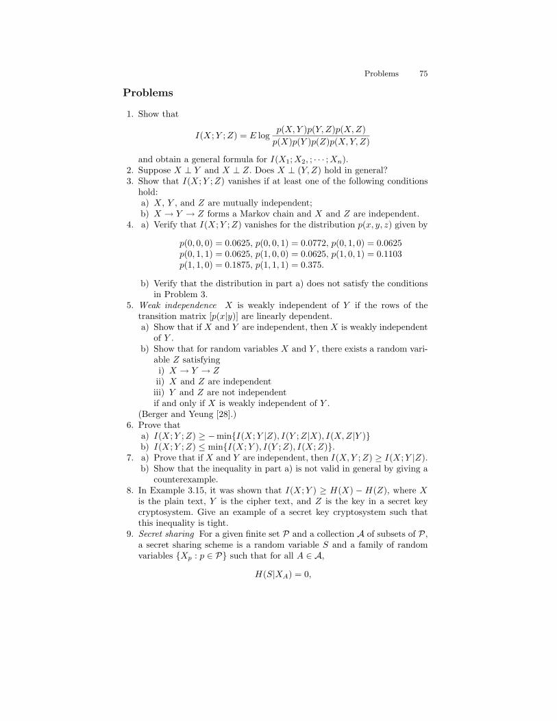
Problems 75
Problems
1. Show that
I(X;Y ;Z) = E logp(X,Y )p(Y,Z)p(X,Z)p(X)p(Y )p(Z)p(X,Y, Z)
and obtain a general formula for I(X1;X2, ; · · · ;Xn).2. Suppose X ⊥ Y and X ⊥ Z. Does X ⊥ (Y,Z) hold in general?3. Show that I(X;Y ;Z) vanishes if at least one of the following conditions
hold:a) X, Y , and Z are mutually independent;b) X → Y → Z forms a Markov chain and X and Z are independent.
4. a) Verify that I(X;Y ;Z) vanishes for the distribution p(x, y, z) given by
p(0, 0, 0) = 0.0625, p(0, 0, 1) = 0.0772, p(0, 1, 0) = 0.0625p(0, 1, 1) = 0.0625, p(1, 0, 0) = 0.0625, p(1, 0, 1) = 0.1103p(1, 1, 0) = 0.1875, p(1, 1, 1) = 0.375.
b) Verify that the distribution in part a) does not satisfy the conditionsin Problem 3.
5. Weak independence X is weakly independent of Y if the rows of thetransition matrix [p(x|y)] are linearly dependent.a) Show that if X and Y are independent, then X is weakly independent
of Y .b) Show that for random variables X and Y , there exists a random vari-
able Z satisfyingi) X → Y → Zii) X and Z are independent
iii) Y and Z are not independentif and only if X is weakly independent of Y .
(Berger and Yeung [28].)6. Prove that
a) I(X;Y ;Z) ≥ −minI(X;Y |Z), I(Y ;Z|X), I(X,Z|Y )b) I(X;Y ;Z) ≤ minI(X;Y ), I(Y ;Z), I(X;Z).
7. a) Prove that if X and Y are independent, then I(X,Y ;Z) ≥ I(X;Y |Z).b) Show that the inequality in part a) is not valid in general by giving a
counterexample.8. In Example 3.15, it was shown that I(X;Y ) ≥ H(X) −H(Z), where X
is the plain text, Y is the cipher text, and Z is the key in a secret keycryptosystem. Give an example of a secret key cryptosystem such thatthis inequality is tight.
9. Secret sharing For a given finite set P and a collection A of subsets of P,a secret sharing scheme is a random variable S and a family of randomvariables Xp : p ∈ P such that for all A ∈ A,
H(S|XA) = 0,

76 3 The I-Measure
and for all B 6∈ A,H(S|XB) = H(S).
Here, S is the secret and P is the set of participants of the scheme. Aparticipant p of the scheme possesses a share Xp of the secret. The setA specifies the access structure of the scheme: For a subset A of P, bypooling their shares, if A ∈ A, the participants in A can reconstruct S,otherwise they can know nothing about S.a) i) Prove that for A,B ⊂ P, if B 6∈ A and A ∪B ∈ A, then
H(XA|XB) = H(S) +H(XA|XB , S).
ii) Prove that if B ∈ A, then
H(XA|XB) = H(XA|XB , S).
(Capocelli et al. [54].)b) Prove that for A,B,C ⊂ P such that A ∪ C ∈ A, B ∪ C ∈ A, and
C 6∈ A, thenI(XA;XB |XC) ≥ H(S).
(van Dijk [330].)10. Consider four random variables X,Y, Z, and T which satisfy the follow-
ing constraints: H(T |X) = H(T ), H(T |X,Y ) = 0, H(T |Y ) = H(T ),H(Y |Z) = 0, and H(T |Z) = 0. Prove thata) H(T |X,Y, Z) = I(Z;T |X,Y ) = 0.b) I(X;T |Y,Z) = I(X;Y ;T |Z) = I(Y ;T |X,Z) = 0.c) I(X;Z;T ) = I(Y ;Z;T ) = 0.d) H(Y |X,Z, T ) = I(X;Y |Z, T ) = 0.e) I(X;Y ;Z) ≥ 0.f) I(X;Z) ≥ H(T ).
The inequality in f) finds application in a secret sharing problem studiedby Blundo et al. [41].
In the following, we use X ⊥ Y |Z to denote that X and Y are independentgiven Z.
11. a) Prove that under the constraint that X → Y → Z forms a Markovchain, X ⊥ Y |Z and X ⊥ Z imply X ⊥ Y .
b) Prove that the implication in a) continues to be valid without theMarkov chain constraint.
12. a) Show that Y ⊥ Z|T does not imply Y ⊥ Z|(X,T ) by giving a coun-terexample.
b) Prove that Y ⊥ Z|T implies Y ⊥ Z|(X,T ) conditioning on X → Y →Z → T .

Historical Notes 77
13. Prove that for random variables X, Y , Z, and T ,
X ⊥ Z|Y(X,Y ) ⊥ T |ZY ⊥ Z|TY ⊥ Z|XX ⊥ T
⇒ Y ⊥ Z.
Hint: Observe that X ⊥ Z|Y and (X,Y ) ⊥ T |Z are equivalent to X →Y → Z → T and use an information diagram.
14. Prove thatX ⊥ YX ⊥ Y |(Z, T )Z ⊥ T |XZ ⊥ T |Y
⇔Z ⊥ TZ ⊥ T |(X,Y )X ⊥ Y |ZX ⊥ Y |T.
(Studeny [314].)
Historical Notes
The original work on the set-theoretic structure of Shannon’s informationmeasures is due to Hu [155]. It was established in this paper that every infor-mation identity implies a set identity via a substitution of symbols. This allowsthe tools for proving information identities to be used in proving set identi-ties. Since the paper was published in Russian, it was largely unknown to theWest until it was described in Csiszar and Korner [75]. Throughout the years,the use of Venn diagrams to represent the structure of Shannon’s informationmeasures for two or three random variables has been suggested by variousauthors, for example, Reza [274], Abramson [2], and Papoulis [258], but noformal justification was given until Yeung [359] introduced the I-Measure.
McGill [240] proposed a multiple mutual information for any number ofrandom variables which is equivalent to the mutual information between twoor more random variables discussed here. Properties of this quantity have beeninvestigated by Kawabata [176] and Yeung [359].
Along a related direction, Han [133] viewed the linear combination of en-tropies as a vector space and developed a lattice-theoretic description of Shan-non’s information measures.


4
Zero-Error Data Compression
In a random experiment, a coin is tossed n times. Let Xi be the outcome ofthe ith toss, with
PrXi = HEAD = p and PrXi = TAIL = 1− p, (4.1)
where 0 ≤ p ≤ 1. It is assumed that Xi are i.i.d., and the value of p is known.We are asked to describe the outcome of the random experiment without error(with zero error) by using binary symbols. One way to do this is to encodea HEAD by a ‘0’ and a TAIL by a ‘1.’ Then the outcome of the randomexperiment is encoded into a binary codeword of length n. When the coin isfair, i.e., p = 0.5, this is the best we can do because the probability of everyoutcome of the experiment is equal to 2−n. In other words, all the outcomesare equally likely.
However, if the coin is biased, i.e., p 6= 0.5, the probability of an outcome ofthe experiment depends on the number of HEADs and the number of TAILsin the outcome. In other words, the probabilities of the outcomes are no longeruniform. It turns out that we can take advantage of this by encoding morelikely outcomes into shorter codewords and less likely outcomes into longercodewords. By doing so, it is possible to use fewer than n bits on the average todescribe the outcome of the random experiment. In particular, in the extremecase in which p = 0 or 1, we actually do not need to describe the outcome ofthe experiment because it is deterministic.
At the beginning of Chapter 2, we mentioned that the entropy H(X)measures the amount of information contained in a random variable X. Inthis chapter, we substantiate this claim by exploring the role of entropy in thecontext of zero-error data compression.

80 4 Zero-Error Data Compression
4.1 The Entropy Bound
In this section, we establish that H(X) is a fundamental lower bound on theexpected length of the number of symbols needed to describe the outcome ofa random variable X with zero error. This is called the entropy bound.
Definition 4.1. A D-ary source code C for a source random variable X is amapping from X to D∗, the set of all finite length sequences of symbols takenfrom a D-ary code alphabet.
Consider an information source Xk, k ≥ 1, where Xk are discrete ran-dom variables which take values in the same alphabet. We apply a sourcecode C to each Xk and concatenate the codewords. Once the codewords areconcatenated, the boundaries of the codewords are no longer explicit. In otherwords, when the code C is applied to a source sequence, a sequence of codesymbols are produced, and the codewords may no longer be distinguishable.We are particularly interested in uniquely decodable codes which are definedas follows.
Definition 4.2. A code C is uniquely decodable if for any finite source se-quence, the sequence of code symbols corresponding to this source sequence isdifferent from the sequence of code symbols corresponding to any other (finite)source sequence.
Suppose we use a code C to encode a source file into a coded file. If C isuniquely decodable, then we can always recover the source file from the codedfile. An important class of uniquely decodable codes, called prefix codes, arediscussed in the next section. But we first look at an example of a code whichis not uniquely decodable.
Example 4.3. Let X = A,B,C,D. Consider the code C defined by
x C(x)A 0B 1C 01D 10
Then all the three source sequences AAD, ACA, and AABA produce the codesequence 0010. Thus from the code sequence 0010, we cannot tell which of thethree source sequences it comes from. Therefore, C is not uniquely decodable.
In the next theorem, we prove that for any uniquely decodable code, thelengths of the codewords have to satisfy an inequality called the Kraft inequal-ity.

4.1 The Entropy Bound 81
Theorem 4.4 (Kraft Inequality). Let C be a D-ary source code, and letl1, l2, · · · , lm be the lengths of the codewords. If C is uniquely decodable, then
m∑k=1
D−lk ≤ 1. (4.2)
Proof. Let N be an arbitrary positive integer, and consider the identity(m∑k=1
D−lk
)N=
m∑k1=1
m∑k2=1
· · ·m∑
kN=1
D−(lk1+lk2+···+lkN ). (4.3)
By collecting terms on the right-hand side, we write(m∑k=1
D−lk
)N=Nlmax∑i=1
AiD−i (4.4)
wherelmax = max
1≤k≤mlk (4.5)
and Ai is the coefficient of D−i in(∑m
k=1D−lk)N . Now observe that Ai gives
the total number of sequences of N codewords with a total length of i codesymbols. Since the code is uniquely decodable, these code sequences must bedistinct, and therefore Ai ≤ Di because there are Di distinct sequences of icode symbols. Substituting this inequality into (4.4), we have(
m∑k=1
D−lk
)N≤Nlmax∑i=1
1 = Nlmax, (4.6)
orm∑k=1
D−lk ≤ (Nlmax)1/N . (4.7)
Since this inequality holds for any N , upon letting N →∞, we obtain (4.2),completing the proof. ut
Let X be a source random variable with probability distribution
p1, p2, · · · , pm, (4.8)
wherem ≥ 2. When we use a uniquely decodable code C to encode the outcomeof X, we are naturally interested in the expected length of a codeword, whichis given by
L =∑i
pili. (4.9)

82 4 Zero-Error Data Compression
We will also refer to L as the expected length of the code C. The quantity Lgives the average number of symbols we need to describe the outcome of Xwhen the code C is used, and it is a measure of the efficiency of the code C.Specifically, the smaller the expected length L is, the better the code C is.
In the next theorem, we will prove a fundamental lower bound on theexpected length of any uniquely decodable D-ary code. We first explain whythis is the lower bound we should expect. In a uniquely decodable code, we useL D-ary symbols on the average to describe the outcome of X. Recall fromthe remark following Theorem 2.43 that a D-ary symbol can carry at mostone D-it of information. Then the maximum amount of information whichcan be carried by the codeword on the average is L · 1 = L D-its. Since thecode is uniquely decodable, the amount of entropy carried by the codewordon the average is H(X). Therefore, we have
HD(X) ≤ L. (4.10)
In other words, the expected length of a uniquely decodable code is at leastthe entropy of the source. This argument is rigorized in the proof of the nexttheorem.
Theorem 4.5 (Entropy Bound). Let C be a D-ary uniquely decodable codefor a source random variable X with entropy HD(X). Then the expected lengthof C is lower bounded by HD(X), i.e.,
L ≥ HD(X). (4.11)
This lower bound is tight if and only if li = − logD pi for all i.
Proof. Since C is uniquely decodable, the lengths of its codewords satisfy theKraft inequality. Write
L =∑i
pi logDDli (4.12)
and recall from Definition 2.35 that
HD(X) = −∑i
pi logD pi. (4.13)
Then
L−HD(X) =∑i
pi logD(piDli) (4.14)
= (lnD)−1∑i
pi ln(piDli) (4.15)
≥ (lnD)−1∑i
pi
(1− 1
piDli
)(4.16)
= (lnD)−1
[∑i
pi −∑i
D−li
](4.17)

4.2 Prefix Codes 83
≥ (lnD)−1(1− 1) (4.18)= 0, (4.19)
where we have invoked the fundamental inequality in (4.16) and the Kraftinequality in (4.18). This proves (4.11). In order for this lower bound to betight, both (4.16) and (4.18) have to be tight simultaneously. Now (4.16) istight if and only if piDli = 1, or li = − logD pi for all i. If this holds, we have∑
i
D−li =∑i
pi = 1, (4.20)
i.e., (4.18) is also tight. This completes the proof of the theorem. ut
The entropy bound can be regarded as a generalization of Theorem 2.43,as is seen from the following corollary.
Corollary 4.6. H(X) ≤ log |X |.
Proof. Considering encoding each outcome of a random variable X by a dis-tinct symbol in 1, 2, · · · , |X |. This is obviously a |X |-ary uniquely decodablecode with expected length 1. Then by the entropy bound, we have
H|X |(X) ≤ 1, (4.21)
which becomesH(X) ≤ log |X | (4.22)
when the base of the logarithm is not specified. ut
Motivated by the entropy bound, we now introduce the redundancy of auniquely decodable code.
Definition 4.7. The redundancy R of a D-ary uniquely decodable code is thedifference between the expected length of the code and the entropy of the source.
We see from the entropy bound that the redundancy of a uniquely decod-able code is always nonnegative.
4.2 Prefix Codes
4.2.1 Definition and Existence
Definition 4.8. A code is called a prefix-free code if no codeword is a prefixof any other codeword. For brevity, a prefix-free code will be referred to as aprefix code.

84 4 Zero-Error Data Compression
Example 4.9. The code C in Example 4.3 is not a prefix code because thecodeword 0 is a prefix of the codeword 01, and the codeword 1 is a prefix ofthe codeword 10. It can easily be checked that the following code C′ is a prefixcode.
x C′(x)A 0B 10C 110D 1111
A D-ary tree is a graphical representation of a collection of finite sequencesof D-ary symbols. In a D-ary tree, each node has at most D children. If anode has at least one child, it is called an internal node, otherwise it is calleda leaf. The children of an internal node are labeled by the D symbols in thecode alphabet.
A D-ary prefix code can be represented by a D-ary tree with the leaves ofthe tree being the codewords. Such a tree is called the code tree for the prefixcode. Figure 4.1 shows the code tree for the prefix code C′ in Example 4.9.
As we have mentioned in Section 4.1, once a sequence of codewords areconcatenated, the boundaries of the codewords are no longer explicit. Prefixcodes have the desirable property that the end of a codeword can be rec-ognized instantaneously so that it is not necessary to make reference to thefuture codewords during the decoding process. For example, for the source se-quence BCDAC · · ·, the code C′ in Example 4.9 produces the code sequence1011011110110 · · ·. Based on this binary sequence, the decoder can reconstructthe source sequence as follows. The first bit 1 cannot form the first codewordbecause 1 is not a valid codeword. The first two bits 10 must form the firstcodeword because it is a valid codeword and it is not the prefix of any othercodeword. The same procedure is repeated to locate the end of the next code-word, and the code sequence is parsed as 10, 110, 1111, 0, 110, · · ·. Then thesource sequence BCDAC · · · can be reconstructed correctly.
0
10
110
1111
Fig. 4.1. The code tree for the code C′.

4.2 Prefix Codes 85
Since a prefix code can always be decoded correctly, it is a uniquely de-codable code. Therefore, by Theorem 4.4, the codeword lengths of a prefixcode also satisfies the Kraft inequality. In the next theorem, we show that theKraft inequality fully characterizes the existence of a prefix code.
Theorem 4.10. There exists a D-ary prefix code with codeword lengths l1,l2, · · · , lm if and only if the Kraft inequality
m∑k=1
D−lk ≤ 1 (4.23)
is satisfied.
Proof. We only need to prove the existence of a D-ary prefix code with code-word lengths l1, l2, · · · , lm if these lengths satisfy the Kraft inequality. Withoutloss of generality, assume that l1 ≤ l2 ≤ · · · ≤ lm.
Consider all the D-ary sequences of lengths less than or equal to lm andregard them as the nodes of the full D-ary tree of depth lm. We will refer toa sequence of length l as a node of order l. Our strategy is to choose nodesas codewords in nondecreasing order of the codeword lengths. Specifically, wechoose a node of order l1 as the first codeword, then a node of order l2 as thesecond codeword, so on and so forth, such that each newly chosen codeword isnot prefixed by any of the previously chosen codewords. If we can successfullychoose all the m codewords, then the resultant set of codewords forms a prefixcode with the desired set of lengths.
There are Dl1 > 1 (since l1 ≥ 1 ) nodes of order l1 which can be chosenas the first codeword. Thus choosing the first codeword is always possible.Assume that the first i codewords have been chosen successfully, where 1 ≤i ≤ m−1, and we want to choose a node of order li+1 as the (i+1)st codewordsuch that it is not prefixed by any of the previously chosen codewords. In otherwords, the (i + 1)st node to be chosen cannot be a descendant of any of thepreviously chosen codewords. Observe that for 1 ≤ j ≤ i, the codeword withlength lj has Dli+1−lj descendents of order li+1. Since all the previously chosencodewords are not prefeces of each other, their descendents of order li+1 do notoverlap. Therefore, upon noting that the total number of nodes of order li+1
is Dli+1 , the number of nodes which can be chosen as the (i+ 1)st codewordis
Dli+1 −Dli+1−l1 − · · · −Dli+1−li . (4.24)
If l1, l2, · · · , lm satisfy the Kraft inequality, we have
D−l1 + · · ·+D−li +D−li+1 ≤ 1. (4.25)
Multiplying by Dli+1 and rearranging the terms, we have
Dli+1 −Dli+1−l1 − · · · −Dli+1−li ≥ 1. (4.26)

86 4 Zero-Error Data Compression
The left hand side is the number of nodes which can be chosen as the (i+1)stcodeword as given in (4.24). Therefore, it is possible to choose the (i + 1)stcodeword. Thus we have shown the existence of a prefix code with codewordlengths l1, l2, · · · , lm, completing the proof. ut
A probability distribution pi such that for all i, pi = D−ti , where ti is apositive integer, is called a D-adic distribution. When D = 2, pi is called adyadic distribution. From Theorem 4.5 and the above theorem, we can obtainthe following result as a corollary.
Corollary 4.11. There exists a D-ary prefix code which achieves the entropybound for a distribution pi if and only if pi is D-adic.
Proof. Consider a D-ary prefix code which achieves the entropy bound fora distribution pi. Let li be the length of the codeword assigned to theprobability pi. By Theorem 4.5, for all i, li = − logD pi, or pi = D−li . Thuspi is D-adic.
Conversely, suppose pi is D-adic, and let pi = D−ti for all i. Let li = tifor all i. Then by the Kraft inequality, there exists a prefix code with codewordlengths li, because ∑
i
D−li =∑i
D−ti =∑i
pi = 1. (4.27)
Assigning the codeword with length li to the probability pi for all i, we seefrom Theorem 4.5 that this code achieves the entropy bound. ut
4.2.2 Huffman Codes
As we have mentioned, the efficiency of a uniquely decodable code is measuredby its expected length. Thus for a given source X, we are naturally interestedin prefix codes which have the minimum expected length. Such codes, calledoptimal codes, can be constructed by the Huffman procedure, and these codesare referred to as Huffman codes. In general, there exists more than one opti-mal code for a source, and some optimal codes cannot be constructed by theHuffman procedure.
For simplicity, we first discuss binary Huffman codes. A binary prefix codefor a source X with distribution pi is represented by a binary code tree,with each leaf in the code tree corresponding to a codeword. The Huffmanprocedure is to form a code tree such that the expected length is minimum.The procedure is described by a very simple rule:
Keep merging the two smallest probability masses until one probabil-ity mass (i.e., 1) is left.
The merging of two probability masses corresponds to the formation of aninternal node of the code tree. We now illustrate the Huffman procedure bythe following example.

4.2 Prefix Codes 87
Example 4.12. Let X be the source with X = A,B,C,D,E, and the prob-abilities are 0.35, 0.1, 0.15, 0.2, 0.2, respectively. The Huffman procedure isshown in Figure 4.2. In the first step, we merge probability masses 0.1 and 0.15
codeword 0.35 00
0.1
0.15
0.2
0.2
010
011
10
11
1
0.6 0.25
0.4
p i
Fig. 4.2. The Huffman procedure.
into a probability mass 0.25. In the second step, we merge probability masses0.2 and 0.2 into a probability mass 0.4. In the third step, we merge probabilitymasses 0.35 and 0.25 into a probability mass 0.6. Finally, we merge probabil-ity masses 0.6 and 0.4 into a probability mass 1. A code tree is then formed.Upon assigning 0 and 1 (in any convenient way) to each pair of branches atan internal node, we obtain the codeword assigned to each source symbol.
In the Huffman procedure, sometimes there is more than one choice ofmerging the two smallest probability masses. We can take any one of thesechoices without affecting the optimality of the code eventually obtained.
For an alphabet of size m, it takes m − 1 steps to complete the Huffmanprocedure for constructing a binary code, because we merge two probabilitymasses in each step. In the resulting code tree, there are m leaves and m− 1internal nodes.
In the Huffman procedure for constructing a D-ary code, the smallestD probability masses are merged in each step. If the resulting code tree isformed in k + 1 steps, where k ≥ 0, then there will be k + 1 internal nodesand D + k(D − 1) leaves, where each leaf corresponds to a source symbol inthe alphabet. If the alphabet size m has the form D + k(D − 1), then wecan apply the Huffman procedure directly. Otherwise, we need to add a fewdummy symbols with probability 0 to the alphabet in order to make the totalnumber of symbols have the form D + k(D − 1).
Example 4.13. If we want to construct a quaternary Huffman code (D = 4)for the source in the last example, we need to add 2 dummy symbols so thatthe total number of symbols becomes 7 = 4 + (1)3, where k = 1. In general,we need to add at most D − 2 dummy symbols.
In Section 4.1, we have proved the entropy bound for a uniquely decodablecode. This bound also applies to a prefix code since a prefix code is uniquely

88 4 Zero-Error Data Compression
decodable. In particular, it applies to a Huffman code, which is a prefix codeby construction. Thus the expected length of a Huffman code is at least theentropy of the source. In Example 4.12, the entropy H(X) is 2.202 bits, whilethe expected length of the Huffman code is
0.35(2) + 0.1(3) + 0.15(3) + 0.2(2) + 0.2(2) = 2.25. (4.28)
We now turn to proving the optimality of a Huffman code. For simplicity,we will only prove the optimality of a binary Huffman code. Extension of theproof to the general case is straightforward.
Without loss of generality, assume that
p1 ≥ p2 ≥ · · · ≥ pm. (4.29)
Denote the codeword assigned to pi by ci, and denote its length by li. To provethat a Huffman code is actually optimal, we make the following observations.
Lemma 4.14. In an optimal code, shorter codewords are assigned to largerprobabilities.
Proof. Consider 1 ≤ i < j ≤ m such that pi > pj . Assume that in a code, thecodewords ci and cj are such that li > lj , i.e., a shorter codeword is assignedto a smaller probability. Then by exchanging ci and cj , the expected lengthof the code is changed by
(pilj + pj li)− (pili + pj lj) = (pi − pj)(lj − li) < 0 (4.30)
since pi > pj and li > lj . In other words, the code can be improved andtherefore is not optimal. The lemma is proved. ut
Lemma 4.15. There exists an optimal code in which the codewords assignedto the two smallest probabilities are siblings, i.e., the two codewords have thesame length and they differ only in the last symbol.
Proof. The reader is encouraged to trace the steps in this proof by drawinga code tree. Consider any optimal code. From the last lemma, the codewordcm assigned to pm has the longest length. Then the sibling of cm cannot bethe prefix of another codeword.
We claim that the sibling of cm must be a codeword. To see this, assumethat it is not a codeword (and it is not the prefix of another codeword). Thenwe can replace cm by its parent to improve the code because the length ofthe codeword assigned to pm is reduced by 1, while all the other codewordsremain unchanged. This is a contradiction to the assumption that the code isoptimal. Therefore, the sibling of cm must be a codeword.
If the sibling of cm is assigned to pm−1, then the code already has thedesired property, i.e., the codewords assigned to the two smallest probabilitiesare siblings. If not, assume that the sibling of cm is assigned to pi, where i <

4.2 Prefix Codes 89
m− 1. Since pi ≥ pm−1, lm−1 ≥ li = lm. On the other hand, by Lemma 4.14,lm−1 is always less than or equal to lm, which implies that lm−1 = lm = li.Then we can exchange the codewords for pi and pm−1 without changing theexpected length of the code (i.e., the code remains optimal) to obtain thedesired code. The lemma is proved. ut
Suppose ci and cj are siblings in a code tree. Then li = lj . If we replaceci and cj by a common codeword at their parent, call it cij , then we obtaina reduced code tree, and the probability of cij is pi + pj . Accordingly, theprobability set becomes a reduced probability set with pi and pj replaced bya probability pi + pj . Let L and L′ be the expected lengths of the originalcode and the reduced code, respectively. Then
L− L′ = (pili + pj lj)− (pi + pj)(li − 1) (4.31)= (pili + pj li)− (pi + pj)(li − 1) (4.32)= pi + pj , (4.33)
which impliesL = L′ + (pi + pj). (4.34)
This relation says that the difference between the expected length of theoriginal code and the expected length of the reduced code depends only onthe values of the two probabilities merged but not on the structure of thereduced code tree.
Theorem 4.16. The Huffman procedure produces an optimal prefix code.
Proof. Consider an optimal code in which cm and cm−1 are siblings. Such anoptimal code exists by Lemma 4.15. Let p′i be the reduced probability setobtained from pi by merging pm and pm−1. From (4.34), we see that L′ isthe expected length of an optimal code for p′i if and only if L is the expectedlength of an optimal code for pi. Therefore, if we can find an optimal codefor p′i, we can use it to construct an optimal code for pi. Note that bymerging pm and pm−1, the size of the problem, namely the total number ofprobability masses, is reduced by one. To find an optimal code for p′i, weagain merge the two smallest probability in p′i. This is repeated until thesize of the problem is eventually reduced to 2, which we know that an optimalcode has two codewords of length 1. In the last step of the Huffman procedure,two probability masses are merged, which corresponds to the formation of acode with two codewords of length 1. Thus the Huffman procedure indeedproduces an optimal code. ut
We have seen that the expected length of a Huffman code is lower boundedby the entropy of the source. On the other hand, it would be desirable to obtainan upper bound in terms of the entropy of the source. This is given in thenext theorem.

90 4 Zero-Error Data Compression
Theorem 4.17. The expected length of a Huffman code, denoted by LHuff ,satisfies
LHuff < HD(X) + 1. (4.35)
This bound is the tightest among all the upper bounds on LHuff which dependonly on the source entropy.
Proof. We will construct a prefix code with expected length less than H(X)+1. Then, because a Huffman code is an optimal prefix code, its expected lengthLHuff is upper bounded by H(X) + 1.
Consider constructing a prefix code with codeword lengths li, where
li = d− logD pie. (4.36)
Then− logD pi ≤ li < − logD pi + 1, (4.37)
orpi ≥ D−li > D−1pi. (4.38)
Thus ∑i
D−li ≤∑i
pi = 1, (4.39)
i.e., li satisfies the Kraft inequality, which implies that it is possible toconstruct a prefix code with codeword lengths li.
It remains to show that L, the expected length of this code, is less thanH(X) + 1. Toward this end, consider
L =∑i
pili (4.40)
<∑i
pi(− logD pi + 1) (4.41)
= −∑i
pi logD pi +∑i
pi (4.42)
= H(X) + 1, (4.43)
where (4.41) follows from the upper bound in (4.37). Thus we conclude that
LHuff ≤ L < H(X) + 1. (4.44)
To see that this upper bound is the tightest possible, we have to show thatthere exists a sequence of distributions Pk such that LHuff approachesH(X)+1as k →∞. This can be done by considering the sequence ofD-ary distributions
Pk =
1− D − 1k
,1k, · · · , 1
k
, (4.45)

4.3 Redundancy of Prefix Codes 91
where k ≥ D. The Huffman code for each Pk consists of D codewords of length1. Thus LHuff is equal to 1 for all k. As k →∞, H(X)→ 0, and hence LHuff
approaches H(X) + 1. The theorem is proved. ut
The code constructed in the above proof is known as the Shannon code.The idea is that in order for the code to be near-optimal, we should choose liclose to − log pi for all i. When pi is D-adic, li can be chosen to be exactly− log pi because the latter are integers. In this case, the entropy bound istight.
From the entropy bound and the above theorem, we have
H(X) ≤ LHuff < H(X) + 1. (4.46)
Now suppose we use a Huffman code to encode X1, X2, · · · , Xn which are ni.i.d. copies of X. Let us denote the length of this Huffman code by LnHuff .Then (4.46) becomes
nH(X) ≤ LnHuff < nH(X) + 1. (4.47)
Dividing by n, we obtain
H(X) ≤ 1nLnHuff < H(X) +
1n. (4.48)
As n → ∞, the upper bound approaches the lower bound. Therefore,n−1LnHuff , the coding rate of the code, namely the average number of codesymbols needed to encode a source symbol, approaches H(X) as n → ∞.But of course, as n becomes large, constructing a Huffman code becomes verycomplicated. Nevertheless, this result indicates that entropy is a fundamentalmeasure of information.
4.3 Redundancy of Prefix Codes
The entropy bound for a uniquely decodable code has been proved in Sec-tion 4.1. In this section, we present an alternative proof specifically for prefixcodes which offers much insight into the redundancy of such codes.
Let X be a source random variable with probability distribution
p1, p2, · · · , pm, (4.49)
where m ≥ 2. A D-ary prefix code for X can be represented by a D-ary codetree with m leaves, where each leaf corresponds to a codeword. We denote theleaf corresponding to pi by ci and the order of ci by li, and assume that thealphabet is
0, 1, · · · , D − 1. (4.50)

92 4 Zero-Error Data Compression
Let I be the index set of all the internal nodes (including the root) in thecode tree.
Instead of matching codewords by brute force, we can use the code tree ofa prefix code for more efficient decoding. To decode a codeword, we trace thepath specified by the codeword from the root of the code tree until it termi-nates at the leaf corresponding to that codeword. Let qk be the probability ofreaching an internal node k ∈ I during the decoding process. The probabilityqk is called the reaching probability of internal node k. Evidently, qk is equalto the sum of the probabilities of all the leaves descending from node k.
Let pk,j be the probability that the jth branch of node k is taken duringthe decoding process. The probabilities pk,j , 0 ≤ j ≤ D − 1, are called thebranching probabilities of node k, and
qk =∑j
pk,j . (4.51)
Once node k is reached, the conditional branching distribution ispk,0qk
,pk,1qk
, · · · , pk,D−1
qk
. (4.52)
Then define the conditional entropy of node k by
hk = HD
(pk,0qk
,pk,1qk
, · · · , pk,D−1
qk
), (4.53)
where with a slight abuse of notation, we have used HD(·) to denote theentropy in the base D of the conditional branching distribution in the paren-thesis. By Theorem 2.43, hk ≤ 1. The following lemma relates the entropy ofX with the structure of the code tree.
Lemma 4.18. HD(X) =∑k∈I qkhk.
Proof. We prove the lemma by induction on the number of internal nodes ofthe code tree. If there is only one internal node, it must be the root of the tree.Then the lemma is trivially true upon observing that the reaching probabilityof the root is equal to 1.
Assume the lemma is true for all code trees with n internal nodes. Nowconsider a code tree with n+ 1 internal nodes. Let k be an internal node suchthat k is the parent of a leaf c with maximum order. Each sibling of c may ormay not be a leaf. If it is not a leaf, then it cannot be the ascendent of anotherleaf because we assume that c is a leaf with maximum order. Now considerrevealing the outcome of X in two steps. In the first step, if the outcomeof X is not a leaf descending from node k, we identify the outcome exactly,otherwise we identify the outcome to be a child of node k. We call this randomvariable V . If we do not identify the outcome exactly in the first step, whichhappens with probability qk, we further identify in the second step which of

4.3 Redundancy of Prefix Codes 93
the children (child) of node k the outcome is (there is only one child of nodek which can be the outcome if all the siblings of c are not leaves). We call thisrandom variable W . If the second step is not necessary, we assume that Wtakes a constant value with probability 1. Then X = (V,W ).
The outcome of V can be represented by a code tree with n internal nodeswhich is obtained by pruning the original code tree at node k. Then by theinduction hypothesis,
H(V ) =∑
k′∈I\k
qk′hk′ . (4.54)
By the chain rule for entropy, we have
H(X) = H(V ) +H(W |V ) (4.55)
=∑
k′∈I\k
qk′hk′ + (1− qk) · 0 + qkhk (4.56)
=∑k′∈I
qk′hk′ . (4.57)
The lemma is proved. ut
The next lemma expresses the expected length L of a prefix code in termsof the reaching probabilities of the internal nodes of the code tree.
Lemma 4.19. L =∑k∈I qk.
Proof. Define
aki =
1 if leaf ci is a descendent of internal node k0 otherwise. (4.58)
Thenli =
∑k∈I
aki, (4.59)
because there are exactly li internal nodes of which ci is a descendent if theorder of ci is li. On the other hand,
qk =∑i
akipi. (4.60)
Then
L =∑i
pili (4.61)
=∑i
pi∑k∈I
aki (4.62)
=∑k∈I
∑i
piaki (4.63)
=∑k∈I
qk, (4.64)

94 4 Zero-Error Data Compression
proving the lemma. ut
Define the local redundancy of an internal node k by
rk = qk(1− hk). (4.65)
This quantity is local to node k in the sense that it depends only on thebranching probabilities of node k, and it vanishes if and only if pk,j = qk/Dfor all j, i.e., if and only if the node is balanced. Note that rk ≥ 0 becausehk ≤ 1.
The next theorem says that the redundancy R of a prefix code is equal tothe sum of the local redundancies of all the internal nodes of the code tree.
Theorem 4.20 (Local Redundancy Theorem). Let L be the expectedlength of a D-ary prefix code for a source random variable X, and R be theredundancy of the code. Then
R =∑k∈I
rk. (4.66)
Proof. By Lemmas 4.18 and 4.19, we have
R = L−HD(X) (4.67)
=∑k∈I
qk −∑k
qkhk (4.68)
=∑k∈I
qk(1− hk) (4.69)
=∑k∈I
rk. (4.70)
The theorem is proved. ut
We now present an slightly different version of the entropy bound.
Corollary 4.21 (Entropy Bound). Let R be the redundancy of a prefixcode. Then R ≥ 0 with equality if and only if all the internal nodes in the codetree are balanced.
Proof. Since rk ≥ 0 for all k, it is evident from the local redundancy theoremthat R ≥ 0. Moreover R = 0 if and only if rk = 0 for all k, which means thatall the internal nodes in the code tree are balanced. ut
Remark Before the entropy bound was stated in Theorem 4.5, we gavethe intuitive explanation that the entropy bound results from the fact thata D-ary symbol can carry at most one D-it of information. Therefore, when

Problems 95
the entropy bound is tight, each code symbol has to carry exactly one D-itof information. Now consider revealing a random codeword one symbol afteranother. The above corollary states that in order for the entropy bound tobe tight, all the internal nodes in the code tree must be balanced. That is, aslong as the codeword is not completed, the next code symbol to be revealedalways carries one D-it of information because it distributes uniformly on thealphabet. This is consistent with the intuitive explanation we gave for theentropy bound.
Example 4.22. The local redundancy theorem allows us to lower bound theredundancy of a prefix code based on partial knowledge on the structure ofthe code tree. More specifically,
R ≥∑k∈I′
rk (4.71)
for any subset I ′ of I.Let pm−1, pm be the two smallest probabilities in the source distribution.
In constructing a binary Huffman code, pm−1 and pm are merged. Then theredundancy of a Huffman code is lower bounded by
(pm−1 + pm)[1−H2
(pm−1
pm−1 + pm,
pmpm−1 + pm
)], (4.72)
the local redundancy of the parent of the two leaves corresponding to pm−1 andpm. See Yeung [360] for progressive lower and upper bounds on the redundancyof a Huffman code.
Problems
1. Construct a binary Huffman code for the distribution 0.25, 0.05, 0.1,0.13, 0.2, 0.12, 0.08, 0.07.
2. Construct a ternary Huffman code for the source distribution in Prob-lem 1.
3. Show that a Huffman code is an optimal uniquely decodable code for agiven source distribution.
4. Construct an optimal binary prefix code for the source distribution inProblem 1 such that all the codewords have even lengths.
5. Prove directly that the codeword lengths of a prefix code satisfy the Kraftinequality without using Theorem 4.4.
6. Prove that if p1 > 0.4, then the shortest codeword of a binary Huffmancode has length equal to 1. Then prove that the redundancy of such aHuffman code is lower bounded by 1− hb(p1). (Johnsen [172].)
7. Suffix codes A code is a suffix code if no codeword is a suffix of any othercodeword. Show that a suffix code is uniquely decodable.

96 4 Zero-Error Data Compression
8. Fix-free codes A code is a fix-free code if it is both a prefix code and asuffix code. Let l1, l2, · · · , lm be m positive integers. Prove that if
m∑k=1
2−lk ≤ 12,
then there exists a binary fix-free code with codeword lengths l1, l2, · · · , lm.(Ahlswede et al. [6].)
9. Random coding for prefix codes Construct a binary prefix code with code-word lengths l1 ≤ l2 ≤ · · · ≤ lm as follows. For each 1 ≤ k ≤ m, thecodeword with length lk is chosen independently from the set of all 2lkpossible binary strings with length lk according the uniform distribution.Let Pm(good) be the probability that the code so constructed is a prefixcode.a) Prove that P2(good) = (1− 2−l1)+, where
(x)+ =x if x ≥ 00 if x < 0.
b) Prove by induction on m that
Pm(good) =m∏k=1
1−k−1∑j=1
s−lj
+
.
c) Observe that there exists a prefix code with codeword lengths l1, l2, · · ·,lm if and only if Pm(good) > 0. Show that Pm(good) > 0 is equivalentto the Kraft inequality.
By using this random coding method, one can derive the Kraft inequalitywithout knowing the inequality ahead of time. (Ye and Yeung [356].)
10. Let X be a source random variable. Suppose a certain probability masspk in the distribution of X is given. Let
lj =d− log pje if j = kd− log(pj + xj)e if j 6= k,
where
xj = pj
(pk − 2−d− log pke
1− pk
)for all j 6= k.a) Show that 1 ≤ lj ≤ d− log pje for all j.b) Show that lj satisfies the Kraft inequality.c) Obtain an upper bound on LHuff in terms of H(X) and pk which is
tighter than H(X)+1. This shows that when partial knowledge aboutthe source distribution in addition to the source entropy is available,tighter upper bounds on LHuff can be obtained.
(Ye and Yeung [357].)

Historical Notes 97
Historical Notes
The foundation for the material in this chapter can be found in Shannon’soriginal paper [292]. The Kraft inequality for uniquely decodable codes wasfirst proved by McMillan [242]. The proof given here is due to Karush [175].The Huffman coding procedure was devised and proved to be optimal byHuffman [156]. The same procedure was devised independently by Zimmerman[377]. Linder et al. [212] have proved the existence of an optimal prefix codefor an infinite source alphabet which can be constructed from Huffman codesfor truncations of the source distribution. The local redundancy theorem isdue to Yeung [360]. A comprehensive survey of code trees for lossless datacompression can be found in Abrahams [1].


5
Weak Typicality
In the last chapter, we have discussed the significance of entropy in the con-text of zero-error data compression. In this chapter and the next, we exploreentropy in terms of the asymptotic behavior of i.i.d. sequences. Specifically,two versions of the asymptotic equipartition property (AEP), namely the weakAEP and the strong AEP, are discussed. The role of these AEP’s in infor-mation theory is analogous to the role of the weak law of large numbers inprobability theory. In this chapter, the weak AEP and its relation with thesource coding theorem are discussed. All the logarithms are in the base 2unless otherwise specified.
5.1 The Weak AEP
We consider an information source Xk, k ≥ 1 where Xk are i.i.d. withdistribution p(x). We use X to denote the generic random variable andH(X) to denote the common entropy for all Xk, where H(X) < ∞. LetX = (X1, X2, · · · , Xn). Since Xk are i.i.d.,
p(X) = p(X1)p(X2) · · · p(Xn). (5.1)
Note that p(X) is a random variable because it is a function of the randomvariables X1, X2, · · · , Xn. We now prove an asymptotic property of p(X) calledthe weak asymptotic equipartition property (weak AEP).
Theorem 5.1 (Weak AEP I).
− 1n
log p(X)→ H(X) (5.2)
in probability as n→∞, i.e., for any ε > 0, for n sufficiently large,
Pr∣∣∣∣− 1
nlog p(X)−H(X)
∣∣∣∣ ≤ ε > 1− ε. (5.3)

100 5 Weak Typicality
Proof. Since X1, X2, · · · , Xn are i.i.d., by (5.1),
− 1n
log p(X) = − 1n
n∑k=1
log p(Xk). (5.4)
The random variables log p(Xk) are also i.i.d. Then by the weak law of largenumbers, the right hand side of (5.4) tends to
−E log p(X) = H(X), (5.5)
in probability, proving the theorem. ut
The weak AEP is nothing more than a straightforward application of theweak law of large numbers. However, as we will see shortly, this property hassignificant implications.
Definition 5.2. The weakly typical set Wn[X]ε with respect to p(x) is the set
of sequences x = (x1, x2, · · · , xn) ∈ Xn such that∣∣∣∣− 1n
log p(x)−H(X)∣∣∣∣ ≤ ε, (5.6)
or equivalently,
H(X)− ε ≤ − 1n
log p(x) ≤ H(X) + ε, (5.7)
where ε is an arbitrarily small positive real number. The sequences in Wn[X]ε
are called weakly ε-typical sequences.
The quantity
− 1n
log p(x) = − 1n
n∑k=1
log p(xk) (5.8)
is called the empirical entropy of the sequence x. The empirical entropy ofa weakly typical sequence is close to the true entropy H(X). The importantproperties of the set Wn
[X]ε are summarized in the next theorem which we willsee is equivalent to the weak AEP.
Theorem 5.3 (Weak AEP II). The following hold for any ε > 0:
1) If x ∈Wn[X]ε, then
2−n(H(X)+ε) ≤ p(x) ≤ 2−n(H(X)−ε). (5.9)
2) For n sufficiently large,
PrX ∈Wn[X]ε > 1− ε. (5.10)

5.1 The Weak AEP 101
3) For n sufficiently large,
(1− ε)2n(H(X)−ε) ≤ |Wn[X]ε| ≤ 2n(H(X)+ε). (5.11)
Proof. Property 1 follows immediately from the definition of Wn[X]ε in (5.7).
Property 2 is equivalent to Theorem 5.1. To prove Property 3, we use thelower bound in (5.9) and consider
|Wn[X]ε|2
−n(H(X)+ε) ≤ PrWn[X]ε ≤ 1, (5.12)
which implies|Wn
[X]ε| ≤ 2n(H(X)+ε). (5.13)
Note that this upper bound holds for any n ≥ 1. On the other hand, usingthe upper bound in (5.9) and Theorem 5.1, for n sufficiently large, we have
1− ε ≤ PrWn[X]ε ≤ |W
n[X]ε|2
−n(H(X)−ε). (5.14)
Then|Wn
[X]ε| ≥ (1− ε)2n(H(X)−ε). (5.15)
Combining (5.13) and (5.15) gives Property 3. The theorem is proved. ut
Remark Theorem 5.3 is a consequence of Theorem 5.1. However, Property2 in Theorem 5.3 is equivalent to Theorem 5.1. Therefore, Theorem 5.1 andTheorem 5.3 are equivalent, and they will both be referred to as the weakAEP.
The weak AEP has the following interpretation. Suppose X = (X1, X2, · · · ,Xn) is drawn i.i.d. according to p(x), where n is large. After the sequence isdrawn, we ask what the probability of occurrence of the sequence is. The weakAEP says that the probability of occurrence of the sequence drawn is closeto 2−nH(X) with very high probability. Such a sequence is called a weaklytypical sequence. Moreover, the total number of weakly typical sequences isapproximately equal to 2nH(X). The weak AEP, however, does not say thatmost of the sequences in Xn are weakly typical. In fact, the number of weaklytypical sequences is in general insignificant compared with the total numberof sequences, because
|Wn[X]δ||X |n
≈ 2nH(X)
2n log |X | = 2−n(log |X |−H(X)) → 0 (5.16)
as n → ∞ as long as H(X) is strictly less than log |X |. The idea is that,although the size of the weakly typical set may be insignificant compared withthe size of the set of all sequences, the former has almost all the probability.
When n is large, one can almost think of the sequence X as being obtainedby choosing a sequence from the weakly typical set according to the uniform

102 5 Weak Typicality
distribution. Very often, we concentrate on the properties of typical sequencesbecause any property which is proved to be true for typical sequences will thenbe true with high probability. This in turn determines the average behaviorof a large sample.
Remark The most likely sequence is in general not weakly typical althoughthe probability of the weakly typical set is close to 1 when n is large. Forexample, for Xk i.i.d. with p(0) = 0.1 and p(1) = 0.9, (1, 1, · · · , 1) is the mostlikely sequence, but it is not weakly typical because its empirical entropy is notclose to the true entropy. The idea is that as n→∞, the probability of everysequence, including that of the most likely sequence, tends to 0. Therefore, itis not necessary for a weakly typical set to include the most likely sequencein order to possess a probability close to 1.
5.2 The Source Coding Theorem
To encode a random sequence X = (X1, X2, · · · , Xn) drawn i.i.d. accordingto p(x) by a block code, we construct a one-to-one mapping from a subset Aof Xn to an index set
I = 1, 2, · · · ,M, (5.17)
where |A| = M ≤ |X |n. We do not have to assume that |X | is finite. Theindices in I are called codewords, and the integer n is called the block lengthof the code. If a sequence x ∈ A occurs, the encoder outputs the correspondingcodeword which is specified by approximately logM bits. If a sequence x 6∈A occurs, the encoder outputs the constant codeword 1. In either case, thecodeword output by the encoder is decoded to the sequence inA correspondingto that codeword by the decoder. If a sequence x ∈ A occurs, then x is decodedcorrectly by the decoder. If a sequence x 6∈ A occurs, then x is not decodedcorrectly by the decoder. For such a code, its performance is measured bythe coding rate defined as n−1 logM (in bits per source symbol), and theprobability of error is given by
Pe = PrX 6∈ A. (5.18)
If the code is not allowed to make any error, i.e., Pe = 0, it is clear thatM must be taken to be |X |n, or A = Xn. In that case, the coding rate isequal to log |X |. However, if we allow Pe to be any small quantity, Shannon[292] showed that there exists a block code whose coding rate is arbitrarilyclose to H(X) when n is sufficiently large. This is the direct part of Shannon’ssource coding theorem, and in this sense the source sequence X is said to bereconstructed almost perfectly.
We now prove the direct part of the source coding theorem by constructinga desired code. First, we fix ε > 0 and take

5.2 The Source Coding Theorem 103
A = Wn[X]ε (5.19)
andM = |A|. (5.20)
For sufficiently large n, by the weak AEP,
(1− ε)2n(H(X)−ε) ≤M = |A| = |Wn[X]ε| ≤ 2n(H(X)+ε). (5.21)
Therefore, the coding rate n−1 logM satisfies
1n
log(1− ε) +H(X)− ε ≤ 1n
logM ≤ H(X) + ε. (5.22)
Also by the weak AEP,
Pe = PrX 6∈ A = PrX 6∈Wn[X]ε < ε. (5.23)
Letting ε → 0, the coding rate tends to H(X), while Pe tends to 0. Thisproves the direct part of the source coding theorem.
The converse part of the source coding theorem says that if we use a blockcode with block length n and coding rate less than H(X) − ζ, where ζ > 0does not change with n, then Pe → 1 as n→∞. To prove this, consider anycode with block length n and coding rate less than H(X)− ζ, so that M , thetotal number of codewords, is at most 2n(H(X)−ζ). We can use some of thesecodewords for the typical sequences x ∈ Wn
[X]ε, and some for the non-typicalsequences x 6∈ Wn
[X]ε. The total probability of the typical sequences coveredby the code, by the weak AEP, is upper bounded by
2n(H(X)−ζ)2−n(H(X)−ε) = 2−n(ζ−ε). (5.24)
Therefore, the total probability covered by the code is upper bounded by
2−n(ζ−ε) + PrX 6∈Wn[X]ε < 2−n(ζ−ε) + ε (5.25)
for n sufficiently large, again by the weak AEP. This probability is equal to1−Pe because Pe is the probability that the source sequence X is not coveredby the code. Thus
1− Pe < 2−n(ζ−ε) + ε, (5.26)
orPe > 1− (2−n(ζ−ε) + ε). (5.27)
This inequality holds when n is sufficiently large for any ε > 0, in particularfor ε < ζ. Then for any ε < ζ, Pe > 1− 2ε when n is sufficiently large. Hence,Pe → 1 as n→∞ and then ε→ 0. This proves the converse part of the sourcecoding theorem.

104 5 Weak Typicality
5.3 Efficient Source Coding
Theorem 5.4. Let Y = (Y1, Y2, · · · , Ym) be a random binary sequence oflength m. Then H(Y) ≤ m with equality if and only if Yi are drawn i.i.d.according to the uniform distribution on 0, 1.
Proof. By the independence bound for entropy,
H(Y) ≤m∑i=1
H(Yi) (5.28)
with equality if and only if Yi are mutually independent. By Theorem 2.43,
H(Yi) ≤ log 2 = 1 (5.29)
with equality if and only if Yi distributes uniformly on 0, 1. Combining(5.28) and (5.29), we have
H(Y) ≤m∑i=1
H(Yi) ≤ m, (5.30)
where this upper bound is tight if and only if Yi are mutually independentand each of them distributes uniformly on 0, 1. The theorem is proved. ut
Let Y = (Y1, Y2, · · · , Yn) be a sequence of length n such that Yi are drawni.i.d. according to the uniform distribution on 0, 1, and let Y denote thegeneric random variable. Then H(Y ) = 1. According to the source codingtheorem, for almost perfect reconstruction of Y, the coding rate of the sourcecode must be at least 1. It turns out that in this case it is possible to use asource code with coding rate exactly equal to 1 while the source sequence Ycan be reconstructed with zero error. This can be done by simply encodingall the 2n possible binary sequences of length n, i.e., by taking M = 2n. Thenthe coding rate is given by
n−1 logM = n−1 log 2n = 1. (5.31)
Since each symbol in Y is a bit and the rate of the best possible code describingY is 1 bit per symbol, Y1, Y2, · · · , Yn are called fair bits, with the connotationthat they are incompressible.
It turns out that the whole idea of efficient source coding by a blockcode is to describe the information source by a binary sequence consistingof “almost fair” bits. Consider a sequence of block codes which encode X =(X1, X2, · · · , Xn) into Y = (Y1, Y2, · · · , Ym), where Xk are i.i.d. with genericrandom variable X, Y is a binary sequence with length
m ≈ nH(X), (5.32)

5.4 The Shannon-McMillan-Breiman Theorem 105
and n → ∞. For simplicity, we assume that the common alphabet X is fi-nite. Let X ∈ Xn be the reconstruction of X by the decoder and Pe be theprobability of error, i.e.,
Pe = PrX 6= X. (5.33)
Further assume Pe → 0 as n → ∞. We will show that Y consists of almostfair bits.
By Fano’s inequality,
H(X|X) ≤ 1 + Pe log |X |n = 1 + nPe log |X |. (5.34)
Since X is a function of Y,
H(Y) = H(Y, X) ≥ H(X). (5.35)
It follows that
H(Y) ≥ H(X) (5.36)
≥ I(X; X) (5.37)
= H(X)−H(X|X) (5.38)≥ nH(X)− (1 + nPe log |X |) (5.39)= n(H(X)− Pe log |X |)− 1. (5.40)
On the other hand, by Theorem 5.4,
H(Y) ≤ m. (5.41)
Combining (5.40) and (5.41), we have
n(H(X)− Pe log |X |)− 1 ≤ H(Y) ≤ m. (5.42)
Since Pe → 0 as n → ∞, the above lower bound on H(Y) is approximatelyequal to
nH(X) ≈ m (5.43)
when n is large (cf. (5.32)). Therefore,
H(Y) ≈ m. (5.44)
In light of Theorem 5.4, Y almost attains the maximum possible entropy. Inthis sense, we say that Y consists of almost fair bits.
5.4 The Shannon-McMillan-Breiman Theorem
For an i.i.d. information source Xk with generic random variable X andgeneric distribution p(x), the weak AEP states that

106 5 Weak Typicality
− 1n
log p(X)→ H(X) (5.45)
in probability as n → ∞, where X = (X1, X2, · · · , Xn). Here H(X) is theentropy of the generic random variables X as well as the entropy rate of thesource Xk.
In Section 2.10, we showed that the entropy rate H of a source Xkexists if the source is stationary. The Shannon-McMillan-Breiman theoremstates that if Xk is also ergodic, then
Pr− limn→∞
1n
log PrX = H
= 1. (5.46)
This means that if Xk is stationary and ergodic, then − 1n log PrX not
only almost always converges, but it also almost always converges to H. Forthis reason, the Shannon-McMillan-Breiman theorem is also referred to as theweak AEP for ergodic stationary sources.
The formal definition of an ergodic source and the statement of theShannon-McMillan-Breiman theorem require the use of measure theory whichis beyond the scope of this book. We point out that the event in (5.46) in-volves an infinite collection of random variables which cannot be describedby a joint distribution except in very special cases. Without measure theory,the probability of this event in general cannot be properly defined. However,this does not prevent us from developing some appreciation of the Shannon-McMillan-Breiman theorem.
Let X be the common alphabet for a stationary source Xk. Roughlyspeaking, a stationary source Xk is ergodic if the time average exhibitedby a single realization of the source is equal to the ensemble average withprobability 1. More specifically, for any k1, k2, · · · , km,
Pr
limn→∞
1n
n−1∑l=0
f(Xk1+l, Xk2+l, · · · , Xkm+l)
= Ef(Xk1 , Xk2 , · · · , Xkm)
= 1, (5.47)
where f is a function defined on Xm which satisfies suitable conditions. Forthe special case that Xk satisfies
Pr
limn→∞
1n
n∑l=1
Xl = EXk
= 1, (5.48)
we say that Xk is mean ergodic.
Example 5.5. The i.i.d. source Xk is mean ergodic under suitable conditionsbecause the strong law of the large numbers states that (5.48) is satisfied.

5.4 The Shannon-McMillan-Breiman Theorem 107
Example 5.6. Consider the source Xk defined as follows. Let Z be a binaryrandom variable uniformly distributed on 0, 1. For all k, let Xk = Z. Then
Pr
limn→∞
1n
n∑l=1
Xl = 0
=
12
(5.49)
and
Pr
limn→∞
1n
n∑l=1
Xl = 1
=
12. (5.50)
Since EXk = 12 ,
Pr
limn→∞
1n
n∑l=1
Xl = EXk
= 0. (5.51)
Therefore, Xk is not mean ergodic and hence not ergodic.
If an information source Xk is stationary and ergodic, by the Shannon-McMillan-Breiman theorem,
− 1n
log PrX ≈ H (5.52)
when n is large. That is, with probability close to 1, the probability of thesequence X which occurs is approximately equal to 2−nH . Then by means ofarguments similar to the proof of Theorem 5.3, we see that there exist approx-imately 2nH sequences in Xn whose probabilities are approximately equal to2−nH , and the total probability of these sequences is almost 1. Therefore, byencoding these sequences with approximately nH bits, the source sequence Xcan be recovered with an arbitrarily small probability of error when the blocklength n is sufficiently large. This is a generalization of the direct part of thesource coding theorem which gives a physical meaning to the entropy rate ofan ergodic stationary sources. We remark that if a source is stationary butnot ergodic, although the entropy rate always exists, it may not carry anyphysical meaning.
As an example, by regarding printed English as a stationary ergodic pro-cess, Shannon [295] estimated by a guessing game that its entropy rate isabout 1.3 bits per letter. Cover and King [70] described a gambling estimateof the entropy rate of printed English which gives 1.34 bits per letter. Theseresults show that it is not possible to describe printed English accurately byusing less than about 1.3 bits per letter.

108 5 Weak Typicality
Problems
1. Show that for any ε > 0, Wn[X]ε is nonempty for sufficiently large n.
2. The source coding theorem with a general block code In proving the con-verse of the source coding theorem, we assume that each codeword in Icorresponds to a unique sequence in Xn. More generally, a block codewith block length n is defined by an encoding function f : Xn → I and adecoding function g : I → Xn. Prove that Pe → 1 as n → ∞ even if weare allowed to use a general block code.
3. Following Problem 2, we further assume that we can use a block codewith probabilistic encoding and decoding. For such a code, encoding isdefined by a transition matrix F from Xn to I and decoding is defined bya transition matrix G from I to Xn. Prove that Pe → 1 as n → ∞ evenif we are allowed to use such a code.
4. In the discussion in Section 5.3, we made the assumption that the com-mon alphabet X is finite. Can you draw the same conclusion when X iscountable but H(X) is finite? Hint: use Problem 2.
5. Alternative definition of weak typicality Let X = (X1, X2, · · · , Xn) bean i.i.d. sequence whose generic random variable X is distributed withp(x). Let qx be the empirical distribution of the sequence x, i.e., qx(x) =n−1N(x; x) for all x ∈ X , where N(x; x) is the number of occurrence ofx in x.a) Show that for any x ∈ Xn,
− 1n
log p(x) = D(qx‖p) +H(qx).
b) Show that for any ε > 0, the weakly typical set Wn[X]ε with respect to
p(x) is the set of sequences x ∈ Xn such that
|D(qx‖p) +H(qx)−H(p)| ≤ ε.
c) Show that for sufficiently large n,
Pr|D(qx‖p) +H(qx)−H(p)| ≤ ε > 1− ε.
(Ho and Yeung [150].)6. Let p and q be two probability distributions on the same alphabet X such
that H(p) 6= H(q). Show that there exists an ε > 0 such that
pn(
xn ∈ Xn :
∣∣∣− 1
nlog pn(xn)−H(q)
∣∣∣ < ε)→ 0
as n → ∞. Give an example that p 6= q but the above convergence doesnot hold.
7. Let p and q be two probability distributions on the same alphabet X withthe same support.

Problems 109
a) Prove that for any δ > 0,
pn(
xn ∈ Xn :
∣∣∣− 1
nlog qn(xn)− (H(p) +D(p‖q))
∣∣∣ < δ)→ 1
as n→∞.b) Prove that for any δ > 0,∣∣∣xn ∈ Xn :
∣∣∣− 1
nlog qn(xn)− (H(p) +D(p‖q))
∣∣∣ < δ∣∣∣ ≤ 2n(H(p)+D(p‖q)+δ).
8. Universal source coding Let F = X(s)k , k ≥ 1 : s ∈ S be a family
of i.i.d. information sources indexed by a finite set S with a commonalphabet X . Define
H = maxs∈S
H(X(s))
where X(s) is the generic random variable for X(s)k , k ≥ 1, and
Anε (S) =⋃s∈S
Wn[X(s)]ε,
where ε > 0.a) Prove that for all s ∈ S,
PrX(s) ∈ Anε (S) → 1
as n→∞, where X(s) = (X(s)1 , X
(s)2 , · · · , X(s)
n ).b) Prove that for any ε′ > ε,
|Anε (S)| ≤ 2n(H+ε′)
for sufficiently large n.c) Suppose we know that an information source is in the family F but
we do not know which one it is. Devise a compression scheme for theinformation source such that it is asymptotically optimal for everypossible source in F .
9. Let Xk, k ≥ 1 be an i.i.d. information source with generic random vari-able X and alphabet X . Assume∑
x
p(x)[log p(x)]2 <∞
and define
Zn = − log p(X)√n
−√nH(X)
for n = 1, 2, · · ·. Prove that Zn → Z in distribution, where Z is a Gaussianrandom variable with mean 0 and variance
∑x p(x)[log p(x)]2 −H(X)2.

110 5 Weak Typicality
Historical Notes
The weak asymptotic equipartition property (AEP), which is instrumental inproving the source coding theorem, was first proved by Shannon in his originalpaper [292]. In this paper, he also stated that this property can be extended toan ergodic stationary source. Subsequently, McMillan [241] and Breiman [46]proved this property for an ergodic stationary source with a finite alphabet.Chung [66] extended the theme to a countable alphabet.

6
Strong Typicality
Weak typicality requires that the empirical entropy of a sequence is close tothe true entropy. In this chapter, we introduce a stronger notion of typicalitywhich requires that the relative frequency of each possible outcome is close tothe corresponding probability. As we will see later, strong typicality is morepowerful and flexible than weak typicality as a tool for theorem proving formemoryless problems. However, strong typicality can be used only for randomvariables with finite alphabets. Throughout this chapter, typicality refers tostrong typicality and all the logarithms are in the base 2 unless otherwisespecified.
6.1 Strong AEP
We consider an information source Xk, k ≥ 1 where Xk are i.i.d. withdistribution p(x). We use X to denote the generic random variable andH(X) to denote the common entropy for all Xk, where H(X) < ∞. LetX = (X1, X2, · · · , Xn).
Definition 6.1. The strongly typical set Tn[X]δ with respect to p(x) is the setof sequences x = (x1, x2, · · · , xn) ∈ Xn such that N(x; x) = 0 for x 6∈ SX , and∑
x
∣∣∣∣ 1nN(x; x)− p(x)∣∣∣∣ ≤ δ, (6.1)
where N(x; x) is the number of occurrences of x in the sequence x, and δ isan arbitrarily small positive real number. The sequences in Tn[X]δ are calledstrongly δ-typical sequences.
Throughout this chapter, we adopt the convention that all the summations,products, unions, etc, are taken over the corresponding supports unless oth-erwise specified. The strongly typical set Tn[X]δ shares similar properties with

112 6 Strong Typicality
its weakly typical counterpart, which is summarized as the strong asymptoticequipartition property (strong AEP) below. The interpretation of the strongAEP is similar to that of the weak AEP.
Theorem 6.2 (Strong AEP). There exists η > 0 such that η → 0 as δ → 0,and the following hold:
1) If x ∈ Tn[X]δ, then
2−n(H(X)+η) ≤ p(x) ≤ 2−n(H(X)−η). (6.2)
2) For n sufficiently large,
PrX ∈ Tn[X]δ > 1− δ. (6.3)
3) For n sufficiently large,
(1− δ)2n(H(X)−η) ≤ |Tn[X]δ| ≤ 2n(H(X)+η). (6.4)
Proof To prove Property 1, for x ∈ Tn[X]δ, we write
p(x) =∏x
p(x)N(x;x). (6.5)
Then
log p(x)
=∑x
N(x; x) log p(x) (6.6)
=∑x
(N(x; x)− np(x) + np(x)) log p(x) (6.7)
= n∑x
p(x) log p(x)− n∑x
(1nN(x; x)− p(x)
)(− log p(x)) (6.8)
= −n
[H(X) +
∑x
(1nN(x; x)− p(x)
)(− log p(x))
]. (6.9)
Since x ∈ Tn[X]δ, ∑x
∣∣∣∣ 1nN(x; x)− p(x)∣∣∣∣ ≤ δ, (6.10)
which implies ∣∣∣∣∣∑x
(1nN(x; x)− p(x)
)(− log p(x))
∣∣∣∣∣

6.1 Strong AEP 113
≤∑x
∣∣∣∣ 1nN(x; x)− p(x)∣∣∣∣ (− log p(x)) (6.11)
≤ − log(
minxp(x)
)∑x
∣∣∣∣ 1nN(x; x)− p(x)∣∣∣∣ (6.12)
≤ −δ log(
minxp(x)
)(6.13)
= η, (6.14)
whereη = −δ log
(minxp(x)
)> 0. (6.15)
Therefore,
−η ≤∑x
(1nN(x; x)− p(x)
)(− log p(x)) ≤ η. (6.16)
It then follows from (6.9) that
−n(H(X) + η) ≤ log p(x) ≤ −n(H(X)− η), (6.17)
or2−n(H(X)+η) ≤ p(x) ≤ 2−n(H(X)−η), (6.18)
where η → 0 as δ → 0, proving Property 1.To prove Property 2, we write
N(x; X) =n∑k=1
Bk(x), (6.19)
where
Bk(x) =
1 if Xk = x0 if Xk 6= x. (6.20)
Then Bk(x), k = 1, 2, · · · , n are i.i.d. random variables with
PrBk(x) = 1 = p(x) (6.21)
andPrBk(x) = 0 = 1− p(x). (6.22)
Note thatEBk(x) = (1− p(x)) · 0 + p(x) · 1 = p(x). (6.23)
By the weak law of large numbers, for any δ > 0 and for any x ∈ X ,
Pr
∣∣∣∣∣ 1nn∑k=1
Bk(x)− p(x)
∣∣∣∣∣ > δ
|X |
<
δ
|X |(6.24)
for n sufficiently large. Then
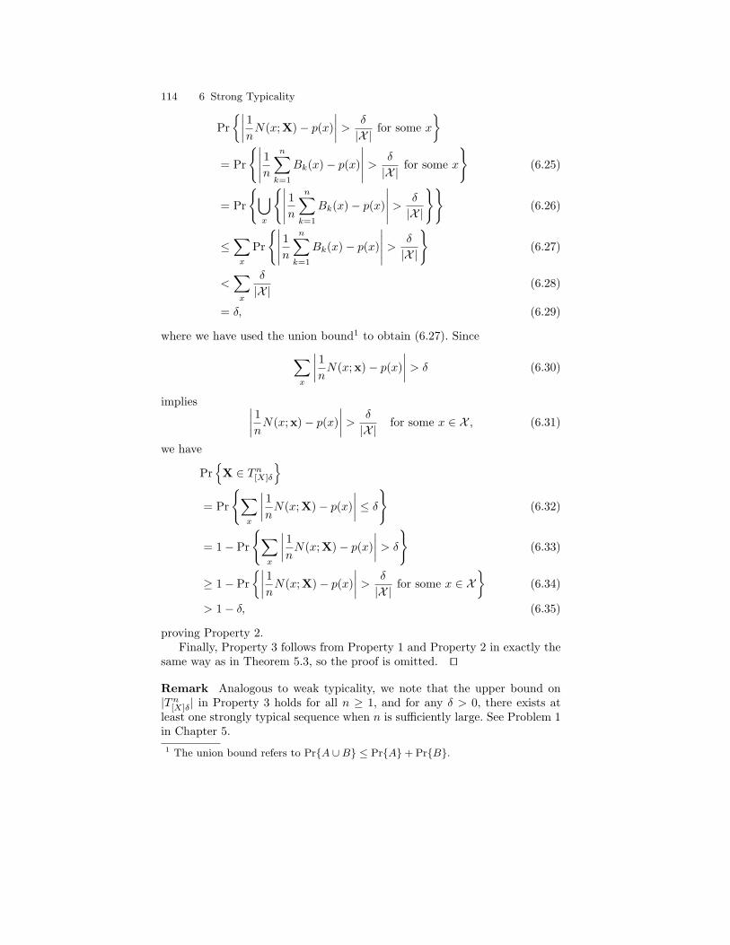
114 6 Strong Typicality
Pr∣∣∣∣ 1nN(x; X)− p(x)
∣∣∣∣ > δ
|X |for some x
= Pr
∣∣∣∣∣ 1nn∑k=1
Bk(x)− p(x)
∣∣∣∣∣ > δ
|X |for some x
(6.25)
= Pr
⋃x
∣∣∣∣∣ 1nn∑k=1
Bk(x)− p(x)
∣∣∣∣∣ > δ
|X |
(6.26)
≤∑x
Pr
∣∣∣∣∣ 1nn∑k=1
Bk(x)− p(x)
∣∣∣∣∣ > δ
|X |
(6.27)
<∑x
δ
|X |(6.28)
= δ, (6.29)
where we have used the union bound1 to obtain (6.27). Since∑x
∣∣∣∣ 1nN(x; x)− p(x)∣∣∣∣ > δ (6.30)
implies ∣∣∣∣ 1nN(x; x)− p(x)∣∣∣∣ > δ
|X |for some x ∈ X , (6.31)
we have
Pr
X ∈ Tn[X]δ
= Pr
∑x
∣∣∣∣ 1nN(x; X)− p(x)∣∣∣∣ ≤ δ
(6.32)
= 1− Pr
∑x
∣∣∣∣ 1nN(x; X)− p(x)∣∣∣∣ > δ
(6.33)
≥ 1− Pr∣∣∣∣ 1nN(x; X)− p(x)
∣∣∣∣ > δ
|X |for some x ∈ X
(6.34)
> 1− δ, (6.35)
proving Property 2.Finally, Property 3 follows from Property 1 and Property 2 in exactly the
same way as in Theorem 5.3, so the proof is omitted. ut
Remark Analogous to weak typicality, we note that the upper bound on|Tn[X]δ| in Property 3 holds for all n ≥ 1, and for any δ > 0, there exists atleast one strongly typical sequence when n is sufficiently large. See Problem 1in Chapter 5.1 The union bound refers to PrA ∪B ≤ PrA+ PrB.

6.1 Strong AEP 115
In the rest of the section, we prove an enhancement of Property 2 of thestrong AEP which gives an exponential bound on the probability of obtaininga non-typical vector2. This result, however, will not be used until Chapter 21.
Theorem 6.3. For sufficiently large n, there exists ϕ(δ) > 0 such that
PrX 6∈ Tn[X]δ < 2−nϕ(δ). (6.36)
The proof of this theorem is based on the Chernoff bound [63] which weprove in the next lemma.
Lemma 6.4 (Chernoff Bound). Let Y be a real random variable and s beany nonnegative real number. Then for any real number a,
log PrY ≥ a ≤ −sa+ logE[2sY]
(6.37)
andlog PrY ≤ a ≤ sa+ logE
[2−sY
]. (6.38)
Proof. Let
u(y) =
1 if y ≥ 00 if y < 0. (6.39)
Then for any s ≥ 0,u(y − a) ≤ 2s(y−a). (6.40)
This is illustrated in Fig. 6.1. Then
!1 0 1 2 3 4 50
0.2
0.4
0.6
0.8
1
1.2
1.4
1.6
1.8
2
a y
1
s y!a 2 ( )
u y!a ( )
Fig. 6.1. An illustration of u(y − a) ≤ 2s(y−a).
2 This result is due to Ning Cai and Raymond W. Yeung. An alternative proofbased on Pinsker’s inequality (Theorem 2.33) and the method of types has beengiven by Prakash Narayan (private communication).

116 6 Strong Typicality
E[u(Y − a)] ≤ E[2s(Y−a)
]= 2−saE
[2sY]. (6.41)
Since
E[u(Y − a)] = PrY ≥ a · 1 + PrY < a · 0 = PrY ≥ a, (6.42)
we see thatPrY ≥ a ≤ 2−saE
[2sY]
= 2−sa+logE[2sY ]. (6.43)
Then (6.37) is obtained by taking logarithm in the base 2. Upon replacing Yby −Y and a by −a in (6.37), (6.38) is obtained. The lemma is proved. ut
Proof of Theorem 6.3. We will follow the notation in the proof of Theorem 6.2.Consider x ∈ X such that p(x) > 0. Applying (6.37), we have
log Pr
n∑k=1
Bk(x) ≥ n (p(x) + δ)
≤ −sn (p(x) + δ) + logE
[2s∑n
k=1Bk(x)
](6.44)
a)= −sn (p(x) + δ) + log
(n∏k=1
E[2sBk(x)
])(6.45)
b)= −sn (p(x) + δ) + n log(1− p(x) + p(x)2s) (6.46)c)
≤ −sn (p(x) + δ) + n(ln 2)−1(−p(x) + p(x)2s) (6.47)= −n
[s (p(x) + δ) + (ln 2)−1p(x)(1− 2s)
], (6.48)
where
a) follows because Bk(x) are mutually independent;b) is a direct evaluation of the expectation from the definition of Bk(x) in(6.20);
c) follows from the fundamental inequality ln a ≤ a− 1.
In (6.48), upon defining
βx(s, δ) = s (p(x) + δ) + (ln 2)−1p(x)(1− 2s), (6.49)
we have
log Pr
n∑k=1
Bk(x) ≥ n (p(x) + δ)
≤ −nβx(s, δ), (6.50)
or
Pr
n∑k=1
Bk(x) ≥ n (p(x) + δ)
≤ 2−nβx(s,δ). (6.51)
It is readily seen that

6.1 Strong AEP 117
βx(0, δ) = 0. (6.52)
Regarding δ as fixed and differentiate with respect to s, we have
β′x(s, δ) = p(x)(1− 2s) + δ. (6.53)
Thenβ′x(0, δ) = δ > 0 (6.54)
and it is readily verified that
β′x(s, δ) ≥ 0 (6.55)
for
0 ≤ s ≤ log(
1 +δ
p(x)
). (6.56)
Therefore, we conclude that βx(s, δ) is strictly positive for
0 < s ≤ log(
1 +δ
p(x)
). (6.57)
On the other hand, by applying (6.38), we can obtain in the same fashionthe bound
log Pr
n∑k=1
Bk(x) ≤ n (p(x)− δ)
≤ −nσx(s, δ), (6.58)
or
Pr
n∑k=1
Bk(x) ≤ n (p(x)− δ)
≤ 2−nσx(s,δ), (6.59)
whereσx(s, δ) = −s (p(x)− δ) + (ln 2)−1p(x)(1− 2−s). (6.60)
Thenσx(0, δ) = 0, (6.61)
andσ′x(s, δ) = p(x)(2−s − 1) + δ, (6.62)
which is nonnegative for
0 ≤ s ≤ − log(
1− δ
p(x)
). (6.63)
In particular,σ′x(0, δ) = δ > 0. (6.64)
Therefore, we conclude that σx(s, δ) is strictly positive for

118 6 Strong Typicality
0 < s ≤ − log(
1− δ
p(x)
). (6.65)
By choosing s satisfying
0 < s ≤ min[log(
1 +δ
p(x)
),− log
(1− δ
p(x)
)], (6.66)
both βx(s, δ) and σx(s, δ) are strictly positive. From (6.51) and (6.59), wehave
Pr
∣∣∣∣∣ 1nn∑k=1
Bk(x)− p(x)
∣∣∣∣∣ ≥ δ
= Pr
∣∣∣∣∣n∑k=1
Bk(x)− np(x)
∣∣∣∣∣ ≥ nδ
(6.67)
≤ Pr
n∑k=1
Bk(x) ≥ n (p(x) + δ)
+Pr
n∑k=1
Bk(x) ≤ n (p(x)− δ)
(6.68)
≤ 2−nβx(s,δ) + 2−nσx(s,δ) (6.69)≤ 2 · 2−nmin(βx(s,δ),σx(s,δ)) (6.70)
= 2−n[min(βx(s,δ),σx(s,δ))− 1n ] (6.71)
= 2−nϕx(δ), (6.72)
whereϕx(δ) = min(βx(s, δ), σx(s, δ))− 1
n. (6.73)
Then ϕx(δ) is strictly positive for sufficiently large n because both βx(s, δ)and σx(s, δ) are strictly positive.
Finally, consider
PrX ∈ Tn[X]δ
= Pr
∑x
∣∣∣∣ 1nN(x; X)− p(x)∣∣∣∣ ≤ δ
(6.74)
≥ Pr∣∣∣∣ 1nN(x; X)− p(x)
∣∣∣∣ ≤ δ
|X |for all x ∈ X
(6.75)
= 1− Pr∣∣∣∣ 1nN(x; X)− p(x)
∣∣∣∣ > δ
|X |for some x ∈ X
(6.76)
≥ 1−∑x
Pr∣∣∣∣ 1nN(x; X)− p(x)
∣∣∣∣ > δ
|X |
(6.77)

6.2 Strong Typicality Versus Weak Typicality 119
= 1−∑x
Pr
∣∣∣∣∣ 1nn∑k=1
Bk(x)− p(x)
∣∣∣∣∣ > δ
|X |
(6.78)
= 1−∑
x:p(x)>0
Pr
∣∣∣∣∣ 1nn∑k=1
Bk(x)− p(x)
∣∣∣∣∣ > δ
|X |
(6.79)
≥ 1−∑
x:p(x)>0
2−nϕx(δ|X|
), (6.80)
where the last step follows from (6.72). Define
ϕ(δ) =12
[min
x:p(x)>0ϕx
(δ
|X |
)]. (6.81)
Then for sufficiently large n,
PrX ∈ Tn[X]δ > 1− 2−nϕ(δ), (6.82)
orPrX 6∈ Tn[X]δ < 2−nϕ(δ), (6.83)
where ϕ(δ) is strictly positive. The theorem is proved. ut
6.2 Strong Typicality Versus Weak Typicality
As we have mentioned at the beginning of the chapter, strong typicality ismore powerful and flexible than weak typicality as a tool for theorem provingfor memoryless problems, but it can be used only for random variables withfinite alphabets. We will prove in the next proposition that strong typicality isstronger than weak typicality in the sense that the former implies the latter.
Proposition 6.5. For any x ∈ Xn, if x ∈ Tn[X]δ, then x ∈ Wn[X]η, where
η → 0 as δ → 0.
Proof. By Property 1 of strong AEP (Theorem 6.2), if x ∈ Tn[X]δ, then
2−n(H(X)+η) ≤ p(x) ≤ 2−n(H(X)−η), (6.84)
orH(X)− η ≤ − 1
nlog p(x) ≤ H(X) + η, (6.85)
where η → 0 as δ → 0. Then x ∈ Wn[X]η by Definition 5.2. The proposition is
proved. ut
We have proved in this proposition that strong typicality implies weaktypicality, but the converse is not true. This idea can be explained without

120 6 Strong Typicality
any detailed analysis. Let X be distributed with p such that p(0) = 0.5,p(1) = 0.25, and p(2) = 0.25. Consider a sequence x of length n and let q(i)be the relative frequency of occurrence of symbol i in x, i.e., 1
nN(i; x), wherei = 0, 1, 2. In order for the sequence x to be weakly typical, we need
− 1n
log p(x)
= −q(0) log 0.5− q(1) log 0.25− q(2) log 0.25 (6.86)≈ H(X) (6.87)= −(0.5) log 0.5− (0.25) log 0.25− (0.25) log 0.25. (6.88)
Obviously, this can be satisfied by choosing q(i) = p(i) for all i. But alterna-tively, we can choose q(0) = 0.5, q(1) = 0.5, and q(2) = 0. With such a choiceof q(i), the sequence x is weakly typical with respect to p but obviously notstrongly typical with respect to p, because the relative frequency of occurrenceof each symbol i is q(i), which is not close to p(i) for i = 1, 2.
Therefore, we conclude that strong typicality is indeed stronger than weaktypicality. However, as we have pointed out at the beginning of the chapter,strong typicality can only be used for random variables with finite alphabets.
6.3 Joint Typicality
In this section, we discuss strong joint typicality with respect to a bivariatedistribution. Generalization to a multivariate distribution is straightforward.
Consider a bivariate information source (Xk, Yk), k ≥ 1 where (Xk, Yk)are i.i.d. with distribution p(x, y). We use (X,Y ) to denote the pair of genericrandom variables.
Definition 6.6. The strongly jointly typical set Tn[XY ]δ with respect to p(x, y)is the set of (x,y) ∈ Xn × Yn such that N(x, y; x,y) = 0 for (x, y) 6∈ SXY ,and ∑
x
∑y
∣∣∣∣ 1nN(x, y; x,y)− p(x, y)∣∣∣∣ ≤ δ, (6.89)
where N(x, y; x,y) is the number of occurrences of (x, y) in the pair of se-quences (x,y), and δ is an arbitrarily small positive real number. A pair ofsequences (x,y) is called strongly jointly δ-typical if it is in Tn[XY ]δ.
Strong typicality satisfies the following consistency property.
Theorem 6.7 (Consistency). If (x,y) ∈ Tn[XY ]δ, then x ∈ Tn[X]δ and y ∈Tn[Y ]δ.
Proof. If (x,y) ∈ Tn[XY ]δ, then

6.3 Joint Typicality 121∑x
∑y
∣∣∣∣ 1nN(x, y; x,y)− p(x, y)∣∣∣∣ ≤ δ. (6.90)
Upon observing that
N(x; x) =∑y
N(x, y; x,y), (6.91)
we have ∑x
∣∣∣∣ 1nN(x; x)− p(x)∣∣∣∣
=∑x
∣∣∣∣∣ 1n∑y
N(x, y; x,y)−∑y
p(x, y)
∣∣∣∣∣ (6.92)
=∑x
∣∣∣∣∣∑y
(1nN(x, y; x,y)− p(x, y)
)∣∣∣∣∣ (6.93)
≤∑x
∑y
∣∣∣∣ 1nN(x, y; x,y)− p(x, y)∣∣∣∣ (6.94)
≤ δ. (6.95)
Therefore, x ∈ Tn[X]δ. Similarly, y ∈ Tn[Y ]δ. The theorem is proved. ut
The following thoerem asserts that strong typicality is preserved when afunction is applied to a vector.
Theorem 6.8 (Preservation). Let Y = f(X). If
x = (x1, x2, · · · , xn) ∈ Tn[X]δ, (6.96)
thenf(x) = (y1, y2, · · · , yn) ∈ Tn[Y ]δ, (6.97)
where yi = f(xi) for 1 ≤ i ≤ n.
Proof. Consider x ∈ Tn[X]δ, i.e.,
∑x
∣∣∣∣ 1nN(x; x)− p(x)∣∣∣∣ < δ. (6.98)
Since Y = f(X),p(y) =
∑x∈f−1(y)
p(x) (6.99)
for all y ∈ Y. On the other hand,

122 6 Strong Typicality
N(y; f(x)) =∑
x∈f−1(y)
N(x; x) (6.100)
for all y ∈ Y. Then∑y
∣∣∣∣ 1nN(y; f(x))− p(y)∣∣∣∣
=∑y
∣∣∣∣∣∣∑
x∈f−1(y)
(1nN(x; x)− p(x)
)∣∣∣∣∣∣ (6.101)
≤∑y
∑x∈f−1(y)
∣∣∣∣ 1nN(x; x)− p(x)∣∣∣∣ (6.102)
=∑x
∣∣∣∣ 1nN(x; x)− p(x)∣∣∣∣ (6.103)
< δ. (6.104)
Therefore, f(x) ∈ Tn[Y ]δ, proving the lemma. ut
For a bivariate i.i.d. source (Xk, Yk), we have the strong joint asymp-totic equipartition property (strong JAEP), which can readily be obtained byapplying the strong AEP to the source (Xk, Yk).
Theorem 6.9 (Strong JAEP). Let
(X,Y) = ((X1, Y1), (X2, Y2), · · · , (Xn, Yn)), (6.105)
where (Xi, Yi) are i.i.d. with generic pair of random variables (X,Y ). Thenthere exists λ > 0 such that λ→ 0 as δ → 0, and the following hold:
1) If (x,y) ∈ Tn[XY ]δ, then
2−n(H(X,Y )+λ) ≤ p(x,y) ≤ 2−n(H(X,Y )−λ). (6.106)
2) For n sufficiently large,
Pr(X,Y) ∈ Tn[XY ]δ > 1− δ. (6.107)
3) For n sufficiently large,
(1− δ)2n(H(X,Y )−λ) ≤ |Tn[XY ]δ| ≤ 2n(H(X,Y )+λ). (6.108)
From the strong JAEP, we can see the following. Since there are approxi-mately 2nH(X,Y ) typical (x,y) pairs and approximately 2nH(X) typical x, fora typical x, the number of y such that (x,y) is jointly typical is approximately

6.3 Joint Typicality 123
2nH(X,Y )
2nH(X)= 2nH(Y |X) (6.109)
on the average. The next theorem reveals that this is not only true on theaverage, but it is in fact true for every typical x as long as there exists at leastone y such that (x,y) is jointly typical.
Theorem 6.10. For any x ∈ Tn[X]δ, define
Tn[Y |X]δ(x) = y ∈ Tn[Y ]δ : (x,y) ∈ Tn[XY ]δ. (6.110)
If |Tn[Y |X]δ(x)| ≥ 1, then
2n(H(Y |X)−ν) ≤ |Tn[Y |X]δ(x)| ≤ 2n(H(Y |X)+ν), (6.111)
where ν → 0 as n→∞ and δ → 0.
We first prove the following lemma which is along the line of Stirling’sapproximation [101].
Lemma 6.11. For any n > 0,
n lnn− n < lnn! < (n+ 1) ln(n+ 1)− n. (6.112)
Proof. First, we write
lnn! = ln 1 + ln 2 + · · ·+ lnn. (6.113)
Since lnx is a monotonically increasing function of x, we have∫ k
k−1
lnx dx < ln k <∫ k+1
k
lnx dx. (6.114)
Summing over 1 ≤ k ≤ n, we have∫ n
0
lnx dx < lnn! <∫ n+1
1
lnx dx, (6.115)
orn lnn− n < lnn! < (n+ 1) ln(n+ 1)− n. (6.116)
The lemma is proved. ut
Proof of Theorem 6.10. Let δ be a small positive real number and n be alarge positive integer to be specified later. Fix an x ∈ Tn[X]δ, so that
∑x
∣∣∣∣ 1nN(X; x)− p(x)∣∣∣∣ ≤ δ. (6.117)

124 6 Strong Typicality
This implies that for all x ∈ X ,∣∣∣∣ 1nN(X; x)− p(x)∣∣∣∣ ≤ δ, (6.118)
orp(x)− δ ≤ 1
nN(x; x) ≤ p(x) + δ. (6.119)
We first prove the upper bound on |Tn[Y |X]δ(x)|. For any ν > 0, consider
2−n(H(X)−ν/2)a)
≥ p(x) (6.120)
=∑
y∈Ynp(x,y) (6.121)
≥∑
y∈Tn[Y |X]δ(x)
p(x,y) (6.122)
b)
≥∑
y∈Tn[Y |X]δ(x)
2−n(H(X,Y )+ν/2) (6.123)
= |Tn[Y |X]δ(x)|2−n(H(X,Y )+ν/2), (6.124)
where a) and b) follow from the strong AEP (Theorem 6.2) and the strongjoint AEP (Theorem 6.9), respectively. Then we obtain
|Tn[Y |X]δ(x)| ≤ 2n(H(Y |X)+ν), (6.125)
which is the upper bound to be proved.Assume that |Tn[Y |X]δ(x)| ≥ 1. We now prove the lower bound on |Tn[Y |X]δ(x)|.
LetK(x, y), (x, y) ∈ X × Y (6.126)
be any set of nonnegative integers such that
1. ∑y
K(x, y) = N(x; x) (6.127)
for all x ∈ X , and2. for any y ∈ Yn, if
N(x, y; x,y) = K(x, y) (6.128)
for all (x, y) ∈ X × Y, then (x,y) ∈ Tn[XY ]δ.
Then by Definition 6.6, K(x, y) satisfy∑x
∑y
∣∣∣∣ 1nK(x, y)− p(x, y)∣∣∣∣ ≤ δ, (6.129)

6.3 Joint Typicality 125
which implies that for all (x, y) ∈ X × Y,∣∣∣∣ 1nK(x, y)− p(x, y)∣∣∣∣ ≤ δ, (6.130)
orp(x, y)− δ ≤ 1
nK(x, y) ≤ p(x, y) + δ. (6.131)
Such a set K(x, y) exists because Tn[Y |X]δ(x) is assumed to be nonempty.Straightforward combinatorics reveals that the number of y which satisfy theconstraints in (6.128) is equal to
M(K) =∏x
N(x; x)!∏yK(x, y)!
, (6.132)
and it is readily seen that
|Tn[Y |X]δ(x)| ≥M(K). (6.133)
Using Lemma 6.11, we can lower bound lnM(K) as follows.
lnM(K)
≥∑x
N(x; x) lnN(x; x)−N(x; x)
−∑y
[(K(x, y) + 1) ln(K(x, y) + 1)−K(x, y)]
(6.134)
a)=∑x
[N(x; x) lnN(x; x)
−∑y
(K(x, y) + 1) ln(K(x, y) + 1)
](6.135)
b)
≥∑x
N(x; x) ln(n (p(x)− δ))
−∑y
(K(x, y) + 1) ln[n
(p(x, y) + δ +
1n
)]. (6.136)
In the above, a) follows from (6.127), and b) is obtained by applying thelower bound on n−1N(x; x) in (6.119) and the upper bound on n−1K(x, y) in(6.131). Also from (6.127), the coefficient of lnn in (6.136) is given by
∑x
[N(x; x)−
∑y
(K(x, y) + 1)
]= −|X ||Y|. (6.137)
Let δ be sufficiently small and n be sufficiently large so that

126 6 Strong Typicality
0 < p(x)− δ < 1 (6.138)
andp(x, y) + δ +
1n< 1 (6.139)
for all x and y. Then in (6.136), both the logarithms
ln(p(x)− δ) (6.140)
and
ln(p(x, y) + δ +
1n
)(6.141)
are negative. Note that the logarithm in (6.140) is well-defined by virtue of(6.138). Rearranging the terms in (6.136), applying the upper bound in (6.119)and the lower bound3 in (6.131), and dividing by n, we have
n−1 lnM(K)
≥∑x
(p(x) + δ) ln (p(x)− δ)−∑x
∑y
(p(x, y)− δ +
1n
)× ln
(p(x, y) + δ +
1n
)− |X ||Y| lnn
n(6.142)
= −He(X) +He(X,Y ) + Ll(n, δ) (6.143)= He(Y |X) + Ll(n, δ), (6.144)
where Ll(n, δ) denotes a function of n and δ which tends to 0 as n→∞ andδ → 0. Changing the base of the logarithm to 2, we have
n−1 logM(K) ≥ H(Y |X) + Ll(n, δ). (6.145)
Then it follows from (6.133) that
n−1 log |Tn[Y |X]δ(x)| ≥ H(Y |X) + Ll(n, δ). (6.146)
Upon replacing Ll(n, δ), we obtain
|Tn[Y |X]δ(x)| ≥ 2n(H(Y |X)−ν), (6.147)
where ν → 0 as n→∞ and δ → 0 as discussed. The theorem is proved. ut
The above theorem says that for any typical x, as long as there is onetypical y such that (x,y) is jointly typical, there are approximately 2nH(Y |X)
y such that (x,y) is jointly typical. This theorem has the following corollarythat the number of such typical x grows with n at almost the same rate asthe total number of typical x.3 For the degenerate case when p(x, y) = 1 for some x and y, p(x, y) + δ + 1
n> 1,
and the logarithm in (6.141) is in fact positive. Then the upper bound instead ofthe lower bound should be applied. The details are omitted.

6.3 Joint Typicality 127
Corollary 6.12. For a joint distribution p(x, y) on X × Y, let Sn[X]δ be theset of all sequences x ∈ Tn[X]δ such that Tn[Y |X]δ(x) is nonempty. Then
|Sn[X]δ| ≥ (1− δ)2n(H(X)−ψ), (6.148)
where ψ → 0 as n→∞ and δ → 0.
Proof. By the consistency of strong typicality (Theorem 6.7), if (x,y) ∈Tn[XY ]δ, then x ∈ Tn[X]δ. In particular, x ∈ Sn[X]δ. Then
Tn[XY ]δ =⋃
x∈Sn[X]δ
(x,y) : y ∈ Tn[Y |X]δ(x). (6.149)
Using the lower bound on |Tn[XY ]δ| in Theorem 6.9 and the upper bound on|Tn[Y |X]δ(x)| in the last theorem, we have
(1− δ)2n(H(X,Y )−λ) ≤ |Tn[XY ]δ| ≤ |Sn[X]δ|2
n(H(Y |X)+ν) (6.150)
which implies|Sn[X]δ| ≥ (1− δ)2n(H(X)−(λ+ν)). (6.151)
The theorem is proved upon letting ψ = λ+ ν. ut
We have established a rich set of structural properties for strong typicalitywith respect to a bivariate distribution p(x, y), which is summarized in thetwo-dimensional strong joint typicality array in Figure 6.2. In this array, the
2 nH ( Y )
2 nH ( X,Y ) 2 nH ( X )
y S [ Y ] n
x S [ X ] n
( x , y ) T [ XY ] n
.
.
. . . .
. . . .
. . . .
.
Fig. 6.2. A two-dimensional strong joint typicality array.
rows and the columns are the typical sequences x ∈ Sn[X]δ and y ∈ Sn[Y ]δ,respectively. The total number of rows and columns are approximately equalto 2nH(X) and 2nH(Y ), respectively. An entry indexed by (x,y) receives a dotif (x,y) is strongly jointly typical. The total number of dots is approximatelyequal to 2nH(X,Y ). The number of dots in each row is approximately equal to

128 6 Strong Typicality
2nH(Y |X), while the number of dots in each column is approximately equal to2nH(X|Y ).
For reasons which will become clear in Chapter 16, the strong joint typical-ity array in Figure 6.2 is said to exhibit an asymptotic quasi-uniform structure.By a two-dimensional asymptotic quasi-uniform structure, we mean that inthe array all the columns have approximately the same number of dots, andall the rows have approximately the same number of dots. The strong jointtypicality array for a multivariate distribution continues to exhibit an asymp-totic quasi-uniform structure. The three-dimensional strong joint typicalityarray with respect to a distribution p(x, y, z) is illustrated in Figure 6.3. As
2 nH ( Y )
2 nH ( Z )
( x 0 , y 0 )
z 0
z S [ Z ] n
y S [ Y ] n
2 nH ( X ) x S [ X ] n
Fig. 6.3. A three-dimensional strong joint typicality array.
before, an entry (x,y, z) receives a dot if (x,y, z) is strongly jointly typical.This is not shown in the figure otherwise it will be very confusing. The totalnumber of dots in the whole array is approximately equal to 2nH(X,Y,Z). Thesedots are distributed in the array such that all the planes parallel to each otherhave approximately the same number of dots, and all the cylinders parallelto each other have approximately the same number of dots. More specifically,the total number of dots on the plane for any fixed z0 ∈ Sn[Z]δ (as shown) isapproximately equal to 2nH(X,Y |Z), and the total number of dots in the cylin-der for any fixed (x0,y0) pair in Sn[XY ]δ (as shown) is approximately equal to2nH(Z|X,Y ), so on and so forth.
We see from the strong AEP and Corollary 6.12 that Sn[X]δ and Tn[X]δ growwith n at approximately the same rate. We end this section by stating in thenext proposition that Sn[X]δ indeed contains almost all the probability when nis large. The proof is left as an exercise (see Problem 4).
Proposition 6.13. With respect to a joint distribution p(x, y) on X ×Y, forany δ > 0,
PrX ∈ Sn[X]δ > 1− δ (6.152)

Problems 129
for n sufficiently large.
6.4 An Interpretation of the Basic Inequalities
The asymptotic quasi-uniform structure exhibited in a strong joint typicalityarray discussed in the last section is extremely important in information the-ory. Later in the book, we will see how this structure is involved in provingresults such as the channel coding theorem and the rate-distortion theorem. Inthis section, we show how the basic inequalities can be revealed by examiningthis structure. It has further been shown by Chan [56] that all unconstrainedinformation inequalities can be obtained from this structure, thus giving aphysical meaning to these inequalities.
Consider random variables X,Y , and Z and a fixed z ∈ Sn[Z]δ, so thatTn[XY |Z]δ(z) is nonempty. By the consistency of strong typicality, if (x,y, z) ∈Tn[XY Z]δ, then (x, z) ∈ Tn[XZ]δ and (y, z) ∈ Tn[Y Z]δ, or x ∈ Tn[X|Z]δ(z) andy ∈ Tn[Y |Z]δ(z), respectively. Thus
Tn[XY |Z]δ(z) ⊂ Tn[X|Z]δ(z)× Tn[Y |Z]δ(z), (6.153)
which implies|Tn[XY |Z]δ(z)| ≤ |Tn[X|Z]δ(z)||Tn[Y |Z]δ(z)|. (6.154)
Applying the lower bound in Theorem 6.10 to Tn[XY |Z]δ(z) and the upperbound to Tn[X|Z]δ(z) and Tn[Y |Z]δ(z), we have
2n(H(X,Y |Z)−ζ) ≤ 2n(H(X|Z)+γ)2n(H(Y |Z)+φ), (6.155)
where ζ, γ, φ → 0 as n → ∞ and δ → 0. Taking logarithm to the base 2 anddividing by n, we obtain
H(X,Y |Z) ≤ H(X|Z) +H(Y |Z) (6.156)
upon letting n→∞ and δ → 0. This inequality is equivalent to
I(X;Y |Z) ≥ 0. (6.157)
Thus we have proved the nonnegativity of conditional mutual information.Since all Shannon’s information measures are special cases of conditional mu-tual information, we have proved the nonnegativity of all Shannon’s informa-tion measures, namely the basic inequalities.
Problems
1. Show that (x,y) ∈ Tn[X,Y ]δ and (y, z) ∈ Tn[Y,Z]δ do not imply (x, z) ∈Tn[X,Z]δ.

130 6 Strong Typicality
2. Let X = (X1, X2, · · · , Xn), where Xk are i.i.d. with generic random vari-able X. Prove that
PrX ∈ Tn[X]δ ≥ 1− |X |3
nδ2
for any n and δ > 0. This shows that PrX ∈ Tn[X]δ → 1 as δ → 0 andn→∞ if
√nδ →∞.
3. Prove that for a random variable X with a countable alphabet, Property2 of the strong AEP holds, while Properties 1 and 3 do not hold.
4. Prove Proposition 6.13. Hint: First prove that if (X,Y) ∈ Tn[XY ]δ, thenX ∈ Sn[X]δ.
5. Let P(X ) be the set of all probability distributions over a finite alphabetX . Find a polynomial Q(n) such that for any integer n, there exists asubset Pn(X ) of P(X ) such thata) |Pn(X )| ≤ Q(n);b) for all P ∈ P(X ), there exists Pn ∈ Pn(X ) such that
|Pn(x)− P (x)| < 1n
for all x ∈ X .Hint: Let Pn(X ) be the set of all probability distributions over X such thatall the probability masses can be expressed as fractions with denominatorn.
6. Let p be any probability distribution over a finite set X and η be a realnumber in (0, 1). Prove that for any subset A of Xn with pn(A) ≥ η,
|A ∩ Tn[X]δ| ≥ 2n(H(p)−δ′),
where δ′ → 0 as δ → 0 and n→∞.
In the following problems, for a sequence x ∈ Xn, let qx be the empiricaldistribution of x, i.e., qx(x) = n−1N(x; x) for all x ∈ X . Similarly, for a pairof sequences (x,y) ∈ Xn × Yn, let qx,y be the joint empirical distribution of(x,y), i.e., qx,y(x, y) = n−1N(x, y; x,y) for all (x, y) ∈ X × Y.
7. Alternative definition of strong typicality Show that (6.1) is equivalent to
V (qx, p) ≤ δ,
where V (·, ·) denotes the variational distance. Thus strong typicality canbe regarded as requiring the empirical distribution of a sequence to beclose to the probability distribution of the generic random variable invariational distance. Also compare the result here with the alternativedefinition of weak typicality (Problem 5 in Chapter 5).

Problems 131
8. The empirical distribution qx of the sequence x is also called the type ofx. Assuming that X is finite, show that there are a total of
(n+|X |−1
n
)distinct types qx. Hint: There are
(a+b−1a
)ways to distribute a identical
balls in b boxes.9. Unified typicality Let X = (X1, X2, · · · , Xn) be an i.i.d. sequence whose
generic random variable X is distributed with p(x), where the alpbabetX is countable. For any η > 0, the unified typical set Un[X]η with respectto p(x) is the set of sequences x ∈ Xn such that
D(qx‖p) + |H(qx)−H(p)| ≤ η.
a) Show that for any x ∈ Xn, if x ∈ Un[X]η, then x ∈Wn[X]η.
b) Show that for any x ∈ Xn, if x ∈ Un[X]η, then x ∈ Tn[X]δ, whereδ =√η · 2 ln 2.
Therefore, unified typicality implies both weak typicality and strong typ-icality.
10. The AEP for unified typicality Unified typicality defined in Problem 9,unlike strong typicality, can be applied to random variables whose alpha-bets are countable . At the same time, it preserves the essential propertiesof strong typicality. The following outlines the proof of the AEP whichhas been discussed in Theorem 5.3 and Theorem 6.2 for weak typicalityand strong typicality, respectively.a) Show that
2−n(H(X)+η) ≤ p(x) ≤ 2−n(H(X)−η),
i.e., Property 1 of the AEP.b) Show that for sufficiently large n,
PrH(qx)−H(p) > ε < ε.
Hint: Use the results in Problem 9 above and Problem 5 in Chapter 5.c) It can be proved by means of the result in Problem 9 that
PrH(p)−H(qx) > ε < ε
(see Ho and Yeung [150]). By assuming this inequality, prove that
Pr|H(qx)−H(p)| ≤ ε < 1− 2ε.
d) Show that if |H(qx) −H(p)| ≤ ε and |D(qx‖p) + H(qx) −H(p)| ≤ ε,then
D(qx‖p) + |H(qx)−H(p)| ≤ 3ε.
e) Use the results in c) and d) above and the result in c) in Problem 5in Chapter 5 to show that
PrD(qx‖p) + |H(qx)−H(p)| ≤ η > 1− η.
This proves Property 2 of the AEP. Property 3 of the AEP followsfrom Property 1 as in the proof of Theorem 5.3.

132 6 Strong Typicality
11. Consistency of unified typicality For any η > 0, the unified jointly typicalset Un[XY ]η with respect to pXY (x, y) is the set of sequences (x,y) ∈ Xn×Yn such that
D(qx,y‖pXY ) + |H(qx,y)−H(pXY )|+|H(qx)−H(pX)|+ |H(qy)−H(pY )| ≤ η.
Show that if (x,y) ∈ Un[XY ]η, then x ∈ Un[X]η and y ∈ Un[Y ]η.
Historical Notes
Strong typicality was used by Wolfowitz [348] for proving channel coding the-orems and by Berger [27] for proving the rate-distortion theorem and variousresults in multiterminal source coding. The method of types, a refinementof the notion of strong typicality, was systematically developed in the bookby Csiszar and Korner [75]. The interpretation of the basic inequalities inSection 6.4 is a preamble to the relation between entropy and groups to bediscussed in Chapter 16.
Recently, Ho and Yeung [150] introduced the notion of unified typicalitywhich is stronger than both weak typicality and strong typicality. This notionof typicality can be applied to random variables with countable alphabets,while at the same time preserve the essential properties of strong typicality.See Problems 9, 10, and 11 for a discussion.

7
Discrete Memoryless Channels
In all practical communication systems, when a signal is transmitted fromone point to another point, the signal is inevitably contaminated by randomnoise, i.e., the signal received is correlated with but possibly different from thesignal transmitted. We use a noisy channel to model such a situation. A noisychannel is a “system” which has one input terminal and one output terminal1,with the input connected to the transmission point and the output connectedto the receiving point. When the signal is transmitted through the channel,it is distorted in a random way which depends on the channel characteristics.As such, the signal received may be different from the signal transmitted.
In communication engineering, we are interested in conveying messagesreliably through a noisy channel at the maximum possible rate. We first lookat a simple channel called the binary symmetric channel (BSC), which isrepresented by the transition diagram in Figure 7.1. In this channel both theinput X and the output Y take values in the set 0, 1. There is a certainprobability, denoted by ε, that the output is not equal to the input. That is,if the input is 0, then the output is 0 with probability 1 − ε, and is 1 withprobability ε. Likewise, if the input is 1, then the output is 1 with probability1 − ε, and is 0 with probability ε. The parameter ε is called the crossoverprobability of the BSC.
Let A,B be the message set which contains two possible messages tobe conveyed through a BSC with 0 ≤ ε < 0.5. We further assume that thetwo messages A and B are equally likely. If the message is A, we map it tothe codeword 0, and if the message is B, we map it to the codeword 1. Thisis the simplest example of a channel code. The codeword is then transmittedthrough the channel. Our task is to decode the message based on the output ofthe channel, and an error is said to occur if the message is decoded incorrectly.
Consider
PrA|Y = 0 = PrX = 0|Y = 0 (7.1)
1 The discussion on noisy channels here is confined to point-to-point channels.

134 7 Discrete Memoryless Channels
0
1
0
1
X Y
1
1
Fig. 7.1. A binary symmetric channel.
=PrX = 0PrY = 0|X = 0
PrY = 0(7.2)
=0.5(1− ε)PrY = 0
. (7.3)
SincePrY = 0 = PrY = 1 = 0.5 (7.4)
by symmetry2, it follows that
PrA|Y = 0 = 1− ε (7.5)
andPrB|Y = 0 = 1− PrA|Y = 0 = ε. (7.6)
Since ε < 0.5,PrB|Y = 0 < PrA|Y = 0. (7.7)
Therefore, in order to minimize the probability of error, we decode a received0 to the message A. By symmetry, we decode a received 1 to the message B.
An error occurs if a 0 is received and the message is B, or if a 1 is receivedand the message is A. Therefore, the probability of error, denoted by Pe, isgiven by
Pe = PrY = 0PrB|Y = 0+ PrY = 1PrA|Y = 1 (7.8)= 0.5ε+ 0.5ε (7.9)= ε, (7.10)
2 More explicitly,
PrY = 0 = PrAPrY = 0|A+ PrBPrY = 0|B= 0.5 PrY = 0|X = 0+ 0.5 PrY = 0|X = 1= 0.5(1− ε) + 0.5ε
= 0.5.

7 Discrete Memoryless Channels 135
where (7.9) follows from (7.6) because
PrA|Y = 1 = PrB|Y = 0 = ε (7.11)
by symmetry.Let us assume that ε 6= 0. Then the above scheme obviously does not
provide perfectly reliable communication. If we are allowed to use the channelonly once, then this is already the best we can do. However, if we are allowedto use the same channel repeatedly, then we can improve the reliability bygeneralizing the above scheme.
We now consider the following channel code which we refer to as the binaryrepetition code. Let n ≥ 1 be an odd positive integer which is called the blocklength of the code. In this code, the message A is mapped to the sequence ofn 0’s, and the message B is mapped to the sequence of n 1’s. The codeword,which consists of a sequence of either n 0’s or n 1’s, is transmitted throughthe channel in n uses. Upon receiving a sequence of n bits at the output ofthe channel, we use the majority vote to decode the message, i.e., if there aremore 0’s than 1’s in the sequence, we decode the sequence to the messageA, otherwise we decode the sequence to the message B. Note that the blocklength is chosen to be odd so that there cannot be a tie. When n = 1, thisscheme reduces to the previous scheme.
For this more general scheme, we continue to denote the probability oferror by Pe. Let N0 and N1 be the number of 0’s and 1’s in the receivedsequence, respectively. Clearly,
N0 +N1 = n. (7.12)
For large n, if the message is A, the number of 0’s received is approximatelyequal to
E[N0|A] = n(1− ε) (7.13)
and the number of 1’s received is approximately equal to
E[N1|A] = nε (7.14)
with high probability by the weak law of large numbers. This implies that theprobability of an error, namely the event N0 < N1, is small because
n(1− ε) > nε (7.15)
with the assumption that ε < 0.5. Specifically,
Prerror|A = PrN0 < N1|A (7.16)= Prn−N1 < N1|A (7.17)= PrN1 > 0.5n|A (7.18)≤ PrN1 > (ε+ φ)n|A, (7.19)

136 7 Discrete Memoryless Channels
where0 < φ < 0.5− ε, (7.20)
so that φ is positive andε+ φ < 0.5. (7.21)
Note that such a φ exists because ε < 0.5. Then by the weak law of largenumbers, the upper bound in (7.19) tends to 0 as n → ∞. By symmetry,Prerror|B also tends to 0 as n→∞. Therefore,
Pe = PrAPrerror|A+ PrBPrerror|B (7.22)
tends to 0 as n → ∞. In other words, by using a long enough repetitioncode, we can make Pe arbitrarily small. In this sense, we say that reliablecommunication is achieved asymptotically.
We point out that for a BSC with ε > 0, for any given transmitted se-quence of length n, the probability of receiving any given sequence of lengthn is nonzero. It follows that for any two distinct input sequences, there isalways a nonzero probability that the same output sequence is produced sothat the two input sequences become indistinguishable. Therefore, except forvery special channels (e.g., the BSC with ε = 0), no matter how the encod-ing/decoding scheme is devised, a nonzero probability of error is inevitable,and asymptotically reliable communication is the best we can hope for.
Though a rather naive approach, asymptotically reliable communicationcan be achieved by using the repetition code. The repetition code, however,is not without catch. For a channel code, the rate of the code in bit(s) peruse, is defined as the ratio of the logarithm of the size of the message setin the base 2 to the block length of the code. Roughly speaking, the rate ofa channel code is the average number of bits the channel code attempts toconvey through the channel per use of the channel. For a binary repetitioncode with block length n, the rate is 1
n log 2 = 1n , which tends to 0 as n→∞.
Thus in order to achieve asymptotic reliability by using the repetition code,we cannot communicate through the noisy channel at any positive rate!
In this chapter, we characterize the maximum rate at which informationcan be communicated through a discrete memoryless channel (DMC) with anarbitrarily small probability of error. This maximum rate, which is generallypositive, is known as the channel capacity. Then we discuss the use of feed-back in communicating through a channel, and show that feedback does notincrease the capacity. At the end of the chapter, we discuss transmitting aninformation source through a DMC, and we show that asymptotic optimalitycan be achieved by separating source coding and channel coding.
7.1 Definition and Capacity
Definition 7.1. Let X and Y be discrete alphabets, and p(y|x) be a transitionmatrix from X to Y. A discrete channel p(y|x) is a single-input single-output

7.1 Definition and Capacity 137
system with input random variable X taking values in X and output randomvariable Y taking values in Y such that
PrX = x, Y = y = PrX = xp(y|x) (7.23)
for all (x, y) ∈ X × Y.
Remark From (7.23), we see that if PrX = x > 0, then
PrY = y|X = x =PrX = x, Y = y
PrX = x= p(y|x). (7.24)
Note that PrY = y|X = x is undefined if PrX = x = 0. Nevertheless,(7.23) is valid for both cases.
We now present an alternative description of a discrete channel. Let Xand Y be discrete alphabets. Let X be a random variable taking values in Xand p(y|x) be any transition matrix from X to Y. Define random variablesZx with Zx = Y for x ∈ X such that
PrZx = y = p(y|x) (7.25)
for all y ∈ Y. We assume that Zx, x ∈ X are mutually independent and alsoindependent of X. Further define the random variable
Z = (Zx : x ∈ X ), (7.26)
called the noise variable. Note that Z is independent of X. Now define arandom variable taking values in Y as
Y = Zx if X = x. (7.27)
Evidently, Y is a function of X and Z. Then for x ∈ X such that PrX =x > 0, we have
PrX = x, Y = y = PrX = xPrY = y|X = x (7.28)= PrX = xPrZx = y|X = x (7.29)= PrX = xPrZx = y (7.30)= PrX = xp(y|x), (7.31)
i.e., (7.23) in Definition 7.1, where (7.30) follows from the assumption that Zxis independent of Zx. For x ∈ X such that PrX = x = 0, since PrX = x =0 implies PrX = x, Y = y = 0, (7.23) continues to hold. Then by regardingX and Y as the input and output random variables, we have obtained analternative description of the discrete channel p(y|x).
Since Y is a function of X and Z, we can write
Y = α(X,Z). (7.32)
Then we have the following equivalent definition for a discrete channel.

138 7 Discrete Memoryless Channels
X
Z
Y !
(b)(a)
x y p(y|x)
Fig. 7.2. Illustrations of (a) a discrete channel p(y|x) and (b) a discrete channel(α,Z).
Definition 7.2. Let X , Y, and Z be discrete alphabets. Let α : X × Z → Y,and Z be a random variable taking values in Z, called the noise variable.A discrete channel (α,Z) is a single-input single-output system with inputalphabet X and output alphabet Y. For any input random variable X, thenoise variable Z is independent of X, and the output random variable Y isgiven by
Y = α(X,Z). (7.33)
Figure 7.2 illustrates a discrete channel p(y|x) and a discrete channel(α,Z). The next definition gives the condition for the equivalence of the twospecifications of a discrete channel according to Definitions 7.1 and 7.2, re-spectively.
Definition 7.3. Two discrete channels p(y|x) and (α,Z) defined on the sameinput alphabet X and output alphabet Y are equivalent if
Prα(x, Z) = y = p(y|x) (7.34)
for all x and y.
We point out that the adjective “discrete” in a discrete channel refers to theinput and output alphabets of the channel being discrete. As part of a discrete-time communication system, a discrete channel can be used repeatedly atevery time index i = 1, 2, · · ·. As the simplest model, we may assume thatthe noise for the transmission over the channel at different time indices areindependent of each other. In the next definition, we will introduce the discretememoryless channel (DMC) as a discrete-time extension of a discrete channelthat captures this modeling assumption.
To properly formulate a DMC, we regard it as a subsystem of a discrete-time stochastic system which will be referred to as “the system” in the sequel.In such a system, random variables are generated sequentially in discrete-time,and more than one random variable may be generated instantaneously butsequentially at a particular time index.

7.1 Definition and Capacity 139
X 1 Y 1
X 2 Y 2
X 3 Y 3
...
y x p ( )
y x p ( )
y x p ( )
Fig. 7.3. An illustration of a discrete memoryless channel p(y|x).
Definition 7.4. A discrete memoryless channel (DMC) p(y|x) is a sequenceof replicates of a generic discrete channel p(y|x). These discrete channelsare indexed by a discrete-time index i, where i ≥ 1, with the ith channelbeing available for transmission at time i. Transmission through a channel isassumed to be instantaneous. Let Xi and Yi be respectively the input and theoutput of the DMC at time i, and let Ti− denote all the random variables thatare generated in the system before Xi. The equality
PrYi = y,Xi = x, Ti− = t = PrXi = x, Ti− = tp(y|x) (7.35)
holds for all (x, y, t) ∈ X × Y × Ti−.
Remark Similar to the remark following Definition 7.1, if PrXi = x, Ti− =t > 0, then
PrYi = y|Xi = x, Ti− = t =PrYi = y,Xi = x, Ti− = t
PrXi = x, Ti− = t(7.36)
= p(y|x). (7.37)
Note that PrYi = y|Xi = x, Ti− = t is undefined if PrXi = x, Ti− = t = 0.Nevertheless, (7.35) is valid for both cases.
Invoking Proposition 2.5, we see from (7.35) that
Ti− → Xi → Yi (7.38)
forms a Markov chain, i.e., the output of the DMC at time i is independentof all the random variables that have already been generated in the systemconditioning on the input at time i. This captures the memorylessness of aDMC. Figure 7.3 is an illustration of a DMC p(y|x).
Paralleling Definition 7.2 for a discrete channel, we now present an alter-native definition of a DMC.
Definition 7.5. A discrete memoryless channel (α,Z) is a sequence of repli-cates of a generic discrete channel (α,Z). These discrete channels are indexed

140 7 Discrete Memoryless Channels
X1
Z1
Y1!
X3
Z3
Y3!
X2
Z2
Y2!
. . .
Fig. 7.4. An illustration of a discrete memoryless channel (α,Z).
by a discrete-time index i, where i ≥ 1, with the ith channel being availablefor transmission at time i. Transmission through a channel is assumed to beinstantaneous. Let Xi and Yi be respectively the input and the output of theDMC at time i, and let Ti− denote all the random variables that are generatedin the system before Xi. The noise variable Zi for the transmission at time iis a copy of the generic noise variable Z, and it is independent of (Xi, Ti−).The output of the DMC at time i is given by
Yi = α(Xi, Zi). (7.39)
Figure 7.4 is an illustration of a discrete memoryless channel (α,Z). Wenow show the equivalence between Definitions 7.4 and 7.5. Suppose the genericdiscrete channel p(y|x) in Definition 7.4 is equivalent to the generic discretechannel (α,Z) in Definition 7.5, i.e., (7.34) holds. Consider the DMC (α,Z)in Definition 7.5. We will show that it is equivalent to the DMC p(y|x) inDefinition 7.3. For the DMC (α,Z), consider
0 ≤ I(Ti−;Yi|Xi) (7.40)≤ I(Ti−;Yi, Xi, Zi|Xi) (7.41)= I(Ti−;Xi, Zi|Xi) (7.42)= I(Ti−;Zi|Xi) (7.43)= 0, (7.44)
where the first equality follows from (7.39) and the last equality follows fromthe assumption that Zi is independent of (Xi, Ti−). Therefore,
I(Ti−;Yi|Xi) = 0, (7.45)
or Ti− → Xi → Yi forms a Markov chain. It remains to establish (7.35) forall (x, y, t) ∈ X × Y × Ti−. For x ∈ X such that PrXi = x = 0, both

7.1 Definition and Capacity 141
PrYi = y,Xi = x, Ti− = t and PrXi = x, Ti− = t vanish because they areupper bounded by PrXi = x. Therefore (7.35) holds. For x ∈ X such thatPrXi = x > 0,
PrYi = y,Xi = x, Ti− = ta)= PrXi = x, Ti− = tPrYi = y|Xi = x (7.46)b)= PrXi = x, Ti− = tPrα(Xi, Zi) = y|Xi = x (7.47)= PrXi = x, Ti− = tPrα(x, Zi) = y|Xi = x (7.48)c)= PrXi = x, Ti− = tPrα(x, Zi) = y (7.49)d)= PrXi = x, Ti− = tPrα(x, Z) = y (7.50)e)= PrXi = x, Ti− = tp(y|x), (7.51)
where
a) follows from the Markov chain Ti− → Xi → Yi;b) follows from (7.39);c) follows from Definition 7.5 that Zi is independent of Xi;d) follows from Definition 7.5 that Zi and the generic noise variable Z havethe same distribution;
e) follows from (7.34).
Hence, (7.35) holds for all (x, y, t) ∈ X × Y × Ti−, proving that the DMC(α,Z) in Definition 7.4 is equivalent to the DMC (p(y|x) in Definition 7.5.
Definition 7.5 renders the following physical conceptualization of a DMC.The DMC can be regarded as a “box” which has only two terminals, theinput and the output. The box perfectly shields its contents from the restof the system. At time i, upon the transmission of the input Xi, the noisevariable Zi is generated inside the box according to the distribution of thegeneric noise variable Z. Since the box is perfectly shielded, the generation ofthe Zi is independent of Xi and any other random variable that has alreadybeen generated in the system. Then the function α is applied to (Xi, Zi) toproduce the output Yi.
In the rest of the section, we will define the capacity of a DMC and discusssome of its basic properties. The capacities of two simple DMCs will also beevaluated explicitly. To keep our discussion simple, we will assume that thealphabets X and Y are finite.
Definition 7.6. The capacity of a discrete memoryless channel p(y|x) is de-fined as
C = maxp(x)
I(X;Y ), (7.52)
where X and Y are respectively the input and the output of the generic discretechannel, and the maximum is taken over all input distributions p(x).

142 7 Discrete Memoryless Channels
From the above definition, we see that
C ≥ 0 (7.53)
becauseI(X;Y ) ≥ 0 (7.54)
for all input distributions p(x). By Theorem 2.43, we have
C = maxp(x)
I(X;Y ) ≤ maxp(x)
H(X) = log |X |. (7.55)
Likewise, we haveC ≤ log |Y|. (7.56)
Therefore,C ≤ min(log |X |, log |Y|). (7.57)
Since I(X;Y ) is a continuous functional of p(x) and the set of all p(x) is acompact set (i.e., closed and bounded) in <|X |, the maximum value of I(X;Y )can be attained3. This justifies taking the maximum rather than the supre-mum in the definition of channel capacity in (7.52).
We will prove subsequently that C is in fact the maximum rate at whichinformation can be communicated reliably through a DMC. We first give someexamples of DMC’s for which the capacities can be obtained in closed form.In the following, X and Y denote, respectively, the input and the output ofthe generic discrete channel, and all logarithms are in the base 2.
Example 7.7 (Binary Symmetric Channel). The binary symmetric channel(BSC) has been shown in Figure 7.1. Alternatively, a BSC can be representedby Figure 7.5. Here, Z is a binary random variable representing the noise of
X
Z
Y
Fig. 7.5. An alternative representation for a binary symmetric channel.
the channel, with
PrZ = 0 = 1− ε and PrZ = 1 = ε, (7.58)
and Z is independent of X. Then
3 The assumption that X is finite is essential in this argument.

7.1 Definition and Capacity 143
Y = X + Z mod 2. (7.59)
This representation for a BSC is in the form prescribed by Definition 7.2.In order to determine the capacity of the BSC, we first bound I(X;Y ) as
follows.
I(X;Y ) = H(Y )−H(Y |X) (7.60)
= H(Y )−∑x
p(x)H(Y |X = x) (7.61)
= H(Y )−∑x
p(x)hb(ε) (7.62)
= H(Y )− hb(ε) (7.63)≤ 1− hb(ε), (7.64)
where we have used hb to denote the binary entropy function in the base 2.In order to achieve this upper bound, we have to make H(Y ) = 1, i.e., theoutput distribution of the BSC is uniform. This can be done by letting p(x)be the uniform distribution on 0, 1. Therefore, the upper bound on I(X;Y )can be achieved, and we conclude that
C = 1− hb(ε) bit per use. (7.65)
Figure 7.6 is a plot of the capacity C versus the crossover probability ε. We
1
0 0.5 1
C
Fig. 7.6. The capacity of a binary symmetric channel.
see from the plot that C attains the maximum value 1 when ε = 0 or ε = 1,and attains the minimum value 0 when ε = 0.5. When ε = 0, it is easy to seethat C = 1 is the maximum rate at which information can be communicatedthrough the channel reliably. This can be achieved simply by transmittingunencoded bits through the channel, and no decoding is necessary because all

144 7 Discrete Memoryless Channels
the bits are received unchanged. When ε = 1, the same can be achieved withthe additional decoding step which complements all the received bits. By doingso, the bits transmitted through the channel can be recovered without error.Thus from the communication point of view, for binary channels, a channelwhich never makes error and a channel which always makes errors are equallygood. When ε = 0.5, the channel output is independent of the channel input.Therefore, no information can possibly be communicated through the channel.
Example 7.8 (Binary Erasure Channel). The binary erasure channel is shownin Figure 7.7. In this channel, the input alphabet is 0, 1, while the output
0
1
0
1
X Y e
1
1
Fig. 7.7. A binary erasure channel.
alphabet is 0, 1, e. With probability γ, the erasure symbol e is produced atthe output, which means that the input bit is lost; otherwise the input bit isreproduced at the output without error. The parameter γ is called the erasureprobability.
To determine the capacity of this channel, we first consider
C = maxp(x)
I(X;Y ) (7.66)
= maxp(x)
(H(Y )−H(Y |X)) (7.67)
= maxp(x)
H(Y )− hb(γ). (7.68)
Thus we only have to maximize H(Y ). To this end, let
PrX = 0 = a (7.69)
and define a binary random variable E by
E =
0 if Y 6= e1 if Y = e. (7.70)
The random variable E indicates whether an erasure has occurred, and it isa function of Y . Then

7.2 The Channel Coding Theorem 145
H(Y ) = H(Y,E) (7.71)= H(E) +H(Y |E) (7.72)= hb(γ) + (1− γ)hb(a). (7.73)
Hence,
C = maxp(x)
H(Y )− hb(γ) (7.74)
= maxa
[hb(γ) + (1− γ)hb(a)]− hb(γ) (7.75)
= (1− γ) maxa
hb(a) (7.76)
= (1− γ), (7.77)
where capacity is achieved by letting a = 0.5, i.e., the input distribution isuniform.
It is in general not possible to obtain the capacity of a DMC in closedform, and we have to resort to numerical computation. In Chapter 9 we willdiscuss the Blahut-Arimoto algorithm for computing channel capacity.
7.2 The Channel Coding Theorem
We will justify the definition of the capacity of a DMC by the proving thechannel coding theorem. This theorem, which consists of two parts, will beformally stated at the end of the section. The direct part of the theorem assertsthat information can be communicated through a DMC with an arbitrarilysmall probability of error at any rate less than the channel capacity. Hereit is assumed that the decoder knows the transition matrix of the DMC.The converse part of the theorem asserts that if information is communicatedthrough a DMC at a rate higher than the capacity, then the probability oferror is bounded away from zero. For better appreciation of the definition ofchannel capacity, we will first prove the converse part in Section 7.3 and thenprove the direct part in Section 7.4.
Definition 7.9. An (n,M) code for a discrete memoryless channel with inputalphabet X and output alphabet Y is defined by an encoding function
f : 1, 2, · · · ,M → Xn (7.78)
and a decoding function
g : Yn → 1, 2, · · · ,M. (7.79)
The set 1, 2, · · · ,M, denoted by W, is called the message set. The sequencesf(1), f(2), · · · , f(M) in Xn are called codewords, and the set of codewords iscalled the codebook.

146 7 Discrete Memoryless Channels
In order to distinguish a channel code as defined above from a channel codewith feedback which will be discussed in Section 7.6, we will refer to the formeras a channel code without feedback.
We assume that a message W is randomly chosen from the message setWaccording to the uniform distribution. Therefore,
H(W ) = logM. (7.80)
With respect to a channel code for a DMC, we let
X = (X1, X2, · · · , Xn) (7.81)
andY = (Y1, Y2, · · · , Yn) (7.82)
be the input sequence and the output sequence of the channel, respectively.Evidently,
X = f(W ). (7.83)
We also letW = g(Y) (7.84)
be the estimate on the message W by the decoder. Figure 7.8 is the blockdiagram for a channel code.
Encoder Channel p ( y | x ) Decoder
X Y W
Estimate of message
W
Message
Fig. 7.8. A channel code with block length n.
Definition 7.10. For all 1 ≤ w ≤M , let
λw = PrW 6= w|W = w =∑
y∈Yn:g(y) 6=w
PrY = y|X = f(w) (7.85)
be the conditional probability of error given that the message is w.
We now define two performance measures for a channel code.
Definition 7.11. The maximal probability of error of an (n,M) code is de-fined as
λmax = maxw
λw. (7.86)
Definition 7.12. The average probability of error of an (n,M) code is definedas
Pe = PrW 6= W. (7.87)

7.3 The Converse 147
From the definition of Pe, we have
Pe = PrW 6= W (7.88)
=∑w
PrW = wPrW 6= W |W = w (7.89)
=∑w
1M
PrW 6= w|W = w (7.90)
=1M
∑w
λw, (7.91)
i.e., Pe is the arithmetic mean of λw, 1 ≤ w ≤M . It then follows that
Pe ≤ λmax. (7.92)
In fact, it can be readily seen that this inequality remains valid even withoutthe assumption that W distributes uniformly on the message set W.
Definition 7.13. The rate of an (n,M) channel code is n−1 logM in bits peruse.
Definition 7.14. A rate R is asymptotically achievable for a discrete memo-ryless channel if for any ε > 0, there exists for sufficiently large n an (n,M)code such that
1n
logM > R− ε (7.93)
andλmax < ε. (7.94)
For brevity, an asymptotically achievable rate will be referred to as an achiev-able rate.
In other words, a rate R is achievable if there exists a sequence of codeswhose rates approach R and whose probabilities of error approach zero. Weend this section by stating the channel coding theorem, which gives a charac-terization of all achievable rates. This theorem will be proved in the next twosections.
Theorem 7.15 (Channel Coding Theorem). A rate R is achievable for adiscrete memoryless channel if and only if R ≤ C, the capacity of the channel.
7.3 The Converse
Let us consider a channel code with block length n. The random variablesinvolved in this code are W , Xi and Yi for 1 ≤ i ≤ n, and W . We see

148 7 Discrete Memoryless Channels
from the definition of a channel code in Definition 7.9 that all the randomvariables are generated sequentially according to some deterministic or prob-abilistic rules. Specifically, the random variables are generated in the orderW,X1, Y1, X2, Y2, · · · , Xn, Yn, W . The generation of these random variablescan be represented by the dependency graph4 in Figure 7.9. In this graph, a
W
X 1
X 2
X 3
X n
Y 1
Y 2
Y 3
Y n
X Y p ( ) y x |
W
Fig. 7.9. The dependency graph for a channel code without feedback.
node represents a random variable. If there is a (directed) edge from node Xto node Y , then node X is called a parent of node Y . We further distinguisha solid edge and a dotted edge: a solid edge represents functional (determinis-tic) dependency, while a dotted edge represents the probabilistic dependencyinduced by the transition matrix p(y|x) of the generic discrete channel. For anode X, its parent nodes represent all the random variables on which randomvariable X depends when it is generated.
We now explain the specific structure of the dependency graph. First, Xi
is a function of W , so each Xi is connected to W by a solid edge. Accordingto Definition 7.4,
Ti− = (W,X1, Y1, · · · , Xi−1, Yi−1). (7.95)
By (7.35), the Markov chain
(W,X1, Y1, · · · , Xi−1, Yi−1)→ Xi → Yi (7.96)
prevails. Therefore, the generation of Yi depends only on Xi and not onW,X1, Y1, · · · , Xi−1, Yi−1. So, Yi is connected to Xi by a dotted edge rep-resenting the discrete channel p(y|x) at time i, and there is no connectionbetween Yi and any of the nodes W,X1, Y1, · · · , Xi−1, Yi−1. Finally, W is afunction of Y1, Y2, · · · , Yn, so W is connected to each Yi by a solid edge.4 A dependency graph can be regarded as a Bayesian network [259].

7.3 The Converse 149
We will use q to denote the joint distribution of these random variables aswell as all the marginals, and let xi denote the ith component of a sequence x.From the dependency graph, we see that for all (w,x,y, w) ∈ W×Xn×Yn×Wsuch that q(x) > 0 and q(y) > 0,
q(w,x,y w) = q(w)
(n∏i=1
q(xi|w)
)(n∏i=1
p(yi|xi)
)q(w|y). (7.97)
Note that q(w) > 0 for all w so that q(xi|w) are well-defined, and q(xi|w) andq(w|y) are both deterministic. Denote the set of nodes X1, X2, · · · , Xn by Xand the set of nodes Y1, Y2, · · ·, Yn by Y. We notice the following structure inthe dependency graph: all the edges from W end in X, all the edges from Xend in Y, and all the edges from Y end in W . This suggests that the randomvariables W,X, Y, and W form the Markov chain
W → X→ Y → W . (7.98)
The validity of this Markov chain can be formally justified by applying Propo-sition 2.9 to (7.97), so that for all (w,x,y, w) ∈ W ×Xn ×Yn ×W such thatq(x) > 0 and q(y) > 0, we can write
q(w,x,y, w) = q(w)q(x|w)q(y|x)q(w|y). (7.99)
Now q(x,y) is obtained by summing over all w and w in (7.97), and q(x) isobtained by further summing over all y. After some straightforward algebraand using
q(y|x) =q(x,y)q(x)
(7.100)
for all x such that q(x) > 0, we obtain
q(y|x) =n∏i=1
p(yi|xi). (7.101)
The Markov chain in (7.98) and the relation in (7.101) are apparent fromthe setup of the problem, and the above justification may seem superfluous.However, the methodology developed here is necessary for handling the moredelicate situation which arises when the channel is used with feedback. Thiswill be discussed in Section 7.6.
Consider a channel code whose probability of error is arbitrarily small.Since W,X,Y, and W form the Markov chain in (7.98), the information di-agram for these four random variables is as shown in Figure 7.10. Moreover,X is a function of W , and W is a function of Y. These two relations areequivalent to
H(X|W ) = 0, (7.102)
and

150 7 Discrete Memoryless Channels
0 0
0
0 0
0 0
0
W X Y W
Fig. 7.10. The information diagram for W → X→ Y → W .
H(W |Y) = 0, (7.103)
respectively. Since the probability of error is arbitrarily small, W and W areessentially identical. To gain insight into the problem, we assume for the timebeing that W and W are equivalent, so that
H(W |W ) = H(W |W ) = 0. (7.104)
Since the I-Measure µ∗ for a Markov chain is nonnegative, the constraintsin (7.102) to (7.104) imply that µ∗ vanishes on all the atoms in Figure 7.10marked with a ‘0.’ Immediately, we see that
H(W ) = I(X; Y). (7.105)
That is, the amount of information conveyed through the channel is essentiallythe mutual information between the input sequence and the output sequenceof the channel.
For a single transmission, we see from the definition of channel capacitythat the mutual information between the input and the output cannot exceedthe capacity of the channel, i.e., for all 1 ≤ i ≤ n,
I(Xi;Yi) ≤ C. (7.106)
Summing i from 1 to n, we have
n∑i=1
I(Xi;Yi) ≤ nC. (7.107)
Upon establishing in the next lemma that
I(X; Y) ≤n∑i=1
I(Xi;Yi), (7.108)
the converse of the channel coding theorem then follows from

7.3 The Converse 151
1n
logM =1nH(W ) (7.109)
=1nI(X; Y) (7.110)
≤ 1n
n∑i=1
I(Xi;Yi) (7.111)
≤ C. (7.112)
Lemma 7.16. For a discrete memoryless channel used with a channel codewithout feedback, for any n ≥ 1,
I(X; Y) ≤n∑i=1
I(Xi;Yi), (7.113)
where Xi and Yi are, respectively, the input and the output of the channel attime i.
Proof. For any (x,y) ∈ Xn × Yn, if q(x,y) > 0, then q(x) > 0 and (7.101)holds. Therefore,
q(Y|X) =n∏i=1
p(Yi|Xi) (7.114)
holds for all (x,y) in the support of q(x,y). Then
−E log q(Y|X) = −E logn∏i=1
p(Yi|Xi) = −n∑i=1
E log p(Yi|Xi), (7.115)
or
H(Y|X) =n∑i=1
H(Yi|Xi). (7.116)
Hence,
I(X; Y) = H(Y)−H(Y|X) (7.117)
≤n∑i=1
H(Yi)−n∑i=1
H(Yi|Xi) (7.118)
=n∑i=1
I(Xi;Yi). (7.119)
The lemma is proved. ut
We now formally prove the converse of the channel coding theorem. Let Rbe an achievable rate, i.e., for any ε > 0, there exists for sufficiently large nan (n,M) code such that

152 7 Discrete Memoryless Channels
1n
logM > R− ε (7.120)
andλmax < ε. (7.121)
Consider
logMa)= H(W ) (7.122)= H(W |W ) + I(W ; W ) (7.123)b)
≤ H(W |W ) + I(X; Y) (7.124)c)
≤ H(W |W ) +n∑i=1
I(Xi;Yi) (7.125)
d)
≤ H(W |W ) + nC, (7.126)
where
a) follows from (7.80);b) follows from the data processing theorem since W → X→ Y → W ;c) follows from Lemma 7.16;d) follows from (7.107).
From (7.87) and Fano’s inequality (cf. Corollary 2.48), we have
H(W |W ) < 1 + Pe logM. (7.127)
Therefore, from (7.126),
logM < 1 + Pe logM + nC (7.128)≤ 1 + λmax logM + nC (7.129)< 1 + ε logM + nC, (7.130)
where we have used (7.92) and (7.121), respectively, to obtain the last twoinequalities. Dividing by n and rearranging the terms, we have
1n
logM <1n + C
1− ε, (7.131)
and from (7.120), we obtain
R− ε <1n + C
1− ε. (7.132)
For any ε > 0, the above inequality holds for all sufficiently large n. Lettingn→∞ and then ε→ 0, we conclude that
R ≤ C. (7.133)

7.4 Achievability 153
This completes the proof for the converse of the channel coding theorem.From the above proof, we can obtain an asymptotic bound on Pe when
the rate of the code 1n logM is greater than C. Consider (7.128) and obtain
Pe ≥ 1− 1 + nC
logM= 1−
1n + C
1n logM
. (7.134)
Then
Pe ≥ 1−1n + C
1n logM
≈ 1− C1n logM
(7.135)
when n is large. This asymptotic bound on Pe, which is strictly positive if1n logM > C, is illustrated in Figure 7.11.
1
C n 1 log M
P e
Fig. 7.11. An asymptotic upper bound on Pe.
In fact, the lower bound in (7.134) implies that Pe > 0 for all n if 1n logM >
C because if P (n0)e = 0 for some n0, then for all k ≥ 1, by concatenating k
copies of the code, we obtain a code with the same rate and block length equalto kn0 such that P (kn0)
e = 0, which is a contradiction to our conclusion thatPe > 0 when n is large. Therefore, if we use a code whose rate is greater thanthe channel capacity, the probability of error is non-zero for all block lengths.
The converse of the channel coding theorem we have proved is called theweak converse. A stronger version of this result called the strong converse canbe proved, which says that Pe → 1 as n → ∞ if there exists an ε > 0 suchthat 1
n logM ≥ C + ε for all n.
7.4 Achievability
We have shown in the last section that the channel capacity C is an upperbound on all achievable rates for a DMC. In this section, we show that therate C is achievable, which implies that any rate R ≤ C is achievable.

154 7 Discrete Memoryless Channels
Consider a DMC p(y|x), and denote the input and the output of the genericdiscrete channel by X and Y , respectively. For every input distribution p(x),we will prove that the rate I(X;Y ) is achievable by showing for large n theexistence of a channel code such that
1. the rate of the code is arbitrarily close to I(X;Y );2. the maximal probability of error λmax is arbitrarily small.
Then by choosing the input distribution p(x) to be one which achieves thechannel capacity, i.e., I(X;Y ) = C, we conclude that the rate C is achievable.
Before we prove the achievability of the channel capacity, we first provethe following lemma.
Lemma 7.17. Let (X′,Y′) be n i.i.d. copies of a pair of generic random vari-ables (X ′, Y ′), where X ′ and Y ′ are independent and have the same marginaldistributions as X and Y , respectively. Then
Pr(X′,Y′) ∈ Tn[XY ]δ ≤ 2−n(I(X;Y )−τ), (7.136)
where τ → 0 and δ → 0.
Proof. Consider
Pr(X′,Y′) ∈ Tn[XY ]δ =∑
(x,y)∈Tn[XY ]δ
p(x)p(y). (7.137)
By the consistency of strong typicality, for (x,y) ∈ Tn[XY ]δ, x ∈ Tn[X]δ andy ∈ Tn[Y ]δ. By the strong AEP, all the p(x) and p(y) in the above summationsatisfy
p(x) ≤ 2−n(H(X)−η) (7.138)
andp(y) ≤ 2−n(H(Y )−ζ), (7.139)
where η, ζ → 0 as δ → 0. Again by the strong JAEP,
|Tn[XY ]δ| ≤ 2n(H(X,Y )+ξ), (7.140)
where ξ → 0 as δ → 0. Then from (7.137), we have
Pr(X′,Y′) ∈ Tn[XY ]δ
≤ 2n(H(X,Y )+ξ) · 2−n(H(X)−η) · 2−n(H(Y )−ζ) (7.141)= 2−n(H(X)+H(Y )−H(X,Y )−ξ−η−ζ) (7.142)= 2−n(I(X;Y )−ξ−η−ζ) (7.143)= 2−n(I(X;Y )−τ), (7.144)
whereτ = ξ + η + ζ → 0 (7.145)

7.4 Achievability 155
as δ → 0. The lemma is proved. ut
Fix any ε > 0 and let δ be a small positive quantity to be specified later.Toward proving the existence of a desired code, we fix an input distributionp(x) for the generic discrete channel p(y|x), and let M be an even integersatisfying
I(X;Y )− ε
2<
1n
logM < I(X;Y )− ε
4, (7.146)
where n is sufficiently large. We now describe a random coding scheme in thefollowing steps:
1. Construct the codebook C of an (n,M) code randomly by generating Mcodewords in Xn independently and identically according to p(x)n. Denotethese codewords by X(1), X(2), · · · , X(M).
2. Reveal the codebook C to both the encoder and the decoder.3. A message W is chosen from W according to the uniform distribution.4. The sequence X = X(W ), namely the W th codeword in the codebook C,
is transmitted through the channel.5. The channel outputs a sequence Y according to
PrY = y|X(W ) = x =n∏i=1
p(yi|xi) (7.147)
(cf. (7.101) and Remark 1 in Section 7.6).6. The sequence Y is decoded to the message w if (X(w),Y) ∈ Tn[XY ]δ and
there does not exists w′ 6= w such that (X(w′),Y) ∈ Tn[XY ]δ. Otherwise,
Y is decoded to a constant message in W. Denote by W the message towhich Y is decoded.
Remark 1 There are a total of |X |Mn possible codebooks which can beconstructed in Step 1 of the random coding scheme, where we regard twocodebooks whose sets of codewords are permutations of each other as twodifferent codebooks.
Remark 2 Strong typicality is used in defining the decoding function inStep 6. This is made possible by the assumption that the alphabets X and Yare finite.
We now analyze the performance of this random coding scheme. Let
Err = W 6= W (7.148)
be the event of a decoding error. In the following, we analyze PrErr, theprobability of a decoding error for the random code constructed above. Forall 1 ≤ w ≤M , define the event

156 7 Discrete Memoryless Channels
Ew = (X(w),Y) ∈ Tn[XY ]δ. (7.149)
Now
PrErr =M∑w=1
PrErr |W = wPrW = w. (7.150)
Since PrErr |W = w are identical for all w by symmetry in the code con-struction, we have
PrErr = PrErr |W = 1M∑w=1
PrW = w (7.151)
= PrErr |W = 1, (7.152)
i.e., we can assume without loss of generality that the message 1 is chosen.Then decoding is correct if the received sequence Y is decoded to the message1. This is the case if E1 occurs but Ew does not occur for all 2 ≤ w ≤ M . Itfollows that5
PrErr c|W = 1 ≥ PrE1 ∩ Ec2 ∩ Ec3 ∩ · · · ∩ EcM |W = 1, (7.153)
which implies
PrErr |W = 1= 1− PrErr c|W = 1 (7.154)≤ 1− PrE1 ∩ Ec2 ∩ Ec3 ∩ · · · ∩ EcM |W = 1 (7.155)= Pr(E1 ∩ Ec2 ∩ Ec3 ∩ · · · ∩ EcM )c|W = 1 (7.156)= PrEc1 ∪ E2 ∪ E3 ∪ · · · ∪ EM |W = 1. (7.157)
By the union bound, we have
PrErr |W = 1 ≤ PrEc1|W = 1+M∑w=2
PrEw|W = 1. (7.158)
First, conditioning on W = 1, (X(1),Y) are n i.i.d. copies of the pairof generic random variables (X,Y ). By the strong JAEP (Theorem 6.9), forany ν > 0,
PrEc1|W = 1 = Pr(X(1),Y) 6∈ Tn[XY ]δ|W = 1 < ν (7.159)
for sufficiently large n. This gives an upper bound on the first term on theright hand side of (7.158).
5 If E1 does not occur or Ew occurs for some 1 ≤ w ≤ M , the received sequenceY is decoded to the constant message, which may happen to be the message 1.Therefore, the inequality in (7.153) is not an equality in general.

7.4 Achievability 157
Second, conditioning on W = 1, for 2 ≤ w ≤ M , (X(w),Y) are ni.i.d. copies of the pair of generic random variables (X ′, Y ′), where X ′ and Y ′
have the same marginal distributions as X and Y , respectively. Furthermore,from the random coding scheme and the memorylessness of the DMC, it isintuitively correct that X ′ and Y ′ are independent because X(1) and X(w)are independent and the generation of Y depends only on X(1).
A formal proof of this claim requires a more detailed analysis. In ourrandom coding scheme, the random variables are generated in the orderX(1), X(2), · · · , X(M),W,X1, Y1, X2, Y2, · · · , Xn, Yn, W . By considering thejoint distribution of these random variables, similar to the discussion in Sec-tion 7.3, the Markov chain
(X(1), X(2), · · · , X(M),W )→ X→ Y → W (7.160)
can be established. See Problem 1 for the details. Then for any 2 ≤ w ≤ M ,from the above Markov chain, we have
I(Y; X(w),W |X) = 0. (7.161)
By the chain rule for mutual information, the left hand side can be written as
I(Y;W |X) + I(Y; X(w)|X,W ). (7.162)
By the nonnegativity of conditional mutual information, this implies
I(Y; X(w)|X,W ) = 0, (7.163)
orM∑w=1
PrW = wI(Y; X(w)|X,W = w) = 0. (7.164)
Since I(Y; X(w)|X,W = w) are all nonnegative, we see from the above thatthey must all vanish. In particular,
I(Y; X(w)|X,W = 1) = 0. (7.165)
Then
I(Y; X(w)|X(1),W = 1) = I(Y; X(w)|X(W ),W = 1) (7.166)= I(Y; X(w)|X,W = 1) (7.167)= 0. (7.168)
On the other hand, since X(1), X(w), and W are mutually independent, wehave
I(X(1); X(w)|W = 1) = 0. (7.169)
Hence,

158 7 Discrete Memoryless Channels
I(Y; X(w)|W = 1)≤ I(X(1),Y; X(w)|W = 1) (7.170)= I(X(1); X(w)|W = 1) + I(Y; X(w)|X(1),W = 1) (7.171)= 0 + 0 (7.172)= 0, (7.173)
where (7.172) follows from (7.168) and (7.169), proving the claim.Let us now return to (7.158). For any 2 ≤ w ≤ M , it follows from the
above claim and Lemma 7.17 that
PrEw|W = 1= Pr(X(w),Y) ∈ Tn[XY ]δ|W = 1 (7.174)
≤ 2−n(I(X;Y )−τ), (7.175)
where τ → 0 as δ → 0.From the upper bound in (7.146), we have
M < 2n(I(X;Y )− ε4 ). (7.176)
Using (7.159), (7.175), and the above upper bound on M , it follows from(7.152) and (7.158) that
PrErr < ν + 2n(I(X;Y )− ε4 ) · 2−n(I(X;Y )−τ) (7.177)= ν + 2−n( ε4−τ). (7.178)
Since τ → 0 as δ → 0, for sufficiently small δ, we haveε
4− τ > 0 (7.179)
for any ε > 0, so that 2−n( ε4−τ) → 0 as n → ∞. Then by letting ν < ε3 , it
follows from (7.178) thatPrErr < ε
2(7.180)
for sufficiently large n.The main idea of the above analysis of PrErr is the following. In con-
structing the codebook, we randomly generate M codewords in Xn accordingto p(x)n, and one of the codewords is sent through the channel p(y|x). When nis large, with high probability, the received sequence is jointly typical with thecodeword sent with respect to p(x, y). If the number of codewords M growswith n at a rate less than I(X;Y ), then the probability that the receivedsequence is jointly typical with a codeword other than the one sent throughthe channel is negligible. Accordingly, the message can be decoded correctlywith probability arbitrarily close to 1.
In constructing the codebook in Step 1 of the random coding scheme, wechoose a codebook C with a certain probability PrC from the ensemble ofall possible codebooks. By conditioning on the codebook chosen, we have

7.4 Achievability 159
PrErr =∑C
PrCPrErr |C, (7.181)
i.e., PrErr is a weighted average of PrErr |C over all C in the ensembleof all possible codebooks, where PrErr |C is the average probability of errorof the code, i.e., Pe, when the codebook C is chosen (cf. Definition 7.12). Thereader should compare the two different expansions of PrErr in (7.181) and(7.150).
Therefore, there exists at least one codebook C∗ such that
PrErr |C∗ ≤ PrErr < ε
2. (7.182)
Thus we have shown that for any ε > 0, there exists for sufficiently large n an(n,M) code such that
1n
logM > I(X;Y )− ε
2(7.183)
(cf. (7.146)) andPe <
ε
2. (7.184)
We are still one step away from proving that the rate I(X;Y ) is achievablebecause we require that λmax instead of Pe is arbitrarily small. Toward thisend, we write (7.184) as
1M
M∑w=1
λw <ε
2, (7.185)
orM∑w=1
λw <
(M
2
)ε. (7.186)
Upon ordering the codewords according to their conditional probabilities oferror, we observe that the conditional probabilities of error of the better halfof the M codewords are less than ε, otherwise the conditional probabilities oferror of the worse half of the codewords are at least ε, and they contribute atleast (M2 )ε to the summation in (7.186), which is a contradiction.
Thus by discarding the worse half of the codewords in C∗, for the resultingcodebook, the maximal probability of error λmax is less than ε. Using (7.183)and considering
1n
logM
2=
1n
logM − 1n
(7.187)
>(I(X;Y )− ε
2
)− 1n
(7.188)
> I(X;Y )− ε (7.189)
when n is sufficiently large, we see that the rate of the resulting code is greaterthan I(X;Y )− ε. Hence, we conclude that the rate I(X;Y ) is achievable.

160 7 Discrete Memoryless Channels
Finally, upon letting the input distribution p(x) be one which achievesthe channel capacity, i.e., I(X;Y ) = C, we have proved that the rate C isachievable. This completes the proof of the direct part of the channel codingtheorem.
7.5 A Discussion
In the last two sections, we have proved the channel coding theorem whichasserts that reliable communication through a DMC at rate R is possible ifand only if R < C, the channel capacity. By reliable communication at rate R,we mean that the size of the message set grows exponentially with n at rate R,while the message can be decoded correctly with probability arbitrarily closeto 1 as n → ∞. Therefore, the capacity C is a fundamental characterizationof a DMC.
The capacity of a noisy channel is analogous to the capacity of a waterpipe in the following way. For a water pipe, if we pump water through thepipe at a rate higher than its capacity, the pipe would burst and water wouldbe lost. For a communication channel, if we communicate through the channelat a rate higher than the capacity, the probability of error is bounded awayfrom zero, i.e., information is lost.
In proving the direct part of the channel coding theorem, we showed thatthere exists a channel code whose rate is arbitrarily close to C and whoseprobability of error is arbitrarily close to zero. Moreover, the existence of sucha code is guaranteed only when the block length n is large. However, the proofdoes not indicate how we can find such a codebook. For this reason, the proofwe gave is called an existence proof (as oppose to a constructive proof).
For a fixed block length n, we in principle can search through the ensembleof all possible codebooks for a good one, but this is quite prohibitive even forsmall n because the number of all possible codebooks grows doubly exponen-tially with n. Specifically, the total number of all possible (n,M) codebooks isequal to |X |Mn. When the rate of the code is close to C, M is approximatelyequal to 2nC . Therefore, the number of codebooks we need to search throughis about |X |n2nC .
Nevertheless, the proof of the direct part of the channel coding theoremdoes indicate that if we generate a codebook randomly as prescribed, thecodebook is most likely to be good. More precisely, we now show that theprobability of choosing a code C such that PrErr |C is greater than anyprescribed ψ > 0 is arbitrarily small when n is sufficiently large. Consider
PrErr =∑C
PrCPrErr |C (7.190)
=∑
C:PrErr |C≤ψ
PrCPrErr |C

7.5 A Discussion 161
+∑
C:PrErr |C>ψ
PrCPrErr |C (7.191)
≥∑
C:PrErr |C>ψ
PrCPrErr |C (7.192)
> ψ∑
C:PrErr |C>ψ
PrC, (7.193)
which implies ∑C:PrErr |C>ψ
PrC < PrErrψ
. (7.194)
From (7.182), we havePrErr < ε
2(7.195)
for any ε > 0 when n is sufficiently large. Then∑C:PrErr |C>ψ
PrC < ε
2ψ. (7.196)
Since ψ is fixed, this upper bound can be made arbitrarily small by choosinga sufficiently small ε.
Although the proof of the direct part of the channel coding theorem doesnot provide an explicit construction of a good code, it does give much insightinto what a good code is like. Figure 7.12 is an illustration of a channel codewhich achieves the channel capacity. Here we assume that the input distribu-
... sequences
in
2 n H ( ) Y
T Y [ ] n
2 n H ( ) Y X |
codewords in
2 n I ( ) X ; Y
T X [ ] n
p ( ) y x |
Fig. 7.12. A channel code which achieves capacity.
tion p(x) is one which achieves the channel capacity, i.e., I(X;Y ) = C. Theidea is that most of the codewords are typical sequences in Xn with respectto p(x). (For this reason, the repetition code is not a good code.) When sucha codeword is transmitted through the channel, the received sequence is likely

162 7 Discrete Memoryless Channels
to be one of about 2nH(Y |X) sequences in Yn which are jointly typical withthe transmitted codeword with respect to p(x, y). The association between acodeword and the about 2nH(Y |X) corresponding sequences in Yn is shown asa cone in the figure. As we require that the probability of decoding error issmall, the cones essentially do not overlap with each other. Since the num-ber of typical sequences with respect to p(y) is about 2nH(Y ), the number ofcodewords cannot exceed about
2nH(Y )
2nH(Y |X)= 2nI(X;Y ) = 2nC . (7.197)
This is consistent with the converse of the channel coding theorem. The directpart of the channel coding theorem says that when n is large, as long as thenumber of codewords generated randomly is not more than about 2n(C−ε),the overlap among the cones is negligible with high probability.
Therefore, instead of searching through the ensemble of all possible code-books for a good one, we can generate a codebook randomly, and it is likelyto be good. However, such a code is difficult to use due to the following im-plementation issues.
A codebook with block length n and rate R consists of n2nR symbols fromthe input alphabet X . This means that the size of the codebook, i.e., theamount of storage required to store the codebook, grows exponentially withn. This also makes the encoding process inefficient.
Another issue is regarding the computation required for decoding. Basedon the sequence received at the output of the channel, the decoder needsto decide which of the about 2nR codewords was the one transmitted. Thisrequires an exponential amount of computation.
In practice, we are satisfied with the reliability of communication onceit exceeds a certain level. Therefore, the above implementation issues mayeventually be resolved with the advancement of microelectronics. But beforethen, we still have to deal with these issues. For this reason, the entire field ofcoding theory has been developed since the 1950’s. Researchers in this field aredevoted to searching for good codes and devising efficient decoding algorithms.
In fact, almost all the codes studied in coding theory are linear codes. Bytaking advantage of the linear structures of these codes, efficient encoding anddecoding can be achieved. In particular, Berrou et al. [32] have proposed alinear code called the turbo code6 in 1993, which is now generally believed tobe the practical way to achieve the channel capacity.
Today, channel coding has been widely used in home entertainment sys-tems (e.g., audio CD and DVD), computer storage systems (e.g., CD-ROM,hard disk, floppy disk, and magnetic tape), computer communication, wireless
6 The turbo code is a special case of the class of Low-density parity-check (LDPC)codes proposed by Gallager [115] in 1962 (see MacKay [216]). However, the per-formance of such codes was not known at that time due to lack of high speedcomputers for simulation.

7.6 Feedback Capacity 163
communication, and deep space communication. The most popular channelcodes used in existing systems include the Hamming code, the Reed-Solomoncode7, the BCH code, and convolutional codes. We refer the interested readerto textbooks on coding theory [37] [210] [343] for discussions of this subject.
7.6 Feedback Capacity
Feedback is common in practical communication systems for correcting possi-ble errors which occur during transmission. As an example, during a telephoneconversation, we often have to request the speaker to repeat due to poor voicequality of the telephone line. As another example, in data communication thereceiver may request a packet to be retransmitted if the parity check bits re-ceived are incorrect. In general, when feedback from the receiver is availableat the transmitter, the transmitter can at any time decide what to transmitnext based on the feedback so far, and can potentially transmit informationthrough the channel reliably at a higher rate.
In this section, we study a model in which a DMC is used with completefeedback. The block diagram for the model is shown in Figure 7.13. In this
Encoder Channel p ( y | x ) Decoder
X i =f i ( W, Y i- 1 )
Y i W
Estimate of message
W
Message
Fig. 7.13. A channel code with feedback.
model, the symbol Yi received at the output of the channel at time i is availableinstantaneously at the encoder without error. Then depending on the messageW and all the previous feedback Y1, Y2, · · · , Yi, the encoder decides the valueof Xi+1, the next symbol to be transmitted. Such a channel code is formallydefined below.
Definition 7.18. An (n,M) code with complete feedback for a discrete mem-oryless channel with input alphabet X and output alphabet Y is defined byencoding functions
fi : 1, 2, · · · ,M × Yi−1 → X (7.198)
for 1 ≤ i ≤ n and a decoding function
g : Yn → 1, 2, · · · ,M. (7.199)
7 The Reed-Solomon code was independently discovered by Arimoto [17].

164 7 Discrete Memoryless Channels
We will use Yi to denote (Y1, Y2, · · · , Yi) and Xi to denote fi(W,Yi−1).We note that a channel code without feedback is a special case of a channelcode with complete feedback because for the latter, the encoder can ignorethe feedback.
Definition 7.19. A rate R is achievable with complete feedback for a discretememoryless channel p(y|x) if for any ε > 0, there exists for sufficiently largen an (n,M) code with complete feedback such that
1n
logM > R− ε (7.200)
andλmax < ε. (7.201)
Definition 7.20. The feedback capacity, CFB, of a discrete memoryless chan-nel is the supremum of all the rates achievable by codes with complete feedback.
Proposition 7.21. The supremum in the definition of CFB in Definition 7.20is the maximum.
Proof. Consider rates R(k) which are achievable with complete feedback suchthat
limk→∞
R(k) = R. (7.202)
Then for any ε > 0, for all k, there exists for sufficiently large n an (n,M (k))code with complete feedback such that
1n
logM (k) > R(k) − ε (7.203)
andλ(k)max < ε. (7.204)
By virtue of (7.202), let k(ε) be an integer such that for all k > k(ε),
|R−R(k)| < ε, (7.205)
which impliesR(k) > R− ε. (7.206)
Then for all k > k(ε),
1n
logM (k) > R(k) − ε > R− 2ε. (7.207)
Therefore, it follows from (7.207) and (7.204) that R is achievable with com-plete feedback. This implies that the supremum in Definition 7.20, which canbe achieved, is in fact the maximum. ut

7.6 Feedback Capacity 165
Since a channel code without feedback is a special case of a channel codewith complete feedback, any rate R achievable by the former is also achievableby the latter. Therefore,
CFB ≥ C. (7.208)
A fundamental question is whether CFB is greater than C. The answersurprisingly turns out to be negative for a DMC, as we now show. From thedescription of a channel code with complete feedback, we obtain the depen-dency graph for the random variables W,X,Y, W in Figure 7.14. From this
X 1
X 2
X 3
Y 1
Y 2
Y 3
X n Y n
W W
Y n- 1
p ( ) y x |
Fig. 7.14. The dependency graph for a channel code with feedback.
dependency graph, we see that
q(w,x,y, w) = q(w)
(n∏i=1
q(xi|w,yi−1)
)(n∏i=1
p(yi|xi)
)q(w|y) (7.209)
for all (w,x,y, w) ∈ W × Xn × Yn ×W such that q(w,yi−1), q(xi) > 0 for1 ≤ i ≤ n and q(y) > 0, where yi = (y1, y2, · · · , yi). Note that q(xi|w,yi−1)and q(w|y) are deterministic.
Lemma 7.22. For all 1 ≤ i ≤ n,
(W,Yi−1)→ Xi → Yi (7.210)
forms a Markov chain.
Proof. The dependency graph for the random variables W,Xi, and Yi isshown in Figure 7.15. Denote the set of nodes W,Xi−1, and Yi−1 by Z.Then we see that all the edges from Z end at Xi, and the only edge from Xi
ends at Yi. This means that Yi depends on (W,Xi−1,Yi−1) only through Xi,i.e.,

166 7 Discrete Memoryless Channels
(W,Xi−1,Yi−1)→ Xi → Yi (7.211)
forms a Markov chain, or
I(W,Xi−1,Yi−1;Yi|Xi) = 0. (7.212)
This can be formally justified by Proposition 2.9, and the details are omittedhere. Since
0 = I(W,Xi−1,Yi−1;Yi|Xi) (7.213)= I(W,Yi−1;Yi|Xi) + I(Xi−1;Yi|W,Xi,Yi−1) (7.214)
and mutual information is nonnegative, we obtain
I(W,Yi−1;Yi|Xi) = 0, (7.215)
or(W,Yi−1)→ Xi → Yi (7.216)
forms a Markov chain. The lemma is proved. ut
X i
X 1
X 2
X 3
Y 1
Y 2
Y 3
Y i
W
Y i- 1 X i- 1
Z
Fig. 7.15. The dependency graph for W,Xi, and Yi.
From the definition of CFB and by virtue of Proposition 7.21, if R ≤ CFB,then R is a rate achievable with complete feedback. We will show that if a rateR is achievable with complete feedback, then R ≤ C. If so, then R ≤ CFBimplies R ≤ C, which can be true if and only if CFB ≤ C. Then from (7.208),we can conclude that CFB = C.
Let R be a rate achievable with complete feedback, i.e., for any ε > 0,there exists for sufficiently large n an (n,M) code with complete feedbacksuch that

7.6 Feedback Capacity 167
n−1 logM > R− ε (7.217)
andλmax < ε. (7.218)
ConsiderlogM = H(W ) = I(W ; Y) +H(W |Y) (7.219)
and bound I(W ; Y) and H(W |Y) as follows. First,
I(W ; Y) = H(Y)−H(Y|W ) (7.220)
= H(Y)−n∑i=1
H(Yi|Yi−1,W ) (7.221)
a)= H(Y)−
n∑i=1
H(Yi|Yi−1,W,Xi) (7.222)
b)= H(Y)−
n∑i=1
H(Yi|Xi) (7.223)
≤n∑i=1
H(Yi)−n∑i=1
H(Yi|Xi) (7.224)
=n∑i=1
I(Xi;Yi) (7.225)
≤ nC, (7.226)
where a) follows because Xi is a function of W and Yi−1 and b) follows fromLemma 7.22. Second,
H(W |Y) = H(W |Y, W ) ≤ H(W |W ). (7.227)
ThuslogM ≤ H(W |W ) + nC, (7.228)
which is the same as (7.126). Then by (7.217) and an application of Fano’sinequality, we conclude as in the proof for the converse of the channel codingtheorem that
R ≤ C. (7.229)
Hence, we have proved that CFB = C.
Remark 1 The proof for the converse of the channel coding theorem inSection 7.3 depends critically on the Markov chain
W → X→ Y → W (7.230)
and the relation in (7.101) (the latter implies Lemma 7.16). Both of them donot hold in general in the presence of feedback.

168 7 Discrete Memoryless Channels
Remark 2 The proof for CFB = C in this section is also a proof for theconverse of the channel coding theorem, so we actually do not need the proof inSection 7.3. However, the proof here and the proof in Section 7.3 have differentspirits. Without comparing the two proofs, one cannot possibly understandthe subtlety of the result that feedback does not increase the capacity of aDMC.
Remark 3 Although feedback does not increase the capacity of a DMC, theavailability of feedback often makes coding much simpler. For some channels,communication through the channel with zero probability of error can beachieved in the presence of feedback by using a variable-length channel code.These are discussed in the next example.
Example 7.23. Consider the binary erasure channel in Example 7.8 whose ca-pacity is 1−γ, where γ is the erasure probability. In the presence of completefeedback, for every information bit to be transmitted, the encoder can trans-mit the same information bit through the channel until an erasure does notoccur, i.e., the information bit is received correctly. Then the number of usesof the channel it takes to transmit an information bit through the channelcorrectly has a truncated geometrical distribution whose mean is (1 − γ)−1.Therefore, the effective rate at which information can be transmitted throughthe channel is 1−γ. In other words, the channel capacity is achieved by usinga very simple variable-length code. Moreover, the channel capacity is achievedwith zero probability of error.
In the absence of feedback, the rate 1 − γ can also be achieved, but withan arbitrarily small probability of error and a much more complicated code.
To conclude this section, we point out that the memoryless assumptionof the channel is essential for drawing the conclusion that feedback does notincrease the channel capacity not because the proof presented in this sectiondoes not go through without this assumption, but because if the channel hasmemory, feedback actually can increase the channel capacity. For an illustrat-ing example, see Problem 12.
7.7 Separation of Source and Channel Coding
We have so far considered the situation in which we want to convey a messagethrough a DMC, where the message is randomly selected from a finite setaccording to the uniform distribution. However, in most situations, we wantto convey an information source through a DMC. Let Uk, k > −n be anergodic stationary information source with entropy rate H. Denote the com-mon alphabet by U and assume that U is finite. To convey Uk through thechannel, we can employ a source code with rate Rs and a channel code withrate Rc as shown in Figure 7.16 such that Rs < Rc.

7.7 Separation of Source and Channel Coding 169
source encoder
X Y U channel
encoder p ( ) y x | source
decoder channel decoder
W W U
Fig. 7.16. Separation of source coding and channel coding.
Let fs and gs be respectively the encoding function and the decoding func-tion of the source code, and f c and gc be respectively the encoding functionand the decoding function of the channel code. The block of n informationsymbols U = (U−(n−1), U−(n−2), · · · , U0) is first encoded by the source encoderinto an index
W = fs(U), (7.231)
called the source codeword. Then W is mapped by the channel encoder to adistinct channel codeword
X = f c(W ), (7.232)
where X = (X1, X2, · · · , Xn). This is possible because there are about 2nRssource codewords and about 2nRc channel codewords, and we assume thatRs < Rc. Then X is transmitted through the DMC p(y|x), and the sequenceY = (Y1, Y2, · · · , Yn) is received. Based on Y, the channel decoder first esti-mates W as
W = gc(Y). (7.233)
Finally, the source decoder decodes W to
U = gs(W ). (7.234)
For this scheme, an error occurs if U 6= U, and we denote the probability oferror by Pe.
We now show that if H < C, the capacity of the DMC p(y|x), then it ispossible to convey U through the channel with an arbitrarily small probabilityof error. First, we choose Rs and Rc such that
H < Rs < Rc < C. (7.235)
Observe that if W = W and gs(W ) = U, then from (7.234),
U = gs(W ) = gs(W ) = U, (7.236)
i.e., an error does not occur. In other words, if an error occurs, either W 6= Wor gs(W ) 6= U. Then by the union bound, we have
Pe ≤ PrW 6= W+ Prgs(W ) 6= U. (7.237)
For any ε > 0 and sufficiently large n, by the Shannon-McMillan-Breimantheorem, there exists a source code such that
Prgs(W ) 6= U ≤ ε. (7.238)

170 7 Discrete Memoryless Channels
By the channel coding theorem, there exists a channel code such that λmax ≤ε, where λmax is the maximal probability of error. This implies
PrW 6= W =∑w
PrW 6= W |W = wPrW = w (7.239)
≤ λmax∑w
PrW = w (7.240)
= λmax (7.241)≤ ε. (7.242)
Combining (7.238) and (7.242), we have
Pe ≤ 2ε. (7.243)
Therefore, we conclude that as long as H < C, it is possible to convey Ukthrough the DMC reliably.
In the scheme we have discussed, source coding and channel coding areseparated. In general, source coding and channel coding can be combined.This technique is called joint source-channel coding. It is then natural to askwhether it is possible to convey information through the channel reliably at ahigher rate by using joint source-channel coding. In the rest of the section, weshow that the answer to this question is no to the extent that for asymptoticreliability, we must have H ≤ C. However, whether asymptotical reliabilitycan be achieved for H = C depends on the specific information source andchannel.
We base our discussion on the general assumption that complete feedbackis available at the encoder as shown in Figure 7.17. Let fsci , 1 ≤ i ≤ n, be
Y i U p ( ) y x | U
X i =f i ( W, Y i - 1 ) sc
source- channel encoder
source- channel decoder
Fig. 7.17. Joint source-channel coding.
the encoding functions and gsc be the decoding function of the source-channelcode. Then
Xi = fsci (U,Yi−1) (7.244)
for 1 ≤ i ≤ n, where Yi−1 = (Y1, Y2, · · · , Yi−1), and
U = gsc(Y), (7.245)

7.7 Separation of Source and Channel Coding 171
where U = (U1, U2, · · · , Un). In exactly the same way as we proved (7.226) inthe last section, we can prove that
I(U; Y) ≤ nC. (7.246)
Since U is a function of Y,
I(U; U) ≤ I(U; U,Y) (7.247)= I(U; Y) (7.248)≤ nC. (7.249)
For any ε > 0,H(U) ≥ n(H − ε) (7.250)
for sufficiently large n. Then
n(H − ε) ≤ H(U) = H(U|U) + I(U; U) ≤ H(U|U) + nC. (7.251)
Applying Fano’s inequality (Corollary 2.48), we obtain
n(H − ε) ≤ 1 + nPe log |U|+ nC, (7.252)
orH − ε ≤ 1
n+ Pe log |U|+ C. (7.253)
For asymptotic reliability, Pe → 0 as n → ∞. Therefore, by letting n → ∞and then ε→ 0, we conclude that
H ≤ C. (7.254)
This result, sometimes called the separation theorem for source and chan-nel coding, says that asymptotic optimality can be achieved by separatingsource coding and channel coding. This theorem has significant engineeringimplication because the source code and the channel code can be designedseparately without losing asymptotic optimality. Specifically, we only needto design the best source code for the information source and design the bestchannel code for the channel. Moreover, separation of source coding and chan-nel coding facilitates the transmission of different information sources on thesame channel because we need only change the source code for different in-formation sources. Likewise, separation of source coding and channel codingalso facilitates the transmission of an information source on different channelsbecause we need only change the channel code for different channels.
We remark that although asymptotic optimality can be achieved by sep-arating source coding and channel coding, for finite block length, the proba-bility of error generally can be reduced by using joint source-channel coding.

172 7 Discrete Memoryless Channels
Problems
In the following, X = (X1, X2, · · · , Xn), x = (x1, x2, · · · , xn), and so on.
1. Refer to the discussion in Section 7.4.a) Construct the dependency graph for the random variables involved in
the random coding scheme.b) By considering the joint distribution of these random variables, prove
the Markov chain in (7.160).2. Show that the capacity of a DMC with complete feedback cannot be
increased by using probabilistic encoding and/or decoding schemes.3. Memory increases capacity Consider a BSC with crossover probability
0 < ε < 1 represented by Xi = Yi + Zi mod 2, where Xi, Yi, and Zi arerespectively the input, the output, and the noise variable at time i. Then
PrZi = 0 = 1− ε and PrZi = 1 = ε
for all i. We assume that Xi and Zi are independent, but we makeno assumption that Zi are i.i.d. so that the channel may have memory.a) Prove that
I(X; Y) ≤ n− hb(ε).
b) Show that the upper bound in a) can be achieved by letting Xi bei.i.d. bits taking the values 0 and 1 with equal probability and Z1 =Z2 = · · · = Zn.
c) Show that with the assumptions in b), I(X; Y) > nC, where C =1− hb(ε) is the capacity of the BSC if it is memoryless.
4. Consider the channel in Problem 3, Part b).a) Show that the channel capacity is not increased by feedback.b) Devise a coding scheme without feedback that achieves the channel
capacity.5. In Remark 1 toward the end of Section 7.6, it was mentioned that in the
presence of feedback, both the Markov chain W → X → Y → W andLemma 7.16 do not hold in general. Give examples to substantiate thisremark.
6. Prove that when a DMC is used with complete feedback,
PrYi = yi|Xi = xi,Yi−1 = yi−1 = PrYi = yi|Xi = xi
for all i ≥ 1. This relation, which is a consequence of the causality ofthe code, says that given the current input, the current output does notdepend on all the past inputs and outputs of the DMC.
7. Let
P (ε) =[
1− ε εε 1− ε
]be the transition matrix for a BSC with crossover probability ε. Definea ∗ b = (1− a)b+ a(1− b) for 0 ≤ a, b ≤ 1.

Problems 173
a) Prove that a DMC with transition matrix P (ε1)P (ε2) is equivalent toa BSC with crossover probability ε1 ∗ε2. Such a channel is the cascadeof two BSC’s with crossover probabilities ε1 and ε2, respectively.
b) Repeat a) for a DMC with transition matrix P (ε2)P (ε1).c) Prove that
1− hb(ε1 ∗ ε2) ≤ min(1− hb(ε1), 1− hb(ε2)).
This means that the capacity of the cascade of two BSC’s is upperbounded by the capacity of either of the two BSC’s.
d) Prove that a DMC with transition matrix P (ε)n is equivalent to aBSC with crossover probabilities 1
2 (1− (1− 2ε)n).8. Symmetric channel A DMC is symmetric if the rows of the transition
matrix p(y|x) are permutations of each other and so are the columns.Determine the capacity of such a channel.See Section 4.5 in Gallager [117] for a more general discussion.
9. Let C1 and C2 be the capacities of two DMC’s with transition matrices P1
and P2, respectively, and let C be the capacity of the DMC with transitionmatrix P1P2. Prove that C ≤ min(C1, C2).
10. Two parallel channels Let C1 and C2 be the capacities of two DMC’sp1(y1|x1) and p2(y2|x2), respectively. Determine the capacity of the DMC
p(y1, y2|x1, x2) = p1(y1|x1)p2(y2|x2).
Hint: Prove that
I(X1, X2;Y1, Y2) ≤ I(X1;Y1) + I(X2;Y2)
if p(y1, y2|x1, x2) = p1(y1|x1)p2(y2|x2).11. In the system below, there are two channels with transition matrices
p1(y1|x) and p2(y2|x). These two channels have a common input alphabetX and output alphabets Y1 and Y2, repespectively, where Y1 and Y2 aredisjoint. The position of the switch is determined by a random variable Zwhich is independent of X, where PrZ = 1 = λ.
Y
Y
1
2
X Y
Z = 1
Z = 2
p (y |x)
p (y |x)
1
2
1
2

174 7 Discrete Memoryless Channels
a) Show that
I(X;Y ) = λI(X;Y1) + (1− λ)I(X;Y2).
b) The capacity of the system is given by C = maxp(x) I(X;Y ). Showthat C ≤ λC1 +(1−λ)C2, where Ci = maxp(x) I(X;Yi) is the capacityof the channel with transition matrix pi(yi|x), i = 1, 2.
c) If both C1 and C2 can be achieved by a common input distribution,show that C = λC1 + (1− λ)C2.
12. Feedback increases capacity Consider a ternary channel with memory withinput/output alphabet 0, 1, 2 as follows. At time 1, the output of thechannel Y1 has a uniform distribution on 0, 1, 2 and is independent ofthe input X1 (i.e., the channel outputs each of the values 0, 1, and 2 withprobability 1
3 regardless of the input). At time 2, the transition from X2
to Y2 which depends on the value of Y1 is depicted below:
0
1
2
0
1
2
Y = 01
0
1
2
0
1
2
0
1
2
0
1
2
1 1Y = 1 Y = 2
For every two subsequent transmissions, the channel replicates itself inde-pendently. So we only need to consider the first two transmissions. In thesequel, we regard this channel as described by a generic discrete channel(with transmission duration equals 2) with two input symbols X1 and X2
and two output symbols Y1 and Y2, and we will refer to this channel asthe block channel.a) Determine the capacity this block channel when it is used without
feedback. Hint: Use the results in Problems 8 and 11.b) Consider the following coding scheme when the block channel is used
with feedback. Let the message W = (W1,W2) with W1 = 0, 1, 2and W2 = 0, 1. Let W1 and W2 be independent, and each of themdistributes uniformly on its alphabet. First, Let X1 = W1 and trans-mit X1 through the channel to obtain Y1, which is independent of X1.Then based on the value of Y1, we determine X2 as follows:i) If Y1 = 0, let X2 = 0 if W2 = 0, and let X2 = 1 if W2 = 1.ii) If Y1 = 1, let X2 = 1 if W2 = 0, and let X2 = 2 if W2 = 1.
iii) If Y1 = 2, let X2 = 0 if W2 = 0, and let X2 = 2 if W2 = 1.Then transmit X2 through the channel to obtain Y2. Based on thiscoding scheme, show that for the capacity of this block channel canbe increased by feedback.
13. Channel with memory and directed information The memorylessness of aDMC is characterized by the Markov chain Ti− → Xi → Yi according to

Problems 175
the discussion following Definition 7.4. In general, a channel with memorysatisfies the Markov chain T ′i− → (Xi,Yi−1)→ Yi, where T ′i− denotes allthe random variables generated in the system before Xi (i.e., the randomvariables denoted by Ti−) except for Xi−1 and Yi−1. Consider the use ofsuch a channel in the presence of complete feedback.a) Give the dependency graph for all the random variables involved in the
coding scheme. Note that the memory of the channel is manifested bythe dependence of Yi on Xi−1 and Yi−1 (in addition to its dependenceon Xi) for 1 ≤ i ≤ n.
b) Verify the correctness of the following derivation:
I(W ; Y) = H(Y)−H(Y|W )
=n∑i=1
[H(Yi|Yi−1)−H(Yi|W,Yi−1)]
≤n∑i=1
[H(Yi|Yi−1)−H(Yi|W,Xi,Yi−1)]
=n∑i=1
[H(Yi|Yi−1)−H(Yi|Xi,Yi−1)]
=n∑i=1
I(Yi; Xi|Yi−1).
The above upper bound on I(W ; Y), denoted by I(X→ Y), is calledthe directed information from X to Y.
c) Show that the inequality in the derivation in b) is in fact an equality.Hint: Use Definition 7.18.
d) In the spirit of the informal discussion in Section 7.3, we impose theconstraint H(W |Y) = 0. Show that
H(W ) = I(X→ Y).
This is the generalization of (7.105) for a channel with memory in thepresence of complete feedback.
e) Show that I(X → Y) = I(X; Y) if the channel code does not makeuse of the feedback. Hint: First show that
H(Yi|Xi,Yi−1) = H(Yi|W,Xi,Yi−1) = H(Yi|W,X,Yi−1).
(Marko [221] and Massey [225].)14. Maximum likelihood decoding In maximum likelihood decoding for a given
channel and a given codebook, if a received sequence y is decoded to acodeword x, then x maximizes Pry|x′ among all codewords x′ in thecodebook.a) Prove that maximum likelihood decoding minimizes the average prob-
ability of error.

176 7 Discrete Memoryless Channels
b) Does maximum likelihood decoding also minimize the maximal prob-ability of error? Give an example if your answer is no.
15. Minimum distance decoding The Hamming distance between two binarysequences x and y, denoted by d(x,y), is the number of places where x andy differ. In minimum distance decoding for a memoryless BSC, if a receivedsequence y is decoded to a codeword x, then x minimizes d(x′,y) over allcodewords x′ in the codebook. Prove that minimum distance decoding isequivalent to maximum likelihood decoding if the crossover probability ofthe BSC is less than 0.5.
16. The following figure shows a communication system with two DMC’s withcomplete feedback. The capacities of the two channels are respectively C1
and C2.
Decoder 2
W W Encoder 1
Channel 1
Encoder 2
Channel 2
a) Give the dependency graph for all the random variables involved inthe coding scheme.
b) Prove that the capacity of the system is min(C1, C2).17. Binary arbitrarily varying channel Consider a memoryless BSC whose
crossover probability is time-varying. Specifically, the crossover probabil-ity ε(i) at time i is an arbitrary value in [ε1, ε2], where 0 ≤ ε1 < ε2 < 0.5.Prove that the capacity of this channel is 1 − hb(ε2). (Ahlswede andWolfowitz [12].)
18. Consider a BSC with crossover probability ε ∈ [ε1, ε2], where 0 < ε1 <ε2 < 0.5, but the exact value of ε is unknown. Prove that the capacity ofthis channel is 1− hb(ε2).
Historical Notes
The concept of channel capacity was introduced in Shannon’s original pa-per [292], where he stated the channel coding theorem and outlined a proof.The first rigorous proof was due to Feinstein [98]. The random coding errorexponent was developed by Gallager [116] in a simplified proof.
The converse of the channel coding theorem was proved by Fano [95],where he used an inequality now bearing his name. The strong converse wasfirst proved by Wolfowitz [347]. An iterative algorithm for calculating thechannel capacity developed independently by Arimoto [18] and Blahut [35]will be discussed in Chapter 9. Shannon [296] proved that the capacity of adiscrete memoryless channel cannot be increased by feedback.

Historical Notes 177
The definition of a discrete memoryless channel in this chapter is new.With this definition, coding over such a channel with or without feedback canbe rigorously formulated.


8
Rate-Distortion Theory
Let H be the entropy rate of an information source. By the source coding the-orem, it is possible to design a source code with rate R which reconstructs thesource sequence X = (X1, X2, · · · , Xn) with an arbitrarily small probabilityof error provided R > H and the block length n is sufficiently large. However,there are situations in which we want to convey an information source by asource code with rate less than H. Then we are motivated to ask: what is thebest we can do when R < H?
A natural approach is to design a source code such that for part of the timethe source sequence is reconstructed correctly, while for the other part of thetime the source sequence is reconstructed incorrectly, i.e., an error occurs. Indesigning such a code, we try to minimize the probability of error. However,this approach is not viable asymptotically because the converse of the sourcecoding theorem says that if R < H, then the probability of error inevitablytends to 1 as n→∞.
Therefore, if R < H, no matter how the source code is designed, the sourcesequence is almost always reconstructed incorrectly when n is large. An alter-native approach is to design a source code called a rate-distortion code whichreproduces the source sequence with distortion. In order to formulate theproblem properly, we need a distortion measure between each source sequenceand each reproduction sequence. Then we try to design a rate-distortion codewhich with high probability reproduces the source sequence with a distortionwithin a tolerance level.
Clearly, a smaller distortion can potentially be achieved if we are allowedto use a higher coding rate. Rate-distortion theory, the subject matter of thischapter, gives a characterization of the asymptotic optimal tradeoff betweenthe coding rate of a rate-distortion code for a given information source and theallowed distortion in the reproduction sequence with respect to a distortionmeasure.

180 8 Rate-Distortion Theory
8.1 Single-Letter Distortion Measures
Let Xk, k ≥ 1 be an i.i.d. information source with generic random variableX. We assume that the source alphabet X is finite. Let p(x) be the probabilitydistribution of X, and we assume without loss of generality that the supportof X is equal to X . Consider a source sequence
x = (x1, x2, · · · , xn) (8.1)
and a reproduction sequence
x = (x1, x2, · · · , xn). (8.2)
The components of x can take values in X , but more generally, they can takevalues in any finite set X which may be different from X . The set X , which isalso assumed to be finite, is called the reproduction alphabet. To measure thedistortion between x and x, we introduce the single-letter distortion measureand the average distortion measure.
Definition 8.1. A single-letter distortion measure is a mapping
d : X × X → <+, (8.3)
where <+ is the set of nonnegative real numbers1. The value d(x, x) denotesthe distortion incurred when a source symbol x is reproduced as x.
Definition 8.2. The average distortion between a source sequence x ∈ Xnand a reproduction sequence x ∈ Xn induced by a single-letter distortion mea-sure d is defined by
d(x, x) =1n
n∑k=1
d(xk, xk). (8.4)
In Definition 8.2, we have used d to denote both the single-letter distor-tion measure and the average distortion measure, but this abuse of notationshould cause no ambiguity. Henceforth, we will refer to a single-letter distor-tion measure simply as a distortion measure.
Very often, the source sequence x represents quantized samples of a con-tinuous signal, and the user attempts to recognize certain objects and derivemeaning from the reproduction sequence x. For example, x may represent avideo signal, an audio signal, or an image. The ultimate purpose of a distor-tion measure is to reflect the distortion between x and x as perceived by theuser. This goal is difficult to achieve in general because measurements of thedistortion between x and x must be made within context unless the symbolsin X carry no physical meaning. Specifically, when the user derives meaning
1 Note that d(x, x) is finite for all (x, x) ∈ X × X .

8.1 Single-Letter Distortion Measures 181
from x, the distortion in x as perceived by the user depends on the context.For example, the perceived distortion is small for a portrait contaminated bya fairly large noise, while the perceived distortion is large for the image of abook page contaminated by the same noise. Hence, a good distortion measureshould be context dependent.
Although the average distortion is not necessarily the best way to measurethe distortion between a source sequence and a reproduction sequence, it hasthe merit of being simple and easy to use. Moreover, rate-distortion theory,which is based on the average distortion measure, provides a framework fordata compression when distortion is inevitable.
Example 8.3. When the symbols in X and X represent real values, a populardistortion measure is the square-error distortion measure which is defined by
d(x, x) = (x− x)2. (8.5)
The average distortion measure so induced is often referred to as the mean-square error.
Example 8.4. When X and X are identical and the symbols in X do not carryany particular meaning, a frequently used distortion measure is the Hammingdistortion measure, which is defined by
d(x, x) =
0 if x = x1 if x 6= x. (8.6)
The Hamming distortion measure indicates the occurrence of an error. Inparticular, for an estimate X of X, we have
Ed(X, X) = PrX = X · 0 + PrX 6= X · 1 = PrX 6= X, (8.7)
i.e., the expectation of the Hamming distortion measure between X and X isthe probability of error.
For x ∈ Xn and x ∈ Xn, the average distortion d(x, x) induced by theHamming distortion measure gives the frequency of error in the reproductionsequence x.
Definition 8.5. For a distortion measure d, for each x ∈ X , let x∗(x) ∈ Xminimize d(x, x) over all x ∈ X . A distortion measure d is said to be normalif
cxdef= d(x, x∗(x)) = 0 (8.8)
for all x ∈ X .
The square-error distortion measure and the Hamming distortion measureare examples of normal distortion measures. Basically, a normal distortionmeasure is one which allowsX to be reproduced with zero distortion. Although

182 8 Rate-Distortion Theory
a distortion measure d is not normal in general, a normalization of d can alwaysbe obtained by defining the distortion measure
d(x, x) = d(x, x)− cx (8.9)
for all (x, x) ∈ X × X . Evidently, d is a normal distortion measure, and it isreferred to as the normalization of d.
Example 8.6. Let d be a distortion measure defined by
d(x, x) a b c1 2 7 52 4 3 8
Then d, the normalization of d, is given by
d(x, x) a b c1 0 5 32 1 0 5
Note that for every x ∈ X , there exists an x ∈ X such that d(x, x) = 0.
Let X be any estimate of X which takes values in X , and denote the jointdistribution for X and X by p(x, x). Then
Ed(X, X) =∑x
∑x
p(x, x)d(x, x) (8.10)
=∑x
∑x
p(x, x)[d(x, x) + cx
](8.11)
= Ed(X, X) +∑x
p(x)∑x
p(x|x)cx (8.12)
= Ed(X, X) +∑x
p(x)cx
(∑x
p(x|x)
)(8.13)
= Ed(X, X) +∑x
p(x)cx (8.14)
= Ed(X, X) +∆, (8.15)
where∆ =
∑x
p(x)cx (8.16)
is a constant which depends only on p(x) and d but not on the conditionaldistribution p(x|x). In other words, for a given X and a distortion measure d,the expected distortion between X and an estimate X of X is always reducedby a constant upon using d instead of d as the distortion measure. For reasonswhich will be explained in Section 8.3, it is sufficient for us to assume that adistortion measure is normal.

8.2 The Rate-Distortion Function R(D) 183
Definition 8.7. Let x∗ minimizes Ed(X, x) over all x ∈ X , and define
Dmax = Ed(X, x∗). (8.17)
x∗ is the best estimate of X if we know nothing about X, and Dmax is theminimum expected distortion between X and a constant estimate of X. Thesignificance of Dmax can be seen by taking the reproduction sequence X to be(x∗, x∗, · · · , x∗). Since d(Xk, x
∗) are i.i.d., by the weak law of large numbers
d(X, X) =1n
n∑k=1
d(Xk, x∗)→ Ed(X, x∗) = Dmax (8.18)
in probability, i.e., for any ε > 0,
Prd(X, X) > Dmax + ε ≤ ε (8.19)
for sufficiently large n. Note that X is a constant sequence which does notdepend on X. In other words, even when no description of X is available, wecan still achieve an average distortion no more than Dmax+ε with probabilityarbitrarily close to 1 when n is sufficiently large.
The notation Dmax may seem confusing because the quantity stands forthe minimum rather than the maximum expected distortion between X anda constant estimate of X. But we see from the above discussion that thisnotation is in fact appropriate because Dmax is the maximum distortion wehave to be concerned about. Specifically, it is not meanful to impose a con-straint D ≥ Dmax on the reproduction sequence because it can be achievedeven without receiving any information about the sequence produced by thesource.
8.2 The Rate-Distortion Function R(D)
Throughout this chapter, all the discussions are with respect to an i.i.d. infor-mation source Xk, k ≥ 1 with generic random variable X and a distortionmeasure d. All logarithms are in the base 2 unless otherwise specified.
Definition 8.8. An (n,M) rate-distortion code is defined by an encodingfunction
f : Xn → 1, 2, · · · ,M (8.20)
and a decoding function
g : 1, 2, · · · ,M → Xn. (8.21)
The set 1, 2, · · · ,M, denoted by I, is called the index set. The reproductionsequences g(f(1)), g(f(2)), · · · , g(f(M)) in Xn are called codewords, and theset of codewords is called the codebook.

184 8 Rate-Distortion Theory
Encoder Decoder f ( X ) X
source sequence
reproduction sequence
X
Fig. 8.1. A rate-distortion code with block length n.
Figure 8.1 is an illustration of a rate-distortion code.
Definition 8.9. The rate of an (n,M) rate-distortion code is n−1 logM inbits per symbol.
Definition 8.10. A rate-distortion pair (R,D) is asymptotically achievable iffor any ε > 0, there exists for sufficiently large n an (n,M) rate-distortioncode such that
1n
logM ≤ R+ ε (8.22)
andPrd(X, X) > D + ε ≤ ε, (8.23)
where X = g(f(X)). For brevity, an asymptotically achievable pair will bereferred to as an achievable pair.
Remark It is clear from the definition that if (R,D) is achievable, then(R′, D) and (R,D′) are also achievable for all R′ ≥ R and D′ ≥ D.
Definition 8.11. The rate-distortion region is the subset of <2 containing allachievable pairs (R,D).
Theorem 8.12. The rate-distortion region is closed and convex.
Proof. We first show that the rate-distortion region is closed. Consider achiev-able rate-distortion pairs (R(k), D(k)) such that
limk→∞
(R(k), D(k)) = (R,D). (8.24)
Then for any ε > 0, for all k, there exists for sufficiently large n an (n,M (k))code such that
1n
logM (k) ≤ R(k) + ε (8.25)
andPrd(X(k), X(k)) > D(k) + ε ≤ ε, (8.26)
where f (k) and g(k) are respectively the encoding function and the decodingfunction of the (n,M (k)) code, and X(k) = g(k)(f (k)(X)). By virtue of (8.24),let k(ε) be an integer such that for all k > k(ε),
|R−R(k)| < ε (8.27)

8.2 The Rate-Distortion Function R(D) 185
and|D −D(k)| < ε, (8.28)
which implyR(k) < R+ ε (8.29)
andD(k) < D + ε, (8.30)
respectively. Then for all k > k(ε),
1n
logM (k) ≤ R(k) + ε < R+ 2ε (8.31)
and
Prd(X(k), X(k)) > D + 2ε ≤ Prd(X(k), X(k)) > D(k) + ε (8.32)≤ ε. (8.33)
Note that (8.32) follows because
D + 2ε > D(k) + ε (8.34)
by (8.30). From (8.31) and (8.33), we see that (R,D) is also achievable. Thuswe have proved that the rate-distortion region is closed.
We will prove the convexity of the rate-distortion region by a time-sharingargument whose idea is the following. Roughly speaking, if we can use a codeC1 to achieve (R(1), D(1)) and a code C2 to achieve (R(2), D(2)), then for anyrational number λ between 0 and 1, we can use C1 for a fraction λ of the timeand use C2 for a fraction λ of the time to achieve (R(λ), D(λ)), where
R(λ) = λR(1) + λR(2), (8.35)D(λ) = λD(1) + λD(2), (8.36)
and λ = 1− λ. Since the rate-distortion region is closed as we have proved, λcan be taken as any real number between 0 and 1, and the convexity of theregion follows.
We now give a formal proof for the convexity of the rate-distortion region.Let
λ =r
r + s, (8.37)
where r and s are positive integers. Then λ is a rational number between0 and 1. We now prove that if (R(1), D(1)) and (R(2), D(2)) are achievable,then (R(λ), D(λ)) is also achievable. Assume (R(1), D(1)) and (R(2), D(2)) areachievable. Then for any ε > 0 and sufficiently large n, there exist an (n,M (1))code and an (n,M (2)) code such that
1n
logM (i) ≤ R(i) + ε (8.38)
186 8 Rate-Distortion Theory
andPrd(X, X(i)) > D(i) + ε ≤ ε, (8.39)
i = 1, 2. LetM(λ) = (M (1))r(M (2))s (8.40)
andn(λ) = (r + s)n. (8.41)
We now construct an (n(λ),M(λ)) code by concatenating r copies of the(n,M (1)) code followed by s copies of the (n,M (2)) code. We call these r + scodes subcodes of the (n(λ),M(λ)) code. For this code, let
Y = (X(1),X(2), · · · ,X(r + s)) (8.42)
andY = (X(1), X(2), · · · , X(r + s)), (8.43)
where X(j) and X(j) are the source sequence and the reproduction sequenceof the jth subcode, respectively. Then for this (n(λ),M(λ)) code,
1n(λ)
logM(λ) =1
(r + s)nlog[(M (1))r(M (2))s] (8.44)
=1
(r + s)n(r logM (1) + s logM (2)) (8.45)
= λ
(1n
logM (1)
)+ λ
(1n
logM (2)
)(8.46)
≤ λ(R(1) + ε) + λ(R(2) + ε) (8.47)= (λR(1) + λR(2)) + ε (8.48)= R(λ) + ε, (8.49)
where (8.47) follows from (8.38), and
Prd(Y, Y) > D(λ) + ε
= Pr
1r + s
r+s∑j=1
d(X(j), X(j)) > D(λ) + ε
(8.50)
≤ Prd(X(j), X(j)) > D(1) + ε for some 1 ≤ j ≤ r or
d(X(j), X(j)) > D(2) + ε for some r + 1 ≤ j ≤ r + s
(8.51)
≤r∑j=1
Prd(X(j), X(j)) > D(1) + ε
+r+s∑j=r+1
Prd(X(j), X(j)) > D(2) + ε (8.52)
≤ (r + s)ε, (8.53)

8.2 The Rate-Distortion Function R(D) 187
where (8.52) follows from the union bound and (8.53) follows from (8.39).Hence, we conclude that the rate-distortion pair (R(λ), D(λ)) is achievable.This completes the proof of the theorem. ut
Definition 8.13. The rate-distortion function R(D) is the minimum of allrates R for a given distortion D such that (R,D) is achievable.
Definition 8.14. The distortion-rate function D(R) is the minimum of alldistortions D for a given rate R such that (R,D) is achievable.
Both the functions R(D) and D(R) are equivalent descriptions of theboundary of the rate-distortion region. They are sufficient to describe therate-distortion region because the region is closed. Note that in defining R(D),the minimum instead of the infimum is taken because for a fixed D, the setof all R such that (R,D) is achievable is closed and lower bounded by zero.Similarly, the minimum instead of the infimum is taken in defining D(R). Inthe subsequent discussions, only R(D) will be used.
Theorem 8.15. The following properties hold for the rate-distortion functionR(D):
1. R(D) is non-increasing in D.2. R(D) is convex.3. R(D) = 0 for D ≥ Dmax.4. R(0) ≤ H(X).
Proof. From the remark following Definition 8.10, since (R(D), D) is achiev-able, (R(D), D′) is also achievable for all D′ ≥ D. Therefore, R(D) ≥ R(D′)because R(D′) is the minimum of all R such that (R,D′) is achievable. Thisproves Property 1.
Property 2 follows immediately from the convexity of the rate-distortionregion which was proved in Theorem 8.12. From the discussion toward theend of the last section, we see for any ε > 0, it is possible to achieve
Prd(X, X) > Dmax + ε ≤ ε (8.54)
for sufficiently large n with no description of X available. Therefore, (0, D) isachievable for all D ≥ Dmax, proving Property 3.
Property 4 is a consequence of the assumption that the distortion measured is normalized, which can be seen as follows. By the source coding theorem,for any ε > 0, by using a rate no more than H(X) + ε, we can describe thesource sequence X of length n with probability of error less than ε when n issufficiently large. Since d is normalized, for each k ≥ 1, let
Xk = x∗(Xk) (8.55)
(cf. Definition 8.5), so that whenever an error does not occur,

188 8 Rate-Distortion Theory
d(Xk, Xk) = d(Xk, x∗(Xk)) = 0 (8.56)
by (8.8) for each k, and
d(X, X) =1n
n∑k=1
d(Xk, Xk) =1n
n∑k=1
d(Xk, x∗(Xk)) = 0. (8.57)
Therefore,Prd(X, X) > ε ≤ ε, (8.58)
which shows that the pair (H(X), 0) is achievable. This in turn implies thatR(0) ≤ H(X) because R(0) is the minimum of all R such that (R, 0) isachievable. ut
Figure 8.2 is an illustration of a rate-distortion function R(D). The reader
D
R ( D )
R ( 0 )
H ( X )
The rate distortion region
D max
Fig. 8.2. A rate-distortion function R(D).
should note the four properties of R(D) in Theorem 8.15. The rate-distortiontheorem, which will be stated in the next section, gives a characterization ofR(D).
8.3 The Rate-Distortion Theorem
Definition 8.16. For D ≥ 0, the information rate-distortion function is de-fined by
RI(D) = minX:Ed(X,X)≤D
I(X; X). (8.59)

8.3 The Rate-Distortion Theorem 189
In defining RI(D), the minimization is taken over all random variables Xjointly distributed with X such that
Ed(X, X) ≤ D. (8.60)
Since p(x) is given, the minimization is taken over the set of all p(x|x) suchthat (8.60) is satisfied, namely the setp(x|x) :
∑x,x
p(x)p(x|x)d(x, x) ≤ D
. (8.61)
Since this set is compact in <|X ||X | and I(X; X) is a continuous functional ofp(x|x), the minimum value of I(X; X) can be attained2. This justifies takingthe minimum instead of the infimum in the definition of RI(D).
We have seen in Section 8.1 that we can obtain a normalization d for anydistortion measure d with
Ed(X, X) = Ed(X, X)−∆ (8.62)
for any X, where ∆ is a constant which depends only on p(x) and d. Thus if dis not normal, we can always replace d by d and D by D−∆ in the definitionof RI(D) without changing the minimization problem. Therefore, we do notlose any generality by assuming that a distortion measure d is normal.
Theorem 8.17 (The Rate-Distortion Theorem). R(D) = RI(D).
The rate-distortion theorem, which is the main result in rate-distortiontheory, says that the minimum coding rate for achieving a distortion D isRI(D). This theorem will be proved in the next two sections. In the nextsection, we will prove the converse of this theorem, i.e., R(D) ≥ RI(D), andin Section 8.5, we will prove the achievability of RI(D), i.e., R(D) ≤ RI(D).
In order for RI(D) to be a characterization of R(D), it has to satisfythe same properties as R(D). In particular, the four properties of R(D) inTheorem 8.15 should also be satisfied by RI(D).
Theorem 8.18. The following properties hold for the information rate-distortionfunction RI(D):
1. RI(D) is non-increasing in D.2. RI(D) is convex.3. RI(D) = 0 for D ≥ Dmax.4. RI(0) ≤ H(X).
2 The assumption that both X and X are finite is essential in this argument.

190 8 Rate-Distortion Theory
Proof. Referring to the definition of RI(D) in (8.59), for a larger D, theminimization is taken over a larger set. Therefore, RI(D) is non-increasing inD, proving Property 1.
To prove Property 2, consider any D(1), D(2) ≥ 0 and let λ be any numberbetween 0 and 1. Let X(i) achieves RI(D(i)) for i = 1, 2, i.e.,
RI(D(i)) = I(X; X(i)), (8.63)
whereEd(X, X(i)) ≤ D(i), (8.64)
and let X(i) be defined by the transition matrix pi(x|x). Let X(λ) be jointlydistributed with X which is defined by
pλ(x|x) = λp1(x|x) + λp2(x|x), (8.65)
where λ = 1− λ. Then
Ed(X, X(λ))
=∑x,x
p(x)pλ(x|x)d(x, x) (8.66)
=∑x,x
p(x)(λp1(x|x) + λp2(x|x))d(x, x) (8.67)
= λ
∑x,x
p(x)p1(x|x)d(x, x)
+ λ
∑x,x
p(x)p2(x|x)d(x, x)
(8.68)
= λEd(X, X(1)) + λEd(X, X(2)) (8.69)≤ λD(1) + λD(2) (8.70)= D(λ), (8.71)
whereD(λ) = λD(1) + λD(2), (8.72)
and (8.70) follows from (8.64). Now consider
λRI(D(1)) + λRI(D(2)) = λI(X; X(1)) + λI(X; X(2)) (8.73)≥ I(X; X(λ)) (8.74)≥ RI(D(λ)), (8.75)
where the inequality in (8.74) follows from the convexity of mutual informationwith respect to the transition matrix p(x|x) (see Example 3.13), and theinequality in (8.75) follows from (8.71) and the definition of RI(D). Therefore,we have proved Property 2.
To prove Property 3, let X take the value x∗ as defined in Definition 8.7with probability 1. Then

8.3 The Rate-Distortion Theorem 191
I(X; X) = 0 (8.76)
andEd(X; X) = Ed(X; x∗) = Dmax. (8.77)
Then for D ≥ Dmax,RI(D) ≤ I(X; X) = 0. (8.78)
On the other hand, since RI(D) is nonnegative, we conclude that
RI(D) = 0. (8.79)
This proves Property 3.Finally, to prove Property 4, we let
X = x∗(X), (8.80)
where x∗(x) is defined in Definition 8.5. Then
Ed(X, X) = Ed(X, x∗(X)) (8.81)
=∑x
p(x)d(x, x∗(x)) (8.82)
= 0 (8.83)
by (8.8) since we assume that d is a normal distortion measure. Moreover,
RI(0) ≤ I(X; X) ≤ H(X). (8.84)
Then Property 4 and hence the theorem is proved. ut
Corollary 8.19. If RI(0) > 0, then RI(D) is strictly decreasing for 0 ≤D ≤ Dmax, and the inequality constraint in Definition 8.16 for RI(D) can bereplaced by an equality constraint.
Proof. Assume that RI(0) > 0. We first show that RI(D) > 0 for 0 ≤ D <Dmax by contradiction. Suppose RI(D′) = 0 for some 0 ≤ D′ < Dmax, andlet RI(D′) be achieved by some X. Then
RI(D′) = I(X; X) = 0 (8.85)
implies that X and X are independent, or
p(x, x) = p(x)p(x) (8.86)
for all x and x. It follows that

192 8 Rate-Distortion Theory
D′ ≥ Ed(X, X) (8.87)
=∑x
∑x
p(x, x)d(x, x) (8.88)
=∑x
∑x
p(x)p(x)d(x, x) (8.89)
=∑x
p(x)∑x
p(x)d(x, x) (8.90)
=∑x
p(x)Ed(X, x) (8.91)
≥∑x
p(x)Ed(X, x∗) (8.92)
=∑x
p(x)Dmax (8.93)
= Dmax, (8.94)
where x∗ and Dmax are defined in Definition 8.7. This leads to a contradictionbecause we have assumed that 0 ≤ D′ < Dmax. Therefore, we conclude thatRI(D) > 0 for 0 ≤ D < Dmax.
Since RI(0) > 0 and RI(Dmax) = 0, and RI(D) is non-increasing andconvex from the above theorem, RI(D) must be strictly decreasing for 0 ≤D ≤ Dmax. We now prove by contradiction that the inequality constraint inDefinition 8.16 for RI(D) can be replaced by an equality constraint. Assumethat RI(D) is achieved by some X∗ such that
Ed(X, X∗) = D′′ < D. (8.95)
Then
RI(D′′) = minX:Ed(X,X)≤D′′
I(X; X) ≤ I(X; X∗) = RI(D). (8.96)
This is a contradiction becauseRI(D) is strictly decreasing for 0 ≤ D ≤ Dmax.Hence,
Ed(X, X∗) = D. (8.97)
This implies that the inequality constraint in Definition 8.16 for RI(D) canbe replaced by an equality constraint. ut
Remark In all problems of interest, R(0) = RI(0) > 0. Otherwise, R(D) = 0for all D ≥ 0 because R(D) is nonnegative and non-increasing.
Example 8.20 (Binary Source). Let X be a binary random variable with
PrX = 0 = 1− γ and PrX = 1 = γ. (8.98)
Let X = 0, 1 be the reproduction alphabet for X, and let d be the Hammingdistortion measure. We first consider the case that 0 ≤ γ ≤ 1
2 . Then if we make

8.3 The Rate-Distortion Theorem 193
a guess on the value of X, we should guess 0 in order to minimize the expecteddistortion. Therefore, x∗ = 0 and
Dmax = Ed(X, 0) (8.99)= PrX = 1 (8.100)= γ. (8.101)
We will show that for 0 ≤ γ ≤ 12 ,
RI(D) =hb(γ)− hb(D) if 0 ≤ D < γ0 if D ≥ γ. (8.102)
Let X be an estimate of X taking values in X , and let Y be the Hammingdistortion measure between X and X, i.e.,
Y = d(X, X). (8.103)
Observe that conditioning on X, X and Y determine each other. Therefore,
H(X|X) = H(Y |X). (8.104)
Then for D < γ = Dmax and any X such that
Ed(X, X) ≤ D, (8.105)
we have
I(X; X) = H(X)−H(X|X) (8.106)= hb(γ)−H(Y |X) (8.107)≥ hb(γ)−H(Y ) (8.108)= hb(γ)− hb(PrX 6= X) (8.109)≥ hb(γ)− hb(D), (8.110)
where the last inequality is justified because
PrX 6= X = Ed(X, X) ≤ D (8.111)
and hb(a) is increasing for 0 ≤ a ≤ 12 . Minimizing over all X satisfying (8.105)
in (8.110), we obtain the lower bound
RI(D) ≥ hb(γ)− hb(D). (8.112)
To show that this lower bound is achievable, we need to construct an X suchthat the inequalities in both (8.108) and (8.110) are tight. The tightness ofthe inequality in (8.110) simply says that
PrX 6= X = D, (8.113)

194 8 Rate-Distortion Theory
while the tightness of the inequality in (8.108) says that Y should be inde-pendent of X.
It would be more difficult to make Y independent of X if we specify Xby p(x|x). Instead, we specify the joint distribution of X and X by meansof a reverse binary symmetric channel (BSC) with crossover probability Das the shown in Figure 8.3. Here, we regard X as the input and X as the
0
1
0
1
X X D
D D
D 1
D 1
1 2 D D 1
1 2 D
1
Fig. 8.3. Achieving RI(D) for a binary source via a reverse binary symmetricchannel.
output of the BSC. Then Y is independent of the input X because the errorevent is independent of the input for a BSC, and (8.113) is satisfied by settingthe crossover probability to D. However, we need to ensure that the marginaldistribution of X so specified is equal to p(x). Toward this end, we let
PrX = 1 = α, (8.114)
and consider
PrX = 1 = PrX = 0PrX = 1|X = 0+PrX = 1PrX = 1|X = 1, (8.115)
orγ = (1− α)D + α(1−D), (8.116)
which gives
α =γ −D1− 2D
. (8.117)
SinceD < Dmax = γ ≤ 1
2, (8.118)
we have α ≥ 0. On the other hand,
γ,D ≤ 12
(8.119)
givesγ +D ≤ 1. (8.120)

8.3 The Rate-Distortion Theorem 195
This impliesγ −D ≤ 1− 2D, (8.121)
or α ≤ 1. Therefore,0 ≤ α = PrX = 1 ≤ 1 (8.122)
and0 ≤ 1− α = PrX = 0 ≤ 1. (8.123)
Hence, we have shown that the lower bound on RI(D) in (8.110) can beachieved, and RI(D) is as given in (8.102).
For 12 ≤ γ ≤ 1, by exchanging the roles of the symbols 0 and 1 in the
above argument, we obtain RI(D) as in (8.102) except that γ is replaced by1− γ. Combining the two cases, we have
RI(D) =hb(γ)− hb(D) if 0 ≤ D < min(γ, 1− γ)0 if D ≥ min(γ, 1− γ). (8.124)
for 0 ≤ γ ≤ 1. The function RI(D) for γ = 12 is illustrated in Figure 8.4.
R I
D 0.5 0
(D)
1
Fig. 8.4. The function RI(D) for the uniform binary source with the Hammingdistortion measure.
Remark In the above example, we see that RI(0) = hb(γ) = H(X). Then bythe rate-distortion theorem, H(X) is the minimum rate of a rate-distortioncode which achieves an arbitrarily small average Hamming distortion. It istempting to regarding this special case of the rate-distortion theorem as aversion of the source coding theorem and conclude that the rate-distortiontheorem is a generalization of the source coding theorem. However, this is in-correct because the rate-distortion theorem only guarantees that the averageHamming distortion between X and X is small with probability arbitrarilyclose to 1, but the source coding theorem guarantees that X = X with prob-ability arbitrarily close to 1, which is much stronger.

196 8 Rate-Distortion Theory
It is in general not possible to obtain the rate-distortion function in closedform, and we have to resort to numerical computation. In Chapter 9, wewill discuss the Blahut-Arimoto algorithm for computing the rate-distortionfunction.
8.4 The Converse
In this section, we prove that the rate-distortion function R(D) is lowerbounded by the information rate-distortion function RI(D), i.e., R(D) ≥RI(D). Specifically, we will prove that for any achievable rate-distortion pair(R,D), R ≥ RI(D). Then by fixing D and minimizing R over all achievablepairs (R,D), we conclude that R(D) ≥ RI(D).
Let (R,D) be any achievable rate-distortion pair. Then for any ε > 0,there exists for sufficiently large n an (n,M) code such that
1n
logM ≤ R+ ε (8.125)
andPrd(X, X) > D + ε ≤ ε, (8.126)
where X = g(f(X)). Then
n(R+ ε)a)
≥ logM (8.127)≥ H(f(X)) (8.128)≥ H(g(f(X))) (8.129)
= H(X) (8.130)
= H(X)−H(X|X) (8.131)
= I(X; X) (8.132)
= H(X)−H(X|X) (8.133)
=n∑k=1
H(Xk)−n∑k=1
H(Xk|X, X1, X2, · · · , Xk−1) (8.134)
b)
≥n∑k=1
H(Xk)−n∑k=1
H(Xk|Xk) (8.135)
=n∑k=1
[H(Xk)−H(Xk|Xk)] (8.136)
=n∑k=1
I(Xk; Xk) (8.137)
c)
≥n∑k=1
RI(Ed(Xk, Xk)) (8.138)

8.4 The Converse 197
= n
[1n
n∑k=1
RI(Ed(Xk, Xk))
](8.139)
d)
≥ nRI
(1n
n∑k=1
Ed(Xk, Xk)
)(8.140)
= nRI(Ed(X, X)). (8.141)
In the above,
a) follows from (8.125);b) follows because conditioning does not increase entropy;c) follows from the definition of RI(D) in Definition 8.16;d) follows from the convexity of RI(D) proved in Theorem 8.18 andJensen’s inequality.
Now letdmax = max
x,xd(x, x) (8.142)
be the maximum value which can be taken by the distortion measure d.The reader should not confuse dmax with Dmax in Definition 8.7. Then from(8.126), we have
Ed(X, X)
= E[d(X, X)|d(X, X) > D + ε]Prd(X, X) > D + ε+E[d(X, X)|d(X, X) ≤ D + ε]Prd(X, X) ≤ D + ε (8.143)
≤ dmax · ε+ (D + ε) · 1 (8.144)= D + (dmax + 1)ε. (8.145)
This shows that if the probability that the average distortion between X andX exceeds D+ε is small, then the expected average distortion between X andX can exceed D only by a small amount3. Following (8.141), we have
R+ ε ≥ RI(Ed(X, X)) (8.146)≥ RI(D + (dmax + 1)ε), (8.147)
where the last inequality follows from (8.145) because RI(D) is non-increasingin D. We note that the convexity of RI(D) implies that it is a continuousfunction of D. Then taking the limit as ε→ 0, we obtain
R ≥ limε→0
RI(D + (dmax + 1)ε) (8.148)
= RI
(D + (dmax + 1) lim
ε→0ε)
(8.149)
= RI(D), (8.150)
3 The converse is not true.

198 8 Rate-Distortion Theory
where we have invoked the continuity of RI(D) in obtaining (8.149). Uponminimizing R over all achievable pairs (R,D) for a fixed D in (8.150), we haveproved that
R(D) ≥ RI(D). (8.151)
This completes the proof for the converse of the rate-distortion theorem.
8.5 Achievability of RI(D)
In this section, we prove that the rate-distortion function R(D) is upperbounded by the information rate-distortion function RI(D), i.e., R(D) ≤RI(D). Then by combining with the result that R(D) ≥ RI(D) from the lastsection, we conclude that R(D) = RI(D), and the rate-distortion theorem isproved.
For any 0 ≤ D ≤ Dmax, we will prove that for every random variable Xtaking values in X such that
Ed(X, X) ≤ D, (8.152)
the rate-distortion pair (I(X; X), D) is achievable. This will be proved byshowing for sufficiently large n the existence of a rate-distortion code suchthat
1. the rate of the code is not more than I(X; X) + ε;2. d(X, X) ≤ D + ε with probability almost 1.
Then by minimizing I(X; X) over all X satisfying (8.152), we conclude thatthe rate-distortion pair (RI(D), D) is achievable, which implies RI(D) ≥R(D) because R(D) is the minimum of all R such that (R,D) is achievable.
Fix any 0 ≤ D ≤ Dmax and any ε > 0, and let δ be a small positivequantity to be specified later. Toward proving the existence of a desired code,we fix a random variable X which satisfies (8.152) and let M be an integersatisfying
I(X; X) +ε
2≤ 1n
logM ≤ I(X; X) + ε, (8.153)
where n is sufficiently large.We now describe a random coding scheme in the following steps:
1. Construct a codebook C of an (n,M) code by randomly generating Mcodewords in Xn independently and identically according to p(x)n. Denotethese codewords by X(1), X(2), · · · , X(M).
2. Reveal the codebook C to both the encoder and the decoder.3. The source sequence X is generated according to p(x)n.4. The encoder encodes the source sequence X into an index K in the setI = 1, 2, · · · ,M. The index K takes the value i ifa) (X, X(i)) ∈ Tn
[XX]δ,

8.5 Achievability of RI(D) 199
b) for all i′ ∈ I, if (X, X(i′)) ∈ Tn[XX]δ
, then i′ ≤ i;otherwise, K takes the constant value 1.
5. The index K is delivered to the decoder.6. The decoder outputs X(K) as the reproduction sequence X.
Remark Strong typicality is used in defining the encoding function in Step4. This is made possible by the assumption that both the source alphabet Xand the reproduction alphabet X are finite.
Let us further explain the encoding scheme described in Step 4. After thesource sequence X is generated, we search through all the codewords in thecodebook C for those which are jointly typical with X with respect to p(x, x).If there is at least one such codeword, we let i be the largest index of suchcodewords and let K = i. If such a codeword does not exist, we let K = 1.
The event K = 1 occurs in one of the following two scenarios:
1. X(1) is the only codeword in C which is jointly typical with X.2. No codeword in C is jointly typical with X.
In either scenario, X is not jointly typical with the codewords X(2), X(3), · · ·,X(M). In other words, if K = 1, then X is jointly typical with none of thecodewords X(2), X(3), · · · , X(M).
DefineEi =
(X, X(i)) ∈ Tn
[XX]δ
(8.154)
to be the event that X is jointly typical with the codeword X(i). We see fromthe above discussion that
K = 1 ⊂ Ec2 ∩ Ec3 ∩ · · · ∩ EcM . (8.155)
Since the codewords are generated i.i.d., conditioning on X = x for anyx ∈ Xn, the events Ei are mutually independent4, and they all have the sameprobability. Then for any x ∈ Xn,
PrK = 1|X = x ≤ PrEc2 ∩ Ec3 ∩ · · · ∩ EcM |X = x (8.156)
=M∏i=2
PrEci |X = x (8.157)
= (PrEc1|X = x)M−1 (8.158)= (1− PrE1|X = x)M−1. (8.159)
We now obtain a lower bound on PrE1|X = x for x ∈ Sn[X]δ, where
Sn[X]δ = x ∈ Tn[X]δ : |Tn[X|X]δ
(x)| ≥ 1 (8.160)
4 Without conditioning on X = x, the events Ei are not mutually independentbecause they depend on each other through X.

200 8 Rate-Distortion Theory
(cf. Section 6.3). Consider
PrE1|X = x = Pr
(x, X(1)) ∈ Tn[XX]δ
(8.161)
=∑
x:(x,x)∈Tn[XX]δ
p(x). (8.162)
The summation above is over all x such that (x, x) ∈ Tn[XX]δ
. From the con-sistency of strong typicality (Theorem 6.7), if (x, x) ∈ Tn
[XX]δ, then x ∈ Tn
[X]δ.
By the strong AEP (Theorem 6.2), all p(x) in the above summation satisfy
p(x) ≥ 2−n(H(X)+η), (8.163)
where η → 0 as δ → 0. By Theorem 6.10,
|Tn[X|X]δ
(x)| ≥ 2n(H(X|X)−ξ), (8.164)
where ξ → 0 as δ → 0. Then from (8.162), we have
PrE1|X = x ≥ 2n(H(X|X)−ξ)2−n(H(X)+η) (8.165)
= 2−n(H(X)−H(X|X)+ξ+η) (8.166)
= 2−n(I(X;X)+ζ), (8.167)
whereζ = ξ + η → 0 (8.168)
as δ → 0. Following (8.159), we have
PrK = 1|X = x ≤[1− 2−n(I(X;X)+ζ)
]M−1
. (8.169)
The lower bound in (8.153) implies
M ≥ 2n(I(X;X)+ ε2 ). (8.170)
Then upon taking natural logarithm in (8.169), we obtain
ln PrK = 1|X = x
≤ (M − 1) ln[1− 2−n(I(X;X)+ζ)
](8.171)
a)
≤(
2n(I(X;X)+ ε2 ) − 1
)ln[1− 2−n(I(X;X)+ζ)
](8.172)
b)
≤ −(
2n(I(X;X)+ ε2 ) − 1
)2−n(I(X;X)+ζ) (8.173)
= −[2n( ε2−ζ) − 2−n(I(X;X)+ζ)
]. (8.174)
8.5 Achievability of RI(D) 201
In the above, a) follows from (8.170) by noting that the logarithm in (8.171)is negative, and b) follows from the fundamental inequality ln a ≤ a − 1. Byletting δ be sufficiently small so that
ε
2− ζ > 0, (8.175)
the above upper bound on ln PrK = 1|X = x tends to −∞ as n→∞, i.e.,PrK = 1|X = x → 0 as n→∞. This implies
PrK = 1|X = x ≤ ε
2(8.176)
for sufficiently large n. It then follows that
PrK = 1 (8.177)
=∑
x∈Sn[X]δ
PrK = 1|X = xPrX = x
+∑
x6∈Sn[X]δ
PrK = 1|X = xPrX = x (8.178)
≤∑
x∈Sn[X]δ
ε
2· PrX = x+
∑x6∈Sn[X]δ
1 · PrX = x (8.179)
=ε
2· PrX ∈ Sn[X]δ+ PrX 6∈ Sn[X]δ (8.180)
≤ ε
2· 1 + (1− PrX ∈ Sn[X]δ) (8.181)
<ε
2+ δ, (8.182)
where we have invoked Proposition 6.13 in the last step. By letting δ besufficiently small so that
δ <ε
2(8.183)
and (8.175) is satisfied, we obtain
PrK = 1 < ε. (8.184)
The main idea of the above upper bound on PrK = 1 for sufficientlylarge n is the following. In constructing the codebook, we randomly generateM codewords in Xn according to p(x)n. If M grows with n at a rate higherthan I(X; X), then the probability that there exists at least one codewordwhich is jointly typical with the source sequence X with respect to p(x, x)is very high when n is large. Further, the average distortion between X andsuch a codeword is close to Ed(X, X) because the empirical joint distributionof the symbol pairs in X and such a codeword is close to p(x, x). Then by let-ting the reproduction sequence X be such a codeword, the average distortion

202 8 Rate-Distortion Theory
between X and X is less than D + ε with probability arbitrarily close to 1since Ed(X, X) ≤ D. These will be formally shown in the rest of the proof.
Now for sufficiently large n, consider
Prd(X, X) > D + ε= Prd(X, X) > D + ε|K = 1PrK = 1
+Prd(X, X) > D + ε|K 6= 1PrK 6= 1 (8.185)
≤ 1 · ε+ Prd(X, X) > D + ε|K 6= 1 · 1 (8.186)
= ε+ Prd(X, X) > D + ε|K 6= 1. (8.187)
We will show that by choosing the value of δ carefully, it is possible to maked(X, X) always less than or equal to D + ε provided K 6= 1. Since (X, X) ∈Tn
[XX]δconditioning on K 6= 1, we have
d(X, X)
=1n
n∑k=1
d(Xk, Xk) (8.188)
=1n
∑x,x
d(x, x)N(x, x|X, X) (8.189)
=1n
∑x,x
d(x, x)(np(x, x) +N(x, x|X, X)− np(x, x)) (8.190)
=
∑x,x
p(x, x)d(x, x)
+
∑x,x
d(x, x)(
1nN(x, x|X, X)− p(x, x)
)(8.191)
= Ed(X, X) +∑x,x
d(x, x)(
1nN(x, x|X, X)− p(x, x)
)(8.192)
≤ Ed(X, X) +∑x,x
d(x, x)∣∣∣∣ 1nN(x, x|X, X)− p(x, x)
∣∣∣∣ (8.193)
a)
≤ Ed(X, X) + dmax∑x,x
∣∣∣∣ 1nN(x, x|X, X)− p(x, x)∣∣∣∣ (8.194)
b)
≤ Ed(X, X) + dmaxδ (8.195)c)
≤ D + dmaxδ, (8.196)
where
a) follows from the definition of dmax in (8.142);b) follows because (X, X) ∈ Tn
[XX]δ;

Problems 203
c) follows from (8.152).
Therefore, by takingδ ≤ ε
dmax, (8.197)
we obtain
d(X, X) ≤ D + dmax
(ε
dmax
)= D + ε (8.198)
if K 6= 1. Therefore,
Prd(X, X) > D + ε|K 6= 1 = 0, (8.199)
and it follows that from (8.187) that
Prd(X, X) > D + ε ≤ ε. (8.200)
Thus we have shown that for sufficiently large n, there exists an (n,M)random code which satisfies
1n
logM ≤ I(X; X) + ε (8.201)
(this follows from the upper bound in (8.153)) and (8.200). This implies theexistence of an (n,M) rate-distortion code which satisfies (8.201) and (8.200).Therefore, the rate-distortion pair (I(X; X), D) is achievable. Then upon min-imizing over all X which satisfy (8.152), we conclude that the rate-distortionpair (RI(D), D) is achievable, which implies RI(D) ≥ R(D). The proof iscompleted.
Problems
1. Obtain the forward channel description of R(D) for the binary source withthe Hamming distortion measure.
2. Binary covering radius The Hamming ball with center c = (c1, c2, · · · , cn) ∈0, 1n and radius r is the set
Sr(c) =
x ∈ 0, 1n :
n∑i=1
|xi − ci| ≤ r
.
Let Mr,n be the minimum number M such that there exists Hammingballs Sr(cj), j = 1, 2, · · · ,M such that for all x ∈ 0, 1n, x ∈ Sr(cj) forsome j.a) Show that
Mr,n ≥2n∑rk=0
(nk
) .

204 8 Rate-Distortion Theory
b) What is the relation between Mr,n and the rate-distortion functionfor the binary source with the Hamming distortion measure?
3. Consider a source random variable X with the Hamming distortion mea-sure.a) Prove that
R(D) ≥ H(X)−D log(|X | − 1)− hb(D)
for 0 ≤ D ≤ Dmax.b) Show that the above lower bound on R(D) is tight if X distributes
uniformly on X .See Jerohin [171] (also see [75], p.133) for the tightness of this lower boundfor a general source. This bound is a special case of the Shannon lowerbound for the rate-distortion function [297] (also see [72], p.369).
4. Product source Let X and Y be two independent source random variableswith reproduction alphabets X and Y and distortion measures dx and dy,and the rate-distortion functions for X and Y are denoted by Rx(Dx)and Ry(Dy), respectively. Now for the product source (X,Y ), define adistortion measure d : X × Y → X × Y by
d((x, y), (x, y)) = dx(x, x) + dy(y, y).
Prove that the rate-distortion function R(D) for (X,Y ) with distortionmeasure d is given by
R(D) = minDx+Dy=D
(Rx(Dx) +Ry(Dy)).
Hint: Prove that I(X,Y ; X, Y ) ≥ I(X; X) + I(Y ; Y ) if X and Y areindependent. (Shannon [297].)
5. Compound source Let Θ be an index set and ZΘ = Xθ : θ ∈ Θ be acollection of source random variables. The random variables in ZΘ havea common source alphabet X , a common reproduction alphabet X , and acommon distortion measure d. A compound source is an i.i.d. informationsource whose generic random variable is XΦ, where Φ is equal to some θ ∈Θ but we do not know which one it is. The rate-distortion function RΦ(D)for XΦ has the same definition as the rate-distortion function defined inthis chapter except that (8.23) is replaced by
Prd(Xθ, X) > D + ε ≤ ε for all θ ∈ Θ.
Show thatRΦ(D) = sup
θ∈ΘRθ(D),
where Rθ(D) is the rate-distortion function for Xθ.6. Show that asymptotic optimality can always be achieved by separating
rate-distortion coding and channel coding when the information source isi.i.d. (with a single-letter distortion measure) and the channel is memory-less.

Historical Notes 205
7. Slepian-Wolf coding Let ε, γ, and δ be small positive quantities. For 1 ≤i ≤ 2n(H(Y |X)+ε), randomly and independently select with replacement2n(I(X;Y )−γ) sequences from Tn[Y ]δ according to the uniform distributionto form a bin Bi. Let (x,y) be a fixed pair of sequences in Tn[XY ]δ. Provethe following by choosing ε, γ, and δ appropriately:a) the probability that y is in some Bi tends to 1 as n→∞;b) given that y ∈ Bi, the probability that there exists another y′ ∈ Bi
such that (x,y′) ∈ Tn[XY ]δ tends to 0 as n→∞.Let (X,Y) ∼ pn(x, y). The results in a) and b) say that if (X,Y) is jointlytypical, which happens with probability close to 1 for large n, then it isvery likely that Y is in some bin Bi, and that Y is the unique vector inBi which is jointly typical with X. If X is available as side-information,then by specifying the index of the bin containing Y, which takes about2nH(Y |X) bits, Y can be uniquely specified. Note that no knowledge aboutX is involved in specifying the index of the bin containing Y. This is thebasis of the Slepian-Wolf coding [307] which launched the whole area ofmultiterminal source coding (see Berger [27]).
Historical Notes
Transmission of an information source with distortion was first conceivedby Shannon in his 1948 paper [292]. He returned to the problem in 1959and proved the rate-distortion theorem [297]. The normalization of the rate-distortion function is due to Pinkston [262]. The rate-distortion theoremproved here is a stronger version of the original theorem. Extensions of thetheorem to more general sources were proved in the book by Berger [26].An iterative algorithm for computing the rate-distortion function developedby Blahut [35] will be discussed in Chapter 9. Rose [284] has developed analgorithm for the same purpose based on a mapping approach.


9
The Blahut-Arimoto Algorithms
For a discrete memoryless channel p(y|x), the capacity
C = maxr(x)
I(X;Y ), (9.1)
where X and Y are respectively the input and the output of the generic chan-nel and r(x) is the input distribution, characterizes the maximum asymptot-ically achievable rate at which information can be transmitted through thechannel reliably. The expression for C in (9.1) is called a single-letter charac-terization because it depends only the transition matrix of the generic channelbut not on the block length n of a code for the channel. When both the in-put alphabet X and the output alphabet Y are finite, the computation of Cbecomes a finite-dimensional maximization problem.
For an i.i.d. information source Xk, k ≥ 1 with generic random variableX, the rate-distortion function
R(D) = minQ(x|x):Ed(X,X)≤D
I(X; X) (9.2)
characterizes the minimum asymptotically achievable rate of a rate-distortioncode which reproduces the information source with an average distortion nomore than D with respect to a single-letter distortion measure d. Again, theexpression for R(D) in (9.2) is a single-letter characterization because it de-pends only on the generic random variable X but not on the block length n ofa rate-distortion code. When both the source alphabet X and the reproductionalphabet X are finite, the computation of R(D) becomes a finite-dimensionalminimization problem.
Unless for very special cases, it is not possible to obtain an expressionfor C or R(D) in closed form, and we have to resort to numerical compu-tation. However, computing these quantities is not straightforward becausethe associated optimization problem is nonlinear. In this chapter, we discussthe Blahut-Arimoto algorithms (henceforth the BA algorithms), which is aniterative algorithm devised for this purpose.

208 9 The Blahut-Arimoto Algorithms
In order to better understand how and why the BA algorithm works,we will first describe the algorithm in a general setting in the next section.Specializations of the algorithm for the computation of C and R(D) will bediscussed in Section 9.2, and convergence of the algorithm will be proved inSection 9.3.
9.1 Alternating Optimization
In this section, we describe an alternating optimization algorithm. This al-gorithm will be specialized in the next section for computing the channelcapacity and the rate-distortion function.
Consider the double supremum
supu1∈A1
supu2∈A2
f(u1,u2), (9.3)
where Ai is a convex subset of <ni for i = 1, 2, and f is a function definedon A1 × A2. The function f is bounded from above, and is continuous andhas continuous partial derivatives on A1 × A2. Further assume that for allu2 ∈ A2, there exists a unique c1(u2) ∈ A1 such that
f(c1(u2),u2) = maxu′1∈A1
f(u′1,u2), (9.4)
and for all u1 ∈ A1, there exists a unique c2(u1) ∈ A2 such that
f(u1, c2(u1)) = maxu′2∈A2
f(u1,u′2). (9.5)
Let u = (u1,u2) and A = A1 ×A2. Then (9.3) can be written as
supu∈A
f(u). (9.6)
In other words, the supremum of f is taken over a subset of <n1+n2 whichis equal to the Cartesian product of two convex subsets of <n1 and <n2 ,respectively.
We now describe an alternating optimization algorithm for computing f∗,the value of the double supremum in (9.3). Let u(k) = (u(k)
1 ,u(k)2 ) for k ≥ 0
which are defined as follows. Let u(0)1 be an arbitrarily chosen vector in A1,
and let u(0)2 = c2(u(0)
1 ). For k ≥ 1, u(k) is defined by
u(k)1 = c1(u(k−1)
2 ) (9.7)
andu(k)
2 = c2(u(k)1 ). (9.8)

9.1 Alternating Optimization 209
In other words, u(k)1 and u(k)
2 are generated in the order u(0)1 , u(0)
2 , u(1)1 , u(1)
2 ,
u(2)1 , u(2)
2 , · · ·, where each vector in the sequence is a function of the previousvector except that u(0)
1 is arbitrarily chosen in A1. Let
f (k) = f(u(k)). (9.9)
Then from (9.4) and (9.5),
f (k) = f(u(k)1 ,u(k)
2 ) (9.10)
≥ f(u(k)1 ,u(k−1)
2 ) (9.11)
≥ f(u(k−1)1 ,u(k−1)
2 ) (9.12)
= f (k−1) (9.13)
for k ≥ 1. Since the sequence f (k) is non-decreasing, it must converge becausef is bounded from above. We will show in Section 9.3 that f (k) → f∗ iff is concave. Figure 9.1 is an illustration of the alternating maximizationalgorithm, where in this case both n1 and n2 are equal to 1, and f (k) → f∗.
Fig. 9.1. Alternating optimization.
The alternating optimization algorithm can be explained by the followinganalogy. Suppose a hiker wants to reach the summit of a mountain. Startingfrom a certain point in the mountain, the hiker moves north-south and east-west alternately. (In our problem, the north-south and east-west directions canbe multi-dimensional.) In each move, the hiker moves to the highest possiblepoint. The question is whether the hiker can eventually approach the summitstarting from any point in the mountain.
Replacing f by −f in (9.3), the double supremum becomes the doubleinfimum

210 9 The Blahut-Arimoto Algorithms
infu1∈A1
infu2∈A2
f(u1,u2). (9.14)
All the previous assumptions on A1, A2, and f remain valid except that f isnow assumed to be bounded from below instead of bounded from above. Thedouble infimum in (9.14) can be computed by the same alternating optimiza-tion algorithm. Note that with f replaced by −f , the maximums in (9.4) and(9.5) become minimums, and the inequalities in (9.11) and (9.12) are reversed.
9.2 The Algorithms
In this section, we specialize the alternating optimization algorithm describedin the last section to compute the channel capacity and the rate-distortionfunction. The corresponding algorithms are known as the BA algorithms.
9.2.1 Channel Capacity
We will use r to denote an input distribution r(x), and we write r > 0 if r isstrictly positive, i.e., r(x) > 0 for all x ∈ X . If r is not strictly positive, wewrite r ≥ 0. Similar notations will be introduced as appropriate.
Lemma 9.1. Let r(x)p(y|x) be a given joint distribution on X ×Y such thatr > 0, and let q be a transition matrix from Y to X . Then
maxq
∑x
∑y
r(x)p(y|x) logq(x|y)r(x)
=∑x
∑y
r(x)p(y|x) logq∗(x|y)r(x)
, (9.15)
where the maximization is taken over all q such that
q(x|y) = 0 if and only if p(y|x) = 0, (9.16)
and
q∗(x|y) =r(x)p(y|x)∑x′ r(x′)p(y|x′)
, (9.17)
i.e., the maximizing q is the which corresponds to the input distribution r andthe transition matrix p(y|x).
In (9.15) and the sequel, we adopt the convention that the summation istaken over all x and y such that r(x) > 0 and p(y|x) > 0. Note that the righthand side of (9.15) gives the mutual information I(X;Y ) when r is the inputdistribution for the generic channel p(y|x).
Proof. Letw(y) =
∑x′
r(x′)p(y|x′) (9.18)
9.2 The Algorithms 211
in (9.17). We assume with loss of generality that for all y ∈ Y, p(y|x) > 0 forsome x ∈ X . Since r > 0, w(y) > 0 for all y, and hence q∗(x|y) is well-defined.Rearranging (9.17), we have
r(x)p(y|x) = w(y)q∗(x|y). (9.19)
Consider∑x
∑y
r(x)p(y|x) logq∗(x|y)r(x)
−∑x
∑y
r(x)p(y|x) logq(x|y)r(x)
=∑x
∑y
r(x)p(y|x) logq∗(x|y)q(x|y)
(9.20)
=∑y
∑x
w(y)q∗(x|y) logq∗(x|y)q(x|y)
(9.21)
=∑y
w(y)∑x
q∗(x|y) logq∗(x|y)q(x|y)
(9.22)
=∑y
w(y)D(q∗(x|y)‖q(x|y)) (9.23)
≥ 0, (9.24)
where (9.21) follows from (9.19), and the last step is an application of thedivergence inequality. Then the proof is completed by noting in (9.17) thatq∗ satisfies (9.16) because r > 0. ut
Theorem 9.2. For a discrete memoryless channel p(y|x),
C = supr>0
maxq
∑x
∑y
r(x)p(y|x) logq(x|y)r(x)
, (9.25)
where the maximization is taken over all q which satisfies (9.16).
Proof. Let I(r,p) denote the mutual information I(X;Y ) when r is the inputdistribution for the generic channel p(y|x). Then we can write
C = maxr≥0
I(r,p). (9.26)
Let r∗ achieves C. If r∗ > 0, then
C = maxr≥0
I(r,p) (9.27)
= maxr>0
I(r,p) (9.28)
= maxr>0
maxq
∑x
∑y
r(x)p(y|x) logq(x|y)r(x)
(9.29)
= supr>0
maxq
∑x
∑y
r(x)p(y|x) logq(x|y)r(x)
, (9.30)

212 9 The Blahut-Arimoto Algorithms
where (9.29) follows from Lemma 9.1 (and the maximization is over all qwhich satisfies (9.16)).
Next, we consider the case when r∗ ≥ 0. Since I(r,p) is continuous in r,for any ε > 0, there exists δ > 0 such that if
‖r− r∗‖ < δ, (9.31)
thenC − I(r,p) < ε, (9.32)
where ‖r−r∗‖ denotes the Euclidean distance between r and r∗. In particular,there exists r > 0 which satisfies (9.31) and (9.32). Then
C = maxr≥0
I(r,p) (9.33)
≥ supr>0
I(r,p) (9.34)
≥ I(r,p) (9.35)> C − ε, (9.36)
where the last step follows because r satisfies (9.32). Thus we have
C − ε < supr>0
I(r,p) ≤ C. (9.37)
Finally, by letting ε→ 0, we conclude that
C = supr>0
I(r,p) = supr>0
maxq
∑x
∑y
r(x)p(y|x) logq(x|y)r(x)
. (9.38)
This accomplishes the proof. ut
Now for the double supremum in (9.3), let
f(r,q) =∑x
∑y
r(x)p(y|x) logq(x|y)r(x)
, (9.39)
with r and q playing the roles of u1 and u2, respectively. Let
A1 = (r(x), x ∈ X ) : r(x) > 0 and∑x r(x) = 1 , (9.40)
and
A2 = (q(x|y), (x, y) ∈ X × Y) : q(x|y) > 0if p(x|y) > 0, q(x|y) = 0 if p(y|x) = 0,and
∑x q(x|y) = 1 for all y ∈ Y. (9.41)
Then A1 is a subset of <|X | and A2 is a subset of <|X ||Y|, and it is readilychecked that both A1 and A2 are convex. For all r ∈ A1 and q ∈ A2, byLemma 9.1,

9.2 The Algorithms 213
f(r,q) =∑x
∑y
r(x)p(y|x) logq(x|y)r(x)
(9.42)
≤∑x
∑y
r(x)p(y|x) logq∗(x|y)r(x)
(9.43)
= I(X;Y ) (9.44)≤ H(X) (9.45)≤ log |X |. (9.46)
Thus f is bounded from above. Since for all q ∈ A2, q(x|y) = 0 for all x andy such that p(x|y) = 0, these components of q are degenerated. In fact, thesecomponents of q do not appear in the definition of f(r,q) in (9.39), whichcan be seen as follows. Recall the convention that the double summation in(9.39) is over all x and y such that r(x) > 0 and p(y|x) > 0. If q(x|y) = 0,then p(y|x) = 0, and hence the corresponding term is not included in thedouble summation. Therefore, it is readily seen that f is continuous and hascontinuous partial derivatives on A because all the probabilities involved inthe double summation in (9.39) are strictly positive. Moreover, for any givenr ∈ A1, by Lemma 9.1, there exists a unique q ∈ A2 which maximizes f . Itwill be shown shortly that for any given q ∈ A2, there also exists a uniquer ∈ A1 which maximizes f .
The double supremum in (9.3) now becomes
supr∈A1
supq∈A2
∑x
∑y
r(x)p(y|x) logq(x|y)r(x)
, (9.47)
which by Theorem 9.2 is equal to C, where the supremum over all q ∈ A2 isin fact a maximum. We then apply the alternating optimization algorithm inthe last section to compute C. First, we arbitrarily choose a strictly positiveinput distribution in A1 and let it be r(0). Then we define q(0) and in generalq(k) for k ≥ 0 by
q(k)(x|y) =r(k)(x)p(y|x)∑x′ r
(k)(x′)p(y|x′)(9.48)
in view of Lemma 9.1. In order to define r(1) and in general r(k) for k ≥ 1,we need to find the r ∈ A1 which maximizes f for a given q ∈ A2, where theconstraints on r are ∑
x
r(x) = 1 (9.49)
andr(x) > 0 for all x ∈ X . (9.50)
We now use the method of Lagrange multipliers to find the best r by ignoringtemporarily the positivity constraints in (9.50). Let

214 9 The Blahut-Arimoto Algorithms
J =∑x
∑y
r(x)p(y|x) logq(x|y)r(x)
− λ∑x
r(x). (9.51)
For convenience sake, we assume that the logarithm is the natural logarithm.Differentiating with respect to r(x) gives
∂J
∂r(x)=∑y
p(y|x) log q(x|y)− log r(x)− 1− λ. (9.52)
Upon setting ∂J∂r(x) = 0, we have
log r(x) =∑y
p(y|x) log q(x|y)− 1− λ, (9.53)
orr(x) = e−(λ+1)
∏y
q(x|y)p(y|x). (9.54)
By considering the normalization constraint in (9.49), we can eliminate λ andobtain
r(x) =
∏y q(x|y)p(y|x)∑
x′∏y q(x′|y)p(y|x′)
. (9.55)
The above product is over all y such that p(y|x) > 0, and q(x|y) > 0 for allsuch y. This implies that both the numerator and the denominator on theright hand side above are positive, and therefore r(x) > 0. In other words, ther thus obtained happen to satisfy the positivity constraints in (9.50) althoughthese constraints were ignored when we set up the Lagrange multipliers. Wewill show in Section 9.3.2 that f is concave. Then r as given in (9.55), whichis unique, indeed achieves the maximum of f for a given q ∈ A2 because r isin the interior of A1. In view of (9.55), we define r(k) for k ≥ 1 by
r(k)(x) =
∏y q
(k−1)(x|y)p(y|x)∑x′∏y q
(k−1)(x′|y)p(y|x′). (9.56)
The vectors r(k) and q(k) are defined in the order r(0), q(0), r(1), q(1), r(2),q(2), · · ·, where each vector in the sequence is a function of the previous vectorexcept that r(0) is arbitrarily chosen in A1. It remains to show by inductionthat r(k) ∈ A1 for k ≥ 1 and q(k) ∈ A2 for k ≥ 0. If r(k) ∈ A1, i.e., r(k) > 0,then we see from (9.48) that q(k)(x|y) = 0 if and only if p(x|y) = 0, i.e.,q(k) ∈ A2. On the other hand, if q(k) ∈ A2, then we see from (9.56) thatr(k+1) > 0, i.e., r(k+1) ∈ A2. Therefore, r(k) ∈ A1 and q(k) ∈ A2 for all k ≥ 0.Upon determining (r(k),q(k)), we can compute f (k) = f(r(k),q(k)) for all k.It will be shown in Section 9.3 that f (k) → C.

9.2 The Algorithms 215
9.2.2 The Rate-Distortion Function
This discussion in this section is analogous to the discussion in Section 9.2.1.Some of the details will be omitted for brevity.
For all problems of interest, R(0) > 0. Otherwise, R(D) = 0 for all D ≥ 0since R(D) is nonnegative and non-increasing. Therefore, we assume withoutloss of generality that R(0) > 0.
We have shown in Corollary 8.19 that if R(0) > 0, then R(D) is strictlydecreasing for 0 ≤ D ≤ Dmax. Since R(D) is convex, for any s ≤ 0, thereexists a point on the R(D) curve for 0 ≤ D ≤ Dmax such that the slope of atangent1 to the R(D) curve at that point is equal to s. Denote such a pointon the R(D) curve by (Ds, R(Ds)), which is not necessarily unique. Then thistangent intersects with the ordinate at R(Ds) − sDs. This is illustrated inFigure 9.2.
D
R ( D )
D s
R ( ) D s
R ( ) - s D s
D max
D s
( ,R ( )) D s D s
Fig. 9.2. A tangent to the R(D) curve with slope equal to s.
Let I(p,Q) denote the mutual information I(X, X) and D(p,Q) denotethe expected distortion Ed(X, X) when p is the distribution forX and Q is thetransition matrix from X to X defining X. Then for any Q, (I(p,Q), D(p,Q))is a point in the rate-distortion region, and the line with slope s passingthrough (I(p,Q), D(p,Q)) intersects the ordinate at I(p,Q) − sD(p,Q).Since the R(D) curve defines the boundary of the rate-distortion region andit is above the tangent in Figure 9.2, we see that
R(Ds)− sDs = minQ
[I(p,Q)− sD(p,Q)]. (9.57)
1 We say that a line is a tangent to the R(D) curve if it touches the R(D) curvefrom below.

216 9 The Blahut-Arimoto Algorithms
For each s ≤ 0, if we can find a Qs which achieves the above minimum,then the line passing through (0, I(p,Qs) − sD(p,Qs)), i.e., the tangent inFigure 9.2, gives a tight lower bound on the R(D) curve. In particular, if(R(Ds), Ds) is unique,
Ds = D(p,Qs) (9.58)
andR(Ds) = I(p,Qs). (9.59)
By varying over all s ≤ 0, we can then trace out the whole R(D) curve. In therest of the section, we will devise an iterative algorithm for the minimizationproblem in (9.57).
Lemma 9.3. Let p(x)Q(x|x) be a given joint distribution on X ×X such thatQ > 0, and let t be any distribution on X such that t > 0. Then
mint>0
∑x
∑x
p(x)Q(x|x) logQ(x|x)t(x)
=∑x
∑x
p(x)Q(x|x) logQ(x|x)t∗(x)
, (9.60)
wheret∗(x) =
∑x
p(x)Q(x|x), (9.61)
i.e., the minimizing t(x) is the distribution on X corresponding to the inputdistribution p and the transition matrix Q.
Proof. It suffices to prove that∑x
∑x
p(x)Q(x|x) logQ(x|x)t(x)
≥∑x
∑x
p(x)Q(x|x) logQ(x|x)t∗(x)
(9.62)
for all t > 0. The details are left as an exercise. Note in (9.61) that t∗ > 0because Q > 0. ut
Since I(p,Q) and D(p,Q) are continuous in Q, via an argument similarto the one we used in the proof of Theorem 9.2, we can replace the minimumover all Q in (9.57) by the infimum over all Q > 0. By noting that the righthand side of (9.60) is equal to I(p,Q) and
D(p,Q) =∑x
∑x
p(x)Q(x|x)d(x, x), (9.63)
we can apply Lemma 9.3 to obtain
R(Ds)− sDs
= infQ>0
[mint>0
∑x,x
p(x)Q(x|x) logQ(x|x)t(x) −s
∑x,x
p(x)Q(x|x)d(x,x)
](9.64)
= infQ>0
mint>0
[∑x,x
p(x)Q(x|x) logQ(x|x)t(x) −s
∑x,x
p(x)Q(x|x)d(x,x)
]. (9.65)

9.2 The Algorithms 217
Now in the double infimum in (9.14), let
f(Q, t) =∑x
∑x
p(x)Q(x|x) logQ(x|x)t(x)
−s∑x
∑x
p(x)Q(x|x)d(x, x), (9.66)
A1 =
(Q(x|x), (x, x) ∈ X × X ) : Q(x|x) > 0,
∑x
Q(x|x) = 1 for all x ∈ X
, (9.67)
andA2 = (t(x), x ∈ X ) : t(x) > 0 and
∑x t(x) = 1, (9.68)
with Q and t playing the roles of u1 and u2, respectively. Then A1 is a subsetof <|X ||X | and A2 is a subset of <|X |, and it is readily checked that both A1
and A2 are convex. Since s ≤ 0,
f(Q, t)
=∑x
∑x
p(x)Q(x|x) logQ(x|x)t(x)
− s∑x
∑x
p(x)Q(x|x)d(x, x)
(9.69)
≥∑x
∑x
p(x)Q(x|x) logQ(x|x)t∗(x)
+ 0 (9.70)
= I(X; X) (9.71)≥ 0. (9.72)
Therefore, f is bounded from below.The double infimum in (9.14) now becomes
infQ∈A1
inft∈A2
[∑x
∑x
p(x)Q(x|x) logQ(x|x)t(x)
− s∑x
∑x
p(x)Q(x|x)d(x, x)
],
(9.73)where the infimum over all t ∈ A2 is in fact a minimum. We then apply thealternating optimization algorithm described in Section 9.2 to compute f∗,the value of (9.73). First, we arbitrarily choose a strictly positive transitionmatrix in A1 and let it be Q(0). Then we define t(0) and in general t(k) fork ≥ 1 by
t(k)(x) =∑x
p(x)Q(k)(x|x) (9.74)

218 9 The Blahut-Arimoto Algorithms
in view of Lemma 9.3. In order to define Q(1) and in general Q(k) for k ≥ 1,we need to find the Q ∈ A1 which minimizes f for a given t ∈ A2, where theconstraints on Q are
Q(x|x) > 0 for all (x, x) ∈ X × X , (9.75)
and ∑x
Q(x|x) = 1 for all x ∈ X . (9.76)
As we did for the computation of the channel capacity, we first ignore thepositivity constraints in (9.75) when setting up the Lagrange multipliers. Thenwe obtain
Q(x|x) =t(x)esd(x,x)∑x′ t(x′)esd(x,x′)
> 0. (9.77)
The details are left as an exercise. We then define Q(k) for k ≥ 1 by
Q(k)(x|x) =t(k−1)(x)esd(x,x)∑x′ t
(k−1)(x′)esd(x,x′). (9.78)
It will be shown in the next section that f (k) = f(Q(k), t(k))→ f∗ as k →∞.If there exists a unique point (R(Ds), Ds) on the R(D) curve such that theslope of a tangent at that point is equal to s, then
(I(p,Q(k)), D(p,Q(k)))→ (R(Ds), Ds). (9.79)
Otherwise, (I(p,Q(k)), D(p,Q(k))) is arbitrarily close to the segment of theR(D) curve at which the slope is equal to s when k is sufficiently large. Thesefacts are easily shown to be true.
9.3 Convergence
In this section, we first prove that if f is concave, then f (k) → f∗. We thenapply this sufficient condition to prove the convergence of the BA algorithmfor computing the channel capacity. The convergence of the BA algorithm forcomputing the rate-distortion function can be proved likewise. The details areomitted.
9.3.1 A Sufficient Condition
In the alternating optimization algorithm in Section 9.1, we see from (9.7)and (9.8) that
u(k+1) = (u(k+1)1 ,u(k+1)
2 ) = (c1(u(k)2 ), c2(c1(u(k)
2 ))) (9.80)
for k ≥ 0. Define

9.3 Convergence 219
∆f(u) = f(c1(u2), c2(c1(u2)))− f(u1,u2). (9.81)
Then
f (k+1) − f (k) = f(u(k+1))− f(u(k)) (9.82)
= f(c1(u(k)2 ), c2(c1(u(k)
2 )))− f(u(k)1 ,u(k)
2 ) (9.83)
= ∆f(u(k)). (9.84)
We will prove that f being concave is sufficient for f (k) → f∗. To this end,we first prove that if f is concave, then the algorithm cannot be trapped atu if f(u) < f∗.
Lemma 9.4. Let f be concave. If f (k) < f∗, then f (k+1) > f (k).
Proof. We will prove that ∆f(u) > 0 for any u ∈ A such that f(u) < f∗.Then if f (k) = f(u(k)) < f∗, we see from (9.84) that
f (k+1) − f (k) = ∆f(u(k)) > 0, (9.85)
and the lemma is proved.Consider any u ∈ A such that f(u) < f∗. We will prove by contradiction
that ∆f(u) > 0. Assume ∆f(u) = 0. Then it follows from (9.81) that
f(c1(u2), c2(c1(u2))) = f(u1,u2). (9.86)
Now we see from (9.5) that
f(c1(u2), c2(c1(u2))) ≥ f(c1(u2),u2). (9.87)
If c1(u2) 6= u1, thenf(c1(u2),u2) > f(u1,u2) (9.88)
because c1(u2) is unique. Combining (9.87) and (9.88), we have
f(c1(u2), c2(c1(u2))) > f(u1,u2), (9.89)
which is a contradiction to (9.86). Therefore,
u1 = c1(u2). (9.90)
Using this, we see from (9.86) that
f(u1, c2(u1)) = f(u1,u2), (9.91)
which impliesu2 = c2(u1). (9.92)
because c2(c1(u2)) is unique.Since f(u) < f∗, there exists v ∈ A such that

220 9 The Blahut-Arimoto Algorithms
f(u) < f(v). (9.93)
Considerv − u = (v1 − u1, 0) + (0,v2 − u2). (9.94)
Let z be the unit vector in the direction of v − u, z1 be the unit vector inthe direction of (v1 − u1, 0), and z2 be the unit vector in the direction of(v2 − u2, 0). Then
‖v − u‖z = ‖v1 − u1‖z1 + ‖v2 − u2‖z2, (9.95)
orz = α1z1 + α2z2, (9.96)
where
αi =‖vi − ui‖‖v − u‖
, (9.97)
i = 1, 2. Figure 9.3 is an illustration of the vectors u, v, z, z1, and z2.
z
z 1
z 2
( u u ) 1 2 , ( v u ) 1 2 ,
( u v ) 1 2 , ( v v ) 1 2 ,
Fig. 9.3. The vectors u, v, z, z1, and z2.
We see from (9.90) that f attains its maximum value at u = (u1,u2)when u2 is fixed. In particular, f attains its maximum value at u alone theline passing through (u1,u2) and (v1,u2). Let 5f denotes the gradient of f .Since f is continuous and has continuous partial derivatives, the directionalderivative of f at u in the direction of z1 exists and is given by 5f · z1.It follows from the concavity of f that f is concave along the line passingthrough (u1,u2) and (v1,u2). Since f attains its maximum value at u, thederivative of f along the line passing through (u1,u2) and (v1,u2) vanishes.Then we see that
5f · z1 = 0. (9.98)
Similarly, we see from (9.92) that

9.3 Convergence 221
5f · z2 = 0. (9.99)
Then from (9.96), the directional derivative of f at u in the direction of z isgiven by
5f · z = α1(5f · z1) + α2(5f · z2) = 0. (9.100)
Since f is concave along the line passing through u and v, this implies
f(u) ≥ f(v), (9.101)
which is a contradiction to (9.93). Hence, we conclude that ∆f(u) > 0. ut
Although we have proved that the algorithm cannot be trapped at u iff(u) < f∗, f (k) does not necessarily converge to f∗ because the incrementin f (k) in each step may be arbitrarily small. In order to prove the desiredconvergence, we will show in next theorem that this cannot be the case.
Theorem 9.5. If f is concave, then f (k) → f∗.
Proof. We have already shown in Section 9.1 that f (k) necessarily converges,say to f ′. Hence, for any ε > 0 and all sufficiently large k,
f ′ − ε ≤ f (k) ≤ f ′. (9.102)
Letγ = min
u∈A′∆f(u), (9.103)
whereA′ = u ∈ A : f ′ − ε ≤ f(u) ≤ f ′. (9.104)
Since f has continuous partial derivatives, ∆f(u) is a continuous function ofu. Then the minimum in (9.103) exists because A′ is compact2.
We now show that f ′ < f∗ will lead to a contradiction if f is concave. Iff ′ < f∗, then from Lemma 9.4, we see that ∆f(u) > 0 for all u ∈ A′ andhence γ > 0. Since f (k) = f(u(k)) satisfies (9.102), u(k) ∈ A′, and
f (k+1) − f (k) = ∆f(u(k)) ≥ γ (9.105)
for all sufficiently large k. Therefore, no matter how smaller γ is, f (k) willeventually be greater than f ′, which is a contradiction to f (k) → f ′. Hence,we conclude that f (k) → f∗. ut
2 A′ is compact because it is the inverse image of a closed interval under a contin-uous function and A is bounded.

222 9 The Blahut-Arimoto Algorithms
9.3.2 Convergence to the Channel Capacity
In order to show that the BA algorithm for computing the channel capacityconverges as intended, i.e., f (k) → C, we only need to show that the functionf defined in (9.39) is concave. Toward this end, for
f(r,q) =∑x
∑y
r(x)p(y|x) logq(x|y)r(x)
(9.106)
defined in (9.39), we consider two ordered pairs (r1,q1) and (r2,q2) in A,where A1 and A2 are defined in (9.40) and (9.41), respectively. For any 0 ≤λ ≤ 1 and λ = 1−λ, an application of the log-sum inequality (Theorem 2.32)gives
(λr1(x) + λr2(x)) logλr1(x) + λr2(x)
λq1(x|y) + λq2(x|y)
≤ λr1(x) logr1(x)q1(x|y)
+ λr2(x) logr2(x)q2(x|y)
. (9.107)
Taking reciprocal in the logarithms yields
(λr1(x) + λr2(x)) logλq1(x|y) + λq2(x|y)λr1(x) + λr2(x)
≥ λr1(x) logq1(x|y)r1(x)
+ λr2(x) logq2(x|y)r2(x)
, (9.108)
and upon multiplying by p(y|x) and summing over all x and y, we obtain
f(λr1 + λr2, λq1 + λq2) ≥ λf(r1,q1) + λf(r2,q2). (9.109)
Therefore, f is concave. Hence, we have shown that f (k) → C.
Problems and Historical Notes 223
Problems
1. Implement the BA algorithm for computing channel capacity.2. Implement the BA algorithm for computing the rate-distortion function.3. Explain why in the BA Algorithm for computing channel capacity, we
should not choose an initial input distribution which contains zero prob-ability masses.
4. Prove Lemma 9.3.5. Consider f(Q, t) in the BA algorithm for computing the rate-distortion
function.a) Show that for fixed s and t, f(Q, t) is minimized by
Q(x|x) =t(x)esd(x,x)∑x′ t(x′)esd(x,x′)
.
b) Show that f(Q, t) is convex.
Historical Notes
An iterative algorithm for computing the channel capacity was developed byArimoto [18], where the convergence of the algorithm was proved. Blahut [35]independently developed two similar algorithms, the first for computing thechannel capacity and the second for computing the rate-distortion function.The convergence of Blahut’s second algorithm was proved by Csiszar [74].These two algorithms are now commonly referred to as the Blahut-Arimotoalgorithms. The simplified proof of convergence in this chapter is based onYeung and Berger [364].
The Blahut-Arimoto algorithms are special cases of a general iterative al-gorithm due to Csiszar and Tusnady [79] which also include the EM algorithm[83] for fitting models from incomplete data and the algorithm for finding thelog-optimal portfolio for a stock market due to Cover [68].


10
Differential Entropy
Our discussion in the previous chapters involved only discrete random vari-ables. The actual values taken by these random variables did not play anyrole in establishing the results. In this chapter and the next chapter, our dis-cussion will involve random variables taking real values. As we will see, thevalues taken by these random variables do play a crucial role in the discussion.
Let X be a real random variable with cumulative distribution function(CDF) FX(x) = PrX ≤ x, which by definition is right-continuous. Therandom variable X is said to be
• discrete if FX(x) increases only at a countable number of values of x;• continuous if FX(x) is continuous, or equivalently, PrX = x = 0 for
every value of x;• mixed if it is neither discrete nor continuous.
If FX(x) is differentiable with derivative fX(x), then fX(x) is called the prob-ability density function1 (pdf) of X. The support of X, denoted by SX , is theset of all x such that FX(x) > FX(x− ε) for all ε > 0. For a function g definedon SX , we write
Eg(X) =∫SX
g(x)dFX(x), (10.1)
where the right hand side is a Lebesgue-Stieltjes integration which covers allthe cases (i.e., discrete, continuous, and mixed) for the CDF FX(x). It maybe regarded as a notation for the expectation of g(X) with respect to FX(x)if the reader is not familiar with measure theory.
Let X and Y be two real random variables with joint CDF FXY (x, y) =PrX ≤ x, Y ≤ y. The marginal CDF of X is given by FX(x) = FXY (x,∞)(likewise for Y ). If ∂2
∂x∂yFXY (x, y) exists, it is called the joint pdf of X andY and is denoted by fXY (x, y). For x ∈ SX , the conditional CDF of Y givenX = x is defined as1 More generally, the pdf of X can still be defined if FX(x) is differentiable at all
but a countable number of values of x.

226 10 Differential Entropy
FY |X(y|x) =∫ y
−∞fY |X(v|x)dv, (10.2)
where
fY |X(y|x) =fXY (x, y)fX(x)
(10.3)
is the conditional pdf of Y given X = x. All the above notations naturallyextend to two or more real random variables. When there is no ambiguity, thesubscripts specifying the random variables will be omitted.
All the random variables in this chapter are assumed to be real2. Thevariance of a random variable X is defined as
varX = E(X − EX)2 = EX2 − (EX)2. (10.4)
The covariance between two random variables X and Y is defined as
cov(X,Y ) = E(X − EX)(Y − EY ) = E(XY )− (EX)(EY ). (10.5)
For a random vector X = [X1X2 · · · Xn]>, the covariance matrix is de-fined as
KX = E(X− EX)(X− EX)> = [cov(Xi, Xj)], (10.6)
and the correlation matrix is defined as
KX = EXX> = [EXiXj ]. (10.7)
Then
KX = E(X− EX)(X− EX)> (10.8)= E[XX> −X(EX>)− (EX)X> + (EX)(EX>)] (10.9)= EXX> − (EX)(EX>)− (EX)(EX>) + (EX)(EX>) (10.10)= EXX> − (EX)(EX>) (10.11)= KX − (EX)(EX)>. (10.12)
This implies that if EX = 0, then KX = KX. It can readily be verified thatin general,
KX = KX+EX (10.13)
andKX = KX−EX. (10.14)
Therefore, a correlation matrix is a covariance matrix, and vice versa. Whenthere is no ambiguity, the subscripts in KX and KX will be omitted.
2 If a real random variable X is discrete, i.e., the support SX is a countable subsetof <, all the information measures involving X are unchanged if the alphabet Xis replaced by any countable index set.

10.1 Preliminaries 227
Let N (µ, σ2) denote the Gaussian distribution with mean µ and varianceσ2, i.e., the pdf of the distribution is given by
f(x) =1√
2πσ2e−
(x−µ)2
2σ2 (10.15)
for −∞ < x < ∞. Similarly, let N (µ,K) denote the multivariate Gaussiandistribution with mean µ and covariance matrix K, i.e., the joint pdf is givenby
f(x) =1(√
2π)n |K|1/2 e− 1
2 (x−µ)>K−1(x−µ) (10.16)
for all x ∈ <n, where K is a symmetric positive definite matrix3 and |K| isthe determinant of K.
In the rest of the chapter, we will define various information measuresunder suitable conditions. Whenever these information measures are subse-quently mentioned, they are assumed to be defined.
10.1 Preliminaries
In this section, we present some preliminary results on matrices and lineartransformation of random variables. All the matrices and vectors are assumedto be real.
Definition 10.1. A square matrix K is symmetric if K> = K.
Definition 10.2. An n× n matrix K is positive definite if
x>Kx > 0 (10.17)
for all nonzero column n-vector x, and is positive semidefinite if
x>Kx ≥ 0 (10.18)
for all column n-vector x.
Proposition 10.3. A covariance (correlation) matrix is both symmetric andpositive semidefinite.
Proof. Omitted. ut
If a matrix K is symmetric, it can be diagonalized as
K = QΛQ>, (10.19)
where Λ is a diagonal matrix and Q (also Q>) is an orthogonal matrix, i.e.,3 See Definitions 10.1 and 10.2.

228 10 Differential Entropy
Q−1 = Q>, (10.20)
orQQ> = Q>Q = I. (10.21)
The latter says that the rows (columns) of Q form an orthonormal system.Since
|Q|2 = |Q||Q>| = |QQ>| = |I| = 1, (10.22)
we have|Q| = |Q>| = 1. (10.23)
From (10.19) and (10.21), we have
KQ = (QΛQ>)Q = QΛ(Q>Q) = QΛ. (10.24)
Let λi and qi denote the ith diagonal element of Λ and the ith column of Q,respectively. Then (10.24) can be written as
Kqi = λiqi (10.25)
for all i, i.e., qi is an eigenvector of K with eigenvalue λi. The next propo-sition further shows that these eigenvalues are nonnegative if K is positivesemidefinite.
Proposition 10.4. The eigenvalues of a positive semidefinite matrix are non-negative.
Proof. Let K be a positive semidefinite matrix, and let q be an eigenvectorof K with eigenvalue λ, i.e.,
Kq = λq. (10.26)
Since K is positive semidefinite,
0 ≤ q>Kq = q>(λq) = λ(q>q). (10.27)
Then we conclude that λ ≥ 0 because q>q ≥ 0. ut
The above discussions on diagonalization apply to a covariance matrixbecause a covariance matrix is both symmetric and positive semidefinite. Aswe will see, by diagonalizing the covariance matrix, a set of correlated randomvariables can be decorrelated by an orthogonal transformation. On the otherhand, a set of correlated random variables can be regarded as an orthogonaltransformation of a set of uncorrelated random variables. This is particularlyimportant in the context of Gaussian random variables because a set of jointlydistributed Gaussian random variables are mutually independent if and onlyif they are uncorrelated.

10.1 Preliminaries 229
Proposition 10.5. Let Y = AX, where X and Y are column vectors of nrandom variables and A is an n× n matrix. Then
KY = AKXA> (10.28)
andKY = AKXA
>. (10.29)
Proof. To prove (10.28), consider
KY = E(Y − EY)(Y − EY)> (10.30)= E[A(X− EX)][A(X− EX)]> (10.31)= E[A(X− EX)(X− EX)>A>] (10.32)= A[E(X− EX)(X− EX)>]A> (10.33)= AKXA
>. (10.34)
The proof of (10.29) is similar. ut
Proposition 10.6. Let X and Y be column vectors of n random variablessuch that
Y = Q>X, (10.35)
where QΛQ> is a diagonalization of KX. Then KY = Λ, i.e., the randomvariables in Y are uncorrelated and varYi = λi, the ith diagonal element ofΛ.
Remark The matrix KX is positive semidefinite, so that λi, being an eigen-value of KX, is nonnegative by Proposition 10.4, as required for being thevariance of a random variable.
Proof of Propostion 10.6. By Proposition 10.5,
KY = Q>KXQ (10.36)= Q>(QΛQ>)Q (10.37)= (Q>Q)Λ(Q>Q) (10.38)= Λ. (10.39)
Since KY = Λ is a diagonal matrix, the random variables in Y are uncorre-lated. The variance of Yi is given by the ith diagonal element of KY = Λ, i.e.,λi. The proposition is proved. ut
Corollary 10.7. Let X be a column vector of n random variables such thatQΛQ> is a diagonalization of KX. Then
X = QY, (10.40)
where Y is the column vector of n uncorrelated random variables prescribedin Proposition 10.6.

230 10 Differential Entropy
Proposition 10.8. Let X, Y, and Z be vectors of n random variables suchthat X and Z are independent and Y = X + Z. Then
KY = KX +KZ. (10.41)
Proof. Omitted. ut
In communication engineering, the second moment of a random variableX is very often referred to as the energy of X. The total energy of a randomvector X is then equal to E
∑iX
2i . The following proposition shows that the
total energy of a random vector is preserved by an orthogonal transformation.
Proposition 10.9. Let Y = QX, where X and Y are column vectors of nrandom variables and Q is an orthogonal matrix. Then
E
n∑i=1
Y 2i = E
n∑i=1
X2i . (10.42)
Proof. Consider
n∑i=1
Y 2i = Y>Y (10.43)
= (QX)>(QX) (10.44)= X>(Q>Q)X (10.45)= X>X (10.46)
=n∑i=1
X2i . (10.47)
The proposition is proved upon taking expectation on both sides. ut
10.2 Definition
We now introduce the differential entropy for continuous random variables asthe analog of the entropy for discrete random variables.
Definition 10.10. The differential entropy h(X) of a continuous randomvariable X with pdf f(x) is defined as
h(X) = −∫Sf(x) log f(x)dx = −E log f(X). (10.48)

10.2 Definition 231
The entropy of a discrete random variable X is a measure of the averageamount of information contained in X, or equivalently, the average amountof uncertainty removed upon revealing the outcome of X. This was justifiedby the asymptotic achievability of the entropy bound for zero-error data com-pression discussed in Chapter 4 as well as the source coding theorem discussedin Chapter 5.
However, although entropy and differential entropy have similar mathe-matical forms, the latter does not serve as a measure of the average amountof information contained in a continuous random variable. In fact, a continu-ous random variable generally contains an infinite amount of information, asexplained in the following example.
Example 10.11. Let X be uniformly distributed on [0, 1). Then we can write
X = .X1X2X3 · · · , (10.49)
the dyadic expansion of X, where X1, X2, X3, · · · is a sequence of fair bits4.Then
H(X) = H(X1, X2, X3, · · ·) (10.50)
=∞∑i=1
H(Xi) (10.51)
=∞∑i=1
1 (10.52)
=∞. (10.53)
In the following, we give two examples in which the differential entropycan be evaluated explicitly.
Example 10.12 (Uniform Distribution). Let X be uniformly distributed on[0, a). Then
h(X) = −∫ a
0
1a
log1adx = log a. (10.54)
From this example, we see immediately that h(X) < 0 if a < 1. This posesno contradiction because as we have mentioned, the differential entropy doesnot serve as a measure of the average amount of information contained in X.The physical meaning of differential entropy will be understood through theAEP for continuous random variables to be discussed in Section 10.4.
Example 10.13 (Gaussian Distribution). iGaussian Distribution Let X ∼N (0, σ2). Then taking the natural logarithm, we have4 Fair bits refer to i.i.d. bits, each being distributed uniformly on 0, 1. See Sec-
tion 5.3.

232 10 Differential Entropy
h(X) = −∫f(x) ln f(x)dx (10.55)
= −∫f(x)
(− x2
2σ2− ln
√2πσ2
)dx (10.56)
=1
2σ2
∫x2f(x)dx+ ln
√2πσ2
∫f(x)dx (10.57)
=EX2
2σ2+
12
ln(2πσ2) (10.58)
=varX + (EX)2
2σ2+
12
ln(2πσ2) (10.59)
=σ2 + 0
2σ2+
12
ln(2πσ2) (10.60)
=12
+12
ln(2πσ2) (10.61)
=12
ln e+12
ln(2πσ2) (10.62)
=12
ln(2πeσ2) (10.63)
in nats. Changing the base of the logarithm to any chosen positive value, weobtain
h(X) =12
log(2πeσ2). (10.64)
The following two basic properties of differential entropy can readily beproved from the definition.
Theorem 10.14 (Translation).
h(X + c) = h(X). (10.65)
Proof. Let Y = X + c, so that fY (y) = fX(y− c) and SY = x+ c : x ∈ SX.Letting x = y − c in (10.48), we have
h(X) = −∫SX
fX(x) log fX(x)dx (10.66)
= −∫SY
fX(y − c) log fX(y − c)dy (10.67)
= −∫SY
fY (y) log fY (y)dy (10.68)
= h(Y ) (10.69)= h(X + c), (10.70)
accomplishing the proof. ut

10.2 Definition 233
Theorem 10.15 (Scaling). For a 6= 0,
h(aX) = h(X) + log |a|. (10.71)
Proof. Let Y = aX, so that fY (y) = 1|a|fX(ya ) and SY = ax : x ∈ SX.
Letting x = ya in (10.48), we have
h(X) = −∫SX
fX(x) log fX(x)dx (10.72)
= −∫SY
fX
(ya
)log fX
(ya
) dy|a|
(10.73)
= −∫SY
1|a|fX
(ya
)[log(
1|a|fX
(ya
))+ log |a|
]dy (10.74)
= −∫SY
fY (y) log fY (y)dy − log |a|∫SY
fY (y)dy (10.75)
= h(Y )− log |a| (10.76)= h(aX)− log |a|. (10.77)
Hence,h(aX) = h(X) + log |a|, (10.78)
accomplishing the proof. ut
Example 10.16. We illustrate Theorem 10.14 and Theorem 10.15 by meansof the Gaussian distribution. Let X ∼ N (µX , σ2
X). By Theorem 10.14 (andExample 10.13),
h(X) =12
log(2πeσ2X). (10.79)
Let Y = aX. Then Y ∼ N (µY , σ2Y ), where µY = aµX and σ2
Y = a2σ2X . By
(10.79),
h(Y ) =12
log(2πeσ2Y ) =
12
log(2πea2σ2X) =
12
log(2πeσ2X) + log |a|, (10.80)
which is consistent with Theorem 10.15.
Theorem 10.14 says that the differential entropy of a random variable isunchanged by translation. Theorem 10.15 says that the differential entropy ofa random variable is generally changed by scaling. Specifically, if |a| > 1, thedifferential entropy is increased by log |a|. If |a| < 1, the differential entropyis decreased by − log |a| (note that − log |a| > 0). If a = −1, the differentialentropy is unchanged.
These properties suggest that the differential entropy of a random variabledepends only on the “spread” of the pdf. More specifically, the differentialentropy increases with the “spread” of the pdf. This point will be furtherelaborated in Section 10.6.

234 10 Differential Entropy
10.3 Joint Differential Entropy, Conditional(Differential) Entropy, and Mutual Information
The definition for differential entropy is readily extended to multiple contin-uous random variables. In the rest of the chapter, we let X = [X1X2 · · ·Xn].
Definition 10.17. The joint differential entropy h(X) of a random vector Xwith joint pdf f(x) is defined as
h(X) = −∫Sf(x) log f(x)dx = −E log f(X). (10.81)
It follows immediately from the above definition that if X1, X2, · · · , Xn aremutually independent, then
h(X) =n∑i=1
h(Xi). (10.82)
The following two theorems are straightforward generalizations of Theo-rems 10.14 and 10.15, respectively. The proofs are omitted.
Theorem 10.18 (Translation).
h(X + c) = h(X). (10.83)
Theorem 10.19 (Scaling). Let A be a nonsingular n× n matrix. Then
h(AX) = h(X) + log |det(A)|. (10.84)
Theorem 10.20 (Multivariate Gaussian Distribution). Let X ∼ N (µ,K).Then
h(X) =12
log [(2πe)n|K|] . (10.85)
Proof. Let K be diagonalizable as QΛQ>. Write X = QY as in Corollary 10.7,where the random variables in Y are uncorrelated with varYi = λi, the ithdiagonal element of Λ. Since X is Gaussian, so is Y. Then the random variablesin Y are mutually independent because they are uncorrelated. Now consider

10.3 Joint and Conditional Differential Entropy 235
h(X) = h(QY) (10.86)a)= h(Y) + log |det(Q)| (10.87)b)= h(Y) + 0 (10.88)
c)=
n∑i=1
h(Yi) (10.89)
d)=
n∑i=1
12
log(2πeλi) (10.90)
=12
log
[(2πe)n
n∏i=1
λi
](10.91)
e)=
12
log[(2πe)n|Λ|] (10.92)
f)=
12
log[(2πe)n|K|] (10.93)
In the above
a) follows from Theorem 10.19;b) follows from (10.23);c) follows from (10.82) since Y1, Y2, · · · , Yn are mutually independent;d) follows from Example 10.16;e) follows because Λ is a diagonal matrix;f) follows because
|Λ| = |Q||Λ||Q>| = |QΛQ>| = |K|. (10.94)
The theorem is proved. ut
In describing a communication system, we very often specify the relationbetween two random variables X and Y through a conditional distributionp(y|x) (if Y is discrete) or a conditional pdf f(y|x) (if Y is continuous) definedfor all x, even though certain x may not be in SX . This is made precise bythe following two definitions.
Definition 10.21. Let X and Y be two jointly distributed random variableswith Y being discrete. The random variable Y is related to the random variableX through a conditional distribution p(y|x) defined for all x means that forall x and y,
PrX ≤ x, Y = y =∫ x
−∞pY |X(y|u)dFX(u). (10.95)

236 10 Differential Entropy
Definition 10.22. Let X and Y be two jointly distributed random variableswith Y being continuous. The random variable Y is related to the randomvariable X through a conditional pdf f(y|x) defined for all x means that forall x and y,
FXY (x, y) =∫ x
−∞FY |X(y|u)dFX(u), (10.96)
whereFY |X(y|x) =
∫ y
−∞fY |X(v|x)dv. (10.97)
Definition 10.23. Let X and Y be jointly distributed random variables whereY is continuous and is related to X through a conditional pdf f(y|x) definedfor all x. The conditional differential entropy of Y given X = x is definedas
h(Y |X = x) = −∫SY (x)
f(y|x) log f(y|x)dy (10.98)
where SY (x) = y : f(y|x) > 0, and the conditional differential entropy of Ygiven X is defined as
h(Y |X) = −∫SX
h(Y |X = x)dF (x) = −E log f(Y |X). (10.99)
Definition 10.24. A pdf f(y) is bounded if there exists a positive real numberM such that f(y) < M for all y.
Definition 10.25. A conditional pdf f(y|x) defined for all x is bounded ifthere exists a positive real number M such that f(y|x) < M for all x and y.
Proposition 10.26. Let X and Y be jointly distributed random variableswhere Y is continuous and is related to X through a conditional pdf f(y|x)defined for all x. If f(y|x) is bounded, then f(y) exists and is bounded, andis given by
f(y) =∫f(y|x)dF (x). (10.100)
Proof. We first give an informal proof of the proposition to illustrate the idea.From (10.96), we have
F (y) = FXY (∞, y) =∫F (y|x)dF (x). (10.101)
Assuming that F (y) is differentiable, the proposition can be proved by con-sidering

10.3 Joint and Conditional Differential Entropy 237
f(y) =dF (y)dy
(10.102)
=d
dy
∫F (y|x)dF (x) (10.103)
=∫ [
d
dyF (y|x)
]dF (x) (10.104)
=∫f(y|x)dF (x), (10.105)
provided that (10.104) is justified.We now present a formal proof. Let M be a positive real number such that
f(y|x) < M (10.106)
for all x and y. Since
f(y|x) =d
dyF (y|x) (10.107)
= lim∆y→0
1∆y
[F (y +∆y|x)− F (y|x)], (10.108)
for all ε > 0, there exists δ > 0 such that for all ∆y ∈ (−δ, δ),∣∣∣∣ 1∆y
[F (y +∆y|x)− F (y|x)]∣∣∣∣ < f(y|x) + ε < M + ε. (10.109)
It follows that∫ ∣∣∣∣ 1∆y
[F (y +∆y|x)− F (y|x)]∣∣∣∣ dF (x) <
∫(M + ε)dF (x) (10.110)
< M + ε. (10.111)
Now consider
lim∆y→0
1∆y
[F (y +∆y)− F (y)]
= lim∆y→0
1∆y
[∫F (y +∆y|x)dF (x)−
∫F (y|x)dF (x)
](10.112)
= lim∆y→0
∫1∆y
[F (y +∆y|x)− F (y|x)]dF (x) (10.113)
=∫
lim∆y→0
1∆y
[F (y +∆y|x)− F (y|x)]dF (x) (10.114)
=∫f(y|x)dF (x) (10.115)
< M, (10.116)

238 10 Differential Entropy
where we have invoked the dominated convergence theorem5 in light of(10.111) to obtain (10.114), and (10.116) follows from (10.106). Therefore,
f(y) =dF (y)dy
(10.117)
= lim∆y→0
1∆y
[F (y +∆y)− F (y)] (10.118)
=∫f(y|x)dF (x) (10.119)
< M. (10.120)
This completes the proof. ut
The above proposition says that if Y is related to X through a boundedconditional pdf f(y|x), then the pdf of Y exists regardless of the distribution ofX. The next proposition is a generalization to random vectors, and the proofis left as an exercise. As we will see, the theory in the rest of this chapter andin the next chapter will be developed around this important fact.
Proposition 10.27. Let X and Y be jointly distributed random vectors whereY is continuous and is related to X through a conditional pdf f(y|x) definedfor all x. If f(y|x) is bounded, then f(y) exists and is bounded, and is givenby
f(y) =∫f(y|x)dF (x). (10.121)
Definition 10.28. Let X and Y be jointly distributed random variables whereY is continuous and is related to X through a bounded conditional pdf f(y|x)defined for all x. The mutual information between X and Y is defined as
I(X;Y ) =∫SX
∫SY (x)
f(y|x) logf(y|x)f(y)
dy dF (x) (10.122)
= E logf(Y |X)f(Y )
, (10.123)
where f(y) exists and is given in (10.100) by Proposition 10.26. When bothX and Y are continuous,
5 The dominated convergence theorem states that
limk→∞
∫S
fkdµ =
∫S
fdµ,
where fk and f are real functions defined on S such that fk → f pointwise,provided that |fk| < g pointwise on S and
∫S|g|dµ <∞. See [285] for details.

10.3 Joint and Conditional Differential Entropy 239
I(X;Y ) = E logf(Y |X)f(Y )
= E logf(X,Y )f(X)f(Y )
. (10.124)
Together with our discussion on discrete random variables in Chapter 2,the mutual information I(X;Y ) is defined when each of the random variablesinvolved can be either discrete or continuous. In the same way, we can definethe conditional mutual information I(X;Y |T ).
Definition 10.29. Let X, Y , and T be jointly distributed random variableswhere Y is continuous and is related to (X,T ) through a bounded conditionalpdf f(y|x, t) defined for all x and t. The mutual information between X andY given T is defined as
I(X;Y |T ) =∫STI(X;Y |T = t)dF (t) = E log
f(Y |X,T )f(Y |T )
, (10.125)
where
I(X;Y |T = t) =∫SX(t)
∫SY (x,t)
f(y|x, t) logf(y|x, t)f(y|t)
dy dF (x|t). (10.126)
We now give a physical interpretation of I(X;Y ) when the joint pdf f(x, y)exists. For simplicity, we assume that f(x, y) > 0 for all x and y. Let ∆ be asmall positive quantity. For all integer i, define the interval
Aix = [ i∆, (i+ 1)∆) (10.127)
in <, and for all integer j, define the interval
Ajy = [ j∆, (j + 1)∆). (10.128)
For all integers i and j, define the set
Ai,jxy = Aix ×Ajy, (10.129)
which corresponds to a “rectangle” in <2.We now introduce two discrete random variables X∆ and Y∆ defined by
X∆ = i if X ∈ AixY∆ = j if Y ∈ Ajy.
(10.130)
The random variables X∆ and Y∆ are quantizations of the continuous randomvariables X and Y , respectively. For all i and j, let (xi, yj) ∈ Ai,jxy. Then

240 10 Differential Entropy
I(X∆; Y∆)
=∑i
∑j
Pr(X∆, Y∆) = (i, j) logPr(X∆, Y∆) = (i, j)
PrX∆ = iPrY∆ = j(10.131)
≈∑i
∑j
f(xi, yj)∆2 logf(xi, yj)∆2
(f(xi)∆)(f(yj)∆)(10.132)
=∑i
∑j
f(xi, yj)∆2 logf(xi, yj)f(xi)f(yj)
(10.133)
≈∫ ∫
f(x, y) logf(x, y)f(x)f(y)
dxdy (10.134)
= I(X;Y ). (10.135)
Therefore, I(X;Y ) it can be interpreted as the limit of I(X∆; Y∆) as ∆→ 0.This interpretation carries over to the case when X and Y have a general jointdistribution6 (see Dobrushin [85]). As I(X∆; Y∆) is always nonnegative, thissuggests that I(X;Y ) is also always nonnegative, which will be established inTheorem 10.33.
Definition 10.30. Let X be a continuous random variable and Y be a discreterandom variable, where X is related to Y through a bounded conditional pdff(x|y). The conditional entropy of Y given X is defined as
H(Y |X) = H(Y )− I(X;Y ), (10.136)
where I(X;Y ) is defined as in Definition 10.28.
Proposition 10.31. For two random variables X and Y ,
h(Y ) = h(Y |X) + I(X;Y ) (10.137)
if Y is continuous, and
H(Y ) = H(Y |X) + I(X;Y ) (10.138)
if Y is discrete.
Proposition 10.32 (Chain Rule for Differential Entropy).
h(X1, X2, · · · , Xn) =n∑i=1
h(Xi|X1, · · · , Xi−1). (10.139)
6 In the general setting, the mutual information between X and Y is defined as
I(X;Y ) =
∫SXY
(log
dPXYd(PX × PY )
)dPXY ,
where PXY , PX , and PY are the probability measures of (X,Y ), X, and Y ,respectively, and dPXY
d(PX×PY )denotes the Radon-Nikodym derivative of PXY with
respect to the product measure PX × PY .

10.3 Joint and Conditional Differential Entropy 241
The proofs of these propositions are left as an exercise.
Theorem 10.33.I(X;Y ) ≥ 0, (10.140)
with equality if and only if X is independent of Y .
Proof. Consider
I(X;Y )
=∫SX
∫SY (x)
f(y|x) logf(y|x)f(y)
dy dFX(x) (10.141)
≥ (log e)∫SX
∫SY (x)
f(y|x)(
1− f(y)f(y|x)
)dy dFX(x) (10.142)
= (log e)∫SX
[∫SY (x)
f(y|x)dy −∫SY (x)
f(y)dy
]dFX(x) (10.143)
≥ (log e)∫SX
(1− 1)dFX(x) (10.144)
= 0, (10.145)
where (10.142) results from an application of the fundamental inequality(Corollary 2.102), and (10.144) follows from∫
SY (x)
f(y)dy ≤ 1. (10.146)
This proves (10.140).For equality to hold in (10.140), equality must hold in (10.142) for all
x ∈ SX and all y ∈ SY (x), and equality must hold in (10.144) for all x ∈ SX .For the former, this is the case if and only if
f(y|x) = f(y) for all x ∈ SX and y ∈ SY (x), (10.147)
which implies ∫SY (x)
f(y)dy =∫SY (x)
f(y|x)dy = 1, (10.148)
i.e., equality holds in (10.144). Thus (10.147) is a necessary and sufficientcondition for equality to hold in (10.140).
It is immediate that if X and Y are independent, then (10.147) holds. Itremains to prove the converse. To this end, observe that (10.148), implied by(10.147), is equivalent to that f(y) = 0 on SY \SY (x) a.e. (almost everywhere).By the definition of SY , this means that SY \SY (x) ⊂ ScY , or SY = SY (x).Since this holds for all x ∈ SX , we conclude that f(y|x) = f(y) for all (x, y) ∈SX × SY , i.e., X and Y are independent. The theorem is proved. ut

242 10 Differential Entropy
Corollary 10.34.I(X;Y |T ) ≥ 0, (10.149)
with equality if and only if X is independent of Y conditioning on T .
Proof. This follows directly from (10.125). ut
Corollary 10.35 (Conditioning Does Not Increase Differential En-tropy).
h(X|Y ) ≤ h(X) (10.150)
with equality if and only if X and Y are independent.
Corollary 10.36 (Independence Bound for Differential Entropy).
h(X1, X2, · · · , Xn) ≤n∑i=1
h(Xi) (10.151)
with equality if and only if i = 1, 2, · · · , n are mutually independent.
10.4 The AEP for Continuous Random Variables
The Weak AEP for discrete random variables discussed in Chapter 5 statesthat for n i.i.d. random variables X1, X2, · · · , Xn with generic discrete ran-dom variable X, p(X1, X2, · · · , Xn) is close to 2−nH(X) with high probabilitywhen n is large (Theorem 5.1, Weak AEP I). This fundamental property ofentropy leads to the definition of weak typicality, and as a consequence, thetotal number of weakly typical sequences is approximately equal to 2nH(X)
(Theorem 5.3, Weak AEP II).In the following, we develop the AEP for continuous random variables
in the same way we developed the Weak AEP for discrete random variables.Some of the proofs are exactly the same as their discrete analogs, and they areomitted. We note that for continuous random variables, the notion of strongtypicality does not apply because the probability that a continuous randomvariable takes a particular value is equal to zero.
Theorem 10.37 (AEP I for Continuous Random Variables).
− 1n
log f(X)→ h(X) (10.152)
in probability as n→∞, i.e., for any ε > 0, for n sufficiently large,
Pr∣∣∣∣− 1
nlog f(X)− h(X)
∣∣∣∣ < ε
> 1− ε. (10.153)

10.4 The AEP for Continuous Random Variables 243
Definition 10.38. The typical set Wn[X]ε with respect to f(x) is the set of
sequences x = (x1, x2, · · · , xn) ∈ Xn such that∣∣∣∣− 1n
log f(x)− h(X)∣∣∣∣ < ε, (10.154)
or equivalently,
h(X)− ε < − 1n
log f(x) < h(X) + ε, (10.155)
where ε is an arbitrarily small positive real number. The sequences in Wn[X]ε
are called ε-typical sequences.
The quantity
− 1n
log f(x) = − 1n
n∑k=1
log f(xk) (10.156)
is called the empirical differential entropy of the sequence x. The empiricaldifferential entropy of a typical sequence is close to the true differential entropyh(X).
If the pdf f(x) is continuous, we see from (10.156) that the empiricaldifferential entropy is continuous in x with respect to the Euclidean distancein <n, so that if x is ε-typical, then all the sequences in the neighborhood of xare also ε-typical. As such, the number of ε-typical sequences is uncountably.Therefore, it is not meaningful to discuss the cardinality of a typical set asin the discrete case. Instead, the “size” of a typical set is measured by itsvolume.
Definition 10.39. The volume of a set A in <n is defined as
Vol(A) =∫A
dx. (10.157)
Theorem 10.40 (AEP II for Continuous Random Variables). The fol-lowing hold for any ε > 0:
1) If x ∈Wn[X]ε, then
2−n(h(X)+ε) < f(x) < 2−n(h(X)−ε). (10.158)
2) For n sufficiently large,
PrX ∈Wn[X]ε > 1− ε. (10.159)
3) For n sufficiently large,
(1− ε)2n(h(X)−ε) < Vol(Wn[X]ε) < 2n(h(X)+ε). (10.160)

244 10 Differential Entropy
Proof. Property 1 follows immediately from the definition ofWn[X]ε in (10.155).
Property 2 is equivalent to Theorem 10.37. To prove Property 3, we use thelower bound in (10.158) and consider
1 ≥ PrWn[X]ε (10.161)
=∫Wn
[X]ε
f(x) dx (10.162)
>
∫Wn
[X]ε
2−n(h(X)+ε) dx (10.163)
> 2−n(h(X)+ε)
∫Wn
[X]ε
dx (10.164)
= 2−n(h(X)+ε) Vol(Wn[X]ε), (10.165)
which impliesVol(Wn
[X]ε) < 2n(h(X)+ε). (10.166)
Note that this upper bound holds for any n ≥ 1. On the other hand, usingthe upper bound in (10.158) and Theorem 10.37, for n sufficiently large, wehave
1− ε < PrWn[X]ε (10.167)
=∫Wn
[X]ε
f(x) dx (10.168)
<
∫Wn
[X]ε
2−n(h(X)−ε) dx (10.169)
= 2−n(h(X)−ε) Vol(Wn[X]ε). (10.170)
ThenVol(Wn
[X]ε) > (1− ε)2n(h(X)−ε). (10.171)
Combining (10.166) and (10.171) gives Property 3. The theorem is proved.ut
From the AEP for continuous random variables, we see that the volume ofthe typical set is approximately equal to 2nh(X) when n is large. This gives thefollowing physical interpretations of differential entropy. First, the fact thath(X) can be negative does not incur any difficulty because 2nh(X) is alwayspositive. Second, if the differential entropy is large, then the volume of thetypical set is large; if the differential entropy is small (not in magnitude butin value), then the volume of the typical set is small.

10.5 Informational Divergence 245
10.5 Informational Divergence
We first extend the definition of informational divergence introduced in Sec-tion 2.5 to pdf’s.
Definition 10.41. Let f and g be two pdf’s defined on <n with supports Sfand Sg, respectively. The informational divergence between f and g is definedas
D(f‖g) =∫Sff(x) log
f(x)g(x)
dx = Ef logf(X)g(X)
, (10.172)
where Ef denotes expectation with respect to f .
Remark In the above definition, we adopt the convention c log c0 = ∞ for
c > 0. Furthermore, if the set
Sf \ Sg = x : f(x) > 0 and g(x) = 0 (10.173)
has zero Lebesgue measure, the integral is evaluated by excluding this setfrom Sf . Therefore, if D(f‖g) <∞, then Sf \ Sg has zero Lebesgue measure,i.e., Sf is essentially a subset of Sg.
Theorem 10.42 (Divergence Inequality). Let f and g be two pdf’s definedon <n. Then
D(f‖g) ≥ 0, (10.174)
with equality if and only if f = g a.e.
Proof. Consider
D(f‖g) =∫Sff(x) log
f(x)g(x)
dx (10.175)
= (log e)∫Sff(x) ln
f(x)g(x)
dx (10.176)
≥ (log e)∫Sff(x)
(1− g(x)
f(x)
)dx (10.177)
= (log e)
[∫Sff(x)dx−
∫Sfg(x)dx
](10.178)
≥ 0, (10.179)
where (10.177) follows from the fundamental inequality (Corollary 2.102) and(10.179) follows from ∫
Sfg(x)dx ≤ 1 =
∫Sff(x)dx. (10.180)
Equality holds in (10.177) if and only if f(x) = g(x) on Sf a.e., which implies

246 10 Differential Entropy∫Sfg(x)dx =
∫Sff(x)dx = 1, (10.181)
i.e., equality holds in (10.179). Then we see from (10.181) that g(x) = 0 onScf a.e. Hence, we conclude that equality holds in (10.174) if and only if f = ga.e. The theorem is proved. ut
10.6 Maximum Differential Entropy Distributions
In Section 2.9, we have discussed maximum entropy distributions for a discreterandom variable. We now extend this theme to multiple continuous randomvariables. Specifically, we are interested in the following problem: Maximizeh(f) over all pdf f defined on a subset S of <n, subject to∫
Sfri(x)f(x)dx = ai for 1 ≤ i ≤ m, (10.182)
where Sf ⊂ S and ri(x) is defined for all x ∈ S.
Theorem 10.43. Let
f∗(x) = e−λ0−∑m
i=1λiri(x) (10.183)
for all x ∈ S, where λ0, λ1, · · · , λm are chosen such that the constraints in(10.182) are satisfied. Then f∗ maximizes h(f) over all pdf f defined on S,subject to the constraints in (10.182).
Proof. The proof is analogous to that of Theorem 2.50. The details are omit-ted. ut
Corollary 10.44. Let f∗ be a pdf defined on S with
f∗(x) = e−λ0−∑m
i=1λiri(x) (10.184)
for all x ∈ S. Then f∗ maximizes h(f) over all pdf f defined on S, subject tothe constraints∫
Sfri(x)f(x)dx =
∫Sri(x)f∗(x)dx for 1 ≤ i ≤ m. (10.185)
Theorem 10.45. Let X be a continuous random variable with EX2 = κ.Then
h(X) ≤ 12
log(2πeκ), (10.186)
with equality if and only if X ∼ N (0, κ).

10.6 Maximum Differential Entropy Distributions 247
Proof. The problem here is to maximize h(f) subject to the constraint∫x2f(x)dx = κ. (10.187)
An application of Theorem 10.43 yields
f∗(x) = ae−bx2
(10.188)
which is identified as a Gaussian distribution with zero mean. In order thatthe constraint (10.187) is satisfied, we must have
a =1√2πκ
and b =1
2κ. (10.189)
Hence, in light of (10.64) in Example 10.13, we have proved (10.186) withequality if and only if X ∼ N (0, κ). ut
Theorem 10.46. Let X be a continuous random variable with mean µ andvariance σ2. Then
h(X) ≤ 12
log(2πeσ2), (10.190)
with equality if and only if X ∼ N (µ, σ2).
Proof. Let X ′ = X − µ. Then
EX ′ = E(X − µ) = EX − µ = 0 (10.191)
andE(X ′)2 = E(X − µ)2 = varX = σ2. (10.192)
Applying Theorem 10.14 and Theorem 10.45, we have
h(X) = h(X ′) ≤ 12
log(2πeσ2), (10.193)
and equality holds if and only ifX ′ ∼ N (0, σ2), orX ∼ N (µ, σ2). The theoremis proved. ut
Remark Theorem 10.45 says that with the constraint EX2 = κ, the differ-ential entropy is maximized by the distribution N (0, κ). If we impose the ad-ditional constraint that EX = 0, then varX = EX2 = κ. By Theorem 10.46,the differential entropy is still maximized by N (0, κ).
We have mentioned at the end of Section 10.2 that the differential entropyof a random variable increases with the “spread” of the pdf. Though a sim-ple consequence of Theorem 10.45, the above theorem makes this importantinterpretation precise. By rewriting the upper bound in (10.193), we obtain

248 10 Differential Entropy
h(X) ≤ log σ +12
log(2πe). (10.194)
That is, the differential entropy is at most equal to the logarithm of thestandard deviation plus a constant. In particular, the differential entropy tendsto −∞ as the standard deviation tends to 0.
The next two theorems are the vector generalizations of Theorems 10.45and 10.46.
Theorem 10.47. Let X be a vector of n continuous random variables withcorrelation matrix K. Then
h(X) ≤ 12
log[(2πe)n|K|
], (10.195)
with equality if and only if X ∼ N (0, K).
Proof. By Theorem 10.43, the joint pdf that maximizes h(X) has the form
f∗(x) = e−λ0−
∑i,jλijxixj = e−λ0−x>Lx, (10.196)
where L = [λij ]. Thus f∗ is a multivariate Gaussian distribution with zeromean. Therefore,
cov(Xi, Xj) = EXiXj − (EXi)(EXj) = EXiXj (10.197)
for all i and j. Since f∗ is constrained by K, λ0 and L have the unique solutiongiven by
e−λ0 =1(√
2π)n |K|1/2 (10.198)
andL =
12K−1, (10.199)
so thatf∗(x) =
1(√2π)n |K|1/2 e− 1
2x>K−1x, (10.200)
the joint pdf of X ∼ N (0, K). Hence, by Theorem 10.20, we have proved(10.195) with equality if and only if X ∼ N (0, K). ut
Theorem 10.48. Let X be a vector of n continuous random variables withmean µ and covariance matrix K. Then
h(X) ≤ 12
log [(2πe)n|K|] , (10.201)
with equality if and only if X ∼ N (µ,K).
Proof. Similar to the proof of Theorem 10.46. ut

Problems 249
Problems
1. Prove Propositions 10.3 and 10.8.2. Show that the joint pdf of a multivariate Gaussian distribution integrates
to 1.3. Show that a symmetric positive definite matrix is a covariance matrix.4. Let
K =
7/4√
2/4 −3/4√2/4 5/2 −
√2/4
−3/4 −√
2/4 7/4
.a) Find the eigenvalues and eigenvectors of K.b) Show that K is positive definite.c) SupposeK is the covariance matrix of a random vector X = [X1 X2 X3]>.
i) Find the coefficient of correlation between Xi and Xj for 1 ≤ i <j ≤ 3.
ii) Find an uncorrelated random vector Y = [Y1 Y2 Y3] such that Xis a linear transformation of Y.
iii) Determine the covariance matrix of Y.5. Prove Theorem 10.19.6. For continuous random variables X and Y , discuss why I(X;X) is not
equal to h(X).7. Prove Propostion 10.27.8. Verify Corollary 10.44.9. Each of the following continuous distributions can be obtained as the
distribution that maximizes the differential entropy subject to a suitableset of constraints:a) the exponential distribution,
f(x) = λe−λx
for x ≥ 0, where λ > 0;b) the Laplace distribution,
f(x) =12λe−λ|x|
for −∞ < x <∞, where λ > 0;c) the gamma distribution,
f(x) =λ
Γ (α)(λx)α−1e−λx
for x ≥ 0, where λ, α > 0 and Γ (z) =∫∞
0tz−1e−tdt;
d) the beta distribution,
f(x) =Γ (p+ q)Γ (p)Γ (q)
xp−1(1− x)q−1
for 0 ≤ x ≤ 1 , where p, q > 0;

250 10 Differential Entropy
e) the Cauchy distribution,
f(x) =1
π(1 + x2)
for −∞ < x <∞.Identify the corresponding set of constraints for each of these distributions.
10. Let µ be the mean of a continuous random variable X defined on <+.Obtain an upper bound on h(X) in terms of µ.
11. The inequality in (10.194) gives an upper bound on the differential entropyin terms of the variance. Can you give an upper bound on the variance interms of the differential entropy?
12. For i = 1, 2, suppose fi maximizes h(f) over all the pdf’s defined onSi ⊂ <n subject to the constraints in (10.182), where S1 ⊂ S2. Show thath(f1) ≤ h(f2).
13. Hadamard’s inequality Show that for a positive semidefinite matrixK,|K| ≤
∏ni=1Kii, with equality if and only if K is diagonal. Hint: Consider
the differential entropy of a multivariate Gaussian distribution.14. Let KX and KX be the covariance matrix and the correlation matrix
of a random vector X, respectively. Show that |KX| ≤ |KX|. This is ageneralization of varX ≤ EX2 for a random variable X. Hint: Considera multivariate Gaussian distribution with another multivariate Gaussiandistribution with zero mean and the same correlation matrix.
Historical Notes
The concept of differential entropy was introduced by Shannon [292]. Infor-mational divergence and mutual information were subsequently defined inKolmogorov [184] and Pinsker [264] in the general setting of measure theory.A measure theoretic treatment of information theory for continuous systemscan be found in the book by Ihara [161].
The treatment in this chapter and the next chapter aims to keep thegenerality of the results without resorting to heavy use of measure theory.The bounds in Section 10.6 for differential entropy subject to constraints aredeveloped in the spirit of maximum entropy expounded in Jayes [167].

11
Continuous-Valued Channels
In Chapter 7, we have studied the discrete memoryless channel. For such achannel, transmission is in discrete time, and the input and output are dis-crete. In a physical communication system, the input and output of a channeloften take continuous real values. If transmission is in continuous time, thechannel is called a waveform channel.
In this chapter, we first discuss discrete-time channels with real input andoutput. We will then extend our discussion to waveform channels. All thelogarithms in this chapter are in the base 2.
11.1 Discrete-Time Channels
Definition 11.1. Let f(y|x) be a conditional pdf defined for all x, wheref(y|x) is bounded (cf. Definition 10.25) and
−∫SY (x)
f(y|x) log f(y|x)dy (11.1)
is uniformly bounded for all x. A discrete-time continuous channel f(y|x) isa system with input random variable X and output random variable Y suchthat Y is related to X through f(y|x) (cf. Definition 10.22).
Remark The integral in (11.1) is precisely the conditional differential entropyh(Y |X = x) defined in (10.98), which is required to be uniformly bounded inthis definition of a discrete-time continuous channel.
Definition 11.2. Let α : <×< → <, and Z be a real random variable, calledthe noise variable. A discrete-time continuous channel (α,Z) is a system witha real input and a real output. For any input random variable X, the noiserandom variable Z is independent of X, and the output random variable Y isgiven by
Y = α(X,Z). (11.2)

252 11 Continuous-Valued Channels
For brevity, a discrete-time continuous channel will be referred to as acontinuous channel.
Definition 11.3. Two continuous channels f(y|x) and (α,Z) are equivalentif for every input distribution F (x),
Prα(X,Z) ≤ y,X ≤ x =∫ x
−∞
∫ y
−∞fY |X(v|u)dv dFX(u) (11.3)
for all x and y.
Remark In the above definitions, the input random variable X is not nec-essarily continuous.
Definitions 11.1 and 11.2 are two definitions for a continuous channel whichare analogous to Definitions 7.1 and 7.2 for a discrete channel. While Defi-nitions 7.1 and 7.2 are equivalent, Definition 11.2 is more general than Def-inition 11.1. For a continuous channel defined in Definition 11.2, the noiserandom variable Z may not have a pdf, and the function α(x, ·) may be many-to-one. As a result, the corresponding conditional pdf f(y|x) as required inDefinition 11.1 may not exist. In this chapter, we confine our discussion tocontinuous channels that can be defined by Definition 11.1 (and hence also byDefinition 11.2).
Definition 11.4. A continuous memoryless channel (CMC) f(y|x) is a se-quence of replicates of a generic continuous channel f(y|x). These continuouschannels are indexed by a discrete-time index i, where i ≥ 1, with the ith chan-nel being available for transmission at time i. Transmission through a channelis assumed to be instantaneous. Let Xi and Yi be respectively the input andthe output of the CMC at time i, and let Ti− denote all the random variablesthat are generated in the system before Xi. The Markov chain Ti− → Xi → Yiholds, and
PrYi ≤ y,Xi ≤ x =∫ x
−∞
∫ y
−∞fY |X(v|u)dv dFX(u). (11.4)
Definition 11.5. A continuous memoryless channel (α,Z) is a sequence ofreplicates of a generic continuous channel (α,Z). These continuous channelsare indexed by a discrete-time index i, where i ≥ 1, with the ith channelbeing available for transmission at time i. Transmission through a channelis assumed to be instantaneous. Let Xi and Yi be respectively the input andthe output of the CMC at time i, and let Ti− denote all the random variablesthat are generated in the system before Xi. The noise variable Zi for thetransmission at time i is a copy of the generic noise variable Z, and it isindependent of (Xi, Ti−). The output of the CMC at time i is given by
Yi = α(Xi, Zi). (11.5)

11.1 Discrete-Time Channels 253
Definition 11.6. Let κ be a real function. An average input constraint (κ, P )for a CMC is the requirement that for any codeword (x1, x2, · · · , xn) transmit-ted over the channel,
1n
n∑i=1
κ(xi) ≤ P. (11.6)
For brevity, an average input constraint is referred to as an input constraint.
Definition 11.7. The capacity of a continuous memoryless channel f(y|x)with input constraint (κ, P ) is defined as
C(P ) = supF (x):Eκ(X)≤P
I(X;Y ), (11.7)
where X and Y are respectively the input and output of the generic continuouschannel, and F (x) is the distribution of X.
Theorem 11.8. C(P ) is non-decreasing, concave, and left-continuous.
Proof. In the definition of C(P ), the supremum is taken over a larger set fora larger P . Therefore, C(P ) is non-decreasing in P .
We now show that C(P ) is concave. Let i = 1, 2. For an input distributionFj(x), denote the corresponding input and output random variables by Xj
and Yj , respectively. Then for any Pj , for all ε > 0, there exists Fj(x) suchthat
Eκ(Xj) ≤ Pj (11.8)
andI(Xj ;Yj) ≥ C(Pj)− ε. (11.9)
For 0 ≤ λ ≤ 1, let λ = 1− λ and define the random variable
X(λ) ∼ λF1(x) + λF2(x). (11.10)
ThenEκ(X(λ)) = λEκ(X1) + λEκ(X2) ≤ λP1 + λP2, (11.11)
By the concavity of mutual information with respect to the input distribu-tion1, we have
I(X(λ);Y (λ)) ≥ λI(X1;Y1) + λI(X2;Y2) (11.12)≥ λ(C(P1)− ε) + λ(C(P2)− ε) (11.13)= λC(P1) + λC(P2)− ε. (11.14)
Then1 Specifically, we refer to the inequality (3.121) in Example 3.14 with X and Y
being real random variables related by a conditional pdf f(y|x). The proof of thisinequality is left as an exercise.

254 11 Continuous-Valued Channels
C(λP1 + λP2) ≥ I(X(λ);Y (λ)) ≥ λC(P1) + λC(P2)− ε. (11.15)
Letting ε→ 0, we have
C(λP1 + λP2) ≥ λC(P1) + λC(P2), (11.16)
proving that C(P ) is concave.Finally, we prove that C(P ) is left-continuous. Let P1 < P2 in (11.16).
Since C(P ) is non-decreasing, we have
C(P2) ≥ C(λP1 + λP2) ≥ λC(P1) + λC(P2). (11.17)
Letting λ→ 0, we have
C(P2) ≥ limλ→0
C(λP1 + λP2) ≥ C(P2), (11.18)
which implieslimλ→0
C(λP1 + λP2) = C(P2). (11.19)
Hence, we conclude that
limP↑P2
C(P ) = C(P2), (11.20)
i.e., C(P ) is left-continuous. The theorem is proved. ut
11.2 The Channel Coding Theorem
Definition 11.9. An (n,M) code for a continuous memoryless channel withinput constraint (κ, P ) is defined by an encoding function
e : 1, 2, · · · ,M → <n (11.21)
and a decoding function
g : <n → 1, 2, · · · ,M. (11.22)
The set 1, 2, · · · ,M, denoted by W, is called the message set. The sequencese(1), e(2), · · · , e(M) in Xn are called codewords, and the set of codewords iscalled the codebook. Moreover,
1n
n∑i=1
κ(xi(w)) ≤ P for 1 ≤ w ≤M, (11.23)
where e(w) = (x1(w), x2(w), · · · , xn(w)).

11.2 The Channel Coding Theorem 255
We assume that a message W is randomly chosen from the message setWaccording to the uniform distribution. Therefore,
H(W ) = logM. (11.24)
With respect to a channel code for a given CMC, we let
X = (X1, X2, · · · , Xn) (11.25)
andY = (Y1, Y2, · · · , Yn) (11.26)
be the input sequence and the output sequence of the channel, respectively.Evidently,
X = e(W ). (11.27)
We also letW = g(Y) (11.28)
be the estimate on the message W by the decoder.
Definition 11.10. For all 1 ≤ w ≤M , let
λw = PrW 6= w|W = w =∑
y∈Yn:g(y)6=w
PrY = y|X = e(w) (11.29)
be the conditional probability of error given that the message is w.
We now define two performance measures for a channel code.
Definition 11.11. The maximal probability of error of an (n,M) code is de-fined as
λmax = maxw
λw. (11.30)
Definition 11.12. The average probability of error of an (n,M) code is de-fined as
Pe = PrW 6= W. (11.31)
Evidently, Pe ≤ λmax.
Definition 11.13. A rate R is asymptotically achievable for a continuousmemoryless channel if for any ε > 0, there exists for sufficiently large n an(n,M) code such that
1n
logM > R− ε (11.32)
andλmax < ε. (11.33)
For brevity, an asymptotically achievable rate will be referred to as an achiev-able rate.
Theorem 11.14 (Channel Coding Theorem). A rate R is achievable fora continuous memoryless channel if and only if R ≤ C, the capacity of thechannel.

256 11 Continuous-Valued Channels
11.3 Proof of the Channel Coding Theorem
11.3.1 The Converse
We can establish the Markov chain
W → X→ Y → W (11.34)
very much like the discrete case as discussed in Section 7.3. Here, althoughX is a real random vector, it takes only discrete values as it is a function ofthe message W which is discrete. The only continuous random variable in theabove Markov chain is the random vector Y, which needs to be handled withcaution. The following lemma is essentially the data processing theorem weproved in Theorem 2.42 except that Y is continuous. The reader may skipthe proof at the first reading.
Lemma 11.15.I(W ; W ) ≤ I(X; Y). (11.35)
Proof. We first consider
I(W ; W ) ≤ I(W,X; W ) (11.36)= I(X; W ) + I(W ; W |X) (11.37)= I(X; W ). (11.38)
Note that all the random variables above are discrete. Continuing from theabove, we have
I(W ; W ) ≤ I(X; W ) (11.39)≤ I(X; W ) + I(X; Y|W ) (11.40)
= E logp(X, W )p(X)p(W )
+ E logf(Y|X, W )f(Y|W )
(11.41)
= E logp(X, W )f(Y|X, W )p(X)[p(W )f(Y|W )]
(11.42)
= E logf(Y)p(X, W |Y)
p(X)[f(Y)p(W |Y)](11.43)
= E logp(X, W |Y)p(X)p(W |Y)
(11.44)
= E logp(X|Y)p(W |X,Y)p(X)p(W |Y)
(11.45)
= E logp(X|Y)p(X)
+ E logp(W |X,Y)p(W |Y)
(11.46)

11.3 Proof of the Channel Coding Theorem 257
= E logf(Y|X)f(Y)
+ E logp(X|Y, W )p(X|Y)
(11.47)
= I(X; Y) + E logp(X|Y)p(X|Y)
(11.48)
= I(X; Y) + E log 1 (11.49)= I(X; Y) + 0 (11.50)= I(X; Y). (11.51)
The above steps are justified as follows:
• The relation
f(y|x) =n∏i=1
f(yi|xi) (11.52)
can be established in exactly the same way as we established (7.101) forthe discrete case (when the channel is used without feedback). By ourassumption that f(y|x) is bounded, f(y|x) is also bounded. Moreover,
f(y|x, w) =p(x)f(y|x)p(w|y)
p(x, w)(11.53)
is bounded because f(y|x) is bounded. By Proposition 10.26, f(y|w) ex-ists and is bounded. Therefore, I(X; Y|W ) can be defined as in Defini-tion 10.29. The inequality (11.40) follows from Corollary 10.34.
• In (11.43), since f(y|x) is bounded, it follows from Proposition 10.26 thatf(y) exists and is bounded.
• (11.47) follows from
p(x)f(y|x) = f(y)p(x|y) (11.54)
andp(x|y)p(w|x,y) = p(w|y)p(x|y, w). (11.55)
• (11.48) follows from the Markov chain X→ Y → W .
The proof is accomplished. ut
We now proceed to prove the converse. Let R be an achievable rate, i.e.,for any ε > 0, there exists for sufficiently large n and (n,M) code such that
1n
logM > R− ε (11.56)
andλmax < ε. (11.57)
Consider

258 11 Continuous-Valued Channels
logM = H(W ) (11.58)= H(W |W ) + I(W ; W ) (11.59)≤ H(W |W ) + I(X; Y) (11.60)≤ H(W |W ) + h(Y)− h(Y|X) (11.61)
≤ H(W |W ) +n∑i=1
h(Yi)− h(Y|X) (11.62)
= H(W |W ) +n∑i=1
h(Yi)−n∑i=1
h(Yi|Xi) (11.63)
= H(W |W ) +n∑i=1
I(Xi;Yi). (11.64)
The above steps are justified as follows:
• (11.60) follows from Lemma 11.15.• It follows from (11.52) that
h(Y|X) =n∑i=1
h(Yi|Xi). (11.65)
Then (11.1) in Definition 11.1 implies that h(Yi|Xi) is finite for all i, andhence h(Y|X) is also finite.
• From the foregoing, f(y) exists. Therefore, h(Y) can be defined accordingto Definition 10.10 (but h(Y) may be infinite), and (11.61) follows fromProposition 10.31 because h(Y|X) is finite. Note that it is necessary torequire h(Y|X) to be finite because otherwise h(Y) is also infinite andProposition 10.31 cannot be applied.
• (11.62) follows from Corollary 10.36, the independence bound for differen-tial entropy.
• (11.63) from (11.65) above.• (11.64) follows from Proposition 10.31.
Let V be a mixing random variable distributed uniformly on 1, 2, · · · , nwhich is independent of Xi, 1 ≤ i ≤ n. Let X = XV and Y be the output ofthe channel with X being the input. Then
Eκ(X) = EE[κ(X)|V ] (11.66)
=n∑i=1
PrV = iE[κ(X)|V = i] (11.67)
=n∑i=1
PrV = iE[κ(Xi)|V = i] (11.68)
=n∑i=1
1nEκ(Xi) (11.69)

11.3 Proof of the Channel Coding Theorem 259
= E
[1n
n∑i=1
κ(Xi)
](11.70)
≤ P, (11.71)
where the above inequality follows from (11.23) in the definition of the code.By the concavity of mutual information with respect to the input distribution,we have
1n
n∑i=1
I(Xi;Yi) ≤ I(X;Y ) ≤ C, (11.72)
where the last inequality holds in light of the definition of C and (11.71). Thenit follows from (11.64) that
logM ≤ H(W |W ) + nC, (11.73)
which is precisely (7.126) in the proof of the converse of the channel codingtheorem for the DMC. Following exactly the same steps therein, we concludethat
R ≤ C. (11.74)
11.3.2 Achievability
The proof of the achievability of the channel capacity, which involves theconstruction of a random code, is somewhat different from the constructionfor the discrete case in Section 7.4. On the one hand, we need to take intoaccount the input constraint. On the other hand, since the input distributionF (x) we use for constructing the random code may not have a pdf, it is difficultto formulate the notion of joint typicality as in the discrete case. Instead, wewill introduce a different notion of typicality based on mutual information.
Consider a bivariate information source (Xk, Yk), k ≥ 1, where (Xk, Yk)are i.i.d. with (X,Y ) being the pair of generic real random variables. Theconditional pdf f(y|x) exists in the sense prescribed in Definition 10.22. ByProposition 10.26, with the assumption that f(y|x) is bounded, f(y) existsand is bounded, so that the mutual information I(X;Y ) can be defined as inDefinition 10.28.
Definition 11.16. The mutually typical set Un[XY ]δ with respect to F (x, y) isthe set of (x,y) ∈ Xn × Yn such that∣∣∣∣ 1n log
f(y|x)f(y)
− I(X;Y )∣∣∣∣ ≤ δ, (11.75)
where
f(y|x) =n∏i=1
f(yi|xi) (11.76)

260 11 Continuous-Valued Channels
and
f(y) =n∏i=1
f(yi), (11.77)
and δ is an arbitrarily small positive number. A pair of sequences (x,y) iscalled mutually δ-typical if it is in Un[XY ]δ.
Lemma 11.17. For any δ > 0, for sufficiently large n,
Pr(X,Y) ∈ Un[XY ]δ) ≥ 1− δ. (11.78)
Proof. By (11.76) and (11.77), we write
1n
logf(Y|X)f(Y)
=1n
logn∏i=1
f(Yi|Xi)f(Yi)
=1n
n∑i=1
logf(Yi|Xi)f(Yi)
. (11.79)
Since (Xi, Yi) are i.i.d., so are the random variables log f(Yi|Xi)f(Yi)
. Thus weconclude by the weak law of large numbers that
1n
n∑i=1
logf(Yi|Xi)f(Yi)
→ E logf(Y |X)f(Y )
= I(X;Y ) (11.80)
in probability, i.e., (11.78) holds for sufficiently large n, proving the lemma.ut
The following lemma is analogous to Lemma 7.17 for the discrete case.
Lemma 11.18. Let (X′,Y′) be n i.i.d. copies of a pair of generic randomvariables (X ′, Y ′), where X ′ and Y ′ are independent and have the samemarginal distributions as X and Y , respectively. Then
Pr(X′,Y′) ∈ Un[XY ]δ ≤ 2−n(I(X;Y )−δ). (11.81)
Proof. For (x,y) ∈ Un[XY ]δ, from (11.75), we obtain
1n
logf(y|x)f(y)
≥ I(X;Y )− δ, (11.82)
orf(y|x) ≥ f(y)2n(I(X;Y )−δ) (11.83)
Then
1 ≥ Pr(X,Y) ∈ Un[XY ]δ) (11.84)
=∫ ∫
Un[XY ]δ
f(y|x)dF (x) (11.85)
≥ 2n(I(X;Y )−δ)∫ ∫
Un[XY ]δ
f(y)dF (x) (11.86)
= 2n(I(X;Y )−δ)Pr(X′,Y′) ∈ Un[XY ]δ, (11.87)

11.3 Proof of the Channel Coding Theorem 261
where the last inequality follows from (11.83). Therefore,
Pr(X′,Y′) ∈ Un[XY ]δ ≤ 2−n(I(X;Y )−δ), (11.88)
proving the lemma. ut
Fix any ε > 0 and let δ be a small quantity to be specified later. SinceC(P ) is left-continuous, there exists a sufficiently small γ > 0 such that
C(P − γ) > C(P )− ε
6. (11.89)
By the definition of C(P − γ), there exists an input random variable X suchthat
Eκ(X) ≤ P − γ (11.90)
andI(X;Y ) ≥ C(P − γ)− ε
6. (11.91)
Then choose for a sufficiently large n an even integer M satisfying
I(X;Y )− ε
6<
1n
logM < I(X;Y )− ε
8, (11.92)
from which we obtain
1n
logM > I(X;Y )− ε
6(11.93)
≥ C(P − γ)− ε
3(11.94)
> C(P )− ε
2. (11.95)
We now describe a random coding scheme:
1. Construct the codebook C of an (n,M) code randomly by generating Mcodewords in <n independently and identically according to f(x)n. Denotethese codewords by X(1), X(2), · · · , X(M).
2. Reveal the codebook C to both the encoder and the decoder.3. A message W is chosen from W according to the uniform distribution.4. The sequence X = X(W ), namely the W th codeword in the codebook C,
is transmitted through the channel.5. The channel outputs a sequence Y according to
PrYi ≤ yi, 1 ≤ i ≤ n|X(W ) = x =n∏i=1
∫ yi
−∞f(y|xi)dy. (11.96)
This is the continuous analog of (7.101) and can be established similarly.

262 11 Continuous-Valued Channels
6. The sequence Y is decoded to the message w if (X(w),Y) ∈ Un[XY ]δ andthere does not exist w′ 6= w such that (X(w′),Y) ∈ Un[XY ]δ. Otherwise,
Y is decoded to a constant message in W. Denote by W the message towhich Y is decoded.
We now analyze the performance of this random coding scheme. Let
X(w) = (X1(w), X2(w), · · · , Xn(w)) (11.97)
and define the error eventErr = Ee ∪ Ed, (11.98)
where
Ee =
1n
n∑i=1
κ(Xi(W )) > P
(11.99)
is the event that the input constraint is violated, and
Ed = W 6= W, (11.100)
is the event that a decoding error occurs. By symmetry in the code construc-tion,
PrErr = PrErr|W = 1 (11.101)≤ PrEe|W = 1+ PrEd|W = 1. (11.102)
With Lemma 11.18 in place of Lemma 7.17, the analysis of PrEd|W = 1is exactly the same as the analysis of the decoding error in the discrete case.The details are omitted, and we conclude that by choosing δ to be a sufficientlysmall positive quantity,
PrEd|W = 1 ≤ ε
4(11.103)
for sufficiently large n.We now analyze PrEe|W = 1. By the weak law of large numbers,
PrEe|W = 1 = Pr
1n
n∑i=1
κ(Xi(1)) > P
∣∣∣∣∣W = 1
(11.104)
= Pr
1n
n∑i=1
κ(Xi(1)) > P
(11.105)
= Pr
1n
n∑i=1
κ(Xi(1)) > (P − ν) + ν
(11.106)
≤ Pr
1n
n∑i=1
κ(Xi(1)) > Eκ(X) + ν
(11.107)
≤ ε
4(11.108)

11.3 Proof of the Channel Coding Theorem 263
for sufficiently large n. It then follows from (11.102) and (11.103) that
PrErr ≤ ε
2(11.109)
for sufficiently large n.It remains to show the existence of a codebook such that λmax < ε and
the input constraint (11.23) is satisfied by every codeword. Now consider
PrErr =∑C
PrCPrErr|C, (11.110)
where PrC is the probability of choosing a codebook C from the ensembleof all possible codebooks in Step 1 of the random coding scheme. In light of(11.109), there exists at least one codebook C∗ such that
PrErr|C∗ ≤ ε
2. (11.111)
Furthermore,
PrErr|C∗ =M∑w=1
PrW = w|C∗PrErr|C∗,W = w (11.112)
=M∑w=1
PrW = wPrErr|C∗,W = w (11.113)
=1M
M∑w=1
PrErr|C∗,W = w. (11.114)
By discarding the worst half of the codewords in C∗, if a codeword X(w)remains in C∗, then
PrErr|C∗,W = w ≤ ε. (11.115)
Since Err = Ee ∪ Ed, this implies
PrEe|C∗,W = w ≤ ε (11.116)
andPrEd|C∗,W = w ≤ ε, (11.117)
where the latter implies λmax ≤ ε for the codebook C∗. Finally, observe thatconditioning on C∗,W = w, the codeword X(w) is deterministic. Therefore,PrEe|C∗,W = w is equal to 1 if the codeword X(w) violates the inputconstraint (11.23), otherwise it is equal to 0. Then (11.116) implies that forevery codeword X(w) that remains in C∗, PrEe|C∗,W = w = 0, i.e., theinput constraint is satisfied. This completes the proof.

264 11 Continuous-Valued Channels
11.4 Memoryless Gaussian Channels
In communication engineering, the Gaussian channel is the most commonlyused model for a noisy channel with real input and output. The reasons aretwo-fold. First, the Gaussian channel is highly analytically tractable. Second,the Gaussian noise can be regarded as the worst kind of additive noise subjectto a constraint on the noise power. This will be discussed in Section 11.9.
We first give two equivalent definitions of a Gaussian channel.
Definition 11.19 (Gaussian Channel). A Gaussian channel with noise en-ergy N is a continuous channel with the following two equivalent specifications:
1. f(y|x) = 1√2πN
e−(y−x)2
2N .
2. Z ∼ N (0, N) and α(X,Z) = X + Z.
Definition 11.20 (Memoryless Gaussian Channel). A memoryless Gaus-sian channel with noise power N and input power constraint P is a memory-less continuous channel with the generic continuous channel being the Gaus-sian channel with noise energy N . The input power constraint P refers to theinput constraint (κ, P ) with κ(x) = x2.
Using the formula in Definition 11.7 for the capacity of a CMC, the ca-pacity of a Gaussian channel can be evaluated.
Theorem 11.21 (Capacity of a Memoryless Gaussian Channel). Thecapacity of a memoryless Gaussian channel with noise power N and inputpower constraint P is
12
log(1 +P
N). (11.118)
The capacity is achieved by the input distribution N (0, P ).
We first prove the following lemma.
Lemma 11.22. Let Y = X + Z. Then h(Y |X) = h(Z|X) provided thatfZ|X(z|x) exists for all x ∈ SX .
Proof. For all x ∈ SX , since fZ|X(z|x) exists, fY |X(y|x) also exists and isgiven by
fY |X(y|x) = fZ|X(y − x|x). (11.119)Then
h(Y |X) =∫h(Y |X = x)dFX(x) (11.120)
=∫h(X + Z|X = x)dFX(x) (11.121)
=∫h(x+ Z|X = x)dFX(x) (11.122)
=∫h(Z|X = x)dFX(x) (11.123)
= h(Z|X) (11.124)

11.4 Memoryless Gaussian Channels 265
In the above, (11.120) and (11.124) follow from (10.99), while (11.123) followsfrom the translation property of differential entropy (Theorem 10.14). ut
Remark Since Y and Z uniquely determine each other given X, it is tempt-ing to write h(Y |X) = h(Z|X) immediately. However, this interpretation isincorrect because differential entropy is not the same as entropy.
Proof of Theorem 11.21. Let F (x) be the CDF of the input random vari-able X such that EX2 ≤ P , where X is not necessarily continuous. SinceZ ∼ N (0, N), f(y|x), as given by (11.119), exists and is bounded. By Propo-sition 10.26, f(y) exists and hence h(Y ) is defined. Since Z is independent ofX, by Lemma 11.22,
h(Y |X) = h(Z|X) = h(Z). (11.125)
Then
I(X;Y ) = h(Y )− h(Y |X) (11.126)= h(Y )− h(Z), (11.127)
where (11.126) follows from Proposition 10.31 and (11.127) follows from(11.125).
Since Y = X + Z and Z is independent of X, we have
EY 2 = E(X + Z)2 (11.128)= EX2 + 2(EX)(EZ) + EZ2 (11.129)= EX2 + 2(EX)(0) + EZ2 (11.130)= EX2 + EZ2 (11.131)≤ P +N. (11.132)
Given the above energy constraint on Y , by Theorem 10.45, we have
h(Y ) ≤ 12
log[2πe(P +N)], (11.133)
with equality if Y ∼ N (0, P +N).Recall from Example 10.13 that
h(Z) =12
log(2πeN). (11.134)
It then follows from (11.127), (11.133), and (11.134) that
I(X;Y ) = h(Y )− h(Z) (11.135)
≤ 12
log[2πe(P +N)]− 12
log(2πeN) (11.136)
=12
log(
1 +P
N
). (11.137)

266 11 Continuous-Valued Channels
Evidently, this upper bound is tight if X ∼ N (0, P ), because then
Y = X + Z ∼ N (0, P +N). (11.138)
Therefore,
C = supF (x):EX2≤P
I(X;Y ) (11.139)
= maxF (x):EX2≤P
I(X;Y ) (11.140)
=12
log(
1 +P
N
). (11.141)
The theorem is proved. ut
Theorem 11.21 says that the capacity of a memoryless Gaussian channeldepends only on the ratio of the input power constraint P to the noise powerN . This important quantity is called the signal-to-noise ratio. Note that nomatter how small the signal-to-noise ratio is, the capacity is still strictly pos-itive. That is, reliable communication can be achieved, though at a low rate,even when the noise power is much larger than the signal power. We also seethat the capacity is infinite if there is no constraint on the input power.
11.5 Parallel Gaussian Channels
In Section 11.4, we have discussed the capacity of a memoryless Gaussianchannel. Now suppose k such channels are available for communication, wherek ≥ 1. This is illustrated in Figure 11.1, with Xi, Yi, and Zi being the input,the output, and the noise variable of the ith channel, respectively, whereZi ∼ N (0, Ni) and Zi, 1 ≤ i ≤ k are independent.
We are interested in the capacity of such a system of parallel Gaussianchannels, with the total input power constraint
E
k∑i=1
X2i ≤ P. (11.142)
Let X = [X1X2 · · · Xk], Y = [Y1 Y2 · · · Yk], and Z = [Z1 Z2 · · · Zk]. Then
fY|X(y|x) =k∏i=1
fYi|Xi(yi|xi) (11.143)
=k∏i=1
fZi|Xi(yi − xi|xi) (11.144)
=k∏i=1
fZi(yi − xi). (11.145)

11.5 Parallel Gaussian Channels 267
X1
Z1
Y1+
. . .
X2
Z2
Y2+
Xk
Zk
Yk+ Fig. 11.1. A system of parallel Gaussian channels.
With the existence of f(y|x), by extending Definition 10.23, we have
h(Y|X) = −∫SX
∫SY(x)
f(y|x) log f(y|x)dy dF (x). (11.146)
In light of (11.145), since fZi(zi) is bounded for each i, so is fY|X(y|x). Thenby Proposition 10.27, we see that f(y) exists and therefore h(Y) is defined.By extending Definition 10.28, we have
I(X; Y) =∫SX
∫SY(x)
f(y|x) logf(y|x)f(y)
dy dF (x). (11.147)
It then follows from Definition 11.7 that the capacity of the system is givenby
C(P ) = supF (x):E
∑iX2i≤P
I(X; Y), (11.148)
where F (x) is the joint CDF of the input vector X. As we will see, the supre-mum above is indeed a maximum.
When we calculated the capacity of the memoryless Gaussian channel inTheorem 11.21, we obtained in (11.131) that
EY 2 = EX2 + EZ2, (11.149)
i.e., the output energy is equal to the sum of the input energy and the noiseenergy, provided that the noise has zero mean. By exactly the same argument,we see that

268 11 Continuous-Valued Channels
EY 2i = EX2
i + EZ2i (11.150)
for all i.Toward calculating C(P ), consider
I(X; Y) = h(Y)− h(Y|X) (11.151)= h(Y)− h(Z|X) (11.152)= h(Y)− h(Z) (11.153)
= h(Y)−k∑i=1
h(Zi) (11.154)
= h(Y)− 12
k∑i=1
log(2πeNi) (11.155)
≤k∑i=1
h(Yi)−12
k∑i=1
log(2πeNi) (11.156)
≤ 12
k∑i=1
log[2πe(EY 2i )]− 1
2
k∑i=1
log(2πeNi) (11.157)
=12
k∑i=1
log(EY 2i )− 1
2
k∑i=1
logNi (11.158)
=12
k∑i=1
log(EX2i + EZ2
i )− 12
k∑i=1
logNi (11.159)
=12
k∑i=1
log(Pi +Ni)−12
k∑i=1
logNi (11.160)
=12
k∑i=1
log(
1 +PiNi
), (11.161)
where Pi = EX2i is the input power of the ith channel. In the above, (11.152)
is the vector generalization of Lemma 11.22, (11.154) follows because Zi areindependent, and (11.159) follows from (11.150).
Equality holds in (11.156) and (11.157) if Yi, 1 ≤ i ≤ k are independentand Yi ∼ N (0, Pi + Ni). This happens when Xi are independent of eachother andXi ∼ N (0, Pi). Therefore, maximizing I(X; Y) becomes maximizing∑i log(Pi+Ni) in (11.160) with the constraint
∑i Pi ≤ P and Pi ≥ 0 for all i.
In other words, we are to find the optimal input power allocation among thechannels. Comparing (11.161) with (11.141), we see that the capacity of thesystem of parallel Gaussian channels is equal to the sum of the capacities ofthe individual Gaussian channels when the input power is optimally allocated.
Toward this end, we first apply the method of Lagrange multipliers bytemporarily ignoring the nonnegativity constraints on Pi. Observe that in

11.5 Parallel Gaussian Channels 269
order for the summation∑i log(Pi+Ni) in (11.160) to be maximized,
∑i Pi =
P must hold because log (Pi +Ni) is increasing in Pi. Therefore, the inequalityconstraint
∑i Pi ≤ P can be replaced by the equality constraint
∑i Pi = P .
Let
J =k∑i=1
log (Pi +Ni)− µk∑i=1
Pi. (11.162)
Differentiating with respect to Pi gives
0 =∂J
∂Pi=
1Pi +Ni
− µ, (11.163)
which implies
Pi =1µ−Ni. (11.164)
Upon letting ν = 1µ , we have
Pi = ν −Ni, (11.165)
where ν is chosen such that
k∑i=1
Pi =k∑i=1
(ν −Ni) = P. (11.166)
However, Pi as given in (11.165) is not guaranteed to be nonnegative, so it maynot be a valid solution. Nevertheless, (11.165) suggests the general solutionto be proved in the next proposition.
Proposition 11.23. The problem
For given λi ≥ 0, maximize∑ki=1 log(ai + λi) subject to
∑i ai ≤ P
and ai ≥ 0
has the solutiona∗i = (ν − λi)+, 1 ≤ i ≤ k, (11.167)
where
(x)+ =x if x ≥ 00 if x = 0 (11.168)
and ν satisfiesk∑i=1
(ν − λi)+ = P. (11.169)
Proof. Rewrite the maximization problem as
For given λi ≥ 0, maximize∑i log (ai + λi) subject to

270 11 Continuous-Valued Channels
k∑i=1
ai ≤ P (11.170)
−ai ≤ 0, 1 ≤ i ≤ k. (11.171)
We will prove the proposition by verifying that the proposed solution in(11.167) satisfies the Karush-Kuhn-Tucker (KKT) condition. This is done byfinding nonnegative µ and µi satisfying the equations
12(a∗i + λi)
− µ+ µi = 0 (11.172)
µ
(P −
k∑i=1
a∗i
)= 0 (11.173)
µia∗i = 0, 1 ≤ i ≤ k, (11.174)
where µ and µi are the multipliers associated with the constraints in (11.170)and (11.171), respectively.
To avoid triviality, assume P > 0 so that ν > 0, and observe that thereexists at least one i such that a∗i > 0. For those i, (11.174) implies
µi = 0. (11.175)
On the other hand,a∗i = (ν − λi)+ = ν − λi. (11.176)
Substituting (11.175) and (11.176) into (11.172), we obtain
µ =1
2ν> 0. (11.177)
For those i such that a∗i = 0, it follows from (11.167) that ν ≤ λi. From(11.177) and (11.172), we obtain
µi =1
2ν− 1
2λi≥ 0. (11.178)
Thus we have found nonnegative µ and µi that satisfy (11.172) to (11.174),verifying the KKT condition. The proposition is proved. ut
Hence, following (11.161) and applying the above proposition with ai = Piand λi = Ni, we see that the capacity of the system of parallel Gaussianchannels is equal to
12
k∑i=1
log(
1 +P ∗iNi
), (11.179)
where P ∗i , 1 ≤ i ≤ k is the optimal input power allocation among thechannels given by

11.6 Correlated Gaussian Channels 271
N1
N2
N2 N4
*1P
*2P
*3P
!
Channel 1 Channel 2 Channel 3 Channel 4
Pow
er
Fig. 11.2. Water-filling for parallel Gaussian channels.
P ∗i = (ν −Ni)+, 1 ≤ i ≤ k (11.180)
with ν satisfyingk∑i=1
(ν −Ni)+ = P. (11.181)
The process of obtaining P ∗i , called water-filling, is illustrated in Figure 11.2.One can image that an amount P of water is poured into a reservoir with anuneven bottom, and ν is the level the water rises to. Under this scheme, highinput power is allocated to a channel with low noise power. For a channelwith noise power higher than ν, no input power is allocated, i.e., the channelis not used.
11.6 Correlated Gaussian Channels
In this section, we generalize the results in the last section to the case whenthe noise variables Zi, 1 ≤ i ≤ k are correlated with covariance matrix KZ.We continue to assume that Zi has zero mean for all i, i.e., Z ∼ N (0,KZ),and the total input power constraint
E
k∑i=1
X2i ≤ P (11.182)
prevails.We will derive the capacity of such a system of correlated Gaussian chan-
nels by decorrelating the noise vector Z. Let KZ be diagonalizable as QΛQ>
and consider

272 11 Continuous-Valued Channels
X
Z
Y+ Q Q Y’ X’
! !
Fig. 11.3. An equivalent system of parallel Gaussian channels.
Y = X + Z. (11.183)
ThenQ>Y = Q>X +Q>Z. (11.184)
Upon letting
X′ = Q>X (11.185)Y′ = Q>Y (11.186)
and
Z′ = Q>Z, (11.187)
we obtainY′ = X′ + Z′. (11.188)
Note thatEZ′ = E(QZ) = Q(EZ) = Q · 0 = 0, (11.189)
and Z′ is jointly Gaussian because it is a linear transformation of Z. ByProposition 10.5,
KZ′ = Q>KZQ = Q>(QΛQ>)Q = Λ. (11.190)
Thus the random variables in Z′ are uncorrelated. Since Z′ is jointly Gaussian,this implies that the random variables in Z′ are mutually independent. There-fore, we conclude that Z ′i ∼ N (0, λi), where λi is the ith diagonal element ofΛ.
We are then motivated to convert the given system of correlated Gaussianchannels into the system shown in Figure 11.3, with X′ and Y′ being the inputand output, respectively. Note that in this system, X′ and Y′ are related toX and Y as prescribed in (11.185) and (11.186), respectively. We then seefrom (11.188) that Z′ is the equivalent noise vector of the system with Z ′ibeing the noise variable of the ith channel. Hence, the system in Figure 11.3is a system of parallel Gaussian channels. By Proposition 10.9, the total inputpower constraint in (11.182) for the original system translates to the totalinput power constraint
E
k∑i=1
(X ′i)2 ≤ P (11.191)

11.7 The Bandlimited White Gaussian Channel 273
X
Z
Y+
Y’ X’ Q X’’ Y’’ Q Q ! !Q
Fig. 11.4. A system identical to the system of correlated Gaussian channels.
for the system in Figure 11.3.The question is whether the capacity of the system in Figure 11.3 is the
same as the capacity of the original system. Let us called these two capacitiesC ′ and C, respectively. Intuitively, C ′ and C should be the same because thematrix Q is invertible. A formal proof goes as follows. We remind the readerthat the capacity of a channel is the highest possible asymptotic rate at whichinformation can be transmitted reliably through the channel by means of anyencoding/decoding process. In Figure 11.3, by regarding the transformationQ on X′ as part of the encoding process and the transformation Q> on Yas part of the decoding process, we see that C ′ ≤ C. Now further convertthe system in Figure 11.3 into the system in Figure 11.4 with input X′′ andoutput Y′′, and call the capacity of this system C ′′. By repeating the sameargument, we see that C ′′ ≤ C ′. Thus C ′′ ≤ C ′ ≤ C. However, the system inFigure 11.4 is equivalent to the original system because Q>Q = I. Therefore,C ′′ = C, which implies C ′ = C.
Upon converting the given system of correlated Gaussian channels into anequivalent system of parallel Gaussian channels, we see that the capacity ofthe system is equal to
12
k∑i=1
log(
1 +a∗iλi
)(11.192)
where a∗i is the optimal power allocated to the ith channel in the equivalentsystem, and its value can be obtained by water-filling as prescribed in Propo-sition 11.23. The reader should compare (11.192) with the formula in (11.179)for the capacity of parallel Gaussian channels.
Let A∗ be the k×k diagonal matrix with a∗i being the ith diagonal element.From the discussion in the last section, the optimal distribution for the inputX′ in the equivalent system of parallel channels is N (0, A∗). Accordingly, thedistribution of X is N (0, QA∗Q>). We leave it as an exercise for the readerto verify that this indeed gives the optimal input distribution for the originalsystem of correlated Gaussian channels.
11.7 The Bandlimited White Gaussian Channel
In this section, we discuss a bandlimited waveform channel with zero-meanadditive white Gaussian noise (AWGN). In the rest of this chapter, the letters

274 11 Continuous-Valued Channels
j and f are reserved for√−1 and “frequency,” respectively. We begin with a
few definitions from signal analysis. All the signals are assumed to be real.
Definition 11.24. The Fourier transform of a signal g(t) is defined as
G(f) =∫ ∞−∞
g(t)e−j2πftdt. (11.193)
The signal g(t) can be recovered from G(f) as
g(t) =∫ ∞−∞
G(f)ej2πftdf, (11.194)
and g(t) is called the inverse Fourier transform of G(f). The functions g(t)and G(f) are said to form a transform pair, denoted by
g(t) G(f). (11.195)
The variables t and f are referred to as time and frequency, respectively.
In general, the Fourier transform of a signal g(t) may not exist. A sufficientcondition for the Fourier transform of g(t) to exist is that g(t) has finite energy,i.e., ∫ ∞
−∞|g(t)|2dt <∞. (11.196)
A signal with finite energy is called an energy signal.
Definition 11.25. Let g1(t) and g2(t) be a pair of energy signals. The cross-correlation function for g1(t) and g2(t) is defined as
R12(τ) =∫ ∞−∞
g1(t)g2(t− τ)dt. (11.197)
Proposition 11.26. For a pair of energy signals g1(t) and g2(t),
R12(τ) G1(f)G∗2(f), (11.198)
where G∗2(f) denotes the complex conjugate of G2(f).
Definition 11.27. For a wide-sense stationary process X(t),−∞ < t <∞,the autocorrelation function is defined as
RX(τ) = E[X(t+ τ)X(t)], (11.199)
which does not depend on t, and the power spectral density is defined as
SX(f) =∫ ∞−∞
RX(τ)e−j2πfτdτ, (11.200)
i.e.,RX(τ) SX(f). (11.201)

11.7 The Bandlimited White Gaussian Channel 275
Definition 11.28. Let (X(t), Y (t)),−∞ < t <∞ be a bivariate wide-sensestationary process. Their cross-correlation functions are defined as
RXY (τ) = E[X(t+ τ)Y (t)] (11.202)
andRY X(τ) = E[Y (t+ τ)X(t)], (11.203)
which do not depend on t. The cross-spectral densities are defined as
SXY (f) =∫ ∞−∞
RXY (τ)e−j2πfτdτ (11.204)
andSY X(f) =
∫ ∞−∞
RY X(τ)e−j2πfτdτ, (11.205)
i.e.,RXY (τ) SXY (f) (11.206)
andRY X(τ) SY X(f). (11.207)
We now describe the simplest nontrivial model for a waveform channel. Inwired-line and wireless communication, the frequency spectrum of the mediumis often partitioned into a number of communication channels, where eachchannel occupies a certain frequency band. Consider such a channel that oc-cupies the frequency band [fl, fh] with 0 ≤ fl < fh, where
W = fh − fl (11.208)
is called the bandwidth. The input process X(t) is contaminated by a zero-mean additive white Gaussian noise process with power N0
2 , i.e.,
SZ(f) =N0
2, −∞ < f <∞. (11.209)
In reality, such a noise process cannot exist because its total power is infi-nite. For practical purposes, one can regard the power spectral density to beconstant within the range of interest of the problem.
Let h(t) be the impulse response of an ideal bandpass filter for the fre-quency band [fl, fh], i.e.,
H(f) =
1 if fl ≤ |f | ≤ fh0 otherwise. (11.210)
At the receiver for this channel, the ideal bandpass filter h(t) is applied to thereceived signal in order to filter out the frequency components due to otherchannels. Effectively, we can regard this filtered version of the received signalgiven by

276 11 Continuous-Valued Channels
Y (t) = [X(t) + Z(t)] ∗ h(t) = X(t) ∗ h(t) + Z(t) ∗ h(t) (11.211)
as the output of the channel, where ∗ denotes convolution in the time domain.Letting
X ′(t) = X(t) ∗ h(t) (11.212)
andZ ′(t) = Z(t) ∗ h(t), (11.213)
(11.211) can be written as
Y (t) = X ′(t) + Z ′(t). (11.214)
The only difference between X(t) and X ′(t) is that all the frequency com-ponents of X ′(t) are in [fl, fh], while X(t) can have frequency componentsoutside this range. However, even if such frequency components exist in X(t),they are filtered out by the ideal bandpass filter h(t) and do not appear in theoutput process Y (t). Therefore, we can regard X ′(t) instead of X(t) as theinput process of the channel. By the same argument, we regard Z ′(t) insteadof Z(t) as the noise process of the channel. As for the memoryless Gaussianchannel discussed in the last section, we impose an average power constraintP on the input process X ′(t).
For simplicity, we consider in this section the case that the channel wehave described occupies the frequency band [0,W ]. This channel, called thebandlimited white Gaussian channel, is the special case of the general modelwith fl = 0.
While a rigorous formulation of the bandlimited white Gaussian channelinvolves mathematical tools beyond the scope of this book, we will never-theless give a heuristic argument that suggests the formula for the channelcapacity. The sampling theorem in signal analysis will allow us to “convert”this waveform channel into a memoryless Gaussian channel discussed in thelast section.
Theorem 11.29 (Sampling Theorem). Let g(t) be a signal with Fouriertransform G(f) that vanishes for f 6∈ [−W,W ]. Then
g(t) =∞∑
i=−∞g
(i
2W
)sinc(2Wt− i) (11.215)
for −∞ < t <∞, where
sinc(t) =sin(πt)πt
, (11.216)
called the sinc function, is defined to be 1 at t = 0 by continuity.
Letting
gi =1√2W
g
(i
2W
)(11.217)

11.7 The Bandlimited White Gaussian Channel 277
andψi(t) =
√2W sinc(2Wt− i), (11.218)
the formula in (11.215) can be rewritten as
g(t) =∞∑
i=−∞giψi(t). (11.219)
Proposition 11.30. ψi(t), −∞ < i < ∞ form an orthonormal basis forsignals which are bandlimited to [0,W ].
Proof. Since
ψi(t) = ψ0
(t− i
2W
), (11.220)
ψi(t) and ψ0(t) have the same energy. We first show that∫ ∞−∞
sinc2(2Wt)dt =1
2W. (11.221)
This integral is difficult to evaluate directly. Instead we consider
sinc(2Wt) 1
2Wrect
(f
2W
), (11.222)
where
rect(f) =
1 − 12 ≤ f ≤
12
0 otherwise. (11.223)
Then by Rayleigh’s energy theorem, we have∫ ∞−∞
sinc2(2Wt)dt =∫ ∞−∞
(1
2W
)2
rect2
(f
2W
)df =
12W
. (11.224)
It then follows that∫ ∞−∞
ψ2i (t)dt =
∫ ∞−∞
ψ20(t)dt (11.225)
= (√
2W )2
∫ ∞−∞
sinc2(2Wt)dt (11.226)
= 2W(
12W
)(11.227)
= 1. (11.228)
Next, we show that ∫ ∞−∞
sinc(2Wt− i) sinc(2Wt− i′)dt (11.229)

278 11 Continuous-Valued Channels
vanishes whenever i 6= i′. Again, this integral is difficult to evaluate directly.Since (11.224) implies that both sinc(2Wt− i) and sinc(2Wt− i′) have finiteenergy, we can consider their cross-correlation function, denoted by Rii′(τ).Now
sinc(2Wt− i) e−j2πf(i
2W )(
12W
)rect
(f
2W
):= Gi(f) (11.230)
and
sinc(2Wt− i′) e−j2πf
(i′
2W
) ( 12W
)rect
(f
2W
):= Gi′(f). (11.231)
Then we haveRii′(τ) Gi(f)G∗i′(f), (11.232)
and the integral in (11.229) is given by
Rii′(0) =∫ ∞−∞
Gi(f)G∗i′(f)df, (11.233)
which vanishes whenever i 6= i′. Therefore,∫ ∞−∞
ψi(t)ψi′(t)dt = 2W∫ ∞−∞
sinc(2Wt− i) sinc(2Wt− i′)dt (11.234)
= 0. (11.235)
Together with (11.228), this shows that ψi(t), −∞ < i <∞ form an orthonor-mal set. Finally, since g(t) in (11.219) is any signal bandlimited to [0,W ], weconclude that ψi(t), −∞ < i <∞ form an orthonormal basis for such signals.The theorem is proved. ut
Let us return to our discussion of the waveform channel. The samplingtheorem implies that the input process X ′(t), assuming the existence of theFourier transform, can be written as
X ′(t) =∞∑
i=−∞X ′iψi(t), (11.236)
where
X ′i =1√2W
X ′(
i
2W
), (11.237)
and there is a one-to-one correspondence between X ′(t) and X ′i,−∞ < i <∞. The same applies to (a realization of) the output process Y (t), which weassume can be written as
Y (t) =∞∑
i=−∞Y ′i ψi(t), (11.238)

11.7 The Bandlimited White Gaussian Channel 279
where
Yi =1√2W
Y
(i
2W
). (11.239)
With these assumptions on X ′(t) and Y (t), the waveform channel is equivalentto a discrete-time channel defined at t = i
2W , with the ith input and outputof the channel being X ′i and Yi, respectively.
Toward determining the capacity of this equivalent discrete-time channel,we prove in the following a characterization of the effect of the noise processZ ′(t) at the sampling times.
Proposition 11.31. Z ′(
i2W
), −∞ < i <∞ are i.i.d. Gaussian random vari-
ables with zero mean and variance N0W .
Proof. First of all, Z(t) is a zero-mean Gaussian process and Z ′(t) is a filteredversion of Z(t), so Z ′(t) is also a zero-mean Gaussian process. Consequently,Z ′(
i2W
)are zero-mean Gaussian random variables. The power spectral den-
sity of Z ′(t) is given by
SZ′(f) =N02 −W ≤ f ≤W
0 otherwise.(11.240)
Then the autocorrelation function of Z ′(t), which is the inverse Fourier trans-form of SZ′(f), is given by
RZ′(τ) = N0W sinc(2Wτ). (11.241)
It is seen that the value of RZ′(τ) is equal to 0 when τ = i2W for all i 6= 0,
because the sinc function in (11.216) vanishes at all nonzero integer valuesof t. This shows that Z ′
(i
2W
), −∞ < i < ∞ are uncorrelated and hence
independent because they are jointly Gaussian. Finally, since Z ′(
i2W
)has
zero mean, in light of (11.199), its variance is given by RZ′(0) = N0W . ut
Recall from (11.214) that
Y (t) = X ′(t) + Z ′(t). (11.242)
Then
Y
(i
2W
)= X ′
(i
2W
)+ Z ′
(i
2W
). (11.243)
Upon dividing by√
2W and letting
Z ′i =1√2W
Z ′(
i
2W
), (11.244)
it follows from (11.237) and (11.239) that

280 11 Continuous-Valued Channels
Yi = X ′i + Z ′i. (11.245)
Since Z ′(
i2W
), −∞ < i < ∞ are i.i.d. with distribution N (0, N0W ), Z ′i,
−∞ < i <∞ are i.i.d. with distribution N (0, N02 ).
Thus we have shown that the bandlimited white Gaussian channel is equiv-alent to a memoryless Gaussian channel with noise power equal to N0
2 . As weare converting the waveform channel into a discrete-time channel, we need torelate the input power constraint of the waveform channel to the input powerconstraint of the discrete-time channel. Let P ′ be the average energy (i.e., thesecond moment) of the Xi’s. We now calculate the average power of X ′(t)in terms of P ′. Since ψi(t) has unit energy, the average contribution to theenergy of X ′(t) by each sample is P ′. As there are 2W samples per unit timeand ψi(t), −∞ < i <∞ are orthonormal, X ′(t) accumulates energy from thesamples at a rate equal to 2WP ′. Upon considering
2WP ′ ≤ P, (11.246)
where P is the average power constraint on the input process X ′(t), we obtain
P ′ ≤ P
2W, (11.247)
i.e., an input power constraint P for the bandlimited Gaussian channel trans-lates to an input power constraint P
2W for the discrete-time channel. By The-orem 11.21, the capacity of the memoryless Gaussian channel is
12
log(
1 +P/2WN0/2
)=
12
log(
1 +P
N0W
)bits per sample. (11.248)
Since there are 2W samples per unit time, we conclude that the capacity ofthe bandlimited Gaussian channel is
W log(
1 +P
N0W
)bits per unit time. (11.249)
The argument we have given above is evidently not rigorous because ifthere is no additional constraint on the Xi’s other than their average energynot exceeding P
2W , then X ′(t) may not have finite energy. This induces a gapin the argument because the Fourier transform of X ′(t) may not exist andhence the sampling theorem cannot be applied.
A rigorous formulation of the bandlimited white Gaussian channel involvesthe consideration of an input signal of finite duration, which is analogous to acode for the DMC with a finite block length. Since a signal with finite durationcannot be bandlimited, this immediate leads to a contradiction. Overcomingthis technical difficulty requires the use of prolate spheroidal wave functions[306, 197, 198] which are bandlimited functions with most of the energy on afinite interval. The main idea is that there are approximately 2WT orthonor-mal basis functions for the set of signals which are bandlimited to W and havemost of the energy on [0, T ) in time. We refer the reader to Gallager[117] fora rigorous treatment of the bandlimited white Gaussian channel.

11.8 The Bandlimited Colored Gaussian Channel 281
11.8 The Bandlimited Colored Gaussian Channel
In the last section, we have discussed the bandlimited white Gaussian channeloccupying the frequency band [0,W ]. We presented a heuristic argument thatled to the formula in (11.249) for the channel capacity. Suppose the channelinstead occupies the frequency band [fl, fh], with fl being a multiple of W =fh − fl. Then the noise process Z ′(t) has power spectral density
SZ′(f) =N02 if fl ≤ |f | ≤ fh
0 otherwise.(11.250)
We refer to such a channel as the bandpass white Gaussian channel. By anextenstion of the heuristic argument for the bandlimited white Gaussian chan-nel, which would involve the bandpass version of the sampling theorem, thesame formula for the channel capacity can be obtained. The details are omit-ted here.
We now consider a waveform channel occupying the frequency band [0,W ]with input power constraint P and zero-mean additive colored Gaussian noiseZ(t). We refer to this channel as the bandlimited colored Gaussian channel. Toanalyze the capacity of this channel, divide the interval [0,W ] into subintervals[f il , f
ih] for 1 ≤ i ≤ k, where
f il = (i− 1)∆k (11.251)f ih = i∆k, (11.252)
and∆k =
W
k(11.253)
is the width of each subinterval. As an approximation, assume SZ(f) is equalto a constant SZ,i over the subinterval [f il , f
ih]. Then the channel consists of
k sub-channels, with the ith sub-channel being a bandpass (bandlimited ifi = 1) white Gaussian channel occupying the frequency band [f il , f
ih]. Thus
by letting N0 = 2SZ,i in (11.250), we obtain from (11.249) that the capacityof the ith sub-channel is equal to
∆k log(
1 +Pi
2SZ,i∆k
)(11.254)
if Pi is the input power allocated to that sub-channel.The noise process of the ith sub-channel, denoted by Z ′i(t), is obtained by
passing Z(t) through the ideal bandpass filter with frequency response
Hi(f) =
1 if f il ≤ |f | ≤ f ih0 otherwise. (11.255)
It can be shown (see Problem 10) that the noise processes Zi(t), 1 ≤ i ≤ k areindependent. By converting each sub-channel into an equivalent memoryless

282 11 Continuous-Valued Channels
Gaussian channel as discussed in the last section, we see that the k sub-channels can be regarded as a system of parallel Gaussian channels. Thusthe channel capacity is equal to the sum of the capacities of the individualsub-channels when the power allocation among the k sub-channels is optimal.
Let P ∗i be the optimal power allocation for the ith sub-channel. Then itfollows from (11.254) that the channel capacity is equal to
k∑i=1
∆k log(
1 +P ∗i
2SZ,i∆k
)=
k∑i=1
∆k log
(1 +
P∗i2∆k
SZ,i
), (11.256)
where by Lemma 11.23,P ∗i
2∆k= (ν − SZ,i)+, (11.257)
orP ∗i = 2∆k(ν − SZ,i)+, (11.258)
withk∑i=1
P ∗i = P. (11.259)
Then from (11.258) and (11.259), we obtain
k∑i=1
(ν − SZ,i)+∆k =P
2. (11.260)
As k →∞, following (11.256) and (11.257),
k∑i=1
∆k log
(1 +
P∗i2∆k
SZ,i
)=
k∑i=1
∆k log(
1 +(ν − SZ,i)+
SZ,i
)(11.261)
→∫ W
0
log(
1 +(ν − SZ(f))+
SZ(f)
)df (11.262)
=12
∫ W
−Wlog(
1 +(ν − SZ(f))+
SZ(f)
)df, (11.263)
and following (11.260),
k∑i=1
(ν − SZ,i)+∆k →∫ W
0
(ν − SZ(f))+df (11.264)
=12
∫ W
−W(ν − SZ(f))+df, (11.265)
where (11.263) and (11.265) are obtained by noting that
SZ′(−f) = SZ′(f) (11.266)

11.9 Zero-Mean Gaussian Noise is the Worst Additive Noise 283
W -W 0
!
SZ( f )
f
Fig. 11.5. Water-filling for the bandlimited colored Gaussian channel.
for −∞ < f < ∞ (see Problem 9). Hence, we conclude that the capacity ofthe bandlimited colored Gaussian channel is equal to
12
∫ W
−Wlog(
1 +(ν − SZ(f))+
SZ(f)
)df bits per unit time, (11.267)
where ν satisfies ∫ W
−W(ν − SZ(f))+df = P (11.268)
in view of (11.260). Figure 11.5 is an illustration of the water-filling processfor determining ν, where the amount of water to be poured into the reservoiris equal to P .
11.9 Zero-Mean Gaussian Noise is the Worst AdditiveNoise
In the last section, we derived the capacity for a system of correlated Gaussianchannels, where the noise vector is a zero-mean Gaussian random vector. Inthis section, we show that in terms of the capacity of the system, the zero-mean Gaussian noise is the worst additive noise given that the noise vectorhas a bounded joint pdf and a fixed correlation matrix. Note that the diagonalelements of this correlation matrix specify the power of the individual noisevariables, while the other elements in the matrix give a characterization of thecorrelation between the noise variables.
Theorem 11.32. For a fixed zero-mean Gaussian random vector X∗, let

284 11 Continuous-Valued Channels
Y = X∗ + Z, (11.269)
where the joint pdf of Z exists and is bounded, and Z is independent of X∗.Under the constraint that the correlation matrix of Z is equal to K, where Kis any symmetric positive definite matrix, I(X∗; Y) is minimized if and onlyif Z ∼ N (0,K).
Lemma 11.33. Let X be a zero-mean random vector and
Y = X + Z, (11.270)
where Z is independent of X. Then
KY = KX + KZ. (11.271)
Proof. For any i and j, consider
EYiYj = E(Xi + Zi)(Xj + Zj) (11.272)= E(XiXj +XiZj + ZiXj + ZiZj) (11.273)= EXiXj + EXiZj + EZiXj + EZiZj (11.274)= EXiXj + (EXi)(EZj) + (EZi)(EXj) + EZiZj (11.275)= EXiXj + (0)(EZj) + (EZi)(0) + EZiZj (11.276)= EXiXj + EZiZj , (11.277)
where (11.276) follows from the assumption that Xi has zero mean for all i.The proposition is proved. ut
Lemma 11.34. Let Y∗ ∼ N (0,K) and Y be any random vector with corre-lation matrix K. Then∫
fY∗(y) log fY∗(y)dy =∫SY
fY(y) log fY∗(y)dy. (11.278)
Proof. The random vector Y∗ has joint pdf
fY∗(y) =1(√
2π)k |K|1/2 e− 1
2 (y>K−1y) (11.279)
for all y ∈ <k. Since EY∗ = 0, KY∗ = KY∗ = K. Therefore, Y∗ and Y havethe same correlation matrix. Consider

11.9 Zero-Mean Gaussian Noise is the Worst Additive Noise 285∫[ln fY∗(y)] fY∗(y)dy
=∫ [−1
2(y>K−1y)− ln
[(√
2π)k|K|1/2]]fY∗(y)dy (11.280)
= −12
∫(y>K−1y)fY∗(y)dy − ln
[(√
2π)k|K|1/2]
(11.281)
= −12
∫ ∑i,j
(K−1)ijyiyj
fY∗(y)dy − ln[(√
2π)k|K|1/2]
(11.282)
= −12
∑i,j
(K−1)ij∫
(yiyj)fY∗(y)dy − ln[(√
2π)k|K|1/2]
(11.283)
= −12
∑i,j
(K−1)ij∫SY
(yiyj)fY(y)dy − ln[(√
2π)k|K|1/2]
(11.284)
=∫SY
[−1
2y>K−1y − ln
[(√
2π)k|K|1/2]]fY(y)dy (11.285)
=∫SY
[ln fY∗(y)] fY(y)dy. (11.286)
In the above, (11.284) is justified because Y and Y∗ have the same correla-tion matrix, and (11.285) is obtained by backtracking the manipulations from(11.280) to (11.283) with fY(y) in place of fY∗(y). The lemma is proved uponchanging the base of the logarithm. ut
Proof of Theorem 11.32. Let Z∗ ∼ N (0,K) such that Z∗ is independent ofX∗, and let
Y∗ = X∗ + Z∗. (11.287)
Obviously, the support of Y∗ is <k because Y∗ has a multivariate Gaussiandistribution. Note that the support of Y is also <k regardless of the distri-bution of Z because the support of X∗ is <k. We need to prove that for anyrandom vector Z with correlation matrix K, where Z is independent of X∗
and the joint pdf of Z exists and is bounded,
I(X∗; Y∗) ≤ I(X∗; Y). (11.288)
Since EZ∗ = 0, KZ∗ = KZ∗ = K. Therefore, Z∗ and Z have the samecorrelation matrix. By noting that X∗ has zero mean, we apply Lemma 11.33to see that Y∗ and Y have the same correlation matrix.
The inequality in (11.288) can be proved by considering
I(X∗; Y∗)− I(X∗; Y)a)= h(Y∗)− h(Z∗)− h(Y) + h(Z) (11.289)
= −∫fY∗(y) log fY∗(y)dy +
∫fZ∗(z) log fZ∗(z)dz

286 11 Continuous-Valued Channels
+∫fY(y) log fY(y)dy −
∫SZfZ(z) log fZ(z)dz (11.290)
b)= −
∫fY(y) log fY∗(y)dy +
∫SZfZ(z) log fZ∗(z)dz
+∫fY(y) log fY(y)dy −
∫SZfZ(z) log fZ(z)dz (11.291)
=∫
log(fY(y)fY∗(y)
)fY(y)dy +
∫SZ
log(fZ∗(z)fZ(z)
)fZ(z)dz (11.292)
c)=∫SZ
∫log(fY(y)fZ∗(z)fY∗(y)fZ(z)
)fYZ(y, z)dydz (11.293)
d)
≤ log(∫SZ
∫fY(y)fZ∗(z)fY∗(y)fZ(z)
fYZ(y, z)dydz)
(11.294)
e)= log
(∫ [1
fY∗(y)
∫SZfX∗(y − z)fZ∗(z)dz
]fY(y)dy
)(11.295)
f)
≤ log(∫
fY∗(y)fY∗(y)
fY(y)dy)
(11.296)
= 0. (11.297)
The above steps are explained as follows:
• We assume that the pdf of Z exists and is bounded. Therefore, h(Z) isdefined. Moreover,
fY|X∗(y|x) = fZ(y − x) (11.298)
is bounded. By Proposition 10.26, fY(y) exists and hence h(Y) is defined.• In b), we have replaced fY∗(y) by fY(y) in the first integral and replaced
fZ∗(z) by fZ(z) in the second integral. The former is justified by an ap-plication of Lemma 11.34 to Y∗ and Y by noting that Y∗ is a zero-meanGaussian random vector and Y∗ and Y have the same correlation matrix.The latter is justified similarly.
• To justify c), we need SYZ = <k × SZ, which can be seen by noting that
fYZ(y, z) = fY|Z(y|z)fZ(z) = fX∗(y − z)fZ(z) > 0 (11.299)
for all y ∈ <k and all z ∈ SZ.• d) follows from Jensen’s inequality and the concavity of the logarithmic
function.• e) follows from (11.299).• f) follows because∫
SzfX∗(y − z)fZ∗(z)dz =
∫SzfY∗|Z∗(y|z)fZ∗(z)dz (11.300)
≤∫fY∗|Z∗(y|z)fZ∗(z)dz (11.301)
= fY∗(y). (11.302)

Problems 287
Equality holds in (11.294) if and only if
fY(y)fZ∗(z) = fY∗(y)fZ(z) for all y ∈ <k, z ∈ SZ. (11.303)
If fZ(z) = fZ∗(z) for all z ∈ SZ, then SZ = <k and Z ∼ N (0,K). Thisimplies fY(y) = fY∗(y) for all y ∈ <k in view of (11.269) and (11.287), sothat (11.303) holds. Thus Z ∼ N (0,K) is a sufficient condition for equalityto hold in (11.294). Conversely, if equality holds in (11.294), we obtain from(11.303) that
fZ∗(z)∫fY(y)dy = fZ(z)
∫fY∗(y)dy. (11.304)
Since ∫fY(y)dy =
∫fY∗(y)dy = 1, (11.305)
we see that fZ(z) = fZ∗(z) for all z ∈ SZ, so that SZ = <k and Z ∼ N (0,K).Hence, we conclude that Z ∼ N (0,K) is a necessary and sufficient conditionfor I(X∗; Y) to be minimized. The theorem is proved. ut
Consider the system of correlated Gaussian channels discussed in the lastsection. Denote the noise vector by Z∗ and its correlation matrix by K. Notethat K is also the covariance matrix of Z∗ because Z∗ has zero mean. In otherwords, Z∗ ∼ N (0,K). Refer to this system as the zero-mean Gaussian systemand let C∗ be its capacity. Then consider another system with exactly thesame specification except that the noise vector, denoted by Z, may neither bezero-mean nor Gaussian. We, however, require that the joint pdf of Z existsand is bounded. Refer to this system as the alternative system and let C beits capacity.
We now apply Theorem 11.32 to show that C ≥ C∗. Let X∗ be the inputrandom vector that achieves the capacity of the zero-mean Gaussian system.We have mentioned at the end of Section 11.6 that X∗ is a zero-mean Gaussianrandom vector. Let Y∗ and Y be defined in (11.287) and (11.269), which cor-respond to the outputs of the zero-mean Gaussian system and the alternativesystem, respectively when X∗ is the input of both systems. Then
C ≥ I(X∗; Y) ≥ I(X∗; Y∗) = C∗, (11.306)
where the second inequality follows from (11.288) in the proof of Theo-rem 11.32. Hence, we conclude that the zero-mean Gaussian noise is indeedthe worst additive noise subject to a constraint on the correlation matrix.
Problems
In the following, X, Y, Z, etc denote vectors of random variables.

288 11 Continuous-Valued Channels
1. Verify the two properties in Theorem 11.8 for the capacity of the memo-ryless Gaussian channel.
2. Let X and Y be two jointly distributed random variables with Y beingcontinuous. The random variable Y is related to the random variable Xthrough a conditional pdf f(y|x) defined for all x (cf. Definition 10.22).Prove that I(X;Y ) is concave in F (x).
3. Refer to Lemma 11.18 and prove that
Pr(X′,Y′) ∈ Un[XY ]δ ≥ (1− δ)2−n(I(X;Y )−δ)
for n sufficiently large.4. Show that the capacity of a continuous memoryless channel is not changed
if (11.23) is replaced by
E
[1n
n∑i=1
κ(xi(W ))
]≤ P,
i.e., the average input constraint is satisfied on the average by a randomlyselected codeword instead of by every codeword in the codebook.
5. Show that Rii′(0) in (11.233) vanishes if and only if i 6= i′.6. Let Y = X+Z, where Z is independent of X. Show that KY = KX +KZ.
Note that unlike Lemma 11.33, it is not necessary to assume that eitherX or Z has zero mean.
7. Consider a system of Gaussian channels with noise vector Z ∼ (0,KZ) andinput power constraint equal to 3. Determine the capacity of the systemfor the following two cases:a)
KZ =
4 0 00 5 00 0 2
;
b)
KZ =
7/4√
2/4 −3/4√2/4 5/2 −
√2/4
−3/4 −√
2/4 7/4
.For b), you may use the results in Problem 4 in Chapter 10.
8. In the system of correlated Gaussian channels, let KZ be diagonalizable asQΛQ>. Let A∗ be the k×k diagonal matrix with a∗i being the ith diagonalelement, where a∗i is prescribed in (11.192). Show that N (0, QA∗Q>) isthe optimal input distribution.
9. Show that for a wide-sense stationary process X(t), SX(f) = SX(−f) forall f .

Historical Notes 289
10. Consider a zero-mean white Gaussian noise process Z(t). Let h1(t) andh2(t) be two impulse responses such that the supports of H1(f) and H2(f)do not overlap.a) Show that for any t 6= t′, the two random variables Z(t) ∗ h1(t) and
Z(t) ∗ h2(t) are independent.b) Show that the two processes Z(t) ∗h1(t) and Z(t) ∗h2(t) are indepen-
dent.c) Repeat a) and b) if Z(t) is a zero-mean colored Gaussian noise process.
Hint: Regard Z(t) as obtained by passing a zero-mean white Gaussiannoise process through a coloring filter.
11. Interpret the bandpass white Gaussian channel as a special case of thebandlimited colored Gaussian channel in terms of the channel capacity.
12. Independent Gaussian noise is the worst Let C be the capacity of a systemof k Gaussian channels with Zi ∼ N (0, Ni). By ignoring the possible cor-relation among the noise variables, we can use the channels in the systemindependently as parallel Gaussian channels. Thus C is lower bounded bythe expression in (11.179). In this sense, a Gaussian noise vector is theworst if its components are uncorrelated. Justify this claim analytically.Hint: Show that I(X; Y) ≥
∑i I(Xi;Yi) if Xi are independent.
Historical Notes
Channels with additive Gaussian noise were first analyzed by Shannon in[292], where the formula for the capacity of the bandlimited white Gaussianchannel was given. A rigorous proof of this capacity formula was obtainedby Wyner [350]. The water-filling solution to the capacity of the bandlimitedcolored Gaussian channel was developed by Shannon in [294] and was provedrigorously by Pinsker [264]. The discussion in this chapter on the continuousmemoryless channel with an average input constraint is adapted from thediscussions in the book by Gallager [117] and the book by Ihara [161], wherein the former a comprehensive treatment of waveform channels can also befound. The Gaussian noise being the worst additive noise was proved by Ihara[160]. The proof presented here is based on Diggavi and Cover [84].

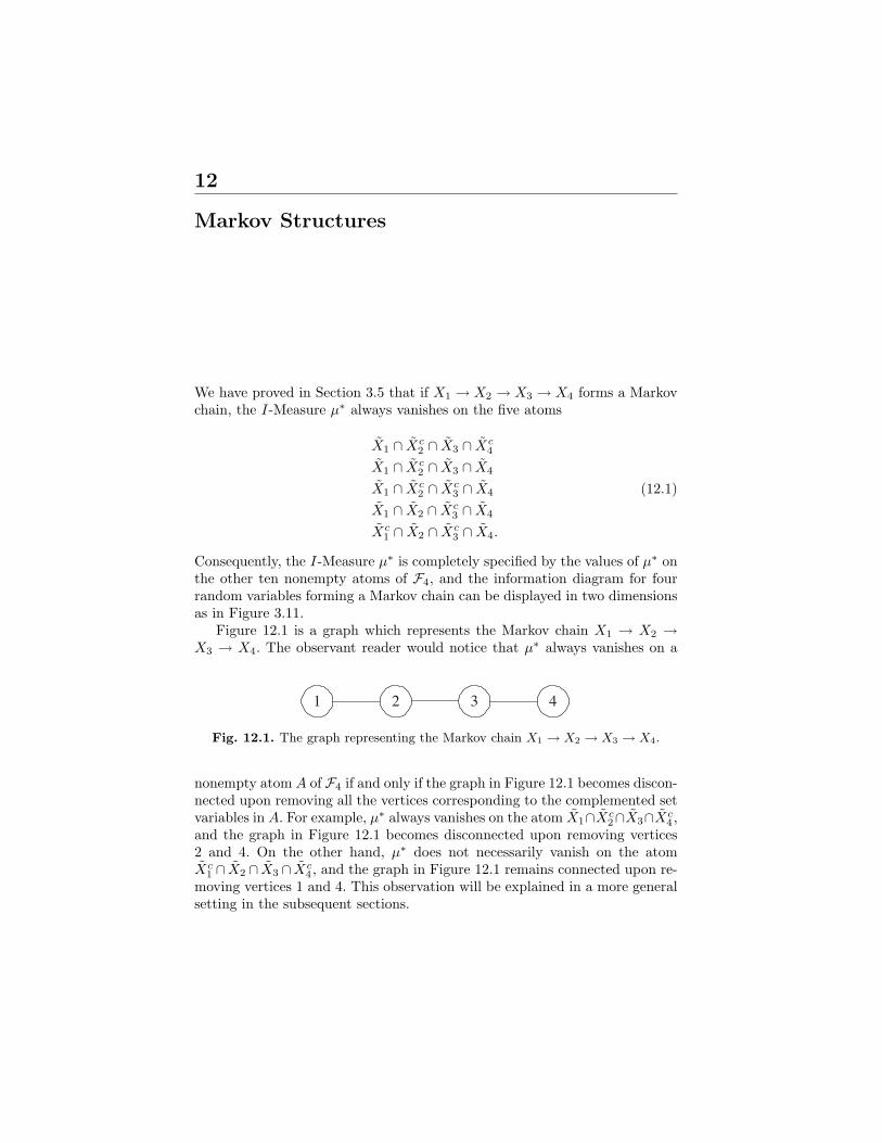
12
Markov Structures
We have proved in Section 3.5 that if X1 → X2 → X3 → X4 forms a Markovchain, the I-Measure µ∗ always vanishes on the five atoms
X1 ∩ Xc2 ∩ X3 ∩ Xc
4
X1 ∩ Xc2 ∩ X3 ∩ X4
X1 ∩ Xc2 ∩ Xc
3 ∩ X4
X1 ∩ X2 ∩ Xc3 ∩ X4
Xc1 ∩ X2 ∩ Xc
3 ∩ X4.
(12.1)
Consequently, the I-Measure µ∗ is completely specified by the values of µ∗ onthe other ten nonempty atoms of F4, and the information diagram for fourrandom variables forming a Markov chain can be displayed in two dimensionsas in Figure 3.11.
Figure 12.1 is a graph which represents the Markov chain X1 → X2 →X3 → X4. The observant reader would notice that µ∗ always vanishes on a
1 2 3 4
Fig. 12.1. The graph representing the Markov chain X1 → X2 → X3 → X4.
nonempty atom A of F4 if and only if the graph in Figure 12.1 becomes discon-nected upon removing all the vertices corresponding to the complemented setvariables in A. For example, µ∗ always vanishes on the atom X1∩Xc
2∩X3∩Xc4 ,
and the graph in Figure 12.1 becomes disconnected upon removing vertices2 and 4. On the other hand, µ∗ does not necessarily vanish on the atomXc
1 ∩ X2 ∩ X3 ∩ Xc4 , and the graph in Figure 12.1 remains connected upon re-
moving vertices 1 and 4. This observation will be explained in a more generalsetting in the subsequent sections.

292 12 Markov Structures
The theory of I-Measure establishes a one-to-one correspondence betweenShannon’s information measures and set theory. Based on this theory, wedevelop in this chapter a set-theoretic characterization of a Markov struc-ture called full conditional mutual independence. A Markov chain, and moregenerally a Markov random field, is a collection of full conditional mutualindependencies. We will show that if a collection of random variables forms aMarkov random field, then the structure of µ∗ can be simplified. In particular,when the random variables form a Markov chain, µ∗ exhibits a very simplestructure so that the information diagram can be displayed in two dimensionsregardless of the length of the Markov chain, and µ∗ is always nonnegative.(See also Sections 3.5 and 3.6.)
The topics to be covered in this chapter are fundamental. Unfortunately,the proofs of the results are very heavy. The reader may skip this chapterwithout affecting further reading of the book.
12.1 Conditional Mutual Independence
In this section, we explore the effect of conditional mutual independence onthe structure of the I-Measure µ∗. We begin with a simple example.
Example 12.1. Let X, Y , and Z be mutually independent random variables.Then
I(X;Y ) = I(X;Y ;Z) + I(X;Y |Z) = 0. (12.2)
Since I(X;Y |Z) ≥ 0, we let
I(X;Y |Z) = a ≥ 0, (12.3)
so thatI(X;Y ;Z) = −a. (12.4)
Similarly,I(Y ;Z) = I(X;Y ;Z) + I(Y ;Z|X) = 0 (12.5)
andI(X;Z) = I(X;Y ;Z) + I(X;Z|Y ) = 0. (12.6)
Then from (12.4), we obtain
I(Y ;Z|X) = I(X;Z|Y ) = a. (12.7)
The relations (12.3), (12.4), and (12.7) are shown in the information diagramin Figure 12.2, which indicates that X, Y , and Z are pairwise independent.
We have proved in Theorem 2.39 that X, Y , and Z are mutually indepen-dent if and only if
H(X,Y, Z) = H(X) +H(Y ) +H(Z). (12.8)

12.1 Conditional Mutual Independence 293
a
a
a -a
X Z
Y
Fig. 12.2. X, Y , and Z are pairwise independent.
By counting atoms in the information diagram, we see that
0 = H(X) +H(Y ) +H(Z)−H(X,Y, Z) (12.9)= I(X;Y |Z) + I(Y ;Z|X) + I(X;Z|Y ) + 2I(X;Y ;Z) (12.10)= a. (12.11)
Thus a = 0, which implies
I(X;Y |Z), I(Y ;Z|X), I(X;Z|Y ), I(X;Y ;Z) (12.12)
are all equal to 0. Equivalently, µ∗ vanishes on
X ∩ Y − Z, Y ∩ Z − X, X ∩ Z − Y , X ∩ Y ∩ Z, (12.13)
which are precisely the atoms in the intersection of any two of the set variablesX, Y , and Z.
Conversely, if µ∗ vanishes on the sets in (12.13), then we see from (12.10)that (12.8) holds, i.e., X, Y , and Z are mutually independent. Therefore, X,Y , and Z are mutually independent if and only if µ∗ vanishes on the sets in(12.13). This is shown in the information diagram in Figure 12.3.
0
0
0 0
X Z
Y
Fig. 12.3. X, Y , and Z are mutually independent.
294 12 Markov Structures
The theme of this example will be extended to conditional mutual inde-pendence among collections of random variables in Theorem 12.9, which isthe main result in this section. In the rest of the section, we will develop thenecessary tools for proving this theorem. At first reading, the reader shouldtry to understand the results by studying the examples without getting intothe details of the proofs.
In Theorem 2.39, we have proved that X1, X2, · · · , Xn are mutually inde-pendent if and only if
H(X1, X2, · · · , Xn) =n∑i=1
H(Xi). (12.14)
By conditioning on a random variable Y , one can readily prove the following.
Theorem 12.2. X1, X2, · · · , Xn are mutually independent conditioning on Yif and only if
H(X1, X2, · · · , Xn|Y ) =n∑i=1
H(Xi|Y ). (12.15)
We now prove two alternative characterizations of conditional mutual in-dependence.
Theorem 12.3. X1, X2, · · · , Xn are mutually independent conditioning on Yif and only if for all 1 ≤ i ≤ n,
I(Xi;Xj , j 6= i|Y ) = 0, (12.16)
i.e., Xi and (Xj , j 6= i) are independent conditioning on Y .
Remark A conditional independency is a special case of a conditional mutualindependency. However, this theorem says that a conditional mutual indepen-dency is equivalent to a set of conditional independencies.
Proof of Theorem 12.3. It suffices to prove that (12.15) and (12.16) are equiva-lent. Assume (12.15) is true, so that X1, X2, · · · , Xn are mutually independentconditioning on Y . Then for all i, Xi is independent of (Xj , j 6= i) conditioningon Y . This proves (12.16).
Now assume that (12.16) is true for all 1 ≤ i ≤ n. Consider
0 = I(Xi;Xj , j 6= i|Y ) (12.17)= I(Xi;X1, X2, · · · , Xi−1|Y )
+I(Xi;Xi+1, · · · , Xn|Y,X1, X2, · · · , Xi−1). (12.18)
Since mutual information is always nonnegative, this implies
I(Xi;X1, · · · , Xi−1|Y ) = 0, (12.19)
or Xi and (X1, X2, · · · , Xi−1) are independent conditioning on Y . Therefore,X1, X2, · · · , Xn are mutually independent conditioning on Y (see the proof ofTheorem 2.39), proving (12.15). Hence, the theorem is proved. ut

12.1 Conditional Mutual Independence 295
Theorem 12.4. X1, X2, · · · , Xn are mutually independent conditioning on Yif and only if
H(X1, X2, · · · , Xn|Y ) =n∑i=1
H(Xi|Y,Xj , j 6= i). (12.20)
Proof. It suffices to prove that (12.15) and (12.20) are equivalent. Assume(12.15) is true, so that X1, X2, · · · , Xn are mutually independent conditioningon Y . Since for all i, Xi is independent of Xj , j 6= i conditioning on Y ,
H(Xi|Y ) = H(Xi|Y,Xj , j 6= i) (12.21)
Therefore, (12.15) implies (12.20).Now assume that (12.20) is true. Consider
H(X1, X2, · · · , Xn|Y )
=n∑i=1
H(Xi|Y,X1, · · · , Xi−1) (12.22)
=n∑i=1
[H(Xi|Y,Xj , j 6= i) + I(Xi;Xi+1, · · · , Xn|Y,X1, · · · , Xi−1)]
(12.23)
=n∑i=1
H(Xi|Y,Xj , j 6= i) +n∑i=1
I(Xi;Xi+1, · · · , Xn|Y,X1, · · · , Xi−1).
(12.24)
Then (12.20) implies
n∑i=1
I(Xi;Xi+1, · · · , Xn|Y,X1, · · · , Xi−1) = 0. (12.25)
Since all the terms in the above summation are nonnegative, they must all beequal to 0. In particular, for i = 1, we have
I(X1;X2, · · · , Xn|Y ) = 0. (12.26)
By symmetry, it can be shown that
I(Xi;Xj , j 6= i|Y ) = 0 (12.27)
for all 1 ≤ i ≤ n. Then this implies (12.15) by the last theorem, completingthe proof. ut

296 12 Markov Structures
Theorem 12.5. Let C and Qi be disjoint index sets and Wi be a subset ofQi for 1 ≤ i ≤ k, where k ≥ 2. Assume that there exist at least two i suchthat Wi 6= ∅. Let XQi = (Xl, l ∈ Qi), 1 ≤ i ≤ k, and XC = (Xl, l ∈ C) becollections of random variables. If XQi , 1 ≤ i ≤ k, are mutually independentconditioning on XC , then XWi such that Wi 6= ∅ are mutually independentconditioning on (XC , XQi−Wi
, 1 ≤ i ≤ k).
We first give an example before we prove the theorem.
Example 12.6. Suppose X1, (X2, X3, X4), and (X5, X6) are mutually indepen-dent conditioning onX7. By Theorem 12.5,X1,X2, and (X5, X6) are mutuallyindependent conditioning on (X3, X4, X7).
Proof of Theorem 12.5. Assume XQi , 1 ≤ i ≤ k, are mutually independentconditioning on XC , i.e.,
H(XQi , 1 ≤ i ≤ k|XC) =k∑i=1
H(XQi |XC). (12.28)
Consider
H(XWi , 1 ≤ i ≤ k|XC , XQi−Wi , 1 ≤ i ≤ k)= H(XQi , 1 ≤ i ≤ k|XC)−H(XQi−Wi , 1 ≤ i ≤ k|XC) (12.29)
=k∑i=1
H(XQi |XC)
−k∑i=1
H(XQi−Wi|XC , XQj−Wj
, 1 ≤ j ≤ i− 1) (12.30)
≥k∑i=1
H(XQi |XC , XQj−Wj , 1 ≤ j ≤ i− 1)
−k∑i=1
H(XQi−Wi|XC , XQj−Wj
, 1 ≤ j ≤ i− 1) (12.31)
=k∑i=1
H(XWi|XC , XQj−Wj
, 1 ≤ j ≤ i) (12.32)
≥k∑i=1
H(XWi|XC , XQj−Wj
, 1 ≤ j ≤ k). (12.33)
In the second step we have used (12.28), and the two inequalities follow be-cause conditioning does not increase entropy. On the other hand, by the chainrule for entropy, we have

12.1 Conditional Mutual Independence 297
H(XWi, 1 ≤ i ≤ k|XC , XQi−Wi
, 1 ≤ i ≤ k)
=k∑i=1
H(XWi|XC , (XQj−Wj
, 1 ≤ j ≤ k), (XWl, 1 ≤ l ≤ i− 1)).
(12.34)
Therefore, it follows from (12.33) that
k∑i=1
H(XWi|XC , XQj−Wj
, 1 ≤ j ≤ k) (12.35)
≤ H(XWi, 1 ≤ i ≤ k|XC , XQi−Wi
, 1 ≤ i ≤ k) (12.36)
=k∑i=1
H(XWi|XC , (XQj−Wj
, 1 ≤ j ≤ k), (XWl, 1 ≤ l ≤ i− 1)).
(12.37)
However, since conditioning does not increase entropy, the ith term in thesummation in (12.35) is lower bounded by the ith term in the summation in(12.37). Thus we conclude that the inequality in (12.36) is an equality. Hence,the conditional entropy in (12.36) is equal to the summation in (12.35), i.e.,
H(XWi , 1 ≤ i ≤ k|XC , XQi−Wi , 1 ≤ i ≤ k) (12.38)
=k∑i=1
H(XWi |XC , XQj−Wj , 1 ≤ j ≤ k). (12.39)
The theorem is proved. ut
Theorem 12.5 specifies a set of conditional mutual independencies (CMI’s)which is implied by a CMI. This theorem is crucial for understanding the effectof a CMI on the structure of the I-Measure µ∗, which we discuss next.
Lemma 12.7. Let (Zi1, · · · , Ziti), 1 ≤ i ≤ r, be r collections of random vari-ables, where r ≥ 2, and let Y be a random variable, such that (Zi1, · · · , Ziti),1 ≤ i ≤ r, are mutually independent conditioning on Y . Then
µ∗
r⋂i=1
ti⋂j=1
Zij − Y
= 0. (12.40)
We first prove the following set identity which will be used in proving thislemma.
Lemma 12.8. Let S and T be disjoint index sets, and Ai and B be sets. Letµ be a set-additive function. Then

298 12 Markov Structures
µ
(⋂i∈S
Ai
)∩
⋂j∈T
Aj
−B
=∑S′⊂S
∑T ′⊂T
(−1)|S′|+|T ′| (µ(AS′ −B) + µ(AT ′ −B)− µ(AS′∪T ′ −B)) ,
(12.41)where AS′ denotes ∪i∈S′Ai.
Proof. The right hand side of (12.41) is equal to∑S′⊂S
∑T ′⊂T
(−1)|S′|+|T ′|µ(AS′ −B) +
∑S′⊂S
∑T ′⊂T
(−1)|S′|+|T ′|µ(AT ′ −B)
−∑S′⊂S
∑T ′⊂T
(−1)|S′|+|T ′|µ(AS′∪T ′ −B). (12.42)
Now∑S′⊂S
∑T ′⊂T
(−1)|S′|+|T ′|µ(AS′ −B) =
∑S′⊂S
(−1)|S′|µ(AS′ −B)
∑T ′⊂T
(−1)|T′|.
(12.43)Since ∑
T ′⊂T(−1)|T
′| =|T |∑k=0
(|T |k
)(−1)k = 0 (12.44)
by the binomial formula1, we conclude that∑S′⊂S
∑T ′⊂T
(−1)|S′|+|T ′|µ(AS′ −B) = 0. (12.45)
Similarly, ∑S′⊂S
∑T ′⊂T
(−1)|S′|+|T ′|µ(AT ′ −B) = 0. (12.46)
Therefore, (12.41) is equivalent to
µ
(⋂i∈S
Ai
)∩
⋂j∈T
Aj
−B =
∑S′⊂S
∑T ′⊂T
(−1)|S′|+|T ′|+1µ(AS′∪T ′ −B)
(12.47)1 This can be obtained by letting a = 1 and b = −1 in the binomial formula
(a+ b)|T | =
|T |∑k=0
(|T |k
)akb|T |−k.

12.1 Conditional Mutual Independence 299
which can readily be obtained from Theorem 3.142. Hence, the lemma isproved. ut
Proof of Lemma 12.7. We first prove the lemma for r = 2. By Lemma 12.8,
µ∗
2⋂i=1
ti⋂j=1
Zij − Y
=
∑S′⊂1,···,t1
∑T ′⊂1,···,t2
(−1)|S′|+|T ′|
µ∗ ⋃j∈S′
Z1j − Y
+µ∗
( ⋃k∈T ′
Z2k − Y
)− µ∗
⋃j∈S′
Z1j
∪( ⋃k∈T ′
Z2k
)− Y
. (12.48)
The expression in the square bracket is equal to
H(Z1j , j ∈ S′|Y ) +H(Z2k, k ∈ T ′|Y )
−H((Z1j , j ∈ S′), (Z2k, k ∈ T ′)|Y ), (12.49)
which is equal to 0 because (Z1j , j ∈ S′) and (Z2k, k ∈ T ′) are independentconditioning on Y . Therefore the lemma is proved for r = 2.
For r > 2, we write
µ∗
r⋂i=1
ti⋂j=1
Zij − Y
= µ∗
r−1⋂i=1
ti⋂j=1
Zij
∩ tr⋂j=1
Zrj
− Y . (12.50)
Since ((Zi1, · · · , Ziti), 1 ≤ i ≤ r − 1) and (Zr1, · · · , Zrtr ) are independentconditioning on Y , upon applying the lemma for r = 2, we see that
µ∗
r⋂i=1
ti⋂j=1
Zij − Y
= 0. (12.51)
The lemma is proved. ut
Theorem 12.9. Let T and Qi, 1 ≤ i ≤ k, be disjoint index sets, where k ≥ 2,and let XQi = (Xl, l ∈ Qi), 1 ≤ i ≤ k, and XT = (Xl, l ∈ T ) be collections ofrandom variables. Then XQi , 1 ≤ i ≤ k, are mutually independent condition-ing on XT if and only if for any W1,W2, · · · ,Wk, where Wi ⊂ Qi, 1 ≤ i ≤ k,if there exist at least two i such that Wi 6= ∅, then
µ∗
k⋂i=1
⋂j∈Wi
Xj
− XT∪(∪ki=1(Qi−Wi))
= 0. (12.52)

300 12 Markov Structures
We first give an example before proving this fundamental result. Thereader should compare this example with Example 12.6.
Example 12.10. Suppose X1, (X2, X3, X4), and (X5, X6) are mutually inde-pendent conditioning on X7. By Theorem 12.9,
µ∗(X1 ∩ X2 ∩ X5 ∩ X6 − (X3 ∪ X4 ∪ X7)) = 0. (12.53)
However, the theorem does not say, for instance, that
µ∗(X2 ∩ X4 − (X1 ∪ X3 ∪ X5 ∪ X6 ∪ X7)) (12.54)
is equal to 0.
Proof of Theorem 12.9. We first prove the ‘if’ part. Assume that for anyW1,W2, · · · ,Wk, where Wi ⊂ Qi, 1 ≤ i ≤ k, if there exist at least two i suchthat Wi 6= ∅, then (12.52) holds. Consider
H(XQi , 1 ≤ i ≤ k|XT ) = µ∗(X∪k
i=1Qi− XT
)(12.55)
=∑B∈S
µ∗(B), (12.56)
where S consists of sets of the form k⋂i=1
⋂j∈Wi
Xj
− XT∪(∪ki=1(Qi−Wi)) (12.57)
with Wi ⊂ Qi for 1 ≤ i ≤ k and there exists at least one i such that Wi 6= ∅.By our assumption, if B ∈ S is such that there exist at least two i for whichWi 6= ∅, then µ∗(B) = 0. Therefore, if µ∗(B) is possibly nonzero, then B mustbe such that there exists a unique i for which Wi 6= ∅. Now for 1 ≤ i ≤ k, letSl be the set consisting of sets of the form in (12.57) with Wi ⊂ Qi, Wi 6= ∅,and Wl = ∅ for l 6= i. In other words, Si consists of atoms of the form ⋂
j∈Wi
Xj
− XT∪(∪l6=iQl)∪(Qi−Wi) (12.58)
with Wi ⊂ Qi and Wi 6= ∅. Then
∑B∈S
µ∗(B) =k∑i=1
∑B∈Si
µ∗(B). (12.59)
Now

12.2 Full Conditional Mutual Independence 301
XQi − XT∪(∪l 6=iQl)
=⋃
Wi⊂QiWi 6=∅
⋂j∈Wi
Xj
− XT∪(∪l 6=iQl)∪(Qi−Wi)
(12.60)
=⋃B∈Si
B. (12.61)
Since µ∗ is set-additive, we have
µ∗(XQi − XT∪(∪l 6=iQl)
)=∑B∈Si
µ∗(B). (12.62)
Hence, from (12.56) and (12.59), we have
H(XQi , 1 ≤ i ≤ k|XT )
=k∑i=1
∑B∈Si
µ∗(B) (12.63)
=k∑i=1
µ∗(XQi − XT∪(∪l6=iQl)
)(12.64)
=k∑i=1
H(XQi |XT , XQl , l 6= i), (12.65)
where (12.64) follows from (12.62). By Theorem 12.4, XQi , 1 ≤ i ≤ k, aremutually independent conditioning on XT .
We now prove the ‘only if’ part. Assume XQi , 1 ≤ i ≤ k, are mutuallyindependent conditioning on XT . For any collection of sets W1,W2, · · · ,Wk,where Wi ⊂ Qi, 1 ≤ i ≤ k, if there exist at least two i such that Wi 6= ∅,by Theorem 12.5, XWi , 1 ≤ i ≤ k, are mutually independent conditioning on(XT , XQi−Wi , 1 ≤ i ≤ k). By Lemma 12.7, we obtain (12.52). The theorem isproved. ut
12.2 Full Conditional Mutual Independence
Definition 12.11. A conditional mutual independency on X1, X2, · · · , Xn isfull if all X1, X2, · · · , Xn are involved. Such a conditional mutual independencyis called a full conditional mutual independency (FCMI).
Example 12.12. For n = 5,
X1, X2, X4, and X5 are mutually independent conditioning on X3
is an FCMI. However,

302 12 Markov Structures
X1, X2, and X5 are mutually independent conditioning on X3
is not an FCMI because X4 is not involved.
As in the previous chapters, we let
Nn = 1, 2, · · · , n. (12.66)
In Theorem 12.9, if
T ∪
(k⋃i=1
Qi
)= Nn, (12.67)
then the tuple (T,Qi, 1 ≤ i ≤ k) defines the following FCMI on X1, X2, · · · ,Xn:
K : XQ1 , XQ2 , · · · , XQk are mutually independent conditioning on XT .
We will denote K by (T,Qi, 1 ≤ i ≤ k).
Definition 12.13. Let K = (T,Qi, 1 ≤ i ≤ k) be an FCMI on X1, X2, · · · ,Xn. The image of K, denoted by Im(K), is the set of all atoms of Fn whichhas the form of the set in (12.57), where Wi ⊂ Qi, 1 ≤ i ≤ k, and there existat least two i such that Wi 6= ∅.
Proposition 12.14. Let K = (T,Q1, Q2) be an FCI (full conditional inde-pendency) on X1, X2, · · · , Xn. Then
Im(K) = A ∈ A : A ⊂ (XQ1 ∩ XQ2 − XT ). (12.68)
Proposition 12.15. Let K = (T,Qi, 1 ≤ i ≤ k) be an FCMI on X1, X2, · · · ,Xn. Then
Im(K) =
A ∈ A : A ⊂⋃
1≤i<j≤k
(XQi ∩ XQj − XT )
. (12.69)
These two propositions greatly simplify the description of Im(K). Theirproofs are elementary and they are left as exercises. We first illustrate thesetwo propositions in the following example.
Example 12.16. Consider n = 4 and FCMI’s K1 = (3, 1, 2, 4) and K2 =(∅, 1, 2, 3, 4). Then
Im(K1) = A ∈ A : A ⊂ (X1 ∩ X2,4 − X3) (12.70)
and
Im(K2) = A ∈ A : A ⊂ (X1 ∩ X2,3)∪ (X2,3 ∩ X4)∪ (X1 ∩ X4). (12.71)

12.2 Full Conditional Mutual Independence 303
Theorem 12.17. Let K be an FCMI on X1, X2, · · · , Xn. Then K holds ifand only if µ∗(A) = 0 for all A ∈ Im(K).
Proof. First, (12.67) is true if K is an FCMI. Then the set in (12.57) can bewritten as ⋂
j∈∪ki=1Wi
Xj
− XNn−∪ki=1Wi, (12.72)
which is seen to be an atom of Fn. The theorem can then be proved by adirect application of Theorem 12.9 to the FCMI K. ut
Let A = ∩ni=1Yi be a nonempty atom of Fn. Define the set
UA = i ∈ Nn : Yi = Xci . (12.73)
Note that A is uniquely specified by UA because
A =
( ⋂i∈Nn−UA
Xi
)∩
( ⋂i∈UA
Xci
)=
( ⋂i∈Nn−UA
Xi
)− XUA . (12.74)
Define w(A) = n− |UA| as the weight of the atom A, the number of Xi in Awhich are not complemented. We now show that an FCMI K = (T,Qi, 1 ≤i ≤ k) is uniquely specified by Im(K). First, by letting Wi = Qi for 1 ≤ i ≤ kin Definition 12.13, we see that the atom ⋂
j∈∪ki=1Qi
Xj
− XT (12.75)
is in Im(K), and it is the unique atom in Im(K) with the largest weight.From this atom, T can be determined. To determine Qi, 1 ≤ i ≤ k, we definea relation q on T c = Nn\T as follows. For l, l′ ∈ T c, (l, l′) is in q if and only if
i) l = l′; orii) there exists an atom of the form
Xl ∩ Xl′ ∩⋂
1≤j≤nj 6=l,l′
Yj (12.76)
in A− Im(K), where Yj = Xj or Xcj .
Recall that A is the set of nonempty atoms of Fn. The idea of ii) is that(l, l′) is in q if and only if l, l′ ∈ Qi for some 1 ≤ i ≤ k. Then q is reflexiveand symmetric by construction, and is transitive by virtue of the structure ofIm(K). In other words, q is an equivalence relation which partitions T c intoQi, 1 ≤ i ≤ k. Therefore, K and Im(K) uniquely specify each other.

304 12 Markov Structures
The image of an FCMI K completely characterizes the effect of K on theI-Measure for X1, X2, · · · , Xn. The joint effect of more than one FCMI caneasily be described in terms of the images of the individual FCMI’s. Let
Π = Kl, 1 ≤ l ≤ m (12.77)
be a set of FCMI’s. By Theorem 12.9, Kl holds if and only if µ∗ vanishes onthe atoms in Im(Kl). Then Kl, 1 ≤ l ≤ m hold simultaneously if and only ifµ∗ vanishes on the atoms in ∪kl=1Im(Kl). This is summarized as follows.
Definition 12.18. The image of a set of FCMI’s Π = Kl, 1 ≤ l ≤ m isdefined as
Im(Π) =k⋃l=1
Im(Kl). (12.78)
Theorem 12.19. Let Π be a set of FCMI’s for X1, X2, · · · , Xn. Then Π holdsif and only if µ∗(A) = 0 for all A ∈ Im(Π).
In probability problems, we are often given a set of conditional indepen-dencies and we need to see whether another given conditional independencyis logically implied. This is called the implication problem which will be dis-cussed in detail in Section 13.5. The next theorem gives a solution to thisproblem if only FCMI’s are involved.
Theorem 12.20. Let Π1 and Π2 be two sets of FCMI’s. Then Π1 implies Π2
if and only if Im(Π2) ⊂ Im(Π1).
Proof. We first prove that if Im(Π2) ⊂ Im(Π1), then Π1 implies Π2. AssumeIm(Π2) ⊂ Im(Π1) and Π1 holds. Then by Theorem 12.19, µ∗(A) = 0 for allA ∈ Im(Π1). Since Im(Π2) ⊂ Im(Π1), this implies that µ∗(A) = 0 for allA ∈ Im(Π2). Again by Theorem 12.19, this implies Π2 also holds. Therefore,if Im(Π2) ⊂ Im(Π1), then Π1 implies Π2.
We now prove that if Π1 implies Π2, then Im(Π2) ⊂ Im(Π1). To provethis, we assume that Π1 implies Π2 but Im(Π2) 6⊂ Im(Π1), and we will showthat this leads to a contradiction. Fix a nonempty atom A ∈ Im(Π2)−Im(Π1).By Theorem 3.11, we can construct random variables X1, X2, · · · , Xn suchthat µ∗ vanishes on all the atoms of Fn except for A. Then µ∗ vanishes on allthe atoms in Im(Π1) but not on all the atoms in Im(Π2). By Theorem 12.19,this implies that for X1, X2, · · · , Xn so constructed, Π1 holds but Π2 does nothold. Therefore, Π1 does not imply Π2, which is a contradiction. The theoremis proved. ut
Remark In the course of proving this theorem and all its preliminaries, wehave used nothing more than the basic inequalities. Therefore, we have shownthat the basic inequalities are a sufficient set of tools to solve the implicationproblem if only FCMI’s are involved.

12.2 Full Conditional Mutual Independence 305
Corollary 12.21. Two sets of FCMI’s are equivalent if and only if their im-ages are identical.
Proof. Two set of FCMI’s Π1 and Π2 are equivalent if and only if
Π1 ⇒ Π2 and Π2 ⇒ Π1. (12.79)
Then by the last theorem, this is equivalent to Im(Π2) ⊂ Im(Π1) and Im(Π1)⊂ Im(Π2), i.e., Im(Π2) = Im(Π1). The corollary is proved. ut
Thus a set of FCMI’s is completely characterized by its image. A set ofFCMI’s is a set of probabilistic constraints, but the characterization by itsimage is purely set-theoretic! This characterization offers an intuitive set-theoretic interpretation of the joint effect of FCMI’s on the I-Measure forX1, X2, · · · , Xn. For example, Im(K1) ∩ Im(K2) is interpreted as the effectcommonly due to K1 and K2, Im(K1) − Im(K2) is interpreted as the effectdue to K1 but not K2, etc. We end this section with an example.
Example 12.22. Consider n = 4. Let
K1 = (∅, 1, 2, 3, 4), K2 = (∅, 1, 2, 4, 3) (12.80)
K3 = (∅, 1, 2, 3, 4), K4 = (∅, 1, 3, 2, 4) (12.81)
and let Π1 = K1,K2 and Π2 = K3,K4. Then
Im(Π1) = Im(K1) ∪ Im(K2) (12.82)
andIm(Π2) = Im(K3) ∪ Im(K4), (12.83)
where
Im(K1) = A ∈ A : A ⊂ (X1,2,3 ∩ X4) (12.84)
Im(K2) = A ∈ A : A ⊂ (X1,2,4 ∩ X3) (12.85)
Im(K3) = A ∈ A : A ⊂ (X1,2 ∩ X3,4) (12.86)
Im(K4) = A ∈ A : A ⊂ (X1,3 ∩ X2,4). (12.87)
It can readily be seen by using an information diagram that Im(Π1) ⊂Im(Π2). Therefore, Π2 implies Π1. Note that no probabilistic argument isinvolved in this proof.

306 12 Markov Structures
12.3 Markov Random Field
A Markov random field is a generalization of a discrete time Markov chain inthe sense that the time index for the latter, regarded as a chain, is replaced bya general graph for the former. Historically, the study of Markov random fieldstems from statistical physics. The classical Ising model, which is defined ona rectangular lattice, was used to explain certain empirically observed factsabout ferromagnetic materials. In this section, we explore the structure of theI-Measure for a Markov random field.
We refer the reader to textbooks on graph theory (e.g. [43]) for formaldefinitions of the graph-theoretic terminologies to be used in the rest of thechapter. Let G = (V,E) be an undirected graph, where V is the set of verticesand E is the set of edges. We assume that there is no loop in G, i.e., thereis no edge in G which connects a vertex to itself. For any (possibly empty)subset U of V , denote by G\U the graph obtained from G by eliminating allthe vertices in U and all the edges joining a vertex in U .
The connectivity of a graph partitions the graph into subgraphs calledcomponents, i.e., two vertices are in the same component if and only if they areconnected. Let s(U) be the number of distinct components in G\U . Denote thesets of vertices of these components by V1(U), V2(U), · · · , Vs(U)(U). If s(U) >1, we say that U is a cutset in G.
Definition 12.23 (Markov random field). Let G = (V,E) be an undi-rected graph with V = Nn = 1, 2, · · · , n, and let Xi be a random vari-able corresponding to vertex i. Then X1, X2, · · · , Xn form a Markov randomfield represented by G if for all cutsets U in G, the sets of random variablesXV1(U), XV2(U), · · · , XVs(U)(U) are mutually independent conditioning on XU .
This definition of a Markov random field is referred to as the global Markovproperty in the literature. If X1, X2, · · · , Xn form a Markov random field rep-resented by a graph G, we also say that X1, X2, · · · , Xn form a Markov graphG. When G is a chain, we say that X1, X2, · · · , Xn form a Markov chain.
In the definition of a Markov random field, each cutset U in G specifies anFCMI on X1, X2, · · · , Xn, denoted by [U ]. Formally,
[U ] : XV1(U), · · · , XVs(U)(U) are mutually independent conditioning on XU .
For a collection of cutsets U1, U2, · · · , Uk in G, we introduce the notation
[U1, U2, · · · , Uk] = [U1] ∧ [U2] ∧ · · · ∧ [Uk] (12.88)
where ‘∧’ denotes ‘logical AND.’ Using this notation, X1, X2, · · · , Xn form aMarkov graph G if and only if
[U ⊂ V : U 6= V and s(U) > 1] (12.89)
holds. Therefore, a Markov random field is simply a collection of FCMI’sinduced by a graph.

12.3 Markov Random Field 307
We now define two types of nonempty atoms of Fn with respect to a graphG. Recall the definition of the set UA for a nonempty atom A of Fn in (12.73).
Definition 12.24. For a nonempty atom A of Fn, if s(UA) = 1, i.e., G\UAis connected, then A is a Type I atom, otherwise A is a Type II atom. The setsof all Type I and Type II atoms of Fn are denoted by T1 and T2, respectively.
Theorem 12.25. X1, X2, · · · , Xn form a Markov graph G if and only if µ∗
vanishes on all Type II atoms.
Before we prove this theorem, we first state the following proposition whichis the graph-theoretic analog of Theorem 12.5. The proof is trivial and is omit-ted. This proposition and Theorem 12.5 together establish an analogy betweenthe structure of conditional mutual independence and the connectivity of agraph. This analogy will play a key role in proving Theorem 12.25.
Proposition 12.26. Let C and Qi be disjoint subsets of the vertex set V ofa graph G and Wi be a subset of Qi for 1 ≤ i ≤ k, where k ≥ 2. Assume thatthere exist at least two i such that Wi 6= ∅. If Qi, 1 ≤ i ≤ k, are disconnected inG\C, then those Wi which are nonempty are disconnected in G\(C∪
⋃ki=1(Qi−
Wi)).
Example 12.27. In the graph G in Figure 12.4, 1, 2, 3, 4, and 5, 6 aredisjoint in G\7. Then Proposition 12.26 says that 1, 2, and 5, 6 aredisjoint in G\3, 4, 7.
1
2
3 4
5 7
6
Fig. 12.4. The graph G in Example 12.27.
Proof of Theorem 12.25. Recall the definition of the set UA for a nonemptyatom A in (12.73). We note that UA, A ∈ A contains precisely all the propersubsets of Nn. Thus the set of FCMI’s specified by the graph G can be writtenas
[UA : A ∈ A and s(UA) > 1] (12.90)
(cf. (12.89)). By Theorem 12.19, it suffices to prove that

308 12 Markov Structures
Im([UA : A ∈ A and s(UA) > 1]) = T2, (12.91)
where T2 was defined in Definition 12.24.We first prove that
T2 ⊂ Im([UA : A ∈ A and s(UA) > 1]). (12.92)
Consider an atom A ∈ T2 so that s(UA) > 1. In Definition 12.13, let T = UA,k = s(UA), and Qi = Vi(UA) for 1 ≤ i ≤ s(UA). By considering Wi = Vi(UA)for 1 ≤ i ≤ s(UA), we see that A ∈ Im([UA]). Therefore,
T2 = A ∈ A : s(UA) > 1 (12.93)
⊂⋃
A∈A:s(UA)>1
Im([UA]) (12.94)
= Im([UA : A ∈ A and s(UA) > 1]). (12.95)
We now prove that
Im([UA : A ∈ A and s(UA) > 1]) ⊂ T2. (12.96)
Consider A ∈ Im([UA : A ∈ A and s(UA) > 1]). Then there exists A∗ ∈ Awith s(UA∗) > 1 such that A ∈ Im([UA∗ ]). From Definition 12.13,
A =
⋂j∈∪s(UA∗ )
i=1 Wi
Xj
− XUA∗∪
(∪s(UA∗ )i=1 (Vi(UA∗ )−Wi)
), (12.97)
where Wi ⊂ Vi(UA∗), 1 ≤ i ≤ s(UA∗), and there exist at least two i such thatWi 6= ∅. It follows from (12.97) and the definition of UA that
UA = UA∗ ∪s(UA∗ )⋃i=1
(Vi(UA∗)−Wi). (12.98)
With UA∗ playing the role of C and Vi(UA∗) playing the role of Qi in Propo-sition 12.26, we see by applying the proposition that those (at least two) Wi
which are nonempty are disjoint in
G \
UA∗ ∪s(UA∗ )⋃
i=1
(Vi(UA∗)−Wi)
= G\UA. (12.99)
This implies s(UA) > 1, i.e., A ∈ T2. Therefore, we have proved (12.96), andhence the theorem is proved. utExample 12.28. With respect to the graph G in Figure 12.5, the Type II atomsare
X1 ∩ X2 ∩ Xc3 ∩ X4, X
c1 ∩ X2 ∩ Xc
3 ∩ X4, X1 ∩ Xc2 ∩ Xc
3 ∩ X4, (12.100)
while the other twelve nonempty atoms of F4 are Type I atoms. The randomvariables X1, X2, X3, and X4 form a Markov graph G if and only if µ∗(A) = 0for all Type II atoms A.

12.4 Markov Chain 309
1
2
3 4
Fig. 12.5. The graph G in Example 12.28.
12.4 Markov Chain
When the graph G representing a Markov random field is a chain, the Markovrandom field becomes a Markov chain. In this section, we will show that theinformation diagram for a Markov chain can be displayed in two dimensions.We will also show that the I-Measure µ∗ for a Markov chain is always nonneg-ative. This characteristic of µ∗ facilitates the use of the information diagrambecause if B is seen to be a subset of B′ in the information diagram, then
µ∗(B′) = µ∗(B) + µ∗(B′ −B) ≥ µ∗(B). (12.101)
These two properties are not possessed by a general Markov random field.Without loss of generality, we assume that the Markov chain is represented
by the graph G in Figure 12.6. This corresponds to the Markov chain X1 →
1 2 n -1 n ...
Fig. 12.6. The graph G representing the Markov chain X1 → X2 → · · · → Xn.
X2 → · · · → Xn. We first prove the following characterization of a Type Iatom for a Markov chain.
Lemma 12.29. For the Markov chain represented by the graph G in Fig-ure 12.6, a nonempty atom A of Fn is a Type I atom if and only if
Nn\UA = l, l + 1, · · · , u, (12.102)
where 1 ≤ l ≤ u ≤ n, i.e., the indices of the set variables in A which are notcomplemented are consecutive.
Proof. It is easy to see that for a nonempty atom A, if (12.102) is satisfied,then G\UA is connected, i.e., s(UA) = 1. Therefore, A is a Type I atom of Fn.On the other hand, if (12.102) is not satisfied, then G\UA is not connected,i.e., s(UA) > 1, or A is a Type II atom of Fn. The lemma is proved. ut

310 12 Markov Structures
We now show how the information diagram for a Markov chain with anylength n ≥ 3 can be constructed in two dimensions. Since µ∗ vanishes onall the Type II atoms of Fn, it is not necessary to display these atoms inthe information diagram. In constructing the information diagram, the re-gions representing the random variables X1, X2, · · · , Xn should overlap witheach other such that the regions corresponding to all the Type II atoms areempty, while the regions corresponding to all the Type I atoms are nonempty.Figure 12.7 shows such a construction. Note that this information diagramincludes Figures 3.7 and 3.9 as special cases, which are information diagramsfor Markov chains with lengths 3 and 4, respectively.
We have already shown that µ∗ is nonnegative for a Markov chain withlength 3 or 4. Toward proving that this is true for any length n ≥ 3, it sufficesto show that µ∗(A) ≥ 0 for all Type I atoms A of Fn because µ∗(A) = 0 forall Type II atoms A of Fn. We have seen in Lemma 12.29 that for a Type Iatom A of Fn, UA has the form as prescribed in (12.102). Consider any suchatom A. Then an inspection of the information diagram in Figure 12.7 revealsthat
µ∗(A) = µ∗(Xl ∩ Xl+1 ∩ · · · ∩ Xu − XUA) (12.103)= I(Xl;Xu|XUA) (12.104)≥ 0. (12.105)
This shows that µ∗ is always nonnegative. However, since Figure 12.7 involvesan indefinite number of random variables, we give a formal proof of this resultin the following theorem.
Theorem 12.30. For a Markov chain X1 → X2 → · · · → Xn, µ∗ is nonneg-ative.
Proof. Since µ∗(A) = 0 for all Type II atoms A of Fn, it suffices to showthat µ∗(A) ≥ 0 for all Type I atoms A of Fn. We have seen in Lemma 12.29that for a Type I atom A of Fn, UA has the form as prescribed in (12.102).Consider any such atom A and define the set
W = l + 1, · · · , u− 1. (12.106)
... X 1 X 2 X n -1 X n
Fig. 12.7. The information diagram for the Markov chain X1 → X2 → · · · → Xn.

Problems 311
Then
I(Xl;Xu|XUA)= µ∗(Xl ∩ Xu − XUA) (12.107)
= µ∗
( ⋃S⊂W
(Xl ∩
(⋂t∈S
Xt
)∩ Xu − XUA∪(W\S)
))(12.108)
=∑S⊂W
µ∗
(Xl ∩
(⋂t∈S
Xt
)∩ Xu − XUA∪(W\S)
). (12.109)
In the above summation, except for the atom corresponding to S = W , namely(Xl ∩ Xl+1 ∩ · · · ∩ Xu − XUA), all the atoms are Type II atoms. Therefore,
I(Xl;Xu|XUA) = µ∗(Xl ∩ Xl+1 ∩ · · · ∩ Xu − XUA). (12.110)
Hence,
µ∗(A) = µ∗(Xl ∩ Xl+1 ∩ · · · ∩ Xu − XUA) (12.111)= I(Xl;Xu|XUA) (12.112)≥ 0. (12.113)
The theorem is proved. ut
Problems
1. Prove Proposition 12.14 and Proposition 12.15.2. In Example 12.22, it was shown that Π2 implies Π1. Show that Π1
does not imply Π2. Hint: Use an information diagram to determineIm(Π2)\Im(Π1).
3. Alternative definition of the global Markov property: For any partitionU, V1, V2 of V such that the sets of vertices V1 and V2 are disconnectedin G\U , the sets of random variables XV1 and XV2 are independent con-ditioning on XU .Show that this definition is equivalent to the global Markov property inDefinition 12.23.
4. The local Markov property: For 1 ≤ i ≤ n, Xi and XV−Ni−i are indepen-dent conditioning on XNi , where Ni is the set of neighbors2 of vertex i inG.a) Show that the global Markov property implies the local Markov prop-
erty.
2 Vertices i and j in an undirected graph are neighbors if i and j are connected byan edge.

312 12 Markov Structures
b) Show that the local Markov property does not imply the globalMarkov property by giving a counterexample. Hint: Consider a jointdistribution which is not strictly positive.
5. Construct a Markov random field whose I-Measure µ∗ can take negativevalues. Hint: Consider a Markov “star.”
6. a) Show that X1, X2, X3, and X4 are mutually independent if and onlyif
X1 ⊥ (X2, X3, X4), X2 ⊥ (X3, X4)|X1, X3 ⊥ X4|(X1, X2).
Hint: Use an information diagram.b) Generalize the result in a) to n random variables.
7. Determine the Markov random field with four random variables X1, X2,X3, and X4 which is characterized by the following conditional indepen-dencies:
(X1, X2, X5) ⊥ X4|X3
X2 ⊥ (X4, X5)|(X1, X3)X1 ⊥ (X3, X4)|(X2, X5).
What are the other conditional independencies pertaining to this Markovrandom field?
Historical Notes
A Markov random field can be regarded as a generalization of a discrete-timeMarkov chain. Historically, the study of Markov random field stems from sta-tistical physics. The classical Ising model, which is defined on a rectangularlattice, was used to explain certain empirically observed facts about ferromag-netic materials. The foundation of the theory of Markov random fields can befound in Preston [268] or Spitzer [311].
The structure of the I-Measure for a Markov chain was first investigatedin the unpublished work of Kawabata [176]. Essentially the same result wasindependently obtained by R. W. Yeung eleven years later in the context ofthe I-Measure, and the result was eventually published in Kawabata and Ye-ung [177]. Full conditional independencies were shown to be axiomatizable byMalvestuto [219]. The results in this chapter are due to Yeung et al. [366],where they obtained a set-theoretic characterization of full conditional in-dependencies and investigated the structure of the I-Measure for a Markovrandom field. In this paper, they also obtained a hypergraph characterizationof a Markov random field based on the I-Measure characterization in Theo-rem 12.25. Ge and Ye [119] have applied these results to characterize a classof graphical models for conditional independence of random variables.

13
Information Inequalities
An information expression f refers to a linear combination1 of Shannon’sinformation measures involving a finite number of random variables. For ex-ample,
H(X,Y ) + 2I(X;Z) (13.1)
andI(X;Y )− I(X;Y |Z) (13.2)
are information expressions. An information inequality has the form
f ≥ c, (13.3)
where the constant c is usually equal to zero. We consider non-strict inequal-ities only because these are usually the form of inequalities in informationtheory. Likewise, an information identity has the form
f = c. (13.4)
We point out that an information identity f = c is equivalent to the pair ofinformation inequalities f ≥ c and f ≤ c.
An information inequality or identity is said to always hold if it holds forany joint distribution for the random variables involved. For example, we saythat the information inequality
I(X;Y ) ≥ 0 (13.5)
always holds because it holds for any joint distribution p(x, y). On the otherhand, we say that an information inequality does not always hold if thereexists a joint distribution for which the inequality does not hold. Consider theinformation inequality
1 More generally, an information expression can be nonlinear, but they do notappear to be useful in information theory.

314 13 Information Inequalities
I(X;Y ) ≤ 0. (13.6)
SinceI(X;Y ) ≥ 0 (13.7)
always holds, (13.6) is equivalent to
I(X;Y ) = 0, (13.8)
which holds if and only if X and Y are independent. In other words, (13.6)does not hold if X and Y are not independent. Therefore, we say that (13.6)does not always hold.
As we have seen in the previous chapters, information inequalities are themajor tools for proving converse coding theorems. These inequalities governthe impossibilities in information theory. More precisely, information inequal-ities imply that certain things cannot happen. As such, they are referred toas the laws of information theory.
The basic inequalities form the most important set of information inequal-ities. In fact, almost all the information inequalities known to date are impliedby the basic inequalities. These are called Shannon-type inequalities. On theother hand, if an information inequality always holds but is not implied bythe basic inequalities, then it is called a non-Shannon-type inequality. We havenot yet explained what it means by that an inequality is or is not implied bythe basic inequalities, but this will become clear later in the chapter.
Let us now rederive the inequality obtained in Example 3.15 (Imperfectsecrecy theorem) without using an information diagram. In this example, threerandom variables X,Y , and Z are involved, and the setup of the problem isequivalent to the constraint
H(X|Y,Z) = 0. (13.9)
Then
I(X;Y )= H(X) +H(Y )−H(X,Y ) (13.10)= H(X) +H(Y )− [H(X,Y, Z)−H(Z|X,Y )] (13.11)≥ H(X) +H(Y )−H(X,Y, Z) (13.12)= H(X) +H(Y )− [H(Z) +H(Y |Z) +H(X|Y, Z)] (13.13)= H(X)−H(Z) + I(Y ;Z)−H(X|Y,Z) (13.14)≥ H(X)−H(Z), (13.15)
where we have usedH(Z|X,Y ) ≥ 0 (13.16)
in obtaining (13.12), andI(Y ;Z) ≥ 0 (13.17)

13.1 The Region Γ ∗n 315
and (13.9) in obtaining (13.15). This derivation is less transparent than the onewe presented in Example 3.15, but the point here is that the final inequality weobtain in (13.15) can be proved by invoking the basic inequalities (13.16) and(13.17). In other words, (13.15) is implied by the basic inequalities. Therefore,it is a (constrained) Shannon-type inequality.
We are motivated to ask the following two questions:
1. How can Shannon-type inequalities be characterized? That is, given aninformation inequality, how can we tell whether it is implied by the basicinequalities?
2. Are there any non-Shannon-type information inequalities?
These are two very fundamental questions in information theory. We point outthat the first question naturally comes before the second question because ifwe cannot characterize all Shannon-type inequalities, even if we are given anon-Shannon-type inequality, we cannot tell that it actually is one.
In this chapter, we develop a geometric framework for information inequal-ities which allows them to be studied systematically. This framework naturallyleads to an answer to the first question, which makes machine-proving of allShannon-type inequalities possible. This will be discussed in the next chap-ter. The second question will be answered positively in Chapter 15. In otherwords, there do exist laws in information theory beyond those laid down byShannon.
13.1 The Region Γ ∗n
LetNn = 1, 2, · · · , n, (13.18)
where n ≥ 2, and letΘ = Xi, i ∈ Nn (13.19)
be any collection of n random variables. Associated with Θ are
k = 2n − 1 (13.20)
joint entropies. For example, for n = 3, the 7 joint entropies associated withrandom variables X1, X2, and X3 are
H(X1), H(X2), H(X3), H(X1, X2),
H(X2, X3), H(X1, X3), H(X1, X2, X3). (13.21)
Let < denote the set of real numbers. For any nonempty subset α of Nn,let
Xα = (Xi, i ∈ α) (13.22)
and

316 13 Information Inequalities
HΘ(α) = H(Xα). (13.23)
For a fixed Θ, we can then view HΘ as a set function from 2Nn to < withHΘ(∅) = 0, i.e., we adopt the convention that the entropy of an empty setof random variable is equal to zero. For this reason, we call HΘ the entropyfunction of Θ.
Let Hn be the k-dimensional Euclidean space with the coordinates labeledby hα, α ∈ 2Nn\∅, where hα corresponds to the value of HΘ(α) for anycollection Θ of n random variables. We will refer to Hn as the entropy spacefor n random variables. Then an entropy function HΘ can be represented bya column vector in Hn. On the other hand, a column vector h ∈ Hn is calledentropic if h is equal to the entropy function HΘ of some collection Θ of nrandom variables. We are motivated to define the following region in Hn:
Γ ∗n = h ∈ Hn : h is entropic. (13.24)
For convenience, the vectors in Γ ∗n will also be referred to as entropy functions.As an example, for n = 3, the coordinates of H3 are labeled by
h1, h2, h3, h12, h13, h23, h123, (13.25)
where h123 denotes h1,2,3, etc, and Γ ∗3 is the region in H3 of all entropyfunctions for 3 random variables.
While further characterizations of Γ ∗n will be given later, we first point outa few basic properties of Γ ∗n :
1. Γ ∗n contains the origin.2. Γ
∗n, the closure of Γ ∗n , is convex.
3. Γ ∗n is in the nonnegative orthant of the entropy space Hn2.
The origin of the entropy space corresponds to the entropy function of n de-generate random variables taking constant values. Hence, Property 1 follows.Property 2 will be proved in Chapter 15. Properties 1 and 2 imply that Γ
∗n
is a convex cone. Property 3 is true because the coordinates in the entropyspace Hn correspond to joint entropies, which are always nonnegative.
13.2 Information Expressions in Canonical Form
Any Shannon’s information measure other than a joint entropy can be ex-pressed as a linear combination of joint entropies by application of one of thefollowing information identities:
H(X|Y ) = H(X,Y )−H(Y ) (13.26)I(X;Y ) = H(X) +H(Y )−H(X,Y ) (13.27)
I(X;Y |Z) = H(X,Z) +H(Y,Z)−H(X,Y, Z)−H(Z). (13.28)2 The nonnegative orthant of Hn is the region h ∈ Hn : hα ≥ 0 for all α ∈
2Nn\∅.

13.2 Information Expressions in Canonical Form 317
The first and the second identity are special cases of the third identity, whichhas already been proved in Lemma 3.8. Thus any information expression whichinvolves n random variables can be expressed as a linear combination of the kassociated joint entropies. We call this the canonical form of an informationexpression. When we write an information expression f as f(h), it means thatf is in canonical form. Since an information expression in canonical form is alinear combination of the joint entropies, it has the form
b>h (13.29)
where b> denotes the transpose of a constant column vector b in <k.The identities in (13.26) to (13.28) provide a way to express every infor-
mation expression in canonical form. However, it is not clear whether such acanonical form is unique. To illustrate the point, we consider obtaining thecanonical form of H(X|Y ) in two ways. First,
H(X|Y ) = H(X,Y )−H(Y ). (13.30)
Second,
H(X|Y ) = H(X)− I(X;Y ) (13.31)= H(X)− (H(Y )−H(Y |X)) (13.32)= H(X)− (H(Y )−H(X,Y ) +H(X)) (13.33)= H(X,Y )−H(Y ). (13.34)
Thus it turns out that we can obtain the same canonical form for H(X|Y )via two different expansions. This is not accidental, as it is implied by theuniqueness of the canonical form which we will prove shortly.
Recall from the proof of Theorem 3.6 that the vector h represents thevalues of the I-Measure µ∗ on the unions in Fn. Moreover, h is related to thevalues of µ∗ on the atoms of Fn, represented as u, by
h = Cnu (13.35)
where Cn is a unique k × k matrix (cf. (3.27)). We now state the followinglemma which is a rephrase of Theorem 3.11. This lemma is essential for provingthe next theorem which implies the uniqueness of the canonical form.
Lemma 13.1. LetΨ∗n = u ∈ <k : Cnu ∈ Γ ∗n. (13.36)
Then the nonnegative orthant of <k is a subset of Ψ∗n.
Theorem 13.2. Let f be an information expression. Then the unconstrainedinformation identity f = 0 always holds if and only if f is the zero function.

318 13 Information Inequalities
Proof. Without loss of generality, assume f is in canonical form and let
f(h) = b>h. (13.37)
Assume f = 0 always holds and f is not the zero function, i.e., b 6= 0. We willshow that this leads to a contradiction. Now f = 0, or more precisely the set
h : b>h = 0, (13.38)
is a hyperplane3 in the entropy space which has zero Lebesgue measure4. Iff = 0 always holds, i.e., it holds for all joint distributions, then Γ ∗n mustbe contained in the hyperplane f = 0, otherwise there exists an h0 ∈ Γ ∗nwhich is not on f = 0, i.e., f(h0) 6= 0. Since h0 ∈ Γ ∗n , it corresponds to theentropy function of some joint distribution. This means that there exists ajoint distribution such that f(h) = 0 does not hold, which cannot be truebecause f = 0 always holds.
If Γ ∗n has positive Lebesgue measure, it cannot be contained in the hyper-plane f = 0 which has zero Lebesgue measure. Therefore, it suffices to showthat Γ ∗n has positive Lebesgue measure. To this end, we see from Lemma 13.1that the nonnegative orthant of Hn, which has positive Lebesgue measure,is a subset of Ψ∗n. Thus Ψ∗n has positive Lebesgue measure. Since Γ ∗n is aninvertible transformation of Ψ∗n, its Lebesgue measure is also positive.
Therefore, Γ ∗n is not contained in the hyperplane f = 0, which implies thatthere exists a joint distribution for which f = 0 does not hold. This leads toa contradiction because we have assumed that f = 0 always holds. Hence, wehave proved that if f = 0 always holds, then f must be the zero function.
Conversely, if f is the zero function, then it is trivial that f = 0 alwaysholds. The theorem is proved. ut
Corollary 13.3. The canonical form of an information expression is unique.
Proof. Let f1 and f2 be canonical forms of an information expression g. Since
g = f1 (13.39)
andg = f2 (13.40)
always hold,f1 − f2 = 0 (13.41)
always holds. By the above theorem, f1−f2 is the zero function, which impliesthat f1 and f2 are identical. The corollary is proved. ut
3 If b = 0, then h : b>h = 0 is equal to Hn.4 The Lebesque measure can be thought of as “volume” in the Euclidean space if
the reader is not familiar with measure theory.

13.3 A Geometrical Framework 319
Due to the uniqueness of the canonical form of an information expression,it is an easy matter to check whether for two information expressions f1 andf2 the unconstrained information identity
f1 = f2 (13.42)
always holds. All we need to do is to express f1 − f2 in canonical form. If allthe coefficients are zero, then (13.42) always holds, otherwise it does not.
13.3 A Geometrical Framework
In the last section, we have seen the role of the region Γ ∗n in proving un-constrained information identities. In this section, we explain the geometricalmeanings of unconstrained information inequalities, constrained informationinequalities, and constrained information identities in terms of Γ ∗n . Withoutloss of generality, we assume that all information expressions are in canonicalform.
13.3.1 Unconstrained Inequalities
Consider an unconstrained information inequality f ≥ 0, where f(h) = b>h.Then f ≥ 0 corresponds to the set
h ∈ Hn : b>h ≥ 0 (13.43)
which is a half-space in the entropy space Hn containing the origin. Specif-ically, for any h ∈ Hn, f(h) ≥ 0 if and only if h belongs to this set. Forsimplicity, we will refer to this set as the half-space f ≥ 0. As an example, forn = 2, the information inequality
I(X1;X2) = H(X1) +H(X2)−H(X1, X2) ≥ 0, (13.44)
written ash1 + h2 − h12 ≥ 0, (13.45)
corresponds to the half-space
h ∈ Hn : h1 + h2 − h12 ≥ 0. (13.46)
in the entropy space H2.Since an information inequality always holds if and only if it is satisfied
by the entropy function of any joint distribution for the random variablesinvolved, we have the following geometrical interpretation of an informationinequality:
f ≥ 0 always holds if and only if Γ ∗n ⊂ h ∈ Hn : f(h) ≥ 0.

320 13 Information Inequalities
This gives a complete characterization of all unconstrained inequalities interms of Γ ∗n . If Γ ∗n is known, we in principle can determine whether any infor-mation inequality involving n random variables always holds.
The two possible cases for f ≥ 0 are illustrated in Figure 13.1 and Fig-ure 13.2. In Figure 13.1, Γ ∗n is completely included in the half-space f ≥ 0,
f 0 n
Fig. 13.1. An illustration for f ≥ 0 always holds.
f 0
. h n
0
Fig. 13.2. An illustration for f ≥ 0 not always holds.
so f ≥ 0 always holds. In Figure 13.2, there exists a vector h0 ∈ Γ ∗n such thatf(h0) < 0. Thus the inequality f ≥ 0 does not always hold.
13.3.2 Constrained Inequalities
In information theory, we very often deal with information inequalities (iden-tities) with certain constraints on the joint distribution for the random vari-

13.3 A Geometrical Framework 321
ables involved. These are called constrained information inequalities (identi-ties), and the constraints on the joint distribution can usually be expressedas linear constraints on the entropies. The following are such examples:
1. X1, X2, and X3 are mutually independent if and only if H(X1, X2, X3) =H(X1) +H(X2) +H(X3).
2. X1, X2, and X3 are pairwise independent if and only if I(X1;X2) =I(X2;X3) = I(X1;X3) = 0.
3. X1 is a function of X2 if and only if H(X1|X2) = 0.4. X1 → X2 → X3 → X4 forms a Markov chain if and only if I(X1;X3|X2)
= 0 and I(X1, X2;X4|X3) = 0.
Suppose there are q linear constraints on the entropies given by
Qh = 0, (13.47)
where Q is a q × k matrix. Here we do not assume that the q constraints arelinearly independent, so Q is not necessarily full rank. Let
Φ = h ∈ Hn : Qh = 0. (13.48)
In other words, the q constraints confine h to a linear subspace Φ in theentropy space. Parallel to our discussion on unconstrained inequalities, wehave the following geometrical interpretation of a constrained inequality:
Under the constraint Φ, f ≥ 0 always holds if and only if (Γ ∗n ∩ Φ) ⊂h : f(h) ≥ 0.
This gives a complete characterization of all constrained inequalities in termsof Γ ∗n . Note that Φ = Hn when there is no constraint on the entropies. In thissense, an unconstrained inequality is a special case of a constrained inequality.
The two cases of f ≥ 0 under the constraint Φ are illustrated in Figure 13.3and Figure 13.4. Figure 13.3 shows the case when f ≥ 0 always holds underthe constraint Φ. Note that f ≥ 0 may or may not always hold when there isno constraint. Figure 13.4 shows the case when f ≥ 0 does not always holdunder the constraint Φ. In this case, f ≥ 0 does not always hold when thereis no constraint, because
(Γ ∗n ∩ Φ) 6⊂ h : f(h) ≥ 0 (13.49)
impliesΓ ∗n 6⊂ h : f(h) ≥ 0. (13.50)
13.3.3 Constrained Identities
As we have pointed out at the beginning of the chapter, an identity
f = 0 (13.51)
always holds if and only if both the inequalities f ≥ 0 and f ≤ 0 always hold.Then following our discussion on constrained inequalities, we have

322 13 Information Inequalities
f 0
Fig. 13.3. An illustration for f ≥ 0 always holds under the constraint Φ.
Under the constraint Φ, f = 0 always holds if and only if (Γ ∗n ∩ Φ) ⊂h : f(h) ≥ 0 ∩ h : f(h) ≤ 0,
or
Under the constraint Φ, f = 0 always holds if and only if (Γ ∗n ∩ Φ) ⊂h : f(h) = 0.
This condition says that the intersection of Γ ∗n and Φ is contained in thehyperplane f = 0.
13.4 Equivalence of Constrained Inequalities
When there is no constraint on the entropies, two information inequalities
f 0
Fig. 13.4. An illustration for f ≥ 0 not always holds under the constraint Φ.

13.4 Equivalence of Constrained Inequalities 323
b>h ≥ 0 (13.52)
andc>h ≥ 0 (13.53)
are equivalent if and only if c = ab, where a is a positive constant. However,this is not the case under a non-trivial constraint Φ 6= Hn. This situation isillustrated in Figure 13.5. In this figure, although the inequalities in (13.52)
b h 0 c h 0
Fig. 13.5. Equivalence of b>h ≥ 0 and c>h ≥ 0 under the constraint Φ.
and (13.53) correspond to different half-spaces in the entropy space, theyactually impose the same constraint on h when h is confined to Φ.
In this section, we present a characterization of (13.52) and (13.53) beingequivalent under a set of linear constraint Φ. The reader may skip this sectionat first reading.
Let r be the rank of Q in (13.47). Since h is in the null space of Q, wecan write
h = Qh′, (13.54)
where Q is a k× (k− r) matrix such that the rows of Q> form a basis of theorthogonal complement of the row space of Q, and h′ is a column (k − r)-vector. Then using (13.54), (13.52) and (13.53) can be written as
b>Qh′ ≥ 0 (13.55)
andc>Qh′ ≥ 0, (13.56)
respectively in terms of the set of basis given by the columns of Q. Then(13.55) and (13.56) are equivalent if and only if
c>Q = ab>Q, (13.57)

324 13 Information Inequalities
where a is a positive constant, or
(c− ab)>Q = 0. (13.58)
In other words, (c − ab)> is in the orthogonal complement of the row spaceof Q>, i.e., (c − ab)> is in the row space of Q. Let Q′ be an r × k matrixwhose row space is the same as that of Q. (Q can be taken as Q′ if Q is fullrank.) Since the rank of Q is r and Q′ has r rows, the rows of Q′ form a basisfor the row space of Q, and Q′ is full rank. Then from (13.58), (13.55) and(13.56) are equivalent under the constraint Φ if and only if
c = ab + (Q′)>e (13.59)
for some positive constant a and some column r-vector e.Suppose for given b and c, we want to see whether (13.55) and (13.56)
are equivalent under the constraint Φ. We first consider the case when eitherb> or c> is in the row space of Q. This is actually not an interesting casebecause if b>, for example, is in the row space of Q, then
b>Q = 0 (13.60)
in (13.55), which means that (13.55) imposes no additional constraint underthe constraint Φ.
Theorem 13.4. If either b> or c> is in the row space of Q, then b>h ≥ 0and c>h ≥ 0 are equivalent under the constraint Φ if and only if both b> andc> are in the row space of Q.
The proof of this theorem is left as an exercise. We now turn to the moreinteresting case when neither b> nor c> is in the row space of Q. The followingtheorem gives an explicit condition for (13.55) and (13.56) to be equivalentunder the constraint Φ.
Theorem 13.5. If neither b> nor c> is in the row space of Q, then b>h ≥ 0and c>h ≥ 0 are equivalent under the constraint Φ if and only if[
(Q′)> b] [ea
]= c. (13.61)
has a unique solution with a > 0, where Q′ is any matrix whose row space isthe same as that of Q.
Proof. For b> and c> not in the row space of Q, we want to see when wecan find unknowns a and e satisfying (13.59) with a > 0. To this end, wewrite (13.59) in matrix form as (13.61). Since b is not in the column space of(Q′)> and (Q′)> is full rank,
[(Q′)> b
]is also full rank. Then (13.61) has
either a unique solution or no solution. Therefore, the necessary and sufficientcondition for (13.55) and (13.56) to be equivalent is that (13.61) has a uniquesolution and a > 0. The theorem is proved. ut

13.4 Equivalence of Constrained Inequalities 325
Example 13.6. Consider three random variables X1, X2, and X3 with theMarkov constraint
I(X1;X3|X2) = 0, (13.62)
which is equivalent to
H(X1, X2) +H(X2, X3)−H(X1, X2, X3)−H(X2) = 0. (13.63)
In terms of the coordinates in the entropy space H3, this constraint is writtenas
Qh = 0, (13.64)
whereQ = [ 0 −1 0 1 1 0 −1 ] (13.65)
andh = [h1 h2 h3 h12 h23 h13 h123 ]>. (13.66)
We now show that under the constraint in (13.64), the inequalities
H(X1|X3)−H(X1|X2) ≥ 0 (13.67)
andI(X1;X2|X3) ≥ 0 (13.68)
are in fact equivalent. Toward this end, we write (13.67) and (13.68) as b>h ≥0 and c>h ≥ 0, respectively, where
b = [ 0 1 −1 −1 0 1 0 ]> (13.69)
andc = [ 0 0 −1 0 1 1 −1 ]>. (13.70)
Since Q is full rank, we may take Q′ = Q. Upon solving
[Q> b
] [ea
]= c, (13.71)
we obtain the unique solution a = 1 > 0 and e = 1 (e is a 1 × 1 matrix).Therefore, (13.67) and (13.68) are equivalent under the constraint in (13.64).
Under the constraint Φ, if neither b> nor c> is in the row space of Q, itcan be shown that the identities
b>h = 0 (13.72)
andc>h = 0 (13.73)
are equivalent if and only if (13.61) has a unique solution. We leave the proofas an exercise.

326 13 Information Inequalities
13.5 The Implication Problem of ConditionalIndependence
We use Xα ⊥ Xβ |Xγ to denote the conditional independency (CI)
Xα and Xβ are conditionally independent given Xγ .
We have proved in Theorem 2.34 that Xα ⊥ Xβ |Xγ is equivalent to
I(Xα;Xβ |Xγ) = 0. (13.74)
When γ = ∅, Xα ⊥ Xβ |Xγ becomes an unconditional independency which weregard as a special case of a conditional independency. When α = β, (13.74)becomes
H(Xα|Xγ) = 0, (13.75)
which we see from Proposition 2.36 that Xα is a function of Xγ . For thisreason, we also regard functional dependency as a special case of conditionalindependency.
In probability problems, we are often given a set of CI’s and we need todetermine whether another given CI is logically implied. This is called theimplication problem, which is perhaps the most basic problem in probabilitytheory. We have seen in Section 12.2 that the implication problem has asolution if only full conditional mutual independencies are involved. However,the general problem is extremely difficult, and it has recently been solved onlyup to four random variables by Matus [231].
We end this section by explaining the relation between the implicationproblem and the region Γ ∗n . A CI involving random variables X1, X2, · · · , Xn
has the formXα ⊥ Xβ |Xγ , (13.76)
where α, β, γ ⊂ Nn. Since I(Xα;Xβ |Xγ) = 0 is equivalent to
H(Xα∪γ) +H(Xβ∪γ)−H(Xα∪β∪γ)−H(Xγ) = 0, (13.77)
Xα ⊥ Xβ |Xγ corresponds to the hyperplane
h : hα∪γ + hβ∪γ − hα∪β∪γ − hγ = 0. (13.78)
For a CI K, we denote the hyperplane in Hn corresponding to K by E(K).Let Π = Kl be a collection of CI’s, and we want to determine whether
Π implies a given CI K. This would be the case if and only if the following istrue:
For all h ∈ Γ ∗n , if h ∈⋂l
E(Kl), then h ∈ E(K).
Equivalently,
Problems and Historical Notes 327
Π implies K if and only if
(⋂l
E(Kl)
)∩ Γ ∗n ⊂ E(K).
Therefore, the implication problem can be solved if Γ ∗n can be characterized.Hence, the region Γ ∗n is not only of fundamental importance in informationtheory, but is also of fundamental importance in probability theory.
Problems
1. Symmetrical information expressions An information expression is saidto be symmetrical if it is identical under every permutation of therandom variables involved. However, sometimes a symmetrical informa-tion expression cannot be readily recognized symbolically. For example,I(X1;X2)− I(X1;X2|X3) is symmetrical in X1, X2, and X3 but it is notsymmetrical symbolically. Devise a general method for recognizing sym-metrical information expressions.
2. The canonical form of an information expression is unique when there isno constraint on the random variables involved. Show by an example thatthis does not hold when certain constraints are imposed on the randomvariables involved.
3. Alternative canonical form Denote ∩i∈GXi by XG and let
C =XG : G is a nonempty subset of Nn
.
a) Prove that a signed measure µ on Fn is completely specified by µ(C),C ∈ C, which can be any set of real numbers.
b) Prove that an information expression involving X1, X2, · · · , Xn can beexpressed uniquely as a linear combination of µ∗(XG), where G arenonempty subsets of Nn.
4. Uniqueness of the canonical form for nonlinear information expressionsConsider a function f : <k → <, where k = 2n − 1 such that h ∈ <k :f(h) = 0 has zero Lebesgue measure.a) Prove that f cannot be identically zero on Γ ∗n .b) Use the result in a) to show the uniqueness of the canonical form for
the class of information expressions of the form g(h) where g is apolynomial.
(Yeung [362].)5. Prove that under the constraint Qh = 0, if neither b> nor c> is in the
row space of Q, the identities b>h = 0 and c>h = 0 are equivalent if andonly if (13.61) has a unique solution.
Historical Notes
The uniqueness of the canonical form for linear information expressions wasfirst proved by Han [133]. The same result was independently obtained in

328 13 Information Inequalities
the book by Csiszar and Korner [75]. The geometrical framework for infor-mation inequalities is due to Yeung [362]. The characterization of equivalentconstrained inequalities in Section 13.4 first appeared in the book by Yeung[363].

14
Shannon-Type Inequalities
The basic inequalities form the most important set of information inequali-ties. In fact, almost all the information inequalities known to date are impliedby the basic inequalities. These are called Shannon-type inequalities. In thischapter, we show that verification of Shannon-type inequalities can be formu-lated as a linear programming problem, thus enabling machine-proving of allsuch inequalities.
14.1 The Elemental Inequalities
Consider the conditional mutual information
I(X,Y ;X,Z,U |Z, T ), (14.1)
in which the random variables X and Z appear more than once. It is readilyseen that I(X,Y ;X,Z,U |Z, T ) can be written as
H(X|Z, T ) + I(Y ;U |X,Z, T ), (14.2)
where in both H(X|Z, T ) and I(Y ;U |X,Z, T ), each random variable appearsonly once.
A Shannon’s information measure is said to be reducible if there exists arandom variable which appears more than once in the information measure,otherwise the information measure is said to be irreducible. Without loss ofgenerality, we will consider irreducible Shannon’s information measures only,because a reducible Shannon’s information measure can always be written asthe sum of irreducible Shannon’s information measures.
The nonnegativity of all Shannon’s information measures form a set ofinequalities called the basic inequalities. The set of basic inequalities, however,is not minimal in the sense that some basic inequalities are implied by theothers. For example,
H(X|Y ) ≥ 0 (14.3)

330 14 Shannon-Type Inequalities
andI(X;Y ) ≥ 0, (14.4)
which are both basic inequalities involving random variables X and Y , imply
H(X) = H(X|Y ) + I(X;Y ) ≥ 0, (14.5)
which again is a basic inequality involving X and Y .Let Nn = 1, 2, · · · , n, where n ≥ 2. Unless otherwise specified, all infor-
mation expressions in this chapter involve some or all of the random variablesX1, X2, · · · , Xn. The value of n will be specified when necessary. Throughapplication of the identities
H(X) = H(X|Y ) + I(X;Y ) (14.6)H(X,Y ) = H(X) +H(Y |X) (14.7)
I(X;Y,Z) = I(X;Y ) + I(X;Z|Y ) (14.8)H(X|Z) = H(X|Y, Z) + I(X;Y |Z) (14.9)
H(X,Y |Z) = H(X|Z) +H(Y |X,Z) (14.10)I(X;Y,Z|T ) = I(X;Y |T ) + I(X;Z|Y, T ), (14.11)
any Shannon’s information measure can be expressed as the sum of Shannon’sinformation measures of the following two elemental forms:
i) H(Xi|XNn−i), i ∈ Nnii) I(Xi;Xj |XK), where i 6= j and K ⊂ Nn − i, j.
This will be illustrated in the next example. It is not difficult to check that thetotal number of the two elemental forms of Shannon’s information measuresfor n random variables is equal to
m = n+(n2
)2n−2. (14.12)
The proof of (14.12) is left as an exercise.
Example 14.1. We can expand H(X1, X2) into a sum of elemental forms ofShannon’s information measures for n = 3 by applying the identities in (14.6)to (14.11) as follows:
H(X1, X2)= H(X1) +H(X2|X1) (14.13)= H(X1|X2, X3) + I(X1;X2, X3) +H(X2|X1, X3)
+I(X2;X3|X1) (14.14)= H(X1|X2, X3) + I(X1;X2) + I(X1;X3|X2)
+H(X2|X1, X3) + I(X2;X3|X1). (14.15)

14.2 A Linear Programming Approach 331
The nonnegativity of the two elemental forms of Shannon’s informationmeasures form a proper subset of the set of basic inequalities. We call them inequalities in this smaller set the elemental inequalities. They are equiv-alent to the basic inequalities because each basic inequality which is not anelemental inequality can be obtained as the sum of a set of elemental inequal-ities in view of (14.6) to (14.11). This will be illustrated in the next example.The proof for the minimality of the set of elemental inequalities is deferred toSection 14.6.
Example 14.2. In the last example, we expressed H(X1, X2) as
H(X1|X2, X3) + I(X1;X2) + I(X1;X3|X2)+H(X2|X1, X3) + I(X2;X3|X1). (14.16)
All the five Shannon’s information measures in the above expression are inelemental form for n = 3. Then the basic inequality
H(X1, X2) ≥ 0 (14.17)
can be obtained as the sum of the following elemental inequalities:
H(X1|X2, X3) ≥ 0 (14.18)I(X1;X2) ≥ 0 (14.19)
I(X1;X3|X2) ≥ 0 (14.20)H(X2|X1, X3) ≥ 0 (14.21)I(X2;X3|X1) ≥ 0. (14.22)
14.2 A Linear Programming Approach
Recall from Section 13.2 that any information expression can be expresseduniquely in canonical form, i.e., a linear combination of the k = 2n − 1 jointentropies involving some or all of the random variables X1, X2, · · · , Xn. Ifthe elemental inequalities are expressed in canonical form, they become linearinequalities in the entropy spaceHn. Denote this set of inequalities by Gh ≥ 0,where G is an m× k matrix, and define
Γn = h : Gh ≥ 0. (14.23)
We first show that Γn is a pyramid in the nonnegative orthant of theentropy space Hn. Evidently, Γn contains the origin. Let ej , 1 ≤ j ≤ k, bethe column k-vector whose jth component is equal to 1 and all the othercomponents are equal to 0. Then the inequality
e>j h ≥ 0 (14.24)

332 14 Shannon-Type Inequalities
corresponds to the nonnegativity of a joint entropy, which is a basic inequal-ity. Since the set of elemental inequalities is equivalent to the set of basicinequalities, if h ∈ Γn, i.e., h satisfies all the elemental inequalities, then halso satisfies the basic inequality in (14.24). In other words,
Γn ⊂ h : e>j h ≥ 0 (14.25)
for all 1 ≤ j ≤ k. This implies that Γn is in the nonnegative orthant of theentropy space. Since Γn contains the origin and the constraints Gh ≥ 0 arelinear, we conclude that Γn is a pyramid in the nonnegative orthant of Hn.
Since the elemental inequalities are satisfied by the entropy function ofany n random variables X1, X2, · · · , Xn, for any h in Γ ∗n , h is also in Γn, i.e.,
Γ ∗n ⊂ Γn. (14.26)
Therefore, for any unconstrained inequality f ≥ 0, if
Γn ⊂ h : f(h) ≥ 0, (14.27)
thenΓ ∗n ⊂ h : f(h) ≥ 0, (14.28)
i.e., f ≥ 0 always holds. In other words, (14.27) is a sufficient condition forf ≥ 0 to always hold. Moreover, an inequality f ≥ 0 such that (14.27) issatisfied is implied by the basic inequalities, because if h satisfies the basicinequalities, i.e., h ∈ Γn, then h satisfies f(h) ≥ 0.
For constrained inequalities, following our discussion in Section 13.3, weimpose the constraint
Qh = 0 (14.29)
and letΦ = h : Qh = 0. (14.30)
For an inequality f ≥ 0, if
(Γn ∩ Φ) ⊂ h : f(h) ≥ 0, (14.31)
then by (14.26),(Γ ∗n ∩ Φ) ⊂ h : f(h) ≥ 0, (14.32)
i.e., f ≥ 0 always holds under the constraint Φ. In other words, (14.31) is asufficient condition for f ≥ 0 to always hold under the constraint Φ. Moreover,an inequality f ≥ 0 under the constraint Φ such that (14.31) is satisfied isimplied by the basic inequalities and the constraint Φ, because if h ∈ Φ andh satisfies the basic inequalities, i.e., h ∈ Γn ∩ Φ, then h satisfies f(h) ≥ 0.

14.2 A Linear Programming Approach 333
14.2.1 Unconstrained Inequalities
To check whether an unconstrained inequality b>h ≥ 0 is a Shannon-typeinequality, we need to check whether Γn is a subset of h : b>h ≥ 0. Thefollowing theorem induces a computational procedure for this purpose.
Theorem 14.3. b>h ≥ 0 is a Shannon-type inequality if and only if theminimum of the problem
Minimize b>h, subject to Gh ≥ 0 (14.33)
is zero. In this case, the minimum occurs at the origin.
Remark The idea of this theorem is illustrated in Figure 14.1 and Fig-ure 14.2. In Figure 14.1, Γn is contained in h : b>h ≥ 0. The minimum
n b h 0
Fig. 14.1. Γn is contained in h : b>h ≥ 0.
of b>h subject to Γn occurs at the origin with the minimum equal to 0. InFigure 14.2, Γn is not contained in h : b>h ≥ 0. The minimum of b>hsubject to Γn is −∞. A formal proof of the theorem is given next.
Proof of Theorem 14.3. We have to prove that Γn is a subset of h : b>h ≥ 0if and only if the minimum of the problem in (14.33) is zero. First of all, since0 ∈ Γn and b>0 = 0 for any b, the minimum of the problem in (14.33) is atmost 0. Assume Γn is a subset of h : b>h ≥ 0 and the minimum of theproblem in (14.33) is negative. Then there exists an h ∈ Γn such that
b>h < 0, (14.34)
which impliesΓn 6⊂ h : b>h ≥ 0, (14.35)

334 14 Shannon-Type Inequalities
n
b h 0
Fig. 14.2. Γn is not contained in h : b>h ≥ 0.
which is a contradiction. Therefore, if Γn is a subset of h : b>h ≥ 0, thenthe minimum of the problem in (14.33) is zero.
To prove the converse, assume Γn is not a subset of h : b>h ≥ 0, i.e.(14.35) is true. Then there exists an h ∈ Γn such that
b>h < 0. (14.36)
This implies that the minimum of the problem in (14.33) is negative, i.e., itis not equal to zero.
Finally, if the minimum of the problem in (14.33) is zero, since the Γncontains the origin and b>0 = 0, the minimum occurs at the origin. ut
By virtue of this theorem, to check whether b>h ≥ 0 is an unconstrainedShannon-type inequality, all we need to do is to apply the optimality test ofthe simplex method [80] to check whether the point h = 0 is optimal for theminimization problem in (14.33). If h = 0 is optimal, then b>h ≥ 0 is anunconstrained Shannon-type inequality, otherwise it is not.
14.2.2 Constrained Inequalities and Identities
To check whether an inequality b>h ≥ 0 under the constraint Φ is a Shannon-type inequality, we need to check whether Γn∩Φ is a subset of h : b>h ≥ 0.
Theorem 14.4. b>h ≥ 0 is a Shannon-type inequality under the constraintΦ if and only if the minimum of the problem
Minimize b>h, subject to Gh ≥ 0 and Qh = 0 (14.37)
is zero. In this case, the minimum occurs at the origin.

14.3 A Duality 335
The proof of this theorem is similar to that for Theorem 14.3, so it isomitted. By taking advantage of the linear structure of the constraint Φ, wecan reformulate the minimization problem in (14.37) as follows. Let r be therank of Q. Since h is in the null space of Q, we can write
h = Qh′, (14.38)
where Q is a k× (k− r) matrix such that the rows of Q> form a basis of theorthogonal complement of the row space of Q, and h′ is a column (k − r)-vector. Then the elemental inequalities can be expressed as
GQh′ ≥ 0, (14.39)
and in terms of h′, Γn becomes
Γ ′n = h′ : GQh′ ≥ 0, (14.40)
which is a pyramid in <k−r (but not necessarily in the nonnegative orthant).Likewise, b>h can be expressed as b>Qh′.
With all the information expressions in terms of h′, the problem in (14.37)becomes
Minimize b>Qh′, subject to GQh′ ≥ 0. (14.41)
Therefore, to check whether b>h ≥ 0 is a Shannon-type inequality under theconstraint Φ, all we need to do is to apply the optimality test of the simplexmethod to check whether the point h′ = 0 is optimal for the problem in(14.41). If h′ = 0 is optimal, then b>h ≥ 0 is a Shannon-type inequalityunder the constraint Φ, otherwise it is not.
By imposing the constraint Φ, the number of elemental inequalities remainsthe same, while the dimension of the problem decreases from k to k − r.
Finally, to verify that b>h = 0 is a Shannon-type identity under theconstraint Φ, i.e., b>h = 0 is implied by the basic inequalities, all we need todo is to verify that both b>h ≥ 0 and b>h ≤ 0 are Shannon-type inequalitiesunder the constraint Φ.
14.3 A Duality
A nonnegative linear combination is a linear combination whose coefficientsare all nonnegative. It is clear that a nonnegative linear combination of basicinequalities is a Shannon-type inequality. However, it is not clear that allShannon-type inequalities are of this form. By applying the duality theoremin linear programming [304], we will see that this is in fact the case.
The dual of the primal linear programming problem in (14.33) is
Maximize y> · 0 subject to y ≥ 0 and y>G ≤ b>, (14.42)

336 14 Shannon-Type Inequalities
wherey = [ y1 · · · ym ]>. (14.43)
By the duality theorem, if the minimum of the primal problem is zero, whichhappens when b>h ≥ 0 is a Shannon-type inequality, the maximum of thedual problem is also zero. Since the cost function in the dual problem is zero,the maximum of the dual problem is zero if and only if the feasible region
Ψ = y : y ≥ 0 and y>G ≤ b> (14.44)
is nonempty.
Theorem 14.5. b>h ≥ 0 is a Shannon-type inequality if and only if b> =x>G for some x ≥ 0, where x is a column m-vector, i.e., b> is a nonnegativelinear combination of the rows of G.
Proof. We have to prove that Ψ is nonempty if and only if b> = x>G forsome x ≥ 0. The feasible region Ψ is nonempty if and only if
b> ≥ z>G (14.45)
for some z ≥ 0, where z is a column m-vector. Consider any z which satisfies(14.45), and let
s> = b> − z>G ≥ 0. (14.46)
Denote by ej the column k-vector whose jth component is equal to 1 and allthe other components are equal to 0, 1 ≤ j ≤ k. Then e>j h is a joint entropy.Since every joint entropy can be expressed as the sum of elemental forms ofShannon’s information measures, e>j can be expressed as a nonnegative linearcombination of the rows of G. Write
s = [ s1 s2 · · · sk ]>, (14.47)
where sj ≥ 0 for all 1 ≤ j ≤ k. Then
s> =k∑j=1
sje>j (14.48)
can also be expressed as a nonnegative linear combinations of the rows of G,i.e.,
s> = w>G (14.49)
for some w ≥ 0. From (14.46), we see that
b> = (w> + z>)G = x>G, (14.50)
where x ≥ 0. The proof is accomplished. ut
From this theorem, we see that all Shannon-type inequalities are actually triv-ially implied by the basic inequalities! However, the verification of a Shannon-type inequality requires a computational procedure as described in the lastsection.

14.4 Machine Proving – ITIP 337
14.4 Machine Proving – ITIP
Theorems 14.3 and 14.4 transform the problem of verifying a Shannon-typeinequality into a linear programming problem. This enables machine-provingof all Shannon-type inequalities. A software package called ITIP1, which runson MATLAB, has been developed for this purpose. The most updated versionsof ITIP can be downloaded from the World Wide Web [368].
Using ITIP is very simple and intuitive. The following examples illustratethe use of ITIP:
1. >> ITIP(’H(XYZ) <= H(X) + H(Y) + H(Z)’)True
2. >> ITIP(’I(X;Z) = 0’,’I(X;Z|Y) = 0’,’I(X;Y) = 0’)True
3. >> ITIP(’I(Z;U) - I(Z;U|X) - I(Z;U|Y) <=0.5 I(X;Y) + 0.25 I(X;ZU) + 0.25 I(Y;ZU)’)Not provable by ITIP
In the first example, we prove an unconstrained inequality. In the secondexample, we prove that X and Z are independent if X → Y → Z forms aMarkov chain andX and Y are independent. The first identity is what we wantto prove, while the second and the third expressions specify the Markov chainX → Y → Z and the independency of X and Y , respectively. In the thirdexample, ITIP returns the clause “Not provable by ITIP,” which means thatthe inequality is not a Shannon-type inequality. This, however, does not meanthat the inequality to be proved cannot always hold. In fact, this inequalityis one of the known non-Shannon-type inequalities which will be discussed inChapter 15.
We note that most of the results we have previously obtained by usinginformation diagrams can also be proved by ITIP. However, the advantageof using information diagrams is that one can visualize the structure of theproblem. Therefore, the use of information diagrams and ITIP very oftencomplement each other. In the rest of the section, we give a few exampleswhich demonstrate the use of ITIP. The features of ITIP are described indetails in the readme file.
Example 14.6. By Proposition 2.10, the long Markov chain X → Y → Z → Timplies the two short Markov chains X → Y → Z and Y → Z → T . Wewant to see whether the two short Markov chains also imply the long Markovchain. If so, they are equivalent to each other.
Using ITIP, we have
>> ITIP(’X/Y/Z/T’, ’X/Y/Z’, ’Y/Z/T’)Not provable by ITIP
1 ITIP stands for Information-Theoretic Inequality Prover.

338 14 Shannon-Type Inequalities
In the above, we have used a macro in ITIP to specify the three Markovchains. The above result from ITIP says that the long Markov chain cannotbe proved from the two short Markov chains by means of the basic inequalities.This strongly suggests that the two short Markov chains is weaker than thelong Markov chain. However, in order to prove that this is in fact the case, weneed an explicit construction of a joint distribution for X, Y , Z, and T whichsatisfies the two short Markov chains but not the long Markov chain. Towardthis end, we resort to the information diagram in Figure 14.3. The Markov
Z X
T
Y
Fig. 14.3. The information diagram for X, Y , Z, and T in Example 14.6.
chain X → Y → Z is equivalent to I(X;Z|Y ) = 0, i.e.,
µ∗(X ∩ Y c ∩ Z ∩ T ) + µ∗(X ∩ Y c ∩ Z ∩ T c) = 0. (14.51)
Similarly, the Markov chain Y → Z → T is equivalent to
µ∗(X ∩ Y ∩ Zc ∩ T ) + µ∗(Xc ∩ Y ∩ Zc ∩ T ) = 0. (14.52)
The four atoms involved in the constraints (14.51) and (14.52) are markedby a dagger in Figure 14.3. In Section 3.5, we have seen that the Markovchain X → Y → Z → T holds if and only if µ∗ takes zero value on theset of atoms in Figure 14.4 which are marked with an asterisk2. ComparingFigure 14.3 and Figure 14.4, we see that the only atom marked in Figure 14.4but not in Figure 14.3 is X ∩ Y c ∩ Zc ∩ T . Thus if we can construct a µ∗ suchthat it takes zero value on all atoms except for X ∩ Y c ∩ Zc ∩ T , then thecorresponding joint distribution satisfies the two short Markov chains but notthe long Markov chain. This would show that the two short Markov chainsare in fact weaker than the long Markov chain. Following Theorem 3.11, sucha µ∗ can be constructed.
2 This information diagram is essentially a reproduction of Figure 3.8.

14.4 Machine Proving – ITIP 339
*
*
* * * Z X
T
Y
Fig. 14.4. The atoms of F4 on which µ∗ vanishes when X → Y → Z → T forms aMarkov chain.
In fact, the required joint distribution can be obtained by simply lettingX = T = U , where U is any random variable such that H(U) > 0, and lettingY and Z be degenerate random variables taking constant values. Then it iseasy to see that X → Y → Z and Y → Z → T hold, while X → Y → Z → Tdoes not hold.
Example 14.7. The data processing theorem says that if X → Y → Z → Tforms a Markov chain, then
I(Y ;Z) ≥ I(X;T ). (14.53)
We want to see whether this inequality holds under the weaker condition thatX → Y → Z and Y → Z → T form two short Markov chains. By using ITIP,we can show that (14.53) is not a Shannon-type inequality under the Markovconditions
I(X;Z|Y ) = 0 (14.54)
andI(Y ;T |Z) = 0. (14.55)
This strongly suggests that (14.53) does not always hold under the constraintof the two short Markov chains. However, this has to be proved by an explicitconstruction of a joint distribution for X, Y , Z, and T which satisfies (14.54)and (14.55) but not (14.53). The construction at the end of the last exampleserves this purpose.
Example 14.8 (Secret Sharing [40][291]). Consider the following secret shar-ing problem. Let S be a secret to be encoded into three pieces, X, Y , and Z.The scheme has to satisfy the following two secret sharing requirements:
1. S can be recovered from any two of the three encoded pieces.

340 14 Shannon-Type Inequalities
2. No information about S can be obtained from any one of the three encodedpieces.
The first requirement is equivalent to the constraints
H(S|X,Y ) = H(S|Y,Z) = H(S|X,Z) = 0, (14.56)
while the second requirement is equivalent to the constraints
I(S;X) = I(S;Y ) = I(S;Z) = 0. (14.57)
Since the secret S can be recovered if all X, Y , and Z are known,
H(X) +H(Y ) +H(Z) ≥ H(S). (14.58)
We are naturally interested in the maximum constant c which satisfies
H(X) +H(Y ) +H(Z) ≥ cH(S). (14.59)
We can explore the possible values of c by ITIP. After a few trials, wefind that ITIP returns a “True” for all c ≤ 3, and returns the clause “Notprovable by ITIP” for any c slightly larger than 3, say 3.0001. This means thatthe maximum value of c is lower bounded by 3. This lower bound is in facttight, as we can see from the following construction. Let S and N be mutuallyindependent ternary random variables uniformly distributed on 0, 1, 2, anddefine
X = N (14.60)Y = S +N mod 3, (14.61)
and
Z = S + 2N mod 3. (14.62)
Then it is easy to verify that
S = Y −X mod 3 (14.63)= 2Y − Z mod 3 (14.64)= Z − 2X mod 3. (14.65)
Thus the requirements in (14.56) are satisfied. It is also readily verified thatthe requirements in (14.57) are satisfied. Finally, all S,X, Y , and Z distributeuniformly on 0, 1, 2. Therefore,
H(X) +H(Y ) +H(Z) = 3H(S). (14.66)
This proves that the maximum constant c which satisfies (14.59) is 3.Using the approach in this example, almost all information-theoretic
bounds reported in the literature for this class of problems can be obtainedwhen a definite number of random variables are involved.

14.5 Tackling the Implication Problem 341
14.5 Tackling the Implication Problem
We have already mentioned in Section 13.5 that the implication problem ofconditional independence is extremely difficult except for the special case thatonly full conditional mutual independencies are involved. In this section, weemploy the tools we have developed in this chapter to tackle this problem.
In Bayesian network (see [259]), the following four axioms are often usedfor proving implications of conditional independencies:
• Symmetry:
X ⊥ Y |Z ⇔ Y ⊥ X|Z (14.67)
• Decomposition:
X ⊥ (Y, T )|Z ⇒ (X ⊥ Y |Z) & (X ⊥ T |Z) (14.68)
• Weak Union:
X ⊥ (Y, T )|Z ⇒ X ⊥ Y |Z, T (14.69)
• Contraction:
(X ⊥ Y |Z) & (X ⊥ T |Y,Z) ⇒ X ⊥ (Y, T )|Z. (14.70)
These axioms form a system called semi-graphoid and were first proposed byDawid [82] as heuristic properties of conditional independence.
The axiom of symmetry is trivial in the context of probability3. The otherthree axioms can be summarized by
X ⊥ (Y, T )|Z ⇔ (X ⊥ Y |Z) & (X ⊥ T |Y, Z). (14.71)
This can easily be proved as follows. Consider the identity
I(X;Y, T |Z) = I(X;Y |Z) + I(X;T |Y,Z). (14.72)
Since conditional mutual informations are always nonnegative by the basicinequalities, if I(X;Y, T |Z) vanishes, I(X;Y |Z) and I(X;T |Y,Z) also vanish,and vice versa. This proves (14.71). In other words, (14.71) is the result of aspecific application of the basic inequalities. Therefore, any implication whichcan be proved by invoking these four axioms can also be proved by ITIP.
In fact, ITIP is considerably more powerful than the above four axioms.This will be shown in the next example in which we give an implication whichcan be proved by ITIP but not by these four axioms4. We will see someimplications which cannot be proved by ITIP when we discuss non-Shannon-type inequalities in the next chapter.3 These four axioms can be used beyond the context of probability.4 This example is due to Zhen Zhang, private communication.

342 14 Shannon-Type Inequalities
Example 14.9. We will show that
I(X;Y |Z) = 0I(X;T |Z) = 0I(X;T |Y ) = 0I(X;Z|Y ) = 0I(X;Z|T ) = 0
⇒ I(X;Y |T ) = 0 (14.73)
can be proved by invoking the basic inequalities. First, we write
I(X;Y |Z) = I(X;Y |Z, T ) + I(X;Y ;T |Z). (14.74)
Since I(X;Y |Z) = 0 and I(X;Y |Z, T ) ≥ 0, we let
I(X;Y |Z, T ) = a (14.75)
for some nonnegative real number a, so that
I(X;Y ;T |Z) = −a (14.76)
from (14.74). In the information diagram in Figure 14.5, we mark the atomI(X;Y |Z, T ) by a “+” and the atom I(X;Y ;T |Z) by a “−.” Then we write
Z X
T
Y
+ _
_ + +
_
Fig. 14.5. The information diagram for X, Y , Z, and T .
I(X;T |Z) = I(X;Y ;T |Z) + I(X;T |Y,Z). (14.77)
Since I(X;T |Z) = 0 and I(X;Y ;T |Z) = −a, we get
I(X;T |Y,Z) = a. (14.78)
In the information diagram, we mark the atom I(X;T |Y,Z) with a “+.”Continue in this fashion, the five CI’s on the left hand side of (14.73) imply

14.6 Minimality of the Elemental Inequalities 343
that all the atoms marked with a “+” in the information diagram take thevalue a, while all the atoms marked with a “−” take the value −a. From theinformation diagram, we see that
I(X;Y |T ) = I(X;Y ;Z|T ) + I(X;Y |Z, T ) = (−a) + a = 0, (14.79)
which proves our claim. Since we base our proof on the basic inequalities, thisimplication can also be proved by ITIP.
Due to the form of the five given CI’s in (14.73), none of the axioms in(14.68) to (14.70) can be applied. Thus we conclude that the implication in(14.73) cannot be proved by the four axioms in (14.67) to (14.70).
14.6 Minimality of the Elemental Inequalities
We have already seen in Section 14.1 that the set of basic inequalities is notminimal in the sense that in the set, some inequalities are implied by theothers. We then showed that the set of basic inequalities is equivalent to thesmaller set of elemental inequalities. Again, we can ask whether the set ofelemental inequalities is minimal.
In this section, we prove that the set of elemental inequalities is minimal.This result is important for efficient implementation of ITIP because it saysthat we cannot consider a smaller set of inequalities. The proof, however, israther technical. The reader may skip this proof without missing the essenceof this chapter.
The elemental inequalities in set-theoretic notations have one of the fol-lowing two forms:
1. µ(Xi − XNn−i) ≥ 0,2. µ(Xi ∩ Xj − XK) ≥ 0, i 6= j and K ⊂ Nn − i, j,
where µ denotes a set-additive function defined on Fn. They will be referredto as α-inequalities and β-inequalities, respectively.
We are to show that all the elemental inequalities are nonredundant, i.e.,none of them is implied by the others. For an α-inequality
µ(Xi − XNn−i) ≥ 0, (14.80)
since it is the only elemental inequality which involves the atom Xi−XNn−i,it is clearly not implied by the other elemental inequalities. Therefore we onlyneed to show that all β-inequalities are nonredundant. To show that a β-inequality is nonredundant, it suffices to show that there exists a measure µ onFn which satisfies all other elemental inequalities except for that β-inequality.
We will show that the β-inequality
µ(Xi ∩ Xj − XK) ≥ 0 (14.81)

344 14 Shannon-Type Inequalities
is nonredundant. To facilitate our discussion, we denote Nn −K − i, j byL(i, j,K), and we let Cij|K(S), S ⊂ L(i, j,K) be the atoms in Xi ∩ Xj − XK ,where
Cij|K(S) = Xi ∩ Xj ∩ XS ∩ XcK ∩ Xc
L(i,j,K)−S . (14.82)
We first consider the case when L(i, j,K) = ∅, i.e., K = Nn − i, j. Weconstruct a measure µ by
µ(A) =−1 if A = Xi ∩ Xj − XK
1 otherwise,(14.83)
where A ∈ A. In other words, Xi ∩ Xj − XK is the only atom with measure−1; all other atoms have measure 1. Then µ(Xi ∩ Xj − XK) < 0 is triviallytrue. It is also trivial to check that for any i′ ∈ Nn,
µ(Xi′ − XNn−i′) = 1 ≥ 0, (14.84)
and for any (i′, j′,K ′) 6= (i, j,K) such that i′ 6= j′ and K ′ ⊂ Nn − i′, j′,
µ(Xi′ ∩ Xj′ − XK′) = 1 ≥ 0 (14.85)
if K ′ = Nn−i′, j′. On the other hand, if K ′ is a proper subset ofNn−i′, j′,then Xi′ ∩ Xj′ − XK′ contains at least two atoms, and therefore
µ(Xi′ ∩ Xj′ − XK′) ≥ 0. (14.86)
This completes the proof for the β-inequality in (14.81) to be nonredundantwhen L(i, j,K) = φ.
We now consider the case when L(i, j,K) 6= φ, or |L(i, j,K)| ≥ 1. Weconstruct a measure µ as follows. For the atoms in Xi ∩ Xj − XK , let
µ(Cij|K(S)) =
(−1)|S| − 1 S = L(i, j,K)(−1)|S| S 6= L(i, j,K).
(14.87)
For Cij|K(S), if |S| is odd, it is referred to as an odd atom of Xi ∩ Xj − XK ,and if |S| is even, it is referred to as an even atom of Xi ∩ Xj − XK . For anyatom A /∈ Xi ∩ Xj − XK , we let
µ(A) = 1. (14.88)
This completes the construction of µ.We first prove that
µ(Xi ∩ Xj − XK) < 0. (14.89)
Consider

14.6 Minimality of the Elemental Inequalities 345
µ(Xi ∩ Xj − XK) =∑
S⊂L(i,j,K)
µ(Cij|K(S))
=
|L(i,j,K)|∑r=0
(|L(i, j,K)|
r
)(−1)r
− 1
= −1,
where the last equality follows from the binomial formula
n∑r=0
(nr
)(−1)r = 0 (14.90)
for n ≥ 1. This proves (14.89).Next we prove that µ satisfies all α-inequalities. We note that for any
i′ ∈ Nn, the atom Xi′ − XNn−i′ is not in Xi ∩ Xj − XK . Thus
µ(Xi′ − XNn−i) = 1 ≥ 0. (14.91)
It remains to prove that µ satisfies all β-inequalities except for (14.81),i.e., for any (i′, j′,K ′) 6= (i, j,K) such that i′ 6= j′ and K ′ ⊂ Nn − i′, j′,
µ(Xi′ ∩ Xj′ − XK′) ≥ 0. (14.92)
Consider
µ(Xi′ ∩ Xj′ − XK′)
= µ((Xi′ ∩ Xj′ − XK′) ∩ (Xi ∩ Xj − XK))
+µ((Xi′ ∩ Xj′ − XK′)− (Xi ∩ Xj − XK)). (14.93)
The nonnegativity of the second term above follows from (14.88). For the firstterm,
(Xi′ ∩ Xj′ − XK′) ∩ (Xi ∩ Xj − XK) (14.94)
is nonempty if and only if
i′, j′ ∩K = φ and i, j ∩K ′ = φ. (14.95)
If this condition is not satisfied, then the first term in (14.93) becomes µ(φ) =0, and (14.92) follows immediately.
Let us assume that the condition in (14.95) is satisfied. Then by simplecounting, we see that the number atoms in
(Xi′ ∩ Xj′ − XK′) ∩ (Xi ∩ Xj − XK) (14.96)
is equal to 2ϕ, where
ϕ = n− |i, j ∪ i′, j′ ∪K ∪K ′|. (14.97)

346 14 Shannon-Type Inequalities
For example, for n = 6, there are 4 = 22 atoms in
(X1 ∩ X2) ∩ (X1 ∩ X3 − X4), (14.98)
namely X1 ∩ X2 ∩ X3 ∩ Xc4 ∩ Y5 ∩ Y6, where Yi = Xi or Xc
i for i = 5, 6. Wecheck that
ϕ = 6− |1, 2 ∪ 1, 3 ∪ φ ∪ 4| = 2. (14.99)
We first consider the case when ϕ = 0, i.e.,
Nn = i, j ∪ i′, j′ ∪K ∪K ′. (14.100)
Then(Xi′ ∩ Xj′ − XK′) ∩ (Xi ∩ Xj − XK) (14.101)
contains exactly one atom. If this atom is an even atom of Xi ∩ Xj − XK ,then the first term in (14.93) is either 0 or 1 (cf., (14.87)), and (14.92) followsimmediately. If this atom is an odd atom of Xi∩ Xj− XK , then the first termin (14.93) is equal to −1. This happens if and only if i, j and i′, j′ haveone common element, which implies that (Xi′ ∩ Xj′ − XK′)− (Xi ∩ Xj − XK)is nonempty. Therefore the second term in (14.93) is at least 1, and hence(14.92) follows.
Finally, we consider the case when ϕ ≥ 1. Using the binomial formula in(14.90), we see that the number of odd atoms and even atoms of Xi∩Xj−XK
in(Xi′ ∩ Xj′ − XK′) ∩ (Xi ∩ Xj − XK) (14.102)
are the same. Therefore the first term in (14.93) is equal to −1 if
Cij|K(L(i, j,K)) ∈ Xi′ ∩ Xj′ − XK′ , (14.103)
and is equal to 0 otherwise. The former is true if and only if K ′ ⊂ K, whichimplies that (Xi′ ∩ Xj′ − XK′) − (Xi ∩ Xj − XK) is nonempty, or that thesecond term is at least 1. Thus in either case (14.92) is true. This completesthe proof that (14.81) is nonredundant.
Appendix 14.A: The Basic Inequalities and thePolymatroidal Axioms
In this appendix, we show that the basic inequalities for a collection of n ran-dom variables Θ = Xi, i ∈ Nn is equivalent to the following polymatroidalaxioms: For all α, β ⊂ Nn,
P1. HΘ(∅) = 0.P2. HΘ(α) ≤ HΘ(β) if α ⊂ β.P3. HΘ(α) +HΘ(β) ≥ HΘ(α ∩ β) +HΘ(α ∪ β).

Problems 347
We first show that the polymatroidal axioms imply the basic inequalities.From P1 and P2, since ∅ ⊂ α for any α ⊂ Nn, we have
HΘ(α) ≥ HΘ(∅) = 0, (14.104)
orH(Xα) ≥ 0. (14.105)
This shows that entropy is nonnegative.In P2, letting γ = β\α, we have
HΘ(α) ≤ HΘ(α ∪ γ), (14.106)
orH(Xγ |Xα) ≥ 0. (14.107)
Here, γ and α are disjoint subsets of Nn.In P3, letting γ = β\α, δ = α ∩ β, and σ = α\β, we have
HΘ(σ ∪ δ) +HΘ(γ ∪ δ) ≥ HΘ(δ) +HΘ(σ ∪ δ ∪ γ), (14.108)
orI(Xσ;Xγ |Xδ) ≥ 0. (14.109)
Again, σ, δ, and γ are disjoint subsets of Nn. When δ = ∅, from P3, we have
I(Xσ;Xγ) ≥ 0. (14.110)
Thus P1 to P3 imply that entropy is nonnegative, and that conditionalentropy, mutual information, and conditional mutual information are non-negative provided that they are irreducible. However, it has been shown inSection 14.1 that a reducible Shannon’s information measure can always bewritten as the sum of irreducible Shannon’s information measures. There-fore, we have shown that the polymatroidal axioms P1 to P3 imply the basicinequalities.
The converse is trivial and the proof is omitted.
Problems
1. Prove (14.12) for the total number of elemental forms of Shannon’s infor-mation measures for n random variables.
2. Shannon-type inequalities for n random variables X1, X2, · · · , Xn refer toall information inequalities implied by the basic inequalities for these nrandom variables. Show that no new information inequality can be gen-erated by considering the basic inequalities for more than n random vari-ables.

348 14 Shannon-Type Inequalities
3. Show by an example that the decomposition of an information expressioninto a sum of elemental forms of Shannon’s information measures is notunique.
4. Elemental forms of conditional independencies Consider random vari-ables X1, X2, · · · , Xn. A conditional independency is said to be elemen-tal if it corresponds to setting an elemental form of Shannon’s informa-tion measure to zero. Show that any conditional independency involvingX1, X2, · · · , Xn is equivalent to a collection of elemental conditional inde-pendencies.
5. Symmetrical information inequalitiesa) Show that every symmetrical information expression (cf. Problem 1 in
Chapter 13) involving random variable X1, X2, · · · , Xn can be writtenin the form
E =n−1∑k=0
akc(n)k ,
where
c(n)0 =
n∑i=1
H(Xi|XN−i)
and for 1 ≤ k ≤ n− 1,
c(n)k =
∑1≤i<j≤n
K⊂N−i,j,|K|=k−1
I(Xi;Xj |XK).
Note that c(n)0 is the sum of all Shannon’s information measures of
the first elemental form, and for 1 ≤ k ≤ n − 1, c(n)k is the sum
of all Shannon’s information measures of the second elemental formconditioning on k − 1 random variables.
b) Show that E ≥ 0 always holds if ak ≥ 0 for all k.c) Show that if E ≥ 0 always holds, then ak ≥ 0 for all k. Hint: Construct
random variables X1, X2, · · · , Xn for each 0 ≤ k ≤ n − 1 such thatc(n)k > 0 and c
(n)k′ = 0 for all 0 ≤ k′ ≤ n− 1 and k′ 6= k.
(Han [134].)6. Strictly positive probability distributions It was shown in Proposition 2.12
thatX1 ⊥ X4|(X2, X3)X1 ⊥ X3|(X2, X4)
⇒ X1 ⊥ (X3, X4)|X2
if p(x1, x2, x3, x4) > 0 for all x1, x2, x3, and x4. Show by using ITIP thatthis implication is not implied by the basic inequalities. This stronglysuggests that this implication does not hold in general, which was shownto be the case by the construction following Proposition 2.12.
7. a) Verify by ITIP that
I(X1, X2;Y1, Y2) ≤ I(X1;Y1) + I(X2;Y2)

Historical Notes 349
under the constraint H(Y1, Y2|X1, X2) = H(Y1|X1) +H(Y2|X2). Thisconstrained inequality was used in Problem 10 in Chapter 7 to obtainthe capacity of two parallel channels.
b) Verify by ITIP that
I(X1, X2;Y1, Y2) ≥ I(X1;Y1) + I(X2;Y2)
under the constraint I(X1;X2) = 0. This constrained inequality wasused in Problem 4 in Chapter 8 to obtain the rate-distortion functionfor a product source.
8. Verify by ITIP the information identity in Example 3.18.9. Repeat Problem 10 in Chapter 3 with the help of ITIP.
10. Prove the implications in Problem 14 in Chapter 3 by ITIP and showthat they cannot be deduced from the semi-graphoidal axioms. (Studeny[314].)
Historical Notes
For almost half a century, all information inequalities known in the literatureare consequences of the basic inequalities due to Shannon [292]. Fujishige [114]showed that the entropy function is a polymatroid (see Appendix 14.6). Yeung[362] showed that verification of all such inequalities, referred to Shannon-typeinequalities, can be formulated as a linear programming problem if the numberof random variables involved is fixed. ITIP, a software package for this purpose,was developed by Yeung and Yan [368]. Non-Shannon-type inequalities, whichhave been discovered only recently, will be discussed in the next chapter.
The recent interest in the implication problem of conditional independencehas been fueled by Bayesian networks. For a number of years, researchers inBayesian networks generally believed that the semi-graphoidal axioms form acomplete set of axioms for conditional independence until it was refuted byStudeny [314].


15
Beyond Shannon-Type Inequalities
In Chapter 13, we introduced the regions Γ ∗n and Γn in the entropy spaceHn for n random variables. From Γ ∗n , one in principle can determine whetherany information inequality always holds. The region Γn, defined by the setof all basic inequalities (equivalently all elemental inequalities) involving nrandom variables, is an outer bound on Γ ∗n . From Γn, one can determinewhether any information inequality is implied by the basic inequalities. If so,it is called a Shannon-type inequality. Since the basic inequalities always hold,so do all Shannon-type inequalities. In the last chapter, we have shown howmachine-proving of all Shannon-type inequalities can be made possible bytaking advantage of the linear structure of Γn.
If the two regions Γ ∗n and Γn are identical, then all information inequalitieswhich always hold are Shannon-type inequalities, and hence all informationinequalities can be completely characterized. However, if Γ ∗n is a proper sub-set of Γn, then there exist constraints on an entropy function which are notimplied by the basic inequalities. Such a constraint, if in the form of an in-equality, is referred to a non-Shannon-type inequality.
There is a point here which needs further explanation. The fact that Γ ∗n 6=Γn does not necessarily imply the existence of a non-Shannon-type inequality.As an example, suppose Γn contains all but an isolated point in Γ ∗n . Then thisdoes not lead to the existence of a non-Shannon-type inequality for n randomvariables.
In this chapter, we present characterizations of Γ ∗n which are more refinedthan Γn. These characterizations lead to the existence of non-Shannon-typeinequalities for n ≥ 4.
15.1 Characterizations of Γ ∗2, Γ
∗3, and Γ ∗
n
Recall from the proof of Theorem 3.6 that the vector h represents the valuesof the I-Measure µ∗ on the unions in Fn. Moreover, h is related to the valuesof µ∗ on the atoms of Fn, represented as u, by

352 15 Beyond Shannon-Type Inequalities
h = Cnu (15.1)
where Cn is a unique k × k matrix with k = 2n − 1 (cf. (3.27)).Let In be the k-dimensional Euclidean space with the coordinates labeled
by the components of u. Note that each coordinate in In corresponds to thevalue of µ∗ on a nonempty atom of Fn. Recall from Lemma 13.1 the definitionof the region
Ψ∗n = u ∈ In : Cnu ∈ Γ ∗n, (15.2)
which is obtained from the region Γ ∗n via the linear transformation inducedby C−1
n . Analogously, we define the region
Ψn = u ∈ In : Cnu ∈ Γn. (15.3)
The region Γ ∗n , as we will see, is extremely difficult to characterize for ageneral n. Therefore, we start our discussion with the simplest case, namelyn = 2.
Theorem 15.1. Γ ∗2 = Γ2.
Proof. For n = 2, the elemental inequalities are
H(X1|X2) = µ∗(X1 − X2) ≥ 0 (15.4)H(X2|X1) = µ∗(X2 − X1) ≥ 0 (15.5)I(X1;X2) = µ∗(X1 ∩ X2) ≥ 0. (15.6)
Note that the quantities on the left hand sides above are precisely the valuesof µ∗ on the atoms of F2. Therefore,
Ψ2 = u ∈ I2 : u ≥ 0, (15.7)
i.e., Ψ2 is the nonnegative orthant of I2. Since Γ ∗2 ⊂ Γ2, Ψ∗2 ⊂ Ψ2. On theother hand, Ψ2 ⊂ Ψ∗2 by Lemma 13.1. Thus Ψ∗2 = Ψ2, which implies Γ ∗2 = Γ2.The proof is accomplished. ut
Next, we prove that Theorem 15.1 cannot even be generalized to n = 3.
Theorem 15.2. Γ ∗3 6= Γ3.
Proof. For n = 3, the elemental inequalities are
H(Xi|Xj , Xk) = µ∗(Xi − Xj − Xk) ≥ 0 (15.8)
I(Xi;Xj |Xk) = µ∗(Xi ∩ Xj − Xk) ≥ 0, (15.9)
and
I(Xi;Xj) = µ∗(Xi ∩ Xj) (15.10)
= µ∗(Xi ∩ Xj ∩ Xk) + µ∗(Xi ∩ Xj − Xk) (15.11)≥ 0 (15.12)

15.1 Characterizations of Γ ∗2, Γ ∗3, and Γ ∗n 353
for 1 ≤ i < j < k ≤ 3. For u ∈ I3, let
u = (u1, u2, u3, u4, u5, u6, u7), (15.13)
where ui, 1 ≤ i ≤ 7 correspond to the values
µ∗(X1 − X2 − X3), µ∗(X2 − X1 − X3), µ∗(X3 − X1 − X2),µ∗(X1 ∩ X2 − X3), µ∗(X1 ∩ X3 − X2), µ∗(X2 ∩ X3 − X1),µ∗(X1 ∩ X2 ∩ X3),
(15.14)
respectively. These are the values of µ∗ on the nonempty atoms of F3. Thenfrom (15.8), (15.9), and (15.12), we see that
Ψ3 = u ∈ I3 : ui ≥ 0, 1 ≤ i ≤ 6; uj + u7 ≥ 0, 4 ≤ j ≤ 6. (15.15)
It is easy to check that the point (0, 0, 0, a, a, a,−a) for any a ≥ 0 is in Ψ3.This is illustrated in Figure 15.1, and it is readily seen that the relations
a a
a
a
0 0
0
X 1
X 2
X 3
Fig. 15.1. The set-theoretic structure of the point (0, 0, 0, a, a, a,−a) in Ψ3.
H(Xi|Xj , Xk) = 0 (15.16)
andI(Xi;Xj) = 0 (15.17)
for 1 ≤ i < j < k ≤ 3 are satisfied, i.e., each random variable is a function ofthe other two, and the three random variables are pairwise independent.
Let SXi be the support of Xi, i = 1, 2, 3. For any x1 ∈ SX1 and x2 ∈ SX2 ,since X1 and X2 are independent, we have
p(x1, x2) = p(x1)p(x2) > 0. (15.18)
Since X3 is a function of X1 and X2, there is a unique x3 ∈ SX3 such that
p(x1, x2, x3) = p(x1, x2) = p(x1)p(x2) > 0. (15.19)

354 15 Beyond Shannon-Type Inequalities
Now since X2 is a function of X1 and X3, and X1 and X3 are independent,we can write
p(x1, x2, x3) = p(x1, x3) = p(x1)p(x3). (15.20)
Equating (15.19) and (15.20), we have
p(x2) = p(x3). (15.21)
Now consider any x′2 ∈ SX2 such that x′2 6= x2. Since X2 and X3 are indepen-dent, we have
p(x′2, x3) = p(x′2)p(x3) > 0. (15.22)
Since X1 is a function of X2 and X3, there is a unique x′1 ∈ SX1 such that
p(x′1, x′2, x3) = p(x′2, x3) = p(x′2)p(x3) > 0. (15.23)
Now since X2 is a function of X1 and X3, and X1 and X3 are independent,we can write
p(x′1, x′2, x3) = p(x′1, x3) = p(x′1)p(x3). (15.24)
Similarly, sinceX3 is a function ofX1 andX2, andX1 andX2 are independent,we can write
p(x′1, x′2, x3) = p(x′1, x
′2) = p(x′1)p(x′2). (15.25)
Equating (15.24) and (15.25), we have
p(x′2) = p(x3), (15.26)
and from (15.21), we havep(x′2) = p(x2). (15.27)
Therefore X2 must have a uniform distribution on its support. The same canbe proved for X1 and X3. Now from Figure 15.1,
H(X1) = H(X1|X2, X3) + I(X1;X2|X3) + I(X1;X3|X2)+I(X1;X2;X3) (15.28)
= 0 + a+ a+ (−a) (15.29)= a, (15.30)
and similarlyH(X2) = H(X3) = a. (15.31)
Then the only values that a can take are logM , where M (a positive integer)is the cardinality of the supports of X1, X2, and X3. In other words, if a is notequal to logM for some positive integer M , then the point (0, 0, 0, a, a, a,−a)is not in Ψ∗3 . This proves that Ψ∗3 6= Ψ3, which implies Γ ∗3 6= Γ3. The theoremis proved. ut
The proof above has the following interpretation. For h ∈ H3, let

15.1 Characterizations of Γ ∗2, Γ ∗3, and Γ ∗n 355
h = (h1, h2, h3, h12, h13, h23, h123). (15.32)
From Figure 15.1, we see that the point (0, 0, 0, a, a, a,−a) in Ψ3 correspondsto the point (a, a, a, 2a, 2a, 2a, 2a) in Γ3. Evidently, the point (a, a, a, 2a, 2a,2a, 2a) in Γ3 satisfies the 6 elemental inequalities given in (15.8) and (15.12)for 1 ≤ i < j < k ≤ 3 with equality. Since Γ3 is defined by all the elementalinequalities, the set
(a, a, a, 2a, 2a, 2a, 2a) ∈ Γ3 : a ≥ 0 (15.33)
is in the intersection of 6 hyperplanes in H3 (i.e., <7) defining the boundary ofΓ3, and hence it defines an extreme direction of Γ3. Then the proof says thatalong this extreme direction of Γ3, only certain discrete points, namely thosepoints with a equals logM for some positive integer M , are entropic. This isillustrated in Figure 15.2. As a consequence, the region Γ ∗3 is not convex.
( a , a , a , a , 2 a , 2 a , 2 a ) log 4 a = 0 log 2 log 3
Fig. 15.2. The values of a for which (a, a, a, 2a, 2a, 2a, 2a) is in Γ3.
Having proved that Γ ∗3 6= Γ3, it is natural to conjecture that the gapbetween Γ ∗3 and Γ3 has zero Lebesgue measure. In other words, Γ
∗3 = Γ3,
where Γ∗3 is the closure of Γ3. This conjecture is indeed true and will be
proved at the end of the section.More generally, we are interested in characterizing Γ
∗n, the closure of Γ ∗n .
Although the region Γ∗n is not sufficient for characterizing all information
inequalities, it is actually sufficient for characterizing all unconstrained in-formation inequalities. This can be seen as follows. Following the discussionin Section 13.3.1, an unconstrained information inequality f ≥ 0 involving nrandom variables always hold if and only if
Γ ∗n ⊂ h : f(h) ≥ 0. (15.34)
Since h : f(h) ≥ 0 is closed, upon taking closure on both sides, we have
Γ∗n ⊂ h : f(h) ≥ 0. (15.35)
On the other hand, if f ≥ 0 satisfies (15.35), then
Γ ∗n ⊂ Γ∗n ⊂ h : f(h) ≥ 0. (15.36)
Therefore, (15.34) and (15.35) are equivalent, and hence Γ∗n is sufficient for
characterizing all unconstrained information inequalities.We will prove in the next theorem an important property of the region
Γ∗n for all n ≥ 2. This result will be used in the proof for Γ
∗3 = Γ3. Further,

356 15 Beyond Shannon-Type Inequalities
this result will be used in Chapter 21 when we use Γ ∗n to characterize theachievable information rate region for multi-source networking coding. It willalso be used in Chapter 16 when we establish a fundamental relation betweeninformation theory and group theory.
We first prove a simple lemma. In the following, we use Nn to denote theset 1, 2, · · · , n.
Lemma 15.3. If h and h′ are in Γ ∗n , then h + h′ is in Γ ∗n .
Proof. Consider h and h′ in Γ ∗n . Let h represents the entropy function forrandom variables X1, X2, · · · , Xn, and let h′ represents the entropy functionfor random variables X ′1, X
′2, · · · , X ′n. Let (X1, X2, · · · , Xn) and (X ′1, X
′2, · · · ,
X ′n) be independent, and define random variables Y1, Y2, · · · , Yn by
Yi = (Xi, X′i) (15.37)
for all i ∈ Nn. Then for any subset α of Nn,
H(Yα) = H(Xα) +H(X ′α) = hα + h′α. (15.38)
Therefore, h + h′, which represents the entropy function for Y1, Y2, · · · , Yn, isin Γ ∗n . The lemma is proved. ut
Corollary 15.4. If h ∈ Γ ∗n , then kh ∈ Γ ∗n for any positive integer k.
Proof. It suffices to write
kh = h + h + · · ·+ h︸ ︷︷ ︸k
(15.39)
and apply Lemma 15.3. ut
Theorem 15.5. Γ∗n is a convex cone.
Proof. Consider the entropy function for random variables X1, X2, · · · , Xn alltaking constant values with probability 1. Then for all subset α of Nn,
H(Xα) = 0. (15.40)
Therefore, Γ ∗n contains the origin in Hn.Let h and h′ in Γ ∗n be the entropy functions for any two sets of random vari-
ables Y1, Y2, · · · , Yn and Z1, Z2, · · · , Zn, respectively. In view of Corollary 15.4,in order to prove that Γ
∗n is a convex cone, we only need to show that if h
and h′ are in Γ ∗n , then bh + bh′ is in Γ∗n for all 0 < b < 1, where b = 1− b.
Let (Y1,Y2, · · · ,Yn) be k independent copies of (Y1, Y2, · · · , Yn) and (Z1,Z2, · · · ,Zn) be k independent copies of (Z1, Z2, · · · , Zn). Let U be a ternaryrandom variable independent of all other random variables such that
PrU = 0 = 1− δ − µ, PrU = 1 = δ, PrU = 2 = µ.

15.1 Characterizations of Γ ∗2, Γ ∗3, and Γ ∗n 357
Now construct random variables X1, X2, · · · , Xn by letting
Xi =
0 if U = 0Yi if U = 1Zi if U = 2.
Note that H(U)→ 0 as δ, µ→ 0. Then for any nonempty subset α of Nn,
H(Xα) ≤ H(Xα, U) (15.41)= H(U) +H(Xα|U) (15.42)= H(U) + δkH(Yα) + µkH(Zα). (15.43)
On the other hand,
H(Xα) ≥ H(Xα|U) = δkH(Yα) + µkH(Zα). (15.44)
Combining the above, we have
0 ≤ H(Xα)− (δkH(Yα) + µkH(Zα)) ≤ H(U). (15.45)
Now takeδ =
b
k(15.46)
and
µ =b
k(15.47)
to obtain0 ≤ H(Xα)− (bH(Yα) + bH(Zα)) ≤ H(U). (15.48)
By letting k be sufficiently large, the upper bound can be made arbitrarilysmall. This shows that bh + bh′ ∈ Γ ∗n. The theorem is proved. ut
In the next theorem, we prove that Γ ∗3 and Γ3 are almost identical. Anal-ogous to Γ
∗n, we will use Ψ
∗n to denote the closure of Ψ∗n.
Theorem 15.6. Γ∗3 = Γ3.
Proof. We first note that Γ∗3 = Γ3 if and only if
Ψ∗3 = Ψ3. (15.49)
SinceΓ ∗3 ⊂ Γ3 (15.50)
and Γ3 is closed, by taking closure on both sides in the above, we obtainΓ∗3 ⊂ Γ3. This implies that Ψ
∗3 ⊂ Ψ3. Therefore, in order to prove the theorem,
it suffices to show that Ψ3 ⊂ Ψ∗3.

358 15 Beyond Shannon-Type Inequalities
We first show that the point (0, 0, 0, a, a, a,−a) is in Ψ∗3 for all a > 0.
Let random variables X1, X2, and X3 be defined as in Example 3.10, i.e., X1
and X2 are two independent binary random variables taking values in 0, 1according to the uniform distribution, and
X3 = X1 +X2 mod 2. (15.51)
Let h ∈ Γ ∗3 represents the entropy function for X1, X2, and X3, and let
u = C−13 h. (15.52)
As in the proof of Theorem 15.2, we let ui, 1 ≤ i ≤ 7, be the coordinates ofI3 which correspond to the values of the quantities in (15.14), respectively.From Example 3.10, we have
ui =
0 for i = 1, 2, 31 for i = 4, 5, 6−1 for i = 7.
(15.53)
Thus the point (0, 0, 0, 1, 1, 1,−1) is in Ψ∗3 , and the I-Measure µ∗ for X1, X2,and X3 is shown in Figure 15.3. Then by Corollary 15.4, (0, 0, 0, k, k, k,−k) is
1 1
1
1
0 0
0
X 1
X 2
X 3
Fig. 15.3. The I-Measure µ∗ for X1, X2, and X3 in the proof of Theorem 15.6.
in Ψ∗3 and hence in Ψ∗3 for all positive integer k. Since Γ
∗3 contains the origin,
Ψ∗3 also contains the origin. By Theorem 15.5, Γ
∗3 is convex. This implies Ψ
∗3
is also convex. Therefore, (0, 0, 0, a, a, a,−a) is in Ψ∗3 for all a > 0.
Consider any u ∈ Ψ3. Referring to (15.15), we have
ui ≥ 0 (15.54)
for 1 ≤ i ≤ 6. Thus u7 is the only component of u which can possibly benegative. We first consider the case when u7 ≥ 0. Then u is in the nonnegativeorthant of I3, and by Lemma 13.1, u is in Ψ∗3 . Next, consider the case whenu7 < 0. Let
t = (0, 0, 0,−u7,−u7,−u7, u7). (15.55)

15.2 A Non-Shannon-Type Unconstrained Inequality 359
Thenu = w + t, (15.56)
wherew = (u1, u2, u3, u4 + u7, u5 + u7, u6 + u7, 0). (15.57)
Since −u7 > 0, we see from the foregoing that t ∈ Ψ∗3. From (15.15), we have
ui + u7 ≥ 0 (15.58)
for i = 4, 5, 6. Thus w is in the nonnegative orthant in I3 and hence in Ψ∗3 byLemma 13.1. Now for any ε > 0, let t′ ∈ Ψ∗3 such that
‖t− t′‖ < ε, (15.59)
where ‖t− t′‖ denotes the Euclidean distance between t and t′, and let
u′ = w + t′. (15.60)
Since both w and t′ are in Ψ∗3 , by Lemma 15.3, u′ is also in Ψ∗3 , and
‖u− u′‖ = ‖t− t′‖ < ε. (15.61)
Therefore, u ∈ Ψ∗3. Hence, Ψ3 ⊂ Ψ∗3, and the theorem is proved. ut
Remark 1 Han [135] has found that Γ3 is the smallest cone that contains Γ ∗3 .This result together with Theorem 15.5 implies Theorem 15.6. Theorem 15.6was also obtained by Golic [124], and it is a consequence of the theorem inMatus [229].
Remark 2 We have shown that the region Γ∗n completely characterizes all
unconstrained information inequalities involving n random variables. SinceΓ∗3 = Γ3, it follows that there exists no unconstrained information inequali-
ties involving three random variables other than the Shannon-type inequali-ties. However, whether there exist constrained non-Shannon-type inequalitiesinvolving three random variables is still unknown.
15.2 A Non-Shannon-Type Unconstrained Inequality
We have proved in Theorem 15.6 at the end of the last section that Γ∗3 = Γ3.
It is natural to conjecture that this theorem can be generalized to n ≥ 4.If this conjecture is true, then it follows that all unconstrained informationinequalities involving a finite number of random variables are Shannon-typeinequalities, and they can all be proved by ITIP running on a sufficientlypowerful computer. However, it turns out that this is not the case even forn = 4.
We will prove in the next theorem an unconstrained information inequalityinvolving four random variables. Then we will show that this inequality is anon-Shannon-type inequality, and that Γ
∗4 6= Γ4.

360 15 Beyond Shannon-Type Inequalities
Theorem 15.7. For any four random variables X1, X2, X3, and X4,
2I(X3;X4) ≤ I(X1;X2) + I(X1;X3, X4)
+3I(X3;X4|X1) + I(X3;X4|X2). (15.62)
Toward proving this theorem, we introduce two auxiliary random variablesX1 and X2 jointly distributed with X1, X2, X3, and X4 such that X1 = X1
and X2 = X2. To simplify notation, we will use p123412(x1, x2, x3, x4, x1, x2)to denote pX1X2X3X4X1X2
(x1, x2, x3, x4, x1, x2), etc. The joint distribution forthe six random variables X1, X2, X3, X4, X1, and X2 is defined by
p123412(x1, x2, x3, x4, x1, x2) =p1234(x1,x2,x3,x4)p1234(x1,x2,x3,x4)
p34(x3,x4) if p34(x3, x4) > 00 if p34(x3, x4) = 0.
(15.63)
Lemma 15.8.(X1, X2)→ (X3, X4)→ (X1, X2) (15.64)
forms a Markov chain. Moreover, (X1, X2, X3, X4) and (X1, X2, X3, X4) havethe same marginal distribution.
Proof. The Markov chain in (15.64) is readily seen by invoking Proposi-tion 2.5. The second part of the lemma is readily seen to be true by noting in(15.63) that p123412 is symmetrical in X1 and X1 and in X2 and X2. ut
From the above lemma, we see that the pair of auxiliary random vari-ables (X1, X2) corresponds to the pair of random variables (X1, X2) inthe sense that (X1, X2, X3, X4) have the same marginal distribution as(X1, X2, X3, X4). We need to prove two inequalities regarding these six ran-dom variables before we prove Theorem 15.7.
Lemma 15.9. For any four random variables X1, X2, X3, and X4 and auxil-iary random variables X1 and X2 as defined in (15.63),
I(X3;X4)− I(X3;X4|X1)− I(X3;X4|X2) ≤ I(X1; X2). (15.65)
Proof. Consider
I(X3;X4)− I(X3;X4|X1)− I(X3;X4|X2)a)= [I(X3;X4)− I(X3;X4|X1)]− I(X3;X4|X2) (15.66)= I(X1;X3;X4)− I(X3;X4|X2) (15.67)= [I(X1;X3;X4; X2) + I(X1;X3;X4|X2)]− I(X3;X4|X2) (15.68)

15.2 A Non-Shannon-Type Unconstrained Inequality 361
= I(X1;X3;X4; X2)− [I(X3;X4|X2)− I(X1;X3;X4|X2)] (15.69)= I(X1;X3;X4; X2)− I(X3;X4|X1, X2) (15.70)= [I(X1;X4; X2)− I(X1;X4; X2|X3)]− I(X3;X4|X1, X2) (15.71)= [I(X1; X2)− I(X1; X2|X4)]− [I(X1; X2|X3)−I(X1; X2|X3, X4)]− I(X3;X4|X1, X2) (15.72)
b)= I(X1; X2)− I(X1; X2|X4)− I(X1; X2|X3)−I(X3;X4|X1, X2) (15.73)
≤ I(X1; X2), (15.74)
where a) follows because we see from Lemma 15.8 that (X2, X3, X4) and(X2, X3, X4) have the same marginal distribution, and b) follows because
I(X1; X2|X3, X4) = 0 (15.75)
from the Markov chain in (15.64). The lemma is proved. ut
Lemma 15.10. For any four random variables X1, X2, X3, and X4 and aux-iliary random variables X1 and X2 as defined in (15.63),
I(X3;X4)− 2I(X3;X4|X1) ≤ I(X1; X1). (15.76)
Proof. Notice that (15.76) can be obtained from (15.65) by replacing X2 byX1 and X2 by X1 in (15.65). The inequality (15.76) can be proved by replacingX2 by X1 and X2 by X1 in (15.66) through (15.74) in the proof of the lastlemma. The details are omitted. ut
Proof of Theorem 15.7. By adding (15.65) and (15.76), we have
2I(X3;X4)− 3I(X3;X4|X1)− I(X3;X4|X2)≤ I(X1; X2) + I(X1; X1) (15.77)= I(X1; X2) + [I(X1; X1|X2) + I(X1; X1; X2)] (15.78)= [I(X1; X2) + I(X1; X1|X2)] + I(X1; X1; X2) (15.79)= I(X1; X1, X2) + I(X1; X1; X2) (15.80)= I(X1; X1, X2) + [I(X1; X2)− I(X1; X2|X1)] (15.81)≤ I(X1; X1, X2) + I(X1; X2) (15.82)a)
≤ I(X1;X3, X4) + I(X1; X2) (15.83)b)= I(X1;X3, X4) + I(X1;X2), (15.84)
where a) follows from the Markov chain in (15.64), and b) follows becausewe see from Lemma 15.8 that (X1, X2) and (X1, X2) have the same marginaldistribution. Note that the auxiliary random variables X1 and X2 disappearin (15.84) after the sequence of manipulations. The theorem is proved. ut
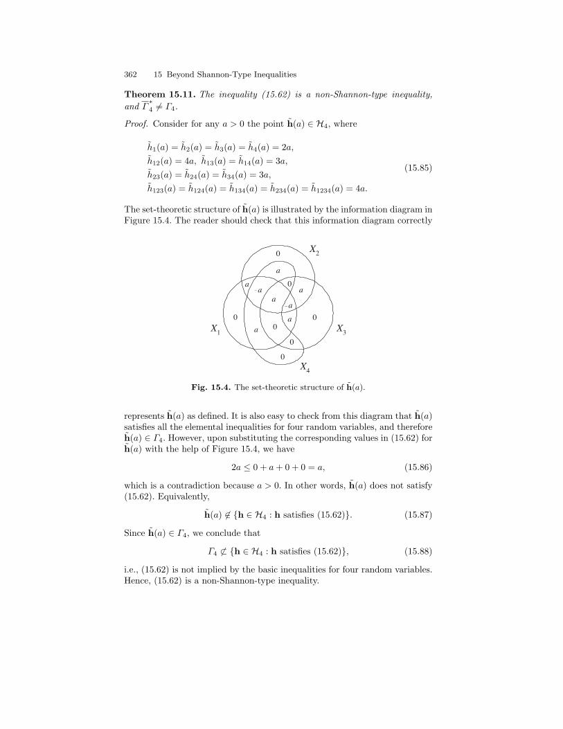
362 15 Beyond Shannon-Type Inequalities
Theorem 15.11. The inequality (15.62) is a non-Shannon-type inequality,and Γ
∗4 6= Γ4.
Proof. Consider for any a > 0 the point h(a) ∈ H4, where
h1(a) = h2(a) = h3(a) = h4(a) = 2a,h12(a) = 4a, h13(a) = h14(a) = 3a,h23(a) = h24(a) = h34(a) = 3a,h123(a) = h124(a) = h134(a) = h234(a) = h1234(a) = 4a.
(15.85)
The set-theoretic structure of h(a) is illustrated by the information diagram inFigure 15.4. The reader should check that this information diagram correctly
a
0
a
a a
a a 0
0
0
0
0
0
X 1
X 2
X 3
X 4
a
a
Fig. 15.4. The set-theoretic structure of h(a).
represents h(a) as defined. It is also easy to check from this diagram that h(a)satisfies all the elemental inequalities for four random variables, and thereforeh(a) ∈ Γ4. However, upon substituting the corresponding values in (15.62) forh(a) with the help of Figure 15.4, we have
2a ≤ 0 + a+ 0 + 0 = a, (15.86)
which is a contradiction because a > 0. In other words, h(a) does not satisfy(15.62). Equivalently,
h(a) 6∈ h ∈ H4 : h satisfies (15.62). (15.87)
Since h(a) ∈ Γ4, we conclude that
Γ4 6⊂ h ∈ H4 : h satisfies (15.62), (15.88)
i.e., (15.62) is not implied by the basic inequalities for four random variables.Hence, (15.62) is a non-Shannon-type inequality.

15.2 A Non-Shannon-Type Unconstrained Inequality 363
Since (15.62) is satisfied by all entropy functions for four random variables,we have
Γ ∗4 ⊂ h ∈ H4 : h satisfies (15.62), (15.89)
and upon taking closure on both sides, we have
Γ∗4 ⊂ h ∈ H4 : h satisfies (15.62). (15.90)
Then (15.87) implies h(a) 6∈ Γ ∗4. Since h(a) ∈ Γ4 and h(a) 6∈ Γ ∗4, we concludethat Γ
∗4 6= Γ4. The theorem is proved. ut
Remark We have shown in the proof of Theorem 15.11 that the inequality(15.62) cannot be proved by invoking the basic inequalities for four randomvariables. However, (15.62) can be proved by invoking the basic inequalities forthe six random variables X1, X2, X3, X4, X1, and X2 with the joint probabilitydistribution p123412 as constructed in (15.63).
The inequality (15.62) remains valid when the indices 1, 2, 3, and 4 arepermuted. Since (15.62) is symmetrical in X3 and X4, 4!/2! = 12 distinctversions of (15.62) can be obtained by permuting the indices, and all thesetwelve inequalities are simultaneously satisfied by the entropy function of anyset of random variables X1, X2, X3, and X4. We will denote these twelveinequalities collectively by 〈15.62〉. Now define the region
Γ4 = h ∈ Γ4 : h satisfies 〈15.62〉. (15.91)
Evidently,Γ ∗4 ⊂ Γ4 ⊂ Γ4. (15.92)
Since both Γ4 and Γ4 are closed, upon taking closure, we also have
Γ∗4 ⊂ Γ4 ⊂ Γ4. (15.93)
Since 〈15.62〉 are non-Shannon-type inequalities as we have proved in the lasttheorem, Γ4 is a proper subset of Γ4 and hence a tighter outer bound on Γ ∗4and Γ
∗4 than Γ4.
In the course of proving that (15.62) is of non-Shannon-type, it was shownin the proof of Theorem 15.11 that there exists h(a) ∈ Γ4 as defined in (15.85)which does not satisfy (15.62). By investigating the geometrical relation be-tween h(a) and Γ4, we prove in the next theorem that (15.62) in fact inducesa class of 214 − 1 non-Shannon-type constrained inequalities. Applications ofsome of these inequalities will be discussed in Section 15.4.
Theorem 15.12. The inequality (15.62) is a non-Shannon-type inequalityconditioning on setting any nonempty subset of the following 14 Shannon’s

364 15 Beyond Shannon-Type Inequalities
information measures to zero:
I(X1;X2), I(X1;X2|X3), I(X1;X2|X4), I(X1;X3|X4),I(X1;X4|X3), I(X2;X3|X4), I(X2;X4|X3), I(X3;X4|X1),I(X3;X4|X2), I(X3;X4|X1, X2), H(X1|X2, X3, X4),H(X2|X1, X3, X4), H(X3|X1, X2, X4), H(X4|X1, X2, X3).
(15.94)
Proof. It is easy to verify from Figure 15.4 that h(a) lies in exactly 14 hy-perplanes in H4 (i.e., <15) defining the boundary of Γ4 which correspond tosetting the 14 Shannon’s measures in (15.94) to zero. Therefore, h(a) for a ≥ 0define an extreme direction of Γ4.
Now for any linear subspace Φ of H4 containing h(a), where a > 0, wehave
h(a) ∈ Γ4 ∩ Φ (15.95)
and h(a) does not satisfy (15.62). Therefore,
(Γ4 ∩ Φ) 6⊂ h ∈ H4 : h satisfies (15.62). (15.96)
This means that (15.62) is a non-Shannon-type inequality under the constraintΦ. From the above, we see that Φ can be taken to be the intersection of anynonempty subset of the 14 hyperplanes containing h(a). Thus (15.62) is anon-Shannon-type inequality conditioning on any nonempty subset of the 14Shannon’s measures in (15.94) being equal to zero. Hence, (15.62) induces aclass of 214 − 1 non-Shannon-type constrained inequalities. The theorem isproved. ut
Remark It is not true that the inequality (15.62) is of non-Shannon-typeunder any constraint. Suppose we impose the constraint
I(X3;X4) = 0. (15.97)
Then the left hand side of (15.62) becomes zero, and the inequality is triv-ially implied by the basic inequalities because only mutual informations withpositive coefficients appear on the right hand side. Then (15.62) becomes aShannon-type inequality under the constraint in (15.97).
15.3 A Non-Shannon-Type Constrained Inequality
In the last section, we proved a non-Shannon-type unconstrained inequality forfour random variables which implies Γ
∗4 6= Γ4. This inequality induces a region
Γ4 which is a tighter outer bound on Γ ∗4 and Γ∗4 then Γ4. We further showed
that this inequality induces a class of 214 − 1 non-Shannon-type constrainedinequalities for four random variables.

15.3 A Non-Shannon-Type Constrained Inequality 365
In this section, we prove a non-Shannon-type constrained inequality forfour random variables. Unlike the non-Shannon-type unconstrained inequalitywe proved in the last section, this constrained inequality is not strong enoughto imply that Γ ∗4 6= Γ4. However, the latter is not implied by the former.
Lemma 15.13. Let p(x1, x2, x3, x4) be any probability distribution. Then
p(x1, x2, x3, x4) =
p(x1,x3,x4)p(x2,x3,x4)
p(x3,x4) if p(x3, x4) > 00 if p(x3, x4) = 0
(15.98)
is also a probability distribution. Moreover,
p(x1, x3, x4) = p(x1, x3, x4) (15.99)
andp(x2, x3, x4) = p(x2, x3, x4) (15.100)
for all x1, x2, x3, and x4.
Proof. The proof for the first part of the lemma is straightforward (see Prob-lem 5 in Chapter 2). The details are omitted here.
To prove the second part of the lemma, it suffices to prove (15.99) for allx1, x3, and x4 because p(x1, x2, x3, x4) is symmetrical in x1 and x2. We firstconsider x1, x3, and x4 such that p(x3, x4) > 0. From (15.98), we have
p(x1, x3, x4) =∑x2
p(x1, x2, x3, x4) (15.101)
=∑x2
p(x1, x3, x4)p(x2, x3, x4)p(x3, x4)
(15.102)
=p(x1, x3, x4)p(x3, x4)
∑x2
p(x2, x3, x4) (15.103)
=[p(x1, x3, x4)p(x3, x4)
]p(x3, x4) (15.104)
= p(x1, x3, x4). (15.105)
For x1, x3, and x4 such that p(x3, x4) = 0, we have
0 ≤ p(x1, x3, x4) ≤ p(x3, x4) = 0, (15.106)
which impliesp(x1, x3, x4) = 0. (15.107)
Therefore, from (15.98), we have

366 15 Beyond Shannon-Type Inequalities
p(x1, x3, x4) =∑x2
p(x1, x2, x3, x4) (15.108)
=∑x2
0 (15.109)
= 0 (15.110)= p(x1, x3, x4). (15.111)
Thus we have proved (15.99) for all x1, x3, and x4, and the lemma is proved.ut
Theorem 15.14. For any four random variables X1, X2, X3, and X4, if
I(X1;X2) = I(X1;X2|X3) = 0, (15.112)
thenI(X3;X4) ≤ I(X3;X4|X1) + I(X3;X4|X2). (15.113)
Proof. Consider
I(X3;X4)− I(X3;X4|X1)− I(X3;X4|X2)
=∑
x1,x2,x3,x4:p(x1,x2,x3,x4)>0
p(x1,x2,x3,x4) logp(x3,x4)p(x1,x3)p(x1,x4)p(x2,x3)p(x2,x4)p(x3)p(x4)p(x1)p(x2)p(x1,x3,x4)p(x2,x3,x4)
= Ep logp(X3, X4)p(X1, X3)p(X1, X4)p(X2, X3)p(X2, X4)p(X3)p(X4)p(X1)p(X2)p(X1, X3, X4)p(X2, X3, X4)
,
(15.114)
where we have used Ep to denote expectation with respect to p(x1, x2, x3, x4).We claim that the above expectation is equal to
Ep logp(X3, X4)p(X1, X3)p(X1, X4)p(X2, X3)p(X2, X4)p(X3)p(X4)p(X1)p(X2)p(X1, X3, X4)p(X2, X3, X4)
,
(15.115)
where p(x1, x2, x3, x4) is defined in (15.98).Toward proving that the claim is correct, we note that (15.115) is the sum
of a number of expectations with respect to p. Let us consider one of theseexpectations, say
Ep log p(X1, X3) =∑
x1,x2,x3,x4:p(x1,x2,x3,x4)>0
p(x1, x2, x3, x4) log p(x1, x3). (15.116)
Note that in the above summation, if p(x1, x2, x3, x4) > 0, then from (15.98),we see that
p(x1, x3, x4) > 0, (15.117)

15.3 A Non-Shannon-Type Constrained Inequality 367
and hencep(x1, x3) > 0. (15.118)
Therefore, the summation in (15.116) is always well-defined. Further, it canbe written as∑
x1,x3,x4
log p(x1, x3)∑
x2:p(x1,x2,x3,x4)>0
p(x1, x2, x3, x4)
=∑
x1,x3,x4
p(x1, x3, x4) log p(x1, x3). (15.119)
Thus Ep log p(X1, X3) depends on p(x1, x2, x3, x4) only through p(x1, x3, x4),which by Lemma 15.13 is equal to p(x1, x3, x4). It then follows that
Ep log p(X1, X3)
=∑
x1,x3,x4
p(x1, x3, x4) log p(x1, x3) (15.120)
=∑
x1,x3,x4
p(x1, x3, x4) log p(x1, x3) (15.121)
= Ep log p(X1, X3). (15.122)
In other words, the expectation on log p(X1, X3) can be taken with respectto either p(x1, x2, x3, x4) or p(x1, x2, x3, x4) without affecting its value. Byobserving that all the marginals of p in the logarithm in (15.115) involve onlysubsets of either X1, X3, X4 or X2, X3, X4, we see that similar conclusionscan be drawn for all the other expectations in (15.115), and hence the claimis proved.
Thus the claim implies that
I(X3;X4)− I(X3;X4|X1)− I(X3;X4|X2)
= Ep logp(X3, X4)p(X1, X3)p(X1, X4)p(X2, X3)p(X2, X4)p(X3)p(X4)p(X1)p(X2)p(X1, X3, X4)p(X2, X3, X4)
=∑
x1,x2,x3,x4:p(x1,x2,x3,x4)>0
p(x1,x2,x3,x4) logp(x3,x4)p(x1,x3)p(x1,x4)p(x2,x3)p(x2,x4)p(x3)p(x4)p(x1)p(x2)p(x1,x3,x4)p(x2,x3,x4)
= −∑
x1,x2,x3,x4:p(x1,x2,x3,x4)>0
p(x1, x2, x3, x4) logp(x1, x2, x3, x4)p(x1, x2, x3, x4)
, (15.123)
where
p(x1, x2, x3, x4) =p(x1,x3)p(x1,x4)p(x2,x3)p(x2,x4)
p(x1)p(x2)p(x3)p(x4) if p(x1), p(x2), p(x3), p(x4) > 00 otherwise.
(15.124)

368 15 Beyond Shannon-Type Inequalities
The equality in (15.123) is justified by observing that if x1, x2, x3, and x4 aresuch that p(x1, x2, x3, x4) > 0, then
p(x1, x3), p(x1, x4), p(x2, x3), p(x2, x4), p(x1), p(x2), p(x3), p(x4) (15.125)
are all strictly positive, and we see from (15.124) that p(x1, x2, x3, x4) > 0.To complete the proof, we only need to show that p(x1, x2, x3, x4) is a
probability distribution. Once this is proven, the conclusion of the theoremfollows immediately because the summation in (15.123), which is identified asthe divergence between p(x1, x2, x3, x4) and p(x1, x2, x3, x4), is always non-negative by the divergence inequality (Theorem 2.31). Toward this end, wenotice that for x1, x2, and x3 such that p(x3) > 0,
p(x1, x2, x3) =p(x1, x3)p(x2, x3)
p(x3)(15.126)
by the assumptionI(X1;X2|X3) = 0, (15.127)
and for all x1 and x2,p(x1, x2) = p(x1)p(x2) (15.128)
by the assumptionI(X1;X2) = 0. (15.129)
Then ∑x1,x2,x3,x4
p(x1, x2, x3, x4)
=∑
x1,x2,x3,x4:p(x1,x2,x3,x4)>0
p(x1, x2, x3, x4) (15.130)
=∑
x1,x2,x3,x4:p(x1),p(x2),p(x3),p(x4)>0
p(x1, x3)p(x1, x4)p(x2, x3)p(x2, x4)p(x1)p(x2)p(x3)p(x4)
(15.131)
a)=
∑x1,x2,x3,x4:
p(x1),p(x2),p(x3),p(x4)>0
p(x1, x2, x3)p(x1, x4)p(x2, x4)p(x1)p(x2)p(x4)
(15.132)
b)=
∑x1,x2,x3,x4:
p(x1),p(x2),p(x3),p(x4)>0
p(x1, x2, x3)p(x1, x4)p(x2, x4)p(x1, x2)p(x4)
(15.133)
=∑
x1,x2,x4:p(x1),p(x2),p(x4)>0
p(x1, x4)p(x2, x4)p(x4)
∑x3:p(x3)>0
p(x3|x1, x2) (15.134)
=∑
x1,x2,x4:p(x1),p(x2),p(x4)>0
p(x1, x4)p(x2, x4)p(x4)
(15.135)

15.3 A Non-Shannon-Type Constrained Inequality 369
=∑x2,x4:
p(x2),p(x4)>0
p(x2, x4)∑
x1:p(x1)>0
p(x1|x4) (15.136)
c)=
∑x2,x4:
p(x2),p(x4)>0
p(x2, x4) (15.137)
d)= 1, (15.138)
where a) and b) follows from (15.126) and (15.128), respectively. The equalityin c) is justified as follows. For x1 such that p(x1) = 0,
p(x1|x4) =p(x1)p(x4|x1)
p(x4)= 0. (15.139)
Therefore ∑x1:p(x1)>0
p(x1|x4) =∑x1
p(x1|x4) = 1. (15.140)
Finally, the equality in d) is justified as follows. For x2 and x4 such that p(x2)or p(x4) vanishes, p(x2, x4) must vanish because
0 ≤ p(x2, x4) ≤ p(x2) (15.141)
and0 ≤ p(x2, x4) ≤ p(x4). (15.142)
Therefore, ∑x2,x4:
p(x2),p(x4)>0
p(x2, x4) =∑x2,x4
p(x2, x4) = 1. (15.143)
The theorem is proved. ut
Theorem 15.15. The constrained inequality in Theorem 15.14 is a non-Shannon-type inequality.
Proof. The theorem can be proved by considering the point h(a) ∈ H4 fora > 0 as in the proof of Theorem 15.11. The details are left as an exercise. ut
The constrained inequality in Theorem 15.14 has the following geometricalinterpretation. The constraints in (15.112) correspond to the intersection oftwo hyperplanes in H4 which define the boundary of Γ4. Then the inequality(15.62) says that a certain region on the boundary of Γ4 is not in Γ ∗4 . It canfurther be proved by computation1 that the constrained inequality in Theo-rem 15.14 is not implied by the twelve distinct versions of the unconstrainedinequality in Theorem 15.7 (i.e., 〈15.62〉) together with the basic inequalities.
We have proved in the last section that the non-Shannon-type inequality(15.62) implies a class of 214 − 1 constrained non-Shannon-type inequalities.We end this section by proving a similar result for the non-Shannon-typeconstrained inequality in Theorem 15.14.1 Ying-On Yan, private communication.

370 15 Beyond Shannon-Type Inequalities
Theorem 15.16. The inequality
I(X3;X4) ≤ I(X3;X4|X1) + I(X3;X4|X2) (15.144)
is a non-Shannon-type inequality conditioning on setting both I(X1;X2) andI(X1;X2|X3) and any subset of the following 12 Shannon’s information mea-sures to zero:
I(X1;X2|X4), I(X1;X3|X4), I(X1;X4|X3),I(X2;X3|X4), I(X2;X4|X3), I(X3;X4|X1),I(X3;X4|X2), I(X3;X4|X1, X2), H(X1|X2, X3, X4),H(X2|X1, X3, X4), H(X3|X1, X2, X4), H(X4|X1, X2, X3).
(15.145)
Proof. The proof of this theorem is very similar to the proof of Theorem 15.12.We first note that I(X1;X2) and I(X1;X2|X3) together with the 12 Shannon’sinformation measures in (15.145) are exactly the 14 Shannon’s informationmeasures in (15.94). We have already shown in the proof of Theorem 15.12that h(a) (cf. Figure 15.4) lies in exactly 14 hyperplanes defining the boundaryof Γ4 which correspond to setting these 14 Shannon’s information measuresto zero. We also have shown that h(a) for a ≥ 0 define an extreme directionof Γ4.
Denote by Φ0 the intersection of the two hyperplanes in H4 which cor-respond to setting I(X1;X2) and I(X1;X2|X3) to zero. Since h(a) for anya > 0 satisfies
I(X1;X2) = I(X1;X2|X3) = 0, (15.146)
h(a) is in Φ0. Now for any linear subspace Φ of H4 containing h(a) such thatΦ ⊂ Φ0, we have
h(a) ∈ Γ4 ∩ Φ. (15.147)
Upon substituting the corresponding values in (15.113) for h(a) with the helpof Figure 15.4, we have
a ≤ 0 + 0 = 0, (15.148)
which is a contradiction because a > 0. Therefore, h(a) does not satisfy(15.113). Therefore,
(Γ4 ∩ Φ) 6⊂ h ∈ H4 : h satisfies (15.113). (15.149)
This means that (15.113) is a non-Shannon-type inequality under the con-straint Φ. From the above, we see that Φ can be taken to be the intersectionof Φ0 and any subset of the 12 hyperplanes which correspond to setting the12 Shannon’s information measures in (15.145) to zero. Hence, (15.113) is anon-Shannon-type inequality conditioning on I(X1;X2), I(X1;X2|X3), andany subset of the 12 Shannon’s information measures in (15.145) being equalto zero. In other words, the constrained inequality in Theorem 15.14 in factinduces a class of 212 constrained non-Shannon-type inequalities. The theoremis proved. ut

15.4 Applications 371
15.4 Applications
As we have mentioned in Chapter 13, information inequalities are the laws ofinformation theory. In this section, we give several applications of the non-Shannon-type inequalities we have proved in this chapter in probability theoryand information theory. An application of the unconstrained inequality provedin Section 15.2 in group theory will be discussed in Chapter 16.
Example 15.17. For the constrained inequality in Theorem 15.14, if we furtherimpose the constraints
I(X3;X4|X1) = I(X3;X4|X2) = 0, (15.150)
then the right hand side of (15.113) becomes zero. This implies
I(X3;X4) = 0 (15.151)
because I(X3;X4) is nonnegative. This means that
X1 ⊥ X2
X1 ⊥ X2|X3
X3 ⊥ X4|X1
X3 ⊥ X4|X2
⇒ X3 ⊥ X4. (15.152)
We leave it as an exercise for the reader to show that this implication cannotbe deduced from the basic inequalities.
Example 15.18. If we impose the constraints
I(X1;X2) = I(X1;X3, X4) = I(X3;X4|X1) = I(X3;X4|X2) = 0, (15.153)
then the right hand side of (15.62) becomes zero, which implies
I(X3;X4) = 0. (15.154)
This means thatX1 ⊥ X2
X1 ⊥ (X3, X4)X3 ⊥ X4|X1
X3 ⊥ X4|X2
⇒ X3 ⊥ X4. (15.155)
Note that (15.152) and (15.155) differ only in the second constraint. Again,we leave it as an exercise for the reader to show that this implication cannotbe deduced from the basic inequalities.
Example 15.19. Consider a fault-tolerant data storage system consisting ofrandom variables X1, X2, X3, X4 such that any three random variables canrecover the remaining one, i.e.,

372 15 Beyond Shannon-Type Inequalities
H(Xi|Xj , j 6= i) = 0, 1 ≤ i, j ≤ 4. (15.156)
We are interested in the set of all entropy functions subject to these con-straints, denoted by Υ , which characterizes the amount of joint informationwhich can possibly be stored in such a data storage system. Let
Φ = h ∈ H4 : h satisfies (15.156). (15.157)
Then the set Υ is equal to the intersection between Γ ∗4 and Φ, i.e., Γ ∗4 ∩ Φ.Since each constraint in (15.156) is one of the 14 constraints specified in
Theorem 15.12, we see that (15.62) is a non-Shannon-type inequality underthe constraints in (15.156). Then Γ4 ∩Φ (cf. (15.91)) is a tighter outer boundon Υ than Γ4 ∩ Φ.
Example 15.20. Consider four random variables X1, X2, X3, and X4 such thatX3 → (X1, X2)→ X4 forms a Markov chain. This Markov condition is equiv-alent to
I(X3;X4|X1, X2) = 0. (15.158)
It can be proved by invoking the basic inequalities (using ITIP) that
I(X3;X4) ≤ I(X3;X4|X1) + I(X3;X4|X2) + 0.5I(X1;X2)
+cI(X1;X3, X4) + (1− c)I(X2;X3, X4), (15.159)
where 0.25 ≤ c ≤ 0.75, and this is the best possible.Now observe that the Markov condition (15.158) is one of the 14 con-
straints specified in Theorem 15.12. Therefore, (15.62) is a non-Shannon-typeinequality under this Markov condition. By replacing X1 and X2 by each otherin (15.62), we obtain
2I(X3;X4) ≤ I(X1;X2) + I(X2;X3, X4)
+3I(X3;X4|X2) + I(X3;X4|X1). (15.160)
Upon adding (15.62) and (15.160) and dividing by 4, we obtain
I(X3;X4) ≤ I(X3;X4|X1) + I(X3;X4|X2) + 0.5I(X1;X2)
+0.25I(X1;X3, X4) + 0.25I(X2;X3, X4). (15.161)
Comparing the last two terms in (15.159) and the last two terms in (15.161),we see that (15.161) is a sharper upper bound than (15.159).
The Markov chain X3 → (X1, X2) → X4 arises in many communicationsituations. As an example, consider a person listening to an audio source. Thenthe situation can be modeled by this Markov chain with X3 being the soundwave generated at the source, X1 and X2 being the sound waves received atthe two ear drums, and X4 being the nerve impulses which eventually arrive atthe brain. The inequality (15.161) gives an upper bound on I(X3;X4) whichis tighter than what can be implied by the basic inequalities.
There is some resemblance between the constrained inequality (15.161)and the data processing theorem, but there does not seem to be any directrelation between them.

Problems 373
Problems
1. Verify by ITIP that the unconstrained information inequality in Theo-rem 15.7 is of non-Shannon-type.
2. Verify by ITIP and prove analytically that the constrained informationinequality in Theorem 15.14 is of non-Shannon-type.
3. Use ITIP to verify the unconstrained information inequality in Theo-rem 15.7. Hint: Create two auxiliary random variables as in the proofof Theorem 15.7 and impose appropriate constraints on the random vari-ables.
4. Verify by ITIP that the implications in Examples 15.17 and 15.18 cannotbe deduced from the basic inequalities.
5. Can you show that the sets of constraints in Examples 15.17 and 15.18are in fact different?
6. Let Nn = 1, 2, · · · , n. Consider an information inequality involving ran-dom variables X1, X2, · · · , Xn, which can be written as∑
α∈2Nn\∅
cαH(Xα) ≥ 0.
For i ∈ Nn, letri =
∑α∈2Nn\∅
cα1α(i),
where 1α(i) is equal to 1 if i ∈ α and is equal to 0 otherwise.a) Show that ri is the coefficient associated with H(Xi|XNn−i) in the
information inequality.b) Show that if the information inequality always holds, then ri ≥ 0 for
all i ∈ Nn.(Chan [58].)
7. Let Xi, i = 1, 2, · · · , n, Z, and T be discrete random variables.a) Prove that
nI(Z;T )−n∑j=1
I(Z;T |Xj)− nI(Z;T |Xi)
≤ I(Xi;Z, T ) +n∑j=1
H(Xj)−H(X1, X2, · · · , Xn).
Hint: When n = 2, this inequality reduces to the unconstrained non-Shannon-type inequality in Theorem 15.7.
b) Prove that
nI(Z;T )− 2n∑j=1
I(Z;T |Xj)
≤ 1n
n∑i=1
I(Xi;Z, T ) +n∑j=1
H(Xj)−H(X1, X2, · · · , Xn).

374 15 Beyond Shannon-Type Inequalities
( Zhang and Yeung [375].)8. Let p(x1, x2, x3, x4) be the joint distribution for random variables X1, X2,X3, and X4 such that I(X1;X2|X3) = I(X2;X4|X3) = 0, and let p bedefined in (15.98).a) Show that
p(x1, x2, x3, x4)
=
c · p(x1,x2,x3)p(x1,x4)p(x2,x4)
p(x1,x2)p(x4) if p(x1, x2), p(x4) > 00 otherwise
defines a probability distribution for an appropriate c ≥ 1.b) Prove that p(x1, x2, x3) = p(x1, x2, x3) for all x1, x2, and x3.c) By considering D(p‖p) ≥ 0, prove that
H(X13) +H(X14) +H(X23) +H(X24) +H(X34)≥ H(X3) +H(X4) +H(X12) +H(X134) +H(X234),
where H(X134) denotes H(X1, X3, X4), etc.d) Prove that under the constraints in (15.112), the inequality in (15.113)
is equivalent to the inequality in c).The inequality in c) is referred to as the Ingleton inequality for entropy inthe literature. For the origin of the Ingleton inequality, see Problem 9 inChapter 16. (Matus [231].)
Historical Notes
In 1986, Pippenger [266] asked whether there exist constraints on the entropyfunction other than the polymatroidal axioms, which are equivalent to thebasic inequalities. He called the constraints on the entropy function the lawsof information theory. The problem had been open since then until Zhang andYeung discovered for four random variables first a constrained non-Shannon-type inequality [374] and then an unconstrained non-Shannon-type inequal-ity [375]. The inequality reported in [375] has been further generalized byMakarychev et al. [218] and Zhang [372]. The existence of these inequalitiesimplies that there are laws in information theory beyond those laid down byShannon [292].
The non-Shannon-type inequalities that have been discovered induce outerbounds on the region Γ ∗4 which are tighter than Γ4. Matus and Studeny [236]showed that an entropy function in Γ4 is entropic if it satisfies the Ingletoninequality (see Problem 9 in Chapter 16). This gives an inner bound on Γ
∗4.
A more explicit proof of this inner bound can be found in [375], where thebound was shown not to be tight. Matus [234] has obtained asymptoticallytight inner bounds on Γ
∗n by constructing entropy functions from matroids.

Historical Notes 375
Dougherty et al. [87] discovered a host of unconstrained non-Shannon-typeinequalities by means of a computer search based on ITIP and the Markovchain construction in [375] (see Problem 3). Recently, Matus [235] proved aninfinite class of unconstrained non-Shannon-type inequalities, implying thatΓ∗n is not polyhedral.
Chan [58] proved a characterization for an inequality for differential en-tropy in terms of its discrete version. Lnenicka [213] proved that the tightnessof the continuous version of the inequality reported in [375] can be achievedby a multivariate Gaussian distribution.
In the 1990’s, Matus and Studeny [229][236][230] studied the structureof conditional independence (which subsumes the implication problem) ofrandom variables. Matus [231] finally settled the problem for four randomvariables by means of a constrained non-Shannon-type inequality which is avariation of the inequality reported in [374].
The von Neumann entropy is an extension of classical entropy (as discussedin this book) to the field of quantum mechanics. The strong subadditivity ofthe von Neumann entropy proved by Lieb and Ruskai [209] plays the same roleas the basic inequalities for classical entropy. Pippenger [267] proved that fora three-party system, there exists no inequality for the von Neumann entropybeyond strong subadditivity. Subsequently, Linden and Winter [211] discov-ered for a four-party system a constrained inequality for the von Neumannentropy which is independent of strong subadditivity. We refer the reader tothe book by Nielsen and Chuang [248] for quantum information theory.
Along a related direction, Hammer et al. [131] have shown that all linearinequalities which always hold for Kolmogorov complexity also always holdfor entropy, and vice versa.


16
Entropy and Groups
The group is the first major mathematical structure in abstract algebra, whileentropy is the most basic measure of information. Group theory and infor-mation theory are two seemingly unrelated subjects which turn out to beintimately related to each other. This chapter explains this intriguing relationbetween these two fundamental subjects. Those readers who have no knowl-edge in group theory may skip this introduction and go directly to the nextsection.
Let X1 and X2 be any two random variables. Then
H(X1) +H(X2) ≥ H(X1, X2), (16.1)
which is equivalent to the basic inequality
I(X1;X2) ≥ 0. (16.2)
Let G be any finite group and G1 and G2 be subgroups of G. We will showin Section 16.4 that
|G||G1 ∩G2| ≥ |G1||G2|, (16.3)
where |G| denotes the order of G and G1 ∩ G2 denotes the intersection ofG1 and G2 (G1 ∩ G2 is also a subgroup of G, see Proposition 16.13). Byrearranging the terms, the above inequality can be written as
log|G||G1|
+ log|G||G2|
≥ log|G|
|G1 ∩G2|. (16.4)
By comparing (16.1) and (16.4), one can easily identify the one-to-one corre-spondence between these two inequalities, namely that Xi corresponds to Gi,i = 1, 2, and (X1, X2) corresponds to G1 ∩ G2. While (16.1) is true for anypair of random variables X1 and X2, (16.4) is true for any finite group G andsubgroups G1 and G2.
Recall from Chapter 13 that the region Γ ∗n characterizes all informationinequalities (involving n random variables). In particular, we have shown in

378 16 Entropy and Groups
Section 15.1 that the region Γ∗n is sufficient for characterizing all unconstrained
information inequalities, i.e., by knowing Γ∗n, one can determine whether any
unconstrained information inequality always holds. The main purpose of thischapter is to obtain a characterization of Γ
∗n in terms of finite groups. An
important consequence of this result is a one-to-one correspondence betweenunconstrained information inequalities and group inequalities. Specifically, forevery unconstrained information inequality, there is a corresponding groupinequality, and vice versa. A special case of this correspondence has beengiven in (16.1) and (16.4).
By means of this result, unconstrained information inequalities can beproved by techniques in group theory, and a certain form of inequalities ingroup theory can be proved by techniques in information theory. In particular,the unconstrained non-Shannon-type inequality in Theorem 15.7 correspondsto the group inequality
|G1 ∩G3|3|G1 ∩G4|3|G3 ∩G4|3|G2 ∩G3||G2 ∩G4|
≤ |G1||G1 ∩G2||G3|2|G4|2|G1 ∩G3 ∩G4|4|G2 ∩G3 ∩G4|, (16.5)
where Gi are subgroups of a finite group G, i = 1, 2, 3, 4. The meaning of thisinequality and its implications in group theory are yet to be understood.
16.1 Group Preliminaries
In this section, we present the definition and some basic properties of a groupwhich are essential for subsequent discussions.
Definition 16.1. A group is a set of objects G together with a binary oper-ation on the elements of G, denoted by “” unless otherwise specified, whichsatisfy the following four axioms:
1. Closure For every a, b in G, a b is also in G.2. Associativity For every a, b, c in G, a (b c) = (a b) c.3. Existence of Identity There exists an element e in G such that ae = ea
= a for every a in G.4. Existence of Inverse For every a in G, there exists an element b in G such
that a b = b a = e.
Proposition 16.2. For any group G, the identity element is unique.
Proof. Let e and e′ be both identity elements in a group G. Since e is anidentity element,
e′ e = e, (16.6)
and since e′ is also an identity element,
e′ e = e′. (16.7)
It follows by equating the right hand sides of (16.6) and (16.7) that e = e′,which implies the uniqueness of the identity element of a group. ut

16.1 Group Preliminaries 379
Proposition 16.3. For every element a in a group G, its inverse is unique.
Proof. Let b and b′ be inverses of an element a, so that
a b = b a = e (16.8)
anda b′ = b′ a = e. (16.9)
Then
b = b e (16.10)= b (a b′) (16.11)= (b a) b′ (16.12)= e b′ (16.13)= b′, (16.14)
where (16.11) and (16.13) follow from (16.9) and (16.8), respectively, and(16.12) is by associativity. Therefore, the inverse of a is unique. ut
Thus the inverse of a group element a is a function of a, and it will bedenoted by a−1.
Definition 16.4. The number of elements of a group G is called the order ofG, denoted by |G|. If |G| <∞, G is called a finite group, otherwise it is calledan infinite group.
There is an unlimited supply of examples of groups. Some familiar ex-amples are: the integers under addition, the rationals excluding zero undermultiplication, and the set of real-valued 2×2 matrices under addition, whereaddition and multiplication refer to the usual addition and multiplication forreal numbers and matrices. In each of these examples, the operation (additionor multiplication) plays the role of the binary operation “” in Definition 16.2.
All the above are examples of infinite groups. In this chapter, however, weare concerned with finite groups. In the following, we discuss two examples offinite groups in details.
Example 16.5 (Modulo 2 Addition). The trivial group consists of only the iden-tity element. The simplest nontrivial group is the group of modulo 2 addition.The order of this group is 2, and the elements are 0, 1. The binary operation,denoted by “+”, is defined by following table:
+ 0 10 0 11 1 0

380 16 Entropy and Groups
The four axioms of a group simply say that certain constraints must holdin the above table. We now check that all these axioms are satisfied. First,the closure axiom requires that all the entries in the table are elements inthe group, which is easily seen to be the case. Second, it is required thatassociativity holds. To this end, it can be checked in the above table that forall a, b, and c,
a+ (b+ c) = (a+ b) + c. (16.15)
For example,0 + (1 + 1) = 0 + 0 = 0, (16.16)
while(0 + 1) + 1 = 1 + 1 = 0, (16.17)
which is the same as 0 + (1 + 1). Third, the element 0 is readily identified asthe unique identity. Fourth, it is readily seen that an inverse exists for eachelement in the group. For example, the inverse of 1 is 1, because
1 + 1 = 0. (16.18)
Thus the above table defines a group of order 2. It happens in this examplethat the inverse of each element is the element itself, which is not true for agroup in general.
We remark that in the context of a group, the elements in the group shouldbe regarded strictly as symbols only. In particular, one should not associategroup elements with magnitudes as we do for real numbers. For instance, in theabove example, one should not think of 0 as being less than 1. The element 0,however, is a special symbol which plays the role of the identity of the group.
We also notice that for the group in the above example, a+ b is equal tob + a for all group elements a and b. A group with this property is called acommutative group or an Abelian group1.
Example 16.6 (Symmetric Group). Consider a permutation of the componentsof a vector
x = (x1, x2, · · · , xr) (16.19)
given byσ[x] = (xσ(1), xσ(2), · · · , xσ(r)), (16.20)
whereσ : 1, 2, · · · , r → 1, 2, · · · , r (16.21)
is a one-to-one mapping. The one-to-one mapping σ is called a permutationon 1, 2, · · · , r, which is represented by
σ = (σ(1), σ(2), · · · , σ(r)). (16.22)1 The Abelian group is named after the Norwegian mathematician Niels Henrik
Abel (1802-1829).

16.1 Group Preliminaries 381
For two permutations σ1 and σ2, define σ1 σ2 as the composite function ofσ1 and σ2. For example, for r = 4, suppose
σ1 = (2, 1, 4, 3) (16.23)
andσ2 = (1, 4, 2, 3). (16.24)
Then σ1 σ2 is given by
σ1 σ2(1) = σ1(σ2(1)) = σ1(1) = 2σ1 σ2(2) = σ1(σ2(2)) = σ1(4) = 3σ1 σ2(3) = σ1(σ2(3)) = σ1(2) = 1σ1 σ2(4) = σ1(σ2(4)) = σ1(3) = 4,
(16.25)
orσ1 σ2 = (2, 3, 1, 4). (16.26)
The reader can easily check that
σ2 σ1 = (4, 1, 2, 3), (16.27)
which is different from σ1 σ2. Therefore, the operation “” is not commuta-tive.
We now show that the set of all permutations on 1, 2, · · · , r and theoperation “” form a group, called the symmetric group on 1, 2, · · · , r. First,for two permutations σ1 and σ2, since both σ1 and σ2 are one-to-one mappings,so is σ1σ2. Therefore, the closure axiom is satisfied. Second, for permutationsσ1, σ2, and σ3,
σ1 (σ2 σ3)(i) = σ1(σ2 σ3(i)) (16.28)= σ1(σ2(σ3(i))) (16.29)= σ1 σ2(σ3(i)) (16.30)= (σ1 σ2) σ3(i) (16.31)
for 1 ≤ i ≤ r. Therefore, associativity is satisfied. Third, it is clear that theidentity map is the identity element. Fourth, for a permutation σ, it is clearthat its inverse is σ−1, the inverse mapping of σ which is defined because σis one-to-one. Therefore, the set of all permutations on 1, 2, · · · , r and theoperation “” form a group. The order of this group is evidently equal to (r!).
Definition 16.7. Let G be a group with operation “”, and S be a subset ofG. If S is a group with respect to the operation “”, then S is called a subgroupof G.
Definition 16.8. Let S be a subgroup of a group G and a be an element of G.The left coset of S with respect to a is the set aS = as : s ∈ S. Similarly,the right coset of S with respect to a is the set S a = s a : s ∈ S.

382 16 Entropy and Groups
In the sequel, only the left coset will be used. However, any result whichapplies to the left coset also applies to the right coset, and vice versa. Forsimplicity, a S will be denoted by aS.
Proposition 16.9. For a1 and a2 in G, a1S and a2S are either identical ordisjoint. Further, a1S and a2S are identical if and only if a1 and a2 belong tothe same left coset of S.
Proof. Suppose a1S and a2S are not disjoint. Then there exists an element bin a1S ∩ a2S such that
b = a1 s1 = a2 s2, (16.32)
for some si in S, i = 1, 2. Then
a1 = (a2 s2) s−11 = a2 (s2 s−1
1 ) = a2 t, (16.33)
where t = s2 s−11 is in S. We now show that a1S ⊂ a2S. For an element a1 s
in a1S, where s ∈ S,
a1 s = (a2 t) s = a2 (t s) = a2 u, (16.34)
where u = ts is in S. This implies that a1 s is in a2S. Thus, a1S ⊂ a2S. Bysymmetry, a2S ⊂ a1S. Therefore, a1S = a2S. Hence, if a1S and a2S are notdisjoint, then they are identical. Equivalently, a1S and a2S are either identicalor disjoint. This proves the first part of the proposition.
We now prove the second part of the proposition. Since S is a group, itcontains e, the identity element. Then for any group element a, a = a e isin aS because e is in S. If a1S and a2S are identical, then a1 ∈ a1S anda2 ∈ a2S = a1S. Therefore, a1 and a2 belong to the same left coset of S.
To prove the converse, assume a1 and a2 belong to the same left coset ofS. From the first part of the proposition, we see that a group element belongsto one and only one left coset of S. Since a1 is in a1S and a2 is in a2S, anda1 and a2 belong to the same left coset of S, we see that a1S and a2S areidentical. The proposition is proved. ut
Proposition 16.10. Let S be a subgroup of a group G and a be an elementof G. Then |aS| = |S|, i.e., the numbers of elements in all the left cosets of Sare the same, and they are equal to the order of S.
Proof. Consider two elements a s1 and a s2 in a S, where s1 and s2 arein S such that
a s1 = a s2. (16.35)
Then
a−1 (a s1) = a−1 (a s2) (16.36)(a−1 a) s1 = (a−1 a) s2 (16.37)
e s1 = e s2 (16.38)s1 = s2. (16.39)

16.2 Group-Characterizable Entropy Functions 383
Thus each element in S corresponds to a unique element in aS. Therefore,|aS| = |S| for all a ∈ G. ut
We are just one step away from obtaining the celebrated Lagrange’s theo-rem stated below.
Theorem 16.11 (Lagrange’s Theorem). If S is a subgroup of G, then |S|divides |G|.
Proof. Since a ∈ aS for every a ∈ G, every element of G belongs to a leftcoset of S. Then from Proposition 16.9, we see that the distinct left cosets ofS partition G. Therefore |G|, the total number of elements in G, is equal tothe number of distinct cosets of S multiplied by the number of elements ineach left coset, which is equal to |S| by Proposition 16.10. This implies that|S| divides |G|, proving the theorem. ut
The following corollary is immediate from the proof of Lagrange’s Theo-rem.
Corollary 16.12. Let S be a subgroup of a group G. The number of distinctleft cosets of S is equal to |G||S| .
16.2 Group-Characterizable Entropy Functions
Recall from Chapter 13 that the region Γ ∗n consists of all the entropy func-tions in the entropy space Hn for n random variables. As a first step towardestablishing the relation between entropy and groups, we discuss in this sec-tion entropy functions in Γ ∗n which can be described by a finite group Gand subgroups G1, G2, · · · , Gn. Such entropy functions are said to be group-characterizable. The significance of this class of entropy functions will becomeclear in the next section.
In the sequel, we will make use of the intersections of subgroups extensively.We first prove that the intersection of two subgroups is also a subgroup.
Proposition 16.13. Let G1 and G2 be subgroups of a group G. Then G1∩G2
is also a subgroup of G.
Proof. It suffices to show that G1∩G2 together with the operation “” satisfyall the axioms of a group. First, consider two elements a and b of G in G1∩G2.Since both a and b are in G1, (a b) is in G1. Likewise, (a b) is in G2.Therefore, a b is in G1 ∩ G2. Thus the closure axiom holds for G1 ∩ G2.Second, associativity for G1 ∩ G2 inherits from G. Third, G1 and G2 bothcontain the identity element because they are groups. Therefore, the identityelement is in G1 ∩G2. Fourth, for an element a ∈ Gi, since Gi is a group, a−1
is in Gi, i = 1, 2. Thus for an element a ∈ G1 ∩ G2, a−1 is also in G1 ∩ G2.Therefore, G1 ∩G2 is a group and hence a subgroup of G. ut

384 16 Entropy and Groups
Corollary 16.14. Let G1, G2, · · · , Gn be subgroups of a group G. Then ∩ni=1Giis also a subgroup of G.
In the rest of the chapter, we let Nn = 1, 2, · · · , n and denote ∩i∈αGi byGα, where α is a nonempty subset of Nn.
Lemma 16.15. Let Gi be subgroups of a group G and ai be elements of G,i ∈ α. Then
|∩i∈αaiGi| =|Gα| if
⋂i∈α aiGi 6= ∅
0 otherwise. (16.40)
Proof. For the special case when α is a singleton, i.e., α = i for some i ∈ Nn,(16.40) reduces to
|aiGi| = |Gi|, (16.41)
which has already been proved in Proposition 16.10.Let α be any nonempty subset of Nn. If
⋂i∈α aiGi = ∅, then (16.40) is
obviously true. If⋂i∈α aiGi 6= ∅, then there exists x ∈
⋂i∈α aiGi such that
for all i ∈ α,x = ai si, (16.42)
where si ∈ Gi. For any i ∈ α and for any y ∈ Gα, consider
x y = (ai si) y = ai (si y). (16.43)
Since both si and y are in Gi, si y is in Gi. Thus xy is in aiGi for all i ∈ α,or x y is in
⋂i∈α aiGi. Moreover, for y, y′ ∈ Gα, if x y = x y′, then y = y′.
Therefore, each element in Gα corresponds to a unique element in⋂i∈α aiGi.
Hence,|∩i∈αaiGi| = |Gα|, (16.44)
proving the lemma. ut
The relation between a finite group G and subgroups G1 and G2 is illus-trated by the membership table in Figure 16.1. In this table, an element of Gis represented by a dot. The first column represents the subgroup G1, withthe dots in the first column being the elements in G1. The other columnsrepresent the left cosets of G1. By Proposition 16.10, all the columns have thesame number of dots. Similarly, the first row represents the subgroup G2 andthe other rows represent the left cosets of G2. Again, all the rows have thesame number of dots.
The upper left entry in the table represents the subgroup G1 ∩G2. Thereare |G1 ∩ G2| dots in this entry, with one of them representing the identityelement. Any other entry represents the intersection between a left coset ofG1 and a left coset of G2, and by Lemma 16.15, the number of dots in eachof these entries is either equal to |G1 ∩G2| or zero.

16.2 Group-Characterizable Entropy Functions 385
G 2
G 1,2
G 1
Fig. 16.1. The membership table for a finite group G and subgroups G1 and G2.
Since all the column have the same numbers of dots and all the rowshave the same number of dots, we say that the table in Figure 16.1 exhibits aquasi-uniform structure. We have already seen a similar structure in Figure 6.1for the two-dimensional strong joint typicality array, which we reproduce inFigure 16.2. In this array, when n is large, all the columns have approximatelythe same number of dots and all the rows have approximately the same numberof dots. For this reason, we say that the two-dimensional strong typicalityarray exhibits an asymptotic quasi-uniform structure. In a strong typicalityarray, however, each entry can contain only one dot, while in a membershiptable, each entry can contain multiple dots.
2 nH ( Y )
2 nH ( X,Y ) 2 nH ( X )
y S [ Y ] n
x S [ X ] n
( x , y ) T [ XY ] n
.
.
. . . .
. . . .
. . . .
.
Fig. 16.2. A two-dimensional strong typicality array.
One can make a similar comparison between a strong joint typicality arrayfor any n ≥ 2 random variables and the membership table for a finite groupwith n subgroups. The details are omitted here.
Theorem 16.16. Let Gi, i ∈ Nn be subgroups of a group G. Then h ∈ Hndefined by
hα = log|G||Gα|
(16.45)

386 16 Entropy and Groups
for all nonempty subset α of Nn is entropic, i.e., h ∈ Γ ∗n .
Proof. It suffices to show that there exists a collection of random variablesX1, X2, · · · , Xn such that
H(Xα) = log|G||Gα|
(16.46)
for all nonempty subset α of Nn. We first introduce a uniform random variableΛ defined on the sample space G with probability mass function
PrΛ = a =1|G|
(16.47)
for all a ∈ G. For any i ∈ Nn, let random variable Xi be a function of Λ suchthat Xi = aGi if Λ = a.
Let α be a nonempty subset of Nn. Since Xi = aiGi for all i ∈ α if andonly if Λ is equal to some b ∈ ∩i∈αaiGi,
PrXi = aiGi : i ∈ α =|⋂i∈α aiGi||G|
(16.48)
=
|Gα||G| if
⋂i∈α aiGi 6= ∅
0 otherwise(16.49)
by Lemma 16.15. In other words, (Xi, i ∈ α) distributes uniformly on itssupport whose cardinality is |G|
|Gα| . Then (16.46) follows and the theorem isproved. ut
Definition 16.17. Let G be a finite group and G1, G2, · · · , Gn be subgroupsof G. Let h be a vector in Hn. If hα = log |G||Gα| for all nonempty subsets α ofNn, then (G,G1, · · · , Gn) is a group characterization of h.
Theorem 16.16 asserts that certain entropy functions in Γ ∗n have a groupcharacterization. These are called group-characterizable entropy functions,which will be used in the next section to obtain a group characterization ofthe region Γ
∗n. We end this section by giving a few examples of such entropy
functions.
Example 16.18. Fix any subset β of N3 = 1, 2, 3 and define a vector h ∈ H3
by
hα =
log 2 if α ∩ β 6= ∅0 otherwise. (16.50)
We now show that h has a group characterization. Let G = 0, 1 be thegroup of modulo 2 addition in Example 16.5, and for i = 1, 2, 3, let

16.2 Group-Characterizable Entropy Functions 387
Gi =0 if i ∈ βG otherwise. (16.51)
Then for a nonempty subset α of N3, if α∩ β 6= ∅, there exists an i in α suchthat i is also in β, and hence by definition Gi = 0. Thus,
Gα =⋂i∈α
Gi = 0. (16.52)
Therefore,
log|G||Gα|
= log|G||0|
= log21
= log 2. (16.53)
If α ∩ β = ∅, then Gi = G for all i ∈ α, and
Gα =⋂i∈α
Gi = G. (16.54)
Therefore,
log|G||Gα|
= log|G||G|
= log 1 = 0. (16.55)
Then we see from (16.50), (16.53), and (16.55) that
hα = log|G||Gα|
(16.56)
for all nonempty subset α of N3. Hence, (G,G1, G2, G3) is a group character-ization of h.
Example 16.19. This is a generalization of the last example. Fix any non-empty subset β of Nn and define a vector h ∈ Hn by
hα =
log 2 if α ∩ β 6= ∅0 otherwise. (16.57)
Then (G,G1, G2, · · · , Gn) is a group characterization of h, where G is thegroup of modulo 2 addition, and
Gi =0 if i ∈ βG otherwise. (16.58)
By letting β = ∅, h = 0. Thus we see that (G,G1, G2, · · · , Gn) is a groupcharacterization of the origin of Hn, with G = G1 = G2 = · · · = Gn.
Example 16.20. Define a vector h ∈ H3 as follows:
hα = min(|α|, 2). (16.59)
Let F be the group of modulo 2 addition, G = F × F , and
G1 = (0, 0), (1, 0) (16.60)G2 = (0, 0), (0, 1) (16.61)G3 = (0, 0), (1, 1). (16.62)
Then (G,G1, G2, G3) is a group characterization of h.

388 16 Entropy and Groups
16.3 A Group Characterization of Γ ∗n
We have introduced in the last section the class of entropy functions in Γ ∗nwhich have a group characterization. However, an entropy function h ∈ Γ ∗nmay not have a group characterization due to the following observation. Sup-pose h ∈ Γ ∗n . Then there exists a collection of random variables X1, X2, · · · ,Xn such that
hα = H(Xα) (16.63)
for all nonempty subset α of Nn. If (G,G1, · · · , Gn) is a group characterizationof h, then
H(Xα) = log|G||Gα|
(16.64)
for all nonempty subset of Nn. Since both |G| and |Gα| are integers, H(Xα)must be the logarithm of a rational number. However, the joint entropy of aset of random variables in general is not necessarily the logarithm of a rationalnumber (see Corollary 2.44). Therefore, it is possible to construct an entropyfunction h ∈ Γ ∗n which has no group characterization.
Although h ∈ Γ ∗n does not imply h has a group characterization, it turnsout that the set of all h ∈ Γ ∗n which have a group characterization is almostgood enough to characterize the region Γ ∗n , as we will see next.
Definition 16.21. Define the following region in Hn:
Υn = h ∈ Hn : h has a group characterization. (16.65)
By Theorem 16.16, if h ∈ Hn has a group characterization, then h ∈ Γ ∗n .Therefore, Υn ⊂ Γ ∗n . We will prove as a corollary of the next theorem thatcon(Υn), the convex closure of Υn, is in fact equal to Γ
∗n, the closure of Γ ∗n .
Theorem 16.22. For any h ∈ Γ ∗n , there exists a sequence f (r) in Υn suchthat limr→∞
1r f
(r) = h.
We need the following lemma to prove this theorem. The proof of thislemma resembles the proof of Theorem 6.10. Nevertheless, we give a sketch ofthe proof for the sake of completeness.
Lemma 16.23. Let X be a random variable such that |X | <∞ and the distri-bution p(x) is rational, i.e., p(x) is a rational number for all x ∈ X . Withoutloss of generality, assume p(x) is a rational number with denominator q forall x ∈ X . Then for r = q, 2q, 3q, · · ·,
limr→∞
1r
logr!∏
x(rp(x))!= H(X). (16.66)

16.3 A Group Characterization of Γ ∗n 389
Proof. Applying Lemma 6.11, we can obtain
1r
lnr!∏
x(rp(x))!
≤ −∑x
p(x) ln p(x) +r + 1r
ln(r + 1)− ln r (16.67)
= He(X) +1r
ln r +(
1 +1r
)ln(
1 +1r
). (16.68)
This upper bound tends to He(X) as r → ∞. On the other hand, we canobtain
1r
lnr!∏
x(rp(x))!
≥ −∑x
(p(x) +
1r
)ln(p(x) +
1r
)− ln r
r. (16.69)
This lower bound also tends to He(X) as r →∞. Then the proof is completedby changing the base of the logarithm if necessary. ut
Proof of Theorem 16.22. For any h ∈ Γ ∗n , there exists a collection of randomvariables X1, X2, · · · , Xn such that
hα = H(Xα) (16.70)
for all nonempty subset α of Nn. We first consider the special case that|Xi| < ∞ for all i ∈ Nn and the joint distribution of X1, X2, · · · , Xn is ra-tional. We want to show that there exists a sequence f (r) in Υn such thatlimr→∞
1r f
(r) = h.Denote
∏i∈α Xi by Xα. For any nonempty subset α of Nn, let Qα be the
marginal distribution of Xα. Assume without loss of generality that for anynonempty subset α of Nn and for all a ∈ Xα, Qα(a) is a rational number withdenominator q.
For each r = q, 2q, 3q, · · ·, fix a sequence
xNn = (xNn,1, xNn,2, · · ·xNn,r)
where for all j = 1, 2, · · · , r, xNn,j = (xi,j : i ∈ Nn) ∈ XNn , such thatN(a|xNn), the number of occurrences of a in sequence xNn , is equal torQNn(a) for all a ∈ XNn . The existence of such a sequence is guaranteedby that all the values of the joint distribution of XNn are rational num-bers with denominator q. Also, we denote the sequence of r elements of Xα,(xα,1, xα,2, · · ·xα,r), where xα,j = (xi,j : i ∈ α), by xα. Let a ∈ Xα. It is easyto check that N(a|xα), the number of occurrences of a in the sequence xα, isequal to rQα(a) for all a ∈ Xα.

390 16 Entropy and Groups
Let G be the group of all permutations on 1, 2, · · · , r, i.e., the symmetricgroup on 1, 2, · · · , r (cf. Example 16.6). The group G depends on r, but forsimplicity, we do not state this dependency explicitly. For any i ∈ Nn, define
Gi = σ ∈ G : σ[xi] = xi,
whereσ[xi] = (xi,σ(1), xi,σ(2), · · · , xi,σ(r)). (16.71)
It is easy to check that Gi is a subgroup of G.Let α be a nonempty subset of Nn. Then
Gα =⋂i∈α
Gi (16.72)
=⋂i∈ασ ∈ G : σ[xi] = xi (16.73)
= σ ∈ G : σ[xi] = xi for all i ∈ α (16.74)= σ ∈ G : σ[xα] = xα, (16.75)
whereσ[xα] = (xα,σ(1), xα,σ(2), · · · , xα,σ(r)). (16.76)
For any a ∈ Xα, define the set
Lxα(a) = j ∈ 1, 2, · · · , r : xα,j = a. (16.77)
Lxα(a) contains the “locations” of a in xα. Then σ[xα] = xα if and only if forall a ∈ Xα, j ∈ Lxα(a) implies σ(j) ∈ Lxα(a). Since
|Lxα(a)| = N(a|xα) = rQα(a), (16.78)
|Gα| =∏a∈Xα
(rQα(a))! (16.79)
and therefore|G||Gα|
=r!∏
a∈Xα(rQα(a))!. (16.80)
By Lemma 16.23,
limr→∞
1r
log|G||Gα|
= H(Xα) = hα. (16.81)
Recall that G and hence all its subgroups depend on r. Define f (r) by
f (r)α = log
|G||Gα|
(16.82)
for all nonempty subset α of Nn. Then f (r) ∈ Υn and

16.4 Information Inequalities and Group Inequalities 391
limr→∞
1rf (r) = h. (16.83)
We have already proved the theorem for the special case that h is theentropy function of a collection of random variables X1, X2, · · · , Xn with finitealphabets and a rational joint distribution. To complete the proof, we onlyhave to note that for any h ∈ Γ ∗n , it is always possible to construct a sequenceh(k) in Γ ∗n such that limk→∞ h(k) = h, where h(k) is the entropy function ofa collection of random variables X(k)
1 , X(k)2 , · · · , X(k)
n with finite alphabets anda rational joint distribution. This can be proved by techniques similar to thoseused in Appendix 2.10 together with the continuity of the entropy functionwith respect to the variational distance for a fixed finite support (Section 2.3).The details are omitted here. ut
Corollary 16.24. con(Υn) = Γ∗n.
Proof. First of all, Υn ⊂ Γ ∗n . By taking convex closure, we have con(Υn) ⊂con(Γ ∗n). By Theorem 15.5, Γ
∗n is convex. Therefore, con(Γ ∗n) = Γ
∗n, and we
have con(Υn) ⊂ Γ∗n. On the other hand, we have shown in Example 16.19
that the origin of Hn has a group characterization and therefore is in Υn. Itthen follows from Theorem 16.22 that Γ
∗n ⊂ con(Υn). Hence, we conclude that
Γ∗n = con(Υn), completing the proof. ut
16.4 Information Inequalities and Group Inequalities
We have proved in Section 15.1 that an unconstrained information inequality
b>h ≥ 0 (16.84)
always holds if and only if
Γ∗n ⊂ h ∈ Hn : b>h ≥ 0. (16.85)
In other words, all unconstrained information inequalities are fully charac-terized by Γ
∗n. We also have proved at the end of the last section that
con(Υn) = Γ∗n. Since Υn ⊂ Γ ∗n ⊂ Γ
∗n, if (16.85) holds, then
Υn ⊂ h ∈ Hn : b>h ≥ 0. (16.86)
On the other hand, if (16.86) holds, since h ∈ Hn : b>h ≥ 0 is closed andconvex, by taking convex closure in (16.86), we obtain
Γ∗n = con(Υn) ⊂ h ∈ Hn : b>h ≥ 0. (16.87)
Therefore, (16.85) and (16.86) are equivalent.Now (16.86) is equivalent to

392 16 Entropy and Groups
b>h ≥ 0 for all h ∈ Υn. (16.88)
Since h ∈ Υn if and only if
hα = log|G||Gα|
(16.89)
for all nonempty subset α of Nn for some finite group G and subgroups G1,G2, · · · , Gn, we see that the inequality (16.84) holds for all random variablesX1,X2,· · · ,Xn if and only if the inequality obtained from (16.84) by replacinghα by log |G||Gα| for all nonempty subset α of Nn holds for all finite group G andsubgroups G1, G2,· · · , Gn. In other words, for every unconstrained informationinequality, there is a corresponding group inequality, and vice versa. Therefore,inequalities in information theory can be proved by methods in group theory,and inequalities in group theory can be proved by methods in informationtheory.
In the rest of the section, we explore this one-to-one correspondence be-tween information theory and group theory. We first give a group-theoreticproof of the basic inequalities in information theory. At the end of the section,we will give an information-theoretic proof for the group inequality in (16.5).
Definition 16.25. Let G1 and G2 be subgroups of a finite group G. Define
G1 G2 = a b : a ∈ G1 and b ∈ G2. (16.90)
G1 G2 is in general not a subgroup of G. However, it can be shown thatG1 G2 is a subgroup of G if G is Abelian (see Problem 1).
Proposition 16.26. Let G1 and G2 be subgroups of a finite group G. Then
|G1 G2| =|G1||G2||G1 ∩G2|
. (16.91)
Proof. Fix (a1, a2) ∈ G1 × G2, Then a1 a2 is in G1 G2. Consider any(b1, b2) ∈ G1 ×G2 such that
b1 b2 = a1 a2. (16.92)
We will determine the number of (b1, b2) in G1 ×G2 which satisfies this rela-tion. From (16.92), we have
b−11 (b1 b2) = b−1
1 (a1 a2) (16.93)(b−1
1 b1) b2 = b−11 a1 a2 (16.94)
b2 = b−11 a1 a2. (16.95)
Thenb2 a−1
2 = b−11 a1 (a2 a−1
2 ) = b−11 a1. (16.96)

16.4 Information Inequalities and Group Inequalities 393
Let k be this common element in G, i.e.,
k = b2 a−12 = b−1
1 a1. (16.97)
Since b−11 a1 ∈ G1 and b2 a−1
2 ∈ G2, k is in G1 ∩ G2. In other words, forgiven (a1, a2) ∈ G1 × G2, if (b1, b2) ∈ G1 × G2 satisfies (16.92), then (b1, b2)satisfies (16.97) for some k ∈ G1∩G2. On the other hand, if (b1, b2) ∈ G1×G2
satisfies (16.97) for some k ∈ G1 ∩G2, then (16.96) is satisfied, which implies(16.92). Therefore, for given (a1, a2) ∈ G1 × G2, (b1, b2) ∈ G1 × G2 satisfies(16.92) if and only if (b1, b2) satisfies (16.97) for some k ∈ G1 ∩G2.
Now from (16.97), we obtain
b1(k) = (k a−11 )−1 (16.98)
and
b2(k) = k a2, (16.99)
where we have written b1 and b2 as b1(k) and b2(k) to emphasize their depen-dence on k. Now consider k, k′ ∈ G1 ∩G2 such that
(b1(k), b2(k)) = (b1(k′), b2(k′)). (16.100)
Since b1(k) = b1(k′), from (16.98), we have
(k a−11 )−1 = (k′ a−1
1 )−1, (16.101)
which impliesk = k′. (16.102)
Therefore, each k ∈ G1 ∩G2 corresponds to a unique pair (b1, b2) ∈ G1 ×G2
which satisfies (16.92). Therefore, we see that the number of distinct elementsin G1 G2 is given by
|G1 G2| =|G1 ×G2||G1 ∩G2|
=|G1||G2||G1 ∩G2|
, (16.103)
completing the proof. ut
Theorem 16.27. Let G1, G2, and G3 be subgroups of a finite group G. Then
|G3||G123| ≥ |G13||G23|. (16.104)
Proof. First of all,
G13 ∩G23 = (G1 ∩G3) ∩ (G2 ∩G3) = G1 ∩G2 ∩G3 = G123. (16.105)
By Proposition 16.26, we have

394 16 Entropy and Groups
|G13 G23| =|G13||G23||G123|
. (16.106)
It is readily seen that G13 G23 is a subset of G3, Therefore,
|G13 G23| =|G13||G23||G123|
≤ |G3|. (16.107)
The theorem is proved. ut
Corollary 16.28. For random variables X1, X2, and X3,
I(X1;X2|X3) ≥ 0. (16.108)
Proof. Let G1, G2, and G3 be subgroups of a finite group G. Then
|G3||G123| ≥ |G13||G23| (16.109)
by Theorem 16.27, or
|G|2
|G13||G23|≥ |G|2
|G3||G123|. (16.110)
This is equivalent to
log|G||G13|
+ log|G||G23|
≥ log|G||G3|
+ log|G||G123|
. (16.111)
This group inequality corresponds to the information inequality
H(X1, X3) +H(X2, X3) ≥ H(X3) +H(X1, X2, X3), (16.112)
which is equivalent toI(X1;X2|X3) ≥ 0. (16.113)
ut
The above corollary shows that all the basic inequalities in informationtheory has a group-theoretic proof. Of course, Theorem 16.27 is also impliedby the basic inequalities. As a remark, the inequality in (16.3) is seen to be aspecial case of Theorem 16.27 by letting G3 = G.
We are now ready to prove the group inequality in (16.5). The non-Shannon-type inequality we have proved in Theorem 15.7 can be expressed incanonical form as
H(X1) +H(X1, X2) + 2H(X3) + 2H(X4)+4H(X1, X3, X4) +H(X2, X3, X4)≤ 3H(X1, X3) + 3H(X1, X4) + 3H(X3, X4)
+H(X2, X3) +H(X2, X4), (16.114)
Problems 395
which corresponds to the group inequality
log|G||G1|
+ log|G||G12|
+ 2 log|G||G3|
+ 2 log|G||G4|
+4 log|G||G134|
+ log|G||G234|
≤ 3 log|G||G13|
+ 3 log|G||G14|
+ 3 log|G||G34|
+ log|G||G23|
+ log|G||G24|
. (16.115)
Upon rearranging the terms, we obtain
|G1 ∩G3|3|G1 ∩G4|3|G3 ∩G4|3|G2 ∩G3||G2 ∩G4|
≤ |G1||G1 ∩G2||G3|2|G4|2|G1 ∩G3 ∩G4|4|G2 ∩G3 ∩G4|, (16.116)
which is the group inequality in (16.5). The meaning of this inequality and itsimplications in group theory are yet to be understood.
Problems
1. Let G1 and G2 be subgroups of a finite group G. Show that G1 G2 is asubgroup if G is Abelian.
2. Let g1 and g2 be group characterizable entropy functions.a) Prove that m1g1 +m2g2 is group characterizable, where m1 and m2
are any positive integers.b) For any positive real numbers a1 and a2, construct a sequence of group
characterizable entropy functions f (k) for k = 1, 2, · · · , such that
limk→∞
f (k)
||f (k)||=
h||h||
,
where h = a1g1 + a2g2.3. Let (G,G1, G2, · · · , Gn) be a group characterization of g ∈ Γ ∗n , where
g is the entropy function for random variables X1, X2, · · · , Xn. Fix anynonempty subset α of Nn, and define h by
hβ = gα∪β − gα
for all nonempty subsets β of Nn. It can easily be checked that hβ =H(Xβ |Xα). Show that (K,K1,K2, · · · ,Kn) is a group characterization ofh, where K = Gα and Ki = Gi ∩Gα.
4. Let (G,G1, G2, · · · , Gn) be a group characterization of g ∈ Γ ∗n , where gis the entropy function for random variables X1, X2, · · · , Xn. Show that ifXi is a function of (Xj : j ∈ α), then Gα is a subgroup of Gi.

396 16 Entropy and Groups
5. Let G1, G2, G3 be subgroups of a finite group G. Prove that
|G||G1 ∩G2 ∩G3|2 ≥ |G1 ∩G2||G2 ∩G3||G1 ∩G3|.
Hint: Use the information-theoretic approach.6. Let h ∈ Γ ∗2 be the entropy function for random variables X1 and X2 such
that h1 + h2 = h12, i.e. X1 and X2 are independent. Let (G,G1, G2) be agroup characterization of h, and define a mapping L : G1 ×G2 → G by
L(a, b) = a b.
a) Prove that the mapping L is onto, i.e., for any element c ∈ G, thereexists (a, b) ∈ G1 ×G2 such that a b = c.
b) Prove that G1 G2 is a group.7. Denote an entropy function h ∈ Γ ∗2 by (h1, h2, h12). Construct a group
characterization for each of the following entropy functions:a) h1 = (log 2, 0, log 2)b) h2 = (0, log 2, log 2)c) h3 = (log 2, log 2, log 2).
Verify that Γ2 is the minimal convex set containing the above three en-tropy functions.
8. Denote an entropy function h ∈ Γ ∗3 by (h1, h2, h3, h12, h23, h13, h123). Con-struct a group characterization for each of the following entropy functions:a) h1 = (log 2, 0, 0, log 2, 0, log 2, log 2)b) h2 = (log 2, log 2, 0, log 2, log 2, log 2, log 2)c) h3 = (log 2, log 2, log 2, log 2, log 2, log 2, log 2)d) h4 = (log 2, log 2, log 2, log 4, log 4, log 4, log 4).
9. Ingleton inequality Let G be a finite Abelian group and G1, G2, G3, andG4 be subgroups of G. Let (G,G1, G2, G3, G4) be a group characterizationof g, where g is the entropy function for random variables X1, X2, X3, andX4. Prove the following statements:a)
|(G1 ∩G3) (G1 ∩G4)| ≤ |G1 ∩ (G3 G4)|
Hint: Show that (G1 ∩G3) (G1 ∩G4) ⊂ G1 ∩ (G3 G4).b)
|G1 G3 G4| ≤|G1||G3 G4||G1 ∩G3 ∩G4||G1 ∩G3||G1 ∩G4|
.
c)
|G1 G2 G3 G4| ≤|G1 G3 G4||G2 G3 G4|
|G3 G4|.

Historical Notes 397
d)
|G1 G2 G3 G4|
≤ |G1||G2||G3||G4||G1 ∩G3 ∩G4||G2 ∩G3 ∩G4||G1 ∩G3||G1 ∩G4||G2 ∩G3||G2 ∩G4||G3 ∩G4|
.
e)
|G1 ∩G3||G1 ∩G4||G2 ∩G3||G2 ∩G4||G3 ∩G4|≤ |G3||G4||G1 ∩G2||G1 ∩G3 ∩G4||G2 ∩G3 ∩G4|.
f)
H(X13) +H(X14) +H(X23) +H(X24) +H(X34)≥ H(X3) +H(X4) +H(X12) +H(X134) +H(X234),
where H(X134) denotes H(X1, X3, X4), etc.g) Is the inequality in f) implied by the basic inequalities? And does it
always hold? Explain.The Ingleton inequality [162] (see also [256]) was originally obtained as aconstraint on the rank functions of vector spaces. The inequality in e) wasobtained in the same spirit by Chan [55] for subgroups of a finite group.The inequality in f) is referred to as the Ingleton inequality for entropyin the literature. (See also Problem 8 in Chapter 15.)
Historical Notes
The results in this chapter are due to Chan and Yeung [60], whose work wasinspired by a one-to-one correspondence between entropy and quasi-uniformarrays previously established by Chan [55] (also Chan [56]). Romashchenko etal. [283] have developed an interpretation of Kolmogorov complexity similarto the combinatorial interpretation of entropy in Chan [55].


Part II
Fundamentals of Network Coding


17
Introduction
For a point-to-point communication system, we see from Section 7.7 and Prob-lem 6 in Chapter 8 that asymptotic optimality can be achieved by separatingsource coding and channel coding. Recall from Section 5.3 that the goal ofsource coding is to represent the information source in (almost) fair bits1.Then the role of channel coding is to enable the transmission of fair bitsthrough the channel essentially free of error with no reference to the meaningof these fair bits. Thus a theme in classical information theory for point-to-point communication is that fair bits can be drawn equivalence to a commod-ity.
It is intuitively appealing that this theme in classical information theorywould continue to hold in network communication where the network consistsof noiseless point-to-point communication channels. If so, in order to multi-cast2 information from a source node to possibly more than one sink node, weonly need to compress the information at the source node into fair bits, orga-nize them into data packets, and route the packets to the sink node throughthe intermediate nodes in the network. In the case when there are more thanone sink node, the information needs to be replicated at certain intermediatenodes so that every sink node can receive a copy of the information. Thismethod of transmitting information in a network is generally referred to asstore-and-forward—bb or routing. As a matter of fact, almost all computernetworks built in the last few decades are based on this paradigm, whererouters are deployed at the intermediate nodes to switch a data packet froman input channel to an output channel without processing the data content.The delivery of data packets in a computer network resembles mail deliveryin a postal system. We refer the readers to textbooks on data communication[195] and switching theory [157][204].
1 Fair bits refer to i.i.d. bits, each being distributed uniformly on 0, 1. See Sec-tion 5.3.
2 Multicast means to transmit information from a source node to a specified set ofsink nodes.
402 17 Introduction
However, we will see very shortly that in network communication, it doesnot suffice to simply route and/or replicate information within the network.Specifically, coding generally needs to be employed at the intermediate nodesin order to achieve bandwidth optimality. This notion, called network coding,is the subject of discussion in the second part of this book.
17.1 The Butterfly Network
In this section, the advantage of network coding over routing is explained bymeans of a few simple examples. The application of network coding in wirelessand satellite communication will be discussed in the next section.
We will use a finite directed graph to represent a point-to-point communi-cation network. A node in the network corresponds to a vertex in the graph,while a communication channel in the network corresponds to an edge in thegraph. We will not distinguish a node from a vertex, nor will we distinguish achannel from an edge. In the graph, a node is represented by a circle, with theexception that the unique source node, denoted by s (if exists), is representedby a square. Each edge is labeled by a positive integer called the capacity3 orthe rate constraint, which gives the maximum number of information symbolstaken from some finite alphabet that can be transmitted over the channel perunit time. In this section, we assume that the information symbol is binary.When there is only one edge from node a to node b, we denote the edge by(a, b).
Example 17.1 (Butterfly Network I). Consider the network in Figure 17.1(a).In this network, two bits b1 and b2 are generated at source node s, and theyare to be multicast to two sink nodes t1 and t2. In Figure 17.1(b), we try todevise a routing scheme for this purpose. By symmetry, we send the two bitson different output channels at node s. Without loss of generality, b1 is sent onchannel (s, 1) and b2 is sent on channel (s, 2). At nodes 1 and 2, the receivedbit is replicated and the copies are sent on the two output channels. At node3, since both b1 and b2 are received but there is only one output channel, wehave to choose one of the two bits to be sent on the output channel (3, 4).Suppose we send b1 as in Figure 17.1(b). Then the bit is replicated at node 4and the two copies are sent to nodes t1 and t2, respectively. At node t2, bothb1 and b2 are received. However, at node t1, two copies of b1 are received andb2 cannot be recovered. Thus this routing scheme does not work. Similarly, ifb2 instead of b1 is sent on channel (3, 4), b1 cannot be recovered at node t2.
However, if network coding is allowed, it is actually possible to achieve ourgoal. Figure 17.1(c) shows a scheme which multicasts both b1 and b2 to nodest1 and t2, where ‘+’ denotes modulo 2 addition. At node t1, b1 is received, andb2 can be recovered by adding b1 and b1 + b2, because
3 Here the term “capacity” is used in the sense of graph theory.

17.1 The Butterfly Network 403
b1 b2 b1 b2
1 2
3
4
t1 t2
b1
b1
b2
b2
b2
s
b1
1 2
3
t1
t2
4
1
1
1 1
1
1
1
s
1
1
(a) (b)
1 2
3
t1
t2
4
b1
b1
b1
b2
b2
s
b2
b1
b1 b1
1 2
3
t1
t2
4
s
(c)
b1
b1
b1
b2
b2
b2
b1+ b2
b1+ b2 b1+ b2
(d)
Fig. 17.1. Butterfly Network I.
b1 + (b1 + b2) = (b1 + b1) + b2 = 0 + b2 = b2. (17.1)
Similarly, b2 is received at node t2, and b1 can be recovered by adding b2 andb1 + b2.
In this scheme, b1 and b2 are encoded into the bit b1 + b2 which is thensent on channel (3, 4). If network coding is not allowed, in order to multicastboth b1 and b2 to nodes t1 and t2, at least one more bit has to be sent.Figure 17.1(d) shows such a scheme. In this scheme, however, the capacity ofchannel (3, 4) is exceeded by 1 bit. If the capacity of channel (3, 4) cannot beexceeded and network coding is not allowed, it can be shown that at most 1.5bits can be multicast per unit time on the average (see Problem 3).

404 17 Introduction
The above example shows the advantage of network coding over routingfor a single multicast in a network. The next example shows the advantage ofnetwork coding over routing for multiple unicasts4 in a network.
Example 17.2 (Butterfly Network II). In Figure 17.1, instead of both beinggenerated at node s, suppose bit b1 is generated at node 1 and bit b2 isgenerated at node 2. Then we can remove node s and obtain the network inFigure 17.2(a). We again want to multicast b1 and b2 to both nodes t1 and t2.Since this network is essentially the same as the previous one, Figure 17.2(b)shows the obvious network coding solution.
1 2
3
t1
t2
4
1
1 1
1
1 1
1
(a)
2
t2
(b)
1
3
t1
4
b1
b1
b2
b2
b1+b2
b1+b2 b1+b2
(c)
3
4
b1
b2
b1+b2
b1+b2 b1+b2
t2’ t1’
Fig. 17.2. Butterfly Network II.
There are two multicasts in this network. However, if we merge node 1 andnode t1 into a new node t′1 and merge node 2 and node t2 into a new node t′2,then we obtain the network and the corresponding network coding solutionin Figure 17.2(c). In this new network, bits b1 and b2 are generated at nodest′1 and t′2, respectively, and the communication goal is to exchange the two
4 Unicast is the special case of multicast with one sink node.

17.2 Wireless and Satellite Communications 405
bits through the network. In other words, the two multicasts in Figure 17.2(a)become two unicasts in Figure 17.2(c).
If network coding is not allowed, we need to route b1 from node t′1 tonode t′2 and to route b2 from node t′2 to node t′1. Since each of these routeshas to go through node 3 and node 4, if b1 and b2 are routed simultaneously,the capacity of channel (3, 4) is exceeded. Therefore, we see the advantage ofnetwork coding over routing when there are multiple unicasts in the network.
For the network in Figure 17.2(b), the two sink nodes are required to re-cover both of the information sources, namely the bits b1 and b2. Even thoughthey are generated at two different source nodes 1 and 2, they can be regardedas being generated at a super source node s connecting to nodes t1 and t2 as inFigure 17.1(c). Precisely, the network (network code) in Figure 17.2(b) is ob-tained from the network (network code) in Figure 17.1(c) by removing node sand all its output channels. A further elaboration on this theme will be givenin Example 19.26 in Chapter 19 when we discuss single-source linear networkcoding.
17.2 Wireless and Satellite Communications
In wireless communication, when a node broadcasts, different noisy versionsof the signal is received by the neighboring nodes. Under certain conditions,with suitable channel coding, we can assume the existence of an error-freechannel between the broadcast node and the neighboring nodes such thateach of the latter receives exactly the same information. Such an abstraction,though generally suboptimal, provides very useful tools for communicationsystems design.
Our model for network communication can be used for modeling the abovebroadcast scenario by imposing the following constraints on the broadcastnode:
1. all the output channels have the same capacity;2. the same symbol is sent on each of the output channels.
We will refer to these constraints as the broadcast constraint. Figure 17.3(a)is an illustration of a broadcast node b with two neighboring nodes n1 andn2, where the two output channels of node b have the same capacity.
In order to express the broadcast constraint in the usual graph-theoreticterminology, we need to establish the following simple fact about networkcoding.
Proposition 17.3. Network coding is not necessary at a node which has onlyone input channel and the capacity of each output channel is the same as thatof the input channel.

406 17 Introduction
b
n1 n2
(a)
b
n1 n2
(b)
Fig. 17.3. A broadcast node b with two neighboring nodes n1 and n2.
Proof. Consider a node in the network as prescribed and denote the symbol(s)received on the input channel by x. (There is more than one symbol in x ifthe input channel has capacity larger than 1.) Let a coding scheme be given,and denote the symbol sent on the ith output channel by gi(x).
We now show that one may assume without loss of generality that x issent on all the output channels. If x instead of gi(x) is sent on the ith out-put channel, then the receiving node can mimic the effect of receiving gi(x)by applying the function gi on x upon receiving it. In other words, any cod-ing scheme that does not send x on all the output channels can readily beconverted into one that does. This proves the proposition. ut
We now show that the broadcast constraint depicted in Figure 17.3(a)is logically equivalent to the usual graph representation in Figure 17.3(b). Inthis figure, the unlabeled node is a dummy node associated with the broadcastnode which is inserted for the purpose of modeling the broadcast constraint,where the input channel and all the output channels of the dummy nodehave the same capacity as an output channel of the broadcast node b inFigure 17.3(a). Although no broadcast constraint is imposed on the dummynode in Figure 17.3(b), by Proposition 17.3, we may assume without loss ofgenerality that the dummy node simply sends the symbol received on theinput channel on each of the output channels. Then Figures 17.3(a) and (b)are logically equivalent to each other because a coding scheme for the formercorresponds to a coding scheme for the latter, and vice versa.
Example 17.4 (A Wireless/Satellite System). Consider a communication sys-tem with two wireless nodes t′1 and t′2 that generate two bits b1 and b2, re-spectively, and the two bits are to be exchanged through a relay node. Such asystem can also be the model of a satellite communication system, where therelay node corresponds to a satellite, and the two nodes t′1 and t′2 correspondto ground stations that communicate with each other through the satellite.
We make the usual assumption that a wireless node cannot simultaneously

17.3 Source Separation 407
b1
b2
b1
b2
(a)
t 1’ t 2’ t 1’ t 2’
b1
b2
b1 + b2
(b)
b1 + b2
t = 1
t = 2
t = 3
t = 4
Fig. 17.4. A network coding application in wireless communication.
1. transmit and receive;2. receive the transmission from more than one neighboring node.
A straightforward routing scheme which takes a total of 4 time units to com-plete is shown in Figure 17.4(a), with t being the time index.
By taking into account the broadcast nature of the relay node, the systemcan be modeled by the network in Figure 17.2(c), where node 3 corresponds tothe relay node and node 4 corresponds to the associated dummy node. Thenthe network coding solution is shown in Figure 17.4(b), which takes a total of3 time units to complete. In other words, a very simple coding scheme at therelay node can save 50 percent of the downlink bandwidth.
17.3 Source Separation
In an error-free point-to-point communication system, suppose we want totransmit two information sources X and Y . If we compress the two sourcesseparately, we need to transmit approximately H(X) +H(Y ) bits. If we com-press the two sources jointly, we need to transmit approximately H(X,Y )bits. If X and Y are independent, we have
H(X,Y ) = H(X) +H(Y ). (17.2)
In other words, if the information sources are independent, asymptoticallythere is no difference between coding them separately or jointly.
We will refer to coding independent information sources separately assource separation. Example 17.2 reveals the important fact that source sepa-ration is not necessary optimal in network communication, which is explainedas follows. Let B1 and B2 be random bits generated at nodes t′1 and t′2, re-spectively, where B1 and B2 are independent and each of them are distributed

408 17 Introduction
uniformly on 0, 1. With B2 as side-information which is independent of B1,node t′2 has to receive at least 1 bit in order to decode B1. Since node t′2 can re-ceive information only from node 4 which in turn can receive information onlyfrom node 3, any coding scheme that transmits B1 from node t′1 to node t′2must send at least 1 bit on channel (3, 4). Similarly, any coding scheme thattransmits B2 from node t′2 to node t′1 must send at least 1 bit on channel(3, 4). Therefore, any source separation solution must send at least 2 bits onchannel (3, 4). Since the network coding solution in Figure 17.2(c) sends only1 bit on channel (3, 4), we see that source separation is not optimal.
For a network coding problem with multiple information sources, sincesource separation does not guarantee optimality, the problem cannot alwaysbe decomposed into a number single-source problems. We will see that whilesingle-source network coding has a relatively simple characterization, the char-acterization of multi-source network coding is much more involved.
Problems
In the following problems, the rate constraint for an edge is in bits per unittime.
1. Consider the following network.
2
1
3
t2
t1
t3
s
We want to multicast information to the sink nodes at the maximum ratewithout using network coding. Let B = b1, b2, · · · , bκ be the set of bitsto be multicast. Let Bi be the set of bits sent in edge (s, i), where |Bi| = 2,i = 1, 2, 3. At node i, the received bits are duplicated and sent in the twoout-going edges. Thus two bits are sent in each edge in the network.a) Show that B = Bi ∪Bj for any 1 ≤ i < j ≤ 3.b) Show that B3 ∪ (B1 ∩B2) = B.c) Show that |B3 ∪ (B1 ∩B2)| ≤ |B3|+ |B1|+ |B2| − |B1 ∪B2|.d) Determine the maximum value of κ and devise a network code which
achieves this maximum value.e) What is the percentage of improvement if network coding is used?

Problems 409
(Ahlswede et al. [7].)2. Consider the following butterfly network.
3 4
1
2 6
5
s
Devise a network coding scheme which multicasts two bits b1 and b2 fromnode s to all the other nodes such that nodes 3, 5, and 6 receive b1 andb2 after 1 unit time and nodes 1, 2, and 4 receive b1 and b2 after 2 unitsof time. In other words, node i receives information at a rate equal tomaxflow(s, i) for all i 6= s.
3. Determine the maximum rate at which information can be multicast tonodes 5 and 6 only in the network in Problem 2 if network coding is notused. Devise a network coding scheme which achieves this maximum rate.
4. Convolutional network code In the following network, maxflow(s, tl) = 3for l = 1, 2, 3. The max-flow bound asserts that 3 bits can be multicast to
t0
v0 t2 t1
u2 u1
v1 v2
s
u0
all the three sink nodes per unit time. We now describe a network codingscheme which achieve this. Let 3 bits b0(k), b1(k), b2(k) be generated atnode s at time k = 1, 2, · · ·, where we assume without loss of generality

410 17 Introduction
that bl(k) is an element of the finite field GF (2). We adopt the conventionthat bl(k) = 0 for k ≤ 0. At time k ≥ 1, information transactions T1 toT11 occur in the following order:
T1. s sends bl(k) to vl, l = 0, 1, 2T2. vl sends bl(k) to ul, tl⊕1, and tl⊕2, l = 0, 1, 2T3. u0 sends b0(k) + b1(k − 1) + b2(k − 1) to u1
T4. u1 sends b0(k) + b1(k − 1) + b2(k − 1) to t2T5. u1 sends b0(k) + b1(k) + b2(k − 1) to u2
T6. u2 sends b0(k) + b1(k) + b2(k − 1) to t0T7. u2 sends b0(k) + b1(k) + b2(k) to u0
T8. u0 sends b0(k) + b1(k) + b2(k) to t1T9. t2 decodes b2(k − 1)T10. t0 decodes b0(k)T11. t1 decodes b1(k)
where “⊕” denotes modulo 3 addition and “+” denotes modulo 2 addition.a) Show that the information transactions T1 to T11 can be performed
at time k = 1.b) Show that T1 to T11 can be performed at any time k ≥ 1 by induction
on k.c) Verify that at time k, nodes t0 and t1 can recover b0(k′), b1(k′), and
b2(k′) for all k′ ≤ k.d) Verify that at time k, node t2 can recover b0(k′) and b1(k′) for all
k′ ≤ k, and b2(k′) for all k′ ≤ k − 1. Note the unit time delay for t2to recover b2(k).
(Ahlswede et al. [7].)
Historical Notes
The concept of network coding was first introduced for satellite communicationnetworks in Yeung and Zhang [370] and then fully developed in Ahlswede et al.[7], where in the latter the term “network coding” was coined. In this work, theadvantage of network coding over store-and-forward was first demonstrated bythe butterfly network, thus refuting the folklore that information transmissionin a point-to-point network is equivalent to a commodity flow.
Prior to [370] and [7], network coding problems for special networks hadbeen studied in the context of distributed source coding. The suboptimalityof source separation was first demonstrated by Yeung [361]. Source separationwas proved to be optimal for special networks by Hau [143], Roche et al. [280],and Yeung and Zhang [369]. Some other special cases of single-source networkcoding had been studied by Roche et al. [279], Rabin [269], Ayanoglu et al.[21], and Roche [278].
For a tutorial on the theory, we refer the reader to the unifying work byYeung et al. [367]. Tutorials on the subject have also been written by Fragouli

Historical Notes 411
and Soljanin [111] and Chou and Wu [64] from the algorithm and applicationperspectives. We also refer the reader to the book by Ho and Lun [147]. For anupdate of the literature, the reader may visit the Network Coding Homepage[247].


18
The Max-Flow Bound
In this chapter, we discuss an important bound for single-source network cod-ing which has a strong connection with graph theory. This bound, called themax-flow min-cut bound, or simply the max-flow bound, gives a fundamentallimit on the amount of information that can be multicast in the network.
The max-flow bound is established in a general setting where informationcan be transmitted within the network in some arbitrary manner. Toward thisend, we first formally define a point-to-point network and a class of codes onsuch a network. In Chapters 19 and 20, we will prove the achievability of themax-flow bound by linear network coding1.
18.1 Point-to-Point Communication Networks
A point-to-point communication network is represented by a directed graphG = (V, E), where V is the set of nodes in the network and E is the set of edgesin G which represent the point-to-point channels. Parallel edges between apair of nodes is allowed2. We assume that G is finite, i.e., |E| < ∞ (andhence |V| <∞). The unique source node in the network, where information isgenerated, is denoted by s. All the other nodes are referred to as non-sourcenodes. The sets of input channels and output channels of a node i are denotedby In(i) and Out(i), respectively.
For a channel e, let Re be the rate constraint, i.e., the maximum num-ber of information symbols taken from a finite alphabet that can be sent onthe channel per unit time. As before, we also refer to Re as the capacity ofchannel e in the sense of graph theory. Let
R = [Re : e ∈ E ] (18.1)
1 A more specific form of the max-flow bound will be proved in Theorem 19.10 forlinear network coding.
2 Such a graph is sometimes called a multigraph.

414 18 The Max-Flow Bound
be the rate constraints for the graph G. To simplify our discussion, we assumethat Re are positive integers for all e ∈ E .
In the following, we introduce some notions in graph theory which willfacilitate the characterization of a point-to-point network. Temporarily regardan edge in the graph G as a water pipe and G as a network of water pipes. Fix anode t 6= s and call it the sink node. Suppose water is generated at a constantrate at node s. We assume that the rate of water flow in each pipe does notexceed its capacity. We also assume that there is no leakage in the network,so that water is conserved at every node other than s and t in the sense thatthe total rate of water flowing into the node is equal to the total rate of waterflowing out of the node. The water generated at node s is eventually drainedat node t.
A flowF = [Fe : e ∈ E ] (18.2)
in G from node s to node t with respect to rate constraints R is a validassignment of a nonnegative integer Fe to every edge e ∈ E such that Fe isequal to the rate of water flow in edge e under all the assumptions in thelast paragraph. The integer Fe is referred to as the value of F on edge e.Specifically, F is a flow in G from node s to node t if for all e ∈ E ,
0 ≤ Fe ≤ Re, (18.3)
and for all i ∈ V except for s and t,
F+(i) = F−(i), (18.4)
whereF+(i) =
∑e∈In(i)
Fe (18.5)
andF−(i) =
∑e∈Out(i)
Fe. (18.6)
In the above, F+(i) is the total flow into node i and F−(i) is the total flowout of node i, and (18.4) is called the conservation conditions.
Since the conservation conditions require that the resultant flow out of anynode other than s and t is zero, it is intuitively clear and not difficult to showthat the resultant flow out of node s is equal to the resultant flow into node t.This common value is called the value of F. F is a max-flow from node s tonode t in G with respect to rate constraints R if F is a flow from node s tonode t whose value is greater than or equal to the value of any other flow fromnode s to node t.
A cut between node s and node t is a subset U of V such that s ∈ U andt 6∈ U . Let
EU = e ∈ E : e ∈ Out(i) ∩ In(j) for some i ∈ U and j 6∈ U (18.7)

18.1 Point-to-Point Communication Networks 415
(b) (a)
!
Fig. 18.1. Illustrations of the max-flow and the min-cut from the source node to(a) a collection of non-source node T and (b) a collection of edges ξ.
be the set of edges across the cut U . The capacity of the cut U with respectto rate constraints R is defined as the sum of the capacities of all the edgesacross the cut, i.e., ∑
e∈EU
Re. (18.8)
A cut U is a min-cut between node s and node t if it is a cut between node sand node t whose capacity is less than or equal to the capacity of any othercut between s and t.
A min-cut between node s and node t can be thought of as a bottleneckbetween node s and node t. Therefore, it is intuitively clear that the value ofa max-flow from node s to node t cannot exceed the capacity of a min-cutbetween the two nodes. The following theorem, known as the max-flow min-cut theorem, states that the capacity of a min-cut is always achievable. Thistheorem will play a key role in the subsequent discussions.
Theorem 18.1 (Max-Flow Min-Cut Theorem [104]). Let G be a graphwith source node s, sink node t, and rate constraints R. Then the value of amax-flow from node s to node t is equal to the capacity of a min-cut betweenthe two nodes.
The notions of max-flow and min-cut can be generalized to a collection ofnon-source nodes T . To define the max-flow and the min-cut from s to T , weexpand the graph G = (V, E) into G′ = (V ′, E ′) by installing a new node τwhich is connected from every node in T by an edge. The capacity of an edge(t, τ), t ∈ T , is set to infinity. Intuitively, node τ acts as a single sink node thatcollects all the flows into T . Then the max-flow and the min-cut from node sto T in graph G are defined as the max-flow and the min-cut from node s tonode τ in graph G′, respectively. This is illustrated in Figure 18.1(a).
The notions of max-flow and min-cut can be further generalized to a col-lection of edges ξ. For an edge e ∈ ξ, let the edge be from node ve to node we.We modify the graph G = (V, E) to obtain the graph G = (V, E) by installing anew node te for each edge e ∈ ξ and replacing edge e by two new edges e′ ande′′, where e′ is from node ve to node te and e′′ is from node te to node we. LetTξ be the set of nodes te, e ∈ ξ. Then the max-flow and the min-cut between

416 18 The Max-Flow Bound
s
t1
1 1
(a)
2
2 2
1 2
s
t1
1 1
(b)
2
2 1
1 2
s
t1
b1 1
(c)
2
b1b2 b3
b2 b1b3
Fig. 18.2. A one-sink network.
node s and the collection of edges ξ in graph G are defined as the max-flowand the min-cut between node s and the collection of nodes Tξ in graph G,respectively. This is illustrated in Figure 18.1(b).
18.2 Examples Achieving the Max-Flow Bound
Let ω be the rate at which information is multicast from source node s to sinknodes t1, t2, · · · , tL in a network G with rate constraints R. We are naturallyinterested in the maximum possible value of ω. With a slight abuse of notation,we denote the value of a max-flow from source node s to a sink node tl bymaxflow(tl). It is intuitive that
ω ≤ maxflow(tl) (18.9)
for all l = 1, 2, · · · , L, i.e.,
ω ≤ minl
maxflow(tl). (18.10)
This is called the max-flow bound, which will be formally established in thenext two sections. In this section, we first show by a few examples that themax-flow bound can be achieved. In these examples, the unit of informationis the bit.
First, we consider the network in Figure 18.2 which has one sink node.Figure 18.2(a) shows the capacity of each edge. By identifying the min-cut tobe s, 1, 2 and applying the max-flow min-cut theorem, we see that
maxflow(t1) = 3. (18.11)
Therefore the flow in Figure 18.2(b) is a max-flow. In Figure 18.2(c), we showhow we can send three bits b1, b2, and b3 from node s to node t1 based on themax-flow in Figure 18.2(b). Evidently, the max-flow bound is achieved.
In fact, we can easily see that the max-flow bound can always be achievedwhen there is only one sink node in the network. In this case, we only need to

18.2 Examples Achieving the Max-Flow Bound 417
s
1
(a)
2 1 3
2
t2
3 1
t1
1
4 2 3 3
s
b3
(b)
b4b5 b3 b1b2b3
2
t2
3 1
t1
b3b4b5 b1b2 b4b5 b1b2b3
Fig. 18.3. A two-sink network without coding.
treat the information bits constituting the message as a commodity and routethem through the network according to any fixed routing scheme. Eventually,all the bits will arrive at the sink node. Since the routing scheme is fixed, thesink node knows which bit is coming in from which edge, and the message canbe recovered accordingly.
Next, we consider the network in Figure 18.3 which has two sink nodes.Figure 18.3(a) shows the capacity of each edge. It is easy to see that
maxflow(t1) = 5 (18.12)
andmaxflow(t2) = 6. (18.13)
So the max-flow bound asserts that we cannot send more than 5 bits to botht1 and t2. Figure 18.3(b) shows a scheme which sends 5 bits b1, b2, b3, b4, andb5 to t1 and t2 simultaneously. Therefore, the max-flow bound is achieved. Inthis scheme, b1 and b2 are replicated at node 3, b3 is replicated at node s, whileb4 and b5 are replicated at node 1. Note that each bit is replicated exactlyonce in the network because two copies of each bit are needed to be sent tothe two sink nodes.
We now revisit the butterfly network reproduced in Figure 18.4(a), whichagain has two sink nodes. It is easy to see that
maxflow(tl) = 2 (18.14)
for l = 1, 2. So the max-flow bound asserts that we cannot send more than 2bits to both sink nodes t1 and t2. We have already seen the network codingscheme in Figure 18.4(b) that achieves the max-flow bound. In this scheme,coding is required at node 3.
Finally, we consider the network in Figure 18.5 which has three sink nodes.Figure 18.5(a) shows the capacity of each edge. It is easy to see that
maxflow(tl) = 2 (18.15)

418 18 The Max-Flow Bound
1 2
3
t1
t2
4
1
1
1 1
1
1
1
s
1
1
(a)
1 2
3
t1
t2
4
s
(b)
b1
b1
b1
b2
b2
b2
b1+ b2
b1+ b2 b1+ b2
Fig. 18.4. Butterfly network I.
for all l. In Figure 18.5(b), we show how to multicast 2 bits b1 and b2 to all thesink nodes. Therefore, the max-flow bound is achieved. Again, it is necessaryto code at the nodes in order to multicast the maximum number of bits to allthe sink nodes.
The network in Figure 18.5 is of special interest in practice because it isa special case of the diversity coding scheme used in commercial disk arrays,which are a kind of fault-tolerant data storage system. For simplicity, assumethe disk array has three disks which are represented by nodes 1, 2, and 3 inthe network, and the information to be stored are the bits b1 and b2. Theinformation is encoded into three pieces, namely b1, b2, and b1 + b2, whichare stored on the disks represented by nodes 1, 2, and 3, respectively. In thesystem, there are three decoders, represented by sink nodes t1, t2, and t3, suchthat each of them has access to a distinct set of two disks. The idea is thatwhen any one disk is out of order, the information can still be recovered fromthe remaining two disks. For example, if the disk represented by node 1 is outof order, then the information can be recovered by the decoder represented by
b1+b2
s
1
(a)
1 1 1
2
t3
3 1
t1 t2
1
1 1
1 1
s
b1
(b)
b1 b2 b1+b2
2
t3
3 1
t1 t2
b2 b2
b1
Fig. 18.5. A diversity coding scheme.

18.3 A Class of Network Codes 419
sink node t3 which has access to the disks represented by node 2 and node 3.When all the three disks are functioning, the information can be recovered byany decoder.
18.3 A Class of Network Codes
In this section, we introduce a general class of codes for the point-to-pointnetwork defined in Section 18.1. In the next section, the max-flow bound willbe proved for this class of network codes.
Since the max-flow bound concerns only the values of max-flows fromsource node s to the sink nodes, we assume without loss of generality thatthere is no loop in the graph G, i.e., In(i) ∩Out(i) = ∅ for all i ∈ V, becausesuch edges do not increase the value of a max-flow from node s to a sink node.For the same reason, we assume that there is no input edge at node s, i.e.,In(s) = ∅.
We consider a block code of length n. Let X denote the information sourceand assume that x, the outcome of X, is obtained by selecting an index froma set X according to the uniform distribution. The elements in X are calledmessages. The information sent on an output channel of a node can dependonly on the information previously received by that node. This constraintspecifies the causality of any coding scheme on the network.
An (n, (ηe : e ∈ E), τ) network code on the graph G that multicasts infor-mation from source node s to sink nodes t1, t2, · · · , tL, where n is the blocklength, is defined by the components listed below; the construction of the codefrom these components will be described after their definitions are given.
1) A positive integer K.2) Mappings
u : 1, 2, · · · ,K → V, (18.16)v : 1, 2, · · · ,K → V, (18.17)
ande : 1, 2, · · · ,K → E , (18.18)
such that e(k) ∈ Out(u(k)) and e(k) ∈ In(v(k)).3) Index sets Ak = 1, 2, · · · , |Ak|, 1 ≤ k ≤ K, such that∏
k∈Te
|Ak| = ηe, (18.19)
whereTe = 1 ≤ k ≤ K : e(k) = e. (18.20)

420 18 The Max-Flow Bound
4) (Encoding functions). If u(k) = s, then
fk : X → Ak, (18.21)
whereX = 1, 2, · · · , d2nτe. (18.22)
If u(k) 6= s, ifQk = 1 ≤ k′ < k : v(k′) = u(k) (18.23)
is nonempty, thenfk :
∏k′∈Qk
Ak′ → Ak; (18.24)
otherwise, let fk be an arbitrary constant taken from Ak.5) (Decoding functions). Mappings
gl :∏k′∈Wl
Ak′ → X (18.25)
for l = 1, 2, · · · , L, where
Wl = 1 ≤ k ≤ K : v(k) = tl (18.26)
such that for all l = 1, 2, · · · , L,
gl(x) = x (18.27)
for all x ∈ X , where gl is the function from X to X induced inductively byfk, 1 ≤ k ≤ K and gl, such that gl(x) denotes the value of gl as a functionof x.
The quantity τ is the rate of the information source X, which is also the rateat which information is multicast from the source node to all the sink nodes.The (n, (ηe : e ∈ E), τ) code is constructed from the above components asfollows. At the beginning of a coding session, the value of X is available tonode s. During the coding session, there are K transactions which take placein chronological order, where each transaction refers to a node sending infor-mation to another node. In the kth transaction, node u(k) encodes accordingto encoding function fk and sends an index in Ak to node v(k). The domainof fk is the set of all possible information that can be received by node u(k)just before the kth transaction, and we distinguish two cases. If u(k) = s, thedomain of fk is X . If u(k) 6= s, Qk gives the time indices of all the previoustransactions for which information was sent to node u(k), so the domain offk is
∏k′∈Qk Ak′ . The set Te gives the time indices of all the transactions
for which information is sent on channel e, so ηe is the number of possibleindex tuples that can be sent on channel e during the coding session. Finally,Wl gives the indices of all the transactions for which information is sent tonode tl, and gl is the decoding function at node tl which recovers x with zeroerror.

18.4 Proof of the Max-Flow Bound 421
18.4 Proof of the Max-Flow Bound
In this section, we state and prove the max-flow bound for the class of networkcodes defined in the last section.
Definition 18.2. For a graph G with rate constraints R, an information rateω ≥ 0 is asymptotically achievable if for any ε > 0, there exists for sufficientlylarge n an (n, (ηe : e ∈ E), τ) network code on G such that
n−1 log2 ηe ≤ Re + ε (18.28)
for all e ∈ E, where n−1 log2 ηe is the average bit rate of the code on channel e,and
τ ≥ ω − ε. (18.29)
For brevity, an asymptotically achievable information rate will be referred toas an achievable information rate.
Remark It follows from the above definition that if ω ≥ 0 is achievable,then ω′ is also achievable for all 0 ≤ ω′ ≤ ω. Also, if ω(k) is achievable forall k ≥ 1, then it can be shown that ω = limk→∞ ω(k), if exists, is alsoachievable. Therefore, the set of all achievable information rates is closed andfully characterized by the maximum value in the set.
Theorem 18.3 (Max-Flow Bound). For a graph G with rate constraintsR, if ω is achievable, then
ω ≤ minl
maxflow(tl). (18.30)
Proof. It suffices to prove that for a graph G with rate constraints R, if forany ε > 0 there exists for sufficiently large n an (n, (ηe : e ∈ E), τ) code on Gsuch that
n−1 log2 ηe ≤ Re + ε (18.31)
for all e ∈ E andτ ≥ ω − ε, (18.32)
then ω satisfies (18.30).Consider such a code for a fixed ε and a sufficiently large n, and consider
any l = 1, 2, · · · , L and any cut U between node s and node tl. Let
wj(x) = (fk(x) : k ∈ ∪e∈In(j)Te), (18.33)
where x ∈ X and fk is the function from X to Ak induced inductively byfk′ , 1 ≤ k′ ≤ k, such that fk(x) denotes the value of fk as a function of x. Thetuple wj(x) is all the information known by node j during the whole codingsession when the message is x. Since fk(x) is a function of the information

422 18 The Max-Flow Bound
previously received by node u(k), it can be shown by induction (see Problem 3)that wtl(x) is a function of fk(x), k ∈ ∪e∈EUTe, where EU is the set of edgesacross the cut U as previously defined in (18.7). Since x can be determined atnode tl, we have
H(X) ≤ H(X,wtl(X)) (18.34)= H(wtl(X)) (18.35)a)
≤ H
(fk(X), k ∈
⋃e∈EU
Te
)(18.36)
b)
≤∑e∈EU
∑k∈Te
H(fk(X)) (18.37)
c)
≤∑e∈EU
∑k∈Te
log2 |Ak| (18.38)
=∑e∈EU
log2
(∏k∈Te
|Ak|
)(18.39)
d)
≤∑e∈EU
log2 ηe, (18.40)
where
• a) follows because wtl(x) is a function of fk(x), k ∈ ∪e∈EUTe;• b) follows from the independence bound for entropy (Theorem 2.39);• c) follows from (18.21) and Theorem 2.43;• d) follows from (18.19).
Thus
ω − ε ≤ τ (18.41)≤ n−1 log2d2nτe (18.42)= n−1 log2 |X | (18.43)= n−1H(X) (18.44)
≤∑e∈EU
n−1 log2 ηe (18.45)
≤∑e∈EU
(Re + ε) (18.46)
≤∑e∈EU
Re + |E|ε, (18.47)
where (18.45) follows from (18.40). Minimizing the right hand side over all U ,we have

Problems 423
ω − ε ≤ minU
∑e∈EU
Re + |E|ε. (18.48)
The first term on the right hand side is the capacity of a min-cut betweennode s and node tl. By the max-flow min-cut theorem, it is equal to the valueof a max-flow from node s to node tl, i.e., maxflow(tl). Letting ε → 0, weobtain
ω ≤ maxflow(tl). (18.49)
Since this upper bound on ω holds for all l = 1, 2, · · · , L,
ω ≤ minl
maxflow(tl). (18.50)
The theorem is proved. ut
Remark 1 In proving the max-flow bound, the time evolution and thecausality of the network code have been taken into account.
Remark 2 Even if we allow an arbitrarily small probability of decoding errorin the usual Shannon sense, by modifying our proof by means of a standardapplication of Fano’s inequality, it can be shown that it is still necessary forω to satisfy (18.50). The details are omitted here.
Problems
1. In a network, for a flow F from a source node s to a sink node t, showthat F+(s) = F−(t) provided that the conservation conditions in (18.4)hold.
2. For the class of codes defined in Section 18.3, show thata) If the rates ω(k) are achievable for all k ≥ 1, then ω = limk→∞ ω(k),
if exists, is also achievable.b) The tuple wtl(x) is a function of fk(x), k ∈ ∪e∈EUTe, where U is any
cut between source node s and sink node tl.3. Prove the claim in the proof of Theorem 18.3 that for any cut U between
node s and node tl, wtl(x) is a function of fk(x), k ∈ ∪e∈EUTe. Hint: Define
wj,κ(x) = (fk(x) : k ∈ ∪e∈In(j)Te and k ≤ κ)
and prove by induction on κ that for all 1 ≤ κ ≤ K, (wj,κ(x) : j 6∈ U) isa function of (fk(x) : k ∈ ∪e∈EUTe and k ≤ κ).
4. Probabilistic network code For a network code defined in Section 18.3, thekth transaction of the coding process is specified by a mapping fk. Supposeinstead of a mapping fk, the kth transaction is specified by a transitionprobability matrix from the domain of fk to the range of fk. Also, insteadof a mapping gl, decoding at sink node tl is specified by a transitionprobability matrix from the domain of gl to the range of gl, 1 ≤ l ≤ L.

424 18 The Max-Flow Bound
Conditioning on the indices received by node u(k) during 1 ≤ k′ < k,the index sent from node u(k) to node v(k) in the kth transaction isindependent of all the previously generated random variables. Similarly,conditioning on all the indices received by sink node tl during the wholecoding session, the decoding at tl is independent of all the previouslygenerated random variables.We refer to such a code as a probabilistic network code. Since a deter-ministic network code is a special case of a probabilistic network code,the latter can potentially multicast at a higher rate compared with theformer. Prove that this is not possible.
5. Consider a probabilistic network code on the network below.
s 1 t
Let X = (X1, X2) be uniformly distributed on GF (2)2, and Z be inde-pendent of X and uniformly distributed on GF (2). We use Fk to de-note the index transmitted in the kth transaction and Wtl to denote(Fk, k ∈ ∪e∈In(tl)Te). The probabilistic network code is specified by thefollowing 5 transactions:
u(1) = s, v(1) = 1, F1 = X1,
u(2) = 1, v(2) = t, F2 = X1 + Z,
u(3) = t, v(3) = s, F3 = X1 + Z,
u(4) = s, v(4) = 1, F4 = (X1, X2 + Z),
u(5) = 1, v(5) = t, F5 = (X1, X2 + Z).
Note that the 4th transaction is possible because upon knowing X1 andX1 + Z, Z can be determined.a) Determine Wt.b) Verify that X can be recovered from Wt.c) Show that X → (F1, F4)→Wt does not form a Markov chain.
Here, F1 and F4 are all the random variables sent on edge (s, 1) duringthe coding session. Although node t receives all the information throughthe edge (s, 1), the Markov chain in c) does not hold.(Ahlswede et al. [7].)

Historical Notes 425
Historical Notes
The max-flow bound presented in this chapter was proved by Ahlswede et al.[7], where the point-to-point channels in the network are noiseless.
The max-flow bound can be established when the point-to-point chan-nels in the network are discrete memoryless channels. Borade [44] proved thebound with the assumptions that the channels are independent of each otherand that the transmissions in the channels are synchronous. Song et al. [310]proved the bound without the latter assumption. These results are networkgeneralizations of the result by Shannon [296] asserting that the capacity ofa discrete memoryless channel is not increased by feedback (see Section 7.6),and they imply the asymptotic optimality of separating network coding andchannel coding under the corresponding assumptions.


19
Single-Source Linear Network Coding: AcyclicNetworks
In the last chapter, we have established the max-flow bound as the funda-mental bound for multicasting a single information source in a point-to-pointcommunication network. In the next two chapters, we will construct linearnetwork codes that achieve the max-flow bound at various levels of generality.
A finite field is a system of symbols on which one can perform operationscorresponding to the four operations in arithmetic for real numbers, namelyaddition, subtraction, multiplication, and division. The set of real numberstogether with the associated operations are referred to as the field of realnumbers, or simply the real field. Unlike the real field that has an infinitenumber of elements, a finite field has only a finite number of elements. Forfinite field theory, we refer the reader to [239]. For our discussions here, sincewe will not make use of the detailed structural properties of a finite field, thereader may by and large regard the algebra on a finite field and the algebraon the real field as the same.
In a linear network code, all the information symbols are regarded aselements of a finite field F called the base field. These include the symbolsthat comprise the information source as well as the symbols transmitted onthe channels. For example, F is taken to be the binary field GF (2) when theinformation unit is the bit. Furthermore, encoding and decoding are basedon linear algebra defined on the based field, so that efficient algorithms forencoding and decoding as well as for code construction can be obtained.
In this chapter, we consider acyclic networks, i.e., networks with no di-rected cycle. We study the network coding problem in which a message con-sisting of a finite block of symbols is multicast. We make the ideal assumptionthat the propagation delay in the network, which includes the processing de-lay at the nodes and the transmission delay over the channels, is zero. In ageneral setting, a pipeline of messages may be multicast, and the propagationdelay may be non-negligible. If the network is acyclic, then the operations inthe network can be so synchronized that sequential messages are processedindependent of each other. In this way, the network coding problem is inde-

428 19 Single-Source Linear Network Coding: Acyclic Networks
pendent of the propagation delay. Therefore, it suffices to study the networkcoding problem as described.
On the other hand, when a network contains directed cycles, the processingand transmission of sequential messages can convolve with together. Then theamount of delay incurred becomes part of the consideration in network coding.This will be discussed in the next chapter.
19.1 Acyclic Networks
Denote a directed network by G = (V, E), where V and E are the sets ofnodes and channels, respectively. A pair of channels (d, e) ∈ E ×E is called anadjacent pair if there exists a node t ∈ V such that d ∈ In(t) and e ∈ Out(t).A directed path in G is a sequence of channels
e1, e2, · · · , em (19.1)
such that (ei, ei+1) is an adjacent pair for all 1 ≤ i < m. Let e1 ∈ Out(t)and em ∈ In(t′). The sequence in (19.1) is called a directed path from e1 toem, or equivalently, a directed path from node t to node t′. If t = t′, thenthe directed path is called a directed cycle. A directed network G is cyclic ifit contains a directed cycle, otherwise G is acyclic.
Acyclic networks are easier to handle because the nodes in the networkcan be ordered in a way which allows encoding at the nodes to be carried outin a sequential and consistent manner. The following proposition and its proofdescribe such an order.
Proposition 19.1. If G is a finite directed acyclic graph, then it is possibleto order the nodes of G in a sequence such that if there is an edge from node ito node j, then node i appears before node j in the sequence.
Proof. We partition the set V into subsets V1,V2, · · ·, such that node i is in Vkif and only if the length of a longest directed path ending at node i is equalto k. We first prove that if node i is in Vk′ and node j is in Vk such that thereexists a directed path from node i to node j, then k′ < k. Since the lengthof a longest directed path ending at node i is equal to k′ and there exists adirected path from node i to node j (with length at least equal to 1), thereexists a directed path ending at node j with length equal to k′+ 1. As node jis in Vk, we have
k′ + 1 ≤ k, (19.2)
so thatk′ < k. (19.3)
Hence, by listing the nodes of G in a sequence such that the nodes in Vk′appear before the nodes in Vk if k′ < k, where the order of the nodes within

19.2 Linear Network Codes 429
each Vk is arbitrary, we obtain an order of the nodes of G with the desiredproperty. ut
Following the direction of the edges, we will refer to an order prescribedby Proposition 19.1 as an upstream-to-downstream order1. For a given acyclicnetwork, such an order (not unique) is implicitly assumed. The nodes in thenetwork encodes according to this order, referred to as the encoding order.Then whenever a node encodes, all the information needed would have alreadybeen received on the input channels of that node.
Example 19.2. Consider ordering the nodes in the butterfly network in Fig-ure 17.1 by the sequence
s, 2, 1, 3, 4, t2, t1. (19.4)
It is easy to check that in this sequence, if there is a directed path from node ito node j, then node i appears before node j.
19.2 Linear Network Codes
In this section, we formulate a linear network code on an acyclic network G.By allowing parallel channels between a pair of nodes, we assume without lossof generality that all the channels in the network have unit capacity, i.e., onesymbol in the base field F can be transmitted on each channel. There existsa unique node s in G, called the source node, where a message consisting ofω symbols taken from the base field F is generated. To avoid trivially, weassume that every non-source node has at least one input channel.
As in Section 18.3, we assume that there is no loop in G, and there is noinput channel at node s. To facilitate our discussion, however, we let In(s) bea set of ω imaginary channels that terminate at node s but have no originatingnodes. The reader may think of the ω symbols forming the message as beingreceived by source node s on these ω imaginary channels. We emphasize thatthese imaginary channels are not part of the network, and the number of thesechannels is context dependent. Figure 19.1(a) illustrates the butterfly networkwith ω = 2 imaginary channels appended at source node s.
Two directed paths P1 and P2 in G are edge-disjoint if the two paths donot share a common channel. It is not difficult to see from the conservationconditions in (18.4) that for a non-source node t, the maximum number ofedge-disjoint paths from node s to node t is equal to maxflow(t).
The message generated at source node s, consisting of ω symbols in thebase field F , is represented by a row ω-vector x ∈ Fω. Based on the value ofx, source node s transmits a symbol over each output channel. Encoding atthe nodes in the network is carried out according to a certain upstream-to-downstream order. At a node in the network, the ensemble of received symbols1 Also called an ancestral order in graph theory.

430 19 Single-Source Linear Network Coding: Acyclic Networks
t
w
y
x
u
z
s
(a)
t
w
y
x
u
z
s
(b)
b1 b2
b1 b2
b1 b2
b1 b2
b1 + b2
b1 + b2 b1 + b2
Fig. 19.1. (a) Two imaginary channels are appended to the source node of thebutterfly network. (b) A 2-dimensional network code for the butterfly network.
is mapped to a symbol in F specific to each output channel, and the symbolis sent on that channel. The following definition of a network code formallydescribes this mechanism. Since the code so defined is not necessarily linear,the base field F can be regarded in this context as any finite alphabet.
Definition 19.3 (Local Description of a Network Code). An ω-dimensionalnetwork code on an acyclic network over a base field F consists of a local en-coding mapping
ke : F |In(t)| → F (19.5)
for every channel e in the network, where e ∈ Out(t).
With the encoding mechanism as described, the local encoding mappingsderive recursively the symbols transmitted over all channels e, denoted byfe(x). The above definition of a network code does not explicitly give thevalues of fe(x), whose mathematical properties are at the focus of the presentdiscussion. Therefore, we also present an equivalent definition below, whichdescribes a network code in terms of both the local encoding mechanisms aswell as the recursively derived values fe(x).
Definition 19.4 (Global Description of a Network Code). An ω-dimensional network code on an acyclic network over a base field F consistsof a local encoding mapping
ke : F |In(t)| → F (19.6)
and a global encoding mapping

19.2 Linear Network Codes 431
fe : Fω → F (19.7)
for each channel e in the network, where e ∈ Out(t), such that:
(19.8) For every node t and every channel e ∈ Out(t), fe(x) is uniquely de-termined by (fd(x), d ∈ In(t)) via the local encoding mapping ke.
(19.9) For the ω imaginary channels e, the mappings fe form the standardbasis of the vector space Fω.
Example 19.5. Let x = [ b1 b2 ] denote a generic row vector in GF (2)2. Fig-ure 19.1(b) shows a 2-dimensional binary network code for the butterfly net-work with the following global encoding mappings:
fe(x) = b1 for e = (o, s), (s, t), (t, w), (t, y) (19.10)fe(x) = b2 for e = (o, s)′, (s, u), (u,w), (u, z) (19.11)
fe(x) = b1 + b2 for e = (w, x), (x, y), (x, z), (19.12)
where (o, s) and (o, s)′ denote the two imaginary channels at node s. Thecorresponding local encoding mappings are
k(s,t)(b1, b2) = b1, k(s,u)(b1, b2) = b2, (19.13)
k(t,w)(b1) = k(t,y)(b1) = b1, (19.14)
k(u,w)(b2) = k(u,z)(b2) = b2, k(w,x)(b1, b2) = b1 + b2, (19.15)
etc.
When a global encoding mapping fe is linear, it corresponds to a columnω-vector fe such that fe(x) is the product x · fe, where the row ω-vector x isthe message generated at node s. Similarly, when a local encoding mappingke, where e ∈ Out(t), is linear, it corresponds to a column |In(t)|-vector kesuch that ke(y) = y · ke, where y ∈ F |In(t)| is the row vector representingthe symbols received at node t. In an ω-dimensional network code on anacyclic network, if all the local encoding mappings are linear, then so are theglobal encoding mappings since they are functional compositions of the localencoding mappings. The converse is also true: If the global encoding mappingsare all linear, then so are the local encoding mappings. We leave the proof asan exercise.
In the following, we formulate a linear network code as a network codewhose local and global encoding mappings are all linear. Again, both thelocal and global descriptions are presented even though they are equivalent.The global description of a linear network code will be very useful when weconstruct such codes in Section 19.4.
Definition 19.6 (Local Description of a Linear Network Code). Anω-dimensional linear network code on an acyclic network over a base field Fconsists of a scalar kd,e, called the local encoding kernel, for every adjacentpair of channels (d, e) in the network. The |In(t)| × |Out(t)| matrix

432 19 Single-Source Linear Network Coding: Acyclic Networks
Kt = [kd,e]d∈In(t),e∈Out(t) (19.16)
is called the local encoding kernel at node t.
Note that the matrix structure of Kt implicitly assumes an ordering amongthe channels.
Definition 19.7 (Global Description of a Linear Network Code). Anω-dimensional linear network code on an acyclic network over a base field Fconsists of a scalar kd,e for every adjacent pair of channels (d, e) in the networkas well as a column ω-vector fe for every channel e such that:
(19.17) fe =∑d∈In(t) kd,e fd, where e ∈ Out(t).
(19.18) The vectors fe for the ω imaginary channels e ∈ In(s) form the stan-dard basis of the vector space Fω.
The vector fe is called the global encoding kernel for channel e.
We now explain how the global description above specifies the linear net-work code. Initially, source node s generates a message x as a row ω-vector.In view of (19.18), the symbols in x are regarded as being received by sourcenode s on the imaginary channels as x·fd, d ∈ In(s). Starting at source node s,any node t in the network receives the symbols x · fd, d ∈ In(t), from whichit calculates the symbol x · fe for sending on each channel e ∈ Out(t) via thelinear formula
x · fe = x∑
d∈In(t)
kd,e fd =∑
d∈In(t)
kd,e(x · fd), (19.19)
where the first equality follows from (19.17). In this way, the symbol x · fe istransmitted on any channel e (which may be an imaginary channel) in thenetwork.
Given the local encoding kernels for all the channels in an acyclic network,the global encoding kernels can be calculated recursively in any upstream-to-downstream order by (19.17), while (19.18) provides the boundary conditions.
Remark A partial analogy can be drawn between the global encoding kernelsfor the channels in a linear network code and the columns of a generator matrixof a linear block code in algebraic coding theory [210][37][343]. The former areindexed by the channels in the network, while the latter are indexed by “time.”However, the global encoding kernels in a linear network code are constrainedby the network topology via (19.17), while the columns in the generator matrixof a linear block code in general are not subject to any such constraint.
The following two examples illustrate the relation between the local en-coding kernels and the global encoding kernels of a linear network code. Thereader should understand these two examples thoroughly before proceedingto the next section.

19.2 Linear Network Codes 433
Kt = ! "11
Kx = ! "11
s
t u
w
y z
x#$
%&'
(11
#$
%&'
(11
f(o,s)) = #$
%&'
(10
f(o,s) = #$
%&'
(01
Ks =
#$
%&'
(1001
Ku= ! "11
Kw = #$
%&'
(11
#$
%&'
(11
#$
%&'
(10
#$
%&'
(10
#$
%&'
(10
#$
%&'
(01
#$
%&'
(01
#$
%&'
(01
Fig. 19.2. The global and local encoding kernels for the 2-dimensional linear net-work code in Example 19.8.
Example 19.8. The network code in Figure 19.1(b) is in fact linear. Assumethe alphabetical order among the channels (o, s), (o, s)′, (s, t), · · ·, (x, z). Thenthe local encoding kernels at nodes are:
Ks =[
1 00 1
], Kt = Ku = Kx =
[1 1], Kw =
[11
]. (19.20)
The corresponding global encoding kernels are:
fe =
[10
]for e = (o, s), (s, t), (t, w), and (t, y)
[01
]for e = (o, s)′, (s, u), (u,w), and (u, z)
[11
]for e = (w, x), (x, y), and (x, z).
(19.21)
The local/global encoding kernels are summarized in Figure 19.2. In fact, theydescribe a 2-dimensional linear network code regardless of the choice of thebase field.
Example 19.9. For a general 2-dimensional linear network code on the networkin Figure 19.2, the local encoding kernels at the nodes can be expressed as
Ks =[a cb d
], Kt =
[e f], Ku =
[g h], (19.22)
Kw =[ij
], Kx =
[k l], (19.23)

434 19 Single-Source Linear Network Coding: Acyclic Networks
where a, b, c, · · · , l, the entries of the matrices, are indeterminates in the basefield F . Starting with
f(o,s) =[
10
]and f(o,s)′ =
[01
], (19.24)
we can obtain all the global encoding kernels below by applying (19.17) re-cursively:
f(s,t) =[ab
], f(s,u) =
[cd
], f(t,w) =
[aebe
], f(t,y) =
[afbf
], (19.25)
f(u,w) =[cgdg
], f(u,z) =
[chdh
], f(w,x) =
[aei+ cgjbei+ dgj
], (19.26)
f(x,y) =[aeik + cgjkbeik + dgjk
], f(x,z) =
[aeil + cgjlbeil + dgjl
]. (19.27)
For example, f(w,x) is obtained from f(t,w) and f(u,w) by
f(w,x) = k(t,w),(w,x)f(t,w) + k(u,w),(w,x)f(u,w) (19.28)
= i
[aebe
]+ j
[cgdg
](19.29)
=[aei+ cgjbei+ dgj
]. (19.30)
The local/global encoding kernels of the general linear network code are sum-marized in Figure 19.3.
19.3 Desirable Properties of a Linear Network Code
We have proved in Section 18.4 that in a communication network representedby a graph G, the rate at which information is transmitted from source node sto any node t cannot exceed maxflow(t), the value of a max-flow from node sto node t. For a collection of non-source nodes T , denote by maxflow(T ) thevalue of a max-flow from node s to T . Then it is readily seen that the rateat which information is transmitted from source node s to the collection ofnodes T cannot exceed maxflow(T ).
In the sequel, we adopt the conventional notation 〈·〉 for the linear spanof a set of vectors. For a node t, let
Vt = 〈fe : e ∈ In(t)〉 (19.31)
and for a collection T of nodes, let
VT = 〈∪t∈T Vt〉. (19.32)

19.3 Desirable Properties of a Linear Network Code 435
Kt = ! "fe
Kx = ! "lk
s
t u
w
y z
x
#$
%&'
())
dgjlbeilcgjlaeil
#$
%&'
())
dgjkbeikcgjkaeik
f(o,s)* = #$
%&'
(10
f(o,s) = #$
%&'
(01
Ks =
#$
%&'
(dbca
Ku= ! "hg
Kw = #$
%&'
(ji
#$
%&'
())
dgjbeicgjaei
#$
%&'
(dgcg
#$
%&'
(dhch
#$
%&'
(dc
#$
%&'
(ba
#$
%&'
(beae
#$
%&'
(bfaf
Fig. 19.3. Local/global encoding kernels of a general 2-dimensional linear networkcode.
For a collection ξ of channels, let
Vξ = 〈fe : e ∈ ξ〉, (19.33)
with the convention V∅ = 0, where 0 denotes the zero column ω-vector.In the next theorem, we first establish a specific form of the max-flow
bound which applies to linear network coding.
Theorem 19.10 (Max-Flow Bound for Linear Network Coding). Foran ω-dimensional linear network code on an acyclic network, for any collectionT of non-source nodes,
dim(VT ) ≤ minω,maxflow(T ). (19.34)
Proof. Let the acyclic network be G = (V, E). Consider a cut U between sourcenode s and a collection T of non-source nodes, and let EU be the set of edgesacross the cut U as in (18.7). Then VT is a linear transformation of VEU , where
dim(VT ) ≤ dim(VEU ) ≤ |EU | (19.35)
Minimizing over all the cuts between s and T and invoking the max-flowmin-cut theorem, we have
dim(VT ) ≤ maxflow(T ). (19.36)
On the other hand, VT is a linear transformation of the standard basis of Fω
whose dimension is equal to ω. Therefore,

436 19 Single-Source Linear Network Coding: Acyclic Networks
dim(VT ) ≤ ω. (19.37)
Then the proof is completed by combining (19.36) and (19.37). ut
For a collection of channels ξ ⊂ E (i.e., not including the imaginary chan-nels), we denote by maxflow(ξ) the value of a max-flow from source node s toξ. Theorem 19.10 has the following straightforward corollary.
Corollary 19.11. For an ω-dimensional linear network code on an acyclicnetwork, for any collection of channels ξ ⊂ E,
dim(Vξ) ≤ minω,maxflow(ξ). (19.38)
Whether the max-flow bound in Theorem 19.10 or Corollary 19.11 isachievable depends on the network topology, the dimension ω, and the codingscheme. Three special classes of linear network codes are defined below by theachievement of this bound to three different extents.
Definition 19.12. An ω-dimensional linear network code on an acyclic net-work qualifies as a linear multicast, a linear broadcast, or a linear dispersion,respectively, if the following hold:
(19.39) dim(Vt) = ω for every non-source node t with maxflow(t) ≥ ω.(19.40) dim(Vt) = minω,maxflow(t) for every non-source node t.(19.41) dim (VT ) = minω,maxflow(T ) for every collection T of non-source
nodes.
For a set ξ of channels, including possibly the imaginary channels, let
Fξ =[fe]e∈ξ (19.42)
be the ω × |ξ| matrix obtained by putting fe, e ∈ ξ in juxtaposition. Fora node t, the symbols x · fe, e ∈ In(t) are received on the input channels.Equivalently, the row |In(t)|-vector
x · FIn(t) (19.43)
is received. Obviously, the message x, consisting of ω information units, canbe uniquely determined at the node if and only if the rank of FIn(t) is equalto ω, i.e.,
dim(Vt) = ω. (19.44)
The same applies to a collection T of non-source nodes.For a linear multicast, a node t can decode the message x if and only if
maxflow(t) ≥ ω. For a node t with maxflow(t) < ω, nothing is guaranteed.An application of an ω-dimensional linear multicast is for multicasting infor-mation at rate ω to all (or some of) those non-source nodes with max-flow atleast equal to ω.

19.3 Desirable Properties of a Linear Network Code 437
For a linear broadcast, like a linear multicast, a node t can decode themessage x if and only if maxflow(t) ≥ ω. For a node t with maxflow(t) < ω,the set of all received vectors, namely
x · FIn(t) : x ∈ Fω, (19.45)
form a vector subspace of Fω with dimension equal to maxflow(t), but thereis no guarantee on which such subspace is actually received2. An applicationof linear broadcast is for multicasting information on a network at a variablerate (see Problem 13). A random version of linear broadcast (to be discussedin Section 19.4) is also useful for identifying the max-flow of a non-source inan unknown network topology [321].
For a linear dispersion, a collection T of non-source nodes can decode themessage x if and only if maxflow(T ) ≥ ω. If maxflow(T ) < ω, the collection Treceives a vector subspace with dimension equal to maxflow(T ). Again, thereis no guarantee on which such subspace is actually received. An applicationof linear dispersion is in a two-tier network system consisting of the backbonenetwork and a number of local area networks (LANs), where each LAN isconnected to one or more nodes on the backbone network. An informationsource with rate ω, generated at a node s in the backbone network, is to betransmitted to every user on the LANs. With a linear dispersion on the back-bone network, every user on a LAN can receive the information source as longas the LAN acquires through the backbone network an aggregated max-flowfrom node s at least equal to ω. Moreover, new LANs can be established underthe same criterion without modifying the linear dispersion on the backbonenetwork.
Note that for all the three classes of linear network codes in Defini-tion 19.12, a sink node is not explicitly identified. Also, it is immediate fromthe definition that every linear dispersion is a linear broadcast, and everylinear broadcast is a linear multicast. The example below shows that a lin-ear broadcast is not necessarily a linear dispersion, a linear multicast is notnecessarily a linear broadcast, and a linear network code is not necessarily alinear multicast.
Example 19.13. Figure 19.4(a) shows a 2-dimensional linear dispersion on anacyclic network with the global encoding kernels as prescribed. Figure 19.4(b)shows a 2-dimensional linear broadcast on the same network that is not alinear dispersion because
maxflow(t, u) = 2 = ω, (19.46)
while the global encoding kernels of the channels in In(t)∪In(u) span only a 1-dimensional subspace. Figure 19.4(c) shows a 2-dimensional linear multicastthat is not a linear broadcast since node u receives no information at all.Finally, the 2-dimensional linear network code in Figure 19.4(d) is not a linearmulticast.2 Here Fω refers to the row vector space.

438 19 Single-Source Linear Network Coding: Acyclic Networks
!"
#$%
&01
!"
#$%
&01
!"
#$%
&10
!"
#$%
&10
!"
#$%
&00
!"
#$%
&01
!"
#$%
&01
!"
#$%
&00
!"
#$%
&00
!"
#$%
&10
!"
#$%
&01
!"
#$%
&01
!"
#$%
&01
!"
#$%
&10
!"
#$%
&01
!"
#$%
&01
!"
#$%
&10
!"
#$%
&01
!"
#$%
&00 !
"
#$%
&00
t u
s
t u
w
(a) (b)
t u t u
(c) (d)
w
w w
s
s s
Fig. 19.4. (a) A 2-dimensional linear dispersion over an acyclic network. (b) A2-dimensional linear broadcast that is not a linear dispersion. (c) A 2-dimensionallinear multicast that is not a linear broadcast. (d) A 2-dimensional linear networkcode that is not a linear multicast.
Example 19.14. The linear network code in Example 19.8 meets all the criteria(19.39) through (19.41) in Definition 19.12. Thus it is a 2-dimensional lineardispersion, and hence also a linear broadcast and linear multicast, regardlessof the choice of the base field. The same applies to the linear network code inFigure 19.4(a).
Example 19.15. The general linear network code in Example 19.9 meets thecriterion (19.39) for a linear multicast when
• f(t,w) and f(u,w) are linearly independent;• f(t,y) and f(x,y) are linearly independent;• f(u,z) and f(x,z) are linearly independent.
Equivalently, the criterion says that e, f, g, h, k, l, ad− bc, abei+adgj− baei−bcgj, and daei + dcgj − cbei − cdgj are all nonzero. Example 19.8 has beenthe special case with
a = d = e = f = g = h = i = j = k = l = 1 (19.47)
andb = c = 0. (19.48)

19.3 Desirable Properties of a Linear Network Code 439
Transformation of a Linear Network Code
Consider an ω-dimensional linear network code C on an acyclic network. Sup-pose source node s, instead of encoding the message x, encodes
x′ = xA, (19.49)
where A is an invertible ω×ω matrix. Then the symbol sent on a channel e ∈ Eis given by
x′ · fe = (xA) · fe = x · (A fe). (19.50)
This gives a new linear network code C′ with respect to the message x withglobal encoding kernels
f ′e =A fe if e ∈ Efe if e ∈ In(s). (19.51)
Recall the definition of the matrix Fξ in (19.42) for a set of channels ξ. Then(19.17) can be written in matrix form as
FOut(t) = FIn(t)Kt (19.52)
for all nodes t, where Kt is the local encoding kernel at node t. Similarly,letting
F ′ξ =[f ′e]e∈ξ , (19.53)
we obtain from (19.51) that
F ′Out(t) = AFOut(t) (19.54)
for all nodes t,F ′In(t) = AFIn(t) (19.55)
for all nodes t 6= s, andF ′In(s) = FIn(s). (19.56)
For a node t 6= s, from (19.54), (19.52), and (19.55),
F ′Out(t) = AFOut(t) (19.57)= A(FIn(t)Kt) (19.58)= (AFIn(t))Kt (19.59)= F ′In(t)Kt. (19.60)
Since fe, e ∈ In(s) form the standard basis of Fω,
FIn(s) = F ′In(s) = I, (19.61)
the ω × ω identity matrix. It then follows from (19.54), (19.52), and (19.61)that

440 19 Single-Source Linear Network Coding: Acyclic Networks
F ′Out(s) = AFOut(s) (19.62)= A(FIn(s)Ks) (19.63)= AKs (19.64)= F ′In(s)(AKs). (19.65)
Comparing (19.60) and (19.65) with (19.52), we see that the local encodingkernels of C′ are given by
K ′t =Kt if t 6= sAKs if t = s. (19.66)
The network code C′ is called the transformation of the network code Cby the (invertible) matrix A. In view of Definition 19.12, the requirementsof a linear multicast, a linear broadcast, and a linear dispersion are all interms of the linear independence among the global encoding kernels. We leaveit as an exercise for the reader to show that if a network code is a linearmulticast, broadcast, or dispersion, then any transformation of it is also alinear multicast, broadcast, or dispersion, respectively.
Suppose C is an ω-dimensional linear multicast and let C′ be a transfor-mation of C. When the network code C′ is employed, the message x can bedecoded by any node t with maxflow(t) ≥ ω, because from the foregoing C′ isalso a linear multicast. For the purpose of multicasting, there is no differencebetween C and C′, and they can be regarded as equivalent.
If C is an ω-dimensional linear broadcast and C′ is a transformation ofC, then C′ is also an ω-dimensional linear broadcast. However, C as a linearbroadcast may deliver to a particular node t with maxflow(t) < ω a certainsubset of symbols in the message x, while C′ may not be able to achieve thesame. Then whether C and C′ can be regarded as equivalent depends on thespecific requirements of the application. As an example, the linear networkcode in Figure 19.1(b) delivers b1 to node t. However, taking a transformationof the network code with matrix
A =[
1 01 1
], (19.67)
the resulting network code can no longer deliver b1 to node t, althoughnodes w, v, and z can continue to decode both b1 and b2.
Implementation of a Linear Network Code
In implementation of a linear network code, be it a linear multicast, a linearbroadcast, a linear dispersion, or any linear network code, in order that thecode can be used as intended, the global encoding kernels fe, e ∈ In(t) must beknown by each node t if node t is to recover any useful information from thesymbols received on the input channels. These global encoding kernels can bemade available ahead of time if the code is already decided. Alternatively, they

19.4 Existence and Construction 441
can be delivered through the input channels if multiple usage of the networkis allowed.
One possible way to deliver the global encoding kernels to node t in acoding session of length n, where n > ω, is as follows. At time k = 1, 2, · · · , ω,the source node transmits the dummy message mk, a row ω-vector with allthe components equal to 0 except that the kth component is equal to 1. Notethat
m1
m2
...mω
= Iω, (19.68)
the ω × ω identity matrix. At time k = ω + i, where i = 1, 2, · · · , n − ω, thesource node transmits the message xi. Then throughout the coding session,node t receives
m1
m2
...mω
x1
x2
...xn−ω
FIn(t) =
Iωx1
x2
...xn−ω
FIn(t) =
FIn(t)
x1 · FIn(t)
x2 · FIn(t)
...xn−ω · FIn(t)
(19.69)
on the input channels. In other words, the global encoding kernels of the inputchannels at node t are received at the beginning of the coding session. Thisapplies to all the sink nodes in the network simultaneously because the ωdummy messages do not depend on the particular node t. If FIn(t) has fullrank, then node t can start to decode x1 upon receiving x1 · FIn(t).
Since n− ω messages are transmitted in a coding session of length n, theutilization of the network is equal to (n− ω)/n, which tends to 1 as n→∞.That is, the overhead for delivering the global encoding kernels through thenetwork is asymptotically negligible.
19.4 Existence and Construction
For a given acyclic network, the following three factors dictate the existenceof an ω-dimensional linear network code with desirable properties:
• the value of ω,• the network topology,• the choice of the base field F .
We begin with an example illustrating the third factor.

442 19 Single-Source Linear Network Coding: Acyclic Networks
Example 19.16. On the network in Figure 19.5, a 2-dimensional ternary linearmulticast can be constructed by the following local encoding kernels at thenodes:
Ks =[
0 1 1 11 0 1 2
]and Kui =
[1 1 1
](19.70)
for 1 ≤ i ≤ 4. On the other hand, we can prove the nonexistence of a 2-dimensional binary linear multicast on this network as follows. Assuming thecontrary that a 2-dimensional binary linear multicast exists, we will derive acontradiction. Let the global encoding kernel f(s,ui) = [ yi zi ]> for 1 ≤ i ≤ 4.Since maxflow(tk) = 2 for all 1 ≤ k ≤ 6, the global encoding kernels for the twoinput channels to each node tk must be linearly independent. Thus, if node tk isat the downstream of both nodes ui and uj , then the two vectors [ yi zi ]> and[ yi zi ]> must be linearly independent. As each node tk is at the downstreamof a different pair of nodes among u1, u2, u3, and u4, the four vectors [ yi zi ]>,1 ≤ i ≤ 4, are pairwise linearly independent, and consequently, must be fourdistinct vectors in GF (2)2. Then one of them must be [ 0 0 ]> since there areonly four vectors in GF (2)2. This contradicts the pairwise linear independenceamong the four vectors.
s
u2 u1
t3 t1 t4 t2 t5 t6
u4 u3
!"
#$%
&
1
1
zy !
"
#$%
&
4
4
zy
!"
#$%
&
2
2
zy
!"
#$%
&
3
3
zy
Fig. 19.5. A network with a 2-dimensional ternary linear multicast but without a2-dimensional binary linear multicast.
In order for the linear network code to qualify as a linear multicast, alinear broadcast, or a linear dispersion, it is required that certain collectionsof global encoding kernels span the maximum possible dimensions. This isequivalent to certain polynomial functions taking nonzero values, where theindeterminates of these polynomials are the local encoding kernels. To fixideas, take ω = 3, consider a node t with two input channels, and put the

19.4 Existence and Construction 443
global encoding kernels of these two channels in juxtaposition to form a 3× 2matrix. Then, this matrix attains the maximum possible rank of 2 if and onlyif there exists a 2× 2 submatrix with nonzero determinant.
According to the local description, a linear network code is specified bythe local encoding kernels, and the global encoding kernels can be derived re-cursively in an upstream-to-downstream order. From Example 19.14, it is nothard to see that every component in a global encoding kernel is a polynomialfunction whose indeterminates are the local encoding kernels.
When a nonzero value of a polynomial function is required, it does notmerely mean that at least one coefficient in the polynomial is nonzero. Rather,it means a way to choose scalar values for the indeterminates so that thepolynomial function is evaluated to a nonzero scalar value.
When the base field is small, certain polynomial equations may be un-avoidable. For instance, for any prime number p, the polynomial equationzp − z = 0 is satisfied for any z ∈ GF (p). The nonexistence of a binary lin-ear multicast in Example 19.16 can also trace its root to a set of polynomialequations that cannot be avoided simultaneously over GF (2).
However, when the base field is sufficiently large, every nonzero polynomialfunction can indeed be evaluated to a nonzero value with a proper choice ofthe values taken by the set of indeterminates involved. This is formally statedin the following elementary lemma, which will be instrumental in the proofof Theorem 19.20 asserting the existence of a linear multicast on an acyclicnetwork when the base field is sufficiently large.
Lemma 19.17. Let g(z1, z2, · · · , zn) be a nonzero polynomial with coefficientsin a field F . If |F | is greater than the degree of g in every zj for 1 ≤ j ≤ n,then there exist a1, a2, · · · , an ∈ F such that
g(a1, a2, · · · , an) 6= 0. (19.71)
Proof. The proof is by induction on n. For n = 0, g is a nonzero constantin F , and the lemma is obviously true. Assume that the lemma is true forn − 1 for some n ≥ 1. Express g(z1, z2, · · · , zn) as a polynomial in zn withcoefficients in the polynomial ring F [z1, z2, · · · , zn−1], i.e.,
g(z1, z2, · · · , zn) = h(z1, z2, · · · , zn−1)znk + · · · , (19.72)
where k is the degree of g in zn and the leading coefficient h(z1, z2, · · · , zn−1)is a nonzero polynomial in F [z1, z2, · · · , zn−1]. By the induction hypothe-sis, there exist a1, a2, · · · , an−1 ∈ F such that h(a1, a2, · · · , an−1) 6= 0. Thusg(a1, a2, · · · , an−1, z) is a nonzero polynomial in z with degree k < |F |. Sincethis polynomial cannot have more than k roots in F and |F | > k, there existsan ∈ F such that
g(a1, a2, · · · , an−1, an) 6= 0. (19.73)
Corollary 19.18. Let g(z1, z2, · · · , zn) be a nonzero polynomial with coeffi-cients in a field F with |F | > m, where m is the highest degree of g in zj for

444 19 Single-Source Linear Network Coding: Acyclic Networks
1 ≤ j ≤ n. Let a1, a2, · · · , an be chosen independently according to the uniformdistribution on F . Then
Prg(a1, a2, · · · , an) 6= 0 ≥(
1− m
|F |
)n. (19.74)
In particular,Prg(a1, a2, · · · , an) 6= 0 → 1 (19.75)
as |F | → ∞.
Proof. The first part of the corollary is proved by induction on n. For n = 0,g is a nonzero constant in F , and the proposition is obviously true. Assumethat the proposition is true for n − 1 for some n ≥ 1. From (19.72) and theinduction hypothesis, we see that
Prg(z1, z2, · · · , zn) 6= 0 (19.76)= Prh(z1, z2, · · · , zn−1) 6= 0Prg(z1, z2, · · · , zn) 6= 0| (19.77)h(z1, z2, · · · , zn−1) 6= 0 (19.78)
≥(
1− m
|F |
)n−1
Prg(z1, z2, · · · , zn) 6= 0| (19.79)
h(z1, z2, · · · , zn−1) 6= 0 (19.80)
≥(
1− m
|F |
)n−1(1− m
|F |
)(19.81)
=(
1− m
|F |
)n. (19.82)
This proves the first part of the corollary. As n is fixed, the lower bound abovetends to 1 as |F | → ∞. This completes the proof. ut
Example 19.19. Recall the 2-dimensional linear network code in Example 19.9that is expressed in the 12 indeterminates a, b, c, · · · , l. Place the vectors f(t,w)
and f(u,w) in juxtaposition into the 2× 2 matrix
Lw =[ae cgbe dg
], (19.83)
the vectors f(t,y) and f(x,y) into the 2× 2 matrix
Ly =[af aeik + cgjkbf beik + dgjk
], (19.84)
and the vectors f(u,z) and f(x,z) into the 2× 2 matrix
LZ =[aeil + cgjl chbeil + dgjl dh
]. (19.85)

19.4 Existence and Construction 445
Clearly,det(Lw) · det(Ly) · det(Lz) 6= 0 ∈ F [a, b, c, · · · , l]. (19.86)
Applying Lemma 19.17 to the polynomial on the left hand side above, we canset scalar values for the 12 indeterminates so that it is evaluated to a nonzerovalue in F when F is sufficiently large. This implies that the determinantson the left hand side of (19.86) are evaluated to nonzero values in F simul-taneously. Thus these scalar values yield a 2-dimensional linear multicast. Infact,
det(Lw) · det(Ly) · det(Lz) = 1 (19.87)
whenb = c = 0 (19.88)
anda = d = e = f = · · · = l = 1. (19.89)
Therefore, the 2-dimensional linear network code depicted in Figure 19.2 is alinear multicast, and this fact is regardless of the choice of the base field F .
Theorem 19.20. There exists an ω-dimensional linear multicast on an acyclicnetwork for sufficiently large base field F .
Proof. For a directed path P = e1, e2, · · · , em, define
KP =∏
1≤j<m
kej ,ej+1 . (19.90)
Calculating by (19.17) recursively from the upstream channels to the down-stream channels, it is not hard to find that
fe =∑
d∈In(s)
(ΣP : a path from d to e KP
)fd (19.91)
for every channel e (see Example 19.23 below). Denote by F [∗] the polynomialring over the field F with all the kd,e as indeterminates, where the total numberof such indeterminates is equal to
∑t |In(t)| · |Out(t)|. Thus, every component
of every global encoding kernel belongs to F [∗]. The subsequent argumentsin this proof actually depend on this fact alone but not on the exact form of(19.91).
Let t be a non-source node with maxflow(t) ≥ ω. Then there exist ω edge-disjoint paths from the ω imaginary channels to ω distinct channels in In(t).Put the global encoding kernels of these ω channels in juxtaposition to forman ω×ω matrix Lt. We will prove that
det(Lt) = 1 (19.92)
for properly set scalar values of the indeterminates.Toward proving this claim, we set

446 19 Single-Source Linear Network Coding: Acyclic Networks
kd,e = 1 (19.93)
for all adjacent pairs of channels (d, e) along any one of the ω edge-disjointpaths, and set
kd,e = 0 (19.94)
otherwise. With such local encoding kernels, the symbols sent on the ω imag-inary channels at source node s are routed to node t via the ω edge-disjointpaths. Thus the columns in Lt are simply the global encoding kernels of theimaginary channels, which form the standard basis of the space Fω. Then(19.92) follows, and the claim is proved.
Consequently,det(Lt) 6= 0 ∈ F [∗], (19.95)
i.e., det(Lt) is a nonzero polynomial in the indeterminates kd,e. Since thisconclusion applies to every non-source node t with maxflow(t) ≥ ω,∏
t:maxflow(t)≥ω
det(Lt) 6= 0 ∈ F [∗]. (19.96)
Applying Lemma 19.17 to the above polynomial when the field F is sufficientlylarge, we can set scalar values in F for the indeterminates so that∏
t:maxflow(t)≥ω
det(Lt) 6= 0 ∈ F, (19.97)
which in turns implies that
det(Lt) 6= 0 ∈ F (19.98)
for all t such that maxflow(t) ≥ ω. These scalar values then yield a linearnetwork code that meets the requirement (19.39) for a linear multicast. ut
Corollary 19.21. There exists an ω-dimensional linear broadcast on an acyclicnetwork for sufficiently large base field F .
Proof. For every non-source node t in the given acyclic network, install anew node t′ and ω input channels to this new node, with minω,maxflow(t)of them from node t and the remaining ω −minω,maxflow(t) from sourcenode s. This constructs a new acyclic network. Now consider an ω-dimensionallinear multicast on the new network whose existence follows from Theo-rem 19.20. For every node t′ as described above, dim(Vt′) = ω becausemaxflow(t′) = ω. Moreover, since |In(t′)| = ω, the global encoding kernelsfe, e ∈ In(t′) are linearly independent. Therefore,
dim(〈fe : e ∈ In(t′) ∩Out(t)〉) = |In(t′) ∩Out(t)| (19.99)= minω,maxflow(t). (19.100)
By (19.17),

19.4 Existence and Construction 447
〈fe : e ∈ In(t′) ∩Out(t)〉 ⊂ Vt. (19.101)
Therefore,
dim(Vt) ≥ dim(〈fe : e ∈ In(t′) ∩Out(t)〉) (19.102)= minω,maxflow(t). (19.103)
Then by invoking Theorem 19.10, we conclude that
dim(Vt) = minω,maxflow(t). (19.104)
In other words, an ω-dimensional linear multicast on the new network incor-porates an ω-dimensional linear broadcast on the original network. ut
Corollary 19.22. There exists an ω-dimensional linear dispersion on anacyclic network for sufficiently large base field F .
Proof. For every nonempty collection T of non-source nodes in the givenacyclic network, install a new node uT and maxflow(t) channels from everynode t ∈ T to this new node. This constructs a new acyclic network with
maxflow(uT ) = maxflow(T ) (19.105)
for every T . Now consider an ω-dimensional linear broadcast on the newnetwork whose existence follows from Corollary 19.21. By (19.17),
VuT ⊂ VT . (19.106)
Then
dim(VT ) ≥ dim(VuT ) (19.107)= minω,maxflow(uT ) (19.108)= minω,maxflow(T ). (19.109)
By invoking Theorem 19.10, we conclude that
dim(VT ) = minω,maxflow(T ). (19.110)
In other words, an ω-dimensional linear broadcast on the new network incor-porates an ω-dimensional linear dispersion on the original network. ut
Example 19.23. We now illustrate the formula (19.91) in the proof of Theo-rem 19.20 with the 2-dimensional linear network code in Example 19.9 whichis expressed in the 12 indeterminates a, b, c, · · · , l. The local encoding kernelsat the nodes are
Ks =[a cb d
], Kt =
[e f], Ku =
[g h], (19.111)

448 19 Single-Source Linear Network Coding: Acyclic Networks
Kw =[ij
], Kx =
[k l]. (19.112)
Starting with f(o,s) = [ 1 0 ]> and f(o,s)′ = [ 0 1 ]>, we can calculate the globalencoding kernels by the formula (19.91). Take f(x,y) as the example. There aretwo paths from (o, s) to (x, y) and two from (o, s)′ to (x, y). For these paths,
KP =
aeikbeikcgjkdgjk
for P = (o, s), (s, t), (t, w), (w, x), (x, y)for P = (o, s)′, (s, t), (t, w), (w, x), (x, y)for P = (o, s), (s, u), (u,w), (w, x), (x, y)for P = (o, s)′, (s, u), (u,w), (w, x), (x, y).
(19.113)
Thus
f(x,y) = (aeik)f(o,s) + (beik)f(o,s)′ + (cgjk)f(o,s) + (dgjk)f(o,s)′ (19.114)
=[aeik + cgjkbeik + dgjk
], (19.115)
which is consistent with Example 19.9.
The proof of Theorem 19.20 provides an algorithm for constructing a lin-ear multicast that uses Lemma 19.17 as a subroutine to search for scalarsa1, a2, · · · , an ∈ F such that g(a1, a2, · · · , an) 6= 0 whenever g(z1, z2, · · · , zn)is a nonzero polynomial over a sufficiently large field F . The straightforwardimplementation of this subroutine is exhaustive search, which is generallycomputationally inefficient. Nevertheless, the proof of Theorem 19.20 rendersa simple method to construct a linear multicast randomly.
Corollary 19.24. Consider an ω-dimensional linear network code on anacyclic network. By choosing the local encoding kernels kd,e for all adjacentpairs of channels (d, e) independently according to the uniform distribution onthe base field F , a linear multicast can be constructed with probability tendsto 1 as |F | → ∞.
Proof. This follows directly from Corollary 19.18 and the proof of Theo-rem 19.20. ut
The technique described in the above theorem for constructing a linearnetwork code is called random network coding. Random network coding hasthe advantage that the code construction can be done independent of the net-work topology, making it very useful when the network topology is unknown.A case study for an application of random network coding will be presentedin Section 19.7.
While random network coding offers a simple construction and more flex-ibility, a much larger base field is usually required. In some applications, it isnecessary to verify that the code randomly constructed indeed possesses thedesired properties. Such a task can be computationally non-trivial.

19.4 Existence and Construction 449
The next algorithm constructs a linear multicast deterministically in poly-nomial time. Unlike the algorithm given in the proof of Theorem 19.20 thatassigns values to the local encoding kernels, this algorithm assigns values tothe global encoding kernels.
Algorithm 19.25 (Jaggi-Sanders Algorithm). This algorithm constructsan ω-dimensional linear multicast over a finite field F on an acyclic net-work when |F | > η, the number of non-source nodes t in the network withmaxflow(t) ≥ ω. Denote these η non-source nodes by t1, t2, · · · , tη.
A sequence of channels e1, e2, · · · , el is called a path leading to a node tq ife1 ∈ In(s), el ∈ In(tq), and (ej , ej+1) is an adjacent pair for all 1 ≤ j ≤ l− 1.For each q, 1 ≤ q ≤ η, there exist ω edge-disjoint paths Pq,1, Pq,2, · · · , Pq,ωleading to tq. All together there are ηω such paths. The following procedureassigns a global encoding kernel fe for every channel e in the network in anupstream-to-downstream order such that dim(Vtq ) = ω for 1 ≤ q ≤ η.
// By definition, the global encoding kernels of the ω// imaginary channels form the standard basis of Fω.
for (q = 1; q ≤ η; q + +)for (i = 1; i ≤ ω; i+ +)
eq,i = the imaginary channel initiating path Pq,i;// This initializes eq,i. Subsequently, eq,i will be// dynamically updated by moving down path Pq,i// until it finally becomes a channel in In(tq).
for (every node t, in any upstream-to-downstream order)
for (every channel e ∈ Out(t))
// With respect to this channel e, define a “pair” as a// pair (q, i) of indices such that channel e is on the// path Pq,i. Note that for each q, there exists at most// one pair (q, i). Thus the number of pairs is at least 0// and at most η. Since the nodes t are chosen in// an upstream-to-downstream order, if (q, i) is a pair,// then eq,i ∈ In(t) by induction, so that feq,i ∈ Vt. For// reasons to be explained in the algorithm verification// below, feq,i 6∈ 〈feq,j : j 6= i〉, and therefore// feq,i ∈ Vt\〈feq,j : j 6= i〉.
Choose a vector w in Vt such that w /∈ 〈feq,j : j 6= i〉 forevery pair (q, i);
// To see the existence of such a vector w, let// dim(Vt) = ν. Then, dim(Vt ∩ 〈feq,j : j 6= i〉) ≤// ν − 1 for every pair (q, i) since// feq,i ∈ Vt\〈feq,j : j 6= i〉. Thus

450 19 Single-Source Linear Network Coding: Acyclic Networks
// |Vt ∩ (∪(q,i): a pair〈feq,j : j 6= i〉)|// ≤ η|F |ν−1 < |F |ν = |Vt|.
fe = w;// This is equivalent to choosing scalar values for local// encoding kernels kd,e for all d ∈ In(t) such that//∑d∈In(t) kd,efd /∈ 〈feq,j : j 6= i〉 for every pair (q, i).
for (every pair (q, i))eq,i =e;
Algorithm Verification. For 1 ≤ q ≤ η and 1 ≤ i ≤ ω, the channel eq,i is onthe path Pq,i. Initially eq,i is an imaginary channel at source node s. Throughdynamic updating, it moves downstream along the path until finally reachinga channel in In(tq).
Fix an index q, where 1 ≤ q ≤ η. Initially, the vectors feq,1 , feq,2 , · · · , feq,ωare linearly independent because they form the standard basis of Fω. At theend, they need to span the vector space Fω. Therefore, in order for the eventu-ally constructed linear network code to qualify as a linear multicast, it sufficesto show the preservation of the linear independence among feq,1 , feq,2 , · · · , feq,ωthroughout the algorithm.
We need to show the preservation in the generic step inside the “for loop”for each channel e in the algorithm. The algorithm defines a “pair” as a pair(q, i) of indices such that channel e is on path Pq,i. When no (q, i) is a pairfor 1 ≤ i ≤ ω, the channels eq,1, eq,2, · · · , eq,ω are not changed in the genericstep; neither are the vectors feq,1 , feq,2 , · · · , feq,ω . So we only need to considerthe scenario that a pair (q, i) exists for some i. The only change among thechannels eq,1, eq,2, · · · , eq,ω is that eq,i becomes e. Meanwhile, the only changeamong the vectors feq,1 , feq,2 , · · · , feq,ω is that feq,i becomes a vector
w /∈ 〈feq,j : j 6= i〉. (19.116)
This preserves the linear independence among feq,1 , feq,2 , · · · , feq,ω as desired.
Complexity Analysis. There are a total of |E| channels in the network. In thealgorithm, the generic step in the “for loop” for each channel e processesat most η pairs. Throughout the algorithm, at most |E|η such collections ofchannels are processed. From this, it is not hard to implement the algorithmwithin a polynomial time in |E| for a fixed ω. The computational details canbe found in [165].
Remark 1 In the Jaggi-Sanders algorithm, all nodes t in the network withmaxflow(t) ≥ ω serve as a sink node that receives the message x. The algo-rithm can easily be modified accordingly if only a subset of such nodes need

19.4 Existence and Construction 451
to serve as a sink node. In that case, the field size requirement is |F | > η′,where η′ is the total number of sink nodes.
Remark 2 It is not difficult to see from the lower bound on the required fieldsize in the Jaggi-Sanders algorithm that if a field much larger than sufficientis used, then a linear multicast can be constructed with high probability byrandomly choosing the global encoding kernels.
Example 19.26 (Multi-Source Multicast). Consider a network coding problemon an acyclic network G with a set S of source nodes. At node s ∈ S, amessage xs in the form of a row vector in Fωs is generated. Let
ω =∑s∈S
ωs (19.117)
be the total dimension of all the messages, and let
x = (xs : s ∈ S) (19.118)
be referred to as the message. Here, we do not impose the constraint that anode s ∈ S has no input channels.
Expand the network G into a network G′ by installing a new node 0, andωs channels from node 0 to node s for each s ∈ S. Denote the value of amax-flow from node 0 to node t in G′ by maxflowG′(t).
Suppose there exists a coding scheme on G such that a node t can decodethe message x. Such a coding scheme induces a coding scheme on G′ for which
1. the message x is generated at node 0;2. for all s ∈ S, the message xs is sent uncoded from node 0 to node s
through the ωs channels from node 0 to node s.
Applying the max-flow bound to node t with respect to this coding schemeon G′, we obtain
maxflowG′(t) ≥ ω. (19.119)
Thus we have shown that if a node t in G can decode the message x, then(19.119) has to be satisfied.
We now show that for a sufficiently large base field F , there exists a codingscheme on G such that a node t satisfying (19.119) can decode the message x.Let η be the number of nodes in G that satisfies (19.119). To avoid trivial-ity, assume η ≥ 1. By Theorem 19.20, there exists an ω-dimensional linearmulticast C on G′ when the base field is sufficiently large. From the proof ofTheorem 19.10, we see that for this linear multicast, the ω×ω matrix FOut(0)
must be invertible, otherwise a node t satisfying (19.119) cannot possibly de-code the message x. Transforming C by the matrix [FOut(0)]−1, we obtain from(19.54) a linear multicast C′ with
F ′Out(0) =[FOut(0)
]−1FOut(0) = Iω. (19.120)
452 19 Single-Source Linear Network Coding: Acyclic Networks
Accordingly, for this linear multicast, the message xs is sent uncoded fromnode 0 to node s for all s ∈ S. Thus a coding scheme on G with the message xsbeing generated at node s for all s ∈ S instead of being received from node 0is naturally induced, and this coding scheme inherits from the linear multicastC′ that a node t satisfying (19.119) can decode the message x.
Therefore, instead of tackling the multi-source multicast problem on G, wecan tackle the single-source multicast problem on G′. This has already seenillustrated in Examples 17.1 and 17.2 for the butterfly network.
19.5 Generic Network Codes
In the last section, we have seen how to construct a linear multicast by theJaggi-Sanders algorithm. In light of Corollaries 19.21 and 19.22, the same al-gorithm can be used for constructing a linear broadcast or a linear dispersion.
It is not difficult to see that if the Jaggi-Sanders algorithm is used forconstructing a linear broadcast, then the computational complexity of thealgorithm remains polynomial in |E|, the total number of channels in the net-work. However, if the algorithm is used for constructing a linear dispersion,the computational complexity becomes exponential because the number ofchannels that need to be installed in constructing the new network in Corol-lary 19.22 grows exponentially with the number of channels in the originalnetwork.
In this section, we introduce a class of linear network codes called genericnetwork codes. As we will see, if a linear network code is generic, then it isa linear dispersion, and hence also a linear broadcast and a linear multicast.Toward the end of the section, we will present a polynomial time algorithmthat constructs a generic network code.
Imagine that in an ω-dimensional linear network code, the base field Fis replaced by the real field R. Then arbitrary infinitesimal perturbation ofthe local encoding kernels would place the global encoding kernels at generalpositions with respect to one another in the space Rω. General positions of theglobal encoding kernels maximize the dimensions of various linear spans byavoiding linear dependence in every conceivable way. The concepts of generalpositions and infinitesimal perturbation do not apply to the vector space Fω
when F is a finite field. However, they can be emulated when F is sufficientlylarge with the effect of avoiding unnecessary linear dependence.
The following definitions of a generic network code captures the notionof placing the global encoding kernels in general positions. In the sequel, fora channel ej ∈ E , let ej ∈ Out(tj), and for a collection of channels ξ =e1, e2, · · · , e|ξ| ⊂ E , let ξk = ξ\ek.
Definition 19.27 (Generic Network Code I). An ω-dimensional linearnetwork code on an acyclic network is generic if for any m ≥ 1 and any

19.5 Generic Network Codes 453
collection of channels ξ = e1, e2, · · · , em ⊂ E, if there exists 1 ≤ k ≤ m suchthat
a) there is no directed path from tk to tj for j 6= k,b) Vtk 6⊂ Vξk ,
then fek 6∈ Vξk .
Definition 19.28 (Generic Network Code II). An ω-dimensional linearnetwork code on an acyclic network is generic if for any m ≥ 1 and anycollection of channels ξ = e1, e2, · · · , em ⊂ E, if there exists 1 ≤ k ≤ m suchthat
a) there is no directed path from tk to tj for j 6= k,b) Vtk 6⊂ Vξk ,c) fe, e ∈ ξk are linearly independent3,
then fek 6∈ Vξk .
In Definitions 19.27 and 19.28, if a) does not hold, then fek 6∈ Vξk may notbe possible at all as we now explain. Let ξ = e1, e2 and k = 1. SupposeIn(t2) = e1 so that a) is violated. Since node t2 has only e1 as the inputchannel, fe1 cannot possibly be linear independent of fe2 .
The only difference between Definitions 19.27 and 19.28 is the additionalrequirement c) in the latter. The equivalence between these two definitions ofa generic network code can be seen as follows. It is obvious that if a linearnetwork code satisfies Definition 19.27, then it also satisfies Definition 19.28.Conversely, suppose a linear network code satisfies Definition 19.28. Considerany collection of channels ξ = e1, e2, · · · , em ⊂ E such that there exists1 ≤ k ≤ m satisfying a) and b) in Definition 19.27 but not necessarily c)in Definition 19.28. Then we can always find a subset ξ′
kof ξk such that
fe, e ∈ ξ′k are linearly independent and Vξ′k
= Vξk . Upon letting ξ′ = ek ∪ ξ′kand applying Definition 19.28 with ξ′ in place of ξ, we have
fek 6∈ Vξ′k
= Vξk , (19.121)
so the network code also satisfies Definition 19.27. This shows that the two def-initions of a generic network code are equivalent. Note that in Definition 19.28,if ξ satisfies all the prescribed conditions, then m ≤ ω because c) and fek 6∈ Vξktogether imply that fe, e ∈ ξ are linearly independent. Definition 19.28, whichhas a slightly more complicated form compared with Definition 19.27, will beinstrumental in the proof of Theorem 19.32 that establishes different charac-terizations of a generic network code.
3 We adopt the convention that an empty collection of vectors is linearly indepen-dent.

454 19 Single-Source Linear Network Coding: Acyclic Networks
Proposition 19.29. For a generic network code, for any collection of m out-put channels at a node t, where 1 ≤ m ≤ dim(Vt), the corresponding globalencoding kernels are linearly independent.
Proof. Since the proposition becomes degenerate if dim(Vt) = 0, we assumedim(Vt) > 0. In Definition 19.27, let all the nodes tj be equal to node t andlet 1 ≤ m ≤ dim(Vt). First note that there is no directed path from node tto itself because the network is acyclic. For m = 1, ξ1 = ∅ and Vξ1 = V∅ = ∅.Since dim(Vt) > 0, we have Vt 6⊂ Vξ1 . Then fe1 6∈ Vξ1 , which implies fe1 6= 0.This proves the proposition for m = 1.
Assume that the proposition is true for m− 1 some 2 ≤ m ≤ dim(Vt). Wenow prove that the proposition is true for m. By the induction hypothesis,fe1 , fe2 , · · · , fem−1 are linearly independent. Since
dim(〈fe1 , fe2 , · · · , fem−1〉) = m− 1 < dim(Vt), (19.122)
we haveVt 6⊂ 〈fe1 , fe2 , · · · , fem−1〉. (19.123)
Then by Definition 19.27,
fem 6∈ 〈fe1 , fe2 , · · · , fem−1〉. (19.124)
Hence, fe1 , fe2 , · · · , fem are linearly independent. The proposition is proved.ut
Corollary 19.30. For a generic network code, if |Out(t)| ≤ dim(Vt) for anode t, then the global encoding kernels of all the output channels of t arelinearly independent.
A linear dispersion on an acyclic network is not necessarily a generic net-work code. The following is a counterexample.
Example 19.31. The 2-dimensional linear dispersion on the network in Fig-ure 19.6 is not generic because the global encoding kernels of two of theoutput channels from source node s are equal to [ 1 1 ]>, a contradiction toProposition 19.29. It can be shown, however, that a generic network code onan acyclic network G can be constructed through a linear dispersion on anexpanded network G′. See Problem 12 for details.
Together with Example 19.13, the example above shows that the fourclasses of linear network codes we have discussed, namely linear multicast,linear broadcast, linear dispersion, and generic network code, achieve the max-flow bound to strictly increasing extents.
In the following theorem, we prove two characterizations of a generic net-work code, each can be regarded as an alternative definition of a genericnetwork code. The reader should understand this theorem before proceedingfurther but may skip the proof at the first reading.

19.5 Generic Network Codes 455
x
s
y
!"
#$%
&11
!"
#$%
&11
!"
#$%
&10
!"
#$%
&01
!"
#$%
&01
Fig. 19.6. A 2-dimensional linear dispersion that is not a generic network code.
Theorem 19.32. For an ω-dimensional linear network code on an acyclicnetwork, the following conditions are equivalent:
1) The network code is generic.2) For any m ≥ 1 and any collection of channels ξ = e1, e2, · · · , em ⊂ E,if Vtj 6⊂ Vξj for all 1 ≤ j ≤ m, then fe, e ∈ ξ are linearly independent.
3) For any nonempty collection of channels ξ ⊂ E, if
|ξ| = minω,maxflow(ξ), (19.125)
then fe, e ∈ ξ are linearly independent.
Proof. Throughout this proof, we use Definition 19.28 as the definition of ageneric network code. We will prove the theorem by showing that 1) ⇒ 2) ⇒3) ⇒ 1).
We first show that 1) ⇒ 2). Assume 1) holds. Consider any m ≥ 1 andany collection of channels ξ = e1, e2, · · · , em ⊂ E , and assume Vtj 6⊂ Vξj forall 1 ≤ j ≤ m. We will show by induction on m that fe, e ∈ ξ are linearlyindependent. The claim is trivially true for m = 1. Assume the claim is truefor m− 1 for some 2 ≤ m ≤ ω, and we will show that it is true for m.
Consider ξ = e1, e2, · · · , em and assume Vtj 6⊂ Vξj for all 1 ≤ j ≤ m. Wefirst prove by contradiction that there exists at least one k such that there isno directed path from tk to tj for all j 6= k, where 1 ≤ j, k ≤ m. Assume thatfor all k, there is at least one directed path from node tk to node tj for somej 6= k. Starting at any node tk, by traversing such directed paths, we see thatthere exists a directed cycle in the network because the set tk : 1 ≤ k ≤ mis finite. This leads to a contradiction because the network is acyclic, provingthe existence of k as prescribed. Then apply Definition 19.28 to see that
fek 6∈ Vξk = 〈fe : e ∈ ξk〉. (19.126)

456 19 Single-Source Linear Network Coding: Acyclic Networks
Now for any j 6= k, since Vtj 6⊂ Vξj and Vξk\ej = Vξj\ek ⊂ Vξj , we have
Vtj 6⊂ Vξk\ej. (19.127)
Then apply the induction hypothesis to ξk to see that fe, e ∈ ξk are linearlyindependent. It then follows from (19.126) that fe, e ∈ ξ are linearly indepen-dent. Thus 1) ⇒ 2).
We now show that 2) ⇒ 3). Assume 2) holds and consider any collectionof channel ξ = e1, e2, · · · , em ⊂ E satisfying (19.125), where m ≥ 1. Then
m = |ξ| = minω,maxflow(ξ), (19.128)
which impliesmaxflow(ξ) ≥ m. (19.129)
Therefore, there exist m edge-disjoint paths P1, P2, · · · , Pm from source node sto the channels in ξ, where the last channel on path Pj is ej .
Denote the length of Pj by lj and let
L =m∑j=1
lj (19.130)
be the total length of all the paths. We will prove the claim that fe1 , fe2 , · · · , femare linearly independent by induction on L. For the base case L = m, sincem ≤ ω by (19.128), the claim is true by Proposition 19.29 with t = s. As-sume that the claim is true for L − 1 for some L ≥ m + 1, and we willprove that it is true for L. Let A = j : lj > 1 and for j ∈ A, letξ′j = e1, e2, · · · , ej−1, e
′j , ej+1, · · · , em, where e′j is the channel preceding ej
on Pj . Then by the induction hypothesis, fe, e ∈ ξ′j are linearly independent,which implies that
Vtj 6⊂ Vξj . (19.131)
For j 6∈ A, lj = 1, i.e., tj = s. It follows from (19.128) that m ≤ ω. Then
Vtj = Vs 6⊂ Vξj (19.132)
because dim(Vξj ) ≤ |ξj | = m − 1 < m ≤ ω. Therefore, (19.131) holds for allj, and hence by 2), fe, e ∈ ξ are linearly independent. Thus 2) ⇒ 3).
Finally, we show that 3)⇒ 1). Assume 3) holds and consider any collectionof channels ξ = e1, e2, · · · , em ⊂ E , where 1 ≤ m ≤ ω, such that a) to c)in Definition 19.28 hold for some 1 ≤ k ≤ m. Then either tj = s for all1 ≤ j ≤ m, or tk 6= s, because otherwise a) in Definition 19.28 is violated.
If tj = s for all 1 ≤ j ≤ m, then
m = |ξ| = maxflow(ξ). (19.133)
Since m ≤ ω, we have

19.5 Generic Network Codes 457
|ξ| = minω,maxflow(ξ). (19.134)
Then fe, e ∈ ξ are linearly independently by 3), proving that fek 6∈ Vξk .Otherwise, tk 6= s. Following b) in Definition 19.28, there exists e′k ∈
In(tk) ⊂ E such that fe′k
and fe, e ∈ ξk are linearly independent. Let ξ′k =e1, e2, · · · , ek−1, e
′k, ek+1, · · · , em. By Corollary 19.11,
maxflow(ξ′k) ≥ dim(Vξ′k) = m, (19.135)
so e1, e2, · · · , ek−1, e′k, ek+1, em can be traced back to source node s via some
edge-disjoint paths P1, P2, · · · , Pk−1, P′k, Pk+1, · · · , Pm, respectively. Let Pk be
obtained by appending ek to P ′k. Since there is no directed path from tk to tjand ek 6= ej for all j 6= k, P1, P2, · · · , Pk−1, Pk, Pk+1, · · · , Pm are edge-disjoint.Therefore,
maxflow(ξ) ≥ m. (19.136)
On the other hand,maxflow(ξ) ≤ |ξ| = m. (19.137)
Therefore,m = |ξ| = maxflow(ξ), (19.138)
i.e., (19.133). As before, we can further obtain (19.134). Then by 3), fe, e ∈ ξ,are linearly independent, and therefore fek 6∈ Vξk . Thus 3) ⇒ 1).
Hence, the theorem is proved. ut
Corollary 19.33. An ω-dimensional generic network code on an acyclic net-work is an ω-dimensional linear dispersion on the same network.
Proof. Consider an ω-dimensional generic network code on an acyclic networkand let T be any collection of non-source nodes. Let
m = minω,maxflow(T ). (19.139)
Since maxflow(T ) ≥ m, there exists m edge-disjoint paths P1, P2, · · · , Pm fromsource node s to T . Let ei be the last channel on path Pi, and let
ξ = e1, e2, · · · , em. (19.140)
Evidently,maxflow(ξ) = m. (19.141)
It follows from (19.139) that m ≤ ω. Therefore,
|ξ| = m = maxflow(ξ) = minω,maxflow(ξ). (19.142)
By Theorem 19.32, fe, e ∈ ξ are linearly independent. Then
dim(VT ) ≥ dim(Vξ) = m = minω,maxflow(T ). (19.143)

458 19 Single-Source Linear Network Coding: Acyclic Networks
By Theorem 19.10, we conclude that
dim(VT ) = minω,maxflow(T ). (19.144)
Hence, we have shown that a generic network code is a linear dispersion. ut
Theorem 19.32 renders the following important interpretation of a genericnetwork code. Consider any linear network code and any collection of channelsξ ⊂ E . If fe, e ∈ ξ are linearly independent, then
|ξ| = dim(Vξ). (19.145)
By Corollary 19.11,
dim(Vξ) ≤ minω,maxflow(ξ). (19.146)
Therefore,|ξ| ≤ minω,maxflow(ξ). (19.147)
On the other hand,maxflow(ξ) ≤ |ξ|, (19.148)
which impliesminω,maxflow(ξ) ≤ |ξ|. (19.149)
Combining (19.147) and (19.149), we see that
|ξ| = minω,maxflow(ξ) (19.150)
is a necessary condition for fe, e ∈ ξ to be linearly independent. For a genericnetwork code, this is also a sufficient condition for fe, e ∈ ξ to be linearlyindependent. Thus for a generic network code, if a set of global encodingkernels can possibly be linearly independent, then it is linear independent. Inthis sense, a generic network code captures the notion of placing the globalencoding kernels in general positions.
The condition 2) in Theorem 19.32 is the original definition of a genericnetwork code given in [206]. Unlike 1) and 3), this condition is purely algebraicand does not depend upon the network topology. However, it does not suggestan algorithm for constructing such a code.
Motivated by Definition 19.28, we now present an algorithm for construct-ing a generic network code. The computational complexity of this algorithmis polynomial in |E|, the total number of channels in the network.
Algorithm 19.34 (Construction of a Generic Network Code). This al-gorithm constructs an ω-dimensional generic network code over a finite field Fwith |F | >
∑ωm=1
(|E|−1m−1
)by prescribing global encoding kernels that constitute
a generic network code.

19.5 Generic Network Codes 459
for (every node t, following an upstream-to-downstream order)
for (every channel e ∈ Out(t))
Choose a vector w in Vt such that w /∈ Vζ , where ζ is anycollection of m− 1 already processed channels, where 1 ≤ m ≤ ω,such that fe, e ∈ ζ are linearly independent and Vt 6⊂ Vζ ;
// To see the existence of such a vector w, denote dim(Vt)// by ν. If ζ is any collection of m− 1 channels with Vt 6⊂ Vζ ,// then dim(Vt ∩ Vζ) ≤ ν − 1. There are at most
∑ωm=1
(|E|−1m−1
)// such collections ζ. Thus// |Vt ∩ (∪ζVζ)| ≤
∑ωm=1
(|E|−1m−1
)|F |ν−1 < |F |ν = |Vt|.
fe = w;// This is equivalent to choosing scalar values for the local// encoding kernels kd,e for all d such that
∑d∈In(t) kd,efd
// /∈ Vζ for every collection ζ of channels as prescribed.
Algorithm Verification. We will verify that the code constructed is indeedgeneric by way of Condition 3) in Theorem 19.32. Consider any collectionof channels ξ = e1, e2, · · · , em ⊂ E satisfying (19.125), where 1 ≤ m ≤ ω.Then there exist m edge-disjoint paths P1, P2, · · · , Pm from source node s tothe channels in ξ, where the last channel on path Pj is ej . Denote the lengthof Pj by lj and let
L =m∑j=1
lj (19.151)
be the total length of all the paths. We will prove the claim that fe, e ∈ ξ arelinearly independent by induction on L.
It is easy to verify that for any set of m channels in Out(s), the globalencoding kernels assigned are linearly independent, so the base case L = mis verified. Assume the claim is true for L − 1 for some L ≥ m + 1, and wewill prove that it is true for L. Let ek be the channel whose global encodingkernel is last assigned among all the channels in ξ. Note that Pk ≥ 2 sinceL ≥ m + 1 and the global encoding kernels are assigned by the algorithm inan upstream-to-downstream order. Then let e′k be the channel preceding ekon Pk, and let
ξ′ = e1, e2, · · · , ek−1, e′k, ek+1, · · · , em. (19.152)
By the induction hypothesis, fe, e ∈ ξ′ are linearly independent. Since fe′k
islinearly independent of fe for e ∈ ξ′\e′k = ξk, Vtk 6⊂ Vξk . It then followsfrom the construction that fek 6∈ Vξk because ξk is one of the collections ζ

460 19 Single-Source Linear Network Coding: Acyclic Networks
considered when fek is assigned. Hence, fe, e ∈ ξ are linearly independent,verifying that the network code constructed is generic.
Complexity Analysis. In the algorithm, the “for loop” for each channel e pro-cesses at most
∑ωm=1
(|E|−1m−1
)collections of m − 1 channels. The processing
includes the detection of those collections ζ as well as the computation of theset Vt\(∪ζVζ). This can be done, for instance, by Gauss elimination. Through-out the algorithm, the total number of collections of channels processed is atmost |E|
∑ωm=1
(|E|−1m−1
), a polynomial in |E| of degree ω. Thus for a fixed ω,
it is not hard to implement the algorithm within a polynomial time in |E|.This is similar to the polynomial-time implementation of the Jaggi-Sandersalgorithm for constructing a linear multicast.
Algorithm 19.34 constitutes a constructive proof for the next theorem.
Theorem 19.35. There exists an ω-dimensional generic network code on anacyclic network for sufficiently large base field F .
By noting the lower bound on the required field size in Algorithm 19.34, ageneric network code can be constructed with high probability by randomlychoosing the global encoding kernels provided that the base field is muchlarger than sufficient.
19.6 Static Network Codes
In the discussion so far, a linear network code has been defined on a networkwith a fixed topology, where all the channels are assumed to be availableat all times. In a real network, however, a channel may fail due to variousreasons, for example, hardware failure, cable cut, or natural disasters. Withthe failure of some subset of channels, the communication capacity of theresulting network is generally reduced.
Consider the use of, for instance, an ω-dimensional multicast on an acyclicnetwork for multicasting a sequence of messages generated at the source node.When no channel failure occurs, a non-source node with the value of a max-flow at least equal to ω would be able to receive the sequence of messages.In case of channel failures, if the value of a max-flow of that node in theresulting network is at least ω, the sequence of messages in principle can stillbe received at that node. However, this would involve the deployment of anetwork code for the new network topology, which not only is cumbersomebut also may cause a significant loss of data during the switchover.
In this section, we discuss a class of linear network codes called staticnetwork codes that can provide the network with maximum robustness incase of channel failures. To fix ideas, we first introduce some terminology.The status of the network is specified by a mapping λ : E → 0, 1 called aconfiguration. A channel being in the set

19.6 Static Network Codes 461
λ−1(0) = e ∈ E : λ(e) = 0 (19.153)
indicates the failure of that channel, and the subnetwork resulting from thedeletion of all the channels in λ−1(0) is called the λ-subnetwork. For the λ-subnetwork, the value of a max-flow from source node s to a non-source node tis denoted by maxflowλ(t). Likewise, the value of a max-flow from sourcenode s to a collection T of non-source nodes is denoted by maxflowλ(T ). Itis easy to see that the total number of configurations is equal to 2|E|.
Definition 19.36. Let λ be a configuration of the network. For an ω-dimensionallinear network code on the network, the λ-global encoding kernel of channel e,denoted by fe,λ, is the column ω-vector calculated recursively in an upstream-to-downstream order by:
(19.154) fe,λ = λ(e)∑d∈In(t) kd,e fd,λ for e ∈ Out(t).
(19.155) The λ-global encoding kernels of the ω imaginary channels are inde-pendent of λ and form the standard basis of the space Fω.
Note that in the above definition, the local encoding kernels kd,e arenot changed with the configuration λ. Given the local encoding kernels, theλ-global encoding kernels can be calculated recursively by (19.154), while(19.155) serves as the boundary conditions. For a channel e ∈ Out(t) withλ(e) = 0, we see from (19.154) that
fe,λ = 0. (19.156)
Equivalently, we can think of the local encoding kernels for all the adjacentpairs of channels (d, e), d ∈ In(t) as being set to 0. This can be seen byrewriting the formula in (19.154) as
fe,λ =∑
d∈In(t)
(λ(e)kd,e) fd,λ. (19.157)
As before, the message generated at source node s is denoted by a row ω-vector x. When the prevailing configuration is λ, a node t receives the symbolsx · fd,λ, d ∈ In(t), from which it calculates the symbol x · fe,λ to be sent oneach channel e ∈ Out(t) via
x · fe,λ = x
λ(e)∑
d∈In(t)
kd,e fd,λ
(19.158)
= λ(e)∑
d∈In(t)
kd,e(x · fd,λ). (19.159)
In particular, if λ(e) = 0, the zero symbol is sent on channel e regardless ofthe symbols received at node t.

462 19 Single-Source Linear Network Coding: Acyclic Networks
In a real network, the zero symbol is not sent on a failed channel. Rather,whenever a symbol is not received on an input channel, the symbol is regardedby the receiving node as being the zero symbol.
For a configuration λ of the network, we let
Vt,λ = 〈fe,λ : e ∈ In(t)〉 (19.160)
for a node t,VT ,λ = 〈∪t∈T Vt,λ〉. (19.161)
for a collection T of nodes, and
Vξ,λ = 〈fe,λ : e ∈ ξ〉, (19.162)
for a collection ξ of channels.
Definition 19.37. An ω-dimensional linear network code on an acyclic net-work qualifies as a static linear multicast, a static linear broadcast, a staticlinear dispersion, or a static generic network code, respectively, if the followinghold:
(19.163) dim(Vt,λ) = ω for every configuration λ and every non-source node twith maxflowλ(t) ≥ ω.
(19.164) dim(Vt,λ) = minω,maxflowλ(t) for every configuration λ and everynon-source node t.
(19.165) dim(VT ,λ) = minω,maxflowλ(T ) for every configuration λ and ev-ery collection T of non-source nodes.
(19.166) For any configuration λ and any nonempty collection of channels ξ ⊂E, if ξ = minω,maxflowλ(ξ), then fe,λ, e ∈ ξ are linearly independent.
Here we have adopted Condition 3) in Theorem 19.32 for the purposeof defining a static generic network code. The qualifier “static” in the termsabove stresses the fact that, while the configuration λ varies, the local encodingkernels remain unchanged. The advantage of using a static linear multicast,broadcast, or dispersion is that in case of channel failures, the local operationat every node in the network is affected only at the minimum level. Eachreceiving node in the network, however, needs to know the configuration λbefore decoding can be done correctly. In implementation, this informationcan be provided by a separate signaling network.
For each class of static network codes in Definition 19.37, the requirementfor its non-static version is applied to the λ-subnetwork for every configura-tion λ. Accordingly, a static linear multicast, a static linear broadcast, a staticlinear dispersion, and a static generic network code are increasingly strongerlinear network codes as for the non-static versions.
Example 19.38. A 2-dimensional linear network code over GF (5) on the net-work in Figure 19.7 is prescribed by the local encoding kernels

19.6 Static Network Codes 463
y
s
g
c d e
x
Ks = !"
#$%
&110101
Kx = !!!
"
#
$$$
%
&
112331
!"
#$%
&01
!"
#$%
&10
h
Fig. 19.7. A 2-dimensional GF (5)-valued static generic network code.
Ks =[
1 0 10 1 1
](19.167)
and
Kx =
1 33 21 1
. (19.168)
We claim that this is a static generic network code. Denote the three channelsin In(x) by c, d, and e and the two channels in Out(x) by g and h. The vectorsfg,λ and fh,λ for all possible configurations λ are tabulated in Table 19.1, fromwhich it is straightforward to verify the condition (19.166).
The following is an example of a generic network code that does not qualifyeven as a static linear multicast.
Example 19.39. On the network in Figure 19.7, a 2-dimensional generic net-work code over GF (5) is prescribed by the local encoding kernels
Ks =[
1 0 10 1 1
](19.169)
λ(c) 0 0 0 1 1 1 1
λ(d) 0 1 1 0 0 1 1
λ(e) 1 0 1 0 1 0 1
fg,λ λ(g)
[11
]λ(g)
[03
]λ(g)
[14
]λ(g)
[10
]λ(g)
[21
]λ(g)
[13
]λ(g)
[24
]fh,λ λ(h)
[11
]λ(h)
[02
]λ(h)
[13
]λ(h)
[30
]λ(h)
[41
]λ(h)
[32
]λ(h)
[43
]Table 19.1. The vectors fg,λ and fh,λ for all possible configurations λ in Exam-ple 19.38.

464 19 Single-Source Linear Network Coding: Acyclic Networks
and
Kx =
2 11 20 0
. (19.170)
For a configuration λ such that
λ(c) = 0 (19.171)
andλ(d) = λ(e) = 1, (19.172)
we have the λ-global encoding kernels
fg,λ =[
01
](19.173)
and
fh,λ =[
02
], (19.174)
and therefore dim(Vy,λ) = 1. On the other hand, maxflowλ(y) = 2. Hence,this generic network code is not a static linear multicast.
Recall that in Algorithm 19.34 for constructing a generic network code,the key step chooses for a channel e ∈ Out(t) a vector in Vt to be the globalencoding kernel fe such that
fe /∈ Vζ , (19.175)
where ζ is any collection of m − 1 channels as prescribed with 1 ≤ m ≤ ω.This is equivalent to choosing scalar values for the local encoding kernels kd,efor all d ∈ In(t) such that ∑
d∈In(t)
kd,e fd /∈ Vζ . (19.176)
Algorithm 19.34 is adapted below for the construction of a static genericnetwork code.
Algorithm 19.40 (Construction of a Static Generic Network Code).This algorithm constructs an ω-dimensional static generic network code overa finite field F on an acyclic network with |F | > 2|E|
∑ωm=1
(|E|−1m−1
).
for (every node t, following an upstream-to-downstream order)
for (every channel e ∈ Out(t))
Choose scalar values for kd,e for all d ∈ In(t) such that for

19.6 Static Network Codes 465
any configuration λ,∑d∈In(t) kd,efd /∈ Vζ,λ, where ζ is any
collection of m− 1 already processed channels such thatfe,λ, e ∈ ζ are linearly independent and Vt,λ 6⊂ Vζ,λ;
// To see the existence of such values kd,e, denote// dim(Vt,λ) by ν. For any collection ζ of channels// with Vt,λ 6⊂ Vζ,λ, dim(Vt,λ ∩ Vζ,λ) < ν. Consider// the linear mapping [kd,e]d∈In(t) 7→
∑d∈In(t) kd,e fd,λ
// from F |In(t)| to Fω. The nullity of this linear// mapping is |In(t)| − ν, so the pre-image of// the space (Vt,λ ∩ Vζ,λ) has dimension less than// |In(t)|. Thus the pre-image of ∪λ,ζ(Vt,λ ∩ Vζ,λ)// contains at most 2|E|
∑ωm=1
(|E|−1m−1
)|F ||In(t)|−1
// elements, which are fewer than |F ||In(t)| if// |F | > 2|E|
∑ωm=1
(|E|−1m−1
).
for (every configuration λ)fe,λ = λ(e)
∑d∈In(t) kd,e fd,λ;
Algorithm Verification. The explanation for the code constructed by Algo-rithm 19.40 being a static generic network code is exactly the same as thatgiven for Algorithm 19.34. The details are omitted.
Algorithm 19.40 constitutes a constructive proof for the next theorem. Bynoting the lower bound on the required field size in the algorithm, we see thata generic network code can be constructed with high probability by randomlychoosing the local encoding kernels provided that the base field is much largerthan sufficient.
Theorem 19.41. There exist an ω-dimensional static linear multicast, astatic linear broadcast, a static linear dispersion, and a static generic networkcode on an acyclic network for sufficiently large base field F .
The requirements (19.163) through (19.166) in Definition 19.37 refer toall the 2|E| possible configurations. Conceivably, a practical application mayonly need to deal with a certain collection λ1, λ2, · · · , λκ of configurations,where κ 2|E|. Thus we may define, for instance, an λ1, λ2, · · · , λκ-staticlinear multicast and an λ1, λ2, · · · , λκ-static linear broadcast by replacingthe conditions (19.19) and (19.20), respectively by
(19.177) dim(Vt,λ) = ω for every configuration λ ∈ λ1, λ2, · · · , λκ and everynon-source node t with maxflowλ(t) ≥ ω.
(19.178) dim(Vt,λ) = minω,maxflowλ(t) for every configuration λ ∈ λ1, λ2,· · · , λκ and every non-source node t.

466 19 Single-Source Linear Network Coding: Acyclic Networks
Recall that Algorithm 19.34 is converted into Algorithm 19.40 by modify-ing the key step in the former. In a similar fashion, Algorithm 19.25 can beadapted for the construction of an λ1, λ2, · · · , λκ-static linear multicast orbroadcast. This will lower the threshold on the sufficient size of the base fieldas well as the computational complexity. The details are left as an exercise.
19.7 Random Network Coding: A Case Study
We have seen in Corollary 19.24 that if the local encoding kernels of a linearnetwork code are randomly chosen, a linear multicast can be obtained withhigh probability provided that the base field is sufficiently large. Since thecode construction is independent of the network topology, the network codeso constructed can be used when the network topology is unknown. In thissection, we study an application of random network coding in peer-to-peer(P2P) networks. The system we will analyze is based on a prototype for largescale content distribution on such networks proposed in [121].
19.7.1 How the System Works
A file originally residing on a single server is to be distributed to a largenumber of users through a network. The server divides the file into k datablocks, B1, B2, · · · , Bk, and uploads coded versions of these blocks to differentusers according to some protocol. These users again help distributing the fileby uploading blocks to other users in the network. By means of such repeatedoperations, a logical network called an overlay network is formed by the usersas the process evolves. On this logical network, henceforth referred to as thenetwork, information can be dispersed very rapidly, and the file is eventuallydelivered to every user in the network. Note that the topology of the networkis not known ahead of time.
In the system, new users can join the network as a node at any timeas long as the distribution process is active. Upon arrival, a new user willcontact a designated node called the tracker that provides a subset of theother users already in the system, forming the set of neighboring nodes of thenew user. Subsequent information flow in the network is possible only betweenneighboring nodes.
For the purpose of coding, the data blocks B1, B2, · · · , Bk are representedas symbols in a large finite field F referred to as the base field4. At the begin-ning of the distribution process, a Client A contacts the server and receives anumber of encoded blocks. For example, the server uploads two encoded blocksE1 and E2 to Client A, where for i = 1, 2,
Ei = ci1B1 + ci2B2 + · · ·+ cikBk, (19.179)
4 In the system proposed in [121], the size of the base field is of the order 216.

19.7 Random Network Coding: A Case Study 467
with cij , 1 ≤ j ≤ k being chosen randomly from the base field F . Note thateach E1 and E2 is some random linear combination of B1, B2, · · · , Bk.
In general, whenever a node needs to upload an encoded block to a neigh-boring node, the block is formed by taking a random linear combination of allthe blocks possessed by that node. Continuing with the above example, whenClient A needs to upload an encoded block E3 to a neighboring Client B, wehave
E3 = c31E1 + c32E2, (19.180)
where c31 and c32 are randomly chosen from F . Substituting (19.179) into(19.180), we obtain
E3 =k∑j=1
(c31c1j + c32c
2j )Bj . (19.181)
Thus E3 and in general every encoded block subsequently uploaded by anode in the network is some random linear combination of the data blocksB1, B2, · · · , Bk.
The exact strategy for downloading encoded blocks from the neighboringnodes so as to avoid receiving redundant information depends on the imple-mentation. The main idea is that downloading from a neighboring node isnecessary only if the neighboring node has at least one block not in the lin-ear span of all the blocks possessed by that particular node. Upon receivingenough linearly independent encoded blocks, a node is able to decode thewhole file.
Compared with store-and-forward, the application of network coding asdescribed in the above system can reduce the file download time because anencoded block uploaded by a node contains information about every blockpossessed by that node. Moreover, in case some nodes leave the system beforethe end of the distribution process, it is more likely that the remaining nodeshave the necessary information to recover the whole file if network codingis used. In the following, we will give a quantitative analysis to substantiatethese claimed advantages of network coding.
19.7.2 Model and Analysis
Let V be the set of all the nodes in the system. In implementation, blocks ofdata are transmitted between neighboring nodes in an asynchronous manner,and possibly at different speeds. To simplify the analysis, we assume thatevery transmission from one node to a neighboring node is completed in anintegral number of time units. Then we can unfold the network of nodes indiscrete time into a graph G∗ = (V∗, E∗) with the node set
V∗ = it : i ∈ V and t ≥ 0, (19.182)
where node it ∈ V∗ corresponds to node i ∈ V at time t. The edge set E∗specified below is determined by the strategy adopted for the server as well

468 19 Single-Source Linear Network Coding: Acyclic Networks
t= 3t= 2t= 1t= 0
Client B
Client A
Client C
2
24
1
1
2
1
1
. . .
Server S
Fig. 19.8. A illustration of the graph G∗.
as for all the other nodes in V to request uploading of data blocks from theneighboring nodes. Specifically, there are two types of edges in E∗:
1. There is an edge with capacity m from node it to node jt′ , where t < t′,if m blocks are transmitted from node i to node j, starting at time t andending at time t′.
2. For each i ∈ V and t ≥ 0, there is an edge with infinite capacity fromnode it to node it+1.
An edge of the second type models the assumption that the blocks, oncepossessed by a node, are retained in that node indefinitely over time. Withoutloss of generality, we may assume that all the blocks possessed by nodes il, l ≤ tare transmitted uncoded on the edge from node it to node it+1.
An illustration of the graph G∗ up to t = 3 with V consisting of the server Sand three clients A, B, and C is given in Figure 19.8, where the edges withinfinite capacities are lightened for clarity. Note that the graph G∗ is acyclicbecause each edge is pointed in the positive time direction and hence a cyclecannot be formed.
Denote the server S by node s ∈ V and regard node s0 in G∗ as the sourcenode generating the whole file consisting of k data blocks and multicasting itto all the other nodes in G∗ via random linear network coding, with the coef-ficients in the random linear combinations forming the encoded blocks beingthe local encoding kernels of the network code. Note that random networkcoding is applied on G∗, not the logical network formed by the user nodes.
Also note that in order to simplify our description of the system, we haveomitted the necessity of delivering the global encoding kernels to the nodesfor the purpose of decoding. We refer the reader to the discussion toward theend of Section 19.3 for this implementation detail.
We are now ready to determine the time it takes for a particular node i ∈ Vto receive the whole file. Denote the value of a max-flow from node s0 to anode v ∈ G∗ other than s0 by maxflow(v). When the base field is sufficientlylarge, by Corollary 19.24, with probability close to 1, the network code gen-erated randomly during the process is a linear multicast, so that those nodesit with

19.7 Random Network Coding: A Case Study 469
maxflow(it) ≥ k (19.183)
can receive the whole file. In other words, with high probability, the time ittakes a node i ∈ V to receive the whole file is equal to t∗, the minimum tthat satisfies (19.183). Obviously, this is a lower bound on the time it takes anode i ∈ V to receive the whole file, and it is achievable with high probabilityby the system under investigation. In the rare event that node i cannot de-code at time t∗, it can eventually decode upon downloading some additionalencoded blocks from the neighboring nodes.
When some nodes leave the system before the end of the distribution pro-cess, an important question is whether the remaining nodes have the necessaryinformation to recover the whole file. To be specific, assume that a subset ofusers Uc ⊂ V leave the system after time t, and we want to know whetherthe users in U = V\Uc have sufficient information to recover the whole file.If they do, by further exchanging information among themselves, every userin U can eventually receive the whole file (provided that no more nodes leavethe system). Toward this end, again consider the graph G∗. Let
Ut = ut : u ∈ U (19.184)
and denote the value of a max-flow from node s0 to the set of nodes Ut bymaxflow(Ut). If
maxflow(Ut) ≥ k, (19.185)
then the users in U with high probability would have the necessary informationto recover the whole file. This is almost the best possible performance one canexpect from such a system, because if
maxflow(Ut) < k, (19.186)
it is simply impossible for the users in U to recover the whole file even if theyare allowed to exchange information among themselves.
Thus we see that random network coding provides the system with bothmaximum bandwidth efficiency and maximum robustness. However, addi-tional computational resource is required compared with store-and-forward.These are engineering tradeoffs in the design of such systems.
We conclude this section by an example demonstrating the advantage ofrandom network coding when it is applied to packet networks with packetloss.
Example 19.42. The random network coding scheme discussed in this sectioncan be applied to packet networks with packet loss. Consider the networkdepicted in Figure 19.9 consisting of three nodes, s, t, and u. Data packets aresent from node s to node u via node t. Let the packet loss rates of channels (s, t)and (t, u) be γ, i.e., a fraction γ of packets are lost during their transmissionthrough the channel. Then the fraction of packets sent by node s that areeventually received at node u is (1− γ)2.

470 19 Single-Source Linear Network Coding: Acyclic Networks
s t u
Fig. 19.9. A simple packet network.
To fix idea, assume the packet size is sufficiently large and one packet issent on each channel per unit time. To remedy the problem of packet loss, afountain code [49] can be employed at node s. This would allow data packetsto be sent from node s to node u reliably at an effective rate equal to (1−γ)2.On the other hand, by using the random network coding scheme we havediscussed, data packets can be sent from node s to node u reliably at aneffective rate equal to 1 − γ, which is strictly higher than (1 − γ)2 wheneverγ > 0. This can be proved by means of the analysis presented in this section.The details are left as an exercise.
While a fountain code can remedy the problem of packet loss between thesource node and the sink node, it cannot prevent the packet loss rate fromaccumulating when packets are routed through the network. On the otherhand, the use of random network coding allows information to be transmittedfrom the source node to the sink node at the maximum possible rate, namelythe min-cut between the source node and the sink node after the packet lossin the channels has been taken into account.
Problems
In the following, let G = (V, E) be the underlying directed acyclic network onwhich the linear network code is defined, and let s be the unique source nodein the network.
1. Show that in a network with the capacities of all the edges equal to 1, thenumber of edge-disjoint paths from source node s to a non-source node tis equal to maxflow(t).
2. For the network code in Definitions 19.4 and 19.6, show that if the globalencoding mappings are linear, then so are the local encoding mappings.(Yeung et al. [367].)
3. Network transfer matrix Consider an ω-dimensional linear network code.a) Prove (19.91).b) Fix an upstream-to-downstream order for the channels in the network
and let K be the |E| × |E| matrix with the (d, e)th element equal tokd,e if (d, e) is an adjacent pair of channels and equal to 0 otherwise.Let A be the ω × |E| matrix obtaining by appending |E| − |Out(s)|columns of zeroes to Ks, and Be be the |E|-column vector with all thecomponents equal to 0 except that the eth component is equal to 1.Show that

Problems 471
fe = A(I −K)−1Be
for all e ∈ E . The matrix M = (I−K)−1 is called the network transfermatrix.
(Koetter and Medard [182].)4. Apply Lemma 19.17 to obtain a lower bound on the field size for the
existence of a 2-dimensional linear multicast on the butterfly network.5. Show that
∑ωm=1
(|E|−1m−1
)is a polynomial in |E| of degree ω. This is the
lower bound on the required field size in Algorithm 19.34.6. Verify that the network code in Example 19.38 is a generic network code.7. Simplified characterization of a generic network code Consider an ω-
dimensional generic network code on a network for which |Out(s)| ≥ ω.a) Show that Condition 3) in Theorem 19.32 can be modified to restrict-
ing the cardinality of ξ to ω. Hint: If |ξ| < ω, expand ξ by including acertain subset of the channels in Out(s).
b) Simplify Algorithm 19.34 and tighten the lower bound on the requiredfield size accordingly.
(Tan et al. [316].)8. For the network below, prove the non-existence of a two-dimensional bi-
nary generic network code.
s
y
!"
#$%
&10
!"
#$%
&01
x
9. Modify the Jaggi-Sanders algorithm for the construction of a static linearmulticast.
10. Obtain a lower bound on the required field size and determine the compu-tational complexity when Algorithm 19.40 is adapted for the constructionof an λ1, λ2, · · · , λκ-static generic network code.
11. Show that a transformation of a static generic network code is also a staticgeneric network code.
12. A generic network code as a linear dispersion Expand the network G intoa network G′ = (V ′, E ′) as follows. For an edge e ∈ E , let the edge be fromnode ve to node we. Install a new node te and replace edge e by two newedges e′ and e′′, where e′ is from node ve to node te and e′′ is from node teto node we. Show that a linear dispersion on G′ is equivalent to a generic

472 19 Single-Source Linear Network Coding: Acyclic Networks
network code on G. Hint: Use Theorem 19.32. (Kwok and Yeung [196],Tan et al. [316].)
13. Multi-rate linear broadcast Consider a network on which an ω-dimensionallinear network code over a base field F is defined. For all e ∈ E , let
f ′e = [ I b ] fe,
where I is the (ω−1)× (ω−1) identity matrix and b is an (ω−1)-columnvector.a) Show that f ′e, e ∈ E constitute the global encoding kernels of an (ω−1)-
dimensional linear network code on the same network.b) Show that the (ω − 1)-dimensional linear network code in a) and the
original ω-dimensional linear network code have the same local encod-ing kernels for all the non-source nodes.
It was shown in Fong and Yeung [103] that an (ω − 1)-dimensional linearbroadcast can be constructed from any ω-dimensional linear broadcast bychoosing a suitable vector b, provided |F | ≥ |V|. As such, multi-rate linearmulticast/broadcast can be supported on a network without changing thelocal encoding kernels of the non-source nodes.
14. Let a message x ∈ Fω be generated at source node s in a network for whichmaxflow(t) ≥ ω for all non-source nodes t. Show that x can be multicastto all the non-source nodes by store-and-forward. In other words, for thisspecial case, network coding has no advantage over store-and-forward ifcomplete information on the network topology is known ahead of time.This result is implied by a theorem on directed spanning tree packing byEdmonds [90] (see also Wu et al. [349]).
15. Let L be the length of the message x generated at source node s, where L isdivisible by maxflow(t) for all non-source nodes t. Allowing multiple usageof the network, devise a linear network coding scheme such that each non-source node t can receive x in L/maxflow(t) units of time. Such a schemeenables each non-source node in the network to receive the message withinthe shortest possible time.
16. Consider distributing a message of 5 data blocks in a P2P network with4 nodes, Server S and Clients A, B, and C, by the system discussed inSection 19.7. Assume each data block is sufficiently large. The followingtransmissions take place during the process.
From To Start Time End Time # BlocksS A 0 1 2S B 0 1 3S C 0 1 2B A 1 2 1C B 1 3 2S B 2 3 1B C 2 3 2
a) Which client is the first to receive the whole message?

Historical Notes 473
b) If Client B leaves the system after t = 3, do Clients A and C havesufficient information to reconstruct the whole message?
c) Suppose the hard disk of Client B crashes at t = 1.5 and loses 2 blocksof data. Repeat b) by making the assumption that the transmissionsby Client B starting at t ≤ 1 are not affected by the disk failure.
17. Prove the claim in Example 19.42 that by using random network coding,data packets can be sent from node s to node u at an effective rate equalto 1− γ.
Historical Notes
The achievability of the max-flow bound by linear network codes was provedby Li et al. [206] using a vector space approach and then by Koetter andMedard [182] using a matrix approach. These two approaches correspond re-spectively to the notions of global encoding kernel and local encoding kerneldiscussed here. Neither the construction in [206] for a generic network codenor the construction in [182] for a linear multicast are polynomial-time algo-rithms. Jaggi and Sanders et al. [165] obtained a polynomial-time algorithmfor constructing a linear multicast by modifying the construction of a genericnetwork code in [206]. A polynomial-time algorithm for constructing a genericnetwork code was subsequently obtained in Yeung et al. [367].
In [182], static network code was introduced and its existence was proved.An explicit construction of such codes was given in [367].
The optimality of random network coding was proved in Ahlswede et al.[7]. Ho et al. [145] proved the optimality of random linear network codingand proposed the use of such codes on an unknown network topology. A tightupper bound on the probability of decoding error for random linear networkcoding has recently been obtained by Balli et al. [22].
Implementation issues of network coding were discussed in Chou et al. [65].The application of random network coding in peer-to-peer networks discussedin Section 19.7 is due to Gkantsidis and Rodriguez [121].
Cai and Yeung have generalized single-source network coding on acyclicnetworks to network error correction [51][365][52] and secure network coding[50]. Network error correction subsumes classical algebraic coding, while securenetwork coding subsumes secret sharing in cryptography.
The presentation in this chapter is largely based on the tutorial paper byYeung et al. [367]. The various characterizations of a generic network code isdue to Tan et al. [316].


20
Single-Source Linear Network Coding: CyclicNetworks
A directed network is cyclic if it contains at least one directed cycle. In Chap-ter 19, we have discussed network coding over an acyclic network, in whichthere exists an upstream-to-downstream order on the nodes. Following suchan order, whenever a node encodes, all the information needed would have al-ready been received on the input channels of that node. For a cyclic network,such an order of the nodes does not exists. This makes network coding over acyclic network substantially different from that over an acyclic network.
20.1 Delay-Free Cyclic Networks
When we discussed network coding over an acyclic network in Chapter 19,we assume that there is no propagation delay in the network. Based on thisassumption, a linear network code can be specified by either the local de-scription in Definition 19.6 or the global description in Definition 19.7. Thelocal and global descriptions of a linear network code are equivalent over anacyclic network because given the local encoding kernels, the global encodingkernels can be calculated recursively in any upstream-to-downstream order.In other words, the equation (19.17) has a unique solution for the global en-coding kernels in terms of the local encoding kernels, while (19.18) serves asthe boundary conditions.
If these descriptions are applied to a cyclic network, it is not clear whetherfor given local encoding kernels, there exists a unique solution for the globalencoding kernels. In the following, we give one example with a unique solution,one with no solution, and one with multiple solutions.
Example 20.1. Consider the cyclic network in Figure 20.1. Let (s, t) precede(v, t) in the ordering among the channels. Similarly, let (s, t′) precede (v, t′).Given the local encoding kernels
Ks =[
1 00 1
], Kt = Kt′ =
[10
], Ku =
[11
], Kv =
[1 1], (20.1)

476 20 Single-Source Linear Network Coding: Cyclic Networks
t u t’
Ks =
Kt = Kt’ =
Kv =
Ku =
s
v
! "11
#$
%&'
(1001
#$
%&'
(10#
$
%&'
(01
#$
%&'
(01
#$
%&'
(01
#$
%&'
(11
#$
%&'
(01
#$
%&'
(10
#$
%&'
(01
#$
%&'
(10
#$
%&'
(11
#$
%&'
(11
#$
%&'
(11
Fig. 20.1. A 2-dimensional linear broadcast on a cyclic network.
the equation (19.17) yields the following unique solution for the global encod-ing kernels:
f(s,t) = f(t,u) =[
10
], f(s,t′) = f(t′,u) =
[01
](20.2)
f(u,v) = f(v,t) = f(v,t′) =[
11
]. (20.3)
These global encoding kernels are shown in Figure 20.1, and they in fact definea 2-dimensional linear broadcast regardless of the choice of the base field. Notethat
k(v,t),(t,u) = 0 (20.4)
andk(v,t′),(t′,u) = 0 (20.5)
in the prescribed local encoding kernels prevent information from looping inthe directed cycles
(t, u), (u, v), (v, t) (20.6)
and(t′, u), (u, v), (v, t′), (20.7)
respectively.
Example 20.2. An arbitrarily prescribed set of local encoding kernels on acyclic network is unlikely to be compatible with any global encoding kernels.In Figure 20.2(a), a local encoding kernel is prescribed at each node in a

20.1 Delay-Free Cyclic Networks 477
cyclic network. Had a global encoding kernel fe existed for each channel e, therequirement (19.17) would imply the equations
f(x,y) =[
10
]+ f(w,x) (20.8)
f(y,w) =[
01
]+ f(x,y) (20.9)
f(w,x) = f(y,w), (20.10)
which sum up to [10
]=[
01
], (20.11)
a contradiction.The nonexistence of compatible global encoding kernels can also be in-
terpreted in terms of message transmission. Let the message x = [ a b ] be ageneric vector in F 2, where F denotes the base field. The symbol transmittedon channel e, given by x · fe, are shown in Figure 20.2(b). In particular, thesymbols transmitted on channels (x, y), (y, w), and (w, x), namely p, q, and r,are related through
p = a+ r (20.12)q = b+ p (20.13)r = q. (20.14)
These equalities imply thata+ b = 0, (20.15)
a contradiction to the independence between the two components a and b ofa generic message.
Example 20.3. Let F be an extension field of GF (2)1. Consider the same pre-scription of the local encoding kernels at the nodes as in Example 20.2 exceptthat
KS =[
1 10 0
]. (20.16)
The following three sets of global encoding kernels meet the requirement(19.17) in the definition of a linear network code:
f(s,x) = f(s,y) =[
10
], f(x,y) =
[00
], f(y,w) = f(w,x) =
[10
]; (20.17)
f(s,x) = f(s,y) =[
10
], f(x,y) =
[10
], f(y,w) = f(w,x) =
[00
]; (20.18)
f(s,x) = f(s,y) =[
10
], f(x,y) =
[01
], f(y,w) = f(w,x) =
[11
]. (20.19)
1 In an extension field of GF (2), the arithmetic on the symbols 0 and 1 are modulo2 arithmetic.

478 20 Single-Source Linear Network Coding: Cyclic Networks
q = b+p
a b
p = a+r
r = q
a b
f(x,y) = + f(w,x)
f(y,w) = + f(x,y) f(w,x) = f(y,w)
Ky =
Ks =
Kx =
!"
#$%
&01
!"
#$%
&10
!"
#$%
&01
!"
#$%
&10
!"
#$%
&10
!"
#$%
&01
!"
#$%
&1001
!"
#$%
&11
!"
#$%
&11
(a) (b)
s
x y
w
s
x y
w
Kw = ' (1
Fig. 20.2. An example of a cyclic network and local encoding kernels that do notrender a solution for the global encoding kernels.
20.2 Convolutional Network Codes
In a real network, the propagation delay, which includes the processing delayat the nodes and the transmission delay over the channels, cannot be zero.For a cyclic network, this renders the implementation non-physical becausethe transmission on an output channel of a node can only depend on theinformation received on the input channels of that node. Besides, technicaldifficulties as described in the last section arise even with the ideal assumptionthat there is no propagation delay.
In this section, we introduce the unit-delay network as a model for net-work coding on a cyclic network G = (V, E), where V and E are the sets ofnodes and channels of the network, respectively. In this model, a symbol istransmitted on every channel in the network at every discrete time index,with the transmission delay equal to exactly one time unit. Intuitively, thisassumption on the transmission delay over a channel ensures no informationlooping in the network even in the presence of a directed cycle. The resultsto be developed in this chapter, although discussed in the context of cyclicnetworks, apply equally well to acyclic networks.
As a time-multiplexed network in the combined space-time domain, a unit-delay network can be unfolded with respect to the time dimension into anindefinitely long network called a trellis network . Corresponding to a physicalnode t is a sequence of nodes t0, t1, t2, · · · in the trellis network, with thesubscripts being the time indices. A channel ej in the trellis network representsthe transmission on the physical channel e between times j and j + 1. Whenthe physical channel e is from node t to node u, the channel ej in the trellisnetwork is from node tj to node uj+1. Note that the trellis network is acyclic

20.2 Convolutional Network Codes 479
a1
j = 0 j = 1 j = 2 j = 3 j = 4 j = 5 j = 6
0
a0 0
b0
0
a0
b0
a1
b1
0
a0+b1
b0
a2
b2
a1+b2
a0+b1
a2+b0
a3
b3
a0+ a3+b1
a2+b0+b3
a1+b2
a4
b4
w0
0
0 0
0
0
a1
b0
a0
b1
a2
b2
a3
b3
a4
b4
a5
b5
w2 w3 w4 w5 w6w1
y0 y1 y2 y3 y4 y5 y6
s0 s1 s2 s3 s4 s5 s6
x0 x1 x2 x3 x4 x5 x6
Fig. 20.3. The trellis network depicting a convolutional network code defined onthe physical network in Figure 20.2.
regardless of the topology of the physical network, because all the channelsare pointing in the forward time directions so that a directed cycle cannot beformed.
Example 20.4. Regard the network in Figure 20.2 as a unit-delay network. Foreach channel e in the network, the scalar values in the base field F transmittedon the channels ej , j ≥ 0 in the corresponding trellis network are determinedby the local encoding kernels. This is illustrated in Figure 20.3. For instance,the channels (x, y)j , j ≥ 0 carry the scalar values
0, 0, a0, a1, a2 + b0, a0 + a3 + b1, a1 + a4 + b2, · · · , (20.20)
respectively. This constitutes an example of a convolutional network code tobe formally defined in Definition 20.6.
Let cj be the scalar value in F transmitted on a particular channel in thenetwork at time j. A succinct mathematical expression for the sequence ofscalars c0, c1, c2, · · · is the z-transform
∞∑j=0
cjzj = c0 + c1z + c2z
2 + · · · , (20.21)
where the power j of the dummy variable z represents discrete time. Thepipelining of scalars transmitted over a time-multiplexed channel can thus beregarded as the transmission of a power series over the channel. For example,

480 20 Single-Source Linear Network Coding: Cyclic Networks
the transmission of a scalar value on the channel (x, y)j for each j ≥ 0 in thetrellis network in Figure 20.3 translates into the transmission of the powerseries
a0z2 + a1z
3 + (a2 + b0)z4 + (a0 + a3 + b1)z5 + (a1 + a4 + b2)z6 + · · ·(20.22)
over the channel (x, y) in the network in Figure 20.2.The z-transform in (20.21) is a power series in the dummy variable z,
which is regarded as either a real or a complex number in the context of signalanalysis. However, in the context of convolutional coding, the reader shouldnot regard the z-transform in (20.21) as anything more than a representationof the sequence of scalars c0, c1, c2, · · ·. Specifically, the dummy variable z isnot associated with any value, and there is no notion of convergence. Suchpower series are called formal power series.
Given a field F , consider rational functions of a dummy variable z of theform
p(z)1 + zq(z)
, (20.23)
where p(z) and q(z) are polynomials. The following properties of such a func-tion are relevant to our subsequent discussion:
1. The denominator has a constant term, so the function can be expandedinto a power series by long division (see Example 20.5).
2. If p(z) is not the zero polynomial, the inverse function, namely
1 + zq(z)p(z)
, (20.24)
exists.
Note that the rational function in (20.24) does not represent a power series ifp(z) contains the factor z, or equivalently, does not contain a constant term.
The ring of power series over F is conventionally denoted by F [[z]]. Ra-tional functions of the form (20.23) will be called rational power series whichconstitute a ring denoted by F 〈z〉 [367]. It follows directly from the definitionsthat F 〈z〉 is a subring of F [[z]]. We refer the reader to [112] for a comprehen-sive treatment of abstract algebra.
In the following, we illustrate the concepts of rational power series througha few simple examples.
Example 20.5. If z is a complex number, then we can write
11− z
= 1 + z + z2 + z3 + · · · (20.25)
provided that |z| < 1, where we have interpreted the coefficients in the powerseries on the right hand side as real (or complex) numbers. If |z| > 1, theabove expression is not meaningful because the power series diverges.

20.2 Convolutional Network Codes 481
However, if we do not associate z with a value but regard the coefficientsin the power series as elements in a commutative ring, we can always write
(1− z)(1 + z + z2 + z3 + · · ·)= (1 + z + z2 + z3 + · · ·)− (z + z2 + z3 + · · ·) (20.26)= 1. (20.27)
In this sense, we say that 1 − z is the reciprocal of the power series 1 + z +z2 + z3 + · · · and write
11− z
= 1 + z + z2 + z3 + · · · . (20.28)
We also say that 1 + z + z2 + z3 + · · · is the power series expansion of 11−z .
In fact, the power series on the right hand side can be readily obtained bydividing 1 by 1− z using long division.
Alternatively, we can seek the inverse of 1− z by considering the identity
(1− z)(a0 + a1z + a2z2 + · · ·) = 1. (20.29)
By equating the powers of z on both sides, we have
a0 = 1 (20.30)−a0 + a1 = 0 (20.31)−a1 + a2 = 0 (20.32)
... (20.33)
Then by forward substitution, we immediately obtain
1 = a0 = a1 = a2 = · · · , (20.34)
which gives exactly the power series obtained by long division. The reader caneasily verify that long division indeed mimics the process of forward substitu-tion.
For polynomials p(z) and q(z) where q(z) is not the zero polynomial, wecan always expand the rational function p(z)
q(z) into a series. However, such aseries is not always a power series. For example,
1z − z2
=1z
[1
1− z
](20.35)
=1z
(1 + z + z2 + · · ·) (20.36)
= z−1 + 1 + z + z2 + · · · . (20.37)
The above is not a power series because of the term involving a negative powerof z. In fact, the identity

482 20 Single-Source Linear Network Coding: Cyclic Networks
(z − z2)(a0 + a1z + a2z2 + · · ·) = 1 (20.38)
has no solution for a0, a1, a2, · · · since there is no constant term on the lefthand side. Therefore, 1
z−z2 indeed does not have a power series expansion.
From the above example, we see that p(z)q(z) represents a rational power
series if and only if q(z) has a nonzero constant term, or equivalently, doesnot contain the factor z.
Definition 20.6 (Convolutional Network Code). An ω-dimensional con-volutional network code on a unit-delay network over a base field F consistsof an element kd,e(z) ∈ F 〈z〉 for every adjacent pair of channels (d, e) in thenetwork as well as a column ω-vector fe(z) over F 〈z〉 for every channel e suchthat:
(20.39) fe(z) = z∑d∈In(t) kd,e(z)fd(z) for e ∈ Out(t).
(20.40) The vectors fe(z) for the imaginary channels e ∈ In(s) consist of scalarcomponents that form the standard basis of the vector space Fω.
The vector fe(z) is called the global encoding kernel for channel e, and kd,e(z)is called the local encoding kernel for the adjacent pair of channels (d, e). The|In(t)| × |Out(t)| matrix
Kt(z) = [kd,e(z)]d∈In(t),e∈Out(t) (20.41)
is called the local encoding kernel at node t.
The constraint (20.39) is the time-multiplexed version of (19.17), withthe factor z in the equation indicating a unit-time delay that represents thetransmission delay over a channel. In the language of electronic circuit theory,for an adjacent pair of channels (d, e), the “gain” from channel d to channel eis given by zkd,e(z).
A convolutional network code over a unit-delay network can be viewed as adiscrete-time linear time-invariant (LTI) system defined by the local encodingkernels, where the local encoding kernel kd,e(z) specifies the impulse responseof an LTI filter from channel d to channel e. The requirement that kd,e(z) isa power series corresponds to the causality of the filter. The additional re-quirement that kd,e(z) is rational ensures that the filter is implementable by afinite circuitry of shift registers. Intuitively, once the local encoding kernels aregiven, the global encoding kernels are uniquely determined. This is explainedas follows. Write
fe(z) =∞∑j=0
fe,jzj = fe,0 + fe,1z + fe,2z2 + · · · (20.42)
and

20.2 Convolutional Network Codes 483
kd,e(z) =∞∑j=0
kd,e,jzj = kd,e,0 + kd,e,1z + kd,e,2z
2 + · · · , (20.43)
where fe,j is a column ω-vector in Fω and kd,e,j is a scalar in F . Then theequation in (20.39) can be written in time domain as the convolutional equa-tion
fe,j =∑
d∈In(t)
(j−1∑u=0
kd,e,u fd,j−1−u
)(20.44)
for j ≥ 0, with the boundary conditions provided by (20.40):
• The vectors fe,0, e ∈ In(t) form the standard basis of the vector space Fω.• The vectors fe,j , e ∈ In(t) are the zero vector for all j ≥ 1.
For j = 0, the summation in (20.44) is empty, so that fe,0 vanishes. Forj ≥ 0, the right hand side of (20.44) involves the vectors fd,i for only 0 ≤ i ≤j − 1. Thus the vectors fe,j , j ≥ 1 can be calculated recursively via (20.44)with the boundary condition
fd,0 = 0 for all d ∈ E . (20.45)
Together with fe,0 = 0, the global encoding kernel fe(z) is determined (cf.(20.42)). In other words, in a convolutional network code over a unit-delaynetwork, the global encoding kernels are determined once the local encodingkernels are given. From (20.42), we see that the components of fe(z) are powerseries in z, so fe(z) is a column ω-vector over F [[z]]. In Theorem 20.9, we willfurther establish that the components of the global encoding kernels are infact rational functions in z, proving that fe(z) is indeed a column ω-vectorover f〈z〉 as required in Definition 20.6 for a convolutional network code.
Example 20.7. In Figure 20.2, denote the two imaginary channels by (o, s) and(o, s)′. A convolutional network code is specified by the prescription of a localencoding kernel at every node as shown in the figure:
Ks(z) =[
1 00 1
], Kx(z) = Ky(z) =
[11
], Kw(z) =
[1], (20.46)
and a global encoding kernel for every channel:
f(o,s)(z) =[
10
], f(o,s)′(z) =
[01
](20.47)
f(s,x)(z) = z
[1 00 1
] [10
]=[z0
](20.48)
f(s,y)(z) = z
[1 00 1
] [01
]=[
0z
](20.49)

484 20 Single-Source Linear Network Coding: Cyclic Networks
f(x,y)(z) =[z2/(1− z3)z4/(1− z3)
](20.50)
f(y,w)(z) =[z3/(1− z3)z2/(1− z3)
](20.51)
f(w,x)(z) =[z4/(1− z3)z3/(1− z3)
], (20.52)
where the last three global encoding kernels have been solved from the fol-lowing equations:
f(x,y)(z) = z[f(s,x)(z) f(w,x)(z)
] [11
]= z2
[10
]+ z f(w,x)(z) (20.53)
f(y,w)(z) = z[f(s,y)(z) f(x,y)(z)
] [ 11
]= z2
[01
]+ z f(x,y)(z) (20.54)
f(w,x)(z) = z(f(y,w)(z))[
1]
= z f(y,w)(z). (20.55)
These local and global encoding kernels of a 2-dimensional convolutional net-work code are summarized in Figure 20.4.
Ky =
Ks =
Kx =
!"
#$%
&01
!"
#$%
&10
!"
#$%
&0z
!"
#$%
&z0
!"
#$%
&
''
)1/()1/(
32
33
zzzz
!"
#$%
&
''
)1/()1/(
34
32
zzzz
!"
#$%
&1001
!"
#$%
&11
!"
#$%
&11
s
x y
w
Kw = ( )1
!"
#$%
&
''
)1/()1/(
33
34
zzzz
Fig. 20.4. The local and global encoding kernels of the convolutional network codein Example 20.7.

20.2 Convolutional Network Codes 485
Represent the message generated at source node s at time j, where j ≥ 0,by a row ω-vector xj ∈ Fω. Equivalently, source node s generates the messagepipeline represented by the z-transform
x(z) =∞∑j=0
xjzj , (20.56)
which is a row ω-vector over F [[z]], the ring of power series over F . Here, x(z)is not necessarily rational.
Through a convolutional network code, each channel e carries the powerseries x(z) fe(z). Write
x(z) fe(z) =∞∑j=0
me,jzj , (20.57)
where
me,j =j∑
u=0
xu fe,j−u. (20.58)
For e ∈ Out(t), from the equation in (20.39), we obtain
x(z) fe(z) = x(z)
z ∑d∈In(t)
kd,e(z) fd(z)
(20.59)
= z∑
d∈In(t)
kd,e(z) [ x(z) fd(z) ] , (20.60)
or equivalently in time domain,
me,j =∑
d∈In(t)
(j−1∑u=0
kd,e,umd,j−1−u
). (20.61)
The reader should compare (20.61) with (20.44). Note that the scalar val-ues me,j , j ≥ 1 can be calculated recursively via (20.61) with the boundarycondition
md,0 = 0 for all d ∈ E . (20.62)
Thus a node t calculates the scalar value me,j for transmitting on eachoutput channel e at time j from the cumulative information it has receivedon all the input channels up to time j−1. The convolutional equation (20.61)can be implemented by a finite circuit of shift-registers in a causal mannerbecause the local encoding kernels belong to F 〈z〉, the ring of rational powerseries over F (cf. Definition 20.6).

486 20 Single-Source Linear Network Coding: Cyclic Networks
Example 20.8. Consider the convolutional network code in Example 20.7. Letsource node s pipelines the message
x(z) =
∞∑j=0
ajzj∞∑j=0
bjzj
. (20.63)
Then the five channels (s, x), (s, y), (x, y), (y, w), and (w, x) carry the followingpower series, respectively:
x(z) f(s,x)(z) =∞∑j=0
ajzj+1 (20.64)
x(z) f(s,y)(z) =∞∑j=0
bjzj+1 (20.65)
x(z) f(x,y)(z) =
∞∑j=0
ajzj+2 +
∞∑j=0
bjzj+4
/(1− z3) (20.66)
=
∞∑j=0
ajzj+2 +
∞∑j=0
bjzj+4
∞∑j=0
z3j (20.67)
= a0z2 + a1z
3 + (a2 + b0)z4
+(a0 + a3 + b1)z5 + · · · (20.68)
x(z) f(y,w)(z) =
∞∑j=0
ajzj+3 +
∞∑j=0
bjzj+2
/(1− z3) (20.69)
x(z) f(w,x)(z) =
∞∑j=0
ajzj+4 +
∞∑j=0
bjzj+3
/(1− z3). (20.70)
At each time j ≥ 0, the source generates a message xj = [ aj bj ]. Thus chan-nel (s, x) carries the scalar 0 at time 0 and the scalar aj−1 at time j ≥ 1.Similarly, channel (s, y) carries the scalar 0 at time 0 and the scalar bj−1 attime j ≥ 1. For every channel e, write
x(z) fe(z) =∞∑j=0
me,jzj (20.71)
as in (20.57). The actual encoding process at node x is as follows. At time j,node x has received the sequence md,0,md,1, · · · ,md,j−1 for d = (s, x) and(w, x). Accordingly, at time j ≥ 1, channel (x, y) transmits the scalar value
m(x,y),j =j−1∑u=0
k(s,x),(x,y),um(s,x),j−1−u

20.2 Convolutional Network Codes 487
+j−1∑u=0
k(w,x),(x,y),um(w,x),j−1−u (20.72)
= m(s,x),j−1 +m(w,x),j−1. (20.73)
Similarly, channels (y, w) and (w, x) transmit the scalar values
m(y,w),j = m(s,y),j−1 +m(x,y),j−1 (20.74)
andm(w,x),j = m(y,w),j−1, (20.75)
respectively. The values m(x,y),j , m(y,w),j , and m(w,x),j for j ≥ 1 can be cal-culated recursively by the above formulas with the boundary condition
me,0 = 0 for all e ∈ E , (20.76)
and they are shown in the trellis network in Figure 20.3 for small values of j.For instance, the channel (x, y) carries the scalar values
m(x,y),0 = 0, m(x,y),1 = 0, m(x,y),2 = a0, m(x,y),3 = a1,
m(x,y),4 = a2 + b0, m(x,y),5 = a0 + a3 + b1, · · · . (20.77)
The z-transform of this sequence is
x(z) f(x,y)(z) =
∞∑j=0
ajzj+2 +
∞∑j=0
bjzj+4
/(1− z3), (20.78)
as calculated in (20.68).
In the discussion following Definition 20.6, we have shown that once thelocal encoding kernels of a convolutional network code over a unit-delay net-work are given, the global encoding kernels are determined. The proof of thenext theorem further provides a simple closed-form expression for the globalencoding kernels fe(z), from which it follows that the entries in fe(z) indeedbelong to F 〈z〉 as required in Definition 20.6.
Theorem 20.9. Let F be the base field and kd,e(z) ∈ F 〈z〉 be given for everyadjacent pair of channels (d, e) on a unit-delay network. Then there exists aunique ω-dimensional convolutional network code over F with kd,e(z) as thelocal encoding kernel for every (d, e).
Proof. Let the unit-delay network be represented by a directed graph G =(V, E). Let [kd,e(z)] be the |E|×|E| matrix in which both the rows and columnsare indexed by E , with the (d, e)th entry equal to the given kd,e(z) if (d, e) isan adjacent pair of channels, and equal to zero otherwise. Denote the globalencoding kernel of channel e by fe(z) if exists. Let [fe(z)] be the ω×|E| matrix

488 20 Single-Source Linear Network Coding: Cyclic Networks
obtained by putting the global encoding kernels fe(z), e ∈ E in juxtaposition,Let Hs(z) be the ω×|E| matrix obtained by appending |E|−|Out(s)| columnsof zeroes to the local encoding kernel Ks(z). The requirements (20.39) and(20.40) in Definition 20.6 can be written as
[fe(z)] = z[fe(z)] [kd,e(z)] + zIHs(z), (20.79)
where I in the above denotes the ω×ω identity matrix representing the globalencoding kernels fe(z), e ∈ In(s) in juxtaposition. Rearranging the terms in(20.79), we obtain
[fe(z)](I − z[kd,e(z)]) = zHs(z). (20.80)
In the matrix z[kd,e(z)], the diagonal elements are equal to zero because (e, e)does not form an adjacent pair of channels for all e ∈ E , while the non-zerooff-diagonal elements all contain the factor z. Therefore, det(I − z[kd,e(z)])has the form
1 + zq(z), (20.81)
where q(z) ∈ F 〈z〉, so that it is invertible inside F 〈z〉 because
[det(I − z[kd,e(z)])]−1 =1
1 + zq(z)(20.82)
is a rational power series. It follows that
(I − z[kd,e(z)])−1 (20.83)
exists and is a matrix over F 〈z〉. Then the unique solution for [fe(z)] in (20.80)is given by
[fe(z)] = zHs(z)(I − z[kd,e(z)])−1. (20.84)
With the two matrices [kd,e(z)] and Hs(z) representing the given local en-coding kernels and the matrix [fe(z)] representing the global encoding kernels,(20.84) is a closed-form expression for the global encoding kernels in termsof the local encoding kernels. In particular, [fe(z)] is a matrix over F 〈z〉 be-cause all the matrices on the right hand side of (20.84) are over F 〈z〉. Thuswe conclude that all the components of the global encoding kernels are inF 〈z〉. Hence, the given local encoding kernels kd,e(z) for all adjacent pairs(d, e) together with the associated global encoding kernels fe(z), e ∈ In(s)∪ Econstitute a unique convolutional network code over the unit-delay networkG. ut
In view of Definition 19.7 for the global description of a linear networkcode over an acyclic network, Definition 20.6 can be regarded as the globaldescription of a convolutional network code over a unit-delay network, whileTheorem 20.9 renders a local description by specifying the local encodingkernels only.

20.3 Decoding of Convolutional Network Codes 489
20.3 Decoding of Convolutional Network Codes
For a node t, letFt(z) = [fe(z)]e∈In(t) (20.85)
be the ω × |In(t)| matrix obtained by putting the global encoding kernelsfe(z), e ∈ In(t) in juxtaposition. In the following, we define a convolutionalmulticast, the counterpart of a linear multicast defined in Chapter 19, for aunit-delay cyclic network. The existence of a convolutional multicast will alsobe established.
Definition 20.10 (Convolutional Multicast). An ω-dimensional convo-lutional network code on a unit-delay network qualifies as an ω-dimensionalconvolutional multicast if for every non-source node t with maxflow(t) ≥ ω,there exists an |In(t)| × ω matrix Dt(z) over F 〈z〉 and a positive integer τsuch that
Ft(z)Dt(z) = zτI, (20.86)
where τ > 0 depends on node t and I is the ω × ω identity matrix. Thematrix Dt(z) are called the decoding kernel and the decoding delay at node t,respectively.
Source node s generates the message pipeline
x(z) =∞∑j=0
xjzj , (20.87)
where xj is a row ω-vector in Fω and x(z) is a row ω-vector over F [[z]].Through the convolutional network code, a channel e carries the power seriesx(z) fe(z). The power series x(z) fe(z) received by a node t from the inputchannels e ∈ In(t) form the row |In(t)|-vector x(z)Ft(z) over F [[z]]. If theconvolutional network code is a convolutional multicast, node t can use thedecoding kernel Dt(z) to calculate
(x(z)Ft(z))Dt(z) = x(z)(Ft(z)Dt(z)) (20.88)= x(z)(zτI) (20.89)= zτx(z). (20.90)
The row ω-vector zτx(z) of power series represents the message pipeline gen-erated by source node s delayed by τ time units. Note that τ > 0 because themessage pipeline x(z) is delayed by one time unit at node s.
Example 20.11. Consider the network in Figure 20.4. Again let source node spipelines the message
x(z) =
∞∑j=0
ajzj∞∑j=0
bjzj
. (20.91)

490 20 Single-Source Linear Network Coding: Cyclic Networks
For node x, we have
Fx(z) =[z z4/(1− z3)0 z3/(1− z3)
]. (20.92)
Let
Dx(z) =[z2 −z3
0 1− z3
]. (20.93)
ThenFx(z)Dt(z) = z3I2 (20.94)
(I2 is the 2 × 2 identity matrix). From channels (s, x) and (w, x), node xreceives the row vector
x(z)Fx(z) =
∞∑j=0
ajzj+1
∞∑j=0
ajzj+4 + bjz
j+3
1− z3
(20.95)
and decodes the message pipeline as
z3 x(z) =
∞∑j=0
ajzj+1
∞∑j=0
ajzj+4 + bjz
j+3
1− z3
[ z2 −z3
0 1− z3
]. (20.96)
Decoding at node y is similar. Thus the 2-dimensional convolutional networkcode is a convolutional multicast.
Toward proving the existence of a convolutional multicast, we first observethat Lemma 19.17 can be strengthened as follows with essentially no changein the proof.
Lemma 20.12. Let g(y1, y2, · · · , ym) be a nonzero polynomial with coefficientsin a field F . For any subset E of F , if |E| is greater than the degree of g inevery yj, then there exist a1, a2, · · · , am ∈ E such that
g(a1, a2, · · · , am) 6= 0. (20.97)
In the above lemma, the values a1, a2, · · · , am can be found by exhaustivesearch in E provided that E is finite. If E is infinite, simply replace E by asufficiently large finite subset of E.
Theorem 20.13. There exists an ω-dimensional convolutional multicast overany base field F . Furthermore, the local encoding kernels of the convolutionalmulticast can be chosen in any sufficiently large subset Φ of F 〈z〉.
Proof. Recall the equation (20.84) in the proof of Theorem 20.10:
[fe(z)] = zHs(z)(I − z[kd,e(z)])−1. (20.98)
In this equation, the ω × |E| matrix [fe(z)] on the left hand side representsthe global encoding kernels, while the ω × |E| matrix Hs(z) and the |E| × |E|

20.3 Decoding of Convolutional Network Codes 491
matrix [kd,e(z)] on the right hand side represent the local encoding kernels.Analogous to the proof of Theorem 19.20, denote by (F 〈z〉)[∗] the polynomialring over F 〈z〉 with all the kd,e(z) as indeterminates.
Let t be a non-source node with maxflow(t) ≥ ω. Then there exist ω edge-disjoint paths from the ω imaginary channels to ω distinct channels in In(t).Put the global encoding kernels of these ω channels in juxtaposition to formthe ω × ω matrix Lt(z) over (F 〈z〉)[∗]. We will show that
det(Lt(z)) 6= 0 ∈ (F 〈z〉)[∗]. (20.99)
Toward proving (20.99), it suffices to show that
det(Lt(z)) 6= 0 ∈ F 〈z〉 (20.100)
when the determinant is evaluated at some particular values for the indeter-minates kd,e(z). Analogous to the proof of Theorem 19.20, we set
kd,e(z) = 1 (20.101)
for all adjacent pairs of channels (d, e) along any one of the ω edge-disjointpaths, and set
kd,e(z) = 0 (20.102)
otherwise. Then with a suitable indexing of the columns, the matrix Lt(z)becomes diagonal with all the diagonal entries being powers of z. Hence,det(Lt(z)) is equal to some positive power of z, proving (20.100) for this par-ticular choice of the indeterminates kd,e(x) and hence proving (20.99). As theconclusion (20.99) applies to every non-source node t with maxflow(t) ≥ ω, itfollows that ∏
t:maxflow(t)≥ω
det(Lt(z)) 6= 0 ∈ (F 〈z〉)[∗]. (20.103)
Let F (z) be the conventional notation for the field of rational functions inz over the given base field F . The ring F 〈z〉 of rational power series is a subsetof F (z). Then any subset Φ of F 〈z〉 is also a subset of F (z). Note that thering F 〈z〉 is infinite. Then for any sufficiently large subset Φ of F 〈z〉, we canapply Lemma 20.12 to the polynomial in (20.103) with F = F (z) and E = Φto see that we can choose a value ad,e(z) ∈ F 〈z〉 for each of the indeterminateskd,e(z) so that ∏
t:maxflow(t)≥ω
det(Lt(z)) 6= 0 ∈ F 〈z〉. (20.104)
when evaluated at kd,e(z) = ad,e(z) for all (d, e), which in turn implies that
det(Lt(z)) 6= 0 ∈ F 〈z〉 (20.105)
for all nodes t such that maxflow(t) ≥ ω.Henceforth, the local encoding kernel kd,e(z) will be fixed at the appro-
priately chosen value ad,e(z) for all (d, e) as prescribed above. Without loss

492 20 Single-Source Linear Network Coding: Cyclic Networks
of generality, we assume that Lt(z) consists of the first ω columns of Ft(z).From (20.105), we can write
det(Lt(z)) = zτ[
1 + zq(z)p(z)
], (20.106)
where p(z) and q(z) are polynomials over F and p(z) is not the zero poly-nomial. Note that the right hand side of (20.106) is the general form for anonzero rational function in z. In this particular context, since the columnsof Lt(z) are global encoding kernels as prescribed by (20.84), each containingthe factor z in the numerator, we see that τ > 0.
Denote by Jt(z) the adjoint matrix2 of Lt(z). Take the ω × ω matrix[p(z)
1 + zq(z)
]Jt(z) (20.107)
and append to it |In(t)|−ω rows of zeroes to form an |In(t)|×ω matrix Dt(z).Then
Ft(z)Dt(z) =[Lt(z) 0
] [ [ p(z)1+zq(z)
]Jt(z)
0
](20.108)
=[
p(z)1 + zq(z)
]Lt(z)Jt(z) (20.109)
=[
p(z)1 + zq(z)
]det(Lt(z))I (20.110)
= zτI, (20.111)
where the last equality follows from (20.106). Hence, the matrix Dt(z) qualifiesas a decoding kernel at node t in Definition 20.10. This proves the existenceof the convolutional multicast as required. ut
The proof of Theorem 20.13 constitutes an algorithm for constructinga convolutional multicast. By noting the lower bound on the size of E inLemma 20.12, a convolutional multicast can be constructed with high proba-bility by randomly choosing the local encoding kernels in the subset Φ of F 〈z〉provided that Φ is much larger than sufficient.
Example 20.14. When the base field F is sufficiently large, Theorem 20.13 canbe applied with Φ = F so that the local encoding kernels of the convolutionalmulticast can be chosen to be scalars. This special case is the convolutionalcounterpart of Theorem 19.20 for the existence of a linear multicast overan acyclic network. In this case, the local encoding kernels can be found byexhaustive search over F .2 For a matrix B whose entries are elements in a ring, denote by Adj(B) the adjoint
matrix of B. Then Adj(B)B = BAdj(B) = det(A)I.

Problems and Historical Notes 493
More generally, by virtue of Lemma 20.12, the same exhaustive searchapplies to any large enough subset Φ of F 〈z〉. For example, F can be GF (2)and Φ can be the set of all binary polynomials up to a sufficiently large degree.
Problems
1. Show that the right hand side of (20.106) is the general form for a nonzerorational function in z.
2. A formal Laurent series over a field F has the form
a−mz−m + a−(m−1)z
−(m−1) + · · ·+ a−1z−1 + a0 + a1z + a2z
2 + · · · ,
where m is a nonnegative integer. Show that for any formal Laurent seriesf(z) over F , there exists a unique formal Laurent series g(z) over F suchthat f(z)g(z) = 1.
3. Verify the following series expansion:
11− z
= −z−1 − z−2 − z−3 − · · · .
Can you obtain this series by long division?4. Construct a finite circuit of shift-registers that implements a discrete-time
LTI system with transfer function
a0 + a1z + · · ·+ anzn
b0 + b1z + · · ·+ bnzn,
where ai and bi are elements in a finite field and b0 6= 0.5. Consider the convolutional network code in Figure 20.4.
a) Is it a convolutional multicast?b) If your answer in a) is positive, give the decoding kernel at node y
with minimum decoding delay.
c) Change Ks to[
1 10 1
]and determine the corresponding global encoding
kernels.d) Instead of a convolutional multicast, can you construct a linear mul-
ticast on the network?
Historical Notes
The asymptotic achievability of the max-flow bound for cyclic networks wasproved by Ahlswede et al. [7], where an example of a convolutional networkcode achieving this bound was given. Li et al. [206] conjectured the existenceof a convolutional multicast, which was subsequently proved by Koetter and

494 20 Single-Source Linear Network Coding: Cyclic Networks
Medard [182]. Construction and decoding of convolutional multicast have beenstudied by Erez and Feder [93][94], Fragouli and Soljanin [110], and Barberoand Ytrehus [23]. The formulation and treatment of convolutional codes hereis based on Li and Yeung [205] (see also Yeung et al. [367]).

21
Multi-Source Network Coding
In Chapters 19 and 20, we have discussed single-source network coding inwhich an information source is multicast in a point-to-point communicationnetwork. The maximum rate at which information can be multicast has a sim-ple characterization in terms of the maximum flows in the graph represent-ing the network. In this chapter, we consider the more general multi-sourcenetwork coding problem in which more than one mutually independent in-formation sources are generated at possibly different nodes, and each of theinformation sources is multicast to a specific set of nodes.
The achievable information rate region of a multi-source network codingproblem, which will be formally defined in Section 21.4, refers to the setof all possible rates at which multiple information sources can be multicastsimultaneously on a network. In a single-source network coding problem, weare interested in characterizing the maximum rate at which information canbe multicast from the source node to all the sink nodes. In a multi-sourcenetwork coding problem, we are interested in characterizing the achievableinformation rate region.
As discussed in Section 17.3, source separation is not necessarily optimalfor multi-source network coding. It is therefore not a simple extension of single-source network coding. Unlike the single-source network coding problem whichhas an explicit solution, the multi-source network coding problem has notbeen completely solved. In this chapter, by making use of the tools we havedeveloped for information inequalities in Chapter 13 to Chapter 15, we willdevelop an implicit characterization of the achievable information rate regionfor multi-source network coding on acyclic networks.
21.1 The Max-Flow Bounds
The max-flow bound, which fully characterizes the maximum rate of an in-formation source that can be multicast in a network, plays a central role insingle-source network coding. We now revisit this bound in the context of

496 21 Multi-Source Network Coding
(a)
2 3
1
4 b 1 b 2
b 2 b 1
(b)
2 3
1
4
[ X 1 ] [ X 2 ]
[ X 1 X 2 ]
X 1 X 2
Fig. 21.1. A network which achieves the max-flow bound.
multi-source network coding. In the following discussion, the unit of informa-tion is the bit.
Consider the graph in Figure 21.1(a). The capacity of each edge is equalto 1. Two independent information sources X1 and X2 with rates ω1 andω2, respectively are generated at node 1. Suppose we want to multicast X1 tonodes 2 and 4 and multicast X2 to nodes 3 and 4. In the figure, an informationsource in square brackets is one which is to be received at that node.
It is easy to see that the values of a max-flow from node 1 to node 2, fromnode 1 to node 3, and from node 1 to node 4 are respectively 1, 1, and 2. Atnode 2 and node 3, information is received at rates ω1 and ω2, respectively.At node 4, information is received at rate ω1 + ω2 because X1 and X2 areindependent. Applying the max-flow bound at nodes 2, 3, and 4, we have
ω1 ≤ 1 (21.1)ω2 ≤ 1 (21.2)
andω1 + ω2 ≤ 2, (21.3)
respectively. We refer to (21.1) to (21.3) as the max-flow bounds. Figure 21.2is an illustration of all (ω1, ω2) which satisfy these bounds, where ω1 and ω2
are obviously nonnegative.We now show that the rate pair (1, 1) is achievable. Let b1 be a bit gener-
ated by X1 and b2 be a bit generated by X2. In the scheme in Figure 21.1(b),b1 is received at node 2, b2 is received at node 3, and both b1 and b2 arereceived at node 4. Thus the multicast requirements are satisfied, and theinformation rate pair (1, 1) is achievable. This implies that all (ω1, ω2) whichsatisfy the max-flow bounds are achievable because they are all inferior to(1, 1) (see Figure. 21.2). In this sense, we say that the max-flow bounds areachievable.

21.1 The Max-Flow Bounds 497
(2,0)
(1,1)
(0,2)
1
2
Fig. 21.2. The max-flow bounds for the network in Figure 21.1.
Suppose we now want to multicast X1 to nodes 2, 3, and 4 and multicastX2 to node 4 as illustrated in Figure 21.3. Applying the max-flow bound ateither node 2 or node 3 gives
ω1 ≤ 1, (21.4)
and applying the max-flow bound at node 4 gives
ω1 + ω2 ≤ 2. (21.5)
Figure 21.4 is an illustration of all (ω1, ω2) which satisfy these bounds.We now show that the information rate pair (1, 1) is not achievable. Sup-
pose we need to send a bit b1 generated by X1 to nodes 2, 3, and 4 and senda bit b2 generated by X2 to node 4. Since b1 has to be recovered at node 2,the bit sent to node 2 must be an invertible transformation of b1. This impliesthat the bit sent to node 2 cannot not depend on b2. Similarly, the bit sentto node 3 also cannot depend on b2. Therefore, it is impossible for node 4 torecover b2 because both the bits received at nodes 2 and 3 do not depend on
2 3
1
4
[ X 1 ] [ X 1 ]
[ X 1 X 2 ]
X 1 X 2
Fig. 21.3. A network which does not achieve the max-flow bounds.

498 21 Multi-Source Network Coding
(2,0)
(1,1)
(0,2)
1
2
Fig. 21.4. The max-flow bounds for the network in Figure 21.3.
b2. Thus the information rate pair (1, 1) is not achievable, which implies thatthe max-flow bounds (21.4) and (21.5) are not achievable.
From this example, we see that the max-flow bounds do not always fullycharacterize the achievable information rate region. We leave it as an exercisefor the reader to show that for this example, source separation is in factoptimal.
21.2 Examples of Application
Multi-source network coding is a very rich model which encompasses manycommunication situations arising from fault-tolerant network communication,disk array, satellite communication, etc. In this section, we discuss some ap-plications of the model.
21.2.1 Multilevel Diversity Coding
Let X1, X2, · · · , XK be K information sources in decreasing order of impor-tance. These information sources are encoded into pieces of information. Thereare a number of users, each of them having access to a certain subset of theinformation pieces. Each user belongs to a level between 1 and K, where aLevel k user can decode X1, X2, · · · , Xk. This model, called multilevel diver-sity coding, finds applications in fault-tolerant network communication, diskarray, and distributed data retrieval.
Figure 21.5 shows a graph which represents a 3-level diversity coding sys-tem. The graph consists of three layers of nodes. The top layer consists ofa node at which information sources X1, X2, and X3 are generated. Theseinformation sources are encoded into three pieces, each of which is stored ina distinct node in the middle layer. A dummy node is associated with such a

21.2 Examples of Application 499
X1X2X3
[X1X2][X1] [X1X2X3]
Information Sources
Storage nodes
Users
[X1] [X1] [X1X2] [X1X2]
Level 1 Level 2 Level 3
Fig. 21.5. A 3-level diversity coding system.
node to model the effect that the same information is retrieved every time thenode is accessed (see the discussion in Section 17.2). The nodes in the bottomlayer represent the users, each of them belonging to one of the three levels.Each of the three Level 1 users has access to a distinct node in the secondlayer (through the associated dummy node) and decodes X1. Similarly, eachof the three Level 2 users has access to a distinct set of two nodes in thesecond layer and decodes X1 and X2. There is only one Level 3 user, who hasaccess to all the three nodes in the second layer and decodes X1, X2, and X3.
The model represented by the graph in Figure 21.5 is called symmetrical3-level diversity coding because the model is unchanged by permuting thenodes in the middle layer. By degenerating information sources X1 and X3,the model is reduced to the diversity coding model discussed in Section 18.2.
In the following, we describe two applications of symmetrical multileveldiversity coding:Fault-Tolerant Network Communication In a computer network, a datapacket can be lost due to buffer overflow, false routing, breakdown of commu-nication links, etc. Suppose the packet carries K messages, X1, X2, · · · , XK , indecreasing order of importance. For improved reliability, the packet is encodedinto K sub-packets, each of which is sent over a different channel. If any ksub-packets are received, then the messages X1, X2, · · · , Xk can be recovered.Disk Array Consider a disk array which consists of K disks. The data tobe stored in the disk array are segmented into K pieces, X1, X2, · · · , XK , indecreasing order of importance. Then X1, X2, · · · , XK are encoded into Kpieces, each of which is stored on a separate disk. When any k out of the Kdisks are functioning, the data X1, X2, · · · , Xk can be recovered.

500 21 Multi-Source Network Coding
Transmitter
Receiver
Fig. 21.6. A satellite communication network.
21.2.2 Satellite Communication Network
In a satellite communication network, a user is at any time covered by oneor more satellites. A user can be a transmitter, a receiver, or both. Throughthe satellite network, each information source generated at a transmitter ismulticast to a certain set of receivers. A transmitter can transmit to all thesatellites within the line of sight, while a receiver can receive from all thesatellites within the line of sight. Neighboring satellites may also communicatewith each other. Figure 21.6 is an illustration of a satellite communicationnetwork.
The satellite communication network in Figure 21.6 can be represented bythe graph in Figure 21.7 which consists of three layers of nodes. The top layerrepresents the transmitters, the middle layer consists of nodes representingthe satellites as well as the associated dummy nodes modeling the broadcastnature of the satellites, and the bottom layer represents the receivers. If asatellite is within the line-of-sight of a transmitter, then the correspondingpair of nodes are connected by a directed edge. Likewise, if a receiver is withinthe line-of-sight of a satellite, then the corresponding pair nodes are connectedby a directed edge. An edges between two nodes in the middle layer representthe communication links between two neighboring satellites. Each informationsource is multicast to a specified set of receiving nodes as shown.
21.3 A Network Code for Acyclic Networks
Let G = (V, E) denote an acyclic point-to-point communication network,where V and E are the set of nodes and the set of channels, respectively.We assume that each channel e ∈ E is error-free with rate constraint Re.

21.3 A Network Code for Acyclic Networks 501
X1X2 X3 X4X5X6 X7 X8
[X1X8] [X2X7] [X5X6] [X3X5][X4] [X3X7X8]
Transmitters
Satellites
Receivers
Fig. 21.7. A graph representing a satellite communication network.
As in our previous discussions, we let In(t) and Out(t) be the set of inputchannels and the set of output channels of node t, respectively.
Let S ⊂ V be the set of source nodes and T ⊂ V be the set of sink nodes.Without loss of generality, we assume G has the structure that a source nodehas no input channel and a sink node has no output channel. Accordingly, Sand T are disjoint subsets of V.
An information source represented by a random variable Xs is generatedat a source node s ∈ S, where Xs takes values in
Xs = 1, 2, · · · , d2nτse (21.6)
according to the uniform distribution, where τs is the rate of the informa-tion source. The information sources Xs, s ∈ S are assumed to be mutuallyindependent.
To simplify the notation, we will denote (Xs : s ∈ A) by XA,∏s∈A Xs by
XA, etc. At a sink node t ∈ T , the set of information sources Xβ(t), whereβ(t) ⊂ S, is received. We assume that each information source is received atat least one sink node, i.e., for every s ∈ S, s ∈ β(t) for some t ∈ T . In thecase when β(t) = S for all t ∈ T , the problem is reduced to the single-sourcenetwork coding problem.
Definition 21.1. An (n, (ηe : e ∈ E), (τs : s ∈ S)) block code of length n on agiven communication network is defined by
1) for all source node s ∈ S and all channels e ∈ Out(s), a local encodingfunction
ke : Xs → 0, 1, · · · , ηe; (21.7)
2) for all node i ∈ V \ (S ∪ T ) and all channels e ∈ Out(i), a local encodingfunction

502 21 Multi-Source Network Coding
ke :∏
d∈In(i)
0, 1, · · · , ηd → 0, 1, · · · , ηe; (21.8)
3) for all sink node t ∈ T , a decoding function
gt :∏
d∈In(t)
0, 1, · · · , ηd → Xβ(t). (21.9)
The nodes in V are assumed to be ordered in an upstream-to-downstreammanner as prescribed in Proposition 19.1. This defines a coding order amongthe nodes such that whenever a node encodes, all the information neededwould have already been received on the input channels of that node.
For all sink node t ∈ T , define
∆t = Prgt(XS) 6= Xβ(t)
, (21.10)
where gt(XS) denotes the value of gt as a function of XS . ∆t is the probabilitythat the set of information sources Xβ(t) is decoded correctly at sink node t.
Throughout this chapter, all the logarithms are in the base 2.
Definition 21.2. An information rate tuple ω = (ωs : s ∈ S), where ω ≥ 0(componentwise) is asymptotically achievable if for any ε > 0, there exists forsufficient large n an (n, (ηe : e ∈ E), (τs : s ∈ S)) code such that
n−1 log ηe ≤ Re + ε, e ∈ E (21.11)τs ≥ ωs − ε, s ∈ S (21.12)∆t ≤ ε, t ∈ T . (21.13)
For brevity, an asymptotically achievable information rate tuple will be referredto as an achievable information rate tuple.
21.4 The Achievable Information Rate Region
In this section, we define the achievable information rate region and give acharacterization of this region.
Definition 21.3. The achievable information rate region, denoted by R, isthe set of all achievable information rate tuple ω.
Remark It follows from the definition of the achievability of an informationrate vector that if ω is achievable, then ω′ is achievable for all 0 ≤ ω′ ≤ ω.Also, if ω(k), k ≥ 1 are achievable, then it can be proved by techniques similarto those in the proof of Theorem 8.12 that
ω = limk→∞
ω(k) (21.14)

21.4 The Achievable Information Rate Region 503
is also achievable, i.e., R is closed. The details are omitted here.
Consider the set of all information rate tuples ω such that there existauxiliary random variables Ys, s ∈ S and Ue, e ∈ E which satisfy thefollowing conditions:
H(Ys) ≥ ωs, s ∈ S (21.15)
H(YS) =∑s∈S
H(Ys) (21.16)
H(UOut(s)|Ys) = 0, s ∈ S (21.17)H(UOut(i)|UIn(i)) = 0, i ∈ V \ (S ∪ T ) (21.18)
H(Ue) ≤ Re, e ∈ E (21.19)H(Yβ(t)|UIn(t)) = 0, t ∈ T , (21.20)
where YS denotes (Ys : s ∈ S), UOut(s) denotes (Ue : e ∈ Out(s)), etc. Here,Ys is an auxiliary random variable associated with the information source Xs,and Ue is an auxiliary random variable associated with the codeword senton channel e. The interpretations of (21.15) to (21.20) are as follows. Theinequality in (21.15) says that the entropy of Ys is greater than or equal toωs, the rate of the information source Xs. The equality in (21.16) says thatYs, s ∈ S are mutually independent, which corresponds to the assumption thatthe information sources Xs, s ∈ S are mutually independent. The equality in(21.17) says that UOut(s) is a function of Ys for s ∈ S, and the equalityin (21.18) says that UOut(i) is a function of UIn(i) for i ∈ V \ (S ∪ T ). Thesecorrespond to the requirement that the codewords sent out by a source node sare functions of the information source Xs, and that the codewords sent outby a non-source node i are functions of the codewords received by node i. Theinequality in (21.19) says that the entropy of Ue is less than or equal to Re,the rate constraint for channel e. The equality in (21.20) says that Yβ(t) is afunction of UIn(t) for t ∈ T , which corresponds to the requirement that theinformation sources to be received at a sink node t can be decoded from thecodewords received at node t.
For a given multi-source network coding problem, let
N = Ys : s ∈ S;Ue : e ∈ E (21.21)
be a collection of discrete random variables whose joint distribution is unspec-ified, and let
QN = 2N \ φ (21.22)
with cardinality 2|N | − 1. Let HN be the |QN |-dimensional Euclidean spacewith the coordinates labeled by hA, A ∈ QN . A vector
h = (hA : A ∈ QN ) (21.23)
in HN is said to be finitely entropic if there exists a joint distribution for allX ∈ N , where |X | <∞ for all X ∈ N and

504 21 Multi-Source Network Coding
hA = H(X : X ∈ A) (21.24)
for all A ∈ QN . Note that h ∈ HN is entropic if it is finitely entropic, but notvice versa. We then define the region
Γ ∗∗N = h ∈ HN : h is finitely entropic. (21.25)
To simplify notation, for any nonempty A,A′ ∈ QN , define
hA|A′ = hAA′ − hA′ , (21.26)
where we have used juxtaposition to denote the union of two sets. In usingthe above notation, we do not distinguish elements and singletons of N , i.e.,for a random variable Z ∈ N , hZ is the same as hZ. We now define thefollowing regions in HN :
C1 =
h ∈ HN : hYS =
∑s∈S
hYs
(21.27)
C2 =
h ∈ HN : hUOut(s)|Ys = 0, s ∈ S
(21.28)
C3 =
h ∈ HN : hUOut(i)|UIn(i)= 0, i ∈ V \ (S ∪ T )
(21.29)
C4 = h ∈ HN : hUe ≤ Re, e ∈ E (21.30)
C5 =
h ∈ HN : hYβ(t)|UIn(t)= 0, t ∈ T
. (21.31)
Evidently, (21.27) to (21.31) are the regions in HN corresponding to (21.16)to (21.20), respectively. We further denote
⋂i∈α Ci by Cα for α ⊂ 1, 2, 3, 4, 5.
We now introduce a few notations. For a vector h ∈ HN , let hYS = (hYs :s ∈ S). For a subset B of HN , let
1. projYS (B) = hYS : h ∈ B be the projection of the set B on the coordi-nates hYs , s ∈ S;
2. Λ(B) = h ∈ HN : 0 ≤ h ≤ h′ for some h′ ∈ B;3. con(B) be the convex hull of B;4. B be the closure of B.
Note that a vector h ≥ 0 is in Λ(B) if and only if it is inferior to some vectorh′ in B. The following theorem gives a characterization of the achievableinformation rate region R in terms of the region Γ ∗∗N .
Definition 21.4. Define the region
R′ = Λ(
projYS(
con(Γ ∗∗N ∩ C123) ∩ C4 ∩ C5))
. (21.32)
Theorem 21.5. R = R′.
This theorem, which characterizes the achievable information rate regionR, will be proved in Sections 21.6 and 21.7. In the next section, we first discusshow more explicit inner and outer bounds on R can be obtained.

21.5 Explicit Inner and Outer Bounds 505
21.5 Explicit Inner and Outer Bounds
Theorem 21.5 gives a characterization of the achievable information rate re-gion R in terms of the region Γ ∗∗N . However, so far there exists no completecharacterization of Γ ∗∗N . Therefore, the region R cannot be evaluated explic-itly.
In the definition of R′ in (21.32), if Γ ∗∗N is replaced by an inner bound(outer bound) on Γ ∗∗N , then an inner bound (outer bound) on R is obtained.The results in [236] and [234] which are beyond the scope of our discussionhere, provide explicit constructions of inner bounds on Γ ∗∗N .
We now discuss how an explicit outer bound on R can be obtained. Tofacilitate our discussion, we further define
iA;A′ = hA − hA|A′ (21.33)
andiA;A′|A′′ = hA|A′′ − hA|A′A′′ (21.34)
for A,A′, A′′ ∈ QN . Let ΓN be the set of h ∈ HN such that h satisfies all thebasic inequalities involving some or all of the random variables in N , i.e., forall A,A′, A′′ ∈ QN ,
hA ≥ 0 (21.35)hA|A′ ≥ 0 (21.36)iA;A′ ≥ 0 (21.37)
iA;A′|A′′ ≥ 0. (21.38)
We know from Section 14.2 that Γ∗∗N ⊂ ΓN . Then upon replacing Γ
∗∗N by ΓN
in (21.32), we obtain an outer bound on Rout. This outer bound, called theLP bound (LP for linear programming), is given by
RLP = Λ(
projYS(
con(ΓN ∩ C123) ∩ C4 ∩ C5))
. (21.39)
Since RLP involves only a finite number of linear constraints, RLP can beevaluated explicitly.
Using the technique in [370], it can be proved that RLP is tight for mostspecial cases of multi-source network coding on an acyclic network for whichthe achievable information region is known. In addition to single-source net-work coding, these include the models described in [143] [361] [280] [369] [370][309]. Since RLP encompasses all Shannon-type information inequalities andthe converse proofs of the achievable information rate region for all these spe-cial cases do not involve non-Shannon-type inequalities, the tightness of RLPfor all these cases is expected.
However, there exist multi-source network coding problems that requiresnon-Shannon-type inequalities for the characterization of the achievable in-formation rate region [88] [59]. As new non-Shannon-type inequalities arediscovered from time to time, improved outer bounds on R can be obtainedby incorporating these inequalities.

506 21 Multi-Source Network Coding
21.6 The Converse
In this section, we establish the converse part of Theorem 21.5, namely
R ⊂ Λ(
projYS(
con(Γ ∗∗N ∩ C123) ∩ C4 ∩ C5))
= R′. (21.40)
Let εk be a sequence such that 0 < εk < 1 for all k and εk monotonicallydecreases to 0 as k → ∞. Consider an achievable information rate tupleω ∈ R. Then for all k, for all sufficiently large n, there exists an(
n, (η(k)e : e ∈ E), (τ (k)
s : s ∈ S))
(21.41)
code satisfying
n−1 log η(k)e ≤ Re + εk, e ∈ E (21.42)τ (k)s ≥ ωs − εk, s ∈ S (21.43)
∆(k)t ≤ εk, t ∈ T , (21.44)
where ∆(k)t denotes the decoding error probability at sink node t (cf. (21.10)).
We now fix k to be any positive integer and temporarily suppress all thesuperscripts involving k. For all e ∈ E , let Ue be the codeword sent on channel eand denote the alphabet of Ue by Ue. The following lemma, whose proof willbe deferred to the end of the section, is a consequence of Fano’s inequality.
Lemma 21.6. For all n and k, for all t ∈ T ,
H(Xβ(t)|UIn(t)) ≤ nφt(n, εk), (21.45)
where
1. φt(n, εk) is bounded;2. φt(n, εk)→ 0 as n, k →∞;3. φt(n, εk) is monotonically decreasing in both n and k.
Since the information source Xs, s ∈ S are mutually independent,
H(XS) =∑s∈S
H(Xs). (21.46)
For any s ∈ S, since UOut(s) is a function of Xs,
H(UOut(s)|Xs) = 0. (21.47)
Similarly, for all i ∈ V \ (S ∪ T ),
H(UOut(i)|XIn(i)) = 0. (21.48)

21.6 The Converse 507
For all e ∈ E ,
H(Ue) ≤ log |Ue| (21.49)= log(ηe + 1) (21.50)≤ n(Re + 2εk) (21.51)
where (21.51) follows from (21.42) assuming that n is sufficiently large. Forall t ∈ T , from Lemma 21.6, we have
H(Xβ(t)|UIn(t)) ≤ nφt(n, εk). (21.52)
For all s ∈ S, from (21.43),
H(Xs) = log |Xs| = logd2nτse ≥ nτs ≥ n(ωs − εk). (21.53)
By letting Ys = Xs for all s ∈ S, we then obtain from (21.46) to (21.48) and(21.51) to (21.53) that
H(YS) =∑s∈S
H(Ys) (21.54)
H(UOut(s)|Ys) = 0, s ∈ S (21.55)H(UOut(i)|UIn(i)) = 0, i ∈ V \ (S ∪ T ) (21.56)
H(Ue) ≤ n(Re + 2εk), e ∈ E (21.57)H(Yβ(t)|UIn(t)) ≤ nφt(n, εk), t ∈ T (21.58)
H(Ys) ≥ n(ωs − εk), s ∈ S. (21.59)
Now define the following two regions in HN :
Cn4,εk = h ∈ HN : hUe ≤ n(Re + 2εk), e ∈ E (21.60)Cn5,εk = h ∈ HN : hYβ(t)|UIn(t)
≤ nφt(n, εk), t ∈ T . (21.61)
Note that all the auxiliary random variables Ys, s ∈ S and Ue, e ∈ E havefinite alphabets, because
|Ys| = |Xs| = d2nτse <∞ (21.62)
andlog |Ue| ≤ n(Re + 2εk) <∞ (21.63)
(cf. (21.49) through (21.51)). Then we see from (21.54) to (21.59) that thereexists
h(k) ∈ Γ ∗∗N (21.64)
such thath(k) ∈ C123 ∩ Cn4,εk ∩ C
n5,εk
(21.65)
and

508 21 Multi-Source Network Coding
h(k)Ys≥ n(ωs − εk) (21.66)
for all s ∈ S. From (21.64) and (21.65), we obtain
h(k) ∈ Γ ∗∗N ∩ C123 ∩ Cn4,εk ∩ Cn5,εk
. (21.67)
Upon dividing by n, (21.66) becomes
n−1h(k)Ys≥ ωs − εk. (21.68)
Since Γ ∗∗N ∩ C123 contains the origin in HN , we see that
n−1h(k) ∈ con(Γ ∗∗N ∩ C123) ∩ C4,εk ∩ C5,εk , (21.69)
where
C4,εk = h ∈ HN : hUe ≤ Re + 2εk, e ∈ E (21.70)C5,εk = h ∈ HN : hYβ(t)|UIn(t)
≤ φt(n, εk), t ∈ T . (21.71)
Note that the region C5,εk depends on n though it is not indicated explicitly.For all n and k, define the set
B(n,k) = h ∈ con(Γ ∗∗N ∩ C123) ∩ C4,εk ∩ C5,εk :hYs ≥ ωs − εk for all s ∈ S. (21.72)
Lemma 21.7. For all n and k, the set B(n,k) is compact1.
Again, the proof of this lemma is deferred to the end of the section. Nowfrom Lemma 21.6, φt(n, εk) is monotonically decreasing in both n and k, sofor all n and k,
B(n+1,k) ⊂ B(n,k) (21.73)
andB(n,k+1) ⊂ B(n,k). (21.74)
For any fixed k and all sufficiently large n, we see from (21.68) and (21.69)that B(n,k) is nonempty. Since B(n,k) is compact by Lemma 21.7,
limn→∞
B(n,k) =∞⋂n=1
B(n,k) (21.75)
is both compact and nonempty. By the same argument, we conclude that
limk→∞
limn→∞
B(n,k) =∞⋂k=1
∞⋂n=1
B(n,k) (21.76)
is also nonempty. Now the set1 A subset of the Euclidean space is compact if and only if it is closed and bounded.

21.6 The Converse 509
limk→∞
limn→∞
B(n,k) (21.77)
is equal toh ∈ con(Γ ∗∗N ∩ C123) ∩ C4 ∩ C5 : hYs ≥ ωs for all s ∈ S
. (21.78)
Hence, there exists h′ satisfying
h′ ∈ con(Γ ∗∗N ∩ C123) ∩ C4 ∩ C5 (21.79)
andh′Ys ≥ ωs, s ∈ S. (21.80)
Let r = projYS (h′). Then we have
r ∈ projYS(
con(Γ ∗∗N ∩ C123) ∩ C4 ∩ C5)
(21.81)
andr ≥ ω (21.82)
componentwise. By (21.81) and (21.82), we finally conclude that
ω ∈ Λ(
projYS(
con(Γ ∗∗N ∩ C123) ∩ C4 ∩ C5))
. (21.83)
This completes the proof of the converse part of Theorem 21.5.
Proof of Lemma 21.6. For any t ∈ T , by Fano’s inequality, we have
H(Xβ(t)|UIn(t)) ≤ 1 +∆t log |Xβ(t)| (21.84)= 1 +∆tH(Xβ(t)) (21.85)≤ 1 + εkH(Xβ(t)), (21.86)
where (21.85) follows because Xs distributes uniformly on Xs and Xs, s ∈ Sare mutually independent, and (21.86) follows from (21.44). Then
H(Xβ(t)) = I(Xβ(t);UIn(t)) +H(Xβ(t)|UIn(t)) (21.87)a)
≤ I(Xβ(t);UIn(t)) + 1 + εkH(Xβ(t)) (21.88)≤ H(UIn(t)) + 1 + εkH(Xβ(t)) (21.89)
b)
≤
∑e∈In(t)
log ηe
+ 1 + εkH(Xβ(t)) (21.90)
c)
≤
∑e∈In(t)
n(Re + εk)
+ 1 + εkH(Xβ(t)), (21.91)
where

510 21 Multi-Source Network Coding
a) follows from (21.86);b) follows from Theorem 2.43;c) follows from (21.42).
Rearranging the terms in (21.91), we obtain
H(Xβ(t)) ≤n
1− εk
∑e∈In(t)
(Re + εk) +1n
. (21.92)
Substituting (21.92) into (21.86), we have
H(Xβ(t)|UIn(t)) < n
1n
+εk
1− εk
∑e∈In(t)
(Re + εk) +1n
(21.93)
= nφt(n, εk), (21.94)
where
φt(n, εk) =1n
+εk
1− εk
∑e∈In(t)
(Re + εk) +1n
. (21.95)
Invoking the assumption that 0 < εk < 1 for all k and εk monotonicallydecreases to 0 as k →∞, it is evident that
1. φt(n, εk) is bounded for all n and k;2. φt(n, εk)→ 0 as n, k →∞;3. φt(n, εk) is monotonically nonincreasing in both n and k.
The lemma is proved. ut
Proof of Lemma 21.7. We need to show that the set B(n,k) is both closedand bounded. The closedness of B(n,k) is immediate from its definition. Toestablish the boundedness of B(n,k), we need to show that for any h ∈ B(n,k),all the components of h are bounded. Consider any h ∈ B(n,k). Since
B(n,k) ⊂ C4,εk , (21.96)
we see from (21.70) that hUe are bounded for all e ∈ E . Since
B(n,k) ⊂ C5,εk , (21.97)
we see from (21.71) that for every t ∈ T ,
hYβ(t) ≤ hYβ(t)UIn(t) (21.98)= hYβ(t)|UIn(t)
+ hUIn(t) (21.99)≤ φt(n, εk) + hUIn(t) (21.100)
≤ φt(n, εk) +∑
e∈In(t)
hUe (21.101)

21.7 Achievability 511
where (21.99) and the boundedness of φt(n, εk) follow from Lemma 21.6. Thisshows that hYβ(t) is bounded for all t ∈ T .
In our model, for every s ∈ S, there exists at least one t ∈ T such thats ∈ β(t). Then the boundedness of hYβ(t) for all t ∈ T implies the boundednessof hYs for all s ∈ S. Finally, the boundedness of all the other components ofh is established by invoking the independence bound for entropy. The lemmais proved. ut
21.7 Achievability
In this section, we establish the direct part of Theorem 21.5, namely,
R′ = Λ(
projYS(
con(Γ ∗∗N ∩ C123) ∩ C4 ∩ C5))⊂ R. (21.102)
Before we proceed, we first prove an alternative form of R′ that will be usedin constructing the random code. For a subset B of HN , let
D(B) = αh : h ∈ HN and 0 ≤ α ≤ 1. (21.103)
Define the two subsetsA1 = con(Γ ∗∗N ∩ C123) (21.104)
andA2 = D(Γ ∗∗N ∩ C123) (21.105)
of HN .
Lemma 21.8. A1 = A2.
Proof. Since the origin of HN is in Γ ∗∗N , it is also in Γ ∗∗N ∩ C123 because C123
is a linear subspace of HN . Upon observing that for 0 ≤ α ≤ 1,
αh = (1− α)0 + αh (21.106)
is a convex combination of 0 and h, we obtain
D(Γ ∗∗N ∩ C123) ⊂ con(Γ ∗∗N ∩ C123). (21.107)
It follows that A2 ⊂ A1.To prove that A1 ⊂ A2, it suffices to show that A2 is convex because
1. (Γ ∗∗N ∩ C123) ⊂ A2, where A2 is closed;2. A1 is the smallest closed convex set containing Γ ∗∗N ∩ C123.
Toward this end, consider any h1,h2 ∈ A2 and any 0 ≤ λ ≤ 1. We will showthat
h = λh1 + (1− λ)h2 ∈ A2. (21.108)

512 21 Multi-Source Network Coding
Here, we can assume without loss of generality that h1,h2 6= 0, becauseotherwise (21.108) holds by the definition of A2. Since h1,h2 ∈ A2, thereexist hk1 ,h
k2 ∈ D(Γ ∗∗N ∩C123) such that hk1 → h1 and hk2 → h2. Since hk1 ,h
k2 ∈
D(Γ ∗∗N ∩ C123),hk1 = αk1 hk1 (21.109)
andhk2 = αk2 hk2 , (21.110)
where hk1 , hk2 ∈ Γ ∗∗N ∩ C123 and 0 < αk1 , α
k2 ≤ 1. Note that αk1 and αk2 are
strictly positive because h1,h2 6= 0. Now let nk1 and nk2 be integer sequencessuch that
nk1αk1
nk2αk2
→ λ
1− λ, (21.111)
and lethk = nk1hk1 + nk2hk2 . (21.112)
By Lemma 15.3 (also Corollary 15.4),
hk ∈ Γ ∗∗N . (21.113)
Furthermore, since hk1 ,hk2 ∈ C123 and C123 is a linear subspace, hk ∈ C123.
Therefore,hk ∈ Γ ∗∗N ∩ C123. (21.114)
Let
hk =hk
nk1αk1 + nk2α
k2
. (21.115)
Thenhk ∈ D(Γ ∗∗N ∩ C123) ⊂ D(Γ ∗∗N ∩ C123) = A2. (21.116)
Substituting (21.112), (21.109), and (21.110) into (21.115), we obtain
hk =nk1α
k1
nk1αk1 + nk2α
k2
hk1 +nk2α
k2
nk1αk1 + nk2α
k2
hk2 . (21.117)
It can readily be seen from (21.111) that
nk1αk1
nk1αk1 + nk2α
k2
→ λ (21.118)
andnk2α
k2
nk1αk1 + nk2α
k2
→ 1− λ. (21.119)
Since hk1 → h1 and hk2 → h2, we see from (21.108) that hk → h. Finally, sincehk ∈ A2 and A2 is closed, we conclude that h ∈ A2. Therefore, A2 is convex,and hence A1 ⊂ A2. The lemma is proved. ut

21.7 Achievability 513
By virtue of this lemma, we can write
R′ = Λ(
projYS(D(Γ ∗∗N ∩ C123) ∩ C4 ∩ C5
)), (21.120)
and we will establish R′ ⊂ R by proving that
Λ(
projYS(D(Γ ∗∗N ∩ C123) ∩ C4 ∩ C5
))⊂ R. (21.121)
By the remark following Definition 21.3, we only need to show the achiev-ability of the region
projYS(D(Γ ∗∗N ∩ C123) ∩ C4 ∩ C5
). (21.122)
Consider any ω in this region. Then there exists
h ∈ D(Γ ∗∗N ∩ C123) ∩ C4 ∩ C5 (21.123)
such thatω = projYS (h). (21.124)
Sinceh ∈ D(Γ ∗∗N ∩ C123), (21.125)
there exist a sequenceh(k) ∈ D(Γ ∗∗N ∩ C123) (21.126)
such thath = lim
k→∞h(k). (21.127)
Letω(k) = projYS (h(k)). (21.128)
It then follows from (21.127) that
limk→∞
ω(k) = ω. (21.129)
By (21.126),h(k) = α(k)h(k) (21.130)
where h(k) ∈ Γ ∗∗N ∩ C123 and
0 ≤ α(k) ≤ 1. (21.131)
Note that h(k) is an entropy function because it is in Γ ∗∗N , but h(k) and hare not necessarily entropy functions. Since h(k) ∈ Γ ∗∗N ∩ C123, there exists acollection of random variables with finite alphabets
N (k) =
(Y (k)s : s ∈ S), (U (k)
e : e ∈ E)
(21.132)

514 21 Multi-Source Network Coding
such that
α(k)H(Y (k)s
)= ω(k)
s , s ∈ S (21.133)
H(Y
(k)S
)=∑s∈S
H(Y (k)s
)(21.134)
H(U
(k)Out(s)
∣∣∣Y (k)s
)= 0, s ∈ S (21.135)
H(U
(k)Out(i)
∣∣∣U (k)In(i)
)= 0, i ∈ V \ (S ∪ T ), (21.136)
where (21.133) is implied by (21.128). Furthermore, since h ∈ C4∩C5, it followsfrom (21.127) and (21.130) that
α(k)H(U (k)e
)≤ Re + µ(k), e ∈ E (21.137)
α(k)H(Y
(k)β(t)
∣∣∣U (k)In(t)
)≤ γ(k), t ∈ T , (21.138)
where µ(k), γ(k) → 0 as k → ∞. In the rest of the section, we will provethe achievability of ω(k) for all sufficiently large k. Then the closedness of Rimplies the achievability of ω by the remark following Definition 21.3.
21.7.1 Random Code Construction
Fix k and ε > 0, and let δ be a small positive quantity to be specified later.We first construct a random
(n, (η(k)e : e ∈ E), (τ (k)
s : s ∈ S)) (21.139)
code withη(k)e ≤ 2n(α(k)H(U(k)
e )+ψ(k)e ) (21.140)
for all e ∈ E andω(k)s −
ε
2≤ τ (k)
s ≤ ω(k)s −
ε
3, (21.141)
where ψ(k)e > 0 and ψ
(k)e → 0 as δ → 0, by the steps below. For the sake of
simplicity, we temporarily suppress all the superscripts involving k.
1. Letn = dnαe. (21.142)
Here n is the block length of the random code we will construct, while n isthe length of a sequence of the typical sets that we will use for constructingthe random code. For each source s ∈ S, let
θs = d2nτse (21.143)
and construct a codebook Cs by generating θs codewords in Y ns ran-domly and independently according to pn(ys). Denote these sequences byYs(1),Ys(2), · · · ,Ys(θs), and let Ys(0) be an arbitrary constant sequencein Y ns .

21.7 Achievability 515
2. Reveal the codebook Cs, s ∈ S to all the nodes in the network.3. At a source node s ∈ S, the information source Xs is generated according
to the uniform distribution on
Xs = 1, 2, · · · , θs. (21.144)
4. Let T n[Ue]δ denote the set of strongly typical sequences2 with respect to thedistribution p(ue). Let
ζe = |T n[Ue]δ|. (21.145)
By the strong AEP and (21.142),
ζe ≤ 2n(H(Ue)+ψe/(2α)) ≤ 2n(αH(Ue)+ψe/2), (21.146)
where ψe → 0 as δ → 0. For all channels e ∈ E , choose an ηe satisfying
2n(αH(Ue)+ψe/2) ≤ ηe ≤ 2n(αH(Ue)+ψe). (21.147)
Denote the sequences in T n[Ue]δ by Ue(1),Ue(2), · · · , Ue(ζe), and let Ue(0)be an arbitrary constant sequence in U ne .a) Let the outcome of Xs be xs for a source node s. For a channel e ∈
Out(s), define the local encoding function
ke : Xs → 0, 1, · · · , ηe (21.148)
as follows. By (21.135), for each channel e ∈ Out(s), there exists afunction ue such that
Ue = ue(Ys), (21.149)
i.e.,PrUe = ue(y)|Ys = y = 1 (21.150)
for all y ∈ Ys. By the preservation property of strong typicality (The-orem 6.8), if
Ys(xs) ∈ T n[Ys]δ, (21.151)
thenue(Ys(xs)) ∈ T n[Ue]δ, (21.152)
where in ue(Ys(xs)), the function ue is applied to Ys(xs) componen-twise. If so, let ke(xs) be the index of ue(Ys(xs)) in T n[Ue]δ, i.e.,
Ue(ke(xs)) = ue(Ys(xs)). (21.153)
Otherwise, let ke(xs) be 0. Note that ke is well-defined because
ζe ≤ ηe (21.154)
by (21.146) and (21.147).2 Strong typicality applies because all the random variables in N (k) have finite
alphabets.

516 21 Multi-Source Network Coding
b) Let Ce be the index sent on channel e. For a channel e ∈ Out(i), wherei ∈ V\(S ∪ T ), define the local encoding function
ke :∏
d∈In(i)
0, 1, · · · , ηd → 0, 1, · · · , ηe (21.155)
as follows. By (21.136), there exists a function ue such that
Ue = ue(UIn(i)). (21.156)
With a slight abuse of notation, we write
UE′(CE′) = (Ud(Cd) : d ∈ E ′) (21.157)
for E ′ ⊂ E , andYS′(xS′) = (Ys(xs) : s ∈ S ′) (21.158)
for S ′ ⊂ S. By the preservation property of strong typicality, if
UIn(i)(CIn(i)) ∈ T n[UIn(i)]δ, (21.159)
thenue(UIn(i)(CIn(i))) ∈ T n[Ue]δ. (21.160)
If so, let ke(CIn(i)) be the index of ue(UIn(i)(CIn(i))) in T n[Ue]δ, i.e.,
Ue(ke(CIn(i))) = ue(UIn(i)(CIn(i))). (21.161)
Otherwise, let ke(CIn(i)) be 0. Again, ke is well-defined because(21.154) holds.
5. For a sink node t ∈ T , define the decoding function
gt :∏
d∈In(t)
0, 1, · · · , ηd → Xβ(t) (21.162)
as follows. If the received index Cd on channel d is nonzero for all d ∈ In(t)and there exists a unique tuple
xβ(t) ∈ Xβ(t) (21.163)
such that
(Yβ(t)(xβ(t)),UIn(i)(CIn(t))) ∈ T n[UIn(t)Yβ(t)]δ, (21.164)
then let gt(CIn(t)) be xβ(t). Otherwise, declare a decoding error.

21.7 Achievability 517
21.7.2 Performance Analysis
Let us reinstate all the superscripts involving k that were suppressed when wedescribed the construction of the random code. Our task is to show that forany sufficiently large k and any ε > 0, the random code we have constructedsatisfies the following when n is sufficiently large:
n−1 log η(k)e ≤ Re + ε, e ∈ E (21.165)τ (k)s ≥ ω(k)
s − ε, s ∈ S (21.166)
∆(k)t ≤ ε, t ∈ T . (21.167)
For e ∈ E , consider
n−1 log η(k)e ≤ α(k)H(U (k)
e ) + ψ(k)e (21.168)
≤ Re + µ(k) + ψ(k)e , (21.169)
where the first inequality follows from the upper bound in (21.147) and thesecond inequality follows from (21.137). Since µ(k) → 0 as k →∞, we can letk be sufficiently large so that
µ(k) < ε. (21.170)
With k fixed, since ψ(k)e → 0 as δ → 0, by letting δ be sufficiently small, we
haveµ(k) + ψ(k)
e ≤ ε, (21.171)
and (21.165) follows from (21.169). For s ∈ S, from the lower bound in(21.141), we have
τ (k)s ≥ ω(k)
s − ε, (21.172)
proving (21.166).The proof of (21.167), which is considerably more involved, will be orga-
nized into a few lemmas. For the sake of presentation, the proofs of theselemmas will be deferred to the end of the section.
For i ∈ S and i ∈ V\(S ∪ T ), the function ue, where e ∈ Out(i), has beendefined in (21.149) and (21.156), respectively. Since the network is acyclic,we see by induction that all the auxiliary random variables Ue, e ∈ E arefunctions of the auxiliary random variables YS . Thus there exists a functionue such that
Ue = ue(YS). (21.173)
Equating the above with (21.149) and (21.156), we obtain
ue(Ys) = ue(YS) (21.174)
andue(UIn(i)) = ue(YS), (21.175)
respectively. These relations will be useful subsequently.

518 21 Multi-Source Network Coding
In the rest of the section, we will analyze the probabilities of decodingerror for the random code we have constructed for a fixed k, namely ∆(k)
t , fort ∈ T . With a slight abuse of notation, we write
uE′(·) = (ud(·) : d ∈ E ′) (21.176)
for E ′ ⊂ E . Again, we temporarily suppress all the superscripts invoking k.
Lemma 21.9. Let
XS = xS (21.177)YS(xS) = yS ∈ T n[YS ]δ, (21.178)
and for e ∈ E, let Ce take the value ce, which by the code construction is afunction of xS and yS . Then
UIn(t)(cIn(t)) = uIn(t)(yS). (21.179)
and(yS ,UIn(t)(cIn(t))) ∈ T n[YSUIn(t)]δ
(21.180)
for all t ∈ T .
Let
Errt = gt(CIn(t)) 6= Xβ(t) = gt(XS) 6= Xβ(t) (21.181)
be the event of a decoding error at sink node t, i.e.,
PrErrt = ∆t (21.182)
(cf. (21.10)). In the following, we will obtain an upper bound on PrErrt.Consider
PrErrt =∑
xβ(t)∈Xβ(t)
PrErrt|Xβ(t) = xβ(t)PrXβ(t) = xβ(t), (21.183)
and for S ′ ⊂ S, let1S′ = (1, 1, · · · , 1)︸ ︷︷ ︸
|S′|
. (21.184)
Since PrErrt|Xβ(t) = xβ(t) are identical for all xβ(t) by symmetry in thecode construction, from (21.183), we have
PrErrt= PrErrt|Xβ(t) = 1β(t)
∑xβ(t)∈Xβ(t)
PrXβ(t) = xβ(t) (21.185)
= PrErrt|Xβ(t) = 1β(t). (21.186)

21.7 Achievability 519
In other words, we can assume without loss of generality that Xβ(t) = 1β(t).To facilitate our discussion, define the event
ES = YS(1S) ∈ T n[YS ]δ. (21.187)
Following (21.186), we have
PrErrt= PrErrt|Xβ(t) = 1β(t), ESPrES |Xβ(t) = 1β(t)
+PrErrt|Xβ(t) = 1β(t), EcSPrEcS |Xβ(t) = 1β(t) (21.188)
= PrErrt|Xβ(t) = 1β(t), ESPrES+PrErrt|Xβ(t) = 1β(t), E
cSPrEcS (21.189)
≤ PrErrt|Xβ(t) = 1β(t), ES · 1 + 1 · PrEcS (21.190)≤ PrErrt|Xβ(t) = 1β(t), ES+ λ, (21.191)
where the last inequality follows from the strong AEP and λ → 0 as δ → 0.Upon defining the event
E′S = Xβ(t) = 1β(t) ∩ ES , (21.192)
we havePrErrt ≤ PrErrt|E′S+ λ. (21.193)
We now further analyze the conditional probability in (21.193). For xβ(t) ∈Xβ(t), define the event
Et(xβ(t)) =
(Yβ(t)(xβ(t)),UIn(t)(CIn(t))) ∈ T n[Yβ(t)UIn(t)]δ
. (21.194)
Since Xβ(t) = 1β(t), decoding at sink node t is correct if the received indicesCIn(t) is decoded to 1β(t). This is the case if and only if Et(1β(t)) occurs butEt(xβ(t)) does not occur for all xβ(t) 6= 1β(t). It follows that
Errct = Et(1β(t)) ∩(∩xβ(t) 6=1β(t)Et(xβ(t))c
), (21.195)
orErrt = Et(1β(t))c ∪
(∪xβ(t) 6=1β(t)Et(xβ(t))
), (21.196)
which implies
PrErrt|E′S = PrEt(1β(t))c ∪
(∪xβ(t) 6=1β(t)Et(xβ(t))
)∣∣E′S . (21.197)
By the union bound, we have
PrErrt|E′S≤ PrEt(1β(t))c|E′S+
∑xβ(t) 6=1β(t)
PrEt(xβ(t))|E′S (21.198)
=∑
xβ(t) 6=1β(t)
PrEt(xβ(t))|E′S, (21.199)

520 21 Multi-Source Network Coding
where the last step follows because PrEt(1β(t))c|E′S in (21.198) vanishes byLemma 21.9. The next two lemmas will be instrumental in obtaining an upperbound on PrEt(xβ(t))|E′S in (21.199).
For any proper subset Ψ of β(t), let
ΛΨ = xβ(t) 6= 1β(t) : xs = 1 if and only if s ∈ Ψ. (21.200)
Note that ΛΨ is a partition of the set Xβ(t)\1β(t). For xβ(t) ∈ ΛΨ , xβ(t)
and 1β(t) are identical for exactly the components indexed by Ψ .
Lemma 21.10. For xβ(t) ∈ ΛΨ , where Ψ is a proper subset of β(t),
PrEt(xβ(t))|E′S ≤ 2−nα(H(Yβ(t)\Ψ )−H(Yβ(t)|UIn(t))−ϕt), (21.201)
where ϕt → 0 as n→∞ and δ → 0.
Lemma 21.11. For all sufficiently large n,
|ΛΨ | ≤ 2n(αH(Yβ(t)\Ψ )−ε/4). (21.202)
We now reinstate all the superscript involving k that have been suppressed.By Lemma 21.10, Lemma 21.11, and (21.199),
PrErrt|E′S≤
∑xβ(t) 6=1β(t)
PrEt(xβ(t))|E′S (21.203)
≤∑Ψ
∑xβ(t)∈Ψ
PrEt(xβ(t))|E′S (21.204)
≤ 2|E| 2−nα(k)[(H(Y
(k)β(t)\Ψ
)−H(Y
(k)β(t)|U
(k)In(t)
)−ϕt]
·2n[α(k)H
(Y
(k)β(t)\Ψ
)−ε/4
](21.205)
= 2|E| 2−n[ε/4−α(k)H
(Y
(k)β(t)|U
(k)In(t)
)−α(k)ϕt
](21.206)
≤ 2|E| 2−n(ε/4−γ(k)−α(k)ϕt) (21.207)
≤ 2|E| 2−n(ε/4−γ(k)−ϕt) (21.208)
where (21.207) follows from (21.138) and (21.208) follows from (21.131). Thenfrom (21.182), (21.193), and (21.208), we have
∆(k)t ≤ 2|E| 2−n(ε/4−γ(k)−ϕt) + λ (21.209)
We now choose k, n, and δ to make the upper bound above smaller than anyprescribed ε > 0. Since γ(k) → 0 as k → ∞, we can let k to be sufficientlylarge so that

21.7 Achievability 521
γ(k) < ε/4. (21.210)
Then with k fixed, since ϕt → 0 as n → ∞ and δ → 0, and λ → 0 as δ → 0,by letting n be sufficiently large n and δ be sufficiently small, we have
1. γ(k) + ϕt < ε/4, so that 2|E| 2−n(ε/4−γ(k)−ϕt) → 0 as n→∞;2. ∆(k)
t ≤ ε.
This completes the proof of (21.167).Hence, we have proved the achievability of ω(k) for all sufficiently large k.
Then the closedness of R implies the achievability of ω = limk→∞ ω(k), where
ω ∈ R′. The achievability of R′ is established.
Proof of Lemma 21.9. We first prove that given
XS = xS (21.211)
andYS(xS) = yS ∈ T n[YS ]δ, (21.212)
the following hold for all non-source nodes i (i.e., i ∈ V\S):
i) UIn(i)(cIn(i)) ∈ T n[UIn(i)]δ;
ii) ke(cIn(i)) 6= 0, e ∈ Out(i);iii) Ue(ke(cIn(i))) = ue(yS), e ∈ Out(i).
Note that for i ∈ T , Out(i) = ∅ in ii) and iii). By the consistency of strongtypicality (Theorem 6.7),
ys ∈ T n[Ys]δ (21.213)
for all s ∈ S. Then according to the construction of the code, for all e ∈ Out(s),
ke(xs) 6= 0 (21.214)
andUe(ke(xs)) = ue(ys). (21.215)
We now prove i) to iii) by induction on the non-source nodes according to anygiven coding order. Let i1 be the first non-source node to encode. Since
In(i1) ⊂ S, (21.216)
for all d ∈ In(i1), d ∈ Out(s) for some s ∈ S. Then
Ud(cd) = Ud(kd(xs)) (21.217)= ud(ys) (21.218)= ud(yS), (21.219)
where (21.218) and (21.219) follows from (21.215) and (21.174), respectively.Thus

522 21 Multi-Source Network Coding
UIn(i1)(cIn(i1)) = uIn(i1)(yS). (21.220)
Since UIn(i1) is a function of YS , in light of (21.178),
UIn(i)(cIn(i)) ∈ T n[UIn(i)]δ(21.221)
by the preservation property of strong typicality, proving i). According to thecode construction, this also implies ii). Moreover,
Ue(ke(cIn(i1))) = ue(UIn(i1)(cIn(i1))) (21.222)= ue(yS), (21.223)
where the last equality is obtained by replacing in (21.175) the random vari-able Ud by the sequence Ud(cd) and the random variable Ys by the sequenceYS(xS) = yS , proving iii).
We now consider any non-source node i in the network. Assume that i) toiii) are true for all the nodes upstream to node i. For d ∈ In(i), if d ∈ Out(s)for some s ∈ S, we have already proved in (21.219) that
Ud(cd) = ud(yS). (21.224)
Otherwise, d ∈ Out(i′), where node i′ is upstream to node i. Then
Ud(cd) = Ud(kd(cIn(i′))) (21.225)= ud(UIn(i′)(cIn(i′))) (21.226)= ud(yS), (21.227)
In the above, (21.226) follows from ii) for node i′ by the induction hypothesisand the code construction, and (21.227) follows from (21.175). Therefore,(21.224) is valid for all d ∈ In(i). Hence,
UIn(i)(cIn(i)) = uIn(i)(yS). (21.228)
which is exactly the same as (21.220) except that i1 is replaced by i. Then bymeans of the same argument, we conclude that i), ii), and iii) hold for node i.
As (21.228) holds for any non-source node i, it holds for any sink node t.This proves (21.179) for all t ∈ T . Furthermore, since UIn(t) is a function ofYS , (YS , UIn(t)) is also a function of YS . Then in view of (21.179), (21.180)follows from the preservation property of strong typicality. This completes theproof of the lemma. ut
Proof of Lemma 21.10. Consider
PrEt(xβ(t))|E′S
=∑
yS∈T n[YS ]δ
PrEt(xβ(t))|YS(1S) = yS , E′S PrYS(1S) = yS |E′S.
(21.229)

21.7 Achievability 523
To analyze PrEt(xβ(t))|YS(1S) = yS , E′S in the above summation, let uscondition on the event YS(1S) = yS , E′S, where yS ∈ T n[YS ]δ. It then followsfrom (21.179) in Lemma 21.9 that
UIn(t)(cIn(t)) = uIn(t)(yS). (21.230)
Therefore, the event Et(xβ(t)) is equivalent to
(yΨ ,Yβ(t)\Ψ (xβ(t)\Ψ ), uIn(t)(yS)) ∈ T n[YΨYβ(t)\ΨUIn(t)]δ(21.231)
(cf. (21.194)), or
Yβ(t)\Ψ (xβ(t)\Ψ ) ∈ T n[Yβ(t)\Ψ |YΨUIn(t)]δ(yΨ , uIn(t)(yS)). (21.232)
Thus
PrEt(xβ(t))|YS(1S) = yS , E′S
=∑
yβ(t)\Ψ∈T n[Yβ(t)\Ψ |YΨUIn(t)]δ(yΨ ,uIn(t)(yS))
PrYβ(t)\Ψ (xβ(t)\Ψ ) = yβ(t)\Ψ |YS(1S) = yS , E′S. (21.233)
Since xs 6= 1 for s ∈ β(t)\Ψ , Yβ(t)\Ψ (xβ(t)\Ψ ) is independent of the randomsequences YS(1S) and the event E′S by construction. Therefore,
PrYβ(t)\Ψ (xβ(t)\Ψ ) = yβ(t)\Ψ |YS(1S) = yS , E′S= PrYβ(t)\Ψ (xβ(t)\Ψ ) = yβ(t)\Ψ. (21.234)
By the consistency of strong typicality, if
yβ(t)\Ψ ∈ T n[Yβ(t)\Ψ |YΨUIn(t)]δ(yΨ , uIn(t)(yS)), (21.235)
thenyβ(t)\Ψ ∈ T n[Yβ(t)\Ψ ]δ. (21.236)
Since Yβ(t)\Ψ (xβ(t)\Ψ ) are generated i.i.d. according to the distribution ofYβ(t)\Ψ , by the strong AEP,
PrYβ(t)\Ψ (xβ(t)\Ψ ) = yβ(t)\Ψ ≤ 2−n(H(Yβ(t)\Ψ )−ρ), (21.237)
where ρ→ 0 as δ → 0. Combining (21.234) and (21.237), we have
PrYβ(t)\Ψ (xβ(t)\Ψ ) = yβ(t)\Ψ |YS(1S) = yS , E′S ≤ 2−n(H(Yβ(t)\Ψ )−ρ).
(21.238)
By Theorem 6.10,

524 21 Multi-Source Network Coding
|T n[Yβ(t)\Ψ |YΨUIn(t)]δ(yΨ , uIn(t)(yS))| ≤ 2n(H(Yβ(t)\Ψ |YΨUIn(t))+σ), (21.239)
where σ → 0 as n → ∞ and δ → 0. It then follows from (21.233), (21.238),and (21.239) that
PrEt(xβ(t))|YS(1S) = yS , E′S≤ 2n(H(Yβ(t)\Ψ |YΨUIn(t))+σ)2−n(H(Yβ(t)\Ψ )−ρ) (21.240)= 2−n(H(Yβ(t)\Ψ )−H(Yβ(t)\Ψ |YΨUIn(t))−σ−ρ) (21.241)≤ 2−n(H(Yβ(t)\Ψ )−H(Yβ(t)|UIn(t))−σ−ρ) (21.242)≤ 2−nα(H(Yβ(t)\Ψ )−H(Yβ(t)|UIn(t))−ϕt) (21.243)
where (21.242) is justified by
H(Yβ(t)\Ψ |YΨUIn(t)) ≤ H(Yβ(t)\Ψ |YΨUIn(t)) +H(YΨ |UIn(t)) (21.244)= H(Yβ(t),\Ψ , YΨ |UIn(t)) (21.245)= H(Yβ(t)|UIn(t)), (21.246)
(21.243) follows from (21.142), and ϕt → 0 as n→∞ and δ → 0.In (21.229),
PrYS(1S) = yS |E′S= PrYS(1S) = yS |Xβ(t) = 1β(t), ES (21.247)= PrYS(1S) = yS |ES (21.248)= PrYS(1S) = yS |YS(1S) ∈ T n[YS ]δ. (21.249)
Hence, it follows from (21.229) and (21.243) that
PrEt(xβ(t))|E′S≤ 2−nα(H(Yβ(t)\Ψ )−H(Yβ(t)|UIn(t))−ϕt) ·∑
yS∈T n[YS ]δ
PrYS(1S) = yS |YS(1S) ∈ T n[YS ]δ (21.250)
= 2−nα(H(Yβ(t)\Ψ )−H(Yβ(t)|UIn(t))−ϕt) · 1 (21.251)= 2−nα(H(Yβ(t)\Ψ )−H(Yβ(t)|UIn(t))−ϕt). (21.252)
The lemma is proved. ut
Proof of Lemma 21.11. Let n be sufficiently large. Consider
|ΛΨ | =∏
s∈β(t)\Ψ
|Xs| (21.253)
a)=
∏s∈β(t)\Ψ
θs (21.254)

Problems 525
b)=
∏s∈β(t)\Ψ
d2nτse (21.255)
c)
≤∏
s∈β(t)\Ψ
d2n(ωs−ε/3)e (21.256)
≤∏
s∈β(t)\Ψ
2n(ωs−ε/4) (21.257)
d)=
∏s∈β(t)\Ψ
2n(αH(Ys)−ε/4) (21.258)
= 2n∑
s∈β(t)\Ψ(αH(Ys)−ε/4) (21.259)
= 2n
[α∑
s∈β(t)\ΨH(Ys)−(|β(t)|−|Ψ |)ε/4
](21.260)
= 2n[αH(Yβ(t)\Ψ )−(|β(t)|−|Ψ |)ε/4] (21.261)e)
≤ 2n(αH(Yβ(t)\Ψ )−ε/4), (21.262)
where
a) follows from (21.144);b) follows from (21.143);c) follows from (21.141);d) follows from (21.133);e) follows because Ψ is a proper subset of β(t).
The lemma is proved. ut
Problems
1. Show that source separation is optimal for the networking problem de-picted in Figure 21.3.
2. Consider the following network. ??a) Let ωi be the rate of information source Xi. Determine and illustrate
the max-flow bounds.b) Are the max-flow bounds achievable?c) Is source separation always optimal?
3. Repeat Problem 2 for the following network in which the capacities of allthe edges are equal to 1.
4. Consider a disk array with 3 disks. Let X1, X2, and X3 be 3 mutuallyindependent pieces of information to be retrieved from the disk array, andlet S1, S2, and S3 be the data to be stored separately in the 3 disks. It isrequired that X1 can be retrieved from Si, i = 1, 2, 3, X2 can be retrievedfrom (Si, Sj), 1 ≤ i < j ≤ 3, and X3 can be retrieved from (S1, S2, S3).

526 21 Multi-Source Network Coding
[ X 1 X 2 ] [ X 1 X 2 ] [ X 1 X 2 ] [ X 1 ] [ X 1 ]
X 1 X 2
1 2 2
2 1 2 1 1
2 1 1
[ X 1 X 2 ] [ X 1 X 2 ] [ X 1 ]
X 1 X 2
[ X 1 ]
a) Prove that for i = 1, 2, 3,
H(Si) = H(X1) +H(Si|X1).
b) Prove that for 1 ≤ i < j ≤ 3,
H(Si|X1) +H(Sj |X1) ≥ H(X2) +H(Si, Sj |X1, X2).
c) Prove thatH(S1, S2, S3|X1, X2) = H(X3).
d) Prove that for i = 1, 2, 3,
H(Si) ≥ H(X1).
e) Prove that
H(Si) +H(Sj) ≥ 2H(X1) +H(X2) +H(Si, Sj |X1, X2).
f) Prove that

Problems 527
2Si + Si⊕1 + Si⊕2 ≥ 4H(X1) + 2H(X2) +H(X3),
where i = 1, 2, 3 and
i⊕ j =i+ j if i+ j ≤ 3i+ j − 3 if i+ j > 3
for 1 ≤ i, j ≤ 3.g) Prove that
H(S1) +H(S2) +H(S3) ≥ 3H(X1) +32H(X2) +H(X3).
Parts d) to g) give constraints on H(S1), H(S2), and H(S3) in terms ofH(X1), H(X2), and H(X3). It was shown in Roche et al. [280] that theseconstraints are the tightest possible.
5. Generalize the setup in Problem 4 to K disks and show that
K∑i=1
H(Si) ≥ KK∑α=1
H(Xα)α
.
Hint: Use the inequalities in Problem 18 in Chapter 2 to prove that fors = 0, 1, · · · ,K − 1,
K∑i=1
H(Si) ≥ nK
s∑α=1
H(Xα)α
+K(Ks+1
)×
∑T :|T |=s+1
H(ST |X1, X2, · · · , Xs)s+ 1
by induction on s, where T is a subset of 1, 2, · · · ,K.6. Write out the achievable information rate region R for the network in
Problem 2.7. By letting S = s and β(t) = s for all t ∈ T , the multi-source network
coding problem described in Section 21.3 becomes a single-source networkcoding problem. Write ω = ωs.a) Write out the achievable information rate region R.b) Show that if ωs ∈ R, then ωs ≤ maxflow(t) for all t ∈ T .
8. Show that if there exists an
(n, (ηij : (i, j) ∈ E), (τs : s ∈ S))
code which satisfies (21.11) and (21.13), then there always exists an
(n, (ηij : (i, j) ∈ E), (τ ′s : s ∈ S))
code which satisfies (21.11) and (21.13), where τ ′s ≤ τs for all s ∈ S. Hint:use a random coding argument.

528 21 Multi-Source Network Coding
Historical Notes
Multilevel diversity coding was studied by Yeung [361], where it was shownthat source separation is not always optimal. Roche et al. [280] showed thatsource separation is optimal for symmetrical three-level diversity coding. Thisresult was extended to any level by Yeung and Zhang [369] with a painstak-ing proof. Hau [143] studied all the one hundred configurations of a three-encoder diversity coding systems and found that source separation is optimalfor eighty-six configurations.
Yeung and Zhang [370] introduced the distributed source coding modeldiscussed in Section 21.2.2 which subsumes multilevel diversity coding. Theregion of all entropy functions previously introduced by Yeung [362] for study-ing information inequalities enabled them to obtain inner and outer boundson the achievable information rate region for a variety of networks.
Distributed source coding is equivalent to multi-source network coding on aspecial class of acyclic networks. The inner and outer bounds on the achievableinformation rate region in [370] were generalized to arbitrary acyclic networksby Song et al. [309]. The gap between these bounds was finally closed byYan et al. [353].
The insufficiency of specific forms of linear coding for multi-source networkcoding were demonstrated and discussed by Riis [275], Rasala Lehman andLehman [271], and Medard et al. [243]. The insufficiency of very general formsof linear coding has been proved by Dougherty et al. [86].
Even though the achievable information rate region for multi-source net-work coding is characterized by all information inequalities (Shannon-type andnon-Shannon-type), it is not clear whether there exists a multi-source networkcoding problem for which the characterization of the achievable informationrate region necessarily involves non-Shannon-type inequalities. This importantquestion was resolved by Dougherty et al. [88]. In this work, they constructeda multi-source network coding problem from matroids and demonstrated thata tighter outer bound on the achievable information rate region can be ob-tained by invoking the unconstrained non-Shannon-type inequality discoveredby Zhang and Yeung [375]. Chan and Grant [59] recently proved that for ev-ery non-Shannon-type inequality that exists, there is a multi-source networkcoding problem for which the characterization of the achievable informationrate region necessarily involves that particular inequality.

References
1. J. Abrahams, “Code and parse trees for lossless source encoding,” Comm. Info.and Syst., 1: 113-146, 2001 (http://www.ims.cuhk.edu.hk/~cis/).
2. N. Abramson, Information Theory and Coding, McGraw-Hill, New York, 1963.
3. Y. S. Abu-Mostafa, Ed., Complexity in Information Theory, Springer-Verlag,New York, 1988.
4. J. Aczel and Z. Daroczy, On Measures of Information and Their Characteriza-tions, Academic Press, New York, 1975.
5. A. Argawal and M. Charikar, “On the advantage of network coding for im-proving network throughput,” 2004 IEEE Information Theory Workshop, SanAntonio, TX, Oct. 25-29, 2004.
6. R. Ahlswede, B. Balkenhol and L. Khachatrian, “Some properties of fix-freecodes,” preprint 97-039, Sonderforschungsbereich 343, Universitat Bielefeld,1997.
7. R. Ahlswede, N. Cai, S.-Y. R. Li, and R. W. Yeung, “Network informationflow,” IEEE Trans. Info. Theory, IT-46: 1204-1216, 2000.
8. R. Ahlswede and I. Csiszar, “Common randomness in information theory andcryptography – Part I: Secret sharing,” IEEE Trans. Info. Theory, IT-39: 1121-1132, 1993.
9. R. Ahlswede and I. Csiszar, “Common randomness in information theory andcryptography – Part II: CR capacity,” IEEE Trans. Info. Theory, IT-44: 225-240, 1998.
10. R. Ahlswede and J. Korner, “Source coding with side information and a con-verse for degraded broadcast channels,” IEEE Trans. Info. Theory, IT-21: 629-637, 1975.
11. R. Ahlswede and I. Wegener, Suchprobleme, Teubner Studienbcher. B. G. Teub-ner, Stuttgart, 1979 (in German). English translation: Search Problems, Wiley,New York, 1987.
12. R. Ahlswede and J. Wolfowitz, “The capacity of a channel with arbitrarilyvarying cpf’s and binary output alphabet,” Zeitschrift fur Wahrscheinlichkeit-stheorie und verwandte Gebiete, 15: 186-194, 1970.
13. P. Algoet and T. M. Cover, “A sandwich proof of the Shannon-McMillan-Breiman theorem,” Ann. Prob., 16: 899-909, 1988.

530 References
14. S. Amari, Differential-Geometrical Methods in Statistics, Springer-Verlag, NewYork, 1985.
15. V. Anantharam and S. Verdu, “Bits through queues,” IEEE Trans. Info. The-ory, IT-42: 4-18, 1996.
16. J. B. Anderson and S. Mohan, Source and Channel Coding: An AlgorithmicApproach, Kluwer Academic Publishers, Boston, 1991.
17. S. Arimoto, “Encoding and decoding of p-ary group codes and the correctionsystem,” Information Processing in Japan, 2: 321-325, 1961 (in Japanese).
18. S. Arimoto, “An algorithm for calculating the capacity of arbitrary discretememoryless channels,” IEEE Trans. Info. Theory, IT-18: 14-20, 1972.
19. S. Arimoto, “On the converse to the coding theorem for discrete memorylesschannels,” IEEE Trans. Info. Theory, IT-19: 357-359, 1973.
20. R. B. Ash, Information Theory, Interscience, New York, 1965.21. E. Ayanoglu, R. D. Gitlin, C.-L. I, and J. Mazo, “Diversity coding for trans-
parent self-healing and fault-tolerant communication networks,” 1990 IEEEInternational Symposium on Information Theory, San Diego, CA, Jan. 1990.
22. H. Balli, X. Yan, and Z. Zhang, “Error correction capability of random networkerror correction codes,” submitted to IEEE Trans. Info. Theory.
23. A. I. Barbero and Ø. Ytrehus, “Cycle-logical treatment for “cyclopathic” net-works,” joint special issue of IEEE Trans. Info. Theory and IEEE/ACM Trans.Networking on Networking and Information Theory, IT-52: 2795-2804, 2006.
24. A. R. Barron, “The strong ergodic theorem for densities: Generalized Shannon-McMillan-Breiman theorem,” Ann. Prob., 13: 1292-1303, 1985.
25. L. A. Bassalygo, R. L. Dobrushin, and M. S. Pinsker, “Kolmogorov remem-bered,” IEEE Trans. Info. Theory, IT-34: 174-175, 1988.
26. T. Berger, Rate Distortion Theory: A Mathematical Basis for Data Compres-sion, Prentice-Hall, Englewood Cliffs, New Jersey, 1971.
27. T. Berger, “Multiterminal source coding,” in The Information Theory Ap-proach to Communications, G. Longo, Ed., CISM Courses and Lectures #229,Springer-Verlag, New York, 1978.
28. T. Berger and R. W. Yeung, “Multiterminal source coding with encoder break-down,” IEEE Trans. Info. Theory, IT-35: 237-244, 1989.
29. T. Berger, Z. Zhang, and H. Viswanathan, “The CEO problem,” IEEE Trans.Info. Theory, IT-42, 887-902, May 1996.
30. E. R. Berlekamp, “Block coding for the binary symmetric channel with noise-less, delayless feedback,” in H. B. Mann, Error Correcting Codes, Wiley, NewYork, 1968.
31. E. R. Berlekamp, Ed., Key Papers in the Development of Coding Theory, IEEEPress, New York, 1974.
32. C. Berrou, A. Glavieux, and P. Thitimajshima, “Near Shannon limit error-correcting coding and decoding: Turbo codes,” Proceedings of the 1993 Inter-national Conferences on Communications, 1064-1070, 1993.
33. J. Berstel and D. Perrin, Theory of Codes, Academic Press, Orlando, 1985.34. D. Blackwell, L. Breiman, and A. J. Thomasian, “The capacities of certain
channel classes under random coding,” Ann. Math. Stat., 31: 558-567, 1960.35. R. E. Blahut, “Computation of channel capacity and rate distortion functions,”
IEEE Trans. Info. Theory, IT-18: 460-473, 1972.36. R. E. Blahut, “Information bounds of the Fano-Kullback type,” IEEE Trans.
Info. Theory, IT-22: 410-421, 1976.

References 531
37. R. E. Blahut, Theory and Practice of Error Control Codes, Addison-Wesley,Reading, Massachusetts, 1983.
38. R. E. Blahut, Principles and Practice of Information Theory, Addison-Wesley,Reading, Massachusetts, 1987.
39. R. E. Blahut, D. J. Costello, Jr., U. Maurer, and T. Mittelholzer, Ed., Com-munications and Cryptography: Two Sides of One Tapestry, Kluwer AcademicPublishers, Boston, 1994.
40. G. R. Blakley, “Safeguarding cryptographic keys,” in Proceedings of the Na-tional Computer Conference, 48: 313-317, 1979.
41. C. Blundo, A. De Santis, R. De Simone, and U. Vaccaro, “Tight bounds on theinformation rate of secret sharing schemes,” Designs, Codes and Cryptography,11: 107-110, 1997.
42. B. Bollobas, Graph Theory: An Introductory Course, Springer-Verlag, NewYork, 1979.
43. J. A. Bondy and U. S. R. Murty, Graph Theory with Applications, North Hol-land, New York, 1976.
44. S. Borade, “Network information flow: Limits and achievability,” 2002 IEEEInternational Symposium on Information Theory, Lausanne, Switzerland, Jun.30-Jul. 5, 2002.
45. R. C. Bose and D. K. Ray-Chaudhuri, “On a class of error correcting binarygroup codes,” Info. Contr., 3: 68-79, Mar. 1960.
46. L. Breiman, “The individual ergodic theorems of information theory,” Ann.Math. Stat., 28: 809-811, 1957.
47. Encyclopedia Britannica, http://www.britannica.com/48. M. Burrows and D. J. Wheeler, “A block-sorting lossless data compression
algorithm,” Technical Report 124, Digital Equipment Corporation, 1994.49. J. Byers, M. Luby, M. Mitzenmacher, “A digital fountain approach to asyn-
chronous reliable multicast,” IEEE J. Selected Areas Comm., 20: 1528-1540,2002.
50. N. Cai and R. W. Yeung, “Secure network coding,” 2002 IEEE InternationalSymposium on Information Theory, Lausanne, Switzerland, Jun. 30-Jul. 5,2002.
51. N. Cai and R. W. Yeung, ”Network coding and error correction,” 2002 IEEEInformation Theory Workshop, Bangalore, India, Oct. 20-25, 2002.
52. N. Cai and R. W. Yeung, “Network Error Correction, Part II: Lower Bounds,”Comm. Info. and Syst., 6: 37-54, 2006 (http://www.ims.cuhk.edu.hk/~cis/).
53. R. Calderbank and N. J. A. Sloane, “Obituary: Claude Shannon (1916-2001),”Nature, 410: 768, April 12, 2001.
54. R. M. Capocelli, A. De Santis, L. Gargano, and U. Vaccaro, “On the size ofshares for secret sharing schemes,” J. Cryptology, 6: 157-168, 1993.
55. H. L. Chan (T. H. Chan), “Aspects of information inequalities and its applica-tions,” M.Phil. thesis, The Chinese University of Hong Kong, 1998.
56. T. H. Chan, “A combinatorial approach to information inequalities,” Comm.Info. and Syst., 1: 241 - 253, 2001 (http://www.ims.cuhk.edu.hk/~cis/).
57. H. L. Chan (T. H. Chan), “New results in probabilistic modeling,” Ph.D. thesis,The Chinese University of Hong Kong, 2001.
58. T. H. Chan, “Balanced information inequalities,” IEEE Trans. Info. Theory,IT-49: 3261-3267, 2003.

532 References
59. T. Chan and A. Grant, “Entropy vectors and network codes,” 2007 IEEE In-ternational Symposium on Information Theory, Nice, France, Jun. 24-29, 2007.
60. T. H. Chan and R. W. Yeung, “On a relation between information inequalitiesand group theory,” IEEE Trans. Info. Theory. IT-48:1992-1995, 2002.
61. G. J. Chatin, Algorithmic Information Theory, Cambridge University Press,Cambridge, 1987.
62. C. Chekuri, C. Fragouli, and E. Soljanin, “On average throughput benefitsand alphabet size for network coding,” joint special issue of IEEE Trans. Info.Theory and IEEE/ACM Trans. Networking on Networking and InformationTheory, IT-52: 2410-2424, 2006.
63. H. Chernoff, “A measure of the asymptotic efficiency of test of a hypothesisbased on a sum of observations,” Ann. Math. Stat., 23: 493-507, 1952.
64. P. A. Chou and Y. Wu, “Network coding for the Internet and wireless net-works,” IEEE Signal Processing Magazine, 77-85, Sept. 2007.
65. P. A. Chou, Y. Wu, and K. Jain, “Practical network coding,” 41st AnnualAllerton Conference on Communication, Control, and Computing, Monticello,IL, Oct. 2003.
66. K. L. Chung, “A note on the ergodic theorem of information theory,” Ann.Math. Stat., 32: 612-614, 1961.
67. T. M. Cover, “A proof of the data compression theorem of Slepian and Wolffor ergodic sources,” IEEE Trans. Info. Theory, IT-21: 226-228, 1975.
68. T. M. Cover, “An algorithm for maximizing expected log investment return,”IEEE Trans. Info. Theory, IT-30: 369-373, 1984.
69. T. M. Cover, P. Gacs, and R. M. Gray, “Kolmogorov’s contribution to infor-mation theory and algorithmic complexity,” Ann. Prob., 17: 840-865, 1989.
70. T. M. Cover and R. King, “A convergent gambling estimate of the entropy ofEnglish,” IEEE Trans. Info. Theory, IT-24: 413-421, 1978.
71. T. M. Cover and S. K. Leung, “Some equivalences between Shannon entropyand Kolmogorov complexity,” IEEE Trans. Info. Theory, IT-24: 331-338, 1978.
72. T. M. Cover and J. A. Thomas, Elements of Information Theory, Wiley, 1991,2nd ed., Wiley-Interscience, 2006.
73. I. Csiszar, “Information type measures of difference of probability distributionsand indirect observations,” Studia Sci. Math. Hungar., 2: 229-318, 1967.
74. I. Csiszar, “On the computation of rate-distortion functions,” IEEE Trans.Info. Theory, IT-20: 122-124, 1974.
75. I. Csiszar and J. Korner, Information Theory: Coding Theorems for DiscreteMemoryless Systems, Academic Press, New York, 1981.
76. I. Csiszar and P. Narayan, “Arbitrarily varying channels with constrained in-puts and states,” IEEE Trans. Info. Theory, IT-34: 27-34, 1988.
77. I. Csiszar and P. Narayan, “The capacity of the arbitrarily varying channelrevisited: Positivity, constraints,” IEEE Trans. Info. Theory, IT-34: 181-193,1988.
78. I. Csiszar and P. Narayan, “Secrecy capacities for multiple terminals,” IEEETrans. Info. Theory, IT-50: 3047-3061, 2004.
79. I. Csiszar and G. Tusnady, “Information geometry and alternating minimizationprocedures,” Statistics and Decisions, Supplement Issue 1: 205-237, 1984.

References 533
80. G. B. Dantzig, Linear Programming and Extensions, Princeton UniversityPress, Princeton, New Jersey, 1962.
81. L. D. Davisson, “Universal noiseless coding,” IEEE Trans. Info. Theory, IT-19:783-795, 1973.
82. A. P. Dawid, “Conditional independence in statistical theory (with discussion),”J. Roy. Statist. Soc., Series B, 41: 1-31, 1979.
83. A. P. Dempster, N. M. Laird, and D. B. Rubin, “Maximum likelihood formincomplete data via the EM algorithm,” Journal Royal Stat. Soc., Series B, 39:1-38, 1977.
84. S. N. Diggavi and T. M. Cover, “The worst additive noise under a covarianceconstraint,” IEEE Trans. Info. Theory, IT-47: 3072-3081, 2001.
85. R. L. Dobrushin, “General formulation of Shannon’s main theorem in informa-tion theory,” Uspekhi Mat. Nauk, 14: 3-104; Translated in AMS Transl. Ser. 2,33: 323-438, 1963.
86. R. Dougherty, C. Freiling, and K. Zeger, “Insufficiency of linear coding in net-work information flow,” IEEE Trans. Info. Theory, IT-51: 2745-2759, 2005.
87. R. Dougherty, C. Freiling, and K. Zeger, “Six new non-Shannon information in-equalities,” 2006 IEEE International Symposium on Information Theory, Seat-tle, WA, Jul. 9-14, 2006.
88. R. Dougherty, C. Freiling, and K. Zeger, “Networks, matriods, and non-Shannon information inequalities,” IEEE Trans. Info. Theory, IT-53: 1949-1969, 2007.
89. G. Dueck and J. Korner, “Reliability function of a discrete memoryless channelat rates above capacity,” IEEE Trans. Info. Theory, IT-25: 82-85, 1979.
90. J. Edmonds, “Edge-disjoint branchings,” in Combinatorial Algorithms, R.Rustin, Ed., 91-96, Algorithmics Press, New York, 1973.
91. P. Elias, “Universal codeword sets and representations of the integers,” IEEETrans. Info. Theory, IT-21: 194-203, 1975.
92. E. Erez and M. Feder, “Capacity region and network codes for two receiversmulticast with private and common data,” Workshop on Coding, Cryptographyand Combinatorics, Huangshen City, China, 2003.
93. E. Erez and M. Feder, “Convolutional network codes,” 2004 IEEE InternationalSymposium on Information Theory, Chicago, IL, Jun. 27-Jul. 2, 2004.
94. E. Erez and M. Feder, “Convolutional network codes for cyclic networks,” Net-Cod 2005, Riva del Garda, Italy, Apr. 7, 2005.
95. R. M. Fano, Class notes for Transmission of Information, Course 6.574, MIT,Cambridge, Massachusetts, 1952.
96. R. M. Fano, Transmission of Information: A Statistical Theory of Communi-cation, Wiley, New York, 1961.
97. M. Feder, N. Merhav, and M. Gutman, “Universal prediction of individualsequences,” IEEE Trans. Info. Theory, IT-38: 1258-1270, 1992.
98. A. Feinstein, “A new basic theorem of information theory,” IRE Trans. Info.Theory, IT-4: 2-22, 1954.
99. A. Feinstein, Foundations of Information Theory, McGraw-Hill, New York,1958.
100. J. Feldman, T. Malkin, C. Stein, and R. A. Servedio, “On the capacity ofsecure network coding”, 42nd Annual Allerton Conference on Communication,Control, and Computing, Monticello, IL, Sept. 29-Oct. 1, 2004.

534 References
101. W. Feller, An Introduction to Probability Theory and Its Applications, Vol. 1,Wiley, New York, 1950.
102. B. M. Fitingof, “Coding in the case of unknown and changing message statis-tics,” PPI 2: 3-11, 1966 (in Russian).
103. S. L. Fong and R. W. Yeung, “Variable-rate linear network coding,” 2006 IEEEInformation Theory Workshop, Chengdu, China, Oct. 22-26, 2006.
104. L. K. Ford, Jr. and D. K. Fulkerson, Flows in Networks, Princeton UniversityPress, Princeton, New Jersey, 1962.
105. G. D. Forney, Jr., “Convolutional codes I: Algebraic structure,” IEEE Trans.Info. Theory, IT-16: 720 - 738, 1970.
106. G. D. Forney, Jr., Information Theory, unpublished course notes, StanfordUniversity, 1972.
107. G. D. Forney, Jr., “The Viterbi algorithm,” Proc. IEEE, 61: 268-278, 1973.108. C. Fragouli, J.-Y. Le Boudec, and J. Widmer, “Network coding: An instant
primer,” ACM SIGCOMM Comp. Comm. Review, 36: 63-68, 2006.109. C. Fragouli and E. Soljanin, “A connection between network coding and con-
volutional codes,” IEEE International Conference on Communications, Paris,France, Jun. 20-24, 2004.
110. C. Fragouli and E. Soljanin, “Information flow decomposition for network cod-ing,” IEEE Trans. Info. Theory, IT-52: 829-848, 2006.
111. C. Fragouli and E. Soljanin, “Network coding fundamentals,” Foundations andTrends in Networking, vol. 2, no. 1, 1-133, 2007.
112. J. B. Fraleigh, A First Course in Abstract Algebra, 7th ed., Addison Wesley,2003.
113. F. Fu and R. W. Yeung, “On the rate-distortion region for multiple descrip-tions,” IEEE Trans. Info. Theory, IT-48: 2012-2021, 2002.
114. S. Fujishige, “Polymatroidal dependence structure of a set of random vari-ables,” Info. Contr., 39: 55-72, 1978.
115. R. G. Gallager, “Low-density parity-check codes,” IEEE Trans. Info. Theory,IT-8: 21-28, Jan. 1962.
116. R. G. Gallager, “A simple derivation of the coding theorem and some applica-tions,” IEEE Trans. Info. Theory, IT-11: 3-18, 1965.
117. R. G. Gallager, Information Theory and Reliable Communication, Wiley, NewYork, 1968.
118. R. G. Gallager, “Variations on a theme by Huffman,” IEEE Trans. Info. The-ory, IT-24: 668-674, 1978.
119. Y. Ge and Z. Ye, “Information-theoretic characterizations of lattice conditionalindependence models,” unpublished.
120. A. Gersho and R. M. Gray, Vector Quantization and Signal Compression,Kluwer Academic Publishers, Boston, 1992.
121. C. Gkantsidis and P. R. Rodriguez, “Network coding for large scale contentdistribution,” IEEE INFOCOM 2005, Miami, FL, Mar. 13-17, 2005.
122. S. Goldman, Information Theory, Prentice-Hall, Englewood Cliffs, New Jersey,1953.
123. A. Goldsmith, Wireless Communications, Cambridge University Press, 2006.124. J. Dj. Golic, “Noiseless coding for multiple channels,” 1994 International Sym-
posium on Information Theory and Its Applications, Sydney, Australia, 1994.

References 535
125. S. W. Golomb, R. E. Peile, and R. A. Scholtz, Basic Concepts in InformationTheory and Coding : The Adventures of Secret Agent 00111, Plenum Press,New York, 1994.
126. R. M. Gray, “On the asymptotic eigenvalue distribution of Toeplitz matrices,”IEEE Trans. Info. Theory, IT-18: 725-730, 1972.
127. R. M. Gray, Entropy and Information Theory, Springer-Verlag, New York,1990.
128. S. Guiasu, Information Theory with Applications, McGraw-Hill, New York,1976.
129. J. Hadamard, “Resolution d’une question relative aux determinans,” Bull. Sci.Math. Ser. 2, 17: 240-246, 1893.
130. B. E. Hajek and T. Berger, “A decomposition theorem for binary Markovrandom fields,” Ann. Prob., 15: 1112-1125, 1987.
131. D. Hammer, A. Romashchenko, A. Shen, and N. K. Vereshchagin, “Inequalitiesfor Shannon Entropy and Kolmogorov Complexity,” J. Comp. and Syst. Sci.,60: 442-464, 2000.
132. R. V. Hamming, “Error detecting and error correcting codes,” Bell Sys. Tech.Journal, 29: 147-160, 1950.
133. T. S. Han, “Linear dependence structure of the entropy space,” Info. Contr.,29: 337-368, 1975.
134. T. S. Han, “Nonnegative entropy measures of multivariate symmetric correla-tions,” Info. Contr., 36: 133-156, 1978.
135. T. S. Han, “A uniqueness of Shannon’s information distance and related non-negativity problems,” J. Comb., Info., and Syst. Sci., 6: 320-321, 1981.
136. T. S. Han, “An information-spectrum approach to source coding theorems witha fidelity criterion,” IEEE Trans. Info. Theory, IT-43: 1145-1164, 1997.
137. T. S. Han and K. Kobayashi, “A unified achievable rate region for a generalclass of multiterminal source coding systems,” IEEE Trans. Info. Theory, IT-26: 277-288, 1980.
138. T. S. Han and K. Kobayashi, Mathematics of Information and Coding, Amer-ican Mathematical Society, 2003.
139. T. S. Han and S. Verdu, “Generalizing the Fano inequality,” IEEE Trans. Info.Theory, IT-40: 1247-1251, 1994.
140. G. H. Hardy, J. E. Littlewood, and G. Polya, Inequalities, 2nd ed., CambridgeUniversity Press, London, 1952.
141. P. Harremoes, “Information topologies with applications,” in Entropy, Search,Complexity (Bolyai Society Mathematical Studies), I. Csiszar, G. O. H. Katona,and G. Tardos, Ed., Springer, Berlin, 2007.
142. P. Harremoes and F. Topsoe, “Inequalities between entropy and index of coin-cidence derived from information diagrams,” IEEE Trans. Info. Theory, IT-47:2944-2960, 2001.
143. K. P. Hau, “Multilevel diversity coding with independent data streams,”M.Phil. thesis, The Chinese University of Hong Kong, Jun. 1995.
144. C. Heegard and S. B. Wicker, Turbo Coding, Kluwer Academic Publishers,Boston, 1999.
145. T. Ho, R. Koetter, M. Medard, D. R. Karger, and M. Effros, “The benefits ofcoding over routing in a randomized setting,” 2003 IEEE International Sym-posium on Information Theory, Yokohama, Japan, Jun. 29-Jul. 4, 2003.

536 References
146. T. Ho, B. Leong, R. Koetter, M. Medard, M. Effros, and D. R. Karger, “Byzan-tine modification detection in multicast networks using randomized networkcoding”, 2004 IEEE International Symposium on Information Theory, Chicago,IL, Jun. 27-Jul. 2, 2007.
147. T. Ho and D. S. Lun, Network Coding: An Introduction, Cambridge UniversityPress, 2008.
148. S.-W. Ho, “The interplay between entropy and variational distance, Part II:Applications,” submitted to IEEE Trans. Info. Theory.
149. S.-W. Ho and R. W. Yeung, “On the discontinuity of the Shannnon informa-tion measures,” 2005 IEEE International Symposium on Information Theory,Adelaide, South Australia, Australia, Sept. 4-9, 2005.
150. S.-W. Ho and R. W. Yeung, “On information divergence measures and a uni-fied typicality,” 2006 IEEE International Symposium on Information Theory,Seattle, WA, Jul. 9-14, 2006.
151. S.-W. Ho and R. W. Yeung, “The interplay between entropy and variationaldistance,” 2007 IEEE International Symposium on Information Theory, Nice,France, Jun. 24-29, 2007.
152. S.-W. Ho and R. W. Yeung, “The interplay between entropy and variationaldistance, Part I: Basic concepts and bounds,” submitted to IEEE Trans. Info.Theory.
153. A. Hocquenghem, “Codes correcteurs d’erreurs,” Chiffres, 2: 147-156, 1959.154. Y. Horibe, “An improved bound for weight-balanced tree,” Info. Contr., 34:
148-151, 1977.155. Hu Guo Ding, “On the amount of Information,” Teor. Veroyatnost. i Prime-
nen., 4: 447-455, 1962 (in Russian).156. D. A. Huffman, “A method for the construction of minimum redundancy
codes,” Proc. IRE, 40: 1098-1101, 1952.157. J. Y. Hui, Switching and Traffic Theory for Integrated Broadband Networks,
Springer, 1990.158. L. P. Hyvarinen, Information Theory for Systems Engineers, Springer-Verlag,
Berlin, 1968.159. B. Ibinson, N. Linden, and A. Winter, “All inequalities for the relative entropy,”
Comm. Math. Phys., 269: 223-238, 2006.160. S. Ihara, “On the capacity of channels with additive non-Gaussian noise,” Info.
Contr., 37: 34-39, 1978.161. S. Ihara, Information Theory for Continuous Systems, World Scientific, Singa-
pore, 1993.162. A. W. Ingleton, “Representation of matroids,” in Combinatorial Mathematics
and Its Applications, D. J. A. Welsh, Ed., 149-167, Academic Press, London,1971.
163. C. Intanagonwiwat, R. Govindan, and D. Estrin, “Directed diffusion: A scalableand robust communication paradigm for sensor networks,” 6th Annual Inter-national Conference on Mobile Computing and Networking (Mobicom 2000),Boston, MA, Aug. 6-11, 2000.
164. P. Jacquet and W. Szpankowski, “Entropy computations via analytic depois-sonization,” IEEE Trans. Info. Theory, IT-45: 1072-1081, 1999.
165. S. Jaggi, P. Sanders, P. A. Chou, M. Effros, S. Egner, K. Jain, and L. Tolhuizen,“Polynomial time algorithms for multicast network code construction,” IEEETrans. Info. Theory, IT-51: 1973-1982, 2005.

References 537
166. S. Jaggi, M. Langberg, S. Katti, D. Katabi, M. Medard, and M. Effros, “Re-silient network coding in the presence of Byzantine adversaries,” IEEE INFO-COM 2007, Anchorage, AK, May 6-12, 2007.
167. E. T. Jaynes, “On the rationale of maximum entropy methods,” Proc. IEEE,70: 939-052, 1982.
168. E. T. Jaynes, Probability Theory: The Logic of Science, Cambridge UniversityPress, 2003.
169. F. Jelinek, Probabilistic Information Theory, McGraw-Hill, New York, 1968.170. J. L. W. V. Jensen, “Sur les fonctions convexes et les inegalites entre les valeurs
moyennes,” Acta Mathematica, 30: 175-193, 1906.171. V. D. Jerohin, “ε-entropy of discrete random objects,” Teor. Veroyatnost. i
Primenen, 3: 103-107, 1958.172. O. Johnsen, “On the redundancy of binary Huffman codes,” IEEE Trans. Info.
Theory, IT-26: 220-222, 1980.173. G. A. Jones and J. M. Jones, Information and Coding Theory, Springer, Lon-
don, 2000.174. Y. Kakihara, Abstract Methods in Information Theory, World-Scientific, Sin-
gapore, 1999.175. J. Karush, “A simple proof of an inequality of McMillan,” IRE Trans. Info.
Theory, 7: 118, 1961.176. T. Kawabata, “Gaussian multiterminal source coding,” Master thesis, Math.
Eng., Univ. of Tokyo, Japan, Feb. 1980.177. T. Kawabata and R. W. Yeung, “The structure of the I-Measure of a Markov
chain,” IEEE Trans. Info. Theory, IT-38: 1146-1149, 1992.178. A. I. Khinchin, Mathematical Foundations of Information Theory, Dover, New
York, 1957.179. J. C. Kieffer, “A survey of the theory of source coding with a fidelity criterion,”
IEEE Trans. Info. Theory, IT-39: 1473-1490, 1993.180. J. C. Kieffer and E.-h. Yang, “Grammar-based codes: A new class of universal
lossless source codes,” IEEE Trans. Info. Theory, IT-46: 737-754, 2000.181. R. Kindermann and J. Snell, Markov Random Fields and Their Applications,
American Math. Soc., Providence, Rhode Island, 1980.182. R. Koetter and M. Medard, “An algebraic approach to network coding,”
IEEE/ACM Trans. Networking, 11: 782-795, 2003.183. R. Koetter and F. Kischischang, “Coding for errors and erasures in random
network coding,” 2007 IEEE International Symposium on Information Theory,Nice, France, Jun. 24-29, 2007.
184. A. N. Kolmogorov, “On the Shannon theory of information transmission in thecase of continuous signals,” IEEE Trans. Info. Theory, IT-2: 102-108, 1956.
185. A. N. Kolmogorov, “Three approaches to the quantitative definition of infor-mation,” Prob. Info. Trans., 1: 4-7, 1965.
186. A. N. Kolmogorov, “Logical basis for information theory and probability the-ory,” IEEE Trans. Info. Theory, IT-14: 662-664, 1968.
187. L. G. Kraft, “A device for quantizing, grouping and coding amplitude modu-lated pulses,” M.S. thesis, Dept. of Elec. Engr., MIT, 1949.
188. G. Kramer, “Directed information for channels with feedback,” Ph.D. thesis,Swiss Federal Institute of Technology, Zurich, 1998.
189. G. Kramer and S. A. Savari, “Cut sets and information flow in networks of two-way channels,” 2004 IEEE International Symposium on Information Theory,Chicago, IL, Jun. 27-Jul. 2, 2004.

538 References
190. F. R. Kschischang, B. J. Frey, and H.-A. Loeliger, “Factor graphs and thesum-product algorithm,” IEEE Trans. Info. Theory, IT-47: 498-519, 2001.
191. H. W. Kuhn and A. W. Tucker, “Nonlinear programming,” Proceedings of 2ndBerkeley Symposium: 481-492, University of California Press, 1951.
192. S. Kullback, Information Theory and Statistics, Wiley, New York, 1959.193. S. Kullback, Topics in Statistical Information Theory, Springer-Verlag, Berlin,
1987.194. S. Kullback and R. A. Leibler, “On information and sufficiency,” Ann. Math.
Stat., 22: 79-86, 1951.195. J. F. Kurose and K. W. Ross, Computer Networking: A Top-Down Approach
Featuring the Internet, 3rd ed., Addison Wesley, 2004.196. P.-W. Kwok and R. W. Yeung, “On the relation between linear dispersion and
generic network code,” 2006 IEEE Information Theory Workshop, Chengdu,China, Oct. 22-26, 2006.
197. H. J. Landau and H. O. Pollak, “Prolate spheroidal wave functions, Fourieranalysis, and uncertainty-II,” Bell Sys. Tech. Journal, 40: 65-84, 1961.
198. H. J. Landau and H. O. Pollak, “Prolate spheroidal wave functions, Fourieranalysis, and uncertainty-III,” Bell Sys. Tech. Journal, 41: 1295-1336, 1962.
199. M. Langberg, A. Sprintson, and J. Bruck, “The encoding complexity of networkcoding,” joint special issue of IEEE Trans. Info. Theory and IEEE/ACM Trans.Networking on Networking and Information Theory, IT-52: 2386-2397, 2006.
200. G. G. Langdon, “An introduction to arithmetic coding,” IBM J. Res. Devel.,28: 135-149, 1984.
201. S. L. Lauritzen, Graphical Models, Oxford Science Publications, Oxford, 1996.
202. J. Li, P. A. Chou, and C. Zhang, “Mutualcast: An efficient mechanism forone-to many content distribution,” ACM SIGCOMM Asia Workshop, Beijing,China, Apr. 11-13, 2005.
203. M. Li and P. Vitanyi, An Introduction to Kolmogorov Complexity and Its Ap-plications, 2nd ed., Springer, New York, 1997.
204. S.-Y. R. Li, Algebraic Switching Theory and Boardband Applications, AcademicPress, 2000.
205. S.-Y. R. Li and R. W. Yeung, “On convolutional network coding,” 2006 IEEEInternational Symposium on Information Theory, Seattle, WA, Jul. 9-14, 2006.
206. S.-Y. R. Li, R. W. Yeung and N. Cai, “Linear network coding,” IEEE Trans.Info. Theory, IT-49: 371-381, 2003.
207. Z. Li, B. Li, and L. C. Lau, “On achieving optimal multicast throughputin undirected networks,” joint special issue of IEEE Trans. Info. Theory andIEEE/ACM Trans. Networking on Networking and Information Theory, IT-52:2410-2424, 2006.
208. X.-B. Liang, “Matrix games in the multicast networks: maximum informationflows with network switching,” joint special issue of IEEE Trans. Info. Theoryand IEEE/ACM Trans. Networking on Networking and Information Theory,IT-52: 2433-2466, 2006.
209. E. H. Lieb and M. B. Ruskai, “Proof of the strong subadditivity of quantum-mechanical entropy,” J. Math. Phys., 14: 1938-1941, 1973.
210. S. Lin and D. J. Costello, Jr., Error Control Coding: Fundamentals and Appli-cations, Prentice-Hall, 1983, 2nd ed., 2004.

References 539
211. N. Linden and A. Winter, “A new inequality for the von Neumann entropy,”Comm. Math. Phys., 259: 129-138, 2005.
212. T. Linder, V. Tarokh, and K. Zeger, “Existence of optimal codes for infinitesource alphabets,” IEEE Trans. Info. Theory, IT-43: 2026-2028, 1997.
213. R. Lnenicka, “On the tightness of the Zhang-Yeung inequal-ity for Guassian vectors,” Comm. Info. and Syst., 6: 41-46, 2003(http://www.ims.cuhk.edu.hk/~cis/).
214. L. Lovasz, “On the Shannon capacity of a graph,” IEEE Trans. Info. Theory,IT-25: 1-7, 1979.
215. D. S. Lun, N. Ratnakar, M. Medard, R. Koetter, D. R. Karger, T. Ho, E.Ahmed, and F. Zhao, “Minimum-cost multicast over coded packet networks,”joint special issue of IEEE Trans. Info. Theory and IEEE/ACM Trans. Net-working on Networking and Information Theory, IT-52: 2608-2623, 2006.
216. D. J. C. MacKay, “Good error-correcting codes based on very sparse matrices,”IEEE Trans. Info. Theory, IT-45: 399-431, Mar. 1999.
217. D. J. C. MacKay, Information Theory, Inference, and Learning Algorithms,Cambridge University Press, 2003.
218. K. Makarychev, Y. Makarychev, A. Romashchenko, and N. Vereshchagin, “Anew class of non-Shannon-type inequalities for entropies,” Comm. Info. andSyst., 2: 147-166, 2002 (http://www.ims.cuhk.edu.hk/~cis/).
219. F. M. Malvestuto, “A unique formal system for binary decompositions ofdatabase relations, probability distributions, and graphs,” Info. Sci., 59: 21-52, 1992; with Comment by F. M. Malvestuto and M. Studeny, Info. Sci., 63:1-2, 1992.
220. M. Mansuripur, Introduction to Information Theory, Prentice-Hall, EnglewoodCliffs, New Jersey, 1987.
221. H. Marko, “The bidirectional communication theory – A generalization of in-formation theory,” IEEE Trans. Comm., 21: 1345-1351, 1973.
222. A. W. Marshall and I. Olkin, Inequalities: Theory of Majorization and ItsApplications, Academic Press, New York, 1979.
223. K. Marton, “Error exponent for source coding with a fidelity criterion,” IEEETrans. Info. Theory, IT-20: 197 - 199, 1974.
224. J. L. Massey, “Shift-register synthesis and BCH decoding,” IEEE Trans. Info.Theory, IT-15: 122-127, 1969.
225. J. L. Massey, “Causality, feedback and directed information,” in Proc. 1990Int. Symp. on Info. Theory and Its Applications, 303-305, 1990.
226. J. L. Massey, “Contemporary cryptology: An introduction,” in ContemporaryCryptology: The Science of Information Integrity, G. J. Simmons, Ed., IEEEPress, Piscataway, New Jersey, 1992.
227. J. L. Massey, “Conservation of mutual and directed information,” 2005 IEEEInternational Symposium on Information Theory, Adelaide, South Australia,Australia, Sept. 4-9, 2005.
228. A. M. Mathai and P. N. Rathie, Basic Concepts in Information Theory andStatistics: Axiomatic Foundations and Applications, Wiley, New York, 1975.
229. F. Matus, “Probabilistic conditional independence structures and matroid the-ory: Background,” Int. J. of General Syst., 22: 185-196, 1994.
230. F. Matus, “Conditional independences among four random variables II,” Com-binatorics, Probability and Computing, 4: 407-417, 1995.
231. F. Matus, “Conditional independences among four random variables III: Finalconclusion,” Combinatorics, Probability and Computing, 8: 269-276, 1999.

540 References
232. F. Matus, “Inequalities for Shannon entropies and adhesivity of polymatroids,”9th Canadian Workshop on Information Theory, McGill University, Montreal,Quebec, Canada, 2005.
233. F. Matus, “Piecewise linear conditional information inequalities,” IEEE Trans.Info. Theory, IT-52: 236-238, 2006.
234. F. Matus, “Two constructions on limits of entropy functions,” IEEE Trans.Info. Theory, IT-53: 320-330, 2007.
235. F. Matus, “Infinitely many information inequalities,” 2007 IEEE InternationalSymposium on Information Theory, Nice, France, Jun. 24-29, 2007.
236. F. Matus and M. Studeny, “Conditional independences among four randomvariables I,” Combinatorics, Probability and Computing, 4: 269-278, 1995.
237. U. M. Maurer, “Secret key agreement by public discussion from common in-formation,” IEEE Trans. Info. Theory, IT-39: 733-742, 1993.
238. R. J. McEliece, The Theory of Information and Coding, Addison-Wesley, Read-ing, Massachusetts, 1977.
239. R. J. McEliece, Finite Fields for Computer Scientists and Engineers, KluwerAcademic Publishers, 1987.
240. W. J. McGill, “Multivariate information transmission,” Transactions PGIT,1954 Symposium on Information Theory, PGIT-4: pp. 93-111, 1954.
241. B. McMillan, “The basic theorems of information theory,” Ann. Math. Stat.,24: 196-219, 1953.
242. B. McMillan, “Two inequalities implied by unique decipherability,” IRE Trans.Info. Theory, 2: 115-116, 1956.
243. M. Medard, M. Effros, T. Ho, and D. Karger, “On coding for nonmulticastnetworks,” 41st Annual Allerton Conference on Communication, Control, andComputing, Monticello, IL, Oct. 2003.
244. M. Mitzenmacher, “Digital fountains: A survey and look forward,” 2004 IEEEInformation Theory Workshop, San Antonio, TX, Oct. 24-29, 2004.
245. P. Moulin and J. A. O’Sullivan, “ Information-theoretic analysis of informationhiding,” IEEE Trans. Info. Theory, IT-49: 563-593, 2003.
246. S. C. Moy, “Generalization of the Shannon-McMillan theorem,” Pacific J.Math., 11: 705-714, 1961.
247. Network Coding Homepage, http://www.networkcoding.info248. M. A, Nielsen and I. L. Chuang, Quantum Computation and Quantum Infor-
mation, Cambridge University Press, 2000.249. H. Nyquist, “Certain factors affecting telegraph speed,” Bell Sys. Tech. Jour-
nal, 3: 324, 1924.250. J. K. Omura, “A coding theorem for discrete-time sources,” IEEE Trans. Info.
Theory, IT-19: 490-498, 1973.251. J. M. Ooi, Coding for Channels with Feedback, Kluwer Academic Publishers,
Boston, 1998.252. A. Orlitsky, “Worst-case interactive communication I: Two messages are almost
optimal,” IEEE Trans. Info. Theory, IT-36: 1111-1126, 1990.253. A. Orlitsky, “Worst-case interactive communication II: Two messages are not
optimal,” IEEE Trans. Info. Theory, IT-37: 995-1005, 1991.254. A. Orlitsky, N. P. Santhanam, and J. Zhang, “Universal compression of mem-
oryless sources over unknown alphabets,” IEEE Trans. Info. Theory, IT-50:1469-1481, 2004.
255. D. S. Ornstein, “Bernoulli shifts with the same entropy are isomorphic,” Ad-vances in Math., 4: 337-352, 1970.

References 541
256. J. G. Oxley, Matroid Theory, Oxford University Press, Oxford, 1992.257. C. H. Papadimitriou and K. Steiglitz, Combinatorial Optimization: Algorithms
and Complexity, Prentice-Hall, Englewood Cliffs, New Jersey, 1982.258. A. Papoulis, Probability, Random Variables and Stochastic Processes, 2nd ed.,
McGraw-Hill, New York, 1984.259. J. Pearl, Probabilistic Reasoning in Intelligent Systems, Morgan Kaufman, San
Meteo, California, 1988.260. A. Perez, “Extensions of Shannon-McMillan’s limit theorem to more general
stochastic processes,” in Trans. Third Prague Conference on Information The-ory, Statistical Decision Functions and Random Processes, 545-574, Prague,1964.
261. J. R. Pierce, An Introduction to Information Theory: Symbols, Signals andNoise, 2nd rev. ed., Dover, New York, 1980.
262. J. T. Pinkston, “An application of rate-distortion theory to a converse to thecoding theorem,” IEEE Trans. Info. Theory, IT-15: 66-71, 1969.
263. M. S. Pinsker, “Calculation of the rate of information transmission of stationaryrandom processes and the capacity of stationary channels,” Dokl. Akad. NaukSSSR, 111: 753-756 (in Russian).
264. M. S. Pinsker, Information and Information Stability of Random Variables andProcesses, vol. 7 of the series Problemy Peredaci Informacii, AN SSSR, Moscow,1960 (in Russian). English translation: Holden-Day, San Francisco, 1964.
265. M. S. Pinsker, “Gaussian sources,” Prob. Info. Trans., 14: 59-100, 1963 (inRussian).
266. N. Pippenger, “What are the laws of information theory?” 1986 Special Prob-lems on Communication and Computation Conference, Palo Alto, CA, Sept.3-5, 1986.
267. N. Pippenger, “The inequalities of quantum information theory,” IEEE Trans.Info. Theory, IT-49: 773-789, 2003.
268. C. Preston, Random Fields, Springer-Verlag, New York, 1974.269. M. O. Rabin, “Efficient dispersal of information for security, load balancing,
and fault-tolerance,” J. ACM, 36: 335-348, 1989.270. A. Rasala Lehman, “Network coding,” Ph.D. thesis, MIT, Dept. of Elec. Engr.
and Comp. Sci., Feb. 2005.271. A. Rasala Lehman and E. Lehman, “Complexity classification of network infor-
mation flow problems,” 41st Annual Allerton Conference on Communication,Control, and Computing, Monticello, IL, Oct. 2003.
272. I. S. Reed and G. Solomon, “Polynomial codes over certain finite fields,” SIAMJournal Appl. Math., 8: 300-304, 1960.
273. A. Renyi, Foundations of Probability, Holden-Day, San Francisco, 1970.274. F. M. Reza, An Introduction to Information Theory, McGraw-Hill, New York,
1961.275. S. Riis, “Linear versus nonlinear boolean functions in network flows,” 38th
Annual Conference on Information Sciences and Systems (CISS), Princeton,NJ, Mar. 17-19, 2004.
276. J. Rissanen, “Generalized Kraft inequality and arithmetic coding,” IBM J.Res. Devel., 20: 198, 1976.
277. J. Rissanen, “Universal coding, information, prediction, and estimation,” IEEETrans. Info. Theory, IT-30: 629-636, 1984.
278. J. R. Roche, “Distributed information storage,” Ph.D. thesis, Stanford Univer-sity, Mar. 1992.

542 References
279. J. R. Roche, A. Dembo, and A. Nobel, “Distributed information storage,”1988 IEEE International Symposium on Information Theory, Kobe, Japan, Jun.1988.
280. J. R. Roche, R. W. Yeung, and K. P. Hau, “Symmetrical multilevel diversitycoding,” IEEE Trans. Info. Theory, IT-43: 1059-1064, 1997.
281. R. T. Rockafellar, Convex Analysis, Princeton University Press, Princeton,New Jersey, 1970.
282. S. Roman, Coding and Information Theory, Springer-Verlag, New York, 1992.
283. A. Romashchenko, A. Shen, and N. K. Vereshchagin, “Combinatorial interpre-tation of Kolmogorov complexity,” Electronic Colloquium on ComputationalComplexity, vol. 7, 2000.
284. K. Rose, “A mapping approach to rate-distortion computation and analysis,”IEEE Trans. Info. Theory, IT-40: 1939-1952, 1994.
285. W. Rudin, Principles of Mathematical Analysis, McGraw Hill, 1976.286. F. Ruskey, “A survey of Venn diagrams,”
http://www.combinatorics.org/Surveys/ds5/VennEJC.html287. S. A. Savari, “Redundancy of the Lempel-Ziv incremental parsing rule,” IEEE
Trans. Info. Theory, IT-43: 9-21, 1997.288. S. A. Savari and R. G. Gallager, “Generalized Tunstall codes for sources with
memory,” IEEE Trans. Info. Theory, IT-43: 658-668, 1997.289. S. Shamai and S. Verdu, “The empirical distribution of good codes,” IEEE
Trans. Info. Theory, IT-43: 836-846, 1997.290. S. Shamai, S. Verdu, and R. Zamir, “Systematic lossy source/channel coding,”
IEEE Trans. Info. Theory, IT-44: 564-579, 1998.291. A. Shamir, “How to share a secret,” Comm. ACM, 22: 612-613, 1979.292. C. E. Shannon, “A Mathematical Theory of Communication,” Bell Sys. Tech.
Journal, 27: 379-423, 623-656, 1948.293. C. E. Shannon, “Communication theory of secrecy systems,” Bell Sys. Tech.
Journal, 28: 656-715, 1949.294. C. E. Shannon, “Communication in the presence of noise,” Proc. IRE, 37:
10-21, 1949.295. C. E. Shannon, “Prediction and entropy of printed English,” Bell Sys. Tech.
Journal, 30: 50-64, 1951.296. C. E. Shannon, “The zero-error capacity of a noisy channel,” IRE Trans. Info.
Theory, IT-2: 8-19, 1956.297. C. E. Shannon, “Coding theorems for a discrete source with a fidelity criterion,”
IRE National Convention Record, Part 4, 142-163, 1959.298. C. E. Shannon, R. G. Gallager, and E. R. Berlekamp, “Lower bounds to error
probability for coding in discrete memoryless channels,” Info. Contr., 10: 65-103(Part I), 522-552 (Part II), 1967.
299. C. E. Shannon and W. W. Weaver, The Mathematical Theory of Communica-tion, University of Illinois Press, Urbana, Illinois, 1949.
300. A. Shen, “Multisource information theory,” Electronic Colloquium on Compu-tational Complexity, Report No. 6, 2006.
301. P. C. Shields, The Ergodic Theory of Discrete Sample Paths, American Math.Soc., Providence, Rhode Island, 1996.
302. J. E. Shore and R. W. Johnson, “Axiomatic derivation of the principle ofmaximum entropy and the principle of minimum cross-entropy,” IEEE Trans.Info. Theory, IT-26: 26-37, 1980.

References 543
303. I. Shunsuke, Information theory for continuous systems, World Scientific, Sin-gapore, 1993.
304. M. Simonnard, Linear Programming, translated by William S. Jewell, Prentice-Hall, Englewood Cliffs, New Jersey, 1966.
305. D. Slepian, Ed., Key Papers in the Development of Information Theory, IEEEPress, New York, 1974.
306. D. Slepian and H. O. Pollak, “Prolate spheroidal wave functions, Fourier anal-ysis, and uncertainty-I,” Bell Sys. Tech. Journal, 40: 43-64.
307. D. Slepian and J. K. Wolf, “Noiseless coding of correlated information sources,”IEEE Trans. Info. Theory, IT-19: 471-480, 1973.
308. N. J. A. Sloane and A. D. Wyner, Ed., Claude Elwood Shannon CollectedPapers, IEEE Press, New York, 1993.
309. L. Song, R. W. Yeung and N. Cai, “Zero-error network coding for acyclicnetworks,” IEEE Trans. Info. Theory, IT-49: 3129-3139, 2003.
310. L. Song, R. W. Yeung and N. Cai, “A separation theorem for single-sourcenetwork coding,” IEEE Trans. Info. Theory, IT-52: 1861-1871, 2006.
311. F. Spitzer, “Random fields and interacting particle systems,” M. A. A. SummerSeminar Notes, 1971.
312. D. R. Stinson, “An explication of secret sharing schemes,” Designs, Codes andCryptography, 2: 357-390, 1992.
313. D. R. Stinson, “New general lower bounds on the information rate of secretsharing schemes,” in Adv. in Cryptology – CRYPTO ’92, Lecture Notes in Com-put. Sci., vol. 740, 168-182, 1993.
314. M. Studeny, “Multiinformation and the problem of characterization ofconditional-independence relations,” Prob. Contr. Info. Theory, 18: 3-16, 1989.
315. W. Szpankowski, “Asymptotic average redundancy of Huffman (and other)block codes,” IEEE Trans. Info. Theory, IT-46: 2434-2443, 2000.
316. M. Tan, R. W. Yeung, and S.-T. Ho, “A unified framework for linear networkcodes,” NetCod 2008, Hong Kong, Jan. 3-4, 2008.
317. I. J. Taneja, Generalized Information Measures and Their Applications,http://www.mtm.ufsc.br/~taneja/book/book.html
318. S. Tatikonda and S. Mitter, “Channel coding with feedback,” 38th AnnualAllerton Conference on Communication, Control, and Computing, Monticello,IL, Oct. 2000.
319. I. E. Telatar, “Capacity of multi-antenna Gaussian channels,” Euro. Trans.Telecom., 10: 585-595, 1999.
320. D. Tse and P. Viswanath, Fundamentals of Wireless Communication, Cam-bridge University Press, 2005.
321. A. L. Toledo and X. Wang, “Efficient multipath in sensor networks using dif-fusion and network coding,” 40th Annual Conference on Information Sciencesand Systems, Princeton University, Princeton, NJ, Mar. 22-24, 2006.
322. F. Topsoe, “Information theoretical optimization techniques,” Kyberneticka,15: 8-27, 1979.
323. F. Topsoe, “Some inequalities for information divergence and related measuresof discrimination,” IEEE Trans. Info. Theory, IT-46: 1602-1609, 2000.
324. F. Topsoe, “Basic concepts, identities and inequalities – the toolkit of informa-tion theory,” Entropy, 3: 162-190, 2001.

544 References
325. F. Topsoe, “Information theory at the service of science,” in Entropy, Search,Complexity (Bolyai Society Mathematical Studies), I. Csiszar, G. O. H. Katona,and G. Tardos, Ed., Springer, Berlin, 2007.
326. B. P. Tunstall, “Synthesis of noiseless compression codes,” Ph.D. dissertation,Georgia Institute of Technology, Atlanta, GA, 1967.
327. J. C. A. van der Lubbe, Information Theory, Cambridge University Press,Cambridge, 1997 (English translation).
328. E. C. van der Meulen, “A survey of multi-way channels in information theory:1961-1976,” IEEE Trans. Info. Theory, IT-23: 1-37, 1977.
329. E. C. van der Meulen, “Some reflections on the interference channel,” in Com-munications and Cryptography: Two Side of One Tapestry, R. E. Blahut, D. J.Costello, Jr., U. Maurer, and T. Mittelholzer, Ed., Kluwer Academic Publishers,Boston, 1994.
330. M. van Dijk, “On the information rate of perfect secret sharing schemes,”Designs, Codes and Cryptography, 6: 143-169, 1995.
331. M. van Dijk, “Secret key sharing and secret key generation,” Ph.D. thesis,Eindhoven University of Technology, Dec. 1997.
332. S. Vembu, S. Verdu, and Y. Steinberg, “The source-channel separation theoremrevisited,” IEEE Trans. Info. Theory, IT-41: 44-54, 1995.
333. S. Verdu and T. S. Han, “A general formula for channel capacity,” IEEE Trans.Info. Theory, IT-40: 1147-1157, 1994.
334. S. Verdu and T. S. Han, “The role of the asymptotic equipartition property innoiseless source coding,” IEEE Trans. Info. Theory, IT-43: 847-857, 1997.
335. S. Verdu and S. W. McLaughlin, Ed., Information Theory : 50 Years of Dis-covery, IEEE Press, New York, 2000.
336. A. J. Viterbi, “Error bounds for convolutional codes and an asymptoticallyoptimum decoding algorithm,” IEEE Trans. Info. Theory, IT-13: 260-269, 1967.
337. A. J. Viterbi and J. K. Omura, Principles of Digital Communications andCoding, McGraw-Hill, New York, 1979.
338. J. von Neumann, Mathematical Foundations of Quantum Mechanics, PrincetonUniversity Press, 1996 (translation from German edition, 1932).
339. A. Wald, “Sequential tests of statistical hypothesis,” Ann. Math. Stat., 16:117-186, 1945.
340. H. Weingarten, Y. Steinberg, and S. Shamai, “The capacity region of the Gaus-sian multiple-input multiple-output broadcast channel,” IEEE Trans. Info.Theory, IT-52: 3936-3964, 2006.
341. T. A. Welch, “A technique for high-performance data compression,” Computer,17: 8-19, 1984.
342. P. M. Woodard, Probability and Information Theory with Applications toRadar, McGraw-Hill, New York, 1953.
343. S. B. Wicker, Error Control Systems for Digital Communication and Storage,Prentice-Hall, Englewood Cliffs, New Jersey, 1995.
344. S. B. Wicker and V. K. Bhargava, Ed., Reed-Solomon Codes and Their Appli-cations, IEEE Press, Piscataway, New Jersey, 1994.
345. F. M. J. Willems, Y. M. Shtarkov, and T. J. Tjalkens, “The context-tree weight-ing method: basic properties,” IEEE Trans. Info. Theory, IT-41: 653-664, 1995.

References 545
346. E. T. Whittaker, “On the functions which are represented by the expansionsof the interpolation theory”, Proc. Royal Soc. Edinburgh, Sec. A, 35: 181-194,1915.
347. J. Wolfowitz, “The coding of messages subject to chance errors,” Illinois Jour-nal of Mathematics, 1: 591-606, 1957.
348. J. Wolfowitz, Coding Theorems of Information Theory, Springer, Berlin-Heidelberg, 2nd ed., 1964, 3rd ed., 1978.
349. Y. Wu, K. Jain, and S.-Y. Kung, “A unification of network coding and tree-packing (routing) theorems,” joint special issue of IEEE Trans. Info. Theoryand IEEE/ACM Trans. Networking on Networking and Information Theory,IT-52: 2398-2409, 2006.
350. A. D. Wyner, “The capacity of the band-limited Gaussian channel,” Bell Syst.Tech. J., 45: 359-371, 1966.
351. A. D. Wyner, “On source coding with side information at the decoder,” IEEETrans. Info. Theory, IT-21: 294-300, 1975.
352. A. D. Wyner and J. Ziv, “The rate-distortion function for source coding withside information at the decoder,” IEEE Trans. Info. Theory, IT-22: 1-10, 1976.
353. X. Yan, R. W. Yeung, and Z. Zhang, “The capacity region for multi-sourcemulti-sink network coding,” 2007 IEEE International Symposium on Informa-tion Theory, Nice, France, Jun. 24-29, 2007.
354. E.-h. Yang and J. C. Kieffer, “Efficient universal lossless data compression al-gorithms based on a greedy sequential grammar transform – Part one: Withoutcontext models,” IEEE Trans. Info. Theory, IT-46: 755-777, 2000.
355. S. Yang, R. W. Yeung, and Z. Zhang, “Weight properties of network codes,”submitted to Euro. Trans. Telecom.
356. C. Ye and R. W. Yeung, “Some basic properties of fix-free codes,” IEEE Trans.Info. Theory, IT-47: 72-87, 2001.
357. C. Ye and R. W. Yeung, “A simple upper bound on the redundancy of Huffmancodes,” IEEE Trans. Info. Theory, IT-48: 2132-2138, 2002.
358. Z. Ye and T. Berger, Information Measures for Discrete Random Fields, Sci-ence Press, Beijing/New York, 1998.
359. R. W. Yeung, “A new outlook on Shannon’s information measures,” IEEETrans. Info. Theory, IT-37: 466-474, 1991.
360. R. W. Yeung, “Local redundancy and progressive bounds on the redundancyof a Huffman code,” IEEE Trans. Info. Theory, IT-37: 687-691, 1991.
361. R. W. Yeung, “Multilevel diversity coding with distortion,” IEEE Trans. Info.Theory, IT-41: 412-422, 1995.
362. R. W. Yeung, “A framework for linear information inequalities,” IEEE Trans.Info. Theory, IT-43: 1924-1934, 1997.
363. R. W. Yeung, A First Course in Information Theory, Kluwer Aca-demic/Plenum Publishers, New York, 2002.
364. R. W. Yeung and T. Berger, “Multi-way alternating minimization,” 1995 IEEEInternation Symposium on Information Theory, Whistler, British Columbia,Canada, Sept. 1995.
365. R. W. Yeung and N. Cai, “Network Error Correction, Part I: BasicConcepts and Upper Bounds,” Comm. Info. and Syst., 6: 19-36, 2006(http://www.ims.cuhk.edu.hk/~cis/).

546 References
366. R. W. Yeung, T. T. Lee and Z. Ye, “Information-theoretic characterizationof conditional mutual independence and Markov random fields,” IEEE Trans.Info. Theory, IT-48: 1996-2011, 2002.
367. R. W. Yeung, S.-Y. R. Li, N. Cai, and Z. Zhang, “Network coding theory,”Foundations and Trends in Comm. and Info. Theory, vol. 2, nos. 4 and 5, 241-381, 2005.
368. R. W. Yeung and Y.-O. Yan, Information-Theoretic Inequality Prover (ITIP),http://user-www.ie.cuhk.edu.hk/~ITIP/
369. R. W. Yeung and Z. Zhang, “On symmetrical multilevel diversity coding,”IEEE Trans. Info. Theory, IT-45: 609-621, 1999.
370. R. W. Yeung and Z. Zhang, “Distributed source coding for satellite communi-cations,” IEEE Trans. Info. Theory, IT-45: 1111-1120, 1999.
371. R. W. Yeung and Z. Zhang, “A class of non-Shannon-type information in-equalities and their applications,” Comm. Info. and Syst., 1: 87-100, 2001(http://www.ims.cuhk.edu.hk/~cis/).
372. Z. Zhang, “On a new non-Shannon-type information inequality,” Comm. Info.and Syst., 3: 47-60, 2003 (http://www.ims.cuhk.edu.hk/~cis/).
373. Z. Zhang, “Linear network error correction codes in packet networks,” submit-ted to IEEE Trans. Info. Theory.
374. Z. Zhang and R. W. Yeung, “A non-Shannon-type conditional inequality ofinformation quantities,” IEEE Trans. Info. Theory, IT-43: 1982-1986, 1997.
375. Z. Zhang and R. W. Yeung, “On characterization of entropy function via in-formation inequalities,” IEEE Trans. Info. Theory, IT-44: 1440-1452, 1998.
376. L. Zheng and D. N. C. Tse, “Communication on the Grassmann manifold:A geometric approach to the noncoherent multiple-antenna channel,” IEEETrans. Info. Theory, IT-48: 359-383, 2002.
377. S. Zimmerman, “An optimal search procedure,” Am. Math. Monthly, 66: 8,690-693, 1959.
378. K. Sh. Zigangirov, “Number of correctable errors for transmission over a bi-nary symmetrical channel with feedback,” Prob. Info. Trans., 12: 85-97, 1976.Translated from Problemi Peredachi Informatsii, 12: 3-19 (in Russian).
379. J. Ziv and A. Lempel, “A universal algorithm for sequential data compression,”IEEE Trans. Info. Theory, IT-23: 337-343, 1977.
380. J. Ziv and A. Lempel, “Compression of individual sequences via variable-ratecoding,” IEEE Trans. Info. Theory, IT-24: 530-536, 1978.

Index
a posterior distribution, 210
Abel, N.H., 380
Abelian group, 380, 392, 395, 396
Abrahams, J., 97, 529
Abramson, N., 77, 529
abstract algebra, 377, 480
Abu-Mostafa, Y.S., 529
acyclic network, 427–470, 475, 478, 492,528, see also directed graph
Aczel, J., 529
additive colored Gaussian noise, 281
additive noise, worst, 264, 283, 289
additive white Gaussian noise (AWGN),273, 275
adjacent pair of channels, 428, 431, 432,446, 449, 461, 470, 482, 488
adjoint matrix, 492
Ahlswede, R., 96, 176, 409, 410, 424,425, 473, 493, 529
Ahmed, E., 539
algebraic coding, 432, 473
Algoet, P., 529
algorithm, 427, 448, 449, 449, 458, 458,464
exponential-time, 452
polynomial-time, 449, 450, 452, 458,460, 473
almost everywhere (a.e.), 241
almost perfect reconstruction, 102, 104
alternating optimization algorithm,208–210, 213
convergence, 218
Amari, S., 47, 530
Anantharam, V., 530
ancestral order, 429, see upstream-to-downstream order
Anderson, J.B., 530
applied mathematics, 4
applied probability, 3
Argawal, A., 529
Arimoto, S., 163, 176, 223, 530, see alsoBlahut-Arimoto algorithms
arithmetic, 427
arithmetic mean, 147
ascendant, 92
Ash, R.B., 530
asymptotic equipartition property(AEP)
for continuous random variables, 242,242–244
typical sequence, 243
typical set, 243
strong, see also strong asymptoticequipartition property
weak, see also weak asymptoticequipartition property
asymptotically reliable communication,136
atom of a field, 50
weight of, 303
audio signal, 180
audio source, 372
autocorrelation function, 274, 279
auxiliary random variable, 360, 361,373, 525

548 Index
average distortion, 180, 181, 183, 197,201, 207
expected, 197average input constraint, 262, 263, 288average probability of error, 146, 175,
255Ayanoglu, E., 410, 530
backbone network, 437Balkenhol, B., 96, 529Balli, H., 473, 530bandlimited signal, 277, 278, 280
orthonormal basis, 277, 278bandpass filter, 275, 281bandwidth, 275, 402, 469
downlink, 407Barbero, A.I., 494, 530Barron, A.R., 530base field, 429–434, 438, 441, 443,
445–448, 451, 452, 460, 465–468,472, 476, 477, 479, 482, 487,490–492
basic inequalities, 27, 26–28, 57, 129,304, 314, 329–349, 351, 362, 363,371–375, 377, 392
Bassalygo, L.A., 530Bayesian network, 11, 148, 341, 349
intersection, 11BCH (Bose-Chaudhuri-Hocquenghem)
code, 163Beethoven’s violin concerto, 1Bell Telephone Laboratories, 2Berger, T., 75, 132, 205, 223, 530, 535,
545Berlekamp, E.R., 530, 542Berrou, C., 162, 530Berstel, J., 530beta distribution, 249Bhargava, V.K., 544biased coin, 79binary arbitrarily varying channel, 176binary covering radius, 203binary entropy function, 13, 32, 33, 193binary erasure channel, 144, 168binary symmetric channel (BSC), 133,
142, 172, 176binomial formula, 298, 345, 346bit, 3, 13, 416Blackwell, D., 530
Blahut, R.E., 176, 205, 223, 530, 531,544
Blahut-Arimoto algorithms, 145, 196,207–223
channel capacity, 210–214, 223convergence, 222
rate-distortion function, 215–218, 223Blakley, G.R., 531block code, 102
linear, 432block length, 102, 135, 147, 179, 207,
280, 419Blundo, C., 76, 531Bollobas, B., 531Bondy, J.A., 306, 531Borade, S., 425, 531Bose, R.C., 531, see also BCH codebottleneck, 415boundary condition, 432, 475, 483, 485brain, 372branching probabilities, 92Breiman, L., 110, 530, 531, see also
Shannon-McMillan-Breimantheorem
broadcast, 405constraint, 406
broadcast constraint, 405Bruck, J., 538BSC, see binary symmetric channelBurrows, M., 531butterfly network, 402–405, 410, 417,
452, 471Byers, J., 531
cable cut, 460Cai, N., 115, 409, 410, 424, 425, 473,
493, 494, 528, 529, 531, 538, 543,545, 546
Calderbank, R., 531Capocelli, R.M., 76, 531Cartesian product, 208cascade of channels, 173Cauchy distribution, 250causality, 172, 419, 423, 482, 485CDF, see cumulative distribution
functionCesaro mean, 39chain rule for
conditional entropy, 21

Index 549
conditional mutual information, 22differential entropy, 240entropy, 20, 29mutual information, 21, 30
Chan, T.H., 12, 129, 373, 375, 397, 528,531, 532
channel characteristics, 133channel code, 133, 147, 171
probability of error, 134rate, 136, 147with feedback, 163, 174without feedback, 145
channel coding, 401, 405channel coding theorem, 132
for continuous memoryless channel,255, 254–255
achievability, 259–263converse, 256–259random code, 259
for discrete memoryless channel, 3,47, 147, 145–147, 176
achievability, 145, 153–160converse, 145, 167random code, 155strong converse, 153, 176
channel failure, 460channel with memory, 168, 172, 174,
175Charikar, M., 529Chatin, G.J., 532Chekuri, C., 532Chernoff bound, 115Chernoff, H., 532child, 92Chou, P.A., 411, 473, 532, 536, 538chronological order, 420Chuang, I.L., 375, 540Chung, K.L., 110, 532cipher text, 69, 75classical entropy, 375closure, of a group, 378CMC, see continuous memoryless
channelcode alphabet, 80code tree, 84, 84–95, 97
pruning of, 93codebook, 145, 183, 198, 254, 261codeword, 102, 145, 183, 198, 254coding session, 420, 441
transaction, 410, 420coding theory, 162coefficient of correlation, 249coloring filter, 289column space, 324combinatorics, 125commodity, 401, 417commodity flow, 410communication channel, 275, 402
capacity, 402error-free, 405receiver, 275
communication engineer, 3communication engineering, 133, 230,
264communication system, 1, 3, 235, 251,
401, 406design of, 405discrete-time, 138practical, 133, 163Shannon’s model, 2
communication theory, 3commutative, 380, 381, 481commutative group, see Abelian groupcompact disc, 1compact set, 142, 221complex conjugate, 274complex number, 480composite function, 381compound source, 204computational
complexity, 450, 452, 458, 460, 466,471
procedure, 333, 336resource, 469
computer communication, 162computer science, 13computer storage systems, 162concavity, 43, 46, 66, 68, 218–221, 253,
286conditional branching distribution, 92conditional distribution, 235conditional entropy, 7, 14conditional independence, 8, 312,
326–327, 341, 349elemental forms, 348structure of, 12, 375
conditional mutual independence,292–301

550 Index
conditional mutual information, 7, 16,19, 239
conditional probability of error, 146,255
configuration, 460, 462, 463constant sequence, 183constant term, 480, 482continuous extension, 19continuous memoryless channel (CMC),
252, 252–263, 288, 289achievable rate, 255average input constraint, 253capacity, 253, 255
continuous partial derivatives, 208, 213,220, 221
convergence, 480in divergence, 26, 45in probability, 99, 100, 106, 260in variational distance, 18, 26, 45, 46
convex closure, 388, 391convex cone, 356convexity, 24, 43, 44, 67, 184, 187, 189,
197, 208, 212, 217, 316, 358convolution, 276convolutional code, 163convolutional coding, 480convolutional multicast, 489, 490, 492,
493convolutional network code, 409, 482,
477–493decoding, 488–493decoding delay, 489, 493decoding kernel, 489, 492, 493multicast, 489
correlation matrix, 226, 227, 250,283–285, 287
cosetleft, 381, 382–384right, 381
Costello, Jr., D.J., 531, 538, 544countable alphabet, 32–34, 40, 45, 108,
110, 130–132covariance, 226covariance matrix, 226–228, 248–250,
271Cover, T.M., 223, 289, 529, 532, 533cross-correlation function, 274, 275, 278cross-spectral density, 275crossover probability, 133, 173, 176, 194
cryptography, 473Csiszar, I., 47, 77, 132, 223, 328, 529,
532, 535, 544cumulative distribution function (CDF),
225conditional, 225joint, 225, 267marginal, 225
cyclic network, 475–493, see alsodirected graph
delay-free, 475–477
D-adic distribution, 86, 91D-ary source code, 80D-it, 13, 82, 94Dmax, 182, 187, 189, 193dmax, 197Dantzig, G.B., 533Daroczy, Z., 529data block, 466
aysnchronous transmission, 467encoded, 466, 467
data communication, 163, 401data packet, 401, 469, 473data processing theorem, 31, 71, 152,
256, 339, 372Davisson, L.D., 533Dawid, A.P., 341, 533De Santis, A., 76, 531De Simone, R., 76, 531decoder, 102, 155, 198decoding function, 108, 145, 163, 183,
254, 420decorrelation, 228, 271deep space communication, 163delay
processing, 427, 478propagation, 427, 475, 478transmission, 427, 478, 482
Dembo, A., 410, 542Dempster, A.P., 533denominator, 480dependency graph, 148–149, 165, 175,
176directed edge, 148dotted edge, 148parent node, 148solid edge, 148
descendant, 85, 93

Index 551
destination, 2
determinant, 227, 234, 443
deterministic distribution, 45
diagonal element, 228, 229, 272, 273,283, 288, 488
diagonal matrix, 227, 229, 235, 250,273, 288, 491
diagonalization, 227, 228, 229, 234, 271,288
differential entropy, 230, 225–250, 265,375
conditional, 236, 251
joint, 234
scaling, 233, 234
translation, 232–234, 265
Diggavi, S.N., 289, 533
digital, 2
digital communication system, 3
directed cycle, 427, 428, 475, 476, 478,479
directed graph, 402, 413
acyclic, 427, 428
cut, 414
capacity of, 415
cyclic, 428, 475
directed cycle, 427, 428
directed path, 428
edge, 402, 413
max-flow, 414
min-cut, 415
node, 402, 413
non-source node, 413
rate constraint, 414, 415
sink node, 401, 414, 416
source node, 401, 413, 416
directed network, 428, 475, see alsodirected graph
directed path, 428, 445, 455
longest, 428
directional derivative, 220, 221
discrete alphabet, 136, 138
discrete channel, 136–141
noise variable, 137, 138
discrete memoryless channel (DMC),136–145, 163, 172, 174, 207, 251,280, 425
achievable rate, 147
capacity, 3, 141, 133–177, 207
computation of, 145, 176, 210–214,218, 223
feedback, 163–168, 172, 174, 425generic noise variable, 140, 141, 252symmetric, 173
discrete-time continuous channel, 251,252
noise variable, 251discrete-time stochastic system, 138disk array, 418, 498, 525distortion measure, 179–205
average, 180context dependent, 181Hamming, 181, 192, 195normalization, 181, 191single-letter, 180square-error, 181
distortion-rate function, 187distributed source coding, 410, 528divergence, 7, 23, 22–26, 43, 45, 46,
245, 245–246, 250, 368convexity of, 44
divergence inequality, 24, 25, 44, 211,245, 368
diversity coding, 418, 499DMC, see discrete memoryless channelDobrushin, R.L., 240, 530, 533dominated convergence theorem, 238double infimum, 209, 217double supremum, 208, 209, 212, 213Dougherty, R., 375, 528, 533duality theorem, 335
dual, 335primal, 335
Dueck, G., 533dummy message, 441dummy node, 406, 407dyadic distribution, 86dyadic expansion, 231
ear drum, 372east-west direction, 209eavesdropper, 70edge-disjoint paths, 429, 445, 449, 456,
457, 459, 470, 491Edmonds, J., 472, 533efficient source coding, 104–105Effros, M., 473, 528, 536, 537, 540Egner, S., 473, 536

552 Index
eigenvalue, 228, 229, 249eigenvector, 228, 249electronic circuit, 482elemental inequalities, 331, 329–331,
335, 351, 352α-inequalities, 343–347β-inequalities, 343–347minimality of, 343–347
Elias, P., 533EM algorithm, 223emotion, 1empirical differential entropy, 243empirical distribution, 108, 130, 131
joint, 130, 201empirical entropy, 100, 102, 111encoder, 102, 155, 198encoding function, 108, 145, 163, 183,
254, 420Encyclopedia Britannica, 3, 531energy constraint, 265energy signal, 274engineering, 3, 171engineering tradeoff, 469English, entropy rate of, 107ensemble average, 106entropic, 316, 355, 386entropies, linear combination of, 12, 27,
77, 316, 331entropy, 3, 7, 12, 18, 46, 265, 383, 407
concavity of, 66relation with groups, 377–397
entropy bound, 82, 80–83, 86, 87, 91, 94for prefix code, 91
entropy function, 316, 351, 356, 358,363, 372, 374, 383
continuity of, 46, 391discontinuity of, 45, 46group characterization, 386, 383–387
entropy rate, 7, 37, 37–40, 179of English, 107
entropy space, 316, 319, 331, 351, 383equivalence relation, 303erasure probability, 144Erez, E., 494, 533ergodic, 106ergodic stationary source, 106, 110, 168
entropy rate, 107Estrin, D., 536Euclidean distance, 212, 243, 359
Euclidean space, 316, 352expected distortion, 182, 215
minimum, 183, 193exponential distribution, 249extreme direction, 355, 364, 370
facsimile, 1fair bits, 104, 231, 401
almost fair bits, 104, 105fair coin, 79Fano’s inequality, 33, 31–35, 47, 105,
152, 167, 171, 176, 423, 506, 509simplified version, 34tightness of, 45
Fano, R.M., 47, 176, 533fault-tolerant data storage system, 371,
418fault-tolerant network communication,
498FCMI, see full conditional mutual
independenciesFeder, M., 494, 533feedback, 136, 172, 175, 176Feinstein, A., 176, 533Feldman, J., 533Feller, W., 534ferromagnetic material, 306, 312field, 493, see also finite field
real, 427, 452field size, 448, 449, 451, 458, 460, 464,
465, 471field, in measure theory, 50file, 466finite alphabet, 18, 32, 34, 43, 46, 105,
108, 110, 120, 130, 131, 141, 155,168, 180, 199, 207, 391, 402, 413
finite duration, 280finite field, 427, 452, 493
algebra, 427extension field, 477
finite group, 379, 377–397finite resolution, 1finite-dimensional maximization, 207Fitingof, B.M., 534fix-free code, 96flow on a directed graph, 414
conservation conditions, 414value of, 414
Fong, S.L., 472, 534

Index 553
Ford, Jr., L.K., 534Forney, Jr., G.D., 534forward substitution, 481fountain code, 470Fourier transform, 274, 276, 278, 280
inverse, 274, 279Fragouli, C., 410, 494, 532, 534Fraleigh, J.B., 534Freiling, C., 375, 528, 533frequency, 274frequency band, 275, 281frequency component, 276frequency of error, 181frequency response, 281frequency spectrum, 275Frey, B.J., 538Fu, F., 73, 534Fujishige, S., 349, 534Fulkerson, D.K., 534full conditional mutual independencies,
292, 301–305, 341axiomatization, 312image of, 302, 304set-theoretic characterization, 312
functional dependence, 326fundamental inequality, 23, 83, 241, 245fundamental limits, 3
Gacs, P., 532Gallager, R.G., 162, 173, 176, 280, 289,
534, 542Galois field, see finite fieldgamma distribution, 249Γn, 331–349, 351Γ ∗n , 316, 332, 351, 377Γ∗n, 355group characterization of, 388–391
Gargano, L., 76, 531Gauss elimination, 460Gaussian channel, 264
bandlimited colored Gaussianchannel, 280–283, 289
capacity, 283, 289bandlimited white Gaussian channel,
273–281, 289capacity, 276, 289
bandpass white Gaussian channel,281, 289
capacity, 281
correlated Gaussian channels,271–273, 287, 289
capacity, 273, 283, 288noise variable, 271, 272
memoryless Gaussian channel, 264,263–266, 276, 280, 282
capacity, 264–267, 288parallel Gaussian channels, 266–272,
289capacity, 270, 273, 288noise variable, 266
Gaussian distribution, 227, 233, 280multivariate, 227, 228, 234, 248–250,
272, 279, 285, 375zero-mean, 273, 279
Gaussian noise, 264, 289independent, 289process, 273, 279, 281zero-mean, 267, 271, 273, 281,
283–287, 289Ge, Y., 312, 534generator matrix, 432generic continuous channel, 252, 253,
264generic discrete channel, 139, 154, 207,
210generic message, 477generic network code, 452, 452–460,
463, 471, 473alternative definition, 454construction, 458simplified characterization, 471static, 462, 463, 465, 471
construction, 464transformation of, 471
geometric distribution, 37Gersho, A., 534Gitlin, R.D., 410, 530Gkantsidis, C., 473, 534Glavieux, A., 530global encoding kernel, 432, 437, 440,
442, 443, 445, 446, 449, 451, 454,458, 459, 464, 472, 473, 475–477,482, 483, 487, 490, 492, 493
general positions, 452, 458global Markov property, 306, 311Goldman, S., 534Goldsmith, A., 534Golic, J.Dj., 359, 534

554 Index
Golomb, S.W., 535Govindan, R., 536gradient, 220Grant, A., 528, 532graph theory, 306, 402, 405, 413, 414,
429graphical models, 312Gray, R.M., 532, 534, 535group, 378, 377–397
associativity, 378, 379–381, 383axioms of, 378closure, 380, 381, 383identity, 378, 380–384inverse, 378–381order of, 377, 379, 381
group inequalities, 377–391, 395, 397group theory, 132, 356
relation with information theory,377–397
group-characterizable entropy function,386, 383–387
Guiasu, S., 535Gutman, M., 533
Hadamard’s inequality, 250Hadamard, J., 535Hajek, B.E., 535half-space, 319Hammer, D., 375, 535Hamming ball, 203Hamming code, 163Hamming distance, 46, 176Hamming distortion measure, 181Hamming, R.V., 535Han, T.S., 44, 47, 77, 327, 359, 535, 544hard disk, 473hardware failure, 460Hardy, G.H., 46, 535Harremoes, P., 26, 535Hau, K.P., 410, 527, 528, 535, 542Heegard, C., 535heuristic argument, 276, 281hiker, 209Ho, S.-T., 471–473, 543Ho, S.-W., 47, 108, 131, 132, 536Ho, T., 411, 473, 528, 535, 536, 539, 540Hocquenghem, A., 536, see also BCH
codehome entertainment systems, 162
Horibe, Y., 536Hu, G.D., 77, 536Huffman code, 86, 86–91
expected length, 88, 89optimality of, 88
Huffman procedure, 86, 86–91dummy symbols, 87
Huffman, D.A., 97, 536Hui, J.Y., 536human factor, 1hypergraph, 312hyperplane, 318, 322, 326, 355, 370Hyvarinen, L.P., 536
I, C.-L., 410, 530I-Measure, 56, 49–77, 150, 291–312,
351, 358empty atom, 54Markov chain, 58–65, 73, 309–311Markov structures, 291–312negativity of, 57–58nonempty atom, 54uniqueness, 56, 61universal set, 51, 54
i.i.d. source, 102, 105, 109, 111, 180,204, 207
bivariate, 120, 122Ibinson, B., 536identity matrix, 439, 472, 488, 489Ihara, S., 250, 289, 536image, 180imaginary channel, 429, 436, 445, 449,
450, 482, 483, 491imperfect secrecy theorem, 69implication problem, 326–327, 341–343,
349, 375involves only FCMI’s, 304, 326
impulse response, 275, 289, 482inclusion-exclusion formula, 53
a variation of, 73incomplete data, 223incompressible, 104independence bound for
differential entropy, 242, 258entropy, 28, 104
independence of random variables, 7–12mutual, 8, 29, 30, 38, 42, 60, 75, 199,
272, 321, 340pairwise, 8, 42, 57, 353

Index 555
indeterminate, 434, 442–447, 491inferior, 496, 504infinite group, 379infinitesimal perturbation, 452Information Age, 4information diagram, 59, 49–77, 337,
342, 362Markov chain, 61–65, 73, 149,
309–311information expressions, 313
canonical form, 316–319alternative, 327uniqueness, 317, 327
nonlinear, 327symmetrical, 327
information identities, 27, 77, 313constrained, 321, 334–335unconstrained, 319
information inequalities, 27, 66, 313,377, 391–395, 528
constrained, 320–321, 334–335equivalence of, 322–325, 328
framework for, 313–328machine-proving, ITIP, 315, 337–340non-Shannon-type, 28, 351–375Shannon-type, 329–349symmetrical, 348unconstrained, 319, 333–334, 355,
378, 391information looping, 476, 478information rate-distortion function,
188, 198continuity of, 198properties of, 189
information source, 2, 37, 80, 179, 259,401, 407, 420, 427
informational divergence, see divergenceIngleton inequality, 374, 396Ingleton, A.W., 536input distribution, 141, 154, 207, 210,
216, 259strictly positive, 213, 223
input energy, 267input power allocation, 268, 270, 273,
282, 288input power constraint, 264, 266, 271,
272, 276, 280, 281, 288Intanagonwiwat, C., 536internal node, 84, 84–95
conditional entropy of, 92inverse function, 480invertible matrix, 273, 439, 488invertible transformation, 318Ising model, 306, 312iterative algorithm, 176, 205, 207, 216,
223ITIP, 337–340, 349, 359, 373, 375
efficient implementation, 343
Jacquet, P., 536Jaggi, S., 473, 536, 537Jaggi-Sanders algorithm, 449, 450–452,
460, 471Jain, K., 472, 473, 532, 536, 545Jaynes, E.T., 47, 537Jelinek, F., 537Jensen’s inequality, 197, 286Jensen, J.L.W.V., 537Jerohin, V.D., 204, 537Jewell, W.S., 543Johnsen, O., 95, 537Johnson, R.W., 542joint entropy, 13, 315joint source-channel coding, 170, 171Jones, G.A., 537Jones, J.M., 537
Kakihara, Y., 537Karger, D., 528, 540Karger, D.R., 473, 535, 536, 539Karush, J., 97, 270, 537Karush-Kuhn-Tucker (KKT) condition,
270Katabi, D., 537Katona, G.O.H., 535, 544Katti, S., 537Kawabata, T., 61, 77, 312, 537key, of a cryptosystem, 69, 75Khachatrian, L., 96, 529Khinchin, A.I., 537Kieffer, J.C., 537, 545Kindermann, R., 537King, R., 532Kischischang, F., 537Kobayashi, K., 535Koetter, R., 471, 473, 493, 535–537, 539Kolmogorov complexity, 375, 397Kolmogorov, A.N., 250, 537

556 Index
Korner, J., 77, 132, 328, 529, 532, 533Kraft inequality, 80, 82, 83, 85, 86, 90,
95–97Kraft, L.G., 537Kramer, G., 537Kschischang, F.R., 538Kuhn, H.W., 270, 538, see also
Karush-Kuhn-Tucker (KKT)condition
Kullback, S., 47, 538Kullback-Leibler distance, see diver-
genceKung, S.-Y., 472, 545Kurose. J.F., 538Kwok, P.-W., 472, 538
Lagrange multipliers, 213, 268Lagrange’s theorem, 383Laird, N.M., 533Landau, H.J., 538Langberg, M., 537, 538Langdon, G.G., 538Laplace distribution, 249large scale content distribution, 466lattice theory, 77Lau, L.C., 538Laurent series, formal, 493Lauritzen, S.L., 538laws of information theory, 314, 371,
374Le Boudec, J.-Y., 534leaf, 84, 84–95Lebesgue measure, 245, 327, 355Lebesgue-Stieltjes integration, 225Lee, T.T., 312, 546left-continuous, 253, 254, 261Lehman, E., 528, 541Leibler, R.A., 47, 538Lempel, A., 546Leong, B., 536letter, 37Leung, S.K., 532Li, B., 538Li, J., 538Li, M., 538Li, S.-Y.R., 409, 410, 424, 425, 473, 493,
494, 529, 538, 546Li, Z., 538Liang, X.-B., 538
Lieb, E.H., 375, 538Lin, S., 538Linden, N., 375, 536, 539Linder, T., 97, 539line of sight, 500linear broadcast, 436, 437, 440, 442,
446, 452, 454, 476multi-rate, 437, 472static, 462, 465
linear code, 162linear constraints, 321, 323linear dispersion, 436, 437, 440, 442,
447, 452, 454, 457, 471static, 462, 465
linear mappingnullity, 465pre-image, 465
linear multicast, 436, 437, 440, 442,445, 451, 452, 454, 460, 466, 468,471, 473, 489, 492, 493
construction, see Jaggi-Sandersalgorithm
random, 448static, 462, 465, 471transformation of, 451
linear network code, 429–470, 473, 477base field, 427dimension, 431global description, 432, 475implementation of, 440–441, 468
overhead, 441linear broadcast, 436linear dispersion, 436linear multicast, 436local description, 431, 443, 475transformation of, 439–440
linear network coding, 413matrix approach, 473vector space approach, 473
linear programming, 329, 331–335, 337,349
linear span, 434linear subspace, 321, 364, 370linear time-invariant (LTI) system, 482,
493causality, 482
linear transformation, 435linear transformation of random
variables, 227–230, 249, 272

Index 557
Littlewood, J.E., 46, 535Lnenicka, R., 375, 539local area network (LAN), 437local encoding kernel, 431, 432, 442,
443, 446, 447, 463, 465, 466, 472,473, 475–477, 479, 482, 483, 485,487, 488, 490–492
local Markov property, 311local redundancy, 94local redundancy theorem, 94–95Loeliger, H.-A., 538log-optimal portfolio, 223log-sum inequality, 24, 44, 222logical network, 466long division, 480, 481, 493Longo, G., 530lossless data compression, 3, 97Lovasz, L., 539low-density parity-check (LDPC) code,
162Luby, M., 531Lun, D.S., 536, 539
MacKay, D.J.C., 162, 539majority vote, 135majorization, 46Makarychev, K., 374, 539Makarychev, Y., 374, 539Malkin, T., 533Malvestuto, F.M., 312, 539Mann, H.B., 530Mansuripur, M., 539mapping approach, 205marginal distribution, 260, 360, 361Marko, H., 175, 539Markov chain, 7, 9, 30, 61, 62, 65, 66,
69, 71, 73, 139, 149, 167, 172, 174,252, 256, 291, 292, 306, 309–311,325, 337, 339, 360, 361, 372, 375
information diagram, 61–65, 73, 149,309–311
Markov graph, 306Markov random field, 65, 292, 306–308,
312hypergraph characterization of, 312
Markov star, 312Markov structures, 291–312Markov subchain, 10Marshall, A.W., 539
Marton, K., 539
Massey, J.L., 70, 175, 539
Mathai, A.M., 539
MATLAB, 337
matroid, 374, 528
Matus, F., 326, 359, 374, 375, 539, 540
Maurer, U.M., 531, 540, 544
max-flow, 414, 423, 434, 436, 437, 451,460, 461, 468, 469
collection of edges, 415
collection of non-source nodes, 415
max-flow bound, 421, 413–423, 427,451, 454, 473, 493, 495
for linear network coding, 435
max-flow bounds, 495–498, 525
max-flow min-cut theorem, 415, 423,435
maximal probability of error, 146, 154,170, 176, 255
maximization, 269
maximum differential entropy, 246–248
maximum entropy, 35–37, 250
maximum likelihood decoding, 175
Mazo, J., 410, 530
McEliece, R.J., 540
McGill, W.J., 77, 540
McLaughlin, S.W., 544
McMillan, B., 97, 110, 540, see alsoShannon-McMillan-Breimantheorem
mean ergodic, 106
mean-square error, 181
meaningful information, 1
measure theory, 50, 106, 225, 250
membership table, 384
Merhav, N., 533
message, 417
message pipeline, 427, 485, 486, 489
message set, 133, 145, 146, 254, 255
method of types, 115, 132
microelectronics, 162
min-cut, 415, 423, 470
minimization, 333–335
minimum distance decoding, 176
Mittelholzer, T., 531, 544
Mitter, S., 543
Mitzenmacher. M., 531, 540
mixing random variable, 67, 258

558 Index
modulo 2 addition, 379–380, 386, 387,402, 410
modulo 2 arithmetic, 477modulo 3 addition, 410Mohan, S., 530most likely sequence, 102Moulin, P., 540Moy, S.C., 540µ∗, see I-Measuremulti-dimensional direction, 209multi-source multicast, 451multi-source network coding, 408,
495–528achievable information rate region,
495LP bound, 505
information rate region, 528insufficiency of linear coding, 528network code for acyclic network, 500source separation, 525, 528
multicast, 401, 402, 413, 427, 495–528multigraph, 413multilevel diversity coding, 498–499,
528symmetrical, 499, 528
multiple descriptions, 73multiple unicasts, 404multiterminal source coding, 132, 205Murty, U.S.R., 306, 531mutual information, 7, 15, 215, 238,
239, 250, 259between more than two random
variables, 58concavity of, 68, 253, 259, 288convexity of, 67, 190
mutual typicality, 259–260typical sequence, 260typical set, 259
mutually independent informationsources, 495–525
Medard, M., 471, 473, 494, 528,535–537, 539, 540
Narayan, P., 115, 532nat, 13, 232natural disasters, 460neighborhood, 243neighboring node, 405nerve impulse, 372
network codedeployment, 460global description, 430global encoding mapping, 430, 470local description, 430local encoding mapping, 430, 470
network coding, 495–528advantage of, 402–405, 410source separation, 407–408, 410
Network Coding Homepage, 411network communication, 401, 402, 405,
407network error correction, 473network topology, 441, 460, 472
unknown, 437, 448, 466, 473network transfer matrix, 470Nielsen, M.A., 375, 540Nobel, A., 410, 542noise energy, 264, 267noise power, 264, 271, 275, 280noise process, 275, 279, 281noise source, 2noise variable, 251, 266, 271, 272noise vector, 271, 272, 283, 287–289noisy channel, 3, 133, 160noisy environment, 1non-decreasing, 253non-increasing, 187non-Shannon-type inequalities, 28, 314,
315, 337, 351–375, 528constrained, 364–370unconstrained, 359–364, 378, 394, 528
nonlinear optimization, 207nonnegative linear combination, 335,
336nonnegative orthant, 316, 318, 331, 352,
359normal distribution, see Gaussian
distributionnorth-south direction, 209null space, 323numerator, 492numerical computation, 145, 196,
207–223Nyquist, H., 540
O’Sullivan, J.A., 540off-diagonal element, 488Olkin, I., 539

Index 559
Omura, J.K., 540, 544Ooi, J.M., 540optimal coding scheme, 3order of a node, 85ordinate, 215Orlitsky, A., 540Ornstein, D.S., 540orthogonal complement, 323, 324orthogonal matrix, 227, 230orthogonal transformation, 228, 230orthonormal basis, 277, 278, 280orthonormal set, 278orthonormal system, 228output channel, 402overlay network, 466Oxley, J.G., 541
P2P, see peer-to-peer networkpacket loss, 469
rate, 469packet network, 469Papadimitriou, C.H., 541Papoulis, A., 77, 541parallel channels, 173, 349parity check, 163partition, 303pdf, see probability density functionPearl, J., 541peer-to-peer (P2P) network, 466, 473
client, 466neighboring node, 466, 467, 469server, 466tracker, 466
Peile, R.E., 535perceived distortion, 180Perez, A., 541perfect secrecy theorem, Shannon’s, 70permutation, 380Perrin, D., 530physical network, 479physical system, 4Pierce, J.R., 541Pinkston, J.T., 205, 541Pinsker’s inequality, 25, 26, 44, 46, 47,
115Pinsker, M.S., 47, 250, 289, 530, 541Pippenger, N., 374, 375, 541plain text, 69, 75point-to-point channel, 133
noiseless, 401, 413, 425capacity, 413
point-to-point communication network,402, 413, 416, 427, 495
point-to-point communication system,2, 407
Pollak, H.O., 538, 543Polya, G., 46, 535polymatroid, 346, 349, 374polynomial, 327, 442, 443, 471, 480,
481, 490–493equation, 443degree, 443nonzero, 443, 446root, 443
polynomial ring, 443, 445, 491positive definite matrix, 227, 249, 284positive semidefinite matrix, 227, 228,
229, 250postal system, 401power series, 479
expansion, 481formal, 480rational, 480, 482, 488, 491
ring of, 480, 485ring of, 480, 485
power spectral density, 274, 275, 279,281
prefix code, 80, 83, 83–95existence of, 85expected length, 93random coding, 96redundancy, 91–95
prefix-free code, see prefix codePreston, C., 312, 541prime number, 443probabilistic coding, 108, 172probability density function (pdf), 225
bounded, 236conditional, 226, 235, 236
bounded, 236, 238joint, 225, 283–285, 287
probability distributionrational, 388strictly positive, 7, 11, 210, 348
factorization of, 12with zero masses, 7, 210, 312
probability of error, 33, 102, 134, 153,181, 187

560 Index
probability theory, 326, 371product measure, 240product source, 204, 349projection, 504prolate spheroidal wave functions, 280pyramid, 331, 332, 335
quantization, 239quantized samples, 180quantum information theory, 375quantum mechanics, 375quasi-uniform structure, 385
asymptotic, 128, 385
Rabin, M.O., 410, 541Radon-Nikodym derivative, 240random code, 155, 198, 262, 527random coding error exponent, 176random linear combination, 467, 468random network coding, 448, 466–470,
473robustness, 469
random noise, 133random variable, real, 35, 225–289
continuous, 225discrete, 225mixed, 225second moment, 230, 280
rank function, 397rank of a matrix, 323
full, 324, 325, 441Rasala Lehman, A., 528, 541rate constraint, 402, 413, 414, 416, 421rate-distortion code, 183, 179–205, 207rate-distortion function, 187, 183–188,
198, 204, 207binary source, 192
forward channel description, 203reverse channel description, 194
computation of, 196, 205, 215–218,223
normalization, 205product source, 204, 349properties of, 187Shannon lower bound, 204
rate-distortion pair, 184, 196rate-distortion region, 184, 187, 215rate-distortion theorem, 132, 189,
188–196, 205
achievability, 198–203converse, 196–198random code, 198relation with source coding theorem,
195rate-distortion theory, 179–205Rathie, P.N., 539rational function, 480, 492
field of, 491rational number, 185, 388Ratnakar, N., 539Ray-Chaudhuri, D.K., 531, see also
BCH codeRayleigh’s energy theorem, 277reaching probability, 92, 93real number, 427receiver, 2reciprocal, 481rectangular lattice, 306, 312reduced code tree, 89reduced probability set, 89redundancy
of prefix code, 91–95of uniquely decodable code, 83
Reed, I.S., 541Reed-Solomon code, 163relative entropy, see divergencerelative frequency, 111, 120relay node, 406, 407Renyi, A., 541repetition code, 135replication of information, 417reproduction alphabet, 180, 192, 199reproduction sequence, 179–181, 186,
199reservoir, 271, 283resultant flow, 414Reza, F.M., 77, 541right-continuous, 225Riis, S., 528, 541ring, 443, 445, 480, 492
commutative, 481Rissanen, J., 541Roche, J.R., 410, 527, 528, 541, 542Rockafellar, R.T., 542Rodriguez, P.R., 473, 534Roman, S., 542Romashchenko, A., 374, 375, 397, 535,
539, 542

Index 561
Rose, K., 205, 542Ross, K.W., 538routing, 401, 401, 402, 417row space, 323, 324Rubin, D.B., 533Rudin, W., 542Ruskai, M.B., 375, 538Ruskey, F., 542Russian, 77Rustin, R., 533
sampling theorem, 276, 278bandpass, 281sampling time, 279
Sanders, P., 473, 536, see alsoJaggi-Sanders algorithm
Santhanam, N.P., 540satellite communication, 402, 405–407,
410satellite communication network, 498,
500Savari, S.A., 537, 542Scholtz, R.A., 535Schur-concave function, 46science, 3science of information, the, 3secret key cryptosystem, 69, 75secret sharing, 75, 76, 339, 473
access structure, 76information-theoretic bounds, 75–76,
340participants, 76
secure network coding, 473security level of cryptosystem, 70self-information, 16semi-graphoid, 349
axioms of, 341separation of
network and channel coding, 425source and channel coding, 136,
168–171, 204, 401Servedio, R.A., 533set function, 316
additive, 50, 73, 301set identity, 53, 77, 297set operations, 49, 50set theory, 49Shamai, S., 542, 544Shamir, A., 542
Shannon code, 91Shannon’s information measures, 7,
12–18, 27, 49continuity of, 18–20discontinuity of, 20elemental forms, 330, 348irreducible, 329, 347linear combination of, 313reducible, 329, 347set-theoretic structure of, see
I-MeasureShannon’s papers, collection of, 4Shannon, C.E., 2, 46, 97, 102, 110, 176,
204, 205, 250, 289, 349, 374, 542Shannon-McMillan-Breiman theorem,
40, 106, 105–107, 169Shannon-type identities
constrained, 334–335Shannon-type inequalities, 314, 315,
329–349, 359, 528constrained, 334–335machine-proving, ITIP, 329, 337–340,
351unconstrained, 333–334
Shen, A., 375, 397, 535, 542Shields, P.C., 542shift-register, 482, 485, 493Shore, J.E., 542Shtarkov, Y.M., 544Shunsuke, I., 543sibling, 88side-information, 205, 408signal, 133signal analysis, 274, 276, 480signal-to-noise ratio, 266signaling network, 462signed measure, 50, 56, 57Simmons, G.J., 539Simonnard, M., 543simplex method, 334, 335
optimality test, 334, 335sinc function, 276, 279single-input single-output system, 133,
136, 138single-letter characterization, 207single-letter distortion measure, 207single-source network code
a class of, 419causality, 419, 423

562 Index
single-source network coding, 410, 413,495
achievable information rate, 421acyclic network, 427–470cyclic network, 475–493one sink node, 416three sink nodes, 417two sink nodes, 417
sink node, 401, 414, 416, 417, 451Slepian, D., 205, 543Slepian-Wolf coding, 205Sloane, N.J.A., 531, 543Snell, J., 537Soljanin, E., 411, 494, 532, 534Solomon, G., 541, see also Reed-
Solomon codeSong, L., 425, 528, 543sound wave, 372source code, 80, 171, 179source coding theorem, 3, 102, 102–103,
110, 179, 187, 195coding rate, 102converse, 103direct part, 102general block code, 108
source node, 401, 413, 416super, 405
source random variable, 204source sequence, 179–181, 186, 198space-time domain, 478spanning tree packing, 472Spitzer, F., 312, 543Sprintson, A., 538standard basis, 432, 435, 446, 450, 482standard deviation, 248static network code, 461, 460–466, 473
configuration, 460generic, 462, see also generic network
code, staticlinear broadcast, 462, see also linear
broadcast, staticlinear dispersion, 462, see also linear
dispersion, staticlinear multicast, 462, see also linear
multicast, staticrobustness, 460
stationary source, 38, 106entropy rate, 7, 37–40
Steiglitz, K., 541
Stein, C., 533Steinberg, Y., 544still picture, 2Stinson, D.R., 543Stirling’s approximation, 123stock market, 223store-and-forward, 401, 410, 467, 469,
472strong asymptotic equipartition prop-
erty (AEP), 99, 112, 111–119,130, 200
strong law of large numbers, 106strong typicality, 111–132, 199, 242
alternative definition, 130consistency, 120, 154, 200joint, 120–129joint AEP, 122joint typicality array, 127, 385jointly typical sequence, 120jointly typical set, 120typical sequence, 111typical set, 111vs. weak typicality, 119
Studeny, M., 77, 349, 374, 375, 539,540, 543
sub-channel, 281subcode, 186subgroups, 377–397
intersection of, 377, 383membership table, 384
subnetwork, 461subring, 480substitution of symbols, 53suffix code, 95summit of a mountain, 209support, 7, 13, 22, 35, 43, 108, 111, 180,
225, 285, 289, 354, 386supremum, 253, 267switching theory, 401symmetric group, 380, 390symmetric matrix, 227, 228, 249, 284synchronous transmission, 425Szpankowski, W., 536, 543
Tan, M., 471–473, 543Taneja, I.J., 543tangent, 215Tardos, G., 535, 544Tarokh, V., 97, 539

Index 563
Tatikonda, S., 543Telatar, I.E., 543telephone conversation, 163telephone line, 1, 163television broadcast channel, 2ternary channel, 174thermodynamics, 46Thitimajshima, P., 530Thomas, J.A., 532Thomasian, A.J., 530time average, 106time domain, 276, 483, 485time-sharing, 185Tjalkens, T.J., 544Toledo, A.L., 543Tolhuizen, L., 473, 536Topsoe, F., 535, 543, 544transfer function, 493transition matrix, 136, 172, 190, 207,
210, 215, 216strictly positive, 217
transmitter, 2trellis network, 478–480, 487
acyclicity of, 478triangular inequality, 23, 43Tse, D.N.C., 543, 546Tucker, A.W., 270, 538, see also
Karush-Kuhn-Tucker (KKT)condition
Tunstall, B.P., 544turbo code, 162Tusnady, G., 223, 532Type I atom, 307Type II atom, 307type of a sequence, 131
uncertainty, 2, 13uncorrelated random variables, 228,
229, 234, 272, 279undirected graph, 306
component, 306cutset, 306edge, 306loop, 306vertex, 306
unified asymptotic equipartitionproperty (AEP), 131
unified typicality, 131, 132consistency, 132
uniform distribution, 35, 37, 143, 145,146, 155, 204, 231, 255, 258, 261,354, 358, 386, 419, 444
union bound, 114, 156, 169, 187unique solution, 475, 476uniquely decodable code, 80, 83, 85–87,
91, 95, 97expected length, 81redundancy, 83
unit-delay network, 478, 478–493universal source coding, 109upstream-to-downstream order, 429,
432, 443, 449, 459, 464, 470, 475
Vaccaro, U., 76, 531van der Lubbe, J.C.A., 544van der Meulen, E.C., 544van Dijk, M., 76, 544variable-length channel code, 168variance, 226, 229, 247, 279variational distance, 18, 20, 25, 26,
43–46, 130, 391vector space, 397Vembu, S., 544Venn diagram, 16, 50, 59, 77Verdu, S., 47, 530, 535, 542, 544Vereshchagin, N., 374, 539Vereshchagin, N.K., 375, 397, 535, 542video signal, 180Viswanath, P., 543Viswanathan, H., 530Vitanyi, P., 538Viterbi, A.J., 544von Neumann entropy, 375
strong subadditivity, 375von Neumann, J., 544
Wald, A., 544Wang, X., 543water flow, 414water leakage, 414water pipe, 160, 414water-filling, 271, 273, 283, 289waveform channel, 251, 273, 275, 276,
278–281, 289weak asymptotic equipartition property
(AEP), 99, 99–110, 242, seealso Shannon-McMillan-Breimantheorem

564 Index
weak independence, 75weak law of large numbers, 99, 100, 135,
260, 262weak typicality, 99–111, 119, 131, 132,
242alternative definition, 108typical sequence, 100, 100–110, 242typical set, 100, 100–110
Weaver, W.W., 542Wegener, I., 529Weingarten, H., 544Welch, T.A., 544Welsh, D.J.A., 536Wheeler, D.J., 531Whittaker, E.T., 545Wicker, S.B., 535, 544wide-sense stationary process, 274, 275,
288Widmer, J., 534Willems, F.M.J., 544Winter, A., 375, 536, 539wired-line communication, 275wireless communication, 162, 275, 402,
405–407Wolf, J.K., 205, 543, see also Slepian-
Wolf codingWolfowitz, J., 132, 176, 529, 545Woodard, P.M., 544World Wide Web, 337Wu, Y., 411, 472, 473, 532, 545Wyner, A.D., 289, 543, 545
WYSIWYG, 66
Yan, X., 473, 528, 530, 545Yan, Y.-O., 349, 369, 546Yang, E.-h., 537, 545Yang, S., 545Ye, C., 96, 545Ye, Z., 312, 534, 545, 546Yeung, R.W., 73, 75, 77, 95–97, 108,
115, 131, 132, 223, 312, 328, 349,374, 409, 410, 424, 425, 471–473,493, 494, 527–532, 534, 536–538,542, 543, 545, 546
Ytrehus, Ø., 494, 530
z-transform, 479, 480, 485, 487dummy variable, 479
Zamir, R., 73, 542Zeger, K., 97, 375, 528, 533, 539zero mean, 247, 248, 250, 267, 271zero-error data compression, 79–97, 99zero-error reconstruction, 420Zhang, C., 538Zhang, J., 540Zhang, Z., 341, 374, 410, 473, 494, 528,
530, 545, 546Zhao, F., 539Zheng, L., 546Zigangirov, K.Sh., 546Zimmerman, S., 97, 546Ziv, J., 545, 546
Related Documents