Information Theoretic Sensor Management by Jason L. Williams B.E.(Electronics)(Hons.) B.Inf.Tech., Queensland University of Technology, 1999 M.S.E.E., Air Force Institute of Technology, 2003 Submitted to the Department of Electrical Engineering and Computer Science in partial fulfillment of the requirements for the degree of Doctor of Philosophy in Electrical Engineering and Computer Science at the Massachusetts Institute of Technology February, 2007 c 2007 Massachusetts Institute of Technology All Rights Reserved. Signature of Author: Depar tment of Electrical Engineering and Comput er Scien ce January 12, 2007 Certified by: John W. Fisher III Principal Research Scientist, CSAIL Thesis Supervisor Certified by: Alan S. Willsky Edwin Sibley Webster Professor of Electrical Engineering Thesis Supervisor Accepted by: Arthur C. Smith Professor of Electrical Engineering Chair, Committee for Graduate Students

Welcome message from author
This document is posted to help you gain knowledge. Please leave a comment to let me know what you think about it! Share it to your friends and learn new things together.
Transcript
8/2/2019 Information Theoretic Sensor Management
http://slidepdf.com/reader/full/information-theoretic-sensor-management 1/203
Information Theoretic Sensor Management
by
Jason L. Williams
B.E.(Electronics)(Hons.) B.Inf.Tech., Queensland University of Technology, 1999M.S.E.E., Air Force Institute of Technology, 2003
Submitted to the Department of Electrical Engineering and Computer Sciencein partial fulfillment of the requirements for the degree of
Doctor of Philosophyin Electrical Engineering and Computer Science
at the Massachusetts Institute of Technology
February, 2007
c 2007 Massachusetts Institute of TechnologyAll Rights Reserved.
Signature of Author:
Department of Electrical Engineering and Computer Science
January 12, 2007
Certified by:
John W. Fisher III
Principal Research Scientist, CSAIL
Thesis Supervisor
Certified by:
Alan S. Willsky
Edwin Sibley Webster Professor of Electrical Engineering
Thesis Supervisor
Accepted by:
Arthur C. Smith
Professor of Electrical Engineering
Chair, Committee for Graduate Students

8/2/2019 Information Theoretic Sensor Management
http://slidepdf.com/reader/full/information-theoretic-sensor-management 2/203
2
8/2/2019 Information Theoretic Sensor Management
http://slidepdf.com/reader/full/information-theoretic-sensor-management 3/203
Information Theoretic Sensor Management
by Jason L. Williams
Submitted to the Department of Electrical Engineering
and Computer Science on January 12, 2007
in Partial Fulfillment of the Requirements for the Degree of
Doctor of Philosophy in Electrical Engineering and Computer Science
Abstract
Sensor management may be defined as those stochastic control problems in which con-
trol values are selected to influence sensing parameters in order to maximize the utility
of the resulting measurements for an underlying detection or estimation problem. While
problems of this type can be formulated as a dynamic program, the state space of the
program is in general infinite, and traditional solution techniques are inapplicable. De-
spite this fact, many authors have applied simple heuristics such as greedy or myopic
controllers with great success.
This thesis studies sensor management problems in which information theoretic
quantities such as entropy are utilized to measure detection or estimation performance.
The work has two emphases: firstly, we seek performance bounds which guarantee per-
formance of the greedy heuristic and derivatives thereof in certain classes of problems.
Secondly, we seek to extend these basic heuristic controllers to find algorithms that pro-
vide improved performance and are applicable in larger classes of problems for which
the performance bounds do not apply. The primary problem of interest is multiple ob-
ject tracking and identification; application areas include sensor network management
and multifunction radar control.
Utilizing the property of submodularity, as proposed for related problems by differ-
ent authors, we show that the greedy heuristic applied to sequential selection problems
with information theoretic objectives is guaranteed to achieve at least half of the optimalreward. Tighter guarantees are obtained for diffusive problems and for problems involv-
ing discounted rewards. Online computable guarantees also provide tighter bounds in
specific problems. The basic result applies to open loop selections, where all decisions
are made before any observation values are received; we also show that the closed loop
8/2/2019 Information Theoretic Sensor Management
http://slidepdf.com/reader/full/information-theoretic-sensor-management 4/203
4
greedy heuristic, which utilizes observations received in the interim in its subsequent
decisions, possesses the same guarantee relative to the open loop optimal, and that no
such guarantee exists relative to the optimal closed loop performance.The same mathematical property is utilized to obtain an algorithm that exploits
the structure of selection problems involving multiple independent objects. The algo-
rithm involves a sequence of integer programs which provide progressively tighter upper
bounds to the true optimal reward. An auxiliary problem provides progressively tighter
lower bounds, which can be used to terminate when a near-optimal solution has been
found. The formulation involves an abstract resource consumption model, which allows
observations that expend different amounts of available time.
Finally, we present a heuristic approximation for an object tracking problem in a
sensor network, which permits a direct trade-off between estimation performance and
energy consumption. We approach the trade-off through a constrained optimization
framework, seeking to either optimize estimation performance over a rolling horizon
subject to a constraint on energy consumption, or to optimize energy consumption sub-
ject to a constraint on estimation performance. Lagrangian relaxation is used alongside
a series of heuristic approximations to find a tractable solution that captures the essen-
tial structure in the problem.
Thesis Supervisors: John W. Fisher III† and Alan S. Willsky‡
Title: † Principal Research Scientist,
Computer Science and Artificial Intelligence Laboratory
‡ Edwin Sibley Webster Professor of Electrical Engineering
8/2/2019 Information Theoretic Sensor Management
http://slidepdf.com/reader/full/information-theoretic-sensor-management 5/203
Acknowledgements
We ought to give thanks for all fortune: if it is good, because it is good,
if bad, because it works in us patience, humility and the contempt of this world
and the hope of our eternal country.
C.S. Lewis
It has been a wonderful privilege to have been able to study under and alongside such a
tremendous group of people in this institution over the past few years. There are many
people whom I must thank for making this opportunity the great experience that it has
been. Firstly, I offer my sincerest thanks to my advisors, Dr John Fisher III and Prof
Alan Willsky, whose support, counsel and encouragement has guided me through these
years. The Army Research Office, the MIT Lincoln Laboratory Advanced Concepts
Committee and the Air Force Office of Scientific Research all supported this research
at various stages of development.
Thanks go to my committee members, Prof David Castanon (BU) and Prof Dimitri
Bertsekas for offering their time and advice. Prof Castanon suggested applying columngeneration techniques to Section 4.1.2, which resulted in the development in Section 4.3.
Various conversations with David Choi, Dan Rudoy and John Weatherwax (MIT Lin-
coln Laboratory) as well as Michael Schneider (BAE Systems Advanced Information
Technologies) provided valuable input in the development of many of the formulations
studied. Vikram Krishnamurthy (UBC) and David Choi first pointed me to the recent
work applying submodularity to sensor management problems, which led to the results
in Chapter 3.
My office mates, Pat Kreidl, Emily Fox and Kush Varshney, have been a constant
sounding board for half-baked ideas over the years—I will certainly miss them on a
professional level and on a personal level, not to mention my other lab mates in the
Stochastic Systems Group. The members of the Eastgate Bible study, the Graduate
Christian Fellowship and the Westgate community have been an invaluable source of
friendship and support for both Jeanette and I; we will surely miss them as we leave
Boston.
5

8/2/2019 Information Theoretic Sensor Management
http://slidepdf.com/reader/full/information-theoretic-sensor-management 6/203
6 ACKNOWLEDGEMENTS
I owe my deepest gratitude to my wife, Jeanette, who has followed me around the
world on this crazy journey, being an ever-present source of companionship, friendship
and humour. I am extremely privileged to benefit from her unwavering love, supportand encouragement. Thanks also go to my parents and extended family for their support
as they have patiently awaited our return home.
Finally, to the God who creates and sustains, I humbly refer recognition for all
success, growth and health with which I have been blessed over these years. The Lord
gives and the Lord takes away; may the name of the Lord be praised.

8/2/2019 Information Theoretic Sensor Management
http://slidepdf.com/reader/full/information-theoretic-sensor-management 7/203
Contents
Abstract 3
Acknowledgements 5
List of Figures 13
1 Introduction 19
1.1 Canonical problem structures . . . . . . . . . . . . . . . . . . . . . . . . 20
1.2 Waveform selection and beam steering . . . . . . . . . . . . . . . . . . . 20
1.3 Sensor networks . . . . . . . . . . . . . . . . . . . . . . . . . . . . . . . . 22
1.4 Contributions and thesis outline . . . . . . . . . . . . . . . . . . . . . . 22
1.4.1 Performance guarantees for greedy heuristics . . . . . . . . . . . 23
1.4.2 Efficient solution for beam steering problems . . . . . . . . . . . 231.4.3 Sensor network management . . . . . . . . . . . . . . . . . . . . 23
2 Background 25
2.1 Dynamical models and estimation . . . . . . . . . . . . . . . . . . . . . 25
2.1.1 Dynamical models . . . . . . . . . . . . . . . . . . . . . . . . . . 26
2.1.2 Kalman filter . . . . . . . . . . . . . . . . . . . . . . . . . . . . . 27
2.1.3 Linearized and extended Kalman filter . . . . . . . . . . . . . . . 29
2.1.4 Particle filters and importance sampling . . . . . . . . . . . . . . 30
2.1.5 Graphical models . . . . . . . . . . . . . . . . . . . . . . . . . . . 32
2.1.6 Cramer-Rao bound . . . . . . . . . . . . . . . . . . . . . . . . . . 33
2.2 Markov decision processes . . . . . . . . . . . . . . . . . . . . . . . . . . 35
2.2.1 Partially observed Markov decision processes . . . . . . . . . . . 37
2.2.2 Open loop, closed loop and open loop feedback . . . . . . . . . . 38
2.2.3 Constrained dynamic programming . . . . . . . . . . . . . . . . . 38
7

8/2/2019 Information Theoretic Sensor Management
http://slidepdf.com/reader/full/information-theoretic-sensor-management 8/203
8 CONTENTS
2.3 Information theoretic objectives . . . . . . . . . . . . . . . . . . . . . . . 40
2.3.1 Entropy . . . . . . . . . . . . . . . . . . . . . . . . . . . . . . . . 41
2.3.2 Mutual information . . . . . . . . . . . . . . . . . . . . . . . . . 422.3.3 Kullback-Leibler distance . . . . . . . . . . . . . . . . . . . . . . 43
2.3.4 Linear Gaussian models . . . . . . . . . . . . . . . . . . . . . . . 44
2.3.5 Axioms resulting in entropy . . . . . . . . . . . . . . . . . . . . . 45
2.3.6 Formulations and geometry . . . . . . . . . . . . . . . . . . . . . 46
2.4 Set functions, submodularity and greedy heuristics . . . . . . . . . . . . 48
2.4.1 Set functions and increments . . . . . . . . . . . . . . . . . . . . 48
2.4.2 Submodularity . . . . . . . . . . . . . . . . . . . . . . . . . . . . 50
2.4.3 Independence systems and matroids . . . . . . . . . . . . . . . . 51
2.4.4 Greedy heuristic for matroids . . . . . . . . . . . . . . . . . . . . 54
2.4.5 Greedy heuristic for arbitrary subsets . . . . . . . . . . . . . . . 55
2.5 Linear and integer programming . . . . . . . . . . . . . . . . . . . . . . 57
2.5.1 Linear programming . . . . . . . . . . . . . . . . . . . . . . . . . 57
2.5.2 Column generation and constraint generation . . . . . . . . . . . 58
2.5.3 Integer programming . . . . . . . . . . . . . . . . . . . . . . . . . 59
R e l a x a t i o n s . . . . . . . . . . . . . . . . . . . . . . . . . . . . . . 59
Cutting plane methods . . . . . . . . . . . . . . . . . . . . . . . . 60
Branch and bound . . . . . . . . . . . . . . . . . . . . . . . . . . 60
2.6 Related work . . . . . . . . . . . . . . . . . . . . . . . . . . . . . . . . . 61
2.6.1 POMDP and POMDP-like models . . . . . . . . . . . . . . . . . 61
2.6.2 Model simplifications . . . . . . . . . . . . . . . . . . . . . . . . . 62
2.6.3 Suboptimal control . . . . . . . . . . . . . . . . . . . . . . . . . . 62
2.6.4 Greedy heuristics and extensions . . . . . . . . . . . . . . . . . . 62
2.6.5 Existing work on performance guarantees . . . . . . . . . . . . . 65
2.6.6 Other relevant work . . . . . . . . . . . . . . . . . . . . . . . . . 65
2.6.7 Contrast to our contributions . . . . . . . . . . . . . . . . . . . . 66
3 Greedy heuristics and performance guarantees 69
3.1 A simple performance guarantee . . . . . . . . . . . . . . . . . . . . . . 70
3.1.1 Comparison to matroid guarantee . . . . . . . . . . . . . . . . . 72
3.1.2 Tightness of bound . . . . . . . . . . . . . . . . . . . . . . . . . . 72
3.1.3 Online version of guarantee . . . . . . . . . . . . . . . . . . . . . 73
3.1.4 Example: beam steering . . . . . . . . . . . . . . . . . . . . . . . 74
3.1.5 Example: waveform selection . . . . . . . . . . . . . . . . . . . . 76
8/2/2019 Information Theoretic Sensor Management
http://slidepdf.com/reader/full/information-theoretic-sensor-management 9/203
CONTENTS 9
3.2 Exploiting diffusiveness . . . . . . . . . . . . . . . . . . . . . . . . . . . 79
3.2.1 Online guarantee . . . . . . . . . . . . . . . . . . . . . . . . . . . 81
3.2.2 Specialization to trees and chains . . . . . . . . . . . . . . . . . . 823.2.3 Establishing the diffusive property . . . . . . . . . . . . . . . . . 83
3.2.4 Example: beam steering revisited . . . . . . . . . . . . . . . . . . 84
3.2.5 Example: bearings only measurements . . . . . . . . . . . . . . . 84
3.3 Discounted rewards . . . . . . . . . . . . . . . . . . . . . . . . . . . . . . 87
3.4 Time invariant rewards . . . . . . . . . . . . . . . . . . . . . . . . . . . . 91
3.5 Closed loop control . . . . . . . . . . . . . . . . . . . . . . . . . . . . . . 93
3.5.1 Counterexample: closed loop greedy versus closed loop optimal . 97
3.5.2 Counterexample: closed loop greedy versus open loop greedy . . 98
3.5.3 Closed loop subset selection . . . . . . . . . . . . . . . . . . . . . 99
3.6 Guarantees on the Cramer-Rao bound . . . . . . . . . . . . . . . . . . . 101
3.7 Estimation of rewards . . . . . . . . . . . . . . . . . . . . . . . . . . . . 104
3.8 Extension: general matroid problems . . . . . . . . . . . . . . . . . . . . 105
3.8.1 Example: beam steering . . . . . . . . . . . . . . . . . . . . . . . 106
3.9 Extension: platform steering . . . . . . . . . . . . . . . . . . . . . . . . . 106
3.10 Conclusion . . . . . . . . . . . . . . . . . . . . . . . . . . . . . . . . . . 110
4 Independent objects and integer programming 111
4.1 Basic formulation . . . . . . . . . . . . . . . . . . . . . . . . . . . . . . . 112
4.1.1 Independent objects, additive rewards . . . . . . . . . . . . . . . 1124.1.2 Formulation as an assignment problem . . . . . . . . . . . . . . . 113
4.1.3 Example . . . . . . . . . . . . . . . . . . . . . . . . . . . . . . . . 116
4.2 Integer programming generalization . . . . . . . . . . . . . . . . . . . . . 119
4.2.1 Observation sets . . . . . . . . . . . . . . . . . . . . . . . . . . . 120
4.2.2 Integer programming formulation . . . . . . . . . . . . . . . . . . 120
4.3 Constraint generation approach . . . . . . . . . . . . . . . . . . . . . . . 122
4.3.1 Example . . . . . . . . . . . . . . . . . . . . . . . . . . . . . . . . 124
4.3.2 Formulation of the integer program in each iteration . . . . . . . 126
4.3.3 Iterative algorithm . . . . . . . . . . . . . . . . . . . . . . . . . . 130
4.3.4 Example . . . . . . . . . . . . . . . . . . . . . . . . . . . . . . . . 131
4.3.5 Theoretical characteristics . . . . . . . . . . . . . . . . . . . . . . 135
4.3.6 Early termination . . . . . . . . . . . . . . . . . . . . . . . . . . 140
4.4 Computational experiments . . . . . . . . . . . . . . . . . . . . . . . . . 141
4.4.1 Implementation notes . . . . . . . . . . . . . . . . . . . . . . . . 141

8/2/2019 Information Theoretic Sensor Management
http://slidepdf.com/reader/full/information-theoretic-sensor-management 10/203
10 CONTENTS
4.4.2 Waveform selection . . . . . . . . . . . . . . . . . . . . . . . . . . 142
4.4.3 State dependent observation noise . . . . . . . . . . . . . . . . . 146
4.4.4 Example of potential benefit: single time slot observations . . . . 1504.4.5 Example of potential benefit: multiple time slot observations . . 151
4.5 Time invariant rewards . . . . . . . . . . . . . . . . . . . . . . . . . . . . 153
4.5.1 Avoiding redundant observation subsets . . . . . . . . . . . . . . 155
4.5.2 Computational experiment: waveform selection . . . . . . . . . . 156
4.5.3 Example of potential benefit . . . . . . . . . . . . . . . . . . . . 158
4.6 Conclusion . . . . . . . . . . . . . . . . . . . . . . . . . . . . . . . . . . 160
5 Sensor management in sensor networks 163
5.1 Constrained Dynamic Programming Formulation . . . . . . . . . . . . . 164
5.1.1 Estimation objective . . . . . . . . . . . . . . . . . . . . . . . . . 165
5.1.2 Communications . . . . . . . . . . . . . . . . . . . . . . . . . . . 166
5.1.3 Constrained communication formulation . . . . . . . . . . . . . . 167
5.1.4 Constrained entropy formulation . . . . . . . . . . . . . . . . . . 168
5.1.5 Evaluation through Monte Carlo simulation . . . . . . . . . . . . 169
5.1.6 Linearized Gaussian approximation . . . . . . . . . . . . . . . . . 169
5.1.7 Greedy sensor subset selection . . . . . . . . . . . . . . . . . . . 171
5.1.8 n-Scan pruning . . . . . . . . . . . . . . . . . . . . . . . . . . . . 177
5.1.9 Sequential subgradient update . . . . . . . . . . . . . . . . . . . 177
5.1.10 Roll-out . . . . . . . . . . . . . . . . . . . . . . . . . . . . . . . . 1795.1.11 Surrogate constraints . . . . . . . . . . . . . . . . . . . . . . . . . 179
5.2 Decoupled Leader Node Selection . . . . . . . . . . . . . . . . . . . . . . 180
5.2.1 Formulation . . . . . . . . . . . . . . . . . . . . . . . . . . . . . . 180
5.3 Simulation results . . . . . . . . . . . . . . . . . . . . . . . . . . . . . . 181
5.4 Conclusion and future work . . . . . . . . . . . . . . . . . . . . . . . . . 184
6 Contributions and future directions 189
6.1 Summary of contributions . . . . . . . . . . . . . . . . . . . . . . . . . . 189
6.1.1 Performance guarantees for greedy heuristics . . . . . . . . . . . 189
6.1.2 Efficient solution for beam steering problems . . . . . . . . . . . 190
6.1.3 Sensor network management . . . . . . . . . . . . . . . . . . . . 190
6.2 Recommendations for future work . . . . . . . . . . . . . . . . . . . . . 191
6.2.1 Performance guarantees . . . . . . . . . . . . . . . . . . . . . . . 191
Guarantees for longer look-ahead lengths . . . . . . . . . . . . . 191

8/2/2019 Information Theoretic Sensor Management
http://slidepdf.com/reader/full/information-theoretic-sensor-management 11/203
CONTENTS 11
Observations consuming different resources . . . . . . . . . . . . 191
Closed loop guarantees . . . . . . . . . . . . . . . . . . . . . . . . 192
Stronger guarantees exploiting additional structure . . . . . . . . 1926.2.2 Integer programming formulation of beam steering . . . . . . . . 192
Alternative update algorithms . . . . . . . . . . . . . . . . . . . 192
Deferred reward calculation . . . . . . . . . . . . . . . . . . . . . 192
Accelerated search for lower bounds . . . . . . . . . . . . . . . . 193
Integration into branch and bound procedure . . . . . . . . . . . 193
6.2.3 Sensor network management . . . . . . . . . . . . . . . . . . . . 193
Problems involving multiple objects . . . . . . . . . . . . . . . . 193
Performance guarantees . . . . . . . . . . . . . . . . . . . . . . . 194
Bibliography 195

8/2/2019 Information Theoretic Sensor Management
http://slidepdf.com/reader/full/information-theoretic-sensor-management 12/203
12 CONTENTS

8/2/2019 Information Theoretic Sensor Management
http://slidepdf.com/reader/full/information-theoretic-sensor-management 13/203
List of Figures
2.1 Contour plots of the optimal reward to go function for a single time step
and for four time steps. Smaller values are shown in blue while larger
values are shown in red. . . . . . . . . . . . . . . . . . . . . . . . . . . . 49
2.2 Reward in single stage continuous relaxation as a function of the param-
eter α. . . . . . . . . . . . . . . . . . . . . . . . . . . . . . . . . . . . . . 49
3.1 (a) shows total reward accrued by the greedy heuristic in the 200 time
steps for different diffusion strength values (q), and the bound on optimal
obtained through Theorem 3.2. (b) shows the ratio of these curves,
providing the factor of optimality guaranteed by the bound. . . . . . . . 75
3.2 (a) shows region boundary and vehicle path (counter-clockwise, starting
from the left end of the lower straight segment). When the vehicle islocated at a ‘’ mark, any one grid element with center inside the sur-
rounding dotted ellipse may be measured. (b) graphs reward accrued by
the greedy heuristic after different periods of time, and the bound on the
optimal sequence for the same time period. (c) shows the ratio of these
two curves, providing the factor of optimality guaranteed by the bound. 77
3.3 Marginal entropy of each grid cell after 75, 225 and 525 steps. Blue
indicates the lowest uncertainty, while red indicates the highest. Vehicle
path is clockwise, commencing from top-left. Each revolution takes 300
steps. . . . . . . . . . . . . . . . . . . . . . . . . . . . . . . . . . . . . . 78
3.4 Strongest diffusive coefficient versus covariance upper limit for various
values of q, with r = 1. Note that lower values of α∗ correspond to
stronger diffusion. . . . . . . . . . . . . . . . . . . . . . . . . . . . . . . 85
13
8/2/2019 Information Theoretic Sensor Management
http://slidepdf.com/reader/full/information-theoretic-sensor-management 14/203
14 LIST OF FIGURES
3.5 (a) shows total reward accrued by the greedy heuristic in the 200 time
steps for different diffusion strength values (q), and the bound on optimal
obtained through Theorem 3.5. (b) shows the ratio of these curves,providing the factor of optimality guaranteed by the bound. . . . . . . . 86
3.6 (a) shows average total reward accrued by the greedy heuristic in the
200 time steps for different diffusion strength values (q), and the bound
on optimal obtained through Theorem 3.5. (b) shows the ratio of these
curves, providing the factor of optimality guaranteed by the bound. . . . 88
3.7 (a) shows the observations chosen in the example in Sections 3.1.4 and
3.2.4 when q = 1. (b) shows the smaller set of observations chosen in the
constrained problem using the matroid selection algorithm. . . . . . . . 107
4.1 Example of operation of assignment formulation. Each “strip” in the
diagram corresponds to the reward for observing a particular object at
different times over the 10-step planning horizon (assuming that it is only
observed once within the horizon). The role of the auction algorithm is to
pick one unique object to observe at each time in the planning horizon in
order to maximize the sum of the rewards gained. The optimal solution
is s h own as b lac k d ots . . . . . . . . . . . . . . . . . . . . . . . . . . . . . 115
4.2 Example of randomly generated detection map. The color intensity in-
dicates the probability of detection at each x and y position in the region.117
4.3 Performance tracking M = 20 objects. Performance is measured as theaverage (over the 200 simulations) total change in entropy due to in-
corporating chosen measurements over all time. The point with a plan-
ning horizon of zero corresponds to observing objects sequentially; with a
planning horizon of one the auction-based method is equivalent to greedy
selection. Error bars indicate 1-σ confidence bounds for the estimate of
av e r age total r e war d . . . . . . . . . . . . . . . . . . . . . . . . . . . . . . 118

8/2/2019 Information Theoretic Sensor Management
http://slidepdf.com/reader/full/information-theoretic-sensor-management 15/203
LIST OF FIGURES 15
4.4 Subsets available in iteration l of example scenario. The integer program
may select for each object any candidate subset in T il , illustrated by
the circles, augmented by any subset of elements from the correspondingexploration subset, illustrated by the rectangle connected to the circle.
The sets are constructed such that there is a unique way of selecting
any subset of observations in S i. The subsets selected for each ob ject
must collectively satisfy the resource constraints in order to be feasible.
The shaded candidate subsets and exploration subset elements denote
the solution of the integer program at this iteration. . . . . . . . . . . . 125
4.5 Subsets available in iteration (l+1) of example scenario. The subsets that
were modified in the update between iterations l and (l + 1) are shaded.
There remains a unique way of selecting each subset of observations; e.g.,
the only way to select elements g and e together (for object 2) is to select
the new candidate subset {e, g}, since element e was removed from the
exploration subset for candidate subset {g} (i.e., B2l+1,{g}). . . . . . . . . 127
4.6 Four iterations of operations performed by Algorithm 4.1 on object 1 (ar-
ranged in counter-clockwise order, from the top-left). The circles in each
iteration show the candidate subsets, while the attached rectangles show
the corresponding exploration subsets. The shaded circles and rectangles
in iterations 1, 2 and 3 denote the sets that were updated prior to that
iteration. The solution to the integer program in each iteration is shown
along with the reward in the integer program objective (“IP reward”),
which is an upper bound to the exact reward, and the exact reward of
the integer program solution (“reward”). . . . . . . . . . . . . . . . . . . 133
4.7 The two radar sensor platforms move along the racetrack patterns shown
by the solid lines; the position of the two platforms in the tenth time slot
is shown by the ‘*’ marks. The sensor platforms complete 1.7 revolutions
of the pattern in the 200 time slots in the simulation. M objects are
positioned randomly within the [10, 100]×[10, 100] according to a uniform
distribution, as illustrated by the ‘’ marks. . . . . . . . . . . . . . . . 143

8/2/2019 Information Theoretic Sensor Management
http://slidepdf.com/reader/full/information-theoretic-sensor-management 16/203
16 LIST OF FIGURES
4.8 Results of Monte Carlo simulations for planning horizons between one
and 30 time slots (in each sensor). Top diagram shows results for 50
objects, while middle diagram shows results for 80 objects. Each tracein the plots shows the total reward (i.e., the sum of the MI reductions in
each time step) of a single Monte Carlo simulation for different planning
horizon lengths divided by the total reward with the planning horizon
set to a single time step, giving an indication of the improvement due to
additional planning. Bottom diagram shows the computation complexity
(measured through the average number of seconds to produce a plan for
the planning horizon) versus the planning horizon length. . . . . . . . . 145
4.9 Computational complexity (measured as the average number of seconds
to produce a plan for the 10-step planning horizon) for different numbers
of ob jects. . . . . . . . . . . . . . . . . . . . . . . . . . . . . . . . . . . . 147
4.10 Top diagram shows the total reward for each planning horizon length
divided by the total reward for a single step planning horizon, averaged
over 20 Monte Carlo simulations. Error bars show the standard deviation
of the mean performance estimate. Lower diagram shows the average
time required to produce plan for the different length planning horizon
lengths. . . . . . . . . . . . . . . . . . . . . . . . . . . . . . . . . . . . . 149
4.11 Upper diagram shows the total reward obtained in the simulation using
different planning horizon lengths, divided by the total reward when the
planning horizon is one. Lower diagram shows the average computation
time to produce a plan for the following N s t e p s . . . . . . . . . . . . . . 152
4.12 Upper diagram shows the total reward obtained in the simulation using
different planning horizon lengths, divided by the total reward when the
planning horizon is one. Lower diagram shows the average computation
time to produce a plan for the following N s t e p s . . . . . . . . . . . . . . 154
4.13 Diagram illustrates the variation of rewards over the 50 time step plan-
ning horizon commencing from time step k = 101. The line plots the
ratio between the reward of each observation at time step in the plan-
ning horizon and the reward of the same observation at the first time slotin the planning horizon, averaged over 50 objects. The error bars show
the standard deviation of the ratio, i.e., the variation between objects. 157

8/2/2019 Information Theoretic Sensor Management
http://slidepdf.com/reader/full/information-theoretic-sensor-management 17/203
LIST OF FIGURES 17
4.14 Top diagram shows the total reward for each planning horizon length
divided by the total reward for a single step planning horizon, averaged
over 17 Monte Carlo simulations. Error bars show the standard deviationof the mean performance estimate. Lower diagram shows the average
time required to produce plan for the different length planning horizon
lengths. . . . . . . . . . . . . . . . . . . . . . . . . . . . . . . . . . . . . 159
4.15 Upper diagram shows the total reward obtained in the simulation using
different planning horizon lengths, divided by the total reward when the
planning horizon is one. Lower diagram shows the average computation
time to produce a plan for the following N s t e p s . . . . . . . . . . . . . . 161
5.1 Tree structure for evaluation of the dynamic program through simulation.
At each stage, a tail sub-problem is required to be evaluated each new
control, and a set of simulated values of the resulting observations. . . 172
5.2 Computation tree after applying the linearized Gaussian approximation
of Section 5.1.6. . . . . . . . . . . . . . . . . . . . . . . . . . . . . . . . . 172
5.3 Computation tree equivalent to Fig. 5.2, resulting from decomposition of
control choices into distinct stages, selecting leader node for each stage
and then selecting the subset of sensors to activate. . . . . . . . . . . . . 173
5.4 Computation tree equivalent to Fig. 5.2 and Fig. 5.3, resulting from
further decomposing sensor subset selection problem into a generalized
stopping problem, in which each substage allows one to terminate andmove onto the next time slot with the current set of selected sensors, or
to add an additional sensor. . . . . . . . . . . . . . . . . . . . . . . . . . 174
5.5 Tree structure for n-scan pruning algorithm with n = 1. At each stage
new leaves are generated extending each remaining sequence with using
each new leader node. Subsequently, all but the best sequence ending
with each leader node is discarded (marked with ‘×’), and the remaining
sequences are extended using greedy sensor subset selection (marked with
‘G’). . . . . . . . . . . . . . . . . . . . . . . . . . . . . . . . . . . . . . . 176
8/2/2019 Information Theoretic Sensor Management
http://slidepdf.com/reader/full/information-theoretic-sensor-management 18/203
18 LIST OF FIGURES
5.6 Position entropy and communication cost for dynamic programming
method with communication constraint (DP CC) and information
constraint (DP IC) with different planning horizon lengths (N ),compared to the methods selecting as leader node and activating the
sensor with the largest mutual information (greedy MI), and the sensor
with the smallest expected square distance to the object (min expect
dist). Ellipse centers show the mean in each axis over 100 Monte Carlo
runs; ellipses illustrate covariance, providing an indication of the
variability across simulations. Upper figure compares average position
entropy to communication cost, while lower figure compares average of
the minimum entropy over blocks of the same length as the planning
horizon (i.e., the quantity to which the constraint is applied) to
communication cost. . . . . . . . . . . . . . . . . . . . . . . . . . . . . . 183
5.7 Adaptation of communication constraint dual variable λk for different
horizon lengths for a single Monte Carlo run, and corresponding cumu-
lative communication costs. . . . . . . . . . . . . . . . . . . . . . . . . . 185
5.8 Position entropy and communication cost for dynamic programming
method with communication constraint (DP CC) and information
constraint (DP IC), compared to the method which dynamically
selects the leader node to minimize the expected communication cost
consumed in implementing a fixed sensor management scheme. The
fixed sensor management scheme activates the sensor (‘greedy’) or two
sensors (‘greedy 2’) with the observation or observations producing the
largest expected reduction in entropy. Ellipse centers show the mean in
each axis over 100 Monte Carlo runs; ellipses illustrate covariance,
providing an indication of the variability across simulations. . . . . . . . 186

8/2/2019 Information Theoretic Sensor Management
http://slidepdf.com/reader/full/information-theoretic-sensor-management 19/203
Chapter 1
Introduction
DETECTION and estimation theory considers the problem of utilizing
noise-corrupted observations to infer the state of some underlying process or
phenomenon. Examples include detecting the presence of a heart disease usingmeasurements from MRI, estimating ocean currents using image data from satellite,
detecting and tracking people using video cameras, and tracking and identifying
aircraft in the vicinity of an airport using radar.
Many modern sensors are able to rapidly change mode of operation and steer be-
tween physically separated objects. In many problem contexts, substantial performance
gains can be obtained by exploiting this ability, adaptively controlling sensors to maxi-
mize the utility of the information received. Sensor management deals with such situa-
tions: where the objective is to maximize the utility of measurements for an underlying
detection or estimation task.
Sensor management problems involving multiple time steps (in which decisions at a
particular stage may utilize information received in all prior stages) can be formulated
and, conceptually, solved using dynamic programming. However, in general the optimal
solution of these problems requires computation and storage of continuous functions
with no finite parameterization, hence it is intractable even problems involving small
numbers of objects, sensors, control choices and time steps.
This thesis examines several types of sensor resource management problems. We fol-
low three different approaches: firstly, we examine performance guarantees that can be
obtained for simple heuristic algorithms applied to certain classes of problems; secondly,
we exploit structure that arises in problems involving multiple independent objects toefficiently find optimal or guaranteed near-optimal solutions; and finally, we find a
heuristic solution to a specific problem structure that arises in problems involving sen-
sor networks.
19

8/2/2019 Information Theoretic Sensor Management
http://slidepdf.com/reader/full/information-theoretic-sensor-management 20/203
20 CHAPTER 1. INTRODUCTION
1.1 Canonical problem structures
Sensor resource management has received considerable attention from the research com-
munity over the past two decades. The following three canonical problem structures,
which have been discussed by several authors, provide a rough classification of existing
work, and of the problems examined in this thesis:
Waveform selection. The first problem structure involves a single object, which can
be observed using different modes of a sensor, but only one mode can be used at
a time. The role of the controller is to select the best mode of operation for the
sensor in each time step. An example of this problem is in object tracking using
radar, in which different signals can be transmitted in order to obtain information
about different aspects of the object state (such as position, velocity or identity).
Beam steering. A related problem involves multiple objects observed by a sensor.
Each object evolves according to an independent stochastic process. At each time
step, the controller may choose which object to observe; the observation models
corresponding to different objects are also independent. The role of the controller
is to select which object to observe in each time step. An example of this problem
is in optical tracking and identification using steerable cameras.
Platform steering. A third problem structure arises when the sensor possesses an
internal state that affects which observations are available or the costs of obtain-
ing those observations. The internal state evolves according to a fully observed
Markov random process. The controller must choose actions to influence the sen-
sor state such that the usefulness of the observations is optimized. Examples of
this structure include control of UAV sensing platforms, and dynamic routing of
measurements and models in sensor networks.
These three structures can be combined and extended to scenarios involving wave-
form selection, beam steering and platform steering with multiple objects and multiple
sensors. An additional complication that commonly arises is when observations require
different or random time durations (or, more abstractly, costs) to complete.
1.2 Waveform selection and beam steering
The waveform selection problem naturally arises in many different application areas. Its
name is derived from active radar and sonar, where the time/frequency characteristics
8/2/2019 Information Theoretic Sensor Management
http://slidepdf.com/reader/full/information-theoretic-sensor-management 21/203
Sec. 1.2. Waveform selection and beam steering 21
of the transmitted waveform affect the type of information obtained in the return.
Many other problems share the same structure, i.e., one in which different control
decisions obtain different types of information about the same underlying process. Otherexamples include:
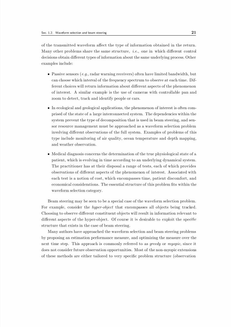
• Passive sensors (e.g., radar warning receivers) often have limited bandwidth, but
can choose which interval of the frequency spectrum to observe at each time. Dif-
ferent choices will return information about different aspects of the phenomenon
of interest. A similar example is the use of cameras with controllable pan and
zoom to detect, track and identify people or cars.
• In ecological and geological applications, the phenomenon of interest is often com-
prised of the state of a large interconnected system. The dependencies within thesystem prevent the type of decomposition that is used in beam steering, and sen-
sor resource management must be approached as a waveform selection problem
involving different observations of the full system. Examples of problems of this
type include monitoring of air quality, ocean temperature and depth mapping,
and weather observation.
• Medical diagnosis concerns the determination of the true physiological state of a
patient, which is evolving in time according to an underlying dynamical system.
The practitioner has at their disposal a range of tests, each of which provides
observations of different aspects of the phenomenon of interest. Associated witheach test is a notion of cost, which encompasses time, patient discomfort, and
economical considerations. The essential structure of this problem fits within the
waveform selection category.
Beam steering may be seen to be a special case of the waveform selection problem.
For example, consider the hyper-object that encompasses all objects being tracked.
Choosing to observe different constituent objects will result in information relevant to
different aspects of the hyper-object. Of course it is desirable to exploit the specific
structure that exists in the case of beam steering.
Many authors have approached the waveform selection and beam steering problems
by proposing an estimation performance measure, and optimizing the measure over the
next time step. This approach is commonly referred to as greedy or myopic, since it
does not consider future observation opportunities. Most of the non-myopic extensions
of these methods are either tailored to very specific problem structure (observation

8/2/2019 Information Theoretic Sensor Management
http://slidepdf.com/reader/full/information-theoretic-sensor-management 22/203
22 CHAPTER 1. INTRODUCTION
models, dynamics models, etc), or are limited to considering two or three time intervals
(longer planning horizons are typically computationally prohibitive). Furthermore, it
is unclear when additional planning can be beneficial.
1.3 Sensor networks
Networks of wireless sensors have the potential to provide unique capabilities for mon-
itoring and surveillance due to the close range at which phenomena of interest can be
observed. Application areas that have been investigated range from agriculture to eco-
logical and geological monitoring to object tracking and identification. Sensor networks
pose a particular challenge for resource management: not only are there short term
resource constraints due to limited communication bandwidth, but there are also long
term energy constraints due to battery limitations. This necessitates long term plan-
ning: for example, excessive energy should not be consumed in obtaining information
that can be obtained a little later on at a much lower cost. Failure to do so will result
in a reduced operational lifetime for the network.
It is commonly the case that the observations provided by sensors are highly infor-
mative if the sensor is in the close vicinity of the phenomenon of interest, and compara-
tively uninformative otherwise. In the context of object tracking, this has motivated the
use of a dynamically assigned leader node, which determines which sensors should take
and communicate observations, and stores and updates the knowledge of the object as
new observations are obtained. The choice of leader node should naturally vary as theobject moves through the network. The resulting structure falls within the framework
of platform steering, where the sensor state is the currently activated leader node.
1.4 Contributions and thesis outline
This thesis makes contributions in three areas. Firstly, we obtain performance guaran-
tees that delineate problems in which additional planning is and is not beneficial. We
then examine two problems in which long-term planning can be beneficial, finding an
efficient integer programming solution that exploits the structure of beam steering, and
finally, finding an efficient heuristic sensor management method for object tracking insensor networks.

8/2/2019 Information Theoretic Sensor Management
http://slidepdf.com/reader/full/information-theoretic-sensor-management 23/203
Sec. 1.4. Contributions and thesis outline 23
1.4.1 Performance guarantees for greedy heuristics
Recent work has resulted in performance guarantees for greedy heuristics in some ap-
plications, but there remains no guarantee that is applicable to sequential problems
without very special structure in the dynamics and observation models. The analysis
in Chapter 3 obtains guarantees similar to the recent work in [46] for the sequential
problem structures that commonly arise in waveform selection and beam steering. The
result is quite general in that it applies to arbitrary, time varying dynamics and obser-
vation models. Several extensions are obtained, including tighter bounds that exploit
either process diffusiveness or objectives involving discount factors, and applicability
to closed loop problems. The results apply to objectives including mutual information,
and the posterior Cramer-Rao bound. Examples demonstrate that the bounds are tight,
and counterexamples illuminate larger classes of problems to which they do not apply.
1.4.2 Efficient solution for beam steering problems
The analysis in Chapter 4 exploits the special structure in problems involving large
numbers of independent objects to find an efficient solution of the beam steering prob-
lem. The analysis from Chapter 3 is utilized to obtain an upper bound on the objective
function. Solutions with guaranteed near-optimality are found by simultaneously re-
ducing the upper bound and raising a matching lower bound.
The algorithm has quite general applicability, admitting time varying observation
and dynamical models, and observations requiring different time durations to complete.Computational experiments demonstrate application to problems involving 50–80 ob-
jects planning over horizons up to 60 time slots. An alternative formulation, which is
able to address time invariant rewards with a further computational saving, is also dis-
cussed. The methods apply to the same wide range of objectives as Chapter 3, including
mutual information and the posterior Cramer-Rao bound.
1.4.3 Sensor network management
In Chapter 5, we seek to trade off estimation performance and energy consumed in an
object tracking problem. We approach the trade off between these two quantities by
maximizing estimation performance subject to a constraint on energy cost, or the dual
of this, i.e., minimizing energy cost subject to a constraint on estimation performance.
We assign to each operation (sensing, communication, etc) an energy cost, and then
we seek to develop a mechanism that allows us to choose only those actions for which
the resulting estimation gain received outweighs the energy cost incurred. Our analysis

8/2/2019 Information Theoretic Sensor Management
http://slidepdf.com/reader/full/information-theoretic-sensor-management 24/203
24 CHAPTER 1. INTRODUCTION
proposes a planning method that is both computable and scalable, yet still captures
the essential structure of the underlying trade off. Simulation results demonstrate a
dramatic reduction in the communication cost required to achieve a given estimationperformance level as compared to previously proposed algorithms.

8/2/2019 Information Theoretic Sensor Management
http://slidepdf.com/reader/full/information-theoretic-sensor-management 25/203
Chapter 2
Background
THIS section provides an outline of the background theory which we utilize to de-
velop our results. The primary problem of interest is that of detecting, tracking
and identifying multiple objects, although many of the methods we discuss could beapplied to any other dynamical process.
Sensor management requires an understanding of several related topics: first of all,
one must develop a statistical model for the phenomenon of interest; then one must
construct an estimator for conducting inference on that phenomenon. One must select
an objective that measures how successful the sensor manager decisions have been, and,
finally, one must design a controller to make decisions using the available inputs.
In Section 2.1, we briefly outline the development of statistical models for object
tracking before describing some of the estimation schemes we utilize in our experiments.
Section 2.2 outlines the theory of stochastic control, the category of problems in which
sensor management naturally belongs. In Section 2.3, we describe the information
theoretic objective functions that we utilize, and certain properties of the objectives
that we utilize throughout the thesis. Section 2.4 details some existing results that
have been applied to related problems to guarantee performance of simple heuristic
algorithms; the focus of Chapter 3 is extending these results to sequential problems.
Section 2.5 briefly outlines the theory of linear and integer programming that we utilize
in Chapter 4. Finally, Section 2.6 surveys the existing work in the field, and contrasts
the approaches presented in the later chapters to the existing methods.
2.1 Dynamical models and estimation
This thesis will be concerned exclusively with sensor management systems that are
based upon statistical models. The starting point of such algorithms is a dynamical
model which captures mathematically how the physical process evolves, and how the
observations taken by the sensor relate to the model variables. Having designed this
25

8/2/2019 Information Theoretic Sensor Management
http://slidepdf.com/reader/full/information-theoretic-sensor-management 26/203
26 CHAPTER 2. BACKGROUND
model, one can then construct an estimator which uses sensor observations to refine
one’s knowledge of the state of the underlying physical process.
Using a Bayesian formulation, the estimator maintains a representation of the condi-tional probability density function (PDF) of the process state conditioned on the obser-
vations incorporated. This representation is central to the design of sensor management
algorithms, which seek to choose sensor actions in order to minimize the uncertainty in
the resulting estimate.
In this section, we outline the construction of dynamical models for object tracking,
and then briefly examine several estimation methods that one may apply.
2.1.1 Dynamical models
Traditionally, dynamical models for object tracking are based upon simple observationsregarding behavior of targets and the laws of physics. For example, if we are tracking
an aircraft and it moving at an essentially constant velocity at one instant in time, it
will probably still be moving at a constant velocity shortly afterward. Accordingly, we
may construct a mathematical model based upon Newtonian dynamics. One common
model for non-maneuvering objects hypothesizes that velocity is a random walk, and
position is the integral of velocity:
v(t) = w(t) (2.1)
˙ p(t) = v(t) (2.2)
The process w(t) is formally defined as a continuous time white noise with strength
Q(t). This strength may be chosen in order to model the expected deviation from the
nominal trajectory.
In tracking, the underlying continuous time model is commonly chosen to be a
stationary linear Gaussian system. Given any such model,
x(t) = Fcx(t) + w(t) (2.3)
where w(t) is a zero-mean Gaussian white noise process with strength Qc, we can
construct a discrete-time model which has the equivalent effect at discrete sample points.
This model is given by: [67]xk+1 = Fxk + wk (2.4)
where1
F = exp[Fc∆t] (2.5)
1exp[·] denotes the matrix exponential.
8/2/2019 Information Theoretic Sensor Management
http://slidepdf.com/reader/full/information-theoretic-sensor-management 27/203
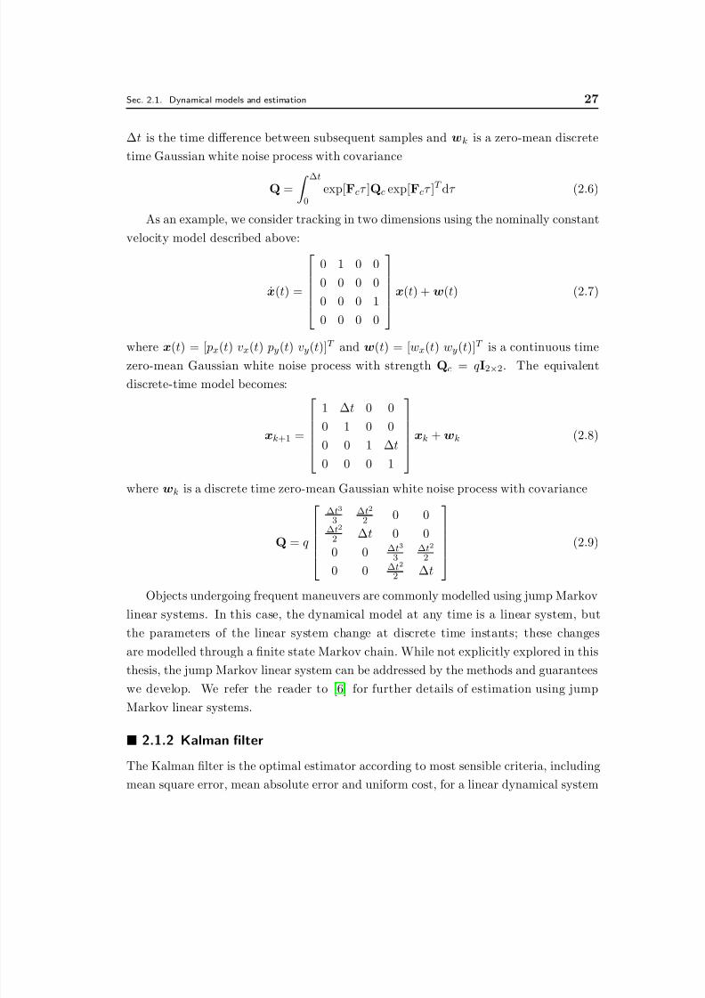
Sec. 2.1. Dynamical models and estimation 27
∆t is the time difference between subsequent samples and wk is a zero-mean discrete
time Gaussian white noise process with covariance
Q =
∆t
0exp[Fcτ ]Qc exp[Fcτ ]T dτ (2.6)
As an example, we consider tracking in two dimensions using the nominally constant
velocity model described above:
x(t) =
0 1 0 0
0 0 0 0
0 0 0 1
0 0 0 0
x(t) + w(t) (2.7)
where x(t) = [ px(t) vx(t) py(t) vy(t)]T
and w(t) = [wx(t) wy(t)]T
is a continuous timezero-mean Gaussian white noise process with strength Qc = qI2×2. The equivalent
discrete-time model becomes:
xk+1 =
1 ∆t 0 0
0 1 0 0
0 0 1 ∆t
0 0 0 1
xk + wk (2.8)
where wk is a discrete time zero-mean Gaussian white noise process with covariance
Q = q
∆t3
3
∆t2
2
0 0∆t2
2 ∆t 0 0
0 0 ∆t3
3∆t2
2
0 0 ∆t2
2 ∆t
(2.9)
Objects undergoing frequent maneuvers are commonly modelled using jump Markov
linear systems. In this case, the dynamical model at any time is a linear system, but
the parameters of the linear system change at discrete time instants; these changes
are modelled through a finite state Markov chain. While not explicitly explored in this
thesis, the jump Markov linear system can be addressed by the methods and guarantees
we develop. We refer the reader to [6] for further details of estimation using jump
Markov linear systems.
2.1.2 Kalman filter
The Kalman filter is the optimal estimator according to most sensible criteria, including
mean square error, mean absolute error and uniform cost, for a linear dynamical system
8/2/2019 Information Theoretic Sensor Management
http://slidepdf.com/reader/full/information-theoretic-sensor-management 28/203
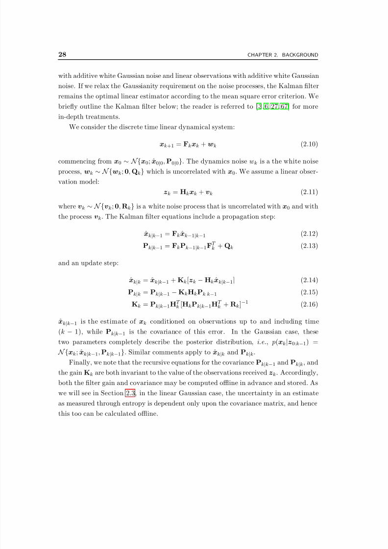
28 CHAPTER 2. BACKGROUND
with additive white Gaussian noise and linear observations with additive white Gaussian
noise. If we relax the Gaussianity requirement on the noise processes, the Kalman filter
remains the optimal linear estimator according to the mean square error criterion. Webriefly outline the Kalman filter below; the reader is referred to [3,6, 27, 67] for more
in-depth treatments.
We consider the discrete time linear dynamical system:
xk+1 = Fkxk + wk (2.10)
commencing from x0 ∼ N{x0; x0|0, P0|0}. The dynamics noise wk is a the white noise
process, wk ∼ N{wk; 0, Qk} which is uncorrelated with x0. We assume a linear obser-
vation model:
zk = Hkxk + vk (2.11)
where vk ∼ N{vk; 0, Rk} is a white noise process that is uncorrelated with x0 and with
the process vk. The Kalman filter equations include a propagation step:
xk|k−1 = Fkxk−1|k−1 (2.12)
Pk|k−1 = FkPk−1|k−1FT k + Qk (2.13)
and an update step:
xk|k = xk|k−1 + Kk[zk
−Hkxk|k−1] (2.14)
Pk|k = Pk|k−1 − KkHkPk|k−1 (2.15)
Kk = Pk|k−1HT k [HkPk|k−1HT
k + Rk]−1 (2.16)
xk|k−1 is the estimate of xk conditioned on observations up to and including time
(k − 1), while Pk|k−1 is the covariance of this error. In the Gaussian case, these
two parameters completely describe the posterior distribution, i.e., p(xk|z0:k−1) =
N{xk; xk|k−1, Pk|k−1}. Similar comments apply to xk|k and Pk|k.
Finally, we note that the recursive equations for the covariance Pk|k−1 and Pk|k, and
the gain Kk are both invariant to the value of the observations received zk. Accordingly,
both the filter gain and covariance may be computed offline in advance and stored. Aswe will see in Section 2.3, in the linear Gaussian case, the uncertainty in an estimate
as measured through entropy is dependent only upon the covariance matrix, and hence
this too can be calculated offline.

8/2/2019 Information Theoretic Sensor Management
http://slidepdf.com/reader/full/information-theoretic-sensor-management 29/203
Sec. 2.1. Dynamical models and estimation 29
2.1.3 Linearized and extended Kalman filter
While the optimality guarantees for the Kalman filter apply only to linear systems,
the basic concept is regularly applied to nonlinear systems through two algorithms
known as the linearized and extended Kalman filters. The basic concept is that a mild
nonlinearity may be approximated as being linear about a nominal point though a
Taylor series expansion. In the case of the linearized Kalman filter, the linearization
point is chosen in advance; the extended Kalman filter relinearizes online about the
current estimate value. Consequently, the linearized Kalman filter retains the ability to
calculate filter gains and covariance matrices in advance, whereas the extended Kalman
filter must compute both of these online.
In this document, we assume that the dynamical model is linear, and we present
the equations for the linearized and extended Kalman filters for the case in which theonly nonlinearity present is in the observation equation. This is most commonly the
case in tracking applications. The reader is directed to [68], the primary source for
this material, for information on the nonlinear dynamical model case. The model we
consider is:
xk+1 = Fkxk + wk (2.17)
zk = h(xk, k) + vk (2.18)
where, as in Section 2.1.2, wk and vk are uncorrelated white Gaussian noise processes
with known covariance, both of which are uncorrelated with x0. The linearized Kalmanfilter calculates a linearized measurement model about a pre-specified nominal state
trajectory {xk}k=1,2,...:
zk ≈ h(xk, k) + H(xk, k)[xk − xk] + vk (2.19)
where
H(xk, k) = [xh(x, k)T ]T |x=xk (2.20)
and x [ ∂ ∂ x1
, ∂ ∂ x2
, . . . , ∂ ∂ xnx
]T where nx is the number of elements in the vector x.
The linearized Kalman filter update equation is therefore:
xk|k = xk|k−1 + Kk{zk − h(xk, k) − H(xk, k)[xk − xk]} (2.21)
Pk|k = Pk|k−1 − KkH(xk, k)Pk|k−1 (2.22)
Kk = Pk|k−1H(xk, k)T [H(xk, k)Pk|k−1H(xk, k)T + Rk]−1 (2.23)
8/2/2019 Information Theoretic Sensor Management
http://slidepdf.com/reader/full/information-theoretic-sensor-management 30/203
30 CHAPTER 2. BACKGROUND
Again we note that the filter gain and covariance are both invariant to the observation
values, and hence they can be precomputed.
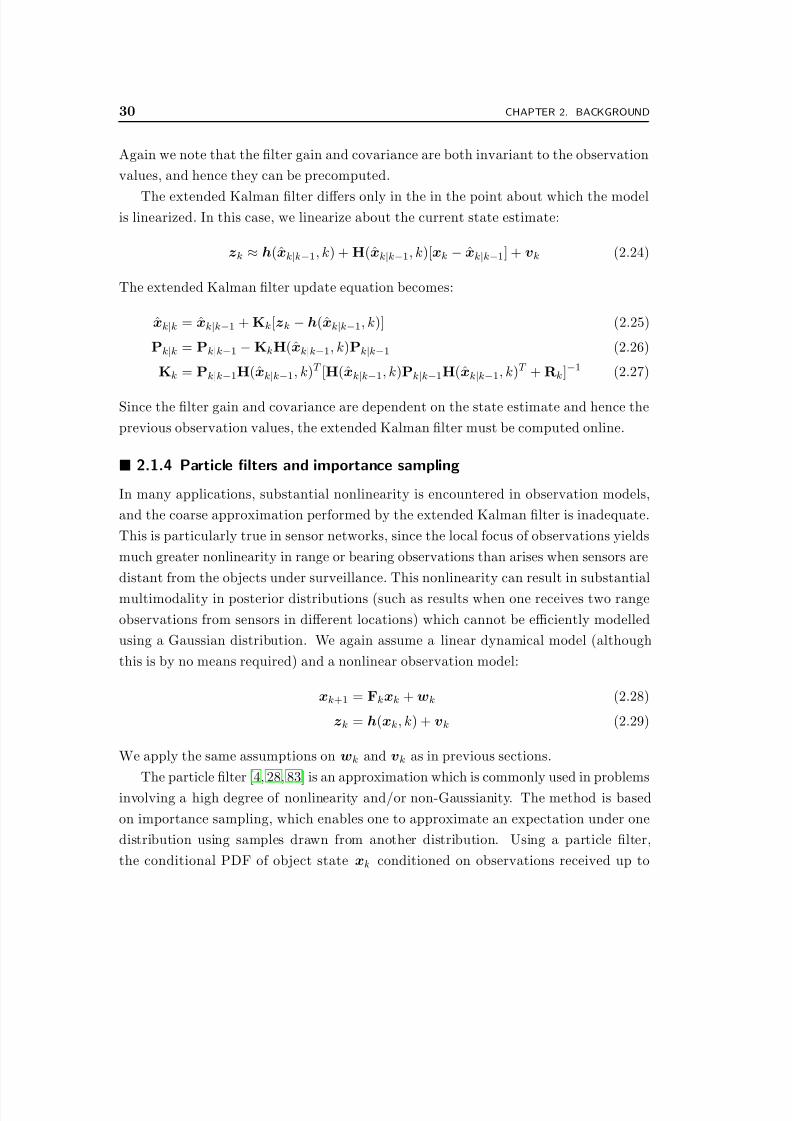
The extended Kalman filter differs only in the in the point about which the modelis linearized. In this case, we linearize about the current state estimate:
zk ≈ h(xk|k−1, k) + H(xk|k−1, k)[xk − xk|k−1] + vk (2.24)
The extended Kalman filter update equation becomes:
xk|k = xk|k−1 + Kk[zk − h(xk|k−1, k)] (2.25)
Pk|k = Pk|k−1 − KkH(xk|k−1, k)Pk|k−1 (2.26)
Kk = Pk|k−1H(xk|k−1, k)T [H(xk|k−1, k)Pk|k−1H(xk|k−1, k)T + Rk]−1 (2.27)
Since the filter gain and covariance are dependent on the state estimate and hence the
previous observation values, the extended Kalman filter must be computed online.
2.1.4 Particle filters and importance sampling
In many applications, substantial nonlinearity is encountered in observation models,
and the coarse approximation performed by the extended Kalman filter is inadequate.
This is particularly true in sensor networks, since the local focus of observations yields
much greater nonlinearity in range or bearing observations than arises when sensors are
distant from the objects under surveillance. This nonlinearity can result in substantial
multimodality in posterior distributions (such as results when one receives two range
observations from sensors in different locations) which cannot be efficiently modelled
using a Gaussian distribution. We again assume a linear dynamical model (although
this is by no means required) and a nonlinear observation model:
xk+1 = Fkxk + wk (2.28)
zk = h(xk, k) + vk (2.29)
We apply the same assumptions on wk and vk as in previous sections.
The particle filter [4, 28, 83] is an approximation which is commonly used in problems
involving a high degree of nonlinearity and/or non-Gaussianity. The method is based
on importance sampling, which enables one to approximate an expectation under one
distribution using samples drawn from another distribution. Using a particle filter,
the conditional PDF of object state xk conditioned on observations received up to
8/2/2019 Information Theoretic Sensor Management
http://slidepdf.com/reader/full/information-theoretic-sensor-management 31/203
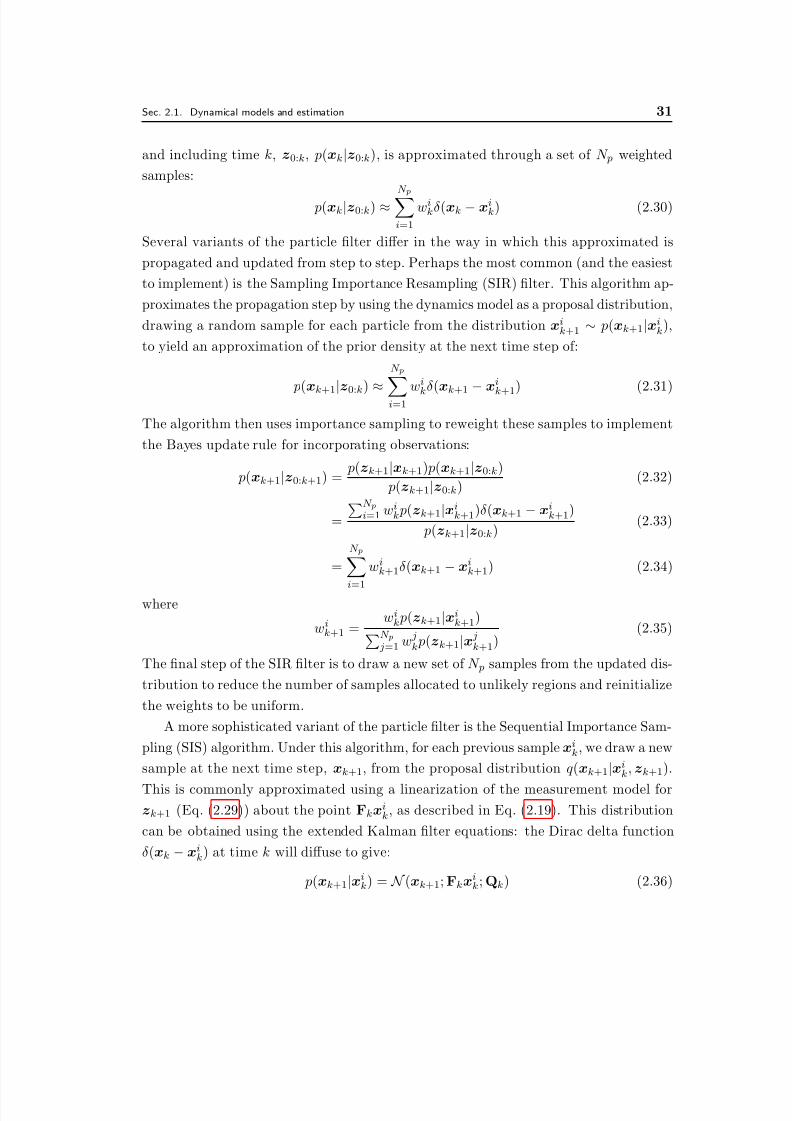
Sec. 2.1. Dynamical models and estimation 31
and including time k, z0:k, p(xk|z0:k), is approximated through a set of N p weighted
samples:
p(xk|z0:k) ≈N pi=1
wikδ(xk − xi
k) (2.30)
Several variants of the particle filter differ in the way in which this approximated is
propagated and updated from step to step. Perhaps the most common (and the easiest
to implement) is the Sampling Importance Resampling (SIR) filter. This algorithm ap-
proximates the propagation step by using the dynamics model as a proposal distribution,
drawing a random sample for each particle from the distribution xik+1 ∼ p(xk+1|xi
k),
to yield an approximation of the prior density at the next time step of:
p(xk+1|z0:k) ≈
N pi=1 w
i
kδ(xk+1 − x
i
k+1) (2.31)
The algorithm then uses importance sampling to reweight these samples to implement
the Bayes update rule for incorporating observations:
p(xk+1|z0:k+1) =p(zk+1|xk+1) p(xk+1|z0:k)
p(zk+1|z0:k)(2.32)
=
N pi=1 wi
k p(zk+1|xik+1)δ(xk+1 − xi
k+1)
p(zk+1|z0:k)(2.33)
=
N p
i=1
wik+1δ(xk+1 − xi
k+1) (2.34)
where
wik+1 =
wik p(zk+1|xi
k+1)N p j=1 w j
k p(zk+1|x jk+1)
(2.35)
The final step of the SIR filter is to draw a new set of N p samples from the updated dis-
tribution to reduce the number of samples allocated to unlikely regions and reinitialize
the weights to be uniform.
A more sophisticated variant of the particle filter is the Sequential Importance Sam-
pling (SIS) algorithm. Under this algorithm, for each previous sample xik, we draw a new
sample at the next time step, xk+1, from the proposal distribution q(xk+1
|xi
k, zk+1).
This is commonly approximated using a linearization of the measurement model for
zk+1 (Eq. (2.29)) about the point Fkxik, as described in Eq. (2.19). This distribution
can be obtained using the extended Kalman filter equations: the Dirac delta function
δ(xk − xik) at time k will diffuse to give:
p(xk+1|xik) = N (xk+1; Fkx
ik; Qk) (2.36)
8/2/2019 Information Theoretic Sensor Management
http://slidepdf.com/reader/full/information-theoretic-sensor-management 32/203
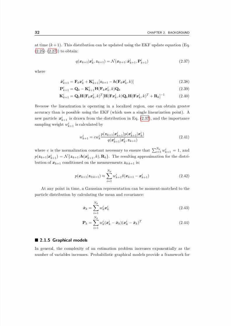
32 CHAPTER 2. BACKGROUND
at time (k + 1). This distribution can be updated using the EKF update equation (Eq.
(2.25)–(2.27)) to obtain:
q(xk+1|xik, zk+1) = N (xk+1; xi
k+1, Pik+1) (2.37)
where
xik+1 = Fkx
ik + Ki
k+1[zk+1 − h(Fkxik, k)] (2.38)
Pik+1 = Qk − Ki
k+1H(Fkxik, k)Qk (2.39)
Kik+1 = QkH(Fkx
ik, k)T [H(Fxi
k, k)QkH(Fxik, k)T + Rk]−1 (2.40)
Because the linearization is operating in a localized region, one can obtain greater
accuracy than is possible using the EKF (which uses a single linearization point). Anew particle xi
k+1 is drawn from the distribution in Eq. (2.37), and the importance
sampling weight wik+1 is calculated by
wik+1 = cwi
k
p(zk+1|xik+1) p(xi
k+1|xik)
q(xik+1|xi
k,zk+1)(2.41)
where c is the normalization constant necessary to ensure thatN p
i=1 wik+1 = 1, and
p(zk+1|xik+1) = N{zk+1;h(xi
k+1, k), Rk}. The resulting approximation for the distri-
bution of xk+1 conditioned on the measurements z0:k+1 is:
p(xk+1|z0:k+1) ≈N pi=1
wik+1δ(xk+1 − xi
k+1) (2.42)
At any point in time, a Gaussian representation can be moment-matched to the
particle distribution by calculating the mean and covariance:
xk =
N pi=1
wikx
ik (2.43)
Pk =
N p
i=1
wik(xi
k − xk)(xik − xk)T (2.44)
2.1.5 Graphical models
In general, the complexity of an estimation problem increases exponentially as the
number of variables increases. Probabilistic graphical models provide a framework for

8/2/2019 Information Theoretic Sensor Management
http://slidepdf.com/reader/full/information-theoretic-sensor-management 33/203
Sec. 2.1. Dynamical models and estimation 33
recognizing and exploiting structure which allows for efficient solution. Here we briefly
describe Markov random fields, a variety of undirected graphical model. Further details
can be found in [38, 73, 92].We assume that our model is represented as as graph G consisting of vertices V and
edges E ⊆ V × V . Corresponding to each vertex v ∈ V is a random variable xv and
several possible observations (from which we may choose some subset) of that variable,
{z1v , . . . , znvv }. Edges represent dependences between the local random variables, i.e.,
(v, w) ∈ E denotes that variables xv and xw have direct dependence on each other. All
observations are assumed to depend only on the corresponding local random variable.
In this case, the joint distribution function can be shown to factorize over the max-
imal cliques of the graph. A clique is defined as a set of vertices C ⊆ V which are fully
connected, i.e., (v, w)∈ E ∀
v, w∈ C
. A maximal clique is a clique which is not a subset
of any other clique in the graph (i.e., a clique for which no other vertex can be added
while still retaining full connectivity). Denoting the collection of all maximal cliques as
M , the joint distribution of variables and observations can be written as:
p({xv, {z1v , . . . , znvv }}v∈V ) ∝
C∈M
ψ({xv}v∈C)v∈V
nvi=1
ψ(xv, ziv) (2.45)
Graphical models are useful in recognizing independence structures which exist. For
example, two random variables xv and xw (v, w ∈ V ) are independent conditioned on a
given set of vertices D if there is no path connecting vertices v and w which does not
pass through any vertex in D. Obviously, if we denote by N (v) the neighbors of vertexv, then xv will be independent of all other variables in the graph conditioned on N (v).
Estimation problems involving undirected graphical models with a tree as the graph
structure can be solved efficiently using the belief propagation algorithm. Some prob-
lems involving sparse cyclic graphs can be addressed efficiently by combining small
numbers of nodes to obtain tree structure (referred to as a junction tree), but in gen-
eral approximate methods, such as loopy belief propagation, are necessary. Estimation
in time series is a classical example of a tree-based model: the Kalman filter (or, more
precisely, the Kalman smoother) may be seen to be equivalent to belief propagation
specialized to linear Gaussian Markov chains, while [35, 88,89] extends particle filtering
from Markov chains to general graphical models using belief propagation.
2.1.6 Cramer-Rao bound
The Cramer-Rao bound (CRB) [84, 91] provides a lower limit on the mean square error
performance achievable by any estimator of an underlying quantity. The simplest and

8/2/2019 Information Theoretic Sensor Management
http://slidepdf.com/reader/full/information-theoretic-sensor-management 34/203
34 CHAPTER 2. BACKGROUND
most common form of the bound, presented below in Theorem 2.1, deals with unbiased
estimates of nonrandom parameters (i.e., parameters which are not endowed with a
prior probability distribution). We omit the various regularity conditions; see [84, 91]for details. The notation A B implies that the matrix A−B is positive semi-definite
(PSD). We adopt convention from [90] that ∆z
x =xT z .
Theorem 2.1. Let x be a nonrandom vector parameter, and z be an observation with
distribution p(z|x) parameterized by x. Then any unbiased estimator of x based on z,
x(z), must satisfy the following bound on covariance:
Ez|x
[x(z) − x][x(z) − x]T
Cz
x [Jzx]−1
where J
z
x is the Fisher information matrix, which can be calculated equivalently through either of the following two forms:
Jzx Ez|x
[x log p(z|x)][x log p(z|x)]T
= E
z|x{−∆x
x log p(z|x)}
From the first form above we see that the Fisher information matrix is positive semi-
definite.
The posterior Cramer-Rao bound (PCRB) [91] provides a similar performance limit
for dealing with random parameters. While the bound takes on the same form, theFisher information matrix now decomposes into two terms: one involving prior in-
formation about the parameter, and another involving information gained from the
observation. Because we take an expectation over the possible values of x as well as z,
the bound applies to any estimator, biased or unbiased.
Theorem 2.2. Let x be a random vector parameter with probability distribution p(x),
and z be an observation with model p(z|x). Then any estimator of x based on z, x(z),
must satisfy the following bound on covariance:
Ex,z
[x(z) − x][x(z) − x]T C
z
x [J
z
x]−1
where Jzx is the Fisher information matrix, which can be calculated equivalently through
8/2/2019 Information Theoretic Sensor Management
http://slidepdf.com/reader/full/information-theoretic-sensor-management 35/203
Sec. 2.2. Markov decision processes 35
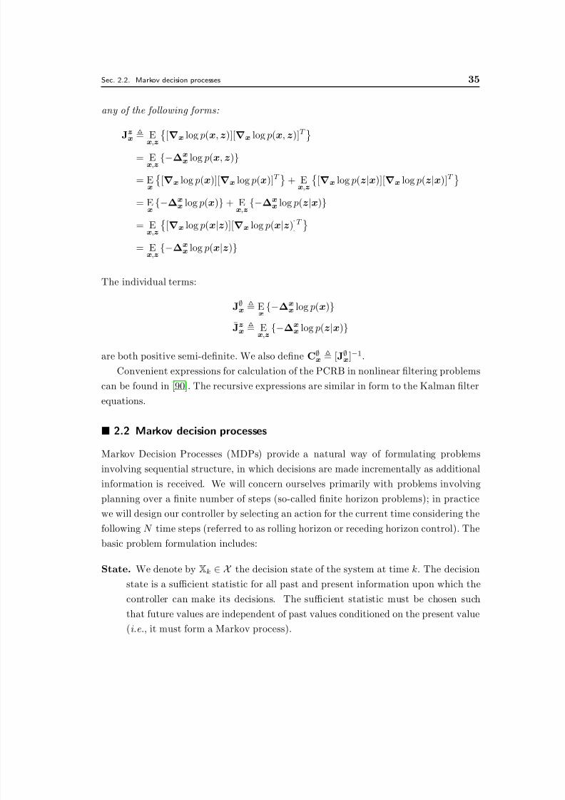
any of the following forms:
J
z
x
Ex,z
[x log p(x,z)][
x log p(x, z)]
T = E
x,z{−∆x
x log p(x, z)}
= Ex
[x log p(x)][x log p(x)]T
+ Ex,z
[x log p(z|x)][x log p(z|x)]T
= E
x
{−∆x
x log p(x)} + Ex,z
{−∆x
x log p(z|x)}
= Ex,z
[x log p(x|z)][x log p(x|z)]T
= E
x,z{−∆x
x log p(x|z)}
The individual terms:
J∅x E
x
{−∆x
x log p(x)}Jzx E
x,z{−∆x
x log p(z|x)}
are both positive semi-definite. We also define C∅x [J∅
x]−1.
Convenient expressions for calculation of the PCRB in nonlinear filtering problems
can be found in [90]. The recursive expressions are similar in form to the Kalman filter
equations.
2.2 Markov decision processes
Markov Decision Processes (MDPs) provide a natural way of formulating problems
involving sequential structure, in which decisions are made incrementally as additional
information is received. We will concern ourselves primarily with problems involving
planning over a finite number of steps (so-called finite horizon problems); in practice
we will design our controller by selecting an action for the current time considering the
following N time steps (referred to as rolling horizon or receding horizon control). The
basic problem formulation includes:
State. We denote by Xk ∈ X the decision state of the system at time k. The decision
state is a sufficient statistic for all past and present information upon which the
controller can make its decisions. The sufficient statistic must be chosen such
that future values are independent of past values conditioned on the present value
(i.e., it must form a Markov process).
8/2/2019 Information Theoretic Sensor Management
http://slidepdf.com/reader/full/information-theoretic-sensor-management 36/203
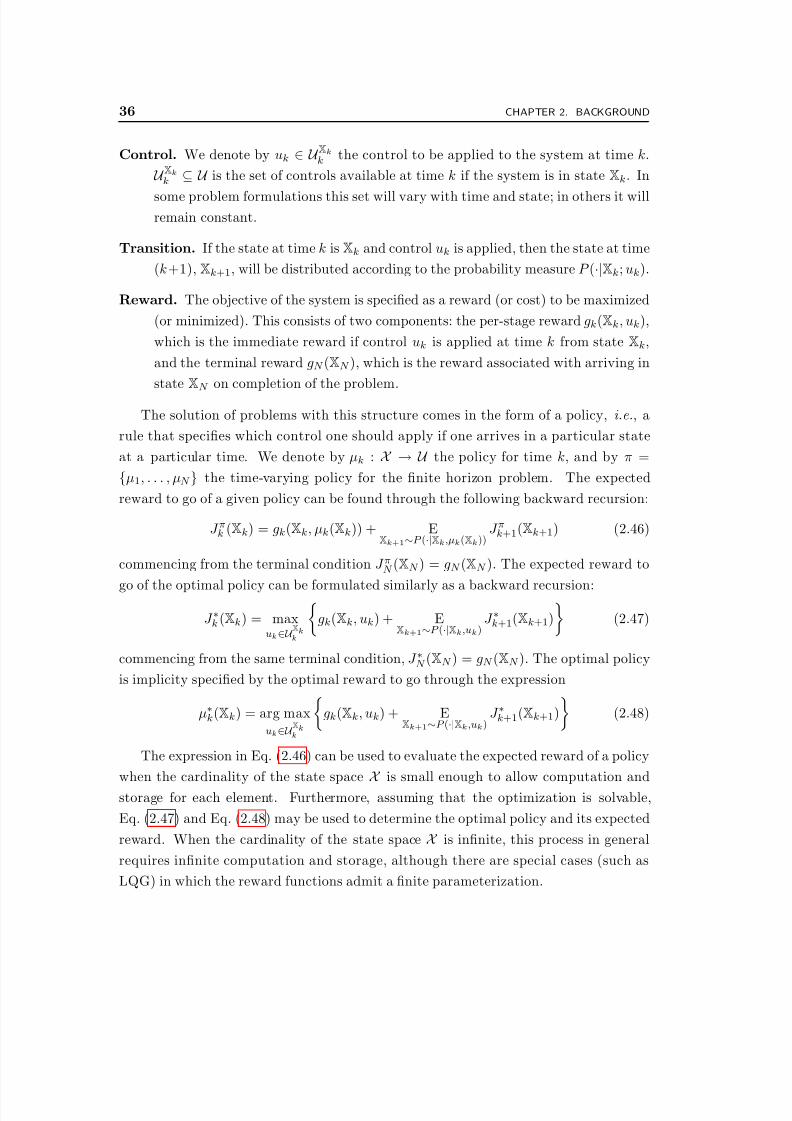
36 CHAPTER 2. BACKGROUND
Control. We denote by uk ∈ U Xkk the control to be applied to the system at time k.
U Xkk ⊆ U is the set of controls available at time k if the system is in state Xk. In
some problem formulations this set will vary with time and state; in others it willremain constant.
Transition. If the state at time k is Xk and control uk is applied, then the state at time
(k+1), Xk+1, will be distributed according to the probability measure P (·|Xk; uk).
Reward. The objective of the system is specified as a reward (or cost) to be maximized
(or minimized). This consists of two components: the per-stage reward gk(Xk, uk),
which is the immediate reward if control uk is applied at time k from state Xk,
and the terminal reward gN (XN ), which is the reward associated with arriving in
state XN on completion of the problem.
The solution of problems with this structure comes in the form of a policy, i.e., a
rule that specifies which control one should apply if one arrives in a particular state
at a particular time. We denote by µk : X → U the policy for time k, and by π =
{µ1, . . . , µN } the time-varying policy for the finite horizon problem. The expected
reward to go of a given policy can be found through the following backward recursion:
J πk (Xk) = gk(Xk, µk(Xk)) + EXk+1∼P (·|Xk,µk(Xk))
J πk+1(Xk+1) (2.46)
commencing from the terminal condition J πN (XN ) = gN (XN ). The expected reward to
go of the optimal policy can be formulated similarly as a backward recursion:
J ∗k (Xk) = maxuk∈U
Xkk
gk(Xk, uk) + E
Xk+1∼P (·|Xk,uk)J ∗k+1(Xk+1)
(2.47)
commencing from the same terminal condition, J ∗N (XN ) = gN (XN ). The optimal policy
is implicity specified by the optimal reward to go through the expression
µ∗k(Xk) = arg max
uk∈U Xkk
gk(Xk, uk) + E
Xk+1∼P (·|Xk,uk)J ∗k+1(Xk+1)
(2.48)
The expression in Eq. (2.46) can be used to evaluate the expected reward of a policy
when the cardinality of the state spaceX
is small enough to allow computation and
storage for each element. Furthermore, assuming that the optimization is solvable,
Eq. (2.47) and Eq. (2.48) may be used to determine the optimal policy and its expected
reward. When the cardinality of the state space X is infinite, this process in general
requires infinite computation and storage, although there are special cases (such as
LQG) in which the reward functions admit a finite parameterization.
8/2/2019 Information Theoretic Sensor Management
http://slidepdf.com/reader/full/information-theoretic-sensor-management 37/203
Sec. 2.2. Markov decision processes 37
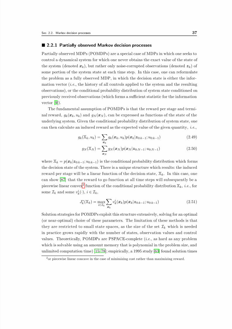
2.2.1 Partially observed Markov decision processes
Partially observed MDPs (POMDPs) are a special case of MDPs in which one seeks to
control a dynamical system for which one never obtains the exact value of the state of
the system (denoted xk), but rather only noise-corrupted observations (denoted zk) of
some portion of the system state at each time step. In this case, one can reformulate
the problem as a fully observed MDP, in which the decision state is either the infor-
mation vector (i.e., the history of all controls applied to the system and the resulting
observations), or the conditional probability distribution of system state conditioned on
previously received observations (which forms a sufficient statistic for the information
vector [9]).
The fundamental assumption of POMDPs is that the reward per stage and termi-
nal reward, gk(xk, uk) and gN (xN ), can be expressed as functions of the state of theunderlying system. Given the conditional probability distribution of system state, one
can then calculate an induced reward as the expected value of the given quantity, i.e.,
gk(Xk, uk) =xk
gk(xk, uk) p(xk|z0:k−1; u0:k−1) (2.49)
gN (XN ) =xN
gN (xN ) p(xN |z0:N −1; u0:N −1) (2.50)
where Xk = p(xk|z0:k−1; u0:k−1) is the conditional probability distribution which forms
the decision state of the system. There is a unique structure which results: the induced
reward per stage will be a linear function of the decision state, Xk. In this case, onecan show [87] that the reward to go function at all time steps will subsequently be a
piecewise linear convex2 function of the conditional probability distribution Xk, i.e., for
some I k and some vik(·), i ∈ I k,
J ∗k (Xk) = maxi∈I k
xk
vik(xk) p(xk|z0:k−1; u0:k−1) (2.51)
Solution strategies for POMDPs exploit this structure extensively, solving for an optimal
(or near-optimal) choice of these parameters. The limitation of these methods is that
they are restricted to small state spaces, as the size of the set
I k which is needed
in practice grows rapidly with the number of states, observation values and control
values. Theoretically, POMDPs are PSPACE-complete (i.e., as hard as any problem
which is solvable using an amount memory that is polynomial in the problem size, and
unlimited computation time) [15, 78]; empirically, a 1995 study [63] found solution times
2or piecewise linear concave in the case of minimizing cost rather than maximizing reward.

8/2/2019 Information Theoretic Sensor Management
http://slidepdf.com/reader/full/information-theoretic-sensor-management 38/203
38 CHAPTER 2. BACKGROUND
in the order of hours for problems involving fifteen underlying system states, fifteen
observation values and four actions. Clearly, such strategies are intractable in cases
where there is an infinite state space, e.g., when the underlying system state involvescontinuous elements such as position and velocity. Furthermore, attempts to discretize
this type of state space are also unlikely to arrive at a sufficiently small number of states
for this class of algorithm to be applicable.
2.2.2 Open loop, closed loop and open loop feedback
The assumption inherent in MDPs is that the decision state is revealed to the controller
at each decision stage. The optimal policy uses this new information as it becomes avail-
able, and anticipates the arrival of future information through the Markov transition
model. This is referred to as closed loop control (CLC). Open loop control (OLC)represents the opposite situation: where one constructs a plan for the finite horizon
(i.e., single choice of which control to apply at each time, as opposed to a policy), and
neither anticipates the availability of future information, nor utilizes that information
as it arrives.
Open Loop Feedback Control (OLFC) is a compromise between these two extremes:
like an open loop controller, a plan (rather than a policy) is constructed for the finite
horizon at each step of the problem. This plan does not anticipate the availability
future information; only a policy can do so. However, unlike an open loop controller,
when new information is received it is utilized in constructing an updated plan. The
controller operates by constructing a plan for the finite horizon, executing one or more
steps of that plan, and then constructing a new plan which incorporates the information
received in the interim.
There are many problems in which solving the MDP is intractable, yet open loop
plans can be found within computational limitations. The OLFC is a commonly used
suboptimal method in these situations. One can prove that the performance of the
optimal OLFC is no worse than the optimal OLC [9]; the difference in performance
between OLFC and CLC can be arbitrarily large.
2.2.3 Constrained dynamic programmingIn Chapter 5 we will consider sensor resource management in sensor networks. In this
application, there is a fundamental trade-off which arises between estimation perfor-
mance and energy cost. A natural way of approaching such a trade-off is as a constrained
optimization, optimizing one quantity subject to a constraint on the other.
8/2/2019 Information Theoretic Sensor Management
http://slidepdf.com/reader/full/information-theoretic-sensor-management 39/203
Sec. 2.2. Markov decision processes 39
Constrained dynamic programming has been explored by previous authors in [2, 13,
18, 94]. We describe a method based on Lagrangian relaxation, similar to that in [18],
which yields a convenient method of approximate evaluation for the problem examinedin Chapter 5.
We seek to minimize the cost over an N -step rolling horizon, i.e., at time k, we
minimize the cost incurred in the planning horizon involving steps {k , . . . , k + N − 1}.
Denoting by µk(Xk) the control policy for time k, and by πk = {µk, . . . , µk+N −1} the set
of policies for the next N time steps, we seek the policy corresponding to the optimal
solution to the constrained minimization problem:
minπ
E
k+N −1
i=k
g(Xi, µi(Xi))
s.t.E
k+N −1
i=k
G(Xi, µi(Xi))
≤ M (2.52)
where g(Xk, uk) is the per-stage cost and G(Xk, uk) is the per-stage contribution to the
additive constraint function. We address the constraint through a Lagrangian relax-
ation, a common approximation method for discrete optimization problems, by defining
the dual function:
J Dk (Xk, λ) = minπ
E
k+N −1
i=k
g(Xi, µi(Xi)) + λ
k+N −1
i=k
G(Xi, µi(Xi)) − M
(2.53)
and solving the dual optimization problem involving this function:
J Lk (Xk) = maxλ≥0
J Dk (Xk, λ) (2.54)
We note that the dual function J Dk (Xk, λ) takes the form of an unconstrained dynamic
program with a modified per-stage cost:
g(Xk, uk, λ) = g(Xk, uk) + λG(Xk, uk) (2.55)
The optimization of the dual problem provides a lower bound to the minimum value
of the original constrained problem; the presence of a duality gap is possible since the
optimization space is discrete. The size of the duality gap is given by the expression
λ E[
i G(Xi, µi(Xi)) − M ], where πk = {µi(·, ·)}i=k:k+N −1 is the policy attaining the
minimum in Eq. (2.53) for the value of λ attaining the maximum in Eq. (2.54). If
it happens that the optimal solution produced by the dual problem has no duality

8/2/2019 Information Theoretic Sensor Management
http://slidepdf.com/reader/full/information-theoretic-sensor-management 40/203
40 CHAPTER 2. BACKGROUND
gap, then the resulting solution is also the optimal solution of the original constrained
problem. This can occur in one of two ways: either the Lagrange multiplier λ is zero,
such that the solution of the unconstrained problem satisfies the constraint, or thesolution yields a result for which the constraint is tight. If a duality gap exists, a better
solution may exist satisfying the constraint; however, the solution returned would have
been optimal if the constraint level had been lower such that the constraint was tight.
The method described in [18] avoids a duality gap utilizing randomized policies.
Conceptually, the dual problem in Eq. (2.54) can be solved using a subgradient
method [10]. The following expression can be seen to be a supergradient3 of the dual
objective:
S (Xk, πk, λ) = Ei
G(Xi, µi(Xi)) − M (2.56)
In other words, S (Xk, πk, λ) ∈ ∂J Dk (Xk, λ), where ∂ denotes the superdifferential, i.e.,
the set of all supergradients. The subgradient method operates according to the same
principle as a gradient search, iteratively stepping in the direction of a subgradient
with a decreasing step size [10]. For a single constraint, one may also employ methods
such a line search; for multiple constraints the linear programming column generation
procedure described in [16, 94] can be more efficient.
2.3 Information theoretic objectives
In some circumstances, the most appropriate choice of reward function might be obviousfrom the system specification. For example, if a sensing system is being used to estimate
the location of a stranded yachtsman in order to minimize the distance from the survivor
to where air-dropped supplies land, then a natural objective would be to minimize the
expected landing distance, or to maximize the probability that the distance is less than a
critical threshold. Each of these relates directly to a specific quantity at a specific time.
As the high-level system objective becomes further removed from the performance of the
sensing system, the most appropriate choice of reward function becomes less apparent.
When an application demands continual tracking of multiple objects without a direct
terminal objective, it is unclear what reward function should be selected.
Entropy is a commonly-used measure of uncertainty in many applications including
sensor resource management, e.g., [32, 41, 61, 95]. This section explores the definitions
of and basic inequalities involving entropy and mutual information. All of the results
3Since we are maximizing a non-differentiable concave function rather than minimizing a non-
differentiable convex function, subgradients are replaced by supergradients.
8/2/2019 Information Theoretic Sensor Management
http://slidepdf.com/reader/full/information-theoretic-sensor-management 41/203
Sec. 2.3. Information theoretic objectives 41
presented are well-known, and can be found in classical texts such as [23]. Throughout
this document we use Shannon’s entropy, as opposed to the generalization referred to as
Renyi entropy. We will exploit various properties that are unique to Shannon entropy.
2.3.1 Entropy
Entropy, joint entropy and conditional entropy are defined as:
H (x) = −
p(x)log p(x)dx (2.57)
H (x, z) = −
p(x, z)log p(x, z)dxdz (2.58)
H (x|z) = − p(z) p(x|z)log p(x|z)dxdz (2.59)
= H (x, z) − H (z) (2.60)
The above definitions relate to differential entropy, which concerns continuous variables.
If the underlying sets are discrete, then a counting measure is used, effectively replacing
the integral by a summation. In the discrete case, we have H (x) ≥ 0. It is traditional
to use a base-2 logarithm when dealing with discrete variables, and a natural logarithm
when dealing with continuous quantities. We will also use a natural logarithm in cases
involving a mixture of continuous and discrete quantities.
The conditioning in H (x|z) in Eq. (2.59) is on the random variable z, hence an
expectation is performed over the possible values that the variable may ultimatelyassume. We can also condition on a particular value of a random variable:
H (x|z = ζ ) = −
p(x|z = ζ )log p(x|z = ζ )dx (2.61)
We will sometimes use the notation H (x|z) to denote conditioning on a particular value,
i.e., H (x|z) H (x|z = z). Comparing Eq. (2.59) and Eq. (2.61), we observe that:
H (x|z) =
pz(ζ )H (x|z = ζ )dζ (2.62)
8/2/2019 Information Theoretic Sensor Management
http://slidepdf.com/reader/full/information-theoretic-sensor-management 42/203
42 CHAPTER 2. BACKGROUND
2.3.2 Mutual information
Mutual information (MI) is defined as the expected reduction in entropy in one random
variable due to observation of another variable:
I (x; z) =
p(x, z)log
p(x, z)
p(x) p(z)dxdz (2.63)
= H (x) − H (x|z) (2.64)
= H (z) − H (z|x) (2.65)
= H (x) + H (z) − H (x, z) (2.66)
Like conditional entropy, conditional MI can be defined with conditioning on either a
random variable, or a particular value. In either case, the conditioning appears in all
terms of the definition, i.e., in the case of conditioning on a random variable y,
I (x; z|y) =
py(ψ)
p(x, z|y = ψ)log
p(x, z|y = ψ)
p(x|y = ψ) p(z|y = ψ)dxdzdψ (2.67)
= H (x|y) − H (x|z, y) (2.68)
= H (z|y) − H (z|x, y) (2.69)
= H (x|y) + H (z|y) − H (x, z|y) (2.70)
and in the case of conditioning on a particular value, ψ:
I (x; z|y = ψ) =
p(x, z|y = ψ)log p(x, z|y = ψ) p(x|y = ψ) p(z|y = ψ) dxdz (2.71)
= H (x|y = ψ) − H (x|z, y = ψ) (2.72)
= H (z|y = ψ) − H (z|x, y = ψ) (2.73)
= H (x|y = ψ) + H (z|y = ψ) − H (x, z|y = ψ) (2.74)
Again, we will sometimes use the notation I (x; z|y) to indicate conditioning on a par-
ticular value, i.e. I (x; z|y) I (x; z|y = y). Also note that, like conditional entropy, we
can write:
I (x; z
|y) = py(ψ)I (x; z
|y = ψ)dψ (2.75)
The chain rule of mutual information allows us to expand a mutual information
expression into the sum of terms:
I (x; z1, . . . , zn) =n
i=1
I (x; zi|z1, . . . , zi−1) (2.76)

8/2/2019 Information Theoretic Sensor Management
http://slidepdf.com/reader/full/information-theoretic-sensor-management 43/203
Sec. 2.3. Information theoretic objectives 43
The i-th term in the sum, I (x; zi|z1, . . . , zi−1) represents the incremental gain we obtain
in our knowledge of x due to the new observation zi, conditioned on the previous
observation random variables (z1, . . . , zi−1).Suppose we have observations (z1, . . . , zn) of an underlying state (x1, . . . , xn), where
observation zi is independent of all other observations and underlying states when
conditioned on xi. In this case, we find:
I (x1, . . . , xn; zi) = H (zi) − H (zi|x1, . . . , xn)
= H (zi) − H (zi|xi)
= I (xi; zi) (2.77)
In this case, the chain rule may be written as:
I (x1, . . . , xn; z1, . . . , zn) =n
i=1
I (xi; zi|z1, . . . , zi−1) (2.78)
It can be shown (through Jensen’s inequality) that mutual information is nonneg-
ative, i.e., I (x; z) ≥ 0, with equality if and only if x and z are independent.4 Since
I (x; z) = H (x) − H (x|z), this implies that H (x) ≥ H (x|z), i.e., that conditioning on a
random variable reduces entropy. The following example illustrates that conditioning
on a particular value of a random variable may not reduce entropy.
Example 2.1. Suppose we want to infer a state x ∈ {0, . . . , N } where p(x = 0) =
(N − 1)/N and p(x = i) = 1/N 2, i = 0 (assume N > 1). Calculating the entropy, weobtain H (x) = log N − 1
N log (N −1)N −1
N = 1
N log N + 1
N log N N
(N −1)N −1 > 0. We have an
observation z ∈ {0, 1}, with p(z = 0|x = 0) = 1 and p(z = 0|x = 0) = 0. If we receive
the observation value z = 0, then we know that x = 0, hence H (x|z = 0) = 0 < H (x). If
we receive the observation value z = 1 then H (x|z = 1) = log N > H (x). Conditioning
on the random variable, we find H (x|z) = 1N
log N < H (x).
2.3.3 Kullback-Leibler distance
The relative entropy or Kullback-Leibler (KL) distance is a measure of the difference
between two probability distributions, defined as:
D( p(x)||q(x)) =
p(x)log
p(x)
q(x)dx (2.79)
4This is also true for conditional MI, with conditioning on either an observation random variable or
an observation value, with equality iff x and z are independent under the respective conditioning.
8/2/2019 Information Theoretic Sensor Management
http://slidepdf.com/reader/full/information-theoretic-sensor-management 44/203
44 CHAPTER 2. BACKGROUND
Comparing Eq. (2.79) with Eq. (2.63), we obtain:
I (x; z) = D( p(x, z)|| p(x) p(z)) (2.80)
Manipulating Eq. (2.63) we also obtain:
I (x; z) =
p(z)
p(x|z)log
p(x|z)
p(x)dxdz = E
zD( p(x|z)|| p(x)) (2.81)
Therefore the MI between x and z is equivalent to the expected KL distance between
the posterior distribution p(x|z) and the prior distribution p(x).
Another interesting relationship can be obtained by considering the expected KL
distance between the posterior given a set of observations {z1, . . . , zn} from which we
may choose a single observation, and the posterior given the single observation zu
(u ∈ {1, . . . , n}):
ED( p(x|z1, . . . , zn)|| p(x|zu))
=
p(z1, . . . , zn)
p(x|z1, . . . , zn)log
p(x|z1, . . . , zn)
p(x|zu)dxdz1, . . . , dzn
=
p(x, z1, . . . , zn)log
p(x, z1, . . . , zn) p(zu)
p(x, zu) p(z1, . . . , zn)dxdz1, . . . , dzn
=
p(x, z1, . . . , zn)
log
p(x) p(zu)
p(x, zu)+ log
p(z1, . . . , zn, x)
p(x) p(z1, . . . , zn)
dxdz1, . . . , dzn
= −I (x; zu) + I (x; z1, . . . , zn)
Since the second term is invariant to the choice of u, we obtain the result that choosing
u to maximize the MI between the state x and the observation zu is equivalent to
minimizing the expected KL distance between the posterior distribution of x given all
observations and the posterior given only the chosen observation zu.
2.3.4 Linear Gaussian models
Entropy is closely related to variance for Gaussian distributions. The entropy of
an n-dimensional multivariate Gaussian distribution with covariance P is equal to12
log
|2πeP
|= n
2log2πe + 1
2log
|P
|. Thus, under linear-Gaussian assumptions, mini-
mizing conditional entropy is equivalent to minimizing the determinant of the posterior
covariance, or the volume of the uncertainty hyper-ellipsoid.
Suppose x and z are jointly Gaussian random variables with covariance:
P =
Px Pxz
PT xz Pz

8/2/2019 Information Theoretic Sensor Management
http://slidepdf.com/reader/full/information-theoretic-sensor-management 45/203
Sec. 2.3. Information theoretic objectives 45
Then the mutual information between x and z is given by:
I (x; z) =1
2log
|Px
||Px − PxzP−1z PT xz|(2.82)
=1
2log
|Pz||Pz − PT
xzP−1x Pxz|
(2.83)
In the classical linear Gaussian case (to which the Kalman filter applies), where z =
Hx + v and v ∼ N{v; 0, R} is independent of x,
I (x;z) =1
2log
|Px||Px − PxHT (HPxHT + R)−1HPx| (2.84)
=1
2log
|P−1x + HT R−1H|
|P−1x | (2.85)
= 12
log |HPxHT
+ R||R| (2.86)
Furthermore, if x, y and z are jointly Gaussian then:
I (x;z|y) = I (x; z|y = ψ) ∀ ψ (2.87)
The result of Eq. (2.87) is due to the fact that the posterior covariance in a Kalman
filter is not affected by the observation value (as discussed in Section 2.1.2), and that
entropy and MI are uniquely determined by the covariance of a Gaussian distribution.
2.3.5 Axioms resulting in entropy
One may show that Shannon’s entropy is the unique (up to a multiplicative constant)
real-valued measure of the uncertainty in a discrete probability distribution which sat-
isfies the following three axioms [7]. We assume x ∈ {x1, . . . , xn} where n < ∞, and
use the notation pxi = P [x = xi], and H ( px1, . . . , pxn) = H (x).
1. H ( px1, . . . , pxn) is a continuous5 function of the probability distribution
( px1, . . . , pxn) (defined for all n).
2. H ( px1, . . . , pxn) is permutation symmetric, i.e., if π(x) is a permutation of x then
H ( px1, . . . , pxn) = H ( pπ(x1), . . . , pπ(xn)).
3. If xn,1 and xn,2 partition the event xn (so that pxn,1 + pxn,2 = pxn > 0) then:
H ( px1 , . . . , pxn−1, pxn,1 , pxn,2) = H ( px1 , . . . , pxn) + p(xn)H
pxn,1
pxn
,pxn,2
pxn
5This condition can be relaxed to H (x) being a Lebesgue integrable function of p(x) (see [7]).
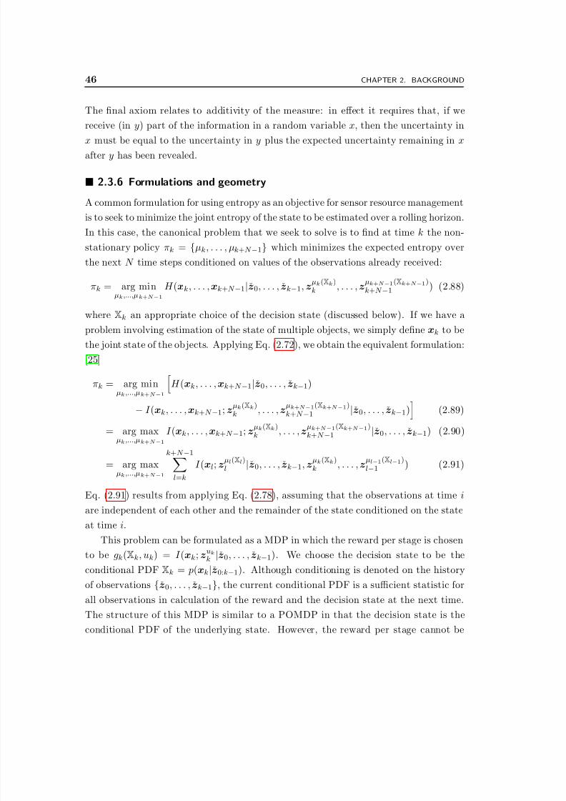
8/2/2019 Information Theoretic Sensor Management
http://slidepdf.com/reader/full/information-theoretic-sensor-management 46/203
46 CHAPTER 2. BACKGROUND
The final axiom relates to additivity of the measure: in effect it requires that, if we
receive (in y) part of the information in a random variable x, then the uncertainty in
x must be equal to the uncertainty in y plus the expected uncertainty remaining in xafter y has been revealed.
2.3.6 Formulations and geometry
A common formulation for using entropy as an objective for sensor resource management
is to seek to minimize the joint entropy of the state to be estimated over a rolling horizon.
In this case, the canonical problem that we seek to solve is to find at time k the non-
stationary policy πk = {µk, . . . , µk+N −1} which minimizes the expected entropy over
the next N time steps conditioned on values of the observations already received:
πk = arg minµk,...,µk+N −1
H (xk, . . . ,xk+N −1|z0, . . . , zk−1,zµk(Xk)k , . . . ,zµk+N −1(Xk+N −1)
k+N −1 ) (2.88)
where Xk an appropriate choice of the decision state (discussed below). If we have a
problem involving estimation of the state of multiple objects, we simply define xk to be
the joint state of the objects. Applying Eq. (2.72), we obtain the equivalent formulation:
[25]
πk = arg minµk,...,µk+N −1
H (xk, . . . ,xk+N −1|z0, . . . , zk−1)
−I (xk, . . . ,xk+N −1; z
µk(Xk)k , . . . ,z
µk+N −1(Xk+N −1)k+N −1
|z0, . . . , zk−1) (2.89)
= arg maxµk,...,µk+N −1
I (xk, . . . ,xk+N −1; zµk(Xk)k , . . . ,z
µk+N −1(Xk+N −1)k+N −1 |z0, . . . , zk−1) (2.90)
= arg maxµk,...,µk+N −1
k+N −1l=k
I (xl; zµl(Xl)l |z0, . . . , zk−1,z
µk(Xk)k , . . . ,z
µl−1(Xl−1)l−1 ) (2.91)
Eq. (2.91) results from applying Eq. (2.78), assuming that the observations at time i
are independent of each other and the remainder of the state conditioned on the state
at time i.
This problem can be formulated as a MDP in which the reward per stage is chosen
to be gk(Xk, uk) = I (xk; zuk
k |z0, . . . , zk
−1). We choose the decision state to be the
conditional PDF Xk = p(xk|z0:k−1). Although conditioning is denoted on the history
of observations {z0, . . . , zk−1}, the current conditional PDF is a sufficient statistic for
all observations in calculation of the reward and the decision state at the next time.
The structure of this MDP is similar to a POMDP in that the decision state is the
conditional PDF of the underlying state. However, the reward per stage cannot be
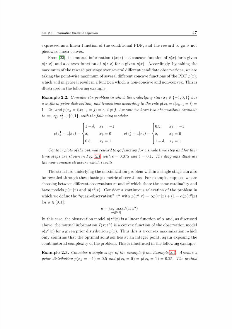
8/2/2019 Information Theoretic Sensor Management
http://slidepdf.com/reader/full/information-theoretic-sensor-management 47/203
Sec. 2.3. Information theoretic objectives 47
expressed as a linear function of the conditional PDF, and the reward to go is not
piecewise linear convex.
From [23], the mutual information I (x; z) is a concave function of p(x) for a given p(z|x), and a convex function of p(z|x) for a given p(x). Accordingly, by taking the
maximum of the reward per stage over several different candidate observations, we are
taking the point-wise maximum of several different concave functions of the PDF p(x),
which will in general result in a function which is non-concave and non-convex. This is
illustrated in the following example.
Example 2.2. Consider the problem in which the underlying state xk ∈ {−1, 0, 1} has
a uniform prior distribution, and transitions according to the rule p(xk = i|xk−1 = i) =
1 − 2, and p(xk = i|xk−1 = j) = , i = j. Assume we have two observations available
to us, z1k, z2k ∈ {0, 1}, with the following models:
p(z1k = 1|xk) =
1 − δ, xk = −1
δ, xk = 0
0.5, xk = 1
p(z2k = 1|xk) =
0.5, xk = −1
δ, xk = 0
1 − δ, xk = 1
Contour plots of the optimal reward to go function for a single time step and for four
time steps are shown in Fig. 2.1, with = 0.075 and δ = 0.1. The diagrams illustrate
the non-concave structure which results.
The structure underlying the maximization problem within a single stage can alsobe revealed through these basic geometric observations. For example, suppose we are
choosing between different observations z1 and z2 which share the same cardinality and
have models p(z1|x) and p(z2|x). Consider a continuous relaxation of the problem in
which we define the “quasi-observation” zα with p(zα|x) = αp(z1|x) + (1 − α) p(z2|x)
for α ∈ [0, 1]:
u = arg maxα∈[0,1]
I (x; zα)
In this case, the observation model p(zα|x) is a linear function of α and, as discussed
above, the mutual information I (x; zα) is a convex function of the observation model
p(zα|x) for a given prior distribution p(x). Thus this is a convex maximization, whichonly confirms that the optimal solution lies at an integer point, again exposing the
combinatorial complexity of the problem. This is illustrated in the following example.
Example 2.3. Consider a single stage of the example from Example 2.2 . Assume a
prior distribution p(xk = −1) = 0.5 and p(xk = 0) = p(xk = 1) = 0.25. The mutual
8/2/2019 Information Theoretic Sensor Management
http://slidepdf.com/reader/full/information-theoretic-sensor-management 48/203
48 CHAPTER 2. BACKGROUND
information of the state and the quasi-observation zα is shown as a function of α in
Fig. 2.2 . The convexity of the function implies that gradient-based methods will only
converge to an extreme point, not necessarily to a solution which is good in any sense.
It should be noted that these observations relate to a particular choice of parameter-
ization and continuous relaxation. Given the choice of objective, however, there are no
known parameterizations which avoid these difficulties. Furthermore, there are known
complexity results: for example, selection of the best n-element subset of observations
to maximize MI is N P -complete [46].
2.4 Set functions, submodularity and greedy heuristics
Of the methods discussed in the previous section, the greedy heuristic and extensionsthereof provide the only generally applicable solution to the sensor management problem
which is able to handle problems involving a large state space. The remarkable charac-
teristic of this algorithm is that, in certain circumstances, one can establish bounds on
the loss of performance for using the greedy method rather than the optimal method
(which is intractable). Sections 2.4.1, 2.4.2 and 2.4.3 provide the theoretical background
required to derive these bounds, mostly from [75] and [26], after which Sections 2.4.4
and 2.4.5 present proofs of the bounds from existing literature. These bounds will be
adapted to alternative problem structures in Chapter 3.
Throughout this section (and Chapter 3) we assume open loop control, i.e., we
make all of our observation selections before any observation values are received. In
practice, the methods described could be employed in an OLFC manner, as described
in Section 2.2.2.
2.4.1 Set functions and increments
A set function is a real-valued function which takes as its input subsets of a given set.
For example, consider the function f : 2 U → R (where 2 U denotes the set of subsets of
the finite set U ) defined as:
f (A) = I (x; zA)
where zA denotes the observations corresponding to the set A ⊆ U . Thus f (A) would
denote the information learned about the state x by obtaining the set of observations
zA.
Definition 2.1 (Nonnegative). A set function f is nonnegative if f (A) ≥ 0 ∀ A.
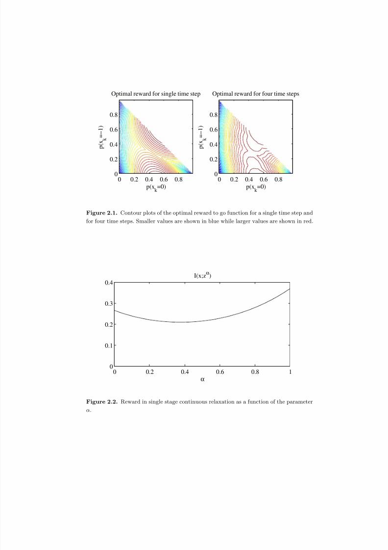
8/2/2019 Information Theoretic Sensor Management
http://slidepdf.com/reader/full/information-theoretic-sensor-management 49/203
p ( x k = − 1 )
p(x
k
=0)
Optimal reward for single time step
0 0.2 0.4 0.6 0.80
0.2
0.4
0.6
0.8
p ( x k = − 1 )
p(x
k
=0)
Optimal reward for four time steps
0 0.2 0.4 0.6 0.80
0.2
0.4
0.6
0.8
Figure 2.1. Contour plots of the optimal reward to go function for a single time step and
for four time steps. Smaller values are shown in blue while larger values are shown in red.
0 0.2 0.4 0.6 0.8 10
0.1
0.2
0.3
0.4
α
I(x;zα
)
Figure 2.2. Reward in single stage continuous relaxation as a function of the parameter
α.

8/2/2019 Information Theoretic Sensor Management
http://slidepdf.com/reader/full/information-theoretic-sensor-management 50/203
50 CHAPTER 2. BACKGROUND
Definition 2.2 (Nondecreasing). A set function f is non-decreasing if
f (B) ≥ f (A) ∀ B ⊇ A.
Obviously, a non-decreasing function will be nonnegative iff f (∅) ≥ 0. MI is an
example of a nonnegative, non-decreasing function, since I (x; ∅) = 0 and I (x; zB) −I (x; zA) = I (x; zB\A|zA) ≥ 0. Intuitively, this corresponds to the notion that includ-
ing more observations must increase the information (i.e., on average, the entropy is
reduced).
Definition 2.3 (Increment function). We denote the single element increment by
ρ j(A) f (A ∪ { j}) − f (A), and the set increment by ρB(A) f (A ∪ B) − f (A).
Applying the chain rule in reverse, the increment function for MI is equivalent to
ρB(A) = I (x; zB|zA).
2.4.2 Submodularity
Submodularity captures the notion that as we select more observations, the value of the
remaining unselected observations decreases, i.e., the notion of diminishing returns.
Definition 2.4 (Submodular). A set function f is submodular if f (C ∪ A) − f (A) ≥f (C ∪ B) − f (B) ∀ B ⊇ A.
From Definition 2.3, we note that ρC(A) ≥ ρC(B) ∀ B ⊇ A for any increment function
ρ arising from a submodular function f . The following lemma due to Krause andGuestrin [46] establishes conditions under which mutual information is a submodular
set function.
Lemma 2.1. If the observations are conditionally independent conditioned on the state,
then the mutual information between the state and the subset of observations selected is
submodular.
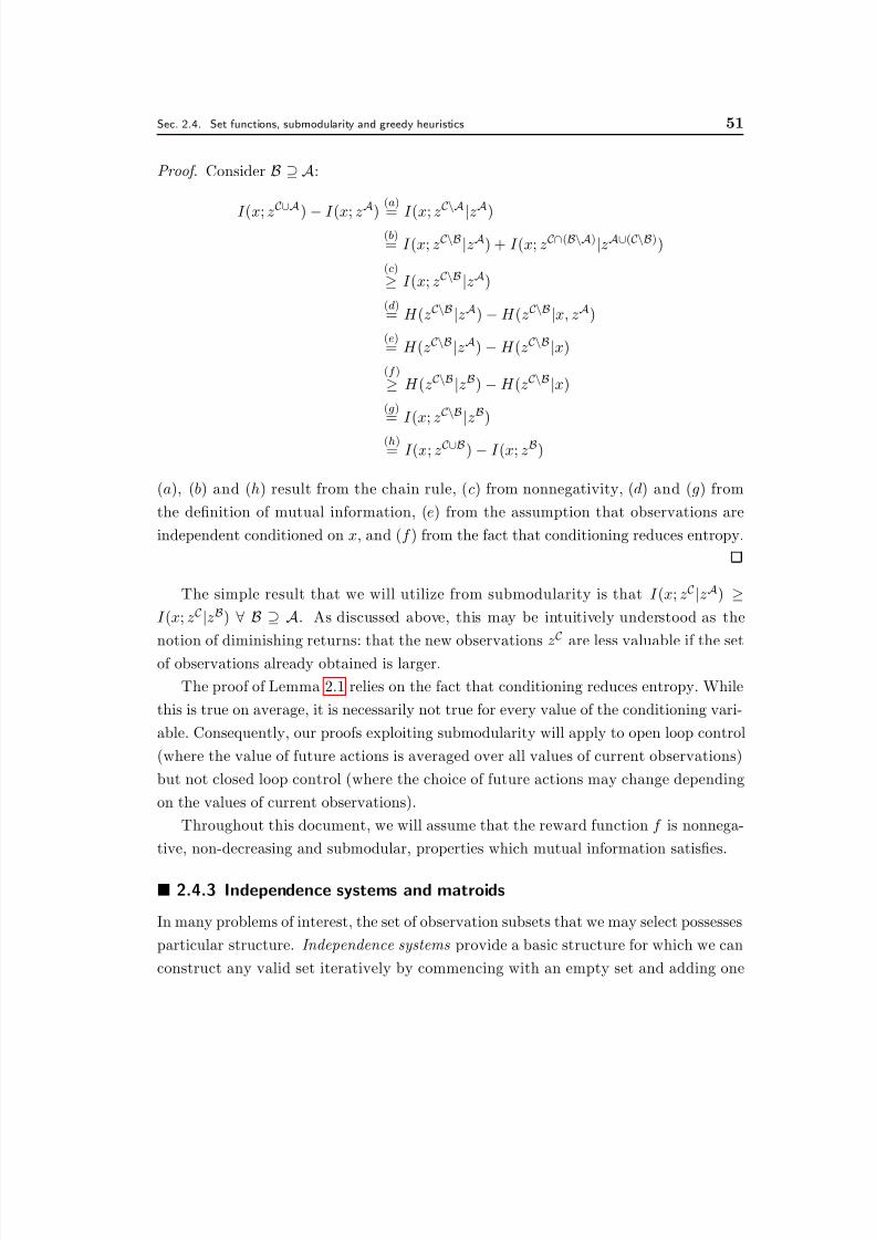
8/2/2019 Information Theoretic Sensor Management
http://slidepdf.com/reader/full/information-theoretic-sensor-management 51/203
Sec. 2.4. Set functions, submodularity and greedy heuristics 51
Proof. Consider B ⊇ A:
I (x; zC∪A
) − I (x; zA
)
(a)
= I (x; zC\A
|zA
)(b)= I (x; zC\B |zA) + I (x; zC∩(B\A)|zA∪(C\B))
(c)
≥ I (x; zC\B |zA)
(d)= H (zC\B |zA) − H (zC\B |x, zA)
(e)= H (zC\B |zA) − H (zC\B |x)
(f )
≥ H (zC\B |zB) − H (zC\B |x)
(g)= I (x; zC\B
|zB)
(h)= I (x; zC∪B) − I (x; zB)
(a), (b) and (h) result from the chain rule, (c) from nonnegativity, (d) and (g) from
the definition of mutual information, (e) from the assumption that observations are
independent conditioned on x, and (f ) from the fact that conditioning reduces entropy.
The simple result that we will utilize from submodularity is that I (x; zC |zA) ≥I (x; zC |zB) ∀ B ⊇ A. As discussed above, this may be intuitively understood as the
notion of diminishing returns: that the new observations zC are less valuable if the set
of observations already obtained is larger.
The proof of Lemma 2.1 relies on the fact that conditioning reduces entropy. While
this is true on average, it is necessarily not true for every value of the conditioning vari-
able. Consequently, our proofs exploiting submodularity will apply to open loop control
(where the value of future actions is averaged over all values of current observations)
but not closed loop control (where the choice of future actions may change depending
on the values of current observations).
Throughout this document, we will assume that the reward function f is nonnega-
tive, non-decreasing and submodular, properties which mutual information satisfies.
2.4.3 Independence systems and matroids
In many problems of interest, the set of observation subsets that we may select possesses
particular structure. Independence systems provide a basic structure for which we can
construct any valid set iteratively by commencing with an empty set and adding one
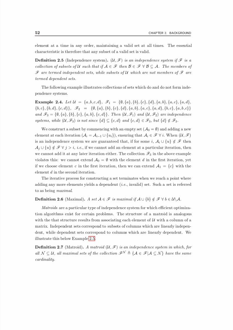
8/2/2019 Information Theoretic Sensor Management
http://slidepdf.com/reader/full/information-theoretic-sensor-management 52/203
52 CHAPTER 2. BACKGROUND
element at a time in any order, maintaining a valid set at all times. The essential
characteristic is therefore that any subset of a valid set is valid.
Definition 2.5 (Independence system). ( U ,F ) is an independence system if F is a
collection of subsets of U such that if A ∈ F then B ∈ F ∀ B ⊆ A. The members of
F are termed independent sets, while subsets of U which are not members of F are
termed dependent sets.
The following example illustrates collections of sets which do and do not form inde-
pendence systems.
Example 2.4. Let U = {a,b,c,d}, F 1 = {∅, {a}, {b}, {c}, {d}, {a, b}, {a, c}, {a, d},
{b, c}, {b, d}, {c, d}}, F 2 = {∅, {a}, {b}, {c}, {d}, {a, b}, {a, c}, {a, d}, {b, c}, {a,b,c}}
and F 3 = {∅, {a}, {b}, {c}, {a, b}, {c, d}}. Then ( U ,F 1) and ( U ,F 2) are independencesystems, while ( U ,F 3) is not since {d} ⊆ {c, d} and {c, d} ∈F 3, but {d} /∈ F 3.
We construct a subset by commencing with an empty set (A0 = ∅) and adding a new
element at each iteration (Ai = Ai−1 ∪ {ui}), ensuring that Ai ∈ F ∀ i. When ( U ,F )is an independence system we are guaranteed that, if for some i, Ai ∪ {u} /∈ F then
A j ∪ {u} /∈ F ∀ j > i, i.e., if we cannot add an element at a particular iteration, then
we cannot add it at any later iteration either. The collection F 3 in the above example
violates this: we cannot extend A0 = ∅ with the element d in the first iteration, yet
if we choose element c in the first iteration, then we can extend A1 = {c} with the
element d in the second iteration.The iterative process for constructing a set terminates when we reach a point where
adding any more elements yields a dependent (i.e., invalid) set. Such a set is referred
to as being maximal .
Definition 2.6 (Maximal). A set A ∈ F is maximal if A ∪ {b} /∈ F ∀ b ∈ U\A.
Matroids are a particular type of independence system for which efficient optimiza-
tion algorithms exist for certain problems. The structure of a matroid is analogous
with the that structure results from associating each element of U with a column of a
matrix. Independent sets correspond to subsets of columns which are linearly indepen-
dent, while dependent sets correspond to columns which are linearly dependent. We
illustrate this below Example 2.5.
Definition 2.7 (Matroid). A matroid ( U ,F ) is an independence system in which, for
all N ⊆ U , all maximal sets of the collection F N {A ∈ F |A ⊆ N} have the same
cardinality.
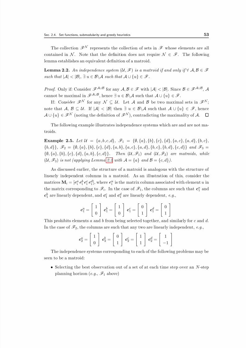
8/2/2019 Information Theoretic Sensor Management
http://slidepdf.com/reader/full/information-theoretic-sensor-management 53/203
Sec. 2.4. Set functions, submodularity and greedy heuristics 53
The collection F N represents the collection of sets in F whose elements are all
contained in N . Note that the definition does not require N ∈ F . The following
lemma establishes an equivalent definition of a matroid.
Lemma 2.2. An independence system ( U ,F ) is a matroid if and only if ∀ A, B ∈ F such that |A| < |B|, ∃ u ∈ B\A such that A ∪ {u} ∈ F .
Proof. Only if: Consider F A∪B for any A, B ∈F with |A| < |B|. Since B ∈F A∪B, Acannot be maximal in F A∪B, hence ∃ u ∈ B\A such that A ∪ {u} ∈F .
If: Consider F N for any N ⊆ U . Let A and B be two maximal sets in F N ;
note that A, B ⊆ U . If |A| < |B| then ∃ u ∈ B\A such that A ∪ {u} ∈ F , hence
A ∪ {u} ∈F N (noting the definition of F N ), contradicting the maximality of A.
The following example illustrates independence systems which are and are not ma-
troids.
Example 2.5. Let U = {a,b,c,d}, F 1 = {∅, {a}, {b}, {c}, {d}, {a, c}, {a, d}, {b, c},
{b, d}}, F 2 = {∅, {a}, {b}, {c}, {d}, {a, b}, {a, c}, {a, d}, {b, c}, {b, d}, {c, d}} and F 3 =
{∅, {a}, {b}, {c}, {d}, {a, b}, {c, d}}. Then ( U ,F 1) and ( U ,F 2) are matroids, while
( U ,F 3) is not (applying Lemma 2.2 with A = {a} and B = {c, d}).
As discussed earlier, the structure of a matroid is analogous with the structure of
linearly independent columns in a matroid. As an illustration of this, consider the
matrices Mi = [cai c
bi c
ci c
di ], where c
ui is the matrix column associated with element u in
the matrix corresponding to F i. In the case of F 1, the columns are such that ca1 and
cb1 are linearly dependent, and cc
1 and cd1 are linearly dependent, e.g.,
ca1 =
1
0
cb1 =
1
0
cc1 =
0
1
cd1 =
0
1
This prohibits elements a and b from being selected together, and similarly for c and d.
In the case of F 2, the columns are such that any two are linearly independent, e.g.,
ca2 = 1
0 cb
2 = 0
1 cc
2 = 1
1 cd
2 = 1
−1
The independence systems corresponding to each of the following problems may be
seen to be a matroid:
• Selecting the best observation out of a set of at each time step over an N -step
planning horizon (e.g., F 1 above)
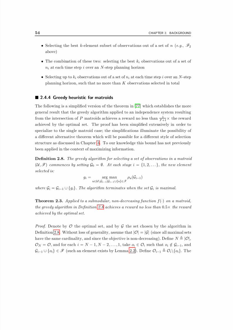
8/2/2019 Information Theoretic Sensor Management
http://slidepdf.com/reader/full/information-theoretic-sensor-management 54/203
54 CHAPTER 2. BACKGROUND
• Selecting the best k-element subset of observations out of a set of n (e.g., F 2
above)
• The combination of these two: selecting the best ki observations out of a set of
ni at each time step i over an N -step planning horizon
• Selecting up to ki observations out of a set of ni at each time step i over an N -step
planning horizon, such that no more than K observations selected in total
2.4.4 Greedy heuristic for matroids
The following is a simplified version of the theorem in [77] which establishes the more
general result that the greedy algorithm applied to an independence system resulting
from the intersection of P matroids achieves a reward no less than 1P +1× the reward
achieved by the optimal set. The proof has been simplified extensively in order to
specialize to the single matroid case; the simplifications illuminate the possibility of
a different alternative theorem which will be possible for a different style of selection
structure as discussed in Chapter 3. To our knowledge this bound has not previously
been applied in the context of maximizing information.
Definition 2.8. The greedy algorithm for selecting a set of observations in a matroid
( U ,F ) commences by setting G0 = ∅. At each stage i = {1, 2, . . . }, the new element
selected is:
gi = arg maxu∈U\Gi−1|Gi−1∪{u}∈F
ρu(Gi−1)
where Gi = Gi−1 ∪ {gi}. The algorithm terminates when the set Gi is maximal.
Theorem 2.3. Applied to a submodular, non-decreasing function f (·) on a matroid,
the greedy algorithm in Definition 2.8 achieves a reward no less than 0.5× the reward
achieved by the optimal set.
Proof. Denote by
Othe optimal set, and by
Gthe set chosen by the algorithm in
Definition 2.8. Without loss of generality, assume that |O| = |G| (since all maximal sets
have the same cardinality, and since the objective is non-decreasing). Define N |O|,ON = O, and for each i = N − 1, N − 2, . . . , 1, take oi ∈ Oi such that oi /∈ Gi−1, and
Gi−1 ∪ {oi} ∈F (such an element exists by Lemma 2.2). Define Oi−1 Oi\{oi}. The

8/2/2019 Information Theoretic Sensor Management
http://slidepdf.com/reader/full/information-theoretic-sensor-management 55/203
Sec. 2.4. Set functions, submodularity and greedy heuristics 55
bound can be obtained through the following steps:
f (O) − f (∅)
(a)
≤ f (G ∪O) − f (∅)(b)
≤ f (G) +
j∈O\G
ρ j(G) − f (∅)
(c)
≤ f (G) + j∈O
ρ j(G) − f (∅)
(d)= f (G) +
N i=1
ρoi(G) − f (∅)
(e)
≤f (
G) +
N
i=1
ρoi(
Gi−1)
−f (
∅)
(f )
≤ f (G) +N
i=1
ρgi(Gi−1) − f (∅)
(g)= 2(f (G) − f (∅))
where (a) and (c) result from the non-decreasing property, (b) a n d (e) result
from submodularity, (d) is a simple rearrangement using the above construction
O = {o1, . . . , oN }, (f ) is a consequence of the structure of the greedy algorithm in
Definition 2.8, and (g) is a simple rearrangement of (f ).
2.4.5 Greedy heuristic for arbitrary subsets
The following theorem specializes the previous theorem to the case in which F consists
of all K -element subsets of observations, as opposed to an arbitrary matroid. In this
case, the bound obtainable is tighter. The theorem comes from [76], which addresses
the more general case of a possibly decreasing reward function. Krause and Guestrin
[46] first recognized that the bound can be applied to sensor selection problems with
information theoretic objectives.
Theorem 2.4. Suppose that F = {N ⊆ U s.t. |N| ≤ K }. Then the greedy algorithm applied to the non-decreasing submodular function f (·) on the independence system
( U ,F ) achieves a reward no less than (1 − 1/e) ≈ 0.632× the reward achieved by the
optimal set.
8/2/2019 Information Theoretic Sensor Management
http://slidepdf.com/reader/full/information-theoretic-sensor-management 56/203
56 CHAPTER 2. BACKGROUND
Proof. Denote by O the optimal K -element subset, and by G the set chosen by the
algorithm in Definition 2.8. For each stage of the greedy algorithm, i ∈ {1, . . . , K }, we
can write from line (b) of the proof of Theorem 2.3:
f (O) ≤ f (Gi) +
j∈O\Gi
ρ j(Gi)
By definition of gi+1 in Definition 2.8, ρgi+1(Gi) ≥ ρ j(Gi) ∀ j, hence
f (O) ≤ f (Gi) +
j∈O\Gi
ρgi+1(Gi)
= f (Gi) + |O\Gi|ρgi+1(Gi)
≤ f (Gi) + Kρgi+1(Gi)
By definition of the increment function ρ, we can write
f (Gi) = f (∅) +i
j=1
ρgj(G j−1)
where we use the convention that G0 = ∅. Thus we can write ∀ i ∈ {1, . . . , K }:
f (O) − f (∅) ≤i
j=1
ρgj (G j−1) + Kρgi+1(Gi) (2.92)
Now consider the linear program in variables ρ1, . . . , ρK +1, parameterized by Z :
P (Z ) =minK
j=1
ρ j (2.93)
s.t. Z ≤i
j=1
ρ j + Kρi+1, i ∈ {1, . . . , K }
Taking the dual of the linear program:
D(Z ) =maxK
j=1
Zx j
s.t. Kxi +
K j=i+1
x j = 1, i ∈ {1, . . . , K }The system of constraints has a single solution which can found through a backward
recursion commencing with xK :
xK =1
K , xK −1 =
K − 1
K 2, . . . , x1 =
(K − 1)K −1
K K

8/2/2019 Information Theoretic Sensor Management
http://slidepdf.com/reader/full/information-theoretic-sensor-management 57/203
Sec. 2.5. Linear and integer programming 57
which yields
D(Z ) = Z 1 −K − 1
K
K
which, by strong duality, is also the solution to P (Z ). Thus, any set O which respects
the series of inequalities in Eq. (2.92) must have
K j=1
ρgj (G j−1) = f (G) − f (∅) ≥
1 −
K − 1
K
K
[f (O) − f (∅)]
Finally, note that
1 − K − 1
K K
> 1 − 1/e ∀ K > 1; 1 −K − 1
K K
→ 1 − 1/e, K → ∞
Thus
f (G) − f (∅) ≥ [1 − 1/e][f (O) − f (∅)] ≥ 0.632[f (O) − f (∅)]
2.5 Linear and integer programming
Chapter 4 will utilize an integer programming formulation to solve certain sensor re-
source management problems with manageable complexity. This section briefly outlines
the idea behind linear and integer programming; the primary source for the material is
[12].
2.5.1 Linear programming
Linear programming is concerned with solving problems of the form:
minx
cT x
s.t. Ax ≥ b(2.94)
Any problem of the form Eq. (2.94) can be converted to the standard form:
minx
cT x
s.t. Ax = b
x ≥ 0
(2.95)

8/2/2019 Information Theoretic Sensor Management
http://slidepdf.com/reader/full/information-theoretic-sensor-management 58/203
58 CHAPTER 2. BACKGROUND
The two primary mechanisms for solving problems of this type are simplex methods
and interior point methods. Primal-dual methods simultaneously manipulate both the
original problem (referred to as the primal problem), and a dual problem which providesa lower bound on the optimal objective value achievable. The difference between the
current primal solution and the dual solution is referred to as the duality gap; this
provides an upper bound on the improvement possible through further optimization.
Interior point methods have been observed to be able to reduce the duality gap by a
factor γ in a problem of size n in an average number of iterations of O(log n log γ ); the
worst-case behavior is O(√
n log γ ).
2.5.2 Column generation and constraint generation
In many large scale problems, it is desirable to be able to find a solution withoutexplicitly considering all of the optimization variables. Column generation is a method
which is used alongside the revised simplex method to achieve this goal. The method
involves the iterative solution of a problem involving a small subset of the variables in
the full problem. We assume availability of an efficient algorithm that tests whether
incorporation of additional variables would be able to improve on the present solution.
Occasionally this algorithm is executed, producing additional variables to be added to
the subset. The process terminates when the problem involving the current subset of
variables reaches an optimal solution and the algorithm producing new variables finds
that there are no more variables able to produce further improvement.
Constraint generation is commonly used to solve large scale problems without ex-
plicitly considering all of the constraints. The method involves iterative solution of a
problem involving the a small subset of the constraints in the full problem. We assume
availability of an efficient algorithm that tests whether the current solution violates
any of the constraints in the full problem, and returns one or more violated constraints
if any exist. The method proceeds by optimizing the problem involving the subset of
constraints, occasionally executing the algorithm to produce additional constraints that
were previously violated. The process terminates when we find an optimal solution to
the subproblem which does not violate any constraints in the full problem. Constraint
generation may be interpreted as column generation applied to the dual problem.

8/2/2019 Information Theoretic Sensor Management
http://slidepdf.com/reader/full/information-theoretic-sensor-management 59/203
Sec. 2.5. Linear and integer programming 59
2.5.3 Integer programming
Integer programming deals with problems similar to Eqs. (2.94) and (2.95), but in which
the optimization variables are constrained to take on integer values:
minx
cT x
s.t. Ax = b
x ≥ 0
x integer
(2.96)
Some problem structures possess a property in which, when the integer constraint is
relaxed, there remains an integer point that attains the optimal objective. A common
example is network flow problems in which the problem data takes on integer values.In this case, solution of the linear program (with the integrality constraint relaxed)
can provide the optimal solution to the integer program. In general the addition of
the integer constraint dramatically increases the computational complexity of finding a
solution.
Relaxations
Two different relaxations are commonly used in integer programming: the linear pro-
gramming relaxation, and the Lagrangian relaxation. The linear programming relax-
ation is exactly that described in the previous section: solving the linear program which
results from relaxing the integrality constraint. If the problem possesses the necessary
structure that there is an integer point that attains the optimal objective in the relaxed
problem, then this point is also optimal in the original integer programming problem.
In general this will not be the case, however the solution of the linear programming
relaxation provides a lower bound to the solution of the integer program (since a wider
range of solutions is considered).
As described in Section 2.2.3, Lagrangian relaxation involves solution of the La-
grangian dual problem. By weak duality, the dual problem also provides a lower bound
on the optimal cost attainable in the integer program. However, since the primal prob-
lem involves a discrete optimization strong duality does not hold, and there may be
a duality gap (i.e., in general there will not be an integer programming solution that
obtains the same cost as the solution of the Lagrangian dual). It can be shown that
the Lagrangian relaxation provides a tighter lower bound than the linear programming
relaxation.

8/2/2019 Information Theoretic Sensor Management
http://slidepdf.com/reader/full/information-theoretic-sensor-management 60/203
60 CHAPTER 2. BACKGROUND
Cutting plane methods
Let
X be the set of feasible solutions to the integer program in Eq. (2.96) (i.e., the
integer points which satisfy the various constraints), and let CH (X ) be the convex hull
of these points. Then the optimal solution of Eq. (2.96) is also an optimal solution of
the following linear program:
minx
cT x
s.t. x ∈ CH (X )(2.97)
Cutting plane methods, one of the two most common methods for solving integer pro-
grams, exploit this fact. We solve a series of linear programs, commencing with the
linear programming relaxation. If, at any stage, we find an integer solution that is op-
timal, this is the optimal solution to the original problem. At each iteration, we add a
constraint that is violated by the solution of the linear program in the current iteration,
but is satisfied by every integer solution in the the original problem ( i.e., every point in
X ). Thus the feasible region is slowly reduced, and approaches CH (X ). There are two
difficulties associated with this method: firstly, it can be difficult to find constraints
with the necessary characteristics; and secondly, it may be necessary to generate a very
large number of constraints in order to obtain the integer solution.
Branch and bound
Branch and bound is the other commonly used method for solving integer programming
problems. The basic concept is to divide the feasible region into sub-regions, and
simultaneously search for “good” feasible solutions and tight lower bounds within in
each sub-region. Any time we find that a sub-region R has a lower bound that is greater
than a feasible solution found in another sub-region, the region R can be discarded. For
example, suppose that we are dealing with a binary problem, where the feasible set is
X = {0, 1}N . Suppose we branch on variable x1, i.e., we divide the feasible region up
into two sub-regions, where in the first we fix x1 = 0, and in the second we fix x1 = 1.
Suppose we find a feasible solution within the sub-region in which x1 = 1 with objective
3.5, and, furthermore we find that the objective of the sub-problem in which we fix thevalue x1 = 0 is bounded below by 4.5. Then the optimal solution cannot have x1 = 0,
so this sub-region may be discarded without further investigation. Linear programming
relaxations and cutting plane methods are commonly used in concert with a branch
and bound approach to provide the lower bounds.
8/2/2019 Information Theoretic Sensor Management
http://slidepdf.com/reader/full/information-theoretic-sensor-management 61/203
Sec. 2.6. Related work 61
2.6 Related work
The attention received by sensor resource management has steadily increased over the
past two decades. The sections below summarize a number of strategies proposed by
different authors. We coarsely categorize the material, although many of the methods
do not fit precisely into any one category. We conclude in Section 2.6.7 by contrasting
our approach to the work described.
2.6.1 POMDP and POMDP-like models
In [55, 56,57], Krishnamurthy and Evans present two sensor management methods
based upon POMDP methods. In [56,57], the beam scheduling problem is cast as
a multi-arm bandit, assuming that the conditional PDF of unobserved objects remains
unchanged between decision intervals (this is slightly less restrictive than requiring the
state itself to remain unchanged). Under these assumptions, it is proven that there
exists an optimal policy in the form of index rule, and that the index function is piece-
wise linear concave. In [55], Krishnamurthy proposes a similar method for waveform
selection problems in which the per stage reward is approximated by a piecewise linear
concave function of the conditional PDF. In this regime, the reward to go function
remains piecewise linear concave at each time in the backward recursion and POMDP
methods can be applied. In [56], it is suggested that the continuous kinematic quantities
could be discretized into coarse quantities such as “near” and “far”. A similar method
is proposed for adaptive target detection in [60]. Computational examples in [55, 59]utilize underlying state space alphabets of three, six and 25. This reveals the primary
limitation of this category of work: its inability to address problems with large state
spaces. Many problems of practical interest cannot be represented with this restriction.
Castanon [18] formulates the problem of beam scheduling and waveform selection
for identification of a large number of objects as a constrained dynamic program. By
relaxing the sample path constraints to being constraints in expectation, a dual solution,
which decouples the problem into a series of single object problems coupled only through
the search for the correct values of the Lagrange multipliers, can be found using a
method similar to that discussed in Section 2.2.3. By requiring observations at different
times in the planning horizon to have identical characteristics, observations needing
different time durations to complete are naturally addressed. The method is extended
in [16] to produce a lower bound on the classification error performance in a sensor
network. Again, the primary limitation of this method is the requirement for the state
space to be small enough that traditional POMDP solution methods should be able to
8/2/2019 Information Theoretic Sensor Management
http://slidepdf.com/reader/full/information-theoretic-sensor-management 62/203
62 CHAPTER 2. BACKGROUND
address the decoupled single object problem. In the context of ob ject identification,
this state space alphabet size restriction precludes addition of latent states such as
object features (observations will often be dependent conditioned on the object class,but the object state can be expanded to incorporate continuous object features in order
to regain the required conditional independence).
2.6.2 Model simplifications
Washburn, et al [93] observe that, after a minor transformation of the cost function,
the solution method from multi-arm bandit problems method may be applied to beam
steering, assuming that the state of unobserved objects remains unchanged. The policy
based on this assumption is then used as a base policy in a roll-out with a one or two
step look-ahead. The authors also suggest methods for practical application such asselecting as the decision state an estimate of the covariance matrix rather than condi-
tional PDF, and simplifying stochastic disturbance to simple models such as detection
and no detection. The ideas are explored further in [85].
2.6.3 Suboptimal control
Common suboptimal control methods such as roll-out [9] have also been applied to
sensor management problems. Nedich, et al [74] consider tracking move-stop targets,
and utilize an approximation of the cost to go of a heuristic base policy which captures
the structure of the future reward for the given scenario. He and Chong [29] describe
how a simulation-based roll-out method with an unspecified base policy could be used
in combination with particle filtering.
2.6.4 Greedy heuristics and extensions
Many authors have approached the problem of waveform selection and beam steering
using greedy heuristics which choose at each time the action which maximizes some
instantaneous reward function. Information theoretic ob jectives are commonly used
with this method; this may be expressed equivalently as
• Minimizing the conditional entropy of the state at the current time conditionedon the new observation (and on the values of the previous observations)
• Maximizing the mutual information between the state at the current time and
the new observation
8/2/2019 Information Theoretic Sensor Management
http://slidepdf.com/reader/full/information-theoretic-sensor-management 63/203
Sec. 2.6. Related work 63
• Maximizing the Kullback-Leibler distance between the prior and posterior distri-
bution.
• Minimizing the Kullback-Leibler distance between the posterior distribution and
the posterior distribution that would be obtained if all possible observations were
incorporated.
Use of these objectives in classification problems can be traced back as early as [ 61].
Hintz [32] and Kastella [41] appear to be two of the earliest instances in sensor fusion
literature. Formally, if gk(Xk, uk) is the reward for applying control uk at time k, then
the greedy heuristic operates according to the following rule:
µgk(Xk) = arg max
uk∈U Xkk
gk(Xk, uk) (2.98)
McIntyre and Hintz [69] apply the greedy heuristic, choosing mutual information as
the objective in each stage to trade off the competing tasks of searching for new objects
and maintaining existing tracks. The framework is extended to consider higher level
goals in [31]. Kershaw and Evans [42] propose a method of adaptive waveform selection
for radar/sonar applications. An analysis of the signal ambiguity function provides
a prediction of the of the posterior covariance matrix. The use of a greedy heuristic
is justified by a restriction to constant energy pulses. Optimization criteria include
posterior mean square error and validation gate volume. The method is extended to
consider the impact of clutter through Probabilistic Data Association (PDA) filter in[43].
Mahler [66] discusses the use of a generalization of Kullback-Leibler distance, global
Csiszar c-discrimination, for sensor resource management within the finite set statistics
framework, i.e., where the number of objects is unknown and the PDF is invariant
to any permutation of the objects. Kreucher, et al [49,50,51, 52, 54] apply a greedy
heuristic to the sensor management problem in which the joint PDF of a varying number
of objects is maintained using a particle filter. The objective function used is Renyi
entropy; motivations for using this criterion are discussed in [50, 51]. Extensions to
a two-step look-ahead using additional simulation, and a roll-out approach using a
heuristic reward to go capturing the structure of long-term reward due to expected
visibility and obscuration of objects are proposed in [53].
Kolba, et al [44] apply the greedy heuristic with an information objective to land-
mine detection, addressing the additional complexity which occurs when sensor motion
is constrained. Singh, et al [86] show how the control variates method can be used to
8/2/2019 Information Theoretic Sensor Management
http://slidepdf.com/reader/full/information-theoretic-sensor-management 64/203
64 CHAPTER 2. BACKGROUND
reduce the variance of estimates of Kullback-Leibler divergence (equivalent to mutual
information) for use in sensor management; their experiments use a greedy heuristic.
Kalandros and Pao [40] propose a method which allows for control of process co-variance matrices, e.g., ensuring that the covariance matrix of a process P meets a
specification S in the sense that P − S 0. This objective allows the system designer
to dictate a more specific performance requirement. The solution method uses a greedy
heuristic.
Zhao, et al [95] discuss object tracking in sensor networks, proposing methods based
on greedy heuristics where the estimation objectives include nearest neighbor, Maha-
lanobis distance, entropy and Kullback-Leibler distance; inconsistencies with the mea-
sures proposed in this paper are discussed in [25].
Chhetri, et al [21] examine scheduling of radar and IR sensors for object tracking
to minimize the mean square error over the next N time steps. The method proposed
utilizes a linearized Kalman filter for evaluation of the error predictions, and performs a
brute-force enumeration of all sequences within the planning horizon. Experiments are
performed using planning horizons of one, two and three. In [20], the sensor network
object tracking problem is approached by minimizing energy consumption subject to
a constraint on estimation performance (measured using Cramer-Rao bounds). The
method constructs an open loop plan by considering each candidate solution in ascend-
ing order of cost, and evaluating the estimation performance until a feasible solution
is found (i.e., one which meets the estimation criterion). Computational examples use
planning horizons of one, two and three.
Logothetis and Isaksson [65] provide an algorithm for pruning the search tree in the
problems involving control of linear Gauss-Markov systems with information theoretic
criteria. If two candidate sequences obtain covariance matrices P1 and P2, and P1 P2, then the total reward of any extension of the first sequence will be less than or
equal to the total reward of the same extension of the second sequence, thus the first
sequence can be pruned from the search tree. Computational examples demonstrate a
reduction of the tree width by a factor of around five.
Zwaga and Driessen examine the problem of selecting revisit rate and dwell time for a
multifunction radar to minimize the total duty cycle consumed subject to a constraint onthe post-update covariance [97] and prediction covariance [96]. Both methods consider
only the current observation interval.
8/2/2019 Information Theoretic Sensor Management
http://slidepdf.com/reader/full/information-theoretic-sensor-management 65/203
Sec. 2.6. Related work 65
2.6.5 Existing work on performance guarantees
Despite the popularity of the greedy heuristic, little work has been done to find guar-
antees of performance. In [17], Castanon shows that a greedy heuristic is optimal for
the problem of dynamic hypothesis testing (e.g., searching for an object among a finite
set of positions) with symmetric measurement distributions (i.e., P [missed detection] =
P [false alarm]) according to the minimum probability of error criterion. In [33], Howard,
et al prove optimality of greedy methods for the problem of beam scheduling of inde-
pendent one-dimensional Gauss-Markov processes when the cost per stage is set to the
sum of the error variances. The method does not extend to multi-dimensional processes.
Krause and Guestrin [46] apply results from submodular optimization theory to
establish the surprising and elegant result that the greedy heuristic applied to the sensor
subset selection algorithm (choosing the best n-element subset) is guaranteed to achieveperformance within a multiple of (1 − 1/e) of optimality (with mutual information as
the objective), as discussed in Section 2.4.5. A similar performance guarantee is also
established in [46] for the budgeted case, in which each observation incurs a cost, and
there is a maximum total cost that can be expended. For this latter bound to apply, it
is necessary to perform a greedy selection commencing from every three-element subset.
The paper also establishes a theoretical guarantee that no polynomial time algorithm
can improve on the performance bound unless P = NP , and discusses issues which arise
when the reward to go values are computed approximately. This analysis is applied to
the selection of sensor placements in [47], and the sensor placement model is extended
to incorporate communication cost in [48].
2.6.6 Other relevant work
Berry and Fogg [8] discuss the merits of entropy as a criterion for radar control, and
demonstrate its application to sample problems. The suggested solutions include min-
imizing the resources necessary to satisfy a constraint on entropy, and selecting which
targets to observe in a planning horizon in order to minimize entropy. No clear guid-
ance is given on efficient implementation of the optimization problem resulting from
either case. Moran, et al [70] discuss sensor management for radar, incorporating both
selection of which waveform from a library to transmit at any given time, and how to
design the waveform library a priori .
Hernandez, et al [30] utilize the posterior Cramer-Rao bound as a criterion for
iterative deployment and utilization of sonar sensor resources for submarine tracking.
8/2/2019 Information Theoretic Sensor Management
http://slidepdf.com/reader/full/information-theoretic-sensor-management 66/203
66 CHAPTER 2. BACKGROUND
Sensor positions are determined using a greedy6 simulated annealing search, where the
objective is the estimation error at a particular time instant in the future. Selection
of the subset of sensors to activate during tracking is performed either using brute-force enumeration or a genetic algorithm; the subset remains fixed in between sensor
deployments.
The problem of selecting the subset of sensors to activate in a single time slot to
minimize energy consumption subject to a mean square error estimation performance
constraint is considered in [22]. An integer programming formulation using branch and
bound techniques enables optimal solution of problems involving 50–70 sensors in tens
of milliseconds. The branch and bound method used exploits quadratic structure that
results when the performance criterion is based on two states (i.e., position in two
dimensions).
2.6.7 Contrast to our contributions
As outlined in Section 2.6.4, many authors have applied greedy heuristics and short-
time extensions (e.g., using open loop plans over two or three time steps) to sensor
management problems using criteria such as mutual information, mean square error
and the posterior Cramer-Rao bound. Thus it is surprising that little work has been
done toward obtaining performance guarantees for these methods. As discussed in Sec-
tion 2.6.5, [46] is the first generally applicable performance guarantee to a problem
with structure resembling the type which results to sensor management. However, this
result is not directly applicable to sensor management problems involving sequential
estimation (e.g., object tracking), where there is typically a set of observations corre-
sponding to each time slot, the elements of which correspond to the modes in which we
may operate the sensor in that time slot, rather than a single set of observations. The
typical constraint structure is one which permits selection of one element (or a small
number of elements) from each of these sets, rather than a total of n elements from a
larger subset.
The analysis in Chapter 3 extends the performance guarantees of [46] to problems
involving this structure, providing the surprising result that a similar guarantee applies
to the greedy heuristic applied in a sequential fashion, even though future observa-tion opportunities are ignored. The result is applicable to a large class of time-varying
models. Several extensions are obtained, including tighter bounds that exploit either
6The search is greedy in that proposed locations are accepted with probability 1 if the objective is
improved and probability 0 otherwise.

8/2/2019 Information Theoretic Sensor Management
http://slidepdf.com/reader/full/information-theoretic-sensor-management 67/203
Sec. 2.6. Related work 67
process diffusiveness or objectives involving discount factors, and applicability to closed
loop problems. We also show that several of the results may be applied to the posterior
Cramer-Rao bound. Examples demonstrate that the bounds are tight, and counterex-amples illuminate larger classes of problems to which they do not apply.
Many of the existing works that provide non-myopic sensor management either rely
on very specific problem structure, and hence they are not generally applicable, or they
do not allow extensions to planning horizons past two or three time slots due to the
computational complexity. The development in Chapter 4 provides an integer pro-
gramming approach that exploits submodularity to find optimal or near-optimal open
loop plans for problems involving multiple objects over much longer planning horizons;
experiments utilize up to 60 time slots. The method can be applied to any submod-
ular, nondecreasing objective function, and does not require any specific structure in
dynamics or observation models.
Finally, Chapter 5 approaches the problem of sensor management in sensor networks
using a constrained dynamic programming formulation. The trade off between esti-
mation performance and communication cost is formulated by maximizing estimation
performance subject to a constraint on energy cost, or the dual of this, i.e., minimizing
energy cost subject to a constraint on estimation performance. Heuristic approxima-
tions that exploit the problem structure of tracking a single object using a network
of sensors again enable planning over dramatically increased horizons. The method is
both computable and scalable, yet still captures the essential structure of the underlying
trade off. Simulation results demonstrate a significant reduction in the communication
cost required to achieve a given estimation performance level as compared to previously
proposed algorithms.

8/2/2019 Information Theoretic Sensor Management
http://slidepdf.com/reader/full/information-theoretic-sensor-management 68/203
68 CHAPTER 2. BACKGROUND
8/2/2019 Information Theoretic Sensor Management
http://slidepdf.com/reader/full/information-theoretic-sensor-management 69/203
Chapter 3
Greedy heuristics and
performance guarantees
THE performance guarantees presented in Section 2.4 apply to algorithms with aparticular selection structure: firstly, where one can select any set within a ma-
troid, and secondly where one can select any arbitrary subset of a given cardinality.
This section develops a bound which is closely related to the matroid selection case,
except that we apply additional structure, in which we have N subsets of observations
and from each we can select a subset of a given cardinality. This structure is natu-
rally applicable to dynamic models, where each subset of observations corresponds to
a different time stage of the problem, e.g., we can select one observation at each time
stage. Our selection algorithm allows us to select at each time the observation which
maximizes the reward at that time, ignorant of the remainder of the time horizon. The
analysis establishes that the same performance guarantee that applies to the matroid
selection problem also applies to this problem.
We commence the chapter by deriving the simplest form of the performance guar-
antee, with both online and offline variants, in Section 3.1. Section 3.2 examines a
potentially tighter guarantee which exists for processes exhibiting diffusive characteris-
tics, while Section 3.3 presents a similar guarantee for problems involving a discounted
objective. Section 3.5 then extends the results of Sections 3.1–3.3 to closed loop policies.
While the results in Sections 3.1–3.5 are presented in terms of mutual information,
they are applicable to a wider class of objectives. Sections 3.1 and 3.3 apply to any
submodular, non-decreasing objective for which the reward of an empty set is zero
(similar to the requirements for the results in Sections 2.4.4 and 2.4.5). The additional
requirements in Sections 3.2 and 3.5 are discussed as the results are presented. In
Section 3.6, we demonstrate that the log of the determinant of the Fisher information
matrix is also submodular and non-decreasing, and thus that the various guarantees of
69

8/2/2019 Information Theoretic Sensor Management
http://slidepdf.com/reader/full/information-theoretic-sensor-management 70/203
70 CHAPTER 3. GREEDY HEURISTICS AND PERFORMANCE GUARANTEES
Sections 2.4.4, 2.4.5, 3.1 and 3.3 can also be applied to the determinant of the covariance
through the Cramer-Rao bound.
Section 3.8 presents examples of some slightly different problem structures which donot fit into the structure examined in Section 3.1 and Section 3.2, but are still able to
be addressed by the prior work discussed in Section 2.4.4. Finally, Section 3.9 presents
a negative result regarding a particular extension of the greedy heuristic to platform
steering problems.
3.1 A simple performance guarantee
To commence, consider a simple sequential estimation problem involving two time steps,
where at each step we must choose a single observation (e.g., in which mode to operate
a sensor) from a different set of observations. The goal is to maximize the informationobtained about an underlying quantity X . Let {o1, o2} denote the optimal choice for
the two stages, which maximizes I (X ; zo11 , zo2
2 ). Let {g1, g2} denote the choice made
by the greedy heuristic, where g1 is chosen to maximize I (X ; zg11 ) and g2 is chosen
to maximize I (X ; zg22 |zg1
1 ) (where conditioning is on the random variable zg11 , not on
the resulting observation value). Then the following analysis establishes a performance
guarantee for the greedy algorithm:
I (X ; zo11 , zo2
2 )(a)
≤ I (X ; zg11 , zg2
2 , zo11 , zo2
2 )
(b)
= I (X ; zg1
1 ) + I (X ; zg2
2 |zg1
1 ) + I (X ; zo11 |z
g1
1 , zg2
2 ) + I (x; zo22 |z
g1
1 , zg2
2 , zo11 )
(c)
≤ I (X ; zg11 ) + I (X ; zg2
2 |zg11 ) + I (X ; zo1
1 ) + I (x; zo22 |zg1
1 )
(d)
≤ 2I (X ; zg11 ) + 2I (X ; zg2
2 |zg11 )
(e)= 2I (X ; zg1
1 , zg22 )
where (a) results from the non-decreasing property of MI, (b) is an application of the
MI chain rule, (c) results from submodularity (assuming that all observations are inde-
pendent conditioned on X ), (d) from the definition of the greedy heuristic, and (e) from
a reverse application of the chain rule. Thus the optimal performance can be no more
than twice that of the greedy heuristic, or, conversely, the performance of the greedy
heuristic is at least half that of the optimal.1
Theorem 3.1 presents this result in its most general form; the proof directly follows
the above steps. The following assumption establishes the basic structure: we have N
1Note that this is considering only open loop control; we will discuss closed loop control in Section 3.5.

8/2/2019 Information Theoretic Sensor Management
http://slidepdf.com/reader/full/information-theoretic-sensor-management 71/203
Sec. 3.1. A simple performance guarantee 71
sets of observations, and we can select a specified number of observations from each set
in an arbitrary order.
Assumption 3.1. There are N sets of observations, {{z11, . . . , zn11 }, {z12, . . . , zn2
2 }, . . . ,
{z1N , . . . , znN N }}, which are mutually independent conditioned on the quantity to be esti-
mated ( X ). Any ki observations can be chosen out of the i-th set ( {z1i , . . . , znii }). The
sequence (w1, . . . , wM ) (where wi ∈ {1, . . . , N } ∀ i) specifies the order in which we visit
observation sets using the greedy heuristic (i.e., in the i-th stage we select a previously
unselected observation out of the wi-th set).
Obviously we require |{ j ∈ {1, . . . , M }|w j = i}| = ki ∀ i (i.e., we visit the i-th set
of observations ki times, selecting a single additional observation at each time), thus
N
i=1 ki = M . The abstraction of the observation set sequence (w1, . . . , wM ) allows usto visit observation sets more than once (allowing us to select multiple observations
from each set) and in any order. The greedy heuristic operating on this structure is
defined below.
Definition 3.1. The greedy heuristic operates according to the following rule:
g j = arg maxu∈{1,...,nwj }
I (X ; zuwj
|zg1w1
, . . . , zgj−1wj−1)
We assume without loss of generality that the same observation is not selected twice
since the reward for selecting an observation that was already selected is zero. We are
now ready to state the general form of the performance guarantee.
Theorem 3.1. Under Assumption 3.1, the greedy heuristic in Definition 3.1 has per-
formance guaranteed by the following expression:
I (X ; zo1w1
, . . . , zoM wM
) ≤ 2I (X ; zg1w1
, . . . , zgM wM
)
where {zo1w1
, . . . , zoM wM
} is the optimal set of observations, i.e., the one which maximizes
I (X ; zo1w1
, . . . , zoM wM
).

8/2/2019 Information Theoretic Sensor Management
http://slidepdf.com/reader/full/information-theoretic-sensor-management 72/203
72 CHAPTER 3. GREEDY HEURISTICS AND PERFORMANCE GUARANTEES
Proof. The performance guarantee is obtained through the following steps:
I (X ;zo1
w1
, . . . , zoM
wM
)
(a)
≤ I (X ; zg1w1
, . . . , zgM wM
, zo1w1
, . . . , zoM wM
)
(b)=
M j=1
I (X ; z
gjwj |zg1
w1, . . . , z
gj−1wj−1) + I (X ; z
ojwj |zg1
w1, . . . , zgM
wM , zo1
w1, . . . , z
oj−1wj−1)
(c)
≤M
j=1
I (X ; z
gjwj |zg1
w1, . . . , z
gj−1wj−1) + I (X ; z
ojwj |zg1
w1, . . . , z
gj−1wj )
(d)
≤ 2M
j=1
I (X ; zgjwj |zg1
w1, . . . , z
gj−1wj−1)
(e)= 2I (X ; zg1
w1, . . . , zgM
wM )
where (a) is due to the non-decreasing property of MI, (b) is an application of the
MI chain rule, (c) results from submodularity, (d) from Definition 3.1, and (e) from a
reverse application of the chain rule.
3.1.1 Comparison to matroid guarantee
The prior work using matroids (discussed in Section 2.4.3) provides another algorithm
with the same guarantee for problems of this structure. However, to achieve the guar-
antee on matroids it is necessary to consider every observation at every stage of the
problem. Computationally, it is far more desirable to be able to proceed in a dynamic
system by selecting observations at time k considering only the observations available
at that time, disregarding future time steps (indeed, all of the previous works described
in Section 2.6.4 do just that). The freedom of choice of the order in which we visit
observation sets in Theorem 3.1 extends the performance guarantee to this commonly
used selection structure.
3.1.2 Tightness of bound
The bound derived in Theorem 3.1 can be arbitrarily close to tight, as the followingexample shows.
Example 3.1. Consider a problem with X = [a, b]T where a and b are independent
binary random variables with P (a = 0) = P (a = 1) = 0.5 and P (b = 0 ) = 0.5 −; P (b = 1) = 0.5 + for some > 0. We have two sets of observations with n1 = 2,
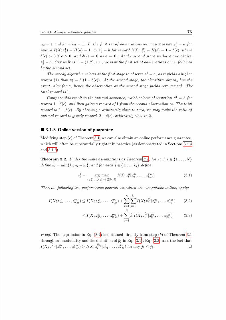
8/2/2019 Information Theoretic Sensor Management
http://slidepdf.com/reader/full/information-theoretic-sensor-management 73/203
Sec. 3.1. A simple performance guarantee 73
n2 = 1 and k1 = k2 = 1. In the first set of observations we may measure z11 = a for
reward I (X ; z11) = H (a) = 1, or z21 = b for reward I (X ; z21) = H (b) = 1 − δ(), where
δ() > 0 ∀ > 0, and δ() → 0 as → 0. At the second stage we have one choice,z12 = a. Our walk is w = (1, 2), i.e., we visit the first set of observations once, followed
by the second set.
The greedy algorithm selects at the first stage to observe z11 = a, as it yields a higher
reward (1) than z21 = b (1 − δ()). At the second stage, the algorithm already has the
exact value for a, hence the observation at the second stage yields zero reward. The
total reward is 1.
Compare this result to the optimal sequence, which selects observation z21 = b for
reward 1 − δ(), and then gains a reward of 1 from the second observation z12. The total
reward is 2−
δ(). By choosing arbitrarily close to zero, we may make the ratio of
optimal reward to greedy reward, 2 − δ(), arbitrarily close to 2.
3.1.3 Online version of guarantee
Modifying step (c) of Theorem 3.1, we can also obtain an online performance guarantee,
which will often be substantially tighter in practice (as demonstrated in Sections 3.1.4
and 3.1.5).
Theorem 3.2. Under the same assumptions as Theorem 3.1, for each i ∈ {1, . . . , N }define ki = min
{ki, ni
−ki
}, and for each j
∈ {1, . . . , ki
}define
g ji = arg max
u∈{1,...,ni}−{gli|l<j}
I (X ; zui |zg1
w1, . . . , zgM
wM ) (3.1)
Then the following two performance guarantees, which are computable online, apply:
I (X ; zo1w1
, . . . , zoM wM
) ≤ I (X ; zg1w1
, . . . , zgM wM
) +N
i=1
ki j=1
I (X ; zgji
i |zg1w1
, . . . , zgM wM
) (3.2)
≤ I (X ; zg1w1
, . . . , zgM wM
) +N
i=1
kiI (X ; zg1ii |zg1
w1, . . . , zgM
wM ) (3.3)
Proof. The expression in Eq. (3.2) is obtained directly from step (b) of Theorem 3.1
through submodularity and the definition of g ji in Eq. (3.1). Eq. (3.3) uses the fact that
I (X ; zgj1i |zg1
w1, . . . , zgM wM ) ≥ I (X ; z
gj2i |zg1
w1 , . . . , zgM wM ) for any j1 ≤ j2.
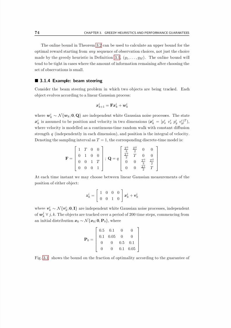
8/2/2019 Information Theoretic Sensor Management
http://slidepdf.com/reader/full/information-theoretic-sensor-management 74/203
74 CHAPTER 3. GREEDY HEURISTICS AND PERFORMANCE GUARANTEES
The online bound in Theorem 3.2 can be used to calculate an upper bound for the
optimal reward starting from any sequence of observation choices, not just the choice
made by the greedy heuristic in Definition 3.1, (g1, . . . , gM ). The online bound willtend to be tight in cases where the amount of information remaining after choosing the
set of observations is small.
3.1.4 Example: beam steering
Consider the beam steering problem in which two objects are being tracked. Each
object evolves according to a linear Gaussian process:
xik+1 = Fxi
k + wik
where wik ∼ N{wk; 0, Q} are independent white Gaussian noise processes. The statexi
k is assumed to be position and velocity in two dimensions (xik = [ pi
x vix pi
y viy]T ),
where velocity is modelled as a continuous-time random walk with constant diffusion
strength q (independently in each dimension), and position is the integral of velocity.
Denoting the sampling interval as T = 1, the corresponding discrete-time model is:
F =
1 T 0 0
0 1 0 0
0 0 1 T
0 0 0 1
; Q = q
T 3
3T 2
2 0 0T 2
2 T 0 0
0 0 T 3
3T 2
2
0 0 T 2
2 T
At each time instant we may choose between linear Gaussian measurements of the
position of either object:
zik =
1 0 0 0
0 0 1 0
xi
k + vik
where vik ∼ N{vi
k; 0, I} are independent white Gaussian noise processes, independent
of w jk ∀ j, k. The objects are tracked over a period of 200 time steps, commencing from
an initial distribution x0 ∼ N{x0; 0, P0}, where
P0 =
0.5 0.1 0 00.1 0.05 0 0
0 0 0.5 0.1
0 0 0.1 0.05
Fig. 3.1 shows the bound on the fraction of optimality according to the guarantee of
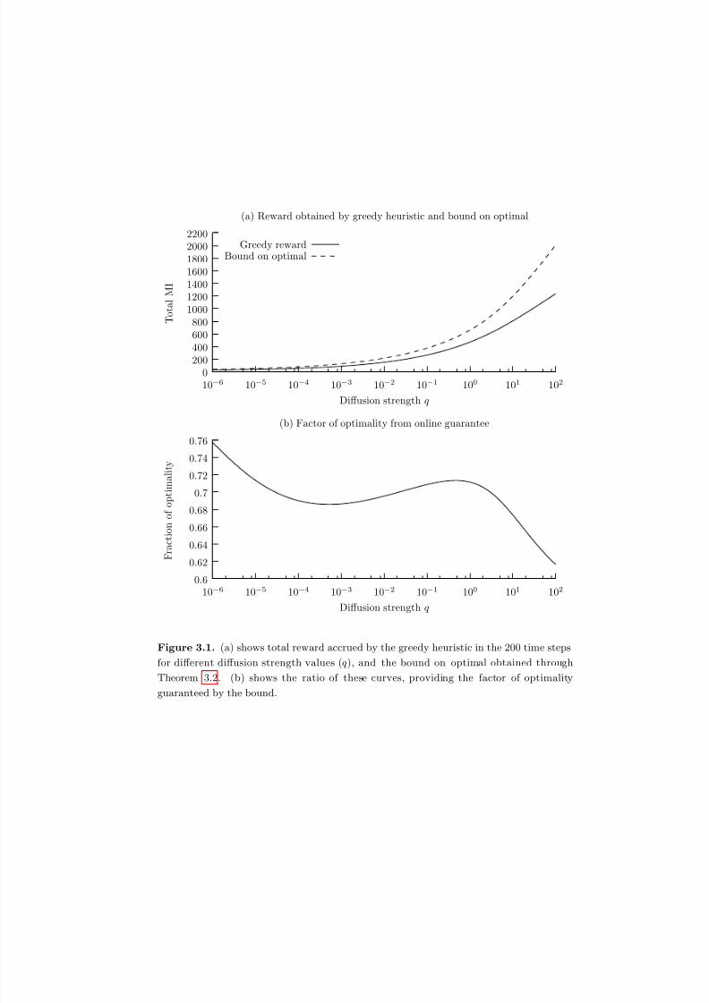
8/2/2019 Information Theoretic Sensor Management
http://slidepdf.com/reader/full/information-theoretic-sensor-management 75/203
0200400
600800
1000120014001600180020002200
10−6 10−5 10−4 10−3 10−2 10−1 100 101 102
T o
t a l M I
Diffusion strength q
(a) Reward obtained by greedy heuristic and bound on optimal
Greedy rewardBound on optimal
0.6
0.62
0.64
0.66
0.68
0.7
0.72
0.74
0.76
10−6 10−5 10−4 10−3 10−2 10−1 100 101 102
F r a c t i o n
o f o p
t i m a
l i t y
Diffusion strength q
(b) Factor of optimality from online guarantee
Figure 3.1. (a) shows total reward accrued by the greedy heuristic in the 200 time steps
for different diffusion strength values (q), and the bound on optimal obtained through
Theorem 3.2. (b) shows the ratio of these curves, providing the factor of optimality
guaranteed by the bound.

8/2/2019 Information Theoretic Sensor Management
http://slidepdf.com/reader/full/information-theoretic-sensor-management 76/203
76 CHAPTER 3. GREEDY HEURISTICS AND PERFORMANCE GUARANTEES
Theorem 3.2 as a function of the diffusion strength q. In this example, the quantity
being estimated, X , is the combination of the states of both objects over all time steps
in the problem:X = [x11; x21; x12; x22; . . . ; x1200; x2200]
Examining Fig. 3.1, the greedy controller obtains close to the optimal amount of infor-
mation as diffusion decreases since the measurements that were declined become highly
correlated with the measurements that were chosen.
3.1.5 Example: waveform selection
Suppose that we are using a surface vehicle travelling at a constant velocity along a fixed
path (as illustrated in Fig. 3.2(a)) to map the depth of the ocean floor in a particular
region. Assume that, at any position on the path (such as the points denoted by ‘’),
we may steer our sensor to measure the depth of any point within a given region around
the current position (as depicted by the dotted ellipses), and that we receive a linear
measurement of the depth corrupted by Gaussian noise with variance R. Suppose that
we model the depth of the ocean floor as a Gauss-Markov random field with a 500×100
thin membrane grid model where neighboring node attractions are uniformly equal to
q. One cycle of the vehicle path takes 300 time steps to complete.
Defining the state X to be the vector containing one element for each cell in the
500×100 grid, the structure of the problem can be seen to be waveform selection: at
each time we choose between observations which convey information about differentaspects of the same underlying phenomenon.
Fig. 3.2(b) shows the accrual of reward over time as well as the bound on the optimal
sequence obtained using Theorem 3.2 for each time step when q = 100 and R = 1/40,
while Fig. 3.2(c) shows the ratio between the achieved performance and the optimal
sequence bound over time. The graph indicates that the greedy heuristic achieves at
least 0.8× the optimal reward. The tightness of the online bound depends on particular
model characteristics: if q = R = 1, then the guarantee ratio is much closer to the value
of the offline bound (i.e., 0.5). Fig. 3.3 shows snapshots of how the uncertainty in the
depth estimate progresses over time. The images display the marginal entropy of each
cell in the grid.

8/2/2019 Information Theoretic Sensor Management
http://slidepdf.com/reader/full/information-theoretic-sensor-management 77/203
0
50
100
150
200
250
0 100 200 300 400 500 600 A c c r u e
d r e w a r d (
M I )
Time step
(b) Reward obtained by greedy heuristic and bound on optimal
Greedy rewardBound on optimal
0.70.720.740.76
0.780.8
0.820.84
0 100 200 300 400 500 600 F r a c t i o n o
f o p
t i m a
l i t y
Time step
(c) Factor of optimality from online guarantee
(a) Region boundary and vehicle path
Figure 3.2. (a) shows region boundary and vehicle path (counter-clockwise, starting from
the left end of the lower straight segment). When the vehicle is located at a ‘’ mark,
any one grid element with center inside the surrounding dotted ellipse may be measured.
(b) graphs reward accrued by the greedy heuristic after different periods of time, and the
bound on the optimal sequence for the same time period. (c) shows the ratio of these two
curves, providing the factor of optimality guaranteed by the bound.
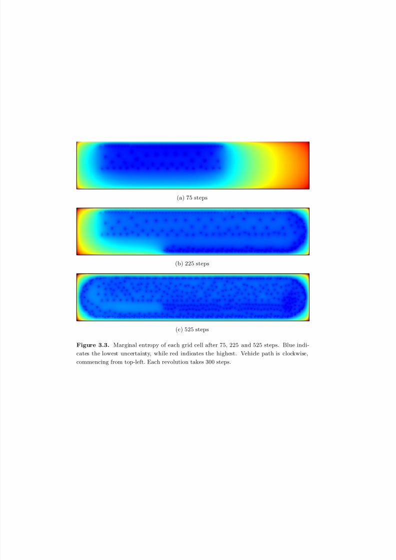
8/2/2019 Information Theoretic Sensor Management
http://slidepdf.com/reader/full/information-theoretic-sensor-management 78/203
(a) 75 steps
(b) 225 steps
(c) 525 steps
Figure 3.3. Marginal entropy of each grid cell after 75, 225 and 525 steps. Blue indi-
cates the lowest uncertainty, while red indicates the highest. Vehicle path is clockwise,
commencing from top-left. Each revolution takes 300 steps.
8/2/2019 Information Theoretic Sensor Management
http://slidepdf.com/reader/full/information-theoretic-sensor-management 79/203
Sec. 3.2. Exploiting diffusiveness 79
3.2 Exploiting diffusiveness
In problems such as object tracking, the kinematic quantities of interest evolve according
to a diffusive process, in which correlation between states at different time instants
reduces as the time difference increases. Intuitively, one would expect that a greedy
algorithm would be closer to optimal in situations in which the diffusion strength is
high. This section develops a performance guarantee which exploits the diffusiveness of
the underlying process to obtain a tighter bound on performance.
The general form of the result, stated in Theorem 3.3, deals with an arbitrary graph
(in the sense of Section 2.1.5) in the latent structure. The simpler cases involving trees
and chains are discussed in the sequel. The theorem is limited to only choosing a single
observation from each set; the proof of Theorem 3.3 exploits this fact. The basic model
structure is set up in Assumption 3.2.
Assumption 3.2. Let the latent structure which we seek to infer consist of an undi-
rected graph G with nodes X = {x1, . . . , xL}, with an arbitrary interconnection structure.
Assume that each node has a set of observations {z1i , . . . , znii }, which are independent
of each other and all other nodes and observations in the graph conditioned on xi. We
may select a single observation from each set. Let (w1, . . . , wL) be a sequence which
determines the order in which nodes are visited ( wi ∈ {1, . . . , L} ∀ i); we assume that
each node is visited exactly once.
The results of Section 3.1 were applicable to any submodular, non-decreasing ob-
jective for which the reward of an empty set was zero. In this section, we exploit an
additional property of mutual information which holds under Assumption 3.2, that for
any set of conditioning observations zA:
I (X ; z ji |zA) = H (z j
i |zA) − H (z ji |X, zA)
= H (z ji |zA) − H (z j
i |x j)
= I (xi; z ji |zA) (3.4)
We then utilize this property in order to exploit process diffusiveness. The general form
of the diffusive characteristic is stated in Assumption 3.3. This is a strong assumption
that is difficult to establish globally for any given model; we examine it for one simple
model in Section 3.2.3. In Section 3.2.1 we present an online computable guarantee
which exploits the characteristic to whatever extent it exists in a particular selection
problem. In Section 3.2.2 we then specialize the assumption to cases where the latent
graph structure is a tree or a chain.
8/2/2019 Information Theoretic Sensor Management
http://slidepdf.com/reader/full/information-theoretic-sensor-management 80/203
80 CHAPTER 3. GREEDY HEURISTICS AND PERFORMANCE GUARANTEES
Assumption 3.3. Under the structure in Assumption 3.2 , let the graph G have the
diffusive property in which there exists α < 1 such that for each i ∈ {1, . . . , L} and each
observation z jwi at node xwi,
I (x N (wi); z jwi
|zg1w1
, . . . , zgi−1wi−1) ≤ αI (xwi
; z jwi
|zg1w1
, . . . , zgi−1wi−1)
where x N (wi) denotes the neighbors of node xwiin the latent structure graph G.
Assumption 3.3 states that the information which the observation z jwi contains about
xwi is discounted by a factor of at least α when compared to the information it contains
about the remainder of the graph. Theorem 3.3 uses this property to bound the loss of
optimality associated with the greedy choice to be a factor of (1 + α) rather than 2.
Theorem 3.3. Under Assumptions 3.2 and 3.3 , the performance of the greedy heuristicin Definition 3.1 satisfies the following guarantee:
I (X ; zo1w1
, . . . , zoLwL
) ≤ (1 + α)I (X ; zg1w1
, . . . , zgLwL
)
Proof. To establish an induction step, assume that (as trivially holds for j = 1),
I (X ; zo1w1
, . . . , zoLwL
) ≤ (1 + α)I (X ; zg1w1
, . . . , zgj−1wj−1) + I (X ; z
ojwj , . . . , zoL
wL|zg1
w1, . . . , z
gj−1wj−1)
(3.5)
Manipulating the second term in Eq. (3.5),
I (X ; zojwj , . . . , zoL
wL|zg1
w1, . . . , z
gj−1wj−1)
(a)= I (xwj
; zojwj |zg1
w1, . . . , z
gj−1wj−1) + I (xwj+1, . . . , xwL
; zoj+1wj+1, . . . , zoL
wL|zg1
w1, . . . , z
gj−1wj−1 , z
ojwj)
(b)
≤ I (xwj; z
gjwj |zg1
w1, . . . , z
gj−1wj−1) + I (xwj+1, . . . , xwL
; zoj+1wj+1, . . . , zoL
wL|zg1
w1, . . . , z
gj−1wj−1)
(c)
≤ I (xwj; z
gjwj |zg1
w1, . . . , z
gj−1wj−1) + I (xwj+1, . . . , xwL
; zgjwj , z
oj+1wj+1, . . . , zoL
wL|zg1
w1, . . . , z
gj−1wj−1)
(d)= I (xwj ; z
gjwj |zg1
w1, . . . , z
gj−1wj−1) + I (x N (wj); z
gjwj |zg1
w1, . . . , z
gj−1wj−1)
+ I (xwj+1, . . . , xwL; z
oj+1wj+1, . . . , zoL
wL|zg1
w1, . . . , z
gjwj)
(e)≤ (1 + α)I (xwj ; zgjwj |zg1
w1, . . . , z
gj−1wj−1) + I (xwj+1, . . . , xwL
; zoj+1wj+1, . . . , zoL
wL|zg1
w1, . . . , z
gjwj )
(f )= (1 + α)I (X ; z
gjwj |zg1
w1, . . . , z
gj−1wj−1) + I (X ; z
oj+1wj+1, . . . , zoL
wL|zg1
w1, . . . , z
gjwj )
where (a) and (f ) result from the chain rule, from independence of zojwj and z
gjwj on the re-
maining latent structure conditioned on xwj, and from independence of {z
oj+1wj+1, . . . , zoL
wL}
8/2/2019 Information Theoretic Sensor Management
http://slidepdf.com/reader/full/information-theoretic-sensor-management 81/203
Sec. 3.2. Exploiting diffusiveness 81
on the remaining latent structure conditioned on {xwj+1, . . . , xwL}; (b) from submodu-
larity and the definition of the greedy heuristic; (c) from the non-decreasing property;
(d) from the chain rule (noting that zgjwj is independent of all nodes remaining to be vis-
ited conditioned on the neighbors of xwj); and (e) from the assumed diffusive property
of Assumption 3.3. Replacing the second term in Eq. (3.5) with the final result in (f ),
we obtain a strengthened bound:
I (X ; zo1w1
, . . . , zoLwL
) ≤ (1 + α)I (X ; zg1w1
, . . . , zgjwj ) + I (X ; z
oj+1wj+1, . . . , zoL
wL|zg1
w1, . . . , z
gjwj)
Applying this induction step L times, we obtain the desired result.
3.2.1 Online guarantee
For many models the diffusive property is difficult to establish globally. Following from
step (d) of Theorem 3.3, one may obtain an online computable bound which does not
require the property of Assumption 3.3 to hold globally, but exploits it to whatever
extent it exists in a particular selection problem.
Theorem 3.4. Under the model of Assumption 3.2, but not requiring the diffusive prop-
erty of Assumption 3.3 , the following performance guarantee, which can be computed
online, applies to the greedy heuristic of Definition 3.1:
I (X ; zo1w1, . . . , z
oLwL) ≤ I (X ; z
g1w1, . . . , z
gLwL) +
L j=1
I (x N (wj); zgjwj |z
g1w1, . . . , z
gj−1
wj−1)
Proof. The proof directly follows Theorem 3.3. Commence by assuming (for induction)
that:
I (X ; zo1w1
, . . . , zoLwL
) ≤ I (X ; zg1w1
, . . . , zgj−1wj−1) +
j−1i=1
I (x N (wi); zgiwi
|zg1w1
, . . . , zgi−1wi−1)
+ I (X ; zojwj , . . . , zoL
wL|zg1
w1, . . . , z
gj−1wj−1) (3.6)
Eq. (3.6) trivially holds for j = 1. If we assume that it holds for j then step (d) of
Theorem 3.3 obtains an upper bound to the the final term in Eq. (3.6) which establishes
that Eq. (3.6) also holds for ( j + 1). Applying the induction step L times, we obtain
the desired result.
8/2/2019 Information Theoretic Sensor Management
http://slidepdf.com/reader/full/information-theoretic-sensor-management 82/203
82 CHAPTER 3. GREEDY HEURISTICS AND PERFORMANCE GUARANTEES
3.2.2 Specialization to trees and chains
In the common case where the latent structure X =
{x1, . . . , xL
}forms a tree, we may
avoid including all neighbors a node in the condition of Assumption 3.3 and in the
result of Theorem 3.4. The modified assumptions are presented below. An additional
requirement on the sequence (w1, . . . , wL) is necessary to exploit the tree structure.
Assumption 3.4. Let the latent structure which we seek to infer consist of an undi-
rected graph G with nodes X = {x1, . . . , xL}, which form a tree. Assume that each
node has a set of observations {z1i , . . . , znii }, which are independent of each other and
all other nodes and observations in the graph conditioned on xi. We may select a single
observation from each set. Let (w1, . . . , wL) be a sequence which determines the order
in which nodes are visited ( wi
∈ {1, . . . , L
} ∀i); we assume that each node is visited
exactly once. We assume that the sequence is “bottom-up”, i.e., that no node is visited
before all of its children have been visited.
Assumption 3.5. Under the structure in Assumption 3.4, let the graph G have the
diffusive property in which there exists α < 1 such that for each i ∈ {1, . . . , L} and each
observation z jwi at node xwi
,
I (xπ(wi); z jwi
|zg1w1
, . . . , zgi−1wi−1) ≤ αI (xwi ; z j
wi|zg1
w1, . . . , z
gi−1wi−1)
where xπ(wi)
denotes the parent of node xwi
in the latent structure graph G
.
Theorem 3.3 holds under Assumptions 3.4 and 3.5; the proof passes directly once
x N (wj) is replaced by xπ(wj) in step (d). The modified statement of Theorem 3.4 is
included below. Again, the proof passes directly once x N (wi) is replaced by xπ(wi).
Theorem 3.5. Under the model of Assumption 3.4, but not requiring the diffusive prop-
erty of Assumption 3.5 , the following performance guarantee, which can be computed
online, applies to the greedy heuristic of Definition 3.1:
I (X ; zo1w1
, . . . , zoLwL
)
≤I (X ; zg1
w1, . . . , zgL
wL) +
L
j=1
I (xπ(wj); zgjwj
|zg1w1
, . . . , zgj−1wj−1)
The most common application of the diffusive model is in Markov chains (a special
case of a tree), where the i-th node corresponds to time i. In this case, the sequence
is simply wi = i, i.e., we visit the nodes in time order. Choosing the final node in the
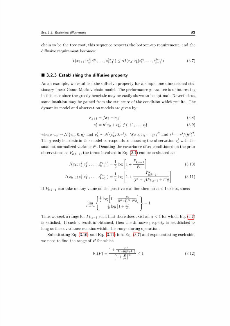
8/2/2019 Information Theoretic Sensor Management
http://slidepdf.com/reader/full/information-theoretic-sensor-management 83/203
Sec. 3.2. Exploiting diffusiveness 83
chain to be the tree root, this sequence respects the bottom-up requirement, and the
diffusive requirement becomes:
I (xk+1; z jk|zg1
1 , . . . , zgk−1k−1 ) ≤ αI (xk; z j
k|zg11 , . . . , z
gk−1
k−1 ) (3.7)
3.2.3 Establishing the diffusive property
As an example, we establish the diffusive property for a simple one-dimensional sta-
tionary linear Gauss-Markov chain model. The performance guarantee is uninteresting
in this case since the greedy heuristic may be easily shown to be optimal. Nevertheless,
some intuition may be gained from the structure of the condition which results. The
dynamics model and observation models are given by:
xk+1 = f xk + wk (3.8)
z jk = h jxk + v j
k, j ∈ {1, . . . , n} (3.9)
where wk ∼ N{wk; 0, q} and v jk ∼ N {v j
k; 0, r j}. We let q = q/f 2 and r j = r j/(h j)2.
The greedy heuristic in this model corresponds to choosing the observation z jk with the
smallest normalized variance r j. Denoting the covariance of xk conditioned on the prior
observations as P k|k−1, the terms involved in Eq. (3.7) can be evaluated as:
I (xk; z jk|zg1
1 , . . . , zgk−1k−1 ) =
1
2log 1 +
P k|k−1
r j (3.10)
I (xk+1; z jk|zg1
1 , . . . , zgk−1k−1 ) =
1
2log
1 +
P 2k|k−1
(r j + q)P k|k−1 + r j q
(3.11)
If P k|k−1 can take on any value on the positive real line then no α < 1 exists, since:
limP →∞
12 log
1 + P 2
(rj+q)P +rj q
12 log
1 + P rj
= 1
Thus we seek a range for P k|k−1 such that there does exist an α < 1 for which Eq. (3.7)
is satisfied. If such a result is obtained, then the diffusive property is established as
long as the covariance remains within this range during operation.Substituting Eq. (3.10) and Eq. (3.11) into Eq. (3.7) and exponentiating each side,
we need to find the range of P for which
bα(P ) =1 + P 2
(rj+q)P +rj q1 + P
rj
α ≤ 1 (3.12)
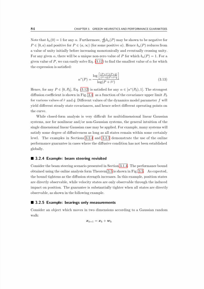
8/2/2019 Information Theoretic Sensor Management
http://slidepdf.com/reader/full/information-theoretic-sensor-management 84/203
84 CHAPTER 3. GREEDY HEURISTICS AND PERFORMANCE GUARANTEES
Note that bα(0) = 1 for any α. Furthermore, ddP bα(P ) may be shown to be negative for
P ∈ [0, a) and positive for P ∈ (a, ∞) (for some positive a). Hence bα(P ) reduces from
a value of unity initially before increasing monotonically and eventually crossing unity.For any given α, there will be a unique non-zero value of P for which bα(P ) = 1. For a
given value of P , we can easily solve Eq. (3.12) to find the smallest value of α for which
the expression is satisfied:
α∗(P ) =log(P +rj)(P +q)(rj+q)P +rj q
log(P + r j)
(3.13)
Hence, for any P ∈ [0, P 0], Eq. (3.12) is satisfied for any α ∈ [α∗(P 0), 1]. The strongest
diffusion coefficient is shown in Fig. 3.4 as a function of the covariance upper limit P 0
for various values of r and q. Different values of the dynamics model parameter f willyield different steady state covariances, and hence select different operating points on
the curve.
While closed-form analysis is very difficult for multidimensional linear Gaussian
systems, nor for nonlinear and/or non-Gaussian systems, the general intuition of the
single dimensional linear Gaussian case may be applied. For example, many systems will
satisfy some degree of diffusiveness as long as all states remain within some certainly
level. The examples in Sections 3.2.4 and 3.2.5 demonstrate the use of the online
performance guarantee in cases where the diffusive condition has not been established
globally.
3.2.4 Example: beam steering revisited
Consider the beam steering scenario presented in Section 3.1.4. The performance bound
obtained using the online analysis form Theorem 3.5 is shown in Fig. 3.5. As expected,
the bound tightens as the diffusion strength increases. In this example, position states
are directly observable, while velocity states are only observable through the induced
impact on position. The guarantee is substantially tighter when all states are directly
observable, as shown in the following example.
3.2.5 Example: bearings only measurements
Consider an object which moves in two dimensions according to a Gaussian random
walk:
xk+1 = xk + wk

8/2/2019 Information Theoretic Sensor Management
http://slidepdf.com/reader/full/information-theoretic-sensor-management 85/203
0
0.1
0.2
0.3
0.4
0.5
0 5 10 15 20 25
D i ff u s i v e c o e ffi c i e n
t α ∗
Covariance limit P 0
Lowest diffusive coefficient vs covariance limit
q = 20q = 10
q = 5
Figure 3.4. Strongest diffusive coefficient versus covariance upper limit for various values
of q, with r = 1. Note that lower values of α∗ correspond to stronger diffusion.

8/2/2019 Information Theoretic Sensor Management
http://slidepdf.com/reader/full/information-theoretic-sensor-management 86/203
400
600
800
1000
1200
1400
1600
1800
2000
100 101 102
T o
t a l M I
Diffusion strength q
(a) Reward obtained by greedy heuristic and bound on optimal
Greedy rewardBound on optimal
0.5
0.52
0.54
0.56
0.58
0.6
0.62
0.64
100 101 102
F r a c t i o n
o f o p
t i m a
l i t y
Diffusion strength q
(b) Factor of optimality from online diffusive guarantee
Figure 3.5. (a) shows total reward accrued by the greedy heuristic in the 200 time steps
for different diffusion strength values (q), and the bound on optimal obtained through
Theorem 3.5. (b) shows the ratio of these curves, providing the factor of optimality
guaranteed by the bound.

8/2/2019 Information Theoretic Sensor Management
http://slidepdf.com/reader/full/information-theoretic-sensor-management 87/203
Sec. 3.3. Discounted rewards 87
where wk ∼ N{wk; 0, I}. The initial position of the object is distributed according
to x0 ∼ N {x0; 0, I}. Assume that bearing observations are available from four sen-
sors positioned at (±100, ±100), but that only one observation may be utilized at anyinstant. Simulations were run for 200 time steps. The total reward and the bound
obtained from Theorem 3.5 are shown in Fig. 3.6(a) as a function of the measurement
noise standard deviation (in degrees). The results demonstrate that the performance
guarantee becomes stronger as the measurement noise decreases; the same effect occurs
if the observation noise is held constant and the dynamics noise increased. Fig. 3.6(b)
shows the ratio of the greedy performance to the upper bound on optimal, demonstrat-
ing that the greedy heuristic is guaranteed to be within a factor of 0.77 of optimal with
a measurement standard deviation of 0.1 degrees.
In this example, we utilized the closed loop greedy heuristic examined in Section 3.5,
hence it was necessary to use multiple Monte Carlo simulations to compute the online
guarantee. Tracking was performed using an extended Kalman filter, hence the bounds
are approximate (the EKF variances were used to calculate the rewards). In this sce-
nario, the low degree of nonlinearity in the observation model provides confidence that
the inaccuracy in the rewards is insignificant.
3.3 Discounted rewards
In Sections 3.1 and 3.2 the objective we were seeking to optimize was the mutual
information between the state and observations through the planning horizon, and theoptimal open loop reward to which we compared was I (X ; zo1
w1, . . . , zoM
wM ). In some
sequential estimation problems, it is not only desirable to maximize the information
obtained within a particular period of time, but also how quickly, within the planning
horizon, the information is obtained. One way2 of capturing this notion is to incorporate
a discount factor in the objective, reducing the value of information obtained later in
the problem. Subsequently, our optimization problem is changed from:
minu1,...,uM
I (X ; zu11 , . . . , zuM
N ) = minu1,...,uM
M
k=1
I (X ; zukk |zu1
1 , . . . , zuk−1
k−1 )
2Perhaps the most natural way of capturing this would be to reformulate the problem, choosing as
the objective (to be minimized) the expected time required to reduce the uncertainty below a desired
criterion. The resulting problem is intractable, hence the approximate method using MI is an appealing
substitute.
8/2/2019 Information Theoretic Sensor Management
http://slidepdf.com/reader/full/information-theoretic-sensor-management 88/203
0
50
100
150
200
250
300
350
400
450
500
10−1 100 101
T o
t a l M I
Measurement noise standard deviation σ
(a) Reward obtained by greedy heuristic and bound on optimal
Greedy rewardBound on optimal
0.5
0.55
0.6
0.65
0.7
0.75
0.8
10−1 100 101
F r a c t i o n
o f o p
t i m a
l i t y
Measurement noise standard deviation σ
(b) Factor of optimality from online guarantee
Figure 3.6. (a) shows average total reward accrued by the greedy heuristic in the 200
time steps for different diffusion strength values (q), and the bound on optimal obtained
through Theorem 3.5. (b) shows the ratio of these curves, providing the factor of optimality
guaranteed by the bound.

8/2/2019 Information Theoretic Sensor Management
http://slidepdf.com/reader/full/information-theoretic-sensor-management 89/203
Sec. 3.3. Discounted rewards 89
to:
minu1,...,uM
M
k=1
αk−1I (X ; zukk
|zu11 , . . . , z
uk−1
k−1 )
where α < 1. Not surprising, the performance guarantee for the greedy heuristic be-
comes tighter as the discount factor is decreased, as Theorem 3.6 establishes. We define
the abbreviated notation for the optimal reward to go from stage i to the end of the
problem conditioned on the previous observation choices (u1, . . . , uk):
J oi [(u1, . . . , uk)] M
j=i
α j−1I (X ; zojwj |zu1
w1, . . . , zuk
wk, zoi
wi, . . . , z
oj−1wj−1)
and the reward so far for the greedy heuristic in i stages:
J g→i
i j=1
α j−1I (X ; zgjwj |zg1
w1, . . . , z
gj−1wj−1)
We will use the following lemma in the proof of Theorem 3.6.
Lemma 3.1. The optimal reward to go for the discounted sequence satisfies the rela-
tionship:
J oi+1[(g1, . . . , gi−1)] ≤ αiI (X ; zgiwi
|zg1w1
, . . . , zgi−1wi−1) + J oi+1[(g1, . . . , gi)]

8/2/2019 Information Theoretic Sensor Management
http://slidepdf.com/reader/full/information-theoretic-sensor-management 90/203
90 CHAPTER 3. GREEDY HEURISTICS AND PERFORMANCE GUARANTEES
Proof. Expanding the left-hand side and manipulating:
J oi+1[(g1, . . . , gi−1)] =
M j=i+1
α j−1I (X ; zojwj |zg1w1 , . . . , zgi−1wi−1 , zoi+1wi+1, . . . , zoj−1wj−1)
(a)= αi
I (X ; z
oi+1wi+1, . . . , zoM
wM |zg1
w1, . . . , z
gi−1wi−1)
+M
j=i+1
(α j−i−1 − 1)I (X ; zojwj |zg1
w1, . . . , z
gi−1wi−1, z
oi+1wi+1, . . . , z
oj−1wj−1)
(b)
≤ αi
I (X ; zgi
wi, z
oi+1wi+1, . . . , zoM
wM |zg1
w1, . . . , z
gi−1wi−1)
+
M j=i+1
(α j−i−1 − 1)I (X ; zojwj |zg1w1, . . . , zgi−1wi−1, zoi+1wi+1, . . . , zoj−1wj−1)
(c)= αi
I (X ; zgi
wi|zg1
w1, . . . , z
gi−1wi−1) + I (X ; z
oi+1wi+1, . . . , zoM
wM |zg1
w1, . . . , zgi
wi)
+M
j=i+1
(α j−i−1 − 1)I (X ; zojwj |zg1
w1, . . . , z
gi−1wi−1, z
oi+1wi+1, . . . , z
oj−1wj−1)
(d)
≤ αi
I (X ; zgi
wi|zg1
w1, . . . , z
gi−1wi−1) + I (X ; z
oi+1wi+1, . . . , zoM
wM |zg1
w1, . . . , zgi
wi)
+
M j=i+1
(α j−i−1 − 1)I (X ; zojwj |zg1w1, . . . , zgiwi , zoi+1wi+1, . . . , zoj−1wj−1)
(e)= αiI (X ; zgi
wi|zg1
w1, . . . , z
gi−1wi−1) + J oi+1[(g1, . . . , gi)]
where (a) results from adding and subtracting αiI (X ; zoi+1wi+1, . . . , zoM
wM |zg1
w1, . . . , zgi−1wi−1),
(b) from the non-decreasing property of MI (introducing the additional observation zgiwi
into the first term), (c) from the MI chain rule, (d) from submodularity (adding the
conditioning zgiwi into the second term, noting that the coefficient is negative), and (e)
from cancelling similar terms and applying the definition of J oi+1.
Theorem 3.6. Under Assumption 3.1, the greedy heuristic in Definition 3.1 has per-
formance guaranteed by the following expression:
M j=1
α j−1I (X ; zojwj |zo1
w1, . . . , z
oj−1wj−1) ≤ (1 + α)
M j=1
α j−1I (X ; zgjwj |zg1
w1, . . . , z
gj−1wj−1)

8/2/2019 Information Theoretic Sensor Management
http://slidepdf.com/reader/full/information-theoretic-sensor-management 91/203
Sec. 3.4. Time invariant rewards 91
where {zo1w1
, . . . , zoM wM
} is the optimal set of observations, i.e., the one which maximizes
M j=1
α j−1I (X ; zojwj |zo1w1, . . . , zoj−1
wj−1)
Proof. In the abbreviated notation, we seek to prove:
J o1 [∅] ≤ (1 + α)J g→M
The proof follows an induction on the expression
J o1 [∅] ≤ (1 + α)J g→i−1 + J oi [(g1, . . . , gi−1)]
which is trivially true for i = 1. Suppose it is true for i; manipulating the expression
we obtain:
J o1 [∅] ≤ (1 + α)J g→i−1 + J oi [(g1, . . . , gi−1)]
(a)= (1 + α)J g→i−1 + αi−1I (X ; zoi
wi|zg1
w1, . . . , z
gi−1wi−1) + J oi+1[(g1, . . . , gi−1, oi)]
(b)
≤ (1 + α)J g→i−1 + αi−1I (X ; zgiwi
|zg1w1
, . . . , zgi−1wi−1) + J oi+1[(g1, . . . , gi−1, oi)]
(c)
≤ (1 + α)J g→i−1 + αi−1I (X ; zgiwi
|zg1w1
, . . . , zgi−1wi−1) + J oi+1[(g1, . . . , gi−1)]
(d)≤ (1 + α)J g→i−1 + (1 + α)αi−1I (X ; zgiwi
|zg1w1
, . . . , zgi−1wi−1) + J oi+1[(g1, . . . , gi)]
= (1 + α)J g→i + J oi+1[(g1, . . . , gi)]
where (a) results from the definition of J oi , (b) results from the definition of the greedy
heuristic, (c) results from submodularity (allowing us to remove the conditioning on oi
from each term in J oi+1) and (d) from Lemma 3.1.
Applying the induction step M times we get the desired result.
3.4 Time invariant rewards
The reward function in some problems is well-approximated as being time invariant.
In this case, a tighter bound, (1 − 1/e)×, may be obtained. The structure necessary is
given in Assumption 3.6.

8/2/2019 Information Theoretic Sensor Management
http://slidepdf.com/reader/full/information-theoretic-sensor-management 92/203
8/2/2019 Information Theoretic Sensor Management
http://slidepdf.com/reader/full/information-theoretic-sensor-management 93/203
Sec. 3.5. Closed loop control 93
Example 3.2. Suppose that our state consists of four independent binary random vari-
ables, X = [a b c d]T , where H (a) = H (b) = 1, and H (c) = H (d) = 1 − for some
small > 0. In each stage k ∈ {1, 2} there are three observations available, z1k = [a b]T ,z2k = [a c]T and z3k = [b d]T .
In stage 1, the greedy heuristic selects observation z11 since I (X ; z11) = 2 whereas
I (X ; z21) = I (X ; z31) = 2 − . In stage 2, the algorithm has already learned the values of
a and b, hence I (X ; z12 |z11) = 0, and I (X ; z22 |z11) = I (X ; z32 |z11) = 1 −. The total reward
is 3 − .
An optimal choice is z21 and z32, achieving reward 4 − 2. The ratio of the greedy
reward to optimal reward is3 −
4 − 2
which approaches 0.75 as → 0. Examining Theorem 2.4, we see that the performanceof the greedy heuristic over K = 2 stages is guaranteed to be within a factor of [1 − (1 −1/K )K ] = 0.75 of the optimal, hence this factor is the worst possible over two stages.
The intuition behind the scenario in this example is that information about dif-
ferent portions of the state can be obtained in different combinations, therefore it is
necessary to use additional planning to ensure that the observations we obtain provide
complementary information.
3.5 Closed loop control
The analysis in Sections 3.1-3.3 concentrates on an open loop control structure, i.e., it
assumes that all observation choices are made before any observation values are received.
Greedy heuristics are often applied in a closed loop setting, in which an observation is
chosen, and then its value is received before the next choice is made.
The performance guarantees of Theorems 3.1 and 3.3 both apply to the expected
performance of the greedy heuristic operating in a closed loop fashion, i.e., in expec-
tation the closed loop greedy heuristic achieves at least half the reward of the optimal
open loop selection. The expectation operation is necessary in the closed loop case since
control choices are random variables that depend on the values of previous observations.
Theorem 3.8 establishes the result of Theorem 3.1 for the closed loop heuristic. The
same process can be used to establish a closed loop version of Theorem 3.3. To obtain
the closed loop guarantee, we need to exploit an additional characteristic of mutual
information:
I (X ; zA|zB) =
I (X ; zA|zB = ζ ) pzB(ζ )dζ (3.14)
8/2/2019 Information Theoretic Sensor Management
http://slidepdf.com/reader/full/information-theoretic-sensor-management 94/203
94 CHAPTER 3. GREEDY HEURISTICS AND PERFORMANCE GUARANTEES
While the results are presented in terms of mutual information, they apply to any other
objective which meets the previous requirements as well as Eq. (3.14).
We define h j = (u1, zu1w1, u2, zu2w2, . . . , u j−1, zuj−1wj−1) to be the history of all observation
actions chosen, and the resulting observation values, prior to stage j (this constitutes
all the information which we can utilize in choosing our action at time j). Accordingly,
h 1 = ∅, and h j = (h j−1, u j, zujwj). The greedy heuristic operating in closed loop is defined
in Definition 3.2.
Definition 3.2. Under the same assumptions as Theorem 3.1, define the closed loop
greedy heuristic policy µg:
µg j (h j) = arg max
u∈{1,...,nwj }I (X ; zu
wj|h j) (3.15)
We use the convention that conditioning on h i in an MI expression is always on
the value, and hence if h i contains elements which are random variables we will always
include an explicit expectation operator. The expected reward to go from stage j to
the end of the planning horizon for the greedy heuristic µg j (h j) commencing from the
history h j is denoted as:
J µg
j (h j) = I (X ; zµgj (h j)
wj , . . . , zµgN (h N )
wN |h j) (3.16)
= E
N
i= j
I (X ; zµgi (h i)
wi |h i)
h j
(3.17)
The expectation in Eq. (3.17) is over the random variables corresponding to the ac-
tions {µg j+1(h j+1), . . . , µg
N (h N )},3 along with the observations resulting from the actions,
{zµgj (h j)
wj , . . . , zµgN (h N )
wN }, where h i is the concatenation of the previous history sequence
h i−1 with the new observation action µgi (h i) and the new observation value z
µgi (h i)
wi . The
expected reward of the greedy heuristic over the full planning horizon is J µg
1 (∅). We
also define the expected reward accrued by the greedy heuristic up to and including
stage j, commencing from an empty history sequence (i.e., h 1 = ∅), as:
J µg
→ j = E j
i=1I (X ; z
µgi (h i)
wi |h i)
(3.18)
This gives rise to the recursive relationship:
J µg
→ j = E[I (X ; zµgj (h j)
wj |h j)] + J µg
→ j−1 (3.19)
3We assume a deterministic policy, hence the action at stage j is fixed given knowledge of h j .

8/2/2019 Information Theoretic Sensor Management
http://slidepdf.com/reader/full/information-theoretic-sensor-management 95/203
Sec. 3.5. Closed loop control 95
Comparing Eq. (3.17) with Eq. (3.18), we have J µg
→N = J µg
1 (∅). We define J µg
→0 = 0.
The reward of the tail of the optimal open loop observation sequence (o j , . . . , oN )
commencing from the history h j is denoted by:
J o j (h j) = I (X ; zojwj , . . . , zoN
wN |h j) (3.20)
Using the MI chain rule and Eq. (3.14), this can be written recursively as:
J o j (h j) = I (X ; zojwj |h j) + E
zojwj
|h j
J o j+1[(h j, o j, zojwj )] (3.21)
where J oN +1(h N +1) = 0. The reward of the optimal open loop observation sequence over
the full planning horizon is:
J
o
1 (∅) = I (X ; z
o1
w1, . . . , z
oN
wN ) (3.22)
We seek to obtain a guarantee on the performance ratio between the optimal open
loop observation sequence and the closed loop greedy heuristic. Before we prove the
theorem, we establish a simple result in terms of our new notation.
Lemma 3.2. Given the above definitions:
Ezojwj
|h j
J o j+1[(h j , o j , zojwj)] ≤ J o j+1(h j) ≤ I (X ; z
µgj (h j)
wj |h j) + E
zµgj(h j)
wj|h j
J o j+1[(h j, µg j (h j), z
µgj (h j)
wj )]
Proof. Using Eq. (3.20), the first inequality corresponds to:
I (X ; zoj+1wj+1, . . . , zoN
wN |h j, z
ojwj) ≤ I (X ; z
oj+1wj+1, . . . , zoN
wN |h j)
where conditioning is on the value h j throughout (as per the convention introduced
below Eq. (3.15)), and on the random variable zojwj . Therefore, the first inequality
results directly from submodularity.
The second inequality results from the non-decreasing property of MI:
I (X ; zoj+1wj+1, . . . , zoN
wN |h j)
(a)
≤ I (X ; zµgj (h j)
wj , zoj+1wj+1, . . . , zoN
wN |h j)
(b)
= I (X ; z
µgj (h j)
wj |h j) + I (zoj+1
wj+1, . . . , zoN wN |h j , z
µgj (h j)
wj )(c)= I (X ; z
µgj (h j)
wj |h j) + E
zµgj(h j)
wj|h j
J o j+1[(h j , µg j (h j), z
µgj (h j)
wj )]
(a) results from the non-decreasing property, (b) from the chain rule, and (c) from the
definition in Eq. (3.20).

8/2/2019 Information Theoretic Sensor Management
http://slidepdf.com/reader/full/information-theoretic-sensor-management 96/203
96 CHAPTER 3. GREEDY HEURISTICS AND PERFORMANCE GUARANTEES
We are now ready to prove our result, that the reward of the optimal open loop
sequence is no greater than twice the expected reward of the greedy closed loop heuristic.
Theorem 3.8. Under the same assumptions as Theorem 3.1,
J o1 (∅) ≤ 2J µg
1 (∅)
i.e., the expected reward of the closed loop greedy heuristic is at least half the reward of
the optimal open loop policy.
Proof. To establish an induction, assume that
J o1 (∅) ≤ 2J µg
→ j−1 + E J o j (h j) (3.23)
Noting that h 1 = ∅, this trivially holds for j = 1 since J µg
→0 = 0. Now, assuming that it
holds for j, we show that it also holds for ( j + 1). Applying Eq. (3.21),
J o1 (∅) ≤ 2J µg
→ j−1 + E
I (X ; z
ojwj |h j) + E
zojwj
|h j
J o j+1[(h j, o j, zojwj )]
By the definition of the closed loop greedy heuristic (Definition 3.2),
I (X ; zojwj |h j) ≤ I (X ; z
µgj (h j)
wj |h j)
hence:
J o1 (∅) ≤ 2J µg
→ j−1 + E
I (X ; z
µgj (h j)
wj |h j) + Ezojwj
|h j
J o j+1[(h j , o j , zojwj )]
Applying Lemma 3.2, followed by Eq. (3.19):
J o1 (∅) ≤ 2J µg
→ j−1 + E
2I (X ; z
µgj (h j)
wj |h j) + E
zµgj(h j)
wj|h j
J o j+1[(h j, µg j (h j), z
µgj (h j)
wj )]
= 2J µg
→ j + E J o j+1(h j+1)
where h j+1 = (h j, µg j (h j), zµ
gj (h j)
wj ). This establishes the induction step.
Applying the induction step N times, we obtain:
J o1 (∅) ≤ 2J µg
→N + E J oN +1(h N +1) = 2J µg
1 (∅)
since J oN +1(h N +1) = 0 and J µg
→N = J µg
1 (∅).

8/2/2019 Information Theoretic Sensor Management
http://slidepdf.com/reader/full/information-theoretic-sensor-management 97/203
Sec. 3.5. Closed loop control 97
We emphasize that this performance guarantee is for expected performance: it does
not provide a guarantee for the change in entropy of every sample path. An online
bound cannot be obtained on the basis of a single realization, although online boundssimilar to Theorems 3.2 and 3.4 could be calculated through Monte Carlo simulation
(to approximate the expectation).
3.5.1 Counterexample: closed loop greedy versus closed loop optimal
While Theorem 3.8 provides a performance guarantee with respect to the optimal open
loop sequence, there is no guarantee relating the performance of the closed loop greedy
heuristic to the optimal closed loop controller, as the following example illustrates. One
exception to this is linear Gaussian models, where closed loop policies can perform no
better than open loop sequences, so that the open loop guarantee extends to closedloop performance.
Example 3.3. Consider the following two-stage problem, where X = [a,b,c]T , with
a ∈ {1, . . . , N }, b ∈ {1, . . . , N + 1}, and c ∈ {1, . . . , M }. The prior distribution of each
of these is uniform and independent. In the first stage, we may measure z11 = a for
reward log N , or z21 = b for reward log(N + 1). In the second stage, we may choose zi2,
i ∈ {1, . . . , N }, where
zi2 =
c, i = a
d, otherwise
where d is independent of X , and is uniformly distributed on {1, . . . , M }. The greedy
algorithm in the first stage selects the observation z21 = b, as it yields a higher reward
( log(N +1)) than z11 = a ( log N ). At the second stage, all options have the same reward,1N log M , so we choose one arbitrarily for a total reward of log(N + 1 ) + 1
N log M . The
optimal algorithm in the first stage selects the observation z11 = a for reward log N ,
followed by the observation za2 for reward log M , for total reward log N + log M . The
ratio of the greedy reward to the optimal reward is
log(N + 1) + 1N
log M
log N + log M → 1
N , M → ∞
Hence, by choosing N and M to be large, we can obtain an arbitrarily small ratio
between the greedy closed-loop reward and the optimal closed-loop reward.
The intuition of this example is that the value of the observation at the first time
provides guidance to the controller on which observation it should take at the second
8/2/2019 Information Theoretic Sensor Management
http://slidepdf.com/reader/full/information-theoretic-sensor-management 98/203
98 CHAPTER 3. GREEDY HEURISTICS AND PERFORMANCE GUARANTEES
time. The greedy heuristic is unable to anticipate the later benefit of this guidance.
Notice that the reward of any observation zi2 without conditioning on the first observa-
tion z11 is I (X ; zi2) = 1N log M . In contrast, the reward of za2 conditioned on the valueof the observation z11 = a is I (X ; za
2 |z11) = log M . This highlights that the property of
diminishing returns (i.e., submodularity) is lost when later choices (and rewards) are
conditioned earlier observation values.
We conjecture that it may be possible to establish a closed loop performance guar-
antee for diffusive processes, but it is likely to be dramatically weaker than the bounds
presented in this chapter.
3.5.2 Counterexample: closed loop greedy versus open loop greedy
An interesting side note is that the closed loop greedy heuristic can actually result inlower performance than the open loop greedy heuristic, as the following example shows.
Example 3.4. Consider the following three-stage problem, where X = [a,b,c]T , with
a ∈ {1, 2}, b ∈ {1, . . . , N + 1}, and c ∈ {1, . . . , N }, where N ≥ 2. The prior distribution
of each of these is uniform and independent. In the first stage, a single observation is
available, z1 = a. In the second stage, we may choose z12 , z22 or z32 = c, where z12 and
z22 are given by:
zi2 =
b, i = a
d, otherwise
where d is independent of X , and is uniformly distributed on {1, . . . , N + 1}. In the
third stage, a single observation is available, z3 = b. The closed loop greedy algorithm
gains reward log2 for the first observation. At the second observation, the value of a
is known, hence it selects za2 = b for reward log(N + 1). The final observation z3 = b
then yields no further reward; the total reward is log 2(N + 1). The open loop greedy
heuristic gains the same reward ( log2) for the first observation. Since there is no prior
knowledge of a, z12 and z22 yield the same reward ( 12 log(N + 1)) which is less than the
reward of z32 ( log N ), hence z32 is chosen. The final observation yields reward log N
for a total reward of log2N √
N + 1. For any N ≥ 2, the open loop greedy heuristic
achieves higher reward than the closed loop greedy heuristic.
Since the open loop greedy heuristic has performance no better than the optimal
open loop sequence, and the closed loop greedy heuristic has performance no worse than
half that of the optimal open loop sequence, the ratio of open loop greedy performance
to closed loop greedy performance can be no greater than two. The converse is not

8/2/2019 Information Theoretic Sensor Management
http://slidepdf.com/reader/full/information-theoretic-sensor-management 99/203
Sec. 3.5. Closed loop control 99
true since the performance of the closed loop greedy heuristic is not bounded by the
performance of the optimal open loop sequence. This can be demonstrated with a slight
modification of Example 3.3 in which the observation z21 is made unavailable.
3.5.3 Closed loop subset selection
A simple modification of the proof of Theorem 3.8 can also be used to extend the
result of Theorem 2.4 to closed loop selections. In this structure, there is a single set
of observations from which we may choose any subset of ≤ K elements out of the
finite set U . Again, we obtain the value of each observation before making subsequent
selections. We may simplify our notation slightly in this case since we have a single pool
of observations. We denote the history of observations chosen and the resulting values
to beh j = (u1, z
u1
, . . . , u j−1, zuj−1
). The optimal choice of observations is denoted as(o1, . . . , oK ); the ordering within this choice is arbitrary.
The following definitions are consistent with the previous definitions within the new
notation:
µg(h j) = arg maxu∈U\{u1,...,uj−1}
I (X ; zu|h j)
J µg
→ j = E
j
i=1
I (X ; zµg(h i)|h i)
= E[I (X ; zµg(h j)
|h j)] + J µ
g
→ j−1
J o j (h j) = I (X ; zoj , . . . , zoN |h j)
where h 1 = ∅ and h j+1 = (h j , µg(h j), zµg(h j)). Lemmas 3.3 and 3.4 establish two results
which we use to prove the theorem.
Lemma 3.3. For all i ∈ {1, . . . , K },
J o1 (∅) ≤ J µg
→i + E J o1 (h i+1)
Proof. The proof follows an induction on the desired result. Note that the expressiontrivially holds for i = 0 since J µ
g
→0 = 0 and h 1 = ∅. Now suppose that the expression
8/2/2019 Information Theoretic Sensor Management
http://slidepdf.com/reader/full/information-theoretic-sensor-management 100/203
100 CHAPTER 3. GREEDY HEURISTICS AND PERFORMANCE GUARANTEES
holds for (i − 1):
J
o
1 (∅) ≤ J
µg
→i−1 + E J
o
1 (h i)
(a)= J µ
g
→i−1 + E[I (X ; zo1 , . . . , zoK |h i)]
(b)
≤ J µg
→i−1 + E[I (X ; zµg(h i), zo1 , . . . , zoK |h i)]
(c)= J µ
g
→i−1 + E[I (X ; zµg(h i)|h i)] + E[I (X ; zo1, . . . , zoK |h i, zµg(h i))]
(d)= J µ
g
→i + E
E
zµg(h i)|h i
J o1 [(h i, µg(h i), zµg(h i))]
(e)= J µ
g
→i + E J o1 [(h i+1)]
where (a) uses the definition of J o1 , (b) results from the non-decreasing property of MI,(c) results from the MI chain rule, (d) uses the definition of J µ
g
→i and J o1 , and (e) uses
the definition of h i+1.
Lemma 3.4. For all i ∈ {1, . . . , K },
J o1 (h i) ≤ KI (X ; zµg(h i)|h i)
Proof. The following steps establish the result:
J o1 (h i)(a)= I (X ; zo1, . . . , zoK |h i)
(b)=
K j=1
I (X ; zoj |h i, zo1, . . . , zoj−1)
(c)
≤K
j=1
I (X ; zoj |h i)
(d)
≤K
j=1
I (X ; zµg(h i)|h i)
= KI (X ; zµg(h i)|h i)
where (a) results from the definition of J o1 , (b) from the MI chain rule, (c) from sub-
modularity, and (d) from the definition of µg.
8/2/2019 Information Theoretic Sensor Management
http://slidepdf.com/reader/full/information-theoretic-sensor-management 101/203
Sec. 3.6. Guarantees on the Cramer-Rao bound 101
Theorem 3.9. The expected reward of the closed loop greedy heuristic in the K -element
subset selection problem is at least (1 − 1/e)× the reward of the optimal open loop
sequence, i.e.,J µ
g
→K ≥ (1 − 1/e)J o1 (∅)
Proof. To commence, note from Lemma 3.4 that, for all i ∈ {1, . . . , K }:
E J o1 (h i) ≤ K E[I (X ; zµg(h i)|h i)]
= K (J µg
→i − J µg
→i−1)
Combining this with Lemma 3.3, we obtain:
J o
1 (∅) ≤ J
µg
→i−1 + K (J
µg
→i − J
µg
→i−1) ∀ i ∈ {1, . . . , K } (3.24)
Letting ρ j = J µg
→ j − J µg
→ j−1 and Z = J o1 (∅) and comparing Eq. (3.24) with Eq. (2.93) in
Theorem 2.4, we obtain the desired result.
3.6 Guarantees on the Cramer-Rao bound
While the preceding discussion has focused exclusively on mutual information, the re-
sults are applicable to a larger class of ob jectives. The following analysis shows that the
guarantees in Sections 2.4.4, 2.4.5, 3.1 and 3.3 can also yield a guarantee on the pos-
terior Cramer-Rao bound. We continue to assume that observations are independentconditioned on X .
To commence, assume that the objective we seek to maximize is the log of the
determinant of the Fisher information: (we will later show that a guarantee on this
quantity yields a guarantee on the determinant of the Cramer-Rao bound matrix)
D(X ; zA) log
J∅X +
a∈A Jza
X
|J∅
X | (3.25)
where J∅X and Jza
X are as defined in Section 2.1.6. We can also define an increment
function similar to conditional MI:
D(X ; zA|zB) D(X ; zA∪B) − D(X ; zB) (3.26)
= log
J∅X +
a∈A∪B Jza
X
J∅X +
b∈B Jzb
X
(3.27)

8/2/2019 Information Theoretic Sensor Management
http://slidepdf.com/reader/full/information-theoretic-sensor-management 102/203
102 CHAPTER 3. GREEDY HEURISTICS AND PERFORMANCE GUARANTEES
It is easy to see that the reward function D(X ; zA) is a non-decreasing, submodular
function of the set A by comparing Eq. (3.25) to the MI of a linear Gaussian process
(see Section 2.3.4; also note that I (X ; zA) = 12D(X ; zA) in the linear Gaussian case).The following development derives these properties without using this link. We will
require the following three results from linear algebra; for proofs see [1].
Lemma 3.5. Suppose that A B 0. Then B−1 A−1 0.
Lemma 3.6. Suppose that A B 0. Then |A| ≥ |B| > 0.
Lemma 3.7. Suppose A ∈ Rn×m and B ∈ Rm×n. Then |I + AB| = |I + BA|.
Theorem 3.10. D(X ; zA) is a non-decreasing set function of the set
A, with
D(X ; z∅) = 0. Assuming that all observations are independent conditioned on X ,
D(X ; zA) is a submodular function of A.
Proof. To show that D(X ; zA) is non-decreasing, consider the increment:
D(X ; zA|zB) = log
J∅X +
a∈A∪B Jza
X
J∅X +
b∈B Jzb
X
Since J∅
X + a∈A∪B Jza
X J∅X + b∈B Jzb
X , we have by Lemma 3.6 that
|J∅X +
a∈A∪B Jz
a
X | ≥ |J∅X +
b∈B Jz
b
X |, hence D(X ; zA|zB) ≥ 0. If A = ∅, we triviallyfind D(X ; zA) = 0.
For submodularity, we need to prove that ∀ B ⊇ A,
D(X ; zC∪A) − D(X ; zA) ≥ D(X ; zC∪B) − D(X ; zB) (3.28)
For convenience, define the short-hand notation:
JCX JzC
X c∈C
Jzc
X
JAX JzA
X J∅X +
a∈A
Jza
X

8/2/2019 Information Theoretic Sensor Management
http://slidepdf.com/reader/full/information-theoretic-sensor-management 103/203
Sec. 3.6. Guarantees on the Cramer-Rao bound 103
We proceed by forming the difference of the two sides of the expression in Eq. (3.28):
[D(X ;zC∪A)
−D(X ; zA)]
−[D(X ; zC∪B)
−D(X ; zB)]
=
log
|JAX + J
C\AX |
|J∅X | − log
|JAX |
|J∅X |
−
log|JB
X + JC\BX |
|J∅X | − log
|JBX |
|J∅X |
= log|JA
X + JC\AX |
|JAX | − log
|JBX + J
C\BX |
|JBX |
= logI + JA
X
−12 J
C\AX JA
X
− 12− log
I + JBX
− 12 J
C\BX JB
X
− 12
where JBX
− 12 is the inverse of the symmetric square root matrix of JB
X . Since JC\AX
JC\BX , we can write through Lemma 3.6:
≥ logI + JAX −
12 JC\B
X JAX −12− log
I + JBX −12 JC\B
X JBX −12
Factoring JC\BX and applying Lemma 3.7, we obtain:
= logI + J
C\BX
12
JAX
−1JC\BX
12− log
I + JC\BX
12
JBX
−1JC\BX
12
Finally, since JAX
−1 JBX
−1(by Lemma 3.5), we obtain through Lemma 3.6:
≥ 0
This establishes submodularity of D(X ; zA).
Following Theorem 3.10, if we use the greedy selection algorithm on D(X ; zA), then
we obtain the guarantee from Theorem 3.1 that D(X ; zG) ≥ 0.5D(X ; zO) where zG is
the set of observations chosen by the greedy heuristic and zO is the optimal set. The
following theorem maps this into a guarantee on the posterior Cramer-Rao bound.
Theorem 3.11. Let zG be the set of observations chosen by the greedy heuristic op-
erating on D(X ; zA), and let zO be the optimal set of observations for this objective.
Assume that, through one of guarantees (online or offline) in Section 3.1 or 3.3 , we
have for some β :
D(X ; zG)
≥βD(X ; zO)
Then the determinants of the matrices in the posterior Cramer-Rao bound in Sec-
tion 2.1.6 satisfy the following inequality:
|CGX | ≤ |C∅
X |
|COX |
|C∅X |
β
8/2/2019 Information Theoretic Sensor Management
http://slidepdf.com/reader/full/information-theoretic-sensor-management 104/203
104 CHAPTER 3. GREEDY HEURISTICS AND PERFORMANCE GUARANTEES
The ratio |CGX |/|C∅
X | is the fractional reduction of uncertainty (measured through
covariance determinant) which is gained through using the selected observations rather
than the prior information alone. Thus Theorem 3.11 provides a guarantee on how muchof the optimal reduction you lose by using the greedy heuristic. From Section 2.1.6 and
Lemma 3.6, the determinant of the error covariance of any estimator of X using the
data zG is lower bounded by |CGX |.
Proof. By the definition of D(X ; zA) (Eq. (3.25)) and from the assumed condition we
have:
[log |JzG
X | − log |J∅X |] ≥ β [log |JzO
X | − log |J∅X |]
Substituting in C
zA
X = [JzA
X ]
−1
and using the identity |A−1
| = |A|−1
we obtain:
[log |CzG
X | − log |C∅X |] ≤ β [log |CzO
X | − log |C∅X |]
Exponentiating both sides this becomes:
|CzG
X ||C∅
X | ≤
|CzO
X ||C∅
X |
β
which is the desired result.
The results of Sections 3.2 and 3.5 do not apply to Fisher information since therequired properties (Eq. (3.4) and Eq. (3.14) respectively) do not generally apply to
D(X ; zA). Obviously linear Gaussian processes are an exception to this rule, since
I (X ; zA) = 12D(X ; zA) in this case.
3.7 Estimation of rewards
The analysis in Sections 3.1–3.6 assumes that all reward values can be calculated exactly.
While this is possible for some common classes of problems (such as linear Gaussian
models), approximations are often necessary. The analysis in [46] can be easily extended
to the algorithms described in this chapter. As an example, consider the proof of Theorem 3.1, where the greedy heuristic is used with estimated MI rewards,
g j = arg maxg∈{1,...,nwj}
I (X ; zgwj
|zg1w1
, . . . , zgj−1wj−1)
8/2/2019 Information Theoretic Sensor Management
http://slidepdf.com/reader/full/information-theoretic-sensor-management 105/203
Sec. 3.8. Extension: general matroid problems 105
and the error in the MI estimate is bounded by , i.e.,
|I (X ; z
g
wj |zg1
w1, . . . , z
gj−1
wj−1) −ˆI (X ; z
g
wj |zg1
w1, . . . , z
gj−1
wj−1)| ≤
From step (c) of Theorem 3.1,
I (X ; zo1w1
, . . . , zoM wM
) ≤ I (X ; zg1w1
, . . . , zgM wM
) +M
j=1
I (X ; zojwj |zg1
w1, . . . , z
gj−1wj )
≤ I (X ; zg1w1
, . . . , zgM wM
) +M
j=1
I (X ; z
ojwj |zg1
w1, . . . , z
gj−1wj ) +
≤ I (X ; zg1w1
, . . . , zgM wM
) +M
j=1I (X ; z
gjwj |zg1
w1, . . . , z
gj−1wj ) +
≤ I (X ; zg1w1
, . . . , zgM wM
) +M
j=1
I (X ; z
gjwj |zg1
w1, . . . , z
gj−1wj ) + 2
= 2I (X ; zg1w1
, . . . , zgM wM
) + 2M
Hence the deterioration in the performance guarantee is at most 2 M .
3.8 Extension: general matroid problems
The guarantees described in this chapter have concentrated on problem structures in-
volving several sets of observations, in which we select a fixed number of observations
from each set. In this section, we briefly demonstrate wider a class of problems that
may be addressed using the previous work in [77] (described in Section 2.4.4), which,
to our knowledge, has not been previously applied in this context.
As described in Section 2.4.3, ( U ,F ) is a matroid if ∀ A, B ∈F such that |A| < |B|,∃ u ∈ B\A such that A ∪ {u} ∈ F . Consider the class of problems described in
Assumption 3.1, in which we are choosing observations from N sets, and we may choose
ki elements from the i-th set. It is easy to see that this class of selection problems fits in
to the matroid class: given any two valid4 observation selection sets A, B with |A| < |B|,
pick any set i such that the number of elements in A from this set is fewer than thenumber of elements in B from this set (such an i must exist since A and B have different
cardinality). Then we can find an element in B from the i-th set which is not in A, but
can be added to A while maintaining a valid set.
4By valid , we mean that no more than ki elements are chosen from the i-th set.
8/2/2019 Information Theoretic Sensor Management
http://slidepdf.com/reader/full/information-theoretic-sensor-management 106/203
106 CHAPTER 3. GREEDY HEURISTICS AND PERFORMANCE GUARANTEES
A commonly occurring structure which cannot be addressed within Assumption 3.1
is detailed in Assumption 3.7. The difference is that there is an upper limit on the total
number of observations able to be taken, as well as on the number of observations ableto be taken from each set. Under this generalization, the greedy heuristic must consider
all remaining observations at each stage of the selection problem: we cannot visit one
set at a time in an arbitrary order as in Assumption 3.1. This is the key advantage of
Theorem 3.1 over the prior work described in Section 2.4.4 when dealing with problems
that have the structure of Assumption 3.1.
Assumption 3.7. There are N sets of observations, {{z11, . . . , zn11 }, . . . ,
{z1N , . . . , znN N }}, which are mutually independent conditioned on the quantity to be
estimated ( X ). Any ki observations can be chosen out of the i-th set ( {z1i , . . . , znii }),
but the total number of observations chosen cannot exceed K .
The structure in Assumption 3.7 clearly remains a matroid: as per the previous
discussion, take any two observation selection sets A, B with |A| < |B| and pick any
set i such that the number of elements in A from this set is fewer than the number of
elements in B from this set. Then we can find an element in B from the i-th set which
is not in A, but can be added to A while maintaining a valid set (since |A| < |B| ≤ K ).
3.8.1 Example: beam steering
As an example, consider a beam steering problem similar to the one described in Sec-
tion 3.1.4, but where the total number of observations chosen (of either object) in the
200 steps should not exceed 50 (we assume an open loop control structure, in which we
choose all observation actions before obtaining any of the resulting observation values).
This may be seen to fit within the structure of Assumption 3.7, so the selection algo-
rithm and guarantee of Section 2.4.4 applies. Fig. 3.7 shows the observations chosen
at each time in the previous case (where an observation was chosen in every time step)
and in the constrained case in which a total of 50 observations is chosen.
3.9 Extension: platform steering
A problem structure which generalizes the open-loop observation selection problem in-
volves control of sensor state. In this case, the controller simultaneously selects obser-
vations in order to control an information state, and controls a finite state, completely
observed Markov chain (with a deterministic transition law) which determines the sub-
set of measurements available at each time. We now describe a greedy algorithm which

8/2/2019 Information Theoretic Sensor Management
http://slidepdf.com/reader/full/information-theoretic-sensor-management 107/203
1
2
0 50 100 150 200
O b j e c t o
b s e r v e d
Time step
(a) Choosing one observation in every time step
1
2
0 50 100 150 200
O b j e c t
o b s e r v e
d
Time step
(b) Choosing up to 50 total observations using matroid algorithm
Figure 3.7. (a) shows the observations chosen in the example in Sections 3.1.4 and 3.2.4
when q = 1. (b) shows the smaller set of observations chosen in the constrained problem
using the matroid selection algorithm.
8/2/2019 Information Theoretic Sensor Management
http://slidepdf.com/reader/full/information-theoretic-sensor-management 108/203
108 CHAPTER 3. GREEDY HEURISTICS AND PERFORMANCE GUARANTEES
one may use to control such a problem. We assume that in each sensor state there is a
single measurement available.
Definition 3.3. The greedy algorithm for jointly selecting observations and controlling
sensor state commences in the following manner: ( s0 is the initial state of the algorithm
which is fixed upon execution)
Stage 0: Calculate the reward of the initial observation
J 0 = I (x; s0)
Stage 1: Consider each possible sensor state which can follow s0. Calculate the reward
J 1(s1) =
J 0 + I (x; s1|s0), s1 ∈ S s0
−∞, otherwise
Stage i: For each si, calculate the highest reward sequence which can precede that state:
sgi−1(si) = arg max
si−1|si∈S si−1J i−1(si−1)
Then, for each si, add the reward of the new observation obtained in that state:
J i(si) = J i−1(sg
i−1(si)) + I (x; si|sg
i−1(si), sg
i−2(sg
i−1(si)), . . . , s0)
After stage N , calculate sgN = arg maxs J N (s). The final sequence is found through
the backward recursion sgi = sg
i (sgi+1).
The following example demonstrates that the ratio between the greedy algorithm
for open loop joint observation and sensor state control and the optimal open loop
algorithm can be arbitrarily close to zero.
Example 3.5. We seek to control the sensor state sk ∈ {0, . . . , 2N + 1}. In stage 0 we
commence from sensor state s0 = 0. From sensor state 0 we can transition to any other sensor state. From sensor state s = 0, we can stay in the same state, or transition to
sensor state (s − 1) (provided that s > 1) or (s + 1) (provided that s < 2N + 1).
The unobserved state, x, about which we seek to gather information is
static ( x1 = x2 = · · · = x), and consists of N (2N + 1) binary elements
8/2/2019 Information Theoretic Sensor Management
http://slidepdf.com/reader/full/information-theoretic-sensor-management 109/203
Sec. 3.9. Extension: platform steering 109
{x1,1, . . . , x1,2N +1, . . . , xN,1, . . . , xN,2N +1}. The prior distribution of these elements is
uniform.
The observation in sensor state 2 j − 2, j ∈ {1, . . . , N } is uninformative. The obser-vation in sensor state 2 j − 1, j ∈ {1, . . . , N } at stage i provides a direct measurement
of the state elements {x j,1, . . . , x j,i}.
The greedy algorithm commences stage 0 with J 0 = 0. In stage 1, we obtain:
J 1(s1) =
−∞, s1 = 0
0, s1 positive and even
1, s1 odd
Suppose that we commence stage i with
J i−1(si−1) =
−∞, si−1 = 0
i − 2, si−1 positive and even
i − 1, si−1 odd
Settling ties by choosing the state with lower index, we obtain:
sgi−1(si) =
undefined , si = 0
si − 1, si positive and even
si, si odd
Incorporating the new observation, we obtain:
J i(si) =
−∞, si = 0
i − 1, si positive and even
i, si odd
At the end of stage 2N + 1, we find that the best sequence remains in any odd-numbered
state for all stages, and obtains a reward of 2N + 1.
Compare this result to the optimal sequence, which visits state i at stage i. The
reward gained in each stage is:
I (x; si|s0, . . . , si−1) =
0, i even
i, i odd

8/2/2019 Information Theoretic Sensor Management
http://slidepdf.com/reader/full/information-theoretic-sensor-management 110/203
110 CHAPTER 3. GREEDY HEURISTICS AND PERFORMANCE GUARANTEES
The total reward is thusN
j=0
(2 j + 1) = N 2 + 2N + 1
The ratio of greedy reward to optimal reward for the problem involving 2N + 1 stages
is:2N + 1
N 2 + 2N + 1→ 0, N → ∞
3.10 Conclusion
The performance guarantees presented in this chapter provide theoretical basis for sim-
ple heuristic algorithms that are widely used in practice. The guarantees apply to both
open loop and closed loop operation, and are naturally tighter for diffusive processes, or
discounted objectives. The examples presented throughout the chapter demonstrate the
applicability of the guarantees to a wide range of waveform selection and beam steering
problems, and the substantially stronger online guarantees that can be obtained for spe-
cific problems through computation of additional quantities after the greedy selection
has been completed.
8/2/2019 Information Theoretic Sensor Management
http://slidepdf.com/reader/full/information-theoretic-sensor-management 111/203
Chapter 4
Independent objects and
integer programming
IN this chapter, we use integer programming methods to construct an open loop planof which sensor actions to perform within a given planning horizon. We may either
execute this entire plan, or execute some portion of the plan before constructing an
updated plan (so-called open loop feedback control, as discussed in Section 2.2.2).
The emphasis of our formulation is to exploit the structure which results in sensor
management problems involving observation of multiple independent objects. In addi-
tion to the previous assumption that observations should be independent conditioned
on the state, three new assumptions must be met for this structure to arise:
1. The prior distribution of the objects must be independent
2. The objects must evolve according to independent dynamical processes
3. The objects must be observed through independent observation processes
When these three assumptions are met, the mutual information reward of observations
of different objects becomes the sum of the individual observation rewards—i.e., sub-
modularity becomes additivity. Accordingly, one may apply a variety of techniques that
exploit the structure of integer programming with linear objectives and constraints.
We commence this chapter by developing in Section 4.1 a simple formulation that
allows us to select up to one observation for each object. In Section 4.2, we generalize
this to our proposed formulation, which finds the optimal plan, permits multiple ob-
servations of each object, and can address observations that require different durations
to complete. In Section 4.4, we perform experiments which explore the computational
efficiency of this formulation on a range of problems. The formulation is generalized
to consider resources with arbitrary capacities in Section 4.5; this structure is useful in
111
8/2/2019 Information Theoretic Sensor Management
http://slidepdf.com/reader/full/information-theoretic-sensor-management 112/203
112 CHAPTER 4. INDEPENDENT OBJECTS AND INTEGER PROGRAMMING
problems involving time invariant rewards.
4.1 Basic formulation
We commence by presenting a special case of the abstraction discussed in Section 4.2.
As per the previous chapter, we assume that the planning horizon is broken into discrete
time slots, numbered {1, . . . , N }, that a sensor can perform at most one task in any
time slot, and that each observation action occupies exactly one time slot. We have a
number of objects, numbered {1, . . . , M }, each of which can be observed in any time
slot. Our task is to determine which object to observe in each time slot. Initially, we
assume that we have only a single mode for the sensor to observe each object in each
time slot, such that the only choice to be made in each time slot is which object to
observe; this represents the purest form of the beam steering structure discussed in
Section 1.1.
To motivate this structure, consider a problem in which we use an airborne sensor to
track objects moving on the ground beneath foliage. In some positions, objects will be
in clear view and observation will yield accurate position information; in other positions,
objects will be obscured by foliage and observations will be essentially uninformative.
Within the time scale of a planning horizon, objects will move in and out of obscuration,
and it will be preferable to observe objects during the portion of time in which they are
expected to be in clear view.
4.1.1 Independent objects, additive rewards
The basis for our formulation is the fact that rewards for observations of independent
objects are additive. Denoting by X i = {xi1, . . . , xi
N } the joint state (over the planning
horizon) of object i, we define the reward of observation set Ai ⊆ {1, . . . , N } of object
i (i.e., Ai represents the subset of time slots in which we observe object i) to be:
riAi = I (X i; zi
Ai) (4.1)
where ziAi are the random variables corresponding to the observations of object i in the
time slots in Ai
. As discussed in the introduction of this chapter, if we assume that theinitial states of the objects are independent:
p(x11, . . . , xM
1 ) =M i=1
p(xi1) (4.2)

8/2/2019 Information Theoretic Sensor Management
http://slidepdf.com/reader/full/information-theoretic-sensor-management 113/203
Sec. 4.1. Basic formulation 113
and that the dynamical processes are independent:
p(x1k, . . . , xM k |x1k−1, . . . , xM k−1) =
M i=1
p(xik|xik−1) (4.3)
and, finally, that observations are independent conditioned on the state, and that each
observation relates to a single object:
p(z1A1, . . . , zM AM |X 1, . . . , X M ) =
M i=1
k∈Ai
p(zik|X i) (4.4)
then the conditional distributions of the states of the objects will be independent con-
ditioned on any set of observations:
p(X 1, . . . , X M |z1A1, . . . , zM AM ) =
M i=1
p(X i|ziAi) (4.5)
In this case, we can write the reward of choosing observation set Ai for object i ∈{1, . . . , M } as:
I (X 1, . . . , X M ; z1A1, . . . , zM AM ) = H (X 1, . . . , X M ) − H (X 1, . . . , X M |z1A1, . . . , zM
AM )
=M i=1
H (X i) −M i=1
H (X i|ziAi)
=M i=1
I (X i; ziAi)
=M i=1
riAi (4.6)
4.1.2 Formulation as an assignment problem
While Eq. (4.6) shows that rewards are additive across objects, the reward for taking
several observations of the same object is not additive. In fact, it can be easily shown
through submodularity that (see Lemma 4.3)
I (X i; ziAi) ≤k∈Ai
I (X i; zik)
As an initial approach, consider the problem structure which results if we restrict our-
selves to observing each object at most once. For this restriction to be sensible, we must

8/2/2019 Information Theoretic Sensor Management
http://slidepdf.com/reader/full/information-theoretic-sensor-management 114/203
114 CHAPTER 4. INDEPENDENT OBJECTS AND INTEGER PROGRAMMING
assume that the number of time slots is no greater than the number of objects, so that
an observation will be taken in each time slot. In this case, the overall reward is simply
the sum of single observation rewards, since each set Ai has cardinality at most one.Accordingly, the problem of determining which object to observe at each time reduces
to an asymmetric assignment problem, assigning time slots to objects. The assignment
problem may be written as a linear program in the following form:
maxωik
M i=1
N k=1
ri{k}ωi
k (4.7a)
s.t.M i=1
ωik ≤ 1 ∀ k ∈ {1, . . . , N } (4.7b)
N k=1
ωik ≤ 1 ∀ i ∈ {1, . . . , M } (4.7c)
ωik ∈ {0, 1} ∀ i, k (4.7d)
The binary indicator variable ωik assumes the value of one if object i is observed in time
slot k and zero otherwise. The integer program may be interpreted as follows:
• The objective in Eq. (4.7a) is the sum of the rewards corresponding to each ωik
that assumes a non-zero value, i.e., the sum of the rewards of each choice of a
particular object to observe in a particular time slot.
• The constraint in Eq. (4.7b) requires that at most one object can be observed in
any time slot. This ensures that physical sensing constraints are not exceeded.
• The constraint in Eq. (4.7c) requires that each object can be observed at most
once. This ensures that the additive reward objective provides the exact reward
value (the reward for selecting two observations of the same object is not the sum
of the rewards of each individual observation).
• The integrality constraint in Eq. (4.7d) requires solutions to take on binary values.
Because of the structure of the assignment problem, this can be relaxed to allow
any ωik ∈ [0, 1], and there will still be an integer point which attains the optimalsolution.
The assignment problem can be solved efficient using algorithms such as Munkres
[72], Jonker-Volgenant-Castanon [24], or Bertsekas’ auction [11]. We use the auction
algorithm in our experiments.
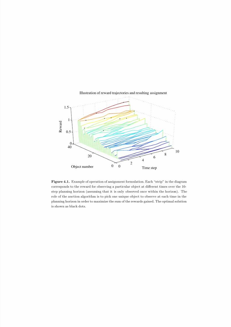
8/2/2019 Information Theoretic Sensor Management
http://slidepdf.com/reader/full/information-theoretic-sensor-management 115/203
02
46
810
0
20
400
0.5
1
1.5
Time step
Illustration of reward trajectories and resulting assignment
Object number
R e w a r d
Figure 4.1. Example of operation of assignment formulation. Each “strip” in the diagram
corresponds to the reward for observing a particular object at different times over the 10-
step planning horizon (assuming that it is only observed once within the horizon). The
role of the auction algorithm is to pick one unique object to observe at each time in the
planning horizon in order to maximize the sum of the rewards gained. The optimal solution
is shown as black dots.

8/2/2019 Information Theoretic Sensor Management
http://slidepdf.com/reader/full/information-theoretic-sensor-management 116/203
116 CHAPTER 4. INDEPENDENT OBJECTS AND INTEGER PROGRAMMING
One can gain an intuition for this formulation from the diagram in Fig. 4.1. The
rewards correspond to a snapshot of the scenario discussed in Section 4.1.3. The sce-
nario considers the problem of object tracking when probability of detection varies withposition. The diagram illustrates the trade-off which the auction algorithm performs:
rather than taking the highest reward observation at the first time (as the greedy heuris-
tic would do), the controller defers measurement of that object until a later time when
a more valuable observation is available. Instead, it measures at the first time an ob-
ject with comparatively lower reward value, but one for which the observations at later
times are still less valuable.
4.1.3 Example
The approach was tested on a tracking scenario in which a single sensor is used tosimultaneously track 20 objects. The state of object i at time k, xi
k, consists of position
and velocity in two dimensions. The state evolves according to a linear Gaussian model:
xik+1 = Fxi
k + wik (4.8)
where wik ∼ N{wi
k; 0, Q} is a white Gaussian noise process. F and Q are set as:
F =
1 T 0 0
0 1 0 0
0 0 1 T
0 0 0 1
; Q = q
T 3
3T 2
2 0 0T 2
2 T 0 0
0 0 T 3
3T 2
2
0 0 T 22 T
(4.9)
The diffusion strength q is set to 0.01. The sensor can be used to observe any one of the
M objects in each time step. The measurement obtained from observing object uk with
the sensor consists of a detection flag dukk ∈ {0, 1} and, if duk
k = 1, a linear Gaussian
measurement of the position, zukk :
zukk = Hx
ukk + v
ukk (4.10)
where vukk ∼ N{vuk
k ; 0, R} is a white Gaussian noise process, independent of wukk . H
and R are set as:H =
1 0 0 0
0 0 1 0
; R =
5 0
0 5
(4.11)
The probability of detection P dukk |xukk
(1|xukk ) is a function of object position. The
function is randomly generated for each Monte Carlo simulation; an example of the

8/2/2019 Information Theoretic Sensor Management
http://slidepdf.com/reader/full/information-theoretic-sensor-management 117/203
x position
y
p o s i t i o n
Probability of detection
200 400 600
100
200
300
400
500
600
700 0
0.2
0.4
0.6
0.8
1
Figure 4.2. Example of randomly generated detection map. The color intensity indicates
the probability of detection at each x and y position in the region.
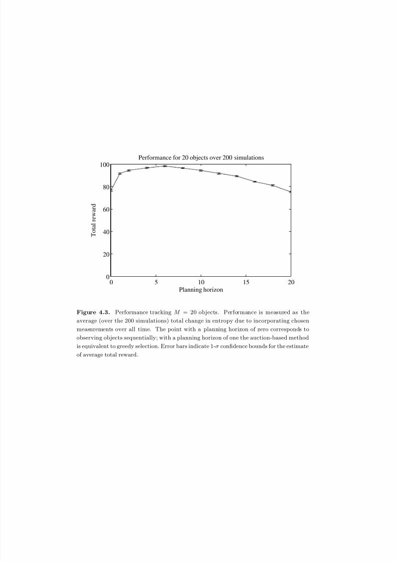
8/2/2019 Information Theoretic Sensor Management
http://slidepdf.com/reader/full/information-theoretic-sensor-management 118/203
0 5 10 15 200
20
40
60
80
100
Planning horizon
T o t a l r e w a r d
Performance for 20 objects over 200 simulations
Figure 4.3. Performance tracking M = 20 objects. Performance is measured as the
average (over the 200 simulations) total change in entropy due to incorporating chosen
measurements over all time. The point with a planning horizon of zero corresponds to
observing objects sequentially; with a planning horizon of one the auction-based method
is equivalent to greedy selection. Error bars indicate 1-σ confidence bounds for the estimate
of average total reward.
8/2/2019 Information Theoretic Sensor Management
http://slidepdf.com/reader/full/information-theoretic-sensor-management 119/203
Sec. 4.2. Integer programming generalization 119
function is illustrated in Fig. 4.2. The function may be viewed as an obscuration map,
e.g. due to foliage. Estimation is performed using the Gaussian particle filter [45].
The performance over 200 Monte Carlo runs is illustrated in Fig. 4.3. The pointwith a planning horizon of zero corresponds to a raster, in which objects are observed
sequentially. With a planning horizon of one, the auction-based algorithm corresponds
to greedy selection. The performance is measured as the average (over the 200 sim-
ulations) total change in entropy due to incorporating chosen measurements over all
time. The diagram demonstrates that, with the right choice of planning horizon, the
assignment formulation is able to improve performance over the greedy method. The
reduction in performance for longer planning horizons is a consequence of the restriction
to observe each object at most once in the horizon. If the planning horizon is on the
order of the number of objects, we are then, in effect, enforcing that each object must
be observed once. As illustrated in Fig. 4.1, in this scenario there will often be objects
receiving low reward values throughout the planning interval, hence by forcing the con-
troller to observe each object, we are forcing it to (at some stage) take observations
of little value. It is not surprising that the increase in performance above the greedy
heuristic is small, since the performance guarantees discussed in the previous chapter
apply to this scenario.
These limitations motivate the generalization explored in the following section,
which allows us to admit multiple observations of each object, as well as observations
that require different durations to complete (note that the performance guarantees of
Chapter 3 require all observations to consume a single time slot, hence they are not
applicable to this wider class of problems).
4.2 Integer programming generalization
An abstraction of the previous analysis replaces the discrete time slots {1, . . . , N } with
a set of available resources, R (assumed finite), the elements of which may correspond
to the use of a particular sensor over a particular interval of time. As in the previous
section, each element of R can be assigned to at most one task. Unlike the previous
section and the previous chapter, the formulation in this section allows us to accom-
modate observations which consume multiple resources (e.g., multiple time slots on the
same sensor, or the same time slot on multiple sensors). We also relax the constraint
that each object may be observed at most once, and utilize a more advanced integer
programming formulation to find an efficient solution.

8/2/2019 Information Theoretic Sensor Management
http://slidepdf.com/reader/full/information-theoretic-sensor-management 120/203
120 CHAPTER 4. INDEPENDENT OBJECTS AND INTEGER PROGRAMMING
4.2.1 Observation sets
Let
U i =
{ui1, . . . , ui
Li
}be the set of elemental observation actions (assumed finite) that
may be used for object i, where each elemental observation ui j corresponds to observing
object i using a particular mode of a particular sensor within a particular period of
time. An elemental action may occupy multiple resources; let t(ui j) ⊆ R be the subset
of resource indices consumed by the elemental observation action ui j. Let S i ⊆ 2 U
ibe
the collection of observation subsets which we allow for object i. This is assumed to
take the form of Eq. (4.12), (4.13) or (4.14); note that in each case it is an independence
system, though not necessarily a matroid (as defined in Section 2.4), since observations
may consume different resource quantities. If we do not limit the sensing resources that
are allowed to be used for object i, the collection will consist of all subsets of U i for
which no two elements consume the same resource:
S i = {A ⊆ U i|t(u1)∩t(u2) = ∅ ∀ u1, u2 ∈ A} (4.12)
Alternatively we may limit the total number of elemental observations allowed to be
taken for object i to ki:
S i = {A ⊆ U i|t(u1)∩t(u2) = ∅ ∀ u1, u2 ∈ A, |A| ≤ ki} (4.13)
or limit the total quantity of resources allowed to be consumed for object i to Ri:
S i =A ⊆ U i t(u1)∩t(u2) = ∅ ∀ u1, u2 ∈ A,
u∈A
|t(u)| ≤ Ri
(4.14)
We denote by t(A) ⊆ R the set of resources consumed by the actions in set A, i.e.,
t(A) =
u∈A
t(u)
The problem that we seek to solve is that of selecting the set of observation actions
for each object such that the total reward is maximized subject to the constraint that
each resource can be used at most once.
4.2.2 Integer programming formulation
The optimization problem that we seek to solve is reminiscent of the assignment problem
in Eq. (4.7), except that now we are assigning to each object a set of observations, rather
8/2/2019 Information Theoretic Sensor Management
http://slidepdf.com/reader/full/information-theoretic-sensor-management 121/203
Sec. 4.2. Integer programming generalization 121
than a single observation:
maxωiAi
M i=1
Ai∈S i
riAiωiAi (4.15a)
s.t.M i=1
Ai∈S i
t∈t(Ai)
ωiAi ≤ 1 ∀ t ∈ R (4.15b)
Ai∈S i
ωiAi = 1 ∀ i ∈ {1, . . . , M } (4.15c)
ωiAi ∈ {0, 1} ∀ i, Ai ∈ S i (4.15d)
Again, the binary indicator variables ωiAi are 1 if the observation set
Ai is chosen and
0 otherwise. The interpretation of each line of the integer program follows.
• The objective in Eq. (4.15a) is the sum of the rewards of the subset selected for
each object i (i.e., the subsets for which ωiAi = 1).
• The constraints in Eq. (4.15b) ensure that each resource (e.g., sensor time slot)
is used at most once.
• The constraints in Eq. (4.15c) ensure that exactly one observation set is chosen
for any given object. This is necessary to ensure that the additive ob jective is the
exact reward of corresponding selection (since, in general, ri
A∪B = ri
A + ri
B). Notethat the constraint does not force us to take an observation of any object, since
the empty observation set is allowed (∅ ∈S i) for each object i.
• The integrality constraints in Eq. (4.15d) ensure that the selection variables take
on the values zero (not selected) or one (selected).
Unlike the formulation in Eq. (4.7), the integrality constraints in Eq. (4.15d) can-
not be relaxed. The problem is not a pure assignment problem, as the observation
subsets Ai ∈ S i consume multiple resources and hence appear in more than one of
the constraints defined by Eq. (4.15b). The problem is a bundle assignment problem,and conceptually could be addressed using combinatorial auction methods (e.g., [79]).
However, generally this would require computation of riAi for every subset Ai ∈ S i. If
the collections of observation sets S i, i ∈ {1, . . . , M } allow for several observations to
be taken of the same object, the number of subsets may be combinatorially large.
8/2/2019 Information Theoretic Sensor Management
http://slidepdf.com/reader/full/information-theoretic-sensor-management 122/203
122 CHAPTER 4. INDEPENDENT OBJECTS AND INTEGER PROGRAMMING
Our approach exploits submodularity to solve a sequence of integer programs, each
of which represents the subsets available through a compact representation. The solu-
tion of the integer program in each iteration provides an upper bound to the optimalreward, which becomes increasingly tight as iterations progress. The case in which
all observations are equivalent, such that the only decision is to determine how many
observations to select for each object, could be addressed using [ 5]. In this thesis, we
address the general case which arises when observations are heterogeneous and require
different subsets of resources (e.g., different time durations). The complexity associated
with evaluating the reward of each of an exponentially large collection of observation
sets can be ameliorated using a constraint generation approach, as described in the
following section.
4.3 Constraint generation approach
The previous section described a formulation which conceptually could be used to find
the optimal observation selection, but the computational complexity of the formulation
precludes its utility. This section details an algorithm that can be used to efficiently
solve the integer program in many practical situations. The method proceeds by se-
quentially solving a series of integer programs with progressively greater complexity. In
the limit, we arrive at the full complexity of the integer program in Eq. (4.15), but in
many practical situations it is possible to terminate much sooner with an optimal (or
near-optimal) solution.The formulation may be conceptually understood as dividing the collection of sub-
sets for each object (S i) at iteration l into two collections: T il ⊆ S i and the remainder
S i\T il . The subsets in T il are those for which the exact reward has been evaluated;
we will refer to these as candidate subsets.
Definition 4.1 (candidate subset). The collection of candidate subsets, T il ⊆ S i,
is the collection subsets of observations for object i for which the exact reward has
been evaluated prior to iteration l. New subsets are added to the collection at each
iteration (and their rewards calculated), so that T il ⊆ T il+1 for all l. We commence
with T i
l = {∅}.
The reward of each of the remaining subsets (i.e., those in S i\T il ) has not been
evaluated, but an upper bound to each reward is available. In practice, we will not
explicitly enumerate the elements in S i\T il ; rather we use a compact representation
which obtains upper bounds through submodularity (details of this will be given later
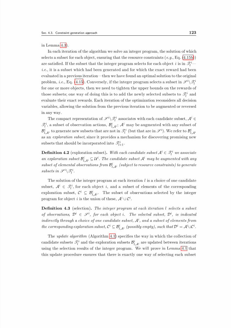
8/2/2019 Information Theoretic Sensor Management
http://slidepdf.com/reader/full/information-theoretic-sensor-management 123/203
Sec. 4.3. Constraint generation approach 123
in Lemma 4.3).
In each iteration of the algorithm we solve an integer program, the solution of which
selects a subset for each object, ensuring that the resource constraints (e.g., Eq. (4.15b))are satisfied. If the subset that the integer program selects for each object i is in T il —
i.e., it is a subset which had been generated and for which the exact reward had been
evaluated in a previous iteration—then we have found an optimal solution to the original
problem, i.e., Eq. (4.15). Conversely, if the integer program selects a subset in S i\T ilfor one or more objects, then we need to tighten the upper bounds on the rewards of
those subsets; one way of doing this is to add the newly selected subsets to T il and
evaluate their exact rewards. Each iteration of the optimization reconsiders all decision
variables, allowing the solution from the previous iteration to be augmented or reversed
in any way.
The compact representation of S i\T il associates with each candidate subset, Ai ∈T il , a subset of observation actions, Bi
l,Ai ; Ai may be augmented with any subset of
Bil,Ai to generate new subsets that are not in T il (but that are in S i). We refer to Bi
l,Ai
as an exploration subset , since it provides a mechanism for discovering promising new
subsets that should be incorporated into T il+1.
Definition 4.2 (exploration subset). With each candidate subset Ai ∈ T il we associate
an exploration subset Bil,Ai ⊆ U i. The candidate subset Ai may be augmented with any
subset of elemental observations from Bil,Ai (subject to resource constraints) to generate
subsets in S i\T
i
l .
The solution of the integer program at each iteration l is a choice of one candidate
subset, Ai ∈ T il , for each object i, and a subset of elements of the corresponding
exploration subset, Ci ⊆ Bil,Ai . The subset of observations selected by the integer
program for object i is the union of these, Ai ∪ Ci.
Definition 4.3 (selection). The integer program at each iteration l selects a subset
of observations, Di ∈ S i, for each object i. The selected subset, Di, is indicated
indirectly through a choice of one candidate subset, Ai, and a subset of elements from
the corresponding exploration subset,C
i
⊆ Bi
l,Ai (possibly empty), such that
Di =
Ai
∪Ci.
The update algorithm (Algorithm 4.1) specifies the way in which the collection of
candidate subsets T il and the exploration subsets Bil,Ai are updated between iterations
using the selection results of the integer program. We will prove in Lemma 4.1 that
this update procedure ensures that there is exactly one way of selecting each subset
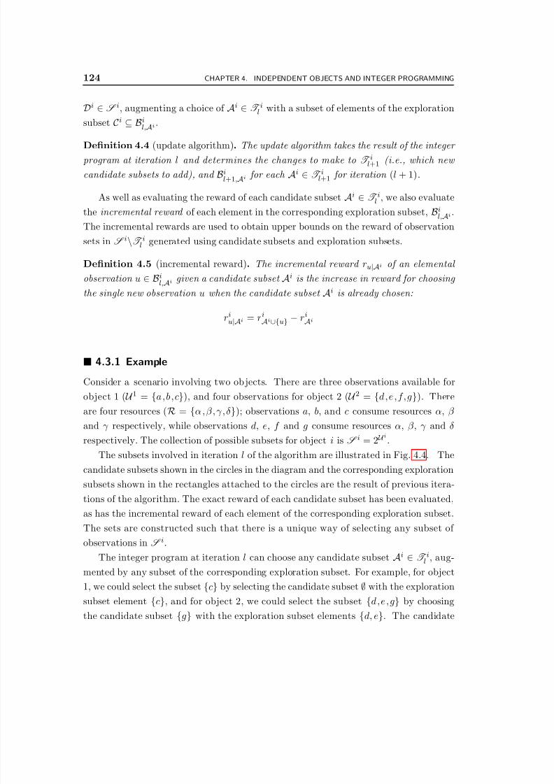
8/2/2019 Information Theoretic Sensor Management
http://slidepdf.com/reader/full/information-theoretic-sensor-management 124/203
124 CHAPTER 4. INDEPENDENT OBJECTS AND INTEGER PROGRAMMING
Di ∈ S i, augmenting a choice of Ai ∈ T il with a subset of elements of the exploration
subset Ci ⊆ Bil,Ai .
Definition 4.4 (update algorithm). The update algorithm takes the result of the integer
program at iteration l and determines the changes to make to T il+1 (i.e., which new
candidate subsets to add), and Bil+1,Ai for each Ai ∈ T il+1 for iteration (l + 1).
As well as evaluating the reward of each candidate subset Ai ∈ T il , we also evaluate
the incremental reward of each element in the corresponding exploration subset, Bil,Ai .
The incremental rewards are used to obtain upper bounds on the reward of observation
sets in S i\T il generated using candidate subsets and exploration subsets.
Definition 4.5 (incremental reward). The incremental reward ru|Ai of an elemental
observation u ∈ Bil,Ai given a candidate subset Ai is the increase in reward for choosing
the single new observation u when the candidate subset Ai is already chosen:
riu|Ai = ri
Ai∪{u} − riAi
4.3.1 Example
Consider a scenario involving two ob jects. There are three observations available for
object 1 ( U 1 = {a,b,c}), and four observations for object 2 ( U 2 = {d,e,f,g}). There
are four resources (R = {α ,β ,γ ,δ}); observations a, b, and c consume resources α, β and γ respectively, while observations d, e, f and g consume resources α, β , γ and δ
respectively. The collection of possible subsets for object i is S i = 2 U i.
The subsets involved in iteration l of the algorithm are illustrated in Fig. 4.4. The
candidate subsets shown in the circles in the diagram and the corresponding exploration
subsets shown in the rectangles attached to the circles are the result of previous itera-
tions of the algorithm. The exact reward of each candidate subset has been evaluated,
as has the incremental reward of each element of the corresponding exploration subset.
The sets are constructed such that there is a unique way of selecting any subset of
observations in S i.
The integer program at iteration l can choose any candidate subset Ai ∈ T il , aug-
mented by any subset of the corresponding exploration subset. For example, for object
1, we could select the subset {c} by selecting the candidate subset ∅ with the exploration
subset element {c}, and for object 2, we could select the subset {d,e,g} by choosing
the candidate subset {g} with the exploration subset elements {d, e}. The candidate
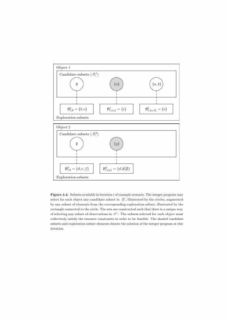
8/2/2019 Information Theoretic Sensor Management
http://slidepdf.com/reader/full/information-theoretic-sensor-management 125/203
B2
l,{g} = {d,e,f }B2
l,∅ = {d,e,f }
∅ {g}
Object 2
Candidate subsets (T 2
l )
B1
l,{a,b} = {c}B1
l,{a} = {c}B1
l,∅ = {b, c}
∅ {a} {a, b}
Object 1
Candidate subsets (T 1
l )
Exploration subsets
Exploration subsets
Figure 4.4. Subsets available in iteration l of example scenario. The integer program may
select for each object any candidate subset in T il , illustrated by the circles, augmented
by any subset of elements from the corresponding exploration subset, illustrated by the
rectangle connected to the circle. The sets are constructed such that there is a unique way
of selecting any subset of observations in S i. The subsets selected for each ob ject must
collectively satisfy the resource constraints in order to be feasible. The shaded candidate
subsets and exploration subset elements denote the solution of the integer program at thisiteration.

8/2/2019 Information Theoretic Sensor Management
http://slidepdf.com/reader/full/information-theoretic-sensor-management 126/203
126 CHAPTER 4. INDEPENDENT OBJECTS AND INTEGER PROGRAMMING
subsets and exploration subsets are generated using an update algorithm which ensures
that there is exactly one way of selecting each subset; e.g., to select the set {a, c} for
object 1, we must choose candidate subset {a} and exploration subset element c; wecannot select candidate subset ∅ with exploration subset elements {a, c} since a /∈ B1
l,∅.
We now demonstrate the operation of the update algorithm that is described in
detail in Section 4.3.3. Suppose that the solution of the integer program at iteration
l selects subset {a} for object 1, and subset {e ,f ,g} for object 2 (i.e., the candidate
subsets and exploration subset elements that are shaded in Fig. 4.4). Since {a} ∈ T 1lthe exact reward of the subset selected for object 1 has already been evaluated and we
do not need to modify the candidate subsets for object 1, so we simply set T 1l+1 = T 1l .
For object 2, we find that {e ,f ,g} /∈ T 2l , so an update is required. There are many
ways that this update could be performed. Our method (Algorithm 4.1) creates a new
candidate subset A consisting of the candidate subset selected for the object ({g}),
augmented by the single element (out of the selected exploration subset elements) with
the highest incremental reward. Suppose in our case that the reward of the subset {e, g}is greater than the reward of {f, g}; then A = {e, g}.
The subsets in iteration (l + 1) are illustrated in Fig. 4.5. The sets that were
modified in the update are shaded in the diagram. There remains a unique way of
selecting each subset of observations; e.g., the only way to select elements g and e
together (for object 2) is to select the new candidate subset {e, g}, since element e
was removed from the exploration subset for candidate subset
{g
}(i.e.,
B2l+1,{g}). The
procedure that assuring that this is always the case is part of the algorithm which we
describe in Section 4.3.3.
4.3.2 Formulation of the integer program in each iteration
The collection of candidate subsets at stage l of the solution is denoted by T il ⊆ S i,
while the exploration subset corresponding to candidate subset Ai ∈ T il is denoted by
Bil,Ai ⊆ U i. To initialize the problem, we select T i0 = {∅}, and Bi
0,∅ = U i for all i. The

8/2/2019 Information Theoretic Sensor Management
http://slidepdf.com/reader/full/information-theoretic-sensor-management 127/203
B2l+1,{e,g} = {d, f }B2l+1,{g} = {d, f }B2l+1,∅ = {d, e, f }
∅ {g} {e, g}
Object 2
Candidate subsets (T 2l+1)
B1l+1,{a,b} = {c}B1l+1,{a} = {c}B1l+1,∅ = {b, c}
∅ {a} {a, b}
Object 1
Candidate subsets (T 1l+1)
Exploration subsets
Exploration subsets
Figure 4.5. Subsets available in iteration (l + 1) of example scenario. The subsets that
were modified in the update between iterations l and (l + 1) are shaded. There remains a
unique way of selecting each subset of observations; e.g., the only way to select elements
g and e together (for object 2) is to select the new candidate subset {e, g}, since element
e was removed from the exploration subset for candidate subset {g} (i.e., B2l+1,{g}).

8/2/2019 Information Theoretic Sensor Management
http://slidepdf.com/reader/full/information-theoretic-sensor-management 128/203
128 CHAPTER 4. INDEPENDENT OBJECTS AND INTEGER PROGRAMMING
integer program that we solve at each stage is:
maxωiAi
, ωiu|Ai
M i=1
Ai∈T i
l
riAiω
iAi +
u∈Bil,Ai
riu|Aiω
iu|Ai
(4.16a)
s.t.M i=1
Ai∈T ilt∈t(Ai)
ωiAi +
M i=1
Ai∈T il
u∈Bi
l,Ai
t∈t(u)
ωiu|Ai ≤ 1 ∀ t ∈ R (4.16b)
Ai∈T i
ωiAi = 1 ∀ i ∈ {1, . . . , M } (4.16c)
u∈Bi
l,Ai
ωiu|Ai − |Bi
l,Ai |ωiAi ≤ 0 ∀ i, Ai ∈ T il (4.16d)
ωiAi ∈ {0, 1} ∀ i, Ai ∈ T i (4.16e)
ωiu|Ai ∈ {0, 1} ∀ i, Ai ∈ T i, u ∈ Bi
l,Ai (4.16f)
If there is a cardinality constraint of the form of Eq. (4.13) on the maximum number of
elemental observations allowed to be used on any given object, we add the constraints:
Ai∈T il
|Ai|ωi
Ai +
u∈Bil,Ai
ωiu|Ai
≤ ki ∀ i ∈ {1, . . . , M } (4.16g)
Alternatively, if there is a constraint of the form of Eq. (4.14) on the maximum number
of elements of the resource set R allowed to be utilized on any given object, we add the
constraints:
Ai∈T il
t(Ai)ωi
Ai +
u∈Bil,Ai
t(u)ωiu|Ai
≤ Ri ∀ i ∈ {1, . . . , M } (4.16h)
The selection variable ωiAi indicates whether candidate subset Ai ∈ T il is chosen; the
constraint in Eq. (4.16c) guarantees that exactly one candidate subset is chosen for each
object. The selection variables ωiu|Ai indicate the elements of the exploration subset
corresponding to Ai that are being used to augment the candidate subset. All selection
variables are either zero (not selected) or one (selected) due to the integrality constraints
in Eq. (4.16e) and Eq. (4.16f ). In accordance with Definition 4.3, the solution of the
integer program selects for each object i a subset of observations:

8/2/2019 Information Theoretic Sensor Management
http://slidepdf.com/reader/full/information-theoretic-sensor-management 129/203
Sec. 4.3. Constraint generation approach 129
Definition 4.6 (selection variables). The values of the selection variables, ωiAi, ωi
u|Ai
determine the subsets selected for each object i. The subset selected for object i is
Di = Ai ∪ Ci where Ai is the candidate subset for object i such that ωiAi = 1 and Ci = {u ∈ Bi
l,Ai |ωiu|Ai = 1}.
The objective and constraints in Eq. (4.16) may be interpreted as follows:
• The objective in Eq. (4.16a) is the sum of the reward for the candidate subset
selected for each object, plus the incremental rewards of any exploration subset
elements that are selected. As per Definition 4.5, the reward increment riu|Ai =
(riAi∪{u} − ri
Ai) represents the additional reward for selecting the elemental action
u given that the candidate subset Ai has been selected. We will see in Lemma 4.3
that, due to submodularity, the sum of the reward increments u riu|Ai is an
upper bound for the additional reward obtained for selecting those elements given
that the candidate set Ai has been selected.1
• The constraint in Eq. (4.16b) dictates that each resource can only be used once,
either by a candidate subset or an exploration subset element; this is analogous
with Eq. (4.15b) in the original formulation. The first term includes all candidate
subsets that consume resource t, while the second includes all exploration subset
elements that consume resource t.
• The constraint in Eq. (4.16c) specifies that exactly one candidate subset should
be selected per object. At each solution stage, there will be a candidate subsetcorresponding to taking no observations (Ai = ∅), hence this does not force the
system to take an observation of any given object.
• The constraint in Eq. (4.16d) specifies that exploration subset elements which
correspond to a given candidate subset can only be chosen if that candidate subset
is chosen.
• The integrality constraints in Eq. (4.16e) and Eq. (4.16f ) require each variable to
be either zero (not selected) or one (selected).
Again, the integrality constraints cannot be relaxed—the problem is not an assign-ment problem since candidate subsets may consume multiple resources, and there are
side constraints (Eq. (4.16d)).
1Actually, the reward for selecting a candidate subset and one exploration subset variable is a exact
reward value; the reward for selecting a candidate subset and two or more exploration subset variables
is an upper bound.

8/2/2019 Information Theoretic Sensor Management
http://slidepdf.com/reader/full/information-theoretic-sensor-management 130/203
130 CHAPTER 4. INDEPENDENT OBJECTS AND INTEGER PROGRAMMING
4.3.3 Iterative algorithm
Algorithm 4.1 describes the iterative manner in which the integer program in Eq. (4.16)
is applied:
T i0 = ∅ ∀ i; Bi0,∅ = U i ∀ i; l = 01
evaluate riu|∅ ∀ i, u ∈ Bi
0,∅2
solve problem in Eq. (4.16)3
while ∃ i Ai such that
u∈Bil,Ai
ωiu|Ai > 1 do
4
for i ∈ {1, . . . , M } do5
let Ail be the unique subset such that ωi
Ail
= 16
if u∈Bi
l,Ail
ωi
u|˚A
i
l ≤1 then
7
T il+1 = T il8
Bil+1,Ai = Bi
l,Ai ∀ Ai ∈ T il9
else10
let uil = arg maxu∈Bi
l,Ail
riu|Ai
l11
let Ail = Ai
l ∪ {uil}12
T il+1 = T il ∪ {Ail}13
Bil+1,Ai
l
= Bil,Ai
l
\{uil}\{u ∈ Bi
l,Ail
|Ail ∪ {u} /∈ S i}
14
evaluate riAil
= riAil
+ riu|Ai
l15
evaluate riu|Ai
l
∀ u ∈ Bil+1,Ai
l16
Bil+1,Ai
l
= Bil,Ai
l
\{uil}17
Bil+1,Ai = Bi
l,Ai ∀ Ai ∈ T il , Ai = Ail18
end19
end20
l = l + 121
re-solve problem in Eq. (4.16)22
end23
Algorithm 4.1: Constraint generation algorithm which iteratively utilizes
Eq. (4.16) to solve Eq. (4.15).
• In each iteration (l) of the algorithm, the integer program in Eq. (4.16) is re-solved.
8/2/2019 Information Theoretic Sensor Management
http://slidepdf.com/reader/full/information-theoretic-sensor-management 131/203
Sec. 4.3. Constraint generation approach 131
If no more than one exploration subset element is chosen for each object, then the
rewards of all subsets selected correspond to the exact values (as opposed to upper
bounds), the optimal solution has been found (as we will show in Theorem 4.1),and the algorithm terminates; otherwise another iteration of the “while” loop
(line 4 of Algorithm 4.1) is executed.
• Each iteration of the “while” loop considers decisions corresponding to each object
(i) in turn: (the for loop in line 4)
– If no more than one exploration subset element is chosen for object i then
the reward for that object is an exact value rather than an upper bound, so
the collection of candidate subsets (T il ) and the exploration subsets (Bil,Ai)
remain unchanged for that object in the following iteration (lines 8–9).– If more than one exploration subset element has been chosen for a given
object, then the reward obtained by the integer program for that object is
an upper bound to the exact reward (as we show in Lemma 4.3). Thus we
generate an additional candidate subset (Ail) which augments the previously
chosen candidate subset (Ail) with the exploration subset element with the
highest reward increment (uil) (lines 11–13). This greedy exploration is anal-
ogous to the greedy heuristic discussed in Chapter 3. Here, rather than using
it to make greedy action choices (which would result in loss of optimality),
we use it to decide which portion of the action space to explore first. As wewill see in Theorem 4.1, this scheme maintains a guarantee of optimality if
allowed to run to termination.
– Exploration subsets allow us to select any subset of observations for which the
exact reward has not yet been calculated, using an upper bound to the exact
reward. Obviously we want to preclude selection of a candidate subset along
with additional exploration subset elements to construct a subset for which
the exact reward has already been calculated; the updates of the exploration
subsets in lines 14 and 17 achieve this, as shown in Lemma 4.1.
4.3.4 Example
Suppose that there are three objects (numbered {1, 2, 3}) and three resources (R =
{α ,β ,γ }), and that the reward of the various observation subsets are as shown in
Table 4.1. We commence with a single empty candidate subset for each object (T i0 =
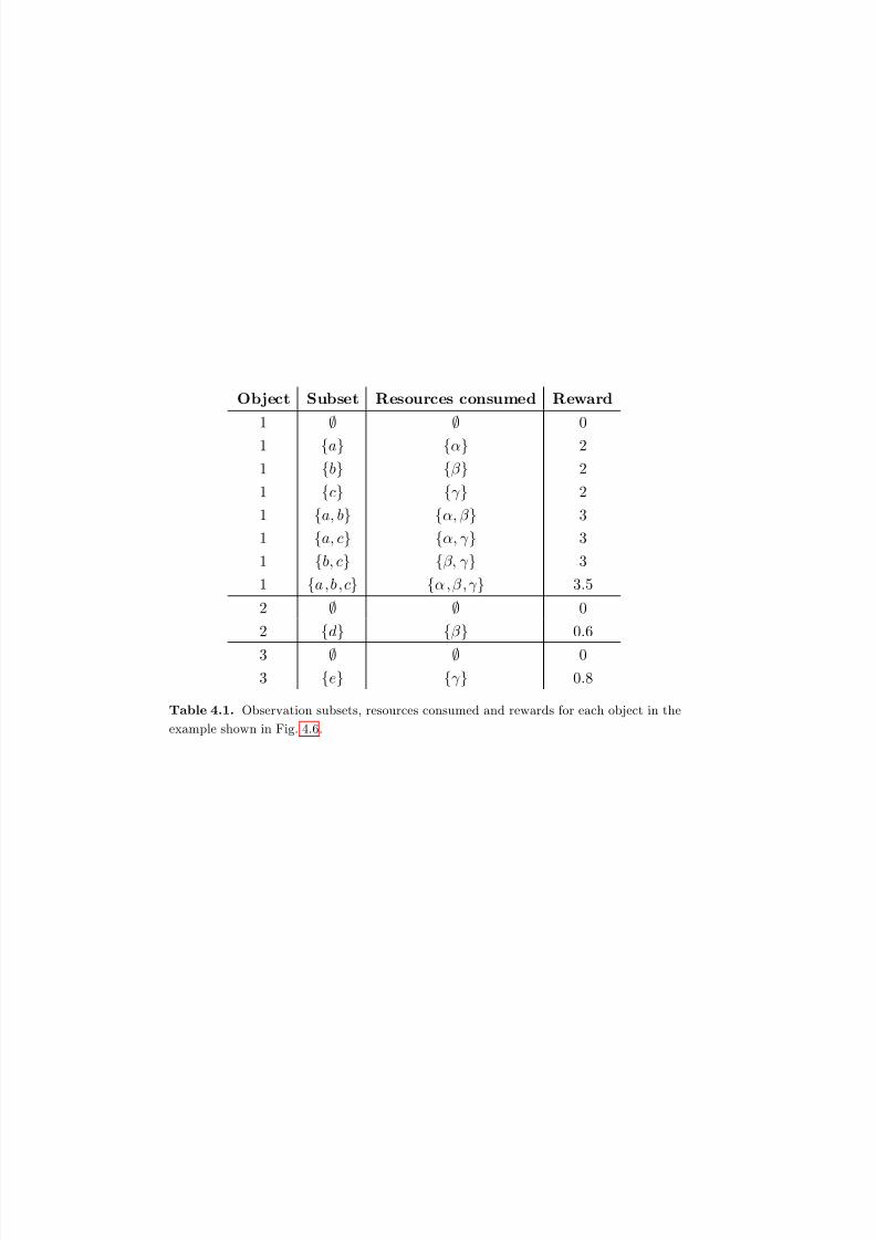
8/2/2019 Information Theoretic Sensor Management
http://slidepdf.com/reader/full/information-theoretic-sensor-management 132/203
Object Subset Resources consumed Reward
1∅ ∅
0
1 {a} {α} 2
1 {b} {β } 2
1 {c} {γ } 2
1 {a, b} {α, β } 3
1 {a, c} {α, γ } 3
1 {b, c} {β, γ } 3
1 {a,b,c} {α ,β ,γ } 3.5
2 ∅ ∅ 0
2 {d} {β } 0.6
3 ∅ ∅ 03 {e} {γ } 0.8
Table 4.1. Observation subsets, resources consumed and rewards for each object in the
example shown in Fig. 4.6.
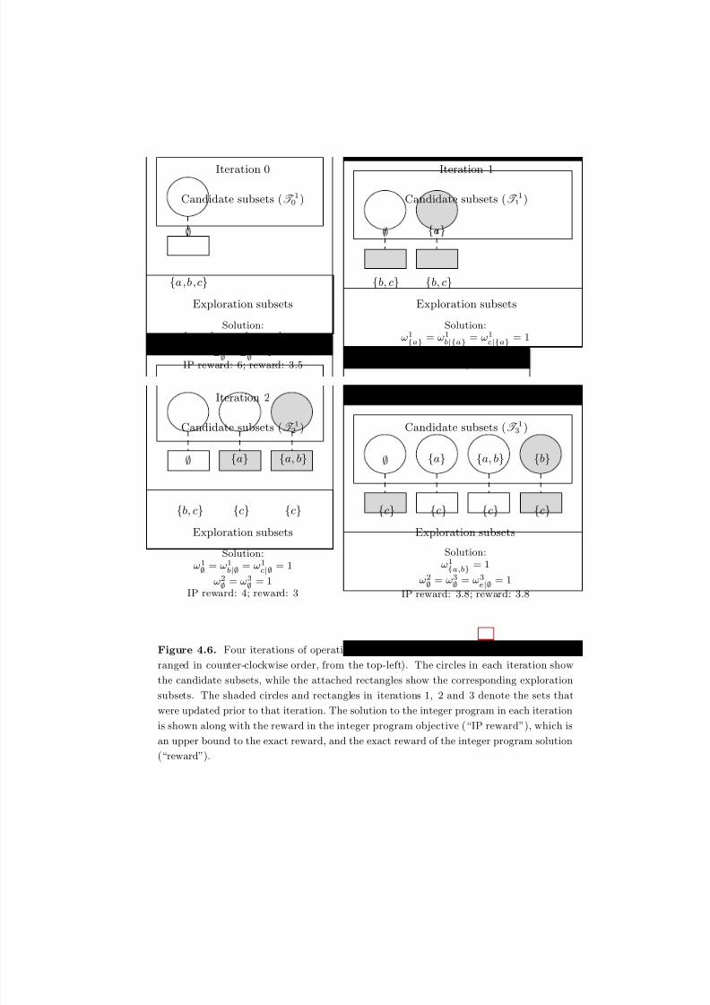
8/2/2019 Information Theoretic Sensor Management
http://slidepdf.com/reader/full/information-theoretic-sensor-management 133/203
{a,b,c}
∅
Iteration 0
Candidate subsets (T 1
0 )
Exploration subsets
{b, c}
∅
Candidate subsets (T 1
1 )
{b, c}
{a}
{b, c}
∅
Candidate subsets (T 1
2 )
Exploration subsets
{c}
{a}
{c}
{a, b}
Solution:
ω1
∅= ω
1
a|∅= ω
1
b|∅= ω
1
c|∅= 1
ω2∅ = ω3∅ = 1IP reward: 6; reward: 3.5
Exploration subsets
{c}
∅
Candidate subsets (T 1
3 )
Exploration subsets
{c}
{a}
{c}
{a, b}
{c}
{b}
Iteration 1
Iteration 2 Iteration 3
Solution:
ω1
{a}= ω
1
b|{a}= ω
1
c|{a}= 1
ω2∅ = ω3∅ = 1IP reward: 4; reward: 3.5
Solution:
ω1
∅= ω
1
b|∅= ω
1
c|∅= 1
ω2
∅= ω
3
∅= 1
IP reward: 4; reward: 3
Solution:
ω1
{a,b}= 1
ω2
= ω
3
= ω
3
e= 1
IP reward: 3.8; reward: 3.8
Figure 4.6. Four iterations of operations performed by Algorithm 4.1 on object 1 (ar-
ranged in counter-clockwise order, from the top-left). The circles in each iteration show
the candidate subsets, while the attached rectangles show the corresponding exploration
subsets. The shaded circles and rectangles in iterations 1, 2 and 3 denote the sets that
were updated prior to that iteration. The solution to the integer program in each iteration
is shown along with the reward in the integer program objective (“IP reward”), which is
an upper bound to the exact reward, and the exact reward of the integer program solution
(“reward”).
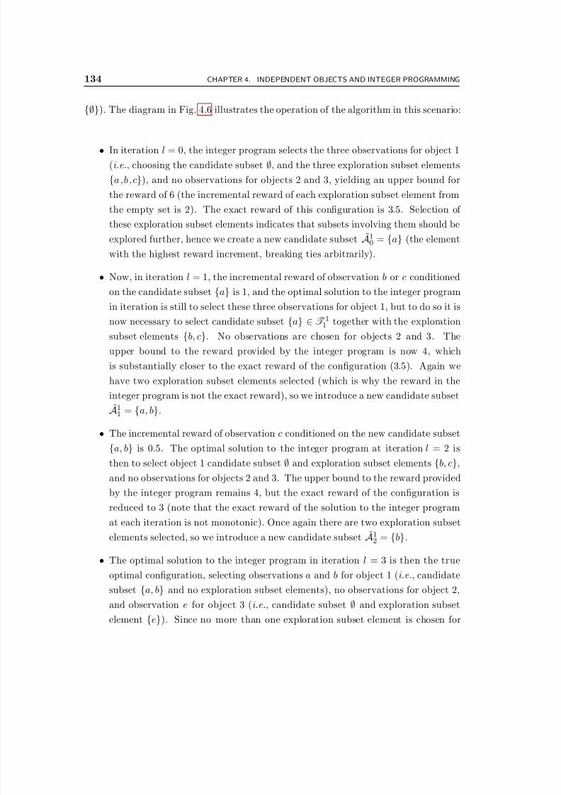
8/2/2019 Information Theoretic Sensor Management
http://slidepdf.com/reader/full/information-theoretic-sensor-management 134/203
134 CHAPTER 4. INDEPENDENT OBJECTS AND INTEGER PROGRAMMING
{∅}). The diagram in Fig. 4.6 illustrates the operation of the algorithm in this scenario:
• In iteration l = 0, the integer program selects the three observations for object 1
(i.e., choosing the candidate subset ∅, and the three exploration subset elements
{a,b,c}), and no observations for objects 2 and 3, yielding an upper bound for
the reward of 6 (the incremental reward of each exploration subset element from
the empty set is 2). The exact reward of this configuration is 3.5. Selection of
these exploration subset elements indicates that subsets involving them should be
explored further, hence we create a new candidate subset A10 = {a} (the element
with the highest reward increment, breaking ties arbitrarily).
• Now, in iteration l = 1, the incremental reward of observation b or c conditionedon the candidate subset {a} is 1, and the optimal solution to the integer program
in iteration is still to select these three observations for object 1, but to do so it is
now necessary to select candidate subset {a} ∈T 11 together with the exploration
subset elements {b, c}. No observations are chosen for objects 2 and 3. The
upper bound to the reward provided by the integer program is now 4, which
is substantially closer to the exact reward of the configuration (3.5). Again we
have two exploration subset elements selected (which is why the reward in the
integer program is not the exact reward), so we introduce a new candidate subset˜
A1
1
={
a, b}
.
• The incremental reward of observation c conditioned on the new candidate subset
{a, b} is 0.5. The optimal solution to the integer program at iteration l = 2 is
then to select object 1 candidate subset ∅ and exploration subset elements {b, c},
and no observations for objects 2 and 3. The upper bound to the reward provided
by the integer program remains 4, but the exact reward of the configuration is
reduced to 3 (note that the exact reward of the solution to the integer program
at each iteration is not monotonic). Once again there are two exploration subset
elements selected, so we introduce a new candidate subset A12 = {b}.
• The optimal solution to the integer program in iteration l = 3 is then the true
optimal configuration, selecting observations a and b for object 1 (i.e., candidate
subset {a, b} and no exploration subset elements), no observations for object 2,
and observation e for object 3 (i.e., candidate subset ∅ and exploration subset
element {e}). Since no more than one exploration subset element is chosen for

8/2/2019 Information Theoretic Sensor Management
http://slidepdf.com/reader/full/information-theoretic-sensor-management 135/203
Sec. 4.3. Constraint generation approach 135
each object, the algorithm knows that it has found the optimal solution and thus
terminates.
4.3.5 Theoretical characteristics
We are now ready to prove a number of theoretical characteristics of our algorithm. Our
goal is to prove that the algorithm terminates in finite time with an optimal solution;
Theorem 4.1 establishes this result. Several intermediate results are obtained along the
way. Lemma 4.1 proves that there is a unique way of selecting each subset in S i in
each iteration, while Lemma 4.2 proves that no subset that is not in S i can be selected;
together, these two results establish that the collection of subsets from which we may
select remains the same (i.e.,S
i) in every iteration. Lemma 4.3 establishes that the
reward in the integer program of any selection is an upper bound to the exact reward of
that selection, and that the upper bound is monotonically non-increasing with iteration.
Lemma 4.4 establishes that the reward in the integer program of the solution obtained
upon termination of Algorithm 4.1 is an exact value (rather than an upper bound).
This leads directly to the final result in Theorem 4.1, that the algorithm terminates
with an optimal solution.
Before we commence, we prove a simple proposition that allows us to represent
selection of a feasible observation subset in two different ways.
Proposition 4.1. If C ∈S i
, Ai
∈T i
l and Ai
⊆ C ⊆ Ai
∪Bi
l,Ai then the configuration:
ωiAi = 1
ωu|Ai =
1, u ∈ C\Ai
0, otherwise
is feasible (provided that the required resources are not consumed on other objects),
selects subset C for object i, and is the unique configuration doing so that has ωiAi =
1. Conversely, if a feasible selection variable configuration for object i selects C, and
ωiAi = 1, then
Ai
⊆ C ⊆ Ai
∪ BiAi.
Proof. Since C ∈ S i, no two resources in C utilize the same resource. Hence the
configuration is feasible, assuming that the required resources are not consumed on
other objects. That the configuration selects C is immediate from Definition 4.6. From
Algorithm 4.1, it is clear that Ai ∩ Bil,Ai = ∅ ∀ l, Ai ∈ T il (it is true for l = 0, and
8/2/2019 Information Theoretic Sensor Management
http://slidepdf.com/reader/full/information-theoretic-sensor-management 136/203

8/2/2019 Information Theoretic Sensor Management
http://slidepdf.com/reader/full/information-theoretic-sensor-management 137/203
Sec. 4.3. Constraint generation approach 137
The following result establishes that only subsets in S i can be generated by the
integer program. Combined with the previous result, this establishes that the subsets
in S i and the configurations of the selection variables in the integer program for objecti are in a bijective relationship at every iteration.
Lemma 4.2. In every iteration l, any feasible selection of a subset for object i, Di, is
in S i.
Proof. Suppose, for contradiction, that there is a subset Di that is feasible for object
i (i.e., there exists a feasible configuration of selection variables with ωiAi = 1 and
Ci = {u ∈ Bil,Ai|ωi
l,Ai = 1}, such that Di = Ai ∪ Ci), but that Di /∈ S i. Assume that
S i is of the form of Eq. (4.12). Since
Di /
∈S i, there must be at least one resource in
Di that is used twice. This selection must then be infeasible due to the constraint in
Eq. (4.16b), yielding a contradiction. If S i is of the form of Eq. (4.13) or (4.14), then
a contradiction will be obtained from Eq. (4.16b), (4.16g) or (4.16h).
The following lemma uses submodularity to show that the reward in the integer
program for selecting any subset at any iteration is an upper bound to the exact reward
and, furthermore, that the bound tightens as more iterations are performed. This is a
key result for proving the optimality of the final result when the algorithm terminates.
As with the analysis in Chapter 3, the result is derived in terms of mutual information,
but applies to any non-decreasing, submodular reward function.
Lemma 4.3. The reward associated with selecting observation subset C for object i in
the integer program in Eq. ( 4.16 ) is an upper bound to the exact reward of selecting that
subset in every iteration. Furthermore, the reward for selecting subset C for object i in
the integer program in iteration l2 is less than or equal to the reward for selecting C in
l1 for any l1 < l2.
Proof. Suppose that subset C is selected for object i in iteration l. Let Ail be the subset
such that ωiAil
= 1. Introducing an arbitrary ordering {u1, . . . , un} of the elements of
Bi
l,Ail for which ω
i
ui|Ail = 1 (i.e., C = A
i
l ∪ {u1, . . . , un}), the exact reward for selecting

8/2/2019 Information Theoretic Sensor Management
http://slidepdf.com/reader/full/information-theoretic-sensor-management 138/203
138 CHAPTER 4. INDEPENDENT OBJECTS AND INTEGER PROGRAMMING
observation subset C is:
r
i
C
I (X
i
; z
i
C)(a)= I (X i; zi
Ail
) +n
j=1
I (X i; ziuj
|Ail, zi
u1, . . . , zi
uj−1)
(b)
≤ I (X i; ziAil
) +n
j=1
I (X i; ziuj
|ziAil
)
(c)= ri
Ail
+n
j=1
riuj |Ai
l
where (a) is an application of the chain rule, (b) results from submodularity, and (c)
results from the definition of ri
i|Ai and conditional mutual information. This establishesthe first result, that the reward for selecting any observation set in any iteration of the
integer program is an upper bound to the exact reward of that set.
Now consider the change which occurs between iteration l and iteration (l + 1).
Suppose that the set updated for object i in iteration l, Ail, is the unique set (by
Lemma 4.1) for which Ail ⊆ C ⊆ Ai
l ∪ Bil,Ai
l
, and that uil ∈ C. Assume without loss of
generality that the ordering {u1, . . . , un} from the previous stage was chosen such that
un = uil. Then the reward for selecting subset C at stage (l + 1) will be:
r
i
Ail +
n−1
j=1 (r
i
Ail∪{uj} − r
i
Ail)
(a)
= I (X
i
; z
i
Ail) +
n−1
j=1 I (X
i
; z
i
uj |zi
Ail)
(b)= I (X i; zi
Ail
) + I (X i; ziuil
|ziAil
)
+n−1 j=1
I (X i; ziuj
|ziAil
, ziun)
(c)
≤ I (X i; ziAil
) +n
j=1
I (X i; ziuj
|ziAil
)
(d)= ri
Ail
+n
j=1
riuj |Ai
l
where (a) and (d) result from the definition or riA and conditional mutual information,
(b) from the chain rule, and (c) from submodularity. The form in (d) is the reward for
selecting C at iteration l.
If it is not true that Ail ⊆ C ⊆ Ai
l ∪ Bil,Ai
l
, or if uil /∈ C, then the configuration
8/2/2019 Information Theoretic Sensor Management
http://slidepdf.com/reader/full/information-theoretic-sensor-management 139/203
Sec. 4.3. Constraint generation approach 139
selecting set C in iteration (l + 1) will be identical to the configuration in iteration l,
and the reward will be unchanged.
Hence we have found that the reward for selecting subset C at iteration (l + 1) isless than or equal than the reward for selecting C at iteration l. By induction we then
obtain the second result.
At this point we have established that, at each iteration, we have available to us
a unique way of selecting each subset in same collection of subsets, S i; that in each
iteration the reward in the integer program for selecting any subset is an upper bound
to the exact reward of that subset; and that the upper bound becomes increasingly
tight as iterations proceed. These results directly provide the following corollary.
Corollary 4.1. The reward achieved in the integer program in Eq. ( 4.16 ) at each
iteration is an upper bound to the optimal reward, and is monotonically non-increasing
with iteration.
The last result that we need before we prove the final outcome is that the reward
in the integer program for each object in the terminal iteration of Algorithm 4.1 is the
exact reward of the selection chosen for that object.
Lemma 4.4. At termination, the reward in the integer program for the subset Di
selected for object i is the exact reward of that subset.
Proof. In accordance with Definition 4.6, let Ai
be the subset such that ωiAi = 1, and
let Ci = {u ∈ Bil,Ai |ωu|Ai = 1}, so that Di = Ai ∪ Ci. Since the algorithm terminated at
iteration l, we know that (from line 4 of Algorithm 4.1)
|Ci| =
u∈Bil,Ai
ωiu|Ai ≤ 1
Hence either no exploration subset element is chosen, or one exploration subset element
is chosen. If no exploration subset element is chosen, then Ai = Di, and the reward
obtained by the integer program is simply riAi , the exact value. If an exploration subset
element u is chosen (i.e.,
Ci =
{u
}), then the reward obtained by the integer program
is
riAi + ri
u|Ai = riAi + (ri
Ai∪{u} − riAi) = ri
Ai∪{u} = riDi
which, again, is the exact value. Since the objects are independent, the exact overall
reward is the sum of the rewards of each object, which is the objective of the integer
program.

8/2/2019 Information Theoretic Sensor Management
http://slidepdf.com/reader/full/information-theoretic-sensor-management 140/203
140 CHAPTER 4. INDEPENDENT OBJECTS AND INTEGER PROGRAMMING
We now utilize these outcomes to prove our main result.
Theorem 4.1. Algorithm 4.1 terminates in finite time with an optimal solution.
Proof. To establish that the algorithm terminates, note that the number of observation
subsets in the collection S i is finite for each object i. In every iteration, we add a new
subset Ai ∈ S i into the collection of candidate subsets T il for some object i. If no such
subset exists, the algorithm must terminate, hence finite termination is guaranteed.
Since the reward in the integer program for the subset selected for each object is the
exact reward for that set (by Lemma 4.4), and the rewards for all other other subsets
are upper bounds to the exact rewards (by Lemma 4.3), the solution upon termination
is optimal.
4.3.6 Early termination
Note that, while the algorithm is guaranteed to terminate finitely, the complexity may
be combinatorially large. It may be necessary in some situations to evaluate the reward
of every observation subset in S i for some objects. At each iteration, the reward
obtained by the integer program is an upper bound to the optimal reward, hence if we
evaluate the exact reward of the solution obtained at each iteration, we can obtain a
guarantee on how far our existing solutions are from optimality, and decide whether
to continue processing or terminate with a near-optimal solution. However, while the
reward in the integer program is a monotonically non-increasing function of iteration
number, the exact reward of the subset selected by the integer program in each iteration
may increase or decrease as iterations progress. This was observed in the the example
in Section 4.3.4: the exact reward of the optimal solution in iteration l = 1 was 3.5,
while the exact reward of the optimal solution in iteration l = 2 was 3.
It may also be desirable at some stage to terminate the iterative algorithm and
select the best observation subset amongst the subsets for which the reward has been
evaluated. This can be achieved through a final execution of the integer program in
Eq. (4.16), adding the following constraint:
Ai∈T il
u∈Bi
l,Ai
ωiu|Ai ≤ 1 ∀ i ∈ {1, . . . , M } (4.17)
Since we can select no more than one exploration subset element for each object, the
reward given for any feasible selection will be the exact reward (as shown in Lemma 4.4).
8/2/2019 Information Theoretic Sensor Management
http://slidepdf.com/reader/full/information-theoretic-sensor-management 141/203
Sec. 4.4. Computational experiments 141
The reward that can be obtained by this augmented integer program is a non-decreasing
function of iteration number, since the addition of new candidate subsets yields a wider
range of subsets that can be selected without using multiple exploration actions.
4.4 Computational experiments
The experiments in the following sections illustrate the utility of our method. We com-
mence in Section 4.4.1 by describing our implementation of the algorithm. Section 4.4.2
examines a scenario involving surveillance of multiple objects using two moving radar
platforms. Section 4.4.3 extends this example to incorporate additional non-stationarity
(through observation noise which increases when objects are closely spaced), as well as
observations consuming different numbers of time slots. The scenario discussed in Sec-
tion 4.4.4 was constructed to demonstrate the increase in performance that is possible
due to additional planning when observations all consume a single time slot (so that
the guarantees of Chapter 3 apply). Finally, the scenario discussed in Section 4.4.5
was constructed to demonstrate the increase in performance which is possible due to
additional planning when observations consume different numbers of time slots.
4.4.1 Implementation notes
The implementation utilized in the experiments in this section was written in C++,
solving the integer programs using ILOG CPLEX 10.1 through the callable library
interface. In each iteration of Algorithm 4.1, we solve the integer program, terminatingwhen we find a solution that is guaranteed to be within 98% of optimality, or after
15 seconds of computation time have elapsed. Before commencing the next iteration,
we solve the augmented integer program described in Section 4.3.6, again terminating
when we find a solution that is guaranteed to be within 98% of optimality or after 15
seconds. Termination occurs when the solution of the augmented integer program is
guaranteed to be within 95% of optimality,2 or after 300 seconds have passed. The
present implementation of the planning algorithm is limited to addressing linear Gaus-
sian models. We emphasize that this is not a limitation of the planning algorithm; the
assumption merely simplifies the computations involved in reward function evaluations.
Unless otherwise stated, all experiments utilized an open loop feedback control strat-
egy (as discussed in Section 2.2.2). Under this scheme, at each time step a plan was
constructed for the next N -step planning horizon, the first step was executed, the re-
2The guarantee is obtained by accessing the upper bound found by CPLEX to the optimal reward
of the integer program in Algorithm 4.1.

8/2/2019 Information Theoretic Sensor Management
http://slidepdf.com/reader/full/information-theoretic-sensor-management 142/203
142 CHAPTER 4. INDEPENDENT OBJECTS AND INTEGER PROGRAMMING
sulting observations were incorporated, and then a new plan was constructed for the
following N -step horizon.
The computation times presented in the following sections include only the com-putation time involved in the solution of the integer program in Algorithm 4.1. The
computation time expended in the augmented integer program of Section 4.3.6 are
excluded as the results of these computations are not used as inputs to the following it-
erations. As such, the augmented integer program could easily be executed on a second
processor core in a modern parallel processing architecture. All times were measured
using a 3.06 GHz Intel Xeon processor.
4.4.2 Waveform selection
Our first example models surveillance of multiple objects by two moving radar plat-forms. The platforms move along fixed racetrack patterns, as shown in Fig. 4.7. We
denote by yik the state (i.e., position and velocity) of platform i at time k. There are
M objects under track, the states of which evolve according to the nominally constant
velocity model described in Eq. (2.8), with ∆t = 0.03 sec and q = 1. The simulation
length is 200 steps; the sensor platforms complete 1.7 revolutions of the racetrack pat-
tern in Fig. 4.7 in this time.3 The initial positions of objects are distributed uniformly
in the region [10, 100] × [10, 100]; the initial velocities in each direction are drawn from
a Gaussian distribution with mean zero and standard deviation 0 .25. The initial esti-
mates are set to the true state, corrupted by additive Gaussian noise with zero mean
and standard deviation 1 (in position states) and 0.1 (in velocity states).
In each time slot, each sensor may observe one of the M objects, obtaining either
an azimuth and range observation, or an azimuth and range rate observation, each of
which occupies a single time slot:
zi,j,rk =
tan−1
[xik−y
jk]3
[xik−y
jk]1
([xik − y
jk]1)2 + ([xi
k − y jk]3)2
+
b(xi
k,y jk) 0
0 1
v
i,j,rk (4.18)
z
i,j,d
k =
tan−1
[xik−y
jk]3
[xik−y
jk]1
[xik−yjk]1[xik−yjk]2+[xik−yjk]3[xik−yjk]4q ([xi
k−yjk]1)2+([xi
k−yjk]3)2
+ b(xi
k,y jk) 0
0 1v
i,j,d
k (4.19)
where zi,j,rk denotes the azimuth/range observation for object i using sensor j at time k,
3The movement of the sensor is accentuated in order to create some degree of non-stationarity in
the sensing model.
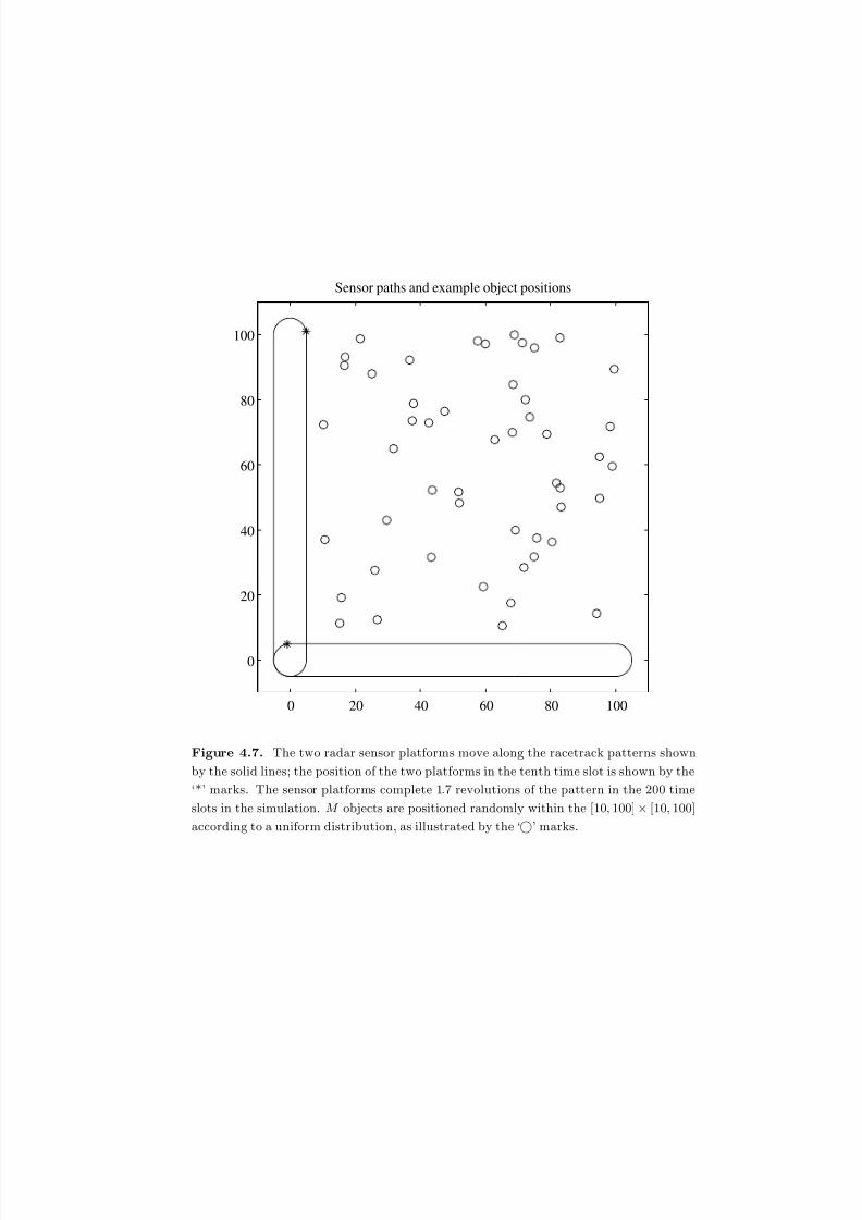
8/2/2019 Information Theoretic Sensor Management
http://slidepdf.com/reader/full/information-theoretic-sensor-management 143/203
0 20 40 60 80 100
0
20
40
60
80
100
Sensor paths and example object positions
Figure 4.7. The two radar sensor platforms move along the racetrack patterns shown
by the solid lines; the position of the two platforms in the tenth time slot is shown by the
‘*’ marks. The sensor platforms complete 1.7 revolutions of the pattern in the 200 time
slots in the simulation. M objects are positioned randomly within the [10, 100]× [10, 100]
according to a uniform distribution, as illustrated by the ‘’ marks.

8/2/2019 Information Theoretic Sensor Management
http://slidepdf.com/reader/full/information-theoretic-sensor-management 144/203
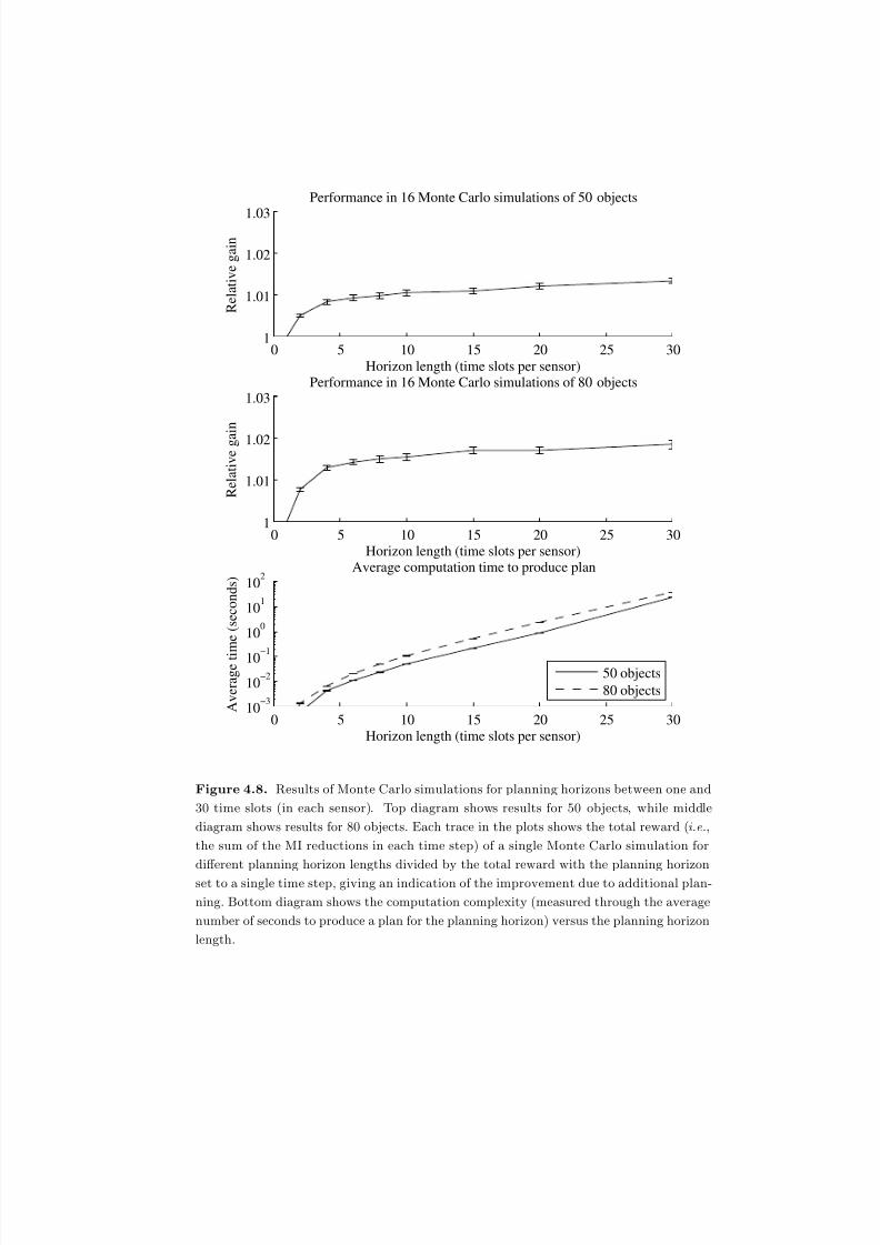
8/2/2019 Information Theoretic Sensor Management
http://slidepdf.com/reader/full/information-theoretic-sensor-management 145/203
0 5 10 15 20 25 301
1.01
1.02
1.03
Horizon length (time slots per sensor)
R e l a t i v e g a i n
Performance in 16 Monte Carlo simulations of 50 objects
0 5 10 15 20 25 301
1.01
1.02
1.03
Horizon length (time slots per sensor)
R e l a t i v e g a
i n
Performance in 16 Monte Carlo simulations of 80 objects
0 5 10 15 20 25 3010
−3
10−2
10−1
100
101
102
Horizon length (time slots per sensor)
Average computation time to produce plan
A v e r a g e t i m e ( s e c o n d s )
50 objects
80 objects
Figure 4.8. Results of Monte Carlo simulations for planning horizons between one and
30 time slots (in each sensor). Top diagram shows results for 50 objects, while middle
diagram shows results for 80 objects. Each trace in the plots shows the total reward (i.e.,
the sum of the MI reductions in each time step) of a single Monte Carlo simulation for
different planning horizon lengths divided by the total reward with the planning horizon
set to a single time step, giving an indication of the improvement due to additional plan-
ning. Bottom diagram shows the computation complexity (measured through the average
number of seconds to produce a plan for the planning horizon) versus the planning horizon
length.

8/2/2019 Information Theoretic Sensor Management
http://slidepdf.com/reader/full/information-theoretic-sensor-management 146/203
146 CHAPTER 4. INDEPENDENT OBJECTS AND INTEGER PROGRAMMING
Fig. 4.8. The diagram shows that, as expected, the complexity increases exponentially
with the planning horizon length. However, using the algorithm it is possible to produce
a plan for 50 objects over 20 time slots each in two sensors using little over one secondin computation time. Performing the same planning through full enumeration would
involve evaluation of the reward of 1080 different candidate sequences, a computation
which is intractable on any foreseeable computational hardware.
The computational complexity for problems involving different numbers of objects
for a fixed planning horizon length (10 time slots per sensor) is shown in Fig. 4.9.
When the planning horizon is significantly longer than the number of objects, it be-
comes necessary to construct plans involving several observations of each object. This
will generally involve enumeration of an exponentially increasing number of candidate
subsets in S i for each object, resulting in an increase in computational complexity.
As the number of objects increases, it quickly becomes clear that it is better to spread
the available resources evenly across objects rather than taking many observations of
a small number of objects, so the number of candidate subsets in S i requiring consid-
eration is vastly lower. Eventually, as the number of objects increases, the overhead
induced by the additional objects again increases the computational complexity.
4.4.3 State dependent observation noise
The second scenario involves a modification of the first in which observation noise
increases when objects become close to each other. This is a surrogate for the impact
of data association, although we do not model the dependency between objects which
generally results. The dynamical model has ∆t = 0.01 sec, and q = 0.25; the simulation
runs for 100 time slots. As per the previous scenario, the initial positions of the objects
are distributed uniformly on the region [10, 100] × [10, 100]; velocity magnitudes are
drawn from a Gaussian distribution with mean 30 and standard deviation 0 .5, while
the velocity directions are distributed uniformly on [0, 2π]. The initial estimates are set
to the true state, corrupted by additive Gaussian noise with zero mean and standard
deviation 0.02 (in position states) and 0.1 (in velocity states). The scenario involves
a single sensor rather than two sensors; the observation model is essentially the same
as the previous case, except that there is a state-dependent scalar multiplier on the
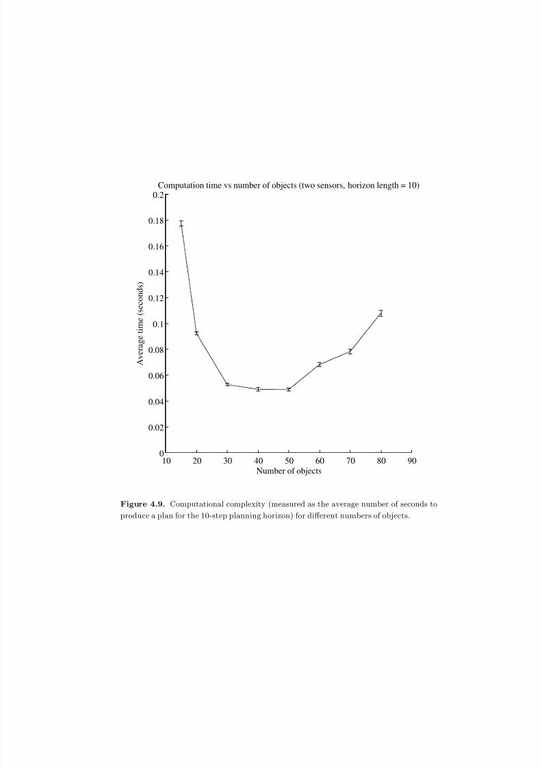
8/2/2019 Information Theoretic Sensor Management
http://slidepdf.com/reader/full/information-theoretic-sensor-management 147/203
10 20 30 40 50 60 70 80 900
0.02
0.04
0.06
0.08
0.1
0.12
0.14
0.16
0.18
0.2
A v e r a g e t i m e ( s e c o n d s )
Number of objects
Computation time vs number of objects (two sensors, horizon length = 10)
Figure 4.9. Computational complexity (measured as the average number of seconds to
produce a plan for the 10-step planning horizon) for different numbers of objects.
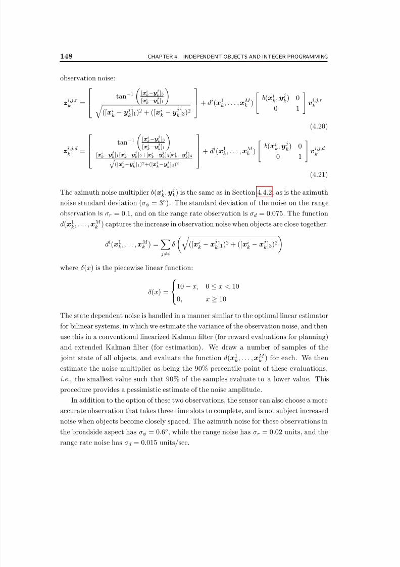
8/2/2019 Information Theoretic Sensor Management
http://slidepdf.com/reader/full/information-theoretic-sensor-management 148/203
148 CHAPTER 4. INDEPENDENT OBJECTS AND INTEGER PROGRAMMING
observation noise:
zi,j,rk = tan
−1 [xik−yjk]3[xik−yjk]1
([xi
k − y jk]1)2 + ([xi
k − y jk]3)2
+ di(x1k, . . . ,xM k )
b(xik,y
j
k) 00 1
vi,j,r
k
(4.20)
zi,j,dk =
tan−1
[xik−y
jk]3
[xik−y
jk]1
[xik−y
jk]1[x
ik−y
jk]2+[xik−y
jk]3[x
ik−y
jk]4q
([xik−y
jk]1)2+([xi
k−yjk]3)2
+ di(x1k, . . . ,xM
k )
b(xi
k,y jk) 0
0 1
v
i,j,dk
(4.21)
The azimuth noise multiplier b(xik,y j
k) is the same as in Section 4.4.2, as is the azimuth
noise standard deviation (σφ = 3◦). The standard deviation of the noise on the range
observation is σr = 0.1, and on the range rate observation is σd = 0.075. The function
d(x1k, . . . ,xM k ) captures the increase in observation noise when objects are close together:
di(x1k, . . . ,xM k ) = j=i
δ
([xi
k − x jk]1)2 + ([xi
k − x jk]3)2
where δ(x) is the piecewise linear function:
δ(x) = 10 − x, 0 ≤ x < 10
0, x ≥ 10
The state dependent noise is handled in a manner similar to the optimal linear estimator
for bilinear systems, in which we estimate the variance of the observation noise, and then
use this in a conventional linearized Kalman filter (for reward evaluations for planning)
and extended Kalman filter (for estimation). We draw a number of samples of the
joint state of all objects, and evaluate the function d(x1k, . . . ,xM k ) for each. We then
estimate the noise multiplier as being the 90% percentile point of these evaluations,
i.e., the smallest value such that 90% of the samples evaluate to a lower value. This
procedure provides a pessimistic estimate of the noise amplitude.
In addition to the option of these two observations, the sensor can also choose a more
accurate observation that takes three time slots to complete, and is not subject increased
noise when objects become closely spaced. The azimuth noise for these observations in
the broadside aspect has σφ = 0.6◦, while the range noise has σr = 0.02 units, and the
range rate noise has σd = 0.015 units/sec.

8/2/2019 Information Theoretic Sensor Management
http://slidepdf.com/reader/full/information-theoretic-sensor-management 149/203
0 5 10 15 201
1.05
1.1
1.15
Horizon length (time slots)
R e l a t i v e g a i n
Performance in 20 Monte Carlo simulations of 50 objects
0 5 10 15 2010
−3
10−2
10−1
100
101
102
Horizon length (time slots)
Average computation time to produce plan
A v e r a g e t i
m e ( s e c o n d s )
Figure 4.10. Top diagram shows the total reward for each planning horizon length divided
by the total reward for a single step planning horizon, averaged over 20 Monte Carlo
simulations. Error bars show the standard deviation of the mean p erformance estimate.Lower diagram shows the average time required to produce plan for the different length
planning horizon lengths.
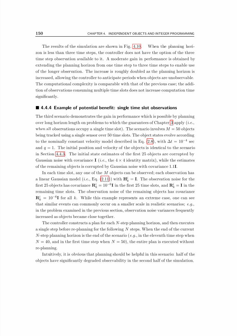
8/2/2019 Information Theoretic Sensor Management
http://slidepdf.com/reader/full/information-theoretic-sensor-management 150/203
150 CHAPTER 4. INDEPENDENT OBJECTS AND INTEGER PROGRAMMING
The results of the simulation are shown in Fig. 4.10. When the planning hori-
zon is less than three time steps, the controller does not have the option of the three
time step observation available to it. A moderate gain in performance is obtained byextending the planning horizon from one time step to three time steps to enable use
of the longer observation. The increase is roughly doubled as the planning horizon is
increased, allowing the controller to anticipate periods when objects are unobservable.
The computational complexity is comparable with that of the previous case; the addi-
tion of observations consuming multiple time slots does not increase computation time
significantly.
4.4.4 Example of potential benefit: single time slot observations
The third scenario demonstrates the gain in performance which is possible by planningover long horizon length on problems to which the guarantees of Chapter 3 apply (i.e.,
when all observations occupy a single time slot). The scenario involves M = 50 objects
being tracked using a single sensor over 50 time slots. The object states evolve according
to the nominally constant velocity model described in Eq. (2.8), with ∆t = 10−4 sec
and q = 1. The initial position and velocity of the objects is identical to the scenario
in Section 4.4.3. The initial state estimates of the first 25 objects are corrupted by
Gaussian noise with covariance I (i.e., the 4 × 4 identity matrix), while the estimates
of the remaining objects is corrupted by Gaussian noise with covariance 1.1I.
In each time slot, any one of the M objects can be observed; each observation has
a linear Gaussian model (i.e., Eq. (2.11)) with Hik = I. The observation noise for the
first 25 objects has covariance Rik = 10−6I in the first 25 time slots, and Ri
k = I in the
remaining time slots. The observation noise of the remaining objects has covariance
Rik = 10−6I for all k. While this example represents an extreme case, one can see
that similar events can commonly occur on a smaller scale in realistic scenarios; e.g.,
in the problem examined in the previous section, observation noise variances frequently
increased as objects became close together.
The controller constructs a plan for each N -step planning horizon, and then executes
a single step before re-planning for the following N steps. When the end of the current
N -step planning horizon is the end of the scenario (e.g., in the eleventh time step whenN = 40, and in the first time step when N = 50), the entire plan is executed without
re-planning.
Intuitively, it is obvious that planning should be helpful in this scenario: half of the
objects have significantly degraded observability in the second half of the simulation,
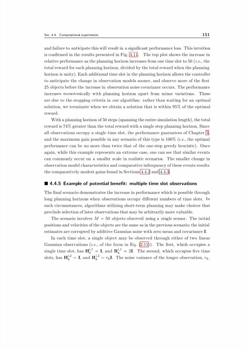
8/2/2019 Information Theoretic Sensor Management
http://slidepdf.com/reader/full/information-theoretic-sensor-management 151/203
Sec. 4.4. Computational experiments 151
and failure to anticipate this will result in a significant performance loss. This intuition
is confirmed in the results presented in Fig. 4.11. The top plot shows the increase in
relative performance as the planning horizon increases from one time slot to 50 ( i.e., thetotal reward for each planning horizon, divided by the total reward when the planning
horizon is unity). Each additional time slot in the planning horizon allows the controller
to anticipate the change in observation models sooner, and observe more of the first
25 objects before the increase in observation noise covariance occurs. The performance
increases monotonically with planning horizon apart from minor variations. These
are due to the stopping criteria in our algorithm: rather than waiting for an optimal
solution, we terminate when we obtain a solution that is within 95% of the optimal
reward.
With a planning horizon of 50 steps (spanning the entire simulation length), the total
reward is 74% greater than the total reward with a single step planning horizon. Since
all observations occupy a single time slot, the performance guarantees of Chapter 3,
and the maximum gain possible in any scenario of this type is 100% (i.e., the optimal
performance can be no more than twice that of the one-step greedy heuristic). Once
again, while this example represents an extreme case, one can see that similar events
can commonly occur on a smaller scale in realistic scenarios. The smaller change in
observation model characteristics and comparative infrequency of these events results
the comparatively modest gains found in Sections 4.4.2 and 4.4.3.
4.4.5 Example of potential benefit: multiple time slot observations
The final scenario demonstrates the increase in performance which is possible through
long planning horizons when observations occupy different numbers of time slots. In
such circumstances, algorithms utilizing short-term planning may make choices that
preclude selection of later observations that may be arbitrarily more valuable.
The scenario involves M = 50 objects observed using a single sensor. The initial
positions and velocities of the objects are the same as in the previous scenario; the initial
estimates are corrupted by additive Gaussian noise with zero mean and covariance I.
In each time slot, a single object may be observed through either of two linear
Gaussian observations (i.e., of the form in Eq. (2.11)). The first, which occupies asingle time slot, has H
i,1k = I, and R
i,1k = 2I. The second, which occupies five time
slots, has Hi,2k = I, and R
i,2k = rkI. The noise variance of the longer observation, rk,

8/2/2019 Information Theoretic Sensor Management
http://slidepdf.com/reader/full/information-theoretic-sensor-management 152/203
0 10 20 30 40 501
1.2
1.4
1.6
1.8
Horizon length (time slots)
R e l a t i v e g a i n
Reward relative to one−step planning horizon
0 10 20 30 40 5010
−3
10−2
10−1
100
101
102
A v e r a g e t i m
e ( s e c o n d s )
Horizon length (time slots)
Average computation time to produce plan
Figure 4.11. Upper diagram shows the total reward obtained in the simulation using
different planning horizon lengths, divided by the total reward when the planning horizon
is one. Lower diagram shows the average computation time to produce a plan for the
following N steps.
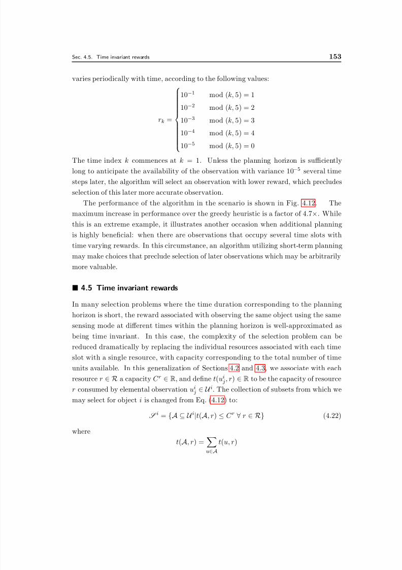
8/2/2019 Information Theoretic Sensor Management
http://slidepdf.com/reader/full/information-theoretic-sensor-management 153/203
Sec. 4.5. Time invariant rewards 153
varies periodically with time, according to the following values:
rk =
10−1 mod (k, 5) = 1
10−2 mod (k, 5) = 2
10−3 mod (k, 5) = 3
10−4 mod (k, 5) = 4
10−5 mod (k, 5) = 0
The time index k commences at k = 1. Unless the planning horizon is sufficiently
long to anticipate the availability of the observation with variance 10−5 several time
steps later, the algorithm will select an observation with lower reward, which precludes
selection of this later more accurate observation.
The performance of the algorithm in the scenario is shown in Fig. 4.12. The
maximum increase in performance over the greedy heuristic is a factor of 4.7×. While
this is an extreme example, it illustrates another occasion when additional planning
is highly beneficial: when there are observations that occupy several time slots with
time varying rewards. In this circumstance, an algorithm utilizing short-term planning
may make choices that preclude selection of later observations which may be arbitrarily
more valuable.
4.5 Time invariant rewards
In many selection problems where the time duration corresponding to the planning
horizon is short, the reward associated with observing the same object using the same
sensing mode at different times within the planning horizon is well-approximated as
being time invariant. In this case, the complexity of the selection problem can be
reduced dramatically by replacing the individual resources associated with each time
slot with a single resource, with capacity corresponding to the total number of time
units available. In this generalization of Sections 4.2 and 4.3, we associate with each
resource r ∈ R a capacity C r ∈ R, and define t(ui j, r) ∈ R to be the capacity of resource
r consumed by elemental observation ui j ∈ U i. The collection of subsets from which we
may select for object i is changed from Eq. (4.12) to:
S i = {A ⊆ U i|t(A, r) ≤ C r ∀ r ∈ R} (4.22)
where
t(A, r) =u∈A
t(u, r)
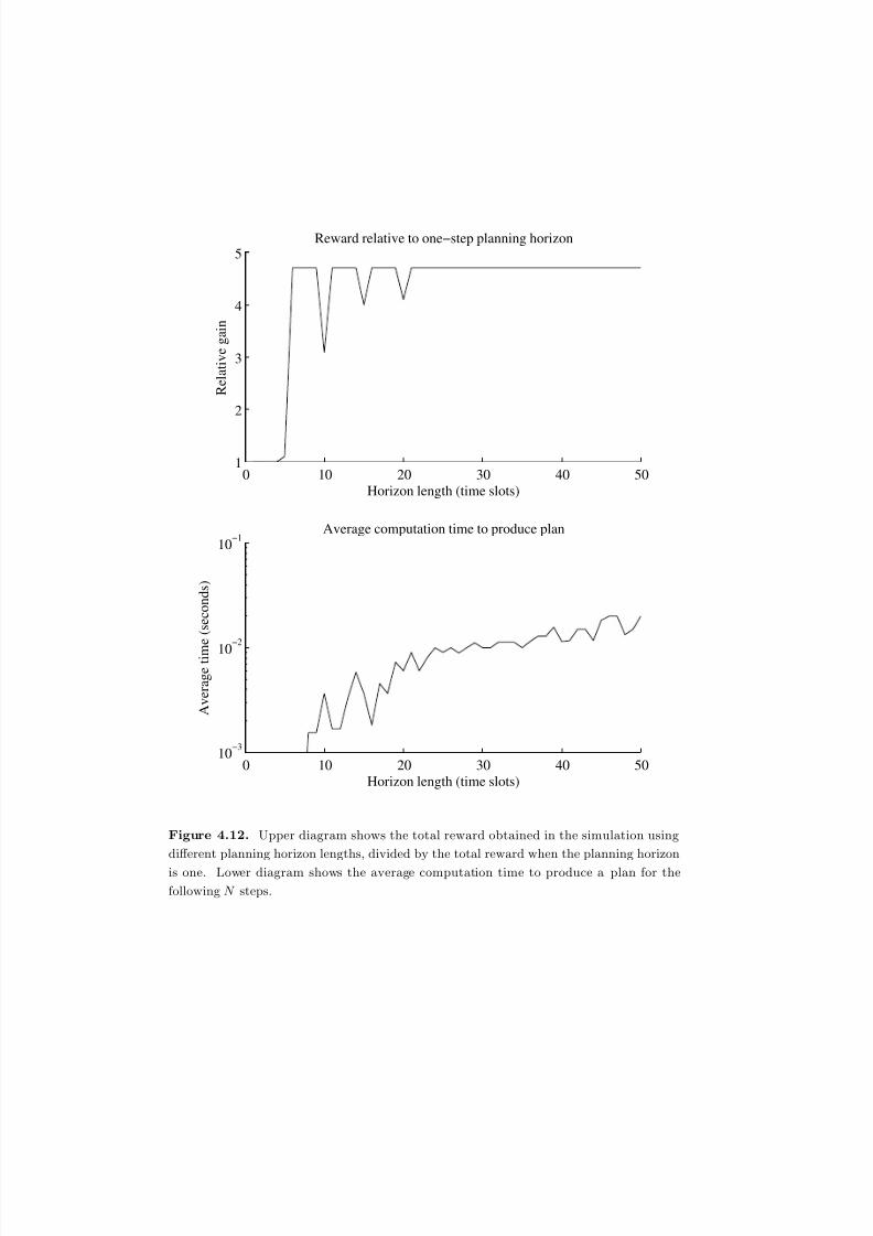
8/2/2019 Information Theoretic Sensor Management
http://slidepdf.com/reader/full/information-theoretic-sensor-management 154/203
0 10 20 30 40 501
2
3
4
5
Horizon length (time slots)
R e l a t i v e g a i n
Reward relative to one−step planning horizon
0 10 20 30 40 5010
−3
10−2
10−1
A v e r a g e t i m
e ( s e c o n d s )
Horizon length (time slots)
Average computation time to produce plan
Figure 4.12. Upper diagram shows the total reward obtained in the simulation using
different planning horizon lengths, divided by the total reward when the planning horizon
is one. Lower diagram shows the average computation time to produce a plan for the
following N steps.

8/2/2019 Information Theoretic Sensor Management
http://slidepdf.com/reader/full/information-theoretic-sensor-management 155/203
Sec. 4.5. Time invariant rewards 155
The full integer programming formulation of Eq. (4.15) becomes:
maxωiAi
M i=1
Ai∈S i
ri
Aiωi
Ai (4.23a)
s.t.M i=1
Ai∈S i
t(Ai, r)ωiAi ≤ C r ∀ r ∈ R (4.23b)
Ai∈S i
ωiAi = 1 ∀ i ∈ {1, . . . , M } (4.23c)
ωiAi ∈ {0, 1} ∀ i, Ai ∈ S i (4.23d)
The iterative solution methodology in Section 4.3 may be generalized to this case
by replacing Eq. (4.16) with:
maxωiAi
, ωiu|Ai
M i=1
Ai∈T il
ri
AiωiAi +
u∈Bil,Ai
riu|Aiω
iu|Ai
(4.24a)
s.t.M i=1
Ai∈T il
t(Ai, r)ωiAi +
M i=1
Ai∈T il
u∈Bi
l,Ai
t(u, r)ωiu|Ai ≤ C r ∀ r ∈ R (4.24b)
Ai∈T i
ωiAi = 1 ∀ i ∈ {1, . . . , M } (4.24c)
u∈B
i
l,Ai
ωiu|Ai − |Bi
l,Ai |ωiAi ≤ 0 ∀ i, Ai ∈ T il (4.24d)
ωiAi ∈ {0, 1} ∀ i, Ai ∈ T i (4.24e)
ωiu|Ai ∈ {0, 1} ∀ i, Ai ∈ T i, u ∈ Bi
l,Ai (4.24f)
The only change from Eq. (4.16) is in the form of the resource constraint, Eq. (4.24b).
Algorithm 4.1 may be applied without modification using this generalized integer pro-
gram.
4.5.1 Avoiding redundant observation subsets
Straight-forward implementation of the formulation just described will yield a substan-
tial inefficiency due to redundancy in the observation subset S i, as illustrated in the
following scenario. Suppose we seek to generate a plan for the next N time slots,
where there are η total combinations of sensor and mode within each time slot. For
each sensor mode4 ui j , j ∈ {1, . . . , η}, we generate for each duration d ∈ {1, . . . , N }
4We assume that the index j enumerates all possible combinations of sensor and mode.

8/2/2019 Information Theoretic Sensor Management
http://slidepdf.com/reader/full/information-theoretic-sensor-management 156/203
156 CHAPTER 4. INDEPENDENT OBJECTS AND INTEGER PROGRAMMING
(i.e., the duration for which the sensor mode is applied) an elemental observation ui j,d,
which corresponds to applying sensor mode ui j for d time slots, so that U i = {ui
j,d| j ∈{1, . . . , η}, d ∈ {1, . . . , N }}. With each sensor s ∈ S (where S is the set of sensors) weassociate a resource rs with capacity C r
s= N , i.e., each sensor has up to N time slots
available for use. Denoting by s(ui j) the sensor associated with ui
j, we set
t(ui j,d, s) =
d, s = s(ui
j)
0, otherwise
We could generate the collection of observation subsets S i from Eq. (4.22) using
this structure, with U i and t(·, ·) as described above, and R = {rs|s ∈ S}. However,
this would introduce a substantial inefficiency which is quite avoidable. Namely, in
addition to containing the single element observation subset {ui j,d}, the collection of
subsets S i may also contain several subsets of the form {ui j,dl
|l dl = d}.5 We would
prefer to avoid this redundancy, ensuring instead that the only way observe object i
using sensor mode j for a total duration of d time slots is to choose the elemental
observation ui j,d alone. This can be achieved by introducing one additional resource for
each combination of object and sensor mode, {ri,j|i ∈ {1, . . . , M }, j ∈ {1, . . . , η}}, each
with capacity C ri,j
= 1, setting:
t(ui j,d, ri,j) =
1, i = i, j = j
0, otherwise
The additional constraints generated by these resources ensure that (at most) a single
element from the set {ui j,d|d ∈ {1, . . . , N }} can be chosen for each (i, j). As the following
experiment demonstrates, this results in a dramatic decrease in the action space for each
object, enabling solution of larger problems.
4.5.2 Computational experiment: waveform selection
To demonstrate the reduction in computational complexity that results from this for-
mulation, we apply it to a modification of the example presented in Section 4.4.2. We
set ∆t = 0.01 and reduce the sensor platform motion to 0.01 units/step. Fig. 4.13
shows variation in rewards for 50 objects being observed with a single mode of a single
sensor over 50 time slots in one realization of the example, confirming that the rewards
are reasonably well approximated as being time-invariant.
5For example, as well as providing an observation subset for observing object i with sensor mode j
8/2/2019 Information Theoretic Sensor Management
http://slidepdf.com/reader/full/information-theoretic-sensor-management 157/203
100 110 120 130 140 150 1601
1.05
1.1
1.15
Time step (k)
Reward at time k / reward at time 101
R a t i o o f r e w a r d s
Azimuth/range rate observation
Azimuth/range observation
Figure 4.13. Diagram illustrates the variation of rewards over the 50 time step planning
horizon commencing from time step k = 101. The line plots the ratio between the reward
of each observation at time step in the planning horizon and the reward of the same
observation at the first time slot in the planning horizon, averaged over 50 ob jects. The
error bars show the standard deviation of the ratio, i.e., the variation between objects.
8/2/2019 Information Theoretic Sensor Management
http://slidepdf.com/reader/full/information-theoretic-sensor-management 158/203
158 CHAPTER 4. INDEPENDENT OBJECTS AND INTEGER PROGRAMMING
The simulations run for 200 time slots. The initial position and velocity of the
objects is identical to that in Section 4.4.2; the initial state estimates are corrupted by
additive Gaussian noise with covariance (1 + ρi)I, where ρi is randomly drawn, inde-pendently for each object, from a uniform distribution on [0, 1] (the values are known
to the controller). The observation model is identical to that described in Section 4.4.2.
If the controller chooses to observe an object for d time slots, the variance is reduced
by a factor of d from that of the same single time slot observation; in the absence of
the dynamics process this is equivalent to d single time slot observations.
At each time step, the controller constructs an N -step plan. Since rewards are
assumed time invariant, the elements of this plan are not directly attached to time
slots. We assign time slots to each task in the plan by processing objects in random
order, assigning the first time slots to the observations assigned to the first object in
the random order, etc. We then execute the action assigned to the first time slot in
the plan, before constructing a new plan; this is consistent with the open loop feedback
control methodology used in the examples in Section 4.4.
The results of the simulations are shown in Fig. 4.14. There is a very small gain in
performance as the planning horizon increases from one time slot to around five time
slots. Beyond this limit, the performance drops to be lower than the performance of
the greedy heuristic (i.e., using a single step planning horizon). This is due to the
mismatch between the assumed model (that rewards are time invariant) and the true
model (that rewards are indeed time varying), which worsens as the planning horizon
increases. The computational cost in the lower diagram demonstrates the efficiency
of this formulation. With a planning horizon of 40, we are taking an average of four
observations per object. This would attract a very large computational burden in the
original formulation discussed in the experiments of Section 4.4.
4.5.3 Example of potential benefit
To demonstrate the benefit that additional planning can provide in problems involving
time invariant rewards, we construct an experiment that is an extension of the example
presented in Section 3.4. The scenario involves M = 50 objects being observed using a
single sensor over 100 time slots. The four-dimensional state of each object is static in
for d = 10 steps, there are also subsets for observing object i with sensor mode j multiple times for the
same total duration—e.g., for 4 and 6 steps, for 3 and 7 steps, and for 1, 4 and 5 steps.
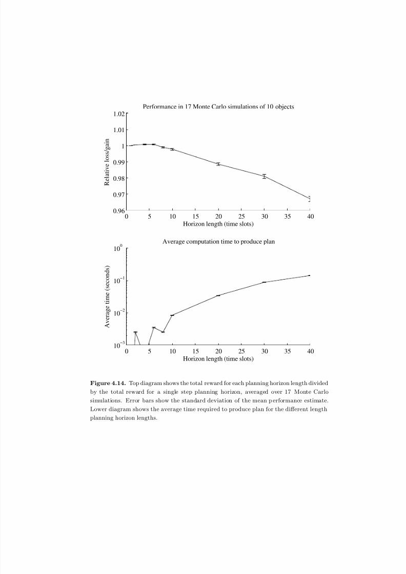
8/2/2019 Information Theoretic Sensor Management
http://slidepdf.com/reader/full/information-theoretic-sensor-management 159/203
0 5 10 15 20 25 30 35 400.96
0.97
0.98
0.99
1
1.01
1.02
Horizon length (time slots)
R e l a t i v e l o s s / g a i n
Performance in 17 Monte Carlo simulations of 10 objects
0 5 10 15 20 25 30 35 4010
−3
10−2
10−1
100
Horizon length (time slots)
Average computation time to produce plan
A v e r a g e t i m e ( s e c o n d s )
Figure 4.14. Top diagram shows the total reward for each planning horizon length divided
by the total reward for a single step planning horizon, averaged over 17 Monte Carlo
simulations. Error bars show the standard deviation of the mean p erformance estimate.Lower diagram shows the average time required to produce plan for the different length
planning horizon lengths.
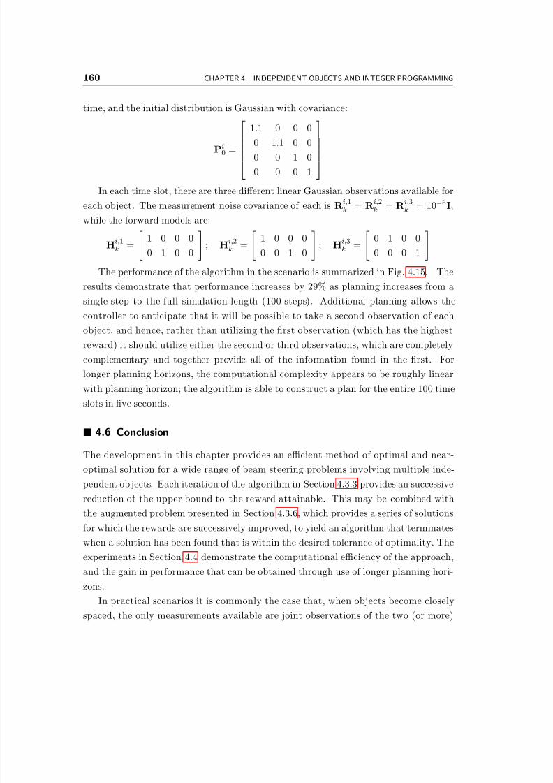
8/2/2019 Information Theoretic Sensor Management
http://slidepdf.com/reader/full/information-theoretic-sensor-management 160/203
160 CHAPTER 4. INDEPENDENT OBJECTS AND INTEGER PROGRAMMING
time, and the initial distribution is Gaussian with covariance:
Pi0 =
1.1 0 0 0
0 1.1 0 0
0 0 1 0
0 0 0 1
In each time slot, there are three different linear Gaussian observations available for
each object. The measurement noise covariance of each is Ri,1k = R
i,2k = R
i,3k = 10−6I,
while the forward models are:
Hi,1k =
1 0 0 0
0 1 0 0
; H
i,2k =
1 0 0 0
0 0 1 0
; H
i,3k =
0 1 0 0
0 0 0 1
The performance of the algorithm in the scenario is summarized in Fig. 4.15. Theresults demonstrate that performance increases by 29% as planning increases from a
single step to the full simulation length (100 steps). Additional planning allows the
controller to anticipate that it will be possible to take a second observation of each
object, and hence, rather than utilizing the first observation (which has the highest
reward) it should utilize either the second or third observations, which are completely
complementary and together provide all of the information found in the first. For
longer planning horizons, the computational complexity appears to be roughly linear
with planning horizon; the algorithm is able to construct a plan for the entire 100 time
slots in five seconds.
4.6 Conclusion
The development in this chapter provides an efficient method of optimal and near-
optimal solution for a wide range of beam steering problems involving multiple inde-
pendent ob jects. Each iteration of the algorithm in Section 4.3.3 provides an successive
reduction of the upper bound to the reward attainable. This may be combined with
the augmented problem presented in Section 4.3.6, which provides a series of solutions
for which the rewards are successively improved, to yield an algorithm that terminates
when a solution has been found that is within the desired tolerance of optimality. The
experiments in Section 4.4 demonstrate the computational efficiency of the approach,
and the gain in performance that can be obtained through use of longer planning hori-
zons.
In practical scenarios it is commonly the case that, when objects become closely
spaced, the only measurements available are joint observations of the two (or more)
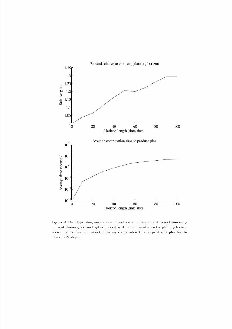
8/2/2019 Information Theoretic Sensor Management
http://slidepdf.com/reader/full/information-theoretic-sensor-management 161/203
0 20 40 60 80 1001
1.05
1.1
1.15
1.2
1.25
1.3
1.35
Horizon length (time slots)
R e l a t i v e g a i n
Reward relative to one−step planning horizon
0 20 40 60 80 10010
−3
10−2
10−1
100
101
102
A v e r a g e t i m
e ( s e c o n d s )
Horizon length (time slots)
Average computation time to produce plan
Figure 4.15. Upper diagram shows the total reward obtained in the simulation using
different planning horizon lengths, divided by the total reward when the planning horizon
is one. Lower diagram shows the average computation time to produce a plan for the
following N steps.

8/2/2019 Information Theoretic Sensor Management
http://slidepdf.com/reader/full/information-theoretic-sensor-management 162/203
162 CHAPTER 4. INDEPENDENT OBJECTS AND INTEGER PROGRAMMING
objects, rather than observations of the individual objects. This inevitably results
in statistical dependency between object states in the conditional distribution; the
dependency is commonly represented through association hypotheses (e.g., [14, 19, 58,71, 82]).
If the objects can be decomposed into many small independent “groups”, as in the
notion of independent clusters in Multiple Hypothesis Tracking (MHT), then Algo-
rithm 4.1 may be applied to the transformed problem in which each independent group
of objects is treated as a single object with state and action space corresponding to the
cartesian product of the objects forming the group. This approach may be tractable if
the number of objects in each group remains small.

8/2/2019 Information Theoretic Sensor Management
http://slidepdf.com/reader/full/information-theoretic-sensor-management 163/203
Chapter 5
Sensor management in
sensor networks
NETWORKS of intelligent sensors have the potential to provide unique capabilitiesfor monitoring wide geographic areas through the intelligent exploitation of local
computation (so called in-network computing) and the judicious use of inter-sensor
communication. In many sensor networks energy is a dear resource to be conserved so
as to prolong the network’s operational lifetime. Additionally, it is typically the case
that the energy cost of communications is orders of magnitude greater than the energy
cost of local computation [80,81].
Tracking moving objects is a common application in which the quantities of inter-
est (i.e., kinematic state) are inferred largely from sensor observations which are in
proximity to the object (e.g., [62]). Consequently, local fusion of sensor data is suffi-
cient for computing an accurate estimate of object state, and the knowledge used to
compute this estimate is summarized by the conditional probability density function
(PDF). This property, combined with the need to conserve energy, has led to a variety
of approaches (e.g., [37, 64]) which effectively designate the responsibility of computing
the conditional PDF to one sensor node (referred to as the leader node) in the network.
Over time the leader node changes dynamically as function of the kinematic state of the
object. This leads to an inevitable trade-off between the uncertainty in the conditional
PDF, the cost of acquiring observations, and the cost of propagating the conditional
PDF through the network. In this chapter we examine this trade-off in the context of
object tracking in distributed sensor networks.
We consider a sensor network consisting a set of sensors (denoted S , where |S| = N s),
in which the sensing model is assumed to be such that the observation provided by
the sensor is highly informative in the region close to the node, and uninformative in
regions far from the node. For the purpose of addressing the primary issue, trading off
163

8/2/2019 Information Theoretic Sensor Management
http://slidepdf.com/reader/full/information-theoretic-sensor-management 164/203
164 CHAPTER 5. SENSOR MANAGEMENT IN SENSOR NETWORKS
energy consumption for accuracy, we restrict ourselves to sensor resource planning issues
associated with tracking a single object. While additional complexities certainly arise
in the multi-object case (e.g., data association) they do not change the basic problemformulation or conclusions.
If the energy consumed by sensing and communication were unconstrained, then the
optimal solution would be to collect and fuse the observations provided by all sensors
in the network. We consider a scheme in which, at each time step, a subset of sensors is
selected to take an observation and transmit to a sensor referred to as the leader node,
which fuses the observations with the prior conditional PDF and tasks sensors at the
next time step. The questions which must be answered by the controller are how to
select the subset of sensors at each point in time, and how to select the leader node at
each point in time.
The approach developed in Section 5.1 allows for optimization of estimation per-
formance subject to a constraint on expected communication cost, or minimization of
communication cost subject to a constraint on expected estimation performance. The
controller uses a dual problem formulation to adaptively utilize multiple sensors at
each time step, incorporating a subgradient update step to adapt the dual variable
(Section 5.1.9), and introducing a heuristic cost to go in the terminal cost to avoid
anomalous behavior (Section 5.1.10). Our dual problem formulation is closely related
to [18], and provides an approximation which extends the Lagrangian relaxation ap-
proach to problems involving sequential replanning. Other related work includes [29],
which suggests incorporation of sensing costs and estimation performance into a unified
objective without adopting the constrained optimization framework that we utilize, and
[20], which adopts a constrained optimization framework without incorporating estima-
tion performance and sensing cost into a unified objective, a structure which results in
a major computational saving for our approach.
5.1 Constrained Dynamic Programming Formulation
The sensor network object tracking problem involves an inherent trade-off between
performance and energy expenditure. One way of incorporating both estimation per-
formance and communication cost into an optimization procedure is to optimize one of
the quantities subject to a constraint on the other. In the development which follows,
we provide a framework which can be used to either maximize the information obtained
from the selected observations subject to a constraint on the expected communication
cost, or to minimize the communication cost subject to a constraint on the estimation

8/2/2019 Information Theoretic Sensor Management
http://slidepdf.com/reader/full/information-theoretic-sensor-management 165/203
Sec. 5.1. Constrained Dynamic Programming Formulation 165
quality. This can be formulated as a constrained Markov Decision Process (MDP), as
discussed in Section 2.2.3.
As discussed in the introduction to this chapter, the tracking problem naturally fitsinto the Bayesian state estimation formulation, such that the role of the sensor network
is to maintain a representation of the conditional PDF of the object state (i.e., position,
velocity, etc) conditioned on the observations. In our experiments, we utilize a parti-
cle filter to maintain this representation (as described in Section 2.1.4), although the
planning method that we develop is equally applicable to any state estimation method
including the Kalman filter (Section 2.1.2), extended Kalman filter (Section 2.1.3), or
unscented Kalman filter [39]. An efficient method of compressing particle representa-
tions of PDFs for transmission in sensor networks is studied in [36]; we envisage that
any practical implementation of particle filters in sensor networks would use such a
scheme.
The estimation objective that we employ in our formulation is discussed in Sec-
tion 5.1.1, while our communication cost is discussed in Section 5.1.2. These two
quantities are utilized differently in dual formulations, the first of which optimizes
estimation performance subject to a constraint on communication cost (Section 5.1.3),
and the second of which optimizes communication cost subject to a constraint on esti-
mation performance (Section 5.1.4). In either case, the control choice available at each
time is uk = (lk, S k), where lk ∈ S is the leader node at time k and S k ⊆ S is the
subset of sensors activated at time k. The decision state of the dynamic program is the
combination of conditional PDF of object state, denoted Xk p(xk|z0, . . . , zk−1), and
the previous choice of leader node, lk−1 ∈ S .
5.1.1 Estimation objective
The estimation objective that we utilize in our formulation is the joint entropy of the
object state over the N steps commencing from the current time k:
H (xk, . . . ,xk+N −1|z0, . . . , zk−1, zS kk , . . . ,z
S k+N −1
k+N −1 )
where zS ll denotes the random variables corresponding to the observations of the sensors
in the set S l ⊆ S at time l. As discussed in Section 2.3.6, minimizing this quantitywith respect to the observation selections S l is equivalent to maximizing the following
mutual information expression:
k+N −1l=k
I (xl; zS ll |z0, . . . , zk−1, zS k
k , . . . ,zS l−1l−1 )
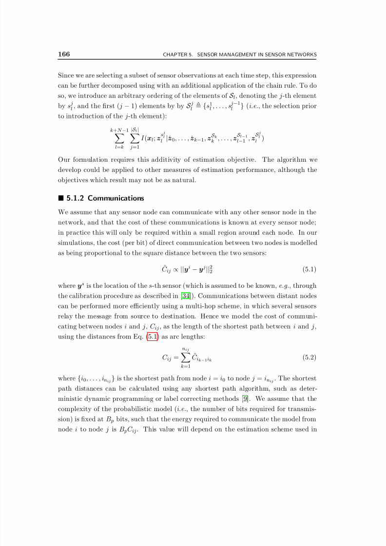
8/2/2019 Information Theoretic Sensor Management
http://slidepdf.com/reader/full/information-theoretic-sensor-management 166/203
166 CHAPTER 5. SENSOR MANAGEMENT IN SENSOR NETWORKS
Since we are selecting a subset of sensor observations at each time step, this expression
can be further decomposed using with an additional application of the chain rule. To do
so, we introduce an arbitrary ordering of the elements of S l, denoting the j-th elementby s jl , and the first ( j − 1) elements by by S jl {s1l , . . . , s j−1
l } (i.e., the selection prior
to introduction of the j-th element):
k+N −1l=k
|S l| j=1
I (xl; zsjl
l |z0, . . . , zk−1,zS kk , . . . ,z
S l−1l−1 , z
S jll )
Our formulation requires this additivity of estimation objective. The algorithm we
develop could be applied to other measures of estimation performance, although the
objectives which result may not be as natural.
5.1.2 Communications
We assume that any sensor node can communicate with any other sensor node in the
network, and that the cost of these communications is known at every sensor node;
in practice this will only be required within a small region around each node. In our
simulations, the cost (per bit) of direct communication between two nodes is modelled
as being proportional to the square distance between the two sensors:
C ij ∝ ||yi − y j||22 (5.1)
where ys
is the location of the s-th sensor (which is assumed to be known, e.g., throughthe calibration procedure as described in [34]). Communications between distant nodes
can be performed more efficiently using a multi-hop scheme, in which several sensors
relay the message from source to destination. Hence we model the cost of communi-
cating between nodes i and j, C ij, as the length of the shortest path between i and j,
using the distances from Eq. (5.1) as arc lengths:
C ij =
nijk=1
C ik−1ik (5.2)
where{
i0, . . . , inij}
is the shortest path from node i = i0 to node j = inij
. The shortest
path distances can be calculated using any shortest path algorithm, such as deter-
ministic dynamic programming or label correcting methods [9]. We assume that the
complexity of the probabilistic model (i.e., the number of bits required for transmis-
sion) is fixed at B p bits, such that the energy required to communicate the model from
node i to node j is B pC ij. This value will depend on the estimation scheme used in

8/2/2019 Information Theoretic Sensor Management
http://slidepdf.com/reader/full/information-theoretic-sensor-management 167/203
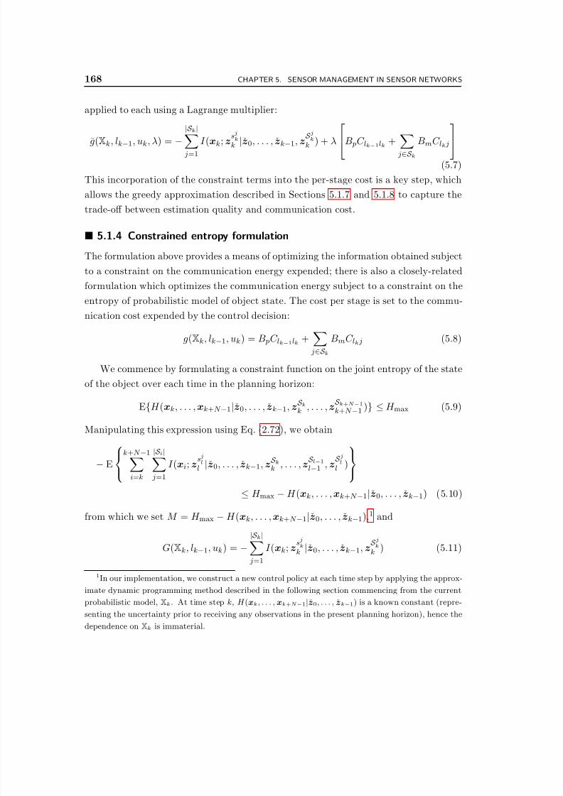
8/2/2019 Information Theoretic Sensor Management
http://slidepdf.com/reader/full/information-theoretic-sensor-management 168/203
168 CHAPTER 5. SENSOR MANAGEMENT IN SENSOR NETWORKS
applied to each using a Lagrange multiplier:
g(Xk, lk−1, uk, λ) = −|S k| j=1
I (xk;zs
j
kk |z0, . . . , zk−1, zS
j
kk ) + λ
B pC lk−1lk +
j∈S k
BmC lk j
(5.7)
This incorporation of the constraint terms into the per-stage cost is a key step, which
allows the greedy approximation described in Sections 5.1.7 and 5.1.8 to capture the
trade-off between estimation quality and communication cost.
5.1.4 Constrained entropy formulation
The formulation above provides a means of optimizing the information obtained subject
to a constraint on the communication energy expended; there is also a closely-related
formulation which optimizes the communication energy subject to a constraint on the
entropy of probabilistic model of object state. The cost per stage is set to the commu-
nication cost expended by the control decision:
g(Xk, lk−1, uk) = B pC lk−1lk +
j∈S k
BmC lk j (5.8)
We commence by formulating a constraint function on the joint entropy of the state
of the object over each time in the planning horizon:
E
{H (xk, . . . ,xk+N −1
|z0, . . . , zk−1, zS k
k , . . . ,zS k+N −1
k+N −1 )
} ≤H max (5.9)
Manipulating this expression using Eq. (2.72), we obtain
− E
k+N −1i=k
|S i| j=1
I (xi; zsjl
l |z0, . . . , zk−1,zS kk , . . . ,z
S l−1l−1 , z
S jl
l )
≤ H max − H (xk, . . . ,xk+N −1|z0, . . . , zk−1) (5.10)
from which we set M = H max − H (xk, . . . ,xk+N −1|z0, . . . , zk−1),1 and
G(Xk, lk−1, uk) =
−
|S k|
j=1
I (xk; zsjk
k
|z0, . . . , zk−1, z
S jkk ) (5.11)
1In our implementation, we construct a new control policy at each time step by applying the approx-
imate dynamic programming method described in the following section commencing from the current
probabilistic model, Xk. At time step k, H (xk, . . . ,xk+N −1|z0, . . . , zk−1) is a known constant (repre-
senting the uncertainty prior to receiving any observations in the present planning horizon), hence the
dependence on Xk is immaterial.

8/2/2019 Information Theoretic Sensor Management
http://slidepdf.com/reader/full/information-theoretic-sensor-management 169/203
Sec. 5.1. Constrained Dynamic Programming Formulation 169
Following the same procedure as described previously, the elements of the information
constraint in Eq. (5.10) can be integrated into the per-stage cost, resulting in a for-
mulation which is identical to Eq. (5.7), except that the Lagrange multiplier is on themutual information term, rather than the communication cost terms:
g(Xk, lk−1, uk, λ) = B pC lk−1lk +
j∈S k
BmC lk j − λ
|S k|
j=1
I (xk; zS jkk |z0, . . . , zk−1,z
S 1:j−1k
k )
(5.12)
5.1.5 Evaluation through Monte Carlo simulation
The constrained dynamic program described above has an infinite state space (the space
of probability distributions over object state), hence it cannot be evaluated exactly.
The following sections describe a series of approximations which are applied to obtain
a practical implementation.
Conceptually, the dynamic program of Eq. (5.6) could be approximated by sim-
ulating sequences of observations for each possible sequence of controls. There are
N s2N s possible controls at each time step, corresponding all possible selections of leader
node and subsets of sensors to activate. The complexity of the simulation process is
formidable: to evaluate J Dk (Xk, lk−1, λ) for a given decision state and control, we draw a
set of N p samples of the set of observations zS kk from the distribution p(zS k
k |z0, . . . , zk−1)
derived from Xk, and evaluate the cost to go one step later J Dk+1(Xk+1, lk, λ) correspond-
ing to the decision state resulting from each set of observations. The evaluation of each
cost to go one step later will yield the same branching. A tree structure develops, where
for each previous leaf of the tree, N s2N sN p new leaves (samples) are drawn, such that
the computational complexity increases as O(N sN 2N sN N p
N ) as the tree depth N (i.e.,
the planning horizon) increases, as illustrated in Fig. 5.1. Such an approach quickly
becomes intractable even for a small number of sensors (N s) and simulated observation
samples (N p), hence we seek to exploit additional structure in the problem to find a
computable approximate solution.
5.1.6 Linearized Gaussian approximation
In Section 2.3.4, we showed that the mutual information of a linear-Gaussian observation
of a quantity whose prior distribution is also Gaussian is a function only of the prior
covariance and observation model, not of the state estimate. Since the covariance of
a Kalman filter is independent of observation values (as seen in Section 2.1.2), this
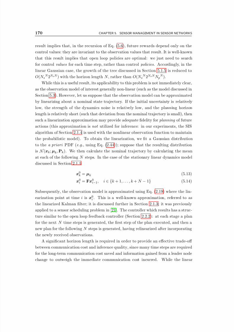
8/2/2019 Information Theoretic Sensor Management
http://slidepdf.com/reader/full/information-theoretic-sensor-management 170/203
170 CHAPTER 5. SENSOR MANAGEMENT IN SENSOR NETWORKS
result implies that, in the recursion of Eq. (5.6), future rewards depend only on the
control values: they are invariant to the observation values that result. It is well-known
that this result implies that open loop policies are optimal: we just need to searchfor control values for each time step, rather than control policies. Accordingly, in the
linear Gaussian case, the growth of the tree discussed in Section 5.1.5 is reduced to
O(N sN 2N sN ) with the horizon length N , rather than O(N s
N 2N sN N pN ).
While this is a useful result, its applicability to this problem is not immediately clear,
as the observation model of interest generally non-linear (such as the model discussed in
Section 5.3). However, let us suppose that the observation model can be approximated
by linearizing about a nominal state trajectory. If the initial uncertainty is relatively
low, the strength of the dynamics noise is relatively low, and the planning horizon
length is relatively short (such that deviation from the nominal trajectory is small), then
such a linearization approximation may provide adequate fidelity for planning of future
actions (this approximation is not utilized for inference: in our experiments, the SIS
algorithm of Section 2.1.4 is used with the nonlinear observation function to maintain
the probabilistic model). To obtain the linearization, we fit a Gaussian distribution
to the a priori PDF (e.g., using Eq. (2.44)); suppose that the resulting distribution
is N (xk;µk, Pk). We then calculate the nominal trajectory by calculating the mean
at each of the following N steps. In the case of the stationary linear dynamics model
discussed in Section 2.1.1:
x0k = µk (5.13)x0i = Fx0i−1, i ∈ {k + 1, . . . , k + N − 1} (5.14)
Subsequently, the observation model is approximated using Eq. (2.19) where the lin-
earization point at time i is x0i . This is a well-known approximation, referred to as
the linearized Kalman filter; it is discussed further in Section 2.1.3; it was previously
applied to a sensor scheduling problem in [21]. The controller which results has a struc-
ture similar to the open loop feedback controller (Section 2.2.2): at each stage a plan
for the next N time steps is generated, the first step of the plan executed, and then a
new plan for the following N steps is generated, having relinearized after incorporating
the newly received observations.
A significant horizon length is required in order to provide an effective trade-off
between communication cost and inference quality, since many time steps are required
for the long-term communication cost saved and information gained from a leader node
change to outweigh the immediate communication cost incurred. While the linear
8/2/2019 Information Theoretic Sensor Management
http://slidepdf.com/reader/full/information-theoretic-sensor-management 171/203
Sec. 5.1. Constrained Dynamic Programming Formulation 171
Gaussian approximation eliminates the O(N pN ) factor in the growth of computational
complexity with planning horizon length, the complexity is still exponential in both time
and the number of sensors, growing as O(N sN 2N sN ). The following two sections describetwo tree pruning approximations we introduce to obtain a tractable implementation.
5.1.7 Greedy sensor subset selection
To avoid the combinatorial complexity associated with optimization over subsets of sen-
sors, we decompose each decision stage into a number of substages and apply heuris-
tic approximations in a carefully chosen way. Following the application of the lin-
earized Gaussian approximation (Section 5.1.6), the branching of the computation tree
of Fig. 5.1 will be reduced to the structure shown in Fig. 5.2. Each stage of control
branching involves selection of a leader node, and a subset of sensors to activate; wecan break these two phases apart, as illustrated in Fig. 5.3. Finally, one can decom-
pose the choice of which subset of sensors to activate (given a choice of leader node)
into a generalized stopping problem [9] in which, at each substage (indexed by i), the
control choices are to terminate (i.e., move on to portion of the tree corresponding to
the following time slot) with the current set of selections, or to select an additional
sensor. This is illustrated in Fig. 5.4; the branches labelled ‘T ’ represent the decision
to terminate with the currently selected subset.
For the communication constrained formulation, the DP recursion becomes:
J i(Xi, li−1, λ) = minli∈S {λB pC li−1li + J 0i (Xi, li, {∅}, λ)} (5.15)
for i ∈ {k , . . . , k + N − 1}, terminated by setting J N (XN , lN −1, λ) = −λM , where
J i
i (Xi, li, S ii , λ) = min
E
Xi+1|Xi,S ii
J i+1(Xi+1, li, λ),
minsii ∈S\S i
i
{g(Xi, li, S ii , si
i , λ) + J i+1
i (Xi, li, S ii ∪ {si
i }, λ)}
(5.16)
S ii is the set of sensors chosen in stage i prior to substage i, and the substage cost
g(Xi, li, S i
i , si
i , λ) is
g(Xi, li, S ii , si
i , λ) = λBmC lis
ii
− I (xi; zsi
i
i |z0, . . . , zi−1, zS i
i
i ) (5.17)
The cost to go J i(Xi, li−1, λ) represents the expected cost to the end of the problem
(i.e., the bottom of the computation tree) commencing from the beginning of time slot
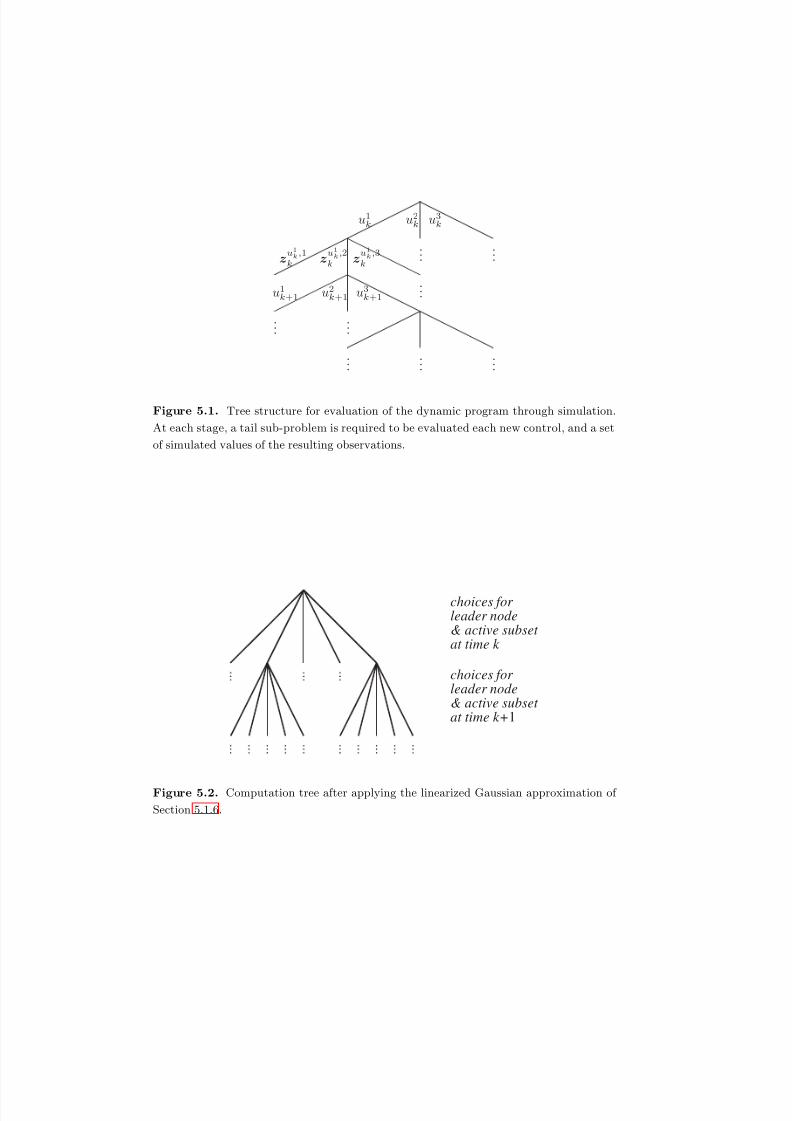
8/2/2019 Information Theoretic Sensor Management
http://slidepdf.com/reader/full/information-theoretic-sensor-management 172/203
zu1k,1
k zu1k,2
k zu1k,3
k
u1k+1 u
2k+1 u
3k+1
.
.
.
.
.
.
.
.
.
.
.
.
.
.
.
.
.
.
.
.
.
.
.
.
u1k u
2k u
3k
Figure 5.1. Tree structure for evaluation of the dynamic program through simulation.
At each stage, a tail sub-problem is required to be evaluated each new control, and a set
of simulated values of the resulting observations.
choices for leader node& active subset at time k
choices for leader node& active subset at time k+1
Figure 5.2. Computation tree after applying the linearized Gaussian approximation of
Section 5.1.6.
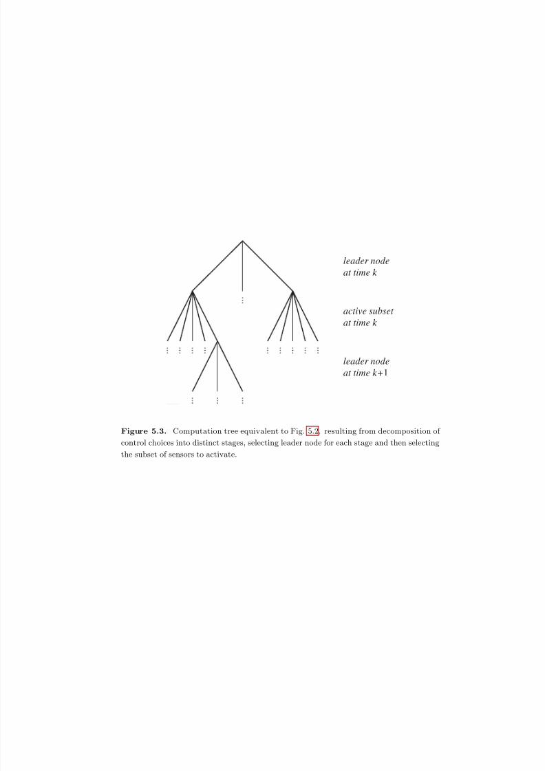
8/2/2019 Information Theoretic Sensor Management
http://slidepdf.com/reader/full/information-theoretic-sensor-management 173/203
leader node
at time k
leader node
at time k+1
active subset
at time k
Figure 5.3. Computation tree equivalent to Fig. 5.2, resulting from decomposition of
control choices into distinct stages, selecting leader node for each stage and then selecting
the subset of sensors to activate.

8/2/2019 Information Theoretic Sensor Management
http://slidepdf.com/reader/full/information-theoretic-sensor-management 174/203
leader node
at time k
leader node
at time k+1
second active sensor
at time k
first active sensor
at time k
T T
Figure 5.4. Computation tree equivalent to Fig. 5.2 and Fig. 5.3, resulting from further
decomposing sensor subset selection problem into a generalized stopping problem, in which
each substage allows one to terminate and move onto the next time slot with the current
set of selected sensors, or to add an additional sensor.
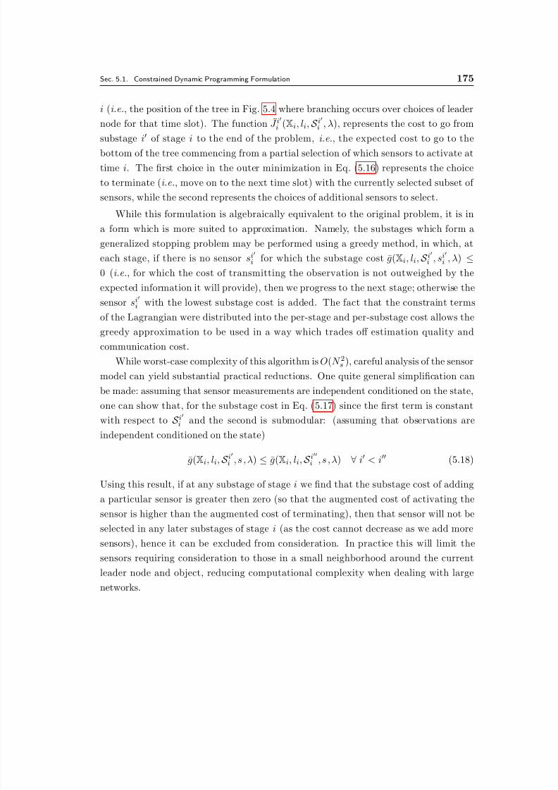
8/2/2019 Information Theoretic Sensor Management
http://slidepdf.com/reader/full/information-theoretic-sensor-management 175/203
Sec. 5.1. Constrained Dynamic Programming Formulation 175
i (i.e., the position of the tree in Fig. 5.4 where branching occurs over choices of leader
node for that time slot). The function J i
i (Xi, li, S ii , λ), represents the cost to go from
substage i of stage i to the end of the problem, i.e., the expected cost to go to thebottom of the tree commencing from a partial selection of which sensors to activate at
time i. The first choice in the outer minimization in Eq. (5.16) represents the choice
to terminate (i.e., move on to the next time slot) with the currently selected subset of
sensors, while the second represents the choices of additional sensors to select.
While this formulation is algebraically equivalent to the original problem, it is in
a form which is more suited to approximation. Namely, the substages which form a
generalized stopping problem may be performed using a greedy method, in which, at
each stage, if there is no sensor si
i for which the substage cost g(Xi, li, S ii , si
i , λ) ≤
0 (i.e., for which the cost of transmitting the observation is not outweighed by theexpected information it will provide), then we progress to the next stage; otherwise the
sensor si
i with the lowest substage cost is added. The fact that the constraint terms
of the Lagrangian were distributed into the per-stage and per-substage cost allows the
greedy approximation to be used in a way which trades off estimation quality and
communication cost.
While worst-case complexity of this algorithm is O(N 2s ), careful analysis of the sensor
model can yield substantial practical reductions. One quite general simplification can
be made: assuming that sensor measurements are independent conditioned on the state,
one can show that, for the substage cost in Eq. ( 5.17) since the first term is constant
with respect to S ii and the second is submodular: (assuming that observations are
independent conditioned on the state)
g(Xi, li, S ii , s , λ) ≤ g(Xi, li, S ii , s , λ) ∀ i < i (5.18)
Using this result, if at any substage of stage i we find that the substage cost of adding
a particular sensor is greater then zero (so that the augmented cost of activating the
sensor is higher than the augmented cost of terminating), then that sensor will not be
selected in any later substages of stage i (as the cost cannot decrease as we add more
sensors), hence it can be excluded from consideration. In practice this will limit the
sensors requiring consideration to those in a small neighborhood around the current
leader node and object, reducing computational complexity when dealing with large
networks.
8/2/2019 Information Theoretic Sensor Management
http://slidepdf.com/reader/full/information-theoretic-sensor-management 176/203
.
.
.
.
.
.
.
.
.
l1
kl2
k
l3
k
l1k+1
l2k+1
l3k+1
l1k+2 l
2k+2 l
3k+2
G
G G G
G G
Figure 5.5. Tree structure for n-scan pruning algorithm with n = 1. At each stage new
leaves are generated extending each remaining sequence with using each new leader node.Subsequently, all but the best sequence ending with each leader node is discarded (marked
with ‘×’), and the remaining sequences are extended using greedy sensor subset selection
(marked with ‘G’).

8/2/2019 Information Theoretic Sensor Management
http://slidepdf.com/reader/full/information-theoretic-sensor-management 177/203
Sec. 5.1. Constrained Dynamic Programming Formulation 177
5.1.8 n-Scan pruning
The algorithm described above is embedded within a slightly less coarse approxima-
tion for leader node selection, which incorporates costs over multiple time stages. This
approximation operates similarly to the n-scan pruning algorithm, which is commonly
used to control computational complexity in the Multiple Hypothesis Tracker [58]. Set-
ting n = 1, the algorithm is illustrated in Fig. 5.5. We commence by considering each
possible choice of leader node2 for the next time step and calculating the greedy sensor
subset selection from Section 5.1.7 for each leader node choice (the decisions made in
each of these branches will differ since the sensors must transmit their observations to
a different leader node, incurring a different communication cost). Then, for each leaf
node, we consider the candidate leader nodes at the following time step. All sequences
ending with the same candidate leader node are compared, the one with the lowestcost value is kept, and the other sequences are discarded. Thus, at each stage, we keep
some approximation of the best control trajectory which ends with each sensor as leader
node.
Using such an algorithm, the tree width is constrained to the number of sensors,
and the overall worst case computational complexity is O(NN s3) (in practice, at each
stage we only consider candidate sensors in some neighborhood of the estimated ob-
ject location, and the complexity will be substantially lower). This compares to the
simulation-based evaluation of the full dynamic programming recursion which, as dis-
cussed in Section 5.1.5, has a computation complexity of the order O(N sN 2N sN N p
N ).
The difference in complexity is striking: even for a problem with N s = 20 sensors, a
planning horizon of N = 10 and simulating N p = 50 values of observations at each
stage, the complexity is reduced from 1.6 × 1090 to (at worst case) 8 × 10⁵.
Because the communication cost structure is Markovian with respect to the leader
node (i.e., the communication cost of a particular future control trajectory is unaffected
by the control history given the current leader node), it is captured perfectly by this
model. The information reward structure, which is not Markovian with respect to the
leader node, is approximated using the greedy method.
5.1.9 Sequential subgradient update
The previous two sections provide an efficient algorithm for generating a plan for the
next N steps given a particular value of the dual variable λ. Substituting the resulting
2The set of candidate leader nodes would, in practice, be limited to sensors close to the object,
similar to the sensor subset selection.
8/2/2019 Information Theoretic Sensor Management
http://slidepdf.com/reader/full/information-theoretic-sensor-management 178/203
178 CHAPTER 5. SENSOR MANAGEMENT IN SENSOR NETWORKS
plan into Eq. (2.56) yields a subgradient which can be used to update the dual variables
(under the linear Gaussian approximation, feedback policies correspond to open loop
plans, hence the argument of the expectation of E[
i G(Xi, li−1, µi(Xi, li−1)) − M ] isdeterministic). A full subgradient implementation would require evaluation for many
different values of the dual variable each time re-planning is performed, which is un-
desirable since each evaluation incurs a substantial computational cost.3 Since the
planning is over many time steps, in practice the level of the constraint (i.e., the value
of E[
i G(Xi, li−1, µi(Xi, li−1))−M ]) will vary little between time steps, hence the slow
adaptation of the dual variable provided by a single subgradient step in each iteration
may provide an adequate approximation.
In the experiments which follow, at each time step we plan using a single value of
the dual variable, and then update it for the next time step utilizing either an additive
update:
λk+1 =
min{λk + γ +, λmax}, E[
i G(Xi, li−1, µi(Xi, li−1))] > M
max{λk − γ −, λmin}, E[
i G(Xi, li−1, µi(Xi, li−1))] ≤ M (5.19)
or a multiplicative update:
λk+1 =
min{λkβ +, λmax}, E[
i G(Xi, li−1, µi(Xi, li−1))] > M
max{λk/β −, λmin}, E[
i G(Xi, li−1, µi(Xi, li−1))] ≤ M
(5.20)
where γ + and γ − are the increment and decrement sizes, β + and β − are the increment
and decrement factors, and λmax and λmin are the maximum and minimum values of
the dual variable. It is necessary to limit the values of the dual variable since the
constrained problem may not be feasible. If the variable is not constrained, undesirable
behavior can result such as utilizing every sensor in a sensor network in order to meet
an information constraint which cannot be met in any case, or because the dual variable
in the communication constraint was adapted such that it became too low, effectively
implying that communications are cost-free.
The dual variables may be initialized using several subgradient iterations or some
form of line search when the algorithm is first executed in order to commence with avalue in the right range.
3The rolling horizon formulation necessitates re-optimization of the dual variable at every time step,
as opposed to [18].

8/2/2019 Information Theoretic Sensor Management
http://slidepdf.com/reader/full/information-theoretic-sensor-management 179/203
Sec. 5.1. Constrained Dynamic Programming Formulation 179
5.1.10 Roll-out
If the horizon length is set to be too small in the communications constrained for-
mulation, then the resulting solution will be to hold the leader node fixed, and take
progressively fewer observations. To prevent this degenerate behavior, we use a roll-out
approach (a commonly used suboptimal control methodology), in which we add to the
terminal cost in the DP recursion (Eq. (5.6)) the cost of transmitting the probabilistic
model to the sensor with the smallest expected distance to the object at the final stage.
Denoting by µ(Xk) ∈ S the policy which selects as leader node the sensor with the
smallest expected distance to the object, the terminal cost is:
J k+N (Xk+N , lk+N −1) = λB pC lk+N −1µ(Xk+N ) (5.21)
where the Lagrange multiplier λ is included only in the communication-constrained
case. This effectively acts as the cost of the base policy in a roll-out [9]. The resulting
algorithm constructs a plan which assumes that, at the final stage, the leader node will
have to be transferred to the closest sensor, hence there is no benefit in holding it at its
existing location indefinitely. In the communication-constrained case, this modification
can make the problem infeasible for short planning horizons, but the limiting of the
dual variables discussed in Section 5.1.9 can avoid anomalous behavior.
5.1.11 Surrogate constraints
A form of information constraint which is often more desirable is one which capturesthe notion that it is acceptable for the uncertainty in object state to increase for short
periods of time if informative observations are likely to become available later. The
minimum entropy constraint is such an example:
E
min
i∈{k,...,k+N −1}H (xi|z0, . . . , zi−1) − H max
≤ 0 (5.22)
The constraint in Eq. (5.22) does not have an additive decomposition (cf Eq. (5.10)),
as required by the approximations in Sections 5.1.7 and 5.1.8. However, we can use
the constraint in Eq. (5.10) to generate plans for a given value of the dual variable λ
using the approximations, and then perform the dual variable update of Section 5.1.9
using the desired constraint, Eq. (5.22). This simple approximation effectively uses the
additive constraint in Eq. (5.10) as a surrogate for the desired constraint in Eq. (5.22),
allowing us to use the computationally convenient method described above with a more
meaningful criterion.

8/2/2019 Information Theoretic Sensor Management
http://slidepdf.com/reader/full/information-theoretic-sensor-management 180/203
180 CHAPTER 5. SENSOR MANAGEMENT IN SENSOR NETWORKS
5.2 Decoupled Leader Node Selection
Most of the sensor management strategies proposed for object localization in existing
literature seek to optimize the estimation performance of the system, incorporating
communication cost indirectly, such as by limiting the maximum number of sensors
utilized. These methods typically do not consider the leader node selection problem
directly, although the communication cost consumed in implementing them will vary
depending on the leader node since communications costs are dependent on the trans-
mission distance. In order to compare the performance of the algorithm developed in
Section 5.1 with these methods, we develop an approach which, conditioned on a par-
ticular sensor management strategy (that is insensitive to the choice of leader node),
seeks to dynamically select the leader node to minimize the communications energy
consumed due to activation, deactivation and querying of sensors by the leader node,and transmission of observations from sensors to the leader node. This involves a trade-
off between two different forms of communication: the large, infrequent step increments
produced when the probability distribution is transferred from sensor to sensor during
leader node hand-off, and the small, frequent increments produced by activating, de-
activating and querying sensors. The approach is fundamentally different from that in
Section 5.1 as we are optimizing the leader node selection conditioned on a fixed sensor
management strategy, rather than jointly optimizing sensor management and leader
node selection.
5.2.1 Formulation
The objective which we seek to minimize is the expected communications cost over
an N -step rolling horizon. We require the sensor management algorithm to provide
predictions of the communications performed by each sensor at each time in the fu-
ture. As in Section 5.1, the problem corresponds to a dynamic program in which the
decision state at time k is the combination of the conditional PDF of object state,
Xk p(xk|z0, . . . , zk−1), and the previous leader node, lk−1. The control which we
may choose is the leader node at each time, uk = lk ∈ S . Denoting the expected cost of
communications expended by the sensor management algorithm (due to sensor activa-
tion and deactivation, querying and transmission of obervations) at time k if the leader
node is lk as gc(Xk, lk), the dynamic program for selecting the leader node at time k
can be written as the following recursive equation:
J i(Xi, li−1) = minli∈S
gc(Xi, li) + B pC li−1li + E
Xi+1|Xi,liJ i+1(Xi+1, li)
(5.23)

8/2/2019 Information Theoretic Sensor Management
http://slidepdf.com/reader/full/information-theoretic-sensor-management 181/203
Sec. 5.3. Simulation results 181
for i ∈ {k , . . . , k + N − 1}. In the same way as discussed in Section 5.1.10, we set the
terminal cost to the cost of transmitting the probabilistic model from the current leader
node to the node with the smallest expected distance to the object, µ(Xk+N ):
J k+N (Xk+N , lk+N −1) = B pC lk+N −1µ(Xk+N ) (5.24)
In Section 5.3 we apply this method using a single look-ahead step (N = 1) with a
greedy sensor management strategy selecting firstly the most informative observation,
and then secondly the two most informative observations.
5.3 Simulation results
As an example of the employment of our algorithm, we simulate a scenario involving
an object moving through a network of sensors. The state of the object is position andvelocity in two dimensions (xk = [ px vx py vy]T ); the state evolves according to the
nominally constant velocity model described in Eq. (2.8), with ∆t = 0.25 and q = 10−2.
The simulation involves N s = 20 sensors positioned randomly according to a uniform
distribution inside a 100×100 unit region; each trial used a different sensor layout and
object trajectory. Denoting the measurement taken by sensor s ∈ S = {1 : N s} (where
N s is the number of sensors) at time k as zsk, a nonlinear observation model is assumed:
zsk = h(xk, s) + vs
k (5.25)
where vsk
∼ N{vs
k; 0, 1
}is a white Gaussian noise process, independent of wk
∀k and
of v jk, j = s ∀ k. The observation function h(·, s) is a quasi-range measurement, e.g.,
resulting from measuring the intensity of an acoustic emission of known amplitude:
h(xk, s) =a
||Lxk − ys||22 + b(5.26)
where L is the matrix which extracts the position of the object from the object state
(such that Lxk is the location of the object), and ys is the location of the s-th sensor.
The constants a and b can be tuned to model the signal-to-noise ratio of the sensor,
and the rate at which the signal-to-noise ratio decreases as distance increases; we use
a = 2000 and b = 100. The information provided by the observation reduces as the
range increases due to the nonlinearity.As described in Section 2.1.3, the measurement function h(·, s) can be approximated
as a first-order Taylor series truncation in a small vicinity around a nominal point x0:
zsk ≈ h(x0, s) + Hs(x0)(xk − x0) + vs
k
Hs(x0) =xh(x, s)|x=x0
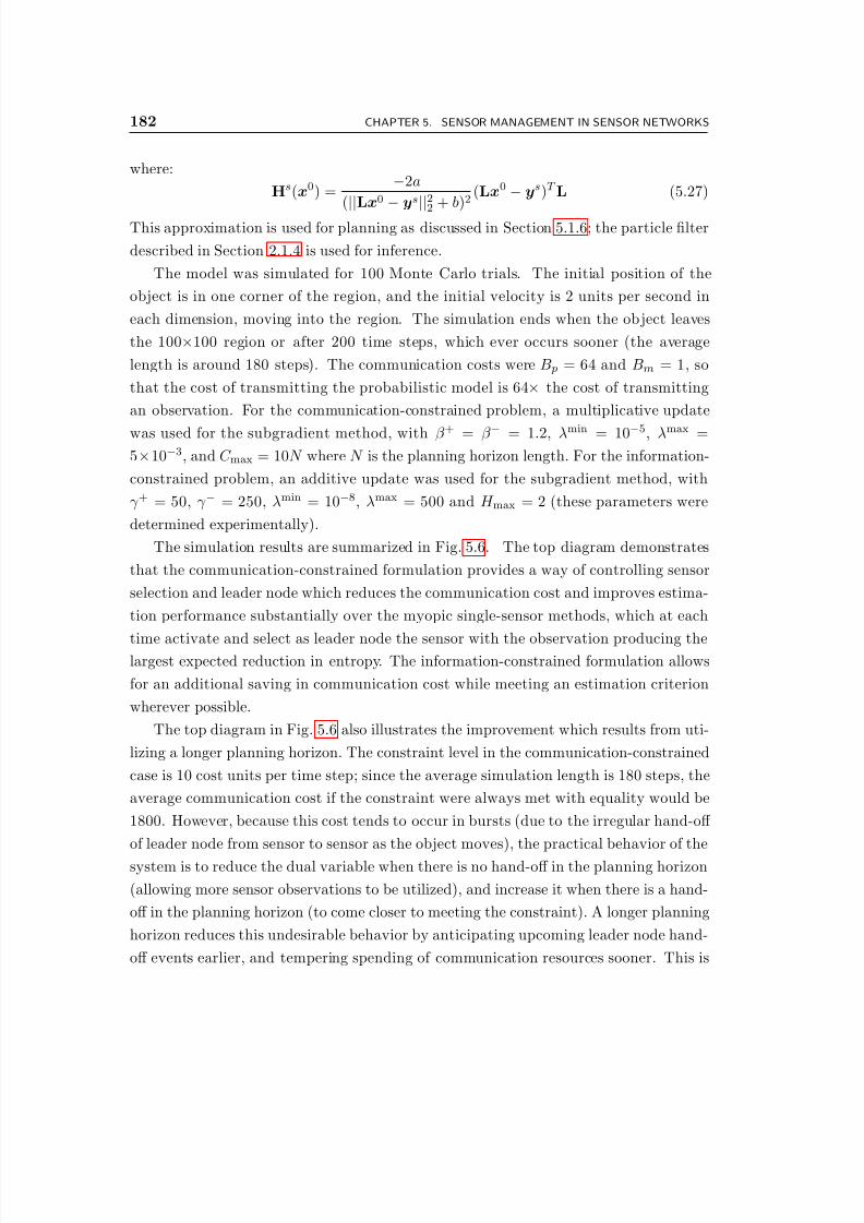
8/2/2019 Information Theoretic Sensor Management
http://slidepdf.com/reader/full/information-theoretic-sensor-management 182/203
182 CHAPTER 5. SENSOR MANAGEMENT IN SENSOR NETWORKS
where:
Hs(x0) =−2a
(||
Lx0
−ys
||22 + b)2
(Lx0 − ys)T L (5.27)
This approximation is used for planning as discussed in Section 5.1.6; the particle filter
described in Section 2.1.4 is used for inference.
The model was simulated for 100 Monte Carlo trials. The initial position of the
object is in one corner of the region, and the initial velocity is 2 units per second in
each dimension, moving into the region. The simulation ends when the object leaves
the 100×100 region or after 200 time steps, which ever occurs sooner (the average
length is around 180 steps). The communication costs were B p = 64 and Bm = 1, so
that the cost of transmitting the probabilistic model is 64× the cost of transmitting
an observation. For the communication-constrained problem, a multiplicative update
was used for the subgradient method, with β + = β − = 1.2, λmin = 10−5, λmax =
5×10⁻³, and C max = 10N where N is the planning horizon length. For the information-
constrained problem, an additive update was used for the subgradient method, with
γ + = 50, γ − = 250, λmin = 10−8, λmax = 500 and H max = 2 (these parameters were
determined experimentally).
The simulation results are summarized in Fig. 5.6. The top diagram demonstrates
that the communication-constrained formulation provides a way of controlling sensor
selection and leader node which reduces the communication cost and improves estima-
tion performance substantially over the myopic single-sensor methods, which at each
time activate and select as leader node the sensor with the observation producing thelargest expected reduction in entropy. The information-constrained formulation allows
for an additional saving in communication cost while meeting an estimation criterion
wherever possible.
The top diagram in Fig. 5.6 also illustrates the improvement which results from uti-
lizing a longer planning horizon. The constraint level in the communication-constrained
case is 10 cost units per time step; since the average simulation length is 180 steps, the
average communication cost if the constraint were always met with equality would be
1800. However, because this cost tends to occur in bursts (due to the irregular hand-off
of leader node from sensor to sensor as the object moves), the practical behavior of the
system is to reduce the dual variable when there is no hand-off in the planning horizon
(allowing more sensor observations to be utilized), and increase it when there is a hand-
off in the planning horizon (to come closer to meeting the constraint). A longer planning
horizon reduces this undesirable behavior by anticipating upcoming leader node hand-
off events earlier, and tempering spending of communication resources sooner. This is
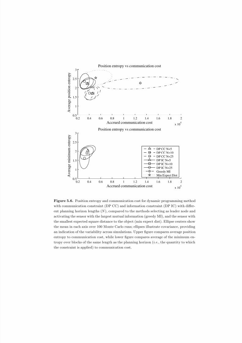
8/2/2019 Information Theoretic Sensor Management
http://slidepdf.com/reader/full/information-theoretic-sensor-management 183/203
0.2 0.4 0.6 0.8 1 1.2 1.4 1.6 1.8 2
x 104
0.5
1
1.5
2
2.5
3
Accrued communication cost
A v e r a g e p o s i t i o n e n t r o p y
Position entropy vs communication cost
0.2 0.4 0.6 0.8 1 1.2 1.4 1.6 1.8 2
x 104
0.5
1
1.5
2
2.5
3
Accrued communication cost
A v e r a g e m i n i m u m e
n t r o p y
Position entropy vs communication cost
DP CC N=5
DP CC N=10
DP CC N=25
DP IC N=5
DP IC N=10
DP IC N=25
Greedy MI
Min Expect Dist
Figure 5.6. Position entropy and communication cost for dynamic programming method
with communication constraint (DP CC) and information constraint (DP IC) with differ-
ent planning horizon lengths (N ), compared to the methods selecting as leader node and
activating the sensor with the largest mutual information (greedy MI), and the sensor with
the smallest expected square distance to the object (min expect dist). Ellipse centers show
the mean in each axis over 100 Monte Carlo runs; ellipses illustrate covariance, providing
an indication of the variability across simulations. Upper figure compares average position
entropy to communication cost, while lower figure compares average of the minimum en-
tropy over blocks of the same length as the planning horizon (i.e., the quantity to which
the constraint is applied) to communication cost.

8/2/2019 Information Theoretic Sensor Management
http://slidepdf.com/reader/full/information-theoretic-sensor-management 184/203
184 CHAPTER 5. SENSOR MANAGEMENT IN SENSOR NETWORKS
demonstrated in Fig. 5.7, which shows the adaptation of the dual variable for a single
Monte Carlo run.
In the information-constrained case, increasing the planning horizon relaxes theconstraint, since it requires the minimum entropy within the planning horizon to be
less than a given value. Accordingly, using a longer planning horizon, the average
minimum entropy is reduced, and additional communication energy is saved. The lower
diagram in Fig. 5.6 shows the average minimum entropy in blocks of the same length as
the planning horizon, demonstrating that the information constraint is met more often
with a longer planning horizon (as well as resulting in a larger communication saving).
Fig. 5.8 compares the adaptive Lagrangian relaxation method discussed in Sec-
tion 5.1 with the decoupled scheme discussed in Section 5.2, which adaptively selects
the leader node to minimize the expected communication cost expended in implement-
ing the decision of the fixed sensor management method. The fixed sensor management
scheme activates the sensor or two sensors with the observation or observations produc-
ing the largest expected reduction in entropy. The results demonstrate that for this case
the decoupled method using a single sensor at each time step results in similar estima-
tion performance and communication cost to the Lagrangian relaxation method using
an information constraint with the given level. Similarly, the decoupled method using
two sensors at each time step results in similar estimation performance and commu-
nication cost to the Lagrangian relaxation method using a communication constraint
with the given level. The additional flexibility of the Lagrangian relaxation method
allows one to select the constraint level to achieve various points on the estimation
performance/communication cost trade-off, rather than being restricted to particular
points corresponding to different numbers of sensors.
5.4 Conclusion and future work
This paper has demonstrated how an adaptive Lagrangian relaxation can be utilized
for sensor management in an energy-constrained sensor network. The introduction
of secondary objectives as constraints provides a natural methodology to address the
trade-off between estimation performance and communication cost.
The planning algorithm may be applied alongside a wide range of estimation meth-
ods, ranging from the Kalman filter to the particle filter. The algorithm is also ap-
plicable to a wide range of sensor models. The linearized Gaussian approximation
in Section 5.1.6 results in a structure identical to the OLFC. The remainder of our
algorithm (removing the linearized Gaussian approximation) may be applied to find

8/2/2019 Information Theoretic Sensor Management
http://slidepdf.com/reader/full/information-theoretic-sensor-management 185/203
0 20 40 60 80 100 120 140 1600
1
2
3
4
5x 10
−3
Time step (k)
Adaptation of dual variable λk
0 20 40 60 80 100 120 140 1600
1000
2000
3000
Time step (k)
Communication cost accrual
N=5
N=10
N=25
Figure 5.7. Adaptation of communication constraint dual variableλk for different horizon
lengths for a single Monte Carlo run, and corresponding cumulative communication costs.
8/2/2019 Information Theoretic Sensor Management
http://slidepdf.com/reader/full/information-theoretic-sensor-management 186/203
0.2 0.4 0.6 0.8 1 1.2 1.4 1.6 1.8 2
x 104
0.5
1
1.5
2
2.5
3
Accrued communication cost
A v e r a g e p o s i t i o n e
n t r o p y
Position entropy vs communication cost
Greedy/Decoupled
Greedy 2/Decoupled
DP CC N=25
DP IC N=25
Figure 5.8. Position entropy and communication cost for dynamic programming method
with communication constraint (DP CC) and information constraint (DP IC), compared
to the method which dynamically selects the leader node to minimize the expected com-
munication cost consumed in implementing a fixed sensor management scheme. The fixed
sensor management scheme activates the sensor (‘greedy’) or two sensors (‘greedy 2’) with
the observation or observations producing the largest expected reduction in entropy. El-
lipse centers show the mean in each axis over 100 Monte Carlo runs; ellipses illustrate
covariance, providing an indication of the variability across simulations.

8/2/2019 Information Theoretic Sensor Management
http://slidepdf.com/reader/full/information-theoretic-sensor-management 187/203
Sec. 5.4. Conclusion and future work 187
an efficient approximation of the OLFC as long as an efficient estimate of the reward
function (mutual information in our case) is available.
The simulation results in Section 5.3 demonstrate that approximations based on
dynamic programming are able to provide similar estimation performance (as measured
by entropy), for a fraction of the communication cost in comparison to simple heuristics
which consider estimation performance alone and utilize a single sensor. The discussion
in Section 5.1.7 provides a guide for efficient implementation strategies that can enable
implementation on the latest generation wireless sensor networks. Future work includes
incorporation of the impact on planning caused by the interaction between objects when
multiple objects are observed by a single sensor, and developing approximations which
are less coarse than the linearized Gaussian model.

8/2/2019 Information Theoretic Sensor Management
http://slidepdf.com/reader/full/information-theoretic-sensor-management 188/203
188 CHAPTER 5. SENSOR MANAGEMENT IN SENSOR NETWORKS

8/2/2019 Information Theoretic Sensor Management
http://slidepdf.com/reader/full/information-theoretic-sensor-management 189/203
Chapter 6
Contributions and future directions
THE preceding chapters have extended existing sensor management methods in
three ways: firstly, obtaining performance guarantees for sequential sensor man-
agement problems; secondly, finding an efficient integer programming solution thatexploits the structure of beam steering; and finally, finding an efficient heuristic sen-
sor management method for object tracking in sensor networks. This chapter briefly
summarizes these contributions, before outlining suggestions of areas for further inves-
tigation.
6.1 Summary of contributions
The following sections outline the contributions made in this thesis.
6.1.1 Performance guarantees for greedy heuristicsThe analysis in Chapter 3 extends the recent work in [46] to the sequential problem
structures that commonly arise in waveform selection and beam steering. The extension
is quite general in that it applies to arbitrary, time varying observation and dynamical
models. Extensions include tighter bounds that exploit either process diffusiveness or
objectives involving discount factors, and applicability to closed loop problems. The
results apply to objectives including mutual information; the log-determinant of the
Fisher information matrix was also shown to be submodular, yielding a guarantee on
the posterior Cramer-Rao bound. Examples demonstrate that the bounds are tight,
and counterexamples illuminate larger classes of problems to which they do not apply.The results are the first of their type for sequential problems, and effectively justify
the use of the greedy heuristic in certain contexts, delineating problems in which addi-
tional open loop planning can be beneficial from those in which it cannot. For example,
if a factor of 0.5 of the optimal performance is adequate, then additional planning is un-
189

8/2/2019 Information Theoretic Sensor Management
http://slidepdf.com/reader/full/information-theoretic-sensor-management 190/203
190 CHAPTER 6. CONTRIBUTIONS AND FUTURE DIRECTIONS
necessary for any problem that fits within the structure. The online guarantees confirm
cases in which the greedy heuristic is even closer to optimality.
6.1.2 Efficient solution for beam steering problems
The analysis in Chapter 4 exploits the special structure in problems involving large
numbers of independent objects to find an efficient solution of the beam steering prob-
lem. The analysis from Chapter 3 was utilized to obtain an upper bound on the objec-
tive function. Solutions with guaranteed near-optimality were found by simultaneously
reducing the upper bound and raising a matching lower bound.
The algorithm has quite general applicability, admitting time varying observation
and dynamical models, and observations requiring different time durations to complete.
An alternative formulation that was specialized to time invariant rewards provided afurther computational saving. The methods are applicable to a wide range of objectives,
including mutual information and the posterior Cramer-Rao bound.
Computational experiments demonstrated application to problems involving 50–80
objects planning over horizons up to 60 time slots. Performing planning of this type
through full enumeration would require evaluation of the reward of more than 10100
different observation sequences. As well as demonstrating that the algorithm is suitable
for online application, these experiments also illustrate a new capability for exploring
the benefit that is possible through utilizing longer planning horizons. For example, we
have quantified the small benefit of additional open loop planning in problems where
models exhibit low degrees of non-stationarity.
6.1.3 Sensor network management
In Chapter 5, we presented a method trading off estimation performance and energy
consumed in an object tracking problem. The trade off between these two quanti-
ties was formulated by maximizing estimation performance subject to a constraint on
energy cost, or the dual of this, i.e., minimizing energy cost subject to a constraint
on estimation performance. Our analysis has proposed a planning method that is both
computable and scalable, yet still captures the essential structure of the underlying trade
off. The simplifications enable computation over much longer planning horizons: e.g.,
in a problem involving N s = 20 sensors, closed loop planning over a horizon of N = 20
time steps using N p = 50 simulated values of observations at each stage would involve
complexity of the order O([N s2N s ]N N N p ) ≈ 10180; the simplifications yield worst-case
computation of the order O(NN 3s ) = 1.6 × 10⁵. Simulation results demonstrate the
8/2/2019 Information Theoretic Sensor Management
http://slidepdf.com/reader/full/information-theoretic-sensor-management 191/203
Sec. 6.2. Recommendations for future work 191
dramatic reduction in the communication cost required to achieve a given estimation
performance level as compared to previously proposed algorithms. The approximations
are applicable to a wide range of problems; e.g., even if the linearized Gaussian as-sumption is relaxed, the remaining approximations may be applied to find an efficient
approximation of the open loop feedback controller as long as an efficient estimate of
the reward function (mutual information in our case) is available.
6.2 Recommendations for future work
The following sections describe some promising areas for future investigation.
6.2.1 Performance guarantees
Chapter 3 has explored several performance guarantees that are possible through ex-
ploitation of submodular objectives, as well as some of the boundaries preventing wider
application. Directions in which this analysis may be extended include those outlined
in the following paragraphs.
Guarantees for longer look-ahead lengths
It is easy to show that no stronger guarantees exist for heuristics using longer look-
ahead lengths for general models; e.g., if we introduce additional time slots, in which
all observations are uninformative, in between the two original time slots in Exam-
ple 3.1, we can obtain the same factor of 0.5 for any look-ahead length. However, underdiffusive assumptions, one would expect that additional look-ahead steps would yield
an algorithm that is closer to optimal.
Observations consuming different resources
Our analysis inherently assumes that all observations utilize the same resources: the
same options available to us in later stages regardless of the choice we make in the
current stage. In [46], a guarantee is obtained for the subset selection problem in which
each observation j has a resource consumption c j, and we seek the most informative
subset A of observations for which
j∈A c j ≤ C . Expanding this analysis to sequentialselection problems involving either a single resource constraint encompassing all time
slots, or separate resource constraints for each time slot, would be an interesting exten-
sion. A guarantee with a factor of (e − 1)/(2e − 1) ≈ 0.387 can be obtained quite easily
in the latter case, but it may be possible to obtain tighter guarantees ( i.e., 0.5).
8/2/2019 Information Theoretic Sensor Management
http://slidepdf.com/reader/full/information-theoretic-sensor-management 192/203
192 CHAPTER 6. CONTRIBUTIONS AND FUTURE DIRECTIONS
Closed loop guarantees
Example 3.3 establishes that there is no guarantee on the ratio of the performance of
the greedy heuristic operating in closed loop to the performance of the optimal closed
loop controller. However, it may be possible to introduce additional structure (e.g.,
diffusiveness and/or limited bandwidth observations) to obtain some form of weakened
guarantee.
Stronger guarantees exploiting additional structure
Finally, while the guarantees in Chapter 3 have been shown to be tight within the level
of generality to which they apply, it may be possible to obtain stronger guarantees
for problems with specific structure, e.g., linear Gaussian problems with dynamics and
observation models satisfying particular properties. An example of this is the resultthat greedy heuristics are optimal for beam steering of one-dimensional linear Gaussian
systems [33].
6.2.2 Integer programming formulation of beam steering
Chapter 4 proposed a new method for efficient solution of beam steering problems, and
explored its performance and computation complexity. There are several areas in which
this development may be extended, as outlined in the following sections.
Alternative update algorithms
The algorithm presented in Section 4.3.3 represents one of many ways in which the
update between iterations could be performed. It remains to explore the relative benefits
of other update algorithms; e.g., generating candidate subsets for each of the chosen
exploration subset elements, rather than just the one with the highest reward increment.
Deferred reward calculation
It may be beneficial to defer calculation of some of the incremental rewards, e.g., the
incremental reward of an exploration subset element conditioned on a given candidate
subset is low enough that it is unlikely to be chosen, it would seem unnecessary torecalculate the incremental reward when the candidate subset is extended.

8/2/2019 Information Theoretic Sensor Management
http://slidepdf.com/reader/full/information-theoretic-sensor-management 193/203
Sec. 6.2. Recommendations for future work 193
Accelerated search for lower bounds
The lower bound in Section 4.3.6 utilizes the results of the Algorithm 4.1 to find the
best solution amongst those explored so far (i.e., those for which the exact reward
has been evaluated). However, the decisions made by Algorithm 4.1 tend to focus on
reducing the upper bound to the reward rather than on finding solutions for which the
reward is high. It may be beneficial to incorporate heuristic searches that introduce
additional candidate subsets that appear promising in order to raise the lower bound
quickly as well as decreasing the upper bound. One example of this would be to include
candidate subsets corresponding to the decisions made by the greedy heuristic—this
would ensure that a solution at least as good as that of the greedy heuristic will be
obtained regardless of when the algorithm is terminated.
Integration into branch and bound procedure
In the existing implementation, changes made between iterations of the integer program
force the solver to restart the optimization. A major computational saving may result
if a method is found that allows the solution of the previous iteration to be applied to
the new solution. This is easily performed in linear programming problems, but is more
difficult in integer programming problems since the bounds previously evaluated in the
branch and bound process are (in general) invalidated. A further extension along the
same line would be to integrate the algorithm for generating new candidate sets with
the branch and bound procedure for the integer program.
6.2.3 Sensor network management
Chapter 5 provides a computable method for tracking an object using a sensor network,
with demonstrated empirical performance. Possible extensions include multiple objects
and performance guarantees.
Problems involving multiple objects
While the discussion in Chapter 5 focused on the case of a single object, the concept
may be easily extended to multiple objects. When objects are well-separated in space,
one may utilize a parallel instance of the algorithm from Chapter 5 for each object.
When objects become close together and observations induce conditional dependency
in their states, one may either store the joint conditional distribution of the object
group at one sensor, or utilize a distributed representation across two or more sensors.
In the former case, there will be a control choice corresponding to breaking the joint
8/2/2019 Information Theoretic Sensor Management
http://slidepdf.com/reader/full/information-theoretic-sensor-management 194/203
194 CHAPTER 6. CONTRIBUTIONS AND FUTURE DIRECTIONS
distribution into its marginals after the objects separate again. This will result in a loss
of information and a saving in communication cost, both of which could be incorporated
into the trade-off performed by the constrained optimization. In the case of a distributedrepresentation of the joint conditional distribution, it will be necessary to quantify both
the benefit (in terms of estimation performance) and cost of each of the communications
involved in manipulating the distributed representation.
Performance guarantees
The algorithm presented in Chapter 5 does not possess any performance guarantee;
Section 3.9 provides an example of a situation in which one element of the approxi-
mate algorithm performs poorly. An extension of both Chapters 3 and 5 is to exploit
additional problem structure and amend the algorithm to guarantee performance.

8/2/2019 Information Theoretic Sensor Management
http://slidepdf.com/reader/full/information-theoretic-sensor-management 195/203
Bibliography
[1] Karim M. Abadir and Jan R. Magnus. Matrix Algebra . Cambridge University
Press, 2005.
[2] Eitan Altman. Constrained Markov decision processes. Chapman and Hall, Lon-
don, UK, 1999.
[3] Brian D. O. Anderson and John B. Moore. Optimal filtering . Prentice-Hall, En-
glewood Cliffs, NJ, 1979.
[4] M. Sanjeev Arulampalam, Simon Maskell, Neil Gordon, and Tim Clapp. A tuto-
rial on particle filters for online nonlinear/non-Gaussian Bayesian tracking. IEEE
Transactions on Signal Processing , 50(2):174–188, February 2002.
[5] Lawrence M. Ausubel. An efficient ascending-bid auction for multiple ob jects.
American Economic Review , 94(5):1452–1475, December 2004.
[6] Yaakov Bar-Shalom and Xiao-Rong Li. Estimation and Tracking: Principles, Tech-
niques and Software. Artech House, Norwood, MA, 1993.
[7] M Behara. Additive and Nonadditive Measures of Entropy . Wiley Eastern Ltd,
New Delhi, India, 1990.
[8] P.E. Berry and D.A.B. Fogg. On the use of entropy for optimal radar resource man-
agement and control. In Radar Conference, 2003. Proceedings of the International ,
pages 572–577, 2003.
[9] Dimitri P. Bertsekas. Dynamic Programming and Optimal Control . Athena Scien-
tific, Belmont, MA, second edition, 2000.
[10] Dimitri P. Bertsekas. Nonlinear Programming . Athena Scientific, Belmont, MA,
second edition, 1999.
195
8/2/2019 Information Theoretic Sensor Management
http://slidepdf.com/reader/full/information-theoretic-sensor-management 196/203
196 BIBLIOGRAPHY
[11] D.P. Bertsekas. Auction algorithms for network flow problems: A tutorial intro-
duction. Computational Optimization and Applications, 1:7–66, 1992.
[12] Dimitris Bertsimas and John N. Tsitsiklis. Introduction to Linear Optimization .
Athena Scientific, Belmont, MA, 1997.
[13] Frederick J. Beutler and Keith W. Ross. Optimal policies for controlled Markov
chains with a constraint. Journal of Mathematical Analysis and Applications, 112
(1):236–252, November 1985.
[14] Samuel S. Blackman and Robert Popoli. Design and Analysis of Modern Tracking
Systems. Artech House, Norwood, MA, 1999.
[15] V.D. Blondel and John N. Tsitsiklis. A survey of computational complexity resultsin systems and control. Automatica , 36(9):1249–1274, September 2000.
[16] David A. Castanon. Stochastic control bounds on sensor network performance. In
IEEE Conference on Decision and Control , pages 4939–4944, 2005.
[17] David A. Castanon. Optimal search strategies in dynamic hypothesis testing. Sys-
tems, Man and Cybernetics, IEEE Transactions on , 25(7):1130–1138, July 1995.
[18] David A. Castanon. Approximate dynamic programming for sensor management.
In Proc 36th Conference on Decision and Control , pages 1202–1207. IEEE, Decem-
ber 1997.
[19] Lei Chen, Martin J. Wainwright, Mujdat Cetin, and Alan S. Willsky. Data as-
sociation based on optimization in graphical models with application to sensor
networks. Mathematical and Computer Modelling , 43(9-10):1114–1135, May 2006.
[20] Amit S. Chhetri, Darryl Morrell, and Antonia Papandreou-Suppappola. Energy
efficient target tracking in a sensor network using non-myopic sensor scheduling.
In Proc. Eighth International Conference of Information Fusion , July 2005.
[21] A.S. Chhetri, D. Morrell, and A. Papandreou-Suppappola. Scheduling multiple
sensors using particle filters in target tracking. In IEEE Workshop on Statistical Signal Processing , pages 549–552, September/October 2003.
[22] A.S. Chhetri, D. Morrell, and A. Papandreou-Suppappola. Sensor scheduling using
a 0-1 mixed integer programming framework. In Fourth IEEE Workshop on Sensor
Array and Multi-channel Processing , 2006.

8/2/2019 Information Theoretic Sensor Management
http://slidepdf.com/reader/full/information-theoretic-sensor-management 197/203
BIBLIOGRAPHY 197
[23] Thomas M. Cover and Joy A. Thomas. Elements of Information Theory . John
Wiley and Sons, New York, NY, 1991.
[24] O.E. Drummond, David A. Castanon, and M.S. Bellovin. Comparison of 2-D as-
signment algorithms for sparse, rectangular, floating point, cost matrices. Journal
of the SDI Panels on Tracking , (4):81–97, December 1990.
[25] Emre Ertin, John W. Fisher, and Lee C. Potter. Maximum mutual information
principle for dynamic sensor query problems. In Proc IPSN 2003 , pages 405–416.
Springer-Verlag, April 2003.
[26] Satoru Fujishige. Submodular functions and optimization , volume 58 of Annals of
discrete mathematics. Elsevier, Boston, MA, second edition, 2005.
[27] Arthur Gelb. Applied optimal estimation . MIT Press, Cambridge, MA, 1974.
[28] Neil Gordon, David J. Salmond, and A.F.M. Smith. Novel approach to non-linear
and non-Gaussian Bayesian state estimation. IEE Proceedings F: Radar and Signal
Processing , 140:107–113, 1993.
[29] Ying He and Edwin K. P. Chong. Sensor scheduling for target tracking: A Monte
Carlo sampling approach. Digital Signal Processing . to appear.
[30] M.L. Hernandez, T. Kirubarajan, and Y. Bar-Shalom. Multisensor resource de-
ployment using posterior cramer-rao bounds. IEEE Transactions on Aerospace and Electronic Systems, 40(2):399–416, 2004.
[31] Kenneth J. Hintz and Gregory A. McIntyre. Goal lattices for sensor management.
In Signal Processing, Sensor Fusion, and Target Recognition VIII , volume 3720,
pages 249–255. SPIE, 1999.
[32] K.J. Hintz and E.S. McVey. Multi-process constrained estimation. Systems, Man
and Cybernetics, IEEE Transactions on , 21(1):237–244, 1991.
[33] Stephen Howard, Sofia Suvorova, and Bill Moran. Optimal policy for scheduling
of Gauss-Markov systems. In Proceedings of the Seventh International Conferenceon Information Fusion , 2004.
[34] A. T. Ihler, J. W. Fisher III, R. L. Moses, and A. S. Willsky. Nonparametric belief
propagation for self-calibration in sensor networks. IEEE Journal of Selected Areas
in Communication , 2005.
8/2/2019 Information Theoretic Sensor Management
http://slidepdf.com/reader/full/information-theoretic-sensor-management 198/203
198 BIBLIOGRAPHY
[35] A.T. Ihler, E.B. Sudderth, W.T. Freeman, and A.S. Willsky. Efficient multiscale
sampling from products of Gaussian mixtures. In Neural Information Processing
Systems 17 , 2003.
[36] A.T. Ihler, J.W. Fisher III, and A.S. Willsky. Communications-constrained infer-
ence. Technical Report 2601, Massachusetts Institute of Technology Laboratory
for Information and Decision Systems, 2004.
[37] Mark Jones, Shashank Mehrotra, and Jae Hong Park. Tasking distributed sensor
networks. International Journal of High Performance Computing Applications, 16
(3):243–257, 2002.
[38] Michael I. Jordan. Graphical models. Statistical Science, 19(1):140–155, 2004.
[39] S.J. Julier and J.K. Uhlmann. Unscented filtering and nonlinear estimation. Pro-
ceedings of the IEEE , 92(3):401–422, March 2004.
[40] M. Kalandros and L.Y. Pao. Covariance control for multisensor systems. IEEE
Transactions on Aerospace and Electronic Systems, 38(4):1138–1157, 2002.
[41] Keith D. Kastella. Discrimination gain to optimize detection and classification.
SPIE Signal and Data Processing of Small Targets, 2561(1):66–70, 1995.
[42] D.J. Kershaw and R.J. Evans. Optimal waveform selection for tracking systems.
IEEE Transactions on Information Theory , 40(5):1536–1550, September 1994.
[43] D.J. Kershaw and R.J. Evans. Waveform selective probabilistic data association.
IEEE Transactions on Aerospace and Electronic Systems, 33(4):1180–1188, Octo-
ber 1997.
[44] Mark P. Kolba, Peter A. Torrione, and Leslie M. Collins. Information-based sensor
management for landmine detection using multimodal sensors. In Detection and
Remediation Technologies for Mines and Minelike Targets X , volume 5794, pages
1098–1107. SPIE, 2005.
[45] J.H. Kotecha and P.M. Djuric. Gaussian particle filtering. Signal Processing,IEEE Transactions on [see also Acoustics, Speech, and Signal Processing, IEEE
Transactions on] , 51(10):2592–2601, October 2003.
[46] Andreas Krause and Carlos Guestrin. Near-optimal nonmyopic value of information
in graphical models. In UAI 2005 , July 2005.

8/2/2019 Information Theoretic Sensor Management
http://slidepdf.com/reader/full/information-theoretic-sensor-management 199/203
BIBLIOGRAPHY 199
[47] Andreas Krause, Carlos Guestrin, and Ajit Paul Singh. Near-optimal sensor place-
ments in Gaussian processes. In International Conference on Machine Learning ,
August 2005.
[48] Andreas Krause, Carlos Guestrin, Anupam Gupta, and John Kleinberg. Near-
optimal sensor placements: Maximizing information while minimizing communica-
tion cost. In Fifth International Conference on Information Processing in Sensor
Networks, April 2006.
[49] Chris Kreucher, Keith Kastella, and Alfred O. Hero III. Information-based sensor
management for multitarget tracking. In SPIE Signal and Data Processing of
Small Targets, volume 5204, pages 480–489. The International Society for Optical
Engineering, 2003.
[50] Chris Kreucher, Alfred O. Hero III, and Keith Kastella. A comparison of task
driven and information driven sensor management for target tracking. In IEEE
Conference on Decision and Control , December 2005.
[51] Chris Kreucher, Keith Kastella, and Alfred O. Hero III. Sensor management using
an active sensing approach. Signal Processing , 85(3):607–624, March 2005.
[52] Chris M. Kreucher, Keith Kastella, and Alfred O. Hero III. A bayesian method for
integrated multitarget tracking and sensor management. In International Confer-
ence on Information Fusion , volume 1, pages 704–711, 2003.
[53] Chris M. Kreucher, Alfred O. Hero III, Keith Kastella, and Daniel Chang. Efficient
methods of non-myopic sensor management for multitarget tracking. In 43rd IEEE
Conference on Decision and Control , December 2004.
[54] Christopher M. Kreucher, Alfred O. Hero III, Keith D. Kastella, and Ben Shapo.
Information-based sensor management for simultaneous multitarget tracking and
identification. In Proceedings of The Thirteenth Annual Conference on Adaptive
Sensor Array Processing (ASAP), June 2005.
[55] V. Krishnamurthy. Algorithms for optimal scheduling and management of hidden
Markov model sensors. Signal Processing, IEEE Transactions on , 50(6):1382–1397,
2002.

8/2/2019 Information Theoretic Sensor Management
http://slidepdf.com/reader/full/information-theoretic-sensor-management 200/203
200 BIBLIOGRAPHY
[56] V. Krishnamurthy and R.J. Evans. Hidden Markov model multiarm bandits: a
methodology for beam scheduling in multitarget tracking. Signal Processing, IEEE
Transactions on , 49(12):2893–2908, December 2001.
[57] V. Krishnamurthy and R.J. Evans. Correction to ‘Hidden Markov model multi-
arm bandits: a methodology for beam scheduling in multitarget tracking’. Signal
Processing, IEEE Transactions on , 51(6):1662–1663, June 2003.
[58] Thomas Kurien. Issues in the design of practical multitarget tracking algorithms. In
Multitarget-Multisensor Tracking: Advanced Applications, pages 43–83, Norwood,
MA, 1990. Artech-House.
[59] B. La Scala, M. Rezaeian, and B. Moran. Optimal adaptive waveform selection for
target tracking. In Proceedings of the Eighth International Conference on Infor-
mation Fusion , volume 1, pages 552–557, 2005.
[60] B.F. La Scala, W. Moran, and R.J. Evans. Optimal adaptive waveform selection
for target detection. In Proceedings of the International Radar Conference, pages
492–496, September 2003.
[61] II Lewis, P. The characteristic selection problem in recognition systems. IEEE
Transactions on Information Theory , 8(2):171–178, February 1962. ISSN 0018-
9448.
[62] Dan Li, Kerry D. Wong, Yu Hen Hu, and Akbar M. Sayeed. Detection, classi-
fication, and tracking of targets. IEEE Signal Processing Magazine, 19(2):17–29,
March 2002.
[63] Michael L. Littman, Anthony R. Cassandra, and Leslie Pack Kaelbling. Efficient
dynamic-programming updates in partially observable Markov decision processes.
Technical Report CS-95-19, Brown University, 1995.
[64] Juan Liu, James Reich, and Feng Zhao. Collaborative in-network processing for
target tracking. EURASIP Journal on Applied Signal Processing , (4):378–391,
2003.
[65] A. Logothetis and A. Isaksson. On sensor scheduling via information theoretic
criteria. In Proceedings of the American Control Conference, volume 4, pages
2402–2406, San Diego, CA, June 1999.

8/2/2019 Information Theoretic Sensor Management
http://slidepdf.com/reader/full/information-theoretic-sensor-management 201/203
BIBLIOGRAPHY 201
[66] Ronald P. S. Mahler. Global posterior densities for sensor management. In Acqui-
sition, Tracking, and Pointing XII , volume 3365, pages 252–263. SPIE, 1998.
[67] Peter S. Maybeck. Stochastic Models, Estimation, and Control , volume 1. Navtech,
Arlington, VA, 1994.
[68] Peter S. Maybeck. Stochastic Models, Estimation, and Control , volume 2. Navtech,
Arlington, VA, 1994.
[69] Gregory A. McIntyre and Kenneth J. Hintz. Information theoretic approach to
sensor scheduling. In Signal Processing, Sensor Fusion, and Target Recognition V ,
volume 2755, pages 304–312. SPIE, 1996.
[70] Bill Moran, Sofia Suvorova, and Stephen Howard. Advances in Sensing with Se-curity Applications, chapter Sensor management for radar: a tutorial. Springer-
Verlag, 2006.
[71] S. Mori, Chee-Yee Chong, E. Tse, and R. Wishner. Tracking and classifying mul-
tiple targets without a priori identification. IEEE Transactions on Automatic
Control , 31(5):401–409, May 1986. ISSN 0018-9286.
[72] James Munkres. Algorithms for the assignment and transportation problems. Jour-
nal of the Society for Industrial and Applied Mathematics, 5(1):32–38, March 1957.
[73] Kevin P. Murphy. Dynamic Bayesian networks: representation, inference and learning . PhD thesis, University of California, Berkeley, 2002.
[74] A. Nedich, M.K. Schneider, and R.B. Washburn. Farsighted sensor management
strategies for move/stop tracking. In Proceedings of the Eighth International Con-
ference on Information Fusion , volume 1, pages 566–573, 2005.
[75] George L. Nemhauser and Laurence A. Wolsey. Integer and combinatorial opti-
mization . Wiley, 1988.
[76] G.L. Nemhauser, L.A. Wolsey, and M.L. Fisher. An analysis of approximations
for maximizing submodular set functions–I. Mathematical Programming , 14(1):
265–294, December 1978.
[77] G.L. Nemhauser, L.A. Wolsey, and M.L. Fisher. An analysis of approximations
for maximizing submodular set functions–II. In M.L. Balinski and A.J. Hoffman,
8/2/2019 Information Theoretic Sensor Management
http://slidepdf.com/reader/full/information-theoretic-sensor-management 202/203
202 BIBLIOGRAPHY
editors, Polyhedral combinatorics, volume 8 of Mathematical programming study ,
pages 73–87. Elsevier, 1978.
[78] C.H. Papadimitrou and John N. Tsitsiklis. The complexity of Markov decision
processes. Mathematics of Operations Research , 12(3):441–450, August 1987.
[79] David C. Parkes and Lyle H. Ungar. Iterative combinatorial auctions: Theory
and practice. In Proc 17th National Conference on Artificial Intelligence (AAAI),
pages 74–81, 2000.
[80] Kris Pister. Smart dust (keynote address). In IPSN ’03 , April 2003.
[81] G.J. Pottie and W.J. Kaiser. Wireless integrated network sensors. Communications
of the ACM , 43(5):51–58, May 2000.
[82] Donald B. Reid. An algorithm for tracking multiple targets. IEEE Transactions
on Automatic Control , AC-24(6):843–854, December 1979.
[83] Branko Ristic, Sanjeev Arulampalam, and Neil Gordon. Beyond the Kalman Filter:
Particle Filters for Tracking Applications. Artech House, 2004.
[84] Louis L. Scharf. Statistical Signal Processing: Detection, Estimation and Time
Series Analysis. Addison-Wesley, Reading, MA, 1991.
[85] M.K. Schneider, G.L. Mealy, and F.M. Pait. Closing the loop in sensor fusion sys-
tems: stochastic dynamic programming approaches. In Proceedings of the Ameri-can Control Conference, volume 5, pages 4752–4757, 2004.
[86] Sumeetpal Singh, Ba-Ngu Vo, Robin J. Evans, and Arnaud Doucet. Variance
reduction for monte carlo implementation of adaptive sensor management. In Proc.
Seventh International Conference of Information Fusion , pages 901–908, 2004.
[87] Richard D. Smallwood and Edward J. Sondik. The optimal control of partially
observable Markov decision processes over a finite horizon. Operations Research ,
21(5):1071–1088, 1973.
[88] E. Sudderth, A.T. Ihler, W. Freeman, and A.S. Willsky. Nonparametric belief prop-agation. Technical Report LIDS-TR-2551, Massachusetts Institute of Technology,
2002.
[89] E.B. Sudderth, A.T. Ihler, W.T. Freeman, and A.S. Willsky. Nonparametric belief
propagation. In Computer Vision and Pattern Recognition , 2003.
8/2/2019 Information Theoretic Sensor Management
http://slidepdf.com/reader/full/information-theoretic-sensor-management 203/203
BIBLIOGRAPHY 203
[90] P. Tichavsky, C.H. Muravchik, and A. Nehorai. Posterior Cramer-Rao bounds for
discrete-time nonlinear filtering. IEEE Transactions on Signal Processing , 46(5):
1386–1396, 1998.
[91] Harry L. Van Trees. Detection, Estimation, and Modulation Theory . Wiley-
Interscience, 2001.
[92] Martin J. Wainwright. Stochastic Processes on Graphs: Geometric and Variational
Approaches. PhD thesis, Massachusetts Institute of Technology, 2002.
[93] R.B. Washburn, M.K. Schneider, and J.J. Fox. Stochastic dynamic programming
based approaches to sensor resource management. In Proceedings of the Fifth
International Conference on Information Fusion volume 1 pages 608 615 2002
Related Documents