Information Technology Services Created by: Lorena Lambert Basics.pdf · BI/Query Basics 11/20/2002 8 of 8 Data model: A (BI) data model is a graphical representation of your underlying

Information Technology Services Created by: Lorena Lambert

BI/Query Basics

11/20/2002 2 of 2

BI/Query Basics

11/20/2002 3 of 3

Table of Contents INTRODUCTION...............................................................................................................5

SYMBOLS USED IN THIS MANUAL .....................................................................................5

CHANGING YOUR PASSWORD.....................................................................................6

TERMINOLOGY ...............................................................................................................7

CONNECTING................................................................................................................11

AD HOC QUERY GENERATION ...................................................................................12 CREATING A BASIC QUERY ............................................................................................12 DEFINING THE PROBLEM................................................................................................12 SELECTING DATA OBJECTS AND ATTRIBUTES.................................................................13 SETTING COLUMN ORDER .............................................................................................13 SORTING.......................................................................................................................14 APPLYING QUERY MODIFIERS........................................................................................15 ADDING QUALIFICATIONS...............................................................................................17

Inserting Qualifiers ...................................................................................................17 Basic Operators .......................................................................................................19

Applying negative operators.................................................................................19 Matching character patterns.................................................................................21 Using multiple values for comparison...................................................................21

Data Values .............................................................................................................22 Dynamic data values ............................................................................................22 Static data values .................................................................................................23

Data Values Files and Queries ................................................................................25 Data values files (Static).......................................................................................25 Data values queries (Dynamic) ............................................................................27 Data values aliases ..............................................................................................27

MODIFYING OR CLEARING QUERIES ...............................................................................29 SAVING A QUERY ..........................................................................................................29 LOADING A QUERY ........................................................................................................30

RESULTS WINDOW.......................................................................................................31 MANIPULATING RESULTS ...............................................................................................31 EXPORTING RESULTS....................................................................................................33 SAVING RESULTS ..........................................................................................................33

ADDING COMPLEXITY TO QUERIES ..........................................................................34 VALUES IN A RANGE ......................................................................................................34 QUALIFYING WITH ATTRIBUTES......................................................................................36 QUERYING FROM MULTIPLE DATA OBJECTS...................................................................37 INCLUDING MULTIPLE QUALIFIERS..................................................................................39

Grouping Qualifications............................................................................................40 WORKING WITH NULL...................................................................................................42

BI/Query Basics

11/20/2002 4 of 4

COMBINING RESULT SETS .............................................................................................43 Appending Rows......................................................................................................43 Joining Columns ......................................................................................................44

Getting All the Data ..............................................................................................44 SUPER-QUERIES ...........................................................................................................47

Creating Super-Queries ...........................................................................................48 Viewing and Saving Super-Queries .........................................................................49 Loading and Editing Super-Queries.........................................................................52 Adding Components ................................................................................................53 Naming Component Queries ...................................................................................54

GROUPED DATA...........................................................................................................55 GROUPING ....................................................................................................................55 APPLYING AGGREGATE FUNCTIONS ...............................................................................56

Available Aggregate Functions ................................................................................57 GROUP QUALIFICATIONS ...............................................................................................59

AD HOC DRILL-DOWN MODE ......................................................................................61

EXECUTIVE BUTTONS .................................................................................................62 APPEARANCE ................................................................................................................62 LINKAGE .......................................................................................................................63

Linking Queries ........................................................................................................63 Linking Reports ........................................................................................................63 Linking Design Windows..........................................................................................63 Linking Scripts..........................................................................................................65

OUTPUT........................................................................................................................65 Export to an Application...........................................................................................65 Export to an ASCII (Text) File ..................................................................................67 Export to a Database Table .....................................................................................68

ADVANCED QUERY TOPICS........................................................................................69 PROMPTS......................................................................................................................69

Creating Prompts .....................................................................................................69 Applying Prompts.....................................................................................................70 Using Wildcards with Prompts .................................................................................71 Group Prompts.........................................................................................................72

IMPLEMENTING VARIABLES ............................................................................................73 USING SUBQUERIES ......................................................................................................76 MODIFYING SQL CODE .................................................................................................78 CREATING CUSTOM ATTRIBUTES ...................................................................................79

APPENDIX A ..................................................................................................................82 CHARACTER FUNCTIONS ...............................................................................................82 NUMERICAL FUNCTIONS ................................................................................................84 DATE FUNCTIONS..........................................................................................................86

INDEX .............................................................................................................................87

BI/Query Basics

11/20/2002 5 of 5

Introduction So, you’ve been charged with the task of using a data store or warehouse, what now?

This manual will take you from the basics all the way through some of the more complex

uses of BI/Query. It has been written for use with BI/Query 7.0. However, those of you

still on version 6.0 should not have much difficulty using this as a reference guide.

Symbols Used in This Manual

To help you identify the information you need, the symbols below represent different

types of information.

♦ Lists of information, usually expounded on later in the text

Actions. Skip to these icons for the direct “how-to” information.

Notes to supplement the main text.

Warnings. The advice pointed to by these symbols will steer you away from

common pitfalls.

Technical tips. The information found here is directed at those who are familiar

with SQL programming.

✘ Tips. These are helpful hints that will save you time and grief.

BI/Query Basics

11/20/2002 6 of 6

Changing Your Password Log in to BI/Query using your current username and password

From the Information window click the Change Password button

Enter your current username – If there is already text in the prompt, delete it

Enter your new password – If there is already text in the prompt, delete it

Close the result window

Remove your password text from the prompt

Click the Change Password button

For the Password prompt click the box

Choose Delete All Entries from the resulting menu

Click Cancel

BI/Query Basics

11/20/2002 7 of 7

Terminology Aggregate Function: Mathematical operations that allow you to summarize the values

of a given attribute. Examples include: Sum, Average, and Count.

Attribute: The data elements that are available for selection. If the data were displayed

in a spreadsheet, an attribute name would be synonymous with a column

heading.

Connection File: The connection file specifies which database you will be connecting

to. Files of this type have the extension .con and usually are included with your

model.

Database: A database is simply a collection of related information. It could be as

simple as an address book, or as complex as a customer and stock order

system.

In a computer database, information is held in tables. A table usually relates to

something in the real world. For example, benefit and deduction information

would be found in one table, employee demographics in another, and so on.

Tables are made up of rows or records, and columns or attributes. Each column

or attribute tells us something about the object the table represents. For

example, each employee has a name and position title.

These tables are related to one another and are managed by what is called a

relational database management system (RDBMS). This allows us to get the

information we need without worrying how it is set up in the tables of the

database.

BI/Query Basics

11/20/2002 8 of 8

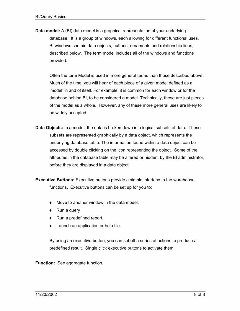
Data model: A (BI) data model is a graphical representation of your underlying

database. It is a group of windows, each allowing for different functional uses.

BI windows contain data objects, buttons, ornaments and relationship lines,

described below. The term model includes all of the windows and functions

provided.

Often the term Model is used in more general terms than those described above.

Much of the time, you will hear of each piece of a given model defined as a

‘model’ in and of itself. For example, it is common for each window or for the

database behind BI, to be considered a model. Technically, these are just pieces

of the model as a whole. However, any of these more general uses are likely to

be widely accepted.

Data Objects: In a model, the data is broken down into logical subsets of data. These

subsets are represented graphically by a data object, which represents the

underlying database table. The information found within a data object can be

accessed by double clicking on the icon representing the object. Some of the

attributes in the database table may be altered or hidden, by the BI administrator,

before they are displayed in a data object.

Executive Buttons: Executive buttons provide a simple interface to the warehouse

functions. Executive buttons can be set up for you to:

♦ Move to another window in the data model.

♦ Run a query

♦ Run a predefined report.

♦ Launch an application or help file.

By using an executive button, you can set off a series of actions to produce a

predefined result. Single click executive buttons to activate them.

Function: See aggregate function.

BI/Query Basics

11/20/2002 9 of 9

NULL: A placeholder that occurs when no value has been entered into the database. It

is not the same as a zero or a character space, NULL is simply a placeholder

where the value would be, if one were assigned. Operator: A symbol or word set that provides mathematical or computational capability.

This symbol specifies the equivalency requirement in a qualification. The

operator defines how the values on either side of it will be compared. Examples

include arithmetic operators, such as + (plus) and - (minus); comparison

operators, such as = (equal), >= (greater than or equal to), Contains, and

Between. Ornaments: Ornaments are text or graphical objects such as titles, logos, borders,

backgrounds, or notes. They provide additional information, act as visual

organizers, or simply enhance the appearance of design windows and reports. Parameter: A value that is required as input to a called function. Qualification: A constraint or restriction that is placed on the data before it is returned.

A qualification is used to eliminate unneeded or unwanted rows that would

otherwise be returned by your query. Relationships (Joins): The lines between data objects represent a direct relationship

between those objects. If there is no line connecting two objects, their

relationship is not considered direct. They must be related by going through an

object they both have direct relationships with. For example, employees are

related to jobs and jobs are related to position budgets, but employees are not

directly related to position budgets. For this reason if we want to get information

from both Employee Profile and Salary/Budget you must establish the

relationship through Job Summary. Query: A way of requesting specific data in a specified format from a database. The

designer of a data model typically makes it possible for the user to create and

modify his or her own queries (sometimes called “add hoc queries”). The

designer can also create queries and save them with the data model, so that the

user can load the queries from the data model, then submit them to the

database.

BI/Query Basics

11/20/2002 10 of 10

Connecting The connection file tells BI which database to access for your model. If you use more

than one data model that pulls from the same database, you will use the same

connection file for all of them. For example: the HRIS, FIS, and Space data models all

exist on CODW, therefore, all three would use the same connection file (codw.con).

Choose the Host<Connections menu option

Choose the connection file from the Connection Names list box by clicking on the file

name

If the connection file you wish to use does not appear in the box, click the Browse

button to find the file (the connections file will have an extension of .con)

Once you have chosen a connection file, click the Set Default button (a black dot will

appear next to the file name). The next time you open this data model it will

automatically ask you to connect using this connection file

Click the Connect button

Fill in your username and password (if you don’t know your username/password or

need an account, contact 7-EASY)

Once your connection file has been set as default you can Connect and Disconnect

using the button on the toolbar or the Host<Connect/Disconnect menu option.

BI/Query Basics

11/20/2002 11 of 11

Ad Hoc Query Generation Creating a Basic Query This section will describe the steps for creating queries. The basic steps are:

Clearly define the problem and expected results

Start a new query using the toolbar button, Query<New, or Ctrl+N

Select the data object(s) you want to pull data from

Select the attributes to be collected

Apply conditions such as sort order, modifiers and qualifications (optional)

Submit the query using the button, the Query<Submit Query menu option, or

Ctrl+G.

View or manipulate results

Make any additions or corrections to query

Save your query (This is not accomplished by saving from the File menu)

Defining the Problem

When defining your query, have a general idea of what kind, and how much, data should

be returned. Review your results and make sure the data returned is what you expect.

You can be confident that the data is trustworthy, but be careful that your method of

acquiring it is correct. If you are unsure if the data you received is representative of what

you expect, try writing your query in another way (possibly selecting extra attributes to

clarify your results), you can always hide or remove unwanted columns later.

It is important to remember that the data you can pull out of your warehouse is

only as good as the data that has been put into Banner. When creating your

queries try to take common data entry errors and abbreviations into account.

BI/Query Basics

11/20/2002 12 of 12

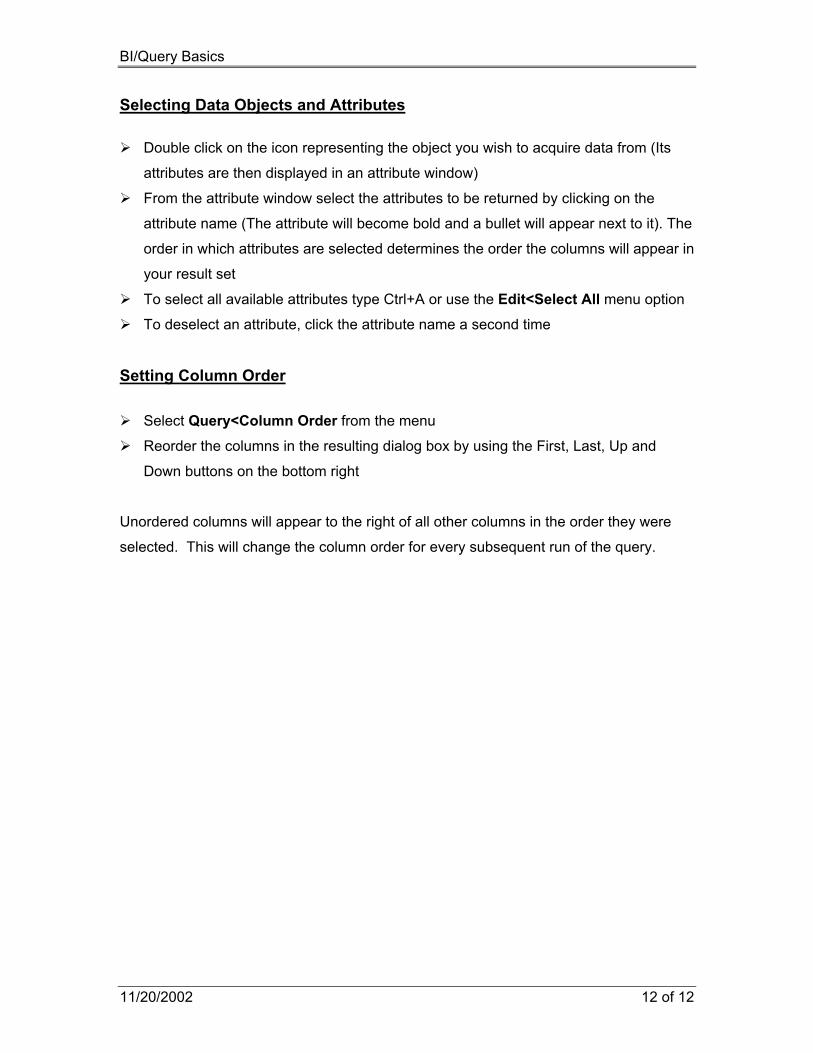
Selecting Data Objects and Attributes

Double click on the icon representing the object you wish to acquire data from (Its

attributes are then displayed in an attribute window)

From the attribute window select the attributes to be returned by clicking on the

attribute name (The attribute will become bold and a bullet will appear next to it). The

order in which attributes are selected determines the order the columns will appear in

your result set

To select all available attributes type Ctrl+A or use the Edit<Select All menu option

To deselect an attribute, click the attribute name a second time

Setting Column Order Select Query<Column Order from the menu

Reorder the columns in the resulting dialog box by using the First, Last, Up and

Down buttons on the bottom right

Unordered columns will appear to the right of all other columns in the order they were

selected. This will change the column order for every subsequent run of the query.

BI/Query Basics

11/20/2002 13 of 13

Sorting

To set the sort order for your query:

In the attribute window click the sort box for each attribute you wish to sort by (a

number appears in the box indicating the sort order); the sort defaults to ascending

order

To remove an attribute from the sort, click the sort box a second time

To change the sort order for your query:

Double click the sort box for any selected attribute (or use the Query<Sort Order menu option)

In the resulting dialog box, move the desired attributes from the Selected (or

unsorted) Columns box into the Sort Order Box

Click the attribute you would like to change and use the First, Last, Up or Down

button to change its sort priority

To apply the sort for a given attribute in descending order, select the attribute and

choose the button marked Descending

BI/Query Basics

11/20/2002 14 of 14

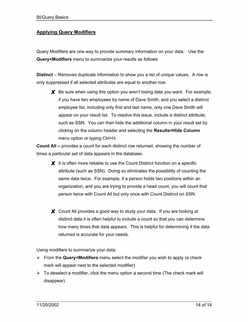
Applying Query Modifiers Query Modifiers are one way to provide summary information on your data. Use the

Query<Modifiers menu to summarize your results as follows:

Distinct – Removes duplicate information to show you a list of unique values. A row is

only suppressed if all selected attributes are equal to another row.

✘ Be sure when using this option you aren’t losing data you want. For example,

if you have two employees by name of Dave Smith, and you select a distinct

employee list, including only first and last name, only one Dave Smith will

appear on your result list. To resolve this issue, include a distinct attribute,

such as SSN. You can then hide the additional column in your result set by

clicking on the column header and selecting the Results<Hide Column

menu option or typing Ctrl+H.

Count All – provides a count for each distinct row returned, showing the number of

times a particular set of data appears in the database.

✘ It is often more reliable to use the Count Distinct function on a specific

attribute (such as SSN). Doing so eliminates the possibility of counting the

same data twice. For example, if a person holds two positions within an

organization, and you are trying to provide a head count, you will count that

person twice with Count All but only once with Count Distinct on SSN.

✘ Count All provides a good way to study your data. If you are looking at

distinct data it is often helpful to include a count so that you can determine

how many times that data appears. This is helpful for determining if the data

returned is accurate for your needs.

Using modifiers to summarize your data:

From the Query<Modifiers menu select the modifier you wish to apply (a check

mark will appear next to the selected modifier)

To deselect a modifier, click the menu option a second time (The check mark will

disappear)

BI/Query Basics

11/20/2002 15 of 15

BI/Query Basics

11/20/2002 16 of 16

Adding Qualifications Qualifications allow you to place conditions on what data is returned by your query.

When implementing qualifiers you can:

♦ Add qualifications by clicking the Qualify box for the chosen attribute

♦ Place qualifications on attributes that are not selected

♦ Choose from a list of available operators

♦ Use pattern matching

♦ Apply negative operators (e.g., not equal to)

Inserting Qualifiers

To insert a qualification, or condition, into your query you will take these steps, which

are defined in detail below:

In the attribute window, Click the Qualify Box for the attribute you wish to qualify

In the Edit Box, enter the value(s) you wish to qualify on (or use the Data Values

Box to select value(s) from the resulting list)

Choose an appropriate Operator

When a Qualify box is chosen, a qualification tree appears in the lower windowpane

of the attribute window. Each time you click a Qualify box, a branch is added to this

tree. The resulting tree will be visible from all objects within the model. (See diagram

on next page)

BI/Query Basics

11/20/2002 17 of 17

Handle

Operator Edit Box List Box Data Values Box

Handle − By clicking on the handle you can select the qualifier. Once selected a

qualification can be deleted, negated or combined with another

qualification.

Operator − Clicking on the Operator box brings up a list of available operators.

Select the operator you wish to use from this list and it will appear in

the Operator box.

Edit Box − Populate the edit box with the value you wish to qualify on.

List Box − Clicking on the list box allows you to view the chosen value(s), add

additional values, or delete all values, currently in the edit box.

Data Values − From this box you can acquire a list of possible data values for the

selected attribute, insert a prompt or use a variable.

To delete a qualification select the Handle and press the Delete key on your

keyboard

Once a qualification has been added to the tree, clicking elsewhere on the

screen before entering data into the edit box will cause the qualification branch to

disappear.

A few of the available operators do not allow for multiple values in the edit box.

These operators are <, >, <=, and >=.

If the qualification tree is too large to be seen in the window, resize the

qualification section. To do this:

Click and drag the blue divider upwards until the whole qualification tree can

be seen

BI/Query Basics

11/20/2002 18 of 18

Basic Operators

The basic operators provided by BI include:

♦ = (Equal to)

♦ < (Less than)

♦ < = (Less than or Equal to)

♦ > (Greater than)

♦ >= (Greater than or Equal to)

♦ Begins with

♦ Contains

♦ Ends with

♦ In

♦ Between

♦ Is NULL

Applying negative operators Each of the operators mentioned above can be negated. BI provides a list of

these negative operators in the operators list box, these are:

♦ ! = (Not Equal to)

♦ Does not begin with

♦ Does not contain

♦ Does not end with

♦ Not In

♦ Not Between

♦ Is not NULL

Each of these operators will return the opposite of what is returned by their

positive counterparts.

Any qualifier can be negated, by selecting the handle and choosing

Query<Qualification<Negate Clause from the menu. However, it is best to

use the predefined negative operators whenever possible.

BI/Query Basics

11/20/2002 19 of 19

All available operators can be used to compare any data type including:

♦ Numbers

♦ Characters

♦ Strings

♦ Dates

BI/Query Basics

11/20/2002 20 of 20

Matching character patterns Pattern matching allows you to qualify on sections of data. This is useful for

selecting data when you are unsure what the data looks like in its entirety. It is

also useful for selecting data that has not been entered into Banner in a

consistent format. For example: if you want to return all employees with a

current job title of “Information Analyst” you would also want to be sure to include

employees with a current job title of “Info Analyst”.

To provide this ability the following operators are provided:

Begins with – Selects all data that begins with the given string

Ends with – Selects all data that ends with the given string

Contains – Returns data that contains the given string (including those that

begin or end with the string)

Examples

– Begins with Account returns: Account, Accountant, Accountant

Assistant…

Ends with Assistant returns: Assistant, Office Assistant…

Contains Assistant returns: Assistant, Office Assistant, Office

Assistant I…

Using multiple values for comparison

When multiple values are input into the edit box for the Contains operator, you

must specify Match Any or Match All (if you do not select one of these, Match

Any will be used as the default). This can be set from the List Box portion of

the qualification tree:

Click on the List Box of the qualification tree (click the List Box/New Entry

for adding additional values)

Choose Match Any or Match All from the resulting menu

Match Any – Will return all values that include any one of the input character sets

Ex: Contains U, 301 Match Any returns: UF301, UA301, CU301, UX401, CA30

Match All – Will return values only if all input character sets can be matched.

Ex: Contains U, 301 Match All returns: UF301, UA301, CU301

BI/Query Basics

11/20/2002 21 of 21

Data Values

Data values provide you with the ability to retrieve a list of possible values for input

into the edit box of a qualification. They can be used to retrieve a list from the

database of all available values or to display only a portion of the available values.

The designer of the model may set up data values, which will be available for use by

all users. Individual users may also set up their own data values if they want to only

select from the same list every time. The first two sections below (Dynamic data

values and Static data values) will define the two types of data values and describe

how to use them, and the next sections (Data Values Files and Queries, Data values

files (Static), Data values files (Dynamic), and Data values aliases) will describe how

to actually create both types of data values.

Dynamic data values The dynamic data values window shows you all possible values for a specific

attribute. When you select Data Values from the Data Values Box, BI runs a

query to select all distinct values for that attribute from the underlying table.

Therefore, any values not currently in use will not be returned. For example: if

the validation table for Gender allows for three codes, ((M)ale, (F)emale, and

(U)nknown), and no employee has a gender assignment of (U)nknown, the

dynamic Data Values dialog box will only list the used values, ((M)ale (F)emale).

To select dynamic data values:

On the Data Values list box , click and hold the mouse button down

Select Data Values… (a dynamic data values list box will appear)

BI/Query Basics

11/20/2002 22 of 22

Click the value(s) you wish to qualify on. Hold down the Ctrl key to select

more than one, press Ctrl+A on your keyboard to select them all

Press the Insert button and the value(s) will be returned to the edit box in

your qualification

Static data values

The most commonly used values can be represented in a static list that is part of

the Data Values drop down menu in the qualification tree. This list can be set up

to include all available values or only a select few. If all values are not

represented in this list, you can access a dynamic data values list by selecting

More… from the drop-down menu.

To select static data values:

Click the Data Values box and hold to display a drop down menu

From the resulting static values list, select the value you wish to qualify on

Or select More… to bring up a dynamic data values list

BI/Query Basics

11/20/2002 23 of 23

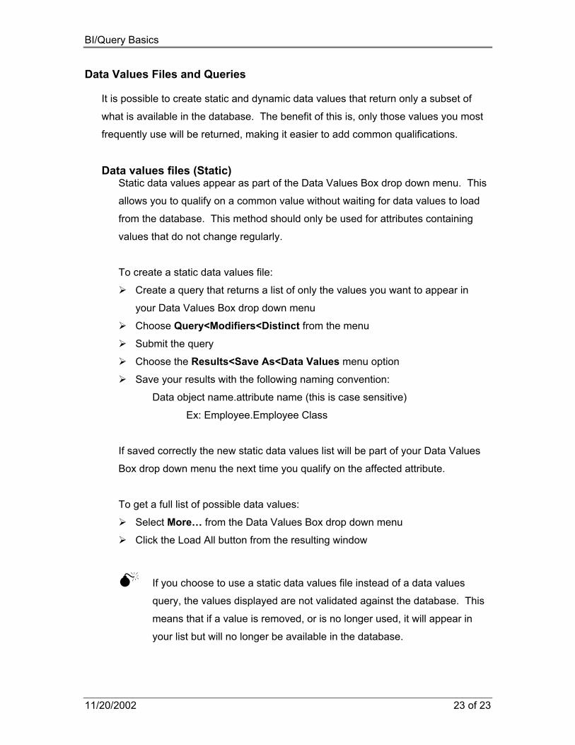
Data Values Files and Queries

It is possible to create static and dynamic data values that return only a subset of

what is available in the database. The benefit of this is, only those values you most

frequently use will be returned, making it easier to add common qualifications.

Data values files (Static) Static data values appear as part of the Data Values Box drop down menu. This

allows you to qualify on a common value without waiting for data values to load

from the database. This method should only be used for attributes containing

values that do not change regularly.

To create a static data values file:

Create a query that returns a list of only the values you want to appear in

your Data Values Box drop down menu

Choose Query<Modifiers<Distinct from the menu

Submit the query

Choose the Results<Save As<Data Values menu option

Save your results with the following naming convention:

Data object name.attribute name (this is case sensitive)

Ex: Employee.Employee Class

If saved correctly the new static data values list will be part of your Data Values

Box drop down menu the next time you qualify on the affected attribute.

To get a full list of possible data values:

Select More… from the Data Values Box drop down menu

Click the Load All button from the resulting window

If you choose to use a static data values file instead of a data values

query, the values displayed are not validated against the database. This

means that if a value is removed, or is no longer used, it will appear in

your list but will no longer be available in the database.

BI/Query Basics

11/20/2002 24 of 24

Data values queries (Dynamic) By default, BI runs a query to return all distinct values for a given attribute every

time the user requests data values. Creating a data values query lets you

change the definition of the query that will be run each time you load data values.

In this way, you can create a query that returns a dynamic subset of the data

available in the database, thus simplifying the qualification process.

Data values queries are different from data values files in that the defined query

is run every time you request data values. Although this requires you to wait

while the data is loaded from the database, the values presented will always be

consistent with the values in the database. It is good to use a data values query

any time there is too much data to display in the Data Value Box drop down

menu, or when values change periodically.

To create a data values query:

Create a query that qualifies the data in such a way that the desired values

are returned each time

Choose Query<Modifiers<Distinct from the menu

Choose the Query<Save menu option

In the resulting window click the Data Values check box on the bottom left

Save your query with the following naming convention:

Data object name.attribute name (this is case sensitive)

Ex: Employee.Employee Class

Use the new data values query by loading data values from the Data Values

drop down menu

To load all values click the Load All button

To reload the restricted list of values using your data values query click the

Load Values button

Data values aliases Data values aliases can be used to change the values seen in the data values list

box to be more descriptive. Aliases are particularly useful for attributes that

contain a code rather than a description. Once a data values alias is created, the

Data Values box will return the code descriptions. You can then select the

BI/Query Basics

11/20/2002 25 of 25

description from the Data Values box, and the appropriate code is automatically

inserted into the qualification.

To create a Data Values File using aliases:

Create a query that returns two attributes, the first being the code or value to

qualify with and the second being the alias that will be visible to the user

Choose Query<Modifiers<Distinct from the menu

Submit the query

Choose the Results<Save As<Data Values menu option (this saves the

results only, not the query)

Save your results with the following naming convention:

Data object name.attribute name (name the file after the first attribute)

Ex: Person.Ethnic Code

To create a Data Values Query with aliases:

Create a query that qualifies the data in such a way that the desired values

are returned each time

Be sure the query returns two attributes; the first being the code to qualify

with and the second being the alias that will be visible to the user

Choose Query<Modifiers<Distinct from the menu

Choose the Query<Save menu option

In the resulting box, click the Data Values check box on the bottom left

Save your query with the following naming convention:

Data object name.attribute name (name the file after the first attribute)

Ex: Person.Ethnic Code

You may need to click the Load Data button the first time you retrieve data

values after creating this query.

BI/Query Basics

11/20/2002 26 of 26

Modifying or Clearing Queries

Any query created, whether it has been run or not, will remain active until it is cleared

using one of the new query options. This allows you to make changes to your query

even after it has been submitted. To make these changes or start a new query:

Close the results window

Add or remove selections as before

or

Clear the active query by clicking the button on the toolbar, choosing the

Query<New menu option or typing Ctrl+N

Closing the attribute window will not clear your query. You must clear it manually

by choosing one of the New Query options.

Saving a Query

To save your query for use at a later date:

Select Query<Save from the menu

Use the Export button if you wish to save in a directory other than the default

Select an Export Option (almost always, Export Query)

Click the Save button

By default your query will be saved in the User\Queries subdirectory of the folder your

data model is stored in.

If you use the Export button to save your query elsewhere the query will not

automatically appear in the list of available queries for loading.

Keep in mind that when you save a query you are not saving the data that it

retrieved, you are only saving the means of retrieving it. To save the retrieved

data you must save the result set (Results< Save As< Results).

BI/Query Basics

11/20/2002 27 of 27

The Export SQL Only export option is used to save only the actual SQL code

generated by BI. Use this if you want to import your code into another program.

Loading a Query

To reuse a previously saved query:

Choose the Query<Load menu option

Select the desired query from the saved queries list (If it does not appear in the list,

click the browse button to look for it elsewhere on your computer)

Click the Submit button to submit the query as is

OR

Load it into memory for further development using the Load button

Both submitting the query and loading it will open the Show Query window. Minimize the

Show Query Window.

If you are familiar with SQL, the Show Query window is good for viewing your entire

query, or reviewing the code that is automatically generated by BI.

Submitting the query also loads it into the model. So, you can alter the query as before.

BI/Query Basics

11/20/2002 28 of 28

Results Window When data is retrieved it is displayed on your screen in a Query Results window. The

default display format is spreadsheet view. Resize the columns by positioning the mouse pointer on the border between the

column headings and dragging to the desired size.

Manipulating Results

Hiding columns – Click on the column header for the column you wish to hide

and choose the Results<Hide Columns menu option.

Column order – Choose Results<Reorder Columns from the menu. In the

resulting dialog box reorder the list of columns to represent

the desired order.

Sort order – Select Results<Filter <Sort. Reorder the list of columns to

represent the desired sort order. Each column can be

changed to sort in ascending or descending order.

Compute Values – Choose Results< Filter <Compute. This returns the MIN,

MAX values for each column in the result set. For numerical

columns, SUM and AVG will also be calculated.

Limited Range – Select Results< Filter <Range from the menu. This allows

you to limit the data that is displayed in your result window.

For example, you can choose to only show salary from 20000

to 30000 or only names that start with A (to accomplish this

choose a min value of A and a max value of AZ).

BI/Query Basics

11/20/2002 29 of 29

✘ Each time you manipulate the results, a new result window will open on top of

the old. Each of these result windows will be uniquely numbered, the integer

being the number of your current query and the numbers behind the decimal

representing the number of altered results windows. To go back to your

previous results, simply close the current result window.

✘ The Results< Options menu item allows column headings and query name

to appear when pasting, as well as other options.

To start a new query, or make changes to your existing one, you must first

close, or minimize, all open results windows. If you find that you cannot

perform the function you wish, check in the Windows menu to be sure no

result windows have been left maximized.

The changes you make to the data in the result window do not affect your

query. Once you close your result windows your changes will be lost; the

next time you run the query the results will return to their original state.

BI/Query Basics

11/20/2002 30 of 30

Exporting Results

Once you have your results in the format you want them, you can export them

into another application (such as word or excel). To do this:

Select all the results by clicking on the top left corner of the spreadsheet (the

cell displaying the total number of rows returned)

or Select only a portion of the data by depressing your mouse button and

dragging it across the desired cells.

Copy the selected data to the clipboard (use the Edit<Copy menu option).

Paste data into your application (using the Edit<Paste menu option)

Saving Results

Results can be saved to a text file, either to be reopened in BI/User or to be

opened in other applications.

Saving a result set for use in BI:

Choose Results<Save As<Results

Specify a name and location for the file. BI will automatically supply the .qrd

extension.

Any time you save a results file, BI will create both a .qrd file and a .qrr file.

The .qrd file is the actual text file, which can be opened in any application that

accepts text files, the .qrr file stores additional information that BI needs to

reopen the file.

Saving a result set as an external text file:

Choose Results<Options

In the Field text box select the delimiter (separator)

Choose the Tab delimiter if you want to open the file in a spreadsheet

Choose the comma delimiter to create a comma delimited text file

Click the OK button

Choose Results<Save As<Results

Specify a name a location for the file. Give the file name an extension of .txt

BI/Query Basics

11/20/2002 31 of 31

Adding Complexity to Queries

In this section, you will learn how to do the following:

♦ Qualifying on values within a range

♦ Qualifying with attributes

♦ Querying from multiple data objects

♦ Including multiple qualifications

♦ Grouping qualifications

♦ Working with NULL values

♦ Applying aggregate functions

♦ Grouping and adding Group Qualifications

♦ Using Ad Hoc Drill-down

Values in a Range The IN and BETWEEN operators provide you with the ability to qualify an attribute with

multiple values. Often times this can replace the need to add multiple qualifiers, thus

simplifying your query.

To enter more than one value in the Edit Box either use the down-arrow key on your

keyboard, click the New Entry option in the list box, or select more than one value

from the data values list box (by holding down the ctrl key while selecting the desired

values)

IN – Allows for comparing an attribute to a list of values. Any value matching one of

those in the list will be returned. For example: Transaction date IN 06/12/98, 7/12/98,

8/12/98, will return all transactions that occurred on any one of the dates listed.

The = operator can also be used to perform this function.

✘

BI/Query Basics

11/20/2002 32 of 32

If BANNER stores the dates you are using down to the microsecond (such as

with financial transactions) it is better to use the BETWEEN operator. For

example: a date of 06/12/98, will not match 06/12/98 12:45:11:09 AM

✘

BETWEEN – Allows for determining if an attribute's value falls between two set values.

Any value falling alphabetically, numerically, or chronologically between the two given

values will be returned. For example: Transaction Date BETWEEN 06/12/98 AND

07/12/98, will return transactions that occurred on 06/12/98, 07/12/98 or any date in

between.

The BETWEEN operator will only work if the edit box contains exactly two values.

BI/Query Basics

11/20/2002 33 of 33

Qualifying With Attributes Qualifying with an attribute allows you to compare one attributes value with another, then

return only those values that meet the qualification. For example, you may want to

select any employee whose annual salary is above the job high salary.

Click the Qualify box for the attribute to qualify on

Select Edit<Insert DB Name (make sure the cursor is in the Edit box)

From the DB Name dialog box select the Data Object Name from the list provided

Select the attribute name of the attribute to qualify by

Press the Insert Name button

BI also allows you to qualify on some calculated version of an attribute, such as, where

the annual salary > job high salary * 1.05.

Follow the instructions to insert an attribute into your qualification Edit box

Click inside the Edit box

Edit the text to include your calculation

If you have clicked outside the qualification before editing it { } will appear on either

side of the attribute name. Once this occurs you must be sure to include your

calculations inside the { }.

Your finished qualification should look like this:

BI/Query Basics

11/20/2002 34 of 34

Querying From Multiple Data Objects Some queries will require you to retrieve attributes from more than one data object. To

do this:

Select the attributes needed from the first object

Close the attribute window

Double click on the second object to access its attribute window (A bold dot will

appear next to each object being used in the query.)

Select required attributes

Make sure a relationship has been established (A dark blue line will connect all

objects used in the query)

If the attributes are directly related (or have a relationship line drawn directly from one to

the other) BI will automatically establish the relationship for you. When a relationship is

established the line connecting the objects becomes bold. If the objects do not have a

direct relationship, meaning there is no line directly connecting them, create the

necessary connections; click on the lines connecting the objects, so that you have a bold

line connecting all objects you plan to use. Doing this may create a relationship with one

or more objects that do not have any select attributes in the query. It is not necessary to

select any attributes from the extra object(s).

For example: using the model below, if you were to select from both Fund and General

Ledger, BI would automatically create the relationship. However, if you select from Fund

and Account, there is no direct relationship. To create a relationship, connect Fund to

General Ledger by clicking on the line connecting them, and then connect General

Ledger to Account.

BI/Query Basics

11/20/2002 35 of 35

✘ When creating your queries it is best to use as few data objects as possible. The

more objects that must be joined, the longer your query will take to complete. For

this reason, much data is repeated in more than one data object. For example: the

index code, which can be found in the Fund object, will return the same value as the

index code found in the General Ledger or Account objects.

BI/Query Basics

11/20/2002 36 of 36

Including Multiple Qualifiers

Often one qualification is not enough to insure you retrieve the desired results.

To include more than one qualification:

Click the Qualify Box of the attribute you wish to qualify on

Enter the desired value into the Edit Box

Choose the Qualify Box of the next attribute to qualify on or to qualify on the same

attribute, click its Qualify Box a second time

Toggle the connection operator to the desired option (AND or OR)

Group qualifications as needed (see the next section for details)

Repeat for as many qualifications as needed

Each time you add an additional qualification, a branch is added to your qualification

tree. These branches are connected by a connection operator which is, by default, set

to AND. To toggle between AND and OR, click on the word (AND or OR).

AND – All qualifications connected with the AND operator must but true for the row to be

retrieved. In queries that include both AND and OR operators between qualifications the

AND operator has a higher priority and is performed first.

OR – Only one of the qualifications connected with the OR operator must be true for the

row to be returned.

BI/Query Basics

11/20/2002 37 of 37

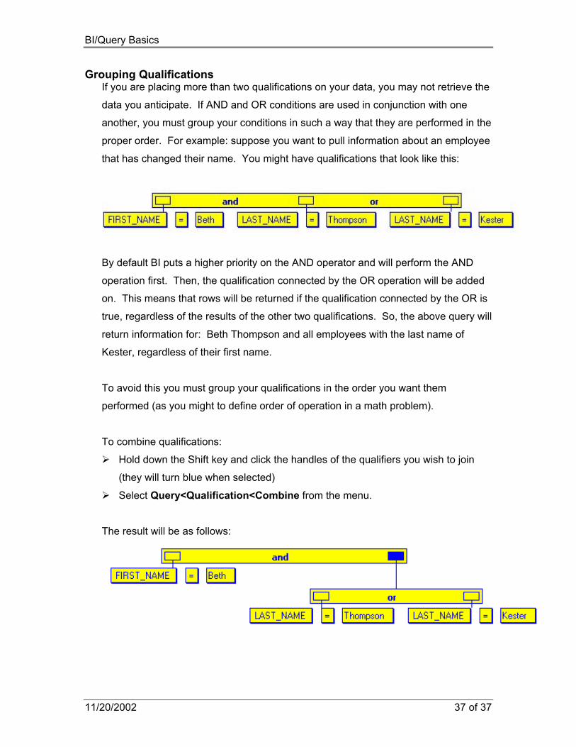
Grouping Qualifications If you are placing more than two qualifications on your data, you may not retrieve the

data you anticipate. If AND and OR conditions are used in conjunction with one

another, you must group your conditions in such a way that they are performed in the

proper order. For example: suppose you want to pull information about an employee

that has changed their name. You might have qualifications that look like this:

By default BI puts a higher priority on the AND operator and will perform the AND

operation first. Then, the qualification connected by the OR operation will be added

on. This means that rows will be returned if the qualification connected by the OR is

true, regardless of the results of the other two qualifications. So, the above query will

return information for: Beth Thompson and all employees with the last name of

Kester, regardless of their first name.

To avoid this you must group your qualifications in the order you want them

performed (as you might to define order of operation in a math problem).

To combine qualifications:

Hold down the Shift key and click the handles of the qualifiers you wish to join

(they will turn blue when selected)

Select Query<Qualification<Combine from the menu.

The result will be as follows:

BI/Query Basics

11/20/2002 38 of 38

The query will now return only those employees with the first name of Beth and a last

name of either Thompson OR Kester. So, this query would return only Beth

Thompson and Beth Kester.

To Uncombine the qualifications:

Select the handle that represents the group (as seen above)

Choose Query<Qualification<Uncombine

Note that in BI 6.0, the Uncombine menu option did not work.

✘ To negate a group of qualifications you can select the handle that represents the

group and choose Query<Qualification<Negate Clause from the menu. If this

were done in the example above, the query would return all employees with the

first name Beth who do not have a last name of Thompson or a last name of

Kester.

BI/Query Basics

11/20/2002 39 of 39

Working With NULL

A NULL value is one that represents a lack of data. It is not a zero or an empty

character string, it is merely a placeholder for missing data. For this reason, if you are

querying on data that may be NULL, (meaning no one has entered a value into Banner)

it is possible to obtain incorrect data. For example: if you are querying to count the

number of classes held in a specific room, your count may be off if any classes held in

that room do not have a room number assigned in Banner.

To acquire a list of rows that are missing a specific attribute (often used for creating an

exception report), you can use the IS NULL operator. However, because NULL is

assigned only if no other value was entered, it is often a good idea to pull empty

character strings as well when looking for missing data.

The qualification below illustrates a query to retrieve all classes that were not assigned a

room number.

BI also provides the ability to pull data only if the value is not NULL. To do this use the

IS NOT NULL operator.

BI/Query Basics

11/20/2002 40 of 40

Combining Result Sets

There are times when the information you need is so complex that it requires two or

more separate queries to acquire it. For this reason, BI provides you with the ability to

combine the result sets of those queries. To do this you can either append one result set

to the end of another, or you can join the columns of two result sets based on their

common values.

Appending Rows

Appending rows has the effect of taking the rows of one result set and attaching

them to the end of another. This makes it possible for a single column to display one

value for the first group and another for a second group.

For example: assume you want a phone list that includes the home phone for those

who have one and the work phone for those without a home phone number. To

accomplish this you would need to run two queries, the first including the home

phone number for those who have one and the second including work phone number

for everyone else. After appending the rows of the two sets, you can sort the final

results and have a sorted set of data with one column containing the appropriate

phone number.

Appending the rows of the two result sets performs the same function as the

UNION ALL function in SQL.

To append rows:

Create and run a query to return the first set of results

Click the minimize button on the results window

Create and run a query to return the second set of results

Select Results<Combine <Append Rows…

Choose the correct result sets from the lists provided

In order to append rows, all attributes in both result sets must be of the same

type, in the same column order.

BI/Query Basics

11/20/2002 41 of 41

Joining Columns

Joining columns allows you to create a relationship between two result sets and

combine them into one complete set. You may wish to join columns when:

♦ You want to perform an outer join. That is, include rows of data from one result

set that don’t have a match in the other

♦ The model doesn’t provide a relationship (join) for objects you wish to join

When joining columns, your result sets must have a column that you can join on.

This column is one that will be equal in both sets. By default, only those rows where

the specified columns match exactly in both sets will be included in the final result set

after joining columns. This is called an equijoin.

Getting All the Data There are times when joining objects, either by selecting from both of them in the

model or by joining their result sets, can cause rows of data to be lost. This

occurs when two objects are joined because only values that exist in both objects

will appear in your result set. For example: Jobs and Position are related data

objects. When you join them (meaning you select attributes from both) you will

only get data that is represented in both. In the picture below, a circle represents

each object. The shaded area represents the data you would get from a query

that joins the two objects.

Position Jobs

Assume you select Position Number with Fund information from the Position

object, and the Position Number with Employee information from the Jobs object.

Note that, by default, the Position object includes all positions, while the Jobs

object includes only filled positions. When you run the query, you will only

receive rows where a specific Position Number exists in both the objects.

Therefore, vacant positions would be excluded from your results because there

are no matching rows in the Jobs object.

BI/Query Basics

11/20/2002 42 of 42

If you select the Include All Left Rows or Include All Right Rows box, you will

receive all rows regardless of whether they match a row in the other result set. In

the pictures below, a circle represents each object. The shaded area represents

the data that you would get from a query that joins the two with Include All Left

Rows or Include All Right Rows.

Position Jobs Position Jobs Position Jobs

Include All Left Rows Include All Right Rows Both

From the example above, you may want to create a query that returns all

positions, including those that are vacant, and the name of the employee for

those positions that are filled. To do this, get a list of positions from Position and

a list of filled positions with employee names from Jobs (by default, results from

Jobs will include only filled positions), then join columns using Include All Right

Rows. By including all right rows you are forcing BI to include positions that do

not have a matching (filled) position in the Jobs object.

To join Columns:

Create and run a query that returns results from the first object

Click the minimize button on the results window

Create and run a query to return results from the second object

Select Results<Combine <Join Columns…

Choose the first result set from the available list on the left side of the window

Choose the second result set from the list on the right side of the window

In the lower section of the dialog, select the columns that are equal in both sets

To include all rows from the left set, check the Include All Left Rows box

To include all rows from the right set, check the Include All Right Rows box

To include all rows from either side, check both boxes

BI/Query Basics

11/20/2002 43 of 43

In most cases, when selecting data from multiple objects in the model the join

that is created is an equijoin. This means that by simply joining two data objects

in your query, data can be eliminated from the final results. When this occurs,

use the Include Left Rows and/or Include Right Rows options in the Join

Columns window. An example of this is seen above in combining the Position

object with the Jobs object.

Joining columns with Include Left or Right Rows produces the same results as

left, right and outer joins in SQL.

The number representing a result set will appear in the upper left corner of the

result window.

✘ When selecting the columns to join on in the lower section of the Join Columns

dialog box, select all columns that could be equal in both sets. This doesn’t

mean all values will be equal, only that they contain the same data. For

example: Original Hire Date could be set equal to Current Hire Date and in the

final result set only one date column would appear.

BI/Query Basics

11/20/2002 44 of 44

Super-Queries Any changes made to a result set after it has been created are tracked and stored in a

super query. In this way you can create and save a query that performs many steps. In

essence, a super query is much like a macro in Word or Excel in that it records a group

of actions and allows the user to execute those actions later as an automated group.

If you create and run two separate queries and then combine their result sets using the

Append Rows or Join Columns capability of BI, you have created a super query. Any

steps you take to further alter the display or meaning of the result set will be recorded

and added onto the super query. If this super query is then saved and run, it will

automatically perform all of the steps initially taken. That is, it will run query#1, run

query#2, and combine the results. Any sorting, re-ordering, or filtering is then

performed.

Super-queries can be used to automate a wide array of post-query tasks:

♦ Combining result sets through joining columns

♦ Combining result sets through appending rows

♦ Sorting the new combined data

♦ Changing the initial sort order

♦ Altering the range of data displayed

♦ Hiding columns (from the re-order columns window)

♦ Reordering columns

BI/Query Basics

11/20/2002 45 of 45

Creating Super-Queries

Create the first query

Save with a unique name (optional, but recommended)

Submit this component query

Alter the result set (by changing column or sort order, restricting the range, etc.)

AND/OR

Minimize the result set

Create and run a second query (saving is optional, but recommended)

Combine the two result sets by appending rows or joining columns

Make any additional alterations to the final result set

Repeat as many times as necessary

If the same prompt is used in multiple component queries of a given super query,

the user will only be prompted once and the given value will be used for all

occurrences of the prompt.

Changes made to the format of the columns at the result set level are not saved

in the super query.

BI/Query Basics

11/20/2002 46 of 46

Viewing and Saving Super-Queries

As you create a super query, it’s components and their relationships become

accessible through the Super Query window. From this window you can see all the

steps that make up your super query or you can take a more in-depth look at any

one component.

To view the Super Query window for the first time:

Create a super query by combining result sets or altering the display from the

Results menu

Once the results are in the final stage, select Query<Super Queries<Show Super-Query from the main menu

To activate the Super Query window after the first time:

Select Window<Super Query-<<Query Name>> from the menu

Selecting Query<Super Queries<Show Super-Query from the main menu

should only be done when the query is first created or the first time you want

to see the query after loading it. This should only be done from the final

Result Set window. If this menu option is chosen from any other place, the

resulting Super Query window will not display the correct query. If this menu

option is selected from the final Result Set window a second time, a second

Super Query window will be opened. Be careful not to edit the wrong super

query.

✘ Once you have selected the Show Super-Query menu option once, access the

super query from the Windows menu each succeeding time.

BI/Query Basics

11/20/2002 47 of 47

The top pane of the Super Query window is used to represent your super query as a

whole. Each component is represented by an icon and placed in the super query

tree. The order in which a component appears in the tree determines the order in

which it will be executed. The inner most components are executed first. The action

components (such as sort order, range, column order, join columns, and append

rows) appear above, and slightly to the left of, the queries affected by the action.

Each query is labeled with the query name, or ‘Untitled’ if a name has not been

assigned. This section of the window can be simplified by expanding or compressing

sections. To change the level of detail displayed, click on the ‘+’ or ‘-‘ sign located to

the left of any component that has other components beneath it in the tree.

Selecting a query or action in the top pane of the Super Query window causes the

description of that component to appear in the bottom pane. If a query is selected,

the bottom pane will display the actual SQL code generated by your query.

However, if an action component is selected, a brief description of the component’s

definition is displayed.

BI/Query Basics

11/20/2002 48 of 48

Once the super query has been created it is a good idea to save it before making

any changes. This is done in much the same way as saving any other query. Be

sure that the Super Query window is visible and active before saving.

✘ It is a good idea to save each of the component queries before combining their

results and creating a super query. This protects you from having to re-write all

of the components if something happens to your super query.

To save a super query:

Create a super query

Activate the Super Query window

Make sure the final result set is visible and active

Select Query<Super Queries<Show Super Query from the menu

OR

Select the Window<Super Query-<<Query Name>> menu option

While the Super Query window is visible and active select Query<Save

Assign a name to the query or save over the top of an existing one

When saving a super query, it is wise to identify it as a super query by using some

sort of naming convention. For instance, instead of naming a query position

information you might name it something like Super position information.

It is a good idea to save each of the component queries before combining their

results and creating a super query. This protects you from having to re-write all of

the components if something happens to your super query.

BI/Query Basics

11/20/2002 49 of 49

Loading and Editing Super-Queries

Once a Super Query has been created, each component can be individually

accessed and changed.

Loading a super query:

Choose the Query<Load Query menu option

Select the desired super query and click the Load or Submit button

Editing super-queries:

Activate the Super Query window

Right-click on the component query you want to edit

Choose Copy Query to Model from the pop-up menu

Close the component’s Show Query window

Make the desired changes to the query as usual

Select Window<Super-Query-<<Query Name>> from the menu

In the Super Query window, right-click on the component query you just edited

From the resulting menu, choose Paste Query from Model Make changes to desired action components

Double click on the action you wish to modify (Sort, Join, Append…)

The original properties window will appear, make desired changes

Select OK

Save your super query, making sure first that the Super Query window is active

Selecting Query<Show Query from the main menu will only show the super

query if it is selected with the result set active. Otherwise, the component query

currently in memory will be shown.

If you intend to make multiple changes to a super query, it is best to start with the

innermost components.

BI/Query Basics

11/20/2002 50 of 50

Adding Components

Once a super query has been created, extra steps or components can be added to

the process from the Super Query window.

To affect the display of the data currently being collected by the query:

Activate the Super Query window

In the Super Query window, click the component that will be executed just before

the new action

From the Query<Add Operation menu select the desired component from the

available list (Sort, Reorder, or Range)

Make the necessary changes in the resulting dialog box

To add another query through combining results:

Create the additional query you would like to add

Save it with a unique name (optional)

Load or activate the super query that you want to alter

In the Super Query window, click the component that will be executed just before

combining the new results

From the Query<Add Operation menu, select Append or Join to combine the

results

Select either the current query or a saved query to be added

Fill in other options as described in the Combine Result Sets section of this

manual

BI/Query Basics

11/20/2002 51 of 51

Naming Component Queries

If the component queries in your super query did not have saved names at the time

they were added to the super query, they will appear in the super query tree as

‘Untitled’. To title these queries:

In the Super Query window, click on the query to be named

Select Query<Super Queries<Rename Selected Query from the menu

In the Super Query window, type in the new name of the selected component

query

This will rename the component within the super query but will not rename the

query if it was independently saved external to the super query.

BI/Query Basics

11/20/2002 52 of 52

Grouped Data Grouping

Much of the data you will work with lends itself to being studied as groups of data. For

instance, when dealing with large numbers of people it is often helpful to study them in

logical groups such as, by department, physical location, or status. Whenever you

choose to summarize on the data you are selecting by using aggregate functions, BI

groups the data for you. The group order is set, by default, to the order in which the

attributes where selected. So, if you select Department, Job Title, and a Sum of Annual

Salary, in that order, BI will group first by department and then by job title. Meaning, the

resulting data will be arranged in order of department, then job title within each

department. If you want to change this grouping order without changing column order,

you can do so by clicking the corresponding Group Boxes in the attribute window to

remove the grouping then clicking them a second time to replace it in the new order.

The same effect can be accomplished by applying a sort, overriding the default sort

caused by grouped data.

You can gather grouped data without including summary information. To do this, click in

the Group Boxes of the selected attributes to be grouped on. Grouping non-summarized

data has the same effect as removing duplicates and sorting. In some cases grouping

will be faster than selecting distinct sorted data.

If you apply a group order to any one selected attribute, all remaining selected

attributes that do not include an aggregate function must also include a group order.

If your query includes aggregate functions and you do not select the group order, it

will be done for you automatically.

BI/Query Basics

11/20/2002 53 of 53

Applying Aggregate Functions

Aggregate functions are used to summarize the information you retrieve from the

database. Unlike the modifiers discussed earlier, functions are applied to a specific

attribute. For instance you might request a sum of all annual salaries, or a distinct

headcount of employee SSNs within each department.

To apply an aggregate function to an attribute:

Click the function box for the correct attribute (a list of available functions will appear)

Move the mouse to highlight the desired function and click the text (a checkmark will

appear next to the chosen function)

To remove the function click the None option

Once you have applied an aggregate function, you will notice the group boxes of all

other chosen attributes will automatically be numbered. This automatic numbering

defines the way your data will be grouped. Consequently, if you have selected

department and a sum on annual salaries, you will receive a salary summation of all the

employees within each department. However, if you select department, job title and a

sum on annual salaries, BI will group on department and then job title and give you a

salary summation for the employees within each department with a given job title. The

results would look something like this:

BI/Query Basics

11/20/2002 54 of 54

Available Aggregate Functions

Average − Provides an average value for all non-NULL values within the group.

Average can only be performed on numeric data.

Maximum − Displays the highest numerical, alphabetical or chronological value

found within the group.

Minimum − Displays the lowest numerical, alphabetical or chronological value found

within the group.

Sum − Provides a total summation of all non-NULL values within the group.

Sum can only be applied to numeric data.

Count − Provides a total count of, non-NULL values returned within each group.

Distinct − The distinct versions of the Average, Sum or Count functions perform

the same function but disregard duplicate values.

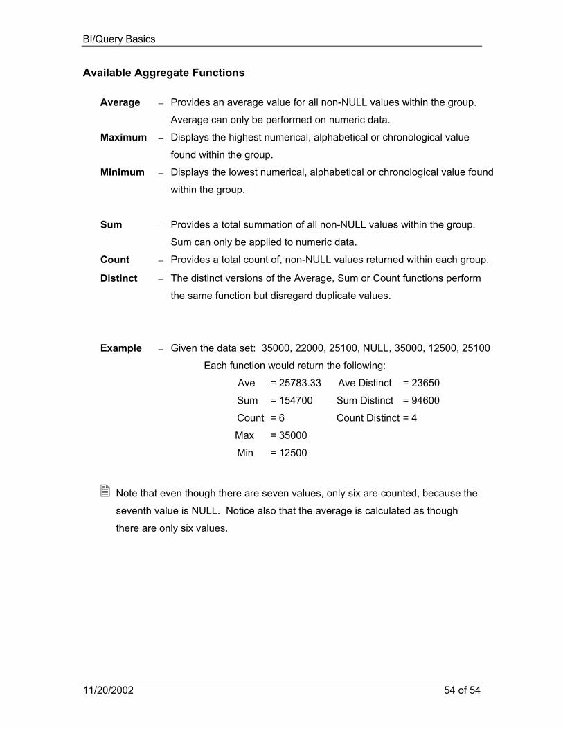
Example − Given the data set: 35000, 22000, 25100, NULL, 35000, 12500, 25100

Each function would return the following:

Ave = 25783.33 Ave Distinct = 23650

Sum = 154700 Sum Distinct = 94600

Count = 6 Count Distinct = 4

Max = 35000

Min = 12500

Note that even though there are seven values, only six are counted, because the

seventh value is NULL. Notice also that the average is calculated as though

there are only six values.

BI/Query Basics

11/20/2002 55 of 55

Group Qualifications

There are two ways to qualify on summarized data. The first is to apply a qualification

as you usually would, using the Qualify Box in the attribute window. Applying the

qualification in this manner places a condition on what data will be returned and then

summarizes the returned data. The second is to apply a group qualification to the

summarized data. This second technique first summarizes and then applies the

condition to the summarized data.

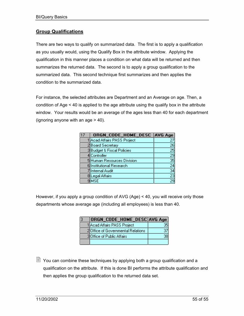
For instance, the selected attributes are Department and an Average on age. Then, a

condition of Age < 40 is applied to the age attribute using the qualify box in the attribute

window. Your results would be an average of the ages less than 40 for each department

(ignoring anyone with an age > 40).

However, if you apply a group condition of AVG (Age) < 40, you will receive only those

departments whose average age (including all employees) is less than 40.

You can combine these techniques by applying both a group qualification and a

qualification on the attribute. If this is done BI performs the attribute qualification and

then applies the group qualification to the returned data set.

BI/Query Basics

11/20/2002 56 of 56

Applying Group Qualifications:

Create a query as usual

Select Query<Qualification<Group from the menu

Choose the summarized column to qualify on, double click or press the move button

Enter the condition manually into the provided text box

Insert any prompts, variables, and other attributes (DB names) as needed (Optional)

Connect multiple group qualifications, using the same text box, with AND or OR

Click OK

The group qualification attribute of BI represents the HAVING clause in SQL.

Once you have created a group qualification there is no indication of its existence

elsewhere in BI. To determine if a group qualification has been applied to the

query you must go to Query<Qualification<Group on the menu.

BI/Query Basics

11/20/2002 57 of 57

Ad Hoc Drill-Down Mode

This section will describe how to narrow down the results of your query, by following

these steps:

Create a query that returns all attributes you wish to study

Submit the query

Select Results<Ad Hoc Drill Down

In the results set, click the cells you wish to base your Drill Down query on (you can

select as many as you like)

Submit the query as normal

Repeat as many times as needed

Ad Hoc Drill-Down is the perfect tool for studying your existing data. Once you have

selected this function you can select one or more values from your result set, then

submit a query that qualifies your results on the selected values. In this way you can run

one query that returns all the information you need and then “drill-down” on that data to

represent many subsets. For example: to learn about the usage of a given building on

campus you could select the building code, room number, type, room code and

department for classes offered on Monday. Then from the resulting data, drill-down on

type and room code to determine lab usage or the number of lower division classrooms

in use. You could then drill-down on type code and department to determine if one

department is monopolizing a given lab, etc.

When you use Ad Hoc Drill Down a qualification is added to your qualification tree.

This qualification is then given the value {drilldown} representing the cells you have

selected from the results window. When you drill down on a second results list, you

are working from the same base query as before, but your new selections are used

for the {drilldown} value. This is why when you drill down for a second and third time,

your query performs the “drill-down” on the original set of results. Every time you

“drill-down”, think of it as creating a new qualification tree for your original query.

BI/Query Basics

11/20/2002 58 of 58

Executive Buttons

Executive Buttons are a great tool for performing routine tasks or simplifying complex

processes. When executed a button performs a series of predefined queries, reports

and other tasks, eliminating the need for extra steps. Executive buttons should be

created in the Reports Window or the Query Window of the model instead of the main

window of the model.

To create a custom executive button:

Create the task to be automated (Query, Report, Window …)

Save this task

Choose from the toolbar to switch to design mode

Click the button tool from the layout toolbar

Click and drag to create a box where you want the button

Double click the resulting button (the Edit Button dialog box appears)

Specify the button’s appearance (see below)

Assign the button’s task to automate (linkage)

Define the output specification

Click Ok

Test the button by exiting design mode and clicking the button

Appearance

A button’s appearance can take three forms: Text, Icon or Picture.

Select the desired appearance using the provided radio buttons

Edit the text, or select an icon or picture (Graphics with the extensions: .wmf, .bmp,

or .gif can be used)

Or click From Clipboard to paste a previously copied text or graphic from the

clipboard

Click the Border checkbox to remove the button’s border (optional)

Click the Autosize checkbox to set the button’s size manually (optional)

BI/Query Basics

11/20/2002 59 of 59

Linkage

An executive button can be linked to:

♦ Previously saved queries (including BI Standard Reports)

♦ The query currently in memory (<Current Query>)

♦ Predefined reports (created in BI/Query Reports)

♦ BI windows

♦ Scripts

Linking Queries

Create and save a query

Select Query from the Linkage drop down box

Choose a query from the drop down list on the right (only queries saved in the

Queries subdirectory will appear in this list)

Reports created using BI Standard Reports in BI/Query should be linked to a

button using the Query linkage option.

Linking Reports

Create a report in BI/Reports, Save your report

Select the BI/Query Reports linkage option

Choose the report you wish to automate (if it is not in the Reports subdirectory,

click the Browse button to find it)

If you do not want to refresh the data for each run, click the refresh button to

remove the check mark

If the refresh check box is not checked, your report will return the data retrieved

last time the report was refreshed.

Linking Design Windows

Select the Window linkage option

Choose the window you wish to navigate to from the list on the right

BI/Query Basics

11/20/2002 60 of 60

Linking Scripts

A script is a command or set of commands that interact with an application outside of

BI. For instance, a script can be used to launch a text editor such as notepad, open

a help file, launch a Web browser and navigate to a specified page, or even print the

results of a BI report.

Select Script from the Linkage list box

Type in a valid application script (this can be anything that would be a valid entry

in the Run dialog box found in the Start menu of your computer)

Or choose an executable file (.exe) using the browse button

Alter text to include the name of the document to be opened (optional)

Output

The output portion of the Edit Button dialog box allows you to specify where you want

the result set of the specified query to be sent. By default the output is set to Window,

meaning your results will appear in a result window as usual. By changing this

assignment you can export your query results to:

♦ Another application

♦ An ASCII (text) file

♦ A database table

Export to an Application

This option can be used to run either the current or a saved query and then send the

results to another application, such as Excel or Word.

Select Application from the Output portion of the window

Click the Export Options button

Select an application name from the Application drop down list

Click the button to browse for the application (.exe file) on your computer

In the Service name edit box, fill in the application name

Assign DDE commands to perform the desired function(s)

BI/Query Basics

11/20/2002 61 of 61

DDE commands:

[paste()] Open Application, open a new worksheet, and

paste results

[new()][paste()] Open a new workbook with Application already

running and paste the results

[open(“c:\test.xls”)][paste()] Open the test.xls workbook (if Excel isn’t already

running) and paste the results

[open(“c:\test.xls”)]

|[run(“test.xlm!macro1”)]

Open the test.xls worksheet, open the

test.xlm!macro1 macro sheet, and run a macro

Example for exporting results to Excel:

Export to an ASCII (Text) File

Choose File from the Output portion of the dialog box

Enter desired filename into the provided text box

Click Results Options

Choose the Options to be included

Select how the file will be delimited (Field Separators)

Click OK

BI/Query Basics

11/20/2002 62 of 62

Export to a Database Table

Select the DB Table Output option

Enter the corresponding data object in the DB Table text box (if left blank BI will

prompt for one each time the button is used)

BI/Query Basics

11/20/2002 63 of 63

Advanced Query Topics This last section will cover the following advanced topics: ♦ Implementing Prompts

♦ Using Variables

♦ Qualifying with Subqueries

♦ Modifying SQL code directly

♦ Creating Custom Attributes

Prompts Often you want to pull one group of information qualified on a different value every time

you run it. For example: at the end of each term you want to pull a list of all graduating

seniors. To accomplish this you run the same query every term but change the term

code qualification to represent the current term. By inserting a prompt you can do this

without ever changing the underlying query. The prompt is inserted into the edit box in

place of a value. Then each time the query is run, the user is asked to provide a value

to qualify on.

Creating Prompts

Select Edit< Prompts from the menu or choose Prompts… from the Data

Values box in your qualification tree

Click New to create a new prompt

Or select an existing prompt and click Edit

Fill in a unique name for the Prompt ID (The end user will not see this name)

Enter a Prompt String (Ex. Please enter current term:)

Click OK (your new prompt will appear in the Prompt Ids list)

Delete an unused prompt by selecting it from the list and pressing Delete

Click Done

BI/Query Basics

11/20/2002 64 of 64

Applying Prompts

Using a prompt is done in much the same way as using a value to qualify your query.

Add a qualification to your query as before

Choose Prompts… from the Data Values box

Select the desired prompt from the list or create a new one

Click Insert Prompt

Repeat as needed

✘ If an operator that allows for multiple values is used, you can insert as many

prompts as are needed into a single qualification. For example, if the BETWEEN

operator is used you can prompt for both values.

The prompts you create are saved in one file located in the local Queries

directory of your data model. The Import button found in the Prompts dialog box

could be used to import the prompts file from another model.

To do this:

Click the Import button

Browse for the new prompts file

From the resulting Prompts to Import list box choose the desired prompts

Click the Import>> button to move them to the Current Prompts list box

Click Done

BI/Query Basics

11/20/2002 65 of 65

Using Wildcards with Prompts

A wildcard is a character that is used in place of a value to represent all possible

values. When a prompt is set up to allow wildcards as the input value, the user is

then able to qualify the query on a specific value or to use a wildcard to return all

values (as though there were no qualification placed on the query for that attribute).

To allow for wildcards:

Qualify on the desired attribute

Change the qualification operator to contains

When prompted either input a value or a wildcard (%)

The wildcard used is %. When used this wildcard stands for any value.

If a prompt is set up in this way the qualification is no longer a straight equals

comparison. So, if a value other than the wildcard is input you will get all rows where

the attribute contains the input value.

BI/Query Basics

11/20/2002 66 of 66

Group Prompts

Prompts can be defined in such a way that, when selected, they will appear in the

same dialog box as all other selected group prompts for that query.

To accomplish this:

Place an ! in front of the Prompt ID.

Unless the order is otherwise specified, the selected group prompts will appear in the

dialog box in alphabetical order. However, often times you will want to set a

predefined order for your prompts. For example, if you are prompting for a start and

end date, you want the user to be asked for the start date first.

To specify the prompt order:

Number the Prompt IDs in the order you wish them to appear

For example: inserting the prompt Ids !2End Date and !1Start Date will, in one dialog

box, prompt the user for Start date and then for End Date. To display the questions

in separate dialog boxes remove the ! from the ID field. Your Ids would then be

2End Date and 1Start Date.

Both group prompt capabilities can be used independently of one another. Your

prompts can be set to appear in a given order, they can be grouped into one

dialog box, or they can be set to appear in one dialog box in a specified order.

Up to five prompts can be grouped into one dialog box. If more than five group

prompts are used in a given query, the remaining prompts will appear in a

second dialog.

Any saved queries that use the old ID will no longer work correctly. For this

reason, if you edit an existing prompt ID, you will have to re-insert the prompt

anywhere that it is used. Be careful when deleting prompts not to eliminate a

prompt that is in use by a saved query.

BI/Query Basics

11/20/2002 67 of 67

Implementing Variables Variables are used to replace qualifications in your query with a user-defined operation.

Defining and implementing a variable is much the same as defining a custom attribute.

However, when defining a custom attribute you are specifying what is to be selected, but

when using a variable you are defining the conditions to be placed on your query. With

variables you can:

♦ Pre-define the Attribute to be qualified

♦ Enforce the use of a given operator

♦ Include prompts

♦ Incorporate functions

♦ Use nested variables

♦ Perform calculations

A variable can be used in one of three ways. First, it can be used to replace the

qualification branch where it is applied. In this case, it is unimportant what attribute the

variable qualifies because the variable itself replaces the entire qualification branch. For

example, you could define a variable to qualify your query where the enrollment count >

AVG(enrollment count). When used, this variable would ignore the attribute and

operator in the qualification tree.

The second use allows you to define a variable that replaces only the value in the Edit

Box of your qualification. This is done using placeholders for the attribute name and/or

operator. These placeholders are then replaced at run time by the attribute and operator

in the qualification branch. For instance, a variable defined as:

^Attribute^^Operator^SYSDATE will use both the attribute and operator from the

qualification tree to qualify on today’s date (returned by SYSDATE).

Finally, you can use a variable to pre-define only the attribute or the operator. This can

be used to eliminate the need for the user to know what exactly the variable does. For

instance, if your variable qualifies on a list of values, you may want to pre-define the

operator to IN. For example, if a given set of indexes are used in your department, a

variable can be defined to qualify on that list of indexes: ^Attribute^ IN (A1, A2, B5).

BI/Query Basics

11/20/2002 68 of 68

To create a variable:

Choose Edit<Variables from the menu

Enter a name and description for your variable (description is optional)

Create the Expression to be used

Select an attribute to be qualified, or click the ^Attribute^ button to insert a

place holder

Enter an appropriate operator, or click the ^Operator^ button to insert a place

holder

Enter the value to qualify on

To insert a function click the Function… button

Choose from the list of functions provided

Replace the parameters (inside the ( )) with the correct values

To insert a variable click the Variable… button

Choose a Variable from the list

Click Insert Variable

To insert a prompt press the Prompt… button

Choose a prompt from the list

Click Insert Prompt

Enter any calculations manually, using the keyboard

Click OK

A variable can contain any valid SQL where clause.

To use a variable in your qualification tree:

Click the Qualify Box of the attribute you wish to qualify on (if the variable does not

include the ^Attribute^ placeholder the selected attribute will be ignored)

Click the Data Values box in the qualification branch

Choose Variable… from the resulting menu

Double click the variable you wish to insert

BI/Query Basics

11/20/2002 69 of 69

Variable examples

This example replaces the entire branch in the qualification tree. It qualifies the

query to return only those courses with a start date earlier than today.

In the example below the variable replaces the operator and qualifier of the

qualification branch, but qualifies the attribute selected in the attribute window.

BI/Query Basics

11/20/2002 70 of 70

Using Subqueries There are some problems that cannot be solved using one query. For example, if you

need to get a list of employees who are above the average age, you would first need to

determine the average age and then determine whose age is above it. To do this with

two separate queries, you would first write a query that selects the age attribute with the

AVERAGE aggregate function applied to it. Keeping the returned number in mind, you

would write a second query, to select the employees, with age qualified by the average

value.

Using a subquery to retrieve the list of employees would allow you to write one query

that actually qualifies on the value returned by another. When creating a query using a

subquery, you want to work from the inside out. Meaning you write the subquery first,

then the outer or main query. Think about how you would have to do it by hand. First,

you need the information to qualify on then you can use it to place your condition. To

qualify one query with another:

Create the query that will be used as a subquery first (in the normal fashion)

Select only one attribute to be returned

Qualify on as many attributes as needed

Add aggregate functions as needed

Save the query in the normal way

Create the outer (main) query

Select desired attributes

Click the Qualify box of the attribute to be qualified on

Choose Edit<Insert Subquery from the menu

Select an appropriate operator (if the subquery will return more than one row be

sure to select an operator that can handle more than one value, such as IN or

BETWEEN)

Submit the query

Do not use Begins with, Does not Begin with, Contains, Does not Contain, Ends

with, or Does not end with as the operator in a qualification that includes a

subquery.

BI/Query Basics

11/20/2002 71 of 71

✘ You can use a query with a subquery as a subquery. This process is called using

nested subqueries.

✘ You can qualify an attribute in the subquery and an attribute in the main query with

the same prompt. The user is only prompted once and the value is used for both

queries.

Any query that returns only one attribute can be used as a subquery.

BI/Query Basics

11/20/2002 72 of 72

Modifying SQL Code If you are familiar with SQL, you can directly modify the SQL code generated by your

query. In doing so, you must be careful to mimic the syntax used by BI/Query or the

results you receive may not be as expected.

Choose Query<Show from the menu

Edit the SQL text in the text box at the bottom of the resulting window

✘ If you are unable to access the Show Query window, check the permissions to be

sure you have the Edit Queries permission. Also, set your preferences to include

Show SQL String. Both can be found in the Tools menu

Be sure when editing SQL that you use the database names for the selected

attributes and not the BI display name.

Editing the SQL should be the last thing you do to your query. Once it has been

edited you cannot alter your query using the tools provided in BI without reverting

to the original SQL.

BI/Query Basics

11/20/2002 73 of 73

Creating Custom Attributes

To manipulate the data retrieved at the query level, you can create custom, or

calculated, attributes. These attributes are added to your personal data model and can

be saved for use with future queries. By creating custom attributes you can:

♦ Perform calculations on existing attributes

Annual_Salary/12

♦ Create a calculation based on two or more attributes

Annual_Salary – Job_Low_Salary

♦ Pull attributes from more than one data object

♦ Perform aggregate functions

SUM(Enrollment Count)

♦ Select from a list of pre-defined functions to manipulate the data (Appendix A)

Decode(sp_util.COAS, ‘B’, ‘OSU’,’C’,’OSU’,’D’,’PSU’,’E’,’WOU’,’Other’)

♦ Make use of any valid SQL Select statement

Last Name || ’,‘ || First Name

♦ Select Literals

2000, Eastern Oregon State

Once you have created a custom attribute it can be selected in the same way that other

attributes in the object are. Calculated columns are useful for reusing a preset

calculation, simplifying data, changing the data format, or creating attributes that are not

otherwise available. For example, if your model provides the building code but not the

building name, you can create a custom attribute using the decode function, to show the

building name instead. Likewise, if you have a need to show the current year in a

column of your returned data set, you can do so by assigning your calculated column to

a literal such as 2000.

BI/Query Basics

11/20/2002 74 of 74

To create a custom attribute:

Click on the Function box of the attribute above the location where you would like to

add the calculated attribute (this attribute does not need to be related to your custom

attribute)

Choose Calculation from the resulting menu

Fill in the name as you want it to appear in the attribute window

Compose the expression (or calculation) that defines the new attribute

Insert needed attributes

Choose a data object from the tables/attribute dropdown box

Select an attribute

Press the Insert Attribute button or double click the attribute

Insert Functions

Click the Insert Functions button

Choose a function from one of the available function lists

Click Insert

Replace the parameters (found inside the ( )) with the correct attribute or

literal value

Insert numerical values or mathematical operators by typing or using the keypad

Press the Data Type button to select a data type (usually either Automatic numeric or

Automatic Character, or Date)

Make sure the Save definition box is checked if you want your attribute to remain in

the model after you close it

To edit a calculation, click the Function box of the custom attribute and select Edit

Calculation from the resulting menu.

When adding attributes to your calculation be sure to use the list box to insert

them. Doing this adds the database name of the attribute to the equation. If you

type in the attribute name as you see it in BI, your attribute will not work correctly.

✘ It is a good idea to give your calculated attributes a different look, such as all caps or

placing an * after the name. This makes it very clear which attributes come standard

with the model, and which are specific to your personal data model.

BI/Query Basics

11/20/2002 75 of 75

To use straight SQL to define an attribute, simply type in the code as you would after

the Select keyword when writing SQL code. You should be familiar with SQL before

attempting to use this functionality.

If a calculated attribute includes an aggregate function (such as COUNT or SUM) the

aggregate check box is automatically selected. This forces your query to group the

selected attributes whenever your calculated attribute is selected. The effect is the

same as when you apply an aggregate function to an existing attribute.

Pulling attributes from more than one data object still creates a join relationship

between the two objects. Therefore, the slowdown caused by joining objects cannot

be avoided by creating custom attributes.

Example:

BI/Query Basics

11/20/2002 76 of 76

Appendix A Character Functions

Function Description Example

CONCAT(char1, char2) Returns char1 concatenated with

char2. This is the same function

that || does in SQL.

CONCAT(‘volks’,’wagon’) returns

‘volkswagon’

DECODE(attribute,

comparison value, new

value, other value)

Compares attribute to

comparison value. If they are

equal it returns new value if they

are not equal it returns other

value.

DECODE(first_name,’David’, ‘Dave’,

‘Not Dave’) returns ‘Dave’ for anyone

named ‘David’ and ‘Not Dave’ for

everyone else

INITCAP(char) Returns char, with the first letter

of each word in uppercase.

INITCAP(‘paul smith’) returns ‘Paul

Smith’

INTSTR(char1,char2,n,m) Searches char1 beginning with

it’s nth character, for the mth

occurrence of char2. Returns the

position in the string of char1.

INSTR(‘Corporate Floor’,’or’,3,2)

returns 14

LENGTH(char) Returns the length of char in

number of characters

LENGTH(‘Smith’) returns 5

LOWER(char) Returns char, with all letters in

lowercase.

LOWER(‘FIS’) returns ‘fis’

LPAD(char1, n, char2) Returns char1, padded to total

length n with the value of char2.

LPAD(‘Page 1’, 10, ‘*’) returns

****Page1

LTRIM(char, set) Returns char, with the first

leftmost characters that appear in

set removed; set defaults to a

single blank.

LTRIM(‘Corporate’,’or’) returns

‘Cporate’

REPLACE(char, search,

replacement)

Returns char with every

occurrence of search replaced

with replacement.

REPLACE(‘GQL/Query’,’GQL’,’BI’)

returns ‘BI/Query’

BI/Query Basics

11/20/2002 77 of 77

RPAD(char1,char2) Returns char1, right padded to

length n, with char2, replicated as

many times as necessary; char2

defaults to a single blank.

RPAD(‘80’,4,’0’) returns ‘0080’

RTRIM(char, set) Returns char, with all the

rightmost characters that appear

in set removed; set defaults to a

single blank.

RTRIM(‘HR Datastore’,’store’)

returns ‘HR Data’

SOUNDEX(char) Returns a character set

containing the phonetic

representation of char. This

function allows you to compare

words that are spelled differently,

but sound alike in English.

SOUNDEX(‘SMYTHE’) returns

‘Smith’

SUBSTR(char,m,n) Returns a portion of char, starting

at character position m, and

going n characters long.

SUBSTR(‘BI/Query’,4,5) returns

‘Query’

TO_CHAR(n) Converts n, of numeric datatype,

to character.

TO_CHAR(16) returns ‘16’

TO_DATE(char) Converts char, of character

datatype, to a date.

TO_DATE(‘5-Nov-99’) returns the

date ‘5-Nov-99’

TO_NUMBER(char) Converts char, of character

datatype to a number.

TO_NUMBER(‘16’) returns 16

TRANSLATE(char,from,to) Returns char with all occurrences

of each character in from

replaced by it’s corresponding

character in to.

TRANSLATE(‘Hummingbird’,’in’, ‘14’)

returns ‘Humm14gb1rd’

UPPER(char) Returns char, with all letters

uppercase.

UPPER(‘McDonald’) returns

‘MCDONALD’

BI/Query Basics

11/20/2002 78 of 78

Numerical Functions

Function Description Example

ABS(n) Returns the absolute value of n. ABS(-2) returns 2

CEIL(n) Returns the smallest integer

greater than or equal to n.

CEIL(7.3) returns 8

COS(n) Returns the cosine of n (an angle

expressed in radians)

COS(180 * 3.14159265359/180)

returns –1 (Cosine of 180 degrees)

EXP(n) Returns e raised to the nth

power, where e = 2.71828183...

EXP(4) returns 54.59815

FLOOR(n) Returns largest integer equal to

or less than n.

FLOOR(7.3) returns 7

LN(n) Returns the natural logarithm of

n, where n is greater than 0.

LN(95) returns 4.5538769

LOG(m,n) Returns logarithm, base m, of n.

m must be a positive integer > 1

LOG(10,100) returns 2

MOD(m,n) Returns remainder of m divided

by n. Returns m if n is 0.

MOD(10,3) returns 1

POWER(n,m) Returns m raised to the nth

power. The base m and the

exponent n can be any numbers.

POWER(3,3) returns 27

ROUND(n,m) Returns n rounded to m places

right of the decimal.

ROUND(15.193,1) returns 15.2

SIGN(n) If n<0, function returns –1; if n=0,

the function returns 0; if n>0, the

function returns 1.

SIGN(5) returns 1

SIN(n) Returns the sine of n (an angle

expressed in radians)

SIN(30 * 3.14159265359/180)

returns .5 (Sine of 30 degrees)

SQRT(n) Returns the square root of n. SQRT(9) returns 3

TAN(n) Returns the tangent of n (an

angle expressed in radians)

TAN(135 * 3.14159265359/180)

returns -1 (Tangent of 135 degrees)

TRUNC(n,m) Returns n truncated to m decimal

places.

TRUNC(15.4248,2) returns 15.42

BI/Query Basics

11/20/2002 79 of 79

Date Functions

Function Description Example

ADD_MONTHS(d,n) Returns the date d plus n

months.

ADD_MONTHS(‘1/1/97’,3) returns

‘1/4’97’

LAST_DAY(d) Returns the date of the last day

of the month that contains d.

LAST_DAY(6) returns 31

MONTHS_BETWEEN(d1,

d2)

Returns the number of months

between dates d1 and d2.

MONTHS_BETWEEN(‘1/1/95’,’2/3/96’)

returns 14

NEW_TIME(d,z1,z2) Returns the date and time in

time zone z2 for date and time

d in time zone z2.

NEW_TIME(‘1-JAN-95 10:00 am’,

PST, AST) returns ‘1-JAN-95 1:00 pm’

NEXT_DAY(d,char) Returns the date of the first

weekday named by char that is

later than the date d.

NEXT_DAY(‘5-Nov-1996’, ‘Monday’)

returns ‘11-Nov-1996’)

ROUND(d, fmt) Returns d rounded to the unit

specified by the format model

fmt.

ROUND(‘05-NOV-96’,’YEAR’) returns

01-JAN-97

SYSDATE Returns the current date and

time.

TRUNC(d, fmt) Returns d with the time portion

of the day truncated to the unit

specified by the format model

fmt.

TRUNC(‘05-NOV-96’,’YEAR’) returns

01-JAN-96

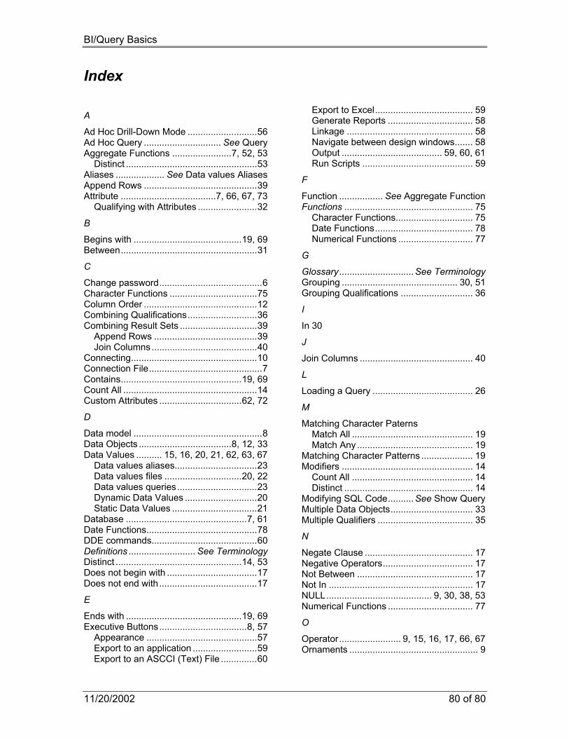
BI/Query Basics

11/20/2002 80 of 80

Index A

Ad Hoc Drill-Down Mode ...........................56 Ad Hoc Query .............................. See Query Aggregate Functions .......................7, 52, 53

Distinct ...................................................53 Aliases ................... See Data values Aliases Append Rows ............................................39 Attribute .....................................7, 66, 67, 73

Qualifying with Attributes .......................32

B

Begins with ..........................................19, 69 Between.....................................................31

C

Change password........................................6 Character Functions ..................................75 Column Order ............................................12 Combining Qualifications...........................36 Combining Result Sets ..............................39

Append Rows ........................................39 Join Columns.........................................40

Connecting.................................................10 Connection File............................................7 Contains...............................................19, 69 Count All ....................................................14 Custom Attributes ................................62, 72

D

Data model ..................................................8 Data Objects ....................................8, 12, 33 Data Values .......... 15, 16, 20, 21, 62, 63, 67

Data values aliases................................23 Data values files ..............................20, 22 Data values queries...............................23 Dynamic Data Values ............................20 Static Data Values .................................21

Database ...............................................7, 61 Date Functions...........................................78 DDE commands.........................................60 Definitions .......................... See Terminology Distinct .................................................14, 53 Does not begin with ...................................17 Does not end with......................................17

E

Ends with .............................................19, 69 Executive Buttons..................................8, 57

Appearance ...........................................57 Export to an application .........................59 Export to an ASCCI (Text) File ..............60

Export to Excel...................................... 59 Generate Reports ................................. 58 Linkage ................................................. 58 Navigate between design windows....... 58 Output ....................................... 59, 60, 61 Run Scripts ........................................... 59

F

Function ................. See Aggregate Function Functions .................................................. 75

Character Functions.............................. 75 Date Functions...................................... 78 Numerical Functions ............................. 77

G

Glossary.............................See Terminology Grouping ............................................. 30, 51 Grouping Qualifications ............................ 36

I

In 30

J

Join Columns ............................................ 40

L

Loading a Query ....................................... 26

M

Matching Character Paterns Match All ............................................... 19 Match Any ............................................. 19

Matching Character Patterns .................... 19 Modifiers ................................................... 14

Count All ............................................... 14 Distinct .................................................. 14

Modifying SQL Code.......... See Show Query Multiple Data Objects................................ 33 Multiple Qualifiers ..................................... 35

N

Negate Clause .......................................... 17 Negative Operators................................... 17 Not Between ............................................. 17 Not In ........................................................ 17 NULL......................................... 9, 30, 38, 53 Numerical Functions ................................. 77

O

Operator........................ 9, 15, 16, 17, 66, 67 Ornaments .................................................. 9

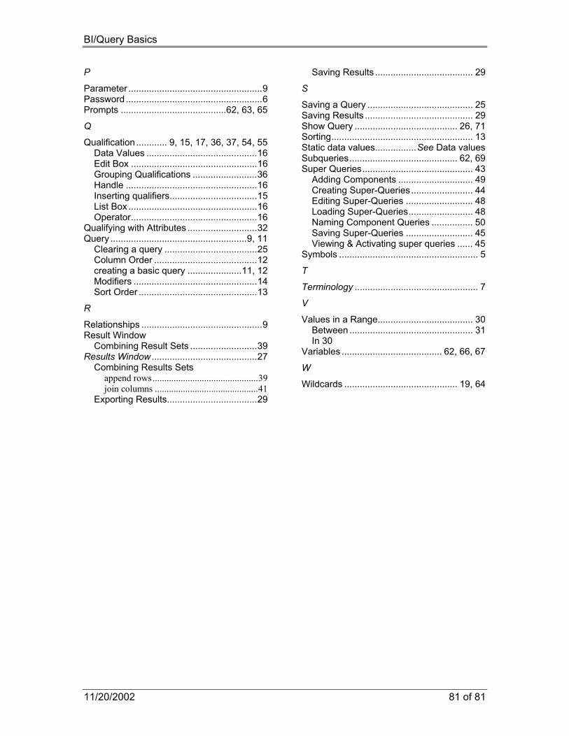
BI/Query Basics

11/20/2002 81 of 81

P

Parameter ....................................................9 Password .....................................................6 Prompts .........................................62, 63, 65

Q

Qualification ............ 9, 15, 17, 36, 37, 54, 55 Data Values ...........................................16 Edit Box .................................................16 Grouping Qualifications .........................36 Handle ...................................................16 Inserting qualifiers..................................15 List Box ..................................................16 Operator.................................................16

Qualifying with Attributes ...........................32 Query .....................................................9, 11

Clearing a query ....................................25 Column Order ........................................12 creating a basic query .....................11, 12 Modifiers ................................................14 Sort Order ..............................................13

R

Relationships ...............................................9 Result Window

Combining Result Sets ..........................39 Results Window .........................................27

Combining Results Sets append rows.............................................39 join columns ............................................41

Exporting Results...................................29

Saving Results ...................................... 29

S

Saving a Query ......................................... 25 Saving Results .......................................... 29 Show Query ........................................ 26, 71 Sorting....................................................... 13 Static data values................See Data values Subqueries.......................................... 62, 69 Super Queries........................................... 43

Adding Components ............................. 49 Creating Super-Queries........................ 44 Editing Super-Queries .......................... 48 Loading Super-Queries......................... 48 Naming Component Queries ................ 50 Saving Super-Queries .......................... 45 Viewing & Activating super queries ...... 45

Symbols ...................................................... 5

T

Terminology ................................................ 7

V

Values in a Range..................................... 30 Between ................................................ 31 In 30

Variables ....................................... 62, 66, 67

W

Wildcards ............................................ 19, 64