Information Sharing in Supply Chains: An Empirical and ... · An Empirical and Theoretical Valuation Ruomeng Cui, ... point of sale and inventory) ... The literature studies demand

Information Sharing in Supply Chains:An Empirical and Theoretical Valuation

Ruomeng Cui, Gad Allon, Achal Bassamboo, Jan A. Van Mieghem*Kellogg School of Management, Northwestern University, Evanston, IL

April 10, 2013

We provide an empirical and theoretical assessment of the value of information sharing in a two-stage supply

chain. The value of downstream sales information to the upstream firm stems from improving upstream order

fulfillment forecast accuracy. Such improvement can lead to lower safety stock and better service. According

to recent theoretical work, the value of information sharing is zero under a large spectrum of parameters.

Based on the data collected from a CPG company, however, we empirically show that if the company includes

the downstream demand data to forecast orders, the mean squared error percentage improvement ranges from

7.1% to 81.1% in out-of-sample tests. Thus, there is a discrepancy between the empirical results and existing

literature: the empirical value of information sharing is positive even when the literature predicts zero value.

While the literature assumes that the decision maker strictly adheres to a given inventory policy, our model

allows him to deviate, accounting for private information held by the decision maker, yet unobservable to

the econometrician. This turns out to reconcile our empirical findings with the literature. These “decision

deviations” lead to information losses in the order process, resulting in strictly positive value of downstream

information sharing. We prove that this result holds for any forecast lead time and for more general policies.

We also systematically map the product characteristics to the value of information sharing.

Key words : supply chain, information sharing, information distortion, decision deviation, time series,

forecast accuracy, empirical forecasting, ARIMA process.

1. Introduction

The abundance of information technology has had a massive impact on supply chain coordina-

tion. Sharing downstream demand information with upstream suppliers has improved supply chain

performance in practice. Costco and 7-Eleven share warehouse-specific, daily, item level point of

sale data with their suppliers via SymphonyIRI platform, a company offering business advice to

retailers (see Costco collaboration 2006). In addition to this uni-directional information sharing,

Collaborative Planning, Forecasting and Replenishment (CPFR) programs advocate joint visibil-

ity and joint replenishment. According to Terwiesch et al. (2005), the benefit of CPFR programs

*E-mail addresses are: r-cui, g-allon, a-bassamboo, vanmieghem all @kellogg.northwestern.edu.

1

2

can be significant: the GlobalNetXchange, a consortium consisting of more than 30 trade partners

including Sears, Kroger etc, have reported a 5% to 20% reduction in inventory costs and an increase

in off-the-shelf availability of 2% to 12% following the launch of their CPFR programs.

In sharp contrast, however, the academic literature shows that the value of sharing downstream

customer sales to improve upstream forecasting is limited. (We will also refer to customer sales as

customer demand or demand.) For example, Gaur et al. (2005) model the demand process as an

autoregressive moving average ARMA(1,1) and show that the value of information sharing is zero

under 75% of the demand parameters. Therefore, a direct conclusion of this literature is that the

value of information sharing is zero under a large spectrum of parameters.

Companies spend billions of dollar on demand forecasting software and other supply chain solu-

tions (Ledesma 2004). Given the implementation cost of collaboration technology and the limited

theoretical benefits, it is not clear in practice whether a firm should invest in information sharing

systems. The decision to implement an information sharing system thus hinges on the following

question: how much would sharing downstream information improve the supplier’s order forecast

accuracy? We were approached with this question by the statistical forecasting team of a leading

global consumer packaged goods (CPG) company that manufactures and sells beverages and snack

foods to wholesalers and retail chains. Forecasting is necessary for the company due to the lead

time to adjust manufacturing runs and deploy inventory. In the absence of downstream demand

information, the upstream supplier uses its own demand history (i.e., its retailer’s order history),

to forecast how much to manufacture. Not satisfied with its current forecasting performance, the

firm sought solutions in information sharing by collecting downstream operations data (e.g., point

of sale and inventory) from both its customers and a third party organization (e.g., RSI). Using

this data set, we directly measure the supplier’s forecast accuracy improvement.

Surprisingly, our empirical results indicate a substantial value of information sharing: (1) incor-

porating order and demand correlation yields a statistically significant improvement for some prod-

ucts even without accounting for the applied inventory policies; and (2) applying the underlying

replenishment policies, we find that the value of information sharing is strictly positive (7.1% to

81.1% MSE percentage improvement) across all products with stationary demand while the litera-

ture suggests positive value for only 30% (4 out of 14) of products. To put this in perspective, the

company views the forecast accuracy improvement opportunities of 10% as important and 30% as

very significant. These empirical findings suggest that we need a better theoretical understanding

of how demand propagation impacts forecasting.

The works of Gaur et al. (2005) and Giloni et al. (2012) are important antecedents of our paper.

In their setting, the decision maker strictly follows an order-up-to policy, via which the demand

process propagates upstream and becomes the order process. If, for example, the retailer follows

3

a demand replacement policy (the retailer orders the demand in the current week), the order

process then equals the demand process. It is as if the demand process propagates fully upstream

and the order process carries full demand information. In such setting, the value of including the

downstream demand process is zero. The downstream demand information might be lost in this

demand-to-order transformation. The authors derive the following insights: the value of information

sharing is zero when the order process effectively carries all demand information, or equivalently,

when the order is invertible with respect to demand shocks. The authors show that the order is

invertible (thus the value of information sharing is zero) under 75% of demand parameters for an

ARMA(1,1) demand process.

The key underlying assumption in the theoretical literature is that the decision maker consis-

tently and strictly follows a given replenishment policy. In practice, however, we learned that the

decision makers deviate from their target inventory policy based on private information that we

cannot observe. The planner might round the order quantity due to truck load constraints and

delivery multiple brands of products in batches. From an econometric perspective, we model the

agent’s deviation from the exact policy, in the spirit of Rust (1997), by an “error term” that

accounts for a state variable which is observed by the agent but not by the statistician. We demon-

strate that including these idiosyncratic shocks in the model significantly increases the theoretical

value of information sharing, in agreement with the empirical findings.

In the presence of decision deviations, we provide a different and important insight into the

value of information sharing. Unlike before, the demand process now propagates together with the

decision deviation. The value of information sharing is zero if the order process carries both all

demand information and all decision deviation information. The demand and decision deviation

processes follow distinct evolution patterns to produce the order process: the evolution of inventory

governs the translation of decision deviations into replenishment decisions while the evolution of

inventory and current demand together dictates the translation of demand. This difference causes

the order process to no longer carry full downstream information. Information sharing then becomes

valuable to recover the order’s elaborate information structure and to forecast more accurately. At

first glance, the decision uncertainty seems to diminish the attractiveness of analyzing a retailer’s

replenishment process due to the unpredictability of the order decision. Such uncertainty, however,

opens the door to information loss in the upstream orders, because the decision deviation distorts

the normal demand propagation. We prove that as long as the variability in decision deviation and

demand are both nonzero, the value of information sharing is strictly positive for any forecast lead

time (regardless of the demand and policy). Our extended model induces qualitatively different

results than the literature and reconciles our empirical findings.

4

We also conduct comparative statics and detailed numerical studies to examine the impact of

product demand characteristics on the value of information sharing. These insights can help man-

agers rank the potential gains from information sharing depending on the demand characteristics

for different products such as sport drinks and orange juice.

Our study is grounded in both empirical evidence and theory and attempts to understand the

cause of strictly positive value of information sharing. We analyze a data set containing weekly

downstream demand, upstream order fulfillment, and the price plan over a period of two and a half

years. This allows us to make the following four main contributions: first, this paper complements

the emerging area of research in information sharing with empirical evidence. Specifically, we

directly measure the value of information sharing at a leading CPG company and demonstrate

a positive value of information sharing in all the settings that we study. Second, we allow for

decision deviations in our theoretical model to explicitly capture the decision maker’s private

information that is unobservable to us. This model extends the existing literature and recovers

the results from the literature as a special case where decision deviation is zero. Third, we prove

that if both demands and order decisions are subject to random shocks, the value of information

sharing is always positive. We demonstrate that the decision deviation distorts the normal demand

propagation in a way that obscures the detailed information of the two processes. The resulting less

informative order process induces larger forecast uncertainty, which indicates a positive value from

using the downstream demand to recover the original elaborate information structure. Finally, we

provide guidelines for the magnitude of the value of information sharing depending on the demand

characteristics.

2. Literature Review

Motivated by practice and theory, we study the value of a retailer to share its retailer’s downstream

demand information with its supplier to help the supplier forecast the retailer’s order. We find that

the results in the literature point towards the inconsistencies between the empirical evaluation of

the benefit and the theoretical predictions. This paper reconciles these findings by extending the

established theory. Therefore, our paper is related to two streams of literature: (1) theoretical work

on information sharing and demand propagation through supply chains and (2) empirical work

that bridges the above theory and operational data.

There is a vast theoretical literature on the subject of demand propagation and information

sharing in supply chains. A company’s demand propagates through the supply chain and becomes

its order to the supplier. The properties of orders can help answer important questions in supply

chains, e.g. is sharing retailer’s demand information beneficial for the supplier to forecast its own

order and manage its inventory; is there incentive for the agents to share their own information; is

5

there a bullwhip effect and what is the driver? The demand propagation relies on two basic char-

acteristics of the supply chain: demand structure and replenishment policy. We focus on the work

that assumes truthful and complete information disclosure. We begin by introducing the various

demand and policy structures studied in the literature. Next, we discuss our paper’s contribution

relative to the two most related work: Gaur et al. (2005) and Giloni et al. (2012).

Theoretical Work. The literature studies demand propagation under various demand struc-

tures. Lee et al. (2000) and Raghunathan (2001) adopt an autoregressive AR(p) process, Miyaoka

and Hausman (2004) and Graves (1999) assume an integrated moving average IMA(d, q) process,

Zhang (2004), Gaur et al. (2005), Kovtun et al. (2012) and Giloni et al. (2012) consider an autore-

gressive and moving average ARMA(p, q) process, Gilbert (2005) applies an ARMA with integra-

tion model called ARIMA(p, d, q) process, and Aviv (2003) uses the linear state space framework.

Another body of literature applies the Martingale Model of Forecast Evolution (MMFE) structure.

It uses the incremental signal, generated from the minimum mean squared error, to model the

evolution of a process. Heath and Jackson (1994), Graves et al. (1998), Aviv (2001a) and Chen

and Lee (2009) apply such demand structure to study production and forecasting. The general

expression in the optimal forecast revision drives MMFE’s theoretical advantage: most time-series

models can be interpreted as a special case of the MMFE model (Chen and Lee 2009). We will

show our main conclusion holds under the MMFE structure (see Online Companion). Gaur et al.

(2005) point out the ARMA model closely resembles the real-life demand structure and finds it

valuable from the manager perspective to study such demand process. For our studies, we use an

ARIMA structure to model and empirically fit the demand process.

In the above literatures, the most commonly studied replenishment decision is the myopic order-

up-to policy. The following papers investigate information sharing and the bullwhip effect under

other policies. Caplin (1985) proves the existence of the bullwhip effect under periodically reviewed

(s,S) policy. Cachon and Fisher (2000) quantify the value of information sharing with a batching

allocation rule between one supplier and multiple retailers. These two papers model batching in

replenishment, which is not amenable to exact and mathematically-tractable analysis. The following

papers adopt a “linear replenishment rule,” in which orders are linear in past observed variables.

Balakrishnan et al. (2004) propose an “order smoothing” inventory policy where the order is a

convex combination of historical demands. Miyaoka and Hausman (2004) use the old demand

forecasts to set the base stock level and show this can reduce the bullwhip effect. Graves et al.

(1998) and Aviv (2001b) study the production smoothing policy and Chen and Lee (2009) extend it

to a more general order-up-to policy (GOUTP), which bears an affine and time-invariant structure

of the forecast revisions. We prove that our main result still holds under GOUTP (see Online

Companion). According to the replenishment policy we observed at the firm that provided us with

6

the data, our paper introduces an order rule that keeps the days of inventory constant and uses

some order smoothing. Such policy specifies the order as a linear combination of past demands

and inventory. To summarize, the ARIMA model determines our input demand structure and the

linear policy dictates how demand propagates through the supply chain.

As reviewed in Section 1, Gaur et al. (2005) and Giloni et al. (2012) are the two most closely

related works to our paper. They assume that the decision maker strictly and consistently follows

the replenishment policy. They conclude that under certain demand and policy parameters, the

value of sharing the demand information is zero. Under such strict policy adherence, orders only

depend on the observed demand or demand signals. In practice, however, decision makers adjust

their purchases by other factors. To account for these factors, we introduce an “error term” into

the empirical model with the interpretation of a state variable observed by the agent but not by the

statistician, in the spirit of Rust (1997). Therefore, our theoretical model differs from the existing

literature in relaxing the strict adherence to the replenishment policy. Such an extension explains

our substantial empirically evaluated value of information sharing, thus fills the gap between the

literature and the empirical observation.

Empirical Work. A growing body of empirical literature analyzes the bullwhip effect and infor-

mation sharing. Cachon et al. (2007) investigate a wide range of industries and show insignificant

variance amplification for some industries. Bray and Mendelson (2012b) further decompose the

bullwhip by short, middle and long lead time signals. In the gaming environment, agents have

incentives to partially rely on the data or share untruthful information. Cohen et al. (2003) model

the supplier’s optimal production starting time after receiving forecasts by the retailer. The esti-

mated high cost of starting the production too early indicates the supplier’s tendency to ignore the

retailer’s early forecast, thus inferring the low efficiency of forecast sharing. Terwiesch et al. (2005)

also conclude the low efficient forecast sharing by finding the agent’s forecast behavior falls in the

noncooperative scenario. Bray and Mendelson (2012a) characterize the demand propagation under

the MMFE structure and GOUTP rule. The authors suggest the positive value for the upstream

supplier if the retailer better forecasts the demand.

Using an econometric model, Dong et al. (2011) find that the inventory decision-making transfer

between firms, which means the supplier manages the retailer’s inventory, benefit both upstream

and downstream firms. They show a negative relation between the decision transfer and distribu-

tor’s average inventory. Route (2003) captures the order demand correlation including the retailer’s

point of sale data, and evaluates the forecast accuracy improvement. Our study also applies the

method to include the downstream demand information. In our paper, the retailer’s demand infor-

mation is an additional indicator included to help forecasting supplier orders. Similarly, one can use

other potential indicators to predict customer demand, e.g. financial market index or accounting

variables (see Gaur et al. 2009 and Kesavan et al. 2009, among others).

7

3. Including Downstream Demand Improves Order Forecasting

The goal of this section is to provide an empirical evidence that incorporating downstream sales

data improves order forecast accuracy compared to the benchmark where the sales information

is not shared. In this section, we proceed as follows: we first explain the supply chain structure;

we then describe the data set; we next illustrate the forecasting procedure and finally show the

empirical results.

Supply chain setting. We consider a two-echelon supply chain with a supplier and a retailer.

The retailer places an order Ot to the supplier in each period t. In each period, the supplier predicts

the future order, e.g. the 1-step prediction for period t given the history through period t−1, which

we denote as Ot−1,t (throughout the paper, hat denotes forecasted quantities). The prediction error

is the difference between the actual order and its predicted value, Ot − Ot−1,t. We will measure

the forecast accuracy as a function of the prediction error using two metrics for our empirical

study. The supplier aims to improve the forecast accuracy of future orders. We will compare the

forecast accuracy under two settings: NoInfoSharing and InfoSharing. The NoInfoSharing denotes

the setting when the supplier only has access to the retailer’s order history. Under the InfoSharing

setting, in addition to the order data, the retailer also shares her sales history with the supplier.

Data. We obtain the data from a CPG company, which is a leading manufacturer and supplier

in the US beverage and snack food industry. We utilize a specific retail customer’s (1) sales from

the retailer distribution center and (2) replenishment fulfillment from the supplier, over 126 weeks

between 2009 and 2011. The sales data corresponds to the actual demand due to the few stockout.

We study two brands of products: a sports drink and orange juice. We choose 14 low-promotional

products for the study because of their stationary nature1.

Forecasting procedure. For the purpose of our study, we choose the last 26 weeks in our data

as the out-of-sample test period. This out-of-sample comparison is made in two stages. First, we

forecast the 1-period-ahead order over the out-of-sample test period. To be specific, the forecast

begins 26 weeks before the end of the data. Given information history through the end of period

t−1, we predict the order for period t. Then we update the information history from the beginning

of the data through the end of week t to predict for period t+1. We periodically update the available

information history to obtain the order forecast and calculate the forecast error by comparing the

actual observation and predicted value. Second, we conduct tests of equal forecast accuracy on the

two sequences of forecast errors generated from two candidate forecasting methods.

Next we explain the NoInfoSharing and InfoSharing forecasting methods. For the NoInfoShar-

ing benchmark, we use order history to predict future orders. We fit the autoregressive inte-

grated moving average (ARIMA) model to the order history to obtain the best estimator with the

1 The stationary nature means the sales process has constant mean and covariance over time.

8

lower Bayesian information criterion (BIC)2. We then predict the order by applying the estimated

ARIMA model.

The ARIMA model is generally referred to as an ARIMA(p, d, q) model where p, d and q are

non-negative integers that refer to the degree of the autoregressive, integrated and moving average

parts of the model respectively. In the ARIMA structure, the order is a linear combination of past

observations and shocks. The “first order differenced” process Ot −Ot−1 will be denoted by O1t .

We assume O1t is an ARMA(p, q) process

O1t = µ+ ρ1O

1t−1 + ρ2O

1t−2 + · · ·+ ρpO

1t−p + ηt +λ1ηt−1 +λ2ηt−2 + · · ·+λqηt−q. (1)

where µ is the process mean, ηt is the order shock, ρi is the autoregressive parameter and λi is the

moving average coefficient. Suppose the available information history is through the end of period

t− 1, the differenced order forecast for period t is O1t−1,t = µ+ ρ1O

1t−1 + ρ2O

1t−2 + · · ·+ ρpO

1t−p +

λ1ηt−1 + λ2ηt−2 + · · ·+ λqηt−q or the order forecast for period t is Ot−1,t = Ot−1 + µ+ ρ1O1t−1 +

ρ2O1t−2 + · · ·+ ρpO

1t−p +λ1ηt−1 +λ2ηt−2 + · · ·+λqηt−q.

To analyze the impact of including retail demand data, we consider four InfoSharing forecasting

methods: three “naive” methods and our “advanced” method. The “naive” methods capture the

correlation between order and demand by specifying a linear model. The “advanced” method

considers a specific replenishment policy, which we will discuss in detail in Section 4 and Section

6. The “advanced” method is used to evaluate the additional value of carefully considering the

underlying order policy structure over the naive ones. We refer to such forecast scheme as the

policy structure method.

The first two naive methods capture the order demand correlation by regressing order on

demands, or on both orders and demands, within the past five periods. If regressing order only on

demands, we refer to this method as Reg D method where the order is expressed as

Ot = c0Dt + c1Dt−1 + · · ·+ c5Dt−5 + εt. (2)

We fit the ARIMA model to the demand process to forecast Dt−1,t. With the parameters estimated

from equation (2), the order prediction in period t becomes Ot−1,t = c0Dt−1,t+c1Dt−1+ · · ·+c5Dt−5.

In the second naive method refered to as “Reg D and O” method, we regress order on historical

demands and orders. This method expresses the order as

Ot = c0Dt + c1Dt−1 + · · ·+ c5Dt−5 + b1Ot−1 + · · ·+ b5Ot−5 + εt. (3)

As the demand Dt is not known at time t− 1, we fit the ARIMA model to the demand process to

forecast Dt−1,t. With the parameters estimated from equation (3), the order prediction in period t

becomes Ot−1,t = c0Dt−1,t + c1Dt−1 + · · ·+ c5Dt−5 + b1Ot−1 + · · ·+ b5Ot−5.

2 BIC is a criterion for model section for time series analysis and model regression. It selects the set of parametersthat maximizes the likelihood function with the least number of parameters in the model.

9

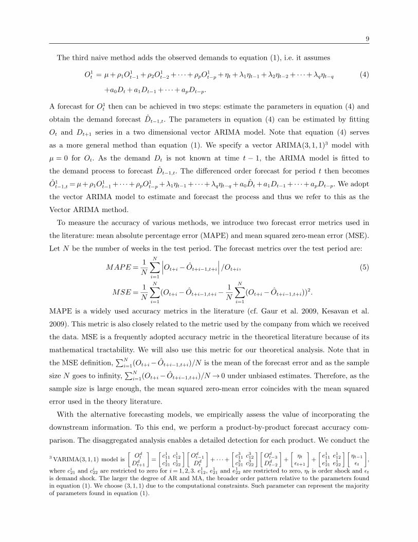
The third naive method adds the observed demands to equation (1), i.e. it assumes

O1t = µ+ ρ1O

1t−1 + ρ2O

1t−2 + · · ·+ ρpO

1t−p + ηt +λ1ηt−1 +λ2ηt−2 + · · ·+λqηt−q (4)

+a0Dt + a1Dt−1 + · · ·+ apDt−p.

A forecast for O1t then can be achieved in two steps: estimate the parameters in equation (4) and

obtain the demand forecast Dt−1,t. The parameters in equation (4) can be estimated by fitting

Ot and Dt+1 series in a two dimensional vector ARIMA model. Note that equation (4) serves

as a more general method than equation (1). We specify a vector ARIMA(3,1,1)3 model with

µ = 0 for Ot. As the demand Dt is not known at time t − 1, the ARIMA model is fitted to

the demand process to forecast Dt−1,t. The differenced order forecast for period t then becomes

O1t−1,t = µ+ρ1O

1t−1+ · · ·+ρpO1

t−p+λ1ηt−1+ · · ·+λqηt−q +a0Dt+a1Dt−1+ · · ·+apDt−p. We adopt

the vector ARIMA model to estimate and forecast the process and thus we refer to this as the

Vector ARIMA method.

To measure the accuracy of various methods, we introduce two forecast error metrics used in

the literature: mean absolute percentage error (MAPE) and mean squared zero-mean error (MSE).

Let N be the number of weeks in the test period. The forecast metrics over the test period are:

MAPE =1

N

N∑i=1

∣∣∣Ot+i − Ot+i−1,t+i

∣∣∣/Ot+i, (5)

MSE =1

N

N∑i=1

(Ot+i − Ot+i−1,t+i −1

N

N∑i=1

(Ot+i − Ot+i−1,t+i))2.

MAPE is a widely used accuracy metrics in the literature (cf. Gaur et al. 2009, Kesavan et al.

2009). This metric is also closely related to the metric used by the company from which we received

the data. MSE is a frequently adopted accuracy metric in the theoretical literature because of its

mathematical tractability. We will also use this metric for our theoretical analysis. Note that in

the MSE definition,∑N

i=1(Ot+i− Ot+i−1,t+i)/N is the mean of the forecast error and as the sample

size N goes to infinity,∑N

i=1(Ot+i− Ot+i−1,t+i)/N → 0 under unbiased estimates. Therefore, as the

sample size is large enough, the mean squared zero-mean error coincides with the mean squared

error used in the theory literature.

With the alternative forecasting models, we empirically assess the value of incorporating the

downstream information. To this end, we perform a product-by-product forecast accuracy com-

parison. The disaggregated analysis enables a detailed detection for each product. We conduct the

3 VARIMA(3,1,1) model is

[Od

t

Ddt+1

]=

[c111 c112c121 c122

][Od

t−1

Ddt

]+ · · ·+

[c311 c312c321 c322

][Od

t−3

Ddt−2

]+

[ηtϵt+1

]+

[e111 e112e121 e122

][ηt−1

ϵt

],

where ci21 and ci22 are restricted to zero for i= 1,2,3. e112, e121 and e122 are restricted to zero, ηt is order shock and ϵt

is demand shock. The larger the degree of AR and MA, the broader order pattern relative to the parameters foundin equation (1). We choose (3,1,1) due to the computational constraints. Such parameter can represent the majorityof parameters found in equation (1).

10

Table 1 MAPE and MSE percentage improvement for the four methods that incorporate the

downstream demand data. Significant accuracy improvement over the no sharing method is marked by

star. Significant (p= 0.1) accuracy improvement of the policy structure method over the unbold others

is marked with bold value.

MAPE percentage improvement MSE percentage improvementVector Reg D Reg D Policy Vector Reg D Reg D Policy

Brand Product ARIMA and O Structure ARIMA and O StructureOrange 128 OR 11.1% 12.2%* -14.6% 45.0%** 8.7% 14.0%** 0.4% 18.1%**

Juice 128 ORCA -18.3% 8.1% 1.9% 30.3%* -0.5% 7.8% 18.8%* 26.5%**

12 OR 31.6% 15.7% 50.2%* 58.6%* 32.4%** 33.8%** 35.1%** 53.4%**

12 ORCA 40.8%** 40.0%** 38.0%** 50.2%** 30.5% 36.3% 57.3%** 53.1%**

59 ORST 16.1%* 4.1% 5.0% 18.8%* 13.2%* 10.9% 10.7% 7.1%59 ORPC 12.8%** 29.1%** 23.8%** 27.7%** 16.2%** 31.0%** 11.4% 29.4%**

Sports 500 BR 21.2% 26.2% 25.5% 39.8%** 54.1%** 48.7%** 41.7%* 62.5%**

Drink 500 GP 30.9%* 25.7% 26.5% 36.0%** 53.1%** 42.9%* 38.7%* 68.4%**

PD LL 2.8% -15.5% -18.4% 4.7% 5.6% 30.9% 31.3% 51.3%PD OR 26.8%** 26.2%** 26.2%** 44.2%** 43.3%* 81.0%* 81.0%* 81.1%*

PD FRZ 22.1% 8.2% 11.4% 39.5%* 44.5%** 8.2% 9.2% 56.9%**

1GAL GLC 23.7%** 30.3%** 26.4%** 38.0%** 50.1%** 42.9%* 40.1%* 54.2%**

1GAL FRT 24.3%** 21.4%* 17.2% 29.9%** 46.4%** 40.3%** 31.3%* 54.0%**

1GAL OR 16.9%* 18.3%* 14.0% 30.4%* 30.2% 21.2% 18.3% 44.8%**

** At level p < 0.05, the accuracy improvement over no information sharing method is significant.

* At level p < 0.1, the accuracy improvement over no information sharing method is significant.

pairwise t-test to determine the statistical significance of forecast performance improvement. Table

1 presents the MAPE and MSE percentage improvement of the four InfoSharing methods over the

NoInfoSharing method for each product. The MAPE percentage improvement of method 1 over

method 2 is given by (MAPE1−MAPE2)/MAPE1. Similarly, the MSE percentage improvement

is (MSE1 −MSE2)/MSE1. The larger the percentage improvement, the more accurate the fore-

cast with information sharing. We carry out two sets of comparisons: the improvement with respect

to the NoInfoSharing forecast and the improvement of the policy structure forecast over other

forecasts. The star mark means that the forecast improvement with respect to the NoInfoShar-

ing method is statistically significant. The policy structure forecast in bold induces a statistically

significant improvement over the unbold forecasts.

Table 1 delivers two key messages. First, for all products, at least one of the InfoSharing meth-

ods generates statistically significant improvement over the NoInfoSharing method for one error

metric4. On average, the NoInfoSharing forecasts have the lowest accuracy with MAPE around

56%, the number of which is representative of the typical number we observe at the CPG company.

From these, we infer that for each product, the improvement of including the downstream demand

4 The mean absolute error (MAE) is defined as∑N

i=1

∣∣∣Ot+i − Ot+i−1,t+i

∣∣∣/∑Ni=1Ot+i. For the product PD LL, the

MAE metric shows that the policy structure method is statistically significantly (p < 0.1) better than the NoInfoS-haring method, although both MAPE and MSE metrics indicate insignificant improvement.

11

information is statistically significant. Furthermore, we test whether considering the replenishment

policy further strengthens the InfoSharing forecasts. The second message is that incorporating the

policy structure yields the greatest or one of the greatest improvements. For the MAPE metric,

the policy structure method has the highest improvement for all products and statistically higher

improvement than all other forecast methods at p < 0.1 for 5 out 14 products. For the MSE metric,

the policy structure method has statistically significantly higher improvement than all other fore-

cast methods at p < 0.1 for 6 out of 14 products. The forecasts generated from the naive methods

can be statistically indistinguishable from the policy structure method for some products. This

means the naive methods can correctly capture the correlation between orders and demands for

those products. On average, however, the policy structure method yields 40% MAPE percentage

improvement, which is statistically significantly (p= 0.05) higher than the three naive methods5. To

summarize, (1) the downstream demand information adds positive value to the order forecast even

if it is incorporated in a simple way but (2) incorporating the policy structure shows the largest

improvement. Moreover, we will later develop theory to predict for which product characteristics

we expect high forecast accuracy improvement.

4. Model Setup

In this section, we describe the model setup and some preliminary results on the value of sharing

information. Recall that we introduced a two-echelon supply chain in section 3. There are two key

ingredients in our model: customer demand and the firm’s replenishment policy. Notice that the

policy we will illustrate coincides with the policy structure method we discussed in section 3. In

this section, we introduce the actual policy followed by the company that we studied, which we will

call the ConDI policy with order smoothing. We then show that the main result from Giloni et al.

(2012) and Gaur et al. (2005) still holds if the retailer follows such a replenishment policy. The

contradicting empirical evidence, however, suggests the theoretical model fails to capture a key

element which is the decision deviation. The decision deviation relaxes the assumption, commonly

made in the literature, that the decision maker perfectly adheres to the inventory replenishment

policy. And finally, we develop the order process under such relaxation.

Recall that we consider a supply chain with two stages. The retailer is faced with demand Dt

and places order Ot to the supplier during week t. There is a transportation lead time LR from

the supplier to the retailer. The supplier is the retailer’s only source. Backlogging is allowed for

the retailer. The retailer and supplier review their inventory periodically. Within each period, the

following sequence of events occur: (1) the retailer’s demand is realized and then the retailer places

an order to the supplier, (2) after receiving the order, the supplier releases the shipment, (3) then

5 We also assess the overall prediction improvement for these four InfoSharing methods (see Online Companion).

12

the supplier collects the latest information and predicts the future h-step ahead orders, (4) based

on the updated prediction, the supplier makes production and replenishment decisions.

4.1. Demand Process

During each week t, the retailer faces demandDt. We assume thatDt follows an autoregressive inte-

grated moving average (ARIMA) process. The model is generally referred to as an ARIMA(p, d, q)

model, where p, d and q represent the degree of the autoregressive, integrated and moving average

parts of the model, respectively. The ARIMA model assumes that demand is a linear combination

of historical observations and demand shocks. We first illustrate the demand process under d= 0

and then derive the abbreviated expression for d≥ 0. When d= 0, the ARIMA(p,0, q) process is

reduced to an ARMA(p, q) process

Dt = µ+ ρ1Dt−1 + ρ2Dt−2 + · · ·+ ρpDt−p + ϵt −λ1ϵt−1 −λ2ϵt−2 − · · ·−λqϵt−q. (6)

where µ is the process mean, ϵt is an i.i.d. normal demand shock with zero mean and variance σ2ϵ ,

ρi is the autoregressive coefficient and λi is the moving average coefficient.

The backward shift operatorB shifts variables backward in time; e.g.BdDt shifts demand back by

d times BdDt =Dt−d, and (1−B)Dt differences demand once (1−B)Dt =Dt−Dt−1. Differencing

the demand twice means differencing Dt −Dt−1 one more time, (1−B)2Dt =Dt − 2Dt−1 +Dt−2.

Similarly, (1−B)dDt differences the demand d times, which we refer to as the dth-order differenced

demand. We assume the mean of demand is constant. Under this assumption, E[(1−B)dDt] = 0 for

d> 0, which means the differenced demand (1−B)dDt is a zero-mean ARMA process. Therefore,

the differenced demand has process mean µ= 0 for d> 0.

Let the AR coefficient be denoted as ϕAR(B) = 1 − ρ1B − ρ2B2 − · · · − ρpB

p, the integration

coefficient as π(B) = (1−B)d, the ARI coefficient as ϕARI(B) = ϕAR(B)π(B) and the MA coefficient

as φMA(B) = 1− λ1B − λ2B2 − · · · − λqB

q. If we assume π(B)Dt is an ARMA(p, q) process, then

Dt is an ARIMA(p, d, q) process with d ≥ 0. Then we replace Dt by (1−B)dDt in equation (6),

and rewrite equation (6) as

ϕARI(B)Dt = µ+φMA(B)ϵt. (7)

We can rewrite the dth differenced demand π(B)Dt in equation(7) as an MA representation

π(B)Dt = µ+φ(B)ϵt. (8)

where µ is the process mean, φ(B) = ϕ−1AR(B)φMA(B) is the coefficient. We work with the MA

representation because it provides the same intuition as an ARMA representation with a more

concise analysis.

In the rest of this section, we will review two basic, yet important, properties of an MA process

from the time series literature: covariance stationarity and invertibility. For details, we refer readers

13

to Hamilton (1994) and Brockwell and Davis (2002). We assume the dth differenced demand is

covariance stationary; that is, the differenced demand has a finite and constant mean, finite variance

and time invariant covariance of π(B)Dt and π(B)Dt+h for any t and h. One might think that the

MA model is restricted to a convenient class of models. However, representation (7) is fundamental

for any covariance stationary time series. Any covariance stationary process is equivalent to an

MA process in terms of the same covariance matrix (Wold 1938). Therefore, assuming the ARIMA

model is not restrictive. We adopt Hamilton (1994, p. 109)’s description of the equivalence between

the stationarity and MA representation, which is known as the Wold Decomposition property.

Property 1 (Wold Decomposition) Any zero-mean covariance stationary process Xt can be

represented in the MA form Xt =∑∞

i=0αiϵt−i, where αo = 1 and∑∞

i=0iα2 <∞. The term ϵt is

white noise and represents the error in forecasting: ϵt ≡Xt − E(Xt|Xt−1,Xt−2, . . .).

An MA process is determined by a unique covariance matrix. A covariance stationary process

may have multiple MA representations in terms of different sets of coefficients αi relative to their

corresponding white noise series. Among the alternative representations, we are only interested in

one that leads to the second property: invertibility. An MA process Xt = µ+φ(B)ϵt is invertible

relative to ϵt if the shock can be written as an absolutely summable sequence of past demands.

An infinite sequence αt is said to be absolutely summable if limn→∞∑n

i=0 |αi| is finite.

Property 2 (Invertibility) Define φ(z) = 1−λ1z1−λ2z

2−· · ·−λqzq. Then ϵt can be written as

an absolutely summable series of Xs with s≤ t, if and only if all roots of φ(z) = 0 lie outside of

the unit circle, z ∈C, |z|> 1. We say that Xt is invertible relative to ϵt.

The invertibility guarantees future-independence: Xt is only correlated with past value of ϵt.

Noninvertibility would allow for correlation with future values, which is undesirable. Invertibility

is a property of the MA coefficients relative to the corresponding white noise series. According

to Brockwell and Davis (2002, p. 54), for any noninvertible process Xt = φ(B)ϵt, we can find

a new white noise sequence wt such that Xt = φ′(B)wt and Xt is invertible relative to wt.We say that the coefficient φ′(B) is in the invertible representation. Therefore, when estimating

the parameters of a time series process, estimators are restricted in the invertible set. That is,

the empirically identified parameters have invertible representations. Henceforth, we assume the

differenced demand process, (1−B)dDt, satisfies invertibility. This assumption has both intuitive

appeal and technical consequences (for Proposition 1 and 3).

As Hamilton (1994, p. 68) points out, an MA process has at most one invertible representation,

which has larger white noise variance than any other noninvertible representations. Later, we will

illustrate that the enlarged white noise caused by converting from the noninvertible to invertible

representation, is one trigger to the positive value of information sharing.

14

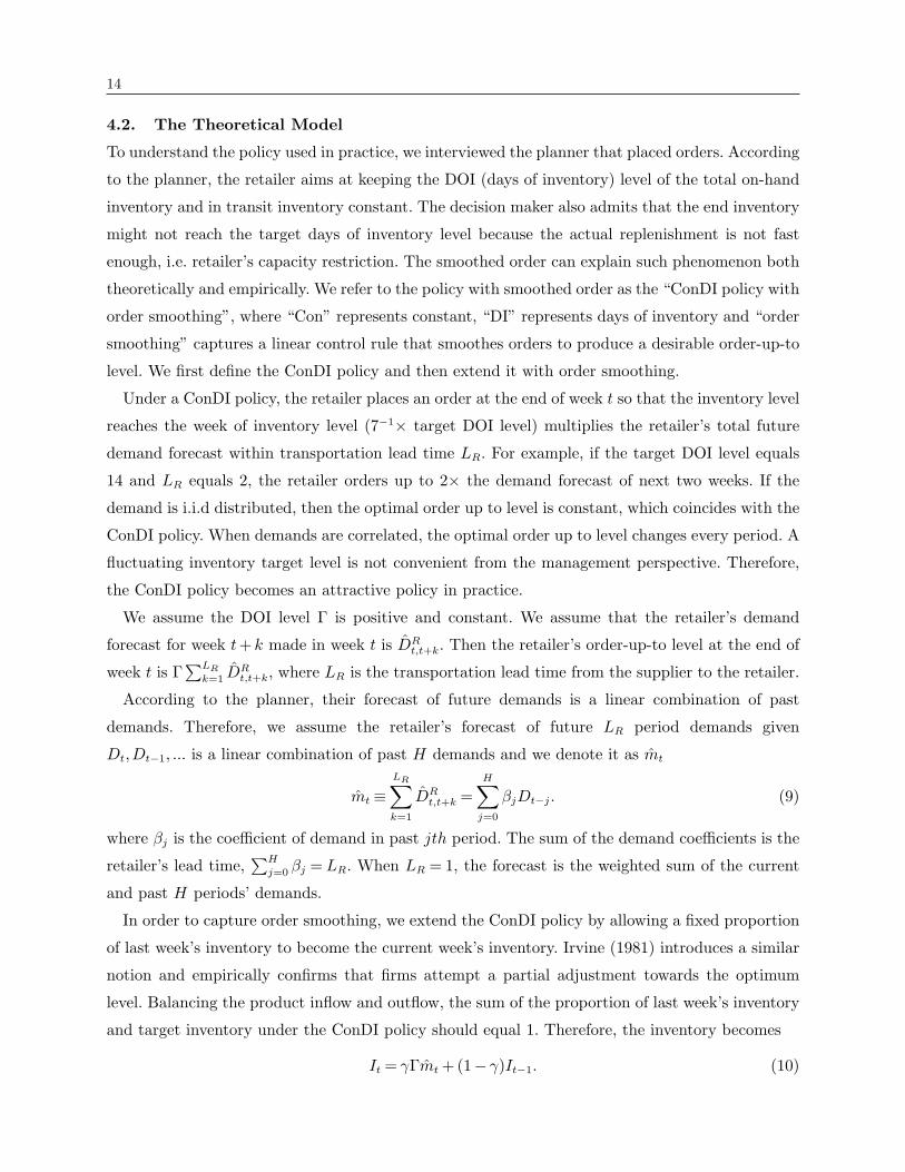
4.2. The Theoretical Model

To understand the policy used in practice, we interviewed the planner that placed orders. According

to the planner, the retailer aims at keeping the DOI (days of inventory) level of the total on-hand

inventory and in transit inventory constant. The decision maker also admits that the end inventory

might not reach the target days of inventory level because the actual replenishment is not fast

enough, i.e. retailer’s capacity restriction. The smoothed order can explain such phenomenon both

theoretically and empirically. We refer to the policy with smoothed order as the “ConDI policy with

order smoothing”, where “Con” represents constant, “DI” represents days of inventory and “order

smoothing” captures a linear control rule that smoothes orders to produce a desirable order-up-to

level. We first define the ConDI policy and then extend it with order smoothing.

Under a ConDI policy, the retailer places an order at the end of week t so that the inventory level

reaches the week of inventory level (7−1× target DOI level) multiplies the retailer’s total future

demand forecast within transportation lead time LR. For example, if the target DOI level equals

14 and LR equals 2, the retailer orders up to 2× the demand forecast of next two weeks. If the

demand is i.i.d distributed, then the optimal order up to level is constant, which coincides with the

ConDI policy. When demands are correlated, the optimal order up to level changes every period. A

fluctuating inventory target level is not convenient from the management perspective. Therefore,

the ConDI policy becomes an attractive policy in practice.

We assume the DOI level Γ is positive and constant. We assume that the retailer’s demand

forecast for week t+ k made in week t is DRt,t+k. Then the retailer’s order-up-to level at the end of

week t is Γ∑LR

k=1 DRt,t+k, where LR is the transportation lead time from the supplier to the retailer.

According to the planner, their forecast of future demands is a linear combination of past

demands. Therefore, we assume the retailer’s forecast of future LR period demands given

Dt,Dt−1, ... is a linear combination of past H demands and we denote it as mt

mt ≡LR∑k=1

DRt,t+k =

H∑j=0

βjDt−j. (9)

where βj is the coefficient of demand in past jth period. The sum of the demand coefficients is the

retailer’s lead time,∑H

j=0 βj = LR. When LR = 1, the forecast is the weighted sum of the current

and past H periods’ demands.

In order to capture order smoothing, we extend the ConDI policy by allowing a fixed proportion

of last week’s inventory to become the current week’s inventory. Irvine (1981) introduces a similar

notion and empirically confirms that firms attempt a partial adjustment towards the optimum

level. Balancing the product inflow and outflow, the sum of the proportion of last week’s inventory

and target inventory under the ConDI policy should equal 1. Therefore, the inventory becomes

It = γΓmt +(1− γ)It−1. (10)

15

where γ is the order smoothing level, which takes values in [0,1].

Given the fundamental law of material conservation, Ot =Dt+ It− It−1, equation (10) becomes

Ot =Dt + γ(Γmt − It−1). (11)

The order in week t is the current week’s demand plus γ fraction of the net inventory under the

ConDI policy. If γ = 1, it is reduced to the strict ConDI policy. If γ = 0, it becomes the demand

replenishment policy. The larger γ, the faster the order adjusts to the target ConDI inventory level.

The order smoothing component enables the extension of the ConDI policy to a rich family of

linear policies.

We can iteratively replace It−i with γΓmt−i + (1− γ)It−i−1 for any i≥ 0 in equation (11). We

define ai ≡ Γβi for 0 ≤ i ≤ H, where ai is the policy coefficient of the past ith demand. Then

Γmt =∑H

j=0 ajDt−j and the order becomes

Ot =Dt + γH∑i=0

aiDt−i − γ2

∞∑i=1

(1− γ)i−1

H∑j=0

ajDt−i−j. (12)

We define ψ(B) ≡ 1 + γ∑H

i=0 aiBi − γ2

∑∞i=1

∑H

j=0(1 − γ)i−1ajBi+j as the policy parameter.

Applying the backshift operator, we abbreviate equation (12) as Ot = ψ(B)Dt. Thus we have

π(B)Ot = π(B)ψ(B)Dt. Since demand satisfies π(B)Dt = µ+φ(B)ϵt, the demand process can be

written as π(B)ψ(B)Dt = µ+φ(B)ψ(B)ϵt. Therefore, the order process follows an ARIMA process

with white noise ϵt:

π(B)Ot = µ+φ(B)ψ(B)ϵt. (13)

Equation (13) has the same expression as equation (7) in Gaur et al. (2005): order is linear in

demand shocks. It is worth noting that our policy parameters ψ(B) capture a broader linear policy

than the myopic order up to policy considered in Gaur et al. (2005). The myopic order up to policy

corresponds to a special case when γ = 1 in equation (12) (this is equivalent to equation (4) in

Gaur et al. 2005).

The coefficients of ϵt in equation (13) are obtained by multiplying the demand coefficient φ(B)

of ϵt in Dt with the policy coefficient ψ(B) of Dt in Ot. Therefore, the first coefficient in equation

(13) is C ≡ 1+ γa0. We normalize the first coefficient to be 1. Then the centered order follows an

MA process with white noise Cϵt

π(B)Ot −µ=C−1φ(B)ψ(B)Cϵt. (14)

The analysis of the value of information sharing. As introduced in section 3, the supplier

aims to forecast the future order. In the rest of this section, we will focus on the 1-step ahead

forecast as it provides the insight to the positive value of information sharing and serves as the

16

theoretical foundation that we can compare with the empirical results. Section 6 will discuss the

h-step ahead forecast in detail in a more general setting.

In our theoretical analysis, we adopt a mathematically tractable forecast error metric: the mean

squared forecast error. We denote the space that contains the linear combination of the order

history from period 1 to period t and all its limit points as ΩOt . By definition, ΩO

t is the Hilbert

space generated by the order history. Therefore, ΩOt ∪ ΩD

t includes both the order and demand

history. According to the Projection Theorem, the unique optimal estimator to minimize the mean

squared error can be found conditional on either ΩOt or ΩO

t ∪ΩDt . As before, we denote it as Ot,t+1.

The 1-step mean squared forecast error without information sharing is Var(Ot+1 − Ot,t+1|ΩOt ) and

with sharing is Var(Ot+1 − Ot,t+1|ΩOt ∪ΩD

t ). The value of information sharing is positive if

Var(Ot+1 − Ot,t+1|ΩOt )>Var(Ot+1 − Ot,t+1|ΩO

t ∪ΩDt ). (15)

With downstream demand information, the demand and policy parameters can be estimated.

We assume the parameters can be correctly estimated and are known to the supplier. The only

uncertainty in Ot,t+1−Ot+1 stems from the demand shock occurring in t+1. Therefore, Var(Ot+1−

Ot,t+1|ΩOt ∪ΩD

t ) =Var(Cϵt).

Without information sharing, the supplier analyzes the order history as an MA process. The

MA process in equation (14) may not be invertible with respect to Cϵt. If not, we can find an

invertible representation relative to a new white noise series wt, which has a larger variance than

Var(Cϵt). Then inequality (15) holds and thus the value is positive. Gaur et al. (2005) and Giloni

et al. (2012) show similar intuitions for the positive value of information sharing. The following

proposition states the sufficient and necessary condition that sharing demand benefit the supplier’s

order forecast.

Proposition 1 If the decision maker strictly adheres to the replenishment policy, the value of

information sharing under the one step forecast lead time is positive if and only if at least one root

of ψ(z) = 0 lies inside the unit circle.

The value of information sharing is positive if and only if φ(B)ψ(B) is in the noninvertible

representation, which in turn is equivalent to the existence of at least one root of φ(z)ψ(z) = 0 that

lies inside the unit circle. Since all roots of φ(z) = 0 lie outside the unit circle due to the invertible

assumption, the order is noninvertible relative to ϵt if and only if there exists at least one root of

ψ(z) = 0 that lies inside the unit circle.

Remark. We next illustrate two extreme setting of γ = 0 and γ = 1 and show that in both setting

there is no value of information sharing. When γ = 0, it becomes the demand replacement policy

Ot =Dt and ψ(z) = 1. Since no root of ψ(z) = 0 lies inside the unit circle, the value of information

17

sharing is zero. When γ = 1 and H = 0, it becomes the ConDI policy with policy parameter ψ(z) =

1+ a0 − a0z. Since∑H

j=0 aj = ΓLR, coefficient a0 is positive. Since the unique root of ψ(z) = 0 is

larger than 1, z = (1+ a0)/a0 > 1, the value of sharing is zero. From these two examples, we can

see that the value of information sharing under a strict replenishment policy can be zero.

4.3. The Empirical Model: Decision Deviations

The empirical results in section 3 indicate incorporating the downstream demand properly yields

statistically significantly positive value of information sharing for all low-promotional products.

The above theoretical results, however, suggest zero value for 10 out of 14 products based on the

estimated parameters that we will show in Section 6. These empirical deviations call for a better

theoretical understanding of the model in previous literature.

The key underlying assumption in the theoretical model described above and in the literature

is that the decision maker strictly and consistently follows a family of linear decision rules. Our

discussion with the replenishment decision maker suggests this is rarely the case because the

decision makers can implement their own adjustment based on the additional signals that we do

not observe. The empirically observed idiosyncratic shocks in the order decisions also indicate that

the decision makers may not replenish as the theory requires, or that the theoretical model does

not capture all elements of reality.

From the interview with the planner, we understand that the deviation from the theoretical

model stems from several operational causes. The order quantity is rounded due to transportation

and truck load constraints. To increase transportation efficiency, the retailer tries to fill up a full

truck when placing an order. Products with inventory above the target DOI level might still be

replenished because delivering in batches can decrease set up cost. Such a phenomenon is common

as the week approaches Friday, because the decision maker needs to guarantee enough inventory.

Orders might be moved from peak to nonpeak periods if planners anticipate a spike in future

demands (Donselaar et al. 2010 also points out such advancing orders as an important consideration

of the decision maker). In practice, the retailer might place orders daily. However, for this study,

we have access only to the weekly aggregate level instead of daily information. Looking through

the lens of the aggregate data, we lose the detail on the replenishment decision, which is reflected

by the actual order’s departure from the theory.

Among the above different operational drivers, a common characteristic is that the decision

maker adjusts replenishment according to those drivers while statisticians cannot observe them.

We rationalize the agent’s departure from the exact policy following the same spirit as Rust (1997):

it is a state variable which is observed by the agent but not by the statistician. Since the actual

observations always contain randomness from the observational perspective of the analyst, the

18

empirical model should successfully capture it and might yield qualitatively different results than

the literature.

We extend the theoretical framework by including the idiosyncratic shocks in decision making,

and thus relax the strict adherence to the ConDI with order smoothing policy. We refer to such

idiosyncratic shocks as decision deviation. The decision deviation is observable to the retailer, but

not to statistician. We assume the decision deviation δt is normally distributed with zero mean

and variance σ2δ , and independent with historical demand shock ϵs, s < t. However, contemporane-

ous demand signals and decision deviation signals can be correlated. A common approach in the

empirical literature is to model this error term as additively separable, in the decision. Using this

approach, we obtain

Ot =Dt + γ(Γmt − It−1)+ δt. (16)

As before, we iteratively replace It−i with γΓmt−i + (1− γ)It−i−1 + δt−i in equation (16) and

obtain

Ot =Dt + γH∑i=0

aiDt−i − γ2

∞∑i=1

(1− γ)i−1

H∑j=0

ajDt−i−j + δt −∞∑i=1

γ(1− γ)i−1δt−i. (17)

We define κ(B) = 1−γ∑∞

i=1(1−γ)i−1Bi as the order smoothing parameter. Applying the back-

shift operator, equation (17) can be abbreviated as Ot =ψ(B)Dt+κ(B)δt. Applying π(B) to both

sides, order process can be abbreviated as:

π(B)Ot = µ+φ(B)ψ(B)ϵt +π(B)κ(B)δt. (18)

where µ is the process mean, φ(B)ψ(B) is the demand shock coefficient and π(B)κ(B) is the

decision deviation coefficient.

ARMA-in-ARMA-out property. The order with decision deviation has a stationary covariance.

According to property 1, the order process in equation (18) follows an ARIMA model. This is

consistent with the “ARMA-in-ARMA-out” (AIAO) property discussed in the literature (Zhang

2004, Gilbert 2005, Gaur et al. 2005 and Giloni et al. 2012), where AIAO means that the retailer’s

order process is also an ARMA process with respect to the demand shock. If the replenishment

policy is an affine and time invariant function of the historical demand, inventory, demand shock

and decision deviation, the order process has a stationary covariance. Therefore, the AIAO property

holds for such policies.

5. Strictly Positive Value of Information Sharing

In this section, we study the impact of decision deviation on the value of information sharing and

prove that the value of information sharing is always positive if there is uncertainty in both decision

deviation and demand processes.

19

We rewrite the order in equation (18) as a centered process

Ot −π−1(B)µ=C−1π−1(B)φ(B)ψ(B)Cϵt +κ(B)δt. (19)

where the constant C normalizes the first coefficient to one as defined before. Let qϵ denote the

degree of π−1(B)φ(B)ψ(B) and qδ denote the degree of κ(B). The centered order is the summation

of two MA processes with demand shock and decision deviation as their corresponding white noise

series. We study the value of information sharing with the existence of decision deviations.

Preliminary results. Our key question is closely related to the general goal of forecasting the

aggregation of multiple MA processes.

Consider N MA processes (N can be infinite) where the process i is X it = χi(B)ϵit with i.i.d.

random shock ϵit. The coefficient is χi(B) = 1+λi1B+λi

2B2+ · · ·+λi

qiBqi with degree qi. When pre-

dicting future value beyond qi periods, the forecast is constant and uncertainty cannot be resolved.

Thus qi denotes the effective forecasting range for process X it . We allow contemporaneous signals

to be correlated, but require signals to be independent across periods. That is, ϵit is independent

of ϵjs for any s < t. The summation of these N processes is

St =N∑i=1

X it . (20)

According to Property 1, St can be rewritten as an MA process with degree qS ≥ 0, where qS is

the largest k that guarantees nonzero covariance Cov(St, St+k) = 0.

With full information (or with information sharing), we have access to each process’s history

and parameters. With aggregate information (or without information sharing), we only have access

to the aggregate process St. As before, ΩXi

t and ΩSt denotes the Hilbert space generated by X i

t

and St history through period t. Let X it,t+h and St+h denote the best estimator to minimize the

mean squared forecast error for X it+h and St+h. With information sharing, the h-step ahead mean

squared error is Var(St+h − St,t+h| ∪i ΩXi

t ). Without information sharing, the h-step ahead mean

squared error is Var(St+h − St,t+h|ΩSt ). The value is positive for forecast lead time h if Var(St+h −

St,t+h| ∪i ΩXi

t )< Var(St+h − St,t+h|ΩSt ). The following theorem states the sufficient and necessary

condition for the zero value of information sharing.

Theorem 2 The 1-step mean squared forecast error is the same with and without sharing,

Var(St+1 − St,t+1| ∪i ΩXi

t ) = Var(St+1 − St,t+1|ΩSt ) if and only if the MA processes satisfy χi(B) =

χj(B) for any i, j. If there exists i = j such that χi(B) = χj(B), then Var(St+h − St,t+h| ∪i ΩXi

t )<

Var(St+h − St,t+h|ΩSt ) for any finite forecast lead time h≤maxiqi.

Among N processes, if coefficients of any two processes differ, the aggregate process has strictly

larger mean squared forecast error as long as the forecast is within the effective forecast range of one

20

process, h≤maxiqi. If qi = 0, X it becomes an i.i.d. normal model with the coefficient χi(B) = 1.

If qi = 0 for all i, the processes have the same coefficients, and thus the value of information sharing

is zero. If maxiqi=∞, the value of information sharing is strictly positive for any finite forecast

lead time if φi(B) =φj(B).

Analysis of our model. Let us apply this general result to the order process in our setting in

equation (19). The centered order has the same structure as equation (20), where the two processes

are with respect to demand shocks and decision deviations

X1t = C−1π−1(B)φ(B)ψ(B)Cϵt, (21)

X2t = κ(B)δt.

We can apply Theorem 2 to determine whether the value of information sharing is positive. Similar

as before, if Var(Ot+h − Ot,t+h|ΩOt ) > Var(Ot+h − Ot,t+h|ΩO

t ∪ΩDt ), then the value of information

sharing is positive. The following proposition illustrates the result.

Proposition 3 If the demand shock and decision deviation are nonzero, the value of information

sharing is strictly positive for any finite forecast lead time h≤maxqϵ, qδ.

When qϵ = qδ = 0, both X1t and X2

t are i.i.d. processes and St is also an i.i.d. process. Any forecast

is a constant, and thus there is no value from sharing the downstream sales information. This

situation can only occur when φ(B) = π(B) = ψ(B) = κ(B) = 1, which means the retailer faces

an i.i.d. demand processes and adopts a demand replacement policy, which we refer to as “i.i.d

demand replacement”. In the rest of the paper, we will exclude the discussion on this situation,

because using historical observations cannot resolve any uncertainty of the future forecast.

If not both processes are i.i.d. models, or equivalently qϵ = qδ = 0 is not true, then the two sets of

parameters C−1π−1(B)φ(B)ψ(B) and κ(B) can never be the same. The key ingredient in the proof

is to show that the polynomial (1−B) is a factor in κ(B) but not a factor in C−1π−1(B)φ(B)ψ(B).

Therefore, the value of information is strictly positive for any forecast lead time.

Compared with the conditions on the policy parameter ψ(B) that induces positive value of infor-

mation sharing under the strict adherence to a linear policy, Proposition 3 establishes a qualitatively

different conclusion: the benefit of information sharing is strictly positive within any forecasting

period. Under the strict adherence to the inventory policy, the planner makes replenishment deci-

sions based only on information that statisticians also have access to, which leads to a pure demand

propagation. The interview with the planner and our data suggests that this is rarely the case and

the decision departures from the ideal policy due to private information that statisticians can not

observe. Thus, unlike before, the demand now propagates together with the decision deviation.

The value of information sharing is zero if the order process carries all demand information and

21

all decision deviation information. The different propagation patterns of the demand process and

decision deviation process, however, drive the loss of information as demand and decision deviation

propagate upstream. To be specific, the ending inventory level carries current period’s decision

deviation and rolls it over to next period’s replenishment decision which further determines the

next period’s ending inventory. Thus the evolution of inventory governs the translation of exoge-

nous decision deviation signals into orders. Demand signals, on the other hand, are governed by

the evolution of both inventory and current demand. As both signals propagate together to become

orders in such innately different patterns, the detailed information of two processes is lost and is

replaced with the less informative (larger uncertainty) order signals. Consequently, the value of

information sharing becomes positive regardless of the policy parameter ψ(B).

The same intuition holds for any linear replenishment policy. It’s worth noting that the evolution

patterns of the demand signals and decision deviation signals are different as illustrated above for

other ordering policy that is linear in demands and demand signals, i.e. the myopic order up to

policy, the ConDI policy with retailer’s demand forecast being optimal (we assume that it is linear

in past H demands due to practice in our study) and the generalized order-up-to policy introduced

by Chen and Lee (2009) (see Online Companion for more discussion), except for the “i.i.d demand

replacement” (of which we care less since forecasting beyond zero period is constant). Therefore,

the distinct propagation patterns obscure the detailed information structure, which drives positive

value of information sharing for any linear inventory policy under any forecast lead time.

Proposition 3 illustrates the value of information sharing when both demand and decision uncer-

tainties are nonzero. If there is no decision deviation, Proposition 1 demonstrates the sufficient

and necessary condition of positive value of information sharing. The following proposition, on the

other hand, considers another extreme case when demand uncertainty is zero.

Proposition 4 When the demand shock is zero, the value of information sharing is zero for any

forecast lead time.

In absence of demand shock, the centered order is reduced to an MA process with respect to

decision deviations, Ot − π−1(B)µ= κ(B)δt. For the value of sharing downstream information to

be zero, the centered order must be invertible relative to δt (equivalent to κ(B) has an invertible

representation). The unique root of κ(z∗) = 0 lies on the unit circle, which Plosser and Schwert

(1997) defined as strictly non-invertibility. When |z∗| = 1, there is no corresponding invertible

representation. The author shows that the univariate MA parameter’s estimator is asymptotically

similar to the invertible processes, which indicates parameters κ(B) can be correctly estimated from

historical orders. Therefore, we can still apply the result for the invertible process and conclude

that the value of information sharing is zero.

22

Figure 1 The MSE percentage improvement against the decision deviation weight for an

ARIMA(0,1,1) demand with λ= 0.5 and a ConDI policy with order smoothing with γ = 0.8 and Γ= 2.

0 0.1 0.2 0.3 0.4 0.5 0.6 0.7 0.8 0.9 10

0.1

0.2

0.3

0.4

0.5

0.6

0.7

0.8

0.9

1

β

0= 1.2; β

1=−0.2

β0= 0.2; β

1= 0.8

β0=−0.2; β

1= 1.2

Decision Deviation Weight

MS

E−

PI

To summarize the above theoretical findings, we characterize the value of information sharing

with a numerical analysis. We apply the MSE percentage improvement metric introduced in Section

3. LetMSE-PI denote the MSE percentage improvement over no information sharing. Recall that

MSE-PI = (Var(Ot+h − Ot,t+h|ΩOt )−Var(Ot+h − Ot,t+h|ΩO

t ∪ΩDt ))/Var(Ot+h − Ot,t+h|ΩO

t ), which

takes value between 0 and 1.

Figure 1 displays the MSE-PI of the 1-step-ahead forecast with respect to the relative weight

of the decision deviation under several sets of policy parameters. We define σ2δ/(σ

2ϵ + σ2

δ) as the

deviation decision weight. The retailer places weights βi on historical demands to determine their

future forecast as in equation (9). Keeping the DOI level and the order smoothing level fixed,

we choose three sets of policy weight βi (i = 0,1) that correspond to three lines in Figure 1.

We consider the retailer faces an ARIMA(0,1,1) demand, Dt = Dt−1 + ϵt − λϵt−1, with the MA

parameter λ = 0.5. The policy parameter ψ(B) is non-invertible for the top two processes while

invertible for the bottom one.

Our theoretical prediction aligns with the numerical observations. When the decision uncertainty

is zero, the value of information sharing is positive for the first two and zero for the last policy

parameters. This pattern is consistent with Proposition 1. Note that the studies in the literature

correspond to the points on the vertical axis where the decision deviation weight is zero. As decision

deviation become dominant, there is no gain from sharing the downstream sales information, which

coincides with Proposition 4. When the decision deviation and demand uncertainty both exist,

Figure 1 presents a strictly positive value of information sharing, which agrees with Proposition 3.

23

Figure 2 Summary of sales, orders and point-of-sale price for product PD OR.

6. Data, Estimation and Model Validation6.1. Data

As we introduced in Section 3, our data set is provided by a leading supplier in the beverage and

snack food industry and consists of three elements corresponding to a specific retail customer: (1)

the retailer’s sales, (2) the retailer’s orders to the supplier and (3) the products’ retail price. The

data spans over 126 weeks between 2009 and 2011. To be specific, the raw data consists of the

retailer’s sales from its six distribution centers to local stores, and orders from the retailer’s six

distribution centers to the supplier’s distribution center. For the purpose of our analysis, we work

with the aggregated sales and orders. We calculate the retailer’s inventory using the fundamental

law of material conservation, given sales and orders. Without information sharing, the supplier only

observes the retailer’s order and the price plan. With information sharing, the supplier observes

additional information: the retailer’s sales. We eliminate untrustworthy data, the new-entering

products that have not reached the stationary state or obsolete products that are existing the

market. After cleaning the data, we have 51 product lines in total: 19 orange juice products and

32 sports drink products.

We summarize the sales, orders and price of a specific product over 126 weeks in Figure 2. It

shows the bullwhip effect: the upstream order has larger volatility than the downstream sales.

Further, when there is a price promotion, the demand experiences a spike during the discount

activity and suffers a slump as price returns to normal.

For the purpose of our study, we shall classify the products into low-promotional and high-

promotional products and focus on the former6. This classification is based on the price discount

6 The Online Companion provides a discussion on the promotional products.

24

and frequency of discount being offered on the product. From the data, we observe that the bev-

erage products are frequently on sale. A promotional activity can last for several weeks. During a

promotional activity, all retailer’s local stores execute the same price discount plan. Negotiating at

the beginning of each year, the supplier has a fixed price plan throughout the year. Thus the future

price can help predict demand changes for promotional products. The spikes in orders caused by

promotions result in a non-constant demand mean and perhaps a time-variant covariance matrix,

breaking the stationary assumption that we use to develop our theory.

To make the above precise, we define promotional depth metric to capture price discount and

frequency. Promotional depth sums every promotion activity’s price discount measured as a per-

centage within the last 26 weeks in our data,∑

idiscount ratei where i≤ the number of activities

in 26 weeks. We define the low-promotional product as those with positive depth ≤ 0.15 (or equiv-

alently no promotional activity or one promotional activity), and the high-promotional product

as those with higher promotional depth. The low-promotional items contain 14 product lines and

occupy 20% of the total ordering volume of all products. In the rest of this section, we will only

discuss the methods and results for these 14 low-promotional items.

6.2. Estimation Procedure and Parameter Results

In Section 3, we presented the forecast accuracy of the policy structure method and concluded

that the forecast improvement of adopting such method to incorporate the downstream demand

is statistically significant. In this section, we first describe the estimation of the policy structure

method. Next, we show the estimated demand and policy parameters. Note that our analysis only

uses sales and orders data.

We assume that the retailer adopts the ConDI policy with order smoothing. In each period, the

order is Dt + γ(Γmt − It−1) + δt. Recall that mt =∑H

i=0 aiDt−i. In practice, the retailer’s forecast

usually accounts for last months’ demands. Thus, we let H = 3. We rewrite equation (16) as

Ot = (1+γΓβ0)Dt+γΓβ1Dt−1+γΓβ2Dt−2+γΓβ3Dt−3−γΓIt−1+δt. The estimating equation then

becomes

Ot = c0Dt + c1Dt−1 + c2Dt−2 + c3Dt−3 + cinvIt−1 + δt (22)

We run a linear regression of equation (22) to estimate the policy parameters for each week in

the test period. We apply the step-wise variable selection method to only include variables with

p < 0.05 in the regression. The idiosyncratic shock in the order equation is the decision deviation.

If δt is positive, the retailer orders more than what our policy predicts and vice versa.

To forecast supplier’s order in t+1, we first forecast future demands. We fit the ARIMA model

to forecast Dt,t+1. With the parameters estimated from equation (22), the order prediction for

period t+1 uses Dt,t+1 and Ds where s≤ t and It:

Ot,t+1 = c0Dt,t+1 + c1Dt + c2Dt−1 + c3Dt−2 + cinvIt. (23)

25

Table 2 Estimated demand and policy parameters. The number in parenthesis denotes the standard

error of the estimate.

Demand parameters Policy parametersBrand Product (p, d, q) λ1 λ2 λ3 c0 c1 c2 c3 cinv DOI

Orange 128 OR (0,1,1) 0.93 1.30 0.27 -0.63 6.36Juice (0.04) (0.18) (0.16) (0.12)

128 ORCA (0,1,1) 0.93 1.33 0.30 -0.53 8.48(0.04) (0.18) (0.17) (0.12)

12 OR (0,1,2) 0.48 0.33 1.46 0.60 -0.87 8.56(0.10) (0.10) (0.17) (0.18) (0.12)

12 ORCA (0,1,2) 0.28 0.25 0.97 1.09 0.36 -0.86 11.54(0.10) (0.10) (0.21) (0.23) (0.19) (0.12)

59 ORST (0,1,1) 0.72 1.55 -0.39 9.76(0.07) (0.10) (0.07)

59 ORPC (0,1,1) 0.8 1.84 -0.46 -0.28 9.58(0.07) (0.18) (0.22) (0.08)

Sports 500 BR (0,1,3) 0.12 0.16 0.49 1.17 0.55 -0.35 14.50Drink (0.09) (0.09) (0.09) (0.29) (0.33) (0.07)

500 GP (0,1,0) 0.39 0.67 0.63 -0.36 13.43(0.25) (0.38) (0.29) (0.07)

PD LL (0,1,0) 0.61 1.11 -0.24 21.06(0.40) (0.44) (0.06)

PD OR (0,1,1) 0.3 1.37 0.39 -0.29 18.35(0.10) (0.16) (0.23) (0.07)

PD FRZ (0,1,1) 0.32 1.27 0.47 -0.32 16.22(0.09) (0.16) (0.22) (0.07)

1GAL GLC (0,1,2) 0.2 0.43 0.76 1.17 -0.54 -0.22 12.38(0.09) (0.09) (0.25) (0.28) (0.21) (0.08)

1GAL FRT (0,1,2) 0.37 0.36 1.49 -0.25 13.38(0.10) (0.10) (0.13) (0.07)

1GAL OR (0,1,2) 0.29 0.34 1.52 -0.30 12.33(0.10) (0.10) (0.12) (0.07)

We present the demand and policy parameters in Table 2. For all products, demand has d= 1,

which implies that the first-order differenced demand is an ARMA process. The transportation

lead time from the supplier to the retailer is one week, thus we consider the case that LR = 1.

Therefore,∑H

i=0 ai = 1 and Γ = −c−1inv(

∑H

i=0 ci − 1). The last column displays the DOI level. In

practice, the retailer targets at a lower DOI level for the orange juice brand and a higher DOI for

the sports drink brand. Our estimated DOI level is consistent with the actual target level claimed

by the decision maker.

6.3. Model Validation

In this section, we validate whether the signal propagation agrees with our theory predictions.

To this end, we compare the predicted and actual root mean squared forecast error, separately

under the policy structure method and NoInfoSharing method. To be specific, we first derive the

actual forecast. We follow the above estimation procedure to obtain the actual forecast under

information sharing. We fit the ARIMA model and forecast order using only order information

without information sharing. Second, based on the theory we explained in section 5, we calculate

the root mean square error, which we refer to as the predicted value.

We next elaborate on the procedure used to obtain the predicted value. We calculate the in-

sample mean squared error from demand when fitting the ARIMA model in Table 2, and we use

26

Figure 3 Actual vs predicted root mean squared forecast error with information sharing (left) and

without information sharing (right).

it as σ2ϵ . We calculate the in-sample mean squared error from estimating policy in equation (22),

and we use it as σ2δ . Together with the estimated demand and policy parameters, we know all the

parameters in the model7. We empirically test the correlation between contemporaneous shocks δt

and ϵt. The result suggests weak correlation or no correlation. Therefore, when there is information

sharing, the mean squared forecast error is c20σ2ϵ +σ

2δ . In absence of information sharing, we calculate

the mean squared error by applying the Innovation Algorithm used in the time series literature

(see Online Technical Companion).

We present the results in Figure 3. We plot the fitted against actual root mean squared prediction

error under both information sharing (left) and no information sharing (right) case. A perfect

model fit would lead to the points lying on the 45-degree dashed line in the figure. The fitted

points from our model are overall close to the 45-degree line for both with information and no

information, indicating a good fit. We fit a regression of the theoretical prediction on the actual

observation. The 95% confidence interval is [1.01,1.27] under the information sharing setting and

[0.86,1.14] under the no information sharing setting.

The good fit indicates that our theoretical model with decision deviations can well explain how

demands prorogate upstream, and thus well predict the value of information sharing. In Section

5, we proved that the presence of decision deviations guarantees strictly positive value under any

forecast lead time. In the following section, we will investigate how the value of sharing changes

with respect to the demand, policy and lead time on the value of information sharing.

7 In the policy parameter sector of Table 2, for some products, the coefficient of current week’s demand is zero, whichmeans the retailer’s replenishment fulfillment places zero weight on current week’s demand. This is unlikely to occurin practice. Our estimation shows zero coefficient because the retailer may replenish inventory during the week, butour data set consists of system’s snapshots at the end of the each week. If the retailer replenishes certain productsalways on Monday, the current week’s order should be a linear combination of past weeks’ demand, not includingthe current week (since current week’s demand has not been realized yet). Therefore, for products with zero c0 inTable 2, we interpret a1 as the actual coefficient of current week (shift a2 and a3 in the same way).

27

7. Properties of the Value of Information Sharing

While we have shown that the value is positive, we have not specified its magnitude and how it

changes relative to other key variables. In this section, we investigate the impact of demand on the

value of information sharing. We study how the value changes with respect to the parameter of an

ARIMA(0,1,1) demand process. (We focus on this particular form of ARIMA demand process as

8 out of 14 products in the data have this structure). We then show that the theoretically obtained

relation is consistent with our empirical observations. We focus on the 1-step-ahead forecast. We

theoretically analyze two special cases to understand the intuition and resort to numerical studies

for more involved settings.

We analyze a simple yet reasonable model to derive the theoretical prediction. The empirical

estimation suggests that 8 out of 14 products follow an ARIMA(0,1,1) demand. Therefore, in this

section, we assume that the demand follows an ARIMA(0,1,1) process with parameter λ∈ [0,1),

Dt =Dt−1 + ϵt −λϵt−1,

which can be equivalently written as Dt = (1 − λ)∑∞

i=1 λi−1Dt−i + ϵt. The current observation

is a weighted average of historical observations with exponentially decaying coefficients. Values

of λ closer to one put greater weight on recent data and thus react more intensely to recent

variations, while processes with λ closer to zero smooth the weight on past observations and thus

are less responsive to recent changes. Therefore, the process trends more slowly with a smaller

λ. For example, the products that we study can be classified according to λ. Orange juice is an

everyday drink for consumers since it is usually served with breakfast. A sports drink is designed for

rehydration and energy-providing, which is mainly consumed for exercising. Thus its consumption

is influenced by weather, temperature and sport events. The data exhibits a clearer slowly trending

pattern in demand for sports drinks. Consistent with the above analysis, orange juice products has

larger λ while sports drink have smaller λ according to our demand parameter estimations. We

refer to demands with small λ as slowly trending demands.

Recall that the retailer’s future demand forecast is a linear combination of historical H + 1

periods demands. In the rest of this section, we assume the retailer’s order relies on current and last

week’s demand, H = 1. The order-up-to level of the ConDI policy becomes Γmt =Γβ0Dt+Γβ1Dt−1

(β0 + β1 = 1 due to β0 + β1 = LR = 1). We will refer to the two parameters β0 and β1 as policy

weights. The order can be written as a summation of two processes in equation (21)

X1t = (1+ γΓβ0 + γΓβ1B)(1+λB)ϵt − γ2

∞∑i=1

(1− γ)i−1(Γβ0 +Γβ1B)(1+λB)ϵt−i,

X2t = δt − δt−1 −

∞∑i=1

γ(1− γ)i−1(δt−i − δt−i−1),

28

Figure 4 The MSE percentage improvement with respect to an ARIMA(0,1,1) demand with λ and a

ConDI policy with order smoothing with β0, γ and Γ= 2.

0 0.5 10

0.2

0.4

0.6

0.8

1

β0=1.5

0 0.5 1

β0=0.5

0 0.5 1

β0=−0.2

λ=0

λ=0.5

λ=0.9

Decision deviation weight

MS

E−

PI

where ϵt is the demand shock and δt is the decision deviation. We assume ϵt is independent with

δs for any s.

For the purpose of our theoretical analysis, we focus on processes X1t and X2

t with degree smaller

or equal to 3. When the degree of either process exceeds 3, the complexity of the problem precludes

analytically tractable solutions and necessitates numerical analysis. Therefore, we first focus on two

simple policies: (1) the retailer follows a demand replacement policy (γ = 0) and (2) the retailer

adopt a ConDI policy (γ = 1) with zero weight on previous week’s demand (a1 = 0). Under (1),

the order process is Ot =Dt + δt and under (2), the order process becomes Ot = (1 + Γβ0)Dt −Γβ0Dt−1 + δt − δt−1. The following proposition demonstrates that under the demand replacement

policy, the value strictly decreases with λ.

Proposition 5 The value of information sharing under the 1-step-ahead forecast strictly decreases

with λ if (1) the retailer follows a demand replacement policy, or (2) the retailer follows a ConDI

policy with β1 = 0.

To further explore the demand’s impact under other parameters, we conduct numerical studies.

Figure 4 presents the relation of MSE-PI with respect to λ under three policy weight parameters.

The DOI level is set to 2 and the order smoothing level is set to 0.5. In each sub-figure, the three

lines from top to bottom correspond to λ = 0,0.5 and 0.9. The three columns from left to right

correspond to β0 = 1.5,0.5 and −0.2.

Consistent with the theoretical prediction, the value of information sharing with demand param-

eters closer to zero dominates those with larger λ. This indicates that the products with slowly

trending demands have strictly larger forecast accuracy improvement, regardless of the decision

deviation weight, policy and demand parameter. Let us revisit the empirically obtained MSE-PI

results in the last column of Table 1 in Section 3. The two orange drinks 12 OR and 12 ORCA

29

have much smaller bottle volume compared to other orange juice products. In Table 2 in Section

6, their λ is closer to zero which differs substantially from the other orange drinks. Thus, their

demand structure is closer to the sports drink products. Consistent with our theoretical prediction,

the percentage improvement of the sports drink and the above two products are in general larger

than the rest of orange juice. In short, our theory can provide correct mapping from the demand

pattern to the potential gain from information sharing.

The result implies that it’s more worthwhile for managers to invest in the information sharing

system for products with slow trending consumption under the one-step-ahead forecast lead time.

It’s worth noting that forecasting beyond one period might reverse the relation of the value of

information sharing and demand parameter λ. We recommend that the managers run a numerical

study to validate the potential gain based on demand and policy characteristics.

8. Conclusion and Discussions

This paper empirically evaluates the supplier’s forecast improvement by incorporating downstream

retail sales data and supports the observations with an extended theoretical model. Table 1 in

Section 3 summarizes our main empirical findings. Overall, the forecast accuracy improvement can

be statistically significant, even when including demand data in a naive way. We further show that

a more refined inclusion of demand (by modeling the underlying policy structure along with the

demand) yields the highest forecast accuracy and its forecast improvement over the NoInfoSharing

method is statistically significant across all products. Our observations highlight the positive value

to suppliers from incorporating retailers’ sales data: 7.1% to 81.1% MSE percentage improvement

across 14 products and 40% MAPE percentage improvement on an overall level, which is regarded

as a significant improvement by the CPG company we studied.

We also revisit and extend the theoretical model in the existing literature. Until now, the theoret-

ical literature showed no value of information sharing for 10 out of 14 products. We recognize that

the key assumption in the theoretical model is that the decision maker strictly and consistently

follows the specified replenishment policy, which in practice is rarely the case. A decision maker

may implement adjustments according to private information that we do not observe. Following

the same spirit as the “error term” defined by Rust (1997), we introduce “decision deviations”

that stem from a state variable observable to the agent but not to us. Our extended theory yields

qualitatively different results than the previous literature. We demonstrate that if both demand

shock and decision shock are nonzero, the value of information sharing is strictly positive for any

forecast lead time. We identify that the distinct evolution patterns of demand process and decision

deviation process drive such conclusion. As both processes propagate together in different man-

ners, the detailed information is lost and is replaced with an order signal with larger variance.

30

Our extended theory reconciles our empirical observations. Our paper therefore underscores the

importance of extending the theoretical model by recognizing that the decision maker may deviate

from the exact policy, a phenomenon that is common in practice and is absent in earlier theoretical

models. We not only show that the value is positive, but also investigate the impact of demand

characteristics on the magnitude of the value of information sharing. We suggest that managers

invest in information sharing systems for products with slow trending consumption. This shows

another contribution of our framework: we provide guidelines for evaluating the potential gain of

information sharing.

Our study focuses on a specific linear and stationary inventory policy with a stationary demand

process. The conclusion regarding the strictly positive value of information sharing can be general-

ized to both broader linear and stationary inventory policies and nonstationary demand processes.

For any linear and stationary inventory policy and stationary demand, the evolution patterns of the

demand process and decision deviation process are different because of the distinct way that they

accumulate in the order decision. This implies that if a retailer follows the generalized order-up-to

policy under the MMFE demand (studied in Chen and Lee 2009), the value of sharing the retailer’s

demand forecast revision is always positive for any forecast lead time. It’s worth noting that the

information shared by the retailer is no longer sales history but sales forecast revision history (based

on the MMFE structure). In this paper, we restrict our attention to low-promotional products,

the demand of which follows the stationary process. The demand of high-promotional products,

however, can become nonstationary due to the spikes and slumps caused by the promotions. The

nonstationary demand indicates that the order structure (in demand signals and decision deviation

signals) changes over time. Therefore, the optimal estimator for the order structure obtained in the

current period might be suboptimal for the next period, if the supplier has access to only the order

(and price schedule) information. The suboptimal estimator together with the distinct evolution

pattern reinforce our conclusion: the value of information is strictly positive.

Our model demonstrates that the decision deviation from a linear policy can allow the supplier to

reap higher benefit from incorporating downstream sales data. We believe that our model can well

represent many industries in practice, but our analysis has limitations and future work is needed

to test the robustness of our results. In particular, future theoretical research should explore non-

linear policies such as the (s,S) policy and forecasting multiple products with correlated demands.

The former breaks the affine structure and thus requires a re-examination via a non-linear time

series model or a proper approximation.

References

Aviv, Yossi. 2001a. The effect of collaborative forecasting on supply chain performance. Management Sci.

47(10) 1326–1343.

31

Aviv, Yossi. 2001b. On the benefits of collaborative forecasting partnerships between retailers and manufac-

turers. Management Sci. 53(5) 777–794.

Aviv, Yossi. 2003. A time-series framework for supply chain inventory management. Oper. Res. 51(2)

210–227.

Balakrishnan, Anantaram, Joseph Geunes, Michael S. Pangburn. 2004. Coordinating supply chains by

controlling upstream variability propagation. Manufacturing Service Oper. Management 6(2) 163–183.

Bray, Robert L., Haim Mendelson. 2012a. Deriving supply chain metrics from financial statements. working

paper .

Bray, Robert L., Haim Mendelson. 2012b. Information transmission and the bullwhip effect: An empirical

investigation. Management Sci. 58(5) 860–875.

Brockwell, Peter J., Richard A. Davis. 2002. Introduction to Time Series and Forecasting . Springer.

Cachon, Gerard P., Marshall Fisher. 2000. Supply chain inventory management and the value of shared

information. Management Sci. 46(8) 1032–1048.

Cachon, Gerard P., Taylor Randall, Glen M. Schmidt. 2007. In search of the bullwhip effect. Manufacturing

Service Oper. Management 9(4) 457–479.

Caplin, Andrew S. 1985. The variability of aggregate demand with (s, s) inventory policies. Econometrica

53(6) 1395–1409.

Chen, Li, Hau L. Lee. 2009. Information sharing and order variability control under a generalized demand

model. Management Sci. 55(5) 781–797.

Cohen, Morris A., Teck H. Ho, Z. Justin Ren, Christian Terwiesch. 2003. Measuring imputed cost in the

semiconductor equipment supply chain. Management Sci. 49(12) 1653–1670.

Costco collaboration. 2006. Iri costco collaborative retail exchange. http://www.symphonyiri.com (as of

8/23/2012).

Dong, Yan, Martin Dresner, Oliver Yao. 2011. An empirical analysis of the value of managing information

asymmetry in vendor managed inventory Working paper.

Donselaar, Karel H. Van, Vishal Gaur, Tom Van Woensel, Rob A. C. M. Broekmeulen, Jan C. Fransoo.

2010. Ordering behavior in retail stores and implications for automated replenishment. Management

Sci. 56(5) 766–784.

Gaur, Vishal, Avi Giloni, Sridhar Seshadri. 2005. Information sharing in a supply chain under arma demand.

Management Sci. 51(6) 961–969.

Gaur, Vishal, Nikolay Osadchiy, Sridhar Seshadri. 2009. Sales forecasting with financial indicators and

experts’ input. Working Paper, Cornell University.

Gilbert, Kenneth. 2005. An arima supply chain model. Management Sci. 51(2) 305–310.

32

Giloni, Avi, Clifford Hurvich, Sridhar Seshadri. 2012. Forecasting and information sharing in supply chains

under arma demand. working paper .

Graves, Stephen C. 1999. A single-item inventory model for a nonstationary demand process. Manufacturing

Service Oper. Management 1(1) 50–61.

Graves, Stephen C., David B. Kletter, William B. Hetzel. 1998. A dynamic model for requirements planning

with application to supply chain optimization. Oper. Res. 46(3) S35–S49.

Hamilton, James D. 1994. Time Series Analysis. Princeton University Press.

Heath, David C., Peter L. Jackson. 1994. Modelling the evolution of demand forecasts with application to

safety stock analysis in production/distribution systems. IIE Trans 26(3) 17–30.

Irvine, F. Owen. 1981. Retail inventory investment and the cost of capital. The American Economic Review

71(4) 633–648.

Kesavan, Saravanan, Vishal Gaur, Ananth Raman. 2009. Incorporating price and inventory endogeneity in

firm level sales forecasting. Working Paper.

Kovtun, Vladimir, Avi Giloni, Clifford M. Hurvich. 2012. Assessing the value of demand sharing in supply

chains Working paper.

Ledesma, Gabi. 2004. Waste not, want not. http://mhlnews.com/global-supply-chain/waste-not-want-not

(as of 2/4/2013).

Lee, Hau L., Kut C. So, Christopher S. Tang. 2000. The value of information sharing in a two-level supply

chain. Management Sci. 46(5) 626–643.

Miyaoka, Julia, Warren Hausman. 2004. How a base stock policy using “stale” forecasts provides supply

chain benefits. Manufacturing Service Oper. Management 6(2) 149–162.

Plosser, Charles I., G. William Schwert. 1997. Estimation of a non-invertible moving average process: The

case of overdifferencing. Journal of Econometrics (6) 199–244.

Raghunathan, Srinivasan. 2001. Information sharing in a supply chain: A note on its value when demand is

nonstationary. Management Sci. 47(4) 605–610.

Route, Robert. 2003. Impact of pos data sharing on order forecasts with stationary demand series. Unpub-

lished manuscript.

Rust, John. 1997. Structural estimation of markov decision processes. Handbook of econometrics 4 3081–

3143. Edited by Robert F. Engle and Daniel L. McFadden. Amsterdam: North-Holland.

Terwiesch, Christian, Z. Justin Ren, Teck H. Ho, Morris A. Cohen. 2005. An empirical analysis of forecast

sharing in the semiconductor equipment supply chain. Management Sci. 51(2) 208–220.

Wold, Herman. 1938. A study in the analysis of stationary time series. Uppsala: Almqvist and Wiksell.

Zhang, Xiaolong. 2004. Technical note: Evolution of arma demands in supply chains. Manufacturing Service

Oper. Management 6(2) 195–198.

33

9. Appendix

Proof of Theorem 2: With information sharing. The process i is X it = χi(B)ϵit with

coefficient χi(B) = 1 + λi1B + λi

2B2 + · · · + λi

qiBqi . Recall that ΩXi

t = spϵi1, ..., ϵit is the plane

containing the historical shocks ϵi1, ..., ϵit. According to the definition, ϵit+1 ⊥ΩXi

t . Since we assume

ϵit ⊥ ϵjt−k for any k > 0, the general orthogonal condition is

ϵit+1 ⊥ΩXjt ,∀i, j. (24)

The future forecast of a process depends only on its realized historical shocks. Therefore, with

full information, it is optimal to generate predictors for each process and aggregate the optimal

individual forecast as the total prediction.

The h-step-ahead forecast of process X it made in period t isX i

t,t+h = λihϵt + λi

h+1ϵit−1 + · · · +

λiqiϵit+h−qi

. The h-step-ahead mean squared forecast error is Var(St+h− St,t+h|∪iΩXi

t ) =Var(St+h−∑N

i=1 Xit,t+h).

Without information sharing. In absence of demand information, the order process is an MA

model. We consider the invertible MA representation and define it as St = χS(B)ηt, where ηt

is the white noise series, the MA coefficient is χS(B) = 1 + θ1B + θ2B2 + · · · + θqSB

qS . Recall

that ΩSt = spη1, ..., ηt is the plane containing the order process signals η1, ..., ηt. Since χS(B)ηt =∑N

i=1χi(B)ϵit, then ηt = χ−1S (B)

∑N

i=1χi(B)ϵit. Since ηt is a linear combination of ϵis, s ≤ t, then

ΩSt ∈∪iΩ

Xi

t .

According to the orthogonal condition in equation (24), we have ϵjt+1 ⊥ ∪iΩXi

t for any j. Since

ΩSt ∈∪iΩ

Xi

t , then

ϵit+1 ⊥ΩSt ,∀i. (25)

The h-step-ahead forecast of process St made in period t isSt,t+h = θhηt + θh+1ηt−1 + · · · +

θqSηt+h−qS . We abbreviate the h-step-ahead mean squared error under no information sharing

Var(St+h − St,t+h|ΩSt ) as Var(St+h − St,t+1) in the rest of the proof.

The Value of Information Sharing. Next we prove that if χi(B) = χj(B) for any i, j, then∑N

i=1 Xit,t+h = St,t+h for any finite forecast lead time h≤maxiqi. We rewrite Var(St+1− St,t+1) as

Var(St+1 −∑N

i=1 Xit,t+1 +

∑N

i=1 Xit,t+1 − St,t+1). According to the orthogonal condition in equation

(24) and (25), Var(St+1 − St,t+1) can be simplified to

Var(St+h − St,t+h) =Var(St+h −N∑i=1

X it,t+h)+Var(

N∑i=1

X it,t+h − St,t+h). (26)

Var(St,t+h − St,t+h)>Var(St+h −∑N

i=1 Xit,t+h) if and only if

∑N

i=1 Xit,t+1 = St,t+h .

If qS <maxiqi, then for the forecast lead time h that satisfies qS < h≤maxiqi, X it,t+h = 0

for qi ≥ h and St,t+h = 0. Therefore,∑N

i=1 Xit,t+h = St,t+h. Suppose that there exists a finite forecast

34

lead time h≤ qS ≤maxiqi (the latter inequality is from the MA process aggregation) such that∑N

i=1 Xit,t+h = St,t+h. This is equivalent to

∑N

i=1 Xit−h,t = St−h,t, which can be expanded as

θhηt−h + θh+1ηt−h−1 + · · ·+ θqSηt−qS =N∑i=1

λihϵt−h +λi

h+1ϵit−h−1 + · · ·+λi

qiϵit−qi

. (27)

For notational convenience, let λij = 0 for j > qi. Since ηt + θ1ηt−1 + θ2ηt−2 + · · · + θqSηt−qS =∑N

i=1(ϵit +λi

1ϵit−1 + · · ·+λi

qiϵit−qi

), we subtract equation (27) from it,

ηt + θ1ηt−1 + · · ·+ θh−1ηt−h+1 =N∑i=1

ϵit +λi1ϵ

it−1 + · · ·+λi

h−1ϵit−h+1. (28)

We replace ηt−j with χ−1S (B)

∑N

i=1χi(B)ϵit−j for all j, equation (28) becomes

ηt + θ1ηt−1 + · · ·+ θh−1ηt−h+1 =h−1∑j=0

θjχ−1S (B)

N∑i=1

χi(B)ϵit−j. (29)

We denote the degree of χ−1S (B) as qinvS . Since qS ≥ 0 and χS(B) is the invertible representation

(which guarantees nonnegative qinvS ), then qinvS ≥ 0. Therefore, according to the above equation,

χS(B)ηt is the summation of N processes with degree qi + qinvS +minh− 1, qS relative to shock

ϵit. Then from equation (28), the degree with respect to ϵit is minh− 1, qi. When there exist two

processes with different coefficients, then we can find a pair of processes with different coefficients,

one of which has the largest degree maxiqi and we denote the process as Xkt . Since h<maxiqi,

Xkt has a degree of h− 1 with respect to ϵkt according to equation (28). Since h ≤ qS, X

kt has a

degree of qi + qinvS +h− 1 with respect to ϵkt in equation (28) is. Since qk + qinvS +h− 1>h− 1, we

have reached a contradiction. As a result, for any finite forecast lead time h≤maxiqi, we have∑N

i=1 Xit,t+h = St,t+h and according to equation (26), Var(St,t+h− St,t+h)>Var(St+h−

∑N

i=1 Xit,t+h)

for all h≤ qS.

The contrapositive of the above statement is that if there exists a forecast lead time h≤ qS such

that Var(St,t+h − St,t+h) = Var(St+h −∑N

i=1 Xit,t+h), then χi(B) = χj(B) for any i, j. If χi(B) =

χj(B) for any i, j, then it is obvious that the aggregated process has the same parameters and

ηt =∑N

i=1 ϵit. Therefore, Var(St+h − St,t+h| ∪i Ω

Xi

t ) = Var(St+h − St,t+h|ΩSt ) for any forecast lead

time h including h= 1.

Proof of Proposition 5: The retailer follows the demand replacement policy. Recall

that the centered order is the summation of two MA processes Ot −Ot−1 = ϵt − λϵt−1 + δt − δt−1.

We denote the aggregate MA process (or the order process) as St = ηt + θηt−1, where Var(ηt) = v.

It satisfies the covariance equations

−λσ2ϵ −σ2

δ = vθ, (30)

(1+λ2)σ2ϵ +2σ2

δ = v(1+ θ2).

35

We use equation (30) to solve for θ and v given parameters σϵ, σϵ and λ. We substitute θ with v in

equation (30) to obtain a function f(v,λ) with variable v and parameter λ such that the solutions

of f(v,λ) = 0 is the variance of ηt. The function f(v,λ) satisfies f(v,λ) = v2− ((1+λ2)σ2ϵ +2σ2

δ)v+

(−λσ2ϵ −σ2

δ)2.

The aggregate process St has an invertible representation and a noninvertible representation.

Each representation corresponds to a solution of (30). Therefore, fixing λ, f(v,λ) = 0 has two

solutions: the variance of the invertible process and the noninvertible process. We denote the former

as v∗. The value of information sharing is 1− (σ2ϵ +σ

2δ)/v

∗. We will prove the invertible white noise

variance of the aggregated process is decreasing in λ.

We first take derivatives of f(v,λ) with respect to v, ∂f(v,λ)/∂v = 2v − ((1 + λ2)σ2ϵ + 2σ2

δ).

Since the invertible solution θ of (30) is smaller than 1, 2v∗ = 2((1 + λ2)σ2ϵ + 2σ2

δ)/(1 + θ2) >

(1+λ2)σ2ϵ +2σ2

δ . As a result, ∂f(v,λ)/∂v > 0 at v∗. Since f(v,λ) is continuous, ∂f(v,λ)/∂v > 0 in

an open interval of v∗(λ). v∗ is decreasing in λ. Therefore, it suffices to show that ∂f(v,λ)/∂λ> 0.

We have∂f(v,λ)

∂λ= 2σ2

ϵ (−λv+λσ2ϵ +σ2

δ) =−2σ2ϵv(θ+λ). (31)

The covariance generating functions of the two MA processes are gϵ = σ2ϵ (1−λz)(1−λz−1) and

gδ = σ2δ(1− z)(1− z−1), where z = cos(ω)− i sin(ω) = e−iω. The covariance generating function for

the aggregated process is gη = v(1+ θz)(1+ θz−1), where gη = gϵ + gδ,

σ2ϵ (1−λz)(1−λz−1)+σ2

δ(1− z)(1− z−1) = v(1+ θz)(1+ θz−1). (32)

Let z = 1, equation(32) then becomes σ2ϵ (1−λ)2 = v(1+ θ)2. Since v∗ >σ2

ϵ +σ2δ , then (1+ θ)2 <

(1−λ)2. Since 1+θ and 1−λ are both positive, θ+λ< 0. Therefore, the right hand side of equation

(31) is positive and v∗ is decreasing in λ.

The retailer follows the ConDI policy. The order under the ConDI policy is (1+Γβ0)ϵt− (λ+

λΓβ0 + Γβ0)ϵt−1 + λΓβ0ϵt−2 + δt − 2δt−1 + δt−2. Let α = Γβ0/(1 + Γβ0). We denote the aggregate

process as St = ηt + θ1ηt−1 + θ2ηt−2, with the covariance equations

σ2δ +αλσ2

ϵ = θ2v, (33)

−4σ2δ − (λ+ a)(1+αλ)σ2

ϵ = θ1(1+ θ2)v,

6σ2δ +(1+ (λ+ a)2 +α2λ2)σ2

ϵ = (1+ θ21 + θ22)v.

Following the same spirit as above, we substitute θ1 and θ2 with v in equation (33) to obtain

a function f(v,λ) with variable v and parameter λ. The function f(v,λ) satisfiesf(v,λ) = v2(v+

γ(2))2 + v2γ(1)2 + (v + γ(2))2(γ(2)2 − γ(0)v), where γ(2)≡ σ2δ + αλσ2

ϵ , γ(1)≡−4σ2δ − (λ+ a)(1 +

αλ)σ2ϵ , γ(0)≡ 6σ2

δ +(1+ (λ+ a)2 +α2λ2)σ2ϵ .

36

As before, we denote v∗ as the invertible white noise variance of the aggregated process. We need

to prove that v∗ is decreasing in λ. Following the same argument from before, it is equivalent to

prove ∂f(v,λ)/∂λ> 0.

We take derivatives of f(v,λ) with respect to λ

∂f(v,λ)

∂λ= 2(v+ γ(2))γ′(2)[v2 +(γ(2)− γ(0))v+2γ(2)2] + 2v2γ′(1)γ(1)− (v+ γ(2))2vγ′(0) (34)

= −2v3σ2ϵ (1+ θ2)[θ1(1+2αλ+α2)+ (1+ θ2)(λ+α+λα2)−α(θ2 + θ22 − θ21)]

= −2v3σ2ϵ (1+ θ2)[(α+λ−αλ+ θ1 + θ2)(αθ1 +1+ θ2)− (−αλ+ θ2)(1+α)(θ1 + θ2 +1)]

For the process ηt + θ1ηt−1 + θ2ηt−2, the invertible solutions of 1 + θ1m+ θ2m2 lie outside the

unit circle. Since 1 + θ1m+ θ2m2 = 1 at m = 0, then the function takes positive value at m = 1,

θ1 + θ2 +1> 0. Using the same argument, the function 1− (λ+α)m+αλm2 takes positive value

at m= 1, 1−λ−α+αλ> 0.

The covariance generating functions satisfy σ2ϵ (1 − λz)(1 − αz)(1 − λz−1)(1 − αz−1) + σ2

δ(1 −

z)2(1 − z−1)2 = v(1 + θ1z + θ2z2)(1 + θ1z

−1 + θ2z−2). Let z = 1, we have σ2

ϵ (1 − λ − α + αλ)2 =

v(1+θ1+θ2)2. Since v > σ2

ϵ +σ2δ , (1+θ1+θ2)

2 < (1−λ−α+αλ)2 and 1+θ1+θ2 < 1−λ−α+αλ.

Therefore, α+ λ−αλ+ θ1 + θ2 < 0. Since γ(2)> 0 and γ(1)< 0, θ2 is positive and θ1 is negative.

Since θ1+θ2+1> 0 and θ1 < 0, αθ1+1+θ2 > θ1+θ2+1> 0. Therefore, (α+λ−αλ+θ1+θ2)(αθ1+

1+ θ2)< 0.

We next prove −αλ+ θ2 > 0. If σδ/σϵ = 0, then θ2 = αλ. If σδ/σϵ →∞, then θ2 = 1. As σδ/σϵ

increases from 0 to ∞, θ2 changes continuously from αλ to 1. If there exists a θ2 <αλ, there must

be a θ2 = αλ when σδ/σϵ = 0. Then according to equation(33), v= σ2δ/αλ+σ

2ϵ and θ1 = αλ(−4σ2

δ −

(λ+α)(1+αλ)σ2ϵ )/(1+αλ)(αλσ

2ϵ +σ

2δ). Plugging v and θ1, θ2 into equation σ2

ϵ (1−λ−α+αλ)2 =

v(1+ θ1 + θ2)2, we have

((1+αλ)(1−λ)(1−α)− 2(1−αλ)2)αλ(1−λ−α+αλ)(1+αλ)σ2ϵσ

2δ − (1−αλ)4σ4

δ

αλ(1+αλ)2(αλσ2ϵ +σ2

δ)= 0

Since 2> 1+αλ, 1−αλ> 1−λ and 1−αλ> 1−α, then (1+αλ)(1−λ)(1−α)< 0. Since 1−αλ> 0,

1+λ− a− aλ> 0, λ< 0 and −(1−αλ)4σ4δ < 0, the numerator is negative. Since the denominator

is positive, the equation is violated. Therefore −αλ+ θ2 > 0.

The right hand side of equation(34) is positive at v∗. Applying the same argument as before, v∗

is decreasing in λ.