LETTER Communicated by Valerie Ventura Information-Geometric Measures as Robust Estimators of Connection Strengths and External Inputs Masami Tatsuno [email protected] Arizona Research Laboratories, Division of Neural Systems, Memory and Aging, University of Arizona, Tucson, AZ 85724, U.S.A., and Laboratory for Mathematical Neuroscience, RIKEN Brain Science Institute, Wako, Saitama 351-0198, Japan Jean-Marc Fellous [email protected] Arizona Research Laboratories, Division of Neural Systems, Memory and Aging; Department of Psychology; and Evelyn F. McKnight Brain Institute, University of Arizona, Tucson, AZ 85724, U.S.A. Shun-ichi Amari [email protected] Laboratory for Mathematical Neuroscience, RIKEN Brain Science Institute, Wako, Saitama 351-0198, Japan Information geometry has been suggested to provide a powerful tool for analyzing multineuronal spike trains. Among several advantages of this approach, a significant property is the close link between information-geometric measures and neural network architectures. Previous modeling studies established that the first- and second-order information-geometric measures corresponded to the number of exter- nal inputs and the connection strengths of the network, respectively. This relationship was, however, limited to a symmetrically connected network, and the number of neurons used in the parameter estimation of the log-linear model needed to be known. Recently, simulation studies of biophysical model neurons have suggested that information geometry can estimate the relative change of connection strengths and external inputs even with asymmetric connections. Inspired by these studies, we analytically investigated the link between the information-geometric measures and the neural network structure with asymmetrically connected networks of N neurons. We focused on the information-geometric measures of orders one and two, which can be derived from the two-neuron log-linear model, because unlike higher-order measures, they can be easily estimated experimentally. Considering the equilibrium state of a network of binary model neurons that obey stochastic dynamics, we analytically showed that the corrected Neural Computation 21, 2309–2335 (2009) C 2009 Massachusetts Institute of Technology

Welcome message from author
This document is posted to help you gain knowledge. Please leave a comment to let me know what you think about it! Share it to your friends and learn new things together.
Transcript

LETTER Communicated by Valerie Ventura
Information-Geometric Measures as Robust Estimatorsof Connection Strengths and External Inputs
Masami [email protected] Research Laboratories, Division of Neural Systems, Memory and Aging,University of Arizona, Tucson, AZ 85724, U.S.A., and Laboratory for MathematicalNeuroscience, RIKEN Brain Science Institute, Wako, Saitama 351-0198, Japan
Jean-Marc [email protected] Research Laboratories, Division of Neural Systems, Memory and Aging;Department of Psychology; and Evelyn F. McKnight Brain Institute, Universityof Arizona, Tucson, AZ 85724, U.S.A.
Shun-ichi [email protected] for Mathematical Neuroscience, RIKEN Brain Science Institute, Wako,Saitama 351-0198, Japan
Information geometry has been suggested to provide a powerful toolfor analyzing multineuronal spike trains. Among several advantagesof this approach, a significant property is the close link betweeninformation-geometric measures and neural network architectures.Previous modeling studies established that the first- and second-orderinformation-geometric measures corresponded to the number of exter-nal inputs and the connection strengths of the network, respectively.This relationship was, however, limited to a symmetrically connectednetwork, and the number of neurons used in the parameter estimationof the log-linear model needed to be known. Recently, simulationstudies of biophysical model neurons have suggested that informationgeometry can estimate the relative change of connection strengthsand external inputs even with asymmetric connections. Inspiredby these studies, we analytically investigated the link between theinformation-geometric measures and the neural network structurewith asymmetrically connected networks of N neurons. We focusedon the information-geometric measures of orders one and two, whichcan be derived from the two-neuron log-linear model, because unlikehigher-order measures, they can be easily estimated experimentally.Considering the equilibrium state of a network of binary model neuronsthat obey stochastic dynamics, we analytically showed that the corrected
Neural Computation 21, 2309–2335 (2009) C© 2009 Massachusetts Institute of Technology

2310 M. Tatsuno, J. Fellous, and S. Amari
first- and second-order information-geometric measures provided robustand consistent approximation of the external inputs and connectionstrengths, respectively. These results suggest that information-geometricmeasures provide useful insights into the neural network architectureand that they will contribute to the study of system-level neuroscience.
1 Introduction
To understand how populations of neurons interact in the brain, it is im-portant to record from as many neurons as possible simultaneously. Dueto recent technological developments, multielectrode recordings have be-come a standard tool in electrophysiology, enabling the recording of spik-ing activity from tens to hundreds of neurons simultaneously (Wilson &McNaughton, 1993; Hoffman & McNaughton, 2002; Nicolelis & Ribeiro,2002; Buzsaki, 2004). To understand how simultaneously recorded spikesare related to the dynamics of cell assemblies, a number of data analy-sis techniques have been proposed (Gerstein & Perkel, 1969; Abeles &Gerstein, 1988; Aertsen, Gerstein, Habib, & Palm, 1989; Riehle, Grun,Diesmann, & Aertsen, 1997; Zhang, Ginzburg, McNaughton, & Sejnowski,1998; Nadasdy, Hirase, Czurko, Csicsvari, & Buzsaki, 1999; Louie & Wilson,2001; Grun, Diesmann, & Aertsen, 2002; Brown, Kass, & Mitra, 2004; Fellous,Tiesinga, Thomas, & Sejnowski, 2004; Czanner, Grun, & Iyengar, 2005; Kass,Ventura, & Brown, 2005; Tatsuno, Lipa, & McNaughton, 2006; Shimazaki& Shinomoto, 2007; Houghton & Sen, 2008). Among those, information-geometric analyses of multineuronal spike data have been actively studied(Nakahara & Amari, 2002; Amari, Nakahara, Wu, & Sakai, 2003; Tatsuno& Okada, 2004; Eleuteri, Tagliaferri, & Milano, 2005; Ikeda, 2005; Miura,Okada, & Amari, 2006; Nakahara, Amari, & Richmond, 2006) since theoriginal proposal by Amari (2001).
Isolated pairs and triplets of model neurons were used (Ginzburg& Sompolinsky, 1994) to investigate the possible relationship betweenthe information-geometric measures and some of the features of theunderlying neural architectures such as the connection strengths and thenumber of external inputs (Tatsuno & Okada, 2004). This study showedthat for symmetrically connected networks, the first- and second-orderinformation-geometric measures directly represented the external inputs,and the connection strengths, respectively, provided that the number ofneurons used in the parameter estimation of the log-linear model wasknown. For asymmetric networks, however, the information-geometricmeasures were shown to be dependent on both the connection strengthsand the external inputs. In other words, the information-geometricmeasures could not disentangle the connection strengths and the externalinputs correctly for asymmetrically connected networks.

Information Geometry and Network Parameters 2311
In an effort to develop an analytical framework for the characterizationof multineuronal spike patterns, we have also proposed a novel methodby integrating spike train clustering (Fellous et al., 2004) and informa-tion geometry (Lipa, Tatsuno, Amari, McNaughton, & Fellous, 2006; Lipa,Tatsuno, McNaughton, & Fellous, 2007). In these studies, ensemble spiketrains were generated with asymmetric recurrent networks of biophysicalmodel neurons connected by AMPA and GABAA synapses. We found notonly that the clustering method successfully identified subgroups of neu-rons that were characterized by partial temporal correlations but also thatthe information-geometric method correctly estimated the relative changeof connection strengths and external inputs even with asymmetric connec-tions (Lipa et al., 2006, 2007). This finding leads to the theoretical investiga-tions of information geometry that are presented here.
In this study, we show that the difficulty for the general asymmetric casecan be corrected by analytically approximating the bias term that arisesfrom interactions with many other neurons. In addition, we show that theinformation-geometric measures based on the two-neuron log-linear modelcan be used in a network of N neurons, avoiding the complexity of usingthe multineuronal log-linear model.
2 Information-Geometric Measures
We provide a brief introduction to the information-geometric method;detailed descriptions can be found elsewhere (Amari, 2001; Nakahara &Amari, 2002).
Information geometry is a subfield of probability theory that has emergedfrom investigations of the geometrical structures of the parameter space ofprobability distributions (Amari, 1985; Amari & Nagaoka, 2000). Utiliz-ing a hierarchical structure in an exponential family or mixture family ofdistributions, Amari (2001) proposed an orthogonal decomposition of in-teractions among random variables. When a spike train is represented asbinary random variables, the joint probability distribution of N-neuronalfirings px1x2,...,xN can be represented by the log-linear model: log px1x2,...,xN isexpanded as
log px1x2...xN =∑
i
θ(N)i xi +
∑i< j
θ(N)i j xi x j +
∑i< j<k
θ(N)i jk xi x j xk + · · ·
+ θ(N)1...Nx1, . . . , xN − ψ (N), (2.1)
where xi is a binary variable representing neural firing of the ith neuronand θ
(N)1,2,...,k represent the kth order neural interactions among N neurons.
2312 M. Tatsuno, J. Fellous, and S. Amari
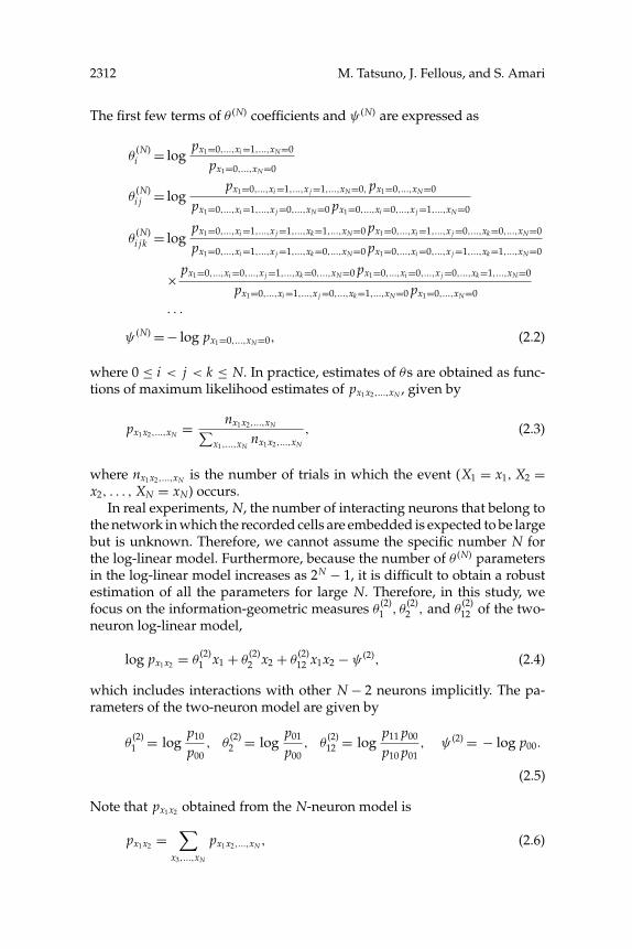
The first few terms of θ (N) coefficients and ψ (N) are expressed as
θ(N)i = log
px1=0,...,xi =1,...,xN=0
px1=0,...,xN=0
θ(N)i j = log
px1=0,...,xi =1,...,xj =1,...,xN=0, px1=0,...,xN=0
px1=0,...,xi =1,...,xj =0,...,xN=0 px1=0,...,xi =0,...,xj =1,...,xN=0
θ(N)i jk = log
px1=0,...,xi =1,...,xj =1,...,xk=1,...,xN=0 px1=0,...,xi =1,...,xj =0,...,xk=0,...,xN=0
px1=0,...,xi =1,...,xj =1,...,xk=0,...,xN=0 px1=0,...,xi =0,...,xj =1,...,xk=1,...,xN=0
× px1=0,...,xi =0,...,xj =1,...,xk=0,...,xN=0 px1=0,...,xi =0,...,xj =0,...,xk=1,...,xN=0
px1=0,...,xi =1,...,xj =0,...,xk=1,...,xN=0 px1=0,...,xN=0
· · ·ψ (N) = − log px1=0,...,xN=0, (2.2)
where 0 ≤ i < j < k ≤ N. In practice, estimates of θs are obtained as func-tions of maximum likelihood estimates of px1x2,...,xN , given by
px1x2,...,xN = nx1x2,...,xN∑x1,...,xN
nx1x2,...,xN
, (2.3)
where nx1x2,...,xN is the number of trials in which the event (X1 = x1, X2 =x2, . . . , XN = xN) occurs.
In real experiments, N, the number of interacting neurons that belong tothe network in which the recorded cells are embedded is expected to be largebut is unknown. Therefore, we cannot assume the specific number N forthe log-linear model. Furthermore, because the number of θ (N) parametersin the log-linear model increases as 2N − 1, it is difficult to obtain a robustestimation of all the parameters for large N. Therefore, in this study, wefocus on the information-geometric measures θ
(2)1 , θ
(2)2 , and θ
(2)12 of the two-
neuron log-linear model,
log px1x2 = θ(2)1 x1 + θ
(2)2 x2 + θ
(2)12 x1x2 − ψ (2), (2.4)
which includes interactions with other N − 2 neurons implicitly. The pa-rameters of the two-neuron model are given by
θ(2)1 = log
p10
p00, θ
(2)2 = log
p01
p00, θ
(2)12 = log
p11 p00
p10 p01, ψ (2) = − log p00.
(2.5)
Note that px1x2 obtained from the N-neuron model is
px1x2 =∑
x3,...,xN
px1x2,...,xN , (2.6)
Information Geometry and Network Parameters 2313
and the parameters θ(2)1 , θ
(2)2 , and θ
(2)12 in equation 2.5 are different from θ
(N)1 ,
θ(N)2 , and θ
(N)12 in equation 2.2. The two-neuron model gives the marginal
distribution of the N-neuron model. When this simple model is considered,the number of parameters that need to be estimated reduces to three. Sincethe above two neurons are members of an N-neuron network, θ
(2)1 , θ
(2)2 ,
and θ(2)12 will be affected by the other N − 2 neurons. By calculating these
interaction terms from the other N − 2 neurons, the method becomesapplicable in realistic experimental conditions. In the following, weinvestigate in detail how θ
(2)i and θ
(2)i j are related to the external inputs
and the connection strengths in the general N-neuron network, with bothsymmetric and asymmetric connections.
3 Model Network
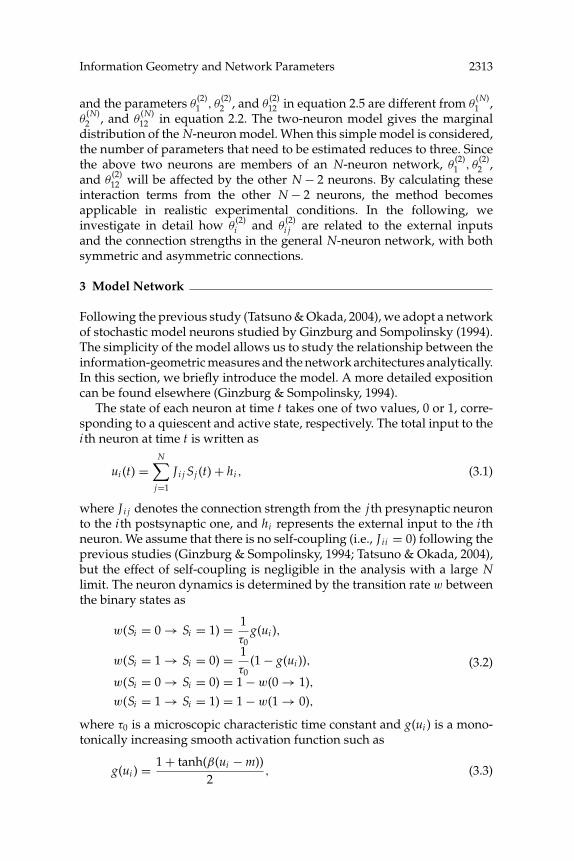
Following the previous study (Tatsuno & Okada, 2004), we adopt a networkof stochastic model neurons studied by Ginzburg and Sompolinsky (1994).The simplicity of the model allows us to study the relationship between theinformation-geometric measures and the network architectures analytically.In this section, we briefly introduce the model. A more detailed expositioncan be found elsewhere (Ginzburg & Sompolinsky, 1994).
The state of each neuron at time t takes one of two values, 0 or 1, corre-sponding to a quiescent and active state, respectively. The total input to theith neuron at time t is written as
ui (t) =N∑
j=1
J i j Sj (t) + hi , (3.1)
where J i j denotes the connection strength from the j th presynaptic neuronto the ith postsynaptic one, and hi represents the external input to the ithneuron. We assume that there is no self-coupling (i.e., J ii = 0) following theprevious studies (Ginzburg & Sompolinsky, 1994; Tatsuno & Okada, 2004),but the effect of self-coupling is negligible in the analysis with a large Nlimit. The neuron dynamics is determined by the transition rate w betweenthe binary states as
w(Si = 0 → Si = 1) = 1τ0
g(ui ),
w(Si = 1 → Si = 0) = 1τ0
(1 − g(ui )),
w(Si = 0 → Si = 0) = 1 − w(0 → 1),
w(Si = 1 → Si = 1) = 1 − w(1 → 0),
(3.2)
where τ0 is a microscopic characteristic time constant and g(ui ) is a mono-tonically increasing smooth activation function such as
g(ui ) = 1 + tanh(β(ui − m))2
, (3.3)

2314 M. Tatsuno, J. Fellous, and S. Amari
where β > 0 and m are constants determining the slope and offset thresh-old of the sigmoid. The probability of finding the system in a stateP(S1, . . . , SN, t) at time t is then provided by the following master equation:
ddt
P(S1, . . . , SN, t) = −N∑
i=1
w(Si → (1 − Si ))P(S1, . . . , SN, t)
+N∑
i=1
w((1 − Si ) → Si )P(S1 . . . , 1 − Si , . . . , SN, t).
(3.4)
4 First- and Second-Order Information-Geometric Measures andNetwork Parameters
4.1 Network of Two Neurons. Before we discuss a general N neuroncase, it is instructive to summarize the results from a simple example of two-neuron networks. Here, we briefly show the results (the detailed derivationcan be found in Tatsuno & Okada, 2004).
For an asymmetrically connected two-neuron network, the mean firingrate of each neuron in the equilibrium state is obtained as
〈S1〉 = g(h1) + �g1g(h2)1 − �g1�g2
, (4.1)
〈S2〉 = g(h2) + �g2g(h1)1 − �g1�g2
, (4.2)
where �g1 = g(J12 + h1) − g(h1) and �g2 = g(J21 + h2) − g(h2), respec-tively. Because the right-hand sides of equations 4.1 and 4.2 involve J12, J21,h1, and h2 only, the mean firing rate is expressed by the network parameters.Using 〈S1〉 and 〈S2〉, the mean coincident firing rate is also given as
〈S1S2〉 = 12{〈S1〉g(J21 + h2) + 〈S2〉g(J12 + h1)}. (4.3)
The firing rates (〈S1〉, 〈S2〉) and the covariance are related in a nontrivialmanner to the external input (h1, h2) and the connection strength (J12, J21).
For the two-neuron information-geometric measure, the joint probabilitydistribution is related to the above quantities by
p00 = 1 − 〈S1〉 − 〈S2〉 + 〈S1S2〉,p01 = 〈S2〉 − 〈S1S2〉,p10 = 〈S1〉 − 〈S1S2〉,p11 = 〈S1S2〉.
(4.4)

Information Geometry and Network Parameters 2315
Substituting these into equation 2.5 and using equation 3.3 gives analyticalexpressions for the two-neuron information-geometric measures in termsof the network parameters,
θ(2,A2)1 = 2β(h1 − m)
+ log(
2 exp[2β(h1 + h2 + J12)] + 2 exp [4βm] + 2 exp [2β (h1 + J12 + m)]exp [2β (h1 + h2 + J12)] + exp [2β (h1 + h2 + J21)] + 2 exp [4βm]
× + exp [2β (h2 + J12 + m)] + exp [2β (h2 + J21 + m)]+2 exp [2β (h1 + J12 + m)] + 2 exp [2β (h2 + J21 + m)]
),
θ(2,A2)2 = 2β (h2 − m)
+ log(
2 exp [2β (h1 + h2 + J21)] + 2 exp [4βm] + 2 exp [2β (h2 + J21 + m)]exp [2β (h1 + h2 + J12)] + exp [2β (h1 + h2 + J21)] + 2 exp [4βm]
× + exp [2β (h1 + J12 + m)] + exp [2β (h1 + J21 + m)]+2 exp [2β (h1 + J12 + m)] + 2 exp [2β (h2 + J21 + m)]
),
θ(2,A2)12 = β (J12 + J21)
+ log
( (exp [2β (h1 + h2 + J12)] + exp [2β (h1 + h2 + J21)] + 2 exp [2βm](
2 exp [2β (h1 + h2 + J12)] + 2 exp [4βm] + 2 exp [2β (h1 + J12 + m)]
×+2 exp[2β(h1 + J12 + m)] + 2 exp[2β(h2 + J21 + m)])(2 exp[β(2h1 + 2h2 + J12 + J21)]+ exp[2β(h2 + J12 + m)] + exp[2β(h2 + J21 + m)])(2 exp[2β (h1 + h2 + J21)]
× +2 exp [β (2h1 + J12 + J21 + 2m)] + 2 exp [2h2 + J12 + J21 + 2m]+2 exp [4βm] + exp [2β (h1 + J12 + m)] + exp [2β (h1 + J21 + m)]
× + exp [β (J12 − J21 + 4m)] + exp [β (J21 − J12 + 4m)])
+2 exp [2β (h2 + J21 + m)])
). (4.5)
Here the superscript (2, A2) means that the information-geometric measuresare calculated with the two-neuron log-linear model in an asymmetricallyconnected two-neuron network. The first-order information-geometricmeasures (θ (2,A2)
1 , θ(2,A2)2 ) are expressed by the term corresponding to the ex-
ternal input and an additional logarithmic bias term. Similarly, the second-order information-geometric measure θ
(2,A2)12 has the term corresponding to
the sum of the connection strength and an additional logarithmic bias term.If we assume the symmetric connection (J12 = J21), the above expression
is significantly simplified as
θ(2,S2)1 = 2β (h1 − m) , θ
(2,S2)2 = 2β (h2 − m) , θ
(2,S2)12 = 2β J12. (4.6)
These equations show that the first- and second-order information-geometric measures correspond to the external inputs and the connectionstrengths, respectively, as previously shown (Tatsuno & Okada, 2004).
4.2 Network of N Neurons. In the previous section, we already see thatcomplexity differs significantly for asymmetric and symmetric connections
2316 M. Tatsuno, J. Fellous, and S. Amari
(see equations 4.5 and 4.6) for even a simple two-neuron network. Becausethe analytical expressions for the asymmetrically connected N neurons willbe extremely complicated, we first investigate the analytical results for thesymmetrically connected N neuron case. We then extend our investigationsto the asymmetric case.
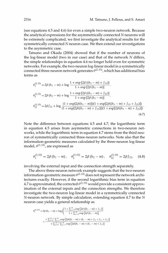
Tatsuno and Okada (2004) showed that if the number of neurons ofthe log-linear model (two in our case) and that of the network N differs,the simple relationships in equation 4.6 no longer hold even for symmetricnetworks. For example, the two-neuron log-linear model in a symmetricallyconnected three-neuron network generates θ (2,S3), which has additional biasterms as
θ(2,S3)1 = 2β (h1 − m) + log
1 + exp [2β ((h3 − m) + J13)]1 + exp [2β (h3 − m)]
,
θ(2,S3)2 = 2β (h2 − m) + log
1 + exp [2β ((h3 − m) + J23)]1 + exp [2β (h3 − m)]
,
θ(2,S3)12 = 2β J12 + log
(1 + exp[2β(h3 − m)])(1 + exp[2β((h3 − m) + J13 + J23)])(1 + exp[2β((h3 − m) + J13)])(1 + exp[2β((h3 − m) + J23)])
.
(4.7)
Note the difference between equations 4.5 and 4.7; the logarithmic termin equation 4.5 arises from asymmetric connections in two-neuron net-works, while the logarithmic term in equation 4.7 stems from the third neu-ron of symmetrically connected three-neuron networks. Note also that theinformation-geometric measures calculated by the three-neuron log-linearmodel, θ (3,S3), are expressed as
θ(3,S3)1 = 2β (h1 − m) , θ
(3,S3)2 = 2β (h2 − m) , θ
(3,S3)12 = 2β J12, (4.8)
involving the external input and the connection strength separately.The above three-neuron network example suggests that the two-neuron
information-geometric measure θ (2,S3) does not represent the network archi-tectures exactly. However, if the second logarithmic bias term in equation4.7 is approximated, the corrected θ (2,S3) would provide a consistent approx-imation of the external inputs and the connection strengths. We thereforeinvestigate the two-neuron log-linear model in a symmetrically connectedN-neuron network. By simple calculation, extending equation 4.7 to the Nneuron case yields a general relationship as
θ(2,SN)1 = 2β (h1 − m) + log
(1 +∑N
j=3 exp[2β((
h j − m)+ J1 j
)]1 +∑N
j=3 exp[2β(h j − m
)]
× +∑N−1i=3
∑Nj>i exp
[2β((hi − m) + (h j − m) + J1i + J1 j + J i j )
]+∑N−1
i=3∑N
j>i exp[2β((hi − m) + (h j − m) + J i j )
]
Information Geometry and Network Parameters 2317
×+ · · · + exp
[2β(∑N
i=3 (hi − m) +∑N−1i=1, �=2
∑Nj>i, �=2 J i j
)]+ · · · + exp
[2β(∑N
i=3 (hi − m) +∑N−1i=3
∑Nj>i J i j
)] ,
θ(2,SN)2 = 2β (h2 − m) + log
(1 +∑N
j=3 exp[2β((
h j − m)+ J2 j
)]1 +∑N
j=3 exp[2β(h j − m
)]
× +∑N−1i=3
∑Nj>i exp
[2β((hi − m) + (h j − m) + J1i + J1 j + J i j )
]+∑N−1
i=3∑N
j>i exp[2β((hi − m) + (h j − m) + J i j )
]
×+ · · · + exp
[2β(∑N
i=3 (hi − m) +∑N−1i=2
∑Nj>i J i j
)]+ · · · + exp
[2β(∑N
i=3 (hi − m) +∑N−1i=3
∑Nj>i J i j
)] ,
θ(2,SN)12 = 2β J12 + log
(
1 +∑Nj=3 exp
[2β((
h j − m)+ J1 j + J2 j
)](
1 +∑Nj=3 exp
[2β((
h j − m)+ J i j
)]
× +∑N−1i=3
∑Nj>i exp
[2β((hi − m) + (
h j − m)+ J1i + J1 j + J2i + J2 j + J i j
)]+∑N−1
i=3∑N
j>i exp[2β((hi − m) + (
h j − m)+ J1i + J1 j + J i j
)]
×+ · · · + exp
[2β(∑N
i=3 (hi − m) +∑N−1i=1
∑Nj>i, �=2 J i j
)]) (1 +∑N
j=3 exp[2β(h j − m
)]+ · · · + exp
[2β(∑N
i=3 (hi − m) + ∑N−1i=1, �=2
∑Nj>i, �=2 J i j
)]) (1 + ∑N
j=3 exp[2β((h j − m) + J i j
)]
× +∑N−1i=3
∑Nj>i exp
[2β((hi − m) + (
h j − m)+ J i j
)]+∑N−1
i=3∑N
j>i exp[2β((hi − m) + (
h j − m)+ J1i + J1 j + J i j
)]
×+ · · · + exp
[2β(∑N
i=3 (hi − m) +∑N−1i=3
∑Nj>i J i j
)])+ · · · + exp
[2β(∑N
i=3 (hi − m) +∑N−1i=2
∑Nj>i J i j
)]) .
(4.9)
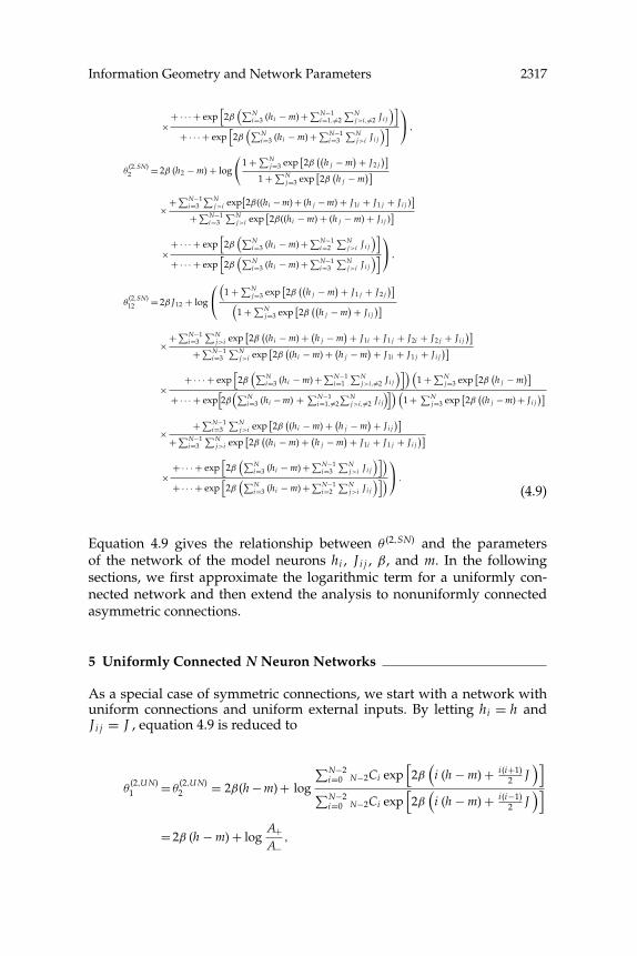
Equation 4.9 gives the relationship between θ (2,SN) and the parametersof the network of the model neurons hi , J i j , β, and m. In the followingsections, we first approximate the logarithmic term for a uniformly con-nected network and then extend the analysis to nonuniformly connectedasymmetric connections.
5 Uniformly Connected N Neuron Networks
As a special case of symmetric connections, we start with a network withuniform connections and uniform external inputs. By letting hi = h andJ i j = J , equation 4.9 is reduced to
θ(2,U N)1 = θ
(2,U N)2 = 2β(h − m) + log
∑N−2i=0 N−2Ci exp
[2β(
i (h − m) + i(i+1)2 J
)]∑N−2
i=0 N−2Ci exp[2β(
i (h − m) + i(i−1)2 J
)]
= 2β (h − m) + logA+A−
,

2318 M. Tatsuno, J. Fellous, and S. Amari
θ(2,U N)12 = 2β J + log
∑N−2
i=0 N−2Ci exp[2β(
i (h − m) + i(i+3)2 J
)]∑N−2
i=0 N−2Ci exp[2β(
i (h − m) + i(i+1)2 J
)]
×∑N−2
i=0 N−2Ci exp[2β(
i (h − m) + i(i−1)2 J
)]∑N−2
i=0 N−2Ci exp[2β(
i (h − m) + i(i+1)2 J
)]
= 2β J + logA3+ A−
A2+, (5.1)
where N−2Ci is a binomial coefficient and
A± =N−2∑i=0
N−2Ci exp[
2β
(i (h − m) + i (i ± 1)
2J)]
,
A3+ =N−2∑i=0
N−2Ci exp[
2β
(i (h − m) + i (i + 3)
2J)]
.
(5.2)
In this study, we investigate the fully connected networks where each neu-ron is connected to all other neurons. Therefore, we consider the case whereeach connection is weak, typically on the order of 1/N. Otherwise thetotal synaptic inputs will drive the neuron into saturation. By Stirling’sapproximation,
N! =√
2π NNNe−N{
1 + O(
1N
)}, (5.3)
and by rewritingN′ = N − 2, J = c/N, and i = (N − 2)r = N′r , we obtain
N−2Ci = N′CN′r
= 1√2π N′r (1 − r )
exp[N′ {−r log r − (1 − r ) log (1 − r )
}]
×{
1 + O(
1N′
)}
= 1√2π N′r (1 − r )
exp[N′ H(r )
] {1 + O
(1N′
)}, (5.4)

Information Geometry and Network Parameters 2319
where H(r ) = −r log r − (1 − r ) log(1 − r ). Note that this approximation isaccurate when N’ is large. We then obtain
A≡N−2∑i=0
N−2Ci exp[
2β
(i (h − m) + i2
2J)]
=1∑
r=01
N′ step
1√2π N′r (1 − r )
exp[N′ H(r ) + 2βN′(h − m)r + β(N′r )2 J
]
×{
1 + O(
1N′
)}
=∑
r
exp[
N′{
H(r ) + 2β(h − m)r + βcr2 − 12N′ log N′
− 12N′ log(2πr (1 − r ))
}]{1 + O
(1N′
)}
=∑
r
exp[N′ f (r )
] {1 + O
(1N′
)}, (5.5)
where f (r ) = H(r ) + 2β(h − m)r + βcr2 − log N′/(2N′) − log(2πr (1 − r ))/(2N′).
To investigate further, by taking a large N’ limit, we approximateequation 5.5 using a continuous variable r. With Taylor’s expansion, A iswritten as
A≈∫ 1
0exp[N′ f (r )]
{1 + O
(1N′
)}dr
=∫ 1
0exp
[N′{
f (r0) + 12
f ′′(r0) (r − r0)2 + 16
f (3)(r0) (r − r0)3
+ 124
f (4)(r0) (r − r0)4 + O((r − r0)5)}]
×{
1 + O(
1N′
)}dr
≈ exp[N′ f (r0)]∫ ∞
−∞exp
[N′
2
{f ′′(r0) (r − r0)2 + 1
3f (3)(r0) (r − r0)3
+ 112
f (4)(r0) (r − r0)4 + O((r − r0)5)}]
×{
1 + O(
1N′
)}dr
= exp[N′ f (r0)
]G(r0), (5.6)

2320 M. Tatsuno, J. Fellous, and S. Amari
where r0 is given by r0 = arg maxr f (r ), yielding
log1 − r0
r0+ 2β (h − m) + 2βcr0 = 0, (5.7)
and G(r0) is given by
G(r0) =∫ ∞
−∞exp
[N′
2
{f ′′(r0) (r − r0)2 + 1
3f (3)(r0) (r − r0)3
+ 112
f (4)(r0) (r − r0)4 + O((r − r0)5)}]
×{
1 + O(
1N′
)}dr. (5.8)
When a new variable u is defined as
u =√
N′r, (5.9)
G(r0) is written as
G(u0) = 1√N′
∫ ∞
−∞exp
[12
{f ′′(u0) (u − u0)2 + 1
3f (3)(u0)
(u − u0)3
√N′
+ 112
f (4)(u0)(u − u0)4
N′ + O(
1
N′√N′
)}]
×{
1 + O(
1N′
)}du. (5.10)
Since the integral of the (u − u0)3 term is 0 and that of the (u − u0)4 term isin O (1/N′), G(u0) is given as
G(u0) = 1√N′
∫ ∞
−∞exp
[12
{f ′′(u0) (u − u0)2 + O
(1N′
)}]
×{
1 + O(
1N′
)}du
=∫ ∞
−∞exp
[N′
2f ′′(r0) (r − r0)2
]{1 + O
(1N′
)}dr. (5.11)

Information Geometry and Network Parameters 2321
With the saddle point approximation, we have
G(r0) ≈√
2π
N′| f ′′(r0)|{
1 + O(
1N′
)}. (5.12)
Thus, A is given as
A = exp[N′ f (r0)
]√ 2π
N′| f ′′(r0)|{
1 + O(
1N′
)}. (5.13)
A± and A3+ are similarly calculated as
A± =∑
r
exp[N′ f (r ) ± βcr
] {1 + O
(1N′
)}
≈∫
exp[N′ f (r ) ± βcr
] {1 + O
(1N′
)}dr
≈ Aexp [±βcr0]{
1 + O(
1N′
)},
A3+ =∑
r
exp[N′ f (r ) + 3βcr
] {1 + O
(1N′
)}
≈∫
exp[N′ f (r ) + 3βcr
] {1 + O
(1N′
)}dr
≈ Aexp [3βcr0]{
1 + O(
1N′
)}. (5.14)
Therefore, we obtain
logA+A−
= logAexp [βcr0]
{1 + O
( 1N′)}
Aexp [−βcr0]{1 + O
( 1N′)}
= log(
exp [2βcr0]{
1 + O(
1N′
)})
= 2βcr0 + O(
1N′
), (5.15)
and similarly,
logA3+ A−
A2+
= log
(Aexp [3βcr0]
{1 + O
( 1N′)}) (
Aexp [−βcr0]{1 + O
( 1N′)})
(Aexp [βcr0]
{1 + O
( 1N′)})2

2322 M. Tatsuno, J. Fellous, and S. Amari
= log(
exp [0]{
1 + O(
1N′
)})
= 0 + O(
1N′
). (5.16)
From equations 5.15 and 5.16 and letting N′ = N in a large N limit, weobtain
θ(2,U N)1 = θ
(2,U N)2 = 2β (h − m) + 2βcr0 + O
(1N
),
θ(2,U N)12 = 2β J + O
(1N
). (5.17)
Equation 5.17 shows that in a large N limit, the second logarithmic biasterm of the first-order information-geometric measures (θ (2,U N)
1 and θ(2,U N)2 )
can be approximated by 2βcr0 and that the second logarithmic bias termof the second-order information-geometric measure θ
(2,U N)12 reduces to 0.
θ(2,U N)12 therefore provides a consistent approximation of the connection
strengths. By defining the corrected first-order information-geometric mea-sures, θ
(2,U N)1 and θ
(2,U N)2 , as
θ(2,U N)1 = θ
(2,U N)1 − 2βcr0,
θ(2,U N)2 = θ
(2,U N)2 − 2βcr0,
(5.18)
we obtain
θ(2,U N)1 = θ
(2,U N)2 = 2β (h − m) + O
(1N
), (5.19)
which provide a consistent approximation of the external inputs.To further investigate the bias term 2βcr0, we calculated r0 in equation
5.7 by finding an intersecting point between y = − log ((1 − r0) /r0) andy = 2β(h − m) + 2βcr0. Because the second equation represents a linear linewith a slope of 2βc with positive β, the number of intersecting pointsdepends on the connection strength parameterc. For negative c, there isonly one intersecting point. For positive c, in the weak connection range ofc < 2/β, only one intersecting point exists as well. For the strong connectionrange of c > 2/β, there are two cases in which only one intersecting pointor three intersection points exist, depending on the strength of the externalinput h.
To calculate the concrete value of r0, we assume that the network parame-ters are known. Here, we used biologically plausible parameters following
Information Geometry and Network Parameters 2323
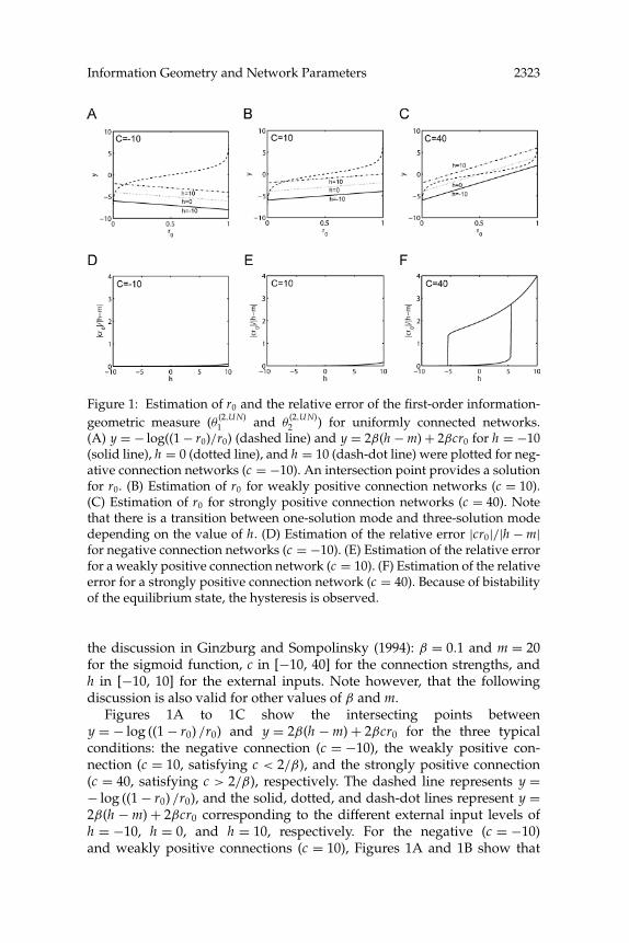
Figure 1: Estimation of r0 and the relative error of the first-order information-geometric measure (θ (2,U N)
1 and θ(2,U N)2 ) for uniformly connected networks.
(A) y = − log((1 − r0)/r0) (dashed line) and y = 2β(h − m) + 2βcr0 for h = −10(solid line), h = 0 (dotted line), and h = 10 (dash-dot line) were plotted for neg-ative connection networks (c = −10). An intersection point provides a solutionfor r0. (B) Estimation of r0 for weakly positive connection networks (c = 10).(C) Estimation of r0 for strongly positive connection networks (c = 40). Notethat there is a transition between one-solution mode and three-solution modedepending on the value of h. (D) Estimation of the relative error |cr0|/|h − m|for negative connection networks (c = −10). (E) Estimation of the relative errorfor a weakly positive connection network (c = 10). (F) Estimation of the relativeerror for a strongly positive connection network (c = 40). Because of bistabilityof the equilibrium state, the hysteresis is observed.
the discussion in Ginzburg and Sompolinsky (1994): β = 0.1 and m = 20for the sigmoid function, c in [−10, 40] for the connection strengths, andh in [−10, 10] for the external inputs. Note however, that the followingdiscussion is also valid for other values of β and m.
Figures 1A to 1C show the intersecting points betweeny = − log ((1 − r0) /r0) and y = 2β(h − m) + 2βcr0 for the three typicalconditions: the negative connection (c = −10), the weakly positive con-nection (c = 10, satisfying c < 2/β), and the strongly positive connection(c = 40, satisfying c > 2/β), respectively. The dashed line represents y =− log ((1 − r0) /r0), and the solid, dotted, and dash-dot lines represent y =2β(h − m) + 2βcr0 corresponding to the different external input levels ofh = −10, h = 0, and h = 10, respectively. For the negative (c = −10)and weakly positive connections (c = 10), Figures 1A and 1B show that
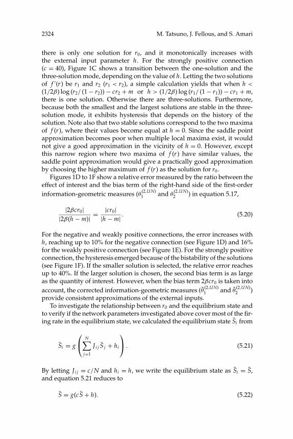
2324 M. Tatsuno, J. Fellous, and S. Amari
there is only one solution for r0, and it monotonically increases withthe external input parameter h. For the strongly positive connection(c = 40), Figure 1C shows a transition between the one-solution and thethree-solution mode, depending on the value of h. Letting the two solutionsof f ′(r ) be r1 and r2 (r1 < r2), a simple calculation yields that when h <
(1/2β) log (r2/ (1 − r2)) − cr2 + m or h > (1/2β) log (r1/ (1 − r1)) − cr1 + m,there is one solution. Otherwise there are three-solutions. Furthermore,because both the smallest and the largest solutions are stable in the three-solution mode, it exhibits hysteresis that depends on the history of thesolution. Note also that two stable solutions correspond to the two maximaof f (r ), where their values become equal at h = 0. Since the saddle pointapproximation becomes poor when multiple local maxima exist, it wouldnot give a good approximation in the vicinity of h = 0. However, exceptthis narrow region where two maxima of f (r ) have similar values, thesaddle point approximation would give a practically good approximationby choosing the higher maximum of f (r ) as the solution for r0.
Figures 1D to 1F show a relative error measured by the ratio between theeffect of interest and the bias term of the right-hand side of the first-orderinformation-geometric measures (θ (2,U N)
1 and θ(2,U N)2 ) in equation 5.17,
|2βcr0||2β(h − m)| = |cr0|
|h − m| . (5.20)
For the negative and weakly positive connections, the error increases withh, reaching up to 10% for the negative connection (see Figure 1D) and 16%for the weakly positive connection (see Figure 1E). For the strongly positiveconnection, the hysteresis emerged because of the bistability of the solutions(see Figure 1F). If the smaller solution is selected, the relative error reachesup to 40%. If the larger solution is chosen, the second bias term is as largeas the quantity of interest. However, when the bias term 2βcr0 is taken intoaccount, the corrected information-geometric measures (θ (2,U N)
1 and θ(2,U N)2 )
provide consistent approximations of the external inputs.To investigate the relationship between r0 and the equilibrium state and
to verify if the network parameters investigated above cover most of the fir-ing rate in the equilibrium state, we calculated the equilibrium state Si from
Si = g
N∑
j=1
J i j S j + hi
. (5.21)
By letting J i j = c/N and hi = h, we write the equilibrium state as Si = S,and equation 5.21 reduces to
S = g(c S + h). (5.22)

Information Geometry and Network Parameters 2325
Figure 2: Stability of the equilibrium state of uniformly connected networks.(A) y = S (dashed line) and y = g(c S + h) for h = −10 (solid line), h = 0 (dot-ted line) and h = 10 (dash-dot line) were plot for negative connection networks(c = −10). An intersecting point provides the solution for S. When the condition|g′(c S + h)| < 1 holds, the intersecting point is stable. (B) The equilibrium solu-tion S for a weakly positive connection network (c = 10). (C) The equilibriumsolution S for a strongly positive connection network (c = 40). Note that thereis transition between one-stable-equilibrium state and three-equilibrium stateswhere the smallest and largest ones are stable. Note also that S obtained by theinvestigated network parameters covers practically all firing rate from nearly 0through almost 1.
Figures 2A to 2C show the intersecting point between y = S andy = g(c S + h) for the negative connection (c = −10), the weakly positiveconnection (c = 10), and the strongly positive connection (c = 40), respec-tively. The intersecting point is stable when the condition |g′(c S + h)| < 1holds. As we saw in Figures 1A through 1C, one stable equilibrium stateexists for the negative and weakly positive connections (see Figures 2A and2B), but there is a transition between the one-stable-solution mode and thethree-solutions mode for the strongly positive connection (see Figure 2C). Itis also clearly seen that the equilibrium state S covers practically the entirefiring rate range from 0 to 1.
We also derived the relationship between r0 and S. From equation 5.7,we obtain
r0
1 − r0= exp [2β (cr0 + h − m)] . (5.23)
Rewriting this equation yields
r0 = exp [2β (cr0 + h − m)]1 + exp [2β (cr0 + h − m)]
. (5.24)
As for S, equation 5.22 yields,
S = exp[2β(c S + h − m
)]1 + exp
[2β(c S + h − m
)] . (5.25)

2326 M. Tatsuno, J. Fellous, and S. Amari
Thus, this analysis yields the relationship
S = r0, (5.26)
suggesting that r0 can be replaced by the equilibrium state S. This relation-ship will be useful because S can be estimated from observed spike traindata.
In summary, the corrected first-order information-geometric measures(θ (2,U N)
1 and θ(2,U N)2 ) and the second-order information-geometric measure
θ(2,U N)12 provide consistent approximation of the external inputs and the
connection strengths, respectively.
6 Nonuniformly and Asymmetrically ConnectedN Neuron Networks
We next consider a nonuniformly connected case, where connections areasymmetric in general. We first write hi and J i j as the mean and thedeviation,
hi = h + εi
J i j = J + ε′i j
N= c + ε′
i j
N, (6.1)
where h and J = c/N represent their average value, respectively. A, A±,and A3+ are then written as
A=N−2∑i=0
N−2Ci exp
2β
i∑j=1
(h j − m
)+ β
i2∑j=1
J i j
A± =N−2∑i=0
N−2Ci exp
2β
i∑j=1
(h j − m
)+ β
i2∑j=1
J i j ± β
i∑j=1
J i j
(6.2)
A3+ =N−2∑i=0
N−2Ci exp
2β
i∑j=1
(h j − m
)+ β
i2∑j=1
J i j + 3β
i∑j=1
J i j
.
Here we can rewrite J i j as Jk , k representing index pairs (i,j), without losinggenerality. A is then calculated as
A=N−2∑i=0
N−2Ci exp
2β
i∑j=1
((h + ε j
)− m)+ β
i2∑k=1
(c + ε′
k
N
)
=∑
rN′CN′r exp
2β(h − m)N′r + β c N′r2 + 2β
N′r∑j=1
ε j + β
N
(N′r )2∑k=1
ε′k
Information Geometry and Network Parameters 2327
=∑
r
1√2π N′r (1 − r )
exp[N′ H(r )
] {1 + O
(1N′
)}
× exp
2β(h − m)N′r + β cN′r2 + 2β
N′r∑j=1
ε j + β
N
(N′r )2∑k=1
ε′k
≈∑
r
1√2π N′r (1 − r )
exp
[N′{
H(r ) + 2β(h − m)r + β cr2
+2β
(1
N′r
N′r∑j=1
ε j
)r + β
(1
(N′r )2
(N′r )2∑k=1
ε′k
)r2
}]
×{
1 + O(
1N′
)}
=∑
r
exp[
N′{
H(r ) + 2β(h − m)r + β cr2
− 12N′ log N′ − 1
2N′ log (2πr (1 − r )) + hε(r )r + Jε′ (r )r2}]
×{
1 + O(
1N′
)}
=∑
r
exp[N′ f (r )
] {1 + O
(1N′
)}, (6.3)
where
hε(r ) = 1
N′r
N′r∑j=1
ε j
,
Jε′ (r ) = 1
(N′r )2
(N′r )2∑k=1
ε′k
, (6.4)
and
f (r ) = H(r ) + 2β(h − m)r + β cr2 − 12N′ log N′
− 12N′ log (2πr (1 − r )) + hε(r )r + Jε′ (r )r2. (6.5)

2328 M. Tatsuno, J. Fellous, and S. Amari
When hε(r ) and hε(r ) are small, they can be replaced by hε(r0) and hε(r0),respectively. Thus, we obtain
f (r ) = H(r ) + 2β(h − m)r + β cr2 − 12N′ log N′
− 12N′ log (2πr (1 − r )) + hε(r0)r + Jε′ (r0)r2. (6.6)
When the saddle point approximation is used,
A≈∫
exp[N′ f (r )]{
1 + O(
1N′
)}dr
≈ exp[N′ f (r0)]
√2π
N′| f ′′(r0)|{
1 + O(
1N′
)}(6.7)
holds where r0 is obtained by r0 = arg maxr f (r ). It yields
log1 − r0
r0+ 2β
(h − m
)+ 2β cr0 + hε(r0) + 2Jε′ (r0)r0 = 0. (6.8)
A± and A3+ are now calculated as
A± =∑
rN′CN′r exp
2β
(h − m
)N′r + β c N′r2 + 2β
N′r∑j=1
ε j
+ β
N′
(N′r )2∑k=1
ε′k ±
{β cr + β
N′
N′r∑k=1
ε′k
}
=∑
r
1√2π N′r (1 − r )
exp[N′ {H(r ) + 2β(h − m)r + β cr2
+2βhε(r )r + β Jε′ (r )r2}±{β cr + β J (1)
ε′ (r )r}]
×{
1 + O(
1N′
)}
=∑
r
exp[
N′ f (r ) ±{β cr + β J (1)
ε′ (r )r}]{
1 + O(
1N′
)},
Information Geometry and Network Parameters 2329
A3+ =∑
rN′CN′r exp
2β
(h − m
)N′r + β c N′r2 + 2β
N′r∑j=1
ε j
+ β
N′
(N′r )2∑k=1
ε′k + 3
{β cr + β
N′
N′r∑k=1
ε′k
}
=∑
r
1√2π N′r (1 − r )
exp[N′ {H(r ) + 2β(h − m)r + β cr2
+2βhε(r )r + β Jε′ (r )r2}+ 3{β cr + β J (1)
ε′ (r )r}]
×{
1 + O(
1N′
)}
=∑
r
exp[
N′ f (r ) + 3{β cr + β J (1)
ε′ (r )r}]{
1 + O(
1N′
)}, (6.9)
where
J (1)ε′ (r ) =
(1
N′r
N′r∑k=1
ε′k
)(6.10)
By the saddle point approximation, A± and A3+ are approximated as
A± ≈ Aexp[±(βcr0 + β J (1)
ε′ (r0)r0
)]{1 + O
(1N′
)}
A3+ ≈ Aexp[3(βcr0 + β J (1)
ε′ (r0)r0
)]{1 + O
(1N′
)}.
(6.11)
By letting N′ = N for large N, we obtain,
θ(2,AN)1 = 2β (h1 − m) + 2βcr0 + 2β J (1)
ε′ (r0)r0 + O(
1N
)
θ(2,AN)2 = 2β (h2 − m) + 2βcr0 + 2β J (1)
ε′ (r0)r0 + O(
1N
)
θ(2,AN)12 = β (J12 + J21) + O
(1N
).
(6.12)
By assuming that ε′k is a random variable with the mean 0 and variance σ ′2,
ε′k ∼ N
(0, σ ′2) , (6.13)

2330 M. Tatsuno, J. Fellous, and S. Amari
the distribution of J (1)ε′ (r0) is estimated as
J (1)ε′ (r0) = 1
Nr0
Nr0∑k=1
ε′k ∼ N
(0,
σ ′2
Nr0
). (6.14)
Therefore, we obtain
θ(2,AN)1 = 2β (h1 − m) + 2βcr0 + O
(1N
)
θ(2,AN)2 = 2β (h2 − m) + 2βcr0 + O
(1N
)
θ(2,AN)12 = β (J12 + J21) + O
(1N
).
(6.15)
Finally, by assuming that ε j is a random variable with the mean 0 andvariance σ 2,
ε j ∼ N(0, σ 2) , (6.16)
the distribution of hε(r ) and Jε′ (r ) in equation 6.4 is estimated as
hε(r ) ∼ N(
0,σ 2
Nr
),
Jε′ (r ) ∼ N
(0,
σ ′2
(Nr )2
).
(6.17)
Therefore, for the large N limit, equation 6.8 reduces to
log1 − r0
r0+ 2β
(h − m
)+ 2βcr0 = 0, (6.18)
which is the same as equation 5.6. Thus, by letting r0 = r0, we obtain
θ(2,AN)1 = 2β (h1 − m) + 2βcr0 + O
(1N
),
θ(2,AN)2 = 2β (h2 − m) + 2βcr0 + O
(1N
),
θ(2,AN)12 = β (J12 + J21) + O
(1N
),
(6.19)

Information Geometry and Network Parameters 2331
which is equivalent to equation 5.10. Finally, by defining the corrected first-order information-geometric measures as
θ(2,AN)1 = θ
(2,AN)1 − 2βcr0,
θ(2,AN)2 = θ
(2,AN)2 − 2βcr0,
(6.20)
they provide consistent approximation of the external inputs,
θ(2,AN)1 = 2β (h1 − m) + O
(1N
),
θ(2,AN)2 = 2β (h2 − m) + O
(1N
). (6.21)
In summary, the corrected first-order information-geometric measures(θ (2,AN)
1 and θ(2,AN)2 ) and the second-order information geometric-measure
θ(2,AN)12 provide consistent approximation of the external inputs and the
connection strengths, respectively. In other words, the corrected first- andsecond-order information-geometric measures of the two-neuron log-linearmodel are proven to provide useful insights into the network architectureseven in the case of nonuniformly connected asymmetric networks.
7 Discussion
We have investigated the relationship between the information-geometricmeasures and two network parameters, corresponding to the connectionstrengths and the external inputs, in an N neuron network. We focusedon the information-geometric measures given by the two-neuron log-linearmodel because it is the simplest of all possible information-geometric mea-sures and can be estimated rather easily in real experimental settings. Usinga stochastic binary model neural network in the equilibrium state, we de-rived an explicit relationship between the measures θ (2) and the networkparameters for symmetrically connected networks (see equation 4.9) andsimplified it for uniformly connected networks (see equation 5.1). Then inthe large N limit, we estimated the accuracy of the information-geometricmeasures. We showed that the information-geometric measures provideda consistent approximation of the network parameters for both uniformlyconnected (see equations 5.17 and 5.19) and nonuniformly and asymmet-rically connected networks (see equations 6.19 and 6.21). These resultstherefore suggest that the corrected first- and second-order information-geometric measures of the two-neuron log-linear model provide usefulinsights into the underlying network architecture.

2332 M. Tatsuno, J. Fellous, and S. Amari
In this letter, we considered only the lag-zero information-geometricmeasure, θ (2)
12 = θ(2)12 (0), as an estimator of the connection strength. We could
extend the measure to the time-lagged information-geometric measureθ
(2)12 (τ ). As previous studies (Ginzburg & Sompolinsky, 1994; Tatsuno &
Okada, 2004) suggest, the time-lagged measure would provide informationabout the directionality of connections. Therefore, one of the future direc-tions to take will be to investigate the time-lagged information-geometricmeasure θ
(2)12 (τ ) and estimate the directionality of asymmetrically connected
networks. In addition, in this study, we considered only the case of randomgaussian connections with small variance. It is therefore interesting to in-vestigate the case with large variance, for example, the regime in which thesystem becomes glassy, in the future.
Regarding the number of neurons included in the log-linear model, wefocused on the two-neuron log-linear model. When an experimental situa-tion allows only a limited number of trials, the two-neuron log-linear modelwill provide a robust estimation of all three parameters: θ (2)
1 , θ (2)2 , and θ
(2)12 . As
the previous study indicated (Tatsuno & Okada, 2004), however, if a largernumber of trials is available, the higher-order log-linear model is expectedto provide better estimations. Thus, it is interesting to extend the result ofthis study to a higher-order log-linear model in the future.
Our previous work showed that the information-geometric measurescould not disentangle the connection strengths and the external inputs cor-rectly for asymmetrically connected networks (Tatsuno & Okada, 2004). Onthe other hand, our previous biophysical simulations indicated that theyindeed estimated the relative change of connection strengths and externalinputs successfully even with asymmetric connections (Lipa et al., 2006,2007). This study explains this apparent discrepancy. The discrepancy be-tween these two works arises because the former study used a network ofonly a couple of neurons in a high-firing-rate range where the estimationerror is high. The latter study used a network of 10 neurons in a low butrealistic firing-rate range where the error is smaller. Both studies used theuncorrected information-geometric measures. In this letter, we showed thatthe corrected information-geometric measures can indeed approximate thenetwork parameters regardless of firing-rate range.
The second-order information-geometric measure of the two-neuron log-linear model θ
(2)12 can be considered an alternative to the correlation coef-
ficient to quantify the statistical dependence between two binary randomvariables. Both θ
(2)12 and the correlation coefficient are calculated from two
spike trains, but θ(2)12 has significant advantages; it can quantify pure interac-
tions that are independent of the mean firing-rate modulations, and it pro-vides a consistent approximation of the connection strengths, as we showedin this letter. These two properties of the information-geometric measureswill be very useful when applied to multineuronal electrophysiological

Information Geometry and Network Parameters 2333
data. With the information-geometric measures, neuronal assemblies thatexhibit increased pure correlations can be detected and may lead to the iden-tification of neuronal subgroups that play important cognitive functions.Furthermore, assessment of the connection strengths by the information-geometric measures may lead, for the first time, to estimates on networkchanges from in vivo recordings and thus is expected to have a significantimpact on the study of learning and memory consolidation (Lipa et al.,2006, 2007).
In this letter, we chose the value of model parameters β and m. In practice,these parameters should be calculated from spike train data. Generally,however, this task may be an ill-posed problem because multiple sets ofparameters may produce the same spike trains. But because p00, p01,p10,p11, and mean firing rate Si can be estimated from the data, they maybe used for the model parameter estimation. For example, for a uniformconnection case, the following equations are obtained:
p00 = exp [−βcS]exp [−βcS] + exp [2β (h − m) + cS] + exp
[2 c
N + 3cS + 4β (h − m)] ,
p01 = p10 = exp[2β(h − m) + cS]exp[−βcS] + exp[2β(h − m) + cS] + exp[2 c
N + 3cS + 4β(h − m)],
p11 = exp[2 c
N + 3cS + 4β (h − m)]
exp [−βcS] + exp [2β (h − m) + cS] + exp[2 c
N + 3cS + 4β (h − m)] ,
log1 − S
S+ 2β (h − m) + 2βcS = 0. (7.1)
Assuming that N is a typical number of synaptic inputs in the neocortex(i.e., between 5,000 and 10,000), these equations can be solved for β, m, c,and h. Obtaining analytical solutions may be difficult because this is a setof four nonlinear equations, but they can be solved numerically. Althoughthe calculations for general asymmetric connections are more difficult, ourbiophysical simulation using the NEURON simulator suggests that rela-tive changes of connection strengths and external inputs can be estimatedfrom spike train data (Lipa et al., 2006, 2007). Electrophysiological experi-ments could therefore use such an analysis to determine whether connectionstrengths are modified by experience. In summary, with values of β and r0
estimated from spike trains, the bias correction term of the information-geometric measures can also be estimated. This makes the method valuablenot only theoretically but also in practice.
To understand how the brain works in terms of groups of interactingneurons, further development of analytical techniques and recording tech-nology is necessary. The information-geometric method is a promising an-alytical technique and will provide a useful tool for spike train analysis inboth in vitro and in vivo recordings.

2334 M. Tatsuno, J. Fellous, and S. Amari
Acknowledgments
We thank Bruce L. McNaughton, Peter Lipa, Masato Okada, and ToshiakiOmori for useful discussion and critical reading of the manuscript and twoanonymous reviewers for helpful comments and suggestions. This workwas supported by the National Institutes of Health (MH46823).
References
Abeles, M., & Gerstein, G. L. (1988). Detecting spatiotemporal firing patterns amongsimultaneously recorded single neurons. J. Neurophysiol., 60(3), 909–924.
Aertsen, A. M., Gerstein, G. L., Habib, M. K., & Palm, G. (1989). Dynamics of neuronalfiring correlation: Modulation of “effective connectivity.” J. Neurophysiol., 61(5),900–917.
Amari, S. (1985). Differential geometrical methods in statistics. Berlin: Springer-Verlag.Amari, S. (2001). Information geometry on hierarchy of probability distributions.
IEEE Transactions on Information Theory, 47(5), 1701–1711.Amari, S., & Nagaoka, H. (2000). Methods of information geometry. New York: Oxford
University Press.Amari, S., Nakahara, H., Wu, S., & Sakai, Y. (2003). Synchronous firing and higher-
order interactions in neuron pool. Neural Comput., 15(1), 127–142.Brown, E. N., Kass, R. E., & Mitra, P. P. (2004). Multiple neural spike train data
analysis: State-of-the-art and future challenges. Nat. Neurosci., 7(5), 456–461.Buzsaki, G. (2004). Large-scale recording of neuronal ensembles. Nat. Neurosci., 7(5),
446–451.Czanner, G., Grun, S., & Iyengar, S. (2005). Theory of the snowflake plot and its
relations to higher-order analysis methods. Neural Comput., 17(7), 1456–1479.Eleuteri, A., Tagliaferri, R., & Milano, L. (2005). A novel information geometric
approach to variable selection in MLP networks. Neural Netw., 18(10), 1309–1318.Fellous, J. M., Tiesinga, P. H., Thomas, P. J., & Sejnowski, T. J. (2004). Discovering
spike patterns in neuronal responses. J. Neurosci., 24(12), 2989–3001.Gerstein, G. L., & Perkel, D. H. (1969). Simultaneously recorded trains of action
potentials: Analysis and functional interpretation. Science, 164(881), 828–830.Ginzburg, I. I., & Sompolinsky, H. (1994). Theory of correlations in stochastic neu-
ral networks. Physical Review, E, Statistical Physics, Plasmas, Fluids, and RelatedInterdisciplinary Topics, 50(4), 3171–3191.
Grun, S., Diesmann, M., & Aertsen, A. (2002). Unitary events in multiple single-neuron spiking activity: I. Detection and significance. Neural Comput., 14(1), 43–80.
Hoffman, K. L., & McNaughton, B. L. (2002). Coordinated reactivation of distributedmemory traces in primate neocortex. Science, 297(5589), 2070–2073.
Houghton, C., & Sen, K. (2008). A new multineuron spike train metric. Neural Com-put., 20, 1495–1511.
Ikeda, K. (2005). Information geometry of interspike intervals in spiking neurons.Neural Comput., 17(12), 2719–2735.

Information Geometry and Network Parameters 2335
Kass, R. E., Ventura, V., & Brown, E. N. (2005). Statistical issues in the analysis ofneuronal data. J. Neurophysiol., 94(1), 8–25.
Lipa, P., Tatsuno, M., Amari, S., McNaughton, B. L., & Fellous, J. M. (2006). A novelanalysis framework for characterizing ensemble spike patterns using spike trainclustering and information geometry. Soc. Neurosci. Abstr., 36:371, 6.
Lipa, P., Tatsuno, M., McNaughton, B. L., & Fellous, J. M. (2007). Dynamics of neuralassemblies involved in memory-trace replay. Soc. Neurosci. Abstr., 37.308, 13.
Louie, K., & Wilson, M. A. (2001). Temporally structured replay of awake hippocam-pal ensemble activity during rapid eye movement sleep. Neuron, 29(1), 145–156.
Miura, K., Okada, M., & Amari, S. (2006). Estimating spiking irregularities underchanging environments. Neural Comput., 18(10), 2359–2386.
Nadasdy, Z., Hirase, H., Czurko, A., Csicsvari, J., & Buzsaki, G. (1999). Replay andtime compression of recurring spike sequences in the hippocampus. J. Neurosci.,19(21), 9497–9507.
Nakahara, H., & Amari, S. (2002). Information-geometric measure for neural spikes.Neural Comput., 14(10), 2269–2316.
Nakahara, H., Amari, S., & Richmond, B. J. (2006). A comparison of descriptivemodels of a single spike train by information-geometric measure. Neural Comput.,18(3), 545–568.
Nicolelis, M. A., & Ribeiro, S. (2002). Multielectrode recordings: The next steps. Curr.Opin. Neurobiol., 12(5), 602–606.
Riehle, A., Grun, S., Diesmann, M., & Aertsen, A. (1997). Spike synchronizationand rate modulation differentially involved in motor cortical function. Science,278(5345), 1950–1953.
Shimazaki, H., & Shinomoto, S. (2007). A method for selecting the bin size of a timehistogram. Neural Comput., 19(6), 1503–1527.
Tatsuno, M., Lipa, P., & McNaughton, B. L. (2006). Methodological considerationson the use of template matching to study long-lasting memory trace replay. J.Neurosci., 26(42), 10727–10742.
Tatsuno, M., & Okada, M. (2004). Investigation of possible neural architectures un-derlying information-geometric measures. Neural Comput., 16(4), 737–765.
Wilson, M. A., & McNaughton, B. L. (1993). Dynamics of the hippocampal ensemblecode for space. Science, 261(5124), 1055–1058.
Zhang, K., Ginzburg, I., McNaughton, B. L., & Sejnowski, T. J. (1998). Interpretingneuronal population activity by reconstruction: Unified framework with appli-cation to hippocampal place cells. J. Neurophysiol., 79(2), 1017–1044.
Received April 4, 2008; accepted January 8, 2009.
Related Documents