Informal self-employment and macroeconomic fluctuations Norbert M. Fiess a , Marco Fugazza b , William F. Maloney a, ⁎ a The World Bank, 1818 H Street, NW, Washington, DC 20433, United States b UNCTAD, Palais des Nations, 8-14, Av. de la Paix, 1211 Geneva 10, Switzerland abstract article info Article history: Received 11 August 2008 Received in revised form 25 August 2009 Accepted 30 September 2009 Available online xxxx JEL classification: F41 J21 J24 J31 017 Keywords: Informality Labor market dynamics Self-employment Real exchange rates Co-integration Informal self-employment is a major source of employment in developing countries. Its cyclical behavior is important to our understanding of the functioning of LDC labor markets, but turns out to be surprisingly complex. We develop a flexible model with two sectors: a formal salaried (tradable) sector that may be affected by wage rigidities, and an informal (non tradable) self-employment sector faced with liquidity constraints to entry. This labor market is then embedded in a standard small economy macro model. We show that different types of shocks interact with different institutional contexts to produce distinct patterns of comovement between key variables of the model: relative salaried/self-employed incomes, relative salaried/self-employed sector sizes and the real exchange rate. Model predictions are then tested empirically for Argentina, Brazil, Colombia and Mexico. We confirm episodes where the expansion of informal self- employment is consistent with the traditional segmentation views of informality. However, we also identify episodes where informal self-employment behaves “pro-cyclically”; here, informality is driven by relative demand or productivity shocks to the non tradable sector. © 2009 Elsevier B.V. All rights reserved. 1. Introduction This paper examines the adjustment of informal self-employment, a major component of developing country labor markets, to macro- economic shocks. It models both the decisions and credit constraints facing heterogeneous workers to enter self-employment, as well as standard labor market rigidities potentially found as impediments to entering the formal sector. Taking advantage of the fact that the vast majority of informal self-employed are found in the non tradable sectors, and most formal in the tradable sector, it then locates this labor market in a standard two sector open economy model. Together, this permits the development of a typology of movements of relative labor shares, relative incomes and the real exchange rate with respect to different sectoral shocks that underlie aggregate business cycles, and degrees of labor market rigidity. Such an approach is valuable for several reasons. First, the model offers insights into the reasons behind the multiple and shifting pat- terns of comovement (regimes) of an important component of the in- formal sector with macroeconomic fluctuations. In particular, it offers an explanation for observed episodes of procyclicality of self-employ- ment which run counter to all existing models of the informal sector. The rationale underlying these procyclical movements adds support to an emerging view of informal self-employment that stresses a large voluntary component of entry and hence the desirability of the sector for many workers. However, the model is also general enough to allow for varying degrees of involuntary entry driven by conventional seg- mentation considerations. In this sense, we offer a very rich and flexi- ble view of the developing country labor market. Second, the derived typology of regimes can be used by analysts and policy makers em- pirically to exploit the observed comovements of macroeconomic time series for diagnostic purposes: to establish the presence or absence of formal sector segmenting distortions; or to identify the sources of changes in the size of the informal sector. Finally, the framework is flexible enough to incorporate more secular issues of regulation and taxation, and growth that are also relevant to explaining the size of the informal self-employed sector. 1.1. Background We focus on self-employment, defined in the present case as own account workers as well as owners of firms with under five employees for several reasons. First, in Latin America, the sector accounts for 25 to 50% of employment and in other poorer regions, like Africa, substantially more. Understanding the behavior and raison d'être of Journal of Development Economics xxx (2009) xxx–xxx ⁎ Corresponding author. E-mail address: [email protected] (W.F. Maloney). DEVEC-01499; No of Pages 16 0304-3878/$ – see front matter © 2009 Elsevier B.V. All rights reserved. doi:10.1016/j.jdeveco.2009.09.009 Contents lists available at ScienceDirect Journal of Development Economics journal homepage: www.elsevier.com/locate/devec ARTICLE IN PRESS Please cite this article as: Fiess, N.M., et al., Informal self-employment and macroeconomic fluctuations, Journal of Development Economics (2009), doi:10.1016/j.jdeveco.2009.09.009

Welcome message from author
This document is posted to help you gain knowledge. Please leave a comment to let me know what you think about it! Share it to your friends and learn new things together.
Transcript
Journal of Development Economics xxx (2009) xxx–xxx
DEVEC-01499; No of Pages 16
Contents lists available at ScienceDirect
Journal of Development Economics
j ourna l homepage: www.e lsev ie r.com/ locate /devec
ARTICLE IN PRESS
Informal self-employment and macroeconomic fluctuations
Norbert M. Fiess a, Marco Fugazza b, William F. Maloney a,⁎a The World Bank, 1818 H Street, NW, Washington, DC 20433, United Statesb UNCTAD, Palais des Nations, 8-14, Av. de la Paix, 1211 Geneva 10, Switzerland
⁎ Corresponding author.E-mail address: [email protected] (W.F. Ma
0304-3878/$ – see front matter © 2009 Elsevier B.V. Aldoi:10.1016/j.jdeveco.2009.09.009
Please cite this article as: Fiess, N.M., et al.,(2009), doi:10.1016/j.jdeveco.2009.09.009
a b s t r a c t
a r t i c l e i n f oArticle history:Received 11 August 2008Received in revised form 25 August 2009Accepted 30 September 2009Available online xxxx
JEL classification:F41J21J24J31017
Keywords:InformalityLabor market dynamicsSelf-employmentReal exchange ratesCo-integration
Informal self-employment is a major source of employment in developing countries. Its cyclical behavior isimportant to our understanding of the functioning of LDC labor markets, but turns out to be surprisinglycomplex. We develop a flexible model with two sectors: a formal salaried (tradable) sector that may beaffected by wage rigidities, and an informal (non tradable) self-employment sector faced with liquidityconstraints to entry. This labor market is then embedded in a standard small economy macro model. Weshow that different types of shocks interact with different institutional contexts to produce distinct patternsof comovement between key variables of the model: relative salaried/self-employed incomes, relativesalaried/self-employed sector sizes and the real exchange rate. Model predictions are then tested empiricallyfor Argentina, Brazil, Colombia and Mexico. We confirm episodes where the expansion of informal self-employment is consistent with the traditional segmentation views of informality. However, we also identifyepisodes where informal self-employment behaves “pro-cyclically”; here, informality is driven by relativedemand or productivity shocks to the non tradable sector.
loney).
l rights reserved.
Informal self-employment and macroeconom
© 2009 Elsevier B.V. All rights reserved.
1. Introduction
This paper examines the adjustment of informal self-employment,a major component of developing country labor markets, to macro-economic shocks. It models both the decisions and credit constraintsfacing heterogeneous workers to enter self-employment, as well asstandard labor market rigidities potentially found as impediments toentering the formal sector. Taking advantage of the fact that the vastmajority of informal self-employed are found in the non tradablesectors, and most formal in the tradable sector, it then locates thislabormarket in a standard two sector open economymodel. Together,this permits the development of a typology of movements of relativelabor shares, relative incomes and the real exchange rate with respectto different sectoral shocks that underlie aggregate business cycles,and degrees of labor market rigidity.
Such an approach is valuable for several reasons. First, the modeloffers insights into the reasons behind the multiple and shifting pat-terns of comovement (regimes) of an important component of the in-formal sector with macroeconomic fluctuations. In particular, it offersan explanation for observed episodes of procyclicality of self-employ-
ment which run counter to all existing models of the informal sector.The rationale underlying these procyclical movements adds supportto an emerging view of informal self-employment that stresses a largevoluntary component of entry and hence the desirability of the sectorformanyworkers. However, themodel is also general enough to allowfor varying degrees of involuntary entry driven by conventional seg-mentation considerations. In this sense, we offer a very rich and flexi-ble view of the developing country labor market. Second, the derivedtypology of regimes can be used by analysts and policy makers em-pirically to exploit the observed comovements ofmacroeconomic timeseries for diagnostic purposes: to establish the presence or absence offormal sector segmenting distortions; or to identify the sources ofchanges in the size of the informal sector. Finally, the framework isflexible enough to incorporate more secular issues of regulation andtaxation, and growth that are also relevant to explaining the size of theinformal self-employed sector.
1.1. Background
We focus on self-employment, defined in the present case as ownaccount workers as well as owners of firmswith under five employeesfor several reasons. First, in Latin America, the sector accounts for25 to 50% of employment and in other poorer regions, like Africa,substantially more. Understanding the behavior and raison d'être of
ic fluctuations, Journal of Development Economics

2 N.M. Fiess et al. / Journal of Development Economics xxx (2009) xxx–xxx
ARTICLE IN PRESS
the sector is of clear importance. Second, in the countries we study,the self-employed or micro firm sector is the heart of the informalsector. It has been a longstanding proxy for informality by Interna-tional Labor Organization and it is highly correlated with informalitymeasured as being unprotected by social and labor protections: InArgentina 75%, Brazil 61%, and Mexico 77% of uncovered workers arefound in firms of five or fewer workers and most of these in singleperson firms, that is, the self-employed. Further, the share of workersthat are informal in these firms is over 80%.
The debate over the role of the informal goes back almost half acentury. A prominent stream of the literature has intellectual rootsperhaps best distilled in Harris and Todaro's (1970) vision of marketssegmented by wage setting in the formal sector that leaves the tradi-tional sector rationed out of modern salaried employment.1 The viewof the informal sector as the inferior segment of a dual labor market,expanding during downturns to absorb increased unemployment,became highly influential in the International Labor Organization,its Latin America affiliate, the Latin America Regional EmploymentProgram (PREALC), and the World Bank.2
However, dating at least from Hart's (1973) work in Africa, a par-allel stream has stressed the sector's dynamism and the likely volun-tary nature of much of the entry into informal self-employment.3
Increasingly, theoretical discussions of the sector assume mainstreammodels of worker sectoral selection, and the firm.4 Still, two of thesepapers derive and present evidence for the countercyclicality of infor-mality (Loayza and Rigolini, 2006) or a correlation of informality withunemployment (Boeri andGaribaldi, 2006), consistentwith the earlierliterature. Were it the focus of his paper, Rauch's formalization of thismore traditional model of markets segmented, in this case, by a mini-mum wage would generate a similar pattern.
However, greater disaggregation of the data suggests more com-plex patterns ofmovement of self informal employment acrossmacro-economic fluctuations. In particular, in several country-episodes westudy, self-employment appears to be procyclical. As an example, afirst look at time series for Mexico suggests cyclical behavior distinctfrom that of a shock absorber during downturns. Fig. 1a plots the evo-lution of the relative salaried/informal self-employed sector sizes andGDP growth and shows that during the recovery of 1987–1991 theywere negatively correlated. Fig. 1b further shows that across this sameperiod, the earnings of the self-employed relative to formal salariedworkers rose. Both are consistent with a procylical expansion of self-employment. Since over 80% of self-employed are found in domesticservices, transportation, commerce, or construction, we argue thatthat the boom in real estate and other non-tradable industries acrossthis period created new opportunities for micro-entrepreneurs. Con-trarily, it is also the case that in the subsequent period leading up tothe crisis of 1995, the countercyclical movements envisaged by moretraditional segmentation views appear, manifested as a positive co-movement relative salaried/informal self-employed sector sizes andGDP growth (Fig. 1a) , as well as a negative comovement of earningsand labor market sector sizes (Fig. 1b). Similar structural shifts in the
1 In fact, in Harris and Todaro's model, the “traditional” sector was the rural sectordisposed to migrate. However, it represents perhaps the first analytically worked outview of the dual labor market and remains highly relevant to the debate over theinformal sector and its relative inferiority. See Schneider and Enste (2000) for a morecomprehensive review of existing views. A rich theoretical literature is emerging thatposes more sophisticated mechanisms that relate informality to unemployment. See,for example, Boeri and Garibaldi (2006).
2 For early statements, see Sethuraman (1981), Tokman (1978), andMazumdar (1975),respectively.
3 See for more recent formulations in this vein, de Soto (1989), Loayza (1996) andMaloney (1999).
4 A group of papers with roots in Lucas (1978), for instance, Rauch (1991), Boeri andGaribaldi (2006), de Paula and Scheinkman (2007), and Loayza and Rigolini (2006)postulate a continuum of entrepreneurial ability and workers sorting themselves amongdifferent formal and informal sectors of work.
Please cite this article as: Fiess, N.M., et al., Informal self-employment a(2009), doi:10.1016/j.jdeveco.2009.09.009
relationship between self-employment and growth are visible acrossthe other countries shown in Fig. 1a and b.
We argue that these distinct and changing patterns suggest thatthe pro- or countercyclicality of the two labor market sectors maydepend on the sectoral origin of the shocks, and the presence orabsence of binding wage rigidities. That is, a conventional focus on thecorrelation between self-employment and GDP in the aggregate mayconceal important patterns of comovement and hence muddy ourunderstanding of the raison d'être and dynamics of the informal self-employed.
The existence of different regimes with distinct identifying pat-terns of comovement among a few variables also suggests that timeseries data on these series may offer potentially useful labor marketdiagnostics for policy makers, for instance, in identifying the roots ofexpansion of the informal sector across a given period: That is, it couldshed light on whether it is due to more onerous union or legislationinduced rigidities that may require politically costly reforms to off-set, or alternatively a construction boom, or simply a slowdown ofthe formal manufacturing sector that would not. Studying the rela-tionship among three variables easily extracted from repeated crosssections and financial data can offer a wealth of insight into the under-lying operation of the labor market that has not been previouslypossible. It also provides an alternative to the conditional income com-parisons commonly used to demonstrate the inferiority of informalwork, which are rendered highly suspect by their inability to controlfor unobserved job and individual effects.5
2. Modeling approach
2.1. The labor market
For such diagnostics to be feasible, we need to understand thedrivers of the very large observedmovements in relative wages whichin a simple textbook world, would be forced to equivalence. Threeeffects in principle may be at play: barriers to the arbitrage of laborearnings due to barriers to entry to either sector either through quan-tity or price rigidities, barriers to arbitraging of returns to capital ofthe self-employed which are generally not separable in labor marketsurveys from earnings of labor per se, and changes in the skills com-position of the sectoral work forces.
To capture these effects, we begin by constructing a model of thelabor market in developing countries that is firmly rooted in theestablished advanced country literature and which enjoys increasingsupport from the developing country data. We postulate two sectors:a tradable sector where workers receive a wage and are covered bylabor legislation or unions that may or may not introduce distortions;and a non tradable self-employed sector of the kind postulated byLucas (1978) with heterogeneity in level of entrepreneurial ability,and where, credit constraints can constitute a barrier to entry fromsalaried work. The idea that the self-employed enter voluntarily, butthat there may be barriers to salaried workers opening an enterpriseenjoys increasing support from the both the economics and sociologyliterature. To begin, surveys from both Mexico and Brazil suggest thataround 70% of the self-employed entered or have remained therevoluntarily, largely for reasons of higher incomes or greater flexibility.Indeed, the sociologists Balan, Browning, and Jelin (1973) interviewedMexican workers and found being one's own boss to be well regardedand that movements into self-employment from salaried position
5 See Maloney (1999), and Pratap and Quintin (2006). Total returns to informal self-employment and salaried employment incorporate differences in taxes, risk premia,flexibility, etc., all of which will lead to incomes not being equated, even in the absenceof segmentation.
nd macroeconomic fluctuations, Journal of Development Economics
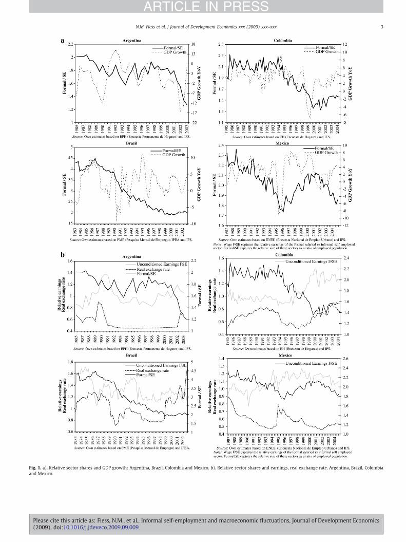
Fig. 1. a). Relative sector shares and GDP growth: Argentina, Brazil, Colombia and Mexico. b). Relative sector shares and earnings, real exchange rate. Argentina, Brazil, Colombiaand Mexico.
3N.M. Fiess et al. / Journal of Development Economics xxx (2009) xxx–xxx
ARTICLE IN PRESS
Please cite this article as: Fiess, N.M., et al., Informal self-employment and macroeconomic fluctuations, Journal of Development Economics(2009), doi:10.1016/j.jdeveco.2009.09.009
7 We include utilities, construction, wholesale and retail trade, hospitality, transport,public administration, education, health and social work, community service, privatehousehold service, and real estate as non tradables. We assign all of agriculture, fishingmining, manufacturing, financial intermediation to tradables which probably over-states the share of tradables. These numbers are for firms of under six individualswhere possible. The statistics for the self-employed per se are roughly ten percentagepoints higher. Statistics correspond to most recent available waves of surveys: for
4 N.M. Fiess et al. / Journal of Development Economics xxx (2009) xxx–xxx
ARTICLE IN PRESS
generally represented an improvement in job status.6 Entrants tendnot to be misfits or those most likely to be dismissed: Fajnzylber et al.(2006) document that in Mexico, entrants into self-employmenttended to have conditionally high wages in their previous job sug-gesting that they were relatively successful before moving.
Second, Fajnzylber et al. (2006) document patterns of entry intoself-employment for Mexico that are very similar to those docu-mented by Evans and Jovanovic (1989) for the US — namely that itincreases at a diminishing rate with age. In cross section, a similar pat-tern across age cohorts of share of the work force in self-employmentby age is found across the countries we study suggesting that this isnot a Mexico-specific phenomenon (see Perry et al. 2007). Evans andJovanovic explain this by credit constraints that inhibit less risk averseyoung people from entering. Again, the sociology literature suggeststhat such constraints are critical in developing countries as well. AsBalan, Browning, and Jelin (1973: page 213) interviews with informalmicro firm owners suggest
“First, the man must accumulate capital. This is no easy matterwhen he has a manual job and must provide for a large family, soit generally takes years to accumulate enough capital. There mustbe sufficient funds not only to set up the business, but also to keepit going during the months or years while it runs at a deficit….These kinds of capital requirements are modest enough, but thecapital is not easy to come by for the working classes of Monterreyor elsewhere in Mexico.”
As our simplest case, we assume this is the only rigidity and that,otherwise, labor moves freely across sectors although moving backinto salaried employment logically would require disinvesting in thiscapital. However, later we introduce the traditional view of informal-ity as being driven by segmentation inducing regulation such as min-imum wages as part of our core specifications.
Critical to our approach is the fact that we can map the informalself-employed to the non tradable sector and the formal salaried tothe tradable: the high concentration of the informal self-employed ormicrofirms in the non tradable sector is 81% inArgentina, 84% in Brazil,83% in Colombia, and 87% in Mexico. Recent evidence from La Portaand Shleifer (2008) based on World Bank firm level surveys furthersupports the mapping. It first confirms that informal firms are small insize (on average less than three employees in the Informal Survey andless than four employees in the Micro Survey). Second informal firmsare found to export on average only 0.1% of their sales. Clearly, there isanother sector comprised of non tradable such as financial services ortelecommunications which are likely to be produced by larger formalfirms. Modeling this group would add additional complexity with-out affecting the central intuition. Empirically, though there are sometradable among the informal and somenon tradable among the formal,what is important is that the former is relativelymore non-traded thanthe latter.
2.2. The macro context
We then locate this labor market in a standard macroeconomicframework (Obstfeld and Rogoff, 1996) that allows us to capture addi-tional information on the sectoral origin of the shocks through thereal exchange rate — a measure of relative prices of tradables andnon tradables. This allows us to move beyond simply defining cycli-cal movements as a deviation from trend and to characterize thenature of the shocks driving it. We are thus able to derive patterns ofcomovement between the relative returns and relative sizes of salaried
6 Of the moves from formal positions into self-employment they studies, 57% wereupward moves in job quality, 30% were horizontal (which they argue was welfareimproving because of the greater independence) and only 11% were downward.
Please cite this article as: Fiess, N.M., et al., Informal self-employment a(2009), doi:10.1016/j.jdeveco.2009.09.009
and self-employed sectors, and the real exchange rate in response toproductivity and demand shocks.7
Finally, we introduce potential wage rigidities in the salaried trad-able sector. As in the classic Harris–Todaro formulation, formalizedin Rauch (1991), the labor market can become segmented with work-ers rationed out of salaried/tradable employment and being forcedinto the self-employed/non tradable sector where earnings adjust toequate labor supply and demand. This segmentation gives rise todistinct patterns of comovement of the three series.
Thus, we provide a very flexible model of a large segment of LDClabor markets that permits developing a typology of comovements ofmacroeconomic time series that, once identified, can help identify thesource of shocks and the presence or absence of formal sector seg-menting distortions. Empirically, we employ multivariate co-integra-tion techniques to establish these predicted patterns of comovementand their evolution over the last two decades in Argentina, Brazil,Colombia and Mexico. These countries all have large informal self-employed sectors, and have experienced very large movements inlevels of economic activity, the relative sizes of the two labor marketsectors, and real exchange rates.8
We confirm episodes of expansion of informal self-employmentconsistent with the traditional segmentation views. However, we alsoidentify episodes consistent with the sectoral expansion being drivenby relative demand or productivity shocks to the non tradable sectorthat can lead to “procyclical” behavior of the informal self-employedsector.
Two final points are worth noting. First, while the necessary intro-duction of worker heterogeneity prevents the model from beingsimple, nor is it especially restrictive and the results do not hinge onunusual assumptions. Fundamentally, we have mapped the two laborsectors to the tradable and non tradable sector of the workhorse openeconomy macro model and then incorporated a mainstream view ofentry into self-employment in the simplest way possible. Thoughempirically supported, mechanically this has the effect of throwingsand into the labor market so that wages do not adjust instanta-neously and we thus generate the observed large swings in relativeearnings across sectors in the short run. Adding a standard nominalwage rigidity in the formal sector permits generating a very rich set ofrelatively intuitive findings that, in the end, are supported by the data.
Second, the model is not at all incompatible with approachesthat stress informality as the result of taxation or regulation. To thedegree that these represent a reduction in formal sector productivityor change in the relative earnings across sectors, they are easilynestable. Hence, both innovations in this area aswell as well as secularrises in productivity arising from growth fit comfortably with ourapproach.
3. Model details
We consider the case of a small economy that produces two com-posite goods, tradable and non tradable. The salaried sector is assumedto produce tradables (T), the numeraire, while the production of non
Argentina 2003:1 EPH, Brazil PME (2002), Colombian ENH (2004), and Mexico ENEU(2004).
8 In Mexico from 1988–1995, Argentina 1990–1995, and Brazil beginning in 1992,the exchange rate appreciated, often dramatically, following stabilization policies thatfixed the nominal exchange rate, liberalized capital markets, and implemented otherreforms.
nd macroeconomic fluctuations, Journal of Development Economics

5N.M. Fiess et al. / Journal of Development Economics xxx (2009) xxx–xxx
ARTICLE IN PRESS
tradables is concentrated in the self-employed sector (N)9. All workersare homogenous when salaried. However, following Lucas (1978),self-employed sector individuals (j) differ in terms of entrepreneurialcapability, ϕj distributed uniformly on [0, 1]. For simplicity, we alsonormalize the labor force to unity so that, provided that the economyis not in a corner solution, the value of entrepreneurial ability of indi-vidual m, who is indifferent between salaried work and self-employ-ment, also corresponds to the size of the salaried labor force, LT. Thatis, ϕm=ϕ⁎=LT where ϕ⁎ is the ability of the individual who isindifferent between self-employment and wage work. Thus, wepreserve the overall labor supply constraintwhile building in a decreasein the marginal entrepreneurial ability as labor shifts toward self-employment. The size of self-employment is referred to as LN thereafter.
Tradable output YT is CRS in capital KT and labor LT: YT=ATF(KT, LT)=ATKT
αTLT1−αT. Production of individual j in the self-employed
sector is given by yj=ANϕj kjαN.
Labor is supplied inelastically and is mobile across sectors. How-ever, entrepreneurs planning to switch sectors must accumulateor decumulate their capital before doing so. Because we appear toobserve non-arbitraged wage differentials, we assume that, thoughcapital is mobile both internationally and across sectors, there areadjustment costs that prevent this from happening instantaneously.For the self-employed sector, capital markets are not perfect and, asEvans and Jovanovic (1989) demonstrated for the US, entrepreneursare often credit constrained. We capture this by assuming that thoseentering self-employment must install some capital the period beforeproducing and pay a standard deadweight installation cost (paid in
terms of tradables) of χ2
I2jhðkjÞ
� �, where Ij represents the change in
capital stock between two successive periods for self-employed indi-vidual j and χ is inversely related to the speed of adjustment. h(kj), alinear function of capital accumulated by the self-employed individualj. We further assume that individualswilling to leave self-employmentmust dispose of all the capital they have in place before they becomeemployed in the salaried sector.10 This specification ensures that thelabormarket will not adjust fully in one period and that differentials innet remuneration among sectors are not instantly arbitraged by laborflows. This permits us to analyze both steady state movements in rela-tive wages, relative sector sizes and exchange rates, but, also transi-tional dynamics.
3.1. Production
The representative tradable sector firm maximizes
max∑∞s = t
11 + r
� �s−t
AT;sFðKT;s; LT;sÞ−wT;sLT;s−IT;sh i
; subject to : Is = Ks + 1−Ks
wherewT,s is the wage (gross) prevailing in the tradable sector at timet=s. The world interest rate r, expressed in terms of tradables, isassumed to be constant. The first order conditions are standard:
AT f0ðkT Þ = r ð1Þ
AT f ðkT Þ−f 0ðkT ÞkT� �
= wT ð2Þ
Because r is the world interest rate expressed in terms of tradables,it must correspond to the marginal product of capital in the salaried/
9 As usually assumed, one unit of tradables can be transformed into a unit of capitalat no cost. The reverse is also true. Non tradables can be used only for consumption.Capital can be used for production and then consumed (as a tradable) at the end of thesame period.10 This specification ensures that (de)installation costs are always finite. Further,since marginal costs of capital (de)installation are increasing, capital adjustment willnot happen instantaneously.
Please cite this article as: Fiess, N.M., et al., Informal self-employment a(2009), doi:10.1016/j.jdeveco.2009.09.009
tradable sector. The wage prevailing in the sector is equal to labor'smarginal productivity. Because both factors do not shift instanta-neously across sectors, these two conditions may fail to hold ex-postin the event of unanticipated shocks.
In the self-employed sector, individual j maximizes
∑∞s = t
11 + r
� �s−t
psAN;sϕjkαNj;s −
χ2
I2j;shðkj;sÞ
!−Ij;s
" #subject to : Ij;s = kj;s + 1−kj;s:
The first order condition is given by
Ij;s =qs−1χ
hðkj;sÞ ð3Þ
qs + 1−qs = rqs−ps + 1AN;s + 1ϕjαNkαN−1j;s + 1−
12χ
ðqs + 1−1Þ2: ð4Þ
where q denotes the shadow price of installed capital in non tradablesand p denotes the price of non tradables relative to the price of trad-ables. In other words, p is simply the inverse of the real exchange ratedefined as the relative price of traded goods in terms of non-tradedgoods. Eq. (3) indicates that investment is positive only for values of qlarger than 1. Eq. (4) is a standard investment Euler equation. In thelong run, it must also be true for all self-employed individuals thatreturns to capital equal the market rate of interest:
pANϕjαNkαN−1j = r ð4′Þ
and that the pivotal individual is indifferent between wage work andself-employment:
ð1−αNÞpANϕ⁎kαN
⁎= wT :
Though we do not model them explicitly here, taxation and gov-ernment regulation are easily incorporated. Since in our model, eco-nomic agents do not value public goods taxation and regulation affectequilibrium conditions as any other scale parameter. For instance, forthe pivotal individual, wT would represent the formal wage net oftaxes on labor earnings in the formal-tradable sector. A rise in taxesincreases the relative attractiveness of informality and decreases thesize of the formal sector. Regulation can also be more loosely seen asreducing the returns to either labor or capital.
By the same logic, a steady rise in formal sector productivity acrossthe development process leads to a secular rise in wT and henceimplies the observed decline of the informal sector with GDP.
3.2. Consumption
As is standard, we assume that the economy is inhabited by aninfinitely-lived representative consumer whose demand and assetholdings are identified with aggregate national counterparts and whomaximizes a lifetime utility function of the form
Ut = ∑∞
s= tβs−tuðΦðCT ;CNÞÞ
where CT and CN stand for consumption in the tradable and nontradable sectors.Φ(CT, CN) is a linear function of its arguments and u(.)is isoelastic with inter-temporal substitution elasticity σ. The β ele-ment is the standard time-preference factor which is exogenouslygiven. We assume that the representative consumer owns a shareequal to one of the representative tradable firm and in each entre-preneurial activity, and receives dividends.11
11 It would be equivalent to consider the case where producers directly borrowcapital from the representative consumer and the latter is the one who would take theinvestment decisions as shown in Obstfeld and Rogoff (1996) chapter 2.5.
nd macroeconomic fluctuations, Journal of Development Economics

Table 1Predicted patterns of comovement among relative earnings, relative sector sizes, andthe real exchange rate.
Δ(wT/wN) Δ(LT/LN) Δp Co-integratingvector
TYPE
Short /Medium runFlexiblewage
ΔATN0 N0 N0 N0 1, b0, b0 AΔANN0 b0 b0 b0
(undersh.)1, b0, b0 A
Δγb0 b0 b0 0N(oversh.)
1, b0, N0 B
Wagerigidities
ΔATb0 N0 b0 b0 1, N0, N0 C
Long runFlexiblewage
ΔATN0 N0 N0 N0 1, b0, b0 AΔANN0 b0 b0 b0 1, b0, b0 AΔγb0 b0 b0 0 1, b0, 0 D
Wagerigidities
ΔATb0 N0 b0 b0 1, N0, N0 C
6 N.M. Fiess et al. / Journal of Development Economics xxx (2009) xxx–xxx
ARTICLE IN PRESS
The representative consumer faces a lifetime budget constraint
∑∞
s= t
11 + r
� �s−t
ðCT;s + pCN;sÞ = ð1 + rÞQt + ∑∞
s= t
11 + r
� �s−t
× wT;sLT;s + ð1−αNÞ∫1
ϕ*psAN;sϕjk
αNj;s dϕj−
χ2
IK
� �N;s
0@ 1A
where IK
� �N;s = ∫
1
ϕ*
I2j;shðkj;sÞ
dϕj and where national financial wealth Qt=
Bt+KN,t+KT,t is measured in terms of tradables and B stands for netaggregate holdings of foreign assets. IN,s represents total investment andKN,s total capital accumulated in the self-employed sector at date s.
For the general case of a CES utility function12
CT
CN=
γð1−γÞp
θ ð5Þ
relative intra-temporal consumption depends only on the relativeprice p and not upon consumer's spending level where γ indicates theweight of the traded good in the utility function and θ represents theconstant (and strictly positive) elasticity of substitution betweentradable and non-tradable goods.
Moreover
CT;s + 1
CN;s + 1=
ps + 1
ps
� �θCT;s
CN;s: ð6Þ
A rise in the relative price of non tradables causes growth in trad-ables consumption growth relative to non tradables consumption.13
Since, by assumption non tradables can only be consumed, in equi-librium consumption equals production in the self-employed sector.Substitution and the combination of the Euler equation for tradablesconsumption with the lifetime budget constraint of the representa-tive consumer yield an expression for the optimal consumption oftradables:
CT ;t =
ð1 + rÞBt + ∑∞
s= t
11 + r
� �s−t
YT;s−Is−χ2
IK
� �N;s
!
∑∞
s= t
11 + r
� �s−t PtPs
� �σ−θ ; ð7Þ
where P is the price index P=[γ+(1−γ)p1− θ]1/1− θ] which is in-creasing in p.
3.3. Properties of the model
Before turning to the dynamics of the economy, we first describe itssteady state equilibrium and assess the impact of permanent pro-ductivity and consumption shocks.We then introduce awage rigidity inthe salaried sector. The results of all exercises are tabulated in Table 1.
3.3.1. Shocks in the long runProductivity shocks are represented by a permanent variation in the
A productivity scale coefficients and demand shocks by a permanentvariation in the γ parameter. In the following, variables with hats referto rates of change x = Δx
x
� �. Log differentiation leads to the following
results, assuming that initial p=1 and initial γ is equal to one half.
12 See Obstfeld and Rogoff (1996, pp 226–235) for a full derivation.13 Note that if σ=θ, tradables consumption remains constant along the perfectforesight paths.
Please cite this article as: Fiess, N.M., et al., Informal self-employment a(2009), doi:10.1016/j.jdeveco.2009.09.009
3.3.1.1. Relative prices. Differentiating Eq. (4′) and aggregating acrossall j gives
p + AN + ϕ⁎−ð1−αNÞ k⁎ = r = 0
Although individual ability remains constant by assumption, ϕj=0and hence the capital growth rate is the same for everyone, the laborreallocation after a shock results in a change in the pivotal individualso that ϕ⁎ is no longer equal to zero for the labor force as a whole. Bythe same logic
p + AN + ϕ⁎ + αNk⁎ = wT
where k⁎=kj and is given by Eq. ((4′)). Defining ηL;T = wTLTYT
, labors'share in tradables output, wT = 1
ηLTAT , and then
p =1−αN
ηLTAT−AN
This simply restates the Balassa–Samuelson result that, for values
of1−αN
ηLTclose to 1, the real exchange rate is determined by the
relative rates of productivity growth.
3.3.1.2. Relative sector size. Demand for tradables and non tradablescan be re-written as,
CT =γZ
γ + ð1−γÞp1−θ and CN =p−θð1−γÞZ
γ + ð1−γÞp1−θ ;
where Z = wTLT + ð1−αNÞ∫1
ϕ⁎
ðpANϕjkαNj Þdϕj + r Q :
In order to simplify the analysis we assume that total financialwealth remains constant at Q across steady states. We assume impli-citly that any variation in the total level of physical capital is fullyoffset by an equal, but opposite variation in foreign assets holdings.That is, with international borrowing, a rise in the stock of physicalcapital for instance, can be financed by an equal fall in B withoutaffecting the level of total financial wealth14. This allows us to write
Z = φLT ½wT + LT � + φse1
1−αNAN +
11−αN
p− ϕ⁎Ψ�
14 See Obstfeld and Rogoff (1996, chap. 4) for an application.
nd macroeconomic fluctuations, Journal of Development Economics
15 Reference equations for determining on-impact effects become: Z = φLT wT +φse
1−αNAN and CN=−γ+ Z−(θγ+(1−γ))p=0.
Fig. 2. Self-employment and gradual capital adjustment.
7N.M. Fiess et al. / Journal of Development Economics xxx (2009) xxx–xxx
ARTICLE IN PRESS
where φLT =wTLTZ
;φse =
ð1−αNÞ∫1
ϕ⁎
ðpANϕjkαNj Þdϕj
Z
and Ψ =2−αN
1−αN
ðϕ⁎Þ2−αN1−αN
1−ðϕ⁎Þ2−αN1−αN
24 35:
Changes in non tradables consumption can be written as
CN = −γ + Z−ðθγ + ð1−γÞÞp
and changes in total production in the self-employment sector (ex-pressed in units of tradables) by
ˆpYN =1
1−αN½AN + p �−Ψϕ⁎:
Since non tradable goodsmarket equilibrium requires that CN=YN,the entrepreneurial ability of the pivotal worker, and implicitly, theshare of the workforce in tradables, can be written as:
ϕ⁎ = −Ω1 − γ +AT
ηLT½φLT + φse−1 + ð1−αNÞðγð1−θÞ−1Þ� + ANð1−γð1−θÞÞ
" #;
where Ω1=[(1−φse)Ψ+φLT]−1.
3.3.1.3. Relative earnings. The change in self-employment productionexpressed in tradable units is now:
ˆpYN =AT
ηLT−Ψϕ⁎ =
AT
ηLT
+ Ω2½−γ +AT
ηLT½φLT + φse−1 + ð1−αNÞðγð1−θÞ−1Þ� + ANð1−γð1−θÞÞ�
whereΩ2 = Ψð1−φseÞΨ + φLT
. The relative change in total production alsocorresponds to the relative variation in total entrepreneurs' earnings,as the latter is a constant proportion of the former. Thus, averageinformal workers earnings expressed in terms of tradable units wN
vary according to:
wN =AT
ηLT−Ψϕ⁎ +
ϕ⁎1−ϕ⁎
ϕ⁎ =AT
ηLT
+ Ω3 −γ +AT
ηLT½φLT + φse−1 + ð1−αNÞðγð1−θÞ−1Þ� + ANð1−γð1−θÞÞ
" #
where Ω3 =Ψ− ϕ⁎
1−ϕ⁎ð1−φseÞΨ + φLT
N 0. It is straightforward to verify thatΩ3bΩ2.
3.3.2. DynamicsIn order to qualify the dynamics of the model in the event of a
shock, we linearize the first order conditions for profit maximizationby the self-employed around the steady state. The latter beingcharacterized by q—=1 (q denotes the shadow price of installedcapital in non tradables) and, k
—j we obtain
kj;t + 1−kj;t =qt−1χ
hð―kjÞ
qt + 1−qt = r ð1−αNÞhð―kjÞχ
―kj + 1
" #ðqt−1Þ + r½ð1−αNÞ
―kj�ðkj;t−
―kjÞ:
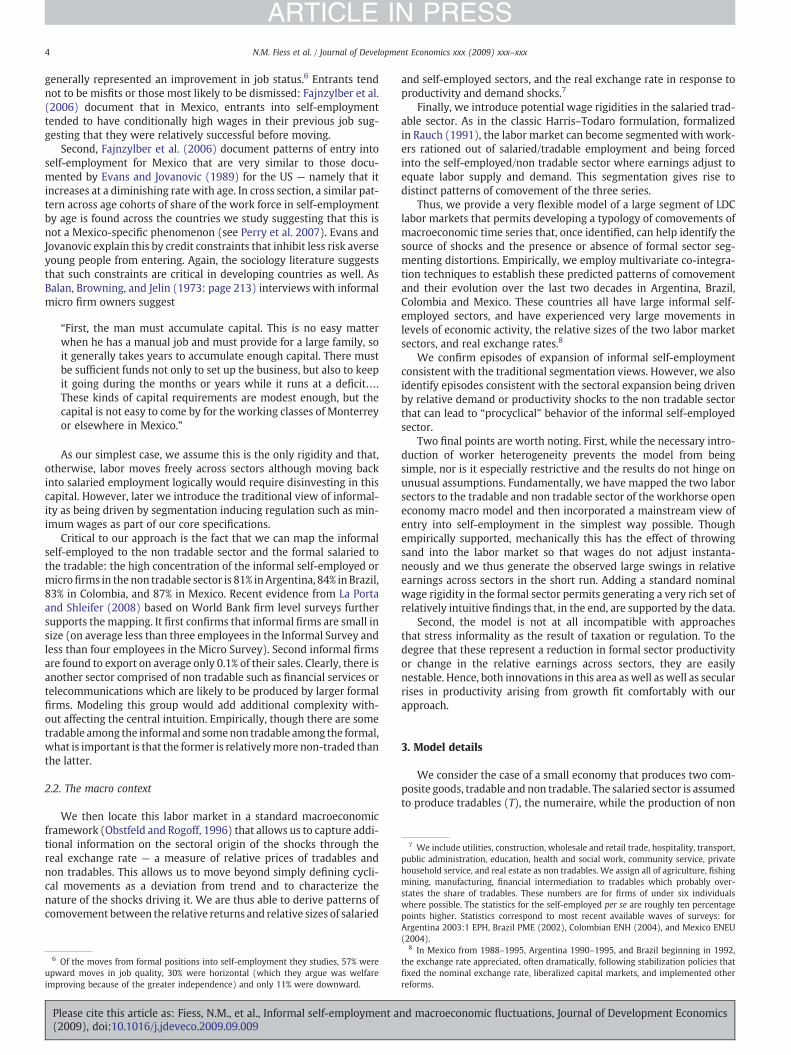
The equations Δkj=0 and Δqj=0 characterize the equilibriumdynamics. They are depicted in a two-equation phase diagram in qand kj that shows the dynamics of the investment decisions of self-
Please cite this article as: Fiess, N.M., et al., Informal self-employment a(2009), doi:10.1016/j.jdeveco.2009.09.009
employed individuals (Fig. 2). The line denoted by SS indicates theperfect foresight path.
As the steady state level of investment chosen by each individual isnot identical, we expect to observe that a common shock affectsheterogeneous individuals differently. When a shock leads to acontraction of the self-employment sector, for workers whose entre-preneurial ability falls below the threshold steady state value of ϕ⁎(those who would be better off in the wage work sector), the perfectforesight path leads to zero capital and zero capital shadow value atsteady state, as depicted inFig. 3. Should self-employment expand, new-entrants invest initially I0 = 1−r
rχ a — independent of the wageprevailing in the salaried sector since the initial shadow value of theircapital is above 1 (q0=1/r). Due to heterogeneous entrepreneurialability, workers will not all move across sectors in the same period. Forinstance, in the case of a shock leading to a rise in returns to self-employment, more able entrepreneurs in the salaried sector wouldmove first. A detailed analysis is presented in Appendix A1.
The adjustment to the steady state depends on the relative values ofσ and θ. Indeed, CT,t is given by Eq. (7) which suggests that the level oftradables consumption along the saddle path is affected by variations inp in a manner that could either reinforce or offset the impact of a shock.The impact of a rise in p on consumption is dampened by consumers'inter-temporal choices ifσNθ, andamplified ifσbθ. IfσNθ, consumptionof non tradables declines slower than consumption of tradables. Theopposite occurs if σbθ. This implies that migration takes longer in asituationwhen inter-temporal substitution prevails over intra-temporalsubstitution.
3.4. Responses to productivity and demand shocks
In order to define short/medium term properties we need to qualify“on-impact” effects of various shocks. Short/medium term propertieswould then reflect variables' behavior after impact and during thetransition towards the new steady state. On impact, levels of productionand consumption must remain constant. Thus any wealth effectsgenerated by the shock must be offset by an instantaneous change inprices. In order to simplify the analysis, we assume that changes inwealth occurring on impact reflect only the shock's direct effects.15 Thatis, changes inwealth due to subsequent changes in prices are accountedfor in the long run. This assumption does not affect qualitatively theproperties of the model.
We first assess the impact of permanent productivity and consump-tion shocks which, as mentioned earlier, could include changes inregulation or taxes. We then introduce wage rigidities in the salariedsector. The results of all exercises as well as their empirically testablecounterpart are presented in Table 1.
nd macroeconomic fluctuations, Journal of Development Economics
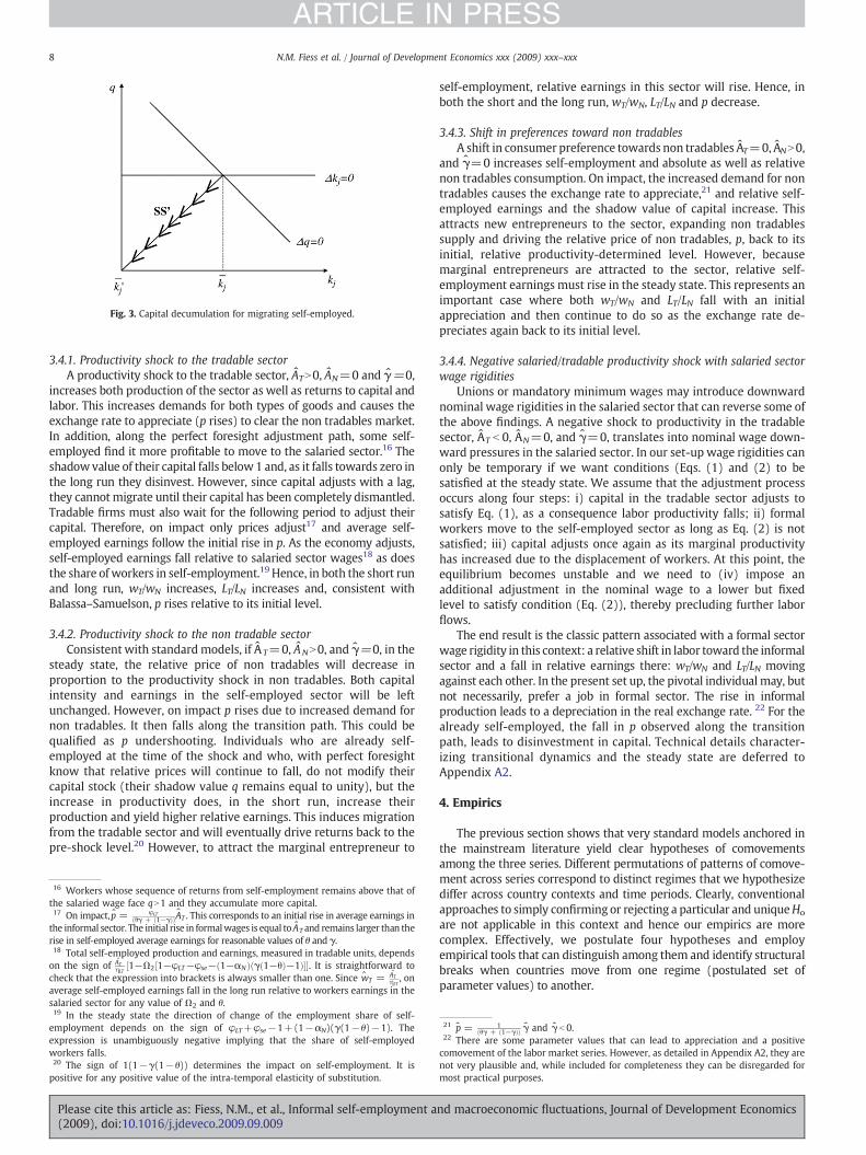
Fig. 3. Capital decumulation for migrating self-employed.
8 N.M. Fiess et al. / Journal of Development Economics xxx (2009) xxx–xxx
ARTICLE IN PRESS
3.4.1. Productivity shock to the tradable sectorA productivity shock to the tradable sector, ATN0, AN=0 and γ =0,
increases both production of the sector as well as returns to capital andlabor. This increases demands for both types of goods and causes theexchange rate to appreciate (p rises) to clear the non tradables market.In addition, along the perfect foresight adjustment path, some self-employed find it more profitable to move to the salaried sector.16 Theshadowvalue of their capital falls below1 and, as it falls towards zero inthe long run they disinvest. However, since capital adjusts with a lag,they cannot migrate until their capital has been completely dismantled.Tradable firms must also wait for the following period to adjust theircapital. Therefore, on impact only prices adjust17 and average self-employed earnings follow the initial rise in p. As the economy adjusts,self-employed earnings fall relative to salaried sector wages18 as doesthe share of workers in self-employment.19 Hence, in both the short runand long run, wT/wN increases, LT/LN increases and, consistent withBalassa–Samuelson, p rises relative to its initial level.
3.4.2. Productivity shock to the non tradable sectorConsistent with standardmodels, if A T=0, ANN0, and γ=0, in the
steady state, the relative price of non tradables will decrease inproportion to the productivity shock in non tradables. Both capitalintensity and earnings in the self-employed sector will be leftunchanged. However, on impact p rises due to increased demand fornon tradables. It then falls along the transition path. This could bequalified as p undershooting. Individuals who are already self-employed at the time of the shock and who, with perfect foresightknow that relative prices will continue to fall, do not modify theircapital stock (their shadow value q remains equal to unity), but theincrease in productivity does, in the short run, increase theirproduction and yield higher relative earnings. This induces migrationfrom the tradable sector and will eventually drive returns back to thepre-shock level.20 However, to attract the marginal entrepreneur to
16 Workers whose sequence of returns from self-employment remains above that ofthe salaried wage face qN1 and they accumulate more capital.17 On impact, p = φLT
ðθγ + ð1−γÞÞAT . This corresponds to an initial rise in average earnings inthe informal sector. The initial rise in formalwages is equal to AT and remains larger than therise in self-employed average earnings for reasonable values of θ and γ.18 Total self-employed production and earnings, measured in tradable units, dependson the sign of AT
ηLT½1−Ω2½1−φLT−φse−ð1−αNÞðγð1−θÞ−1Þ��. It is straightforward to
check that the expression into brackets is always smaller than one. Since wT = ATηLT
, onaverage self-employed earnings fall in the long run relative to workers earnings in thesalaried sector for any value of Ω2 and θ.19 In the steady state the direction of change of the employment share of self-employment depends on the sign of φLT+φse−1+(1−αN)(γ(1−θ)−1). Theexpression is unambiguously negative implying that the share of self-employedworkers falls.20 The sign of 1(1−γ(1−θ)) determines the impact on self-employment. It ispositive for any positive value of the intra-temporal elasticity of substitution.
Please cite this article as: Fiess, N.M., et al., Informal self-employment a(2009), doi:10.1016/j.jdeveco.2009.09.009
self-employment, relative earnings in this sector will rise. Hence, inboth the short and the long run, wT/wN, LT/LN and p decrease.
3.4.3. Shift in preferences toward non tradablesA shift in consumer preference towards non tradables AT=0, ANN0,
and γ=0 increases self-employment and absolute as well as relativenon tradables consumption. On impact, the increased demand for nontradables causes the exchange rate to appreciate,21 and relative self-employed earnings and the shadow value of capital increase. Thisattracts new entrepreneurs to the sector, expanding non tradablessupply and driving the relative price of non tradables, p, back to itsinitial, relative productivity-determined level. However, becausemarginal entrepreneurs are attracted to the sector, relative self-employment earnings must rise in the steady state. This represents animportant case where both wT/wN and LT/LN fall with an initialappreciation and then continue to do so as the exchange rate de-preciates again back to its initial level.
3.4.4. Negative salaried/tradable productivity shock with salaried sectorwage rigidities
Unions or mandatory minimum wages may introduce downwardnominal wage rigidities in the salaried sector that can reverse some ofthe above findings. A negative shock to productivity in the tradablesector, AT b 0, AN=0, and γ=0, translates into nominal wage down-ward pressures in the salaried sector. In our set-up wage rigidities canonly be temporary if we want conditions (Eqs. (1) and (2) to besatisfied at the steady state. We assume that the adjustment processoccurs along four steps: i) capital in the tradable sector adjusts tosatisfy Eq. (1), as a consequence labor productivity falls; ii) formalworkers move to the self-employed sector as long as Eq. (2) is notsatisfied; iii) capital adjusts once again as its marginal productivityhas increased due to the displacement of workers. At this point, theequilibrium becomes unstable and we need to (iv) impose anadditional adjustment in the nominal wage to a lower but fixedlevel to satisfy condition (Eq. (2)), thereby precluding further laborflows.
The end result is the classic pattern associated with a formal sectorwage rigidity in this context: a relative shift in labor toward the informalsector and a fall in relative earnings there: wT/wN and LT/LN movingagainst each other. In the present set up, the pivotal individual may, butnot necessarily, prefer a job in formal sector. The rise in informalproduction leads to a depreciation in the real exchange rate. 22 For thealready self-employed, the fall in p observed along the transitionpath, leads to disinvestment in capital. Technical details character-izing transitional dynamics and the steady state are deferred toAppendix A2.
4. Empirics
The previous section shows that very standard models anchored inthe mainstream literature yield clear hypotheses of comovementsamong the three series. Different permutations of patterns of comove-ment across series correspond to distinct regimes that we hypothesizediffer across country contexts and time periods. Clearly, conventionalapproaches to simply confirming or rejecting a particular and uniqueHo
are not applicable in this context and hence our empirics are morecomplex. Effectively, we postulate four hypotheses and employempirical tools that can distinguish among them and identify structuralbreaks when countries move from one regime (postulated set ofparameter values) to another.
21 p = 1ðθγ + ð1−γÞÞ γ and γ b 0.
22 There are some parameter values that can lead to appreciation and a positivecomovement of the labor market series. However, as detailed in Appendix A2, they arenot very plausible and, while included for completeness they can be disregarded formost practical purposes.
nd macroeconomic fluctuations, Journal of Development Economics

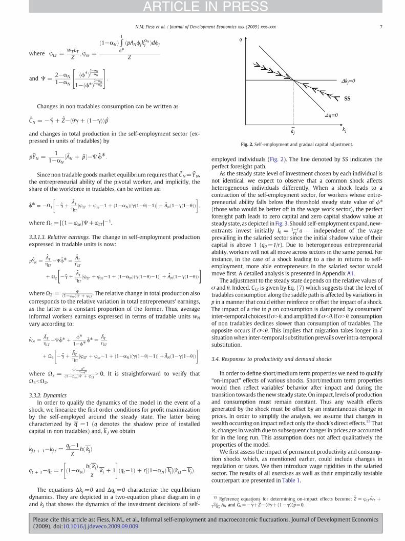
Fig. 4.Mexico: Parameter stability of co-integration space.Note: Parameter stability of co-integration spaces is assessed usingHansen and Johansen (1993, 1999). The test displayedis for constancy of full sample estimate as in Table 2, Interpretation is as follows, 1 presentsthe normalized critical value at the 5% level of significance. Values below 1 indicateparameter stability. Black dotted line represent to test statistic based on backward re-cursion (using the period of 1998Q1 to 2004Q4 as base sample and adding one period at atime until the start of the sample is reached. The grey line represents the test statisticsbased on forward recursion (usingperiod of 1987Q1 to 1993Q4 as baseperiod and addingone observation at the time until the end of the sample is reached. Backward and forwardrecursions are used to in parallel to investigate parameter stability at the beginning andend of the sample. The full sample estimate points to integration, as such, we supportintegration pre 1991 and post 1997. During 1992–1996 the full sample estimate ofintegration is rejected. This merits further subsample analysis.
9N.M. Fiess et al. / Journal of Development Economics xxx (2009) xxx–xxx
ARTICLE IN PRESS
Before proceeding, two conclusions are important. First, indepen-dent of skill heterogeneity and adjustment costs, under no conditionscan we generate a counter movement of relative sector sizes andearnings in the absence of a wage rigidity: observed counter move-ments imply segmentation and if we detect them empirically, this isevidence of labormarket distortions. Second, in all cases, the short runlabor market dynamics move in the same direction as the steady stateand only in the case of a shock to preferences for non tradables doesthe exchange rate overshoot in the short-run.
We explore the patterns of comovement between relative sectorsizes, relative earnings and the real exchange rate for Argentina,Mexico, Brazil and Colombia using the multivariate Johansen (1988)approach. (see Appendix A3). Although co-integration is sometimesgiven the economic interpretation of capturing “long run” relations,as Granger (1991) and Hakkio and Rush (1991) at core it is a statisticalrelationship existing among non-stationary series that can occur atany frequency or span.23 In our case, relative sector sizes, earningsand the real exchange rate are plausibly non-stationary and in-tegrated of order of one and they always appear to be so in theanalysis.24 Since overshooting or undershooting (as found in the caseof a productivity shock or a demand shock respectively to the nontradable sector) can take a number of years to return to long runequilibrium, our short/medium runs can, in fact, represent quitepersistent phenomena that will be identified by the co-integrationrelationship as well.
4.1. Data
We use quarterly data for Mexico, Brazil and Colombia and semi-annual data for Argentina (see Appendix A4 for data definitions anddetails) to generate the earnings ratio of salaried over self-employedworkers, wT/wN, and the ratio of the absolute size of the salaried overthe self-employed sector, LT/LN. To the degree possible, we try to beconsistent across surveys and in spirit be close to the traditional ILOdefinition based on firm size and the more recent focus on laborprotections:we treat themale population that reports being employedin firms of greater than 6workers as salaried (tradable)workers. Own-account workers or heads of firms employing fewer than 5 employeespaying no social security contributions and excluding professionalsand technicians, constitute the informal self-employed (non tradable)sector. Real exchange rates, p, were taken from International FinancialStatistics. The series are plotted in Fig. 1b with the exchange rateinverted for greater graphical clarity (an upward movement here andhere alone is a depreciation).
Three issues merit note. First, even if remuneration is equalized inboth sectors, we do not observe non-monetary remuneration(independence, benefits foregone, taxes avoided, implicit returns tocapital, etc.) and hence we may observe a wedge in observed returnseven in equilibrium.We assume that these non-monetary componentsare a constant fraction ofmonetary earnings and hence that changes inrelative monetary earnings are a good proxy for relative changes intotal remuneration. Second, variations in definitions and the compo-sition of payment can cause substantial differences in ratios of relativeearnings across countries. As a final reminder, we do not model orstudy those salaried workers who are uncovered by labor legislationand hence are informal. The particular cyclical behavior of this groupmerits independent study in another paper.
23 See Hakkio and Rush (1991) Cointegration: How long is the long-run?: “Clearly, thelength of the ‘long-run’ may vary between problems, that is, for some issues the long-run may be a matter of decades while for others a matter of months.”24 Theoretically, however, it is legitimate to include an I(0) variable in the co-integrating relationship, although we would expect at least one co-integrating vectorto emerge that captures simply the stationary series. In practice, these series werenever stationary across our sample and the problem was moot.
Please cite this article as: Fiess, N.M., et al., Informal self-employment a(2009), doi:10.1016/j.jdeveco.2009.09.009
4.2. Results
We begin by estimating separate VAR models for Argentina,Mexico, Brazil and Colombia (Figs. 4–7). We include a constant, lagsfor p, wT/wN and LT/LN as well as time dummies in the co-integrationspace. These specifications prove sufficient to produce random errors.The specifications for the models are presented in Tables A1–A3 in theAppendix A5 along with tests for long run exclusion, stationarity andweak-exogeneity. All variables appear to be non-stationary and thediagnostics on the residuals appear reasonable in terms of autocorre-lation and normality. Sensitivity analysis for different lag lengths andwith and without dummies sustains the robustness of the findings.Trace tests (λtrace) indicate one significant co-integrating vector for allthree models (Table A4).
Normalizing the co-integration vectors on the 1st element, yieldsthe estimates for the βs (Table 2) as a co-integration vector that canbe read as:
LT = LN + βWwT =wN + βpp + βC = 0 ð8Þ
Eq. (8) provides the workhorse specification for generating co-integration vectors which correspond to one of the four regimesdetailed in Table 1.
Regime A (HA: βWb0, βpb0) corresponds to productivity shocks toone or the other sectors in the presence of a integrated (non-segmented) labor market captured by βWb0.
Regime B (HB: βWb0, βpN0) corresponds to a demand shock andthe resulting over (under) shooting in the case of shift in preferencestoward (away from) non tradable/informal goods. Again, βWb0 sincelabor markets adjust freely, but βpN0 corresponds to the reversemovement exchange rate in this case.
Regime C (HC: βWN0, βpN0) corresponds to the case of a negativeshock to the formal sector where wages cannot adjust downward andthe labor market becomes segmented, βWN0: the two labor variablesmove oppositely — workers are shed from the tradable/formal sectorand rationed into the non tradable/informal sector depressing relativeearnings in that sector. βpN0 since the exchange rate depreciates.
nd macroeconomic fluctuations, Journal of Development Economics

Fig. 5. Brazil: parameter stability of co-integration space. Note: Parameter stability of co-integration spaces is assessed using Hansen and Johansen (1993, 1999). The test displayedis for constancy of full sample estimate as in Table 2, Interpretation is as follows, 1 presentsthe normalized critical value at the 5% level of significance. Values below 1 indicateparameter stability. Black dotted line represent to test statistic based on backwardrecursion (using the period of 1995Q1 to 2002Q4 as base sample and adding one period ata time until the start of the sample is reached. The grey line represents the test statisticsbased on forward recursion (usingperiodof 1984Q1 to 1989Q4 as base period and addingone observation at the time until the end of the sample is reached. Backward and forwardrecursions are used to in parallel to investigate parameter stability at the beginning andend of the sample.
Fig. 7. Argentina: parameter stability of co-integration space. Note: Parameter stabilityof co-integration spaces is assessed using Hansen and Johansen (1993, 1999). The testdisplayed is for constancy of full sample estimate as in Table 2, Interpretation is asfollows, 1 presents the normalized critical value at the 5% level of significance. Valuesbelow1 indicate parameter stability. Black dotted line represent to test statistic based onbackward recursion (using the period of 1996 H1 to 2003 H1 as base sample and addingone period at a time until the start of the sample is reached. The grey line represents thetest statistics based on forward recursion (using period of 1987 H2 to 1994 H1 as baseperiod and adding one observation at the time until the end of the sample is reached.Backward and forward recursions are used to in parallel to investigate parameterstability at the beginning and end of the sample.
10 N.M. Fiess et al. / Journal of Development Economics xxx (2009) xxx–xxx
ARTICLE IN PRESS
Regime D (HD: βWb0, βp=0) corresponds to the long run (in theeconomic sense) version of “B” where capital has moved to equalizerates of return, expanding production of non tradables and hencelowering their relative price again rendering βp=0: taste changeshave no long run effect on the exchange rate.
We identify three of these regimes in the data plus one more thatwill be discussed later. That is, co-integration vectors corresponding tothe restrictions of each regime are estimated for at least one subperiod.Since we deal with 10 separate periods, we will discuss only a few indetail.
The estimates across the whole sample are presented in the firstcolumn of each country panel of Table 2. However, the theoreticalmodel suggests that different shocks, or differing degrees of formal
Fig. 6. Colombia: parameter stability of co-integration space. Note: Parameter stability ofco-integration spaces is assessed using Hansen and Johansen (1993, 1999). The testdisplayed is for constancy of full sample estimate as in Table 2, Interpretation is as follows,1 presents the normalized critical value at the 5% level of significance. Values below 1indicate parameter stability. Black dotted line represent to test statistic based onbackwardrecursion (using the periodof 1996Q1 to 2004Q2as base sample and addingone period ata time until the start of the sample is reached. The grey line represents the test statisticsbased on forward recursion (usingperiodof 1985Q3 to 1995Q4 as base period and addingone observation at the time until the end of the sample is reached. Backward and forwardrecursions are used to in parallel to investigate parameter stability at the beginning andend of the sample.
Please cite this article as: Fiess, N.M., et al., Informal self-employment a(2009), doi:10.1016/j.jdeveco.2009.09.009
sector rigidities, should lead to different regimes and hence differentco-integration vectors across subsamples. To investigate the stabilityof the co-integration space, we follow Hansen and Johansen (1993,1999). We perform backward and forward recursions stability toexplore the stability of the co-integration space at both sample ends. Inthe event of parameter instability, we then test for specific co-integrating vectors across subperiods.
For Argentina, theHansen and Johansen tests identify no significantchange in co-integration coefficients across the sample. The fullsample estimations are reported in Table 2 and suggest a classicsegmented labor market that corresponds to Regime “C”. Thecomovements of the series, βWN0, βpb0 appear driven by shocks tothe formal sector in the presence of binding wage rigidities. This isarguably consistent with the very high rates of unemployment thatrose from roughly 6.5% in 1991 to 18% in 1995 and remained in thehigh double digits for much of the rest of our sample period.
However, recursive estimations of the co-integration space in theother three country cases do suggest significant co-efficient instability.Due to the existence of thesemultiple regimes, we label the full sampleestimates “mixed” even though the estimated vector may suggest aparticular regime.
Taking the full sample, Colombia presents a case similar toArgentina with βWN0 suggesting segmentation in the labor market.The sub-period from 1997–2004, in particular is consistent with aclassic segmentedmarket and productivity shocks to the formal sectordriving themovements of the three series. Colombia, in fact, entered asevere recession in the late 1990s concomitant with a sharp rise in thereal minimum wage. The latter was driven by indexing wages to aforecast of inflation that later turned out to be pessimistically high by asubstantial margin. Although the co-efficient on βp is not estimatedprecisely, Fig. 1b shows a classic case of Regime “C” across this periodwhere the two labormarket series are very clearlymoving against eachother while the exchange rate depreciates.
The backward recursion test suggests, however, that this vectoris not stable across the whole period and we identify two otherregimes. In the intermediate 1991–1996 period, we find βWb0suggesting the labor market is behaving in an integrated fashionand the βpN0 consistent with an increase in relative informal sectorsize and earnings driven by a positive demand shock to the informal/non tradable sector. In this example of Regime “B,” informality is“procyclical.”
A similar pattern appears broadly to characterize the full sample inMexico: βW is not significant suggesting the absence of significant
nd macroeconomic fluctuations, Journal of Development Economics
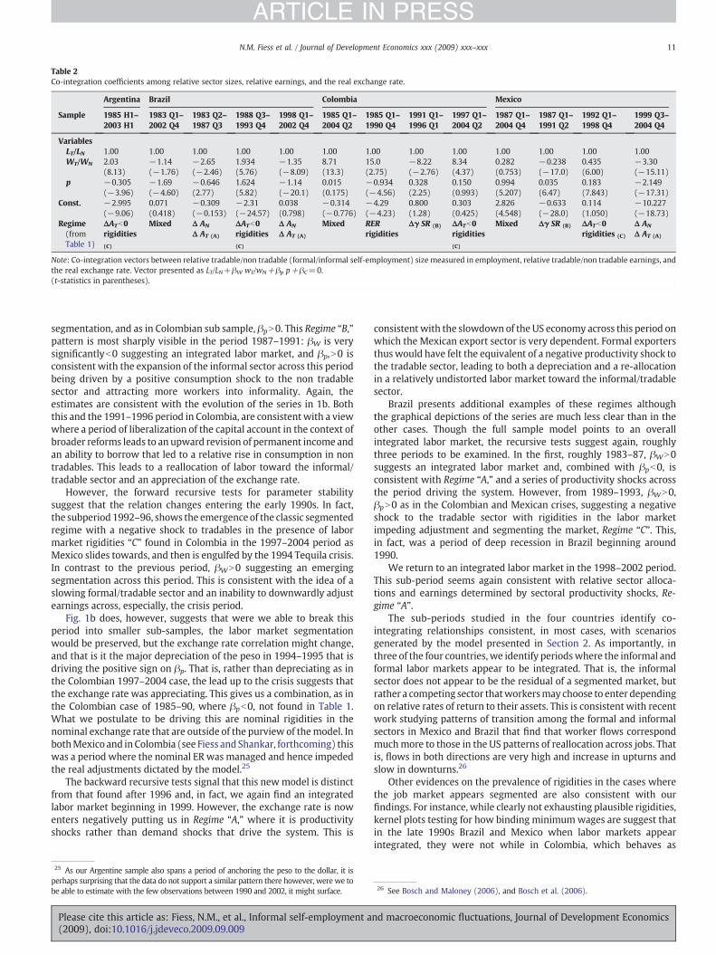
Table 2Co-integration coefficients among relative sector sizes, relative earnings, and the real exchange rate.
Argentina Brazil Colombia Mexico
Sample 1985 H1–2003 H1
1983 Q1–2002 Q4
1983 Q2–1987 Q3
1988 Q3–1993 Q4
1998 Q1–2002 Q4
1985 Q1–2004 Q2
1985 Q1–1990 Q4
1991 Q1–1996 Q1
1997 Q1–2004 Q2
1987 Q1–2004 Q4
1987 Q1–1991 Q2
1992 Q1–1998 Q4
1999 Q3–2004 Q4
VariablesLT/LN 1.00 1.00 1.00 1.00 1.00 1.00 1.00 1.00 1.00 1.00 1.00 1.00 1.00WT/WN 2.03
(8.13)−1.14(−1.76)
−2.65(−2.46)
1.934(5.76)
−1.35(−8.09)
8.71(13.3)
15.0(2.75)
−8.22(−2.76)
8.34(4.37)
0.282(0.753)
−0.238(−17.0)
0.435(6.00)
−3.30(−15.11)
p −0.305(−3.96)
−1.69(−4.60)
−0.646(2.77)
1.624(5.82)
−1.14(−20.1)
0.015(0.175)
−0.934(−4.56)
0.328(2.25)
0.150(0.993)
0.994(5.207)
0.035(6.47)
0.183(7.843)
−2.149(−17.31)
Const. −2.995(−9.06)
0.071(0.418)
−0.309(−0.153)
−2.31(−24.57)
0.038(0.798)
−0.314(−0.776)
−4.29(−4.23)
0.800(1.28)
0.303(0.425)
2.826(4.548)
−0.633(−28.0)
0.114(1.050)
−10.227(−18.73)
Regime(fromTable 1)
ΔATb0rigidities(C)
Mixed Δ AN
Δ AT (A)
ΔATb0rigidities(C)
Δ AN
Δ AT (A)
Mixed RERrigidities
Δγ SR (B) ΔATb0rigidities(C)
Mixed Δγ SR (B) ΔATb0rigidities (C)
Δ AN
Δ AT (A)
Note: Co-integration vectors between relative tradable/non tradable (formal/informal self-employment) size measured in employment, relative tradable/non tradable earnings, andthe real exchange rate. Vector presented as LT/LN+βW wT/wN+βp p+βC=0.(t-statistics in parentheses).
11N.M. Fiess et al. / Journal of Development Economics xxx (2009) xxx–xxx
ARTICLE IN PRESS
segmentation, and as in Colombian sub sample, βpN0. This Regime “B,”pattern is most sharply visible in the period 1987–1991: βW is verysignificantlyb0 suggesting an integrated labor market, and βp,N0 isconsistent with the expansion of the informal sector across this periodbeing driven by a positive consumption shock to the non tradablesector and attracting more workers into informality. Again, theestimates are consistent with the evolution of the series in 1b. Boththis and the 1991–1996 period in Colombia, are consistentwith a viewwhere a period of liberalization of the capital account in the context ofbroader reforms leads to an upward revision of permanent income andan ability to borrow that led to a relative rise in consumption in nontradables. This leads to a reallocation of labor toward the informal/tradable sector and an appreciation of the exchange rate.
However, the forward recursive tests for parameter stabilitysuggest that the relation changes entering the early 1990s. In fact,the subperiod 1992–96, shows the emergence of the classic segmentedregime with a negative shock to tradables in the presence of labormarket rigidities “C” found in Colombia in the 1997–2004 period asMexico slides towards, and then is engulfed by the 1994 Tequila crisis.In contrast to the previous period, βWN0 suggesting an emergingsegmentation across this period. This is consistent with the idea of aslowing formal/tradable sector and an inability to downwardly adjustearnings across, especially, the crisis period.
Fig. 1b does, however, suggests that were we able to break thisperiod into smaller sub-samples, the labor market segmentationwould be preserved, but the exchange rate correlation might change,and that is it the major depreciation of the peso in 1994–1995 that isdriving the positive sign on βp. That is, rather than depreciating as inthe Colombian 1997–2004 case, the lead up to the crisis suggests thatthe exchange rate was appreciating. This gives us a combination, as inthe Colombian case of 1985–90, where βpb0, not found in Table 1.What we postulate to be driving this are nominal rigidities in thenominal exchange rate that are outside of the purview of themodel. InbothMexico and in Colombia (see Fiess and Shankar, forthcoming) thiswas a period where the nominal ER was managed and hence impededthe real adjustments dictated by the model.25
The backward recursive tests signal that this newmodel is distinctfrom that found after 1996 and, in fact, we again find an integratedlabor market beginning in 1999. However, the exchange rate is nowenters negatively putting us in Regime “A,” where it is productivityshocks rather than demand shocks that drive the system. This is
25 As our Argentine sample also spans a period of anchoring the peso to the dollar, it isperhaps surprising that the data do not support a similar pattern there however, were we tobe able to estimate with the few observations between 1990 and 2002, it might surface.
Please cite this article as: Fiess, N.M., et al., Informal self-employment a(2009), doi:10.1016/j.jdeveco.2009.09.009
consistent with the slowdown of the US economy across this period onwhich the Mexican export sector is very dependent. Formal exportersthuswould have felt the equivalent of a negative productivity shock tothe tradable sector, leading to both a depreciation and a re-allocationin a relatively undistorted labor market toward the informal/tradablesector.
Brazil presents additional examples of these regimes althoughthe graphical depictions of the series are much less clear than in theother cases. Though the full sample model points to an overallintegrated labor market, the recursive tests suggest again, roughlythree periods to be examined. In the first, roughly 1983–87, βWN0suggests an integrated labor market and, combined with βpb0, isconsistent with Regime “A,” and a series of productivity shocks acrossthe period driving the system. However, from 1989–1993, βWN0,βpN0 as in the Colombian and Mexican crises, suggesting a negativeshock to the tradable sector with rigidities in the labor marketimpeding adjustment and segmenting the market, Regime “C”. This,in fact, was a period of deep recession in Brazil beginning around1990.
We return to an integrated labor market in the 1998–2002 period.This sub-period seems again consistent with relative sector alloca-tions and earnings determined by sectoral productivity shocks, Re-gime “A”.
The sub-periods studied in the four countries identify co-integrating relationships consistent, in most cases, with scenariosgenerated by the model presented in Section 2. As importantly, inthree of the four countries, we identify periodswhere the informal andformal labor markets appear to be integrated. That is, the informalsector does not appear to be the residual of a segmented market, butrather a competing sector thatworkersmay choose to enter dependingon relative rates of return to their assets. This is consistent with recentwork studying patterns of transition among the formal and informalsectors in Mexico and Brazil that find that worker flows correspondmuchmore to those in the US patterns of reallocation across jobs. Thatis, flows in both directions are very high and increase in upturns andslow in downturns.26
Other evidences on the prevalence of rigidities in the cases wherethe job market appears segmented are also consistent with ourfindings. For instance, while clearly not exhausting plausible rigidities,kernel plots testing for how binding minimumwages are suggest thatin the late 1990s Brazil and Mexico when labor markets appearintegrated, they were not while in Colombia, which behaves as
26 See Bosch and Maloney (2006), and Bosch et al. (2006).
nd macroeconomic fluctuations, Journal of Development Economics
12 N.M. Fiess et al. / Journal of Development Economics xxx (2009) xxx–xxx
ARTICLE IN PRESS
segmented in this period, they were among the most binding in theregion.27 Further, the periods of apparent segmentation in Brazil,Colombia and Mexico correspond to periods of deep recession where,as is often the case, wages do not adjust enough to prevent un-employment or, in this case, segmentation.
We find several episodes where the informal sector appears toexpand concomitant with a rise in its relative earnings, during up-turns. That is, it is procyclical. Loayza and Rigolini do find somecountries in their global panel, for which self-employment (also theirmeasure of informality) is procyclical, however the majority are not.Since, for both Colombia and Mexico (insignificantly) full samplefindings of segmentation conceal periods of integration and procycli-cality, we suspect that their sample averages are similarly concealingsome more complex cyclical stories. The same can be said about thecross sectional correlations found in Boeri and Gribaldi. Henceempirically, the various papers are probably not necessarily inconsis-tent. Conceptually, our guess is that were most of the discussedmodels to add a second sector, their models could likely accommodatethe findings here as well.
5. Conclusion
This paper has offered a framework through which to study self-employment across macroeconomic fluctuations. We model a two-sector labor market in an Obstfeld–Rogoff small economy modelto include heterogeneous entrepreneurial ability and credit con-straints to entering informal self-employment. This allows us togenerate a set of hypotheses about the comovement of relative sectorsizes and earnings and sectoral shocks as captured by the real exchangerate.
These patterns of comovement are then tested in a co-integrationframework in Argentina, Brazil, Colombia and Mexico. Three impor-tant general findings emerge. First, we find examples of all the co-integration vectors suggested by theory suggesting that attention tocountry and period context is important to approaching the informalsector. In particular, and second, although the informal self-employedand formal salaried sectors often appear as elements of segmented ordual labor markets as customarily envisaged, we also find numerousepisodeswhere they appear as one integrated labormarket: numerousperiods show strong comovement between relative sector sizes andearnings. This suggests that a large component of the informal sectorshould not be viewed as somehow inferior or queuing for formal sectoremployment. However, it is also the case that rigidities in the formalsalaried sector can become very binding, as is most clearly the case inthe dramatic crises that affected all four countries at some period, andapparently in Argentina across the entire sample. Third, these distinctpatterns suggest that the pro or countercyclicality of the sectors maydepend on the sectoral origin of the shocks, and the presence ofbinding wage rigidities. We find numerous examples where either apositive productivity or demand shock to the non tradable/informalsector leads to its expansion.
Acknowledgment
Thiswork partially financed by the Regional Studies Programof theOffice of the Chief Economist for LatinAmerica and the Caribbean. It is asubstantially reworked version of the previous “Exchange RateAppreciations, Labor Market Rigidities and Informality” (2002). Weare grateful to Rashmi Shankar for early conceptual discussions, toLeonardo Gaspirini for helpful comments, to Norman Loayza andClaudio Montenegro for help with data, and to Gabriel Montes forexpert research assistance.
27 See Maloney and Nuñez (2004).
Please cite this article as: Fiess, N.M., et al., Informal self-employment a(2009), doi:10.1016/j.jdeveco.2009.09.009
Appendix A1. Migration timing
Because we assume that the self-employed individual, who iswilling to move to the wage-work sector, has to disinstall the capitalshe borrowed before moving, migration occurs whenever,
ptAn;tϕjkαNN;t−
χ2
ðI2j;tÞhðkj;tÞ
−rkn;t + ∑∞
s= t + 1
11 + r
� �s−t
psAn;sϕjkαNN;s−
χ2
ðI2j;sÞhðkj;sÞ
−rkn;s
" #
≤ptAn;tϕjkαNN;t−
χ2ð−kj;tÞ2hðkj;tÞ
−rkn;t + ∑∞
s= t + 1
11 + r
� �s−t
wT ;s
Labor could adjust within the first period following the shock.However, because individuals are non homogenous when producingin the self-employed sector, the optimal time for leaving the lattermay differ across workers.
The Left Hand Side of the above expression is increasing withentrepreneurial ability. Namely, more able individuals earnmore thanless able ones. Then the opportunity cost of migrating to the salariedsector at time t, without considering the direct migration costs corres-ponding to capital disinstallation, is increasing in the level ofentrepreneurial capability. The last term of the RHS, which representsthe present value of labor earnings in the salaried sector is identical forall individuals at time t. However, the first term of the RHS is likely tobe different. The sign of the partial derivative of the latter with respectto ϕ j is given by
1− χ2ð1−αNÞ
αN
rða + kjÞ2−a2
ða + kjÞ2" #
If the above expression appears to be positive, that would implythat the cost of migrating to the salaried sector at time is increasingwith the level of entrepreneurial capability. If this is the case, then thetotal cost of migration is unambiguously increasing with ϕ j. As aconsequence we may expect more able entrepreneurs to postponetheirmigration towards thewage sectorwith respect to less able ones.
In the case of a shock leading to an expansion of the self-employedsector, migration can occur within the first period following the shock,even though capital accumulation may take more than a periodbecause of installation costs. Individuals migrate at the end of period swhenever
wT ;t−χk2j;t + 1
hð0Þ
!+ ∑
∞
s= t + 1
11 + r
� �s−t
psAn;sϕjkαNN;s−
χ2
ðI2j;sÞhðkj;sÞ
−rkn;s
" #
≥wT ;t + ∑∞
s= t + 1
11 + r
� �s−t
wT;s
Following arguments similar to those presented above, we caninfer that more able entrepreneurs will leave the salaried sector first,in order to “cash in” the expected earnings differential the soonest.
Appendix A2. Details on negative tradables productivity shockwith salaried sector wage rigidities
Unions or mandatory minimum wages may introduce downwardnominal wage rigidities in the salaried sector that can reverse many ofthe findings above.
A negative shock to productivity in the tradable sector translatesinto nominal wage downward pressures in the salaried sector.Nominal wage downward rigidities, if persistent, would lead to anon-optimal and thus unstable equilibrium. In order to obtain apossibly stable equilibrium, we assume that nominal wages areadjusted to satisfy the first order conditions of firms operating in thetradable sector. However, we assume that wage variations representthe last element of adjustment. That is, labor movements are
nd macroeconomic fluctuations, Journal of Development Economics

13N.M. Fiess et al. / Journal of Development Economics xxx (2009) xxx–xxx
ARTICLE IN PRESS
precluded after wages have been adjusted. As a consequence, thepivotal individual could endup in a situationwhere belonging to eitherone or the other sector does make a difference. This is a case ofsegmentation where the non tradable sector behaves in part as aresidual sector.
In summary, capital adjustment is a two-step process while laboradjustment is only a one-step process. Capital first adjusts to meetEq. (1) in a context of constant salaried labor force. It further adjusts tomeet Eq. (1) considering labor variation obtainedby solvingEq. (2)withconstant wage. Wages adjust in a final stage to satisfy Eq. (2).
Taking for instance the case of a Cobb–Douglas productionfunction, salaried labor outflow28 corresponds to
LT =AT
ηLT ð1−ηLT Þð= ϕ*Þ b 0;
⌢KT =
ð1 + ηLT ÞAT
ηLT ð1−ηLT Þb 0 and w =
AT
ηLTb 0:
Equilibrium of the demand and supply conditions in the nontradable sector
CN = ðð2−ηLT ÞφLT−φseΨÞ AT
ηLT ð1−ηLT Þ+ φse
11−αN
−ðθγ + ð1−γÞÞ�
p
and
YN =αN
1−αNp−Ψ
AT
ηLT ð1−ηLT Þ
give
p =AT
ηLT ð1−ηLT Þð1−αNÞðð2−ηLT ÞφLT + ð1−φseÞΨÞαN−φse + ð1−αNÞðγθ + ð1−γÞÞ�
and
EðpYNÞ =AT
ηLT ð1−ηLT Þð2−ηLT ÞφLT + ð1−φseÞΨ
αN−φse + ð1−αNÞðγθ + ð1−γÞÞ− Ψ− ϕ⁎1−ϕ⁎
" #" #
The sign of both real exchange rate and average earnings dependsupon the sign and magnitude of expression αN−φse+(1−αN)(γθ+(1−γ)). This expression is increasing with θ, the elasticity of sub-stitution. For θ=1 (preferences are Cobb–Douglas) for instance, theexpression is equal to 1−φse. In that case, both the real exchange rateand average self-employed earnings are decreasing unambiguously.A sufficient condition for the real exchange rate to depreciate isð1−φseÞð1−αNÞγNð1−θÞ. Unless αN and θ are both very close to zero and γ veryclose to one the condition is likely to be always satisfied. However, thesufficient condition for both the relative price of non tradables andaverage earnings to be decreasing is more restrictive, namely θ≤1.Average earnings in the self-employment sector could rise despite the fallin p because in the context of an expansion of the sector the contributionper unit of entrepreneurial ability is higher for less able workers. This is afeature of the model essentially due to the fact that ability enters in alinear manner in the production function of self-employed workers.
As far as relative earnings are concerned, self-employed workerswould become on averageworst off with respect to salariedworkers if
ð2−ηLT ÞφLT + ð1−φseÞΨαN−φse + ð1−αNÞðγθ + ð1−γÞÞ− Ψ− ϕ⁎
1−ϕ⁎
" #" #Nð1−ηLT Þ ðA1Þ
28 In that case, labor demand in the salaried sector at period s can be expressed asLT;s =
ð1−ηLT ÞAT;swT;s
h i1=ηLTKT ;s:
Please cite this article as: Fiess, N.M., et al., Informal self-employment a(2009), doi:10.1016/j.jdeveco.2009.09.009
for θ=1 we must have that
ð2−ηLT ÞφLT
ð1−φseÞ+
ϕ⁎1−ϕ⁎
" #Nð1−ηLT Þ
This condition is likely to be satisfied for any plausible set ofparameters values.
When conditions presented above are satisfied, as labor migratestowards the self-employed sector, production rises, the real exchangerate depreciates, and average earnings in the self-employed sector fall.Moreover, as workers cannot migrate back to the salaried sector, thosewhose entrepreneurial ability is relatively low earn less than what theywould get in the salaried sector. For thoseworkers “trapped” in the self-employed sector earnings performance has worsened relative to thoseemployed in the salaried sector as earnings in the salaried sector arepreserved by institutional rigidities. The two labor force series moveagainst each other. Critically, the same result would hold in the casewhere indexation of wages to past inflation forces salaried sectorwagesabove equilibrium: we should see relative sector sizes and incomesmove against each other.
Appendix A3. Details of Johansen co-integration procedure
The Johansen procedure allows us to test for co-integration in amultivariate system. Starting from an unrestricted vector autoregres-sive model (VAR), the hypothesis of co-integration is formulated as ahypothesis of reduced rank of the long run impact matrix Π(Johansen, 1988, Johansen and Juselius, 1990). The VAR is generatedby the vector zt, which defines the potential endogenous variables ofthe model, in our case, the three series. Taking first differences of thevariables, the VAR can be transformed into an error correction model
Δzt = Γ1Δzt−1 + ::: + Γk−1Δzt−k=1 + Πzt−k + ψDt + εt ; εte INð0; ΣÞwhere the estimates of Γi=−(I−A1−…−Ai),(i=1,…,k−1) describethe short run dynamics to changes in zt and Π=−(I−A1−…−Ai)captures the long run adjustments and D contains deterministic terms.
Co-integration occurs in the case of reduced rank ofΠ. If the rank isreduced (rbn) it is possible to factorize Π into Π(=αβ′) where αdenotes the adjustment coefficients and β the co-integration vectors.The co-integration vectors β have the property that β′ zt is stationaryeven though zt itself is non-stationary. If the rank is reduced it is alsopossible to interpret the VAR in first differences as a vector errorcorrection model and to obtain estimates of α and β via the reducedrank regression. Since the rank of Π is equal to the number ofindependent co-integration vectors and the rank of Π is also equal tothe number of non-zero Eigenvalues, the test of co-integration thusamounts to a test for the number of non-zero Eigenvalues. The tracestatistics, λtrace, is a non-standard distributed likelihood-ratio test,which is commonly used to determine the number of co-integrationvectors, (Johansen, 1988). The trace statistic tests the null hypothesisthat there are at most r co-integration vectors:
H0 : λi = 0; for i = r + 1; ::n
where only the first r Eigenvalues, λ, are non-zero against theunrestricted hypothesis that n.29
29 The null hypothesis of at most r co-integration vectors implies that there are n–runit roots and, theoretically, n–r zero Eigenvalues. This is because the hypothesis ofco-integration is formulated as the reduced rank of Π=αβ′ and the full rank of α⊥′Γβ⊥,where α and β are n× r matrices and α⊥ and β⊥ are n×(n–r) matrices orthogonal to αand β. This allows us then to distinguish between r+co-integrating I(0) relations andn–r non-co-integrating I(1) relations.
nd macroeconomic fluctuations, Journal of Development Economics
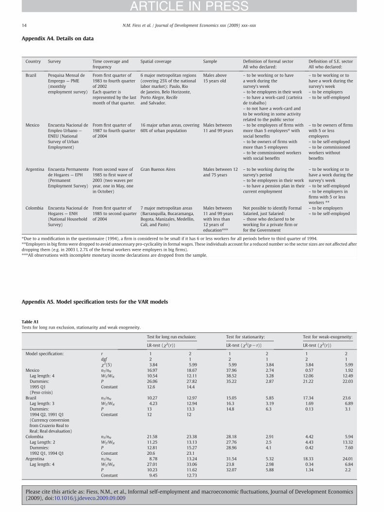
14 N.M. Fiess et al. / Journal of Development Economics xxx (2009) xxx–xxx
ARTICLE IN PRESS
Appendix A4. Details on data
Country Survey Time coverage andfrequency
Spatial coverage Sample Definition of formal sectorAll who declared:
Definition of S.E. sectorAll who declared:
Brazil Pesquisa Mensal deEmprego — PME(monthlyemployment survey)
From first quarter of1983 to fourth quarterof 2002
6 major metropolitan regions(covering 25% of the nationallabor market): Paulo, Riode Janeiro, Belo Horizonte,Porto Alegre, Recifeand Salvador.
Males above15 years old
– to be working or to havea work during thesurvey's week
– to be working or tohave a work during thesurvey's week
Each quarter isrepresented by the lastmonth of that quarter.
– to be employees in their work – to be employers– to have a work-card (carteirade trabalho)
– to be self-employed
– to not have a work-card andto be working in some activityrelated to the public sector
Mexico Encuesta Nacional deEmpleo Urbano —
ENEU (NationalSurvey of UrbanEmployment)
From first quarter of1987 to fourth quarterof 2004
16 major urban areas, covering60% of urban population
Males between11 and 99 years
– to be employees of firms withmore than 5 employees⁎ withsocial benefits
– to be owners of firmswith 5 or lessemployees
– to be owners of firms withmore than 5 employees
– to be self-employed
– to be commissioned workerswith social benefits
– to be commissionedworkers withoutbenefits
Argentina Encuesta Permanentede Hogares — EPH(PermanentEmployment Survey)
From second wave of1985 to first wave of2003 (two waves peryear, one in May, onein October)
Gran Buenos Aires Males between 12and 75 years
– to be working during thesurvey's period
– to be working or tohave a work during thesurvey's week– to be employees in their work– to be self-employed– to have a pension plan in their
current employment – to be employers infirms with 5 or lessworkers ⁎⁎
Colombia Encuesta Nacional deHogares — ENH(National HouseholdSurvey)
From first quarter of1985 to second quarterof 2004
7 major metropolitan areas(Barranquilla, Bucaramanga,Bogota, Manizales, Medellin,Cali, and Pasto)
Males between11 and 99 yearswith less than12 years ofeducation⁎⁎⁎
Not possible to identify FormalSalaried, just Salaried:
– to be employers
– those who declared to beworking for a private firm orfor the Government
– to be self-employed
⁎Due to a modification in the questionnaire (1994), a firm is considered to be small if it has 6 or less workers for all periods before to third quarter of 1994.⁎⁎Employers in big firmswere dropped to avoid unnecessary pro-cyclicality in formal wages. These individuals account for a reduced number so the sector sizes are not affected afterdropping them (e.g. in 2003 I, 2.7% of the formal workers were employers in big firms).⁎⁎⁎All observations with incomplete monetary income declarations are dropped from the sample.
Appendix A5. Model specification tests for the VAR models
Table A1Tests for long run exclusion, stationarity and weak exogeneity.
Test for long run exclusion: Test for stationarity: Test for weak-exogeneity:
LR-test (χ2(r)) LR-test (χ2(p−r)) LR-test (χ2(r))
Model specification: r 1 2 1 2 1 2dgf 2 1 2 1 2 1χ2(5) 3.84 5.99 5.99 3.84 3.84 5.99
Mexico nT/nN 16.97 18.67 37.96 2.74 0.57 1.92Lag length: 4 WT/WN 10.54 12.11 38.52 3.28 12.06 12.49Dummies: P 26.06 27.82 35.22 2.87 21.22 22.031995 Q1 Constant 12.6 14.4(Peso crisis)
Brazil nT/nN 10.27 12.97 15.05 5.85 17.34 23.6Lag length: 3 WT/WN 4.23 12.94 16.3 3.19 1.69 6.89Dummies: P 13 13.3 14.8 6.3 0.13 3.11994 Q2, 1991 Q1 Constant 12 12(Currency conversionfrom Cruzerio Real toReal; Real devaluation)
Colombia nT/nN 21.58 23.38 28.18 2.91 4.42 5.94Lag Length: 2 WT/WN 11.25 13.13 27.76 2.5 4.43 13.32Dummies: P 12.81 15.27 28.96 4.1 0.42 7.601992 Q1, 1994 Q1 Constant 20.6 23.1
Argentina nT/nN 8.78 13.24 31.54 5.32 18.33 24.01Lag length: 4 WT/WN 27.01 33.06 23.8 2.98 0.34 6.84
P 10.23 11.62 32.07 5.88 1.34 2.2Constant 9.45 12.73
Please cite this article as: Fiess, N.M., et al., Informal self-employment and macroeconomic fluctuations, Journal of Development Economics(2009), doi:10.1016/j.jdeveco.2009.09.009
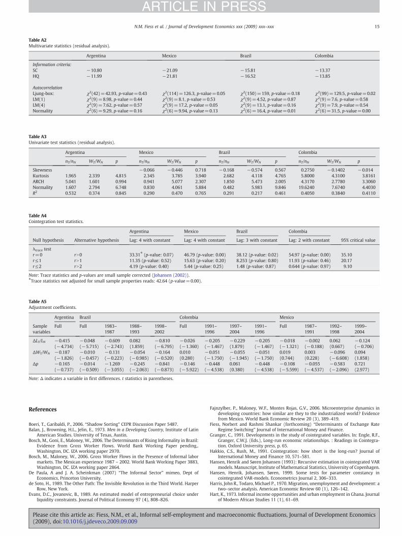
Table A2Multivariate statistics (residual analysis).
Argentina Mexico Brazil Colombia
Information criteria:SC −10.80 −21.09 −15.81 −13.37HQ −11.99 −21.81 −16.52 −13.85
AutocorrelationLjung-box: χ2(42)=42.93, p-value=0.43 χ2(114)=126.3, p-value=0.05 χ2(150)=159, p-value=0.18 χ2(99)=129.5, p-value=0.02LM(1) χ2(9)=8.98, p-value=0.44 χ2(9)=8.1, p-value=0.53 χ2(9)=4.52, p-value=0.87 χ2(9)=7.6, p-value=0.58LM(4) χ2(9)=7.62, p-value=0.57 χ2(9)=17.2, p-value=0.05 χ2(9)=13.1, p-value=0.16 χ2(9)=7.9, p-value=0.54Normality χ2(6)=9.29, p-value=0.16 χ2(6)=9.94, p-value=0.13 χ2(6)=16.4, p-value=0.01 χ2(6)=31.5, p-value=0.00
Table A3Univariate test statistics (residual analysis).
Argentina Mexico Brazil Colombia
nT/nN WT/WN p nT/nN WT/WN p nT/nN WT/WN p nT/nN WT/WN p
Skewness −0.066 −0.446 0.718 −0.168 −0.574 0.567 0.2750 −0.1402 −0.014Kurtosis 1.965 2.339 4.815 2.345 3.785 3.940 2.682 4.118 4.765 5.8000 4.3100 3.8161ARCH 5.041 1.601 0.994 0.941 5.077 2.307 1.850 5.473 2.005 4.3170 2.7780 3.3060Normality 1.607 2.794 6.748 0.830 4.061 5.884 0.482 5.983 9.846 19.6240 7.6740 4.4030R2 0.532 0.374 0.845 0.290 0.470 0.765 0.291 0.217 0.461 0.4050 0.3840 0.4110
Table A5Adjustment coefficients.
Argentina Brazil Colombia Mexico
Samplevariables
Full Full 1983–1987
1988–1993
1998–2002
Full 1991–1996
1997–2004
1991–1996
Full 1987–1991
1992–1998
1999–2004
ΔLT/LN −0.415(−4.734)
−0.048(−5.715)
−0.609(−2.743)
0.082(1.859)
−0.810(−6.795)
−0.026(−1.360)
−0.205(−1.467)
−0.229(1.879)
−0.205(−1.467)
−0.018(−1.321)
−0.002(−0.188)
0.062(0.667)
−0.124(−0.706)
ΔWT/WN −0.187(−1.826)
−0.010(−0.457)
−0.131(−0.223)
−0.054(−0.985)
−0.164(−0.520)
0.010(0.280)
−0.051(−1.750)
−0.055(−1.945)
−0.051(−1.750)
0.019(0.744)
0.003(0.228)
−0.096(−6.608)
0.094(1.858)
Δp −0.165(−0.737)
−0.014(−0.509)
−1.269(−3.055)
−0.245(−2.063)
−0.841(−0.873)
−0.146(−5.922)
−0.448(−4.538)
0.061(0.380)
−0.448(−4.538)
−0.108(−5.599)
−0.055(−4.537)
−0.583(−2.096)
0.721(2.977)
Note: Δ indicates a variable in first differences. t statistics in parentheses.
Table A4Cointegration test statistics.
Argentina Mexico Brazil Colombia
Null hypothesis Alternative hypothesis Lag: 4 with constant Lag: 4 with constant Lag: 3 with constant Lag: 2 with constant 95% critical value
λtrace testr=0 rN0 33.31⁎ (p-value: 0.07) 46.79 (p-value: 0.00) 38.12 (p-value: 0.02) 54.97 (p-value: 0.00) 35.10r≤1 rN1 11.35 (p-value: 0.52) 15.63 (p-value: 0.20) 8.253 (p-value: 0.80) 11.93 (p-value: 0.46) 20.17r≤2 rN2 4.19 (p-value: 0.40) 5.44 (p-value: 0.25) 1.48 (p-value: 0.87) 0.644 (p-value: 0.97) 9.10
Note: Trace statistics and p-values are small sample corrected (Johansen (2002)).⁎Trace statistics not adjusted for small sample properties reads: 42.64 (p-value=0.00).
15N.M. Fiess et al. / Journal of Development Economics xxx (2009) xxx–xxx
ARTICLE IN PRESS
References
Boeri, T., Garibaldi, P., 2006. “Shadow Sorting” CEPR Discussion Paper 5487.Balan, J., Browning, H.L., Jelin, E., 1973. Men in a Developing Country, Institute of Latin
American Studies. University of Texas, Austin.Bosch, M., Goni, E., Maloney, W., 2006. The Determinants of Rising Informality in Brazil:
Evidence from Gross Worker Flows. World Bank Working Paper pending,.Washington, DC. IZA working paper 2970.
Bosch, M., Maloney, W., 2006. Gross Worker Flows in the Presence of Informal labormarkets. The Mexican experience 1987 – 2002. World Bank Working Paper 3883,Washington, DC. IZA working paper 2864.
De Paula, A and J. A. Scheinkman (2007) “The Informal Sector” mimeo, Dept ofEconomics, Princeton University.
de Soto, H., 1989. The Other Path: The Invisible Revolution in the Third World. HarperRow, New York.
Evans, D.C., Jovanovic, B., 1989. An estimated model of entrepreneurial choice underliquidity constraints. Journal of Political Economy 97 (4), 808–826.
Please cite this article as: Fiess, N.M., et al., Informal self-employment a(2009), doi:10.1016/j.jdeveco.2009.09.009
Fajnzylber, P., Maloney, W.F., Montes Rojas, G.V., 2006. Microenterprise dynamics indeveloping countries: how similar are they to the industrialized world? Evidencefrom Mexico. World Bank Economic Review 20 (3), 389–419.
Fiess, Norbert and Rashmi Shankar (forthcoming) “Determinants of Exchange RateRegime Switching” Journal of International Money and Finance.
Granger, C., 1991. Developments in the study of cointegrated variables. In: Engle, R.F.,Granger, C.W.J. (Eds.), Long-run economic relationships. : Readings in Cointegra-tion. Oxford University press, p. 65.
Hakkio, C.S., Rush, M., 1991. Cointegration: how short is the long-run? Journal ofInternational Money and Finance 10, 571–581.
Hansen, Henrik and Søren Johansen (1993): Recursive estimation in cointegrated VARmodels. Manuscript, Institute of Mathematical Statistics, University of Copenhagen.
Hansen, Henrik, Johansen, Søren, 1999. Some tests for parameter constancy incointegrated VAR-models. Econometrics Journal 2, 306–333.
Harris, John R., Todaro, Michael P., 1970. Migration, unemployment and development: atwo–sector analysis. American Economic Review 60 (1), 126–142.
Hart, K., 1973. Informal income opportunities and urban employment in Ghana. Journalof Modern African Studies 11 (1), 61–69.
nd macroeconomic fluctuations, Journal of Development Economics
16 N.M. Fiess et al. / Journal of Development Economics xxx (2009) xxx–xxx
ARTICLE IN PRESS
Johansen, S., 1988. Statistical analysis of cointegrating vectors. Journal of EconomicDynamics and Control (Netherlands) 12, 231–254 June–September 1988.
Johansen, S., 2002. A small sample correction for the test of cointegration rank in thevector autoregressive model. Econometrica 70, 1929–1961.
Johansen, S., Juselius, K, 1990. Maximum Likelihood Estimation and Interference on Co-integration with the Apllication to the Demand for Money. Oxford Bulletin ofEconomics and Statistics, vol. 52, pp. 169–210.
La Porta, R., Shleifer, A., 2008. The Unofficial Economy and Economic Development.Brookings Papers on Economic Activity, Fall.
Loayza, N., 1996. The Economics of the Informal Sector: a Simple Model and SomeEmpirical Evidence from Latin America. : Carnegie Rochester Conference Series onPublic Policy, vol. 45. North Holland, pp. 129–162.
Loayza, N. and J. Rigolini (2006) “Informality Trends and Cycles” mimeo, World Bank.Lucas Jr, R.E., 1978. On the size distribution of business firms. Bell Journal of Economics 2,
508–523.Maloney, W.F., 1999. Does informality imply segmentation in urban labor markets?
Evidence from sectoral transitions in Mexico. The World Bank Economic Review 13(2), 275–302.
Maloney, W.F., Nuñez, J., 2004. Measuring the Impact of Minimum Wages: Evidencefrom Latin America. James J. Heckman and Carmen Pagés Law and Employment,Lessons from Latin America and the Caribbean. University of Chicago Press.
Please cite this article as: Fiess, N.M., et al., Informal self-employment a(2009), doi:10.1016/j.jdeveco.2009.09.009
Mazumdar, D., 1975. “The Urban Informal Sector” Working Paper 211. World Bank,Washington, DC.
Obstfeld, M., Rogoff, K., 1996. Foundations of International Macroeconomics. Massa-chusetts Institute of Technology, Boston.
Perry, G., Maloney, W.F., Arias, O.S., Fajnzylber, P., Mason, A.D., Saavedra-Chanduvi, J.,2007. Informality: Exit and Exclusion. World Bank, Washington, DC.
Pratap, S., Quintin, E., 2006. Are labor markets segmented in developing countries? Asemiparametric approach. European Economic Review 50 (7), 1817–1841 1817–1841, October.
Rauch, J.E., 1991. Modelling the informal sector formally. Journal of DevelopmentEconomics 35, 35–47.
Schneider, F, Enste, D.H., 2000. Shadow Economies: Size, Causes and Consequences.Journal of Economic Literature.
Sethuraman, S.V., 1981. The Urban Informal Sector in Developing Countries.International Labor Office, Geneva.
Tokman, V.E., 1978. An exploration into the nature of the informal–formal sectorrelationships. World Development 6 (9/10), 1065–1075.
nd macroeconomic fluctuations, Journal of Development Economics
Related Documents