Informal Risk Sharing in an Infinite‐Horizon Experiment*

eScholarship provides open access, scholarly publishingservices to the University of California and delivers a dynamicresearch platform to scholars worldwide.

Department of Economics, UCSBUC Santa Barbara

Title:Informal Risk Sharing in an Infinite-horizon Experiment

Author:Charness, Gary B, University of California, Santa BarbaraGenicot, Garance, Georgetown University

Publication Date:02-01-2008

Series:Departmental Working Papers

Permalink:http://escholarship.org/uc/item/9sn8t91g

Keywords:experiment, gift exchange, informal insurance, risk sharing

Abstract:This paper presents the first laboratory study of risk-sharing without commitment. Our experimentcaptures the main features of a simple model of voluntary insurance between two agents. In themodel, two individuals interact over a potential infinite horizon and suffer random income shocks.Risk-averse individuals have incentives to smooth consumption by making transfers to eachother. These transfers being voluntary, only self-enforcing risk-sharing arrangements are possible:transfers can never be so large as to tempt individuals to renege on them. This constraint, whenbinding, has strong implications for the shape of the constrained optimal risk-sharing arrangement.In our experiment, participants are matched in pairs. Each period, one of them, randomly drawn,receives a given amount in addition to its regular income. After observing both incomes, eachperson in a pair chooses a non-negative transfer to make to the other person. Two features of theexperimental design are crucial. First, it is common information that all pairs will be dissolved atthe end of each period with a given probability. Participants are informed when this occurs andrandomly re-matched. This replicates the effect of infinite-horizon and discounting in the model.Second, at the end of the experiment, a single period is randomly drawn to count for cash payment.This feature is essential for individuals to care about the utility outcome of each period. We findevidence generally consistent with risk sharing, with most transfers coming from individuals whoreceived h in the period. Moreover, in support of the theory, transfers are much higher with ahigher continuation probability and they also are highly correlated with the individual’s degree ofrisk aversion. However, while the model predicts an increase in transfers with ex ante inequality,we observe the opposite effect. This may reflect considerations of identity or group membership.

Copyright Information:All rights reserved unless otherwise indicated. Contact the author or original publisher for anynecessary permissions. eScholarship is not the copyright owner for deposited works. Learn moreat http://www.escholarship.org/help_copyright.html#reuse

Informal Risk Sharing in an Infinite-horizon Experiment

Gary Charness University of California, Santa Barbara

Garance Genicot

Georgetown University

February, 2008

Abstract: This paper presents the first laboratory study of risk-sharing without commitment. Our experiment captures the main features of a simple model of voluntary insurance between two agents. In the model, two individuals interact over a potential infinite horizon and suffer random income shocks. Risk-averse individuals have incentives to smooth consumption by making transfers to each other. These transfers being voluntary, only self-enforcing risk-sharing arrangements are possible: transfers can never be so large as to tempt individuals to renege on them. This constraint, when binding, has strong implications for the shape of the constrained optimal risk-sharing arrangement.

In our experiment, participants are matched in pairs. Each period, one of them, randomly drawn, receives a given amount in addition to its regular income. After observing both incomes, each person in a pair chooses a non-negative transfer to make to the other person. Two features of the experimental design are crucial. First, it is common information that all pairs will be dissolved at the end of each period with a given probability. Participants are informed when this occurs and randomly re-matched. This replicates the effect of infinite-horizon and discounting in the model. Second, at the end of the experiment, a single period is randomly drawn to count for cash payment. This feature is essential for individuals to care about the utility outcome of each period.

h

We find evidence generally consistent with risk sharing, with most transfers coming from individuals who received h in the period. Moreover, in support of the theory, transfers are much higher with a higher continuation probability and they also are highly correlated with the individual’s degree of risk aversion. However, while the model predicts an increase in transfers with ex ante inequality, we observe the opposite effect. This may reflect considerations of identity or group membership.

JEL Classification Numbers: O17, A49, C91, C92, D31, D81.

Key Words: experiment, gift exchange, informal insurance, risk sharing.

We are grateful to the California Social Science Experimental Laboratory at UCLA, particularly to Patricia Wong for arranging the logistics and to Raj Advani for expert programming. We also thank Arik Levinson and Roger Lagunoff for their helpful suggestions, as well as seminar participants at Princeton University, the World Bank DECRG, Boston University, Georgetown University, George Washington University, the University of Virginia, the NEUDC at Yale University and the SED conference in Florence. Charness thanks the UCSB Academic Senate and the Russell Sage Foundation for support. Please address all correspondence to [email protected] and [email protected].

1. INTRODUCTION

Risk is a pervasive fact of life for most people, particularly in developing countries.

Individuals have often been shown to respond to the large fluctuations in their income by

engaging in informal risk sharing by providing each other with help in the form of loans, gifts

and transfers in time of need. There is considerable empirical evidence that risk sharing provides

significant, albeit limited, insurance in village communities.1 The most important limitation

appears to arise from the lack of enforceability of these risk-sharing agreements. The fact that

these agreements must be designed to elicit voluntary participation often seriously limits the

extent of insurance they can provide. A growing theoretical literature provides a characterization

of the optimal self-enforcing risk-sharing agreement and some of its consequences.2

How well does this theoretical literature match actual risk sharing, particularly when is

this motivation effectively isolated? In the field, risk sharing may be mixed in with a variety of

motivations. There is of course a lack of anonymity, and participants are typically engaged in

many other interactions than risk sharing per se. Thus, motivations outside of these models are

likely to enter into the picture, and so the interpretation of the observed field behavior in terms of

these models may not be clear.

In this sense, laboratory experiments offer certain advantages. Such experiments are

typically conducted with anonymity, so relationships external to risk sharing should not have any

effect. It is possible to control the environment to a high degree, and the researcher can

systematically vary particular features of the environment that are relevant or even crucial to

theoretical models. As a result, laboratory experiments can provide perhaps the clearest test of

1 See for example Deaton (1992), Townsend (1994), Udry (1994), Jalan and Ravallion (1999), Ligon, Thomas and Worrall (2002), Grimard (1997), Gertler and Gruber (1997) and Foster and Rosenzweig (2002). 2 Among others, see Kimball (1988), Coate and Ravallion (1993), Kocherlakota (1996), Kletzer and Wright (2000), Ligon, Thomas and Worrall (2002), Genicot and Ray (2003) and Genicot (2007).

1

the various elements of theoretical models. In this way, theory can be brought into closer

alignment with behavior. Of course, it is important that laboratory experiments are externally

valid, successfully distilling the essential elements of the field environment.

This paper is, to the best of our knowledge, the first laboratory study of risk sharing

without commitment. We chose a very simple model in which one of two paired agents, selected

at random in each period, receives a given amount of money that we shall denote h in addition

to his or her fixed income. In what follows, we describe an experiment in which we replicated

the setting of this model and tested specific features of risk sharing, such as the various effects of

risk aversion, the time horizon, ex ante inequality, and beliefs.

Our experiment captures the main features of a simple model of risk-sharing without

commitment. Individuals are matched in pairs; matches have uncertain duration, with all pairs

dissolved at the end of each period with a ten or twenty percent chance, depending on the

treatment. In every period, each person observes the interim income and may then make a

transfer to the other person. Participants all face the same variance in their income, but do not

necessarily have the same mean income. At the end of the experiment, one period is randomly

drawn to count for cash payment.

We find evidence of significant but limited risk sharing in the experimental data. Within

pairs, transfers are essentially flowing from individuals who received h to the other. To be sure,

the fact that experimental transfers are providing insurance does not per se establish that the

strategic considerations highlighted in the model are at play, since these transfers can also reflect

some form of altruism or social preference. However, we find evidence in the experimental data

for some specific implications of our model.

2

First, we find that average transfers double when there is a 90% likelihood that a match

will continue into the next round compared to when there is only an 80% likelihood of

continuation. Second, we find a positive correlation between the individuals’ degree of risk

aversion and the extent of risk-sharing in which they engage. Unless altruism is correlated with

risk aversion, social-preference models would not predict this correlation. In fact, the degree of

(measured) risk aversion helps predict transfers, in the expected direction. Finally, reciprocal

behavior is shown to be an important factor: the higher the first transfer made by an individual’s

partner within a match, the higher the individual’s transfer made upon receiving a good shock.

Without denying that other considerations could simultaneously be in effect, this evidence

suggests that strategic considerations are important in explaining the data.

Since we examine matches where the individuals have the same fixed income as well as

matches featuring unequal fixed payoffs, we test for the effect of ex ante inequality on risk

sharing. Genicot (2007) studies risk sharing between two agents who face the same income

fluctuations and preferences but differ in their fixed income; in theory, inequality should increase

risk sharing for a large range of preferences. We instead find that inequality actually decreases

risk sharing, and we discuss explanations based on both ease of coordination and one’s identity

(as in Akerlof and Kranton, 2000) or salient group membership (Charness, Rigotti, and

Rustichini, 2007).

Finally, we examine whether we see systematically different risk sharing for males and

females. Economists and policy-makers have observed gender differences in a number of

different economic domains, with important implications for policy; see Croson and Gneezy

(2004) for a review. Controlling for females’ greater risk aversion, we find that males transfer

significantly more than females do. While this result seems surprising, it is consistent with

3

evidence that women’s consumption in developing countries fluctuates more than men’s (see for

instance Dercon and Krishnan, 2000, and Dubois and Ligon, 2004, for young women).

The remainder of this paper is organized as follows: Section 2 reviews the related

literature, and we present the basic model of risk sharing without commitment and describes

some important implications in Section 3. We describe the experimental design in Section 4, and

the main results of the experiment are presented in Section 5. Section 6 offers a discussion of

some implications of the paper, and Section 7 concludes.

2. RELATED EXPERIMENTAL LITERATURE

Previous experimental work on risk sharing is rather limited. In a field experiment in

Zimbabwe, Barr and Genicot (2007) conducted one-shot risk-sharing games among villagers

who had been observed to share risk with each other. Prior to choosing a lottery in which they

wish to participate, individuals are explicitly provided with some risk-sharing options either with

commitment to an equal split or, in other villages, with the possibility of keeping one’s return

without this being directly disclosed to others (though they can infer some information from the

payoff they receive, especially in small groups). They find more participation in risk-sharing

groups, larger groups and more risk taking in the first case. Looking at the possibility of public

withdrawals from risk-sharing groups, they conclude that both intrinsic and extrinsic

motivations, as well as the cost of punishing peers are important to understand the results.

Yet, while field experiments have the advantage of using truly representative participants,

they may not be ideal for testing theoretical models, as they suffer from limitations such as a

potential lack of anonymity and a resulting mélange of motivations. Perhaps the most closely-

related laboratory experiment to ours is the Selten and Ockenfels (1998) “Solidarity Game” since

our experiment is effectively a solidarity game if the match continuation probability is zero. In

4

their game, each of three players has an ex ante independent 2/3 chance of winning 10 DM and a

1/3 chance of receiving nothing. Before learning the outcome, each player decides on an amount

that she commits to give to one loser or to each of two losers, if she actually won the 10 DM and

there are one or two losers. The great majority of subjects were willing to make some

conditional gifts.3 They distinguish five behavioral types, with the most common type (36%)

giving the same total amount to one loser and to two losers. This behavior is not readily

explained by altruistic utility maximization.

Bone et al. (2004) report an experiment designed to test whether pairs of individuals are

able to exploit efficiency gains in the sharing of a risky financial prospect (taking advantage of

their difference in risk aversion, with commitment). Their results indicate that fairness is not a

significant consideration, but rather that having to choose between prospects diverts partners

from allocating the chosen prospect efficiently. The pattern of agreements suggests that, where

allocation is the sole issue, partners largely favor ex ante efficiency over ex post equality. From

the transcripts there is little indication that ex post fairness is a significant consideration.

Our experiment is also related to the literature on cooperation in “infinitely-repeated

games”, where there is a known likelihood of the experimental session terminating after each

round, possibly after some initial rounds played with certainty. There have been many

experimental studies in which a game is repeated finitely many times, and it is well-known that

behavior differs in one-shot games and repeated games. Yet there is a tendency for the finite

version to unravel when the known last period approaches, coloring the behavior along the way.

Axelrod (1980) was the first to use a stochastic ending in an experimental tournament on

the prisoner’s dilemma. Roth and Murnighan (1978) and Murnighan and Roth (1983) examine

3 However, the design of their experiment and the fact that transfers are elicited only from winners may be driving some of their results.

5

the effects on behavior of changing the termination probability, finding some differences

between a low probability of continuation and moderate or high probabilities of continuation, but

little difference across moderate and high continuation probabilities. Aoyagi and Fréchette

(2003) find that in infinitely-repeated games with imperfect public monitoring the level of

cooperation increases with the quality of the public signal. Dal Bó (2005) performs a careful

study of infinitely-repeated games, with control sessions with finitely-repeated games of the

same length as that expected in the infinitely-repeated version. The main findings are that

behavior varies considerably across different continuation probabilities and that the “shadow of

the future” has an effect, as there is more cooperation with ‘infinite repetition’.4 In spirit, these

results bear some similarity to ours, although the games are quite different.

Nevertheless, while other studies have explored behavior in an infinite-horizon context,

we are unaware of any previous experiment that is explicitly designed to study risk sharing

without commitment.

3. A MODEL OF RISK SHARING WITHOUT COMMITMENT

A standard model of risk sharing without commitment goes as follows: Time is discrete

and the number of periods is infinite. In each period t , two agents, indexed by , receive

an income and one of them (chosen at random) also receives a fixed monetary gain . They

each have probability 1/2 of receiving but the aggregate income is constant at

}2,1{∈i

iy h

h hyyY ++= 21

in each period. The following table summarizes the income distribution of the two agents:

4 There are other studies in experimental economics using an explicit stochastic ending, such as Cason (1995) and Charness and Garoupa (2000).

6

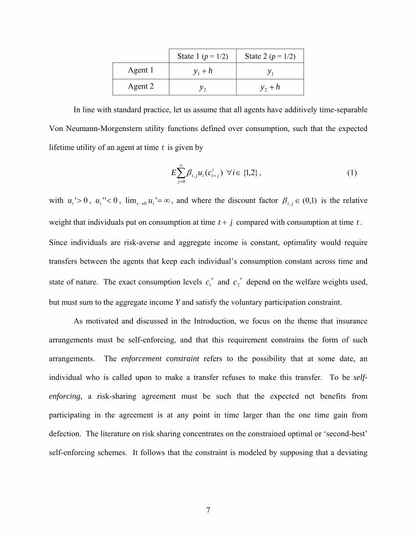
State 1 (p = 1/2) State 2 (p = 1/2)

Agent 1 hy +1 1y

Agent 2 2y hy +2

In line with standard practice, let us assume that all agents have additively time-separable

Von Neumann-Morgenstern utility functions defined over consumption, such that the expected

lifetime utility of an agent at time t is given by

, (1) ∑∞

=+ ∈∀

0, }2,1{)(

j

ijtijt icuE β

with , , , and where the discount factor 0'>iu 0'' <iu ∞=→ 'lim 0 ic u )1,0(, ∈jtβ is the relative

weight that individuals put on consumption at time jt + compared with consumption at time . t

Since individuals are risk-averse and aggregate income is constant, optimality would require

transfers between the agents that keep each individual’s consumption constant across time and

state of nature. The exact consumption levels and depend on the welfare weights used,

but must sum to the aggregate income Y and satisfy the voluntary participation constraint.

∗1c ∗

2c

As motivated and discussed in the Introduction, we focus on the theme that insurance

arrangements must be self-enforcing, and that this requirement constrains the form of such

arrangements. The enforcement constraint refers to the possibility that at some date, an

individual who is called upon to make a transfer refuses to make this transfer. To be self-

enforcing, a risk-sharing agreement must be such that the expected net benefits from

participating in the agreement is at any point in time larger than the one time gain from

defection. The literature on risk sharing concentrates on the constrained optimal or ‘second-best’

self-enforcing schemes. It follows that the constraint is modeled by supposing that a deviating

7

individual is excluded and must then bear stochastic fluctuations alone.5 A risk-sharing

agreement consists in a profile of transfers for all date t and realized state that result in a

stream of consumptions . These consumptions implies an expected continuation utility

}2,1{∈s

tiit sc ,)}({ ∀

∑∞

=++ ≡

1,1 )(

j

ijtijtt

it cuE βν at any date for individual t }2,1{∈i . In contrast, an individual i who

deviates at time t would consume his or her income (the sum of and , if received this

period) from time t onwards with a continuation utility

itz iy h

∑∞

=++ ≡

1,

,1 )(

j

ijtijtt

autit zuE βν . Hence, a risk-

sharing agreement is self-enforcing if, for every period t and individual }2,1{∈i ,

. (2) autit

iti

it

iti zucu ,

11 )()( ++ +≥+ νν

If the power of such punishment is limited, then perfect insurance may not be possible.

However, even when full risk sharing is not possible, individuals may be able to design a risk-

sharing agreement by limiting transfers in states for which the enforcement constraint is binding

(see Coate and Ravallion, 1993 and Kocherlakota, 1996, among others).

In fact, with this simple distribution, the constrained optimal agreement and its

associated continuation utility

titc ∀*}{

it 1* +ν at any time are easy to characterize. Individuals make

positive transfers to each other in the state in which they receive a good income shock , so that

an individual’s incentive constraint would only bind when he has received . If an individual i’s

incentive constraint binds at time t , her consumption is determined by the binding constraint

t

h

h

(3) ,)(**)( ,11auti

tiiit

iti hyucu ++ ++=+ νν

5 Equivalently, the deviator could be given the same continuation utility as in autarchy.

8

and for ** it

jt cYc −= ij ≠ ; otherwise the individuals’ consumptions at time t are just kept at

the same level as the previous period.

For simple exponential discounting, where for all t and jtj δβ =, j , the constrained

optimal agreement is characterized by two values, , the transfer made by 1 to 2 when 1

received and, , the transfer made by 2 to 1 when 2 received .

*1t

h *2t h 6 These transfers are such

that the incentive constraints (2) hold with equality for both agents, that is t* is

defined by:

*)*,( 21 tt=

).(

2)()

21(*)(

2*)()

21(

);(2

)()2

1(*)(2

*)()2

1(

2222122222

1111211111

yuhyutyuthyu

yuhyutyuthyu

δδδδ

δδδδ

++−=++−+−

++−=++−+− (4)

A first implication of this model is that, when full insurance is not achieved, a higher

discount factor δ increases the weight put on the long-term gain from insurance relative to the

short-term gain from deviating. It is easy to check that higher values of δ would relax the

constraints in (4). When constrained, a higher δ raises the transfers that individuals are able to

make to each other and so the insurance that they can provide for each other. There are threshold

values δ and δ , with 10 <<< δδ , such that for values of δ smaller or equal to δ no risk

sharing is possible, for ),( δδδ ∈ there is some constrained insurance, and for values of δ

greater than or equal to δ , first-best risk sharing can be achieved (see Thomas and Worrall 1994,

Kocherlakota 1996 and Ligon, Thomas and Worrall 2002).

6 This is true for all constrained optimal arrangement, irrespective of the initial bargaining power of the agent. The constrained-optimal scheme may specify a slightly smaller transfer than to an agent as long as only she has received h in order to give to this agent a larger share of the surplus. However, as soon as the state in which the other agent receives h occurs, then the constrained optimal agreement is stationary and consists of t*. In this special case, the stationary agreement studied in Coate and Ravallion (1993) is therefore optimal.

*1t

9

A second implication of this model is that an overall increase in the risk aversion

exhibited by the agents increases t* and the level of risk sharing that individuals can achieve, by

increasing the long term gain from insurance. For instance, if individuals have utility

i

ii

ρ

ρ−

−= 1c

11(c)u , where iρ is the Arrow-Pratt coefficient of relative risk aversion, then an

increased iρ relaxes i’s incentive constraint (4), thereby improving the insurance possibilities

(see the proof in Appendix A.2).

Finally, what is the effect of inequality? Let’s consider different values of and

keeping the aggregate income Y �constant. Clearly, if

1y 2y

21 yy = �both individuals are ex ante

identical. Now, increasing �and decreasing to keep Y unchanged would make 1

relatively wealthier than 2, while keeping the variance of their income constant. To be sure, the

set of Pareto optimal allocations is unaffected since the aggregate income is the same. However,

the division of wealth affects the autarchic utility and thereby does affect the set of self-enforcing

allocations. Genicot (2007) shows that for a large range of utility functions such spread-

preserving inequality between the two agents increases the likelihood of first-best risk sharing

and increases the transfers that agents make within the constrained optimal agreement.

1y 2y

7 This is

because a spread-preserving increase in inequality relaxes the constraint of the poorer agent

relatively more than it worsens the constraint of the richer agent.

Before we proceed to the description of our experiment, we wish to mention a couple of

caveats. First, this game suffers from the familiar problem of multiplicity of equilibria in

infinitely-repeated games. For instance, neither individual making any transfer is always an

equilibrium of the game. As it is usual practice in the theoretical and the empirical literature, we

7 See http://www.georgetown.edu/faculty/gg58/IIdraft.pdf.

10

focus on the constrained optimal arrangements, the arrangements that provide the most risk-

sharing given the presumption of self-enforcement. Using this refinement, what is striking is that

when full insurance is not possible, as soon as both agents have once received , all constrained

optimal arrangements -- irrespective of the initial bargaining weight of the agents -- are fully

characterized by the two transfers t* in (4).

h

Second, in the theoretical model we jus outlined, it is assumed that the utility function of

the other person is known; however, in the experiment this utility function is not known. To be

sure, this uncertainty would introduce learning effects. The contract would be non-stationary (as

beliefs are updated) and the results would also depend on unobservable priors. Nevertheless, we

don’t expect this uncertainty to change the way partial insurance responds to changes in the

discount factor, risk aversion, etc.

4. EXPERIMENTAL DESIGN

The challenge for our experimental design was to create an environment in which the

behavior of our experimental subjects is interpretable in terms of the infinite-horizon model of

risk sharing without commitment described in the previous section. Of course, in practical terms

it is impossible to conduct an experiment with an infinite number of periods. One technique

used by experimenters to avoid the unraveling problem present with a finite horizon is to have an

uncertain (stochastic) ending. To achieve this, we set up our sessions as a sequence of matches

in which pairs of participants play an unknown number of periods in each match. After each

period, there is a random draw (with a set probability) that determines whether that is the last

period or whether the match continues to the next period. Each period, one randomly-drawn

11

person in the pair receives a given amount h in addition to his or her regular income.8 After

observing both incomes, both subjects in a pair simultaneously choose a non-negative transfer to

make to the other person. When the match ends, we continue with a new match with new pairs.

Below we highlight some key features of our experimental design and then describe the

implementation in more detail.

Design Considerations

Infinite-horizon models of risk sharing with commitment are typically intended to reflect

a field environment where individuals living in the same community experience large stochastic

fluctuations in individual income, make voluntary transfers to each other to smooth consumption,

and see no clear termination to their repeated interaction. We refrained from using the terms

“risk sharing” or “insurance” during the experiment and allowed individuals to make transfers

irrespective of whether they received or not in order to avoid guiding the participants’

behavior. We also precluded explicit agreements by not permitting communication. These

factors make risk sharing more difficult to achieve; on the other hand, this is balanced against the

assumption of constant aggregate income for each pair, which facilitates sharing.

h

A crucial feature of our design is that we paid participants for only one period, drawn at

random at the end of the experiment, from the numerous periods (typically 60 to 80) played over

many matches; this was highlighted in bold in our instructions. Otherwise, if every round

counted towards her payoff, an individual would care about the distribution of the sum of income

8 We avoided using a simple alternation scheme, where each person in a pair would receive h with certainty every other period.

12

net of transfers over all rounds instead of the income net of transfers earned in each round.9 This

would not only substantially reduce the variance in the subject’s payoff in the absence of

transfer, but knowledge of the accumulated income to date would also affect behavior. In

contrast, our procedure gives equal probability to any realized round within a match to be the

‘payoff round’, so that individuals would face incentives constraints similar to (4) in each match.

Appendix A.1 explains in detail how our procedure achieves this result. We show that the

structure of the discounting implied by our procedure is very simple and, in an experiment with

sufficiently many rounds overall, the per-period discounting factors tends to the continuation

probability δ .10

We expected one’s risk attitude to be important in determining one’s transfer. Hence,

prior to the main experiment, we asked subjects to participate in a lottery to elicit a measure of

their risk aversion. An alternative approach would be to induce risk neutrality (the binary lottery

procedure). Although this method should in theory enable the experimenter to predetermine any

functional form for subjects' utility functions, experimental evidence shows that in practice

subjects’ own preferences affect their choices, making it very difficult to interpret the results

(Camerer and Ho 1994, Selten, Sadrieh and Abbink 1999). As a result, we chose to measure risk

attitudes and directly control for them.

One might also be concerned that the monetary rewards are relatively small compared to

the field environment. However, our payoffs are quite in line with normal experimental rewards,

and the size of the stochastic payoff from the chosen period was rather large in experimental

9 If every round counted for her payoff, individual i would maximize )(

0∑∞

=titi cEu where is individual i’s income

(fixed plus variable) plus the net transfer received in round t. In contrast in our experiment, her expected utility is , where is the round selected for payoff.

itc

)(,ititc cuE )) t̂

10 As we show in Appendix A.1 and A.2, within a match, the implied per period discount factor would slightly increase with the number of round played, but, with an expected 50 to 70 rounds overall, the effect on transfers over time is minimal so that the predictions of Section 3 are unaffected.

13

terms (nearly $12). Thus, the degree of payoff risk from not engaging in risk sharing was not

inconsequential. Nevertheless, this risk is clearly not as severe as it can be in the field.

Finally, we needed to pay attention to the time duration of the experiment. If, for

example, participants know that an experiment is scheduled to last for one hour, and 55 minutes

have already passed, they might expect the experiment to end very soon and we might observe

serious unraveling. To minimize this concern, we calibrated sessions to last for only 60 minutes

while advertising sessions of 90 minutes in duration. We retained control over the duration of

sessions: Participants played in up to 7-10 matches in a session, but we were prepared to reduce

the number of matches played if necessary by announcing at the appropriate time that the next

match would be the last one. In this manner, we kept the time horizon at a considerable distance.

Implementation

All experiments were conducted at the CASSEL Laboratory in UCLA. We had six

sessions, with an even number of participants ranging from 12 to 18 in a session (depending on

show-ups). Participants earned an average of about $17 for about an hour of their time. The

procedures that we followed are described below and the complete experimental instructions for

the δ = 0.9 treatment are shown in Appendix B.

Prior to the main experiment, we first asked people to complete an investment question.

For this exercise, each person was provisionally endowed with 100 units and could invest any

portion of this amount in a risky asset that had a 50% chance of success. The investment paid

2.5 times the amount invested if successful, but nothing if unsuccessful; the decision-maker

retained all units not invested. All of this was verbally explained in detail to the participants.

This technique was adapted from the design in Gneezy and Potters (1997) and is an easy-to-

14

understand mechanism for measuring risk aversion. Using a 50% probability of success also

avoids the problem of subjective over-weighting of low-probability events.

We told the participants that we would later choose two people at random in each session

for actual payoff implementation; we did so at the end of the session. We then flipped a coin to

determine success or failure for these investors, and added this payment to the amount earned in

the main experiment. For this exercise, each unit was worth $0.10 for the investors who were

selected. This investment question provides us with a measure of risk aversion for each

individual; clearly, the higher the investment the less risk averse is the individual.

The body of the session then consisted of a number of matches. For the duration of each

match, every participant was paired with one other person. We matched individuals within a

high risk-aversion group and within a low risk-aversion group, based on whether their

investment choice was above or below 67.11 After each period, the computer determined (for all

current matches) whether another round would follow.

In three of our sessions (Treatment 1), the continuation probability δ was 80%, and in

the other three sessions (Treatment 2), the continuation probability δ was 90%. In the first

case, the expected number of subsequent rounds in a match (at any point in time after the first

round) was four, and in the latter case, the expected number of subsequent periods was nine. The

participants in the corresponding sessions were informed of the relevant mathematical fact. The

continuation probability is designed to capture the model’s assumption of an infinite-horizon

with discounting. Ex ante, we expected each match to last 5 rounds in Treatment 1 and 10

rounds in Treatment 2. We ended all matches at the same time, and all participants were

11 We did so to reduce the heterogeneity between participants; we did not inform the participants about this feature.

15

randomly re-matched within their category for the next match. We had ten matches in each 80%

session and seven matches in each 90% session.12

In each round, each person received an income, which is comprised of a fixed portion and

an amount added to the fixed income (for that round) for one of the subject in each

match. The person receiving this extra amount was randomly chosen in each pair for every

round of the match. The fixed portions did not vary during the match, but did change from

match to match. Over time, matches alternated between having both fixed portions be 70 units

(equality) and having the fixed portions be 20 and 120 (inequality). In all cases, the amount

randomly assigned and added was kept at 200 units. This income distribution corresponds to the

two-state distribution with constant aggregate income described in Section 2. Participants

received $1 for every 17 experimental payoff units in these matches, as is clearly indicated in the

instructions.

200=h

h

In the beginning of a new match, each participant is informed that he or she is matched

with a new person, and learns his or her fixed income as well as the fixed income of this new

person. In the beginning of each round within a match, both individuals see which one of them

received the extra 200 in this round. Participants then simultaneously choose a non-negative

amount (no greater than the total income received in the period) to transfer to the other person;

these amounts were then transferred. We allowed individuals to make transfers whether or not

they had received the 200 units as we did not want to bias the experiment in favor of risk sharing,

and as we did not want the subjects to infer the main topic of the experiment. Participants saw a

12 While random re-matching means that a participant might be anonymously matched with another participant more than once, the resulting possible repeated-play issue was not really salient, given the number of matches played and the number of participants visibly present in a session. Results from Duffy and Ochs (2006) support this element of our experimental design.

16

history of the income and transfers for each previous round in that match, and could also review

their previous matches.

We also asked participants individuals who did not receive h in the beginning of the first

and fourth matches for their expectation of the transfer to be made by the other person. At the

end of the session, participants answered questions concerning their gender and major before

receiving their payoff.

5. MAIN RESULTS

We first present some summary statistics about our data. We then address the following

questions:

Question 1: Does a higher continuation probability increase the amount of risk sharing?

Question 2: Does a higher degree of risk aversion increase the transfer made?

Question 3: What is the effect of ex ante inequality on risk sharing?

Question 4: How do past transfers affect the transfer made?

Question 5: Are transfers sensitive to whether expectations are met?

Question 6: Are there differences in transfer choices for men and women?

The first three questions are directly related to the theoretical predictions of Section 3. In

this model, there is no uncertainty so that deviations from the risk-sharing arrangement would be

punished by the strongest punishment (autarchic payoff) but never occur in equilibrium. Now, in

the experimental setting there is likely to be some uncertainty due to the coordination process. If

we added a little bit of noise to the model such as a small probability of making a mistake in the

transfer, the punishment would be smaller and would occur in equilibrium. Agents respond to

smaller transfers than expected by reducing their transfers, at least in the short term. Learning

17

about the preference characteristics of one’s partner would only accentuate this effect.13 Hence,

in response to Questions 4 and 5, we predict that transfers will respond positively to past

transfers from the other and in particular that transfers will decrease when expectations are not

met.

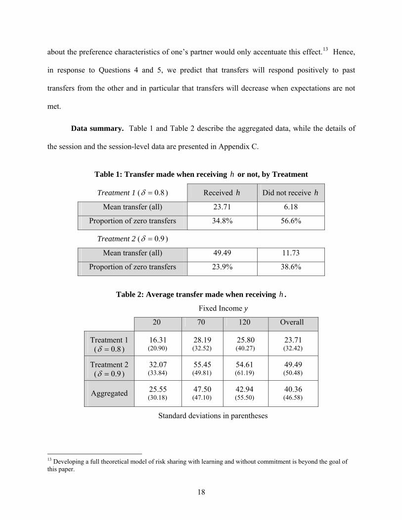
Data summary. Table 1 and Table 2 describe the aggregated data, while the details of

the session and the session-level data are presented in Appendix C.

Table 1: Transfer made when receiving h or not, by Treatment

Treatment 1 ( 8.0=δ ) Received h Did not receive h

Mean transfer (all) 23.71 6.18

Proportion of zero transfers 34.8% 56.6%

Treatment 2 ( 9.0=δ )

Mean transfer (all) 49.49 11.73

Proportion of zero transfers 23.9% 38.6%

Table 2: Average transfer made when receiving . h

Fixed Income y�

20 70 120 Overall

Treatment 1 ( 8.0=δ )

16.31 (20.90)

28.19 (32.52)

25.80 (40.27)

23.71 (32.42)

Treatment 2 ( 9.0=δ )

32.07 (33.84)

55.45 (49.81)

54.61 (61.19)

49.49 (50.48)

Aggregated

25.55 (30.18)

47.50 (47.10)

42.94 (55.50)

40.36 (46.58)

Standard deviations in parentheses

13 Developing a full theoretical model of risk sharing with learning and without commitment is beyond the goal of this paper.

18

Table 1 shows that a substantial amount of transfers takes place, and that average

transfers when ahead (upon receiving ) are much larger than average transfers when behind;

this effectively provides insurance to individuals. A simple binomial test (Siegel and Castellan,

1988) on individual data finds the difference to be highly significant (Z = 7.98, p = 0.000).

h

14,15 It

is clear that people are not just arbitrarily making transfers, but are instead sensitive to which

matched person receives h in the round. In addition, with a continuation probability of 80%, the

average transfer is 23.71 upon receiving and, with a continuation probability of 90%, the

average transfer when receiving rises to 49.49. Some subjects who do not receive make

positive but small transfers: the median transfer is 0 in Treatment 1 and 3 in Treatment 2. Note

that transfers when not receiving are not predicted by the risk-sharing model, or indeed by any

of the social-preference models. We discuss possible explanations in Section 5.

h

h h

h

Table 2 shows average transfers after receiving . In every case, transfers are highest

when individuals have the same fixed income and lowest for people with a fixed income of 20; it

is a bit surprising that transfers are slightly higher with a fixed income of 70 than with a fixed

income of 120, particularly since all of the distributional models of social utility predict the

opposite. Once again, we expect higher transfers with a higher

h

δ , holding the fixed income

constant and we observe this for each level of fixed income.

The aggregation in these tables ignores the substantial heterogeneity present in the

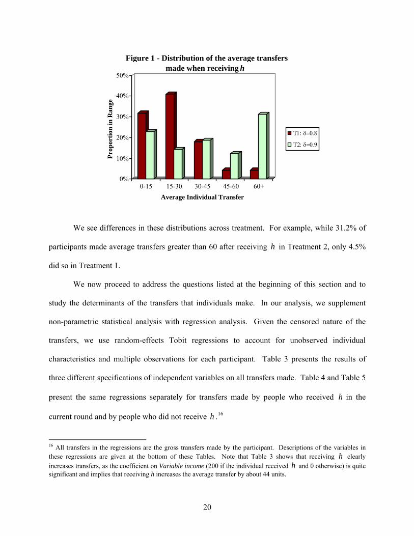
population, indicated by the large standard deviation in Table 1. Figure 1 shows the distribution

of the average transfer made after receiving h by each individual in the two treatments.

14 Throughout the paper, we round p-values to three decimal places. 15 A very conservative test considers each session to be only one observation. The transfers are higher in each of the six sessions when the chooser received . This would happen by chance in only one case out of 64, so the difference is statistically significant (p = 0.016, one-tailed test).

h

19

0%

10%

20%

30%

40%

50%

Prop

ortio

n in

Ran

ge

0-15 15-30 30-45 45-60 60+Average Individual Transfer

Figure 1 - Distribution of the average transfers made when receiving h

Τ1: δ=0.8

Τ2: δ=0.9

We see differences in these distributions across treatment. For example, while 31.2% of

participants made average transfers greater than 60 after receiving in Treatment 2, only 4.5%

did so in Treatment 1.

h

We now proceed to address the questions listed at the beginning of this section and to

study the determinants of the transfers that individuals make. In our analysis, we supplement

non-parametric statistical analysis with regression analysis. Given the censored nature of the

transfers, we use random-effects Tobit regressions to account for unobserved individual

characteristics and multiple observations for each participant. Table 3 presents the results of

three different specifications of independent variables on all transfers made. Table 4 and Table 5

present the same regressions separately for transfers made by people who received in the

current round and by people who did not receive .

h

h 16

16 All transfers in the regressions are the gross transfers made by the participant. Descriptions of the variables in these regressions are given at the bottom of these Tables. Note that Table 3 shows that receiving clearly increases transfers, as the coefficient on Variable income (200 if the individual received and 0 otherwise) is quite significant and implies that receiving h increases the average transfer by about 44 units.

hh

20

[Tables 3, 4 and 5 here]

The regressions in these tables use random effects to account for unobservable time-

invariant individual characteristics that affect all the transfers that a same individual makes. For

another comparison, we also present two tables that focus only on the transfers made in the first

round of any given match. These tables confirm the robustness of our findings.

[Tables 6 and 7 here]

Table 6 shows that the first transfer made when receiving is on average higher for Treatment 2

(

h

9.0=δ ) than for Treatment 1 (δ = 0.8). The same is true for participants with higher risk

aversion than for participants with lower risk aversion; in fact, holding the fixed income and

discount factor constant, the first-round transfer is higher for more risk-averse people in all six

comparisons. Finally, the first transfer is considerably lower for participants with a fixed income

of 20. Table 7 shows the same results using a Tobit model with random effects.

Question 1: Continuation probability. One important prediction of the risk-sharing

model is that we should see higher transfers when the expected time horizon is more distant.

Tables 1 and 2 show that the average transfer doubles when the continuation probability is 90%

instead of 80%. Even if we conservatively consider each session to be only one independent

observation, note that transfers were higher in each of the three sessions in Treatment 2 than in

any of the three sessions in Treatment 1. Since this would occur by chance only 5% of the time,

transfers are significantly higher in Treatment 2 (at the 5% level).

In both Tables 3 and 4, we see that a higher continuation probability substantially

increases the transfers. Specifications (1) and (2) in Table 3 indicate that increasing the

continuation probability from 0.8 to 0.9 increases transfers by about 21 units, while

21

specifications (1) and (2) in Table 4 indicates that it raises the transfers made by people who

receive by about 27 units. h

A closer examination shows that there are significantly different patterns over time with

the different continuation probabilities. The coefficient on 9.=δ becomes insignificant in

Tables 3 and 4 for specifications (3), which include an interaction term Round* 9.=δ . In

specification (1) in both tables we see no significant time effect within a match but specifications

(2) and (3) reveal different time effects depending on the continuation probability and ex ante

equality. For instance, in Table 4, when 8.0=δ and fixed incomes are equal, transfers decrease

by 5.7 units per round within a match, while when 9.0=δ , transfers do not decrease within a

match; we see a similar pattern when fixed incomes are not equal, as well as in Table 3. Thus,

transfers don’t decline over a match when 9.0=δ , but do decline when 8.0=δ , and much of

the effect of different continuation probabilities appears to stem from differences over the course

of matches.

Question 2: Risk aversion. A second prediction of risk-sharing without commitment is

that people who are more risk averse will engage in more risk sharing, so that we should observe

higher transfers by more risk-averse individuals. Our initial investment question provides us

with an estimate of individual attitude towards risk. As illustrated in Figure 2, we observed a

large range of answers to the investment question.

[Figure 2 here]

In both Tables 3 and 4, the coefficients on Investment (the amount invested in the risky

investment) are significantly negative in all specifications. Since a larger investment in the risky

asset indicates less risk aversion, a negative impact on the transfers is exactly what the model

predicts. To be sure, subject in this experiments face some uncertainty about the risk aversion of

22

their partner and are therefore playing a game of imperfect information. Individual’s beliefs on

her partner’s risk aversion affect her choice of transfers too. Nevertheless, as long as these

beliefs have a small support and are independent or positively correlated with own risk aversion,

we expect that a higher degree of risk aversion increases the transfer that one chooses when high

and therefore increases risk sharing. Specification (1) in Tables 3 and 4 indicates that a person

who chose to invest 30 would transfer 13 units more on average and 26 units more upon

receiving than another person who chose to invest 80. Specifications (2) and (3) in Table 4

indicate that the other person’s investment in the risky asset also has a negative and substantial

impact on the transfers made when high. The patterns are similar, but not significant, in Table 3.

h

Question 3: The effect of inequality. The risk-sharing model predicts higher transfers

with HARA (hyperbolic absolute risk aversion) preferences and greater ex ante inequality;

however, we do not find support for this prediction.

We can assess the overall effect of equality on transfers by looking at the effect of the

fixed income. Indeed, recall that changes to an individual’s fixed income are concurrent with

changes in his partner’s income. We find that average transfers with ex ante inequality are in

fact lower than with ex ante equality (34.24 compared to 47.50). Table 3 indicates that total

transfers are on average higher by 20 units with equality than with inequality (twice the

coefficient of D70 compared with the coefficient of D120); Table 4 specification (1) shows that

an -receiving person in an equal match transfers 26 more than in an unequal match.h 17

We can supplement our regression analysis here by considering whether each individual

made larger transfers on average with equality or inequality, since each person participated in

both environments. It turns out that average transfers were higher for 60 people with equality 17 There was not much difference in the transfers made by the person not receiving with equality (10.40) and inequality (9.20).

h

23

and for 32 people with inequality (with no difference for the other two people). If behavior were

random, we would expect these numbers to be roughly equal. Thus, the binomial test on

individual data finds this difference highly significant (Z = 2.92, p = 0.004, two-tailed test); using

session-level data (see Appendix C), transfers are higher with ex ante equality than without it in

every session, so we have statistical significance on this basis (p = 0.032, two-tailed test).

Question 4: Past transfers and time. Risk sharing requires reciprocal response. Tables

3 and 4 clearly show that the first transfer made by the individual’s partner within a match has a

strong positive effect on his transfers, and that this effect differs according to whether the partner

had or not received in the first period. In specification (1) of Table 3, we see that an

additional 10 units of transfer in the first period by one’s counterpart who had not received

(Other’s 1

h

h st transfer) increases an individual’s average transfer in each period by 3 units; in

Table 4, the corresponding figure is 4.5 units. Interestingly, the coefficient on Other’s 1st

transfer| �is significantly negative in Table 3, indicating that an individual’s transfers are more

responsive to the first transfers made by his or her partner when the latter did not receive ,

perhaps being interpreted as a form of signal. Specifications (2) and (3) highlight a gender

effect, in that females respond more to the transfer made in the first period. A female subject

who receives a small transfer from the other in the first period reduces her transfer more than a

male subject does.

h

h

Table 3 also shows a different evolution of transfers over time within matches, depending

on whether the individuals’ fixed incomes are the same. The coefficient of Round*D70 is

significantly positive, and in specification (2) more than offsets the negative coefficient of

24

Round. Thus, when people have the same fixed income, transfers within a match are fairly flat

over time. In contrast, transfers decrease over time when the fixed incomes differ.18

Question 5: Beliefs. If transfers depend on past actions, we might also expect transfers

to be affected by how one’s expectations are met. In the first round of a couple of matches per

session, we elicited the beliefs of subject who did not receive the 200 regarding the transfer they

expect to receive from the other. We find that 38% received more than they expected, 9%

received exactly what they expected and 53% received less than expected (94 observations).

Table 8 shows the effect of meeting individual’s expectations or not on the transfers, as

we include the difference between an individual’s expectations and the transfer actually received.

[Table 8 here]

Bdiff takes values in {+1, 0, -1} if the transfer received earlier in the last round of current match

was respectively above, at, or below expectations. Clearly, its effect in the random-effects

specifications is quite significant and positive on the transfers made by an individual. These

results could be interpreted as the use of punishment following transfers lower than expected. It

is interesting to see that the effect of the round within the match is not significant when we

control for the difference between expectations and received transfers, so that we don’t observe a

pure time-decay effect (within a match) even in the 8.0=δ treatment.

Question 6: Gender Patterns. The average transfer by males was 29 while the average

transfer by females was 22.19 Given that females are more risk averse than males in our

experiment,20 we might have expected females to make higher transfers. However, we observe

18 We also find (not shown) that transfers significantly increase with a higher number of rounds in the previous match. This is consistent with our discounting structure described in Appendix A.1. 19 Note that each individual is unaware of the gender of the other person in the match. 20 This gender investment result is extremely robust, as is discussed in Charness and Gneezy (2007).

25

in specification (1) of both Tables 3 and 4 that, controlling for risk aversion, females make

smaller transfers. The coefficient is not significant in Table 3, but is double in size and

significant in Table 4, indicating that the difference is driven by behavior after receiving . The

coefficient on Female is lower when we include the interaction term Round*Female in

specification (3), as it appears that transfers decrease over time relative to male transfers. We

also mentioned earlier that females’ transfers are more sensitive to the first transfer received.

The lower transfers by females results in a significantly lower net consumption for males (Z =

2.68, p = 0.007), using a Wilcoxon-Mann-Whitney ranksum test (see Siegel and Castellan 1988)

on individual average consumption.

h

21 Using session-level data (see Appendix C), we see that

consumption is higher for females than for males in each of the six sessions, so a binomial test

confirms statistical significance (p = 0.032, two-tailed test).22

6. DISCUSSION

Our experiment provides evidence that is qualitatively consistent with the model of risk

sharing without commitment, with the exception of the effect of ex ante inequality. Net positive

transfers go from individuals receiving a high shock to those not receiving the high shock and

these transfers substantially reduces the standard deviation of consumption; this could be

considered insurance. A longer expected time horizon has a strong positive effect on transfers,

as does a higher degree of risk aversion. None of these effects would be expected to arise if

transfers were motivated purely by altruism or distributive preferences. As we also find that

21 Note that this is not due to females having better draws; females comprised 56.4% of the population and females had the larger endowment 55.6% of the time. 22 Despite the mean transfer being lower for females, males are actually slightly more likely to choose to transfer zero when ahead, 29.8% versus 27.8%. On the other hand, the average non-zero transfer made when ahead is higher for males than for females with each combination of continuation probability and fixed income.

26

one’s chosen transfer depends positively on the other party’s first transfer and on receiving

transfers that meet or exceed expectations, there is clear evidence of reciprocal relationships.

One may wonder whether the behavior we observe is really risk sharing or is simply a

form of social preference. For example, models of utility such as Fehr and Schmidt (1999),

Bolton and Ockenfels (2000) and Charness and Rabin (2002) all predict that, holding the total

payoff constant, net transfers will go toward the person with the lower total income.

Furthermore, since we observe reciprocal behavior, one might be tempted to conclude that we

are observing a form of ‘reciprocity’. However, this term has had many meanings in the

literature, and one must be careful to clearly specify what is meant by it. We feel that reciprocity

in its purest sense is not a strategic notion, but refers to a per se preference to help or hurt

someone else due to one’s perceptions of the other party’s actions and motivation for these

actions.23 Given the observed patterns of behavior, the reciprocal relationships we observe in

our experiment instead seem the result of strategic considerations; nevertheless, one could also

imagine preference-based behavior, based only on the individual’s behavior when receiving ,

that would also result in effective risk sharing.

h

To help interpret our results in the light of alternative interpretations, we present some

predictions of the risk-sharing model and various models of social preferences in Table 9:

23 Models of kindness-based reciprocity, such as Rabin (1993) and Dufwenberg and Kirchsteiger (2004), formalize this idea; also see Charness and Rabin (2002), Charness (2004) and Cox (2004) for discussions of this point.

27

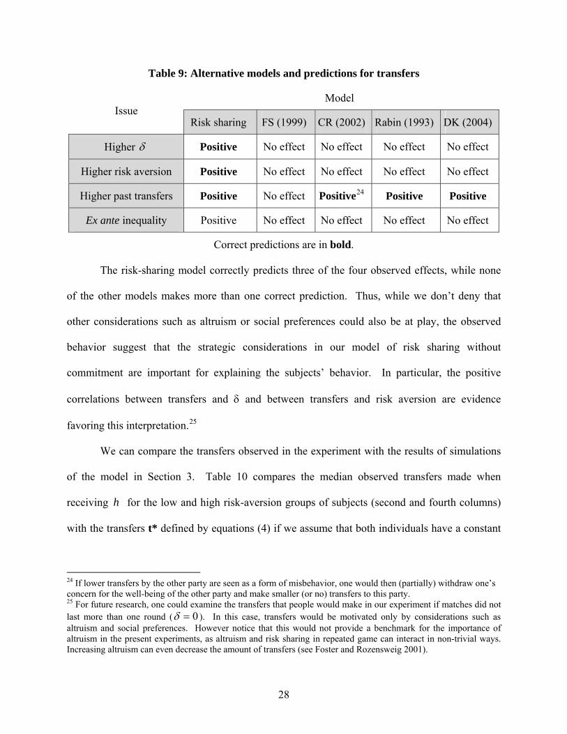
Table 9: Alternative models and predictions for transfers

Model

Issue Risk sharing FS (1999) CR (2002) Rabin (1993) DK (2004)

Higher δ Positive No effect No effect No effect No effect

Higher risk aversion Positive No effect No effect No effect No effect

Higher past transfers Positive No effect Positive24 Positive Positive

Ex ante inequality Positive No effect No effect No effect No effect

Correct predictions are in bold.

The risk-sharing model correctly predicts three of the four observed effects, while none

of the other models makes more than one correct prediction. Thus, while we don’t deny that

other considerations such as altruism or social preferences could also be at play, the observed

behavior suggest that the strategic considerations in our model of risk sharing without

commitment are important for explaining the subjects’ behavior. In particular, the positive

correlations between transfers and δ and between transfers and risk aversion are evidence

favoring this interpretation.25

We can compare the transfers observed in the experiment with the results of simulations

of the model in Section 3. Table 10 compares the median observed transfers made when

receiving for the low and high risk-aversion groups of subjects (second and fourth columns)

with the transfers t* defined by equations (4) if we assume that both individuals have a constant

h

24 If lower transfers by the other party are seen as a form of misbehavior, one would then (partially) withdraw one’s concern for the well-being of the other party and make smaller (or no) transfers to this party. 25 For future research, one could examine the transfers that people would make in our experiment if matches did not last more than one round ( 0=δ ). In this case, transfers would be motivated only by considerations such as altruism and social preferences. However notice that this would not provide a benchmark for the importance of altruism in the present experiments, as altruism and risk sharing in repeated game can interact in non-trivial ways. Increasing altruism can even decrease the amount of transfers (see Foster and Rozensweig 2001).

28

relative risk aversion utility function, ρ

ρ−

−= 1c

11u(c) (first and third columns). The simulated

transfers are computed using the median coefficient of relative risk aversion ρ implied by the

choice of investment of the high risk-aversion ( ρ = 0.324) and the low risk-aversion ( ρ = 0.174)

groups.26

Table 10: Predicted and actual transfers

δ = 0.8 δ = 0.9

Predicted Actual Predicted Actual

Equality ( ) 7021 == yy

ρ = 0.324 t*1 = t*2 =12 20 t*1 = t*2 =100 70

ρ = 0.174 t*1 = t* 2 =0 15 t*1 = t*2 =31 20

Inequality ( ) 20,120 21 == yy

ρ = 0.324 t*1=32, t* 2=37 t 1=13, t 2=18 t*1=98, t*2=102† t 1=57, t 2=39

ρ = 0.174 t*1=0, t*2=0 t 1=8, t 2=0 t*1=40, t*2=43 t 1=8, t 2=24

†There is an interval of first-best allocations that is feasible; this is the most equal.

Overall, we note that transfers are limited in a way that is consistent with the modest

levels of risk aversion exhibited by the participants.27 With equality and 8.0=δ , predicted

transfers are a bit lower than what is observed, while with equality and 9.0=δ , this pattern is

26 Assuming constant relative risk aversion utility, the coefficient of risk aversion is given by the following formula:

ρ ≡ln(1.5)

ln(inv* 2.5 +100 - inv) - ln(100 - inv)

0

if inv <100if inv =100

⎧ ⎨ ⎪

⎩ ⎪ . An investment choice of 25 thus corresponds to ρ = 0.67, an

investment choice of 50 corresponds to ρ = 0.32, and an investment choice of 75 corresponds to ρ = 0.19. 27 These levels of risk aversion are similar to the ones found in other experiments (see among others Biswanger, 1980 and Goeree, Holt, and Palfrey, 2000). While our estimates for the coefficient of risk aversion may seem surprisingly low, recall that this estimation presumes that this investment is the only source of income for the individual. This is not the case even if we restrict our attention to experimental earnings. For example, if individuals expect earnings of $17 (the average in our sessions), this would give us estimates of 0.81 for the low risk-aversion group and 1.29 for the high risk-aversion group.

29

reversed. We see that although there is a reasonably close fit between the predictions and the

observed transfers for the equal sharing, with inequality the actual transfers are substantially less

than the predicted levels. For utility functions of the HARA class, we should observe individuals

with lower fixed income making higher transfers when receiving than individuals with higher

fixed income make when receiving , as the poorest agent trades mean consumption in

exchange for insurance. Yet, we find that high-fixed-income individuals actually transfer more

than low-fixed-income individuals. In fact, none of the other models predict the result that ex

ante equality leads to higher transfers. This consideration is irrelevant for the Fehr and Schmidt

(1999) model, the Charness and Rabin (2002) model and the pure-reciprocity models.

h

h

28

Thus, we must look for another explanation. In some sense, equal fixed payoffs may

make coordinating on reciprocal transfers easier. Table 4 clearly suggests that the inequality

results stem from people with low fixed income making substantially lower transfers. This may

reflect the fact that even when the person with the low fixed income receives , he or she is

nevertheless poorer in expected terms during the remainder of the match. Since we pay for only

one period, this story might not apply, but it could still influence behavior. In any event, by this

logic we should also see substantially higher transfers with the high fixed income than with equal

fixed incomes, and we don’t. Perhaps one views one’s ‘local’ wealth in a self-serving manner,

and this divergence in perspectives makes risk sharing more difficult.

h

In another sense equal fixed payoffs make it easier for one to identify with the other

person and interpret the transfers made. Previous studies have shown that participants in

28 To see this for the Fehr and Schmidt (1999) model, note that the only factor involved is the expected difference in ex post payoffs; this will always be 200 with ex ante equality, and will be either 100 or 300 with ex ante inequality. But since this is on average 200 and the model is linear, there should be no difference for these cases. The relevant factor in the Charness and Rabin (2002) model is the minimum payoff, rather than the difference in payoffs, but this also averages the same in the two cases. All of the distributional models make the clear prediction that an individual with the highest fixed income (120) should make greater transfers than an individual with medium fixed income (70), and this is not the case (see Table 2, for example).

30

experiments are prone to identification or ‘solidarity’ with an arbitrary group. Tajfel, Billig,

Bundy and Flament (1971) find that subjects treat people who have been designated to be part of

their ‘group’ quite differently than people not in their group. Charness, Rigotti and Rustichini

(2007) achieve strong group identification affecting play in Battle-of-the-Sexes and Prisoner’s

Dilemma games. If, as Akerlof and Kranton (2000, p. 748) assert, “a person’s self is associated

with different social categories and how people in these categories should behave,” perhaps it is

reasonable to expect that people who are ex ante equal to more readily form reciprocal

relationships and higher transfers.

7. CONCLUSION

In this paper, we test experimentally for risk sharing without commitment and some of its

implications. The experiment was designed to fit as closely as possible the models of risk

sharing without commitment used in the literature, and, following the literature, we focused on

the constrained optimal equilibrium. While our income process and experimental setting are

simplified, we feel that this approach is well suited as a first laboratory test of risk sharing

without commitment or enforcement. The laboratory environment allows us to isolate the effect

of various factors with respect to the theoretical model.

We find evidence of risk-sharing behavior, including significant support for some

important features of the models of risk sharing without commitment. Net transfers flow from

the individual who received a good shock in the period to the other, whether or not the fixed

incomes are the same. Both a higher continuation probability and a higher degree of risk

aversion strongly and significantly increase the level of risk sharing that individuals choose.

Moreover, a form of reciprocal behavior is shown to be important for risk sharing: The higher

the first transfer made by an individual’s partner, the higher the individual’s eventual transfers.

31

We also find that beliefs matter, in that how actual transfers compare to expected

transfers plays a role in subsequent transfers. However, in contrast with the model’s predictions,

inequality between individuals in a match actually decreases risk sharing, suggesting the

influence of some form of social cohesion or identification process.

Finally, we also observe that the person with less income in a round often makes a small

positive transfer to the other person. Perhaps such a transfer is seen as a signal of intent; such

transfers in the first round of a match are (dollar-for-dollar) more effective in increasing one’s

counterpart’s transfers than transfers made in the first round when receiving the larger income.

While we have provided evidence that is consistent with risk sharing in the laboratory,

our study is only a first step towards examining how this behavior might evolve and how it might

be sensitive to institutional considerations. Next steps include utilizing a more realistic income

process and allowing communication between the parties. We feel that this is a promising area

for future research, as informal risk sharing is a critical feature of the economy in many

contemporary environments.

REFERENCES

Akerlof, G. and Kranton, R. (2000). “Economics and Identity,” Quarterly Journal of Economics, vol. 115(3) (August), pp. 715-753.

Aoyagi, M. and Fréchette, G. (2003). “Collusion in Repeated Games with Imperfect Public Monitoring,” mimeo.

Axelrod, R. (1980). “More Effective Choice in the Prisoner’s Dilemma,” Journal of Conflict Resolution, vol. 24(3) (September), pp. 379-403.

Barr, A. and Genicot, G. (forthcoming). “Risk Pooling, Commitment, and Information: An Experimental Test,” Journal of the European Economic Association.

Biswanger, H. (1981). “Attitudes Towards Risk: Theoretical Implications of an Experiment in Rural India,” ECONOMIC JOURNAL, vol. 91(364) (December), pp. 867-890.

Bolton, G., and Ockenfels, A. (2000). “ERC – A Theory of Equity, Reciprocity, and Competition,” American Economic Review, vol. 90(1) (March), pp. 166-193.

Bone, J., Hey, J. and Suckling, J. (2004). “A Simple Risk-Sharing Experiment,” Journal of Risk and Uncertainty, vol. 28(1) (January), pp. 23-38.

Camerer, C. and T. Ho (1994). “Violations of Betweenness Axiom and Nonlinearity in Probability,” Journal of Risk and Uncertainty, vol. 8(2) March, pp. 167-196.

32

Cason, T. (1995). “Cheap Talk Price Signaling in Laboratory Markets,” Information Economics and Policy, vol. 7(2) (June), pp. 183-204.

Charness, G. and Garoupa, N. (2000). “Reputation, Honesty, and Efficiency with Insider Information: An Experiment,” Journal of Economics and Management Strategy, vol. 9(3) (Summer), pp. 425-451

Charness, G. and Gneezy, U. (2007). “Strong Evidence for Gender Differences in Experimental Investing,” mimeo.

Charness, G. and Rabin, M. (2002). “Understanding Social Preferences with Simple Tests,” Quarterly Journal of Economics, 117(3), August, pp. 817-869.

Charness, G., Rigotti, L., and Rustichini, A. (2007). “Individual Behavior and Group Membership,” American Economic Review, 97(4) (September), pp. 1340-1352.

Coate, S. and Ravallion, M. (1993). “Reciprocity without Commitment: Characterization and Performance of Informal Insurance Arrangements,” Journal of Development Economics, 40(1) (February), pp. 1-24.

Cox, J. (2004). “How to Identify Trust and Reciprocity: Implications of Game Triads and Social Contexts,” Games and Economic Behavior, 46(2) (February), pp. 260-81.

Croson, R. and U. Gneezy (2004), “Gender Differences in Preferences,” mimeo. Dal Bó, P. (2005). “Cooperation under the Shadow of the Future: Experimental Evidence from

Infinitely Repeated Games,” American Economic Review, 95(5), December, pp. 1591-1604

Deaton, A. (1992). Understanding Consumption, Oxford: Clarendon Press. Dercon S. and Krishnan, P. (2000). “In Sickness and in Health: Risk sharing within households

in rural Ethiopia,” Journal of Political Economy, 108(4) (August), 688-727. Dubois, P. and Ligon, E. (2004). “Incentives and Nutrition for Rotten Kids: Intra-Household

Food Allocation in the Philippines,” mimeo. Duffy, J. and Ochs, J. (2006). “Cooperative Behavior and the Frequency of Social Interaction,”

mimeo. Fehr, E. and Schmidt, K. (1999), “A Theory of Fairness, Competition, and Cooperation,”

Quarterly Journal of Economics, 114(3) August , pp. 817-868. Foster, A. and Rosenzweig, M. (2001). “Imperfect Commitment, Altruism, and the Family:

Evidence from Transfer Behavior in Low-Income Rural Areas,” Review of Economics and Statistics, 83(3) (August), pp. 389-407.

Genicot, G. (2007). “Does Inequality Help Risk Sharing?,” mimeo. [http://www.georgetown.edu/faculty/gg58/IIdraft.pdf]

Genicot, G. and Ray, D. (2003). “Endogenous Group Formation in Risk-Sharing Arrangements,” Review of Economic Studies, 70(1) (January), pp. 87-113.

Gertler, P. and Gruber, J. (2002). “Insuring Consumption Against Illness,” American Economic Review, 92(1) (March), pp. 51-70.

Gneezy, U., and Potters, J. (1997), “An Experiment on Risk Taking and Evaluation Periods,” Quarterly Journal of Economics, 112(2) (May), pp. 631-645

Grimard, F. (1997). “Household Consumption Smoothing through Ethnic Ties: Evidence from Côte D'Ivoire,” Journal of Development Economics 53(2) (December), pp. 391-422.

Jalan, J. and Ravallion, M. (1999). “Are the Poor Less Well Insured? Evidence on Vulnerability to Income Risk in Rural China,” Journal of Development Economics, 58(1) (February), pp. 61-81.

33

Kimball, M. (1988). “Farmer Cooperatives as Behavior Toward Risk,” American Economic Review, 78(1) (March), pp. 224-232.

Kletzer, K. and Wright, B. (2000). “Sovereign Debt as Intertemporal Barter,” American Economic Review, 90(3) (June), pp. 621-639.

Kocherlakota, N. (1996). “Implications of Efficient Risk Sharing without Commitment,” Review of Economic Studies, 63(4) (October), pp. 595-609.

Ligon, E., Thomas, J., and Worrall, T. (2002). “Informal Insurance Arrangements with Limited Commitment: Theory and Evidence from Village Economies,” Review of Economic Studies, 69(1) (January), pp. 209-44.

Murnighan, J. and Roth, A. (1983). “Expecting Continued Play in Prisoner’s Dilemma Games: A Test of Several Models,” Journal of Conflict Resolution, 27(2) (June), pp. 279-300.

Roth, A. and Murnighan, J. (1978). “Equilibrium Behavior and Repeated Play of the Prisoner’s Dilemma,” Journal of Mathematical Psychology, 17(2) (April), pp. 189-198.

Selten, R., and Ockenfels, A. (1998). “An Experimental Solidarity Game,” Journal of Economic Behavior and Organization, 34(4) (March), pp. 517-539.

Selten, R., Sadrieh, A., and Abbink, K. (1999). “Money Does Not Induce Risk Neutral Behavior, But Binary Lotteries Do Even Worse,” Theory and Decision, 46(3) (June), pp. 213-252.

Siegel, S. and Castellan, N., Jr. (1988), Nonparametric Statistics for the Behavioral Sciences, New York: McGraw-Hill.

Tajfel, H., Billig, M., Bundy, R., and Flament, C. (1971). “Social Categorization and Intergroup Behavior,” European Journal of Social Psychology, 1(2) (April/June), pp. 149-78.

Thomas, J. and Worrall, T. (1994). “Informal Insurance Arrangements in Village Economies,” Liverpool Research Papers in Economics and Finance 9402.

Townsend, R. (1994). “Risk and Insurance in Village India,” Econometrica, 62(3) (May), pp. 539-91.

Udry, C. (1994), “Risk and Insurance in a Rural Credit Market: An Empirical Investigation in Northern Nigeria,” Review of Economic Studies, 61(3) (July), pp. 495-526.

34

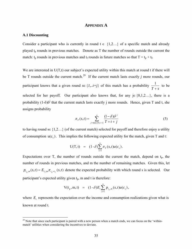
APPENDIX A

A.1 Discounting

Consider a participant who is currently in round t ∈ {1,2…} of a specific match and already

played tp rounds in previous matches. Denote as T the number of rounds outside the current the

match: tp rounds in previous matches and tf rounds in future matches so that T = tp + tf.

We are interested in U(T,t) our subject’s expected utility within this match at round t if there will

be T rounds outside the current match.29 If the current match lasts exactly j more rounds, our

participant knows that a given round s∈{1,..t+j} of this match has a probability sT +

1 to be

selected for her payoff. Our participant also knows that, for any j∈{0,1,2…}, there is a

probability (1-δ)δj that the current match lasts exactly j more rounds. Hence, given T and t, she

assigns probability

∑∞

−= ++−

=},0max{

)1(),(tsj

j

T jtTts δδπ (5)

to having round s∈{1,2…} (of the current match) selected for payoff and therefore enjoy a utility

of consumption . This implies the following expected utility for the match, given T and t: )u(cs

∑∞

=

=1

s )(),()-(1t)U(T,s

T cutsπδ .

Expectations over T, the number of rounds outside the current the match, depend on tp, the

number of rounds in previous matches, and m the number of remaining matches. Given this, let

),(),( |, tsEtspfpfp ttmtmt += π denote the expected probability with which round s is selected. Our

participant’s expected utility given tp, m and t is therefore:

∑∞

=

=1

s,p )(),()-(1t)m,,V(ts

mtt cutspEp

δ ,

where represents the expectation over the income and consumption realizations given what is

known at round t.

tE

29 Note that since each participant is paired with a new person when a match ends, we can focus on the ‘within-match’ utilities when considering the incentives to deviate.

35

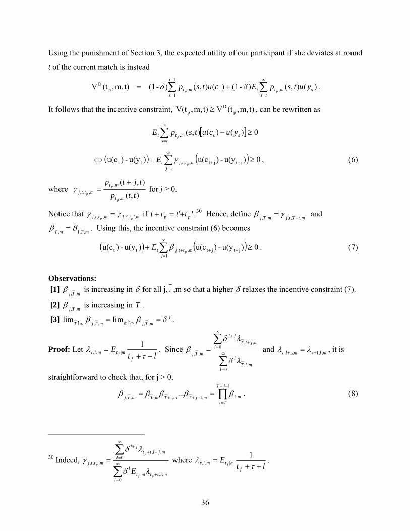
Using the punishment of Section 3, the expected utility of our participant if she deviates at round

t of the current match is instead

∑∑∞

=

−

=

+=ts

mtt

t

smt yutspEcutsp

pp)(),()-(1)(),()-(1t)m,,(tV s,

1

1s,p

D δδ .

It follows that the incentive constraint, , can be rewritten as t)m,,(tVt)m,,V(t pD

p ≥

[ ] 0)()(),( ss, ≥−∑∞

=tsmtt yucutspE

p

, (6) ( ) ( ) 0)u(y-)u(c)u(y-)u(c1

jtjt,,,tt ≥+⇔ ∑∞

=++

jmttjt p

E γ

where ),(

),(

,

,,,, ttp

tjtp

mt

mtmttj

p

p

p

+=γ for j ≥ 0.

Notice that mttjmttj pp ,',',,,, γγ = if '' pp tttt +=+ .30 Hence, define mtTtjmTj ,,,,, −

= γβ and

mTmT ,,1,ββ = . Using this, the incentive constraint (6) becomes

. (7) ( ) ( ) 0)u(y-)u(c)u(y-)u(c1

jtjt,,tt ≥+ ∑∞

=+++

jmttjt p

E β

Observations: [1]

mTj ,,β is increasing in δ for all j, T ,m so that a higher δ relaxes the incentive constraint (7).

[2] mTj ,,

β is increasing in T .

[3] jmTjmmTjT

δββ == ∞↑∞↑ ,,,,limlim .

Proof: Let lt

Ef

mtml f ++=

τλτ

1|,, . Since

∑

∑∞

=

∞

=+

+

=

0,,

0,,

,,

lmlT

l

lmjlT

jl

mTj

λδ

λδβ and mlml ,,1,1, ++ = ττ λλ , it is

straightforward to check that, for j > 0,

∏−+

=−++

==1

,,1,1,,,...

jT

TtmtmjTmTmTmTj

βββββ . (8)

30 Indeed, ∑

∑∞

=+

∞

=++

+

=

0,,|

0,,

,,,

lmlttmt

l

lmjltt

jl

mttj

pf

p

p

E λδ

λδγ where

ltE

fmtml f ++

=τ

λτ1

|,, .

36

The weight an individual puts at time T on his consumption at time T +j is the product of the

weight she puts today on his consumption at time T +1 with the weight she puts at time T +1 on

his consumption at time T +2, etc.

Now notice that

.111

0 ,0,

,,

0,,

,0,

0,,

1,,

0,,

0,1,

1

,

∑∑∑

∑

∑

∑∞

=

∞

=

∞

=

∞

=∞

=

∞

=+

+

−=−===

l mt

mltl

lmlt

l

mt

lmlt

l

kmkt

k

lmlt

l

lmlt

l

mt

λλ

δλδ

λ

λδ

λδ

λδ

λδβ

Clearly, mt ,β is increasing in δ and therefore

mTj ,,β in (8) is too.

Since δ > 0 and mt

mjt

,0,

,,

λλ

<1 for all j > 0, it follows that δλ

λδ

−<∑

∞

= 11

,0,

,,

0 mt

mjt

j

j and that δβ <mt , .

Now notice that mt

mjt

,0,

,,

λλ

is increasing in t or m and that mt

mjt

,0,

,,

λλ

tends to 1 for large t or m. Hence,

mt ,β is increasing in t and m, and tends to δ . It then follows directly from (8) thatmTj ,,

β is

increasing in T , and tends to for large jδ T or m.

We have just shown that the implied discount factor mTj ,,

β is increasing in T , so that a higher

relaxes the incentive constraint (7). Hence, we may expect transfers within a match to

increase over time. However, this effect is rather small. When the continuation probability δ is

0.8, assuming that 40 rounds have been played in the other 8 matches and that we are in round t,

the discount factor on round t+1 would increase from 0.722 to 0.727 from round t = 1 to round t

= 11. When the continuation probability δ is 0.9, assuming that 50 rounds have been played in

the other 5 matches and that we are in round t, the discount factor on round t+1 would increase

from 0.87 to 0.872 from round t = 1 to round t = 11. In our simulations this would result in an

increase in transfer no larger than 2 over a match of ten rounds.

ptt +

37

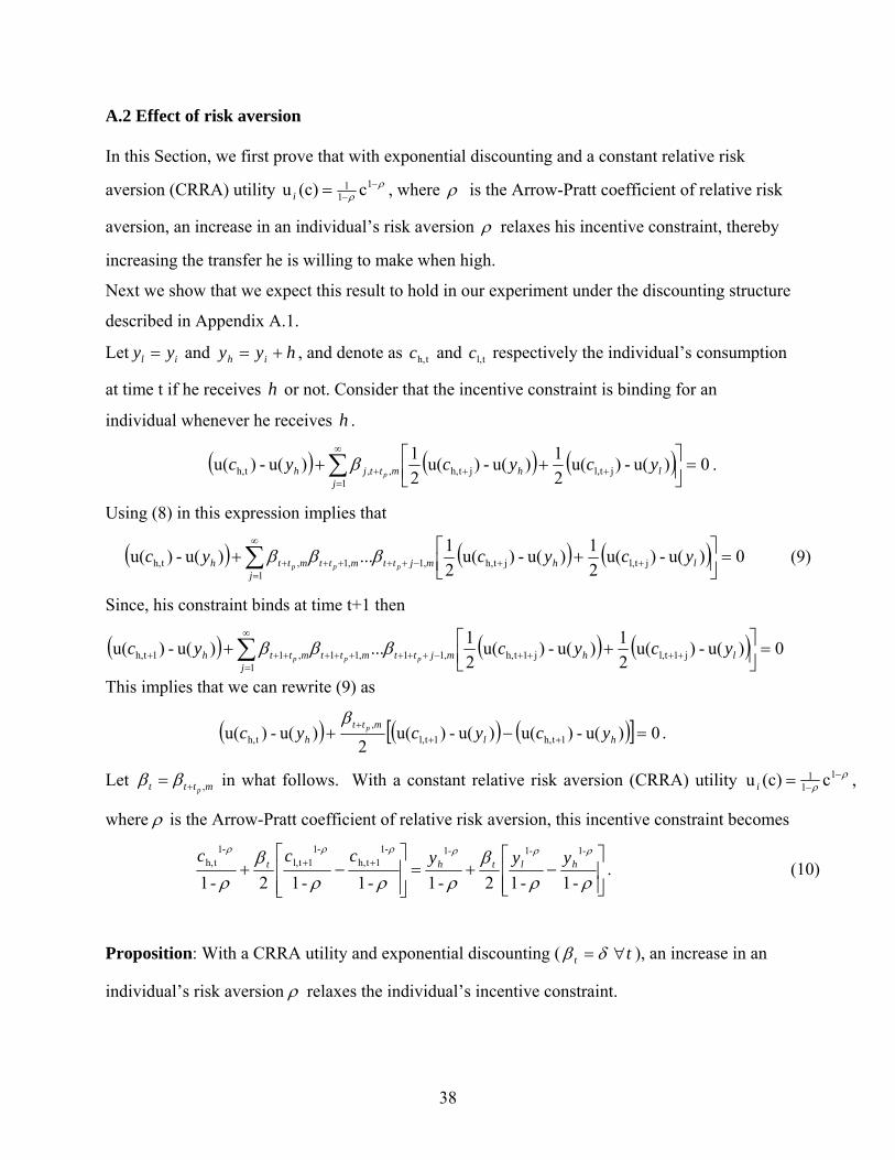
A.2 Effect of risk aversion

In this Section, we first prove that with exponential discounting and a constant relative risk

aversion (CRRA) utility ρρ

−−= 1

11 c(c)u i , where ρ is the Arrow-Pratt coefficient of relative risk

aversion, an increase in an individual’s risk aversion ρ relaxes his incentive constraint, thereby

increasing the transfer he is willing to make when high.

Next we show that we expect this result to hold in our experiment under the discounting structure

described in Appendix A.1.

Let and , and denote as and respectively the individual’s consumption

at time t if he receives or not. Consider that the incentive constraint is binding for an

individual whenever he receives .

il yy = hyy ih += th,c tl,c

h

h

( ) ( ) ( 0)u(-)u(21)u(-)u(

21)u(-)u(

1jtl,jth,,,th, =⎥⎦

⎤⎢⎣⎡ ++ ∑

∞

=+++

jlhmttjh ycycyc

pβ ) .

Using (8) in this expression implies that

( ) ( ) ( 0)u(-)u(21)u(-)u(

21...)u(-)u(

1jtl,jth,,1,1,th, =⎥⎦

⎤⎢⎣⎡ ++ ∑

∞

=++−+++++

jlhmjttmttmtth ycycyc

pppβββ ) (9)

Since, his constraint binds at time t+1 then

( ) ( ) ( ) 0)u(-)u(21)u(-)u(

21...)u(-)u(

1j1tl,j1th,,11,11,11th, =⎥⎦

⎤⎢⎣⎡ ++ ∑

∞

=++++−+++++++++

jlhmjttmttmtth ycycyc

pppβββ

This implies that we can rewrite (9) as

( ) ( ) ([ 0)u(-)u()u(-)u(2

)u(-)u( 1th,1tl,,

th, =−+ +++

hlmtt

h ycycyc p )]β.

Let mttt p ,+= ββ in what follows. With a constant relative risk aversion (CRRA) utility ρρ

−−= 1

11 c(c)u i ,

where ρ is the Arrow-Pratt coefficient of relative risk aversion, this incentive constraint becomes

⎥⎥⎦

⎤

⎢⎢⎣

⎡−+=

⎥⎥⎦

⎤

⎢⎢⎣

⎡−+ ++

ρρβ

ρρρβ

ρ

ρρρρρρ

-1-12-1-1-12-1

-1-1-1-11th,

-11tl,

-1th, hltht yyyccc

. (10)

Proposition: With a CRRA utility and exponential discounting ( tt ∀= δβ ), an increase in an

individual’s risk aversion ρ relaxes the individual’s incentive constraint.

38

Proof. An increase in individual i’s risk aversion ρ increases the left-hand-side of this equality,

thereby relaxing the constraint, if

.1

)(ln21

)(ln2

11

ln1

ln21

ln111

1,1,

11,

1,

1,

, ρδ

ρβ

ρρβ

ρ

ρρρρρ

−−

−⎟⎠⎞

⎜⎝⎛ −−>⎟

⎟⎠

⎞⎜⎜⎝

⎛

−−

−−

−−

−−−+

+

−+

+

−l

hh

htth

thtl

tltth

thyyyy

cc

cc

cc (11)

We now show that this inequality holds. To do so, it is useful to define

.1

)()ln(1

)()ln(21

)()ln(),,(111

⎟⎟⎠

⎞⎜⎜⎝

⎛−

−−

−−−

−≡−−−

ραα

ρβ

ρα

ρρρ cccctycccF th

We call an “IC-neutral change” a simultaneous decrease in c by one unit and increase in c by

( )ρ

ρρ

β

ααβ

−

−−−

)(2

)(2

c

cc

t

t

. Such change keeps ⎟⎟⎠

⎞⎜⎜⎝

⎛−

−−

+−

−−−

ρα

ρβ

ρ

ρρρ

1)(

1)(

21)( 111 ccc t constant, and therefore

keeps the incentive constraint (3) binding if cc =th, , cc α=+1th, and cc =+1tl, .

The effect of an IC-neutral change on ),,( αccF is given by

ρ

ρρ

ρ

ρρ

β

ααβ

ρβ

ραα

αβρ

−

−−

−

−−

−

⎟⎟⎠

⎞⎜⎜⎝

⎛−

+−

⎟⎟⎠

⎞⎜⎜⎝

⎛−

+−⎟⎟⎠

⎞⎜⎜⎝

⎛−

+=Δ

)(2

)(2

)(

11)ln()(

2

11)ln()(

211)ln()(

c

cccc

cccc

t

t

t

t

( ) ( ))ln()ln()(2

)ln()ln()( 1 cccccc t −−−= −−− ααβ ρρρ . (12)

The incentive constraint (10) implies that, if we let th

th

cc

,

1, +=α , applying a sequence of IC-neutral

changes starting from autarchy would get us to the consumption allocation to

. As a result, to show that inequality (11) is satisfied , it suffices to show that

>0 along this sequence of changes.

),( hl yy

),,( 1tl,1th,th, ++ ccc

Δ

To be sure this is the case with exponential discounting. Indeed, in this case transfers are

stationary (α =1) so that

39

( ) 02

1)ln()ln()( >⎟⎠⎞

⎜⎝⎛ −−=Δ − δρ ccc .

since cc > all along.

Notice that this is also clearly the case for our non exponential discounting (where transfers are

non-stationary) as long as α is not too small (if 1≥ρ it is true for any α ). Given that our

discount factor is only increasing slightly from period to period we do not expect transfers to

increase much over the rounds. This is confirmed using simulations. Assuming that the number

of rounds outside a match equals the expectation (40 for δ = 0.8 and δ = 0.9) we found that in

each case the predicted transfers would increase by no more than 2 over 10 rounds. We found

values of α ranging from 0.9999 to no lower than 0.9981, and Δ >0 in all cases. Table A.1

shows the range of values for the transfers over ten rounds that we found in each case.

Table A.1: Predicted range and actual transfers 8.0=δ 9.0=δ

Predicted Actual Predicted Actual

Equality ( ) 7021 == yy

ρ = 0.324 t*1 = t*2 = 0 20 t*1 = t*2 =77.5-79.5 70

ρ = 0.174 t*1 = t* 2 = 0 15 t*1 = t*2 =0 20

Inequality ( ) 20,120 21 == yy

ρ = 0.324 t*1 = 3.7-4.1, t*2 = 4.6-5.2

t 1=13, t

2=18 t*1=91-93,

t*2=100-102 t 1=57, t 2=39

ρ = 0.174 t*1=t*2=0 t 1=8, t 2=0 t*1=18.7-20.1, t*2=20.1-22.1

t 1=8, t 2=24

40

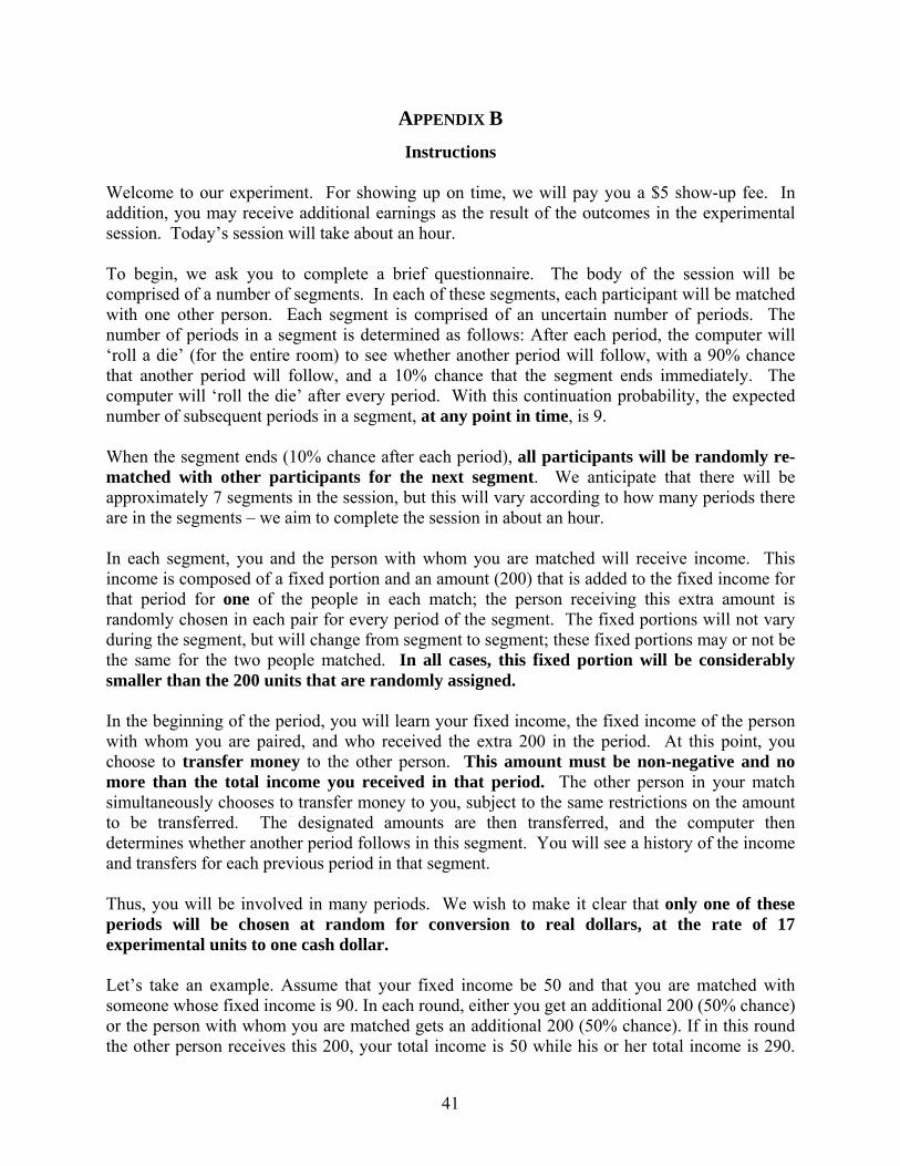
APPENDIX B Instructions

Welcome to our experiment. For showing up on time, we will pay you a $5 show-up fee. In addition, you may receive additional earnings as the result of the outcomes in the experimental session. Today’s session will take about an hour. To begin, we ask you to complete a brief questionnaire. The body of the session will be comprised of a number of segments. In each of these segments, each participant will be matched with one other person. Each segment is comprised of an uncertain number of periods. The number of periods in a segment is determined as follows: After each period, the computer will ‘roll a die’ (for the entire room) to see whether another period will follow, with a 90% chance that another period will follow, and a 10% chance that the segment ends immediately. The computer will ‘roll the die’ after every period. With this continuation probability, the expected number of subsequent periods in a segment, at any point in time, is 9. When the segment ends (10% chance after each period), all participants will be randomly re-matched with other participants for the next segment. We anticipate that there will be approximately 7 segments in the session, but this will vary according to how many periods there are in the segments – we aim to complete the session in about an hour. In each segment, you and the person with whom you are matched will receive income. This income is composed of a fixed portion and an amount (200) that is added to the fixed income for that period for one of the people in each match; the person receiving this extra amount is randomly chosen in each pair for every period of the segment. The fixed portions will not vary during the segment, but will change from segment to segment; these fixed portions may or not be the same for the two people matched. In all cases, this fixed portion will be considerably smaller than the 200 units that are randomly assigned. In the beginning of the period, you will learn your fixed income, the fixed income of the person with whom you are paired, and who received the extra 200 in the period. At this point, you choose to transfer money to the other person. This amount must be non-negative and no more than the total income you received in that period. The other person in your match simultaneously chooses to transfer money to you, subject to the same restrictions on the amount to be transferred. The designated amounts are then transferred, and the computer then determines whether another period follows in this segment. You will see a history of the income and transfers for each previous period in that segment. Thus, you will be involved in many periods. We wish to make it clear that only one of these periods will be chosen at random for conversion to real dollars, at the rate of 17 experimental units to one cash dollar. Let’s take an example. Assume that your fixed income be 50 and that you are matched with someone whose fixed income is 90. In each round, either you get an additional 200 (50% chance) or the person with whom you are matched gets an additional 200 (50% chance). If in this round the other person receives this 200, your total income is 50 while his or her total income is 290.

41

Now, you and the person with whom you are matched decide on transfers. Suppose you transfer x to the other person while he or she transfers y to you; then your “income net of transfer” or “consumption” for this round is 50-x+y while his “income net of transfer” or “consumption” for this round is 290-y+x. If this round happens to be the one selected to count for actual payoffs, these are your and your match’s payoffs for the experiment. For instance if x = 1 and y = 61 then your payoff would be 110 and your match’s payoff would be 230. At some points along the way, you will be asked for some information about your decisions and/or your expectations. The history of income and transfers for the current match appears on your screen. By pressing the “full view” button you can also review the history of your past matches. At the end of the experiment, one period will be chosen at random for payment. The screen will state your earnings. When you have completed a short questionnaire on your demographics, we will distribute receipts forms for participants to sign, and will pay people individually and privately. We highly encourage clarifying questions. Thank you for your participation.

42

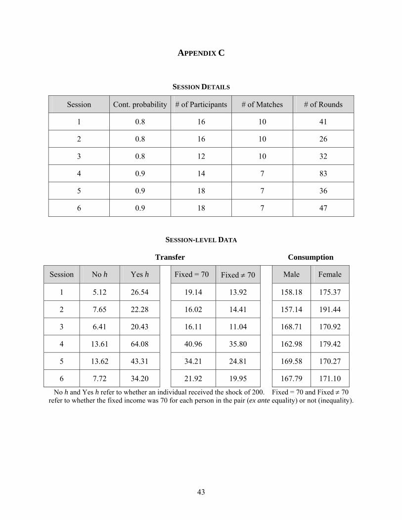
APPENDIX C

SESSION DETAILS

Session Cont. probability # of Participants # of Matches # of Rounds

1 0.8 16 10 41

2 0.8 16 10 26

3 0.8 12 10 32

4 0.9 14 7 83

5 0.9 18 7 36

6 0.9 18 7 47

SESSION-LEVEL DATA Transfer Consumption

Session No h Yes h Fixed = 70 Fixed ≠ 70 Male Female

1 5.12 26.54 19.14 13.92 158.18 175.37

2 7.65 22.28 16.02 14.41 157.14 191.44

3 6.41 20.43 16.11 11.04 168.71 170.92

4 13.61 64.08 40.96 35.80 162.98 179.42

5 13.62 43.31 34.21 24.81 169.58 170.27

6 7.72 34.20 21.92 19.95 167.79 171.10

No h and Yes h refer to whether an individual received the shock of 200. Fixed = 70 and Fixed ≠ 70 refer to whether the fixed income was 70 for each person in the pair (ex ante equality) or not (inequality).

43

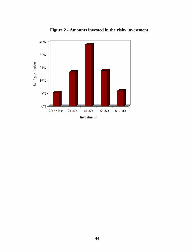
0%

8%

16%

24%

32%

40%

% o

f pop

ulat

ion

20 or less 21-40 41-60 61-80 81-100

Investment

Figure 2 - Amounts invested in the risky investment

44

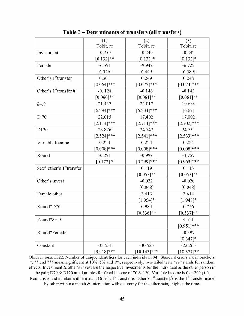
Table 3 – Determinants of transfers (all transfers) (1) (2) (3) Tobit, re Tobit, re Tobit, re Investment -0.259 -0.249 -0.242 [0.132]** [0.132]* [0.132]* Female -6.591 -9.949 -6.722 [6.356] [6.449] [6.589] Other’s 1sttransfer 0.301 0.249 0.248 [0.064]*** [0.075]*** [0.074]*** Other’s 1sttransfer|h -0. 128 -0.146 -0.143 [0.060]** [0.061]** [0.061]** δ=.9 21.432 22.017 10.684 [6.284]*** [6.234]*** [6.67] D 70 22.015 17.402 17.002 [2.114]*** [2.714]*** [2.702]*** D120 23.876 24.742 24.731 [2.524]*** [2.541]*** [2.533]*** Variable Income 0.224 0.224 0.224 [0.008]*** [0.008]*** [0.008]*** Round -0.291 -0.999 -4.757 [0.172] * [0.299]*** [0.963]*** Sex* other’s 1sttransfer 0.119 0.113 [0.053]** [0.053]** Other’s invest -0.022 -0.020 [0.048] [0.048] Female other 3.413 3.614 [1.954]* [1.948]* Round*D70 0.984 0.756 [0.336]** [0.337]** Round*δ=.9 4.351 [0.951]*** Round*Female -0.597 [0.347]* Constant -33.551 -30.523 -22.265 [9.918]*** [10.143]*** [10.377]**

Observations: 3322. Number of unique identifiers for each individual: 94. Standard errors are in brackets. *, ** and *** mean significant at 10%, 5% and 1%, respectively, two-tailed tests. “re” stands for random effects. Investment & other’s invest are the respective investments for the individual & the other person in

the pair; D70 & D120 are dummies for fixed income of 70 & 120; Variable income is 0 or 200 ( h ); Round is round number within match; Other’s 1st transfer & Other’s 1st transfer| h is the 1st transfer made

by other within a match & interaction with a dummy for the other being high at the time.

45

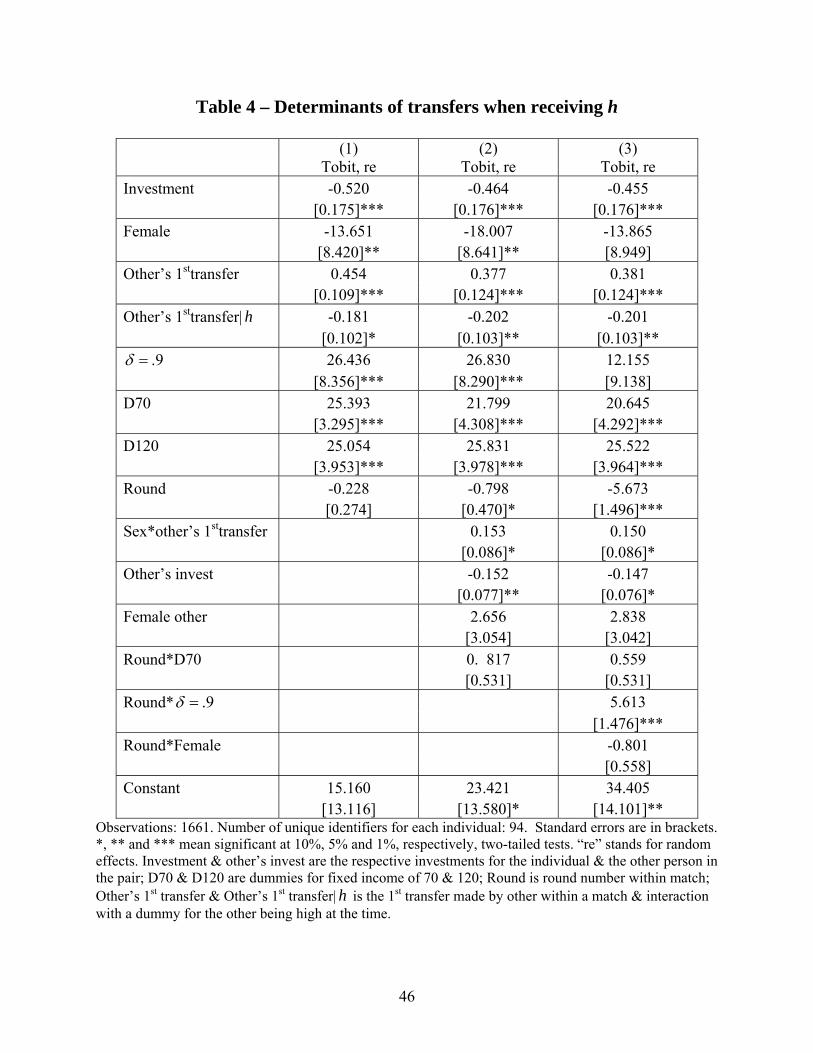
Table 4 – Determinants of transfers when receiving h

(1) (2) (3) Tobit, re Tobit, re Tobit, re Investment -0.520 -0.464 -0.455 [0.175]*** [0.176]*** [0.176]*** Female -13.651 -18.007 -13.865 [8.420]** [8.641]** [8.949] Other’s 1sttransfer 0.454 0.377 0.381 [0.109]*** [0.124]*** [0.124]*** Other’s 1sttransfer| h -0.181 -0.202 -0.201 [0.102]* [0.103]** [0.103]**

9.=δ 26.436 26.830 12.155 [8.356]*** [8.290]*** [9.138] D70 25.393 21.799 20.645 [3.295]*** [4.308]*** [4.292]*** D120 25.054 25.831 25.522 [3.953]*** [3.978]*** [3.964]*** Round -0.228 -0.798 -5.673 [0.274] [0.470]* [1.496]*** Sex*other’s 1sttransfer 0.153 0.150 [0.086]* [0.086]* Other’s invest -0.152 -0.147 [0.077]** [0.076]* Female other 2.656 2.838 [3.054] [3.042] Round*D70 0. 817 0.559 [0.531] [0.531] Round* 9.=δ 5.613 [1.476]*** Round*Female -0.801 [0.558] Constant 15.160 23.421 34.405 [13.116] [13.580]* [14.101]**

Observations: 1661. Number of unique identifiers for each individual: 94. Standard errors are in brackets. *, ** and *** mean significant at 10%, 5% and 1%, respectively, two-tailed tests. “re” stands for random effects. Investment & other’s invest are the respective investments for the individual & the other person in the pair; D70 & D120 are dummies for fixed income of 70 & 120; Round is round number within match; Other’s 1st transfer & Other’s 1st transfer| is the 1h st transfer made by other within a match & interaction with a dummy for the other being high at the time.

46

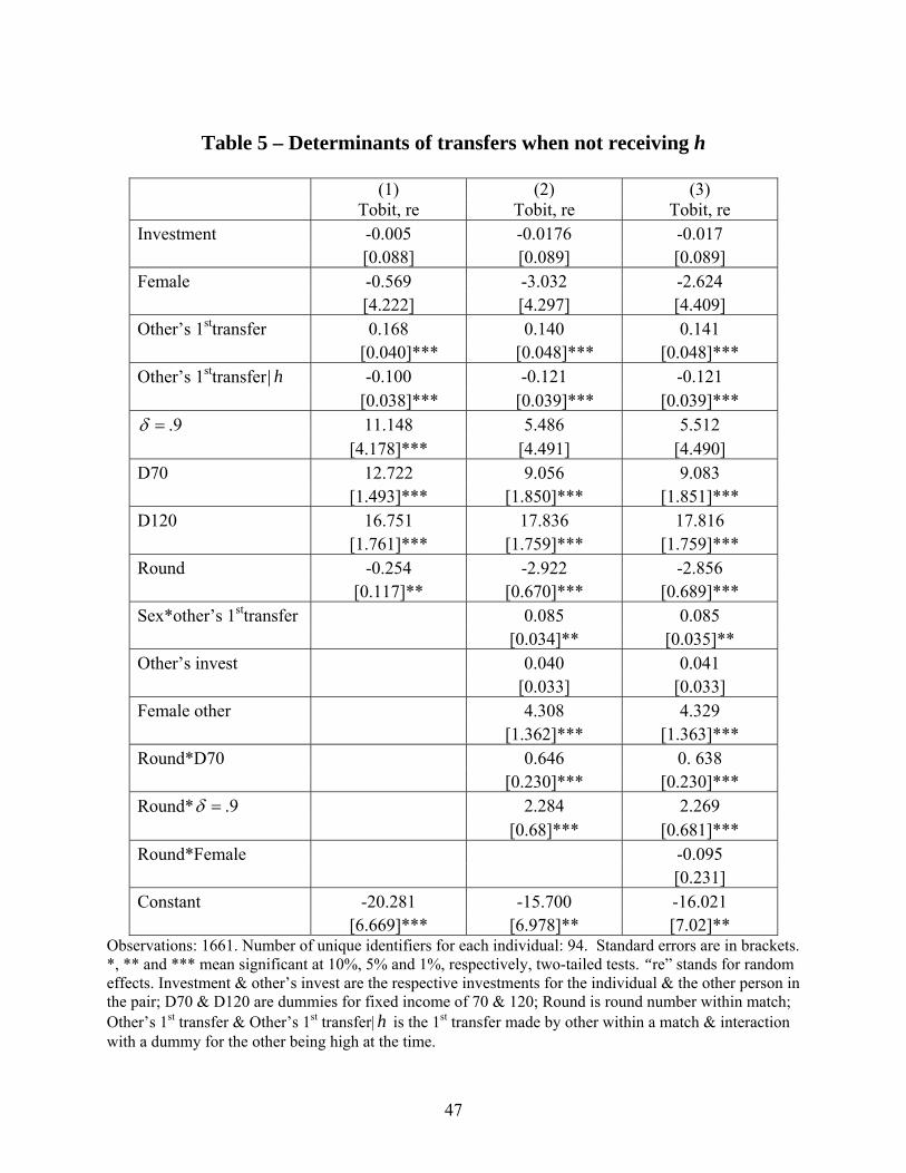
Table 5 – Determinants of transfers when not receiving h

(1) (2) (3) Tobit, re Tobit, re Tobit, re Investment -0.005 -0.0176 -0.017 [0.088] [0.089] [0.089] Female -0.569 -3.032 -2.624 [4.222] [4.297] [4.409] Other’s 1sttransfer 0.168 0.140 0.141 [0.040]*** [0.048]*** [0.048]*** Other’s 1sttransfer| h -0.100 -0.121 -0.121 [0.038]*** [0.039]*** [0.039]***

9.=δ 11.148 5.486 5.512 [4.178]*** [4.491] [4.490] D70 12.722 9.056 9.083 [1.493]*** [1.850]*** [1.851]*** D120 16.751 17.836 17.816 [1.761]*** [1.759]*** [1.759]*** Round -0.254 -2.922 -2.856 [0.117]** [0.670]*** [0.689]*** Sex*other’s 1sttransfer 0.085 0.085 [0.034]** [0.035]** Other’s invest 0.040 0.041 [0.033] [0.033] Female other 4.308 4.329 [1.362]*** [1.363]*** Round*D70 0.646 0. 638 [0.230]*** [0.230]*** Round* 9.=δ 2.284 2.269 [0.68]*** [0.681]*** Round*Female -0.095 [0.231] Constant -20.281 -15.700 -16.021 [6.669]*** [6.978]** [7.02]**

Observations: 1661. Number of unique identifiers for each individual: 94. Standard errors are in brackets. *, ** and *** mean significant at 10%, 5% and 1%, respectively, two-tailed tests. “re” stands for random effects. Investment & other’s invest are the respective investments for the individual & the other person in the pair; D70 & D120 are dummies for fixed income of 70 & 120; Round is round number within match; Other’s 1st transfer & Other’s 1st transfer| is the 1h st transfer made by other within a match & interaction with a dummy for the other being high at the time.

47

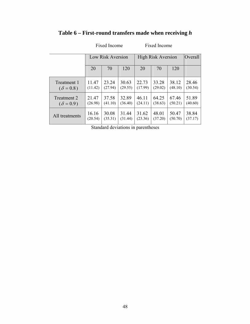
Table 6 – First-round transfers made when receiving h

Fixed Income Fixed Income

Low Risk Aversion High Risk Aversion Overall

20 70 120 20 70 120

Treatment 1 ( 8.0=δ )

11.47 (11.42)

23.24 (27.94)

30.63 (29.55)

22.73 (17.99)

33.28 (29.02)

38.12 (48.10)

28.46 (30.54)

Treatment 2 ( 9.0=δ )

21.47 (26.98)

37.58 (41.10)

32.89 (36.40)

46.11 (24.11)

64.25 (38.63)

67.46 (50.21)

51.89 (40.60)

All treatments

16.16 (20.54)

30.08 (35.31)

31.44 (31.44)

31.62 (23.36)

48.01 (37.20)

50.47 (50.70)

38.84 (37.17)

Standard deviations in parentheses

48

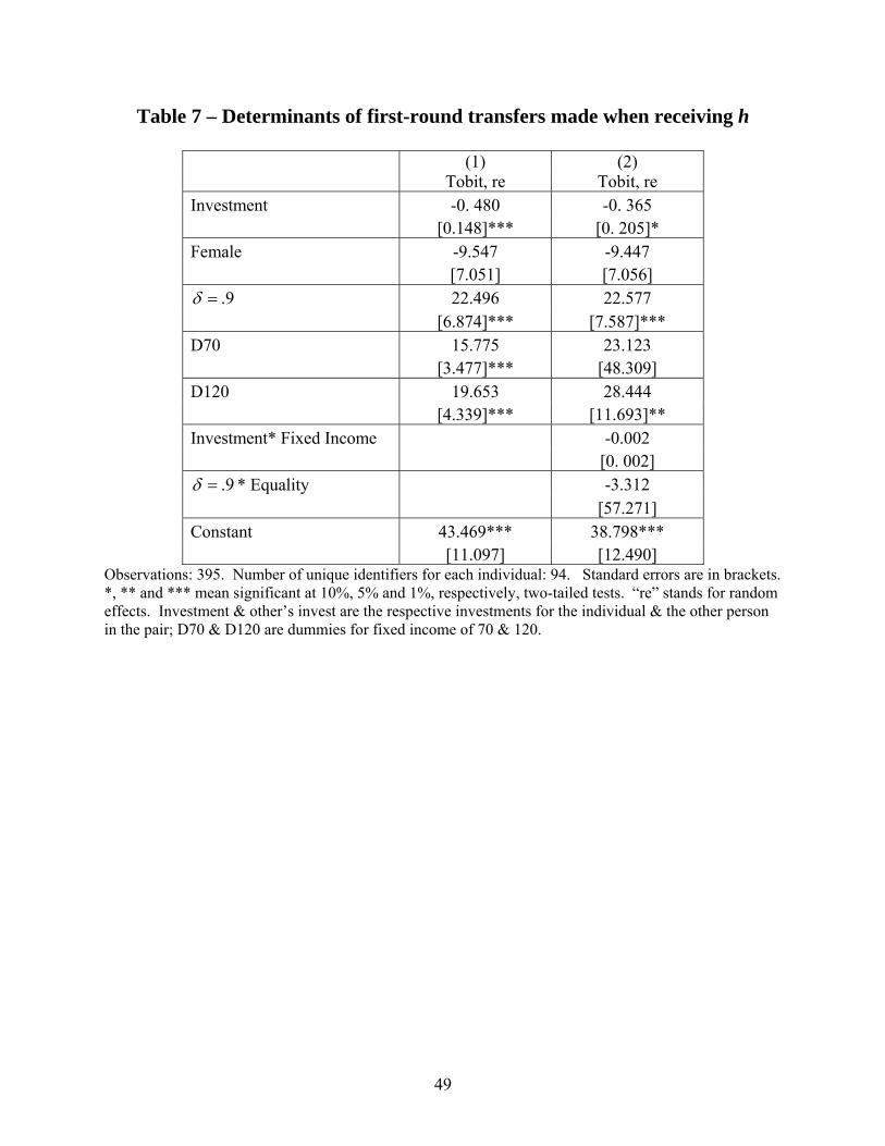
Table 7 – Determinants of first-round transfers made when receiving h

(1) (2) Tobit, re Tobit, re Investment -0. 480 -0. 365 [0.148]*** [0. 205]* Female -9.547 -9.447 [7.051] [7.056]

9.=δ 22.496 22.577 [6.874]*** [7.587]*** D70 15.775 23.123 [3.477]*** [48.309] D120 19.653 28.444 [4.339]*** [11.693]** Investment* Fixed Income -0.002 [0. 002]

9.=δ * Equality -3.312 [57.271] Constant 43.469*** 38.798*** [11.097] [12.490]

Observations: 395. Number of unique identifiers for each individual: 94. Standard errors are in brackets. *, ** and *** mean significant at 10%, 5% and 1%, respectively, two-tailed tests. “re” stands for random effects. Investment & other’s invest are the respective investments for the individual & the other person in the pair; D70 & D120 are dummies for fixed income of 70 & 120.

49

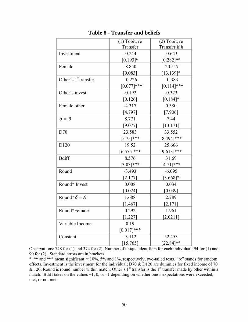
Table 8 - Transfer and beliefs (1) Tobit, re (2) Tobit, re Transfer Transfer if h Investment -0.244 -0.643 [0.193]* [0.282]** Female -8.850 -20.517 [9.083] [13.139]* Other’s 1sttransfer 0.226 0.383 [0.077]*** [0.114]*** Other’s invest -0.192 -0.323 [0.126] [0.184]* Female other -4.317 0.380 [4.797] [7.906]

9.=δ 8.771 7.44 [9.077] [13.171] D70 23.583 33.552 [5.75]*** [8.494]*** D120 19.52 25.666 [6.575]*** [9.613]*** Bdiff 8.576 31.69 [3.03]*** [4.71]*** Round -3.493 -6.095 [2.177] [3.668]* Round* Invest 0.008 0.034 [0.024] [0.039] Round* 9.=δ 1.688 2.789 [1.467] [2.171] Round*Female 0.292 1.961 [1.227] [2.0211] Variable Income 0.19 [0.017]*** Constant -3.112 52.453 [15.765] [22.84]**

Observations: 748 for (1) and 374 for (2). Number of unique identifiers for each individual: 94 for (1) and 90 for (2). Standard errors are in brackets. *, ** and *** mean significant at 10%, 5% and 1%, respectively, two-tailed tests. “re” stands for random effects. Investment is the investment for the individual; D70 & D120 are dummies for fixed income of 70 & 120; Round is round number within match; Other’s 1st transfer is the 1st transfer made by other within a match. Bdiff takes on the values +1, 0, or –1 depending on whether one’s expectations were exceeded, met, or not met.

50